
Indexing Mobile Objects on the plane Indexing Mobile Objects on the plane RevisitedRevisited
Computer Engineering and Informatics Department, Polytechnic School, University of Patras
The authors would like to thank the The authors would like to thank the Greek-Bulgarian Bilateral Scientific Greek-Bulgarian Bilateral Scientific
ProtocolProtocol for funding the above work. for funding the above work.
S.Sioutas, K.Tsakalidis, K.Tsihlas, C. Makris
& Y. Manolopoulos
Informatics Department, Ionian University
Informatics Department, Aristotle University of Thessaloniki
Data Engineering Lab

2
Definition of Problem -Literature Survey
Literature Survey - Methods
Geometric Duality Transformation and B+ Trees / Partition Trees
TPR*-trees
STRIPES
Problem:
Report the mobile objects located inside the rectangle [xReport the mobile objects located inside the rectangle [x1q1q ,x ,x2q2q] ] [y [y1q1q ,y ,y2q2q ] at the time ] at the time instants between tinstants between t1q1q and t and t2q2q (where t (where tnownowtt1q1qtt2q2q ) given the current motion information of all ) given the current motion information of all objectsobjects
3
Problem Description
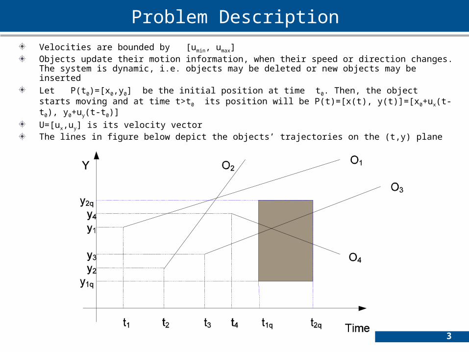
Velocities are bounded by [umin, umax] Objects update their motion information, when their speed or direction changes. The system is dynamic, i.e. objects may be deleted or new objects may be insertedLet P(t0)=[x0,y0] be the initial position at time t0. Then, the object starts moving and at time t>t0 its position will be P(t)=[x(t), y(t)]=[x0+ux(t-t0), y0+uy(t-t0)] U=[ux,uy] is its velocity vectorThe lines in figure below depict the objects’ trajectories on the (t,y) plane
4
Indexing Mobile Objects in one dimension
Hough – X dual Transformation
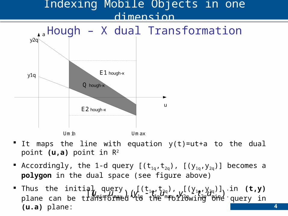
It maps the line with equation y(t)=ut+a to the dual point (u,a) point in R2
Accordingly, the 1-d query [(t1q,t2q), [(y1q,y2q)] becomes a polygon in the dual space (see figure above)
Thus the initial query [(t1q,t2q), [(y1q,y2q)] in (t,y) plane can be transformed to the following one query in (u.a) plane:
a
u
Umin Umax
y1q
y2q
Q hough-x
E1 hough-x
E2 hough-x
)],(),,[( min22max11maxmin utyutyuu qqqq
5
Indexing Mobile Objects in one dimension
Hough – Y dual Transformationn
b
1/u max
Q hough-y
E1 hough-y
E2 hough-y
1/u min
t1q t2q
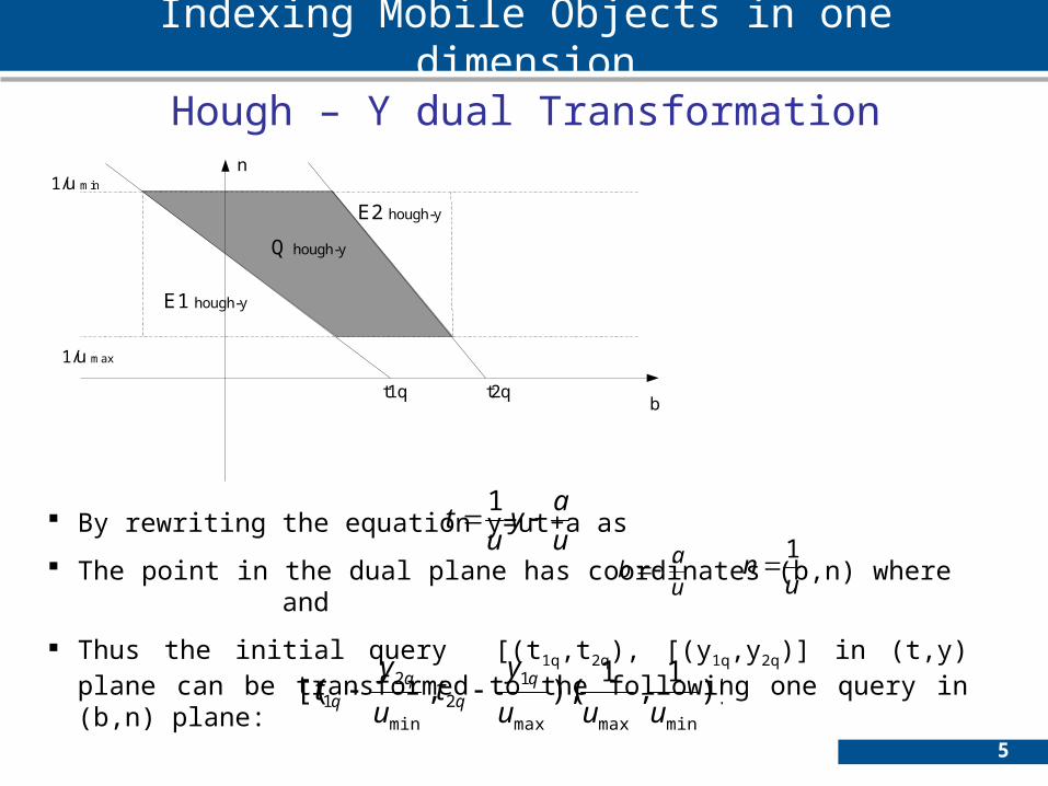
By rewriting the equation y=ut+a as
The point in the dual plane has coordinates (b,n) where and
Thus the initial query [(t1q,t2q), [(y1q,y2q)] in (t,y) plane can be transformed to the following one query in (b,n) plane:
u
ay
ut 1
u
ab
un
1
)]1
,1
(),,[(minmaxmax
12
min
21 uuu
yt
u
yt q
q

6
CRITERION
Hough Dual Transformations
Motions with small velocities in the Hough-Y approach are mapped into dual points (b,n) having large n coordinates (n=1/u)By storing the Hough-Y dual points in an index structure such as an R* -tree, MBR's with large extents are introduced, and the performance is severely affected. By using a Hough-X for the small velocities' partition, this effect is eliminated
The query area in Hough-X plane is enlarged by the area E Hough-X =E1 hough-X + E2 hough-X and in Hough-Y plane by E Hough-Y =E1 hough-Y + E2 hough-Y
Q Hough-X = actual area of the simplex query in Hough-X plane QHough-Y = actual area of the simplex query in Hough-Y plane Thus, the overall solution proposes the choice of that transformation which minimizes the following criterion:
YHough
YHough
XHough
XHough
Q
E
Q
Ec

7
The procedure for building the index
1. Decompose the 2-d motion into two 1-d motions on the (t,x) and (t,y) planes.
2. For each projection, build the corresponding index structure.
Partition the objects according to their velocity:Objects with small velocity are stored using the Hough-X dual transform, while the rest are stored using the Hough-Y dual transform.Motion information about the other projection is also included.

8
Algorithm for answering the exact 2-d query
(1) Decompose the query into two 1-d queries, for the (t,x) and (t,y) projection
(2) For each projection get the dual - simplex query(3) For each projection calculate the criterion c and
choose the one (say p) that minimizes it(4) Search in projection p the Hough-X or Hough-Y
partition(5) Perform a refinement or filtering step ``on the fly", by
using the whole motion information. Thus, the result set contains only the objects that satisfy the query
9
INNOVATION
Q Hough-X is computed by querying a 2-d partition tree
Q Hough-Y is computed by querying a B+ tree that indexes the b parameters
Our construction instead is based: (a) on the use of the Lazy B-tree [ISAAC 05] instead of the B + tree when handling queries with the Hough-Y transform and (b) on the employment of a new index that outperforms partition trees in handling polygon queries with the Hough-X transform.
10
1st solution: Handling polygon queries when using the Hough-Y transform with method of LBT’s
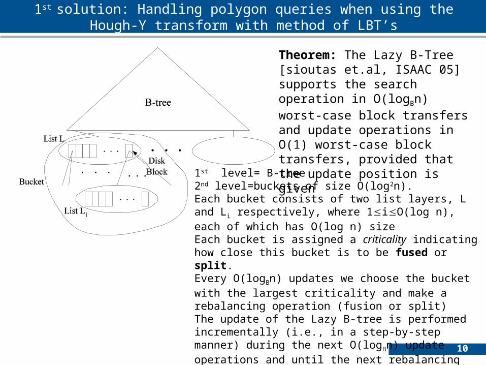
Theorem: The Lazy B-Tree [sioutas et.al, ISAAC 05] supports the search operation in O(logBn) worst-case block transfers and update operations in O(1) worst-case block transfers, provided that the update position is given
1st level= B-tree2nd level=buckets of size O(log2n). Each bucket consists of two list layers, L and L i respectively, where 1iO(log n), each of which has O(log n) sizeEach bucket is assigned a criticality indicating how close this bucket is to be fused or split. Every O(logBn) updates we choose the bucket with the largest criticality and make a rebalancing operation (fusion or split)The update of the Lazy B-tree is performed incrementally (i.e., in a step-by-step manner) during the next O(logBn) update operations and until the next rebalancing operation. The global rebalancing lemma ensures that the size of the buckets will never be larger than O(log2n).
11
Optimal Update PerformanceIndexing of b parameters in O(logBn) I/O’s in each dimensionCombination of the results produced in each dimension and FilteringIndexing Performance depends on area of spatial query rectangleFor sensibly realistic levels of query rectangles Very good time performance
1st Solution:Method of LBT’s“Two Lazy B-trees for indexing the b parameters of each
dimension”
12
2nd solution: Handling polygon queries when using the Hough-X transform
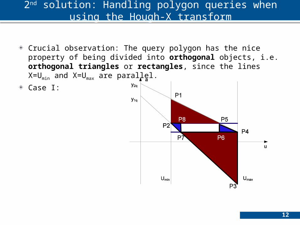
Crucial observation: The query polygon has the nice property of being divided into orthogonal objects, i.e. orthogonal triangles or rectangles, since the lines X=Umin and X=Umax are parallel.
Case I:

13
Case II Case III
2nd solution: Handling polygon queries when using the Hough-X transform

14
2nd solution: Handling polygon queries when using the Hough-X transform
The problem of handling orthogonal range search queries has been handled in PODS 99 [Arge, Samoladas,Viter 99], where an optimal solution was presented to handle general (4-sided) range queries in O((N/B)(log(N/B))loglogBN) disk blocks and could answer queries in O(logBN+T/B) I/O's, the structure also supports updates in O((logBN)(log(N/B))/loglogBN) I/O's.
Let us now consider the problem of devising an access method for handling orthogonal triangle range queries; in this problem we have to determine all the points from a set S of n points on the plane lying inside an orthogonal triangle
Let T be an orthogonal triangle defined by the point (xq,yq) and the line Lq that is not axis-parallel
15
A new 3-layered Access Method for Triangle Range Queries
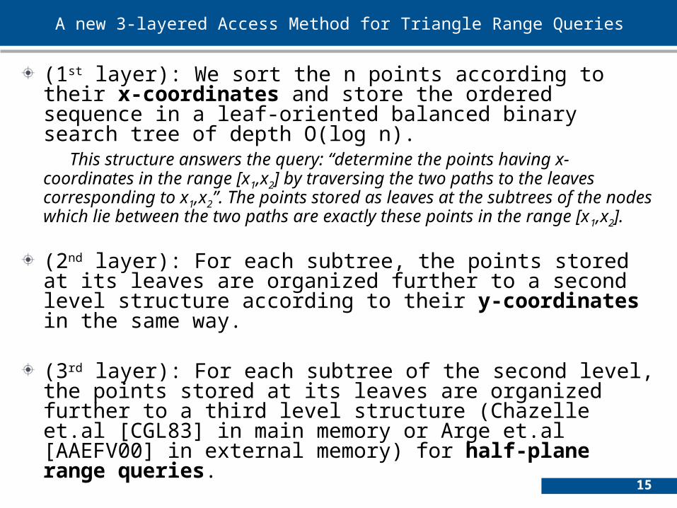
(1st layer): We sort the n points according to their x-coordinates and store the ordered sequence in a leaf-oriented balanced binary search tree of depth O(log n).
This structure answers the query: “determine the points having x-coordinates in the range [x1,x2] by traversing the two paths to the leaves corresponding to x1,x2”. The points stored as leaves at the subtrees of the nodes which lie between the two paths are exactly these points in the range [x1,x2].
(2nd layer): For each subtree, the points stored at its leaves are organized further to a second level structure according to their y-coordinates in the same way.
(3rd layer): For each subtree of the second level, the points stored at its leaves are organized further to a third level structure (Chazelle et.al [CGL83] in main memory or Arge et.al [AAEFV00] in external memory) for half-plane range queries.

16
Algorithm for Orthogonal Triangle Range Query
1. In the tree storing the pointset S according to x-coordinates, traverse the path to xq. All the points having x-coordinate in the range [xq,) are stored at the subtrees on the nodes that are right sons of a node of the search path and do not belong to the path. There are at most O(log n) such disjoint subtrees.
2. For every such subtree traverse the path to yq. By a similar argument as in the previous step, at most O(logn) disjoint subtrees are located, storing points that have y-coordinate in the range [yq, ).
3. For each subtree in Step 2, apply the half-plane range query of Chazelle or Arge to retrieve the points that lie on the side of line Lq towards the triangle.
The correctness of the above algorithm follows from the structure used. In each of the first two steps we have to visit O(logn) subtrees. If in step 3 we apply the main memory solution of [CGL83], then the query time becomes O(log3n+A), whereas the required space is O(nlog2n). Otherwise, if we apply the external memory solution of [AAEFV00], then our method above requires O(log2nlogBn +A) I/O's and O(nlog2n) disk blocks. Although the space becomes superlinear the O(log2nlogBn +A) worst-case I/O complexity of our method is better than the O((n/B)+A/B)) worst-case I/O complexity of a partition tree.
17
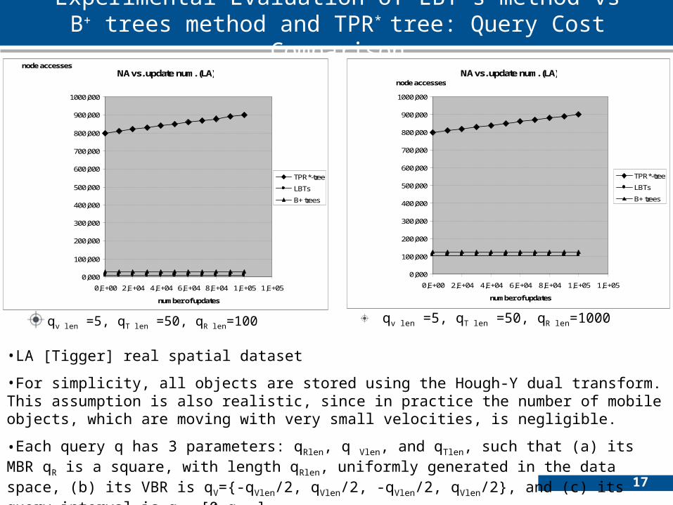
Experimental Evaluation of LBT’s method vs B+ trees method and TPR* tree: Query Cost
Comparison
qv len =5, qT len =50, qR len=100
NA vs. update num. (LA)
0,000
100,000
200,000
300,000
400,000
500,000
600,000
700,000
800,000
900,000
1000,000
0,E+00 2,E+04 4,E+04 6,E+04 8,E+04 1,E+05 1,E+05
number of updates
node accesses
TPR*-tree
LBTs
B+ trees
qv len =5, qT len =50, qR len=1000
•LA [Tigger] real spatial dataset
•For simplicity, all objects are stored using the Hough-Y dual transform. This assumption is also realistic, since in practice the number of mobile objects, which are moving with very small velocities, is negligible.
•Each query q has 3 parameters: qRlen, q Vlen, and qTlen, such that (a) its MBR qR is a square, with length qRlen, uniformly generated in the data space, (b) its VBR is qV={-qVlen/2, qVlen/2, -qVlen/2, qVlen/2}, and (c) its query interval is qT= [0,qTlen]
NA vs. update num. (LA)
0,000
100,000
200,000
300,000
400,000
500,000
600,000
700,000
800,000
900,000
1000,000
0,E+00 2,E+04 4,E+04 6,E+04 8,E+04 1,E+05 1,E+05
number of updates
node accesses
TPR*-tree
LBTs
B+ trees

18
Experimental Evaluation of LBT’s method vs B+ trees method and TPR* tree: Query Cost
Comparison
When the length of the query rectangle becomes extremely large, f.e. 2000, meaning 400 hectares of query's surface, our method degrades. While the surface of the query rectangle grows, the answer's size in each projection may grow too, thus the performance of LBT's method that combines and filters the two answers may degrade. In real GIS applications, for a vast spatial terrain of 106 hectares, f.e. the road network of a big town where each road square covers no more than 1 hectare (or 10.000 m2) the most frequent queries consider spatial query's surface no more than 100 road squares (or 100 hectares) and future time interval no larger than 100 seconds. This is what we later say sensibly realistic levels.
qv len =5, qT len =50, qR len=2000
NA vs. update num. (LA)
0,000
100,000
200,000
300,000
400,000
500,000
600,000
700,000
800,000
900,000
1000,000
0,E+00 2,E+04 4,E+04 6,E+04 8,E+04 1,E+05 1,E+05
number of updates
node accesses
TPR*-tree
LBTs
B+ trees

19
Experimental Evaluation of LBT’s method vs B+ trees method and TPR* tree: Query Cost
Comparison
qv len =10, qT len =50, qR len=400 qv len =10, qT len =50, qR len=1000
Figures depict the efficiency of our solution in case the velocity vector grows upObviously, the velocity factor is very important for TPR-like solutions, but it isn't for the other methods, especially this one of LBTs, which depends exclusively on query's surface factor.
NA vs. update num. (LA)
0,000
100,000
200,000
300,000
400,000
500,000
600,000
0,E+00 2,E+04 4,E+04 6,E+04 8,E+04 1,E+05 1,E+05
number of updates
node accesses
TPR*-tree
LBTs
B+ trees
NA vs. update num. (LA)
0,000
100,000
200,000
300,000
400,000
500,000
600,000
0,E+00 2,E+04 4,E+04 6,E+04 8,E+04 1,E+05 1,E+05
number of updates
node accesses
TPR*-tree
LBTs
B+ trees
20
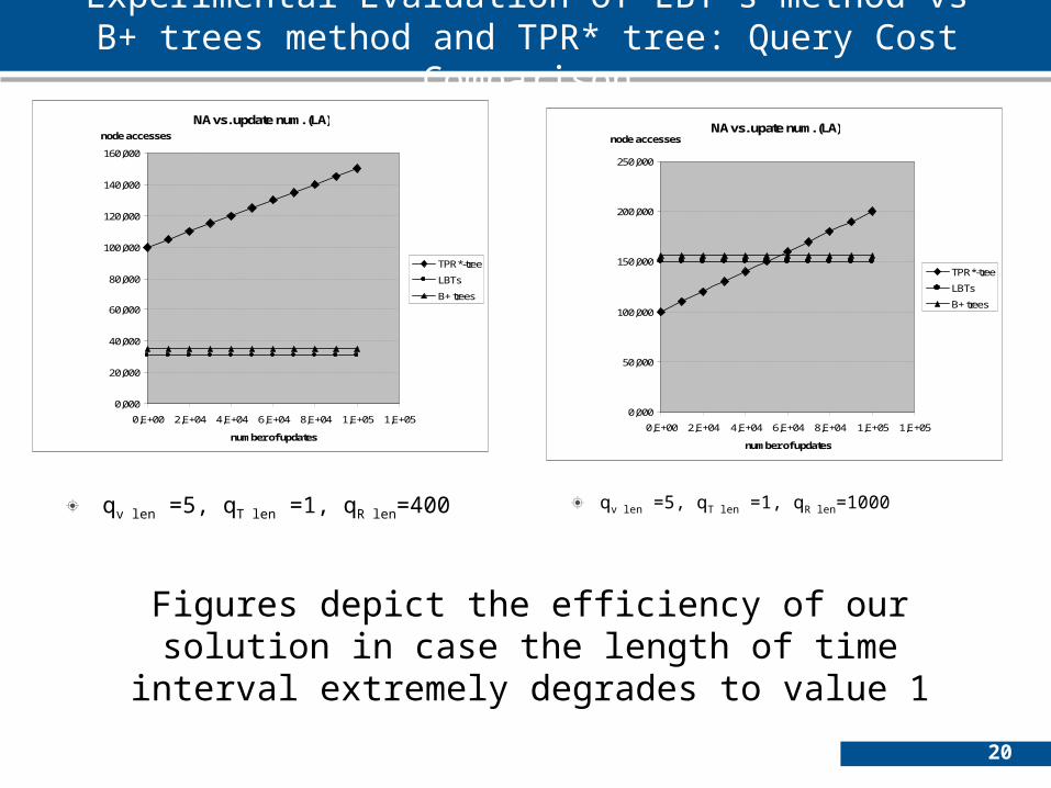
Experimental Evaluation of LBT’s method vs B+ trees method and TPR* tree: Query Cost
Comparison
qv len =5, qT len =1, qR len=400 qv len =5, qT len =1, qR len=1000
Figures depict the efficiency of our solution in case the length of time interval extremely degrades to value 1
NA vs. update num. (LA)
0,000
20,000
40,000
60,000
80,000
100,000
120,000
140,000
160,000
0,E+00 2,E+04 4,E+04 6,E+04 8,E+04 1,E+05 1,E+05
number of updates
node accesses
TPR*-tree
LBTs
B+ trees
NA vs. upate num. (LA)
0,000
50,000
100,000
150,000
200,000
250,000
0,E+00 2,E+04 4,E+04 6,E+04 8,E+04 1,E+05 1,E+05
number of updates
node accesses
TPR*-tree
LBTs
B+ trees
21
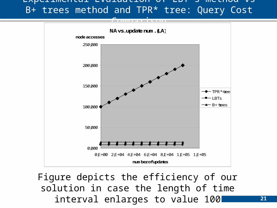
Experimental Evaluation of LBT’s method vs B+ trees method and TPR* tree: Query Cost
Comparison
qv len =5, qT len =100, qR len=400
Figure depicts the efficiency of our solution in case the length of time interval enlarges to value 100
NA vs. update num. (LA)
0,000
50,000
100,000
150,000
200,000
250,000
0,E+00 2,E+04 4,E+04 6,E+04 8,E+04 1,E+05 1,E+05
number of updates
node accesses
TPR*-tree
LBTs
B+ trees
22
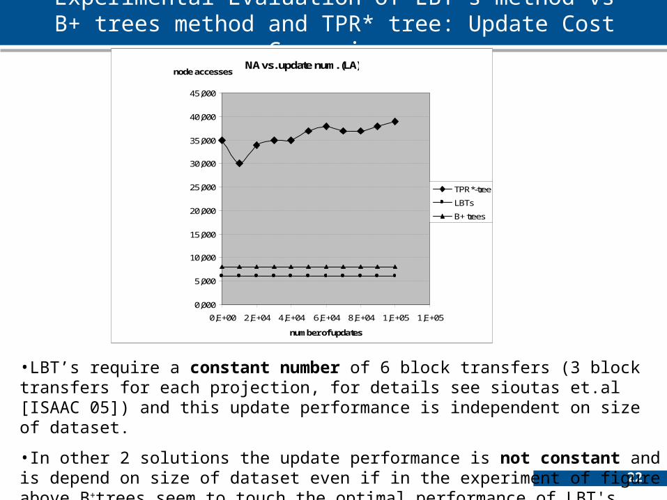
Experimental Evaluation of LBT’s method vs B+ trees method and TPR* tree: Update Cost
Comparison
•LBT’s require a constant number of 6 block transfers (3 block transfers for each projection, for details see sioutas et.al [ISAAC 05]) and this update performance is independent on size of dataset.
•In other 2 solutions the update performance is not constant and is depend on size of dataset even if in the experiment of figure above B+trees seem to touch the optimal performance of LBT's requiring 8 block transfers respectively (TPR* tree requires 35 block transfers in average).
NA vs. update num. (LA)
0,000
5,000
10,000
15,000
20,000
25,000
30,000
35,000
40,000
45,000
0,E+00 2,E+04 4,E+04 6,E+04 8,E+04 1,E+05 1,E+05
number of updates
node accesses
TPR*-tree
LBTs
B+ trees
23
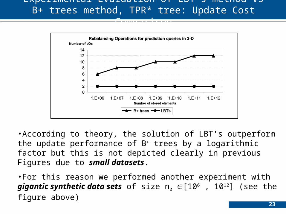
Experimental Evaluation of LBT’s method vs B+ trees method, TPR* tree: Update Cost Comparison
•According to theory, the solution of LBT's outperform the update performance of B+ trees by a logarithmic factor but this is not depicted clearly in previous Figures due to small datasets.
•For this reason we performed another experiment with gigantic synthetic data sets of size n0 [106 , 1012] (see the figure above)
24
CONCLUSIONS
We presented access methods for indexing mobile objects that move on the plane to efficiently answer range queries about their location in the future Concerning the update performance evaluation our 1st solution is the most efficient (optimal)The query performance evaluation illustrates the applicability of our 1st solution in case the length of the query rectangle remain in sensibly realistic levels. Finally, the 2nd very efficient solution is somehow complicated and thus it has only theoretical interestFuture plan: (1) Experimental Comparison with STRIPES (it was already done in Journal Version and the results are very promising) (2) The simplification of 2nd solution in order to be more applicable in practice.

25
END
Indexing Mobile Objects on the plane revisited


