Download - In Situ Determination of Elastic Moduli of Pavement Systems by Spectral-Analysis-of-Surface
2. Government Acc .. ,i.n No.
FHWA/TX-86/l3+368-lF
... Titl. and Subtitl.
IN SITU DETERMINATION OF ELASTIC MODULI OF PAVEMENT SYSTEMS BY SPECTRAL-ANALYSIS-OFSURFACE-WAVES METHOD: PRACTICAL ASPECTS 7. Autharfs)
Soheil Nazarian and Kenneth H. Stokoe II
9. Pe,forming Organilotion N_e and Addr ...
TECHNICAL REPORT STANDARD TITLE PAGE
5. R.po,1 Dole
August 1985 6. Pe,forming Orgonizalion Cod"
8. Performing Orllonilolion Repor' No.
Research Report 368-lF
10. Worle Unit No.
11. Contract or Grant No.
Research Report 368-lF
Center for Transportation Research The University of Texas at Austin Austin, Texas 78712-1075
13. Type of R.port and P.riod Cov.,.d ~~~----~---~--~~-----------------------------~ 12. Sponlo,ing Agency Nome and Addre ..
Texas State Department of Highways and Public Transportation; Transportation Planning Division
P. O. Box 5051 Austin, Texas 78763 15. Suppl.menta,y Not ..
Final
1 ... Spon,o,ing Ag.ncy Cod.
Study conducted in cooperation with the U. S. Department of Transportation, Federal Highway Administration. Research Study Title: "Nondestructive Measurement of Thickness and Elastic Stiffness of Pavement Layers"
16. Abstract
The Spectral-Analysis-of-Surface-Waves (SASW) method is an in situ testing method for determining shear wave velocity profi~es of soil sites and stiffness profiles of pavement systems. The method is non-destructive, is performed from the ground surface, and generally requires no boreholes. The key elements in SASW testing are the generation and measurement of surface waves. Two receivers are located on the ground surface and a transient impact containing a large range of frequencies is transmitted to the soil by means of a simple hammer. One of the most important steps in SASW testing is the inversion process, an analytical technique for reconstructing the shear wave velocity profile.
Data collection and analysis used in the SASW technique are discussed in detail. Several case studies are presented to illustrate the utility and versatility of the SASW method. In each case, the results are compared with those of other well-established testing methods performed independently at the same locations. Generally, the shear wave velocity and Young's moduli profiles from these independent methods compare closely.
17. Key Wordl
Spectral Analysis of Surface Waves, SASW, shear wave velocity profiles, soil sites, stiffness profiles, data collection, analysis, case studies
No restrictions. This document is available to the public through the National Technical Information Service, Springfield, Virginia 22161.
19. s.eurlty Cloilif. (of thll report)
Unclassified
20. Security CI ... U. (of thb page)
Unclassified
21. No. of Pooe, 22. Price
190
Fofftl DOT F 1700.7 c.· •• )
IN SITU DETERMINATION OF ELASTIC MODULI OF PAVEMENT SYSTEMS BY SPECTRAL-ANAL YSIS-OF-SURFACE-WAVES METHOD:
PRACTICAL ASPECTS
by
Soheil Nazarian Kenneth H. Stokoe, II
Research Report Number 368-1F
Nondestructive Measurement of Thickness and Elastic Stiffness of Pavement Layers
Research Project 3-8-84-368
conducted for
Texas State Department of Highways and Public Transportation
in cooperation with the U. S. Department of Transportation
Federal Highway Administration
by the
CENTER FOR TRANSPORTATION RESEARCH THE UNIVERSITY OF TEXAS AT AUSTIN
August 1985
The contents of this report reflect the views of the authors, who are responsible for the facts and the accuracy of the data presented herein. The contents do not necessarily reflect the official views or policies of the Federal Highway Administration. This report does not constitute a standard, specification, or regulation.
There was no invention or discovery conceived or first actually reduced to practice in the course of or under this contract, including any art, method, process, machine, manufacture, design or composition of matter, or any new and useful improvement thereof, or any variety of plant which is or may be patentable under the patent laws of the United States of America or any foreign country.
ii
PREFACE
This report is the first report in a series of three reports on
the Spectral-Analysis-of-Surface-Waves (SASW method). The second re
port will be issued on Project 437 and will be a detailed description
of the theoretical aspects employed in the SASW technique. The third
report will consist of a manual for an interactive computer program
called INVERT. This program is essential for determining the
stiffnesses of the different layers from the in situ data. In this
volume, (Report 1), the practical aspects of SASW testing are described.
Many practical examples are provided so that a person not familiar with
the method can understand and apply it.
The division of reports on Projects 368 and 437 into three volumes
was necessary so that readers with different levels of knowledge or
interest could easily access the required material. However, this re
port has been prepared in a manner that the overall approach and the
diversified application of the SASW method can be fully followed without referring to the other reports.
iii

!!!!!!!!!!!!!!!!!!!"#$%!&'()!*)&+',)%!'-!$-.)-.$/-'++0!1+'-2!&'()!$-!.#)!/*$($-'+3!
44!5"6!7$1*'*0!8$($.$9'.$/-!")':!

ACKNOWLEDGEMENT
This work was supported by the Texas State Department of Highways
and Public Transportation under Research Project 3-8-84-368. The
technical assistance and funding support provided by the organization
are gratefully acknowledged. The writers specifically wish to thank
Messers Gerald Peck, Richard B. Rogers and Kenneth Hankins for their
interest, advice and support.
Appreciation is extended to Drs. Alvin H. Meyer, Clark R. Wilson,
Roy O. Stearman, Stephen G. Wright and W.R. Hudson for their advice and
interest in this work. The writers would also like to thank Tony Ni,
Glenn Rix, Ignacio Sanchez, J.C. Sheu, Waheed Uddin and other graduate
students at the University of Texas whose valuable assistance during
the course of this study accelerated greatly the advancements.
Several other organizations have contributed to the advancement
of the technique by their financial and technical assistance. The au
thors wish to thank,
- T.L. Youd and Mike Bennett from the United States Geological Survey,
- Andy Vicksne and Jerry Wright from the United States Bureau of Rec-
lamation, and
- Captains Joe Amend and J.D. Wilson from the United States Air Force.
v

!!!!!!!!!!!!!!!!!!!"#$%!&'()!*)&+',)%!'-!$-.)-.$/-'++0!1+'-2!&'()!$-!.#)!/*$($-'+3!
44!5"6!7$1*'*0!8$($.$9'.$/-!")':!
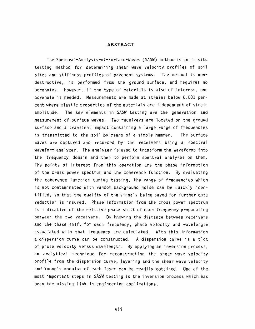
ABSTRACT
The Spectral-Analysis-of-Surface-Waves (SASW) method is an in situ
testing method for determining shear wave velocity profiles of soil
sites and st; ffness profi 1 es of pavement systems. The method ; s non
destruct i ve, is performed from the ground surface, and requi res no
boreholes. However, if the type of materials is also of interest, one
borehole is needed. Measurements are made at strains below 0.001 per
cent where elastic properties of the materials are independent of strain
amplitude. The k.ey elements in SASW testing are the generation and
measurement of surface waves. Two receivers are located on the ground
surface and a transient impact containing a large range of frequencies
is transmitted to the soil by means of a simple hammer. The surface
waves are captured and recorded by the recei vers using a spectral
waveform analyzer. The analyzer is used to transform the waveforms into
the frequency domain and then to perform spectral analyses on them.
The points of interest from this operation are the phase information
of the cross power spectrum and the coherence function. By evaluating
the coherence function during testing, the range of frequencies which
is not contaminated with random back.ground noise can be quickly iden
tified, so that the quality of the signals being saved for further data
reduction is insured. Phase information from the cross power spectrum
is indicative of the relative phase shift of each frequency propagating between the two recei Vers. By k.nowi n9 the di stance between recei vers
and the phase shift for each frequency, phase velocity and wavelength
associated with that frequency are calculated. With this information a dispersion curve can be constructed. A dispersion curve is a plot of phase velocity versus wavelength. By applying an inversion process, an analytical technique for reconstructing the shear wave velocity
profile from the dispersion curve, layering and the shear wave velocity
and Young's modulus of each layer can be readily obtained. One of the
most important steps in SASW testing is the inversion process which has
been the missing link in engineering applications.
vii
viii
Data collection and analysis used in the SASW technique are dis
cussed in detail. Several case studies are presented to illustrate the
utility and versatility of the SASW method. In each case, the results
are compared with those of other well-established testing methods per
formed independently at the same locations. Generally. the shear wave
velocity and Young1s moduli profiles from these independent methods
compare closely.
SUMMARY
In this report, improvements in the practical aspects of the
Spectral-Analysis-of-Surface-Waves (SASW) method since Research Report
256-4 are presented. The SASW method is used to determine the shear
wave velocity and elastic modulus profiles of pavement sections and soil
sites. With this method, a transient vertical impulse is applied to
the surface, and a group of surface waves with different frequencies
are generated in the medium. These waves propagate along the surface
with velocities that vary with frequency and the properties of the
different layers comprising the medium. Propagation of the waves are
monitored with two receivers a known di stance apart at the surface.
By analysis of the phase informaion of the cross power spectrum and by
knowing the distance between receivers, phase velocity, shear wave ve
locity and moduli of each layer are determined. This report contains a comprehensive description of the in situ
testing technique and the in-house data reduction procedure used in
conducting SASW tests.
ix

!!!!!!!!!!!!!!!!!!!"#$%!&'()!*)&+',)%!'-!$-.)-.$/-'++0!1+'-2!&'()!$-!.#)!/*$($-'+3!
44!5"6!7$1*'*0!8$($.$9'.$/-!")':!
IMPLEMENTATION STATEMENT
The Spectral-Analysis-of-Surface-Waves (SASW) method has many ap
plications in material characterization of pavement systems. With this
method, elastic moduli and layer thicknesses of pavement systems can
be evaluated in situ. The method can be utilized as a tool for quality
control during construction and during regular maintenance inspections.
The method can be implemented to evaluate the integrity of flexible
and rigid pavements. Reduction of the experimental data collected in
situ is fully automated. The inversion process is not automated, as
yet. The method has been employed at more than 35 pavement sites to
study the precision and reliability of the method. From this study it
can be concluded that the thicknesses of different layers are generally
within ten percent of those measured from boreholes and the moduli are,
on the average, within 20 percent of moduli measured with other inde
pendent methods employing in situ seismic techniques.
xi

!!!!!!!!!!!!!!!!!!!"#$%!&'()!*)&+',)%!'-!$-.)-.$/-'++0!1+'-2!&'()!$-!.#)!/*$($-'+3!
44!5"6!7$1*'*0!8$($.$9'.$/-!")':!
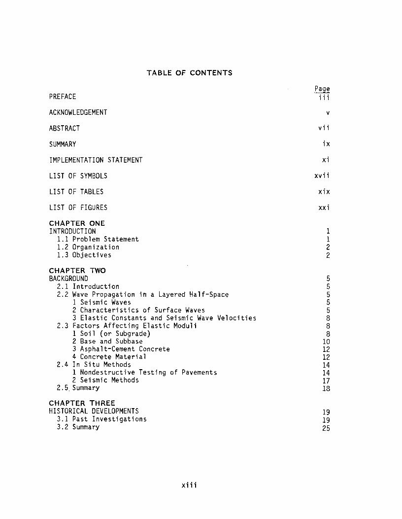
TABLE OF CONTENTS
PREFACE
ACKNOWLEDGEMENT
ABSTRACT
SUMMARY
IMPLEMENTATION STATEMENT
LIST OF SYMBOLS
LIST OF TABLES
LIST OF FIGURES
CHAPTER ONE INTRODUCTION
1.1 Problem Statement 1.2 Organization 1.3 Objectives
CHAPTER TWO BACKGROUND
2.1 Introduction 2.2 Wave Propagation in a Layered Half-Space
1 Seismic Waves 2 Characteristics of Surface Waves 3 Elastic Constants and Seismic Wave Velocities
2.3 Factors Affecting Elastic Moduli 1 Soil (or Subgrade) 2 Base and Subbase 3 Asphalt-Cement Concrete 4 Concrete Material
2.4 In Situ Methods 1 Nondestructive Testing of Pavements 2 Seismic Methods
2.5, Summary
CHAPTER THREE HISTORICAL DEVELOPMENTS
3.1 Past Investigations 3.2 Summary
xiii
Page i ;;
v
vii
ix
x;
xv; ;
xix
xxi
1 1 2 2
5 5 5 5 5 8 8 8
10 12 12 14 14 17 18
19 19 25
xiv
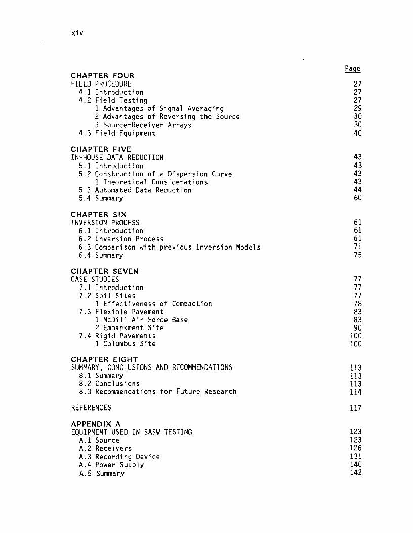
CHAPTER FOUR FIELD PROCEDURE
4.1 Introduction 4.2 Field Testing
1 Advantages of Signal Averaging 2 Advantages of Reversing the Source 3 Source-Receiver Arrays
4.3 Field Equipment
CHAPTER FIVE IN-HOUSE DATA REDUCTION
5.1 Introduction 5.2 Construction of a Dispersion Curve
1 Theoretical Considerations 5.3 Automated Data Reduction 5.4 Summary
CHAPTER SIX INVERSION PROCESS
6.1 Introduction 6.2 Inversion Process 6.3 Comparison with previous Inversion Models 6.4 Summary
CHAPTER SEVEN CASE STUDIES
7.1 Introduction 7.2 Soil Sites
1 Effectiveness of Compaction 7.3 Flexible Pavement
1 McDill Air Force Base 2 Embankment Site
7.4 Rigid Pavements 1 Columbus Site
CHAPTER EIGHT SUMMARY, CONCLUSIONS AND RECOMMENDATIONS
8.1 Summary 8.2 Conclusions 8.3 Recommendations for Future Research
REFERENCES
APPENDIX A EQUIPMENT USED IN SASW TESTING
A.1 Source A.2 Receivers A.3 Recording Device A.4 Power Supply A.5 Summary
Page
27 27 27 29 30 30 40
43 43 43 43 44 60
61 61 61 71 75
77 77 77 78 83 83 90
100 100
113 113 113 114
117
123 123 126 131 140 142
xv
APPENDIX B CONSTRUCTION OF A DISPERSION CURVE FOR A FLEXIBLE PAVEMENT SITE 143
APPENDIX C COMPARISON OF THEORETICAL AND EXPERIMENTAL DISPERSION CURVES AFTER COMPLETION OF INVERSION PROCESS AT WILDLIFE SITE 149
APPENDIX 0 COMPARISON OF THEORETICAL AND EXPERIMENTAL DISPERSION CURVES AFTER COMPLETION OF INVERSION PROCESS AT A FLEXIBLE PAVEMENT SITE 155

!!!!!!!!!!!!!!!!!!!"#$%!&'()!*)&+',)%!'-!$-.)-.$/-'++0!1+'-2!&'()!$-!.#)!/*$($-'+3!
44!5"6!7$1*'*0!8$($.$9'.$/-!")':!

E
exp
f
FFT G
i
v
p
CPR
+
LIST OF SYMBOLS
= Young's Modulus
= Exponential
= Frequency
= Fast Fourier Transform
= Shear Modulus
= 1-1
= Wavelength
= Integer
= Integer = (1<.2 - 1<.2 )
n = Time = Fundamental Period = Compression Wave Velocity
= Shear Wave Velocity = Phase Velocity
= Rayleigh Wave Velocity
= Distance between Receivers
= Depth to Interface n = Coherence Function
= Total Unit Weight = Shear Strain = Increment of Frequency = Increment of Time = Normal Strain = Poisson's Ratio = Pi = 3.14159 ... = Mass Density
= Raw Phase
= Phase
.xvii

!!!!!!!!!!!!!!!!!!!"#$%!&'()!*)&+',)%!'-!$-.)-.$/-'++0!1+'-2!&'()!$-!.#)!/*$($-'+3!
44!5"6!7$1*'*0!8$($.$9'.$/-!")':!
le
2.1
2.2
5.1
7.1
7.2
7.3
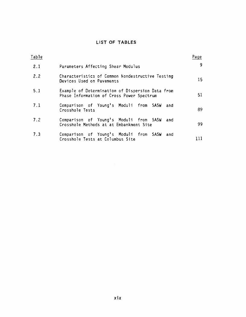
LIST OF TABLES
Parameters Affecting Shear Modulus
Characteristics of Common Nondestructive Testing Devices Used on Pavements
Example of Determination of Dispersion Data from Phase Information of Cross Power Spectrum
Comparison of Young1s Moduli from SASW and Crosshole Tests
Comparison of Young1s Moduli from SASW and Crosshole Methods at at Embankment Site
Comparison of Young1s Moduli from SASW and Crosshole Tests at Columbus Site
xix
15
51
89
99
111

!!!!!!!!!!!!!!!!!!!"#$%!&'()!*)&+',)%!'-!$-.)-.$/-'++0!1+'-2!&'()!$-!.#)!/*$($-'+3!
44!5"6!7$1*'*0!8$($.$9'.$/-!")':!
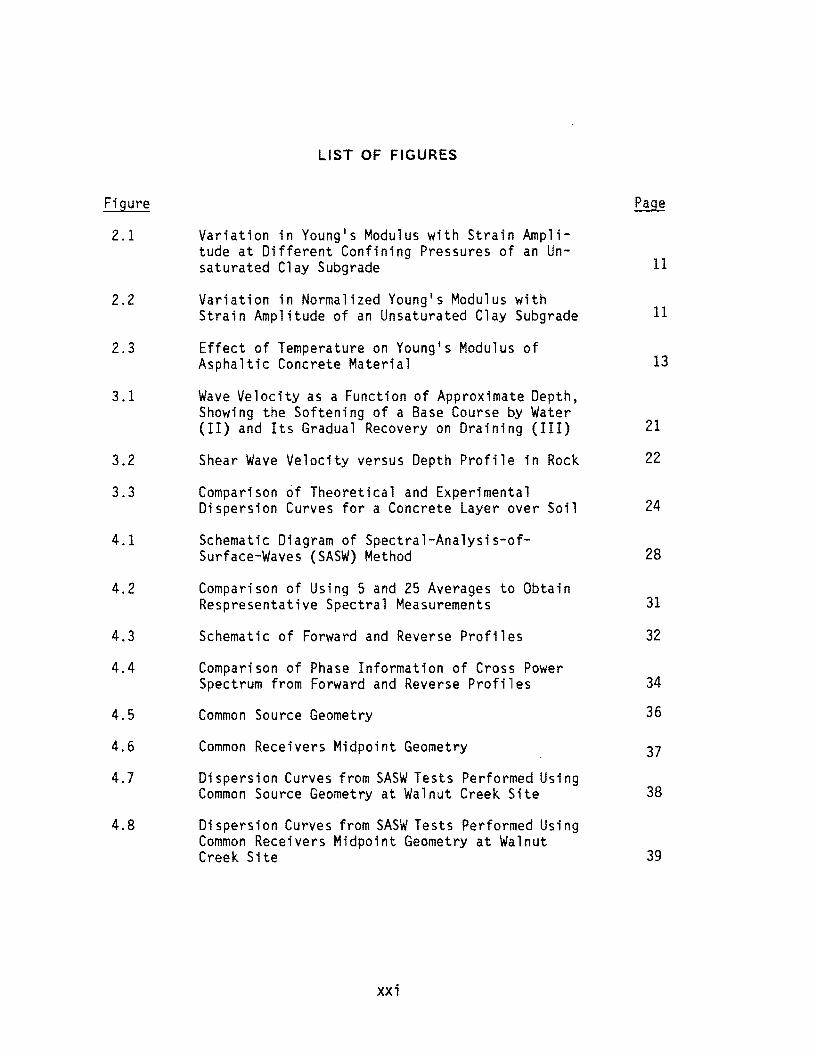
Fi gure
2.1
2.2
2.3
3.1
3.2
3.3
4.1
4.2
4.3
4.4
4.5
4.6
4.7
4.8
LIST OF FIGURES
Variation in Young1s Modulus with Strain Amplitude at Different Confining Pressures of an Unsaturated Clay Subgrade
Variation in Normalized Young1s Modulus with Strain Amplitude of an Unsaturated Clay Subgrade
Effect of Temperature on Young's Modulus of Asphaltic Concrete Material
Wave Velocity as a Function of Approximate Depth, Showing the Softening of a Base Course by Water (II) and Its Gradual Recovery on Draining (III)
Shear Wave Velocity versus Depth Profile in Rock
Comparison of Theoretical and Experimental Dispersion Curves for a Concrete Layer over Soil
Schematic Diagram of Spectral-Analysis-ofSurface-Waves (SASW) Method
Comparison of Using 5 and 25 Averages to Obtain Respresentative Spectral Measurements
Schematic of Forward and Reverse Profiles
Comparison of Phase Information of Cross Power Spectrum from Forward and Reverse Profiles
Common Source Geometry
Common Receivers Midpoint Geometry
Dispersion Curves from SASW Tests Performed Using Common Source Geometry at Walnut Creek Site
Dispersion Curves from SASW Tests Performed Using Common Receivers Midpoint Geometry at Walnut Creek Site
xxi
11
11
13
21
22
24
28
31
32
34
36
37
38
39
xxii
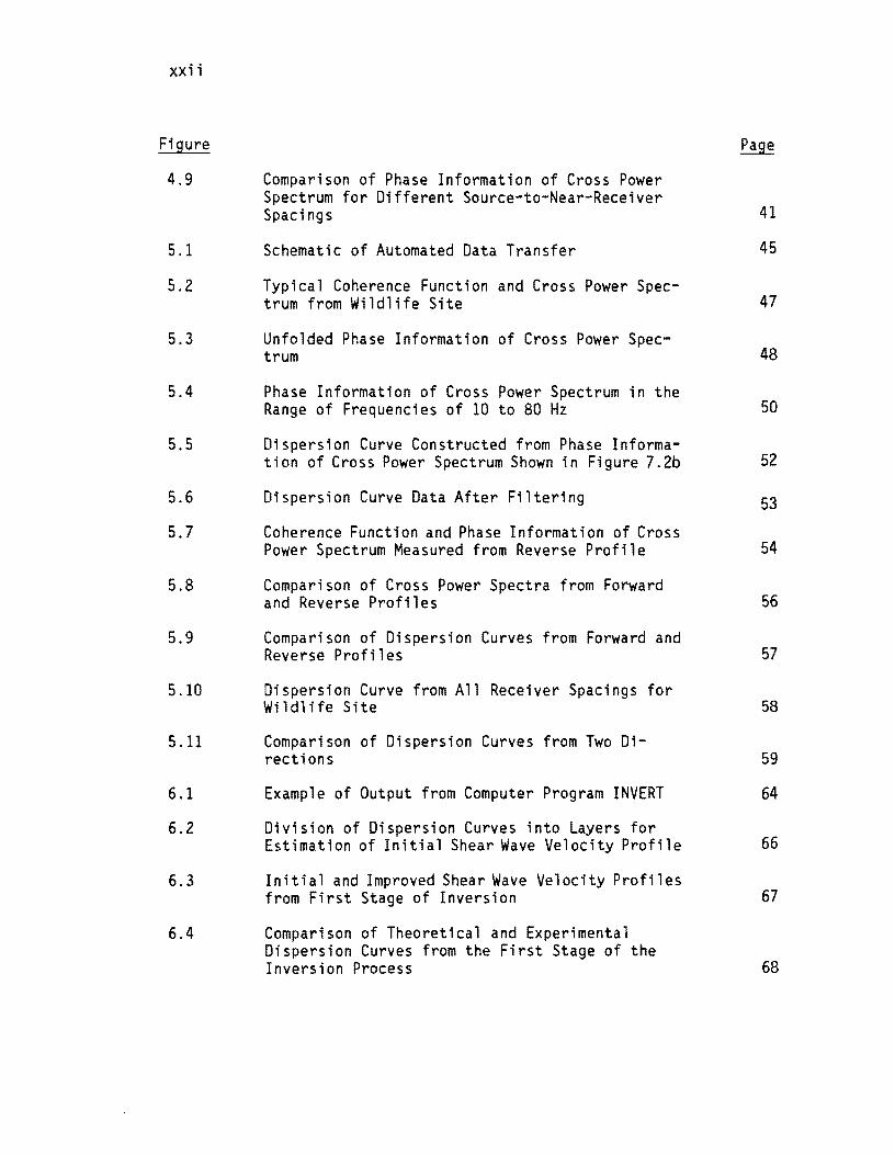
Figure
4.9
5.1
5.2
Comparison of Phase Information of Cross Power Spectrum for Different Source-to-Near-Receiver Spacings
Schematic of Automated Data Transfer
Typical Coherence Function and Cross Power Spectrum from Wildlife Site
5.3 Unfolded Phase Information of Cross Power Spectrum
5.4
5.5
5.6
5.7
5.8
5.9
5.10
5.11
6.1
6.2
6.3
6.4
Phase Information of Cross Power Spectrum in the Range of Frequencies of 10 to 80 Hz
Dispersion Curve Constructed from Phase Information of Cross Power Spectrum Shown in Figure 7.2b
Dispersion Curve Data After Filtering
Coherence Function and Phase Information of Cross Power Spectrum Measured from Reverse Profile
Comparison of Cross Power Spectra from Forward and Reverse Profiles
Comparison of Dispersion Curves from Forward and Reverse Profiles
Dispersion Curve from All Receiver Spacings for Wildlife Site
Comparison of Dispersion Curves from Two Directions
Example of Output from Computer Program INVERT
Division of Dispersion Curves into Layers for Estimation of Initial Shear Wave Velocity Profile
Initial and Improved Shear Wave Velocity Profiles from First Stage of Inversion
Comparison of Theoretical and Experimental Dispersion Curves from the First Stage of the Inversion Process
41
45
47
48
50
52
53
54
56
57
58
59
64
66
67
68
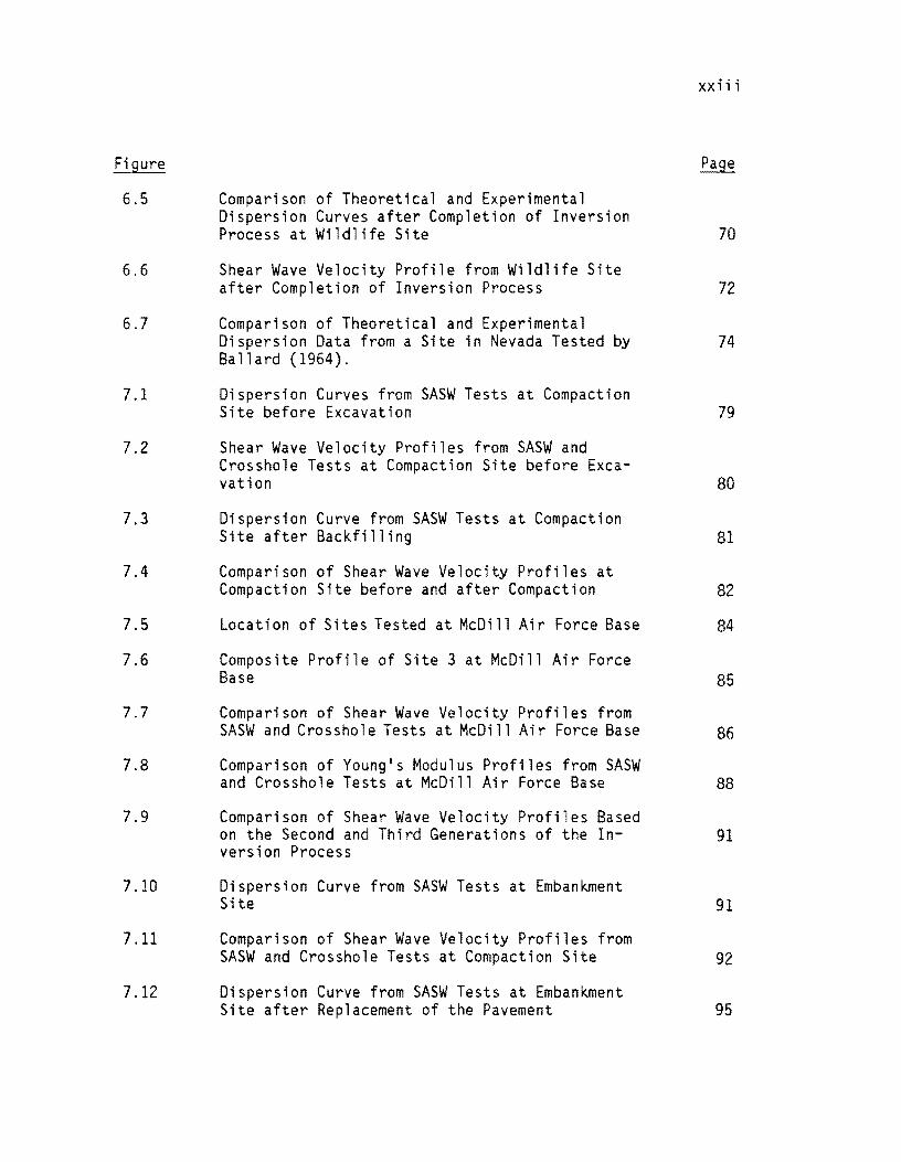
Figure
6.5
6.6
6.7
7.1
7.2
7.3
7.4
7.5
7.6
7.7
7.8
7.9
7.10
7.11
7.12
Comparison of Theoretical and Experimental Dispersion Curves after Completion of Inversion Process at Wildlife Site
Shear Wave Velocity Profile from Wildlife Site after Completion of Inversion Process
Comparison of Theoretical and Experimental Dispersion Data from a Site in Nevada Tested by Ba 11 a rd (1964).
Dispersion Curves from SASW Tests at Compaction Site before Excavation
Shear Wave Velocity Profiles from SASW and Crosshole Tests at Compaction Site before Excavation
Dispersion Curve from SASW Tests at Compaction Site after Backfilling
Comparison of Shear Wave Velocity Profiles at Compaction Site before and after Compaction
Location of Sites Tested at McDill Air Force Base
Composite Profile of Site 3 at McDill Air Force Base
Comparison of Shear Wave Velocity Profiles from SASW and Crosshole Tests at McDill Air Force Base
Comparison of Young's Modulus Profiles from SASW and Crosshole Tests at McDill Air Force Base
Comparison of Shear Wave Velocity Profiles Based on the Second and Third Generations of the Inversion Process
Dispersion Curve from SASW Tests at Embankment Site
Comparison of Shear Wave Velocity Profiles from SASW and Crosshole Tests at Compaction Site
Dispersion Curve from SASW Tests at Embankment Site after Replacement of the Pavement
xx;;;
70
72
74
79
80
81
82
84
85
86
88
91
91
92
95
xxiv
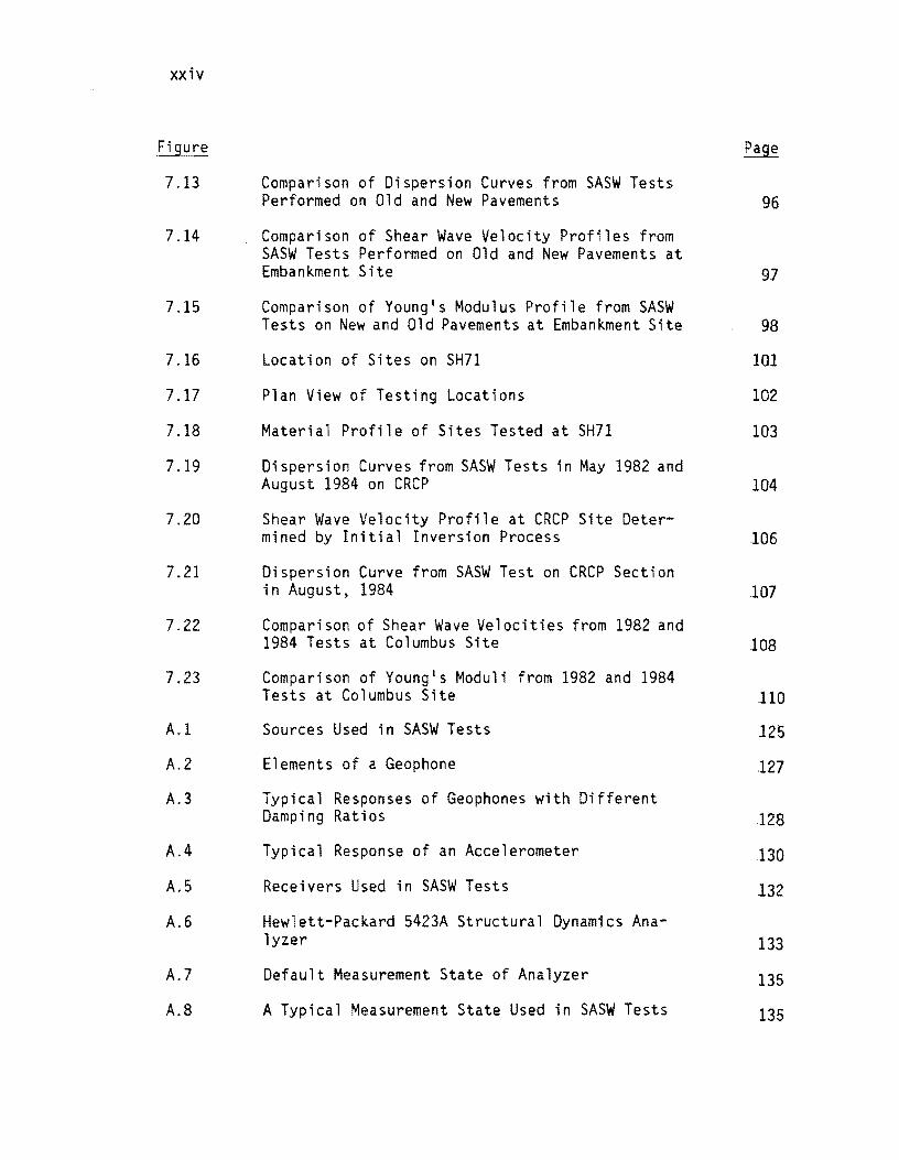
Figure
7.13
7.14
7.15
7.16
7.17
7.18
7.19
7.20
7.21
7.22
7.23
A.l
A.2
A.3
A.4
A.5
A.6
A.7
A.S
Comparison of Dispersion Curves from SASW Tests Performed on Old and New Pavements
Comparison of Shear Wave Velocity Profiles from SASW Tests Performed on Old and New Pavements at Embankment Site
Comparison of Young's Modulus Profile from SASW Tests on New and Old Pavements at Embankment Site
Location of Sites on SH71
Plan View of Testing Locations
Material Profile of Sites Tested at SH71
Dispersion Curves from SASW Tests in May 1982 and August 1984 on CRCP
Shear Wave Velocity Profile at CRCP Site Determined by Initial Inversion Process
Dispersion Curve from SASW Test on CRCP Section in August, 1984
Comparison of Shear Wave Velocities from 1982 and 1984 Tests at Columbus Site
Comparison of Young's Moduli from 1982 and 1984 Tests at Columbus Site
Sources Used in SASW Tests
Elements of a Geophone
Typical Responses of Geophones with Different Damping Ratios
Typical Response of an Accelerometer
Receivers Used in SASW Tests
Hewlett-Packard 5423A Structural Dynamics Analyzer
Default Measurement State of Analyzer
A Typical Measurement State Used in SASW Tests
96
97
98
101
102
103
104
106
107
108
110
J25
127
128
130
132
l33
135
135
Figure
A.9
A.I0
A.ll
A.12
B.1
B.2
B.3
8.4
C.1
C.2
C.3
C.4
C.5
Phase Information of Cross Power Spectra from Different Bandwidths
Effect of Bandwidth on Time Domain Records
Effect of Sensitivity of Recording Channels on Time Records
Effect of Pretriggering Delay on Signals
Typical Spectral Analysis Measurements on a Flexible Pavement Site
Dispersion Curve Constructed from Phase Information of Cross Power Spectrum at Pavement Site (from Fig. B.1b)
Comparison of Dispersion Curve from Forward and Reverse Profiles at Pavement Site
Dispersion Curve from All Receiver Spacings for Flexible Pavement Site
Comparison of Theoretical and Experimental Dispersion Curves after Completion of Inversion Process at Wildlife Site (Range of Wavelengths of 3 to 10 ft)
Comparison of Theoretical and Experimental Dispersion Curves after Completion of Inversion Process at Wildlife Site (Range of Wavelengths of 10 to 20 ft)
Comparison of Theoretical and Experimental Dispersion Curves after Completion of Inversion Process at Wildlife Site (Range of Wavelengths of 20 to 35 ft)
Comparison of Theoretical and Experimental Dispersion Curves after Completion of Inversion Protess at Wildlife Site (Range of Wavelengths of 35 to 50 ft)
Comparison of Theoretical and Experimental Dispersion Curves after Completion of Inversion Process at Wildlife Site (Range of Wavelengths of 50 to 100 ft)
xxv
137
138
139
141
144
145
146
147
150
151
152
153
154
xxvi
Figure
0.1
0.2
0.3
0.4
0.5
0.6
Comparison of Theoretical and Experimental Dispersion Curves after Completion of Inversion Process at Pavement Site (Range of Wavelengths of 0.80 to 1.30 ft)
Comparison of Theoretical and Experimental Dispersion Curves after Completion of Inversion Process at Pavement Site (Range of Wavelengths of 1.30 to 1.80 ft)
Comparison of Theoretical and Experimental Dispersion Curves after Completion of Inversion Process at Pavement Site (Range of Wavelengths of 1.50 to 4.50 ft)
Comparison of Theoretical and Experimental Dispersion Curves after Completion of Inversion Process at Pavement Site (Range of Wavelengths of 4 to 8 ft)
Comparison of Theoretical and Experimental Dispersion Curves after Completion of Inversion Process at Pavement Site (Range of Wavelengths of 5 to 20 ft)
Shear Wave Velocity Profile of the Flexible Pavement Site after Completion of Inversion
156
157
158
159
160
161
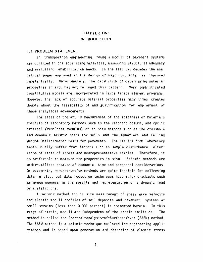
1.1 PROBLEM STATEMENT
CHAPTER ONE
INTRODUCTION
In transportion engineering, Young's moduli of pavement systems
are utilized in characterizing materials, assessing structural adequacy
and evaluating rehabilitation needs. In the last two decades the ana
lytical power employed in the design of major projects has improved
substantially. Unfortunately, the capability of determining material
properties in situ has not followed this pattern. Very sophisticated
constitutive models are incorporated in large finite element programs.
However, the lack of accurate material properties many times creates
doubts about the feasibil ity of and justification for employment of
these analytical advancements.
The state-of-the-art in measurement of the stiffness of materials
consists of laboratory methods such as the resonant column, and cyclic
triaxial (resiliant modulus) or in situ methods such as the crosshole
and downhole seismic tests for soils and the Dynaflect and Falling
Weight Deflectometer tests for pavements. The results from laboratory
tests usually suffer from factors such as sample di sturbance, a 1 ter
ation of state of stress and nonrepresentative samples. Therefore, it
is preferable to measure the properties in situ. Seismic methods are
under-utilized because of economic, time and personnel considerations.
On pavements, nondestructive methods are quite feasible for collecting data in situ, but data reduction techniques have major drawbacks such
as nonuniqueness in the results and representation of a dynamic load
by a static one.
A seismic method for in situ measurement of shear wave velocity and elastic moduli profiles of soil deposits and pavement systems at
small strains (less than 0.001 percent) is presented herein. In this
range of strain, moduli are independent of the strain amplitude. The
method is called the Spectral-Analysis-of-Surface-Waves (SASW) method.
The SASW method is a seismic technique tailored for engineering appli
cations and is based upon generation and detection of elastic stress
1
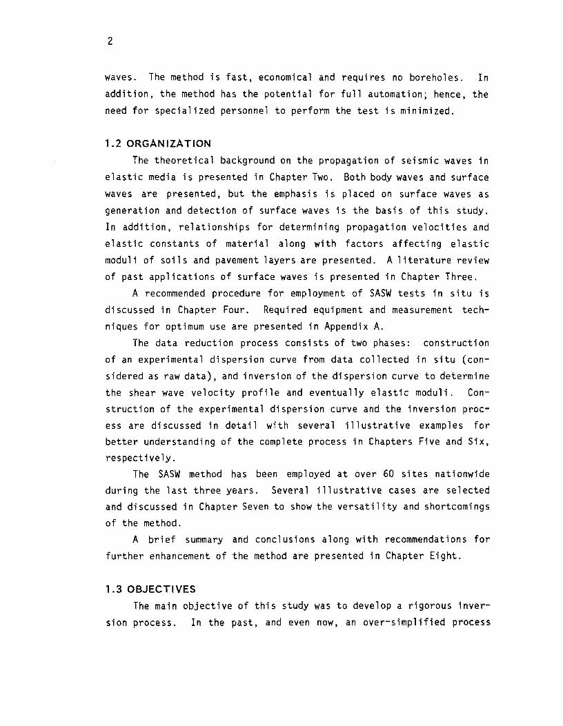
2
waves. The method is fast, economical and requires no boreholes. In
addition, the method has the potential for full automation; hence, the
need for specialized personnel to perform the test ;s minimized.
1.2 ORGANIZATION
The theoretical background on the propagation of seismic waves in
elastic media is presented in Chapter Two. Both body waves and surface
waves are presented, but the emphasis is placed on surface waves as
generation and detection of surface waves is the basis of this study.
In addition, relationships for determining propagation velocities and
elastic constants of material along with factors affecting elastic
moduli of soils and pavement layers are presented. A literature review
of past applications of surface waves ;s presented in Chapter Three.
A recommended procedure for employment of SASW tests in situ is
di scussed in Chapter Four. Requi red equi pment and measurement tech
niques for optimum use are presented in Appendix A.
The data reduct; on process cons; sts of two phases: construction
of an experimental dispersion curve from data collected in situ (con
sidered as raw data), and inversion of the dispersion curve to determine
the shear wave velocity profile and eventually elastic moduli. Construction of the experimental dispersion curve and the inversion proc
ess are discussed in detail with several illustrative examples for better understanding of the complete process in Chapters Five and Six, respectively.
The SASW method has been employed at over 60 sites nationwide during the last three years. Several illustrative cases are selected and discussed in Chapter Seven to show the versatility and shortcomings
of the method. A brief summary and conclusions along with recommendations for
further enhancement of the method are presented in Chapter Eight.
1.3 OBJECTIVES
The main objective of this study was to develop a rigorous inver
si on process. In the past, and even now, an over-simp 1 i fi ed process
3
is used in civil engineering applications. This approximate process
is performed by changing the axes of the dispersion curve; the velocity
axis is multiplied by a constant in the range of 1 to 1.10 and the
wavelength axis ;s divided by 2 or 3. The results from this process
are significantly in error except in the case of near-uniform profiles
as shown by work of Heisey (1981) on pavements as well as earlier in
vestigations by the Corps of Engineers and others as reviewed in Chapter
Three. The rigorous inversion was successfully developed, as discussed
in Chapters Seven and Eight.
Another objective was to apply the SASW method at sites with dif
ferent properties to investigate experimentally the inversion process
which was developed. Over 60 soil and pavement sites and a concrete
dam have been tested. From these tests, a new testing pattern was de
veloped to reduce scatter in the experimental dispersion curve. Also,
during the course of this study, the process of transferring data col
lected in the field to the computer has been fully automated. This work illustrates the applicability of the method for engi
neering purposes. However, more work is needed to refine this process further in aspects concerning the required equipment and the inversion
process in the region of high velocity contrasts.

!!!!!!!!!!!!!!!!!!!"#$%!&'()!*)&+',)%!'-!$-.)-.$/-'++0!1+'-2!&'()!$-!.#)!/*$($-'+3!
44!5"6!7$1*'*0!8$($.$9'.$/-!")':!
2.1 INTRODUCTION
CHAPTER TWO
BACKGROUND
A comprehensive discussion of the theoretical background required
to fully understand the various aspects of SASW testing includes dis
cussions of: 1. wave propagation in a layered medium; 2. Fourier
transforms and spectral analyses; 3. descriptions of alternative test
ing techniques; and 4. theoretical characteristics of surface waves
(which the study is based upon). Such a discussion is presented in an
accompanying report (Nazarian and Stokoe, 1985a). Herein, a brief
overview of essential topics is included for completeness. Should more
information be required on each topic-, the reader is referred to
Nazarian and Stokoe (1985a).
2.2 WAVE PROPAGATION IN A LAYERED HALF-SPACE
For engineering purposes, many soil and most pavement sites can
be approximated by a layered half-space with reasonable accuracy; es
pecially over short lateral distances. With this approximation, the
profiles are assumed to be homogeneous and to extend to infinity in two
horizontal directions while being heterogeneous in the vertical direc
tion. This heterogeneity is often modelled by a number of layers with
constant properties within each layer. In addition, it is assumed that
the material in each layer is elastic and isotropic. The waves are assumed to be plane. A medium characterized by these assumptions is called an ideal medium.
2.2.1 Seismic Waves
Wave motion created by a disturbance within an ideal whole-space
can be described by two kinds of waves: compression waves and shear
waves. These waves are collectively called body waves as they travel
within the body of the medium. Compression (P) and shear (S) waves can
be distinguished by the direction of particle motion relative to the
direction of wave propagation.
5
6
In a half-space, other types of waves occur in addition to body
waves. These waves are ca 11 ed surface waves or Rayl ei gh waves.
Rayleigh waves propagate near the surface of the half-space. Rayleigh
waves (R-waves) propagate at a speed of approximately 90±5 percent of
S-waves. Particle motion associated with R-waves is composed of both
vertical and horizontal components, which, when combined, form a
retrograde ellipse close to the surface.
2.2.2 Characteristics of Surface Waves
In a homogeneous, isotropic, elastic, half-space, the velocity of
surface waves does not vary with frequency. However, since the prop
erties of earth materials typically exhibit variations with depth (are
not homogeneous vertically), surface wave velocities vary with fre
quency. This frequency dependency of wave velocity in a heterogeneous
medium is termed dispersion, and surface waves are thus said to be
dispersive. A plot of wave velocity versus frequency (or wavelength)
is called a dispersion curve.
The di spersive character; stic of a wave can be demonstrated by
means of phase velocity. Phase velocity is defined as the velocity with
which a seismic disturbance of a given frequency is propagated in the
medium over the horizontal distance between the source and receivers.
The study of dispersion of waves in a horizontally-layered halfspace relies upon derivation of the so-called dispersion function
(i.e., the relationship between phase velocity and frequency). Thomson
(1950) and Haskell (1953) introduced the first matrix solution to this
problem. In the classical approach, the dispersion function and wavelengths
(or frequencies) are obtained by vanishing a determinant whose elements
are functions of mass densities and elastic moduli of the layers as well
as phase velocity and frequency.
The Haskell-Thomson technique builds up the (surface wave)
dispersion function as the product of layer matrices which relate the
displacement components as well as the stress components acting on the
interface to those associated with the next interface. The product of
7
these layer matrices then relates the stress and displacement compo
nents of motion at the deepest interface to those at the free surface.
However, the Haskell-Thomson solution exhibits numerical difficulties
at high frequencies. Dunkin (1965) presented a new approach to cir
cumvent these numerical difficulties. Thrower (1965) also proposed an
approach whi ch is more appropri ate for determi nat i on of di spers ion
curves in 1 aye red medi a such as pavements where the 1 ayers become
gradua lly softer. The 1 ast two approaches are used in thi s study.
These different approaches are discussed in full detail in Nazarian and
Stokoe (1985a).
The shape of a dispersion curve is affected by three independent
properties of the material composing each layer for a given profile.
These properties are:
and (iii) mass density.
(i) shear wave velocity, (ii) Poisson's ratio,
It is demonstrated (Nazarian and Stokoe, 1985a)
that the effect of the last two parameters on dispersion of waves is quite small. Therefore, only the effect of shear wave velocity is
discussed herein.
In an elastic medium, surface waves are dispersive only if a ve
locity contrast exists in the layering. At short wavelengths, the phase
velocities are close to the R-wave velocity of the top layer. In other
words, for waves with short wavelengths (relative to the height of the
layers) the half-space has very little effect on the dispersion curve.
For these short wavelengths, the top layer acts like a half-space by
itself. The other extreme involves long wavelengths. In this case phase
velocities are quite close to the R-wave velocity of the last layer which means that the top layers do not have an appreciable affect on
the dispersion curve. However, between these two extremes there is a transition zone in which the phase velocity is bound between the R-wave
velocities of the least stiff and stiffest layers in the profile. The
extent of this transition zone in the intermediate wavelengths depends
on the velocity contrast between the layers.
8
The topics introduced in this section are detailed in Nazarian and
Stokoe (1985a). It is recommended that the reader refer to that ref
erence for more information on these matters.
2.2.3 ELASTIC CONSTANTS AND SEISMIC WAVE VELOCITIES
In transportation engineering for material characterization and
the design of overlays, Young's moduli of the different layers should
be measured. Calculation of elastic moduli from propagation velocities
is, thus, important.
Shear wave velocity, Vs ' is used to calculate shear modulus, G, by:
G = p • V 2 S
(2.1)
in which p is the mass density. Mass density is equal to, ltjg, where
It is total unit weight of the material and g is gravitational accel
eration. If Poisson's ratio (or compression wave velocity) 1s known,
other moduli can be calculated for a given Vs' Young's and shear moduli are re 1 a ted by:
E = 2G (1 + v) (2.2)
2.3 FACTORS AFFECTING ELASTIC MODULI
2.3.1 Soil (or Subgrade)
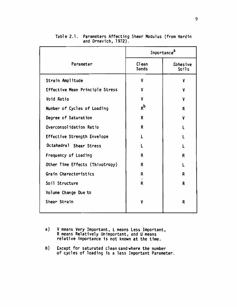
Based upon numerous laboratory tests, Hardin and Drnevich (1972) proposed many parameters that affect the modul i of soil s. These pa
rameters, along with their degree of importance in affecting moduli, are tabulated in Table 2.1. They suggested that state of stress, void
ratio, and strain amplitude are the main parameters affecting moduli
measured in the laboratory. However, for this study dealing with
measurement of moduli in situ, the main factors affecting the elastic
moduli and wave velocities are void ratio and state of stress (confining
stress).
Tabl e 2.l. Parameters Affecting Shear Modulus (from Hardin and Drnevich, 1972).
Importancea
Parameter Clean Cohesive Sands
Strain Amplitude V
Effective Mean Principle Stress V
Void Ratio V
Number of Cycles of Loading Rb
Degree of Saturation R
Overconsolidation Ratio R
Effective Strength Envelope L
Octahedral Shear Stress L
Frequency of Loading R
Other Time Effects (Thixotropy) R
Grain Characteristics R .
Soil Structure R
Vo 1 ume Change Due to
Shear Strain V
a) V means Very Important, L means Less Important, R means Relatively Unimportant, and U means relative importance is not known at the time.
b) Except for saturated clean sand where the number of cycles of loading is a less Important Parameter.
Soils
V
V
V
R
V
L
L
L
R
L
R
R
R
9
10
Strain amplitude has essentially no effect on the in situ tests
because the measurements are performed at very low strains. Up to a
strain amplitude of about 0.01 percent, moduli are nearly constant, with
a slight decrease in the range from 0.001 to 0.01 percent. This constant
modulus is called the elastic modulus, or maximum modulus.
strain level of 0.01 percent, moduli decrease significantly. Above a
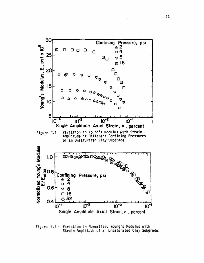
A typi ca 1 example of the variation in Young's modulus, E, with normal strain, £,
for a stiff clay is shown in Figs. 2.1 and 2.2. An undisturbed sample
of stiff clay from San Antonio, Texas was tested using the resonant
column method (Richart et al, 1970). The variation of E with log £ at
several confining pressures is shown in Fig. 2.1. As the confining
stress increases, the low-amplitude modulus increases, as shown in this
figure. Also, it is evident that below strain levels of 0.001, E is constant and independent of strain at each pressure.
The effect of strain on modulus is easily seen by plotting the
variation of normalized modulus, E/Emax ' versus log £ as shown in Fig.
2.2. In this figure, Emax is taken as the maximum value of Young's modulus at each confining pressure. It can be seen that normalized
modulus is constant below a strain of about 0.001 percent and is equal
to Emax Also, all modulus-strain curves are nearly independent of confining pressure once they are normalized. If a normalized modulus
strain curve such as that shown in Fig. 2.2 is available for the material, then moduli at higher strains can be determined once Emax has been measured.
2.3.2 Base and Subbase Two types of base and subbase materials are usually used, granular
or treated materials. Granular base and subbase materials demonstrate
the same characteristic as natural soil deposits. The base or subbase material are sometimes treated by additives such as cement, bitumen,
or lime. In this situation, the moduli of the layer depends on addi
tional factors such as type of aggregate and percentage of additive.
Typical values of Young's moduli for granular and treated layers are
in the range of 15 to 110 ksi (100 to 750 MPa) and 50 to 2000 ksi (350
30-------------------------------Confining Pressure t psi
JC 251-.... en Q.
l::J l::J l::J l::J l::J 62
l::J Q4
l::J l::J ~ 8 l::JIS
l::J l::J o
5 I •• 1 1,,,.1 I I •• 1 I
10-4 10-3 10-2 10-' Single Amplitude Axial Strain. c • percent
Figure 2.1 - Variation in Young's Modulus with Strain Amplitude at Different Confining Pressures of an Unsaturated Clay Subgrade.
en .a .a ~ 1.0
Confining a. 2 Q 4 ~ 8
Pressure. psi
-
-
-
-
l::J IS 032 0.4 '--~...I....I....&....J...u..u..-=---'--'-'-L..I.,..J.J~~--J.....L..L..L..L..I.i~
10-4 10-5 10-2 10-1
Single Amplitude Axial Strain, ~ , percent
Figure 2.2 - Variation in Nonnalized Young's Modulus with Strain Amplitude of an Unsaturated Clay Subgrade.
11
12
to 14000 MPa), respectively. Poisson's ratio of these materials are
on the order of 0.20 to 0.45 (Yoder and Witczak, 1975).
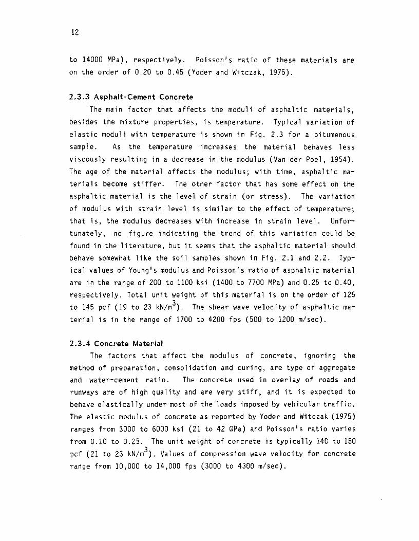
2.3.3 Asphalt-Cement Concrete
The main factor that affects the moduli of asphaltic materials,
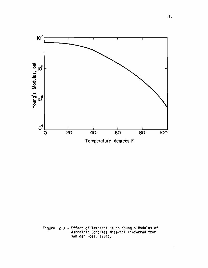
besides the mixture properties, is temperature. Typical variation of
elastic moduli with temperature is shown in Fig. 2.3 for a bitumenous
sample. As the temperature increases the material behaves less
viscously resulting in a decrease in the modulus (Van der Poel, 1954).
The age of the material affects the modulus; with time, asphaltic ma
terials become stiffer. The other factor that has some effect on the
asphaltic material is the level of strain (or stress). The variation
of modulus with strain level is similar to the effect of temperature;
that is, the modulus decreases with increase in strain level. Unfor
tunately, no figure indicating the trend of this variation could be
found in the literature, but it seems that the asphaltic material should
behave somewhat like the soil samples shown in Fig. 2.1 and 2.2. Typ
ical values of Young's modulus and Poisson's ratio of asphaltic material
are in the range of 200 to 1100 ksi (1400 to 7700 MPa) and 0.25 to 0.40,
respectively. Total unit weight of this material is on the order of 125 to 145 pcf (19 to 23 kN/m3). The shear wave velocity of asphaltic ma
terial is in the range of 1700 to 4200 fps (500 to 1200 m/sec).
2.3.4 Concrete Material
The factors that affect the modulus of concrete, ignoring the
method of preparation, consolidation and curing, are type of aggregate and water-cement ratio. The concrete used in over1 ay of roads and
runways are of high quality and are very stiff, and it is expected to
behave elastically under most of the loads imposed by vehicular traffic.
The elastic modulus of concrete as reported by Yoder and Witczak (1975)
ranges from 3000 to 6000 ksi (21 to 42 GPa) and Poisson's ratio varies
from 0.10 to 0.25. The unit weight of concrete is typically 140 to 150
pcf (21 to 23 kN/m3). Values of compression wave velocity for concrete
range from 10,000 to 14,000 fps (3000 to 4300 m/sec).
�o7--------~------~------~--------~------~
Id' O~-----2~O------4~O------6~O------8~O-----IO~O
Temperature, degrees F
Figure 2.3 - Effect of Temperature on Young's Modulus of Asphaltic Concrete Material (inferred from Van der Poel, 1954).
13
14
2.4 IN SITU METHODS
Properties of materials are either measured in the laboratory or
in situ, or are determined by empirical methods. Normally, values from
laboratory tests underestimate the in situ results by anywhere from 10
to several hundred percent. The major reasons for this discrepancy can
be due to sampling disturbance, differences in the state-of-stress be
tween the sample and actual deposits, nonrepresentative samples, long
term time effect, and inherent errors in in situ tests (Anderson and
Woods, 1975). Laboratory tests are essential to study the parameters
that affect the properties of the material. In situ tests are more
suitable for determining accurate values of low-amplitude dynamic
properties in the field. However, in situ methods are under-utilized
as they are expensive and highly specialized personnel are often re
quired to perform them.
2.4.1 Nondestructive Testing of Pavements
Nondestructive testing of pavements is done by making surface
measurements of the response of a pavement structure to an external
force. The response is generally in terms of measurement of surface
deflection at several points. Elastic theory in a layered medium is
then employed to back-calculate the elastic properties of different
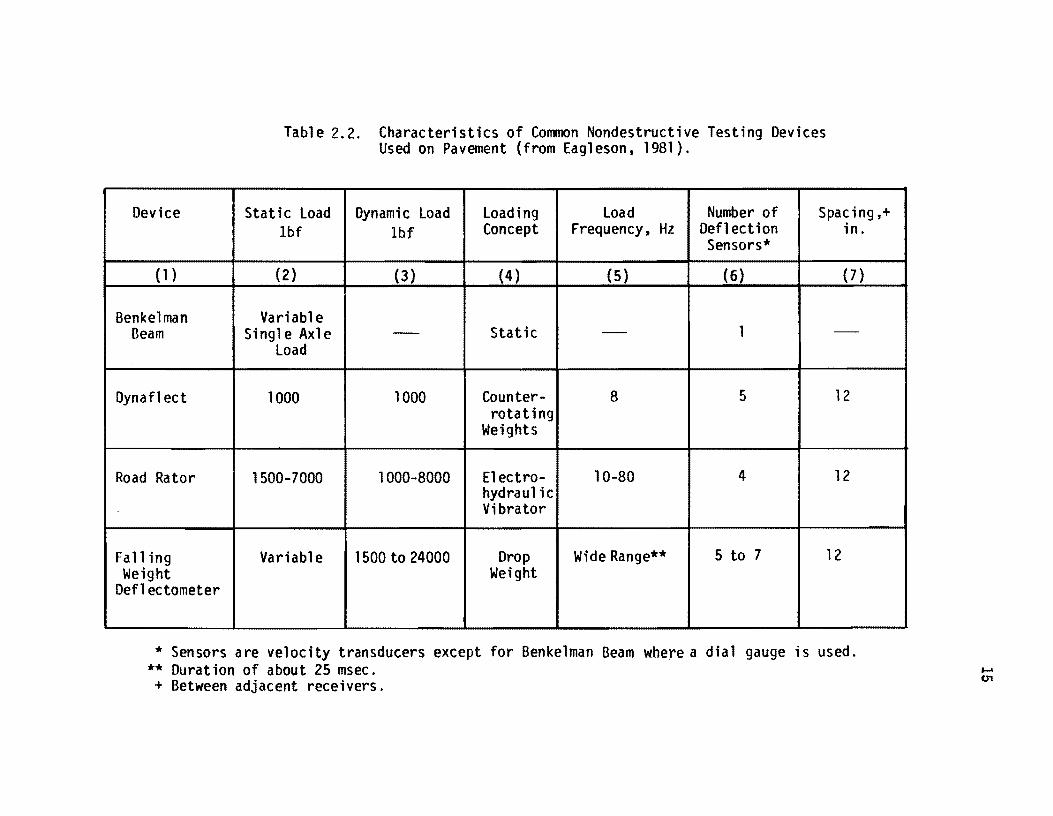
1 ayers. Lytton et al (1975) studied different nondestructive methods in
some detail. The major differences between different methods is the way the load is imparted to the pavement and the number and position
of points at which deflections are measured. The characteristics of
some deflection measuring devices are presented in Table 2.2. The methods that are based upon application of static loads consist of the
Plate loading test, Benkelman beam, traveling deflectometer, Lacroix
deflectograph, and curvature meter (see Haas and Hudson, 1978). Vi
bratory nondestructive methods apply a steady-state load to the pave
ment surface after applying some static seating load. The main devices
in this category are Dynaflect, road rator, Waterways Experiment Sta
tion (WES) vibrator, and Federal Highway Adm'inistration (FHWA) thumper.
Device
(1)
Benkelman Beam
Dynafl ect
Road Rator
Fall ing Weight
Defl ectometer
Table 2.2. Characteristics of Common Nondestructive Testing Devices Used on Pavement (from Eagleson, 1981).
Static load Dynami c load loading load Number of Spacing ,+ Ibf Ibf Concept Frequency, Hz Deflection in.
Sensors*
{2} (3) (4 ) (5) (6) (7)
Vari ab1 e Single Axle - Static - 1 -
load
1000 1000 Counter- 8 5 12 rotating
Weights
1500-7000 1000-8000 Electro- 10-80 4 12 hydraul ic Vibrator
Variabl e 1500 to 24000 Drop Wide Range** 5 to 7 12 Weight
* Sensors are velocity transducers except for Benkelman Beam where a dial gauge is used. ** Duration of about 25 msec. + Between adjacent receivers.
..... en
16
Devices that use an impact as the source are the falling weight
deflectometer. California (CAL) impulse testing. and Washington State
University impulse testing. although the WES vibrator, FHWA thumper and
road rator can also be used as impact (or static) devices.
Two devices which are widely used today to nondestructively test
pavements are the Dynaflect and falling weight deflectometer. In the
Dynaflect device. a peak dynamic force of 1000 lb (4500 N) is generated
by two counter-rotating eccentric masses at a frequency of 8 Hz. This
fOt'ce is transmitted to the pavement by two, 4-in. (lO-cm) wide wheels.
Five equally spaced geophones are used to measure deflections of the
pavement system due to the load.
The falling weight deflectometer (FWD) is different ft'om the
dynaflect device in terms of field testing procedure. The differences
are basically in the number of receivers. as seven geophones are used,
and the load. The load is developed by dropping a weight on a plate
set on the pavement surface. The energy of the impact can be varied
by changing the drop height or drop weight. The peak loading force
varies ft'om 1.5 to 24 k.ips (6.6 to 106 kN). The duration of impulse
is around 25 to 30 msec. which simulates the duration of a load imposed
by a moving wheel at 40 mph (64 km/h).
In the ana lys is of the 1 oad-defl ect i on measurements, both the
Dynaflect and FWD are similar. The pavement is modelled as a multi
layered linear elastic system, and each layer is characterized by
Young's modulus and Poisson's ratio. A computer program based upon
linear elastic theory with static loading is then used to predict the
defl ect ions at the measurement poi nts. Computed and measured de
flections are compared. and necessary adjustments in the value of the
elastic modulus of each layer are made until measured and computed de
flections compare well. This process is called "deflection-basin fit
ting.1I
The major assumptions in the deflection-basin fitting approach
are:
1. the layers are assumed to be elastic,
2. the dynamic load can be replaced by an equal static load,
17
3. measured dynamic deflections are assumed equal to theoretical
static deflections, and 4. the pavement layers extend horizontally to infinity, and
5. the subgrade has constant stiffness and is extended to infinity or to a rigid layer underlying the subgrade at some depth.
The main advantages of these two methods are mobility and rapid
testing in the field. However, these methods do not yield a unique
solution as several combinations of moduli can be determined to produce
a theoretical basin which matches the experimental deflection basin.
This nonuniqueness becomes more pronounced as the number of layers as
sumed in the theoretical profiles is increased. As such, the number
of layers are normally limited to three or four and the thickness of
each layer must be assumed.
2.4.2 Seismic Methods
Seismic methods are normally performed at low-strain levels. Low-strain moduli are presently the most important dynamic property of
soils measured in the field. Once this parameter is combined with laboratory tests, values of moduli in the field at different strain
levels can be obtained. Several different procedures to predict the
in situ shear modulus-strain relationship based upon field and labora
tory tests have been proposed (Stokoe and Richart, 1973; Anderson and Woods, 1975; and Stokoe and Chen, 1980). A detailed discussion on the
sources of differences between in situ and laboratory results; methods of estimating the in situ shear moduli from laboratory tests; and other in situ tests such as the standard penetration tests (SPT) and cone penetration test (CPT) which have also been used to estimate modulusstrain relationships can be found in Hoar (1982).
Common methods used for in situ measurement of propagation velocities and moduli at low strains are discussed in Nazarian (1984). The state-or-practice in field seismic measurements for engineering pur
poses have been reviewed by Richart (1978), Woods (1978), Geophysical
Exploration by U.S. Corps of Engineers (1979), Stokoe (1980), and Hoar
(1982).
18
2.5 SUMMARY
In this chapter, the different types of waves that propagate in a
layered medium are presented. Waves of most importance to this study
are compression, shear and Rayleigh waves. The propagation velocities
of these waves are defined, and the relationship of material stiffness
to propagation velocities are presented. Also factors that affect the
stiffness of different types of materials such as soil, asphalt-cement
concrete, and portland-cement concrete are discussed. In soils, strain
amplitude has the most effect on elastic moduli, but it can be neglected
in this study as testing is being performed in the low-strain range
where moduli are independent of strain. Therefore, the major parameters
that affect moduli of soils are void ratio and state of stress. Tem
perature and age are parameters that affect moduli the most for asphalt
concrete, while for portland-cement concrete type of aggregates,
water-cement ratio and curing are the significant factors.
CHAPTER THREE
HISTORICAL DEVELOPMENTS
3.1 PAST INVESTIGATIONS
The first known use of surface waves to determine soil properties
for engineering purposes was credited to the German Society of Soil
Mechanics before World War II (DEGEBO, 1938). The primary interest of
that study was to investigate the response of a foundation to steady
state vibration. A rotating-mass oscillator was used as a source to
excite foundations in the range of frequencies between 10 and 60 Hz.
Due to the lack of sensitive receivers in that period, excessive loads
had to be imposed on the soil to generate adequate signals. As a re
sult, nonlinear behavior was generated in the soil and somewhat unsuc
cessful application of the method occurred.
Bergstrom and Linderho1m carried out similar tests in Sweden in 1946. Thi s work was done on a fai r1y uniform soil whi ch resulted in
the surface waves exhibiting little dispersion in the study range of
14 to 32 Hz. They compared Young's moduli determined from surface wave
and plate bearing tests in an attempt to correlate the modulus of sub
grade reaction with Young's modulus. Plates with different diameters were used in the plate bearing tests. They found that the moduli of
subgrade reaction from the large-diameter plates correlated well with the dynamic moduli from the surface wave tests. However, results from the smaller-diameter plates did not yield any appreciable relationship between the subgrade and dynamic moduli.
Van der Poe1 (1951) and Nijboer and Van del Poe1 (1953) investigated a flexible pavement system in Holland using surface waves. The range of frequencies in their tests was 10 to 60 Hz which corresponded to waves predominantly propagating in the subgrade soil.
Henke10m and Klomp (1962) used steady-state vibrators to perform
surface wave tests on pavements. Mechanical and electrodynamic vibra
tors were used to generate low frequency (4 to 60 Hz) and high frequency
(greater than 60 Hz) waves in their tests. The effect of drainage of
the subgrade after a flood was investigated. The S-wave velocity pro-
19
20
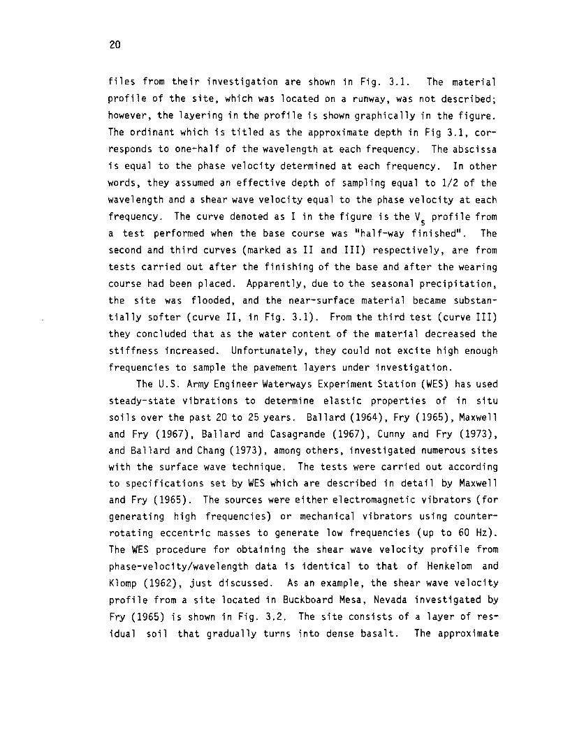
files from their investigation are shown in Fig. 3.1. The material
profile of the site, which was located on a runway, was not described;
however, the layering in the profile is shown graphically in the figure.
The ordinant which is titled as the approximate depth in Fig 3.1, cor
responds to one-half of the wavelength at each frequency. The abscissa
is equal to the phase velocity determined at each frequency. In other
words, they assumed an effective depth of sampling equal to 1/2 of the
wavelength and a shear wave velocity equal to the phase velocity at each
frequency. The curve denoted as I in the figure is the Vs profile from
a test performed when the base course was "ha 1 f-way fi ni shed" . The
second and third curves (marked as II and III) respectively, are from
tests carried out after the finishing of the base and after the wearing course had been placed. Apparently, due to the seasonal precipitation,
the site was flooded, and the near-surface material became substan
tially softer (curve II, in Fig. 3.1). From the third test (curve III)
they concluded that as the water content of the material decreased the stiffness increased. Unfortunately, they could not excite high enough
frequencies to sample the pavement layers under investigation.
The U.S. Army Engineer Waterways Experiment Station (WES) has used steady-state vibrations to determine elastic properties of in situ
soils over the past 20 to 25 years. Ballard (1964), Fry (1965), Maxwell
and Fry (1967), Ballard and Casagrande (1967), Cunny and Fry (1973), and Ballard and Chang (1973), among others, investigated numerous sites with the surface wave technique. The tests were carried out according to specifications set by WES which are described in detail by Maxwell and Fry (1965). The sources were either electromagnetic vibrators (for generating high frequencies) or mechanical vibrators using counterrotating eccentric masses to generate low frequencies (up to 60 Hz).
The WESprocedure for obtaining the shear wave velocity profile from
phase-velocity/wavelength data is identical to that of Henkelom and
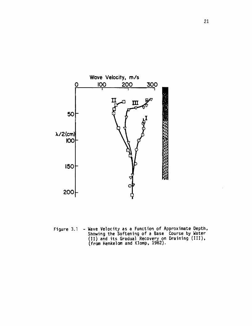
Klomp (1962), just discussed. As an example, the shear wave velocity
profile from a site located in Buckboard Mesa, Nevada investigated by
Fry (1965) ;s shown in Fig. 3.2. The site consists of a layer of res
idual soil that gradually turns into dense basalt. The approximate
50
)./2(cm 100
150
200
21
Wave Velocity. m/s o 100 200 300
Figure 3.1 - Wave Velocity as a Function of Approximate Depth, Showing the Softening of a Base Course by Water (II) and its Gradual Recovery on Draining (III), (from Henkelom and Klomp, 1962).
22
0
10
20
30
40
--.If 0..50 Q.) o Q.) -o .§ 60 )(
o .... R <t 70
80
90
1500 2000 0
0
0
100 L..---J.-__ J.-__ J.-_---J
Residual Topsoi I
Transitional Zone Top Soil and Fractured Rack
VesiCular Basalt
Dense Bosalt
Fig. 3.2 - Shear Wave Velocity versus Depth Profile in Rock (after FrYt 1965).
23
depths correspond to one-half of the wavelengths, and the shear wave
velocities are assumed to be identical to propagation velocities meas
ured in situ. Cunny and Fry (1973) compared in situ elastic moduli from
surface waves tests with moduli obtained by resonant column tests at
14 sites. Cunny and Fry concluded that the laboratory-determined shear
and Young's moduli were generally within ±50 percent of the in situ
modul i. Woods and Richart (1967) performed a series of surface wave
tests in conjunction with a testing program set up to study the effect
of trenches in screening elastic waves. They followed the procedure
proposed by WES.
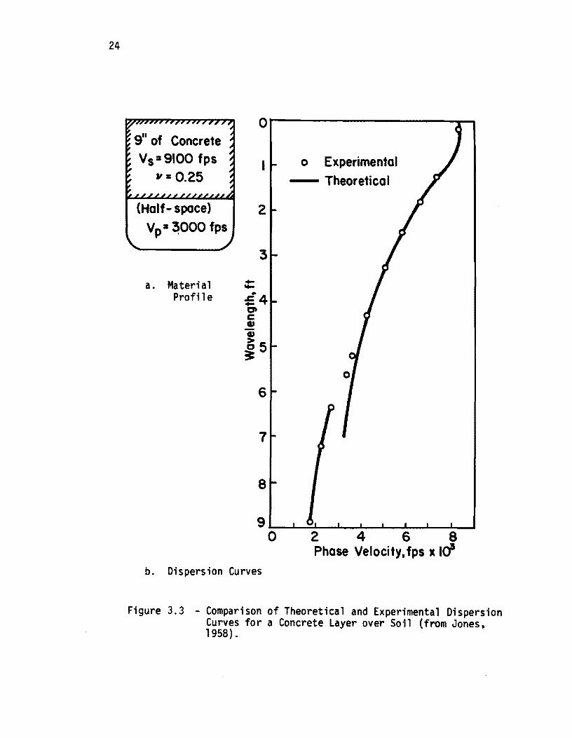
The greatest recent contribution in theoretical and practical as
pects of surface wave testing on pavements was by Jones (1958). He
proposed an analytical procedure to compute the moduli of different
layers in a pavement system. An example of his investigation on a
pavement section consisting of a 9-in. (23-cm) thick (nominally) con
crete layer over subgrade is shown in Fig. 3.3. He assumed that the
subgrade was a liquid layer and treated the concrete slab as a plate.
From his study he reported the thickness of the concrete as 9.5 in. (24 cm). Upon coring, the concrete thickness was found to be quite close
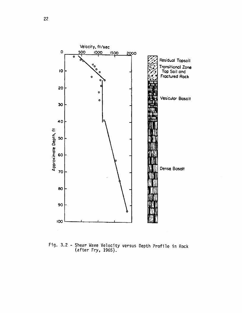
to 9.5 in. (24 cm). Four groups of investigators have employed the spectral analysis
of surface waves principles to collect data in situ. Williams (1981)
used a vibrator connected to broad-band noi se- generator (as opposed
to a sine wave-generator) and a hammer as sources. These two sources, and sources similar to them, have the ability to generate waves over a wide range of frequencies. If the waves generated by these sources are captured on an appropriate recording device, Fourier transformed, and spectral analysis performed on them, the testing time can be reduced quite significantly (see Chapter Four). Williams' interest was solely limited to constructing the experimental dispersion curves, and he did
not report any shear wave velocity profile.
Heisey (1981) used hammer blows to generate transient signals to
construct the dispersion curves. He used a spectral analyzer as the
recording device which accelerated the in-house data reduction several
24
9" of Concrete V s :I 9100 fps
If = 0.25
(Half- space) Vp=~OOO fps
a. Material Profile
Or---------------------~
-""" .£4 c:P c cu a; ~5 :t
6
o Experimental -- Theoretical
0
9~~~~~~~~~ __ ~~ o 2 4 6 8
Phase Velocity, fps x 10' b. Dispersion Curves
Figure 3.3 - Comparison of Theoretical and Experimental Dispersion Curves for a Concrete Layer over Soil (from Jones, 1958) •
25
folds over Williams' approach (a tape recorder). Based upon tests on
several soil and pavement sites, Heisey suggested an effective depth
of sampling equal to 1/3 of the wavelength for each frequency. He also
divided the surface wave velocities measured in the field by a factor
approximately equal to 0.90 to obtain shear wave velocities.
Neilson and Baird (1975, and 1977) and Baird (1982) from the New
Mexico Engineering Research Institute constructed a van to collect
surface wave data conveniently. This van consists of a system operators
area and a support equipment area. A data acquisition system along with
a system to control the deployment of an impact system are located in
the system operators area. The support equipment area houses a 215-lb
(950-N) programmable drop weight and two generators. The height of the
drop and the wei ght of the 1 oadi ng system can be changed. The drop
weight impacts a 12-in. (3D-cm) diameter plate. The impulses are si
multaneously monitored with as many as eight accelerometers. The data
reduction is arbitrary and requires empirical correction factors to
obtain moduli of the different layers.
3.2 SUMMARY
In summary, in all the investigations reported above, in situ
testing procedures may differ; however, invariably the goal is to de
termine the relationship between the propagation velocity of surface
waves and wavelengths, called a dispersion curve. The next step is then
to obtain a shear wave velocity-depth relationship based upon the dispersion information. In all the studies [except Jones (1958)J. the
dispersive characteristic of surface waves was neglected which caused an inaccuracy in the values of shear wave velocities. The reason for
this inaccuracy and an alternative process for determining the shear
wave velocity profile from a given dispersion curve are presented in Chapter Six.

!!!!!!!!!!!!!!!!!!!"#$%!&'()!*)&+',)%!'-!$-.)-.$/-'++0!1+'-2!&'()!$-!.#)!/*$($-'+3!
44!5"6!7$1*'*0!8$($.$9'.$/-!")':!
4.1 INTRODUCTION
CHAPTER FOUR
FIELD PROCEDURE
With the SASW method, both the source and receivers are located
on the surface of a site. Surface waves at low-strain levels are then
generated and detected with this equipment. A complete investigation
of each site consists of the following phases:
1. field testing,
2. determination of the dispersion curve, and
3. inversion of the dispersion curve.
The first phase, the experimental procedure used in collecting in
situ data, is discussed herein. In addition different factors affecting
the tests are di scussed. The equi pment requi red to perform the test
;s presented in Appendix A.
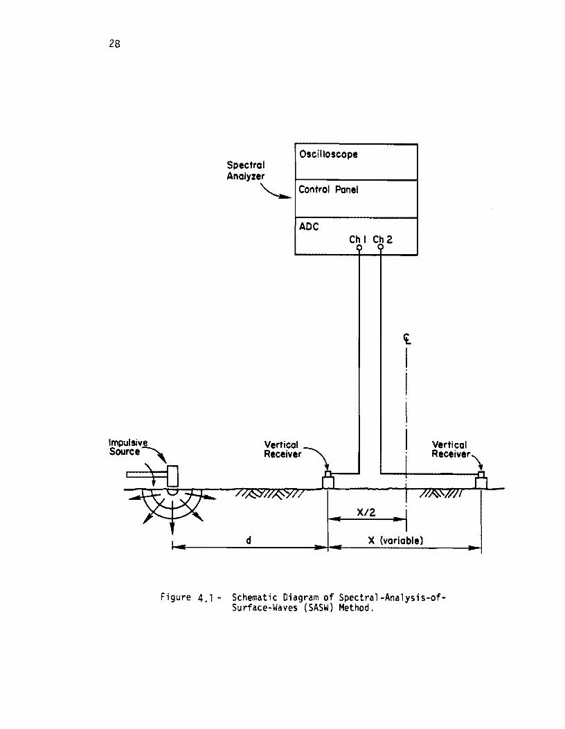
4.2 FIELD TESTING
The testing configuration used in the field is shown in Fig. 4.1.
To perform a test, the steps are as follows:
1. An imaginary centerline for the receiver array is selected.
2. Two receivers are then placed on the ground surface an equal
distance from the centerline (Section A.2). 3. A vertical impulse is applied to the ground by means of a hammer
(Section A.l). A major portion of the various types of stress waves generated by the impulse propagates as surface waves of various frequencies.
4. Impulses are delivered several times, and the signals are averaged together (Section 4.2.1).
5. After testing in one direction is completed, the receivers are kept in their original positions, but the source is moved to
the opposite side of the imaginary centerline. The test is then
repeated (Section 4.2.2).
6. The same procedure (steps 2 through 5) is repeated for other receiver spacings (Section 4.2.3).
27
28
Spectrol Anolyzer
Oscilloscope
~ Control Panel
AOC Ch I Ch 2
X/2
~
I I I I
x (variable)
Vertical Receiver \
Figure 4.1 - Schematic Diagram of Spectral-Analysis-ofSurface-Waves (SASW) Method.
29
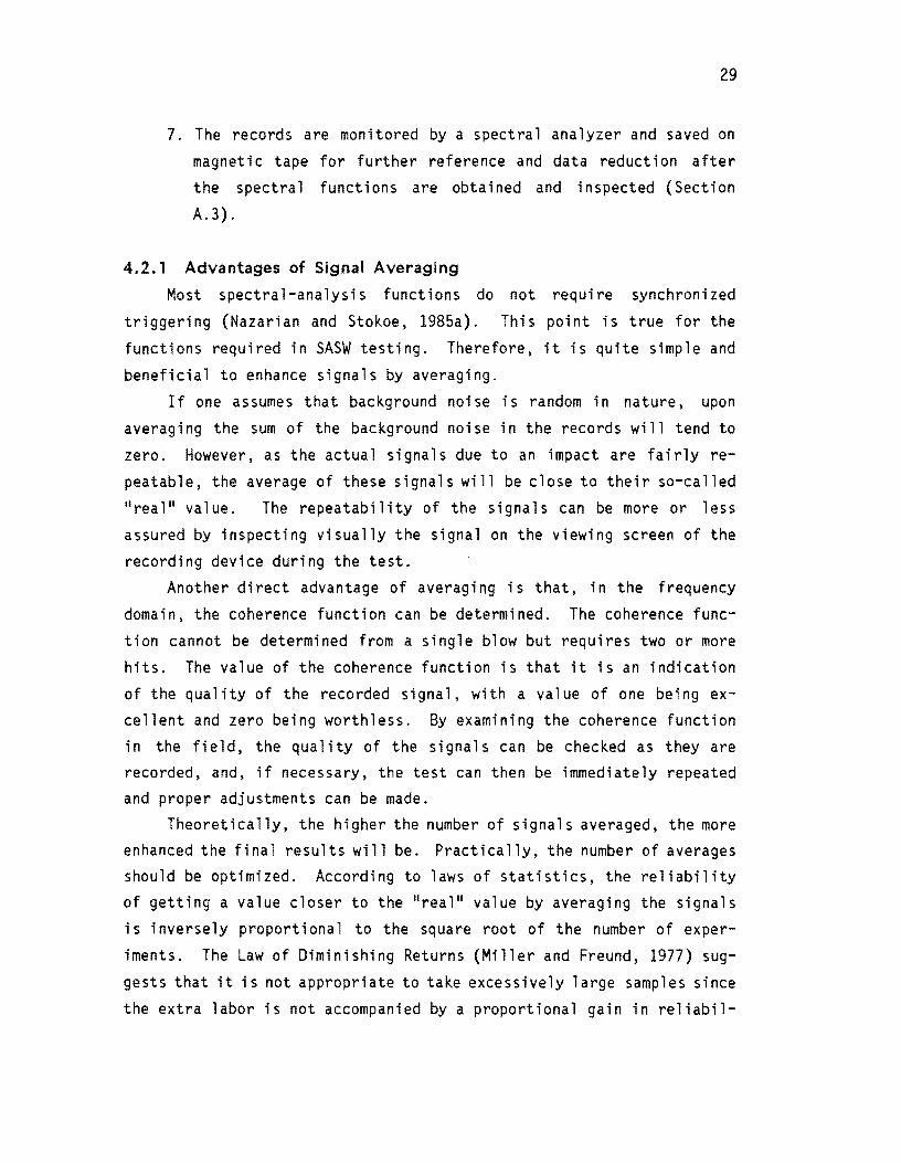
7. The records are monitored by a spectral analyzer and saved on
magnet i c tape for further reference and data reduction after the spectral functions are obtained and inspected (Section
A.3) .
4.2.1 Advantages of Signal Averaging
Most spectral-analysis functions do not require synchronized
triggering (Nazarian and Stokoe, 1985a). This point is true for the
functions required in SASW testing. Therefore, it is quite simple and
beneficial to enhance signals by averaging.
I f one assumes that background noi se is random in nature, upon
averaging the sum of the background noise in the records will tend to
zero. However, as the actual signals due to an impact are fairly re
peatable, the average of these signals will be close to their so-called
"real" value. The repeatability of the signals can be more or less
assured by inspecting visually the signal on the viewing screen of the
recording device during the test. Another di rect advantage of averagi ng is that, in the frequency
domain, the coherence function can be determined. The coherence func
tion cannot be determined from a single blow but requires two or more
hits. The value of the coherence function is that it is an indication
of the quality of the recorded signal, with a value of one being excellent and zero being worthless. By examining the coherence function in the field, the quality of the signals can be checked as they are recorded, and, if necessary, the test can then be immediately repeated and proper adjustments can be made.
Theoretically, the higher the number of signals averaged, the more enhanced the final results will be. Practically, the number of averages should be optimized. According to laws of statistics, the reliability of getting a value closer to the urealu value by averaging the signals
is inversely proportional to the square root of the number of exper
iments. The Law of Diminishing Returns (Miller and Freund, 1977) sug
gests that it is not appropriate to take excessively large samples since
the extra labor is not accompanied by a proportional gain in reliabil-

30
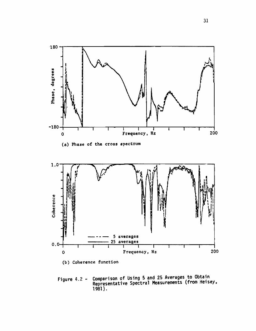
ity. Based on experimental investigations at several soil sites, Heisey
(1981) recommended the average of five runs as being adequate. An ex
amp 1 e of representative cross power spectra and coherence functi ons
after for averages of 5 and 25 runs are shown in Fig. 4.2. No appre
ciable difference can be detected and, therefore averaging five signals
is adequate and recommended.
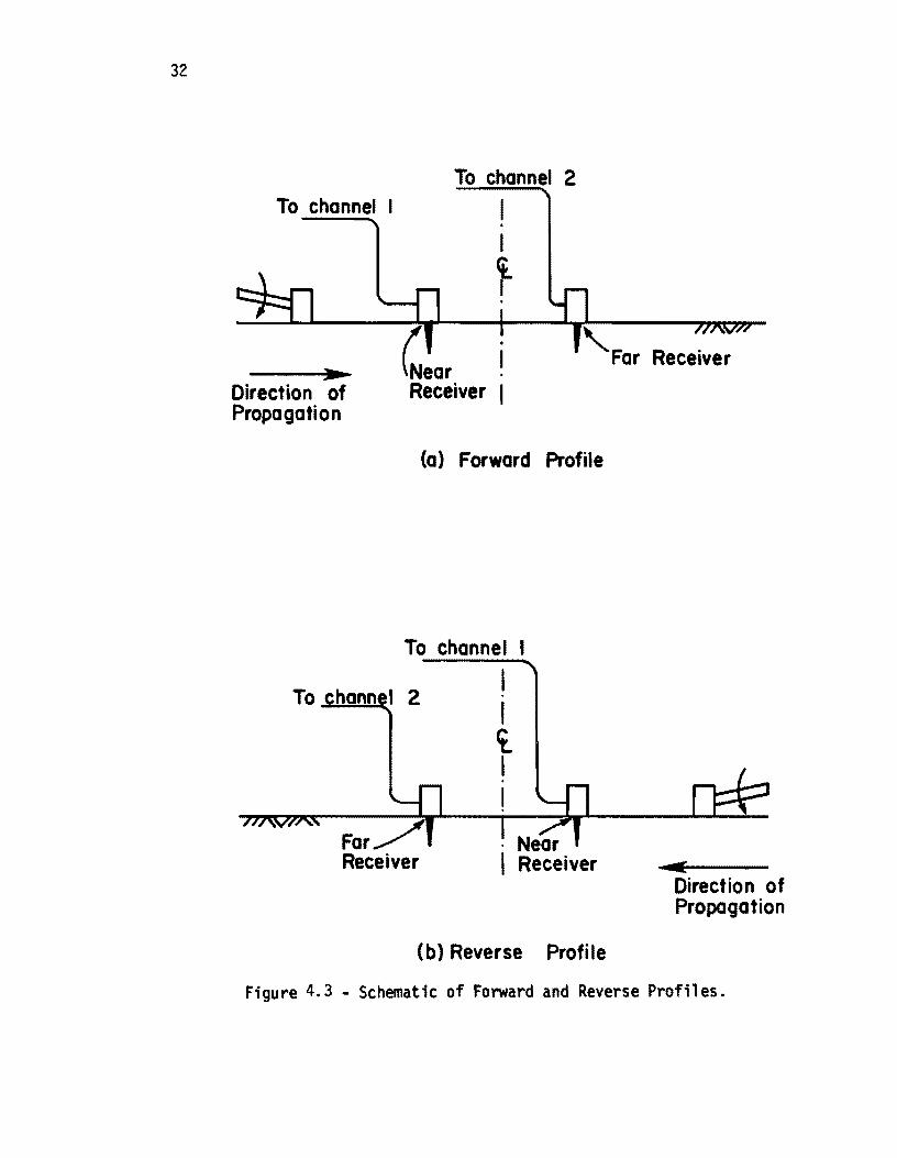
4.2.2 Advantages of Reversing the Source
Reversing the source is the process of performing a test from two
opposite sides of the receiver array as shown in Fig. 4.3. In this
process the test is first performed in one direction (which is termed
the forward profile, hereafter). Then, without moving the receivers
from their original position, the source is moved to the opposite side
of the array. The input channels of the recording device are switched
so that the far receiver in the forward profile is now the near receiver
for the ongoi ng test. The test is performed again with thi s confi g
uration (reverse profile). By averaging the forward and reverse pro
files, the effect of any (undesirable) internal phase shifts associated
with the receivers or the recording device are minimized or eliminated.
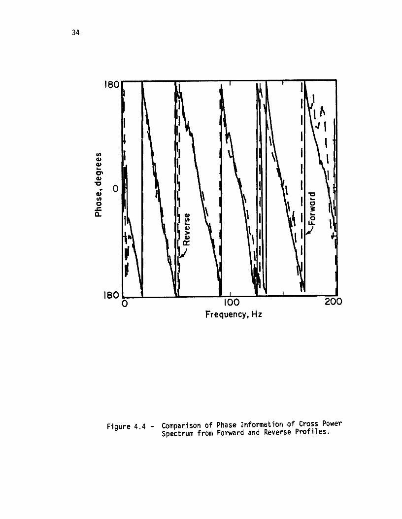
In Fi g. 4.4 the cross power spectra of typi ca 1 forward and reverse
profiles are compared.
A point of interest is that if layers in the substructure are di ppi ng, by runni ng forward and reverse profi 1 es the average can be interpreted as the average properties of equivalent horizontal layers.
4.2.3 Source-Receiver Arrays
The factors that affect appropriate spacing of receivers have been studied by Heisey (1981). These factors include: velocity of material;
depth of investigation; range of frequencies; attenuation properties
of substructure; and sensitivity of the instrumentation (receivers and
recording device). On the basis of studies at several soil sites, Heisey (1981) sug
gested that the distance between the receivers, X, should be less than
31
1801r----~----------------------------------
.. cu us III
f
-180~---rL--r---r---r---r~~---a--~------~ o Frequency, Hz 200
(a) Phase of the cross spectrum
averages
o Frequency, Hz 200
(b) Coherence function
Figure 4.2 - Comparison of Using 5 and 25 Averages to Obtain Representative Spectral Measurements (from Heisey, 1981) •
32
To channel I
Direction of Propagation
To channel 2
I } .
(a) Forward Profile
To channel
To channel 2
(b) Reverse Profile
Direction of Propagation
Figure 4.3 - Schematic of Forward and Reverse Profiles.
33
two wavelengths and greater than one-third of a wavelength. This re
lationship can be expressed as:
(4.1 )
As the velocities of different layers are unknown before testing, it
is difficult to know if these limits are satisfied. Practically
speaking, it is more appropriate to test with various distances between
the receivers in the field and then evaluate the range of wavelengths
over which reliable measurements were made. The relationship between
receiver spacing and wavelength is then better expressed as:
X/2 < Lph < 3X (4.2)
The procedure is to select a spaci ng between recei vers, perform the
test, and reduce the data to determine the wavelengths and velocities. The next step is to eliminate the points that do not satisfy Eq. 4.2.
Theoretically, one experiment in seismic testing is enough to
evaluate the properties of the medium. For a more precise measurement,
severa 1 tests are generally requi red. Vari ous geometri es of the
source-recei ver set-up can be used in test; ng. The two most common
types of geometrical arrangements for the source and receivers are the common source/receiver and the common midpoint geometries.
In the common source/recei ver (CSR) geometry, either the source or receivers are fixed in one location and the other is moved during testing. In the common midpoint (CMP) geometry, both the source and receivers are moved the same di stance about an imaginary centerl i ne. For a medium consisting of a stack of horizontal layers with lateral homogeneity, the results of the tests performed with both methods should theoret i ca lly be i dent i ca 1 . If the 1 ayers are not hori zonta 1 or the
elastic properties of any layer varies laterally, the CMP geometry ;s
preferred. In the CMP arrangement, the velocities are averaged over
the testing range. There is a trade-off, however; in a single CMP test
there is no way to determine the dip of the layers.
34
180~~--~~----~--~~~--~--~ I ., I I I ~
..J ,
I , I , I 1 I
200 Frequency, Hz
Figure 4.4 - Comparison of Phase Information of Cross Power Spectrum from Forward and Reverse Profiles.
35
In the SASW method, the area between the two receivers is impor
tant, and the properties of the materials between the source and the near receiver have little effect on the test. Thus, the imaginary
centerline in the CMP method ;s selected between the receivers. The
two receivers are moved away from the imaginary centerline at an equal
pace, and the source is moved such that the distance between the source
and near receiver is equal to the distance between the two receivers.
This geometry of source and receivers is called Common Receivers Mid
point (CRMP) geometry, hereafter.
To study the effect of set-up configuration during SASW testing,
a seri es of tests was performed at a soil site located at the Walnut
Creek Treatment Plant in Austin, Texas. This site has been used ex
tensively as a pilot site. Heisey (1981), Patel (1981), and Hoar
(1982), among others have performed studies at this site and the prop
erties of the materials are known quite well. Thus, both the CSR and
CRMP were studi ed at Walnut Creek. Schematics of the two geometri es
are shown in Figs. 4.5 and 4.6.
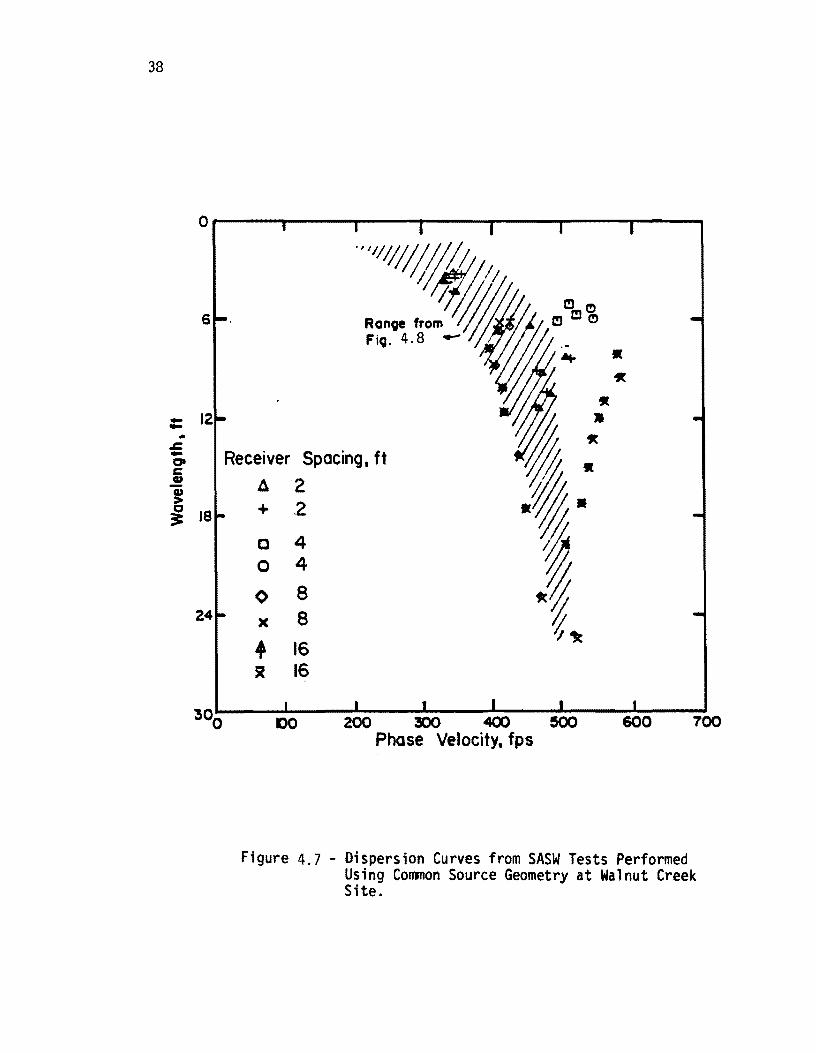
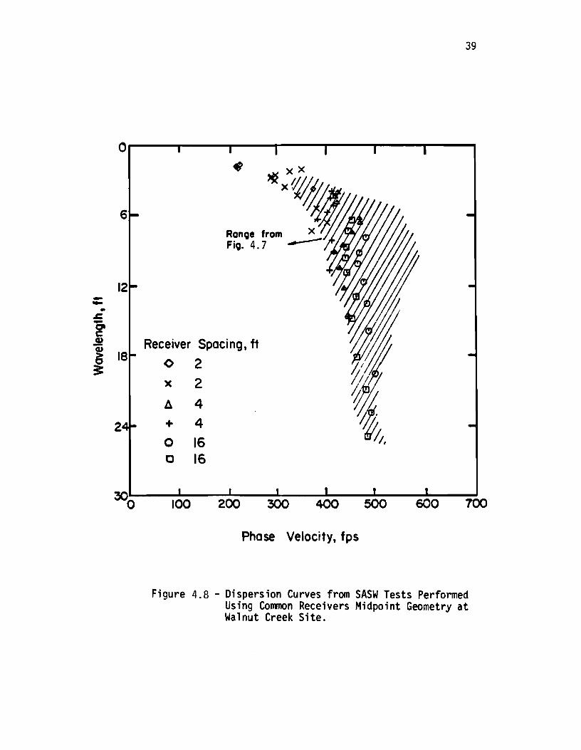
The di spers i on curves obtained from these two set-ups are shown
in Figs. 4.7 and 4.8. Also shown on each figure is the range in ve
locities from the other figure. The scatter in the dispersion curves
is much less in the CRMP approach. As such, the average dispersion
curve obtained from the CRMP geometry is more reliable and more representative of the subsurface material.
The distances between the receivers used in one series of tests depend mainly on the depth of investigation and properties of the sub
structure. In soil sites the receivers are placed 2 ft (0.6 m) apart for the first test and the distance is, generally, doubled for each subsequent test. The maximum spacing is normally 64 ft (19 m) and di stances of up to 128 ft (38 m) have been used successfully. On pavements the same pattern is employed except that the receivers are
placed one ft (0.3 m) apart for the initial test and generally spacings
no larger than 24 ft (7 m) are used.
The other factor of importance in the experimental set-up is the
distance between the source and the near receiver. Lysmer (1968), based
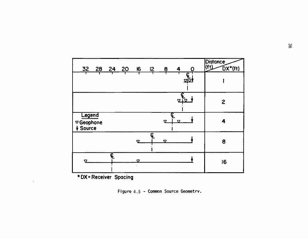
32 28 24 20 16 12 8 4 0 I I , I I I I I ct.' rlrJ
I
~ I
Legend { + 'i1 Geophone o I 0
+ Source I
Cl + q I 0
I
t t 0 I \7
I .. ox = Receiver Spacing
Figure 4.5 - Common Source Geometrv.
~ (ft OX.(ft)
I
2
4
8
16
W 0'\
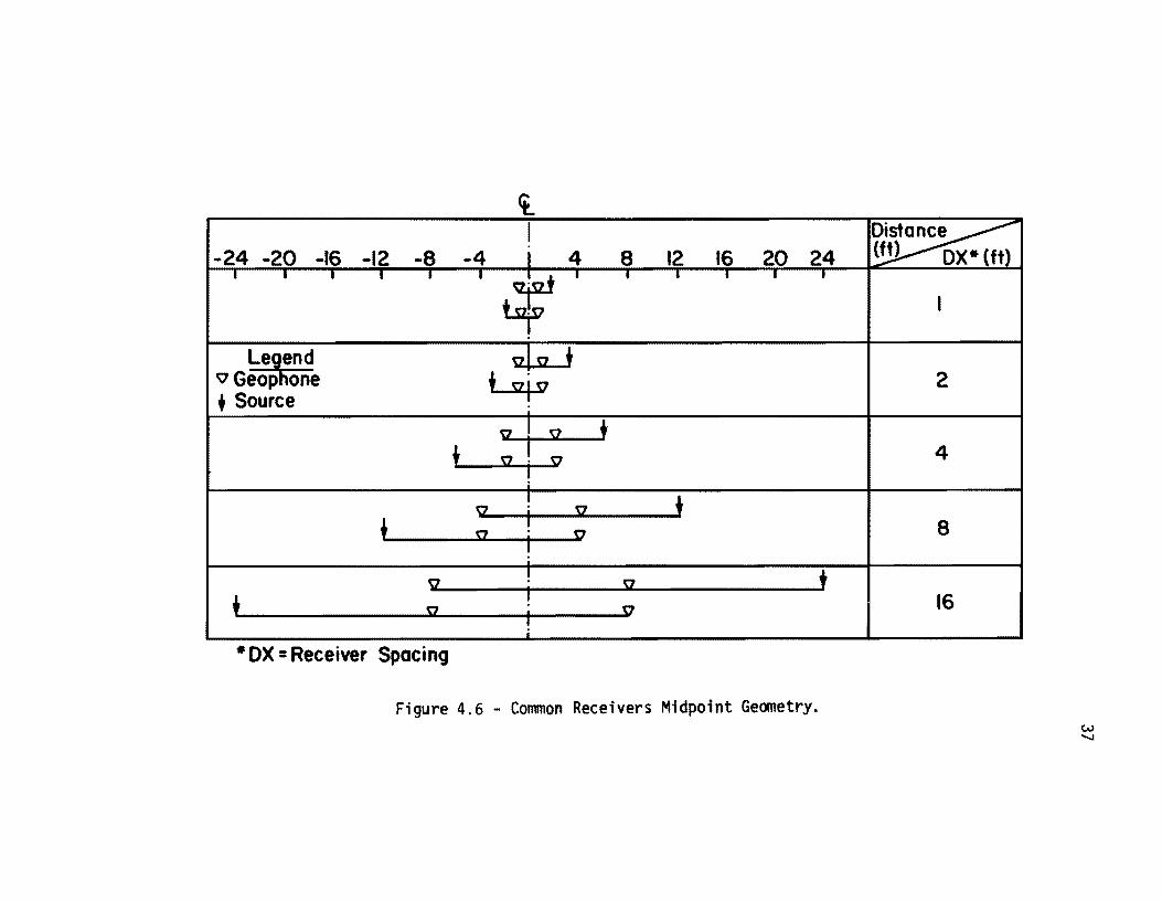
<t. I
-24 -20 -16 -12 -8 -4 i 4 8 12 16 20 24 I I I I I I
~I I I I I I
+-sf Leghnd 010 +
QGeop one ~ + Source ;
01 0 + t 2 . 'il
I
9 !
2 t t I
a I 'i1
'iZ ! sz + +
I sz I 'il
i
• OX : Receiver Spacing
Figure 4.6 - Common Receivers Midpoint Geometry_
~ (ft) ox. (ft)
I
2
4
8
16
W "-J
38
0
6
- 12 -• .s:: -0' c .!! ~ ~ 18
24
300
."'11/11/$1 I~/ I!l ~
• ~
'II[ ,. ~
Receiver Spacing, ft
A 2
.~. + .2
c 4 ~ 0 4
0 8 .~ )( 8 ~~ • 16 5l 16
DO 200 300 400 700 Phase Velocity, fps
Figure 4.7 - Dispersion Curves from SASW Tests Performed Using Common Source Geometry at Walnut Creek Site.
--• .&: -~ c cu Q; > c 3:
39
O----~----~----~--~-----r----,---~
6
12
18
2
300
Receiver Spaci ng, ft
0 2 x 2
~ A 4
+ 4 ~/. 0 16 0 16
100 200 300 400 SOO 700
Phase Velocity, fps
Figure 4.8 - Dispersion Curves from SASW Tests Performed Using Common Receivers Midpoint Geometry at Walnut Creek Site.
40
on theoretical studies, suggested that, at a distance of 2.5 wavelengths
from the source, the wave field for the surface waves is fully developed. Hei sey (1981) based on several experimental stud; es suggested
-that a distance equal to the distance between the receivers is adequate,
provided the criteria expressed in Eq. 4.1 are met during data re
duction. Although in most of the experiments carried out in this study
Heisey's suggestion was employed, it seems that this matter should be
studied more thoroughly. Recently, the distance between the source and
near receiver was increased to several times the distance between the
receivers. Preliminary studies at one site indicate that the effect
of this was small on the experimental dispersion curve. As an example,
the phase information of cross power spectra for a receiver spacing of
two ft (0.6 m) for source-to-near-receiver distances of two, four and
six ft (0.3, 0.6 and 1.2 m) are shown in Fig. 4.9. The curves follow
each other closely except in the range of 2000 to 3000 Hz where the
coherence values for the spacing of four ft (1.2 m) was not high.
4.3 FIELD EQUIPMENT
The necessary elements for performing a SASW test are a source, receivers, and recording device. Each of these items are discussed in
Appendix A.
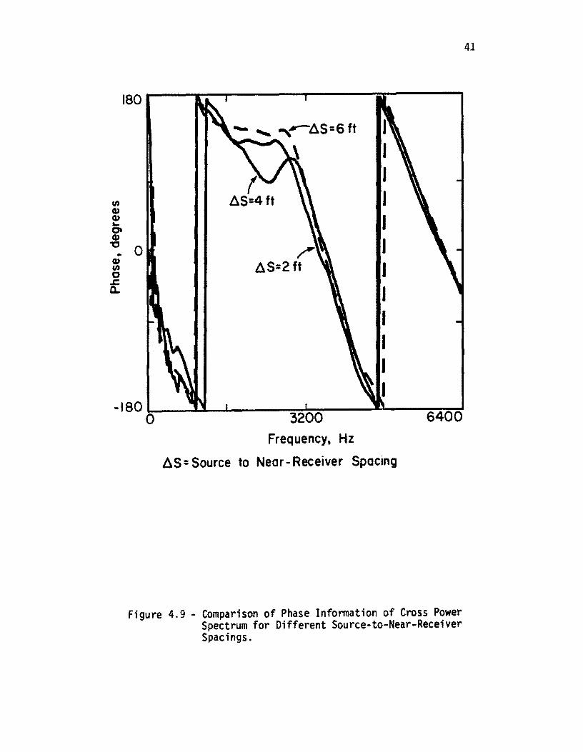
en Q) Q) ... '" Q)
180
,~~S=6ft J ~--.....""""""
~ I
"': 0
I I I I I
Q) en a ..c 0.. I
I I I I
-180 L.--_-LlL---'--__ --.....~......._--.&J..--"""""!"-~ o 3200 6400 Frequency, Hz
~S = Source to Near - Receiver Spacing
Figure 4.9 - Comparison of Phase Information of Cross Power Spectrum for Different Source-to-Near-Receiver Spacings.
41

!!!!!!!!!!!!!!!!!!!"#$%!&'()!*)&+',)%!'-!$-.)-.$/-'++0!1+'-2!&'()!$-!.#)!/*$($-'+3!
44!5"6!7$1*'*0!8$($.$9'.$/-!")':!
5.1 INTRODUCTION
CHAPTER FIVE
IN-HOUSE DATA REDUCTION
Once data have been collected in the field as discussed in Chapter
Four, they must be manipulated in a fashion appropriate for data re
duction. Field data are in the form of phase information of cross power
spectra and coherence funct; ons from forward and reverse profi 1 es at
different receiver spacings. From the coherence function of each test,
the range of frequencies with high quality data are selected. In the
selected frequency ranges, phase information of the cross power spec
trum is used to calculate phase velocities and associated wavelengths
for each frequency. The wavelength/phase velocity relationships from
a 11 records are determi ned and combi ned with the outcome bei ng a
dispersion curve (see Nazarian and Stokoe, 1985a). This dispersion
curve can be considered as the raw data from SASW testing. The proce
dure used in this study for construction of dispersion curves is dis
cussed in the next sections.
5.2 CONSTRUCTION OF A DISPERSION CURVE
5.2.1 Theoretical Considerations
Assume that for a given frequency, f, the phase difference is equal
to~. By using the principle of a rotating vector. a phase shift of 360 degrees is equivalent to a travel time of one period. For a har
monic wave, the period, T, is the reciprocal of the frequency of that wave (i.e., T = l/f). Therefore, the travel time, t, can be obtained by:
t = (~/360)· T (5.1)
or alternatively:
t = ¢/(360.f) (5.2)
43
44
Now, if the distance between receivers, X, is known, phase velocity of propagation, Vph is equal to:
Vph = X/t (5.3)
For a wave propagating in an elastic medium, the product of frequency
and wavelength is constant, with this constant value equal to the ve
locity of propagation associated with that frequency. Therefore, wave
length for each phase velocity, Lph ' can be determined by:
(5.4)
It can be seen then that if phase and frequency are known, phase ve
locity and wavelength can be easily determined utilizing Eqs. 5.2 through 5.4.
5.3 Automated Data Reduction
Practically speaking, the process described in Section 5.2 is
carried out for each record through an automated process. A schematic of thi s process is shown in Fi g. 5.1. The spectral analyzer is con
nected to a mi cro-computer (Hewl ett Packard 98365). The HP 98365 is
connected to a terminal which enables the operator to communicate with the CDC dual Cyber system of The University of Texas. Three computer programs are coded to facilitate this process.
The first one, called TRANSl is used with the micro-computer so that phase information of the cross power spectrum (or transfer function) can be transferred from the analyzer through the HP 98365 to the CDC computer. In the next step, tha data are consolidated and arranged
in a manner usable with the CDC system by program TRANSl1. Program
TRANSl2 is then used to utilize Eqs. 5.2 through 5.4 to calculate the
dispersion curves. Finally, Program EX PERl is used for statistical
evaluation of the data at each frequency and to obtain the final
dispersion curve. This statistical procedure is discussed later in this
section.
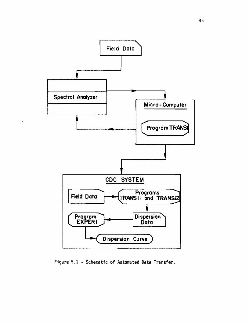
45
Field Data 'I
.. -Spectra I Analyzer
Micro- Computer
- ~rooramT~
I
III
CDC SYSTEM
....... c:: Programs ~ Field Data -I{ rWs II and TRANS~ I
t Pro~m 1_ EX RI
Dispersion'l Data
....... ( Oi spersion Curve)
Figure 5.1 - Schematic of Automated Data Transfer.
46
To clarify the process, typical phase information from one cross
power spectrum and an associated coherence function are selected, and
the different steps described above are illustrated.
The cross power spectrum and coherence function for one
source/receiver set-up at a soil site is shown in Fig. 5.2. The site
is called the Wildlife site hereafter, as the actual testing was per
formed in a wildlife preserve in southern California. The receiver
spacing is equal to 8 ft (2.4 m), and the source/near-receiver distance
is also 8 ft (2.4 m). To conserve space and to maintain good resol
ution, the phase plot shown in Fig. 5.2b oscillates between -180 and
180 degrees. (Thi sis a typi ca 1 di sp 1 ay techni que used by waveform
analysis equipment.) The first step is to find the actual phase for each frequency by counting the number of 360-degree cycles preceeding
each frequency and adding that to the fraction of the remaining cycle
to obtain the actual phase. This process is called unfolding of the
phase. Figure 5.3 shows the same phase plot as in Fig. 5.2b after the
appropriate number of cycles is added to each value of phase read off
Fig. 5.2b. Four regions with low coherence values exist in Fig. 5.2a.
A low va 1 ue of coherence at a certa infrequency corresponds to poor quality of data at that frequency. There are several reasons for low
coherence value which are discussed in Nazarian and Stokoe (1985a). The four regions which are marked as I, II, III and IV in Fig. 5.2a are four typical reasons for low coherence. The first zone (I), which covers from 0 to 5 Hz, exhibits low coherence because of the nonlinear behavior of the geophones around and below their natural frequency, and, more importantly, because no energy is generated in this region. Zone II is in the vicinity of 30 Hz, which corresponds to the frequency of
rotation of the mechanical parts of the power generator. The third zone
of low coherence is due to 60-cycle electrical noise. In the range of
120 to 140 Hz, the last zone of low coherence occurs. In this region
the energy coupled to the ground does not contain appreciable energy,
especially at the far receiver.
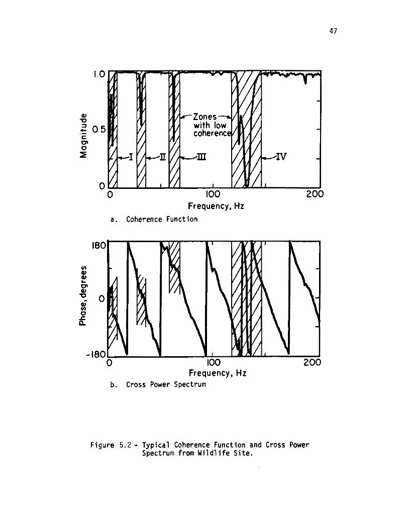
cu '1:J
::::J -I: 0 0
:::E
." cu cu ... o cu "C .. cu ." o .s::.
Q..
0.5
180
m
100 Frequency, Hz
a. Coherence Function
200
-180 "'--~ __ .L-__ --L~---&''''''&&-'''''---~ ......... ~ o 100 200
Frequ ency, Hz b. Cross Power Spectrum
Figure 5.2 - Typical Coherence Function and Cross Power Spectrum from Wildlife Site.
47
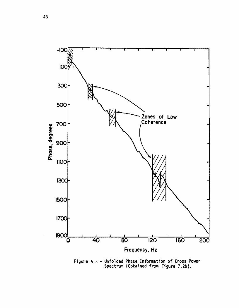
48
Frequency, Hz
Figure 5.3 - Unfolded Phase Information of Cross Power Spectrum (Obtained from Figure 7. 2b).
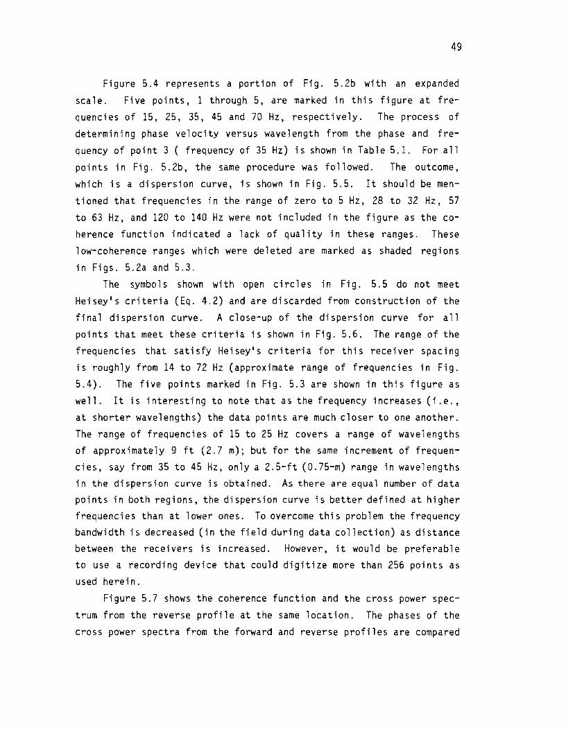
49
Figure 5.4 represents a portion of Fig. 5.2b with an expanded
scale. Five points, 1 through 5, are marked in this figure at frequencies of 15, 25, 35, 45 and 70 Hz, respectively. The process of
determining phase velocity versus wavelength from the phase and fre
quency of point 3 ( frequency of 35 Hz) is shown in Table 5.1. For all
points in Fig. 5.2b, the same procedure was followed. The outcome,
which is a dispersion curve, is shown in Fig. 5.5. It should be men
tioned that frequencies in the range of zero to 5 Hz, 28 to 32 Hz, 57
to 63 Hz, and 120 to 140 Hz were not included in the figure as the coherence function indicated a lack of quality in these ranges. These
low-coherence ranges which were deleted are marked as shaded regions
in Figs. 5.2a and 5.3.
The symbols shown with open circles in Fig. 5.5 do not meet
Heisey's criteria (Eq. 4.2) and are discarded from construction of the
final dispersion curve. A close-up of the dispersion curve for all
points that meet these criteria is shown in Fig. 5.6. The range of the
frequencies that satisfy Heisey's criteria for this receiver spacing
is roughly from 14 to 72 Hz (approximate range of frequencies in Fig.
5.4). The five pOints marked in Fig. 5.3 are shown in this figure as
well. It is interesting to note that as the frequency increases (i .e.,
at shorter wavelengths) the data points are much closer to one another.
The range of frequencies of 15 to 25 Hz covers a range of wavelengths of approximately 9 ft (2.7 m); but for the same increment of frequencies, say from 35 to 45 Hz, only a 2.5-ft (0.75-m) range in wavelengths in the dispersion curve is obtained. As there are equal number of data pOints in both regions, the dispersion curve is better defined at higher frequencies than at lower ones. To overcome this problem the frequency bandwidth is decreased (in the field during data collection) as distance between the receivers is increased. However, it would be preferable to use a recording device that could digitize more than 256 points as used herein.
Figure 5.7 shows the coherence function and the cross power spec
trum from the reverse profile at the same location. The phases of the
cross power spectra from the forward and reverse profiles are compared
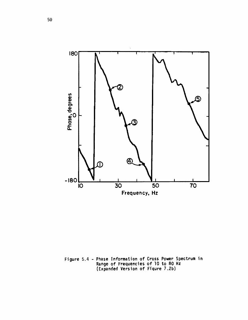
50
180r--'~--1I--~--~--~----~~
-180 __ --~----~--~--~~--~----~~ 10 30 50 70
Frequency, Hz
Figure 5.4 - Phase Information of Cross Power Spectrum in Range of Frequencies of 10 to 80 Hz (Expanded Version of Fiqure 7.2b)
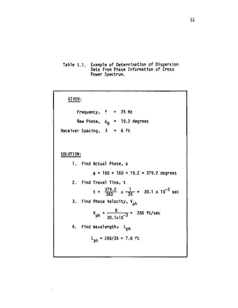
Table 5.1. Example of Determination of Dispersion Data from Phase Information of Cross Power Spectrum.
GIVEN:
Frequency. f = 35 Hz
Raw Phase. ~R = 19.2 degrees
Receiver Spacing. X = 8 ft
SOLUTION:
1. Find Actual Phase. ~
~ = 180 + 180 + 19.2 = 379.2 degrees
2. Find Travel Time. t
t = 3;t0 2 x i5 = 30.1 x 10.3 sec
3. Find Phase Velocity. Vph
V = 8 = 266 ft/sec ph 30.1xlO·3
4. Find Wavelength, Lph
Lph = 266/35 = 7.6 ft
51
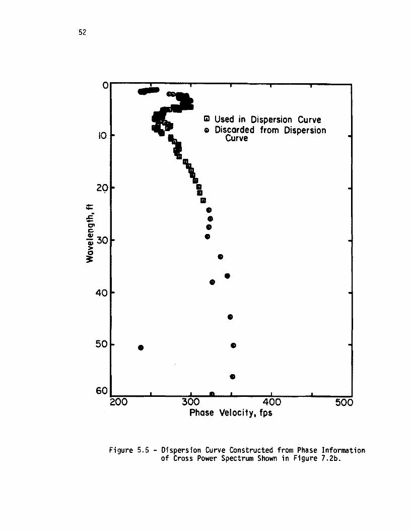
'52
0 • m Used in Dispersion Curve
10
'\ " Discarded from Dispersion
Curve
20 II II II -- • .-
.t::. • -C' • c.
~30 • > 0 ~ •
• • 40
• 50 • •
• 60
-20-0--~----3~0~0~--~--~40~O----~---50~O
Phase Velocity, fps
Figure 5.5 - Dispersion Curve Constructed from Phase Information of Cross Power Spectrum Shown in,Figure 7.2b.
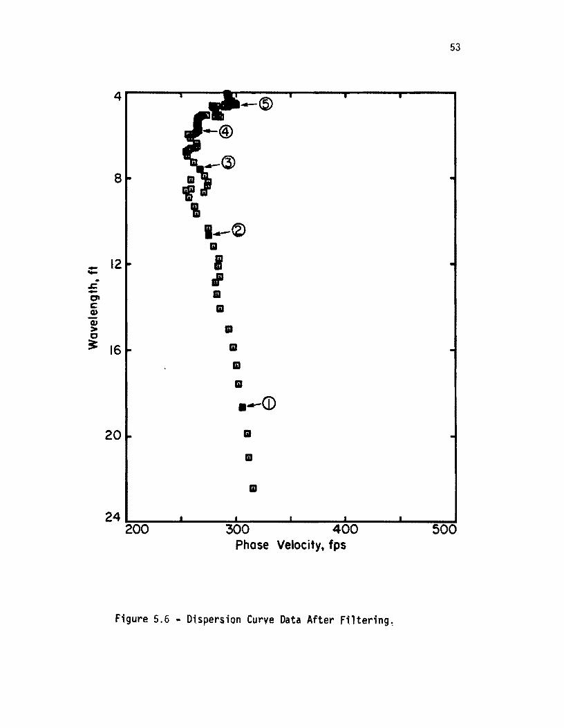
53
4
(3) 8 II
'I '&
I...-(Z) II
- 12 i ....
" .. .s::. - II C* c:: II CIJ CIJ
II > c 3= 16 II
II
II
• ..-Ci)
20 II
II
II
24 300 4 500
Phase Velocity, fps
Figure 5.6 .. Dispersion Curve Data After Filtering~
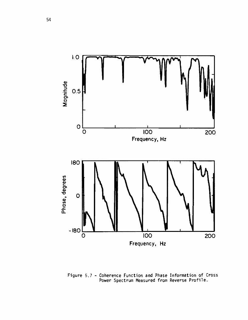
54
QJ "0 ::I
:!:: 0 5 c: . 0'1 C ::e
VI QJ QJ ... 0'1 QJ "0 .. QJ VI C
.c. a..
o~------~------~--------~----__ ~ o
180
0
100 Frequency, Hz
200
-180 L..--L __ .1L. __ --a.....L..._--=-_--'-_..I.-_---'
o 100 Frequency, Hz
200
Figure 5.7 - Coherence Function and Phase Information of Cross Power Spectrum Measured from Reverse Profile.
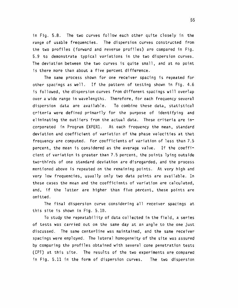
55
in Fig. 5.8. The two curves follow each other quite closely in the
range of usable frequenci es. The di spers i on curves constructed from
the two profiles (forward and reverse profiles) are compared in Fig.
5.9 to demonstrate typical variations in the two dispersion curves.
The deviation between the two curves is quite small, and at no point
;s there more than about a five percent difference.
The same process shown for one receiver spacing is repeated for
other spacings as well. If the pattern of testing shown in Fig. 4.6
is followed, the dispersion curves from different spacings will overlap
over a wide range in wavelengths. Therefore, for each frequency several
dispersion data are available. To combine these data, statistical
criteri a were defi ned primarily for the purpose of identifyi ng and
eliminating the outliers from the actual data. These criteria are in
corporated in Program EXPERl. At each frequency the mean, standard
deviation and coefficient of variation of the phase velocities at that
frequency are computed. For coefficients of variation of less than 7.5
percent, the mean is considered as the average value. If the coeffi
cient of variation is greater than 7.5 percent, the points lying outside
two-thirds of one standard deviation are disregarded, and the process
mentioned above is repeated on the remaining points. At very high and
very low frequencies, usually only two data points are available. In
these cases the mean and the coefficients of variation are calculated,
and, if the latter are higher than five percent, these points are
omitted. The final dispersion curve conSidering all receiver spacings at
this site is shown in Fig. 5.10.
To study the repeatability of data collected in the field, a series
of tests was carried out on the same day at an angle to the one just
discussed. The same centerline was maintained, and the same receiver
spacings were employed. The lateral homogeneity of the site was assured
by comparing the profiles obtained with several cone penetration tests
(CPT) at thi s site. The results of the two experiments are compared
in Fig. 5.11 in the form of dispersion curves. The two dispersion
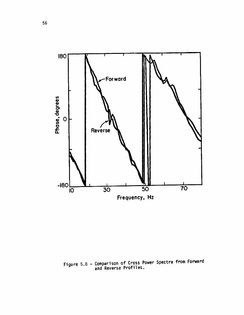
56
180 .---rr--..,----r--~~-r-----~-
-180!-=---olI~_~----,--~~-~_.....J._--I 10
Frequency. Hz
Figure 5.8 - Comparison of Cross Power Spectra from Forward and Reverse Profiles.
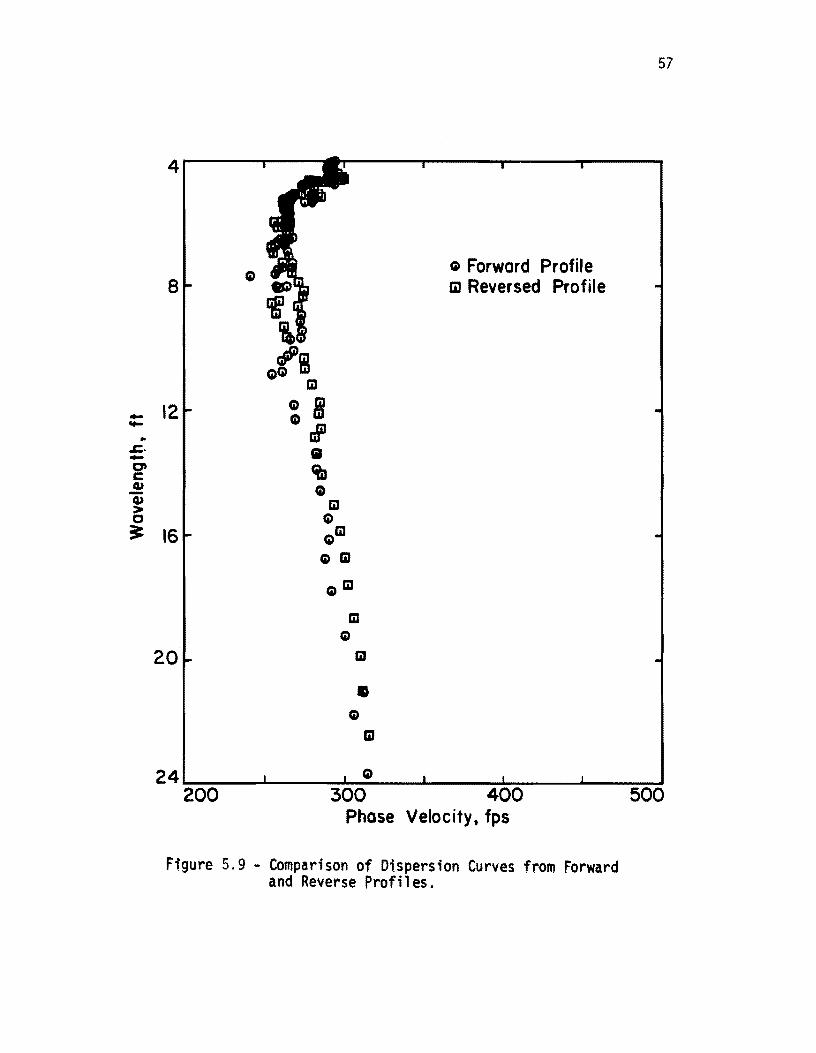
-.... .. ,z:. -D' C .!! Q) > 0 ~
4
8
12
16
20
lil
CD ~ CDr9l
• tJ CD
lil CD
CDlil
fa lil
faGJ
lil fa
GJ
• fa
lil
G Forward Profile m Reversed Profile
57
24L-____ ~ ____ ~~fa ____ ~ ____ ~~--~----~
200 300 400 500 Phose Velocity t fps
Figure 5.9 - Comparison of Dispersion Curves from Forward and Reverse profiles.
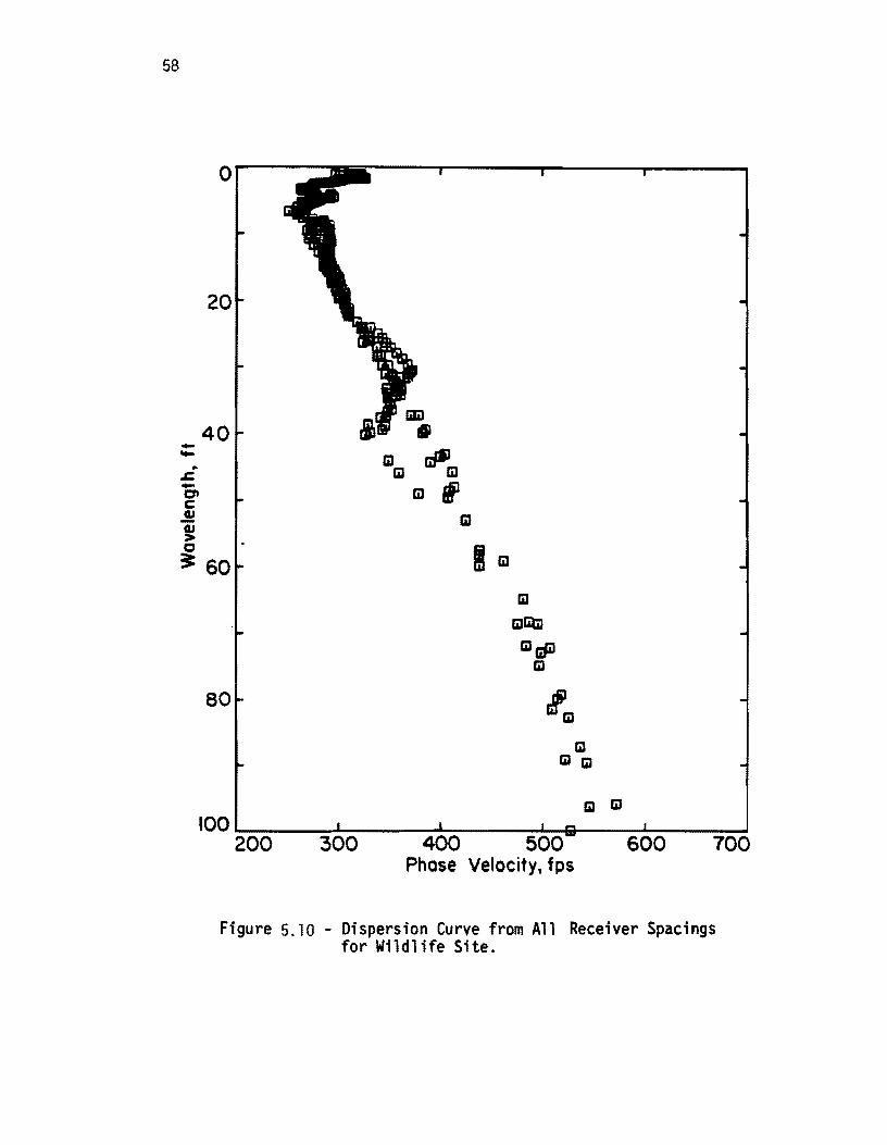
58
o
40 --.. .t:. -0'1 C ~ ~ CI
~ 60 M m
100 ________________________ ~-------------
200 300 400 500 600 700 Phose Velocity, fps
Figure 5.10 - Dispersion Curve from All Receiver Spacings for Wildlife Site.
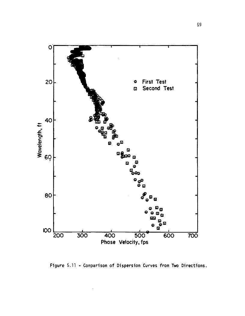
59
o
20 Q First Test til Second Test
40 j
GlitJI~ iii G)1iI
--.. .s=. t;, c:: Q)
'i o 3: 60 lilt.! iii
r.
80
iii iii G)
"A,~ G)GP
G)1iI
'iii G) iii
G IiIIiI G G iii iii
IiliJIiI G Glil
~O iii ~20~0~~3~0~O~--~4~0~0----~5~0~0~---6~0~0--~1~O~0
Phase Velocity, fps
Figure 5.11 - Comparison of Dispersion Curves from Two Directions.
60
curves are in excellent agreement. Thus, it can be concluded that the
tests are quite repeatable.
A similar data reduction process is followed for pavement sites and is presented in Appendix B.
5.4 SUMMARY
In this chapter, the practical details of data reduction in SASW
testing are presented (once data have been collected in the field).
Construction of the dispersion curve from in situ data in the form of
phase information from cross power spectra is discussed. During the
course of this study, full-automation of the process of construction
of dispersion curves was achieved. In this process, a desk-top computer
has been utilized to transfer data to the more efficient CDC computer
(more efficient for use in the inversion process) in a matter of min
utes.
6.1 INTRODUCTION
CHAPTER SIX
INVERSION PROCESS
The final task in SASW testing is to determine the shear wave ve
locity profile. This step is called inversion of the dispersion curve
or simply inversion. (Sometimes this step is called forward modelling
in geophysics or system identification in structural dynamics). In
version is an iterative process in which a theoretical dispersion curve
is calculated for an assumed shear wave velocity profile. The theore
tical and experimental dispersion curves are compared, and the assumed
profile is modified to improve the match. This process is continued
until the two curves closely match. The inversion process is described
in the next sections.
6.2 INVERSION PROCESS
Three generations of inversion evolved during the course of this
study. In the first generation the following steps were used:
1. the thicknesses of the layers were determined by dividing
the dispersion curve into several sections and by assuming
that 1/3 of the wavelength was equal to the effective sampling depth,
2. the shear wave velocity of the top layer was then assumed to be approximately equal to 110 percent of the phase velocity of the top layer,
3. the second layer was assumed to be a half-space, and the shear wave velocity of this layer was changed until the theoretical and experimental dispersion curves compared
well up to approximately three times the sum of thicknesses
of layers one and two (although the second layer was assumed
to extend to infinity for the inversion process, the
thickness of this layer was determined in Step 1),
61
62
4. the next layer was then added and assumed to be the new
half-space and the thickness of the second layer was
changed to its assumed value (from Step 1), and the matching
process identical to Step 3 but for a three-layered system
was performed, and
5. sequentially all the other layers were included by repeat
ing the process described in Steps 3 and 4.
This process was quite tedious and time consuming. In addition, when
the profil e cons i sted of layers wi th 1 arge contrasts in st iffnesses
(such as pavements), the intermediate layers had unrealistically high
velocities. An example of this effect is included in Section 7.4. This
first-generation inversion process was abandoned (improved upon) in the
early stages of this study.
In the second-generation inversion, the velocities of the layers
in the profile were estimated at the beginning and input into the com
puter program based upon Dunkin's (1965) approach (see Nazarian and
Stokoe, 1985a). The process was quite similar to the procedure of the
third level described below. In the case of soil sites, the ordinary construction of the determinant based upon discussion in Nazarian and
Stokoe (1985a) was used. For pavement sites, layers with shear wave
velocities greater than the phase velocity under consideration were included in construction of the determinant so that the real roots of the dispersion equation were always calculated.
In the third generation, the inversion program was modified by adding Thrower's (1965) recommendations, as presented below. The approach used herein is based upon construction of a theoretical
dispersion curve from an assumed shear wave velocity profile and com
parison of this curve with the experimental dispersion curve.
The dispersive characteristic of surface waves is discussed in
Nazarian and Stokoe (1985a). The theory discussed in that report was
incorporated into a computer algorithm. The main feature of the algo
rithm is to generate a theoretical dispersion curve once the thick
nesses, stiffnesses (S- and P-wave velocities), and densities of
63
different layers are input. The program is interactive for ease of use
and a user's manual is provided in a separate report (Nazarian, 1985b).
Ranges of frequencies and velocities are selected for each search.
These ranges are divided into several increments (on the order of 10
to 25 increments). The dispersion equation ;s only a function of fre
quency and phase velocity for a given stiffness profile. Therefore,
the dispersion equation can be written as:
o (6.5)
To solve this equation, either the value of frequency or phase velocity
should be assumed.
Equation 6.5 is solved numerically by the computer as an explicit
solution is not available, except for simple one- or two- layered sys
tems. Schwab and Knopoff (1970) have shown that, to solve the
dispersion equation numerically, it is more desirable to assume the
frequency and to determine the value of Vph at that frequency. At very
high and very low frequencies, phase velocities do not vary by much,
and they are quite close to the R-wave velocities of the top and bottom
layers, respectively. If the frequency is assumed as the dependent
variable in Eq. 6.5, and if the assumed phase velocity is close to the
R-wave velocity of the first or last layer, the solution to the equation
will have many roots that may cause numerical difficulties. Therefore,
in program INVERT, frequency is assumed as the independent variable.
At each increment of frequency. the program computes the determi nant
for each increment of velocity in the range of velocities selected.
Roots of the dispersion equation, for that increment of frequency, are
located between two phase velocities whose determinants have opposite
signs.
An example of output from program INVERT is shown in Fi g. 6.1.
The location of the roots are marked by dashed lines. A more detailed
description of the program is presented in Nazarian (1985) and Nazarian
and Stokoe (1985b).
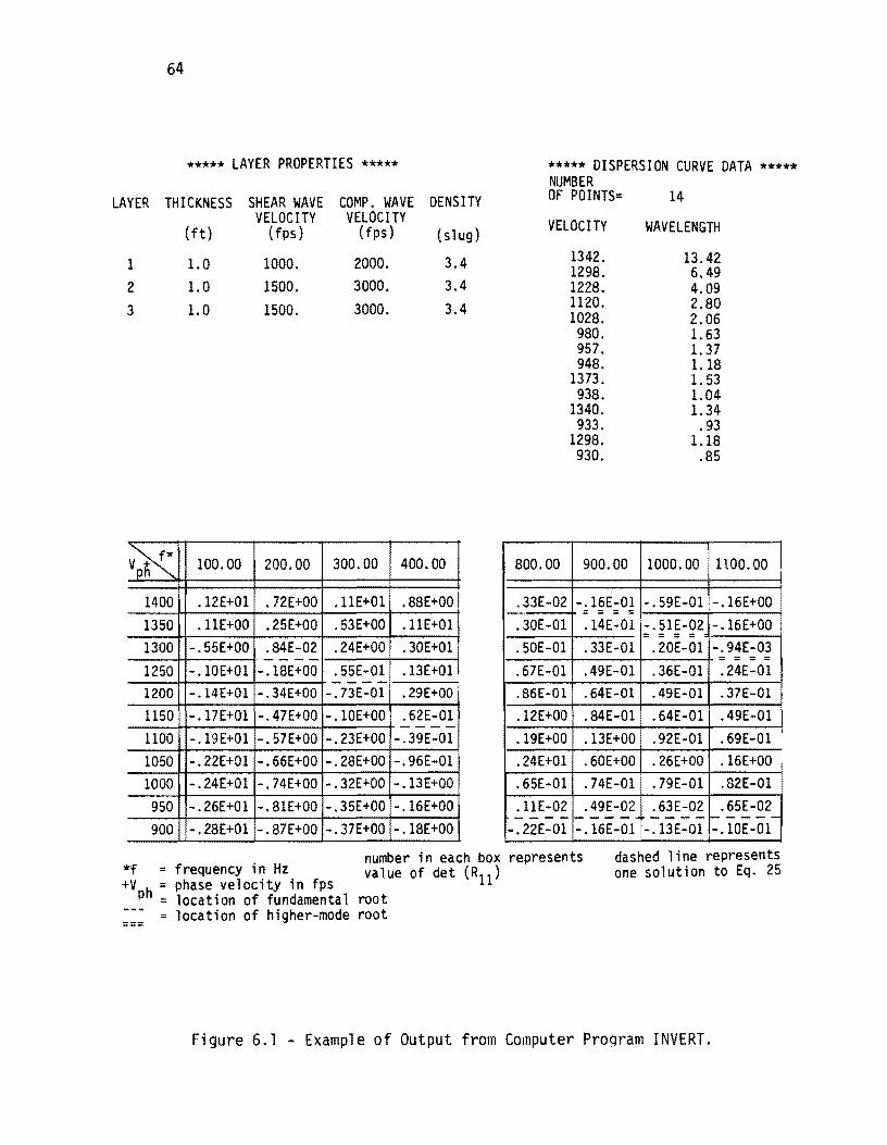
64
***** LAYER PROPERTIES *****
LAYER THICKNESS SHEAR WAVE COMP. WAVE DENSITY VELOCITY VELOCITY
(ft) (fps) (fps) (slug)
1 1.0 1000. 2000. 3.4
2 1.0 1500. 3000. 3.4
3 1.0 1500. 3000. 3.4
~ 100.00 200.00 300.00 400.00
1400 . 12E+01 . 72E+00 . 11E+01 . 88E+00 1350 . 11E+OO . 25E+00 . 53E+00 . 11E+01 1300 -.55E+00 . 84E-02 . 24E+00 .30E+011 ----1250 -.10£+01 -.18£+00 .55E-01 .13E+011 ---1200 -.14£+01 -.34£+00 -.73E-Ol . 29E+00,
1150 -.17E+01 -.47E+00 -.10E+00 .62E-01 ----1100 -.19E+01 -.57E+00 -.23E+00 -.39E-01 1050 -.22E+01 -.66E+00 -.28E+00 -.96E-01 1000 -.24£+01 -.74E+00 -.32E+OO -.13£+00 950 -.26E+01 -.81E+00 -.35E+00 -.16E+00 900 -.28E+01 -.87E+00 -.37E+00 -.18E+00
***** DISPERSION CURVE DATA ***** NUMBER OF POINTS= 14
VELOCITY
1342. 1298. 1228. 1120. 1028.
800.00
.33£-02
.30E-01
.50E-01
.67E-01
.86E-Ol
. 12E+00
. 19E+00
. 24E+01
980. 957. 948.
1373. 938.
1340. 933.
1298. 930.
900.00
-.16E-01 ;: = = :: . 14E-01 .33E-01 .49E-01 .64E-Ol .84E-01 . 13E+00 .60E+00
WAV£LENGTH
13.42 6.49 4.09 2.80 2.06 1. 63 1.37 1.18 1. 53 1.04 1. 34 .93
1.18 .85
1000.00 1100.00 l -.59£-01 -.16£+00 -.51E-02 -.16E+00 - - - -- - - -
.20E-01 -.94E-03 :: = = =
. 36E-01 .24E-01
.49E-Ol .37E-Ol
.64E-01 .49E-01
.92E-01 .69E-01
. 26E+00 . 16E+00 .65E-01 .74E-~.79E-01 .82E-01 . 11E-02 .49E-02 .63E-02 .65E-02 ---- ---- ---- -----
-.22E-01 -.16E-01 -.13E-01 -.10E-01
number in each box represents *f frequency in Hz value of det (R11 )
dashed line represents one solution to Eq. 25
+V = phase velocity in fps ph = location of fundamental root
= location of higher-mode root ===
Figure 6.1 - Example of Output from Computer Proqram INVERT.
65
A high number of increments is desirable for obtaining accurate
results. However, the computation time increases drastically as the
number of increments is increased. Pract i ca lly speaking, instead of
selecting a wide range of frequencies and velocities with a large number
of increments, it is more economical to limit the ranges and number of
increments and to perform more runs.
The first step in the inversion process is to assess a shear wave
velocity profile from the dispersion curve. For more clarity, different
steps di scussed here are app 1 i ed to the di spers i on curve from the
Wildlife site. To avoid confusion the dispersion curve should be di
vided into small sections which are plotted with an expanded scale.
Several layers (on the order of 3 to 5) are selected, and a shear wave
velocity is assigned to each layer. It is beneficial to use the sim
plified inversion method (discussed in Chapter Three) as the first as
sumed profile. With more experience, more realistic assumptions can be made. Any additional information available about the site can be
used to accelerate significantly the inversion process. It should be
mentioned that this is mainly a preliminary trial just to obtain a
(reasonable) starting point for the second stage of matching process.
In the case of Wildlife, the dispersion curve is divided into four,
constant-velocity layers as shown in Fig. 6.2. The Vs profile is ob
tained by dividing the wavelength axis by three, multiplying the velocity axis by 1.1 and lIeye-balling" the velocities and thicknesses.
The profile obtained is shown in Fig. 6.3. The theoretical dispersion curve from this profile is compared with the experimental one in Fig.
6.4. The velocities of different layers are changed until the two curves roughly match. The theoretical dispersion curve after some im
provement in the Vs profile is shown in Fig. 6.4, and the shear wave velocity profile is compared with the initial profile in Fig. 6.3.
In the second stage, each layer in the shear wave velocity profile
obtained in the first stage is divided into sublayers, and a more re
fined matching process is employed. When the theoretical and exper
imental curves match over the range of available wavelengths, the final
shear wave velocity profile is obtained.
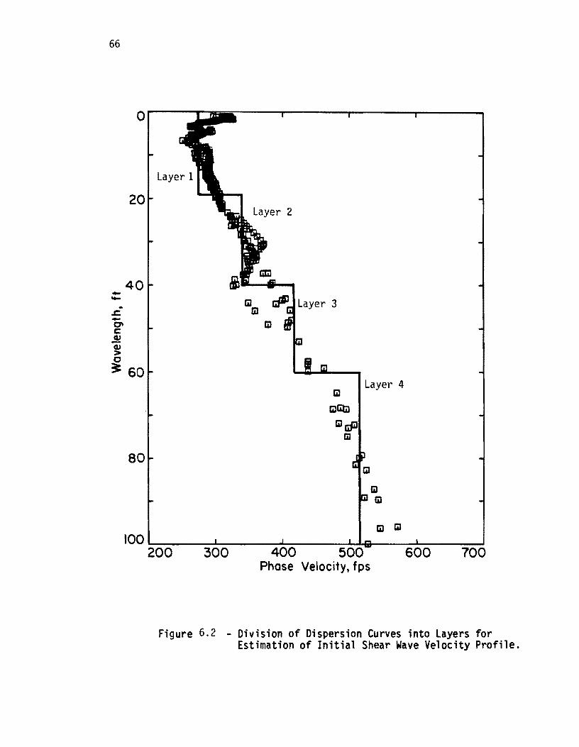
66
--.. .r::. -o c: ~ G> > C
20
40
~ 60
80
100
m Layer 4
mGt) m
CD CD
m m
200 300 400 500 600 700 Phose Velocity, fps
Figure 6.2 - Division of Dispersion Curves into Layers for Estimation of Initial Shear Wave Velocity Profile.
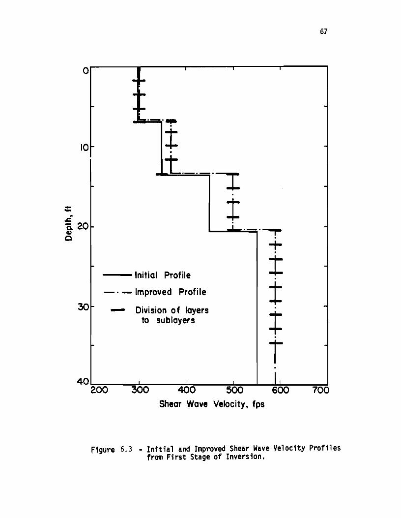
67
o I I
--• ~
• -I! ~.- .....
•
10 l- t -•
t.._._.~ -.
! --. .c Q. 20 ~ ..L._.~ -II)
o
~
Initial Profile
_. - Improved Profi Ie
30 I-
l-
40 200
- Division of layers to sublayers
I I I
300 400 500 Shear Wave Velocity, fps
· + · ! -·
t -·
4: · T -
· L 600 700
Figure 6.3 - Initial and Improved Shear Wave Velocity Profiles from First Stage of Inversion.
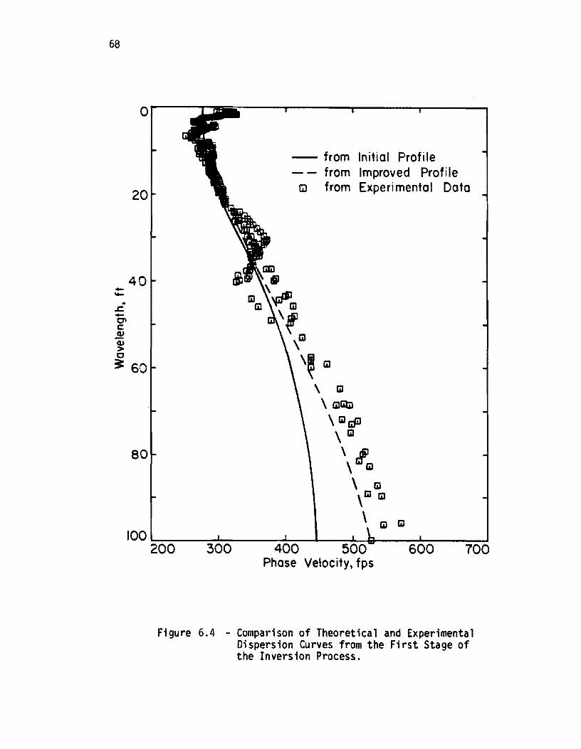
68
o
20
40 --.. .c -C'I c: .!! OJ > 0
3= 60
80
100
- from Initial Profile - - from Improved Profi Ie
[jJ from Experimental Data
,m
~m \
'~ m , EiI
\mtitl \ EiI liP
\ EiI
',1m , Gl
,Gl EiI
\ Gl Gl
200 300 400 500 700 Phase Velocity, fps
Figure 6.4 - Comparison of Theoretical and Experimental Dispersion Curves from the First Stage of the Inversion Process.
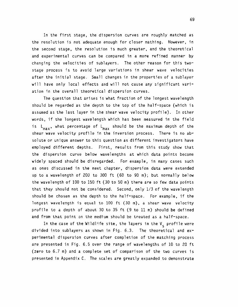
69
In the first stage, the dispersion curves are roughly matched as
the resolution ;s not adequate enough for closer mathing. However, in
the second stage, the resolution is much greater, and the theoretical
and experimental curves can be compared in a more refined manner by
changing the velocities of sublayers. The other reason for this two
stage process is to avoid large variations in shear wave velocities
after the initial stage. Small changes in the properties of a sublayer
will have only 1 oca 1 effects and wi 11 not cause any s i gnifi cant vari
ation in the overall theoretical dispersion curves.
The question that arises is what fraction of the longest wavelength
should be regarded as the depth to the top of the half-space (which is
assumed as the last layer in the shear wave velocity profile). In other
words, if the longest wavelength which has been measured in the field
is Lmax' what percentage of Lmax should be the maximum depth of the shear wave velocity profile in the inversion process. There;s no ab
solute or unique answer to this question as different investigators have
emp 1 oyed different depths. Fi rst, results from thi s study show that
the dispersion curve below wavelengths at which data points become
widely spaced should be disregarded. For example, in many cases such
as ones discussed in the next chapter, dispersion data were extended
up to a wavelength of 200 to 300 ft (60 to 90 m); but normally below
the wavelength of 100 to 150 ft (30 to 50 m) there are so few data points
that they should not be considered. Second, only 1/3 of the wavelength
shoul d be chosen a s the depth to the half-space. For examp 1 e, if the longest wavelength is equal to 100 ft (30 m), a shear wave velocity
profile to a depth of about 30 to 35 ft (9 to 11 m) should be defined and from that point on the medium should be treated as a half-space.
In the case of the Wildlife site, the layers in the Vs profile were divided into sublayers as shown in Fig. 6.3. The theoretical and ex
perimental dispersion curves after completion of the matching process
are presented in Fig. 6.5 over the range of wavelengths of 10 to 20 ft
(zero to 6.7 m) and a complete set of comparison of the two curves is
presented in Appendix C. The scales are greatly expanded to demonstrate
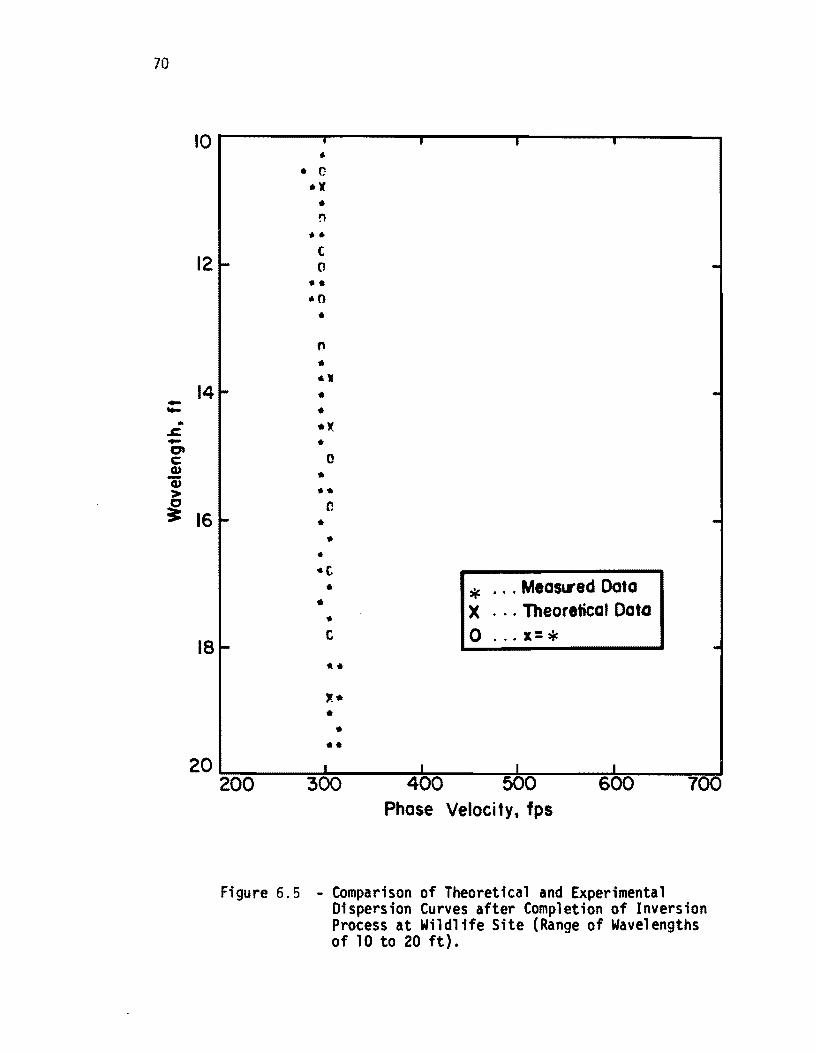
70
10
12
14 -..... .. .s::. -0' C Q)
Gi > ~ 16
18
20
• • 0 .x • n
•• C 0
•• • 0
• 0
• 6l(
• • *)( •
0
• ••
Cl
• .. .. .. c. • * · .. MeaslSed Data
* X · .. Theoretical Data .. t 0 · .. l= * .... x* • .. ••
200 300 400 500 600 700 Phase Veloci ty t fps
Figure 6.5 - Comparison of Theoretical and Experimental Dispersion Curves after Completion of Inversion Process at Wildlife Site (Range of Wavelengths of 10 to 20 ft).
71
the closeness of the match. The curves follow each other very closely.
The shear wave velocity profile after inversion is shown in Fig. 6.6.
In the inversion process, the mass densities were assumed to be
constant and Poisson's ratios of all layers were selected as 1/3. In
Nazarian and Stokoe (1985a) it is shown that the effect of these two
parameters are quite small in construction of theoretical dispersion
curves. However, the effect of misjudging Poisson's ratio and mass
density on determining elastic moduli is more pronounced. The values
of shear and Young's moduli are proportional to mass density and the
square of the shear wave velocity for a given material. Therefore,
mis-estimation of the mass density has a linear effect on shear modulus.
For example, if the actual mass density is 20 percent more than the
estimated value, the calculated shear modulus will be 20 percent less
than the actual value.
Mis-estimation of Poisson's ratio has little effect on shear
modulus, but it will affect Young's modulus. Shear modulus, G, and Young's modulus, E, are interrelated by Poisson's ratio, v, as follows:
E/G = 2(1 + v) (6.1)
Therefore, for Poisson's ratios of 1/4 and 1/2, the ratio of Young's
to shear moduli are equal to 2.5 and 3, respectively. An error of about 20 percent is introduced to the value of Young's modul us if the Poisson's ratio of 1/2 is assumed while the actual value is 1/4.
Fortunately, mass densities and Poisson's ratios of soil deposits and pavement systems are relatively well known so that ranges of 20-percent errors mentioned in both examples are usually in excess of actual cases.
To complete the discussion, the inversion process on a flexible pavement site is presented in Appendix D.
6.3 COMPARISON WITH PREVIOUS INVERSION MODELS
In the simplest form, inversion has been carried out by assuming
that the shear wave velocity is equal to anywhere from 1.0 to 1.1 times

72
-.... ..
o
10
= 20 Q. Q)
C
30
40 ~20-0----3~OO------4~OO~----5~0-0-----6~00-----70~0
Shear Wave Velocity t fps
Figure 6.6 - Shear Wave Velocity Profile from Wildlife Site after Completion of Inversion Process.
73
the phase velocity and the depth of sampling is equal to 1/3 or 1/2 of
the wavelength. For soil deposits in which the properties vary only slightly, utilization of this process may cause only a small error.
However, for media in which there exists a significant variation in
material properties with depth, the final shear wave velocity profile
is significantly in error. For example, the dispersion curve reported
by Ballard (1964) for a site in Nevada is shown by the data points in
Fig. 6.7. This site was selected because the results are well docu
mented. Frequencies measured in these tests ranged from 11 to 120 Hz.
For frequencies less than 25 Hz [wavelengths greater than 40 ft (12 m)],
a hydraulic vibrator with variable mass was used as the source. Above
that frequency (from 35 to 120 Hz), an electromagnetic vibrator was
employed to generate Rayleigh waves. A discontinuity in the dispersion
curve at a wavelength of about 40 ft (12 m) exists. This discontinuity corresponds to the point where the sources were changed. Therefore, it
seems that changing the sources caused some inconsistency in this region.
To perform inversion, Ballard assumed that the shear wave velocity was equal to the phase velocity and that the effective depth of sampling
was equal to 1/2 of the wavelength. Based upon this shear wave velocity profile, a theoretical dispersion curve was generated with program IN
VERT. The phase velocities that should have been measured by Ballard
are shown by the solid line in Fig. 6.7. It can be seen that the experimental and theoretical curves do not agree.
An attempt was made to invert correctly the dispersion curve gathered by Ballard. In this attempt, the Vs profile reported by Ballard was used as the initial profile in program INVERT, so that shear wave velocities reported by Ballard and from this attempt could be compared directly. An approximate shear wave velocity profile was determined so that the theoretical dispersion curve approximately fol
lowed the experimental curve. This profile ;s called an approximate
one due to the fact that an accurate dispersion curve cannot be defined
with so few data points over a range of wavelengths of 2 to 200 ft (0.6
to 60 m). The differences with shear wave velocity profiles are quite
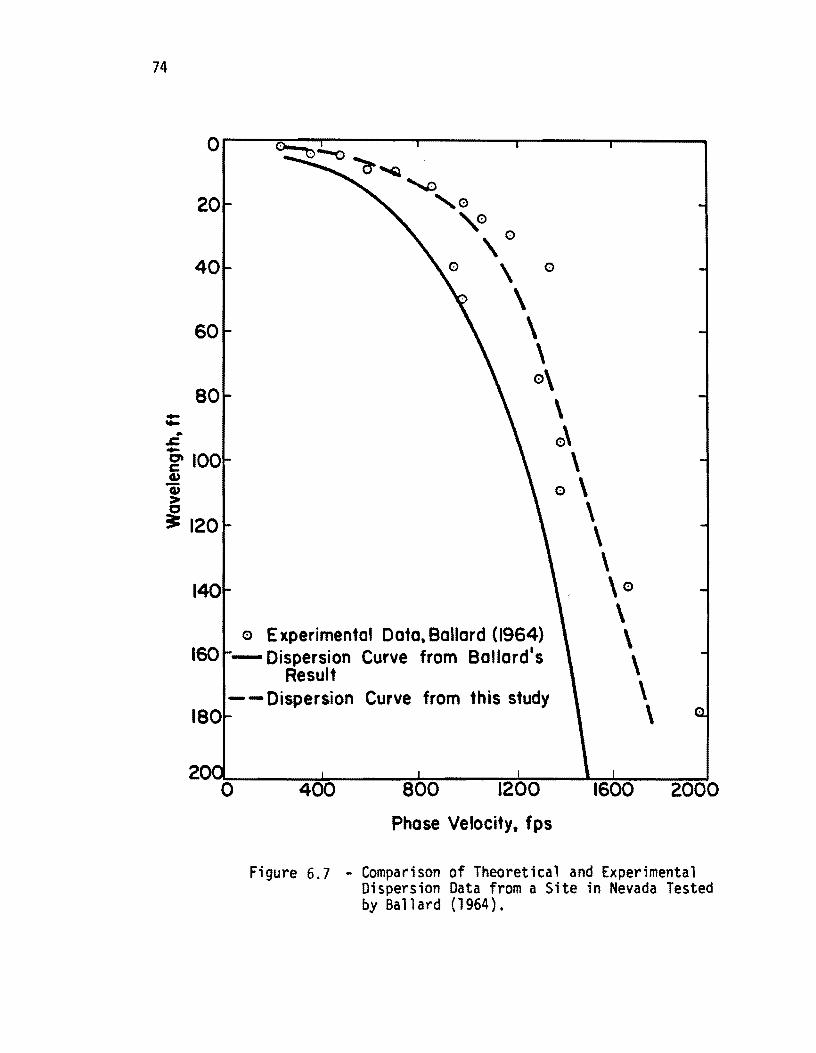
74
-.... • .s::. -80
0'100 c Q)
'ii > c
;C 120
e Experimental Data. Bdllard (964) 160 - Dispersion Curve from Bollard's
Result Curve from this study
400 800 2000
Phose Velocity, fps
Figure 6.7 - Comparison of Theoretical and Experimental Dispersion Data from a Site in Nevada Tested by Ballard (1964).
75
drastic, and, therefore, the simplified inversion process employed by
many investigators in the past should no longer be used.
6.4 SUMMARY
The inversion process which is the procedure for determining the
shear wave velocity profile from the dispersion curve is discussed and
illustrative examples are included for better understanding of this
process. Finally, with an example, it is shown that the simplified
inversion process, performed in the past by geotechnical and pavement
engineers, of scaling dispersion curves is not appropriate and should
be avoided.

!!!!!!!!!!!!!!!!!!!"#$%!&'()!*)&+',)%!'-!$-.)-.$/-'++0!1+'-2!&'()!$-!.#)!/*$($-'+3!
44!5"6!7$1*'*0!8$($.$9'.$/-!")':!
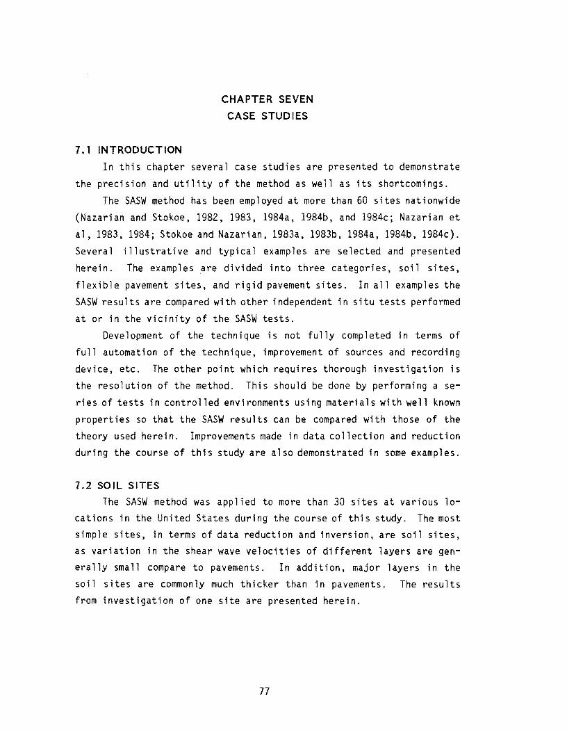
7.1 INTRODUCTION
CHAPTER SEVEN
CASE STUDIES
In this chapter several case studies are presented to demonstrate
the preC1Slon and utility of the method as well as its shortcomings.
The SASW method has been employed at more than 60 sites nationwide
(Nazarian and Stokoe, 1982, 1983, 1984a, 1984b, and 1984c; Nazarian et
al, 1983, 1984; Stokoe and Nazarian, 1983a, 1983b, 1984a, 1984b, 1984c).
Several illustrative and typical examples are selected and presented
herein. The examples are divided into three categories, soil sites,
flexible pavement sites, and rigid pavement sites. In all examples the
SASW results are compared with other independent in situ tests performed
at or in the vicinity of the SASW tests.
Development of the technique is not fully completed in terms of
full automation of the technique, improvement of sources and recording
device, etc. The other point which requires thorough investigation is
the resolution of the method. This should be done by performing a se
ries of tests in controlled environments using materials with well known
properties so that the SASW results can be compared with those of the
theory used herein. Improvements made in data collection and reduction during the course of this study are also demonstrated in some examples.
7.2 SOIL SITES
The SASW method was applied to more than 30 sites at various locations in the United States during the course of this study. The most simple sites, in terms of data reduction and inversion, are soil sites, as variation in the shear wave velocities of different layers are generally small compare to pavements. In addition, major layers in the
soil sites are commonly much thicker than in pavements. The results from investigation of one site are presented herein.
77
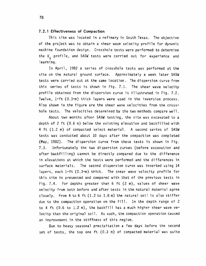
78
7.2.1 Effectiveness of Compaction
This site was located in a refinery in South Texas. The objective
of the project was to obtain a shear wave velocity profile for dynamic
machine foundation design. Crosshole tests were performed to determine
the V profi 1 e, and SASW tests were carri ed out for experience and s learning.
In April. 1982 a series of crosshole tests was performed at the
site on the natural ground surface. Approximately a week later SASW
tests were carried out at the same location. The dispersion curve from
this series of tests is shown in Fig. 7.1. The shear wave velocity
profile obtained from the dispersion curve is illustrated in Fig. 7.2.
Twelve, I-ft (O.3-m) thick layers were used in the inversion process.
Also shown in the figure are the shear wave velocities from the cross
hole tests. The velocities determined by the two methods compare well.
About two months after SASW testing, the site was excavated to a depth of 2 ft (0.6 m) below the existing elevation and backfilled with
4 ft (1.2 m) of compacted select material. A second series of SASW
tests was conducted about 10 days after the compaction was completed
(May, 1982). The dispersion curve from these tests is shown in Fig.
7.3. Unfortunately the two dispersion curves (before excavation and after backfilling) cannot be directly compared due to the difference
in elevations at which the tests were performed and the differences in surface materials. The second dispersion curve was inverted using 14 layers, each I-ft (O.3-m) thick. The shear wave velocity profile for this site is presented and compared with that of the previous tests in Fig. 7.4. For depths greater than 6 ft (2 m), values of shear wave velocity from both before and after tests in the natural material agree
closely. From 4 to 6 ft (1.2 to 1.8 m) the natural soil is also stiffer
due to the compaction operation on the fill. In the depth range of 2 to 4 ft (0.6 to 1.2 m), the backfill has a much higher shear wave ve
locity than the original soil. As such, the compaction operation caused
an improvement in the stiffness of this region. Due to heavy seasonal precipitation a few days before the second
set of tests, the top one ft (0.3 m) of compacted material was quite
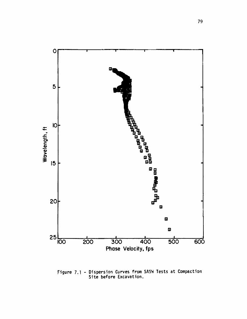
--.. .c. -0' C G> G> > 0 3:
79
o~------------~·--.--------------.-------
5
10
15
20
25
IiIm iii
I Iifn
" iii iii
iii
100 200 300 400 500 600 Phase Velocity, fps
Figure 7.1 - Dispersion Curves from SAS~ Tests at Compaction Site before Excavation.
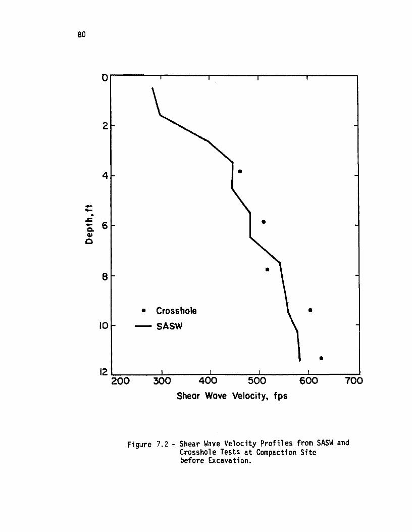
80
-~ ..
O.------,------~------~--------------
2
4
.c - 6 0-Q)
o
8
• Crosshole
10 - SASW •
• 12 ~20~0~--~~0~--~40~0~---5~0~0~--~600~--~7~00
Shear Wave Velocity, fps
Figure 7.2 • Shear Wave Velocity Profiles from SASW and Crosshole Tests at Compaction Site before Excavation.
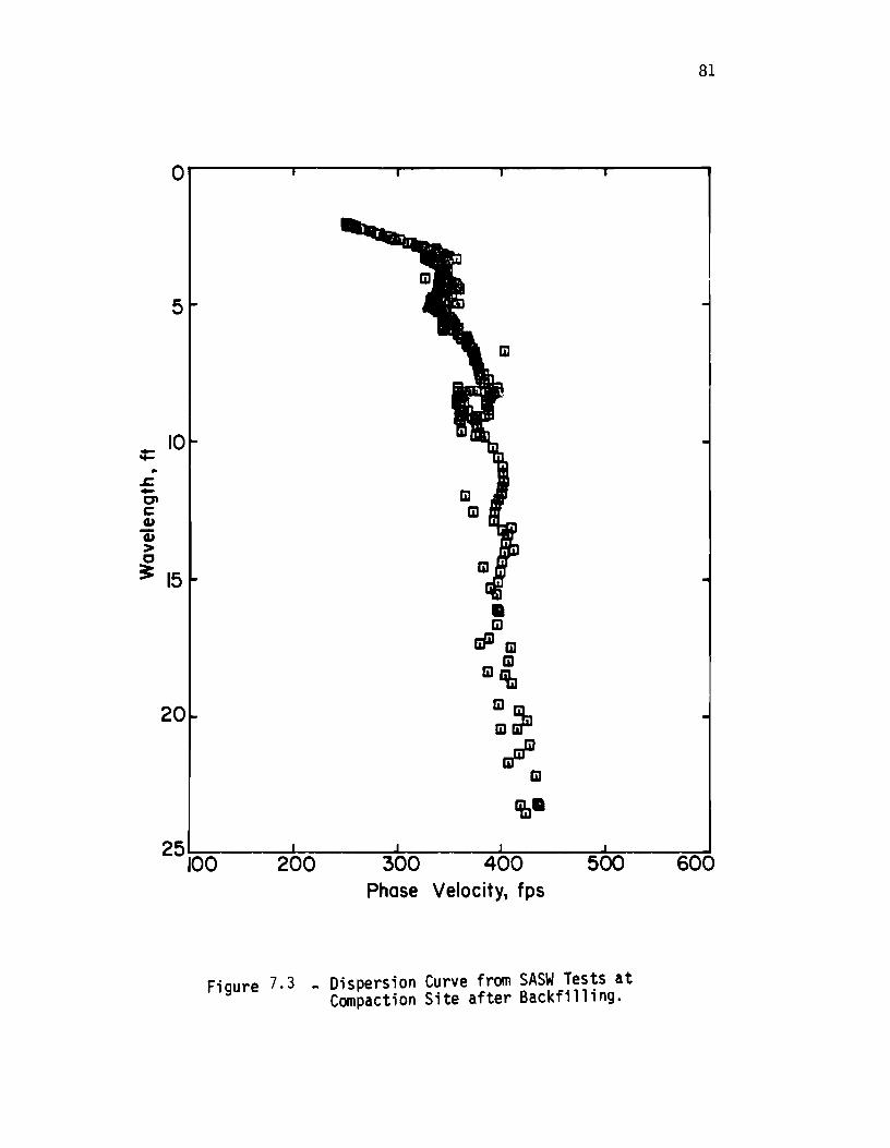
81
or-----.-----~------~----~------
5
_ 10 -.. ~ -C' c:: cu
Q) > 0
~ 15
20
25
• ELI Gfil ELI
ELI ELI 'tJ
:~ arP
ELI
'tl.
100 200 300 400 500 Phase Velocity, fps
Figure 7.3 ~ Dispersion Curve from SASW Tests at Compaction Site after Backfilling.
600
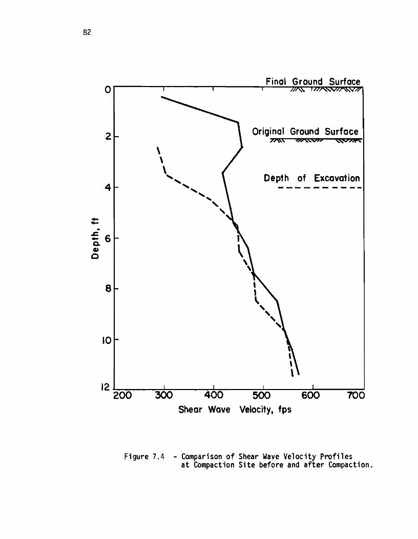
82
.... .... ..
2
4
-= 6 Q. CI.)
o
8
10
Original Ground Surface
I , "
De pt h of Excavat ion
, " ,
Shear Wave Velocity, fps
Figure 7.4 - Comparison of Shear Wave Velocity Profiles at Compaction Site before and after Compaction.
83
soft [Vs less than 400 fps (120 m/s)]. If the crude inversion technique
presented in Section 6.3 had been used, the stiffness of the fill ma
terial would have been underestimated as the existence of a low velocity
layer (as in this example) has the tendency to shift the whole
dispersion curve towards lower phase velocities.
7.3 FLEXI BLE PAVEMENT
Next to soil sites, inversion of the dispersion curves from flex
ible sites can be performed reasonably easily. More than 15 asphaltic
pavement sites have been tested, and the results from two sites are
presented to demonstrate the function of the·SASW method as well as some
of the limitations on this type of pavement.
7.3.1 McDill Air Force Base
The SASW method was employed at five sites at McDill Air Force Base
(AFB), in Tampa, Florida in August, 1983 (Stokoe and Nazarian, 1984b).
The crosshole method was also used at three of the SASW sites for
comparison. The airfield layout along with location of the test sites
are shown in Fig. 7.5a. The site discussed herein is site 3, and its
exact location is shown in Fig. 7.5b. Personnel of the Air Force had
run California Bearing Ratio (CBR) tests at the location marked as the
test pit in Figure 7.5b. The centerline of the SASW array was located
close to test pit.
A composite profile of the site is shown in Fig. 7.6. The profile consists of approximately 5 in. (12.5 em) of high quality asphaltie
concrete (AC) underlain by 8.5 in. (21 em) of lime rock, 5.5 in. (13.5
cm) of sandy-silt and then a sandy subgrade. Thisaterial profile agrees
reasonab ly well wi th that measured duri ng the drill i ng operation for
the crosshole seismic tests.
The dispersion curve from this site is presented in Fig. B.4, and
the process of inversion is discussed in detail in Appendix D. The
shear wave velocity profile along with the layering used in inversion
are shown in Fig. 7.7. A total of 20 layers was used, and the thick
nesses of the 1 ayers were increased gradually a,s the properties of
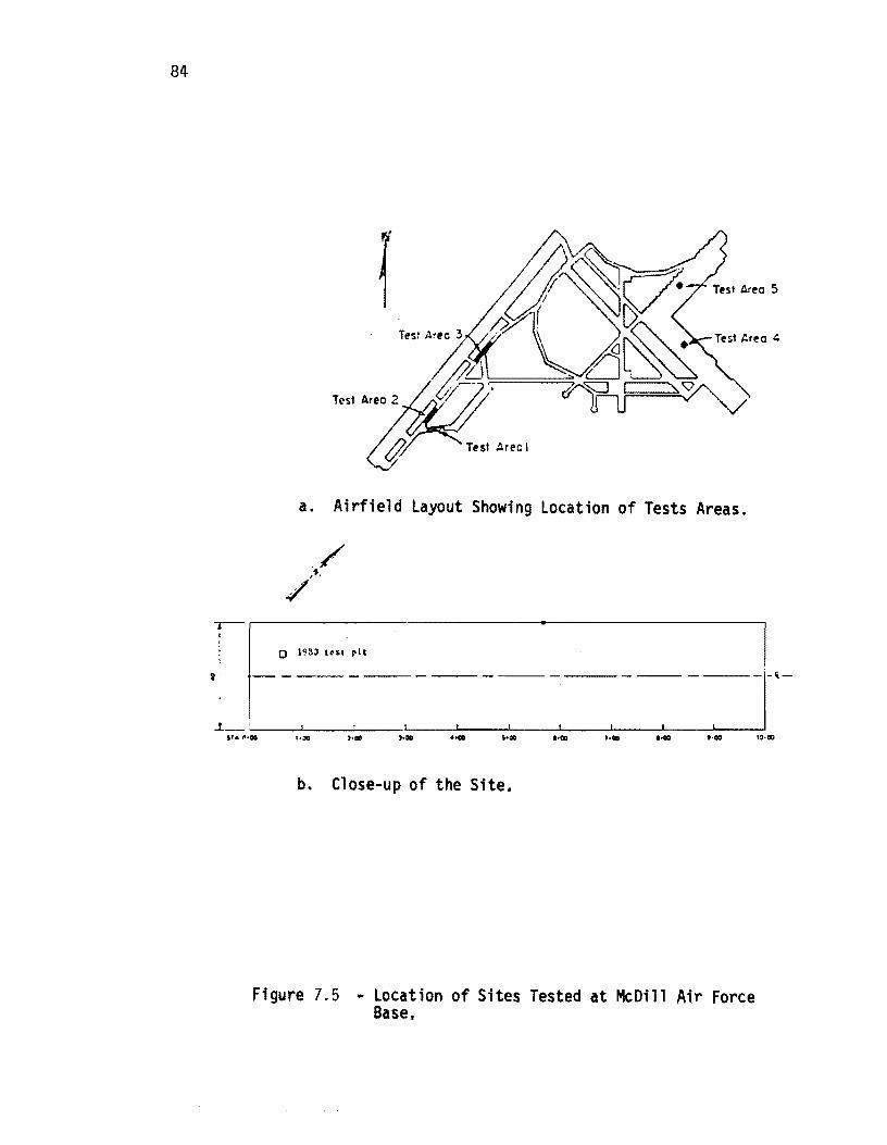
84
a. Airfield Layout Showing Location of Tests Areas .
. / ,oJ •
./ ~'----------~I
o 19SJ IC'SI rlt
-1-'-~ __ L. __ ~! ____ ~ ___ L! __ ~I~~~!~~I~ __ ~!~~=,~~I~~1
,fa f\~OO ":10 ,.QD ).00 ... '-00 '-<II '-GO .... ,,41) ',~ao
b. Close-up of the Site.
Figure 7.5 ~ Location of Sites Tested at McDill Air Force Base.
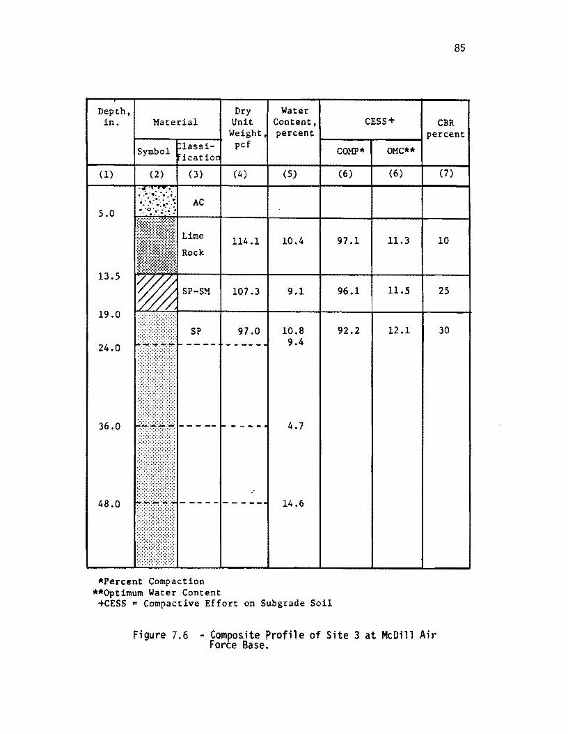
85
Dry Water Depth, in. Material
:lassiSymbol
Unit Weight,
pef
Content, percent
CESS+ CBR
t---......,...---~ percent
ieatior
(1) (2) (3)
5.0
13.5
l~ SP-SM
19.0
24.0
36.0
48.0
*Percent Compaction **Optimum Water Content
(4)
114.1
107.3
(5)
10.4
9.1
10.8 9.4
4.7
14.6
+CESS • Compactive Effort on Sub grade Soil
COMP* OMC**
(6) (6)
97.1 11.3
96.1 1l.S
92.2 12.1
Figure 7.6 - Composite Profile of Site 3 at McDill Air Force Base.
(7)
10
25
30
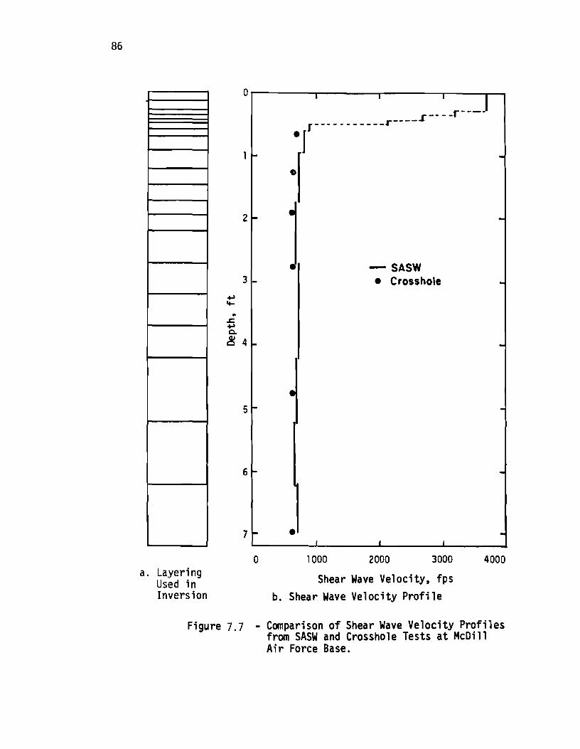
86
a. Layering Used in Inversion
Or--------r-------,--------.-----~_
-J
-I 2
3
5
6
,r----r---r-----------r
-SASW - Crosshole
7 -
o 1000 2000 3000
Shear Wave Velocity, fps b. Shear Wave Velocity Profile
4000
Figure 7.7 - Comparison of Shear Wave Velocity Profiles from SASW and Crosshole Tests at McDill Air Force Base.
87
near-surface materials are generally of most interest in a pavement
system. The results of the SASW tests are compared with S-wave velocities
obtained from crosshole tests in Fig. 7.7. The velocities compare well
below a depth of 1.5 ft (0.45 m). Unfortunately. S-wave velocities in
the asphalt could not be measured with the crosshole test. The shear
wave velocity of the lime rock is quite low as predicted by the cross
hole test and as reflected in the California Bearing Ratio (CBR) results
presented in Fig. 7.6. Young I s modul us profi 1 e from the crossho 1 e and SASW tests are
presented in Fig. 7.8 and Table 7.1. To obtain Young1s moduli from the
crosshole tests, the following procedure was followed.
1. As both P- and S-wave velocities of the layers were deter
mined, Poisson's ratio was calculated from:
(7.1)
2. Shear modulus was calculated for the measured S-wave ve
locity and an assumed unit weight using Eq. 2.1. 3. Young's modulus was then calculated utilizing Eq. 2.2 as
shear modulus and Poisson's ratio were known.
Young's moduli obtained from the SASW tests were determined based on the assumed Poisson's ratios and unit weights used in the inversion process. Values of Poisson's ratio of 0.25 for the asphalt and 0.33 for the other materials were assumed. Unit weights were assumed to be equal to 135 and 110 pcf (21.2 and 17.3 kN/m3) for the asphalt and remainder of the profile. respectively. The difference in the moduli from SASW and crosshole tests is 15 percent on the average, with a maximum
deviation of 26 percent as shown in column 6 of Table 7.1.
In pavement sites (such as in this case), the inversion process
is not sensitive to change in the velocity of the layer immediately
below because of the the large velocity contrast between the surface
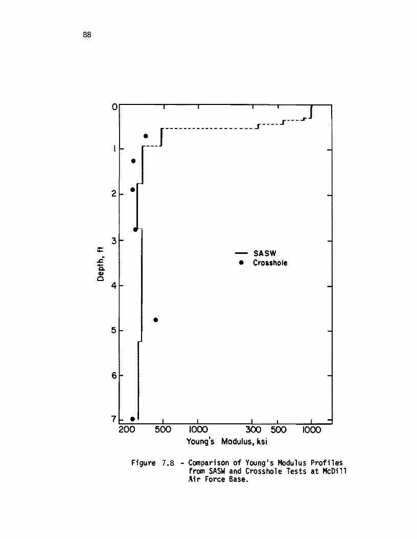
88
--.. .c -Q. Q)
0
or-------r-----~--------r---,-----~~
• J-------------------.1" J---..r
· r-2 •
3 - SASW
• Crosshole
4
• 5
6
7 • 200 1000
Young's Modulus, ksi
Figure 7.8 - Comparison of Young's Modulus Profiles from SASW and Crosshole Tests at McDill ,IUr Force Base.
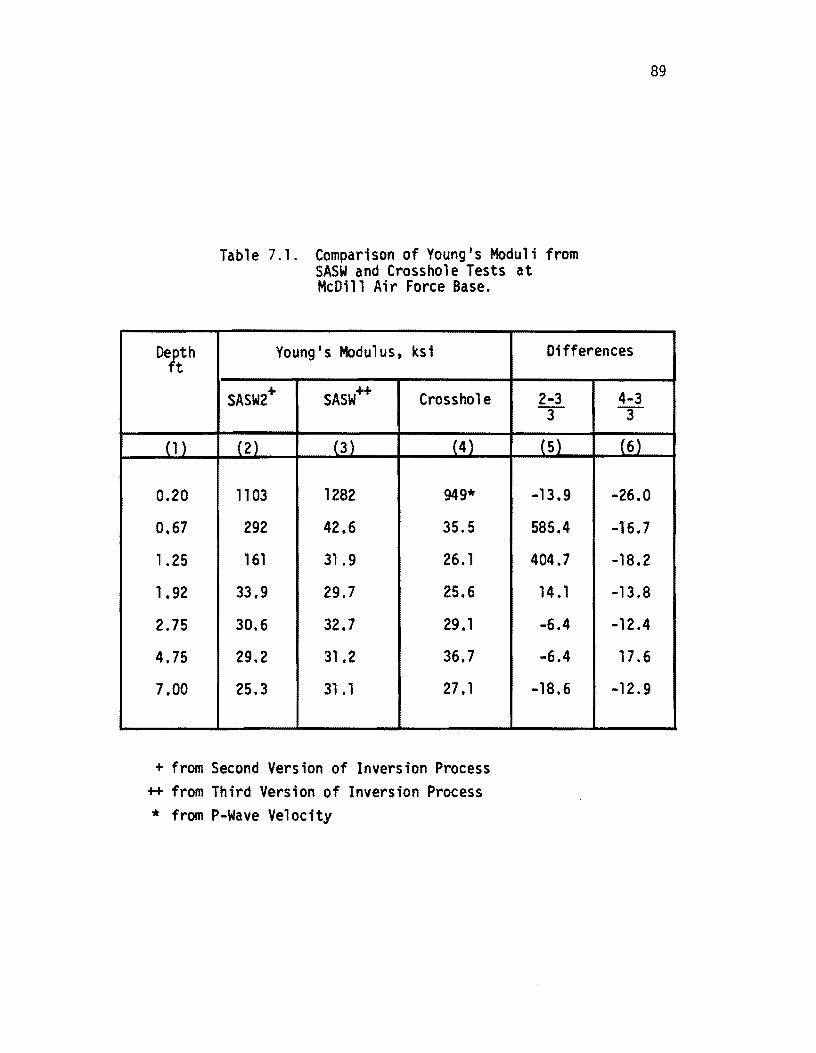
Table 7.1. Comparison of Young's Moduli from SASW and Crosshole Tests at McDill Air Force Base.
Depth Young's Modulus, ksi Differences ft
SASW2+ SASW++ Crosshole
(1) (2) (3 ) (4 )
0.20 1103 1282 949*
0.67 292 42.6 35.5
1.25 161 31.9 26.1
1.92 33.9 29.7 25.6
2.75 30.6 32.7 29.1
4.75 29.2 31.2 36.7
7.00 25.3 31.1 27.1
+ from Second Version of Inversion Process ++ from Third Version of Inversion Process * from P-Wave Velocity
2-3 4-3 -3- """3
(5) (6)
-13.9 -26.0
585.4 -16.7
404.7 -18.2
14.1 -13.8
-6.4 -12.4
-6.4 17 .6
-18.6 -12.9
89

90
layer and the base. The velocity in this region may be in error which
results in a nonuniqeness in the results in this region. This matter
is the greatest weakness of the latest inversion process and should be
studied more thoroughly in the future.
Shear wave velocities obtained by the second phase of the inversion
process, discussed in Section 6.2, are shown in Fig. 7.9 along with
shear wave velocities determined from program INVERT. Young's moduli
from the second inversion process are also given in Table 7.1. At
depths below 2 ft (0.6 m), moduli from both inversion processes compare
well. Near-surface moduli from the second process are as much as five
times stiffer (and incorrectly estimated). The two profiles follow each
other in the subgrade soil, as expected. However, near the surface,
the moduli of the lime rock is overestimated by as much as five times
relative to the new process. Notice that the CBR value of the lime rock
is only 10, whereas a typical base material has a CBR of nearly an order
of magnitude higher. Therefore, it can be seen that the new version of inversion is more apt to predict the stiffnesses of near-surface
materials.
7.3.2 Embankment Site
A series of tests was performed in Austin, Texas on a flexible
pavement section in October, 1982. The profile consisted of 2.5 in. (6.3 cm) of asphaltic concrete over 15 in. (38 cm) of cement treated base underlain by clayey subgraded. The dispersion curve from this site is shown in Fig. 7.10. The shear wave velocity profile after inversion is shown in Fig. 7.11 along with the layering used in the inversion process. A series of crosshole tests was also performed approximately two weeks prior to the SASW tests. The results from the crosshole tests
are shown in Fig. 7.11. The shear wave velocity profiles from the two
tests compare well except at a depth of 1.5 ft (0.45 m) which corre
sponds to the base material. Deviation between the velocities at this
depth is about 25 percent. It seems that this difference is due to the
fact that the inversion process still overestimates somewhat the prop
erty of the material adjacent to the top layer because a stiff layer
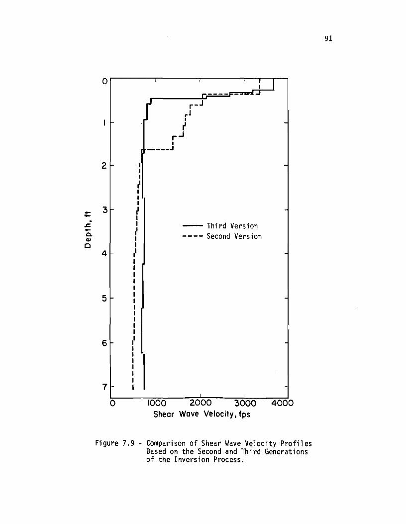
--. .c. -~ Q,)
o
o
2
3
4
5
6
7
o
II I I I
~ I I I I I I
-- Third Version ---- Second Version
1000 2000 3000 4000 Shear Wove Velocity, fps
Figure 7.9 - Comparison of Shear Wave Velocity Profiles Based on the Second and Third Generations of the Inversion Process.
91

92
-.... .. .c -t:P c Q)
Qi > 0 3=
or-----,------.------~----~------
5
10
15
20
25
30 0
m
mm
I aIil'I
m m
m
m m
m
" 500 1000 1500 2000 2500
Phase VelocitYt fps
fi.gure 7. 1 0 .. 01 spers 1.on Curve from SASW Tests at EJnbankment Si.te.
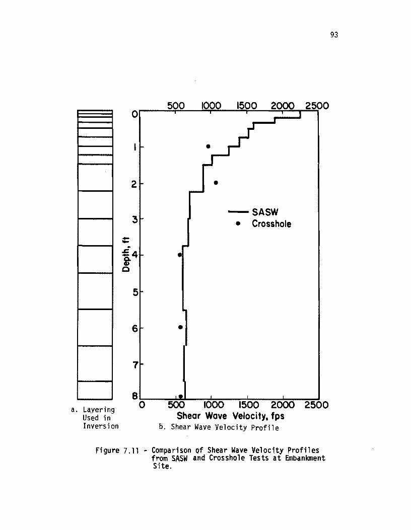
a. Layering Used in Inversion
-....
500 1000 1500 2000 2500 o
--SASW • Crosshole
6 •
7
8~ __ ~~ __ ~~~~~~~~~ o 500 1000 1500 2000 2500 Shear Wave Velocity. fps
D. Shear WaveYelocity Profile
Figure 7.11 • Comparison Qf Shear Wave Velocity profiles from SASW and Crossho1e Tests at Embankment Site.
93
94
is immediately underlain by a much softer material. More research on
this subject is required, and the inversion algorithm should be improved
to solve this deficiency.
In May, 1983 a second set of the SASW tests was carried out at this
site. In the period between the two experiments, the original pavement
was removed and replaced by a new pavement. The new pavement consists
of 2.5 in. (6.3 cm) of asphaltic concrete underlain by 15 in. (38 cm)
of flexible base and then subgrade. The dispersion curve from this
series of tests ;s presented in Fig. 7.12 and is compared with the curve
obtained before replacement of the pavement in Fig. 7.13. The two
curves follow each other quite well, within ten percent for wavelengths
greater than 5 ft (1.5 m) within ten percent. Above this wavelength
the dispersion curve from the old pavement lies below the curve from
the new pavement, resulting in a higher stiffness for the old pavement.
The shear wave velocity from the new pavement is presented and compared
with the profile from the old pavement in Fig. 7.14. To accelerate the
inversion process, the shear wave velocity profile from the first series
of tests was input as the first estimate of the profile in the second
set, because the thicknesses of the layers in both new and old pavements
were equal. It is interesting to note that the asphalt layer is stiffer for the old pavement section, possibly due to an aging affect or tem
perature differences. The base material is stiffer in the first pavement as well, due to use of stabilized material as opposed to granular base material used for the new section.
Young's modulus profiles from the two series of SASW tests are shown in Fig. 7.15 and are compared in Table 7.2. Young's modulus of the asphalt layer is 20 percent higher in the old pavement section. The base material is on the average 15 percent stiffer for the old
pavement. The subgrade moduli are within 20 percent, with a maximum
difference of 40 percent at a depth of 4 ft (1.2 m). In the subgrade
the moduli from the tests performed on the new pavement are consistently
higher. However, the variation in the results from the two sets of
tests is in the range of accuracy expected from this method. Therefore,
it cannot, at this time, be determined if these differences in subgrade
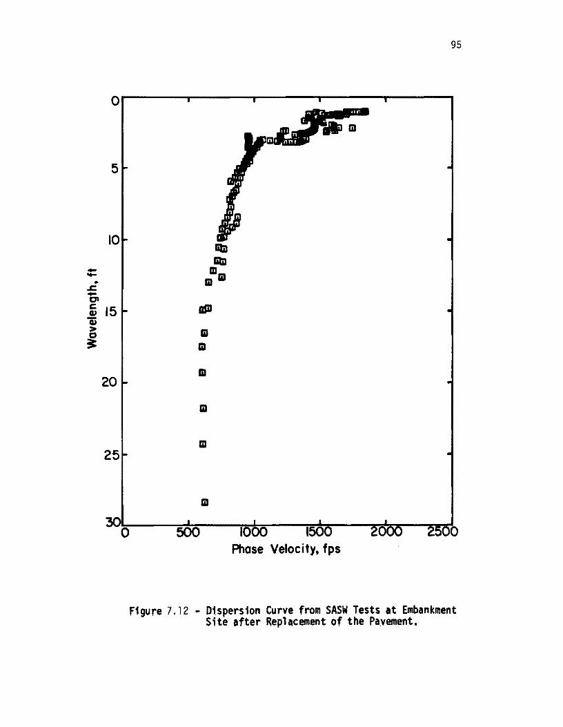
-.... .. .s::. -0' c:: cu
0::; > ~
95
o~----~~----~------~------~------~
5
10
15
20
25
o
BID IiID
GIGI GI
aID
GI GI
GI
GI
GI
GI
500 1000 1500 2000 25 Phase Velocity. fps
Figure 7.12 - Dispersion Curve from SASW Tests at Embankment Site after Replacement of the Pa,vement.
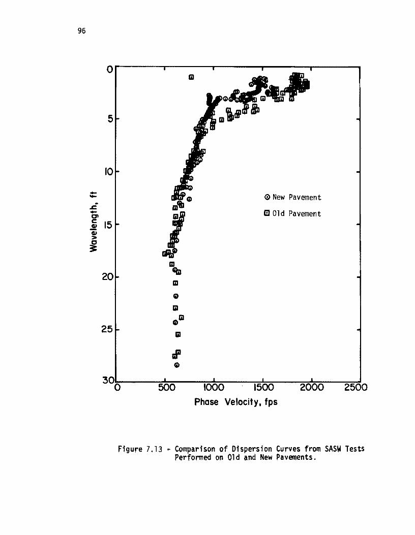
96
-.... .. .t::. -0' c:: ~ cu >
~
or------r------.-----~------~----~
OJ
5
10
<:) New Pavement
mOld Pavement 15
OJ
20 Gb1 OJ
G)
OJ
G)GJ 25
GJ
rI G)
300 500 1000 1500 2000 2500
Phase Velocity, fps
Figure 7.13 ~ Comparison of Dispersion Curves from SASW Tests Performed on Old and New Pavements.
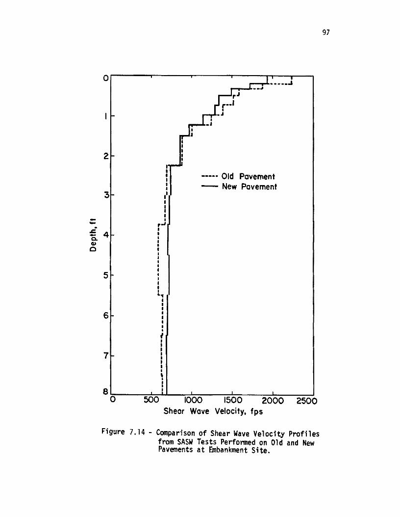
97
a
2
I ...... Old Pavement • • I - New Pavement I
3 " • I I I - • - ,-' . • .t::. 4 I -Q. I
• G) • 0 f • • • • ,
5 I
• I I • .. , ,
I I
6 • I I • • t • I I
7 I I I I I , • • • 8 I
a SOO 1000 1500 2000 2500 Shear Wove Velocity, fps
Figure 7.14 - Comparison of Shear Wave Velocity Profiles from SASW Tests Performed on Old and New Pavements at Bmbankment Site.
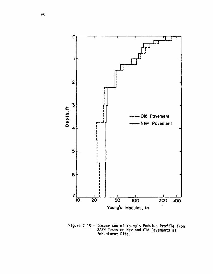
98
O~--~------~----~--------n-~~
2 r I I I I I
- 3 I I .... I ..
.r::. I ---- Old Pavement - I
Q. I CI,) r--J - New Pavement 0 I
4 I
• I I ~ • I I
5 I I I I ..,
I I I
6 I I I I I I
7 I
10 20 50 100 300 500 Young's Modulus, ksi
Figure 7.15 - Comparison of Young's Modulus Profile from SASW Tests on New and Old Pavements at Emban~ent Site.
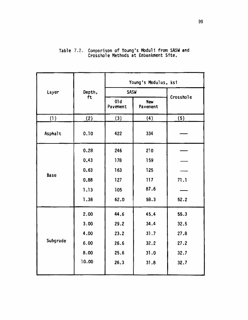
Table 7.2. Comparison of Young's Moduli from SASW and Crosshole Methods at Embankment Sfte.
Youngls Modulus, ksi
Layer Depth, SASW ft Crosshole
Old New Pavement Pavement
(1) (2) (3) (4 ) (5)
Asphalt 0.10 422 334 -
0.28 246 210 -0.43 178 159 -0.63 163 125 -
Base 0,88 127 117 71.1
1.13 105 87.6 -1.38 62.0 58.3 52.2
2.00 44.6 45.4 55.3
3.00 29.2 34.4 32.5
4.00 23.2 31.7 27.8 Subgrade 6.00 26.6 32.2 27.2
8.00 25.6 31.0 32.7
10.00 26.3 31.8 32.7
99
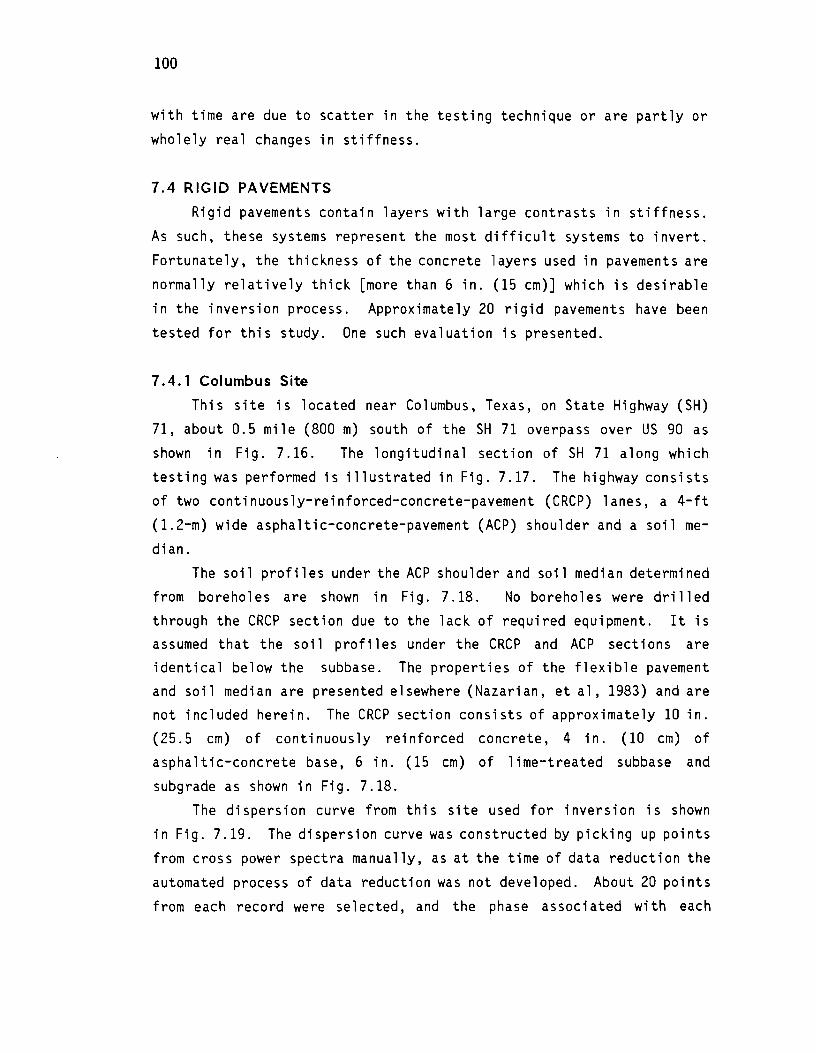
100
with time are due to scatter in the testing technique or are partly or
wholely real changes in stiffness.
7.4 RIGID PAVEMENTS
Rigid pavements contain layers with large contrasts in stiffness.
As such, these systems represent the most difficult systems to invert.
Fortunately, the thickness of the concrete layers used in pavements are
normally relatively thick [more than 6 in. (15 cm)] which is desirable
in the inversion process. Approximately 20 rigid pavements have been
tested for this study. One such evaluation is presented.
7.4.1 Columbus Site
This site is located near Columbus, Texas, on State Highway (SH)
71, about 0.5 mile (800 m) south of the SH 71 overpass over US 90 as
shown in Fig. 7.16. The longitudinal section of SH 71 along which
testing was performed is illustrated in Fig. 7.17. The highway consists
of two continuously-reinforced-concrete-pavement (CRCP) lanes, a 4-ft
(1.2-m) wide asphaltic-concrete-pavement (ACP) shoulder and a soil me
dian.
The soil profiles under the ACP shoulder and soil median determined
from boreholes are shown in Fig. 7.18. No boreho 1 e s were dri 11 ed
through the CRCP section due to the lack of required equipment. It is assumed that the soil profiles under the CRCP and ACP sections are identical below the subbase. The properties of the flexible pavement
and soil median are presented elsewhere (Nazarian, et al, 1983) and are
not included herein. The CRCP section consists of approximately 10 in.
(25.5 cm) of continuous ly rei nforced concrete, 4 in. (10 cm) of
asphaltic-concrete base, 6 in. (15 cm) of lime-treated subbase and
subgrade as shown in Fig. 7.18.
The dispersion curve from this site used for inversion is shown
in Fig. 7.19. The dispersion curve was constructed by picking up points
from cross power spectra manually, as at the time of data reduction the
automated process of data reduction was not developed. About 20 points
from each record were selected, and the phase associated with each
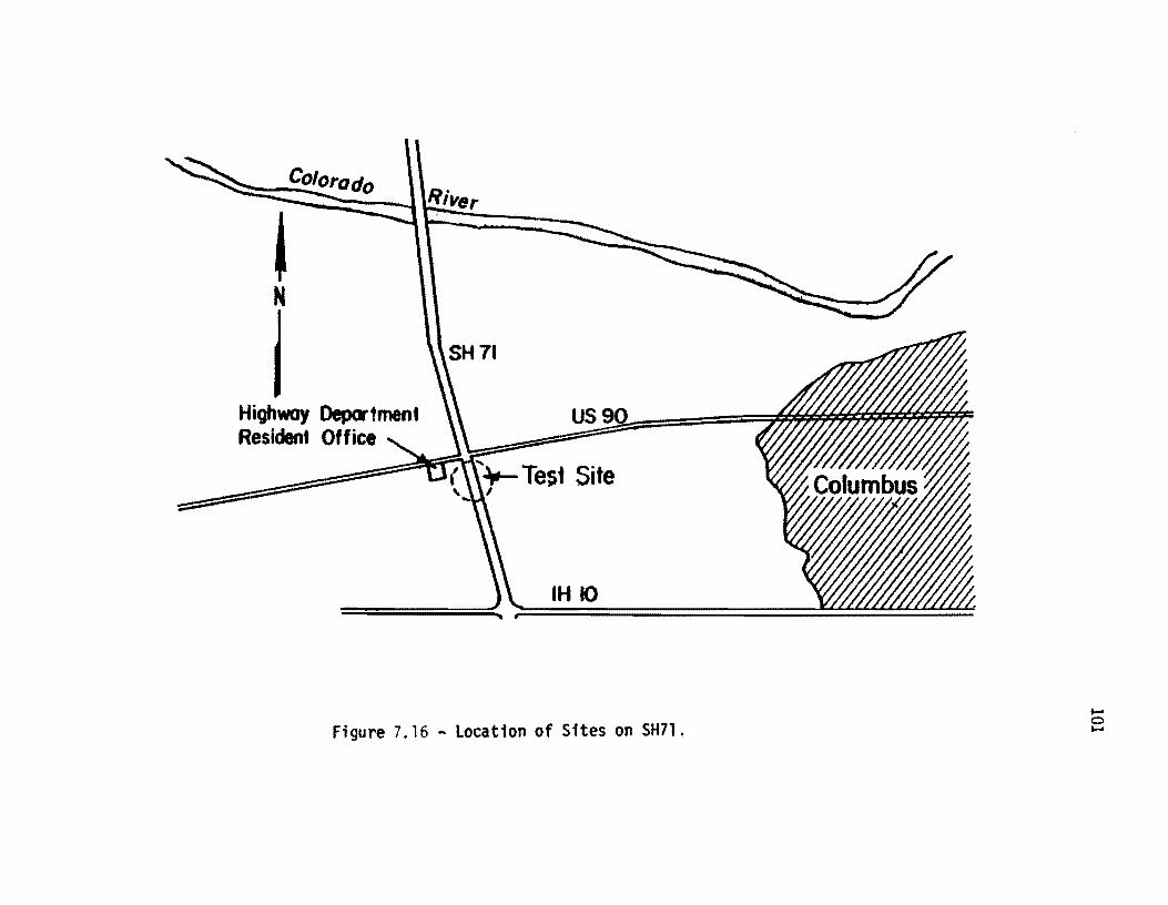
1 ""'_U~ ~iver . :::-
N
j ~l= ~' Highway Deportment ~ Resident Office .... ~
IH 10
Figure 7.16 - Location of Sites on SH71. .o .-
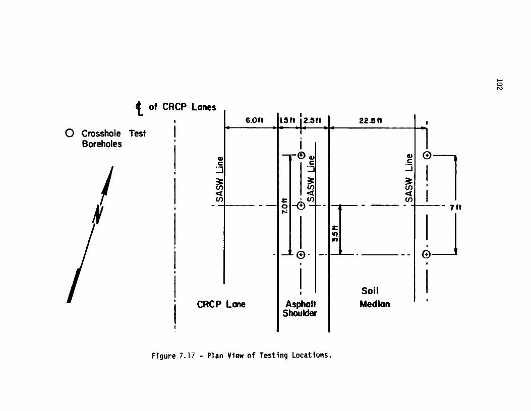
t of CRCP Lones
o Crosshole Test Boreholes
•
•
I •
I •
I I
!! : ~
~ « (J)
- -
CRCP Lme
6.0ft I
1.5 It i 2.5 ft I · I
- .... C!) Go)
c :.:J :c (J) «
I: • (J) -- 0 -(i)- -. ,...:
- _L_t!.>- --o
I •
Asphalt Shoulder
Figure 7.17 - Plan View of Testing locations.
22.5"
-
I: lID .,;
.
Soil Median
Go) c .-..J
:c (J) « (J) -
--
•
G>-
I •
I
I
G-•
I I
- 7ft
eo N
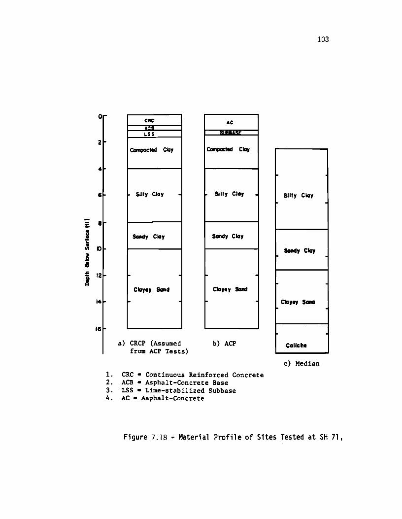
-:: § -..
6
8
J; D
J I ~ 1 12
C"C "'~B
LSS
Compacted CIa,
Silt, Clo, -
Sand, Cia,
. CIo,., Sand
~ .
a) CRCP (Assumed from ACP Tests)
AC
ComCIQCted Clay
Slit, Cia, ·
Sond, Cia,
~ · Claye, Sand
~ ·
b) ACP
1. CRC· Continuous Reinforced Concrete 2. ACB· Asphalt-Concrete Base 3. LSS· Lime-stabilized Subbase 4. AC. Asphalt-Concrete
103
~
sm, Cia, ~ ·
Sand, Clay t- ·
· Clayey Sand
~ ·
~
Caliche
c) Median
Figure 7.18 .. Materi.a1 Prof'ile of Sites Tested at SH 71,
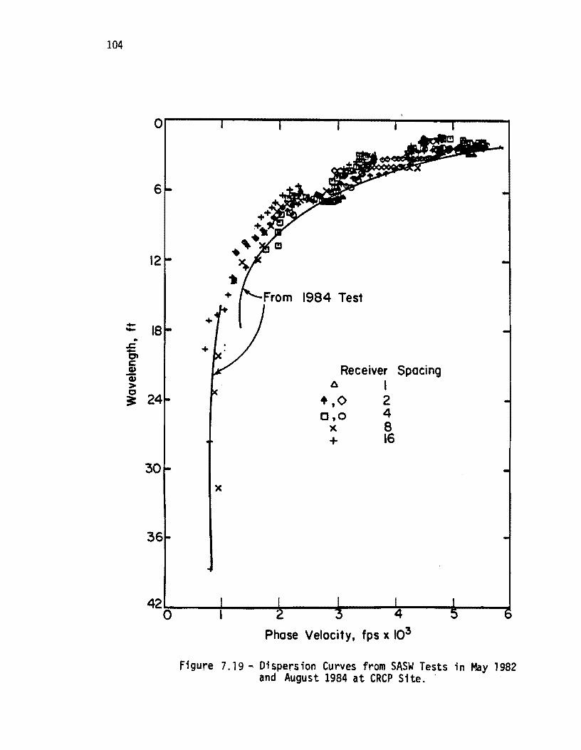
104
--.. ..c -t7' c: Q)
a:; > 0 :c
o
6
12
18
Receiver Spacing 6 I
24 + to 2 Ot O 4
)(. 8 + 16
30 x
36
42~ ____ ~ ____ ~ ____ ~ ____ ~ ____ ~ ____ ~ o
Phose Velocity, fps x 103
Figure 7.19 ~ Dispersion Curves from SASW Tests in May 1982 and August 1984 at CRCP Site ..
105
frequency was read off the analyzer screen. The phases were then un
folded (proper number of cycles was added as discussed in Section 5.2 and illustrated in Fig. 5.3). and Eqs. 5.2 through 5.4 were employed
to determine the wavelength and phase velocity associated with each data
point by using a computer program coded by Heisey (1981). The criteria
defined by Heisey for filtering the dispersion data (Eqs. 4.1 and 4.2)
were utilized. and eventually. all the phase velocity-wavelength data
from all the receiver-spacings were plotted. with no statistical ma
nipulation. The first inversion process where the layers were added
sequentially (discussed in Section 6.2) was utilized to obtain the V s profile. The shear wave velocity profile determined by this process
is shown in Fig. 7.20 and compared with the results of crosshole tests.
Since no crosshole tests were performed at this section. wave velocities
measured at the ACP section [about 7 ft (2.1 m) away] were assumed to
be representative of the S-wave velocity profile in similar material beneath the CRCP. It can be seen from Fig. 7.20 that below a depth of
2.5 ft (75 cm) the profiles from the SASW and crosshole methods compare
favorably with the velocities within 20 percent.
Recently (August, 1984) a series of SASW tests was performed at
the same location. In the first series. geophones were employed as
receivers. In this series, accelerometers were used so that higher
frequencies (up to 12.5 kHz) would be measured. The dispersion curve obtained from the second attempt is presented in Fig. 7.21. The nearsurface phase velocities are as high as about 9000 fps (2700 m/sec). The dispersion curve from the two series of tests are compared in Fig. 7.19. The solid lines in this figure represents the average dispersion curve from the 1984 attempt. The agreement between the two curves is excellent. However. the dispersion curve from recent tests suggests that the profil e near the surface is stiffer than that of the 1982 profil e. The importance of generating hi gh frequenci es duri ng SASW
tests can be realized by comparing of the dispersion curves. If high
eno~gh frequencies are not measured, the results may be in error (as
is the case in the first set of tests). The shear wave velocity profile
after inversion with program INVERT is shown in Fig. 7.22, and is com-
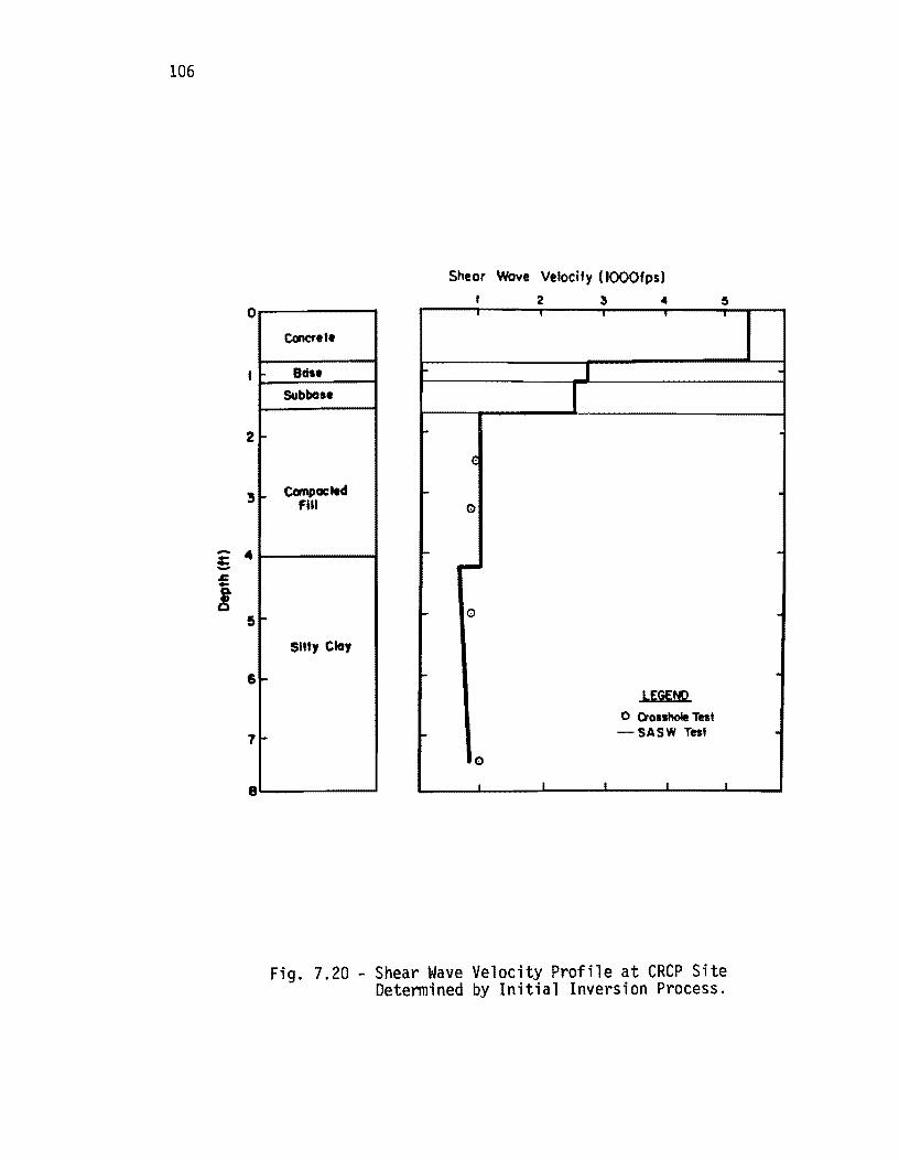
106
o
2
t-
= 4 -5
6 l-
7 t-
a
Sheer Wove Velocity (IOOOfps)
2 .. , ,
Coner,t,
ed .. ~ J Subba .. r
c:;
Compacted I-Fill G
l-
I'""'"
... 0
Sltt, Cia,
LEKfjQ o O'O.lhoIt Test
I- -SASW Test
0
I I I I I
Fig. 7.20 - Shear Wave Velocity Profile at CRCP Site Determined by Initial Inversion Process.
.
.
.
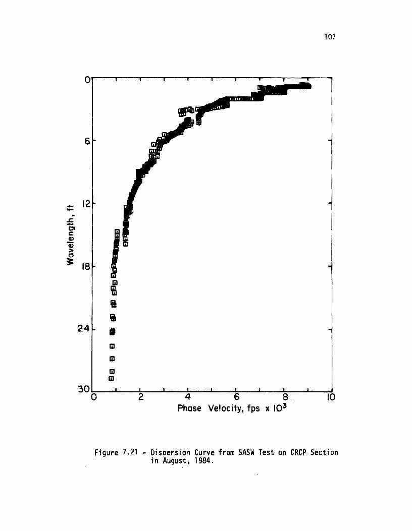
- 12 "'"' .. ~ -C7' C G,)
a:; > 0 ~ 18
24
30
107
G1 ~ II II
• G1
G1
m m
0 10 Phose
figure 7.21 - Dispersion Curve from SASW Test on CRCP Section ; n Augu s t, 1 984 .
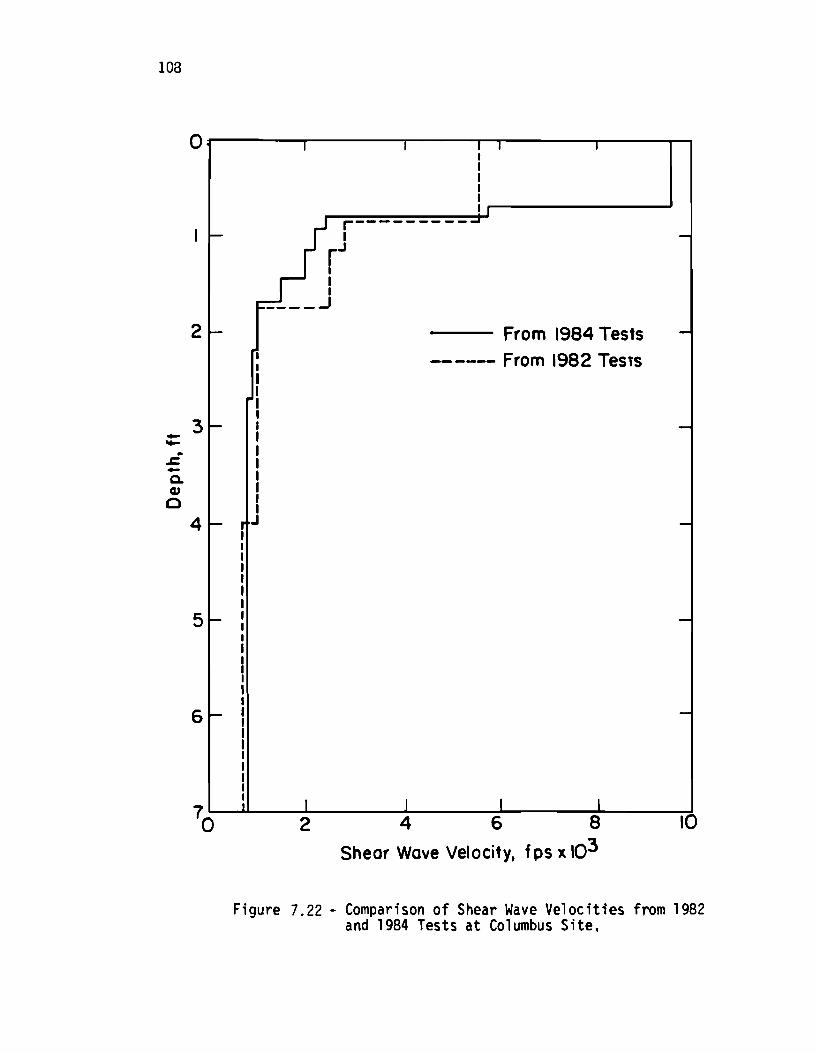
loa
0
I ~
2 -
3 ---.. .&; -Q.
CIJ 0
4 -
5-
I I : I I
I I I I , J
r--- ' ... I -
r.J I ,
------' From 1984 Tests -
------ From 1982 TesTs
-
r J -
-
-
I 1 J I I 2 4 6 8 10
Shear Wove Velocity, f ps x 103
Figure 7.22 - Comparison of Shear Wave Velocities from 1982 and 1984 Tests at Columbus Site,
109
pared with the profile obtained from the 1982 tests. The shear wave
velocity of the concrete from the recent tests is 9800 fps (2950 m/s)
which is more representative of the stiffness of the good quality con
crete used in construction of SH 71.
Young's modulus profiles from the two test series are shown in Fig.
7.23 and compared in Table 7.3. Poisson's ratios of 0.15, 0.25, 0.33
and 0.33 were assumed for the concrete, base and subbase, and subgrade,
respectively. The mass densities used in calculation of Young's moduli
were, 150, 125, 110 and 110 pcf ( 24.5, 20.4, and 18 kN/m3) for con
crete, base and subbase, and subgrade, respectively. The stiffness of
the concrete layer is much higher from the tests performed in 1984 (as
it should be for such a high quality concrete). At the same time,
Young's moduli of the base and subbase differ by almost a factor of two
from the two series of tests. The profile from the 1982 tests was used
as the first trial for the inversion of the 1984 tests. If the high
frequency waves were measured in the first series of tests, the devi
ation between the moduli of the base and subbase would be much greater.
The moduli of the subgrade compare favorably (within 20 percent). It should be mentioned that the first series of tests performed
on this site was the first experience of the first author with pave
ments, and the 1984 testing was the last site tested for this study.
The improvements in all aspects of data collection, reduction and inversion process is evident from this example. However, more research ;s required to extend all the aspects mentioned.
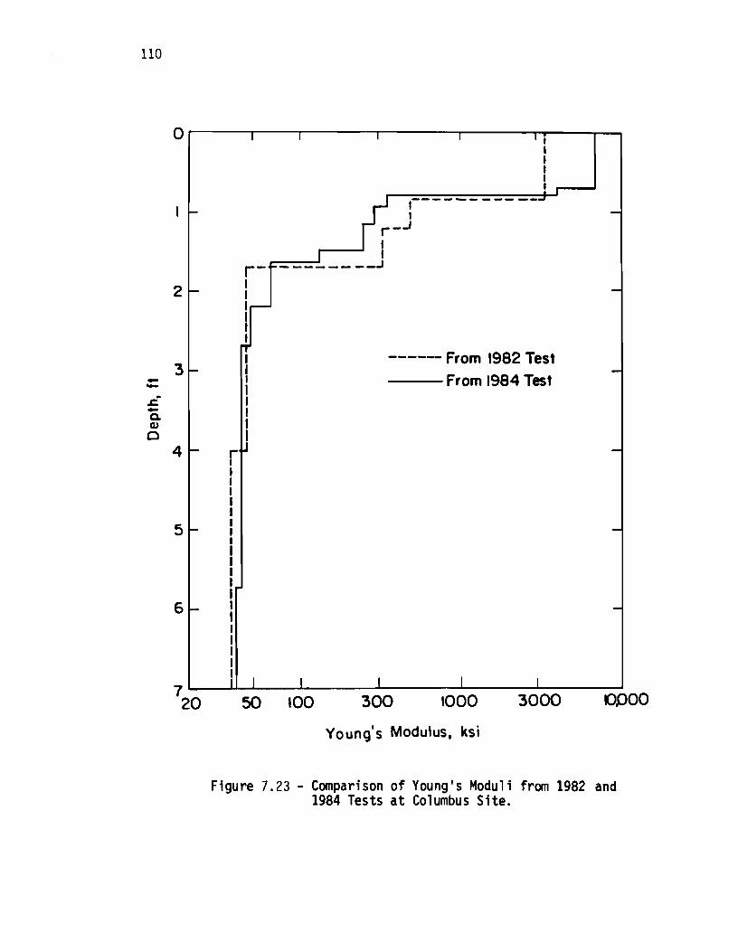
110
--£ -Q. CI)
o
o
~
2 I-
3 ~
4 I-
5 I-
6 I-
7 20
I r I I I I I I I I I
- ---I - ~
I -r--' ,
I , r- fo------ ---'
-~
rt ----- From 1982 Test -
From 1984 Test
r U -
-
-
I I I I I I
50 100 300 1000 3000 0.000
Young's Modulus, ksi
Figure 7.23 - Comparison of Young's Moduli from 1982 and 1984 Tests at Columbus Site.
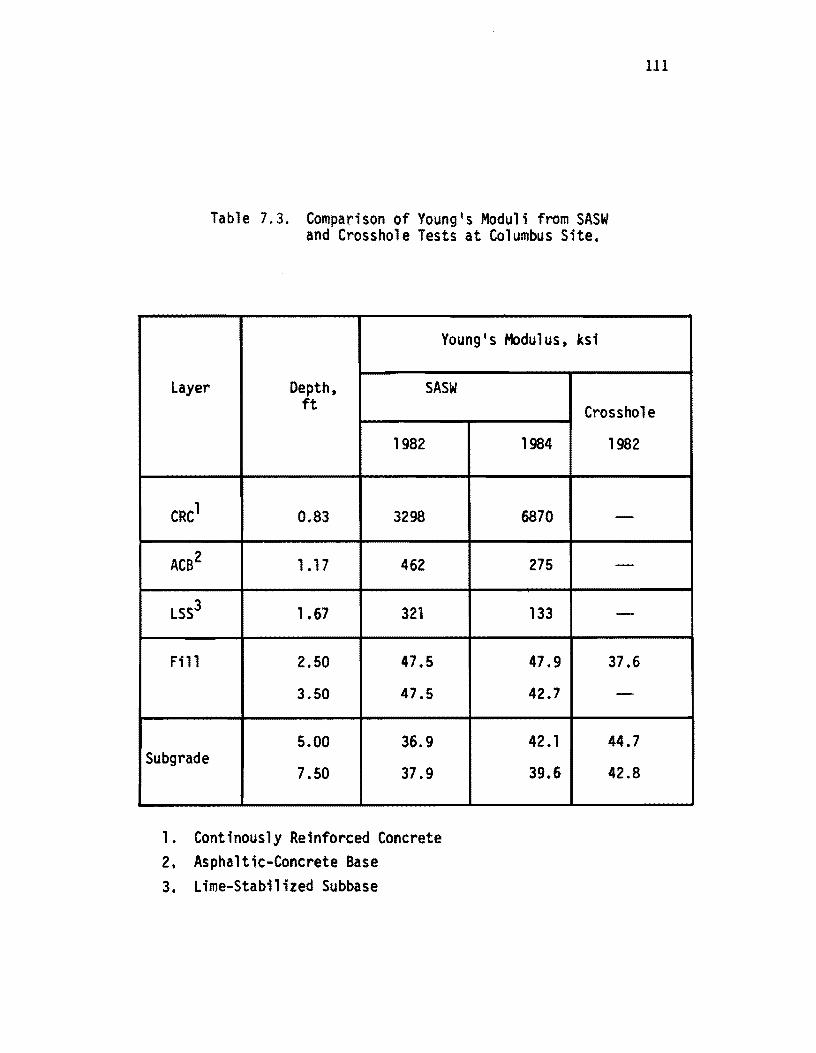
Layer
Table 7.3. Comparison of Young's Moduli from SASW and Crossho1e Tests at Columbus Site.
Young's Modulus, ksi
Depth, SASW
111
ft Crossho1e
1982 1984 1982
CRC1 0.83 3298 6870 -
ACB2 1.17 462 275 -
LSS3 1.67 321 133 -
Fill 2.50 47.5 47.9 37.6
3.50 47.5 42.7 -
5.00 36.9 42.1 44.7 Subgrade
7.50 37.9 39.6 42.8
1. Continously Re1nforced Concrete 2. Asphaltic-Concrete Base 3. Lime-Stabilized Subbase

!!!!!!!!!!!!!!!!!!!"#$%!&'()!*)&+',)%!'-!$-.)-.$/-'++0!1+'-2!&'()!$-!.#)!/*$($-'+3!
44!5"6!7$1*'*0!8$($.$9'.$/-!")':!
CHAPTER EIGHT
SUMMARY, CONCLUSIONS AND RECOMMENDATIONS
8.1 SUMMARY
The Spectral-Analysis-of-Surface-Waves (SASW) method is described
herei n. The method is used to determi ne the shear wave velocity and
elastic modulus profiles of soil sites and pavement sections. With this
method, a transient vertical impulse is applied to the surface, and a
group of surface waves with different frequencies are generated in the
medium. These waves propagate along the surface with velocities which
vary with frequency and the properties of the different layers in the
medium. Propagation of the waves are monitored with two receivers a
known distance apart at the surface. By analysis of phase information
from the cross power spectrum and by knowing the distance between re
ceivers, phase velocity, shear wave velocity and moduli of each layer
are determined. Measurement of the seismic waves are performed at
strains below 0.001 percent where wave behavior is essentially elastic
and independent of strain amplitude and strain rate.
8.2 CONCLUSIONS
Based upon employment of this testing technique at many sites with
substantially different profiles, the following conclusions are drawn.
1. The SASW method is well suited for determining moduli and
thicknesses of pavement layers as well as shear wave ve
locity profiles of soil sites.
2. The results of SASW tests performed in situ are quite re
peatable as dispersion curves from different tests per
formed at the same locations follow each other closely.
3. Use of the common-receiver-midpoint geometry reduces scat
ter in field data and, hence, is most accurate.
4. The simplified inversion process based upon scaling the
dispersion curve is not suitable for determining shear wave
113
114
velocity profiles and a more rigorous inversion process
such as the one presented herein should be utilized.
5. Shear wave velocities obtained with the SASW method are
genera lly withi n 20 percent of those determi ned by other
independent seismic methods.
6. Thicknesses of different layers are normally predicted with
an accuracy of about 10 percent relative to layering re
ported from coring or construction plans.
7. When a large contrast exists in the stiffness of two layers
in the profile, the inversion program used for construction
of the theoretical dispersion curve is not sensitive to the
stiffness of the layer immediately adjacent to the stiffer
layer. Therefore, the results in this region are somewhat
in error.
8.3 RECOMMENDATIONS FOR FUTURE RESEARCH
This study is the start of an extensive research project on in situ
nondestruct i ve measurements of materi a 1 s. More refi nement is needed
in the SASW method to develop fully the method. However, the study
presented herein demonstrates the positive aspects and potential of the SASW method. The following are recommended for future research.
First, in situ data collection should be improved by:
1. adding a source capable of generating frequencies below 5
Hz so that deeper deposits can be sampled, 2. investigating the effect of distance between the source and
near receiver to define the optimum distance for each set
up, 3. fully automating the in situ data collection process to
reduce testing time (greatly); design and construction of
this type of equipment should be accelerated so that rapid
collection of data can be performed at pavement sites open
to traffic, and
115
4. updating the recording device with one capable of sampling
data with a much higher resolution to achieve a more refined dispersion curve at lower frequencies (longer wavelengths).
Second, theoretical aspects of the SASW method also require some
modifications as follows:
1. elimination of the nonuniqueness in the results at regions
where a large velocity contrast exists in the profile, and
2. improvement in the statistical package for combining the dispersion curves is desirable for better definition of the
final dispersion curve.
Finally, a series of model tests on materials with well known properties in the laboratory environment should be carried out for
better understanding of the behavior of the waves, effect of receiver coupling, effect of shape and weight of sources, and configuration of source-receiver array.

!!!!!!!!!!!!!!!!!!!"#$%!&'()!*)&+',)%!'-!$-.)-.$/-'++0!1+'-2!&'()!$-!.#)!/*$($-'+3!
44!5"6!7$1*'*0!8$($.$9'.$/-!")':!
REFERENCES
1. Anderson, D.G., and Woods, R.D. (1975), "Comparison of Field and Laboratory Shear Moduli ," Proceedings, Conference on In Situ Measurement of Soil Properties, ASCE, Vol. I, Raleigh, NC, pp. 69-92.
2. Baird, G.T. (1982), "Wave Propagation Method of Pavement Evalu-ation," New Mexico Engineering Research Institute, University of New Mexico, Albuquerque, NM.
3. Ballard, R.F., Jr. (1964), "Determination of Soil Shear Moduli at Depths by In Situ Vibratory Techniques," Miscellaneous Paper No. 4-691, U.S. Army Engineer Waterways Experiment Station, Vicksburg, MS.
4. Ballard, R.F., Jr., and Casagrande, D.R. (1967), "Dynamic Founda-tion Investigations, TAA-2A Radar Site, Cape Kennedy, Florida," Miscellaneous Paper 4-878, U.S. Army Engineer Waterways Experiment Station, Vicksburg, MS.
5. Ballard, R.F., Jr., and Chang, F.K. (1973), "Rapid Subsurface Exploration; Review of Selected Geophysical Techniques," Miscellaneous Paper No. S-69-30, U.S. Army Engineer Waterways Experiment Station, Vicksburg, MS.
6. Bennette, M.J., and Chen, A.T.F. (1982), "Site Characterization for Stations 6 and 7, El Centro Motion Array, Imperial Valley, California," Open File Report 82-1040, U.S. Geological Survey, Menlo Park, CA, 37 pages.
7. Bergstrom, S.G., and Linderholm, S. (1946), "Dynamisk Metod att Utrona Ultiga Marklagers Genomsnittliga Elasticitetsegens kaper," Handlinger No.7, Svenska Forsknings-Institutet for Cement och Betong Vid. Kungl. Tekniska, Hogskolan.
8. Cunny, R.W., and Fry, Z.B. (1973), "Vibratory In Situ and Labora-tory Soil Moduli Compared,lI Journal of the Soil Mechanics and Foundations Division, ASCE Vol. 99, No. SM12, pp. 1055-1076.
9. DEGEBO (1938), "Deutsche Gesellschaft fur Bodenmechanik," Vol. 4, Springer, Berlin.
117
118
10. Dunkin, J.W. (1965), "Computation of Modal Solutions in Layered, Elastic Media at High Frequencies," Bulletin of Seismological Society of America, Vol. 55, No.2, pp. 335-358.
11. Eagleson, B., Heisey, J.S., Hudson, W.R., Meyer, A.H., and Stokoe, K.H., II (1981), IIComparison of Falling Weight Deflectometer and Dynaflect for Pavement Evaluation,1I Report No. 256-1, Center for Transportation Research, University of Texas, Austin, TX.
12. Engineer Manual 1110-1-1802 (1979), Geophysical Exploration, Department of the Army, Corps of Engineers, U.S.A.
13. Fry, Z.B. (1965), "Dynamic Soils Investigations Project Buggy, Buckboard Mesa Nevada Test Site, Mercury, Nevada," Miscellaneous Paper No. 4-666, U.S. Army Engineer Waterways Experiment Station, Vicksburg, MS.
14. Geological Survey (1982), liThe Imperial Valley, California, Earthquake of October 15, 1979,11 Professional Paper 1254, U. S. Department of Interior, Washington, DC, 451 pages.
15. Haag, E.D. (1984), "Laboratory Investigation of the Static and Dynami c Soil Properties of Sands from the Imperi alVa 11 ey, Cal ifornia after the 1981 Westmorland Earthquake, II Master ' s Thesis, University of Texas, Austin, Texas.
16. Haag, E.D., Stokoe, K.H., II, and Nazarian S. (1984), "Seismic Investigation of Five Sites in the Imperial Valley, California after the 1981 Westmorland Earthquake, II Geotechnical Engineering Center, University of Texas, Austin, Texas.
17. Haas, R., and Hudson, W.R. (1978), Pavement Management Systems, Mcgraw Hill Book Co., New York, NY, 456 pages.
18. Haskell, N.A. (1953), liThe Dispersion of Surface Waves on Multi-layered Media,lI Bulletin of Seismological Society of America, Vol. 43, No.1, pp. 17-34.
19. Hardin, B.D., and Drnevich, V.P. (1972), IIShear Modulus and Damping in Soils: Measurement and Parameter Effects," Journal of the Soil Mechanics and Foundations Division, ASCE, Vol. 95, No. SM6, pp. 603-624.
20. Heisey, J.S. (1982), "Determination of In Situ Shear Wave Velocity from Spectral Analysis of Surface Waves,1I Master's Thesis, University of Texas, Austin, TX, 300 pages.
21. Heukelom, W., and Klomp, J.G. (1962), IIDynamic Testing as a Means of Contro 11 i ng Pavements duri ng and after Construction ,II
119
Proceedings, International Conference on Structural Design of Asphalt Pavements," Ann Arbor, MI, pp. 495-510.
22. Hoar, R.J. (1982), "Field Measurement of Seismic Wave Velocity and Attenuation for Dynamic Analyses," Ph.D. Dissertation, The University of Texas, Austin, TX, 479 pages.
23. Krohn, C.E. (1984), "Geophone Ground Coupling," Geophysics, Vol. 49, No.6, pp. 722-731.
24. Lamb, H. (1904), "On the Propagation of Tremors Over the Surface of an Elastic Solid," Philosophical Transactions of the Royal Society of London, Vol. A203, pp. 1-42.
25. Lytton, R.L., Moore, W.M., and Mahoney, J.P. (1975), "Pavement Evaluation: Phase I, Pavement Evaluation Equipment," Report No. FHWA-RD-75-78, Federal Highway Administration, Washington, D.C.
26. Mark Products (1981), "Geophone General Information," Marks Products, Inc., Houston, TX., 17 pages.
27. Maxwell, A.A., and Fry, F.B. (1967), "A Procedure for Determining Elastic Moduli of In Situ Soils by Dynamic Techniques," Proceedings, International Symposium on Wave Propagation and Dynamic Properties of Earth Materials, Albuquerque, NM, pp. 913-920.
28. Miller,!., and Freund, J.E. (1977), Probability and Statistics for Engineers, Prentice-Hall, Inc., Englewood Cliffs, NJ, 529 pages.
29. Nazarian, S. (1984), "In Situ Determination of Elastic Moduli of Soil Deposits and Pavement Systems by Spectral-Analysis-ofSurface-Waves Method," Doctoral Dissertation, The University of Texas, Austin, Texas, 452 pages.
30. Nazarian, S. and K.H. Stokoe, II (1982), IIEvaluation of Moduli and Thi cknesses of Pavement Systems by SASW methods, II Report No. 256-4, Center for Transportation Research, The Universty of Texas, Austin, TX.
31. Nazarian, S., Stokoe, K.H., II and W.R. Hudson (1983), "Use of Spectral Analysis of Surface Waves for Determination of Modul i and Thi cknesses of Pavement Systems, II Transportation Research Record, No. 954, Washington, D.C.
32. Nazarian, S., and K.H. Stokoe, II (1984a), "Nondestructive Testi ng of Pavements Using Surface Waves, II Transportation Research Record, 993, Washington, D.C.
120
33. Nazarian, S., and K.H. Stokoe, II (1984b), "In Situ Shear Wave Velocities from Spectral Analysis of Surface Waves," Proceedings, Eighth World Conference on Earthquake Engineering, San Francisco, California.
34. Nazarian, S. and K.H. Stokoe, II (1984c), "Investigation of Five Pavement Sections at Homestead Ai r Force Base, Flori da by Surface Wave Technique," Geotechnical Engineering Center, The University of Texas, Austin, TX.
35. Nazarian, S. and K.H. Stokoe, II (1985a), "In Situ Determination of Elastic Moduli of Pavement Systems by Spectral-Analysisof-Surface-Waves Method (Theoretical Aspects), II Report No. 437-1, Center for Transportation Research, The University of Texas, Austin, TX (in press).
36. Nazarian, S. and K.H. Stokoe, II (1985b), "User1s Guide for Interactive Program "INVERT" Used in Inversion of Dispersion Curves, II Report No. 437-2, Center for Transportation Research, The University of Texas, Austin, TX (in press).
37. Nazarian, S., W. Uddin, K.H. Stokoe, II and A.H. Meyer (1984), "Modul i and Thi cknesses of Pavement Systems from Spectral Ana lysi s of Surface Waves, II Proceedi ngs, Tenth Worl d Meeting of International Road Federation, Brazil.
38. Neilson, J.R., and Baird, G.T. (1975), "Air Force System for Nondestruct i ve Testing of Pavements, II Presented at, Symposi urn on Nondestructive Test and Evaluation of Airport Pavements, Vicksburg, MS.
39. Neilson, J.P., and Baird, G.T. (1977), "Evaluation of an Impulse Test i ng Techni que for Nondestructi ve Testing of Pavements, II Research Report CEEDO-TR-77-46, Tyndall AFB, Panama City, FL.
40. Nijober, L.W., and Van der Poel, C. (1953), IIA Study of Vibration Phenomena in Asphaltic Road Construction,1I Proceedings, Association of Asphaltic Pavement Technology, pp. 197-231.
41. PCB Piezotronics (1983), "Quartz Piezoelectric Transducers," (from) Catalog No. 375, PCB Piezotronics,Inc., Depew, NY.
42. Rayl ei gh, L. (1887), liOn Waves Propagated along the Pl ane Surface of an Elastic Solid," Proceedings, London Mathematical Society, Vol. 17, pp. 4-11.
43. Richart, F.E., Jr. (1978), "Field and Laboratory Measurement of Dynami c Soi 1 Properties, II Proceedi ngs of the Conference on Dynamical Methods in Soil and Rock Mechanics, Karlsruhe, Germany, Vol. I, pp. 3-36.
121
44. Richart, F.E., Jr., Hall, J.R., Jr., and Woods, R.D. (1970), Vibrations of Soils and Foundations, Prentice-Hall, Inc., Englewood Cliffs, NJ, 414 pages.
45. Schwab, F., and Knopoff, L. (1970), IISurface Wave Dispersion Computations,1I Bulletin of Seismological Society of America, Vol. 60, No.2, pp. 321-344.
46. Stokoe, K.H., II (1980), IIField Measurement of Dynamic Soil Properties,1I presented to the Specialty Conference on Civil Engineering and Nuclear Power, ASCE, Sept. 15-17, Knoxville, Tennessee, 31 pp.
47. Stokoe, K.H., II, and Chen, A.T.F. (1980), IIEffects on Site Response of Methods of Estimating In Situ Soil Behavior,1I Proceedi ngs, Seventh World Conference on Earthquake Engineering, Turkey.
48. Stokoe, K.H., II, and Hoar, R.J. (1978), "Variables Affecting in Situ Seismic Measurements ,II Proceedings, Conference on Earthquake Engineering and Soil Dynamics, ASCE, Pasadena, CA, Vol. II, pp. 919-939.
49. Stokoe, K.H., II, and Lodde, P.F. (1978), "Dynamic Response of San Franci sco Bay Mud, II Proceedi ngs, Conference on Earthquake Engineering and Soil Dynamics, ASCE, Pasadena, CA, Vol. II, pp. 940-959.
50. Stokoe, K.H., II and S. Nazarian (1983a), II Effecti veness of Ground Improvement from Spectral Analysis of Surface Waves," Proceedi ngs, Ei ghth European Conference on Soil Mechani cs and Foundation Engineering, Helsinki, Finland, Vol. 1, pp. 91-95.
51. Stokoe, K.H., II and S. Nazarian (1983b), "Comparative Study of Two Pavement Sections at Tyndall Air Force Base, Florida,1I Report No. GR83-23, Geotechnical Engineering Center, The Universty of Texas, Austin, TX.
52. Stokoe, K.H., II and S. Nazarian (1984a), IIInvestigation of Stability of Debris Blockage Imponding Lakes of Mt. St. Helens, Washington, by Surface Wave Method,1I Report No. GR84-2, Geotechnical Engineering Center, The University of Texas, Austin, TX.
53. Stokoe, K.H., II and S. Nazarian (1984b), IIDetermination of Mudu-1 i and Thi cknesses of Fi ve Pavement Sect; ons, McDi 11 Ai r Force Base, Florida by Different In Situ Seismic Tests,1I Report No. GR84-7, Geotechnical Engineering Center, The University of Texas, Austin, TX.
122
54. Stokoe, K.H., II and S. Nazarian (1984c), IIInvestigation of Two Earth Dams inCa 1 Horni a Acquaduct System by Surface Wave Technique," Report No. GR84-4, Geotechnical Engineering Center, The University of Texas, Austin, TX.
55. Stokoe, K.H., II, and Woods R.D. (1972), "In Situ Shear Wave Velocity by Cross-Hole Method,1I Journal of Soil Mechanics and Foundations Division, ASCE, Vol. 98, No. SM5, pp. 443-460.
56. Thomson, W.T. (1950), "Transmission of Elastic Waves through a Stratified Solid Medium," Journal of Applied Physics, Vol. 21, pp. 89-93.
57. Thrower, E.N. (1965), "The Compution of the Dispersion of Elastic Waves in Layered Media," Journal of Sound Vibration, Vol. 2, No.3, pp. 210-226.
58. Uddi n, W. (1984), "A Structural System for Pavements Based on Dynamic Deflections," Ph.D. Dissertation, The Universty of Texas, Austin, TX.
59. Uddin, W., Nazarian, S., Hudson, W.R., Meyer, A.H., and Stokoe, K.H., II (1983), "Investigation into Oynaflect Deflections in Re 1 at; on to Location/Temperature Parameters and In Situ Material Characteristics of Rigid Pavements," Research Report No. 256-5, Center for Tran sporta t ion Research, The University of Texas, Austin, TX, 273 pages.
60. Van der Poel, C. (1951), "Dynamic Testing of Road Construction," Journal of Applied Chemistry, Vol. 1, No.7, pp. 281-290.
61. Van der Poel, C. (1954), "A General System Describing the ViscoElastic Properties of Bitumens and its Relation to Routine Test Data," Shell Bitumen Reprint No.9, Shell Laboratories-Kominklikike.
62. Woods, R.D. (1978), "Measurment of Dynamic Soil Properties," Proceedings of the Conference Placement and Improvement of SOTl to Support Structures, ASCE, Cambridge, Massachusetts, pp. 407-435.
63. Woods, R.D., and Richart, F.E., Jr. (1967), "Screening of Elastic Surface Waves by Trenches," Proceedi ngs, Internat i ona 1 Symposium on Wave Propagation and Dynamic Properties of Earth Materials," Albuquerque, NM, pp. 275-290.
64. Yoder, E.J., and Witczak, M.W. (1975), Principles of Pavement Design, John Wiley & Sons, Inc., New York, NY, 2nd Edition, 711 pages.

APPENDIX A
EQUIPMENT USED IN SASW TESTING
A.l SOURCE
The source should be able to generate surface waves over a wide
range in frequencies with adequate amplitude so that they can be de
tected by the recei vers. Simultaneously, the source shoul d generate
minimal P- and S-wave energy. Near the surface, P- and S-waves (body
waves) attenuate much more rapidly than surface waves. The distance
between the first receiver (receiver closer to the source) and the
source should be large enough so that a significant amount of the energy
associated with the body waves dies out before arrival at the first
receiver. On the other hand, if the source is too far from the first
or second receiver, another problem arises. The energy (amplitude)
associated with different frequencies may not be sufficient to be de
tected by the recei vers, and background noi se domi nates the records.
The optimum di stance between the source and fi rst receiver is bei ng
studied in a separate investigation.
For sampling shallow depths, the maximum frequency excited is of
utmost importance. For shallow sampling, the receivers and source are
placed close to one another; therefore, it is not necessary to transfer
much energy to the medium. High frequencies translate to short wave
lengths, which correspond to shallower depths of sampling. The highest
frequency required in an experiment depends on the stiffness of the material near the surface as well as the particle size of this material.
For a constant wavelength, the maximum frequency required in testing
will increase as the stiffness of the layer increases. However, it cannot be expected to measure meaningful velocities for wavelengths shorter than about the maximum aggregate size. For a typical soil de
posit, the highest frequency necessary is on the other of 200 to 800
Hz; for a flexible pavement, the source should generate frequencies up
to 6 kHz, and, for a rigid pavement, this upper boundary ;s on the order
of 10 to 20 kHz.
123
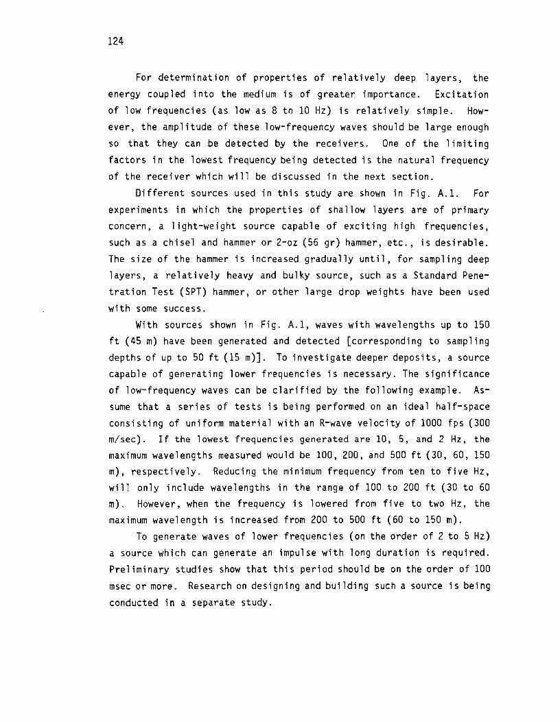
124
For determination of properties of relatively deep layers, the
energy coupled into the medium is of greater importance. Excitation
of low frequencies (as low as 8 to 10 Hz) is relatively simple. How
ever, the amplitude of these low-frequency waves should be large enough
so that they can be detected by the rece i vers. One of the 1 i mit i ng
factors in the lowest frequency being detected is the natural frequency
of the receiver which will be discussed in the next section.
Different sources used in this study are shown in Fig. A.I. For
experiments in which the properties of shallow layers are of primary
concern, a light-weight source capable of exciting high frequencies,
such as a chisel and hammer or 2-oz (56 gr) hammer, etc., is desirable.
The size of the hammer is increased gradually until, for sampling deep
layers, a relatively heavy and bulky source, such as a Standard Pene
tration Test (SPT) hammer, or other large drop weights have been used
with some success.
With sources shown in Fig. A.1, waves with wavelengths up to 150
ft (45 m) have been generated and detected [corresponding to sampling
depths of up to 50 ft (15 m)J. To investigate deeper deposits, a source
capable of generating lower frequencies is necessary. The significance
of low-frequency waves can be clarified by the following example. As
sume that a series of tests is being performed on an ideal half-space
consisting of uniform material with an R-wave velocity of 1000 fps (300 m/sec). If the lowest frequencies generated are 10, 5, and 2 Hz, the
maximum wavelengths measured would be 100, 200, and 500 ft (3~, 60, 150 m), respectively. Reducing the minimum frequency from ten to five Hz,
will only include wavelengths in the range of 100 to 200 ft (30 to 60 m). However, when the frequency is lowered from fi ve to two Hz, the
maximum wavelength is increased from 200 to 500 ft (60 to 150 m).
To generate waves of lower frequencies (on the order of 2 to 5 Hz)
a source which can generate an impulse with long duration is required.
Preliminary studies show that this period should be on the order of 100
msec or more. Research on designing and building such a source is being
conducted in a separate study.
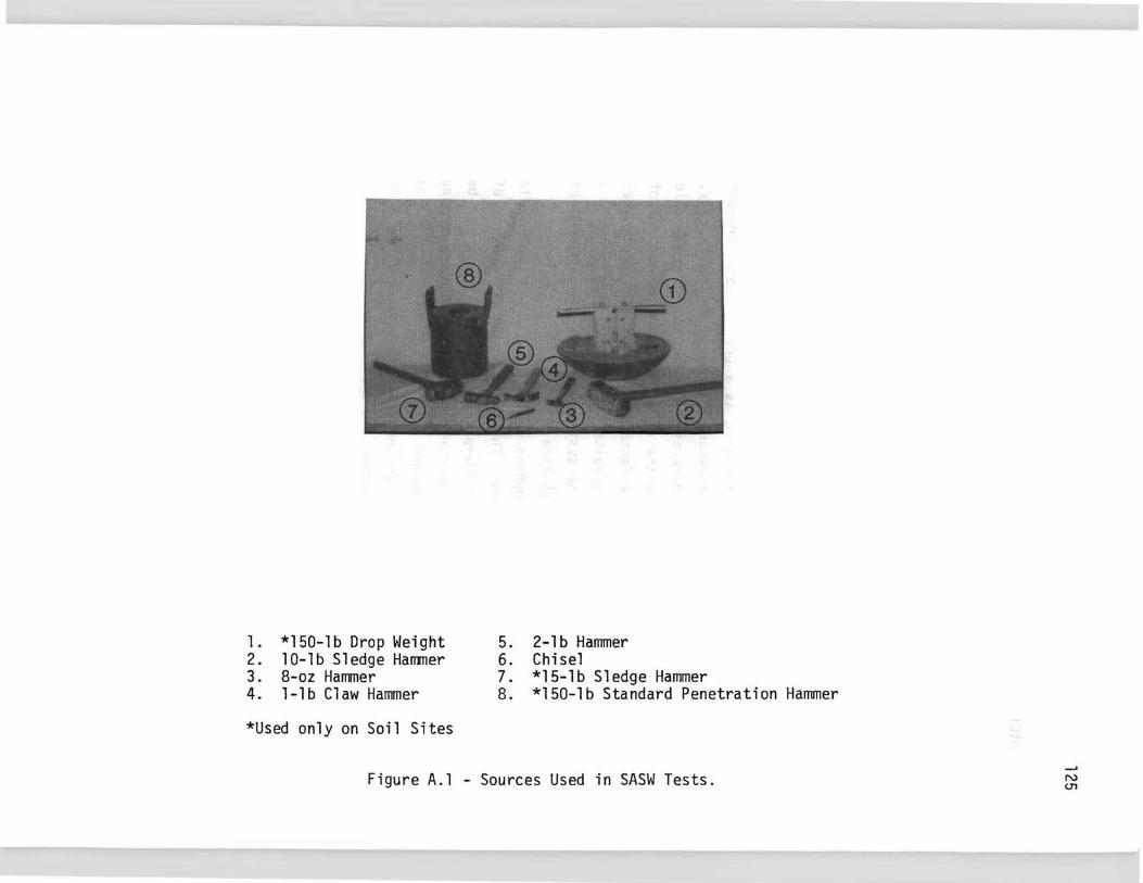
1. *150-lb Drop Weight 5. 2-lb Hammer 2. lO-lb Sledge Hammer 6. Chisel 3. 8-oz Hammer 7. *15-lb Sledge Hammer 4. l-lb Claw Hammer 8. *150-lb Standard Penetration Hammer
*Used only on Soil Sites
Figure A.l - Sources Used in SASW Tests. -' N <..T1
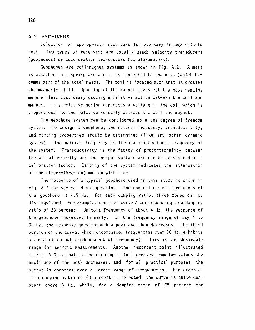
126
A.2 RECEIVERS
Selection of appropriate receivers is necessary in any seismic
test. Two types of receivers are usually used: velocity transducers
(geophones) or acceleration transducers (accelerometers).
Geophones are coil-magnet systems as shown in Fig. A.2. A mass
is attached to a spring and a coil is connected to the mass (which be
comes part of the total mass). The coil is located such that it crosses
the magnetic field. Upon impact the magnet moves but the mass remains
more or less stationary causing a relative motion between the coil and
magnet. This relative motion generates a voltage in the coil which is
proportional to the relative velocity between the coil and magnet.
The geophone system can be considered as a one-degree-of-freedom
system. To design a geophone, the natural frequency, transductivity,
and damping properties should be determined (like any other dynamic
system). The natural frequency is the undamped natural frequency of
the system. Transductivity is the factor of proportionality between
the actual velocity and the output voltage and can be considered as a
calibration factor. Damping of the system indicates the attenuation
of the (free-vibration) motion with time.
The response of a typical geophone used in this study is shown in
Fig. A.3 for several damping ratios. The nominal natural frequency of
the geophone is 4.5 Hz. For each damping ratio, three zones can be
distinguished. For example, consider curve A corresponding to a damping
ratio of 28 percent. Up to a frequency of about 4 Hz, the response of
the geophone increases 1 i nearly. In the frequency range of say 4 to
30 Hz, the response goes through a peak and then decreases. The third
portion of the curve, which encompasses frequencies over 30 Hz, exhibits
a constant output (independent of frequency). This is the desirable
range for seismic measurements. Another important point illustrated
in Fig. A.3 is that as the damping ratio increases from low values the
amplitude of the peak decreases, and, for all practical purposes, the
output is constant over a 1 arger range of frequenci es. For example.
if a damping ratio of 60 percent is selected, the curve is quite con
stant above 5 Hz, while, for a damping ratio of 28 percent the
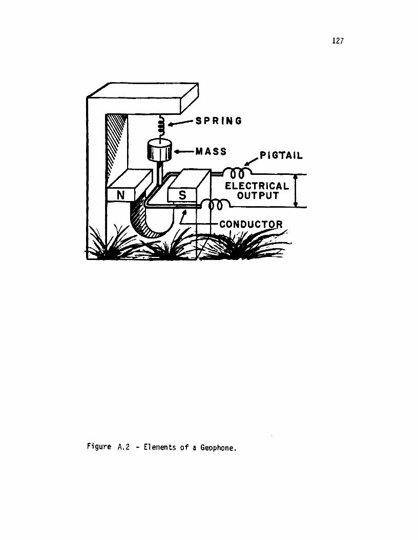
,PIGTAIL
ELECTRICAL OUTPUT
Figure A.2 - Elements of a Geophone.
127
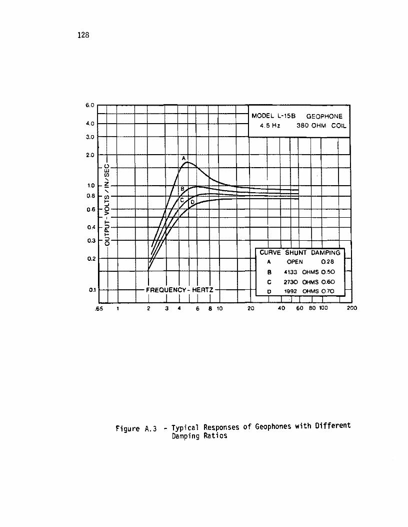
128
6,0
4,0
3,0
2,0
1.0
0.8
0.6
0,4
0.3
0.2
0.1
_u w rJ)
" -~
" -cJ)
s f-O
> -, I-
-6: I-
-::I 0
.65
MODEL L-15B GEOPHONE 4.5 Hz 380 OHM COIL
~ ......
" / ........ -/ I~ II ill .~ l.9--~
J I) "7 I 'II
Ih I 1// CURVE SHUNT DAMPING
~ A OPEN 0.28 l-
S 4133 OHMS 0,50 l-
e 2730 OHMS 0.60 FREQUENCY - HERTZ 0 1992 OHMS 070 l-
I I f I I I I I ·1 I 1 I I 2 3 4 6 8 10 20 40 60 80 100 200
Figure A.3 - Typi cal Responses of Geophones with Different Damping Rat; os
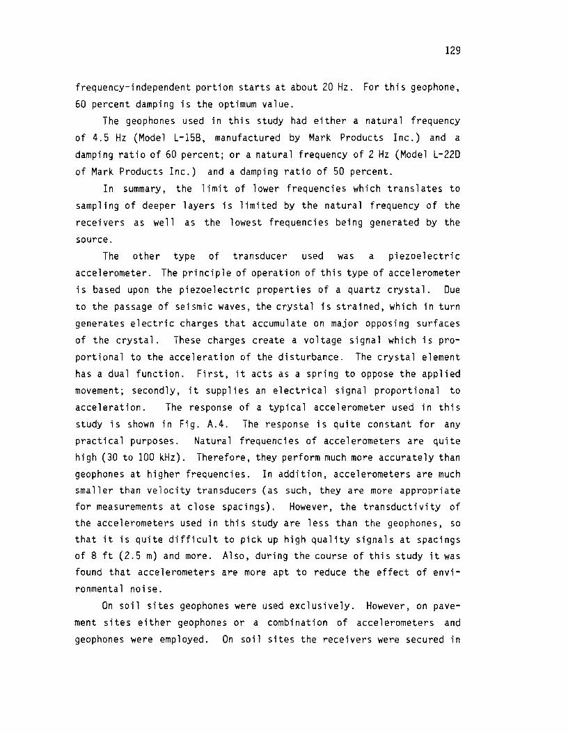
129
frequency-independent portion starts at about 20 Hz. For this geophone,
60 percent damping is the optimum value.
The geophones used in thi s study had either a natural frequency
of 4.5 Hz (Model L-15B, manufactured by Mark Products Inc.) and a
damping ratio of 60 percent; or a natural frequency of 2 Hz (Model L-22D
of Mark Products Inc.) and a damping ratio of 50 percent.
In summary, the limit of lower frequencies which translates to
sampling of deeper layers is limited by the natural frequency of the
recei vers as well as the lowest frequenci es bei ng generated by the
source.
The other type of transducer used was a piezoelectric
accelerometer. The principle of operation of this type of accelerometer
is based upon the pi ezoe 1 ectri c properties of a quartz crystal. Due
to the passage of seismic waves, the crystal is strained, which in turn
generates electric charges that accumulate on major opposing surfaces
of the crystal. These charges create a voltage signal which is pro
portional to the acceleration of the disturbance. The crystal element
has a dual function. First, it acts as a spring to oppose the applied
movement; secondly, it supplies an electrical signal proportional to
acceleration. The response of a typical accelerometer used in this
study is shown in Fig. A.4. The response is quite constant for any
practical purposes.
high (30 to 100 kHz).
Natura 1 frequenc; es of accelerometers are quite Therefore, they perform much more accurately than
geophones at higher frequencies. In addition, accelerometers are much smaller than velocity transducers (as such, they are more appropriate for measurements at close spacings). However, the transductivity of the accelerometers used in this study are less than the geophones, so that it is quite difficult to pick up high quality signals at spacings
of 8 ft (2.5 m) and more. Also, during the course of this study it was found that accelerometers are more apt to reduce the effect of envi
ronmental noise.
On soil sites geophones were used exclusively. However, on pave
ment sites either geophones or a combination of accelerometers and
geophones were employed. On soil sites the receivers were secured in
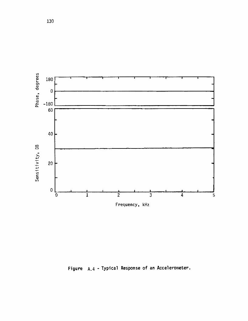
130
III (J)
180 (J) S-
• • --. • J -T • en ~ · (J) -0 0 .. (J) III ~ -1'0
-180 .J: 0..
60
- · 40 l- ·
co Cl .. >, +-' .,... > .,... 20 l- · +-' .,... III C (J) -V)
0 I I I I I • I I
o 1 2 3 4 5
Frequency, kHz
Figure A.4 - Typical Response of an Accelerometer.
131
place by means of spikes approximately 2-;n. (S-cm) long.
Accelerometers were mounted on the pavement surface with bees-wax, and
geophones were epoxied to the surface with S-minute epoxy glue. The
accelerometers and geophones used are shown in Fig. A.S. It should be
mentioned that the casings of the geophones were built at the in-house
machine shop.
Good coupling between the receivers and the material being tested
is essential. Recently Krohn (1984) studied the geophone-ground cou
pling in detail in the laboratory and the field. He concluded that for
very loose soils the geophones should be buried for better coupling.
For firm soils he indicated that use of the conventional method of using
spikes is adequate.
A.3 RECORDING DEVICE
A conveni ent recordi ng devi ce for performi ng SASW tests is a
spectral analyzer. An in-depth review of Fourier transforms and spec
tral analyses is presented in Chapter Three. A spectral analyzer is a
digital oscilloscope that, by means of a microprocessor attached to it,
has the ability to perform signal analysis directly in either the time or frequency domain.
The analyzer used in this study is a Hewlett-Packard (HP) 5423A
structural dynamics analyzer. The HPS423A, shown in Fig. A.6, is portable and consists of three components which stack together vertically during operation and are connected by means of appropriate cables. The three units are:
(1) oscilloscope, microprocessor, and recording device, (2) control panel, and (3) ana10g-to-digita1/digital-to-ana10g convertors.
This analyzer is hard wired and dual channel (i.e., only two receivers can be recorded simultaneously).
The procedure used in the field to test with the analyzer is as
follows. Upon turning on, a menu similar to one shown in Fig. A.7 ap
pears on the screen which indicates the default features of the device.
Each of these items can be changed quite easily. The menu usually used

1. 4.5-Hz Geophone 4. Large Accelerometer 2. 2-Hz Geophone 5. Power Supply for Accelerometer 3. Small Accelerometer 6. Cables Used with Accelerometer
Figure A.5 - Receivers Used in SASW Tests.
--' W N
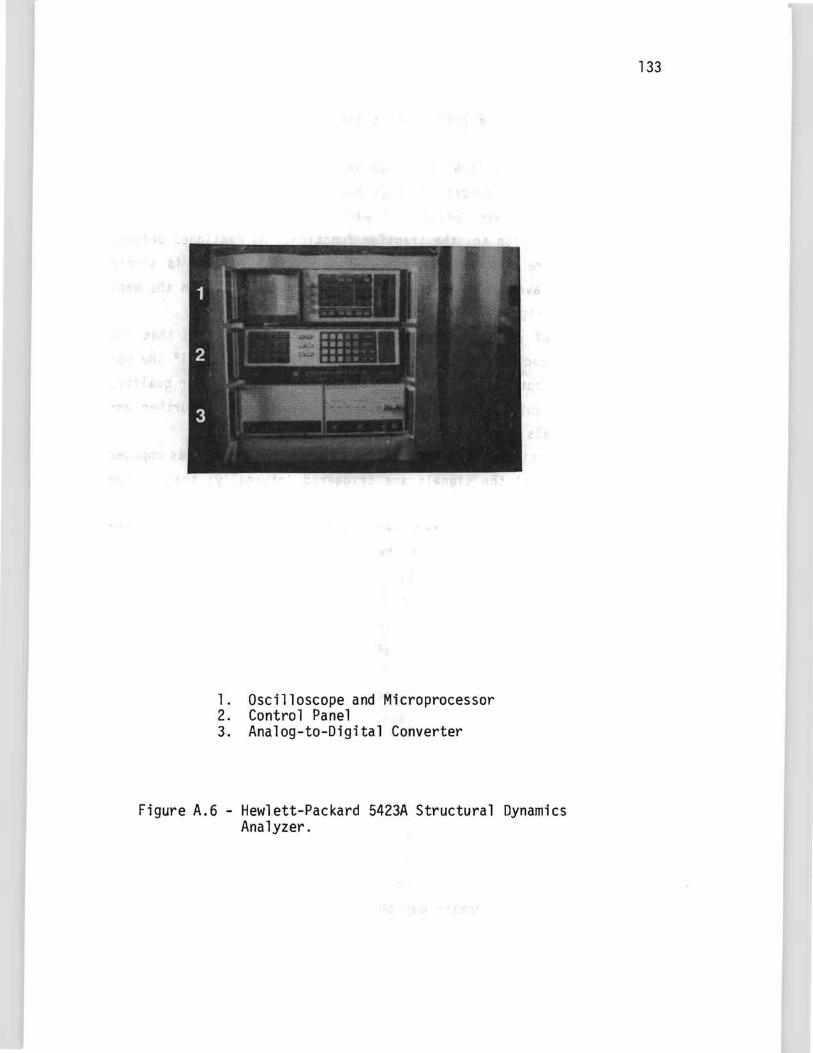
1. Oscilloscope and Microprocessor 2. Control Panel 3~ Analog-to-Digital Converter
Figure A.6 - Hewlett-Packard 5423A Structural Dynamics Analyzer.
133
134
for the SASW test on a soil site at the initial receiver spacing is
shown in Fig. A.S.
The "TRANSFER FUNCTION" is chosen as the measurement type. In this
state, the coherence function, cross power spectrum between the two
signals,and auto power spectrum of each signal is determined by the
analyzer, in addition to the transfer function. As mentioned before,
five averages are used to enhance the signals. The average is simply
the arithmetic average of the signals denoted by IISTABLE II on the menu
illustrated in Fig. A.S.
The type of signal is selected as "IMPACT" which means that the
signals are expected to be transient. By indicating IIIMPACT II the op
erator has the option of discarding signals which are of poor quality.
This option is quite beneficial in the field as a tool to further en
hance the signals.
As the relative phase of the two signals is of interest (as opposed
to absolute phase) the signals are triggered internally; that ;s the
records are captured at about the time the first half sine wave of the
impulse passes by the first receiver. A pretriggering delay, for in
spection of a small portion of the record before the arrival of the
actual signal is chosen as discussed later in this section. The range of the frequencies (bandwidth) is also selected. As a rule of thumb,
for each measurement the optimum bandwidth is obtained when more than three-fourth of the frequency range is of good qual i ty (generally, identified by a coherence value greater than 0.90).
The HP5423A digitizes each record into 256 points. Time length, T, and frequency bandw; dth, F, are related by the number of poi nts
digitized, N, by:
(A.I)
So that if either the bandwidth or time length is set, the other will
be set automat i ca lly by the analyzer. Thi smatter is of importance
because if good resolution in the frequency domain is sought, the re
so 1 ut ion in the time doma in may be poor and vice versa. For SASW
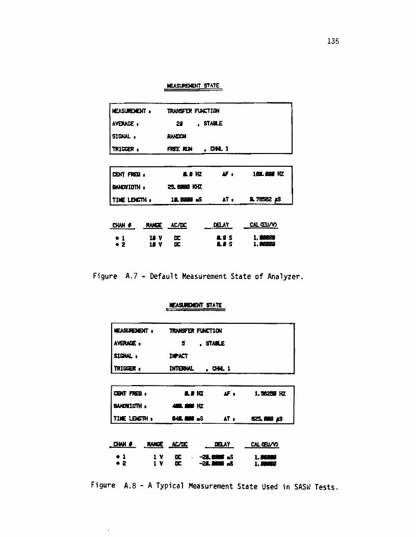
MEASt.JEIENT •
AVERAGE • 21 • STALE
SIGNAL • RANDOM
TRIGGER • FREE RUN • OK. 1
CENT FISCI •
twlNIDTH •
TIME LEtCnI •
I.. HZ
25._ I(IfZ
11._.s
.1
.2 1. V DC 1. V DC
II.
&T.
DEl..AY
I..S
"'S
1_. HZ
CAL<E1J1V>
1._ I."
Figure A.7 - Default Measurement State of Analyzer.
tEASI.IENENT •
AVERAGE •
TRIGGER •
CENT FISCI •
INDIDTH •
TIME LEtCnI •
EASI.N:MEN1' STATE
• STAR.E
INTEJIW. • OK. 1
...HZ __ .HZ
II. 1.S112S1 HZ
... • .s &T. 1125._ ~ --------------~--~
IV DC IV DC
IELAY
-21._ .s -a_.s
CALCEUIV)
t._ t._
135
Figure A.S - A Typical Measurement State Used in SAS~J Tests.
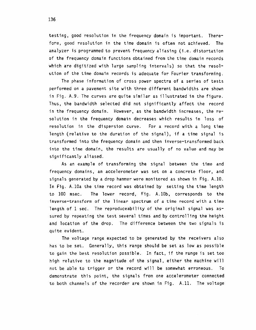
136
testing, good resolution in the frequency domain is important. There
fore, good resolution in the time domain is often not achieved. The
analyzer is programmed to prevent frequency aliasing (i.e. distortation
of the frequency domain functions obtained from the time domain records
which are digitized with large sampling intervals) so that the resol
ution of the time domain records is adequate for Fourier transforming.
The phase information of cross power spectra of a series of tests
performed on a pavement site with three different bandwidths are shown
in Fig. A.9. The curves are quite similar as illustrated in the figure.
Thus, the bandwidth selected did not significantly affect the record
in the frequency domain. However, as the bandwidth increases, the re
solution in the frequency domain decreases which results in loss of
resolution in the dispersion curve. For a record with a long time
length (relative to the duration of the signal), if a time signal is
transformed into the frequency domain and then inverse-transformed back
into the time domain, the results are usually of no value and may be
significantly aliased.
As an example of transforming the signal between the time and
frequency domains, an accelerometer was set on a concrete floor, and
signals generated by a drop hammer were monitored as shown in Fig. A.lO.
In Fig. A.lOa the time record was obtained by setting the time length
to 100 msec. The lower record, Fig. A.lOb, corresponds to the
inverse-transform of the linear spectrum of a time record with a time
length of 1 sec. The reproduceability of the original signal was as
sured by repeating the test several times and by controlling the height
and location of the drop. The difference between the two signals is
quite evident.
The voltage range expected to be generated by the receivers also
has to be set. Generally, this range should be set as low as possible
to gain the best resolution possible. In fact, if the range is set too
high relative to the magnitude of the signal, either the machine will
not be abl e to tri gger or the record wi 11 be somewhat erroneous. To
demonstrate this point, the signals from one accelerometer connected
to both channels of the recorder are shown in Fig. A.ll. The voltage
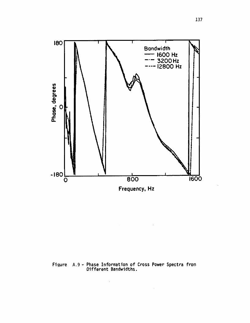
180 Bandwidth -1600 Hz _.- 3200Hz ---- 12800 Hz
137
-180 I--"::'-__ &..-:. __ ~~ ___ L-_~~
o 800 1600
Frequency, Hz
Figure A.9 - Phase Information of Cross Power Spectra from Different Bandwidths.
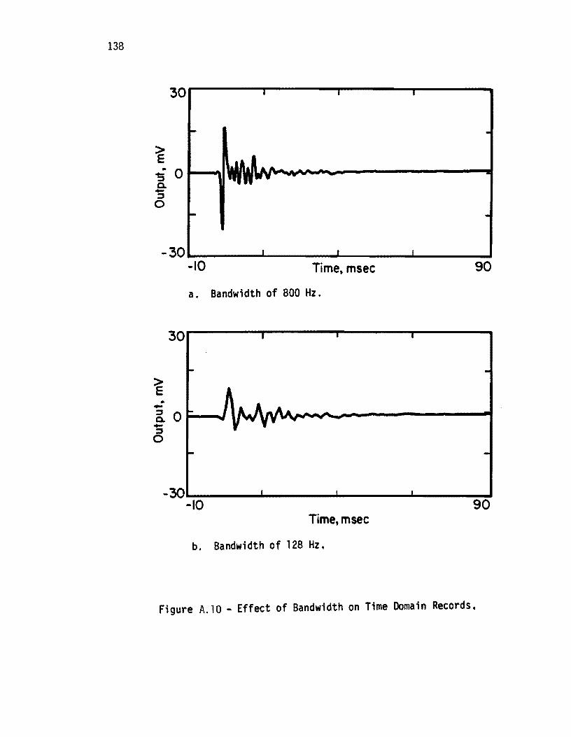
138
3or------r------~----~------~
-30~----~------~----~------~ -10 Time, msec 90
.. -
a. Bandwidth of 800 Hz.
30r------.------~----~------~
a 0 t-o--.I -:::J o
-30 ~_10~----~----~~----~------9-J0
Time,msec
b. Bandwidth of 128 Hz.
Figure A.l0 - Effect of Bandwidth on Time Domain Records,
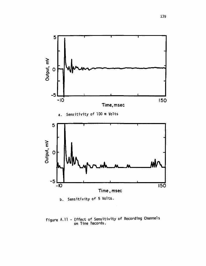
139
5~~---r------r-----~-------
-'S 0 Q. -::J o
> E -
-5~~--~------~----~------~ -10 150 Time,msec
a. Sensitivity of 100 m Volts
5~r---~----~~----~------
-&. 0 -::J o
-5~~ __ ~ ____ ~ ______ ~ ____ ~ -10 150
Time, msec
b. Sensitivity of 5 Volts.
Figure A.ll - Effect of Sensitivity of Recording Channels on Time Records.
140
range for channel one (Fig. A.lla) and channel two (Fig. A.lIb) were
0.1 and five volts, respectively. The record from the second channel
contains sharp peaks and troughs because of loss of resolution during
digitization of the output voltage. Upon using identical ranges on both channels, the outputs were identical.
A negative time delay, also called a pretrigger delay, imposed on
a signal allows the operator to inspect a small portion of the record
before the arrival of the actual signal at the first receiver. For
triggering a signal, the voltage and slope of the first major event to
be captured are set. The effect of voltage is discussed above. If the
slope is too flat, the recorder may not be able to trigger. However,
if the slope is too steep, part of the major signal may be lost during
testing. Travel time records from a geophone set on a concrete floor are shown in Fig. A.12. In the first case (Fig. A.12a), a pretriggering
delay was imposed on the signal. In the lower trace (Fig. A.12b), the
delay was omitted, and the test was repeated. By comparing these two records it can be seen that a major portion of the travel time record
in the second case is lost. The importance of the pretrigger delay is
that the operator can detect this undesirable loss of signal and can
make the appropriate adjustments. Pretriggering should be identical
for both channels or a false internal phase will be introduced between the two signals. Also, experience has shown that the duration of the pretriggering delay should be on the order of ten percent of the time length sampled.
A.4 POWER SUPPLY
The power supply used is a portable generator with a maximum power of two kva. A signal conditioner is placed between the generator and
recorder to minimize voltage fluctuations so as to regulate the voltage before entering the analyzer. The frequency and voltage of the current
generated by the power supply should be checked before the test, as the
performance of digital recorders are quite sensitive to the quality of
the input power.
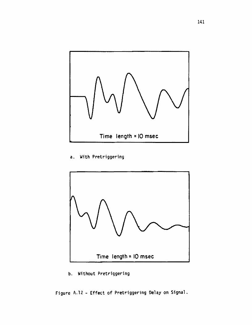
141
Time length = 10 msec
a. With Pretriggering
Time length = 10 msec
b. Without Pretriggering
Figure A.12 - Effect of Pretriggering Delay on Signal.
142
A.5 SUMMARY
The practical aspects and equipment used in SASW testing were
discussed in this chapter. It is shown that:
1. seismic signals can be effectively enhanced by averaging,
2. many external parameters having undesirable effects on
testing can be minimized by reversing the source, and
3. the CRMP geometry reduces scatter in the dispersion curve.
Equipment necessary for performing SASW tests are an appropriate
source, high quality receivers and a spectral analyzer. The source
should be able to generate surface waves over a wide range of frequen
cies. Two types of receivers can be used, geophones and accelerometers,
dependi ng on recei ver spaci ng. A spectral analyzer accelerates sub
stantially the testing time and has essential features such as rapid
determination of the coherence function which can ensure the quality
of the signals in the field and the ability to trigger the signals
internally.
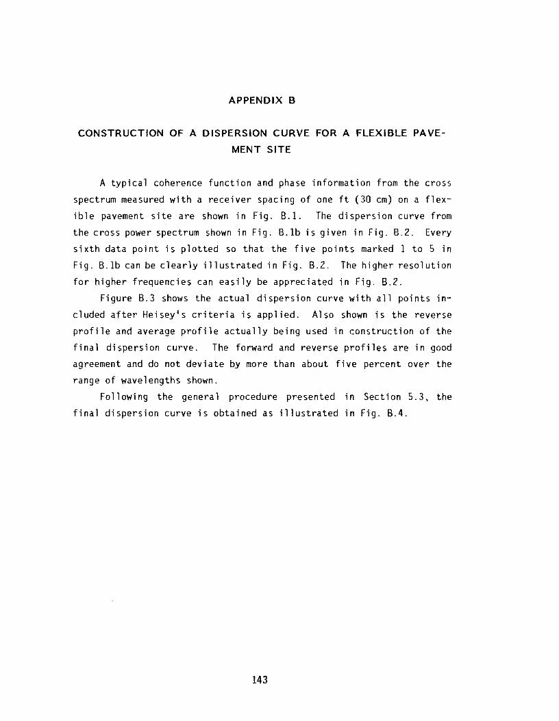
APPENDIX B
CONSTRUCTION OF A DISPERSION CURVE FOR A FLEXIBLE PAVE
MENT SITE
A typical coherence function and phase information from the cross
spectrum measured with a receiver spacing of one ft (30 cm) on a flex
ible pavement site are shown in Fig. B.1. The dispersion curve from
the cross power spectrum shown in Fig. B.lb is given in Fig. B.2. Every
sixth data point is plotted so that the five points marked 1 to 5 in
Fig. B.lb can be clearly illustrated in Fig. B.2. The higher resolution
for higher frequencies can easily be appreciated in Fig. B.2.
Figure B.3 shows the actual dispersion curve with all points in
cluded after Heisey's criteria is applied. Also shown is the reverse
profile and average profile actually being used in construction of the
fi na 1 di spers i on curve. The forward and reverse profi les are in good
agreement and do not deviate by more than about five percent over the
range of wavelengths shown.
Fa 11 owi ng the genera 1 procedure presented inSect ion 5.3, the
final dispersion curve is obtained as illustrated in Fig. B.4.
143
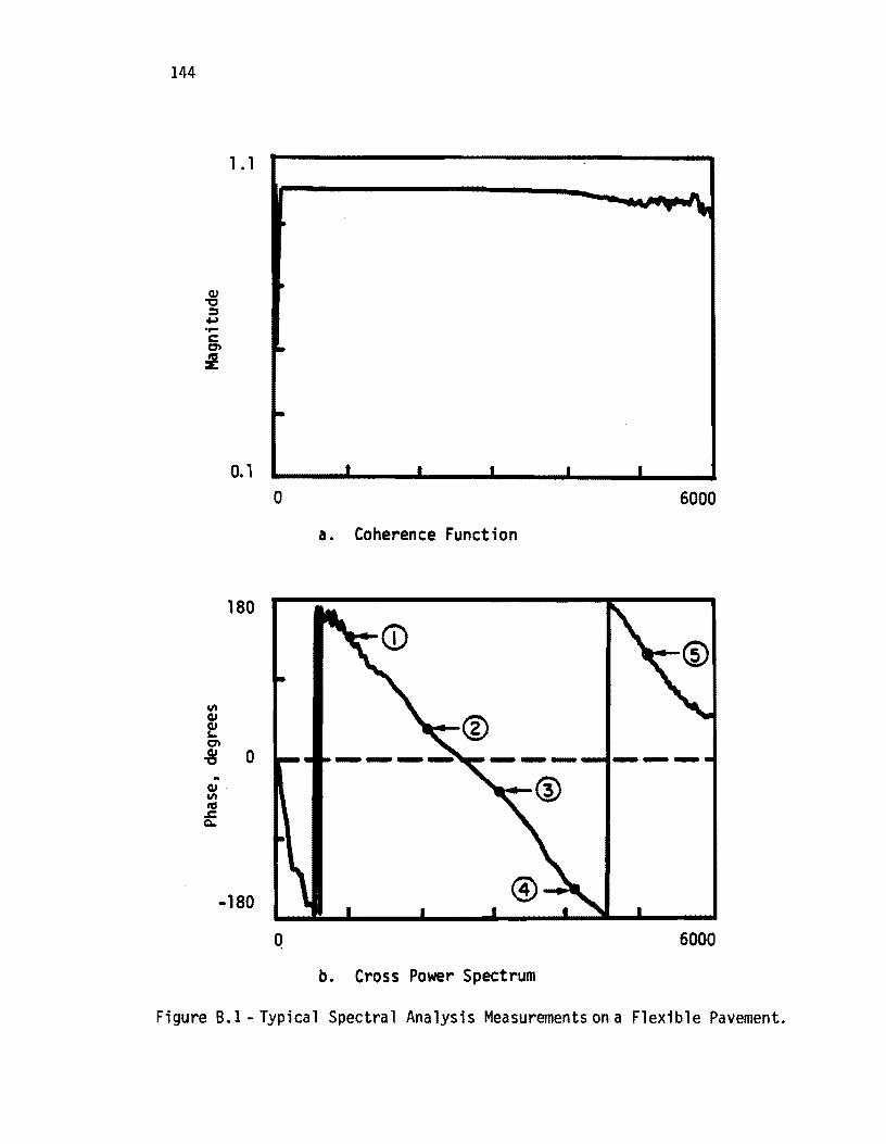
144
.. GJ· ell IG
.s::. Q..
1.1
0.1
180
-180
-- .
t • I I I
a 6000
a. Coherence Function
Q 6000
b. Cross Power Spectrum
Figure B.1 - Typical Spectral Analysis Measurements on a Flexible Pavement.
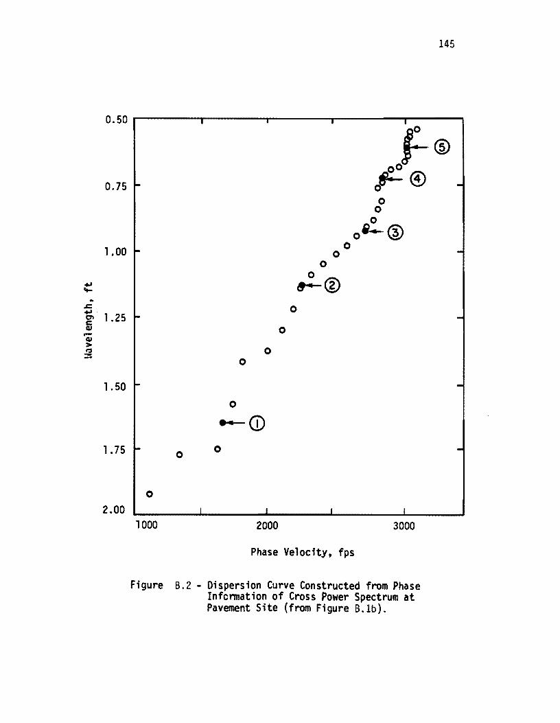
0.50
0.75
1.00
... ...... .. .c ... CT! 1.25 C QJ .-QJ > t:'J 3
1.50
1.75
2.00
145
, t ,
f-® 00
,.. ~® -0 0
0 0
Oi ....... ® 0 - 0
0 0
~® 0
~
0
0 0
~
0
----CD - 0
0
o I I I I
1000 2000 3000
Phase Velocity, fps
Figure B.2 - Dispersion Curve Constructed from Phase Infcrmation of Cross Power Spectrum at Pavement Site (from Figure B.lb).
-
-
-
-
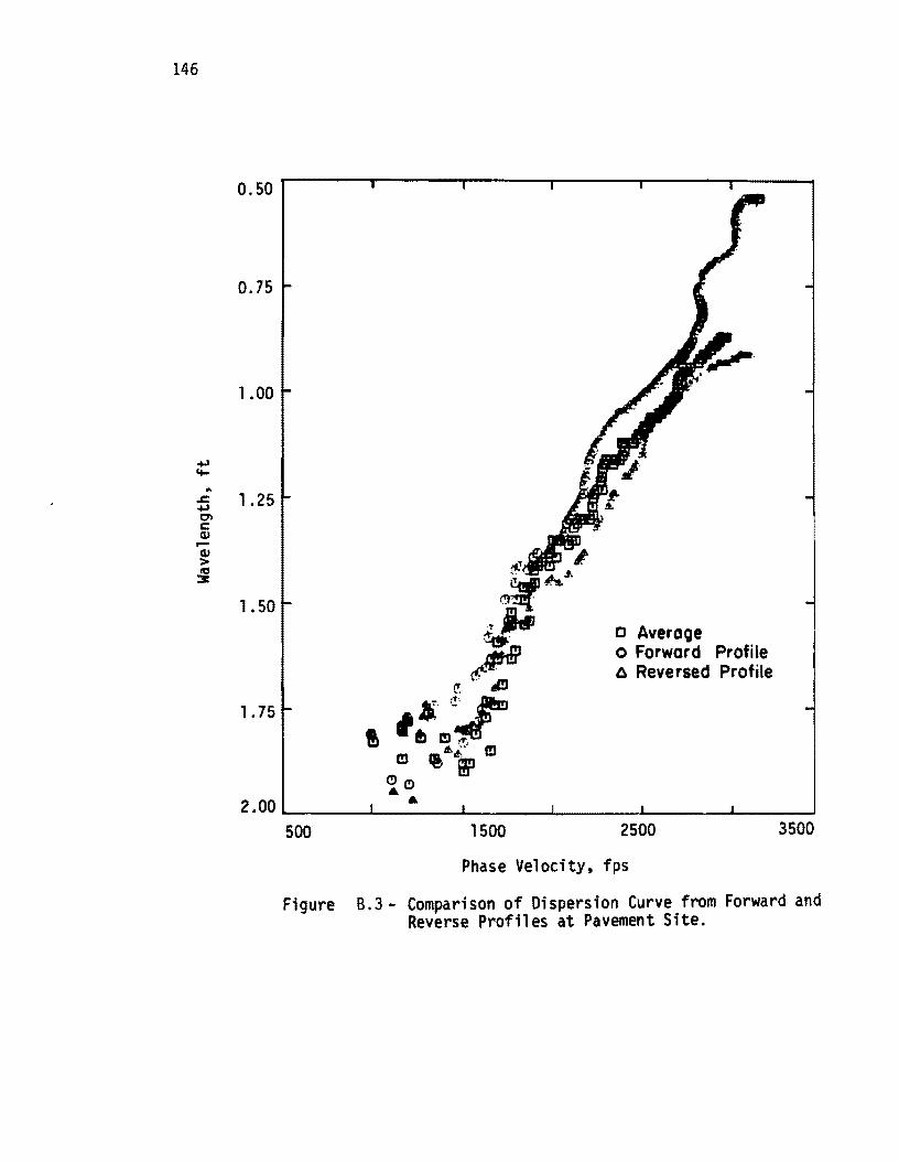
146
...,:I '+-.. .s::. ...,:I en c OJ -OJ > ~
0.50r------.----~r-----,-----~-------------
0.75
1.00
1.25
1.50
1. 75
500 1500
o Average o Forward Profile c. Reversed Profile
2500
Phase Velocity, fps
3500
Figure B.3· Comparison of Dispersion Curve from Forward and Reverse Profiles at Pavement Site.
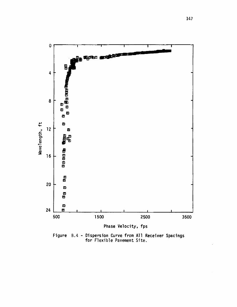
., ct-.. .s:::. ., I:n C Q.I ...... Q.I > ~
147
O--------~------r-----~------~-------,------~
4
8
12
16
20
m
,~
i m m m m
m m m m m
m
7
~--aII-=-
24 I!I
500 1500 2500 3500
Phase Velocity, fps
Figure B.4 - Dispersion Curve from All Receiver Spacings for Flexible Pavement Site.

!!!!!!!!!!!!!!!!!!!"#$%!&'()!*)&+',)%!'-!$-.)-.$/-'++0!1+'-2!&'()!$-!.#)!/*$($-'+3!
44!5"6!7$1*'*0!8$($.$9'.$/-!")':!
APPENDIX C
COMPARISON OF THEORETICAL AND EXPERIMENTAL DISPERSION CURVES AFTER COMPLETION OF INVERSION PROCESS AT WILDLIFE
SITE
149
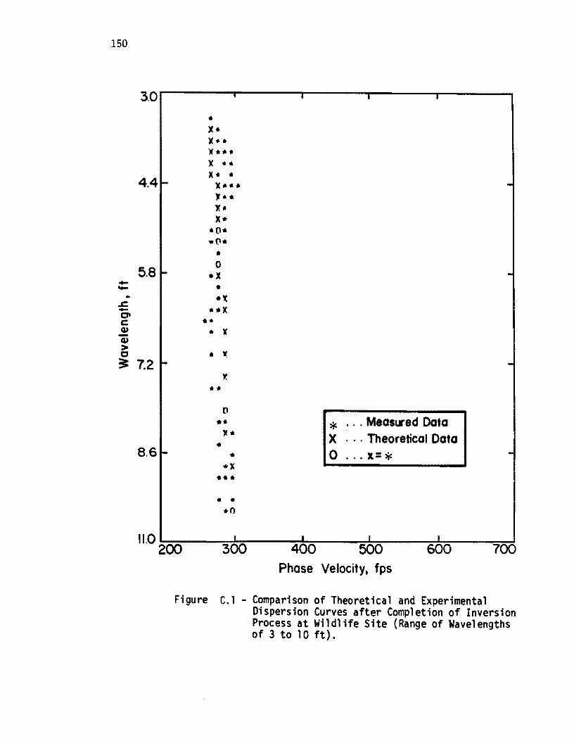
150
--.. .c:. -o c: 4)
4)
> c
3.0
4.4
5.8
3: 7.2
8.6
•
x .... x •• x ...
• o
•
• x
• l(
... o
••
• ..
• • .. 0
* ... MeaslSed Data X ... Theoretical Data o ... x=*
11.0 2~OO~--=3~0"::::"0---:4~0"::::"0---=500±-:----=60::!::-:0::::-----::7=OO~
Phase Velocity, fps
Figure C.l - Comparison of Theoretical and Experimental Dispersion Curves after Completion of Inversion Process at Wildlife Site (Range of Wavelengths of 3 to 10ft).
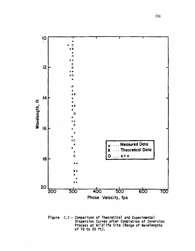
10
12
14 --.. .&! -CJI C C»
Q) > ~ 16
18
20
151
• • C
*1 • " •• t 0
'I •
• 0
• C"
• 'I" • • -. •
0
• 'I. r.
• •
• ... c. • *
... Meas .... ed Dota
- X . . . Theoretical Data • t 0 ... x= * •• ,.-• • 'I.
200 300 400 500 600 700 Phase Veloci ty, fps
Figure C.2 - Comparison of Theoretical and Experimental Dispersion Curves after Completion of Inversion Process at Wildlife Site (Range of Wavelengths of 10 to 20 ft).
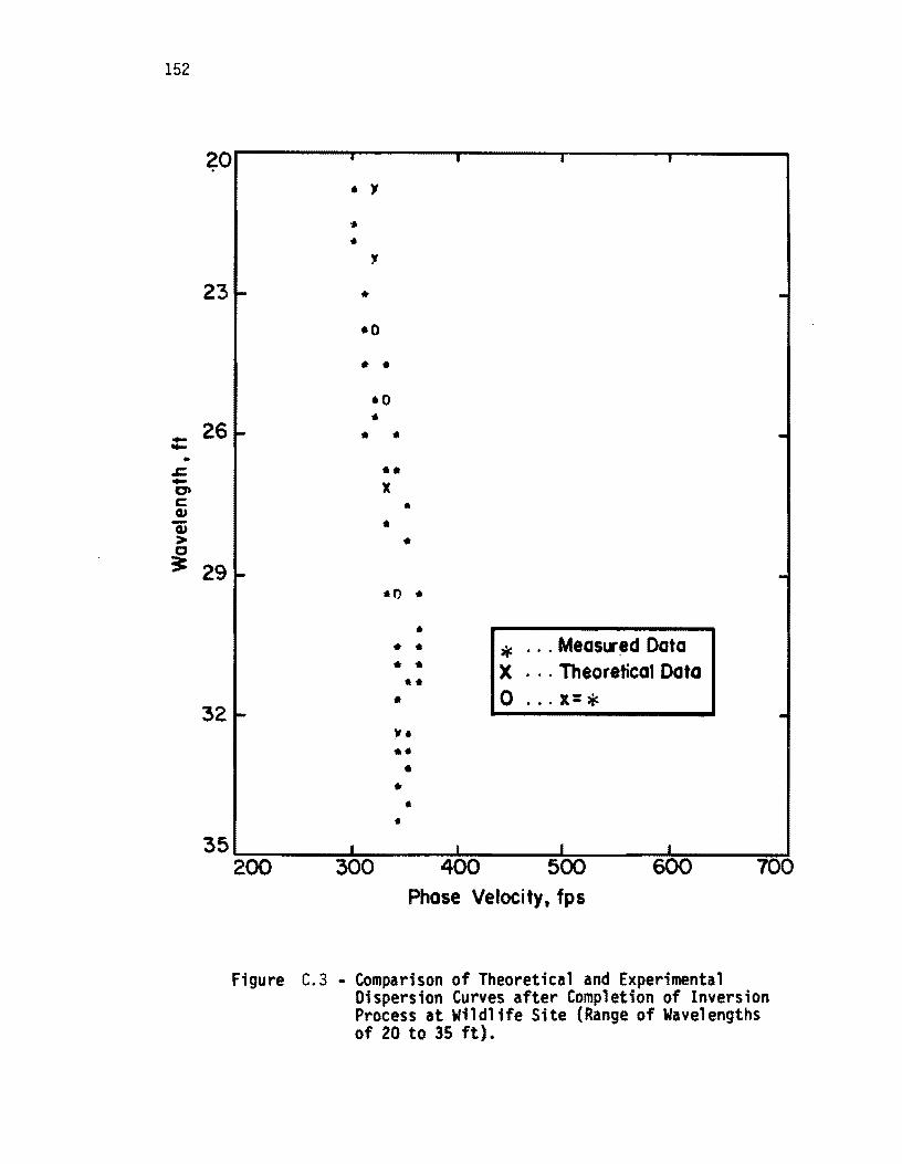
152
~o
23
- 26 ..... •
.s::. -at c: Q) -Q)
> ~ 29
32
35
- ., • • ,
.. -0
.. -·0 •
• • • • X
• .. ...
." ...
,. .. ... * · .. MeaslS.d Data .. . X · .. Theoretical Data
-.. .. 0 · . . 1= * Y •
•• • .. •
•
200 300 400 500 600 700 Phase Velocity. fps
Figure C.3 - Comparison of Theoretical and Experimental Dispersion Curves after Completion of Inversion Process at Wildlife Site (Range of Wavelengths of 20 to 35 ft).
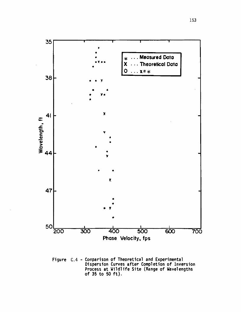
35
38
_ 41 -.. &! -0-c: Q.) -Q.) > 0
3: 44
47
50 200
Figure
..
• .. J
.. " ... .. • y
. .. .. ,. . ..
't
.. .. y
•
.. ..
.. x
• •
* 11'
•
400
* ... MeoslSed Dota X ... Theor.tical Data
o ... x= *
500 600 Phase Velocity, fps
153
700
C.4 - Comparison of Theoretical and Experimental Dispersion Curves after Completion of Inversion Process at Wildlife Site (Range of Wavelengths of 35 to 50 ft).
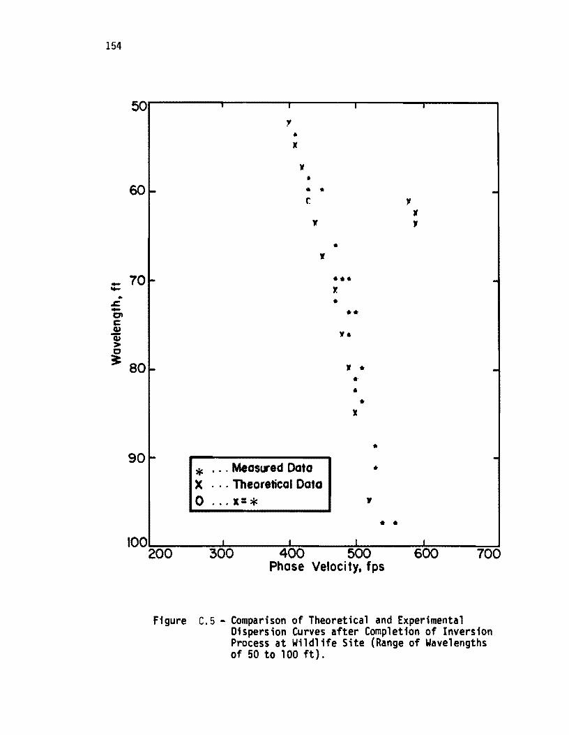
154
50
60
_ 70 ..... .. .r; -at c: Q)
Q) > c
:= 80
90
100
'!
• "
)t .. 6 ..
r , If
r , ..
r
••• x •
•• v.
If •
• • •
)I
..
* · .. Meas .... ed Data • X · . . Theoretical Data 0 · .. x= * r
• •
200 300 400 500 600 700 Phase Veloci ty. fps
Figure C.5 - Comparison of Theoretical and Experimental Dispersion Curves after Completion of Inversion Process at Wildlife Site (Range of Wavelengths of 50 to 100 ft).

APPENDIX D
COMPARISON OF THEORETICAL AND EXPERIMENTAL DISPERSION
CURVES AFTER COMPLETION OF INVERSION PROCESS AT A FLEXI
BLE PAVEMENT SITE
The experimental and theoretical dispersion curves after the
matching process has been completed are shown in Figs. 0.1 through 0.6.
These curves are presented on expanded scales to show the accuracy of
the match. This site is the one shown in Appendix B where development
of the dispersion curve is illustrated. It can be seen that the experimental and theoretical curves are
in good agreement, with the average difference on the order of plus or
minus five percent. However, around wavelengths of 1.8 to 2.0 ft (54
to 60 cm) where the transition between the pavement system and subgrade
is expected, aport i on of the curve canot be matched due to a sharp
change in the velocity. This is a typical characteristic of transition
zones and occurs universally in dispersion curves of pavement systems measured in this study. Practically speaking, these transition zones
appear either as a step in the dispersion curve or as data which is so
erratic that, during construction of the dispersion curves, the data
points in this range do not fulfill the statistical criterion discussed
in the last section. Scatter in the data in the upper part of Fig. 0.3
illustrate the erraticness in the transition zone.
Another point of interest is the presence of jumps in the theoretical curve like the one shown in Fig. 0.4. These jumps occur in the vicinity of shear wave velocities of layers when a big contrast in velocities is present. This is due to a weakness in the program, and, at these boundaries phase velocities are somewhat inaccurate.
The shear wave velocity profile after inversion is presented in
Fig. 0.6. More discussion of this site is presented in Section 7.3.1.
155
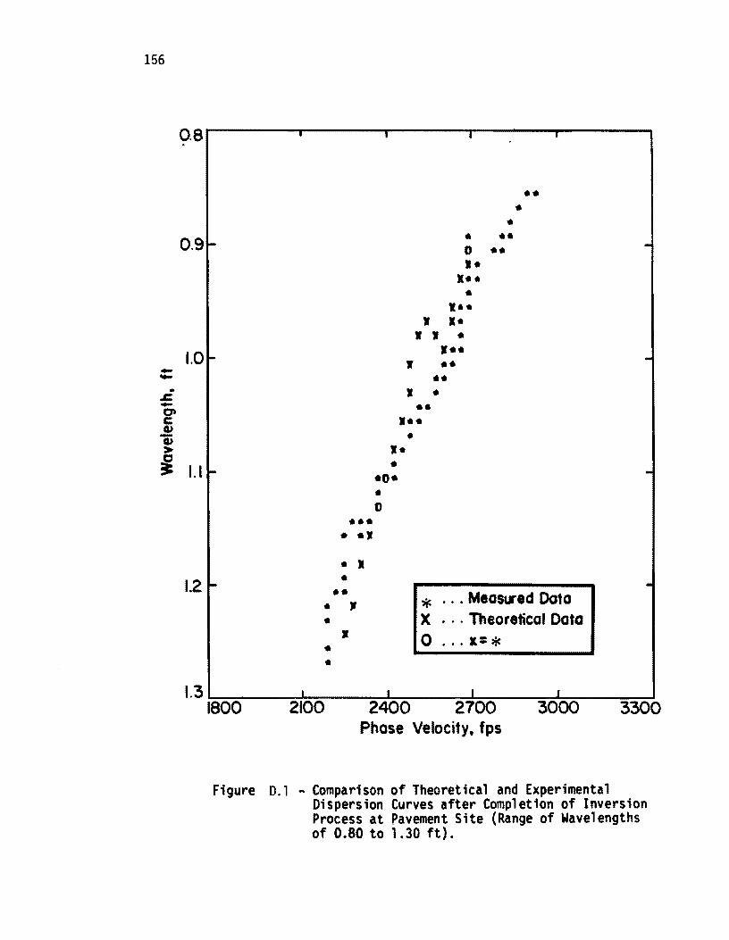
156
-.... .. s;; -0' c: G> "ii > ~
Q8r-------r-----~--------------------~
0.9
1.0
1.1
1.2
••• · ., • 1l •
•• • I • • •
I
• • •• o •• I.
x •• • x··
I I. I I • I·· I ••
• • • • •• I ••
• I-
-
•• •
.0· e o
* ... MeaSlJ'ed Dota X ... Theoretical Data
o ... x= *
1.3 ~=--_-=*-=--_-=-='=-=-_--=-=~_----=-~~---"""~ 1800 2100 2400 2700 3000 3300
Phase Velocity t fps
Figure 0.1 - Comparison of Theoretical and Experimental Dispersion Curves after Completion of Inversion Process at Pavement Site (Range of Wavelengths of 0.80 to 1.30 ft).
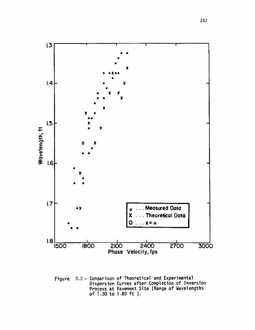
-..... ... s::. -c-c: G> -G> > 0 3:
157
l.3 • •
• •
I
• •••• •
1.4 • x •
• , , • • I
• • x • ••
1.5 If
• , o x
• • •
1.6 •
I
• • •
1.7 •• * '" MeaSLI"ed Data X ... Theoretical Data
• o ... x= * • •
1.8 ~=--_-:-=,=-=-_-=-:-±-=--_~~_---"...~ __ ---..J 1500 1800 2100 2400 2700 3000
Phose Velocity. fps
ngure D.2 - Comparison of Theoretical and Experimental Dispersion Curves after Completion of Inversion Process at Pavement Site (Range of Wavelengths of 1.30 to 1.80 ft ).
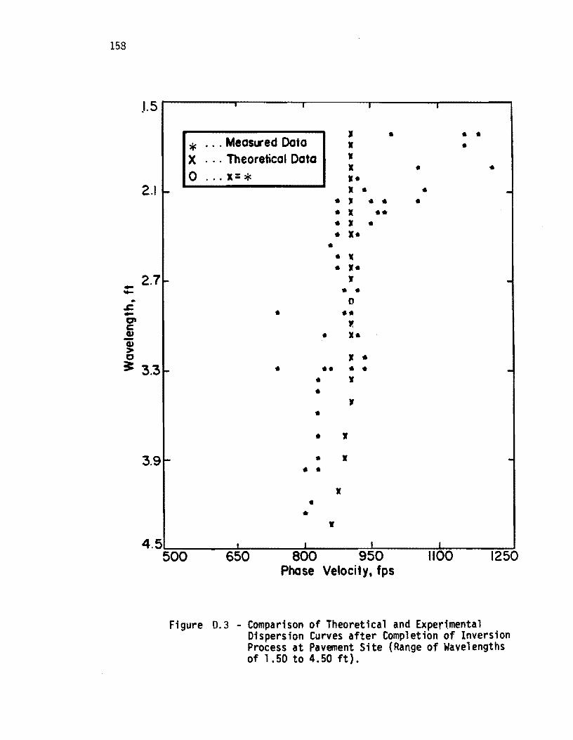
158
,1.5
2.1
2.7 -.... • .r:. -Ot C cu -cu > 0
~ 3.3
3.9
4.5
J • . .. * · .. Meas .... ed Data • .. X · .. Theoretical Data J
x • • a · . . x= * ,. Jl • • · , .. .. •
• • •• • • .. .. x •
• .. " • ••
J .. .. 0
• •• " • x • · .. • •• · .. • J
• J
• .. I
.. " • • • ..
• I'
500 650 800 950 1100 1250 Phase Velocity. fps
Figure D.3 - Comparison of Theoretical and Experimental DisperSion Curves after Completion of Inversion Process at Pavement Site (Range of Wavelengths of 1.50 to 4.50 ft).
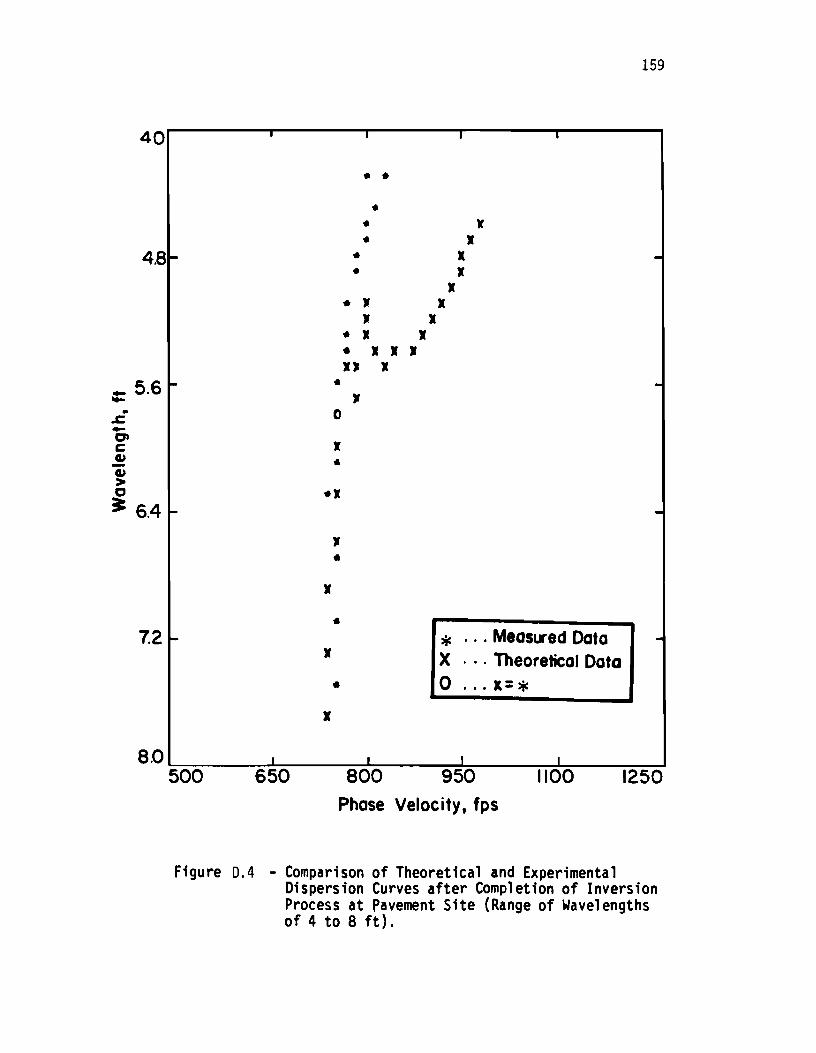
• .c -01 C Q>
Q> > C
4.0
4.8
~ 6.4
7.2
• 0
x •
.x
,. •
x
• x
• I
• •
• •
• •
· , , • x
•
· x. x, x ,
• • J
• •
* X 0
• x
x x
... Measl.I"ed Data
. . . Theoretical Data
... x= *
159
8.0 L--___ ~--~~--~~--~~--~~ 500 650 800 950 1100 1250
Phase Velocity. fps
Figure D.4 - Comparison of Theoretical and Experimental Dispersion Curves after Completion of Inversion Process at pavement Site (Range of Wavelengths of 4 to 8 ft).
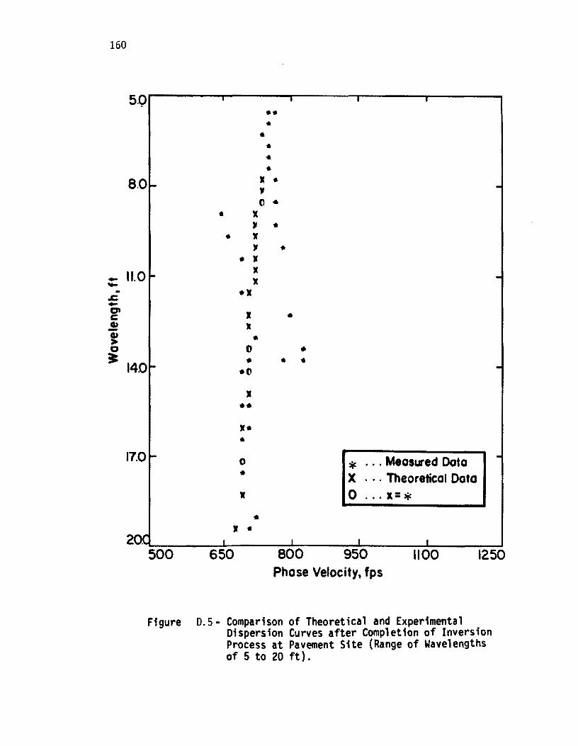
160
5·0.------,.---..,.------r---~------a
8.0
_ 11.0 .... .. .t= -~ .!! Q) > o
• 140
17.0
2 500
• x
•• • .. .. ..
x • , (I ..
, -• r
, -• • • • " • 0
--" • ••
•• .. 0 • .. • •
650
• r
..
•
•
• • •
800
* ... Measured Dota X ... Theoretical Data o ... 1= *
950 1100 Phase Velocity, fps
1250
Figure D.5- Comparison of Theoretical and Experimental Dispersion Curves after Completion of Inversion Process at Pavement Site (Range of Wavelengths of 5 to 20 ft) •
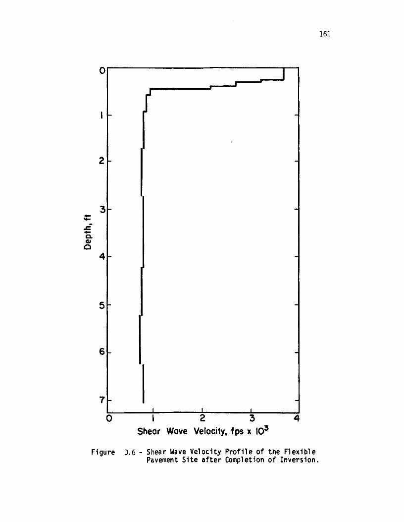
o
1 ~
:3 --~ .. .c -c. cu 0
4 -
7~
o
Figure
r
I I I
12:3 Shear Wove Velocity, fps x 103
1
-
-
-
-
-
-
-4
0.6 - Shear Wave Velocity Profile of the Flexible Pavement Site after Completion of Inversion.
161


