Generation of a Realistic Discrete Fracture Network Model using Deterministic Input Data
Derived from 3D Multicomponent Seismic Amplitude Data Simon Emsley*, Shihong Chi, Jim Hallin and Jhon Rivas, ION Geophysical
Summary
Unconventional reservoirs that include: carbonates,
basement reservoirs and resource plays, require the
development of realistic subsurface models that integrate
geology, geophysics and rock physics to enable the
“plumbing” of the reservoir to be analyzed. Generally,
unconventional reservoirs are more complicated due to the
presence of fractures; varying geomechanical properties
and in the case of resource plays, where the source rock is
also the reservoir, variable total organic carbon (TOC). The
development of resource plays is moving on from drilling
on a regular grid; but it is not sufficient to ‘simply’ identify
a sweetspot in a resource play. It is also necessary to
understand connectivity and compartmentalisation; this
may be achieved through the development of a realistic
fractured reservoir model. Seismic amplitude and inversion
attribute data volumes along with rock physics provide a
wealth of information covering reservoir intervals. Co-
rendering of these data volumes leads to a more easily
interpretable image of the subsurface and a better
understanding of the reservoir. An enhanced understanding
of the reservoir can be achieved by constructing a discrete
fracture network (DFN).
Presented here is a realistic DFN model built using inputs
derived from a 3D multicomponent seismic amplitude data
set, seismic attributes, anisotropy information derived from
azimuthal velocity analysis of the seismic data, seismic
inversion results and well data. The DFN model was
populated with elastic moduli data derived from pre-stack
seismic inversion. The resulting models were used to
appraise various well plans and predict inter-well
connectivity. The models can also be used to optimize the
generation of a stimulated rock volume by forward
modeling different hydraulic fracture completion scenarios.
This modeling demonstrated that different well designs
(different horizontal location and drilling
direction/azimuth) resulted in differences of between 3 –
30% in the stimulated volume from stage to stage. This has
clear financial implications and can impact drilling,
completion strategies and production.
Introduction
The development of resource plays tended to be based on
drilling on a regular grid with uniformly spaced laterals
(horizontal wells) drilled on a predefined azimuth.
Additionally, the direction and spacing between the laterals
remained constant from one well pad to the next regardless
of any changes in local stress direction or the presence of
faulting (Goodway et al., 2012). This is an inefficient way
of exploiting the reserves and utilizing financial capital.
The development of resource plays is now moving from
drilling on a regular grid; with the application of
geophysics and logging, it is argued that it is not sufficient
to ‘simply’ identify a sweetspot in a resource play.
This paper describes the construction of a realistic DFN
model that was built using inputs derived from a 3D
multicomponent seismic data set, seismic attributes,
anisotropy information, seismic inversion results and well
data. The advantages of building a DFN model are many
and include: understanding connectivity,
compartmentalization and drainage volumes. In this case,
as the model incorporates the information derived from the
seismic amplitude data deterministically, the DFN can be
used to guide well placement and planning and predict
inter-well connectivity. Such models may also show that
more than one well is producing from the same
compartment and therefore allows for optimum well
placement and any infill well drilling locations. The models
can be used to simulate hydraulic fracture completions,
which are required as the natural permeability of the
reservoirs is too low for production. These models can also
be used to test different possibilities in terms of well
placement, drilling directions, spacing between laterals and
spacing between stages.
Case Study
A DFN model has been constructed covering a 3-D
multicomponent survey, which was acquired in Western
Pennsylvania over the Marcellus Shale, the Allegheny
Survey. The case study illustrates the additional benefits of
using azimuthal velocity analysis (PP datasets) and/or shear
wave splitting analysis (PS datasets) to provide valuable
inputs to the construction of DFN models. These often
indicate the presence of faulting or fracturing that may
otherwise go uninterpreted and may be of significance to
well placement, performance, and completions (hydraulic
stimulation).
One of the perceived issues with DFN modeling is that the
fractures in the model tend to be too uniform in length, area
and spatial distribution, although the stochastic generation
process should avoid this situation. The challenge in DFN
model construction can be summarized as two main
concerns:
Paucity of data or the difficulty in obtaining suitable
data on small scale faulting and fracturing (sub-seismic
Page 2382SEG Denver 2014 Annual MeetingDOI http://dx.doi.org/10.1190/segam2014-0158.1© 2014 SEG
Main Menu
T
Realistic Discrete Fracture Network Modelling using Deterministic Input Data
faults and/or those having little or no throw and fractures
that are on a millimeter scale that are only visible on
image logs or in core) and
Constructing a realistic model that matches all
deterministic and inferred data.
The question here is what is the difference between a
realistic and a less realistic model? Often, in DFN models
the fractures appear to be fairly uniform in volumetric
density and have apparent uniform size distribution. This
last point should be avoided in the stochastic generation of
the fractures sets. The generation of less realistic models
may be a function of point 1 above where there is a paucity
of data or where assumptions on fracture dip and dip
direction are made. Noting these two points, the creation of
a realistic DFN model, which has been constructed using a
rich dataset. The inputs were derived from seismic data and
well logs and this information was included in the
modeling process deterministically. The data sources
available for the modeling included:
Seismic amplitude volumes covering an area of 85
square miles
Azimuthal velocity analysis of PP datasets, to determine
the PP fast and slow directions and differences in their
velocity values
Shear wave splitting analysis of PS datasets to determine
the fast and slow shear directions and the magnitude
(delta t) of the shear wave birefringence
Seismic Interpretation of horizons defining the zone of
interest
Seismic attributes
Wireline log data
Seismic Inversion results
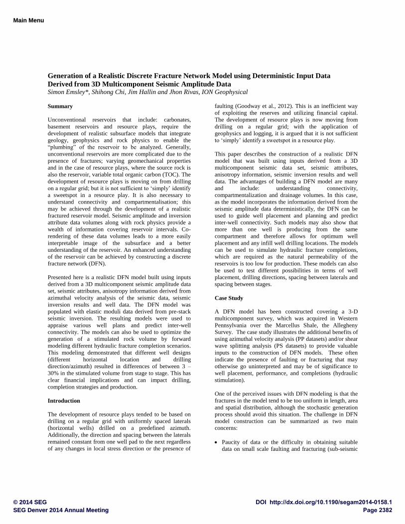
The DFN was constructed using a relatively straight
forward workflow (Figure 1).
Figure 1: Simplifed DFN workflow.
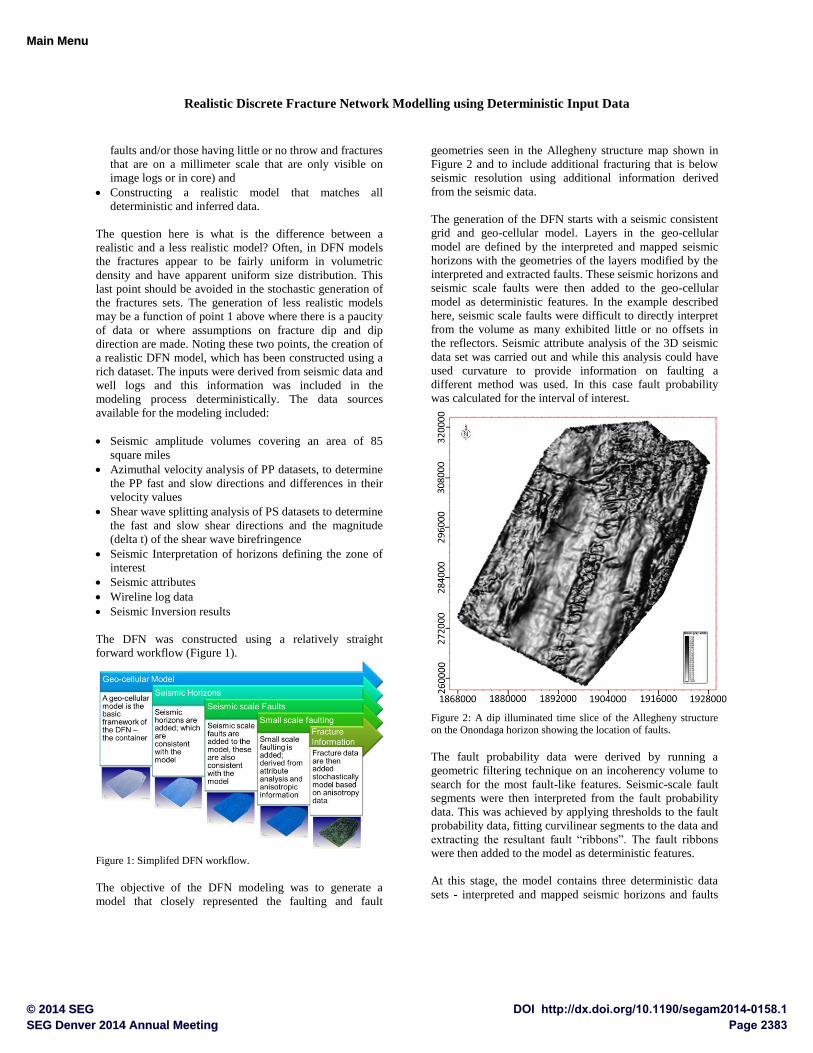
The objective of the DFN modeling was to generate a
model that closely represented the faulting and fault
geometries seen in the Allegheny structure map shown in
Figure 2 and to include additional fracturing that is below
seismic resolution using additional information derived
from the seismic data.
The generation of the DFN starts with a seismic consistent
grid and geo-cellular model. Layers in the geo-cellular
model are defined by the interpreted and mapped seismic
horizons with the geometries of the layers modified by the
interpreted and extracted faults. These seismic horizons and
seismic scale faults were then added to the geo-cellular
model as deterministic features. In the example described
here, seismic scale faults were difficult to directly interpret
from the volume as many exhibited little or no offsets in
the reflectors. Seismic attribute analysis of the 3D seismic
data set was carried out and while this analysis could have
used curvature to provide information on faulting a
different method was used. In this case fault probability
was calculated for the interval of interest.
Figure 2: A dip illuminated time slice of the Allegheny structure on the Onondaga horizon showing the location of faults.
The fault probability data were derived by running a
geometric filtering technique on an incoherency volume to
search for the most fault-like features. Seismic-scale fault
segments were then interpreted from the fault probability
data. This was achieved by applying thresholds to the fault
probability data, fitting curvilinear segments to the data and
extracting the resultant fault “ribbons”. The fault ribbons
were then added to the model as deterministic features.
At this stage, the model contains three deterministic data
sets - interpreted and mapped seismic horizons and faults
Page 2383SEG Denver 2014 Annual MeetingDOI http://dx.doi.org/10.1190/segam2014-0158.1© 2014 SEG
Main Menu
T

Realistic Discrete Fracture Network Modelling using Deterministic Input Data
and seismic scale faults that showed little of no
interpretable offsets in the reflectors. Once the
deterministic seismic scale data have been added to the
model the next step is to add the small scale faulting and
fracturing that are below the resolution of the seismic data.
This is often a stochastic process where the input data may
be derived from sources including image logs, well logs,
core and analog data. In this case, the fault probability data
formed a deterministic input to the stochastic generation of
a fracture set that honored the fault probability data. The
results of this process are shown in Figure 3. Figure 3
shows the same faults as Figure 2 and that the density of
the added fracture set is not uniform spatially but is higher
in proximity to faults than in areas in between.
Figure 3: Fracture model including interpreted, extracted faults and
fractures based on fault probability data.
Azimuthal velocity analysis performed during the
processing of the 3D multicomponent data provided
information on the magnitude, and azimuths of Vpfast and
Vpslow. These data were used to compute anisotropy
information that provided an additional deterministic input
to the generation of fractures. While such data provide
information on the intensity and direction of fractures they
do not provide dip information, this information is required
for modelling both fracture sets and was obtained from
published literature (Engelder, et al., 2009).
The results of generating a fracture set based on the
seismically derived anisotropy information are shown in
Figure 4. Again, it can be observed that the fracture
generation is not uniform, as would be anticipated as the
fractures were generated based on deterministic data;
unlike a purely stochastic process that results in more
uniformity in numbers and sizes of fractures. As such it is
considered that the fracture generation process has met the
objective of producing a realistic static fracture model.
Figure 4 Fracture model including interpreted, extracted faults
and fractures based on seismically derived anisotropy data.
The complete DFN model for the Marcellus interval
(Figure 5) includes the interpreted and extracted faults, the
fracture set generated based on the fault probability data
(Figure 3) and those fractures based on anisotropy
information (Figure 4) calculated from the results of the
azimuthal velocity analysis.
Additional work was conducted that included petrophysical
analysis, rock physics studies and seismic inversion. The
DFN model was populated with elastic properties derived
from pre-stack joint and simultaneous seismic inversion
products that included Young’s Modulus and Poisson’s
Ratio. Geomechanical information was also included to
forward model or simulate well completion and hydraulic
fracturing (Figure 6). This process uses a critical stress
analysis and solving for a constitutive relation conserving
material mass. Where fractures intersect the wellbore
covered by the completion stages fluids are pumped into
the dilatable fractures. If no fractures intersected the stages
the simulation was parameterized to generate new tensile
fractures.
Figure 6 shows the results of simulating hydraulic
fracturing with the multicoloured curvilinear fractures
showing those which have either been stimulated or are
new tensile fractures; this effectively shows the modelled
stimulated rock volume (ignoring far-field pressure
changes) and the locations where micro-seismic events are
Page 2384SEG Denver 2014 Annual MeetingDOI http://dx.doi.org/10.1190/segam2014-0158.1© 2014 SEG
Main Menu
T

Realistic Discrete Fracture Network Modelling using Deterministic Input Data
likely to be observed where these are related to fracture
creation or movement. In areas where higher fracture
densities are modelled (towards the toe and heel of the
wells; right and left, respectively) seen by the purple
fractures, larger numbers of stimulated fractures are seen
suggesting reactivation of pre-existing structures.
Figure 5: Fracture model including all fracture sets.
The modeling suggests that hydraulic fracturing would also
increase fracture density, as shown by the multi-coloured
fractures (Figure 6), particularly in the central sections of
the wells where the fracture density in the model is lower.
Figure 6: Enlarged section of the DFN model showing
stimulated/created fractures (multi-coloured) and one of the
modelled fracture sets based on fault probability (purple).
This forward modelling exercise suggests that the majority
of the fluid and proppant pumped in the stages towards the
toe and heel of both wells are used in reactivating pre-
existing fractures and faults which may not result in a
significant increase in permeability. Whereas the fractures
generated for the central stages of the wells are indicative
of the formation of new fracture systems. Additional
predictions can be made that suggest that communication
between and along the wells from one stage to another
would be anticipated. It is also noted that the stimulated
and generated fractures from one well intersect the position
of the other lateral. This has clear implications for well
planning and design. The wells shown in Figure 6 are
hypothetical, the plan could be optimized based on the
results obtained from this type of forward modeling to
assess effectiveness of the stimulation processes. The
locations of the wells in the model were changed and
additional forward modeling was conducted efficiently,
with the results indicating that a relatively small change in
the horizontal position and drilling direction had a
significant change in the stimulated volume with
implication for production. The observed differences from
stage to stage were between 3% and 30%, this was
observed particularly in the central stages where lower
modeled natural fracturing was present.
Conclusions
The construction of a DFN model utilizing deterministic
inputs derived from 3D seismic amplitude data sets
indicates that seismic data are very relevant and useful in
exploiting unconventional resource plays. A DFN model
was constructed based on information derived from 3D
multicomponent seismic data, including seismic horizons,
seismic attributes, interpreted faults and seismic scale faults
that were extracted and mapped from fault probability data
with additional information derived from anisotropy data,
in turn computed from azimuthal velocity analysis of the
seismic data. The DFN model was populated with elastic
moduli data obtained from pre-stack joint and simultaneous
seismic inversion. The resulting models were used to
appraise various well plans and can be used to optimize the
generation of a stimulated rock volume by forward
modeling different hydraulic fracture completion scenarios.
In this case different well designs (different well drilling
direction and location) were modelled that resulted in
differences of between 3 – 30% in the stimulated volume
from stage to stage and this was particularly evident in the
central stages where there the natural fracture density in the
model was lower. This has clear financial implications and
can impact drilling, completion strategies and production.
Acknowledgments
The authors acknowledge ION Geophysical for permission
to present this work and colleagues who reviewed the
paper.
Page 2385SEG Denver 2014 Annual MeetingDOI http://dx.doi.org/10.1190/segam2014-0158.1© 2014 SEG
Main Menu
T

http://dx.doi.org/10.1190/segam2014-0158.1 EDITED REFERENCES Note: This reference list is a copy-edited version of the reference list submitted by the author. Reference lists for the 2014 SEG Technical Program Expanded Abstracts have been copy edited so that references provided with the online metadata for each paper will achieve a high degree of linking to cited sources that appear on the Web. REFERENCES
Engelder, T., G. G. Lash, and R. S. Uzcátegui, 2009, Joint sets that enhance production from Middle and Upper Devonian gas shales of the Appalachian Basin: AAPG Bulletin, 93, no. 7, 857–889, http://dx.doi.org/10.1306/03230908032.
Goodway, B., D. Monk, M. Perez, G. Purdue, D. Close, and A. Iverson, 2012, A combined microseismic and 3D case study to confirm surface azimuthal AVO/LMR predictions of well completions and production in the Horn R. Gas Shales: GSH-SEG Spring Symposium.
Page 2386SEG Denver 2014 Annual MeetingDOI http://dx.doi.org/10.1190/segam2014-0158.1© 2014 SEG
Main Menu
T


