Banco de Mexico
Documentos de Investigacion
Banco de Mexico
Working Papers
N◦ 2009-01
Forecasting Exchange Rate Volatility: The SuperiorPerformance of Conditional Combinations of Time
Series and Option Implied Forecasts
Guillermo Benavides Carlos CapistranBanco de Mexico Banco de Mexico
January 2009
La serie de Documentos de Investigacion del Banco de Mexico divulga resultados preliminares detrabajos de investigacion economica realizados en el Banco de Mexico con la finalidad de propiciarel intercambio y debate de ideas. El contenido de los Documentos de Investigacion, ası como lasconclusiones que de ellos se derivan, son responsabilidad exclusiva de los autores y no reflejannecesariamente las del Banco de Mexico.
The Working Papers series of Banco de Mexico disseminates preliminary results of economicresearch conducted at Banco de Mexico in order to promote the exchange and debate of ideas. Theviews and conclusions presented in the Working Papers are exclusively the responsibility of theauthors and do not necessarily reflect those of Banco de Mexico.

Documento de Investigacion Working Paper2009-01 2009-01
Forecasting Exchange Rate Volatility: The SuperiorPerformance of Conditional Combinations of Time
Series and Option Implied Forecasts*
Guillermo Benavides† Carlos Capistran‡
Banco de Mexico Banco de Mexico
Abstract: This paper provides empirical evidence that combinations of option impliedand time series volatility forecasts that are conditional on current information are statisticallysuperior to individual models, unconditional combinations, and hybrid forecasts. Superiorforecasting performance is achieved by both, taking into account the conditional expectedperformance of each model given current information, and combining individual forecasts.The method used in this paper to produce conditional combinations extends the applicationof conditional predictive ability tests to select forecast combinations. The application is forvolatility forecasts of the Mexican Peso–US Dollar exchange rate, where realized volatilitycalculated using intra-day data is used as a proxy for the (latent) daily volatility.Keywords: Composite Forecasts, Forecast Evaluation, GARCH, Implied volatility, MexicanPeso - U.S. Dollar Exchange Rate, Regime-Switching.JEL Classification: C22, C52, C53, G10.
Resumen: Este documento provee evidencia empırica de que combinaciones de pronosti-cos de volatilidad implıcitos en opciones y pronosticos de series de tiempo condicionadas eninformacion actual son estadısticamente superiores a modelos individuales, combinacionesno condicionales, y pronosticos hıbridos. El desempeno superior en terminos de pronosticose obtiene tanto por tomar en cuenta el desempeno esperado de cada modelo individualcondicionado en informacion actual, como por combinar los modelos individuales. El metodoutilizado en este documento para producir las combinaciones condicionales extiende la apli-cacion de pruebas condicionales de habilidad de prediccion a la seleccion de combinacionesde pronosticos. La aplicacion es para pronosticos de volatilidad del tipo de cambio PesoMexicano - Dolar Estadounidense, donde la volatilidad realizada calculada utilizando datosintra-dıa es utilizada como una aproximacion de la volatilidad diaria (latente).Palabras Clave: Cambio de Regimen, Evaluacion de Pronosticos, GARCH, PronosticosCompuestos, Tipo de Cambio Peso Mexicano - Dolar Estadounidense, Volatilidad Implıcita.
*We thank Alejandro Dıaz de Leon, Antonio E. Noriega, Carla Ysusi, and seminar participants at the 2008Latin American Meeting of the Econometric Society at Rio de Janeiro, the XII Meeting of CEMLA’s CentralBank Researchers’ Network at Banco de Espana, the 2008 Meeting of the Society of Nonlinear Dynamics andEconometrics at the Federal Reserve Bank of San Francisco, Banco de Mexico, ITAM, ITESM Campus Cd. deMexico, and Universidad del Valle de Mexico for helpful comments. We also thank Antonio Sibaja and PabloBravo for helping us with the exchange rate intraday data. Andrea San Martın, Gabriel Lopez-Moctezuma,Luis Adrian Muniz, and Carlos Munoz Hink provided excellent research assistance.
† Direccion General de Investigacion Economica. Email: [email protected]‡ Direccion General de Investigacion Economica. Email: [email protected]
1 Introduction
Volatility forecasts are fundamental in several �nancial applications. For instance, volatility
inputs are widely used for portfolio optimization, hedging, risk management, and pricing
of options and other type of derivatives (Taylor, 2005). Given that �nancial volatility is
a measure of risk, policy makers often rely on market volatility to have an idea of the
vulnerability of �nancial markets and the economy (Poon and Granger, 2003). Furthermore,
many decisions are taken anticipating what could occur in the future, thus, a forecast of the
volatility of �nancial variables is a relevant piece of information.
There are basically two classes of models used in volatility forecasting: models based on
time series, and models based on options (Poon and Granger, 2003). Among the time series
models, there are models based on past volatility, such as historical averages of squared price
returns, Autoregressive Conditional Heteroskedasticity-type models (ARCH-Type), such as
ARCH, GARCH, and EGARCH, and stochastic volatility models. Among the options based
volatility models, typically called option implied volatilities (IV), there are the Black-Scholes-
type models (Black and Scholes, 1973), the model-free, and those based on hard data on
volatility trading.1
Even though several models are widely used by academics and practitioners to forecast
volatility, nowadays there is no consensus about which method is superior in terms of fore-
casting accuracy (Poon and Granger, 2003; Taylor, 2005; Andersen et al., 2006).2 Some
authors believe that time series volatility forecasting models are superior because they are
speci�cally designed to capture the persistence of volatility, a salient feature of �nancial
volatility (Engle, 1982; Bollerslev, 1986). Others believe that implied volatility is infor-
mationally superior to forecasts based on time series models because it is the �market�s�
forecast, and hence it may be based on a wider information set and also may have a forward
looking component (Xu and Taylor, 1995).
In part, this has led researchers to suggest that combining a number of volatility forecasts
may be preferable. Patton and Sheppard (2007), and Andersen et al. (2006), among others,
highlight the importance of analyzing in more detail composite speci�cations for volatility
forecasting. Becker and Clements (2008) show that combination forecasts of S&P 500 volatil-
ity are statistically superior to individual forecasts. Pong et al. (2004) and Benavides (2006)
show that combinations of backward-looking and forward-looking forecasts can also be suc-
1For exchange rate over-the-counter option markets investors often trade with implied volatilities. Thisis why there is hard data available of implied volatilities.
2Other methods to forecast �nancial volatility have been suggested. These are: nonparametric, neuralnetworks, genetic programming and models based upon time change and duration. However, it has beenfound that these have relatively less predictive power and the number of publications using these methodsis substantially lower (Poon and Granger, 2003).
1
cessfully used to forecast exchange rate volatility. This is intuitively appealing given that
the volatility obtained from forward-looking methods may have di¤erent dynamics than the
volatility obtained from backward-looking ones. Thus, combining them could be useful to
incorporate features of several forecasting methods in one single forecast, aiming at obtain-
ing a more realistic prediction of the volatility of a �nancial asset. In addition, combining
forecasts has had a very respectable record forecasting other economic and �nancial variables
(Timmermann, 2006).
There is some evidence in the combination literature, speci�cally to forecast macro-
economic variables, that time-varying combination schemes that condition the weights on
current and past information may outperform linear combinations (Deutch et al., 1994; El-
liott and Timmermann, 2005; Aiol� and Timmermann, 2006; Guidolin and Timmermann,
2006). This time-varying type of forecast combinations may be particularly well suited for
forecasting �nancial volatility due to the observed volatility clustering e¤ect. If the dynam-
ics of high volatility are well captured by a particular method (or set of methods), whereas
the dynamics of low volatility are well captured by another method (or set of methods),
then a time-varying combination of the forecasts may be the right tool to capitalize on their
comparative advantage. This may be true even if one method seems to have an absolute ad-
vantage, or an absolute disadvantage. At this regard, Poon and Granger (2003) and Patton
and Sheppard (2007) have suggested that more research should be carried out on this issue,
given that there is almost no published research about it.
Two speci�c time-varying combinations captured our attention, one proposed by Deutch
et al. (1994) with weights that change through time in a discrete manner, and the �Hybrid�
forecast of Giacomini and White (2006) (GW), that recursively selects the best forecast. In
Deutch et al.�s (1994) methodology, the appropriate combination weights can be used given
an indicator function that points out the future regime, although they do not propose a
method to come about the indicator function. GW, in contrast, propose a technique, based
on their conditional predictive ability test (CPA), to diagnose if current information can be
used to determine which forecasting model will be more accurate at a speci�c future date.
GW explore the model-selection implications of adopting a conditional perspective with a
simple example of a two-step decision rule that tests for equal performance of the competing
forecasts and then �in case of rejection- uses currently available information to select the
best forecast for the future date of interest.
In this paper we show that the two-step procedure proposed by GW to select forecasting
methods can be extended to select forecast combinations. This results in a conditional
combination of the type suggested by Deutch et al. (1994), but with the advantage that
we can test if current information can be used to select the future regime. The extension is
2
simple, as it involves the use unconditional combinations in the second step.
In order to evaluate our proposed methodology, we �rst evaluate the forecasting accuracy
of some of the most commonly used methods for �nancial volatility forecasting, as well as
combinations of them, using data on the Mexican peso (MXN)�U.S. dollar (USD) exchange
rate. The methods applied in this study are: 1) univariate Generalized Autoregressive
Conditional Heteroskedasticity Models (GARCH; Bollerslev, 1986; Taylor, 1986); 2) model-
based implied volatilities obtained using Garman and Kohlhagen�s (1983) procedure; 3)
hard data of implied volatilities from quotes recorded on trading in speci�c over-the-counter
option�s exchange rate deltas; 4) linear combinations of the aforementioned models�forecasts;
and, 5) time-varying combinations, or what we call �conditional combinations�.3
Our results indicate that statistically superior out-of-sample accuracy in terms of Mean
Squared Forecast Errors (MSFEs) is achieved by conditional combinations of GARCH and
(hard-data) IV exchange rate volatility forecasts. These time-varying combinations have
weights that vary according to the past level of volatility, based on the fact that when the
level of realized volatility is high, IV tends to perform better, whereas when the level of
volatility is low, GARCH models tend to be relatively more accurate. Thus, our proposed
conditional combinations take into account the comparative advantage of each, backward-
and forward-looking volatility forecasting methods.
This study is carried out using MXN�USD intraday exchange rate data to construct a
proxy for ex-post volatility to use as a benchmark for forecast evaluation purposes. As shown
by Andersen and Bollerslev (1998), the intraday data can be used to form more accurate
and meaningful ex-post proxies for the (latent) daily volatility than those calculated using
daily data. To the best of our knowledge, high frequency data for this speci�c exchange rate
has not been analyzed anywhere in terms of volatility forecasting.
The layout of this paper is as follows. Section 2 discusses the methodology used to obtain
the individual forecasts, to combine them in linear and non-linear ways, and to evaluate
forecast performance. The data and our proxies for ex-post realized volatility are presented
in Section 3. Section 4 contains the empirical results. Finally, Section 5 concludes.
3Evidence about the performance of some of these methods for the case of the volatility of the peso-dollarexchange rate, using daily data, can be found in Benavides (2006).
3
2 Methodology
2.1 Individual models
All the forecasts produced by the individual models described in this paper are one-step-
ahead forecasts (i.e., one-trading-day-ahead). A detailed description of each of the models
used follows.
2.1.1 ARCH-type
The �rst class of models are the ARCH-type models. It is well documented that ARCH-
type models can provide accurate estimates of asset price volatility. This is because these
type of models capture the time-varying behavior and clustering commonly observed in
the volatility of �nancial data. The predictive out-of-sample superiority of ARCH-type
against historical models has been shown in several studies.4 For the case of exchange rate
volatility, to mention a few, we have the following: Cumby et al., (1993), Guo (1996), and
Andersen and Bollerslev (1998), among others. For other type of assets there are mix results.
However, most of them show that ARCH-type do better than historical models.5 Most of
the literature show ARCH-type models from a predictive accuracy framework. However,
there is less evidence that these type of models increase the information content in simple
regression analysis. For example, Manfredo et al., (2001) �nd, in a Mincer-Zarnowitz (MZ)
regression context, that the explanatory power of out-of-sample forecasts is relatively low. In
most cases, R2s are below 10%. Nonetheless, recent studies have shown that using ex-post
realized volatility measures based on intraday data improves the explanatory power in these
type of regressions. It has been documented that the coe¢ cient of determination increases
about three times compared to the one using volatility measures based only on daily data
(Andersen et al., 2006).
In particular, in this paper we apply an univariate GARCH(1,1).6 This parsimonious
model was chosen from the ARCH-family given the evidence presented in Hansen and Lunde
(2005): In a forecast comparison among 330 ARCH-type models, they �nd no evidence that a
GARCH(1,1) model is outperformed in their analysis of exchange rates.7 In addition, asym-
4Excluding ARFIMA models from the historical method.5See, among others, Taylor (1986) for interest rate futures, Akgiray (1989) for stocks, and Manfredo et
al. (2001) for agricultural commodities.6ARCH-LM tests following Engle�s (1982) methodology were carried out to corroborate that the series
under study has ARCH e¤ects. The results indicate that the series rejected the null in favor of ARCH e¤ects.The procedure was carried out using up to seven lags.
7A speci�cation search for the lag order was also carried out using information criteria. Akaike InformationCriterion (AIC) and Schwartz Bayesian Information Criterion (BIC) were applied. In both cases the selectedmodel was a GARCH(1,1).
4
metric volatility models (EGARCH, GJR, QGARCH, among others) were not considered
given that they are not theoretically justi�able for exchange rate volatility modeling. This
is because there is no proven statistical evidence that exchange volatilities have asymmetric
volatility (Engle and Ng, 1993).8 Finally, fractionally integrated ARCH models were not
analyzed due to an important drawback: in some occasions they produce a time trend in
volatility, but time trends are usually not observed in volatility (Granger, 2003).
The formulae for the GARCH(1,1) are as follows (Andersen et al., 2006). The �rst
equation is:
rt = �tjt�1 + �tjt�1zt (1)
zt � i:i:d:; E (zt) = 0; V ar (zt) = 1;
where rt is the return at time t, calculated as the logarithmic di¤erence of the exchange
rate, i.e. rt = pt � pt�1 where p s the natural logarithm of the exchange rate, �tjt�1 is the
conditional mean, �tjt�1 is the conditional variance, and zt denotes a mean zero, variance
one, serially uncorrelated error process. The GARCH(1,1) model for the conditional variance
is:
�2tjt�1 = ! + �"2t�1 + ��
2t�1jt�2; (2)
where "t � �tjt�1zt and the parameters are restricted in order to ensure that the conditionalvariance remains positive, ! > 0, � > 0, � > 0. We use a t-distribution for the error process.The GARCH(1,1) model is estimated applying the standard procedure, as explained in
Bollerslev (1986) and Taylor (1986), but using rolling windows. Two rolling windows of
�xed size were used. One contains 756 observations (approximately three years of data),
and the other one contains 1526 observations (approximately six years of data). The �xed
size window was chosen considering that six years of daily data is enough to capture the
volatility dynamics of the series having robust coe¢ cients with relatively low standard er-
rors.9 Recursive estimation was not used because the conditional predictive ability test to be
applied later can not be used when the forecasts are obtained using expanding windows (Gi-
acomini and White (2006) rule out expanding window forecasting schemes by assumption).
The parameters, including the degrees of freedom of the t-distribution, were estimated using
maximum likelihood applying the Marquandt procedure.10
8In fact, no asymmetric volatility was found for the data considered for this study. To test for asymmetricvolatility two methods were carried out. These were the Engle and Ng (1993) method and an analysis of thecross-correlations of the squared vs. non-squared standardized residuals.
9Notice that nowadays there is no consensus about which method to use in order to �nd an optimalrolling window size (Pesaran and Timmermann, 2007).10Given that these type of models are well documented in the literature, no more details about these
are given here. If more details are needed the interested reader can consult Bollerslev et al. (1994). In
5
2.1.2 Option-implied
It is widely known that implied volatilities from options prices are accurate estimators of
the price volatility of their underlying assets (Fleming, 1998; Blair, Poon and Taylor, 2001;
Taylor, 2005). The forward-looking nature of IV is intuitively appealing and theoretically
di¤erent from the well-known historical backward-looking conditional volatility ARCH-type
models.
Within the academic literature there is evidence that the information content of estimated
IV from options could be superior to those estimated with time series approaches (see,
among others, Fleming, Ostdiek and Whaley (1995) for futures market indexes; Fleming
(1998), Blair, Poon and Taylor (2001) for stocks; Ederington and Guan (2002) for futures
options of the S&P 500; and Manfredo, Leuthold and Irwin (2001) and Benavides (2003)
for agricultural commodities). On the other hand, some research papers are skeptical about
their out-of-sample forecasting accuracy (see, among others, Day and Lewis, 1992; Canina
and Figlewski, 1993; and Lamoureux and Lastrapes, 1993).
In terms of forecasting exchange rate volatility, most of the literature has found that
IV has both higher accuracy and information content. The evidence is supported by the
works of Jorion (1995), Szakmary et al. (2003), Pong et al. (2004), and Benavides (2006).11
Even though there is not a consensus about which method forecasts with higher accuracy,
for exchange rate volatility forecasting there is a tendency to observe that IV has better
performance compared to its counterparts (Poon and Granger, 2003).
The option IV of an underlying asset is the market�s forecast of the volatility of such
asset during the life of the option. IV is obtained implicitly from the options written on the
underlying asset. In the present paper two types of IV are used. One of them is from price
quotes expressed as IV corresponding to an option�s delta and the other one is model�based.
Considering that volatility is the only unobservable variable in an option-valuation model,
traders in over-the-counter option markets do the trading on volatility-quotes. This latter
measurement is hard-data of IVs, which are commonly used by over-the-counter foreign
exchange option traders. By a mutual agreement, once the option traders set an IV quote
for a transaction it is then substituted into an option-pricing model (usually Garman and
Kohlhagen�s 1983 model (GK)) in order to determine the option�s price in monetary terms.
The �nal �gure obtained is in monetary units, thus the buying and selling is settled in cash
even though the original trade was agreed on volatility annualized percentages.
the present paper these calculations were performed using the UCSD GARCH toolbox for Matlab freelyavailable at www.kevinsheppard.com.11Pong et al. (2004) found that implied volatility forecasts performed at least as well as forecasts from
historical long-memory models, speci�cally, Autoregressive Fractional Integrated Moving Average Models,for one and three month time horizons.
6
To calculate the model-based option implied volatility of an asset, an option valuation
model together with inputs for that model are needed. The inputs for a typical currency
option valuation model are domestic risk-free interest rate, i, foreign risk-free interest rate,
if , time to maturity, T , spot price of the underlying asset, S, the exercise price, X, and
the market price of the option. For the present study, the GK option pricing model is used.
This is a model derived from the Black �Scholes formula and it is commonly used in the
literature to price currency options. The GK model is:
c(X;T ) = Se�ifTN(d1)�Xe�iTN(d2); (3)
p(X;T ) = Xe�iTN(�d2)� Se�ifTN(�d1);
d1 =ln�SX
�+�i� if + 1
2�2�T
�pT
;
d2 = d1 � �pT ;
where c is the value of the European-style call option, p is the value of the European-
style put option, and N(x) is the cumulative probability distribution function, which is
Gaussian. �2 is the annualized price-return variance. The implied volatility is calculated by
a backward induction technique solving for the only unobserved variable, �2, in the call option
price function.12 For each trading day, these implied volatilities are derived from nearby to
expiration over-the-counter one month option contracts for the MXN�USD exchange rate.
Since for this paper a forecast for the next trading day is needed, we transform the annualized
variance by dividing it by 252, the approximate number of trading days in one year.
2.2 Linear combinations
Another method used to forecast �nancial volatility is to combine di¤erent forecasting mod-
els, resulting in a composite forecast. The purpose of this method is to combine such models
in order to obtain a more accurate forecast. The motivation to use a composite approach is
mainly related to forecast errors. It is commonly observed that individual forecast models
generally have less than perfectly correlated forecast errors. Each of the models in the com-
posite approach is expected to add signi�cant information to the model as a whole, given
that the statistical observed di¤erence in their estimated errors is not perfectly correlated.
It is also well known that the variance of out�of-sample errors can be reduced considerably
with composite forecast models (Clemen, 1989; Timmermann, 2006).
Composite approaches to forecasting started to be formally considered at least since the
12The calculation was performed iteratively until the pricing error was less than 0.00001. These calculationswere performed using Visual Basic for Applications.
7
late 1960s, with the seminal work of Bates and Granger (1969). Reviews of the now extensive
literature on this topic are provided by Clemen (1989) and Timmermann (2006). However,
their use for forecasting volatility has been more scarce.
The majority of the research work in the literature about composite models suggests
the application of linear combinations. Granger and Ramanathan (1984) consider three
regressions (the original notation has been changed to adapt it to our context):
(GR1) ~�2t+1 = !0 + !0b�2t+1jt + "t+1
(GR2) ~�2t+1 = !0b�2t+1jt + "t+1 (4)
(GR3) ~�2t+1 = !0b�2t+1jt + "t+1; s.t. !0t� = 1;
where ~�2t+1 refers to some form of ex-post volatility measure, b�2t+1jt is a K-vector of ex-antevolatility forecasts, and � is a K � 1 vector of ones. The �rst and second of these regressionscan be estimated by standard ordinary least squares (OLS), the only di¤erence being that
the second equation omits an intercept term. The third regression omits an intercept and
can be estimated through constrained least squares. The third speci�cation is motivated by
an assumption of unbiasedness of the individual forecasts. Imposing that the weights sum to
one then guarantees that the combined forecast is also unbiased.13 The procedure suggested
by Granger and Ramanathan has two desirable characteristics, it yields a combined forecast,
which is usually better than either of the individual forecasts, and the method is easy to
implement.
In this paper, the three regressions are used. They are estimated recursively. In addition,
for some variables it has been found that a linear combination using equal weights (i.e., simply
averaging the forecasts) yields good results in terms of MSFE (Timmermann, 2006). For this
reason, we also consider this linear combination, where the weights, in terms of the above
notation, are equal to 1K; and !0 = 0.
2.3 Conditional combinations
In some occasions, depending on the particular dynamics of the series to be forecasted, simple
combinations as those considered above may not be �exible enough. This is more likely to
be true if the performance of each of the forecasts to be combined changes conditional on
current and past information.
In this context, Deutch et al. (1994), among others, pointed out that combinations using
time-varying weights may have better performance than simple linear combinations as they
13This speci�cation may not be e¢ cient, however, due to the constraints imposed.
8
may be able to capture some of the non-linearities present in the data. A simple case of
time-varying weights is that of regime switching. For two regimes, there can be a set of
combination weights for one regime and a di¤erent set for the other regime. An important
question arises of how to distinguish the regimes, i.e., how to determine when to switch.
One approach in the combination literature has been to use observable variables, another
has been to use latent variables. The case of observable variables has been studied by Deutch
et al. (1994). The case of latent variables has been studied by Elliott and Timmermann
(2005).14 In the spirit of Deutch et al. (1994), in this paper composite forecast models with
time-varying weights are estimated, hence the present study belongs to the former case.
In particular, Deutch et al. (1994) propose combining forecasts using changing weights
(the original notation has been changed to adapt it to our context):
b�2t+1;t;c = I(�) ��0 +�0b�2t+1jt�+�1� I(�)
� ��0 + �0b�2t+1jt� ;
where b�2t+1;t;c is the combined forecast, and I(�) is an indicator function. They examine severalchoices to construct the indicator function, such as past forecast errors or relevant economic
variables in an aplication to in�ation forecasting. Although they succeed in showing that
time-varying methods can result in a substantial reduction in MSFE, they do not propose
a way to select the variables used to determine the regimes (i.e., to calculate the indicator
function), nor do they have a way to test if the time-varying combination is worth looking
at.15
When working with switching regressions, the problem of �nding the appropriate variable
(or set of variables) to determine a regime is usually encountered. This problem may be even
more problematic in a forecasting context, as what is needed is a variable that is able to
predict the regime in the future. What we propose in this paper is to use the CPA test
of Giacomini and White (2006), to select the appropriate regime. Using this technique, a
variable or a set of variables can be tested to see if they can predict which forecast will
have a better performance for a particular period in the future. The present paper uses
this technique in order to construct an indicator function that can be used to estimate
time-varying combinations as in Deutch et al. (1994).
Giacomini and White (2006) propose a two-step decision rule that uses current informa-
tion to select the best forecast, between a pair of forecasts, for the future date of interest.
14The latent variable in this context refers to the variable or variables used to determine the regime, andnot to the fact that the volatility is itself not observable.15Our procedure, to be developed later, allows to test if time-varying combinations are worth looking at.
9

The �rst step performs a CPA test, where the null hypothesis is:
H0 : Eh�~�2t+1 � b�2t+1jt;1�2 � �~�2t+1 � b�2t+1jt;2�2 j Fti
= E�e2t+1jt;1 � e2t+1jt;2 j Ft
�= 0 t = 1; 2; :::; (5)
where b�2t+1jt;i is the ex-ante volatility forecast produced with model i, et+1jt;i is the forecasterror from model i, and F denotes an information set. From (5), the following orthogonalitycondition can be derived:
E�ht�e2t+1jt;1 � e2t+1jt;2
��= 0 for all Ft �measurable functions ht:
In this context, ht is known as the test function. The test can be performed using the
(out-of-sample) regression:
e2t+1jt;1 � e2t+1jt;2 = �0ht + �tH0 : � = 0:
A rejection is interpreted as implying that ht contains information to predict which
forecast will perform better for the future date of interest. Hence, the �rst step consists
on applying GWs conditional predictive ability test to see if it is possible to �nd a variable
or a set of variables that can predict the future performance of each of the forecasts. The
objective is to predict the forecast that will have the smaller loss for the next period.
In case of a rejection, GW�s second step entails the following decision rule: use b�2t+1;t;2if bdt+1jt � 0 and use b�2t+1;t;1 if bdt+1jt < 0; where bdt+1jt = b�0ht is the predicted loss di¤eren-tial. Hence, the second step uses the information from the CPA tests in order to generate
an indicator function that can be used to distinguish between two regimes. When the loss
di¤erential points out that one forecasts will have a better performance in the future, the in-
dicator function selects that forecast. This is a particular type of combination with changing
weights where the weights are either zero or one, and there is a variable or set of variables
that are used to select the regime.
In this paper, we extend the second step in GW, and propose the following decision rule:use �0+�1b�2t+1;t;1+�2b�2t+1;t;2 if bdt+1jt � 0 and use �0+ �1b�2t+1;t;1+ �3b�2t+1;t;2 if bdt+1jt < 0. Inthis context, we would expect b�2t+1;t;2 to receive relatively more weight when bdt+1jt � 0 andb�2t+1;t;1 to receive relatively more weight when bdt+1jt < 0: Hence, we do not go all the way,as GW, to completely switch from one forecast to the other, but maintain the advantages of
combinations within regimes.
10

Once we obtain the indicator function from GW�s �rst step, we estimate the time-varying
combination using OLS on the following regression:
~�2t+1 = I(bdt+1jt�0)��0 + �1b�2t+1;t;1 + �2b�2t+1;t;2�
+�1� I(bdt+1jt>0)
� ��0 + �1b�2t+1;t;1 + �3b�2t+1;t;2�+ "t+1: (6)
2.4 Evaluation of forecasting performance
The metric employed in the present paper to test for predictive accuracy is MSFE, calculated
for each type of forecast i as: MSFEi = P12
PPt=1
�~�2t � �2tjt�1;i
�2, where P is equal to the
number of out-of-sample observations. The choice of loss function considers its simplicity,
its generalized use, and that it gives consistent model rankings for commonly used volatility
proxies (Patton, 2006).16
The method with the smaller MSFE is considered the most accurate volatility forecasting
method. In order to compare the statistical signi�cance of the MSFEs we use Diebold and
Mariano�s (1995) test (the Diebold-Mariano-West test, West (1996)).
In order to asses the quality of the ex-ante volatility forecasts, we need an ex-post measure
of volatility to use as a benchmark (e.g., to calculate forecast errors and as the dependent
variable in combination regressions). A measure typically used in the literature of volatility
forecast evaluation is the squared daily return. However, recent research has shown that
daily squared returns used as a realized volatility measure are a noisy proxy for that day�s
true (latent) volatility (Taylor, 2005; Andersen et al., 2006).
Instead, several papers have emphasized the bene�ts of using intraday data to calculate
a proxy for �nancial volatility. Parkinson (1980) was about the �rst to propose the use of
this type of high-frequency data. Other authors coincide: Garman and Klass (1980), Taylor
(1986), and Andersen and Bollerslev (1998), among others. Realized volatility constructed
with intraday data has been proven to be a less noisy proxy for the (latent) daily volatility
(Andersen and Bollerslev, 1998). The use of intraday data is based on the idea that, during
a period of time, volatility can be estimated more e¢ ciently as the frequency of returns
increases, providing that the intraperiod returns are uncorrelated to each other. However,
a trade-o¤ exists, since having the most frequent intraday quotes, say one minute, could
increase the bias due to market microstructure e¤ects (e.g., noise from the bid-ask spread,
discreteness of the price grid).
16Patton (2006) derive necessary and su¢ cient conditions on the functional form of the loss for the rankingof volatility forecasts to be robust to the presence of noise in the volatility proxy. He shows that MSE lossis robust. Realized volatility is one of the volatility proxies used in Patton (2006) to derive this result.
11

The realized variance using intraday data can be calculated as:
RVt =
1=�Xj=1
�pt+j� � pt+(j�1)�
�2; (7)
for � small, positive, and with 1=� � 1. Notice that with � = 1 the above measure
coincides with the squared daily return. Andersen and Bollerslev (1998) suggest that �xing
� at 5 minutes is the frequency that favorably trade-o¤s the bias and inconsistency induced
by microstructure noise and the e¢ ciency achieved by using higher frequencies. Andersen et
al. (2006) point out that: �the actual empirical evidence for a host of actively traded assets
indicate that �xing the � somewhere between 5 minutes and 15 minutes typically works
well�(p. 859). In fact, sampling prices at 5 minutes intervals is probably the most popular
choice nowadays.
For the rest of this paper, we take the realized volatility calculated as the realized variance
using intraday data at �ve minutes intervals as our ex-post proxy for volatility. Therefore,
the evaluation of the forecasting performance of di¤erent models is made with respect to
this benchmark. However, the exchange rate that we use is not traded as actively as the
exchange rates on which the evidence for using 5 minutes intervals is based on. Therefore,
we will also report a robustness exercise using as a benchmark the squared daily return.
3 Data
3.1 Daily and intradaily returns
The daily data for the spot exchange rate MXN�USD consists of daily spot prices obtained
from Banco de México�s web page.17 These are daily averages of quotes o¤ered by major
Mexican banks and other �nancial intermediaries. The sample period is from January 2nd,
1998 to December 31st, 2007 for a total of 2,499 observations.
The intraday data are realizations of the MXN�USD exchange rate with a frequency of
5 minutes. The transactions were carried out through the Reuters electronic platform. The
exact reference is Reuters Matching (RIC: MXN=D2). We considered transactions from the
96th observation to the 240th observation. This interval was chosen given that almost 95
percent of the transactions fall within this range. Weekends and holidays were excluded due
to signi�cant infrequent trading. The sample size for intraday data is from January 2nd,
2004 to December 31st, 2007. The sample size was chosen considering data availability.18
17Banco de México�s is México�s Central Bank, with web page: http://www.banxico.org.mx18There were 10 missing trading days in our data base (the �rst two weeks in May 2004). For those days
12
The observations are taken at each 5-minute interval or the last observation if there is no
observation at the exact time interval.
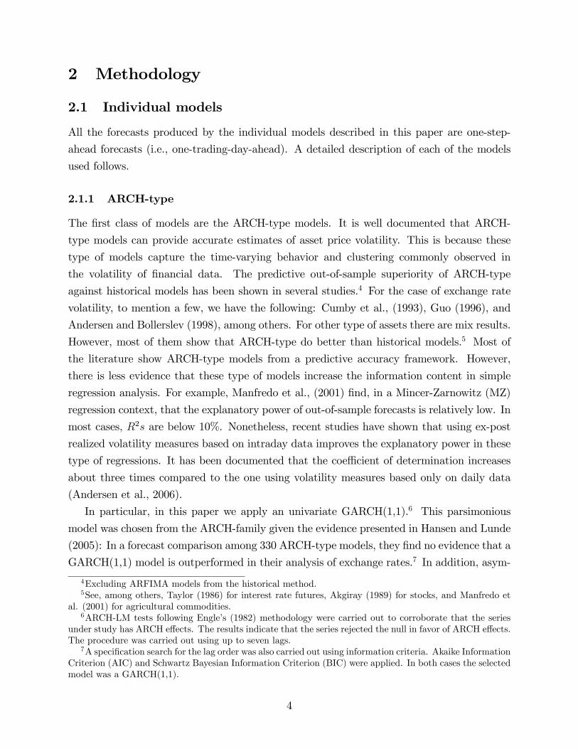
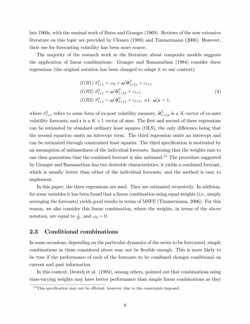
3.2 Realized volatility
The measures of ex-post volatility that we use as the target variable are calculated using
equation (7). Our preferred measure uses the intraday data. But we also calculate realized
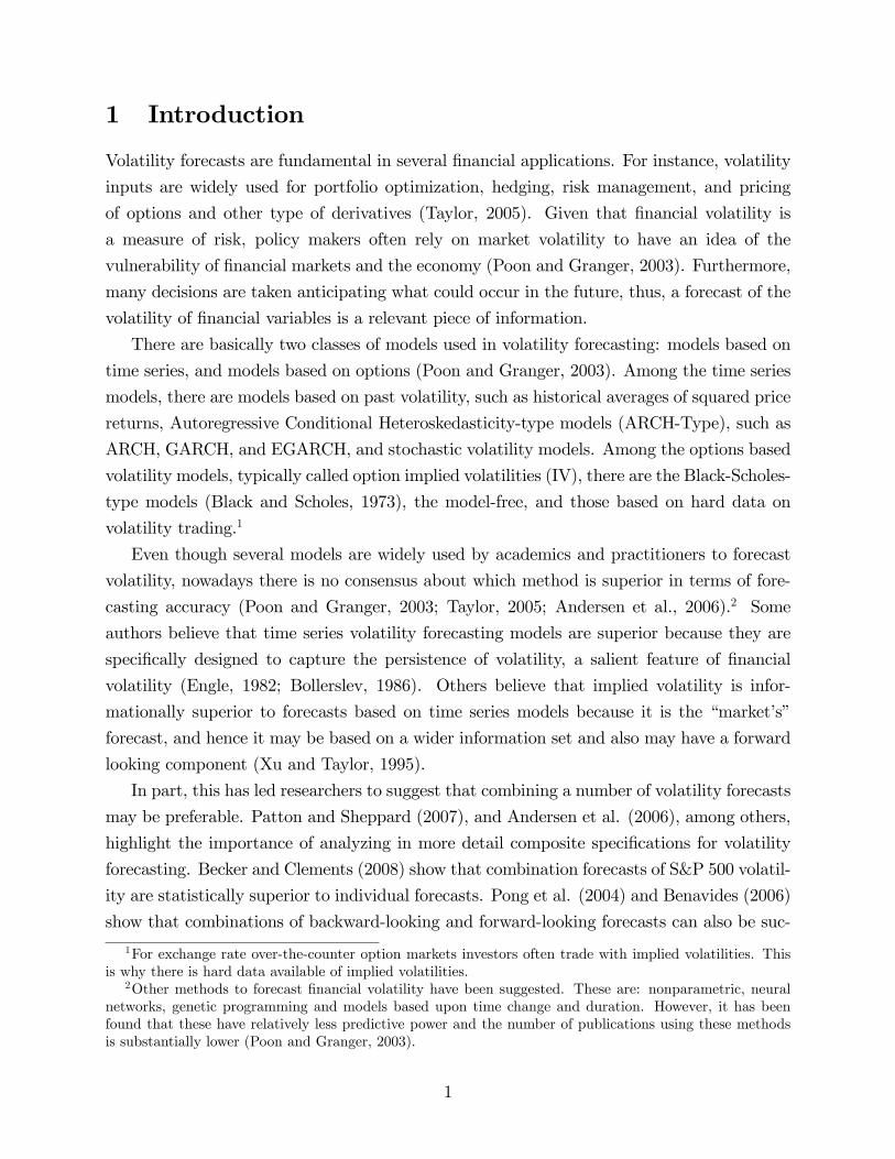
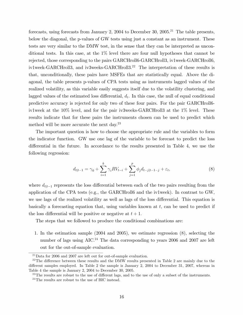
volatility using daily data. Figure 1 shows both estimates for the period from January 2nd,
2004 to December 31st, 2007. As can be seen, the estimate that uses intraday data at
�ve minute intervals captures relatively well the dynamics of the volatility estimated using
daily data. However, the former is less noisy. This re�ects Andersen and Bollerslev�s (1998)
mathematical result that the intraday estimator has lower variance (as �! 0, the variance
decreases).
3.3 Implied volatility
The volatility implied in option data is calculated from daily over-the-counter (OTC) options
for 1-month to maturity contracts of the MXN-USD exchange rate. The hard data on IV was
downloaded from UBS -an international �nancial institution home based in Switzerland- (the
ticker is 1MDNMXNUSDImplied). The sample period for the option data is from January
2nd, 2004 to December 31st, 2007, which consists of 993 daily observations. Mexican and
US risk-free interest rates were obtained in order to estimate the IVs from the model-based
method. Interest rates from 1-month Mexican Federal Government bonds (CETES) were
downloaded from Banco de Mexico�s web page. US CDs with the same maturity were
downloaded from the Board of Governors of the Federal Reserve System�s web page.19 Model-
based IVs are calculated from January 2nd, 2004 to December 31st, 2007.
4 Empirical results
In the following exercises, the out-of-sample evaluation period is from January 2nd, 2004 to
December 31st, 2007 for the individual methods, and from January 2nd, 2006 to December
31st, 2007 for all the methods when the combinations are included among the forecasting
methods. In the latter, data for 2004 and 2005 are used to start the recursive estimation of
the combination weights.
the daily quotes were used instead (as published by Banco de México). The missing data represent less than1% of the total number of observations considered for the out-of-sample evaluations.19The Federal Reserve�s web page is http://www.federalreserve.gov/
13
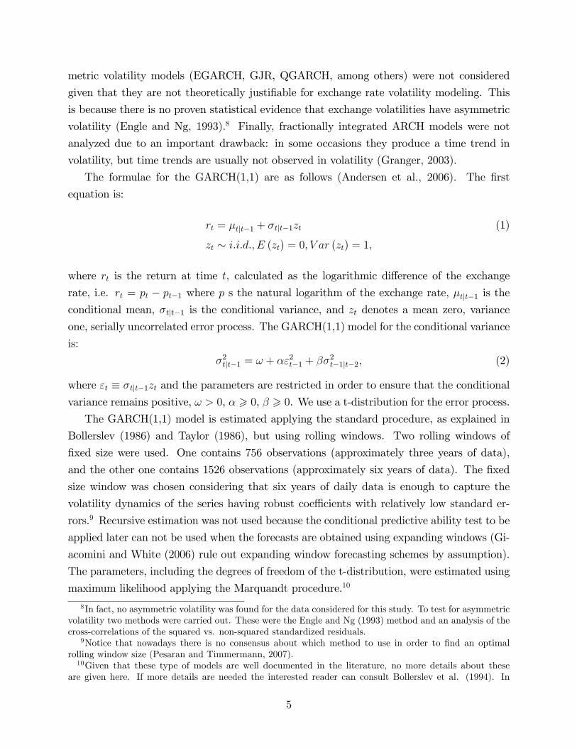
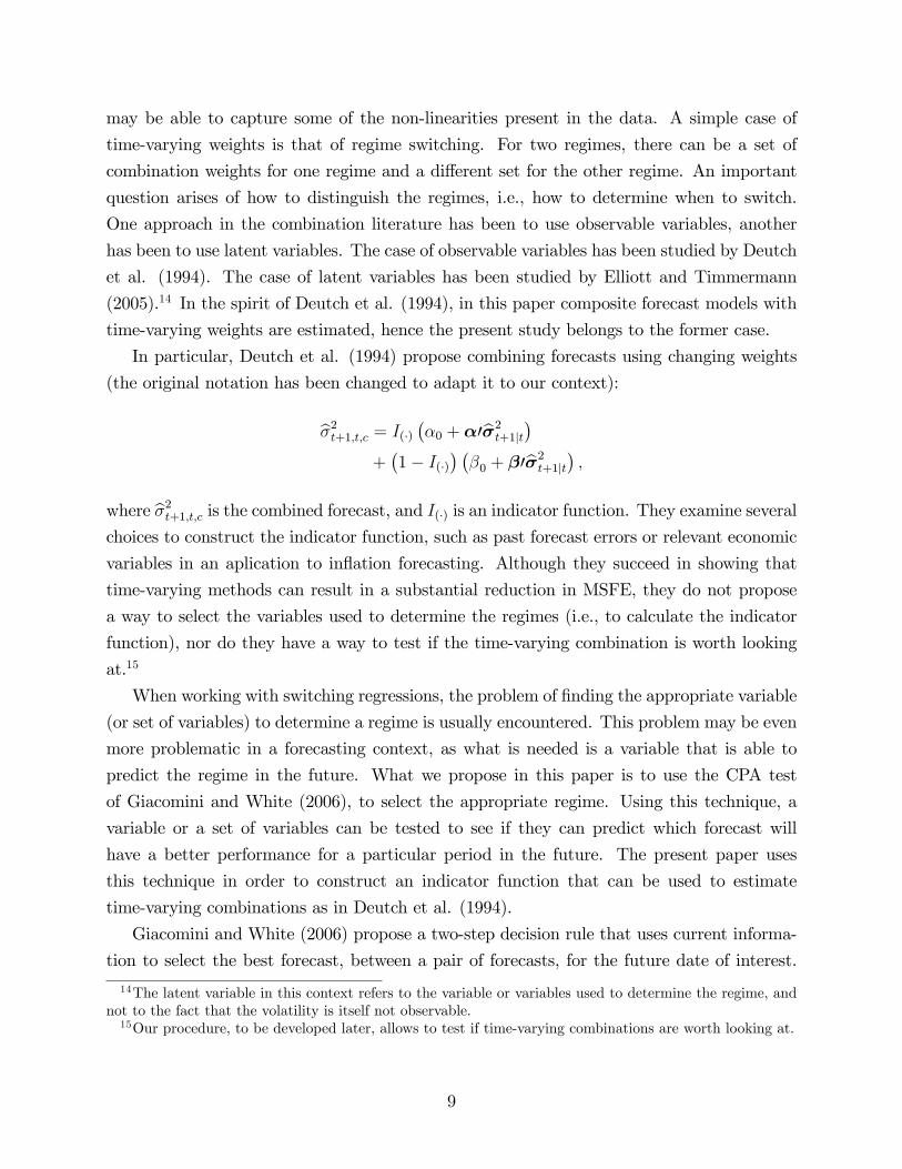
4.1 Individual models
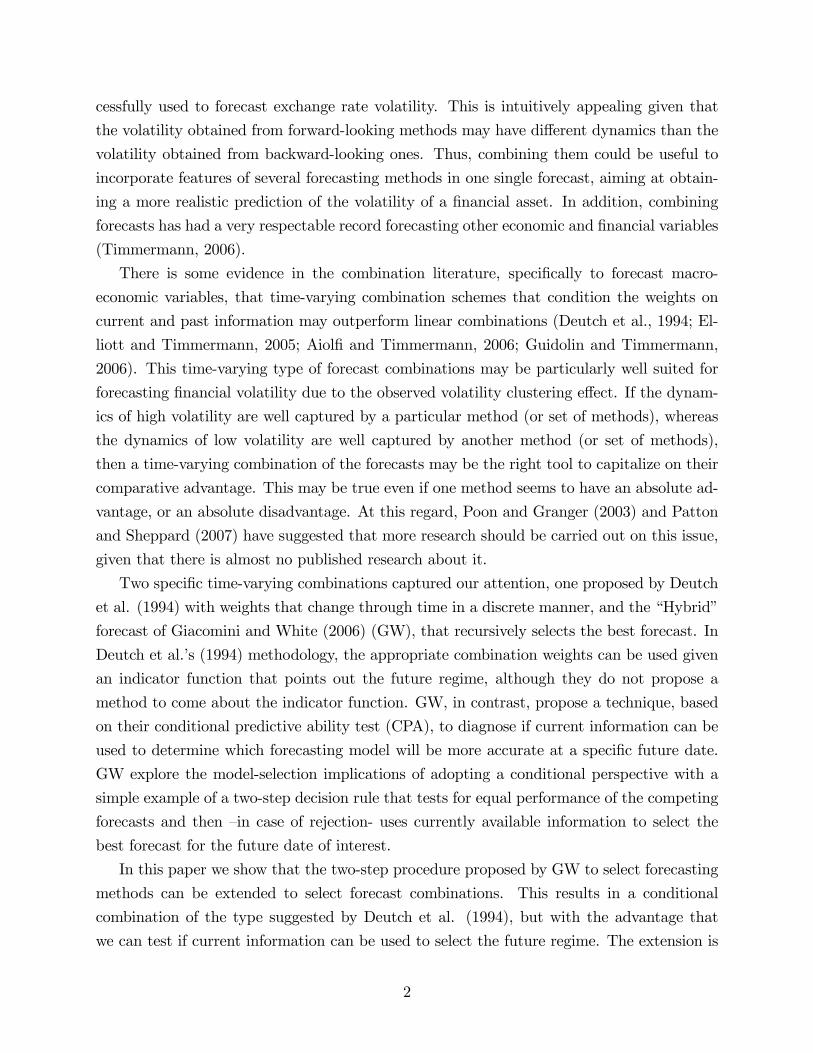
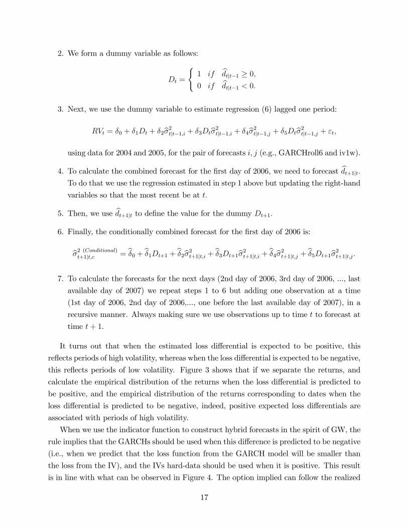
Figure 2 shows the forecast errors of the individual methods. The abbreviations represent the
following: implied volatility model-based (ivmb), hard data on implied volatility one-week-
to-maturity (iv1week) and three-week-to-maturity (iv3week), and GARCH rolling using a
window of 3 years (GARCHroll3) and a window of 6 years (GARCHroll6) of daily data.
From the �gure it is clear that the implied volatility model-based does not provide good
forecasts, compared with the others. Ivmb forecasts are very biased (systematically over-
predict realized volatility) and have high variance.
Table 1 contains descriptive statistics about the performance of the individual methods.
Those with negative mean errors tend to systematically over-predict realized volatility, with
option implied model based showing considerably higher bias. The last column shows the
MSFE ratio, using as common denominator the MSFE of the GARCH with a rolling window
of 6 years given that it is the individual model that performed better in terms of MSFE. The
ratio of the IV model based is extremely high, showing that indeed this method is particularly
bad to forecast realized volatility. In contrast, the di¤erences between both GARCHs and
the IVs (hard data) are smaller, with apparently a small advantage for the GARCHs.20
Table 2 contains the t-statistics (above the diagonal) and the p-values (below the di-
agonal) of pair-wise Diebold-Mariano-West tests, where we have used Newey and West�s
(1987) heteroskedasticity and autocorrelation consistent covariance matrix estimator. Small
p-values can be interpreted as a rejection of the null hypothesis of equal predictive ability.
The table shows evidence that the IV model based is statistically worse than all the other
methods. If inference is conducted at the 5% level, it is clear that: (i) both IV hard data
show statistically the same performance (p-value is 0.3711); (ii) the GARCH estimated using
a rolling window of 6 years is not statistically superior to the one estimated using a rolling
window of 3 years (p-value is 0.1164); and (iii) both IV hard data show statistically the
same performance than both GARCH models (pairwise), i.e., they have statistically indis-
tinguishable MSFEs, as the DMW predictive ability tests are not able to reject the null of
equal predictive accuracy between these forecasts, with the exeption of the pair GARCHroll6
and iv1week, for which there is some evidence of superior performance of the ARCH-type
forecast.
Our results con�rm that indeed it is di¢ cult to choose between forecasts produced using
time series methods and those obtained from �nancial markets (option implieds).
20We also evaluated the performance of historical volatility forecasts, using di¤erent estimation windows,from 5 days to 252 days, but in all cases they perform poorly, even when compared to the option impliedmodel based forecasts.
14

4.2 Linear Combinations
The descriptive statistics about the performance of the linear combinations are presented in
Table 3. All the combinations include forecasts from the �ve di¤erent methods reported in
Table 1. As a reference, the statistics for the GARCHmodel estimated using 6 years windows
are also presented, although in contrast to tables 1 and 2, here the analysis is performed
using only forecasts for 2006 and 2007, since the data for 2004 and 2005 is used to start the
(recursive) estimation of the combination weights. As can be seen, even the combination
that includes a constant (GR1) has a negative mean error, although smaller than that of
the other combinations, as expected. Looking at the MSFE ratios, the combination with
equal weights does not produce good results. In addition, three of the combinations present
a MSFE ratio smaller than 1, which indicates that their MSFEs are smaller than that of the
best individual model (GARCHroll6) calculated over the same reduced sample, con�rming
that combining forecasts is a procedure that improves forecasting accuracy. However, the
results of the DMW tests applied to the linear combinations (taken the GARCHroll6 as the
benchmark) show that only GR1 and GR2 are able to outperform the best individual model
at the 5% signi�cant level.
It is interesting that the best two combinations are GR1, which is the less restrictive of
the Granger-Ramanathan regressions, and GR2, the combination that does not include a
constant. The latter result is a consequence of: (i) the constant in most of the regressions is
close to zero; and (ii) in general, the estimated weights for the GARCH forecasts are usually
negative (around -0.5), while the weights estimated for the IVs are usually positive (around
1), which o¤sets the bias of the individual forecasts. Indeed, the gains from combination arise
from a logic similar to the logic behind diversi�cation when forming investment portfolios.
In this case, because of the negative sign of the weights, the best �portfolio�usually goes
short on the GARCHs models. The heterogeneity in the weights also explains the poor
performance of the mean forecasts in this context, and opens the door for the use of time-
varying combination schemes that can make better use of it.
4.3 Conditional Combinations
In this section, we �rst proceed with the conditional evaluation of the individual forecasts
(the �rst step in GW). Then, we use these results to form and indicator function and then
to estimate the time-varying combinations, following equation (6). Finally, we evaluate the
performance of the proposed time-varying composite forecasts.
Table 4 presents the results of the conditional predictive ability test for the individual
15
forecasts, using forecasts from January 2, 2004 to December 30, 2005.21 The table presents,
below the diagonal, the p-values of GW tests using just a constant as an instrument. These
tests are very similar to the DMW test, in the sense that they can be interpreted as uncon-
ditional tests. In this case, at the 1% level there are four null hypotheses that cannot be
rejected, those corresponding to the pairs GARCHroll6-GARCHroll3, iv1week-GARCHroll6,
iv1week-GARCHroll3, and iv3weeks-GARCHroll3.22 The interpretation of these results is
that, unconditionally, these pairs have MSFEs that are statistically equal. Above the di-
agonal, the table presents p-values of CPA tests using as instruments lagged values of the
realized volatility, as this variable easily suggests itself due to the volatility clustering, and
lagged values of the estimated loss di¤erential, dt. In this case, the null of equal conditional
predictive accuracy is rejected for only two of these four pairs. For the pair GARCHroll6-
iv1week at the 10% level, and for the pair iv3weeks-GARCHroll3 at the 1% level. These
results indicate that for these pairs the instruments chosen can be used to predict which
method will be more accurate the next day.23
The important question is how to choose the appropriate rule and the variables to form
the indicator function. GW use one lag of the variable to be forecast to predict the loss
di¤erential in the future. In accordance to the results presented in Table 4, we use the
following regression:
dtjt�1 = 0 +kXi=1
iRVt�i +
pXj=1
�jdt�jjt�1�j + "t; (8)
where dtjt�1 represents the loss di¤erential between each of the two pairs resulting from the
application of the CPA tests (e.g., the GARCHroll6 and the iv1week). In contrast to GW,
we use lags of the realized volatility as well as lags of the loss di¤erential. This equation is
basically a forecasting equation that, using variables known at t, can be used to predict if
the loss di¤erential will be positive or negative at t+ 1:
The steps that we followed to produce the conditional combinations are:
1. In the estimation sample (2004 and 2005), we estimate regression (8), selecting the
number of lags using AIC.24 The data corresponding to years 2006 and 2007 are left
out for the out-of-sample evaluation.
21Data for 2006 and 2007 are left out for out-of-sample evaluation.22The di¤erence between these results and the DMW results presented in Table 2 are mainly due to the
di¤erent samples employed. In Table 2 the sample is January 2, 2004 to December 31, 2007, whereas inTable 4 the sample is January 2, 2004 to December 30, 2005.23The results are robust to the use of di¤erent lags, and to the use of only a subset of the instruments.24The results are robust to the use of BIC instead.
16
2. We form a dummy variable as follows:
Dt =
(1
0
if
if
bdtjt�1 � 0;bdtjt�1 < 0:3. Next, we use the dummy variable to estimate regression (6) lagged one period:
RVt = �0 + �1Dt + �2b�2tjt�1;i + �3Dtb�2tjt�1;i + �4b�2tjt�1;j + �5Dtb�2tjt�1;j + "t;using data for 2004 and 2005, for the pair of forecasts i; j (e.g., GARCHroll6 and iv1w).
4. To calculate the combined forecast for the �rst day of 2006, we need to forecast bdt+1jt:To do that we use the regression estimated in step 1 above but updating the right-hand
variables so that the most recent be at t:
5. Then, we use bdt+1jt to de�ne the value for the dummy Dt+1:
6. Finally, the conditionally combined forecast for the �rst day of 2006 is:
b�2 (Conditional)t+1jt;c = b�0 + b�1Dt+1 + b�2b�2t+1jt;i + b�3Dt+1b�2t+1jt;i + b�4b�2t+1jt;j + b�5Dt+1b�2t+1jt;j:7. To calculate the forecasts for the next days (2nd day of 2006, 3rd day of 2006, ..., last
available day of 2007) we repeat steps 1 to 6 but adding one observation at a time
(1st day of 2006, 2nd day of 2006,..., one before the last available day of 2007), in a
recursive manner. Always making sure we use observations up to time t to forecast at
time t+ 1.
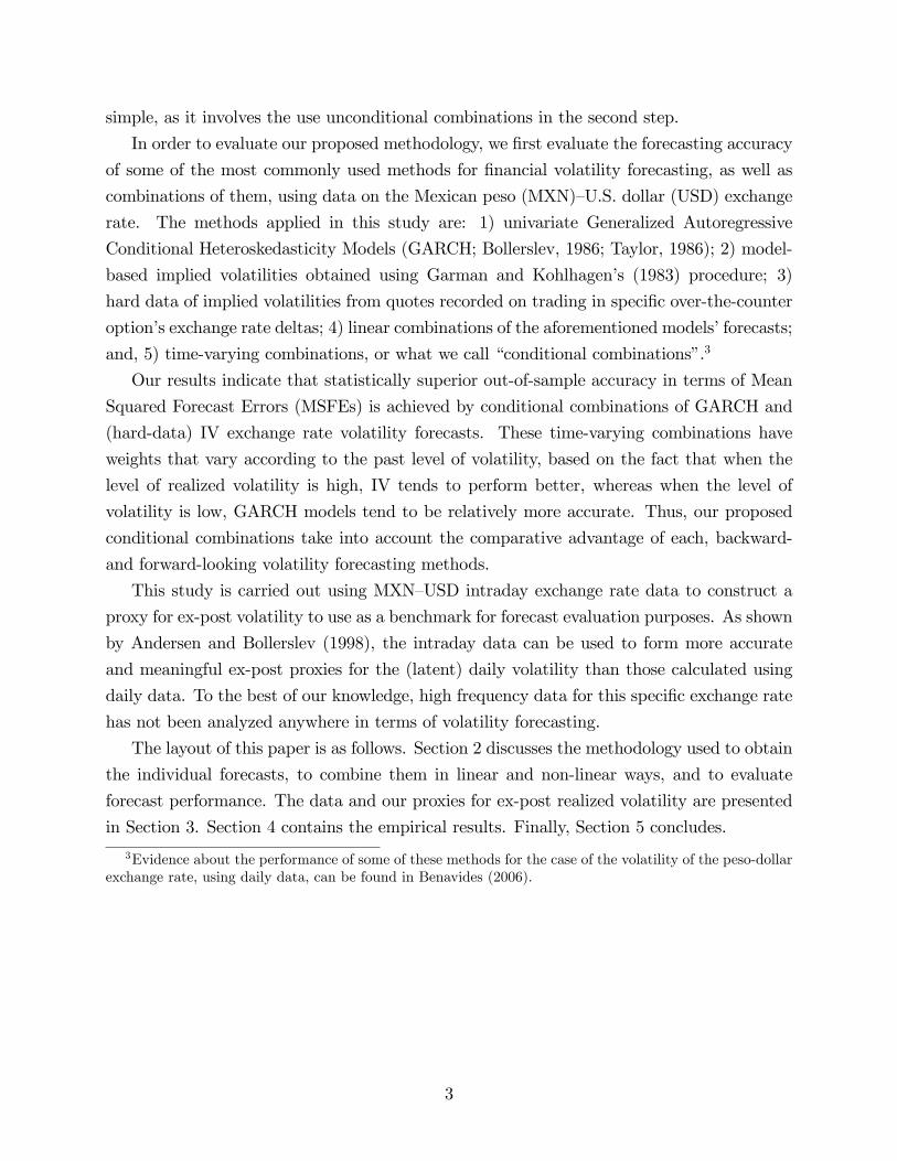
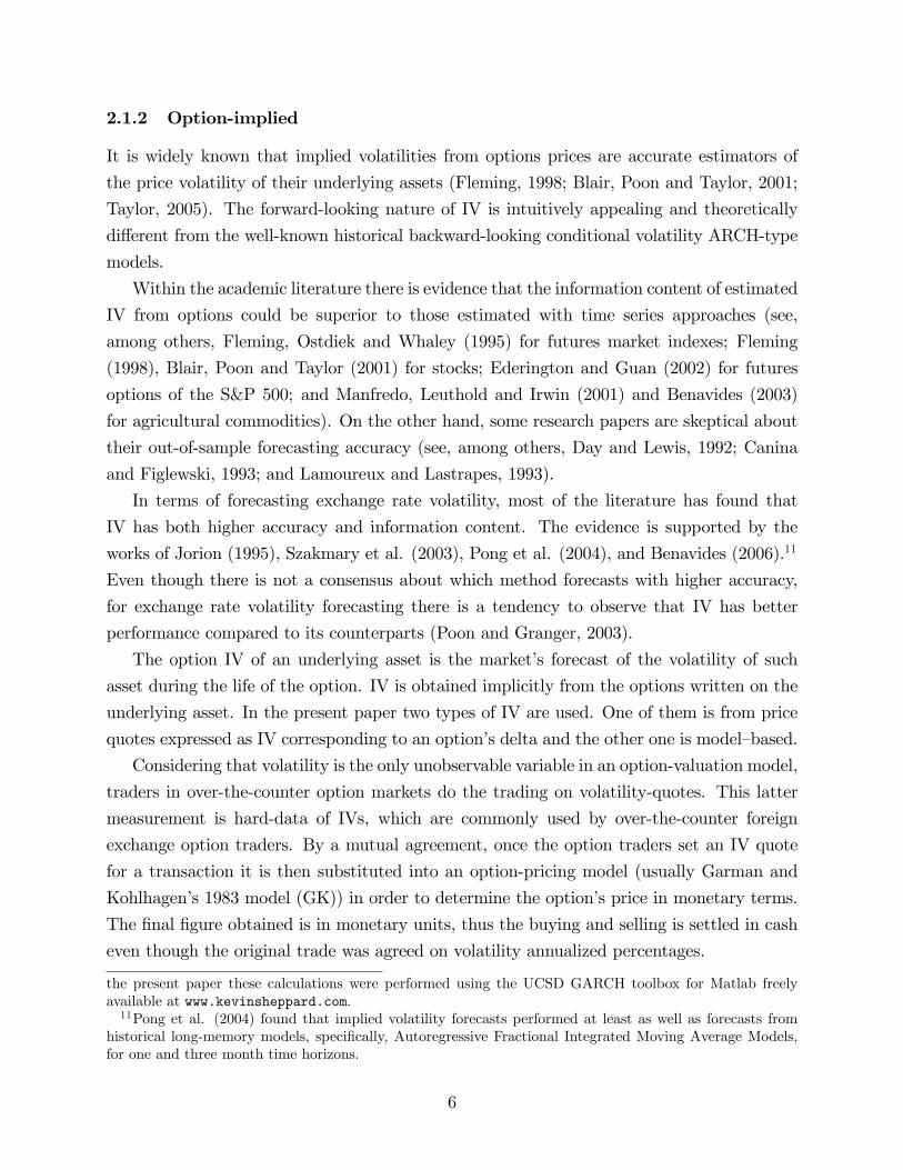
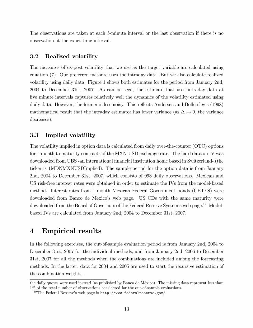
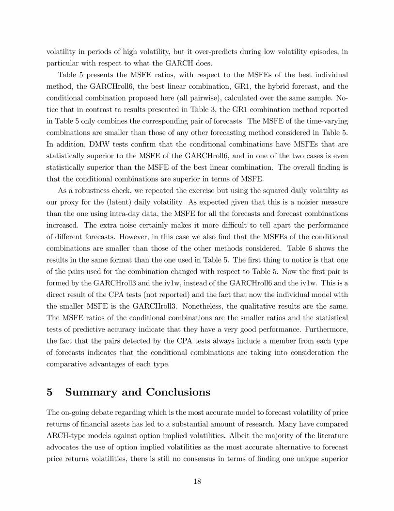
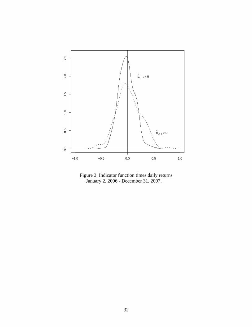
It turns out that when the estimated loss di¤erential is expected to be positive, this
re�ects periods of high volatility, whereas when the loss di¤erential is expected to be negative,
this re�ects periods of low volatility. Figure 3 shows that if we separate the returns, and
calculate the empirical distribution of the returns when the loss di¤erential is predicted to
be positive, and the empirical distribution of the returns corresponding to dates when the
loss di¤erential is predicted to be negative, indeed, positive expected loss di¤erentials are
associated with periods of high volatility.
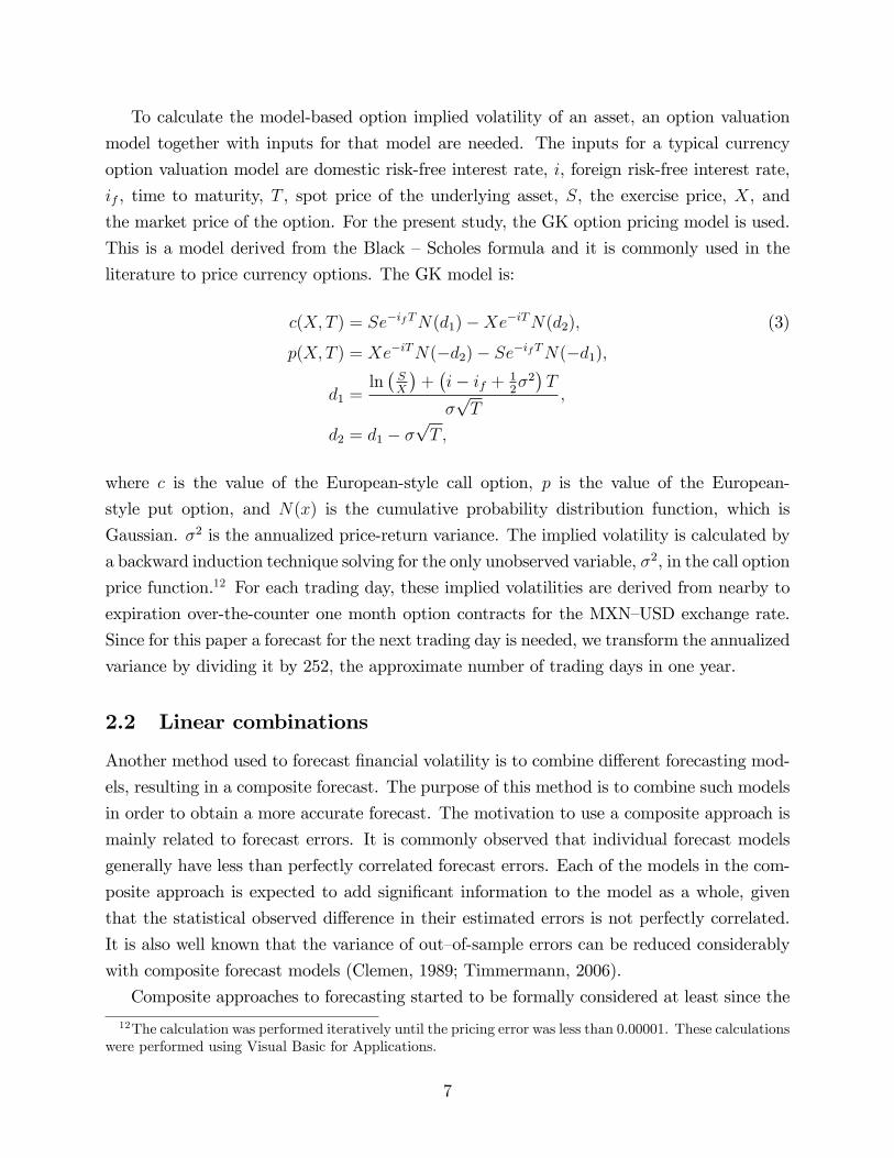
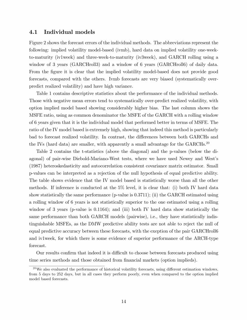
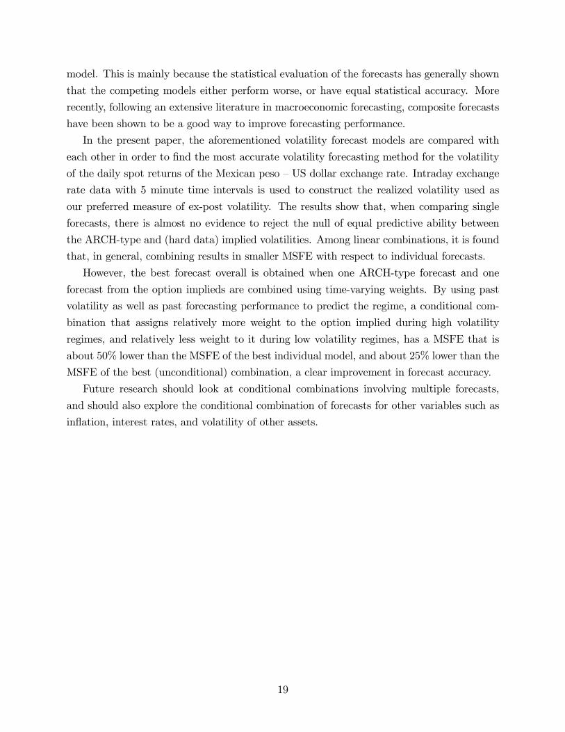
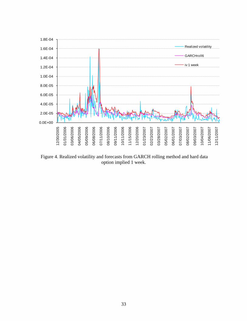
When we use the indicator function to construct hybrid forecasts in the spirit of GW, the
rule implies that the GARCHs should be used when this di¤erence is predicted to be negative
(i.e., when we predict that the loss function from the GARCH model will be smaller than
the loss from the IV), and the IVs hard-data should be used when it is positive. This result
is in line with what can be observed in Figure 4. The option implied can follow the realized
17
volatility in periods of high volatility, but it over-predicts during low volatility episodes, in
particular with respect to what the GARCH does.
Table 5 presents the MSFE ratios, with respect to the MSFEs of the best individual
method, the GARCHroll6, the best linear combination, GR1, the hybrid forecast, and the
conditional combination proposed here (all pairwise), calculated over the same sample. No-
tice that in contrast to results presented in Table 3, the GR1 combination method reported
in Table 5 only combines the corresponding pair of forecasts. The MSFE of the time-varying
combinations are smaller than those of any other forecasting method considered in Table 5.
In addition, DMW tests con�rm that the conditional combinations have MSFEs that are
statistically superior to the MSFE of the GARCHroll6, and in one of the two cases is even
statistically superior than the MSFE of the best linear combination. The overall �nding is
that the conditional combinations are superior in terms of MSFE.
As a robustness check, we repeated the exercise but using the squared daily volatility as
our proxy for the (latent) daily volatility. As expected given that this is a noisier measure
than the one using intra-day data, the MSFE for all the forecasts and forecast combinations
increased. The extra noise certainly makes it more di¢ cult to tell apart the performance
of di¤erent forecasts. However, in this case we also �nd that the MSFEs of the conditional
combinations are smaller than those of the other methods considered. Table 6 shows the
results in the same format than the one used in Table 5. The �rst thing to notice is that one
of the pairs used for the combination changed with respect to Table 5. Now the �rst pair is
formed by the GARCHroll3 and the iv1w, instead of the GARCHroll6 and the iv1w. This is a
direct result of the CPA tests (not reported) and the fact that now the individual model with
the smaller MSFE is the GARCHroll3. Nonetheless, the qualitative results are the same.
The MSFE ratios of the conditional combinations are the smaller ratios and the statistical
tests of predictive accuracy indicate that they have a very good performance. Furthermore,
the fact that the pairs detected by the CPA tests always include a member from each type
of forecasts indicates that the conditional combinations are taking into consideration the
comparative advantages of each type.
5 Summary and Conclusions
The on-going debate regarding which is the most accurate model to forecast volatility of price
returns of �nancial assets has led to a substantial amount of research. Many have compared
ARCH-type models against option implied volatilities. Albeit the majority of the literature
advocates the use of option implied volatilities as the most accurate alternative to forecast
price returns volatilities, there is still no consensus in terms of �nding one unique superior
18
model. This is mainly because the statistical evaluation of the forecasts has generally shown
that the competing models either perform worse, or have equal statistical accuracy. More
recently, following an extensive literature in macroeconomic forecasting, composite forecasts
have been shown to be a good way to improve forecasting performance.
In the present paper, the aforementioned volatility forecast models are compared with
each other in order to �nd the most accurate volatility forecasting method for the volatility
of the daily spot returns of the Mexican peso �US dollar exchange rate. Intraday exchange
rate data with 5 minute time intervals is used to construct the realized volatility used as
our preferred measure of ex-post volatility. The results show that, when comparing single
forecasts, there is almost no evidence to reject the null of equal predictive ability between
the ARCH-type and (hard data) implied volatilities. Among linear combinations, it is found
that, in general, combining results in smaller MSFE with respect to individual forecasts.
However, the best forecast overall is obtained when one ARCH-type forecast and one
forecast from the option implieds are combined using time-varying weights. By using past
volatility as well as past forecasting performance to predict the regime, a conditional com-
bination that assigns relatively more weight to the option implied during high volatility
regimes, and relatively less weight to it during low volatility regimes, has a MSFE that is
about 50% lower than the MSFE of the best individual model, and about 25% lower than the
MSFE of the best (unconditional) combination, a clear improvement in forecast accuracy.
Future research should look at conditional combinations involving multiple forecasts,
and should also explore the conditional combination of forecasts for other variables such as
in�ation, interest rates, and volatility of other assets.
19
References
[1] Aiol�, M. and Timmermann A. (2006). Persistence in Forecasting Performance andConditional Combination Strategies. Journal of Econometrics, 135, 31-53.
[2] Andersen, T.G., Bollerslev, T., Christo¤ersen, P. F., and Diebold, F.X. (2006). Volatilityand Correlation Forecasting. Handbook of Economic Forecasting. Edited by G. Elliott.,C.W.J. Granger., and A. Timmermann. Amsterdam: North Holland.
[3] Andersen, T.G., and Bollerslev, T. (1998). Answering the Skeptics: Yes, StandardVolatility Models Do Provide Accurate Forecasts. International Economic Review, 39,885-905.
[4] Akgiray, V. (1989). Conditional Heteroskedasticity in Time Series of Stock Returns:Evidence and Forecasts. Journal of Business, 62, 55-80.
[5] Bates, J.M. and Granger, C.W.J. (1969). The Combination of Forecasts. OperationsResearch Quarterly, 20, 451-468.
[6] Becker, R. and Clemens, A.E. (2008). Are Combination Forecasts of S&P 500 VolatilityStatistically Superior? International Journal of Forecasting, 24, 122-133.
[7] Benavides, G. (2003). Price Volatility Forecasts for Agricultural Commodities: An Ap-plication of Historical Volatility Models, Option Implieds and Composite Approachesfor Futures Prices of Corn and Wheat. Working Paper, Lancaster University. url:http://papers.ssrn.com/sol3/papers.cfm?abstract_id=611062
[8] Benavides, G. (2006). Volatility Forecasts for the Mexican Peso - US Dol-lar Exchange Rate: An Empirical Analysis of GARCH, Option Impliedand Composite Forecasts Models. Working Paper 2006-04, Banco de Méx-ico. url: http://www.banxico.org.mx/documents/%7B7F1FAAE1-FEFC-EB00-B0C8-55420567F74F%7D.pdf
[9] Black, F. and Scholes, M. S. (1973). The Pricing of Options and Corporate Liabilities.Journal of Political Economy, 81, May-June, 637-654.
[10] Blair, B. J., Poon, S. and Taylor, S. J. (2001). Forecasting S&P 100 Volatility: TheIncremental Information Content of Implied Volatilities and High-Frequency Index Re-turns. Journal of Econometrics, 105, 5-26.
[11] Bollerslev, T. P. (1986). Generalized Autoregressive Conditional Heteroskedasticity.Journal of Econometrics, 31, 307-327.
[12] Bollerslev, T. P., Engle, R. F. and Nelson D. B. (1994). ARCH Models. Handbook ofEconometrics. Vol 4. Edited by R. F. Engle and D. L. McFadden. Amsterdam: Elsevier.
[13] Canina, L and Figlewski, S. (1993) The Informational Content of Implied Volatility.Review of Financial Studies, 6, 659-681.
20
[14] Clemen, R. T. (1989). Combining Forecasts: A Review and Annotated Bibliography.International Journal of Forecasting, 5, 559-583.
[15] Cumby, R., Figlewski, S. and Hasbrouck, J. (1993). Forecasting Volatilities and Corre-lations with EGARCH Models. Journal of Derivatives, 1, 51-63.
[16] Day, T. E. and Lewis, C. M. (1992). Stock Market Volatility and the Information Con-tent of Stock Index Options. Journal of Econometrics, 52, 267-287.
[17] Deutsch, M., Granger, C.W.J. and Terasvirta, T. (1994). The Combination of ForecastsUsing Changing Weights. International Journal of Forecasting, 10, 47-57.
[18] Diebold, F. X. and Mariano, R. S. (1995). Comparing Predictive Accuracy. Journal ofBusiness and Economic Statistics, 13, 253-263.
[19] Ederington, L. and Guan, W. (2002). Is Implied Volatility an Informationally E¢ cientand E¤ective Predictor of Future Volatility? Journal of Risk, 4, 3.
[20] Elliott, G. and Timmermann, A. (2005). Optimal Forecast Combination Weights underRegime Switching. International Economic Review, 46, 1081-1102.
[21] Engle, R. F. (1982). Autoregressive Conditional Heteroskedasticity with Estimates ofthe Variance of U.K. In�ation. Econometrica, 50, 987-1008.
[22] Engle, R.F and Ng, V.K. (1993). Measuring and Testing the Impact of News on Volatil-ity. Journal of Finance, 48, 1749-1778.
[23] Fleming, J. (1998). The Quality of Market Volatility Forecasts Implied by S&P 100Index Option Prices. Journal of Empirical Finance, 5, 317-345.
[24] Fleming, J., Ostdiek, B. and Whaley, R.E. (1995). Predicting Stock Market Volatility :A New Measure. Journal of Futures Markets, 15, 265-302.
[25] Garman, M. B and Klass, M. J. (1980). On the Estimation of Security Price Volatilitiesfrom Historical Data. Journal of Business, 53, 67-78.
[26] Garman, M.B. and Kohlhagen, S.W. (1983). Foreign Currency Option Values. Journalof International Money and Finance, 2, 231-237.
[27] Giacomini, R. and White, H. (2006). Tests of Conditional Predictive Ability. Economet-rica, 74, 1545-1578.
[28] Granger, C.W.J. and Ramanathan, R. (1984). Improved Methods of Combining Fore-casts. Journal of Forecasting, 3, 197-204.
[29] Granger, C.W.J. (2003). Long Memory Process-An Economist�s Viewpoint. Advancesin Statistics, Combinations, and Related Areas, edited by C. Gulats, et al., 100-111.World Scienti�c Publishers.
21
[30] Guidolin, M. and Timmermann, A. (2006). Forecasts of US Short-term Interest Rates:A Flexible Forecast Combination Approach. Federal Reserve Bank of St. Louis, WorkingPaper Series. url: http://research.stlouisfed.org/wp/2005/2005-059.pdf
[31] Guo, D. (1996). The Predictive Power of Implied Stochastic Variance from CurrencyOptions. Journal of Futures Markets, 16, 915-942.
[32] Hansen, P.R. and Lunde, A. (2005). A Forecast Comparison of Volatility Models: DoesAnything Beat a GARCH(1,1)? Journal of Applied Econometrics, 20, 873-889.
[33] Jorion, P. (1995). Predicting Volatility in the Foreign Exchange Market. The Journalof Finance, 50, 507-528.
[34] Lamoureux, C. G. and Lastrapes, W. D. (1993). Forecasting Stock Return Variance:Toward an Understanding of Stochastic Implied Volatilities. The Review of FinancialStudies., 6, 293-326.
[35] Manfredo, M. Leuthold, R. M. and Irwin, S. H. (2001). Forecasting Cash Price Volatilityof Fed Cattle, Feeder Cattle and Corn: Time Series, Implied Volatility and CompositeApproaches. Journal of Agricultural and Applied Economics, 33, 523-538.
[36] Newey, W. and West, K. (1987). A Simple Positive Semi-de�nite, Heteroskedasticityand Autocorrelation Consistent Covariance Matrix. Econometrica, 55, 703-708.
[37] Parkinson, M. (1980) The Extreme Value Method for Estimating the Variance of theRate of Return. Journal of Financial Economics, 18, 199-228.
[38] Patton, A. J. (2006) Volatility Forecast Comparison using Imperfect Volatility Prox-ies. Quantitative Finance Research Centre, University of Technology Sydney, ResearchPaper 175.
[39] Patton, A. J. and Sheppard, K. (2007). Evaluating Volatility and Correlation Forecasts.Handbook of Financial Time Series. Edited y T.G. Andersen, R.A., Davis, J.-P. Kreissand T. Mikosch. Springer Verlag (forthcoming).
[40] Pesaran, M.H. and Timmermann, A. (2007). Selection of Estimation Window in thePresence of Breaks. Journal of Econometrics, 137, 134-161.
[41] Poon, S-H. and Granger, C.W.J. (2003). Forecasting Volatility in Financial Markets: AReview. Journal of Economic Literature, 41, 478-539.
[42] Pong, S., Shackleton, M., Taylor, S. and Xu, X. (2004). Forecasting Currency Volatility:A Comparison of Implied Volatilities and AR(FI)MA Models. Journal of Banking andFinance.
[43] Szakmary, A, Ors, E., Kim, J. K. and Davidson III, W. D. (2003). The PredictivePower of Implied Volatility: Evidence from 35 Futures Markets. Journal of Bankingand Finance, 27, 2151-2175.
22
[44] Taylor, S. J. (1986). Modeling Financial Time Series. Wiley.
[45] Taylor, S. J. (2005). Asset Price Dynamics, Volatility, and Prediction. Princeton Uni-versity Press.
[46] Timmermann, A. (2006). Forecast Combinations. Handbook of Economic Forecasting.Edited by G. Elliott., C.W.J. Granger., and A. Timmermann. Amsterdam: North Hol-land.
[47] West, K.D. (1996). Asymptotic Inference about Predictive Ability. Econometrica, 64,1067-1084.
[48] Xu, X. and Taylor, S. J. (1995). Conditional Volatility and the Informational E¢ ciencyof the PHLX Currency Options Market. Journal of Banking and Finance, 19, 803-821.
23
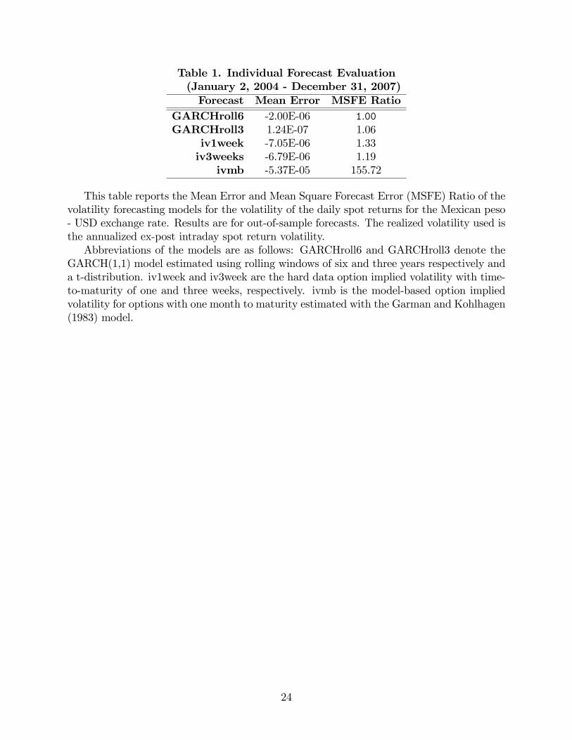
Table 1. Individual Forecast Evaluation(January 2, 2004 - December 31, 2007)Forecast Mean Error MSFE Ratio
GARCHroll6 -2.00E-06 1:00GARCHroll3 1.24E-07 1.06
iv1week -7.05E-06 1.33iv3weeks -6.79E-06 1.19
ivmb -5.37E-05 155.72
This table reports the Mean Error and Mean Square Forecast Error (MSFE) Ratio of thevolatility forecasting models for the volatility of the daily spot returns for the Mexican peso- USD exchange rate. Results are for out-of-sample forecasts. The realized volatility used isthe annualized ex-post intraday spot return volatility.Abbreviations of the models are as follows: GARCHroll6 and GARCHroll3 denote the
GARCH(1,1) model estimated using rolling windows of six and three years respectively anda t-distribution. iv1week and iv3week are the hard data option implied volatility with time-to-maturity of one and three weeks, respectively. ivmb is the model-based option impliedvolatility for options with one month to maturity estimated with the Garman and Kohlhagen(1983) model.
24
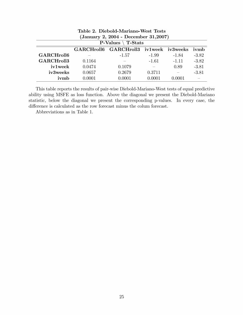
Table 2. Diebold-Mariano-West Tests(January 2, 2004 - December 31,2007)
P-Values n T-StatsGARCHroll6 GARCHroll3 iv1week iv3weeks ivmb
GARCHroll6 � -1.57 -1.99 -1.84 -3.82GARCHroll3 0.1164 � -1.61 -1.11 -3.82
iv1week 0.0474 0.1079 � 0.89 -3.81iv3weeks 0.0657 0.2679 0.3711 � -3.81
ivmb 0.0001 0.0001 0.0001 0.0001 �
This table reports the results of pair-wise Diebold-Mariano-West tests of equal predictiveability using MSFE as loss function. Above the diagonal we present the Diebold-Marianostatistic, below the diagonal we present the corresponding p-values. In every case, thedi¤erence is calculated as the row forecast minus the colum forecast.Abbreviations as in Table 1.
25
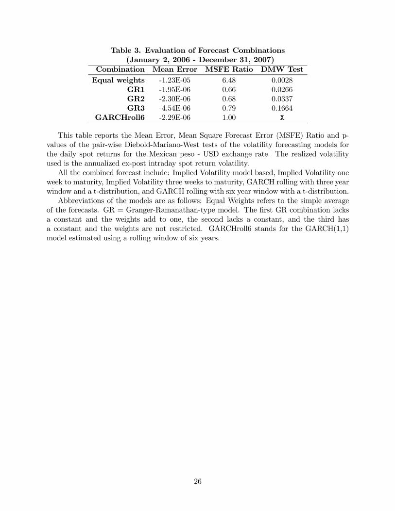
Table 3. Evaluation of Forecast Combinations(January 2, 2006 - December 31, 2007)
Combination Mean Error MSFE Ratio DMW TestEqual weights -1.23E-05 6.48 0.0028
GR1 -1.95E-06 0.66 0.0266GR2 -2.30E-06 0.68 0.0337GR3 -4.54E-06 0.79 0.1664
GARCHroll6 -2.29E-06 1.00 X
This table reports the Mean Error, Mean Square Forecast Error (MSFE) Ratio and p-values of the pair-wise Diebold-Mariano-West tests of the volatility forecasting models forthe daily spot returns for the Mexican peso - USD exchange rate. The realized volatilityused is the annualized ex-post intraday spot return volatility.All the combined forecast include: Implied Volatility model based, Implied Volatility one
week to maturity, Implied Volatility three weeks to maturity, GARCH rolling with three yearwindow and a t-distribution, and GARCH rolling with six year window with a t-distribution.Abbreviations of the models are as follows: Equal Weights refers to the simple average
of the forecasts. GR = Granger-Ramanathan-type model. The �rst GR combination lacksa constant and the weights add to one, the second lacks a constant, and the third hasa constant and the weights are not restricted. GARCHroll6 stands for the GARCH(1,1)model estimated using a rolling window of six years.
26
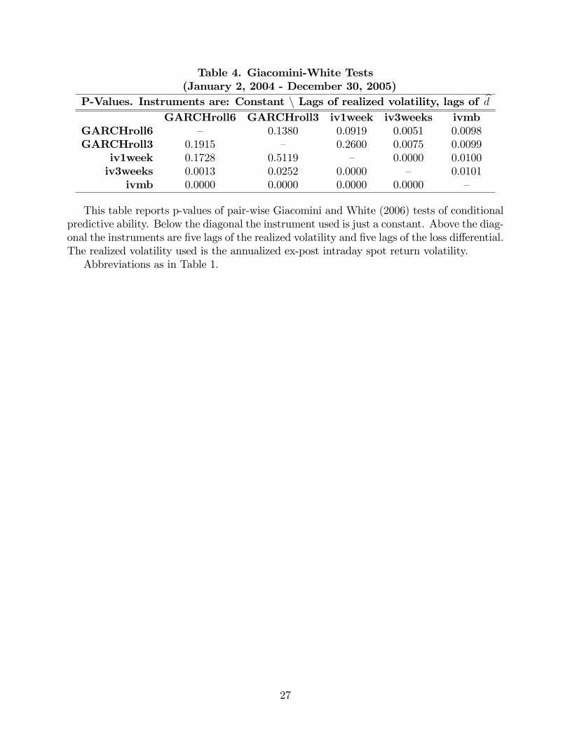
Table 4. Giacomini-White Tests(January 2, 2004 - December 30, 2005)
P-Values. Instruments are: Constant n Lags of realized volatility, lags of bdGARCHroll6 GARCHroll3 iv1week iv3weeks ivmb
GARCHroll6 � 0.1380 0.0919 0.0051 0.0098GARCHroll3 0.1915 � 0.2600 0.0075 0.0099
iv1week 0.1728 0.5119 � 0.0000 0.0100iv3weeks 0.0013 0.0252 0.0000 � 0.0101
ivmb 0.0000 0.0000 0.0000 0.0000 �
This table reports p-values of pair-wise Giacomini and White (2006) tests of conditionalpredictive ability. Below the diagonal the instrument used is just a constant. Above the diag-onal the instruments are �ve lags of the realized volatility and �ve lags of the loss di¤erential.The realized volatility used is the annualized ex-post intraday spot return volatility.Abbreviations as in Table 1.
27
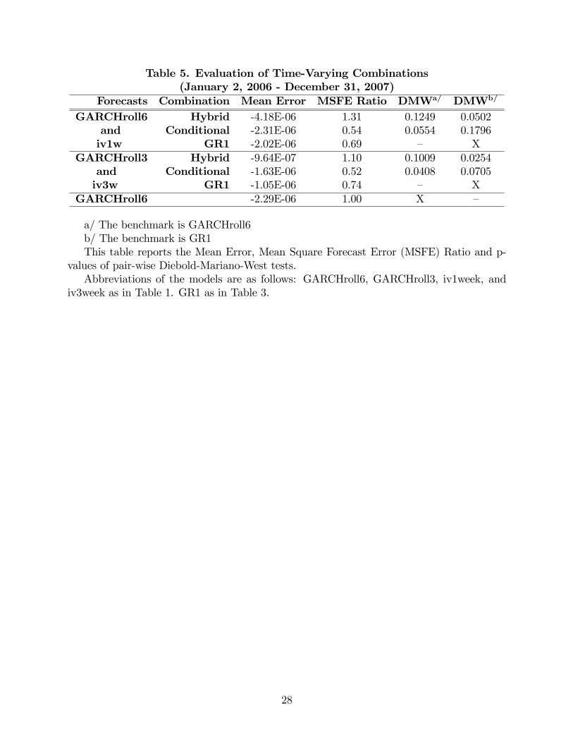
Table 5. Evaluation of Time-Varying Combinations(January 2, 2006 - December 31, 2007)
Forecasts Combination Mean Error MSFE Ratio DMWa/ DMWb/
GARCHroll6 Hybrid -4.18E-06 1.31 0.1249 0.0502and Conditional -2.31E-06 0.54 0.0554 0.1796iv1w GR1 -2.02E-06 0.69 � X
GARCHroll3 Hybrid -9.64E-07 1.10 0.1009 0.0254and Conditional -1.63E-06 0.52 0.0408 0.0705iv3w GR1 -1.05E-06 0.74 � X
GARCHroll6 -2.29E-06 1.00 X �
a/ The benchmark is GARCHroll6b/ The benchmark is GR1This table reports the Mean Error, Mean Square Forecast Error (MSFE) Ratio and p-
values of pair-wise Diebold-Mariano-West tests.Abbreviations of the models are as follows: GARCHroll6, GARCHroll3, iv1week, and
iv3week as in Table 1. GR1 as in Table 3.
28
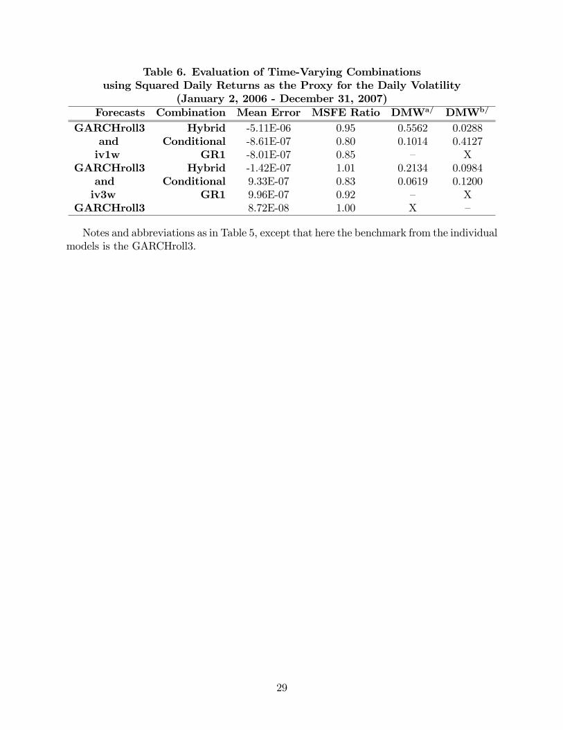
Table 6. Evaluation of Time-Varying Combinationsusing Squared Daily Returns as the Proxy for the Daily Volatility
(January 2, 2006 - December 31, 2007)Forecasts Combination Mean Error MSFE Ratio DMWa/ DMWb/
GARCHroll3 Hybrid -5.11E-06 0.95 0.5562 0.0288and Conditional -8.61E-07 0.80 0.1014 0.4127iv1w GR1 -8.01E-07 0.85 � X
GARCHroll3 Hybrid -1.42E-07 1.01 0.2134 0.0984and Conditional 9.33E-07 0.83 0.0619 0.1200iv3w GR1 9.96E-07 0.92 � X
GARCHroll3 8.72E-08 1.00 X �
Notes and abbreviations as in Table 5, except that here the benchmark from the individualmodels is the GARCHroll3.
29

30
0.00E+00
5.00E-05
1.00E-04
1.50E-04
2.00E-04
2.50E-04
3.00E-04
3.50E-04
01/0
2/20
04
03/1
2/20
04
05/1
8/20
04
07/2
1/20
04
09/2
9/20
04
12/0
1/20
04
02/0
4/20
05
04/1
4/20
05
06/1
7/20
05
08/1
9/20
05
10/2
5/20
05
12/2
7/20
05
03/0
2/20
06
05/0
8/20
06
07/1
1/20
06
09/1
2/20
06
11/1
7/20
06
01/2
6/20
07
04/0
3/20
07
06/0
8/20
07
08/1
0/20
07
10/1
5/20
07
12/2
7/20
07
Squared Daily Return
Intraday Realized Volatility
Figure 1: Exchange rate MXN—USD square daily return and intraday realized volatility.

31
-1.4E-03
-1.2E-03
-1.0E-03
-8.0E-04
-6.0E-04
-4.0E-04
-2.0E-04
0.0E+00
2.0E-0401
/02/
2004
04/2
2/20
04
08/0
3/20
04
11/1
8/20
04
03/0
2/20
05
06/1
7/20
05
09/2
8/20
05
01/0
9/20
06
04/2
4/20
06
08/0
4/20
06
11/1
7/20
06
03/0
7/20
07
06/2
1/20
07
10/0
2/20
07
ivmb
-1.5E-04
-1.0E-04
-5.0E-05
0.0E+00
5.0E-05
1.0E-04
01/0
2/20
04
04/2
2/20
04
08/0
3/20
04
11/1
8/20
04
03/0
2/20
05
06/1
7/20
05
09/2
8/20
05
01/0
9/20
06
04/2
4/20
06
08/0
4/20
06
11/1
7/20
06
03/0
7/20
07
06/2
1/20
07
10/0
2/20
07
iv 1 week
-8.0E-05-6.0E-05-4.0E-05-2.0E-050.0E+002.0E-054.0E-056.0E-058.0E-051.0E-04
01/0
2/20
04
04/2
2/20
04
08/0
3/20
04
11/1
8/20
04
03/0
2/20
05
06/1
7/20
05
09/2
8/20
05
01/0
9/20
06
04/2
4/20
06
08/0
4/20
06
11/1
7/20
06
03/0
7/20
07
06/2
1/20
07
10/0
2/20
07
iv 3 weeks
-4.0E-05-2.0E-050.0E+002.0E-054.0E-056.0E-058.0E-051.0E-041.2E-041.4E-041.6E-04
01/0
2/20
04
04/2
2/20
04
08/0
3/20
04
11/1
8/20
04
03/0
2/20
05
06/1
7/20
05
09/2
8/20
05
01/0
9/20
06
04/2
4/20
06
08/0
4/20
06
11/1
7/20
06
03/0
7/20
07
06/2
1/20
07
10/0
2/20
07
GARCHroll3
-6.0E-05-4.0E-05-2.0E-050.0E+002.0E-054.0E-056.0E-058.0E-051.0E-041.2E-041.4E-041.6E-04
01/0
2/20
04
04/2
2/20
04
08/0
3/20
04
11/1
8/20
04
03/0
2/20
05
06/1
7/20
05
09/2
8/20
05
01/0
9/20
06
04/2
4/20
06
08/0
4/20
06
11/1
7/20
06
03/0
7/20
07
06/2
1/20
07
10/0
2/20
07
GARCHroll6
Figure 2: Forecast errors for the individual models.
32
Figure 3. Indicator function times daily returns
January 2, 2006 - December 31, 2007.
−1.0 −0.5 0.0 0.5 1.0
0.0
0.5
1.0
1.5
2.0
2.5
dt, t−1 ≥ 0
dt, t−1 < 0
33
0.0E+00
2.0E-05
4.0E-05
6.0E-05
8.0E-05
1.0E-04
1.2E-04
1.4E-04
1.6E-04
1.8E-04
12/3
0/20
05
01/3
1/20
06
03/0
6/20
06
04/0
5/20
06
05/0
9/20
06
06/0
8/20
06
07/1
1/20
06
08/1
0/20
06
09/1
1/20
06
10/1
1/20
06
11/1
5/20
06
12/2
0/20
06
01/2
3/20
07
02/2
3/20
07
03/2
8/20
07
05/0
2/20
07
06/0
1/20
07
07/0
3/20
07
08/0
2/20
07
09/0
3/20
07
10/0
4/20
07
11/0
6/20
07
12/1
1/20
07
Realized volatility
GARCHroll6
iv 1 week
Figure 4. Realized volatility and forecasts from GARCH rolling method and hard data option implied 1 week.


