
r
THE FATIGUE STRENGTH OF FILLET WELDED CONNECTIONS
by
Karl Heinz Frank
A Dissertation
Presented to the Graduate Committee
of Lehigh University
in candidacy for- the Degree -of
Doctor of Philosophy
in
Department of Civil"Erigineering
FR11~Z Ei\J(lH'~EERH~ia\
.It\BOFU\TOHY . L1BRPdKY1
Lehigh University
October 197(11
"

ii.CERTIFICATE OF APPROVAL
Approved and recommended for acceptance as a
dissertation in partial fulfillment of the requirement for
the degree of Doctor of Philosophy.
Oefoher 8) t91}(Date)
/'
// Pro/ Pro
Accepted 06-\-o~r\B)\Cn((Date) '"~-~~-_c<~~.~",_S.p81 ial conunittee directing
the doctoral work of KarlH. Frank.
Professor T. J. Hirst
Professor G. R. Irwin
Professor D. A. VanHorn(Ex Officio)
iii.
ACKNOWLEDGEMENTS
The experimental and analytical study was conducted
at Fritz Engineering Laboratory, Lehigh University,
Bethlehem, Pennsylvania. Dr. Lynn S. Beedle is Director of
Fritz Engineering Laboratory and Dr. David A. VanHorn is
Chairman of the Department of Civil Engineering. The work
was part of a low-cycle fatigue research program sponsored
by the Office of Naval Research, Department of Defense,
under contract N 00014-68-A-514; NR 064-509. The program
manager for the overall research project is Dr. Lambert Tall.
The author is indebted to his colleagues at .Fritz
Laboratory. Their many lively and helpful discussions were
of great value to the author. In particular, thanks are due
to Mr. Suresh Desai and Mr. Sampath Iyengar for their help
in computer programming.
The author also wishes to thank the members of his
doctorate committee for their guidance. Dr. A. Pense's help
i~ the analysis of the metallurgical investigation was most
enlightening and stimulating. The guidance of Dr. J. W.
·Fisher, the author's dissertatibn.supervisor, played a major
role in the formation and execution of this dissertation.
iv.
The author would also like to acknowledge the work
of Mr. Vincent Gentilcore who did the rnetallographic work on
the weld joints, Mr. Richard Sopko for his photographic
work, and Mr. John Gera and Mrs.~ Sharon Balogh for their ink
tracings of the figures. The author wishes to express his
sincere thanks to Mrs. Joanne Sarnes whose careful typing
aided in the preparation of this dissertation.
The author's wife, Jeanne, deserves special
thanks for her patience and understanding during the time
this work was in process.
v.
TABLE OF CONTENTS
ABSTRACT
1. INTRODUCTION
2. FATIGUE TESTS OF FXLLET WELDED JOINTS
2.1 Specimen Fabrication
2.2 Testing Procedure
2.3 Failure Modes
2.4 Test Results
Page
1
3
7
-7
9
10
12
3. FRACTURE MECHANICS ANALYSIS OF FATIGUE BEHAVIOR 22
3.1 Crack Tip Stress Field Equations 22
3.2 Relationship Between the Stress-Intensity
Factor and Fatigue Crack Growth Rate 23
3.3 Analysis of Fatigue Life Behavior Using
Fracture Mechanics 24
4. ESTIMATION OF STRAIN ENERGY RELEASE RATES USING
THE FINITE ELEMENT TECHNIQUE· 27
4.1 Finite Element Analysis 27
4.2 Finite Element Compliance Analysis 29
4.3 Evaluation of the Stress Intensity Factor 36
5. COMPARISON OF TEST RESULTS WITH BEHAVIOR PREDICTED
- BY, THE FRACTURE MECHANICS OF STABLE CRACK GROWTH 60
5.1 Crack Growth Behavior of Structural Steels 60
5.2 Analysis of Load Carrying Joints Failing
from the Weld Root 62
5.3 Analysis of Load and Non-Load Carrying Weld
Toe Failures 68
vi.
Page
6. CONCLUSIONS 74
TABLES 78
FIGURES 94
APPENDIX 143
REFERENCES 149
VITA 155
Table
1
2
3
4
5
6
7
8
9
10
11
12
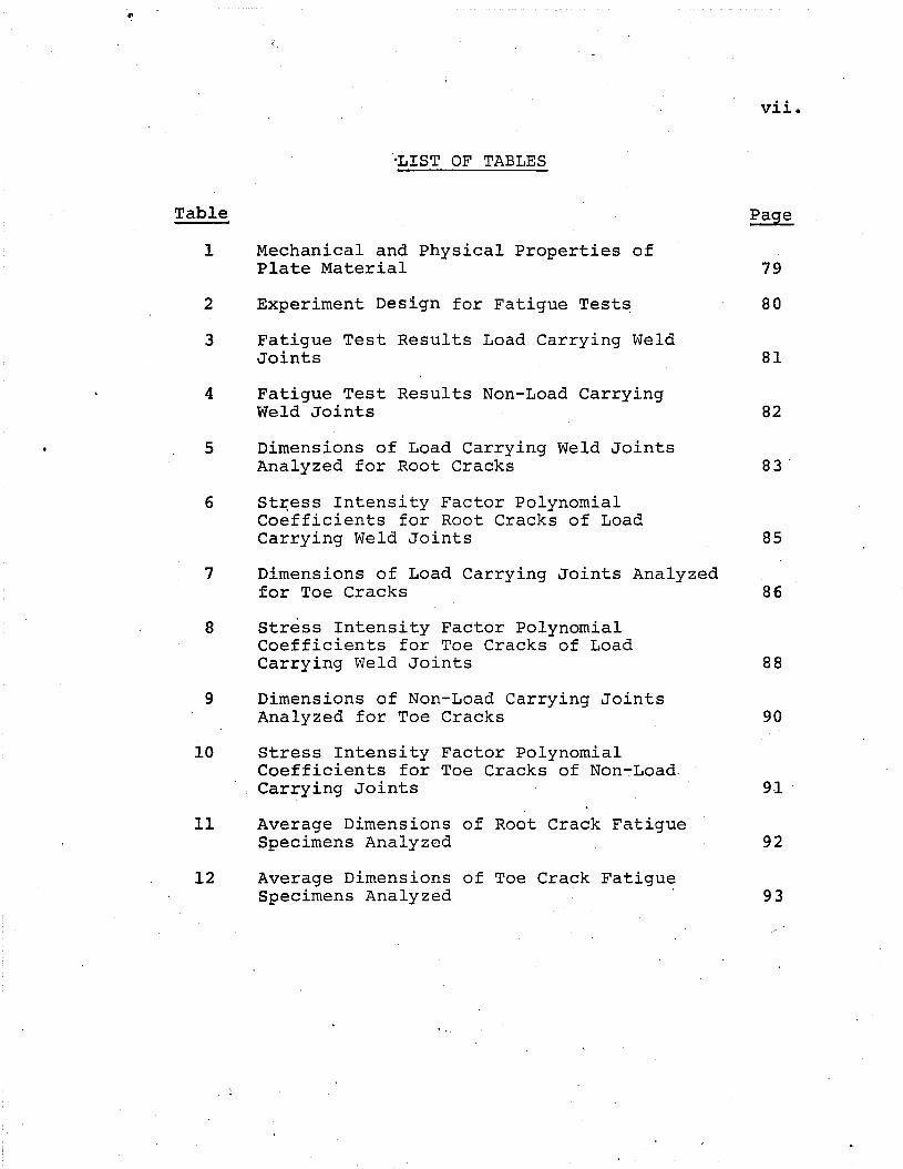
-LIST OF TABLES
Mechanical and Physical Properties ofPlate Material
Experiment Design for Fatigue Test~
Fatigue Test Results Load Carrying WeldJoints
Fatigue Test Results Non-Load CarryingWeld Joints
Dimensions of Load Carrying Weld JointsAnalyzed for Root Cracks
St~ess Intensity Factor PolynomialCoefficients for Root Cracks of LoadCarrying Weld Joints
Dimensions of Load Carrying Joints Analyzedfor Toe Cracks
Stress Intensity Factor PolynomialCoefficients for Toe Cracks of LoadCarrying Weld Joints
Dimensions of Non-Load Carrying JointsAnalyzed for Toe Cracks
Stress Intensity Factor PolynomialCoefficients for Toe Cracks of Non-Load.Carrying Joints
Average Dimensions of Root Crack FatigueSpecimens Analyzed
Average Dimensions of Toe Crack FatigueSpecimens Analyzed
vii.
79
80
81
82
85
86
88
90
9·1
92
93

viii.
LIST OF FIGURES
Figure
1 Fatigue Specimen Dimensions 95
2 Welding Sequence 96
3. Etched Cross Section of Typical Joint 97
4 Toe Failure-Non~LoadCarrying Joint 97
5 Root Failure-Load Carrying Joint 97
6 Shear Failure-Load Carrying Joint 98
7 Fatigue Life of Load and Non-Load CarryingJoints 99
8 Definition of Weld and Crack Angle 100
9 Histogram of Weld- Angle-Non-Load CarryingJoints 101
10 Histogram of e to eF -1 -Non-Load CarryingJoints' a~ ure 101
11 Variation of Fatigue Life of Non-Load CarryingJoints With Weld Angle 102
12 Toe Crack Angle Variation With Weld Angle 103
13 Low Stress Toe Crack Failure - lOOX 104
14 'High Stress Toe Crack Failure - 133X 104
15 Toe Crack Growth Along Fusion Line 105
16 End of Fusion Line Crack - 66X 105
17 Unetched Heat Affected Zone - 133X 106
18 Etched Heat Affected Zone - 532X 106
19 Crack Branching To Included Particles - 66X 107
20 Crack Growth Path At Included Particles - 133X 107
21 Root Crack Tip Untested Specimen - 133X 108

#
Figure
22
23
Root Crack Tip Untested Specimen With LargePlate Gap - 133X
Root Crack Growth Along Grain Boundaries 133x
ix.
108
109
24
25
26
27
28
29
30
31
32
33
34
35
36
37
38
39
40
41
Transgranular Root Crack Growth - 133X 109
Vertical End of Root Crack At Failure - 66X 110
Failure of Joint With P9rous Weld 110
Weld Shear Stress Range versus Cycle Life 111
Crack Tip Stress Field Coordinates 112
Symmetric Joints Analyzed 113
Load Carrying Joint Root Crack FiniteElement Mesh 114
Load Carrying Joint Toe Crack FiniteElement Mesh 115
Non-Load Carrying Toe Crack Finite ElementMesh 116
Change of Compliance With Crack Length 117
Variation of ~/cr with H/T for Root Cracksin Load CarryingP~oints P 118
Variation of Kia 1 with Weld Angle for Root'Cracks in Load C~rrying Joints 119
Change in AR With Crack Length and Weld Size 120
Variation of the Coefficient C1 With H/Tp 121
Variation of the Coefficient C2 With H/Tp 122
Variation of Kia 1 with Weld Penetration anda/wi for Two Pla~e Thicknesses for Toe Cracksin Load Carrying Joints 123
variation of AT for Load Carrying Joints withFull Penetration and 45 G Degree Welds 124
Change in A With Weld -Angle for FullPenetration Welds 125

Figure
42
43
44
45
46
47
48
49
50
51
52
53
54
55
56
57
58
59
x.
Change in AT With Weld Size for Load CarryingJoints With Small Root Penetration 126
Finite Element Used for Stress Analysis ofLoad Carrying Weld Joints 127
variation of Stress Concentration at WeldToe With HIT for Joints with Full and ZeroRoot Penetra~ion 128
Change in Stress Concentration at Weld ToeWith Weld Angle 129
Change in Stress Concentration at Weld ToeWith Root Penetration 129
Correlation of AT With Stress ConcentrationAt Weld Toe 130
Variation of AT/~T With Crack Length - SmallPenetration Welds -131
variation of Kia 1 With a/wi for Non-LoadCarry~ng Weld Jo~nts 132
Variation of K/crpl With Weld Angle 133
Variation of K/crp1 With Weld Penetration 134
Change in AT With"Weld Angle ~35
Change in A"T With Weld Penetration 136
Variation of ATIA T With a/wi Non-LoadCarrying Weld Joints 137
AT versus Stress Concentration at Weld Toefor Non-Load Carrying Welds 138
Crack Growth Rate Behavior of structuralSteels and Weldments 139
Modified Stress Range versus Cycles toFailure for Root Crack Failures 140
Change in the Value of the Integral With,Initial Crack Size (a.) · 141
~ . ~
Stress Range in Main Plate Times AT versusCycles to Failure for Toe Crack Fa11ures 142

1" ~_
-1
ABSTRACT
This dissertation describes a study of the fatigu~
behavior of fillet welded joints stressed perpendicular to
the weld line. The study included an experimental phase in
which the stress-life and cracking behavior of load and non-
load carrying fillet weld joints was determined. This
experimental study ~oncentrated on the fatigue behavior in
the transition region between high and low cycle fatigue
(10 3 cycles to 10 5 cycles of load application) •
The second phase of the study was the determination
of the fracture mechanics stress intensity factor for cracks
at the weld toe or root of fillet welded joints. The finite
e.lement technique was used to determine the compliance of
typical fillet welded joints. The results of this analysis
showed that the -stress intensity factor was a -function of
weld size, weld angle, plate thickness and weld penetration.
-Relationships to estimate the stress intensity factor were
_ developed.
The third phase of the study was the correlation
of the experimental fatigue stress-life behavior of fillet
welded joints with the predicted benavior using the concepts
-2
of the fracture mechanics of stable "crack growth. The
study showed that the fatigue behavior of various joint
geometries could be correlated using the str,ess intensity
factors developed in phase two. The correlation included
failures from cracking at the root and toe of the fillet
weld. The analysis provided a good estimate of the observed
fatigue behavior for fatigue lives from 10 3 to 2xl0 7 cycles
of load application.

..
-3
1. INTRODUCTION
This dissertation is concerned with the study of
the fatigue behavior of fillet welded joints. Historically
this subject has held the interest of many investigators.
Interest was generated by the general use of fillet welded
joints in welded construction. Fillet welds are usually
more economical than other types of welds and are exten-
sively used. However, experimental studies showed that
fillet welded joints had low fatigue strengths when they
were stresse~ in a direction perpendicular to the weld--------~in~. This led to further studies in atte~pts to determine
why these reductions were observed.
Early studies of the fatigue behavior of fillet
welded joints showed that their fatigue lives were a
function of weld size and joint geometry. (1-7) Photoelastic
studies were used to evaluate the influence of the joint
geometry upon the state of stress in the joint. (8,9) These
studies provided insight into the stress distribution
within the joints and provided an indication of the stress
concentrations which exist at the toe and root of the weld.
Nearly all of these stress studies were concerned with the
static behavior of the joint. They did not provide a,

-4
relationship between joint geometry and applied stress and
their relationship to fatigue life.
The increased use of welded construction during
the late 1950's focused attention on the fatigue behavior
of fillet welded joints. Numerous investigations were
undertaken on different joint geometries, steels and
welding processes. (10-25) A review of these studies is
, given in Ref'. 26. This work showed, that the principle----------..._----------~ables~the fatigue life of a fil welded
joint werethe~_o_m_e__t_ry~.-o-f--t-h-e--j-o-i-~dthe applied stress
range. The static strength of the base metal was observed
to have little influence on the fatigue strength for the
range of steels used in bridge and building construc-
t n.,2) ~ddition, the type of weldi Erocess
employed in the manufacturing of the joint as well as ,the
strength of the deposited weld had little influence. They
were observed to only influence the fatigue behavior if they.......
changed the weld profile ~ntlyand!or~ a
wel~witb different sized Qsfeets. (15,27)
Recently fracture mechanics has been employed to
analyze the fatigue behavior of fillet welded
joints. (25,28,29,30) These studies yielded qualitative
information about the influence of join~ geometry upon the

-5
observed fatigue behavior. However, adequate estimates of
the fracture mechanics stress intensity factor for cracks
in fillet welded joints were not available. Quantitative
estimates of fatigue life behavior require more accurate
estimates of the stress intensity relationship.
The results of these previous studies have not
provided a means to quantitatively estimate the fatigue life
of fillet welded joints. Each set of test results must be
treated separately since no means exists to correlate the
behavior of joints with different geometries. The influence
of weld size and penetration, plate thickness and initial
flaw size has not been studied analytically. This disser
tation describes the results of an analytic and experimen
tal study of the fatigue behavior of two simple fillet
welded joints stressed perpendicularly to the weld line. A
method of quantitatively estimating the influence of joint
geometry upon the fatigue life behavior of fillet welded
cruciform joints is developed. The study consisted of
three major phases.
The first phase was an experimental investigation
to determine the low cycle fatigue behavior of two fillet
welded joints •. Previous studies.examined the high cycle
life-low stress region. This st~dy examined. the transition
region between low cycle life (less than 1000 cycles) and

-6
high cycle lif~ (greater than 100,000 cycles) of high
strength steel fillet welded joints. The purpose of this
phase of the study was to determine the stress-life
behavior and the mode of failure.
The second phase of the study involved a stress
analysis of the test joints using the finite element
technique. The purpose was to examine the effect of joint
geometry upon the stress distribution in the joint and
provide fracture mechanics stress intensity factors for the
cracking behavior.
The third phase of this study correlated the
fatigue behavior of the test joints with their geometry.
This was accomplished by relating the stress intensity fac
tors from the_ finite element study to the crack growth rate.
The relationships between fatigue behavior and joint
geometry permitted the results of other studies to be
correlated. In the case of certain welded joints, the
influence'of geometry upon the fatigue can be estimated
quantitatively. Clearly weld imper,fections, such as weld
border cracks and weak regions along solidification boun-
'daries, may cause large variations in fatigue life. Quan
. titative charayterization of suc~ defects in a fracture
mechanics basis is possible by a~signing an initial crack
size corresponding to the observed fatigue life.

-7
2. FATIGUE TESTS OF FILLET WELDED JOINTS
Two cruciform shaped specimens were selected for
investigation in this study. Figure 1 shows a schematic of
the two specimens. The upper specimen is considered a non-
load carrying specimen since the main plate is continuous.~--------
Consequently, the welds and cross plates only carry a small
portion of the load. The lower specimen has a discontinuous
main plate and the full load must be carried by the welds
into the cross plate.
Thes~ specimens were selected due to their ease
.of fabrication and testing at high stress levels. They are
representative of typical joints found in welded construction
and have been used by numerous investigators. Their use
permitted the results of this study to be directly compared
with earlier work. The simple joint geometry facilitated the
stress analysis and reduced the number of geometric
parameters.
2.1 Specimen Fabrication
The specimens were fabricated from 5/8" thick ASTM
grade A514F plate material. Table 1 summarizes the physical
and mechanical properties. -.The specimens were fabricated
from four sets of plates. The plates were cut so that the

-8
direction of rolling of the main plate was the same as the
direction of the applied load. After cutting, the plates
were sand blasted to remove loose mill scale. The surfaces
to be welded were then ground lightly to remove the
remaining tight mill scale. The plate edges, were left
square.
One-hal£ inch fillet welds were used to connect
the cross plates to the main plate. The weld size was
selected to provide· a static weld strength greater than or
equal to the capacity of the main plate. The welds were
made in three passes in the sequence shown in Fig. 2. They
were placed in the horizontal position with the legs
inclined so that the plane of the electrode travel was 45°
, from the surface of the two plates.
The welds were made by the- automatic gas metal arc
process. One-sixteenth inch AX-IIO welding wire was used
with Argon plus 2% oxygen shielding gas.· The average heat
input was 40,000 joules/in with an interpass temperature of
less than 150°F. These welding procedures were selected to
provide a weld which slightly overmatched the strength of
the base plate.
After ~elding, t~~ joints were sliced into pieces
1 3/8 inches wide. The edges were "then Blanchard ground. to

-9
a width of 1.200 inches'+ 0.001. The nominal specimen
dimensions are given in Fig. 1.
Figure 3 shows a polished and etched joint section.
The three weld passes are readily apparent together with the
heat affected zone and the lack of penetration at the weld
roots. The variation of the weld profiles shown is typical
of all the joints tested.
2.2 Testing Procedure
The specimens were tested in a 220 kip Amsler
fatigue testing frame. The hydraulic power was supplied by
a 220 kip Amsler Slow Cycling Unit. The specimens were
tested under a constant amplitude cyclic stress. Due to the
operating characteristics of the slow cycling unit the
waveform was a rounded symmetrical saw tooth. The testing
frequency varied between 20 and 60 CPM. The lower frequency
was used for the highest stress range specimens and the
higher frequency for the lower stress ranges.
The nominal stress in the main plate of the specimen
was selected as the controlled expe~imental variable. The
minimum stress of all the specimens was 20 ksi. Table 2
gives the values of stress range tested and the corresponding
maximum stress. A minimum.of th~ee specimens of both types
of specimens were tested at each stress level to provide a

-10
measure of the variability. The order of testing and the
assignment of specimens to the stress levels was randomized
to minimize the effect of the uncontrolled variables such
as weld geometry, humidity, and ambient temperature.
Foil strain gages with a gage length of 1/4" were
applied to both sides of one end of the main plate. These
were located 3 inches from the cross plates. The gages were
used to measure the load in the main plate since the Slow
Cycling unit's load indication was not accurate during cyclic
loading. The strain gage output was monitored on an x-y
recorder. The system allowed the loads to be set such that
stress range in the main plate was within 2% 6£ the desired
range.
The tests were run continuously until either the
Specimen fractured or its stiffness was reduced suddenly by
a failure of one weld causing the machine to shut off.
2.3 Failure Modes
The results of the fatigue tests are summarized in
Tables 3 and 4. The specimen designation is shown along with
the value of the nominal stress range and maximum stress in
the main plate. The failure mode of each specimen and its
cyclic life is also shown. ··Three failure modes were observed.
All of the non-load carrying welds failed from cracks

-11
extending from the weld toe and are designated as the toe
mode. Figure 4 shows a fracture corresponding to this mode
of failure. The crack propagated through the thickness of
the main plate until failure.
Most of the load carrying weld specimens failed
from cracks which propagated from the initial flaw at the
weld root. This discontinuity resulted from the incomplete
~ration of the weld.' These failures were designated as
the root mode. The crack propagated perpendicular to the
main plate into the weld metal. The final failure occurred .
by a shearing off. across the weld. Figure 5 shows a typical
root failure.
Two other failure modes were observed in the load
carrying weld joints. Five joints failed from cracks
extending from the weld toe and were similar to the failure
shown in Fig. 4. A fourth failure mode observed in three
load carrying joints was a shear failure as shown in Fig. 6.
The failure plane was parallel to the main plate. The
failure initiated at the weld toe from small cracks which
were propagating into the plate until a few cycles before
final failure. The crack growth direction abruptly changed
to a direction parallel to the main plate. The failure
occurring when the crack reached the weld's root.
-12
2.4 Test Results
All test results are plotted in Fig. 7 where the
life of the specimen is plotted as a function of the nominal
stress range in the main plate. The non-load carrying joints
.are seen to yield a longer fatigue life. The different
failure modes are indicated by the symbols in the legend.
Some of the welds exhibited marked amounts of porosity and
are indicated by vertical lines through their symbols. They
are also marked by astericks in Table 3. The shorter lives
of load carrying specimens with porous welds is seen to be
substantial at the higher stress ranges.
2.4.1 Effect of Weld Angle on the Cracking Behavior of theNon-Load Carrying Weld Joints.
All non-load carrying weld joints failed from
cracks starting at the weld toe. Each joint had four weld
toes that provided potential failure sites. photoelastic
studies have shown that the stress at the .weld toe is a
function of the weld angle. (8,9) The influence of the weld
angle, a, on the failure location and specimen life was
,examined to determine its affect. The weld angle was defined
by the weld profile as shown in Fig. 8. The measurements of
the weld height (H) and weld width (W) were made with a
machinist's scale to the nearest hundredth of an inch.

-13
Figure 9 provides a histogram of the measured weld
angles. The mean angle of all four welds of each joint is
seen to be less than the mean weld angle where failure
occurred. This difference suggests that the location of fail-
ure for a particular specimen is related to the weld angle.
The distribution of the ratio of each weld angle
in a specimen to the failure weld angle is given in Fig. 10.
Only 6% of the weld angles were greater than the weld angle
at the weld where failure occurred. It is apparent that the
larger the angle of a weld the more likely the failure will~ ----- ----------------occur at that weld. Ninety-four percent of the joints in~
th~ te~ies failed at welds with the largest angle.
The fact that the failure location for a joint is
dependent upon the angle of the w~lds suggests that the
fatigue life is ~nfluenced by the weld angle. Figure 11 was
constructed to examine this hypothesis. The ordinate defines
the ratio of the weld angle at the failure location to the
mean of the weld angles where failure occurred. The abscissa
was taken as the ratio of the life of the specimen to the
average life for that stress range. Although substantial
scatter is apparent, a trend between weld angle and life is
apparent. The solid line is a least square fit to the
plotted data. The dashed line represents the mean line less
the standard error of estimate. Tne life of a particular
-14
specimen is therefore a function of the weld angle as well
as the applied stress.
The scatter in Fig. 11 seems reasonable since the
weld angle is only a gross indication of the weld profile.
Small irregularities at the toe along the length of the weld
such as undercut also affect the stress condition at the
weld toe and the initial crack condition and hence the
fatigue life. The weld angle defined in this study provides
a rough estimate of the variation in the stress at the weld
toe when the weld profile changes.
The influence of the weld angle upon the fracture
path of the toe failures was also investigated.- The angle,
~, which the crack made with the vertical was measured as
shown in Fig. 8. The measurements were made with a pro~
tractor to an estimated accuracy of +1°. An attempt was
made to correlate the crack angle wit"h the weld angle since
the state of stress at the toe is dependent upon the weld
angle.~~craCkplane was expected to be perpendicular to
the airectian of t~jpal~s. Figure 12.shows a
plot of the weld angle and crack angle. No correlation is
apparent. An average angle of 13 0 seems to be a reasonable
. estimate for all weld angles.

-15
. 2. 4. 2 F·racture Path of Toe Failure
Failures from cracks at the weld toe occurred in
both the load carrying and non-load carrying joints. The
origin of the crack was the same in both joints. The cracks
were observed to start from the intersection of the fusion
line with the weld surface. Figures 13 and 14 are photo
micrographs of typical toe cracks. Crack growth at the
fusion line is visible in both figures. Figure 13 is a
·fractured specimen that was tested at a stress range 30 ksi.
The crack grew away from the weld and the fusion line into
the base metal of the main plate. The crack shown in Fig.
14 is from a specimen tested at a stress range of 80 ksi.
The crack followed the fusion line and wash up zone into
the weld metal. The fracture path followed inclusions that
were observed in this area. The two fracture paths appear
to be stress dependent. Specimens tested at higher stress
ranges showed a distinct tendency for the crack to follow
the fusion line. In the specimens tested at the lower stress
levels the crack grew immediately into the base pla.te. At
. the high~r stress levels the crack followed the fusion line
for a considerable distance before changing direction and
growing in the plate. Figure 15 shows the specimen which
exhibited the longest fusion line growth of all the specimens
tested. In most of the specimens where crack growth was
observed'along the fusion line, Lhe crack length along the
fusion line was of the order of 0.05 inches. Figure 16 shows
-16
an enlargeme~t of the area where the crack deviated from the
fusion line into the plate.
The tendency for the crack to follow the fusion
line at high stress levels seems to ,be related to the inclu
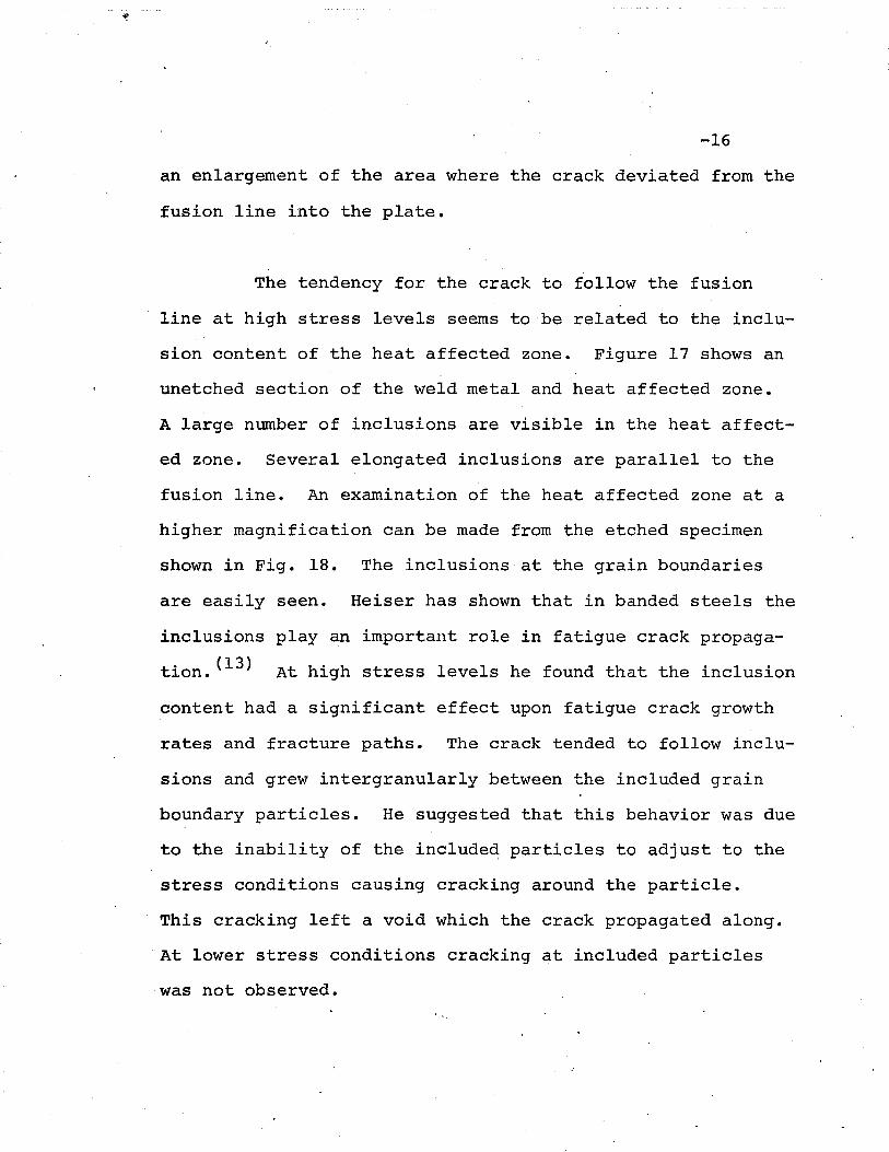
sion content of the heat affected zone. Figure 17 shows an
unetched section of the weld metal and heat affected zone.
A large number of inclusions are visible in the heat affect
ed zone. Several elongated inclusions are parallel to the
fusion line. An examination of the heat affected zone at a
higher magnification can be made from the etched specimen
shown in Fig. 18. The inclusions at the grain boundaries
are easily seen. Heiser has shown that in banded steels the
inclusions play an important role in fatigue crack propaga
tion. (13) At high stress levels he found that the inclusion
content had a significant effect upon fatigue crack growth
rates and fracture paths. The crack tended to follow inclu
sions and grew intergranularly between the included grain
boundary particles. He suggested that this behavior was due
to the inability of the include~ particles to adjust to the
stress conditions causing cracking around the particle.
This cracking left a void which the crack propagated along.
'At lower stress conditions cracking at included particles
was not observed.

-17
The h~gh inclusion content of the area adjacent
to the fusion line seems to be responsible for the crack
following that path. Figure 19 shows a crack which formed
at the toe and propagated in the HAZ following the fusion
line. The crack branching at inclusions is visually evident.
Figure 20 is a higher magnification of the lower part of
Fig. 19.
This study has shown that the length of. the frac
ture path along the fusion line is dependent upon the stress
level. The higher the stress level the longer the crack
followed this path before it grew through the thickness of
the main plate. This behavior was attributed to inclusion
cracking at high stress levels. The larger inclusion con
tent of the HAZ at the fusion line caused the crack to
follow this path at higher stress levels. All toe cracks
initiated at the intersection of the fusion line with the
plate surface.
2.4.3 Fracture Path of Root.Failures
Root failures only occurred in the load carrying
weld joint. No visible evidence of crack growth was found
at the weld roots of the non-load carrying welds.
Figures 21 and 22 show the region at the weld root for two
untested load carrying join~s. The large separation
at the right of the photos is due to the fit up of the
-18
plates. The sharpness of this separation in Fig. 21 is
seen to increase as it ~pproaches the weld metal. Both
figures indicate an extremely sharp crack immediately
adjacent to weld metal. Cracks which caused the root
failures propagated from these initial cracks.
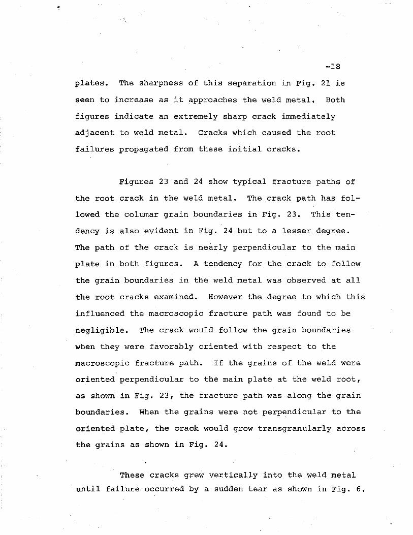
Figures 23 and 24 show typical fracture paths of
the root crack in the weld metal. The ,crack path has fol
lowed the colurnar grain boundaries in Fig. 23. This ten
dency is also evident in Fig. 24 but to a lesser degree.
The path of the crack is nearly perpendicular to the main
plate in both figures. A tendency for the qrack to follow
the grain boundaries in the weld metal was observed at all
the root cracks examined. However the degree to which this
influenced the macroscopic fracture path was found to be
.negligible. The crack would follow the grain boundaries
when they were favorably oriented with respect to the
macroscopic fracture path. If the grains of the weld were
o~iented perpendicular to the main plate at the weld root,
as shown'in Fig. 23, the fracture path was along the grain
boundaries. When the grains were not perp~ndicular to the
9riented plate, the, crack would grow transgranularly across
the grains as shown in Fig. 24.
These cracks grew' vertically into the weld metal
. until failure occurred by a sudden tear as shown in Fig. 6.
-19
Estimates of the stress on the final failure plane 'were
made and found to be smaller than the ultimate strength of
the weld metal. This fact suggests that weld metal may
have experienced fatigue damage during testing. This caused
the fracture to occur at a lower stress than its ultimate
capacity. No evidence of such damage was found, although
as shown in Fig. 15 the failure across this plane may have'
been due to rapid crack growth.
Figure 25 shows the tip of a root crack at failure
after the crack has changed direction. The large open ~rack
is perpendicular to the main plate while the smaller branch
is almost parallel to the main plate. The final failure,
therefore, was due to rapid fatigue crack extension. The
change in the fracture path was attributed to a change in
the principal stress direction caused by the bending moment
introduced in the weld when the root crack is large.
The porosity of the weld also had a dramatic effect
upon the, fatigue lives of specimens which failed from root
cracking. Figure 7 shows that at high stress levels
porosity in the weld caused failure to occur at much shorter
lives. This effect is believed to be due to crack growth'
at the porosity. Crack growth was evident at the porosity
in all specimens with porous werds. These cracks weakened
the weld and decreased its faituge life. Figure 26 shows
-20
the failure of a joint with a porous weld. The failure oc-
curred by the rupture of the weld along the ligaments between
the extending cracks. At lower stress levels the load on
these ligaments was less and failure was similar to the root
. failures of welds without porosity.
2.4.4 Analysis of Shear Type Failures· of the Load CarryingWeld Joint
Three load carrying welds exhibited a shear type
failure mode as shown in Fig. 6. Examination of the welds
revealed that the leg of the weld (W in Fig. 1) was much
smaller than the average. This fact along with the mode of
failure suggested that the failure of these specimens was
due to high shear stresses on the base of the weld. Figure
27 shows the lives of the load carrying welds plotted
against the shear stress range of the weld with the smallest
leg. The stress was calculated by dividing the total load
range per unit width by the smallest weld leg. The line
shown in the figure is a least square fit of the shear
failure data.
The toe failures at high stress levels are the only
points above the least square line. These failures occurred
by crack extension into the main plate after following the
fusion line for a portion o~ their life. The shear failures
were similar to the toe failure except that the crack did

-21
not propagate into the main plate. The failure occurred by
cracking along the fusion line. At lower stress levels less
cracking was evident along the fusion line. The line in
Fig. 27 provides a reasonable estimate of the fatigue life
of the weld in shear. At high stress levels, the crack
propagated along the fusion line due to the inclusion
cracking until the stress conditions favored through the
plate thickness growth (toe failures).
If the inclusion orientation and spacing are
favorable the crack may continue along the fusion line
resulting in a shear mode failure. The tendency for
inclusion cracking is less at lower stress levels and hence
the specimens were not as critical in shear. Other failure
modes were more critical as is apparent in Fig. 27.

-22
., 3. FRACTURE MECHANICS ANALYSIS OF FATIGUE BEHAVIOR
Fracture mechanics, developed from the study of
brittle fracture, has found increasing use in the study of
structural fatigue. (32,33) Fracture mechanics is used to
relate the materials fracture behavior by considering the
energy balance of the energy released in fracture to the
materials ability to absorb this energy. The use. of
fracture mechanics in structural fatigue is based on the
C7~~ that the fatigue crack growth rate is a function
o·f the crack tip stress field.
3.1 Crack Tip Stress !ield Equations
The stress field in the region immediately
adjacent to the crack tip for a two dimensional body is of
the form: (34)
[~j (1)sin8/2cos8/2cos38/2
sin6/2cos6/2cos38/2sin6/2cose/2cos36/2
cos6/2[1-sinB/2sin38/2] -sin8/2[2+cos8/2cos38/2]
~y = {2;r cos8/2[1+sin8/2sin38/2]
where the coordinates urll and e are shown in Fig. 28. The
parameters. K1 and K11 , called the crack tip stress-intensi ty
factors, are two independent parameters which are functionsl
of the body's geometry, crack length and linear functions of
-23
the applied stress. K1 represents the contribu·tion of a
symmetric and K11 an antisymmetric stress distribution with
respect to the crack plane on the crack tip stress field.
The-stre~$ int~nsity factors are independent of the
coordinates " r " and e hence, r~..present-the........~ of the
stress field.
The stress-intensity factors are the leading terms
of an expansion qf the infinite series representing the
total stress distribution of the body. The stress field
adjacent to the crack is dominated by a square root singu-
larity in u r " at the crack tip. The displacement field at
the crack tip is also dependent on the stress intensity
factor. Since the fatigue process takes place at the crack
tip, it is reasonable to assume that it must be a function
of the crack tip stress field and consequently the stress-
'" (35)1ntensity factors.
3.2 Relationship Between the Stress-Intensity Factor andFatigue Crack Growth Rate
Paris proposed the fO'11owing relationship between
the stress intensity range (8K) and the crack growth rate
(da/dN) (36)
da/dN = ~Kn ( 2)
This rela.tionship is a,· -semi-empirical attempt to fit experi
mental data with the stress intensity factor. Numerous
-24
crack growth studies on a variety of materials have
shown that Eq. 2 provides a reasonable estimate of a
material's crack growth rate response. (33,37,38) Other
equations similar to Eq. 2 have been proposed. Some of
these equations have been based on work hard~ning and
fatigue damage considerations at the crack tip region. Other
equatipns have been based on consideration of the crack tip
displacements. Reference 39 gives an up-to-date review of
these different models. Most models reduce to the general
form of Eq. 2 for a particular material and environment.
3.3 Analysis of Fatigue Life Behavior Using ,FractureMechanics
The power law, (Eq. 2), relating the fatigue crack
growth rate to a power of the range of stress-intensity
provides the necessary relationship to estimate the"fatigue
life of a" component. The range of the stress-intensity
factor aK m~y, in general, can be expressed as
LiK SRg(a,w')· (3)
where SR = nominal stress range
a = crack length
w' = a set of geometric constants forthe body.
When Eq. 3 is substituted into Eq. 2 ,it yields
-n ng(a,w') da = C SR dN (4)
Integrating Eq. 4 between the limits of the initial crack
-25
length a i and the final crack lengthaf , defines the
component's fatigue life N as
faf
N = g(a,w,)-nda/ C s nai R
Equation 5 provides a means to estimate the
(5)
fatigue life of a component if the value of SR~ ai' a fl C,
n, and the function g are known. It is also assumed that the
fatigue behavior of the component is totally a function of
crack growth. Crack initiation is not considered.
It is also interesting to note that the values of
C and n can be estimated from Eg. 5. If the values of a.,1
a fl N, and SR are known from a series of fatigue tests, and
the funct,ion "g " is known for the geometry of the specimen,
then the values of C and n can be determined by fitting the
results of the fatigue tests to Eq. 5.
where X
An alternate form of Eq. 5 is
N= [SR/nl:X]-n1/ C
X -_ fa f 9 (a,w') -ndaa.~
(6)
(7)
Equation 6 is analogous to the log-log relationship between
SR and N normally observed ·for most structural details.
-26
This provides a linear relationship of the form
log N = log B - m log SR (8)
or N = B S -mR
(9)
The constant B can be expressed as
B = X/C , (10)
when the exponents "n" and "m" are equated. Equation 6
provides a means of including the effect of component
geometry and ini-tial flaw size, a., by the term nIX. The. 1.
consequences of this equation are explored and analyzed for
fillet welded joints in this dissertation.

-27
4. ESTIMATION OF STRAIN ENERGY RELEASE RATESUSING THE FINITE ELEMENT TECHNIQUE
Irwin has shown that the stress-intensity factor,
K, is related to the strain energy release rate, G. For
a plane stress analysis this can be expressed as(34)
(11)
(12)
The value of the strain energy release is defined as the
energy rate provided by a body containing an extending
crack available for the crack-extension process. In other
words the energy per unit of new crack area generated. This-- ----- ~energy rate can be related to the change in compliance of
the body for a load P as(34)
~. '
where dC/dA is the rate of change of compliance with crack
area where the compliance· is defined as
c = 6/P
4.1 Finite Element Analysis
(13)
The finite element technique has found wide spread
use in the solution of bou~~ary value problems. The

-28
method is of a general nature and can be applieq to any
boundary value problem.
The method of analysis can be divided into two
. stages:
1. The discretizing of the body to be solved into
finite elements, and
2. Minimization of a selected functional in the
body.
The first stage in the analysis is done to make the second
stage more tractable. By dividing the body into discrete
elements the functional to be minimized is represented
continuously in each element. The result is a piecewise
continuous representation of the functional over the body.
The discrete elements are connected at nodes with the fields
in each element written as functions of nodal parameters.
The boundary value problem is therefore reduced to the
solution of a set of simultaneous equations in terms of the
nodal parameters connecting the finite elements. These
sets of equations are of the form of
"{f} = [A]"{o} (14)
where IIf" is a vector of nodal forces and "0" tpe nodal
displacements. The matrix "A" is the stiffness" m'atrix of
the discretized body relating these parameters. The
accuracy of a finite element solution depends on how well

-29
the piecewise representation of the functional from the
analysis approximates its true form.
4.2 Finite Element Compliance Analysis of CruciformWeldments
The compliance of the cruciform joint was deter-
mined from a finite element analysis. The body wasrfl
analyzed as a __~~~_9-!men_~_~oI1a~ l?~aI1e:3tre~? problem.:' Figure"
29 shows a schematic of the idealized shape of the two
joints analyzed. The welds profiles were idealized as
triangular shapes. The weldrnents were also assumed to be
completely symmetric with respect to the, planes shown as
dashed lines in Fig. 29.Q The length of the main plate from
the weld toe was taken as three times the thickness of the
main plate. This located the loaded nodes .far enough away
from the weld toe and/or toe cracks so that the state of
stress at those points would be uniform axial tension. ~
Symmetry of the joint permitted a quarter section of the
total joint to be used.
·4.2.1. Element and Mesh Selection
The selection of the type of elements to be used
and the mesh or discretizing of the body determines the
. accuracy of the finite element solution. The more sophis-
ticated the element the larger the -mesh can be for the same-
-30
accuracy. A more sophisticated element contains a higher
order field and consequently can represent the functional
over a larger area.
The crack tip stress field equations given in
Chapter 3 show that at the crack tip a stress singularity of
the form 1/1r exists. Consequently a displacement field.1.
of the form r 2 ex,ists in the region of the crack tip. Due
to the geometry of the weld joint, a,complex stress distri-
bution exists in the region of the weld and at the weld's
toe and root.
The .experimental study and the work of others have
shown that cracking can occur at two locations in load"""---" ....,
ca!rying wejg jo4Rts. C~acks may occur at the root of the
weld or at the-we±d toe depending upon ~eometry ~he
jo~nt and the penetration of the WQld
carrying weld specimens, cracking nearly always occurs at~ ------------------~--
tha~weld toe. Hence, a finite element analysis of load
carrying joints must provide for toe and root cracks. Only'
toe cracks need to be considered for the non-load carrying
weld joints.
Due t9 the complexity at the stress distribution
and the large number of geometries and crack lengths to be

-31
analyzed, an element was selected that would minimize the
time and cost of the analysis. The Constant Strain
Triangle (CST) element is the simplest finite element
available and was selected. Its chief advantages are that·
its element properties are easily and rapidly calculated
and its triangular shape facilitated the matching of
geometric boundaries.
The displacement field within the element is
linear so consequently the strain and stress field are
constant. Each element provides a constant strain
energy density. Since the strain energy was selected as
the functional to be minimized (as is normally done in the
solution of boundary value problems whose solution is
formulated from displacement fields) it is approximated
s~epwise by each element over the body.
The element mesh and size in the regions of high
displacement gradients must be refined to insure that the
true displacement field or strain energy d~nsity is
adequately represented. Figure 30 shows the mesh used to
evaluate the load carrying weld with a root crack. The
element size near the crack tip and in the region of the
weld toe is seen to be quite small. The elements within
the weld were also made small ~o accommodate the complex
-32
state of stress which existed. Figures 31 and 32 show the
meshes used for the analysis of toe cracks. Again the
refinement in the mesh at the crack tip is evident.
,T~e crack in each of the joints was modele~by ~
two lines of nodal points immediately adjacent to each othe;----~
but not connected. Displacement boundary conditions were~ '----------------------
applied along the planes of symmetry. The nodes at the
bottom of the figures at the mid-thickness of the main
plate were fixed in the vertical direction. The nodes at
the mid-thickness of the cross plate were restrained in the
horizontal direction. The nodes at the end of the main
plate were loaded by concentrated tension loads equivalent
to a uniform stress distribution.
The _small elements used in the mesh near the crack
tip, although much smaller than normally used in finite
element analysis of bodies, are still larger than those
used by previous in~estigators of cracke~ bodies. (40,41,42)
This was not believed to invalidate the results since the .
'values of the stress intensity factors were determined from /
a compliance analysis. Mowbray has recently demonstrated
that this method gives quite accurate results with rather
coarse meshes. (43)
-33
The reason for this accuracy is due to the fact
that although the finite element solution underestimates the
strain energy near the crack tip, the compliance method of
analysis examines the strain energy in the entire body.
'Since the crack tip singularity only dominates the region
close to the tip the overall estimate of the strain energy
is good. The strain energy at the crack tip region. is only
a small percentage of the total strain energy in the body.
Consequently errors in its estimation do not have much effect
on the total strain energy calculation. Methods suggested
by other investigators focus on the local behavior at the
crack tip and consequently require extremely small elements
to accurately estimate the stress and displacement behavior
in this region. (41,42,43) High order e1~ents which include
the stress singularity at the tip do not require the
refinement in mesh size, however displacement discontinuities
arise between these elements and adjacent ones which are
also a source of error. (44)
The effect of the error in the estimation of the
strain energy near the crack tip on the analysis can also be
evaluated by comparison of compliance tests of actual
specimens with analytical solutions. Srawley found the error
to be small for a single edge-notch specimen. (45) The
compliance was measured on a specime~ where the crack tip
-34
radius' was 1/32 inch. The stress at the crack tip is
proportional to the ratio of the crack length to the· crack
tip radius with the value of the stress intensity factor
being defined as the crack tip radius approaches zero.
'Consequently the stress field in the vicini~y of the crack
tip was less than that defined by equation 1. This is
similar to the effect of the underestimate of this stress
field by the finite element solution. Therefore,
the assumption that the error in estimating this energy will
not influence the accuracy of the compliance analysis seems
justified.
The second reason given by Mowbray for the accuracy
of the method is the fact that the values of G and K are
functions of the change in compliance with crack length.
Consequentl~ if the error in compliance is independent of
crack length, the slope of the compliance versus crack length
curve should be close to the true curve. The independence
of the error with crack length should hold if the finite
element mesh is similar for each crack length analyzed as it
was in this study.
4.2.2 Method of Solution of Finite Element Equations
The method of solution of the equations resulting
from the finite element formulation was selected to provide

-35
rapid solution time. The quantities required for a
solution by a compliance analysis are the displacements of
the loaded nodes. The loads at these nodes were based on
the assumption that the state of stress was uniform. The
. applied stress does not influence the resulting load
displacement relationship so for convenience in checking
the results it was taken as 100 ksi for all geometries.
The load-displacement relationship was found by treating the
joint as a series of substructures. The load displacement
relationship was determined for each substructure and then
combined to give the load-displacement relationship for the
joint. Appendix A gives the details of the analysis. This
method reduces the size of the matrix inversions required
and eliminates most of the off diagonal zero terms. For
each crack length analyzed, only the substructures near the
crack are subjected to mesh changes, consequently only
those substructure stiffness matrices need be recomputed for
each crack length.
Each analysis provided the displacements of the
loaded nodes. A set of displacements was determined for
each joint geometry corresponding to a set of crack lengths.
The compliance of a particular geometry and crack length was
then determined by dividing the load, P, in the main plate
by the x-displacement of the loaded node at the plane of

-36
symmetry of the main plate. The x-displacement was
doubled since it represents the total extension of the
symmetric section.
4.3 Evaluation of the Stress Intensity Factor
The set of compliances and crack lengths were
fitted by least squares to a polynomial of the following
form
where
EBC =m
nA
O+ L An- 1 (a/w')
n=2(15)
c = p/lJ. = .specimen' s compliance,
B = specimen's width,
E = Young's Modulus,
a = crack length
and w ' = a geometric constant with dimensions of
length. The elastic Modulus and the specimen's thickness
were constant and taken equal to 30,000 -ksi and unity
respectively. The first order term of the polynomial was
not included since the stress intensity factor
must be zero when the crack length is zero.
Equation 12 can be rewritten as
2G = P
8EB2w,d (EBC)
"d(a,/w')(16)

-37
where the area of the new crack formed is
dA = 4Bw' d(a/w') (17)
The constant four in Eq. 17 is a consequence of the symmetry
used in the finite element analysis. Each specimen contain-
oed four cracks.
Substituting Eq. 15 into Eq. 16 yieldsm
G = p2/8EB2w' E n A 1 (a/w,)n-l (18)n=2 n-
where G is the total strain energy release rate. The value
of the stress intensity f~ctor was evaluated using Eq. 18 asm J::.
A n-1 2K = [EG]2 = P/2Bv'2W' E nA 1 (a/wi) (19)
2n~
n=
where K is an equivalent stress intensity factor equal to2 .6.
K1[1+(K11/Kr ) ]2. The displacements of the nodes along the
crack surface in the finite element analysis revealed that
the ratio of K1r to Kr was less than 10 percent. Therefore
the value K calculated by Eq. 19 is approximately equal to K1 •
The stress intensity factors calculated from the· finite ele-
ment analysis are designated as K in this dissertation •
.4.3.1 Stress Intensity Factors for Root Cracks of LoadCarrying Fillet Welds
Thirty-two different joint geometries were
analyzed to determine the effect of the joint geometry upon
the stress intensity factor. The compliance of each geometry
was determined for sixteen "different crack lengths and the
uncracked joint (full root penetration). Nine of the joint
-38
geometries simulated the average geometry of the fatigue
test specimens. The remaining geometric configurations
correspond to specimens tested in previous investigations.
Table 5 summarizes the dimensions of the joints analyzed
and their source. The dimensions are defined in Fig. 1.
The analysis of the joints simulat£ng the fatigue
test specimens included a variation of' the weld angle, S.
The weld size was defined by the leg dimensions Wand H.
These parameters were determined by maintaining the weld
cross sectional area constant and varying the weld angle.
The weld area was .equated to the average area of the
specimens. One specimen was analyzed with an oversize weld
with equal legs. It is identified with an asterisk in Table
5. The weld angle was a,ssumed equal to 45 degrees for the
earlier studies since its value was not reported.
The results for three test specimens are plotted
in Fig. 33. The quantity EBC is shown as a function of
a/w' for specimens with weld angles of 30, 40 and 45 degrees.
The parameter Wi was defined as
w' = T /2 + H (20)p
for all the geometries analyzed. A fifth order polynomial
of the form of Eg. 15 was used to fit the compliance (EBC)
as a function of ~/Wl for all geometries. This order
-39
polynomial was found to provide the minimum standard error
of estimate. The standard error of estimate of the fitted
polynomial was less than 0.004 for all geometries which
corresponds to an error of less than one-tenth of a percent.
The values of a/wi at which the compliance was
'determined were the same for all geometries.' The crack
lengths included an uncracked joint (a!w'=O) and increments
of a/wi between 0.115 and 0.692. These crack lengths were
believed to be in the most useful range based on visual
examination of the test specimens. The fitted polynomial
provided a means of interpolating the value of the stress
intensity factor for crack lengths smaller than Wi x 0.115.
Accurate calculation of the compliance for cracks of this
size would have required extremely small elements using the
finite element technique. Stress intensity factors were
determined from Eq. 19. The fitted polynomial permitted the
stress intensity factor to be evaluated over a wide range
of crack lengths. Table 6 gives the values of the
coefficients of the polynomial for K of each geometry.
Figure 34 shows the variation of the ratio of the
stress intensity factor ~o nominal plate stress, 0PL'l as the
crack length increased. The five joint conditions shown in
Fig. ~4 correspond to different weld sizes. The main and
-40
cross plate ,thickness were equal and the weld angle is equal
to 45 degrees. The large variation of the stress intensity
factor with weld size is readily apparent. A decrease in
weld size resulted in a substantial increase in the ratio
of K/~PL at all crack sizes.
Figure 35 shows the variation in stress intensity
with weld angle. The weld cross sectional area is the same
for each weld angle. The variation in the stress intensity
with weld angle is seen to be much less than the variation
predicted by changing the weld size (H/T p ) "{see Figi 34).
Increasing the weld angle from 30 0 to 50° results in approx-
imately a ten percent increase in K/U PL • This change in
weld angle represents a change in H/Tp from 0.653 to 0.939.
A similar variation in H/Tp in Fig. 34 for welds with equal
legs and increasing weld size would decrease the stress
intensity factor by approximately forty-five percent. The
effect of weld angle on the stress intensity factor for
welds of equal area is therefore small.
The similarity in the shape of the stress intensity
. factor curves suggests that a functional relationship may
exist which describes the behavior for all joint geometries.
Harrison (28) suggested that the following expression could. . .be used to estimate the stress intensity factor at the root
-41
of load carrying fillet welds
K = v y (2Y' tan ~a/2Y' ( 21)
a was defined as the nominal gross stress acting on the weld·w
and was equal to
(22)
This estimate considers the joint to be equivalent to a
plate of breadth equal to Tp + 2H containing a central crack
of length 2a.
An equation similar to Eq. 22 was found to provide
a reasonable estimate of the relationship between the stress
intensity factor and crack length. The more accurate secant
finite width correction was used in place of the tangent
correction used by Harrison. In addition, a non-dimensional
correction factor was developed to account for the difference
between the cruciform joint and the constant breadth plate.
This resulted in the following relationship for K at the
weld root:
K = a - A l1Ta sec 7faiJ:J/2w'·w 'R
(23)
where AR
is non-dimensional correction factor for the
cruciform shape.
The value of AR
was observed to be a function of
H/Tp ' the weld angle, the ratio of the thickness of the main
'-42
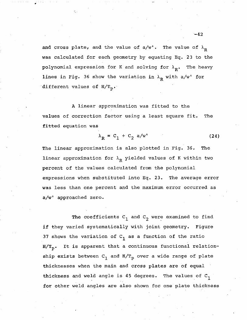
and cross plate, and the value of a/wI. The value of AR
was calculated for each geometry by equating Eq. 23 to the
polynomial expression for K and solving for AR• The heavy
lines in Fig. 36 show the variation in AR
with a/wI for
'different values of- H/Tp .'
A linear approximation was fitted to the
values of correction factor using a least square fit. The
fitted equation was
The linear approximation is also plotted in Fig. 36. The
linear approximation for AR yielded values of K within two
percent of the values calculated from the polynomial
expressions when substituted into Eq. 23. The average error
was less than one percent and the maximum error occurred as
a/wi approached zero.
The coefficients C1 and C2 wer~ examined to find
if they varied systematically with joint geometry. Figure
37 shows the variation of Cl as a function of the ratio
H/Tp • It is apparent that a continuous functional relation
ship exis-ts b~tween C1 and H/Tp over a wide range of plate
thicknesses when the main and cross plates are of equal
thickness and weld angle is 45 degrees. The values.of ~l
for other weld angles are also shown fo~ one plate thickness
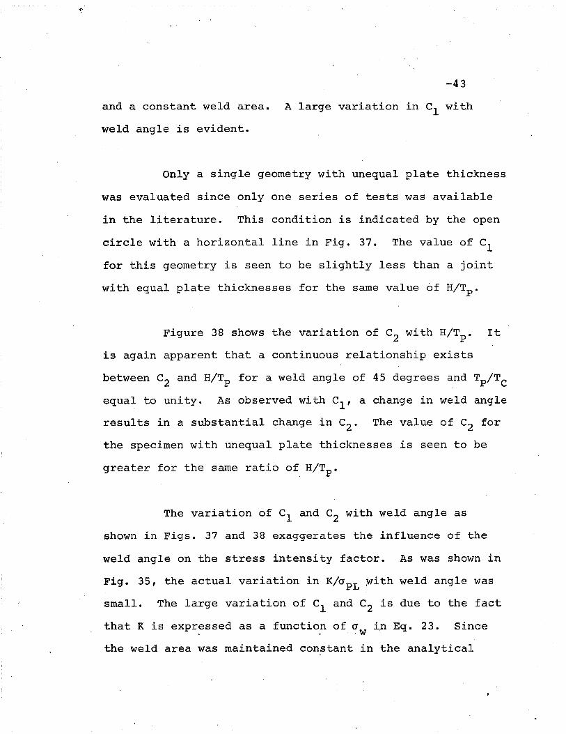
-43
and a constant weld area. A large variation in C1 with
weld angle is evident.
Only a single geometry with unequal plate thickness
was evaluated since only one series of tests was available
in the literature. This condition is indicated by the open
circle with a horizontal line in Fig. 37. The value of C1
for this geometry is seen to be slightly less than a joint
with equal plate thicknesses for the same value 6£ H/Tp •
Figure 38 shows the variation of C2 with H/Tp • It
is again apparent that a continuous relationship exists
between C2 and H/Tp for a weld angle of 45 degrees and Tp/TC
equal to unity. As observed with CI , a change in weld angle
results in a substantial change in C2 . The value of Cz for
the specimen with unequal plate thicknesses is seen to be
greater for the same ratio of, H/Tp •
The 'variation of C1 and C2 with weld angle as
shown in Figs. 37 and 38 exaggerates the influence of the
weld angle on the stress intensity factor. .As was shown in
Fig. 35, the actual variation in K/apL :with weld angle was
small. The large variation of C1 and C2 is due to the fact
that K is expressed as a function of ~w ip Eq. 23. Since
the weld area was maintained constant in the analytical
(25)
,f"
-44
study, an increase in the weld angle decreases ·the nominal
gross weld stress, a w ' since H is increased.
Generally "the load carrying capacity of a joint
is expressed in terms of the plate force. The variation of
K with weld angle is small when expressed as a function of
the plate stress as was shown in Fig. 35.
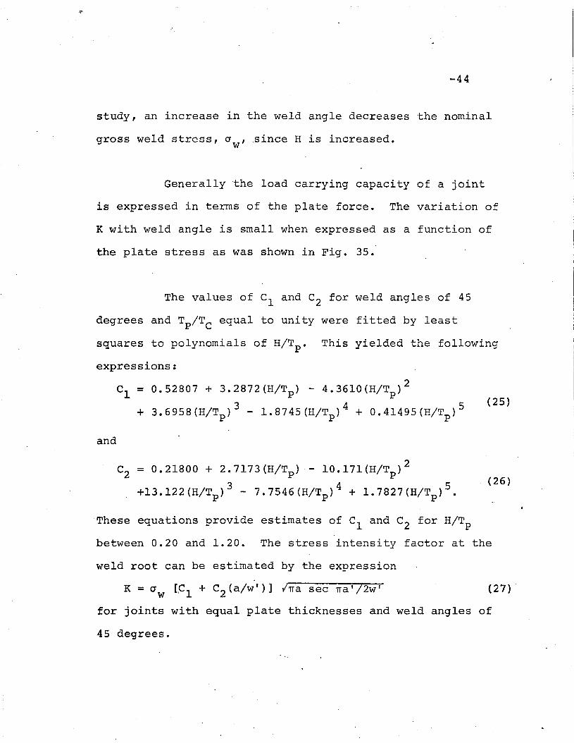
The values of C1 and C2 for weld angles of 45
degrees and Tp/TC equal to unity were fitted by least
squares to polynomials of H/Tp • This yielded the following
expressions:
C1 = 0052807 + 302872(H/Tp ) - 403610(H/Tp )2
+ 3 06958(H/Tp )3 - 1 08745(H/Tp )4 + 0.41495(H/Tp )5
and
C2 = 0.21800 + 2 07173(H/Tp ) - 100171(H/Tp )2
+130122(H/Tp )3 - 707546(H/Tp )4 + 1.7827(H/Tp )5.
'These equations provide estimates of C1 and C2 for H/Tp
(26)
, ,
between 0.20 and 1.20. The stress intensity factor at the
weld root can be estimated by the expression
K = V w [~1 + c2 (a/w')] I~a sec TIa ' /2w' (27) "
for joints with equal plate thicknesses and weld angles of
45 degrees.

-45
The value of K predicted by Eq. 27 is 20 to 70
p~rcent greater than the estimate provided by Harrison's
approximation (Eq. 21). Equation 27 estimates K values
within two percent of the values predicted by the polynomial
expressions. The value of K for joints with'equal plate
thicknesses and other weld angles (e ~ 45°) can also be
estimated from Eq. 27. The variation of Kia L for various. P
weld angles and constant weld area was observed to be small.
A reasonable approximation of K can be found by using a weld
height equivalent to a 45 degree weld of the same area. The
equivalent weld height, H, can be found from the relationship
H = IH*W* where H* and W* are the legs of the actual weld.
Equation 27 can be expressed in a more useful
design form as'!PL '
K - [c1+c2 (a/w')] ITIa sec na/2w' (28)- (1+2H/Tp )
where (] PL lis the main plate stress. This equation provides
a reasonable estimate of the stress inte~sity factor at the
weld root in terms of weld and plate geometry and the nominal
plate stress.
4.3.2 stress Intensity Factors for Toe Cracks of LoadCarrying Fillet Welds
Table 7 summarizes the geometric variables for
the twenty-two load carrying fiilet welded joints that were

available in the literature and this study. All joints had
main and cross plates of equal thickne~s. The effect of
weld angle was also studied. The average size reported in
the literature for each series was used. The weld size
parameters Hand W were calculated from the average weld
area of the specimens. A comparable method was used for
the root crack analysis.
The influence of the weld penetration was also
included in the analysis. The average depth of root
penetration for each geometry is given in Table 7. The
penetration is expressed as a percentage of the half
thickness of the main plate. Thirteen geometric conditions
were analyzed with variable weld penetration. The effect
of weld penetration was included in the analysis since a
preliminary study had indicated that the stress
at the weld toe was a function of the weld penetration.
Increasing the weld penetration decreased the stress at the
weld toe. Thirteen of the twenty-two -geometries were an-
alyzed with full and approximately zero weld penetration to
determine its effect. The other remaining geometries were
analyzed using the average penetration t~ey were fabricated
with.
The cracks at the'toe of the weld were assumed ·to

-47
be inclined. from the vertical at the angle of 13 degrees.
This angle corresponded to the condition observed during
the experimental phase of this investigation. This angle
was also compatible with the inclination of the principle
stress axis at the weld toe.
The geometric constant w' in the compliance
polynomial was defined as
'w' = T /[2 cos 13°] (29)P
The compliance of each joint was determined for thirteen
crack lengths including the uncracked joint. The ratios of
crack length to Wi included in the analysis varied from 0.15
to 0.70 in increments of 0.05.
A .sixth order compliance polynomial was found to
provide the minimum standard error of estimate. The
standard error of estimate was less than one-tenth of a
percent of the measured compliances. The coefficients of
the polynomial expressions for the stress intensity factor
(see Eq. 19) for each geometry. is given in Table 8.
Figure 39 shows the predicted variation of K(~PL
with a/wi for two different plate thicknesses. The effect
of weld size for full and small penetration welds is also
shown. The variation of K/cr pL for joints with full
'.;-.
-48
penetration welds was not affected by weld size. However,
for joints with small penetration the value of K/cr pL is seen
to increase as the weld size decreased. As the weld size
approached the plate thickness, the effect of penetration
on the ratio Kia decreased. Partial and full penetrationPL .
welds provided about the same conditions at the weld toe for
large welds (H/T p ~ 1).
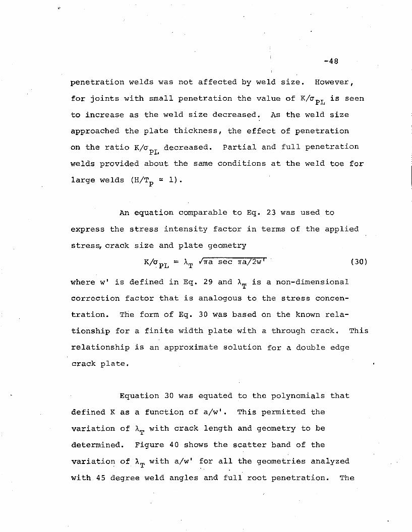
An equation comparable to Eq. 23 was used to
express the stress intensity factor in terms of the applied
stres~ crack size and plate geometry
(30)
where Wi is defined in Eq. 29 and AT is a non-dimensional
correction factor that is analogous to the stress coneen-
tration. The form of Eq. 30 was based on the known rela-
tionship for a finite width plate with a through cracke This
relationship is an approximate solution for a double edge
crack plate.
Equation 30 was equated to the polynomials that
defined K as a function of a/wi. This permitted the
variation of AT with crack length and geometry to be
determined. Figure 40 shows the scatter band of the
variation of AT with a/wi ~or all the geometries analyzed
with. 45 degree weld angles and full root penetration. The

-49
maximum difference between AT for all these geometries was
less than 5% for all crack sizes. The magnitude of AT was
determined at values of a/wi equal to 0.02 through 0.10
in increments of 0.02 and from 0.10 through 0.70 in
'increments of 0.05. These values were then fitted "with a
polynomial of a/w'. The polynomial which provided the
minimum standard error of estimate was
AT = 2.164 - 6.196 (a/w) + 17.09 (a/w) 2 - 20.10 (a/w)3
+ 8.842 (a/w)4 (31)
This equation is plotted in Fig_ 40 as a solid line and is
seen to provide a reasonable estimate of the value of AT-
Figure 41 shows the variation of AT with weld
angle. The weld area was constant for each joint and each
joint had full root penetration. Increasing the weld angle
is seen to increase AT for small cracks. This effect
diminishes as the crack grows. As a/w' approaches 0.30 there
is no significant difference due to the angle of the weld.
Figure 42 shows the variation of AT with a/wi for
jeints· with small root penetration. The value of AT is seen
to increase with decreasing weld size. This behavior was
found for all the geometries analyzed~ The stress intensity
factor at the weld root also increases with smaller weld
---i
-50
sizes and may represent a more critical condition when the
weld penetration is small.
A stress analysis was performed on selected joints
to determine if the behavior of the stress intensity factor
could be related to the stress concentration at the weld toe.
Figure 43 shows the finite element mesh used in the stress
analysis. Constant strain triangular elements were used.
The method of solution is given in Appendix A. The stress
at the weld toe, ~TOE' was taken as the maximum principle
stress in the shaded element (Fig. 43). Figure 44 shows the
variation of the stress concentration at the weld toe ~TOE/
~PL)l with H/Tp for full and zero penetration welds. The
plotted points are from joints with weld angles of 45 degrees.
The variation of the stress concentration with H/Tp for
joints with full penetration welds is small. This is the
same behavior that was found for AT with full penetration
joints. Joints with zero penetration yielded a dramatic
increase in the stress concentration with decreasing weld
size. The values of the stress' concentration for zero
penetration welds also seem to lie on the same curve for all
the plate thicknesses included in the analysis.
The variation in the stress concentration at the
weld toe was investigated further. -Figure 45 shows the
variation of the ~tress concentration factor with weld angle

-51
for constant area welds. Increasi~g the weld a~gle
increases the stress concentration for joints with full
and zero penetration welds. The joints with full penetration
-welds have lower stress concentrations. The variation of
"the stress concentration factor with the weld angle is
approximat~ly linear for both weld conditions.
Figure 46 shows the variation of the stress
concentration with root penetration for four values of H/Tp •
The stress concentration for small welds is seen to increase
much more rapidly with decreasing weld penetration than the
larger welds.
The value of the stress concentrations at the weld
toe were compared to the values of AT as the ratio a/w'
approached zero. This limiting value of AT' which was
labeled AT' was found by taking the limit of Eq. 30 as a/w'
approached zero. This yields
K = '! PLAT /7Ta2
The polynomial expression for K as a/w' approaches zero
yields. T
PK = '!PL
21W'
1[AI (a/w' ) ]"2 (33)
Equating Eqs. 32 and 33 provides an estimate for AT as1
·AT
= [AI /7T.f2Tp / [2w' ] (34)
-52
Figure 47 compares. AT with the stress concentration at the
weld toe for joints of various plate thickness, weld
penetrations, and weld angle. The values of AT are
compatible with the stress concentration factor although
'they appear to be slightly larger. Hence the stress concen
tration factor provides a reasonable estimate of AT.
This correlation seems reasonable since the stress
~ intensity factor for small cracks at the weld toe should be
a function of the local stress field. The toe stress
from the finite element at the weld toe provides an estimate
of this local stress. Since a rather coarse mesh was used
to estimate the stress concentration, (element area ~
(w'/lO)2) the true stress state was underestimated. A better
estimate of the stress concentration factor would provide
better agreement with XT• The dashed line in Fig. 47
represents a least squares fit of limiting value of AT and
the stress concentration factor predicted by the finite
element analysis. AT can be estimated by
for the stress concentrations estimated in this study. If
more refined methods of calculating the stress are used the
value of the stress concentration should approach IT'

-53
The correlation of the stress concentration factor
with AT provides a method to estimate the stress intensity
factor K for various crack lengths and geometric conditions
which were not considered in the compliance analysis.
Figure 48 shows the variation of the ratio of AT
and the limiting value AT" with a/wi. The relationships
correspond to joints with 45 degree weld angles and small
weld penetrations. For small cracks, a/wi less than 0.20,
the ratio is seen to be approximately the same for all
values of H/Tp • The curves tend to diverge at larger crack
sizes.
For fatigue crack growth the estimate of K for
small cracks is more critical since the largest portion of
the life is consumed. in propagating small cracks. An
attempt was made to correlate the stress intensity factors
at the weld toe for both full and partial penetration in
terms of AT/AT and a/wi.
Equation 31 was modified by expressing the ratio
AT/AT as a function of a/wi. This permitted AT to be
expressed in terms of its value as a/wi approaches zero (AT)
. for various crack lengths. Equation 31 in this form yields

-54
AT/AT = l-2.862(a/w') + 7.897(a/w,)2 - 9.288(a/w,)3
+ 4.086(a/w,)4 (36)
The dashed line in Fig. 48 compares this polynomial with the
predicted values of AT/AT. Equation 36 is seen to provide
a reasonable estimate of the AT/AT ratio for these
joints.
The stress intensity factor for cracks at the toe
of load carrying fillet welds with partial root penetration
can be estimated from:--3,2,1 !::.
K =. C! PL ,AT [1~:~~:2~a/w' ) +7 • 897 (a/w' ) 2- 9 • 288 (a/w' ) 3
86 a/w 4) Jrra sec rra72w' (37)
AT can be estimated from the stress concentration at the
weld toe. The magnitude of the stress concentration for a
particular geometry can be estimated from Figs. 45 and 46.
Equation 37 is accurate within 2% for full penetration welds
with 45 degree angle. The average value of AT for all the
joints analyzed with full penetrati9n 45 degree welds was
found to be 2.16. This value is a reasonable estimate of
all joints with full penetration welds. The accuracy for
joints with smaller weld penetration is less. For crack
lengths less than O.30w', Eq. 37 provides an estimate within
. 5% of the valuep determined from ~he polynomials.
/
~55
4.3.3 Stress Intensity Factors for Toe Cracks of NonLoad Carrying Fillet Welds
Test data were available for thirteen non-load
carrying weld joints. The joint geometries are summarized
in Table 9. Specimens NT-l through NT-9 were evaluated
based on the average dimensions of the fatigue specimens.
The weld angle was varied from 30 to 53 degrees with a
constant weld area. Specimen's NT-lO geometry was based
on the average size of the load carrying weld fatigue
specimen. Specimens NT-14 through NT-l9 were selected to
provide an indication of variation due to a wide range of
geometric parameters.
The weld root penetration was taken tO'be zero for
all. joints. The load carrying weld joints with full pene-
tration provide information that would be directly applicable
to the non-load carrying joints with full penetration.
The parameter Wi in the compliance polynomial was
defined in the same manner for load carrying and non-load
carrying joints for crack growth at the toe (see Eq. 20).
This assumed the crack plane to be 13 degrees from the
vertical. The same increments of a/wI were used for the
compliance analysis of both weld types.
-56
A sixth order polynomial ~as again found to
provide the minimum standard error of estimate. The
standard error of estimate was less than one-tenth of a
percent of the measured compliances. The coefficients for,
the stress intensity polynomials for each joint geometry
are summarlzed in Table 10.
Figure 49 shows the typical variation of Kia PL '
with a/wi. The value of K/l!PL ,is seen to increase slightly
with an increase in the cross plate thickness. Figure 50
shows the variation of K/~PL ~ith weld angle. The scale
of the abscissa has been enlarged to show the variation for
small values of a/wi. The value of K/~PL ,is seen to in
crease with increasing weld angle. The sensitivity of the
value of K to weld angle is about the same order magnitude
that was found in the load carrying joints. The effect of
weld angle diminishes with increasing crack lengths. This
behavior with weld angle was also noted in the load carrying
weld joints.
The effect of weld root penetration on Kia ,is
illustrated in Fig. 51. The full penetration joint is seen
to have a substantially higher value Of~(~J:l:I:..,~han the zero
penetration joint at all crack sizes.
-60
5. COMPARISON OF TEST RESULTS WITH BEHAVIOR PREDICTEDBY THE FRACTURE MECHANICS OF STABLE CRACK GROWTH
The fatigue behavior of the joints tested 'in this
study as well as the results of previous investigations were
evaluated using the principles of'the fracture mechanics of
stable crack growth. The equations developed from the simple
power law of crack growth were used to relate the fatigue
life of the test specimens to the applied stress. The
influence of joint geometry and location of the failure were
included in the analysis using the relationships for the
stress intensity factor developed in this dissertation.
5.1 Crack Growth Behavior of Structural Steels
Figure 56 summarizes the results from five crack
growth investigations and defines the crack growth rate,
da/dN, as a function of the range of the stress intensity
f t AK (37,46,47,48,49) Th h fac or, u • e growt rates are or
materials with yield strengths between 24 ksi and 125 ksi.
Also included are data from Ref. 49 where the growth rate was
measured in the weld metal and heat affected zone. The weld
metal yield strengths varied from 70 to 90 ksi. The welds
were made using the manual shielded metal arc process and
the gas metal arc process •.
-61
The data is seen to fall in a narrow scatterband.
The slope of the scatterband is about one-third. This slope
corr,esponds to an exponent, "nil, equal to 3 in Eq. 2.
Barsom and Klingerman observed that an exponent of three
provided the best fit to their test data when the power law
was used to describe the 'relationship between growth rate
and the range of the stress intensity factor. Gurney and
Maddox found that the exponent varied slightly with material
strength. Their studies showed a variation in "nil between
2.4 and 3.4. A fatigue study of the effect of weldments
on steel beams has shown that the relationship between the
stress range at the detail and its life yielded a value of
"m" close to three for the exponential stress-life model, in
Eq. 8. (25) The equivalence of the exponent "n" in the
power law of crack propagation to the exponent "m" in the
exponential stress life relationship was discussed in part
three. This assumption was tested by Hirt in 'his analysis
of the behavior of welded beams. (50) He found that an
exponent of three provided a reasonable estimate of both
lin" and "m" in Eqs. 2 and 8 respectively. An exponent
equal to 3 was also selected for this fatigue study.
Little information is available about the crack
growth rate at the extreme values of ~K. . At low levels of
AK a threshold in crack growth rate has .been suggested. This

-62
has been investigated by Paris in ASTM 9310 steel. (51)
He. found that the growth rate decreased significantly at
ilK c::, 5. 2 ksi lin. Harrison has estimated the value of this
threshold level from an analysis of rotating beam fatigue
results. (52) He estimates a threshold value of 8K between
3.5 and 5.5 ksi lin for steels. These estimates are shown
in Fig. 56 as horizontal lines near the ordinate.
At higher levels of ~K,Parry, Klingerman and
Barsom observed that the crack growth rate increased
k dl (37,46,47)mar e y. Parry and Klingerman observed this
change to occur when the net section stress approached the
yield point. Barsom suggested that the increase occurred
at a critical value of ~o, th~ range of crack opening-
displacement. The bands plotted in Fig. 56 also include
the data from these studies at high AK values. The rate of
crack growth observed at high 6K levels falls within the
same ge'neral scatterband as the lower levels of LiK. The
assumption that the ~K-da/dN is goyerned by Eq. 2 at all
levels of AK seems to be reasonable in view of the
available experimental .evidence.
5.2 Analysis of Load·Carrying Joints Failing from the·Weld Root
Six different joint geometries were included in

~ ,
-63
the analysis. Table 11 gives the average dimensions of the
joints analyzed and their references. In addition, the
analysis included data from a crack growth experiment on a
center crack plates by Klingerman. (46) The dimensions of
the plate are also given in Table 11. Tp was taken as the
plate width and the initial crack length is expressed as a
percentage of the half width under the column giving the
value of the percentage of root penetration. This data
was included in the analysis since Eq. 27, which expresses
the value of K for root cracks, is based on the known
relationship for K for a center cracked plate. By equating
the coefficients C2 and the weld height, H, equal to zero
and C1=l, Eq. 27 yields the K value for the center cracked
plate.
The plate geometry provides a means of evaluating
the error in the estimate of the stress intensity'factor
for the welded joints. The stress conditions and the
geometry of the plate specimens were carefully controlled
thereby minimizing any associated error in their analysis.
Equation 6 can be expressed in the tollowing form
for an exponent of 3:
N = (SR(3~)-3 lie (38)

-64
where SR refers to the gross section stress at the weld.
The integral .. X" i,s defined in Eq. 5 as
, -3= {f He +c? (a/v S ) 1l'Taee 'Ta/?w s} da
a.1.
x =ffa.
1.
-ng (a,w l) da
(39)
where Wi is defined by Eg. 20. The coefficients C1 and C2
are defined by Egs. 25 and 26 respectively as functions of
It is convenient to express Eq. 38 in terms of a
"modified stress range" defined as
S * = S Ix l / 3R R
(40)
where the units of SR* are KSI in1/ 6 • Substituting Eq. 40
into Eq. 38 yields:
N = S *-3/C (41)R
This equation reduces to a linear form with the following
logaithnic transformation
log N = ~log C - 3 log SR*
The load carrying joints were evaluated by
(42)
determining SR* for each joint. The integration to
determine "X" was performed numerically using twelve point
Gaussian Quaduature. Tests of the .integration routine for
-65
comparable integrals have yielded results to within 0.1%
of the closed form solution. The error in "X" is believed
to be less than 1%. The average values of xl/3 for the test
specimens analyzed is given in Table 11. The final crack
size, af
, was taken as the value when the net section stress
at the weld was equal to the yield stress. The influence of
the final crack size on the value of "X" using other
approximations such as the ultimate strength caused less than
a 2% variation in "X". The crack size calculated from the
yield stress criterion gave closer agreement to the measured
size in the fatigue specimens tested in this study. The
value of a. was taken as half the thickness of the main plate1-
minus the weld penetration.
Figure 57 summarizes the results of the analysis.
The "modified stress' range" S * is plotted as a function ofr
cycle fife. The results are seen to fall within a narrow
scatter band. The two parallel lines shown in Fig. 57
represent the variation in the coefficient "C" found by
Barsaro in his study of the crack growth behavior of ferrite-
pearlite steels. These lines are plotted at a slope of -1/3,
corresponding to the exponent n=3 in the crack growth power
law.
The results from'Kling~rman's cracked plate study,
shown as the open squares, are seen to fall within the
-66
limits for the welded joints. The estimates of the K
relationship for welded joints developed in this study seem
to be reasonable.
The large scatter in the data reported in Ref. 15
is believed to be due to the use of average values of the
initial crack size, a., and weld size. The welding process~
was the same for all th~ specimens plotted from Ref. 15.
Since wide variatioris in the average values existed for each
joint of this study, comparable variation in the four welds
could be expected for the joints reported in "Ref. 15~ The
fatigue failure should occur at the weld with the smallest
penetration (largest a i ) and size. The use of average
geometry and crack size would obviously lead to increased
scatter as observed in Fig. 57. The degree of weld
penetration and consequently the initial crack size was
more" precisely defined by the other investigators.
The linear form of the 199 SR* and log life
relationship is seen to be valid over a wide interval of
life. Lives from 10 3 to 5xl0 6 cycles are seen to follow the
linear relationship predicted by Eq. 42. The equation is
seen to be valid in both the high stress-low cycle lif~ and
low stress-high cycle life regions. The results from a
fatigue study in either of these regions can be

-67
extrapolated over a wi~e range of stress and fatigue life.
At low levels of SR* and high cycle life the
Scatter is seen to increase. The estimate of ~K for the
average initial crack size for joints from Ref. 15 tested
at Sp*=11 is 7.0 ksi Jin The crack growth rate at this
level of ~K has not been established experimentally.
Figure 56 indicates that at these low levels of 8K, the
threshold of crack' growth predicted by Paris and Harrison
is approached.
The fatigue life of other load carrying joints
that exhibit failure from the weld root can be estimated
from Fig. 57. The magnitude of "XU can be estimated by
integrating Eq. 39 between the limits provided by the
initial crack size, ai' and the final crack size, af. The
final crack size can be estimated as the crack size at
which the net section stress of the weld is equal to the
yield stress. The initial c~ack size, a. ,1.
is a function of
the weld root penetration. Therefore, for a given weld size,
plate size and alternating plate load, the degree of weld
penetration necessary to provide the desired fatigue life
can be determined.
-57
Since the change in Kia was comparable for bothPL
load carrying and non-load carrying welds, Eq. 30 was used
to estimate the value of K/O pL ,for toe cracks. The non
dimensional correction factor AT was observed to be the
significant parameter needed to"modify the stress intensity
relationship. Figure 52 shows the variation of AT with
weld angle for the geometries which are plotted in Fig. 50.
AT is seen to increase with increasing weld angle. The
effect of weld angle diminished with increasing cr~ck length.
Figure 53 shows the influence of weld penetration on AT'
The magnitude of AT is seen to increase with weld penetra
tion. The geometry corresponding to a full penetration weld
is the same condition provided by a load carrying joint.
Load carrying and non-load carrying joints are identical
when the weld penetration 'is complete. The two relation-
ships plotted in Fig. 53 have comparable shapes. The
similarity in their shapes suggests that the equations
developed for load carrying joints can be used to express
the variation of ~T for non-load carrying joints as well.
The variation of the ratio of AT to the value
AT as a/wI approaches zero is plotted in Fig. 54. The
range of geometric conditions examined correspond to a
range of test joints with 45 degree weld configur~tions.
The values of all the geometries analyzed were found to lie

-58
within the range of the values plot~ed. The value of
AT/AT is seen to be approximately the same for all
geometries for a/w' less than 0.25. Some divergence is
apparent for larger cracks for the different ratios of H/Tp •
Equation 36 which was d~veloped from the analysis
of load carrying joints with toe cracks is plotted in
Fig. 54. This estimate of AT/AT is seen to provide a
conservative estimate of the variation of AT/AT when a/wi
is -less than 0.35. The value for larger crack sizes falls
within the band of the values for the various ratios of
H/Tp • /Equation 36 provides a reasonable estimate of the
variation of for toe cracks in both load carrying
and non-load carrying joints.
The value of AT was found to .correlate reasonably
well with the stress concentration factor· for load carrying
joints. No such correlation was found for the non-load
carrying joints. The stress concentration factor increased
with H/Tp for joints with equal plate thicknesses, Tc /Tp =l,
and with the weld angle. This is similar to the behavior
which was observed for load carrying joints (see Figs. 44
and 45).
-59
Attempts to correlate the stress concentration
factor at the weld toe with. AT were unsuccessful as is
apparent in Fig. 55. The stress concentration is seen to
decrease with increasing AT- The stress concentration
overestimates the value of AT for most of the geometric
conditions examined.
The stress intensity factor for toe cracks in
non-load carrying j~ints for the geometries analyzed can be
estimated from Eq. 37. The value of AT for these geometries
can be found using Eq. 34 with the leading term of theIt>
stress intensity polynomial given in Table -J:'3:. The value
of AT for other similar geometries can be estimated from
these values. When estimating values of AT' consideration
should be given to the fact that AT increased with smaller
welds and increasing weld penetration increased the value

-68
5.3 Analysis of Load and Non~Load Carrying"WeldToe Failures
Three non-load and three load carrying fillet
welded joints were analyzed for crack growth at the weld
toe. The joint geometries are summarized in Table 12. The
analysis of crack growth at the f~llet weld toe was analo-
galls to the study of root cracks. The stress intensity
factor, K, was estimated from Eq. 37 •. The equation can be
expressed in the-following form
K = ~PL ,AT h(a,a/w')
where
h(a,a/w')= AT/AT /na sec na/2w'
(43)
(44)
The function AT/AT was defined by Eq. 36 in terms of a/wi.
The expres~ion for the fatigue life can be obtained from
Eq. 5 and is
where a fJ -3Y = h(a,a/w') daa.1
(45)
(46)
The parameter Y is a function of the initial and final
crack size and WI.
The'initial crack size, ai' existing at the toe
of fillet welds has been examined at the Welding
Institute. (21,27) The toes- of fi11~t welds made be several
welding processes were examined metalographically by taking

-69
slices through the thickness at the. toe. These studies
confirmed that crack like instrusions of slag and other
inpurities existed at the weld toe. These intrusions as
well as crack like cold laps and undercut were observed to.
provide initiation sites for fatigue crack growth. The
dep~h of these defects were found, to range from 0.0004 in.to
0.02 in. Welded specimens tested with artificial notches
cut at the weld toe to a depth of 0.005 in. yielded fatigue
lives comparable 'to those observed from specimens without
notches. (27) The fatigue life was shown to increase when
the toes were treated by grinding or peening to remove or
reduce the initial flaw. Also the life increased when the
welding process was modified to decrease the initial flaw
size. The fatigue behavior of a fillet weld joint is
consequently a function of crack growth since the initial
crack like defects exist at the weld toe.
The integral Y which expresses the relationship _
between the fatigue life and applied stress range is a
function of ai' af
and WI. The value of Y was determined
numerically for various values of ai' af
and WI. Integration
was again performed by the twelve point Gaussian Quadrature
A singularity in the integrand exists as a, approaches zero.1
The integration was performed by dividing the crack interval,
between a i and af
into four'parts .. The first increment was

-70
taken as a. to 2a. to account for the singularity.11'
Figure 58 shows the variation of Y with a. for~
two plate thickness. The final crack size, af
, was also
.varied. a f was taken as O.50w'=O.0641 in. f6r the! in.
plate and O.80w'=O.821 in. for 2 in. thick plate. These
values provide an extreme variation in plate thickness and
final crack size. Values of Y for other plate thickness and
final crack sizes were bounded by the curves shown in
Fig. 58. The variation of Y with plate thickness and final
crack size is seen to be negligible compared to the
influence of the initial crack size. This is particularly
true for small crack sizes. At larger crack sizes the
value of Y was approximately constant. Hence, Y is
primarily a function of a., the initial crack size.1
The value of a i and the corresponding value of Y
was not estimated directly in the analysis. The fatigue
behavior of joints failing from the weld toe was estimated
by assuming that Y was the same for all specimens. Hence,
tbe cyclic life of 'each specimen was plotted a~ a function
of the parameter AT SR- Figure 59 summarizes the available
test data. The data shown includes both load and non-load
carrying fillet welded specimens. The value of AT for each
geometry was estimated as outlined in part four. The value
,-----~---------._-_._.~-_.-
of"
-71
of AT estimated for each geometry is. given in Table 12.
The scatter bands provided by the test data are
plotted· at a slope of -1/3. The data all fall within a
reasonably narrow band. The use of a slope equal to -1/3
is seen to provide a reasonable estimate of the linear
relationship between AT SR and the cycle life. The variation
in the test data is greater than predicted for the root
cracks shown in Fig. 57. This increase in the scatter can be
attributed to the variation in initial flaw size, a., and the~
variation of the crack growth constant for the steels used in
the fabrication of the specimens. Obviously differe~ces in
the welding processes could substantially affect the initial
crack size, a .. The quality of the weld for a particular1
welding process can also vary due to uncontrolled variables
such as operator performance. Manual shielded arc welds were
used in Refs. 11 and 18. The manual welded specimens ,from
Ref. 11 are plotted as open circles. These data define the
lower limit of the scatter. The upper limit of the data is
provided by manually welded specimens from Ref. 18. These
data are shown by the closed circles. The automatic welds
used in the fabrication of the specimens of the experimental
study fall near the center of the scatter bands.
The initial crack size ·can be estimated by eval-
-72
uating the ratio Y/C in terms of the scatter bands shown in
Fig. 59. The value of Y/C corresponding to the upper band
is 1.lx10i1 and the lower band is 1.2x10¹⁰ • Barsom's crack
growth data provided an estimate of the magnitude of C. He
observed C to vary between 1.37 to 3.6x10⁻¹⁰ 'for ferrite-
pearlite steels. The corresponding values of Y vary
between 1.65 and 39.5. If average values are used, Y/C =10 -106.1xlO ,C=2.5xlO , then Y ~ 15. These values of Yare
compatible with the measured initial crack sizes found at
fillet weld toes as shown in Fig. 58. (21,27) A value of 15
for Y corresponds to an initial crack size of about 0.001 in.
in Fig. 58.
The scatter for the results from an individual
study are seen in Fig. 59 to be much less than the total
scatter for all results plotted. The dashed lines in Fig.
59 show the scatter in the results from the fatigue tests
from this study. Consequently the values of Y calculated
from the overall scatterbands and the limits of the C values
from Barsaro's study overestimate the variation of the initial
f+aw size for a particular test series. However, unless the
initial flaw size is measured for each specimen or an
estimate of .the value of C corresponding to the material used
to fabricate the specimen, the two parameters Y and Care
confounded. An estimate of· the variation in a. for the1
results of the present study's fatigue specimens was made by

~. I
-73
taking C equal to 3.6xlO-lO • This value of C was estimated
from Barsaro's study and was felt to be a reasonable estimate
for A514 steel. Using this value for C and the values of
IT SR and cycle life defined by the dashed lines in Fig. 59
yielded a variation of a. between 0.0015 in. and 0.007 in.1
These values of a. correspond to values of Y of 12.6 and 7.311
respectively. They provide a more conci~e measure of the
variability of initial flaw size at the weld toe. These flaw
sizes correspond 'to equivalent lengths of sharp cracks at the
weld toe. A blunt intrusion at the weld toe of greater depth
may provide a longer life then inferred from this analy~is
since fatigue crack initiation may consume an appreciable
portion of the life.
The linear trend between AT SR and cycle life in
Fig. 59 is seen to be valid over a large range of cycle
lives. The range of lives included in the analysis were
2xl0 3 to 2xl0 6 cycles of load. These lives cover the full
range of the high cycle fatigue and into the low cycle
regime of fatigue.
The fatigue life of a load and non-load carrying
weld joint can be estimated directly from Fig. 59 when fail-
ure occurs from crack growth at the weld toe. The factor AT
can be estimated from the relationships developed in this
study.
-74
6. CONCLUSIONS
The main findings of this study are summarized in
this -chapter. They are based on the analysis of the fatigue
performance of fillet welded joints stressed perpendicular
to the weld line.
1. The stress intensity factor for root cracks in
load carrying joints was found to be a function
of weld size, weld angle, and the thickness of
the cross plates. A relationship was developed
which permitted the stress intensity factor, K,
to be estimated for equal leg welds and equal
thickness plates.
2. The stress intensity factor for toe cracks in
load carrying joints was found to be proportional
to the local stress at the weld toe. This stress
was estimated from a finite element analysis and
found to be a function of weld angle, weld size,
plate thickness and weld penetration. Increasing
the weld penetration decreased the stress and the
K value 'as did increasing weld size. The value
of K for full penetratio~ welqs was found to be

-75
approximately the same for all geometries. The
stress intensity relationship was developed in
terms of a non-dimensional correction factor AT
The value of AT was observed to decay as crack
length increased. AT' the value of AT as the
crack length approached' zero, was found to be
proportional to the stress concentration at the
weld toe. Th~ decay function of AT as crack
length increased was found to be the same for all
geometries.
3. The stress intensity factor for several non-load
carrying joints was obtained. The relationship
developed to predict K for load ~arrying weld with
toe cracks was found to be applicable. However
no correlation was found between the stress at
the weld toe and the stress intensity factor.
Further study is desirable. The value of K at the
weld, toe was observed to increase as the weld
penetration increased and weld size was decreased.
4. The failure mode of load carrying welds at high
stress levels is dependent upon the weld size and
the heat affected zone inclusion content. A
shearing mode of failure along the fusion line was
-76
exhibited by joints with -small welds. This
. behavior was attributed to cracking along
included particles at high stress levels.
5. The fatigue behavior of both the non-load
carrying and load carrying joints was analyzed
using fracture mechanics principles. The
fatigue behavior of many different specimen
geometries were correlated. The results provide
a rational means of estimating the fatigue perfor-
mance of a joint for lives between 10 3 and
5xl0 6 cycles of load application. The correlation
provided at low cycle lives provides a means to
determine the fatigue performance of structural
joints subjected to high stress ranges from a
knowledge of their low stress performance.
6. The influence of the initial crack size on the
.life of toe crack failures was found to be great.
The life increased rapidly as the
initial crack size approaches zero. At crack
sizes greater than 0.01, the effect was much less.
Treatment of the weld toe by grinding and peening
to r~duce the initial crack size offer means

-77\
of substantially increasipg the fatigue life.
7. The threshold value of 8K for-toe cracks appeared
to be about 2 ksi {in , much lower than estimated
by others. The value for root cracks appeared to
be about 7 ksi lin. The fatigue behav.ior of
welded joints at low stress ranges is dependent
upon the crack growth behavior at these low levels
of ~K.· Crack growth studies at low levels of bK
are needed to allow the accurate prediction of the
. fatigue performance of joints at low levels of
stress.
8. The finite element technique of stress analysis
WqS shown to provide a method of estimating the
stress intensity factor for cracks in fillet
welded joints. This technique provides a
powerful and straight forward means to estimate
the stress intensity factor for other complex
geometries. The analysis of the
cracking behavior of structures by fracture
mechanics need no longer be restricted to simple
geometries with known stress intensity factors
since these may be estimated by a finite element
analysis.

TABLES
-78
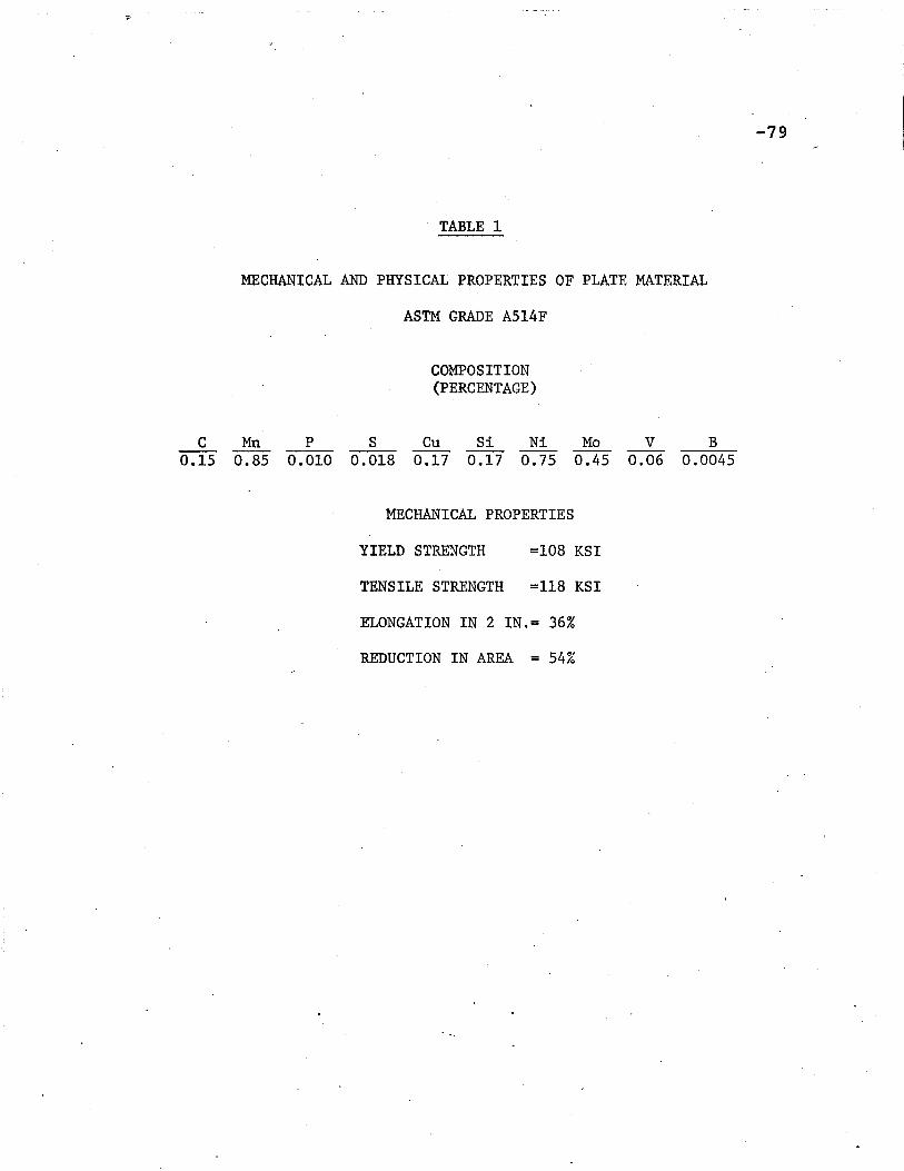
· ·TABLE 1
MECHANICAL AND PHYSICAL PROPERTIES OF PLATE MATERIAL
ASTM GRADE A514F
COMPOSITION(PERCENTAGE)
C Mn P S eu Si Ni Mo V B0.15 0.85 0.010 0.018 0.17 0.17 0.75 0.45 0.06 0.0045
MECHANICAL PROPERTIES
YIELD STRENGTH =108 KSI
TENSILE STRENGTH =118 KSI
ELONGATION IN 2 IN.= 36%
REDUCTION IN AREA = 54%
-79
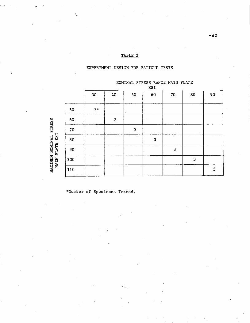
TABLE 2
EXPERIMENT DESIGN FOR FATIGUE TESTS
NOMINAL STRESS RANGE MAIN PLATEKSI
-80
30 40 50 60 70 80 90
50 3*
60 3
70 3
80 3
90 3
100 3I
110 3
*Number of Specimens Tested.

-81
TABLE 3
FATIGUE TEST RESULTS
LOAD CARRYING WELD JOINTS
Specimen Stress Range Maximum Stress Fatigue Life Failure ModeKSI KSI Cycles
L-34 90 110 '610 Shear
L-28 90 110 1,548 Root
L-7 90 110 1,515 Shear
L-19 80 100 4t 224 Toe
L-17 80 100 4,726 Toe
L-39 80 100 740 Root*
L-33 80' 100 2,425 Toe
L-1 70 90 1,267 Root*
L-29 70 90 3,147 Root
L-36 70 90 3,737 Shear
L-5 70 90 2,900 Toe
L-18 60 80 6,948 Root
L-10 60 80 7,497 Root
L-14 60 80 6,681 Root*
L-6 50 70 7,721 Root
L-26 50 70 13,060 Root*
L-21 50 70 17,839 Toe
L-4 40 60 22,026 . Root
L-9 40 60 19,878 Root
L-20 40 60 23,422 Root
L-23 ~O 50 36,091 Root
L-24 30 50 35,526 Root
L-11 30 50 42,959 Root
*Porous Welds.
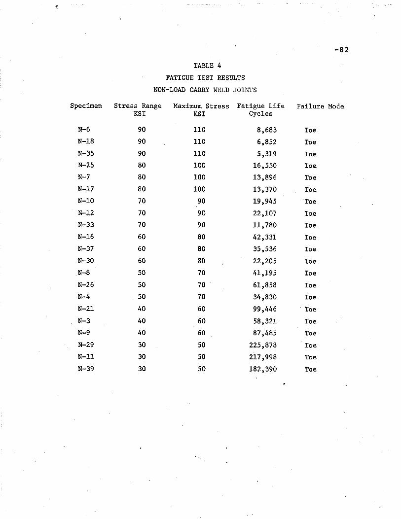
-82
TABLE 4FATIGUE TEST RESULTS
NON-LOAD CARRY WELD JOINTS
Specimen Stress Range Maximum Stress Fatigue Life Failure ModeKSI KSI Cycles
N-6 90 110 8,683 Toe
N-18 90 110 6,852 Toe
N-35 90 110 5,319 Toe
N-25 80 100 16,550 Toe
N-7 80 100 13,896 Toe
N-17 80 100 13,370 Toe
N-IO 70 90 19,945 'Toe
N-12 70 90 22,107 Toe
N-33 70 90 11,780 Toe
N-16 60 80 42,331 Toe
N-37 60 80 35,536 Toe
N-30 60 80 22,205 Toe
N-8 50 70 41,195 Toe
N-26 50 70 61,858 Toe
N-4 50 70 34,830 Toe
N-21 40 60 99,446 Toe
N-3 40 60 58,321 Toe
N-9 40 60 87,485 Toe
N-29 30 50 225,878 Toe
N-ll 30 50 217,998 Toe
N-39 30 50 182,390 Toe

.4j
TABLE 5
DIMENSIONS OF LOAD CARRYI~tG JOINTS ANALYZED FOR ROOT CRACKS
SPECIMEN T T W H H e HI Ref.p c cin. in. in. in. in. Degrees T
p
LR - 1 0.786 0.786 0.378 0.378 1.18 45 0.481 15LR - 2 0.786 0.786 0.372 0.372 1.18 45 0.473 15LR - 3 0.786 0.786 0.333 0.333 1.18 45 0.424 15LR - 4 0.786 0.786 0.339 0.339 · 1.18' 45 0.431 15LR - 5 0.786 0.786 0.328 0.328 1.18 45 0.417 15LR - 6 0.629 0.629 0.478 0.478 1.26 45 0.760 15LR - 7 0.629 0.629 0.483 0.483 1.26 45 0.768 15LR -. 8 0.394 0.394 0.394 0.394 0.788 45 1.000 17LR ~ 9 0.590 0.590 0.200 0.200 1.38 45 0.339 3LR - 10 0.590 0.590 0.470 0.470 1.38 = 45 '0.797 3LR - 11 0.590 0.590 0.710 0.710 1.38 45 - 1.203 3LR - 12 0.630 0.630 0.157 0.157 1.46 45 0.249 16LR - 13 0.630 0.630 0.236 0.236 1.46 45 0.375 16LR - 14 0.630 0.630 0.315 0.315 1.46 45 O. 500 ~ 16LR - 15 0.630 0.630 ' 0.394 0.394 1.46 45 0.625 Q 16L~ - 16 0.630 0.630 0.472 D 0.472 1.46 45 0.749 16LR - 17 0.630 0.6·30 0.551 (. 0.551 1.46 45 0.875 16LR - 18 1.260 1.260 0.394 0.394 3.31 45 J 0.313 16LR - 19 1.260 1.260 0.590 0.590 3.31 . 45 ·0.468 16LR - 20 1.260 1.260 0.787 0.787 3.31 c 45 0.625 16LR - 21 1.260 1.260 0.984 0.984 3.31 45 0.781 16LR - 22 1.260 1.260 1.180 1.1S-0 3.31 ~ 45 0.937 16LR - 23 0.750 0.875 0.3125 0.3125 0.625 45 0.417 2LR - 24 .. 0.662 0.662 0.7492 0.4325 2.00 30 0.653LR - 25 0.662 0.662 0 •.6803 0.4763 2.00 35 0.719LR - 26 0.662 · ,0.662 0.64-40 0;5032 2.00 38 0.760 I
LR - 27 0.662 0.662 0.6212 0.5214 2.00 40 0.788 00w
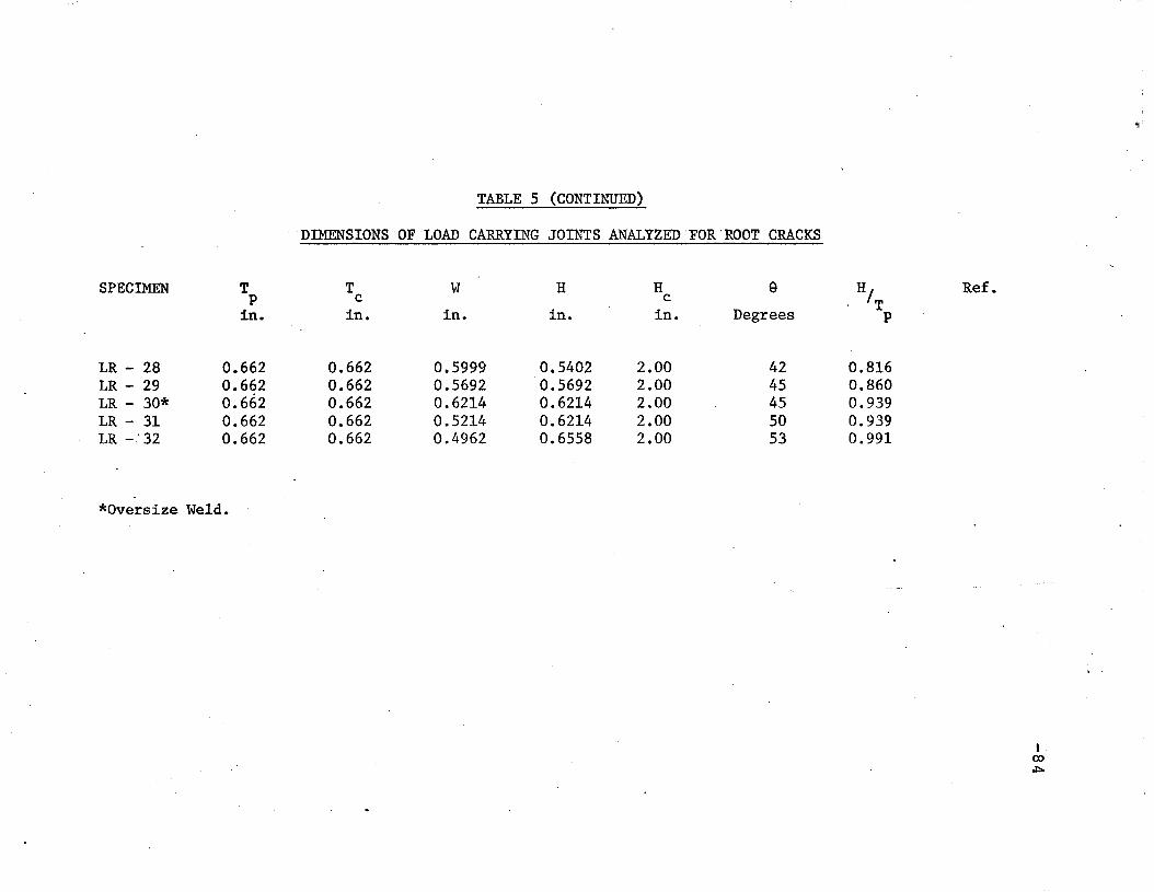
TABLE 5 (CONTINUED)
"DIMENSIONS'OF'LOAD CARRYING JOINTS ANALYZED 'FOR 'ROOT 'CRACKS
SPECIMEN T T W H H 9 HI Ref.p c c . T
in. in. in. in. in. Degrees p
LR - 28 0.662 0.662 0.5999 0.5402 2.00 42 0.816LR - 29 0.662 0.662 0.5692 0.5692 2.00 45 0.860LR - 30* 0.662 0.662 0.6214 0.6214 2.00 45 0.939LR - 31 0.662 0.662 0.5214 0.6214 2.00 50 0.939LR -,' 32 0.662 0.662 0.4962 0.6558 2.00 53 0.991
*Oversize Weld.
I,co.r:::.
' ....

-85'TABLE 6
,STRESS INTENSITY FACTOR POLYNOMIAL COEFFICIENTS FOR
ROOT CRACKS OF LOAD CARRYING WELD JOINTS
SPECIMEN 2A1 3A2 4A
3 SA4
LR - 1 11.812 24.199 - 71.383 121.45LR - 2 11.671 24.270 - 71.220 121.21LR - 3 10.856 24.377 - 71.858 122.38LR - 4 10.930 24.859 - 73.045 123.26LR - 5 10.690 24.853 - 73.181 123.53LR - 6 15.495 19.418 - 68.691 121.62LR - 7 15.535 19.655 - 69.761 122.67LR - 8 17.655 11.122 - 54.809 114.20LR - 9 9.1429 26.497 - 81.572 131.96LR - 10 15.899 18.088 - 66.556 120.39LR - 11 18.816 4.8185 - 41.964 106.31LR - 12 6'.8059 32.931 -106.76 151.33LR - 13 9.9418 24.911 - 74.884 125.69LR - 14 12.078 24.254 - 71.443 121.15LR - 15 13.831 23.329 - 73.408 123.55LR - 16 15.345 20.071 - 70.008 122.50LR - 17 16.631 15.635 - 63.019 118.91LR - 18 8.5541 27.607 - 86.785 136.55LR - 19 11.612 24.112 - 70.835 120.93LR - 20 13.835 23.200 - 72.980 123.12LR - 21 15.680 19.120 - 68.723 121.94LR - 22 17.171 13.373 - 59.038 116.67LR - 23 9.8997 28.347 - 79.376 127.81LR - 24 10.062 9.9706 - 40.911 63.710LR - 25 11.848 11.184 - 46.738 76.725LR - 26 13.127 11.796 - 49.835 85.765LR - 27 14.031 12.560 - 52.662 93.196LR - 28 14.932 14.184 - 57.879 103.51LR - 29 16.489 16.211 - 63.962 119.34LR - 30 17.207 13.087 - 58.234 115.97LR - 31 19.322 22.630 - 80.913 158.91LR - 32 21.199 27.955 - 93.722 190.66

TABLE 7
DIMENSIONS OF LOAD CARRYING JOINTS ANALYZED FOR TOE CRACKS
SPECIMEN T T W H H Q H Root Pene- Ref.p c c IT " trationin. in. in. in. in. Degrees p %
·',-LT - 1 0.630 0.630 0.236 0.236 1.46 45 0.375 100 165.8
LT - 2 0.630 0.630 0.394 . 0.394 1.46 45 0.625 100 164.7
LT ~ 3 0.630 0.630 0.551 0.551 1.46 45 0.875 100 - 1626.0
LT - 4 1.26 1.26 0.394 0.394 3.31 45 0.313 100 16' 12.5
LT - 5 1.26 1.26 . 0.590 0.590 3.31 45 0.468 100 1610.6
LT - 6 1.26 1.26 0.984 0.984 3.31 45 0.781 100 1611.3
LT - 7 1.26 1.26 1.18 1.18 3.31 45 0.937 100 160.5
LT - 8 0.662 0.662 0.749 0.433 2.00 30 0.653 1002.4
LT - 9 0.662 0.662 0.621 0.521 2.00 40 0.788 1001.0
100LT - 10 0.662 0.662 0.5999 0.540 2.00 42 0.816 19.0 I
8.9com
·#j
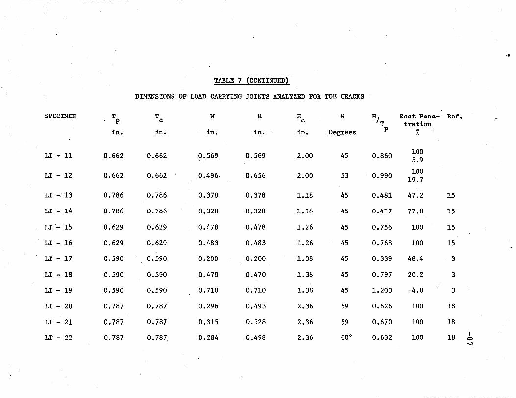
TABLE 7 (CONTINUED)
DIMENSIONS OF LOAD CARRYING JOINTS ANALYZED FOR TOE CRACKS
SPECIMEN T T W H H e HI Root Pene- Ref.p c c trationTin. in. in. in. in. Degrees p %
LT - 11 0.662 0.662 0.569 0.569 2.00 45 0.860 1005.9
LT - 12 0.662 0.662 0.496- 0.656 2.00 53 . 0.990 10019.7
LT -.:13 0.786 0.786 0.378 0.378 1.18 45 0.481 47.2 15
LT - 14 0.786 0.786 0.328 0.328 1.18 45 0.417 77.8 15
LT'- 1'; 0.629 0.629 0.478 . 0.478 1.26 45 0.756 100 15
LT - 16 0.629 0.629 0.483 0.483 1.26 45 0.768 100 15
LT - 17 0.590 0.590 0.200 0.200 1.38 45 0.339 48.4 3
LT - 18 0.590 0.590 0.470 0.470 1.38 45 0.797 20 .. 2 3
LT - 19 0.590 0.590 0.710 0.710 1.38 45 1.203 -4.8 3
LT - 20 0.787 0.787 0.296 0.493 2.36 59 0.626 100 18
LT - 21 0.787 0.787 0.315 0.528 2.36 59 0.670 100 18
LT - 22 0.787 0.787 0.284 0.498 2.36 60 0 0.632 100 18 Ien-...J
·t
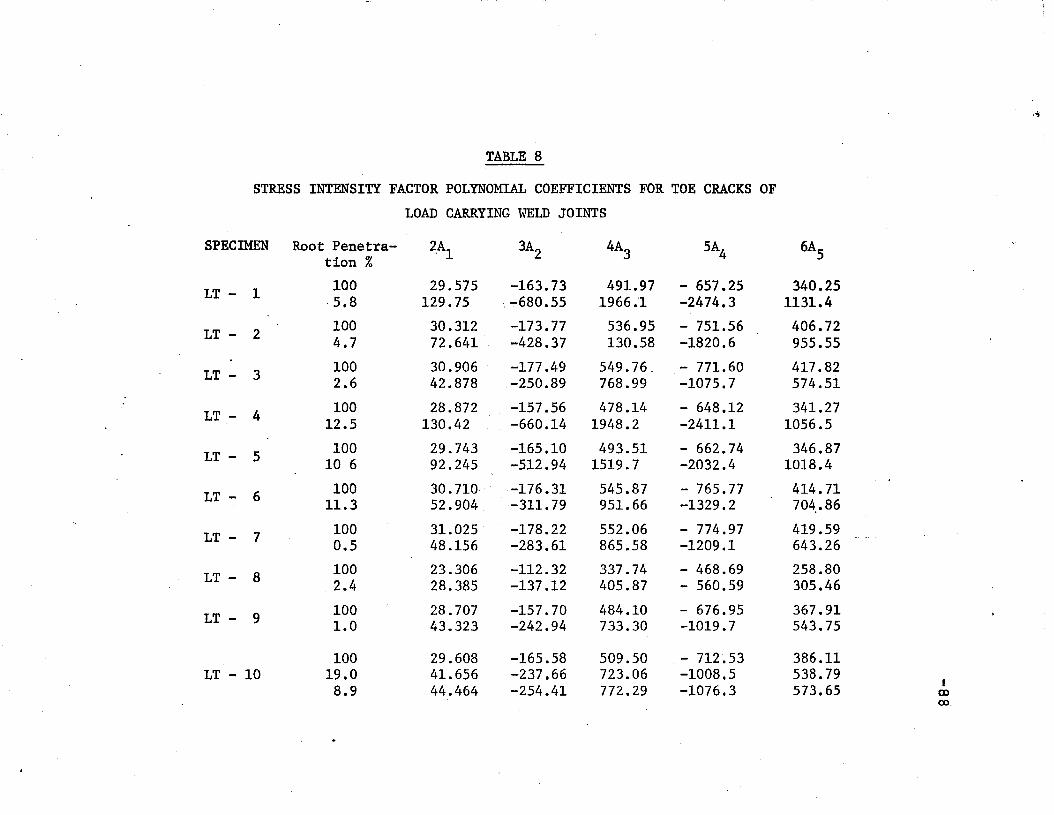
."'J
TABLE 8
STRESS INTENSITY FACTOR POLYNOMIAL COEFFICIENTS FOR TOE CRACKS OF
LOAD CARRYING WELD JOINTS
SPECIMEN Root Penetra- ~Al 3A2
4A3
SA4 6AStion %
LT - 1 100 29.575 -163.73 491.97 - 657.25 340.25·5.8 129.75 -680.55 1966;1 -2474.3 1131.4
LT - 2100 30.312- -173.77 536.95 - 751.56 406.724.7 72.641 -428.37 130.58 -1820.6 955.55
LT - 3100 30.906 -177.49 549.76. - 771.60 417.822.6 42.878 .-250.89 768.99 -1075.7 574.51
LT - 4100 28.872 -157.56 478.14 - 648.12 341.27
12.5 130.42 -660.14 1948.2 -2411.1 1056.5
LT - 5 100 29.743 -165.10 493.51 - 662.74 346.8710 6 92.245 -512.94 1519.7 -2032.4 1018.4
LT - 6100 30. 710-, -176.31 545.87 - 765.77 414.71
11.3 52.904 -311.79 951.66 -1329.2 704,.86
LT - 7100 31.025 -178.22 552.06 - 774.97 419.590.5 48.156 -283.61 865.58 -1209.1 643.26
LT - 8100 23.306 -112.32 337.74 - 468.69 258.802.4 28.385 -137.12 405.87 ~ 560.59 305.46
LT - 9 100 28.707 -157.70 484.10 - 676.95 367.911.0 43.323 -242.94 733.30 -1019.7 543.75
100 29.608 -165.58 509.50 - 712.53 386.11LT - 10 19.0 41.656 -237.66 723.06 -1008.5 538.79
I8.9 44.464 -254.41 772.29 -1076.3 573.65 OJ
co.

'.TABLE 8 (CONTINUED)
STRESS INTENSITY FACTOR POLYNOMIAL COEFFICIENTS FOR TOE CRACKS OF.~
LOAD CARRYING WELD JOINTS
SPECIMEN. Root Penetra- 2A1 3A2 4A
3SA4 6AStion %
LT - 11100 30.876 -177.31 549.18 - 770.75 417.375.9 50.366 -296.86 905.87 -1265.3 672.15
LT - 12100 33.332 -201.43 631.78 - 891.41 481.36
19.7 55.970 -347.15 1077.6 -1516.2 804.76
LT - 13 47.2 46.605 -257.72 770.22 -1027.4 552.39
LT - 14 71.8 34.027 -184.93 544.62 - 707.31 356.14
LT - 15 100 30.659 -175.95 544.52 - 763.48 413.34
LT- 16 100 4 30.677 -176.06 544.89 - 764.05 413.65
LT - 17 48.4 49.344 -255.88 740.86 - 882.40 388.78
LT - 18 20.2 48.071 -282.30 863.48 -1206.9 641.92
LT - 19 -4.8 40.567 -237.07 726.10 -1015.4 543.42
LT - 20 100 : 26.068 -159.08 493.98 - 673.89 349.84
LT - 21 1000 26.052 -158.65 491.23 ~ 669.46 q 347.68
LT - 22 100 26.244 -161.27 503.17 - 688.78 358.19I
co\0
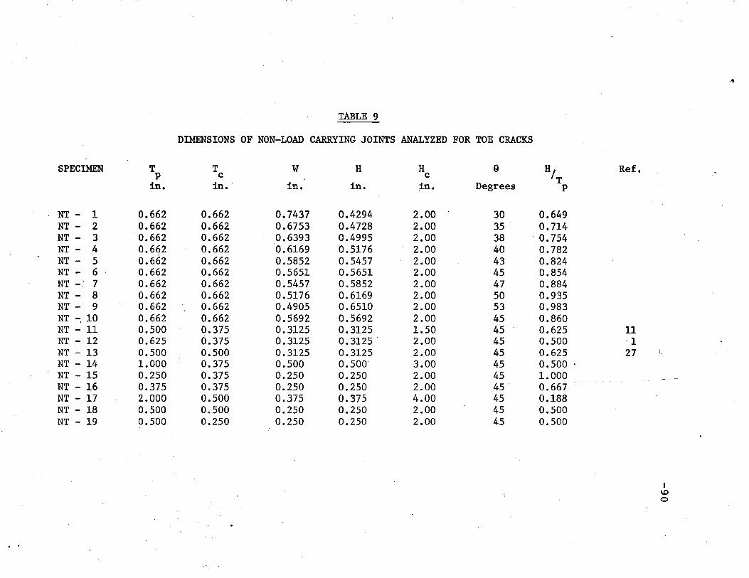
. ~
TABLE 9
DIMENSIONS OF NON-LOAD CARRYING JOINTS ANALYZED FOR TOE CRACKS
SPECIMEN T T W H H Q HI Ref.p c cin. in •. in. in. .in. Degrees T
p
NT - 1 0.662 0.662 0.7437 0.4294 2.00 30 0.649NT - 2 0.662 0.662 0.6753 0.4728 2.00 35 0.714NT - 3 0.662 0.662 0.6393 0.4995 2.00 38 0.754NT- 4 0.662 0.662 0.6169 0.5176 2.00 40 0.782NT - 5 0.662 0.662 0.5852 0.5457 2.00 43 0.824NT - 6 0.662 0.662 0.5651· 0.5651 2.00 45 0.854NT -: 7 0.662 0.662 0.5457 0.5852 2.00 47 0.884NT - 8 0.662 0.662 0.5176 0.6169 2.00 50 0.935NT - 9 0.662 0.662 0.4905 0.6510 2.00 53 0.983NT -. 10 0.662 0.662 0.5692 0.5692 2.00 45 0.860NT - 11 0.500 0.375 0.3125 0.3125 1.50 45 0.625 11NT .... 12 0.625 6.375 0.3125 0.3125 . 2.00 45 0.500 -1NT - 13 0.500 0.500 0.3125 0.3125 2.00 45 0.625 27 I •
NT - 14 1.000 0.375 0.500 0.500· 3.00 45 0.500 ·NT - 15 0.250 0.375 0.250 0.250 2.00 45 1.000NT - 16 0.375 0.375 0.250 0.250. 2.00 45 - 0.667NT - 17 2.000 0.500 0.375 0.375 4.00 45 0.188·NT - 18 0.500 0.500 0.250 0.250 2.00 45 0.500NT - 19 0.500 0.250 0.250 0.250 2.00 45 0.500
I\Do
·t
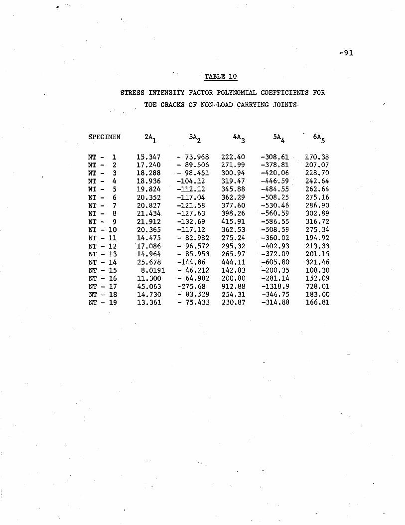
TABLE 10
STRESS INTENSITY FACTOR ~OLYNOMIAL COEFFICIENTS FOR
TOE CRACKS OF NON-LOAD CARRYING JOINTS·
SPECIMEN 2A1 3A2 4A3 5A4 6AS
NT- 1 15.347 - 73.968 222.40 -308.61 170.38NT - 2 17.240 - 89.506 271.99 -378.81 207.07NT- 3 18.288 - - 98.451 300.94 -420.06 228.70NT - 4 18.936 -104.12 319.47 -446'.59 242.64NT - 5 19.824 -112.12 345.88 -484.55 262.64NT - 6 20.352 -117.04 362.29 -508.25 275.16NT - 7 20.827 -121.58 377.60 -530.46 286.90NT- 8 21.434_ -127.63 398.26 -560.59 302.89NT - 9 21.912 -132.69 415.91 -586.55 316.72NT - 10 20.365 -117.12 362.53 -508.59 275.34NT - 11 14.475 - 82.982 275.24 -360.02 194.92NT - 12 '17.086 - 96.572 295.32 -402.93 213.33NT - 13 14.964 - 85.953 265.97 -372.09 201.15NT - 14 25.678 -144.86 '444.11 -605.80 321.46NT - 15 8.0191 - 46.212 142.83 -200.35 108.30NT - 16 11.300 - 64.902 200.80 -281.14 . 152.09NT - 17 45.063 -275.68 912.88 -1318.9 728.01NT - 18 14.730 ..;.- 83.529 254.31 -346.75 183.00NT - 19 13.361 - 75-.433 230.87 -314.88 166.81
-91
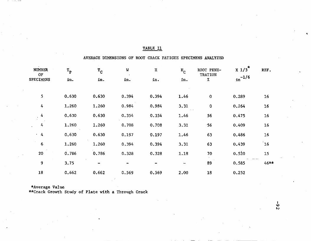
TABLE 11
AVERAGE DIMENSIONS OF ROOT CRACK FATIGUE SPECIMENS ANALYZED
·11
NUMBEROF
SPECIMENS
Tp
in.
TC
in.
w
in.
H
in.
HC
in.
ROOT PENETRATION
%
X 1/3*
in-1/ 6
REF.
5 0.630 0.630 0.394 0.394 1.46 0 0.289 16
4 1.-260 1.260 0.984 0.984 3.31 0 0.264 16
-4 0.630 0.630 0.354 0.354 1.46 56 0.475 16
4 1.260 1.260 0.708 0.708 3.31 ~56 0.409 16
4 0.630 0.630 0.197 0.197 1.46 63 0.486 16
-6 1.260 1.260 0.394 0.394 3.31 63 0.439 16
20 0.786 0.786 0.328 0.328 1.18 70 0.520 15
9 3.75 - - - - 89 0.585 46**
18 0.662 0.662 0.569 0.569 2.00 18 0.252
*Average Value**Crack Growth Study of Plate with a Through Crack
I\0l\.)
L..,
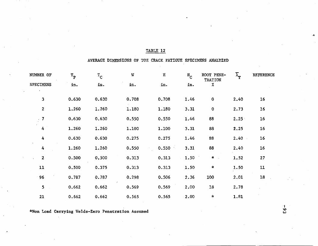
I....
.~
FIGURES
-94
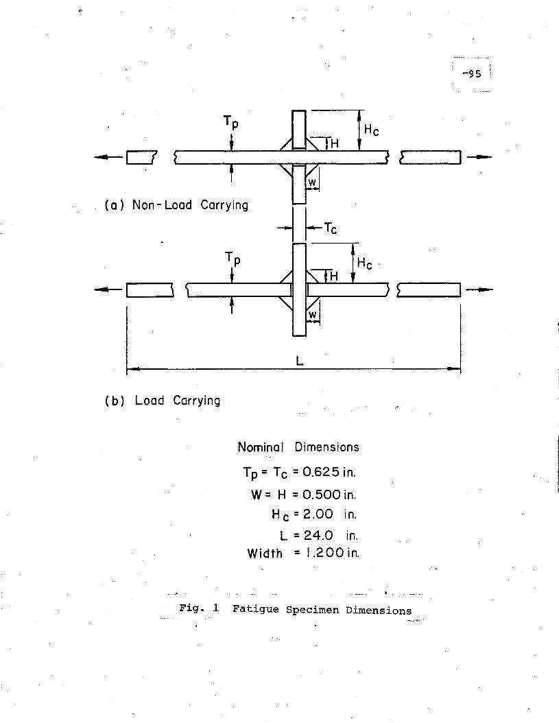
.. LJ
,(Q) Non - Load Carrying
~I--_ .......\
L
( b ) Load Carrying
Nominal Dimensions
Tp =Tc =0.625 in.
W= H =0.500 in.
He =2.00 in.
L = 24.0 in.Width' = 1.200 in.
I -95
.....}---~
S.... I~
___ t__ + _
Fig. 1 Fatigue Specimen Dimensions
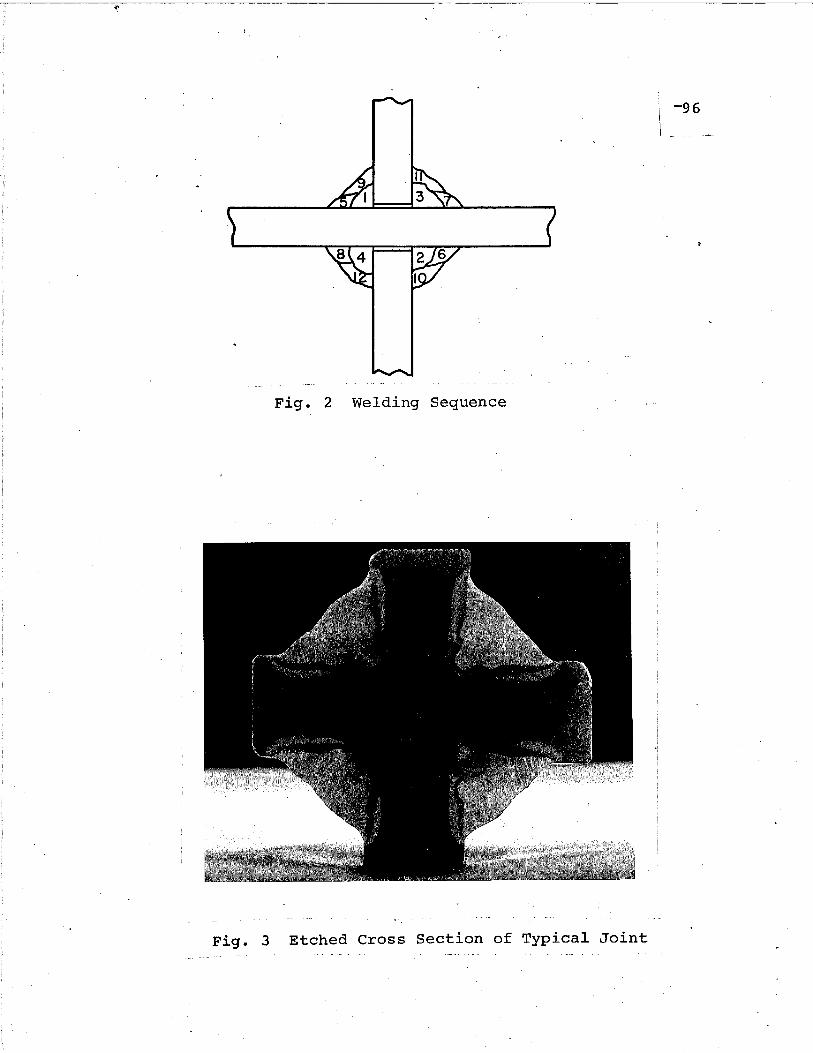
..
Fig. 2 Welding Sequence
Fig. 3 Etched Cross Section of Typical Joint

-97
Fig. 4 Toe Failure-Nan-Load Carrying Joint
Fig. 5 Root Failure-Load'Carrying Joint
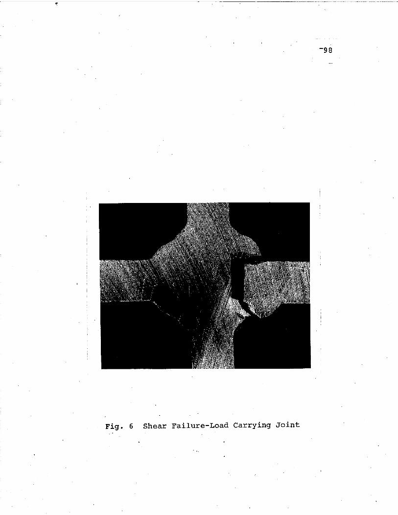
Fig. 6 Shear Failure-Load Carrying Joint
-98
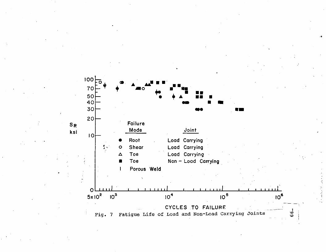
"~
100. 0 ~ A• II.'
70 + +M •••••"0 -+e • -II
50 • +A II • II40 - II •30 •• ••20
SR I Failure
ksi Mode Joint10
• Root Load Carryingiii ' 0 Shear Load Carrying4 -...
A Toe Load Carrying
• Toe Non - Load Carrying
Porous Weld ' .,
-.
106IO!5104
o I I I , I I I I I I I I I I I I I I I I I I I I "" , , I , I
5x 10² 103
CYCLES .TO FAILUREFig. 7 Fatigue Life of Load and Non-Load Carrying Joints
'-----1 ~.
i, i
\.0 l
\0 1
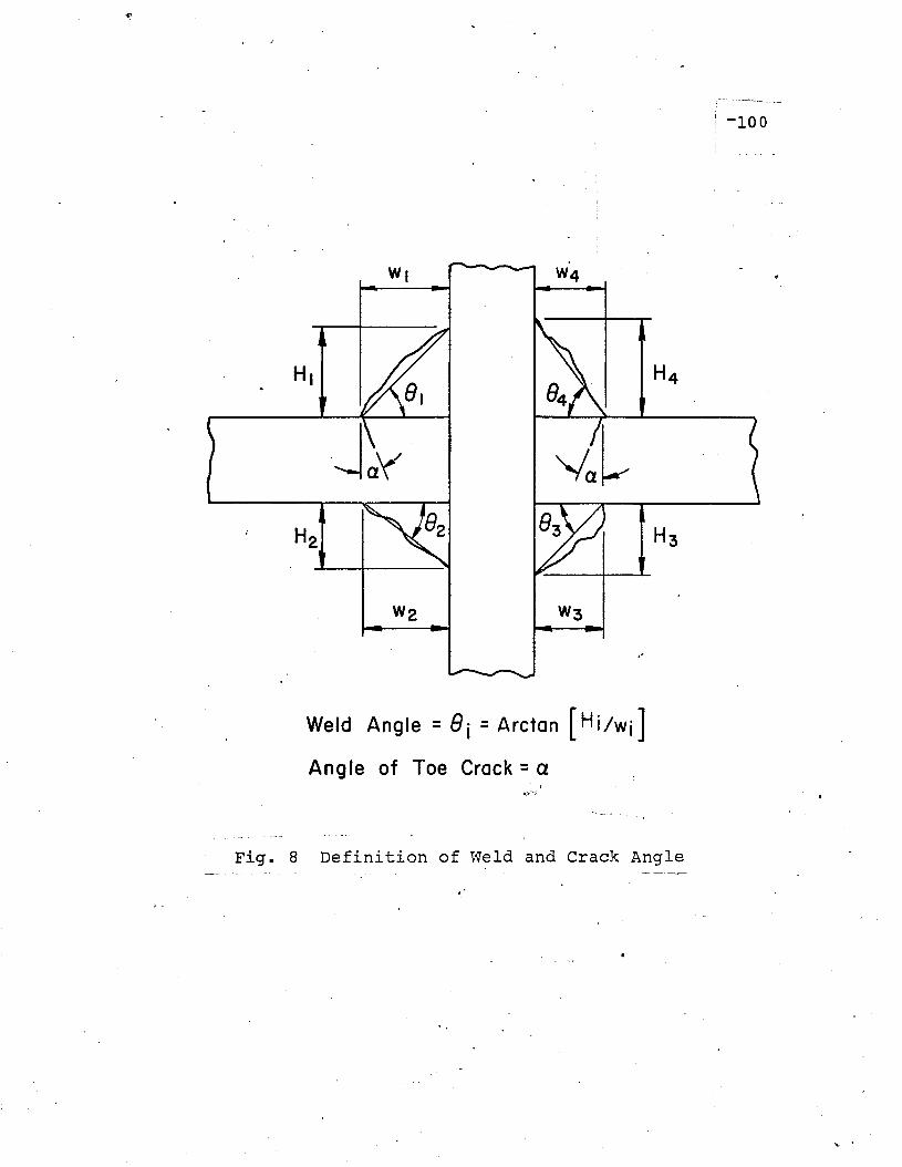
-100
Weld Angle =8 j =Arctan [Hi/wi]
Angle of Toe Crack =a
Fig. 8 Definition of Weld and Crack Angle

30 Meon=44.5° IMean Failures =47.8°
20
10
35° 40° 45° 50°WELD ANGLE
o-----&-+...&.-L..--I---L----L-+-.L---L---1-~--L-
30°
Fig. 9 Histogram of Weld Angle-Nan-Load Carrying Joints
.I .
40
30
20
1.151.050.75 0.85 0.95
.8/8 FAILURE
o-...-......-r---a.--t----a--+--L----I--..L---I--
0.65
10
Fig. 10 -Histogram of e to eF
. 1 -Non Load Carrying Joints'. al ure
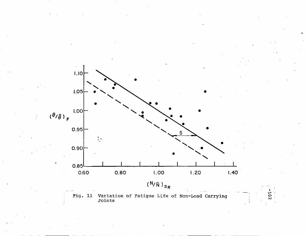
,~
It----lotv
1.40
•
•
•
•
1.20
•
•
•
1.00
(N/N )SR
•
0.80
11-.;/~
•
1.10
Fig. 11 Variation of Fatigue Life of Non-Load CarryingJoints
0.85' , , , , , , I ,
0.60
1.05
0.95
0.90
(8,- 1.008)F

25 ••
.'!f
~ 201
~
•"- IQ)
e_'-
e
en
•Q)
••. "'C
15..0
'6 ~Mean a= 13
•w
•• • --.J
•t9Z« 10~U' I '.
<X:
•a:::0
• •5,
Fig. 12 Toe Crack.Angle Variation With Weld Angle
o 10 20 30 40
WELD ANGLE e, degrees
50
I......ow
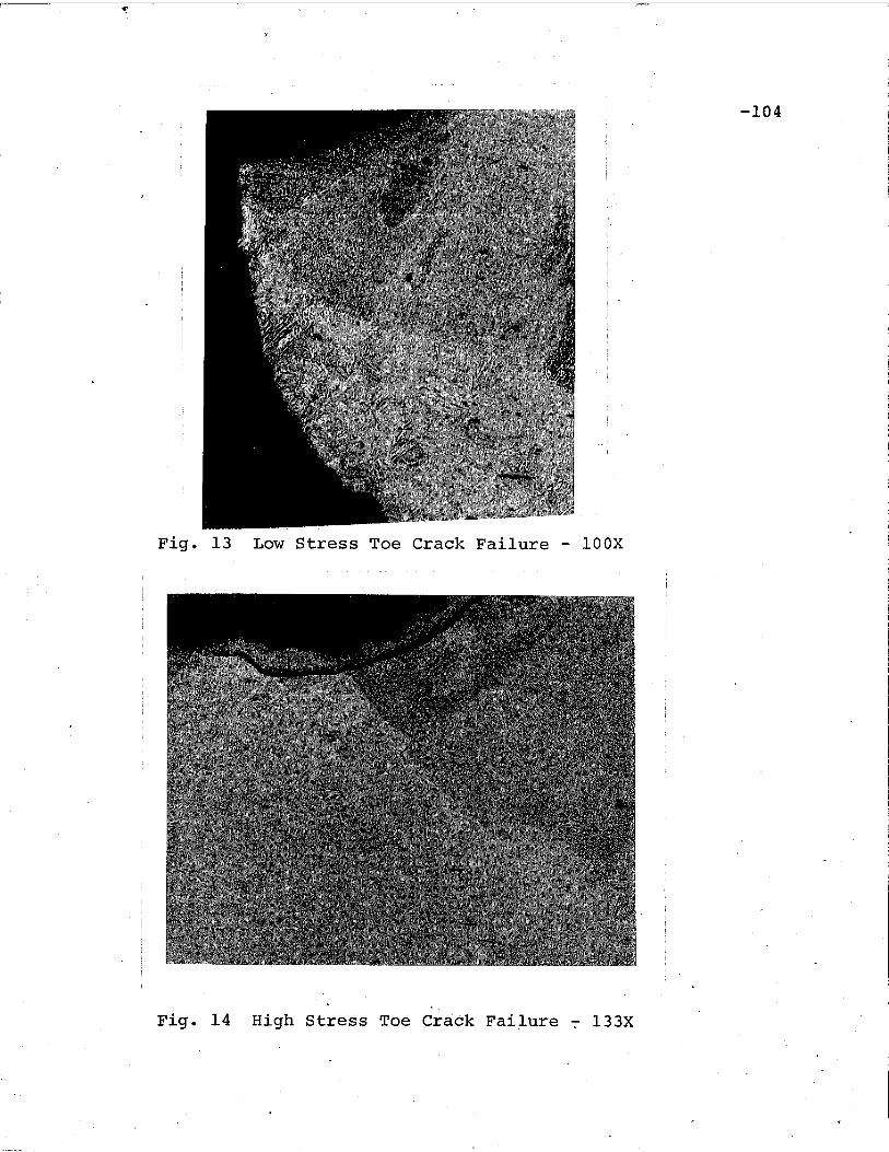
Fig. 13 Low Stress Toe Crack Failure - lOOX
Fig. 14 High Stress Toe Crack Fai~ure 7 133X
-104
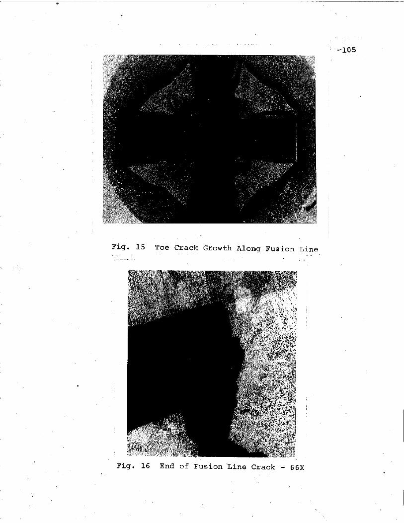
Fig. 15 Toe Crack Growth Along Fusion Line
Fig. 16 End of Fusion "Line Crack - 66X
-105
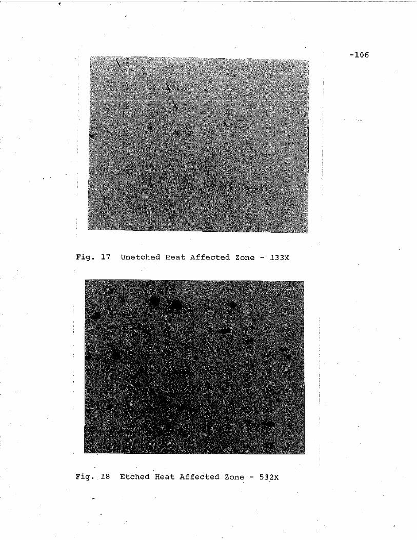
Fig. 17 Unetched Heat Affected Zone - 133X
Fig. 18 Etched Heat Affected Zone - 532X
-106

Fig. 19 Crack Branching to Included Particles - 66X
Fig. 20 Crack Growth Path at Inc~uded Particles - 133X
-107

-108
Fig. 21 Root Crack Tip Untested Specimen 133X
Fig. 22 Root Crack Tip Untested ,Specimen With Large PlateGap - 133X
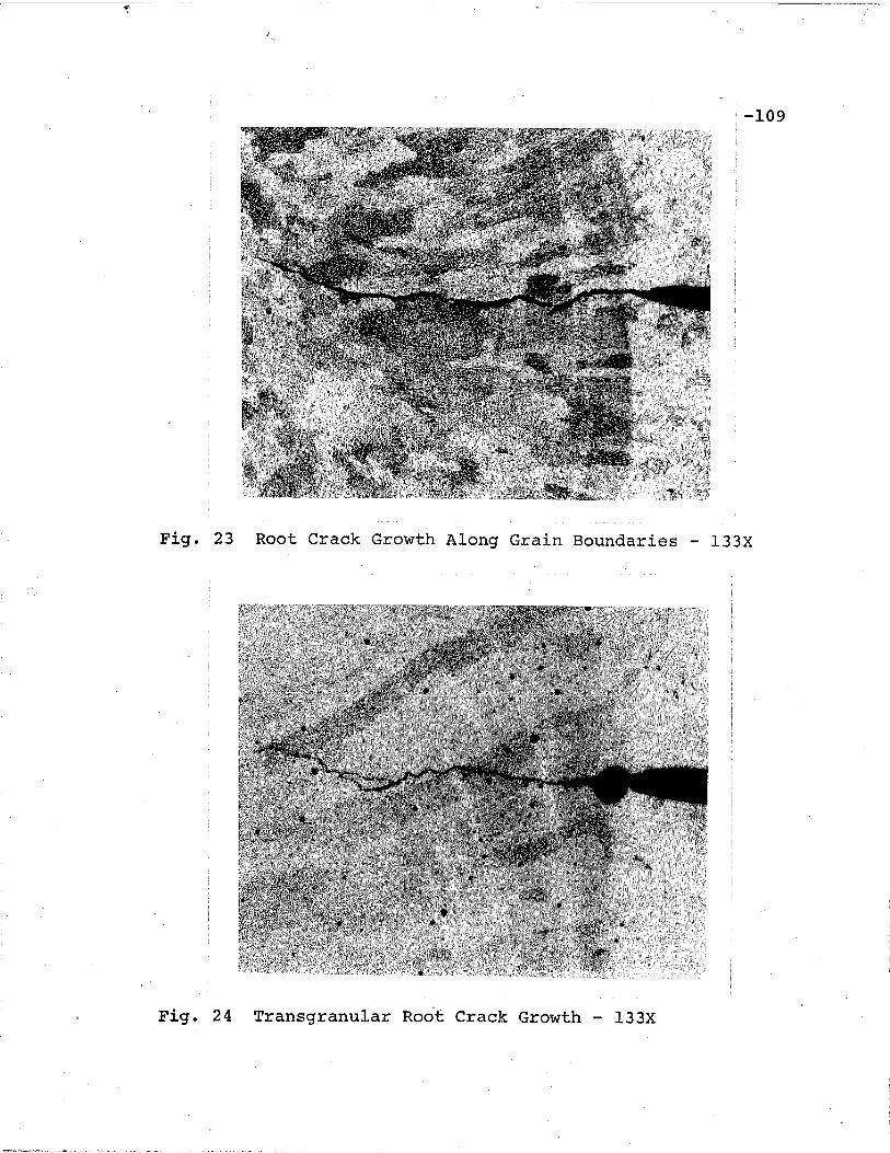
-109
Fig. 23 Root Crack Growth, Along Grain Boundaries - 133X
Fig. 24 Transgranular Root Crack Growth - 133X

Fig. 25 Vertical End of Root Crack At Failure - 66X
Fig. 26 Failure of Joint "With Porous Weld
-110
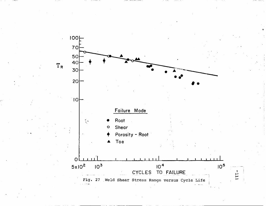
°T R
100
70
5040
30
20
~ 10
+
11'A"-."4;.
• A-~"--'~
•••••
Failure Mode
• Root
o Shear
• Porosity - Root 0
• Toe
I , , , ,
,.,
Fig. 27 Weld Shear Stress Range versus Cycle Life
103 10 4
CYCLES TO FAILURE105 ,
I-'f-II-'

-112
,-
{ CT} =[ f (r, 8 ) ] {K}
-Fig. 28 Crack Tip Stress Field Coordinates
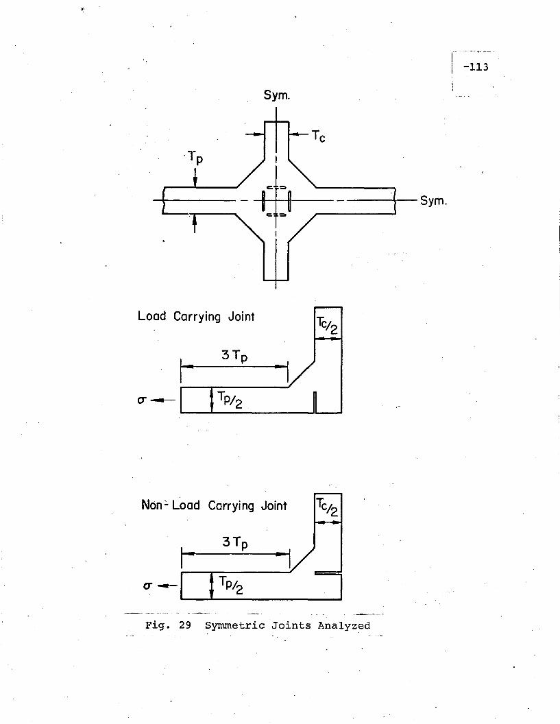
Non~ L
Sym.
--~-Sym.
Load Carrying Joint
3Tp
oad Carrying Joint TC/2---
1-3Tp
--IJ~ Tp~1. 2
Fig. 29 Symmetric Joints Analyz~d
-113

Tp/2
CRACK TIP MESH
3Tp
. Fig. 30 ~oad Carrying Joint Root Crack Finite Element MeshI
I--'.......~
.~

CRACK TIP MESH
Fig. 31 Load Carrying Joint Toe Crack Finite Element MeshI"'
.......
......U1
.tI
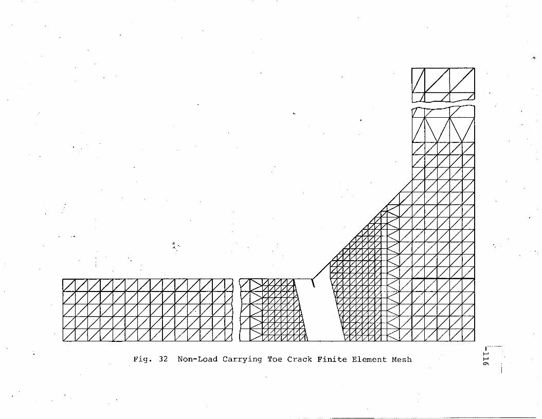
~,f "'-
,~
Fig. 32 Non-Load Carrying Toe Crack Finite Element Mesh
"",------------)
....... ;
......0'\

14
-117
13
P2w I-- ..G
-IJb'l
12 ~Q)
-H
~Ucd~u
II rc:4J-ri:::
ESC (1)·0.~,cd
-.-I
10 r-IP-4
:S:0
C)
'+4:0
Weld Angle (1)
9 tTlr=:
45°cd• ..c:
't)
t::. 40° M;- !M
u.'">-), -
35 00 .·8 :Ol
-..-I
Tp=Tc = 0.662 in. rz...
0.2 0.4 0.6 0.8
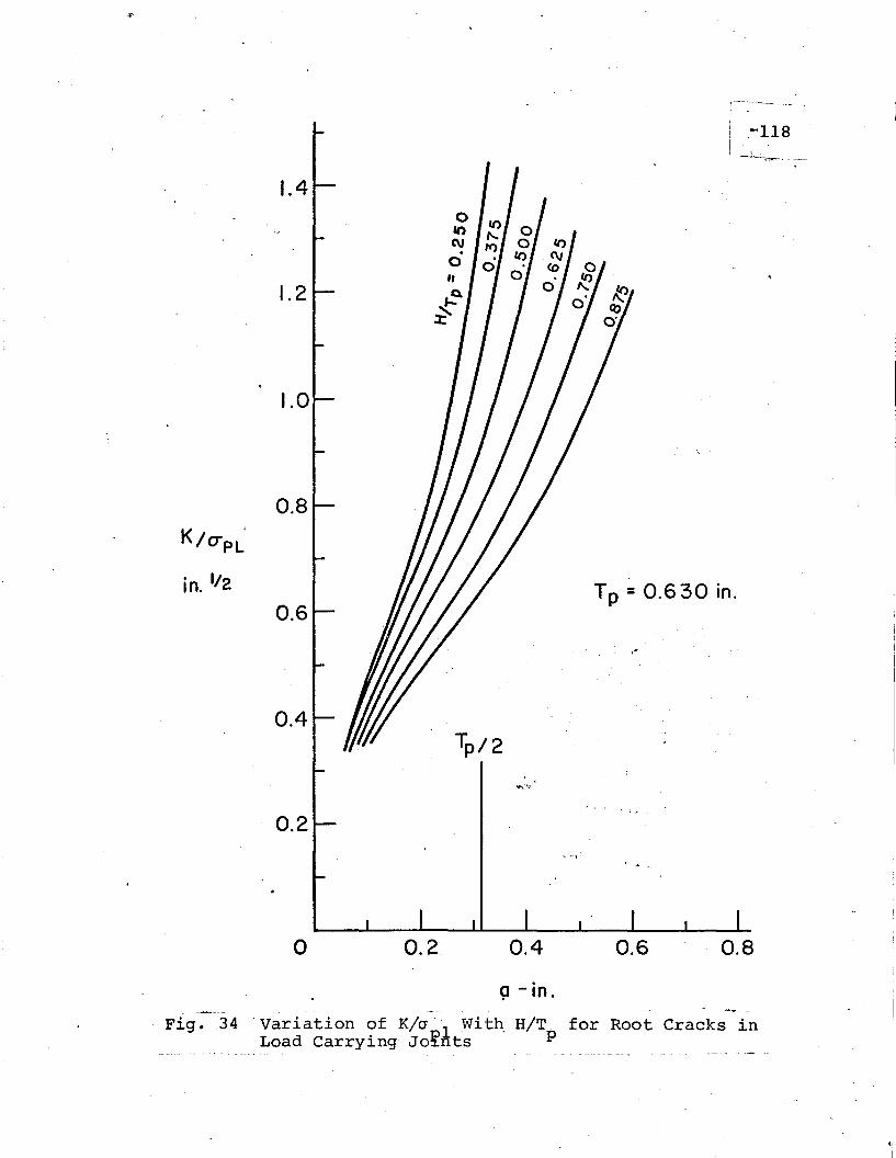
1.4
1.2
1.0
0.8
0.6
0.4
. 0.2
Tp /2
j---~---~._-~._-~
I .~118_.~.~r-: ~, _ _
Tp =0.630 in.
o 0.2 0.4
a - in. ' .
0.6 0.8
--
Fig. 34 . variation of Kia ~ " Wi tho HITLoad Carrying' Jo~nts p
for Root Cracks in
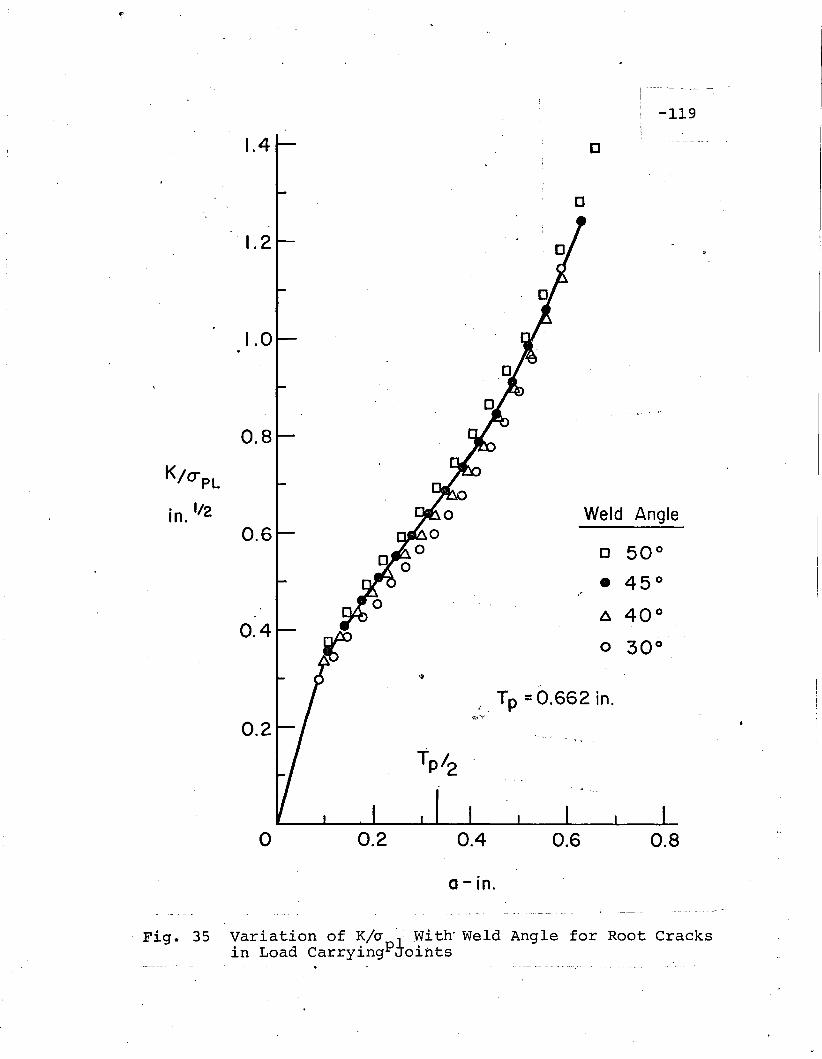
1.4
-119
c
D
o-
j, Tp =0.662 in.~"V;~
K/o-pL
in. 1/2
"1.2
1.0
0.8
0.6
0.4
0.2
o 0.2 0.4
a - in.
0.6
Weld Angle
o 50°
• 45°
A 40°
o 30°
0.8
Fig. 35 variation of Kia t .With·Weld Angle for Root Cracksin Load CarryingPJoints

-120
1.7 HtTp
0.875
~r
1.6
1.5
1.4
1.3
1.2
r. I
" : "':""1 .••1,." .:. ,"_.
0.8 .0.60.40.2
1.0 '----..a- ~ _a.__......_
o- O/Wl
Fig. 36 Change in AR~ith Crack Length and Weld Size
fi ~;
.'J.......
-t.2
-~
. -Tp in.. Tp/TcWeld Angle-
A 1.26 1o _ 0.786 I
1.81- -& 0.750 0.856
• 0.662 I / .0 0.630 I
• 0.629 I'1.6f- .. 0.590 I
<P 0.394 IC, I
1.4
i
I !t; I.I-'
1.21.00.80~6
H/Tp
0.4
variation of the Coefficient C1
With HIT. P
0.2
~ Fig. 37
J.0, F , , , • , , , , , , ,
o
) ,
~._---......,.-~".~ .•-< .-.' •.• .- •.• --------------------------------------------=>.~..,'",..,"..~....,-_.~

C2
. 0.4Weld Angle
0.2
0 1 I I I I I I I :a. I I I I I<tfJ
0 Tp in. Tp/Tc-0.2 1 ~f'
/1 1.26 I0 0.786 I0 0.750 0.856
-0.41- • 0.662 I0 0.630 I
• 0.629 IA 0.5·90 I --_.
0 0.394 I I.•• •_~._~~_. _~ .r ._- ----~--.~-- ~ ........... - ~---~ ~~~~ ~ ~~~ ~ ~ --......- ~~~- ~ -... --...:.~
......, . ... 1 I\)
: Fig •. 38 Variation of the Coefficient C2 with HIT- ',', tv
p'.. .
.4J

.if"
l·~---~~-·"'-I • ,I -1~3
, .. -"--" --...--- ....._--
0.4682.4
2.8
2.0
0.781
K/OPL0.937
{0.3130.468
IN 1/21.6 0.781
0.937J ,
/ 0.625/
"" 0.875",
1.2 ", /~.875~ /7 0.625
.. / / 0.375// ,-
///",
0.8 ."",/",fill'" Tp = Tc = I. 26 in.
Tp =Tc0.630 in. 1.26 in.
0.4 --- Smail Penetration1 --- Full Penetration
0- 0.2 0.4 0.6 0.8
a/Wi
Fig. 39 Variation of K/a 1 ,With Weld Penetration and a/wi'for Two Plate Th~ckness€s ,for Toe Cracks in LoadCarrying Joints
-124
2.2
1.8
1.6
1.4
1.2
1.0
EQ.31
Band of aII Geometrie"s
0.80.60.40.20.. 8 ~--""'_"'-"'----.lt....-----a.-_...a.....------a._--L..._""""
o0/ Iw·
Fig. 40 Variation of ~ for Load Carrying Joints with FullPenetration and 45~ Degr~e WeLds
2.2
2.0
1.8
1.6
1.4
1.2
1.0
Weld Angle
Tp =Tc =0.662 in.
~ .
l-"-'---~-~-- --J -125!ii~ _
0.2 0.4 0.6
. t·
0.8
Fig. 41 Change in AT With ·we.ld "Angle for Full PenetrationWelds

4.8
0.80.60.4
. Weld Angle = 45 0
Tp = Tc
0.2
1.6
0.8 .....-_..-...-_~_-..-_--...&-_---a..._---I._----.lI--_.a...-
o
2.4
3.2
4.0
Fig. 42 Change in AT with Weld Size for Load CarryingJoints with Small Root Penetration

.";
Fig. 43 Finite Element Used for Stress Analysis of Load·Carrying Weld Joints
I.......l\J-....J

4.7
4.3
3.9
A
o
I ----:-------,---_.j\I -.128.--_.---"",~-~-
Penetration TP=TC
Full Zero In.
A A 1.260
+ <I> 0.786... -e- 0.764
• . 0 0.662
• 0 0.630, [J 0.625
_ H /TpFig. 44 variation of Stre~s C6ncentration at Weld Toe with
HIT for Joints with- Full and Zero Root Penetrationp

r~----
'~129
2.8Penet ration
o Zero.• Full
2.4 Tp=0.662in.
2.0
I .6 ..- ...Lo- ...I-- -'-- --L- _
30°
WELD ANGLE
Fig. 45 Change in Stress Concentration at Weld Toe withWeld Angle
4.4
3.6
2.8
H/Tp
t:& 0.425o 0.477c 0.764
~>'c' • 0.800
20 40 60 80
% OF ROOT PENET.RATION
100
Fig. 46 Change in Stress ·Concentration at Weld Toe WithRoot Penetration . ·
'~~130
· .-~,..:-
4.8
4.0
2.4
1.6 2.4 3.2 4.0 4.8
Fig. 47 Correlation of AT With 'stress Conceptration at'Weld Toe
'- -,.--------------.~.----.--.
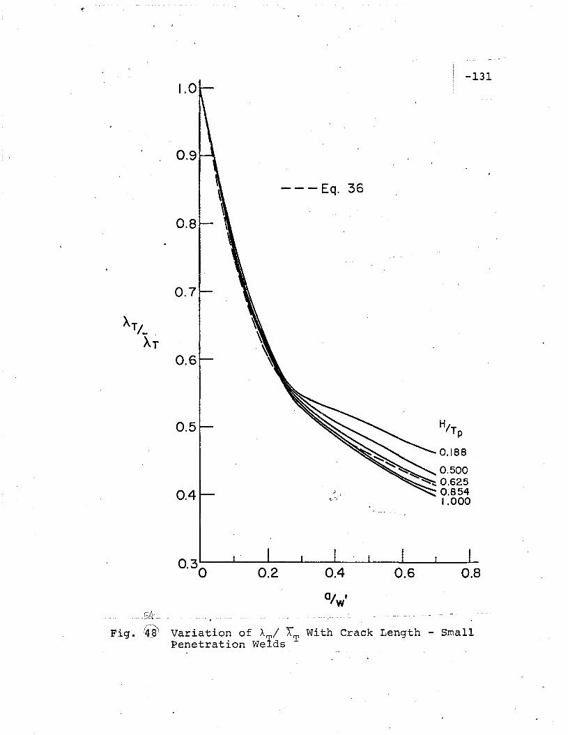
-1311.0
0.9
0.8
0.7
0.6
0.5
0.4
.w· ~ _.. _ •._-
0.2
---Eq. 36
0.4 0.6 0.8
; Fig. ~ Variation of AT/ AT With Crack Length - SmallPenetration Welds '
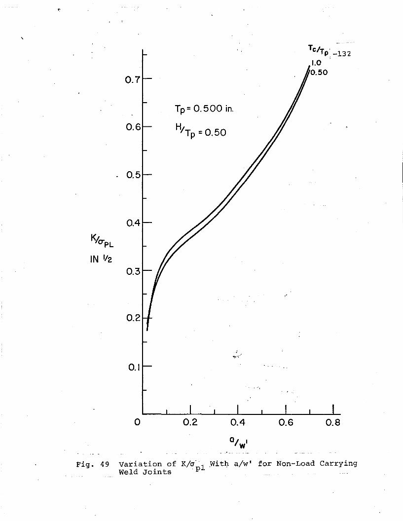
Tp= 0.500 in.
H/Tp =0.50
0.4
TC/Tp~ -1321.0 '
0.50
0.3
0.2
0.6
0.7
~ 0.5
'.
O. I
+, ""
o 0.2 0.4 0.6 0.8
Fig. 49 variation of Kla"l ~itQ a/wi for Non-Load CarryingWeld Joints ,p

0.8
0.7
0.6
0.5
K~ .O"pL 0.4
0.3
0.2
0.1
Weld Angle
-133
Tp =Tc =0.662 in.
L j-r
o 0.1 0.2 0.3 0.4
Fig~ 50
'., OJ I_. _.. _ __.,~_ .w., - _.......=L. ~
Variation of K/Opl With Weld Angle

~134
1.4
1.2Full Penetration
Zero Penetration
TP = Tc =0.662 in.
H =W= 0.569 in.
1.0
0.6
0.2
'·0 · 0.2 0.4 0.6 0.8
a/Wi
Fig. 51 Variation?f ~/crp1 with Weld Penetration
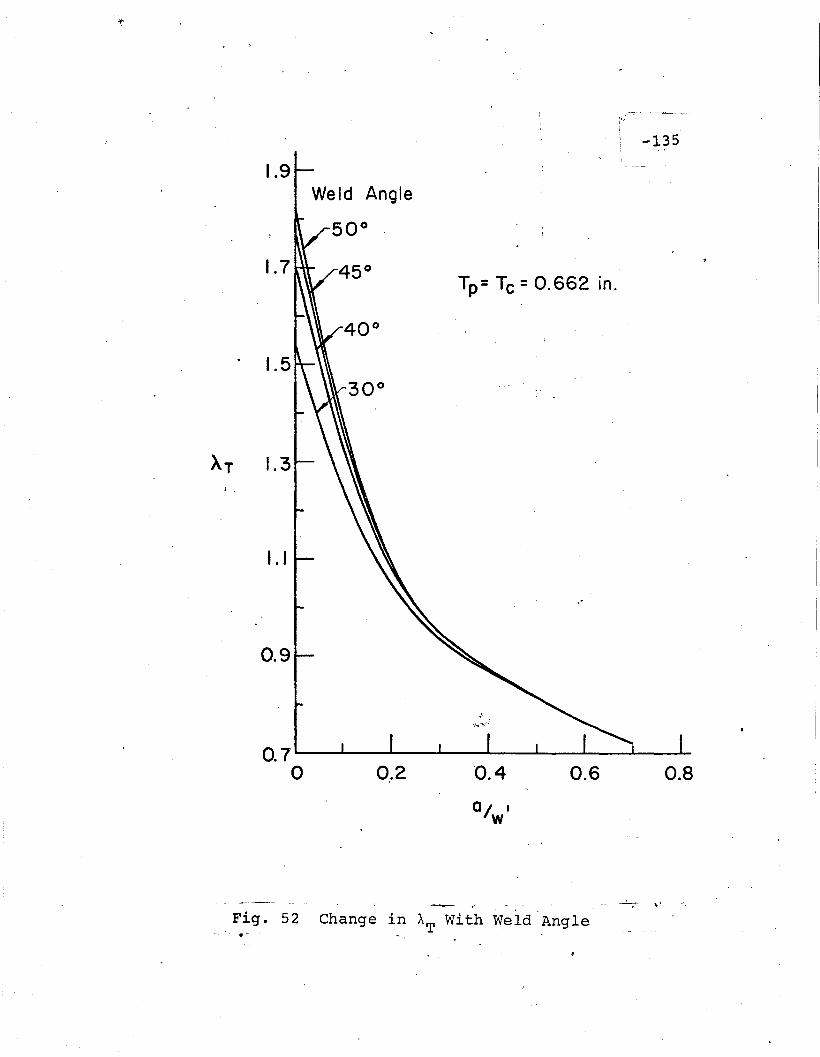
1.9
-135
Weld Angle
0.8
j"
0.6'0.4
Tp=Tc =0.662 in.
0,.2
I . I
1.5
1.7
o. 7 L..----JL....-_L..--_.a.....-_"'--_"'---_.a...-_.a.--_.-..-
o
0.9
-...g'.'. - ,. .'
Fig. 52 Change in AT With Weid·~ngle.-
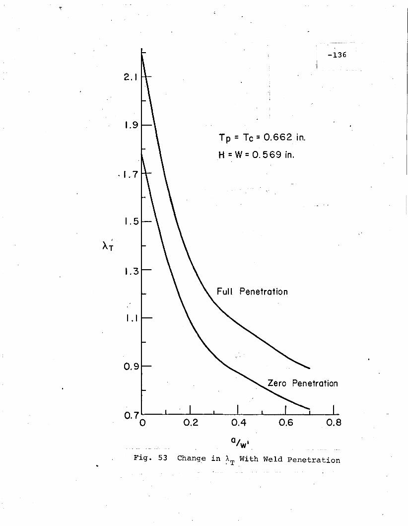
-136
Full Penetration
Tp = Tc = 0.662 in.
H =W= 0.569 in.
2.1
1.9
~ 1.7
1.5
1.3
I . I
0.9
0.7. 0 0.2 0.4 0.6 0.8
a/Wi
Fig. 53 Change in ~T ,With Weld Penetration

1.0
0.9
~ 0.8
0.7
0.6
0.5
0.4
0.2 0.4 0.6 0.8
413
. Figer§() Variati,on of AT/AT-With ~/WI Non-Load CarryingWeld Joints

1.71.3 1.5 1.7 1.9 2.1 2.3 2.5 2.7 .1.1
-AT
- ,. ,~-_._~~.~
Fig. 55 AT versus Stress Concentration at Weld Toe forI
.,V' ~t·- wNon-Load Carrying Welds! ex>
.ofoj
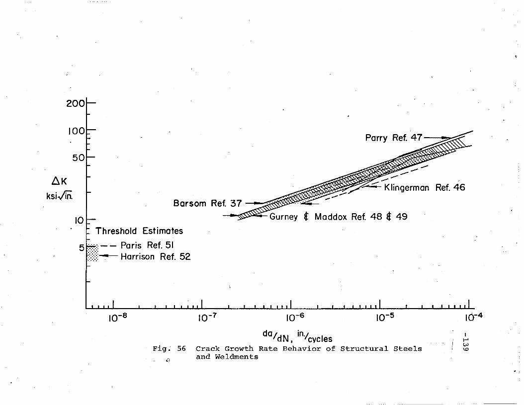
200
100
50
~K
ksi./iii.
10
Parry Ref. 47 .. ~
Ref. 46
Barsom Ref. 37 - ~~,~
~~ Gurney t Maddox Ref. 48 4 49
"5
Threshold Estimates
5 H=: - - Paris Ref. 51?;~:~:~:-- Harrison Ref. 52
~~
10-8 10-7 10-6 10-5 10-4
Fig.' 56
'C' if
do/dN in-/: I, eve asCrack Growth Rate Behavior of Structural Steelsand Weldments
. I
I t;I \0

•.l;t
{O 15.--J I I \--. ., 16
'A Present Study-
-1 I-I [] 46
~~~~~~
~~ .
~............ ~ . .
~~"""""""'oR:L.. ""O~--I::"~~ 0 0
-~o -o~. 0 0 _'. •• I·--.......o~ 0....... 00. ·-.....o~o ~
.~ ~Ref.
5
10
50
100
200
SR·ksi in 1t6
10 3 10 4 10 5
CYCLES' TO FAILURES
10 6 107
· Fig. 57 Modified Stress Range versus Cycles to Failur for, Root Crack Failures
I......~
o

40
.4j
1__ Range of OJ From Ref. 21 a 27 _II
II30
y
in~%20
10
Tp=0.25 in. t -Of = 0.5 Wi
t of =0.8wl
en(/)
~
cc
<:(
Eo...
1..1-
>-t+oCD0'c:ca::
o 0.004 0.008 0.012
0i - in.
0.016 0.020
~'.~-~........._.-.._~~
!r Fig. 58I"
Change in the Value of the Integral With InitialCrack Size (a.)
~
I I
fio J-Ir ~
, f-I
i

.~
300
,200
-100
50
-SR AT
ksi
10
5
Ref.
Non- Load Carr. {CI Present Studyylng 0- IIA. 27
Ref.
.{- Present StudyLoad Carrylng • 18
': A 16.
."
107
If-'~
l'J
106104 105
CYCLES TO FAILURESStress Range in Main Plate Times AT versus Cyclesto Failure for Toe Crack Failures
Fig. ·59
103

-143
APPENDIX
Methods of Solution of Finite Element Equations
The method of solution used to solve the set of
equations resulting from a finite element analysis becomes
important when the size of the system of .equations is 'large.
The mesh used to determine the stress distribution in the
joint had approx~mately four-hundred nodal points. This
resulted in an 800 x 800 stiffness matrix. The solution for
this mesh was found using the Gauss-Seidel procedure with
over relaxation. The form of the program and its logic was
based on the program in Ref. 53. This method was used since
only the non-zero terms of the stiffness matrix need to be
stored. The displacement of all nodal points are solved and
can be used to determine element stresses. The solution was
assumed to have converged when the percent change in the
displacement at the loaded nodes at the end of the main
plate was less than one-tenth of a percent.
The mesh used to determine the compliance of the
joints was'considerably more refined. Fifteen-hundred nodal
points were used and resulted in a global stiffness matrix
0'£ 3000 x 3000. The finite element mesh away from the crack
itself does not change with.crac~ length and therefore the

-144
stiffness matrices of these areas are constant. The method
of solution made use of the constant stiffness of these areas
and minimized the non-zero terms in the global stiffness
matrix.
The procedure used.to solve the load carrying weld
geometry is summarized here •. The solution of other crack
ge-ometries was similar. The first step was to divide the
structure into sub-structures. A total of 19 substructures
were used. The stiffness matrix [A] for a substructure can
be expressed as
(AI)
where subscript a refers to the exterior connected nodes of
the substructure and a the interior nodes. If no loads are
applied to the interior nodes, this reduces to
-
F~ = 0 = Asn on + ASS Os (A2)
The displacement of the interior nodes can be determined as
(A3)
Substituting Eq. A3 into Eq. Al results in the reduced
fully populated stiffness matrix of the substructure.
Equation A4 relates the exterior nodal forces and displace-
ments.

-145
(A4)
Symmetry of the stiffness matrix requires that
tA f3a. = Aa.f3 .(AS)
Hence, Eq. A4 can be expressed as:
(A6 )
Only Aa.a.' Aa.f3' and Af3f3 need be generated in the program.
The displacement boundary conditions along the
planes of symmetry were accounted for by multiplying the
diagonal terms associated with these displacements by one
million. This is analogous to considering the displacement
boundary conditions to be enforced by stiff one way con-
nections or having a stiffness of
6AROLLER = Aii · [10 -1]
where A .. is the value of the diagonal terms associated1.1.
with the displacement boundary condition. The consequence
of this modification to the stiffness matrix is that the
boundary node becomes an interior node connected to the
stiff roller. Therefore the nodes along the lines of
symmetry can be treated as interior nodes and included in the
.~ listing.

-146
After the reduced stiffness matrix for each sub-
structure is found they were combined. For example, consider
two substructu·res i and j with reduced stiffness matrice A.1
and A. and connected at nodes.y. The other unconnectedJ
nodes are u for substructure i and ~ for substructure j.
Equilibrium of the nodes~y requires that
Fy . + F1. Yj
= 0 (A7)
and compatibility of the'displacements requires that
(AS)
Partioning the reduced substructures stiffness matrices
yields the stiffness matrix for the combined substructures
as
{:~} =[Aaa ~ayJ [:~)Ayai.\ yy i i,'
and
{:;} . =ryy A ] {:;}y~
A13y AI313 j jJ
The solution of Eq. A7-AIO yiel'ds
{:;} =[Aaa-l\tyFAya' -l\r.y FAy 13 ] {:; ]-Al3
FA a. AI3I3-Af3¥FAyf3. Y Y
where
F = [AYYi
+ 'A ]":1yy.
oJ
(A9)
(AID)
(All)
(A12)
-147
The substructures to the left of the crack were combined
using Eq. All. This yielded the stiffness matrix for this
part of the structure. This was repeated to the right of the
crack. These stiffness matrices are independent of crack
length and consequently are only determined once for each
joint geometry analyzed.
The stiffness matrices of the substructures near
the crack were determined for each crack length~ ,They, were
then combined with the stiffness matrices for the areas to
the right and left to yield the stiffness matrix relating
the displacement at the loaded nodes' to their nodal forces.
This 12 x 12 matrix was inverted and mU1tipliep by the known
nodal loads to determine the nodal point displacements.
The size of the matrices to be inverted by this
solution, scheme are kept tq a minimum. The inversions
required are dependent on the number' of interior nodes,
matrix A~~ in Eq. A4, and the number of connected nodes,
-1matrix F = A + A ,in .Eq. All. The time required forYYi YYj
the symmetric inversion routine used was proportional to the
cube of the matrix size. ~4) By dividing the structure into
small substructures the time required for inversion was
minimized. As the size of thematrixA~~ decreased, fewer
non-zero off diagonal terms were considered.

-148
Another advantage of the method of substructures
was that the stiffness matrix of the segment of the main
plate ~rom the toe of the weld to the loaded nodes did
not have to be calculated for each joint geometry. This
segment geometry is only a function of the main plate
thickness, t. The stiffness matrix of this segment wasp
independent of t. Therefore the stiffness matrix of thisp
segment need only be developed once for all joint geometries.
This allows a considerable reduction in solution time.
The programs used for both the' compliance and
stress analysis made use of mesh generation subroutines
which determined the nodal point locations and element
coordinates. This minimized the error associated with the
generation of the element stiffness matrix. All calculations
were performed on a CDC 6400 in single precision.
-149
.-REFERENCES
1. Wilson, W.M., Bruckner, W.H., Commbe, J.V. and Wilde,R~A., "Fatigue Tests of ~Aj"elded Joints in, StructuralSteel Plates", University of Illinois Bulletin No. 27,February, 1941.
2. Wilson, W.M., Munse, W.H. and Bruckner, W.H~
"Fatigue S,trength of Fillet Weld, plug,Weld,·- ,and SlotWeld Joints Connecting Steel Structural Members 1t
,
University of Illinois Bulletin No. 68, May, 1949.
3 •. Soete, W. and Van Crombrugge, R. "Fatigue Strength of,Welded Assemblies", Revue de la Saudre, Vol. 7,'1951.
4. de Lieris, H. and Puttillevl, H. "Fatigue Tests ofArc-Welded Joints", Welding Journal, Vol. 31, 1952,p. 104.
5. Lea, F.e. and Whitman, J.G. tiThe Failure of GirdersUnder Repeated Stresses", Journal of the Institute ofCivil Engineers" .Vol. 7, 1937-1938.
6. Chapman, E. "Welded Joints", Welding Journal, Vol. 13,1934, pp. 10-14.
7'. 'Wilson, W. M. "Flexural Fatigue Strength of Steel Beams",Bulletin No. 377, University of Illinois EngineeringExperiment Station, 1948.
8. Solakian, A. G. "Stresse.s in Tranverse Fil-let, -Welds byPhotoelastic Methods", Welding J'ournal, Vol. ,/3~3/ 19,<5-4~,
pp. 22-29. 1<)
9. Cherry, W. R., "Stress Concentration Factors in 'Main'Members -due to Welded Stiffeners", Welding JournalVol. 20, No. 12, 1941.
10. Gurney, T. R., "Influence- of Residual Stresses on', Fatiguestrength of Plates with Fillet Welded Attachments",Welding Research Abroad, Vol. 7, 1961, pp. 46-62.
-150
11. Gurney, T. R., "Fatigue Strength of Beams withStiffeners Welded to the Tension Flange", BritishWelding Journal, September 1960, pp. 569-576.
12. Fisher, J. W. and Viest, I. M., "Fatigue Tests ofBridge Materials of the AASHO Road Test", SpecialReport 66, Highway Research Board, 1961'.
13. Gurney, T. R., "Influence of Artificially InducedResidual Stresses on Fatigue Strength of Load-CarryingFillet Welded Joints in Mild,Steel", Welding ResearchAbroad, Vol. 8, 1962, pp. 2-14
14. Yen, B. T. and Cooper, P. B., "Fatigue Tests ofWelded Plate Girders", Fritz Engineering LaboratoryReport No. 251.26, Lehigh University, February, 1962.
15. Hoisveen, s. and Persson, H. A., "IntrangningerisInverkan pa Utmattningshallfastheten vidAutomatsvetsade Kalsvetsforland", Svetsen, Arg. 22,nr. 3, May, 1963; pp. 75-8~.
16. Ouchida, H. and Nishioka, A. "A Study -of FatigueStrength of Fillet Welded Joints", Hitashi Review,April, 1964, pp. 3-14.
17. Yamaguchi, I. Yasuharu, T., and Nitta, A., I~On TheFatigue Strength of Structural" Steels for Ships",-Trans., of the Society of Naval Architects 'of Japan,Vol. 115, May, 1964.
18. Nilsson, H., Larsson, B., and Westerlund, R.,"Utmattningsundersokning Av SvetsadqProvstavar",The Swedish Shipbuilding Research Foundation ReportNo. 46, 1965.
19. Maefarlane, P. S. and Harrison, J. D.-, ·"Some FatigueTests of Load Carrying Tranverse FilletWelds",Welding Research Abroad, Vol. 12, 1966" pp. 53-63.
20. Gurney, T. R., "Some Fatigue Tests on, Fillet WeldedMild and High Tens,ile Steel Specimens in theAs-Welded and Normalized Condition", British) WeldingJournal, November, 1966, pp. 648-651.
21. Signes, E. G., Baker, R. G., Harrison, J. D., andBurdekin, F. M., "Factors Affecting th'e· FatigueStrength of Welded High Strength Steels", BritishWelding Jo~rnal, FebrUary, "1967, pp. l08~116.
22.
23.
24.
27.
. "/2~9;'.c.. '·"
31.
32.
-151"
Braithwaite, A. B. and Gurney, T. R•. , "Fatigue Testson Cross Girder Connections", British WeldingJournal, February, 1967, pp. 71-81.
Mueller, J. A. and Yen, B. T. , "Girder Web BoundaryStresses and Fatigue", Fritz Engineering LaboratoryReport No. 327.2, Lehigh University, July, 1967.
Harrison, J. D., "Further Techniques for Improvingthe Fatigue Strength of Welded Joints", BritishWelding Journal, November, 196~, pp. 642-647.
Fisher, J. W., Frank, K. H., H~rt, M. A., and McNamee,B. M., "Effect of We·ldments on the Fatigue Strengthof Welded Beams", NCHRP Report No. 102, HighwayResearch Board, National Academy of Sciences National Academy of Engineering, 1970.
Gurney, T. R., Fatigue of Welded Structures,Cambridge Press, 1968.
Watkinson, F., Badger, P. H., and Harrison ..J. D.,"The Fatigue Strength of Welded Joints ~n HighStrength Steels and Methods for Its Impro\Tement" , .
.. Proceedings, Fatigue of Welded Structures Conference,The Welding Institute, Brighton, England, Paper No.7,July, 1970.
Harrison, J. D., "An Analysis of the Fatigue Behaviorof Cruciform Joints", Welding Institute Report No.E/21/12/68, 1968 •
Gurney, T. R. and Maddox, S. J., itA Re-Analysis -ofFatigue Data for Welded Joints in Steel", WeldingInstitute Members Report, The Welding Institute, 1970.
Maddox, S. J., "Calculating the Fatigue Strength of aWelded Joint Using Fracture Mechanics",. MetalConstruction, Vol. 2, NO.8, 1970, p. 327.
Heiser, F. A. and Hertzberg, R. W., "Anisotropyof Fatigue Crack Propagation", Transactions of ASME,Journal of Basic Engineering, Vol. 93, Series D, No.2,1971, p. 211.
"Fatigue Crack propagation", American Society forTesting and Materials Special Technical Publication 415,196.7.
-152
33. "Proceedings of the Air Force Conference on Fatiguea·nd Fracture of Aircraft Structures and Materials",AFFDL TR 70-144, 1970.
34. Paris, P. ·C. and Sih, G. C., "stress Analysis ofCracks", American Society for Testing and Materials,Special Technical Publication 381, 1964.
35. Paris, p.e., "The Fracture Mechanics Approach toFatigue", Fatigue - An Interdisciplinary Approach,Syracuse University Press, 1~64.
36. Paris, P. e., et aI, "A Rational Analytic Theory ofFatigue", The Trend in Engineering, Januar~ 1961.
37. Barsaro, J. M., "Fatigue-Crack Propagation in Steels ofVarious Yield strengths", u.s. Steel Corp., AppliedResearch Laboratory, Monroeville, Pa., 1971.
38. Paris, P. C. and Erdogan, R., "A Critical Analysis ofCrack Propagation Laws", Transactions of ASME,Journal of Basic Engineering, Decembe~ 1963.
39. Pelloux, R. M. I uReview of Theories ·and Law_s .of' FatigueCrack Propagation", Proceeding of the Air ·Force·Conference on Fatigue and·Fracture of AircraftStructures and Materials, AFFDL TR 70-144, 1970, p. 409.
40. Chan, S. K., Tuba, I. S. ,. and Wilson, W. K., liOn theFinite Element Method in Linear Fracture Mechanics II ,
Engineering Fracture Mechanics, Vol. 2, No·. 1, 1970,p. 1.
41. Wilson, W. K., "On Combined Mode Fracture Mechanics",Research Report 69-1E7~FMECH-Rl', Westinghouse ResearchLaboratories, pittsburgh, Pa ..; June,1969.
42. Hilton, P. D. and Hutchinson, .J. W., "-Plastic IntensityFactors For Cracked Plates" ,. Report SN-34, HarvardUniv~r~ity Division. of Engineering and Applied. Physics,Cambridge, Mass., May, 1969.
43. Mowbray, D. F., "A Note on the Finite Element Method inLinear Fracture Mechanics", Engineering FractureMechanics, Vol. 2, No.2, 1970, p. 173.
44.
45.
-46.
47.
49.
50.
51.
.52.
53.
-153
Byskov I Esben, "The Calculation of st'ress IntensityFactors Using the Finite Element Method' with CrackedElements", International Journal of Fracture Mechanics,Vol. 6" No.2, 1970, p. 159.
Shrawley, J. E., Jones, M. H., and Gras,s, B.,"Experimental'Determination of the Dependence of CrackExtension Force on Crack Length for a'Single-EdgeNotch Tension Specimen", NASA Technical Note TN D-2396,August,1964.
Klingerman, D. J., Frank, K. H., and Fisher, J. W.,"Fatigue Crack Growth In' A36 Ste'el ", Fri tz EngineeringLaboratory Report No. 358.31, Lehigh University,May,1971.
Parry, M., Nordberg, H., and Hertzberg, R. W.,"Fatigue Crack" Propagation In AS14 Base Plate andWelded Joints", Fritz Engineering Laboratory ReportNo. 358.33, Lehigh University, September, 1971.
Gurney, T. Ro, "An Investigation 'of the R'ate ofPropagation of Fatigue Cracks in a Range, of Steels",Members' Report No. Ela/12/6B, The Welding rristitute,December, 1968.
Maddox, S. J., "Fatigue Crack Propagation In WeldMetal and Heat Affected Zone Material'f I Members'Report No. E/29/69, The Welding Institute, December, 1969.
Hirt, M. A., "Fatigue, Behavior of Rolled and Wel'dedBeams", Ph.D. Thesis, Lehigh University,. Department ofCivil Engineering, October, 1971.
Paris, P. C., "Testing for Very Slow Growth of FatigueCracks", Closed Loop, MTS System Corp., Vol. 2, No.5,1970 ppe 11-14.
Harrison, J. D., "An Analysis ,of Data on NonPropagating Fatigue Cracks on a Fracture MechanicsBasis", Metal Construction and B+,itish Weld,ing " _',Journal, Vol. 2, No.3, 1970, p. 93.
Schultchen, E. G. and Kostem, C,. N., "User's Manual'For CSTES Finite Element Program", Frit~ EngineeringLaboratory Report No.' '237 .'58, Lehi.gh University,June, 1969.
-154
5"4. Iyengar, S. N. S. and Kostem, C. N., "FLMXPK - AMatrix Package", Fritz Engineering Laboratory ReportNo. 400.4, Lehigh University, September, 1971.
" .

-155
VITA
The author was born in San Francisco, California
.. on April 16, 1944, the second of three sons of Mr •. and Mrs.
Heinz B. Frank. He received his primary education at
Castro Elementary School, Portola Junior High School and
El Cerrito High School in El Cerrito, California.
He received his Bachelor of Science Degree in
Civil Engineering from the University of California at
Davis in December 1966.
He entered graduate school in February 1967 in the
Department of Civil Engineering, Lehigh University. He
received his Master of Science Degree in Civil Engineering
in'January, 1969. He continued his studies at Lehigh
where he studied for a Doctor of Philosophy Degree. He
worked as a h-alf-time research assistant and teaching
assistant during his stay at Lehigh.
The author was wed to the former Miss Jeanne Doelp
in June of 1969.


