
EE3302 Lab Report:
Ziegler-Nichols & Relay Tuning Experiments
Phang Swee King
October 29, 2009
1 Objectives
1. Estimate a first-order plus dead-time process model from an open-loop step response test for theZiegler-Nichols open-loop method of tuning.
2. Obtain the ultimate gain and ultimate period from a relay experiment for the Ziegler-Nichols ultimatecycling method of tuning.
3. Estimate a transfer function model of the process from the ultimate gain and ultimate period.
4. Implement on-off temperature control.
2 Equipment
1. DIGIAC 1750 Transducer and Instrumentation Trainer
2. Connecting Wires
3. Digital Multi-meter
4. Personal Computer
5. Matlab
3 Open-Loop Step Test
Table 1: Open-Loop Step Test (Ambient Temperature = 25.2∘C)Time (minute) 0.0 0.5 1.0 1.5 2.0 2.5 3.0 3.5 4.0 4.5Voltage v, (V) 2.982 2.988 3.000 3.018 3.034 3.049 3.062 3.075 3.085 3.095
Temperature above Ambient (∘C) 0 0.6 1.8 3.6 5.2 6.7 8.0 9.3 10.3 11.3Unit Step Response y (∘C) 0 0.008 0.025 0.050 0.072 0.093 0.111 0.129 0.143 0.157
Time (minute) 5.0 5.5 6.0 6.5 7.0 7.5 8.0 8.5 9.0 9.5Voltage v, (V) 3.103 3.110 3.115 3.120 3.124 3.127 3.129 3.133 3.135 3.138
Temperature above Ambient (∘C) 12.1 12.8 13.3 13.8 14.2 14.5 14.7 15.1 15.3 15.6Unit Step Response y (∘C) 0.168 0.178 0.185 0.191 0.197 0.201 0.204 0.209 0.212 0.216
Time (minute) 10.0 10.5 11.0 11.5 12.0 12.5 13.0 13.5 14.0 14.5Voltage v, (V) 3.142 3.144 3.145 3.148 3.150 3.150 3.149 3.149 3.150 3.151
Temperature above Ambient (∘C) 16.0 16.2 16.3 16.6 16.8 16.8 16.7 16.7 16.8 16.9Unit Step Response y (∘C) 0.222 0.225 0.226 0.230 0.233 0.233 0.232 0.232 0.233 0.234
1
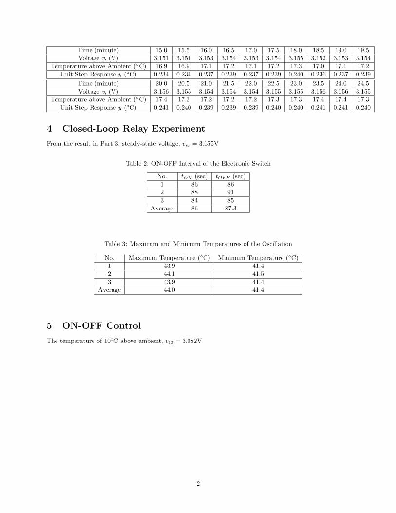
Time (minute) 15.0 15.5 16.0 16.5 17.0 17.5 18.0 18.5 19.0 19.5Voltage v, (V) 3.151 3.151 3.153 3.154 3.153 3.154 3.155 3.152 3.153 3.154
Temperature above Ambient (∘C) 16.9 16.9 17.1 17.2 17.1 17.2 17.3 17.0 17.1 17.2Unit Step Response y (∘C) 0.234 0.234 0.237 0.239 0.237 0.239 0.240 0.236 0.237 0.239
Time (minute) 20.0 20.5 21.0 21.5 22.0 22.5 23.0 23.5 24.0 24.5Voltage v, (V) 3.156 3.155 3.154 3.154 3.154 3.155 3.155 3.156 3.156 3.155
Temperature above Ambient (∘C) 17.4 17.3 17.2 17.2 17.2 17.3 17.3 17.4 17.4 17.3Unit Step Response y (∘C) 0.241 0.240 0.239 0.239 0.239 0.240 0.240 0.241 0.241 0.240
4 Closed-Loop Relay Experiment
From the result in Part 3, steady-state voltage, vss = 3.155V
Table 2: ON-OFF Interval of the Electronic Switch
No. tON (sec) tOFF (sec)1 86 862 88 913 84 85
Average 86 87.3
Table 3: Maximum and Minimum Temperatures of the Oscillation
No. Maximum Temperature (∘C) Minimum Temperature (∘C)1 43.9 41.42 44.1 41.53 43.9 41.4
Average 44.0 41.4
5 ON-OFF Control
The temperature of 10∘C above ambient, v10 = 3.082V
2

Table 4: ON-OFF Period of the Electronic Switch
No. tON (sec) tOFF (sec)1 50 1472 49 1363 51 144
Average 50 142.3
Table 5: Maximum and Minimum Temperatures of the Oscillation
No. Maximum Temperature (∘C) Minimum Temperature (∘C)1 37.5 34.92 37.2 34.93 37.0 34.9
Average 37.2 34.9
6 Discussions
6.1 Experimental Unit Step Response
From Table 1, the experiment unit step response is plotted as shown in Figure 1.
Figure 1: Unit Step Response from the Experiment
3

6.2 Ziegler-Nichols Step Response Method - First-Order Plus Dead-TimeModel
The system is approximated by a first-order plus dead-time model as shown in Figure 2.
Figure 2: Ziegler-Nichols Step Response Approximation
The unit step response of the experiment data is approximated by
Gp(s) =Kp
sT + 1e−sL
with Kp = 0.24, L = 0.5 and T = 4.5.
Unit step response for the transfer function,
Gp(s) =0.24
4.5s+ 1e−0.5s
is superimposed with the unit step response from the experiment data (Figure 3).
4

Figure 3: Unit Step Response of Experiment Data (Solid Line) Approximated by First-Order Plus Dead-TimeModel (Dashed-Line)
6.3 Method of Areas - First-Order Plus Dead-Time Model
By calculating areas from the unit step response of the experiment data shown in Figure 1, we can obtain
A0 = 1.02 = Kp(T + L)
A1 = 0.31 = KpTe−1
Substituting Kp = 0.24, we got T = 3.51 and L = 0.739. Unit step response for the transfer function,
Gp(s) =0.24
3.51s+ 1e−0.739s
is superimposed with the unit step response from the experiment data (Figure 4).
5

Figure 4: Unit Step Response of Experiment Data (Solid Line) Approximated by First-Order Plus Dead-TimeModel (Dashed-Line)
6.4 Least-Square Estimation - First-Order Model
Consider a first-order model,
Y (s)
U(s)=
Kp
Ts+ 1
TsY (s) + Y (s) = KpU(s)
T.y(t) + y(t) = Kpu(t)
With sampling interval 0.5s,
Ty(tk)− y(tk−1)
0.5+ y(tk) = Kpu(tk)
y(tk) =T
T + 0.5y(tk−1) +
0.5Kp
T + 0.5u(tk)
= �1y(tk−1) + �2u(tk)
where
Kp =�2
1− �1(1)
T =0.5�11− �1
(2)
Using least-square approximation method on the experiment data in Table 1, we obtain �1 = 0.9074 and�2 = 0.0230.
6

Substituting �1 = 0.9074 and �2 = 0.0230 into equation 1 and 2 gives us the approximate first-order transferfunction,
Gp(s) =0.2484
4.9016s+ 1
The unit step response from the estimated first-order model is superimposed with the unit step responsefrom the experiment data (Figure 5).
Figure 5: Unit Step Response of Experiment Data (Solid Line) Approximated by First-Order Model (Dashed-Line) using Least-Square Approximation
6.5 Relay Feedback - Second-Order Plus Dead-Time Model
The following parameters are obtained from Table 2 and Table 3 in Section 4.
Tu = 173.3
a = 1.3
d =122
2= 72
Ku =4d
�a= 70.52
By inspection,
L = 0.25
Kp = 0.24
We knowarg Gp(j!u) = −�
7

and
∣Gp(j!u)∣ = 1
Ku
where
Gp(s) =Kp
(sT1 + 1)(sT2 + 1)e−sL
We have
− arctan!uT1 − arctan!uT2 − !uL = −� (3)
Kp√!2uT
21 + 1
√!2uT
21 + 1
=1
Ku(4)
Solving equation 3 and 4 simultaneously after substituting Ku = 70.52, Kp = 0.24, L = 0.25 and !u =2�Tu× 60 = 2.175, we got
T1 = 2.2
T2 = 1.5
The approximated second-order plus dead-time step response of
Gp(s) =0.24
(2.2s+ 1)(1.5s+ 1)e−0.25s
is superimposed with the step response of the experiment data (Figure 6).
Figure 6: Unit Step Response of Experiment Data (Solid Line) Approximated by Second-Order Plus Dead-Time Model (Dashed-Line)
8

6.6 ON-OFF Control
Using Table 4 and 5, the approximate average temperature,
Tave =50× 37.2 + 142.3× 34.9
50 + 142.3= 35.5∘C
7 Conclusions
1. A system can be estimated by a first-order plus dead-time process model using Ziegler-Nichols open-loop method of tuning by obtaining the parameters of the open-loop step response.
2. The system can also be estimated using Ziegler-Nichols ultimate cycling method of tuning by obtainingthe ultimate gain and ultimate period from the relay system.
3. Alternately, method of area and least square estimation can be used to estimate the system.
9


