
Cost Estimation Algorithms for Dynamic Load Balancing of AMR
Simulations
Justin Luitjens, Qingyu Meng, Martin Berzins, John Schmidt, et al.
Thanks to DOE for funding since 1997, NSF since 2008, TACC, NICS

Uintah Parallel Computing Framework
• Uintah - far-sighted design by Steve Parker : – Automated parallelism
• Engineer only writes “serial” code for a hexahedral patch
• Complete separation of user code and parallelism
• Asynchronous communication, message coalescing
– Multiple Simulation Components• ICE, MPM, Arches, MPMICE, et al.
– Supports AMR with a ICE and MPMICE– Automated load balancing & regridding– Simulation of a broad class of fluid-structure
interaction problems

Uintah Applications
Virtual
Soldier
Angiogenesis
Micropin Flow
Shaped Charges
Sandstone
Compaction
Foam
Compaction
Industrial Flares
Plume Fires
Explosions

How Does Uintah Work?
Task-Graph Specification•Computes & Requries
Patch-Based Domain Decomposition
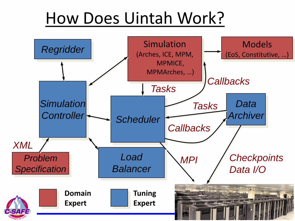
How Does Uintah Work?
Simulation
Controller
Problem
Specification
XML
Simulation(Arches, ICE, MPM,
MPMICE, MPMArches, …)
Scheduler
Tasks
Data
ArchiverTasks
MPILoad
Balancer
Regridder
Callbacks
Callbacks
Checkpoints
Data I/O
Models(EoS, Constitutive, …)
Domain Expert
Tuning Expert

Legacy Issues
• Uintah is 12+ years old
• How do we scale to today’s largest machines?
– Identify and understand bottlenecks
• TAU, hand profiling, complexity analysis
• Reduce O(P) Dependencies– Look at memory footprint?
– Redesigned components for O(100K) processors
• Regridding, Load Balancing, Scheduling, etc
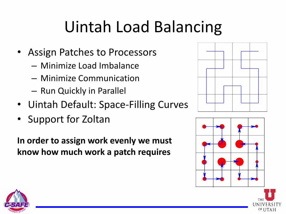
Uintah Load Balancing
• Assign Patches to Processors – Minimize Load Imbalance
– Minimize Communication
– Run Quickly in Parallel
• Uintah Default: Space-Filling Curves
• Support for Zoltan
In order to assign work evenly we must know how much work a patch requires

Cost Estimation: Performance Models
Er,t = c1 Gr + c2 Pr + c3
Er,t: Estimated Time Gr: Number of Grid Cells
Pr: Number of Particles
c1, c2, c3 : Model Constants
G0 P0 1
… … …
Gn Pn 1
c1
c2
c3
=Or,t: Observed TimeO0,t
…
On,t
•Need to be proportionally accurate•Vary with simulation component, sub models, compiler, material, physical state, etc.
Can estimate constants using least squares at runtime
What if the constants are not constant?

Cost Estimation: Fading Memory Filter
Er,t: Estimated Time Or,t: Observed Time α: Decay Rate
Er,t+1 = α Or,t + (1 - α) Er,t
• No model necessary• Can track changing phenomena• May react to system noise• Also known as:
• Simple Exponential Smoothing• Exponential Weighted Average
= α (Or,t - Er,t) + Er,t
Error in last prediction
Compute per patch

Cost Estimation: Kalman Filter, 0th Order
Er,t+1 = Kr,t (Or,t - Er,t) + Er,t
Er,t: Estimated Time Or,t: Observed Time
Kr,t = Mr,t / (Mr,t +σ2)Update Equation:
Gain:
Mr,t = Pr,t-1 + φa priori cov:
a posteri cov: Pr,t = ( 1 - Kr,t ) Mr,t
• Accounts for uncertainty in the measurement: σ2
• Accounts for uncertainty in the model: φ• No model necessary• Can track changing phenomena• May react to system noise• Faster convergence than fading memory filter
P0= ∞

Cost Estimation Comparison
Ex. Cont. M. Trans.
Model LS 6.08 6.63
Memory 3.95 2.64
Kalman 3.44 1.21
Exploding ContainerMaterial Transport
•Filters provide best estimate•Filters spike when regridding

AMR ICE Scalability
One 83 patch per processor
Highly Scalable AMR Framework
Even with small problem sizes
Problem: Compressible Navier-Stokes

AMR MPMICE Scalability
Decent MPMICE scaling
More work is needed
One 83 patch per processor
Problem: Exploding Container

Conclusions
• The complexity and range of applications within Uintah require an adaptable load balancer
• Profiling provides a good method to predict costs without burdening the user
• Large-Scale AMR requires that all portions of the algorithm scale well
• Through lots of work AMR within Uintah now scales to 100K processors
• A lot more work is needed to scale to O(200K-300K) processors

Questions?


![Mark Sh. Levin arXiv:1706.03065v1 [cs.DS] 9 Jun 2017load balancing, assembly line balancing, etc. Solving methods: exact algorithms, approximation algorithms, heuristics, metaheuristics](https://cdn.vdocuments.mx/doc/165x107/5e29132460c3ed681a02330c/mark-sh-levin-arxiv170603065v1-csds-9-jun-2017-load-balancing-assembly-line.jpg)


