new active charge balancing methods and algorithms for
TRANSCRIPT
Année 2018 N° d’ordre :
UNIVERSITÉ DE HAUTE-ALSACE UNIVERSITÉ DE STRASBOURG
THESE
Pour l’obtention du grade de
DOCTEUR DE L’UNIVERSITÉ DE HAUTE-ALSACE
ECOLE DOCTORALE : Mathématiques, sciences de l’information et de l’ingénieur (ED 269)
Discipline : Électronique, Électrotechnique et Automatique
Présentée et soutenue publiquement
par
M.Sc. Manuel RÄBER
Le 17 Décembre 2018
New Active Charge Balancing Methods and Algorithms for Lithium-Ion Battery Systems
Sous la direction du MCF HDR Djaffar Ould Abdeslam et de Prof. Dr.-Ing. Andreas Heinzelmann
Jury : Prof. Marie-Cécile Péra, Université de Franche-Compte (Rapporteur)
Prof. Nicola Schulz, University of Applied Sciences and Arts Northwestern Switzerland
FHNW (Rapporteur)
Prof. Hubert Razik, Université Claude Bernard Lyon 1 UCBL (Examinateur)
Prof. Alain Dieterlen, Université de Haute Alsace UHA (Examinateur)
MCF HDR Djaffar Ould Abdeslam, Université de Haute Alsace UHA (Directeur de thèse)
Prof. Andreas Heinzelmann, Zurich University of Applied Sciences ZHAW (co-Directeur)


iii
Abstract
Active charge balancing is an emerging technique to implement high performing lithium-ion battery systems. Six new active balancing methods are proposed in this thesis to overcome efficiency and power limitations of present balancing architectures. The six methods are different but related in terms of their working principles. Common to all, they rely on the use of non-isolated DC/DC converters and a MOSFET switch-matrix. Depending on the power flow and the switch-matrix configuration, they are able to balance arbitrary cells of a battery system at high currents. Adjacent cells can be balanced simultaneously. The performance comparison is based on batch numerical simulations using calculated and measured efficiency values of DC/DC converter prototypes. The hereby engaged balancing algorithms were implemented in MATLAB. In comparison with the introduced methods, a classic active balancing method C2St2C (Cell-to-stack-to-cell) and passive balancing were analysed as well. For the given system setting with eight battery cells in series, the simulations show an overall balancing efficiency of up to 93.6%, compared to 89.6% for C2St2C and a reduction in balancing time by up to 27.5%. The usable capacity increases from 97.1% in a passively balanced system to 99.7% for the new methods which results in a 2.6% higher battery capacity. A system simulation was set up to demonstrate the working principle of the new methods and verify the numerical calculations. Finally, a hardware prototype was developed which integrates two of the suggested balancing types. First tests have confirmed its ability to actively balance the different state of charge levels of the cells in battery system with high efficacy.

iv
Résumée
L'équilibrage actif de charge est une technique émergente pour mettre en œuvre des systèmes de batteries lithium-ion très performants. Six nouvelles méthodes actives d'équilibrage sont proposées dans cet article pour surmonter les limites d'efficacité et de puissance des architectures d'équilibrage actuelles. Les six méthodes sont différentes, mais liées en termes de principe de fonctionnement. Commun à toutes, elles sont basées sur des convertisseurs DC/DC non isolés et une matrice de commutation MOSFET. En fonction du flux de puissance et de la configuration de la matrice de commutation, elles sont capables d'équilibrer des cellules arbitraires d'un système de batterie à des courants élevés. Les cellules adjacentes peuvent être équilibrées simultanément. La comparaison des performances est basée sur des simulations numériques de lots utilisant les valeurs de rendement calculées et mesurées des prototypes de convertisseurs DC/DC. Les résultats de la simulation sont comparés à une méthode classique d'équilibrage actif C2St2C (Cell-to-stack-to-cell) et à un équilibrage passif. Pour un système donné avec huit cellules de batterie en série, les simulations montrent un rendement d'équilibrage global allant jusqu'à 93,6%, contre 89,6% pour C2St2C et une réduction du temps d'équilibrage pouvant atteindre 27.5%. La capacité utilisable passe de 97,1% dans un système équilibré passivement à 99,7% pour les nouvelles méthodes. Une simulation des systèmes est mise en place pour montrer le principe de fonctionnement des nouvelles méthodes et vérifier les calculs numériques. Enfin, un prototype a été développé qui intègre deux des types d'équilibrage proposés. Les premiers tests ont confirmé sa capacité à équilibrer activement un système de batterie avec une grande efficacité.
v
Zusammenfassung
Aktiver Ladungsaustausch bzw. Balancing ist eine aufkommende Technik zur Implementierung leistungsstarker Lithium-Ionen-Batteriesysteme. In dieser Arbeit werden sechs neue aktive Methoden vorgeschlagen, um die Effizienz- und Leistungsbegrenzungen der bisherigen Architekturen zu überwinden. Die sechs Methoden sind unterschiedlich, aber in Bezug auf ihr Funktionsprinzip verwandt. Allen gemeinsam ist, dass sie auf nicht isolierten DC/DC-Wandlern und einer MOSFET-Schaltmatrix basieren. Je nach Leistungsfluss und Schaltmatrix-konfiguration sind sie in der Lage, beliebige Zellen eines Batteriesystems bei hohen Strömen auszugleichen. Angrenzende Zellen können gleichzeitig ausgeglichen werden. Der Performancevergleich basiert auf numerischen Batch-Simulationen mit berechneten und gemessenen Effizienzwerten von DC/DC-Wandler-Prototypen. Dazu notwendige Algorithmen wurden in MATLAB entwickelt. Die Simulationsergebnisse werden mit einem klassischen aktiven Balancingverfahren C2St2C (Cell-to-Stack-to-Cell) und mit passivem Balancing verglichen. Für das gegebene Systemsetting mit acht Batteriezellen in Serie zeigen die Simulationen einen Gesamtwirkungsgrad der Balancingelektronik von bis zu 93,6%, verglichen mit 89,6% für C2St2C und eine Reduzierung der Ausgleichszeit um bis zu 27.5%. Die nutzbare Kapazität steigt von 97,1% in einem passiven System auf bis zu 99,7% für die neuen Verfahren, was einer Erhöhung der Batteriekapazität von 2.6% entspricht. Eine Systemsimulation demonstriert das Funktionsprinzip des neuen Verfahrens und dient der Überprüfung der numerischen Berechnungen. Zum Schluss wurde ein Hardware-Prototyp entwickelt, der zwei der vorgeschlagenen Balancingmethoden beherrscht. Erste Tests haben bestätigt, dass es damit möglich ist, die Ladezustände der einzelnen Zellen eines Batteriesystems mit hoher Wirksamkeit aktiv auszugleichen.

vi
Acknowledgment
My great thanks for the scientific support go to my supervisors Djaffar Ould Abdeslam from the University of Haute-Alsace UHA in Mulhouse, France and Andreas Heinzelmann from the Zurich University of Applied Sciences ZHAW in Winterthur, Switzerland. It was their personal commitment and the trust they put in me that made this project possible. Thanks to their great experience, they have guided the work in the right direction, motivated me where necessary and greatly enriched the result. I also thank my colleagues who have contributed to the publications that have been produced in the context of this thesis: Adrian Täschler, Andres Ramirez and Dominic Hink. They did important preliminary work and made a lot of things easier for me.
I would further like to extend my thanks to Frank Tillenkamp, head of the Institute for Energy Systems and Fluid-Engineering IEFE, for granting me the opportunity to arrange my working hours flexibly and to work part-time.
For their personal support and patience, I would like to thank my family and friends, especially my girlfriend Laura, who has motivated me time and again. Martin Rohrer was responsible for the proof reading. I am also deeply indebted to him.
During the past three years I have received helpful advice and valuable technical support from many more people at conferences and exhibitions. I also offer my thanks to them and to the companies that supported my work by providing samples and evaluation modules free of charge.

vii
Preface
When I first started to read papers and technical documents on battery management systems it was in the context of my ongoing R&D projects at the Zurich University of Applied Sciences ZHAW in Winterthur. Soon, my attention was drawn to active balancing methods. I found it obvious to recover excess charge during the equalisation process and distribute it to the other cells in the battery system instead of wasting that energy. The wish to estimate the benefit of active charge balancing and the subsequent mathematical analysis represented the beginning of my thesis related work.
I then decided to write my PhD thesis on active charge balancing for lithium ion battery systems in cooperation with the IRIMAS laboratory of the University of Haute Alsace UHA in Mulhouse. My motivation founds on three pillars. Firstly, my position as a research associate at the Zurich University of Applied Sciences includes the supervision of student research projects covering the field of battery systems and energy storage applications. Such a task implies profound knowledge of the related topics as well as constant advancement towards the latest technologies and developments. Secondly, our institute’s R&D activities focus on national projects with industrial collaboration. During the past five years I have worked on battery management systems and power electronic design for several Swiss enterprises and start-up companies such as Kyburz Switzerland, Menu System, Lenze Schmidhauser, Gastros Switzerland, MPower Ventures, Energy Depot and Nexenic. This close collaboration with industrial parties helped me a lot in my thesis related research activities and provided valuable input from the implementation side. Besides that, I believe to have contributed important findings for each project partner as a by-product of my research. Finally and most importantly, my key motivation was my personal interest in batteries, energy efficient applications and power electronic circuits and my wish to contribute to a sustainable, energy responsible and environmental friendly future.

viii
Table of contents
Abstract ....................................................................................................................... iii
Résumée....................................................................................................................... iv
Zusammenfassung......................................................................................................... v
Acknowledgment.......................................................................................................... vi
Preface ........................................................................................................................ vii
Table of contents ....................................................................................................... viii
Introduction ............................................................................................................. 1
Motivation ............................................................................................. 1
Structure of the thesis ............................................................................ 3
Symbols and variables ............................................................................ 4
Technical background .............................................................................................. 5
Historical retrospect ............................................................................... 5
Battery management system .................................................................. 8
Battery state estimation ...................................................................... 10
Battery modelling ................................................................................ 13
Battery ageing ...................................................................................... 16
State of art of balancing methods .......................................................................... 19
Definition of terms ............................................................................... 19
Overview .............................................................................................. 19
Performance and feature comparison ................................................... 34
Cell-to-cell variation of lithium-ion batteries ....................................... 37
Relevant patents .................................................................................. 40
Commercial solutions for active balancing ........................................... 41
Summary of state of art research ......................................................... 43
Analysis of active balancing potential .................................................................... 44
Analytical view on charge transfer during balancing ........................... 44
Available capacity and energy savings ................................................. 45

ix
Numerical parameter sweep simulation ................................................ 49
Module restricted balancing ................................................................. 50
New active balancing methods ............................................................................... 53
Initial position ...................................................................................... 53
Design and components ....................................................................... 53
Description of the proposed circuits ..................................................... 54
Balancing algorithms and simulation model .......................................................... 64
Analysis tool selection .......................................................................... 64
MATLAB numerical simulations ......................................................... 65
Balancing converter efficiencies ............................................................ 71
PLECS equivalent electronic circuit simulation ................................... 74
Hardware implementation ...................................................................................... 79
DC/DC Converter ............................................................................... 79
Switch-matrix unit ............................................................................... 82
Firmware .............................................................................................. 87
BMS controller ..................................................................................... 88
Configuration of the demonstration prototype ..................................... 90
Results .................................................................................................................... 91
MATLAB numerical simulations ......................................................... 91
Verification by electronic circuit simulation ........................................ 97
Measurements ...................................................................................... 99
Part count .......................................................................................... 107
Discussion ............................................................................................................. 109
Comparison by spider chart ............................................................... 109
Applicability of the proposed methods ............................................... 110
Challenges .......................................................................................... 111
Outlook .............................................................................................. 112
Conclusion .......................................................................................... 114
Bibliography .............................................................................................................. 117

x
Lists ........................................................................................................................... 124
A List of acronyms .................................................................................... 124
B List of figures ......................................................................................... 127
C List of tables .......................................................................................... 131
Appendices ................................................................................................................ 132
A Additional patented circuit configurations ............................................ 132
B m-file: Calculation of available capacity ................................................ 134
C m-file: Batch simulation ........................................................................ 134
D m-File: Module restricted balancing ...................................................... 135
E m-File: Definition of battery model parameters ..................................... 136
F m-File: OCV-curve fitting ..................................................................... 136
G m-file: Initialization of PLECS simulation ............................................. 137
H LT8708 Efficiency measurements .......................................................... 138
I BoM of DC/DC converter ..................................................................... 140
J Configuration settings of bq76PL455EVM BMS board ......................... 141
K Schematics of the switch-matrix unit PCB............................................ 142
L Schematics of the DC/DC converter PCB ............................................ 146

Introduction
1
Introduction
The intention of this chapter is to give an introduction into active balancing and to point out the importance of a thorough and multi-objective analysis.
Motivation
Lithium-ion batteries (LIB) are in wide use today in a multitude of applications. It is common knowledge that for a safe use and enduring performance, a battery management system (BMS) is essential. However, what is less widely known is that during each discharge cycle, some unused energy remains in the battery. This is not due to technical design considerations, but to a phenomenon called cell-to-cell variation (C2CV). Due to physical characteristics, individual battery cells in a stack of multiple cells vary in capacity. In battery systems made from series connected cells, this leads to an imbalance in the state of charge (SoC) during use.
The following example in Figure 1 illustrates this effect. Generally, the nominal capacity of a cell Cnom is equal to a state of health (SoH) value of 100%. If a cell has a lower capacity when fully charged, either its Cnom is lower or its SoH value is less than 100%. Figure 1 shows a configuration of two fully charged cells with different SoH values (Cell #1 at 100% SoH and Cell #2 at 80% SoH). Although both SoC are at 100%, the two cells store different amounts of charge. After a full discharge cycle the weak cell reaches its discharge limit first, i.e. is completely empty. If the battery is recharged after such a cycle, the charged state will not exactly be the same as before. Different physical and chemical effects result in less and less energy being stored in the cells over several cycles. In a real battery system, certain cells will be close to their end of discharge level while others are almost fully charged.
Figure 1: Battery states without balancing

Motivation
2
The technical solution to this problem is called ”Balancing”. Simply put, balancing
restores the original state after each full charge (see Figure 2). Depending on the configuration of the battery system and the type of cell, a certain amount of time must be allowed for balancing during each charging cycle. In conventional balancing, the affected charge is dissipated and lost. Therefore it is called passive balancing.
Figure 2: Battery states with balancing
Whereas passive balancing is able to keep a battery system equalized over many
use cycles, it is not capable of utilizing the remaining energy at the end of discharge in some of the cells, as mentioned earlier in this section.
Here active balancing comes into play. To distinguish it from conventional balancing, the terms ”active” and ”passive” have become established. Instead of dissipating the excess charge in resistive networks as for passive balancing, active balancing circuits are able to transfer it to other battery cells. During discharge, as shown in Figure 3, this allows the complete usage of the stored energy.
Figure 3: Active balancing during discharging
During charging, the final state of the battery cells is identical for active and
passive balancing. However, active balancing allows much faster balancing times due to the lower losses. Figure 4 shows the sequence for charging in case of active balancing: Initially, the batteries are completely discharged (final state of Figure 3).

Introduction
3
The charging process has to be stopped in the second step because of Cell #2. At this moment, the balancing unit starts to exchange charge between the two cells. After some time, charging can be continued until both cells reach their full SoC.
Figure 4: Active balancing during charging
Structure of the thesis
The introduction into this work is given in this chapter by pointing out the technical motivation for a thorough investigation of presently used and new active balancing methods. In the next chapter, some important battery related topics are discussed to create a common base for the reader and make the following chapters more comprehensible. After that, the state of art in charge balancing is presented with a focus on non-isolated balancing methods. Theory as well as patents and realized applications have been considered. Chapter 4 contains calculations and considerations of the active balancing potential and compares the performance to passive balancing. Contrary to the hardware related chapters, only theoretical aspect have been considered to make a statement about the maximum achievable benefits.
In Chapter 5, six new active balancing methods are developed and characterized. The required simulation inputs and the associated balancing algorithms are determined in Chapter 6. Furthermore, the implementation into the chosen simulation tools and the simulation setup is explained. The development circle closes with the hardware implementation of one of the proposed balancing methods in Chapter 7. Here, commercially available electronic components are evaluated to realise a high- efficiency balancing hardware.
Finally, Chapter 8 contains the collected simulation and measurement results. The thesis is concluded with a technical discussion of the results and an outlook for the active balancing technology.

Symbols and variables
4
Symbols and variables
Symbol Unit Description
C, CPack, Cnom Ah Capacity, available capacity, nominal capacity
E Expected value
I A Current
m Number of cells in parallel
n Number of cells in series
Q, Qact, Qnom C Charge, current charge, nominal charge
U V Voltage
W J Energy
η Efficiency μ Arithmetic mean value σ Standard deviation

Technical background
5
Technical background
This chapter summarizes the most important historical milestones in the field of rechargeable batteries. Furthermore, different battery related topics are explained as they are supposed to be fundamental for the understanding of the whole thesis.
Historical retrospect
The history of battery research and usage is over 200 years old. Even before the basic principles of electrochemistry were discovered, bright minds such as Luigi Galvani, Alessandro Volta and Johann Wilhelm Ritter experimented with the generation of electricity by bringing together different metals and liquids.
Their findings enabled the reliable use of electrical energy for the first time in the history of mankind. However, the request for remote, mobile or uninterruptable power supply did not start to grow until Werner von Siemens invented the electrical generator in 1866. Very soon, many different user groups asked for electrical energy to supply their electrical pumps, mills and lights. A development was triggered, in which the performance of battery systems, both primary and secondary, has steadily increased and which has continued to this day.
Early rechargeable batteries
In the 1850s, the physicist Wilhelm Josef Sinsteden and Gaston Planté worked with the first lead batteries and used them to store electricity for telegraphic experiments. Both men used lead plates as electrodes, which were given a certain capacity by repeated charging and discharging. However, these batteries were not yet suitable for industrial production. Thanks to the industrialization, electrochemical energy storage developed rapidly. The dynamo and light bulb were invented towards the end of the 19th century. The need to store electrical energy grew rapidly. Lead batteries began to be produced industrially around 1880, when Fauré applied for a patent to produce pasted plates for lead accumulators. For decades, scientists and engineers improved the energy density and lifetime of this battery type, and it remained unrivalled for more than 100 years. In the second half

Historical retrospect
6
of the 20th century, new technologies to store electro-chemical energy slowly emerged. The Nickel-Cadmium (NiCd) battery was invented independently by Jungner and Edison in 1899 and 1901 and roughly doubled the energy density of lead-acid batteries when it was produced on a large scale from 1946 on. However, the technology had its disadvantages: Cadmium is a toxic heavy metal and the battery was unsuitable for many applications due to the so-called memory effect. Nowadays, Ni-Cd batteries are only used in niche applications and have disappeared completely from the consumer sector. Ongoing research on secondary cells lead to the invention of a new technology called Nickel-metal hydride (NiMH) in 1967. Energy density, environmental safety and durability could be increased significantly compared to NiCd. The first consumer-grade NiMH cells became commercially available in 1989 and replaced NiCd in most applications.
Despite all the technical improvements of the past decades, the mentioned technologies were not able to establish themselves along a wide front. Slow charging speed, low charging efficiency and a low energy density limited the range of battery powered applications until the invention of the lithium-ion accumulator.
The rechargeable lithium-ion battery
More than 25 years ago, in 1991, Sony and Asahi Kasei release the first commercial lithium-ion battery. Since then, the energy and power density has steadily increased, and such batteries have replaced other battery technologies in many areas.
A lithium-ion battery consists of two half cells. The first electrode has got a LixMO2 type layered structure, while the second electrode can be made of various materials, most commonly graphite. During the charging process, lithium ions are stored in the "lattice" of the graphite electrode. In charged state, the anode contains a high concentration of intercalated lithium ions while the cathode is depleted of lithium ions. During discharge, lithium ions leave the anode and migrate through the electrolyte to the cathode while their associated electrons are collected by the current collector to power an electric device, as illustrated in Figure 5. Lithium-ion rechargeable batteries have a high nominal voltage compared to conventional rechargeable batteries. Compared to NiMH only one third of series connected cells are required to deliver the same system voltage. They also have no memory effect, a low self-discharge rate and an exceptionally high coulombic efficiency of up to 99.9% [1].
Technical background
7
Figure 5: Electro-chemical processes in lithium-ion cell [2]
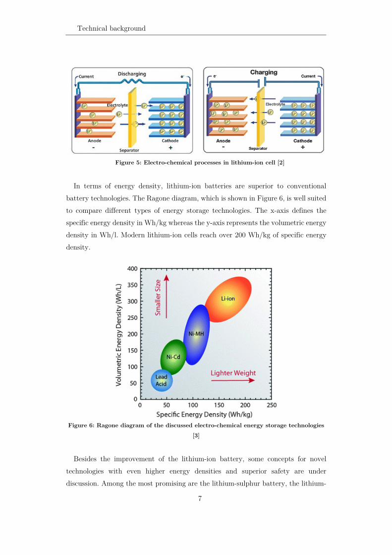
In terms of energy density, lithium-ion batteries are superior to conventional
battery technologies. The Ragone diagram, which is shown in Figure 6, is well suited to compare different types of energy storage technologies. The x-axis defines the specific energy density in Wh/kg whereas the y-axis represents the volumetric energy density in Wh/l. Modern lithium-ion cells reach over 200 Wh/kg of specific energy density.
Figure 6: Ragone diagram of the discussed electro-chemical energy storage technologies
[3]
Besides the improvement of the lithium-ion battery, some concepts for novel
technologies with even higher energy densities and superior safety are under discussion. Among the most promising are the lithium-sulphur battery, the lithium-

Battery management system
8
air battery and the solid-state battery. It is expected that the annual growth rate in energy density of approximately 7% can be maintained for the coming decades [4].
Battery management system
Besides the battery cells, the battery management system (BMS) is the most important part of a battery. Figure 7 shows how a BMS complements a conventional battery system (red box) made from several cells in series. Wires from each cell level connect to the BMS board (green box) where they enable the measurement of all cell voltages. Alternatively, single cell balancer are sometimes used in large battery systems to avoid the connection cables that would otherwise be required.. For batteries with more than one cell in series, balancing is recommended and increases the lifetime of a battery significantly. A mean of short-circuit protection is mandatory and implemented here with a fuse. The microcontroller unit (MCU) and current monitoring are optional but widely used especially for larger battery systems. If a BMS can independently disconnect the battery from the load during fault state, it is sometimes also referred to as “Protection circuit module” (PCM). For low voltage systems, MOSFETs are used almost exclusively as disconnecting devices. In Figure 7, that device is represented by a normally-closed switch.
Figure 7: Function blocks of a BMS and embedding into battery system
The most important task of a BMS is to protect the individual cells by keeping
them in a safe state and to prolong their calendrical and cyclical lifetime. This is

Technical background
9
especially important for lithium-ion battery packs containing several cells connected in series. This type of battery must not be overcharged or over-discharged; otherwise, the cells may be damaged (see [5]). Other tasks of a BMS are:
• Measuring of cell voltage, current and temperature (i.e. Monitoring) • Charge equalization (i.e. Balancing) • Battery condition estimation (SoC, SoH estimation, etc.) • Detection and recording of short-circuit, over-voltage and under-voltage • Load disconnection for short-circuit protection
To perform these tasks, the BMS monitors all cell voltages, the battery current
and the battery temperature in at least one place. These parameters are measured using specially designed integrated circuits (IC). Most commonly, “analog front ends” (AFE) are used. These are described in more detail in Section 3.6.1.
From the measured values, it is possible to calculate the state of charge (SoC) and the state of health (SoH) of the battery. Various procedures are available for this purpose, which are examined in more detail in Section 2.3.1 and 2.3.2.
Exceeding the maximally allowed cell voltage in lithium-ion cells can lead to an overcharging of the cells and cause a thermal run-away if the protective measures are missing or faulty. The same failure can also appear during a short circuit or when operating the battery at overload condition. In contrast, going below the minimum allowed cell voltage causes over-discharging and can also damage or destroy the cell. Therefore, the cell voltage, the temperature and the current must be kept within certain limits so that the cells can be operated safely.
Since lithium-based battery cells normally have a voltage in the range between 2 V and 4.3 V, they must be connected in series for most applications to obtain a useful system voltage. Variations in the internal impedance and the initial state of charge, different degradation and inhomogeneous temperature distribution in the battery pack cause an imbalance in the charge distribution of the individual cells. This means that certain cells have a higher voltage during charging and discharging than others. This imbalance affects the lifetime of the battery system, as it can lead to overcharging or over-discharging of individual cells. Another negative effect of the imbalance is that the nominal capacity of a battery system cannot be fully utilized.

Battery state estimation
10
At the time when large battery systems were made from lead-acid or NiCd/NiMH cells, uneven charge distribution was a minor issue. Overcharging these cells with the usual low charging currents would lead to a relatively harmless increase in charging losses and gas evolution. Lithium-ion cells, however, are much more sensitive to overvoltage. Therefore, a BMS with charge balancing function is required to protect the battery system against damage and premature battery failure. The balancer ensures that all cells are charged to the same SoC. Passive balancing has been the method of choice in the past and is based on a resistive circuit to dissipate excess charge and thereby equalize the charge in the cells. Major drawbacks of passive balancing are a rather high balancing time due to the limited heat dissipation and a reduction in overall charging efficiency. Today, as the demand for large lithium-ion based battery systems increases, these drawbacks become more important to the designers of battery powered devices.
Battery state estimation
A battery cell is a complex, highly nonlinear electrochemical system. However, only a few parameters such as cell voltage, current and temperature can be measured directly. For this reason, the characteristic values SoC and SoH have been defined, which are determined by measured values.
State of charge (SoC)
The state of charge is the remaining charge Cact in a battery and is expressed as a percentage of the nominal capacity Cnom.
𝑆𝑆𝑆𝑆𝑆𝑆(%) = 𝑆𝑆𝑎𝑎𝑎𝑎𝑎𝑎
𝑆𝑆𝑛𝑛𝑛𝑛𝑛𝑛∙ 100% (1)
Different methods exist in literature for determining the state of charge. Detailed
reviews are available in [6], [7] and [8]. Instead of SoC, the term “State of Discharge” (SoD) may be used (see [9]), which is defined as:
𝑆𝑆𝑆𝑆𝑆𝑆(%) = 100% − 𝑆𝑆𝑆𝑆𝑆𝑆(%) (2)

Technical background
11
This section briefly introduces the most popular methods, which are: • Look-up table for C-V characteristics • Coulomb counting or current integration method • Electric equivalent circuit model • Kalman filter
Look-up table for C-V characteristics
The voltage that is present at the battery terminals depends on the SoC. This correlation has been used for decades to indicate the SoC of primary and lead-acid batteries. However, not only does the SoC affect the terminal voltage but also other parameters such as the internal resistance and the chemical reaction time constants. Figure 8 and Figure 9 show the capacity-voltage (C-V) curve of two lithium battery types at different discharge currents. The effect of the load current on the terminal voltage cannot be neglected: In Figure 8, a terminal voltage of 3.6 V appears at either a full or almost empty battery depending on the load current. For LiFePO4 cells, the gradient of the C-V curve is 2 mV/%SoC which is not enough to make a statement on the SoC with the available monitoring equipment. Therefore, look-up table based SoC estimation is not suited for high-current or LiFePO4 applications. Sufficient accuracy can only be achieved by adding a current compensation.
Figure 8: C-V characteristic of NCA-
type Li-ion cell [10]
Figure 9: C-V characteristic of LiFePO4
cell [11]

Battery state estimation
12
Coulomb counting
The current integration method, also called “coulomb counting”, is based on current measurement and its integration. The charge that flows into or out of the battery is added or subtracted from the initial SoC. Consequently, the SoC is calculated according to (2):
𝑆𝑆𝑆𝑆𝑆𝑆(%) = 𝑆𝑆𝑆𝑆𝑆𝑆𝑖𝑖 −∑ 𝐼𝐼∆𝑡𝑡
𝑆𝑆𝑛𝑛𝑛𝑛𝑛𝑛 ∙ 3600∙ 100% (3)
The disadvantage of this method is that even a small offset in the current
measurement over a certain period of time leads to a significant error. Due to the limited sampling rate of the measuring system, rapid current changes also cause inaccuracies. In addition, the self-discharge of the battery cannot be detected by the current integration method.
Electric equivalent electric circuit
This method uses an electrical equivalent model to determine the open circuit voltage (OCV). By using an OCV-SoC characteristic as shown in Figure 64, the charge status can be estimated.
In the field of battery cell modelling, a lot of research has been carried out in recent years. A simple electrical model based on RC elements is the Thévenin model described in [12] and shown in Figure 63. All parameters of the model are dependent on SoC, cell temperature and current; which makes their determination complex. One approach is to fit the parameters based on cell measurement data at different operating points and store them in a multi-dimensional lookup table [13]. With the corresponding parameters for the current operating point, the model allows the open-circuit voltage to be calculated at any time according to equations (3) and (4). It can be built up with any number of RC-elements to increase the accuracy.
However, the exact estimation of the SoC is difficult because of the flat OCV-SoC characteristic of certain lithium-based cells, especially for LiFePO4. Measuring errors of the cell voltage in the order of 10 mV can lead to deviations of up to 20% in the estimation of the SoC [14] depending on the discharge current and temperature. This applies especially in the flat part of the curve between 40% and 60% SoC.

Technical background
13
Kalman filter
The methods described in the previous sections form the base for combined methods such as the Kalman filter method. The SoC determined by the coulomb counter is corrected by an extended Kalman filter, which compares the measured voltage with the calculated voltage ([15] and [16]). This method is very powerful and versatile. It provides good accuracy for SoC estimation without the need of measuring equipment with accuracies below 1%. For detailed information about Kalman filters see [17], [18] and [19].
State of health (SoH)
The chemical processes taking place in the cell also cause ageing without the battery being used. This process is called calendric ageing. In addition, degradation happens from the charging and discharging cycles of the battery, which is referred to as cyclic ageing. Both types of ageing depend on temperature, whereas cyclic ageing also depends on current intensity and the depth of discharge (DoD). As ageing progresses, the cell capacity decreases and the internal resistance increases.
If a lithium-ion battery is operated correctly, it delivers an average of 500-1000 cycles before it has lost 20% to 30% of its capacity, which corresponds to a SoH values of 70% to 80%. At this state, a battery is usually no longer considered usable. There are several definitions of the SoH due to the different ageing mechanisms. The most common ones are based on the loss of capacity SOHC and the increase in internal resistance SOHR [13]:
𝑆𝑆𝑆𝑆𝐻𝐻𝐶𝐶 (%) = 𝑆𝑆𝑎𝑎𝑎𝑎𝑎𝑎
𝑆𝑆𝑛𝑛𝑛𝑛𝑛𝑛∙ 100%, 𝑆𝑆𝑆𝑆𝐻𝐻𝑅𝑅(%) = 100 +
𝑅𝑅𝑛𝑛𝑛𝑛𝑛𝑛 − 𝑅𝑅𝑎𝑎𝑎𝑎𝑎𝑎
𝑅𝑅𝑛𝑛𝑛𝑛𝑛𝑛∙ 100 (4)
Battery modelling
The terminal voltage of a battery varies as it is charged and discharged, exhibiting a nonlinear correlation with the battery SoC. The aim of modelling is to achieve the most efficient replication of the real system, which reproduces all relevant effects with sufficient accuracy. Thus, it is important that a battery model reflects the voltage change as a function of the SoC. Today, computer simulations are often used

Battery modelling
14
to design battery storage systems and optimize operating strategies. The simulations are based on suitable battery models that reproduce the relevant properties with sufficient accuracy. The models can be used, for example, to draw conclusions about the usable energy and the thermal losses occurring under various operating conditions. This is helpful in determining the required nominal capacity of the battery and the dimensioning of the cooling system.
Type of models
Lithium-ion battery models can be divided into three main categories: Electrochemical ([20], [21], [15]), electrical ([22], [23], [24]) and mathematical ([25], [26], [27]).
Electrochemical models
With this type of model, the structure of the individual materials inside the battery are reproduced as accurately as possible. The potential and diffusion gradients in different spatial directions are mathematically described by means of several coupled differential equations. The highly complex modelling approaches can seldom show their potential in practice, since the numerous parameters, such as diffusion coefficients of the individual materials and their dependence on temperature and ageing, are difficult to determine.
Electrical equivalent circuits
These models are based on a network of resistors and capacitors connected to a controllable voltage source and called electrical equivalent circuit (EC). The advantage of this modelling method is its high flexibility. Simple adaptation of the model complexity to the requirements of the respective application is possible. Detailed models achieve a precise replication of the individual electrochemical effects, while highly simplified models with only a few resistances and capacitances allow very fast calculation on low-end computing hardware such as MCU. In complex systems, like a complete vehicle simulation, this can often be more important than the high-resolution simulation of the battery dynamics. By further optimization of the calculation effort, the battery model is even able to be calculated in parallel with the system in use. This establishes new possibilities for many different applications.

Technical background
15
Mathematical black box models
Mathematical black-box models include all approaches based on mathematical models that link the input and output variables of a battery storage device according to empirical findings. This includes analytical terminal voltage models but also more complex approaches such as stochastic battery models, neuronal networks or fuzzy logic, which are trained based on recorded measurement data. Excluded are the EC models described in the previous section.
Electrical model data acquisition
The required electrical data for the different models includes OCV curves and the values of the EC parts. The integration into the electrical model is described in e.g. [28] and [29].
OCV measurement
The equilibrium voltage of a battery in an uncharged idle state depends mainly on its SoC. The more charged the battery, the higher the open-circuit voltage. This can be measured after a certain waiting time at the terminals, when all dynamic reactions have ceased. Waiting times of up to several hours are required. In [30] a common procedure for recording the OCV characteristic curve of a battery is described: It involves systematic discharging or charging with pauses of several minutes to hours between step sizes of 0.5% to 5% of Cnom. The voltages that appear after each waiting pause are then used as reference points for the open-circuit voltage characteristics. Depending on the number of sampling points and the length of the waiting pauses, such a measurement takes several days.
Battery impedance spectroscopy
A modern method to derive the different parameters for electrical equivalent circuit models is impedance spectroscopy (see [31] and [32]). Additionally, the ageing effects in battery cells can be determined from the hereby-acquired measurement data. Impedance spectroscopy does not only deliver the DCR of a cell, but also information on series inductance and parallel capacitance. In theory, the SoC and SoH values can be estimated only from the impedance curve if a set of reference curves of the same cell is available [33]. The procedure is illustrated in Figure 10.

Battery ageing
16
Figure 10: Ideal impedance spectrum of a lithium-ion cell and an EC with three RC-
elements [31]
Battery ageing
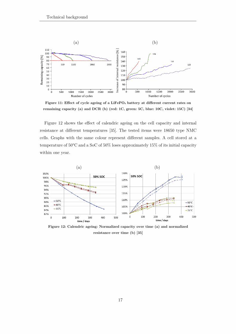
The period between the manufacturing date of a rechargeable battery (Begin of Life, BoL) and the time when previously defined values are undercut due to ageing (End of Life, EoL) is called service life. It provides information on how long a battery can be used for energy storage for a certain application without considerable performance losses. It is difficult to give an exact time value for the service life since it depends on many factors as explained in the previous sections. The ageing process is divided into a calendric and a cyclic ageing part. The value of charge and discharge current is usually found to have the biggest effect on battery ageing. Figure 11 shows the results of capacity and DCR measurements at different current rates [34]. Although the investigated cell was a high power cell and therefore suited for high charge and discharge currents, the lowest and highest cycle numbers differ from each other by a factor of five.
Technical background
17
(a) (b)
Figure 11: Effect of cycle ageing of a LiFePO4 battery at different current rates on
remaining capacity (a) and DCR (b) (red: 1C, green: 5C, blue: 10C, violet: 15C) [34]
Figure 12 shows the effect of calendric ageing on the cell capacity and internal
resistance at different temperatures [35]. The tested items were 18650 type NMC cells. Graphs with the same colour represent different samples. A cell stored at a temperature of 50°C and a SoC of 50% loses approximately 15% of its initial capacity within one year.
(a) (b)
Figure 12: Calendric ageing: Normalized capacity over time (a) and normalized
resistance over time (b) [35]


State of art of balancing methods
19
State of art of balancing methods
This chapter presents the research conducted on balancing methods so far, as well as the technical solutions provided by industry. The following sections give an overview of the most important and interesting balancing methods and their characteristics.
Definition of terms
In the past, the terms “Passive balancing” and “Active balancing” have not always been used consistently. In the introduction of [36] from 2008, “Passive balancing” was meant for battery cells, where internal chemical processes ensure that no undesirable, potentially dangerous processes can occur even in the event of overcharging. In such cells, the excess energy is converted into heat in the battery or degraded by outgassing. In practice, this type of balancing can only be applied to overcharge-resistant lead-acid, NiCd and NiMH batteries. In another early publication on LIB balancing, the term “Natural balancing” is used for the balancing [37]. “Active balancing”, on the other hand, represented an external balancing circuit with a transistor as an active element to e.g. connect a shunting resistor to the cell.
With the emergence of regenerative balancing circuits and the extinction of self-balancing accumulator technologies, the meaning of the term changed. In 2010, Cadar et al. [38] used the following definition: The circuits formerly known as “Active Balancing” are now called “Passive Balancing” and the difference is no longer defined by the presence of an active component but on whether the balancing process is dissipative (referred to as passive) or recuperative (active). This nomenclature has established itself as a standard in modern literature and will be used in this thesis.
Overview
In 2014, Gallardo et al. classified all previously known methods of cell balancing in an extensive review paper [39]. In total, 24 different balancing architectures are described and compared. Many of these methods exist only in theory and have never

Overview
20
been built in hardware not to mention proven themselves against approved techniques. Their classification distinguishes five groups that differ from each other by the direction of the charge transfer: Cell bypass, Cell-to-Cell, Cell-to-Pack, Pack-to-Cell, Cell-to-Pack-to-Cell. Figure 13 shows the complete list from the mentioned review paper. In the following sections, the most important methods are presented in more detail.
Figure 13: Classification of different active balancing methods acc. to [39]
The spider charts that are presented in the following sections are based on the
classification given in Table 1. The rating parameters are defined as follows based on a BMS for eight cells (higher is better):
• Estimated cost of balancing circuit components • Control and implementation complexity • Charge equalization speed • Expected balancing efficiency • Space requirements (Switch-matrix (SWM) and transformer (Tr) are the
relevant parts)

State of art of balancing methods
21
• Power rating of the considered design
Table 1: Classification table for rating of balancing methods
Parameter / Rating
1 2 3 4
Cost ≥ 35 € < 35 € < 20 € < 10 €
Complexity SWM / Multi-winding Tr + uC
SWM / Multi-winding Tr
Simple FET control
No Tr. Analog control
Speed > 10 h > 5 h > 1 h < 1 h Efficiency < 50% < 75% < 85% ≥ 85%
Size Tr + Large SWM Tr + SWM or large SWM
Tr or SWM No Tr No SWM
Power < 0.2 A < 1 A < 3 A ≥ 3 A
Other literature with performance comparison of different balancing methods is
described in Section 3.3.
Passive or shunting balancing
Passive balancing is widely used in today’s applications. The working principle is described in almost every book about battery systems (e.g. [14], [40] or [41]). Technically, the main elements are a power resistor and a controllable MOSFET switch. During the charging process, the voltage of each cell or cell level is continuously monitored by the BMS. As soon as a cell voltage exceeds the balancing threshold, the MOSFET is turned on to create a cell bypass. Consequently, charge is dissipated through the resistor, which discharges the cell slowly. The BMS keeps the switch closed as long as the cell voltage remains above the balancing threshold. This safety feature can also run in analog electronics without the need of a micro-controller. Depending on the charging status and the power rating of the balancing circuit, the battery charger current must be reduced or turned off completely. Figure 14 shows the electric circuit on the left side and the spider chart on the right side. The method is very simple and provides balancing at a very low cost.

Overview
22
(a) (b)
Figure 14: Passive balancing with dissipative element (a) and its spider chart (b)
Active balancing
In recent years, many active balancing solutions have been introduced. These are able to overcome the efficiency issues of passive balancing and transfer charge between individual cells at high efficiency. They represent a promising possibility of enhancing the energy efficiency and eco friendliness of lithium-ion battery systems. Unlike passive balancing, they can also be used during the discharging process and increase the usable battery capacity. The charge transfer paths of the different active balancing types known from Figure 13 are shown in Figure 15. Cell-to-Cell applies if the proposed balancing circuit is able to directly transfer charge between arbitrary cells. Any technology that transfers charge from or to a cell using the battery stack as an energy storage is called Cell-to-Stack, Stack-to-Cell or Cell-to-Stack-to-Cell. Passive balancing is referred to as Cell-to-Null because the charge is not recuperated. The Cell Bypass method does not show up in the figure as there is no charge transfer involved and the method only works if a load current is apparent. More information on these balancing methods can be found in Section 3.2.3.1.

State of art of balancing methods
23
Figure 15: Charge transfer paths of different balancing methods
Switched capacitors
One of the first active balancing topologies was the use of switched capacitors (Figure 16). This method uses capacitors to shift the charge from one cell to another. There are several modifications like double-tiered switched capacitor ([42], [43] and [44]) or single switched capacitor [45] to name the most important ones. The single switched capacitor variant is a cost-optimized implementation of the switched capacitor principle with the disadvantage that charge equalization requires more time.
According to (5), the transferable charge Q is defined by the voltage difference U1 – U2 between the cells and the capacitance of the capacitor. Hence, for small voltage differences, the switched capacitor method is slow. Charge can be transferred between adjacent cells at a limited speed defined by the capacitor size and the switching frequency. A modification of the circuit towards the double-tiered switched capacitor method accelerates the charge transfer by a factor of four [39].
𝑄𝑄 = 𝑆𝑆 (𝑈𝑈1 − 𝑈𝑈2) (5)

Overview
24
(a) (b) (c)
Figure 16: Standard switched capacitor topology [5] (a), Double-tiered switched
capacitor topology [5] (b) and Single switched capacitor topology (c)
New developments in the field of switched capacitors are being driven forward by
IC manufacturers. For certain conversion ratios, e.g. from 48°V to 24 V, the efficiency of such converters goes up to 99% (see [46]).
Switched inductor or boost shunting
Similar to the switched capacitor topology, charge can be transferred between adjacent cells by using inductors instead of capacitors. Technically, switched inductor circuits conform to inverting buck-boost converters or boost converters. The switched inductor method was first proposed in the early 21st century by Hsieh et al. [47] and Zhao et al. [48] when they introduced the multi-switched inductor balancing shown in Figure 17. The circuit operates in the discontinuous current mode (DCM) which simplifies the control of the buck-boost converter and keeps the complexity low. Another type of implementation is the single switched inductor method which was described in [49] and reduces the number of inductive components. The comparative spider chart of these two methods is shown in Figure 19.
A related method was proposed by Xu et al. in [50]. The chosen technology uses coupled inductors instead of single inductors. Because the circuit operates in two different schemes (inverted buck-boost converter and flyback converter), the number

State of art of balancing methods
25
of windings in the transformer can be halved compared to the topologies described in Section 3.2.2.3.
Instead of connecting only one cell to the inductor, Kauer et al. proposed the “Many-to-many” topology in [51]. The advantage of the circuit is the ability to balance adjacent groups of cells simultaneously.
(a) (b)
Figure 17: Multi-switched inductor topology [52] (a) and Single switched inductor
topology [39] (b)
Figure 18: Spider chart of switched
capacitor topologies
Figure 19: Spider chart of switched
inductors topologies
Overview
26
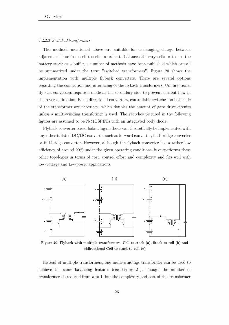
Switched transformers
The methods mentioned above are suitable for exchanging charge between adjacent cells or from cell to cell. In order to balance arbitrary cells or to use the battery stack as a buffer, a number of methods have been published which can all be summarized under the term ”switched transformers”. Figure 20 shows the implementation with multiple flyback converters. There are several options regarding the connection and interfacing of the flyback transformers. Unidirectional flyback converters require a diode at the secondary side to prevent current flow in the reverse direction. For bidirectional converters, controllable switches on both side of the transformer are necessary, which doubles the amount of gate drive circuits unless a multi-winding transformer is used. The switches pictured in the following figures are assumed to be N-MOSFETs with an integrated body diode.
Flyback converter based balancing methods can theoretically be implemented with any other isolated DC/DC converter such as forward converter, half-bridge converter or full-bridge converter. However, although the flyback converter has a rather low efficiency of around 90% under the given operating conditions, it outperforms these other topologies in terms of cost, control effort and complexity and fits well with low-voltage and low-power applications.
(a) (b) (c)
Figure 20: Flyback with multiple transformers: Cell-to-stack (a), Stack-to-cell (b) and
bidirectional Cell-to-stack-to-cell (c)
Instead of multiple transformers, one multi-windings transformer can be used to
achieve the same balancing features (see Figure 21). Though the number of transformers is reduced from n to 1, but the complexity and cost of this transformer

State of art of balancing methods
27
increases, especially for higher winding numbers. For some designs (e.g. stack-to-cell) the secondary current cannot be controlled but naturally flows into the cell with the lowest voltage or eventually divides between several cells. The single switched transformer method shown in Figure 21 uses only one simple flyback transformer with the limitation of being dependent on a switch-matrix.
(a) (b)
Figure 21: Flyback with multi-windings transformer (Stack-to-cell) (a) and with single
switched transformer (Cell-to-stack-to-cell) (b)
Figure 22 and Figure 23 show the spider charts for six different flyback converter
based balancing methods, distinguishing unidirectional as well as bidirectional methods.

Overview
28
Figure 22: Spider chart of unidirectional
flyback converters
Figure 23: Spider chart of bidirectional
flyback converters
Buck-boost converter with energy tank (Super capacitor converter)
This method is a variation of the switched transformer topology. Instead of the battery stack, an additional energy storage is used. Implementations have used super-capacitors [53] and a 12 V battery ([54], [55]). The circuit diagram is shown in Figure 24. The use of a non-isolated bidirectional buck-boost converter enables high transfer efficiencies. However, losses appear both during charging and discharging of the energy storage device.
(a) (b)
Figure 24: Active balancing with buck-boost converter (a) and its spider chart (b)

State of art of balancing methods
29
PWM converter
The PWM converter method uses one MOSFET half-bridge element and one inductor for each cell level. Given a sufficient voltage rating of the MOSFET devices, this topology scales very well with a variable number of battery cells in series. High efficiencies were achieved in experimental tests ([56] and [57], see also Table 3).
(a) (b)
Figure 25: Active balancing with PWM converters (a) and its spider chart (b)
Cûk and resonant converter
Basically, any power conversion stage can be used as a charge transfer converter for active balancing. Two interesting options are the Cûk converter and resonant or quasi-resonant converters shown in Figure 26 and Figure 27, respectively. Although their complexity and part count is rather high, they convince with good efficiency and high power rating as illustrated in the spider chart in Figure 28.

Overview
30
Figure 26: Active balancing with
Cûk converter
Figure 27: Active balancing with
resonant converter
Figure 28: Spider chart of Cûk and resonant converter
Other methods for battery balancing
All previously presented balancing methods are independent of the load or charging current of the battery. In this section, a set of alternative methods is introduced. They control the current flow in each cell and thereby equalize the whole system. In general, these methods require expensive hardware, as they need to be designed for the nominal current of the battery.
State of art of balancing methods
31
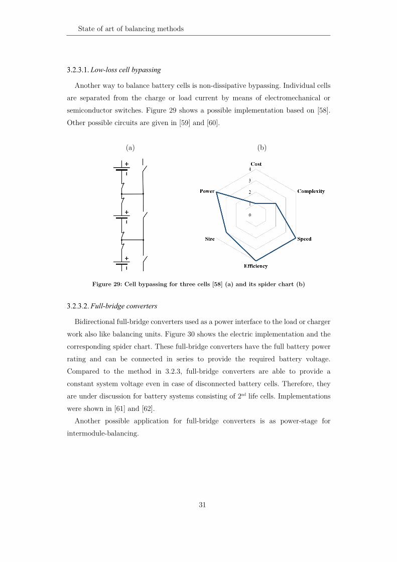
Low-loss cell bypassing
Another way to balance battery cells is non-dissipative bypassing. Individual cells are separated from the charge or load current by means of electromechanical or semiconductor switches. Figure 29 shows a possible implementation based on [58]. Other possible circuits are given in [59] and [60].
(a) (b)
Figure 29: Cell bypassing for three cells [58] (a) and its spider chart (b)
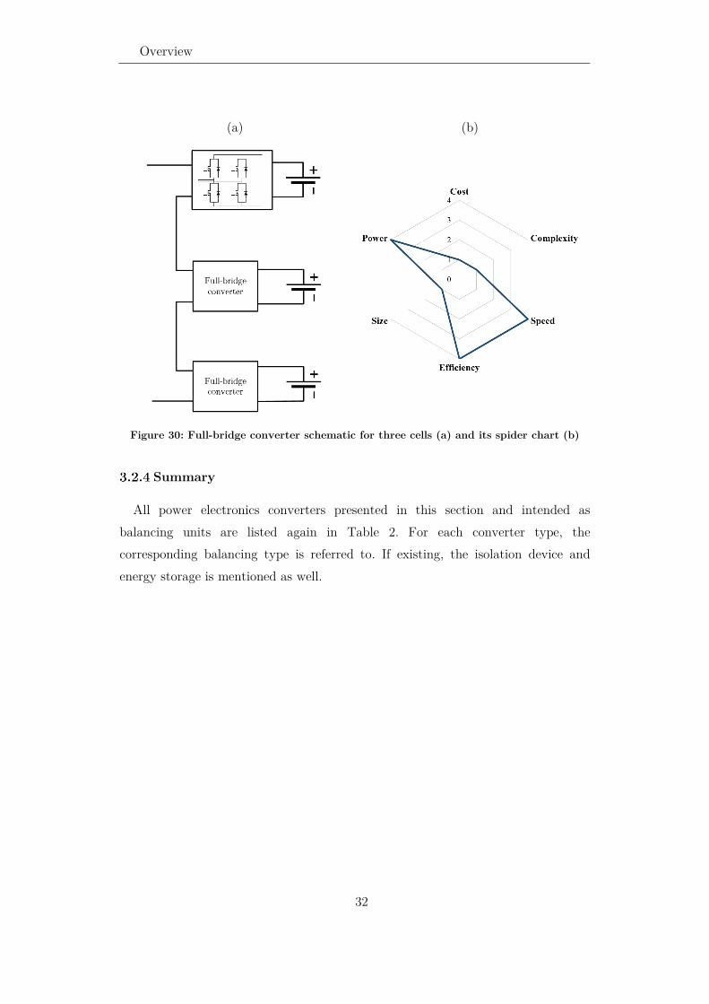
Full-bridge converters
Bidirectional full-bridge converters used as a power interface to the load or charger work also like balancing units. Figure 30 shows the electric implementation and the corresponding spider chart. These full-bridge converters have the full battery power rating and can be connected in series to provide the required battery voltage. Compared to the method in 3.2.3, full-bridge converters are able to provide a constant system voltage even in case of disconnected battery cells. Therefore, they are under discussion for battery systems consisting of 2nd life cells. Implementations were shown in [61] and [62].
Another possible application for full-bridge converters is as power-stage for intermodule-balancing.
Overview
32
(a) (b)
Figure 30: Full-bridge converter schematic for three cells (a) and its spider chart (b)
Summary
All power electronics converters presented in this section and intended as balancing units are listed again in Table 2. For each converter type, the corresponding balancing type is referred to. If existing, the isolation device and energy storage is mentioned as well.

State of art of balancing methods
33
Table 2: Overview of power converter based active balancing methods
Converter type Reference section Isolation device Type of balancing Energy storage Switched capacitors 3.2.2.1 None Cell-to-cell Capacitor Switched inductors 0 None Cell-to-cell Inductor
Flyback converter 3.2.2.3 Multiple transformers Multi-windings transformer Switched transformer
Cell-to-stack [63], [64] Stack-to-cell [65], [66]
Transformer leakage inductance
Bidirectional flyback converter
3.2.2.3 Multiple transformers Multi-windings transformer Switched transformer
Cell-to-stack-to-cell [67] Transformer leakage inductance Battery stack
Single converter 3.2.2.3 Transformer Cell-to-cell None Cûk converter 3.2.2.6 None Cell-to-cell Inductor Resonant converter 3.2.2.6 None Cell-to-cell Inductor PWM half-bridge 3.2.2.5 None Cell-to-stack-to-cell [56] Inductor Supercapacitor converter (Buck-boost)
3.2.2.4 None Cell-to-tank-to-cell [53] Supercapacitor or separate battery (referred to as tank)
Low-loss bypassing 3.2.3.1 None N/A None Full-bridge converter 3.2.3.2 None N/A None

Performance and feature comparison
34
Performance and feature comparison
The focus of this thesis lies on a new set of balancing methods based on non-isolated DC/DC converters. This section summarizes the works published so far on similar methods. Some important patents of non-isolated balancing circuits are available in Section 3.5.4.
Rating balancing methods according to review papers
The publications containing comparison of different active balancing methods are briefly described hereafter. Spider charts from three reviews ([39], [68] and [69]) have been created according to the ratings given in the cited documents. Although some of the results differ greatly from each other, the tendency is obvious, that designs which include transformers suffer from higher costs.
The previously mentioned review in [39] reveals “Complete shunting” (Low-loss bypassing), “Switched capacitor” and “DT Switched capacitor” as the top performing methods. The complete spider chart is shown in
Figure 31: Evaluation of 15 balancing methods according to [39]
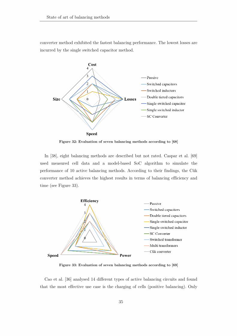
Daowd et al. [68] have compared eight different active balancing topologies in
terms of balancing time, losses, size requirements and cost using MATLAB/Simulink. The analysis is illustrated in Figure 32 as a four-fold spider chart. Passive balancing was found to be superior in terms of size and cost, whereas the supercapacitor
State of art of balancing methods
35
converter method exhibited the fastest balancing performance. The lowest losses are incurred by the single switched capacitor method.
Figure 32: Evaluation of seven balancing methods according to [68]
In [38], eight balancing methods are described but not rated. Caspar et al. [69]
used measured cell data and a model-based SoC algorithm to simulate the performance of 10 active balancing methods. According to their findings, the Cûk converter method achieves the highest results in terms of balancing efficiency and time (see Figure 33).
Figure 33: Evaluation of seven balancing methods according to [69]
Cao et al. [36] analysed 14 different types of active balancing circuits and found
that the most effective use case is the charging of cells (positive balancing). Only

Performance and feature comparison
36
the switched capacitor methods were as well suited for discharge mode. More reviews with a focus on EV batteries are available in [70] and [71].
Rating of balancing types and algorithms
Most research papers on active balancing focus on power electronic circuits to optimize some of the functional parameters of modern BMS such as equalization speed, balancing losses and battery life. There is only little work on algorithms and performance comparison of different balancing architectures. Although many authors present simulation results, their reproducibility is limited due to the dozens of battery cell and system parameters.
Baronti et al. [72] have compared the most common balancing types (cell-to-stack, stack-to-cell, cell-to-stack-to-cell and cell-to-cell) by numerical simulations in terms of balancing losses and equalization speed. They found the cell-to-cell architecture to deliver the best performance. Interestingly, for low efficient stack-to-cell circuits, the losses can exceed the ones that would arise from passive balancing. Figure 34 (a) shows the probability density function of the balancing losses and its dependence on balancing efficiency. In Figure 34 (b), the balancing losses normalized to passive balancing are plotted as a function of the balancing efficiency.
(a) (b)
Figure 34: Probability density of classic active balancing method losses (a) and expected
losses as a function of the balancing efficiency (b) according to [72]
Efficiency measurements of balancing prototypes
In Table 3, the available performance data from measurements of active balancing prototypes is given. Lee et al. have compared active and passive balancing HW also during charging and found a reduction in charging losses of 64% [63]. The maximum

State of art of balancing methods
37
balancing current that is found in literature is 4 to 5 A [73] and 10 A [55]. Most prototypes deliver up to 2 A at an efficiency between 80% and 90%. The information about extra discharge capacity, where it is given, should be treated with caution since it highly depends on the capacity distribution of the battery cells.
Table 3: Published performance data of balancing prototypes
Architecture Max. balancing current
Max. balancing efficiency
Extra discharge capacity
Isolated
Switched inductor [74] 0.8 A 80% N/A No Single switched capacitor [75] 2 A 83% N/A No Supercapacitor converter [76] 1 A 90% N/A No Supercapacitor converter [55] 10 A 85% N/A No Switched inductors [52] 1 A N/A N/A No Switched inductors [73] 5 A 85% N/A No PWM converters [57] 0.5 A 92% N/A No Cell bypass [59] N/A > 90% N/A No Multiple flyback converters [77] 1.5 A 80% 4% Yes Multi-windings transformer [65] 4 A 90% 15% Yes Multiple transformers [78] 4 A 88% N/A Yes
Switched transformer [63] 0.25 A 70% 2.7% Yes
Switched transformer [79] 2 A 81% N/A Yes
ZVS Converter [80] 0.3 A 89% N/A Yes Bidirectional converters [79] 2 A 82% N/A Yes
Cell-to-cell variation of lithium-ion batteries
The distribution of the battery cell capacities must be known to make a statement about charge imbalance in lithium-ion batteries. This section lists the available measurement data of cell-to-cell variation (C2CV) studies. In [81], 20,000 new battery cells were tested before being assembled in electric vehicle (EV) batteries. In Figure 35, the histogram of the measured capacity values (blue) and a normal distribution (yellow) are shown. The curve shape supports the assumption that battery cell capacities are normally distributed with a standard deviation of, in this case, 1.3%. The histogram of the direct current internal resistance (DCR) was found to be 5.8%. Unlike the mathematical curve, cells with a deviation of less than

Cell-to-cell variation of lithium-ion batteries
38
approximately -2.75σ do not show up in the histogram since they fail the factory quality test and are not shipped to the customers.
Figure 35: Distribution of cell capacities at BoL (20’000 cells, LiFePO4, σ=1.3%) [81]
Exactly the same cells were tested after their service life and a capacity standard
deviation of 2.4% resulted from the measurements. This means that the capacity distribution has almost doubled because of inhomogeneous cell ageing. Consequently, the benefits of active balancing increase during the lifetime of the battery as the charge imbalances become more distinctive. Figure 37 illustrates this effect: While a battery system at BoL consists of cells with a low capacity-spread around 100% of Cnom, the capacity deviation significantly increased whereas the mean capacity has dropped to 80% of the initial Cnom.
In [69], a measurement of 96 large automotive NMC battery cells at BoL and EoL is available. Again, the results show a normal distribution of the battery capacities (see Figure 36).

State of art of balancing methods
39
(a) (b)
Figure 36: Capacity distribution of new (a) and aged (b) cells (σBoL = 2.3%, σEoL = 7.3%)
[69]
Einhorn et al. tested active balancing circuits in [77]. In this context they
measured the capacity of 150 battery cells. The histogram resembles a normal distribution with a standard deviation of less than 1% (Figure 38).
Figure 37: Density function of cell
capacity at BoL and EoL (based on [81])
Figure 38: Capacity distribution of 150
cells [77] Similar measurements with 5473 automotive lithium-ion cells were performed and
published in [82]. A correlation between capacity and cell mass was found, as shown in Figure 39. Another C2CV measurement is available in Figure 40. In this case, industrial 18650-type cylindrical cells were tested which seem to spread much less in capacity at BoL compared to prismatic cell types or LiFePO4 cells.

Relevant patents
40
Figure 39: Distributions of cell
capacity and mass of 5473 cells [82]
Figure 40: Histogram of cell capacities of 94
NMC cells [83]
Relevant patents
Many patents exist on active balancing and charge equalization. The most relevant ones are described in the following sections. IC and BMS manufacturers account for most of the relevant patents.
Switched inductors
A non-isolated circuit design based on switched inductors is described in DE102014215724 (A1) [84]. Instead of AC-switches, a single MOSFET and an additional series diode are proposed.
Single switched inductor
A battery cell module with several battery cells connected in series is known from document EP2385605 (A2) [85], whereby the battery cell pack is assigned a common inductive energy storage device, which is connected to the corresponding battery cells via a switching matrix. The disadvantage of this is that the losses due to the high switching frequency of the switches of the switching matrix are large and a powerful driver circuit is required for the switches.
Flyback converters
According to the active charge equalization known from document EP2787594 (A2) [86], it is possible to exchange energy between any battery cell and the battery

State of art of balancing methods
41
cell stack. To carry out such a charge equalization, a large number of fast switching semiconductor devices and inductive transformers is necessary, which increases the complexity and cost. The design protected by this patent has been made available for the public by Linear Technology Corp. with the reference design DC2064A (based on the IC LTC6803-2).
Non-isolated bidirectional converters
Patents US2013015820 (A1) [87], EP0828304 (A2) [88] and DE102006002414 (A1) [89] describe a battery cell module with non-isolated DC/DC converters and a switching matrix. For charge balancing, a certain amount of charge is taken from any battery cell and stored temporarily in an external capacitive energy storage. In the next step, the stored energy is transferred to another battery cell via a different path in the switching matrix. The disadvantage is that an additional energy storage is necessary and the switching matrix consists of at least two switches per battery cell.
Full-bridge converters
From document US2013099579 (A1) [90] a battery cell module with several battery cells connected in series is known, with one non-isolated DC/DC converter assigned to each battery cell. The disadvantage is that the complexity and costs are high due to the large number of fast switching DC/DC converters.
Commercial solutions for active balancing
Due to the increasing use of lithium battery systems, a wide range of integrated circuits is available for implementing the necessary electronic BMS functions. Some manufacturers have implemented active balancing options in their battery cell monitor ICs, such as AMS. Others like TI and LT have released additional ICs to work together with their standard products.
Demonstration or evaluation boards of these suppliers represent one solution for a prototype battery system with active balancing. Another option are commercial products based on the same technology but not following exactly the reference design.

Commercial solutions for active balancing
42
Battery cell monitors for active balancing
Table 4 shows several battery cell monitor ICs capable of active balancing and their electric and electronic properties. Only ICs with an interface for at least six cells were considered.
Table 4: Active balancing ICs (based on [91])
Analog Front End/ Balancing IC
AS8506 LTC6811 / LT8584 / LTC3300
BQ76PL455A EMB1428Q / EMB1499
Manufacturer AMS Linear Technology Texas Instruments Number of cells 3-7 5-12 6-16 Maximum stack voltage
Max. 200 cells Max. 1000 V Max. 256 cells
Cell voltage measurement
12 Bit SAR-ADC ±15 mV
16 Bit ΣΔ-ADC ±2.8 mV
14 Bit SAR-ADC ±5.5 mV
Current measurement
External 16 Bit ΣΔ-ADC ±2.8 mV
14 Bit SAR-ADC ±10 mV
Temperature sensors
2 5 8
Communication interface
SPI I2C, SPI UART
Active balancing Flyback Flyback Bi-directional forward converter
Balancing method Cell-to-stack Cell-to-stack-to-cell Cell-to-tank-to-cell Max. balancing current
100 mA 10 A N/A
Demo Boards (Balancing current)
Active Board for AS8506C
DC2064A (2.5 A) DC2100A-C (4 A)
EM1402EVM (5 A)
Active BMS boards from third-party suppliers
Active balancing boards that are commercially available from industrial suppliers are very rare. Table 5 shows a selection of products. Although more information is available in the corresponding data sheets, the type of balancing or the used components are not specified in detail. The current capability of the devices is in the same range as for the manufacturer’s evaluation boards shown in Table 4.

State of art of balancing methods
43
Table 5: Commercial active balancing BMS boards
Supplier Enerstone Enerstone AutarcTech REC-BMS
Country France France Germany Slovenia
Number of cells 4-16 4-16 4 4-16
Balancing current 2 A 10 A 5 A 2.5 A
Website enerstone.fr enerstone.fr autarctech.de rec-bms.com
Data sheet N/A N/A [92] [93]
In the future, other suppliers are likely to present products with active balancing
ability. Renown manufactures of stand-alone BMS are Energus Power, I+ME Actia, Orion BMS, Lithium Balance and Ficosa to just name a few.
Summary of state of art research
The state of art analysis reveals an intensive research activity on active balancing for the last 10 years. A lot of different methods have been proposed, tested and patented. Different authors rate the different methods inconsistently as shown in Section 3.3.1. Commonly, for low power applications, the switched capacitor methods are classified superiorly. On the other hand, low-loss bypassing, supercapacitor and full-bridge converters are recommended for high power applications.
Regarding balancing algorithms and performance estimation of the different methods, there is few information available in literature.
From the manufacturer's point of view, there is little activity concerning BMS boards with active balancing.

Analytical view on charge transfer during balancing
44
Analysis of active balancing potential
Although there are many publications on active balancing, little information on its technical potential can be found. No systematic work has been done so far to determine the benefits of active balancing based on battery parameter such as cell properties and system configuration. This chapter analyses the potential and the limits of active balancing for large battery packs using statistical methods and numerical simulation. It is partly based on a conference proceeding of the IEEE ISIE 17 in Edinburgh, UK [94].
Analytical view on charge transfer during balancing
We assume that the battery cell capacities are normally distributed acc. to the Gaussian density function with the variables μ (mean capacity) and σ (standard deviation):
𝑓𝑓(𝑥𝑥) = 1
√2𝜋𝜋𝜎𝜎2𝑒𝑒
(𝑥𝑥−𝜇𝜇)2
2𝜎𝜎2 (6)
The mean value μ and the expected value E are identical for symmetric functions:
𝐹𝐹(𝑥𝑥) = 𝑥𝑥𝑓𝑓(𝑥𝑥)𝑑𝑑𝑥𝑥+∞
−∞
(7)
The cumulative density function F cannot be calculated analytically. It is defined
as the integral of the density function
𝐹𝐹(𝑥𝑥) = 𝑓𝑓(𝑥𝑥)𝑑𝑑𝑥𝑥 (8)
For further calculations, the inverse of the cumulative density function 𝐹𝐹−1(𝑥𝑥) is needed. To support a realistic analysis, the density function of the battery cell capacities is not assumed exactly Gaussian but cut at each side at kσ and rescaled to fulfil the equation in(7) and (8). The new density function CCell(x) uses the variable Cnom instead of μ.

Analysis of active balancing potential
45
𝑆𝑆𝐶𝐶𝐶𝐶𝐶𝐶𝐶𝐶(𝑥𝑥) = 𝑓𝑓(𝑥𝑥)
1 − 2𝐹𝐹(𝑆𝑆𝑛𝑛𝑛𝑛𝑛𝑛 − 𝑘𝑘𝜎𝜎) (9)
This is a necessary adaption to prevent capacity values out of realistic range being
considered in the calculation. With Cnom and σ being the mean value and the standard deviation of the deployed cell, it is assumed that the capacity of all cells is within Cnom ± kσ. The integral of the density function is hence defined as:
𝑓𝑓(𝑥𝑥)𝑑𝑑𝑥𝑥+∞
−∞
= 𝑆𝑆𝐶𝐶𝐶𝐶𝐶𝐶𝐶𝐶(𝑥𝑥)𝑑𝑑𝑥𝑥+∞
−∞
= 𝑆𝑆𝐶𝐶𝐶𝐶𝐶𝐶𝐶𝐶(𝑥𝑥)𝑑𝑑𝑥𝑥
𝐶𝐶𝑛𝑛𝑛𝑛𝑛𝑛+𝑘𝑘𝜎𝜎
𝐶𝐶𝑛𝑛𝑛𝑛𝑛𝑛−𝑘𝑘𝜎𝜎
= 1 (10)
The two density functions f(x) and 𝑆𝑆𝐶𝐶𝐶𝐶𝐶𝐶𝐶𝐶(x) are shown in Figure 41 (for μ = 10 /
Cnom = 10 Ah, σ = 0.15 Ah and k = 2).
Figure 41: Normal distribution f(x) and rescaled/cropped function Cnom(x)
Available capacity and energy savings
In this section, the effect of capacity distribution on the available capacity and the resulting energy savings is analysed mathematically.

Available capacity and energy savings
46
Battery systems with one cell in a level (1SnP)
First the variable k is calculated as a function of the number of cells n. The density function margins Cnom ± kσ are defined such that the probability for a cell having a capacity value between -∞ and μ - kσ is 1/n, hence
𝑘𝑘 =𝑆𝑆𝑛𝑛𝑛𝑛𝑛𝑛 − 𝐹𝐹−1 1
𝑛𝑛𝜎𝜎
(11)
During passive balancing, charge is dissipated from cells that are close to their
maximum charging voltage. This process lasts until the strongest cell has reached its maximum charging voltage. For a battery system with an nS1P configuration (n cells in series, 1 cell in parallel), the charge difference ∆𝑄𝑄 of a cell with a capacity of 𝑥𝑥 Ah in relation the strongest cell is given as:
∆𝑄𝑄 = 𝑆𝑆𝑛𝑛𝑛𝑛𝑛𝑛 + 𝑘𝑘𝜎𝜎 − 𝑥𝑥 (12)
The total balanced charge of all cells can be calculated as follows:
𝑄𝑄𝐵𝐵𝑎𝑎𝐶𝐶_𝑝𝑝𝑎𝑎𝑎𝑎𝑘𝑘 = 𝑛𝑛 (𝑆𝑆𝑛𝑛𝑛𝑛𝑛𝑛 + 𝑘𝑘𝜎𝜎 − 𝑥𝑥)𝑓𝑓∗(𝑥𝑥)𝑑𝑑𝑥𝑥
𝐶𝐶𝑛𝑛𝑛𝑛𝑛𝑛+𝑘𝑘𝜎𝜎
𝐶𝐶𝑛𝑛𝑛𝑛𝑛𝑛−𝑘𝑘𝜎𝜎
(13)
Using (7) and (10), (13) can be simplified to:
𝑄𝑄𝐵𝐵𝑎𝑎𝐶𝐶_𝑝𝑝𝑎𝑎𝑎𝑎𝑘𝑘 = 𝑘𝑘𝑛𝑛𝜎𝜎 (14)
The energy losses during charging due to passive balancing 𝑊𝑊𝑃𝑃𝑎𝑎𝑃𝑃𝑃𝑃𝑖𝑖𝑃𝑃𝐶𝐶 for an nS1P
battery system sum up to:
𝑊𝑊𝑃𝑃𝑎𝑎𝑃𝑃𝑃𝑃𝑖𝑖𝑃𝑃𝐶𝐶 = 𝑈𝑈𝐵𝐵𝑎𝑎𝐶𝐶_𝑎𝑎𝑃𝑃𝑎𝑎𝑄𝑄𝐵𝐵𝑎𝑎𝐶𝐶_𝑝𝑝𝑎𝑎𝑎𝑎𝑘𝑘 = 𝑘𝑘𝑛𝑛𝜎𝜎𝑈𝑈𝐵𝐵𝑎𝑎𝐶𝐶_𝑎𝑎𝑃𝑃𝑎𝑎 (15) UBal_avg is the average voltage of the affected cell during the balancing process. For
lithium-ion cells, in most applications UBal_avg will be around 4.0 V.

Analysis of active balancing potential
47
Battery systems with multiple parallel cells (nSmP)
For battery systems with more than one cell on each stack level (nSmP), the calculation has to be adjusted. According to probability theory basics (see [95]), the resulting mean and standard deviation for independent random variables are μ’ = m
μ and σ = sqrt(m)σ. Using μ’ and σ’ instead of μ and σ in (6), the density function becomes
𝑓𝑓𝑛𝑛(𝑥𝑥) = 1
2𝜋𝜋𝜎𝜎′2𝑒𝑒
𝑥𝑥−𝜇𝜇′2
2𝜎𝜎′2 (16)
In line with (13) and using CCellm(x) instead of CCell(x) the total balanced charge
can be written as:
𝑄𝑄𝑛𝑛𝐵𝐵𝑎𝑎𝐶𝐶_𝑝𝑝𝑎𝑎𝑎𝑎𝑘𝑘 = 𝑛𝑛 (𝑆𝑆𝑛𝑛𝑛𝑛𝑛𝑛′ + 𝑘𝑘𝜎𝜎′ − 𝑥𝑥)𝑆𝑆𝐶𝐶𝐶𝐶𝐶𝐶𝐶𝐶𝑛𝑛(𝑥𝑥)𝑑𝑑𝑥𝑥
𝐶𝐶𝑛𝑛𝑛𝑛𝑛𝑛′+𝑘𝑘𝜎𝜎′
𝐶𝐶𝑛𝑛𝑛𝑛𝑛𝑛′−𝑘𝑘𝜎𝜎′
(17)
Using (7) and (10), (17) can be simplified to:
𝑄𝑄𝑛𝑛𝐵𝐵𝑎𝑎𝐶𝐶_𝑝𝑝𝑎𝑎𝑎𝑎𝑘𝑘 = 𝑘𝑘𝑛𝑛𝜎𝜎′ = 𝑘𝑘𝑛𝑛√𝑚𝑚𝜎𝜎 (18)
For an nSmP battery system, the energy losses during charging due to passive
balancing 𝑊𝑊𝑛𝑛𝑃𝑃𝑎𝑎𝑃𝑃𝑃𝑃𝑖𝑖𝑃𝑃𝐶𝐶 sum up to:
𝑊𝑊𝑛𝑛𝑃𝑃𝑎𝑎𝑃𝑃𝑃𝑃𝑖𝑖𝑃𝑃𝐶𝐶 = 𝑈𝑈𝐵𝐵𝑎𝑎𝐶𝐶_𝑎𝑎𝑃𝑃𝑎𝑎𝑄𝑄𝑛𝑛𝐵𝐵𝑎𝑎𝐶𝐶_𝑝𝑝𝑎𝑎𝑎𝑎𝑘𝑘 = 𝑘𝑘𝑛𝑛√𝑚𝑚𝜎𝜎𝑈𝑈𝐵𝐵𝑎𝑎𝐶𝐶𝑎𝑎𝑎𝑎𝑎𝑎 (19)
Energy savings
If active balancing is used instead of passive balancing, a considerable share of the equalizing losses is avoided. An overall charge transfer efficiency of at least 80% can be derived from active balancing prototype measurement data (see Table 3) and will be used for numerical calculations below. Using the energy efficiency variable η, it follows that the energy losses during charging due to active balancing are

Available capacity and energy savings
48
𝑊𝑊𝑛𝑛𝐴𝐴𝑎𝑎𝑎𝑎𝑖𝑖𝑃𝑃𝐶𝐶 = (1 − 𝜂𝜂)𝑘𝑘𝑛𝑛√𝑚𝑚𝜎𝜎𝑈𝑈𝐵𝐵𝑎𝑎𝐶𝐶𝑎𝑎𝑎𝑎𝑎𝑎 (20)
The balancing effort of a battery system increases with its lifetime as the cell
capacities drift apart. Varying operation conditions lead to the inhomogeneous ageing of individual cells. While the capacity mean value decreases, the standard deviation of the cells increases, as illustrated in Section 3.4.
Available capacity
The following equations refer to nSmP battery packs. For nS1P configuration, m can be set to 1.
The lifetime of a battery pack is usually defined as a minimum remaining capacity in relation to the initial capacity (between 70 and 80 percent for most applications). The weakest cell – or cell level in case of more than one parallel cell – in a battery system determines the effective capacity CPack, which is in our case
𝑆𝑆𝑃𝑃𝑎𝑎𝑎𝑎𝑘𝑘 = 𝑆𝑆𝑛𝑛𝑛𝑛𝑛𝑛
′ − 𝑘𝑘𝜎𝜎′ = 𝑚𝑚𝑆𝑆𝑛𝑛𝑛𝑛𝑛𝑛 − 𝑘𝑘√𝑚𝑚𝜎𝜎 (21) If active balancing is performed during discharge as well, the useable capacity can
be increased. For an actively balanced battery pack this capacity value CPack_active depends on the efficiency and power of the balancing electronics and can get as high as:
𝑆𝑆𝑃𝑃𝑎𝑎𝑎𝑎𝑘𝑘_𝑎𝑎𝑎𝑎𝑎𝑎𝑖𝑖𝑃𝑃𝐶𝐶 = 𝑆𝑆𝑛𝑛𝑛𝑛𝑛𝑛
′ − (1 − 𝜂𝜂)𝑘𝑘𝜎𝜎′ = 𝑆𝑆𝑛𝑛𝑛𝑛𝑛𝑛 − (1 − 𝜂𝜂)𝑘𝑘√𝑚𝑚𝜎𝜎 (22) Figure 42 shows the available capacity of a passive respectively active balancing
system at two different standard deviations (1.3% for a system at BoL and 2.4% at EoL, see 3.4). The plots were generated by using the MATLAB code given in Appendix B. With increasing number of parallel cells, the positive effect of active balancing become less. According to Figure 42, designing a battery system with passive balancing in nS1P configuration is not recommendable. By using configuration with several parallel cells, the available capacity can be increased from 93.8% to 95.6% (nS2P) or 96.7% (nS4P).

Analysis of active balancing potential
49
Figure 42: Usable capacity of a battery system at two different cell capacity standard
deviation (with and without balancing)
Numerical parameter sweep simulation
Beside the calculations, a numerical batch simulation with parameter sweep was performed for verification reasons. Figure 43 and Figure 44 show the results of the simulation in comparison with the calculated values from the previous section.
For a realistic view, the individual simulations were based on a 96S1P battery system, which is a common configuration in industrial applications such as EV. On the x-axis, the variable parameter is plotted. In Figure 43, the number of parallel cells varies from 1 to 10 whereas in Figure 44, the standard deviation of the cell capacities varies from 1% to 3% in steps of 0.1%. The overall deviation between simulation and calculation is 0.5% and 0.9%, respectively. It originates from the iteration steps of the balancing algorithm used in the MATLAB simulation. The calculated values represent the maximum achievable capacity gain whereas the simulation includes non-ideality of the system and the balancing algorithm (e.g. over-compensation due to the discrete sampling time).

Module restricted balancing
50
Figure 43: Capacity gain factor for active balancing depending on number of parallel
cells m
Figure 44: Capacity gain factor for active balancing depending on cell distribution for
m=1
Module restricted balancing
Active balancing methods are generally better suited for low voltage battery systems. The most common battery management ICs monitor up to eight, 12 or 16 cells, enabling system voltages of 24 to 60 V in case of lithium-ion or LiFePO4 cells.

Analysis of active balancing potential
51
For higher voltages, several battery modules need to be connected in series. This leads to a segmentation of the battery system. Cells inside the same module (segment) are still easy balanceable, whereas balancing between modules is more complex due to the increasing isolation requirements of the balancing stage or the need for additional inter-module balancing hardware. However, neither is generally necessary. In this section, the influence of segmentation on the available capacity of a battery system for different balancing methods is estimated through numerical simulation. A typical EV battery system (96S1P) is divided into a variable number of modules. Active balancing is only allowed inside a module (i.e. no inter-module balancing). Figure 45 shows two of the six different options that were considered (48S1P modules ≙ two segments and 16S1P modules ≙ six segments).
(a) (b)
Figure 45: Separation of a 96S battery system into two (a) and six (b) modules
In Figure 46, the effect of modularization on the usable battery capacity is
illustrated. The theoretically available capacity of differently segmented systems is shown depending on the standard deviation of the involved battery cells. The converter efficiency is not included in this analysis. A batch simulation in MATLAB with a parameter sweep was used to generate the plot. The program code as m-file is given in Appendix D. For a better readability, some repetitive code rows have been replaced by red dots. In Figure 46, 100% indicates a single 96S1P module where each cell can be balanced without restrictions. Each line represents another total number of modules. Even for the smallest module with eight cells, more than 99% of the theoretical capacity can be recovered through active balancing at ϭ = 1.5%. Compared to passive balancing (blue line) active balancing always provides an additional few percent of capacity.

Module restricted balancing
52
The deviation of the cells has a stronger negative effect on the available capacity for passive balancing compared to active balancing. Without any additional measures, a considerably better utilization of the battery capacity will be achieved. To completely avoid the capacity related drawbacks of segmentation in higher voltage battery systems, the use of inter-module balancing can be implemented as described in [74].
Figure 46: Effect of modularization on the maximum usable capacity of the 96S1P
battery system (Balancing losses not considered)

New active balancing methods
53
New active balancing methods
This chapter describes the development process of the novel methods. In total, six new balancing methods are presented.
Initial position
Most active balancing topologies use a power electronic converter for each cell or cell level, which transfers the charge between cells or an individual cell and the stack. The most common of these types is the bidirectional multiple flyback converter method explained in Section 3.2.2.3. Although there is a corresponding converter for each cell level, most of the balancing time only one or a couple of them are active. By reducing the amount of converters, it is possible to reduce the number of components and thus also the cost. This approach has already been followed by several authors, who have presented circuits with at least one galvanically isolated DC/DC converter and a switch-matrix to select a certain battery cell (see Section 3.2.2.3).
Design and components
The new set of active balancing methods is called “Buck-In/Boost-Out”. The balancing principle is based on selective charging and discharging of a variable number of battery cells connected in series. The topology uses a switch matrix to connect the desired cells with the converters. The main components are:
• At least one non-isolated DC/DC converter (Buck, Boost or Buck-Boost) • A MOSET switch-matrix to connect the DC/DC converter(s) to the
battery cells • Controller to set the converter current(s) and select the correct matrix
configuration

Description of the proposed circuits
54
Depending on the topology, either unidirectional or bidirectional converters are required. For higher transfer efficiencies, the use of synchronous converters is recommended. The switches must be blocking in both directions and can be realized with two N-MOSFETs each.
A total of eight related balancing methods were patented under the title “Electronic circuit for performing state of charge equalization between battery cells of a battery system”, including the ones presented in the following sections. Two additional methods are available in Appendix A. The patent was filed on June 09, 2018 at the Swiss patent office in Berne under the number 00742/18 in the class H02J. It is written in German, has a priority period of 18 months and protects the invention in Switzerland.
Description of the proposed circuits
The following sections describe six different active balancing methods. Some of this section’s content has been published in the proceedings of the IEEE ISIE18 conference in Cairns, Australia [96].
In order to compare the different variants with each other, always the same balancing task is illustrated: Discharging of Cell 2. The current paths for a given balancing task are coloured in the overview schematics for better understanding.
Type Ia: Combination of a buck and boost converter
Figure 47 shows the balancing method Type Ia for a battery system with n cells in series. In accordance with the established nomenclature, the description is stack-to-cells-to-stack. A buck converter works as a charging unit, which transfers charge from the stack to the selected cells. Discharge is performed in the opposite way via a boost converter.
The output voltage range of the buck converter and the input voltage range of the boost converter must be wide enough to cover 1 to n-1 cells. In this way, all cells can be actively charged and discharged up to the highest level in the stack. Simultaneous balancing of multiple cells is only possible for adjacent cells. For the uppermost cell, balancing takes place by accessing all cells below it.
In the following the balancing process illustrated in Figure 47 is explained. The buck converter delivers energy from the stack through switch SwA1 to Cell 1. Cell

New active balancing methods
55
1 is charged with the converter output current IBuck. Simultaneously, the boost converter discharges Cell 1 and Cell 2 through SwB2 with the converter input current IBoost. Given that IBuck = -IBoost = IBal, the sum of the current in Cell 1 is 0 A, and Cell 2 is discharged with IBoost A (negative balancing or “discharge mode”). Generally, cells are charged by connecting the buck converter on a higher position than the boost converter. Discharging is carried out in reverse order.
Figure 47: Type Ia active balancing architecture
The cell currents in idle state can be expressed as a vector according to (23). It
takes account of the positive and negative balancing current as well as the resulting stack current:
𝐼𝐼𝑎𝑎𝐶𝐶𝐶𝐶𝐶𝐶 = 𝐼𝐼𝑆𝑆𝑎𝑎𝑎𝑎𝑎𝑎𝑘𝑘 + 𝐼𝐼𝑛𝑛 ∙ 𝐼𝐼𝐵𝐵𝑎𝑎𝐶𝐶 − 𝑆𝑆𝑂𝑂𝑡𝑡 ∙ 𝐼𝐼𝐵𝐵𝑎𝑎𝐶𝐶 (23)
with 𝐼𝐼𝑆𝑆𝑎𝑎𝑎𝑎𝑎𝑎𝑘𝑘 = 𝐼𝐼𝐵𝐵𝐵𝐵𝐵𝐵 1𝜂𝜂
∑ 𝐼𝐼𝑛𝑛 − 𝜂𝜂 ∑ 𝑆𝑆𝑂𝑂𝑡𝑡 , 𝐼𝐼𝑛𝑛 =
𝑠𝑠𝐴𝐴1⋮
𝑠𝑠𝐴𝐴[𝑛𝑛−1]0
, 𝑆𝑆𝑂𝑂𝑡𝑡 =
𝑠𝑠𝐵𝐵1⋮
𝑠𝑠𝐵𝐵[𝑛𝑛−1]0
, 𝑠𝑠𝑥𝑥 ∈ 0; 1 ,

Description of the proposed circuits
56
where 𝐼𝐼𝑛𝑛 and 𝑆𝑆𝑂𝑂𝑡𝑡 represent the vectors of the switch signals sA[x] of SwA[x] and sB[y] of SwB[y].
The converter power and total losses depend on the number of cells in the stack n and the position of the balanced cell inside the stack. They increase with the increasing number of cells and a higher position. If only one cell is balanced, i = j. Otherwise, i designates the bottom cell of the balancing group and j the top one. Therefore, i ≥ j always applies. For each position i and j, there is a transfer efficiency for the buck and the boost converter (𝜂𝜂Buck and 𝜂𝜂Boost, see Section 6.3). Assuming UStack = nUCell the overall balancing efficiency 𝜂𝜂Bal+ for charging the adjacent cells i to j (positive balancing) is:
𝜂𝜂𝐵𝐵𝑎𝑎𝐶𝐶+ = 1 −𝑗𝑗 ∙
1 − 𝜂𝜂𝐵𝐵𝐵𝐵𝑎𝑎𝑘𝑘𝑗𝑗
𝜂𝜂𝐵𝐵𝐵𝐵𝑎𝑎𝑘𝑘𝑗𝑗 + (𝑖𝑖 − 1) ∙ 1 − 𝜂𝜂𝐵𝐵𝑛𝑛𝑛𝑛𝑃𝑃𝑎𝑎𝑖𝑖−1
𝑗𝑗 − 𝑖𝑖 + 1
(24)
For discharging (negative balancing) of cells i to j, the efficiency 𝜂𝜂Bal- calculates as
follows:
𝜂𝜂𝐵𝐵𝑎𝑎𝐶𝐶− = 1 −(𝑖𝑖 − 1) ∙
1 − 𝜂𝜂𝐵𝐵𝐵𝐵𝑎𝑎𝑘𝑘𝑖𝑖−1𝜂𝜂𝐵𝐵𝐵𝐵𝑎𝑎𝑘𝑘𝑖𝑖−1
+ 𝑗𝑗 ∙ 1 − 𝜂𝜂𝐵𝐵𝑛𝑛𝑛𝑛𝑃𝑃𝑎𝑎𝑗𝑗
𝑗𝑗 − 𝑖𝑖 + 1 (25)
If only one cell needs to be balanced, i equals j (i = j). For i = 1 (i.e. bottom cell),
only one converter is required to perform the balancing. The term (i - 1) and its related part of the numerator become zero in (3) and (4).
For the topmost cell (j = n), no direct balancing is possible. Only one converter is required to perform the balancing, though the balancing performance is low compared to the other cells. The efficiencies for charging and discharging are calculated as following:
𝜂𝜂𝐵𝐵𝑎𝑎𝐶𝐶+ = 1 −(𝑖𝑖 − 1) ∙ 1 − 𝜂𝜂𝐵𝐵𝑛𝑛𝑛𝑛𝑃𝑃𝑎𝑎𝑛𝑛−1
𝑛𝑛 − 𝑖𝑖 + 1 (26)
𝜂𝜂𝐵𝐵𝑎𝑎𝐶𝐶− = 1 −(𝑖𝑖 − 1) ∙
1 − 𝜂𝜂𝐵𝐵𝐵𝐵𝑎𝑎𝑘𝑘𝑛𝑛−1𝜂𝜂𝐵𝐵𝐵𝐵𝑎𝑎𝑘𝑘𝑛𝑛−1
𝑛𝑛 − 𝑖𝑖 + 1
(27)

New active balancing methods
57
The required converters can be conventional buck and boost converters as shown in Figure 48 and Figure 49. To enhance the efficiency of the converters over the whole operating range, a synchronous design can be chosen, where the diode is replaced by an actively controlled MOSFET to reduce losses. The synchronous mode is particularly suited for low voltage applications to increase the efficiency of a converter significantly.
(a) (b)
Figure 48: Schematic of conventional (a) and synchronous (b) buck converter
(a) (b)
Figure 49: Schematic of conventional (a) and synchronous (b) boost converter
Type Ib: Type I with a bidirectional converter
Type Ib is similar to Type Ia in terms of balancing paths. Instead of unidirectional converters, a bidirectional one is used. The schematic for a possible hardware implementation is shown in Figure 55. For the architecture, see Figure 93 in Appendix A.
Type IIa: Buck-boost converter
Figure 50 shows Type IIa of the discussed balancing methods. Again, the battery system consists of n cells in series. In accordance with the established nomenclature, the description is cells-to-cells. If the load current equals the balancing current, this method is similar to the cell bypassing described in Section 3.2.3.1. In discharge

Description of the proposed circuits
58
mode, a buck converter transfers charge from one cell or a multitude of adjacent cells to its subjacent cells in the stack. In charge mode, a boost converter transfers charge in the opposite way. Both converters can be combined to a single bidirectional buck-boost converter. The input and output voltage range of the buck-boost converter must be wide enough to cover 1 to n cells. Simultaneous balancing of multiple cells is only possible for adjacent cells. For each position i and j and their combination, the transfer efficiency is given as ηBuck_ij and ηBoost_ij (see Table 4 for numeric values).
In the following the balancing process illustrated in Figure 50 is explained. The buck converter delivers energy from Cells 1 and 2 through switch SwA2 and SwB1 to Cell 1. Cells 1 and 2 are discharged with IOut. Cell 1 is charged with the converter output current IIn. Consequently, Cell 2 is discharged with IOut A (negative balancing) and Cell 1 is charged with (IIn - IOut) A. IOut equals IBal. Generally, cells are charged when connecting the DC/DC converter parallel to the desired cells and operating in boost mode. Discharging is carried out the same way but in buck mode. Through switch SwA[n] and SwB[n], the same charge and discharge operations are possible as with Type I.
Figure 50: Type IIa active balancing architecture

New active balancing methods
59
The resulting cell current can be expressed as a vector depending on the amount
of balanced cells:
𝐼𝐼𝑎𝑎𝐶𝐶𝐶𝐶𝐶𝐶 = 𝐼𝐼𝑛𝑛 ∙ 𝐼𝐼𝐵𝐵𝑎𝑎𝐶𝐶 − 𝜂𝜂 ∙∑ 𝐼𝐼𝑛𝑛
∑ 𝑆𝑆𝑂𝑂𝑡𝑡 ∙ 𝑆𝑆𝑂𝑂𝑡𝑡 ∙ 𝐼𝐼𝐵𝐵𝑎𝑎𝐶𝐶 (28)
with 𝐼𝐼𝑛𝑛 = 𝑠𝑠𝐴𝐴1
⋮ 𝑠𝑠𝐴𝐴𝑛𝑛
, 𝑆𝑆𝑂𝑂𝑡𝑡 = 𝑠𝑠𝐵𝐵1
⋮ 𝑠𝑠𝐵𝐵𝑛𝑛
, 𝑠𝑠𝑥𝑥 ∈ 0; 1 (see (23) for more information).
With the same assumptions as in 3.1, the overall balancing efficiency 𝜂𝜂Bal+ and
𝜂𝜂Bal- for charging/discharging the adjacent cells i to j is:
𝜂𝜂𝐵𝐵𝑎𝑎𝐶𝐶+ = 1 −𝑗𝑗 ∙
1 − 𝜂𝜂𝐵𝐵𝑛𝑛𝑛𝑛𝑃𝑃𝑎𝑎𝑖𝑖𝑗𝑗
𝜂𝜂𝐵𝐵𝑛𝑛𝑛𝑛𝑃𝑃𝑎𝑎𝑖𝑖𝑗𝑗
𝑗𝑗 − 𝑖𝑖 + 1
(29)
𝜂𝜂𝐵𝐵𝑎𝑎𝐶𝐶− = 1 −𝑗𝑗 ∙ (1 − 𝜂𝜂𝐵𝐵𝐵𝐵𝑎𝑎𝑘𝑘𝑖𝑖𝑗𝑗)
𝑗𝑗 − 𝑖𝑖 + 1 (30)
A possible realization of the buck-boost converter is shown in Figure 51. For buck
mode, the N-MOSFET Q2 is turned off and Q1 switched on and off. For boost mode, Q1 is always turned on whereas Q2 is actively switched. To enable synchronous mode, the four-switch buck-boost converter from Figure 53 may be used instead.
Figure 51: Schematic overview of the buck-boost converter
Type IIb: Bidirectional buck-boost converter
Type IIb is similar to IIa from Section 5.3.3 in terms of balancing paths. Instead of a conventional (unidirectional) buck-boost converter, a bidirectional one is used.

Description of the proposed circuits
60
This reduces the amount of required MOSFETs in the switch-matrix as not every cell level needs a connection to both input and output. Exactly the same operations are feasible as for Type IIa and the same equations apply. The diagram and power paths are shown in Figure 52.
Figure 52: Type IIb active balancing architecture
The required bidirectional buck-boost converter can be realized with a four-switch
buck-boost converter illustrated in Figure 53. The advantage of this design is the possibility of operating the converter in both directions in synchronous mode.
Figure 53: Schematic overview of the 4-switch buck-boost converter

New active balancing methods
61
Type IIIa: High- and low-side buck-boost-converters
Figure 54 shows the system implementation with high- and low-side buck-boost converters. The working principle is similar to Type I, except that charge is transferred successively instead of simultaneously.
The balancing process divides in two phases, one for the buck operation and one for the boost operation. In accordance with the established nomenclature, the description is stack-to-cells-to-stack. To keep the average stack current low over the duration of the two phases, the high- and low-side converter should not operate in the same direction at the same time. For this example, additional to Cell 2 also the balancing paths for Cell [n-1] are shown to illustrate the operation of the high-side converter. An extended version of this architecture uses four converters, which are able to perform the two phases simultaneously. The corresponding schematic is available in Appendix A. Other combinations are possible: By combining the concept of Type II with the high-side converter of Type III, another high-performance variation is possible.
In the following the balancing process illustrated in Figure 54 is explained. In Phase 1, the low-side converter works as boost converter and discharges Cell 1 and Cell 2 through Sw2 with the converter input current IBal similar to the example in Section 5.3.1. Simultaneously, the high-side converter works in buck mode and charges Cell [n-1] and Cell [n] through Sw[n-1] with IBal. In Phase 2, the current flow is reversed to obtain the same balancing results as in Section 5.3.1: Cell 1 is charged in buck mode and Cell [n] is discharged in boost mode. In total, Cell 2 is discharged with IBal and Cell [n-1] is charged with IBal.

Description of the proposed circuits
62
Figure 54: Type IIIa active balancing architecture
The low side converter has a common ground connection and accesses all cells up
to the mid-point of the battery stack including Cell [n/2]. It can be realized as shown in Figure 55. The fact that the two operating modes are only required in one direction simplifies the design. Only two MOSFETs are necessary to enable synchronous operation for both modes. If switch Q1 is not controlled, the anti-parallel intrinsic diode of the MOSFET allows conventional operation with reduced efficiency.
The high-side converter has a common VBat+ connection and interfaces the remaining cells. Regarding design, it uses the same components as the common ground converter but a different structure (see Figure 56).

New active balancing methods
63
Figure 55: Single operation bidirectional buck-boost converter (Low-side)
Figure 56: Single operation bidirectional buck-boost converter (High-side)
Type IIIb: High- and low-side buck-boost-converters
Type IIIb is similar to Type IIIa in terms of balancing paths. Instead of two bidirectional converters, four unidirectional ones are used. Hence, charging and discharging take place simultaneously which reduces the balancing time. The schematic for a possible hardware implementation of the required converters is shown in Figure 55 and Figure 56. For the architecture, see Figure 94 in Appendix A.
Analysis tool selection
64
Balancing algorithms and simulation model
This chapter presents the development of the balancing algorithms and the simulation models for the newly proposed methods. The calculation of the converter efficiency values used for balancing is explained as well.
Analysis tool selection
To simulate the behaviour of an active balancing circuit and hence estimate the performance not just at one point but also over the complete range of operation, many parameters need to be varied.
Performance relevant battery and balancing parameters
In this thesis, the focus is set on the parameters that have the strongest influence on the resulting performance and overall efficiency. These are:
• Transfer efficiency of power electronic balancing stage
- Input current IIn - Input voltage UIn
• Balancing current IBal • Configuration of the battery pack
- Number of cells in series n • Capacity distribution of battery cells
- Standard deviation σ Besides the adjustable parameters of the battery system, the balancing algorithm
has a big influence on the performance as well.
Options for performance analysis
The electrical balancing circuits can be analysed either by mathematical calculation, numerical simulation or measurement. The standard deviation of the battery cell capacity is usually between 1% and 2.5% depending on the SoH (see 3.4). Preparing a battery pack with such a capacity distribution is technically

Balancing algorithms and simulation model
65
feasible: The capacity of each cell has to be determined by a discharge test. After that, the cells are selectively charged according to the required setting. The difficulty is to implement an electronic device for SoC estimation that is accurate enough not to interfere with the balancing algorithm. A SoC estimation accuracy of less than 2% is outside the scope of this thesis. For this reason, it is not practical to determine the performance of the different balancing circuits over the whole range of adjustable parameters by measurements.
By using simulation tools, the SoC estimation problem disappears elegantly. Battery models are used for the cells, which provide the exact SoC or the remaining capacity, respectively. The ease of access and routine handling are strong arguments for MATLAB. Since there are no known disadvantages compared to pure programming languages, the choice fell on MATLAB. For the electrical simulations, PLECS, was chosen in the absence of any counter-arguments.
MATLAB numerical simulations
MATLAB provides powerful tools for data handling and processing. Batch simulations with parameter sweeps are supported as well as multi-objective simulations. Another big advantage of MATLAB code is the easy integration into any Simulink or PLECS system simulation.
Algorithm flow diagram
The algorithms for all investigated balancing methods were written in MATLAB as an m-file script. The time interval for the algorithm is one second. This simplifies the calculation, as charge values appear in As and time values in s. Figure 57 shows the basic sequence of the balancing algorithm.

MATLAB numerical simulations
66
Figure 57: Flow chart diagram of general balancing steps
MATLAB code (m-file)
The code of the balancing algorithm is stored as an m-file. For each algorithm, a separate m-file was generated that can be executed independently. In 6.2.2.1, the code for the cell-to-stack-to-cell-algorithm is presented exactly as it is used in MATLAB. The code files for the other algorithms are not provided in the context of this thesis as they are more extensive.
Cell-to-Stack-to-Cell C2St2C algorithm
The following text box presents the code of the MATLAB m-file used for the balancing algorithm C2St2C.
First, the variables are defined and initialized. They are followed by the battery capacity definition with randomly generated values. The actual algorithm code is in a while-loop that repeats itself until the desired equalization degree has been achieved. Depending on each cell’s deviation from the mean value, either the charging or discharging mode is applied and the resulting stack current is added to all cells. All balancing currents and the losses are summed up for the final efficacy calculation. For each simulation step, the cell capacity values are stored in a matrix column for later use in plotting or analysis. After the while-loop has been exited successfully, the overall balancing efficiency and both the available capacity for passive and active balancing are displayed. Finally, the graph with the eight cell capacity values is plotted.
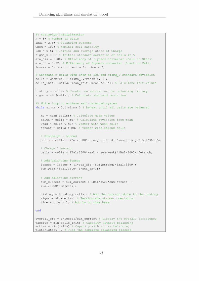
Balancing algorithms and simulation model
67
%% Variables initialization n = 8; % Number of cells iBal = 2.5; % Balancing current Cnom = 100; % Nominal cell capacity SoC = 0.5; % Initial and average state of Charge sigma_0 = 2; % Initial standard deviation of cells in % eta_dis = 0.88; % Efficiency of flyback-converter (Cell-to-Stack) eta_ch = 0.92; % Efficiency of flyback-converter (Stack-to-Cell) losses = 0; sum_current = 0; time = 0; % Generate n cells with Cnom at SoC and sigma_0 standard deviation cells = Cnom*SoC + sigma_0.*randn(n, 1); cells_init = cells; mean_init =mean(cells); % Calculate init values history = cells; % Create new matrix for the balancing history sigma = std(cells); % Calculate standard deviation %% While loop to achieve well-balanced system while sigma > 0.1*sigma_0 % Repeat until all cells are balanced
mu = mean(cells); % Calculate mean values delta = cells - mu; % Calculate deviation from mean weak = cells < mu; % Vector with weak cells strong = cells > mu; % Vector with strong cells
% Discharge 1 second cells = cells - iBal/3600*strong + eta_dis*sum(strong)*iBal/3600/n; % Charge 1 second cells = cells + iBal/3600*weak - sum(weak)*iBal/3600/n/eta_ch; % Add balancing losses losses = losses + (1-eta_dis)*sum(strong)*iBal/3600 + sum(weak)*iBal/3600*(1/eta_ch-1);
% Add balancing current sum_current = sum_current + iBal/3600*sum(strong) + iBal/3600*sum(weak); history = [history,cells]; % Add the current state to the history sigma = std(cells); % Recalculate standard deviation time = time + 1; % Add 1s to time base
end overall_eff = 1-losses/sum_current % Display the overall efficiency passive = min(cells_init) % Capacity without balancing active = min(cells) % Capacity with active balancing plot(history'); % Plot the complete balancing process

MATLAB numerical simulations
68
The plot that is generated by this m-file is shown in Figure 58. Each cell is balanced individually at the same speed. The decrease in capacity due to the balancing losses is visible by the negative slope of the horizontal line that represents the average capacity.
Figure 58: MATLAB simulation output of balancing process for C2St2C method (8 cells
with normally distributed capacity at 50% SoC)
Balancing algorithms for the other methods
The MATLAB code for the new balancing types is similar to the shown C2St2C algorithm in terms of structure but much more complex for the following reasons:
• Integration of two strategies: “Simple” and “Smart” • Charge and discharge balancing processes need two different routines • The bottom cell, and for Type III also the top cell, are balanced differently
and require a separate routine • Selectable arrangement of battery cells in random or in ascending/
descending order in terms of capacity
Therefore, the code is neither presented within this chapter nor in the appendix but available on request. However, a flow-chart diagram of the balancing process is shown in Figure 59. It is valid for the six introduced balancing types. The green

Balancing algorithms and simulation model
69
boxes define the start and end state of the simulation. Actions are explained in blue boxes and the red lozenges stand for if-else decisions. The algorithm is described hereafter:
First, n cells are created with normally distributed capacity values. Then, the arrangement of the cells in the battery stack is adjusted to continue with a sorted stack. Initially, the deviation from the mean value of each cell is calculated. Depending on the algorithm “smart” or “simple”, the cells to be balanced are selected. The corresponding cell capacities are adjusted according to the given equations with a time step of 1 s until one of the balanced cells crosses the stop criterion. Again, cell capacities and mean values are calculated and the balancing process is repeated until the requested state of balancing is reached.

MATLAB numerical simulations
70
Figure 59: Flow-chart diagram of the new balancing types algorithms used in the
numerical simulations

Balancing algorithms and simulation model
71
Batch simulation
For every simulation run, the values for the cell capacities are randomly regenerated. In order to reliably classify the average performance, a large number of simulations must be carried out. Therefore, a MATLAB script for a batch simulation was written. It is quoted in Appendix C.
To determine the minimum required simulation iterations, the random generator of MATLAB was tested using the following command: std(mean(randn(n))). It calculates the standard deviation of the mean value of a matrix of n random values. The output of the command is:
• 0.3564 for n = 10 → ϭ = 35.6% • 0.0956 for n = 100 → ϭ = 9.6% • 0.0317 for n = 1,000 → ϭ = 3.2% • 0.0010 for n = 10,000 → ϭ = 0.1% • n=100,000 exceeds the maximum array size of MATLAB
Based on the result, it was decided to always perform 10,000 simulations for every setup to achieve an accuracy of 0.1%.
Balancing converter efficiencies
The efficiency values of the converters are obtained by calculation. Conduction losses PC, switching losses PSw and gate drive supply PQ of the MOSFETs as well as the ohmic losses PR and magnetic core losses PM of the inductor are taken into account according to (31). The MOSFET data comes from an existing device, the Vishay SIJA58DP with a RDS(ON) of 2.65 mΩ. For the overall losses, the switch-matrix conduction losses PX are added as well using data from the MOSFET NVMFD5C650NL from ON Semi with an RDS(ON) of 4.2 mΩ.
𝜂𝜂𝐶𝐶𝑛𝑛𝑛𝑛𝑃𝑃𝐶𝐶𝐶𝐶𝑎𝑎𝐶𝐶𝐶𝐶 = 𝐼𝐼𝑛𝑛 ⋅ 𝑉𝑉𝑛𝑛
(𝐼𝐼𝑛𝑛 ⋅ 𝑉𝑉𝑛𝑛 + 𝑃𝑃𝐶𝐶 + 𝑃𝑃𝑆𝑆𝑆𝑆 + 𝑃𝑃𝑅𝑅 + 𝑃𝑃𝑄𝑄 + 𝑃𝑃𝑀𝑀) (31)
Figure 60 shows the simulation output for the synchronous buck converter for
eight cells in series (n=8). On the left side, the contour plot provides efficiency

Balancing converter efficiencies
72
information depending on the output current and level. For output level 3 and above, the efficiency is over 96%. On the right side, the distribution of losses as a function of the output current is shown. Losses increase exponentially since the conduction and ohmic losses grow with I2. The corresponding MATLAB code is available upon request.
(a) (b)
Figure 60: Contour plot of the buck converter efficiency (a) and losses distribution (b)
For the maximum output current of 10 A, the resulting efficiency vectors of the
buck and boost converter used in Type Ia balancing are:
𝜂𝜂𝐵𝐵𝐵𝐵𝑎𝑎𝑘𝑘 =
⎝
⎜⎜⎜⎛
0.9090.9520.9680.9760.9800.9840.986⎠
⎟⎟⎟⎞
and 𝜂𝜂𝐵𝐵𝑛𝑛𝑛𝑛𝑃𝑃𝑎𝑎 =
⎝
⎜⎜⎜⎛
0.9450.9710.9800.9850.9870.9890.990⎠
⎟⎟⎟⎞
Combining the two efficiency vectors for all possible configurations and adding
the switch-matrix losses results in an efficiency surface plot shown in Figure 61. The complete calculation was done in MATLAB. The m-file script is available upon request. In Type III balancing, the converters have only four output voltage levels which reduces the size of the efficiency plot. Only the top four values of the efficiency values are required.

Balancing algorithms and simulation model
73
Figure 61: Calculated overall efficiency of active balancing stage
For Type II, the input as well as the output level are variable. Therefore, the
efficiency values are given in a 7x7 matrix and not a single column vector. To keep the code complexity low, the following simplification has been applied for the balancing simulation. A total of four values is defined:
• Buck operation into lowest cell level: ηBu1 = 0.900 • Average value for buck operation into any other level: ηBuX = 0.969 • Boost operation from lowest cell level: ηBo1 = 0.924 • Average value for boost operation of any other level: ηBoX = 0.976
Measurement data from the LT8708 four-switch controller is available in
Appendix H. The corresponding values are ηBu1 = 0.907, ηBuX = 0.964, ηBo1 = 0.918, ηBoX = 0.97 and only little below the calculated ones.
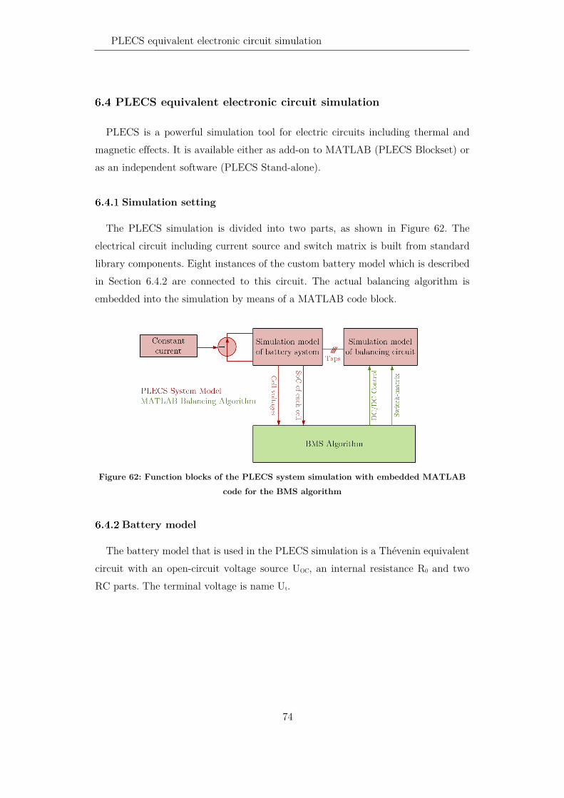
PLECS equivalent electronic circuit simulation
74
PLECS equivalent electronic circuit simulation
PLECS is a powerful simulation tool for electric circuits including thermal and magnetic effects. It is available either as add-on to MATLAB (PLECS Blockset) or as an independent software (PLECS Stand-alone).
Simulation setting
The PLECS simulation is divided into two parts, as shown in Figure 62. The electrical circuit including current source and switch matrix is built from standard library components. Eight instances of the custom battery model which is described in Section 6.4.2 are connected to this circuit. The actual balancing algorithm is embedded into the simulation by means of a MATLAB code block.
Figure 62: Function blocks of the PLECS system simulation with embedded MATLAB
code for the BMS algorithm
Battery model
The battery model that is used in the PLECS simulation is a Thévenin equivalent circuit with an open-circuit voltage source UOC, an internal resistance R0 and two RC parts. The terminal voltage is name Ut.

Balancing algorithms and simulation model
75
Figure 63: Electrical battery model (Thévenin model) according to [12]
The voltages at the circuit elements can be expressed mathematically according
to Kirchhoff's second law:
𝑼𝑼𝑶𝑶𝑶𝑶 = 𝑼𝑼𝐭𝐭 − 𝑼𝑼𝑶𝑶𝑪𝑪𝑪𝑪 − 𝑼𝑼𝑶𝑶𝑪𝑪𝑪𝑪 − 𝑰𝑰𝒕𝒕𝑹𝑹𝑶𝑶 (32) with
𝑼𝑪𝑪𝑪𝑪 =
𝑰𝑰𝒕𝒕
𝑶𝑶𝑪𝑪𝑪𝑪−
𝑼𝑼𝑶𝑶𝑪𝑪𝑪𝑪
𝑹𝑹𝑪𝑪𝑪𝑪𝑶𝑶𝑪𝑪𝑪𝑪
𝑼𝑪𝑪𝑪𝑪 =𝑰𝑰𝒕𝒕
𝑶𝑶𝑪𝑪𝑪𝑪−
𝑼𝑼𝑶𝑶𝑪𝑪𝑪𝑪
𝑹𝑹𝑪𝑪𝑪𝑪𝑶𝑶𝑪𝑪𝑪𝑪
(33)
The PLECS battery model is already parametrized based on measurements of real
cells. All component values except for R0 are dependent on the SoC. These curves are plotted in Figure 64 to Figure 66. The MATLAB code can be found in Appendix E.
Figure 64: Capacity-Voltage (C-V) curve based on OCV measurement values

PLECS equivalent electronic circuit simulation
76
(a) (b)
Figure 65: Resistor Rp1 (a) and Capacitor Cp1 (b) of RC part 1
(a) (b)
Figure 66: Resistor Rp2 (a) and Capacitor Cp2 (b) of RC part 2
Simulation model
The complete simulation is set up in MATLAB/Simulink as shown in Figure 67. Subsystems include the balancing algorithm as an m-file (”BMS Logics”) and the electric simulation model as a PLECS model (”Active BMS battery system”).

Balancing algorithms and simulation model
77
Figure 67: System simulation in Simulink with MATLAB-function block for the
balancing algorithm and PLECS circuit block Figure 68 shows the contents of the PLECS subsystem for Type IIa balancing.
Black wires represent power connections whereas green wires are reserved for signals. The model includes a total of 16 switches implemented as eight changeover switches to reduce the number of elements and wires and therefore increase the clarity of the model. Eight battery models are connected in series (”Li-ion R modelx”). The battery model is provided by Plexim named ”RC-chain-based Li-ion model”. Another subsystem “DC/DC Converter” directs the requested balancing current between the battery cells. A constant current source I2 with a small series resistance of 10 mΩ is included to simulate battery charging or discharging.

PLECS equivalent electronic circuit simulation
78
Figure 68: Detail view of PLECS circuit block for Type IIa balancing
3Iout
1SWM
1SoC
S3
S4
S5
S6
S7
S8
S9
S10
2Iin
R3R4Li-ion
R model8
-
socvout
Li-ionR model1
+-
socvout
Li-ionR model2
+-
socvout
Li-ionR model7
+-
soc
Li-ionR model6
+-
socvout
Li-ionR model3
+-
socvout
Li-ionR model4
+-
socvout
Li-ionR model5
+-
socvout
I24Ibat
2Vcell
R5
DC/DC Converter
In1
In2
Port1
Port2
Port3
Hardware implementation
79
Hardware implementation
The hardware implementation serves as a demonstration prototype to show the working principle of the presented balancing methods. To facilitate the development process and increase the hardware versatility, a modularized design, consisting of a DC/DC converter, a switch-matrix unit and an MCU board was chosen. The switch-matrix unit was developed from scratch, whereas the MCU board was bought as a retail part. The DC/DC converter was a customized engineering sample prototype.
DC/DC converter
Plenty of DC/DC converter implementations are available from literature and by electronic suppliers. In this section, only non-isolated, commonly available designs are considered.
Evaluation of components
The easiest way to cover all technical requirements of Type I and Type II balancing is a four-switch buck-boost converter. Alternatively, two separate buck and boost converters can be used, or the required functions are provided by a micro-controller based custom design. Table 6 lists the three options and their expected performance specifications. The high-side converter for Type III balancing is not considered in this overview. Due to the lack of commercial solutions, the only option for it is a custom design.
A preferable feature of low voltage converters is synchronous mode as described in 5.3.1. The conduction losses of the diode rectifier contribute significantly to the overall losses, especially in low output-voltage applications. The rectifier conduction losses are proportional to the product of its forward-voltage drop VF, and the forward conduction current IF. Below a certain current level, the forward-voltage drop of a synchronous rectifier is lower than that of a diode rectifier, and consequently reduces the rectifier conduction losses. Because synchronous rectifiers are active devices, the design and utilization of synchronous rectification has to be well dimensioned to fully exploit the possible increase in efficiency and maintain a stable operation.
Table 6: Technical concepts for DC/DC converter

DC/DC converter
80
Type Four-switch buck-boost converter
Separate converters (buck and boost)
Custom design
Suppliers Few Many MCU/DSP supplier Bidirectional mode
Yes N/A Possible
Current control Yes Yes Possible Synchronous mode
Yes Yes Possible
Efficiency 96...99% 94..98% 95% Foot print area for 5 A design
840 mm2 (LM5175) 300 mm2 (LM25118) & 710 mm2 (LM5122)
> 1000 mm2
Communication interface
No Available Possible (e.g. SPI or I2C)
Cost Medium Low to medium Low to high
There are only few PMICs that can control four MOSFETs. They are supplied by
the following three manufacturers: Texas Instruments Inc., Analog Devices Corp. (formerly LT) and Renesas Electronics Corp. Table 7 shows the available ICs to operate a four-switch buck-boost converter in stand-alone mode. Only ICs capable of synchronous mode are considered due to the previously stated reasons.
Table 7: Overview of existing four-switch buck-boost converter ICs
IC LT8708 [97] LM5175 [98] ISL81601 [99] LT8390 [100]
Manufacturer Linear Technology
Texas Instruments
Renesas Electronics
Linear Technology
Bidirectional mode
Yes No Yes No
Maximum working voltage
80 V 42 V 60 V 60 V
Current control Yes Yes Yes Yes Synchronous mode
Yes Yes Yes Yes
Efficiency 98% 96% 99% 98% Minimum input voltage
2.8 V 3.5 V 4.5 V 4 V
Communication interface
No No No No
Demo Boards DC2596A PMP10507 ISL81601EVAL DC2457A

Hardware implementation
81
Decision on components
A bidirectional buck-boost converter as shown in Figure 53 enables all presented balancing methods except of Type III. Consequently, this type of converter is selected to be used in the demonstration prototype. Due to the lower minimum input voltage of the LT8708, it was preferred over the ISL81601. Otherwise, boost operation from one battery cell into the stack would not be possible.
Hardware design
Linear Technology has assembled the LT8708 demo circuit board, which is shown in Figure 69, according to our specifications and design considerations as an engineering sample. The voltage capability of formerly 80 V was reduced to 40 V to have a better selection of low RDS(ON) MOSFETs. Finally, the Vishay SIJA58DP was selected in consultation with LT. For the schematic of the board see Appendix L. Further technical specifications are:
• Switching frequency: 250 kHz • Balancing current: max. 10 A • Operation mode: Hybrid current mode (HCM, see [97])
Figure 69: LT8708 Custom evaluation board (DC2596A)

Switch-matrix unit
82
Switch-matrix unit
Unlike for the DC/DC converter and the BMS, there was no readily available switch-matrix design. Therefore, the board was designed from scratch.
Evaluation of components
The switch-matrix is required to connect the DC/DC converters to the cells. MOSFETs instead of electro-mechanical devices are used to keep the necessary switches as low-loss and wear-free as possible. MOSFET transistors are available as N-channel and P-channel types, which differ in the control logics and the ON-state resistance RDS(ON). Both types are available as self-conducting and self-blocking devices. To realize an AC-switch, two transistors with a common source are required and connected in anti-series configuration (see Figure 70). Otherwise, the current could flow in the undesired direction via the body diodes of the transistors and short-circuit certain cells. Figure 71 shows a popular type with two MOSFETs that can be easily connected to the required configuration.
Figure 70: AC switch with two
MOSFET in anti-series connection
Figure 71: Dual MOSFET for convenient AC-switch realization (Vishay SQJQ904E) [101]
It is difficult to find P-channel MOSFETs in the required power range with such
a small RDS(ON) which already fulfil this at drive voltages of VGS = 3.2 V. Since the maximum drive voltage VGS corresponds to the cell voltage, the selection of N-channel MOSFETs is also very limited. Therefore, a gate driver must be used to control the transistors. An additional requirement is galvanic isolation, since the electrical source potential of the MOSFETs is above the potential of the control signals.

Hardware implementation
83
By choosing a gate driver, a wide range of N-channel MOSFET transistors is available. To enable the switch-matrix to work with 36 V to 48 V battery systems, a minimum blocking voltage of 60 V is required. The most important requirements are summarized as follows:
• Blocking voltage VDS ≥ 60 V • Continuous current ID ≥ 20 A • Maximum gate-source voltage VGS ≥ 10 V • On-state resistance RDS(ON) ≤ 6 mΩ with VGS ≤ 10 V
Single or double MOSFET transistors can be used for the bidirectional switches
of the switching matrix. The selection of single transistors is significantly larger but double MOSFETs offer some important benefits like reduced assembly cost and less space requirements. A selection of both single and dual MOSFETs for the above specifications is listed in Table 8.
For the isolated gate driver list in Table 9, the most important criterion is the standby consumption as it defines the storage life of the system. Suitable technical concepts are photovoltaic, inductive and capacitive energy transfer. Except for the TI EMB1428, all products offer one or two channels.
Decision on components
In general, a low on-state resistance RDS(ON) of a MOSFET comes together with a high gate charge QG. The product of RDS(ON) and QG is called figure of merit (FoM) and represents a quality feature for comparison purposes. Based on this feature, the overview in Table 8 delivers four options with a FoM value of less than 200. The ON Semiconductor NVMFD5C650NL combines a good FoM with an unrivalled low RDS(ON) for a dual device. Therefore, this N-channel MOSFET was selected for all related calculations and simulations. For the switch-matrix unit, due to a better handling, the Vishay SQJQ960EL was used. Any other of the dual MOSFETs in the table could be chosen if the focus were set elsewhere (e.g. on small size, low cost, etc.).
The isolated gate driver HT0440 by Microchip was chosen. It requires no external components, has no standby consumption and is compact, but can still be soldered manually. With one driver, it is possible to control two N-channel MOSFET pairs.

Switch-matrix unit
84
In total, four are needed to control all switches. Since the energy for recharging the gate capacitance is obtained directly from the control signal, no external supply is required. However, a level shifting of the signals from the BMS main controller from 3 V to 5 V is necessary to obtain an optimal drive voltage of 10 V at the output of the MOSFET driver. Any suitable level converter with at least eight channels can be used. For this thesis, the TI TXS0108E was selected.
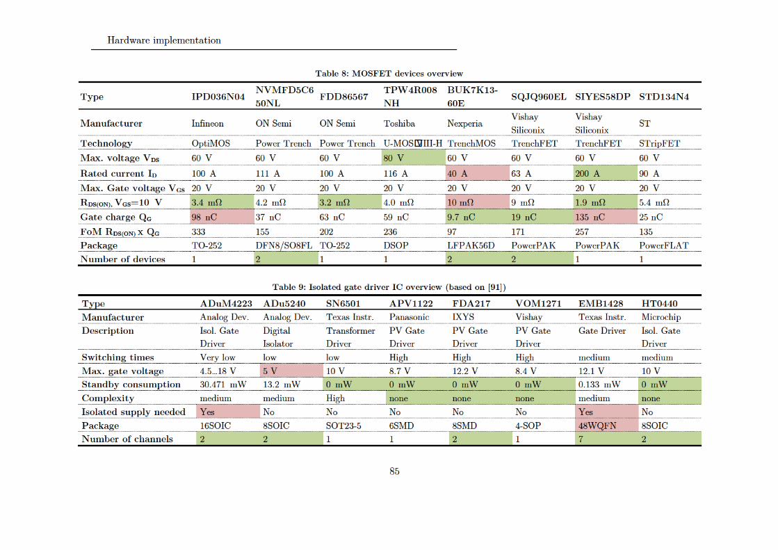
H ar d w ar e i m pl e m e nt ati o n
8 5
T a bl e 8 : M O S F E T d e vi c e s o v e r vi e w
T y p e I P D 0 3 6 N 0 4 N V M F D 5 C 6
5 0 N L F D D 8 6 5 6 7
T P W 4 R 0 0 8
N H
B U K 7 K 1 3 -
6 0 E S Q J Q 9 6 0 E L S I Y E S 5 8 D P S T D 1 3 4 N 4
M a n uf a c t u r e r I nfi n e o n O N S e mi O N S e mi T os hi b a N e x p eri a Vis h a y
Sili c o ni x
Vis h a y
Sili c o ni x S T
T e c h n ol o g y O pti M O S P o w er Tr e n c h P o w er Tr e n c h U -M O S VIII -H Tr e n c h M O S Tr e n c h F E T Tr e n c h F E T S Tri p F E T
M a x. v ol t a g e V D S 6 0 V 6 0 V 6 0 V 8 0 V 6 0 V 6 0 V 6 0 V 6 0 V
R a t e d c u r r e n t I D 1 0 0 A 1 1 1 A 1 0 0 A 1 1 6 A 4 0 A 6 3 A 2 0 0 A 9 0 A
M a x. G a t e v ol t a g e V G S 2 0 V 2 0 V 2 0 V 2 0 V 2 0 V 2 0 V 2 0 V 2 0 V
R D S ( O N ), V G S = 1 0 V 3. 4 m Ω 4. 2 m Ω 3. 2 m Ω 4. 0 m Ω 1 0 m Ω 9 m Ω 1. 9 m Ω 5. 4 m Ω
G a t e c h a r g e Q G 9 8 n C 3 7 n C 6 3 n C 5 9 n C 9. 7 n C 1 9 n C 1 3 5 n C 2 5 n C
F o M R D S ( O N ) x Q G 3 3 3 1 5 5 2 0 2 2 3 6 9 7 1 7 1 2 5 7 1 3 5
P a c k a g e T O -2 5 2 D F N 8 / S O 8 F L T O -2 5 2 D S O P L F P A K 5 6 D P o w er P A K P o w er P A K P o w er F L A T
N u m b e r of d e vi c e s 1 2 1 1 2 2 1 1
T a bl e 9 : I s ol a t e d ga t e d ri v e r I C o v e r vi e w ( b a s e d o n [ 9 1])
T y p e A D u M 4 2 2 3 A D u 5 2 4 0 S N 6 5 0 1 A P V 1 1 2 2 F D A 2 1 7 V O M 1 2 7 1 E M B 1 4 2 8 H T 0 4 4 0
M a n uf a c t u r e r A n al o g D e v. A n al o g D e v. T e x as I nstr . P a n as o ni c I X Y S Vis h a y T e x as I nstr . Mi cr o c hi p
D e s c ri p ti o n Is ol. G at e
Dri v er
Di git al
Is ol at or
Tr a ns f or m er
Dri v er
P V G at e
Dri v er
P V G at e
Dri v er
P V G at e
Dri v er
G at e Dri v er Is ol. G at e
Dri v er
S wi t c hi n g ti m e s V er y l o w l o w l o w Hi g h Hi g h Hi g h m e di u m m e di u m
M a x. g a t e v ol t a g e 4. 5 … 1 8 V 5 V 1 0 V 8. 7 V 1 2. 2 V 8. 4 V 1 2. 1 V 1 0 V
S t a n d b y c o n s u m p ti o n 3 0. 4 7 1 m W 1 3. 2 m W 0 m W 0 m W 0 m W 0 m W 0. 1 3 3 m W 0 m W
C o m pl e xi t y m e di u m m e di u m Hi g h n o n e n o n e n o n e m e di u m n o n e
I s ol a t e d s u p pl y n e e d e d Y es N o N o N o N o N o Y es N o
P a c k a g e 1 6 S OI C 8 S OI C S O T 2 3 -5 6 S M D 8 S M D 4 -S O P 4 8 W Q F N 8 S OI C
N u m b e r of c h a n n el s 2 2 1 1 2 1 7 2

Switch-matrix unit
86
Hardware design
The switch-matrix units for the different types of balancing are not identical. Therefore, a modular and versatile design was chosen with eight AC-switches. The units can easily be used in parallel i.e. for Type IIa balancing. For series operation of more than eight cells, the units can be connected in series but require an insulated level-shifter instead of the used TI TXS0108E. Figure 72 shows a simplified schematic of the circuit. It shows 16 MOSFETs with connected source pins to achieve eight AC-switches. The DC/DC converter input/output connects to “Converter” while the battery cells connect to the eight remaining taps.
Figure 72: Schematic excerpt of switch-matrix for eight AC-switches
The switch-matrix was designed using the electronic design automation tool
“Altium Designer” and produced on a separate PCB shown in Figure 73. The complete schematic is given in Appendix K. A small switched-mode power supply (SMPS) is used to provide 5 V from the battery voltage for the level-shifter IC. In

Hardware implementation
87
a final design, this power supply should be designed carefully to achieve a very low stand-by consumption or include the possibility to completely disable the device.
Figure 73: Switch-matrix PCB for up to eight cells
Firmware
The firmware includes the balancing algorithm to control the switch-matrix and the DC/DC converter operating point. Instead of coding the firmware functions in a text-based programming language such as C, a model-based approach was used.
Model-based programming and automatic code generation
The firmware was programmed graphically in Simulink using the embedded coder plug-in. To control the TI MCU, the hardware-support-package “Energia” was necessary. This setup enables the user to run a program on the controller and simultaneously get a feedback of the controller status as well as having the ability to change program variables online. The feature is called “External Mode”.
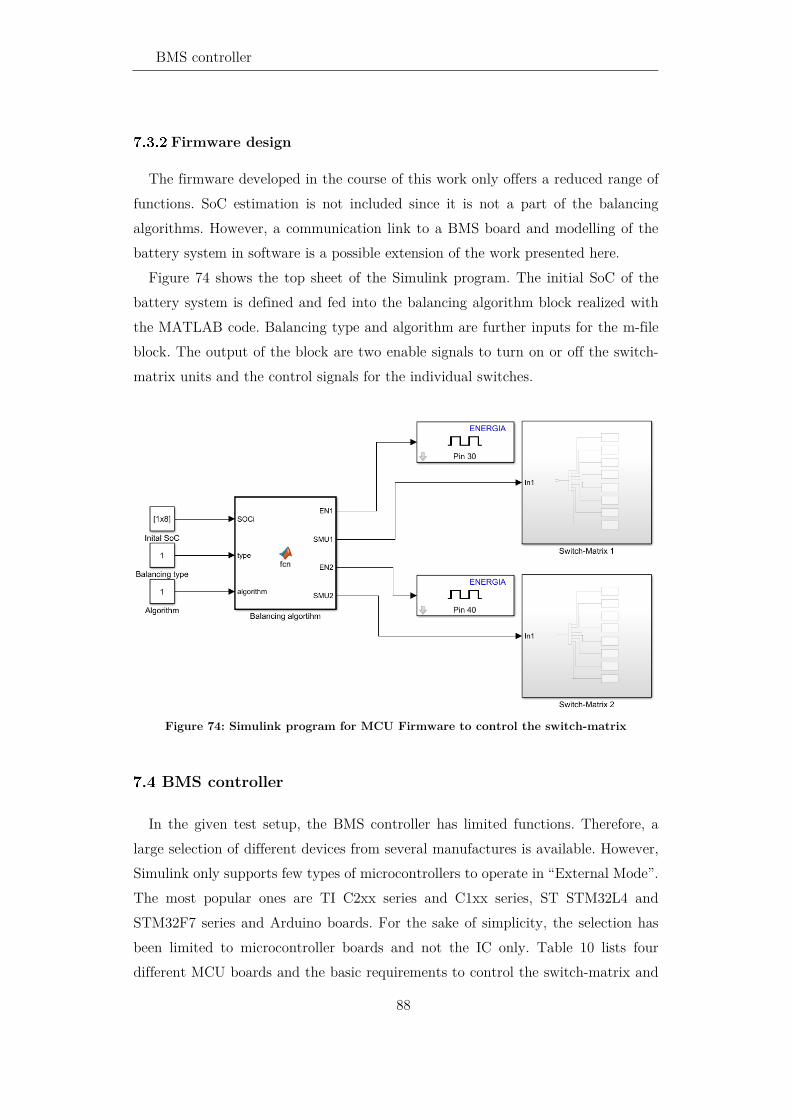
BMS controller
88
Firmware design
The firmware developed in the course of this work only offers a reduced range of functions. SoC estimation is not included since it is not a part of the balancing algorithms. However, a communication link to a BMS board and modelling of the battery system in software is a possible extension of the work presented here.
Figure 74 shows the top sheet of the Simulink program. The initial SoC of the battery system is defined and fed into the balancing algorithm block realized with the MATLAB code. Balancing type and algorithm are further inputs for the m-file block. The output of the block are two enable signals to turn on or off the switch-matrix units and the control signals for the individual switches.
Figure 74: Simulink program for MCU Firmware to control the switch-matrix
BMS controller
In the given test setup, the BMS controller has limited functions. Therefore, a large selection of different devices from several manufactures is available. However, Simulink only supports few types of microcontrollers to operate in “External Mode”. The most popular ones are TI C2xx series and C1xx series, ST STM32L4 and STM32F7 series and Arduino boards. For the sake of simplicity, the selection has been limited to microcontroller boards and not the IC only. Table 10 lists four different MCU boards and the basic requirements to control the switch-matrix and

Hardware implementation
89
the DC/DC converter. Instead of the MCU board, only the IC would be used in a series product together with all other BMS components assembled on one PCB.
For a more sophisticated balancing algorithm and additional control features, further optional requirements have been considered at the bottom of the table.
Table 10: Selection of suitable MCU boards as BMS controller
Features Tiva C-Series LaunchPad
Arduino Uno/Mega
Nucleo-L476RG
MCU Manufacturer TI Atmel ST
Type TM4C123 ATMEGA328 / ATMEGA2560
STM32L476
Bit 32 8 32 18 Digital Out for 16 switches / 2 Enable
/
3.3 V Output Low power Optional: SPI / UART / I2C / PWM / 12 Bit DAC / Floating Point Unit (FPU)
Dimensions 65x50 mm 70x55 mm / 100x55 mm
80x70 mm
HW Cost ~6€ ~1.5€ / 9€ ~5€ Based on the technical comparison, both the Tiva C-series and the Nucleo-
L476RG qualify as BMS controller. The small form factor of the TI MCU board was ultimately the deciding factor for being selected. Photograph of the MCU boards are given in Figure 75 and Figure 76.

Configuration of the demonstration prototype
90
Figure 75: TI Tiva C-Series LaunchPad with debug interface (right side) [102]
Figure 76: ST Nucleo-STM32L476RG with debug interface (right side) [103]
Configuration of the demonstration prototype
The intended test setup for the active balancing demonstration prototype is shown in Figure 77. A battery system consisting of eight lithium-ion cells is connected to the monitoring HW and the switch-matrix. The DC/DC-converter is controlled through the main controller and has a power interface to the switch-matrix. Finally, the main controller and the monitoring HW are connected to the PC.
Figure 77: Active balancing demonstrator setup

Results
91
Results
The performance of the three investigated balancing types is analysed through different approaches:
• MATLAB Numerical simulation • PLECS Simulation • HW Measurements
In Section 8.1, the numerical simulation results are presented. In Section 8.2, these results are compared to the electrical simulation output generated in PLECS. Finally, the HW measurements are used to confirm the simulation-based findings.
MATLAB numerical simulations
The newly introduced balancing methods are rated in terms of balancing efficiency, average balancing time and provided battery capacity. This analysis is done by MATLAB simulations and includes all three types with two different algorithms each. Details on the balancing algorithms are given in Section 5.3 and in the appendix. In order to classify the results, a reference active balancing method (C2St2C) and passive balancing are simulated as well. To illustrate the balancing principle, one battery setting with an initial SoC distribution has been chosen. The simulation output is shown graphically in Section 8.1.2. The MATLAB numerical simulation has been presented in Section 5.3. It was carried out using the equipment and parameters listed below. The simulations were performed on a PC workstation specified in Table 11.
Table 11: PC Workstation specifications
Tool Manufacturer Type / Version PC Dell Precision T3600 PC Operating system Microsoft Windows 10 64 Bit MATLAB/Simulink Mathworks Version 2018a

MATLAB numerical simulations
92
Simulation parameters
For the batch simulations, the cell and balancing parameters are given in Table 12. The efficiency values for the different balancing types are derived in Section 6.3. The current rating of the converters for Type I to III is assumed to be 10 A. For the reference method, the real value of 2.5 A is taken for the simulations.
Table 12: Battery cell and balancing simulation parameters
Cell and HW parameter Symbol Value Nominal capacity Cnom 100 Ah State of charge SoC 50%
Nominal voltage Unom 3.7 V Standard deviation of cell capacities σ0
2% End of balancing criterion σend = 0.1σ0 Number of cells n 8 Balancing current for: Type I and III Type II Reference method C2St2C Passive Balancing
IBal
10 A 10 A 2.5 A 0.2 A
Cell equalization for the different balancing circuits
To illustrate the balancing process of the new methods, one cell configuration has been chosen (Cnom = 0.49875 and σ = 2.75%) and tested with the three different methods and two algorithms. The initial cell capacity distribution is given as:
𝑆𝑆𝑆𝑆𝑆𝑆𝚤𝚤𝑛𝑛𝚤𝚤𝑎𝑎 =
⎝
⎜⎜⎜⎜⎛
0.5000.4800.4700.5100.5200.4900.4950.515⎠
⎟⎟⎟⎟⎞
Figure 78 shows the balancing process for the given setup for each of the
investigated methods and the “Simple” algorithm. For Type Ia and IIIa, the process takes a little less than one hour whereas for Type II, balancing requires less than 50 minutes.

Results
93
(a)
(b)
(c)
Figure 78: Simulation output of balancing process with algorithm ”Simple” for
Type Ia (a), Type II (b) and Type IIIa (c)

MATLAB numerical simulations
94
To illustrate the effect of the different algorithms, the same setup is simulated but with algorithm ”Smart” and with sorted cells. The balancing process can be accelerated by both measures. Using the ”Smart” algorithm reduced the balancing time by 40.1%. If the cells are arranged in the battery system in descending order of their capacity, the balancing time can be further reduced. Compared with the initial setup, the reduction is 66.1%.
(a)
(b)
Figure 79: Simulation output of balancing process for Type II and algorithm ”Smart”
with randomly assembled cells (a) and cells sorted in descending order (b)

Results
95
Summary
In this section, the results of the batch simulations are presented. Contrary to Section 8.1.2, a multitude of different battery settings is simulated. The overall balancing efficiency ηBal is calculated according to (34) as a function of losses and balanced charged.
𝜂𝜂𝐵𝐵𝑎𝑎𝐶𝐶 = 1 − ∑ 𝑄𝑄𝐿𝐿𝑛𝑛𝑃𝑃𝑃𝑃𝐶𝐶𝑃𝑃
∑ 𝑄𝑄𝐵𝐵𝑎𝑎𝐶𝐶 (34)
The output of the batch simulation is compared in terms of balancing time,
efficiency and achievable capacity gain. The best results are highlighted in bold script. Type Ib and Type IIIb have not been simulated separately. Considering the design, the same balancing efficiency is expected as for the a-types. Type IIa and IIb are not distinguished as the balancing behaviour is the same.
Type I to III are listed in Table 13 and compared to the reference method C2St2C and to passive balancing. The cells arrangement is random since this is the normal case. The fastest balancing time is achieved by Type II method with the “Smart” algorithm and the highest overall efficiency by Type IIIa with the “Smart” algorithm as well.
In Table 14, this is done for six settings of Type Ia balancing, which differ in the algorithm involved and either random, ascending or descending cells arrangement. Ascending means that the cell with the lowest capacity is at position 1 and the cell with the highest capacity is at position n. Descending is in reverse order and for random there is no order.

MATLAB numerical simulations
96
Table 13: Comparison of simulations results for the different balancing types and random cells arrangement
Parameter Type Ia Type Ia Type II Type II Type IIIa Type IIIa C2St2C Passive Algorithm Simple Smart Simple Smart Simple Smart N/A N/A Cells arrangement Random Random Random Random Random Random Random Random Avg. balancing time tBal 3619 s 3455 s 3385 s 2612 s 4081 s 3725 s 3501 s 28.4 h Balancing efficiency ηBal 0.865 0.892 0.866 0.905 0.875 0.913 0.896 0 Capacity gain 1-CAct/CPass 2.5% 2.8% 2.6% 2.5% 2.4% 2.4% 2.3% 0%
Table 14: Results for different simulation settings and Type Ia balancing
Algorithm Simple Smart Simple Smart Simple Smart Cells arrangement Random Random Ascending Ascending Descending Descending Avg. balancing time tBal 3619 s 3455 s 3713 s 3193 s 3670 s 3165 s Balancing efficiency ηBal 0.825 0.892 0.865 0.931 0.842 0.936 Capacity gain 1-CAct/CPass 2.5% 2.8% 2.6 % 2.6% 2.5 % 2.4%

Results
97
Verification by electronic circuit simulation
The verification of the calculation results takes place in two ways: Simulation and measurements. Unlike for the numerical simulations, only few SoC distributions can be tested due to increased technical expenses.
The electronic circuit simulation is performed in MATLAB using the power electronics add-on PLECS. Thereby, the electric behaviour of the balancing electronics as well as the batteries can be emulated and the code for the different algorithms can be embedded into the simulation.
Simulation parameter and equipment
In addition to the simulation equipment specified in Section 8.1.1, PLECS 4.2 was used for the simulations presented in this section. The PLECS simulations are based on the same cell and HW parameter as stated in 8.1.1. The same configuration as in Section 8.1.2 was used to allow a direct comparison.
Cell equalization
The cell equalization process can be simulated without any load current. Figure 80 shows the simulation output based on a battery configuration and balancing settings already used in 8.1.2. Exactly the same setup was simulated numerically in in Figure 78 (b). It can be clearly seen that the standard deviation constantly decreases until the stop criterion is reached after approximately 1600 s. The steps that are visible in the SoC curves are due to an increase of the simulation step size from 1 s to 10 s to account for the slow operation switch-matrix.

Verification by electronic circuit simulation
98
Figure 80: Cell equalization during active balancing for Type II method (PLECS
simulation output)
Balancing during battery discharge
To demonstrate the ability of the balancing methods to prolong battery usage, another simulation with constant discharge was performed. Figure 81 shows the situation with passive balancing, where no action is taken during discharging. Cell #7, like in Section 8.2.2, has the lowest initial SoC and therefore first reached the end of discharge level after 3200 s. It should be noted that this level is not exactly at 0% SoC but at around 5% due to the settings of the battery model.
On the other hand, in Figure 82, the cells are balanced by the Type II method. Complete equalization is achieved after 1900 s and the end of discharge is prolonged by 120 s or 3.4% respectively. The initial SoC of the eight cells is similar to the simulation in Section 8.2.2 but scaled to 100%:
𝑆𝑆𝑆𝑆𝑆𝑆𝚤𝚤𝑛𝑛𝚤𝚤𝑎𝑎 =
⎝
⎜⎜⎜⎜⎛
0.9800.9600.9500.990
1.00.9700.9750.995⎠
⎟⎟⎟⎟⎞

Results
99
(a) (b)
Figure 81: Simulation of cell voltages (a) and cells SoCs (b) without balancing during
discharging of eight-cells LIB
(a) (b)
Figure 82: Simulation of cell voltages (a) and cells SoCs (b) with active balancing
(Type II) during discharge of eight-cells LIB
Measurements
For the measurements, a prototype battery was deployed consisting of eight 18650 lithium-ion cells. Compared to the calculations and simulations in the previous chapter, a rather small battery capacity was chosen to keep the test duration low. The purpose of the presented measurements is to compare the different balancing methods and to verify the working principle of the new types proposed in this thesis. The setup is prepared for the equalization through positive balancing during idle

Measurements
100
mode. Unlike for the simulation results, no general performance statement is possible due to the limited configurations that can be tested.
Measurement equipment
All measurement devices and devices under test are listed in Table 15. In the following sections more details can be found about the specifications.
Table 15: Measurement equipment
Device / Tool Manufacturer Type PC Dell Latitude 7490 PC Operating system Microsoft Windows 10 64 Bit MATLAB/Simulink Mathworks Version 2017b Oscilloscope Lecroy HDO4034A USB Interface Linear Technology DC 590B Test battery Samsung SDI INR18650-25R Active balancing board Linear Technology DC 2064A Passive balancing board Texas Instruments bq76PL455A Serial-to-USB adapter FTDI TTL-232R-5V
Test battery system
The parameter of the battery cell involved in the tests (Figure 84) are given in Table 16. To determine the SoC of the cell, an OCV-curve (Figure 83) was generated through linear fitting in MATLAB from data sheet values [104]. The corresponding m-file is available in Appendix F. Because it was not possible to achieve exactly the same SoC values for each cell and setup, the mean SoC is calculated for every test setup and taken as a comparison value.
Table 16: Samsung INR18650-25R cell specification [104]
Manufacturer Samsung SDI Type INR18650-25R Nominal capacity @0.2C 2500 mAh Min. capacity 2460 mAh Nominal voltage 3.6 V - 3.7 V Max. charge voltage 4.2 V ± 0.05 V Min. discharge voltage 2.5 V Max. constant discharge current 20 A Cell chemistry LiNiMnCoO2 (NMC)

Results
101
Figure 83: Linear fit of OCV-curve of 18650 lithium-ion cell
Figure 84:
INR18650-25R battery cell [104]
The test battery system is configured as 8S1P, which means, that eight cells are
connected in series.
Voltage measurement
The initial and end SoC of the battery system is determined by the measured cell
voltages 𝑈𝑈𝐶𝐶 = 𝑈𝑈𝐶𝐶1
⋮𝑈𝑈𝐶𝐶8
prior to the balancing process and after relaxation time. For
this purpose an evaluation BMS board by TI is used, the bq76PL455EVM (see Figure 85). The specifications of the BMS IC are available in Table 4. The board connects to a PC through a Serial-to-USB converter (Type: TTL-232R-5V).
Passive balancing
Passive balancing can be performed by the same PCB that is used for the voltage measurements specified in 8.3.3, the bq76PL455EVM. 75 Ω resistors are built in for passive balancing which corresponds to a balancing current per cell of 40 to 56 mA. The measurement setup is shown in Figure 87. The LT Active balancing board and the USB interface are not used during passive balancing.
Passive balancing does not make sense for the given test case. In practice, during idle mode or discharging no passive balancing is performed. The available battery capacity is defined by the weakest cell, regardless of any balancing operations. The

Measurements
102
equalization of the cells is usually done during charging or at the end of the charging process.
Active balancing with reference board
The reference board for the active balancing is an LT DC2064A with LTC3300-1 AFE and active balancing controller .see. It is shown in Figure 86 and the main specifications are available in Table 17. It provides 12 bidirectional flyback converters to allow cell-to-stack-to-cell balancing. The board is controlled by an application software running on Windows OS. An interface board LT DC590B is used to connect the device to the PC over USB.
Figure 85: TI bq76PL455EVM
Passive balancing BMS board [105]
Figure 86: LT DC2064A Active balancing BMS board [106]
Table 17: Main specifications of the active balancing board LT DC2064A
Manufacturer Linear Technology Type DC2064A AFE LTC3300-1 Balancing controller LTC6803-2 (2 pcs) USB Interface to PC DC590B Max. balancing current 2.5 A Balancing efficiency 88% - 92% Number of cells 3-12 Type of balancing C2St2C
Figure 87 shows the hardware test setup. The test battery system is connected to
the active balancing board as well as to the monitoring BMS.

Results
103
Figure 87: Measurement setup with the prototype battery pack
The test battery system was set for an average SoC of approx. 32% with two
clearly undercharged cells (Cell #2 and Cell #6). The SoC of each cell was determined by linear interpolation as described in 8.3.2.
𝑈𝑈𝐶𝐶_𝚤𝚤𝑛𝑛𝚤𝚤𝑎𝑎 =
⎝
⎜⎜⎜⎜⎛
3.5223.5223.3533.5193.5053.4493.5043.505
⎠
⎟⎟⎟⎟⎞
𝑉𝑉 calculates to 𝑆𝑆𝑆𝑆𝑆𝑆𝚤𝚤𝑛𝑛𝚤𝚤𝑎𝑎 =
⎝
⎜⎜⎜⎜⎛
0.3720.3730.1630.3670.3440.2670.3420.345⎠
⎟⎟⎟⎟⎞
(mean value of 32.2%).
Figure 88 shows the voltage measurement of all eight cells during balancing.
Cell #3 and Cell #6 start balancing together for about 320 s. After that, balancing for Cell #6 is turned off while Cell #3 continues to balance for another 200 s. When

Measurements
104
the balancing stops, the cell voltage need some relaxation time before they show their correct OCV.
Figure 88: Active balancing process for DC2064A
To estimate efficiency and effectiveness, the SoC of each cell was recalculated. In
total, 2.2% of battery capacity was lost due to the balancing process.
𝑈𝑈𝐶𝐶_𝐶𝐶𝑛𝑛𝑒𝑒 =
⎝
⎜⎜⎜⎜⎛
3.4903.4853.5053.4813.4563.4613.4553.457⎠
⎟⎟⎟⎟⎞
𝑉𝑉 calculates to 𝑆𝑆𝑆𝑆𝑆𝑆𝐶𝐶𝑛𝑛𝑒𝑒 =
⎝
⎜⎜⎜⎜⎛
0.3160.3150.3440.3110.2760.2820.2740.277⎠
⎟⎟⎟⎟⎞
(mean value of 30.0%).
Active balancing with Type IIa prototype
The test setup for Type IIa balancing was described in Chapter 7. The components used to set up the demonstration prototype are listed in Table 18 with a reference to the section of their introduction.

Results
105
Table 18: Active balancing prototype Type IIa
Device Type Specifications Reference DC/DC Converter LT DC2596A 40 V / 3 A 7.1.3 Switch-matrix Own design 8 AC-switches 7.2.3 Controller TI Tiva Series 32 bit MCU 7.4 Voltage Logger bq76PL455EVM BMS Board 8.3.3
The hardware setup is described in Figure 77 and a photograph of the prototype
test system is shown in Figure 89. Instead of the LT Board, a combination of two switch-matrix units, a DC/DC converter and an MCU board is used to perform the balancing according to Type I or II. The grey box on the right bottom is not a device but merely represents the electrical connections between the switch-matrix and the DC/DC converter.
Figure 89: Measurement setup with the Type IIa active balancing prototype
The battery system was prepared to accord with the cell distributions in Section
8.3.5. An initial SoC was determined as follows:

Measurements
106
𝑈𝑈𝐶𝐶_𝚤𝚤𝑛𝑛𝚤𝚤𝑎𝑎 =
⎝
⎜⎜⎜⎜⎛
3.4903.4853.3373.4963.4943.4423.4983.497⎠
⎟⎟⎟⎟⎞
𝑉𝑉 calculates to 𝑆𝑆𝑆𝑆𝑆𝑆𝚤𝚤𝑛𝑛𝚤𝚤𝑎𝑎 =
⎝
⎜⎜⎜⎜⎛
0.3290.3150.1500.3300.3280.2570.3340.333⎠
⎟⎟⎟⎟⎞
(mean value of 29.6%).
Similar to Figure 88, the balancing process is illustrated in Figure 90. For this
method, more balancing operations are necessary. An equalized state is achieved after 999 s and three different switch-matrix configurations.
Figure 90: Active balancing process for Type IIa prototype
In total, 1.8% of battery capacity was lost due to the balancing process. The final
SoC of the system is calculated as follows:
𝑈𝑈𝐶𝐶_𝐶𝐶𝑛𝑛𝑒𝑒 =
⎝
⎜⎜⎜⎜⎛
3.4463.4443.4573.4513.4503.4803.4663.466⎠
⎟⎟⎟⎟⎞
𝑉𝑉 calculates to 𝑆𝑆𝑆𝑆𝑆𝑆𝐶𝐶𝑛𝑛𝑒𝑒 =
⎝
⎜⎜⎜⎜⎛
0.2630.2600.2780.2700.2690.3090.2900.290⎠
⎟⎟⎟⎟⎞
(mean value of 27.8%).

Results
107
Findings
For the given setup, it has been shown, that the Type IIa method is able to balance a battery system with a similar performance as the reference method: Balancing took 999 s compared to 570 s for C2St2C but 18% less charge was lost. In contrast to the simulations, the balancing current was only 3 A instead of 10 A. Assuming 10 A, the equalization time would be 300 s and hence 47.4% faster than C2St2C. The informative values of hardware measurements in the field of balancing is limited. The performance depends strongly on the system configuration and the capacity distribution of the battery cells. Therefore, it is recommended to rely on the simulation results for an integral performance overview.
Part count
The cost and complexity of a hardware implementation depend strongly on the amount and type of the used components. Table 19 lists the necessary components for different balancing methods including Type I to Type III. The following parts are considered:
• FET: Converter MOSFET (high switching frequency) • Sw: Switch-matrix MOSFET (low switching frequency) • R: Dissipative resistor • C: Capacitor • L: Inductor • Tr: Transformer • D: Diode

Part count
108
Table 19: Part count comparison of different balancing methods
Architecture Ref. FET Sw R C L Tr D Dissipative (Passive) 3.2.1 0 n n 0 0 0 0 PWM converters 3.2.2.5 2n-2 0 0 0 n-1 0 0 Switched capacitors 3.2.2.1 2n 0 0 n-1 0 0 0 Single switched capacitor 3.2.2.1 2n 0 0 1 0 0 0 Supercap converter 3.2.2.4 0 2n 0 1 0 0 0 Multiple transformer (Cell-to-Stack)
3.2.2.3 n 0 0 0 0 n n
Multi-winding trans-former (Stack-to-cell)
3.2.2.3 1 0 0 0 1 1 n
Bidirectional multiple transformer (C2St2C)
3.2.2.3 2n 0 0 0 0 n 0
Single switched trans-former (Stack-to-cell)
3.2.2.3 1 2n 0 0 0 1 0
Type Ia (This work) 5.3.1 2/41 2n-2 0 0 2 0 2/0 Type Ib (This work) 5.3.2 2 n-1 0 0 1 0 0 Type IIa (This work) 5.3.3 1/21 2n-1 0 0 1 0 1/0 Type IIb (This work) 5.3.4 4 n+1 0 0 1 0 0 Type IIIa (This work) 5.3.5 4 n 0 0 2 0 0 Type IIIb (This work) 5.3.6 4/81 2n 0 0 4 0 4/0
1 Non-synchronous mode / Synchronous mode Most active balancing topologies use many high-frequency MOSFETs. This leads
to high implementation costs for the individual gate drivers and reduced efficiency due to the switching losses. Type I to Type III require only between one and four high-frequency switches but several MOSFETs for the low-speed switch-matrix. Table 19 does not include information on the complexity of the components. E.g., in 3.2.2.3 only one multi-winding transformer is required instead of n transformers for the multiple transformer design. However, the multi-winding transformer can be highly complex and lossy.

109
Discussion
In this chapter, the findings and results are reviewed and the applicability and technical challenges are discussed.
Comparison by spider chart
Each of the six designs has its own advantages: Type Ia uses a simple setup and algorithm and delivers a similar performance compared to the reference circuit C2St2C. Type Ib is a simplified version of Type Ia with one bidirectional instead of two unidirectional converters. It relies on common DC/DC converters, which are widely available in conventional as well as synchronous design. Type IIa and IIb work with only one converter at a high balancing speed but with about the same overall efficiency. In terms of balancing paths, Type IIa and IIb are similar. Whereas Type IIa works with a unidirectional four-switch converter, Type IIb uses a bidirectional, more complex one, but allows to reduce the amount of MOSFETs in the switch-matrix by almost 50%. On the other hand, the Type III methods use more time to balance all cells but outperform the other methods in terms of efficiency. For battery systems with higher number of cells in series, Type III would be the method of choice.
Ia: 2 conventional converters; simple control
Type I Ib: 1 bidirectional converter; lower part count than Ia
IIa: 1 buck/boost converter; high balancing speed Type II IIb: 1 bidirectional buck/boost converter; lower part count than IIa
IIIa: 1 high- and 1 low-side converter; high balancing efficiency Type III IIIb: 4 high- and low-side converter; half the balancing time of IIIa

110
The six different types that are discussed in this thesis are rated according to the
classification method described in Section 3.2 and shown in Figure 91. In general they achieve a high efficiency and power which results in a fast balancing process.
Figure 91: Spider chart of the new balancing methods
Applicability of the proposed methods
As mentioned in earlier chapters, active balancing is usually restricted to battery modules and not the complete system. Common module sizes range between 7 and 16 cells, depending on the battery cell type and the system voltage. In this section, it is shown, what overall balancing efficiency can be expected as a function of the module size (n = 4…16).
For cells positioned high in the module, the balancing efficiency is low and can go down to 54%, even if high-efficient converters are used (see Figure 92). This effect is due to the fact that only a fraction of the total converter power is used for the actual cell balancing. Due to the fact that the Type III methods only access n/2 of the cells in the stack, the average balancing power and hence the losses can be halved.

111
Figure 92: Average balancing efficiency as a function of the number of cells in series
inside the battery module (η for Type I: 97%, η for Type II and III: 96%)
Challenges
The drawbacks of the new methods are the high power rating of the converters involved. For an eight cells battery system and a balancing current of 10 A, the required converter power is more than 280 W for Type I and Type II and around 150 W for Type III. The implementation of innovative power electronics concepts such as synchronous design, wide-bandgap semiconductors and high-frequency core material will further increase the achieved power density and conversion efficiency. Growing activity on the part of the manufacturers is seen in this field as well. LT, TI and Renesas have presented new ICs for high-efficiency DC/DC conversion in 2018. Technically, it is possible to integrate the power management IC together with the switch-matrix and balancing controller into one package and further simplify the design and complexity of the proposed circuits.
The new active balancing methods also compete with different concepts for higher efficiency in today’s passively balanced battery systems. These are optimized battery configurations with a high number of parallel cells, the use of pre-sorted cells to keep the capacity spread low and good thermal pack design for low temperature gradients inside the pack.

112
Outlook
As the development of batteries and BMS progresses, new fields of applications and perhaps a different main focus of active balancing circuits will show up.
Future applications
Second life applications have been mentioned several times throughout the thesis. It is an economic and ecologic requirement of battery system integrators to offer an end-of-life plan for their old batteries. Especially in low power applications, worn-out battery cells can be in use for a considerable amount of time. Here, active balancing provides the option to use cells of different health and age in the same system. The performance of such systems can be further optimized by pre-sorting the cells for confectioning.
Based on the findings on performance-affecting battery parameters, the proposed active balancing methods bear their advantages especially in systems with only one cell in parallel (nS1P). Such systems are found in small size batteries, e.g. for electric tools. But also in HEV, batteries of rather small capacities with a system voltage of several hundred volts are used. In HEV, the proposed methods would also support the fast charging characteristics of this application.
Additional features
The proposed balancing circuits can be used for any other purposes that require direct cell access and monitoring. One of the most promising ones is impedance spectroscopy. By applying a frequency-variable AC current signal to the cell, the battery health can be analysed.
Other possible features are based on the computational power of the BMS. Using the current and historic measurement data, the battery becomes “smart”. Predictive maintenance, diagnostic systems or sophisticated charge and discharge profiles are possible extensions to increase the reliability and lifetime of the battery.
The development of a high-efficient, low-voltage DC/DC converter as a balancing stage could also initiate its use as a power interface rated for the nominal battery power. Such hardware is required for single-cell converters, where the required system voltage is generated from one cell only.
113
Continuation of the work
Additional to the six topologies presented in this thesis, other “Buck-in/Boost-Out” circuits are possible by varying the amount and type of DC/DC converters. Also, the power rating of the balancing stage is flexible: Depending on the parts of the converters and switch-matrix a balancing circuit for e.g. 5 A or 2 A can make sense as it might successfully compete with passive balancing solutions of the same power rating.
The continuation of the presented thesis can be performed in different technical domains, such as:
• New balancing methods
- Deriving and investigating other possible topologies • Hardware
- Redesigning of the active balancing HW and implementation on one PCB
- Implementation of Type III balancing in HW with high-side DC/DC converter
- Increasing the number of accessible cells from 8 to e.g. 16 • Firmware
- Integration of SoC and SoH algorithms into the main controller - Improving balancing efficacy by implementing optimized
algorithms based on neuronal networks or machine learning - Adding communication interfaces, logging capability and remote
configurability to the BMS controller • Tests and measurements
- Performing long-term tests for different end applications and battery sizes and compare with passive balancing systems
- Investigation of the effect of high battery currents on battery ageing and degradation

114
Conclusion
This thesis presents a new set of methods for active balancing in lithium-ion battery systems. The most important findings are:
1) Selective active balancing of battery cells in a stack by means of the
proposed methods using non-isolated DC/DC converters is possible 2) An electric efficiency of approximately 96-98% is technically feasible using
DC/DC converters with synchronous rectification 3) The achievable converter efficiency is sufficient to build a high-
performance balancing circuit for eight cells in series by implementing the proposed balancing circuits
4) In simulation, the presented novel active balancing methods outperform a reference active balancing method based on bidirectional flyback transformers
5) For every battery system configuration and application, the balancing requirements are different
The need for active balancing in industrial applications and the estimated benefits
are derived from analytical calculations using probability theory. Based on numerical simulations, electrical circuit simulations and measurements, the function principle and performance of the new balancing methods have been analysed. The presented balancing types are compared to other methods know from literature in terms of several rating parameters including part count. Considering balancing speed and overall efficiency they outperform the existing approaches.
A comparison with a conventional active balancing solution C2St2C shows a reduction of balancing losses of up to 16.3% and a reduction of the time required to balance a battery system of up to 27.5%. If the battery system is prepared prior to the test with cells assembled in ascending or descending order regarding their capacity, the balancing losses are reduced by 38.5%.
Type IIa and C2St2C balancing are also compared by measurements using a newly developed hardware. For the given setup, it is shown, that the Type IIa method is able to balance a battery system with a similar performance as the reference method. 18% less charge was lost during the balancing process for Type IIa method.
115
The ideal application of the novel balancing methods are battery systems with a high capacity spread like batteries consisting of second-life cells. Under such conditions, the benefits of the active balancing methods can clearly exceed the calculated performance values.
Compared to passive balancing, more charge can be extracted from a battery pack when balancing takes place during the discharging process. The simulations show a high flexibility and configurability of the investigated methods. The proposed circuits provide a competitive alternative to existing active balancing solutions, regardless of the battery system setup and performance demands of the operator.


117
Bibliography
[1] F. Yang, D. Wang, Y. Zhao, K.-L. Tsui, and S. J. Bae, ‘A study of the relationship between coulombic efficiency and capacity degradation of commercial lithium-ion batteries’, Energy, vol. 145, pp. 486–495, Feb. 2018.
[2] P. Voelker, ‘Trace Degradation Analysis of Lithium-Ion Battery Components’, RD Mag., p. 5, Apr. 2014.
[3] ‘Lithium Ion Battery’, University of Washington - Clean Energy Institute. [Online]. Available: https://www.cei.washington.edu/education/science-of-solar/battery-technology/. [Accessed: 26-Sep-2018].
[4] G. Crabtree, E. Kócs, and L. Trahey, ‘The energy-storage frontier: Lithium-ion batteries and beyond’, MRS Bull., vol. 40, no. 12, pp. 1067–1078, Dec. 2015.
[5] E. Cabrera-Castillo, F. Niedermeier, and A. Jossen, ‘Calculation of the state of safety (SOS) for lithium ion batteries’, J. Power Sources, vol. 324, pp. 509–520, Aug. 2016.
[6] W.-Y. Chang, ‘The State of Charge Estimating Methods for Battery: A Review’, ISRN Appl. Math., vol. 2013, pp. 1–7, 2013.
[7] M. A. Hannan, M. S. H. Lipu, A. Hussain, and A. Mohamed, ‘A review of lithium-ion battery state of charge estimation and management system in electric vehicle applications: Challenges and recommendations’, Renew. Sustain. Energy Rev., vol. 78, pp. 834–854, Oct. 2017.
[8] R. Xiong, J. Cao, Q. Yu, H. He, and F. Sun, ‘Critical Review on the Battery State of Charge Estimation Methods for Electric Vehicles’, IEEE Access, vol. 6, pp. 1832–1843, 2018.
[9] Lijun Gao, Shengyi Liu, and R. A. Dougal, ‘Dynamic lithium-ion battery model for system simulation’, IEEE Trans. Compon. Packag. Technol., vol. 25, no. 3, pp. 495–505, Sep. 2002.
[10] ‘Panasonic NCR18650B Data sheet’. Panasonic Industrial Europe GmbH. [11] ‘A123 Cell Datasheet’. A123 Systems Inc., 2008. [12] Y. Tian, B. Xia, M. Wang, W. Sun, and Z. Xu, ‘Comparison Study on Two Model-
Based Adaptive Algorithms for SOC Estimation of Lithium-Ion Batteries in Electric Vehicles’, Energies, vol. 7, no. 12, pp. 8446–8464, Dec. 2014.
[13] A. Hauser and R. Kuhn, ‘12 - Cell balancing, battery state estimation, and safety aspects of battery management systems for electric vehicles’, in Advances in Battery Technologies for Electric Vehicles, Woodhead Publishing, 2015, pp. 283–326.
[14] D. Andrea, Battery management systems for large lithium-ion battery packs. Boston: Artech House, 2010.

118
[15] D. Di Domenico, G. Fiengo, and A. Stefanopoulou, ‘Lithium-ion battery state of charge estimation with a Kalman Filter based on a electrochemical model’, 2008, pp. 702–707.
[16] Z. Yu, R. Huai, and L. Xiao, ‘State-of-Charge Estimation for Lithium-Ion Batteries Using a Kalman Filter Based on Local Linearization’, Energies, vol. 8, no. 8, pp. 7854–7873, Jul. 2015.
[17] G. Plett, ‘Extended Kalman filtering for battery management systems of LiPB-based HEV battery packsPart 1. Background’, J. Power Sources, Jun. 2004.
[18] G. L. Plett, ‘Extended Kalman filtering for battery management systems of LiPB-based HEV battery packs’, J. Power Sources, vol. 134, no. 2, pp. 262–276, Aug. 2004.
[19] G. L. Plett, ‘Extended Kalman filtering for battery management systems of LiPB-based HEV battery packs’, J. Power Sources, vol. 134, no. 2, pp. 277–292, Aug. 2004.
[20] A. Falconi, ‘Electrochemical Li-Ion battery modeling for electric vehicles’, p. 215, Jan. 2018.
[21] A. Akbulut, ‘SOC Estimation Using Electrochemical Battery Model for Electric Vehicles’, presented at the ELECO 2018, Bursa, 2018, p. 5.
[22] S. Kai and S. Qifang, ‘Overview of the Types of Battery Models’, p. 5. [23] B. Yannliaw, ‘Modeling of lithium ion cells. A simple equivalent-circuit model
approach’, Solid State Ion., vol. 175, no. 1–4, pp. 835–839, Nov. 2004. [24] R. Xiong, H. He, H. Guo, and Y. Ding, ‘Modeling for Lithium-Ion Battery used in
Electric Vehicles’, Procedia Eng., vol. 15, pp. 2869–2874, 2011. [25] K. Hariharan, P. Tagade, and S. Ramachandran, Mathematical modeling of lithium
batteries. New York, NY: Springer Berlin Heidelberg, 2017. [26] P. Amiribavandpour, Weixiang Shen, A. Kapoor, and J. Shearer, ‘The mathematical
model of 18650 lithium-ion battery in electric vehicles’, in 2013 IEEE 8th Conference on Industrial Electronics and Applications (ICIEA), Melbourne, VIC, 2013, pp. 1264–1269.
[27] A. A. Hussein and I. Batarseh, ‘An overview of generic battery models’, in Power and Energy Society General Meeting, 2011 IEEE, 2011, pp. 1–6.
[28] L. Lavigne, J. Sabatier, J. M. Francisco, F. Guillemard, and A. Noury, ‘Lithium-ion Open Circuit Voltage (OCV) curve modelling and its ageing adjustment’, J. Power Sources, vol. 324, pp. 694–703, Aug. 2016.
[29] C. Zhang, J. Jiang, L. Zhang, S. Liu, L. Wang, and P. Loh, ‘A Generalized SOC-OCV Model for Lithium-Ion Batteries and the SOC Estimation for LNMCO Battery’, Energies, vol. 9, no. 11, p. 900, Nov. 2016.
[30] M. Petzl and M. A. Danzer, ‘Advancements in OCV Measurement and Analysis for Lithium-Ion Batteries’, IEEE Trans. Energy Convers., vol. 28, no. 3, pp. 675–681, Sep. 2013.
[31] D. Andre, M. Meiler, K. Steiner, H. Walz, T. Soczka-Guth, and D. U. Sauer, ‘Characterization of high-power lithium-ion batteries by electrochemical impedance

119
spectroscopy. II: Modelling’, J. Power Sources, vol. 196, no. 12, pp. 5349–5356, Jun. 2011.
[32] S. Hong and L. Tai-Chin, ‘Electrochemical Impedance Spectroscopy for Battery Research and Development’. Solartron analytical, 1996.
[33] A. Cuadras and O. Kanoun, ‘SoC Li-ion battery monitoring with impedance spectroscopy’, in 2009 6th International Multi-Conference on Systems, Signals and Devices, Djerba, Tunisia, 2009, pp. 1–5.
[34] N. Omar et al., ‘Lithium iron phosphate based battery – Assessment of the ageing parameters and development of cycle life model’, Appl. Energy, vol. 113, pp. 1575–1585, Jan. 2014.
[35] M. Ecker et al., ‘Calendar and cycle life study of Li(NiMnCo)O2-based 18650 lithium-ion batteries’, J. Power Sources, vol. 248, pp. 839–851, Feb. 2014.
[36] J. Cao, N. Schofield, and A. Emadi, ‘Battery balancing methods: A comprehensive review’, in 2008 IEEE Vehicle Power and Propulsion Conference, Harbin, Hei Longjiang, China, 2008, pp. 1–6.
[37] S. W. Moore and P. J. Schneider, ‘A Review of Cell Equalization Methods for Lithium Ion and Lithium Polymer Battery Systems’, presented at the SAE 2001 World Congress, 2001.
[38] D. Cadar, D. Petreus, T. Patarau, and N. Palaghita, ‘Active balancing method for battery cell equalization’, Acta Tech. Napoc., vol. 51, no. 2, p. 1, 2010.
[39] J. Gallardo-Lozano, E. Romero-Cadaval, M. I. Milanes-Montero, and M. A. Guerrero-Martinez, ‘Battery equalization active methods’, J. Power Sources, vol. 246, pp. 934–949, Jan. 2014.
[40] P. Weicker, A System Approach to Lithium-Ion Battery Management. Artech House, 2014.
[41] J. Li, S. Zhou, and Y. Han, Advances in Battery Manufacturing, Service, and Management Systems. Canada: John Wiley & Sons, 2017.
[42] A. Baughman and M. Ferdowsi, ‘Analysis of the double-tiered three-battery switched capacitor battery balancing system’, in Vehicle Power and Propulsion Conference, 2006. VPPC’06. IEEE, 2006, pp. 1–6.
[43] A. C. Baughman and M. Ferdowsi, ‘Double-Tiered Switched-Capacitor Battery Charge Equalization Technique’, IEEE Trans. Ind. Electron., vol. 55, no. 6, pp. 2277–2285, Jun. 2008.
[44] Y.-C. Hsieh, Z.-X. Cai, and W.-Z. Wu, ‘Switched-Capacitor Charge Equalization Circuit for Series-Connected Batteries’, p. 4, 2014.
[45] C. Speltino, A. Stefanopoulou, and G. Fiengo, ‘Cell equalization in battery stacks through State Of Charge estimation polling’, in Proceedings of the 2010 American Control Conference, Baltimore, MD, 2010, pp. 5050–5055.

120
[46] J. Li, J. Zhang, Y. Liu, and M. Macairan, ‘High Efficiency, High Density, Switched Capacitor Converter for High Power Applications’, p. 3.
[47] Y. C. Hsieh, C. S. Moo, and I. S. Tsai, ‘Balance charging circuit for charge equalization’, in Proceedings of the Power Conversion Conference-Osaka 2002 (Cat. No.02TH8579), Osaka, Japan, 2002, vol. 3, pp. 1138–1143.
[48] Juan Zhao, Jiuchun Jiang, and Liyong Niu, ‘A novel charge equalization technique for electric vehicle battery system’, in The Fifth International Conference on Power Electronics and Drive Systems, 2003. PEDS 2003., Singapore, 2003, vol. 2, pp. 853–857.
[49] S.-H. Park, T.-S. Kim, J.-S. Park, G.-W. Moon, and M.-J. Yoon, ‘A new buck-boost type battery equalizer’, in Applied Power Electronics Conference and Exposition, 2009. APEC 2009. Twenty-Fourth Annual IEEE, 2009, pp. 1246–1250.
[50] J. Xu, S. Li, C. Mi, Z. Chen, and B. Cao, ‘SOC Based Battery Cell Balancing with a Novel Topology and Reduced Component Count’, Energies, vol. 6, no. 6, pp. 2726–2740, May 2013.
[51] M. Kauer, S. Narayanaswamy, S. Steinhorst, M. Lukasiewycz, and S. Chakraborty, ‘Many-to-many active cell balancing strategy design’, in Design Automation Conference (ASP-DAC), 2015 20th Asia and South Pacific, 2015, pp. 267–272.
[52] X. Cui, W. Shen, Y. Zhang, and C. Hu, ‘A Fast Multi-Switched Inductor Balancing System Based on a Fuzzy Logic Controller for Lithium-Ion Battery Packs in Electric Vehicles’, Energies, vol. 10, no. 7, p. 1034, Jul. 2017.
[53] F. Baronti, G. Fantechi, R. Roncella, and R. Saletti, ‘High-Efficiency Digitally Controlled Charge Equalizer for Series-Connected Cells Based on Switching Converter and Super-Capacitor’, IEEE Trans. Ind. Inform., vol. 9, no. 2, pp. 1139–1147, May 2013.
[54] ‘EM1402EVM 16-Cell Lithium-Ion Battery Active Balance Reference Design’. Texas Instruments Inc., 2016.
[55] W. Maier, I. C. Bastos, and A. Schmid, ‘Low-Cost, Precision Battery Management System with Active Balancing up to ±10 A’, p. 8, 2014.
[56] F. Mestrallet, ‘Multiphase interleaved converter for lithium battery active balancing’. . [57] F. Mestrallet, L. Kerachev, J.-C. Crebier, and A. Collet, ‘Multiphase Interleaved
Converter for Lithium Battery Active Balancing’, IEEE Trans. Power Electron., vol. 29, no. 6, pp. 2874–2881, Jun. 2014.
[58] V. Muenzel, ‘Battery Management using Secondary Loads: A Novel Integrated Approach’.
[59] A. Manenti, A. Abba, A. Merati, S. M. Savaresi, and A. Geraci, ‘A New BMS Architecture Based on Cell Redundancy’, IEEE Trans. Ind. Electron., vol. 58, no. 9, pp. 4314–4322, Sep. 2011.

121
[60] N. Bouchhima, M. Schnierle, S. Schulte, and K. P. Birke, ‘Active model-based balancing strategy for self-reconfigurable batteries’, J. Power Sources, vol. 322, pp. 129–137, Aug. 2016.
[61] C.-M. Young, N.-Y. Chu, L.-R. Chen, Y.-C. Hsiao, and C.-Z. Li, ‘A Single-Phase Multilevel Inverter With Battery Balancing’, IEEE Trans. Ind. Electron., vol. 60, no. 5, pp. 1972–1978, May 2013.
[62] W. Hong, K. Ng, J.-H. Hu, and C.-S. Moo, ‘Charge equalization of battery power modules in series’, in The 2010 International Power Electronics Conference - ECCE ASIA -, Sapporo, Japan, 2010, pp. 1568–1572.
[63] W. C. Lee, D. Drury, and P. Mellor, ‘Comparison of passive cell balancing and active cell balancing for automotive batteries’, in Vehicle Power and Propulsion Conference (VPPC), 2011 IEEE, 2011, pp. 1–7.
[64] N. Dahan, M. M. Peretz, and I. Zeltser, ‘Cell-level hybrid architectures for active balancing of serially-connected batteries’, in Applied Power Electronics Conference and Exposition (APEC), 2017 IEEE, 2017, pp. 2382–2389.
[65] M. Einhorn, W. Roessler, and J. Fleig, ‘Improved Performance of Serially Connected Li-Ion Batteries With Active Cell Balancing in Electric Vehicles’, IEEE Trans. Veh. Technol., vol. 60, no. 6, pp. 2448–2457, Jul. 2011.
[66] M. Einhorn et al., ‘Current equalization of serially connected battery cells for a possible second life application’, in Vehicle Power and Propulsion Conference (VPPC), 2011 IEEE, 2011, pp. 1–5.
[67] S.-W. Lee, Y.-G. Choi, S.-W. Bae, and J.-J. Yun, ‘A new variable switching frequency control for active cell balancing systems’, in Consumer Electronics (ICCE), 2017 IEEE International Conference on, 2017, pp. 323–324.
[68] M. Daowd, N. Omar, P. Van Den Bossche, and J. Van Mierlo, ‘A review of passive and active battery balancing based on MATLAB/Simulink’, J Int Rev Electr Eng, vol. 6, pp. 2974–2989, 2011.
[69] M. Caspar, T. Eiler, and S. Hohmann, ‘Systematic Comparison of Active Balancing: A Model-based Quantitative Analysis’, IEEE Trans. Veh. Technol., 2016.
[70] L. Lu, X. Han, J. Li, J. Hua, and M. Ouyang, ‘A review on the key issues for lithium-ion battery management in electric vehicles’, J. Power Sources, vol. 226, pp. 272–288, Mar. 2013.
[71] M. Ehsani, Ed., Modern electric, hybrid electric, and fuel cell vehicles: fundamentals, theory, and design. Boca Raton: CRC Press, 2005.
[72] F. Baronti, R. Roncella, and R. Saletti, ‘Performance comparison of active balancing techniques for lithium-ion batteries’, J. Power Sources, vol. 267, pp. 603–609, Dec. 2014.

122
[73] P. A. Cassani and S. S. Williamson, ‘Design, Testing, and Validation of a Simplified Control Scheme for a Novel Plug-In Hybrid Electric Vehicle Battery Cell Equalizer’, IEEE Trans. Ind. Electron., vol. 57, no. 12, pp. 3956–3962, Dec. 2010.
[74] S.-W. Lee, K.-M. Lee, Y.-G. Choi, and B. Kang, ‘Modularized Design of Active Charge Equalizer for Li-Ion Battery Pack’, IEEE Trans. Ind. Electron., vol. 65, no. 11, pp. 8697–8706, Nov. 2018.
[75] Z. Shen, H. Gui, and L. M. Tolbert, ‘A battery cell balancing control scheme with minimum charge transfer’, in Energy Conversion Congress and Exposition (ECCE), 2016 IEEE, 2016, pp. 1–8.
[76] F. Baronti, G. Fantechi, S. Member, R. Roncella, and R. Saletti, ‘High-Efficiency Digitally Controlled Charge Equalizer for Series-Connected Cells Based on Switching Converter and Super-Capacitor’, vol. 9, no. 2, pp. 1139–1147, 2013.
[77] M. Einhorn et al., ‘A Current Equalization Method for Serially Connected Battery Cells Using a Single Power Converter for Each Cell’, vol. 60, no. 9, pp. 4227–4237, 2011.
[78] A. Ramirez and B. Miesch, ‘BSc Thesis: Active balancing battery management system for a Li-ion battery pack used in an electric vehicle’, ZHAW, Winterthur, 2015.
[79] C.-H. Kim, M.-Y. Kim, Y.-D. Kim, and G.-W. Moon, ‘A modularized charge equalizer using battery monitoring IC for series connected Li-Ion battery strings in an electric vehicle’, 2011, pp. 304–309.
[80] Y. Shang, N. Cui, Q. Zhang, and C. Zhang, ‘A battery equalizer with zero-current switching and zero-voltage gap among cells based on three-resonant-state LC converters’, 2017, pp. 1647–1651.
[81] S. Paul, C. Diegelmann, H. Kabza, and W. Tillmetz, ‘Analysis of ageing inhomogeneities in lithium-ion battery systems’, J. Power Sources, vol. 239, pp. 642–650, Oct. 2013.
[82] F. An, L. Chen, J. Huang, J. Zhang, and P. Li, ‘Rate dependence of cell-to-cell variations of lithium-ion cells’, Sci. Rep., vol. 6, no. 1, Dec. 2016.
[83] S. R. Käbitz, ‘Untersuchung der Alterung von Lithium-Ionen-Batterien mittels Elektroanalytik und elektrochemischer Impedanzspektroskopie’, RWTH Aachen, 2016.
[84] C. Tzivanopoulos and D. Hasenkopf, ‘DE102014215724A1’, DE102014215724A1, 11-Feb-2016.
[85] P. Gollob and A. Pechlaner, ‘Active charge balancing circuit’, EP2385605A2, 09-Nov-2011.
[86] D. Kim and R. Milliken, ‘Voltage compensated active cell balancing’, EP2787594A2, 08-Oct-2014.
[87] J. Kim, ‘System and method for balancing electrical energy storage devices via differential power bus and capacitive load switched-mode power supply’, US2013015820A1, 17-Jan-2013.
123
[88] Eiji Agatsuma, Kenji Matsumoto, Osamu Saitoh, and Hideharu Takemoto, ‘Storage battery voltage control apparatus’, 11-Mar-1998.
[89] K. S. Yamamoto and Y. S. Arai, ‘Method and device for matching of secondary cells’, 14-Sep-2006.
[90] A. Murray, ‘System and Method for Providing Active Power Balancing’. [91] D. Hink, ‘Universales aktives Batteriemanagementsystem für Elektrofahrzeuge’,
Master Thesis, ZHAW, Winterthur, 2018. [92] ‘Joulie Application Guide’. AutarchTech GmbH, 08-Jul-2017. [93] ‘User Manual Active BMS’. REC d.o.o., 2018. [94] M. Räber, D. O. Abdeslam, A. Heinzelmann, and A. Ramirez, ‘Performance estimation
of a cell-to-cell-type active balancing circuit for lithium-ion battery systems’, in Industrial Electronics (ISIE), 2017 IEEE 26th International Symposium on, 2017, pp. 1005–1010.
[95] L. Meier, Statistik und Wahrscheinlichkeitsrechnung. ETH Zürich, 2015. [96] M. Räber, D. Hink, A. Heinzelmann, and D. O. Abdeslam, ‘A Novel Non-Isolated
Active Charge Balancing Architecture for Lithium-Ion Batteries’, p. 5. [97] ‘LT8708 Data Sheet’. Linear Technology Corp., 2018. [98] ‘LM5175 Datasheet’. Texas Instruments Inc., May-2016. [99] ‘ISL81601 Datasheet’. Renesas Electronics Corp., 01-Jun-2018. [100] ‘LT8390 - 60V Synchronous 4-Switch Buck-Boost Controller with Spread Spectrum’.
Analog Devices, 2016. [101] ‘Automotive Dual N-Channel 40 V (D-S) 175°C MOSFET’. Vishay Siliconix, 20-Feb-
2017. [102] ‘ARM® Cortex®-M4F Based MCU TM4C123G LaunchPadTM Evaluation Kit’, Texas
Instruments. [Online]. Available: http://www.ti.com/tool/EK-TM4C123GXL. [Accessed: 02-Oct-2018].
[103] ‘STM32 Nucleo-64 development board with STM32L476RG MCU, supports Arduino and ST morpho connectivity’, STMicro. [Online]. Available: https://www.st.com/en/evaluation-tools/nucleo-l476rg. [Accessed: 02-Oct-2018].
[104] ‘Introduction of INR18650-25R’. Samsung Energy Division, Oct-2013. [105] ‘bq76PL455EVM and GUI User Guide’. Texas Instruments Inc., 2015. [106] ‘DC2064A - Bidirectional Cell Balancer’. Linear Technology Corp., 2013.

124
Lists
A List of acronyms
AC Alternating Current AD Analog Devices Inc. ADC Analog-to-Digital Conversion AFE Analog Front End AMS Austria Micro Systems ANSYS Analysis System (Software) BoL Beginning of Life BoM Bill of Material C2C Cell-to-Cell C2CV Cell-to-Cell Variation C2St Cell-to-Stack (i.e. Cell-to-Pack) C2St2C Cell-to-Stack-to-Cell (i.e. Cell-to-Pack-to-Cell) CAD Computer Aided Design CC Constant Current CCM Continuous Current Mode CV Constant Voltage DAC Digital-to-Analog-Conversion DC Direct Current DCM Discontinuous Current Mode DCR Direct Current Internal Resistance DI Digital Input DO Digital Output DoD Depth of Discharge DSP Digital Signal Processor DUT Device Under Test e.g. exempli gratia EC Equivalent Circuit EDA Electronic Design Automation EoL End of Life

125
etc Et Cetera EUT Equipment Under Test EV Electric Vehicle FoM Figure of Merit FPGA Field Programmable Gate Array FPU Floating Point Unit FTDI Future Technology Devices International FW Firmware HCM Hybrid Current Mode HEV Hybrid Electric Vehicle HW Hardware i.e. id est I2C Inter-Integrated Circuit IC Integrated Circuit IEEE Institute of Electrical and Electronics Engineers IEFE Institute for Energy Systems and Fluid-Engineering IGBT Insulated-Gate Bipolar Transistor IRIMAS l'Institut de Recherche en Informatique, Mathématiques,
Automatique et Signal ISIE International Symposium on Industrial Electronics LCO Lithium-Cobalt-Oxide LFP Lithium-Iron-Phosphate LIB Lithium Ion Battery LiFePO4 Lithium-Iron-Phosphate LT Linear Technology Corp. MATLAB MATrix LABoratory (Software) MCU Microcontroller Unit MIPS Modélisation, Intelligence, Processus, Systèmes MOSFET Metal-Oxide-Semiconductor Field-Effect Transistor N/A Not Available or Not Applicable NC Normally Closed NCA Nickel-Cobalt-Aluminium NiCd Nickel-Cadmium NiMH Nickel-Metal Hydride

126
NMC Nickel-Mangan-Cobalt NO Normally Open OCV Open Circuit Voltage OS Operating System OV Over-Voltage PC Personal Computer PCB Printed Circuit Board PCM Protection Circuit Module PDF Probability Density Function PhD Philosophy Doctor PLECS Piecewise Linear Electrical Circuit Simulation (Software) PV Photovoltaic PWM Pulse Width Modulation R&D Research and Development SAR Successive Approximation Register SMPS Switch-Mode Power Supply SOA Safe Operating Area SoC State of Charge SoD State of Discharge SoH State of Health SoS State of Safety SPI Serial Peripheral Interface ST STMicroelectronics N.V. St2C Stack-to-Cell (i.e. Pack-to-Cell) SW Software SWM Switch Matrix TI Texas Instruments Inc. UART Universal Asynchronous Receiver Transmitter uC / μC Microcontroller UHA University of Haute-Alsace USB Universal Serial Bus UV Under-Voltage ZHAW Zürcher Hochschule für Angewandte Wissenschaften

127
B List of figures
Figure 1: Battery states without balancing ...................................................................... 1
Figure 2: Battery states with balancing ........................................................................... 2
Figure 3: Active balancing during discharging ................................................................. 2
Figure 4: Active balancing during charging ..................................................................... 3
Figure 5: Electro-chemical processes in lithium-ion cell [2] .............................................. 7
Figure 6: Ragone diagram of the discussed electro-chemical energy storage technologies [3] ............................................................................................................................................ 7
Figure 7: Function blocks of a BMS and embedding into battery system ........................ 8
Figure 8: C-V characteristic of NCA-type Li-ion cell [10] ............................................. 11
Figure 9: C-V characteristic of LiFePO4 cell [11] .......................................................... 11
Figure 10: Ideal impedance spectrum of a lithium-ion cell and an EC with three RC-elements [31] ...................................................................................................................... 16
Figure 11: Effect of cycle ageing of a LiFePO4 battery at different current rates on remaining capacity (a) and DCR (b) (red: 1C, green: 5C, blue: 10C, violet: 15C) [34] ...... 17
Figure 12: Calendric ageing: Normalized capacity over time (a) and normalized resistance over time (b) [35] ............................................................................................................... 17
Figure 13: Classification of different active balancing methods acc. to [39] .................... 20
Figure 14: Passive balancing with dissipative element (a) and its spider chart (b) ........ 22
Figure 15: Charge transfer paths of different balancing methods ................................... 23
Figure 16: Standard switched capacitor topology [5] (a), Double-tiered switched capacitor topology [5] (b) and Single switched capacitor topology (c) ............................................... 24
Figure 17: Multi-switched inductor topology [52] (a) and Single switched inductor topology [39] (b) ............................................................................................................................... 25
Figure 18: Spider chart of switched capacitor topologies ............................................... 25
Figure 19: Spider chart of switched inductors topologies ............................................... 25
Figure 20: Flyback with multiple transformers: Cell-to-stack (a), Stack-to-cell (b) and bidirectional Cell-to-stack-to-cell (c) .................................................................................. 26
Figure 21: Flyback with multi-windings transformer (Stack-to-cell) (a) and with single switched transformer (Cell-to-stack-to-cell) (b) ................................................................. 27
Figure 22: Spider chart of unidirectional flyback converters .......................................... 28
Figure 23: Spider chart of bidirectional flyback converters ............................................ 28
Figure 24: Active balancing with buck-boost converter (a) and its spider chart (b) ...... 28
Figure 25: Active balancing with PWM converters (a) and its spider chart (b) ............ 29
Figure 26: Active balancing with Cûk converter ............................................................ 30
Figure 27: Active balancing with resonant converter ..................................................... 30
Figure 28: Spider chart of Cûk and resonant converter ................................................. 30

128
Figure 29: Cell bypassing for three cells [58] (a) and its spider chart (b) ....................... 31
Figure 30: Full-bridge converter schematic for three cells (a) and its spider chart (b) ... 32
Figure 31: Evaluation of 15 balancing methods according to [39] .................................. 34
Figure 32: Evaluation of seven balancing methods according to [68] ............................. 35
Figure 33: Evaluation of seven balancing methods according to [69] ............................. 35
Figure 34: Probability density of classic active balancing method losses (a) and expected losses as a function of the balancing efficiency (b) according to [72] .................................. 36
Figure 35: Distribution of cell capacities at BoL (20’000 cells, LiFePO4, σ=1.3%) [81] . 38
Figure 36: Capacity distribution of new (a) and aged (b) cells (σBoL = 2.3%, σEoL = 7.3%)
[69] ..................................................................................................................................... 39
Figure 37: Density function of cell capacity at BoL and EoL (based on [81]) ................ 39
Figure 38: Capacity distribution of 150 cells [77] ........................................................... 39
Figure 39: Distributions of cell capacity and mass of 5473 cells [82] .............................. 40
Figure 40: Histogram of cell capacities of 94 NMC cells [83] .......................................... 40
Figure 41: Normal distribution f(x) and rescaled/cropped function Cnom(x) ................... 45
Figure 42: Usable capacity of a battery system at two different cell capacity standard deviation (with and without balancing) ............................................................................. 49
Figure 43: Capacity gain factor for active balancing depending on number of parallel cells m ....................................................................................................................................... 50
Figure 44: Capacity gain factor for active balancing depending on cell distribution for m=1 ................................................................................................................................... 50
Figure 45: Separation of a 96S battery system into two (a) and six (b) modules ........... 51
Figure 46: Effect of modularization on the maximum usable capacity of the 96S1P battery system (Balancing losses not considered) ........................................................................... 52
Figure 47: Type Ia active balancing architecture ........................................................... 55
Figure 48: Schematic of conventional (a) and synchronous (b) buck converter.............. 57
Figure 49: Schematic of conventional (a) and synchronous (b) boost converter ............. 57
Figure 50: Type IIa active balancing architecture.......................................................... 58
Figure 51: Schematic overview of the buck-boost converter ........................................... 59
Figure 52: Type IIb active balancing architecture .......................................................... 60
Figure 53: Schematic overview of the 4-switch buck-boost converter ............................. 60
Figure 54: Type IIIa active balancing architecture ........................................................ 62
Figure 55: Single operation bidirectional buck-boost converter (Low-side) .................... 63
Figure 56: Single operation bidirectional buck-boost converter (High-side) ................... 63
Figure 57: Flow chart diagram of general balancing steps ............................................. 66
Figure 58: MATLAB simulation output of balancing process for C2St2C method (8 cells
with normally distributed capacity at 50% SoC) ............................................................... 68

129
Figure 59: Flow-chart diagram of the new balancing types algorithms used in the numerical simulations ......................................................................................................................... 70
Figure 60: Contour plot of the buck converter efficiency (a) and losses distribution (b) 72
Figure 61: Overall efficiency of active balancing stage ................................................... 73
Figure 62: Function blocks of the PLECS system simulation with embedded MATLAB code for the BMS algorithm ............................................................................................... 74
Figure 63: Electrical battery model (Thévenin model) according to [12] ........................ 75
Figure 64: Capacity-Voltage (C-V) curve based on OCV measurement values .............. 75
Figure 65: Resistor Rp1 (a) and Capacitor Cp1 (b) of RC part 1 .................................... 76
Figure 66: Resistor Rp2 (a) and Capacitor Cp2 (b) of RC part 2 .................................... 76
Figure 67: System simulation in Simulink with MATLAB-function block for the balancing algorithm and PLECS circuit block ................................................................................... 77
Figure 68: Detail view of PLECS circuit block for Type IIa balancing .......................... 78
Figure 69: LT8708 Custom evaluation board (DC2596A) .............................................. 81
Figure 70: AC switch with two MOSFET in anti-series connection ............................... 82
Figure 71: Dual MOSFET for convenient AC-switch realization (Vishay SQJQ904E) [101] .......................................................................................................................................... 82
Figure 72: Schematic excerpt of switch-matrix for eight AC-switches ........................... 86
Figure 73: Switch-matrix PCB for up to eight cells ....................................................... 87
Figure 74: Simulink program for MCU Firmware to control the switch-matrix ............. 88
Figure 75: TI Tiva C-Series LaunchPad with debug interface (right side) [102] ............ 90
Figure 76: ST Nucleo-STM32L476RG with debug interface (right side) [103] ............... 90
Figure 77: Active balancing demonstrator setup ............................................................ 90
Figure 78: Simulation output of balancing process with algorithm ”Simple” for Type Ia
(a), Type II (b) and Type IIIa (c) .................................................................................... 93
Figure 79: Simulation output of balancing process for Type II and algorithm ”Smart” with
randomly assembled cells (a) and cells sorted in descending order (b) ............................... 94
Figure 80: Cell equalization during active balancing for Type II method (PLECS
simulation output) ............................................................................................................. 98
Figure 81: Simulation of cell voltages (a) and cells SoCs (b) without balancing during discharging of eight-cells LIB ............................................................................................. 99
Figure 82: Simulation of cell voltages (a) and cells SoCs (b) with active balancing (Type II)
during discharge of eight-cells LIB ..................................................................................... 99
Figure 83: Linear fit of OCV-curve of 18650 lithium-ion cell ....................................... 101
Figure 84: INR18650-25R battery cell [104] ................................................................. 101
Figure 85: TI bq76PL455EVM Passive balancing BMS board [105] ............................ 102
Figure 86: LT DC2064A Active balancing BMS board [106]........................................ 102
Figure 87: Measurement setup with the prototype battery pack ................................. 103
130
Figure 88: Active balancing process for DC2064A ....................................................... 104
Figure 89: Measurement setup with the Type IIa active balancing prototype ............. 105
Figure 90: Active balancing process for Type II prototype .......................................... 106
Figure 91: Spider chart of the new balancing methods ................................................ 110
Figure 92: Average balancing efficiency as a function of the number of cells in series inside the battery module (η for Type I: 97%, η for Type II and III: 96%) ............................... 111
Figure 93: Type Ib balancing with low part count and bidirectional buck-boost converter
........................................................................................................................................ 132
Figure 94: Extended version of Type III balancing with two high- and low-side converters
for simultanous operation (Type IIIb) .............................................................................. 133

131
C List of tables
Table 1: Classification table for rating of balancing methods ........................................ 21
Table 2: Overview of power converter based active balancing methods ......................... 33
Table 3: Published performance data of balancing prototypes ....................................... 37
Table 4: Active balancing ICs (based on [91]) ............................................................... 42
Table 5: Commercial active balancing BMS boards ....................................................... 43
Table 6: Technical concepts for DC/DC converter ........................................................ 79
Table 7: Overview of existing four-switch buck-boost converter ICs .............................. 80
Table 8: MOSFET devices overview .............................................................................. 85
Table 9: Isolated gate driver IC overview (based on [91]) .............................................. 85
Table 10: Selection of suitable MCU boards as BMS controller ..................................... 89
Table 11: PC Workstation specifications ....................................................................... 91
Table 12: Battery cell and balancing simulation parameters.......................................... 92
Table 13: Comparison of simulations results for the different balancing types and random cells arrangement ............................................................................................................... 96
Table 14: Results for different simulation settings and Type Ia balancing ..................... 96
Table 15: Measurement equipment .............................................................................. 100
Table 16: Samsung INR18650-25R cell specification [104] ........................................... 100
Table 17: Main specifications of the active balancing board LT DC2064A .................. 102
Table 18: Active balancing prototype Type II ............................................................. 105
Table 19: Part count comparison of different balancing methods ................................ 108

132
Appendices
A Additional patented circuit configurations
Beside the architectures shown in Chapter 5, two additional active balancing architectures have been included in the patent file. The meaning of the designations in the drawings is listed below:
40: Active balancing battery system 50: Battery cell stack 60-61: Switch-matrix 70-76: DC/DC converters 80: Balancing unit 90: Measurement and control unit
Figure 93: Type Ib balancing with low part count and bidirectional buck-boost converter

133
Figure 94: Extended version of Type III balancing with two high- and low-side converters for simultanous operation (Type IIIb)

134
B m-file: Calculation of available capacity
%% Calculation of available capacity %init efficiency = 0.8; % balancing efficiency mean_value = 100; % mean value of all cells m = 1; % one parallel cell j = 0; k = 1; factor = 2.5; std_dev = 1.3; % cells at BoL % Calculate for parallel cells acc. to equations for m = 1:10 c_pass_calc_1(k) = mean_value - factor*std_dev/sqrt(m); c_act_calc_1(k) = mean_value - (1-efficiency)*factor* std_dev/sqrt(m); k = k+1; end k = 1; std_dev = 2.5; % Cells at EoL % Calculate for parallel cells acc. to equations for m = 1:10 c_pass_calc_2(k) = mean_value - factor*std_dev/sqrt(m); c_act_calc_2(k) = mean_value - (1-efficiency)*factor*std_dev/sqrt(m); k=k+1; end
C m-file: Batch simulation
%% Batch simulation “for”-loop for i = 1:10000 % Number of simulations
% Insert code for balancing method here (see 6.2.2.1) %....
% Sum of usable capacity active = active + min(cells); % Overall efficiency overall = overall + 1 - (losses/sum_current); average_time = average_time + time;% Sum of time i = i + 1; % Increase index of “for”-loop
end

135
D m-File: Module restricted balancing
%% Calculation of minimum mean capacity values in modularized battery systems % For loop to vary the standard deviation of the cells for m = 1:6 % Batch simulation for loop for I = 1:10000 % Cell matrices are filled with randomly generated capacity values with a standard deviation of m/2% cells = 100+m/2.*randn(96, 1); % 96 100Ah cells cells48(1,:) = 100+m/2.*randn(48, 1); % 48 100Ah cells cells48(2,:) = 100+m/2.*randn(48, 1); % 48 100Ah cells cells32(1,:) = 100+m/2.*randn(32, 1); % 32 100Ah cells cells32(2,:) = 100+m/2.*randn(32, 1); % 32 100Ah cells cells32(3,:) = 100+m/2.*randn(32, 1); % 32 100Ah cells cells24(1,:) = 100+m/2.*randn(24, 1); % 24 100Ah cells cells24(2,:) = 100+m/2.*randn(24, 1); % 24 100Ah cells cells24(3,:) = 100+m/2.*randn(24, 1); % 24 100Ah cells cells24(4,:) = 100+m/2.*randn(24, 1); % 24 100Ah cells cells16(1,:) = 100+m/2.*randn(16, 1); % 16 100Ah cells ... cells16(6,:) = 100+m/2.*randn(16, 1); % 16 100Ah cells cells12(1,:) = 100+m/2.*randn(12, 1); % 12 100Ah cells ... cells12(8,:) = 100+m/2.*randn(12, 1); % 12 100Ah cells cells8(1,:) = 100+m/2.*randn(8, 1); % 8 100Ah cells ... cells8(12,:) = 100+m/2.*randn(8, 1); % 8 100Ah cells %% calculate resulting mean value mu_tot(i) = mean(cells); passive(i) = min(cells); mu_48min(i) = min(mean(cells48’)); mu_32min(i) = min(mean(cells32’)); mu_24min(i) = min(mean(cells24’)); mu_16min(I )= min(mean(cells16’)); mu_12min(i) = min(mean(cells12’)); mu_8min(i) = min(mean(cells8’)); end %% calculate over all mean values mu_overall(m) = mean(mu_tot) mu_passive(m) = mean(passive) mu_overall48min(m) = mean(mu_48min) mu_overall32min(m) = mean(mu_32min) mu_overall24min(m) = mean(mu_24min) mu_overall16min(m) = mean(mu_16min) mu_overall12min(m) = mean(mu_12min) mu_overall8min(m) = mean(mu_8min) end

136
E m-File: Definition of battery model parameters
%% Battery model parameter generation u = 1:-0.01:0; % x-axis u_flip = fliplr(u); % Flip x-axis % OCV curve c_v = -1.031*exp(-35*u)+3.685+0.2156*u-0.1178*u.^2+.3201*u.^3; % RC part 1 r1 = 0.3208*exp(-29.14*u)+0.04669; c1 = -752.9*exp(-13.51*u)+703.6; % RC part 2 r2 = 6.603*exp(-155.2*u)+0.04984; c2 = -6056*exp(-27.12*u)+4475;
F m-File: OCV-curve fitting
%% Battery OCV curve for Li-Ion cell INR 18650 25R soc =[0,0.01,0.02,0.052,0.12,0.2,0.336,0.5,0.604,0.72,0.812, 0.92,1]; ocv = [2.5,2.7,2.9,3.1,3.3,3.4,3.5,3.6,3.7,3.8,3.9,4,4.1]; % Create the linear fitted curve Fit = createFit(ocv, soc); % Define initial and end cell voltages of the battery system voltages_init = [3.522186 3.353119 3.522339 3.518982 3.50502 3.448868 3.503647 3.505402]; voltages_end = [3.485184 3.504715 3.484726 3.481293 3.456116 3.460541 3.454666 3.456573]; % Calculate initial and end SoC and mean values soc_init = fit(voltages_init); soc_end = fit(voltages_end); mean_init = mean(soc_init); mean_end = mean(soc_end); % Calculate overall efficiency efficiency = mean_end/mean_init

137
G m-file: Initialization of PLECS simulation
%%BMS Parameters efficiency = 0.9; ibal = 2.5; %% Battery Parameters n_series = 1; % number of series-connected cells n_parallel = 1; % number of parallel branches SOC_init = [0.5,0.485,0.475,0.51,0.52,0.49,0.495,0.515]; polarizingRshift = 0.10; % shift polarizing R by 10% cellNominalV = 3.6; % voltage at end of nominal zone cellFullChargeV = 4.2; % voltage at full SOC cellExponentialV = 3.9; % voltage at end of exponential zone cellRatedCapacity = 100; % cell rated capacity cellMaximumCapacity = 100; % cell maximum capacity cellNominalCapacity = 90; % cell capacity at end of nominal zone cellExponentialCapacity = 10; % cell capacity at end of exponential zone cellNominalDischargeI = 100; % nominal discharge current for cell cellInternalR = 0.01; % internal cell resistance

138
H LT8708 Efficiency measurements

139

140
I BoM of DC/DC converter

141
J Configuration settings of bq76PL455EVM BMS board
Address Register Name Value Address Register Name Value
3 Command Channel Select 00FF0000 104 Communication Fault Masks 0
7 Command Oversampling 7B 106 System Fault Masks 10
10 Device Address 0 107 Device Fault Masks 0
11 Group ID 0 110 Fault Output Control FFC0
12 Device Control 0 120 General Purpose IO Direction 0
13 Number Channels 8 121 General Purpose Output 0
14 Device Configuration 10 122 General Purpose Pullup 0
15 Power Configuration 80 123 General Purpose Pulldown 0
16 Comm. Configuration 1080 125 General Purpose Fault Input 0
18 UART Transmitter Holdoff 0 140 Comparator UV Threshold 68
19 Balance Configuration 40 141 Comparator OV Threshold 98
20 Balancing Enable 0 142 Cell UV Threshold 70A4
30 Test Configuration 0 144 Cell OV Threshold C28C
32 Test Control 0 146 AUX0 UV Threshold 0
34 ADC Output Test 0 148 AUX0 OV Threshold FFFC
37 AUX Pullup Test Control 0 150 AUX1 UV Threshold 0
40 Comm. Timeout 0 152 AUX1 OV Threshold FFFC
41 Comm. Timeout Counter 0 154 AUX2 UV Threshold 0
50 Auto-Monitor Period 0 156 AUX2 OV Threshold FFFC
51 Auto-Mon. Channel Select 0 158 AUX3 UV Threshold 0
55 Auto-Mon. Oversampling 0 160 AUX3 OV Threshold FFFC
61 Initial Sampling Delay 0 162 AUX4 UV Threshold 0
62 Voltage & Internal Temp Sampling Period
BC 164 AUX4 OV Threshold FFFC
63 AUX Sampling Period 44444444 166 AUX5 UV Threshold 0
67 Test Sampling Periods F999 168 AUX5 OV Threshold FFFC
81 System Status 80 170 AUX6 UV Threshold 0
82 Fault Summary 800 172 AUX6 OV Threshold FFFC
84 Cell UV Fault 0 174 AUX7 UV Threshold 0
86 Cell OV Fault 0 176 AUX7 OV Threshold FFFC
88 Auxiliary Under/Over-Threshold Fault
0 200 Customer Scratchpad 0
90 Comparator UV Fault 00C0 210 Customer Cell Offset 0
92 Comparator OV Fault 0 211 Customer Gain Offset 0
94 Communication Fault 0 240 Customer Checksum 17D292DC
96 System Fault 0 250 EEPROM Burn Count 2
97 Device Fault 0

142
K Schematics of the switch-matrix unit PCB

143
144
145

146
L Schematics of the DC/DC converter PCB