CONTINGENCY CONSTRAINED ECONOMIC LOAD DISPATCH USING PARTICLE SWARM
OPTIMIZATION FOR SECURITY ENHANCEMENT
KATIKALA HEM KUMAR
Department of Electrical Engineering National Institute of Technology, Rourkela
May 2015
CONTINGENCY CONSTRAINED ECONOMIC LOAD DISPATCH USING PARTICLE SWARM
OPTIMIZATION FOR SECURITY ENHANCEMENT
A Thesis Submitted to NIT Rourkela In the Partial Fulfilment of the Requirements for the Degree Of
Master of Technology
In
Electrical Engineering
By
K. HEM KUMAR
(Roll No: 213EE5344)
Under the supervision of
Prof. Sanjeeb Mohanthy
Department of Electrical Engineering
National Institute of Technology, Rourkela May 2015

Dedicated to
My
Professor

iv
NATIONAL INSTITUTE OF TECHNOLOGY
ROURKELA
CERTIFICATE
This is to certify that the thesis entitled, "Contingency constrained economic load dispatch
using particle swarm optimisation for security enhancement” submitted by K. Hem
Kumar (Roll No. 213EE5344) in partial fulfilment of the requirements for the award of
Master of Technology Degree in Electrical Engineering with specialization in Industrial
Electronics during 2014 -2015 at the National Institute of Technology, Rourkela is an
authentic work carried out by him under my supervision and guidance.
To the best of my knowledge, the matter embodied in the thesis has not been submitted to any
other University / Institute for the award of any Degree or Diploma.
Place: NIT Rourkela Date: Prof. Sanjeeb Mohanty
Department of Electrical Engineering
National Institute of Technology
Rourkela-769008

v
DECLARATION
I hereby declare that the investigation carried out in the thesis has been carried out by me.
The work is original and has not been submitted earlier as a whole or in part for a
degree/diploma at this or any other institute/University.
K. Hem Kumar
Roll Num: 213EE5344

vi
ACKNOWLEDGEMENTS
I would like to express my sincere gratitude to my supervisor Prof.Sanjeeb Mohanty
for his guidance, encouragement, and support throughout the course of this work. It was
an invaluable learning experience for me to be one of his students. As my supervisor
his insight, observations and suggestions helped me to establish the overall direction of
their search and contributed immensely for the success of this work.
I express my gratitude to Prof. A. K. Panda, Head of the Department, Electrical
Engineering for his invaluable suggestions and constant encouragement all through this
work.
My thanks are extended to my colleagues in power control and drives, who built an
academic and friendly research environment that made my study at NIT, Rourkela most
fruitful and enjoyable.
I would also like to acknowledge the entire teaching and non-teaching staff of Electrical
department for establishing a working environment and for constructive discussions.
Finally, I am always indebted to all my family members, especially my parents, for
their endless support and love.
K. Hem Kumar
Roll Number: 213EE5344
vii
CONTENTS
ACKNOWLEDGEMENT ........................................................................................................ vi
ABSTRACT .............................................................................................................................. ix
List Of Figures ........................................................................................................................... x
List Of Tables .......................................................................................................................... xi
CHAPTER 1
INTRODUCTION
1.1 Introduction .......................................................................................................................... 1
1.2 Research Background .......................................................................................................... 2
1.3 Motivation of the work ........................................................................................................ 3
1.4 Objectives of the work ........................................................................................................ 3
1.5 Organization of the Thesis ................................................................................................... 3
CHAPTER 2
POWER SYSTEM SECURITY
2.1 Introduction ......................................................................................................................... 6
2.2 Contingency analysis .......................................................................................................... 6
2.3 Power flow analysis ............................................................................................................ 7
2.4 Newton Raphson power flow solution ................................................................................ 8
2.4.1 Algorithm for Newton Raphson power flow solution ............................................. 11
2.5 Severity Index ................................................................................................................... 12
2.6 Economic load dispatch (ELD) .......................................................................................... 13
2.7 Effect of characteristics of generating units ...................................................................... 15
2.7.1 Without valve point loading ..................................................................................... 16
2.7.2 With valve point loading .......................................................................................... 16
2.7.3 ELD Without valve point loading ............................................................................ 17
2.7.4 ELD With valve point loading ................................................................................. 18
viii
CHAPTER 3
CONTINGENCY CONSTRAINED ECONOMIC LOAD DISPATCH USING PSO
3.1 Introduction ....................................................................................................................... 20
3.2 Particle Swarm Optimisation (PSO) .................................................................................. 20
3.3 PSO Algorithm .................................................................................................................. 22
3.4 PSO Flow Chart ................................................................................................................ 23
3.5 Contingency constrained ELD .......................................................................................... 24
CHAPTER 4
RESULTS
4.1 Results ............................................................................................................................... 27
CHAPTER 5
CONCLUSION AND FUTURE SCOPE
5.1 Conclusion ........................................................................................................................ 43
5.2 Future Scope ..................................................................................................................... 43
REFERENCES ....................................................................................................................... 44
ix
ABSTRACT
Power system security plays a very vital role along with the transmission capability. The
power system security is mostly influenced by several contingencies. The mean of
contingency is any outage of transmission line, outage of transformer, outage of generator
etc. from the system. Under contingency the system might get into insecure. Determination of
system state that is whether the system is working under secure condition or not that can be
deal by security analysis. Insecure of the system means all the components in the system are
operating out of the specified limits. If the present operating condition is found that system is
not in secure condition then the remedy must be taken to protect the system from the
violation of specified limits of particular components under contingency. During the
contingency the transmission line power flows will get affected and it might cross the
maximum power flow limit. So we have to control the power flows in the transmission lines
during the contingency. The power flows in the transmission line can be control by
rescheduling of the generators in the system. In this work the particle swarm optimisation
technique has been utilised to reschedule the generators for getting optimum cost. While
rescheduling the generators under contingency the power flows in the transmission line will
get control and they will come within the specified limits and security will get enhance under
contingency.
x
List of Figures
Fig 2.1: Smooth Quadratic fuel cost curve ............................................................................ 16
Fig 2.2: Non smooth quadratic fuel cost curve ...................................................................... 17
Fig 3.1: Flow chart for PSO algorithm .................................................................................. 23
Fig 4.1: Number of iterations Vs best cost curve without valve point loading for load
demand 308.24MW ................................................................................................................. 29
Fig 4.2: Number of iterations Vs best cost curve without valve point loading for load
demand 297.195MW................................................................................................................ 30
Fig 4.3: Number of iterations Vs best cost curve without valve point loading for load
demand 296.873MW. .............................................................................................................. 30
Fig 4.4: Number of iterations Vs best cost curve without valve point loading for load
demand 301.207MW................................................................................................................ 30
Fig 4.5: Number of iterations Vs best cost curve with valve point loading for load demand
308.24MW. .............................................................................................................................. 31
Fig 4.6: Number of iterations Vs best cost curve with valve point loading for load demand
297.195MW. ............................................................................................................................ 32
Fig 4.7: Number of iterations Vs best cost curve with valve point loading for load demand
296.873MW. ............................................................................................................................ 32
Fig 4.8: Number of iterations Vs best cost curve with valve point loading for load demand
301.207MW. ............................................................................................................................ 32
Fig 4.9: Number of iterations Vs best cost curve without valve point loading under 1-2
contingency. ............................................................................................................................ 34
Fig 4.10: Number of iterations Vs best cost curve with valve point loading under 1-2
contingency. ............................................................................................................................. 35
Fig 4.11: Number of iterations Vs best cost curve without valve point loading under 1-3
contingency. ............................................................................................................................. 36
Fig 4.12: Number of iterations Vs best cost curve with valve point loading under 1-3
contingency. ............................................................................................................................. 36
Fig 4.13: Number of iterations Vs best cost curve without valve point loading under 3-4
contingency ............................................................................................................................. 37
Fig 4.14: Number of iterations Vs best cost curve with valve point loading under 3-4
contingency. ............................................................................................................................. 38
Fig 4.15: Number of iterations Vs best cost curve without valve point loading under 2-5
contingency. ............................................................................................................................. 39
Fig 4.16: Number of iterations Vs best cost curve with valve point loading under 2-5
contingency ............................................................................................................................. 39
xi
List of Tables
Table 2.1: Severity Index for different contingencies for IEEE-30 bus system. .................... 13
Table 2.2: Economic load scheduling without valve point loading. ........................................ 18
Table 2.3: Economic load scheduling with valve point loading. ............................................. 18
Table 4.1: Power losses in transmission lines under different contingencies ......................... 28
Table 4.2: Scheduling of generating units under different contingencies without valve point
loading ..................................................................................................................................... 29
Table 4.3: Scheduling of generating units under different contingencies with valve point
loading...................................................................................................................................... 31
Table 4.4: Analysis of Transmission line flows under contingencies .................................... 33
Table 4.5: Rescheduling of generating units under 1-2 contingency ...................................... 34
Table 4.6: Rescheduling of generating units under 1-3 contingency ...................................... 35
Table 4.7: Rescheduling of generating units under 3-4 contingency ...................................... 37
Table 4.8: Rescheduling of generating units under 2-5 contingency ...................................... 38
Table 4.9: Summery of SI of different contingencies before and after rescheduling ............. 39

cHApter 1
iNtrODuctiON
1
Chapter 1
Introduction
1.1 Introduction:
Since 1920s, the power system gained its importance in planning, design and at the operation
stages. Power system is a complex network, which is compelled to operate under highly
stressed conditions closer to their stability limits in the deregulated environment. Under such
circumstances, any perturbation could threaten system security and may cause system
collapse. Therefore it initiates the power system security assessment for monitoring the
system security level and forewarning the operators to take necessary control actions. Power
system security is the ability of the system to withstand unexpected failures (Contingencies)
and continue to operate without interruption of supply to consumers.
The security Assessment (SA) is also called as Security Evaluation, determines the
robustness of the system (security level) to a set of preselected contingencies in its present or
future state. It is the analysis carried out to determine whether, and to what extent, a power
system is reasonably safe from serious interference to its operation. A power system may face
contingencies like outage of transmission line, outage of a generating unit, loss of a
transformer, sudden increase in demand, etc. Although many contingencies can occur, only
those contingencies with high probability of occurrence are to be considered and such
contingencies are called credible contingencies. A set of credible contingencies needs to be
given first priority for security analysis.
The contingency analysis involves the simulation of individual contingency for the power
system model. In order to make the analysis easier, it consists of three basic steps.
Contingency Creation: It comprises of a set of possible contingency that might occur in a
power system. The process consists of creating the contingencies list.
Contingency evaluation: The necessary preventive actions needed to be taken by the
operational engineers.
Thus the power system security assessment is an important aspect for power system
engineers.
2
1.2 Research Background:
The contingency analysis plays a vital role in the power system security, the importance of
which is discussed in [1]. The use of AC power flow solution in the outage studies have been
discussed in [2]. In [3-4], the changes in the line flow for the line and the generator outage
has been discussed. The authors in [5] have introduced the method of concentric relaxation
for the contingency evaluation.
The concept of contingency analysis was first introduced by Ejebe and Wollenberg where the
contingencies are sorted out in the descending order based on the performance index [8]. The
load flow solution is carried for the different contingencies and they are ordered based on
ranking methods.
The authors in [6] have been discussed that the transmission lines get overload in the
presence of contingency. The authors in [7] have been discussed that the line overload can be
alleviate by rescheduling the generator. The authors [8-10] have been discussed that the
different optimization techniques for economic load dispatch.
The authors in [11] exclusively deals with the PSO method of optimization of an economic
load dispatch problem. The authors in [12] gives an insight into the different cost functions
used for optimization of an ELD problem. The authors in [13] tells about the recent advances
in economic load dispatch such as particle swarm optimization, evolutionary programming,
and genetic algorithm and Lagrange method. The authors in [14] takes into consideration
transmission losses for a problem. The authors in [15] gives us the PSO, a toolbox used for
solving the practical problems using PSO. The authors in [16]-[17] gives the advantages and
disadvantages of PSO to solve economic load dispatch problem.
The authors in [18] discussed that the optimal power flow and controlling of real and reactive
power flows in transmission line by using linear programming. In [19] the various
development techniques have been utilised for optimal power flow. The prediction of
location of phase shifters in the network by using mixed integer programming have been
discussed in [20]. In [21] they have been discussed about location of FACTS controllers for
enhancing the system load ability. In [22] power system security has enhanced by optimal
power flow along with phase shifter location. In [23] they have been discussed about genetic
algorithm about search, optimisation and machine learning. In [24] authors have been
3
presented about improved genetic algorithm for enhancing the power system security in both
normal and contingency states. In [25] authors speaks about refined genetic algorithm for
computing the optimal power flow. In [26] a combined genetic algorithm has been introduced
for optimal power flow.
In [27] authors have been discussed about particle swarm optimisation technique for
economic dispatch of generators by considering the generator constraints. In [28] utilised the
application of evolutionary programming for contingency constrained economic load
dispatch. In [29] they have made comparisons between evolutionary programming for
combined economic emission dispatch with line flow constraints. In [30] they have found
economic dispatch by considering the security constraints.
1.3 Motivation of the work:
The power system is a huge complex network, and it always subjected to security problem
because of the contingencies occurred in the power system network. These contingencies
may lead to complete black out of our power system network. So, there is a need to increment
the power system security under these contingencies.
1.4 Objectives of the work:
Obtain the power flows in transmission lines under the contingencies using Newton-
Raphson load flow method.
Obtain the severity index of each contingency.
Reduce the over flow in transmission lines by rescheduling the generation to enhance
system security.
Obtain the optimal dispatch of generators with minimum fuel cost along with the
minimisation severity index.
1.5 Organisation Of the Thesis:
This work has been categorised into four chapters. All chapters are unique less and they were
discussed in detailed manner.
Chapter 1: In this chapter we have introduced the outline of this work and which things made
me to select this work.

4
Chapter 2: In this chapter we have discussed the power security analysis under different
contingencies. The load flow solution by using Newton Raphson method has been discussed
and severity of each contingency has been computed. The economic load dispatch is also
been discussed under with and without valve point loading.
Chapter 3: In this chapter we have discussed the economic load dispatch under contingency
constraints and also discussed the security enhancement of power system network under
contingencies.
Chapter 4: In this chapter we have discussed the results, conclusion of this work.
.

5
cHApter 2
pOWer sYsteM securitY
6
Chapter 2
Power system Security
2.1 Introduction:
In recent times major blackouts has been occurred due to this some million number of
peoples were affected. The most reason for this is that not having good security treatment for
power system network under the different contingencies. As demand is goes on increasing
besides of transmission capacity the power system security also get importance for power
system operation. Security of a power system network deals with weather the network is
withstanding the contingencies without any limit violation or not. Contingency means any
outage of transmission line, generator, transformer etc. from power system network. If the
present condition of power system network is found to be insecure then the action must be
taken to bring the network into the secure condition. If any transmission line get outage from
the network then the power flows in the remaining lines will get affect and it might cross the
transmission line power flow limits also. So because of flowing the unsafe power in that
transmission lines that lines also might get outage. This process will continue and lead to
complete black out if we will not control the power flows in transmission lines under
contingency. So the power system security is essential under the contingency to operate the
power system network in safe mode. The security of a power system network can be enhance
by rerouting of power flows in the transmission lines. The rerouting of power flows in
transmission lines can be done by rescheduling of generators.
2.2 Contingency Analysis:
Any outage of equipment from power system network is called contingency. Due to the
contingency very severe problems can occur within short time. Security assessment is
essential under contingency. Contingency analysis is needed for any power system network
because there is no chance to extensive development of power stations for increasing load
demand. Contingency analysis should be performed for different and unexpected faults which
are occurring in power system network to take particular remedy prior to the fault occur in
power system network.
The contingency analysis for considered power system network has been divided into three
basic steps. They are as given below.
7
i. Contingency creation: This is the first step of contingency analysis and it consists
of different contingencies which are having most chance to occur in power system
network. So finally this process gives the list of different contingencies which are
regularly happened in power system network.
ii. Contingency Selection: This is the second step of contingency analysis and in this
process we will select severe contingency from the list made in contingency
creation process. Severe contingency means the contingencies for which the bus
voltage and power limit violates. The severity of each contingency can calculate
in terms of severity index and we can filter the very sever contingencies and least
sever contingencies in this process.
iii. Contingency evaluation: This is the third step of contingency analysis and in this
process we have to take the particular control action or security action for sever
contingencies to keep the bus voltage and power within specified limits.
2.3 Power flow solution:
Power flow solution is a solution for considered power system bus network under steady state
analysis and it subject to various in equality constrains. Inequality constraints are mainly two
types they are hard type and soft type. In power flow solution we considered the soft type
inequality constraints they are like nodal voltages and power generation of generators. Power
flow studies are essential for controlling the power flows and planning the power station for
its future expansion.
The power flow solution determines the nodal voltages, phase angles, active and reactive
power flows in each transmission line. The power flow solution is needed for both normal
and abnormal conditions. One assumption should be taken during the solving of power flow
solution i.e. considered power system is a single phase and it is operating under balancing
condition. In power flow solution each bus is associated with four quantities they are voltage
magnitude, phase angle, real power and reactive power. The power system network buses
have been categorised into three types.
i. Slack bus: This bus can also call as a swing bus and it is used as reference bus.
This bus is associated with two known quantities they are voltage magnitude and
phase angle. The real power and reactive power are unknown quantities for this
bus. One among the generator bus is used as slack bus because the losses of power
system network will remain unknown until the power flow solution is complete.

8
ii. Load bus: These buses are called as PQ buses and these buses are associated with
two known quantities they are real power and reactive power generation. The
nodal voltage magnitude and phase angle are unknown quantities for this type of
buses.
iii. Generator bus or voltage controlled bus: This bus is also call as regulated bus or
PV buses. This bus is associated with two known quantities they are real power
and voltage magnitude. Reactive power and phase angles are unknown quantities
for this type of buses.
The equations of power flow solution are nonlinear in nature and these nonlinear equations
can be solve by using following iterative methods.
i. Gauss Siedel method
ii. Fat decoupled method
iii. Newton Raphson power flow method
2.4 Newton Raphson power flow method:
The nonlinear equations in power flow solution can be solve by using the Newton Raphson
(NR) method. Because of various advantages NR method is chosen for computing the power
flow solution.
The advantages of NR method are as follows:
i. It has strong convergence characteristics when comparing with remaining
methods and also it require less computation.
ii. The memory requirement is less so that we can solve the problems for large
networks also.
iii. There is no starting problem and it is very sensitive. Because of the good starting
condition it reduces the computational time extremely so that solution will fast
convergence.
iv. Change of the slack bus will not affect the iterations and there is no need of
computing the acceleration factors. It will require very less computational effort
even there is any network changes.
v. By using NR method we can easily represent the on load tap changing, phase
shifting transformer and remote voltage control.
9
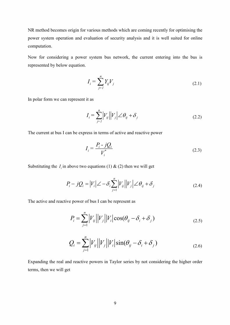
NR method becomes origin for various methods which are coming recently for optimising the
power system operation and evaluation of security analysis and it is well suited for online
computation.
Now for considering a power system bus network, the current entering into the bus is
represented by below equation.
n
i ij jj=1
I = Y V
(2.1)
In polar form we can represent it as
n
i ij j ij jj=1
I = V V
(2.2)
The current at bus I can be express in terms of active and reactive power
i ii *
i
P - jQI =
V
(2.3)
Substituting the iI in above two equations (1) & (2) then we will get
1
n
i i i i ij j ij jj
P jQ V V V
(2.4)
The active and reactive power of bus I can be represent as
1
cos( )n
i ij j i ij i jj
P V V V
(2.5)
1
sin( )n
i ij j i ij i jj
Q V V V
(2.6)
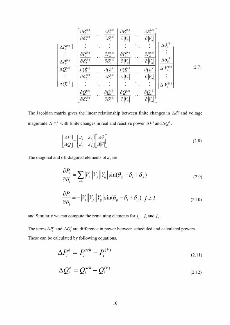
Expanding the real and reactive powers in Taylor series by not considering the higher order
terms, then we will get
10
( ) ( ) ( ) ( )2 2 2 2( ) ( )2 2
( )2
( ) ( ) ( ) ( )
( ) ( )( )2 2
( ) ( ) ( ) ( ) ( )2 2 2 2 2
( ) ( )2 2
( )
( )
2
k k k k
k kn n
k
k k k kn n n n
k kkn nn
k k k k k
k kn n
kn
kn
P P P P
V V
P
P P P P
V VP
Q Q Q Q Q
V V
Q
Q
( )2
( )
( )2
( )
( ) ( ) ( )
( ) ( )2
k
kn
k
kn
k k kn n n
k kn n
V
V
Q Q Q
V V
(2.7)
The Jacobian matrix gives the linear relationship between finite changes in ki and voltage
magnitude kiV with finite changes in real and reactive power k
iP and kiQ .
1 2
3 4
ΔδΔP J J=
Δ VΔQ J J
(2.8)
The diagonal and off diagonal elements of 1J are
sin( )ii j ij ij i j
j ii
PV V Y
(2.9)
sin( )ii j ij ij i j
i
PV V Y
j i
(2.10)
and Similarly we can compute the remaining elements for 2j , 3j and 4j .
The terms kiP and k
iQ are difference in power between scheduled and calculated powers.
These can be calculated by following equations.
( )k sch ki i iP P P
(2.11)
( )k sch ki i iQ Q Q
(2.12)
11
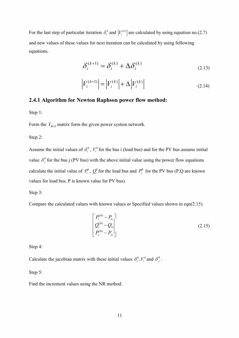
For the last step of particular iteration ki and ( )k
iV are calculated by using equation no.(2.7)
and new values of these values for next iteration can be calculated by using following
equations.
( 1) ( ) ( )k k ki i i
(2.13)
( 1) ( ) ( )k k ki i iV V V
(2.14)
2.4.1 Algorithm for Newton Raphson power flow method:
Step 1:
Form the BUSY matrix form the given power system network.
Step 2:
Assume the initial values of 0i , 0
iV for the bus i (load bus) and for the PV bus assume initial
value 0j for the bus j (PV bus) with the above initial value using the power flow equations
calculate the initial value of 0iP , 0
iQ for the load bus and 0jP for the PV bus (P,Q are known
values for load bus, P is known value for PV bus).
Step 3:
Compare the calculated values with known values or Specified values shown in eqn(2.15).
(0)
(0)
(0)
i is
i is
j js
P P
Q Q
P P
(2.15)
Step 4:
Calculate the jacobian matrix with these initial values 0 0,i iV and 0j .
Step 5:
Find the increment values using the NR method.
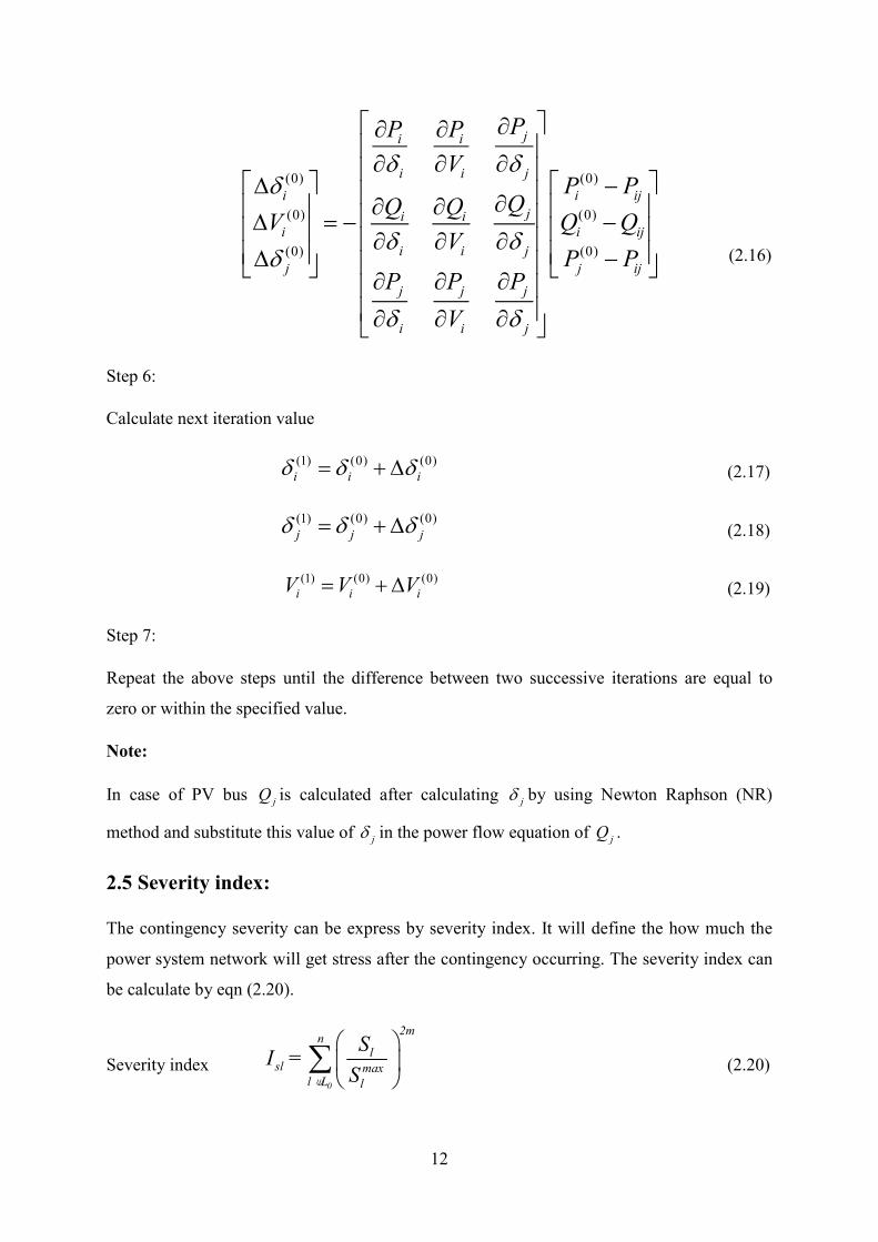
12
(0) (0)
(0) (0)
(0) (0)
ji i
i i j
i i ij
ji ii i ij
i i jj j ij
j j j
i i j
PP P
VP P
QQ QV Q Q
VP P
P P P
V
(2.16)
Step 6:
Calculate next iteration value
(1) (0) (0)i i i
(2.17)
(1) (0) (0)j j j
(2.18)
(1) (0) (0)i i iV V V
(2.19)
Step 7:
Repeat the above steps until the difference between two successive iterations are equal to
zero or within the specified value.
Note:
In case of PV bus jQ is calculated after calculating j by using Newton Raphson (NR)
method and substitute this value of j in the power flow equation of jQ .
2.5 Severity index:
The contingency severity can be express by severity index. It will define the how much the
power system network will get stress after the contingency occurring. The severity index can
be calculate by eqn (2.20).
Severity index 0
2mn
lsl max
l L l
SI =
S
∈
(2.20)
13
Where slI = Severity index of contingency
maxlS = maximum power flow rating of line l
0L = set of over load lines
m = integer exponent
The line flows in above equation can be calculate by using NR load flow method. During
computing the severity index for contingency only the over loaded lines has been considered
for avoiding the masking effects and we fixed the integer exponent value as 1.
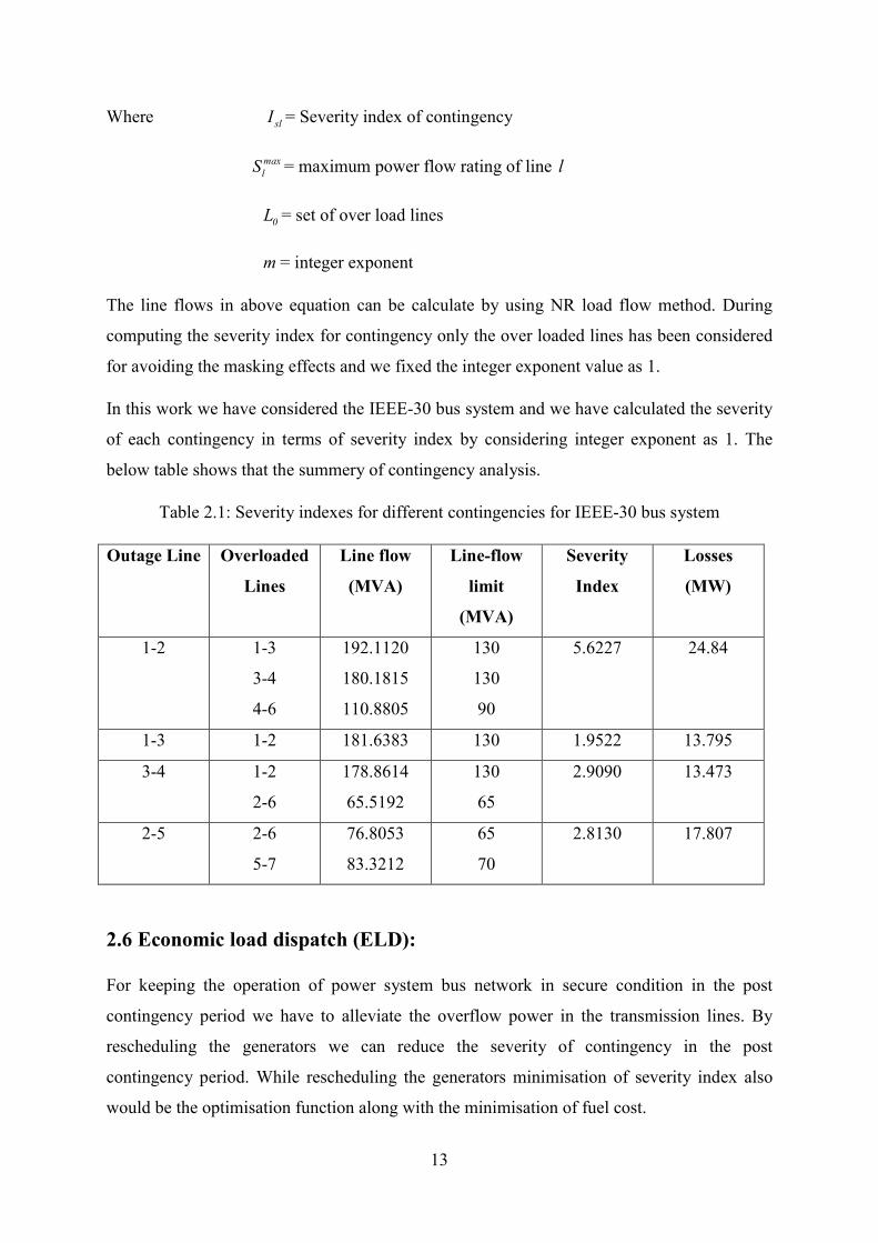
In this work we have considered the IEEE-30 bus system and we have calculated the severity
of each contingency in terms of severity index by considering integer exponent as 1. The
below table shows that the summery of contingency analysis.
Table 2.1: Severity indexes for different contingencies for IEEE-30 bus system
Outage Line Overloaded
Lines
Line flow
(MVA)
Line-flow
limit
(MVA)
Severity
Index
Losses
(MW)
1-2 1-3
3-4
4-6
192.1120
180.1815
110.8805
130
130
90
5.6227
24.84
1-3 1-2 181.6383 130 1.9522 13.795
3-4 1-2
2-6
178.8614
65.5192
130
65
2.9090
13.473
2-5 2-6
5-7
76.8053
83.3212
65
70
2.8130
17.807
2.6 Economic load dispatch (ELD):
For keeping the operation of power system bus network in secure condition in the post
contingency period we have to alleviate the overflow power in the transmission lines. By
rescheduling the generators we can reduce the severity of contingency in the post
contingency period. While rescheduling the generators minimisation of severity index also
would be the optimisation function along with the minimisation of fuel cost.
14
The severity of each contingency can be reduce by minimising the below objective function
T slF = min(F )+min(I )
(2.21)
Where; TF = Total fuel cost
slI = Severity index of each contingency
By minimising the above objective function the power system security can be enhance under
contingency analysis.
The economic load dispatch is the planning the generating units such that to reach load
demand along with the transmission losses at minimum fuel cost without violating the any
system constraints.
The cost function of all available generating units can be express by using the below
equation.
nF = F (P )i iT i=1
(2.22)
Where; TF = Total fuel cost of all available generating units
iF = Fuel cost of ith generator
System constraints are categorised into two types. They are
i. Equality Constraints
ii. Inequality Constraints
Equality constraints:
n
i d li=1
P = P + P
(2.23)
Where; dP = load demand
iP = power generation of ith generator
lP = power loss in system network
15
By observing the total fuel cost equation we can decide that the fuel cost is mainly depend
upon real power not in reactive power . So only the real power balance is the main attention
in power system balance.
Inequality constraints:
Inequality constraints are considered as 2 types. They are
i. Hard type
ii. Soft type
Hard type are constraints which are mainly depend on the tapping range of on-load tap
changing transformer and soft type are constraints which are mainly depend on the nodal
voltages, phase angles, real power and reactive power limits.
The maximum active power limit of generation is depending on the thermal condition and
lower limit of the active power generation is depend on the flame instability in the boiler. So
for secure operation of the generating unit, the real power generation of that unit should be in
the specified limits.
imin i imaxP < P < P (2.24)
The reactive power constraint is given by
min maxi i iQ Q Q
(2.25)
Here miniQ depends upon stability of the generator and maxiQ depends upon the heating of the
rotor.
The voltage Constraints is given by
min maxi i iV V V (2.26)
The components which are connected to the power system should be maintain with in. If V is
less than miniV then life time of the equipment will reduce. If V becomes more than maxiV then
there will severe effect on insulation of the windings.
2.7 Effect of characteristics of generating units:
The input-output characteristics of a boiler turbine of a generating unit can be represented as
monotonically increasing or piece wise linear function. However when comes to practical the
16
characteristics of a generating unit is higher order nonlinear because of valve point loading.
The valve point loading effect means the input-output characteristics of a generating unit will
also depend on the effect of sudden close and open of valve of turbine.
2.7.1 Without valve point loading:
If we will not consider the effect of valve point loading then the cost equation of each
generating unit can be represented as smooth quadratic function. The relationship between
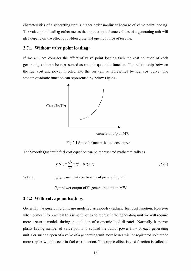
the fuel cost and power injected into the bus can be represented by fuel cost curve. The
smooth quadratic function can represented by below Fig 2.1.
Cost (Rs/Hr)
Generator o/p in MW
Fig.2.1 Smooth Quadratic fuel cost curve
The Smooth Quadratic fuel cost equation can be represented mathematically as
n2
i i i i i i ii=1
F (P )= a P +b P +c
(2.27)
Where; i i ia ,b ,c are cost coefficients of generating unit
iP = power output of ith generating unit in MW
2.7.2 With valve point loading:
Generally the generating units are modelled as smooth quadratic fuel cost function. However
when comes into practical this is not enough to represent the generating unit we will require
more accurate models during the solution of economic load dispatch. Normally in power
plants having number of valve points to control the output power flow of each generating
unit. For sudden open of a valve of a generating unit more losses will be registered so that the
more ripples will be occur in fuel cost function. This ripple effect in cost function is called as
17
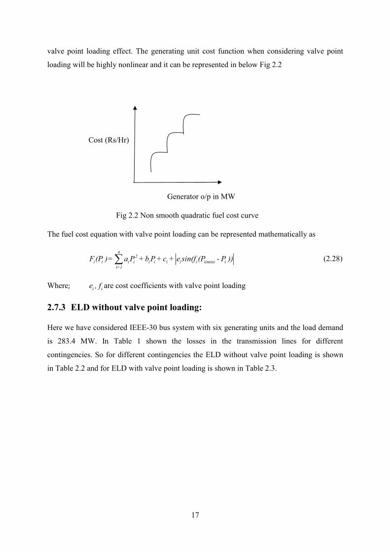
valve point loading effect. The generating unit cost function when considering valve point
loading will be highly nonlinear and it can be represented in below Fig 2.2
Cost (Rs/Hr)
Generator o/p in MW
Fig 2.2 Non smooth quadratic fuel cost curve
The fuel cost equation with valve point loading can be represented mathematically as
n2
i i i i i i i i i i(min) ii=1
F (P )= a P +b P +c + e sin(f (P - P ))
(2.28)
Where; i ie , f are cost coefficients with valve point loading
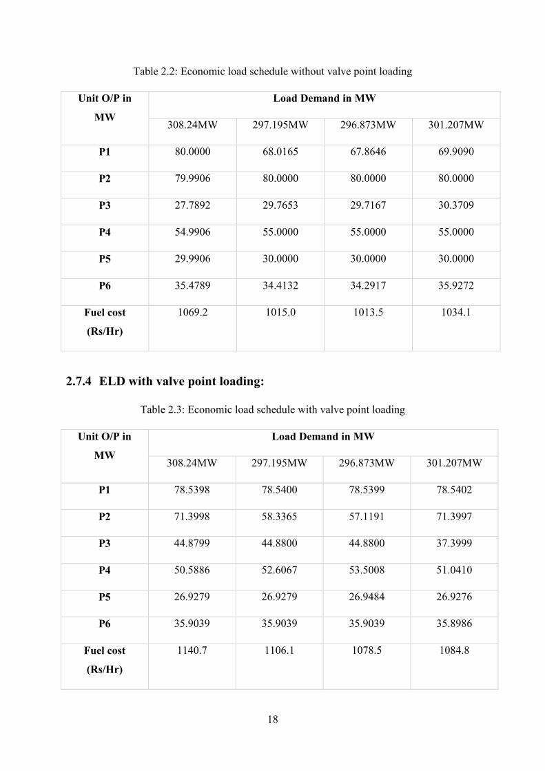
2.7.3 ELD without valve point loading:
Here we have considered IEEE-30 bus system with six generating units and the load demand
is 283.4 MW. In Table 1 shown the losses in the transmission lines for different
contingencies. So for different contingencies the ELD without valve point loading is shown
in Table 2.2 and for ELD with valve point loading is shown in Table 2.3.
18
Table 2.2: Economic load schedule without valve point loading
Unit O/P in
MW
Load Demand in MW
308.24MW 297.195MW 296.873MW 301.207MW
P1 80.0000 68.0165 67.8646 69.9090
P2 79.9906 80.0000 80.0000 80.0000
P3 27.7892 29.7653 29.7167 30.3709
P4 54.9906 55.0000 55.0000 55.0000
P5 29.9906 30.0000 30.0000 30.0000
P6 35.4789 34.4132 34.2917 35.9272
Fuel cost
(Rs/Hr)
1069.2 1015.0 1013.5 1034.1
2.7.4 ELD with valve point loading:
Table 2.3: Economic load schedule with valve point loading
Unit O/P in
MW
Load Demand in MW
308.24MW 297.195MW 296.873MW 301.207MW
P1 78.5398 78.5400 78.5399 78.5402
P2 71.3998 58.3365 57.1191 71.3997
P3 44.8799 44.8800 44.8800 37.3999
P4 50.5886 52.6067 53.5008 51.0410
P5 26.9279 26.9279 26.9484 26.9276
P6 35.9039 35.9039 35.9039 35.8986
Fuel cost
(Rs/Hr)
1140.7 1106.1 1078.5 1084.8
19
cHApter 3
cONtiNGeNcY
cONstrAiNeD ecONOMic
lOAD DispAtcH usiNG psO
20
Chapter 3
Contingency constrained economic load dispatch using PSO
3.1 Introduction:
Under the contingency the power system security can be enhance by rescheduling the
generating units. While rescheduling the generators different constraints should take into
consideration. The minimum and maximum limits of power flow and nodal voltages of
different transmission lines are the main constraints during the rescheduling under
contingency. In this work the rescheduling has been done by using an optimisation technique
called Particle Swarm Optimisation (PSO).
3.2 Particle Swarm Optimisation (PSO):
PSO is a population based optimisation technique and it is adopted from the simulation of the
fish schooling and birds flocking. PSO having some inherent capability so that it will take
less time to compute and require less memory space. The basic consideration behind the PSO
technique is that birds are finding their food by flocking as a group. The PSO is also same as
some other evolutionary algorithms. The problem is first initialised with stochastic solutions
(swarm). The potential solution of each stochastic solution can call as particle (agent) and it is
associated with stochastic velocity and it is flying through the problem space. Each particle
have some amount knowledge with that they will move around the problem space. All the
particles have memory and each particle keeps track with its previous best position (Pbest)
and corresponding the fitness value. The best of all particles of Pbest will be global best
position (Gbest). The position of each particle will be updated by updating their velocity by
following equation.
k+1 k kk
1 1 best1 - 2 2 best11 1 1V =WV +c * rand ()* (P )+c * rand ()* (G - S )S (3.1)
The position of the particle will be updated by using above equation by
k+1 k k+11 1 1S = S +V
(3.2)
Where; k1V = The velocity of individual i at iteration k
k = The pointer of iterations
W = The weighting factor
21
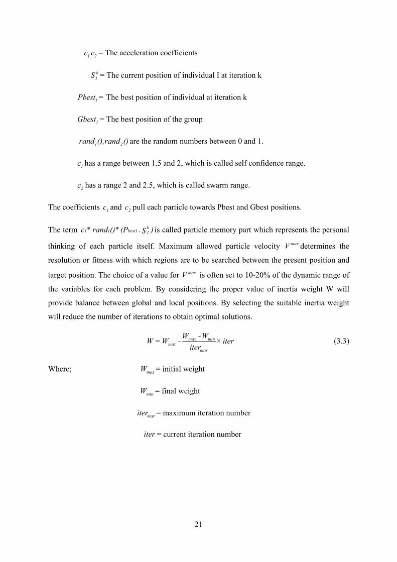
1, 2c c = The acceleration coefficients
k1S = The current position of individual I at iteration k
1Pbest = The best position of individual at iteration k
1Gbest = The best position of the group
1 2rand (),rand () are the random numbers between 0 and 1.
1c has a range between 1.5 and 2, which is called self confidence range.
2c has a range 2 and 2.5, which is called swarm range.
The coefficients 1c and 2c pull each particle towards Pbest and Gbest positions.
The term k1 1 best1 - 1c * rand ()* (P )S is called particle memory part which represents the personal
thinking of each particle itself. Maximum allowed particle velocity maxV determines the
resolution or fitness with which regions are to be searched between the present position and
target position. The choice of a value for maxV is often set to 10-20% of the dynamic range of
the variables for each problem. By considering the proper value of inertia weight W will
provide balance between global and local positions. By selecting the suitable inertia weight
will reduce the number of iterations to obtain optimal solutions.
max minmax
max
W -WW = W - ×iter
iter
(3.3)
Where; maxW = initial weight
minW = final weight
maxiter = maximum iteration number
iter = current iteration number

22
3.3 PSO Algorithm:
Algorithm steps for PSO technique.
• Initialise the population with random values and velocities.
• Computing the fitness of each agent (particle) and assign the position of particles to P-
best position and fitness of particle to P-best fitness.
• Identify the best value among the P-best and store the fitness value as a G-best.
• Update the Velocity and position of each particle (agent) by using below equations.
k+1 k kk
1 1 best1 - 2 2 best11 1 1V =WV +c * rand ()* (P )+c * rand ()* (G - S )S
k+1 k k+11 1 1S = S +V
• Check the velocities and positions whether it will be within the range or not then
again find the fitness of each particle (agent).
• Compare the current fitness value with its previous P-best. If present value is better
than the P-best then update the P-best as a current value.
• Now compare the present value with the G-best. If present value is better than the G-
best then update the G-best as a present value.
• Repeat the above steps until to get sufficiently good G-best or until to reach maximum
number of iterations
23
Fitness evaluation for each particle (agent) position
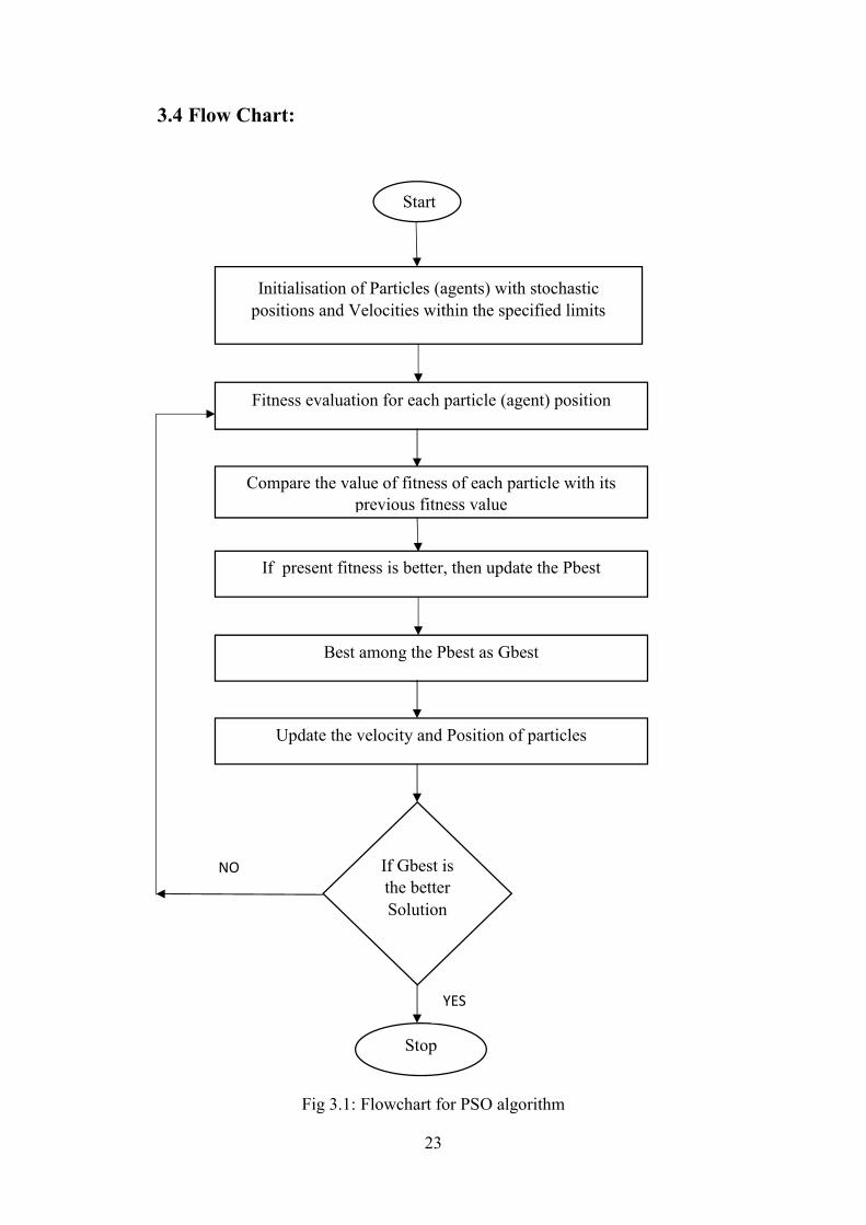
3.4 Flow Chart:
Fig 3.1: Flowchart for PSO algorithm
Start
Initialisation of Particles (agents) with stochastic
positions and Velocities within the specified limits
Compare the value of fitness of each particle with its previous fitness value
If present fitness is better, then update the Pbest
Best among the Pbest as Gbest
Update the velocity and Position of particles
If Gbest is the better
Solution
Stop
NO
YES
24
3.5 Contingency constrained ELD:
In Chapter 2 we have discussed the different contingency analysis. In Table No:1(Severity
indexes for different contingencies for IEEE-30 bus system) shown that the severity of each
contingency and also shown that which lines are getting overload under different
contingencies. Because of overloaded lines the total power system may get effect. So we have
to reduce the loading effect in overloaded lines for that we have to reschedule the generating
units. While rescheduling the generators we have taken the severity index also one of the
constraint so that the power flow in overloaded lines will come under specified limits.
During the rescheduling the generation by utilising PSO optimisation technique will be as
follows;
Step 1
We have calculated the Severity index for each contingency by running the load flow with
contingency.
Step 2
The Rank has been given for different contingencies according to the Severity index.
Step 3
We have initialised the generating units with random values along with velocities within
specified limits expect for slack unit.
Step 4
We have calculated the power flow in each transmission line by using the NR load flow
method and also calculated the fuel cost and severity index.
Step 5
We have chosen the Gbest vector for particle position vector which has given the minimum
fuel cost and minimum severity index and rest of all position vectors has been considered as
Pbest.
Step 6
Updated the particle position by updating the position velocity. So that we got new
population for next iteration.
25
Step 7
We have calculated the fuel cost and severity index with new population members by running
the NR load flow method with single line outage.
Step 8
We have updated the Gbest and Pbest values by comparing previous values of Gbest and
Pbest values.
Step 9
Completed the procedure up to maximum iterations has been reached.
Step 10
The iteration values of Gbest is the best solution for particular contingency.

26
cHApter 4
results
27
Chapter 4
Results
The security of the power system network has been improved under contingency analysis.
The optimisation technique PSO has been used to rescheduling the generators. The results
have been compared between the pre-contingency period and contingency period and also
taken the cases with valve point loading and without valve point loading. In all the cases
losses have been computed by using NR load flow method.
4.1 Results:
Here we have considered the IEEE-30 bus system which is having 6 generating units. The
cost function of each generating unit in Rs/Hr is given as.
CASE 1: Without valve point loading
21 1 1F = 0.02P +2P +0
22 2 2F = 0.0175P +1.75P +0
23 3 3F = 0.0625P +1P +0
24 4 4F = 0.00834P +3.25P +0
25 5 5F = 0.025P +3P +0
26 6 6F = 0.025P +3P +0 (4.1)
CASE 2: With valve point loading
1min 1300*sin(0.2( ))21 1 1F = 0.02P +2P +0+ P P
2min 2200*sin(0.22( ))22 2 2F = 0.0175P +1.75P +0+ P P
3min 3150*sin(0.42( ))23 3 3F = 0.0625P +1P +0+ P P
4min 4100*sin(0.3( ))24 4 4F = 0.00834P +3.25P +0+ P P
5min 5200*sin(0.35( ))25 5 5F = 0.025P +3P +0+ P P
28
6min 6200*sin(0.35( ))26 6 6F = 0.025P +3P +0+ P P
(4.2)
The constraints for each generating unit is mentioned below
10 80MW P MW
20 80MW P MW
30 50MW P MW
40 55MW P MW
50 30MW P MW
60 40MW P MW
(4.3)
For IEEE-30 bus system we have considered the load demand 283.4MW. For each
contingency power flows and losses in transmission line have been calculated by using NR
load flow method. The below table shows the transmission line losses under different
contingencies.
Table 4.1: Power losses in transmission lines under different contingencies
S.No Outage line Losses in MW
1 1-2 24.84
2 1-3 13.795
3 3-4 13.473
4 2-5 17.807
We have scheduled the generating units under each contingency losses to meet the load
demand without considering the severity index in both cases with and without valve point
loading.
29
CASE 1: Without valve point loading
Table 4.2: Scheduling of generating units under different contingencies without valve point
loading
Unit O/P in
MW
Load Demand in MW
308.24MW 297.195MW 296.873MW 301.207MW
P1 80.0000 68.0165 67.8646 69.9090
P2 79.9906 80.0000 80.0000 80.0000
P3 27.7892 29.7653 29.7167 30.3709
P4 54.9906 55.0000 55.0000 55.0000
P5 29.9906 30.0000 30.0000 30.0000
P6 35.4789 34.4132 34.2917 35.9272
Fuel cost
(Rs/hr)
1069.2 1015.0 1013.5 1034.1
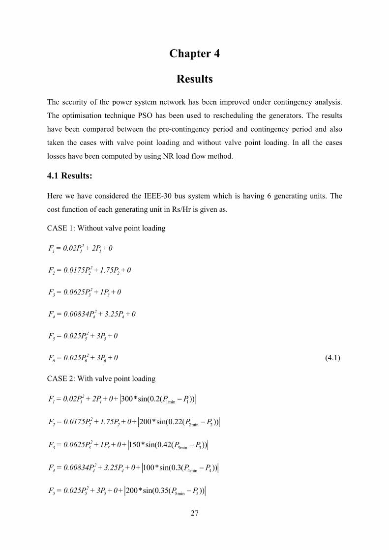
Fuel Cost Minimisation curves for without valve point load under contingency:
Plot 1:
Fig.4.1 No. of iterations Vs best cost without valve point Loading (load demand=308.24MW)
30
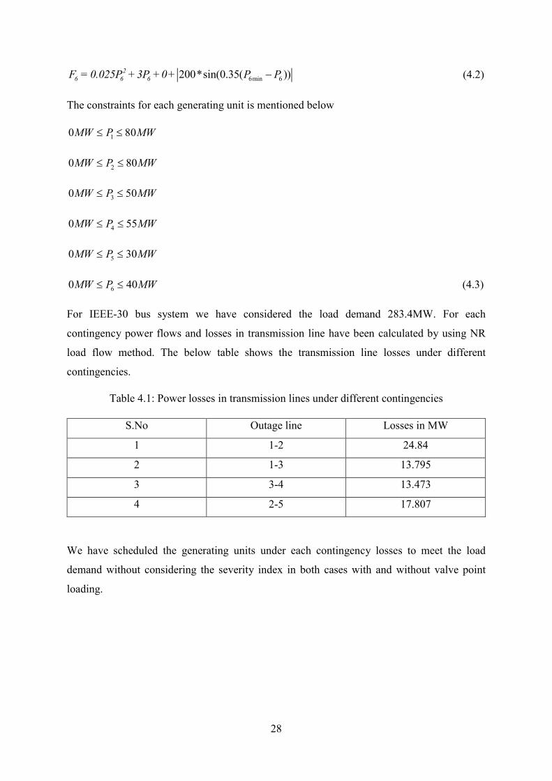
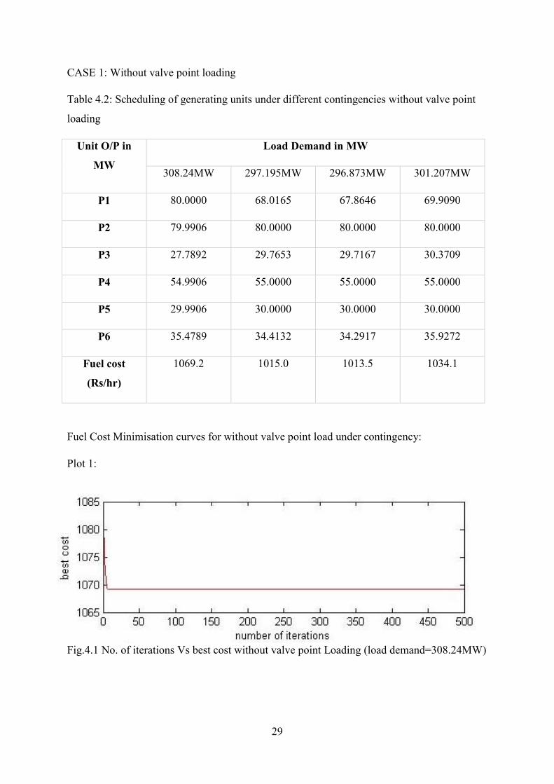
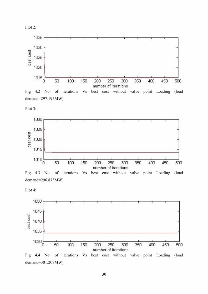
Plot 2:
Fig 4.2 No. of iterations Vs best cost without valve point Loading (load
demand=297.195MW)
Plot 3:
Fig 4.3 No. of iterations Vs best cost without valve point Loading (load
demand=296.873MW)
Plot 4:
Fig 4.4 No. of iterations Vs best cost without valve point Loading (load
demand=301.207MW)
31
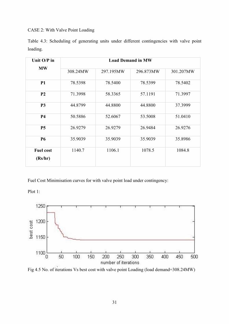
CASE 2: With Valve Point Loading
Table 4.3: Scheduling of generating units under different contingencies with valve point
loading.
Unit O/P in
MW
Load Demand in MW
308.24MW 297.195MW 296.873MW 301.207MW
P1 78.5398 78.5400 78.5399 78.5402
P2 71.3998 58.3365 57.1191 71.3997
P3 44.8799 44.8800 44.8800 37.3999
P4 50.5886 52.6067 53.5008 51.0410
P5 26.9279 26.9279 26.9484 26.9276
P6 35.9039 35.9039 35.9039 35.8986
Fuel cost
(Rs/hr)
1140.7 1106.1 1078.5 1084.8
Fuel Cost Minimisation curves for with valve point load under contingency:
Plot 1:
Fig 4.5 No. of iterations Vs best cost with valve point Loading (load demand=308.24MW)
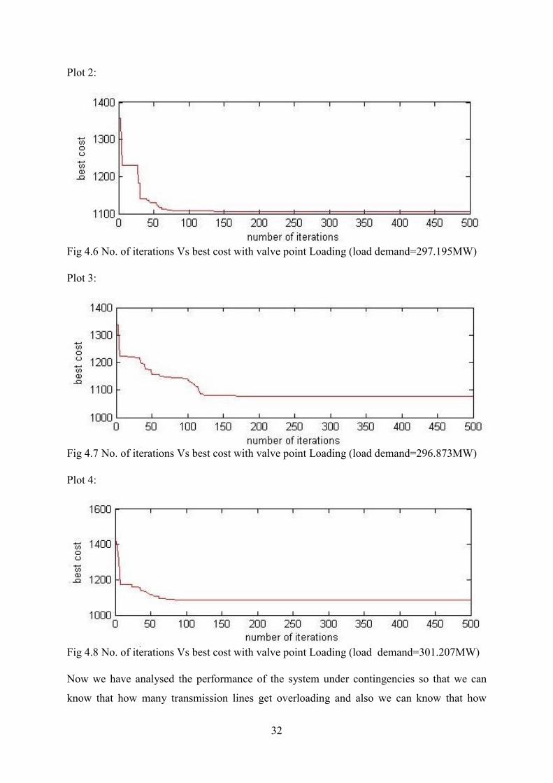
32
Plot 2:
Fig 4.6 No. of iterations Vs best cost with valve point Loading (load demand=297.195MW)
Plot 3:
Fig 4.7 No. of iterations Vs best cost with valve point Loading (load demand=296.873MW)
Plot 4:
Fig 4.8 No. of iterations Vs best cost with valve point Loading (load demand=301.207MW)
Now we have analysed the performance of the system under contingencies so that we can
know that how many transmission lines get overloading and also we can know that how
33
much excess power is flowing in that transmission lines and also can know that losses of the
network. The below table shows information regarding to transmission lines flows under
contingencies.
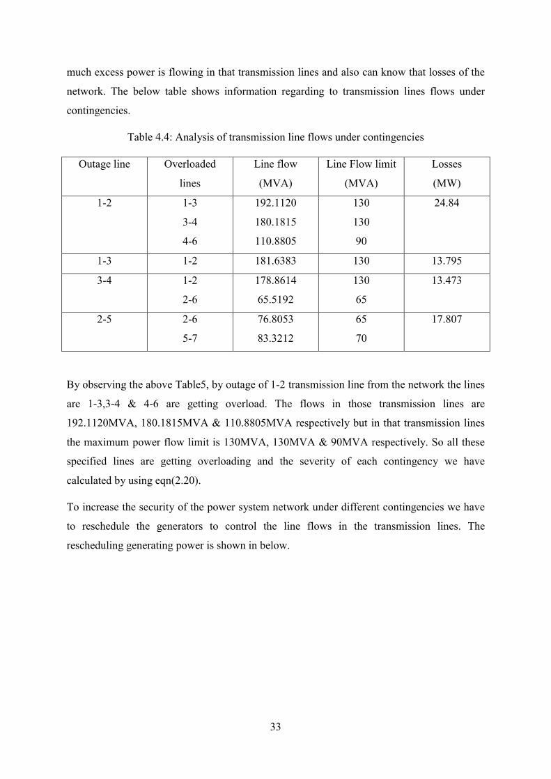
Table 4.4: Analysis of transmission line flows under contingencies
Outage line Overloaded
lines
Line flow
(MVA)
Line Flow limit
(MVA)
Losses
(MW)
1-2 1-3
3-4
4-6
192.1120
180.1815
110.8805
130
130
90
24.84
1-3 1-2 181.6383 130 13.795
3-4 1-2
2-6
178.8614
65.5192
130
65
13.473
2-5 2-6
5-7
76.8053
83.3212
65
70
17.807
By observing the above Table5, by outage of 1-2 transmission line from the network the lines
are 1-3,3-4 & 4-6 are getting overload. The flows in those transmission lines are
192.1120MVA, 180.1815MVA & 110.8805MVA respectively but in that transmission lines
the maximum power flow limit is 130MVA, 130MVA & 90MVA respectively. So all these
specified lines are getting overloading and the severity of each contingency we have
calculated by using eqn(2.20).
To increase the security of the power system network under different contingencies we have
to reschedule the generators to control the line flows in the transmission lines. The
rescheduling generating power is shown in below.
34
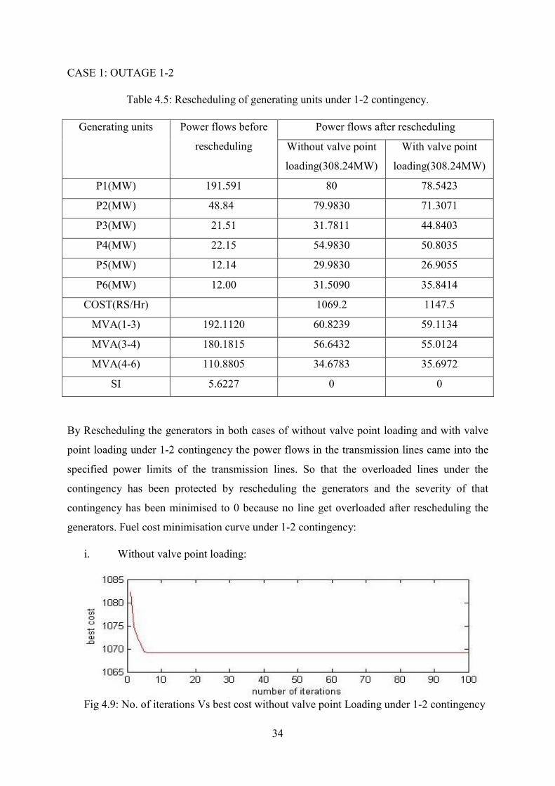
CASE 1: OUTAGE 1-2
Table 4.5: Rescheduling of generating units under 1-2 contingency.
Generating units Power flows before
rescheduling
Power flows after rescheduling
Without valve point
loading(308.24MW)
With valve point
loading(308.24MW)
P1(MW) 191.591 80 78.5423
P2(MW) 48.84 79.9830 71.3071
P3(MW) 21.51 31.7811 44.8403
P4(MW) 22.15 54.9830 50.8035
P5(MW) 12.14 29.9830 26.9055
P6(MW) 12.00 31.5090 35.8414
COST(RS/Hr) 1069.2 1147.5
MVA(1-3) 192.1120 60.8239 59.1134
MVA(3-4) 180.1815 56.6432 55.0124
MVA(4-6) 110.8805 34.6783 35.6972
SI 5.6227 0 0
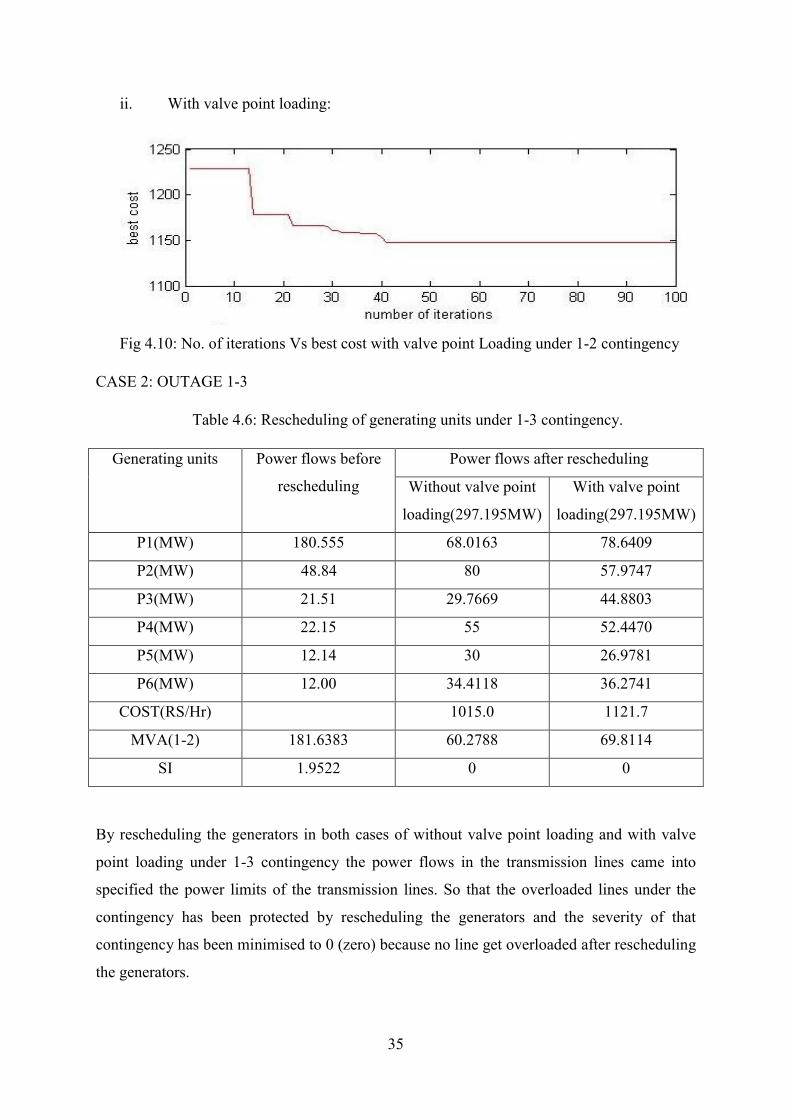
By Rescheduling the generators in both cases of without valve point loading and with valve
point loading under 1-2 contingency the power flows in the transmission lines came into the
specified power limits of the transmission lines. So that the overloaded lines under the
contingency has been protected by rescheduling the generators and the severity of that
contingency has been minimised to 0 because no line get overloaded after rescheduling the
generators. Fuel cost minimisation curve under 1-2 contingency:
i. Without valve point loading:
Fig 4.9: No. of iterations Vs best cost without valve point Loading under 1-2 contingency
35
ii. With valve point loading:
Fig 4.10: No. of iterations Vs best cost with valve point Loading under 1-2 contingency
CASE 2: OUTAGE 1-3
Table 4.6: Rescheduling of generating units under 1-3 contingency.
Generating units Power flows before
rescheduling
Power flows after rescheduling
Without valve point
loading(297.195MW)
With valve point
loading(297.195MW)
P1(MW) 180.555 68.0163 78.6409
P2(MW) 48.84 80 57.9747
P3(MW) 21.51 29.7669 44.8803
P4(MW) 22.15 55 52.4470
P5(MW) 12.14 30 26.9781
P6(MW) 12.00 34.4118 36.2741
COST(RS/Hr) 1015.0 1121.7
MVA(1-2) 181.6383 60.2788 69.8114
SI 1.9522 0 0
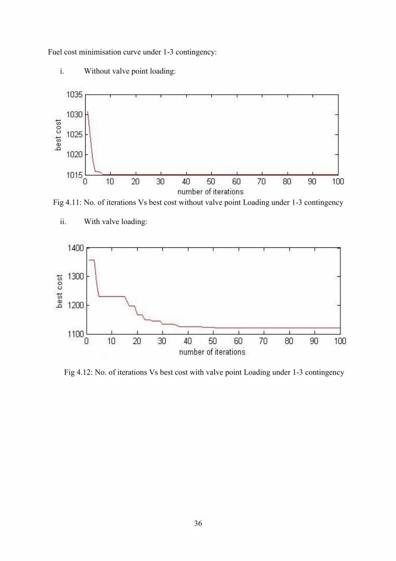
By rescheduling the generators in both cases of without valve point loading and with valve
point loading under 1-3 contingency the power flows in the transmission lines came into
specified the power limits of the transmission lines. So that the overloaded lines under the
contingency has been protected by rescheduling the generators and the severity of that
contingency has been minimised to 0 (zero) because no line get overloaded after rescheduling
the generators.
36
Fuel cost minimisation curve under 1-3 contingency:
i. Without valve point loading:
Fig 4.11: No. of iterations Vs best cost without valve point Loading under 1-3 contingency
ii. With valve loading:
Fig 4.12: No. of iterations Vs best cost with valve point Loading under 1-3 contingency
37
CASE 3: OUTAGE 3-4
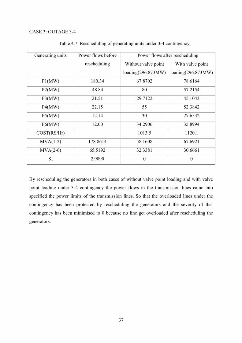
Table 4.7: Rescheduling of generating units under 3-4 contingency.
Generating units Power flows before
rescheduling
Power flows after rescheduling
Without valve point
loading(296.873MW)
With valve point
loading(296.873MW)
P1(MW) 180.34 67.8702 78.6164
P2(MW) 48.84 80 57.2154
P3(MW) 21.51 29.7122 45.1043
P4(MW) 22.15 55 52.3842
P5(MW) 12.14 30 27.6532
P6(MW) 12.00 34.2906 35.8994
COST(RS/Hr) 1013.5 1120.1
MVA(1-2) 178.8614 58.1608 67.6921
MVA(2-6) 65.5192 32.3381 30.6661
SI 2.9090 0 0
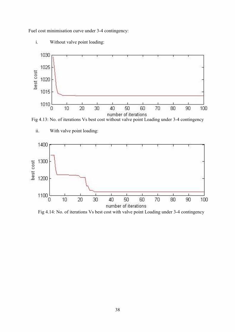
By rescheduling the generators in both cases of without valve point loading and with valve
point loading under 3-4 contingency the power flows in the transmission lines came into
specified the power limits of the transmission lines. So that the overloaded lines under the
contingency has been protected by rescheduling the generators and the severity of that
contingency has been minimised to 0 because no line get overloaded after rescheduling the
generators.
38
Fuel cost minimisation curve under 3-4 contingency:
i. Without valve point loading:
Fig 4.13: No. of iterations Vs best cost without valve point Loading under 3-4 contingency
ii. With valve point loading:
Fig 4.14: No. of iterations Vs best cost with valve point Loading under 3-4 contingency
39
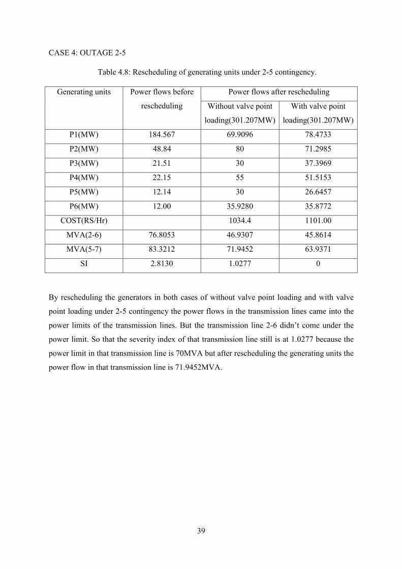
CASE 4: OUTAGE 2-5
Table 4.8: Rescheduling of generating units under 2-5 contingency.
Generating units Power flows before
rescheduling
Power flows after rescheduling
Without valve point
loading(301.207MW)
With valve point
loading(301.207MW)
P1(MW) 184.567 69.9096 78.4733
P2(MW) 48.84 80 71.2985
P3(MW) 21.51 30 37.3969
P4(MW) 22.15 55 51.5153
P5(MW) 12.14 30 26.6457
P6(MW) 12.00 35.9280 35.8772
COST(RS/Hr) 1034.4 1101.00
MVA(2-6) 76.8053 46.9307 45.8614
MVA(5-7) 83.3212 71.9452 63.9371
SI 2.8130 1.0277 0
By rescheduling the generators in both cases of without valve point loading and with valve
point loading under 2-5 contingency the power flows in the transmission lines came into the
power limits of the transmission lines. But the transmission line 2-6 didn’t come under the
power limit. So that the severity index of that transmission line still is at 1.0277 because the
power limit in that transmission line is 70MVA but after rescheduling the generating units the
power flow in that transmission line is 71.9452MVA.
40
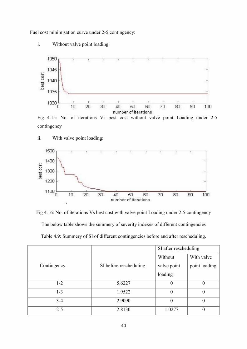
Fuel cost minimisation curve under 2-5 contingency:
i. Without valve point loading:
Fig 4.15: No. of iterations Vs best cost without valve point Loading under 2-5
contingency
ii. With valve point loading:
Fig 4.16: No. of iterations Vs best cost with valve point Loading under 2-5 contingency
The below table shows the summery of severity indexes of different contingencies
Table 4.9: Summery of SI of different contingencies before and after rescheduling.
Contingency
SI before rescheduling
SI after rescheduling
Without
valve point
loading
With valve
point loading
1-2 5.6227 0 0
1-3 1.9522 0 0
3-4 2.9090 0 0
2-5 2.8130 1.0277 0
41
Therefore by rescheduling the generators the severity of each contingency has been reduced
to zero except for the contingency 2-5 without valve point loading. During the rescheduling
the power flows in the transmission lines has been controlled and maintained in the specified
limits but for the contingency 2-5 the power flow in the transmission line (5-7) is
71.9452MVA and the maximum limit for power flow in that transmission line (5-7) is
70MVA. So after rescheduling also somewhat exceeding power is flowing in 5-7
transmission line. But before rescheduling the generators the power flow in that transmission
line is 83.3212MVA. So the severity of this contingency before rescheduling the generators is
2.8130. After rescheduling the generators the power flow in transmission line 5-7 is reduced
83.3212MVA to 71.9452MVA so the severity of 2-5 contingency has been reduced 2.8130 to
1.0277. The rest of all contingencies of severity are reduced to zero after rescheduling the
generators.

42
cHApter 5
cONclusiON AND future
scOpe
43
Chapter 5
Conclusion and Future scope
5.1 Conclusion:
There is an essential need to improve the power system security under any circumstances
along with the transmission capability. Here we are enhancing the power system security
under contingency analysis. The performance of power system network under contingency
has been predicted by using NR method and the severity of each contingency has been
calculated. During the contingency period we have notified the transmission lines which are
getting over flow. Because of these over flow power lines might lead the network to complete
blackout. So we have to increase the power system security under the contingencies, it can be
done by rescheduling the generators. Here we have rescheduled the generators by using
particle swarm optimisation technique. After rescheduling the generators the severity of each
contingency has been reduced, So that the power system security has been enhanced under
different contingencies and the generation is also at minimum cost.
5.2 Future Scope:
During this work we have taken IEEE-30 bus system in future it can be extended to more
than 30 bus system. In this work during the rescheduling of generators we have utilised the
PSO optimisation technique. In future for different bus systems generators can be
rescheduled by using different optimisation technique and comparisons can be done between
the different optimisation techniques.
44
REFERENCES:
[1] Scott B, Alsac O, and Monticelli A.J, “ Security analysis and optimization”, in proc. 1987 IEEE Transaction on power Apparatus and systems, vol. 75, pp.1623-1644.
[2] Peterson N.M, Tinney W.F, and Bree D.W, “Iterative linear AC power flow for fast approximate outage studies”, IEEE Transaction on power Apparatus and systems, vol.91, no.5,Oct. 1972,pp.2048-2058.
[3] Ching-Yin Lee and Nanming chen, "Distribution factors of reactive power flow in transmission line and transformer outage studies”, IEEE Transaction on Power systems, vol. 7, no. 1, Feb. 1992, pp.194-200.
[4] Singh S.N, and Srivastava S.C., “Improved voltage and reactive power distribution for outage studies”, IEEE Transaction on power systems, vol. 12, no. 3, Aug. 1997,pp. 1085-1093.
[5] Zaborsky J, Whang K.W, and Prasad K., “Fast contingency evaluation using concentric relaxation”, IEEE Transaction on power Apparatus and Systems, vol. PAS-99, no.1 Jan. 1980,pp. 28-36.
[6] Medicherla T.K.P,Billington R., and Sachdev M.S, “Generation rescheduling and load shedding to alleviate line overload- analysis”, IEEE Transaction on power Apparatus and systems, vol.98,no.6 1979,pp.1876-1884.
[7] Hadi S, “Power System Analysis”, Tata MCGraw-Hill, New Delhi, 1999.
[8] Lachs W.R., “ Transmission line overloads: real-time control ”, Proc. IEEE, 1987, vol.134, no.5, pp. 342–347
[9] Udupa A.N., Purushothama G.K, Parthasarathy K., and Thukaram D, “A fuzzy control for network overload alleviation”, IEEE Transaction on Electr. Power Energy Systems., 2001, vol. 23, pp. 119–129
[10] Monticelli, A., Pereira, M.V.F., and Granville, S, “Security-constrained optimal power flow with post-contingency corrective .rescheduling”, IEEE Trans., 1987, PWRS-2, no.1, pp. 175–182
[11] GaingZwe-Lee, “Particle Swarm Optimization to solving the Economic Dispatch Considering the Generator Constraints”, IEEE Transaction On Power Systems, vol.17, no.3, pp. 1188-1196, Aug. 2004. [12] Liang Z.X. and Glover J.D., “ Improved Cost Functions for Economic Dispatch considerations”, IEEE Transaction On Power Systems, May 1990, pp.821-829 [13] Rehman S. and Choudhury B.H., “A review of recent advance in economic dispatch”, IEEE Transaction On Power Systems, Dec. 1998, pp 1248-1249 [14] Jiang A. and Ertem S., “ Economic dispatch with non-monotonically increasing incremental cost units and transmission system losses”, IEEE Transaction on Power Systems, vol. 11, no. 2, pp. 891-897, May 1999. [15] Birge, B., “ PSO, A Particle Swarm Optimization Toolbox for Matlab”, IEEE Transaction on Swarm Intelligence Symposium Proceedings, April 24-26,2004. [16] Lee K.Y. and Park J., “Application of particle swarm optimization to economic dispatch problem:Advantages and disadvantages”, in Proc IEEE PES Power System Conference Expo. Oct 2006, pp 188-192
45
[17] Sudhakaran M., Vimal Raj D, Ajay P. and Palanivelu T.G, “Application of Particle Swarm Optimization for Economic Load Dispatch Problems” The 14th International Conference on Intelligent System Applications to Power Systems, ISAP 2008.
[18] Mangoli M.K., and Lee K.Y, “Optimal real and reactive power control using linear programming”, IEEE Transaction on Power Systems, 1993, vol. 26, pp. 1-10
[19] Scott B, Alsacc O, Bright J, and Paris M, “Further developments in LP-based optimal power flow”, IEEE Transaction on Power Systems, 1990, PWRS-5, no.3,pp. 697-711
[20] Lima, G.M. etal, “Phase shifter placement in large scale systems via mixed Integer Programming”, IEEE Transaction on Power Systems, 2003, PWRS-18 , no.3, pp.1029-1034
[21] Kumar A., and Parida S, “Enhancement of power system loadability with location of FACTS controllers in competitive electricity markets using MILP” Proc. Int. Conf. Energy, Information Technology and Power sector, Kolkata, Jan. 2005, pp. 515-523
[22] Momoh J.A., Zhu J.Z., Boswell G.D., and Hoffman, S, “ Power system security enhancement by OPF with phase shifter”, IEEE Transaction on Power Systems, 2001 PWRS-16, no.2, pp.287-293.
[23] Goldberg D, “Genetic algorithms in search, optimisation and machine learning” (Addison-Wesley,1989)
[24] Lai L.L., Ma J.T., Yokayama R., and zhao M, “Improved genetic algorithm for optimal power flow under both normal and contingent operation states”, Int. J. Electr. Power compon. Syst., 1997, vol.9, no.5, pp.287-292.
[25] Paranjothi S.R., and Anburaja K, “ Optimal power flow using refined genetic algorithms”, IEEE Transaction on Electr. Power Compon. Syst., 2002, vol.30, pp. 1055-1063
[26] Devraj D, and Yegnanarayana, B, “A combimed genetic algorithm approach for optimal power flow”. Proc. 11th National Power systems Conf., Bangalore, India, 2000, vol. 2, pp.524-528.
[27] Gaing Z.-L, “Particle swarm optimization to solving ED considering the generator constraints”, IEEE Transaction on Power Systems.vol.18, no.3, (2003) 1182–1195. [28] Somasundram P, Kuppusamy P, “Application of evolutionary programming to security constrained economic dispatch”, IEEE Transaction on Electric. Power Energy Syst. Vol.27 (2005) 343–351. [29] Venkatesh P., Nanadass R., and Padhy N.P, “Comparison and application of evolutionary programming techniques to combined economic emission dispatch with line flow constraints”, IEEE Transaction on Power Systems. Vol. 18, no. 2, (2003) 688–697. [30] Pancholi R.K, Swarup K.S, “Particle Swarm Optimization for security constrained economic dispatch”, in Proceedings of the International Conference on Intelligent Sensing and Information (ICISIP), 2002, pp. 7–12.


