
University of Kentucky University of Kentucky
UKnowledge UKnowledge
Theses and Dissertations--Electrical and Computer Engineering Electrical and Computer Engineering
2013
CONTINGENCY ANALYSIS OF POWER SYSTEMS IN PRESENCE OF CONTINGENCY ANALYSIS OF POWER SYSTEMS IN PRESENCE OF
GEOMAGNETICALLY INDUCED CURRENTS GEOMAGNETICALLY INDUCED CURRENTS
Sivarama Karthik Vijapurapu University of Kentucky, [email protected]
Right click to open a feedback form in a new tab to let us know how this document benefits you. Right click to open a feedback form in a new tab to let us know how this document benefits you.
Recommended Citation Recommended Citation Vijapurapu, Sivarama Karthik, "CONTINGENCY ANALYSIS OF POWER SYSTEMS IN PRESENCE OF GEOMAGNETICALLY INDUCED CURRENTS" (2013). Theses and Dissertations--Electrical and Computer Engineering. 32. https://uknowledge.uky.edu/ece_etds/32
This Master's Thesis is brought to you for free and open access by the Electrical and Computer Engineering at UKnowledge. It has been accepted for inclusion in Theses and Dissertations--Electrical and Computer Engineering by an authorized administrator of UKnowledge. For more information, please contact [email protected].

STUDENT AGREEMENT: STUDENT AGREEMENT:
I represent that my thesis or dissertation and abstract are my original work. Proper attribution
has been given to all outside sources. I understand that I am solely responsible for obtaining
any needed copyright permissions. I have obtained and attached hereto needed written
permission statements(s) from the owner(s) of each third-party copyrighted matter to be
included in my work, allowing electronic distribution (if such use is not permitted by the fair use
doctrine).
I hereby grant to The University of Kentucky and its agents the non-exclusive license to archive
and make accessible my work in whole or in part in all forms of media, now or hereafter known.
I agree that the document mentioned above may be made available immediately for worldwide
access unless a preapproved embargo applies.
I retain all other ownership rights to the copyright of my work. I also retain the right to use in
future works (such as articles or books) all or part of my work. I understand that I am free to
register the copyright to my work.
REVIEW, APPROVAL AND ACCEPTANCE REVIEW, APPROVAL AND ACCEPTANCE
The document mentioned above has been reviewed and accepted by the student’s advisor, on
behalf of the advisory committee, and by the Director of Graduate Studies (DGS), on behalf of
the program; we verify that this is the final, approved version of the student’s dissertation
including all changes required by the advisory committee. The undersigned agree to abide by
the statements above.
Sivarama Karthik Vijapurapu, Student
Dr. Yuan Liao, Major Professor
Dr. Cai-Cheng Lu, Director of Graduate Studies

CONTINGENCY ANALYSIS OF POWER SYSTEMS IN PRESENCE OF GEOMAGNETICALLY INDUCED CURRENTS
___________________________
THESIS
___________________________
A thesis submitted in the partial fulfillment of the
requirements for the degree of Masters of Science in Electrical Engineering
in the College of Engineering at the University of Kentucky.
By
Sivarama Karthik Vijapurapu
Lexington, Kentucky
Director: Dr. Yuan Liao, Associate Professor
Department of Electrical and Computer Engineering
College of Engineering, University of Kentucky.

ABSTRACT
CONTINGENCY ANALYSIS OF POWER SYSTEMS IN PRESENCE OF GEOMAGNETICALLY INDUCED CURRENTS
Geomagnetically induced currents (GIC) are manifestations of space weather phenomena on the electric power grid. Although not a new phenomenon, they assume great importance in wake of the present, ever expanding power grids. This thesis discusses the cause of GICs, methodology of modeling them into the power system and the ramifications of their presence in the bulk power system. GIC is treated at a micro level considering its effects on the power system assets like Transformers and also at a macro level with respect to issues like Voltage instability. In illustration, several simulations are made on a transformer & the standard IEEE 14 bus system to reproduce the effect of a geomagnetic storm on a power grid. Various software tools like PowerWorld Simulator, SimPower Systems have been utilized in performing these simulations. Contingency analysis involving the weakest elements in the system has been performed to evaluate the impact of their loss on the system. Test results are laid out and discussed in detail to convey the consequences of a geomagnetic phenomenon on the power grid in a holistic manner. Keywords: Geomagnetically Induced Currents, PowerWorld simulator, IEEE 14 bus system, Voltage instability, Contingency Analysis. Sivarama Karthik Vijapurapu.

CONTINGENCY ANALYSIS OF POWER SYSTEMS IN PRESENCE OF GEOMAGNETICALLY INDUCED CURRENTS
By
Sivarama Karthik Vijapurapu
________________________
Director of Thesis: Dr. Yuan Liao
___________________________
Director of Graduate Studies: Dr. Cai-Cheng Lu
_________________________
Date: 7/24/12

Dedication
“If I have seen further it is by standing on ye sholders of Giants.”—Sir Isaac Newton
To my grandfather Ramadas Vijapurapu, for exemplifying the man I strive to become.
To my grandmother Venku Bai Vijapurapu, a shining gem in the shadows, for her
perpetual affection, warmth and encouragement.
To Sri Lakshmi Bai, for everything she said, did and is for me.
To my parents, Narayana Rao and Swarana Latha Vijapurapu, for I owe my all to
them. Their confidence in me supersedes my own.
I stand overwhelmed by all your love and reciprocate it humbly thorough this work as
a token of my gratitude.
Sivarama Karthik Vijapurapu
7/24/12

iii
ACKNOWLEDGEMENTS
The best thing about writing this thesis is getting to thank the people who have supported
me in this endeavor. I would like to thank my thesis director Dr. Yuan Liao who has been
a constant support all through the course of my stint here at UK and for having oriented
me in a progressive direction with regard to this thesis. I appreciate his patience and
confidence in my abilities.
I would also like to thank Dr. Paul Dolloff and Dr. Aaron Cramer for accepting to be on
the committee. I am grateful for their valuable suggestions and support which has helped
shape this thesis to its best.
I would like to pay my sincere respect and thanks to my parents who have supported me
in the course of my education. A gratuitous acknowledgement goes out to my sister
Sandhya Parimala Vijapurapu, my elder brother Vamsi Krishna Vijapurapu and friend
Suhaas Bhargava Ayyagari for their invaluable assistance and constant encouragement.
Lastly, my sincere regards to the Dept. of Electrical and Computer Engineering and to
the Power and Energy Institute of Kentucky(PEIK) at UK for providing all the necessary
resources and financial support and paving way for the successful completion of my
Master’s Degree.

iv
TABLE OF CONTENTS
ACKNOWLEDGEMENTS ............................................................................................. iii
LIST OF TABLES............................................................................................................. vi
LIST OF FIGURES .......................................................................................................... vii
CHAPTER ONE: INTRODUCTION ................................................................................ 1
1.1 OVERVIEW ...................................................................................................... 1
1.2 MOTIVATION.................................................................................................. 6
1.3 OUTLINE ......................................................................................................... 8
CHAPTER TWO: LITERATURE REVIEW .................................................................. 10
2.1 HISTORY OF GEOMAGNETIC STORMS & GIC ..................................... 10
2.2 EFFECTS OF GIC ON THE POWER SYSTEM ........................................... 14
CHAPTER THREE: GIC MODELLING ........................................................................ 17
3.1 METHODS OF GIC MODELLING ............................................................... 17
3.1.1 PREDICTIVE METHODS ................................................................... 18
3.1.2 ANALYTICAL METHODS ................................................................. 20
3.2 GIC MAPPING AND MODELING-POWERWORLD SIMULATOR ......... 23
3.2.1 GIC CALCULATION TOOL ............................................................... 24
3.3 TEST SYSTEM DESCRIPTION .................................................................... 27
3.4 GIC CALCULATION ..................................................................................... 32
CHAPTER FOUR: INVESTIGATION OF GIC EFFECTS ON TRANSFORMERS .... 34
4.1 INTRODUCTION ........................................................................................... 34
4.2 HALF CYCLE SATURATION IN TRANSFORMERS ................................ 36
4.3 SIMULINK MODEL OF INDUCTANCE MATRIX TRANSFORMER ...... 39
4.4 CIRCUIT DESCRIPTION .............................................................................. 43

v
4.5 ILLUSTRATION OF GIC EFFECTS IN SIMULINK ................................... 45
4.5.1 DISTORTION OF SATURATION CHARACTERISTICS ................... 45
4.5.2 HARMONICS IN CURRENT WAVEFORMS ..................................... 48
4.5.2.1 TOTAL HARMONIC DISTORTION ........................................... 52
4.5.3 INCREMENT IN REACTIVE POWER CONSUMPTION ................... 57
4.5.4 THERMAL DEGRADATION & STRUCTURAL DEFORMATION .. 61
CHAPTER FIVE: VOLTAGE STABILITY AND GRID RESPONSE .......................... 64
5.1 INTRODUCTION ........................................................................................... 64
5.2 SIGNIFICANCE OF REACTIVE POWER ................................................... 66
5.3 MODAL ANALYSIS FOR VOLTAGE STABILITY ASSESSMENT ........ 67
5.4 Q-V CURVE GENERATION ......................................................................... 72
CHAPTER SIX: SIMULATION RESULTS & DISCUSSION ...................................... 74
6.1 RESULTS FROM TRANSFORMER ANALYSIS ........................................ 74
6.2 RESULTS FROM GRID & VOLTAGE STABILITY ANALYSIS .............. 79
6.3 EVALUATION OF CONTINGENICES ........................................................ 91
CHAPTER SEVEN: CONCLUSION AND SCOPE FOR FUTURE WORK ................ 95
APPENDIX ...................................................................................................................... 98
BIBILIOGRAPHY ......................................................................................................... 100
VITA ............................................................................................................................... 105

vi
LIST OF TABLES
Table 3.1 IEEE 14 Bus data .............................................................................................. 29
Table 3.2 IEEE 14 Bus-Line Data ..................................................................................... 30
Table 3.3 Regulated Bus Data ........................................................................................... 31
Table 3.4 Static Capacitor Data ......................................................................................... 31
Table 3.5 Substation Records ............................................................................................ 32
Table 4.1 Transformer Loss VAR Tabulation .................................................................. 60
Table 6.1 Transformer Current & Voltage Distortion Results .......................................... 75
Table 6.2 Results from QV curve Analysis for Operating point ‘A’ ................................ 81
Table 6.3 Results from QV curve Analysis for Operating point ‘B’ ................................ 85
Table 6.4 Results from QV curve Analysis for Operating point ‘C’ ................................ 89
Table 6.5 Contingency Evaluation at Operating point ‘A’ ............................................... 92
Table 6.6 Contingency Evaluation at Operating point ‘B’ ................................................ 92
Table 6.7 Contingency Evaluation at Operating point ‘C’ ................................................ 92

vii
LIST OF FIGURES
Figure 1.1 Graphical Description of a Coronal Mass Ejection ........................................... 3
Figure 1.2 Geomagnetic effects on electric power grids .................................................... 4
Figure 2.1 Illustration of GIC entry into the Power Grid. ................................................. 14
Figure 2.2 GIC Effects on Power Systems ....................................................................... 15
Figure 3.1 Flow Chart of the Power Grid GIC Calculation Software .............................. 21
Figure 3.2 GIC Analysis Form ......................................................................................... 25
Figure 3.3 Single Line Diagram -IEEE 14 Bus System .................................................... 27
Figure 3.4 IEEE 14 Bus System in PowerWorld Simulator ............................................. 28
Figure 4.1 Flux-Magnetization Current curve for a Transformer .................................... 36
Figure 4.2 Flux-Magnetization Curve Bias in presence of GIC ....................................... 38
Figure 4.3 Simulink model of Induction Matrix Three phase Transformer ..................... 39
Figure 4.4 Configuration & Parameters Tab of the Transformer Model ......................... 40
Figure 4.5 Calculation of Positive and Zero-Sequence parameters ................................. 41
Figure 4.6 External Saturation block for the Transformer ............................................... 42
Figure 4.7 Simulink Model illustrating GIC effects on Transformer ............................... 44
Figure 4.8 Saturation characteristics for transformer core for rated conditions ............... 46
Figure 4.9 Saturation characteristics of a 10A GIC saturated transformer core .............. 47

viii
Figure 4.10 Variation of Excitation Current I exc with GIC Injection ............................ 49
Figure 4.11 PowerGUI FFT Analysis Tool ...................................................................... 51
Figure 4.12 FFT Analysis of Primary winding current I abc_B1 for rated conditions .... 53
Figure 4.13 FFT Analysis of Primary winding current I abc_B1 for GIC=25 A ............. 55
Figure 4.14 Waveform and Spectrum of RMS I exc with GIC =25 A ............................ 56
Figure 4.15 Active Power profile with increase in GIC ................................................... 59
Figure 4.16 Reactive Power profile with increase in GIC ............................................... 59
Figure 4.17 Transformer Damage in Salem Nuclear Plant .............................................. 62
Figure 4.18 Transformer Failures in South Africa ........................................................... 63
Figure 5.1 Standard Q-V curve ........................................................................................ 72
Figure 6.1 THD versus GIC injection for phase A ........................................................... 74
Figure 6.2 Saturation characteristics with increasing GIC Injection................................. 77
Figure 6.3 Deterioration of I exc with increasing GIC Injection ....................................... 78
Figure 6.4 Test case at operating point ‘A’ ...................................................................... 80
Figure 6.5 Q-V curve of the critical bus-Bus 14 at operating point ‘A’ .......................... 81
Figure 6.6 Test case at operating point ‘B’ ...................................................................... 84
Figure 6.7 Q-V curve of the critical bus-Bus 14 at operating point ‘B’ ........................... 85
Figure 6.8 Test case at operating point ‘C’ ...................................................................... 88
Figure 6.9 Q-V curve of the critical bus-Bus 14 at operating point ‘C’ ........................... 89
Figure 6.10 Test case with Contingency Plan .................................................................. 94
1
CHAPTER 1: INTRODUCTION
1.1 OVERVIEW
Owing to the escalating demand for electricity and the inclusion of renewable energy
resources in remote locations into the energy portfolio, power grids in the US and around
the world have witnessed an enormous increase in the span of area they encompass. With
the expanding power grid and the need for continual supply of electricity, reliability is of
paramount importance. Any unforeseen disturbance in the usual functioning of the grid
can have very far reaching consequences if necessary contingency measures are not put
in place. Large scale disruptions of the power grid not only cause stress in the tightly knit
power system but also voltage instability, un-coordinated load shedding, damage, loss or
erratic operation of power system assets propelling it towards collapse and system
blackout. Advent of marketing strategies like deregulation of electricity rates has also
increased the need for incessant supply of power to the end users who are sensitive to
outages [1].
Although the power grid is robust and impervious to most disturbances , its vulnerability
cannot be ruled out as power systems nowadays tend to be operated near their respective
operating limits owing to increasing demand from industries, communications and for
general domestic usage. This situation arises due to growing economic and environmental
concerns in building new power transmission systems to harness energy sources located
in spatially distant areas.

2
Expansion in the span of the power systems make them come into contact with several
factors that have been previously unidentified or neglected altogether and can
considerably affect the normal operation of the grid . Apart from transmission line faults
and equipment failures which generally cause disruptions in the power grid, weather
conditions are also an important factor during system planning and design. Although
terrestrial weather is taken into consideration by planners and system designers, space
weather is an issue that is becoming increasingly important.
Space weather is defined as a consequence of the interaction between the Sun, the Earth’s
magnetic field and the atmosphere [2]. It is mainly driven by the activity in the Sun and
its effect on the earth. Any significant variation in the space weather causes a
corresponding Geomagnetic Disturbance (GMD). A GMD is defined as a temporary
perturbation in the earth’s magnetosphere caused by solar phenomenon such as Solar
flares, Coronal Mass Ejections (CME) approaching towards the earth from the sun.
NERC’s Interim Reliability Assessment Report [2] attributes this solar activity due to the
reactions taking place inside the Sun. Space weather phenomena such as Solar Flares,
Radiation Storms and Geomagnetic storms are three acknowledged solar activities
directed towards the earth.
Of the above three phenomena, Geomagnetic storms were observed to have the most
adverse effect on the power systems. A Geomagnetic storm is caused by the rapid influx
of Coronal Mass Ejections(CME) comprised of electrically charged particles and strong
magnetic fields from the Sun directed toward the upper layers of the earth’s atmosphere.

3
These electrically charged particles create a stream of current called Electrojets in the
atmosphere. Beams of these particles hurling towards the earth collide with the
constituents of the earth’s ionosphere and produce fluorescence commonly known as
Aurora.
Figure 1.1 Graphical Description of a Coronal Mass Ejection [2].
Substantial alterations in the intensity and direction of these electrojet currents can induce
ground-based voltage (potential) differentials between locations spatially apart. These
ground potential differences can cause currents to flow through the grounded connections
of transmission lines and transformers if the resistivity of the ground to a sizable depth is
greater than the resistivity of the transmission or transformer. This event occurs more
often in greater degree in areas that sit atop igneous rocks [3]. These currents induce a
potential on the earth called Earth Surface Potential (ESP).

4
The effect of this ESP is prominent between the grounded points of the AC power system
giving rise to flowing currents. The sequence of events described above drives the quasi-
dc current through one grounded point of the system into another. Fig 1.2 illustrates the
entire phenomenon.
Figure 1.2 Geomagnetic effects on electric power grids [4]
Manifestation of all these solar and geological reactions can be seen as fluctuations in the
magnetosphere of the earth giving rise to quasi–dc stray currents called Geomagnetically
Induced currents (GIC) abbreviated henceforth as GIC in the power system. GICs have
adverse effects on conductive equipment such as Power grids, Transmission lines,
Underground pipelines and Telecommunications cables.

5
Critical space and terrestrial infrastructure can suffer damage during the course of a
CME. In the past, communication satellites have observed disruptions in their operations
during the course of a geomagnetic event. Of all the conducting equipment, Electric
Power Transmission Networks faces the greatest threat from GIC as they have a vast
footprint which makes them better receptive to stray GIC currents. As susceptibility to
GIC increases, the grid becomes overloaded leading to subsequent problems like voltage
fluctuations and widespread power outages due to equipment failure [5].
Interdependence of Industrial, Communications and other infrastructural sectors require
power as a basic necessity for their function. Hence, a disruption of Power over a long
period of time spanning a large area can have globally resounding consequences in terms
of economic losses incurred. Needless to say, the damage caused to public and
emergency infrastructure due to a power blackout [6].
In most natural disasters, the less developed areas suffer the biggest impacts. Ironically,
during a geomagnetic storm, the sophisticated power grids that couple so well to the
space environment is that which makes highly developed areas with more power needs
bear its brunt.

6
1.2 MOTIVATION
The prime motivation of this thesis was the significant impact an organized strategy
could make in dealing with GIC over a very large power grid. In doing so, several
valuable power system assets can be shielded from the hazardous effects of GIC thereby
saving a lot of time and money in having to replace them.
There exists no universal or single preventive measure for GIC because geomagnetic
storms vary in direction and intensity through space and along the spatial location of the
power system. Geomagnetic storms were initially thought of being restricted to higher
latitude regions near the poles, but during recent events, GICs were observed to have
effect as far as countries like South Africa. Hence, a multi-faceted, tactical and layered
approach is required. This includes equipment hardening to GIC and augmenting system
operations evolving into a suitable contingency plan. GIC being a phenomenon having a
continental footprint, mitigation measures differ from case-to-case basis, as do the
impacts on the power system in different areas.
Developing a unique mitigation measure for GIC is particularly difficult because not
much data exists from previous storms when space monitoring and GIC monitoring
devices were not in vogue. Thus, an in-depth analysis and integration of GICs is to be
undertaken to observe the impacts.
Modeling GICs into the system is an important step in studying its effects so that system
operators can take educated, real-time decisions in countering the flow of GIC.

7
Operational measures in terms of protecting system assets, maintaining voltage stability,
variable system configurations are essential in arresting the effects produced by GICs.
The thesis focuses on modeling GICs into the power system, observing the effects on the
power system assets, identify vulnerable areas and develop an organized strategy to
mitigate GIC. Due to the hazardous effects of GIC, this kind of an approach is an
important step in assessing the dangers posed to the system holistically so that power
system operators can make educated decisions when countered by a GMD.
By identifying the vulnerable points and observing the impact of a GIC on them, a
valuable insight can be developed which can help in design of power system equipment
that can withstand the effect of a GMD, and also aids professionals while planning the
system.
The thesis drew its initial motivation from [7] in which a software tool was used to
simulate the effects of GIC on a power network. The thesis uses the tool to simulate the
scenario of a geomagnetic storm with as little input as possible and observe the deviation
of the grid from its stable operating point. Building on the observations made, the
problems posed to the grid by the disturbance are identified.
Basing on the existing guide lines set by utilities during natural disasters, best system
practices are developed for geomagnetic terms in terms of a systematic schedule
addressing each issue posed by GIC flows in the system. This is possible only after
analyzing the system in detail which this thesis hopes to accomplish.

8
1.3 OUTLINE
The first chapter prefaces background information about space weather
phenomena leading to a geomagnetic storm and introduces several prerequisite terms in
understanding the underlying sequence of events that cause this activity. Consequences
of such an event on the present day bulk power system are inferred and the necessity to
broach the issue is outlined.
The second chapter details several previous occurrences of a geomagnetic
storm and their associated effects such as GIC on the power systems in various countries.
This is intended to elucidate and establish the risks and hazards posed in the aftermath of
a geomagnetic disturbance. Based on this knowledge, the effects are explained illatively
and foundations are laid to discuss them in specific in the following chapters.
The third chapter discusses the various methods in modeling the
circulating GIC currents into the power system. GIC calculation tool in PowerWorld
Simulator used in this thesis is suggested and explained elaborately. The IEEE 14 bus
system is used as a test case to explain GIC calculation and it is again revisited in the fifth
chapter while addressing voltage stability.
The fourth chapter constitutes the observed effects of GIC on
transformers in a comprehensive manner. Several aspects such as saturation
characteristics, current harmonics, variation in power statistics and thermal degradation
are hashed out and substantiated by a series of simulations performed using SimPower
systems toolbox in Simulink.

9
The fifth chapter broaches the subject of Voltage Stability. A technique
called Modal analysis is utilized in determining steadiness of the system voltage levels in
presence of GIC. A MATLAB program is developed to observe the voltage stability of
the system. The GIC calculation tool introduced previously is used to subject the IEEE 14
bus test case to several operating points and to observe its stability at each instance.
The sixth chapter comprises of numerical and pictorial results of various
simulations undertaken in the preceding chapters. These results are discussed and several
inferences are made which validate the hypothesis discussed earlier.
The seventh chapter concludes the entire research work in this thesis. The
results obtained are laid down along with some useful recommendations. In addition,
scope for future work and possible extension pertaining to the content discussed in this
thesis is briefly stated.

10
CHAPTER 2: LITERATURE REVIEW
This chapter comprises a brief account of previous occurrences of geomagnetic storms
& their associated effects on the bulk power system around the world. The section
2.2 takes a closer look at the effects of a GIC storm on power system assets.
2.1 HISTORY OF GEOMAGNETIC STORMS & GIC
In order to completely understand the disturbances caused by a GMD to the power grid, it
is necessary to be cognizant of previous instances of such occurrences. Geomagnetic
storms coincide by the reactions occurring in the core of the sun. The main threat that a
Geomagnetic storm poses to the Power grid are the circulating low frequency currents
called Geomagnetically induced currents(GIC) that are generated as a result of a GMD
event owing to the conductive nature of the earth. These currents enter and exit the
discretely earthed power grid at several points affecting the operation of the grid
significantly. GICs have been observed to cause several problems like harmonic loading
and tripping of reactive power elements and transformer saturation thereby creating a
cascading effect possibly leading to voltage collapse and load blackout of the entire grid.
There have been several instances of GICs disrupting the power network, the most recent
being the GMD storm that caused the collapse of the Hydro-Quebec system in Canada in
March 1989. Even though, such phenomenon is termed as a low frequency event i.e., the
possibility of such an event occurring being meager, it is a high impact event due to the
scope of the area it encompasses [8].

11
a. 1859 Carrington Event
The geomagnetic storm that occurred in 1859 was the first identified such event in
modern times. The storm was characterized by an intense flare associated with auroras
visible as far as South Panama and the Caribbean. Since the bulk power system was not
in existence, the effect of the storm was seen in the telegraphic system that was
extensively used at that time. Several telegraph stations in Europe and North America
experienced disturbances during transmission owing to strong magnetic field being
induced from the earth. Later statistics have shown that it was the largest geomagnetic
storm to have been recorded and several researchers have opined that if such a storm was
experienced today, the consequences would be have been disastrous [2].
b. 1989 Geomagnetic “Super Storm”.
The Geomagnetic storm that struck the Hydro One Quebec transmission system in
Canada was in many ways a landmark event in terms of the research that was carried out
after the event, in protecting electric grids from geomagnetic storms. On March 10th
1989, astronomers observed an unprecedented discharge of electrically charged solar
material towards the earth. The effects of this event were felt three days later on March
13th when due to the rapidly changing magnetic field exerted by the earth gave rise to
ground currents called GICs in the 9500 MW ,745 KV Hydro One transmission system in
the Quebec province in Canada. On account of the igneous, low conductive nature of the
ground the transmission system sat on, these currents entered the system through the
grounded neutrals of the transformers.

12
Due to the low frequency of GICs, the transformers were driven into the saturation region
of their causing half cycle saturation resulting in harmonics in the output. Apart from the
harmonics generated, GICs have also been observed to cause increased Reactive Power
consumption by transformers, heating and charring of windings due to the leakage of
magnetic flux. The interesting thing to note is that equipment damage was mainly caused
due to uncoordinated load shedding and system separation leading to temporary voltages.
The storm caused the blackout of 745 KV transmission system due to the generation
Geomagnetically induced currents(GIC) which caused the harmonic overloading of 7
Static VAR Compensators(SVC) which were essential in maintaining the voltage stability
of the system. Owing to the high harmonic content in the currents, the protection systems
tripped several long distance transmission lines and reactive power elements leading to
voltage collapse of the system. The storm which took 92 seconds to cause this province
wide blackout ultimately left 6 million of customers without power for 9 hours [2].
c. 2003 Halloween Storm
The GMD events that occurred during October 29-September 2 were termed as the
Halloween storms. This GMD was particularly distinct characterized by a number of
solar flares spread over several days causing high levels of GIC to be detected in several
transformer units in several countries in Europe. Disturbances were detected in the
British Isles [9] and the Scottish Power Network [10] during the storm.

13
In Sweden, this storm knocked out power in the HV transmission system in Malmo in the
Southern province leaving about 50,000 customers in the dark for about 1 hour. An
unprecedented high value of transformer GIC neutral current of 330 A was observed
during this event leading to its failure [11].
Early researchers opined that Geomagnetic storm is a problem that is only relevant to HV
power systems in countries which are situated in high latitude regions near the poles.
Contrary to this notion, GICs were observed in several mid latitude countries such as
South Africa [12], Spain [13] and New Zealand [14].
The locational significance but latitudinal independence was brought to the front by the
effects of GIC in countries which are geographically disparate. Observations in several
countries once again emphasize the continental footprint of a geomagnetic storm.
It is to be noted that the incidents mentioned are only a few among the many number of
disturbances that have been caused by GICs. A detailed list of damage caused by GICs is
referenced at the end of this thesis.

14
2.2 EFFECTS OF GIC ON THE BULK POWER SYSTEM
The effects of GIC on the bulk power system can be described as accretive with time.
Being currents with frequency as low as 0.01 Hz, they can be regarded as dc currents
with respect to the traditional 60 Hz ac power system. Being aberrant currents in the
power network, they spawn several disturbances which are cumulative and lead to several
other problems. GICs can be characterized by power system configuration, earth features
and the storm parameters.
Figure 2.1 Illustration of GIC entry into the power system
Since the entry point of GICs is through the grounded neutrals of the transformer, they
are the most affected equipment during a geomagnetic disturbance. During a geomagnetic
disturbance, transformers are driven to saturation region of their operating curve which is
described as half cycle saturation.

15
Half cycle saturation causes several other problems like increase in reactive power
consumption in the windings which is a power loss, heating up of windings due to
leakage of magnetic flux, high harmonic content in phase currents. Recurrence of this
phenomenon over several cycles leads to deformation of transformer windings,
decrement of equipment lifetime and increased vulnerability to other disturbances.
Normally, a few amperes of current is enough to disrupt transformer but currents over
hundreds of amperes were detected in the ground neutrals of transformers in affected
areas previously in countries like Finland [25]. A separate chapter has been dedicated to
observe the effect of GIC on transformers in due course of this thesis.
Figure 2.2 GIC Effects on Power Systems
Apart from internal damage to transformers, flow of these stray currents cause harmonic
propagation into the transmission lines causing power losses and disruption of other
power system assets like capacitor banks and protection/control systems [26] which are
susceptible to any unusual current flow in the system.

16
Owing to the loss of Reactive power and capacitor bank tripping due to harmonic
overloading, the voltage stability of the grid is jeopardized leading to widespread outage
and equipment damage. Also, drastic variations in Active and reactive Power flow may
trip Transmission line operating at their limits. Unplanned power outage and load
shedding will result causing huge losses to the industry and domestic sectors.
It has been observed that even low intensity GMD events can produce significant
magnitude of GICs which can saturate the steel core of transformers. The prime example
of this type of event is March 1989 blackout in Canada in which the entire Hydro-Quebec
grid operation came to a standstill owing to saturation of transformers ensued by tripping
of protection equipment leading to about 80% of grid blackout.
The general trend of increase in power demand every year and the lack of proper, local
generation facilities will necessitate the transmission of power over long distances to
keep up with the power needs. Continual growth of Load along with absence of necessary
additional reactive power resources will cause reduced stability margins and also make it
difficult to maintain a stable operating point.
Utility companies have to remain constantly vigilant by performing periodic vulnerability
studies and developing mitigation mechanisms so that future real-time GIC assessment is
possible.

17
CHAPTER 3: GIC MODELLING
This chapter talks about the different approaches that have been used before to model
GICs into the power system. GIC modeling is an important step with regards to the
protection of the bulk power system from the numerous hazards posed by it. GIC
modeling is defined as a specific approach taken to reproduce the conditions that occur
during a geomagnetic storm and calculation of the currents that evolve as a result of the
variation of the earth’s magnetic field. Section 3.1 describes previous propositions put
forward to quantitate GIC. The following section discusses the method that has been used
in this method to model GIC into the bulk power system.
3.1 METHODS OF GIC MODELLING
In order to better understand and evaluate the grid response to GICs, modeling them into
the predominantly AC system is an important step in characterizing their impact on the
bulk power system. Quantifying GIC is a continuous travail for researchers because of
the inherent non-linearity in the factors that induce GIC. Several factors have to be taken
into consideration while modeling because of the vast nature of the grid.
GIC modeling can be broadly divided into two categories:
Predictive Methods
Analytical Methods

18
3.1.1 PREDICTIVE METHODS
Predictive methods make use of a certain quantity and its variation to correlate that with
induced GICs using Neural Networks, Fuzzy Systems or several statistical analyses.
Previously, using this approach, GICs were predicted by establishing a correlation
between the temporal variation of ground induced magnetic field (∂B/∂t) using Artificial
Neural Networks (ANN) by Lotz in [15].
On the same vein, forecasting Sunspot Numbers utilizing different ANNs which are then
correlated to GICs in the system has been performed by Samin in [16].
A more localized approach was undertaken by Ngiwra in [17] by investigating the
properties of geomagnetic field, their time derivatives and locally recorded geomagnetic
indices were used to correlate with observed GIC values in the past.
Similarly, Pirjola et al propose a multi layered ground conductivity model by defining
new network coefficients to characterize GICs in the system in [17]. The results were
then compared with those obtained by correlating GICs with locally observed
geomagnetic field indices. Meager availability of data from magnetic observatories is a
serious limitation to this approach.
Prediction of GICs was performed by determining the induced Geoelectric field using a
technique called Complex Image Method (CIM) in [17]. The method although accurate
does not directly calculate GIC but uses the induced electric field to predict them by
assuming the earth to be a perfect conductor.

19
The ANN approach, although being useful in cases like GIC prediction where many non-
linear relations exist, is highly specific as there is a difference in many important factors
like ground conductivity, geographic location and system configuration from region to
region. Another hurdle is the data set required to train such network due to the dearth of
adequate GIC data in the network as GIC monitoring is a relatively new concept. Owing
to these factors, the neural network approach in predicting GICs is highly localized to
regions that usually experience or have experienced this phenomenon in the past.
Since GIC is a complex phenomenon and it being the final impact of a geomagnetic
storm, physical modeling requires the induced Geoelectric field which causes the ESP to
drive these stray dc currents into the power system. Determining them is beyond the
scope of this thesis and is a topic of interest to a geophysicist rather than a utility
engineer. Hence, GIC modeling can be divided into two independent steps-Geophysical
step and Engineering step. The Geophysical step involves calculating the geo-electric
field while the engineering step involves calculating GIC [18].
Thus, the above hindrances necessitate a more universal, adaptable technique in modeling
GICs into the system involving network modeling.

20
3.1.2 ANALYTICAL METHODS
Analytical Methods can be characterized by the inclusion of the grid properties during
GIC calculation. This approach is of more relevance to a utility engineer as it offers a
focalized strategy in dealing with GIC hazards to the bulk power system.
It was observed that a geomagnetic storm causes a significant variation in the earth’s
magnetic field. This varying magnetic field gives rise to an electric field termed as the
“Geoelectric field”. Geoelectric fields precipitate potential differences between grounded
points of the ac power system especially grounded wye neutrals of transformers. This
potential difference is then used to calculate the GIC entering and exiting the system at
grounded points.
Berge et al have envisioned a software simulator to map GIC into the power system by
modeling the entire power system as an admittance matrix in [20]. A computing script
known as GIC Simulator was developed in MATLAB to map the network components in
a HV transmission system. Geographical co-ordinates are used to calculate the Voltage
induced termed as ESP due to Geoelectric field. This voltage is then used as an input to
the entire grid to calculate the GIC and to evaluate the grid response.
Another simplified method based on Singular valued Decomposition has been proposed
by Trichtchenko et al in [21].In this method, measured GIC values are included in the
load flow equations of the grid which leads to an over determined system. The Least

21
Squares approximation method is then used to solve these equations so that accurate
values of GIC currents can be calculated.
Similarly, Zou and Liu have proposed a GIC calculation software in [22] illustrated in
Fig 3.1 based on a step wise algorithmic approach using a layered conductive model of
the earth, the next algorithm for ESP calculation, and the ESP contribution to the network
as a voltage source to calculate GIC.
Figure 3.1 Flow Chart of the Power Grid GIC Calculation Software
Geomagnetic Data
Calculating the horizontal magnetic field
Performing FFT
ESP calculation in the frequency domain
The Earth’s Electrical Structure
Network Configuration
Calculating the Surface Wave Impedance
Network Model
GIC

22
The main hurdle in modeling GICs into the grid using Analytical methods is that they are
relevant for small systems containing a few buses. A typical power network maintained
by a utility contains thousands of buses with huge number of network components and
their respective grid values. Calculations involving all of these quantities are very tedious
since GIC is a phenomenon having a large foot print. Thus, there is a need for an
elaborate GIC mapping model that can include all the network components with their
associated values, geographical co-ordinates so that the grid response is apprehensible to
power system operators. Depending on the response of the grid, mitigation plans can be
devised, tested and established.
This need was realized by several research institutes like EPRI which developed an open
source software program called OpenDSS to evaluate the grid response to GICs.
PowerWorld Corporation developed a tool in its simulator to calculate GIC values
pertinent to the grid. This tool is extensively used in this thesis owing to its ease of
operation, apprehensible GUI and in built data formulation. The following section
discusses GIC calculations in PowerWorld using the GIC Calculation tool elaborately.

23
3.2 GIC MAPPING AND MODELING USING POWERWORLD SIMULATOR
PowerWorld Simulator is a power system simulation software capable of handling many
a multitude of buses in a power grid. A specialized tool called Geomagnetically Induced
Current Calculations was recently developed by Overbye et al in [7] to evaluate the risks
posed by geomagnetic storms to the electric grid. Espousing the notion of power system
vulnerability to time and spatial variations of dc voltages caused by GMD, this tool
underlines the need for a focalized approach in evaluating GIC effects on power systems.
By integrating this tool into the simulator, power system operators can observe real time
changes in the power system with the entry of GICs into the grid.
Owing the vastness of the grid, it was felt to use as little as inputs as possible in assessing
the risks due to GIC. Hence, apart from common power flow parameters, very few
additional inputs were used in developing the tool. Substation parameters like grounding
resistance, transformer coil resistances and their winding characteristics along with the
geographical co-ordinates of each power system asset is required to facilitate GIC
calculations. The simulations in the thesis make use of default values in the software.
As previously discussed, a dc voltage that is induced on the earth called the Earth Surface
Potential (ESP) is used as the primary input into the system. This can be calculated by the
GMD induced Electric fields that cause this voltage. These electric field values are
readily available from weather monitoring services like the Space Weather Prediction
Centre (SWPC) in USA and the Canadian Space Weather Forecast Centre (CSWFC) for
Canada and the magnetic observatories associated with these corporations.
24
3.2.1 GIC CALCULATION TOOL
The GIC Calculation tool that is included in the simulation package was developed as an
add-on feature. With a few additional inputs to the already existing system, GIC response
can be easily evaluated. GIC is regarded to flow because of a potential difference
between the earth and the substation ground neutral. Thus, substation parameters like
Grounding Resistance, Transformer grounding resistance and their winding
configurations are required for calculations.
There are two main strategies in evaluating the grid response using an input voltage. One
is to consider the voltage as a dc voltage in the ground and the other as a voltage in series
with the transmission lines [23]. Since the voltage is induced on the ground, it is but
natural to take the first approach in modeling but as opined by Boteler and Pirjola in [24],
the first approach has a limitation of being applicable for a uniformly induced electric
field which is usually not the case in a real GMD event.
It is also possible to create a time varying GMD using an Electric Field (V/Km).Using
this input, GMD induced transmission line voltages can be calculated which are depicted
as the AC Line Input voltages tab in the figure. Such values can be generated on a time
varying basis using different inputs of electric fields to simulate a continuous GMD
event. The AC line Input voltages are calculated using the Electric Field and
Geographical co-ordinates of the Substations.

25
Figure 3.2 GIC Analysis Form

26
According to [24], the induced dc voltage is the dot product of the electric field over the
entire length of the transmission line.
V ind = E•L = Ex Lx +Ey Ly………………………………………………….(3.1)
Where E and L are Electric Field (V/Km) and Length of the Transmission Line(Km)
vectors respectively.
Ex=Northward Electric Field Component; Lx=Northward Tx Line distance.
Ey=Eastward electric Field Component; Ly=Northward Tx Line distance.
The induced transmission line voltage is the sum of the voltages calculated over small
segments of the line.
The GIC Analysis form also contains other sub-pages like Areas, Buses, Generators,
Lines and Substations which contain the system data of the grid. The Areas sub-page
consists of the GIC MVar Loss field which is the sum of all GIC related Reactive power
losses in the grid.
The calculations performed using this tool is directly integrated into the power flow of
the entire grid using Include GIC in Power flow checkbox on the form. The Specified
Time Point field is used to select the instance at which the GMD dc voltage values to be
used in the GIC calculations. For simulative convenience, only the case of a uniformly
induced electric field over the standard IEEE 14 bus system (Figure) has been studied in
this thesis.

27
3.3 TEST SYSTEM DESCRIPTION
Figure 3.3 Single Line Diagram -IEEE 14 Bus System.
The IEEE 14 Bus system by American Electric Power (AEP) represents a small power
system in Mid-Western USA. As seen from the Figure, only Buses 1 & 2 generate Active
power ‘P’ with the former being the Swing bus in the system. Buses 3, 6 & 8 are the PV
or Generator Buses in the system supplying Reactive power ‘Q’. The remaining Buses- 4,
5, 7, 9, 10, 11, 12, 13 & 14 represent the Load buses of the system. This system has been
modeled using PowerWorld Simulator (Figure 3.4) for simulation purposes followed by
the system data (Tables 3.1 and 3.2).

28
Figure 3.4 IEEE 14 Bus System in PowerWorld Simulator

29
Table 3.1 IEEE 14 Bus Data
14
13
12
11
10
9
+8
7
+6
5
4
+3
+2
*1
#
1.035
1.050
1.055
1.056
1.050
1.055
1.09
1.061
1.07
1.019
1.017
1.01
1.045
11.06
PU Volt
-16.03
-15.16
-15.08
-14.79
-15.10
-14.94
-13.36
-13.36
-14.22
-8.77
-10.31
-12.73
-4.98
0
Ө
14.90
13.50
6.10
3.50
9.00
29.50
11.20
7.60
47.80
94.20
21.70
MW
Load
5.00
5.80
1.60
1.80
5.80
16.60
7.50
1.60
-3.90
19.00
12.70
MVar
0
0
0
40
232.39
MW
Generation
17.63
12.74
25.08
43.56
-16.55
MVar
0
0
0
0
0
0
0
0
0
0
0
0
0
0
G(MW)
0
0
0
0
0
21.18
0
0
0
0
0
0
0
0
B(MVar)
0.95
0.92
0.97
0.89
0.84
0.87
0.83
0.98
1
0.98
0.86
P.F
* - Swing Bus, + -Generator (PV) Bus.

30
Table 3.2 IEEE 14 Bus-Line Data
From Bus To Bus Device R (p.u) X (p.u) B (p.u) Tap Ratio Loss
MW MVar
1 2 Line 0.01938 0.05917 0.0528 1 4.3 7.3
1 5 Line 0.05403 0.22304 0.0492 1 2.8 6.1
2 3 Line 0.04699 0.19797 0.0438 1 2.3 5.2
2 4 Line 0.05811 0.17632 0.034 1 1.7 1.5
2 5 Line 0.05695 0.17388 0.0346 1 0.9 -0.9
3 4 Line 0.06701 0.17103 0.0128 1 0.4 -0.4
4 5 Line 0.01335 0.04211 0 1 0.5 1.6
4 7 Xfmr 0 0.20912 0 0.978 0 1.7
4 9 Xfmr 0 0.55618 0 0.969 0 1.3
5 6 Xfmr 0 0.25202 0 0.932 0 4.4
6 11 Line 0.09498 0.1989 0 1 0.1 0.1
6 12 Line 0.12291 0.25581 0 1 0.1 0.1
6 13 Line 0.06615 0.13027 0 1 0.2 0.4
8 7 Xfmr 0 0.17615 0 1 0 0.5
7 9 Xfmr 0 0.11001 0 1 0 0.8
9 10 Line 0.03181 0.0845 0 1 0 0
9 14 Line 0.12711 0.27038 0 1 0.1 0.2
10 11 Line 0.08205 0.19207 0 1 0 0
12 13 Line 0.22092 0.19988 0 1 0 0
13 14 Line 0.17093 0.34802 0 1 0.1 0.1

31
Table 3.3 Regulated Bus Data
Bus Number Voltage
Magnitude
(p.u)
Minimum MVar
Capability
Maximum MVar
Capability
2 1.045 -40.0 50.0
3 1.010 0.0 50.0
6 1.070 -6.0 24.0
8 1.090 -6.0 24.0
Table 3.4 Static Capacitor Data
Bus Number Susceptance (p.u)
9 0.19

32
3.4 GIC CALCULATION
Since geographic location plays a key factor in a geomagnetic disturbance, all the buses
are assigned arbitrary geographic coordinates and sorted into substations.
Table 3.5 Substation Records
Substation Buses Geographical Co-ordinates
Latitude Longitude
Substation A 1 33.61 -87.37
Substation B 2 34.31 -86.37
Substation C 3 33.95 -84.68
Substation D
8 34.25 -82.84
Substation E 5 & 6 33.55 -86.08
Substation F 4,7 &9 32.97 -83.62
Substation G 10& 11 33.38 -82.62
Substation H 12,13&14 32.08 -84.66
The relations used to calculate distance from one degree of latitude and longitude is as
follows:
1o latitude = 111.133 - 0.560*cos(2ø) km……………………………(3.2)
1o longitude 111.32 cos(
√1- . 669 ( km……………………(3.3)

33
From Equation 3.1, the voltage generated in a transmission line from Bus 1 to Bus 2 is
calculated to illustrate the use of this tool. In case of a uniform electric field, the co-
ordinates used in equations 3.2 and 3.3 is the average of the co-ordinates at either points
of the transmission line. In this thesis, a uniform electric field is simulated for
computational convenience and illustrative ease.
Considering the transmission line from Bus 1 to Bus 2, the potential developed during a
geomagnetic storm of intensity 3.4 V/km uniform electric field aligned at a direction 90o.
Ex = 3.4 * cos(90o) = 0 ; Ey = 3.4*sin(90o) = 3.4 V/km.
Lx = (34.3100- 33.6130)*110.922; Ly = (87.3740-86.3660)*92.950
According to equation 3.1,
V ind = E•L = Ex Lx +Ey Ly
= 0* 110.922 + 3.4 * 92.950
= 316.03 V.
Likewise, the induced voltage in all the transmission lines are calculated and tabulated.
This obtained voltage is then used to calculate the GIC current circulating in the grid
between different buses.

34
CHAPTER 4: INVESTIGATION OF GIC EFFECTS ON TRANSFORMERS
The most serious hazard that has been observed during previous instances of a
Geomagnetic storm is the damage to HV transformers. Grounded neutrals of High
Voltage Power Transformers have been identified as the entry points of GIC into the
power system. Due to the penetration of these stray currents into the system, there is a
pronounced deviation in the operating point of the transformer leading to several
undesirable effects propagated through the transmission lines into the entire grid. This
chapter attempts to dissect and observe the impacts of GIC on a HV Transformer using
simulations in the SimPower Systems Toolbox in MATLAB. Section 4.1 gives a brief
overview of the toll of GIC on the operation of the transformer whilst the following
sections elaborate and illustrate the issue in further detail.
4.1 INTRODUCTION
GIC currents entering and exiting along several grounded points, flow through the
windings of HV transformers driving the core into magnetic saturation. Normally,
transformers are designed to operate at the knee point of the saturation curve to extract
maximum efficiency. Owing to superimposition of GIC currents, the transformer
operating point shifts into the saturation region from the linear region. A small magnitude
of DC current is enough to disrupt the operation of the transformer. This susceptibility of
transformers to GIC currents makes researchers attribute them to be the weakest links in
the entire power grid. Owing to the large scale geographical impact of a Geomagnetic
storm, a multitude of transformers are severely affected simultaneously.

35
Such cumulative and concurrent damage of transformers over a small zone can be
overwhelming for the operator at the control station to handle because of the impulsive
nature of the phenomenon. It also becomes particularly difficult if there is no prior
analysis or specific guidelines to deal with such an event. The present industry strategy is
to deal with a disruption using the ‘N-1’ operation criterion giving it the ability to
withstand the next disruption and prevent a collapse. The simultaneous failure of several
power system assets is one scenario that is held unlikely disregarding the possibility of a
Geomagnetic storm in the ‘N-1’ NERC operation criteria.
Ideally, in the AC power system, transformers are designed to operate on sinusoidal
waves, but in practice DC currents are superimposed causing a combination of AC and
DC excitation in the transformer core. Due to this combined excitation of the core,
several issues arise, much to the detriment of the functioning of the transformer.
As discussed earlier, GICs arise because of the sudden, drastic variation of the normally
dormant geomagnetic field. The slow varying GIC currents which appear as DC to the
predominantly AC power system causes severe bias to the transformer core. This
phenomenon is termed as Half Wave or Half Cycle Saturation.
Half Cycle Saturation causes several undesired effects like harmonics in secondary and
excitation currents, distortion of core hysteresis curve, increased reactive power
consumption and power losses, heating and charring of windings and other tank parts
leading to decrement of normal life expectancy, failure and break down of the
transformer.

36
4.2 HALF CYCLE SATURATION IN TRANSFORMERS
Previous research on transformer biasing suggests that the core undergoes a phenomenon
called Half Cycle Saturation on injection of GIC. The entire phenomenon is as illustrated
below.
Transformers are designed to operate in the linear region as shown in the figure where the
excitation current ‘I’ has a linear relation with the flux ‘ɸ’ produced in the windings. In
steady-state operation, almost all the flux is confined to the core of the transformer. The
operation of a transformer is constrained by their magnetic constraints of the steel core.
Excessive flux causes the core to operate beyond its saturation limits in the saturation
region. This excessive flux pulls even more exciting current into the core affecting its
linearity resulting in increased losses in the core and harmonics in the current ‘I’.
Figure 4.1 Flux-Magnetization Current curve for a transformer [2].

37
As GIC enters the windings of the transformer through the grounded neutral, the quasi
DC currents cause additional flux due to the high number of windings. This excessive
flux biases the operating point of the Flux-Magnetization characteristics into the
saturation region from the linear region. Now, the core is not only excited by the
sinusoidal excitation current but also the quasi dc GIC current. Thus, in one cycle, the ac
flux and dc bias are in the same direction causing an excursion in the flux-current
operating point.
The Flux-Magnetization characteristics of a transformer with GIC is biased in one half
cycle as the MMF due to GIC and normal MMF used to magnetize the core are in the
same direction indicating non-linear operation in one cycle of operation and hence the
name Half Cycle saturation. The Flux-Magnetization current characteristics of the
transformer with GIC operating in the saturation region and under normal conditions in
the linear region are juxtaposed in Fig for illustrative purposes.
The continuous operation of the transformer in the saturation region causes the core to
saturate with flux. After a few cycles of operation, magnetic reluctance increases owing
to core saturation and the excess flux induced due to the DC bias tends to escape and
stray out of the core and penetrates into the other internal components of the transformer
tank as indicated by magnetic simulations.
38
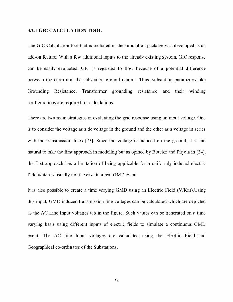
Figure 4.2 Flux-Magnetization Curve Bias in presence of GIC [2]
Thus, a higher excitation current is required to maintain the same flux in the core so as to
maintain sinusoidal output voltage. In addition, the non-linearity of the core incites
harmonics in the excitation current. Since the core is now a high reluctance path, a lot of
stray flux is generated which causes heating in the windings, loss of insulation, formation
of hot spots leading to structural damage and subsequently equipment failure.

39
4.3 SIMULINK MODEL OF INDUCTANCE MATRIX TRANSFORMER
To illustrate all the above discussed phenomena on transformers, a simulation model was
developed in Simulink using the SimPower systems toolbox. The default transformer
model does not allow current in the grounded neutral of the transformer to be directly
coupled with the inductance of the winding. Hence, the Inductance Matrix type
transformer model is used for simulation in this thesis.
Figure 4.3 Simulink model of Induction Matrix Three phase Transformer
The transformer model can be expressed as
[
]
=[
] *
[ ]
+[
]*
[ ]
……………….. (4.1)
R1…….R6 represent Winding Resistances.
L11……L66 represent Self Inductances.
L12…….L65 represent Mutual Inductances.

40
The Inductance matrix model type has a limitation of no provision for Core Saturation.
Hence, to implement saturation, an external saturation block is set up in parallel with the
primary winding of the saturable transformer while using the same specifications such as
winding configuration (Y g, D1 or D11), same winding resistance for the two windings
connected in parallel and desired saturation characteristics.
Figure 4.4 Configuration & Parameters Tab of the Transformer Model
Core Type: The Core Type selected for the simulation is a three limb core which implies
that both positive and zero sequence parameters are used to calculate the Inductance
Matrix in equation (1).

41
Winding connections: The primary winding is of Y- grounded configuration with
accessible neutral while the secondary winding is Y-grounded.
Since the Inductance Matrix model of the transformer involves coupling of the phases in
the core type of construction to minimize the quantity of iron in the core, the model has
different reactance and excitation currents in the positive and zero sequences.
Due to imbalances in the voltage source or load, there is a zero sequence component of
voltage in addition to the positive and negative sequences which leads to higher
excitation currents. These can be measured by using Positive and Zero sequence
measurement blocks as shown in fig
Figure 4.5 Calculation of Positive and Zero-Sequence parameters
42
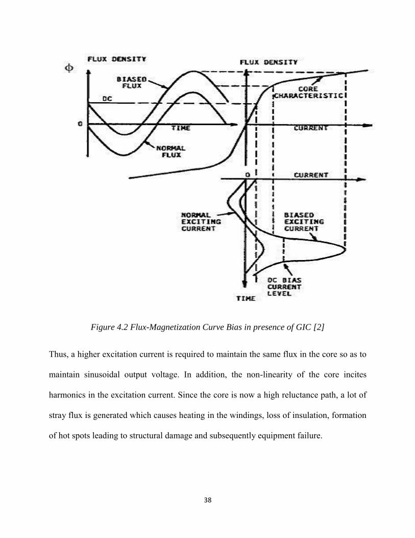
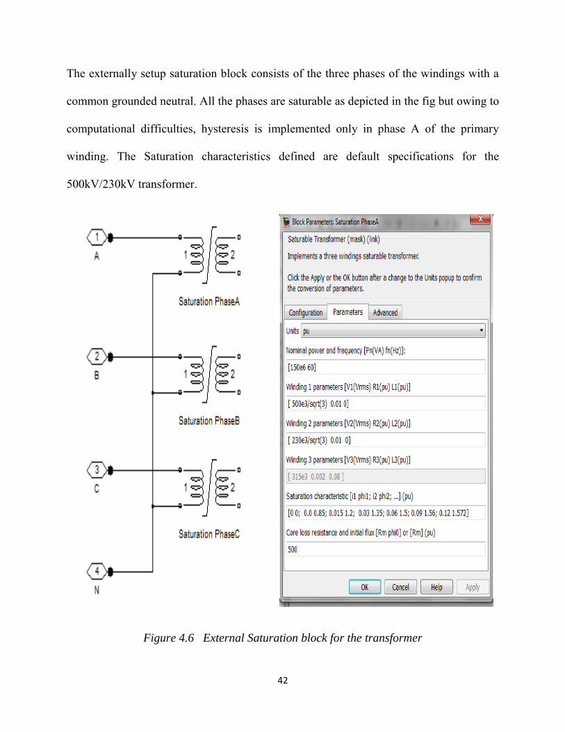
The externally setup saturation block consists of the three phases of the windings with a
common grounded neutral. All the phases are saturable as depicted in the fig but owing to
computational difficulties, hysteresis is implemented only in phase A of the primary
winding. The Saturation characteristics defined are default specifications for the
500kV/230kV transformer.
Figure 4.6 External Saturation block for the transformer

43
4.4 CIRCUIT DESCRIPTION
The entire circuit is laid out for simulation purposes in the Simulink window as shown in
Fig 5.7. It is used to demonstrate the operation of a 3 ø, two winding, 500kV / 230kV
step down transformer along with saturation modeling. The details of the circuit are as
follows:
The source is a 3000 MVA, 500 kV phase-phase equivalent block which excites
the primary winding of the transformer.
GIC is introduced as a slow varying ac current source in the grounded neutral of
the primary winding.
The Saturation block is setup in parallel to the primary winding.
Three phase V-I measurement blocks B1 & B2 are used in the primary and
secondary windings respectively.
Transmission line to a 3 ø Load is simulated using a Distributed Parameters Line
block.
The load which is assumed to be 20% of the Nominal Power of the transformer is
simulated using a 3 ø RLC parallel load.
The remaining blocks in the circuit which are used to illustrate GIC effects will be
discussed in detail in the following section.

44
Figure 4.7 Simulink Model illustrating GIC effects on Transformer

45
4.5 ILLUSTRATION OF GIC EFFECTS IN SIMULINK
To demonstrate the effects of GIC on a transformer, several other blocks in the SimPower
systems toolbox are added to the Simulink model as shown in the above figure. The
following sections describe in detail the effects of GIC on the transformer unit and half
cycle saturation of the core.
4.5.1 DISTORTION OF SATURATION CHARACTERISTICS
The excess flux that saturates the core, biases the operating point of the transformer into
saturation region in the ‘ɸ- I’ curve thereby disturbing the equilibrium and causing non-
linear operation of the core in one half cycle. As additional flux is thrust upon the core, it
gets saturated to greater flux linkages than it was intended to be. Thus, the current
produced in the primary winding is not proportional to that in the secondary winding and
hence the efficiency is severely reduced.
Saturation limit is a measure of how much magnetic flux linkage is achievable between
the primary and the secondary windings of the core thus influencing the core size.
Saturation characteristics represent the piece-wise linear relationship between Flux and
the Magnetizing Current of the transformer. The default characteristics specified as (ɸ,
I) pairs also represent the hysteresis modeling using a static model in the Power System
Block set (PSB)[27]. Under normal operation, the flux produced in the primary winding
core ɸ ac is 1 p.u which is near the knee point of the operation curve.

46
When the quasi-dc GIC current I dc enters the windings through the neutral, it creates
additional flux ɸ dc. Even for a small magnitude of dc current entering the transformer, a
large amount of dc flux is generated due to the high number of turns.
ɸ dc =N1 • I dc (4.2)
Hence, the total flux produced in the core ɸ t = ɸ ac + ɸ dc= F (I ac+ I dc)
Where ɸ ac, ɸ dc are fluxes produced by ac and dc currents respectively.
I ac is the ac current flowing through the windings, I dc is the GIC current entering the
winding and F being the ɸ- I curve of the transformer.
Figure 4.8 Saturation characteristics for transformer core for rated conditions

47
Figure 4.9 Saturation characteristics of a 10A GIC saturated transformer core
As this flux saturates the core, excitation currents of higher magnitude and different
harmonics are required to maintain the flux linkage between the primary and secondary
windings leading to distorted saturation characteristics.
In the simulation, the flux-current characteristics are plotted using an XY signal scope
after converting both the quantities into per unit system. Using the transformer model and
different blocks in the SimPower Systems library, this is illustrated for different GIC
levels entering the transformer through the grounded neutral and the results are tabulated
in Chapter 6.

48
4.5.2 HARMONICS IN CURRENT WAVEFORMS
The power system in the US runs at 60 Hz but disturbances such as GIC create currents
which run at a frequency which are integer multiples of 60 Hz. These are called harmonic
disturbances and this phenomenon is a perennial problem in the operation of the power
system. A Harmonic disturbance can be described as a steady state periodic phenomenon
which causes continuous distortion in the normally sinusoidal voltage and current
waveforms. These disturbances can be characterized by their magnitudes and phase
angles which can be computed using the Fourier analysis technique [28].
Using Fourier analysis, a periodic waveform can be decomposed into a continuous series
of terms each representing a component of the integer multiple of the fundamental
frequency (60Hz).
Harmonic analysis is an important step in order to analyze the response of the power
system to GIC so that necessary mitigation steps can be formulated. Hence, it is
necessary to measure the harmonics that are generated in the currents due to the entry of
GIC into the power grid via the transformer. Thus, Fourier analysis has been carried on
several currents waveforms to measure their respective harmonic contribution.
As the transformer displays non-linear behavior due to saturation, it generates harmonics
in the Excitation current I exc and the primary and secondary currents I p and I s leading
to increased harmonic distortion in current waveforms associated with the transformer.

49
The normal excitation current of the transformer is found to be 5.625 A for phase A.
With gradual increase in GIC, there is a corresponding increase in the magnitude of the
excitation current I exc illustrated in the following graph Fig 5.8.
Figure 4.10 Variation of Excitation Current I exc with GIC Injection
As GIC increases beyond a certain threshold (in this case 20A), I exc shoots up
drastically owing to the saturation of the core and its non-linear behavior.

50
Apart from increased magnitude, there is also a pronounced increase in the harmonic
content of the current waveforms. To analyze this, FFT computation is performed on the
waveforms
The Fourier series of any waveform in time domain can be written as:
( ∑ (
)
Where is the dc component of the signal while each term represents the harmonics of
the signal.
Thus, for the current waveform
I (t) = I0 + ∑ ( ( (
(4.3)
= I0 + ∑ ( (
(4.4)
Where I0 represents the DC current component, I n is the peak magnitude of the nth
harmonic with being the fundamental frequency and Ө n being the respective phase
angle of individual harmonic components.
To perform this computation, the FFT (Fast Fourier Transform) Analysis Tool in the
PowerGUI block is used, shown in the Fig 4.11.

51
Figure 4.11 PowerGUI FFT Analysis Tool
Using this tool, the contribution of each harmonic in the waveform can be computed.
Ideally, the fundamental frequency (60 Hz) should be the harmonic present in the signal
but in practice, we see the presence of various other harmonics.

52
4.5.2.1 TOTAL HARMONIC DISTORTION
Total Harmonic Distortion (THD) is a measure of the harmonic disturbance present in
the current waveforms. It can be defined as the value of the RMS value of all the
harmonics except the fundamental with respect to that of the RMS value of the
fundamental.
THD=
= (I22+I3
2+I4
2+I5
2…………………………..In
2)0.5/ I1 (4.5)
Where I1, I2, I3, I4 ………….In are RMS values of respective harmonic currents.
Every utility sets its own limits of acceptable THD in the current and voltage waveforms.
Usually, the amount of acceptable THD in voltage waveforms is below 10%. Any
increase in THD beyond the limits set causes problems like Voltage drops, Capacitor
tripping, increased power losses and voltage stresses on sensitive loads.
Maintaining THD within tolerable limits is an important part of keeping power quality.
Much research has been done on this subject and its discussion is beyond the scope of
this thesis. IEEE 519 standard is useful is formulating harmonic standards for electrical
systems.

53
Figure 4.12 FFT Analysis of Primary winding current I abc_B1 for rated conditions.

54
From the Fourier analysis of the primary winding current I abc_B1, we observe that
during normal operation, the fundamental frequency(60 Hz) has the major contribution
to the signal while the other harmonic contributions(h2,h3,h4…) and the dc component
are negligible compared to the h1.
The THD is computed from the equation shows that the current & voltage distortions are
1.03% and 0.12% respectively which are within acceptable limits.
But, in the presence of GIC, the saturated core operating in the non-linear region of the
‘ɸ- I’ curve derives harmonics of excitation current I exc and these harmonics are further
propagated into the system through the primary winding towards the voltage source and
through the secondary winding into the load and other power system equipment like
capacitor banks susceptible to harmonic currents with high levels of harmonic distortion.

55
Figure 4.13 FFT Analysis of Primary winding current I abc_B1 for GIC=25 A

56
After FFT Analysis of the Primary winding current I abc_B1 in the presence of a GIC of
25 A, we see that there is an increase in the contribution of higher harmonics
(h2,h3,h4…) and the dc component increases to a large extent and these are not
negligible to that of the fundamental frequency h1.
In addition to harmonics in winding currents, extremely large harmonics are witnessed in
the excitation current of the transformer. With the on-set of GIC, the spectrum of I exc
contain more harmonic components which excite the core improperly leading to
excessive flux and non-linear relation between the flux ‘ɸ’ and I exc.
Figure 4.14 Waveform and Spectrum of RMS Excitation current I exc with GIC =25 A

57
4.5.3 INCREMENT IN REACTIVE POWER CONSUMPTION
GIC saturation makes transformer behave as a source of harmonics causing a drastic
increase in Reactive power consumption which has profound effect over the system
stability. The reactive power consumption of the transformer block in phase A is
observed using the Active & Reactive power block in SimPower Systems Library. This
sudden fluctuation in VAR consumption is attributed to be the main reason for several
other problems like Voltage Stability and decrease in power quality.
As excess flux starts building up in the core, it is driven into saturation and causes
harmonics in the exciting current I exc. These harmonics result in an increase in the VAR
Consumption for the obvious reason that they excite the core without being in phase with
the fundamental frequency h1.
Half cycle saturation reduces the magnetizing reactance of the transformer causing a
surge in the magnitude of the excitation current causing the transformer to behave as an
inductive load ultimately resulting in an increase in VAR demand [29].
In the presence of GIC, non-sinusoidal excitation is present in the transformer which
leads to improper excitation of the core and harmonics in I exc .These harmonics cause
higher VAR consumption than normal.

58
The VAR consumption in presence of non-sinusoidal currents can be defined as the
product of the AC voltage and the harmonic components of the currents [30]:
Q= V√∑ (4.6)
Where Q is the Reactive power consumption in VARS
V is the RMS AC voltage in Volts
Ii is the respective harmonic current magnitude in Amperes.
As GIC injection into the transformer increases, we see the appearance higher degree
harmonics in the currents leading to increased reactive power consumption. As a
secondary effect, the Active power (P) also decreases due to losses caused by the
deformation of transformer windings as a result of repeated excitation by current
harmonics.
For this task, the Active and Reactive Power block from the SimPower systems library is
used. The block measures the active power P and reactive power Q of a voltage-current
pair that contains harmonics with the output being the vector [P Q] based on the
following integral equations:
∫ ( (
(4.7)
∫ ( (
(4.8)

59
In the simulation, using the voltage and current measured on phase A, the Active power
‘P’ and Reactive power ‘Q’ of the transformer are calculated for different levels of GIC
injected through the grounded neutral of the transformers. Figs 5.13 & 5.14 elaborate the
sharp increase in VAR consumption along with a drop in Active power P signifying
increased losses.
Figure 4.15 Active Power profile with increase in GIC
Figure 4.16 Reactive Power profile with increase in GIC

60
In the IEEE 14 Bus simulation in PowerWorld simulator, the reactive power loss in a
transformer due to GIC is calculated by solving a simple DC circuit at its respective bus.
As explained in Section 3.4, voltage induced due to a geomagnetic storm is calculated at
every bus taking into account the geographic location of the substation it is present at.
Then, using Ohm’s law, the current developed in the neutral of the transformer due
to this induced voltage Vind is calculated by dividing it with the sum of the
corresponding substation resistances, per phase transmission line and coil resistances of
the transformer.
Table 4.1 Transformer VAR loss tabulation.
With the obtained neutral current and the voltage induced,the excess reactive power
consumed by the transformer is calculated. By carrying out these calculations for every
transformer present in the system, the total VAR loss in the system is estimated for a
particular magnitude of a geomagetic storm.

61
4.5.4 THERMAL DEGRADATION & STRUCTURAL DEFORMATION
As discussed earlier, when the core gets saturated with flux, there is a sharp increase in
its reluctance as compared to the surrounding. Thus, the leakage flux exits through
plausive locations of the core into the transformer tank. This additional flux leads to eddy
current activity which causes intense heating in the tank wall, shunts, clamps and other
structural parts of the transformer [31].
The core saturation results in internalized local heating and charring of the windings and
damage to the insulation. Structural deformation follows as the leakage flux escapes out
of the core into the transformer tank and formation of high temperature zones called
‘hotspots’ in the transformer unit reducing the life of the transformer and it efficiency.
A brief account of previous encounters of Transformers with GIC is as follows:
a. The March 1989 Geomagnetic storm resulted in a Generator Step-Up Unit at
Salem Nuclear Power Plant operated by PSE& G was damaged and had to be
taken off-service due to excessive GIC heating. The GSU was a bank of three
single phase transformers rated at 500 kV Y-24kV ∆ recorded a sudden increase in
Reactive power consumption by 50 MVar along with high content of dissolved
gases combustible gases in cooling oil and noise levels. On inspection after the
incident, charring of windings caused by circulating currents and the impingement
of flux on structural parts not expected during normal operation, has been
observed as shown in Fig 5.15 [2].

62
Figure 4.17 Transformer Damage in Salem Nuclear Plant, NY [2]
b. A 3-ø shell form 500kV/138kV autotransformer operated by Allegheny Power
System at Meadowbrook Substation also saw significant damage during the 1989
Geomagnetic storm. Drastic increase in MVar consumption and high level of THD
in the currents were attributed to be the main reason for the breakdown leading to
high amount of dissolved combustible gases in insulation oil and intense heating.
Analyses post the disruption showed that the temperature measured on the walls of
the tank ran up to 173o C [2].
c. During the 2003 Halloween Storm, several transformers operated by Eskom
Power Corp., in South Africa were reported to have contained high content of
dissolved gases due to excessive saturation of the core. A comparison of Dissolved
Gas Analysis (DGA) records prior to and after the storm has shown that after the
onset of GIC, there was a marked increase in the reactive loading.

63
Unintended tripping of transformer protection and partial breakdown of winding
insulation has been attributed to the high amount of harmonic content in the
currents and intense localized heating. Subsequently, the units had to be promptly
removed out of service [32].
Figure 4.18 Transformer Failures in South Africa [32]
Apart from these, there have been several other reported incidents of transformer
disruption, failure and breakdown due to GIC activity in them located in countries like
the UK, New Zealand and Japan etc [2].
Failure of transformer units of such high voltage levels is a huge setback to the operation
of the transformer, as they are huge and expensive to construct and assemble along with
the long lead-time associated with their replacement. A GSU Transformer is even more
difficult to supplicate with absence of redundancy unlike a transmission network
transformer. Owing to the wide area scope of a geomagnetic storm, multiple
simultaneous failures can seriously hamper restoration efforts.

64
CHAPTER 5: VOLTAGE STABILITY AND GRID RESPONSE
In addition to damage to HV Power Transformers, a geomagnetic event has the adverse
effect of VAR loss in a power grid thereby causing widespread voltage instability
ultimately leading to the collapse of the entire grid. The logical approach in dealing with
this problem is to assess the vulnerabilities of the grid to voltage instability using an
analytical method so that necessary mitigation measures and methods can be devised and
put in place to combat GIC effects. This chapter is based on the paper [34] which predicts
voltage stability of a bus system systematically. Section 5.1 introduces the concept of
Voltage Stability and the following sections describe a method to assess it.
5.1 INTRODUCTION
Voltage stability refers to the capacity of a power network to maintain steady, permissible
voltage levels at all the buses perpetually even after experiencing a disturbance or a
contingent event. Voltage stability analysis warrants observation of voltage profiles when
a contingency occurs. During voltage stability, there is a loss in the stable operating point
of the grid due to the diminution of voltage levels around the point of voltage collapse.
Disproportion between ‘P’ and ‘Q’ leads to bus voltage fluctuation and these values at
each bus indicate the degree of this discrepancy. In this case, since voltage instability is
an issue that is expected to arise due to fluctuation or loss of reactive power support in
the grid, a method that relates the voltage at each bus and the reactive power support is
required. In practice, not every bus is the grid can be assessed for stability.

65
Thence, it is a crucial step in locating the critical bus or the group of buses which are
likely to experience voltage instability during a contingency. According to [37], a critical
bus can be characterized as having the following qualities during a contingency:
• Highest voltage collapse point on the V-Q curve
• Smallest reactive power margin
• Greatest reactive power deficiency
• Greatest excursion in voltage levels.
PV & QV curves are generally used to assess the voltage stability at a particular bus.
They represent the variation of bus voltages with Power Injection. By using the QV
curve, it is possible to estimate the amount of VAR support that can be attained or lent to
achieve voltage stability at the bus most vulnerable to voltage collapse.
Based on the stability margin obtained from the curve, reactive power producing systems
such as SVC (Static VAR Compensators) & STATCOM (Static synchronous
compensator) can be installed to maintain required voltage levels. But, for large systems
which contain numerous buses, generating QV curves for each bus is tedious. Hence, a
fast computational method is to be adopted in this case. Due to the extensive study of
voltage stability analysis, various methods have evolved over the years which can be
broadly divided as Static and Analytic methods [35]. Several other methods have been
discussed in [36] outlining various approaches in identifying areas and components
susceptible to voltage instability.
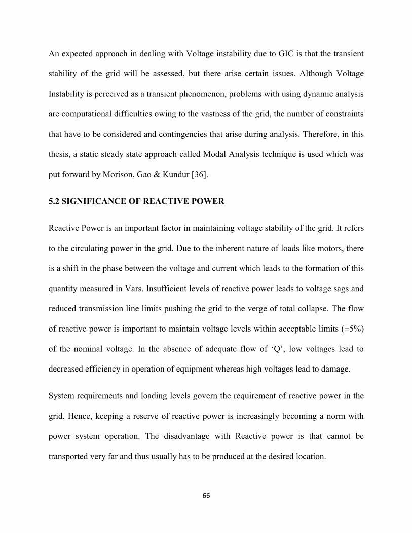
66
An expected approach in dealing with Voltage instability due to GIC is that the transient
stability of the grid will be assessed, but there arise certain issues. Although Voltage
Instability is perceived as a transient phenomenon, problems with using dynamic analysis
are computational difficulties owing to the vastness of the grid, the number of constraints
that have to be considered and contingencies that arise during analysis. Therefore, in this
thesis, a static steady state approach called Modal Analysis technique is used which was
put forward by Morison, Gao & Kundur [36].
5.2 SIGNIFICANCE OF REACTIVE POWER
Reactive Power is an important factor in maintaining voltage stability of the grid. It refers
to the circulating power in the grid. Due to the inherent nature of loads like motors, there
is a shift in the phase between the voltage and current which leads to the formation of this
quantity measured in Vars. Insufficient levels of reactive power leads to voltage sags and
reduced transmission line limits pushing the grid to the verge of total collapse. The flow
of reactive power is important to maintain voltage levels within acceptable limits (±5%)
of the nominal voltage. In the absence of adequate flow of ‘Q’, low voltages lead to
decreased efficiency in operation of equipment whereas high voltages lead to damage.
System requirements and loading levels govern the requirement of reactive power in the
grid. Hence, keeping a reserve of reactive power is increasingly becoming a norm with
power system operation. The disadvantage with Reactive power is that cannot be
transported very far and thus usually has to be produced at the desired location.

67
5.3 MODAL ANALYSIS FOR VOLTAGE STABILITY ASSESSMENT
The Modal analysis technique utilizes the Power Flow Jacobian to evaluate the relation
between Reactive power injection and Bus voltages by keeping the remaining constraints
in the Linearized power flow state equations such as Active Power and Bus Voltage angle
constant. The Power flow Jacobian matrix is reduced in order to depict the incremental
variation in Voltage with respect to Reactive Power injection at each bus [36].
The Steady state system Power flow equations are given by:
[
] = [
] [
] (5.1)
With Jac = [
] being the Power flow Jacobian matrix of the system.
Where
= Incremental change in Bus Real power.
= Incremental change in Bus Reactive power.
Incremental change in Bus Voltage Angle.
Incremental change in Bus Voltage Magnitude.
In order to study the relation between reactive power and Bus voltage variation, the
remaining two quantities in the equation i.e. Real Power and Bus Voltage angle are to be
eliminated. This is accomplished by reducing the Jacobian matrix by keeping .

68
Thus,
+ (5.2)
Which implies -1 (5.3)
&
+ . (5.4)
Substituting the value for , we deduce a relation between and
-1 ] (5.5)
= J or J-1 (5.6)
J being the reduced form of the Power flow Jacobian.
Thus, J= -1 . (5.7)
The matrix J represents the linearized power flow relation between the Reactive Power
Injection and Bus Voltage which is achieved by omitting the Real power and Bus Voltage
Angle from the Steady State power flow Equation [38].
The advantage in doing this operation on the Power flow Jacobian is to exclusively focus
on the variation of voltage stability due to change in Reactive Power injections at
different buses which address the voltage instability issue in the grid.

69
The obtained reduced Jacobian matrix contains the reactive power and voltage
characteristics of the buses. The Eigen values of the matrix signify the different modes of
Reactive power and voltage characteristics thereby giving information about the voltage
stability of the grid. The magnitudes of the Eigen values give information about the
propinquity of the entire grid to voltage instability and the magnitudes of its associated
Eigen vectors of each mode give information about the proximity of each bus to voltage
instability [36].
The reduced Jacobian matrix ‘J’ can be written as a product of three different matrices:
J= ξ ˄ η (5.8)
Where ξ is the right eigen vector of matrix J.
^ is the diagonal eigen vector of matrix J.
η is the left eigen vector of matrix J.
Conversely,
J-1 = ξ ˄ -1 η (5.9)
Substituting the value of J-1 in equation 5.6,
∆V= ξ ˄ -1 η ∆Q (5.10)

70
Or ∆V = ∑ ∆Q (5.11)
where λi is the ith eigenvalue, i is the of ith column right eigenvector and i is the ith row
left eigenvector of matrix J. The product of the left and right eigen vectors is identity
matrix I.
Hence, ∆Vi =
∆Qi is the ith modal voltage variation. (5.12)
Now, the value of the Eigen vector determines the relationship between the voltage and
the reactive power value at a particular mode. A positive value of i signifies its stability
whereas a negative value signifies instability and a value of ‘ ’ represents voltage
collapse.
Using this method, the tendency of an area to collapse during a contingency can be
assessed. This is deemed to be an important step in assessing the vulnerability of the grid
as it gives system operators to identify areas exposed to voltage instability due to reactive
power loss. The Eigen values represent the V-Q sensitivities at each bus and their
magnitude is a measure of voltage instability for that particular bus in the least stable
modes in the grid.
The Modal Analysis technique then developed an index called Participation factor.
Participation factor indicates the contribution of a specific Eigen value to the voltage
sensitivity at a particular bus to identify its vicinity to voltage collapse[36]. Participation
factor is calculated from the Eigen vectors of the reduced Jacobian matrix ‘J’ from
equation 5.7.

71
The participation factor of bus k during ith mode is:
Pki = ξki ηik (5.13)
The value indicates the contribution of the ith Eigen value to the Q-V sensitivity at bus k.
The magnitude of this value represents the tendency of its corresponding eigen value i
to cause voltage instability at bus k. Since, the modes with smallest Eigen values are
close to voltage instability; their corresponding Bus Participation factors are calculated.
The Buses are then ranked in terms of their participation factors which indicate
decreasing voltage stability.
To perform all these operations, the Power flow Jacobian in PowerWorld Simulator was
saved as a sparse matrix .m file. A function called modal (); was then developed in
MATLAB to execute the whole process.
By identifying and ranking the buses in terms of their tendency to voltage
collapse, this method eliminates the need to generate Q-V curve for every bus in the
system. Utilizing the participation factor in the weakest mode, buses can be ranked in
terms of their proximity to voltage collapse at different operating points. The bus with the
highest participation in the critical mode is said to be the weakest bus in terms of voltage
stability and thus its Q-V curve is generated to calculate its Reactive Power Margin
(RPM). For the purpose of this simulation, three different contingencies were chosen
corresponding to increasing magnitudes of induced electric field ‘E’. To better observe
the dynamic nature of voltage variation with increasing Reactive Power loss, a color
contour was used a background in the test system.

72
5.4 Q-V CURVE GENERATION
The next step in voltage stability assessment is to generate Q-V curves at the critical bus
i.e., the bus which is more prone to voltage collapse. Load buses are generally the
weakest buses in a power system as they do not have a continuous generation of reactive
power. Hence, they are highly sensitive to any kind of voltage disturbance. Q-V curve
gives system designers a notion of the reactive power injection required at a particular
bus to attain voltage security. A typical Q-V curve is shown in the Figure 5.1.
Figure 5.1 Standard Q-V curve [38].
The distance from the stable operating point to the point of Qmax is defined as the
Reactive Power Margin (RPM) at the bus. Apart from the calculation of RPM, Q-V
curves aid in identifying whether a bus has a stable operating point or not.

73
The slope of the curve represents the V-Q sensitivity (
) at a particular operating point.
The upper part of the curve is designated as the stable region as the V-Q sensitivity is
positive in that region indicating the fact that as reactive power injection increases,
voltage increases. When the reactive power reserve is depleted due to losses at a bus in
such a way that it reaches the critical point Qmax, anymore further injection beyond this
point causes a voltage drop indicating a negative V-Q sensitivity and voltage instability.
In order to generate this curve, a fictitious generator is placed on a bus whose reactive
power output is of interest. By varying the voltage set point in small steps, the VARs
required to maintain this voltage is then measures and the co-ordinates are plotted on a
curve with Voltage and VAR output being its axes.
At rated conditions, the output of the fictitious generator is ‘0’. As the reactive power
losses due to GIC mount, they behave as increasing MVar load on the system depleting
the RPM at the weakest bus. When the losses increase to such an extent that it consumes
the entire RPM, then voltage collapse ensues.
For the IEEE 14 bus system used in this thesis, after identifying and ranking the critical
bus or cluster of buses, their QV curves are observed to see how sensitive they are to a
geomagnetic storm and their voltage stability is determined at three different operating
points. The results are laid down in Chapter 6 for further illustration.

74
CHAPTER 6: SIMULATION RESULTS AND DISCUSSION
6.1 RESULTS FROM TRANSFORMER ANALYSIS
Figure 6.1 THD versus GIC injection for phase A
Figure 6.1 represents Total Harmonic Distortion (THD) versus injected GIC current into
the transformer. With steady increase in GIC, THD also increases due to increment in
harmonic content. After reaching a certain point, any further increase in GIC causes a
drop in THD as the dc starts dominating in the current. Table 6.1 contains data about
THD of primary and secondary, voltages and currents which indicate escalating
harmonics with increasing GIC.

75
Table 6.1 Transformer Current & Voltage Distortion Results
TOTAL HARMONIC DISTORTION (%) PRIMARY WINDING
GIC(A) Ip Vp Is Vs Iexc(A) P (W)
Q (Var)
0 1.03 0.12 0.09 0.09 -5.626 3.39E+07 -1.27E+06 5 1.37 0.15 0.11 0.11 -8.704 3.38E+07 -1.15E+06
10 2.50 0.23 0.18 0.18 -15.67 3.38E+07 -7.15E+05
15 4.67 0.41 0.33 0.33 -28.09 3.36E+07 1.26E+05 20 8.53 0.73 0.59 0.59 -49.03 3.35E+07 1.59E+06
25 28.28 7.34 2.92 2.92 -141.1 3.32E+07 5.68E+06
30 52.03 5.81 4.95 4.95 -248.3 3.27E+07 1.28E+07 35 64.73 7.49 6.53 6.53 -342.3 3.22E+07 2.04E+07
40 68.70 9.08 7.71 7.71 -426.3 3.17E+07 2.80E+07
45 68.07 10.30 8.53 8.53 -502.3 3.11E+07 3.52E+07 50 65.36 13.46 9.79 9.79 -571.8 3.06E+07 4.20E+07
55 61.57 25.89 11.56 11.56 -641 3.01E+07 5.01E+07
60 58.28 13.15 12.72 12.72 -730.3 2.93E+07 5.96E+07 65 54.67 13.82 13.53 13.53 -750.3 2.91E+07 6.02E+07
70 51.21 14.22 14.13 14.13 -801.8 2.87E+07 6.74E+07
75 47.95 14.40 14.62 14.62 -850.2 2.83E+07 7.28E+07 80 44.91 14.72 14.98 14.98 -895.5 2.79E+07 7.80E+07
85 42.07 15.11 15.19 15.19 -938.3 2.75E+07 8.21E+07
90 39.43 15.09 15.27 15.27 -978.2 2.71E+07 8.72E+07 95 36.97 15.18 15.24 15.24 -1016 2.67E+07 9.13E+07
100 34.71 15.15 15.12 15.12 -1051 2.63E+07 9.53E+07
105 32.61 15.26 14.94 14.94 -710.8 3.57E+07 -1.38E+11 110 30.63 16.47 14.69 14.69 -1115 2.57E+07 1.02E+08
115 28.79 14.71 14.39 14.39 -1144 2.54E+07 1.04E+08
120 27.02 14.77 14.02 14.02 -1172 2.50E+07 1.08E+08 125 25.34 14.68 13.57 13.57 -1199 2.48E+07 1.19E+08

76
From the power stats in the above table, at about after 20A of GIC injection, the
distortion levels shoot up rapidly indicating that the core is completely saturated with
excess flux. At this point,we also see a decrease in Active Power is attributed to
increasing losses due to heat formation, displaced flux which implies depreciating
efficiency of the transformer.
Figure 6.2 depicts saturation characteristics with step wise increase in GIC injection with
an increase of 15 A per step. The Flux-Current magnetisation curve is biased to one side
In the Figure 6.3 ,we see the difference in exciting current waveforms at rated conditions
and when the transformer is in a saturated state. The magnitude of I exc increases
manifold with saturation of the core inciting harmonic components in the current
waveform. An increasing trend in THD is also witnessed in the waveforms.

77
Figure 6.2 Saturation characteristic distortion with increasing GIC Injection

78
Figure 6.3 Deterioration of Excitation current Iexc with GIC injection

79
6.2 RESULTS FROM GRID AND VOLTAGE STABILITY ANALYSIS
The test case system was subjected to three different intensities of a geomagnetic storm
as represented in the following results and are discussed in detail.
a) Operating point ‘A’ (E=0 V/km)
>> Jacobian 1 65.34 2 39.95 3 21.98 4 18.92 5 16.43 6 2.71 7 5.57 8 7.66 9 11.34 Critical mode of the system is 6 th eigen value 2.706 Participation factors of buses corresponding to the critical mode 1 0.000 2 -0.000 3 -0.000 4 0.008 5 0.004 6 -0.000 7 0.070 8 -0.000 9 0.200 10 0.239 11 0.111 12 0.019 13 0.032 14 0.316 The ranking of the buses in order of their participation factors are 14 10 9 11 7 13 12 4 5 1 2 3 6 8 The critical bus of the system is 14 th bus with participation factor 0.316

80
Figure 6.4 Test case at operating point ‘A’

81
Figure 6.5 Q-V curve of the critical bus-Bus 14 at operating point ‘A’
Table 6.2 Results from QV curve Analysis for Operating point ‘A’
Bus Number
V at Q0
Q0 Qinj_0 Vmax Q at VMax
Qinj at Vmax
V at Qmin
Qmin Qinj_min
14 1.04 0.00 0.00 1.1000 32.27 32.27 0.5855 -70.46 -70.46

82
Figure 6.4 represents the test case at a chosen operating point ‘A’ succeeded by its
respective modal analysis simulation results. Bus 14 is identified to be the critical bus
with a participation factor ‘ .316’ followed by the remaining load buses. It is to be noted
that at this standpoint, only load buses are somewhat prone to voltage instability whereas
the remaining PV buses and swing bus possess a null participation factor indicating their
stability.
Subsequently, the QV curve of Bus 14 (Figure 6.5) was generated as the main effect of
GIC was conveyed as loss in reactive power. The Q-V curve was then generated to see if
the bus has a stable operating point and to evaluate its Reactive Power Margin (RPM).
Table 6.2 contains data of the generated Q-V curve of the bus 14 at this operating point
with a RPM of 70.46 MVar.

83
b) Operating point ‘B’(E=5V/km)
>> Jacobian 1 49.44 2 33.81 3 27.69 4 21.29 5 16.48 6 13.58 7 11.83 8 0.49 9 8.67 10 2.25 11 5.28 12 4.50 13 4.09 Critical mode of the system is 8 th eigen value 0.487 Participation factors of buses corresponding to the critical mode 1 0.000 2 0.003 3 0.009 4 0.016 5 0.014 6 0.099 7 0.063 8 0.059 9 0.096 10 0.114 11 0.122 12 0.135 13 0.129 14 0.140 The ranking of the buses in order of their participation factors are 14 12 13 11 10 6 9 7 8 4 5 3 2 1 The critical bus of the system is 14 th bus with participation factor 0.140

84
Figure 6.6 Test case at operating point ‘B’

85
Figure 6.7 Q-V curve of the critical bus-Bus 14 at ‘B’
Table 6.3 Results from QV curve Analysis for Operating point ‘B’
Bus Number
V at Q0
Q0 Qinj_0 Vmax Q at VMax Qinj at Vmax V at Qmin
Qmin Qinj_min
14 0.92 0 0 1.1 52.92 52.92 0.4967 -48.9 -48.9

86
Figure 6.6 represents the test case at a chosen operating point ‘A’ succeeded by its
respective modal analysis simulation results. Bus 14 is identified to be the critical bus
with a participation factor ‘ . 140’ followed by the remaining load buses. It is to be noted
that at this standpoint, not only load buses, but all other buses except Bus 1 (swing bus)
also have a non-zero participation factor due to their instability.
Subsequently, the QV curve of Bus 14 (Figure 6.7) was generated to see if the bus has a
stable operating point and to evaluate its Reactive Power Margin (RPM). Compared to
the previous operating point, there is a pronounced decrease in the RPM of the critical
most bus i.e., Bus 14 from 70.46 MVar to 48.9 MVar due to the loss of reactive power.
Even though the bus has a stable operating point at this instant, it is well beneath its
normally accepting limit and also suffers a loss in reactive power. To bring the bus
voltage levels within the acceptable limits 0.95 pu and 1.05 pu , there needs to be an
additional injection of reactive power.
At this point, several transformers and transmission lines indicated in red are beyond their
normal operating limits which indicates this to be an unstable operating point.

87
c) Operating Point ‘C’ (E=9.5 V/km)
>> Jacobian 1 41.15 2 31.27 3 21.66 4 17.51 5 13.58 6 11.38 7 9.78 8 6.99 9 0.52 10 5.10 11 3.64 12 3.39 13 1.96 Critical mode of the system is 9 th eigen value 0.519 Participation factors of buses corresponding to the critical mode 1 -0.000 2 0.001 3 0.005 4 0.011 5 0.010 6 0.100 7 0.056 8 0.048 9 0.095 10 0.117 11 0.129 12 0.145 13 0.136 14 0.148 The ranking of the buses in order of their participation factors are 14 12 13 11 10 6 9 7 8 4 5 3 2 1 The critical bus of the system is 14 th bus with participation factor 0.148

88
Figure 6.8 Test case at operating point ‘C’
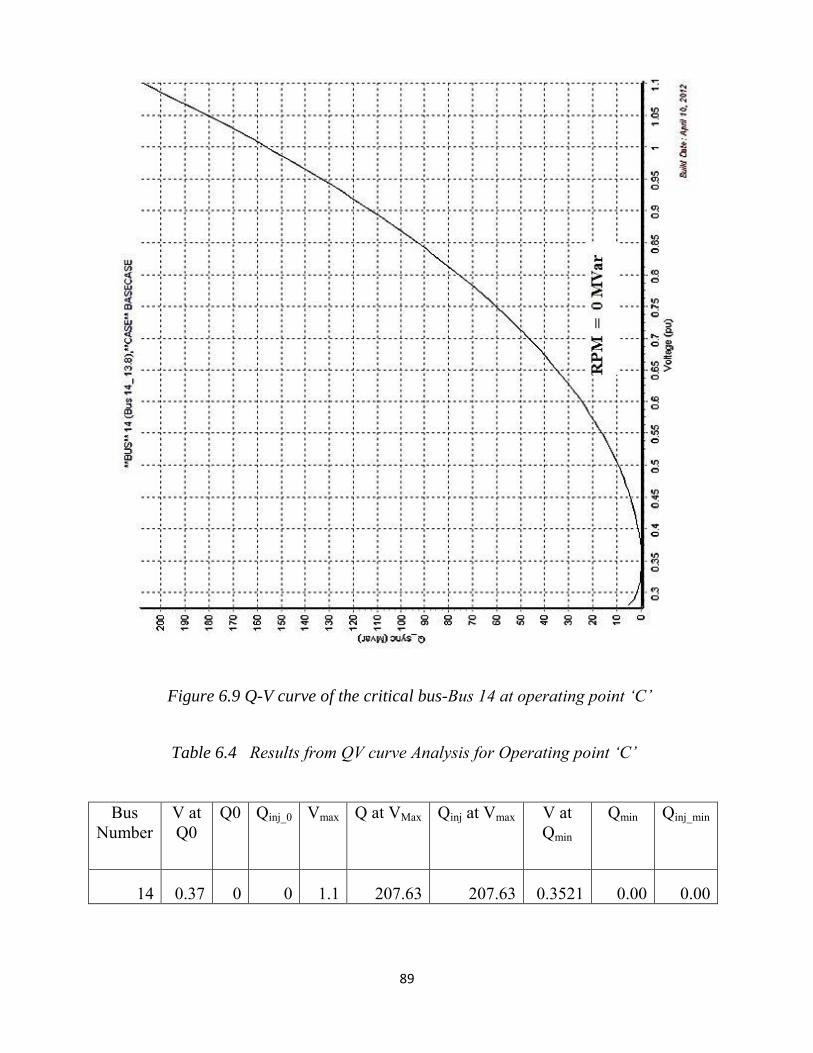
89
Figure 6.9 Q-V curve of the critical bus-Bus 14 at operating point ‘C’
Table 6.4 Results from QV curve Analysis for Operating point ‘C’
Bus Number
V at Q0
Q0 Qinj_0 Vmax Q at VMax Qinj at Vmax V at Qmin
Qmin Qinj_min
14 0.37 0 0 1.1 207.63 207.63 0.3521 0.00 0.00

90
Figure 6.8 represents the test case at a chosen operating point ‘A’ succeeded by its
respective modal analysis simulation results. Bus 14 is identified to be the critical bus
with a participation factor ‘ . 146’ followed by the remaining load buses. It is to be noted
that at this standpoint, all the load buses are somewhat prone to voltage instability except
Bus 1 (swing bus) possess a non-zero participation factor indicating their stability.
Subsequently, the QV curve of Bus 14 (Figure 6.9) was generated as the main effect of
GIC was conveyed as loss in reactive power. The Q-V curve was then generated to see if
the bus has a stable operating point and to evaluate its Reactive Power Margin (RPM).
The results shown above show that, with increase in the intensity of the geomagnetic
storm, the voltage levels drop considerably which are depicted by the voltage contours.
The number of buses which participate in voltage collapse also increases signifying the
spread of voltage disturbances if they are left unmitigated.
Also, the components of the system such as transformers and transmission lines are
required to function beyond their rated limits which will stress the system and restrict
power transfer to the load areas. Persistent low voltage levels are hazardous to power
system assets.
From the Q-V curves, it was observed that there is a drastic decline in the Reactive Power
Margin (RPM) stresses the system and pushes the grid towards voltage collapse which
confirms the hypothesis discussed in earlier chapters.
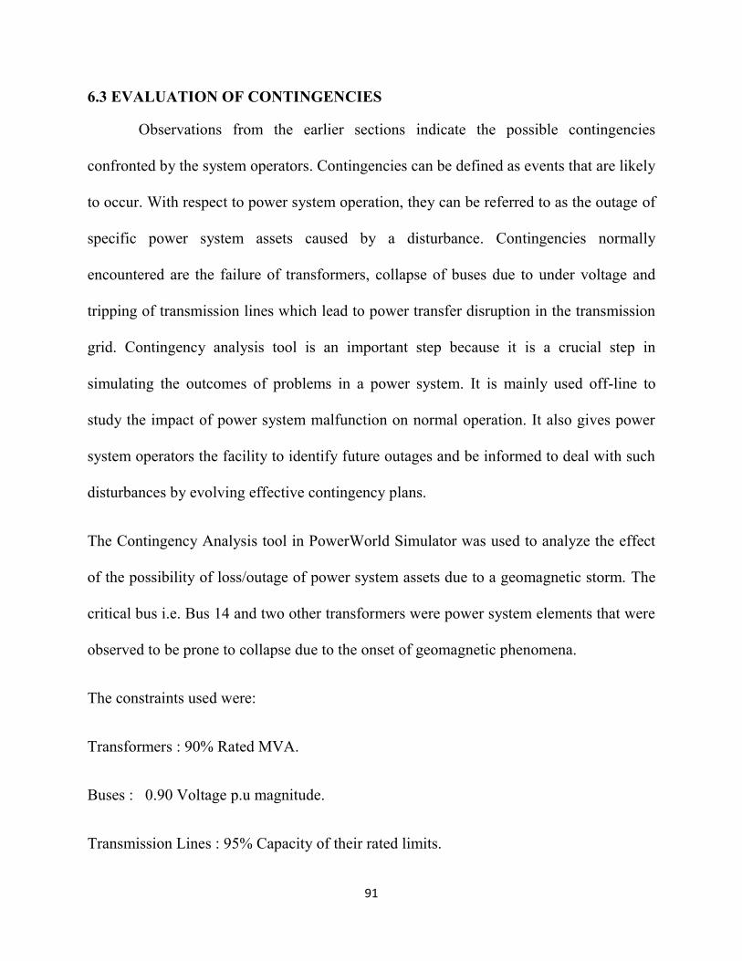
91
6.3 EVALUATION OF CONTINGENCIES
Observations from the earlier sections indicate the possible contingencies
confronted by the system operators. Contingencies can be defined as events that are likely
to occur. With respect to power system operation, they can be referred to as the outage of
specific power system assets caused by a disturbance. Contingencies normally
encountered are the failure of transformers, collapse of buses due to under voltage and
tripping of transmission lines which lead to power transfer disruption in the transmission
grid. Contingency analysis tool is an important step because it is a crucial step in
simulating the outcomes of problems in a power system. It is mainly used off-line to
study the impact of power system malfunction on normal operation. It also gives power
system operators the facility to identify future outages and be informed to deal with such
disturbances by evolving effective contingency plans.
The Contingency Analysis tool in PowerWorld Simulator was used to analyze the effect
of the possibility of loss/outage of power system assets due to a geomagnetic storm. The
critical bus i.e. Bus 14 and two other transformers were power system elements that were
observed to be prone to collapse due to the onset of geomagnetic phenomena.
The constraints used were:
Transformers : 90% Rated MVA.
Buses : 0.90 Voltage p.u magnitude.
Transmission Lines : 95% Capacity of their rated limits.
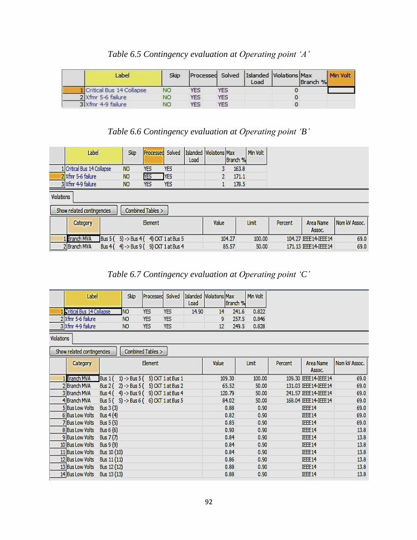
92
Table 6.5 Contingency evaluation at Operating point ‘A’
Table 6.6 Contingency evaluation at Operating point ‘B’
Table 6.7 Contingency evaluation at Operating point ‘C’
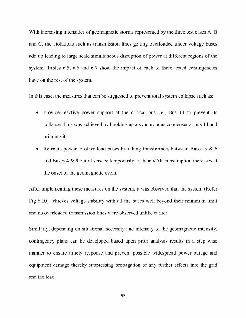
93
With increasing intensities of geomagnetic storms represented by the three test cases A, B
and C, the violations such as transmission lines getting overloaded under voltage buses
add up leading to large scale simultaneous disruption of power at different regions of the
system. Tables 6.5, 6.6 and 6.7 show the impact of each of three tested contingencies
have on the rest of the system.
In this case, the measures that can be suggested to prevent total system collapse such as:
Provide reactive power support at the critical bus i.e., Bus 14 to prevent its
collapse. This was achieved by hooking up a synchronous condenser at bus 14 and
bringing it
Re-route power to other load buses by taking transformers between Buses 5 & 6
and Buses 4 & 9 out of service temporarily as their VAR consumption increases at
the onset of the geomagnetic event.
After implementing these measures on the system, it was observed that the system (Refer
Fig 6.10) achieves voltage stability with all the buses well beyond their minimum limit
and no overloaded transmission lines were observed unlike earlier.
Similarly, depending on situational necessity and intensity of the geomagnetic intensity,
contingency plans can be developed based upon prior analysis results in a step wise
manner to ensure timely response and prevent possible widespread power outage and
equipment damage thereby suppressing propagation of any further effects into the grid
and the load

94
Figure 6.10 Test Case with Contingency Plan

95
CHAPTER 7: CONCLUSION AND SCOPE FOR FUTURE WORK
This thesis intends to raise the issue of geomagnetic phenomenon as a potential
disturbance to the bulk power system. A systematic approach was adopted in bringing the
issue forward in a suitable manner. This was achieved by studying the internal sequence
of events that give rise to GIC. The next step was to quantify the issue and represent it in
the system whilst also examining several other methods that have been previously used.
PowerWorld Simulator was adopted to simulate GIC into the standard IEEE
14 bus system. The effect of GIC on a single component on the power system viz., High
Voltage Transformer was assessed. Simulink was used to model the transformer and
explain the effects due to the entry of GIC into the transformer. The results were taken
into perspective and then extended to a standard IEEE 14 bus system. The simultaneous
loss of reactive power and harmonic injection into the system causes low voltage levels
leading the system towards collapse. Voltage stability is an important issue which was
studied and analyzed during a GIC storm. A method called Modal Analysis was utilized
to study the voltage stability of the system and the most critical and vulnerable buses in
the system were identified and ranked in terms of their proximity to voltage collapse
The participation factors of all the buses are observed and ranked in order their
magnitude which represents their likelihood to undergo voltage collapse. The bus which
had the highest participation factor was chosen and its Q-V cure was generated to
illustrate the loss in reactive power due to GIC circulation in the grid.

96
Some important conclusions that can be drawn from this thesis are:
Geomagnetically Induced Currents are a credible threat to the bulk power system and
should be appropriately analyzed and incorporated as a constraint while designing the
system. An industry standard procedure needs to be developed in dealing Geomagnetic
Disturbance like all other natural calamities. Utility wide GIC monitoring is suggested to
enhance quick response to any disturbances.
Steady state Power System Analysis has been performed before and after a contingency
to observe if all active and reactive power generation limits, bus voltage magnitude
limits, transformer and transmission line loading limits is abided by. The threshold limit
of operational stress during such disturbances can also be approximated by suitable
analysis.
It is very essential to investigate and analyze the effects of a GIC over a system
component viz., Transformers, Generators so that suitable mitigation measures can be
devised. Various possible GMD scenarios have to be tested to see if they can endure the
stresses impinged upon them. The necessity of advanced tools for vulnerability
assessments has been demonstrated.
Dynamic Cable Rating (DCR) and series compensation of transmission lines has to be
extensively put into practice in regions prone to such disturbances to combat GIC effects
such as sudden loss in line limits and power transfer capability.
Installation of mitigation devices such as neutral resistances and capacitors in neutrals of
grounded transformers to obstruct GIC flow into the system.

97
NERC has recently reviewed several commercial GIC reducing/blocking devices to serve
as a guide for system planners to choose the optimum device basing on the transformers
technical specifications and configuration [39].
Equipment design specifications have to be inspected for necessary improvements and a
base case criterion has to be established which can be incorporated in the manufacturing
process.
Reactive power producing components should be located as close as possible to the
critical buses in the system. After sufficient research, it is opined that Synchronous
condensers are to be preferred to produce the necessary MVar to maintain voltage levels
since they are known to be absorptive of harmonic components and are quite stable
during power swings in the system.
As a possible extension to this thesis, similar analyses can be performed with
real data obtained from utilities. Models for GIC blocking devices can be developed,
simulated, tested and validated. More field research is suggested to understand how these
devices react to a geomagnetic disturbance. A contingency plan can be formulated basing
on the results to protect the assets in the system from GIC effects, keeping the current
waveform distortion within limits, preserving a stable operating point and maintaining the
reliability.

98
APPENDIX
A. Function for Modal Analysis and Jacobian operation.
function []= modal(Jac) % This function takes the Power flow Jacobian ‘Jac’ generated from the PowerWorld Simulator as input and performs Modal analysis operations on it. % The eigen vectors and eigen values are calculated and subsequently, the participation factors of buses in voltage collapse in the critical mode of the system are determined and ranked in order. m=length(Jac); reshape(Jac,m,m); Y=mat2cell(Jac,[m/2,m/2],[m/2,m/2]); %Calculation of Reduced Jacobian Matrix J. J= Y{2,2}-(Y{2,1}/(Y{1,1})*Y{1,2}); J=full(J); %Eigen value & Eigen vector calculation. [V,D]=eig(J); Vl=(inv(V'))'; n=length(J); eigJ=eig(J); newLength=0; for k=1:n if(eigJ(k) ~= 1) fprintf('%d %3.2f\n',k, eigJ(k)); newLength=newLength+1; end end [C,I]=min(eigJ(1:newLength)); fprintf('\n Critical mode of the system is %d th eigen value %3.3f\n',I,C);

99
P=zeros; for k=1:n for i=1:n % Participation factor of bus k to mode i : P(k,i)=V(k,i)*Vl(i,k); end end %Participation factors corresponding to the weakest mode: [PF]=P(:,I); display('Participation factors of buses corresponding to the critical mode'); for j=1:length(PF) fprintf('%d %3.3f\n',j,PF(j)); end [R,IX]=sort(PF,'descend'); fprintf('\n The ranking of the buses in order of their participation factors are\n'); fprintf('%d \n',IX); [W,I]=max(PF);fprintf('\n The critical bus of the system is %d th bus with participation factor %3.3f\n',I,W); end

100
BIBLIOGRAPHY
1. Das R, Novosel D, “Review of fault location techniques for transmission and sub
– transmission lines”. Proceedings of the 54th Annual Georgia Tech Protective
Relaying Conference, 2000.
2. NERC, "Effects of Geomagnetic Disturbances on the Power System". Special
Reliability Assessment Report, February 2012.
3. NPCC, "Procedures for Solar Magnetic Disturbances Which Affect Electric Power
Systems", January 2007.
4. John Kappenman, Metatech. Posted on NOAA Space Weather Prediction Center
web site, http://www.swpc.noaa.gov/Media/graphics/Geomag.gif
5. Office of Risk Management and Analysis, "Geomagnetic Storms: An Evaluation
of Risks and Risks Assessment".
6. CENTRA Technology, OECD, "Future Global Shocks", Geomagnetic storms.
7. Thomas J Overbye, Trevor R Hutchins, Komal Shetye, Jamie Weber, Scott
Dahman, "Integration of Geomagnetic Disturbance Modeling into the Power
Flow: A Methodology for large Scale System Studies", September 2012.
8. NERC, "High Impact Low Frequency Event Risk to the North American Bulk
Power System", June 2010.
9. Allan John McKay, "Geoelectric Fields and Geomagnetically Induced Currents in
the United Kingdom", Ph.D. Thesis, University of Edinburgh, 2003.

101
10. Alan P Thompson, Toby D G Clark, Ellen Clark, Allan McKay, "Monitoring
Geomagnetically Induced Currents in the Scottish Power Grid", European Space
Agency.
11. Antti Pulkkinen, S. Lindahl, Ari Viljanen, and Risto Pirjola (2005), Geomagnetic
storm of 29–31 October 2003: Geomagnetically induced currents and their relation
to problems in the Swedish high-voltage power transmission system, Space
Weather, 3, S08C03, doi:10.1029/2004SW000123
12. Jacko Koen, Trevor Gaunt, "Geomagnetically Induced Currents in the Southern
African Electricity Transmission Network". Proceedings of the 2003 IEEE
Bologna Powertech Conference, June 23-26, Bologna, Italy.
13. Torta, J. M., L. Serrano, J. R. Regué, A. M. Sánchez, and E. Roldán (2012),
"Geomagnetically induced currents in a power grid of northeastern Spain", Space
Weather, 10, S06002, doi:10.1029/2012SW000793.
14. Marshall, R. A., M. Dalzell, C. L. Waters, P. Goldthorpe, and E. A. Smith (2012),
"Geomagnetically induced currents in the New Zealand power network", Space
Weather, 10, S08003, doi:10.1029/2012SW000806.
15. Stefan Lotz, "Predictability of Geomagnetically induced currents using neural
networks", M.S Thesis, Rhodes University, August 2008.
16. Reza Ezua Bin Samin, "Forecasting Sunspot Number Using Neural Networks:
Effect to the Electrical System", M.S Thesis, Kolej Universiti Teknologi Tun
Hussein Onn, November 2006.

102
17. Chigomezyo Mudala Ngwira, "Geomagnetically Induced Current Characteristics
in Southern Africa", M.S Thesis, Rhodes University, June 2008.
18. Risto Pirjola, David Boteler, Ari Viljanen, Olaf Amm, "Prediction of
Geomagnetically Induced Currents in Power Transmission Systems", COSPAR-
Elsevier Science Ltd.2000
19. Antti Pulkkinen, Ari Viljanen, Olaf Amm and Risto Pirjola, "Nowcasting
Geomagnetically Induced currents in power systems and pipelines based on ",
Finnish Meteorological Institute. Helsinki, Finland, December 2002.
20. Jon Berge, Rajiv K Varma, "A Software simulator for Geomagnetically induced
currents in electrical power systems", The University of Western Ontario, London,
Canada.
21. Alexandre A Trichtchenko , David H Boteler , Aidan M Foss, "GIC Modeling for
an Over determined system", Ottawa University, Geomagnetic Laboratory, ANF
Energy Solutions, Ottawa, ON,Canada.2007
22. Ming Zou, Lianguang Liu, "GIC Calculation in Power Grid Based on Layered
Earth Mode", 2010.
23. V.D. Albertson, J.G. Kappenman, N. Mohan, and G.A. Skarbakka, “Load‐Flow
Studies in the Presence of Geomagnetically‐Induced Currents,” IEEE Trans. on
Power Apparatus and Systems, vol. PAS‐ 100, February 1981, pp. 594‐606.
24. D.H. Boteler, R.J. Pirjola, “Modeling Geomagnetically Induced Currents Produced
by Realistic and Uniform Electric Fields,” Proc. IEEE Trans. on Power Delivery,
vol. 13, October 1998, pp. 1303‐1308.

103
25. A.Viljanen, R. Pirjola, "Geomagnetically Induced Currents in the Finnish High-
Voltage Power System", Finnish Meteorological Institute, Department of
Geophysics, January 1994.
26. J.W. Ingleson, S. Mazumdar, P.G. McLaren, K.K. Mustaphi, F.M. Phillips, R.V.
Rebbapragada, G.D. Rockefeller B. Bomki (Chair), S.R. Chano, L.L. Dvorak,
W.E. Feero, G. Fenner, E.A. Guro, C.F. Henville, "The Effects Of GIC On
Protective Relaying", IEEE Transactions on Power Delivery, Vol. 11, No. 2, April
1996.
27. Silvano Casoria, Patrice Brunelle, "Hysteresis Modeling In the Matlab/Power
System Block set", IEEE Transactions on Power delivery.
28. W. Mack Grady, Surya Santoso,"Understanding Power System Harmonics", IEEE
Transaction on Power delivery, September 2001.
29. North American Electric Reliability Corporation, "Geo-Magnetic Disturbances
(GMD): Monitoring, Mitigation, and Next Steps", October 2011.
30. A. E. Emaneul, “Power in Non-sinusoidal Situations-A Review of Definitions and
Physical Meanings”, IEEE Trans. on Power Del. vol.5, no.3, pp. 1377-1389, Jul.
1990.
31. L.A.T. Amuanyena, C.T. Gaunt, "Effects of Geomagnetically Induced Currents
(GIC) On Power Transformers And Reactors", University of Cape Town, Cape
Town, South Africa.
32. C.T.Gaunt, G.Coetzee, "Transformer failures in regions incorrectly considered to
have low GIC-risk" IEEE Power Tech, Lausanne, pp 807-812.

104
33. “Modeling Geomagnetically Induced Currents in PowerWorld Simulator”,
PowerWorld Simulator-GIC Tool Help document, 2012.
34. C.R. Hemavathi, “Prediction of Voltage Stability using Modal Analysis”,
National Conference on Electrical Sciences-2012, ISBN: 978-93-81583-72-2.
35. B.Gao, G.K.Morrison, P.Kundur, “Voltage Stability Evaluation using Static and
Dynamic Approaches”, IEEE Transaction on Power Systems, vol.8, no.3, August
1993.
36. B.Gao, G.K.Morrison, P.Kundur, “ Voltage Stability Evaluation using Modal
Analysis”, IEEE Transaction on Power Systems, vol.7, no.4, November 1992.
37. Western Electricity Coordinating Council, “Guide to WECC/NERC Planning
Standards I.D: Voltage Support and Reactive Power”, Reactive Reserve Working
Group(RRWG), March 2006.
38. Amer Al-Hinai, “Voltage Collapse Prediction for Interconnected Power
Systems”, Master’s thesis, Dept. of Electrical Engineering, West Virginia
University,2000.
39. NERC, “Geomagnetic Induced Current (GIC) Mitigation System Summary for
the White Paper”.

105
VITA
Sivarama Karthik Vijapurapu was born in Visakhapatnam, Andhra Pradesh, India. He
received his Bachelor of Engineering degree in the field of Electronics and
Communication Engineering from Andhra University, Andhra Pradesh, India in April
2007.
In August 2011, he enrolled as a MSEE student in the Department of Electrical and
Computer Engineering at the University of Kentucky. In April 2013, he was qualified as
an Engineer in Training (FE) by the National Council of Examiners for Engineering and
Surveying (NCEES).
He currently works as a Power Systems Engineer in the Power Systems Engineering
Division of Schneider Electric Inc., at Lexington, Kentucky.


