Classification:Logistic Regression and Naive Bayes
Book Chapter 4.
Carlos M. CarvalhoThe University of Texas McCombs School of Business
1
1. Classification2. Logistic Regression, One Predictor3. Inference: Esimtating the Parameters4. Multiple Logistic Regression5. AIC and BIC in Logistic Regression6. Log Odds7. Making Decisions and Loss8. Out of Sample9. Lift and ROC10. Bayes Theorem and Classification
10.1. Quick Basic Probability Review10.2. Conditional Probability and Classification103. Bayes Theorem10.4. Naive Bayes
1. Classification
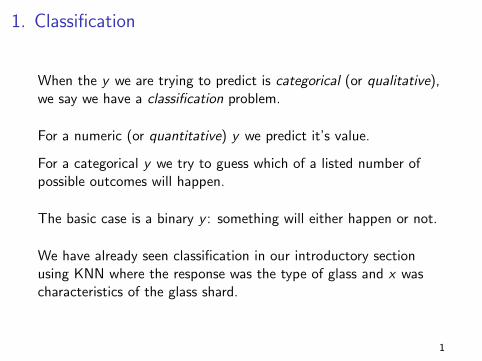
When the y we are trying to predict is categorical (or qualitative),we say we have a classification problem.
For a numeric (or quantitative) y we predict it’s value.
For a categorical y we try to guess which of a listed number ofpossible outcomes will happen.
The basic case is a binary y : something will either happen or not.
We have already seen classification in our introductory sectionusing KNN where the response was the type of glass and x wascharacteristics of the glass shard.
1
Classification
There are a large number of methods for classification.We have seen KNN.
In this section of notes we will learn about logistic regression andnaive Bayes.
Later, we will study trees, Random Forests, and boosting, whichare also important classification methods.
2
Classification
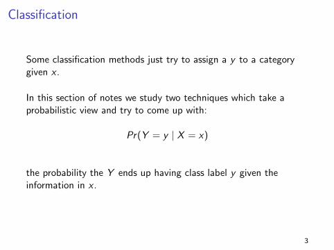
Some classification methods just try to assign a y to a categorygiven x .
In this section of notes we study two techniques which take aprobabilistic view and try to come up with:
Pr(Y = y | X = x)
the probability the Y ends up having class label y given theinformation in x .
3
Classification
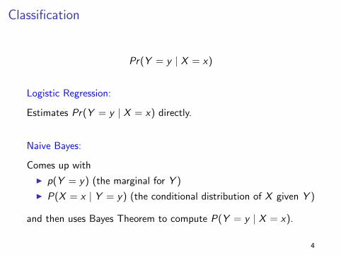
Pr(Y = y | X = x)
Logistic Regression:
Estimates Pr(Y = y | X = x) directly.
Naive Bayes:
Comes up with
I p(Y = y) (the marginal for Y )
I P(X = x | Y = y) (the conditional distribution of X given Y )
and then uses Bayes Theorem to compute P(Y = y | X = x).
4
Classification
In section 10 we will review Bayes Theorem and some basicprobability ideas we have used informally.
In section 7 we will look at decision theory and loss in more detail.We have already made extensive use of the idea of a loss function,but now add another layer which plays an important role inclassification.
5
2. Logistic Regression, One Predictor
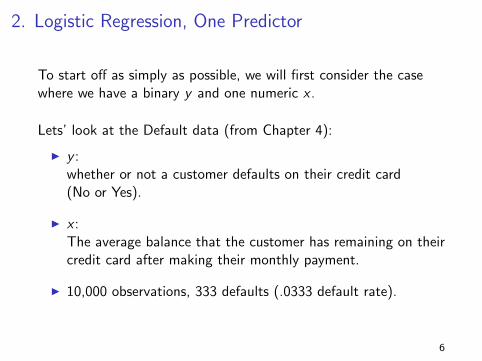
To start off as simply as possible, we will first consider the casewhere we have a binary y and one numeric x .
Lets’ look at the Default data (from Chapter 4):
I y :whether or not a customer defaults on their credit card(No or Yes).
I x :The average balance that the customer has remaining on theircredit card after making their monthly payment.
I 10,000 observations, 333 defaults (.0333 default rate).
6
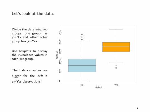
Let’s look at the data.
Divide the data into twogroups, one group hasy=No and other othergroup has y=Yes.
Use boxplots to displaythe x=balance values ineach subgroup.
The balance values are
bigger for the default
y=Yes observations!
●
●
●●
●
●
●●
●
●
●
●
No Yes
050
010
0015
0020
0025
00
default
bala
nce
7
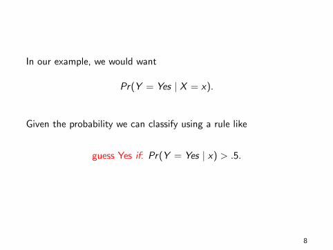
In our example, we would want
Pr(Y = Yes | X = x).
Given the probability we can classify using a rule like
guess Yes if: Pr(Y = Yes | x) > .5.
8
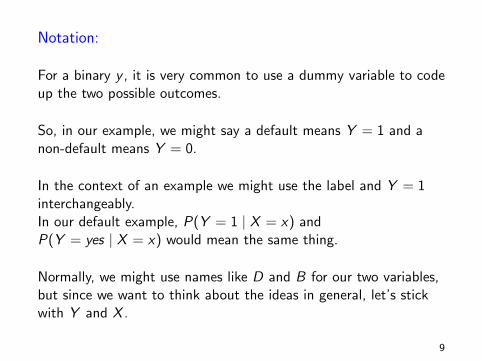
Notation:
For a binary y , it is very common to use a dummy variable to codeup the two possible outcomes.
So, in our example, we might say a default means Y = 1 and anon-default means Y = 0.
In the context of an example we might use the label and Y = 1interchangeably.In our default example, P(Y = 1 | X = x) andP(Y = yes | X = x) would mean the same thing.
Normally, we might use names like D and B for our two variables,but since we want to think about the ideas in general, let’s stickwith Y and X .
9
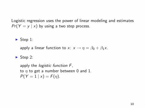
Logistic regression uses the power of linear modeling and estimatesPr(Y = y | x) by using a two step process.
I Step 1:
apply a linear function to x : x → η = β0 + β1x .
I Step 2:
apply the logistic function F ,to η to get a number between 0 and 1.P(Y = 1 | x) = F (η).
10
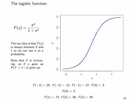
The logistic function:
F (η) =eη
1 + eη.
The key idea is that F (η)is always between 0 and1 so we can use it as aprobability.
Note that F is increas-ing, so if η goes upP(Y = 1 | x) goes up.
-10 -5 0 5
0.0
0.2
0.4
0.6
0.8
1.0
η
F
F (−3) = .05, F (−2) = .12, F (−1) = .27, F (0) = .5
F (0) = .5
F (1) = .73, F (2) = .88, F (3) = .95 11
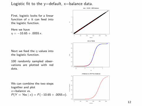
Logistic fit to the y=default, x=balance data.
First, logistic looks for a linearfunction of x it can feed intothe logistic function.
Here we haveη = −10.65 + .0055 x .
Next we feed the η values intothe logistic function.
100 randomly sampled obser-vations are plotted with reddots.
We can combine the two stepstogether and plotx=balance vs.P(Y = Yes | x) = F (−10.65 + .0055 x).
●
●
●
●
●
●
●●
●
●●
●
●
●
●
●
●
●●
●
●
●
●
●
●
●
●
●
●
●
●●
●
●
●
●
●
●
●
●
●●
●
●
●
●
●●
●●
●
●
●
●
●
●●
●
●
●
●
●
●
●
●
●
●
●
●
●
●
●
●
●
●
●●●
●
●
●
●●
●
●
●
●
●
●●
●
●
●
●
●
●
●
●
●●
●
●
●
●
●
●
●
●
●
●
●
●
●
●
●
●
●
●
●
●
●
●
●
●
●
●
●
●
●
●
●
●
●
●
●
●
●
●
●
●
●
●
●
●
●
●
●
●
●
●
●
●
●
●
●
●
●
●
●
●
●
●
●
●
●
●
●
●
●
●
●●
●
●
●●
●
●
●
●
●
●●●
●
●
●
●
●
●
●
●
●
●
●●
●
●
●
●●
●
●
●
●
●
●
●
●
●
●
●
●
●
●
●
●
●
●
●
●
●
●
●
●●
●
●
●
●
●
●
●
●
●●
●
●
●
●
●
●
●
●
●
●●
●
●
●
●
●
●
●
●
●
●
●
●
●
●
●
●
●
●
●
●
●
●
●
●●
●
●●
●
●
●
●
●
●
●
●
●
●
●
●
●
●
●
●
●
●
●
●
●
●
●
●
●
●
●●●
●
●●
●
●
●
●
●
●
●
●
●
●
●
●
●
●
●
●
●
●
●
●
●
●
●
●
●
●
●
●
●
●
●
●●●
●
●
●
●
●
●●
●
●
●
●
●
●●
●●
●
●
●
●
●
●
●
●
●
●
●
●
●
●
●
●
●
●
●
●
●
●
●
●
●
●
●
●
●
●
●
●
●●
●
●
●
●
●
●
●
●
●
●
●
●
●
●
●
●
●
●
●
●
●
●
●
●
●
●
●
●
●●
●●
●
●
●
●
●
●
●
●
●●
●
●
●
●
●
●●●
●
●
●
●
●●
●
●
●
●
●
●
●
●
●
●●
●
●
●
●
●●
●
●
●
●
●
●●
●
●
●
●
●
●
●
●
●
●
●
●
●
●
●●
●
●
●
●
●
●
●
●
●
●
●●
●
●
●
●
●
●
●
●
●
●
●
●
●
●
●
●
●
●
●
●
●
●
●
●
●
●
●
●
●
●
●
●
●
●
●
●
●
●
●
●
●
●
●
●
●
●
●
●
●
●
●
●
●●
●
●
●●
●
●
●●
●
●
●
●
●
●
●
●
●
●
●
●
●●
●
●
●
●
●
●
●
●
●
●
●
●
●
●
●
●
●
●
●
●
●
●
●
●
●
●
●
●
●
●
●
●
●
●
●
●
●
●●
●
●
●
●
●
●
●
●
●
●
●
●
●
●
●
●
●●
●
●
●
●
●
●
●●
●
●
●
●
●
●
●
●
●
●
●
●●
●●
●
●
●
●
●
●
●
●●
●●
●
●●
●
●
●●
●
●
●
●
●
●
●
●
●
●
●●
●
●
●
●
●
●
●●
●
●
●
●
●●
●
●
●●
●●
●
●
●
●
●
●
●
●
●
●
●
●
●
●
●
●●
●
●
●
●
●
●
●
●
●
●
●
●
●
●
●
●
●
●
●
●
●●●
●
●●
●●●
●
●
●
●
●
●
●●
●
●
●
●
●
●
●
●●
●
●
●
●
●
●
●
●
●
●
●
●
●
●
●
●
●
●
●
●
●
●
●
●
●
●
●
●
●
●
●
●●
●
●
●
●
●●
●
●●
●●●
●
●
●
●
●●
●
●
●
●
●
●
●●
●
●
●
●
●
●
●
●
●
●
●
●●
●
●
●●
●
●
●
●
●
●
●
●
●
●
●
●
●
●
●
●
●
●
●
●
●
●
●
●
●
●
●
●
●
●
●
●
●●
●
●
●
●
●
●
●
●
●●
●
●
●
●
●
●
●
●
●
●
●
●
●
●
●
●
●
●
●
●●
●
●
●
●
●
●
●
●
●
●
●
●
●
●
●
●
●
●
●
●
●
●
●
●
●
●
●
●
●
●
●●●●
●
●
●
●
●
●
●
●
●
●
●●
●●
●●
●
●
●
●●
●
●
●
●
●
●
●
●
●
●
●
●
●
●
●
●
●
●
●
●
●
●
●
●
●
●
●
●
●
●
●
●●
●
●
●
●
●
●
●
●
●
●
●
●
●
●
●
●
●
●
●
●
●
●
●
●
●
●
●
●
●
●
●
●
●
●●
●
●
●
●
●
●
●
●
●
●
●
●
●
●
●
●
●
●
●
●
●
●
●●
●
●
●
●
●
●●
●
●
●
●
●
●
●
●
●
●
●
●
●
●
●●
●
●
●
●
●
●
●
●
●
●
●
●
●
●
●
●
●
●
●
●
●
●
●
●
●
●
●
●
●
●●
●
●
●
●
●
●
●
●
●
●
●
●
●
●
●
●
●
●
●
●
●
●
●
●
●
●
●
●●
●
●
●
●●
●
●
●
●
●
●
●
●
●●●
●
●
●
●
●
●
●
●
●
●
●
●
●●
●
●
●
●
●
●
●
●
●
●
●
●
●
●
●
●
●
●
●
●
●
●
●
●
●
●
●
●
●
●
●
●
●
●
●
●
●
●
●
●
●
●
●
●●
●
●
●
●
●
●
●
●
●
●
●
●
●
●
●
●
●
●
●
●
●
●
●
●
●
●
●
●●
●
●
●
●
●
●
●
●
●
●
●
●
●
●
●
●
●
●
●
●●
●
●
●
●
●
●
●
●
●
●
●
●
●
●
●
●
●
●
●
●
●
●
●
●
●
●
●
●
●
●
●
●
●
●
●
●
●
●
●
●
●
●
●
●
●●
●
●
●
●
●
●
●
●
●
●
●
●
●
●
●
●
●
●
●
●
●
●
●
●
●
●
●
●
●
●
●
●
●
●
●
●●
●
●
●
●
●
●
●
●
●
●
●
●
●
●
●
●
●●
●
●
●●
●
●
●
●
●
●
●
●
●
●
●
●
●●
●
●
●
●●
●
●
●
●
●
●
●
●
●
●
●
●
●
●
●
●●
●
●
●
●
●
●
●
●
●
●
●
●●
●●
●
●
●
●
●
●
●
●●●
●
●
●
●
●
●
●
●
●
●
●
●
●●
●
●
●
●
●
●
●
●
●
●
●
●
●
●
●
●●
●
●
●●
●
●
●
●
●
●
●
●
●
●●
●
●
●
●
●
●
●
●
●
●
●
●
●
●
●
●
●
●
●
●
●
●
●
●
●
●
●
●
●
●
●
●
●
●
●
●
●
●
●
●
●
●
●
●
●
●
●●
●
●
●
●
●
●
●●
●
●●
●
●
●
●
●
●
●
●
●
●
●
●
●
●
●
●
●
●
●
●
●
●
●
●
●
●
●
●
●
●
●
●
●
●
●
●
●
●
●
●
●
●
●
●●
●
●
●
●
●
●
●
●
●
●
●
●
●
●
●
●
●
●
●
●
●
●●
●
●
●
●
●
●
●
●
●
●
●
●
●
●
●
●
●
●
●
●
●
●
●
●
●
●
●
●
●
●
●
●
●
●
●
●
●●
●
●
●
●
●
●
●
●
●●
●
●
●●
●
●
●
●
●
●
●
●
●
●
●
●
●●
●●
●
●
●
●
●
●
●
●
●
●
●
●
●
●
●
●●
●
●
●
●
●
●
●
●
●
●
●
●
●
●
●
●
●
●
●
●
●
●
●
●
●
●
●
●
●
●
●
●
●
●●
●●
●
●
●
●
●
●
●
●
●
●
●
●
●
●
●
●
●
●
●
●●
●
●
●
●
●
●
●●
●
●
●
●
●
●
●
●
●
●
●
●
●
●
●
●
●
●●
●
●
●
●
●
●
●
●
●●
●
●
●
●
●
●
●
●
●
●
●●
●
●
●
●
●
●
●
●
●
●
●
●
●
●
●
●
●
●
●
●
●
●●●
●
●
●
●
●
●
●
●
●
●
●
●
●
●
●
●
●
●
●
●
●
●●
●
●
●
●●
●
●
●
●
●
●
●
●
●
●
●
●
●●
●
●
●
●●
●
●
●
●
●
●
●
●
●
●
●
●
●
●●
●
●
●
●
●●
●
●
●
●●
●
●
●
●
●
●
●
●●
●
●
●
●
●
●
●
●
●●
●●
●
●
●
●
●
●
●
●
●
●
●
●
●
●
●
●
●
●
●
●●
●
●
●●
●
●
●
●
●●
●
●
●
●
●
●
●●
●
●
●
●
●
●
●
●
●
●
●
●
●
●
●
●
●
●
●
●
●
●
●
●
●
●
●
●
●
●
●●●
●
●
●
●
●
●
●
●
●
●
●
●
●
●●
●
●
●
●●
●
●
●
●
●
●
●●
●
●
●
●
●
●
●
●
●
●●
●
●
●●
●
●
●
●●
●
●
●
●
●
●
●
●
●
●
●
●
●
●
●
●
●
●
●
●
●
●
●
●
●●
●
●
●●
●
●
●
●
●
●
●
●
●
●
●
●
●●
●
●
●
●
●
●
●
●
●
●
●
●
●
●
●
●
●
●
●
●
●
●
●
●
●
●
●
●
●
●
●
●
●
●
●
●
●●
●
●
●
●
●
●
●
●
●
●
●
●
●
●
●
●
●
●
●●
●
●
●
●
●
●
●
●
●
●
●
●
●
●
●●
●
●
●
●
●
●
●●
●●
●
●
●
●
●
●
●
●
●
●
●
●
●
●
●
●
●
●
●
●
●
●
●
●
●
●
●
●
●
●
●
●
●
●
●●
●●
●
●
●
●
●
●
●
●
●
●
●
●
●
●
●
●
●
●
●
●
●
●
●
●
●
●
●
●
●
●
●
●
●
●
●
●
●
●
●
●●
●
●
●
●
●
●
●
●
●
●
●
●
●
●
●
●
●
●
●
●
●
●
●
●
●
●
●
●●
●
●
●
●
●
●
●
●●
●
●
●
●
●
●
●
●
●
●
●
●
●
●
●
●
●
●
●
●
●
●
●
●
●
●●
●●
●
●
●
●●
●
●
●
●
●
●
●
●
●
●
●
●
●
●
●
●
●●●
●
●
●
●
●
●
●
●
●
●
●
●
●
●
●
●
●
●
●
●
●
●
●
●
●
●
●
●
●
●
●
●
●
●
●
●
●
●
●
●
●●
●
●
●
●
●
●
●
●
●●
●
●
●
●●
●
●
●
●
●●
●
●
●
●
●
●
●
●
●
●
●
●
●
●
●
●
●
●
●
●●
●
●
●
●
●
●
●
●
●
●
●
●
●
●
●
●
●
●
●
●
●
●●
●
●
●
●
●
●
●
●
●
●
●
●
●
●
●
●
●
●
●
●
●
●
●
●
●
●
●
●
●●
●
●
●
●
●
●●
●
●
●
●
●
●
●
●
●
●
●
●
●
●
●
●
●
●
●
●
●
●
●
●
●●
●
●
●
●
●
●
●
●
●
●
●
●
●●
●
●
●
●
●
●
●
●
●
●
●
●
●
●
●
●
●
●
●
●
●
●
●
●
●
●●
●
●
●
●
●
●●
●
●
●
●
●
●
●
●
●
●
●
●
●
●
●
●
●
●
●●●
●
●
●
●
●
●
●
●
●
●
●
●
●
●
●
●
●
●
●
●
●
●
●
●
●
●●
●
●
●
●
●●
●
●
●
●
●
●
●
●
●
●
●
●
●
●
●●
●
●
●
●
●
●●●
●
●
●
●
●
●
●
●
●
●
●
●
●
●
●
●
●
●
●
●
●
●●●
●
●
●
●●
●
●
●
●
●
●
●
●
●
●
●
●
●●
●
●
●
●
●
●
●
●
●
●
●
●
●
●
●
●
●●
●
●
●
●●
●
●
●
●
●●
●●
●
●
●
●
●●
●
●
●
●●
●
●
●
●
●
●
●
●
●
●
●
●
●
●
●
●
●
●
●
●
●
●
●
●
●●
●
●
●
●
●
●
●●
●●
●
●●
●
●
●
●
●
●
●
●
●
●
●
●
●
●
●
●
●
●
●●
●●●
●
●●
●
●
●
●
●
●
●
●
●
●
●
●
●
●
●●
●
●
●
●
●
●
●
●
●
●
●
●
●
●
●
●●
●
●
●
●
●
●
●
●
●
●
●
●
●
●
●
●
●
●
●
●
●
●●
●
●
●
●
●
●
●
●
●
●
●
●
●
●
●
●
●
●
●
●
●
●
●
●
●
●
●
●
●
●
●
●
●●●
●●
●
●
●
●
●
●
●
●
●
●
●
●
●
●
●
●
●●
●
●
●●
●
●
●
●
●●
●
●
●
●
●
●
●
●
●
●
●
●
●
●
●
●
●
●
●
●
●
●
●
●
●
●●
●
●
●
●
●
●
●
●●
●
●
●
●
●
●
●
●
●
●
●
●
●
●
●
●
●
●●
●●
●
●
●
●
●
●
●
●
●
●
●●
●
●
●
●
●
●
●
●
●
●
●
●
●
●
●
●
●
●
●
●
●●
●
●
●
●
●
●
●
●
●
●
●
●
●
●
●
●
●
●
●
●
●
●
●
●
●
●
●
●
●
●●
●
●
●●
●
●
●
●
●
●
●
●
●
●
●
●
●
●
●
●
●
●
●
●
●
●
●
●
●
●
●
●
●
●
●
●
●
●
●
●
●
●
●
●
●
●
●
●
●
●
●
●
●
●
●
●
●
●
●
●
●
●
●
●
●
●
●
●●
●
●
●
●
●
●
●
●
●
●
●●
●
●
●
●
●●
●
●●
●
●
●
●
●
●
●
●
●
●
●●
●
●
●
●
●
●
●●
●
●
●
●
●
●
●
●
●
●
●
●
●●
●
●
●●
●
●
●●
●
●
●
●
●
●
●
●
●●
●
●
●●
●
●
●
●
●
●
●
●
●
●
●●
●
●
●
●
●
●●
●
●●
●
●
●
●
●
●
●
●
●
●
●
●
●
●
●
●
●
●
●
●
●
●
●
●
●
●
●
●●
●
●
●
●
●
●
●
●●
●
●
●
●
●
●
●●
●
●
●
●
●
●
●
●
●
●
●
●●
●
●
●
●●
●
●
●
●
●
●
●
●
●
●
●●●
●
●
●
●
●
●●
●
●
●
●
●
●●
●
●●
●
●
●
●
●
●
●
●
●
●
●
●
●
●●
●
●
●
●
●
●
●
●
●
●
●
●
●
●
●
●
●
●
●
●
●
●
●
●
●
●
●
●
●
●
●
●
●
●
●
●
●
●
●
●●
●
●
●
●
●
●
●
●
●
●
●
●
●
●●
●
●
●
●
●
●
●
●
●
●
●●
●
●
●
●
●
●
●
●
●
●
●
●
●
●
●
●
●●
●
●
●
●
●
●
●
●
●
●
●
●
●
●
●
●
●
●
●
●
●
●
●
●
●
●
●
●
●
●
●
●
●
●
●●
●
●
●
●
●
●
●
●
●●
●
●
●
●
●
●●
●
●
●
●
●
●
●
●
●
●
●
●
●
●
●
●
●
●
●
●
●
●
●
●
●
●
●
●
●
●
●
●
●
●
●
●
●
●
●
●
●
●
●●
●
●
●
●
●
●
●
●
●
●●
●
●
●
●●
●
●
●●
●
●
●
●
●
●
●
●
●
●●
●
●
●
●
●
●
●
●
●●
●
●
●
●
●
●
●
●
●
●
●●
●
●●
●
●
●
●
●
●
●
●
●
●
●
●
●
●
●
●
●●
●
●
●
●
●
●
●
●
●
●
●●
●
●
●
●
●
●
●●
●
●
●
●●
●
●
●
●
●
●
●
●
●
●
●
●
●
●
●●
●
●
●
●
●
●
●
●
●
●
●
●●
●
●
●
●
●
●
●
●
●
●
●
●
●
●
●
●
●
●
●
●
●
●
●
●
●
●
●
●
●
●
●
●
●
●
●
●
●
●
●
●
●
●
●
●
●
●
●
●
●
●
●
●
●
●
●
●
●
●
●●
●●
●
●
●
●
●
●
●
●
●
●
●
●●
●
●
●
●
●
●
●●
●
●
●●
●
●
●
●
●
●●
●
●
●
●
●
●
●
●●●
●
●
●
●
●
●
●
●
●
●●●
●
●
●
●
●●
●
●●
●
●
●
●●
●
●
●
●
●
●
●
●
●
●
●
●
●
●
●
●
●
●
●
●
●
●●
●
●●
●
●
●
●
●
●
●
●
●
●
●
●
●
●
●
●
●
●
●
●
●
●
●
●
●●
●
●
●
●
●
●
●
●
●
●
●
●●
●
●
●
●
●
●
●
●
●
●
●
●
●
●
●
●
●
●
●
●
●
●
●
●
●
●
●
●
●
●
●
●
●●
●
●
●
●
●
●
●●
●
●
●
●
●
●
●
●
●
●
●
●
●
●
●●
●
●
●
●
●
●
●
●
●
●●
●
●
●
●
●
●
●
●
●
●
●
●
●
●●●
●
●●
●
●
●
●
●
●
●
●●
●
●
●
●
●
●
●
●
●
●●
●
●
●
●
●
●
●
●
●●
●
●
●
●
●
●
●
●
●
●
●
●
●
●
●
●
●
●
●
●
●
●
●●
●
●
●
●
●●
●
●
●
●
●
●
●
●
●
●
●
●
●
●
●●
●
●
●
●
●
●
●●
●
●
●
●
●
●
●
●
●
●
●
●
●
●
●
●
●
●
●
●
●
●
●
●
●
●
●
●
●
●
●
●
●
●
●
●
●●
●
●
●
●
●
●
●
●
●
●
●
●
●
●
●
●
●
●
●
●
●
●
●
●
●
●
●
●
●
●
●
●
●
●
●
●
●
●
●
●
●
●●
●
●●
●
●
●
●
●
●●●
●
●
●
●
●●
●
●
●
●
●
●
●
●
●
●
●
●
●
●
●
●
●
●
●
●
●●
●
●
●
●
●
●
●
●
●
●
●
●
●●
●
●
●
●
●
●
●
●
●
●
●
●
●
●
●
●
●
●
●
●
●
●
●
●
●
●
●
●
●
●
●
●
●
●
●
●
●
●
●
●
●
●
●
●
●
●
●●
●
●●
●
●
●
●
●
●
●
●
●
●
●
●
●
●
●
●
●
●●
●
●
●
●
●
●
●
●
●●
●
●
●
●
●
●
●
●
●
●
●
●
●
●
●
●
●
●
●●
●
●
●
●
●
●
●
●
●
●
●
●
●
●
●
●
●
●
●
●
●
●
●
●
●
●
●
●
●
●
●
●
●
●
●
●
●
●
●
●
●
●
●
●
●
●
●
●
●
●
●
●
●
●
●
●
●
●
●
●
●
●
●
●
●
●
●●
●●
●
●
●
●●
●
●
●
●
●
●
●
●
●
●●
●●●
●
●
●●●
●
●●
●
●
●
●
●
●
●
●
●
●
●
●
●
●
●
●
●
●
●
●●
●
●
●
●
●
●
●
●
●
●
●
●
●
●
●
●
●
●
●●
●
●
●
●
●
●
●
●
●
●
●
●
●
●
●
●
●
●●
●
●
●●
●
●
●●
●
●
●
●
●
●
●
●
●
●
●
●
●
●
●
●
●
●●
●
●
●●
●
●
●
●
●
●
●
●
●
●●
●
●
●
●
●
●
●
●
●
●
●
●
●
●
●●
●
●
●●
●
●
●
●
●
●
●
●●
●
●
●
●
●
●
●
●
●
●
●
●
●
●
●
●
●
●
●
●
●
●
●●
●
●
●
●
●
●
●
●
●
●
●
●●
●
●
●
●
●
●
●
●
●
●●
●
●
●
●
●
●
●
●
●
●
●
●
●●
●
●
●
●
●
●
●
●
●
●
●
●
●
●
●
●
●
●
●
●
●●
●
●
●
●
●
●
●
●
●
●
●
●●●
●
●
●
●
●
●
●
●
●
●
●●
●
●
●
●
●
●
●●
●
●
●
●
●
●
●
●
●
●
●
●
●
●
●
●
●
●
●
●
●
●
●
●
●
●
●
●
●
●
●
●
●
●
●
●
●
●
●●
●
●
●
●
●
●
●
●
●
●
●
●
●
●
●
●
●
●
●
●
●
●●
●
●
●
●
●
●
●
●●
●
●
●●
●
●
●
●
●
●
●
●
●
●
●
●
●
●
●●
●
●
●
●
●
●
●
●
●
●
●
●
●
●
●
●
●
●
●
●
●
●●
●
●
●●●
●
●●
●
●
●
●●
●
●
●
●
●
●
●
●
●●
●
●
●
●
●
●
●
●
●
●●
●
●
●
●
●
●
●
●●
●
●●
●
●
●
●
●
●
●
●
●
●
●
●
●●
●
●
●
●
●
●
●
●
●
●
●
●
●
●
●
●
●
●●
●
●
●
●
●
●
●
●
●
●
●
●
●
●
●
●
●●
●
●
●
●●
●
●
●
●
●
●
●
●●
●
●
●
●
●
●
●
●
●●
●●
●●
●
●
●
●
●
●
●
●
●
●
●
●
●
●
●
●
●
●
●
●●
●
●
●
●
●
●
●
●
●
●
●
●
●
●
●
●
●
●
●
●
●
●
●
●
●
●
●●●
●
●
●
●
●
●
●
●
●
●
●
●
●●
●
●
●
●
●
●
●
●
●●
●
●
●
●
●
●●
●
●
●
●
●
●
●●
●
●
●
●
●
●
●
●
●
●
●
●
●
●
●
●
●
●
●
●
●
●
●●
●
●
●
●
●
●
●
●●
●
●
●
●
●
●
●
●
●
●
●
●
●
●
●●
●
●
●
●
●
●
●
●●
●
●
●
●
●
●
●
●
●
●
●●
●
●●
●
●
●
●
●●
●
●
●
●
●
●
●
●
●
●
●
●
●
●
●
●
●
●
●
●
●
●
●
●
●
●
●
●
●
●
●
●
●
●
●
●
●
●
●●
●
●●
●
●
●●
●
●
●
●
●
●
●●
●
●
●
●
●
●
●
●
●●
●
●
●
●
●●
●
●
●
●
●
●
●
●
●
●
●
●
●
●
●
●
●
●
●
●●
●
●
●
●
●
●
●
●
●
●
●
●
●
●
●
●
●
●
●
●
●
●
●
●
●
●
●
●
●
●
●
●
●
●
●
●
●
●
●
●
●
●
●
●
●
●
●
●
●
●●
●
●
●
●●
●
●
●
●
●
●
●
●
●
●
●
●
●
●
●
●
●
●
●
●
●
●
●
●
●
●
●
●
●
●●
●
●
●
●
●
●
●
●
●
●
●
●
●
●
●
●
●
●
●
●●
●
●
●
●●
●
●
●
●
●
●●
●
●
●
●
●
●
●
●
●
●
●
●
●
●
●
●●
●
●
●
●●
●
●
●
●
●
●●
●
●
●
●
●
●
●
●
●
●
●●
●
●●
●
●●
●
●
●
●
●
●
●
●
●
●
●
●
●
●
●
●
●
●
●
●
●
●
●
●
●
●
●
●
●
●
●
●
●
●
●
●
●●
●
●
●
●
●
●
●
●
●
●
●
●●●
●
●
●
●●
●
●
●
●
●
●
●
●
●
●
●
●
●
●
●
●
●
●
●
●
●
●●
●●
●
●
●
●
●
●
●
●
●
●
●
●
●
●
●
●
●
●
●
●
●
●
●
●
●
●
●
●
●
●
●
●
●
●
●
●●
●
●●
●
●
●
●
●
●
●●
●
●
●
●
●●
●
●
●
●
●
●●
●
●
●
●
●
●
●
●●
●
●
●
●
●
●
●
●
●
●
●
●
●
●
●
●
●
●
●
●
●
●
●
●
●
●
●
●
●
●
●
●
●
●
●
●
●●
●
●
●
●
●
●●
●
●
●
●
●
●
●
●
●
●
●
●
●
●
●
●
●
●
●
●
●
●
●
●
●
●
●
●
●
●
●
●
●
●
●
●
●
●
●
●
●●
●
●●
●
●
●
●●
●
●
●
●
●
●
●
●
●
●
●
●
●
●
●
●
●
●
●
●
●●
●
●
●
●
●
●
●
●
●●
●
●
●
●
●
●
●
●
●
●●
●
●
●
●
●
●
●
●
●
●
●
●
●
●
●●
●
●
●
●
●
●
●
●
●
●
●
●
●
●
●
●
●
●●
●
●
●
●
●
●
●
●
●
●
●
●
●
●
●
●
●
●
●
●
●
●
●
●
●●
●
●
●
●
●
●
●
●
●
●●
●
●
●
●
●
●●●
●
●
●
●
●●
●
●
●
●
●
●
●
●
●
●
●
●
●
●
●
●
●
●
●
●
●
●
●
●
●
●
●
●
●
●●●
●
●
●
●
●
●
●●
●
●
●
●
●
●
●●
●
●
●
●
●
●
●
●
●
●
●
●
●
●
●
●
●
●
●
●
●
●
●
●
●
●
●
●
●
●
●
●
●
●●
●
●
●
●
●
●
●
●
●
●
●
●
●
●
●●
●
●●
●
●
●
●
●
●
●
●
●
●
●
●
●
●
●
●●●
●
●
●
●●
●
●
●
●
●
●
●
●
●
●
●
●
●
●●
●
●
●
●
●
●
●
●
●
●
●
●
●
●
●
●●
●
●
●
●
●
●
●
●
●
●
●
●
●●
●
●
●
●
●
●
●
●
●
●
●
●
●
●
●
●●
●
●
●
●
●
●
●
●
●
●
●
●
●
●
●
●
●
●
●
●
●
●
●
●
●
●
●
●
●
●
●
●
●
●
●
●
●
●
●
●
●
●
●
●
●●
●
●
●
●
●
●
●
●
●
●
●●
●
●
●
●
●
●
●
●
●
●
●
●
●
●
●
●
●
●
●
●
●●
●
●●
●
●
●
●
●
●
●
●
●
●
●
●
●
●
●
●
●
●
●
●
●
●
●
●
●
●●
●
●
●
●
●
●
●
●
●
●
●
●
●
●
●
●
●
●
●
●
●
●●
●
●
●
●
●
●
●
●
●
●
●
●
●
●●
●
●
●
●
●
●
●
●
●
●
●
●
●
●
●
●
●
●
●
●
●
●
●
●
●
●
●
●
●
●
●
●
●
●
●
●
●
●
●
●
●
●
●
●
●
●
●
●
●
●
●
●
●
●●
●
●
●●
●
●
●
●
●●
●
●
●
●
●
●●
●
●
●●●
●
●
●●
●
●
●
●
●
●
●
●
●
●
●
●
●
●●
●
●
●
●
●
●
●
●
●
●
●
●
●
●
●●
●
●
●●
●●
●
●
●
●
●
●
●
●
●
●
●
●
●
●
●
●
●
●
●
●
●
●
●
●
●
●
●
●
●
●
●
●
●
●
●
●●
●
●
●
●
●●●
●
●
●
●●
●
●
●
●
●
●
●
●
●
●
●
●
●
●
●
●
●
●
●
●
●
●
●
●
●
●
●
●
●
●
●
●
●
●
●
●
●
●
●
●
●
●
●
●
●●
●
●
●
●
●●
●
●
●
●
●●
●●
●
●
●
●
●
●
●
●
●
●
●
●●
●
●
●
●
●
●
●
●
●●
●
●
●
●
●
●
●
●
●
●
●
●
●
●
●●
●
●
●●
●
●
●●
●
●
●
●
●
●
●
●
●
●
●
●
●
●
●●
●
●
●
●
●
●
●
●
●
●
●
●
●
●
●
●
●
●
●
●
●
●
●
●
●
●
●
●
●
●
●
●
●
●●
●
●
●
●
●
●
●
●
●
●
●
●
●
●●
●
●
●
●
●
●
●
●
●
●
●
●
●
●
●
●
●
●●
●
●
●
●
●
●
●
●
●
●
●
●●
●
●
●
●●
●
●
●
●
●
●
●
●
●
●
●
●●
●
●
●
●
●
●
●
●
●
●
●
●
●
●
●
●
●
●
●
●
●
●
●
●●
●
●
●
●●●
●
●
●
●
●
●
●
●
●
●
●
●
●●
●
●
●
●
●
●
●
●
●●
●
●
●
●
●
●
●
●
●
●
●
●
●
●
●
●
●
●
●
●
●●
●
●
●●
●
●
●
●
●●
●
●
●
●
●
●
●
●
●
●
●
●
●
●
●
●
●
●
●
●
●
●
●
●
●
●
●
●
●
●
●
●
●
●
●
●
●
●
●
●
●
●
●
●●
●
●
●●
●
●
●
●
●
●
●
●
●
●
●
●
●
●
●
●
●
●
●●
●
●
●
●
●
●
●
●
●
●
●
●
●
●
●
●
●
●
●
●
●●
●
●
●
●
●
●
●
●
●
●
●
●
●
●
●
●
●
●
●
●
●
●
●
●
●
●
●
●
●
●
●
●
●
●
●
●
●●
●
●
●
●
●
●
●●
●●
●
●
●
●
●
●
●●
●
●
●
●
●
●
●
●
●
●
●
●
●
●
●
●
●
●
●
●
●
●
●●
●
●
●
●
●
●
●
●
●
●
●
●
●
●
●
●
●●
●
●
●
●
●
●
●
●
●
●
●
●
●
●
●
●
●
●
●
●
●
●
●
●
●
●
●
●●
●
●
●
●
●●
●
●
●
●
●
●
●
●
●
●
●
●
●
●
●
●
●
●
●
●
●
●
●
●
●
●
●
●
●
●
●
●
●
●
●
●
●
●
●
●
●
●
●
●
●
●
●
●
●
●
●
●
●
●
●●
●
●
●
●
●
●
●
●●
●
●
●
●
●
●
●●
●
●
●
●
●●
●
●
●
●
●
●
●
●
●
●
●
●
●
●
●
●
●
●
●
●
●
●
●
●
●
●
●
●
●
●
●
●
●
●
●
●
●
●
●
●
●
●
●
●
●
●
●
●
●
●
●
●
●
●
●
●
●
●
●
●
●
●
●
●
●
●
●
●
●
●
●
●●
●
●●
●
●
●
●
●
●
●
●
●
●
●
●
●●
●
●
●
●
●
●
●
●
●●●
●●
●
●●
●
●
●
●
●
●
●
●
●
●
●
●
●
●
●
●
●
●
●●
●
●
●
●
●
●
●
●
●
●
●
●
●
●
●
●
●
●
●
●
●●
●
●
●●
●
●
●
●
●
●
●
●●
●
●
●
●
●
●
●
●
●
●
●
●
●●
●
●
●
●
●
●
●
●
●
●
●
●
●●●
●
●
●
●
●
●
●
●
●
●
●
●
●
●
●
●●
●●
●
●
●
●
●
●
●
●
●
●
●
●
●
●
●
●
●
●
●
●
●
●
●
●●
●
●
●
●
●
●
●
●
●
●
●
●
●
●
●
●
●
●●
●
●
●
●
●
●
●
●
●
●
●
●
●
●
●
●
●
●
●
●
●
●
●
●
●
●
●
●
●
●
●
●
●
●
●
●
●
●●
●
●
●
●
●
●
●
●
●
●
●
●
●●
●
●●
●
●
●
●
●●
●
●●
●
●
●
●
●●
●
●
●
●●
●
●
●
●
●●
●
●
●
●
●
●
●
●
●
●
●
●
●
●
●
●
●
●
●
●
●
●
●
●
●
●
●
●
●
●
●
●●
●●
●●
●
●
●
●
●
●
●
●
●
●
●
●
●
●
●
●
●
●
●
●
●●
●
●
●
●
●
●
●●
●
●
●
●
●
●
●
●
●
●
●
●
●
●
●
●
●
●●
●
●●
●
●
●
●
●
●
●
●
●
●
●
●●
●
●
●
●
●
●
●
●
●
●
●
●
●
●
●
●
●
●
●
●
●●
●
●
●
●
●
●
●
●
●
●
●
●
●
●
●
●
●●
●
●
●
●
●
●
●
●
●
●●
●
●
●
●
●
●
●
●
●
●
●
●
●
●
●
●
●
●
●
●
●
●
●
●
●
●
●
●
●
●
●
●
●
●●
●
●
●●
●
●
●
●
●
●
●
●
●
●
●
●
●
●●
●
●
●
●
●
●
●
●
●
●
●
●
●
●
●
●
●
●
●
●
●
●
●●
●
●
●
●
●
●
●
●●
●
●
●
●
●
●
●
●
●
●
●
●●
●
●
●
●
●
●
●
●
●●
●●
●
●
●
●
●
●
●
●
●
●
●
●
●
●
●
●
●
●
●●
●
●
●
●●
●
●
●
●●
●
●
●
●
●
●
●
●
●
●
●
●
●
●
●
●
●
●
●
●
●
●
●
●
●
●
●●
●
●
●
●
●
●
●
●
●
●
●
●
●
●
●
●
●
●
●
●
●
●
●
●
●
●
●
●
●
●
●
●
●
●
●
●
●
●●
●
●
●
●
●
●
●
●
●
●
●
●
●
●
●
●
●
●
●
●
●
●
●
●
●
●
●
●
●●
●
●
●
●
●
●
●
●●
●
●
●
●
●
●
●
●
●
●
●
●●
●●
●●
●
●
●
●
●
●
●
●
●
●
●
●
●
●
●
●
●
●
●
●
●
●
●
●
●
●
●
●
●●
●
●
●
●
●
●
●
●
●
●
●
●
●
●
●
●
●
●
●●
●
●
●
●
●
●
●
●
●
●
●
●
●
●
●
●
●
●
●
●●
●
●
●
●
●
●
●
●
●
●
●
●
●
●●
●
●
●
●
●
●
●
●
●
●
●
●
●
●
●
●
●
●
●●
●●
●
●
●
●
●
●
●
●
●
●
●
●
●
●
●
●
●●
●
●
●
●
●
●
●
●●
●
●
●
●
●
●
●
●
●●
●
●
●
●
●●
●
●
●
●
●
●
●
●
●
●●●
●
●
●●
●
●
●
●
●
●
●
●
●
●
●
●
●
●
●
●
●
●
●
●
●
●
●
●
●
●
●
●
●
●
●
●
●
●
●
●●
●
●
●
●
●
●
●
●
●
●
●
●
●●
●
●
●
●●
●
●
●●●
●
●
●
●
●
●
●
●
●
●
●
●
●
●
●
●
●
●
●●
●
●
●
●●
●
●
●
●
●●
●
●
●●
●
●
●
●●
●●
●
●
●
●
●
●
●
●
●
●
●
●
●
●
●
●
●
●
●
●
●
●
●
●
●
●
●
●
●
●●
●
●
●●
●
●
●
●
●
●
●
●
●
●
●
●
●
●
●
●
●
●
●
●
●
●
●
●
●
●
●
●●
●
●
●
●
●
●
●
●
●
●
●
●
●
●
●
●
●
●
●
●
●
●
●
●
●
●
●
●●
●
●
●
●
●
●
●
●
●
●
●
●
●
●
●
●
●
●
●
●
●
●
●
●
●
●
●
●
●
●
●
●
●
●
●
●
●
●
●
●
●
●
●
●
●
●
●
●
●
●
●
●
●
●●
●
●
●
●
●
●
●
●
●
●
●
●
●
●
●
●
●●
●
●
●
●
●
●
●
●
●
●
●
●
●
●
●
●
●
●
●
●
●
●
●
●●
●
●
●
●
●
●
●
●
●
●
●
●
●
●
●
●
●
●
●
●
●
●
●
●
●
●
●
●
●
●
●
●
●
●●
●
●●
●
●
●
●●
●
●●
●
●
●
●
●
●
●●
●
●
●
●
●
●
●
●
●
●
●
●
●
●
●
●
●●
●●
●
●
●
●
●
●
●
●
●
●
●
●
●
●
●
●
●
●
●
●
●
●
●
●
●
●
●
●
●
●
●
●
●
●
●●
●
●●●
●
●
●
●
●
●
●
●
●
●
●
●
●
●
●●
●
●
●
●
●
●
●
●
●
●
●
●
●
●
●
●
●
●
●
●
●
●
●
●
●
●
●
●
●
●
●
●
●
●
●
●
●
●
●
●
●
●
●●
●
●
●
●
●
●
●●
●
●
●
●
●
●
●
●
●
●
●
●
●
●
●
●
●
●
●●
●●
●
●
●
●
●
●
●
●●
●
●
●
●
●
●
●
●
●
●
●
●
●
●
●
●
●
●
●
●●
●
●
●
●
●●
●
●
●
●
●
●●
●●●
●
●
●
●
●
●●
●
●
●
●
●
●
●
●
●
●
●
●
●
●
●
●
●
●
●
●
●
●
●
●
●
●
●
●
●
●
●
●
●
●
●●
●
●
●
●
●
●
●
●
●
●
●
●
●
●
●
●
●
●
●
●
●
●
●
●●
●
●
●
●
●●
●
●●
●
●
●
●
●
●
●
●
●
●
●
●
●
●
●
●
●
●
●
●
●
●
●
●
●
●
●
●
●
●
●
●
●
●
●
●
●
●
●
●
●●
●
●
●
●
●
●
●
●
●
●
●
●
●
●
●
●
●
●
●
●
●●
●
●
●
●
●
●
●
●
●
●
●●
●
●●
●
●
●
●
●
●
●●
●
●●
●
●
●
●●
●
●
●
●
●
●
●
●
●
●
●
●
●●
●
●
●
●
●
●
●
●●
●
●
●
●
●
●
●
●
●
●
●
●
●
●
●●
●
●
●
●
●
●
●
●
●
●
●
●
●
●
●
●
●
●
●
●
●
●
●
●
●
●
●
●●
●
●
●
●
●
●
●
●
●
●
●
●
●
●●
●
●
●
●
●
●
●
●
●
●
●
●●
●
●
●
●
●
●
●
●
●
●
●
●
●
●
●
●
●
●
●
●
●
●
●
●
●
●
●
●
●
●
●
●
●
●
●
●
●
●
●
●
●
●
●
●
●
●
●
●
●
●
●
●●
●
●
●
●
●
●
●
●
●
●
●
●
●
●
●
●
●
●
●
●●
●
●
●
●
●
●
●
●
●
●
●
●
●
●
●
●
●
●
●
●
●
●
●
●
●
●
●
●
●
●
●
●
●
●
●
●
●
●
●
●
●
●
●
●
●
●
●
●
●
●
●●●
●
●
●
●
●●
●
●
●
●
●
●
●
●
●
●
●
●
●
●
●
●
●
●
●
●
●
●●
●●
●
●
●
●
●
●
●
●
●
●
●
●●
●
●
●
●●
●
●
●
●●
●
●
●
●
●
●
●
●
●
●
●
●
●
●
●
●
●
●
●
●
●
●
●
●
●
●
●
●
●
●
●
●
●
●
●
●
●
●
●
●
●
●
●
●
●
●
●
●
●
●
●
●
●
●
●
●
●
●
●
●
●
●
●
●
●
●
●
●
●
●
●
●
●
●
●
●
●
●
●
●
●
●
●
●
●
●
●
●
●
●
●
●●
●
●
●
●
●●
●
●
●
●
●
●
●
●
●
●
●
●
●
●
●
●
●
●
●
●
●
●
●●
●
●
●
●
●
●
●
●
●
●
●
●
●
●
●
●
●
●
●
●
●●
●
●
●
●
●
●
●
●
●
●
●●
●
●
●
●
●
●●
●
●
●
●
●
●
●
●
●
●
●
●
●
●
●
●
●
●
●
●
●
●
●
●
●
●
●
●
●
●
●
●●
●
●
●
●
●
●
●
●
●
●
●
●
●
●
●
●
●
●
●
●
●
●
●
●
●
●
●
●
●
●
●
●
●
●
●
●
●
●
●
●●
●
●
●
●
●
●
●
●
●
●
●
●
●
●
●
●
●●
●
●
●
●
●
●
●
●
●
●
●
●
●
●
●
●
●
●
●
●
●
●
●
●●
●
●●
●
●
●
●
●
●●
●
●
●
●
●
●
●
●
●
●
●
●
●
●
●
●●
●
●●
●
●
●
●
●
●
●
●
●
●
●
●
●
●
●
●
●
●
●
●
●
●
●
●
●
●
●
●
●
●
●
●
●
●●
●
●
●
●●
●
●
●
●
●
●
●
●
●
●
●
●
●
●
●
●
●
●
●
●
●
●
●
●
●
●
●
●
●
●
●
●
●
●
●
●
●●
●
●
●
●
●
●
●
●
●
●
●
●
●
●
●
●
●
●
●
●
●
●
●
●
●
●
●
●
●
●
●
●
●
●
●
●
●
●
●
●
●
●
●
●
●
●●
●
●
●
●
●
●
●
●
●
●
●
●
●
●
●
●
●
●
●
●
●
●
●●
●
●
●
●●
●
●
●
●
●
●
●
●
●
●
●
●
●
●
●
●
●●
●
●
●
●
●
●
●
●
●
●
●
●
●
●
●
●
●
●
●
●
●
●
●●
●
●
●
●
●
●
●
●
●
●
●
●
●
●
●
●
●●
●
●
●
●
●
●
●
●●
●
●
●
●
●
●
●
●●
●
●
●
●
●
●
●
●
●
●
●●
●
●●
●
●
●
●
●
●
●
●●
●
●
●
●●
●
●
●
●
●
●
●
●
●
●
●
●
●●
●●
●
●●
●
●
●
●
●
●
●
●
●
●
●
●
●
●
●
●
●
●●
●
●
●
●
●
●
●
●
●
●
●
●
●
●
●
●
●
●
●
●
●
●
●
●
●
●
●
●
●
●
●
●
●
●
●
●
●
●
●
●
●
●
●
●
●
●
●
●
●
●
●
●
●
●
●
●●
●
●
●
●
●
●
●
●
●
●
●
●
●
●
●
●
●
●
●
●
●
●
●
●
●
●
●
●
●
●
●●
●
●
●
●
●
●
●
●
●
●
●
●
●
●
●
●
●
●●
●
●
●
●
●
●
●
●
●
●
●
●
●
●
●
●
●
●
●
●
●
●●
●
●
●
●
●
●
●
●
●
●
●●
●
●
●
●
●
●
●
●
●
●
●
●
●●
●
●
●
●
●
●
●
●
●
●
●
●
●
●
●
●
●
●●
●
●
●
●●
●
●
●
●
●
●
●●
●
●
●●
●
●
●
●●
●
●
●
●
●
●
●●
●
●
●
●
●
●
●
●
●
●
●
●
●
●
●
●
●
●
●
●
●
●
●
●●
●
●
●
●
●
●●
●
●
●
●
●
●
●
●
●
●
●
●
●
●
●
●
●
●
●
●
●
●
●
●
●
●
●●
●
●
●
●
●
●
●
●
●
●
●
●
●
●
●
●
●●
●
●
●●
●
●
●
●
●
●
●
●
●
●
●
●
●
●
●
●
●
●
●
●
●
●
●●
●
●
●
●
●
●
●
●
●
●
●
●
●
●
●
●
●
●
●
●
●●
●
●
●
●
●
●
●
●
●●
●
●
●
●
●
●
●●
●
●●
●
●
●
●
●
●
●
●●
●
●
●
●
●
●
●
●
●
●
●
●
●
●
●
●
●
●
●
●
●
●
●
●
●
●
●
●
●
●
●
●
●●
●
●
●●
●●
●
●●
●
●
●
●
●
●
●
●
●
●
●
●
●
●
●
●
●
●
●
●
●
●●
●
●
●
●
●
●
●
●
●
●●●
●
●
●
●
●
●
●
●
●
●
●
●
●
●
●●
●
●
●
●
●
●
●
●
●
●
●
●
●●
●
●
●
●●
●
●
●
●
●
●
●●
●
●
●
●
●●
●
●
●
●
●
●
●●
●
●
●
●
●
●
●
●
●●
●
●
●
●
●
●
●
●
●
●
●
●
●●
●
●
●
●
●
●
●
●
●
●
●
●
●
●
●
●
●●
●
●
●
●
●
●
●
●
●
●
●
●
●
●
●
●
●
●
●
●●
●
●
●
●
●
●
●
●●
●
●
●●
●
●
●
●
●
●
●
●
●
●
●
●
●
●
●
●
●●
●
●
●
●●
●
●
●
●
●
●
●
●
●●
●●
●
●
●
●●
●
●
●
●
●
●
●
●
●
●
●
●
●
●
●
●
●
●
●
●
●
●
●
●
●
●●
●
●
●
●
●
●
●●
●
●
●
●
●
●
●
●
●
●
●
●
●
●
●
●
●
●
●
●
●
●●●
●
●
●
●
●
●
●
●
●
●
●
●
●
●
●
●
●●
●
●
●
●●
●
●
●
●
●
●
●●
●
●
●
●
●
●
●
●
●
●
●
●
●
●
●
●
●
●
●
●
●
●
●
●
●
●
●
●
●
●
●
●●●
●
●
●
●
●●
●
●
●●
●
●
●
●
●
●
●
●
●
●●
●
●
●
0 500 1000 1500 2000 2500
−10
−5
0
balance
eta
●
●
●
●
●
●
●
●
●
●
●
●
●
●●
●
●
●
●
●
●
●
●
●
●
●
●
●
●
●
●
●
●
●
●
●
●
●
●
●
●●
●
●
●
●
●
●
●
●
eta = −10.65 + .0055 balance
−10 −5 0 5
0.0
0.2
0.4
0.6
0.8
1.0
eta
F(e
ta)
●
●
● ●● ●●
● ● ●● ● ●●●
●
●
●
●●
●
●● ●
●
● ●●
●
●●
●●
● ● ●●
●
●
● ●● ●● ●
●
● ●●
●
eta vs. F(eta)
0 500 1000 1500 2000 2500
0.0
0.2
0.4
0.6
0.8
1.0
x=balance
P(Y
=Ye
s | x
=ba
lanc
e)
x=balance vs. P(Y=Yes | balance)
12
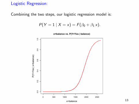
Logistic Regression:
Combining the two steps, our logistic regression model is:
P(Y = 1 | X = x) = F (β0 + β1 x).
0 500 1000 1500 2000 2500
0.0
0.2
0.4
0.6
0.8
1.0
x=balance
P(Y
=Yes
| x=
bala
nce)
x=balance vs. P(Y=Yes | balance)
13
3. Inference: Esimtating the Parameters
Logistic regression gives us a formal parametric statistical model(like linear regression with normal errors).
Our model is:
Yi ∼ Bernoulli(pi ), pi = F (β0 + β1 xi ).
Our model has two parameters β0 and β1 which can estimate givendata.
We usually assume that the given the parameters and xi , the Yi
are independent.
14
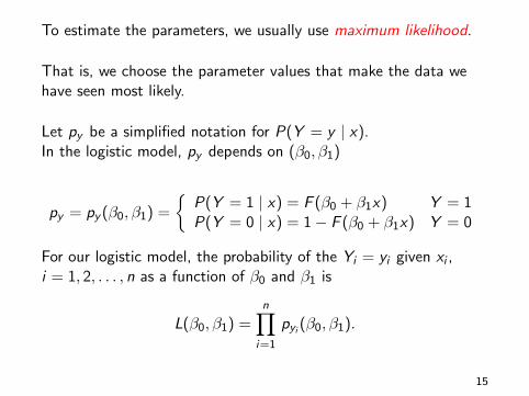
To estimate the parameters, we usually use maximum likelihood.
That is, we choose the parameter values that make the data wehave seen most likely.
Let py be a simplified notation for P(Y = y | x).In the logistic model, py depends on (β0, β1)
py = py (β0, β1) =
{P(Y = 1 | x) = F (β0 + β1x) Y = 1P(Y = 0 | x) = 1− F (β0 + β1x) Y = 0
For our logistic model, the probability of the Yi = yi given xi ,i = 1, 2, . . . , n as a function of β0 and β1 is
L(β0, β1) =n∏
i=1
pyi (β0, β1).
15
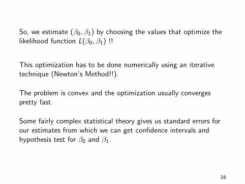
So, we estimate (β0, β1) by choosing the values that optimize thelikelihood function L(β0, β1) !!
This optimization has to be done numerically using an iterativetechnique (Newton’s Method!!).
The problem is convex and the optimization usually convergespretty fast.
Some fairly complex statistical theory gives us standard errors forour estimates from which we can get confidence intervals andhypothesis test for β0 and β1.
16
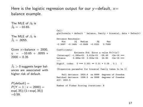
Here is the logistic regression output for our y=default, x=balance example.
The MLE of β0 isβ0 = −10.65.
The MLE of β1 isβ1 = .0055.
Given x=balance = 2000,η = −10.65 + .0055 ∗2000 = 0.35
β1 > 0 suggests larger bal-ances are associated withhigher risk of default.
P(default) =P(Y = 1 | x = 2000) =exp(.35)/(1+exp(.35))=0.59.
Call:
glm(formula = default ~ balance, family = binomial, data = Default)
Deviance Residuals:
Min 1Q Median 3Q Max
-2.2697 -0.1465 -0.0589 -0.0221 3.7589
Coefficients:
Estimate Std. Error z value Pr(>|z|)
(Intercept) -1.065e+01 3.612e-01 -29.49 <2e-16 ***
balance 5.499e-03 2.204e-04 24.95 <2e-16 ***
---
Signif. codes: 0 *** 0.001 ** 0.01 * 0.05 . 0.1 1
(Dispersion parameter for binomial family taken to be 1)
Null deviance: 2920.6 on 9999 degrees of freedom
Residual deviance: 1596.5 on 9998 degrees of freedom
AIC: 1600.5
Number of Fisher Scoring iterations: 8
17
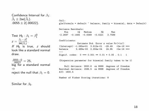
Confidence Interval for β1:β1 ± 2se(β1)..0055± 2(.00022).
Test H0 : β1 = β01
z =β1−β0
1
se(β1).
If H0 is true, z shouldlook like a standard normaldraw.
.0055−0.00022
= 25,big for a standard normal⇒reject the null that β1 = 0.
Similar for β0.
Call:
glm(formula = default ~ balance, family = binomial, data = Default)
Deviance Residuals:
Min 1Q Median 3Q Max
-2.2697 -0.1465 -0.0589 -0.0221 3.7589
Coefficients:
Estimate Std. Error z value Pr(>|z|)
(Intercept) -1.065e+01 3.612e-01 -29.49 <2e-16 ***
balance 5.499e-03 2.204e-04 24.95 <2e-16 ***
---
Signif. codes: 0 *** 0.001 ** 0.01 * 0.05 . 0.1 1
(Dispersion parameter for binomial family taken to be 1)
Null deviance: 2920.6 on 9999 degrees of freedom
Residual deviance: 1596.5 on 9998 degrees of freedom
AIC: 1600.5
Number of Fisher Scoring iterations: 8
18
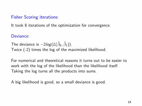
Fisher Scoring iterations:
It took 8 iterations of the optimization for convergence.
Deviance:
The deviance is −2log(L(β0, β1)).Twice (-2) times the log of the maximized likelihood.
For numerical and theoretical reasons it turns out to be easier towork with the log of the likelihood than the likelihood itself.Taking the log turns all the products into sums.
A big likelihood is good, so a small deviance is good.
19
Null and Residual Deviance:
The Residual deviance is just the one you get by plugging theMLE’s of β0 and β1 into the likelihood.
The Null deviance is what you get by setting β1 = 0 and thenoptimizing the likelihood over β0 alone.
You can see that the deviance is a lot smaller when we don’trestrict β1 to be 0!!
20
Deviance as a sum of losses:
If we letpy = py (β0, β1),
then the deviance isn∑
i=1
−2 log(pyi ).
The sum over observations of -2 times the log of the estimatedprobability of the y you got.
21
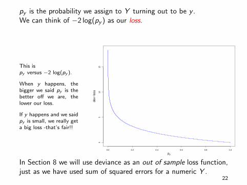
py is the probability we assign to Y turning out to be y .We can think of −2 log(py ) as our loss.
This ispy versus −2 log(py ).
When y happens, thebigger we said py is thebetter off we are, thelower our loss.
If y happens and we saidpy is small, we really geta big loss -that’s fair!!
0.0 0.2 0.4 0.6 0.8 1.0
05
1015
py
dev−
loss
In Section 8 we will use deviance as an out of sample loss function,just as we have used sum of squared errors for a numeric Y .
22
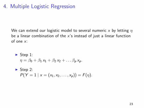
4. Multiple Logistic Regression
We can extend our logistic model to several numeric x by letting ηbe a linear combination of the x ’s instead of just a linear functionof one x :
I Step 1:η = β0 + β1 x1 + β2 x2 + . . . βp xp.
I Step 2:P(Y = 1 | x = (x1, x2, . . . , xp)) = F (η).
23
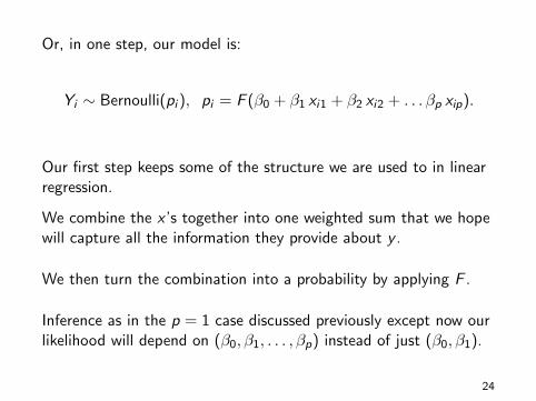
Or, in one step, our model is:
Yi ∼ Bernoulli(pi ), pi = F (β0 + β1 xi1 + β2 xi2 + . . . βp xip).
Our first step keeps some of the structure we are used to in linearregression.
We combine the x ’s together into one weighted sum that we hopewill capture all the information they provide about y .
We then turn the combination into a probability by applying F .
Inference as in the p = 1 case discussed previously except now ourlikelihood will depend on (β0, β1, . . . , βp) instead of just (β0, β1).
24
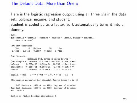
The Default Data, More than One x
Here is the logistic regression output using all three x ’s in the dataset: balance, income, and student.student is coded up as a factor, so R automatically turns it into adummy.Call:
glm(formula = default ~ balance + student + income, family = binomial,
data = Default)
Deviance Residuals:
Min 1Q Median 3Q Max
-2.4691 -0.1418 -0.0557 -0.0203 3.7383
Coefficients:
Estimate Std. Error z value Pr(>|z|)
(Intercept) -1.087e+01 4.923e-01 -22.080 < 2e-16 ***
balance 5.737e-03 2.319e-04 24.738 < 2e-16 ***
studentYes -6.468e-01 2.363e-01 -2.738 0.00619 **
income 3.033e-06 8.203e-06 0.370 0.71152
---
Signif. codes: 0 *** 0.001 ** 0.01 * 0.05 . 0.1 1
(Dispersion parameter for binomial family taken to be 1)
Null deviance: 2920.6 on 9999 degrees of freedom
Residual deviance: 1571.5 on 9996 degrees of freedom
AIC: 1579.5
Number of Fisher Scoring iterations: 8
25
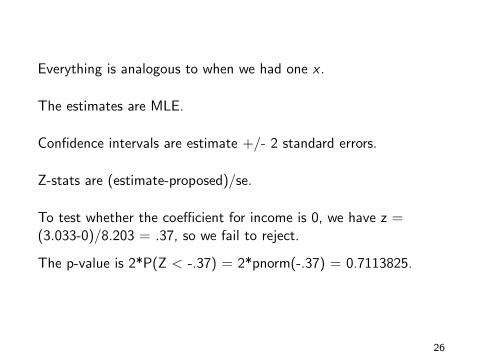
Everything is analogous to when we had one x .
The estimates are MLE.
Confidence intervals are estimate +/- 2 standard errors.
Z-stats are (estimate-proposed)/se.
To test whether the coefficient for income is 0, we have z =(3.033-0)/8.203 = .37, so we fail to reject.
The p-value is 2*P(Z < -.37) = 2*pnorm(-.37) = 0.7113825.
26
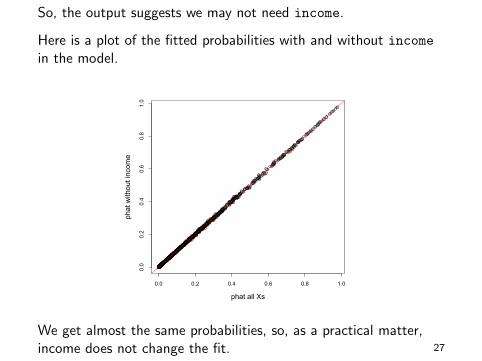
So, the output suggests we may not need income.
Here is a plot of the fitted probabilities with and without incomein the model.
0.0 0.2 0.4 0.6 0.8 1.0
0.0
0.2
0.4
0.6
0.8
1.0
phat all Xs
phat
with
out i
ncom
e
We get almost the same probabilities, so, as a practical matter,income does not change the fit. 27

Here is the output using balance and student.
Call:
glm(formula = default ~ balance + student, family = binomial,
data = Default)
Deviance Residuals:
Min 1Q Median 3Q Max
-2.4578 -0.1422 -0.0559 -0.0203 3.7435
Coefficients:
Estimate Std. Error z value Pr(>|z|)
(Intercept) -1.075e+01 3.692e-01 -29.116 < 2e-16 ***
balance 5.738e-03 2.318e-04 24.750 < 2e-16 ***
studentYes -7.149e-01 1.475e-01 -4.846 1.26e-06 ***
---
Signif. codes: 0 *** 0.001 ** 0.01 * 0.05 . 0.1 1
(Dispersion parameter for binomial family taken to be 1)
Null deviance: 2920.6 on 9999 degrees of freedom
Residual deviance: 1571.7 on 9997 degrees of freedom
AIC: 1577.7
Number of Fisher Scoring iterations: 8
28
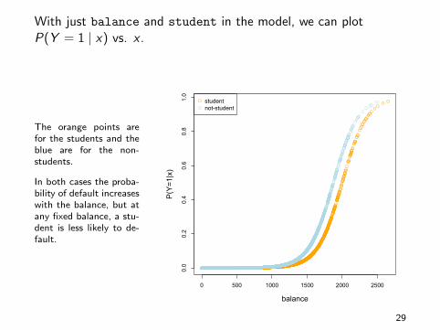
With just balance and student in the model, we can plotP(Y = 1 | x) vs. x .
The orange points arefor the students and theblue are for the non-students.
In both cases the proba-bility of default increaseswith the balance, but atany fixed balance, a stu-dent is less likely to de-fault.
0 500 1000 1500 2000 2500
0.0
0.2
0.4
0.6
0.8
1.0
balance
P(Y=1|x)
studentnot-student
29
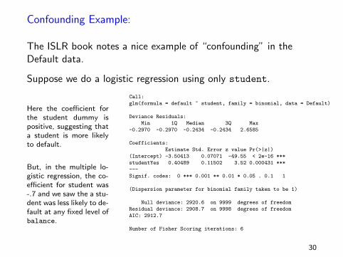
Confounding Example:
The ISLR book notes a nice example of “confounding” in theDefault data.
Suppose we do a logistic regression using only student.
Here the coefficient forthe student dummy ispositive, suggesting thata student is more likelyto default.
But, in the multiple lo-gistic regression, the co-efficient for student was-.7 and we saw the a stu-dent was less likely to de-fault at any fixed level ofbalance.
Call:
glm(formula = default ~ student, family = binomial, data = Default)
Deviance Residuals:
Min 1Q Median 3Q Max
-0.2970 -0.2970 -0.2434 -0.2434 2.6585
Coefficients:
Estimate Std. Error z value Pr(>|z|)
(Intercept) -3.50413 0.07071 -49.55 < 2e-16 ***
studentYes 0.40489 0.11502 3.52 0.000431 ***
---
Signif. codes: 0 *** 0.001 ** 0.01 * 0.05 . 0.1 1
(Dispersion parameter for binomial family taken to be 1)
Null deviance: 2920.6 on 9999 degrees of freedom
Residual deviance: 2908.7 on 9998 degrees of freedom
AIC: 2912.7
Number of Fisher Scoring iterations: 6
30
How can this be?
This is the sort of thing where our intuition from linear multipleregression can carry over to logistic regression. Since bothmethods start by mapping a p dimensional x down to just onenumber, the have some basic features in common. That is a nicething about using logistic regression.
We know that when x ’s are correlated the coefficients for old x ’scan change when we add new x ’s to a model.
Are balance and student “correlated”?
31
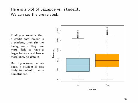
Here is a plot of balance vs. student.We can see the are related.
If all you know is thata credit card holder isa student, then (in thebackground) they aremore likely to have alarger balance and hencemore likely to default.
But, if you know the bal-ance, a student is lesslikely to default than anon-student.
No Yes
0500
1000
1500
2000
2500
student
balance
32
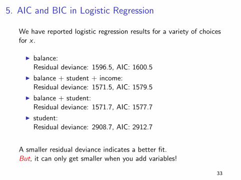
5. AIC and BIC in Logistic Regression
We have reported logistic regression results for a variety of choicesfor x .
I balance:Residual deviance: 1596.5, AIC: 1600.5
I balance + student + income:Residual deviance: 1571.5, AIC: 1579.5
I balance + student:Residual deviance: 1571.7, AIC: 1577.7
I student:Residual deviance: 2908.7, AIC: 2912.7
A smaller residual deviance indicates a better fit.But, it can only get smaller when you add variables!
33
The deviance is just -2 times the maximized log likelihood. Whenyou add x variables the maximized likelihood can only get biggerso the deviance can only get smaller.
If you have more coefficients to optimize over you can only dobetter since you can set them to zero if you want.
This is analogous to the fact that in linear multiple regression R2
can only go up when you add x ’s.
34
AIC is analogous to the BIC and adjusted R2 in that it penalizesyou for adding variables.
Rather than choosing the model with the smallest deviance, somepeople advocate choosing the model with the smallest AIC value:
AIC = −2log(L) + 2(p + 1) = deviance + 2(p + 1),
where L is maximized likelihood and p is the number of xs(we add 1 for the intercept).
The idea is that as you add variables (the model gets morecomplex), deviance goes down but 2*(p+1) goes up.
The suggestion is to pick the model with the smallest AIC.
35
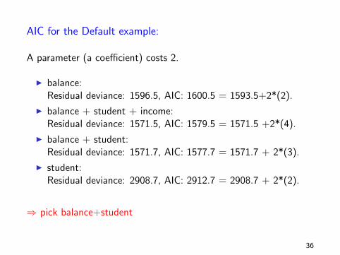
AIC for the Default example:
A parameter (a coefficient) costs 2.
I balance:Residual deviance: 1596.5, AIC: 1600.5 = 1593.5+2*(2).
I balance + student + income:Residual deviance: 1571.5, AIC: 1579.5 = 1571.5 +2*(4).
I balance + student:Residual deviance: 1571.7, AIC: 1577.7 = 1571.7 + 2*(3).
I student:Residual deviance: 2908.7, AIC: 2912.7 = 2908.7 + 2*(2).
⇒ pick balance+student
36
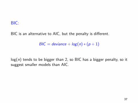
BIC:
BIC is an alternative to AIC, but the penalty is different.
BIC = deviance + log(n) ∗ (p + 1)
log(n) tends to be bigger than 2, so BIC has a bigger penalty, so itsuggest smaller models than AIC.
37
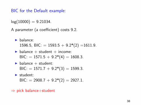
BIC for the Default example:
log(10000) = 9.21034.
A parameter (a coefficient) costs 9.2.
I balance:1596.5, BIC: = 1593.5 + 9.2*(2) =1611.9.
I balance + student + income:BIC: = 1571.5 + 9.2*(4) = 1608.3.
I balance + student:BIC: = 1571.7 + 9.2*(3) = 1599.3.
I student:BIC: = 2908.7 + 9.2*(2) = 2927.1.
⇒ pick balance+student
38

Which is better, AIC or BIC??nobody knows.
R prints out AIC, which suggests you might want to use it, but alot of people like the fact that BIC suggests simpler models.
A lot of academic papers report both AIC and BIC and if they pickthe same model are happy with that. Lame.
Checking the out of sample performance is safer !!!
39
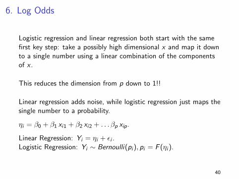
6. Log Odds
Logistic regression and linear regression both start with the samefirst key step: take a possibly high dimensional x and map it downto a single number using a linear combination of the componentsof x .
This reduces the dimension from p down to 1!!
Linear regression adds noise, while logistic regression just maps thesingle number to a probability.
ηi = β0 + β1 xi1 + β2 xi2 + . . . βp xip.
Linear Regression: Yi = ηi + εi .Logistic Regression: Yi ∼ Bernoulli(pi ), pi = F (ηi ).
40
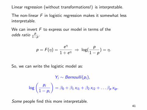
Linear regression (without transformations!) is interpretable.
The non-linear F in logistic regression makes it somewhat lessinterpretable.
We can invert F to express our model in terms of theodds ratio p
1−p .
p = F (η) =eη
1 + eη⇒ log(
p
1− p) = η.
So, we can write the logistic model as:
Yi ∼ Bernoulli(pi ),
log
(pi
1− pi
)= β0 + β1 xi1 + β2 xi2 + . . . βp xip.
Some people find this more interpretable.41
7. Making Decisions
Let’s consider the simple (but very important) case whereY is 0 or 1.
If p(x) is our estimate of P(Y = 1 | x) the obvious thing to do isclassify (predict) Y = 1 if p(x) > .5. We can then look at themissclassification rate.
Sometimes we need to consider the consequences of our actionsmore carefully!
The simple rule “guess Y = 1 if p(x) > .5” may not beappropriate.
42
Target Marketing:
You are trying to decide whether or not to mail a promotion to ahousehold.
Y = 1 if they buy something (when mailed the promotion)and 0 if they don’t.
x : stuff about the household
I demographics
I past purchase history.
p(x):
Probability household like x , will buy when prompted by promotion.
43
p(x): Probability household like x , will buy when prompted bypromotion.
Typically, in target marketing applications,almost all p(x) are less than .5!!!
It does not make sense to predict that nobody will buy andconsequently send out zero promotions.
In this application, p(x) = .1 is huge since there a “real” chancethey will respond and then spend an amount which is large relativeto the cost of the mailing.
44
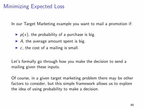
Minimizing Expected Loss
In our Target Marketing example you want to mail a promotion if:
I p(x), the probability of a purchase is big.
I A, the average amount spent is big.
I c, the cost of a mailing is small.
Let’s formally go through how you make the decision to send amailing given these inputs.
Of course, in a given target marketing problem there may be otherfactors to consider, but this simple framework allows us to explorethe idea of using probability to make a decision.
45
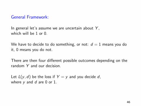
General Framework:
In general let’s assume we are uncertain about Y ,which will be 1 or 0.
We have to decide to do something, or not: d = 1 means you doit, 0 means you do not.
There are then four different possible outcomes depending on therandom Y and our decision.
Let L(y , d) be the loss if Y = y and you decide d ,where y and d are 0 or 1.
46
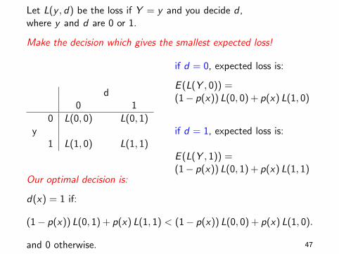
Let L(y , d) be the loss if Y = y and you decide d ,where y and d are 0 or 1.
Make the decision which gives the smallest expected loss!
d0 1
0 L(0, 0) L(0, 1)y
1 L(1, 0) L(1, 1)
if d = 0, expected loss is:
E (L(Y , 0)) =(1− p(x)) L(0, 0) + p(x) L(1, 0)
if d = 1, expected loss is:
E (L(Y , 1)) =(1− p(x)) L(0, 1) + p(x) L(1, 1)
Our optimal decision is:
d(x) = 1 if:
(1− p(x)) L(0, 1) + p(x) L(1, 1) < (1− p(x)) L(0, 0) + p(x) L(1, 0).
and 0 otherwise. 47
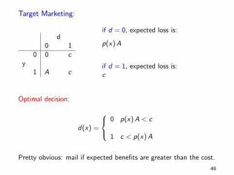
Target Marketing:
d0 1
0 0 cy
1 A c
if d = 0, expected loss is:
p(x) A
if d = 1, expected loss is:c
Optimal decision:
d(x) =
0 p(x) A < c
1 c < p(x) A
Pretty obvious: mail if expected benefits are greater than the cost.
48
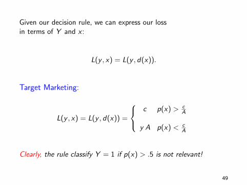
Given our decision rule, we can express our lossin terms of Y and x :
L(y , x) = L(y , d(x)).
Target Marketing:
L(y , x) = L(y , d(x)) =
c p(x) > c
A
y A p(x) < cA
Clearly, the rule classify Y = 1 if p(x) > .5 is not relevant!
49
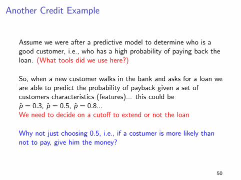
Another Credit Example
Assume we were after a predictive model to determine who is agood customer, i.e., who has a high probability of paying back theloan. (What tools did we use here?)
So, when a new customer walks in the bank and asks for a loan weare able to predict the probability of payback given a set ofcustomers characteristics (features)... this could bep = 0.3, p = 0.5, p = 0.8...We need to decide on a cutoff to extend or not the loan
Why not just choosing 0.5, i.e., if a costumer is more likely thannot to pay, give him the money?
50
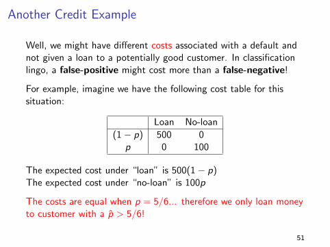
Another Credit Example
Well, we might have different costs associated with a default andnot given a loan to a potentially good customer. In classificationlingo, a false-positive might cost more than a false-negative!
For example, imagine we have the following cost table for thissituation:
Loan No-loan
(1− p) 500 0p 0 100
The expected cost under “loan” is 500(1− p)The expected cost under “no-loan” is 100p
The costs are equal when p = 5/6... therefore we only loan moneyto customer with a p > 5/6!
51
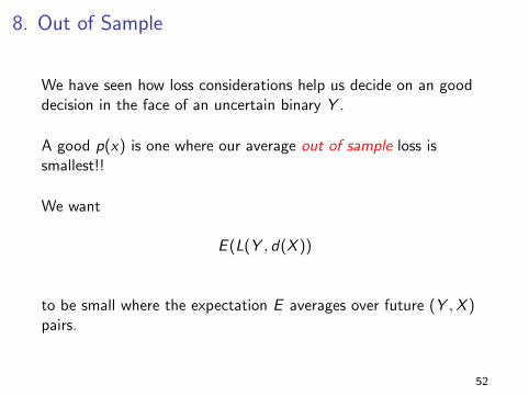
8. Out of Sample
We have seen how loss considerations help us decide on an gooddecision in the face of an uncertain binary Y .
A good p(x) is one where our average out of sample loss issmallest!!
We want
E (L(Y , d(X ))
to be small where the expectation E averages over future (Y ,X )pairs.
52
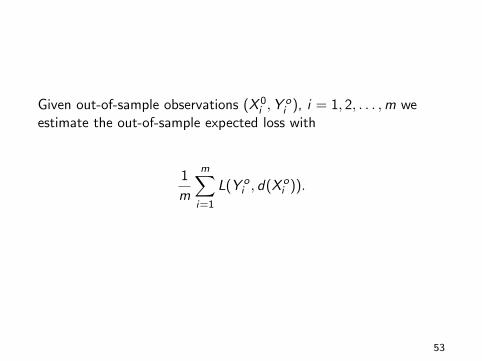
Given out-of-sample observations (X 0i ,Y
oi ), i = 1, 2, . . . ,m we
estimate the out-of-sample expected loss with
1
m
m∑i=1
L(Y oi , d(X o
i )).
53
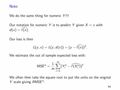
Note:
We do the same thing for numeric Y !!!
Our notation for numeric Y is to predict Y given X = x with
d(x) = f (x).
Our loss is then
L(y , x) = L(y , d(x)) = (y − f (x))2.
We estimate the out of sample expected loss with:
MSE o =1
m
m∑i=1
(Y oi − f (X o
i ))2
We often then take the square root to put the units on the originalY scale giving RMSE o .
54
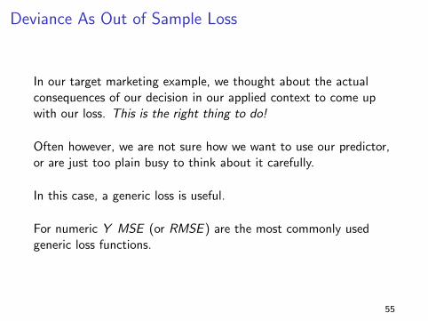
Deviance As Out of Sample Loss
In our target marketing example, we thought about the actualconsequences of our decision in our applied context to come upwith our loss. This is the right thing to do!
Often however, we are not sure how we want to use our predictor,or are just too plain busy to think about it carefully.
In this case, a generic loss is useful.
For numeric Y MSE (or RMSE ) are the most commonly usedgeneric loss functions.
55
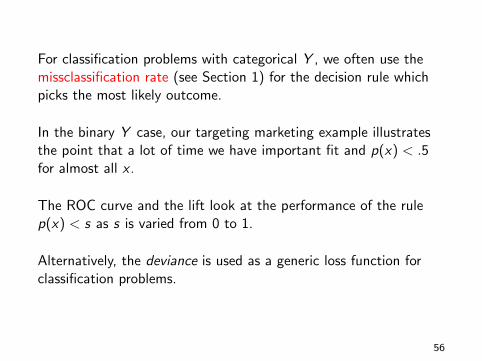
For classification problems with categorical Y , we often use themissclassification rate (see Section 1) for the decision rule whichpicks the most likely outcome.
In the binary Y case, our targeting marketing example illustratesthe point that a lot of time we have important fit and p(x) < .5for almost all x .
The ROC curve and the lift look at the performance of the rulep(x) < s as s is varied from 0 to 1.
Alternatively, the deviance is used as a generic loss function forclassification problems.
56
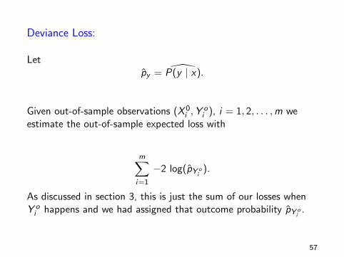
Deviance Loss:
Letpy = P(y | x).
Given out-of-sample observations (X 0i ,Y
oi ), i = 1, 2, . . . ,m we
estimate the out-of-sample expected loss with
m∑i=1
−2 log(pY oi
).
As discussed in section 3, this is just the sum of our losses whenY o
i happens and we had assigned that outcome probability pY oi
.
57
Default Data
Let’s go back to the default data and use out of sampleperformance to do variable selection.
Let’s do a simple train/test split.
I train: randomly pick 75%.
I test: the remaining 25%.
58
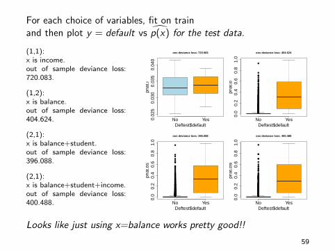
For each choice of variables, fit on trainand then plot y = default vs p(x) for the test data.
(1,1):x is income.out of sample deviance loss:720.083.
(1,2):x is balance.out of sample deviance loss:404.624.
(2,1):x is balance+student.out of sample deviance loss:396.088.
(2,1):x is balance+student+income.out of sample deviance loss:400.488.
No Yes0.02
50.
030
0.03
50.
040
Deftest$default
phat
.i
oos deviance loss: 720.083
●●
●●
●
●●
●
●●
●
●
●
●
●
●
●
●
●●●
●●
●
●
●
●
●
●
●
●●
●●
●●●
●
●
●
●
●
●●●●
●
●●●
●
●
●
●
●
●
●●
●●
●●
●
●
●
●
●
●
●
●
●
●●●
●
●
●
●
●
●
●●●
●●●
●
●●●
●
●●
●●
●
●
●●
●●●
●
●●
●
●
●
●●
●
●●●
●
●
●
●
●
●
●
●
●
●
●
●
●
●
●
●
●
●
●●●
●
●
●●●
●
●
●
●
●●●
●
●
●●●
●
●
●●
●●
●
●
●
●
●
●●
●●
●
●●●
●●
●
●
●
●
●●
●●
●
●
●
●
●
●●
●
●●●
●
●
●●●
●
●
●
●
●●●
●●
●
●●
●
●
●
●●●
●
●●
●
●
●
●
●●
●●●
●
●
●
●●
●
●
●
●●
●
●
●
●
●
●●●
●
●
●●
●
●
●●●●●
●
●
●
●
●
●
●
●
●
●
●●●
●
●
●●
●
●●●
●●●
●
●
●
●●●
●
●
●●●
●
●
●
●
●
●
●
●●●
●
●●●●●●
●
●●
●
●
●●
●
●
●
●
●
●
●
●
●
●
●●●●
●●
●
●
●
●
●●
●
●
●
●
●●●
●
●
●
●●●●●●
●
●
●
●●
●
●
●
●●●
●●●
●
●
●●
●●
●
●
●
●●
No Yes
0.0
0.2
0.4
0.6
0.8
1.0
Deftest$default
phat
.b
oos deviance loss: 404.624
●
●
●●
●
●
●●●●
●●
●
●
●●
●
●
●
●●
●●
●
●
●
●
●
●
●●●●
●
●
●
●●●●
●
●●
●●
●
●
●
●
●
●●
●
●●
●
●
●
●
●
●●
●●
●
●●
●
●
●
●
●
●
●●●●●●●
●
●
●
●
●
●●
●
●
●
●
●
●
●
●●
●
●
●
●●
●
●
●●●
●●
●●
●
●
●
●
●
●
●
●
●●
●
●●
●
●
●
●
●
●●
●
●
●●●
●
●
●
●
●
●
●
●
●
●●
●●
●●
●●
●
●
●
●
●
●
●
●
●
●●
●
●●
●
●
●
●
●
●
●●
●
●
●
●
●
●
●
●
●
●●
●
●
●●
●
●
●
●
●
●
●
●●●
●
●●
●
●
●
●
●
●●●●
●
●
●
●
●●
●●●●
●
●●
●
●●
●
●
●
●
●●
●
●
●
●
●
●●●
●●
●●
●
●●●
●
●
●
●
●
●
●
●
●
●●
●
●
●
●
●●●
●●●
●
●
●
●
●
●●●
●●
●
●
●
●
●
●
●
●
●
●
●
●
●
●
●●●
●
●
●
●
●
●
●
●●
●
●
●
●
●
●
●
●
●
●
●
●●●●
●
●
●
●
●●
●
●
●
●
●●
●
●
●
●
●
●●●●●
●
●
●●
●
●
●
●
●
●●●●●●
●
●
●●●●
●
●
●
●
●
No Yes
0.0
0.2
0.4
0.6
0.8
1.0
Deftest$default
phat
.bs
oos deviance loss: 396.088
●
●
●●
●
●
●●●●
●
●
●
●
●
●
●
●
●
●
●●
●●
●
●
●
●
●
●
●●●●
●
●
●
●●●●●●
●
●●●●●
●
●
●
●
●
●
●●●
●●
●
●
●
●
●
●
●
●●
●●●●
●
●
●
●
●
●●●●●●●
●
●
●
●
●
●●
●
●
●
●
●
●●●
●
●●●
●
●
●
●
●
●
●●●
●●
●
●
●
●
●
●
●
●
●
●●
●
●●
●
●
●
●
●
●●
●
●
●●●●
●
●
●
●●
●
●
●
●
●●
●●
●
●
●
●
●
●
●
●
●
●
●
●
●
●●●●
●
●
●
●
●
●
●
●●
●
●
●
●
●
●
●
●
●
●●
●
●
●
●
●
●
●
●
●
●●
●●●●
●
●●
●
●
●
●
●
●●●●
●
●
●
●
●
●
●
●
●●●
●
●●
●
●●
●
●
●
●
●●
●
●
●
●
●
●●●
●●
●●
●
●●●
●
●
●
●
●
●
●
●
●
●
●
●
●
●
●
●
●
●●●
●●●
●
●
●
●
●
●
●
●
●
●●
●
●
●
●●
●
●
●
●
●
●
●
●
●
●
●●●
●
●
●
●
●
●
●
●●
●
●
●
●
●
●
●
●
●
●
●●●
●●
●
●
●
●
●●
●
●
●
●
●●
●
●
●
●
●
●
●
●●●
●
●●●
●
●
●
●●●●●●
●
●
●●
●●●
●
●
●
●
●
No Yes
0.0
0.2
0.4
0.6
0.8
1.0
Deftest$default
phat
.bsi
oos deviance loss: 400.488
Looks like just using x=balance works pretty good!!
59
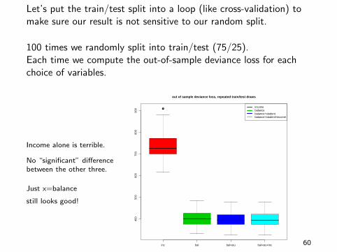
Let’s put the train/test split into a loop (like cross-validation) tomake sure our result is not sensitive to our random split.
100 times we randomly split into train/test (75/25).Each time we compute the out-of-sample deviance loss for eachchoice of variables.
Income alone is terrible.
No “significant” differencebetween the other three.
Just x=balance
still looks good!
●
inc bal bal+stu bal+stu+inc
400
500
600
700
800
900
incomebalancebalance+studentbalance+student+income
out of sample deviance loss, repeated train/test draws
60
9. Lift and ROC
Lift and ROC are two popular methods for assessing the quality ofa classifier for a binary y .
Lift is particularly popular in Marketing.
ROC stands for the incomprehensible term “receiver operatorcharacteristics”.
Both look at missclassification rates for various values of s usingthe rule: classify Y = 1 if p(x) > s.
61
Let’s look at our trusty default data again.
Of course, it is interesing to think about what your actual decisionproblem is in the default data context!!!
Kick them out if p(x) > .2?Send them a nasty letter if .1 < p(x) < .2?
Again, lift and ROC look at the performance of “Y = 1 ifp(x) > s” for a variety of s values. It is not what you wouldactually do, but it gives a sense of how p(x) is dong.
62
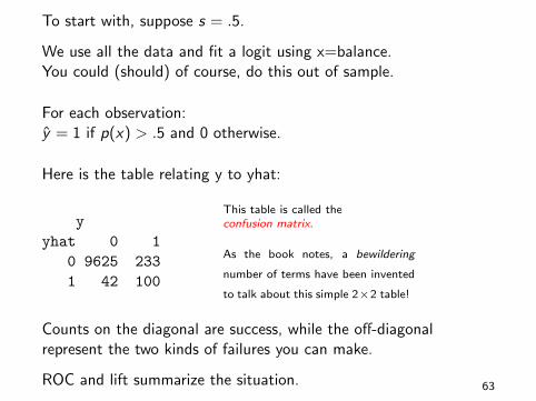
To start with, suppose s = .5.
We use all the data and fit a logit using x=balance.You could (should) of course, do this out of sample.
For each observation:y = 1 if p(x) > .5 and 0 otherwise.
Here is the table relating y to yhat:
yyhat 0 1
0 9625 2331 42 100
This table is called theconfusion matrix.
As the book notes, a bewildering
number of terms have been invented
to talk about this simple 2×2 table!
Counts on the diagonal are success, while the off-diagonalrepresent the two kinds of failures you can make.
ROC and lift summarize the situation. 63
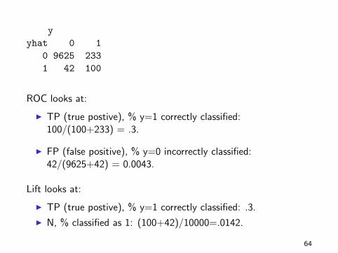
yyhat 0 1
0 9625 2331 42 100
ROC looks at:
I TP (true postive), % y=1 correctly classified:100/(100+233) = .3.
I FP (false positive), % y=0 incorrectly classified:42/(9625+42) = 0.0043.
Lift looks at:
I TP (true postive), % y=1 correctly classified: .3.
I N, % classified as 1: (100+42)/10000=.0142.
64
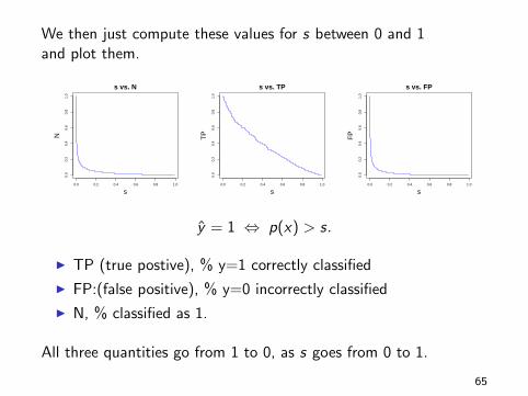
We then just compute these values for s between 0 and 1and plot them.
0.0 0.2 0.4 0.6 0.8 1.0
0.0
0.2
0.4
0.6
0.8
1.0
s
N
s vs. N
0.0 0.2 0.4 0.6 0.8 1.0
0.0
0.2
0.4
0.6
0.8
1.0
s
TP
s vs. TP
0.0 0.2 0.4 0.6 0.8 1.0
0.0
0.2
0.4
0.6
0.8
1.0
s
FP
s vs. FP
y = 1 ⇔ p(x) > s.
I TP (true postive), % y=1 correctly classified
I FP:(false positive), % y=0 incorrectly classified
I N, % classified as 1.
All three quantities go from 1 to 0, as s goes from 0 to 1.
65
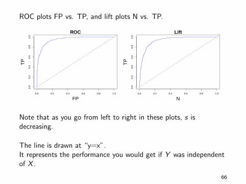
ROC plots FP vs. TP, and lift plots N vs. TP.
0.0 0.2 0.4 0.6 0.8 1.0
0.0
0.2
0.4
0.6
0.8
1.0
FP
TP
ROC
0.0 0.2 0.4 0.6 0.8 1.0
0.0
0.2
0.4
0.6
0.8
1.0
N
TP
Lift
Note that as you go from left to right in these plots, s isdecreasing.
The line is drawn at “y=x”.It represents the performance you would get if Y was independentof X .
66

More on Lift:
There is another simple way to think about the lift curve withoutreferring to the cutoff s. Again let’s using a Marketing problem tomotivate things.
Suppose you have a budget that allows you to mail out to Npercent of the potential customers you have on file.
For customer with information x , p(x) tells you how likely they areto respond.
Given budget N, you mail out to the N percent of potentialcustomers on file that have the large values of p(x).
For each N (% of the ones you try) compute
number of (y=1) from N%
number of (y=1) 100%= % of the good ones you got.
(which is just TP again).67
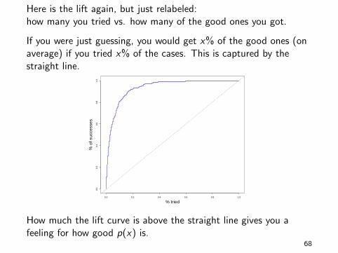
Here is the lift again, but just relabeled:how many you tried vs. how many of the good ones you got.
If you were just guessing, you would get x% of the good ones (onaverage) if you tried x% of the cases. This is captured by thestraight line.
0.0 0.2 0.4 0.6 0.8 1.0
0.0
0.2
0.4
0.6
0.8
1.0
% tried
% o
f suc
cess
es
How much the lift curve is above the straight line gives you afeeling for how good p(x) is.
68
Let’s use lift to compare some classifiers on the default data.
Let’s try logits with:
(i) x=income.(ii) x=balance.(iii) x=balance + balance squared.
Each one will give us a p(x) and will compare them based on theirout-of-sample lift.
69
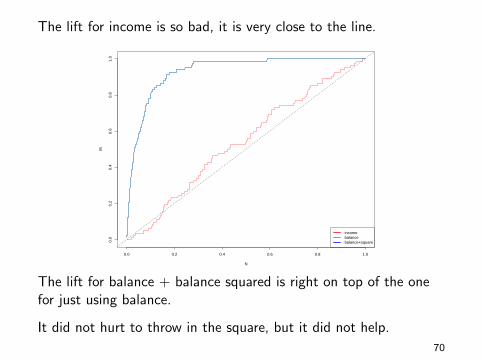
The lift for income is so bad, it is very close to the line.
0.0 0.2 0.4 0.6 0.8 1.0
0.0
0.2
0.4
0.6
0.8
1.0
N
lift
incomebalancebalance+square
The lift for balance + balance squared is right on top of the onefor just using balance.
It did not hurt to throw in the square, but it did not help.
70
10. Bayes Theorem and Classification
We noted that you can think of logistic regression as a parametricmodel for
P(Y = y | X = x)
the conditional distribution of Y given X = x .
A number of classification techniques work by specifying themarginal distribution of Y , the conditional distribution of X givenY and then using Bayes Theorem to compute the conditionaldistribution of Y given X .
71
Conceptually, this is a very nice approach.
But it is tricky in that a lot of probability distributions have to bespecified. In particular, you have to specify the possiblyhigh-dimension distribution of X given Y .
Up to know we have been intuitive in our use of probability.Let’s quickly review the basic definitions and Bayes Theorem.
72
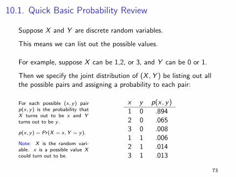
10.1. Quick Basic Probability Review
Suppose X and Y are discrete random variables.
This means we can list out the possible values.
For example, suppose X can be 1,2, or 3, and Y can be 0 or 1.
Then we specify the joint distribution of (X ,Y ) be listing out allthe possible pairs and assigning a probability to each pair:
For each possible (x , y) pairp(x , y) is the probability thatX turns out to be x and Yturns out to be y .
p(x , y) = Pr(X = x ,Y = y).
Note: X is the random vari-able. x is a possible value Xcould turn out to be.
x y p(x , y)
1 0 .8942 0 .0653 0 .0081 1 .0062 1 .0143 1 .013
73
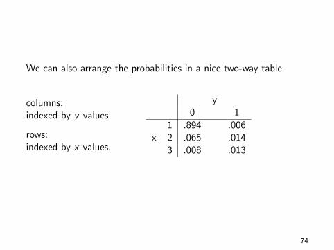
We can also arrange the probabilities in a nice two-way table.
columns:indexed by y values
rows:indexed by x values.
y0 1
1 .894 .006x 2 .065 .014
3 .008 .013
74
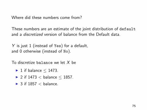
Where did these numbers come from?
These numbers are an estimate of the joint distribution of defaultand a discretized version of balance from the Default data.
Y is just 1 (instead of Yes) for a default,and 0 otherwise (instead of No).
To discretize balance we let X be
I 1 if balance ≤ 1473.
I 2 if 1473 < balance ≤ 1857.
I 3 if 1857 < balance.
75
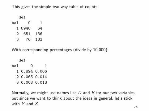
This gives the simple two-way table of counts:
defbal 0 1
1 8940 642 651 1363 76 133
With corresponding percentages (divide by 10,000):
defbal 0 1
1 0.894 0.0062 0.065 0.0143 0.008 0.013
Normally, we might use names like D and B for our two variables,but since we want to think about the ideas in general, let’s stickwith Y and X .
76
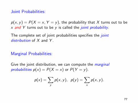
Joint Probabilities:
p(x , y) = P(X = x ,Y = y), the probability that X turns out to bex and Y turns out to be y is called the joint probability.
The complete set of joint probabilities specifies the jointdistribution of X and Y .
Marginal Probabilities:
Give the joint distribution, we can compute the marginalprobabilities p(x) = P(X = x) or P(Y = y).
p(x) =∑y
p(x , y), p(y) =∑x
p(x , y).
77
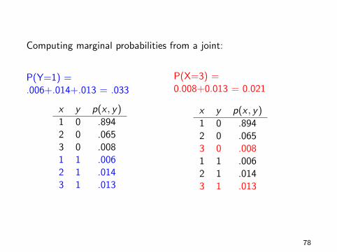
Computing marginal probabilities from a joint:
P(Y=1) =.006+.014+.013 = .033
x y p(x , y)
1 0 .8942 0 .0653 0 .0081 1 .0062 1 .0143 1 .013
P(X=3) =0.008+0.013 = 0.021
x y p(x , y)
1 0 .8942 0 .0653 0 .0081 1 .0062 1 .0143 1 .013
78
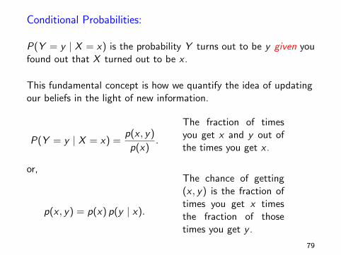
Conditional Probabilities:
P(Y = y | X = x) is the probability Y turns out to be y given youfound out that X turned out to be x .
This fundamental concept is how we quantify the idea of updatingour beliefs in the light of new information.
P(Y = y | X = x) =p(x , y)
p(x).
The fraction of timesyou get x and y out ofthe times you get x .
or,
p(x , y) = p(x) p(y | x).
The chance of getting(x , y) is the fraction oftimes you get x timesthe fraction of thosetimes you get y .
79
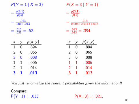
P(Y = 1 | X = 3)
= p(3,1)p(3)
= .013.008+.013
= .013.021 = .62.
x y p(x , y)
1 0 .8942 0 .0653 0 .0081 1 .0062 1 .0143 1 .013
P(X = 3 | Y = 1)
= p(3,1)p(1)
= .0130.006+0.014+0.013
= .013.033 = .394.
x y p(x , y)
1 0 .8942 0 .0653 0 .0081 1 .0062 1 .0143 1 .013
You just renormalize the relevant probabilities given the information!!
Compare:P(Y=1) = .033 P(X=3) = .021.
80
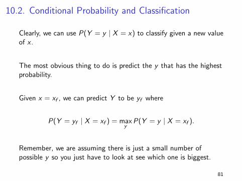
10.2. Conditional Probability and Classification
Clearly, we can use P(Y = y | X = x) to classify given a new valueof x .
The most obvious thing to do is predict the y that has the highestprobability.
Given x = xf , we can predict Y to be yf where
P(Y = yf | X = xf ) = maxy
P(Y = y | X = xf ).
Remember, we are assuming there is just a small number ofpossible y so you just have to look at see which one is biggest.
81
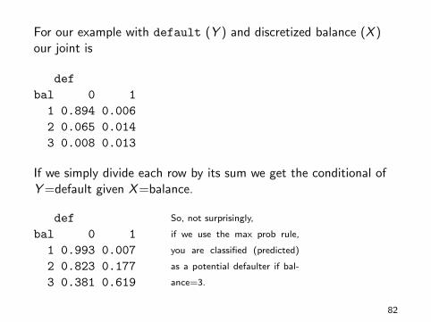
For our example with default (Y ) and discretized balance (X )our joint is
defbal 0 1
1 0.894 0.0062 0.065 0.0143 0.008 0.013
If we simply divide each row by its sum we get the conditional ofY =default given X =balance.
defbal 0 1
1 0.993 0.0072 0.823 0.1773 0.381 0.619
So, not surprisingly,
if we use the max prob rule,
you are classified (predicted)
as a potential defaulter if bal-
ance=3.
82
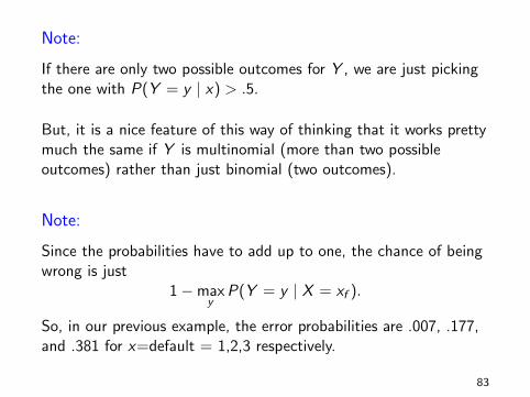
Note:
If there are only two possible outcomes for Y , we are just pickingthe one with P(Y = y | x) > .5.
But, it is a nice feature of this way of thinking that it works prettymuch the same if Y is multinomial (more than two possibleoutcomes) rather than just binomial (two outcomes).
Note:
Since the probabilities have to add up to one, the chance of beingwrong is just
1−maxy
P(Y = y | X = xf ).
So, in our previous example, the error probabilities are .007, .177,and .381 for x=default = 1,2,3 respectively.
83
10.3. Bayes Theorem
In the previous section we saw that if Y is discrete, and we havethe joint distribution of (X ,Y ) we can “classify” y be computingP(Y = y | X = x) for all possible y .
Note that a nice feature of this approach is that it naturallyhandles the case where Y can take on more than two values.
Logistic regression assumes two categories for Y .There is a multinomial version of logistic regression but it is morecomplex.
84
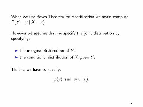
When we use Bayes Theorem for classification we again computeP(Y = y | X = x).
However we assume that we specify the joint distribution byspecifying:
I the marginal distribution of Y .
I the conditional distribution of X given Y .
That is, we have to specify:
p(y) and p(x | y).
85
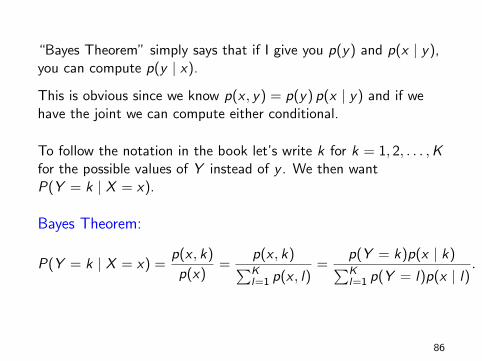
“Bayes Theorem” simply says that if I give you p(y) and p(x | y),you can compute p(y | x).
This is obvious since we know p(x , y) = p(y) p(x | y) and if wehave the joint we can compute either conditional.
To follow the notation in the book let’s write k for k = 1, 2, . . . ,Kfor the possible values of Y instead of y . We then wantP(Y = k | X = x).
Bayes Theorem:
P(Y = k | X = x) =p(x , k)
p(x)=
p(x , k)∑Kl=1 p(x , l)
=p(Y = k)p(x | k)∑Kl=1 p(Y = l)p(x | l)
.
86
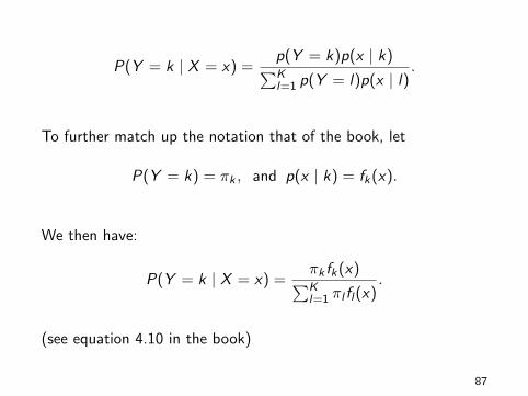
P(Y = k | X = x) =p(Y = k)p(x | k)∑Kl=1 p(Y = l)p(x | l)
.
To further match up the notation that of the book, let
P(Y = k) = πk , and p(x | k) = fk(x).
We then have:
P(Y = k | X = x) =πk fk(x)∑Kl=1 πl fl(x)
.
(see equation 4.10 in the book)
87
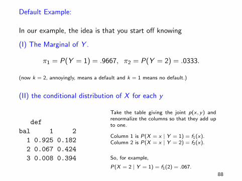
Default Example:
In our example, the idea is that you start off knowing
(I) The Marginal of Y .
π1 = P(Y = 1) = .9667, π2 = P(Y = 2) = .0333.
(now k = 2, annoyingly, means a default and k = 1 means no default.)
(II) the conditional distribution of X for each y
defbal 1 2
1 0.925 0.1822 0.067 0.4243 0.008 0.394
Take the table giving the joint p(x , y) andrenormalize the columns so that they add upto one.
Column 1 is P(X = x | Y = 1) = f1(x).Column 2 is P(X = x | Y = 2) = f2(x).
So, for example,
P(X = 2 | Y = 1) = f1(2) = .067.
88
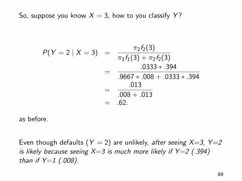
So, suppose you know X = 3, how to you classify Y ?
P(Y = 2 | X = 3) =π2f2(3)
π1f1(3) + π2f2(3)
=.0333 ∗ .394
.9667 ∗ .008 + .0333 ∗ .394
=.013
.008 + .013= .62.
as before.
Even though defaults (Y = 2) are unlikely, after seeing X=3, Y=2is likely because seeing X=3 is much more likely if Y=2 (.394)than if Y=1 (.008).
89
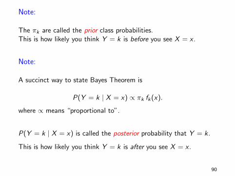
Note:
The πk are called the prior class probabilities.This is how likely you think Y = k is before you see X = x .
Note:
A succinct way to state Bayes Theorem is
P(Y = k | X = x) ∝ πk fk(x).
where ∝ means “proportional to”.
P(Y = k | X = x) is called the posterior probability that Y = k .
This is how likely you think Y = k is after you see X = x .
90
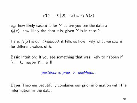
P(Y = k | X = x) ∝ πk fk(x)
πk : how likely case k is for Y before you see the data x .fk(x): how likely the data x is, given Y is in case k.
Here, fk(x) is our likelihood, it tells us how likely what we saw isfor different values of k .
Basic Intuition: If you see something that was likely to happen ifY = k , maybe Y = k !!
posterior ∝ prior × likelihood .
Bayes Theorem beautifully combines our prior information with theinformation in the data.
91
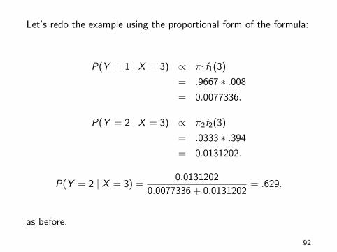
Let’s redo the example using the proportional form of the formula:
P(Y = 1 | X = 3) ∝ π1f1(3)
= .9667 ∗ .008
= 0.0077336.
P(Y = 2 | X = 3) ∝ π2f2(3)
= .0333 ∗ .394
= 0.0131202.
P(Y = 2 | X = 3) =0.0131202
0.0077336 + 0.0131202= .629.
as before.
92
Note:
There is a lot of theory that basically says Bayes Theorem is theright thing to do.
However this assumes the πk and fk(x) are “right”, and we arealmost never sure of this.
93
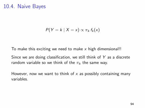
10.4. Naive Bayes
P(Y = k | X = x) ∝ πk fk(x)
To make this exciting we need to make x high dimensional!!
Since we are doing classification, we still think of Y as a discreterandom variable so we think of the πk the same way.
However, now we want to think of x as possibly containing manyvariables.
94
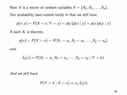
Now X is a vector of random variables X = (X1,X2, . . . ,Xp).
Our probability laws extend nicely in that we still have
p(x , y) = P(X = x ,Y = y) = p(y)p(x | y) = p(x)p(y | x)
If each Xi is discrete,
p(x) = P(X = x) = P(X1 = x1,X2 = x2, . . . ,Xp = xp).
and,
fk(x) = P(X1 = x1,X2 = x2, . . . ,Xp = xp | Y = k).
And we still have
P(Y = k | X = x) ∝ πk fk(x)
95
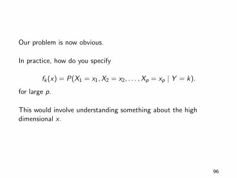
Our problem is now obvious.
In practice, how do you specify
fk(x) = P(X1 = x1,X2 = x2, . . . ,Xp = xp | Y = k).
for large p.
This would involve understanding something about the highdimensional x .
96
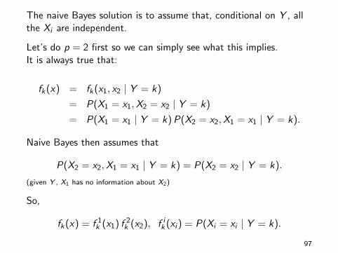
The naive Bayes solution is to assume that, conditional on Y , allthe Xi are independent.
Let’s do p = 2 first so we can simply see what this implies.It is always true that:
fk(x) = fk(x1, x2 | Y = k)
= P(X1 = x1,X2 = x2 | Y = k)
= P(X1 = x1 | Y = k) P(X2 = x2,X1 = x1 | Y = k).
Naive Bayes then assumes that
P(X2 = x2,X1 = x1 | Y = k) = P(X2 = x2 | Y = k).
(given Y , X1 has no information about X2)
So,
fk(x) = f 1k (x1) f 2
k (x2), f ik (xi ) = P(Xi = xi | Y = k).
97
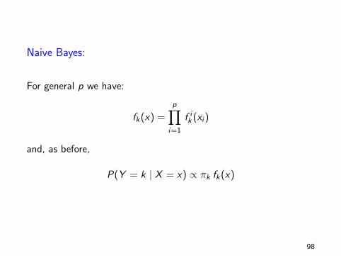
Naive Bayes:
For general p we have:
fk(x) =
p∏i=1
f ik (xi )
and, as before,
P(Y = k | X = x) ∝ πk fk(x)
98
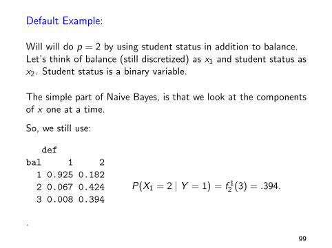
Default Example:
Will will do p = 2 by using student status in addition to balance.Let’s think of balance (still discretized) as x1 and student status asx2. Student status is a binary variable.
The simple part of Naive Bayes, is that we look at the componentsof x one at a time.
So, we still use:
defbal 1 21 0.925 0.1822 0.067 0.4243 0.008 0.394
.
P(X1 = 2 | Y = 1) = f 12 (3) = .394.
99
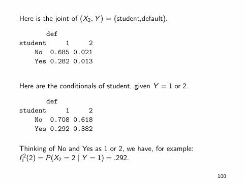
Here is the joint of (X2,Y ) = (student,default).
defstudent 1 2
No 0.685 0.021Yes 0.282 0.013
Here are the conditionals of student, given Y = 1 or 2.
defstudent 1 2
No 0.708 0.618Yes 0.292 0.382
Thinking of No and Yes as 1 or 2, we have, for example:f 21 (2) = P(X2 = 2 | Y = 1) = .292.
100
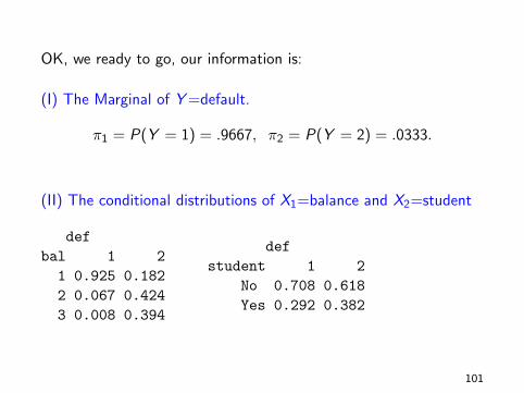
OK, we ready to go, our information is:
(I) The Marginal of Y =default.
π1 = P(Y = 1) = .9667, π2 = P(Y = 2) = .0333.
(II) The conditional distributions of X1=balance and X2=student
defbal 1 2
1 0.925 0.1822 0.067 0.4243 0.008 0.394
defstudent 1 2
No 0.708 0.618Yes 0.292 0.382
101
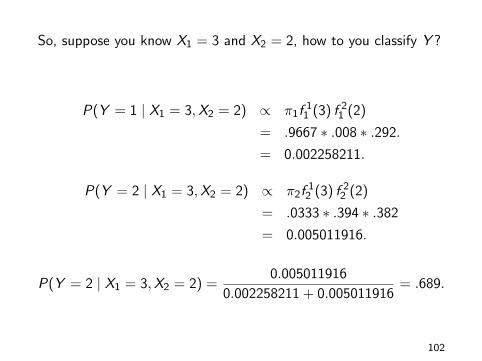
So, suppose you know X1 = 3 and X2 = 2, how to you classify Y ?
P(Y = 1 | X1 = 3,X2 = 2) ∝ π1f 11 (3) f 2
1 (2)
= .9667 ∗ .008 ∗ .292.
= 0.002258211.
P(Y = 2 | X1 = 3,X2 = 2) ∝ π2f 12 (3) f 2
2 (2)
= .0333 ∗ .394 ∗ .382
= 0.005011916.
P(Y = 2 | X1 = 3,X2 = 2) =0.005011916
0.002258211 + 0.005011916= .689.
102
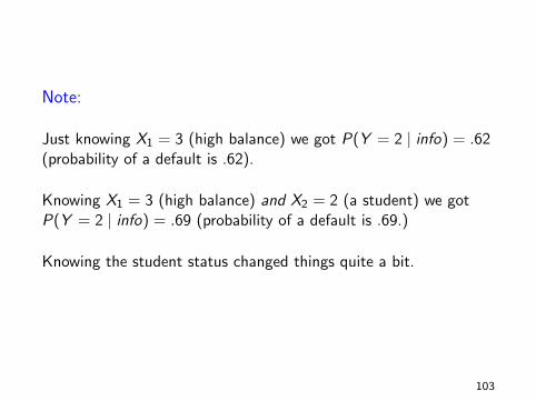
Note:
Just knowing X1 = 3 (high balance) we got P(Y = 2 | info) = .62(probability of a default is .62).
Knowing X1 = 3 (high balance) and X2 = 2 (a student) we gotP(Y = 2 | info) = .69 (probability of a default is .69.)
Knowing the student status changed things quite a bit.
103
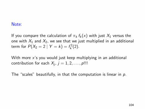
Note:
If you compare the calculation of πk fk(x) with just X1 versus theone with X1 and X2, we see that we just multiplied in an additionalterm for P(X2 = 2 | Y = k) = f 2
k (2).
With more x ’s you would just keep multiplying in an additionalcontribution for each Xj , j = 1, 2, . . . , p!!!
The “scales” beautifully, in that the computation is linear in p.
104
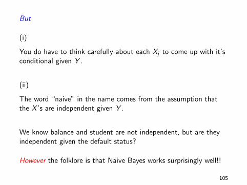
But
(i)
You do have to think carefully about each Xj to come up with it’sconditional given Y .
(ii)
The word “naive” in the name comes from the assumption thatthe X ’s are independent given Y .
We know balance and student are not independent, but are theyindependent given the default status?
However the folklore is that Naive Bayes works surprisingly well!!
105
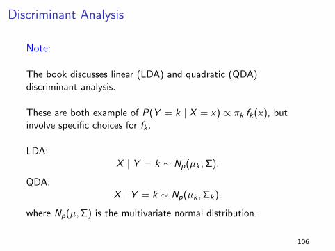
Discriminant Analysis
Note:
The book discusses linear (LDA) and quadratic (QDA)discriminant analysis.
These are both example of P(Y = k | X = x) ∝ πk fk(x), butinvolve specific choices for fk .
LDA:X | Y = k ∼ Np(µk ,Σ).
QDA:X | Y = k ∼ Np(µk ,Σk).
where Np(µ,Σ) is the multivariate normal distribution.
106
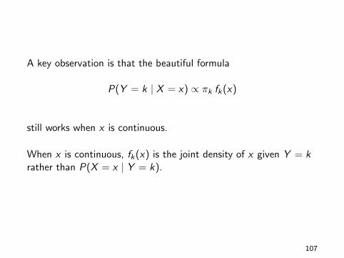
A key observation is that the beautiful formula
P(Y = k | X = x) ∝ πk fk(x)
still works when x is continuous.
When x is continuous, fk(x) is the joint density of x given Y = krather than P(X = x | Y = k).
107


