
Policy, Research, and External Affairs
WORKING PAPERS j
[ Public Economics
Country Economics DepartmentThe World BankFebruary 1990
WPS 334
An Econometric Methodfor Estimating
the Tax Elasticityand the Impact on Revenues
of Discretionary Tax Measures
(Applied to Malawi and Mauritius)
Jaber Ehdaie
The author develops an econometric technique that deals withshortcomings of existing methods for estimating the tax elastic-ity and the impact on revenues of discretionary tax measures. Heapplies this model to Malawi and Mauritius to highlight the rolesthat discretionary tax measures and economic growth play ineffecting the shift from the taxation of international trade to the ,
taxation of domestic transactions. - . V 5
The Policy, Research, and Extemal Affairs Cornplex distnbutes PRE Working Papers to dissemr,uate the findings of work in progressand to encourage the exchange of ideas among Bank staff and all others inte.:sted 'n development issues. These papers carry the namesof the authors, reflect only thetr views, and should be used and cited accordingly The findings, interpretations, and conclusions are theauthors' own They should not be attrbuted tothe World Bank. its Board of Directors ts management, or any of its member countnes.
Pub
lic D
iscl
osur
e A
utho
rized
Pub
lic D
iscl
osur
e A
utho
rized
Pub
lic D
iscl
osur
e A
utho
rized
Pub
lic D
iscl
osur
e A
utho
rized
Pub
lic D
iscl
osur
e A
utho
rized
Pub
lic D
iscl
osur
e A
utho
rized
Pub
lic D
iscl
osur
e A
utho
rized
Pub
lic D
iscl
osur
e A
utho
rized

Policy, Research, and External Affairs
Public Economics
This paper -a product of thc Public Economics Division, Country Economics Dcpartnment -is part ofa larger effort in PPR to study the fiscal aspects of structural adjustment. It proposes a mcthod forestimating the additional revenues that might be mobilized within the existing tax system as GDP grows.Copies are available free from the World Bank, 1818 H Street NW, Washington DC 20433. Please contactAnn Bhalla, room Nl()-059, cxtension 37699 (90 pages with figures and tables).
In reducing the fiscal deficit as part of structural the taxation of domestic transactions. Hisadjustment programs, it is important to be able overall conclusions arc:to project what additional revenues can bemobilized within ihe existing tax system as GDP * Discrctionary tax mcasures havc becngrows. effective in mobilizing resources from the
privatc sector in both countries.To know if it is necessary to generate more
revenues - particularly through politically * Individual and overall tax revenues havedifficult discretionary tax measures - it is becn inelastic in connection with GDP - exceptimportant to be able to estimate the built-in tax for corporate income tax in Malawi and importelasticity as percentage increascs in tax revenue tax in Mauritius, whosc long-term elasticities ex-that result from endogenous incrcases in the base cecd one. Thcsc two taxes are inclastic inwhen GDP rises I pcrcent. tcrms of their own tax bascs. Imports in Mauri-
tius and value added in the nonagriculture sectorExisting methods for estimating this elastic- in Malawi havc grown faster than GDP.
ity are inadequate, so Ehdaic develops an econ-omctric method for estimating built-in tax * The domestic consumption tax had moreelasticity and the impact on revenues of discre- built-in elasticity than import tax in Malawi; intionary tax measures. Mauritius, the domestic consumption tax fell
short of the import tax. Because of thescHis dynamic simultaneous-equation macro- structural differences, economic growth has fed
econometric model of taxation captures the the shift from taxing imports to taxing domesticinteraction between GDP, individual tax sys- transactions in Malawi: it has reversed the shifttems, and individual Lax revenues and bases. It in Mauritius. Without cconomic growth, bothrequires only timc series data on tax revenues, countries would shift from taxing imports totax bascs, and GDP. taxing domestic transactions.
Ehdaic's model can also bc used to (1) * In both countries, discretionary tax mcas-evaluatc thc macrocconomic impact of a tax ures have contributed more to the trcnd towardrcfomi program and (2) examine various tax-re- domestic consumption tax than to the trendlated economic issues. toward import taxes.
In this paper, Ehdaic applies this model to * In Malawi, economic growth and discre-the time series data for Malawi and Mauritius to tionary tax measures have played almost equalhighlight the roles that economic growth and roles in the shift from taxing intemational tradediscretionary tax measures play in cffecting the to taxing domestic transactions. In Mauritius,shift from the taxation of international trade to economic growth has been the principal factor in
revcrsing this shift.
The PRE Working Paper Series disseminates thc Findings of wo-k under wa, ni the Bank's Policy, Research, and ExternalAffairs CorTiplex. An objectivc Of the scrics is to gc; thcsc findings out quickly, even if presenitations arc lcss than f ailypolished. The findings, interpretations, and conclusions in these papers do not neccessarily represent official policy if thc Bank.
Produced at the PRE Dissemination Center

TABLE OF CONTENTS
LIST OF TABLES
LIST OF FIGURES
hapters
I. INTRODUCTION ................................................. 1
II. THEORETICAL DEVELOPMENT OF THE MODEL .......................... 16
Individual Tax Yield Equations Block .......... . ........... 17Individual Tax Base Functions Block ........................ 25Identities Block ........................................... 32Entire Model and Its Dynamic Multipliers ................... 34
III. APPLICATION OF THE MODEL ...................................... 47
Estimation Method and Empirical Results .................... 47Trends of Tax Effort and Tax Shares ........................ 58
IV. CONCLUSION ................................................... 65
APPENDIX A: Historical Time Series Data .............................. 71APPENDIX B: Generalized Version of the Model ......................... 79APPENDIX C: An Operational Guidlin3 on the Application of the Model..82
BIBLIOGRAPHY ...................................................... 88
I am grateful to Javad Khalilzadeh-Shirazi, JesuLs Seade, Pradeep Mitra,Wayne Thirsk, and William McCleary, who inspired me to undertake this studyand provided useful comments. I am also thankful to Bela Balassa, EmmanuelJimenez, Martha de Melo, P. Shome, Zmarak Shalizi and Anwar Shah for helpfulcomments.

LIST OF TABLES
1. Structural Form of the Model ........................................ 35
2. Entire Model with Estimable Parameters .............................. 36
3. Short Run and Long Run Individual and Overall Tax Elasticitiesin Terms of the Parameters Included in the Model ................ 40
4. Direct and Indirect Responses of Individual and Overall Tax Revenuesto the Changes in the Import Tax System ........................ 41
5. Direct and Indirect Responses of Individual and Overall Tax Revenuesto the Changes in the Domestic Consumption Tax System ........... 42
6. Direct and Indirect Responses of Individual and Overall Tax Revenuesto the Changes in the Corporate Income Tax System .............. 43
7. Direct and Indirect Responses of Individual and Overall Tax Revenuesto the Changes in the other direct Taxes System ................ 44
8. Test Results For Serial Correlation ................................. 49
9. Econometric Model of Taxation of Malawi(N3SLS Estimation Results) ....................................... 51
10. Econometric Model of Taxation of Mauritius(N3SLS Estimation Results) ....................................... 52
11. Short Run and Long Run Impacts of Changes in Individual Tax Systemsand GDP on Tax Revenues and Bases in Malawi ...................... 56
12. Short Run and Long Run Impacts of Changes in Individual Tax Systemsand GDP on Tax Revenues and Bases in Mauritius .................. 57
13. Individual and Overall Tax Buoyancies and Elasticities in Malawiand Mauritius .................................................... 61
14. Contribution of Economic Growth and Discretionary Tax Measures toTrends of Tax Shares and Effort in Malawi and Mauritius .......... 63

LIST OF FIGURES
1. Decomposition of response of An Individual Tax Yield to DiscretionaryTax Measures ................................................... 6
2. Actual and Predicted Values of Individual Tax Yields in Malawi ..... 53
a. Import Tax ..................................................... 53
b. Domestic Consumption Tax ....................................... 53
c. Corporate Income Tax ........................................... 53
d. Other Direct Taxes ............................................. 53
3. Actual and Predicted Values of Individual Tax Yields in Mauritius..54
a. Import Tax ..................................................... 54
b. Domestic Consumption Tax ....................................... 54
c. Corporate Income Tax ........................................... 54
d. Other Direct Ta-tes ............................................. 54

CHAPTER I
INTRODUCTION
The objective of this study is twofold: first, to develop an
econometric method of estimating built-in tax elasticity and, hence,
isolating the revenue impact of discretionary tax measures from that of
economic growth; and second, to apply this model to selected Sub-Saharan
Africa countries in order to highlight the contribution of discretionary
actions taken by fiscal authorities to trends of tax effort and individual
tax shares during the past two decades.1
The structural adjustment programs of sloping countries use
fiscal deficit reduction as one of the policy tools for achieving real
economic growth with price stability and balance of payments viability. In
dealing with this deficit within such a framework, projections need to be
made of the additional revenues which can be mobilized within the existing
tax system as GDP grows. These projections indicate the need to activate
additional means of revenue generation, particularly politically difficult
discretionary tax measures. Thus, it becomes essential to be able to
estimate built-in tax elasticity (hereafter, tax elasticity) which measures
1/ There are a variety of taxes, such as import tax, export tax, excisetax, sales/value added/turnover tax, corpora-e income tax and so on;throughout this study, the term "individual tax" will be used to referto each of these taxes. Each tax has its own tax system--a set of lawsand regulations governing the process of estimation, assessment andcollection of its corresponding tax revenue--which will be called the"individual tax system". The term "discretionary tax measures (DTMs)"will be used to describe changes in these systems which include changesin statutory tax rates, tax bases, tax allowances and credits, and oftax administrative efficiency.

-2-
percentage increases in tax revenue resulting from the endogenous changes
in the base caused by a one percent rise in GDP. However, its estimation by
means of any of the existing methods suffers from a specification bias due
to the lack of an observable quantitative variable capable of reflecting
all changes in an individual (or overall) tax system in public finance.
There have been two major approaches employed by priori studies on
this subject to deal with this gap. One approach has been, first, to
eliminate discretionary tax changes from the historical time series tax
data (HTSTD), and then to estimate tax elasticity using the adjusted HTSTD
by means of the following single-equation econometric model.
ln(T' )t - "o + plln(Y)t + Et (1)
where
T'- adjusted HTSTD to discretionary tax changes,
Y - tax base (or GDP in aggregate level),
E = disturbance term, and
p1l tax elasticity, defined as percentage increases in tax revenue net
of discretionary tax changes due to one percent rise in the base
(or GDP in aggregate level).
However, a complete adjustment of HTSTD to discretionary tax
changes is impossIh'e by means of any of the existing two major adjustment
methods --proportional adjustment (PA) and constant rate structure (CRS)
techniques.
In accordance with the proportional adjustment technique, the
historical time series tax data are first adjusted to a preceding-year

-3-
base.2 This is done by subtracting the budget estimate of the revenue
impact o1 DTMs implemented in a given year from the actual tax revenue
collected in that year, that is,
Tt,t = Tt - Dt
where
Tt - the actual tax revenue collected in the tth year,
Dt - the budget estimate of the revenue impact (negative or positive)
of the DTMs implemented in the tth year, and
Tt,t- the actual revenue in the tth year adjusted to the structure of
that year.
Then, to convert the Tt,ts to the first-year base, the adjusted tax revenue
for the tth year (Tt,t) is multiplied by the previous year's ratio of the
adjusted tax revenue according to tha first year's structure (Tl,t-l) over
the actual tax yield (Tt.l), that is,
(T) )1 Tl,l
- [ (T')1t|
(T')t = T tl3Tt,t
Tt -1
After making successive substitutions, the following formula is
derived for (T )t, which is in terms of Tts and Dts.
2/ This technique was first developed by Prest (1962). Later, Sahota (1961)employed a PA technique that, on the face of it, seemed different fromPrest's method but yielded an identical result.

- 4 -
t- Ti -D;(T )t -(Tt-DtJ) I (2)
jl1 Ti
According to this method, changes in an individual tax system
directly result in an exogenous change in its tax revenue, in other words,
a shift in equation (1). These changes are, however, assLmed not to affect
its own and other individual tax bases endogenously, and thus, its
consequences are not applied to the tax revenue. This is a strong
assumption which is not supported theoretically3 and its validity has not
been tested empirically by any of the studies using this method.4
For example, an increase in the tariff on imports of consumption
goods raises the price of these products (Pm) compared with that of
competitive goods produced in the home economy (Rd), in other words, Pm/Pd*
In an attempt to maximize their utilities, consumers will decrease and
increase their demand respectively for the imported goods and domestic
products. As a result, the import tax yield will decline due to the
decrease in its base inducer. by an increase in its rate through the price
mechanism. Domestic production of these products and/or their price will
rise because of the increased demand, causing an increase in the companies'
profit (corporate income tax base) and a rise in the potential base for
taxes on domestic transactions, such as value added, turnover or sales tax.
Consequently, the revenues stemming from the taxation of these sources will
3/ This assumption is strongly rejected, at least by the studies which dealwith the use of tariffs as a policy instrument to protect domesticindustries, for example, see Balassa (1989).
4/ For examples, see Prest (1962), Mansfield (1972), Jeetun (1978), Sury(1985), Gillani (1986), Lambert and Suckling (1986) and Sahota (1961).

-5-
rise due to the increased tariff on imports of consumption goods (a change
in other individual tax yip-ds).
Similarly, the impcrt tax revenue endogenously responds to changes
in other individual tax systems. For instance, an ir.crease in the income
tax rate will reduce disposable income; private consumption will decline,
including the consumption of goods imported from abroad. As a consequence,
the import tax yield will fail because of the decrease in its base induced
by a rise in the income tax rate through the income channel.
Figure 1 represents the decomposition of response of an individual
tax yield to DTMs within this framework. It is apparent from this Figure
that an individual tax revenue directly responds to changes in its own tax
system ("own-DTM direct response") and to endogenous changes in its base.
The base is endogenouslv influenced (i) by changes in its own and other
individual tax systems throu6h price mechanism, investment, savings and/or
income channels, and (ii) by factors other than DTMs, particularly
variations in GDP. Therefore, the tax revenue indirectly responds to
changes in its own ("own-DTM indirect response") and other i.dividual tax
systems ("cross-DTM indirect response") through their impacts on its base.
More specifically, in the PA method, the own- and cross-DTM
indirect responses of tax revenues are not incorporated in the procpss of
the adjustment of HTSTD to discretionary tax changes. Furthermore, this
method ignores the impact of changes in the degree of evasion or of
administrative efficiency on tax revenues.
Finally, the PA method uses the budget estimates of discretionary
tax changes (Dts). Such data are difficult to obtain in many countries and,

- 6 -
FIGURE 1: Decomposition of Response of an Individual Tax Yieldto Discretionary Tax Measures
'Own-DTMs Direct Response".0 > @or
flvr"Direct Resporse to DTMs"
An Ir.dividual Tax Yield
0v s A"Own-DTMs Indirect Response" "Cross-DTMs Indirect Response"
Endogenous Changes in itsBase
Changes in Changes in OtherIts Own Tax Individual TaxSystem Systems
Factors Other than DTMs,particularly CDP
"Indirect Response to DTMs"-sum of own- and cross-DTMs indirect responses.

7.
if available, they are of qt1zstionable reliability as they differ
substantially from actual discretionary outturns.
The CRS method requires data on income bracket (or commodity) rates
and sufficAently disaggregated information on the growth and distribution
of the reported tax bases.5 If such disaggregated information is
available, it would be possible to construct a constant rate-base series
that would represent hypothetical yields under a system assumed to remain
unchanged during the period under review as follows:6
n(T )t _ z (Ti)O(Xi)t (3)
i=O
where
(ri)o - the base-year statutory tax rate on the ith income bracket
(or commodity),
(Xi)t - the reported tax base in the ith income bracket (or
commodity) in the tth year, and
n - number of income brackets (or commodities).
It is revealed from equation (3) that the CRS method incorporates
only the discretionary tax changes resulting from changes in statutory tax
rates; thus, it ignores those discretionary tax changes which emerge from
changes in administrative efficiency and in tax base, tax credit and tax
allowances. Also, in this method, as in the PA technique, the own- and
cross-DTM indirect responses of tax revenues are not taken into account in
the process of the adjustment.
5/ See Bahl (1972), Andersen (1973), Chelliah and Sheetal (1974) andChoudhry (1975).
6/ Chelliah and Sheetal (1974), PP. 12-13.

-8-
Furthermore, the needed information, particularly on the
distribution of tax bases by rate categories, is not readily available;
hence, the effective tax rates --defined as assessed tax revenue over the
base-- of broad income classes (or commodity groupings) that are
empirically used assume that interaclass (or irteragrouping) distribution
of the base will remain unchanged during the period under review.
Naturally, the validity of this assumption will decline as the number of
the income classes or commodity groupings in the breakdown falls due to
aggregation.
Finally, Choudhry (1979) argues that the constant rate structure
method becomes inefficient (P. 110), first, where a tax system has many
progressive elements and, second, where tax bases grow at the same rates.
Under the first circumstance, this method does not guarantee that the
estimate of tax elasticity will be larger (or smaller) than that of tax
buoyancy even when discretionary changes produce overall negative (or
positive) revenue effects.7 Under the second circumstance, there is the
possibility that the elasticity estimate fails to detect the effects of
discretionary changes.
Consequently, the adjusted HTSTD to discretionary tax changes by
means of any of the existing methods (PA and CRS) involve measurement
7/ Tax buoyancy measures percentage changes in tax revenue, includingdiscretionary tax changes, due to a one percent increase in the base(CDP, in aggregate level). It is simply estimated by means of thefollowing single-equation econometric model:
log(T) - ao + allog(Y) +cwhere
T = total tax revenue,Y - tax base, andal- tax buoyancy.

- 9 -
errors which, in turn, create a specification bias in the estimate of tax
elasticity.
The other approach has been to estimate tax elasticity directly
from HTSTD using time trends or dummy variables as proxy for DTMs. Choudhry
(1979) employs a divisia index (DI) method in which time trends are
introduced as proxy for DTMs in the tax and base functions.8 Briefly, this
method involves three steps. First, a formula is derived which generates an
index representing the revenue impact of DTMs. Second, the growth rate of
this index is divided by that of the tax base; this ratio measures the
growth rate of tax revenue resulting from DTMs in terms of a one percent
increase in the base. Finally, tax elasticity is calculated by subtracting
this ratio from the tax buoyancy.
Apart from the questionability of using time trends as
representative of DTMs, the major empirical implication of this technique
is that the formula derived in the first step is a line integral and, in
practical application, its discrete version is used, causing bias in the
estimate of the revenue impact of discretionary measures. The bias is
downward (or upward) when the discretionary changes produce positive (or
negative) revenue effects, resulting in an overestimate (or underestimate)
of tax elasticity.9
Singer (1968), Chand and Wolf (1973), Khan (1973) and Artus (1974)
use one dummy variable (simple or mixed) as proxy for each of the DTMs
8/ This method is widely used in measuring the impact of changes intechnology on the productivity of labor.
9/ For proof of this implication see Choudhry (1979), pp. 87-121.

- 10 -
taken during the period under review and they estimate tax elasticity by
means of the following single-equation econometric model.
nln(T)t -= + Olln(Y)t + Zfi2iDi + Ut (4)
i-i
where
T - tax revenue,
Y - tax base or GDP in aggregate level,
Di- dummy variable (simple or mixed) as proxy for the ith DTM taken
during the period under review, and
01 tax elasticity; in aggregate level, it measures percentage
increases in the tax revenue resulting from the endogenous changes
in the base caused by a one percent rise in GDP.
However, the estimate of tax elasticity obtained by this technique
is not precise and reliable because of the serious multicolinearity problem
created as a result of entering more than one dummy variable into the tax
function.10 The degree of preciseness of and reliability on the elasticity
estimate are inversely related to the degree of multicolinearity which, in
turn, greatly depends on the time-intervel that existed between two
successive discretiornary actions taken by fiscal authorities. For instance,
the partial correlation coefficient of two dummy variables is 99 percent
and 84 percent when the time-intervals are one year and five years
respectively. This indicates that the degree of multicolinearity rises as
the time interval between two successive DTMs falls, and it is still too
10/ For more details on the impact of multicolinearity on the precisenessof the parameters estimates see G.S. Maddala (1977), pp. 183-190.

- 11 -
high even when the time interval is five years. This simply means that
getting a precise and reliable estimate of tax elasticity by means of this
technique is empirically impossible, particularly when thera are frequent
discretionary tax changes during the period under review.
Therefore, all the existing estimation methods of tax elasticity
suffer from a specification bias which is mainly due to the lack of an
observable quantitative variable capable of reflecting all changes in an
individual (o; overall) tax system in public finance. The primary objective
of this study is to develop an econometric method of estimating tax
elasticity and the revenue impact of DTMs which deals with this lack and,
thus, with its consequences on the estimate of tax elasticity. Briefly,
this method is a dynamic simultaneous-equation econometric model of
taxation which captures the interaction of individual tax systems,
individual tax revenues and bases and GDP. As representative of each
individual tax system, its "average effective tax rate net of endogenous
(built-in) changes in the tax yield and base" (AETRN) is introduced into
the model. Time series data on AETRNs are automatically generated in the
process of estimating the model parameters. The model explicitly
incorporates both the direct and indirect responses of each individual tax
revenue to changes in its own and other individual tax systems, i.e., own-
DTM direct, own-DTM indirect and cross-DTM indirect responses. Its
application requires only historical time series data on tax revenues, tax
bases and CDP, all of which are already available for most countries.
In addition to its application as a method for estimating tax
elasticity and the revenue impact of DTMs, this model can be used as an
empirical framework:

- 12 -
(a) to forecast a government's revenue stemming from various sources of
taxation;
(b) to evaluate the macroeconomic impact of a tax reform program which is
aimed at either generating additional revenue and/or dealing with
specific economic problems; and
(c) to deal with various tax related economic issues-- for example, to
investigate the welfare impact of moving from differential tariffs
towards uniform ones, which is often recommended by the Bank, or
to examine the controversial view that uniform tariffs results in
uniform rates of effective protection in industrial and non-
industrial activities.
In this study, this model is used as an empirical tool to highlight
the contribution of discretionary tax measures to trends of tax shares and
tax effort in selected Sub-Saharan Africa countries during the 1965-85
period.
A shift from the taxation of international trade to the taxation of
domestic transactions is recommended as one of the main objectives of an
administratively feasible tax reform program in SSA countries, where such
reform is often included in structural adjustment programs. The
presumption, however, is that discretionary tax measures play a crucial
role in effecting this shift. This description emerges from the experience
of a number of Sub-Saharan Africa countries where tax effort has grown, the
share of tax on domestic transactions in total tax revenue has risen and
the import tax share has declined at least since the mid-1960s, though all
three trends have halted or reversed since the late 1970s.11
11/ Shalizi and Squire (1988), P. 2.

- 13 -
However, discretionary tax measures have not been the only source
of variation of tax shares; they have also been affected by endogenous
changes in tax bases causcd by factors other than these measures,
particularly econo:ic growth.
In SSA countries, fiscal authorities have taken a variety of
discretionary actions in order to generate revenue and to deal with
specific economic issues during the past two decades. In addition to their
revenue generating objective, corporate income tax has been used to improve
investment incentives and stimulate private sector investment in specific
economic activities/regions; import tax has been applied as one of the
policy instruments to protect infant domestic industries against
competition of foreign ones; and domestic consumption tax has been utilized
to deal with equity issues and cascading problems in the production chain.
During the same period, nominal and real gross domestic product
have also grown, recording annual average rates of 13.4 percent and 2.6
percent respectively.1 2
Among the major economic sectors, non-agriculture (industry and
service) has been the principal contributor to the overall economic growth;
the share of its value added in GDP has increased from 61 percent in 1965
to 67.8 percent in 1985. This has been associated with the vertical and
horizontal expansion of companies in this sector, resulting in endogenous
changes in companies' net operating profit which is the potential corporate
income tax base.13
12/ The World Bank, World Development Report, (Oxford: Oxford UniversityPress, 1987), PP. 16 & 173.
13/ Table 1 in Appendix A.

- 14 -
Expansion of the non-agriculture sector has been mainly due to
sharp increases in domestic demand for consumption goods produced in this
sector. This inLcrease in demand has been influenced by a consumption goods
import-substitution policy implemented by governments in order to
industrialize the economy. So the share of consumption goods produced and
consumed in the home economy (consumption tax base) in GDP has risen from
66 percent in 1965 to 78 percent in 1985; in the same period, the share of
consumption goods imported from abroad in GDP has declined from 15 percent
to 10 percent and that of other imports has grown slightly from 10 percent
to 11 percent resulting in an annual average decrease of 0.20 percentage
point in the share of total imports (import tax base) in GDP.
These historical observations indicate the interaction of economic
growth with the trends of tax shares and efforts in SSA countries.
This study highlights the contribution that discretionary tax
measures have made to the shift from the taxation of international trade to
the taxation of domestic transactions in countries, such as Malawi, where
such a shift has taken place. It also questions the effectiveness of these
measures as a policy instrument for bringing about such a shift in other
countries, like Mauritius, where the country's reliance on the foreign
trade tax has risen during the past two decades. These are the tasks which
have been neglected by previous studies and are addressed by this research.
The theoretical development of the model is discussed in Chapter
II. To simplify its discussion, the model is disaggregat3d into three
blocks--individual tax yield functions, individual tax base equations and
identities. After discussing each block separately, the entire model as a
method for estimating tax elasticity and the revenue impact of DTMs is

- 15 -
represented, and its dynamic multipliers are derived. These multipliers
measure the short run and long run impacts of economic growth and changes
in each individual tax system on tax revenues and bases.
The application of the model to Malawi and Mauritius is discussed
in Chapter III which consists of two sections. In the first section, the
estimation method and results are discussed and the dynamic multipliers of
the model are derived. Using these results, the contribution of
discretionary tax measures to trends of tax effort and shares is analyzed
in the second section. Briefly, the econometric application of the model to
these countries yields a number of interesting results. For instance, it
shows that: (i) discretionary tax measures have been an effective policy
instrument in mobilizing resources from the private sector to the public
sector, to the extent that tax effort would fall in the absence of DTMs;
(ii) individual and overall tax revenues have been inelastic with respect
to GDP, except corporate income tax in Malawi and import tax in Mauritius;
(iii) economic growth and discretionary tax measures have had almost equal
roles in shifting from the taxation of international trade to the taxation
of domestic transactions in Malawi, contributing respectively 51 percent
and 49 percent to the overall growth rate of domestic consumption tax-
import tax; and (iv) in Mauritius, economic growth has been the principal
factor in reversing this shift, to the extent that the country would sh::ft
from the taxation of international trade to the taxation of domestic
transactions in the absence of nominal economic growth.
Finally, a summary of findings and suggestions for further research
is presented in Chapter IV.

CHAPTER II
THEORETICAL DEVELOPMENT OF THE MODEL
It is revealed from Figure 1 that changes in an individual tax
revenue directly result from changes in its own tax system and/or
"endogenous changes" in its base. Its base is endogenously affected (i) by
changes in its own and other individual tax systems through price
mechanism, investment, savings or income channels, and (ii) by factors
other than DTMs, particularly variations in GDP. In other words, individual
tax systems, individual tax bases and yields and GDP are all interrelated.
Tt.eir interaction is modelled in this chapter in order to estimate (a) the
direct and indirect responses of each individual tax yield to changes in
its own and other individual tax systems, and (b) elasticities of
indiriidual tax yields, individual tax bases and overall tax revenue with
respect to GDP.
The concept of "tax elasticity" is defined to measure percentage
increases in *hte tax revenue resulting from the endogenous changes in its
base caused by a one percent rise in GDP. It is the product of elasticities
of the tax yield to its base and the base to GDP.
Regarding the second objective of this research, all individual
taxes are classified into five major categories. These are: (1) corporate
income tax, (2) other direct taxes (individual income tax, social security,
payroll tax, tax on property and other taxes on net income and profits),
(3) import tax ( tariff/customs duties and other charges), (4) tax on
exports, and (5) tax on domestic consumption (general sales, turnover or
value added taxes, selective excises on goods and services, taxes on use of

- 17 -
goods or property and permission to perform activities, stamp tax and other
domestic indirect taxes).
To simplify this discussion, the model is disaggregated into three
blocks--individual tax revenue equations, individual tax base functions,
and identities. First, each of these blocks is separately discussed; then,
the entire model as an empirical framework for estimating tax elasticity
and the revenue impact of DTMs is discussed.
Individual Tax Revenue Equations Block
As explained above, an individual tax revenue is directly affected
by changes in its own tax system and its base. To separate out the direct
revenue impacts of these two factors, each individual tax revenue assessed
by tax inspectors (Ti*) is considered to be a function of two proxy
variables, one for its potential tax base (Xi) and another as
representative of its own tax system (ri), that is,
log(Ti*)t- QiO+ aillog(Xi)t+ ai2(7i)t+ Lit (1)
where
Ei - disturbance terms as representative of other explanatory,
variables excluded from the model,
i - d, tax on domestic transactions,
- m, tax on imports,
- x, tax on exports,
- c, corporate income tax, and

- 18 -
o, other direct taxes.
This function was specified in semi-log-linear form essentially for a
reason of convenience, that is, it allows a direct estimate of tax
elasticity which is the primary objective of this research; furthermore,
this is also a preferred functional form used in the previous studies.1 Its
generalized version is, however, discussed in appendix B.
Given a discrepancy between the assessed and actual tax revenue,
tax inspectors will adjust the actual tax yields toward their assessed
level. This adjustment process is not, however, completed instantaneously.
Using a partial adjustment method, let us assume that they adjust actual
individual tax revenues, (Ti)t, toward their assessed level, (Ti*)t, by
adding a fraction of the difference between the assessed tax yield, (Ti*)t,
and the actual tax revenue of previous period, (Ti)t.l, to the actual tax
revenue collected in the previous period, (Ti)t.l. This adjustment
mechanism is written in its log-linear form as follows:
Alog(Ti)t- Ai[log(Ti*)t-olg(Ti)t_l] (2)
where
Ai denotes the coefficient of adjustment of the ith individual tax
yield, and 1> Ai >0.
The average time lag of the adjustment of the ith indi-idual tax revenue is
(l-Ai)/Ai, measuring the average period of time needed vy tax inspectors to
complete inspection of the tax files related to the it!, individual tax.
1/ For examples, see Mansfield (1972), Khan (1973), Artus (1974) andChelliah and Sheetal (1974).

- 19 -
By substituting (2) in (1), actual individual tax revenue function
is derived, that is,
log(Ti)t- AiaiO+ Ajcillog(Xi)t + (l-Ai)log(Tj)t_.+ Aiai2(Ti)t+ Uit (3)
where
Uit = XiEit, stochastic term.
Estimating parameters of this equation, Dwever, requires the
specification of proxy variables for the potential tax bases--time series
data on these bases are not available in most developing countries--and the
definition of ri, an observable quantitative variable as representative of
the ith individual tax system.
Specifying proxy variables for potential tax bases is straight-
forward. For instance, regarding the data availability and tax structure in
SSA countries, Skinner (1988) considers respectively private consumption
(Xd), imports (Xm), exports (Xx), value added in the non-agriculture sector
(Xc) and gross domestic product (XO) as proxy for the potential bases of
domestic consumption tax (Td), import tax (Tm), export tax (Tx), corporate
income tax (Tc) and other direct taxes (TO).
However, it has been the lack of an observable quantitative
variable as representative of an individual (or overall) tax system in
public finance which has complicated the issue of estimating individual and
overall tax elasticities discussed in the previous chapter. To deal with
this gap, this study defines ri as follows:
(ri)t= [Ri/Xi*]t (4)

20 -
where
(Ri)t - the ith individual tax yield at time 'It" net of the changes
caused by endogenous changes in its base during the first
year through the tth year of the period under review, and
(Xi*)t- the ith individual tax base at time "t" net of endogenous
changes during the first year through the tth year of the
period under review.
It is revealed from this definition that value of ri in a given year, say
'tt", represents the average effective tax rate of the ith individual tax in
that year in the absence of endogenous changes in its base and in its tax
yield during the first year through the tth year of the period under
review. Therefore, ri directly reflects all changes in the ith individual
tax system which are the only source of its variations.
However, ri is not an observable variable because time series data
on Xi* and Ri are not available. This study derives a formula for each of
these variables and, hence, for ri in terms of the observable variables ana
parameters included in the model, whose substitution in equation (3)
generates an individual tax equation with estimable parameters.
Let git denote percentage endogenous changes in the ith individual
tax base during the first year through the tth y.-ar of the period under
review--on which time series data are endogenously generated within the
model proposed to be developed in this chapter (see tax base functions
block). Using gits, the ith individual tax base (Xi) is decomposed into two
separable parts in terms of its two major sources of variation mentioned
above, that is,

- 21 -
(Xi)t- (Xi*)t(l + git) (5)
(Xi*)t is that part of (Xi)t which is exogenously affected by changes ii
its potential tax base made by fiscal authorities and (l+git) is that part
of (Xi)t which is influenced by the factors resulting in endogenous changes
ih (Xi) t.
By solving equation (5), the following formnula is obtained for Xi*
(Xi*)t= [(Xi)t/ (l+git)] (6)
According to the definition of ri, its coefficient in equation
(3), Aia2i, measures the direct response of the ith individual tax to DTMs
(own-DTM direct response), and the coefficient of Xi, Aiali, measures its
response to the endogenous changes in its base--percentage changes in Ti
due to a one percent endogenous increase in Xi (elasticity of Ti with
respect to Xi). Using Aialis, each individual tax yield can be decomposed
into two separable parts in terms of its two major sources of variation-
-these are changes in its own tax system and endogenous changes in its tax
base--as follows:
(Ti)t= (Ri)t(l + Aiacilgit) (7)
where
Aiailgitthe percentage changes in the ith individual tax yield during
the first year through the tth year of the period under review

- 22 -
which result from git percent endogenous change in its base
taken place throughout the same period.
Ri is that part of Ti which is directly affected by changes in the ith
individual tax system, which is the only source of its variation; its value
at any point of time, say "t", represents the amount of the tax yield
collected from the ith individual tax source at that time in the absence of
endogenous changes in its tax base during the first year through the tth
year of the period under review. Changes in Ti resulting from endogenous
changes in its base are realized through (1+Aiailgit).
By solving equation (7), the following formula is derived for Ri.
(Ri)t= [(Ti)t/ (1 + Ajiilgit)] (8)
Now, by sub_tituting (6) and (8) in (4), the following formula is
obtained for ri, which is in terms of the parameters and observable
variables included in the model proposed to be developed in this study.
(Ti)t
(1 + Aiailgi)t [ (1 + gi)t(ri)t -ri_ | )t (9)
(Xi)t (1 + Aiailgi)t
(1 + gi)t
where
(ri)t= (Ti/ Xi)t= average effactive indi-idual tax rate.
In accordance to equation (9), in fact, ri is the ratio of the ith
individual tax yield (Ti) deflated by the index of that part of the tax

- 23 -
revenue gained from endogenous changes in its base, (l+Aiailgi), over its
base (Xi) deflated by ihe index of that part of the base which is not
directly affected by changes in its potential base made by fiscal
authorities, (l+gi).
Substituting (9) in (3) produces the following equation with
estimable parameters for individual tax yields.
log(Ti)t= AiaiO+ Aiaillog(Xi)t + (l-Ai)log(Ti)t_l
+ Aiai2(ri[(l+gi)/(l+Aicilgi)]}t+ Acit (3)
where
Ai = coefficient of adjustment,
ail =long-run elasticity of Ti with respect to Xi
Aiail=short-run elasticity of Ti with respect to Xi,
Aiai2=percentage changes in Ti due to one percentage point increase in
ri 'own-DTM direct response) in the short-run
ai2 =percentage changes in Ti due to one percentage point increase
in ri (own-DTM direct response) in the long-run.
Equation (3)' is non-linear in both parameters and variables. It
is exact identified. Its parameters can be estimated by means of a non-
linear econometric estimation method. After estimating its parameters, time
series data on ris are generated by means of equation (9) using a
simulation technique~. These data can be used independently to deal with
various tax related economic issues.

- 24 -
Equation (3), for i-d, m, c, x, and o, stands for the individual
tax yield functions 'lock of the model. Estimates of its parameters are
obtained by estimating parameters of equation (3)'.
If the specified proxy variables for potential tax bases are not
exogenously affected by discretionary changes in potential tax bases (or
there have not been any discretionary changes in these tax bases during the
period under review), historical time series data on Xis can be used to
generate time series data on gis. However, in the theoretical framework,
each individual tax base (Xi) is linked to its own as well as other
individual tax systems (ris) through various economic channels--that is,
the impact of changes in rc and ro on individual tax bases are realized
through investment, savings and/or income channels, and that of changes in
rm, Td, and rx are recognized through the price mechanism. This linok, may
empirically result in a high degree of linear correlation between Xi and ri
in equation (3) as a single-eguation econometric model, thereby reducing
the degree of preciseness and reliability of the estimate of its parameters
and, hence, of the generated time series data on ris.
Fortunately, this econometric issue is not a multicolinearity
problem which is a feature of the sample; it is a simultaneity issue which
can be easily overcome by expanding the single-equation econometric model,
in other words, equation (3), to a simultaneous-equation model in which
individual tax base functions become an integral part of it.
Having defined ris as observable proxy variables representing
individual tax systems, the development of individual tax base equations is
straight-forward.

- 25 -
Individual Tax Base Eguations Block
Unlike in the case of individual tax revenue equations, developing
a single-functional form as representative of all individual tax base
equations is impossible. Because, as explained above, there is not a
single-economic channel through which changes in individual tax systems
affect individual tax bases. For this, the development of each individual
tax base equation is discussed separately, using as an example a country
whose economic structure and tax system is similar to those of Sub-Saharan
Africa countries. In particular, this means a country in which private
consumption, imports, exports, value added in non-agriculture sector and
GDP can respectively be used as proxy variables for potential tax bases of
domestic consumption tax, import tax, export tax, corporate income tax and
other direct taxes.
Domestic Consumption Tax Base Function
Using a Keynsian approach, private consumption (Xd)--as a proxy
variable for the potential base of tax on domestic transactions--is
considered to be a function of disposable income (yd) defined as gross
domestic product (GDP) minus total direct taxes (Tc+To). By entering Yd as
an explanatory variable in this function, the impact of the DTMs related to
direct taxes (changes in rc and ro) on Xd is explicitly taken into account.
That is, any change in rc and/or ro directly affects Tc and/or To through

- 26 -
equation (3), resulting in changes in disposable income and, hence, private
consumption.
Consumers also react to the discretionary tax measures related to
indirect taxes (changes in rm and Td) through the price mechanism channel.
For example, an increase in the tariff on imported consumption goods will
raise the price of these products (Pm) compared with that of competitive
products (Pd) produced in the home economy, in other words, Pm/Pd. In an
attempt to maximize their utilities, consumers will increase their demand
for the competitive products produced in the home country and decrease
their demand tor those imported from abroad. As a result, the potential
base for the cax on domestic transactions will go up while the import tax
base will fall.
Another explanatory variable, (rm/Td), is entered into the
consumption function in order to take into account the impact of .he DTMs
related to indirect taxes on Xd explicitly. Obviously, the impact of that
part of the changes in Pm/Pd caused by the factors other than DTMs on Xd is
implicitly incorporated in the model by entering the nominal values of Xd
(private consumption net of Td) and Yd in it.
The equation for this tax base is assumed to have the following
functional form.
ln(Xd)t- fdO 6dlln(Yd)t+ Pd2(7m/rd)t+ Vdt (10)
where
Xd = nominal private consumption at factor cost,
Yd = GDP - Tc- T., nominal disposable,
Odl >O, elasticity of Xd with respect to Yd'

- 27 -
Pd2 >0, percentage changes in Xd due to one unit increase in (Tm/rd),
Vd- disturbance terms as representative of the explanatory
variables excluded from the model with standard classical
assumptions.
By substituting equation (9) in (10), the domestic consumption tax base
function with estimable parameters is derived, that is,
rrm[ (l+gm)/(l+amlgm ), ln(Xd)t -dO+ Pdlln(Yd)t+ 8d2 ---- --r------------ + vdt (10)'
rd[(l+gd)/(l+adlgd)] t
Import Tax Base Function
Similarly, using the traditional approach to import function, the
nominal value of imports net of import taxes--as a proxy for the import tax
base--is considered to be a function of nominal GDP at factor cost, (rm/rd)
and rc' that is,
ln(Xm)t- PmO+ Pmlln(ODP)t+ fm2(Tm/Td)t+ Pm3(Tc)t + Vmt (11)
where
Xm =nominal value of imports net of Tm,
GDP-nominal gross domestic products at factor cost,
Pml>,1 elasticity of Xm with respect to GDP,
fim2<0, percentage changes in Xm due to a one percentage point increase
in (rm/rd),
,m3>0, percentage changes in Xm due to a one percentage point increase

- 28 -
in rc,
Pm3>O, percentage changes in Xm due to a one percentage point increase
in rc' and
vmt-disturbance terms as representative of other sources of variation
in Xm resulting from the factors excluded from the model.
The import tax base function with estimable parameters is derived
by substituting (9) in (11), that is,
rm[ (l+gm)/(l+amlgm) Ii rc(l+gc)ln(Xm)t=OmO+f6mlln(GDP)t+6m2 - -| +fm3 +vmt (11)
rd[(l+gd)/(l+adlgd)] t (l+aclgc)
Corporate Income Tax Base Function
The impacts of changes in the corporate income tax system (rc) and
the variations in GDP on value added in the non-agriculture sector (X,)--as
representative of the potential base of corporate income tax--are realized
through investment channels.2 Any change in the corporate income tax
system (say, a decrease in rc) will affect (raise) the after-tax marginal
rate of return to capital in this sector which will influence (enhance) the
level of investment in the non-agriculture sector resulting in a change (an
increase) in Xc.
Variations in GDP can also affect investment through the
acceleration principle which, in turn, influences value added in the non-
agriculture sector; that is, an increase (or a decrease) in GDP raises (or
2/ Value added in the non-agriculture sector (Xc) is considered as a proxyfor the potential base of corporate income tax due to the lack of timeseries data on the wage bill in this sector in most LDCs. However, inthe countries where such time series data are available, the wage billshould be deducted from Xc.

- 29 -
reduces) aggregate demand, including demand for goods and services produced
in the non-agriculture sector. As a result, investment in this sector rises
(or falls), resulting in an increase (or a decrease) in Xc.
Consequently, Xc is negatively related to rc and positively linked
to gross domestic product. Its equation is assumed o have the following
functional form.3
ln(Xc)t- PcO+ Pclln(GDP)t+ fc2(rc)t + Pc3(Tm/Td)t+ vct (12)
where
XC -nominal value of value added in non-agriculture sector net of
corporate income tax at factor cost,
vct'disturbance terms as representative of other sources of variation
of Xc resulting from the factors excluded from the model,
Pcl> 0 , elasticity of Xc with respect to GDP, and
6c2<O, percentage changes in Xc due to one percentage point change in
I-c.
Furthermore, the value added in the non-agriculture sector is
linked to the DTMs related to indirect individual taxes (changes in rw and
rd) through price mechanism. For instance, a decrease in the tariff on the
import of raw materials utilized in the non-agriculture sector will reduce
3/ Using Lewis' approach, labor as another factor of production has beendropped from this equation because there is an excess supply of labor inSSA countries, as in most LDCs. One may argue that there is a shortageof a skilled labor force in the non-agriculture sector. However,training unskilled labor, in turn, requires more investment; therefore,it is plausible to assume that the level of employment in this sector ishighly dependent on the rate of capital formation rather than on otherfactors, and to drop it from equation 12.

- 30 -
the production cost and, hence, will raise the value added in this sector
or an increase in the tariff on the import of industrial consumption goods
will raise demand for competitive commodities produced in the hoi,ie country
resulting in a rise in production and, thus, an increase in Xn.
This study entered (rm/rd) into equation (12) as another explanatory
variable in order to capture the impact of the DTMs related to indirect
taxes on Xc directly. However, the sign of the coefficient of this
variable (Pc3) will depend on the sizes of the estimates of Oml and #dl,
and the shares of Xd and Xm into GDP as well as on the structure of the
import tax system and imports. For example, in the countries where Imports
of non-consumption goods are not subject to import tax, flc3 will be
positive if and only if Ocl(Xc/GDP) > Pml(Xm/GDP)
However, the ambiguity on the sign of Pc3 can be easily overcome by
disaggregating import taxes into two major categories of imports, in other
words, imports of consumption goods and other imports.
By substituting equation (9) in (12), the corporate income tax base
function with estimable parameters is obtained, that is,
ln(Xc)t- Pco+ 6clln(GDP)t+ Oc2(rd[(l+gd)/(l+cdlgd)])t
+ rm[ (l+gm)/(l'+mlgm) ] 1 t
+ Pc3 + vct (12)'rd[(l+gd)/(l+adlgd) it
Export Tax Base Function
The nominal value of exports net of export taxes as a proxy for an
export tax base is simply considered to be a function of the weighted
- 31 -
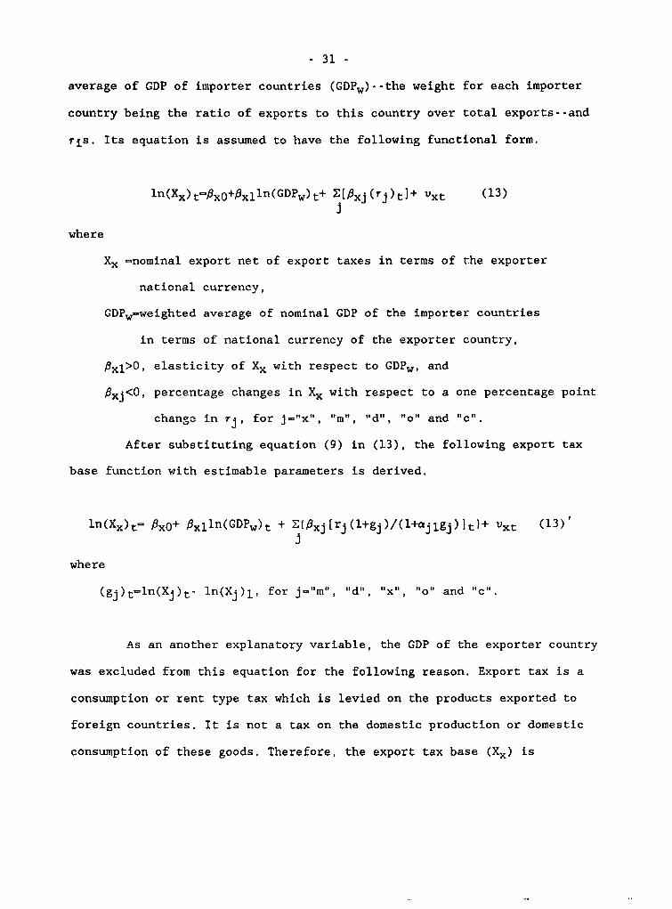
average of GDP of importer countries (GDPw)--the weight for each importer
country being the ratio of exports to this country over total exports--and
ris. Its equation is assumed to have the following functional form.
ln(Xx)t.pxo+,8xlln(GDPw)t+ E[Pxj(rj)t]+ vXt (13)
where
Xx -nominal export net of export taxes in terms of the exporter
national currency,
GDPW-weighted average of nominal GDP of the importer countries
in terms of national currency of the exporter country,
Px1>O, elasticity of Xx with respect to GDPW, and
Pxj<O, percentage changes in Xx with respect to a one percentage point
chango in rj, for j- "x", mti, "d", "o" and "c".
After substituting equation (9) in (13), the following export tax
base function with estimable parameters is derived.
ln(Xx)t= PxO+ Pxlln(GDPw)t + E(Pxj[rj(l+gj)/(l+ajlgj)]t)+ vxt (13)'
where
(gj)t=ln(Xi)t- ln(Xj)l, for j-"m", "d", x, and c
As an another explanatory variable, the GDP of the exporter country
was excluded from this equation for the following reason. Export tax is a
consumption or rent type tax which is levied on the products exported to
foreign countries. It is not a tax on the domestic production or domestic
consumption of these goods. Therefore, the export tax base (Xx) is

- 32 -
considered to be a function of the factors which affect the demand of
foreigners for the exportable products, in other words, the GDP of importer
countries, relative prices and ris. Indeed, the factors which inflt?nce
domestic production or consumption of these products may affect Xx through
the price mechanism. Equation (13)' implicitly incorporates the impact of
such changes on Xx because the nominal value of Xx and GDPW are entered
into that equation.
Since the primary objective of this study is to estimate individual
and overall tax elasticities with respect to the GDP of the home country,
the export tax revenue and base functions are excluded from the entire
model as an empirical framework for estimating tax elasticity and the
revenue impact of discretionary tax measures.
Equations (10), (11) and (12) perform the individual tax base
functions block of the model. Estimates of their parameters are obtained by
estimating the parameters of equations (3)', (10)', (11)' and (12)' by
means of a non-linear simultaneous-equation econometric estimation method.
Identities Block
Disposable income is the difference between GDP and direct taxes,
that is,
(yd)t (GDP)t- (Tc)t- (To)t (14)

- 33 -
All of the variables included in (14) appear in logarithmic form in the
equations developed above--equations (3), (10), (11) and (12). For reasons
of convenience, it is also transferred to a log-linear form as follows:
ln(yd)t In(GDP)t ln(TC)t In(TO)t
e -e -e - e (15)
Using Taylor's series, equation (15) is expanded around the
geometric mean value of the variables included in it, that is,
ln(Yd)t - 7o + lln(GDP)t + 721n(Tc)t + 731n(TO)t (16)
where
an ln(yd)* (GDP/Yd)*ln(GDP)*+(Tc/yd)*ln(Tc)*+(To/yd)*ln(To)*
71-(GDP/yd) >0,
72-(Tc/Yd)* <0,
73-(To/Yd)* <0,
and "*" denotes geometric mean value.
The total tax revenue net of export taxes is simply the sum of the
other individual tax yields, that is,
(T)t= (Tc)t + (To)t + (Td)t +(Tm)t (17)
Using the method mentioned above and expanding equation (17) around
the geometric mean value of the variables included in it and then making a
simple manipulation, this equation is converted to the following log-linear
form which allows a direct estimate to be made of the automatic response of
the overall tax system to variation in GDP:

- 34 -
ln(T)t- 60+ 6eln(Tc)t+ Soln(TO)t+6dln(Td)t+6mln(Tm)t (18)
where
60- log(T)*- E[(Ti/T)*log(Ti)*,
6 i- (Ti/T)* >0, and i-c, o, d, m.
Equations (16), (17) and (19) are deterministic functions whose
parameters can be estimated either by using the mean value of time series
data on the variables included in them or by the OLS estimation method.
Entire Model And Its Dynamic Multipliers
Equations (3)--for isc, d, m, o--, (10), (11), (12), (16) and (18)
provide the structural form of the model developed in this s,udy (Table 1).
Efficient and consistent estimates of its parameters are obtained by
estimating the parameters of equations (3)', (10)', (11)', (12)', (16) and
(18) by means of a simultaneous-equation non-linear econometric estimation
technique (Table 2).4
Using the estimated parameters, the time series data on ris are
generated by means of equation (9). These data can be used independently to
investigate the impact of changes in individual tax systems on various key
macroeconomic variables, such as savings, inflation, investment, economic
growth, international balance of payments, and so on. To simplify the
derivation of the revenue impact of changes in each individual tax system
4/ There are four simultaneous-equation non-linear estimation methods.These are: three-stage non-linear least squares, iteration, search andmaximum likelihood estimation techniques. For more details, seeMaddala(1977), pp. 144-146; also Fair(1984) pp. 120-138.

- 35 -
Table 1: Structural Form of the Model
log(Td)t A.dadO+ Adadll0g(Xd)t + (l-Ad)log(Td)t-l+ Adad2(Td)t+ Udt
log(Tm)t- AlnamO+ Am*mllg(Xm)t + (l-Am)log(Tm)t-l+ A%im2(7m)t+ Umt
log(Tc)t- caco+ Acacllog(Xc)t + (l-Xc)log(Tc)t-l-. Acac2(rc)t+ Uct
log(To)t-= AoaoO+ Xoaollog(Xo)t + (l-Ao)logkTO)t_.+ XoQo2(ro)t+ Uot
ln(Xd)t- OdO Pdlln(Yd)t+ Pd2(7m/fd)t+ vdt
ln(Xm)t- PmO+ 8mlln(GDP)t+ Pm2(rm/rd)t+ Pm3(rc)t + umc
ln(XC)t- Pco+ 6clln(GDP)t+ Pc2(Tc)t + Pc3(?m/Td)t+ Vct
ln(T)t - 60+ Sdln(Td)t+ 6mln(Tm)t+ Scln(Tc)t+ Soln(TO)-
ln(Yd)t °O +-tlln(GDP)t+ 721n(TC)t+ 131n(TO)t
(Tm/Td)t= 90 + l(rm)t + 02(fd)t
whereTd= Tax on domestic transactions (endogenous variable),Tm- Import tax (endogenous variable),Tc= Corporate income tax (endogenous variable),To= Other direct taxes (endogenous variable),Xd- Private consumption (endogenous variable),Xm= Imports (endogenous variables),Xc= Value added in non-agriculture sector (endogenous variable),XO= GDP- gross domestic products (exogenous variable),ri= The ith individual realized tax rate (exogenous variable),
for i- d, m, c, o,Yd- Disposable income (endogenous varI'able),r- Total tax revenue net of export taxes (endogenous variable).

- 36 -
Table 2: Entire Model with Estimable Parameters
l+9d1ln(Td)t- AdcadO+ Adadlln(Xd)t + (l-Ad)ln(Td)t-l +Adc1d2 rd -+g 1 - I-+dt
1+Adcldlgd J t
ln(Tm)t° Amamo+ Amamlln(Xm)t + (l-Xm)ln(Tm)t-l +Amsm2 jrm ]+mtl+Amamlgm t
[ 1+g 1ln(Tc)t Acaco+ Acaclln(Xc)t + (l-Ac)ln(Tc)t-l +Ac%2 rc g J
1+A\CIc lgC- t
r l+g0 1ln(TO)t- Aoaoo+ Aoaolii-.Xo)t + (l-Ao)ln(To)t-l +Aoao2 r0 - g +
1 +A\oaolgo .t
r rm[ (l+gm)/(l+amlgm)] 1ln(Xd)t P-dO+ Pdlln(Yd)t+ Pd2 g + vdt
rd[(l+gd)/(l+adlgd)] t
frm[ (l+gm)/(l+amlgm)] 1 rC(l+gc)ln(Xm)tsPmo+PmllnC(GDP)t+Pm2 +Pm3 +vmt
rd[(l+gd)/(l+adlgd)] t (l+aclgc)
l+gd 1 rrm(l+gm)/(l+amlgm)ln(X0)t- PcO+ Pclln(GDP)t+ 1+c2 rd + Pc3 - +Uct
1+atdlgd Jt rd(l+gd)/(I+cgdlgd) t
ln(T)t - 60+ 6dln(Td)t+ 6mln(Tm)t+ 6cln(Tc)t+ 601n(To)t
ln(Yd)t = YO +ylln(GDP)t+ y2ln(Tc)t+ y31n(TO)t
g(i)t- ln(Xi)t- ln(Xi)O for i-d, m, c, o
Est-mating the parameters of the model requires time series data on Tis, T,Xis, ria, and GDP which are readily available for most LDCs in GFS(an IMFpublication) and World Tables (a World Bank publication).

-37 -
from the estimated parameters of the model, this study uses the generated
time series data on ris to linearize ('m/'d) in order to keep the entire
model in semi-log linear form. Its linear form is obtained by expanding it
around the mean value of ris using Taylor's series, which is,
(Tm/rd)t -0 + 1l(rm)t + 6 2(id)t (19)
where
00(Tm/rd)* >0,
0l1(l/rm)* >0, and
2- [rm/(Td)2]* <0.
Equation (19) is a deterministic equation whose parameters can be
estimated using either the mean value of the generated time series data on
ris or the OLS estimation technique.
Consequently, the structural form of the model with estimated
parameters will include ten equations--equations (3), for i-d, c, o, m, and
(10), (11), (12), (16), (18) and (19)-- and ten endogenous, five exogenous,
and four predetermined endogenous variables. It is a simultaneous equations
system which can be written in the following form using matrix notation.
A + B(Y)t + C(Y)t-l + D(X)t 0. (21)
where
A- lOxlO matrix of constant terms,
B- lOxlO matrix of coefficients of dependent variables,
C- lOxlO matrix of coefficients of lagged dependent variables,

- 38 -
D- lOx5 matrix of coefficients of exogenous variables,
Yt- lOxI column vector of endogenous variables, and
Xt- 5xl column vector of exogenous variables.
By treating predetermined lagged dependent variables as exogenous
ones, the model is an ordinary equations system; by solving it, the reduced
form of the model is obtained, that is,
Yt= -B-1A - B-lC(Y)t-l B-lD(X)t (22)
In this equation, each of the endogenous variables is a function of all the
exogenous variables included in the model--these are ln(GDP)t, ln(Ti)t-l
and ris. The ijth element of [-B-1 D] measures the instantaneous impact of a
unit change in the jth exogenous variable on the ith endogenous variable
(impact multipliers).
For instance, the ith individual tax yield equation in its reduced
form will be:
ln(Ti)t=4iO + 4illn(GDP)t + ZOij2ln(Tj)t-l + ZOij3(rj)t (20)
where
j cm, d, c, o,
Oil -short-run elasticity of the Ti with respect to GDP,
4ij3=percentage changes in Ti due to a one percentage point change in
rj; for i#j, it measures the short-run impact of changes in the
jth individual tax system on the ith individual tax revenue
(cross-DTM indirect response),

- 39 -
and, for i-J, it measures the short run overall impact of a one percentage
point increase in ri on its corresponding tax yield (sum of the own-DTM
direct and indirect responses). Its short run own-DTM direct response is
measured by the coefficient of ri in equation (3), in other words, ai3;
therefore, its short run own-DTM indirect response is simply measured by
'ii3-ji3-
The elements of [-B-1D] related to the coefficients of ln(GDP),
measuring the short-run tax elasticities, and rjs, measuring the short-run
revenue impacts of DTMs, are presented in Tables 3-7.
By treating lagged dependent variables as endogenous ones, the
structural form of the model is a system of difference eguations; by
solving it, the final form of the model is obtained which is,
Yt [I + B 1lC]Pl B-1 A] + [I + B-lC]-G[-B-lD](X)t (23)
where
I= lOxlO unit matrix.
In this equation, each of the endogenous variables is a function of all the
exogenous variables included in the model--these are ln(GDP) and rjs. The
ijth element of ([I+B-lC]-l[-B-lD]) measures the total impact of a unit
change in the jth exogenous variable on the ith endogenous variable (total
multipliers). For instance, the ith individual tax yield equation in its
final form will be:
ln(Ti)t= 'iO + Oilln(GDP)t + ZOij2(rj)t for j=m,d,c,o (21)

- 40 -
Table 3: Short Run and Long Run Individual and Overall Tax Elasticitiesin Terms of the Parameters Included in the Model
Tax Yields Tax Elasticities
A. Short Run:
Total Tax $mamlPml+6dadlpdl(Yl+aclOcl72+Y3aol)+6c%clpcl+&oaol(T)
-Import Tax %mlpml(Tm)
-Consumption Tax adlpdl(l+aclPcl72+Y73aol)(Td)
-Corporate Income Tax aclocl(Ta)
-Other Direct Taxes a(To)
B. Lon, Run:
Total Tax (T)
6mamlfml 6d'tdlpdl [ alcl72+ 73aol 1 6caclcl boaol+ - x Xy + + 1+ +
1- am2 1-Qd2 1 - ac2 1-o 2 J 1 -ac2 l-ao 2
-Import Tax amlpml(Tm)
1- am2
-Consumption Tax adlpdl aclPcl72+ 73l1ol(Td) x al + - +
l-ad2 1 - %c2 1-ao2
-Corporate Income Tax aclocl(TC)
1 -ac2
-Other Direct Taxes aol(To)
1-ao2

- 41 -
Table 4: Direct and Indirect Responses of Individual and Overall TaxRevenues to the Changes in the Domestic Consumption Tax System
Type of Tax Percentage Changes in Tax Yields due to A7d=l%
A. Short Run Response:
Total TaxDirect Response Sdad3
Indirect Response 6mamlfm262+&dadlO2(Pd2+72PdlaclPc3)+6cac1Pc382
-Import TaxIndirect Response Qmlflm202
-Consumption TaxDirect Response cad3
Indirect Response adl62(pd2+ 72#dlaclfc3)
-Corporate Income TaxIndirect Response aclPc362
B. Long Run Response:
Total TaxDirect Response 6d(ad3)/(l - ad2)
Indirect Response
6d'dl 6 2 [ 72Pdl%clfc3 6 mamlfm262 6 cac%1c302x d2 + + +
1-cad2 L - 'c2 1 - am2 1 - ac2
-Import TaxIndirect Response (`mlfm202)/(l - dm2)
-Consumption TaxDirect Response (ad3)/(l - td2)
Indirect Response adlO2 72 `dl%clfc3 1x fd2+
1~~ -lad2 1 2 JC-Corporate Income Tax
Indirect Response (aclPc362)/(1 - %c2)
- 42 -
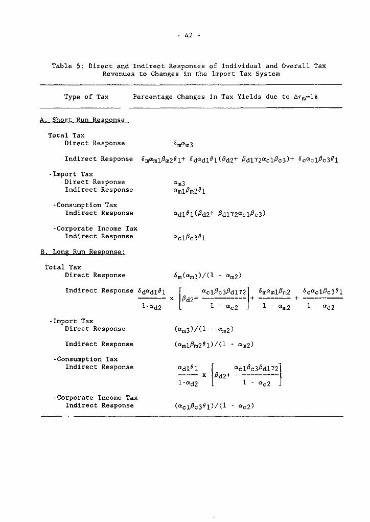
Table 5: Direct and Indirect Responses of Individual and Overall TaxRevenues to Changes in the Import Tax System
Type of Tax Percentage Changes in Tax Yields due to Arm=l%
A. Short Run Response:
Total TaxDirect Response 6mQm3
Indirect Response 6mamlPm2Gl+ Sdadl0l(Pd2+ Pdl2Y2acl/3c3)+ ScaclPc3Ol
-Import TaxDirect Response am3Indirect Response amlPn281
-Consumption TaxIndirect Response adl0l(Pd2+ PdlM2aclPc3)
-Corporate Income TaxIndirect Response aclfic3O1
B. Long Run ResRonse:
Total TaxDirect Response 6m(am3)/(l - am2)
Indirect Response 6dodl9l r %clc3fidl121] 6mmlfin2 Sc'clPc301x /d2+ --- ---- + +
1-id2 1 -ac22 1am2 1 -c2
-Import TaxDirect Response (am3)/(l - `m2)
Indirect Response (am1Pm2Ol)/(l - am2)
-Consumption TaxIndirect Response crdlOl aclOc3fidl2
fx d2+ -
1-'d2 1 - ac2
-Corporate Income TaxIndirect Response (QclPc30l)/(l - ac2)

- 43 -
Table 6: Direct and Indirect Responses of Individual and Overall TaxRevenues to the Changes in the Corporate Income Tax System
Type of Tax Pe.centage Changes in Tax Yields due to Arc=l%
A. Short Run Response:
Total TaxDirect Response 6ccc3
Indirect Response 6cQcl6c2 + 6dadlPdlY2(cclPc2 + ac3) +6mamlOm3
-Import TaxIndirect Response amlPm3
-Consumption TaxIndirect Response adlPdly2(%clPc2 + ac3)
-Corporate Income TaxDirect Response ac3
Indirect Response %clPc2
B. Long Run Response:
Total TaxDirect Response (6c%c3)/(1 - ac2)
Indirect Response 6caclfc2 6dcdlPdl72(acl#c2 + ac3) amlfm3= ==_+ +
(1 - ac2) (1 - ac2)(1 -ad2) I-am2
-Import taxIndirect Response aml6m3/(l-m2)
-Consumption TaxIndirect Response cdlPdl72(aclPc2 + ac3)
(1 - ad2)( 1 - ac2)
-Corporate Income TaxDirect Response (ac3)/(l - ac2)
Indirect Resnonse (aclPc2)/(l - 'c2)
- 44 -
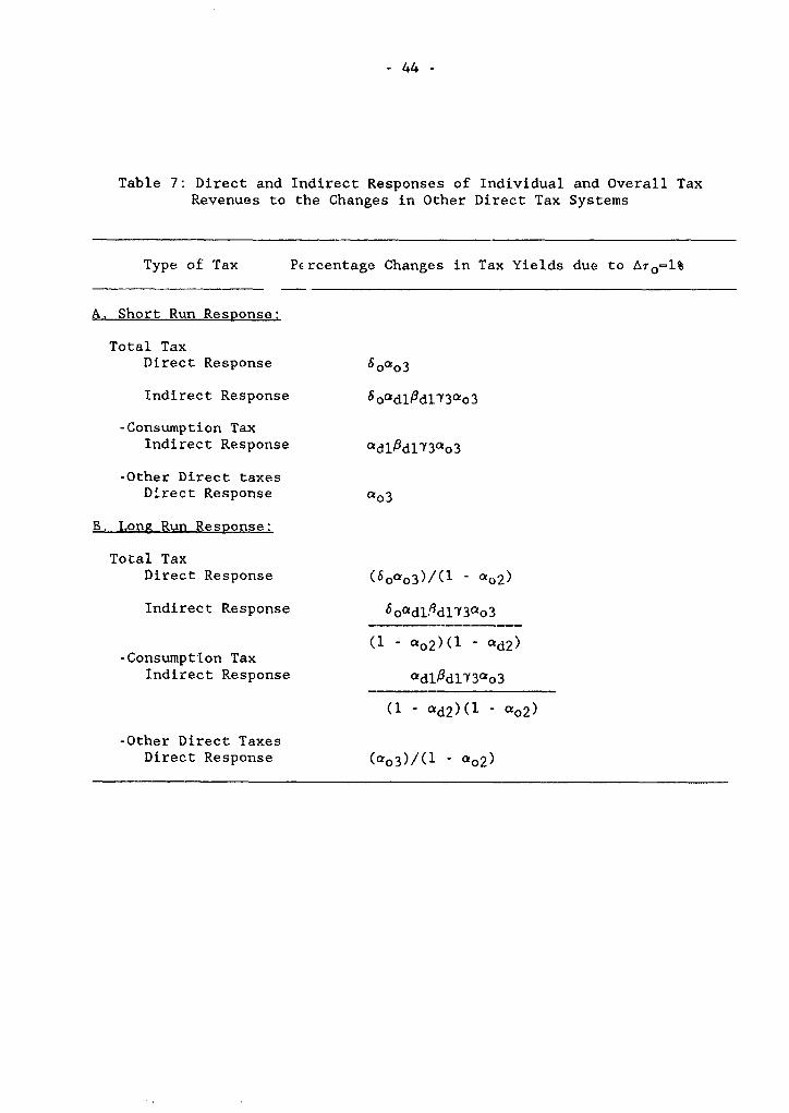
Table 7: Direct and Indirect Responses of Individual and Overall TaxRevenues to the Changes in Other Direct Tax Systems
Type of Tax PErcentage Changes in Tax Yields due to Arol%
A. Short Run Response:
Total TaxDirect Response Soao3
Indirect Response Soadlfdld3ao3
-Consumption TaxIndirect Response adl6dl73ao3
-Other Direct taxesDirect Response ao3
B. Long Run Response:
Total TaxDirect Response (60ao3)/(l - a0 2)
Indirect Response 6oadlPdl73ao3
(1 - a 0 2 ) (1 - ckd2)-Consumption Tax
Indirect Response adlPdl3czO3
(1 - ad2)(1 - ao2)
-Other Direct TaxesDirect Response (ao3)/(l - ao2)

- 45 -
where
i'il -long-run elasticity of Ti with respect to GDP, and
Oij2-the long-run Response of Ti to one percentage point change in rj
The elements of ([I+B-lC]-l[-B-lD]) which are related to the
coefficients of ln(GDP)--the long run individual and overall tax
elasticities--and r;s--the long run direct and indirect responses of tax
revenues to DTMs-- are presented in Tables 3-7.
To summarize, all the existing estimation methods of tax elasticity
suffer from a specification bias which is created in the process of dealing
with the lack of an observable quantitative variable capable of reflecting
all changes in an individual (or overall) tax system in public finance. The
estimation technique developed in this chapter is a dynamic simultaneous-
equation econometric model of taxation which deals with this lack and thus,
with its consequences on the estimate of tax elasticity. That is: (i) as
representative of each individual tax system, its "average effective tax
rate net of endogenous changes in its tax yield and base" (AETRN) is
introduced in the model on which time series data are automatically
generated in the process of estimating the model parameters; (ii) this
model incorporates both the direct and indirect responses of each
individual tax yield to the changes in its own as well as other individual
tax systems, i.e., own-DTM direct, own-DTM indirect and cross-DTM indirect
responses; and (iii) its application requires only historical time series
data on individual tax revenues and bases and gross domestic products, all
of which are already available for most countries.
The parapeters of the model are estimated by means of a
simultaneous-equation econometric technique. Its impact and total

- 46 -
multipliers (dynamic multipliers) are then derived by solving it
respectively as an ordinary and a difference equations system. These
multipliers measure the short run and long run (i) elasticities of
individual tax yields, individual tax bases and overall tax revenue with
respect to CDP, and (ii) responses of each individual tax yield and tax
base to the changes in its own and other individual tax systems.
In addition to its application as a method for estimating tax
elasticity and the revenue impact of DTMs, this model can be used as an
empirical fiamework:
(1) to forecast a government's revenue from various sources of
taxation;
(2) to evaluate the macroeconomic impact of a cax reform program which
is aimed at either generating additional revenue and/or dealing
with specific economic problems--this simply requires converting
the DTMs included in that reform into AETRNis (for more details see
Appendix C); and
(3) to deal with various tax related economic issues which may require
further disaggregation of individual tax yields and bases--for
example, to investigate the welfare impact of moving from
differer.tial tariffs towards uniform ones, which is often
recommended by the Bank, or to examine the controversial view that
uniform tariffs result in uniform rates of effective protection in
industrial and non-industrial activities.

CHAPTER III
APPLICATION OF THE MODEL
The objective of this chapter is to highlight the contribution of
discretionary tax measures to trends of tax shares and tax effort in two
SSA countries during the past two decades. These are Malawi and Mautitius
which have exhibited different trends in an important aspect of public
finance, that is, a shift from the taxation of international trade to the
taxation of domestic transactions which has taken place in Malawi while, in
Mauritius, government's reliance on foreign trade taxes has risen. The
model developed in the previous chapter is econometrically applied to the
time series data of these countries in order to accomplish this aim.
In the first section, the estimation method and results are
discussed, and the dynamic multipliers of the model are derived. Using the
obtained results, the trends of tax shares and effort are analyzed in the
second section.
Estimation Method and Empirical Results
Time series data are used to estimate the parameters of the model.
These data and their corresponding sources are supplied in the Appendix A.
Because of using time series data, there is the possibility of the
presence of serial correlation. If this is ignored, the estimate of the
parameters will be (a) inconsistent, which means that conducting any kind
of test related to these parameters will be unreliable, and (b) biased,

- 48 -
that is, parameters of such an equation will be overestimated (or
underestimated) if the coefficient of the serial correlation is positive
(or negative).1 To test the hypothesis of zero autocorreiation in the tax
base and tax yield equations, "DW" and "h" statistics are respectively used
in this study.2
To estimate these two statistics, the parameters of the model were
estimated by means of a non-linear two-stage least squares (N2SLS) method.
All of the estimated parameters had the expected signs and plausible sizes
except those of the lagged depender.c variable in Malawi's domestic
consumption tax yield function and those of other direct tax and domestic
consumption tax equations of Mauritius, which had contrary signs and were
insignificant. These variables were dropped from those equations and the
model parameters re-estimated by means of N2SLS. Then, the estimation
results were used to calculate the "h" and "DW" statistics which are
presented in Table 8.
It is apparent from the information supplied in this Table that the
hypothesis of zero serial correlation is not rejected at the 5 percent
level in the domestic consumption tax yield and import tax base equations
1/ See Maddala (1987), pp. 371-73.
2/ DW statistics are derived under the assumption that regressors are fixed(non-stochastic); hence, they are not applicable in cases where some ofthe regressors are lagged dependent variables, such as the tax revenueequations in the model developed in this study. In such cases, "h"statistics are applied whose estimate is derived as follows:
h-p[n/ (l-na2)]0.5
where p-coefficient of serial correlation, n-number of observation anda-sample standard deviation of coefficient of the lagged dependentvariables. This statistic has standard normal distribution and the nullhypothesis of zero autocorrelation is rejected at the 5 percentsignificance level if h > 1.64; for more details see Durbin (1970).

of Malawi. The test is inconclusive in the import and corporate income tax
base functions of Mauritius.
The following procedure was used to deal with this econometric
problem in these equations. Using the first-order autocorrelation scheme,
Table 8: Test Results for Serial Correlation
Equations Malawi Mauritius
DW h DW h
Tax Revenue Block:Import Tax -- 2.54 -- 2.07Consumption Tax 0.512* - 1.86 -Corporate Income Tax - 1.70 - 2.72
Other Direct Tax - 1.84 1.77
Tax Base Block:Import Tax 0.940* - 1.16**Consumption Tax 1.65 1.98Corporate Income Tax 1.54 3.04**
* Hypothesis of no serial correlation is not rejected.**The test is inconclusive.
the original equation was lagged one period. Both sides of thie equation
were then multiplied by the coefficient of serial correlation (p) whose
estimate is unknown; its subtraction from the original equatior produced a
new equation in which disturbance terms were not correlated pairwisely.
Finally, this new equation was replaced by the original one in the process
of estimation.
After correcting for serial correlation, the efticient and
consistent estimates of r,arameters of the model as a difference equations

- 50 -
system were obtained by means of a non-linear 3SLS technique. The N3SLS
estimation results--the stzuctural form of the models with estimated
parameters--for Malawi and Mauritius respectively are presented in lables 9
and 10.
In order to test the goodness-of-fit of the entire estimated model
a within-sample dynamic simul&tion was performed for all of the endogenous
variables. A comparison of the actual and simulated values gives an
indication of whether the model is able to capture the historical behavior
of the endogcnous variables. The simulated and actual values of the
individual tax yields (logs) for Malawi and Mauritius respectively are
shown in figures 2a-2d and 3a-3d. These charts indicate that these models
are fairly accurate in capturing the historical movements of those
variables. The coefficients of determination and mean-sum of squares of
errors presented in Tables 9 and 10 support the goodness-of-fits observed
in Figures 2a-2d and 3a-3d.
The estimated coefficients of all of the explanatory variables in
these models have the expected signs and plausible sizes. All are
significantly different from zero at more than 95 percent probability level
except (a) those of ris in the corporate income tax base equation of
Malawi--these being significantly different from zero at the 85 percent
probability level--and (b) the adjustment coefficients of the Tm and To in
this country--these being significantly equal to one.
Consequently, in both countries, discretionary tax measures have had
a significant impact on both individual tax revenues and bases during the
past two decades. This means that the market mechanism works fairly well in
these countries and that tax policy has been an effective policy instrument
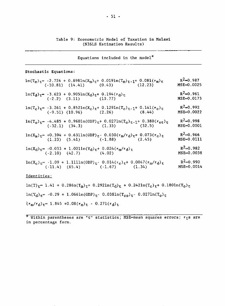
- 51 -
Table 9: Econometric Model of Taxation in Malawi(N3SLS Estimation Results)
Equations included in the model*
Stochastic Equations:
ln(Tm)t- -2.726 + 0.8 981n(Xm)t+ 0.0191n(Tm)t.l+ 0.081(rm)t R2-0.987(-10.81) (14.41) (0.43) (12.23) MSE=0.0025
ln(Td)t- -3.623 + 0.9051n(Xd)t+ 0 .1 94(7d)t R2-0.961(-2.2) (3.11) (15.77) MSE=0.0173
ln(Tc)t- -3.261 + 0.8521n(Xc)t+ 0.12 91n(Tc)t-l+ 0.1 4 1(rc)t R2-0.992(-9.51) (10.96) (2.26) (8.44) MSE=0.0022
ln(TO)t= -4.485 + 0.9601n(GDP)t+ 0.0271n(TO)t-l+ 0 .38 0(rot)t R2=0.998(-32.1) (34.3) (1.35) (32.5) MSE=0.0001
ln(Xm)t- +0.394 + 0.6311n(GDP)t- 0.03 0(rm/rd)t+ 0 .0 73(rc)t R2 -0.966(1.23) (5.41) (-1.88) (2.45) MSE-0.0111
ln(Xd)t= -0.033 + 1.0211n(Yd)t+ 0.02 4(7m/rd)t R2=0.982(-2.10) (42.7) (4.02) MSE=0.0038
ln(Xc)t= -1.09 + 1.lllln(GDP)t- 0 .0 1 4(rc)t+ 0.004 7 (Tr/rd)t R2=0.990(-11.4) (65.4) (-1.67) (1.34) MSE=0.0014
Identities:
ln(T)t= 1.41 + 0.28 6n(Tm)t+ 0.2 9 21n(Td)t + 0.24 21n(Tc)t+ 0.1801n(TO)t
ln(Yd)t= -0.29 + 1.0661n(GDP)t- 0.0381n(Tco)t- 0.0271n(TO)t
(rm/rd)t- 1.845 +0.08(rm)t - 0.271(Td)t
* Within parentheses are "t" statistics; MSE-mean squares errors; ris arein percentage form.

- 52 -
Table 10: Econometric Model of Taxation in Mauritius(N3SLS Estimation Results)
Equations included in the model*
Stochastic Equations:
ln(Tm)t- -1.643 + 0.6 8 31n(Xm)t+ 0.2 311n(Tm)t-l+ 0.04 8(rm)t R2 -0.998(-6.30) (10.41) (4.22) (8.53) MSE-0.0001
ln(Td)t- -3.817 + 0.9 9 81n(Xd)t + 0 .1 6 9(rd)t R2C0.999(-236.4) (429.5) (83.7) MSE-0.00004
ln(TC)t -3.68b + 0.8 2 81n(Xc)t+ 0.0951n(Tc)t-l+ 0.3 30(rc)t R2 -0.992(-7.91) (10.1) (1.44) (8.31) MSE=0.0089
ln(TO)t- -3.965 + 0.9721nkGDP)t+ 0 .22 3(rot)t R2=0.997(-31.6) (69.7) (23.9) MSE=0.0022
ln(Xm)t- -1.844 + 1.1571n(GDP)t- 0 09 1(rm/rd)t+ 0.04 7(rc)t R2 -0.994(-1.12) (50.9) (-2.30) (3.44) MSE=0.0066
ln(Xd)t- 2.296 + 0.7 6 3Ln(Yd)t+ 0.08 8(7m/Td)t R20.996(1.19) (8.62) (2.51) MSE-0.0041
ln(Xc)t- -0.258 + 0.9931n(GDP)t- 0.0 20(rc)t+ 0.0 9 5(rm/rd)t R20.999(-2.85) (83.2) (-3.41) (6.43) MSE=0.0009
Identities:
ln(T)t- 1.25 + 0.5041n(Tm)t+ 0.1551n(Td)t + 0.0991n(Tc)t+ 0.2451n(TO)t
ln(Yd)t- -0.258 + 1.0561n(GDP)t- 0.0201n(Tc)t- 0.0361n(TO)t
(Tm/fd)t 2.99 + 0.06(rm)t - 0.54(7d)t
* Within parentheses are "t" statistics; MSE=mean squares errors; ris arein percentage form.

- 53 -
Figures 2a-2d: Actual and Predicted Values of IndividualTax Yields in Malawi (1965-85)
a: Import Tax b: Dan. Commptiou tax
:Corporate Income Ta d: Other direct Taxes
a Actual tax yield Predicted tax yield

- 54 -
Figures 3a-3d: Actual and Predicted Values of IndividualTax Yields in Mauritius (1965-85)
I: mport Tax b: Don. Cousimption Tax
66. ~ ~ ~ ~ ~ ~ ~ .
- ~~~~~~~~~~~~~~~~~*
* e - u a.a X a a-
c: Corporate Income Tax d: Other Direct Taxes
~~~~~~~~~~~'m
40.~~~~~~~e
a*Actua t yield * ee * e *ld
* Actual tax yield __ Predicted Ta x ield

- 55
in mobilizing resources from the private sector to the public sector. This
result strongly rejects the view that mobilizing resources through the tax
system has been difficult in SSA countries (see Shalizi and Squire).
Tables 9 and 10 respectively presented the structural form of the
models with estimated parameters for Malawi and Mauritius. Using the method
explained in Chapter II, each of these models was solved as ordinary and
difference equations systems in order to estimate the short run and long
run impacts of changes in exogenous variables, ln(GDP) and ris, on
endogenous ones, individual tax yields and bases and total tax revenue. The
obtained results for Malawi and Mauritius are respectively presented in
Tables 11 and 12 --where built-in elasticity of tax yields and bases with
respect to GDP are supplied in column (a) and columns (b)-(e) represent the
responses of each of the tax yields and bases to the changes in each of the
individual tax systems (Ari-l) included in the model.
It is revealed from column (a) that the total and individual tax
revenues are inelastic with respect to GDP except for import tax yield in
Mauritius and corporate income tax revenue in Malawi whose long run
elasticities exceed one. These exceptions emerge from the fact that imports
in Mauritius and value added in the non-agriculture sector in Malawi grow
faster than GDP. In other words, these two individual taxes are still
inelastic with respect to their corresponding economic tax bases (0.78 and
0.91 respectively).
The data presented in columns (b) and (c) indicate that the overall
response of the total tax revenue to a one percentage point increase in Tm
is larger than its direct response in both countries. This is due to the
fact that a rise in rm reduces imports but raises private consumption and

- 56 -
Table 11: Short Run and Long Run Impact of Changes in Individual TaxSystems and GDP on Tax Revenues and Bases in Malawi*
Tax Revenues and Aln(GDP)-l% ATm-l Ard-1 A 1ro-Bases (a) (b) (c) (d) (e)
A.Short Run Impacts:
Aln(T) 0.8336 0.0229 0.0567 0.0486 0.0657(0.0232) (0.0566) (0.0341) (0.0684)
Aln(Tm) 0.5666 0.0788 0.0073 0.0656 0.0000(0.0810)
Aln(Td) 0.9295 0.0017 0.1881 -0.0042 -0.0091(0.1940)
Aln(T.) 0.9466 0.0003 -0.0011 0.1291 0.0000(0.1410)
tln(TO) 0.9600 0.0000 0.0000 0.0000 0.3800(0.3800)
Aln(Xm) 0.6310 -0.0024 0.0081 0.0730 0.0000Aln(Xd) 1.0270 0.0019 -0.0065 -0.0046 -0.0101Aln(XC) 1.1110 0.0004 -0.0013 -0.0140 0.0000
B.Long Run Impacts:
Aln(T) 0.8740 0.0233 0.0567 0.0534 0.0676(0.0236) (0.0567) (0.0392) (0.0703)
Aln(Tm) 0.5776 0.0804 0.0074 0.0668 0.0000(0.0826)
Aln(Td) 0.9243 0.0017 0.1882 -0.0048 -0.0094(0.1940)
Aln(TC) 1.0868 0.0004 -0.0012 0.1482 0.0000(0.1619)
Aln(TO) 0.9866 0.0000 0.0000 0.0000 0.3905(0.3905)
Aln(Xm) 0.6310 -0.0024 0.0081 0.0730 0.0000Aln(Xd) 1.0213 0.0019 -0.0065 -0.0053 -0.0104Aln(Xc) 1.1110 0.0004 -0.0013 -0.0140 0.0000
F Within the parentheses is the direct response of tax revenue to the DTMs.

57 -
Table 12: Short Run and Long Run Impacts of Changes in Individual TaxSystems and GDP on Tax Yields and Bases in Mauritius*
Tax Revenues and Aln(GDP)-1% Arm-1 A?dl Arc-l ArO-Bases (a) (b) (c) (d) (e)
A.Short Run Impacts:
Aln(T) 0.8364 0.0237 0.0317 0.0465 0.0537(0.0328) (0.0262) (0.0327) (0.0546)
Aln(Tm) 0.7902 0.0445 0.0336 0.0321 0.0000(0.0650)
Aln(Td) 0.7649 0.0052 0.1221 -0.0048 -0.0061(0.169)
Aln(TC) 0.8222 0.0047 -0.0426 0.3134 0.0000(0.3300)
Aln(TO) 0.9720 0.0000 0.0000 0.0000 0.2230(0.2230)
Aln(Xm) 1.1570 -0.0055 0.0492 0.0470 0.0000Aln(Xd) 0.7665 0.0052 -0.0470 -0.0048 -0.0061Aln(Xc) 0.9930 0.0057 -0.0514 -0.2000 0.0000
B.Long Run Impacts:
Aln(T) 0.9644 0.0305 0.0363 0.0545 0.0537(0.0426) (0.0262) (0.0361) (0.0546)
Aln(Tm) 1.0276 0.0578 0.0437 0.0417 0.0000(0.0845)
Aln(Td) 0.7636 0.0052 0.1222 -0.0053 -0.0061(0.1690)
Aln(TC) 0.9085 0.0052 -0.0470 0.3463 0.0000(0.3650)
Aln(TO) 0.9720 0.0000 0.0000 0.0000 0.2230(0.2230)
Aln(Xm) 1.1570 -0.0055 0.0492 0.0470 0.0000Aln(Xd) 0.7652 0.0052 -0.0469 -0.0053 -0.0061Aln(Xc) 0.9930 0.0057 -0.0514 -0.0200 0.0000
§ Within the parentheses is the direct response of tax revenue to the DTMs.

- 58 -
hence, value-added in the non-agriculture sector. As a result, import tax
declines and domestic consumption and corporate income taxes rise, causing
a net indirect increase in total tax revenue. This process is reversed
when rd rises, that is, the overall response of the total tax revenue to a
one percentage point rise in rd falls short of its direct response in both
countries.
As far as changes in corporate income and other direct taxes are
concerned, an increase in rc indirectly raises import tax and reduces
domestic consumption and corporate income tax yields, resulting in a
decline in the direct response of the total tax yield to rTc This process
is reversed when ro rises.
It is worth mentioning that, in Malawi, the elasticity of the
domestic consumption tax revenue with respect to GDP is higher than that of
the import tax yield while, in Mauritius, the former falls short of the
latter. Furthermore, in Malawi, the direct revenue impact of changes in
the domestic consumption tax system is much higher than that of the same
changes in the import tax system while, in Mauritius, the former is smaller
than the latter. These differences will obviously require a different
reform combination of discretionary tax measures if such a reform is aimed
at shifting from the taxation of international trade to the taxation of
domestic transactions in these countries.
Trends of Tax shares and Tax Effort
During the 1965-1985 period, the tax effort (total tax revenue over
GDP) has grown by an annual average rate of 4.6 percent in Malawi and 1.4

- 59 -
percent in Mauritius. The share of domestic consumption in total tax
revenue 4n Malawi has increased by an average annual rate of 2.56 percent
and that of import tax yield has declined by 1.72 percent. In Mauritius,
the trends of these shares have been reversed, recording average annual
percentage changes of -0.62 and +1.83 respectively. As a result, the ratio
of domestic consumption tax over import tax, measuring the size and
direction of shift from the taxation of imports to the taxation of domestic
transactions has changed by +4.3 and -2.4 percent per annum in these
countries respectively.3
The time series data generated on ris reveal that fiscal
authorities have taken a variety of discretionary tax measures in both
countries during the same period, to the extent that rm' Td, rc and ro have
increased respectively by average annual percentage points of 0.49, 0.44,
0.91 and 0.03 in Malawi and 0.45, 0.10, -0.02 and zero in Mauritius.
Furthermore, nominal GDP has grown by an average annual rate of 12 percent
in Malawi and 14 percent in Mauritius.4
It is important to isolate the contribution of DTMs from that of
economic growth to the trends of tax effort and tax shares in these
ccuntries, as it makes it possible to explore the role that DTMs have
played in effecting the shift from the taxation of imports to the taxation
of domestic transactions in Malawi, and to question the effectiveness of
DTMs as a policy instrument for bringing about such a shift in Mauritius.
To accomplish this aim, first, the built-in elasticity of each of these
trends with respect to GDP is derived using the individual and overall tax
3/ Tables 2-7 in Appendix A.
4/ Tables 2-7 in Appendix A.

- 60 -
elasticities estimated in the previous section. Then, their buoyancies are
estimated using the estimate of the individual and overall tax buoyancies
presented in Table 13, and finally, the contribution of DTMs to each of
these trends is calculated by subtracting the elasticity of that trend from
its buoyancy.
The built-in elasticity of each of these trends is the difference
between the built-in elasticities of the variables appearing in its
numerator and denominator, that is,
[Aln(Ti/T)I/[Aln(GDP)] - pi - (i)
[Aln(T/GDP)I/[Aln(GDP)] - p - 1 (ii)
[Aln(Td/Tm)]/[Aln(GDP)] - Ad - Pm (iii)
where
i= d, domestic consumption tax,
- m, import tax,
- c, corporate income tax,
-o, other direct taxes,
pj= built-in elasticity of the ith individual tax yield, and
p -built-in elasticity of overall tax revenue.
Using the estimates of p and pis presented in Table 13, the built-in
elasticities of these tren.ds--measuring their automatic response to
variations in GDP--were estimated by means of equations (i), (ii) and
(iii). The results are presented in Table 14.
Similarly, the buoyancy of each of them is the difference between
the buoyancies of the variables appearing in its numerator and denominator,
that is,

. 61 -
tAln(Ti/T)*]/[Aln(GDP)] - ( ' (i)
[Aln(T/GDP)*]/[Aln(GDP)]- - 1 (ii)
[Aln(Td/T.)*]/[Aln(GDP)]- Cd -m (iii)
where
buoyancy of overall tax revenue, and
(i buoyancy of the ith individual tax yield.
Using estimates of 4 and eis presented in Table 13, the buoyancy of these
trends--measuring their total response, including the impact of DTMs, to
variations in GDP--were estimated by means of equations (i)', (ii)' and
(iii)'. The results are presented in 'fable 14.
Table 13: Individual and Overall Tax Elasticitiesand Buoyancies in Malawi and Mauri.tius
Malawi Mauritius
Buoyancyl Elasticity2 Buoyancyl Elasticity2
Total Tax 1.31 0.88 1.09 0.97
Import Tax 1.06 0.58 1.19 1.03
Consumption Tax 1.72 0.92 1.05 0.76
Corporate Income Tax 1.43 1.09 0.97 0.91
Other Direct Taxes 1.09 0.99 0.95 O.27
I/ Tax Buoyancies were obtained by estimating the parameters of thefollowing econometric model.
ln(Ti)t-wo + wiln(GDP)t + utwhere wi is buoyancy.
2/ From Tables 11 and 12.

- 62 -
Finally, by subtracting the elasticity of each of these trends from
its buoyancy, the contribution of DTMs to that trend was estimated in terms
of variations in GDP. The results are presented in Table 14.
It is revealed from this Table that the growth of tax effort has
been mainly due to discretionary tax measures, to the extent that tax
effort would fall in the absence of these measures during the period under
review. This result is in strong opposition to the view that mooilizing
resources from the private sector to the public sector through the tax
system has been difficult in SSA countries.
In Malawi, 88 percent of the overall growth rate of domestic
consumption tax share has emerged from discretionary tax measures while, in
Mauritius, economic growth has dominated the trend of this tax share,
contributing 500 percent to its overall negative growth rate.
Economic growth has been the principal contribuLor to the downward
trend of import tax share in Malawi. Its contribution accounts for 116
percent of the overall average annual percentage decline in this tax share.
In Mauritius, both discretionary tax measures and economic growth have
significantly contributed to the overall growth rate of import tax share,
out of which 40 percent has emerged from the former factor and 60 percent
has come from the latter one.
It is apparent from the information presenced in Table 14 that the
contribution of discretionary tax measures to the trend of domestic tax
share has been higher than its contribution to the trend of import tax
share in both countries. This simply means that both countries would shift
from the taxation of international trade to the taxation of domestic
transactions in the absence of any change in GDP. However, due to

- 63 -
Table 14: Contribution of Discretionary Tax Measures and Economic Growvhto Trends of Tax Shares and Effort in Malawi & Mauritius
(percentage changes)
Contribition ofBuoyancy Built-in Discretionary
Elasticity TaxMeasures
Malawi:
Tax Effort +0.31 -0.12 +0.43
Import Tax Share -0.25 -0.29 +0.04
Domestic ConsumptionTax Share +0.41 +0.05 +0.36
Corporate Income Tax Share +0.10 +0.21 -0.11
Other Direct Tax Share -0.21 +0.11 -0.33
Domestic Consumption Tax over +0.66 +0.34 +0.32Import Tax
Mauritius:
Tax Effort +0.09 -0.03 +0.11
Import Tax Share +0.10 +0.06 +0.04
Domestic ConsumptionTax Share -0.04 -0.20 +0.16
Corporate Income Tax Share -0.12 -0.06 -0.06
Other Direct Taxes Share -0.14 +0.01 -0.15
Domestic Consumption Tax over -0.14 -0.26 +0.12Import Tax

- 64
structural differences mentioned in the previous section, this shift has
been accelerated in Malawi and has been reversed in Mauritius. In Malawi,
economic growth and discretionary tax measures have played almost equal
roles in shifting from the taxation of international trade to the taxation
of domestic transactions; they have contributed 51 and 49 percent
respectively to the overall growth in domestic consumption tax-import tax
ratio. In Mauritius, ecoromic growth has dominated the downward trend of
this ratio, indicating that this trend can be reversed only by means of an
appropriate combination of discretionary tax measures.

- 65 -
CHAPTER IV
CONCLUSION
The structural adjustment programs of developing countries use
fiscal deficit reduction as one of the policy tools for achieving real
economic growth with price stability and balance of payments viability. In
dealing with this deficit within such a framework, projections need to be
made of the additional revenues which can be mobilized within the existing
tax system as GDP grows. These projections indicate the need to activate
additional means of revenue generation, particularly politically difficult
discretionary tax measures. Thus, it becomes essential to be able to
estimate built-in tax elasticity which measures percentage increases in tax
revenue resulting from the endogenous changes in the base caused by a one
percent rise in CDP. However, its estimation by means of any of the
existing methods suffers from a specification bias due to lack of an
obervable quantitative variable capable of reflecting all changes in an
individual (or overall) tax system in public finance.
The central theme of this study has been twofold: first, to develop
an econometric method of estimating tax elasticity and the revenue impact
of DTMs which deals with this lack and, thus, with its consequences on the
estimate of tax elasticity; and second, to use this model as an empirical
framework to highlight the contribution of DTMs to trends of tax effort and
tax shares in selected SSA countries during the past two decades.
The method to be developed in this research is a dynamic
simultaneous-equation macroeconometric model of taxation which captures the

- 66 -
interaction of individual tax systems, individual tax revenues and bases
and GDP. As representative of each individual tax system, its "average
effective tax rate net of endogenous (built-in) changes in the tax yield
and base" (AETRN) is introduced into the model. Time series data on AETRNs
are automatically generated in the process of estimating the model
parameters. This model explicitly incorporates both the direct and indirect
responses of each individual tax revenue to changes in its own and other
individual tax systems, i.e., own-DTM direct, own-DTM indirect and cross-
DTM indirect responses. Its application requires only historical time
series data on tax revenues, tax bases and GDP, all of which are already
available for most countries.
In addition to its application as a method for estimating tax
elasticity and the revenue impact of DTMs, this model can be used as an
empirical framework:
(a) to forecast a government's revenue from various sources of taxation;
(b) to evaluate the macroeconomic impact of a tax reform program which is
aimed at either generating additional revenue and/or dealing with
specific economic problems; and
(c) to deal with various tax related economic issues--for example, to
investigate the welfare impact of moving from differential tariffs
towards uniform ones, which is often recommended by the Bank, or
to examine the controversial view that uniform tariffs result in
uniform rates of effective protection in industrial and non-
industrial activities.
A shift from the taxation of international trade to the taxation of
domestic transactions is recommended, by both the Bank and the Fund, as one

- 67 -
of the main objectives oL a tax reform program in most developing
countries. Such a reform is often included in structural adjustment
programs. The presumption is that discretionary tax measures play a crucial
role in effecting this shift. However, there is evidence indicating that
this shift is also affected by endogenous changes in tax bases caused by
factors other than these measures, particularly economic growth. The model
developed in this study has been used as an empirical tool 'n order (i) to
highlight the contribution that discretionary tax measures have made to the
shift from the taxation of international trade to the taxation o, domestic
transactions in the countries, such as Malawi, where such a shift has taken
place, and (ii) to question the effectiveness of these measures as a policy
instrument for bringing about such a shift in other countries, such as
Mauritius, where the country's reliance orL the foreign trade tax has risen
during the past two decades.
The econometric application of the model to the time series data of
these countries yields a number of interesting results, for example:
(a) Discretionary tax measures have been an effective policy instrument
for mobilizing resources from the private sector to the public sector
in both countries, to the extent that tax effort would decline in the
absence of DTMs. This result is strongly opposed to the view that
mobilizing resources through the tax system has been difficult in SSA
countries.
(b) Individual and overall tax revenues have been inelastic with respect
to GDP in both countries except corporate income tax in Malawi and
import tax in Mauritius whose long run built-in elasticities exceed
one. These exceptions emerge from the fact that imports in Mauritius

- 68 -
and value added in non-agriculture sector in Malawi have grown faster
than GDP; in other words, these two individual taxes are still
inelastic with respect to their corresponding tax base.
(c) The built-in elasticity of domestic consumption tax has exceeded that
of import tax in Malawi while, in Mauritius, the former has fallen
short of the latter. Therefore, economic growth has contributed to
the shift from the taxation of imports to the taxation of domestic
transactions in Malawi and has had a negative impact on this shift in
Mauritius.
(d) The contribution of discretionary tax measures to the trend of
domestic consumption tax share has been higher than its contribution
to the trend of import tax share in both countries. This simply means
that both countries would shift from the taxation of imports to the
taxation of domestic transactions in the absence of economic growth.
However, due to the structural differences mentioned above, economic
growth accelerated such a shift in Malawi and reversed it in
Mauritius.
(e) Finally, economic growth and discretionary tax measures have had
almost equal roles in the shift from the taxation of international
trade to the taxation of domestic transactions in Malawi,contributing
51 and 49 percent to the overall growth rate of domestic consumption
tax-import tax ratio respectively. In Mauritius, economic growth has
been the principal factor 'n reversing this shift, to the extent that
this country would shift from the taxation of international trade to
the taxation of domestic transactions in the absence of nominal
economic growth.

- 69 -
The low degree of automatic responsiveness of tax yields to
variations in GDP (tax elasticity) in these countries raises the following
interesting question, which demands further research:
"Is there any way to improve the elasticity of these inelastictax systems and, hence, gradually to reduce the need to takepolitically difficult discretionary tax measures?"
This is a major gap remaining in the design of a tax reform.5 It is an
empirical matter which demands country-specific and/or cross-country
analysis of trends of individual and overall tax elasticities. The model
developed in this study can be used as an empirical tool to conduct such
research.
Furthermore, it has been recognized, both by the Bank and the Fund,
that most LDCs are in need of tax reform. A proper design of such reform,
however, requires quantitative information on the impact of changes in each
individual tax system not only on its correspondirg tax revenue and base
but also on the other individual tax yields and bases. Providing such
information has been a complicated issue due to the lack of a satisfactory
empirical framework. The model developed in this research is capable of
producing this information. However, the generated information is at a
highly aggregated level. That is, it provides estimates of impact of
overall changes in each individual tax system on its corresponding and
other individual tax bases and revenues, but it is not directly capable of
disaggregating these impacts in terms of the various sources of changes in
that individual tax system, such as changes in the statutory tax rate, tax
5/ See Shome (1987).

- 70 -
base, tax credits, tax allowances and tax administrative efficiency.
Providing such disaggregated information demands further effort.

APPENDiX A: HISTORICAL TIME SERIES DATA
Table 1: Trends of Tax Shares, Tax Bases and Tax Effort in Sub-SaharanAfrica Countries
Table 2: Individual and Overall Tax Revenues in Malawi
Table 3: Individual and Total Tax Bases in Malawi
Table 4: Individual and Total Tax Revenues in Mauritius
Table 5:Individual and Total Tax Bases in Mauritius
Table 6: Generated Time Series on ris in Malawi
Table 7: Generated Time Series on ris in Mauritius

- 72 -
Table 1: Trends of Tax Shares, Tax Bases and Tax Effort inSub-Saharan Africa Countries
(annual average percentage point changes)
Trends
A. Tax Effort +0.40
B. Tax Shares-Corporate Income Tax +0.32-Domestic Consumption Tax +0.15-Import Tax -0.62
C. Tax Bases-Corporate Income Tax
Vn/GDP +0.31(Vi/GDP) (+0.40)
-Domestic Consumption TaxCp/CDP +0.30
L (Cp+G)/GDP] [+0.31][(Cp+G-Mc)/GDP] [+0.09]
-Import TaxM/GDP -0.20(Mc/GDP) (-0.24)
W Vi-value added in industry sector, Vn-value added in non-agriculturesector, Cp=private consumption, C-government consumption, Mc-consumptiongoods import,M-total imports, and GDP-gross domestic products.
Sources: For A Ehdaie, Gandhi and Shalizi and for B World DevelopmentReport 1987, pp. 16, 172, 212.

- 73 -
Table 2 : Individual and Overall Tax Revenues in Malawi(000 000)
Tax on Corporate OtherTotal Import Export Domestic Income Direct
Year Tax Tax Tax transactions Tax Taxes
1965 11.8 4.2 0.0 2.4 1.8 3.41966 16.2 7.1 0.0 2.8 2.6 3.71967 19.1 8.9 0.0 1.9 4.2 4.11968 20.9 8.9 0.0 2.2 5.2 4.61969 27.5 11.1 0.0 3.9 6.1 6.41970 28.2 9.3 0.0 7.0 6.1 5.81971 36.1 10.6 0.0 11.4 7.7 6.51972 39.3 10.3 0.0 12.7 9.1 7.11973 43.6 10.6 0.0 14.3 10.5 8.11974 53.8 13.6 0.0 18.5 12.8 9.01975 66.6 14.9 0.0 21.1 20.3 10.31976 73.2 13.3 0.0 24.6 24.2 11.11977 89.9 16.3 0.0 30.4 29.5 13.71978 121.9 25.8 0.0 38.8 38.9 18.41979 143.9 32.7 0.0 51.8 38.1 21.31980 166.9 42.1 0.0 59.8 39.5 25.61981 178.9 50.2 0.0 66.7 34.1 27.91982 207.7 52.5 0.0 75.6 45.2 34.41983 240.0 58.5 0.0 87.5 53.3 40.71984 296.3 66.6 0.0 112.3 72.2 45.21985 367.1 92.6 0.0 124.7 102.3 47.5
Sources: NA data file of Bank Economic and Social Data Base; GFSdata file of IMF; Country Economic Memorandums, WorldBank; and Recent Economic Development Report, IMF.

- 74 -
Table 3 : Individual and Total Tax Bases in Malawi(000'000)
ValuePrivate Added in
Year GDPMP Import Consumption Export Non-Ag.
1965 157.3 54.5 137.7 85.3 31.91966 176.1 69.4 152.5 100.6 40.01967 184.6 68.2 156.9 109.4 47.01968 193.2 80.0 167.2 117.7 48.71969 206.5 87.7 179.9 129.1 52.01970 225.8 94.8 176.3 142.9 58.71971 281.7 107.7 236.9 178.5 71.21972 302.5 123.5 248.6 187.1 75.81973 339.1 136.8 270.0 222.3 100.61974 429.5 179.8 320.2 283.1 129.31975 493.7 243.1 365.2 336.0 154.31976 574.1 237.9 416.6 378.9 186.31977 681.3 252.1 483.4 430.0 218.41978 736.1 329.2 502.2 505.8 185.71979 747.4 380.4 577.0 532.3 209.71980 913.0 410.5 714.3 696.1 269.71981 986.9 348.6 773.4 758.6 284.41982 1114.3 359.3 835.7 837.4 280.21983 1288.9 407.1 979.8 965.3 298.21984 1509.4 433.6 1150.4 1115.5 478.61985 1807.0 568.2 1409.5 1360.8 475.0
Source: NA data file of Bank Economic and Social DataBase.

- 75 -
Table 4 : Individual and Total Tax Revenues in Mauritius(000'000)
Tax on Corporate OtherTotal Import Export Domestic Income Direct
Year Tax Tax Tax transaction Tax Taxes
1965 200.4 56.2 12.9 35.4 na na1966 146.9 52.3 15.2 38.6 12.0 28.81967 161.5 56.6 13.4 41.8 13.8 35.91968 174.8 62.2 15.3 43.7 18.0 35.61969 182.6 64.1 14.6 47.8 17.6 38.51970 179.0 63.8 16.8 48.2 14.3 35.91971 204.2 73.8 18.7 50.1 23.2 38.41972 234.2 86.6 19.6 55.7 24.7 47.61973 313.0 107.1 29.9 82.9 36.2 56.91974 439.8 141.6 48.2 108.1 59.1 82.81975 660.0 187.8 129.8 123.0 92.5 126.91976 946.5 260.5 126.1 136.3 138.8 284.81977 1072.9 349.1 124.9 173.3 224.0 201.61978 1109.5 412.7 139.8 220.2 132.2 204.61979 1260.7 469.9 145.2 271.1 128.4 246.11980 1601.5 647.4 287.3 319.8 118.5 228.51981 1801.1 713.4 268.2 373.4 180.9 260.21982 1953.4 701.0 377.8 420.7 162.7 291.21983 2436.5 1001.1 416.4 538.9 146.9 333.21984 2802.7 1174.4 442.0 667.4 154.3 364.61985 2993.0 1375.7 369.9 716.2 134.9 396.31986 3502.3 1740.6 459.3 788.1 169.0 345.3
Sources: NA data file of Bank Economic and Social Data Base; GFSdata file of IMF; Country Economic Memoranda, WorldBank; and Recent Economic Development Report, IMF.

76 -
Table 5 :Individual and Total Tax Bases in Mauritius(000'000)
ValuePrivate Added in
Year GDPmp Import consumption Export Non-Ag.
1965 976.3 435.0 799.8 933.3 393.01966 963.0 402.0 814.1 927.6 392.01967 1024.1 435.0 842.9 984.7 378.01968 1011.2 479.0 870.4 988.6 452.01969 1088.0 449.0 863.5 1047.7 475.01970 1099.8 515.0 924.6 1063.2 531.01971 1218.4 583.0 1042.0 1165.8 523.01972 1516.7 722.0 1165.6 1415.7 759.01973 1951.1 1037.0 1441.0 1803.0 991.01974 3471.8 1902.0 2237.7 2784.3 2124.01975 3563.4 2227.0 2466.0 3233.8 2269.01976 4181.1 2712.0 2956.0 3766.0 2388.01977 4794.7 3235.0 3658.0 4503.0 2656.01978 5485.3 3477.0 4249.0 5281.0 2705.01979 6753.8 4158.0 5144.0 6416.0 3260.01980 7442.5 5342.0 6562.0 7783.0 4450.01981 8849.0 5634.0 7277.0 8952.0 4566.01982 10225.5 5859.0 8301.0 10195.0 5529.01983 10806.6 5999.0 8874.0 11298.0 5953.01984 12076.2 7470.0 9841.0 12624.0 6989.01985 14155.2 9210.0 11127.0 14494.0 8885.01986 15812.0 10515.0 12090.0 16405.0 11880.0
Source: The same as Table 4.

77 -
Table 6 Generated Time Series on risin Malawi(percentage)
Import Consumption Corporate OtherYear Tax Tax Income Tax Direct Taxes
1965 8.35 1.77 5.64 2.071966 11.65 1.91 6.75 2.0019G7 15.28 1.26 9.47 2.121968 12.93 1.38 11.36 2.281969 15.05 2.32 12.56 2.931970 11.37 4.30 11.25 2.441971 11.44 5.43 11.85 2.181972 9.67 5.83 13.23 2.251973 8.97 6.10 11.70 2.291974 8.76 6.76 11.18 2.011975 7.07 6.82 14.98 2.021976 6.40 7.05 14.91 1.891977 7.46 7.60 15 58 1.961978 9.26 9.49 24.03 2.391979 10.24 11.24 20.94 2.671980 12.46 10.50 16.95 2.631981 18.30 10.88 13.90 2.641982 18.61 11.49 18.69 2.901983 18.27 11.39 20.76 2.971984 19.79 12.62 17.69 2.601985 21.31 11.38 25.24 2.46
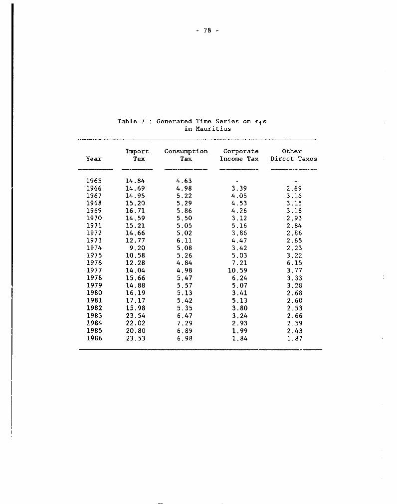
- 78 -
Table 7 Generated Time Series on Tisin Mauritius
Import Consumption Corporate OtherYear Tax Tax Income Tax Direct Taxes
1965 14.84 4.63 -1966 14.69 4.98 3.39 2.691967 14.95 5.22 4.05 3.161968 15.20 5.29 4.53 3.151969 16.71 5.86 4.26 3.181970 14.59 5.50 3.12 2.931971 15.21 5.05 5.16 2.841972 14.66 5.02 3.86 2.861973 12.77 6.11 4.47 2.651974 9.20 5.08 3.42 2.231975 10.58 5.26 5.03 3.221976 12.28 4.84 7.21 6.151977 14.04 4.98 10.59 3.771978 15.66 5.47 6.24 3.331979 14.88 5.57 5.07 3.281980 16.19 5.13 3.41 2.681981 17.17 5.42 5.13 2.601982 15.98 5.35 3.80 2.531983 23.54 6.47 3.24 2.661984 22.02 7.29 2.93 2.591985 20.80 6.89 1.99 2.431986 23.53 6.98 1.84 1.87

- 79 -
APPENDIX B: GENERALIZED VERSION OF THE MODEL
In Chapter II, all of the equatior.s included in the model are
assumed to have a specific functional form, i.e., semi-log linear. This
assumption is relaxed in this annex and, hence, the generalized version of
the model is discussed.
An individual tax yield assessed by tax inspectors is considered to
be a function of Xi and ri, that is,
(Ti*)t- Fi[(Xi)t, (ri)t] (1)
Let us assume that tax inspectors adjust actual tax revenues
towards their assessed level according to a partial adjustment mechanism,
that is,
A(Ti)t- Ai[(Ti*)t - (Ti)t.l] (2)
Then, the actual tax y.eld function is obtained by substituting (2)
in (1), that is,
(Ti)t= (l-Ai)(Ti)t-l + AiFi[(Xi)t,(ri)t] for i-l to n (3)
where
(aTi/aXi)=coefficient of built-in flexibility of Ti with respect
to Xi (CBFXi),
(8ri/8ri)-own-DUMs direct response
; ' - - !~~~~~~~~~~~~~~~~~~~~

- 80 -
Using the concept of the "realized individual tax rate" defined in
Chapter II, its formula will have the following form after making a simple
manipulation.
1 + Gitrit= rit (4)
Git(l+Git)1+ ( CBFXi ) -
rio+ Git(CBFXi)
where rit is average effective tax rate of Ti at time "t" and
(Gi)t=ln(X,)t-ln(Xi)o (5)
In its final form, each individual tax base is related to all ris
and GDP, that is,
(Xi)t - Di[(GDP)t, (rI)t .................. 9(rn)t] (6)
where
[(CBFXi)(pXi/3GDP)]- coefficient of built-in flexibility of Ti with
respect to GDP (CBFYi),
(CBFXi)(8Xi/8ri)- own-DTMs indirect response, and
(CBFXi) (83Xi/.-,j)= cross DTMs indirect response.
Finally, the model is closed by adding the overall tax revenue
identity, that is,
(T)t(Ti)t+ .............. +(Tn)t (7)

- 81 -
Equations (3), (5), (6) and (7) perform the structural form of the
model. Parameters of the model are estimated after substituting equation
(4) in it.
After estimating CBFYis, the built-in tax elasticity of each
individual tax with respect to GDP will be:
Eit- (CBFYi) (GDP/ATi)t
where ATi is the adjusted tax revenue to discretionary tax changes obtained
by simulating, the model for rit-riO.

- 82 -
APPENDIX C: AN OPERATIONAL GUIDELINE ON THE APPLICATION OF THE MODEL
This appendix provides a brief guideline on the application of the
model as an empirical framework for: (i) estimating tax elasticity and the
revenue impact of DTMs, and (ii) evaluating the macroeconomic impact of a
tax reform program aimed at generating additional revenue and/or dealing
with various tax related economic issues which require converting the DTMs
included in the reform to AETRNs and vice versa.
i. Estimating Tax Elasticity and the Revenue Impact of DTMs
The structural form of the model is presented in Table 1. Estimates
of its parameters are obtained by estimating the parameters of the model
presented in Table 2. Estimating its parameters requires time series data
on the following variables, which are readily available for most countries
in GFS (an IMF publication) and the World Tables (a World Bank
publication):
Td =Tax on domestic transactions
Tm -Tax on imports
Tc -Corporate income tax
To -Other direc. r-xes
T =Overall ta-' re'4?nte ret of export taxes
Xd -Private consumption
Xc -Value added in non-agriculture sector net out of wage bill
Xm -Imports
XO =GDP

- 83 -
Table 1: Structural Form of the Model
log(Td)t- AdadO+ Xdadll0g(Xd)t + (I-Ad)lvg(Td)t-l+ Adad2(7d)t+ Udt
log(Tm)t- Amamo+ Amamllog(Xm)t + (l-Xm)log(Tm)t-l+ Aemm2(Tm)t+ Umt
log(Tc)t= Ac%cO+ AXccllog(Xc)t + (l-Ac)log(Tc)t-l+ Acac2(Tc)t+ Uct
log(To)t= Aoaoo+ Aoaollog(Xo)t + (l-Ao)log(To)t-l+ Aoao2(ro)t+ Uot
l(Xd)t= fidO Odlln(yd)t+ fd2(rm/rd)t+ udt
ln(Xm)t= PmO+ Pmlln(GDP)t+ flm2(rm/Td)t+ Pm3(rc)t + Vmt
ln(Xc)t- PcO+ Pclln(GDP)t+ Pc2(7c)t + fc3(rm/fd)t+ vct
ln(T)t = 0+ dln(Td)t+ Smln(Tm)t+ 6cln(Tc)t+ 6oln(To)t
ln(Yd)t = 70 +7yln(GDP)t+ 721n(TC)t+ -y31n(To)t
(rm/rd)t= 00 + l(rm)t + 02(td)t
where,
Td- Tax on domestic transactions (endogenous variable),
t Tc=1 - w ! r r r e5- , .fe r>-,
To- Other direct taxes &cndogenous variable),Xd= Private consumption (endogenoun variAble),
….lt-- - -_s~ :_ ; ;__;_ . g.l;t
Xc- Value adodei. I!- AsgenCsa;bZ
Xv- CD°- grcss domestic r,oducts (exoRenuus va&1d1,1>)r 1 - The it" 'Lndividual realized tax rate (exogenous variable),
tor i= d, m, c, o,Yd- Disposable income (endogenous variable),T= Total tax revenue net of export taxes (endogenous variable).

- 84 -
Table 2: Entire Model with Estimable Parameters*
I- l+gd ln(Td)t- Xd*dO+ AdQdlln(Xd)t + (l-Xd)ln(Td)t-l +IXdad2 rd +dt
1+,\dadlgd -t
ln(Tm)t AmamO+ Amamlln(Xm)t + (l-Am)ln(Tm)t l +Amam4rm l+g +mt1+,\mamlgm t
ln(Tc)t= XcacO+ Acaclln(Xc)t + (l-Xc)ln(Tc)tl +Xcac2Irc -+g- 1 +l+,\caclgc Jt
[ l+Aago 1t
ln(To)t XoaOo+ Aoaolln(Xo)t + (l-Xo)ln(To)tl r +o | +otl+Aotolgo it
r rm,[ (l+gm)/(l+amlgm)] 1ln(Xd)t - fdO+ Pdlln(yd)t+ fld2 [rdl egm/l+amg )] + vdt
rdl(l+gd)/(]+adlgd)] tld
ln(X -Oo+Omll(GDP)tpm rm [( l+gm) / ( +amlgm) ] rc (l+gc )ln(Xm)tfmO+ mll (GDP)t+m2 +lm3 +vmt
rdf(l+gd)/(I+adlgd)]- t (I+Oclgc)
+d 1 rm(l+gm)/(l+emlgm)ln(Xc)t= RcO+ 3clln(GDP)t+ BC9 rd ,. 1+ .
14..-. 1, I .(t1 4.og\Jf!-4 L-dlgd t L-U'-' \C' '-' uF .ol/J -l_
nfT j , , U- 3.an(Th:?; + 2 l T.)+ 6Cln(Tc)t+ 60 1n(To)t
-;d; ti il;- 2 f 1cSt: 731n(TO)t
9(i)t l'(Xi)t- ln(Xi)O for i=d, in, C, O
* Estimating the parameters of the model requires time series data on Tis, T,Xis, ris and GDP which are readily available for most LDCs in GFS(an IMFpublication) and World Tables (a World Bank publication).

- 85 -
Yd=Disposable income
ri-The ith individual average effective tax rate (T/X),
for i-d, m, c, o, and
GDP- Gross domestic product.
Using these time series data, the efficient and consistent estimates of the
parameters of the model presented in Table 2 are obtained by means of a
simultaneous-equation econometric technique.
A within-sample dynamic simulation is performed for all the
endogenous variables included in the model in order to generate time series
data on gis. Using this data and estimates of Ais and ais, time series data
on ris are generated by means of the following equation.
- ~(1 + gi)t(ri)t [ (ri)t (-]
(1 + Xiailgi) t
The generated time series data on ris can be used independently to explore
the impact of changes in each individual tax system on key macroeconomic
variables such as inflation, economic growth, budget deficit, real exchange
rate and internathonal balance of paymentR. To linearize the structural
form of the msodel presented in Table 1, tl-hese data are used to estimate thz
pArAn1terE of- the follc;ir'- rN-mi; d' -r -crds, t_
linearize (r,jr. !) lcinci one '-f tcchnfccLn.J .q ...- ' ii the Le;Xt
(Tm/rd)t= 00 + 0 1(7m)t + 82(7d)t

- 86 -
Now, by substituting the estimated value of the parameters in the
original equations of the model presented in Table 1, the structural form
of the model with estimated parameters (SFM) is obtained.
The short run and the long run elasticities of individual tax
yields and base and overall tax revenue wich respect to GDP, and the direct
and indirect responses of each individual tax yield to the changes in its
own and other individual tax systems are simply obtained either by
substituting the estimated parameters into the formulas presented in Tables
3 to 7 of the text or by directly solving the SFM as an ordinary and a
difference equations systems and, hence, deriving the reduced (RFM) and
final (FFM) forms of the model.1
ii. Evaluatine/Designing A Ouantitative Tax Reform Program
The reduced/final form of the model can be used as an empirical
framework to evaluate the sport run/long run macroeconomic impact of a tax
reform program and to forecast a government's revenues from various sources
of taxation. However this requires converting the proposed DTMs to ris or
vice versa. An example from Malawi is considered to illustrate how to
convert the proposed DTMs to ris and vice versa.
Let us assume that the Malawian government wants to raise total
tax revenue by 5.67 percent using statutory surtax rate (SSR) as a policy
instrument- Then, the eue!Etions are: How much of an increase in the surtax
rate will result in a 5 67 percent increase in total tax revenlie? And what
'zS -cvz. t. ^ impct n4^f^rtli,7 1 ° )o
these quesLions requires quantitative knowledge ua LLie iimpact of a orne
percentage point increase in SSR on both its corresponding and other
1/ For more details on solution of a dynamic macroeconometric model seeEhdaie (1987).

- 87 -
individual tax yields and bases. Providing such information, first of all,
requires converting a one percentage point increase in SSR to rd.
In this country, surtax was introduced in 1970/71 at a statutory
tax rate of 18 percent. Then, this rate was increased to 25 percent in
1983/84. Given one of these DTMs, say the former, and time series data on
rd, the amount of increase in Td due to a one percentage point increase in
SSR is calculated as follows. As a result of introducing surtax in 1970
(fiscal year 1970/71), Td rose from 2.32 percent in 1969 to 4.30 percent in
1970 (see Table 6 in Appendix A). Given 18 percent SSR, rd went up by
0.111 percentage points due to a one percent point increase in SSR (the
same result is obtained using the DTMs of 1983/84).
It is apparent from the coefficient of Td in the overall tax
e(quation presented in Table 11 of the text that total tax revenue will rise
by 5.67 percent as result of a one percentage point increase in 7d, whose
equivalent is a 9 percentage point increase in the statutory surtax rate.
In other words, the new SSR will be 34 percent (25 percent plus 9 percent)
which will result in a 5.67 percent increase in overall tax yield.
Using the coefficients of rd in the other equations included in
the model presented in Table 11 of the text, the macroeconomic impact of
this di8cretionary tax measure will us as follows. First, tax on imports
>-. wi i--creasc by 0.73 and 18.81 percLZt-
re.spcc4-Je&y. S-conc, corporate income tax will decline by 0.11 Percent.
iiiild, pri-vave cousw-nption ana vaiue aaded in the non-agriculture sector of
the economv will fall by 0.65 and 0.13 percent respectively, and finally,
imports will rise by 0.81 percent.

- 88 -
BIBLIOGRAPHY
Andersen, S.P. (1973) "Built-in Flexibility of Sensitivity of the PersonalIncome Tax in Denmark" Swedish Journal of Economics, vol. 75.
Artus, K.K. (1974) "Tax Revenue Forecasting: A Methodological Study withApplication to Turkey", Studies in Domestic Finance, no. 5Washington, D.C.: IBRD.
Bahl, R.W. (1972) "Alternative Methods for Tax Revenue Forecasting inDeveloping Countries: A Conceptual Analysis", IMF, unpublished paper,October.
Balassa, Bela (1989) "U.S. Trade Policy Towards Developing Countries", TheWorld Bank, PPR Working Paper 151.
Chamley, C. (1984) "A Framework for Tax Reforms in Developing Economies withTwo Sectors", CPD Discussion Paper no. 1985-14.
Chand, S.K., and B. Wolf (1973) "The Elasticity and Bouyancy of the Tax Systemof Peru, 1960-71: an Empirical Analysis", IMF, unpublished.
Chelliah, R.J. and C. K. Sheetal (1974) "A Note on Techniques of Adjusting TaxRevenue Series for Discretionary Changes", IMF, unpublished paper.
Chelliah, R.J., H.J. Bass and M.R. Kelly (1975) "Tax Ratios and rax Effort inDeveloping Countries, 1969-71", IMF Staff Papers, Vol. 22.
Choudhry, N.N. (1975) "A Study of the Elasticity of the West Malaysian IncomeTax System", IMF Staff Papers, vol. 22.
Choudhry, N.N. (1979) "Measuring the Elastic!ty of Tax Revenue: A DivisiaIndex Approach", IMF staff papers, Vol. 26.
Dernburg, T.F., and J.D. Dernberg (1982) Macroeconomic Analysis: AnTntrodtlrtion to Comparative Statistics and Dynamics. London: Addison-Wesley Publication Company.
Diamond, P.A k ii laxation anLd Public hQ-Quctioii in a GLOWLh S-Alng,>J.A. Mirriees and N.H. Stetxi, eds., Models oL Economic Growth,London: MacMillan.
V,- (i el TA*-t-ien ThFnrv Tn the lDen Economyv. in A.J. Auerbach andM.S. Feldstein, eds. Handbook of Public Fconomics, vol. 1Amsterdam: North-Holland Publication.
Durbin, J. (1970) "Test for Serial Correlation in Least Squa.es Regressionwhen Some of the Regressors are lagged Dependent Variables", Econometrica39, pp. 25-48
Ebrill, L.P. (1988) "The Effects of Taxation on Labour Supply, Saving, andInvestment in Developing Countries: A Survey of the EmpiricalLiterature", IMF Staff Paper, 1988.

- 89 -
Ehdaie, J. (1987) "Dynamic Properties of the Colombian Macroeconometric Model:An Empirical Tool For Dynamic Macroeconomic Policy Analysis", memo,February, CECEM.
Ehdaie, J., V. Gandhi and Z. Shalizi, (1985) "Patterns of Taxation Tn Sub-Saharan Africa Countries: Trends in Tax effort and Decompositions,1966-1981", CPD Discussion paper, No. 1985-48.
Fair, R.C. (1984) Specification, Estimation. and Analysis of MacroeconomicModels, Cambridge: Harvard University Press.
Gillani, F.S. (1986) "Elasticity and Buoyancy of Federal Taxes in Pakistan",The Pakistan Development Review, Vol. XXV, no. Z.
Goode, R. (1984) Government Finance in Developing Countries, Washington D.C.:Brookings Institution.
Hinrichs, H.H. (1966) A General Theory of Tax Structure Change During EconomicDevelopment, Camv',ridge, Mass.: Harvard University Press.
Jeetun, A. (1978) "Buoyancy and Elasticity of Taxes in Pakistan:, ApRliedEconomics Research Institute Research Paper, no. 11.
Johnston, J. (1985) Econometric Methods, 3d ed., New York:McGraw-Hill, 1985.
Khan, M.Z. (1973) "Responsiveness of Tax Yields to Increase in NationalIncome", Pakistan Development Review, Vol. XII, no. 4.
Lambert, J.D. and R. J. Suckling (1986) "Revenue Elasticity of the ZimbabweanIndividual Income Tax 1967-1981", Zimbanbwe Journal of Economics,Januarv.
Lewis, W.A. (i973) "Economic Development with Unlimited Supplies of Labour",Manchester School, vol. 24, no. 63.
Maddala, G.S. (1987) Econometrics New York: McGraw-Hill Book Company.
Mansfiela, u.x. (L9/z) "tiasticity and buoyancy of a Tax System: A MethodApplied To Paraguay", IMF Staff Papers, vol. 19.
Musgrave, R.n. Zub i. . usg;-e . Public Finance in T-Ieoiy andPractice, 3d ed., New York: MacGraw Hill Inc.
lNeWbEr;.Y, D.1 81ii-i ;N. SLt:LJI (19i57), eds, uxirora: oxford Universit:v llress.
Prrst .:.r. (l^2) "-it! SeibiLiviLy of the Lieid of Personial income in tneUnltfd Kingdom", Economic Journal, vol. 72.
SahoLa, G.S. (1961) Indian Tax Structure and Economic Development, London:Asia Publishing House.
Shoven, J.B. (1983) "Applied General Equilibrium Tax Modelling", IMF StaffPapers vol. 30.

- 90 -
Skinncr, J. (1988) "Taxation and Output Growth in Africa", CECPE, WKS 73,August.
Singer, N.M. (1968) "The Use of Dummy Variables in Estimating the IncomeElasticiLy of State Income-Tax Revenue", National Tax Journal, Vol.21.
Shalizi, Z., V. Gandhi and J. Ehdaie (1985) "Patterns of Taxation In Sub-Saharan Africa Countries: Trends in Tax effort and Decompositions,1966-1981", CPD Discussion paper, No. 1985-48.
Shalizi, Z. and L. Squire (1988) "A Framework for Tax Policy in Sub-SaharanAfrica", CECPE.
Shome, P. (1987) "On the Elasticity of 'eveloping Country Tax System",Unpublished paper presented at the inual conference of the AmericanEconomic Association, Chicago, Decem n.
Fury, M.M. (1985) "Buoyancy and Elasticity of Unior Excise Tax Revenues inIndia: 1950-51 to 1980-81", National Council ,i Applied EconomicResearch, vol. 18, October.
Tait, A.A., W.L. Gratz, and B.J. Eichengreen (1979) " InternationalComposition of Taxacion for Selected Developing Countries, 1972-76" IMFStaff Papers, vol. 26.
Tanzi, V. (1981) "Taxation in Sub-Saharan Africa: A Statisticil Evaluation",IMF Occasional Paper 8, 1981.
(1983) "Tax Systems and Policy Objectives in Developing Countries:General Principles and Diagnostic Tests", IMF; processed, 1983.
Taylcr, L. (1979) Macro Models for DeveloRing Countries, New York: McGraw-HillInc.
Theil, H., and J.C.G. Book (1969) "The Final Form of Econometric EquationSys_em_s", rVevIew of International Statistics Institute, vol. XXX.
World Bank (1987) World DeveloRment ReRort. Oxford O(ford llniver.cirv Prpcc

PPR Working Paper Series
ContacttIjuAuthor D= for paper
WPS320 Protection Facing Exports from Refik Erzan November 1989 G. IlogonSub-Saharan Africa in the EEC, Peter Svedberg 33732Japan, and the United States
WPS321 Economic and Policy Determinants Jorge Marshall December 1989 S. Jonnakutyof Public Sector Deficits Klaus Schmidt-Hebbel 37453
WPS322 Earmarking Government William McCieary December 1989 A. BhallaRevenues: Does it Work? 37699
WPS323 The Old and the New in Heterodox Miguel A. Kiguel December 1989 R. LuzStabilization Programs: Lessons Nissan Liviatan 61588trom the 1960s and the 1980s
WPS 324 Ethical Approaches to Family F. T. Sai December 1989 S. AinsworthPlanning in Africa K. Newman 31091
WPS325 Manufacturers' Responses to Infra- Kyu Sik Lee December 1989 L. Victoriostructure Deficiencies in Nigeria Alex Anas 31009
WPS326 Do Exporters Gain from Voluntary Jaime de Melo January 1990 M. AmealExport Restraints? L. Alan Winters 61466
WPS327 Making Noisy Data Sing: A Micro James R. Tybout January 1990 M. AmealApproach to Measuring Industrial 61465Efficiency
WPS328 Europe, Middle East, and North Rodolfo A. Bulatao November 1989 S. AinsworthAfrica (EMN) Region Population Eduard Bos 31091Projections, 1989-90 Edition Patience W. Stephens
My T. Vu
WPS329 Latin America and the Caribbean Rodolfo A. Bulatan November 1QR9 S Ainsworthki_n0) i FU9iVII PU8u;cA1;Qil itLUUaliU OUb
Projections, 1989-90 Edition Patience W. StephcnsM%-, T Vul
WPS330 Africa Region Popu!ation Rodolfo A. Bulatao Novembe' '989 S. A'nsworthProjections, 19ld-90 Edition Eduard Bos 31U91
Paiience YW. StepnensMy T. Vu
WPS331 Asia Regior. Population Projections, Rodolfo A. Bulatao November 1989 S. Ainsworth1989-90 Edition Eduard Bos 31091
Patience W. StephensMy T. Vu
WPS332 Effective Incentives in India's Ashok Gulati January 1990 G. BayardAgriculture: Cotton. G3rouindnuts, with James Hanson 38004Wheat, and Rice and Garry Pursell

PPR Work;ng Paper Series
ContactITlt Author Dae for 12ager
WPS333 An Option-Pricing Approach to Stijn Claessens January 1990 S. King-WatsonSecondary Market Debt (Applied Sweder van '.Vijnbergen 31047to Mexico)
WPS334 An Econometric Method for Jaber Ehdaie February 1990 A. BhallaEstimating the Tax Elasticity and the 37699Impact on Revenues of DiscretionaryTax Measures (Applied to Malawi andMauritius)
WPS335 Macroeconomic Adjustment and Ramon E. Lopez December 1989 L. Riverosthe Labor Market in Four Latin Luis A. Riveros 37465American Countries
WPS336 Complementary Approaches to Germano MwabuFinancing Health Services in Africa
WPS337 Projecting Mortality for All Rodolfo A. Bulatao December 1989 S. AinsworthCountries Eduard Bos 31091
Patience W. StephensMy T. Vu
WPS338 Supply and Use of Essential Drugs S. D. Fosterin Sub-Saharan Africa: Issues andPossible Solutions
WP-,339 Private Investment and Macro- Liis Serven December 1989 E. Khineeconomic Adjustment: An Andres Solimano 37469Overview
WPS340 Prudential Regulation and Banking V/incent P. Polizatto January 1990 WDR OfficeSupervision: Building an Institutional 31393Franework for Banks
WPS341 Cost-of-Living Differences between Martin Ravallion December 1989 C. SpoonerUrban and Rufs' Areas of Indonesia Dominique van de Walle 30464
WPS342 Human Capital and Endogenous Patricio Arrau December 1989 S. King-WatsonGrowth in a Large Scale Life-Cycle 31047Model
WPS343 Po;icy Determinants of Growth: William R. Easterly December 1989 R. LuzSurvey of Theory and Evidence Deborah L. Wetzel 61588
WPS344 Policy Distortions, Size of William Itisterly December 1989 R. LuzGovernment, and Growth 61588
WPS345 Private Transfers and Public Poiicy Donald Cox December 1989 A. Bhallain Developing Countries: Emmanuel Jimenez 37699A Case Study for Peru


