
A MULTILINEAR (TENSOR) ALGEBRAIC FRAMEWORK FOR
COMPUTER GRAPHICS, COMPUTER VISION, AND MACHINE LEARNING
by
M. Alex O. Vasilescu
A thesis submitted in conformity with the requirementsfor the degree of Doctor of Philosophy
Graduate Department of Computer ScienceUniversity of Toronto
Copyright c© 2009 by M. Alex O. Vasilescu

A Multilinear (Tensor) Algebraic Framework forComputer Graphics, Computer Vision, and Machine Learning
M. Alex O. VasilescuDoctor of Philosophy
Graduate Department of Computer Science
University of Toronto
2009
Abstract
This thesis introduces a multilinear algebraic framework for computer graphics, computer vision,
and machine learning, particularly for the fundamental purposes of image synthesis, analysis, and recog-
nition. Natural images result from the multifactor interaction between the imaging process, the scene
illumination, and the scene geometry. We assert that a principled mathematical approach to disentan-
gling and explicitly representing these causal factors, which are essential to image formation, is through
numerical multilinear algebra, the algebra of higher-order tensors.
Our new image modeling framework is based on (i) a multilinear generalization of principal compo-
nents analysis (PCA), (ii) a novel multilinear generalization of independent components analysis (ICA),
and (iii) a multilinear projection for use in recognition that maps images to the multiple causal factor
spaces associated with their formation. Multilinear PCA employs a tensor extension of the conventional
matrix singular value decomposition (SVD), known as the M -mode SVD, while our multilinear ICA
method involves an analogous M -mode ICA algorithm.
As applications of our tensor framework, we tackle important problems in computer graphics, com-
puter vision, and pattern recognition; in particular, (i) image-based rendering, specifically introducing
the multilinear synthesis of images of textured surfaces under varying view and illumination conditions,
a new technique that we call “TensorTextures”, as well as (ii) the multilinear analysis and recognition
of facial images under variable face shape, view, and illumination conditions, a new technique that we
call “TensorFaces”. In developing these applications, we introduce a multilinear image-based rendering
algorithm and a multilinear appearance-based recognition algorithm. As a final, non-image-based ap-
plication of our framework, we consider the analysis, synthesis and recognition of human motion data
using multilinear methods, introducing a new technique that we call “Human Motion Signatures”.
ii

Acknowledgements
First and foremost, I am grateful to my advisor, Professor Demetri Terzopoulos. Although initially
resisting the direction of my research, he eventually became its biggest supporter. This thesis would not
have materialized in its present form without his valuable input and guidance. I am indeed fortunate to
have had him as my advisor.
I thank the other members of my PhD Thesis Committee, Professors Geoffrey Hinton, Alan Jep-
son, and David Fleet, for their constructive critique, which improved the quality of this dissertation. I
also appreciate their flexibility in accommodating my departmental and senate defenses into their busy
schedules.
I am grateful to Professor Amnon Shashua of The Hebrew University of Jerusalem for agreeing to
serve as the external examiner of my thesis on very short notice and for reviewing my dissertation in
record time.
My thanks also go to Greg Ward, who provided encouragement and comments on a draft of my
SIGGRAPH paper on “TensorTextures”.
Many other people at the University of Toronto (UofT), New York University (NYU), the Mas-
sachusetts Institute of Technology (MIT), and elsewhere deserve special mention and my appreciation:
At the UofT, I thank Professor John Tsotsos for his interest in my work as well as for his kindness
and encouragement. I had countless enjoyable discussions about computer vision and related topics
with Chakra Chennubhotla. I also thank Genevieve Arboit, Andrew Brown, Kiam Choo, Florin Cutzu,
Petros Faloutsos, Steven Myers, Michael Neff, Victor Ng, Alberto Paccanaro, Sageev Oore, Faisal
Qureshi, Brian Sallans, Corina Wang, and Howard Zhang for their comradery. Genevieve, Howard,
Kiam, and Steven generously volunteered their time and bodies for motion capture data acquisition.
My work on human motion signatures started with an overambitious term project for a graphics course
taught by Professors Eugene Fiume and James Stewart. Julie Weedmark kindly assisted in dealing with
the administrative and financial obstacles that were unjustly imposed by the UofT School of Graduate
Studies.
At NYU, I thank the MRL/CAT faculty, Professors Davi Geiger, Ken Perlin, Chris Bregler, Denis
Zorin, Yann LeCun, Jack Schwartz, and last but not least Mike Uretsky for encouragement and inter-
esting discussions. Professor Michael Overton deserves a special thanks for pointing me to the work
on tensors by Dr. Tamara Kolda at Sandia. Finally, I have fond memories of interactions with Aaron
Hertzmann, Evgueni Parilov, Wei Shao, Elif Tosun, Lexing Ying, and many other members of the MRL
and CAT. I particularly thank Jared Silver for his valuable assistance with 3D modeling, animation, and
iii

A/V production, and Svetlana Stenchikova for exploring some programming issues.
At MIT, I am grateful to Professor Rosalind Picard for bringing me into the Media Lab and for
her generous support during my two years there. I thank Professors John Maeda, Alex Pentland, and
Marvin Minsky for helpful discussions. I also had memorable conversations with Ian Eslick, my office
mate at the Media Lab. Several years earlier, while I was at the UofT, I was inspired by Professor Josh
Tenenbaum’s bilinear models, and he generously provided me some of his code.
I would like to gratefully acknowledge my amicable interactions with members of the “tensor de-
composition” research community. In particular, I thank Tamara Kolda, Lieven de Lathauwer, Pietr
Kroonenberg, Rasmus Bro, Pierre Comon, Jos ten Berge, Henk Kiers, Lek-Heng Lim, and Charlie van
Loan. I am also grateful to (the late) Richard Harshman and Gene Golub for their interest in my work
and their encouragement.
Motion data were collected at the Gait Laboratory of the Bloorview MacMillan Medical Centre in
Toronto. The data acquisition work was done with the permission of Professor Stephen Naumann, Di-
rector of the Rehabilitation Engineering Department and with the helpful assistance of Mr. Alan Morris.
The 3D Morphable faces database was obtained courtesy of Prof. Sudeep Sarkar of the University of
South Florida as part of the USF HumanID 3D database.
The portions of this research that were carried out at the UofT were funded in part by the Natural
Sciences and Engineering Research Council (NSERC) of Canada through grants to Demetri Terzopou-
los, and at NYU in part by the Technical Support Working Group (TSWG) of the US Department of
Defense through a grant to him and me.
Finally, I am grateful for the essential financial support that my parents, George and Ioanna Vasilescu,
provided to me while I was a student and I greatly appreciate their sacrifices.
iv

Contents
Abstract . . . . . . . . . . . . . . . . . . . . . . . . . . . . . . . . . . . . . . . . . . . . . ii
Acknowledgements . . . . . . . . . . . . . . . . . . . . . . . . . . . . . . . . . . . . . . iii
Contents . . . . . . . . . . . . . . . . . . . . . . . . . . . . . . . . . . . . . . . . . . . . vi
List of Tables . . . . . . . . . . . . . . . . . . . . . . . . . . . . . . . . . . . . . . . . . . vii
List of Figures . . . . . . . . . . . . . . . . . . . . . . . . . . . . . . . . . . . . . . . . . ix
List of Algorithms . . . . . . . . . . . . . . . . . . . . . . . . . . . . . . . . . . . . . . . x
Love and Tensor Algebra . . . . . . . . . . . . . . . . . . . . . . . . . . . . . . . . . . . xi
1 Introduction 1
1.1 Data Analysis and Multilinear Representations . . . . . . . . . . . . . . . . . . . . . 2
1.2 Thesis Contributions . . . . . . . . . . . . . . . . . . . . . . . . . . . . . . . . . . . 4
1.3 Thesis Overview . . . . . . . . . . . . . . . . . . . . . . . . . . . . . . . . . . . . . 8
2 Related Work 10
2.1 Linear and Multilinear Algebra for Factor Analysis . . . . . . . . . . . . . . . . . . . 10
2.2 Bilinear and Multilinear Analysis in Vision, Graphics, and Learning . . . . . . . . . . 13
2.3 Background on Image-Based Rendering . . . . . . . . . . . . . . . . . . . . . . . . . 15
2.4 Background on Appearance-Based Facial Recognition . . . . . . . . . . . . . . . . . 16
2.5 Background on Human Motion Synthesis, Analysis, and Recognition . . . . . . . . . . 17
3 Linear and Multilinear Algebra 19
3.1 Relevant Linear (Matrix/Vector) Algebra . . . . . . . . . . . . . . . . . . . . . . . . . 20
3.2 Relevant Multilinear (Tensor) Algebra . . . . . . . . . . . . . . . . . . . . . . . . . . 21
3.2.1 Tensor Decompositions and Dimensionality Reduction . . . . . . . . . . . . . 25
4 The Tensor Algebraic Framework 32
4.1 PCA and ICA . . . . . . . . . . . . . . . . . . . . . . . . . . . . . . . . . . . . . . . 33
4.2 Multilinear PCA (MPCA) . . . . . . . . . . . . . . . . . . . . . . . . . . . . . . . . . 36
4.3 Multilinear ICA (MICA) . . . . . . . . . . . . . . . . . . . . . . . . . . . . . . . . . 40
4.4 Kernel MPCA/MICA, Multifactor LLE/Isomap/LE, and Other Generalizations . . . . 43
v

5 Multilinear Image Synthesis: TensorTextures 485.1 Multilinear BTF Analysis . . . . . . . . . . . . . . . . . . . . . . . . . . . . . . . . . 51
5.2 Computing TensorTextures . . . . . . . . . . . . . . . . . . . . . . . . . . . . . . . . 54
5.3 Texture Representation and Dimensionality Reduction . . . . . . . . . . . . . . . . . 55
5.4 Multilinear Image-Based Rendering . . . . . . . . . . . . . . . . . . . . . . . . . . . 57
5.5 Rendering on Curved Surfaces . . . . . . . . . . . . . . . . . . . . . . . . . . . . . . 58
5.6 Additional Results . . . . . . . . . . . . . . . . . . . . . . . . . . . . . . . . . . . . 59
6 Multilinear Image Analysis: TensorFaces 646.1 The TensorFaces Representation . . . . . . . . . . . . . . . . . . . . . . . . . . . . . 65
6.2 Strategic Dimensionality Reduction . . . . . . . . . . . . . . . . . . . . . . . . . . . 68
6.3 Application to a Morphable Faces Database . . . . . . . . . . . . . . . . . . . . . . . 70
6.4 The Independent TensorFaces Representation . . . . . . . . . . . . . . . . . . . . . . 74
6.5 Structure and Decomposition of Facial Image Manifolds . . . . . . . . . . . . . . . . 75
7 Multilinear Image Recognition: The Multilinear Projection 797.1 Multiple Linear Projections (MLP) . . . . . . . . . . . . . . . . . . . . . . . . . . . . 81
7.2 The Multilinear Projection (MP) . . . . . . . . . . . . . . . . . . . . . . . . . . . . . 83
7.2.1 Identity and Pseudo-Inverse Tensors . . . . . . . . . . . . . . . . . . . . . . . 86
7.2.2 Multilinear Projection Algorithms . . . . . . . . . . . . . . . . . . . . . . . . 87
7.3 Facial Image Recognition Experiments . . . . . . . . . . . . . . . . . . . . . . . . . . 91
7.4 Discussion . . . . . . . . . . . . . . . . . . . . . . . . . . . . . . . . . . . . . . . . . 94
8 Multilinear Motion Analysis, Synthesis, and Recognition: Human Motion Signatures 968.1 Motion Data Acquisition . . . . . . . . . . . . . . . . . . . . . . . . . . . . . . . . . 97
8.2 Motion Analysis: TensorMotions . . . . . . . . . . . . . . . . . . . . . . . . . . . . . 99
8.3 Motion Synthesis . . . . . . . . . . . . . . . . . . . . . . . . . . . . . . . . . . . . . 101
8.4 Motion Recognition . . . . . . . . . . . . . . . . . . . . . . . . . . . . . . . . . . . . 102
8.5 Experiments and Results . . . . . . . . . . . . . . . . . . . . . . . . . . . . . . . . . 103
8.6 Discussion . . . . . . . . . . . . . . . . . . . . . . . . . . . . . . . . . . . . . . . . . 104
9 Conclusion 1069.1 Summary . . . . . . . . . . . . . . . . . . . . . . . . . . . . . . . . . . . . . . . . . 106
9.2 Future Work . . . . . . . . . . . . . . . . . . . . . . . . . . . . . . . . . . . . . . . . 107
A On Observational Data as Vectors, Matrices, or Tensors 110
B On Data Acquisition and PIE Image Datasets 116
C On Motion Capture Data Processing 119
Bibliography 123
vi

List of Tables
4.1 Common kernel functions . . . . . . . . . . . . . . . . . . . . . . . . . . . . . . . . . 45
7.1 Experimental results with the multiple linear projection (MLP) recognition method . . 92
7.2 PCA, ICA, MPCA, and MICA face recognition experiment . . . . . . . . . . . . . . . 92
7.3 Facial recognition rates using the MLP and MP recognition methods . . . . . . . . . . 93
7.4 MPCA recognition rates for various dimensionality reductions . . . . . . . . . . . . . 93
C.1 Denavit-Hattenberg notation for the kinematic chain of a leg . . . . . . . . . . . . . . 122
vii

List of Figures
1.1 Taxonomy of models . . . . . . . . . . . . . . . . . . . . . . . . . . . . . . . . . . . 4
1.2 Linear and multilinear manifolds . . . . . . . . . . . . . . . . . . . . . . . . . . . . . 5
1.3 TensorTextures system diagram . . . . . . . . . . . . . . . . . . . . . . . . . . . . . . 6
1.4 Architecture of a multilinear facial image recognition system . . . . . . . . . . . . . . 7
2.1 The development of multilinear algebra . . . . . . . . . . . . . . . . . . . . . . . . . 12
3.1 Matrixizing a (3rd-order) tensor . . . . . . . . . . . . . . . . . . . . . . . . . . . . . 22
3.2 Rank-R decomposition of a third order tensor . . . . . . . . . . . . . . . . . . . . . . 26
3.3 The M -mode SVD . . . . . . . . . . . . . . . . . . . . . . . . . . . . . . . . . . . . 29
4.1 Geometric view of the ICA computation . . . . . . . . . . . . . . . . . . . . . . . . . 34
4.2 PCA and ICA may yield different subspaces . . . . . . . . . . . . . . . . . . . . . . . 35
4.3 Subspace spanned by ICA versus MICA . . . . . . . . . . . . . . . . . . . . . . . . . 43
4.4 Comparison of causal factor extraction/representation by MPCA and MICA . . . . . . 44
5.1 Standard vs BTF texture mapping . . . . . . . . . . . . . . . . . . . . . . . . . . . . 49
5.2 Treasure chest . . . . . . . . . . . . . . . . . . . . . . . . . . . . . . . . . . . . . . . 50
5.3 Image acquisition and representation . . . . . . . . . . . . . . . . . . . . . . . . . . . 52
5.4 The rectifying homography . . . . . . . . . . . . . . . . . . . . . . . . . . . . . . . . 53
5.5 TensorTextures bases . . . . . . . . . . . . . . . . . . . . . . . . . . . . . . . . . . . 53
5.6 PCA eigenvectors . . . . . . . . . . . . . . . . . . . . . . . . . . . . . . . . . . . . . 54
5.7 Multilinear rendering . . . . . . . . . . . . . . . . . . . . . . . . . . . . . . . . . . . 55
5.8 Perceptual error . . . . . . . . . . . . . . . . . . . . . . . . . . . . . . . . . . . . . . 56
5.9 Computing a new view representation using barycentric coordinates . . . . . . . . . . 58
5.10 TensorTexture rendering on a curved surface . . . . . . . . . . . . . . . . . . . . . . . 58
5.11 TensorTexture bases for the corn texture . . . . . . . . . . . . . . . . . . . . . . . . . 59
5.12 Standard texture mapping versus TensorTexture mapping . . . . . . . . . . . . . . . . 60
5.13 Renderings of the corn TensorTexture . . . . . . . . . . . . . . . . . . . . . . . . . . 61
5.14 A still image from the Scarecrows’ Quarterly animation . . . . . . . . . . . . . . . . . 62
5.15 TensorTextures rendered on spheres . . . . . . . . . . . . . . . . . . . . . . . . . . . 63
5.16 A still image from the Flintstone Phonograph animation . . . . . . . . . . . . . . . . 63
viii

6.1 The Weizmann facial image database . . . . . . . . . . . . . . . . . . . . . . . . . . . 66
6.2 The TensorFaces representation . . . . . . . . . . . . . . . . . . . . . . . . . . . . . . 67
6.3 The PCA eigenvectors . . . . . . . . . . . . . . . . . . . . . . . . . . . . . . . . . . 67
6.4 Illumination reduction . . . . . . . . . . . . . . . . . . . . . . . . . . . . . . . . . . 69
6.5 The perceptual error of TensorFaces compression . . . . . . . . . . . . . . . . . . . . 70
6.6 A facial image dataset . . . . . . . . . . . . . . . . . . . . . . . . . . . . . . . . . . . 71
6.7 Data tensor . . . . . . . . . . . . . . . . . . . . . . . . . . . . . . . . . . . . . . . . 72
6.8 Eigenfaces and TensorFaces bases . . . . . . . . . . . . . . . . . . . . . . . . . . . . 72
6.9 16 subjects were imaged under 7 view and 20 illumination conditions . . . . . . . . . 73
6.10 The “perceptual error” of TensorFaces compression . . . . . . . . . . . . . . . . . . . 74
6.11 ICA and MICA bases . . . . . . . . . . . . . . . . . . . . . . . . . . . . . . . . . . . 75
6.12 Manifold decomposition and parameterization for a toy example . . . . . . . . . . . . 76
6.13 Manifold structure of facial image ensembles . . . . . . . . . . . . . . . . . . . . . . 77
7.1 A face imaged under multiple illumination conditions . . . . . . . . . . . . . . . . . . 80
7.2 The bases tensor . . . . . . . . . . . . . . . . . . . . . . . . . . . . . . . . . . . . . . 82
7.3 MPCA image representation and coefficient vectors . . . . . . . . . . . . . . . . . . . 84
7.4 MICA image representation and coefficient vectors . . . . . . . . . . . . . . . . . . . 85
7.5 The three identity tensors of order 3 . . . . . . . . . . . . . . . . . . . . . . . . . . . 87
8.1 The motion capture facility . . . . . . . . . . . . . . . . . . . . . . . . . . . . . . . . 98
8.2 Body with reference planes and fundamental directions . . . . . . . . . . . . . . . . . 98
8.3 Markers and coordinate systems . . . . . . . . . . . . . . . . . . . . . . . . . . . . . 99
8.4 Normal walking cycle . . . . . . . . . . . . . . . . . . . . . . . . . . . . . . . . . . . 100
8.5 Motion data collection and analysis model . . . . . . . . . . . . . . . . . . . . . . . . 101
8.6 Synthesizing 3 styles of walking motions . . . . . . . . . . . . . . . . . . . . . . . . 103
8.7 A synthesized stair-ascending motion . . . . . . . . . . . . . . . . . . . . . . . . . . 104
8.8 Frames from an animation short created with synthesized motion data . . . . . . . . . 104
A.1 Image ensemble organizations . . . . . . . . . . . . . . . . . . . . . . . . . . . . . . 111
A.2 PCA computes all possible pairwise pixel covariances . . . . . . . . . . . . . . . . . . 112
A.3 Matrixizing a data tensor and covariance computation . . . . . . . . . . . . . . . . . . 113
ix

List of Algorithms
3.2.1 CANDECOMP/PARAFAC (CP) algorithm . . . . . . . . . . . . . . . . . . . . . . . 27
3.2.2 M -mode SVD algorithm . . . . . . . . . . . . . . . . . . . . . . . . . . . . . . . . . 29
3.2.3 M -mode SVD dimensionality reduction algorithm . . . . . . . . . . . . . . . . . . . 30
4.2.1 Multilinear PCA (MPCA) algorithm . . . . . . . . . . . . . . . . . . . . . . . . . . . 37
4.3.1 Multilinear ICA (MICA) algorithm . . . . . . . . . . . . . . . . . . . . . . . . . . . . 42
4.4.1 Kernel Multilinear PCA/ICA (K-MPCA/MICA) algorithm . . . . . . . . . . . . . . . 46
7.2.1 Multilinear projection (MP) algorithm with MPCA, rank-(1, . . . , 1) decomposition . . 89
7.2.2 Multilinear projection (MP) algorithm with CP, rank-1 decomposition . . . . . . . . . 90
x

Love and Tensor Algebra
1
2
3
4
30
210
60
240
90
270
120
300
150
330
180 0
Come, let us hasten to a higher planeWhere dyads tread the fairy fields of Venn,Their indices bedecked from one to nCommingled in an endless Markov chain!
Come, every frustum longs to be a coneAnd every vector dreams of matrices.Hark to the gentle gradient of the breeze:It whispers of a more ergodic zone.
In Riemann, Hilbert or in Banach spaceLet superscripts and subscripts go their ways.Our asymptotes no longer out of phase,We shall encounter, counting, face to face.I’ll grant thee random access to my heart,Thou’lt tell me all the constants of thy love;And so we two shall all love’s lemmas prove,And in our bound partition never part.
For what did Cauchy know, or Christoffel,Or Fourier, or any Boole or Euler,Wielding their compasses, their pens and rulers,Of thy supernal sinusoidal spell?
Cancel me not – for what then shall remain?Abscissas some mantissas, modules, modes,A root or two, a torus and a node:The inverse of my verse, a null domain.
Ellipse of bliss, converge, O lips divine!the product of four scalars it defines!Cyberiad draws nigh, and the skew mindCuts capers like a happy haversine.
I see the eigenvalue in thine eye,I hear the tender tensor in thy sigh.Bernoulli would have been content to die,Had he but known such a2 cos 2φ!
– Stanislaw Lem“The Cyberiad”(tr. Michael Kandel)
xi

1Introduction
Contents1.1 Data Analysis and Multilinear Representations . . . . . . . . . . . . . . . . . . . 2
1.2 Thesis Contributions . . . . . . . . . . . . . . . . . . . . . . . . . . . . . . . . . 4
1.3 Thesis Overview . . . . . . . . . . . . . . . . . . . . . . . . . . . . . . . . . . . . 8
Image computing concerns the synthesis, analysis, and recognition of images. Image synthesis,
mathematically a forward problem, is primarily of interest in the field of computer graphics. Image
analysis, an inverse problem, is primarily of interest in the field of computer vision. Image recognition,
is primarily of interest in the field of machine learning or pattern recognition. Image computing cuts
across all of these fields.
Linear algebra—i.e., the algebra of matrices—has traditionally been of tremendous value in the
context of image synthesis, analysis, and recognition. The Fourier transform, the Karhunen-Loeve
transform, and other linear techniques have been veritable workhorses. For example, principal com-
ponents analysis (PCA) has been a popular technique in facial image recognition, as has its extension,
independent components analysis (ICA) [Chellappa et al. 1995]. By their very nature, these products
of linear algebra model single-factor, linear variation in image formation or the linear combination of
sources.
Natural images, however, result from the interaction of multiple causal factors related to scene struc-
ture, illumination, and imaging. For example, facial images are the result of facial geometry (person,
facial expression, etc.), the pose of the head relative to the camera, the lighting conditions, and the
type of camera employed. To deal with this complexity, we propose a more sophisticated mathematical
1

CHAPTER 1. INTRODUCTION 2
approach to the synthesis, analysis, and recognition of images that can explicitly represent each of the
multiple causal factors underlying image formation.
This thesis introduces and develops a tensor algebraic framework for image computing. Our novel
approach is that of multilinear algebra—the algebra of higher-order tensors.1 The natural generalization
of matrices (i.e., linear operators defined over a vector space), tensors define multilinear operators over a
set of vector spaces. Hence, multilinear algebra and higher-order tensors, which subsume linear algebra
and matrices/vectors/scalars as special cases, serves as a unifying mathematical framework suitable for
addressing a variety of challenging problems in image computing.
Beyond image computing, we will demonstrate that our tensor algebraic framework is also applica-
ble to non-image data; e.g., motion computing. In particular, we will investigate the analysis, synthesis,
and recognition of human motion data.
1.1 Data Analysis and Multilinear Representations
The goal of many statistical data analysis problems, among them those arising in the domains of com-
puter graphics, computer vision, and machine learning, is to find a suitable representation of multivari-
ate data that facilitates the analysis, visualization, compression, approximation, and/or interpretation
of the data. This is often done by applying a suitable transformation to the space in which the obser-
vational data reside. Several methods have been developed to compute transformations, resulting in
representations with different assumptions and with different optimality properties defined in terms of
dimensionality reduction, the statistical interestingness of the resulting components, the simplicity of
the transformation, and various applications-related criteria.
Representations that are derived through linear transformations of the original observed data have
traditionally been preferred due to their conceptual and computational simplicity. Principal components
analysis (PCA), factor analysis, projection pursuit, and independent components analysis (ICA) are
methods that employ linear transformations. A linear transformation T is a function or mapping from a
domain vector space Rm to a range vector space Rn:
T : Rm 7→ Rn. (1.1)
The transformation is linear if for c ∈ R and for all x,y ∈ Rm,
T(cx + y) = cT(x) + T(y). (1.2)
Methods for finding a suitable linear transformation can be categorized as second-order statistical meth-
ods and higher-order statistical methods.
Second-order statistical methods assume that the data are Gaussian distributed, hence completely
1In our work, the term “tensor” denotes a multilinear map from a set of domain vector spaces to a range vector space. Theterm “data tensor” denotes a multi-dimensional (or m-way) array. This is in contrast to differential geometry, engineering,or physics where the word “tensor” often refers to a tensor field or tensor-valued functions on manifolds (e.g., metric tensor,curvature tensor, strain-tensor, stress tensor, or gravitational field tensor).

CHAPTER 1. INTRODUCTION 3
determined by their mean vector and covariance matrix, which encode the first-order and second-order
statistics of the data, respectively. Second-order methods provide a data representation in the sense of
minimal reconstruction (mean-squared) error using only the information contained in the mean vector
and covariance matrix. PCA and factor analysis are second-order methods whose goal is to reduce
the dimensionality of the data using the covariance matrix. The representation provided by PCA is an
optimal linear dimensionality reduction approach in the least-squares sense.
Second-order methods, however, neglect potentially important aspects of non-Gaussian data, such
as clustering and independence. Unlike second-order methods, which seek an accurate representation,
higher-order methods seek a meaningful representation. Methods such as projection pursuit and ICA
employ additional information about the data distribution not contained in the covariance matrix; they
exploit higher-order statistics. The basic goal of ICA is to find a transformation in which the components
are statistically independent. ICA can be applied to feature extraction or blind source separation where
the observed data are decomposed into a linear combination of source signals.
Whether derived through second-order or higher-order statistical considerations, linear transforma-
tions are limited in their ability to facilitate data analysis. Multilinear transformations are a natural
generalization of linear transformations, which provide significantly more power. Whereas linear trans-
formations are the topic of linear algebra—the algebra of scalars, vectors, and matrices—multilinear
transformations require a more sophisticated multilinear algebra—the algebra of higher-order tensors.
A multilinear transformation is a nonlinear function or mapping from not just one, but a set of M
domain vector spaces Rmi , 1 ≤ i ≤ M , to a range vector space Rn:
T : {Rm1 × Rm2 × . . .× RmM } 7→ Rn. (1.3)
The function is linear with respect to each of its arguments; i.e., for all xi,yi ∈ Rmi ,
T (cx1 + y1,x2, . . . ,xM ) = cT (x1,x2, . . . ,xM ) + T (y1,x2, . . . ,xM )
T (x1, cx2 + y2, . . . ,xM ) = cT (x1,x2, . . . ,xM ) + T (x1,y2, . . . ,xM )... (1.4)
T (x1,x2, . . . , cxM + yM ) = cT (x1,x2, . . . ,xM ) + T (x1,x2, . . . ,yM ).
Multilinear transformations lead to generative models that explicitly capture how the observed data
are influenced by multiple underlying causal factors. These causal factors can be fundamental physi-
cal, behavioral, or biological processes that cause patterns of variation in the observational data, which
comprise a set of measurements or response variables that are affected by the causal factors (see Ap-
pendix B). Analogously to the aforementioned methods for finding linear transformations, there are
second-order and higher-order statistical methods for finding suitable multilinear transformations that
compute accurate or meaningful representations of the causal factors.
The term “multi” in our multilinear generative models connotes “multiple” as well as “multiplica-
tive”. Indeed, our models assume that the multiple causal factors combine with one another in a multi-

CHAPTER 1. INTRODUCTION 4
Linear Multilinear
PCA
2nd - O
rder
Higher-
Order
ICA
MPCA
MICA
Ker
nel
Line
ar
PCA MPCA
Kernel MPCAKernel PCAPr
e-Pr
oces
sing
Model
Stati
stics
MPCA Kern
el
MICA
MICA
Covari
ance
HOS
Kernel
MPC
A
Figure 1.1: Taxonomy of models.
plicative manner. Thus, although our multilinear models are nonlinear, the nonlinearity is not arbitrary.
The tacit assumption (cf. (1.4)) is that the variability in the measurement data due to changes in any
single factor can be adequately modeled in a linear manner when all other factors remain fixed. This
assumption can be further relaxed through particular types of data pre-processing (via nonlinear kernel
functions).
Figure 1.1 presents a taxonomy of the models within the scope of this thesis. We will develop and
gainfully apply multilinear generalizations of the linear PCA and ICA methods. Multilinear general-
izations of factor analysis, projection pursuit, and other related methods can be developed, but we will
not consider them in this thesis. Whereas conventional PCA and ICA are suitable for representing and
analyzing unifactor data through the use of flat, linear subspaces, multilinear PCA and multilinear ICA
are applicable to the representation and analysis of multifactor data through the use of curved, multi-
linear manifolds. Unlike arbitrarily nonlinear manifolds, however, each of the multiple sets of basis
vectors comprising the multilinear model define linear subspaces that combine multiplicatively to form
the multilinear manifold. In the context of manifold learning methods, a simple way of visualizing
(in low-dimensional space) the essential difference between linear and multilinear methods, which are
fundamentally nonlinear, is shown in Figure 1.2.
1.2 Thesis Contributions
The overarching contribution of this thesis is
• a multilinear (tensor) algebraic approach to computer graphics, computer vision, and machine
learning.
Our approach shows promise as a unifying framework spanning these fields. Our primary technical
contributions are as follows:
• The introduction of multilinear PCA (MPCA) to the domains of image-based rendering, appearance-
based face recognition, and human motion computing;

CHAPTER 1. INTRODUCTION 5
−2
0
2
−20
2
−3
−2
−1
0
1
2
3
−4−2024−4−3−2−101234
−10
−8
−6
−4
−2
0
2
4
6
8
10
(a) (b)
Figure 1.2: Linear (a) and multilinear (b) manifolds populated by observational data (the blue dots) inthree-dimensional space.
• The introduction of multilinear ICA (MICA) and its application to appearance-based face recog-
nition;
• The introduction of multilinear projection, with associated novel definitions of the identity and
pseudo-inverse tensors, for the purposes of recognition in our tensor framework.
More specifically, our technical contributions are the following:
1. Multilinear (tensor) analysis of image ensembles: We introduce a multilinear analysis frame-
work for appearance-based image representation. We demonstrate that multilinear algebra offers
a potent mathematical approach to analyzing the multifactor structure of image ensembles and for
addressing the fundamental yet difficult problem of disentangling the causal factors.
2. Multilinear PCA/ICA (MPCA/MICA): We introduce nonlinear, multifactor generalizations of
the principal components analysis (PCA) and independent components analysis (ICA) methods.
Our novel, multilinear ICA model of image ensembles learns the statistically independent com-
ponents of multiple factors. Whereas the conventional PCA and ICA are based on linear algebra,
our efficient multilinear PCA (MPCA) and multilinear ICA (MICA) algorithms exploit the more
general and powerful multilinear algebra. We develop MPCA and MICA dimensionality reduc-
tion algorithms that enable subspace analysis within our multilinear framework. These algorithms
are based on a tensor decomposition known as the M -mode SVD, a natural extension to tensors
of the conventional matrix singular value decomposition (SVD).
3. TensorTextures (Figure 1.3): In the context of computer graphics, we introduce a tensor frame-
work for image synthesis. In particular, we develop a new image-based rendering algorithm called
TensorTextures that learns a parsimonious model of the bidirectional texture function (BTF) from
observational data. Given an ensemble of images of a textured surface, our nonlinear, gener-
ative model explicitly represents the multifactor interaction implicit in the detailed appearance

CHAPTER 1. INTRODUCTION 6
Figure 1.3: TensorTextures analysis/synthesis system diagram. The left half of the figure illustratesthe offline, analysis component, while the right half illustrates the online, synthesis component. Coun-terclockwise from the upper left, (1) training images acquired under different view and illuminationconditions are organized into a data tensor D, (2) the tensor is decomposed and the dimensionality ofthe view and illumination bases are reduced in order to compute the TensorTextures basis T , (3) thebase geometry plus view and illumination parameters are input to the learned generative model in orderto synthesize an image (4) using a multilinear rendering algorithm.
of the surface under varying photometric angles, including local (per-texel) reflectance, complex
mesostructural self-occlusion, interreflection and self-shadowing, and other BTF-relevant phe-
nomena. Applying TensorTextures, we demonstrate the image-based rendering of natural and
synthetic textured surfaces under continuously varying view and illumination conditions.
4. TensorFaces (Figure 1.4): In the context of computer vision, we consider the multilinear analysis
of ensembles of facial images that combine several factors, including different facial geometries
(people), facial expressions, head poses, and lighting conditions. We introduce the TensorFaces
representation, which has important advantages, demonstrating that it yields superior facial recog-
nition rates relative to standard, linear (PCA/eigenfaces) approaches. We demonstrate the power
of multilinear subspace analysis in the context of facial image ensembles, where the relevant
causal factors include different faces, expressions, views, and illuminations. We demonstrate

CHAPTER 1. INTRODUCTION 7
Recognized Person
Tensor Decomposition
Classification
People Signatures UP
UP
UV
UL
View Signatures UV
Illumination Signatures UL
Expression Signatures UE
TensorFaces T
UE
Image Synthesis
Image Decomposition
rp, rv, rl, re
? ?
TensorFaces
Illum
inat
ions
Expressions
Views
People
D
T
Views
People
Expressions
ProbeImage
Multilinear Projection
Views
People
T +x
Expressions
T
Data Tensor
Figure 1.4: Architecture of a multilinear facial image recognition system. A facial training imageensemble including different people, expressions, views, illuminations, and expressions is organized asa data tensor. The tensor is decomposed in the (offline) learning phase to train a multilinear model. In the(online) recognition phase, the model recognizes a previously unseen probe image as one of the knownpeople in the database. In principle, the trained generative model can also synthesize novel images ofknown or unknown persons from one or more of their facial images.

CHAPTER 1. INTRODUCTION 8
factor-specific dimensionality reduction of facial image ensembles. For example, we suppress
illumination effects (shadows, highlights) while preserving detailed facial features.
5. Multilinear projection for recognition (Figure 1.4): TensorFaces leads to a multilinear recog-
nition algorithm that projects an unlabeled test image into the multiple causal factor spaces to
simultaneously infer its factor labels. In the context of facial image ensembles, where the factors
are person, view, illumination, expression, etc., we demonstrate that the statistical regularities
learned by MPCA and MICA capture information that, in conjunction with our multilinear pro-
jection algorithm, improves automatic face recognition rates. The multilinear projection algorithm
employs mode-m identity and mode-m pseudoinverse tensors, concepts that we generalize from
matrix algebra.
6. TensorMotions and human motion signatures: We also investigate the application of our ten-
sor framework to human motion data, introducing an algorithm that extracts human motion signa-
tures, which capture the distinctive patterns of movement of particular individuals. The algorithm
analyzes motion data spanning multiple subjects performing different actions. The analysis yields
a generative motion model that can synthesize new motions in the distinctive styles of these indi-
viduals. Our algorithms can also recognize people and actions from new motions by comparing
motion signatures and action parameters.
The above contributions have been reported in the following publications: [Vasilescu 2001b; Vasilescu
2001a; Vasilescu and Terzopoulos 2002b; Vasilescu 2002; Vasilescu and Terzopoulos 2002a; Vasilescu
and Terzopoulos 2003b; Vasilescu and Terzopoulos 2003c; Vasilescu and Terzopoulos 2003a; Vasilescu
and Terzopoulos 2004b; Vasilescu and Terzopoulos 2004a; Vasilescu and Terzopoulos 2005a; Vasilescu
and Terzopoulos 2005b; Vasilescu 2006a; Vasilescu 2006b; Vasilescu and Terzopoulos 2007a; Vasilescu
and Terzopoulos 2007b; Vasilescu and Terzopoulos 2007c].
1.3 Thesis Overview
The remainder of this thesis is organized as follows:
Chapter 2 reviews related work. We begin, in Section 2.1, with a historical perspective of multilinear
algebra in factor analysis and applied mathematics. We then review, in Section 2.2, the genesis of multi-
linear analysis in vision, graphics, and learning. Then we consider, in turn, the key background literature
on our application topics of image-based rendering in computer graphics (Section 2.3), appearance-
based facial recognition in computer vision (Section 2.4), and human motion analysis, synthesis, and
recognition in graphics and vision (Section 2.5).
Chapter 3 introduces the mathematical background of our work. First, we review the relevant linear
algebraic concepts in Section 3.1. Then, we introduce the terminology and relevant fundamentals of
multilinear algebra in Section 3.2, among them the important concept of tensor decompositions.
Chapter 4 develops our tensor algebraic framework. We first review PCA and ICA in Section 4.1. In
Section 4.2 we generalize PCA to multilinear PCA (MPCA) and develop an efficient MPCA algorithm.

CHAPTER 1. INTRODUCTION 9
Section 4.3 develops a multilinear ICA (MICA) technique and associated MICA algorithm. Finally,
Section 4.4 proposes arbitrarily nonlinear, kernel-based multifactor generalizations of PCA/ICA and
recent manifold mapping methods.
In Chapter 5, we apply our tensor algebraic framework in a machine learning approach to image-
based rendering in computer graphics. Focusing on the rendering of textured surfaces, we develop a
novel, multilinear texture mapping method that we call TensorTextures. Section 5.1 discusses the mul-
tilinear analysis of ensembles of texture images. Section 5.2 discusses the computation of TensorTex-
tures. Section 5.3 investigates their parsimonious representation through dimensionality reduction. Sec-
tion 5.4 develops the multilinear TensorTextures synthesis algorithm for planar surfaces and Section 5.5
generalizes it to handle curved surfaces. In Section 5.6, we present additional results, demonstrating
applications to synthetic and natural textures.
In Chapter 6, we apply our framework to facial image ensemble analysis in computer vision. Sec-
tion 6.1 develops the TensorFaces representation using a database of natural facial images. Section 6.2
investigates strategic dimensionality reduction in our multilinear model. Section 6.3 applies Tensor-
Faces to a different facial image dataset based on 3D face scans. Section 6.4 introduces an independent
TensorFaces model, which is based on MICA. Section 6.5 concludes the chapter with a closer look at
the structure of facial image manifolds.
In Chapter 7, we expand our mathematical framework and apply it to the challenging problem of
facial image recognition under unconstrained view, illumination, and expression conditions. First, in
Section 7.1, we develop a set of linear projection operators for recognition patterned after the conven-
tional linear one used in PCA-based recognition methods. Then, in Section 7.2, we propose a more
natural and powerful multilinear projection operator and associated algorithms, which yields improved
recognition results. We present facial recognition experiments and results in Section 7.3. Section 7.4
discusses the limitations of our face recognition approach.
In Chapter 8, we apply our framework to motion analysis, synthesis, and recognition. Section 8.1
discusses the motion data acquisition process. We develop our multilinear motion analysis, synthesis,
and recognition algorithms in Sections 8.2, 8.3, and 8.4 in turn, and Section 8.5 presents our results.
Finally, section 8.6 discusses the limitations of our multilinear motion analysis/synthesis/recognition
technique.
Chapter 9 concludes the thesis, wherein we summarize our main contributions in Section 9.1 and
propose promising avenues for future work in Section 9.2.
Appendix A discusses the treatment of data as vectors, matrices, and tensors. Appendix B discusses
proper data acquisition for the purposes of multilinear analysis, synthesis, and recognition. Appendix C
presents details regarding motion capture data processing.

2Related Work
Contents2.1 Linear and Multilinear Algebra for Factor Analysis . . . . . . . . . . . . . . . . 10
2.2 Bilinear and Multilinear Analysis in Vision, Graphics, and Learning . . . . . . . 13
2.3 Background on Image-Based Rendering . . . . . . . . . . . . . . . . . . . . . . . 15
2.4 Background on Appearance-Based Facial Recognition . . . . . . . . . . . . . . . 16
2.5 Background on Human Motion Synthesis, Analysis, and Recognition . . . . . . 17
In this chapter, we review prior work that is relevant to the various topics of this thesis. First
we review the history of multilinear algebra for factor analysis and applied mathematics. We then
examine the introduction of bilinear and multilinear analysis in vision, graphics, and learning, including
recent follow-on efforts by other researchers inspired by our work. Finally, we consider, in turn, the
key background literature on our application topics of image-based rendering in computer graphics,
appearance-based facial recognition in computer vision, and human motion analysis, synthesis, and
recognition in graphics and vision.
2.1 Linear and Multilinear Algebra for Factor Analysis
The analysis and decomposition of multi-way arrays, or higher-order data arrays, also known as data
tensors, which generalize two-way arrays, or second-order arrays, also known as data matrices, first
10

CHAPTER 2. RELATED WORK 11
emerged in factor analysis.1 Factor analysis using higher-order tensors has been studied in the field
of psychometrics for the last forty years. References [Law et al. 1984; Coppi and Bolasco 1989] are
collections of important early papers.
The analysis and decomposition of data matrices, or second-order tensors, which have also been
used in factor analysis, have a much longer history. Stewart [1993] discusses the early history of the
singular value decomposition. The SVD was discovered independently in 1873, by Beltrami [1873]
and in 1874 by Jordan [1874] for square, real-valued matrices. Beltrami’s proof used the relationship
of the SVD to the eigenvalue decomposition of the matrices ATA and AAT, while Jordan used an
inductive argument that constructs the SVD from the largest singular value and its associated singular
vectors. A 1936 article by Eckart and Young [1936] published in the journal Psychometrika extends the
theorem underlying the singular value decomposition (SVD) to rectangular matrices, where they show
that the optimal rank-R approximation to a matrix can be reduced to R successive rank-1 approximation
problems to a diminishing residual. The SVD was not used as a computational tool until the 1960s, when
efficient and stable algorithms were developed as a result of Golub’s pioneering efforts [Golub and Kahn
1965; Golub and Reinsch 1970], and its usefulness in a variety of applications was established.
A major breakthrough in the factor analysis of higher order tensors came thirty years later after the
Eckart-Young paper, when Tucker published a 1966 Psychometrika article that described the decompo-
sition of third-order data tensors [Tucker 1966]. Tucker’s decomposition computed three orthonormal
vector spaces associated with the three modes of the tensor. In a 1980 article, Kroonenberg explicitly
made the connection between Tucker’s decomposition and the SVD, and coined the terms “3-mode
PCA”, “Tucker3”, and “Tucker2”, and he also presented a dimensionality reduction algorithm which
employed an alternating least squares algorithm [Kroonenberg and de Leeuw 1980]. These decomposi-
tions and associated dimensionality reduction methods were generalized to M -mode factor analysis by
various authors in the 1980’s, first by Kapteyn et al. [1986] who expressed the decomposition in terms of
vec operators and Kronecker products, and later by Franc [1989; 1992] and d’Aubigny and Polit [1989]
who applied tensor algebra to M -way factor analysis. Figure 2.1 shows a timeline of key publications.
Tucker’s decomposition and associated alternating least squares dimensionality-reduced subspace
decomposition have recently been restated and introduced to the applied math community by De Lath-
auwer as the multilinear SVD and the multilinear (i.e., rank-(R1, R2, . . . , RM )) decomposition, respec-
tively [de Lathauwer 1997; de Lathauwer et al. 2000a; de Lathauwer et al. 2000b].
Unfortunately, unlike the situation in linear algebra, there does not exist a unique tensor decompo-
sition that has all the nice properties of the matrix SVD. Although the M -mode SVD or multilinear
SVD computes M orthonormal subspaces, one for each mode, it does not compute the rank-R tensor
1Factor analysis is related to principal components analysis. Factor analysis postulates that the observed data are thesum of their true values plus additive identically and independently distributed (IID) Gaussian noise. The representation iscomputed by applying PCA or a maximum likelihood estimation method to a modified covariance matrix—the covariance ofthe observed data minus the covariance of the noise, which is either known or must be estimated. Once the principal factorsare computed, it is common to search for a rotation matrix that makes the results easy to interpret; e.g., a sparse representationcan elucidate the relationship between the factors and the observed variables. The factors in factor analysis are intended tocorrespond to real-world phenomena, whereas the components of principal components analysis are geometrical abstractionsthat may not correspond to real-world phenomena.

CHAPTER 2. RELATED WORK 12
Linear Decomposition:Rank-R Decomposition
Multilinear Decomposion:Rank-(R1, R2, ... , RN) Decomposition
1944
1963, 1964, 1966
1970
1980
1976
2000
2002
1998Bro - Parafac models applied in the field of chemometrics
Levin, Tucker - Multilinear Decompositions introduced for three-way data.
Carol and Chang - CANDECOMP - Approximate linear rank model for three-way data based on Catell’s principles.Harshman - PARAFAC - Approximate linear rank model for three-way data based on Catell’s principles (independent work of Carol and Chang).
Kroonenberg - 3-mode PCA/SVD ALS dimensionality reduction algorithm for multilinear models of three-way data; Model expressed using summations and outer products;Coins the terms: Tucker3/TuckerN, Tucker2/Tucker(N-1), and 3-mode PCA .
Cattell - Linear (Rank-R) Decomposition Describes principles for decomposing a multi-way array data in terms of the minimum number of rank-1 terms
Kruskal - Rank and Uniqueness - Generalizes the fundamental concept of rank for multi-way data.
De Lathauwer, De Moor, Vandewalle - Introduce to the SIAM community the N-mode SVD and ALS dimensionalityreduction algorithm for N-way data (Nth order data tensor) expressed using mode-n products and tensor algebra. Coins the terms: Multilinear SVD, HOSVD.
1997 De Lathauwer - Uses N-mode SVD to solve the classical linear ICA problem (BSS). Expresses the kurtosis as a 4thorder tensor and uses the N-mode SVD to compute the independent components.
1984 Kapteyn, Neudecker, Wansbeek - ALS dimensionality reduction for N-way arrays expressed using vec and kronnecker operators.
Franc; d’Aubigny & Polit - Tensor algebra applied to N-way factor analysis
2001
Zhang & Golub - The optimal rank-R approx. for othogonally decomposable tensors is equivalent to sequentially computing the best rank-1 approximation in a greedy way.
Kolda - Eckard-Young SVD cannot be extended to higher order tensors. Optimal Rank-R decomposition for a general class of tensors can not be computed by sequentially extracting the rank-1 approximation in a greedy way. (independent of Denis & Dhorne 1989 work)
2004 - 2007
Vasilescu & Terzopoulos - TensorFaces - N-mode PCA for face recognition.
Vasilescu & Terzopoulos - Multilinear ICA, Multilinear LLE,Multilinear Projection, Mode-Identity Tensor and Mode-Pseudo Inverse Tensor - Concepts of linear algebra generalized for higher order tensors.
Denis & Dhorne - Eckard-Young SVD cannot be extended to higher order tensors. Optimal Rank-R decomposition for a general class of tensors can not be computed by sequentially extracting the rank-1 approximation in a greedy way.
1989
Vasilescu - Human Motion Signatures N-mode PCA for human gait analysis, recognition and synthesis. Models the causal relationship between observations and causal factors.
Shashua & Levin - Sequentially computing the best rank-1 approximation in a greedy way for video compression.
Figure 2.1: The development of multilinear algebra.
CHAPTER 2. RELATED WORK 13
decomposition.
A second major development in tensor decompositions came in 1970. Carroll and Chang [1970]
introduced the CANDECOMP (Canonical Decomposition), while the PARAFAC (Parallel Factor Anal-
ysis) was introduced independently by Harshman [1970].
The CANDECOMP/PARAFAC (CP) decompositions are based on the principles put forth in 1944
by Catell [1944]. CP decomposes a tensor as a sum of K optimal rank-1 tensors.2 Note that this
decomposition does not provide M orthonormal subspaces. Descriptions of some of the development
of these two higher-order SVDs can be found in Figure 2.1.
Denis et al. [1989] and independently Kolda [2001] show that the Eckard-Young theorem does not
extend to higher order tensors, thus the rank-R decomposition for a general class of tensors cannot be
computed sequentially by extracting the rank-1 approximation in a greedy way. Zhang and Golub [2002]
show that for a special class of tensors—orthogonally decomposable tensors—optimal rank-R decom-
position can be computed by sequentially computing the rank-1 approximation in a greedy way.
Vasilescu and Terzopoulos [2005a] introduce a Multilinear-ICA (as opposed to the tensorized com-
putation of the conventional, linear ICA that is described in the work of De Lathauwer [1997]). In 2007,
Vasilescu and Terzopoulos also generalize the concepts of identity, pseudo-inverse, and projection from
linear algebra to multilinear algebra.
2.2 Bilinear and Multilinear Analysis in Vision, Graphics, and Learning
Some of the factor analysis methods reviewed above have recently been applied to vision, graphics and
machine learning problems.
Bilinear models were the first to be explored. The 2-mode analysis technique for analyzing (statis-
tical) data matrices of scalar entries is described by Magnus and Neudecker [1988]. 2-mode analysis
was extended to vector entries by Marimont and Wandel [1992] in the context of characterizing color
surface and illuminant spectra. Freeman and Tenenbaum [1997; 2000] applied this extension in three
different perceptual domains, including face recognition.
In computer vision, Shashua and Levin [2001] organize a collection of image “matrices” as a three-
dimensional array, or 3rd-order data tensor, rather than as a matrix of vectorized images. They develop
an approximate greedy rank-R algorithm for higher-order tensors analogous to Eckard-Young algorithm
and apply it to compress collections of images, such as video images.3 Their algorithm takes advantage
of temporal redundancies as well as horizontal/vertical spatial redundancies, but it fails to take advantage
of diagonal spatial redundancies. Nevertheless, the authors report higher compression rates compared
to applying conventional PCA on vectorized image data matrices. This result is interesting, but when
dealing with higher order tensors, even a true rank-R decomposition can result in the use of more storage
2This decomposition should not be confused with a rank-R decomposition which expresses a tensor as the summation ofthe minimum number of rank-1 terms. However, one can discover the rank-R tensor decomposition using CP through trialand error.
3This extension of the Eckart and Young algorithm has been shown to be suboptimal for higher-order tensors [Denis andDhorne 1989; Kolda 2001].
CHAPTER 2. RELATED WORK 14
than required to store the original data tensor.4
In computer graphics, Furukawa et al. [2002] proposed a compression method like Sashua’s that
expresses sampled bidirectional texture function (BTF) data as a linear combination of lower-rank ten-
sors, but this is inadequate as a possible generalization of PCA. Although the authors report improved
compression rates over PCA, besides the storage issue discussed above, their method does not permit
separate dimensionality reduction (compression) to be guided independently in viewing, illumination,
and spatial variation.
Note that both of the preceding algorithms are approximations of the rank-R tensor decomposition
problem. Other examples in the recent literature are [Wang and Ahuja 2004; Shashua and Hazan 2005].
These are linear models that approximate a tensor as a linear combination of rank-1 tensors. They are
greedy algorithms which do not guarantee to compute the best rank-R decomposition [Denis and Dhorne
1989; Kolda 2001]. They are not guaranteed to find the smallest number of rank-1 elements, nor are they
guaranteed to find the K optimal rank-1 tensors as can be achieved by the CANDECOMP/PARAFAC
algorithms.
Vasilescu and Terzopoulos were the first to introduce true multilinear tensor models to computer
vision [2001a; 2002b; 2003b; 2005a; 2007a], computer graphics [2001b; 2003c; 2004b], and machine
learning [2002; 2002a; 2003a; 2004a; 2006a]. Multilinear models and related tensor methods are cur-
rently attracting increasing interest in these fields.
In computer graphics, interesting follow-up work includes that by Vlasic et al. [2005], which uses
a multilinear model for mapping video-recorded performances of one individual to facial animations of
another. Hsu et al. [2005] show results in synthesizing human motion by implementing the multilinear
algorithm introduced by Vasilescu [2001b; 2001a; 2002]. Wang et al. [2005] proposes a variation on
the TensorTextures algorithm due to Vasilescu and Terzopoulos [2003c; 2004b] by treating a texture
measurement as a matrix.
In computer vision, tensor decompositions have recently been applied to face, expression and human
motion recognition. Like [Vasilescu 2002], Davis et al. [2003] and Elgammal and Lee [2004] use multi-
linear models for motion recognition. Davis et al. decompose human motion into pose and effort, while
Elgammal decomposes it in terms of style and content, but precedes the decomposition by performing
LLE dimensionality reduction. While interesting, performing dimensionality reduction prior to multi-
linear analysis can remove stylistic differences which are important in recognition. Wang et al. [2003]
applied multilinear decomposition for expression recognition. Xu et al. [2005] claim novelty in their
organization of facial images into separate tensors for each person and their computation of the differ-
ent image formation factors in a concurrent way across the different tensors. This approach, however,
4An important task for data analysis is to develop a compressed representation for the data matrix that might be easier tointerpret. Such a compressed representation can be accomplished by a low rank matrix approximation—a rank-R approxima-tion. The rank of a matrix A ∈ RI1×I2 is the maximum number of linearly independent columns (rows). In other words,the rank is at most the minimum of the matrix dimensions, rank(A) ≤ min(I1, I2). By comparison, Kruskal [1989] showedthat the rank of a third order tensor, T ∈ RI1×I2×I3 is at least the maximum of the tensor dimensions. The rank can bebounded by the following inequality: max(I1, I2, I3) ≤ rank(T ) ≤ min(I1I2, I1I3, I2I3). Thus a rank-R decompositioncan result in more storage than the original data tensor. For example, Kruskal reported that for random third order tensors ofdimensionality 2× 2× 2, 79% have rank 2, and 21% have rank 3.

CHAPTER 2. RELATED WORK 15
is equivalent to assembling all the images into one tensor and simply not extracting the person repre-
sentation, which is known as person-specific or view-specific TensorFaces [Vasilescu and Terzopoulos
2002b; Vasilescu and Terzopoulos 2002a].
A primary advantage of multilinear algebra for recognition as executed in this thesis is that through a
relatively more computationally expensive offline algorithm, one computes a unique representation per
person that is invariant of the other factors inherent in image formation. This yields a linearly separable
representation for each person without the need for support vector machines (SVM) or Discriminant
Local Linear Embedding (DLLE) algorithms, hence making the online recognition computation cheap.
Recently, however, a set of papers have appeared in the machine learning [Ye 2005; Dai and Yeung
2006; He et al. 2005; Cai et al. 2006] and computer vision [Xu et al. 2005; Wang and Ahuja 2005; Xia
et al. 2006] literature that, due to their treatment of images as matrices, prompts them to use multilinear
algebra, but with none of the benefits of our work. These approaches yield multiple representations per
person that are not linearly separable despite the use of multilinear algebra. The authors attempt to deal
with the mathematical problems that arize from their treatment of images as matrices by generalizing
SVMs, or by applying SVMs or DLLE to columns/rows of images.5
It is interesting to note that there appears to be some confusion in the literature regarding the fact
that multilinear models are fundamentally nonlinear (refer to Figure 1.2); for example, the recent survey
article by Shakhnarovich and Moghaddam [2004] incorrectly categorizes them under linear models.
This may be because the name “multilinear” inappropriately suggests “multiple linear” models to some.6
For completeness, the remaining sections in this chapter cover relevant, pre-multilinear background
work in the three application areas of our framework—image-based rendering, appearance-based facial
recognition, and human motion analysis, synthesis, and recognition.
2.3 Background on Image-Based Rendering
In computer graphics, “rendering” refers to the synthesis of images by computer from mathematical,
traditionally geometric, models of 3D scenes. Image-based rendering (IBR) is a recent rendering tech-
nique [Shum et al. 2007]. In its purest form, instead of using geometric primitives, a collection of
sample images of a 3D scene are used to synthesize novel views. There are also instances of IBR
with implicit geometry and even IBR with some amount of explicit geometry. IBR was introduced by
Chen and Williams [1993; 1995] and further developed in numerous papers (see, e.g., [McMillan and
5The conventional way of organizing multivariate observations for statistical analysis is as a vector. In recent years,however, several papers have advocated organizing the data elements associated with a single observation, say an ordinaryimage, as the sensor provides them; e.g., representing the array of image pixels as a matrix. What these authors overlook,however, is that when an image is treated as a matrix, from a statistical perspective it becomes an ensemble of row/columnmeasurement variables. Most arguments in favor of the latter approach that are found in the literature are provably false.Appendix A discusses this issue in detail.
6Interestingly, Kernel PCA (KPCA) is often given as an example of a “true” nonlinear model. KPCA first applies anonlinear transformation to the data and then it performs a linear decomposition. Thus, KPCA derives its nonlinearity fromits preprocessing step. By contrast, a multilinear, or rank-(R1, R2, . . . , RM ), decomposition derives its nonlinearity fromthe decomposition step. Clearly, one can have doubly nonlinear models where one performs a nonlinear preprocessing step,followed by a multilinear decomposition (see Section 4.4).

CHAPTER 2. RELATED WORK 16
Bishop 1995; Gortler et al. 1996; Levoy and Hanrahan 1996; Debevec et al. 1996; Seitz and Dyer 1996;
Debevec et al. 2000; Matusik et al. 2003]).
In this thesis, we will be concerned with the image-based rendering of textured surfaces. The ap-
pearance of physical surfaces is determined by a complex interaction of multiple factors related to scene
geometry, illumination, and imaging. The well-known bi-directional reflectance distribution function
(BRDF) [Nicodemus et al. 1977] accounts for surface microstructure at a point [Larson 1992]. Its
generalization, the bidirectional texture function (BTF) [Dana et al. 1999] captures the appearance of
extended, textured surfaces. The BTF, essentially an array of BRDFs, accommodates spatially varying
reflectance, surface mesostructure (i.e., 3D texture caused by local height variation over rough surfaces)
[Koenderink and van Doorn 1996], subsurface scattering, and other phenomena over a finite region of
the surface. It is a function of six variables (x, y, θv, φv, θi, φi), where (x, y) are surface parametric
(texel) coordinates, and where (θv, φv) is the view direction and (θi, φi) is the illumination direction
(a.k.a. the photometric angles).
Several BTF acquisition devices have been described in the literature (see, e.g., [Dana et al. 1999;
Malzbender et al. 2001; Sattler et al. 2003; Han and Perlin 2003]). In essence, these devices sample
the BTF by acquiring images of a surface of interest from several different views under several different
illuminations.
Given only sparsely sampled BTF data, IBR is applicable to the challenging problem of rendering
the appearance of a textured surface viewed from an arbitrary vantage point under arbitrary illumination
[Debevec et al. 1996]. This problem has recently attracted considerable attention [Liu et al. 2001;
Malzbender et al. 2001; Tong et al. 2002; Furukawa et al. 2002; Meseth et al. 2003; Suykens et al. 2003;
Koudelka et al. 2003].
2.4 Background on Appearance-Based Facial Recognition
Object recognition is one of the most fundamental problems in computer vision, and the recognition of
faces has received enormous attention in the literature [Chellappa et al. 1995; Zhao et al. ; Shakhnarovich
and Moghaddam 2004].
Appearance-based recognition attempts to recognize objects, such as human faces, directly from
their appearance in ordinary grey-level images. Sirovich and Kirby were the first to propose the use
of PCA for appearance-based facial image analysis and representation [Sirovich and Kirby 1987]. The
idea was applied by Turk and Pentland [1991b; 1991a] in their famous “Eigenfaces” face recognition
technique (and subsequently by Murase and Nayar [1995] to the appearance-based recognition of arbi-
trary objects). Their subspace projection technique for measuring the similarity between facial images
was improved by Moghaddam and Pentland [1997], who proposed a probabilistic similarity measure
and explicitly represented the principal face subspace and its orthogonal complement.
Arguing that Eigenfaces, although well suited to appearance-based facial representation, are less
than ideal for face recognition, Belhumeur et al. [1997] report better recognition results from their
linear discriminant analysis (LDA) approach, which applies the Fisher linear discriminant to compute

CHAPTER 2. RELATED WORK 17
the linear subspace of greatest separability by maximizing the ratio of between-class scatter to within-
class scatter. A generalization of this idea was presented by Moghaddam et al. [2000] in their Bayesian
approach, which distinguishes between intrapersonal and extrapersonal variations in facial appearance,
reporting better results than LDA.
The above methods apply PCA to dimensionality reduction of the training image ensemble. PCA
represents the second-order statistics of the image ensemble. Independent components analysis (ICA)
represents higher-order statistics as well, but it too yields a linear subspace albeit with different proper-
ties, primarily a non-orthogonal basis set. Bartlett et al. [2001; 2002] applied ICA to face recognition
in two different ways, yielding independent basis images and a factorial representation, which repre-
sent local and global properties of faces, respectively, and they too report better recognition rates than
Eigenfaces.
As we stated previously, our multilinear approach to recognition is fundamentally nonlinear. This
is in contrast to the above linear methods. Other nonlinear methods include nonlinear PCA (NLPCA)
[Kramer 1991], as well as kernel PCA (KPCA) [Scholkoph et al. 1998] and kernel LDA (KLDA) [Yang
2002] methods in which kernel functions that satisfy Mercer’s theorem correspond to inner products in
infinite-dimensional space. Shakhnarovich and Moghaddam [2004] present an empirical comparative
evaluation of some of the above linear and nonlinear techniques.
2.5 Background on Human Motion Synthesis, Analysis, and Recognition
Johansson [1974] and Cutting et al. [1977; 1978] [Kozlowski and Cutting 1977] showed in the 1970s
that observers can recognize actions, classify gender, and identify individuals familiar to them by just
watching video sequences of lights affixed to human joints. These experiments suggest that joint angles
are sufficient for the recognition of people by their gait.
Human gait is determined by a person’s weight, limb length, and typical posture, which makes it a
useful identifying biometric due to its non-intrusive and non-concealable nature, particularly when face,
iris, or fingerprint information is not available. There are two approaches to the study of gait and action
recognition. The first emulates moving light display perception in humans, by tracking a set of feature
points on the body whose motions are used in recognizing the individual or the activity performed
[Tanawongsuwan and Bobick 2001]. However, because the recovery of joint angles from a video of a
walking person is a difficult problem [Bregler and Malik 1998; Cham and Rehg 1999; Sidenbladh et al.
2000], most research focuses on the statistics of patterns generated by a silhouette of the walking person
in an image, such as eigengait space recognition [BenAbdelkader et al. 2002; Murase and Nayar 1995;
Huang et al. 1999]. An important approach that falls in the latter category was developed by Niyogi
and Adelson [1994], which characterizes motion via the entire 3D spatio-temporal (XYT) data volume
spanned by the moving person in the image.
Motion synthesis is the goal of computer animation, which has a vast literature. Human motion
synthesis through the analysis of motion capture data is currently attracting a great deal of attention
within the community as a means of animating graphical characters. Several authors have introduced

CHAPTER 2. RELATED WORK 18
generative motion models for this purpose. Recent papers report the use of neural network learning
models [Grzeszczuk et al. 1998], hidden Markov models [Brand and Hertzmann 2000], and Gaussian
process models [Grochow et al. 2004].

3Linear and Multilinear Algebra
Contents3.1 Relevant Linear (Matrix/Vector) Algebra . . . . . . . . . . . . . . . . . . . . . . 20
3.2 Relevant Multilinear (Tensor) Algebra . . . . . . . . . . . . . . . . . . . . . . . . 21
3.2.1 Tensor Decompositions and Dimensionality Reduction . . . . . . . . . . . . 25
Algorithms
3.2.1 CANDECOMP/PARAFAC (CP) Algorithm. . . . . . . . . . . . . . . . . . . . . . . . . . . . . . . . . . . . . . .27
3.2.2 M -mode SVD Algorithm . . . . . . . . . . . . . . . . . . . . . . . . . . . . . . . . . . . . . . . . . . . . . . . . . . . . . . . 29
3.2.3 M -mode SVD Dimensionality Reduction Algorithm . . . . . . . . . . . . . . . . . . . . . . . . . . . . . . 30
In this chapter, we introduce the relevant mathematical background of our work. We first review
linear algebraic methods, particularly the concepts of rank and the singular value decomposition (SVD)
of matrices. We then present tensor terminology and the fundamentals of multilinear algebra, leading
up to tensor decompositions.
We will use standard textbook notation, denoting scalars by lowercase italic letters (a, b, . . .), vectors
by bold lowercase letters (a,b, . . .), matrices by bold uppercase letters (A,B, . . .), and higher-order
tensors by bold uppercase calligraphic letters (A,B, . . .).
19

CHAPTER 3. LINEAR AND MULTILINEAR ALGEBRA 20
3.1 Relevant Linear (Matrix/Vector) Algebra
The column span of a matrix A is the range of A and its dimension is the rank of A:
Definition 3.1.1 (Matrix Rank) The rank of a matrix A ∈ RI1×I2 denoted by rank(A) is the maxi-
mum number of linearly independent columns (rows). �
The rank can be bounded by the minimum of the matrix dimensions, rank(A) ≤ min(I1, I2).
Definition 3.1.2 (Rank-1 Matrix) A is said to be a rank-1 matrix, i.e., rank(A) = 1, if it is de-
composable in terms of an outer product, denoted by ◦, of two vectors u = [u1, u2, . . . , uI1 ]T and
v = [v1, v2, . . . , vI2 ]T:
A = u ◦ v =
u1v1 u1v2 . . . u1vI2
u2v1 u2v2 . . . u2vI2...
.... . .
...
uI1v1 uI1v2 . . . uI1vI2
. (3.1)
�
Definition 3.1.3 (Rank-R Decomposition) The rank-R decomposition of a matrix A is the minimal
number of rank-1 matrices whose linear combination yields A:
A =R∑
r=1
σr u(r) ◦ v(r). (3.2)
�
Theorem 3.1.1 (SVD) If A is an I1 × I2 matrix with rank(A) = R, its singular value decomposition
can be written as
A = UΣVT = U1ΣUT2 (3.3)
where U1 and U2 are orthonormal matrices of dimensionality I1 × I1 and I2 × I2, respectively, and Σ
is a I1 × I2 diagonal matrix that contains the singular values σ1 ≥ σ2 ≥ . . . σR > 0. �
The best low rank approximation with respect to the Frobenius norm of a matrix is accomplished by
truncating its SVD. This is stated in the Schmidt/Eckart-Young Theorem:1
Theorem 3.1.2 (Eckart-Young Theorem) Let A be a I1 × I2 matrix with rank(A) = R and let
A = UΣVT (3.4)
=R∑
r=1
σr u(r) ◦ v(r) (3.5)
1This is the fundamental theorem of the singular value decomposition. It was proved in 1907 by Schmidt [1907] andrediscovered in 1936 by Eckart and Young [1936].

CHAPTER 3. LINEAR AND MULTILINEAR ALGEBRA 21
be the singular value decomposition of A, where the singular values σ1 ≥ σ2 ≥ . . . σR > 0.2 If
rank(A) = R < R, then the approximation error
e = ‖A− A‖2, (3.6)
where ‖A‖ = 〈A,A〉1/2 =√∑
ij A2ij is the Frobenius norm, is minimized by
A =R∑
r=1
σr u(r) ◦ v(r). (3.7)
�
3.2 Relevant Multilinear (Tensor) Algebra
Next, we review related definitions for higher-order tensors. A tensor, or m-way array, is a generaliza-
tion of a vector (first-order tensor) and a matrix (second-order tensor).
Definition 3.2.1 (Tensor) Tensors are multilinear mappings over a set of vector spaces. The order of
tensor A ∈ RI1×I2×...×IM is M . An element of A is denoted as Ai1...im...iM or ai1...im...iM , where
1 ≤ im ≤ Im. �
Definition 3.2.2 (Rank-1 Tensor) An M th-order tensor A ∈ RI1×I2×...×IM is a rank-1 tensor when it
is expressible as the outer product of M vectors: A = u1 ◦ u2 ◦ . . . ◦ uM . �
Next, we generalize the definition of column and row rank of matrices. In tensor terminology,
column vectors are referred to as mode-1 vectors and row vectors as mode-2 vectors.
Definition 3.2.3 (Mode-m Vectors) The mode-m vectors of an M th-order tensor A ∈ RI1×I2×...×IM
are the Im-dimensional vectors obtained from A by varying index im while keeping the other indices
fixed. �
The mode-m vectors of a tensor are also known as fibers. The mode-m vectors are the column vectors
of matrix A[m] that results from matrixizing (a.k.a. flattening) the tensor A (Figure 3.1).
Definition 3.2.4 (Mode-m Matrixizing) The mode-m matrixizing of tensor A ∈ RI1×I2×...IM is de-
fined as the matrix A[m] ∈ RIm×(I1...Im−1Im+1...IM ). As the parenthetical ordering indicates, the mode-
m column vectors are arranged by sweeping all the other mode indices through their ranges, with smaller
mode indexes varying more rapidly than larger ones; thus,
[A[m]]jk = ai1...im...iM , where j = im and k = 1 +M∑
n=1n6=m
(in − 1)n−1∏l=1l6=m
Il. (3.8)
2This equation can be rewritten as A =PR
r=1 σru(r)v(r)T.

CHAPTER 3. LINEAR AND MULTILINEAR ALGEBRA 22
I3
I3
I1
I2
I2
I2
I1
I1
I3
I1
I2
I3
I1
I2
I1
I2
I3
I3
I1
I1
I1
I1
I2
A(3)
A(2)
A(1)
Figure 3.1: Matrixizing a (3rd-order) tensor. The tensor can be matrixized in 3 ways to obtain matricescomprising its 1-mode, 2-mode, and 3-mode vectors.
�
Definition 3.2.5 (Mode-m Rank) The mode-m rank of A ∈ RI1×I2×...×IM , denoted Rm, is defined as
the rank of the vector space generated by the mode-m vectors:
Rm = rankm(A) = rank(A[m]). (3.9)
�
A generalization of the product of two matrices is the product of a tensor and a matrix [Carroll et al.
1980; de Lathauwer et al. 2000a].
Definition 3.2.6 (Mode-m Product, ×m) The mode-m product of a tensor A ∈ RI1×I2×...×Im×...×IM
and a matrix B ∈ RJm×Im , denoted by A×mB, is a tensor of dimensionality RI1×...×Im−1×Jm×Im+1×...×IM
whose entries are computed by
[A×m B]i1...im−1jmim+1...iM =∑im
ai1...im−1imim+1...iM bjmim . (3.10)
�

CHAPTER 3. LINEAR AND MULTILINEAR ALGEBRA 23
The mode-m product can be expressed in tensor notation as
C = A×m B, (3.11)
or in terms of matrixized tensors as
C[m] = BA[m]. (3.12)
The mode-m product of a tensor and a matrix is a special case of the inner product in multilinear algebra
and tensor analysis.3 In the literature it is often specified using the Einstein summation convention, but
the mode-m product symbol is more intuitive since it highlights its multiplicative nature and more
clearly expresses the analogy between matrix and tensor SVD.4
The mode-m product has the following properties:
1. Given a tensor A ∈ RI1×...In×...Im... and two matrices, U ∈ RJm×Im and V ∈ RJn×In ,
A×m U×n V = (A×m U)×n V (3.13)
= (A×n V)×m U (3.14)
= A×n V ×m U. (3.15)
2. Given a tensor A ∈ RI1×...×Im×...×IM and two matrices, U ∈ RJm×Im and V ∈ RKm×Jm ,
(A×m U)×m V = A×m (VU). (3.16)
3. The mode-m product of a tensor A ∈ RI1×...×Im×...×IM with a set of matrices, Um ∈ RJm×Im
where 1 ≤ m ≤ M , can be expressed in tensor, matrix, or vector notation as follows:
C = A×1 B1 . . .×m Bm . . .×M BM (3.17)
C[m] = BmA[m](BM ⊗ . . .⊗Bm+1 ⊗Bm−1 ⊗ . . .⊗B1)T (3.18)
vec(C) = (BM ⊗ . . .⊗B1)vec(A) (3.19)
where ⊗ is the Kronecker product (see below) and vec(·) denotes the vectorizing operator.5 The
order of the Kronecker products in (3.18) and (3.19) depends on how tensor A is matrixized or on
how it is vectorized. The index that changes fastest across the columns of A[m] is that associated
with mode 1 (see Figure 3.1); thus, B1 is the last matrix in the series of Kronecker products.
Definition 3.2.7 (Kronecker Product, ⊗) The Kronecker product of U ∈ RI×J and V ∈ RK×L is the
3Definition 3.2.6 will be generalized in Definition 7.2.1, which defines mode-m products between two tensors.4Carroll et al. [1980] denoted the mode-m product between a tensor A and a matrix B using the symbol �m as C =
B�m A, which is equivalent to the C = A×m B notation of de Lathauwer et al. [2000a].5The vectorizing operator applied to a matrix A yields a vector vec(A) = [aT
1 aT2 . . .aT
I2 ]T in which each of the I1-
dimensional column vectors ai of A are concatenated. The vectorizing operator applied to a tensor T is vec(T ) = vec(T[1]).

CHAPTER 3. LINEAR AND MULTILINEAR ALGEBRA 24
IK × JL matrix defined as [U⊗V]ik,jl = uijvkl. Thus,
U⊗V =
u11V . . . u1JV
.... . .
...
uI1V . . . uIJV
. (3.20)
�
The following are useful vec-Kronecker properties:
1. vec(ABCT) = (C⊗A)vec(B),
— in particular, vec(a ◦ c) = vec(acT) = (c⊗ a);
2. (A⊗B)T = (AT ⊗BT);
3. (A⊗B)+ = (A+ ⊗B+).
Definition 3.2.8 (Khatri-Rao Product, � ) The Khatri-Rao product of U ∈ RI×L and V ∈ RK×L is
denoted as U�V and its entries are computed by [U�V]ik,l = uilvkl. It is a columnwise Kronecker
product; therefore, it can be expressed as U �V = [(u(1) ⊗ v(1)) . . . (u(l) ⊗ v(l)) . . . (u(L) ⊗ v(L))][Rao and Mitra 1971]. �
The Kahtri-Rao product of a set of matrices Um ∈ RIm×L for 1 ≤ m ≤ M is
U1 � . . .�UM =[
(u(1)1 ⊗ . . .⊗ u(1)
M ) . . . (u(L)1 ⊗ . . .⊗ u(L)
M )], (3.21)
where u(l)m is the lth column of Um for 1 ≤ l ≤ L. An element of the resulting matrix is defined as
[U1 � . . .�UM ]i1i2...iM ,l = [U1]i1l[U2]i2l . . . [UM ]iM l.
Definition 3.2.9 (Hadamard Product, ~) Hadamard product of U,V ∈ RI×J is an element-wise
product defined as [U ~ V]ij = uijvij . �
The Hadamard product is useful in the computation of the rank-K decomposition of a tensor. It is
related to the Khatri-Rao product as follows:
(U�V)T(U�V) =
uT
1 ⊗ vT1
...
uTL ⊗ vT
L
[u1 ⊗ v1 . . . uL ⊗ vL] (3.22)
=
uT
1 u1 ⊗ vT1 v1 . . . uT
1 uL ⊗ vT1 vL
.... . .
...
uTLu1 ⊗ vT
Lv1 . . . uTLuL ⊗ vT
LvL
(3.23)
= (UTU) ~ (VTV) (3.24)
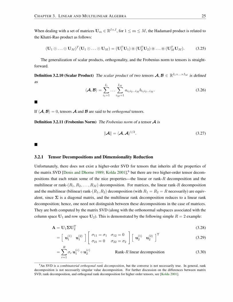
CHAPTER 3. LINEAR AND MULTILINEAR ALGEBRA 25
When dealing with a set of matrices Um ∈ RI×J , for 1 ≤ m ≤ M , the Hadamard product is related to
the Khatri-Rao product as follows:
(U1 � . . .�UM )T (U1 � . . .�UM ) = (UT1 U1) ~ (UT
2 U2) ~ . . . ~ (UTMUM ). (3.25)
The generalization of scalar products, orthogonality, and the Frobenius norm to tensors is straight-
forward.
Definition 3.2.10 (Scalar Product) The scalar product of two tensors A,B ∈ RI1×...×IM is defined
as
〈A,B〉 =I1∑
i1=1
. . .
IM∑iM=1
ai1i2...iM bi1i2...iM . (3.26)
�
If 〈A,B〉 = 0, tensors A and B are said to be orthogonal tensors.
Definition 3.2.11 (Frobenius Norm) The Frobenius norm of a tensor A is
‖A‖ = 〈A,A〉1/2. (3.27)
�
3.2.1 Tensor Decompositions and Dimensionality Reduction
Unfortunately, there does not exist a higher-order SVD for tensors that inherits all the properties of
the matrix SVD [Denis and Dhorne 1989; Kolda 2001],6 but there are two higher-order tensor decom-
positions that each retain some of the nice properties—the linear or rank-R decomposition and the
multilinear or rank-(R1, R2, . . . , RM ) decomposition. For matrices, the linear rank-R decomposition
and the multilinear (bilinear) rank-(R1, R2) decomposition (with R1 = R2 = R necessarily) are equiv-
alent, since Σ is a diagonal matrix, and the multilinear rank decomposition reduces to a linear rank
decomposition; hence, one need not distinguish between these decompositions in the case of matrices.
They are both computed by the matrix SVD (along with the orthonormal subspaces associated with the
column space U1 and row space U2). This is demonstrated by the following simple R = 2 example:
A = U1ΣUT2 (3.28)
=[
u(1)1 u(2)
1
] [ σ11 = σ1 σ12 = 0σ21 = 0 σ22 = σ2
] [u(1)
2 u(2)2
]T(3.29)
=R∑
r=1
σr u(r)1 ◦ u(r)
2 Rank-R linear decomposition (3.30)
6An SVD is a combinatorial orthogonal rank decomposition, but the converse is not necessarily true. In general, rankdecomposition is not necessarily singular value decomposition. For further discussion on the differences between matrixSVD, rank decomposition, and orthogonal rank decomposition for higher order tensors, see [Kolda 2001].

CHAPTER 3. LINEAR AND MULTILINEAR ALGEBRA 26
D
U1
=
I3
U2
U3
Z
R
I2
I3
I1
I1
I2
R
R
R
R
R
= + + ... +
u2
(1)
u1
(1)
u3
(1)
u2
(2)
u1
(2)
u3
(2)
u2
(R)
u1
(R)
u3
(R)
σ1
σ2
σR
Figure 3.2: The rank-R decomposition of the data tensor D yields a sum of rank-1 tensors which can beexpressed as a product of a diagonal core tensor Z and M (not necessarily orthonormal) mode matricesU1 . . .UM . The decomposition D = Z ×1 U1 ×2 U2 ×3 U3 of a third-order (M = 3) tensor D isillustrated.
=R∑
i=1
R∑j=1
σij u(i)1 ◦ u(j)
2 Rank-(R,R) multilinear decomposition (3.31)
When dealing with higher-order tensors, however, the difference between the linear rank-R and multilin-
ear rank-(R1, R2, . . . , RM ) decompositions becomes apparent and important. Furthermore, for higher-
order tensors, there is no trivial counterpart to dimensionality reduction in the matrix SVD case through
truncation.
Linear, Rank-R Decomposition
The tensor rank-R decomposition is a natural generalization of the matrix rank-R decomposition, but
unfortunately the Um are no longer orthonormal matrices.
Definition 3.2.12 (Tensor Rank and Rank-R Decomposition) The rank of an M th-order tensor A,
denoted R = rank(A), is the minimal number of rank-1 tensors that yield A in a linear combination:
A =R∑
r=1
σr u(r)1 ◦ u(r)
2 ◦ . . . ◦ u(r)M (3.32)
= Z ×1 U1 ×2 U2 . . .×M UM , (3.33)
which is known as the rank-R decomposition of A, where for 1 ≤ m ≤ M the u(r)m are unit vectors,
Um ∈ RIm×R = [u(1)m . . .u(r)
m . . .u(R)m ], and Z ∈ RR×R×...×R = diag(σ1 . . . σr . . . σR) is a diagonal
tensor of order M . �
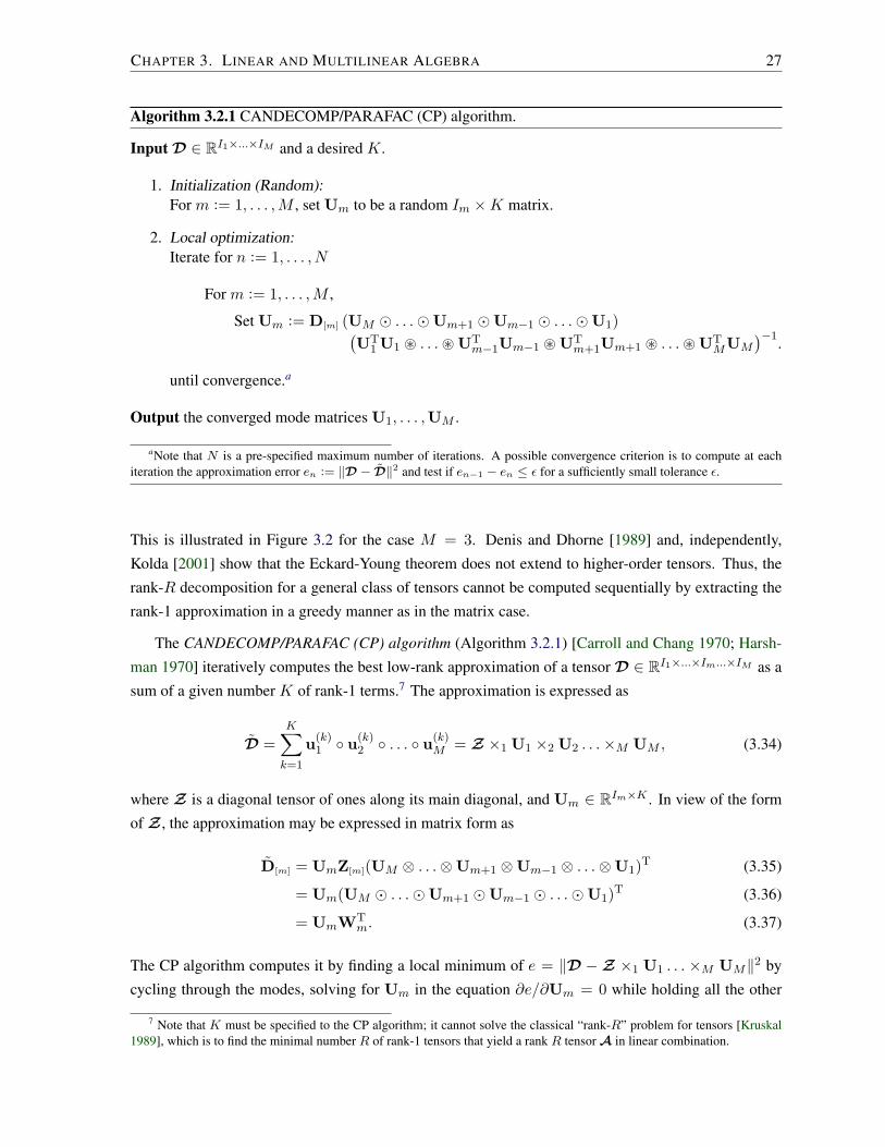
CHAPTER 3. LINEAR AND MULTILINEAR ALGEBRA 27
Algorithm 3.2.1 CANDECOMP/PARAFAC (CP) algorithm.
Input D ∈ RI1×...×IM and a desired K.
1. Initialization (Random):For m := 1, . . . ,M , set Um to be a random Im ×K matrix.
2. Local optimization:Iterate for n := 1, . . . , N
For m := 1, . . . ,M ,
Set Um := D[m] (UM � . . .�Um+1 �Um−1 � . . .�U1)(UT
1 U1 ~ . . . ~ UTm−1Um−1 ~ UT
m+1Um+1 ~ . . . ~ UTMUM
)−1.
until convergence.a
Output the converged mode matrices U1, . . . ,UM .
aNote that N is a pre-specified maximum number of iterations. A possible convergence criterion is to compute at eachiteration the approximation error en := ‖D − D‖2 and test if en−1 − en ≤ ε for a sufficiently small tolerance ε.
This is illustrated in Figure 3.2 for the case M = 3. Denis and Dhorne [1989] and, independently,
Kolda [2001] show that the Eckard-Young theorem does not extend to higher-order tensors. Thus, the
rank-R decomposition for a general class of tensors cannot be computed sequentially by extracting the
rank-1 approximation in a greedy manner as in the matrix case.
The CANDECOMP/PARAFAC (CP) algorithm (Algorithm 3.2.1) [Carroll and Chang 1970; Harsh-
man 1970] iteratively computes the best low-rank approximation of a tensor D ∈ RI1×...×Im...×IM as a
sum of a given number K of rank-1 terms.7 The approximation is expressed as
D =K∑
k=1
u(k)1 ◦ u(k)
2 ◦ . . . ◦ u(k)M = Z ×1 U1 ×2 U2 . . .×M UM , (3.34)
where Z is a diagonal tensor of ones along its main diagonal, and Um ∈ RIm×K . In view of the form
of Z , the approximation may be expressed in matrix form as
D[m] = UmZ[m](UM ⊗ . . .⊗Um+1 ⊗Um−1 ⊗ . . .⊗U1)T (3.35)
= Um(UM � . . .�Um+1 �Um−1 � . . .�U1)T (3.36)
= UmWTm. (3.37)
The CP algorithm computes it by finding a local minimum of e = ‖D − Z ×1 U1 . . . ×M UM‖2 by
cycling through the modes, solving for Um in the equation ∂e/∂Um = 0 while holding all the other
7 Note that K must be specified to the CP algorithm; it cannot solve the classical “rank-R” problem for tensors [Kruskal1989], which is to find the minimal number R of rank-1 tensors that yield a rank R tensor A in linear combination.

CHAPTER 3. LINEAR AND MULTILINEAR ALGEBRA 28
mode matrices constant, and repeating until convergence. Note that
∂e
∂Um=
∂
∂Um‖D[m] −UmWT
m‖2 = −D[m]Wm + UmWTmWm. (3.38)
Thus, ∂e/∂Um = 0 implies that
Um = D[m]Wm(WTmWm)−1
= D[m](UM � . . .�Um+1 �Um−1 � . . .�U1) (3.39)
(UT1 U1 ~ . . . ~ UT
m−1Um−1 ~ UTm+1Um+1 ~ . . .UT
MUM )−1,
where Wm = (UM � . . . � Um+1 � Um−1 � . . . � U1), and WTmWm may be computed more
efficiently by taking advantage of the Hadamard/Khatri-Rao property (3.25). This optimization is the
basis of Algorithm 3.2.1.
Multilinear, Rank-(R1, R2, . . . , RM ) Decomposition
The rank-(R1, R2, . . . , RM ) decomposition (a.k.a. the Tucker decomposition) does not reveal the rank
of the tensor, but it naturally generalizes the orthonormal subspaces corresponding to the left/right ma-
trices computed by the matrix SVD [Tucker 1966; Kroonenberg and de Leeuw 1980; Kapteyn et al.
1986; de Lathauwer et al. 2000b].
Theorem 3.2.1 (Rank-(R1, R2, . . . , RM ) (or Multilinear) Decomposition / M -mode SVD) Let A be
a I1 × I2 . . .× Im . . .× IM tensor for 1 ≤ m ≤ M . Every such tensor can be decomposed as follows:
A = Z ×1 U1 ×2 U2 . . .×m Um . . .×M UM (3.40)
=R1∑
i1=1
R2∑i2=1
. . .
Rm∑im=1
. . .
RM∑iM=1
σi1i2...iM u(i1)1 ◦ u(i2)
2 . . . ◦ u(im)m . . . ◦ u(iM )
M , (3.41)
where Um ∈ RIm×Rm = [u(1)m u(2)
m . . .u(im)m . . .u(Rm)
m ] are orthonormal mode-m matrices, where 1 ≤Rm ≤ Im for 1 ≤ m ≤ M , and Z ∈ RR1×R2...×Rm...×RM .8 The subtensors Z im=a and Z im=b
obtained by fixing the mth index to a and b are orthogonal for all values of m, a, and b when a 6= b. The
‖Z im=a‖ = σ(m)a is the ath mode-m singular value of A and the ath column vector of Um, such that
‖Z im=1‖ ≥ ‖Z im=2‖ ≥ . . . ‖Z im=Rm‖ ≥ 0. �
This is illustrated in Figure 3.3 for the case M = 3. Tensor Z , known as the core tensor, is analogous
to the diagonal singular value matrix in conventional matrix SVD (although it does not have a simple,
diagonal structure). The core tensor contains normalizing parameters associated with the different mode
matrices U1, . . . ,UM . Mode matrix Um contains the orthonormal vectors spanning the column space
of matrix A[m] resulting from the mode-m matrixizing of A (Figure 3.1).
8From (3.19), we can also write in vector form, vec(A) = (UM ⊗UM−1 . . .⊗Um . . .⊗U1)vec(Z).

CHAPTER 3. LINEAR AND MULTILINEAR ALGEBRA 29
D
U1
=
X X
~R1
I3
U2
U3
Z
R1
I2
I3
I1 I
1I2
R3
R2
R3
R1
R2
Figure 3.3: The multilinear, or rank-(R1, R2, . . . , RM ), decomposition decomposes the data tensor Dinto the product of a core tensor Z and M orthogonal mode matrices U1 . . .UM . For the M = 3 caseillustrated here, D = Z ×1 U1 ×2 U2 ×3 U3. Deletion of the last mode-1 eigenvector of U1 incurs anerror in the approximation equal to σ2
I1, which equals the Frobenius norm of the (grey) subtensor of Z
whose row vectors would normally multiply the eigenvector in the mode-1 product Z ×1 U1.
Algorithm 3.2.2 M -mode SVD algorithm.
Input the data tensor D ∈ RI1×...×IM .
1. For m := 1, . . . ,M ,Let Um be the left orthonormal matrix of the SVD of D[m], the mode-m matrixized D.
2. Set Z := D ×1 UT1 ×2 UT
2 . . .×m UTm . . .×M UT
M .
Output the mode matrices U1, . . . ,UM and the core tensor Z .
Algorithm 3.2.2 is the M -mode SVD algorithm for decomposing an M th-order tensor D according
to equation (3.40). It employs M matrix SVDs to compute the M orthonormal mode matrices and then
computes the core tensor.
As we stated earlier, there is no trivial counterpart for higher-order tensors to dimensionality re-
duction in the matrix SVD case. According to [Kroonenberg and de Leeuw 1980; Kapteyn et al.
1986; de Lathauwer et al. 2000b], a useful generalization in the tensor case involves an optimal rank-
(R1, R2, . . . , RM ) approximation which iteratively optimizes each of the modes of the given tensor,
where each optimization step involves a best reduced-rank approximation of a positive semi-definite
symmetric matrix.
A truncation of the mode matrices of the data tensor D results in an approximation D with reduced
ranks Rm ≤ Rm, where Rm = rankm(D) = rank(D[m]) = rank(Um) is the m-rank of D for

CHAPTER 3. LINEAR AND MULTILINEAR ALGEBRA 30
Algorithm 3.2.3 M -mode SVD dimensionality reduction algorithm.
Input the data tensor D ∈ RI1×...×IM and desired ranks R1, . . . , RM .
1. Initialization (Truncated M -Mode SVD):Apply Step 1 of the M -mode SVD algorithm (Algorithm 3.2.2) to D.For m := 1, 2, . . . ,M , truncate to Rm columns the mode matrix Um ∈ RIm×Rm .a
2. Local optimization via alternating least squares:Iterate for n := 1, . . . , N
For m := 1, . . . ,M ,
Set X := D ×1 UT1 . . .×m−1 UT
m−1 ×m+1 UTm+1 . . .×M UT
M .
Set Um to the Rm leading left-singular vectors of the SVD of X[m].
Set Z := X ×M UTM .
until convergence.b
Output the converged core tensor Z and mode matrices U1, . . . ,UM .
a The complexity of computing the SVD of an m × n matrix A is O(mn min(m, n)), which is costly when both mand n are large. However, we can efficiently compute the R leading left-singular vectors of A by first computing the rank-Rmodified Gram-Schmidt (MGS) orthogonal decomposition A ' QR, where Q is m×R and R is R×n, and then computingthe SVD of R and multiplying it as follows: A ' Q(UΣVT) = (QU)ΣVT = UΣVT.
bSee Footnote a in Algorithm 3.2.1.
1 ≤ m ≤ M . The error of this approximation is
‖D − D‖2 =R1∑
i1=R1+1
R2∑i2=R2+1
· · ·RM∑
iM=RM+1
Z2i1i2...iM
(3.42)
The error is bounded by the sum of squared singular values associated with the discarded singular
vectors:
‖D − D‖2 ≤R1∑
i1=R1+1
σ2i1 +
R2∑i2=R2+1
σ2i2 + · · ·+
RM∑iM=RM+1
σ2iM
. (3.43)
Note that the singular value associated with the nth singular vector in mode matrix Um is equal to
‖Z im=n‖; i.e., the Frobenius norm of subtensor Z im=n of the core tensor Z (Figure 3.3).
Truncation of the mode matrices resulting from the M -mode SVD algorithm may yield a good
reduced-dimensionality approximation D, but it is generally not optimal. A locally optimal dimen-
sionality reduction scheme for tensors is to compute a best rank-(R1, R2, . . . , RM ) approximation
D = Z ×1 U1×2 U2 . . .×M UM with orthonormal Im× Rm mode matrices Um, for m = 1, . . . ,M ,

CHAPTER 3. LINEAR AND MULTILINEAR ALGEBRA 31
which minimizes the error function
e = ‖D − D‖+M∑
m=1
Λm‖UTmUm − I‖, (3.44)
where the Λm are Lagrange multiplier matrices.9
To this end, the M -mode dimensionality reduction algorithm (Algorithm 3.2.3) iteratively computes
Um, for m = 1, . . . ,M , and Z by performing in Step 2 a higher-order extension of the orthogonal
iteration for matrices. Note that the M -mode orthogonal iteration finds only a local minimum of this
generally non-convex error function.
9This best rank-(R1, R2, . . . , RM ) problem should also not be confused with the classical “rank-R” problem for tensorsmentioned in Footnote 7.

4The Tensor Algebraic Framework
Contents4.1 PCA and ICA . . . . . . . . . . . . . . . . . . . . . . . . . . . . . . . . . . . . . 33
4.2 Multilinear PCA (MPCA) . . . . . . . . . . . . . . . . . . . . . . . . . . . . . . . 36
4.3 Multilinear ICA (MICA) . . . . . . . . . . . . . . . . . . . . . . . . . . . . . . . 40
4.4 Kernel MPCA/MICA, Multifactor LLE/Isomap/LE, and Other Generalizations 43
Algorithms
4.2.1 Multilinear PCA (MPCA) Algorithm. . . . . . . . . . . . . . . . . . . . . . . . . . . . . . . . . . . . . . . . . . . . . 37
4.3.1 Multilinear ICA (MICA) Algorithm. . . . . . . . . . . . . . . . . . . . . . . . . . . . . . . . . . . . . . . . . . . . . . 42
4.4.1 Kernel Multilinear PCA/ICA (K-MPCA/MICA) Algorithm. . . . . . . . . . . . . . . . . . . . . . . . . 46
In this chapter, we develop a multilinear framework for the analysis of multimodal observational
data. An observation comprises a set of measurements whose values are influenced by multiple under-
lying causal factors. The measurements are also known as response variables since their values change
in response to changes in the causal factors. The causal factors are not directly measurable, and the
variables extracted by data analysis in order to represent them are known as explanatory variables. For
example, an image is an observation whose measurements are pixels, the values of which vary with
changes in the causal factors—scene structure, illumination, view, etc. In the previous chapter, we dis-
cussed the decomposition of an M th-order data tensor in terms of M mode matrices. These matrices are
associated with the measurement mode as well as with the M−1 causal factor modes. When performing
32

CHAPTER 4. THE TENSOR ALGEBRAIC FRAMEWORK 33
data analysis, we are interested in modeling the causal relationship, therefore we will be decomposing
the data tensor only in terms of the M − 1 causal factors.
First we review Principle Components Analysis (PCA) and Independent Components Analysis
(ICA). Next, we develop Multilinear PCA (MPCA) and Multilinear ICA (MICA), the key methods
in our framework, which overcome the limitations of their linear counterparts (in Chapter 7, we will
expand our tensor framework by introducing multilinear projection for recognition). We close the chap-
ter by discussing generalizations of our multilinear algorithms and the extension of our multifactor
approach to include other manifold learning methods.
4.1 PCA and ICA
Principal Components Analysis computes an optimal orthonormal linear data representation by model-
ing the variance in the data, but without distinguishing between different sources of variation. Thus, it
is best suited at capturing single causal factor linear variation in the observed data.
Let a multivariate sensory observation be represented by a column vector. An ensemble of obser-
vations form a data matrix, or two-way array, D where each column is a measurement vector. The
underlying assumption is that the observations reside in a low-dimensional subspace; i.e., that the col-
umn vectors of D span a low dimensional subspace.
Principal components analysis of an ensemble of I2 observations is computed by performing an
SVD on a I1 × I2 data matrix D whose columns are the “vectorized”, “centered” observations. Each
vectorized, centered observation is obtained by subtracting the mean observation from each input ob-
servation of the ensemble and identically arranging the resulting measurements into a column vector.
It is important to realize that this regards entire observations (e.g., images) as vectors or points in high
(I1) dimensional space. This enables PCA to model the full second-order statistics, the covariance be-
tween all possible pairs of measurements (pixel) in the observation (image) as we discuss in detail in
Appendix A.
The data matrix D ∈ RI1×I2 is a two-mode mathematical object that has two associated vector
spaces, a row space and a column space. In a factor analysis of D, the SVD orthogonalizes these two
spaces and decomposes the matrix as
D = UΣVT = U︸︷︷︸PCA Basis
Matrix
ΣVT︸ ︷︷ ︸PCA Coefficient
Matrix
, (4.1)
the product of an orthonormal column-space represented by the left matrix U ∈ RI1×R, a diagonal
singular value matrix Σ ∈ RR×R with diagonal entries σ1 ≥ σ2 ≥ . . . ≥ σR ≥ 0 called the singular
values of D, and an orthonormal row space represented by the right matrix V ∈ RI2×R. The left-
singular vectors in U are also called the principal component (or Karhunen-Loeve) directions of D.1
1This is because the covariance matrix is given by S = DDT/I2, and from (4.1) we have the eigen-decomposition ofDDT = UΣ2UT, which is the eigen-decomposition of S up to a factor I2.

CHAPTER 4. THE TENSOR ALGEBRAIC FRAMEWORK 34
R
(a) (b) (c)
Figure 4.1: Geometric view of the relationship between PCA and ICA. (a) Compute the PCA basisvectors associated with the data. (b) Represent the data relative to the PCA basis vectors. PCA applies arotation to the data. (c) Whiten the data and compute the rotation R that finds the arms in the data, thusyielding the ICA basis vectors.
Optimal dimensionality reduction in matrix principal components analysis is obtained by truncation
of the singular value decomposition (i.e., deleting eigenvectors associated with the smallest singular
values).
While PCA seeks an accurate representation in least-square sense, ICA seeks a meaningful repre-
sentation by employing additional information not contained in the covariance matrix. The independent
components analysis of multivariate data seeks a sequence of projections such that the projected data
are statistically independent. One way of achieving statistical independence is by seeking a set of pro-
jections which results in projected data that looks as far from Gaussian as possible. Figure 4.1 provides
a geometric interpretation of the computation of ICA. ICA and PCA may yield different subspaces, as
shown in Figure 4.2, which will yield different recognition results. The subspaces for PCA and ICA
are identical when the directions of greatest variation and the directions of the independent components
span the same subspace, in which case the recognition results will be identical.
ICA can be applied in two ways [Bartlett et al. 2002]:
1. to DT, each of whose rows is a different image, which finds a spatially independent basis set that
reflects the local properties of imaged objects, or
2. to D, which finds a set of coefficients that are statistically independent while the basis reflects the
global properties of imaged objects.
In Approach 1, ICA starts essentially from the factor analysis or PCA solution (4.1), and applies an
invertible transformation to the principal components such that they become independent components
[Hastie et al. 2001] as follows:
DT ' VΣUT (4.2)
=(VΣW−1
) (WUT
)(4.3)

CHAPTER 4. THE TENSOR ALGEBRAIC FRAMEWORK 35
ICA subspace PCA subspace
Figure 4.2: PCA and ICA may yield different subspaces for analysis. The ellipsoids represent a bi-lobed dataset. The red and green axes capture the greatest data variation and indicate the top twoprincipal components, while the blue and yellow axes indicate the independent components. Thus, inthis example, the directions of greatest variations and the directions of independent components definetwo subspaces that are mutually othogonal.
= KTCT, (4.4)
where every column of D is a different image, U, V, and Σ are rank-reduced, W is an invertible trans-
formation matrix that is computed by the ICA algorithm, C = UWT are the independent components,
and K = W−TΣVT are the coefficients. Various objective functions, such as those based on mu-
tual information, negentropy, higher-order cumulants, etc., are presented in the literature for computing
the independent components along with different optimization methods for extremizing these objective
functions [Hyvarinen et al. 2001]. Dimensionality reduction with ICA is usually performed in the PCA
preprocessing stage.
Alternatively, in Approach 2, ICA is applied to D and it rotates the principal components directions
such that the coefficients are statistically independent, as follows:
D ' UΣVT (4.5)
=(UW−1
) (WΣVT
)(4.6)
= CK, (4.7)
where U, V, and Σ are rank-reduced, C = UW−1 is the basis matrix and K = WΣVT are the
statistically independent coefficients. Note that the W matrices in (4.6) differ from the analogous W
matrices in (4.3); hence, the K and C matrices also differ.
PCA and ICA are linear analysis methods, hence they are not well suited to the representation of
multifactor image ensembles. To address this shortcoming, the next two sections develop their multilin-
ear generalizations in turn.
CHAPTER 4. THE TENSOR ALGEBRAIC FRAMEWORK 36
4.2 Multilinear PCA (MPCA)
The analysis of an ensemble of observations (e.g., images) resulting from the confluence of multiple
causal factors (e.g., scene structure, illumination, view, etc.) is a problem in multilinear algebra. Within
this mathematical framework, the ensemble of observations is organized as a data tensor. This data
tensor D must be decomposed in order to separate and parsimoniously represent the causal factors. To
this end, we prescribe the M -mode SVD (3.40):
D = Z ×1 U1 ×2 U2 . . .×m Um . . .×M UM . (4.8)
As was stated in Section 3.2, multilinear analysis decomposes the tensor as the mode-m product of
M -orthogonal spaces.
Now, let us assume that m = 1 is the measurement (pixel) mode and that the remaining modes
m = 2, . . . ,M are the causal factor modes; i.e., those modes associated with the relevant causal factors
that underlie the generation of observations (images). Rather than computing the core tensor Z , we
prefer to define the basis tensor
T = Z ×1 U1, (4.9)
which we call the extended core tensor, that makes explicit the interaction between the causal factors:
D = T ×2 U2 . . .×m Um . . .×M UM . (4.10)
Given this multilinear model, an observation (image) may be synthetized according to the expression
d = T ×2 rT2 . . .×m rT
m . . .×M rTM , (4.11)
where, for m = 2, . . . ,M , vector rm is the representation vector associated with causal factor m. Note,
in particular, that if rm is chosen to be ci, i = 1, . . . , IM , a row of Um, for m = 2, . . . ,M , then d will
reconstruct any one of the images in the ensemble D.
Efficient MPCA Algorithm
Recall the M -mode SVD algorithm (Algorithm 3.2.2) for decomposing D according to (4.8). Regarding
Step 1 of the algorithm, note that when D[m] is a nonsquare matrix, the computation of Um in the SVD
D[m] = UmΣVTm can be performed efficiently, depending on which dimension of D[m] is smaller,
by decomposing either D[m]DT[m] = UmΣ2UT
m (note that VTm = Σ+UT
mD[m]) or by decomposing
DT[m]D[m] = VmΣ2VT
m and then computing Um = D[m]VmΣ+.
Despite the above improvement, the M -mode SVD algorithm will still be inefficient in practice
when one or more of the dimensions Im are large. We can improve it further for practical use in
applications. To this end, the mode-m covariance matrix D[m]DT[m] for the causal factor modes m =
2, . . . ,M can be computed directly, element by element, by summing the appropriate inner products
between pairs of data points (e.g., images) in the data tensor D that are associated with mode m. In

CHAPTER 4. THE TENSOR ALGEBRAIC FRAMEWORK 37
Algorithm 4.2.1 Multilinear PCA (MPCA) algorithm.
Input the data tensor D ∈ RI1×...×IM , where mode m = 1 is the measurement mode, and the desiredranks R2, . . . , RM .
1. For m := 2, . . . ,M ,
Compute the elements of the mode-m covariance matrix, for j, k := 1, . . . , Im, as follows:
[D[m]DT
[m]
]jk
:=I2∑
i2=1
· · ·Im−1∑
im−1=1
Im+1∑im+1=1
· · ·IM∑
iM=1
dTi2...im−1 j im+1...iM
di2...im−1 k im+1...iM .
(4.13)
Set mode matrix Um to the left matrix of the SVD of D[m]DT[m] = UmΣ2UT
m.
Truncate to Rm columns Um ∈ RIm×Rm . a
2. Set T := D ×2 UT2 . . .×m UT
m . . .×M UTM .
3. Local optimization via alternating least squares:Iterate for n := 1, . . . , N
For m := 2, . . . ,M ,
Set X := D ×2 UT2 . . .×m−1 UT
m−1 ×m+1 UTm+1 . . .×M UT
M .
Set Um to the Rm leading left-singular vectors of the SVD of X[m].
Set T := X ×M UTM .
until convergence.b
Output the converged extended core tensor T ∈ RI1×R2×...×RM and causal factor mode matricesU2, . . . ,UM .
aSee Footnote a of Algorithm 3.2.3.bSee Footnote a in Algorithm 3.2.1.
particular, element j, k of the mode-m covariance matrix is given by
[D[m]DT
[m]
]jk
=I2∑
i2=1
· · ·Im−1∑
im−1=1
Im+1∑im+1=1
· · ·IM∑
iM=1
dTi2...im−1 j im+1...iM
di2...im−1 k im+1...iM , (4.12)
where di2,...,iM is a vectorized image that is packed into the data tensor D. This computation will also
be useful in generalizations of our multilinear algorithms, as we will discuss in Section 4.4.
Given the above considerations, we obtain a Multilinear PCA (MPCA) algorithm (Algorithm 4.2.1)
which includes dimensionality reduction. Step 1 of this algorithm performs an efficient (M − 1)-Mode
SVD of input data tensor D, where the measurement mode is not explicitly computed, and truncates each
of the causal factor mode matrices Um, for m = 2, . . . ,M , to the specified reduced ranks Rm. Then,
Step 3 of the algorithm iteratively optimizes the reduced mode matrices. Its theoretical underpinnings

CHAPTER 4. THE TENSOR ALGEBRAIC FRAMEWORK 38
are the same as for the M -mode dimensionality reduction algorithm (Algorithm 3.2.3). Like the M -
mode orthogonal iteration in Algorithm 3.2.3, the (M−1)-mode orthogonal iteration in Algorithm 4.2.1
finds only a local minimum of the generally non-convex error function (3.44). Note that T is computed
as specified since X = D×2UT2 . . .×m−1UT
m−1×m+1UTm+1 . . .×M UT
M = Z×1U1×mUm. Hence,
upon completion of the previous “For m” step, X = Z ×1 U1 ×M UM . Therefore, after convergence,
X ×M UTM = Z ×1 U1 = T .
After applying Algorithm 4.2.1 to perform an MPCA with dimensionality reduction on an input data
tensor D of order M , where mode m = 1 is the measurement mode, the resulting approximation of the
input data tensor is given by
D ' D = T ×2 U2 . . .×M UM . (4.14)
Relationships to PCA
To show mathematically that PCA is a special case of our MPCA, we write the latter in terms of matrix
notation. A matrix representation of the M -mode SVD can be obtained by matrixizing with respect to
the measurement (i.e., pixel) mode, and using (3.18), as follows:
D[1]︸︷︷︸Data
= U1︸︷︷︸PCA Basis
Matrix
Z[1](UM ⊗ . . .⊗Um ⊗ . . .⊗U2)T︸ ︷︷ ︸PCA Coefficient
Matrix
. (4.15)
The above matrix product can be interpreted as a standard linear decomposition of the data ensemble
(4.1). Note that D[1] is a matrix whose columns are a set of observations; hence, it is the PCA data
matrix. The measurement mode matrix U1 is computed by performing an SVD on D[1]; hence, it is
the PCA basis matrix. Thus, the product of the matrixized core tensor Z[1] and the Kronecker product
of the mode matrices UM , . . . ,U2 associated with the causal factors is the PCA coefficient matrix. As
a consequence, our multilinear analysis subsumes linear, PCA analysis. MPCA goes beyond PCA by
further decomposing the PCA coefficient matrix into a set of coefficient matrices associated with the
different causal factors.
Although the computation of the measurement mode matrix U1 in our MPCA is the PCA basis
matrix (4.15), more interesting is the relationship between standard PCA and the MPCA causal factor
mode matrices. Computing the causal factor mode matrices in our multilinear model amounts to the
computation of a set of mutually constrained, cluster-based PCAs. When dealing with data that can be
separated into clusters, the standard machine learning approach is to compute a separate PCA. When
data from different clusters are generated by the same underlying process (e.g., facial images of the
same people under different viewing conditions), the underlying data can be concatenated in the mea-
surement mode and the common causal factor can be modeled by one PCA.2 Thus, we have defined a
constrained, cluster-based PCA in the sense that the resulting causal factor representation is constrained
2The active appearance model [Cootes et al. 2001] concatenated two different measurements, facial feature locations andtexture, to compute a person representation for a particular viewpoint invariant of measurement. More generally, one canconcatenate the measurements of a person from different viewpoint clusters to compute a person representation that is invariantof the measurement and the viewpoint.

CHAPTER 4. THE TENSOR ALGEBRAIC FRAMEWORK 39
to be identical in every cluster.
MPCA performs M constrained, cluster-based PCAs, since the computation of the mode-m matrix
Um, which involves a mode-m data tensor flattening and subsequent SVD, is equivalent to performing
a constrained, cluster-based PCA; i.e., data cluster concatenation followed by an SVD. In the context of
our multifactor data analysis, we define a cluster as a set of observations for which all factors are fixed
except one, the mth factor. Note that there are Nm = I2I3 . . . Im−1Im+1 . . . IM possible clusters and
the data in each cluster varies with the same causal mode.3 Thus, the data across different clusters share
one of the underlying causal factors. The constrained, cluster-based PCA concatenates the clusters in
the measurement mode and analyzes the data with a linear model, such as PCA.
To see this, let Di2...im−1im+1...iM ∈ RI1×1×...×1×Im×1×...×1 denote a subtensor of D that is ob-
tained by fixing all modes except causal factor mode m and mode 1 (the measurement mode). Matrix-
izing this subtensor in mode 1, we obtain Di2...im−1im+1...iM [1]∈ RI1×Im . This data matrix comprises
a cluster of data obtained by varying the mth causal factor, to which one can traditionally apply PCA.
Since there are Nm = I2I3 . . . Im−1Im+1 . . . IM possible clusters that share the same underlying space
associated with the mth factor, the data can be concatenated and PCA performed in order to extract
the same representation for the mth factor regardless of the cluster. Now, consider the multilinear PCA
computation of mode matrix Um, which can be written in terms of matrixized subtensors as
D[m] =
D1...11...1T[m]
...
DI2...11...1T[m]
...
DI2...Im−1Im+1...IMT[m]
T
= UmΣmVTm. (4.16)
Clearly, this is equivalent to computing a set of Nm = I2I3 . . . Im−1Im+1 . . . IM cluster-based PCAs
concurrently by combining them into a single statistical model and representing the underlying causal
factor m common to the clusters. Thus, rather than computing a separate linear PCA model for each
cluster, MPCA concatenates the clusters into a single statistical model and computes a representation
(coefficient vector) for mode m that is invariant relative to the other causal factor modes 2, . . . , (m −1), (m + 1), . . . ,M . Therefore, MPCA is a multilinear, constrained, cluster-based PCA.
To clarify the relationship, let us number each of the matrices Di2...im−1im+1...iM [m]= D(n)
m with a
parenthetical superscript 1 ≤ n = 1 +∑M
k=2,k 6=m(in − 1)∏k−1
l=2,l 6=m Il ≤ Nm. Let each of the linear
SVDs be D(n)m = U(n)
m Σ(n)m V(n)
m
T. Then D[m] = [U(1)
m Σ(1)m . . .U(Nm)
m Σ(Nm)m ] diag([V(1)
m . . .V(Nm)m ])T,
where diag(·) denotes a diagonal matrix whose elements are each of the elements of its vector argument.
The measurement mode matrix V(n)m contains the eigenvectors that span the observed data in cluster n.
The SVD of the first matrix is [U(1)m Σ(1)
m . . .U(Nm)m Σ(Nm)
m ] = UmΣmWTm. Then we can write (4.16)
3Observations in the cluster may not be in Euclidean proximity in the measurement space. Consequently, a cluster may notbe easily identified through a standard EM algorithm, but may be computable using a “coupled-EM” that would generalize theEM algorithm to extend a set of clusters. Such an algorithm has not been applied to define the clusters in these experiments.

CHAPTER 4. THE TENSOR ALGEBRAIC FRAMEWORK 40
as D[m] = UmΣmVTm, where VT
m = WTm diag([V(1)
m . . .V(Nm)m ])T. Matrix Wm rotates each of the
measurement mode matrices V(n)m for each cluster computed by linear PCA such that the representation
Um is the same across the clusters.
4.3 Multilinear ICA (MICA)
We have discussed MPCA, which computes accurate representations of observational data by optimiz-
ing the reduced-dimensional data approximation error in a least-squares sense. This is done in a mul-
tifactor manner, by accurately representing the underlying causal factor subspaces. However, MPCA
ignores important aspects of non-Gaussian data, such as clustering and independence. Therefore, we
will next develop Multilinear ICA, which employs higher-order statistics to derive meaningful repre-
sentations for each of the underlying causal factors. To compute such representations we will propose
a novel, Multilinear ICA (MICA) algorithm. Our nonlinear, tensor algebraic algorithm should not be
confused with existing tensor algorithms for computing the conventional, linear ICA [de Lathauwer
1997].
Analogously to (4.8) and (4.14), multilinear ICA is obtained by approximating the data tensor D as
the mode-m product of M mode matrices Cm and a core tensor S, as follows:
D = S ×1 C1 ×2 C2 . . .×m Cm . . .×M CM . (4.17)
Analogously to (4.9), (4.10), and (4.11), we have the extended core
M = S ×1 C1, (4.18)
the multilinear approximation
D = M×2 C2 . . .×m Cm . . .×M CM , (4.19)
and the multilinear expression for an observation
d = M×2 rT2 . . .×m rT
m . . .×M rTM . (4.20)
As in ICA, there are two approaches for multilinear independent components analysis (MICA). The
first results in a factorial code, where each set of coefficients is statistically independent, while the
second finds a set of independent bases.
In Approach 1, transposing the matrixized data tensor D in mode m and computing the ICA as in
(4.2)–(4.4), we obtain
DT[m] ' VmΣmUT
m (4.21)
=(VmΣmW−1
m
) (WmUT
m
)(4.22)
= KTmCT
m, (4.23)

CHAPTER 4. THE TENSOR ALGEBRAIC FRAMEWORK 41
where Um, Vm, and Σm are rank-reduced, and the mode matrices are given by
Cm = UmWTm. (4.24)
The columns associated with each of the mode matrices, Cm are statistically independent. We can
derive the relationship between MICA and MPCA (4.14) in the context of this approach as follows:
D = Z ×1 U1 . . .×M UM
= Z ×1 U1WT1 W−T
1 . . .×M UMWTMW−T
M
= Z ×1 C1W−T1 . . .×M CMW−T
M
= (Z ×1 W−T1 . . .×M W−T
M )×1 C1 . . .×M CM
= S ×1 C1 . . .×M CM ,
where the core tensor S = Z ×1 W−T1 . . .×M W−T
M .
Alternatively, in Approach 2, matrixizing the data tensor D in the mth mode and computing the
ICA as in (4.5)–(4.7), we obtain:
D[m] ' UmΣmVTm (4.25)
=(UmW−1
m
) (WmΣmVT
m
)(4.26)
= CmKm, (4.27)
where Um, Vm, and Σm are rank-reduced, and the mode matrices are given by
Cm = UmW−1m . (4.28)
Note that the W matrices in (4.26) and (4.28) differ from the analogous W matrices in (4.22) and
(4.24); hence, the K and C matrices also differ between the two methods. We can derive the relationship
between MICA and MPCA (4.14) in the context of the second approach as follows:
D = Z ×1 U1 . . .×M UM
= Z ×1 U1W−11 W1 . . .×M UMW−1
M WM
= Z ×1 C1W1 . . .×M CMWM
= (Z ×1 W1 . . .×M WM )×1 C1 . . .×M CM
= S ×1 C1 . . .×M CM ,
where the core tensor S = Z ×1 W1 . . .×M WM .
Algorithm 4.3.1 is an efficient Multilinear ICA (MICA) algorithm, which is the analog of our effi-
cient MPCA algorithm (Algorithm 4.2.1). Step 1 of Algorithm 4.3.1 has a structure that is similar to
the M -mode SVD algorithm (Algorithm 3.2.2), but applies one of the above to ICA approaches. Anal-

CHAPTER 4. THE TENSOR ALGEBRAIC FRAMEWORK 42
Algorithm 4.3.1 Multilinear ICA (MICA) algorithm.
Input the data tensor D ∈ RI1×...×IM , where mode m = 1 is the measurement mode, and the desiredranks R2, . . . , RM .
1. For m := 2, . . . ,M ,
Compute the causal factor mode matrix Cm ∈ RIm×Rm in (4.17) using Approach 1 orApproach 2, truncating the initial SVD to dimensionality Rm.
2. Set M := D ×2 C+2 . . .×m C+
m . . .×M C+M .
3. Local optimization via alternating least squares:Iterate for n := 1, . . . , N
For m := 2, . . . ,M ,
Set X := D ×2 C+2 . . .×m−1 C+
m−1 ×m+1 C+m+1 . . .×M C+
M .Compute Cm from X[m] either by Approach 1 (4.24) or Approach 2 (4.28).
Set M := X ×M C+M .
until convergence.a
Output the converged extended core tensor M ∈ RI1×R2×...×RM and causal factor mode matricesC2, . . . ,CM .
aSee Footnote a in Algorithm 3.2.1.
ogously to the case of MPCA, optimal dimensionality reduction in MICA is achieved in Step 3 of the
algorithm by optimizing mode per mode using a straightforward variant of the (M − 1)-mode orthog-
onal iteration, with an additional step that computes the transformation matrix W. Thus, we compute
the independent components for each mode in an iterative manner using alternating least squares, by
holding fixed all mode components except one and solving for the remaining mode. Note that we can
compute the approximation of D from the converged reduced extended core tensor M and reduced
causal factor mode matrices Cm as
D ' D = M×2 C2 . . .×M CM . (4.29)
As in the MPCA case, this algorithm finds only a local minimum of the generally non-convex error
function.
To see the difference between the subspaces spanned by ICA and MICA, consider the representation
computed for the causal factors of the process used to generate the data shown in Figure 4.3. MICA
computes an overcomplete set of basis vectors that extract all the arms in the data while ICA extracts
a combination of two of the arms. To see the difference between MPCA and MICA, consider the data
shown in Figure 4.4. MPCA yields a subspace for a causal factor that is spanned by the directions of
greatest variation, while MICA yields a subspace that is spanned by the directions that define indepen-

CHAPTER 4. THE TENSOR ALGEBRAIC FRAMEWORK 43
Figure 4.3: This data set contains four different arms, but ICA is able to extract only a combination oftwo of the arms while MICA extracts all four.
dent components. These two sets of directions may yield different subspaces.
4.4 Kernel MPCA/MICA, Multifactor LLE/Isomap/LE,and Other Generalizations
The effectiveness of conventional PCA and ICA is limited by their global linearity and their suscepti-
bility to non-Gaussian noise. Our approach to mitigating the linearity limitation has been to generalize
these methods in a natural way, resulting in globally nonlinear, multifactor models and methods that
have a multilinear manifold structure. We will now discuss two alternative classes of nonlinear models,
and then briefly discuss the issue of noise and outliers.
One approach is to handle data complexity via data clustering and the combination (or mixing)
of linear PCA or ICA models fitted to each local data cluster [Tipping and Bishop 1999; Lee et al.
2000]. An important distinction is that mixture-of-PCA/ICA models are additive combinations of lo-
cally Gaussian models, whereas our multilinear approach prescribes a multiplicative combination of
globally Gaussian models. Moreover, a mixture-of-PCA/ICA models yields a different set of basis vec-
tors for each local cluster. In our applications, we seek a single parsimonious set of basis vectors that
globally represent the entire dataset. That said, there seems to be no reason why one could not define
mixture-of-MPCA/MICA models and methods that would generalize the existing mixture-of-PCA/ICA
models. However, this is beyond the scope of the thesis.
An alternative approach is to apply linear models to nonlinear problems through the “kernel trick”,
specifically the kernel PCA [Scholkoph et al. 1998] and kernel ICA [Yang et al. 2005] techniques.4
4The so-called “kernel trick” maps the original non-linear measurements into a higher-dimensional space, where a linearclassifier is subsequently used; this makes a linear classification in the new space equivalent to non-linear classification in theoriginal space. This is done using Mercer’s theorem, which states that any continuous, symmetric, positive semi-definite kernelK(u,v) can be expressed as an inner product in a high-dimensional space. Wherever an inner product between two vectors is

CHAPTER 4. THE TENSOR ALGEBRAIC FRAMEWORK 44
(a) Observed Data
−0.15 −0.1 −0.05 0 0.05 0.1 0.15
−0.1
−0.05
0
0.05
0.1
0.15
x
y
−8 −6 −4 −2 0 2 4 6 8
−4
−2
0
2
4
6
8
x
y
(b) Factor 1 (c) MPCA - Factor 1 Subspace (d) MICA - Factor 1 Subspace
−0.2 −0.15 −0.1 −0.05 0 0.05 0.1 0.15−0.15
−0.1
−0.05
0
0.05
0.1
0.15
x
y
−10 −8 −6 −4 −2 0 2 4 6 8 10
−6
−4
−2
0
2
4
6
8
x
y
(e) Factor 2 (f) MPCA - Factor 2 Subspace (g) MICA - Factor 2 Subspace
Figure 4.4: A Comparison of the causal factor extraction/representation by MPCA and MICA. Theobserved data (a) were generated by the interaction of two unmeasurable causal factors. The distribu-tion of Factor 1 (b) comprises two populations; that of Factor 2 (e) comprises two conditions. Withoutdimensionality reduction, both methods extract the factors in (b), (e). However, analysis implies dimen-sionality reduction, and MPCA and MICA compute the subspaces in (c),(f) and (d),(g). The subspacesfor Factor 1 computed by MPCA (c) and MICA (d) are mutually orthogonal, but the subspaces for Fac-tor 2 computed by MPCA (f) and MICA (g) are identical as the directions of greatest variation and theindependent component directions span the same subspace in this case.

CHAPTER 4. THE TENSOR ALGEBRAIC FRAMEWORK 45
Linear kernel: K(u,v) = uTv = u · v
Polynomial kernel of degree d: K(u,v) = (uTv)d
Polynomial kernel up to degree d: K(u,v) = (uTv + 1)d
Sigmoidal kernel: K(u,v) = tanh(αuTv + β)
Gaussian (radial basis function (RBF)) kernel: K(u,v) = exp(−‖u−v‖2
2σ2
)Table 4.1: Common kernel functions. Kernel functions are symmetric, positive semi-definite functions(corresponding to symmetric, positive semi-definite Gram matrices). The linear kernel does not modifyor warp the feature space.
Kernel PCA/ICA are nonlinear versions of their conventional linear counterparts, but of course they are
not multifactor models.
The kernel trick can also be applied to our multilinear, multifactor PCA/ICA models to further
nonlinearize them, thus enabling them to deal with arbitrarily nonlinear data. To accomplish this, re-
call that the computation (4.13) of the mode-m covariance matrix D[m]DT[m] involves inner products
dTi2...im−1 j im+1...iM
di2...im−1 k im+1...iM between pairs of images in the image data tensor D associated
with causal factor mode m, for m = 2, . . . ,M . We replace the inner products with a generalized dis-
tance measure between images, K(di2...im−1 j im+1...iM ,di2...im−1 k im+1...iM ), where K(·, ·) is a suitable
kernel function (Table 4.1), which corresponds to an inner product in some expanded feature space.
This generalization naturally leads us to a Kernel Multilinear PCA (K-MPCA) Algorithm, where (4.13)
in Algorithm 4.2.1 is replaced by
[D[m]DT
[m]
]jk
:=I2∑
i2=1
· · ·Im−1∑
im−1=1
Im+1∑im+1=1
· · ·IM∑
iM=1
K(di2...im−1 j im+1...iM ,di2...im−1 k im+1...iM ).
(4.30)
Similarly, a Kernel Multilinear ICA (K-MICA) Algorithm results from making the same generalization
in the MICA algorithm (Algorithm 4.3.1). Algorithm 4.4.1 specifies both K-MPCA and K-MICA.
The relationship between the aforementioned models is shown in Figure 1.1. Furthermore, the
kernel M -mode SVD algorithm straightforwardly leads to multifactor generalizations of recent manifold
learning methods, including Locally Linear Embedding (LLE) [Roweis and Saul 2000], Isomap (IM)
[Tenenbaum et al. 2000], and Laplacian Eigenmaps (LE) [Belkin and Niyogi 2003]. This is because
these methods are based on non-Euclidean distance measures between pairs of training data samples
(e.g., images) with respect to the manifold defined by the data, which can be regarded as particular
used, it is replaced with a kernel of the vectors. Thus, a linear algorithm is easily transformed into a nonlinear algorithm. Thistrick has been applied to numerous algorithms in machine learning and statistics.

CHAPTER 4. THE TENSOR ALGEBRAIC FRAMEWORK 46
Algorithm 4.4.1 Kernel Multilinear PCA/ICA (K-MPCA/MICA) algorithm.
Input the data tensor D ∈ RI1×...×IM , where mode m = 1 is the measurement mode, and the desiredranks R2, . . . , RM .
1. For m := 2, . . . ,M ,
Compute the elements of the mode-m covariance matrix, for j, k := 1, . . . , Im, as follows:
[D[m]DT
[m]
]jk
:=I2∑
i2=1
· · ·Im−1∑
im−1=1
Im+1∑im+1=1
· · ·IM∑
iM=1
K(di2...im−1 j im+1...iM ,di2...im−1 k im+1...iM ).
For K-MPCA: Set Ym to the left matrix of the SVD of D[m]DT
[m] = YmΣ2YTm
Truncate to Rm columns Ym ∈ RIm×Rm .
For K-MICA: Compute Ym := Cm ∈ RIm×Rm using Approach 1 (4.24) orApproach 2 (4.28), and truncating the initial SVD to dimensionality Rm.
2. Set T := D ×2 Y+2 . . .×m Y+
m . . .×M Y+M .
3. Local optimization via alternating least squares:Iterate for n := 1, . . . , N
For m := 2, . . . ,M ,
Set X := D ×2 Y+2 . . .×m−1 Y+
m−1 ×m+1 Y+m+1 . . .×M Y+
M .
Set Ym to the Rm leading left-singular vectors of the SVD of X[m].
Set T := X ×M Y+M .
until convergence.
Output the converged extended core tensor T ∈ RI1×R2×...×RM and causal factor mode matricesY2, . . . ,YM .
types of kernels K(·, ·) in (4.30) [Ham et al. 2004]; i.e.,
K(u,v) =
KLLE(u,v) Locally Linear Embedding,
KIM(u,v) Isomap,
KLE(u,v) Laplacian Eigenmap.
Unlike conventional kernels, these kernels are not explicit functions; they must be computed algorith-
mically. The first step involves constructing a graph, where each training image is connected by edges to
its near neighbors in the pixel space, thus describing the local neighborhood relationships between the
training images, and inter-image distances are associated with the edges of the graph. The kernel KLLE is
then based on a specially constructed graph operator. Kernel KIM is based on the geodesic distances on
the manifold between pairs of images, computed using Dijkstra’s shortest path algorithm. Kernel KLE is

CHAPTER 4. THE TENSOR ALGEBRAIC FRAMEWORK 47
related to the commute time of diffusion on the graph, which is related to the graph Laplacian. Ham et
al. [2004] provide the details for each of these cases. Note that these kernels matrixize the curved input
manifold situated in the Euclidean space to a hyperplanar manifold in a “feature space”. Their values
depend not only on the particular pair of training images that are input as arguments, but also on all the
other images in the training set.
The further development and application of our proposed multifactor generalizations of the afore-
mentioned manifold mapping methods is beyond the scope of this thesis. However, we can expect them
to be effective so long as measurement data are available that densely sample the curved manifolds of
interest. Given arbitrarily dense training data, these local methods can, in principle, map out more or
less arbitrarily curved manifolds. Unfortunately, the applications that we will pursue in the remainder
of this thesis are not blessed by observational datasets that densely sample the manifolds of interest.
As they are global models, our multilinear models can be fitted to relatively sparse measurement data,
which is another one of their strengths.
Our nonlinear PCA and ICA models are susceptible to the same problems with noise and outliers as
are the conventional linear PCA and ICA models. Both classes of models are robust against Gaussian
noise, but not against other noise distributions. Fortunately, since our multilinear models are natural
generalizations of their linear counterparts, noisy data can be addressed through the judical application
of the same techniques for dealing with noise and outliers that have been developed for conventional
PCA and ICA. In particular, the techniques known as bootstrap, jackknife, cross validation, etc., as well
as techniques for robust regression and outlier detection are applicable when employing our multilinear
models. However, we will not apply these techniques in this thesis.
Preview and Notation:
In the remainder of the thesis, we will proceed to apply our tensor algebraic framework and the multi-
linear generalizations of PCA and ICA to computer graphics (TensorTextures), computer vision (Ten-
sorFaces), and machine learning or pattern recognition (face recognition and human motion signatures).
In our ensuing applications, rather than generically numbering tensor modes, as we have done in this
and the previous chapter, we will name them. By convention, the first mode, mode 1, will represent the
measurement mode—depending on the application, texels/pixels or joint angles, which will be denoted
by lower case ’x’ or ‘j’ subscripts, respectively. The remaining modes will represent the causal fac-
tors. Depending on the application, these will include people, views, illuminations, expressions, and/or
actions, which will be denoted by upper case ‘P’, ‘V’, ‘L’, ‘E’, ‘A’ subscripts, respectively.
Before proceeding, however, the reader may wish to peruse Appendix A, which discusses the im-
portant issue of data representation in the context of multilinear methods.

5Multilinear Image Synthesis:
TensorTextures
Contents5.1 Multilinear BTF Analysis . . . . . . . . . . . . . . . . . . . . . . . . . . . . . . . 51
5.2 Computing TensorTextures . . . . . . . . . . . . . . . . . . . . . . . . . . . . . . 54
5.3 Texture Representation and Dimensionality Reduction . . . . . . . . . . . . . . 55
5.4 Multilinear Image-Based Rendering . . . . . . . . . . . . . . . . . . . . . . . . . 57
5.5 Rendering on Curved Surfaces . . . . . . . . . . . . . . . . . . . . . . . . . . . . 58
5.6 Additional Results . . . . . . . . . . . . . . . . . . . . . . . . . . . . . . . . . . . 59
We first apply our multilinear framework to computer graphics, which is concerned with the forward
problem of image synthesis.
The appearance of rendered surfaces in computer graphics is determined by a complex interaction of
multiple causal factors related to scene geometry, illumination, and imaging. The bidirectional texture
function or BTF [Dana et al. 1999] captures the appearance of extended, textured surfaces, including
spatially varying reflectance, surface mesostructure (i.e., 3D texture caused by local height variation
over rough surfaces), subsurface scattering, and other phenomena over a finite region of the surface.
The BTF is a function of six variables:
f(x, y, θv, φv, θi, φi), (5.1)
48
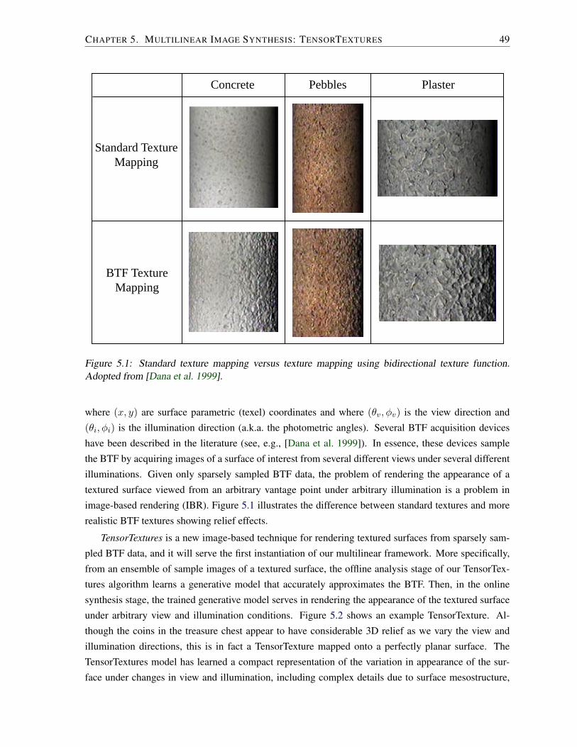
CHAPTER 5. MULTILINEAR IMAGE SYNTHESIS: TENSORTEXTURES 49
Standard TextureMapping
Concrete Pebbles Plaster
BTF TextureMapping
Figure 5.1: Standard texture mapping versus texture mapping using bidirectional texture function.Adopted from [Dana et al. 1999].
where (x, y) are surface parametric (texel) coordinates and where (θv, φv) is the view direction and
(θi, φi) is the illumination direction (a.k.a. the photometric angles). Several BTF acquisition devices
have been described in the literature (see, e.g., [Dana et al. 1999]). In essence, these devices sample
the BTF by acquiring images of a surface of interest from several different views under several different
illuminations. Given only sparsely sampled BTF data, the problem of rendering the appearance of a
textured surface viewed from an arbitrary vantage point under arbitrary illumination is a problem in
image-based rendering (IBR). Figure 5.1 illustrates the difference between standard textures and more
realistic BTF textures showing relief effects.
TensorTextures is a new image-based technique for rendering textured surfaces from sparsely sam-
pled BTF data, and it will serve the first instantiation of our multilinear framework. More specifically,
from an ensemble of sample images of a textured surface, the offline analysis stage of our TensorTex-
tures algorithm learns a generative model that accurately approximates the BTF. Then, in the online
synthesis stage, the trained generative model serves in rendering the appearance of the textured surface
under arbitrary view and illumination conditions. Figure 5.2 shows an example TensorTexture. Al-
though the coins in the treasure chest appear to have considerable 3D relief as we vary the view and
illumination directions, this is in fact a TensorTexture mapped onto a perfectly planar surface. The
TensorTextures model has learned a compact representation of the variation in appearance of the sur-
face under changes in view and illumination, including complex details due to surface mesostructure,

CHAPTER 5. MULTILINEAR IMAGE SYNTHESIS: TENSORTEXTURES 50
Figure 5.2: The chest contains a TensorTexture mapped onto a planar surface, which appears to haveconsiderable 3D relief when viewed from various directions (top and center) and under various illumi-nations (center and bottom).

CHAPTER 5. MULTILINEAR IMAGE SYNTHESIS: TENSORTEXTURES 51
such as self-occlusion, interreflection, and self-shadowing. Figure 1.3 shows a system diagram of our
TensorTextures analysis and rendering technique.
A major technical advantage of our multilinear framework for image-based rendering is that the un-
derlying tensor formulation can disentangle and explicitly represent each of the multiple causal factors
inherent to image formation. This stands in contrast to linear (matrix) PCA, which has so far been the
standard BTF representation/compression method [Sattler et al. 2003] and is, in fact, subsumed by our
more general multilinear framework. A major limitation of PCA is that it captures the overall variation
in the image ensemble without explicitly distinguishing what proportion is attributable to each of the
relevant causal factors—illumination change, view change, etc. Our method prescribes a more sophisti-
cated tensor decomposition that further analyzes this overall variation into individually encoded causal
factors using a novel set of basis functions. Harnessing the power of multilinear algebra, our approach
contributes a novel, explicitly multimodal model with which to tackle the BTF modeling/rendering
problem.
Unlike the approach of [Malzbender et al. 2001] and similar algorithms, ours estimates the complete
BTF, including variations not only in illumination, but also in view. Unlike the BTF synthesis method of
[Tong et al. 2002] and similar algorithms, our technique is purely image based—it avoids the nontrivial
problem of 3D geometric microstructure estimation. Unlike all previous methods, the one that we
develop in this thesis is a nonlinear BTF model.
5.1 Multilinear BTF Analysis
Given an ensemble of images of a textured surface, we define an image data tensor D ∈ RIx×IL×IV ,
where IV and IL, corresponding to the causal factor modes, are, respectively, the number of different
view and illumination conditions associated with the image acquisition process, and Ix, corresponding
to the measurement mode, is the number of texels in each texture image. As a concrete example, which
we will use for illustrative purposes, consider the synthetic scene of scattered coins shown in Figure 5.3.
A total of 777 RGB images of the scene are acquired from IV = 37 different view directions over the
viewing hemisphere (Figure 5.3(a)), each of which is illuminated by a light source oriented in IL = 21different directions over the illumination hemisphere (Figure 5.3(b)). The size of each RGB image is
Ix = 240× 320× 3 = 230, 400 texels.
In order to analyze the texture, images viewed from different angles must be brought into corre-
spondence. The most general assumption we can make is that the texture is planar.1 To align texture
features across all images, we rectify images acquired from oblique angles to bring them into correspon-
dence with the fronto-parallel image, thus undoing the perspective distortion (Figure 5.4(b)). We apply
a planar homography [Hartley and Zisserman 2000; Zhang 1999]
x′i = Hx, (5.2)
1Clearly the textures considered are not planar, but our synthesis results do not suffer much from this weak assumption. Amore accurate model might allow one to do better dimensionality reduction in the view mode.
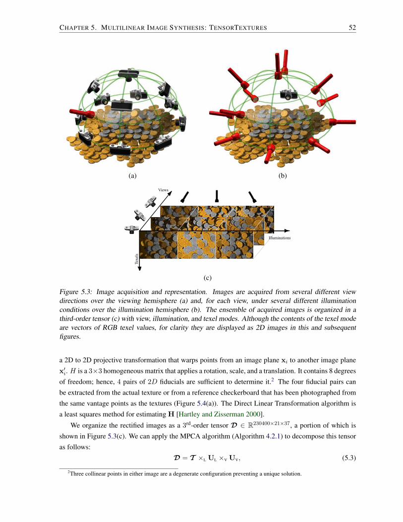
CHAPTER 5. MULTILINEAR IMAGE SYNTHESIS: TENSORTEXTURES 52
(a) (b)
Texels
Views
Illuminations
(c)
Figure 5.3: Image acquisition and representation. Images are acquired from several different viewdirections over the viewing hemisphere (a) and, for each view, under several different illuminationconditions over the illumination hemisphere (b). The ensemble of acquired images is organized in athird-order tensor (c) with view, illumination, and texel modes. Although the contents of the texel modeare vectors of RGB texel values, for clarity they are displayed as 2D images in this and subsequentfigures.
a 2D to 2D projective transformation that warps points from an image plane xi to another image plane
x′i. H is a 3×3 homogeneous matrix that applies a rotation, scale, and a translation. It contains 8 degrees
of freedom; hence, 4 pairs of 2D fiducials are sufficient to determine it.2 The four fiducial pairs can
be extracted from the actual texture or from a reference checkerboard that has been photographed from
the same vantage points as the textures (Figure 5.4(a)). The Direct Linear Transformation algorithm is
a least squares method for estimating H [Hartley and Zisserman 2000].
We organize the rectified images as a 3rd-order tensor D ∈ R230400×21×37, a portion of which is
shown in Figure 5.3(c). We can apply the MPCA algorithm (Algorithm 4.2.1) to decompose this tensor
as follows:
D = T ×L UL ×V UV, (5.3)
2Three collinear points in either image are a degenerate configuration preventing a unique solution.

CHAPTER 5. MULTILINEAR IMAGE SYNTHESIS: TENSORTEXTURES 53
(a)
(b)
Figure 5.4: (a) The rectifying homography is computed using at least 4 pairs of fiducials from a checker-board texture. (b) The texture is unwarped and brought into correspondence to the frontal image byapplying the computed homography.
Texels
Illumination
Variation
Variation
View
Figure 5.5: A partial visualization of the T ∈ R230400×21×37 TensorTextures bases of the coins imageensemble.

CHAPTER 5. MULTILINEAR IMAGE SYNTHESIS: TENSORTEXTURES 54
Eigentextures
Texels
Figure 5.6: Ux contains the PCA eigenvectors, which are the principal axes of variation across allimages.
the product of two orthonormal mode matrices associated with the causal factors and an extended core
tensor T , which is the TensorTextures basis that governs the interaction between the mode matrices.
The rows of the causal factor mode matrix UV ∈ R37×37 are the different illumination-invariant view
representations (the subscript “V” denotes the view mode). The rows of the causal factor mode matrix
UL ∈ R21×21 are the different view-invariant illumination representations (the subscript “L” denotes the
illumination mode). An image dl,v in the ensemble D is represented as
dl,v = T ×L lT ×V vT, (5.4)
where l and v are light and view representations, which are rows in UL,UV.
5.2 Computing TensorTextures
TensorTextures T models how the appearance of a textured surface varies with view and illumination.
The TensorTextures representation, which we illustrate in Figure 5.5, is the product
T = Z ×x Ux (5.5)
= D ×L UTL ×V UT
V . (5.6)
From a computational standpoint, equation (5.6) is preferable to (5.5) in practice, since it prescribes
computing the relatively small matrices UV and UL using the MPCA algorithm rather than the generally
large measurement mode matrix Ux ∈ R230400×777 and core tensor Z ∈ R777×21×37.
Figure 5.6 shows the column vectors of the measurement mode matrix Ux, which span the texture
space (the subscript “x” denotes the texels mode). These are, in fact, the PCA eigenvectors (i.e., “eigen-
images” or “eigentextures”). Our multilinear TensorTextures model subsumes the linear eigentextures
(PCA) model, as we showed in Section 4.2. The TensorTextures representation T in (5.5) transforms
the eigentextures into a tensorial representation of the variation of the causal factors (view and illumina-
tion). It characterizes how the view parameters and illumination parameters interact and multiplicatively
modulate the appearance of a surface under variation in view direction (θv, φv), illumination direction
(θi, φi), and position (x, y) over the surface.

CHAPTER 5. MULTILINEAR IMAGE SYNTHESIS: TENSORTEXTURES 55
l1
l2
l3
[ ]
v1
v2
[
[
v1
v2
v1
v2
v1
v2
l1
l2
l3
l1
l2
l3
...
...
v3
v3
v3
v3
l1
l2
l3
Variation
Variation
Illumination
View
Figure 5.7: The lower left image is rendered by multiplicatively modulating each of the TensorTexturesbasis vectors with the coefficients in the view coefficient vector v and illumination coefficient vector l.
5.3 Texture Representation and Dimensionality Reduction
The dimensionality-reduced PCA image representation is a coefficient vector of length Rx ≤ Ix, whereas
an image in our dimensionality-reduced TensorTextures representation comprises a coefficient vector of
length RL ≤ IL, equal to the number of columns in UL ∈ RIL×RL , plus a coefficient vector of length
RV ≤ IV, equal to the number of columns in UV ∈ RIV×RV . In our example, PCA would decompose
the image ensemble into 777 basis vectors (eigentextures), each of dimension 230,400, and represent
each image by a coefficient vector of length 777, which specifies what proportion of each basis vector to
accumulate in order to obtain that image. By contrast, TensorTextures decomposes the image ensemble
into 37× 21 basis vectors of the same dimension, and represents each image by two coefficient vectors,
one of length 37 to encode the view and the other of length 21 to encode the illumination. Thus,
each image is represented by 37 + 21 = 58 coefficients. Figure 5.7 shows how these coefficients
multiplicatively modulate the TensorTextures basis vectors according to (5.4) in order to approximate a
texture image (which we will soon exploit in multilinear image synthesis or rendering).
Through application of the MPCA algorithm (Algorithm 4.2.1), our multilinear analysis enables a
strategic dimensionality reduction, which is a mode-specific version of the conventional linear dimen-
sionality reduction of PCA. Whereas dimensionality reduction in PCA results in unpredictable image
degradation, multilinear models yield predictable image degradation that can be controlled indepen-

CHAPTER 5. MULTILINEAR IMAGE SYNTHESIS: TENSORTEXTURES 56
(a) Original (b) PCA (c) TensorTexture (d) TensorTexture
37 basis vectors 37 views, 1 illum 2 views, 21 illums37 basis vectors 42 basis vectors
95.2% Compression 95.2% Compression 94.6% Compression25.43 RMS Error 34.31 RMS Error 30.52 RMS Error
(e) PCA (f) TensorTexture (g) PCA (h) TensorTexture
111 basis vectors 37 views, 3 illums 124 basis vectors 31 views, 4 illums111 basis vectors 124 basis vectors
85.7% Compression 85.7% Compression 84.0% Compression 84.0% Compression14.78 RMS Error 20.65 RMS Error 13.46 RMS Error 18.35 RMS Error
Figure 5.8: The “perceptual error” incurred by compressing the illumination representation of the Ten-sorTextures model is smaller than that of indiscriminate PCA compression in a subspace of comparabledimension, despite a higher RMS error incurred by the TensorTextures model for these images in thedatabase. However, the overall RMS error for the entire dataset is lower for the TensorTextures model.(a) Original image. (b)–(h) PCA and TensorTexture compressions of image (a) using various numbersof basis vectors. The label above each image indicates the type of compression, while the annotationsbelow indicate the basis set, the compression rate, and the root mean squared (RMS) error relative tothe original image (a). For example, the PCA compression (e) retains 111 of the 777 most dominanteigentexture basis vectors, while the TensorTexture image compression (f) retains 111 TensorTexturesbases associated with UV ∈ R37×37 and UL ∈ R21×3, which reduces the illumination representationfrom 21 dimensions to 3 (RL = 3). In this instance, the RMS error of the PCA-compressed images arelower, yet comparable TensorTexture compressions have the better perceptual quality.
CHAPTER 5. MULTILINEAR IMAGE SYNTHESIS: TENSORTEXTURES 57
dently in viewing and illumination.
Figure 5.8 compares TensorTexture image compression against PCA compression. Note in Fig-
ure 5.8(c) that the 95.2% reduction of the illumination dimensionality suppresses illumination effects
such as shadows and highlights, but that it does not substantially degrade the clarity of the texture, since
the rank of the view mode matrix has not been reduced. However, a comparable compression using PCA
results in the blurred texture of Figure 5.8(b). Since the multilinear model is less constrained than the
linear model, the RMS error of TensorTexture compression is generally smaller than PCA compression.
However, there is no guarantee that every individual image has a lower RMS error than the PCA RMS
error, since the error function tries to find the best model fit for the entire data set rather than for each
image. In this particular instance, however, the RMS error of the TensorTexture compression relative to
the original image (Figure 5.8(a)) happens to be larger than the PCA compression, yet its “perceptual
error” is smaller, yielding a substantially better image quality than comparable PCA compressions.
Figure 5.8(d) shows the degradation of the TensorTexture if we drastically compress in the view
mode. Applying PCA compression in Figure 5.8(e), we retain the 111 (out of 777) most dominant
eigentextures. Applying TensorTextures, we compress the dimensionality of the illumination mode
from 21 to 3 (RL = 3) in Figure 5.8(f). Since RV = 37, we retain 37 × 3 TensorTexture basis vectors,
equaling the number of retained PCA basis vectors. The total number of coefficients representing the
compressed images is 37 + 3. Figure 5.8(d)–(e) illustrate the same scenario with 31× 4 TensorTexture
basis vectors.
5.4 Multilinear Image-Based Rendering
Our TensorTextures basis (equation (5.6) and Figure 5.5) leads to a straightforward multilinear rendering
algorithm, which is illustrated in Figure 5.7. To render an image d, we compute (cf., (5.4))
d = T ×L lT ×V vT, (5.7)
where v and l are, respectively, the view and illumination representation vectors associated with the
desired view and illumination directions. These will in general be novel directions, in the sense that
they will differ from the observed directions associated with sample images in the ensemble. Given a
novel view (illumination) direction, we first find the three nearest observed view (illumination) direc-
tions which form a triangle on the view (illumination) hemisphere that contains this novel direction. We
then compute the novel view (illumination) representation vector v (l) as a convex combination, using
homogeneous barycentric coordinates, of the view (illumination) representation vectors associated with
the three observed view (illumination) directions (Figure 5.9). Note that this algorithm is appropriate
for a planar surface, since every texel of the rendered texture shares the same view/illumination repre-
sentation. The algorithm (5.7) was applied to render the coins TensorTexture on a planar surface in the
treasure chest under continuously varying view and illumination directions (Figure 5.2).

CHAPTER 5. MULTILINEAR IMAGE SYNTHESIS: TENSORTEXTURES 58
?
V1
V2
V3
t1
t2
t3 V
new
(a) (b)
Figure 5.9: Computing a new view representation using barycentric coordinates.
=
view
illum.
tex
els T
vT
j l
ld
j
vT
1 1
T
j
T
1
Figure 5.10: TensorTexture rendering when every texel j has a different associated view vj and illumi-nation lj direction.
5.5 Rendering on Curved Surfaces
When rendering a TensorTexture d on a curved surface, the view vj and illumination lj representation
vectors associated with each texel j of d are computed with respect to the given view and illumination
directions as well as the direction of the surface normal at the center of texel j. The RGB value dj for
texel j is then computed as follows:
dj = T j ×L lTj ×V vTj , (5.8)
where T j is a subtensor of the TensorTexture which governs the interaction between view and illumi-
nation for texel j (Figure 5.10).

CHAPTER 5. MULTILINEAR IMAGE SYNTHESIS: TENSORTEXTURES 59
Texels
Illumination
Variation
Variation
View
Figure 5.11: TensorTexture bases for the corn texture.
5.6 Additional Results
We have applied the TensorTextures algorithm to two synthetic image ensembles: The “coins” ensem-
ble, which has served to illustrate our TensorTextures algorithm, and a “corn” image ensemble whose
TensorTextures representation is illustrated in Figure 5.11. Figure 5.12 compares standard texture map-
ping to TensorTexture mapping using the corn texture. Figure 5.13 demonstrates the application of the
algorithm of equation (5.8) to render the corn TensorTexture onto a perfect cylinder that forms the head
of a scarecrow, lit from two different directions. As the cylinder is rotated, the TensorTexture shows the
desired 3D effects, including self-occlusion and self-shadowing between the corn kernels, as well as an
appropriately radial pattern of corn kernel orientations around cylinder. Figure 5.14 shows the closing
shot of an animated short called Scarecrows’ Quarterly in which we have employed the TensorTextured
scarecrow head.
Both of our synthetic image datasets were acquired by rendering 3D graphics models of surfaces
featuring considerable mesostructure. As was the case of the coins, the images of the corn surface were
also acquired by rendering the surface from 37 different view and 21 different illumination directions.
Both the coins and the corn TensorTexture models retain 37× 11 = 407 TensorTexture basis vectors by
reducing the illumination mode from 21 to 11, while retaining all of the basis vectors of the view mode
in order to maintain the sharpness of the rendered images.
It takes considerable time to render each of the original sample images because of the nontrivial
scene geometries and rendering methods employed. In particular, Alias’ Maya consumed around 180
seconds on average to render the coins images and around 20 seconds on average to render the corn
images on a 2GHz P4 with 1GB of RAM. After our TensorTextures model has been computed offline,
the online rendering of the TensorTextures is significantly more efficient. For the coins example, the

CHAPTER 5. MULTILINEAR IMAGE SYNTHESIS: TENSORTEXTURES 60
Geometry Texture
Standard TextureMapping
TensorTextureSynthesis & Mapping
+
Figure 5.12: Standard texture mapping versus TensorTexture mapping. TensorTextures is a generativemodel that learns the bidirectional texture function.
rendering of the TensorTextured surfaces for arbitrary views and illuminations, implemented in not
especially well-optimized Matlab code, took on average 1.6 seconds per image on the same workstation.
Furthermore, because it is image-based, the TensorTextures online rendering speed is independent of the
scene complexity.
We have also applied our TensorTextures algorithm to images of natural textured surfaces from the
University of Bonn BTF database. The materials and methods for the image acquisition are detailed
in [Sattler et al. 2003]. Figure 5.15 shows “Impalla” (a stone) and “Corduroy” TensorTextures mapped
onto spheres using the rendering algorithm of equation (5.8). The TensorTextures bases were com-
puted from ensembles of RGB sample images, each of size 256 × 256 × 3, acquired under 81 view
and 81 illumination directions. The image data were organized as tensors D ∈ R196608×81×81. The
view and illumination mode matrices were computed in accordance with Step 1 of the MPCA algorithm
(Algorithm 4.2.1), and their dimensionality was reduced from 81 to 61 (RV = 61) and from 81 to 27
(RL = 61), respectively, yielding the reduced mode matrices UV ∈ R81×61 and UL ∈ R81×27. The
T ∈ R196608×61×27 TensorTextures bases vectors were computed according to (5.6). As a final demon-
stration, we have created a Flintstone Phonograph animation which maps the Impalla TensorTexture on
the planar “turntable” surface (Figure 5.16).

CHAPTER 5. MULTILINEAR IMAGE SYNTHESIS: TENSORTEXTURES 61
Figure 5.13: Renderings, with different light source directions, of the corn TensorTexture mapped ontoa cylinder that forms the scarecrow’s head.

CHAPTER 5. MULTILINEAR IMAGE SYNTHESIS: TENSORTEXTURES 62
Figure 5.14: A still image from the Scarecrows’ Quarterly animation.

CHAPTER 5. MULTILINEAR IMAGE SYNTHESIS: TENSORTEXTURES 63
Figure 5.15: “Impalla” (left) and “Corduroy” (right) TensorTextures rendered on spheres. A third orderimage data tensor associated with 81 view directions, 81 illumination directions, and 196608 texels (256rows × 256 columns × 3 channels) was employed to the TensorTextures bases T = D ×L UT
L ×V UTV .
Image compression was obtained by retaining 61 × 27 TensorTextures basis associated with UV ∈R81×61 and UL ∈ R81×27, which reduces the view representation from 81 dimensions to 61 (RV = 61)and the illumination representation from 81 dimensions to 27 (RL = 27).
Figure 5.16: A still image from the Flintstone Phonograph animation.

6Multilinear Image Analysis:
TensorFaces
Contents6.1 The TensorFaces Representation . . . . . . . . . . . . . . . . . . . . . . . . . . . 65
6.2 Strategic Dimensionality Reduction . . . . . . . . . . . . . . . . . . . . . . . . . 68
6.3 Application to a Morphable Faces Database . . . . . . . . . . . . . . . . . . . . . 70
6.4 The Independent TensorFaces Representation . . . . . . . . . . . . . . . . . . . 74
6.5 Structure and Decomposition of Facial Image Manifolds . . . . . . . . . . . . . . 75
We will now apply our multilinear framework in the context of computer vision, which is concerned
with image analysis, conceptually the inverse problem to computer graphics. A highly-researched class
of methods in computer vision is known as appearance-based methods. They have been applied to
the recognition of images of arbitrary objects, but have attracted the greatest attention in the context
of human facial images. Given a database of suitably labeled training images of numerous individuals,
our multilinear approach aspires to learn parsimonious appearance-based representations of the image
ensemble, which may be used for facial image compression or for facial image recognition, a subject
that we will investigate in the next chapter. Note, however, that in no way is our multilinear approach
limited to appearance-based methods; it is also applicable to range data, 3D vertices, and other types
of geometric models that are commonly used in model-based methods in computer vision [Terzopoulos
et al. 2004].
64

CHAPTER 6. MULTILINEAR IMAGE ANALYSIS: TENSORFACES 65
The conventional appearance-based approach addresses the problem of facial representation by tak-
ing advantage of linear algebra. In particular, PCA has been at the core of the dominant appearance-
based methods, such as the well-known “eigenfaces” face recognition method [Sirovich and Kirby 1987;
Turk and Pentland 1991a]. As we have stated, however, PCA accounts only for single-factor variations
in image ensembles. In our appearance-based recognition work, we confront the fact that natural images
result from the interaction of multiple causal factors related to scene structure, illumination, and imag-
ing. For facial images, these causal factors include different facial geometries and expressions, head
poses, and lighting conditions.
Applied to facial images, our multilinear representation is called TensorFaces. TensorFaces repre-
sents the image ensemble as a higher-dimensional tensor. This image data tensor D must be decom-
posed in order to separate and parsimoniously represent the causal factors related to scene structure,
illumination, and imaging.
6.1 The TensorFaces Representation
We first apply our multilinear analysis technique to ensembles of natural facial images, employing a
portion of the Weizmann face image database [Moses et al. 1996] of 28 male subjects imaged in 15
different views, under 4 different illuminations, performing 3 different expressions.1 For the sake of
concreteness in the ensuing discussion, consider an image ensemble of the 28 subjects acquired from 5
views, under 3 illuminations, and performing 3 expressions, for a total of 1260 images. Using a global
rigid optical flow algorithm, we roughly aligned the original 512 × 352 pixel images relative to one
reference image. The images were then decimated by a factor of 3 and cropped as shown in Figure 6.1,
yielding a total of 7943 pixels per image within the elliptical cropping window.
Thus, the number of modes is M = 5 and our facial image data tensor D ∈ R7943×28×5×3×3
(Figure 6.1(c)). Applying the MPCA algorithm (Algorithm 4.2.1) to D, we obtain the decomposition
D = T ×P UP ×V UV ×L UL ×E UE. (6.1)
The extended core tensor T ∈ R7943×28×5×3×3, which we call TensorFaces (Figure 6.2), captures the
interaction between the four causal factors: The rows of the causal factor mode matrix UP ∈ R28×28
are the representations for different people whose images comprise the data tensor (the subscript “P”
denotes the people mode), the rows of the causal factor mode matrix UV ∈ R5×5 represent different
views (the subscript “V” denotes the view mode), the rows of the causal factor mode matrix UL ∈ R3×3
represent the illuminations (the subscript “L” denotes the illumination mode), and the rows of the causal
factor mode matrix UE ∈ R3×3 represent different expressions (the subscript “E” denotes the expression
mode).
1A computer-controlled robot arm positioned the camera to ±34◦, ±17◦, and 0◦, the frontal view in the horizontal plane.The face was illuminated by turning on and off three light sources fixed at the same height as the face and positioned to theleft, center, and right of the face. For additional details, see [Moses et al. 1996].

CHAPTER 6. MULTILINEAR IMAGE ANALYSIS: TENSORFACES 66
(a)
(b)
People
Expressions
Views
Illumination
(c)
Figure 6.1: The Weizmann facial image database (28 subjects, 45 images per subject). (a) The 28subjects shown in expression 2 (smile), view 3 (frontal), and illumination 2 (frontal). (b) Part of theimage set for subject 1. Left to right, the three panels show images captured in illuminations 1, 2, and3. Within each panel, images of expressions 1, 2, and 3 (neural, smile, yawn) are shown horizontallywhile images from views 1, 2, 3, 4, and 5 are shown vertically. The image of subject 1 in (a) is theimage situated at the center of (b). (c) The 5th-order data tensor D for the image ensemble; only imagesin expression 1 (neutral) are shown.

CHAPTER 6. MULTILINEAR IMAGE ANALYSIS: TENSORFACES 67
Illumination
Variation
People
View
Variation
Expression
Variation
People
Variation
Figure 6.2: A partial visualization of the T ∈ R7943×28×5×3×3 TensorFaces representation of D, ob-tained as T = D ×P UT
P ×V UTV ×L UT
L ×E UTE .
. . .
Figure 6.3: The measurement mode matrix Ux contains the conventional PCA eigenvectors (“eigen-faces”), which are the principal axes of variation across all the images. The first 10 eigenvectors areshown.

CHAPTER 6. MULTILINEAR IMAGE ANALYSIS: TENSORFACES 68
TensorFaces is expressed as
T = Z ×x Ux, (6.2)
where Ux ∈ R7943×1260 is the measurement mode matrix whose orthonormal column vectors span
the image space (the lower case “x” subscript denotes the pixel mode). Note that neither Ux nor the
core tensor Z ∈ R1260×28×5×3×3 are needed in our multilinear analysis and they are not explicitly
computed in practice. Instead, the MPCA algorithm computes TensorFaces T and the 4 causal factor
mode matrices by forming the product
T = D ×P UTP ×V UT
V ×L UTL ×E UT
E . (6.3)
From a computational standpoint, equation (6.3) is preferable to (6.2) since it prescribes computing the
relatively small matrices UP, UV, UL, and UE rather than the generally large matrix Ux that PCA must
compute. This efficiency is exploited by the MPCA algorithm.
In Section 4.2 we showed that multilinear analysis subsumes linear, PCA analysis. Each column
vector in Ux is an “eigenimage” (Figure 6.3), since Ux is computed by performing an SVD of the matrix
D[x], the mode-1 matrixized data tensor D, whose columns comprise all the vectorized facial images.
The resulting eigenimages are identical to the conventional eigenfaces [Sirovich and Kirby 1987; Turk
and Pentland 1991b; Turk and Pentland 1991a]. Eigenimages represent merely the principal axes of
variation of the entire ensemble of images in the dataset. The big advantage of our multilinear analysis
beyond linear PCA is that TensorFaces explicitly represent each of the causal factors and encode how
they interact to produce facial images.
6.2 Strategic Dimensionality Reduction
To illustrate the dimensionality reduction abilities of our MPCA algorithm (Algorithm 4.2.1), we em-
ploy from the Weizmann facial image database an ensemble of images of 11 people, each photographed
in neutral expression from a frontal view under 16 different illuminations. Figure 6.4(a) shows three of
the 176 original 7943-pixel images for one of the subjects.
Applied to the ensemble tensor D ∈ R7943×11×16, the Step 1 of the algorithm yields mode matrices
UP ∈ R11×11 and UL ∈ R16×16. We then truncate the illumination mode matrix UL from 16 columns
to 3 (RL = 3), thus obtaining the reduced-rank matrix UL ∈ R16×3. We iterate in Step 2, updating UL
and the (non-truncated) mode matrix UP, until convergence (3 iterations).
Figure 6.4(b) shows illumination-compressed images of the subject extracted from the dimensionality-
reduced multilinear representation D ' T ×P UP ×L UL. Note that the 81.25% reduction of the illu-
mination dimensionality suppresses illumination effects such as shadows and highlights, but that it does
not substantially degrade the appearance of the person, since the rank of the person mode matrix was
not reduced. When we increase the illumination dimensionality to 6, the shadows and highlights begin
to reappear, as shown in Figure 6.4(c).
Thus, our multilinear model enables a strategic dimensionality reduction, which is more targeted

CHAPTER 6. MULTILINEAR IMAGE ANALYSIS: TENSORFACES 69
Original 3 Illum. Dims. 6 Illum. Dims.
(a) (b) (c)
Figure 6.4: A subject was imaged under 16 different illuminations. (a) Three original images displayingdifferent illumination conditions. (b) Compression of the images in (a) by reducing the illuminationrepresentation from 16 dimensions to 3 (RL = 3); i.e., UL ∈ R16×3. This degrades the illuminationeffects (cast shadows, highlights). Arrows indicate the shadow cast by the nose in the original images(a) and the attenuated shadow in the compressed images (b). The shadow begins to reappear when theillumination dimensionality is increased to 6 (RL = 6) in (c); i.e., UL ∈ R16×6. Image sharpness anddetailed facial features are well-preserved in both (b) and (c).
than linear (PCA) dimensionality reduction. Figure 6.5 compares TensorFaces image compression
against PCA compression. Applying PCA compression, we retain in Figure 6.5(b) the 11 (out of 176)
most dominant eigenfaces and in Figure 6.5(d) the 33 most dominant eigenfaces. Applying Tensor-
Faces, we compress the dimensionality of the illumination mode from 16 to 1 (RL = 1) in Figure 6.5(c)
and from 16 to 3 (RL = 3) in Figure 6.5(e). Since RP = 11, in the first instance we retain 11 × 1 Ten-
sorFaces, while in the second we retain 11× 3 TensorFaces, each time equaling the number of retained
eigenfaces. Note that the total number of coefficients representing the compressed images is 11 + 1 and
11 + 3, respectively. The figure shows shows an unusual case in which the root mean squared errors
(RMSE) relative to the original images, which are indicated in the figure, are larger for the Tensor-
Faces compressions than they are for the PCA compressions. However, the “perceptual error” [Teo and
Heeger 1994] of the TensorFaces compressions are significantly smaller, yielding substantially better
image quality than PCA in subspaces of comparable dimension.

CHAPTER 6. MULTILINEAR IMAGE ANALYSIS: TENSORFACES 70
Original PCA TensorFaces PCA TensorFaces11 Eigenfaces 11 TensorFaces 33 Eigenfaces 33 TensorFaces
RMSE: 14.62 33.47 9.26 20.22
RMSE: 14.33 30.58 7.78 14.69
(a) (b) (c) (d) (e)
Figure 6.5: The “perceptual error” of TensorFaces compression of illumination is smaller than indis-criminate PCA compression in a subspace of comparable dimension. (a) Original images. (b) PCAimage compression obtained by retaining the 11 most dominant eigenfaces. (c) TensorFaces imagecompression obtained by retaining 11 TensorFaces associated with UP ∈ R11×11 and UL ∈ R16×1,which reduces the illumination representation from 16 dimensions to 1 (RL = 1). (d) PCA image com-pression obtained by retaining the 33 most dominant eigenfaces. (e) TensorFaces image compressionobtained by retaining 33 TensorFaces associated with UP ∈ R11×11 and UL ∈ R16×3, which reducesthe illumination representation from 16 dimensions to 3 (RL = 3). Compared to the original images,the root mean squared errors (RMSE) of the PCA-compressed images are lower, yet the TensorFaces-compressed images have significantly better perceptual quality.
6.3 Application to a Morphable Faces Database
We next illustrate our technique using gray-level facial images of 75 subjects (Figure 6.6). Each subject
is imaged from 15 different views (θ = −35◦ to +35◦ in 5◦ steps on the horizontal plane φ = 0◦) under
15 different illuminations (θ = −35◦ to +35◦ in 5◦ steps on an inclined plane φ = 45◦). Figure 6.6(b)
shows the set of 225 images for one of the subjects with views arrayed horizontally and illuminations
arrayed vertically. The image set was rendered from a 3D scan of the subject shown framed in Fig-
ure 6.6(a). Each image is 80 × 107 = 8560 pixels in size. The 75 scans shown in the figure were
recorded using a CyberwareTM 3030PS laser scanner and are part of the 3D morphable faces database
created at the University of Freiburg [Blanz and Vetter 1999].
We select an ensemble of 2700 images from the dataset of Figure 6.6 comprising the dash-framed
images for each person. Thus, M = 4 and our facial image data tensor is D ∈ R8560×75×6×6 (Fig-

CHAPTER 6. MULTILINEAR IMAGE ANALYSIS: TENSORFACES 71
-35 -30 -25 -20 -15 -10 -5 0 5 10 15 20 25 30 35
-35
-30
-25
-20
-15
-10
-5
0
5
10
15
20
25
30
35
(a) (b)
Figure 6.6: A facial image dataset. (a) 3D scans of 75 subjects, recorded using a CyberwareTM 3030PSlaser scanner as part of the University of Freiburg 3D morphable faces database [Blanz and Vetter 1999].(b) Facial images for a subject (framed head in (a)), viewed from 15 different views (across) under15 different illuminations (down). In our recognition experiments, the dash-framed images served astraining images; the solid-framed images served as test images.
ure 6.7). Applying multilinear analysis to D, we obtain
D = T ×P UP ×V UV ×L UL. (6.4)
As before, TensorFaces T ∈ R8560×75×6×6 governs the interaction between the now 3 causal factors:
The rows of the causal factor mode matrix UP ∈ R75×75 represent the different people, those of the
causal factor mode matrix UV ∈ R6×6 represent the different views, and those of the causal factor
mode matrix UL ∈ R6×6 represent the different illuminations. Tensor T = Z ×x Ux, where the
orthonormal column vectors of the measurement mode matrix Ux ∈ R8560×2700 span the image space
of images and the core tensor Z ∈ R2700×75×6×6 contains normalizing parameters associated with the 4
mode matrices. Figure 6.8(a) illustrates the eigenfaces, or column vectors of Ux, for this dataset, while
Figure 6.8(b) illustrates the TensorFaces efficiently computed by MPCA as T = D×PUTP ×VUT
V ×LUTL .
To illustrate dimensionality reduction using the MPCA algorithm (Algorithm 4.2.1), we employed

CHAPTER 6. MULTILINEAR IMAGE ANALYSIS: TENSORFACES 72
Views
People
Illuminations
Figure 6.7: A portion of the 4th-order data tensor D for the image ensemble formed from the dash-framed images of each person in Figure 6.6. Only 4 of the 75 people are shown.
Views
People
Illuminations
(a) (b)
Figure 6.8: Eigenfaces and TensorFaces bases for an ensemble of 2,700 facial images spanning 75 peo-ple, each imaged under 6 viewing and 6 illumination conditions. (a) PCA eigenvectors (eigenfaces) Ux,which are the principal axes of variation across all images. (b) A partial visualization of the TensorFacesT ∈ R8560×75×6×6 representation obtained from D as T = D ×P UT
P ×V UTV ×L UT
L .

CHAPTER 6. MULTILINEAR IMAGE ANALYSIS: TENSORFACES 73
Original 1 Illum. Dim. 2 Illum. Dims.
(a) (b) (c)
Figure 6.9: 16 subjects were imaged under 7 view and 20 illumination conditions. (a) Three originalimages displaying different illumination conditions. (b) Compression of the images in (a) by reducingthe illumination representation from 20 dimensions to 1 (RL = 1); i.e., UL ∈ R20×1. This degrades theillumination effects (cast shadows, highlights). The shadow begins to reappear when the illuminationdimensionality is increased to 2 (RL = 2) in (c); i.e., UL ∈ R20×2 a matrix. Image sharpness anddetailed facial features are well-preserved in both (b) and (c).
an image ensemble in which each of 16 subjects was imaged from 7 different views under 20 different
illumination conditions. Figure 6.9(a) shows three of the 2240 original 8560-pixel images for one of the
subjects.
Applying our MPCA algorithm (Algorithm 4.2.1) to D ∈ R8560×16×7×20, Step 1 yields mode
matrices UP ∈ R16×16, UV ∈ R7×7, and UL ∈ R20×20. We then truncate the illumination mode matrix
UL from 20 columns to RL = 1, thus obtaining the reduced-rank matrix UL ∈ R20×1. We iterate in
Step 2, updating UL along with the other (non-truncated) mode matrices UP and UV until convergence
(3 iterations).
Figure 6.9(b) shows illumination-compressed images of the subject extracted from the dimensionality-
reduced multilinear representation D ' T ×P UP ×V UV ×L UL. Note that the 95% reduction of the
illumination dimensionality suppresses illumination effects such as shadows and highlights, but that it
does not substantially degrade the appearance of the person, since the rank of the person mode ma-
trix was not reduced. Increasing the illumination dimensionality to 2, UL ∈ R20×2, the shadows and
highlights begin to reappear, as shown in Figure 6.9(c).
Thus, our multilinear model again enables a strategic dimensionality reduction, which is more tar-
geted than linear (PCA) dimensionality reduction. Figure 6.10 compares TensorFaces image compres-
sion against PCA compression. Applying PCA compression, we retain in Figure 6.10(b) the 112 (out
of 2240) most dominant eigenfaces and in Figure 6.10(d) the 224 most dominant eigenfaces. Applying

CHAPTER 6. MULTILINEAR IMAGE ANALYSIS: TENSORFACES 74
Original PCA TensorFaces PCA TensorFaces112 Eigenfaces 112 TensorFaces 224 Eigenfaces 224 TensorFaces
RMSE: 4651.3 4062.3 2997.2 2096.5
RMSE: 3495.5 4218.0 2199.4 2343.8
(a) (b) (c) (d) (e)
Figure 6.10: The “perceptual error” of TensorFaces compression of illumination is smaller than in-discriminate PCA compression in a subspace of comparable dimension. (a) Original image. (b) PCAimage compression obtained by retaining the 112 most dominant eigenfaces. (c) TensorFaces imagecompression by reducing the illumination representation from 20 dimensions to 1 (RL = 1). (d) PCAimage compression obtained by retaining the 224 most dominant eigenfaces. (e) TensorFaces imagecompression by reducing the illumination representation from 20 dimensions to 2 (RL = 2). Note thatin the images of the male, the root mean squared errors (RMSE) of the PCA-compressed images arelower, yet the TensorFaces-compressed images have significantly better perceptual quality.
TensorFaces, we compress the dimensionality of the illumination mode from 20 to 1 (RL = 1) in Fig-
ure 6.10(c) by retaining 112 TensorFaces associated with UP ∈ R16×16, UV ∈ R7×7, and UL ∈ R20×1,
and from 20 to 2 (RL = 2) in Figure 6.10(e) obtained by retaining 224 TensorFaces associated with
UP ∈ R16×16, UV ∈ R7×7, and UL ∈ R20×2. Since RP = 16, in the first instance we retain 16× 7× 1TensorFaces, while in the second we retain 16 × 7 × 2 TensorFaces, each time equaling the number
of retained eigenfaces. Note that the total number of coefficients representing the compressed images
is 16 + 7 + 1 and 16 + 7 + 2, respectively. For the compressed images of the male, the root mean
squared errors (RMSE) relative to the original image, which are indicated in the figure, are larger for the
TensorFaces compressions than they are for the PCA compressions. However, the “perceptual error” of
the TensorFaces compressions are significantly smaller, yielding substantially better image quality than
PCA in subspaces of comparable dimension.
6.4 The Independent TensorFaces Representation
We will now demonstrate the application of our multilinear independent components analysis (MICA)
method (Section 4.3) to the image dataset in Figure 6.6.
Our approach performs a multilinear ICA decomposition of the tensor D ∈ R8560×75×6×6 of vec-

CHAPTER 6. MULTILINEAR IMAGE ANALYSIS: TENSORFACES 75
Views
People
Illuminations
(a) (b)
Figure 6.11: ICA and MICA bases for an ensemble of 2,700 8,560-pixel facial images (Figure 6.6)comprising 75 people, each imaged under 6 viewing and 6 illumination conditions. (a) Independentcomponents Cx. (b) A partial visualization of the MICA representation of D ∈ R8560×75×6×6, obtainedas M = S ×x Cx.
torized training images per (4.17):
D = S ×x Cx ×P CP ×V CV ×L CL, (6.5)
thereby extracting a set of causal factor mode matrices—the matrix CP ∈ R75×75 whose column vectors
span the people space, the matrix CV ∈ R6×6 whose column vectors span the view space, and the matrix
CL ∈ R6×6 whose column vectors span the illumination space—and a MICA basis tensor
M = S ×x Cx, (6.6)
which we can call Independent TensorFaces, that governs the interaction between the different mode
matrices. The independent TensorFaces representation is illustrated in Figure 6.11(b). For comparison,
the ordinary ICA basis vectors Cx are shown in Figure 6.11(a).
6.5 Structure and Decomposition of Facial Image Manifolds
Manifold learning methods aspire to recover a low-dimensional parameterization associated with a low-
dimensional submanifold that is embedded in a high-dimensional measurement space. PCA or multidi-
mensional scaling (MDS) extract a linear submanifold that is embedded in the measurement space.

CHAPTER 6. MULTILINEAR IMAGE ANALYSIS: TENSORFACES 76
Figure 6.12: z(x,y), a function of two hidden variables, x and y, is sampled to generate measurementdata confined to a plane in 3D space. Standard manifold learning methods will miss the curvilinearstructure of the data. One should extract the underlying variables and separately map each of theirmanifolds.
When densely sampled training data are available, techniques such as LLE [Roweis and Saul 2000]
and Isomap [Tenenbaum et al. 2000] can recover the intrinsic geometry of a nonlinear submanifold.
Although the well-known toy examples, such as the “swiss roll” spiral [Tenenbaum et al. 2000], that
have been employed to illustrate the latter methods have visually pleasing geometric structures, they
tend to be gross over-simplifications of the manifold structure of real measurement data. In important
real-world situations, particularly involving multimodal measurement data, the data manifold of interest
is actually the result of the interaction of several component manifolds. Furthermore, these multiple
manifolds can be embedded into one another such that the measurement data points that lie on one man-
ifold are not clearly separated from those lying on the other manifolds, thus destroying any recognizable
geometric structure, especially when the measurement data are very sparse.
Figure 6.12 displays a toy example in which the measurement data points were generated by the in-
teraction of two nonlinear component manifolds. The resulting planar manifold is the result of the inter-
action of two different factors, where each factor lies on a separate manifold that has a low-dimensional
parameterization. Clearly, in such a scenario, unsupervised manifold learning methods such as the
aforementioned ones, lack the power to extract a meaningful parameterization.
For a non-toy example, consider facial image ensembles that sparsely sample several constituent
manifolds; e.g., the view manifold, the illumination manifold, the person manifold, and the expression
manifold. These manifolds interact with one another nontrivially, yielding a seemingly unstructured
cloud of measurement data. In Figure 6.13, we display a slice through the data cloud. This slice lies on
a subspace that is made up of several manifolds which are embedded within each other, with the data
points lying on one manifold not clearly separated from the data points on other manifolds.
Our multilinear analysis can be regarded as a manifold decomposition approach that extracts from
a compound manifold constituent component manifolds, each of which can separately be described by
low dimensional parameterizations. Unlike the aforementioned methods, our method is supervised, but

CHAPTER 6. MULTILINEAR IMAGE ANALYSIS: TENSORFACES 77
Figure 6.13: Manifold structure of facial image ensembles. Each blue dot in the image space representsan image. A total of 1050 images are represented. (Each image is represented by its three most rep-resentative pixels.) 25 people were photographed under 7 illumination conditions and from 6 viewingdirections. The images analyzed form 6 major clusters, where a cluster contains all the images pho-tographed from the same viewing direction. As shown in the above diagram, within the image space,the image clusters are organized into a semi-circular structure that can be parameterized by the viewingdirection. Similarly, within each cluster, images for each individual are also organized into a semi-circular structure that can be parameterized by the illumination direction. The red diamonds are imagesof one person under various imaging conditions. Similarly, the purple circles are images of a secondperson under various imaging conditions.

CHAPTER 6. MULTILINEAR IMAGE ANALYSIS: TENSORFACES 78
it can decompose compound data manifolds that are very sparsely sampled. The parameterizations of
the extracted component submanifolds can then be learned using methods such as LLE and Isomap
[Vasilescu 2006a].
Given the image ensemble, our method can map each image from the measurement (pixel) space
simultaneously into three other constituent spaces—the person space, the view space, and the illumi-
nation space. Hence, it can discover the semi-circular structure associated with the view manifold
and the semi-circular structure associated with the illumination manifold embedded in the people/view
subspace. Each constituent manifold can then be parameterized by its own specific low-dimensional
parameterization.

7Multilinear Image Recognition:
The Multilinear Projection
Contents7.1 Multiple Linear Projections (MLP) . . . . . . . . . . . . . . . . . . . . . . . . . 81
7.2 The Multilinear Projection (MP) . . . . . . . . . . . . . . . . . . . . . . . . . . . 83
7.2.1 Identity and Pseudo-Inverse Tensors . . . . . . . . . . . . . . . . . . . . . . 86
7.2.2 Multilinear Projection Algorithms . . . . . . . . . . . . . . . . . . . . . . . 87
7.3 Facial Image Recognition Experiments . . . . . . . . . . . . . . . . . . . . . . . 91
7.4 Discussion . . . . . . . . . . . . . . . . . . . . . . . . . . . . . . . . . . . . . . . 94
Algorithms
7.2.1 Multilinear Projection (MP) Algorithm With MPCA . . . . . . . . . . . . . . . . . . . . . . . . . . . . . . . 89
7.2.2 Multilinear Projection (MP) Algorithm With CP. . . . . . . . . . . . . . . . . . . . . . . . . . . . . . . . . . . 90
We will now apply our multilinear framework to pattern recognition. Facial image recognition is a
classic problem in the field, and appearance-based face recognition has been an active area of biometrics
research in recent years [Chellappa et al. 1995]. Given a database of suitably labeled training images
of numerous individuals, this supervised recognition technique aspires either to recognize the faces of
these individuals in previously unseen test (probe) images or to identify the test images as new faces.
The conventional approach addresses the problem by taking advantage of linear algebra. In particular,
79
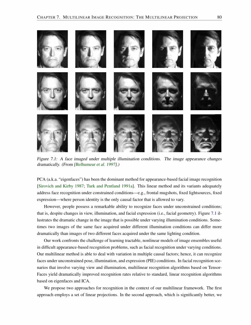
CHAPTER 7. MULTILINEAR IMAGE RECOGNITION: THE MULTILINEAR PROJECTION 80
Figure 7.1: A face imaged under multiple illumination conditions. The image appearance changesdramatically. (From [Belhumeur et al. 1997].)
PCA (a.k.a. “eigenfaces”) has been the dominant method for appearance-based facial image recognition
[Sirovich and Kirby 1987; Turk and Pentland 1991a]. This linear method and its variants adequately
address face recognition under constrained conditions—e.g., frontal mugshots, fixed lightsources, fixed
expression—where person identity is the only causal factor that is allowed to vary.
However, people possess a remarkable ability to recognize faces under unconstrained conditions;
that is, despite changes in view, illumination, and facial expression (i.e., facial geometry). Figure 7.1 il-
lustrates the dramatic change in the image that is possible under varying illumination conditions. Some-
times two images of the same face acquired under different illumination conditions can differ more
dramatically than images of two different faces acquired under the same lighting condition.
Our work confronts the challenge of learning tractable, nonlinear models of image ensembles useful
in difficult appearance-based recognition problems, such as facial recognition under varying conditions.
Our multilinear method is able to deal with variation in multiple causal factors; hence, it can recognize
faces under unconstrained pose, illumination, and expression (PIE) conditions. In facial recognition sce-
narios that involve varying view and illumination, multilinear recognition algorithms based on Tensor-
Faces yield dramatically improved recognition rates relative to standard, linear recognition algorithms
based on eigenfaces and ICA.
We propose two approaches for recognition in the context of our multilinear framework. The first
approach employs a set of linear projections. In the second approach, which is significantly better, we

CHAPTER 7. MULTILINEAR IMAGE RECOGNITION: THE MULTILINEAR PROJECTION 81
introduce a multilinear (tensor) projection operator that generalizes the linear projections.
Figure 1.4 illustrates the architecture of a facial image recognition system within our multilinear
framework. Appendix B discusses some important issues regarding the acquisition of facial image
datasets for the purposes of training multilinear recognition algorithms.
7.1 Multiple Linear Projections (MLP)
For concreteness, consider the Weizmann facial image database from Section 6.1, which comprises 60
images per person that vary with view, illumination, and expression. PCA represents each person as a
set of 45 vector-valued coefficients, one from each image in which the person appears. The length of
each PCA coefficient vector is 28 × 5 × 3 × 3 = 1260. By contrast, multilinear analysis enables us to
represent each person, regardless of view, illumination, and expression, with the same coefficient vector
of dimension 28 relative to the bases comprising the tensor B ∈ R7943×28×5×3×3, where
B = Z ×x Ux ×V UV ×L UL ×E UE (7.1)
= T ×V UV ×L UL ×E UE. (7.2)
some of which are shown in Figure 7.2. Each column in the figure is a basis matrix that comprises 28
basis vectors. In any column, the first basis vector depicts the average person and the remaining basis
vectors capture the variability over people, for the particular combination of view, illumination, and
expression associated with that column. Each image is represented by a set of coefficient vectors for the
person, view, illumination, and expression causal factors that generated the image. This is an important
distinction between our multilinear PCA approach to facial recognition and that for linear PCA.
In the PCA or eigenfaces technique, one decomposes a data matrix D of labeled training facial
images di into a reduced-dimensional basis matrix BPCA = UxΣ and a coefficient matrix UI whose
rows are coefficient vectors cTi associated with each vectorized image di. Given an unlabeled test image
(probe) d, the projection operator B+PCA linearly projects this d into the reduced-dimensional space of
image coefficient vectors. The nearest coefficient vector may be used to label (i.e., recognize) probe d.
By contrast, our facial recognition algorithm performs the TensorFaces decomposition of the ten-
sor D of vectorized training images dpvle, extracts the matrix UP, which contains row vectors pTp of
coefficients for each person p, and constructs the basis tensor B, which contains a collection of basis
matrices, which are view v, illumination l, and expression e specific. We can think of the pTp as person
signatures.
For the Weizmann database example, we index into the basis tensor B ∈ R7943×28×5×3×3 for a
particular view v, illumination l, and expression e to obtain a subtensor Bvle ∈ R7943×28×1×1×1. We
matrixize Bvle in the people mode to obtain the matrix Bvle[P] ∈ R28×7943. Note that a specific training
image dpvle ∈ R7943×1×1×1×1 of person p in view v, illumination l, and expression e can be written as
dpvle = Bvle ×P pTp (7.3)

CHAPTER 7. MULTILINEAR IMAGE RECOGNITION: THE MULTILINEAR PROJECTION 82
Views
Expressions
People
Variation
Illuminations
Figure 7.2: A partial visualization of the bases tensor B ∈ R7943×28×5×3×3 = T ×V UV ×L UL ×E UE
(only the subtensor associated with the neutral expression is shown), which defines 45 different basesfor each combination of views, illuminations and expressions. These bases have 28 basis vectors thatspan the people space. The basis vectors in any particular row play the same role in each column. Thetopmost plane depicts the average person, while the basis vectors in the remaining planes capture thevariability across people in the various view, illumination, and expression combinations.
or, using (3.12), in matrix form as
dpvle[P]= pT
p Bvle[P]; (7.4)
hence,
pp = Bvle+T[P] dpvle
T[P]
(7.5)
= Bvle+T[P] dpvle. (7.6)
Now, given an unlabeled test image d, we can use the projection operator Bvle+T[P] to project d into
a set of candidate coefficient vectors
rvle = Bvle+T[P] d (7.7)
for every v, l, e combination. Our recognition algorithm compares every rvle against the person sig-

CHAPTER 7. MULTILINEAR IMAGE RECOGNITION: THE MULTILINEAR PROJECTION 83
natures pTp . The best matching rvle and pp vector pair, i.e., those vectors that yield the smallest value
of
arg minp; vle
‖pp − rvle‖, (7.8)
result in the unlabeled test image d acquiring the person label of person signature pp and the view,
illumination, and expression labels of rvle, thereby identifying d as portraying person p in view v,
illumination l, and expression e.
7.2 The Multilinear Projection (MP)
The TensorFaces recognition algorithm proposed in the previous section was based on an approach
involving multiple linear projections. It computed a set of linear projection operators, which yielded a
set of candidate coefficient vectors. However, this is less than ideal. We will now develop a multilinear
projection method that simultaneously infers the identity, view, illumination, etc., coefficient vectors of
an unlabeled test image. Our multilinear projection maps an unlabeled test image from the measurement,
pixel space to the multiple causal factor spaces (Figure 6.13). We thus obtain an improved recognition
algorithm that fully exploits the multilinear structure of our tensor framework. For concreteness, we
will continue the development of this superior approach in the context of the facial image dataset of
Figure 6.6.
Given the data tensor D of labeled, vectorized training images dpvle, where the subscripts denote
person p, view v, illumination l, and expression e labels, we can apply the MPCA algorithm (Algo-
rithm 4.2.1) to compute causal mode matrices UP, UV, UL, and UE as well as the TensorFaces basis
T = D ×P UTP ×V UT
V ×L UTL ×E UT
E (6.2) that governs the interaction between them (Figure 6.2(b)).
Then the method represents an image dpvl by the relevant set of person, view, and illumination coeffi-
cient vectors as follows:
dpvle = T ×P pTp ×V vT
v ×L lTl ×E eTe . (7.9)
This multilinear representation is illustrated in Figure 7.3(a) for the data tensor in Figure 6.7, which
lacks the expression mode. Alternatively, we can apply the MICA algorithm (Algorithm 4.3.1), which
employs higher-order statistics to compute a basis tensor M = D ×P C+P ×V C+
V ×L C+L ×E C+
E .
Analogous to the MPCA case, an image can be represented with respect to the MICA basis, as follows:
dpvle = M×P pTp ×V vT
v ×L lTl ×E eTe , (7.10)
which again for the data tensor in Figure 6.7 is illustrated in Figure 7.4.
Given an unlabeled test image (probe) d and T or M, we must determine the unknown coefficient
vectors, pp, vv, ll, and ee in order to recognize the person, view, illumination, and expression associated
with the test image. Solving for these vectors in (7.9) or (7.10) will, in principle, require the computa-
tion of a pseudo-inverse of tensor T or M. In analogy with matrix algebra, this raises the following
questions: How does one “invert” a tensor? When one “multiplies” a tensor with its “inverse tensor”,

CHAPTER 7. MULTILINEAR IMAGE RECOGNITION: THE MULTILINEAR PROJECTION 84
l1v
1 p
4 l1v
2 p
4 l1v
3 p
4 l1v
4 p
4
l1
l2
l3
l4
l5
[ v1
v2
v3
v4 ... ]
[... ]
p1
p2
p3
p4
[
]
. . .
Illuminations
People
=
p
v
l
l1v
1 p
3 l1v
2 p
3 l1v
3 p
3 l1v
4 p
3
l1v
1 p
2 l1v
2 p
2 l1v
3 p
2 l1v
4 p
2
l1v
1 p
1 l1v
2 p
1 l1v
3 p
1 l1v
4 p
1
l2v
1 p
1 l2v
2p
1 l2v
3 p
1 l2v
4 p
1
l3v
1 p
1 l3v
2 p
1 l3v
3 p
1 l3v
4 p
1
l4v
1 p
1 l4v
2 p
1 l4v
3 p
1 l4v
4 p
1
l5v
1 p
1 l5v
2 p
1 l5v
3 p
1 l5v
4 p
1
Views
(a)
p1v
1 l1
p1v
2 l1
p1v
3 l1
p1v
4 l1
p2v
1 l1
p2v
2 l1
p2v
3 l1
p2v
4 l1
p3v
1 l1
p3v
2 l1
p3v
3l1
p3v
4 l1
p4v
1 l1
p4v
2 l1
p4v
3 l1
p4v
4 l1
p5v
1 l1
p5v
2 l1
p5v
3 l1
p5v
4 l1
p1v
1 l2
p1v
2 l2
p1v
3 l2
p1v
4 l2
p1v
1 l3
p1v
2 l3
p1v
3 l3
p1v
4 l3
p1v
1 l4
p1v
2 l4
p1v
3 l4
p1v
4 l4
p1
p2
p3
p4
p5
[ v1
v2
v3
v4 ... ]
[ ... ]
l1
l2
l3
l4
[
]
. . .
Views
Illuminations
People
=
l
p
v
T +x x
Tx
(b)
Figure 7.3: (a) MPCA image representation d = T ×P pT ×V vT ×L lT. (b) Given an unlabeled testimage d, the associated coefficient vectors p, v, l are estimated by decomposing the response tensorR = T +x ×T
x d using a multilinear projection algorithm.

CHAPTER 7. MULTILINEAR IMAGE RECOGNITION: THE MULTILINEAR PROJECTION 85
p1v
1 l1
p1v
2 l1
p1v
3 l1
p1v
4 l1
p2v
1 l1
p2v
2 l1
p2v
3 l1
p2v
4 l1
p3v
1 l1
p3v
2 l1
p3v
3 l1
p3v
4 l1
p4v
1 l1
p4v
2 l1
p4v
3 l1
p4v
4 l1
p5v
1 l1
p5v
2 l1
p5v
3 l1
p5v
4 l1
p1v
1 l2
p1v
2 l2
p1v
3 l2
p1v
4 l2
p1v
1 l3
p1v
2 l3
p1v
3 l3
p1v
4 l3
p1v
1 l4
p1v
2 l4
p1v
3 l4
p1v
4 l4
p1
p2
p3
p4
p5
[ v1
v2
v3
v4 ... ]
[ ... ]
l1
l2
l3
l4
[
]
. . .
Views
Illuminations
People
=
p
v
l
(a)
p1v
1 l1
p1v
2 l1
p1v
3 l1
p1v
4 l1
p2v
1 l1
p2v
2 l1
p2v
3 l1
p2v
4 l1
p3v
1 l1
p3v
2 l1
p3v
3l1
p3v
4 l1
p4v
1 l1
p4v
2 l1
p4v
3 l1
p4v
4 l1
p5v
1 l1
p5v
2 l1
p5v
3 l1
p5v
4 l1
p1v
1 l2
p1v
2 l2
p1v
3 l2
p1v
4 l2
p1v
1 l3
p1v
2 l3
p1v
3 l3
p1v
4 l3
p1v
1 l4
p1v
2 l4
p1v
3 l4
p1v
4 l4
p1
p2
p3
p4
p5
[ v1
v2
v3
v4 ... ]
[ ... ]
l1
l2
l3
l4
[
]
. . .
Views
Illuminations
People
=
l
p
v
M+x x
Tx
(b)Figure 7.4: (a) MICA image representation d = M ×P pT ×V vT ×L lT. (b) Given an unlabeled testimage d, the associated coefficient vectors p, v, l are estimated by decomposing the response tensorR = M+x ×T
x d using a multilinear projection algorithm.

CHAPTER 7. MULTILINEAR IMAGE RECOGNITION: THE MULTILINEAR PROJECTION 86
what should be the resulting “identity tensor”? We will next show that an M th-order tensor has M
pseudo-inverse tensors, one with respect to each mode, and that there are M identity tensors, one per
mode, whose structure is not diagonal with ones along the main diagonal.
7.2.1 Identity and Pseudo-Inverse Tensors
First, we generalize Definition 3.2.6 of the mode-m product of a tensor and a matrix to two tensors:1
Definition 7.2.1 (Generalized Mode-m Product) The generalized mode-m product between two ten-
sors A ∈ RI1×I2×...×Im×...×IM and B ∈ RJ1×J2×...×Jm×...×JM is expressed as follows:
• A ×m B = C ∈ RI1×...×Im−1×Jm×Im+1×...×IM , where Im = J1 . . . Jm−1Jm+1 . . . JM , can be
expressed in matrix form as C[m] = B[m]A[m].
• A ×Tm B = C ∈ RI1×...×Im−1×Km×Im+1×...×IM , where Km = J1 . . . Jm−1Jm+1 . . . JM and
Im = Jm, can be expressed in matrix form as C[m] = BT[m]A[m].
• A ×T m B = C ∈ RIm×Jm , where I1 . . . Im−1Im+1 . . . IM = J1 . . . Jm−1Jm+1 . . . JM , can be
expressed in matrix form as CT[m] = B[m]AT
[m].
• A ×T Tm B = C ∈ RJ1×...×Jm−1×Im×Jm+1×...×JM , where Jm = I1 . . . Im−1Im+1 . . . IM , can be
expressed in matrix form as CT[m] = BT
[m]AT[m].
�
With the above generalization, we define the mode-m identity tensor as follows:
Definition 7.2.2 (Mode-m Identity Tensor) Tensor Im is a mode-m multiplicative identity tensor if
and only if Im ×m A = A, where A ∈ RI1×...×Im×...×IM and Im ∈ RI1×...×Im−1×Jm×Im+1×...×IM ,
where Jm = I1I2 . . . Im−1Im+1 . . . IM . �
While a mode-wise identity tensor might seem to be a construct peculiar to multilinear algebra, one
should recall that in linear algebra there exist left and right identity matrices for every rectangular matrix
A ∈ RI1×I2 . Whereas the left and right identity matrices have different dimensions, they share the
same diagonal structure. By contrast, the mode-m identity tensors are not diagonal tensors. Figure 7.5
illustrates the structure of the three identity tensors of order 3.
The mode-m identity tensor can be used to tensorize a matrix or a row vector via a mode-m product.
It does not change the values of the matrix/vector but simply reorders its elements. In particular, it can
re-tensorize a matrix obtained by matrixizing a tensor; i.e., given a tensor A ∈ RI1×...×Im×...×IM and
an identity tensor, Im ∈ RI1×...×Im−1×Jm×Im+1×...×IM with Jm = I1I2 . . . Im−1Im+1 . . . IM , then
Im ×m A[m] = A. (7.11)
1Note that there have been two previous attempts at such a generalization [Bader and Kolda 2007; Vasilescu and Terzopou-los 2007a], which were informal and/or incomplete.

CHAPTER 7. MULTILINEAR IMAGE RECOGNITION: THE MULTILINEAR PROJECTION 87
(a) (b) (c)
Figure 7.5: The three identity tensors of order 3; (a) mode-1 identity tensor; (b) mode-2 identity tensor;(c) mode-3 identity tensor.
We now define a mode-m pseudo-inverse tensor that generalizes the pseudo-inverse matrix from
linear algebra.
Definition 7.2.3 (Mode-m Pseudo-Inverse Tensor) The mode-m pseudoinverse tensor A+m of tensor
A ∈ RI1×I2×...×IM satisfies:
1. (A×Tm A+
m)×m A = A
2. (A+m ×T m A) ×T T
m A+m = A+
m
The mode-m pseudoinverse tensor A+m of A is the tensorized version of A+T
[m] ; i.e., A+T[m] = [A+
m ][m]
.
�
7.2.2 Multilinear Projection Algorithms
To determine the coefficient vectors that represent an unlabeled observation (image), which is a point
(vector) in the (pixel) measurement space, we must map the observation from the measurement space to
the causal factor spaces (Figure 7.3). Given an unlabeled test (probe) image d and a learned TensorFaces
model T , the image is represented as follows:
d = T ×P rTP ×V rT
V ×L rTL ×E rT
E + ρ, (7.12)
where d ∈ RIx×1×...×1 and ρ is a residual vector that lies outside the range of the multilinear generative
model. Thus, ρ is orthogonal to the TensorFaces basis T and ρ = 0 when d lies in the subspace
spanned by the basis. Thus, to compute the coefficient vector representations, rP, rV, rL, and rE, needed
to recognize the person, view, illumination, and expression depicted in test image d, we must pseudo-
invert T with respect to the (pixel) measurement mode—i.e., compute T +x .
In view of the above considerations, we will now derive a general multilinear projection algorithm.
To this end, we will temporarily revert back to numbering modes for full generality and assume that

CHAPTER 7. MULTILINEAR IMAGE RECOGNITION: THE MULTILINEAR PROJECTION 88
mode 1 is the measurement (e.g., pixel) mode. The general, M -mode form of (7.12) is
d = T ×2 rT2 . . .×M rT
M + ρ. (7.13)
Performing a mode-1 product of both sides of this equation by the mode-1 pseudo-inverse of the Ten-
sorFaces bases, we obtain a response tensor
R = T +1 ×T
1 d = T +1 ×T
1 (T ×2 rT2 . . .×m rT
m . . .×M rTM + ρ) (7.14)
= (T +1 ×T
1 T )×2 rT2 . . .×m rT
m . . .×M rTM + (T +
1 ×T1 ρ) (7.15)
' I1 ×2 rT2 . . .×m rT
m . . .×M cTM + 0 (7.16)
= 1×2 r2 . . .×m rm . . .×M rM Rank-(1, . . . , 1) (7.17)
= r2 ◦ r3 . . . ◦ rM , Rank-1 (7.18)
where d ∈ RI1×1×...×1 and dT[1] = dT, where (T +1 ×T
1 T ) ' I1 when I1 < I2I3 . . . IM , otherwise
(T +1 ×T1 T ) = I1, and where I1 ∈ R(I2I3...IM )×I2×...×IM . The three equalities (7.16)-(7.18) can be
derived using the definition of the mode-m product (3.18) and the vec-Kronecker property vec(a◦b) =vec(abT) = b ⊗ a. The rank-1/rank-(1, . . . , 1) structure of the response tensor R is amenable to a
tensor decomposition using the MPCA algorithm or a modified CP algorithm in order to determine the
rm coefficient vector representations.
We will first develop a multilinear projection (MP) algorithm that computes the coefficient vectors
by applying the MPCA algorithm (Algorithm 4.2.1). Since, in principle, the mode-m vectors of R are
multiples of the rm coefficient vectors (e.g., for facial image recognition, rP, rV, rL, rE; cf. the framed
rows/columns in Figure 7.3(b)), matrixizing R in each mode yields rank-1 matrices, enabling the MPCA
algorithm to compute the corresponding coefficient vector. The MPCA thus maps R into M−1 different
mode spaces that explicitly account for the contribution of each causal factor 2 ≤ m ≤ M (e.g., person,
view, illumination, and expression, when dealing with facial images; in particular, the person coefficient
vector rP is the leading left-singular vector of the SVD of R[P]).
Algorithm 7.2.1 is a Rank-(1, . . . , 1) Multilinear Projection (MP) Algorithm. It exploits the MPCA
algorithm (Algorithm 4.2.1) which achieves dimensionality reduction through alternating least squares.
In practice, the decomposition of R may not result in a rank-(1, . . . , 1) decomposition.
Alternatively, the multilinear projection algorithm can employ a modified CANDECOMP/PARAFAC
(CP) algorithm to compute the best fitting rank-1 term for the response tensor. Like the MPCA algo-
rithm, the CP algorithm takes advantage of the structure of R. The mode-m vectors of R are multiples
of rm and the scalar multiples have a well defined structure that the CP algorithm exploits. Given the
structure of R, the outer product of coefficient vectors rm may be expressed in matrix form as:
R[m] ' (r2 ◦ r3 . . . ◦ rM )[m]
(7.19)
= rm(rM ⊗ . . .⊗ cm+1 � rm−1 ⊗ . . .⊗ r2)T (7.20)
= rm(rM � . . .� rm+1 � rm−1 � . . .� r2)T (7.21)

CHAPTER 7. MULTILINEAR IMAGE RECOGNITION: THE MULTILINEAR PROJECTION 89
Algorithm 7.2.1 Multilinear projection (MP) algorithm with MPCA, rank-(1, . . . , 1) decomposition
Input a TensorFaces basis tensor T ∈ RI1×...×IM ,a where mode m = 1 is the measurement mode, andan unlabeled test observation (image) d.
1. Compute the pseudo-inverse T +1 (in matrix form, T+T
[1] ).
2. Compute the response tensor R := T +1 ×1 dT.
3. Apply the M -mode dimensionality reduction algorithm (Algorithm 3.2.3) to R ∈ R1×I2×...×IM
with reduced ranks R1 := . . . := RM := 1, obtaining mode vectors r1 = r1, r2, . . . , rm.
Output the causal factor representation vectors r2 . . . rM .
aOr given a MICA basis tensor M.
= rmyTm, (7.22)
where ym = (rM � . . .� rm+1 � rm−1 � . . .� r2). Therefore, each coefficient vector representation
is given by
rm = R[m]ym(yTmym)−1 = R[m]ym/‖ym‖2. (7.23)
Given the form of ym, we can compute its norm efficiently using the relationships (3.24) and (3.25)
between the Khatri-Rao and Hadamard products, as follows:
‖ym‖2 = yTmym = rT
MrM ~ . . . ~ rTm+1rm+1 ~ rT
m−1rm−1 ~ . . . ~ rT2 r2 (7.24)
= (rTMrM ) . . . (rT
m+1rm+1)(rTm−1rm−1) . . . (rT
2 r2) (7.25)
= ‖rM‖2 . . . ‖rm+1‖2‖rm−1‖2 . . . ‖r2‖2. (7.26)
Algorithm 7.2.2 is a multilinear projection algorithm using Rank-1 decomposition, a modified CP
algorithm (Algorithm 7.2.2), which computes the best fitting rank-1 decomposition of R. Each rm
is computed efficiently according to (7.23) with (7.26) and in an iterative manner by holding all other
coefficient vectors fixed.
Note that the main difference between the MP-MPCA and MP-CP algorithms is the initialization
step. The MPCA initialization does not constrain the core tensor to be rank-(1, . . . , 1), whereas the CP
initialization does. The latter is a better initial condition because R is a rank-1 tensor.
The MP-MPCA method is sensitive to the sign indeterminacy of the decomposition of the response
tensor; i.e., for any pair of factor representation vectors,
R ' r2 ◦ . . . ◦ ri ◦ . . . ◦ rj ◦ . . . ◦ rM (7.27)
= r2 ◦ . . . ◦ −ri ◦ . . . ◦ −rj ◦ . . . ◦ rM , (7.28)
and alternative decompositions can be obtained by flipping the signs of any number of vector pairs.
Sign consistency in the MP-MPCA can be achieved analogously to how one might achieve consistency
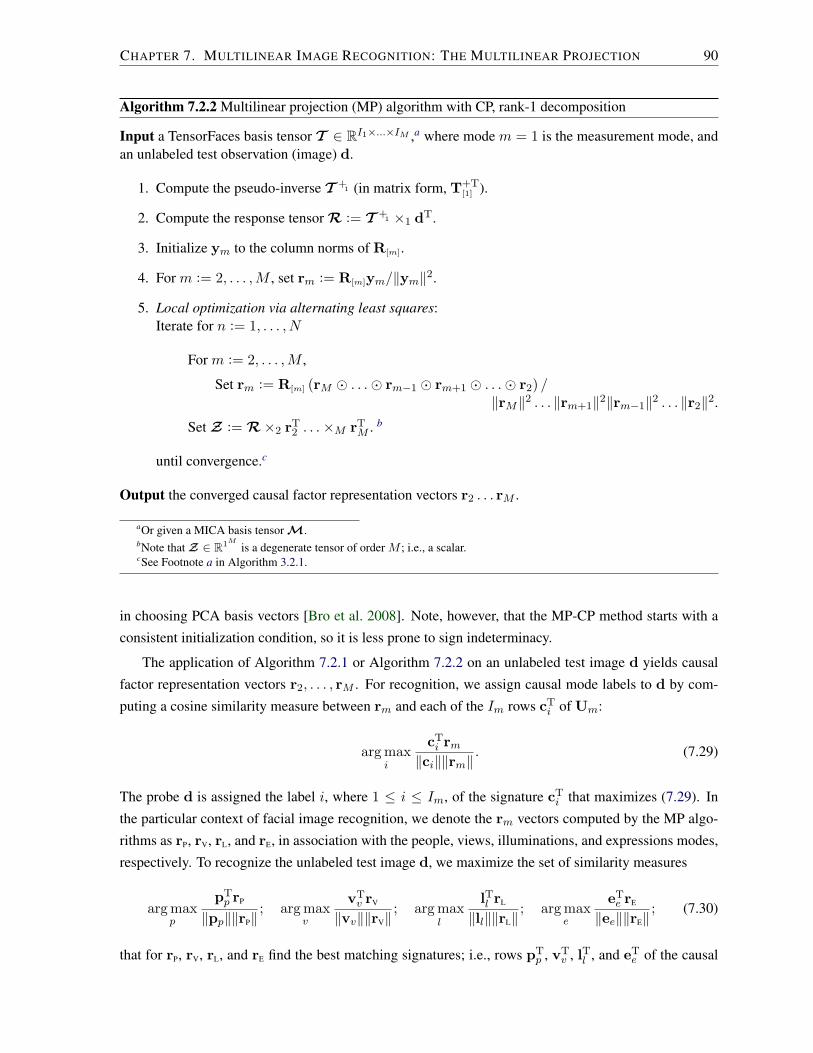
CHAPTER 7. MULTILINEAR IMAGE RECOGNITION: THE MULTILINEAR PROJECTION 90
Algorithm 7.2.2 Multilinear projection (MP) algorithm with CP, rank-1 decomposition
Input a TensorFaces basis tensor T ∈ RI1×...×IM ,a where mode m = 1 is the measurement mode, andan unlabeled test observation (image) d.
1. Compute the pseudo-inverse T +1 (in matrix form, T+T
[1] ).
2. Compute the response tensor R := T +1 ×1 dT.
3. Initialize ym to the column norms of R[m].
4. For m := 2, . . . ,M , set rm := R[m]ym/‖ym‖2.
5. Local optimization via alternating least squares:Iterate for n := 1, . . . , N
For m := 2, . . . ,M ,
Set rm := R[m] (rM � . . .� rm−1 � rm+1 � . . .� r2) /‖rM‖2 . . . ‖rm+1‖2‖rm−1‖2 . . . ‖r2‖2.
Set Z := R×2 rT2 . . .×M rT
M . b
until convergence.c
Output the converged causal factor representation vectors r2 . . . rM .
aOr given a MICA basis tensor M.bNote that Z ∈ R1M
is a degenerate tensor of order M ; i.e., a scalar.cSee Footnote a in Algorithm 3.2.1.
in choosing PCA basis vectors [Bro et al. 2008]. Note, however, that the MP-CP method starts with a
consistent initialization condition, so it is less prone to sign indeterminacy.
The application of Algorithm 7.2.1 or Algorithm 7.2.2 on an unlabeled test image d yields causal
factor representation vectors r2, . . . , rM . For recognition, we assign causal mode labels to d by com-
puting a cosine similarity measure between rm and each of the Im rows cTi of Um:
arg maxi
cTi rm
‖ci‖‖rm‖. (7.29)
The probe d is assigned the label i, where 1 ≤ i ≤ Im, of the signature cTi that maximizes (7.29). In
the particular context of facial image recognition, we denote the rm vectors computed by the MP algo-
rithms as rP, rV, rL, and rE, in association with the people, views, illuminations, and expressions modes,
respectively. To recognize the unlabeled test image d, we maximize the set of similarity measures
arg maxp
pTp rP
‖pp‖‖rP‖; arg max
v
vTv rV
‖vv‖‖rV‖; arg max
l
lTl rL
‖ll‖‖rL‖; arg max
e
eTe rE
‖ee‖‖rE‖; (7.30)
that for rP, rV, rL, and rE find the best matching signatures; i.e., rows pTp , vT
v , lTl , and eTe of the causal

CHAPTER 7. MULTILINEAR IMAGE RECOGNITION: THE MULTILINEAR PROJECTION 91
mode matrices UP, UV, UL, and UE, respectively. Evaluating the set of similarity measures together
enables us to recognize the probe image d as depicting person p in view v, illumination l, and expression
e.
Figure 1.4 illustrates the architecture of our multilinear recognition system, showing the TensorFaces
(MPCA) model trained on the Weizmann facial image database and using (7.30). Of course, if we are
interested only in recognizing the person depicted in d, we can achieve savings by storing only the
person signatures UP and performing only the first similarity optimization in (7.30).
7.3 Facial Image Recognition Experiments
We will now evaluate the recognition algorithms that we have developed in this chapter. There are a
number of meaningful experimental scenarios: We employ either (A) the Weizmann face image database
(Figure 6.1) or (B) the Freiburg image database (Figure 6.6). Using either of these datasets, we train
(1) an MPCA (TensorFaces) model (Figure 6.8) and (2) an MICA (independent TensorFaces) model
(Figure 6.11). Then, in the testing phase, we recognize unlabeled test images (probes) by first inferring
their coefficient vector representations and then using a similarity measure to label the probes, thus
achieving recognition. The inference step may be accomplished using (i) the multiple linear projection
(MLP) method of Section 7.1, or (ii) the multilinear projection (MP) method of Section 7.2 implemented
either (a) by MP-MPCA (Algorithm 7.2.1) or (b) by MP-CP (Algorithm 7.2.2).
We compare the multilinear face recognition results obtained using trained MPCA and MICA mod-
els relative to each other and against those obtained using trained linear PCA [Sirovich and Kirby 1987;
Turk and Pentland 1991a] and ICA [Bartlett 2001; Bartlett et al. 2002] models. In all the experiments
reported below, people depicted in unlabeled test images (probes), which were not part of the training
set, are recognized by inferring the person representation associated with the test image and choosing
the person label using the similarity methods of (7.8) for MLP and (7.29) for MP.
Our first set of experiments employed the Weizmann dataset and the data tensor D illustrated in
Figure 6.1(c). The ensemble of training images were modeled using PCA (eigenfaces) and MPCA
(TensorFaces) and the learned basis vectors are illustrated in Figure 6.3 and Figure 6.2, respectively.
The PCA test image representation was computed by using the conventional linear projection. The
MPCA person representation for test images was computed using the multiple linear projections (MLP)
method (Figure 7.2). The person recognition rates show that MPCA yielded significantly better results
than PCA in scenarios involving the recognition of people imaged in previously unseen views (Table 7.1,
Row 1) and under a previously unseen illuminations (Table 7.1, Row 2).
Our next experiments employed the Freiburg facial image dataset of 16,875 images illustrated in
Figure 6.6 and the data tensor D illustrated in Figure 6.7. We trained PCA, ICA, MPCA, and MICA
models. The trained PCA and MPCA bases are illustrated in Figure 6.3 and Figure 6.2, respectively.
The trained ICA and MICA bases are shown in Figure 6.11. The trained PCA basis matrix (eigenfaces)
has dimensionality Ux ∈ R8560×222, as does the ICA basis matrix, while the MPCA (TensorFaces) basis
and mode matrices have dimensions T ∈ R8560×74×3×1, UP ∈ R75×74, UV ∈ R6×3, and UL ∈ R6×1,

CHAPTER 7. MULTILINEAR IMAGE RECOGNITION: THE MULTILINEAR PROJECTION 92
PCA vs. MPCA Recognition Experiments PCA MPCA
Training: 23 people, 3 views (θ = 0,±34), 4 illuminations (center, left, right, left+right)Testing: 23 people, 2 views (θ = ±17), 4 illuminations (center, left, right, left+right) 61% 80%
Training: 23 people, 5 views (θ = 0,±17,±34), 3 illuminations (center, left, right)Testing: 23 people, 5 views (θ = 0,±17,±34), 1 illumination (left+right) 27% 88%
Table 7.1: Experimental results with the Weizmann image dataset in Figure 6.1 comparing PCA (eigen-faces) against MPCA (TensorFaces) with the multiple linear projection (MLP) recognition method.
PCA & ICA vs. MPCA & MICA Recognition Experiment PCA ICA MPCA MICA
Training: 75 people, 6 views (θ = ±35,±20,±5, φ = 0),6 illuminations (θ = 45, φ = 90 + δ, δ = ±35,±20,±5)
Testing: 75 people, 9 views (φ = 0± 10,±15,±25,±30), 83.90% 89.50% 92.65% 98.14%9 illuminations (θ = 90 + δ, δ = ±35,±20,±5, θ = 0)
Table 7.2: Face recognition experiment using PCA, ICA, MPCA, and MICA models trained on thedataset in Figure 6.6. The MPCA and MICA recognition results were obtained using the MP-MPCAalgorithm.
as do the trained MICA basis tensor and mode matrices. Note that, for a fair comparison, all the
models employ 222 basis vectors. The PCA/ICA image representation has 222 parameters, whereas
our MPCA/MICA image representation has 74 + 3 + 1 = 78 parameters. The MPCA and MICA image
representations and response tensors are shown in Figure 7.3 and Figure 7.4, respectively.
Table 7.2 compares the recognition rates that we obtained in an experiment using these trained mod-
els. The MICA and MPCA models, using the MP-MPCA algorithm, yielded better recognition rates
than PCA (eigenfaces) and ICA in scenarios involving the recognition of people imaged in previously
unseen views and illuminations, with MICA performing significantly better than MPCA in this experi-
ment.
Next, we trained the MPCA (TensorFaces) model and obtained recognition results employing our
different projection algorithms to compute the person representations of unlabeled test images (probes).
Table 7.3 compares the recognition rates obtained when applying the multiple linear projections (MLP)
method and when applying the multilinear projection (MP) method with the MP-MPCA algorithm or
with the MP-CP algorithm. Note that the MP-CP algorithm outperforms the MP-MPCA algorithm used
in the previous recognition experiment.
Table 7.4 provides a detailed study of how dimensionality reduction in the trained MPCA model
affects recognition rates when using the MP-CP algorithm. The table shows recognition percentage
rates obtained for the number of people, view, and illumination basis vectors retained as indicated along
each axis.
Finally, we also experimented with the 2DPCA approach of [Ye 2005; Frangi and Yang 2004],2
2The name 2DSVD chosen by Ye [2005] is a misnomer. The acronym 2DSVD stands for 2D Singular Value Decom-position. (Note that the 2DSVD is known in the literature as a Tucker2 or a 2-mode SVD of a third-order data tensor.) Adecomposition, by definition, should not include a dimensionality reduction step. However, the method described employs
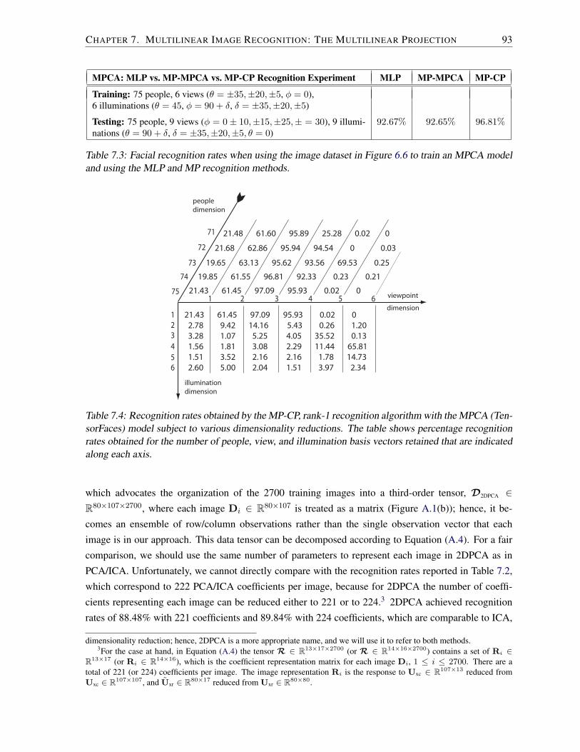
CHAPTER 7. MULTILINEAR IMAGE RECOGNITION: THE MULTILINEAR PROJECTION 93
MPCA: MLP vs. MP-MPCA vs. MP-CP Recognition Experiment MLP MP-MPCA MP-CP
Training: 75 people, 6 views (θ = ±35,±20,±5, φ = 0),6 illuminations (θ = 45, φ = 90 + δ, δ = ±35,±20,±5)
Testing: 75 people, 9 views (φ = 0± 10,±15,±25,± = 30), 9 illumi-nations (θ = 90 + δ, δ = ±35,±20,±5, θ = 0)
92.67% 92.65% 96.81%
Table 7.3: Facial recognition rates when using the image dataset in Figure 6.6 to train an MPCA modeland using the MLP and MP recognition methods.
21.43 61.45 97.09 95.93 0.02 0
2.78 9.42 14.16 5.43 0.26 1.20
3.28 1.07 5.25 4.05 35.52 0.13
1.56 1.81 3.08 2.29 11.44 65.81
1.51 3.52 2.16 2.16 1.78 14.73
2.60 5.00 2.04 1.51 3.97 2.34
viewpoint
dimension
illumination
dimension
people
dimension
21.48 61.60 95.89 25.28 0.02 0
21.68 62.86 95.94 94.54 0 0.03
19.65 63.13 95.62 93.56 69.53 0.25
19.85 61.55 96.81 92.33 0.23 0.21
21.43 61.45 97.09 95.93 0.02 075
74
73
72
71
1
2
3
4
5
6
1 2 3 4 5 6
Table 7.4: Recognition rates obtained by the MP-CP, rank-1 recognition algorithm with the MPCA (Ten-sorFaces) model subject to various dimensionality reductions. The table shows percentage recognitionrates obtained for the number of people, view, and illumination basis vectors retained that are indicatedalong each axis.
which advocates the organization of the 2700 training images into a third-order tensor, D2DPCA ∈R80×107×2700, where each image Di ∈ R80×107 is treated as a matrix (Figure A.1(b)); hence, it be-
comes an ensemble of row/column observations rather than the single observation vector that each
image is in our approach. This data tensor can be decomposed according to Equation (A.4). For a fair
comparison, we should use the same number of parameters to represent each image in 2DPCA as in
PCA/ICA. Unfortunately, we cannot directly compare with the recognition rates reported in Table 7.2,
which correspond to 222 PCA/ICA coefficients per image, because for 2DPCA the number of coeffi-
cients representing each image can be reduced either to 221 or to 224.3 2DPCA achieved recognition
rates of 88.48% with 221 coefficients and 89.84% with 224 coefficients, which are comparable to ICA,
dimensionality reduction; hence, 2DPCA is a more appropriate name, and we will use it to refer to both methods.3For the case at hand, in Equation (A.4) the tensor R ∈ R13×17×2700 (or R ∈ R14×16×2700) contains a set of Ri ∈
R13×17 (or Ri ∈ R14×16), which is the coefficient representation matrix for each image Di, 1 ≤ i ≤ 2700. There are atotal of 221 (or 224) coefficients per image. The image representation Ri is the response to Uxc ∈ R107×13 reduced fromUxc ∈ R107×107, and Uxr ∈ R80×17 reduced from Uxr ∈ R80×80.

CHAPTER 7. MULTILINEAR IMAGE RECOGNITION: THE MULTILINEAR PROJECTION 94
but significantly lower than the recognition rates achieved by our MPCA model with the MP-CP algo-
rithm (96.81%) and our MICA model with the MP-MPCA algorithm (98.14%). Appendix A provides
a more detailed discussion of the drawbacks of the “image-as-a-matrix” approach in general and, in the
final section, a more detailed comparison of the 2DPCA method relative to the other methods in the
above experiment.
7.4 Discussion
We will now discuss the assumptions and limitations of our approach to (facial) object recognition.
As we stated in the introductory chapter, our models make the assumption that the multiple causal
factors combine with one another in a multiplicative manner. Thus, although our multifactor model
is nonlinear, the nonlinearity is not arbitrary. The tacit assumption (cf. (1.4)) is that the variability
in the measurement data due to changes in any single factor can be adequately modeled in a linear
manner when all other factors remain fixed. This assumption can be viewed as a limitation in terms of
the complexity of measurement data with which our models can accurately deal, relative to arbitrarily
nonlinear manifold learning models such as Locally Linear Embedding (LLE) [Roweis and Saul 2000].
However, as we discussed in Section 4.4, such piecewise, local models require dense training data,
whereas our global model can be fitted to rather sparse training data. Furthermore, while a multilinear
analysis may not be able to model arbitrarily nonlinear data accurately, we can decompose the data
in terms of their explanatory variables using a multilinear decomposition and then further analyze and
model each of those variables by a fully nonlinear method such as LLE.
It is more meaningful to compare our multilinear model against the kernel PCA [Scholkoph et al.
1998] and kernel ICA [Yang et al. 2005] techniques that were also discussed in Section 4.4. While these
models make no specific nonlinearity assumptions, they model the distribution of the observed data
from which they try to infer causal information, whereas our multilinear approach explicitly models the
true multifactor causal structure of the measurement data generation process. As we discussed earlier,
our model shares the same Gaussian (non-Gaussian) assumptions made by the PCA (ICA) models, in
their conventional or kernel versions, and as was noted in Section 4.4, we can also further generalize
our multilinear models using kernels.
Compared to unsupervised learning methods, a drawback of our multilinear models is that they
must be trained in a supervised manner using properly labeled multimodal training data that have been
collected in a systematic and comprehensive manner. This can be cumbersome and tedious relative
to, say, training the standard PCA model on a simple collection of images. However, our multifactor
approach has significantly loftier aspirations in terms of data analysis and ultimate recognition rates.
Moreover, the offline labor-intensive data collection and training phase is compensated by the fact that
there exists a computationally inexpensive online classification step. Furthermore, the training data
acquisition and labeling process can be facilitated or even fully automated using special equipment, such
as automated robotic devices to move cameras and lightsources [Moses et al. 1996; Dana et al. 1999], or
multi-camera/multi-illumination systems [Debevec et al. 2000], or kaleidoscopic imaging devices [Han

CHAPTER 7. MULTILINEAR IMAGE RECOGNITION: THE MULTILINEAR PROJECTION 95
and Perlin 2003]. However, collecting large quantities of image data can be tedious and perhaps even
prohibitively expensive, and our current model assumes the availability of complete data sets. It can and
should be expanded to deal with missing data.
Finally, perhaps the biggest limitation of our approach to face recognition is that it is a strictly
appearance-based method and, hence, it shares the well-known advantages and drawbacks of all appearance-
based methods. We do not attempt to extract features from the image or apply any so-called “model-
based techniques”. Nor have we attempted to use any alternative sources of information about the face,
such as 3D data. However, we believe that our approach can be extended to exploit additional sources
of information, but of course at additional data collection costs.

8Multilinear Motion Analysis, Synthesis,
and Recognition:Human Motion Signatures
Contents8.1 Motion Data Acquisition . . . . . . . . . . . . . . . . . . . . . . . . . . . . . . . 97
8.2 Motion Analysis: TensorMotions . . . . . . . . . . . . . . . . . . . . . . . . . . . 99
8.3 Motion Synthesis . . . . . . . . . . . . . . . . . . . . . . . . . . . . . . . . . . . . 101
8.4 Motion Recognition . . . . . . . . . . . . . . . . . . . . . . . . . . . . . . . . . . 102
8.5 Experiments and Results . . . . . . . . . . . . . . . . . . . . . . . . . . . . . . . 103
8.6 Discussion . . . . . . . . . . . . . . . . . . . . . . . . . . . . . . . . . . . . . . . 104
Our development has until now focused exclusively image data. In this chapter, we will consider
the application of our tensor algebraic framework to motion data.
To motivate our motion application, consider the following questions: In analogy with handwritten
signatures, do people have characteristic motion signatures that individualize their movements? If so,
can these signatures be extracted from example motions? If so, can extracted signatures be used to
recognize, say, a particular individual’s walk subsequent to observing examples of other movements
produced by this individual? An ability to perceive motion signatures would seem to be well-grounded
from an evolutionary perspective, since survival depends on recognizing the movements of predator or
prey, or of friend or foe.
96

CHAPTER 8. MULTILINEAR MOTION ANALYSIS, SYNTHESIS, AND RECOGNITION 97
In the 1960s, the psychologist Gunnar Johansson performed a series of famous experiments in which
he attached point light sources to people’s limbs and recorded videos of them performing different
activities, such as walking, running, and dancing [Johansson 1974]. Observers of these moving light
displays, videos in which only the light sources are visible, were asked to classify the activity performed
and to note certain characteristics of the movements, such as a limp or an energetic/tired walk. Observers
can usually perform this task with ease and they could sometimes determine gender and even recognize
specific individuals in this way. This may corroborate the hypothesis that the motion signature is a
perceptible element of human movement.
Our work with motion data has three goals:
1. To develop new algorithms that can analyze everyday human motions and separate out distinctive
motion signatures.
2. To synthesize novel motions that are in accord with extracted motion signatures.
3. To recognize specific individuals performing new motions, using extracted motion signatures
associated with these individuals.
Our approach exploits corpora of motion data which are now reasonably easy to acquire through a
variety of modern motion capture technologies developed for use in the entertainment industry (see, e.g.,
[Gleicher 2001]). Motion synthesis through the analysis of motion capture data is currently attracting
a great deal of attention within the computer graphics community as a means of animating graphical
characters. Several authors have developed generative motion models for this purpose. Recent papers
report the use of neural network learning models [Grzeszczuk et al. 1998] and hidden Markov models
[Brand and Hertzmann 2000].
Within our multilinear framework, corpora of motion capture data including multiple people and
actions are organized as higher-order arrays, or tensors. We apply our MPCA/MICA algorithms to
extract human motion signatures among the other causal factors inherent to human movement.
8.1 Motion Data Acquisition
Human limb motion was recorded using a VICON system that employs four video cameras (Figure 8.1).
The cameras detect infrared light reflected from retroreflective markers placed on each leg of a human
subject. The system computes the 3D position of the markers relative to a fixed lab coordinate frame.
The video cameras are positioned on one side of a 12 meter long walkway such that each marker can be
observed by at least two cameras during motion.
To extract the three angles of a human joint, we must define a plane for each limb whose motion can
be measured relative to the sagittal, frontal, and transverse planes through the body (Figure 8.2). The
motion of each limb is the combined motion carried out in these three planes. The sagittal plane divides
the body into left and right halves. Thus, motion in this plane is front to back. The frontal plane divides
the body into front and back halves. Thus motion in this plane is side to side. The transverse plane
divides the body into upper and lower halves. Thus, motion in this plane is an in-out twisting motion.
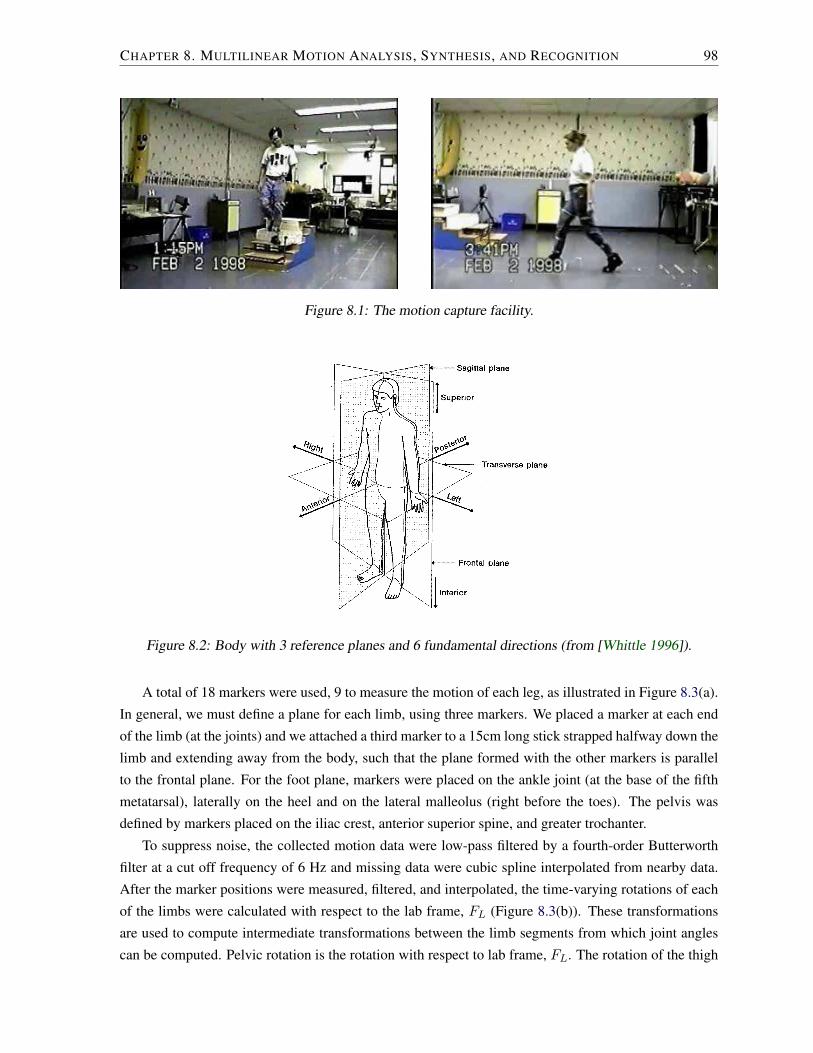
CHAPTER 8. MULTILINEAR MOTION ANALYSIS, SYNTHESIS, AND RECOGNITION 98
Figure 8.1: The motion capture facility.
Figure 8.2: Body with 3 reference planes and 6 fundamental directions (from [Whittle 1996]).
A total of 18 markers were used, 9 to measure the motion of each leg, as illustrated in Figure 8.3(a).
In general, we must define a plane for each limb, using three markers. We placed a marker at each end
of the limb (at the joints) and we attached a third marker to a 15cm long stick strapped halfway down the
limb and extending away from the body, such that the plane formed with the other markers is parallel
to the frontal plane. For the foot plane, markers were placed on the ankle joint (at the base of the fifth
metatarsal), laterally on the heel and on the lateral malleolus (right before the toes). The pelvis was
defined by markers placed on the iliac crest, anterior superior spine, and greater trochanter.
To suppress noise, the collected motion data were low-pass filtered by a fourth-order Butterworth
filter at a cut off frequency of 6 Hz and missing data were cubic spline interpolated from nearby data.
After the marker positions were measured, filtered, and interpolated, the time-varying rotations of each
of the limbs were calculated with respect to the lab frame, FL (Figure 8.3(b)). These transformations
are used to compute intermediate transformations between the limb segments from which joint angles
can be computed. Pelvic rotation is the rotation with respect to lab frame, FL. The rotation of the thigh

CHAPTER 8. MULTILINEAR MOTION ANALYSIS, SYNTHESIS, AND RECOGNITION 99
(a) (b)
Figure 8.3: (a) Marker configuration and coordinate frames. (b) Coordinate systems assigned to the 3measured parts of the leg.
is the rotation with respect to the pelvis through which the hip angles are obtained. The knee angles
are defined as the rotations of the shank with respect to the thigh. The ankle angles are defined as the
rotations of the foot with respect to the shank.
To compute the joint angles, we first calculate the frame coordinate transformation for each limb
with respect to the lab, we then calculate the relative orientation of each limb in the kinematic chain,
and we finally solve the inverse kinematic equations. These three steps are explained in Appendix C.
The result of each motion data acquisition run is a set of time series of the pelvis orientation plus
the joint angles for the thigh, knee, and ankle joints of each leg. A training corpus of motion data was
collected from 6 subjects. Three motions were acquired for each person—walk, ascend-stairs, descend
stairs. Each motion was repeated 10 times. A motion cycle was segmented from each motion sequence.
As shown in Figure 8.4, a motion cycle comprises the following motion events: Foot contact, opposite
toe off the ground, opposite foot contact, toe off the ground, foot contact.
8.2 Motion Analysis: TensorMotions
Given motion sequences acquired from several people, we assemble a training data tensor D ∈ RIj×IP×IA ,
where Ij is the number of joint angle time samples, IP is the number of people, and IA is the number of
action classes. We apply the MPCA algorithm (Algorithm 4.2.1) to D to obtain the model
D = T ×P UP ×A UA, (8.1)
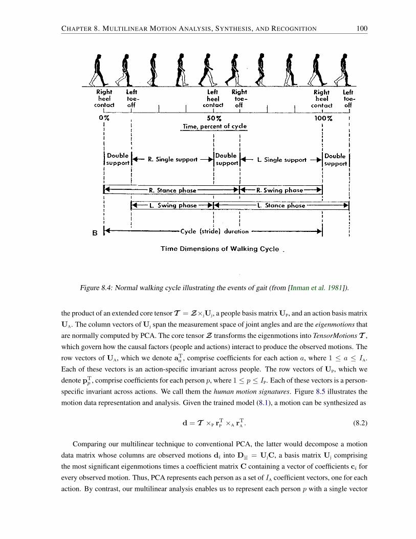
CHAPTER 8. MULTILINEAR MOTION ANALYSIS, SYNTHESIS, AND RECOGNITION 100
Figure 8.4: Normal walking cycle illustrating the events of gait (from [Inman et al. 1981]).
the product of an extended core tensor T = Z×jUj, a people basis matrix UP, and an action basis matrix
UA. The column vectors of Uj span the measurement space of joint angles and are the eigenmotions that
are normally computed by PCA. The core tensor Z transforms the eigenmotions into TensorMotions T ,
which govern how the causal factors (people and actions) interact to produce the observed motions. The
row vectors of UA, which we denote aTa , comprise coefficients for each action a, where 1 ≤ a ≤ IA.
Each of these vectors is an action-specific invariant across people. The row vectors of UP, which we
denote pTp , comprise coefficients for each person p, where 1 ≤ p ≤ IP. Each of these vectors is a person-
specific invariant across actions. We call them the human motion signatures. Figure 8.5 illustrates the
motion data representation and analysis. Given the trained model (8.1), a motion can be synthesized as
d = T ×P rTP ×A rT
A . (8.2)
Comparing our multilinear technique to conventional PCA, the latter would decompose a motion
data matrix whose columns are observed motions di into D[j] = UjC, a basis matrix Uj comprising
the most significant eigenmotions times a coefficient matrix C containing a vector of coefficients ci for
every observed motion. Thus, PCA represents each person as a set of IA coefficient vectors, one for each
action. By contrast, our multilinear analysis enables us to represent each person p with a single vector

CHAPTER 8. MULTILINEAR MOTION ANALYSIS, SYNTHESIS, AND RECOGNITION 101
???
ActionsJoint
Ang
les
Peo
ple
D
U Z
=
U
1
3
U2
Figure 8.5: Motion data collection and analysis model.
of coefficients pTp that is invariant of the action performed.
8.3 Motion Synthesis
By computing the decomposition (8.1), we analyze the training corpus of motion data D acquired from
a group of people and extract the human motion signatures UP, the action representations UA, and the
TensorMotions basis T . We thus learn a generative model with which, given motion data for a new
subject performing one or more, but not all, of the actions previously observed for the IP people in the
motion database, we can synthesize the remaining, unobserved actions in the style particular to this new
subject.
Let Dn ∈ RIj×1×IA be the motions of a new subject, where IA is the number of observed actions,
which are a subset of all the IA actions previously observed and analyzed for the group of people. From
(8.1), we have
Dn = T ×P pTn ×A UA (8.3)
= A×P pTn , (8.4)
where A = T ×A UA is the action-specific basis, UA comprises a subset of the rows of UA, and pTn is
the motion signature of the new person. Therefore, the synthesis algorithm first computes
pTn = A+
P ×TP Dn, (8.5)
where A+P is the people-mode pseudoinverse of tensor A. This model makes the assumption that the
motion signature lies in the subspace spanned by UP. We can then synthesize a complete set of motions
Dn for the new person as follows:
Dn = T ×A UA ×P pTn . (8.6)
Similarly, if we observe a known person or people who contributed motions to the training corpus
CHAPTER 8. MULTILINEAR MOTION ANALYSIS, SYNTHESIS, AND RECOGNITION 102
performing a new action Dn ∈ RIj×IP×1, where IP is the number of people observed performing the
new action, from (8.1), we have
Dn = T × UP ×A aTn (8.7)
= P ×A aTn , (8.8)
where P = T ×P UP is the people-specific basis and UP comprises a subset of the rows of UP. The
associated action parameters aTn are computed as
aTn = P+
A ×TA Dn, (8.9)
where P+A is the action-mode pseudoinverse of tensor P . We can then synthesize the new action in the
style of every person in the database using
Dn = T ×P UP ×A aTn . (8.10)
8.4 Motion Recognition
Our multilinear analysis yields the basis tensor T whose pseudoinverse maps observed motions from
the measurement space—joint angles over time—into the underlying causal factor spaces—the people
space and action space—thereby enabling the recognition of people and actions from the motion data.
Given a test (probe) motion d and the trained TensorMotions T , we can apply the multilinear projec-
tion algorithms of Section 7.2 to compute the causal factor representation vectors rP and rA and then
simultaneously recognize the person p and action a via similarity maximizations like those in (7.30).
However, if we can identify by inspection the action depicted in the probe motion d, the task of
recognizing the person who produced d becomes easier. We map d into the people signature space by
first computing the action-specific basis Ba = T ×A aTa , for the identified action a, where aT
a is the
ath row in UA. We then compare the signature rTP = B
+P
a ×P dT against the person signatures pTp for
1 ≤ p ≤ IP, which are the rows in UP, and the recognized person label assigned to d is the label p of
the best matching signature vector pp; i.e.,
arg maxp
pTp rP
‖pp‖‖rP‖. (8.11)
Conversely, to recognize the action depicted in d generated by an identified person p, we map d into the
action parameter space by computing the person-specific basis tensor Bp = T ×P pTp for the identified
person p and then compare the signature rTA = B+
A ×A dT against the action signatures aTa for 1 ≤ a ≤
IA, which are the rows in UA, and the recognized action label assigned to d is the label a of the best
matching signature vector aa; i.e.,
arg maxa
aTa rA
‖aa‖‖rA‖. (8.12)
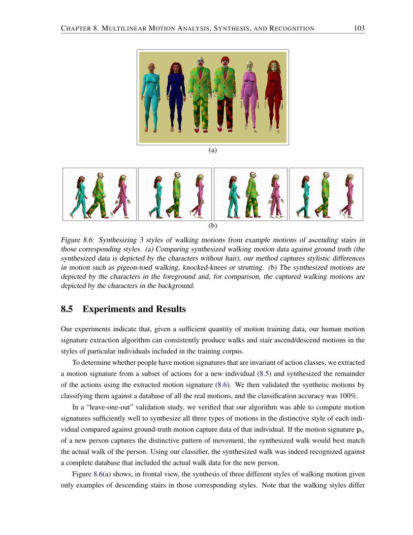
CHAPTER 8. MULTILINEAR MOTION ANALYSIS, SYNTHESIS, AND RECOGNITION 103
(a)
(b)
Figure 8.6: Synthesizing 3 styles of walking motions from example motions of ascending stairs inthose corresponding styles. (a) Comparing synthesized walking motion data against ground truth (thesynthesized data is depicted by the characters without hair), our method captures stylistic differencesin motion such as pigeon-toed walking, knocked-knees or strutting. (b) The synthesized motions aredepicted by the characters in the foreground and, for comparison, the captured walking motions aredepicted by the characters in the background.
8.5 Experiments and Results
Our experiments indicate that, given a sufficient quantity of motion training data, our human motion
signature extraction algorithm can consistently produce walks and stair ascend/descend motions in the
styles of particular individuals included in the training corpus.
To determine whether people have motion signatures that are invariant of action classes, we extracted
a motion signature from a subset of actions for a new individual (8.5) and synthesized the remainder
of the actions using the extracted motion signature (8.6). We then validated the synthetic motions by
classifying them against a database of all the real motions, and the classification accuracy was 100%.
In a “leave-one-out” validation study, we verified that our algorithm was able to compute motion
signatures sufficiently well to synthesize all three types of motions in the distinctive style of each indi-
vidual compared against ground-truth motion capture data of that individual. If the motion signature pn
of a new person captures the distinctive pattern of movement, the synthesized walk would best match
the actual walk of the person. Using our classifier, the synthesized walk was indeed recognized against
a complete database that included the actual walk data for the new person.
Figure 8.6(a) shows, in frontal view, the synthesis of three different styles of walking motion given
only examples of descending stairs in those corresponding styles. Note that the walking styles differ

CHAPTER 8. MULTILINEAR MOTION ANALYSIS, SYNTHESIS, AND RECOGNITION 104
Figure 8.7: A synthesized stair-ascending motion.
Figure 8.8: Frames from an animation short created with synthesized motion data.
subtly: The woman on the left walks in a pigeon-toed style, the clown struts, and the skeleton on the
right walks with knocked knees. Figure 8.6(b) shows a side view of the motions; the figures animated
using synthesized motions are in the foreground. Figure 8.7 shows a stair ascending motion synthesized
for one of the individuals. Our algorithm extracted the motion signature from a sample walk from this
individual. We then used the extracted motion signature to synthesize the stair-ascending motion for
this individual. The motion signature was combined with general stair ascending parameters that were
previously extracted from our database.
We have created an animation short using motion data synthesized by our algorithm (Figure 8.8).
The graphical characters shown are modeled and rendered using the MetaCreations Poser software
package.
8.6 Discussion
The synthesis results that we obtained were adequate to animate our characters in simple ways, and the
observed motion recognition rates were 100% accurate. There exists a substantial literature on motion

CHAPTER 8. MULTILINEAR MOTION ANALYSIS, SYNTHESIS, AND RECOGNITION 105
analysis and synthesis in computer graphics and on motion analysis and recognition in computer vision,
some of which was covered elsewhere in this thesis. A comparison of our recognition rates against those
of related algorithms found in the literature would probably not be meaningful because we employed a
rather small dataset in our experiments. Systematic experiments need to be performed on much more
extensive datasets, but the data collection issues discussed in Appendix B in the context of acquiring
facial image datasets apply analogously to motion capture data. To our knowledge, extensive motion
databases that would be suitable for fully training our multilinear model do not yet exist.
The limitations of our approach to motion recognition are analogous to those that were discussed in
Section 7.4 in the context of face recognition and we refer the reader to that discussion. To summarize,
the limitations include the multilinearity assumption, which can be relaxed to more general nonlinearity
using kernel functions, and the aforementioned training data collection requirements (since we are using
motion capture data, the appearance-based modeling issues do not apply). However, we point out again
that, despite the limitations, our multilinear framework offers significant advantages that are unique
among existing methods, most significantly among them the ability to model the essential multimodal
causal structure of the observational data—in this case, human motion capture data.
9Conclusion
Contents9.1 Summary . . . . . . . . . . . . . . . . . . . . . . . . . . . . . . . . . . . . . . . . 106
9.2 Future Work . . . . . . . . . . . . . . . . . . . . . . . . . . . . . . . . . . . . . . 107
9.1 Summary
We have introduced and developed a tensor framework for visual computing. Within this framework, the
analysis, synthesis, and recognition of image ensembles resulting from the confluence of multiple causal
factors related to scene structure, illumination, and imaging are regarded as problems in multilinear
algebra wherein the image ensemble is represented as a higher-order tensor. This image data tensor is
decomposed in order to separate and parsimoniously represent the causal factors.
We pursued a tensor decomposition approach to tackling these problems based on the M -mode
singular value decomposition for multilinear principal components analysis with truncation and an al-
ternating least squares iteration for dimensionality reduction. One of our novel contributions was a
complimentary multilinear generalization of independent components analysis. Another contribution
was the introduction of multilinear projection, with associated novel definitions of the identity and
pseudo-inverse tensors, for the purposes of recognition in our tensor framework.
We demonstrated our approach to be of value in tackling problems of current importance in computer
graphics, computer vision, and pattern recognition. In particular, we presented a multilinear image-
based rendering method that we call TensorTextures, as well as a multilinear facial image representation
106

CHAPTER 9. CONCLUSION 107
and recognition method that we call TensorFaces. These new multilinear algebraic (tensor) methods
outperform their conventional linear algebraic (matrix) counterparts.
We also applied our multilinear framework to the analysis, synthesis and recognition of human mo-
tion data with promising results. We anticipate numerous other applications to data-intensive domains
where PCA/ICA have been employed in the past.
9.2 Future Work
Our research opens up numerous avenues for future work. Some of the major ones are as follows:
• Kernel MPCA/MICA and Multifactor Generalizations of LLE/Isomap/LE Manifold Learn-ing Methods: As we discussed in Section 4.4, although it is fundamentally nonlinear, our multi-
linear framework can be straightforwardly generalized to deal with nonlinear data through “ker-
nelization”. This leads to Kernel Multilinear PCA (K-MPCA) and Kernel Multilinear ICA (K-
MICA) methods. In future work, we will apply and and evaluate these methods on our datasets.
Further exploiting kernelization within our multilinear framework, we also proposed in Sec-
tion 4.4 multifactor generalizations of the Locally Linear Embedding (LLE), Isomap (IM), and
Laplacian Eigenmap (LE) manifold learning algorithms. We will implement these generalizations
and evaluate their performance in our image synthesis/analysis/recognition applications.
• Applying the Multilinear Framework to Other Fields: We have motivated and demonstrated
our multilinear framework in the domains of computer graphics, computer vision, and machine
learning. However, or framework should, in principle, also be applicable to any other domain
where PCA and ICA have been employed in the past. Interestingly, the application of these
techniques seems to be more or less ubiquitous. Examples include: The analysis of microarrays
in bioinformatics [Alter et al. 2000; Lee and Batzoglou 2003]; in finance for modeling yield
curves and other uses [Alexander 2001; Back and Weigend 1997]; in information technology for
data mining; in the social sciences for discovering social networks; etc. All of these domains can
potentially benefit by generalizing existing domain-specific PCA/ICA-based algorithms to their
natural multilinear extensions.
• Multilinear Texture Synthesis: In our TensorTextures work, we introduced a multilinear ap-
proach to the image-based rendering of textured surfaces via a parsimonious, explicitly multi-
factor generative approximation to the BTF. We believe that our approach can handle data sets
that result from the variation of additional causal factors, such as BTF scale (i.e., zooming into or
away from a textured surface), high dynamic range (HDR) BTF acquisition at multiple exposures,
or temporally varying BTFs, such as aging skin or leaves changing colors in the fall. In future
work, one could also incorporate into TensorTextures a variant of view-dependent displacement
maps [Wang et al. 2003]. Another avenue for future work is multilinear texture synthesis, which
would generalize existing PCA-based texture synthesis approaches [Lefebvre and Hoppe 2006;
Liang et al. 2001].

CHAPTER 9. CONCLUSION 108
• Multilinear Deformable Models: Multilinear analysis is ripe for future exploitation in area of
deformable models in computer vision and graphics. An important category of such models in
vision is known as active shape/appearance models [Cootes et al. 1995; Cootes et al. 1998]. The
deformation modes of these models are learned from a set of training examples by applying PCA
and dimensionality reduction. Among other applications, such models have proven themselves
useful for medical image segmentation. Multilinear analysis promises to generalize and augment
the power of such deformable models, enabling them to learn multiple modes of deformation
arising from different sources—e.g., apparent shape deformations due to view change, versus true
deformations due to pathological conditions, versus true deformations due to non-pathological
conditions, such as aging. In graphics, multilinear analysis should be readily applicable in the
area of morphable models [Blanz and Vetter 1999; Allen et al. 2003] where PCA has been used.
• Computing the M -Mode SVD Incrementally and When Data Are Missing: Our current work
has assumed that we can assemble complete data tensors in order to carry out multilinear analyses.
Unfortunately, this may not be a realistic assumption in real world applications. A promising
statistical technique for dealing with missing data is known as imputation. Furthermore, since
in real world applications data may be acquired sequentially, a multilinear model would best
be updated with every new data acquisition; thus, there is a need for an incremental M -mode
SVD/ICA. An example is biomedical applications that might have a time component, such as
experiments that need to be run at different stages of a chronic illness. Computing the matrix
SVD in an incremental manner while estimating missing data was considered by Brand [2002].
The incremental computation and imputation of missing data in a multilinear framework is in
need of further development.
• Multilinear Local Feature Decomposition: In appearance-based object recognition, it is impor-
tant to be able to decompose and represent an object in terms of local topographic features [Penev
and Atick 1996]. Currently the TensorFaces basis vectors contain global features. In a multilinear
local feature decomposition, the basis vectors for the people mode would contain topographic
representations of the face such as the eyes, nose, and mouth, while the basis vectors for the il-
lumination mode would contain topographic representation associated with illumination, such as
shadow under the eye cast by the brow, the shadow cast by the nose, the shadow cast by the chin,
etc. In principle, this may be achieved by adding constraints to our multilinear models analogous
to the type of constraints that have been added to linear models, such as non-negativity constraints
[Lee and Seung 1999; Shen and Israel 1989] or sparsity constraints [Cadima and Jolliffe 1995;
Chennubhotla and Jepson 2001; d’Aspremont et al. 2004; Zou et al. 2006; Moghaddam et al.
2006]. This should be a promising direction for future work.
• A Multilinear Face Recognition System: Although our multilinear framework is relevant to
biometric systems, it has been beyond the scope of this thesis to implement a practical face recog-
nition system. A big challenge is the recognition of an individual under unconstrained imaging
conditions. Such a system might be structured as shown in Figure 1.4. First, a multilinear model is

CHAPTER 9. CONCLUSION 109
learned from a (hopefully large) set of cooperative participants, each of whom supply a complete
set of training images acquired from multiple views, under multiple illuminations, in multiple
expressions, etc. An uncooperative subject whose face is detected in one or more surveillance
images can then be enrolled into the system, by representing his/her facial image(s) relative to the
statistics encoded in the learned model. This should make it possible, in principle, to synthesize a
complete image set of training images for the subject. The image database can then be augmented
with these new training images and the multilinear model incrementally updated. This should en-
able the recognition of the subject from an arbitrary, unlabeled image, as illustrated at the bottom
of the figure. Implementing a prototype recognition system of this kind, especially one that would
support the multilinear fusion of multimodality biometric data (e.g., video and speech) would be
a worthy future goal.

AOn the Treatment of Observational Data as
Vectors, Matrices, or Tensors
Raw observational data usually comprise sets of random variables. The conventional way of organizing
a multivariate observation for statistical analysis is as a vector of measurement variables. In recent years,
however, several authors have advocated leaving the data elements associated with a single observation
organized in the manner that the acquisition device provides them; in particular, organizing a CCD
image as a matrix of pixel variables, rather than “vectorizing” it. In this context, bilinear and multilinear
models for vision, graphics, and learning fall under four different categories:
1. Multilinear, or rank-(R1, R2, . . . , RM ), decomposition and different generalizations for higher-
order data tensors that contain vectorized measurement data, as in our work and the work of other
authors [Wang et al. 2003; Vlasic et al. 2005; Hsu et al. 2005].
2. Like Category 1 above, but with rank-R decomposition.
3. Multilinear, or rank-(R1, R2, . . . , RM ), decomposition of higher-order data tensors where each
observation is a matrix or higher-order tensor; e.g., an image is treated as a matrix and a unimodal
image ensemble is a third-order tensor [Ye 2005; Xu et al. 2005; Wang and Ahuja 2005; Wang
et al. 2005; Wang and Ahuja 2008].1
1Some authors [Ye 2005; Wang and Ahuja 2005] claim that they perform a generalized rank-R approximation of tensors;however, according to the standard definition of the rank-R and rank-(R1, R2, . . . , RM ) decompositions, they actually per-form a multilinear decomposition of a third-order tensor with dimensionality reduction in only two of the modes—the imagerow/column modes. This multilinear decomposition is also known as a Tucker2 decomposition or a (M − 1)-mode SVD.
110

APPENDIX A. ON OBSERVATIONAL DATA AS VECTORS, MATRICES, OR TENSORS 111
images
pixels
D =
pixels
D =
images
pixe
ls
(a) (b)
Figure A.1: Image ensemble organizations. (a) Images are vectorized, (i.e., the pixels of an image areorganized into a 1-way array). An ensemble of images is organized as a 2-way array or a “data matrix” (amultimodal image ensemble is a higher-order “data tensor”). The thick strips represent single columns.(b) The pixels of an image are organized as a 2-way array. A unimodal image ensemble is organized asa 3-way data tensor.
4. Like Category 3 above, but with rank-R decomposition [Shashua and Levin 2001; Furukawa et al.
2002; Wang and Ahuja 2004; Shashua and Hazan 2005].
We will now evaluate some of the arguments found in recent publications in favor of treating an
image as a matrix rather than vectorizing it (Figure A.1), and conclude that it is preferable to vectorize
images. The following are arguments for treating an image as a matrix, followed by rebuttals:
• “An image (video) is intrinsically a matrix (tensor).”
Technically, a matrix corresponds to a transformation from one vector space to another, so a more
appropriate statement would be that an image (video) is a 2D (3D) array of numbers. However,
this statement merely presupposes a CCD imaging sensor with a rectangular array of receptors;
the photoreceptors in biological eyes are by no means organized as regular matrices. Yet one can
readily treat both cases in a uniform manner by vectorizing the collection of receptor responses,
thus treating the entire image as a point in a high-dimensional image space.
• “An inherent problem of the image-as-a-vector representation is that the spatial redundancy
within each image matrix is not fully utilized, and some local spatial relationships are lost.”
On the contrary, the subdivision of the image into rows and columns, suffers from the very prob-
lem incorrectly attributed to the conventional, vectorized-image representation. PCA applied to
an ensemble of vectorized images encodes the pixel covariances or second-order statistics of the
ensemble. In other words, treating an N1 × N2 image as a vector leads to the computation for
each pixel of all its pairwise covariances with every other pixel in the image (there are N1N2 such
covariances for each pixel) (Figure A.2). By contrast, when one regards an image as a matrix, it
becomes a collection of row (column) observations and PCA explicitly computes how pixels co-
vary with other pixels within the same row (column). There are only N1 + N2 such covariances
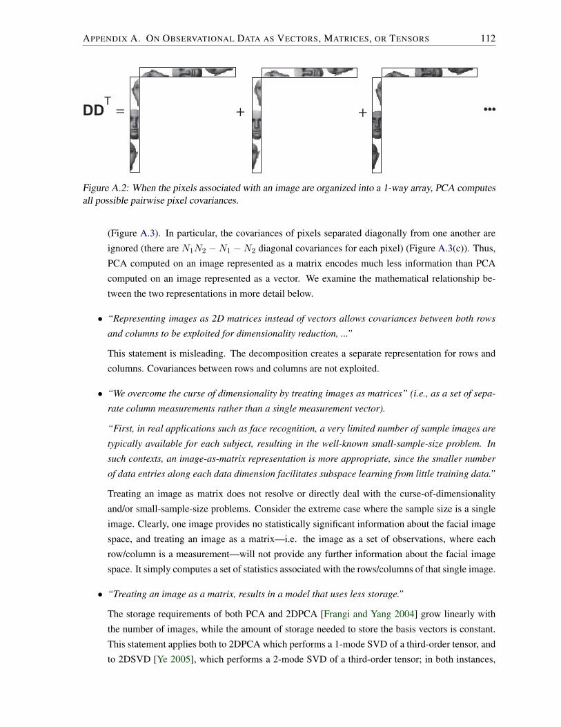
APPENDIX A. ON OBSERVATIONAL DATA AS VECTORS, MATRICES, OR TENSORS 112
+ +DDT
=
Figure A.2: When the pixels associated with an image are organized into a 1-way array, PCA computesall possible pairwise pixel covariances.
(Figure A.3). In particular, the covariances of pixels separated diagonally from one another are
ignored (there are N1N2 −N1 −N2 diagonal covariances for each pixel) (Figure A.3(c)). Thus,
PCA computed on an image represented as a matrix encodes much less information than PCA
computed on an image represented as a vector. We examine the mathematical relationship be-
tween the two representations in more detail below.
• “Representing images as 2D matrices instead of vectors allows covariances between both rows
and columns to be exploited for dimensionality reduction, ...”
This statement is misleading. The decomposition creates a separate representation for rows and
columns. Covariances between rows and columns are not exploited.
• “We overcome the curse of dimensionality by treating images as matrices” (i.e., as a set of sepa-
rate column measurements rather than a single measurement vector).
“First, in real applications such as face recognition, a very limited number of sample images are
typically available for each subject, resulting in the well-known small-sample-size problem. In
such contexts, an image-as-matrix representation is more appropriate, since the smaller number
of data entries along each data dimension facilitates subspace learning from little training data.”
Treating an image as matrix does not resolve or directly deal with the curse-of-dimensionality
and/or small-sample-size problems. Consider the extreme case where the sample size is a single
image. Clearly, one image provides no statistically significant information about the facial image
space, and treating an image as a matrix—i.e. the image as a set of observations, where each
row/column is a measurement—will not provide any further information about the facial image
space. It simply computes a set of statistics associated with the rows/columns of that single image.
• “Treating an image as a matrix, results in a model that uses less storage.”
The storage requirements of both PCA and 2DPCA [Frangi and Yang 2004] grow linearly with
the number of images, while the amount of storage needed to store the basis vectors is constant.
This statement applies both to 2DPCA which performs a 1-mode SVD of a third-order tensor, and
to 2DSVD [Ye 2005], which performs a 2-mode SVD of a third-order tensor; in both instances,

APPENDIX A. ON OBSERVATIONAL DATA AS VECTORS, MATRICES, OR TENSORS 113
D(1) DT
(1)=
pix
els
observations (image columns)observations (image columns)
D(1)=
+ + +
(a)
pix
els
observations (image rows)
D(2)=
D(2) DT
(2)= + + + +
(b)
(c)Figure A.3: Matrixizing a data tensor and covariance computation. (a) The data tensor is matrixized inthe first mode and pixel covariances are computed between pixels within a column. (b) The data tensoris matrixized in the second mode and pixel covariances are computed between pixels within a row. (c)Diagonal covariances are not computed.

APPENDIX A. ON OBSERVATIONAL DATA AS VECTORS, MATRICES, OR TENSORS 114
the tensor is an ensemble of 2D images. The upper bound on the PCA basis storage requirements
(corresponding to no dimensionality reduction) is the number of pixels squared, while that of
the 2DPCA is the number of rows squared plus the number of columns squared. While the basis
vector storage requirements for 2DPCA is less than that of PCA, the dominant factor is the amount
of storage needed to represent the images in the database. By contrast, the storage requirements
of MPCA and MICA grow linearly with the number of people, which is usually only a fraction of
the number of images.
• “Computing PCA on a dataset that treats an image as a matrix is computationally more efficient.”
The PCA of a data matrix of vectorized N1 × N2 images computes the SVD of the pixel co-
variance matrix whose dimensionality is (N1N2)2. When treating images as “matrices” and an
image ensemble as a third-order tensor, one obtains a column-pixel covariance matrix and a row-
pixel covariance matrix, of dimensionality N21 and N2
2 , respectively. Computing the SVDs of
two smaller covariance matrices for 2DSVD is less expensive than performing an SVD on a large
covariance matrix for PCA, but one should bear in mind that this is an offline computational task.
Our MPCA/MICA algorithms treat images as vectors, but they compute SVDs not of the pixel co-
variance matrix, but of the covariance matrices associated with each causal factor. Although this
can be more expensive than PCA or 2DSVD, depending on the size of the causal factor matrices,
it is an offline computational cost that is offset by a less expensive online recognition computa-
tion. Several papers in the literature advocate the computation of the MPCA by treating images
as matrices (e.g., [Wang and Ahuja 2005; Wang et al. 2005]), which additionally necessitates
computing SVDs of the row-pixel covariance and column-pixel covariance matrices.
We now examine the mathematical relationship between image-as-a-vector and image-as-a-matrix
representations in more detail. A data matrix D ∈ RIx×II whose columns are vectorized images (Fig-
ure A.1(a)) can be decomposed using standard matrix SVD. The SVD is expressed in terms of the
mode-m product and matrix multiplication as follows:
D = S×x Ux ×I UI Tensor Notation (A.1)
D[x] = DT[I] = Ux SUT
I︸ ︷︷ ︸RT
, SVD Notation (A.2)
where Ux contains the PCA basis vectors. These basis vectors are computed from the pixel covari-
ance matrix, which contains all possible pairwise pixel covariances (Figure A.2). Matrix R is the
response/coefficient matrix, where the ith column in RT is the coefficient representation relative to the
PCA basis of di, which is the ith observation/column in D.
When an Ixc×Ixr image is organized as a data matrix Di and an ensemble of such images is organized
into a third order data tensor D ∈ RIxc×Ixr×II (Figure A.1(b)), the data tensor can be decomposed using
the M -mode SVD as follows:
D = Z ×xc Uxc ×xr Uxr ×I UI (A.3)

APPENDIX A. ON OBSERVATIONAL DATA AS VECTORS, MATRICES, OR TENSORS 115
= R×xc Uxc ×xr Uxr, (A.4)
where Uxc is computed by matrixizing the data tensor along the row (Figure A.3(a)) and computing
the basis vectors associated with the covariance matrix between pixels within image columns, where
each column is considered a single measurement. Matrix Uxr contains the basis vectors associated
with the covariance matrix between pixels within image rows, where each row is considered a single
measurement (Figure A.3(b)). The product R = Z ×I UI contains the response for each image when
projected onto Uxc and Uxr. Ri is the ith slice of tensor R and it contains the response or coefficients
associated with image Di.
Matrixizing the data tensor along the image mode results in a data matrix D[I] whose transpose is
the same matrix used by PCA in Equation (A.2), thus giving us an opportunity to compare terms: From
Equations (A.3) and (A.2), we have
DT[I] = UxSUT
I (A.5)
= (Uxc ⊗Uxr)ZT[I]︸ ︷︷ ︸
UnnormalizedPCA Basis Matrix
UTI︸︷︷︸
NormalizedPCA Coefficient Matrix
(A.6)
Essentially, M -mode SVD has decomposed the unnormalized PCA basis (UxS) into two basis matri-
ces, Uxc and Uxr, whose columns span column/row pixel covariances. By contrast, when images are
vectorized and organized into a multifactor tensor (akin to the TensorFaces approach), M -mode SVD
further decomposes the PCA coefficient matrix.
Tensor Z contains normalizing parameters associated with UI, Uxr and Uxc. It may be tempting
to think of ZT[I]
as a matrix that spans cross-diagonal pixel covariance from most important to least
important; however, cross-diagonal pixel covariance is not computed, and the M -mode SVD can only
model the data with respect to Uxc and Uxr. Thus, dimensionality reduction cannot discard the least
important redundancies between cross-diagonal pixels. Note that there is an exact relationship only if
no dimensionality reduction is performed.
The same counterargument holds true for organizing a sensory input data into a higher-order tensor.
To summarize, as we stated above, it is preferable to treat images as vectors.

BOn Data Acquisition and PIE Image Datasets
Data collection for machine learning approaches to object analysis and recognition has evolved over
the years from the haphazard aquisition of images to more systematic data collection methodologies.
However, many of the most popular datasets suffer from data capture and processing shortcomings
which hinder their use for the purposes of training machine learning algorithms, especially multimodal
ones like ours. In this appendix, we first discuss important issues in data aquisition that one should
consider in the context of data analysis and inference. Then we evaluate some popular image databases
with regard to the issues and explain the suitability of the datasets that we have used in our work.
A successful statistical analysis usually requires a careful plan for the acquisition of data intended
to answer the specific questions of interest. First, a representative sample of the population is needed.
Second, in order to establish not only the causality, but also the actual mathematical relationship between
a hypothesized explanatory variables and the response variable, the response variable of interest must
be measured while only a single hypothesized explanatory variable is changed and all other variables
are held constant.1 Moreover, the same response variable must be measured while any explanatory
variable is varied. While this point may seem obvious, surprisingly most popular image databases fail
1Modeling image formation or the generative process of any data requires identifying key causal factors. A high correlationbetween two variables need not imply causation between the variables. Some observed associations between two variablesare due to a cause-and-effect relationship between these variables, but others may be explained by so called lurking variables.(Note that if a variable x explains or causes changes in another variable y, the variable x is known as an explanatory variableand y is known as a response variable. A response variable is directly measurable, whereas the explanatory variable is not,and it is sometimes referred to as a hidden variable in machine learning. A lurking variable is one not considered among theexplanatory or response variables, but which nonetheless impacts the relationship between explanatory and response variables.)An observed correlation between variables may be the result of a common response to a lurking variable that causes changes inboth the hypothesized explanatory variable and the response variable. Confounding between two variables, either explanatoryor lurking, means that we cannot distinguish between the effects of the two variables on the response variable.
116

APPENDIX B. ON DATA ACQUISITION AND PIE IMAGE DATASETS 117
to maintain such rigor.
In our multilinear approach, our training method can in principle be extended to deal with incom-
plete datasets, say, through imputation. However, we believe that any data acquisition method that does
not measure how a response variable changes with respect to each of the explanatory variables is flawed
and facial recognition results obtained from the use of such a database are suspect.
In the case of facial data, most so-called PIE (pose (view), illumination, and expression) databases
are either incomplete or suffer serious acquisition flaws. For example, the CMU PIE database [Sim
et al. 2001] is an incomplete database of facial images of 68 subjects in front of varying backgrounds.
It contains two major partitions, the first with 13 pose and 4 expression variations only, the second
with 13 pose and 43 illumination variations. Thus, there is no consistent variation in illumination and
expression. The biggest problem with this database, however, is that the background (a lurking variable)
can change from one pose to the next. In an attempt to mitigate this problem, tight cropping windows
have been placed around each face. Unfortunately, this creates additional complexity. When placing
a tight window around each face, features are no longer in correspondence. Therefore, a pixel in the
middle of the image measures information associated with nose shape for frontal images, while in
another image where an individual is photographed from a side view, the same pixel might now measure
eye information. Thus, the effects of face geometry and the effects of pose cannot be distinguished. This
problem can be ameliorated by pre-processing each image, segmenting each face in an image, bringing
facial features back into correspondence and replacing the background.2
The Yale facial image database [Georghiades et al. 2001] contains images of 10 individuals pho-
tographed under 9 poses and 64 illuminations, but the background again changes for each pose. There-
fore, like the CMU dataset, this dataset requires preprocessing to mitigate the confounding.
The Weizmann Institute facial image dataset [Moses et al. 1996], which we use in our work, is
the only true PIE database that captures images of every person under every possible combination of
pose, illumination, and expression. It includes images for 28 people, 5 views, 4 illuminations and
3 expressions, for a total of 1680 images. Facial images were captured by varying each explanatory
variable—the person, the pose, the illumination, and the expression—in turn while keeping the other
explanatory variables fixed, and without modifying any other lurking variables that would affect the
response variable—the acquired facial image. All the images have an identical and uniform background.
Furthermore, these images were captured such that the eyes are located vertically along the same scan
line in an image and the midpoint between the eyes is horizontally centered in the image regardless of
view or person. Thus, facial features are in near correspondence across the different people and poses.
Another properly acquired facial image database, which we also use, is one that we synthesized us-
ing the full 3D scans of the heads of 100 subjects, recorded using a CyberwareTM 3030PS laser scanner,
which was collected by the University of Freiburg [Blanz and Vetter 1999]. Using the Maya renderer,
we rendered images for each of these 100 subjects under 15 poses and 15 illumination conditions. All
the images were generated such that the eyes are aligned along the same scan line and the midpoint
2A background that changes from one person to another, or whose appearance changes when the pose changes, introducesspurious variance into the observational data.

APPENDIX B. ON DATA ACQUISITION AND PIE IMAGE DATASETS 118
between the eyes is horizontally centered in the image. Each subject is imaged from 15 different views
(θ = −35◦ to +35◦ in 5◦ steps on the horizontal plane φ = 0◦) under 15 different illuminations
(θ = −35◦ to +35◦ in 5◦ steps on an inclined plane φ = 45◦), yielding a total of 22,500 images.

COn Motion Capture Data Processing
This appendix presents the details of the frame coordinate transformations of the limbs with respect to
to lab coordinate system, the relative orientation of limbs in the kinematic chain, and the solution of the
inverse kinematic equations to compute the joint angles (see [Apkarian et al. 1989]).
Global Coordinate Transformations
The transformation matrix that represents the pelvis frame Fp with respect to the lab frame FL is defined
as
Tlabpelvis =
[xp yp zp tp
0 0 0 1
], (C.1)
where the overstruck carets denote unit vectors and where
xp = (m3 −m1)/‖m3 −m1‖,
yp = xp × (m2 −m1)/‖m2 −m1‖,
zp = xp × yp,
tp = m3.
Similarly, we define the matrix that transforms the thigh frame Ft with respect to the lab frame FL as
Tlabthigh =
[xt yt zt tt
0 0 0 1
], (C.2)
119
APPENDIX C. ON MOTION CAPTURE DATA PROCESSING 120
where
xt = (m5 −m3)/‖m5 −m3‖,
zt = xt × (m4 −m5)/‖m4 −m5‖,
yt = zt × xt,
tt = m5.
We define the matrix that transforms the shank frame Fs with respect to the lab frame FL as
Tlabshank =
[xs ys zs ts
0 0 0 1
], (C.3)
where
xs = (m7 −m5)/‖m7 −m5‖,
ys = xs × (m6 −m5)/‖m6 −m5‖,
zs = xs × ys,
ts = m7.
We define the matrix that transforms the foot frame with respect to the lab frame FL, through which the
ankle angles are obtained, as
Tlabfoot =
[xf yf zf tf
0 0 0 1
], (C.4)
where
zf = (m8 −m9)/‖m8 −m9‖,
yf = zf × (m8 −m7)/‖m8 −m7‖,
xf = yf × zf ,
tf = m8.
Finally, we define the transformation matrix of the toe frame with respect to the lab frame FL as
Tlabtoe =
[xo yo zo to
0 0 0 1
], (C.5)
where
zo = (m8 −m9)/‖m8 −m9‖,
yo = zo × (m8 −m7)/‖m8 −m7‖,

APPENDIX C. ON MOTION CAPTURE DATA PROCESSING 121
xo = yo × zo,
to = m9.
Relative Coordinate Transformations
The orientation of each segment relative to other segments is computed as follows:
Tthighpelvis = Tlab
pelvisTthighlab , (C.6)
Tshankthigh = Tlab
thighTshanklab , (C.7)
Tfootshank = Tlab
shankTfootlab , (C.8)
Ttoefoot = Tlab
footTtoelab. (C.9)
Inverse Kinematics
The human body is modeled as an open kinematic mechanism consisting of a sequence of 10 rigid links
connected by 3 spherical joints (Table C.1). The spherical joint allows for rotations around three axis
and is thus modeled as a sequence of three single-axis revolute joints. The sequence of rotations for
each joint is abduction/adduction, rotation in the frontal plane, internal/external rotation, rotation in the
transverse plane, flexion/extension, and rotation in the sagittal plane.
Once the coordinate transformations have been obtained according to (C.6)–(C.9), the inverse kine-
matic solutions are required to compute the joint angles that would give rise to the transformations. Let
θm denote the measured angle θ. Then, the generalized rotary joint, Aii−1, is defined as
Aii−1 =
cos θm
i − sin θmi cos φi sin θm
i sinφi ai cos θmi
sin θmi cos θm
i cos φi − cos θmi sinφi ai sin θm
i
0 sin φi cos φi di
0 0 0 1
(C.10)
and
Tpelvislab = T3
0
= A10A
21A
32, (C.11)
Tthighpelvis = T6
3
= A43A
54A
65, (C.12)
Tshankthigh = T9
6
= A76A
87A
98, (C.13)
Tfootshank = T12
9

APPENDIX C. ON MOTION CAPTURE DATA PROCESSING 122
Link Frame φi θmi ai di
i i− 11 0 90 90 + θ1 0 02 1 90 −90 + θ2 0 03 2 -90 90 + θ3 ‖m1 −m3‖ 04 3 90 90 + θ4 0 05 4 90 90 + θ5 0 06 5 90 90 + θ6 ‖m3 −m5‖ 07 6 90 90 + θ7 0 08 7 90 −90 + θ8 0 09 8 -90 90 + θ9 ‖m5 −m7‖ 0
10 9 90 90 + θ10 0 011 10 90 90 + θ11 0 012 11 90 90 + θ12 ‖m−m9‖ 013 12 0 0 0 ‖m−m8‖14 13 0 0 0 −‖m8 −m9‖15 14 0 0 0 0
Table C.1: Denavit-Hattenberg notation for the kinematic chain of a leg. The common normal betweentwo joint axes zi−1 and zi is xi = zi−1 × zi; the angle θoffset
i = θmi − θi is from xi−1 to xi around
zi−1; the angle θi is the actual angle rotated by a joint; φ is the angle from zi−1 to zi around xi; thedisplacement ai is from Fi−1 to Fi along the common normal; di is the joint displacement, i.e., thedistance along zi−1 between two consecutive common normals; m = [(m7 −m8) · m98]m98 + m8,where m98 = (m9 −m8)/‖m9 −m8‖.
= A109 A11
10A1211. (C.14)
For example, the pelvis angles θ1, θ2, θ3 can be solved for as follows:
θ1 = arctan
(−Tpelvis
lab (1, 2)
Tpelvislab (2, 2)
), (C.15)
θ3 = arctan
(Tpelvis
lab (3, 1)
Tpelvislab (3, 3)
), (C.16)
θ2 = arctan
(Tpelvis
lab (3, 2)
Tpelvislab (3, 1)
sin θ3
). (C.17)
Similar solutions can be obtained for the other joint angles.

Bibliography
ALEXANDER, C. 2001. Market Models: A Guide to Financial Data Analysis. Wiley, Chichester, UK.
107
ALLEN, B., CURLESS, B., AND POPOVIC, Z. 2003. The space of human body shapes: Reconstruction
and parameterization from range scans. ACM Transactions on Graphics 22, 3 (July), 587–594. 108
ALTER, O., BROWN, P. O., AND BOTSTEIN, D. 2000. Singular value decomposition for genome-
wide expression data processing and modeling. Proc. National Academy of Sciences 9, 18 (August),
10101–10106. 107
APKARIAN, J., NAUMANN, S., AND CAIRNS, B. 1989. A three-dimensional kinematic and dynamic
model of the lower limb. Journal of Biomechanics 22, 2, 143–155. 119
BACK, A. D., AND WEIGEND, A. S. 1997. A first application of independent component analysis to
extracting structure from stock returns. International Journal on Neural Systems 8, 4, 473–484. 107
BADER, B. W., AND KOLDA, T. G. 2007. Efficient MATLAB computations with sparse and factored
tensors. SIAM Journal on Scientific Computing 30, 1 (December), 205–231. 86
BARTLETT, M. S., MOVELLAN, J. R., AND SEJNOWSKI, T. J. 2002. Face recognition by independent
component analysis. IEEE Transactions on Neural Networks 13, 6, 1450–1464. 17, 34, 91
BARTLETT, M. S. 2001. Face Image Analysis by Unsupervised Learning. Kluwer Academic, Boston.
17, 91
BELHUMEUR, P. N., HESPANHA, J., AND KRIEGMAN, D. J. 1997. Eigenfaces vs. fisherfaces: Recog-
nition using class specific linear projection. IEEE Transactions on Pattern Analysis and Machine
Intelligence 19, 7 (July), 711–720. 16, 80
BELKIN, M., AND NIYOGI, P. 2003. Laplacian eigenmaps for dimensionality reduction and data
representation. Neural Computation 15, 6, 1373–1396. 45
BELTRAMI, E. 1873. Sulle funzioni bilineari. Giornale di Matematiche ad Uso degli Studenti Delle
Universita 11, 98–106. 11
123

BIBLIOGRAPHY 124
BENABDELKADER, C., CUTLER, R., AND DAVIS, L. 2002. Motion-based recognition of people in
eigengait space. In Proc. 5th IEEE International Conf. on Automatic Face and Gesture Recognition,
267–274. 17
BLANZ, V., AND VETTER, T. A. 1999. Morphable model for the synthesis of 3D faces. In Proc. ACM
SIGGRAPH 99 Conf., 187–194. 70, 71, 108, 117
BRAND, M., AND HERTZMANN, A. 2000. Style machines. In Proc. ACM SIGGRAPH 2000 Conf.,
New Orleans, LA, 183–192. 18, 97
BRAND, M. 2002. Incremental singular value decomposition of uncertain data with missing values.
In Proc. 7th European Conf. on Computer Vision, Springer, vol. 2350 of Lecture Notes in Computer
Science, 707–720. 108
BREGLER, C., AND MALIK, J. 1998. Tracking people with twists and exponential maps. In Proc.
IEEE Computer Vision and Pattern Recognition Conf., 8–15. 17
BRO, R., ACAR, E., AND KOLDA, T. G. 2008. Resolving the sign ambiguity in the singular value
decomposition. Journal of Chemometrics 22 (February), 135–140. 90
CADIMA, J., AND JOLLIFFE, I. 1995. Loadings and correlations in the interpretation of principal
components. Applied Statistics 22, 203–214. 108
CAI, D., HE, X., WEN, J.-R., HAN, J., AND MA., W.-Y. 2006. Support tensor machines for text
categorization. Tech. Rep. UIUCDCS-R-2006-2714, University of Illinois at Urbana-Champaign,
Department of Computer Science, April. 15
CARROLL, J. D., AND CHANG, J. J. 1970. Analysis of individual differences in multidimensional
scaling via an N-way generalization of ‘Eckart-Young’ decomposition. Psychometrika 35, 283–319.
13, 27
CARROLL, J. D., PRUZANSKY, S., AND KRUSKAL, J. B. 1980. CANDELINC: A general approach to
multidimensional analysis of many-way arrays with linear constraints on parameters. Psychometrika
45, 3–24. 22, 23
CATELL, R. B. 1944. Parallel proportional profiles and other principles for determining the choice of
factors by rotation. Psychometrika 9, 267–283. 13
CHAM, D. D. T. J., AND REHG, J. 1999. Recovery of 3D articulated motion from 2D correspondences.
Tech. rep., Compaq Cambridge Research Lab, Cambridge, MA. 17
CHELLAPPA, R., WILSON, C. L., AND SIROHEY, S. 1995. Human and machine recognition of faces:
A survey. Proceedings of the IEEE 83, 5 (May), 705–740. 1, 16, 79
CHEN, S. E., AND WILLIAMS, L. 1993. View interpolation for image synthesis. In Proc. of ACM
SIGGRAPH 93, Computer Graphics Proceedings, Annual Conference Series, 279–288. 15

BIBLIOGRAPHY 125
CHEN, S. E. 1995. Quicktime VR: An image-based approach to virtual environment navigation. In
Proc. of ACM SIGGRAPH 95, Computer Graphics Proceedings, Annual Conference Series, 29–38.
15
CHENNUBHOTLA, C., AND JEPSON, A. 2001. Sparse PCA (S-PCA): Extracting multi-scale structure
from data. In IEEE Proc. International Conf. on Computer Vision (ICCV), Vancouver, Canada, 641–
647. 108
COOTES, T. F., TAYLOR, C. J., COOPER, D. H., AND GRAHAM, J. 1995. Active shape models: Their
training and application. Computer Vision and Image Understanding 61, 1 (January), 38–59. 108
COOTES, T. F., EDWARDS, G. J., AND TAYLOR, C. J. 1998. Active appearance models. In Proc.
Fifth European Conf. on Computer Vision, Springer, vol. 1406 of Lecture Notes in Computer Science,
484–498. 108
COOTES, T., EDWARDS, G., AND TAYLOR, C. 2001. Active appearance models. IEEE Transactions
on Pattern Analysis and Machine Intelligence 23, 6, 681–685. 38
COPPI, R., AND BOLASCO, S., Eds. 1989. Multiway Data Analysis. North-Holland, Amsterdam. 11
CUTTING, J. E., AND KOZLOWSKI, L. T. 1977. Recognizing friends by their walk: Gait perception
without familiarity cues. Bull. Psychonometric Soc 9, 353–356. 17
CUTTING, J. E., PROFFITT, D. R., AND KOZLOWSKI, L. T. 1978. A biomechanical invariant for gait
perception. Journal of Experimental Psychology: Human Perception and Performance 4, 3, 357–372.
17
DAI, G., AND YEUNG, D. Y. 2006. Tensor embedding methods. In Proc. of the 21st National Conf.
on Artificial Intelligence (AAAI), Boston, MA, 330–335. 15
DANA, K. J., VAN GINNEKEN, B., NAYAR, S. K., AND KOENDERINK, J. J. 1999. Reflectance and
texture of real-world surfaces. ACM Trans. on Graphics 18, 1–34. 16, 48, 49, 94
D’ASPREMONT, A., GHAOUI, L. E., JORDAN, M. I., AND LANCKRIET, G. R. G. 2004. A direct
formulation for sparse PCA using semidefinite programming. In Advances in Neural Information
Processing Systems (NIPS), Vancouver, BC, Canada, vol. 17. 108
D’AUBIGNY G., AND E., P. 1989. Some optimality properties of the generalization of the Tucker
method to the analysis of n-way tables with specified metrics. In Multiway Data Analysis, R. Coppi
and S. Bolasco, Eds. North-Holland, Amsterdam, 53–64. 11
DAVIS, J., AND GAO, H. 2003. Recognizing human action efforts: An adaptive three-mode PCA
framework. In Proc. IEEE International Conf. on Computer Vision, (ICCV), Nice, France, 1463–
1469. 14

BIBLIOGRAPHY 126
DE LATHAUWER, L., DE MOOR, B., AND VANDEWALLE, J. 2000. A multilinear singular value
decomposition. SIAM Journal of Matrix Analysis and Applications 21, 4, 1253–1278. 11, 22, 23
DE LATHAUWER, L., DE MOOR, B., AND VANDEWALLE, J. 2000. On the best rank-1 and rank-
(R1, R2, . . . , Rn) approximation of higher-order tensors. SIAM Journal of Matrix Analysis and Ap-
plications 21, 4, 1324–1342. 11, 28, 29
DE LATHAUWER, L. 1997. Signal Processing Based on Multilinear Algebra. PhD thesis, Katholieke
Univ. Leuven, Belgium. 11, 13, 40
DEBEVEC, P. E., TAYLOR, C. J., AND MALIK, J. 1996. Modeling and rendering architecture from
photographs: A hybrid geometry- and image-based approach. In Proc. of ACM SIGGRAPH 96,
Computer Graphics Proceedings, Annual Conference Series, 11–20. 16
DEBEVEC, P., HAWKINS, T., TCHOU, C., DUIKER, H.-P., W., S., AND SAGAR, M. 2000. Acquiring
the reflectance field of a human face. Computer Graphics (ACM SIGGRAPH 00), 145–156. 16, 94
DENIS, J. B., AND DHORNE, T. 1989. Orthogonal tensor decompositon of 3-way tables. In Multiway
Data Analysis, R. Coppi and S. Bolasco, Eds. North-Holland, Amsterdam, 31–37. 13, 14, 25, 27
ECKART, C., AND YOUNG, G. 1936. The approximation of one matrix by another of lower rank.
Psychometrika 1, 211–218. 11, 20
ELGAMMAL, A., AND LEE, C. S. 2004. Separating style and content on a nonlinear manifold. In Proc.
IEEE Conf. on Computer Vision and Pattern Recognition (CVPR 04), vol. I, 478–485. 14
FRANC, A. 1989. Multiway arrays: Some algebraic remarks. In Multiway Data Analysis, R. Coppi and
S. Bolasco, Eds. North-Holland, Amsterdam, 19–29. 11
FRANC, A. 1992. Etude Algebrique des Multitableaux: Apports de l’Algebre Tensorielle. These de
doctorat, specialite statistique, Univ. de Montpellier II, Montpellier. 11
FRANGI, A., AND YANG, J. 2004. Two-dimensional PCA: A new approach to appearance-based face
representation and recognition. IEEE Transactions on Pattern Analysis and Machine Intelligence 26,
1, 131–137. 92, 112
FREEMAN, W., AND TENENBAUM, J. 1997. Learning bilinear models for two-factor problems in
vision. In Proc. IEEE International Conf. on Computer Vision and Pattern Recognition, 554–560. 13
FURUKAWA, R., KAWASAKI, H., IKEUCHI, K., AND SAKAUCHI, M. 2002. Appearance based object
modelling using texture database: Acquisition, compression and rendering. In Proc. 13th Eurograph-
ics Workshop on Rendering, 257–266. 14, 16, 111
GEORGHIADES, A. S., BELHUMEUR, P. N., AND KRIEGMAN, D. J. 2001. From few to many:
Illumination cone models for face recognition under variable lighting and pose. IEEE Trans. Pattern
Anal. Mach. Intelligence 23, 6, 643–660. 117

BIBLIOGRAPHY 127
GLEICHER, M., Ed. 2001. Making Motion Capture Useful, ACM SIGGRAPH 2001 Course 51. 97
GOLUB, G. H., AND KAHN, W. 1965. Calculating the singular values and pseudo-inverse of a matrix.
SIAM Journal on Numerical Analysis 2, 205–224. 11
GOLUB, G. H., AND REINSCH, C. 1970. Singular value decomposition and least squares solution.
Numerische Mathematik 14, 403–420. (Also appeared in vol. 53 pages 134-151). 11
GORTLER, S. J., GRZESZCZUK, R., SZELISKI, R., AND COHEN, M. F. 1996. The lumigraph.
Computer Graphics 30, 43–45. (Proc. of ACM SIGGRAPH 96). 16
GROCHOW, K., MARTIN, S. L., HERTZMANN, A., AND POPOVIC, Z. 2004. Style-based inverse
kinematics. ACM Transactions on Graphics 23, 3 (Aug.), 522–531. 18
GRZESZCZUK, R., TERZOPOULOS, D., AND HINTON, G. 1998. NeuroAnimator: Fast neural network
emulation and control of physics-based models. In Proc. ACM SIGGRAPH 98 Conf., 9–20. 18, 97
HAM, J., LEE, D. D., MIKA, S., AND SCHOLKOPF, B. 2004. A kernel view of the dimensionality
reduction of manifolds. In Proc. 21st International Conf. on Machine learning, 369–376. 46, 47
HAN, J. Y., AND PERLIN, K. 2003. Measuring bidirectional texture reflectance with a kaleidoscope.
In ACM Trans. on Graphics, ACM, vol. 22, 741–748. Proc. of ACM SIGGRAPH 2003. 16, 95
HARSHMAN, R. 1970. Foundations of the PARAFAC procedure: Model and conditions for an explana-
tory factor analysis. Tech. Rep. UCLA Working Papers in Phonetics 16, University of California, Los
Angeles, Los Angeles, CA, December. 13, 27
HARTLEY, R. I., AND ZISSERMAN, A. 2000. Multiple View Geometry in Computer Vision. Cambridge
University Press. 51, 52
HASTIE, T., TIBSHIRANI, R., AND FRIEDMAN, J. 2001. The Elements of Statistical Learning: Data
Mining, Inference, and Prediction. Springer, New York. 34
HE, X., CAI, D., AND NIYOGI, P. 2005. Tensor subspace analysis. In Advances in Neural Information
Processing Systems 18 (NIPS 2005), Vancouver, Canada. 15
HSU, E., PULLI, K., AND POPOVIC, J. 2005. Style translation for human motion. ACM Transactions
on Graphics 24, 3, 1082–1089. 14, 110
HUANG, P. S., HARRIS, C. J., AND NIXON, M. S. 1999. Recognising humans by gait via parametric
canonical space. Artificial Intelligence in Engineering 13, 4 (October), 359–366. 17
HYVARINEN, A., KARHUNEN, J., AND OJA, E. 2001. Independent Component Analysis. Wiley, New
York. 35
INMAN, V. T., RALSTON, H. J., AND TODD, F. 1981. Human Walking. Williams & Wilkins, Balti-
more, MD. 100

BIBLIOGRAPHY 128
JOHANSSON, G. 1974. Visual motion perception. Scientific American (June), 76–88. 17, 97
JORDAN, C. 1874. Memoire sur les formes bilineaires. Journal de Mathematiques Pures et Appliquees,
Deuxieme Series 19, 35–54. 11
KAPTEYN, A., NEUDECKER, H., AND WANSBEEK, T. 1986. An approach to n-mode component
analysis. Psychometrika 51, 2 (June), 269–275. 11, 28, 29
KOENDERINK, J. J., AND VAN DOORN, A. 1996. Illuminance texture due to surface mesostructure.
Journal of the Optical Society of America 13, 3, 452–463. 16
KOLDA, T. G. 2001. Orthogonal tensor decompositions. SIAM J. on Matrix Analysis and Applications
23, 1, 243–255. 13, 14, 25, 27
KOUDELKA, M. L., MAGDA, S., BELHUMEUR, P. N., AND KRIEGMAN, D. J. 2003. Acquisition,
compression, and synthesis of bidirectional texture functions. In Proc. 3rd Int. Workshop on Texture
Analysis and Synthesis, Nice, France, 59–64. 16
KOZLOWSKI, L. T., AND CUTTING, J. E. 1977. Recognizing the sex of a walker from a dynamic
point-light display. Perception and Psychophysics 21, 3, 575–580. 17
KRAMER, M. A. 1991. Nonlinear principal components analysis using autoassociative neural networks.
AIChE Journal 32, 2 (February), 233–243. 17
KROONENBERG, P. M., AND DE LEEUW, J. 1980. Principal component analysis of three-mode data
by means of alternating least squares algorithms. Psychometrika 45, 69–97. 11, 28, 29
KRUSKAL, J. B. 1989. Rank, decomposition, and uniqueness for 3-way and n-way arrays. In Multiway
Data Analysis, R. Coppi and S. Bolasco, Eds. North-Holland, Amsterdam, 7–18. 14, 27
LARSON, G. J. W. 1992. Measuring and modeling anisotropic reflection. Computer Graphics (Proc.
of ACM SIGGRAPH 92) 26, 2 (July), 265–272. 16
LAW, H. G., JR., C. W. S., HATTIE, J. A., AND MCDONALD, R. P., Eds. 1984. Research Methods
for Multimode Data Analysis. Praeger Publishers. 11
LEE, S.-I., AND BATZOGLOU, S. 2003. Application of independent component analysis to microar-
rays. Genome Biology 4, 11, R76. 107
LEE, D. D., AND SEUNG, H. S. 1999. Learning the parts of objects by non-negative matrix factoriza-
tion. Nature 401, 6755 (October), 788–791. 108
LEE, T. W., LEWICKI, M. S., AND SEJNOWSKI, T. J. 2000. ICA mixture models for unsupervised
classification of non-Gaussian classes and automatic context switching in blind signal separation.
IEEE Transactions on Pattern Analysis and Machine Intelligence 22, 10, 1078–1089. 43
BIBLIOGRAPHY 129
LEFEBVRE, S., AND HOPPE, H. 2006. Appearance-space texture synthesis. ACM Transactions on
Graphics 25, 3 (July), 541–548. 107
LEVOY, M., AND HANRAHAN, P. 1996. Light field rendering. Computer Graphics 30, 31–42. (Proc.
of ACM SIGGRAPH 96). 16
LIANG, L., LIU, C., XU, Y.-Q., GUO, B., AND SHUM, H.-Y. 2001. Real-time texture synthesis by
patch-based sampling. ACM Transactions on Graphics 20, 3 (July), 127–150. 107
LIU, X., YU, Y., AND SHUM, H.-Y. 2001. Synthesizing bidirectional texture functions for real-world
surfaces. ACM Trans. Graphics, 97–106. (Proc. ACM SIGGRAPH 01). 16
MAGNUS, J. R., AND NEUDECKER, H. 1988. Matrix Differential Calculus with Applications in
Statistics and Econometrics. John Wiley & Sons, New York, New York. 13
MALZBENDER, T., GELB, D., AND WOLTERS, H. 2001. Polynomial texture maps. Computer Graph-
ics (ACM SIGGRAPH 01) (August), 519–528. 16, 51
MARIMONT, D. H., AND WANDELL, B. A. 1992. Linear models of surface and illuminance spectra.
J. Optical Society of America, A. 9, 11, 1905–1913. 13
MATUSIK, W., PFISTER, H.-P., BRAND, M., AND MCMILLAN, L. 2003. A data driven reflectance
model. Computer Graphics (ACM SIGGRAPH 03) 22, 3 (July), 759–769. 16
MCMILLAN, L., AND BISHOP, G. 1995. Plenoptic modeling: An image-based rendering system. In
Proc. of ACM SIGGRAPH 95, Computer Graphics Proceedings, Annual Conference Series, 39–46.
16
MESETH, J., MULLER, G., SATTLER, M., AND KLEIN, R. 2003. BTF rendering for virtual environ-
ments. In Proc. Virtual Concepts 2003, 356–363. 16
MOGHADDAM, B., AND PENTLAND, A. 1997. Probabilistic visual learning for object representation.
IEEE Transactions on Pattern Analysis and Machine Intelligence 19, 7 (July), 696–710. 16
MOGHADDAM, B., JEBARA, T., AND PENTLAND, A. 2000. Bayesian face recognition. Pattern
Recognition 33, 11 (November), 1771–1782. 17
MOGHADDAM, B., WEISS, Y., AND AVIDAN, S. 2006. Spectral bounds for sparse PCA: Exact and
greedy algorithms. In Advances in Neural Information Processing Systems (NIPS), vol. 18, 915–922.
108
MOSES, Y., EDELMAN, S., AND ULLMAN, S. 1996. Generalization to novel images in upright and
inverted faces. Perception 25, 443–461. 65, 94, 117
MURASE, H., AND NAYAR, S. 1995. Visual learning and recognition of 3D objects from appearance.
Int. Journal of Computer Vision 14, 1. 16, 17

BIBLIOGRAPHY 130
NICODEMUS, F. E., RICHMON, J. C., HSIA, J. J., GINSBERG, I. W., AND LIMPERIS, T. 1977.
Geometric considerations and nomenclature for reflectance, vol. 160 of NBS Monograph. National
Bureau of Standards, Washington, DC, October. 16
NIYOGI, S., AND ADELSON, E. 1994. Analying and recognizing walking figures in xyt. In Proc. IEEE
Conf. on Computer Vision and Pattern Recognition, 469–474. 17
PENEV, P., AND ATICK, J. 1996. Local feature analysis: A general statistical theory for object repre-
sentation. Neural Systems 7, 477–500. 108
RAO, C. R., AND MITRA, S. K. 1971. Generalized Inverse of Matrices and its Applications. Wiley,
New York. 24
ROWEIS, S. T., AND SAUL, L. K. 2000. Nonlinear dimensionality reduction by locally linear embed-
ding. Science 290, 5500 (December), 2323–2326. 45, 76, 94
SATTLER, M., SARLETTE, R., AND KLEIN, R. 2003. Efficient and realistic visualization of cloth. In
Proc. of the 14th Eurographics Workshop on Rendering, Leuven, Belgium, 167–177. 16, 51, 60
SCHMIDT, E. 1907. Zur theorie de linearen und nichtlinearen integralgleichungen. 1. Entwicklung
willkurlichen functionen nach system vorgeschriebener. Mathematische Annalen 63, 433–476. 20
SCHOLKOPH, B., SMOLA, A., AND MULLER, K.-R. 1998. Nonlinear component analysis as a kernel
eigenvalue problem. Neural Computation 10, 5, 1299–1319. 17, 43, 94
SEITZ, S. M., AND DYER, C. R. 1996. View morphing: Synthesizing 3D metamorphoses using image
transforms. In Proc. of ACM SIGGRAPH 96, Computer Graphics Proceedings, Annual Conference
Series, 21–30. 16
SHAKHNAROVICH, G., AND MOGHADDAM, B. 2004. Face recognition in subspaces. In Handbook of
Face Recognition, S. Z. Li and A. K. Jain, Eds. Springer, New York, 141–168. 15, 16, 17
SHASHUA, A., AND HAZAN, T. 2005. Non-negative tensor factorization with applications to statistics
and computer vision. In Proc. International Conf. on Machine Learning (ICML’05), ACM Press,
New York, NY, ACM Press, New York, NY, 792–799. 14, 111
SHASHUA, A., AND LEVIN, A. 2001. Linear image coding for regression and classification using
the tensor-rank principle. In Proc. of the IEEE Conf. on Computer Vision and Pattern Recognition,
Hawai, I–42–49. 13, 111
SHEN, J., AND ISRAEL, G. 1989. A receptor model using a specific non-negative transformation
technique for ambient aerosol. Atmospheric Environment 23, 10, 2289–2298. 108
SHUM, H. Y., CHAN, S. C., AND KANG, S. B. 2007. Image-Based Rendering. Springer, New York.
15

BIBLIOGRAPHY 131
SIDENBLADH, H., BLACK, M., AND FLEET, D. 2000. Stochastic tracking of 3D human figures using
2D image motion. In European Conf. on Computer Vision (ECCV), vol. 2, 702–718. 17
SIM, T., BAKER, S., AND BSAT, M. 2001. The CMU pose, illumination, and expression (PIE) database
of human faces. Tech. Rep. CMU-RI-TR-01-02, Robotics Institute, Pittsburgh, PA, January. 117
SIROVICH, L., AND KIRBY, M. 1987. Low dimensional procedure for the characterization of human
faces. Journal of the Optical Society of America A. 4, 519–524. 16, 65, 68, 80, 91
STEWART, G. W. 1993. On the early history of the singular value decomposition. SIAM Review 35, 4,
551–566. 11
SUYKENS, F., VON BERGE, K., LAGAE, A., AND KLEIN, R. 2003. Interactive rendering with
bidirectional texture functions. Comp. Graphics Forum 22, 3, 463–472. Proc. Eurographics. 16
TANAWONGSUWAN, R., AND BOBICK, A. 2001. Gait recognition from time-normalized joint-angle
trajectories in the walking plane. In Proc. IEEE Conf. on Computer Vision and Pattern Recognition
(CVPR), vol. 2, 726–731. 17
TENENBAUM, J. B., AND FREEMAN, W. T. 2000. Separating style and content with bilinear models.
Neural Computation 12, 1247–1283. 13
TENENBAUM, J. B., DE SILVA, V., AND LANGFORD, J. C. 2000. A global geometric framework for
nonlinear dimensionality reduction. Science 290, 5500 (December), 2319–2323. 45, 76
TEO, P., AND HEEGER, D. 1994. Perceptual image distortion. In IEEE Conf. on Image Processing,
982–986. 69
TERZOPOULOS, D., LEE, Y., AND VASILESCU, M. 2004. Model-based and image-based methods
for facial image synthesis, analysis and recognition. In Proc. Sixth IEEE International Conf. on
Automatic Face and Gesture Recognition, 3–8. 64
TIPPING, M. E., AND BISHOP, C. M. 1999. Mixtures of probabilistic principal component analysers.
Neural Computation 11, 2, 443–482. 43
TONG, X., ZHANG, J., LIU, L., WANG, X., GUO, B., AND SHUM, H.-Y. 2002. Synthesis of
bidirectional texture functions on arbitrary surfaces. ACM Trans. on Graphics 21, 665–672. Proc. of
ACM SIGGRAPH 2002. 16, 51
TUCKER, L. R. 1966. Some mathematical notes on three-mode factor analysis. Psychometrika 31,
279–311. 11, 28
TURK, M. A., AND PENTLAND, A. P. 1991. Eigenfaces for recognition. Journal of Cognitive Neuro-
science 3, 1, 71–86. 16, 65, 68, 80, 91
TURK, M. A., AND PENTLAND, A. P. 1991. Face recognition using eigenfaces. In Proc. IEEE Conf.
on Computer Vision and Pattern Recognition, Hawai, 586–590. 16, 68

BIBLIOGRAPHY 132
VASILESCU, M. A. O., AND TERZOPOULOS, D. 2002. Multilinear analysis for facial image recogni-
tion. In Proc. Int. Conf. on Pattern Recognition, Quebec City, vol. 2, 511–514. 8, 14, 15
VASILESCU, M. A. O., AND TERZOPOULOS, D. 2002. Multilinear analysis of image ensembles:
TensorFaces. In Proc. European Conf. on Computer Vision (ECCV 2002), Copenhagen, Denmark,
447–460. 8, 14, 15
VASILESCU, M. A. O., AND TERZOPOULOS, D. 2003. Learning multilinear models of image ensem-
bles. In Proc. Learning Workshop, Snowbird, UT. 8, 14
VASILESCU, M. A. O., AND TERZOPOULOS, D. 2003. Multilinear subspace analysis of image ensem-
bles. In Proc. IEEE Conf. on Computer Vision and Pattern Recognition, Madison, WI, vol. II, 93–99.
8, 14
VASILESCU, M. A. O., AND TERZOPOULOS, D. 2003. TensorTextures. In ACM SIGGRAPH 2003
Conf. Abstracts and Applications, San Diego, CA. 8, 14
VASILESCU, M. A. O., AND TERZOPOULOS, D. 2004. Multilinear independent components analysis.
In Proc. Learning Workshop, Snowbird, UT. 8, 14
VASILESCU, M. A. O., AND TERZOPOULOS, D. 2004. TensorTextures: Multilinear image-based
rendering. ACM Transactions on Graphics 23, 3 (August), 336–342. Proc. ACM SIGGRAPH 2004
Conf., Los Angeles, CA. 8, 14
VASILESCU, M. A. O., AND TERZOPOULOS, D. 2005. Multilinear independent components analysis.
In Proc. IEEE Conf. on Computer Vision and Pattern Recognition, San Diego, CA, vol. I, 547–553.
8, 13, 14
VASILESCU, M. A. O., AND TERZOPOULOS, D. 2005. Multilinear independent components analysis
and multilinear projection operator for face recognition. In Proc. Workshop on Tensor Decompositions
and Applications, Marseille, France. 8
VASILESCU, M. A. O., AND TERZOPOULOS, D. 2007. Multilinear projection for appearance-based
recognition in the tensor framework. In Proc. 11th IEEE International Conf. on Computer Vision
(ICCV’07), Rio de Janeiro, Brazil, 1–8. 8, 14, 86
VASILESCU, M. A. O., AND TERZOPOULOS, D. 2007. Multilinear (tensor) ICA and dimensionality
reduction. In Independent Component Analysis and Signal Separation, Proc. 7th International Conf.
on Independent Component Analysis (ICA 2007), Springer, vol. 4666 of Lecture Notes in Computer
Science, 818–826. 8
VASILESCU, M. A. O., AND TERZOPOULOS, D. 2007. Multilinear (tensor) image synthesis, analysis,
and recognition [exploratory DSP]. IEEE Signal Processing Magazine 24, 6, 118–123. 8
VASILESCU, M. A. O. 2001. An algorithm for extracting human motion signatures. In IEEE Conf. on
Computer Vision and Pattern Recognition, Hawai. 8, 14

BIBLIOGRAPHY 133
VASILESCU, M. A. O. 2001. Human motion signatures for character animation. In ACM SIGGRAPH
2001 Conf. Abstracts and Applications, Los Angeles, 200. 8, 14
VASILESCU, M. A. O. 2002. Human motion signatures: Analysis, synthesis, recognition. In Proc. Int.
Conf. on Pattern Recognition, Quebec City, vol. 3, 456–460. 8, 14
VASILESCU, M. A. O. 2006. Manifold decomposition and low dimensional parameterization. In Proc.
Learning Workshop, Snowbird, UT. 8, 14, 78
VASILESCU, M. 2006. Incremental multilinear SVD. In Proc. Conf. on ThRee-way methods In Chem-
istry And Psychology (TRICAP 06). 8
VLASIC, D., BRAND, M., PFISTER, H., AND POPOVIC, J. 2005. Face transfer with multilinear
models. ACM Transactions on Graphics (TOG) 24, 3 (July), 426–433. 14, 110
WANG, H., AND AHUJA, N. 2004. Compact representation of multidimensional data using tensor
rank-one decomposition. In IEEE, International Conf. on Pattern Recognition (ICPR), I–44–47. 14,
111
WANG, H., AND AHUJA, N. 2005. Rank-R approximation of tensors using image-as-matrix repre-
sentation. In IEEE Conf. on Computer Vision and Pattern Recognition (CVPR), 346–353. 15, 110,
114
WANG, H., AND AHUJA, N. 2008. A tensor approximation approach to dimensionality reduction.
International Journal of Computer Vision 6, 3 (March), 217–229. 110
WANG, L., WANG, X., TONG, X., LIN, S., HU, S., GUO, B., AND SHUM, H. 2003. View dis-
placement mapping. ACM Trans. Graphics 22, 3, 334–339. Proc. ACM SIGGRAPH 03. 14, 107,
110
WANG, H., WU, Q., SHI, L., YU, Y., AND AHUJA, N. 2005. Out-of-core tensor approximation of
multi-dimensional matrices of visual data. ACM Transactions on Graphics 24, 3, 527–535. 14, 110,
114
WHITTLE, M. W. 1996. Gait Analysis: An introduction. Butterworth-Heinemann, Oxford. 98
XIA, J., YEUNG, D. Y., AND DAI, G. 2006. Local discriminant embedding with tensor representation.
In Proc. of the IEEE International Conf. on Image Processing (ICIP), Atlanta, GA, 929–932. 15
XU, D., YAN, S., ZHANG, L., TANG, X., ZHANG, H., AND LIU, Z. 2005. Concurrent subspaces
analysis. In Proc. IEEE Conf. on Computer Vision and Pattern Recognition (CVPR), San Diego, CA.
14, 15, 110
YANG, J., GAO, X., ZHANG, D., AND YANG, J. 2005. Kernel ICA: An alternative formulation and its
application to face recognition. Pattern Recognition 38, 10, 1784–1787. 43, 94

BIBLIOGRAPHY 134
YANG, M.-H. 2002. Kernel eigenfaces vs kernel fisherfaces: Face recognition using kernel methods.
In Proc. IEEE International Conf. on Automatic Face and Gesture Recognition, Washington, DC,
215–220. 17
YE, J. 2005. Generalized low rank approximations of matrices. Machine Learning 61, 1, 167–191. 15,
92, 110, 112
ZHANG, T., AND GOLUB, G. H. 2002. Rank-one approximation to high order tensors. SIAM Journal
on Matrix Analysis and Applications 23, 2, 534–550. 13
ZHANG, Z. 1999. Flexible camera calibration by viewing a plane from unknown orientations. In Proc.
International Conf. on Computer Vision. 51
ZHAO, W., CHELLAPPA, R., PHILLIPS, P., AND ROSENFELD, A. Face recognition: A literature
survey. ACM Computing Surveys 35, 4 (Dec.), 399–458. 16
ZOU, H., HASTIE, T., AND TIBSHIRANI, R. 2006. Sparse principal component analysis. Journal of
Computational and Graphical Statistics 15, 265–286. 108


