tensor rank - diva portalliu.diva-portal.org/smash/get/diva2:551672/fulltext01.pdf · multilinear...

Examensarbete

Tensor Rank

Elias Erdtman, Carl Jonsson

LiTH - MAT - EX - - 2012/06 - - SE

Tensor Rank

Applied Mathematics, Linkopings Universitet

Elias Erdtman, Carl Jonsson

LiTH - MAT - EX - - 2012/06 - - SE

Examensarbete: 30 hp

Level: A

Supervisor: Goran Bergqvist,Applied Mathematics, Linkopings Universitet

Examiner: Milagros Izquierdo Barrios,Applied Mathematics, Linkopings Universitet

Linkoping June 2012

Abstract

This master’s thesis addresses numerical methods of computing the typical ranksof tensors over the real numbers and explores some properties of tensors overfinite fields.

We present three numerical methods to compute typical tensor rank. Twoof these have already been published and can be used to calculate the lowesttypical ranks of tensors and an approximate percentage of how many tensorshave the lowest typical ranks (for some tensor formats), respectively. The thirdmethod was developed by the authors with the intent to be able to discern ifthere is more than one typical rank. Some results from the method are presentedbut are inconclusive.

In the area of tensors over finite fields some new results are shown, namelythat there are eight GLq(2)×GLq(2)×GLq(2)-orbits of 2× 2× 2 tensors overany finite field and that some tensors over Fq have lower rank when consideredas tensors over Fq2 . Furthermore, it is shown that some symmetric tensors overF2 do not have a symmetric rank and that there are tensors over some otherfinite fields which have a larger symmetric rank than rank.

Keywords: generic rank, symmetric tensor, tensor rank, tensors over finitefields, typical rank.

URL for electronic version:

http://urn.kb.se/resolve?urn=urn:nbn:se:liu:diva-78449

Erdtman, Jonsson, 2012. v

Preface

“Tensors? Richard had no idea what a tensor was, but he had noticed that whenmath geeks started throwing the word around, it meant that they were headed in the

general direction of actually getting something done.”- Neal Stephenson, Reamde (2011).

This text is a master’s thesis, written by Elias Erdtman and Carl Jonssonat Linkopings universitet, with Goran Bergqvist as supervisor and MilagrosIzquierdo Barrios as examiner, in 2012.

Background

The study of tensors of order greater than two has recently had an upswing,both from a theoretical point of view and in applications, and there are lots ofunanswered questions in both areas. Questions of interest are for example whata generic tensor looks like, what are useful tensor decompositions and how canone calculate them, what are and how can one find equations for sets of tensors,etc. Basically one wants to have a theory of tensors as well-developed and easyto use as the theory of matrices.

Purpose

In this thesis we aim to show some basic results on tensor rank and investigatemethods for discerning generic and typical ranks of tensors, i.e., searhing for ananswer to the question, which ranks are the most ”common”?.

Chapter outline

Chapter 1. IntroductionIn the first chapter we present theory relevant to tensors. It is divided infour major parts: the first part is about multilinear algebra, the secondpart is a short introduction to the CP decomposition, the third part givesthe reader the background in algebraic geometry necessary to understandthe results in chapter 2. The fourth and last part of the chapter givesan example of the application of tensor decomposition, more specificallythe multiplication tensor for 2 × 2 matrices and Strassen’s algorithm formatrix multiplication.

Erdtman, Jonsson, 2012. vii

viii

Chapter 2. Tensor rankIn the second chapter we introduce different notions of rank: tensor rank,multilinear rank, Kruskal rank, etc. We show some basic results on tensorsusing algebraic geometry, among them some results on generic ranks overC and typical ranks over R.

Chapter 3. Numerical methods and resultsNumerical results for determining typical ranks are presented in chapterthree. We present an algorithm which can calculate the generic rank forany format of tensor spaces and another algorithm from which one caninfer if there is more than one typical rank over R for some tensor spaceformats. A method developed by the authors is also presented along withresults giving an indication that the method does not seem to work.

Chapter 4. Tensors over finite fieldsThis chapter contains some results on finite fields. We present a classi-fication and the sizes of the eight GLq(2) × GLq(2) × GLq(2)-orbits ofF2q ⊗ F2

q ⊗ F2q and show that the elements of one of the orbits have lower

rank when considered as tensors over Fq2 . Finally we show that there aresymmetric tensors over F2 which do not have a symmetric rank and oversome other finite fields a symmetric tensor can have a symmetric rankwhich is greater than its rank.

Chapter 5. Summary and future workThe results of the thesis are summarized and some directions of futurework are indicated.

Appendix A. ProgramsProgram code for Mathematica or MATLAB used to produce the resultsin the thesis is given in this appendix.

Distribution of work

Since this is a master’s thesis we give account for who has done what in thetable below.

Section Author1.1 CJ/EE1.2 EE1.3 CJ1.4 CJ/EE2.1 CJ/EE2.2-2.4 CJ3.1-3.2 EE/CJ3.3 EE4 CJ5 CJ & EE

Nomenclature

Most of the reoccurring abbreviations and symbols are described here.

Symbols

• F is a field.

• Fq is the finite field of q elements.

• I(V ) is the ideal of an algebraic set V .

• V(I) is the algebraic set of zeros to an ideal I.

• Seg is the Segre mapping.

• σr(X) is the r:th secant variety of X.

• Sd is the symmetric group on d elements.

• ⊗ is tensor product.

• ~ is the matrix Kronecker product.

• X is the affine cone to a set X ∈ PV .

• dxe is the number x rounded up to the nearest integer.

Erdtman, Jonsson, 2012. ix

Contents

1 Introduction 11.1 Multilinear algebra . . . . . . . . . . . . . . . . . . . . . . . . . . 2

1.1.1 Tensor products and multilinear maps . . . . . . . . . . . 21.1.2 Symmetric and skew-symmetric tensors . . . . . . . . . . 51.1.3 GL(V1)× · · · ×GL(Vk) acts on V1 ⊗ · · · ⊗ Vk . . . . . . . 7

1.2 Tensor decomposition . . . . . . . . . . . . . . . . . . . . . . . . 71.3 Algebraic geometry . . . . . . . . . . . . . . . . . . . . . . . . . . 9

1.3.1 Basic definitions . . . . . . . . . . . . . . . . . . . . . . . 91.3.2 Varieties and ideals . . . . . . . . . . . . . . . . . . . . . . 101.3.3 Projective spaces and varieties . . . . . . . . . . . . . . . 111.3.4 Dimension of an algebraic set . . . . . . . . . . . . . . . . 121.3.5 Cones, joins, and secant varieties . . . . . . . . . . . . . . 141.3.6 Real algebraic geometry . . . . . . . . . . . . . . . . . . . 15

1.4 Application to matrix multiplication . . . . . . . . . . . . . . . . 16

2 Tensor rank 192.1 Different notions of rank . . . . . . . . . . . . . . . . . . . . . . . 19

2.1.1 Results on tensor rank . . . . . . . . . . . . . . . . . . . . 212.1.2 Symmetric tensor rank . . . . . . . . . . . . . . . . . . . . 212.1.3 Kruskal rank . . . . . . . . . . . . . . . . . . . . . . . . . 222.1.4 Multilinear rank . . . . . . . . . . . . . . . . . . . . . . . 23

2.2 Varieties of matrices over C . . . . . . . . . . . . . . . . . . . . . 232.3 Varieties of tensors over C . . . . . . . . . . . . . . . . . . . . . . 24

2.3.1 Equations for the variety of tensors of rank one . . . . . . 242.3.2 Varieties of higher ranks . . . . . . . . . . . . . . . . . . . 25

2.4 Real tensors . . . . . . . . . . . . . . . . . . . . . . . . . . . . . . 27

3 Numerical methods and results 293.1 Comon, Ten Berge, Lathauwer and Castaing’s method . . . . . . 29

3.1.1 Numerical results . . . . . . . . . . . . . . . . . . . . . . . 323.1.2 Discussion . . . . . . . . . . . . . . . . . . . . . . . . . . . 32

3.2 Choulakian’s method . . . . . . . . . . . . . . . . . . . . . . . . . 333.2.1 Numerical results . . . . . . . . . . . . . . . . . . . . . . . 353.2.2 Discussion . . . . . . . . . . . . . . . . . . . . . . . . . . . 37

3.3 Surjectivity check . . . . . . . . . . . . . . . . . . . . . . . . . . . 373.3.1 Results . . . . . . . . . . . . . . . . . . . . . . . . . . . . 393.3.2 Discussion . . . . . . . . . . . . . . . . . . . . . . . . . . . 40

Erdtman, Jonsson, 2012. xi

xii Contents

4 Tensors over finite fields 434.1 Finite fields and linear algebra . . . . . . . . . . . . . . . . . . . 434.2 GLq(2)×GLq(2)×GLq(2)-orbits of F2

q ⊗ F2q ⊗ F2

q . . . . . . . . 444.2.1 Rank zero and rank one orbits . . . . . . . . . . . . . . . 484.2.2 Rank two orbits . . . . . . . . . . . . . . . . . . . . . . . 484.2.3 Rank three orbits . . . . . . . . . . . . . . . . . . . . . . . 504.2.4 Main result . . . . . . . . . . . . . . . . . . . . . . . . . . 51

4.3 Lower rank over field extensions . . . . . . . . . . . . . . . . . . . 524.4 Symmetric rank . . . . . . . . . . . . . . . . . . . . . . . . . . . . 52

5 Summary and future work 575.1 Summary . . . . . . . . . . . . . . . . . . . . . . . . . . . . . . . 575.2 Future work . . . . . . . . . . . . . . . . . . . . . . . . . . . . . . 57

A Programs 59A.1 Numerical methods . . . . . . . . . . . . . . . . . . . . . . . . . . 59

A.1.1 Comon, Ten Berge, Lathauwer and Castaing’s method . . 59A.1.2 Choulakian’s method . . . . . . . . . . . . . . . . . . . . . 60A.1.3 Surjectivity check . . . . . . . . . . . . . . . . . . . . . . . 61

A.2 Tensors over finite fields . . . . . . . . . . . . . . . . . . . . . . . 64A.2.1 Rank partitioning . . . . . . . . . . . . . . . . . . . . . . 64A.2.2 Orbit paritioning . . . . . . . . . . . . . . . . . . . . . . . 66

Bibliography 68

List of Tables

3.1 Known typical ranks for 2×N2 ×N3 arrays over R. . . . . . . . 333.2 Known typical ranks for 3×N2 ×N3 arrays over R. . . . . . . . 333.3 Known typical ranks for 4×N2 ×N3 arrays over R. . . . . . . . 343.4 Known typical ranks for 5×N2 ×N3 arrays over R. . . . . . . . 343.5 Known typical ranks for N×d arrays over R. . . . . . . . . . . . . 343.6 Number of real solutions to (3.7) for 10 000 random 5 × 3 × 3

tensors. . . . . . . . . . . . . . . . . . . . . . . . . . . . . . . . . 363.7 Number of real solutions to (3.7) for 10 000 random 7 × 4 × 3




tensors. . . . . . . . . . . . . . . . . . . . . . . . . . . . . . . . . 363.11 Approximate probability that a random I × J × K tensor has

rank I. . . . . . . . . . . . . . . . . . . . . . . . . . . . . . . . . . 363.12 Euclidean distances depending on the fraction of the area on the

n-sphere. . . . . . . . . . . . . . . . . . . . . . . . . . . . . . . . 403.13 Number of points from φ2 close to some control points for the

2× 2× 2 tensor. . . . . . . . . . . . . . . . . . . . . . . . . . . . 403.14 Number of points from φ3 close to some control points for the



3× 3× 4 tensor. . . . . . . . . . . . . . . . . . . . . . . . . . . . 41

4.1 Orbits of F2q ⊗ F2

q ⊗ F2q under the action of GLq(2) × GLq(2) ×

GLq(2) for q = 2, 3. . . . . . . . . . . . . . . . . . . . . . . . . . . 464.2 Orbits of F2

q⊗F2q⊗F2

q under the action of GLq(2)×GLq(2)×GLq(2). 524.3 Number of symmetric 2× 2× 2-tensors generated by symmetric

rank one tensors over some small finite fields. . . . . . . . . . . . 534.4 Number of N×N×N symmetric tensors generated by symmetric

rank one tensors over F2. . . . . . . . . . . . . . . . . . . . . . . 55

Erdtman, Jonsson, 2012. xiii

xiv List of Tables

List of Figures

1.1 The image of t 7→ (t, t2, t3) for −1 ≤ t ≤ 1. . . . . . . . . . . . . . 101.2 The intersection of the surfaces defined by y−x2 = 0 and z−x3 =

0, namely the twisted cubic, for (−1, 0,−1) ≤ (x, y, z) ≤ (1, 1, 1). 111.3 The cuspidal cubic. . . . . . . . . . . . . . . . . . . . . . . . . . . 131.4 An example of a semi-algebraic set. . . . . . . . . . . . . . . . . . 16

3.1 Connection between Euclidean distance and an angle on a 2-dimensional intersection of a sphere. . . . . . . . . . . . . . . . . 39

Erdtman, Jonsson, 2012. xv

xvi List of Figures

Chapter 1

Introduction

This first chapter will introduce basic notions, definitions and results concerningmultilinear algebra, tensor decomposition, tensor rank and algebraic geometry.A general reference for this chapter is [25].

The simplest way to look at tensors is as a generalization of matrices; theyare objects in which one can arrange multidimensional data in a natural way.For instance, if one wants to analyze a sequence of images with small differ-ences in some property, e.g. lighting or facial expression, one can use matrixdecomposition algorithms, but then one has to vectorize the images and lose thenatural structure. If one could use tensors, one can keep the natural structure ofthe pictures and it will be a significant advantage. However, the problem thenbecomes that one needs new results and algorithms for tensor decomposition.

The study of decomposition of higher order tensors has its origins in arti-cles by Hitchcock from 1927 [19, 20]. Tensor decomposition was introduced inpsychometrics by Tucker in the 1960’s [41], and in chemometrics by Appellofand Davidson in the 1980’s [2]. Strassen published his algorithm for matrixmultiplication in 1969 [37] and since then tensor decomposition has received at-tention in the area of algebraic complexity theory. An overview of the subject,its literature and applications can be found in [1, 24].

Tensor rank, as introduced later in this chapter, is a natural generalizationof matrix rank. Kruskal [23] states that is so natural that it was introducedindependently at least three times before he introduced it himself in 1976.

Tensors have recently been studied from the viewpoint of algebraic geometry,yielding results on typical ranks, which are the ranks a random tensor takes withnon-zero probability. The recent book [25] summarizes the results in the field.

Results often concern the typical ranks of certain formats of tensors, methodsfor discerning the rank of a tensor or algorithms for computing tensor decomposi-tions. Algorithms for tensor decompositions are often of interest in applicationsareas, where one wants to find structures and patterns in data. In some cases,just finding a decomposition is not enough, one wants the decomposition to beessentially unique. In these cases one wants an algorithm to find a decomposi-tion of a tensor and some way of determining if it is unique. In other fields ofapplications, one wants to find decompositions of important tensors, since thiswill yield better performing algorithms in the field, e.g. Strassen’s algorithm.Of course, an algorithm for finding a decomposition would be of high interestalso in this case, but uniqueness is not important. However, in this case, just

Erdtman, Jonsson, 2012. 1

2 Chapter 1. Introduction

knowing that a tensor has a certain rank gives one the knowledge that there is abetter algorithm, but if the decomposition is the important part, just knowingthe rank is of little help.

We take a look at efficient matrix multiplication and Strassen’s algorithmas an example application in the end of the chapter. There are other examplesof applications of tensor decomposition and rank, e.g. face recognition in thearea of pattern recognition, modeling fluorescence excitation-emission data inchemistry, blind deconvolution of DS-CDMA signals in wireless communications,Bayesian networks in algebraic statistics, tensor network states in quantuminformation theory [25] and in neuroscience tensors are used in the study ofeffects of new drugs on brain activity [1, 24]. Efficient matrix multiplication is aspecial case of efficient evaluation of bilinear forms, see [22, 21, section 4.6.4 pp.506-524], which, among other things, is studied in algebraic complexity theory[9, 25, chapter 13].

Historically, tensors over R and C have been investigated. In chapter 4, weinvestigate tensors over finite fields and show some new results.

1.1 Multilinear algebra

In this section we introduce the basics of multilinear algebra, which is an exten-sion of linear algebra by expanding the domain from one vector space to several.For an easy introduction to tensor products of vector spaces see [42].

1.1.1 Tensor products and multilinear maps

Definition 1.1.1 (Dual space, dual basis). For a vector space V over the fieldF, the dual space V ∗ of V is the vector space of all linear maps V → F.

If {v1,v2, . . . ,vn} is a basis for V the dual basis {α1, α2, . . . , αn} in V ∗ isdefined by

αi(vj) =

{1 i = j

0 i 6= j

and extending linearly.

Theorem 1.1.2. If V is of finite dimension, the dual basis is a basis of V ∗.Furthermore, V ∗ is isomorphic to V . The dual of the dual, (V ∗)∗ is naturallyisomorphic to V .

Definition 1.1.3 (Tensor product). For vector spaces V,W we define the tensorproduct V ⊗W to be the vector space of all expressions of the form

v1 ⊗w1 + · · ·+ vk ⊗wk

where vi ∈ V,wi ∈W and the following equalities hold for the operator ⊗:

• λ(v ⊗w) = (λv)⊗w = v ⊗ (λw).

• (v1 + v2)⊗w = v1 ⊗w + v2 ⊗w.

• v ⊗ (w1 + w2) = v ⊗w1 + v ⊗w2.

i.e., (· ⊗ ·) is linear in both arguments.

1.1. Multilinear algebra 3

Since V ⊗ W is a vector space, we can iteratively form tensor productsV1 ⊗ V2 ⊗ · · · ⊗ Vk of an arbitrary number of vector spaces V1, V2, . . . , Vk. Anelement of V1 ⊗ V2 ⊗ · · · ⊗ Vk is said to be a tensor of order k.

Theorem 1.1.4. If {vi}nVi=1 and {wj}nW

j=1 are bases for V and W respectively,then {vi⊗wj}nV ,nW

i=1,j=1 is a basis for V ⊗W and dim(V ⊗W ) = dim(V ) dim(W ).

Proof. Any T ∈ V ⊗W can be written

T =

n∑k=1

ak ⊗ bk

for ak ∈ V,bk ∈W . Since vi and wj are bases, we can write

ak =

nV∑i=1

akivi bk =

nW∑j=1

bkjwj

and thus

T =

n∑k=1

(nV∑i=1

akivi

)⊗

nW∑j=1

bkjwj

=

=

n∑k=1

nV∑i=1

nW∑j=1

akibkjvi ⊗wj =

=

nV∑i=1

nW∑j=1

(n∑k=1

akibkj

)vi ⊗wj

so that {vi⊗wj}nV ,nW

i=1,j=1 is a basis follows, and this in turn implies dim(V ⊗W ) =dim(V ) dim(W ).

If {v(i)j }

nij=1 is a basis for Vi, this implies that {v(1)

j1⊗v

(2)j2⊗· · ·⊗v

(k)jk}n1,...,nk

j1=1,...,jk=1

is a basis for V1⊗V2⊗ · · ·⊗Vk. Furthermore, if we have chosen a basis for eachVi, we can identify a tensor T ∈ V1⊗V2⊗· · ·⊗Vk with a k-dimensional array ofsize dimV1×dimV2× · · ·×dimVk where the element in position (j1, j2, . . . , jk)

is the coefficient for v(1)j1⊗v

(2)j2⊗ · · ·⊗v

(k)jk

in the expansion of T in the inducedbasis for V1 ⊗ V2 ⊗ · · · ⊗ Vk. If k = 2, one gets matrices.

If one describes a third order tensor as a three-dimensional array, one candescribe the tensor as a tuple of matrices. For example, say the I × J × Ktensor T has the entries tijk in its array. Then T can be described as the

tuple (T1, T2, . . . TI) where Ti = (tijk)J,Kj=1,k=1, but it can also be described as

the tuples (T ′1, T′2, . . . , T

′J) or (T ′′1 , T

′′2 , . . . , T

′′K), where T ′j = (tijk)

I,Ki=1,k=1 and

T ′′i = (tijk)I,Ji=1,j=1. The matrices in the tuples are called the slices of the array.

Sometimes the adjectives frontal, horizontal and lateral are used to distinguishthe different kinds of slices.

Example 1.1.5 (Arrays). Let {e1, e2} be a basis for R2. Then e1 ⊗ e1 +2e1 ⊗ e2 + 3e2 ⊗ e1 ∈ R2 ⊗ R2 can be expressed as the matrix(

1 23 0

).


The third order tensor e1⊗e1⊗e1 +2e1⊗e2⊗e2 +3e2⊗e1⊗e2 +4e2⊗e2⊗e2 ∈R2 ⊗ R2 ⊗ R2 can be expressed as a 3-dimensional array:(

1 0 0 20 0 3 4

)and the slices of the array are (

1 00 0

),

(0 23 4

)(

1 00 3

),

(0 20 4

)(

1 00 2

),

(0 03 4

)where each pair arises from a different way of cutting the tensor.

Definition 1.1.6 (Tensor rank). The smallest R for which T ∈ V1 ⊗ · · · ⊗ Vkcan be written

T =

R∑r=1

v(1)r ⊗ · · · ⊗ v(k)

r , (1.1)

for arbitrary vectors v(i)r ∈ Vi is called the tensor rank of T .

Definition 1.1.7 (Multilinear map). Let V1, . . . Vk be vector spaces over F. Amap

f : V1 × · · · × Vk → F,

is a multilinear map if f is linear in each factor Vi.

Theorem 1.1.8. The set of all multilinear maps V1 × · · · × Vk → F can beidentified with V ∗1 ⊗ · · · ⊗ V ∗k .

Proof. Let Vi have dimension ni and basis {v(i)1 , . . . ,v

(i)ni }, and let the dual basis

be {α(i)1 , . . . , α

(i)ni }. Then f ∈ V ∗1 ⊗ · · · ⊗ V ∗k can be written

f =∑

i1,...,ik

βi1,...,ikα(1)i1⊗ . . .⊗ α(k)

ik

and for (u1, . . . ,uk) ∈ V1 × · · · × Vk acts as a multilinear mapping by:

f(u1, . . . ,uk) =∑

i1,...,ik

βi1,...,ikα(1)i1

(u1) · · ·α(k)ik

(uk).

Conversely, let f : V1× · · · × Vk → F be a multilinear mapping. Pick a basis

{v(i)1 , . . . ,v

(i)ni } for Vi and let the dual basis be {α(i)

1 , . . . , α(i)ni }. Define

βi1,...,ik = f(v(1)i1, . . . ,v

(k)ik

)

and thus ∑i1,...,ik

βi1,...,ikα(1)i1⊗ . . .⊗ α(k)

ik∈ V ∗1 ⊗ · · · ⊗ V ∗k

f acts as the multilinear map f by the description above.

1.1. Multilinear algebra 5

A multilinear mapping (V1×· · ·×Vk)×W ∗ → F can be seen as an element ofV ∗1 ⊗· · ·⊗V ∗k ⊗W and can also be seen as a map V1⊗· · ·⊗Vk →W . Explicitly,

if f : (V1 × · · · × Vk)×W ∗ → F is written f =∑i α

(1)i ⊗ · · · ⊗ α

(k)i ⊗wi it acts

on an element in V1 × · · · × Vk ×W ∗ by

f(v1, . . . ,vk, β) =∑i

α(1)i (v1) · · ·α(k)

i (vk)wi(β) ∈ F

but it can also act on an element in V1 × · · · × Vk by

f(v1, . . . ,vk) =∑i

α(1)i (v1) · · ·α(k)

i (vk)wi ∈W.

Example 1.1.9 (Linear maps). Given two vector spaces V,W the set of alllinear maps V → W can be identified with V ∗ ⊗W . If f =

∑ni=1 αi ⊗ wi, f

acts as a linear map V →W by

f(v) =n∑i=1

αi(v)wi

or, going in the other direction, if f is a linear map f : V →W , we can describeit as a member of V ∗ ⊗W by taking a basis {v1,v2, . . . ,vn} for V and its dualbasis {α1, α2, . . . , αn} and setting wi = f(vi), so we get

f =

n∑i=1

αi ⊗wi.

1.1.2 Symmetric and skew-symmetric tensors

Two important subspaces of second order tensors V ⊗ V are the symmetrictensors and the skew-symmetric tensors. First, define the map τ : V⊗V → V⊗Vby τ(v1 ⊗ v2) = v2 ⊗ v1 and extending linearly (τ can be interpreted as thenon-trivial permutation on two elements). The spaces of symmetric tensors,S2V , and skew-symmetric tensors, Λ2V , can then be defined as:

S2V := span{v ⊗ v | v ∈ V } =

= {T ∈ V ⊗ V | τ(T ) = T},Λ2V := span{v ⊗w −w ⊗ v| v,w ∈ V } =

= {T ∈ V ⊗ V | τ(T ) = −T}.

Let us define two operators that give the symmetric and anti-symmetric part ofa second order tensor. For v1,v2 ∈ V , define the symmetric part of v1 ⊗ v2 tobe v1v2 = 1

2 (v1⊗v2 +v2⊗v1) ∈ S2V and the anti-symmetric part of v1⊗v2 tobe v1∧v2 = 1

2 (v1⊗v2−v2⊗v1) ∈ Λ2V and we have v1⊗v2 = v1v2 +v1∧v2.To expand the definition of symmetric and skew-symmetric tensor, over R

and C, to higher order we need to generalize these operators. Denote the tensorproduct of the same vector space k times as V ⊗k. Then for the symmetric casethe map πS : V ⊗k → V ⊗k is defined on rank-one tensors by

πS(v1 ⊗ · · · ⊗ vk) =1

k!

∑τ∈Sk

vτ(1) ⊗ · · · ⊗ vτ(k) = v1v2 · · ·vk,


where Sk is the symmetric group on k elements.

For the skew-symmetric tensors the map πΛV⊗k → V ⊗k is defined on rank-

one elements by

πΛ(v1 ⊗ · · · ⊗ vk) =1

k!

∑τ∈Sk

sgn(τ)vτ(1) ⊗ · · · ⊗ vτ(k) = v1 ∧ · · · ∧ vk.

πS and πΛ are then extended linearly to act on the entire space.

Definition 1.1.10 (SkV,ΛkV ). Let V be a vector space. The space of sym-metric tensors SkV is defined as

SkV = πS(V ⊗k) =

= {X ∈ V ⊗k | πS(X) = X}.

The space of skew-symmetric tensors or alternating tensors is defined as

ΛkV = πΛ(V ⊗k) =

= {X ∈ V ⊗k | πΛ(X) = X}.

The space SkV ∗ can be seen as the space of symmetric k-linear forms on V ,but also as the space of homogeneous polynomials of degree k on V , so we canidentify homogeneous polynomials of degree k with symmetric k-linear forms.We do this through a process called polarization.

Theorem 1.1.11 (Polarization identity). Let f be a homogeneous polynomialof degree k. Then

f(x1, x2, . . . , xk) =1

k!

∑I⊂[k],I 6=∅

(−1)k−|I|f

(∑i∈I

xi

)

is a symmetric k-linear form. Here [k] = {1, 2, . . . , k}.

Example 1.1.12. Let P (s, t, u) be a cubic homogenous polynomial in threevariables. Plugging this into the polarization identity yields the folowing mul-tilinear form:

P

s1

t1u1

,

s2

t2u2

,

s3

t3u3

=1

3![P (s1 + s2 + s3, t1 + t2 + t3, u1 + u2 + u3)

− P (s1 + s2, t1 + t2, u1 + u2)− P (s1 + s3, t1 + t3, u1 + u3)

− P (s2 + s3, t2 + t3, u2 + u3) + P (s1, t1, u1) + P (s2, t2, u2) + P (s3, t3, u3)]

For example, if P (s, t, u) = stu one gets

P =1

6(s1t2u3 + s1t3u2 + s2t1u3 + s2t3u1 + s3t1u2 + s3t2u1) .

1.2. Tensor decomposition 7

1.1.3 GL(V1)× · · · ×GL(Vk) acts on V1 ⊗ · · · ⊗ Vk

GL(V ) is the group of invertible linear maps V → V . An element (g1, g2, . . . , gk) ∈GL(V1)× · · ·×GL(Vk) acts on an element v1⊗v2⊗ · · ·⊗vk ∈ V1⊗ · · ·⊗Vk by

(g1, g2, . . . gk) · (v1 ⊗ · · · ⊗ vk) = g1(v1)⊗ · · · ⊗ gk(vk)

and on the whole space V1 ⊗ · · · ⊗ Vk by extending linearly.

If one picks a basis for each V1, . . . , Vk, say {v(i)j }

nij=1 is a basis for Vi, one

can write

gi(v(i)j ) =

ni∑l=1

α(i)j,lv

(i)l , (1.2)

and if T ∈ V1 ⊗ · · · ⊗ Vk,

T =∑

j1,...,jk

βj1,...,jkv(1)j1⊗ · · · ⊗ v

(k)jk. (1.3)

Thus, if g = (g1, . . . , gk),

g · T =∑

j1,...,jk

βj1,...,jkg1(v(1)j1

)⊗ · · · ⊗ g(v(k)jk

) =

=∑

j1,...,jk

βj1,...,jk∑

l1,...,lk

α(1)j1,l1· · ·α(k)

jk,lkv

(1)l1⊗ · · · ⊗ v

(k)lk

=

=∑

l1,...,lk

∑j1,...,jk

βj1,...,jkα(1)j1,l1· · ·α(k)

jk,lk

v(1)l1⊗ · · · ⊗ v

(k)lk. (1.4)

One can note that the α’s in (1.2) gives the matrix of gi, and that the β’s in(1.3) gives the tensor T as a k-dimensional array. Thus the scalars∑

j1,...,jk

βj1,...,jkα(1)j1,l1· · ·α(k)

jk,lk

in (1.4) gives the coefficients in the k-dimensional array representing g · T .

1.2 Tensor decomposition

Let us start to consider how factorisation and decomposition works for tensorsof order two, in other word matrices. Depending on the application and theresources for calculation, different decompositions are used. A very importantdecomposition is the singular value decomposition (SVD). It decomposes a ma-trix M into a sum of outer products (tensor products) of vectors as

M =

R∑r=1

σrurvTr =

R∑r=1

σrur ⊗ vr.

Here ur and vr are pairwise orthonormal vectors, σr are the singular values andR is the rank of the matrix M , and these conditions make the decompositionessentially unique. The rank of M is the number of non-zero singular valuesand the best low rank-approximations of M are given by truncating the sum.


For tensors of order greater than two the situation is different. A decompo-sition that is a generalization of the SVD, but not of all its properties, is calledCANDECOMP (canonical decomposition), PARAFAC (parallel factors analy-sis) or CP decomposition [24]. It is also the sum of tensor products of vectorsas the following:

T =

R∑r=1

v(1)r ⊗ · · · ⊗ v(k)

r ,

where Vj are vector spaces and v(j)i ∈ Vj . As one can see the CP decomposition

is used to define the rank of a tensor, where R is the rank of T if R is thesmallest possible number such that equality holds (definition 1.1.6).

A big issue with higher order tensors is that there is no method or algorithmto calculate the CP decomposition exactly, which would also give the rank ofa tensor. A common algorithm to calculate the CP decomposition is the alter-nating least square (ALS) algorithm. It can be summarized as a least squaremethod where we let the values from one vector space change while the othersare fixed. Then the same is done for the next vector space and so forth for allvector spaces. If the difference between the approximation and the given tensoris too large the whole procedure is repeated until the difference is small enough.

The algorithm is described in algorithm 1 where T is a tensor of size d1 ×· · · × dN . The norm that is used is the Frobenius norm, and it is defined as

‖T‖2 =

d1,...,dN∑i1=1,...,iN=1

|Ti1,...,iN |2, (1.5)

where Ti1,...,iN denotes the i1, . . . , iN component of T . One thing to notice isthat the rank is needed as a parameter for the calculations, so if the rank is notknown it needs to be approximated before the algorithm can start.

Algorithm 1 ALS algorithm to calculate the CP decomposition

Require: T,R

Initialize a(n)r ∈ Rdn for n = 1, . . . , N and r = 1, . . . , R.

repeatfor n = 1,. . . ,N do

Solve mina(n)i ,i=1,...,R

∥∥∥∥∥T −R∑r=1

a(1)r ⊗ · · · ⊗ a(N)

r

∥∥∥∥∥2

.

Update a(n)i to its newly calculated value, for i = 1, . . . R.

end for

until∥∥∥T −∑R

r=1 a(1)r ⊗ · · · ⊗ a

(N)r

∥∥∥2

< threshold or maximum iteration is

reachedreturn a

(1)r , . . .a

(N)r for r = 1, . . . , R.

This is actually a way to decide the rank of a tensor, but the method has afew problems. First of all is the issue with border rank (see section 2.1), whichmakes it possible to approximate some tensors arbitrary well with tensors withlower rank (see example 2.1.1). Furthermore the algorithm is not guaranteedto converge to a global optimum, and even if it does converge, it might need alarge number of iterations [24].

1.3. Algebraic geometry 9

1.3 Algebraic geometry

In this section we introduce basic notions of algebraic geometry, which is thestudy of objects defined by polynomial equations. References for this sectionare [13, 17, 25, 31], and for section 1.3.6, [6].

1.3.1 Basic definitions

Definition 1.3.1 (Monomial). A monomial in variables x1, x2, . . . , xn is a prod-uct of variables

xα11 xα2

2 . . . xαnn

where αi ∈ N = {0, 1, 2, . . . }. Another notation for this is xα where x =(x1, x2, . . . , xn) and α = (α1, α2, . . . , αn) ∈ Nn. α is called a multi-index.

Definition 1.3.2 (Polynomial). Given a field F, a polynomial is a finite linearcombination of monomials with coefficients in F, i.e. if f is a polynomial overF it can be written

f =∑α∈A

cαxα

for some finite set A and cα ∈ F.

A homogenuos polynomial is a polynomial where all the multi-indices α ∈ Asum to the same integer. In other words, all the monomials have the samedegree.

The set F[x1, x2, . . . , xn] of all polynomials over the field F in variablesx1, x2, . . . , xn forms a commutative ring. Since it will be important in the sequel,we remind of some important definitions and results in ring theory.

Definition 1.3.3 (Ideal). If R is a commutative ring (e.g. F[x1, x2, . . . , xn]),an ideal in R is a set I for which the following holds:

• If x, y ∈ I, we have x+ y ∈ I (I is a subgroup of (R,+).)

• If x ∈ I and r ∈ R we have rx ∈ I.

If f1, f2, . . . , fk ∈ R, the ideal generated by f1, f2, . . . , fk, denoted 〈f1, f2, . . . , fk〉,is defined as:

〈f1, f2, . . . , fk〉 =

{k∑i=1

qifi | qi ∈ R

}.

The next theorem is a special case of Hilbert’s basis theorem.

Theorem 1.3.4. Every ideal in the polynomial ring F[x1, x2, . . . , xn] is finitelygenerated, i.e. for every ideal I there exists polynomials f1, f2, . . . , fk such thatI = 〈f1, f2, . . . , fk〉.


1.3.2 Varieties and ideals

Definition 1.3.5 (Affine algebraic set). An affine algebraic set is the set X ⊂Fn of solutions to a system of polynomial equations

f1 = 0

f2 = 0

...

fk = 0

for a given set {f1, f2, . . . , fk} of polynomials in n variables. We write X =V(f1, f2, . . . fk) for this affine algebraic set.

An algebraic set X is called irreducible, or a variety if it cannot be writtenas X = X1 ∪X2 for algebraic sets X1, X2 ⊂ X.

Definition 1.3.6 (Ideal of an affine algebraic set). For an algebraic set X ⊂ Fn,the ideal of X, denoted I(X) is the set of polynomials f ∈ F[x1, x2, . . . , xn] suchthat

f(a1, a2, . . . , an) = 0

for every (a1, a2, . . . , an) ∈ X.

When one works with algebraic sets one wants to find equations for the setand this can mean different things. A set of polynomials P = {p1, p2, . . . , pk} issaid to cut out the algebraic set X set-theoretically if the set of common zeros ofp1, p2, . . . , pk is X. P is said to cut out X ideal-theoretically if P is a generatingset for I(X).

Example 1.3.7 (Twisted cubic). The twisted cubic is a curve in R3 which canbe given as the image of R under the mapping t 7→ (t, t2, t3), fig. 1.1. However,the twisted cubic can also be viewed as an algebraic set, namely V(y−x2, z−x3),fig. 1.2.

Figure 1.1: The image of t 7→ (t, t2, t3) for −1 ≤ t ≤ 1.


Figure 1.2: The intersection of the surfaces defined by y−x2 = 0 and z−x3 = 0,namely the twisted cubic, for (−1, 0,−1) ≤ (x, y, z) ≤ (1, 1, 1).

Example 1.3.8 (Matrices of rank r). Given vector spaces V,W of dimensionsn and m and bases {vi}ni=1 and {wj}mj=1 respectively, V ∗⊗W can be identifiedwith the set of m×n matrices. The set of matrices of rank at most r is a varietyin this space, namely the variety defined as the zero set of all (r + 1)× (r + 1)minors, since a matrix has rank less than or equal to r if and only if all of its(r + 1)× (r + 1) minors are zero.

For example, if n = 4 and m = 3, a matrix defining a map between V andW can be written x11 x12 x13 x14

x21 x22 x23 x24

x31 x32 x33 x34

and the variety of matrices of rank 2 or less is the matrices satisfying∣∣∣∣∣∣

x11 x12 x13

x21 x22 x23

x31 x32 x33

∣∣∣∣∣∣ = 0

∣∣∣∣∣∣x11 x12 x14

x21 x22 x24

x31 x32 x34

∣∣∣∣∣∣ = 0

∣∣∣∣∣∣x11 x13 x14

x21 x23 x24

x31 x33 x34

∣∣∣∣∣∣ = 0

∣∣∣∣∣∣x12 x13 x14

x22 x23 x24

x32 x33 x34

∣∣∣∣∣∣ = 0.

That these equations cut out the set of 4 × 3 matrices of rank 2 or less set-theoreotically is easy to prove. They also generate the ideal for the variety, butthis is harder to prove.

1.3.3 Projective spaces and varieties

Definition 1.3.9 (Projective space). The n-dimensional projective space overF, denoted Pn(F), is the set Fn+1 \{0} modulo the equivalence relation ∼ wherex ∼ y if and only if x = λy for some λ ∈ F \ {0}. For a vector space V we writePV for the projectivization of V , and if v ∈ V , we write [v] for the equivalence


class to which v belongs, i.e. [v] is the element in PV corresponding to the lineλv in V . For a subset X ⊆ PV we will write X for the affine cone of X in V ,i.e. X = {v ∈ V : [v] ∈ X}.

We will now define what is meant by a projective algebraic set. Note thatthe zero locus of a polynomial is not defined in projective space, since in generalf(x) 6= f(λx) for a polynomial f , but x = λx in projective space. However, fora polynomial F which is homogeneous of degree d the zero locus is well defined,since F (λx) = λdF (x). Note that even though the zero locus of a homogeneouspolynomial is well defined on projective space, the homogeneous polynomialsare not functions on projective space.

Definition 1.3.10 (Projective algebraic set). A projetive algebraic set X ⊂Pn(F) is the solution set to a system of polynomial equations

F1(x) = 0

F2(x) = 0

...

Fk(x) = 0

for a set {F1, F2, . . . , Fk} of homogeneous polynomials in n+ 1 variables.A projective algebraic set is called irreducible or a projective variety if it is

not the union of two projective algebraic sets.

Definition 1.3.11 (Ideal of a projective algebraic set). If X ⊂ Pn(F) is analgebraic set, its ideal I(X) is the set of all homogeneous polynomials whichvanish on X, i.e. I(X) consists of all polynomials F such that

F (a1, a2, . . . , an+1) = 0

for all (a1, a2, . . . , an+1) ∈ X.

Definition 1.3.12 (Zariski topology). The Zariski topology on Pn(F) (or Fn)is defined by its closed sets, which are taken to be all the sets X for which thereexists a set S of homogeneous polynomials (or arbritrary polynomials in thecase of Fn) such that

X = {α : f(α) = 0 ∀f ∈ S}.

The Zariski closure of a set X is the set V(I(X)).

1.3.4 Dimension of an algebraic set

Definition 1.3.13 (Tangent space). Let M be a subset of a vector space Vover F = R or C and let x ∈ M . The tangent space TxM ⊂ V is the span ofvectors which are derivatives α′(0) of a smooth curve α : F → M such thatα(0) = x.

For a projective algebraic set X ⊂ PV , the affine tangent space to X at[x] ∈ X is T[x]X := TxX.

Definition 1.3.14 (Smooth and singular points). If dim TxX is constant atand near x, x is called a smooth point of X. If x is not smooth, it is called asingular point. For a variety X, let Xsmooth and Xsing denote the smooth andsingular points of X respectively.


Definition 1.3.15 (Dimension of a variety). For an affine algebraic set X,define the dimension of X as dim(X) := dim(TxX) for x ∈ Xsmooth.

For an projective algebraic set X, define the dimension of X as dim(X) :=dim(TxX)− 1 for x ∈ Xsmooth.

Example 1.3.16 (Cuspidal cubic). The variety X in R2 given by X = V(y2 −x3) is called the cuspidal cubic, see fig. 1.3. The cuspidal cubic has one singularpoint, namely (0, 0). One can see that both the unit vector in the x-directionand the unit vector in the y-direction are tangent vectors to the variety at thepoint (0, 0). Thus dim T(0,0)X = 2, but for all x 6= (0, 0) on the cuspidal cubic

we have dim TxX = 1, so (0, 0) is a singular point but all other points aresmooth and the dimension of the cuspidal cubic is one.

Figure 1.3: The cuspidal cubic.

Example 1.3.17 (Matrices of rank r). Going back to the example of the ma-trices of size m × n with rank r or less, these can also be seen as a projectivevariety. We form the projective space Pm×n−1(F) (i.e. the space of matriceswhere matrices A and B are identified iff A = λB for some λ 6= 0, note that ifA and B are identified they have the same rank). The equations will still bethe same; the minors of size (r+ 1)× (r+ 1), which are homogeneous of degreer + 1.

Example 1.3.18 (Segre variety). This variety will be very important in thesequel. Let V1, V2, . . . be complex vector spaces. The two-factor Segre varietyis the variety defined as the image of the map

Seg : PV1 × PV2 → P(V1 ⊗ V2)

Seg([v1], [v2]) = [v1 ⊗ v2]

and it can be seen that the image of this map is the projectivization of the setof rank one tensors in V1 ⊗ V2.

We can in a similar fashion define the n-factor Segre as the image of

Seg : PV1 × · · · × PVn → P(V1 ⊗ · · · ⊗ Vn)

Seg([v1], . . . , [vn]) = [v1 ⊗ · · · ⊗ vn]


and the image is once again the projectivization of the set of rank one tensorsin V1 ⊗ · · · ⊗ Vn.

That the 2-factor Segre variety is an algebraic set follows from the fact thatthe 2 × 2 minors furnish equations for the variety. In the next chapter we willwork with the 3-factor Segre variety, for which equations are provided in section2.3.1. For a general proof for the n-factor Segre, see [25, page 103].

Any curve in Seg(PV1 × PV2) is of the form v1(t)⊗ v2(t), and its derivativewill be v′1(0)⊗ v2(0) + v1(0)⊗ v′2(0). Thus

T[v1⊗v2] Seg(PV1 × PV2) = V1 ⊗ v2 + v1 ⊗ V2

and the intersection between V1 ⊗ v2 and v1 ⊗ V2 is the one-dimensional spacespanned by v1⊗v2. Therefore the dimension of the Segre variety is n1 +n2−2,where n1, n2 are the dimensions of V1, V2 respectively.

1.3.5 Cones, joins, and secant varieties

Definition 1.3.19 (Cone). Let X ⊂ Pn(F) be a projective variety and p ∈Pn(F) a point. The cone over X with vertex p, J(p,X), is the Zariski closure ofthe union of all the lines pq joining p with a point q ∈ X, i.e.:

J(p,X) =⋃q∈X

pq.

Definition 1.3.20 (Join of varieties). Let X1, X2 ⊂ Pn(F) be two varieties.The join of X1 and X2 is the set

J(X1, X2) =⋃

p1∈X1,p2∈X2,p1 6=p2

p1p2

which can be interpreted as the Zariski closure of the union of all cones over X2

with a vertex in X1, or vice versa.The join of several varieties X1, X2, . . . , Xk is defined inductively:

J(X1, X2, . . . , Xk) = J(X1, J(X2, . . . , Xk)).

Definition 1.3.21 (Secant variety). Let X be a variety. The r:th secant varietyof X is the set

σr(X) = J(X, . . . ,X︸︷︷︸k copies

).

Lemma 1.3.22 (Secant varieties are varieties). Secant varieties of irreduciblealgebraic sets are irreducible, i.e. they are varieties.

Proof. See [17, p. 144, prop. 11.24].

Let X ⊂ Pn(F) be an algebraic set of dimension k. The expected dimensionof σr(X) is min{rk + r − 1, n}. However, the dimension is not always theexpected.

Definition 1.3.23 (Degenerate secant variety). LetX ⊂ Pn(F) be an projectivevariety with dim(X) = k. If dimσr(X) < min{rk + r − 1, n}, then σr(X) iscalled degenerate with defect δr(X) = rk + r − 1− dimσr(X).


Definition 1.3.24 (X-rank). If V is a vector space over C, X ⊂ PV is aprojective variety and p ∈ PV is a point, the X-rank of p is the smallest numberr of points in X such that p lies in their linear span. The X-border rank of p isthe least number r such that p lies in the σr(X), the r:th secant variety of X.

The generic X-rank is the smallest r such that σr(X) = PV .

These notions of X-rank and X-border rank will coincide with the ideas oftensor rank and tensor border rank (see section 2.1) when X is taken to be theSegre variety.

Lemma 1.3.25 (Terracini’s lemma). Let xi for i = 1, . . . , r be general pointsof Xi, where Xi are projective varieties in PV for a complex vector space V andlet [u] = [x1 + · · ·+ xr] ∈ J(X1, . . . , Xr). Then

T[u]J(X1, · · · , Xr) = T[x1]X1 + · · ·+ T[xr]Xr.

Proof. It is enough to consider the case of u = x1 + x2 for x1 ∈ X1,x2 ∈ X2

for varieties X1, X2 ∈ PV and deriving the expression for T[u]J(X1, X2). Theaddition map a : V × V → V is defined by a(v1,v2) = v1 + v2. Then

J(X1, X2) = a(X1 × X2)

and so, for general points x1, x2, T[u]J(X1, X2) is obtained by differentiatingcurves x1(t) ∈ X1, x2(t) ∈ X2 with x1(0) = x1, x2(0) = x2. Thus the tangentspace to x1 +x2 in J(X1, X2) will be the sum of tangent spaces of x1 in X1 andx2 in X2.

1.3.6 Real algebraic geometry

In section 2.4 we will need the following definition.

Definition 1.3.26 (Affine semi-algebraic set). An affine semi-algebraic set isa subset of Rn of the form:

s⋃i=1

ri⋂j=1

{x ∈ R | fi,j�i,j0}

where fi,j ∈ R[x1, . . . , xn] and �i,j is < or =.

Example 1.3.27 (Semi-algebraic set). Consider the semi-algebraic set givenby

f1,1 = x2 + y2 − 2

f1,2 = x− 3

2y

f1,3 = −yf2,1 = x2 + y2 − 2

f2,2 = x+3

2y

f2,3 = y

f3,1 = (x− 2)2 + y2 − 1

4

f4,1 = (x− 7/2)2 + y2 − 1

4


and all �i,j being <. The set can be vizualised as in figure 1.4.

Figure 1.4: An example of a semi-algebraic set.

1.4 Application to matrix multiplication

We take a look at the problem of efficient computation of the product of 2× 2matrices.

Let A,B,C be copies of the space of n× n matrices, and let the multiplica-tion mapping mn : A × B → C given by mn(M1,M2) = M1M2. To computethe matrix M3 = m2(M1,M2) = M1M2 one can naively use eight multiplica-tions and four additions using the standard method for matrix multiplication.Explicitly, if

M1 =

(a1

1 a12

a21 a2

2

)M2 =

(b11 b12b21 b22

)one can compute M3 = M1M2 by

c11 = a11b

11 + a1

2b21

c12 = a11b

12 + a1

2b22

c21 = a21b

11 + a2

2b21

c22 = a21b

12 + a2

2b22.

However, this is not optimal. Strassen [37] showed that one can calculateM3 = M1M2 using only seven multiplications. First, one calculates

k1 = (a11 + a2

2)(b11 + b22)

k2 = (a21 + a2

2)b11

k3 = a11(b12 − b22)

k4 = a22(−b11 + b21)

k5 = (a11 + a1

2)b22

k6 = (−a11 + a2

1)(b11 + b12)

k7 = (a12 − a2

2)(b21 + b22)

1.4. Application to matrix multiplication 17

and the coeffients of M3 = M1M2 can then be calculated as

c11 = k1 + k4 − k5 + k7

c21 = k2 + k4

c12 = k3 + k5

c22 = k1 + k3 − k2 + k6.

Now, the map mn : A×B → C is obviously a bilinear map and as such canbe expressed as a tensor. Let us take a look at m2. Equip A,B,C with thesame basis {(

1 00 0

) (0 10 0

) (0 01 0

) (0 00 1

)}.

For clarity, let m2 : A×B → C and let the bases be {aji}2,2i=1,j=1, {b

ji}

2,2i=1,j=1,

{cji}2,2i=1,j=1. Let the dual bases of A,B be {αji}

2,2i=1,j=1, {β

ji }

2,2i=1,j=1 respectively.

Thus, m2 ∈ A∗ ⊗B∗ ⊗ C and the standard algorithm for matrix multplicationcorresponds to the following rank eight decomposition of m2:

m2 = (α11 ⊗ β1

1 + α12 ⊗ β2

1)⊗ c11 + (α1

1 ⊗ β12 + α1

2 ⊗ β22)⊗ c1

2

+ (α21 ⊗ β1

1 + α22 ⊗ β2

1)⊗ c21 + (α2

1 ⊗ β12 + α2

2 ⊗ β22)⊗ c2

2

whereas Strassen’s algorithm corresponds to a rank seven decomposition of m2:

m2 = (α11 + α2

2)⊗ (β11 + β2

2)⊗ (c11 + c2

2) + (α21 + α2

2)⊗ β11 ⊗ (c2

1 − c22)

+ α11 ⊗ (β1

2 − β22)⊗ (c1

2 + c22) + α2

2 ⊗ (−β11 + β2

1)⊗ (c11 + c2

1)

+ (α11 + α1

2)⊗ β22 ⊗ (−c1

1 + c12) + (−α1

1 + α21)⊗ (β1

1 + β12)⊗ c2

2

+ (α12 − α2

2)⊗ (β21 + β2

2)⊗ c11.

It has been proven that both the rank and border rank of m2 is seven [26].This can be seen from the fact that σ7(Seg(PA× PB × PC)) = P(A⊗B ⊗ C).However, the rank of mn for n ≥ 3 is still unkown. Even for m3, all that isknown is that the rank is between 19 and 23 [25, chapter 11]. It is interestingto note that this is lower than the generic rank for 9 × 9 × 9 tensors, which is30 (theorem 2.3.8). The rank of m2 is however the generic seven.

Chapter 2

Tensor rank

In this chapter we present some results on tensor rank, mainly from the viewof algebraic geometry. We introduce different types of rank of a tensor andshow some basic results concerning these different types of ranks. We deriveequations for the Segre variety and show some basic results on secant defects ofthe Segre variety and generic ranks. A general reference for this chapter is [25].

2.1 Different notions of rank

If T : U → V is a linear operator and U, V are vector spaces, the rank of T isthe dimension of the image T (U). If one considers T as an element of U∗ ⊗ V ,the rank of T coincides with the smallest integer R such that T can be written

T =

R∑i=1

αi ⊗ vi.

However, if one considers a T ∈ V1 ⊗ V2 ⊗ · · · ⊗ Vk, this can be viewed as alinear operator V ∗i → V1 ⊗ · · · ⊗ Vi−1 ⊗ Vi+1 ⊗ · · · ⊗ Vk for any 1 ≤ i ≤ k, so Tcan be viewed as a linear operator in these k different ways, and for every waywe get a different rank. The k-tuple (dimT (V ∗1 ), . . . ,dimT (V ∗k )) is known asthe multilinear rank of T . However, the smallest integer R such that T can bewritten

T =

R∑i=1

v(1)i ⊗ · · · ⊗ v

(k)i

is known as the rank of T (sometimes called the outer product rank). If T is atensor, let R(T ) denote the rank of T .

The idea of tensor rank gets more complicated still. If a tensor T has rankR it is possible that there exist tensors of rank R < R such that T is the limit ofthese tensors, in which case T is said to have border rank R. Let R(T ) denotethe border rank of the tensor T .


20 Chapter 2. Tensor rank

Example 2.1.1 (Border rank). Consider the numerically given tensor T

T =

(01

)⊗(

10

)⊗(

11

)+

(12

)⊗(

10

)⊗(

11

)+

(01

)⊗(

21

)⊗(

11

)+

(01

)⊗(

10

)⊗(−11

)=

(1 0 1 04 1 6 1

).

One can show that T has rank 3, for instance with a method for p×p×2 tensorsused in [36]. Now consider the rank-two tensor T (ε)

T (ε) =ε− 1

ε

(01

)⊗(

10

)⊗(

11

)+

1

ε

((01

)+ ε

(12

))⊗((

10

)+ ε

(21

))⊗((

11

)+ ε

(−11

)).

Calculating T (ε) for a few values of ε gives us the following results

T (1) =

(0 0 6 20 0 18 6

),

T(10−1

)=

(1.0800 0.0900 1.0800 0.11003.9600 1.0800 6.8400 1.3200

),

T(10−3

)=

(1.0010 1.0010 1.0030 0.00104.0000 1.0010 6.0080 1.0030

),

T(10−5

)=

(1.0000 0.0000 1.0000 0.00004.0000 1.0000 6.0001 1.0000

),

which gives us an indication that T (ε)→ T when ε→ 0.The above tensor is a special case of tensors on the form

T = a1 ⊗ b1 ⊗ c1 + a2 ⊗ b1 ⊗ c1 + a1 ⊗ b2 ⊗ c1 + a1 ⊗ b1 ⊗ c2

and even in this general case one can show that T has rank three, but there aretensors of rank two arbitrarly close to it:

T (ε) =1

ε((ε− 1)a1 ⊗ b1 ⊗ c1 + (a1 + εa2)⊗ (b1 + εb2)⊗ (c1 + εc2)) =

=1

ε(εa1 ⊗ b1 ⊗ c1 − a1 ⊗ b1 ⊗ c1 + a1 ⊗ b1 ⊗ c1 + εa2 ⊗ b1 ⊗ c1+

+ εa1 ⊗ b2 ⊗ c1 + εa1 ⊗ b1 ⊗ c2 +O(ε2))→ T , when ε→ 0.

There is a well-known result for matrices which states that if one fills an n×mmatrix with random entries, the matrix will have maximal rank, min{n,m},with probability one. In the case of square matrices, a random matrix willbe invertible with probability one. For tensors over C the situation is similar;a random tensor will have a certain rank with probability one - this rank iscalled the generic rank. Over R however, there can be multiple ranks, calledtypical ranks, which a random tensor takes with non-zero probability, see morein section 2.4. For now, we remind of definition 1.3.24, and that the genericrank is the smallest r such that the r:th secant variety of the Segre variety isthe whole space. Compare these observations and definitions with the fact thatGL(n,C) is a n2-dimensional manifold in the n2-dimensional space of n × nmatrices, and a random matrix in this space is invertible with probability one.

2.1. Different notions of rank 21

2.1.1 Results on tensor rank

Theorem 2.1.2. Given an I × J ×K tensor T , R(T ) is the minimal numberp of rank one J ×K matrices S1, . . . , Sp such that Ti ∈ span(S1, . . . , Sp) for allslices Ti of T .

Proof. For a tensor T one can write

T =

R(T )∑k=1

ak ⊗ bk ⊗ ck

and thus, if ak = (a1k, . . . , a

Ik)T , we have

Ti =

R(T )∑k=1

aikbk ⊗ ck

so Ti ∈ span(b1⊗c1, . . . ,bR(T )⊗cR(T )) for i = 1, . . . , I, which proves R(T ) ≥ p.If Ti ∈ span(S1, . . . , Sp) with rank(Sj) = 1 for i = 1, . . . , I, we can write

Ti =

p∑k=1

xikSk =

p∑k=1

xikyk ⊗ zk

and thus with xk = (x1k, . . . , x

Ik) we get

T =

p∑k=1

xk ⊗ yk ⊗ zk

which proves R(T ) ≤ p, resulting in R(T ) = p.

Corollary 2.1.3. For an I × J ×K-tensor T , R(T ) ≤ min{IJ, IK, JK}.

Proof. One observes from theorem 2.1.2 that one can manipulate any of thethree kinds of slices in T , and thus one can pick the kind which results in thesmallest matrices, say m × n. The space of m × n matrices is spanned by themn matrices Mkl = {δkl(i, j)}m,ni,j=1. Thus one cannot need more than mn rankone matrices to get all the slices in the linear span.

2.1.2 Symmetric tensor rank

Definition 2.1.4 (Symmetric rank). Given a tensor T ∈ SdV , the symmetricrank of T , denoted RS(T ), is defined as the smallest R such that

T =

R∑r=1

vr ⊗ · · · ⊗ vr,

for vi ∈ V . The symmetric border rank of T is defined as the smallest R suchthat T is the limit of symmetric tensors of symmetric rank R.

Since we, over R and C, can put symmetric tensors of order d in bijectivecorrespondence with homogeneous polynomials of degree d, and vectors in bijec-tive correspondence with linear forms, the symmetric rank of a given symmetric


tensor can be translated to the number R of linear forms needed for a givenhomogeneous polynomial of degree d to be expressed as a sum of linear formsto the power of d. That is, if P is a homogeneous polynomial of degree d overC, what is the least R such that

P = ld1 + · · ·+ ldR

for linear forms li? Over C, the following theorem gives an answer to thisquestion in the generic case.

Theorem 2.1.5 (Alexander-Hirschowitz). The generic symmetric rank in SdCnis ⌈(

n+d−1d

)n

⌉(2.1)

except for d = 2, where the generic symmetric rank is n and for (d, n) ∈{(3, 5), (4, 3), (4, 4), (4, 5)} where the generic symmetric rank is (2.1) plus one.

Proof. A proof can be found in [7]. An overview and introduction to the proofcan be found in [25, chapter 15].

During the American Institute of Mathematics (AIM) workshop in Palo Alto,USA, 2008 (see [33]) P. Comon stated the following conjecture:

Conjecture 2.1.6. For a symmetric tensor T ∈ SdCn, its symmetric rankRS(T ) and tensor rank R(T ) are equal.

This far the conjecture has been proved true for R(T ) = 1, 2, R(T ) ≤ n andfor sufficiently large d with respect to n [10], and for tensors of border rank two[3]. Furthermore during the AIM workshop D. Gross showed that the conjectureis also true when R(T ) ≤ R(Tk,d−k) if k < d/2, here Tk,d−k is a way to view Tas a second order tensor, i.e., Tk,d−k ∈ SkV ⊗ Sd−kV .

2.1.3 Kruskal rank

The Kruskal rank is named after Joseph B. Kruskal and is also called k-rank.For a matrix A the k-rank is the largest number, κA, such that any κA columnsof A are linearly independent. Let T =

∑Rr=1 ar ⊗ br ⊗ cr and let A,B and

C denote the matrices with a1, . . . ,aR, b1, . . . ,bR and c1, . . . , cR as columnvectors, respectively. Then the k-rank of T is the tuple (κA, κB , κC) of thek-ranks of the matrices A,B,C.

With the k-rank of T Kruskal showed that the condition

κA + κB + κC ≥ 2R(T ) + 2

is sufficient for T to have a unique, up to trivialities, CP-decomposition ([22]).This result has been generalized in [35] to order d tensors as

d∑i=1

κAi≥ 2R(T ) + d− 1, (2.2)

where Ai is the matrix corresponding to the i:th vector space with k-rank κAi.

2.2. Varieties of matrices over C 23

2.1.4 Multilinear rank

A reason why the multilinear rank is of interest for the tensor rank is that itcan be used to set up lower bounds for the tensor rank.

To find some lower bound we recall the definition of multilinear rank of atensor T ; the k-tuple (dimT (V ∗1 ), . . . ,dimT (V ∗k )). Here T (V ∗i ) is the image ofthe linear operator V ∗i → V1⊗ · · · ⊗ Vi−1⊗ Vi+1⊗ · · · ⊗ Vk. From linear algebrawe know that the rank of a linear operator is at most the same dimension asthe domain, dim(Vi), or at most as the dimension of the codomain, which is∏kj=1,j 6=i dim(Vj). Since elements of T (V ∗i ) can be seen as elements of V1⊗ . . .⊗

Vk with elements of Vi fixed, dimT (V ∗i ) will be at most R(T ). Therefore

dim(T (V ∗i )) ≤ min{R(T ), dim(Vi),

k∏j=1,j 6=i

dim(Vj)},

which can be interpreted as

R(T ) ≥ max{dim(T (V ∗1 )), . . . ,dim(T (V ∗k ))}.

2.2 Varieties of matrices over CAs a warm-up for what is to come, we will consider the two-factor Segre variety(example 1.3.18) and its secant varieties. The Segre variety Seg(PV × PW )corresponds to matrices (of a given size) of rank one and the secant variety(definition 1.3.21) σr(Seg(PV × PW )) to matrices of rank ≤ r.

Let V and W be vector spaces of dimension nV and nW respectively. Thusthe space V ⊗W has dimension nV nW and PV, PW, P(V ⊗W ) have dimensionsnV − 1, nW − 1, nV nW − 1. The Segre map Seg : PV × PW → P(V ⊗W )embeds the whole space PV × PW in P(V ⊗W ). Thus the two-factor Segrevariety, which can be interpreted as the projectivization of the set of matriceswith rank one, has dimension nV + nW − 2.

As noted in chapter 1, the expected dimension of the secant variety σr(X)where dim(X) = k is min{rk+r−1, n} where n is the dimension of the ambientspace. Thus, the expected dimension of σ2(Seg(P3C⊗ P3C)) is min{2 · 4 + 2−1, 8) = 8, so if the dimension would have been the expected, the rank twomatrices would have filled out the whole space. However, we know that this isnot true, since there are 3× 3 matrices of rank three. Therefore σ2(Seg(P3C⊗P3C)) must be degenerate. We want to find the defects of the secant varietiesσr(PV × PW ).

From the definition of dimension of a variety (definition 1.3.15) it is enoughto consider the dimension of the affine tangent space to a smooth point inσr(PV × PW ). Choose bases for V and W and consider the column vectors

xi =

x1i...

xnVi

for i = 1, . . . , r. Construct the matrix

M =

x1 x2 · · · xr∑ri=1 c

r+1i xi · · ·

∑ri=1 c

nWi xi


so rank(M) = r. The xi and the cli are parameters, which gives a total ofrnV +r(nW −r) = r(nV +nW −r) parameters. Thus dimσr(Seg(PV ×PW )) =r(nV + nW − r)− 1 and the defect is

δr = r(nV + nW − 2) + r − 1− r(nV + nW − r) + 1 = r2 − r.

One can see that inserting r = nV or r = nW in the expression for dimσr(Seg(PV×PW )) yields nV nW − 1 = dimP(V ⊗W ), the conclusion being the well-knownresult that the maximal rank for linear maps V →W is min{nV , nW }.

However, there is another way to arrive at the formula for the dimension ofdimσr(PV ×PW ). For this we use lemma 1.3.25. So, let [p] ∈ σr(Seg(PV ×PW ))be a general point, we can take p = v1 ⊗w1 + · · ·+ vr ⊗wr, where the vi andwi are linearly independent. Thus, by Terracini’s lemma:

Tpσr = V ⊗ span(w1, . . . ,wr) + span(v1, . . . ,vr)⊗W

the two spaces have r2-dimensional intersection span(v1, . . . ,vr)⊗span(w1, . . . ,wr),so the tangent space has dimension rnV +rnW−r2 and dimσr(Seg(PV ×PW )) =r(nV + nW − r)− 1.

2.3 Varieties of tensors over CIn this section we will provide equations for the three-factor Segre variety andshow some basic results on generic ranks. Note that it is not possible to have analgebraic set which contains only the tensors of rank R or less, it must containthe tensors of border rank R or less: Assume that p is a polynomial such thatevery tensor of rank R or less is a zero of p and that T is a tensor with borderrank R (or less) but with a rank greater than R. Now, let Ti be a sequence oftensors of rank R (or less) such that Ti → T . Since polynomials are continuouswe get p(T ) = limi→∞ p(Ti) = 0.

One can also note that there is only one tensor of rank zero, namely the zerotensor.

2.3.1 Equations for the variety of tensors of rank one

The easiest case (not counting the case of rank zero tensors), is the tensors ofrank one, which are rather well-behaved.

Lemma 2.3.1. Let T be a third order tensor. Assuming T is not the zerotensor, T has rank one if and only if the first non-zero slice has rank one andall the other slices are multiples of the first.

Proof. Special case of theorem 2.1.2.

Theorem 2.3.2. An I×J×K tensor T with elements xi,j,k has rank less thanor equal to one if and only if

xi1,j1,k1xi2,j2,k2 − xl1,m1,n1xl2,m2,n2 = 0 (2.3)

for all i1, i2, j1, j2, k1, k2, l1, l2,m1,m2, n1, n2 where {i1, i2} = {l1, l2}, {j1, j2} ={m1,m2}, {k1, k2} = {n1, n2}.

2.3. Varieties of tensors over C 25

Proof. Assume T has rank one, i.e. T = a⊗ b⊗ c. Then xi,j,k = aibjck whichmakes (2.3) true.

Conversely, assume (2.3) is satisfied. Fixing i1 = i2 = 1 one gets the 2 × 2minors for the first slice T1 of T , which implies that T1 has rank (at most) one.Assume without loss of generality that T is not the zero tensor and that T1 isnon-zero, and especially x111 6= 0. Take i1 = j1 = k1 = 1 in (2.3) and one gets

x1,1,1xk,i,j = x1,i,jxk,1,1 ⇐⇒ xk,i,j =xk,1,1x1,1,1︸︷︷︸:=αk

x1,i,j

and since αk is only dependent on which slice one picked, k, this shows thatall slices are multiples of the first slice. By lemma 2.3.1 this is equivalent to Thaving rank one.

In other words, (2.3) cuts out the three factor-Segre variety set-theoretically.

Theorem 2.3.3. A tensor has border rank one if and only if it has rank one.

Proof. The Segre variety consists of the projectivization of all tensors of rankone. Since the Segre variety is an algebraic set, there exists an ideal P ofpolynomials such that the Segre variety is V(P ). If (a projectivization of) atensor has border rank one, it too has to be a zero of P and is therefore anelement in the Segre variety, and thus has rank one.

2.3.2 Varieties of higher ranks

Let X = Seg(PA × PB × PC)) where A,B,C are complex vector spaces, so Xis the projective variety of tensors of rank one. We can now form varieties oftensors of higher border ranks by forming secant varieties. The secant varietyσr(X) will be all tensors of border rank r or less. By theorem 1.3.22 the secantvarieties will be irreducible since X is irreducible.

Consider the r:th secant variety of the Segre variety, σr(Seg(PA × PB ×PC)), where dimA = nA,dimB = nB ,dimC = nC and assume that r ≤min{nA, nB , nC}. A general point [p] in the secant variety can then be written

[p] = [a1 ⊗ b1 ⊗ c1 + a2 ⊗ b2 ⊗ c2 + · · ·+ ar ⊗ br ⊗ cr]

and by Terracini’s lemma (lemma 1.3.25), with X = Seg(PA× PB × PC):

T[p]σr(X) = T[a1⊗b1⊗c1]X + · · ·+ T[ar⊗br⊗cr]X =

= a1 ⊗ b1 ⊗ C + a1 ⊗B ⊗ c1 +A⊗ b1 ⊗ c1

+ · · ·+ ar ⊗ br ⊗ C + ar ⊗B ⊗ cr +A⊗ br ⊗ cr.

The spaces ai ⊗ bi ⊗ C, ai ⊗ B ⊗ ci, A ⊗ bi ⊗ ci share the one-dimensionalspace spanned by ai ⊗ bi ⊗ ci and thus ai ⊗ bi ⊗C + ai ⊗B ⊗ ci +A⊗ bi ⊗ cihas dimension nA +nB +nC − 2. It follows that dimσr(Seg(PA×PB×PC)) =r(nA + nB + nC − 2)− 1 which is the expected dimension. We have proved thefollowing:

Theorem 2.3.4. The secant variety σr(Seg(PA× PB × PC)) has the expecteddimension for r ≤ min{dimA,dimB, dimC}.


Corollary 2.3.5. The generic rank for tensors in C2 ⊗ C2 ⊗ C2 is 2.

Theorem 2.3.6. The generic rank in A⊗B ⊗ C is greater than or equal to

nAnBnCnA + nB + nC − 2

.

Proof. Let X = Seg(PA × PB × PC) so dimX = nA + nB + nC − 2. Theexpected dimension of σr(Seg(PA× PB × PC)) is r(nA + nB + nC − 2)− 1. Ifr is the generic rank the dimension of the secant variety is nAnBnC − 1. Thus,r(nA + nB + nC − 2)− 1 ≥ nAnBnC − 1 which implies

r ≥ nAnBnCnA + nB + nC − 2

.

From theorem 2.3.6 we see that the generic rank for a tensor in Cn⊗Cn⊗C2

is at least n. We can also see that if σn(X) is not degenerate, n is the genericrank. This is actually the case.

Theorem 2.3.7 (Generic rank of quadratic two slice-tensors.). The genericrank in Cn ⊗ Cn ⊗ C2 is n.

Proof. With the same notation as the rest of this section, we show that σn(X) ⊂Cn ⊗ Cn ⊗ C2. A general point [p] ∈ σn(X) is given by

[p] =

[n∑i=1

ai ⊗ bi ⊗ ci

]

where {ai}ni=1, {bi}ni=1 are bases for Cn and ci ∈ C2. By Terracini’s lemma:

T[p]σn(X) =

n∑i=1

(Cn ⊗ bi ⊗ ci + ai ⊗ Cn ⊗ ci + ai ⊗ bi ⊗ C2

)where the spaces Cn⊗bi⊗ ci,ai⊗Cn⊗ ci,ai⊗bi⊗C2 have a one-dimensionalintersection ai ⊗ bi ⊗ ci, so the dimension is n(n+ n+ 2− 2)− 1 = 2n2 − 1 =dimP(Cn ⊗ Cn ⊗ C2), so the secant variety is not degenerate and the genericrank is n.

Theorem 2.3.8 (Generic rank of cubic tensors.). The generic rank inCn ⊗ Cn ⊗ Cn for n 6= 3 is ⌈

n3

3n− 2

⌉.

In C3 ⊗ C3 ⊗ C3 the generic rank is 5.

Proof. See [29].

2.4. Real tensors 27

2.4 Real tensors

The case of tensors over R is more complicated than the case of tensors overC. For example, there is not necessarily one single generic rank, but there canbe several ranks for which the tensors with these ranks have positive measure,for any measure compatible with the Euclidean structure of the space, e.g. theLebesgue measure. Such ranks are called typical ranks. For instance, a randomlypicked tensor in R2⊗R2⊗R2, the elements taken from a standard distribution,has rank two with probability π

4 and rank three with probability 1− π4 [4, 5].

We state a theorem describing the situation. First, define the mapping

fk : (Cn1 × Cn2 × Cn3)k → Cn1 ⊗ Cn2 ⊗ Cn3

fk(a1,b1, c1, . . . ,ak,bk, ck) =

k∑r=1

ar ⊗ br ⊗ cr

thus, f1 is the Segre mapping.

Theorem 2.4.1. The space Rn1 ⊗Rn2 ⊗Rn3 contains a finite number of openconnected semi-algebraic sets O1, . . . , Om satisfying:

1. Rn1 ⊗Rn2 ⊗Rn3 \⋃mi=1Oi is a closed semi-algebraic set whose dimension

is strictly smaller than n1n2n3.

2. For i = 1, . . . ,m there is an ri such that ∀T ∈ Oi, the rank of T is ri.

3. The minimum rmin of all the ri is the generic rank in Cn1 ⊗ Cn2 ⊗ Cn3 .

4. The maximum rmax of all the ri is the minimal k such that the closure offk((Rn1 × Rn2 × Rn3)k) is Rn1 ⊗ Rn2 ⊗ Rn3 .

5. For every integer r between rmin and rmax there exists a ri such that ri = r.

Proof. See [15].

The integers rmin, . . . , rmax are the typical ranks, so the theorem states thatthe smallest typical rank is equal to the generic rank over C.

Chapter 3

Numerical methods andresults

In this chapter we present three numerical methods for determining typicalranks of tensors.

When one receives data from any kind of measurement it will always containsome random noise, i.e., a tensor received from measurements can be seen ashaving a random part. We know that a random matrix has the maximumrank with probability one, but for random higher order tensors the rank willbe a typical rank. Therefore if one knows the typical ranks of a type of tensorone has just a few alternatives for its rank to explore in order to calculate adecomposition.

The space of 3 × 3 × 4 tensors is the smallest tensor space where it is stillunknown if there is more than one typical rank. Therefore this space has beenused as a test object.

3.1 Comon, Ten Berge, Lathauwer and Castaing’smethod

The method to calculate the generic rank or the smallest typical rank of tensorspaces described in this section was presented in [11]. The method uses the factthat the set of tensors of border rank at least R, denoted σR, is an irreduciblevariety. Therefore by definition 1.3.15, dim(σR) = dim(TxσR) − 1 for smoothpoints, x in σR. Since σR is smooth almost everywhere x can be generatedrandomly in σR. The generic rank is the first rank where dim(σR) is equal tothe dimension of the ambient space.

To calculate dim(TxσR) we need ψ, which is a map from a given set of vectors

{u(l)r ∈ FNl , 1 ≤ l ≤ L, 1 ≤ r} onto FN1 ⊗ · · · ⊗ FNL as:

{u(l)r ∈ FNl , 1 ≤ l ≤ L, 1 ≤ r ≤ R} 7→

R∑r=1

u(1)r ⊗ u(2)

r ⊗ . . .⊗ u(L)r .

Then the dimension D of the closure of the image of ψ is dim(TxσR), which canbe calculated as the rank of the Jacobian, JR, of ψ, expressed in any basis. This


30 Chapter 3. Numerical methods and results

gives us the lowest typical rank (or generic rank) as the last R for which the rankof the Jacobian matrix increases. The algorithm to use in practice is algorithm2, seen below. To construct JR one needs to know the size of the tensors and ifthe tensors have any restrictions on them, one example of restriction being thatthe tensors are symmetric (see matrix (3.4) for the symmetric restriction and(3.1) for the case of no restriction).

To be able to write down Ji in a fairly simple way we need the Kroneckerproduct. Given two matrices A of size I × J and B of size K ×L the Kroneckerproduct A~B is the IK × JL matrix defined as

A~B =

a11B . . . a1JB...

. . ....

aI1B . . . aIJB

.

For a third order tensor with no restriction, such as symmetry or zero-meanof the vectors, ψ is the map

{ar ∈ FN1 ,br ∈ FN2 , cr ∈ FN3 , r = 1, . . . , R} 7→R∑r=1

ar ⊗ br ⊗ cr.

In a canonical basis, elements of im(ψ), say T , has the coordinate vector

T =

R∑r=1

ar ~ br ~ cr,

where ar,br and cr are row vectors. Let us have an example to illustrate howthe Jacobian matrix is constructed.

Example 3.1.1 (Jacobian matrix). Let T be a 2 × 2 × 2 tensor. Then thecoordinates of T in a canonical basis are:

T =

R(T )∑r=1

ar(1)br(1)cr(1),

R(T )∑r=1

ar(1)br(1)cr(2),

R(T )∑r=1

ar(1)br(2)cr(1),

R(T )∑r=1

ar(1)br(2)cr(2),

R(T )∑r=1

ar(2)br(1)cr(1),

R(T )∑r=1

ar(2)br(1)cr(2),

R(T )∑r=1

ar(2)br(2)cr(1),

R(T )∑r=1

ar(2)br(2)cr(2)

,

where ar(1) denotes the first coordinate of vector ar. Let Ti denote the i:th

3.1. Comon, Ten Berge, Lathauwer and Castaing’s method 31

component then the Jacobian matrix is

J =

∂T1

∂a1(1)∂T2

∂a1(1) · · · ∂T8

∂a1(1)∂T1

∂a1(2)∂T2

∂a1(2) · · · ∂T8

∂a1(2)∂T1

∂b1(1)∂T2

∂b1(1) · · · ∂T8

∂b1(1)∂T1

∂b1(2)∂T2

∂b1(2) · · · ∂T8

∂b1(2)∂T1

∂c1(1)∂T2

∂c1(1) · · · ∂T8

∂c1(1)∂T1

∂c1(2)∂T2

∂c1(2) · · · ∂T8

∂c1(2)

......

......

∂T1

∂ar(1)∂T2

∂ar(1) · · · ∂T8

∂ar(1)∂T1

∂ar(2)∂T2

∂ar(2) · · · ∂T8

∂ar(2)∂T1

∂br(1)∂T2

∂br(1) · · · ∂T8

∂br(1)∂T1

∂br(2)∂T2

∂br(2) · · · ∂T8

∂br(2)∂T1

∂cr(1)∂T2

∂cr(1) · · · ∂T8

∂cr(1)∂T1

∂cr(2)∂T2

∂cr(2) · · · ∂T8

∂cr(2)

,

where ∂T1

∂a1(1) =∂∑R

r=1 a1(1)b1(1)c1(1)

∂a1(1) = b1(1)c1(1).

In the more general case ar,br and cr are row vectors of lengths N1, N2

and N3 respectively. The Jacobian of ψ is after R iterations the following(N1 +N2 +N3)R×N1N2N3 matrix:

J =

IN1 ~ b1 ~ c1

a1 ~ IN2 ~ c1

a1 ~ b1 ~ IN3

...IN1

~ bi ~ ciai ~ IN2

~ ciai ~ bi ~ IN3

...IN1

~ bR ~ cRaR ~ IN2 ~ cRaR ~ bR ~ IN3

. (3.1)

It is also possible to calculate the generic rank of tensors with more restric-tions using this algorithm, such as symmetric tensors (3.2) or tensors that aresymmetric in one slice (3.3).

R∑r=1

ar ~ ar ~ ar, (3.2)

R∑r=1

ar ~ ar ~ br. (3.3)

The symmetric tensor (3.2) gives rise to the following Jacobian matrix:

J =

IN ~ a1 ~ a1 + a1 ~ IN ~ a1 + a1 ~ a1 ~ IN...

IN ~ ar ~ ar + ar ~ IN ~ ar + ar ~ ar ~ IN

. (3.4)


Algorithm 2 Algorithm for Comon, Ten Berge, Lathauwer and Castaing’smethodRequire: N1, . . . , NL, (and the way to construct J specified somehow).R = 0.repeat

R← R+ 1.Randomly generate the set UR+1 = {u(l)

r ∈ FNl , 1 ≤ l ≤ L, 1 ≤ r ≤R+ 1}.

Construct JR+1 from the set UR+1.until rank(JR) 6< rank(JR+1)return R.

3.1.1 Numerical results

Results of the method (along with some theoretical results) for third ordertensors are shown in tables 3.1, 3.2, 3.3 and 3.4. Here we have computed thelowest typical rank of N1 × N2 × N3 tensors where 2 ≤ N1 ≤ 5 and 2 ≤N2, N3 ≤ 12. Table 3.5 presents typical rank of higher order tensors withall the dimensions of the vector spaces equal. All theoretically known results[38, 39, 40, 12, 15] are reported in plain face, and the previously known numericalresults [11] are reported in bold face. Previously unreported results are in boldfont and underlined. Our simulations coincide with all the previously knownresults. For all the numerical results it is unknown if there are more typicalranks than the calculated ones and for the theoretical results a dot marks theones where it is unkown if there are more typical ranks.

To compute the rank of a matrix is an easy task. In the 5 × 12 × 12 casethe matrix reached size 783 × 720 before the rank stopped increasing and thewhole computation took almost 4 seconds wall clock time. For comparison, the2×10 case reached a matrix size of 6320×1024 and took roughly 39 seconds wallclock time. All computations were done on a computer with an Intel i7 withfour cores (eight threads), eight megabytes of cache, running at 3.4 gigahertz,equipped with 4 gigabytes of internal memory running Linux. Mathematica wasused for the computations.

3.1.2 Discussion

Given enough time one can calculate the lowest typical rank for any tensor spaceusing this method. There is still the problem that some tensor spaces over Rhave more than one typical rank. As we see in table 3.11 in the section 3.2,containing results from Choulakian’s method, it seems to be normal case tohave a low probability for the lower typical rank.

When one examines the tables with the typical ranks a question arises: Isit impossible for a tensor space to have a higher typical rank than the lowesttypical rank of a tensor space of larger format? If this is the case, which isbelievable from the look of the tables, then it would lower the upper bound ofmany tensors typical rank. For example the 3 × 3 × 4 tensors would just havetypical rank five because five is the lowest typical rank for both 3 × 3 × 4 and3× 3× 5 tensors.

3.2. Choulakian’s method 33

Table 3.1: Known typical ranks for 2×N2 ×N3 arrays over R.

N3

2 3 4 5 6 7 8 9 10 11 12

N2

2 2,3 3 4 4 4 4 4 4 4 4 43 3,4 4 5 6 6 6 6 6 6 64 4,5 5 6 7 8 8 8 8 85 5,6 6 7 8 9 10 10 106 6,7 7 8 9 10 11 127 7,8 8 9 10 11 128 8,9 9 10 11 129 9,10 10 11 12

10 10,11 11 1211 11,12 1212 12,13


N3

3 4 5 6 7 8 9 10 11 12

N2

3 5 5. 5,6 6 7 8 9 9 9 94 6. 6 7 7,8. 8,9 9 10 11 125 8. 8 9 9 9,10 10 11 126 9. 9 10 11 11 11,12. 12,137 11. 11 12 12 13 138 12. 12 13 14 149 14. 14 15 15

10 15. 15 1611 17. 1712 18.

3.2 Choulakian’s method

This method was presented in [12]. Given an I×J×K tensor where I ≥ J ≥ K,we assume that it has rank I, i.e.

X =

I∑α=1

aα ⊗ bα ⊗ cα

and that {aα} forms a basis for RI . The k:th slice Xk can then be expressed as

Xk =

I∑α=1

ckαaαbTα = A diag(ck)BT



N3

4 5 6 7 8 9 10 11 12

N2

4 7. 8 8 9 10 10 10,11. 11,12. 12,135 9. 10 10 11 12 12 13 136 11. 12 12 13 14 14 157 13. 14 14 15 15 168 15. 16 16 17 189 17. 18 18 19

10 19. 20 2011 21. 2212 23.


N3

5 6 7 8 9 10 11 12

N2

5 10. 11 12 13 14 14 15 156 12. 14 15 15 16 17 187 15 16 17 18 19 208 17 18 20 20 219 20 21 22 23

10 22 23 2411 25 2612 27

Table 3.5: Known typical ranks for N×d arrays over R.

d2 3 4 5 6 7 8 9 10 11 12

N2 2 2,3 4 6 10 16 29 52 94 171 3163 3 5 9 23 57 146 - - - - -

where A =(a1 a2 . . . aI

), B =

(b1 b2 . . . bI

)and C = (ckα). Since

A is invertible, say A−1 = S, we can write

SXk = diag(ck)BT

and if S has rows sα we can write this as

sαXk = ckαbTα k = 1, . . . ,K α = 1, . . . , I. (3.5)

To see if the tensor X really has rank I, we want to find one real solution tothe system of equations (3.5). This is equivalent to finding at least I real roots

3.2. Choulakian’s method 35

to the system of equations

sXk = ckbT k = 1, . . . ,K (3.6)

where s = (s1, . . . , sI) and b = (b1, . . . , bJ)T . If (3.6) does not have I realsolutions then its rank cannot be I and because X is generic we know that itsrank is at least I. In other words it will have a typical rank that is greater thanI. Fixing

c1 = 1, sI = 1

we reach

s(Xk − ckX1) = 0 k = 2, . . . ,K (3.7)

which is a collection of I(K − 1) polynomial equations of degree 2 in I +K − 2variables. This can be solved by finding a Grobner basis, which is a specialkind of generating set for the ideal generated by the polynomials. If one cre-ates a Grobner basis using a lexicographic order on the monomials, one gets anew system of equations where the variables are introduced one by one in theequations, so one can solve the first equation for one variable, use the valuesobtained in the next equation and solve for the second variable, and so on. See[8, 13] for more information on Grobner bases. Algorithm 3 illustrates how aprogram using Choulakian’s method would work.

Algorithm 3 Algorithm for carrying out Choulakian’s method.

Require: Tensor X of format I × J ×K with slices Xi.Let s = (s1, s2, . . . , sI−1, 1) and c2, c3, . . . , cI be variables and let S be anempty set.for all Slices Xi do

Insert the polynomials s(Xk − ckXI) into the set S.end forCompute a Grobner basis G from the set S using lexicographic order basedon s1 < s2 < · · · < sI−1 < cI < cI−1 < · · · < c2.Count the number n of real solutions to the equation system G = 0.return n.

3.2.1 Numerical results

We generated random tensors with integer coefficients between −100 and 100for some types of arrays. The results are shown in tables 3.6, 3.7, 3.8, 3.9 and3.10. The tables give approximative probabilities that a random real I × J ×Ktensor has rank I calculated as the percentage of tensors that gave rise to atleast I roots, summarized in table 3.11. Thus these tensors must have morethan one typical rank, and this rank must be greater than I. From the fifthpoint in theorem 2.4.1 we can draw the conclusion that I + 1 must be a typicalrank.

To compute a Grobner basis is at worst a hard task, having exponential timecomplexity [8]. To run algorithm 3 for a thousand 5× 3× 3 tensors took littlemore than 3 seconds, which is a lot less than the almost 118 seconds it took fora thousand 7× 4× 3 tensors. All computations were done on a computer with


an Intel i7 with four cores (eight threads), eight megabytes of cache, runningat 3.4 gigahertz, equipped with 4 gigabytes of internal memory running Linux.Mathematica was used for the computations.

Our simulations produce almost the same percentage as [12], less than onepercentage point differs. Results for the 11 × 6 × 3 tensors are new results forthis report.

Table 3.6: Number of real solutions to (3.7) for 10 000 random 5×3×3 tensors.Real roots 0 2 4 6Number of tensors 413 5146 3686 755

Table 3.7: Number of real solutions to (3.7) for 10 000 random 7×4×3 tensors.Real roots 0 2 4 6 8 10Number of tensors 160 2813 4620 1995 386 26

Table 3.8: Number of real solutions to (3.7) for 10 000 random 9×5×3 tensors.Real roots 1 3 5 7 9 11 13Number of tensors 444 2910 3945 2086 543 65 7

Table 3.9: Number of real solutions to (3.7) for 10 000 random 10×4×4 tensors.Real roots 0 2 4 6 8 10 12 14Number of tensors 45 806 2841 3564 1976 642 111 15

Table 3.10: Number of real solutions to (3.7) for 10 000 random 11 × 6 × 3tensors.

Real roots 1 3 5 7 9 11 13 15Number of tensors 206 1663 3573 2975 1250 293 38 2

Table 3.11: Approximate probability that a random I × J ×K tensor has rankI.

Format 5× 3× 3 7× 4× 3 9× 5× 3 10× 4× 4 11× 6× 3Probability (%) 7.55 4.12 6.15 7.68 3.33

3.3. Surjectivity check 37

3.2.2 Discussion

A question about this method is if it is possible to remove the constraint thatthe tensor has rank I, where I is the dimension of the largest vector space? LetT be an I × J ×K tensor with typical rank P > I. Then the k:th slice is

Xk =

P∑α=1

ckαaαbTα = Adiag(ck)BT ,

where A =(a1 a2 . . . aP

), B =

(b1 b2 . . . bP

)and C = (ckα). A

difference here is that we cannot use an inverse of A, or a pseudoinverse, totransform the system to a similar system of equations as (3.5). One way to workwith the system is to assume that a part of A is invertible, i.e., A =

(A|A

),

where A is an invertible matrix and A consist of the rest of the columns of Aand S = A−1. This gives us the possibility to lower the degree of most of theterms of the equations.

SXk =(I|SA

)diag(ck)BT = diag(ck)BT + SAdiag(ck)BT .

These equations can be rewritten to a system of vector equations, as equation(3.5),

sαXk = ckαbTα +

P∑i=I+1

ckiaαibTi , α = 1, . . . , I, k = 1, . . . ,K. (3.8)

Here we can see that the only difference from (3.5) are the∑Pi=I+1 ckiaαib

Ti

terms. These terms are troublesome, they make the whole system of equationsdependent on each equation. The only dependency in (3.5) were the slices,so one could reduce them to (3.6) and search for more real solutions to fewerequations. One more thing to notice is that it is these terms that are the onlythird order terms in the system of equations, which might make it easier tocalculate the Grobner basis.

After one day of work for Mathematica to solve the equations (3.8) for a3 × 3 × 4 tensor with help of Grobner basis no results where obtained. Aconclusion from this is that to use this method for a bit larger tensors it is notenough to reduce the degree of most terms in the equations, there are too manyequations.

3.3 Surjectivity check

The idea for this method has its origin in the fact that the tensor of the highesttypical rank cover almost all of its ambient space. If one would find that tensorsof a specific typical rank do not cover the whole space, then one knows that theremust exist tensors of higher typical rank. So this method searches a tensor spacefor regions that do not contain any tensors of a specific typical rank. To seehow the tensor space is covered we use a map defined as a scaling of the mapfk from section 2.4:

φr : (RI × RJ × RK)r → SIJK−1,

φr(a1,b1, c1, . . . ,ar,br, cr) = vec

(fr(a1,b1, c1, . . . ,ar,br, cr)

‖fr(a1,b1, c1, . . . ,ar,br, cr)‖

).

(3.9)


Here the norm is the Frobenius norm (see (1.5)) and SIJK−1 is the unit spherein IJK-dimensional real space. This is done without loss of generality becauseof the fact that the rank is invariant during scaling, i.e., R(λT ) = R(T ), forλ ∈ R \ {0} and T ∈ RI ⊗ RJ ⊗ RK .

From the view of real algebraic geometry, with the set up as for theorem2.4.1, we have that for a typical rank rj the closure of frj ((RI ×RJ ×RK)rj ) isRI⊗RJ ⊗RK only if rj = rmax. If rj < rmax then there will be a semi-algebraicset with maximal dimension in RI ⊗ RJ ⊗ RK that is not in the closure offrj ((RI × RJ × RK)rj ). In the case with φr, where r is a given typical rank,this can be seen as: If im(φr) does not cover the whole of SIJK−1, then thereexist a typical rank greater than r.

The idea is to find a large enough ”area” of the sphere where there are nopoints from im(φr). To find such areas we generated control points/tensors inSIJK−1 and calculated how far away the closest point for a set of randomlygenerated points in im(φr) was.

Area on the n-sphere

The surface area An of a sphere with radius r in the n-dimensional Euclideanspace is well-known as

An(r) =2π

n2

Γ(n2

)rn−1.

To get a fraction of the area of the n-sphere which depends on the Euclideandistance from a point we use the area of a spherical cap [28], which can becalculated as

Acapn (r) =

1

2An(r)Isin2 α

(n− 1

2,

1

2

),

where Ix(a, b) is the regularized incomplete beta function. It is defined throughthe beta function, B(a, b), and the incomplete beta function, B(x; a, b) as

Ix(a, b) =B(x; a, b)

B(a, b).

To get the area of a spherical cap depending on the Euclidean distance d insteadof the angle α, we use a bit of rewriting, using figure 3.1, ending in:

sin2 α =d2 − d4

4r2

r2.

A fraction of the area of an n-sphere can then be calculated as

Acapn (r)

An(r)=

1

2I(d2− d4

4r2

)/r2

(n− 1

2,

1

2

)and for the unit sphere, r = 1, in n dimensions, the fraction is

Acapn (r)

An(r)=

1

2Id2− d4

4

(n− 1

2,

1

2

).


Figure 3.1: Connection between Euclidean distance and an angle on a 2-dimensional intersection of a sphere.

The hyperdeterminant

The hyperdeterminant is a generalization of the determinant for matrices, seee.g. [16] for details. We take a brief look at the hyperdeterminant for 2× 2× 2tensors because its value gives a good connection with the rank. For higherdimensions and order of tensors it is not as easy to calculate.

Given a tensor

T =

(t111 t121 t112 t122

t211 t221 t212 t222

).

the hyperdeterminant can be computed as

Hdet(T ) =(t2111t2222 + t2112t

2221 + t2121t

2212 + t2211t

2122)−

2(t111t112t221t222 + t111t121t212t222 + t111t122t211t222+

t112t121t212t221 + t112t122t221t211 + t121t122t212t211)+

4(t111t122t212t221 + t112t121t211t222).

We make use of the hyperdeterminant by examining its sign. If Hdet(T ) < 0then R(T ) = 3, if Hdet(T ) > 0 then R(T ) = 2 and if Hdet(T ) = 0 it is notpossible to say anyting about the rank, it can be 0, 1, 2 or 3. The case wherethe hyperdeterminant is zero will not be a problem since randomly generatedtensors will have non-zero hyperdeterminant with probability one.

3.3.1 Results

For our simulations we used 2000 control points/tensors that were generatedwith a Gaussian distribution with zero mean and standard deviation one. Thepoints were generated in the spaces R8,R12,R18 and R36 and then projectedon the unit spheres. For each run we calculated the distance from the controlpoints to 2 · 106 test points which where generated through the map φr withrandom values, from a Gaussian distribution, of (RI × RJ × RK)r and thenprojected on the unit spheres.


For the 2 × 2 × 2 tensors it took almost 13.5 minutes and for 3 × 3 × 4tensors about 33 minutes. All computations were done on a computer with anIntel i7 with four cores (eight threads), eight megabytes of cache, running at 3.4gigahertz, equipped with 4 gigabytes of internal memory running Linux. Matlabwas used for the computations.

Table 3.12 shows the distance from a point on the n-sphere to get a certainfraction of the area. In tables 3.13, 3.14, 3.15, 3.16 each column represents acontrol point and on each row is the amount of test points inside the given area.The control points in the table where chosen as those with the largest and thesmallest minimal distance to test points, and for 2× 2× 2 tensors we added twomore where the hyperdeterminant where close to zero. The rank of the 2×3×3tensors was calculated with the method used in [36], by checking the eigenvaluesof X1X

−12 where X1 and X2 are the two 3 × 3 slices. Finally the distance row

denotes the distance to the closest test point.

Table 3.12: Euclidean distances depending on the fraction of the area on then-sphere.

5 · 10−3 1 · 10−3 5 · 10−4 1 · 10−4 5 · 10−5 1 · 10−5 5 · 10−6 1 · 10−6

S7 0.6355 0.5000 0.4511 0.3565 0.3225 0.2555 - -S11 - - 0.6310 0.5400 0.5051 0.4337 0.4065 0.3498S17 - - 0.7835 0.7035 0.6720 0.6060 0.5796 0.5239S35 - - 0.9810 0.9225 0.8991 0.8486 0.8282 0.7837

Table 3.13: Number of points from φ2 close to some control points for the2× 2× 2 tensor.

5 · 10−3 439 399 1866 1822 26814 194031 · 10−3 8 2 287 256 9996 48105 · 10−4 0 0 105 139 6327 23121 · 10−4 0 0 21 21 2221 3095 · 10−5 0 0 10 17 1365 1551 · 10−5 0 0 3 1 354 24distance 0.4691 0.4764 0.2148 0.2149 0.1152 0.1521

Hyperdeterminant -0.2106 -0.2175 0.2461 0.2432 0.0109 -0.0030

3.3.2 Discussion

To find out if this method could work we started to analyze 2 × 2 × 2 tensors.Table 3.13 indicates, by the big difference between the rank 3 tensors with highnegative value on the hyperdeterminant and all the other tensors, that it mightbe possible to find out if there is a tensor of higher rank than the lowest typicalrank. Furthermore we need to know how the tensors with a single typical rank



5 · 10−4 60 94 52 4169 5344 58601 · 10−4 13 9 2 1303 1923 21795 · 10−5 0 3 1 705 1201 14041 · 10−5 0 0 1 158 395 4785 · 10−6 0 0 0 99 226 3031 · 10−6 0 0 0 20 47 92distance 0.4646 0.4791 0.4821 0.2262 0.2152 0.2219


5 · 10−4 96 97 62 726 5519 9901 · 10−4 8 5 3 130 2166 2175 · 10−5 3 0 1 70 1409 1121 · 10−5 0 0 0 13 511 235 · 10−6 0 0 0 6 321 121 · 10−6 0 0 0 1 115 3distance 0.6658 0.6759 0.6619 0.3587 0.3144 0.3003

rank 4 4 3 4 3 3


5 · 10−4 361 351 417 1529 4884 23241 · 10−4 40 33 51 377 1873 6265 · 10−5 20 16 19 205 1382 3811 · 10−5 0 1 2 49 612 885 · 10−6 0 0 1 18 435 631 · 10−6 0 0 0 3 169 11distance 0.8473 0.8401 0.8386 0.6791 0.5460 0.6741

behaves over the mapping on the sphere. The smallest possible space is the2× 2× 3 tensor space for which we can see the results in table 3.14. The resultsfrom the 2 × 2 × 3 tensor space have a simular structure as for the 2 × 2 × 2tensors, but there is a magnitude in difference in the sizes of the fractions of thesphere for which there are no test points close to the control points.

The next step was to check the method with tensors with two known typicalranks, the next smallest is 2 × 3 × 3 tensors which have typical ranks 3 and


4. Some results are shown in table 3.15, the result look more or less the sameas the result for the 2 × 2 × 3 tensors. From these results we can not see astructural difference between a tensor space with one typical rank and one withtwo typical ranks.

An interesting result, is that there exist control points with rank 3 with,more or less, the same empty area around it as the ”best” rank 4 control points(see table 3.15). This occurrence is not just an isolated point, from the 99 pointswith the largest empty area, there where 56 points of rank 3 and 43 of rank 4.

A general problem with this method is that even if we would have had asignificant difference between the tensors with one typical rank and those withtwo typical ranks, it would still end up in the question on how one can decidethe rank of a tensor. The method would have given an indication of tensors thathad higher probability of having another rank than the lowest typical rank, butnot more.

A more specific problem can be seen in table 3.14 with the control pointshaving very different amounts of test points close to them. This shows us thatthe map φ with Gaussian distributed values dose not evenly spread out the testpoints over the sphere, which makes it harder to say how the sphere is covered.

We also need to mention that this method is affected by the so called ”curseof dimensionality” [32]. This tells us, among other things, that the number ofsamples needed to cover an area with a specific distance increases dramaticallywith the increase of dimension.

All in all as the method is right now we cannot say anything about thetypical ranks of tensors.

Chapter 4

Tensors over finite fields

Tensors over finite fields have not been very well explored. Among the fewresults which have been published is the result by Hastad [18] that determiningthe rank of a tensor over a finite field is NP-complete. Applications of tensorsover finite fields in coding theory have also been explored [34]. In [27] a methodfor computing a lower bound for the rank of tensors over finite fields is presented.

In this chapter the GLq(2)×GLq(2)×GLq(2)-orbits of F2q ⊗F2

q ⊗F2q will be

calculated. Previously orbit results have been published for R2⊗R2⊗R2 in [14,p. 1115], and C2 ⊗ C2 ⊗ C2 for which an overiew can be found in [25, section10.3]. It is known that some tensors over R have lower rank when consideredas tensors over C [23, p. 9] and we show an analogous result over Fq. Someresults on symmetric tensor rank will also be considered, showing that Comon’sconjecture, 2.1.6, fails over at least some finite fields.

We start the chapter with some basic results on finite fields. The readerunfamiliar with finite fields can consult any book on basic abstract algebra, or[30] for a more specialized reference.

4.1 Finite fields and linear algebra

There exists, up to isomorphism, exactly one finite field for every prime powerq = pn. For primes p the field Fp can be constructed as the quotient ring Z/pZ.Fields Fpn can be constructed as quotient rings in Fp[x]. If q(x) ∈ Fp[x] is anirreducible polynomial of degree n, the quotient ring

Fp[x]

〈q(x)〉will be a field with pn elements.

One can note that all fields Fpn have characteristic p, i.e. if one adds thesame element to itself p times, one gets zero:

x+ x+ · · ·+ x︸︷︷︸p terms

= 0.

Another thing to note is that the multiplicative group F×q is a cyclic group, i.e.there exists an element a such that

F×q = {a, a2, . . . , aq−1}


44 Chapter 4. Tensors over finite fields

and for all x ∈ Fq we have xq = x (for the zero element this holds trivially).GLq(n) denotes the general linear group over Fq, the group of n×n invertible

matrices over Fq. The special linear group, SLq(n), is the group of matriceswhose determinant is one.

Theorem 4.1.1 (Size of GLq(n)). The number of invertible n×n matrices overFq is

n−1∏i=0

(qn − qi).

Proof. Picking an n× n invertible matrix is equivalent to picking a basis in Fnq .Pick the first vector in qn − 1 ways (any vector except the zero vector), pickthe second vector in qn − q ways (any vector except those parallel to the first),pick the third vector in qn− q2 ways (any vector except those which are a linearcombination of the two first), and so on. When one has picked n vectors, onegets the product in the theorem.

Theorem 4.1.2 (Size of SLq(n)). The size of SLq(n) is

1

q − 1

n−1∏i=0

(qn − qi).

Proof. The determinant is a group homomorphism from GLq(n) to F×q . Thefirst isomorphism theorem for groups states that

GLq(n)

ker det∼= F×q

and using ker det = SLq(n) and |F×q | = q − 1, the result is reached.

4.2 GLq(2)×GLq(2)×GLq(2)-orbits of F2q ⊗F2

q ⊗F2q

One can explore the orbits of F2q ⊗ F2

q ⊗ F2q under the action of G := GLq(2)×

GLq(2) × GLq(2) (see section 1.1) for small q with simple computer programs(algorithm 4 and 5) and construct table 4.1 below. Note that the table displaysthe orbits of F2

2 ⊗ F22 ⊗ F2

2 and F23 ⊗ F2

3 ⊗ F23 - it seems reasonable that all

F2q ⊗ F2

q ⊗ F2q have analogous structure. We will now prove this.

Theorem 4.2.1. There are eight orbits of F2q ⊗ F2

q ⊗ F2q and the normal forms,

with the exception of O3,2, can be taken as in table 4.1.

Proof. This proof is adapted from [14, theorem 7.1]. Let A = (A1|A2) be a2× 2× 2 tensor and let A1, A2 be its slices.

Assume rankA1 = 0. If rankA2 = 0, then A is the zero tensor and belongsto orbit O0. If rankA2 = 1 we can transform A to the normal form of O1. IfrankA2 = 2 we can transfrom A to the normal form of O2,1.

Assume rankA1 = 1, so we can assume

A =

(0 0 a b0 1 c d

)

4.2. GLq(2) ×GLq(2) ×GLq(2)-orbits of F2q ⊗ F2

q ⊗ F2q 45

Algorithm 4 Program for computing the tensors over Fn1q ⊗ Fn2

q ⊗ Fn3q sorted

by rank.

Require: Fq, n1, n2, n3.Let Ri be empty sets.for all v1 ∈ Fn1

q ,v2 ∈ Fn2q ,v3 ∈ Fn3

q ,v1,v2,v3 6= 0 doInsert v1 ⊗ v2 ⊗ v3 in the set R1.

end fori← 1.repeat

i← i+ 1.for all T ∈ Ri−1 do

for all S ∈ R1 doInsert T + S in Ri.

end forend forRi ← Ri \

⋃i−1k=1Rk

until∑ik=1 |Ri| = qn1n2n3 − 1

return (R1, R2, . . . , Ri).

Algorithm 5 Program for separating a list of tensors (R1, R2, . . . Rr), whereRi is all the tensors of rank i into orbits of a group G.

Require: (R1, . . . , Rr), G (and the action of G specified somehow.)Let Oi,j be empty sets.for i = 1 to r do

j ← 1.while Ri 6= ∅ do

Pick an element T ∈ Ri.for all g ∈ G do

Insert g · T in the set Oi,j .end forRi ← Ri \Oi,j .j ← j + 1.

end whileend forreturn ((O1,1, O1,2, . . . ), (O2,1, O2,2, . . . ), . . . , (Or,1, Or,2, . . . )).


Table 4.1: Orbits of F2q⊗F2

q⊗F2q under the action of GLq(2)×GLq(2)×GLq(2)

for q = 2, 3.

Orbit Normal form Rank Multilinear rank F2 size F3 size

O0

(0 0 0 00 0 0 0

)0 (0, 0, 0) 1 1

O1

(0 0 0 00 0 0 1

)1 (1, 1, 1) 27 128

O2,1

(0 0 0 10 0 1 0

)2 (1, 2, 2) 18 192

O2,2

(0 0 0 00 1 1 0

)2 (2, 1, 2) 18 192

O2,3

(0 0 0 10 1 0 0

)2 (2, 2, 1) 18 192

O2,B

(0 0 1 00 1 0 0

)2 (2, 2, 2) 108 3456

O3,1

(0 0 0 10 1 1 0

)3 (2, 2, 2) 54 1536

O3,2

(0 1 1 11 0 0 1

)3 (2, 2, 2) 12 864

and if a 6= 0 we transform A to the normal form of O2,B :(0 0 a b0 1 c d

)∼(

0 0 1 00 1 0 0

).

If a = 0 we get (0 0 0 b0 1 c d

)∼(

0 0 0 b0 1 c 0

)which can be transformed into, depending on the values of b, c:(

0 0 0 00 1 0 0

) (0 0 0 10 1 0 0

) (0 0 0 00 1 1 0

) (0 0 0 10 1 1 0

)which are in O1, O2,3, O2,2, O3,1 respectively.

Assume rankA1 = 2 so we may assume that

A =

(1 0 × ×0 1 × ×

),

now we have two cases, eihter A2 is diagonalizable or it is not. Either way, wecan now use an element of the form (I, T, T−1) to leave the first slice the sameand transform the second slice A2 to TA2T

−1. If A2 is diagonalizable and hastwo equal eigenvales we get(

1 0 λ 00 1 0 λ

)∼(

1 0 0 00 1 0 0

)which is in O2,1. If A2 is diagonalizable and has two distinct eigenvalues λ1, λ2,we get (

1 0 λ1 00 1 0 λ2

)∼(

1 0 0 00 0 0 1

)


q ⊗ F2q 47

which is in O2,B .In the final case, where rankA1 = 2 and A2 is not diagonalizable, we can

use the rational canonical form for A2 to get

A ∼(

1 0 0 −p0

0 1 1 −p1

)where p(x) = x2 + p1x + p0 is the characteristic polynomial for A2. p(x) mustbe either irreducible or have a double root (which has to be non-zero). Usingthe group element ((

p0 00 1

),

( 1p0

0

0 1p0

),

(p0 00 1

))this can be transformed to(

p0 0 0 −10 1 1 −p1p0

)∼(p0 0 p1 −10 1 1 0

)In the case of p(x) having a double root we get p(x) = (x−λ)2 = x2− 2λx+λ2

so p1 = −2λ and p0 = λ2 and thus the above tensor becomes.(λ2 0 −2λ −10 1 1 0

).

If the field has characteristic two one gets(λ2 0 0 10 1 1 0

)which is in O3,1. If the field characteristic is not two it can be transformed into(

λ 0 −2 −10 λ 1 0

)through ((

1λ 00 1

λ

),

(1 00 λ

),

(1 00 λ

))and this tensor is in O3,1.

Now, assume that p(x) is irreducible. Then p(x) has two distinct roots inFq2 which can be written α, αq (special case of [30, page 52, theorem 2.14]).Thus, through the action of GLq2(2)×GLq2(2)×GLq2(2) we can transform ourtensor to

A ∼(

1 0 α 00 1 0 αq

)with an element on the form (I, T, T−1). Now, all elements which are in Fq2but not in Fq can be written c1 + c2α for c1 ∈ Fq, c2 ∈ Fq \ {0}, so if B isanother tensor where the first slice is the identity matrix and the second slicehas a characteristic polynomial which is irreducible in Fq, it can be transferedto

B ∼(

1 0 c1 + c2α 00 1 0 c1 + c2α

q

)


through an element on the form (I, S, S−1), since the second slice’s eigenvaluescan be taken to be c1 + c2α and (c1 + c2α)q = cq1 + cq2α

q = c1 + c2αq. Now, we

can transfer(1 0 α 00 1 0 αq

)∼(

1 0 c1 + c2α 00 1 0 c1 + c2α

q

)with the element

(K, I, I) =

((1 c10 c2

),

(1 00 1

)(1 00 1

))∈ GLq(2)×GLq(2)×GLq(2)

Thus (I, T−1, T )·(K, I, I)·(I, T, T−1)·A will have a second slice having the samecharacteristic polynomial as B, and thus A ∼ B through GLq2(2)×GLq2(2)×GLq2(2), but the GLq2(2)×GLq2(2)×GLq2(2)-elements cancel each other out sowe get (K, I, I)·A ∼ B, or just A ∼ B through GLq(2)×GLq(2)×GLq(2). Thusthe tensors where the second slice has an irreducible characteristic polynomialwhen the first slice is reduced to the identity matrix form an orbit, O3,2.

Next we will calculate the sizes of the orbits.

4.2.1 Rank zero and rank one orbits

First of all, there is exactly one zero tensor in every F2q ⊗ F2

q ⊗ F2q, and it

is the only tensor with rank zero. Consider the rank one tensor a ⊗ b ⊗ c,which can be transformed into any other rank one tensor a′ ⊗ b′ ⊗ c′ usingG, simply by picking (g1, g2, g3) ∈ G with g1(a) = a′, g2(b) = b′, g3(c) = c′.Thus the rank one tensors form one orbit, O1. To count the size of the orbit,we use the Orbit-Stabilizer theorem, |Gx| = |G|/|Gx| where Gx is the orbitof x and Gx is the stabilizer of x. Now, if g = (g1, g2, g3) ∈ G stabilizesx = a ⊗ b ⊗ c, we have g1(a) = αa, g2(b) = βb, g3(c) = γc with αβγ = 1and, for a2,b2, c2 which are linearly independent to a,b, c respectively, we canpick the images g1(a2), g2(b2), g3(c2) to be any vectors not linearly dependentto a,b, c respectively. We can choose the triple (α, β, γ) in (q − 1)2 ways (pickα, β to be any non-zero scalars, this determines γ) and we can pick the triple(g1(a2), g2(b2), g3(c2)) in (q2 − q)3 ways. This determines g uniquely. Since|G| = (q2 − 1)3(q2 − q)3 we have

|O1| =(q2 − 1)3(q2 − q)3

(q − 1)2(q2 − q)3=

(q + 1)3(q − 1)3

(q − 1)2= (q − 1)(q + 1)3 (4.1)

Moreover, since we can pick a,b, c in q2 − 1 ways each, this gives us that everyrank one tensor a⊗ b⊗ c can be expressed in

(q2 − 1)3

(q − 1)(q + 1)3= (q − 1)2

ways.

4.2.2 Rank two orbits

Continuing to the tensors of rank two, we have four different orbits, we callthese O2,1, O2,2, O2,3 and O2,B . In the description below {a1,a2}, {b1,b2} and


q ⊗ F2q 49

{c1, c2} are linearly independent sets.

O2,1 :a1 ⊗ b1 ⊗ c1 + a1 ⊗ b2 ⊗ c2

O2,2 :a1 ⊗ b1 ⊗ c1 + a2 ⊗ b1 ⊗ c2

O2,3 :a1 ⊗ b1 ⊗ c1 + a2 ⊗ b2 ⊗ c1

O2,B :a1 ⊗ b1 ⊗ c1 + a2 ⊗ b2 ⊗ c2

Thus, O2,i for i = 1, 2, 3 consists of tensors where the i:th factor in both termsare the same and O2,B is the set of tensors where the set of i:th factors form abasis for F2

q, for i = 1, 2, 3.

The O2,i orbits

Let us consider O2,1 (the cases O2,2 and O2,3 will be analogous), write a1 ⊗b1 ⊗ c1 + a1 ⊗ b2 ⊗ c2 = a1 ⊗ (b1 ⊗ c1 + b2 ⊗ c2) and consider to start withonly the action of (g2, g3) on b1 ⊗ c1 + b2 ⊗ c2. Say g2(bi) = β1

i b1 + β2i b2 and

g3(ci) = γ1i c1 + γ2

i c2, so we get the equation

k(b1 ⊗ c1 + b2 ⊗ c2) = (g2, g3) · (b1 ⊗ c1 + b2 ⊗ c2) =

2∑i,j=1

2∑k=1

βikγjkbi ⊗ cj

which is equivalent to four determinantial equations, detA1 = detA2 = k anddetB1 = detB2 = 0, where

A1 =

(β1

1 −γ12

β12 γ1

1

)A2 =

(β2

1 −γ22

β22 γ2

1

)B1 =

(β1

1 −γ22

β12 γ2

1

)B2 =

(β2

1 −γ12

β22 γ1

1

)To start, pick k in q − 1 different ways. Then pick A1 to satisfy detA1 = k,which can be done in (q−1)q(q+1) ways (size of SL2(q)). To ensure detB1 = 0,

pick the row vector

(−γ2

2

γ21

)to be a multiple of

(β1

1

β21

), which can be done in

q − 1 ways. Then the equations detA2 = k and detB2 = 0 determines all theother variables. Thus we can pick (g2, g3) in (q − 1)3q(q + 1) ways.

Now, consider the action of g1. g1(a1) = k−1a1 is fixed, but if a2 is linearlyindependent to a1, we can pick g1(a2) in q(q − 1) ways, and this determines g1

completely. Thus, by the orbit-stabilizer theorem:

|O2,i| =(q2 − q)3(q2 − 1)3

(q − 1)4q2(q + 1)= (q − 1)2q(q + 1)2 (4.2)

for i = 1, 2, 3.

The O2,B orbit

The size of O2,B is a bit easier to compute. A tensor in O2,B can be writtena1 ⊗ b1 ⊗ c1 + a2 ⊗ b2 ⊗ c2. First pick the rank one tensor a1 ⊗ b1 ⊗ c1,which can be done in (q− 1)(q+ 1)3 ways. Next, pick vectors a2,b2, c2 linearlyindependent of a1,b1, c1 respectively, which can be done in (q−1)3q3 ways, but


for every rank one tensor there are (q − 1)2 different expressions for it, so wecan pick a2 ⊗ b2 ⊗ c2 in

q3(q − 1)3

(q − 1)2= q3(q − 1)

ways. Using this approach the whole tensor a1 ⊗ b1 ⊗ c1 + a2 ⊗ b2 ⊗ c2 can bepicked in two different ways, so the size of the orbit is

|O2,B | =1

2(q + 1)3(q − 1)q3(q − 1) =

1

2(q − 1)2q3(q + 1)3. (4.3)

4.2.3 Rank three orbits

And so, we continue on to the orbits with rank three, and the first of these canbe described as

O3,1 :a1 ⊗ b1 ⊗ c1 + a2 ⊗ b1 ⊗ c2 + a2 ⊗ b2 ⊗ c1

but we will not give a description of a tensor in O3,2.

The O3,1 orbit

The number of g = (g1, g2, g3) ∈ G which fixes a1⊗b1⊗c1 +a2⊗b1⊗c2 +a2⊗b2⊗ c1 can be determined in the following way: Say g1(al) =

∑i α

ilai, g2(bl) =∑

j βjl bj , g3(cl) =

∑k γ

kl ck. Then

g·(a1 ⊗ b1 ⊗ c1 + a2 ⊗ b1 ⊗ c2 + a2 ⊗ b2 ⊗ c1) =

=∑i,j,k

(αi1βj1γk1 + αi2β

j1γk2 + αi2β

j2γk1 )ai ⊗ bj ⊗ ck =

= a1 ⊗ b1 ⊗ c1 + a2 ⊗ b1 ⊗ c2 + a2 ⊗ b2 ⊗ c1

can be written as eight determinantial equations:

detAijk = det

αi1 βj2 −γk20 βj1 γk1αi2 0 γk1

=

{1 (i, j, k) ∈ {(1, 1, 1), (2, 1, 2), (2, 2, 1)}0 else

.

All of the matrices Aijk contain some combination of six column vectors α1, α2,β1, β2, γ1, γ2 with Aijk =

(αi βj γk

). The conditions detA211 = detA121 =

detA112 = 0 tell us that α2, β2, γ2 are in 〈β1, γ1〉, 〈α1, γ1〉 and 〈β1, γ1〉 respec-tively. Since the vectors have specific formats, we can even deduce that:

α2 = t

β12 + (γ1

1)−1β11γ

12

0−β1

1

, β2 = s

α11 + (γ1

1)−1α12γ

12

−α12

0

, γ2 = u

α11 + (β1

1)−1α12β

12

α12

α12

for parameters t, s, u. Using this in calculating detA122 we get:

0 = detA122 = su(α1

2)2

β11γ

11

α11β

11γ

11 + α1

2β12γ

11 + α1

2β11γ

12︸︷︷︸

=detA111=1


q ⊗ F2q 51

from which we deduce α12 = 0, which inserted into detA222 makes the expression

zero. Continuing on, we get:

1 = detA221 = −stα11β

11γ

11

1 = detA212 = tuα11β

11

so if we pick A111 and then pick one of the parameters, e.g. t, we have completelydetermined the system. Remember that since α1

2 = 0, we have

A111 =

α11 β1

2 −γ12

0 β11 γ1

1

0 0 γ11

thus we pick α1

1 and β11 to be any non-zero value and take γ1

1 to make detA111 =1 and then pick β1

2 and γ12 arbitrarily. Last, pick t to be any non-zero value.

This gives a total of (q − 1)3q2 possibilites, yielding:

|O3,1| =(q2 − q)3(q2 − 1)3

(q − 1)3q2= (q − 1)3q(q + 1)3

The O3,2 orbit

From theorem 4.2.1 we get that the orbits make up the whole space, so we musthave |O3,2| = q8− |O0| − |O1| − |O2,1| − |O2,2| − |O2,3| − |O2,B | − |O3,1| and thus

|O3,2| =1

2(q − 1)4q3(q + 1). (4.4)

However, the result can be achieved in another way. From theorem 4.2.1 wesee that the elements of O3,2 are tensors such that when the first slice, which isof rank 2, is reduced to the identity matrix, the second slice is a matrix whichhas a monic irreducible characteristic polynomial. Now, there are 1

2 (q2 − q)monic irreducible polynomials of degree two over Fq (special case of [30, page93, theorem 3.25]), there are (q − 1)q matrices which have this polynomial ascharacteristic polynomial and there are (q2 − 1)(q2 − q) rank two matrices. So,in total there are 1

2 (q2 − q)(q− 1)q(q2 − 1)(q2 − q) = 12 (q− 1)4q3(q + 1) tensors

in O3,2.

4.2.4 Main result

The preceeding subsections give us the following theorem:

Theorem 4.2.2. The GLq(2)×GLq(2)×GLq(2)-orbits of F2q ⊗F2

q ⊗F2q can be

characterized as in table 4.2.

Corollary 4.2.3. In F2q⊗F2

q⊗F2q the number of rank one tensors is (q−1)(q+1)3,

the number of rank two tensors is 12 (q−1)2q(q+1)2(q3 +q2 +6) and the number

of rank three tensors is 12 (q − 1)3q(q + 1)(q3 + q2 + 4q + 2).

Remark 4.2.4. We have Fp ⊂ Fpk ⊂ Fp2k ⊂ Fp3k ⊂ · · · and the direct limitof this is an infinite field which is the algebraic closure of Fp. If we set q = pnk

and look at the quotient of the orbit sizes with the size of the tensor space, q8,we see that the only orbits with non-zero limits n → ∞ of quotients are O2,B

and O3,2 (the limits of the quotients are both 12 ) - which happen to correspond

to the orbits in R2 ⊗ R2 ⊗ R2 which contain all the typical tensors.


Table 4.2: Orbits of F2q⊗F2

q⊗F2q under the action of GLq(2)×GLq(2)×GLq(2).

Orbit Normal form Rank Multilinear rank Size

O0 0⊗ 0⊗ 0 0 (0, 0, 0) 1O1 a1 ⊗ b1 ⊗ c1 1 (1, 1, 1) (q − 1)(q + 1)3

O2,1 a1 ⊗ b1 ⊗ c1 + a1 ⊗ b2 ⊗ c2 2 (1, 2, 2) (q − 1)2q(q + 1)2

O2,2 a1 ⊗ b1 ⊗ c1 + a2 ⊗ b1 ⊗ c2 2 (2, 1, 2) (q − 1)2q(q + 1)2

O2,3 a1 ⊗ b1 ⊗ c1 + a2 ⊗ b2 ⊗ c1 2 (2, 2, 1) (q − 1)2q(q + 1)2

O2,B a1 ⊗ b1 ⊗ c1 + a2 ⊗ b2 ⊗ c2 2 (2, 2, 2) 12 (q − 1)2q3(q + 1)3

O3,1 a1⊗b1⊗ c1 + a2⊗b1⊗ c2 +a2 ⊗ b2 ⊗ c1

3 (2, 2, 2) (q − 1)3q(q + 1)3

O3,2 - 3 (2, 2, 2) 12 (q − 1)4q3(q + 1)

4.3 Lower rank over field extensions

In theorem 4.2.1 it was stated that one can not take the normal form of O3,2

to be the same over all finite fields. The explanation is given by the followingcorollary:

Corollary 4.3.1. All tensors in the orbit O3,2 over Fq is in O2,B when con-sidered over Fq2 . In particular, they have rank three over Fq but rank two overFq2 .

Proof. From the proof of theorem 4.2.1 we know that the orbit O3,2 is madeup of tensors whose first slice is of rank two, and when reduced to the identitymatrix, the second slice has an irreducible characteristic polynomial. However,all second degree irreducible polynomials over Fq have two simple roots overFq2 , so according to the proof they will be in O2,B over Fq2 .

Here is a concrete example for F2. Let

F4 =F2[x]

〈x2 + x+ 1〉= {x+ αy : x, y ∈ F2, α

2 = α+ 1}

and take the normal form tensor of O3,2 from table 4.1 which then can be writtenas(

0 1 1 11 0 0 1

)=

(α

1 + α

)⊗(

11 + α

)⊗(

1 + αα

)+

(1 + αα

)⊗(

1α

)⊗(

α1 + α

)and thus every tensor in O3,2 of F2

2 ⊗ F22 ⊗ F2

2 has rank two over F4.

4.4 Symmetric rank

Using a computer program (algorithm 6), the symmetric ranks of the symmetric2× 2× 2 tensors which lie in the linear span of the symmetric rank one tensorsover some Fp have been calculated, see table 4.3. Also, the number of N×N×Nsymmetric tensors which lie in the linear span of the symmetric rank one tensors

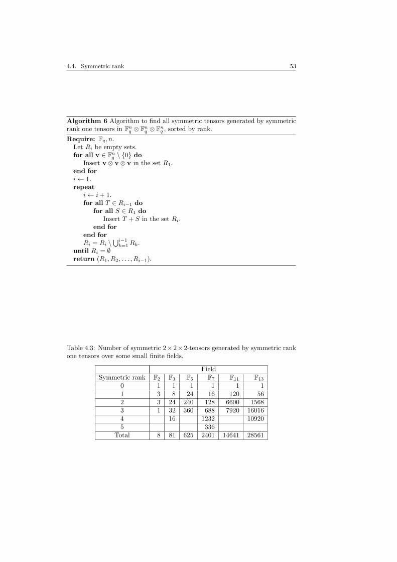
4.4. Symmetric rank 53

Algorithm 6 Algorithm to find all symmetric tensors generated by symmetricrank one tensors in Fnq ⊗ Fnq ⊗ Fnq , sorted by rank.

Require: Fq, n.Let Ri be empty sets.for all v ∈ Fnq \ {0} do

Insert v ⊗ v ⊗ v in the set R1.end fori← 1.repeat

i← i+ 1.for all T ∈ Ri−1 do

for all S ∈ R1 doInsert T + S in the set Ri.

end forend forRi = Ri \

⋃i−1k=1Rk.

until Ri = ∅return (R1, R2, . . . , Ri−1).

Table 4.3: Number of symmetric 2× 2× 2-tensors generated by symmetric rankone tensors over some small finite fields.

FieldSymmetric rank F2 F3 F5 F7 F11 F13

0 1 1 1 1 1 11 3 8 24 16 120 562 3 24 240 128 6600 15683 1 32 360 688 7920 160164 16 1232 109205 336

Total 8 81 625 2401 14641 28561


over F2 for N = 2, 3, 4 have been calculated using the same program, see table4.4.

One might find some things in table 4.3 quite strange. For example, whyare there fewer tensors with symmetric rank one over F7,F13 compared to F5

and F11 respectively? Over F2,F3,F5 and F11 there are the expected numberof symmetric tensors with symmetric rank one, namely p2 − 1, one tensor forevery non-zero vector in F2

p. This means that the tensors (αv)⊗ (αv)⊗ (αv) =α3v ⊗ v ⊗ v are different tensors for different α, but this is not the case in F7

and F13, where the mapping x 7→ x3 is not surjective. In the case of F7 theimage is {0, 1, 6} and in the case of F13 the image is {0, 1, 5, 8, 12}. However,for F2,F3,F5,F11, the mapping x 7→ x3 is bijective.

One can also note that there are tensors that have a symmetric rank higherthan the maximal rank (which is three). In the case of F7, we even have tensorswhich have a symmetric rank two steps higher than the maximal rank. Thus,conjecture 2.1.6 is false over at least some finite fields. For example, over F3 thetensor (

1 0 0 20 2 2 1

)=

(2 0 0 00 0 0 0

)+

(1 2 2 12 1 1 2

)+

(1 1 1 11 1 1 1

)+

(0 0 0 00 0 0 1

)has symmetric rank four, but rank three:(

1 0 0 20 2 2 1

)=

(1 1 0 01 1 0 0

)+

(0 2 0 20 1 0 1

)+

(0 0 0 02 0 2 0

)and over F7 the tensor(

2 5 5 05 0 0 4

)=

(6 1 1 61 6 6 1

)+

(1 2 2 42 4 4 1

)+

(1 2 2 42 4 4 1

)+

(1 0 0 00 0 0 0

)+

(0 0 0 00 0 0 1

)has symmetric rank five, but rank three:(

2 5 5 05 0 0 4

)=

(2 4 0 00 0 0 0

)+

(3 4 6 16 1 5 2

)+

(4 4 6 66 6 2 2

)and one can note that the symmetric rank would have been four if expressionson the form T =

∑Rr=1 λivi ⊗ vi ⊗ vi had been allowed.

One can see from table 4.4 that not all symmetric tensors over F2 have asymmetric rank. Taking a tensor to be symmetric if it is invariant under everypermutation τ ∈ S3, where τ acts as

τ(e1 ⊗ e2 ⊗ e3) = eτ(1) ⊗ eτ(2) ⊗ eτ(3)

and extending linearly, the tensor

T =

(0 1 1 01 0 0 0

)

4.4. Symmetric rank 55

Table 4.4: Number of N × N × N symmetric tensors generated by symmetricrank one tensors over F2.

NSymmetric rank 2 3 4

0 1 1 11 3 7 152 3 21 1053 1 35 4554 35 13655 21 30036 7 50057 1 6435

Total 8 128 16384

is symmetric since it is T = e1⊗ e1⊗ e2 + e1⊗ e2⊗ e1 + e2⊗ e1⊗ e1 but is notin the linear span of the symmetric rank one elements:(

1 0 0 00 0 0 0

),

(0 0 0 00 0 0 1

),

(1 1 1 11 1 1 1

).

Thus the tensor T is symmetric but does not have a symmetric rank.The next theorem summarizes the results so far in this section:

Theorem 4.4.1. Over F2 there are symmetric tensors which do not have a sym-metric rank. Over some other finite fields there are symmetric tensors whichhave a symmetric rank larger than the maximal rank, in particular their sym-metric rank is larger than their rank.

One also sees that the sequences of numbers for N = 2, 3 are binomialsequences, more precisely

(3k

)and

(7k

). For N = 4 we have the sequence(

150

),(

151

), . . . ,

(157

), i.e. half a binomial sequence. This can be explained with

the fact that there are 1 = 20 =(

2N−10

)zero vectors in FN2 , 2N − 1 =

(2N−1

1

)non-zero vectors in FN2 and each one of these corresponds to a symmetric rankone tensor. Picking two of these tensors and adding them results in a symmetricrank two tensor - the results show that these tensors are distinct, since the max-

imum number of symmetric rank two tensors,(

2N−12

), is achieved. Analogous

arguments hold for the higher ranks. In other words, symmetric tensors over F2

which have a symmetric rank have a unique symmetric decomposition with thenumber of terms equal to their rank for N = 2, 3, 4.

Chapter 5

Summary and future work

5.1 Summary

We have, in the first chapters, given the prerequisites for understanding resultsconcerning tensors of order strictly larger than two, and some of the resultsthemselves.

The method in section 3.1 used the Jacobian of a map in a generic point tocompute the lowest typical rank of tensors of arbitrary size. In section 3.2 wepresented a method that, for a few tensor sizes, gave results which show thatthere are more than one typical rank. This was done by calculating solutions toa system of polynomial equations; if there were not enough real solutions thenthe tensor had a rank which was higher than assumed.

The last numerical method, section 3.3, does not work as it is right now.The method is based on the idea that tensors of rank lower than the maximumtypical rank will leave holes in the tensor space, and if one can find these holesit would give an indication that there are more than one typical rank.

A nice property of finite fields is that they are finite, so in small cases it ispractically possible to do an exhaustive search. From these exhaustive searchesthe pattern of the eight orbits of the 2× 2× 2 tensors appeared. That these arethe orbits over any finite field was proved and their sizes were determined. Itwas also shown that one of the orbits over Fq has lower rank when the elementswere considered as tensors over Fq2 .

It was shown, by an exhaustive search, that there are symmetric tensorsover F2 which does not have a symmetric rank and some symmetric tensors oversome other finite fields have greater symmetric rank than rank, even that thesymmetric rank can be greater than the maximal rank, showing that conjecture2.1.6 does not hold true over some finite fields.

5.2 Future work

From the viewpoint of algebraic geometry, one would like to know the genericrank in Cn1⊗Cn2⊗Cn3 , for all n1, n2, n3 . One would also like to know the secantdefects. A lot of partial results have been published in this area. Furthermore,one would like to see in more detail what happens in the real case when one hasmore than one typical rank.


58 Chapter 5. Summary and future work

Since it is theoretically possible to compute the smallest typical rank forany size of tensor with the method in section 3.1, what is needed is a methodwhich enables one to discern if there is more than one typical rank. The methoddescibred in section 3.2 provides this for a few sizes of tensors, but a generalmethod is unknown. A possible way to discern good upper bounds of typicalranks is to examine whether it is possible or not for a tensor space to have atypical rank that is higher than the lowest typical rank of a tensor space oflarger format.

Over finite fields there is much more to be done, how are the ranks distributedover larger tensors than 2 × 2 × 2? For which tensors is the hyperdeterminantnon-zero? For 2×2×2 tensors, if the analogous orbits as over the reals have non-zero hyperdeterminant (O2,B and O3,2), there will be (q4 − 1)(q4 − q3) tensorswith non-zero hyperdeterminant, which can be compared to (q2 − 1)(q2 − q),the number of 2× 2 matrices with non-zero determinant.

Appendix A

Programs

In this appendix we present the programs used to execute the algorithms pre-sented in the main text. All programs are written for Mathematica, except thesurjectivity check program, which is written for MATLAB.

A.1 Numerical methods

A.1.1 Comon, Ten Berge, Lathauwer and Castaing’s method

Third order tensors

The program below can be used to calculate the lowest typical rank of formatn1 × n2 × n3 by calling ComputeLowestTypicalRank[n1, n2, n3].

lowbound = −1;highbound = 1 ;CreateJacobianBlock [ dim1 , dim2 , dim3 ] :=

Block [{ x1 = RandomReal [{ lowbound , highbound } , dim1 ] ,x2 = RandomReal [{ lowbound , highbound } , dim2 ] ,x3 = RandomReal [{ lowbound , highbound } , dim3 ]} ,

Jo in [KroneckerProduct [ Ident i tyMatr ix [ dim1 ] , x2 , x3 ] ,KroneckerProduct [{ x1 } , Ident i tyMatr ix [ dim2 ] , x3 ] ,KroneckerProduct [{ x1 } , x2 , Ident i tyMatr ix [ dim3 ] ]]

]

ComputeLowestTypicalRank [ dim1 , dim2 , dim3 ] :=Block [{ j a cob ian = CreateJacobianBlock [ dim1 , dim2 , dim3 ] , R = 0 ,

D = 0} ,While [D < MatrixRank [ j acob ian ] ,R++;D = MatrixRank [ j acob ian ] ;

j a cob ian = Join [ jacobian , CreateJacobianBlock [ dim1 , dim2 , dim3 ] ]] ;

R]


60 Appendix A. Programs

Higher order tensors

This program can be used to compute the lowest typical rank of format n1 ×n2 × · · · × nk by calling ComputeLowestTypicalRank[{n1, n2, ..., nk}].

lowbound = −1;highbound = 1 ;CreateJacobianBlock [ d i m l i s t ] :=

Block [{ x =Table [ RandomReal [{ lowbound , highbound } , d i m l i s t [ [ i ] ] ] ,

{ i , 1 , Length [ d i m l i s t ] } ]} ,

F la t ten [Table [

Apply [ KroneckerProduct ,Join [

Table [{ x [ [ i ] ] } , { i , 1 , j − 1} ] ,{ Ident i tyMatr ix [ d i m l i s t [ [ j ] ] ] } ,Table [ x [ [ i ] ] , { i , j + 1 , Length [ d i m l i s t ] } ]]

] ,{ j , 1 , Length [ d i m l i s t ] } ] ,

1 ]]

ComputeLowestTypicalRank [ d i m l i s t ] :=Block [{ j a cob ian = CreateJacobianBlock [ d i m l i s t ] , R = 0 , D = 0} ,

While [D < MatrixRank [ j acob ian ] ,R++;D = MatrixRank [ j acob ian ] ;

j a cob ian = Join [ jacobian , CreateJacobianBlock [ d i m l i s t ] ]] ;

R]

A.1.2 Choulakian’s method

The program belows runs Choulakians method for k random n1 × n2 × n3 bycalling TestTesorZeros[n1, n2, n3, k]. If k is not specified, it is taken to be1000.

RandomTensor [ n1 , n2 , n3 ] :=RandomInteger [{−100 , 100} , {n1 , n2 , n3 } ]

TestTensorZeros [ n1 , n2 , n3 , t r i e s : 1000 ] :=With [{ s l i s t =

Append [ Table [ Symbol [ ” s ” <> ToString [ i ] ] , { i , 1 , n3 − 1} ] , 1 ] ,c l i s t =Prepend [ Table [ Symbol [ ” c” <> ToString [ i ] ] , { i , 2 , n1 } ] , 1 ]} ,

Sort [ Tal ly [P a r a l l e l T a b l e [X = RandomTensor [ n1 , n2 , n3 ] ;

A.1. Numerical methods 61

Xpolys =Apply [ Union ,

Table [ (X [ [ i ] ] − c l i s t [ [ i ] ] X [ [ 1 ] ] ) . s l i s t , { i , 2 , n1 } ] ] ;Xgrob =

GroebnerBasis [ Xpolys ,Join [ s l i s t [ [ 1 ; ; −2] ] , Reverse [ c l i s t [ [ 2 ; ; − 1 ] ] ] ]] ;

Length [ So lve [ Xgrob [ [ 1 ] ] == 0 , c2 , Reals ] ] ,{ i , 1 , t r i e s }]

] ]]

A.1.3 Surjectivity check

The calculatins of the surjectivity check was mostly done with a sript for Matlaband it works with tensor spaces size of sizes 2× 2× 2, 2× 2× 3, 2× 3× 3 and3 × 3 × 4. The script generates data for closest distances to the control pointsto the test points and calculate how many there are in certain distances. Thedistances are derived from the amount of area around the control point (seetable 3.12). This is summarized in the matrices summaryIJK, where I × J ×Kis the format of the tensor space.

For the 2 × 2 × 2 tensor space the hyperdeterminant is calculated by thematlab function hyperdeterminant that takes vectorized 2 × 2 × 2 tensors asinput and for the 2×3×3 tensor space the rank is calculated by a method usedin [36].

To calculate the area given a distance we used the matlab function quotaCap.

Support functions

f unc t i on [ quotaA ] = quotaCap ( dim , r , d i s t )quotaA = 1/2∗ beta inc ( ( d i s t . ˆ 2 / ( r ˆ2)− d i s t . ˆ4/(4∗ r ˆ 4 ) ) , . . .

(dim−1) ./2 ,1/2) ;end

func t i on [ va lue ] = hyperdeterminant (T)value = ( (T( 1 , : ) . ∗T( 8 , : ) ) . ˆ 2 + (T( 5 , : ) . ∗T( 4 , : ) ) . ˆ 2 + . . .

(T( 3 , : ) . ∗T( 6 , : ) ) . ˆ 2 + (T( 7 , : ) . ∗T( 2 , : ) ) . ˆ 2 ) − . . .2∗(T( 1 , : ) . ∗T( 4 , : ) . ∗T( 5 , : ) . ∗T( 8 , : ) + . . .

T( 1 , : ) . ∗T( 3 , : ) . ∗T( 6 , : ) . ∗T( 8 , : ) + . . .T( 1 , : ) . ∗T( 2 , : ) . ∗T( 7 , : ) . ∗T( 8 , : ) + . . .T( 3 , : ) . ∗T( 5 , : ) . ∗T( 6 , : ) . ∗T( 4 , : ) + . . .T( 2 , : ) . ∗T( 4 , : ) . ∗T( 5 , : ) . ∗T( 7 , : ) + . . .T( 2 , : ) . ∗T( 3 , : ) . ∗T( 6 , : ) . ∗T(7 , : ) )+ . . .

4∗(T( 1 , : ) . ∗T( 4 , : ) . ∗T( 6 , : ) . ∗T( 7 , : ) + . . .T( 2 , : ) . ∗T( 3 , : ) . ∗T( 5 , : ) . ∗T( 8 , : ) ) ;

end

Main script


t0 = c lo ck ;nrControl = 2000 ;nrTestPoint = 2000 ;d i sp ( ’ S ta r t 2x2x2 ! ’ )dArea222 = [ 0 . 6 3 5 5 0 .5 0 .4511 0 .3565 0 .3225 0 . 2 5 5 5 ] ;s i z eArea = length ( dArea222 ) ;NrCloseToControl222 = ze ro s ( s izeArea , nrContro l ) ;s ho r t e s tD i s t 22 2 = ones (1 , nrControl )∗100 ;Control222 = randn (2∗2∗2 , nrControl ) ;Control222 = Control222 . / ( ones ( 2 ∗ 2 ∗ 2 , 1 ) ∗ . . .

s q r t (sum( Control222 .∗ Control222 ) ) ) ;hypeControl = hyperdeterminant ( Control222 ) ;avgDist222 = ze ro s (1 , nrContro l ) ;r =2;f o r i =1: nrTestPoint

t e s tPo in t = makeTensor ( 2 , 2 , 2 , 2 ) ;t e s tPo in t ( : ) = te s tP o in t ( : ) / norm( t e s tPo in t ( : ) ) ;d i s t = s q r t (sum ( ( Control222−t e s tPo in t ( : ) ∗ . . .

ones (1 , nrContro l ) ) . ∗ ( Control222−t e s tPo in t ( : ) ∗ . . .ones (1 , nrContro l ) ) , 1 ) ) ;

f o r d=1: s i z eAreaNrCloseToControl222 (d , : ) = NrCloseToControl222 (d , : ) + . . .

( d i s t < dArea222 (d ) ) ;ends ho r t e s tD i s t 22 2 ( d i s t < s ho r t e s tD i s t 22 2 ) = . . .

d i s t ( d i s t < s ho r t e s tD i s t 22 2 ) ;avgDist222 = avgDist222+d i s t / nrContro l ;

endsummary222 = [ NrCloseToControl222 ; . . .

round (1000∗ hypeControl ) ; . . .round (1000∗ s ho r t e s tD i s t 22 2 ) ] ;

d i sp ( ’ Done ! 2x2x2 ’ )d i sp ( etime ( c lock , t0 ) )

%%

disp ( ’ S ta r t 2x2x3 ! ’ )dArea223 = [ 0 . 6 3 1 0 .54 0 .5051 0 .4337 0 .4065 0 . 3 4 9 8 ] ;s i z eArea = length ( dArea223 ) ;NrCloseToControl223 = ze ro s ( s izeArea , nrContro l ) ;s ho r t e s tD i s t 22 3 = ones (1 , nrControl )∗100 ;Control223 = randn (2∗2∗3 , nrControl ) ;Control223 = Control223 . / ( ones ( 2 ∗ 2 ∗ 3 , 1 ) ∗ . . .

s q r t (sum( Control223 .∗ Control223 ) ) ) ;avgDist223 = ze ro s (1 , nrContro l ) ;

f o r i =1: nrTestPointt e s tPo in t = makeTensor ( 2 , 2 , 3 , 3 ) ;t e s tPo in t ( : ) = te s tP o in t ( : ) / norm( t e s tPo in t ( : ) ) ;d i s t = s q r t (sum ( ( Control223−t e s tPo in t ( : ) ∗ ones (1 , nrContro l ) ) . ∗ . . .

A.1. Numerical methods 63

( Control223−t e s tPo in t ( : ) ∗ ones (1 , nrContro l ) ) , 1 ) ) ;f o r d=1: s i z eArea

NrCloseToControl223 (d , : ) = NrCloseToControl223 (d , : ) + . . .( d i s t < dArea223 (d ) ) ;

ends ho r t e s tD i s t 22 3 ( d i s t < s ho r t e s tD i s t 22 3 ) = . . .



round (1000∗ s ho r t e s tD i s t 22 3 ) ] ;d i sp ( ’ Done ! 2x2x3 ’ )

%%

disp ( ’ S ta r t 2x3x3 ! ’ )dArea233 = [ 0 . 7 8 3 5 0 .7035 0 .672 0 .606 0 .5796 0 . 5 2 3 9 ] ;s i z eArea = length ( dArea233 ) ;NrCloseToControl233 = ze ro s ( s izeArea , nrContro l ) ;s ho r t e s tD i s t 23 3 = ones (1 , nrControl )∗100 ;Control233 = randn (2∗3∗3 , nrControl ) ;Control233 = Control233 . / ( ones ( 2 ∗ 3 ∗ 3 , 1 ) ∗ . . .

s q r t (sum( Control233 .∗ Control233 ) ) ) ;avgDist233 = ze ro s (1 , nrContro l ) ;f o r i =1: nrTestPoint

t e s tPo in t = makeTensor ( 2 , 3 , 3 , 3 ) ;t e s tPo in t ( : ) = te s t Po in t ( : ) / norm( t e s tPo in t ( : ) ) ;d i s t = s q r t (sum ( ( Control233−t e s tPo in t ( : ) ∗ ones (1 , nrContro l ) ) . ∗ . . .





endr = rank332e ig ( Control233 ) ;summary233 = [ NrCloseToControl233 ; . . .

round (1000∗ s ho r t e s tD i s t 23 3 ) ; r ] ;d i sp ( ’ Done ! 2x3x3 ’ )

%%

disp ( ’ S ta r t 3x3x4 ! ’ )t1 = c lo ck ;dArea334 = [ 1 0 .981 0 .9225 0 .8991 0 .8486 0 .8282 0 .7837 ] ;s i z eArea = length ( dArea334 ) ;Control334 = randn (4∗3∗3 , nrControl ) ;Control334 = Control334 . / ( ones ( 4 ∗ 3 ∗ 3 , 1 ) ∗ . . .


s q r t (sum( Control334 .∗ Control334 ) ) ) ;NrCloseToControl334 = ze ro s ( s izeArea , nrContro l ) ;s ho r t e s tD i s t 33 4 = ones (1 , nrControl )∗100 ;avgDist334 = ze ro s (1 , nrContro l ) ;f o r i =1: nrTestPoint

t e s tPo in t = makeTensor ( 3 , 3 , 4 , 5 ) ;t e s tPo in t ( : ) = te s t Po in t ( : ) / norm( t e s tPo in t ( : ) ) ;d i s t = s q r t (sum ( ( Control334−t e s tPo in t ( : ) ∗ ones (1 , nrContro l ) ) . ∗ . . .






round (1000∗ s ho r t e s tD i s t 33 4 ) ] ;d i sp ( ’ Done 3x3x4 ! ’ )d i sp ( etime ( c lock , t1 ) )

A.2 Tensors over finite fields

A.2.1 Rank partitioning

Tensor rank

The following program gives an output {R0, R1, . . . , Rk} which is an parition ofthe n1×n2×n3 tensors up to rank k over Fp, for a prime number p, where Ri con-tains all the tensors of rank i, given the input GenerateTensorHierarchy[n1, n2, n3, p, k].If k is not specified, the program runs until all the tensors have been generated.If p is not specified, it is taken to be 2.

GenerateRankOneTensors [ dim1 , dim2 , dim3 , mod : 2 ] :=L i s t [ Union [ F lat ten [ Table [

F lat ten [ TensorProduct [ I n t e g e r D i g i t s [ i , mod , dim1 ] ,I n t e g e r D i g i t s [ j , mod , dim2 ] ,I n t e g e r D i g i t s [ k , mod , dim3 ] ,mod ] ] ,

{ i , 1 , modˆdim1 − 1} ,{ j , 1 , modˆdim2 − 1} ,{k , 1 , modˆdim3 − 1} ] ,

2 ] ] ]

GenerateRankTwoTensors [ r a n k o n e l i s t , mod : 2 ] :=Append [ r ankone l i s t ,

Complement [Union [ F lat ten [

P a r a l l e l T a b l e [Mod[ r a n k o n e l i s t [ [ 1 , i ] ] + r a n k o n e l i s t [ [ 1 , j ] ] , mod ] , { i , 1 ,

A.2. Tensors over finite fields 65

Length [ r a n k o n e l i s t [ [ 1 ] ] ] } , { j , i , Length [ r a n k o n e l i s t [ [ 1 ] ] ] } ] ,1 ] ] ,

r a n k o n e l i s t [ [ 1 ] ] ,{Table [ 0 , { i , 1 , Length [ r a n k o n e l i s t [ [ 1 , 1 ] ] ] } ] }

]]

GenerateNextRank [ t e n s o r l i s t , mod : 2 ] :=I f [ Length [ t e n s o r l i s t ] == 1 , GenerateRankTwoTensors [ t e n s o r l i s t , mod ] ,Append [ t e n s o r l i s t ,


P a r a l l e l T a b l e [Mod[ t e n s o r l i s t [ [−1 , i ] ] + t e n s o r l i s t [ [ 1 , j ] ] , mod ] , { i , 1 ,

Length [ t e n s o r l i s t [ [ − 1 ] ] ] } , { j , 1 , Length [ t e n s o r l i s t [ [ 1 ] ] ] } ] ,1 ] ] ,

F la t ten [ t e n s o r l i s t , 1 ] ,{Table [ 0 , { i , 1 , Length [ t e n s o r l i s t [ [ 1 , 1 ] ] ] } ] } ]

]]

GenerateTensorHierarchy [ dim1 , dim2 , dim3 , mod : 2 , maxrank : I n f i n i t y ] :=Module [{ t e n s o r l i s t =

GenerateRankTwoTensors [GenerateRankOneTensors [ dim1 , dim2 , dim3 , mod ] , mod ] , r = 1} ,

While[++r < maxrank &&Count [ t e n s o r l i s t , L i s t , {2} ] < modˆ( dim1 dim2 dim3 ) − 1 ,

t e n s o r l i s t = GenerateNextRank [ t e n s o r l i s t , mod ] ] ;t e n s o r l i s t]

Symmetric rank

The next program is the symmetric version of the program above. Note thatit will only compute the symmetric tensors which lie in the linear span of thesymmetric rank one-tensors.

GenerateSymRankOneTensors [ dim , mod : 2 ] :=L i s t [ Union [ Table [

F lat ten [ TensorProduct [I n t e g e r D i g i t s [ i , mod , dim ] ,I n t e g e r D i g i t s [ i , mod , dim ] ,I n t e g e r D i g i t s [ i , mod , dim ] ,mod ] ] ,

{ i , 1 , modˆdim − 1 } ] ] ]

GenerateSymRankTwoTensors [ r a n k o n e l i s t , mod : 2 ] :=Append [ r ankone l i s t ,



P a r a l l e l T a b l e [Mod[ r a n k o n e l i s t [ [ 1 , i ] ] + r a n k o n e l i s t [ [ 1 , j ] ] , mod ] , { i , 1 ,

Length [ r a n k o n e l i s t [ [ 1 ] ] ] } , { j , i , Length [ r a n k o n e l i s t [ [ 1 ] ] ] } ] ,1 ] ] ,

r a n k o n e l i s t [ [ 1 ] ] ,{Table [ 0 , { i , 1 , Length [ r a n k o n e l i s t [ [ 1 , 1 ] ] ] } ] }

]]

GenerateNextSymRank [ t e n s o r l i s t , mod : 2 ] :=I f [ Length [ t e n s o r l i s t ] == 1 ,GenerateRankTwoTensors [ t e n s o r l i s t , mod ] ,Append [ t e n s o r l i s t ,


P a r a l l e l T a b l e [Mod[ t e n s o r l i s t [ [−1 , i ] ] + t e n s o r l i s t [ [ 1 , j ] ] , mod ] , { i , 1 ,

Length [ t e n s o r l i s t [ [ − 1 ] ] ] } , { j , 1 , Length [ t e n s o r l i s t [ [ 1 ] ] ] } ] ,1 ] ] ,

F la t ten [ t e n s o r l i s t ,1 ] , {Table [ 0 , { i , 1 , Length [ t e n s o r l i s t [ [ 1 , 1 ] ] ] } ] } ]

]]

GenerateSymTensorHierarchy [ dim , mod : 2 , maxrank : I n f i n i t y ] :=Module [{ t e n s o r l i s t =

GenerateSymRankTwoTensors [ GenerateSymRankOneTensors [ dim , mod ] ,mod ] , r = 1} ,

While[++r < maxrank && t e n s o r l i s t [ [ − 1 ] ] != {} ,t e n s o r l i s t = GenerateNextSymRank [ t e n s o r l i s t , mod ] ] ;

t e n s o r l i s t [ [ 1 ; ; −2]]]

A.2.2 Orbit paritioning

Given a rank partition {R0, R1, . . . , Rk} of 2× 2× 2 tensors from the programabove, the next program generates the orbits under GLp(2)×GLp(2)×GLp(2),given the input AllOrbits[{R0, R1, ..., Rk}, G, p], where G is the group forwhich one wants the orbits.

ApplyMatrixElement [ mtuple , t enso r , l 1 , l 2 , l 3 ] :=Sum[ tenso r [ [ j1 , j2 , j 3 ] ] mtuple [ [ 1 , j1 , l 1 ] ] mtuple [ [ 2 , j2 ,

l 2 ] ] mtuple [ [ 3 , j3 , l 3 ] ] , { j1 , 1 , 2} , { j2 , 1 , 2} , { j3 , 1 , 2} ]

ApplyMatrix [ mtuple , t enso r , mod : 2 ] :=Mod[ Table [

ApplyMatrixElement [ mtuple , tensor , l1 , l2 , l 3 ] , { l1 , 1 , 2} ,{ l2 , 1 , 2} , { l3 , 1 , 2} ] , mod ]

GetOrbit [ t ensor , matr i ce s , mod : 2 ] :=

A.2. Tensors over finite fields 67

Union [Map[ ApplyMatrix [# , tensor , mod ] &, matr i ce s ] ]

A l lOrb i t s [ t en so rh i e r a r chy , matr i ce s , mod : 2 ] :=Module [{ temphierarchy = tenso rh i e ra r chy , o r b i t s = {}} ,

For [ i = 1 , i <= Length [ t e n s o r h i e r a r c h y ] , i ++,o r b i t s = Append [ o rb i t s , { } ] ;While [ temphierarchy [ [ i ] ] != {} ,

o r b i t s [ [ − 1 ] ] =Append [ o r b i t s [ [ − 1 ] ] ,

GetOrbit [ temphierarchy [ [ i , 1 ] ] , matr ices , mod ] ] ;temphierarchy [ [ i ] ] =Complement [ temphierarchy [ [ i ] ] , o r b i t s [ [−1 , −1 ] ] ]

]] ;

o r b i t s]

The next program is a simple program for generating GLp(n).

GenerateGL [ n , p : 2 ] :=DeleteCases [Union [ Tuples [ Table [ I n t e g e r D i g i t s [ i , p , n ] , { i , 1 , pˆn − 1} ] ,

2 ] ] , ?(Mod[ Det [#] , p ] == 0 &) , {1} ]

One can write Tuples[GenerateGL[n, p], 3] to get GLp(n)×GLp(n)×GLp(n).

Bibliography

[1] Evrim Acar, Bulent Yener (2009), Unsupervised multiway data analysis: aliterature survey, IEEE Transactions on Knowledge and Data Engineering,vol. 21, no. 1 pp. 6-20.

[2] C.J. Appellof, E.R. Davidson, (1981), Strategies for analyzing data fromvideo fluorometric monitoring of liquid chromatographic effluents, Analyt-ical Chemistry 53, pp. 2053-2056.

[3] E. Ballico, A. Bernardi (2011), Tensor ranks on tangent developable of Segrevarieties, inria-00610362, version 2.

[4] Goran Bergqvist (to appear), Exact probabilities for typical ranks of 2×2×2and 3× 3× 2 tensors, Linear Algebra and its Applications.

[5] Goran Bergqvist, P. J. Forrester (2011) Rank probabilities for real randomN ×N × 2 tensors, Electronic Communications in Probability 16, pp. 630-637.

[6] Jack Bochniak, Michel Coste, Marie-Francoise Roy (1998), Real AlgebraicGeometry, Springer Verlag, A Series of Modern Surveys in Mathematics,ISBN 3-540-64663-9.

[7] Maria Chiara Brambilla, Giorgio Ottaviani (2008), On the Alexan-der–Hirschowitz theorem, Journal of Pure and Applied Algebra 212(5), pp.1229–1251.

[8] Bruno Buchberger (2001), Groebner Bases: A Short Introduction for Sys-tem Theorists, Springer Verlag, Proceedings of EUROCAST 2001, LectureNotes in Computer Science 2178, pp. 1-19.

[9] Peter Burgisser, Michael Clausen, M. Amin Shokrollah (1997), AlgebraicComplexity Theory, Springer Verlag, Grundlehren der matematischen Wis-senschaften 315, ISBN 3-540-60582-7.

[10] Pierre Comon, Gene Golub, Lek-Heng. Lim, Bernard Mourrain (2008),Symmetric tensors and symmetric tensor rank, SIAM Journal on MatrixAnalysis and Applications 30(3), pp 1254-1279.

[11] P. Comon, J.M.F. ten Berge, L. De Lathauwer, J. Castaing (2009), Genericand typical ranks of multi-way arrays, Linear Algebra and its Applications430, pp. 2997-3007.


70 Bibliography

[12] Vartan Choulakian (2010), Some numerical results on the rank of genericthree-way arrays over R, SIAM Journal of Matrix Analysis and its Appli-cations 31(4), pp. 1541-1551.

[13] David A. Cox, John Little, Donal O’Shea (2005), Using Algebraic Geom-etry, Springer Verlag, Graduate Texts in Mathematics 185, ISBN 0-387-20733-3.

[14] Vin de Silva, Lek-Heng Lim (2008), Tensor rank and the ill-posedness ofthe best low-rank approximation problem, SIAM Journal of Matrix Analysisand its Applications 30, pp. 1084-1127.

[15] Shmuel Friedland (2011), On the generic and typical ranks of 3-tensors,arXiv:0805.3777v5[math.AG].

[16] I.M Gelfand, M.M. Kapranov, A.V. Zelevinsky Hyperdeterminants, Ad-vances in mathematics 96, pp. 226-263.

[17] Joe Harris (1992), Algebraic Geometry: A First Course, Springer Verlag,Graduate Texts in Mathematics 133, ISBN 0-387-97716-3.

[18] Johan Hastad (1990), Tensor rank is NP-complete, Journal of Algorithms11, pp. 644-654.

[19] F.L. Hitchcock (1927) The expression of a tensor of a polyadic as a sum ofproducts Journal of Mathematical Physics 6, pp. 164-189.

[20] F.L. Hithcock (1927) Multiple invariants and generalized rank of a p-waymatrix or tensor, Journal of Mathematical Physics 7, pp. 39-79.

[21] Donald Knuth (1998), The Art of Computer Programming, Volume 2:Seminumerical Algorithms, Third Edition, Addison-Wesley, ISBN 978-2-201-89684-8.

[22] Joseph B. Kruskal (1977), Three-way arrays: rank and uniqueness of trilin-ear decompositions, with application to arithmetic complexity and statistics,Linear Algebra and its Applications 18(2), pp. 95-138.

[23] J. B. Kruskal (1989), Rank, decomposition and uniqueness for 3-way arraysand N -way arrays, Multiway Data Analysis, Elseiver, pp. 7-18.

[24] Tamara G. Kolda, Brett W. Bader (2009), Tensor Decompositions andApplications, SIAM Review vol. 51(3), pp. 455-500.

[25] J.M. Landsberg (2012), Tensors: Geometry and Applications, AmericanMathematical Society, Graduate Studies in Mathematics 128, ISBN 978-0-8218-6907.

[26] J.M. Landsberg (2006), The border rank of the multiplication of 2× 2 ma-trices is seven, Journal of the American Mathematical Society 19(2), pp.447-512.

[27] Sharon J. Laskowski (1982), Computing lower bounds on tensor rank overfinite fields, Journal of Computer and System Sciences 24(1), pp. 1-14.

Bibliography 71

[28] S. Li (2011), Concise forumlas for the area and volume of a hyperspericalcap, Asian Journal of Mathematics Statistics 4, pp. 66-70.

[29] Thomas Lickteig (1985), Typical Tensor Rank, Linear Algebra and its Ap-plications 69, pp. 95-120.

[30] Rudolf Lidl, Harald Niederreiter (1997), Finite fields, Cambridge UniversityPress, Encyclopedia of Mathematics and its Applications 20, ISBN 0-521-39231-4.

[31] David Mumford (1976), Algebraic Geometry I: Complex Projective Vari-eties, Springer Verlag, Grundlehren der mathematischen Wissenchaften221, ISBN 0-387-07603-4.

[32] Erich Novak, Klaus Ritter (1997) The curse of dimension and a universalmethod for numerical integration Multivariate Approximation and Splines,eds. G. Nurnberger, J.W. Schmidt and G. Walz, pp 177-188

[33] Luke Oeding (2008), Report on Geometry and representation the-ory of tensor for computer science, statistics and other areas,arXiv:0810.3940[math.AG].

[34] Ron M. Roth (1996), Tensor Codes for the Rank Metric, IEEE Transactionson Information Theory 42(6), pp. 2146-2157.

[35] Nicholas D. Sidiropoulos, Rasmus Bro (2000), On the uniqueness of multi-linear decomposition of n-way arrays, J. Chemometrics 14(3), pp. 229-239.

[36] Alwin Stegeman (2006), Degeneracy in CANDECOMP/PARAFAC ex-plained for p× p× 2 arrays of rank p+ 1 or higher, Psychometrika 71(3),pp. 483-501.

[37] Volker Strassen (1969), Gaussian Elimination is not optimal, NumerischeMathematik 13(4), pp. 354-356.

[38] Jos M.F. ten Berge (2000), The typical rank of tall three-way arrays, Psy-chometrika 65(4), pp. 525-532.

[39] Jos M.F. ten Berge (2004), Partial uniqueness in Candecomp/Parafac,Journal of Chemometrics 18, pp. 12-16.

[40] Jos M.F. ten Berge, Alwin Stegeman (2006), Symmetry transformationsfor square sliced three-way arrays, with applications to their typical rank,Linear Algebra and its Applications 418, pp. 215-224.

[41] L. R. Tucker (1963), Implications of factor analysis of three-way matricesfor measurement of change, in Problems of Measuring Change, C.W. Harris(ed.), University of Wisconsin Press, pp. 122-137.

[42] Sergei Wintzki (2010), Linear Algebra via Exterior Products, available ase-book from http://sites.google.com/site/winitzki/linalg.

72 Bibliography

Copyright

The publishers will keep this document online on the Internet - or its possi-ble replacement - for a period of 25 years from the date of publication barringexceptional circumstances. The online availability of the document implies apermanent permission for anyone to read, to download, to print out single copiesfor your own use and to use it unchanged for any non-commercial research andeducational purpose. Subsequent transfers of copyright cannot revoke this per-mission. All other uses of the document are conditional on the consent of thecopyright owner. The publisher has taken technical and administrative mea-sures to assure authenticity, security and accessibility. According to intellectualproperty law the author has the right to be mentioned when his/her work isaccessed as described above and to be protected against infringement. For ad-ditional information about the Linkoping University Electronic Press and itsprocedures for publication and for assurance of document integrity, please referto its WWW home page: http://www.ep.liu.se/

Upphovsratt

Detta dokument halls tillgangligt pa Internet - eller dess framtida ersattare -under 25 ar fran publiceringsdatum under forutsattning att inga extraordinaraomstandigheter uppstar. Tillgang till dokumentet innebar tillstand for var ochen att lasa, ladda ner, skriva ut enstaka kopior for enskilt bruk och att anvandadet oforandrat for ickekommersiell forskning och for undervisning. Overforingav upphovsratten vid en senare tidpunkt kan inte upphava detta tillstand. Allannan anvandning av dokumentet kraver upphovsmannens medgivande. Foratt garantera aktheten, sakerheten och tillgangligheten finns det losningar avteknisk och administrativ art. Upphovsmannens ideella ratt innefattar rattatt bli namnd som upphovsman i den omfattning som god sed kraver vidanvandning av dokumentet pa ovan beskrivna satt samt skydd mot att doku-mentet andras eller presenteras i sadan form eller i sadant sammanhang som arkrankande for upphovsmannens litterara eller konstnarliga anseende eller ege-nart. For ytterligare information om Linkoping University Electronic Press seforlagets hemsida http://www.ep.liu.se/

c© 2012, Elias Erdtman, Carl Jonsson


tensor rank - diva portalliu.diva-portal.org/smash/get/diva2:551672/fulltext01.pdf · multilinear...

Documents