
A DIRECT THRUST MEASUREMENT SYSTEM FOR A WATERJET-
PROPELLED, FREE RUNNING USV
by
John A. Grimes
A Thesis Submitted to the Faculty of
the College of Engineering and Computer Science
in Partial Fulfillment of the Requirements for the Degree of
Master of Science
Florida Atlantic University
Boca Raton, Florida
December 2013


iii
ABSTRACT
Author: John Grimes
Title: A Direct Thrust Measurement System for a Waterjet Propelled, Free Running USV
Institution: Florida Atlantic University
Thesis Advisor: Dr. Karl von Ellenrieder
Degree: Master of Science
Year: 2013
The relationship between cross-flow at a waterjet inlet and delivered thrust is not
fully understood. A direct thrust measurement system was designed for a waterjet
propelled, free running USV. To induce sway velocity at the waterjet inlet, which was
considered equivalent to the cross flow, circles of varying radii were performed at
Reynolds Numbers between 3.48 x 10⁶ and 8.7 x 10⁶ and radii from 2.7 to 6.3 boat
lengths. Sway velocities were less than twenty percent of mean forward speed with slip
angles that were less than 20°. Thrust Loading Coefficients were compared to sway as
a percent of forward speed. In small radius turns, no relationship was seen, while in
larger radius turns, peaks of sway velocity corresponded with drops in thrust, but this
was determined to be caused by reduced vehicle yaw in these intervals . Decoupling of
thrust and yaw rate is recommended for future research.

iv
A DIRECT THRUST MEASUREMENT SYSTEM FOR A WATERJET-
PROPELLED, FREE RUNNING USV
LIST OF FIGURES ..................................................................................................................... vii
LIST OF TABLES ....................................................................................................................... ix
NOMENCLATURE ...................................................................................................................... x
1 INTRODUCTION ................................................................................................................. 1
1.1 Problem Statement ........................................................................................................ 1
1.2 Background ................................................................................................................... 1
1.2.1 Momentum Flux Method ....................................................................................... 3
1.2.2 Direct Thrust Method ............................................................................................ 3
1.2.3 Cross Flow ............................................................................................................. 4
2 APPROACH .......................................................................................................................... 8
2.1 Platform Identification .................................................................................................. 8
2.2 Design of propulsion system ......................................................................................... 9
2.2.1 Waterjet ............................................................................................................... 10
2.2.2 Motor Controller.................................................................................................. 10
2.2.3 Motors ................................................................................................................. 11
2.2.4 Battery ................................................................................................................. 11
2.2.5 Electrical Design ................................................................................................. 12

v
2.2.5.1 Kill Circuit ........................................................................................................... 13
2.2.6 Structural Design ................................................................................................. 15
2.2.7 Cooling System ................................................................................................... 18
2.3 Control System and Data Collection ........................................................................... 20
2.3.1 Force Transducer Data Collection ........................................................................... 21
2.4 Force transducer calibration ........................................................................................ 22
2.5 Experimental Approach ............................................................................................... 23
3 PROPULSION SYSTEM TESTING .................................................................................. 26
3.1 Motor Pod Testing ....................................................................................................... 26
3.1.1 Hull Seal Testing ................................................................................................. 26
3.1.2 Magnetic Coupling Test ...................................................................................... 26
3.1.3 Run Time Estimation Test ................................................................................... 27
4 EXPERIMENTAL TESTING ............................................................................................. 28
4.1 Experimental Testing .................................................................................................. 28
4.1.1 Testing - June 14, 2013 ....................................................................................... 28
4.1.2 Testing: June 26, 2013 ........................................................................................ 29
4.1.3 Testing: September 19, 2013 .............................................................................. 30
4.1.4 Testing: September 27, 2013 ............................................................................... 31
5 DATA PROCESSING ........................................................................................................ 33
6 RESULTS ............................................................................................................................ 41
7 CONCLUSIONS ................................................................................................................. 48

vi
APPENDIX A - DATA SORTING CODE ................................................................................. 51
A.1 Test Sorter Function .................................................................................................... 51
A.2 Data Splitting Code ..................................................................................................... 52
A.3 Force Transducer Data Splitter .................................................................................... 53
A.4 Data Splitting Code for Straight Line Tests ................................................................ 56
A.5 Force Transducer Data Splitting Code for Strait Line Tests ....................................... 57
APPENDIX B - DATA PROCESSING CODE .......................................................................... 61
APPENDIX C - MOTOR CONTROLLER CODE .................................................................... 72
APPENDIX D - FIGURES ......................................................................................................... 73
APPENDIX E - DESCRIPTION OF MOMENTUM FLUX METHOD .................................. 113
APPENDIX F - WIRING DIAGRAMS ................................................................................... 116
APPENDIX G - CENTER OF GRAVITY CALCULATIONS AND VERIFICATION ......... 118
REFERENCES .......................................................................................................................... 122

vii
LIST OF FIGURES
Figure 1-1: Usage of Reversing Bucket and Nozzle[3] .................................................................... 2
Figure 1-2: Representation of the Intake of a Flush Inlet Waterjet [6] ............................................ 5
Figure 1-3: USV-12 Wave Adaptive Modular Vehicle [7] .............................................................. 6
Figure 1-4: Experimental Setup from 2010 Tests [7]. ...................................................................... 7
Figure 2-1: Planing Hull Platform Considered ................................................................................. 8
Figure 2-2: Roboteq Motor Controller ........................................................................................... 10
Figure 2-3: Motor Pod Block Diagram .......................................................................................... 13
Figure 2-4: Pod Cross Section ........................................................................................................ 15
Figure 2-5: General Arrangements and Side view of Motor Pod ................................................... 16
Figure 2-6: Detail View of Interface and Force Transducer Cable ................................................ 17
Figure 2-7: Cooling System Components ...................................................................................... 18
Figure 2-8: Control and Data Collection Block Diagram .............................................................. 20
Figure 2-9: Force Transducer Calibration Data – FZ Channel ....................................................... 23
Figure 2-10: North Hollywood Finger Lake ................................................................................. 24
Figure 3-1: Battery Discharge Curve at 75% Throttle ................................................................... 27
Figure 5-1: Circle Test 1 - Vehicle Velocities, Waterjet Inlet Local Velocities ............................ 36
Figure 5-2: Circle Test 2 - Frequency Analysis of 1 kHz Force Signal ......................................... 37
Figure 5-3: Circle Test 2 -Frequency Analysis of 10 Hz Force Signal .......................................... 38
Figure 5-4: Circle Test 1 - Two Components of Thrust ................................................................. 39
Figure 6-1: Circle Test 1 - Primary Frequency Thrust Compared to Sway ................................... 42
Figure 6-2: Circle Test 1 - Secondary Frequency Thrust Compared to Sway ............................... 42

viii
Figure 6-3: Circle Test 1 - Normalized Cross-Correlation for Thrust and Sway Velocity ............ 43
Figure 6-4: Circle Test 6 - GPS Path .............................................................................................. 44
Figure 6-5: Circle Test 6 - Primary Frequency Thrust Compared to Sway ................................... 45
Figure 6-6: Circle Test 6 - Normalized Cross-Correlation for Thrust and Sway Velocity ........... 46
Figure 6-7: Circle Test 6 - Slip Angle ........................................................................................... 47

ix
LIST OF TABLES
Table 1-1: Momentum Flux vs. Direct Thrust [5] ............................................................................ 4
Table 2-1: Design Criteria for Electric Pods .................................................................................... 9
Table 2-2: Components of New Propulsion System ........................................................................ 9
Table 2-3: Motor Power and RPM Comparison............................................................................ 11
Table 2-4: Battery Specifications ................................................................................................... 12
Table 2-5: Heat Sink Temperature Test ......................................................................................... 14
Table 2-6: Data Logged on Laptop ................................................................................................ 22
Table 2-7: Expected Yaw Induced Sway Velocities in m/s ........................................................... 24
Table 4-1: Test Run Waypoints Distances ..................................................................................... 31

x
NOMENCLATURE
ITTC International Towing Tank Conference
USV Unmanned Surface Vehicle
DGPS Differential Global Positioning System
LiNiMnCo Lithium Nickel Manganese Cobalt (Lithium Polymer Battery Chemistry)
HDPE High-Density Polyethylene
LCM Lightweight Communications and Marshaling
IMU Inertial Measurement Unit
UA Velocity of location A
UG Velocity of center of gravity
� Rotation rate of vehicle
��� Distance vector between vehicle center of gravity and location A
��� Thrust Loading Coefficient
� Density
Forward Vehicle Speed
�� Nozzle Area

1
1 INTRODUCTION
1.1 Problem Statement
Waterjet propulsion is used for many types of marine vehicles. Currently the
most common method of predicting the thrust of a waterjet involves integrating the
momentum flux through a control volume surrounding the waterjet system[1]. This
method (referred to as the momentum flux method) assumes that the flow enters the
waterjet longitudinally, while non-longitudinal flow, such as what might be encountered
in high speed turns or in certain hull configurations, is not considered. The effects of
non-longitudinal flow, sometimes called cross-flow, on the delivered thrust are not well
understood. The purpose of this thesis is to design a testing platform capable of directly
measuring the thrust delivered by a waterjet propulsion system while simultaneously
recording vehicle behaviors for comparison to the thrust. Of particular interest is the
velocity and yaw rate of the vehicle which will be used to determine a local sway
velocity at the location of the waterjet inlet. This sway velocity will be assumed to be
proportional to the cross-flow ingested by the water jet.
1.2 Background
Waterjet propulsion has been successfully used in marine craft since the 1950’s.
There are three main categories of waterjets. Centrifugal waterjets are primarily used
for low speed operations and axial flow waterjets are used in high speed. A mixed jet,
which incorporates both axial and rotational flows, has been used for mid-range speeds.
2
In addition to describing the jet by the type of flow, jets are also described by their inlet.
One of the most commonly used forms is the flush inlet waterjet. In this form of
waterjet, the inlet is incorporated into the hull as opposed to in a separate pod as might
be used in hydrofoils [2].
Waterjets have many advantages over traditional propeller designs in certain
performance regimes. For example, the elimination of appendages reduces drag and
allows for vessels to be operated in shallow water. Reversing the thrust is accomplished
using a bucket to redirect the flow leaving the nozzle, which allows the vehicle to be
able to apply full thrust in a reverse direction quickly without needing a reversing gear,
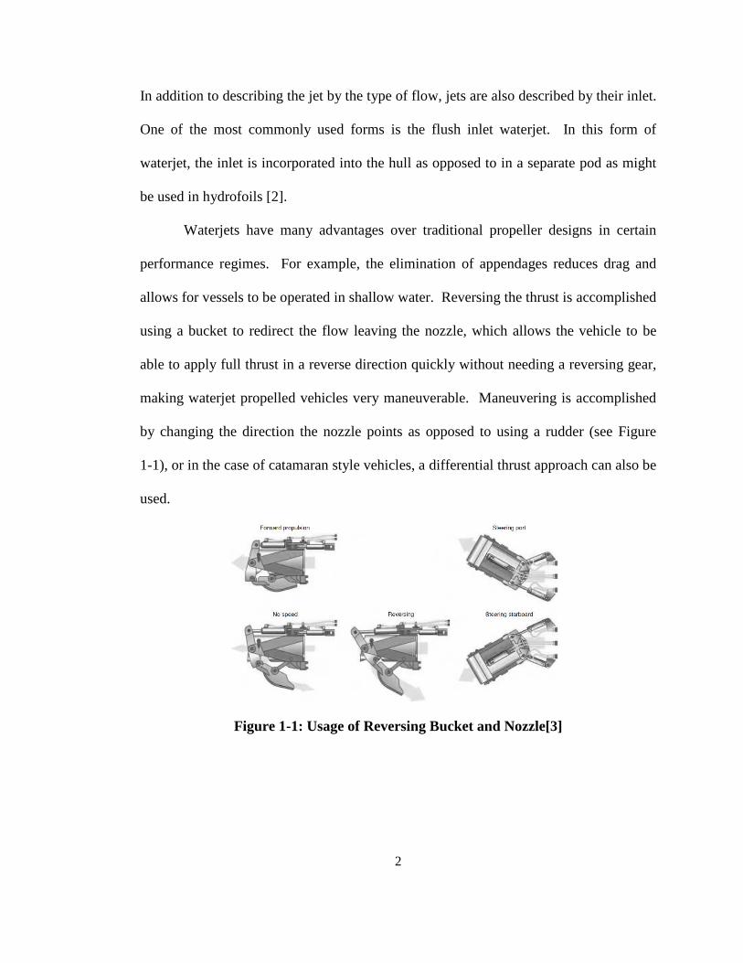
making waterjet propelled vehicles very maneuverable. Maneuvering is accomplished
by changing the direction the nozzle points as opposed to using a rudder (see Figure
1-1), or in the case of catamaran style vehicles, a differential thrust approach can also be
used.
Figure 1-1: Usage of Reversing Bucket and Nozzle[3]

3
1.2.1 Momentum Flux Method
Currently, the standard methodology for predicting the performance of a
waterjet, as defined by the International Towing Tank Conference (ITTC), is a modified
momentum flux method [4]. In this approach, the thrust delivered by the waterjet on
the hull is calculated based on the change in momentum flux between the inlet and
nozzle of the waterjet. This method requires having accurate measurements of the
velocity and volume flow rate at both the inlet and nozzle of the waterjet [1]. A brief
summary of the momentum flux method as described by the ITTC can be found in
APPENDIX E.
1.2.2 Direct Thrust Method
An alternate method of determining the thrust produced by a waterjet is the
Direct Thrust Method. This method requires isolating the propulsion system from the
main hull of the vehicle without losing hull integrity. A force transducer is then placed
between the propulsion system and the hull. At the 22nd ITTC, it was stated that the
preferred method would be the momentum flux method, but further development of the
direct thrust method was deemed important, as measurement of the forces and moments
imparted on the hull by the waterjet could provide insight into waterjet-hull
interactions [1]. As of the 24th ITTC, no institution had reported efforts to conduct
direct thrust measurements. It was assumed that this was due to the inherent
complexities involved and the ITTC developed its procedure based solely on the
momentum flux method.

4
Table 1-1: Momentum Flux vs. Direct Thrust [5]
Momentum Flux Method Direct Thrust Method
Advantages: No complicated watertight sealing boundary between waterjet and hull needed.
Disadvantages Accuracy highly dependent on accurate velocity measurements
Advantages: Jet system performance need not be measured separately.
Disadvantages: Requires separation between waterjet and hull.
1.2.3 Cross Flow
One question that the direct thrust method can be used for is to investigate the
effects of ingestion of non-longitudinal flows by a waterjet on its delivered thrust. This
is still an emerging area of research and there is little published research on the topic.
There are a few circumstances where non-longitudinal flow, or cross-flow, might
develop. One situation is maneuvering in a seaway at speed where any vehicle sway
velocity would be combined with a sway velocity imparted by the vehicle's yaw rate. If
there is substantial sway velocity at the inlet location, a cross-flow may develop,
depending on the hull geometry.
Another situation where a cross-flow might develop is with surface effect ships
(SES). An SES uses an air cushion entrained within catamaran style hulls through the
use of fore and aft skirts. The pressure differential between the air cavity and
atmospheric pressure can cause a cross-flow to develop around the catamaran hulls.
This cross-flow could then affect the performance of the waterjet by inducing cavitation
or flow separation within the waterjet inlet [3].
While little research has been done on this specific topic, a survey of related
topics can provide some insight. When water enters a waterjet inlet longitudinally, it
flows up a changing curve that starts out tangent to the hull surface, and then curves up

5
toward the impeller. This curve guides the flow up smoothly, hopefully preventing
significant flow separation. The slope of the side of the inlet is much steeper.
Figure 1-2: Representation of the Intake of a Flush Inlet Waterjet [6]
The steepness of the slope of the sides varies from one manufacturer to the next,
but if we assume it to be significant, then we can imagine the flow entering the waterjet
from the sides as that flowing over a step, which is a well documented problem that can
lead to the formation of helical flow and eddy currents.
If the flow over the step causes significant flow separation, it could potentially
cause a significant portion of the flow to "skip" over the inlet, reducing the ingested
momentum. Another possible outcome of the problem is the formation of an helical
flow within the waterjet, thus affecting its efficiency. In other types of pumps,
ingestion of swirling flow has been shown to adversely affect pump efficiency.
One reference on the topic of experimental measurement of cross flow came
from previous research at Florida Atlantic University (FAU)[7]. In an effort to better
understand the effect of cross-flow on the delivered thrust of a waterjet, an experiment
was derived using a platform of opportunity. The USV-12 (see Figure 1-3 below) is a
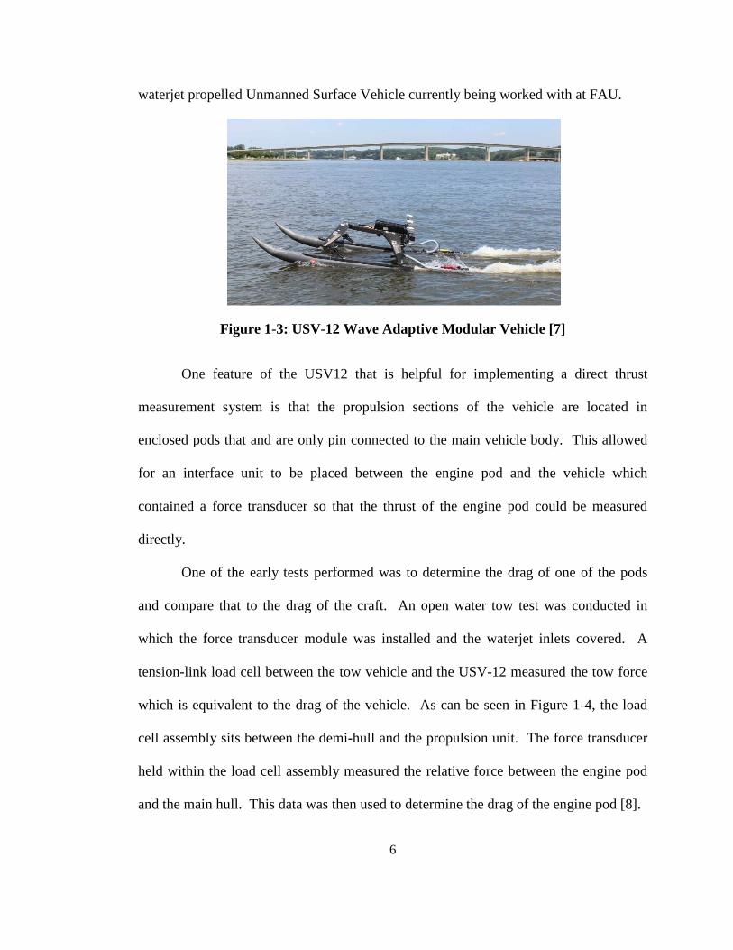
6
waterjet propelled Unmanned Surface Vehicle currently being worked with at FAU.
Figure 1-3: USV-12 Wave Adaptive Modular Vehicle [7]
One feature of the USV12 that is helpful for implementing a direct thrust
measurement system is that the propulsion sections of the vehicle are located in
enclosed pods that and are only pin connected to the main vehicle body. This allowed
for an interface unit to be placed between the engine pod and the vehicle which
contained a force transducer so that the thrust of the engine pod could be measured
directly.
One of the early tests performed was to determine the drag of one of the pods
and compare that to the drag of the craft. An open water tow test was conducted in
which the force transducer module was installed and the waterjet inlets covered. A
tension-link load cell between the tow vehicle and the USV-12 measured the tow force
which is equivalent to the drag of the vehicle. As can be seen in Figure 1-4, the load
cell assembly sits between the demi-hull and the propulsion unit. The force transducer
held within the load cell assembly measured the relative force between the engine pod
and the main hull. This data was then used to determine the drag of the engine pod [8].

7
A series of tests were then performed to induce a sway velocity at the waterjet
inlet. This sway velocity was then assumed to be equivalent to the cross flow. The
vehicle’s motions were measured using a Differential GPS (DGPS) and both the vehicle
motions as well as the force data were logged.
Figure 1-4: Experimental Setup from 2010 Tests [7].
A series of experiments were conducted, but as the vehicle was remote operated,
there was a large amount of deviation between the planned maneuver and the actual
vehicle motion. It was determined that the implementation of a control system would
limit this variability. Another problem identified related to propagation of noise. In the
data analysis, the rate of turn was calculated by differentiating the heading of the
vehicle. The calculated rate of turn was then used in the calculation of the sway
velocity. Signal noise in the heading data created amplified noise in the sway velocity
measurements which then needed to be filtered out. A better approach would be to
include a sensor which would directly measure the yaw rate[7].

8
2 APPROACH
2.1 Platform Identification
As a first step, it was necessary to choose a vehicle to base the testing platform
on. There were two vehicles available to work with. The first was an 80 inch long.
deep-V planing hull. Study of the work necessary to separate the waterjet from the main
hull revealed no simple solution. Additionally, the vehicle was payload-limited.
Figure 2-1: Planing Hull Platform Considered
Another vehicle considered was the USV-12. The USV-12 is a round hulled
catamaran that had previously been used, as described above, to conduct remote
controlled direct thrust measurements. This vehicle had the advantage of already
having the propulsion section separated from the main hull, and had a payload capacity
that was significantly larger than that of the planing hull. After consideration of the
requirements, the USV-12 was chosen for its ease of integration of the force transducer
and its payload capacity.

9
2.2 Design of propulsion system
Previous experience with the USV-12 revealed that in order to have a reliable
vehicle with predictable responses, the original two stroke gasoline engines needed to
be replaced. New propulsion units with electric motors were designed to provide a
solution to the performance issues identified. The criteria used for design decisions can
be seen in Table 2-1.
Table 2-1: Design Criteria for Electric Pods
• Components and replacement parts should be readily available
• Total thrust should be comparable to that of the existing pods
• Maximize runtime while attempting to maintain waterline
• Allow for incorporation of the force transducer into the design
After researching their availability and applicability to the system requirements,
components were chosen (see Table 2-2) to meet the above criteria.
Table 2-2: Components of New Propulsion System
Water Jet Motor
Motor Controller
Battery
Manufacturer Graupner Neumotors Roboteq Battery Space Model Jet Booster 5 2224/24/1Y MBL1650C 36V 30Ah Criteria:
Replacement parts available
Similar impeller size to current pods
RPM/power similar to the existing
Company that is easy to work with.
Controlled either with RC or serial
Feedback on serial lines
Similar to other controllers in use at FAU
LiNiMnCo chemistry gives high energy density.
90A current limit sufficient for motors

10
2.2.1 Waterjet
The Graupner Jet Booster 5 water jet is a model scale axial flow waterjet. The
jet ducting is made of cast Aluminum and the impellor is made of fiber reinforced
plastic. This jet and all replacement parts are available commercially in the US. It is
designed to use either electric motors, or the same Zenoah engine that the previous pods
used. The jet has an impeller diameter of 49mm which is similar to the size of the
impellers in the previous engine pods. Unfortunately, no documentation is available on
the performance or design criteria for this water jet, but the same was also true for all
other model scale jets that were looked at.
2.2.2 Motor Controller
Figure 2-2: Roboteq Motor Controller
The Roboteq MBL1650C (see Figure 2-2) was chosen as the motor controller
for the new system. This motor controller is designed to drive a single brushless DC
motor. This allowed for the motor controller to be located in the pod, minimizing the
length of power transmission lines. One significant advantage to using this motor
controller is that it allows for control the motor speed using an RC control line while

11
simultaneously obtaining feedback from a RS232 serial line. This motor controller also
placed some additional requirements on the design. It has a maximum allowable
voltage of 50 V and requires the motor to have Hall Effect sensors, which can be used
to measure the speed of the motor shaft. The voltage limit drove the decision to have a
36 V operating voltage for the new pods.
2.2.3 Motors
Motors were chosen to match the performance characteristics of two stroke
gasoline engines used in the previous propulsion system. The motor chosen is the
Neumotors 2224/24/1Y manufactured by Neutronics. This motor was operates in the
desired RPM range at the chosen operating voltage, while still providing power similar
to that of a Zenoah engine (see Table 2-3 for a side by side comparison). The company
was also willing to install Hall Effect sensors on the motors, as required for the use of
the Roboteq motor controller.
Table 2-3: Motor Power and RPM Comparison
Waterjet
requirements Zenoah
G260PUM Chosen Motor
Power 700 W electric
or Zenoah Engine
2.2kW 1.8 kW
RPM Not specified 12,500 RPM 15,000 RPM
2.2.4 Battery
One of the biggest design considerations for the choice of battery was energy
density. It was desirable to have the maximum amount of run time with the minimum
amount of extra weight. Lithium based batteries have some of the highest energy
densities of standard battery packs and of lithium batteries the LiNiMnCo batteries have

12
one of the highest densities. Given our operating voltage, and power requirements, a
battery was chosen.
Table 2-4: Battery Specifications
Battery Chemistry: LiNiMnCo Charge density: 160 wh/kg (approximate) Working Voltage: 36V Maximum Voltage: 42V Cutoff Voltage: 27V Capacity: 30 Ah (1080 wh) Discharge Rate: 90 A max Weight: 14 lbs 11.8 oz
The battery selected consists of 30 LiNiMnCo cells arrange in a 3S-10P
configuration (see Table 2-4 for battery specifications). A protection circuit module
(PCM) was installed in the batteries which monitors the charge and discharge of each
cell and balances the current load on the cells accordingly. The PCM also provides
over-discharge protection and will stop discharging the battery if the voltage of the cells
drops below a safe threshold.
2.2.5 Electrical Design
Communication lines, including both RC control and RS232 lines are brought
into the pod through a cord grip on the forward face of the pod. The battery provides
the voltage source to the motor controller which then distributes it to the motor.
Additionally, an RC line is also connected to a servo mounted to the aft bulkhead which
articulates the reversing bucket. By time of testing, the reversing bucket and servo had
not been installed as the ability to control them had not yet been integrated into the
control system.

13
Figure 2-3: Motor Pod Block Diagram
2.2.5.1 Kill Circuit
The system is designed to kill the power to the motor controller if any of several
conditions occurs, including low control system voltage, processor fault, or human
intervention by means of a switch on the vehicle remote. This is accomplished by
placing a pair of 60V, 100A relays between the battery and the motor controller. These
relays are mounted on a heat sink with a fan to dissipate the heat generated from the
relay when it is in a closed position.
The efficiency of the heat sink was tested by placing load resistors of a known
resistance on the heat sink and adjusting the power dissipated though them. For this
test, the heat sink was mounted in a sealed motor pod on a worktable. The temperature
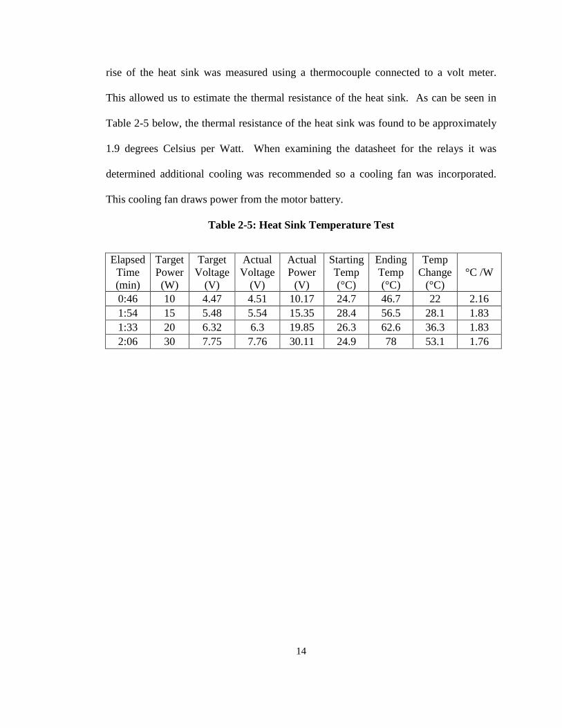
14
rise of the heat sink was measured using a thermocouple connected to a volt meter.
This allowed us to estimate the thermal resistance of the heat sink. As can be seen in
Table 2-5 below, the thermal resistance of the heat sink was found to be approximately
1.9 degrees Celsius per Watt. When examining the datasheet for the relays it was
determined additional cooling was recommended so a cooling fan was incorporated.
This cooling fan draws power from the motor battery.
Table 2-5: Heat Sink Temperature Test
Elapsed Time (min)
Target Power (W)
Target Voltage
(V)
Actual Voltage
(V)
Actual Power
(V)
Starting Temp (°C)
Ending Temp (°C)
Temp Change
(°C) °C /W
0:46 10 4.47 4.51 10.17 24.7 46.7 22 2.16 1:54 15 5.48 5.54 15.35 28.4 56.5 28.1 1.83 1:33 20 6.32 6.3 19.85 26.3 62.6 36.3 1.83 2:06 30 7.75 7.76 30.11 24.9 78 53.1 1.76

15
2.2.6 Structural Design
Figure 2-4: Pod Cross Section
The physical design of the new pods was performed with an eye towards ease of
use and repair. A U-shaped cross-section with lid was used (see Figure 2-4). This
allows access to all of the components from above. Aluminum was chosen for the outer
shell due to its ability to be worked with along with its durability. The lid, as well as
fore and aft bulkheads are made from Starboard and the keel liner is made from high-
density polyethylene (HDPE).
The battery, which is by far the heaviest of the loads in the pods, has been
located slightly forward of the longitudinal center of the pod to accommodate the space
required for the motor and waterjet (see Figure 2-5). The battery is mounted in a
module consisting of fiber two fiber reinforced bulkheads, a tray, and a pair of
cylindrical lifting rails. The battery sits in the tray and is held in place by a restraining
strap. The bulkheads, in addition to raising the battery up off of the bottom of the pod
(to minimize damage that might be caused by small leaks), provide convenient
mounting points for the motor controller, the shut off relay, and cooling system.
16
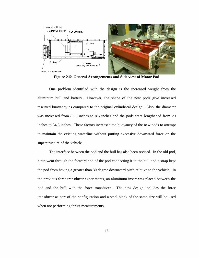
Figure 2-5: General Arrangements and Side view of Motor Pod
One problem identified with the design is the increased weight from the
aluminum hull and battery. However, the shape of the new pods give increased
reserved buoyancy as compared to the original cylindrical design. Also, the diameter
was increased from 8.25 inches to 8.5 inches and the pods were lengthened from 29
inches to 34.5 inches. These factors increased the buoyancy of the new pods to attempt
to maintain the existing waterline without putting excessive downward force on the
superstructure of the vehicle.
The interface between the pod and the hull has also been revised. In the old pod,
a pin went through the forward end of the pod connecting it to the hull and a strap kept
the pod from having a greater than 30 degree downward pitch relative to the vehicle. In
the previous force transducer experiments, an aluminum insert was placed between the
pod and the hull with the force transducer. The new design includes the force
transducer as part of the configuration and a steel blank of the same size will be used
when not performing thrust measurements.
17
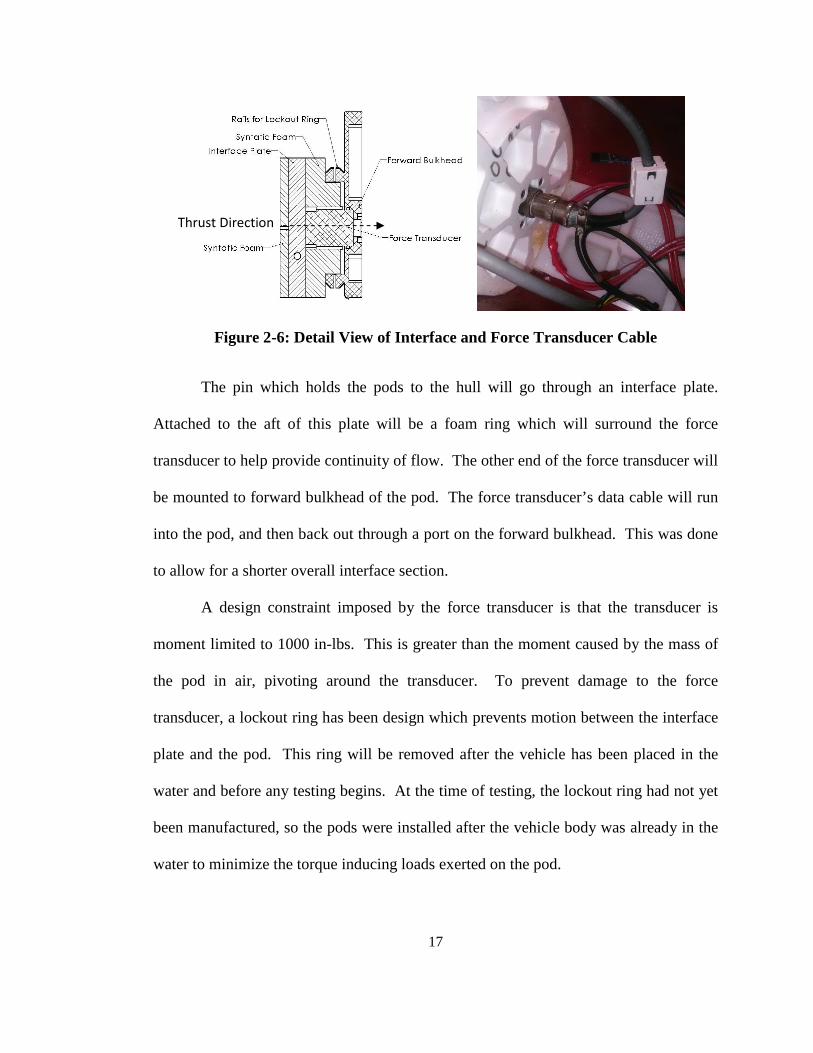
Figure 2-6: Detail View of Interface and Force Transducer Cable
The pin which holds the pods to the hull will go through an interface plate.
Attached to the aft of this plate will be a foam ring which will surround the force
transducer to help provide continuity of flow. The other end of the force transducer will
be mounted to forward bulkhead of the pod. The force transducer’s data cable will run
into the pod, and then back out through a port on the forward bulkhead. This was done
to allow for a shorter overall interface section.
A design constraint imposed by the force transducer is that the transducer is
moment limited to 1000 in-lbs. This is greater than the moment caused by the mass of
the pod in air, pivoting around the transducer. To prevent damage to the force
transducer, a lockout ring has been design which prevents motion between the interface
plate and the pod. This ring will be removed after the vehicle has been placed in the
water and before any testing begins. At the time of testing, the lockout ring had not yet
been manufactured, so the pods were installed after the vehicle body was already in the
water to minimize the torque inducing loads exerted on the pod.
Thrust Direction

18
2.2.7 Cooling System
Originally, the pressure tap that comes preinstalled on the side of the waterjet
was going to be used to provide a flow of water to cool the motor. The water would
then flow up through a tube on the outside of the stern of the pod to a hull penetration
which was located near the top of the pod to make sure that the penetration was far
above waterline. Upon initial testing, it was determined that the waterjet didn't produce
a high enough pressure for the water to reach the hull penetration until the throttle was
greater than 80%. Once the system was "primed" it only had sufficient flow above 50%
throttle. At full speed, the flow rate was determined to be 100 mL per min. This was
determined to be insufficient as the motor still got quite warm at midrange throttle
settings.
Figure 2-7: Cooling System Components
To increase the flow rate, a standalone cooling system was designed to circulate
water through a coil wrapped around the motor (see Figure 2-7 above). The motor that
was chosen was a peristaltic pump. This type of pump is designed for passing fluids
Pump
Coil
Intake
Exhaust
External Pickup

19
through tubing and is known for its self priming capabilities. The specific pump that
was chosen can self prime up to 7.5 meters of pressure head and has a flow rate on the
order of 200 mL per minute. One other feature of this style of pump is its ability to be
able to run dry without causing damage to the pump. This feature makes it easy to both
prime and purge the system.
The pump is powered by a standalone 12V 2400 mAh Nickel Cadmium battery
pack. This should allow the cooling pumps to be run for up to 90 minutes, making it
advisable to change the cooling system batteries at the same time as the main batteries.
The cooling system is activated by turning on either one of two switches that are
placed in parallel in its circuit. The main switch is a voltage controlled solid state relay.
This switch is tied into the kill circuit of the pod making it possible to turn on and off
the cooling system remotely. The second switch is a manual switch. This switch is
designed so that the cooling system can be turned on and off manually to facilitate the
flushing of the system. Please refer to the appendix for a wiring diagram of the cooling
system's electrical components.

20
2.3 Control System and Data Collection
Figure 2-8: Control and Data Collection Block Diagram
Motor throttle was controlled using a control system that has been developed for
use with several of FAU’s autonomous surface vehicles including the USV-12, DUKW
model, USV-14, and the AVUSI Roboboat student competition vehicle. This control
system uses data from a compass, IMU, and GPS to determine what corrections need to
be made to the vehicle motions and then sends the appropriate signals to the motor
controllers. The sensors used by the control system include an OS5000 tilt
compensated compass and an MTI-G IMU. The MTI-G has several sensors of its own
including gyro, accelerometer, magnetometer, barometer, and GPS receiver. The GPS
receiver is capable of obtaining ground based corrections to improve its accuracy.

21
At the heart of the control system is a TS7800 microprocessor board with an
ARM9 CPU. The TS7800 is mounted on an interface board. This board has RC
outputs that can be used to control RC Servos as well as the motor controllers. Several
serial ports are available for various sensors, depending on the platform being used and
the experiments being conducted.
Lightweight Communications and Marshaling (LCM) is used to facilitate
communication on the platform. LCM utilizes a publish/subscribe message passing
system to improve communication between system components [9]. In this application,
signals received from the IMU and motor controllers were announced by the TS7800
over a vehicle based local area network. A laptop was connected to this network
wirelessly for data logging which allowed for significantly increased storage space.
This laptop was also able to be remotely logged into using Windows Remote Desktop,
allowing for real time viewing of the data.
2.3.1 Force Transducer Data Collection
The force transducer used is a MC2.5-2K-SP manufactured by AMTI. It has 6
channels (3 force and 3 moment) and is rated for underwater use. In this experiment,
the unit is situated so that the Z-axis of the force transducer, which has a range of ±
2000 lbs, is aligned with the thrust axis of the pod. The transducer requires that power
be provided by a separate amplifier and signal conditioning module. This module
allows the user to select the excitation voltage and gains used. The amplifier outputs
analog voltages in the ±10V range.

22
The analog outputs of the amplifier were connected to a National Instruments
cDAQ equipped with two modules. The first module use was a 14 bit analog to digital
converter. This module converted the ±10V into a 14 bit digital signal, giving a
resolution of 0.00122V, which equates to 0.348 N of thrust under maximum excitation
voltage and gain.
The second module used was a digital output module. This module is used to
zero the amplifier remotely. This was performed in between each individual test run,
after letting the vehicle come to rest, as it had been noticed that under cyclical loading
the signal from the amplifier does not always return to its zero condition.
The cDAQ was controlled by a laptop running Signal Express. The laptop used
for this was the same as the data logging laptop mentioned above (see Table 2-6 below).
This permitted all data points to be time stamped using the same system clock to make
comparing the data easier in post processing.
Table 2-6: Data Logged on Laptop
Sensor: MTI-G IMU Motor
Controller Force
Transducer Parameters: Velocity (X,Y,Z)*
Rate of Turn (x, y, z) Acceleration (x, y, z)
Pitch Roll Yaw
Latitude Longitude Heading
Battery Voltage Motor Current
Motor Command Motor RPM
Fx Fy Fz Mx My Mz
* Velocities are relative to a North-East-Down Earth-fixed coordinate system
2.4 Force transducer calibration
The force transducer used in this experiment was manually calibrated in an

23
effort to verify that the output of the force transducer was accurate. A series of
calibration tests were performed in which all six channels of the force transducer (three
forces and three moments) were tested in both compression and tension. This data was
then used to determine the actual sensitivity of the sensor. The data (see Figure 2-9)
showed that there was good correspondence between the manufacturer specifications
for the force channels, but a small DC offset was observed at no load. This will be
compensated for in post processing.
Figure 2-9: Force Transducer Calibration Data – FZ Channel
2.5 Experimental Approach
To determine the if cross-flow at the inlet of a waterjet has an effect on its
delivered thrust, a set of tests were conducted to induce varying amounts of sway
velocities, as it was assumed that the primary contributor to cross-flow in this type of
vehicle is due to sway velocities at the waterjet inlet.
0 50 100 150 200 250 300 350 400 450 500-0.5
0
0.5
1
1.5
2
Load (lbs)
Out
put
Vol
tage
(V
)
y=0.0039x-0.0648
R2=0.9998

24
First, the testing location was identified as the North Hollywood Finger Lake
(see Figure 2-10 below). This lake is a relatively calm body of water in close proximity
to the SeaTech Campus of Florida Atlantic University.
Figure 2-10: North Hollywood Finger Lake
Preliminary vehicle testing showed that the minimum turning radius of the
USV-12 with the new motor pods was approximately 10 meters, and the maximum
forward velocity was around 2.5 meters per second. After collecting this information, a
Matlab code was developed to predict how much yaw induced sway velocity could be
anticipated at different speeds and circle diameters (see Table 2-7 below).
Table 2-7: Expected Yaw Induced Sway Velocities in m/s
Speed (m/s) R=10 m 15 m 20 m 25 m 2 0.32 0.21 0.16 0.13
2.5 0.40 0.27 0.20 0.16
Hollywood Sailing Club Boat Ramp
Center of Turning Circles

25
It was determined that these speeds and circle diameters would give a wide
range of induced sway velocities from which a conclusion should be able to be drawn.
To that end, a set of waypoints was derived using the given turning circle radii.

26
3 PROPULSION SYSTEM TESTING
3.1 Motor Pod Testing
During and after construction of the new motor pods, testing was conducted to
determine functionality and reliability of the platform.
3.1.1 Hull Seal Testing
One of the first tests performed was a hull integrity test. During this series of
tests, after assembling the shell of the pod, and installing the waterjet, the pod was
weighted and placed in fresh water to test the integrity of the watertight seals. Initial
tests showed a problem with leakage through some hull penetrations.
It was determined through testing that the root cause of the leaks was that the
silicone adhesive that had been used was not adhering to the starboard and HDPE parts.
Several solutions were considered and the ultimate solution was to place coil type
threaded inserts into the bolt holes that surrounded any watertight seal. This increased
the compression between the materials. Silicone was used to provide a compliant seal,
but not for adhesion.
3.1.2 Magnetic Coupling Test
The magnetic shaft coupling used to connect the motor to the waterjet is
designed to operate with a small air gap between the two halves. To determine what the
appropriate gap distance was, an initial estimate was made and then refined during

27
testing. Testing of the gap involved running the motor throttle at various positions. If
any slippage of the shaft was noted, the distance was adjusted. After testing, the
appropriate air gap was determined to be approximately 1 millimeter.
3.1.3 Run Time Estimation Test
One of the motor pods was tested to determine how long the system would run
for, and to observe the system under operation. The results of the test showed that at
75% throttle, the batteries should provide 77 minutes of run time (see Figure 3-1
below).
Figure 3-1: Battery Discharge Curve at 75% Throttle
0 10 20 30 40 50 60 70 8028
30
32
34
36
38
40
42
Run Time (Minutes)
Bat
tery
Vol
tage
(V
)

28
4 EXPERIMENTAL TESTING
4.1 Experimental Testing
After confirming that the propulsion system and control system both were
working, the experimental tests were performed. Experiments were conducted on
several days with varying success.
4.1.1 Testing - June 14, 2013
Initial testing revealed problems with the logging of the IMU data, and
significant holes were reported in the data. The problem was identified as being caused
by the motor controller signals overloading the system and causing dropouts of the IMU
signal. To solve this several steps were undertaken, the first of which was to change the
format of the telemetry strings from the motor controller.
After consulting with the manufacturer, it was determined that the default
telemetry option, which sends out each parameter in a separate string, was not the ideal
situation. This caused the data to be transmitting much faster than any other device.
Each motor controller was transmitting four types of information (battery voltage,
motor current, RPM, and motor command) with each one being sent out ten times a
second. This made a total of 80 messages being sent between the two motor controllers
each second. To limit this, a script was created in MicroBasic and loaded on the motor
controllers (see APPENDIX C). This code compiled all four pieces of data into a

29
single, tab separated string which was then sent out at 5 Hz. One problem that was
found with this was that the version of MicroBasic supported by the motor controller
does not allow for creation of a checksum value.
The second change that was made was in how the data was processed. In the
initial test run, the data for the motor controllers was being logged on the TS-7800,
while the IMU and compass information was announced on the network across an LCM
channel. To make future logging easier, and to make sure all signals had the same
timestamp, changes were made so that the motor controller data also was announced
using LCM and logged on the same computer as the IMU and force transducer.
Additionally, after looking at the data, it was revealed that the data from the
force transducer had significant noise in the channel of interest. One possible cause for
this was saturation of the moment channels. In this test, the gains and excitation
voltages for all six channels were set to their maximum values. Saturation was
observed in several of the moment channels during most of the test runs. The gains and
excitation voltage were reduced for future tests to limit the noise produced.
4.1.2 Testing: June 26, 2013
During follow-up testing on June 26, 2013 a catastrophic leak occurred in one of
the motor pods. By the time the pod was removed from the water, several inches of
water was in the pod, partially immersing the motor controller and battery, and fully
submerging the motor in salt water. Additionally, the battery leads were also
submerged. This caused serious damage to all of the electronics. The source of the leak
was identified as the shaft seal in the waterjet. The drive shaft as provided by the

30
manufacturer was not made of a corrosion resistant material and had significant
corrosion develop despite rinsing the pod in fresh water after each previous test run.
The corrosion caused sufficient shaft roughness to develop to damage the lip seal and
the sealed bearing, allowing water to penetrate the pod.
New drive shafts were manufactured out of stainless steel and new bearings and
seals were installed in both motor pods, as corrosion was identified on both shafts. The
motor and motor controller were sent back to the manufacturers for repairs. The motor
controller was damaged and needed to be replaced, while the motor only needed new
bearings and hall effect sensors. The damage to the battery was significant enough that
the manufacturer recommended that it not be repaired, as the actual extent of damage to
the cells could not be easily determined. As spare batteries were already on hand, it was
determined that replacing the damaged battery was not a high priority.
4.1.3 Testing: September 19, 2013
After repairs, further testing was conducted. During this test we had several
advances in our testing. The first of which was that this was the first day that we were
able to perform true closed loop tests. Previously, the tests were being conducted with
purely open loop control. A proportional controller was used to perform basic waypoint
following autonomy. Four waypoints were used equidistant from a common center.
This gave a very diamond shaped vehicle path, indicating the need for additional
waypoints in future tests.
Unfortunately, there was a failure of the force transducer amplifier to correctly
amplify the data from the force transducer. While the gains excitation voltages were

31
adjusted from previous test runs so that the channels did not hit saturation, a problem
was observed where zeroing the amplifier did not accurately zero the sensor, and under
no load the signal would then float around. Testing after the fact showed this problem
occurred again outside of the water, in a lab environment. After examining the
amplifier settings, and verifying that all jumpers were well seated, the problem was
corrected.
4.1.4 Testing: September 27, 2013
After the lessons learned in the previous testing days, a new set of waypoints
was created. These waypoints used a constant distance between waypoints for different
circles of different radii. This distance varied based on the speed of the vehicle (see
Table 4-1 below). Additionally, prior to going to the testing location, the functioning of
the force transducer was verified.
Table 4-1: Test Run Waypoints Distances
Circle Radii (m)
Speed (m/s)
Number of waypoints Arc Length
(m) Time between waypoints (s)
10
1.0 1.5 2.0
6 10.5 5.25
2.5 4 15.7 6.28
15 2.0 9 10.5 5.25
2.5 6 15.7 6.28
20 2.0 12 10.5 5.25
2.5 8 15.7 6.28
25 2.0 15 10.5 5.25
2.5 10 15.7 6.28

32
An additional difference to the previous days of testing was that the force
transducer data logging was performed slightly differently. Instead of having one large
data file, a separate data file was created for each test run. This was accomplished by
remotely logging into the laptop on the vehicle using a wireless network connection.
This also allowed us to re-zero the force transducer after each test run to help improve
the accuracy of the transducer.
During this day of testing several observations were made about the different
styles of test runs. In small radius turns, the vehicle frequently had trouble finding
waypoints and would circle the missed waypoint several times at maximum differential
thrust until it came within the threshold of acceptance for the waypoint. This caused
some interesting paths and also had the effect of the vehicle moving faster than planned
for some of the test runs.
Several lower speed test runs were conducted at the ten meter radius circle. This
was in an attempt to cause circles of different yaw induced sway velocity, but it became
clear that even at slower speeds, the vehicle struggled with the small radius turns.

33
5 DATA PROCESSING
Processing of the data began was performed using Matlab. The first step taken
in processing the data was the parsing of the collected data into various test runs. The
collected data was in two different file types. The data from the force transducer was
saved in separate files for each test run, and was stored using LabView Signal Express
in a TDMS file format. This was opened again in Signal Express and exported to a tab
separated text file that could be opened in Matlab. Each test run had identified the exact
start time as well as the sampling frequency. The default collection rate of 1 kHz was
used during experimentation.
The remaining data was saved on the laptop in individual text files for each
sensor (IMU, GPS, and motor controllers), each file containing data from the complete
day of testing. The individual samples were time-stamped as they were logged with a
one second resolution. As we were collecting data from these sensors at sub-second
frequencies (five and ten Hertz), this resulted in several samples having the same
timestamps. This would be addressed in later data processing.
To separate the data from the IMU, GPS and motor controllers into separate
files, a custom Matlab function was used. This function loads the data file and, using a
user specified start and end time, extracts the data points of interest and saves them into
a MAT file which can then be loaded into a different Matlab program. This function
was modified slightly to allow for the parent code to also pass a file name in addition to

34
start and end times instead of waiting for user input (see APPENDIX A).
As a first pass, the start and end times of the force transducer files were used to
parse the data. The individual data sets created from this first pass were then analyzed
to identify the time that the vehicle started and finished its turning circle and the test
sorter function was run again. As previously discussed, in some of the tight radius
turns, the vehicle's path was not circular. For data analysis purposes, circular sections
of the data were identified and extracted for further processing. These refined start and
end times were then used to separate out the force transducer reading from the same
times. Additionally, it was noticed that each time the force transducer amplifier was
zeroed, a slightly different DC bias was observed. To correctly identify this for each
test run, an average was taken of the first 100 samples of the data file. This
corresponded to the time between when the amplifier was zeroed and the test run was
actually begun. During this time, the vehicle was sitting at rest in the waters of the
finger lake.
After parsing the data, a code was written that would look at the data for
individual test runs. After loading the data for the specific test run, the pitch and roll
information from the IMU was used to correct for vehicle's pitch and roll. This allowed
for the surge, sway and heave data to be corrected to accurately reflect the orientation of
the vehicle. To perform this correction, the angle2dcm function that is part of Matlab's
aerospace toolbox was used to create a direction cosine matrix that was then multiplied
to a state space vector of the data to be corrected. This correction was performed for the
vehicle's acceleration, velocity, and gyro data.
A plot was then made showing the data before and after the angular correction

35
was applied. Review of this plot showed that there was a recorded heave velocity that
oscillated around 0.1 meters per second. While some heave velocities could be
expected, they should be oscillating around zero. Upon consultation with the sensor
manufacturer, it was revealed that the maximum accuracy of the sensor is at a vehicle
speed of 30 meters per second. At slower speeds, such as those in these tests, the
accuracy would be less than that, although no information was available to state what
the accuracy would be in this speed regime.
After correcting for pitch and roll, the data needed to be corrected for the
translational offset between the CG of the vehicle and the location of the sensor. To do
this, a coordinate transformation was performed using the following formula:
� = � + � × ���
This formula relates the velocity at any point A with the velocity at the center of
gravity G using the rotation rate and the distance vector between the two points. This
same formula was then used to translate the coordinate system again to the location of
the waterjet inlet (see Figure 5-1 below).

36
Figure 5-1: Circle Test 1 - Vehicle Velocities, Waterjet Inlet Local Velocities
The thrust data was collected at 1 kHz, 100 times faster than the data from the
IMU. In order to be able to compare the IMU data with the force data, the thrust data
was down-sampled. This was accomplished by averaging 100 consecutive samples into
a single sample in the down-sampled data set. In analyzing the thrust, first a frequency
analysis was performed on both on the 1 kHz data and the down-sampled data 10 Hz
data. Reviewing the spectrum of rays from the 1 kHz data set revealed two main things.
The first was a large lobe around zero Hz as well as another signal at approximately 200
Hz. This 200 Hz signal was determined to be at the same frequency as the speed of the
motor.
0 20 40 60 80 100 120-0.5
0
0.5
1
1.5
2
2.5
time (s)
Vel
ocity
(m/s
)
Vehicle SurgeVehicle Sway
Vehicle Heave
Waterjet Surge
Waterjet SwayWaterjet Heave
Heave Velocity Offset - Mean -0.113

37
Figure 5-2: Circle Test 2 - Frequency Analysis of 1 kHz Force Signal
Reviewing the 10 Hz signal showed two lobes of interest, the main lobe,
centered about zero Hertz, and a secondary lobe that varied in position, but tended to
fall between 0.5 and 2.5 Hz.
-500 -400 -300 -200 -100 0 100 200 300 400 500-5
0
5
10
15
20
25
30
Frequency (Hz)
For
ce S
pect
rum
of
Ray
s(N
)
Real Component
Imaginary Component
220 Hz SignalEquates to 13,200 RPM

38
Figure 5-3: Circle Test 2 -Frequency Analysis of 10 Hz Force Signal
To investigate these two signals and their relation to the sway velocity at the
waterjet inlet, they were isolated from each other and the rest of the background
frequencies. A low-pass filter was used for the main signal (with cutoff at 0.75 Hz),
and a band-pass filter was used to isolate the secondary frequency (0.75 Hz - 2 Hz).
-5 -4 -3 -2 -1 0 1 2 3 4 5-5
0
5
10
15
20
25
30
Frequency (Hz)
Fo
rce
spe
ctru
m o
f ra
ys (N
)
Real ComponentImaginary Component
Main Signal
Secondary Frequency

39
Figure 5-4: Circle Test 1 - Two Components of Thrust
Some data points were observed that existed outside of the physically realistic
range (i.e. velocities faster than the speed of sound or accelerations greater than the
sensor can record). These data points were identified and excluded from further
processing.
The signals were then smoothed using the "smooth" function in Matlab. This
function uses a moving average with a span identified by the user. A span of 5 samples
was used for the velocity signal and a span of 11 samples was used for the thrust data.
One thing noticed in reviewing the motor controller data from the experiments
was that there were numerous intervals where the messages being sent by the motor
controller were not logged. This resulted in instances where the data from the motor
0 20 40 60 80 100 120-20
-10
0
10
20
30
40
50
60
70
Time (s)
For
ce (N
)
Primary Frequency Thrust Component
Secondary Frequency Thrust Component
40
controllers was good in some test runs, and lacking in others. Because of this, the data
processing and analysis did not use the data from the motor controllers.
To facilitate comparison, the thrust and sway velocity were both non-
dimensionalized. The thrust was non-dimensionalized using the Thrust Loading
Coefficient, which relates the thrust to the nozzle area and the square of the forward
velocity.
��� = ����12 ����
This was done for both the low frequency and the secondary frequency
components of the thrust. The sway velocity was non-dimensionalized using the
forward velocity in what we will call the "Sway Velocity Ratio."
The Thrust Loading Coefficient for both frequency ranges and the Sway
Velocity Ratio were then plotted, with the yaw rate in a subplot. The yaw rate was
included to be able to easily determine the intervals where the vehicle was turning and
moving strait.
In an effort to quantify the relation between the sway velocity and the thrust, the
biased cross-covariance between thrust and waterjet inlet sway velocity was calculated
and plotted. This was performed for both frequency components.
In addition to looking at the relation between thrust and sway velocity, the
relation between surge acceleration and sway velocity was compared. The same
approach was taken, except that primary frequency was excluded. This was done
because the primary effect of interest was in vibration and not the actual acceleration of
the vehicle.

41
6 RESULTS
Analysis of the data from the test runs revealed that the test runs could be
categorized into two different types of runs; those with relatively constant thrust and
those where the thrust fluctuated. The first category, those with relatively constant
thrust, consisted mainly of the circular sections of the small radius turns. In most of
these turns, the vehicle was at maximum differential thrust for most or all of the data
set. This resulted in an almost constant yaw rate.
As can be seen in Figure 6-1, there is little noticeable relation between the
delivered thrust and the sway velocity in when looking at the primary frequency.
Figure 6-2 shows a certain pulsing that appears to follow peaks of high sway velocity,
but further analysis of subsequent test runs did not show the same relationship.

42
Figure 6-1: Circle Test 1 - Primary Frequency Thrust Compared to Sway
Figure 6-2: Circle Test 1 - Secondary Frequency Thrust Compared to Sway
0 20 40 60 80 100 1200
20
40
Thr
ust/
0.5
ρANU
o2
0 20 40 60 80 100 120-0.2
0
0.2
Vw
j / U
0
Primary Frequency Thrust Loading Coeff
Sway Velocity Ratio
0 20 40 60 80 100 1200.05
0.1
0.15
0.2
0.25
time(s)
Yaw
Rat
e (r
ad/s
ec)
0 20 40 60 80 100 120-2
0
2
Thr
ust/
0.5
ρANU
o2
0 20 40 60 80 100 120-0.2
0
0.2
Vw
j / U
0
Secondary Frequency Thrust Loading Coeff
Sway Velocity Ratio
0 20 40 60 80 100 1200.05
0.1
0.15
0.2
0.25
time(s)
Yaw
Rat
e (r
ad/s
ec)

43
Review of the normalized cross-correlation plots (see Figure 6-3) for the two
frequency ranges showed that in the primary frequency signal, there is a moderate peak
just to the right of zero lag, indicating that the two signals do have some correlation, but
no causal relationship could be derived when plotted against time. . No significant
amplitude was observed in any of the secondary frequency signals.
Figure 6-3: Circle Test 1 - Normalized Cross-Correlation for Thrust and Sway
Velocity
-1500 -1000 -500 0 500 1000 1500-0.4
-0.2
0
0.2
0.4
Lag in number of Samples
Nor
mal
ized
Cro
ss-
Cor
rela
tion
Coe
ffici
ents
Primary Frequency Thrust
-1500 -1000 -500 0 500 1000 1500-0.02
-0.01
0
0.01
0.02
Lag in number of Samples
Nor
mal
ized
Cro
ss-
Cor
rela
tion
Coe
ffici
ents
Secondary Frequency Thrust
44
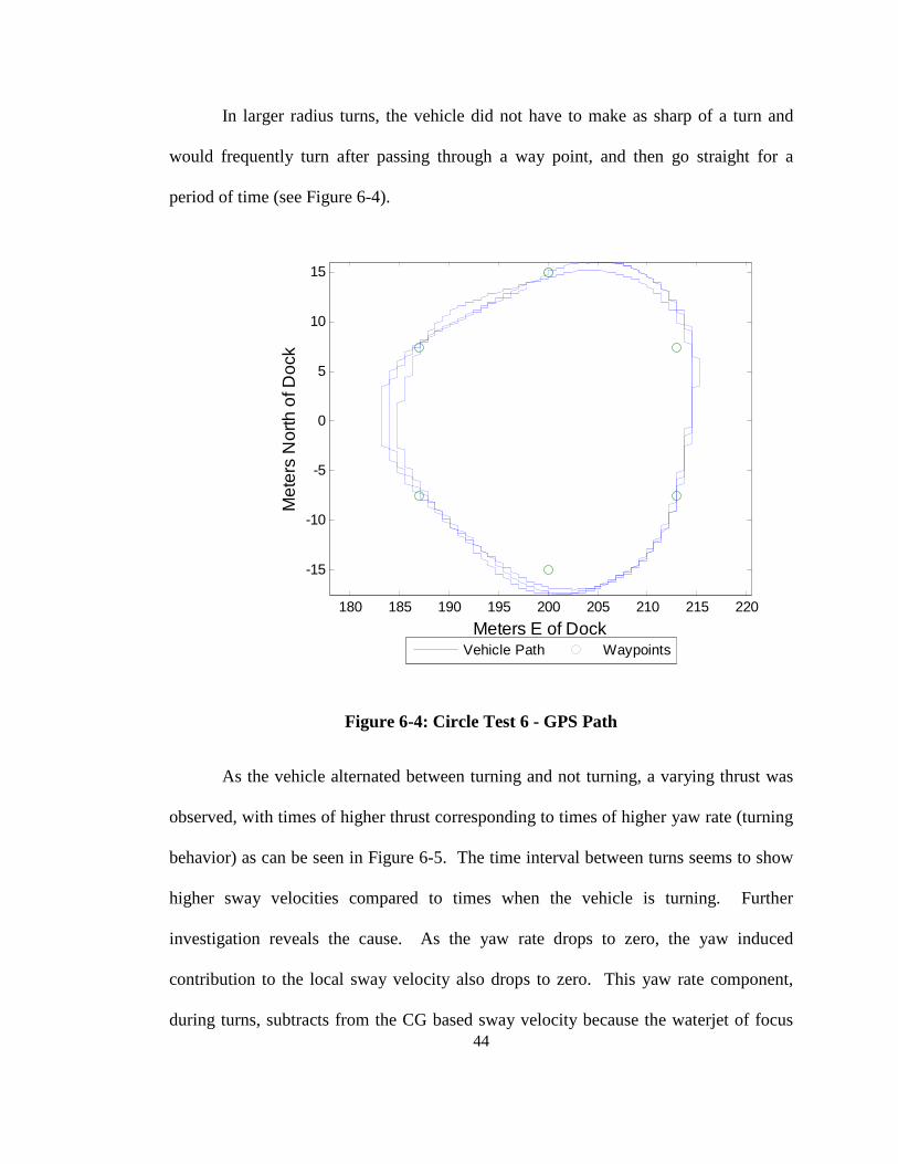
In larger radius turns, the vehicle did not have to make as sharp of a turn and
would frequently turn after passing through a way point, and then go straight for a
period of time (see Figure 6-4).
Figure 6-4: Circle Test 6 - GPS Path
As the vehicle alternated between turning and not turning, a varying thrust was
observed, with times of higher thrust corresponding to times of higher yaw rate (turning
behavior) as can be seen in Figure 6-5. The time interval between turns seems to show
higher sway velocities compared to times when the vehicle is turning. Further
investigation reveals the cause. As the yaw rate drops to zero, the yaw induced
contribution to the local sway velocity also drops to zero. This yaw rate component,
during turns, subtracts from the CG based sway velocity because the waterjet of focus
180 185 190 195 200 205 210 215 220
-15
-10
-5
0
5
10
15
Meters E of Dock
Met
ers
Nor
th o
f Doc
k
Vehicle Path Waypoints

45
was the port pod, and as such, the X and Y and Z components of the waterjet inlet
position vector is negative. relative to the center of gravity. Because of this, the actual
relation between the thrust and sway velocity could not be easily determined in these
test runs. Additionally, the amplitude of the sway velocities in most of the test runs
remained less than twenty percent of the mean forward velocity.
Figure 6-5: Circle Test 6 - Primary Frequency Thrust Compared to Sway
In these larger radius turns, the cross correlation plot (Figure 6-6) shows a
significant relationship between the trust and the sway velocity, with a moderately
significant trough, in this example at a lag of 4 samples and an amplitude of -0.4. This
correlation can most likely be associated to the phenomenon previously discussed,
0 50 100 1500
20
40
Thr
ust/
0.5
ρANU
o2
0 50 100 150-0.2
0
0.2
Vw
j / U
0
Primary Frequency Thrust Loading Coeff
Sway Velocity Ratio
0 50 100 150-0.1
0
0.1
0.2
0.3
time(s)
Yaw
Rat
e (r
ad/s
ec)
TURNS

46
where the sway velocity increases during straight line motion due to the reduced yaw
rate.
Figure 6-6: Circle Test 6 - Normalized Cross-Correlation for Thrust and Sway
Velocity
For all of the test runs, the slip angle was also calculated. This was done by
looking for the angle between the total velocity vector and the surge direction. Analysis
of the plots showed that most of the slip angles ranged between -5 and 12 degrees, with
reduced slip angles being observed in larger radius turns. A Slip angles as high as 50
degrees were recorded in one test run, but this is most likely due to a sensor anomaly.
-1500 -1000 -500 0 500 1000 1500-0.5
0
0.5
Lag in number of Samples
Nor
mal
ized
Cro
ss-
Cor
rela
tion
Coe
ffici
ents
Primary Frequency Thrust
-1500 -1000 -500 0 500 1000 1500-0.1
-0.05
0
0.05
0.1
Lag in number of Samples
Nor
mal
ized
Cro
ss-
Cor
rela
tion
Coe
ffici
ents
Secondary Frequency Thrust
Lag 4 samplesAmplitude: -0.4

47
Figure 6-7: Circle Test 6 - Slip Angle
0 50 100 150-2
0
2
4
6
8
10
12
14
Time (s)
Slip
Ang
le (d
egre
es)

48
7 CONCLUSIONS
While the initial objective of designing a free running waterjet propelled USV to
perform direct thrust measurements was a success, attempting to meet the secondary
objective of investigating the relationship between cross-flow and delivered thrust
proved challenging. Review of the data collected did not conclusively show that cross-
flow at the waterjet inlet causes a noticeable effect in the thrust, but it could not
conclusively disprove it either. Further research is needed before any definitive
conclusion can be drawn about the association between cross-flow and thrust.
As it was not possible to directly observe and quantify the cross-flow, the
assumption was made that sway velocity at the waterjet would be related to the cross-
flow. While this is a logical assumption, further analysis for this platform should be
conducted to verify this., This could be done using computer modeling or experimental
tests where the actual ingested flow can be visualized and compared to the slip angle.
This experiment would most likely need to be performed in a testing tank as visualizing
the flow becomes problematic in a free running condition.
In this experiment, the sway velocities used in the data analysis are derived
solely from the data recorded from the IMU. The IMU used is designed primarily for
aerospace applications where the speed traveled is much greater. It's rated accuracy for
velocity peaks at 0.1 m/s at a velocity 30 m/s with an increasing but unknown error at
slower speeds. The majority of sway velocities recorded were less than 0.5 m/s. This

49
means that error of the senor is approximately 20% of the recorded velocity. Usage of a
sensor designed for the speed regime that the vehicle operates in should significantly
improve the quality of the sway velocity data, and as such might help to identify a
causal relationship. An additional suggestion would be to use an additional sensor
measure the sway velocity, such as a second IMU.
Another item of consideration is the noise observed in the force transducer. The
standard deviation of the recorded force before filtering was approximately 12% of the
mean force. This could possibly cause an actual effect being masked within the noise of
the sensor if it is of a low amplitude or a high frequency. One theorized effect that
cross-flow could have would be increased cavitation due to changing pressure
differentials across the impellor. The effect of this would most likely be a low
amplitude, high frequency vibration which could be missed in the current testing set up.
Additionally, to capture higher frequency signals, a faster sampling rate should be used
for the IMU data. The inclusion of an accelerometer within the pod would help to
detect increased vibration as well.
Another challenge encountered was that the thrust was the item being controlled
by the autonomous control system, so any drop in thrust would have been adjusted for
by a change in the input from the control system. For this reason, an effect in waterjet
efficiency might be easier to identify than an effect in thrust in a closed loop test such as
this, and might be worthy of consideration for future testing. Alternatively, open loop
testing might be helpful.
An additional area that should be addressed in future testing is the coupling of
thrust and yaw. The waypoint following design of the control system created a situation
50
where the vehicle would turn as it oriented on the next waypoint and then go straight for
a few meters until it passed the waypoint. The control system actuated the thrust,
causing the vehicle to yaw, which then created a sway velocity. This made it
particularly difficult to observe any effect on the thrust caused by the sway velocity.
Some suggestions here would be to do one of two things. Instead of using a closed loop
waypoint following control paradigm, it might be a better approach to focus instead on
a closed loop yaw rate control paradigm. This would hold the yaw rate constant, which
should limit the variance in sway velocity caused by a fluctuating yaw rate.
An additional idea for future research would be to completely de-couple the
orientation of the waterjet from its thrust. This could be accomplished by redesigning
the experiment to use a flow tank. The efficiency of the waterjet could be characterized
in a strait on orientation as well as at an angular offset. Another advantage to this
would be the ability to use Laser Doppler Velocimetry or another similar method to
visualize the relation between slip angle and cross-flow.

51
APPENDIX A - DATA SORTING CODE
A.1 Test Sorter Function
function output = TestSorter(value, startmat, finis hmat,Run,Sens) %Ivan Bertaska %6/3/2013 % %This program parses the data collected on 5/22/13 into separate subfolders %as according to the timestamp % % INPUT = matrix to sort, start time matrix, end ti me matrix (both in Unix % Epoch) %9/30/2013 % Modified by John Grimes to accept input from prog ram for file names %determine length count = length(startmat); % disp(count); for i=1:count % %user input to determine file name % usr_string = input('Enter file name: ', 's'); % %start and finish times start = startmat(i); finish = finishmat(i); start_place = find(value(:,1) >= start, 1, 'fir st'); finish_place =find((value(:,1) >= finish & valu e(:,1) < finish + 1), 1, 'last'); values = value(start_place:finish_place, :); save([char(Run(i)), '_',Sens], 'values'); end end

52
A.2 Data Splitting Code
This code was used to sort the IMU, GPS, and Motor Controller data files into separate files for
further processing.
% % Sort of compass, IMU, and GPS data from 9/27 te sts into different files % % based on the individual runs % % % % Identify the start and end times for each run % File name components RunNameArray= [... 'r10u10'; ... 'r10u15'; ... 'r10u20'; ... 'r10u25'; ... 'r15u20'; ... 'r15u25'; ... 'r20u20'; ... 'r20u25'; ... 'r25u20'; ... 'r25u25'; ... ]; RunName=cellstr(RunNameArray); % Testing start and end times for 9/27/13 Start=[... 1380290853 ... r10u10 1380291207 ... r10u15 1380291710 ... r10u20 1380292375 ... r10u25 1380292775 ... r15u20 1380293286 ... r15u25 1380293580 ... r20u20 1380294012 ... r20u25 1380294394 ... r25u20 1380294862 ... r25u25 ]; End=[... 1380290962 ... r10u10 1380291347 ... r10u15 1380292040 ... r10u20 1380292528 ... r10u25 1380292916 ... r15u20 1380293429 ... r15u25 1380293765 ... r20u20

53
1380294170 ... r20u25 1380294516 ... r25u20 1380295060 ... r25u25 ]; % Load Compass Data fname='C:\Users\John\Documents\School\Thesis\WAMV\T ESTS\092713\RawData\Compass.txt'; Compass=importdata(fname); clear fname % Load IMU Data fname='C:\Users\John\Documents\School\Thesis\WAMV\T ESTS\092713\RawData\imu.txt'; IMU=importdata(fname); clear fname % Load GPS Data fname='C:\Users\John\Documents\School\Thesis\WAMV\T ESTS\092713\RawData\gps.txt'; GPS=importdata(fname); clear fname % Load PortMotor Data fname='C:\Users\John\Documents\School\Thesis\WAMV\T ESTS\092713\RawData\PortMotor.txt'; MotorPort=importdata(fname); clear fname % Load StbdMotor Data fname='C:\Users\John\Documents\School\Thesis\WAMV\T ESTS\092713\RawData\StbdMotor.txt'; MotorStbd=importdata(fname); clear fname % Test Sort TestSorter(Compass,Start,End,RunName,'Comp') TestSorter(GPS,Start,End,RunName,'GPS') TestSorter(IMU,Start,End,RunName,'IMU') TestSorter(MotorPort,Start,End,RunName,'Port') TestSorter(MotorStbd,Start,End,RunName,'Stbd')
A.3 Force Transducer Data Splitter
This code was used to create data files that were limited to the extents of the test runs.
% FTSort % by John Grimes % 10/1/2013 %

54
% Used to parse out the data from the various test runs from 9/27/2013 into % different mat files for loading into individual d ata processing programs %% Identify FT Files FTDir='C:\Users\John\Documents\School\Thesis\WAMV\T ESTS\092713\RawData\FTData\'; % File name components RunNameArray= [... 'r10u10'; ... 'r10u15'; ... 'r10u20'; ... 'r10u25'; ... 'r15u20'; ... 'r15u25'; ... 'r20u20'; ... 'r20u25'; ... 'r25u20'; ... 'r25u25'; ... ]; RunName=cellstr(RunNameArray); %% Identify start time of recording and start and end time of experiments %Start Time of recording in Unix Time RecStart=[... 1380290712.589 ... 10:05:12.589 1 1380291125.970 ... 10:12:05.970 2 1380291620.174 ... 10:20:20.174 3 1380292261.453 ... 10:31:01.453 4 1380292673.277 ... 10:37:53.277 5 1380293050.651 ... 10:44:10.651 6 1380293559.411 ... 10:52:39.411 7 1380293942.094 ... 10:59:02.094 8 1380294327.250 ... 11:05:27.250 9 1380294773.797 ... 11:12:53.797 10 ]; RecDt=.001; % Testing start and end times for 9/27/13 Start=[... 1380290853 ... r10u10 1380291207 ... r10u15 1380291710 ... r10u20 1380292375 ... r10u25 1380292775 ... r15u20 1380293286 ... r15u25 1380293580 ... r20u20 1380294012 ... r20u25 1380294394 ... r25u20 1380294862 ... r25u25

55
]; End=[... 1380290961 ... r10u10 1380291347 ... r10u15 1380292040 ... r10u20 1380292528 ... r10u25 1380292921 ... r15u20 1380293429 ... r15u25 1380293765 ... r20u20 1380294170 ... r20u25 1380294516 ... r25u20 1380295060 ... r25u25 ]; %% Create loop to go through all of the ft files an d create data files for k1=1:length(RunName) k1 %load file fname=[FTDir, char(RunName(k1)), '.txt']; voltage=importdata(fname); clear fname; %create time vector tstart=RecStart(k1); t=zeros(length(voltage),1); t(1)=tstart; for k2=2:length(voltage) t(k2)=t(k2-1)+RecDt; end %create separate force vectors for each channel Volts(:,1)=floor(t); Volts(:,2)=voltage(:,1); Volts(:,3)=voltage(:,2); Volts(:,4)=voltage(:,3); Volts(:,5)=voltage(:,4); Volts(:,6)=voltage(:,5); Volts(:,7)=voltage(:,6); Vzero(1)=0; Vzero(2)=mean(voltage(1:100,1)); Vzero(3)=mean(voltage(1:100,2)); Vzero(4)=mean(voltage(1:100,3)); Vzero(5)=mean(voltage(1:100,4)); Vzero(6)=mean(voltage(1:100,5)); Vzero(7)=mean(voltage(1:100,6)); save([char(RunName(k1)),'_Vzero'],'Vzero'); %use test sorter to sort out from exp start to exp end TestSorter(Volts,Start(k1),End(k1),RunName(k1), 'Force') clear v* t* V*

56
end
A.4 Data Splitting Code for Straight Line Tests
% % Sort of compass, IMU, and GPS data from 6/14 te sts into different vectors % % based on the individual runs % % % % Identify the start and end times for each run % File name components RunNameArray= [... 's1 '; ... 's2 '; ... 's3 '; ... 's4 '; ... 's5 '; ... 's6 '; ... 's7 '; ... 's8 '; ... 's9 '; ... 's10'; ... 's15'; ... 's20'; ... 's25'; ... ]; RunName=cellstr(RunNameArray); % Testing start and end times for 9/27/13 Start=[... 1380290755 ... 1 r10u10 1380291140 ... 2 r10u15 1380291642 ... 3 r10u20 1380292303 ... 4 r10u25 1380292698 ... 5 r15u20 1380293264 ... 6 r15u25 1380293572 ... 7 r20u20 1380293983 ... 8 r20u25 1380294343 ... 9 r25u20 1380294820 ... 10 r25u25 1380295207 ... s15 1380295440 ... s20 1380295645 ... s25 ]; End=[... 1380290845 ... 1 r10u10 1380291202 ... 2 r10u15 1380291703 ... 3 r10u20 1380292314 ... 4 r10u25 1380292745 ... 5 r15u20 1380293281 ... 6 r15u25

57
1380293600 ... 7 r20u20 1380293990 ... 8 r20u25 1380294368 ... 9 r25u20 1380294839 ... 10 r25u25 1380295260 ... s15 1380295475 ... s20 1380295677 ... s25 ]; % Load Compass Data fname='C:\Users\John\Documents\School\Thesis\WAMV\T ESTS\092713\RawData\Compass.txt'; Compass=importdata(fname); clear fname % Load IMU Data fname='C:\Users\John\Documents\School\Thesis\WAMV\T ESTS\092713\RawData\imu.txt'; IMU=importdata(fname); clear fname % Load GPS Data fname='C:\Users\John\Documents\School\Thesis\WAMV\T ESTS\092713\RawData\gps.txt'; GPS=importdata(fname); clear fname % Load PortMotor Data fname='C:\Users\John\Documents\School\Thesis\WAMV\T ESTS\092713\RawData\PortMotor.txt'; MotorPort=importdata(fname); clear fname % Load StbdMotor Data fname='C:\Users\John\Documents\School\Thesis\WAMV\T ESTS\092713\RawData\StbdMotor.txt'; MotorStbd=importdata(fname); clear fname % Test Sort TestSorter(Compass,Start,End,RunName,'Comp') TestSorter(GPS,Start,End,RunName,'GPS') TestSorter(IMU,Start,End,RunName,'IMU') TestSorter(MotorPort,Start,End,RunName,'Port') TestSorter(MotorStbd,Start,End,RunName,'Stbd')
A.5 Force Transducer Data Splitting Code for Strait Line Tests
% FTSortStraight % by John Grimes % 10/23/2013

58
% % Used to parse out the data from the various test runs from 9/27/2013 into % different mat files for loading into individual d ata processing programs %% Identify FT Files FTDir='C:\Users\John\Documents\School\Thesis\WAMV\T ESTS\092713\RawData\FTData\'; % File name components RunNameArray= [... 'r10u10'; ... 'r10u15'; ... 'r10u20'; ... 'r10u25'; ... 'r15u20'; ... 'r15u25'; ... 'r20u20'; ... 'r20u25'; ... 'r25u20'; ... 'r25u25'; ... 's15 '; ... 's20 '; ... 's25 '; ... ]; RunName=cellstr(RunNameArray); % File name components SaveNameArray= [... 's1 '; ... 's2 '; ... 's3 '; ... 's4 '; ... 's5 '; ... 's6 '; ... 's7 '; ... 's8 '; ... 's9 '; ... 's10'; ... 's15'; ... 's20'; ... 's25'; ... ]; SaveName=cellstr(SaveNameArray); %% Identify start time of recording and start and end time of experiments %Start Time of recording in Unix Time RecStart=[... 1380290712.589 ... 10:05:12.589 1 1380291125.970 ... 10:12:05.970 2 1380291620.174 ... 10:20:20.174 3 1380292261.453 ... 10:31:01.453 4

59
1380292673.277 ... 10:37:53.277 5 1380293050.651 ... 10:44:10.651 6 1380293559.411 ... 10:52:39.411 7 1380293942.094 ... 10:59:02.094 8 1380294327.250 ... 11:05:27.250 9 1380294773.797 ... 11:12:53.797 10 1380295175.876 ... 11:19:35.876 11 1380295419.428 ... 11:23:39.428 12 1380295580.125 ... 11:26:20.125 13 ]; RecDt=.001; % Testing start and end times for 9/27/13 Start=[... 1380290755 ... r10u10 1380291140 ... r10u15 1380291642 ... r10u20 1380292303 ... r10u25 1380292698 ... r15u20 1380293264 ... r15u25 1380293560 ... r20u20 1380293983 ... r20u25 1380294343 ... r25u20 1380294820 ... r25u25 1380295207 ... s15 1380295440 ... s20 1380295645 ... s25 ]; End=[... 1380290845 ... r10u10 1380291202 ... r10u15 1380291703 ... r10u20 1380292314 ... r10u25 1380292745 ... r15u20 1380293281 ... r15u25 1380293580 ... r20u20 1380293990 ... r20u25 1380294368 ... r25u20 1380294839 ... r25u25 1380295260 ... s15 1380295475 ... s20 1380295677 ... s25 ]; %% Create loop to go through all of the ft files an d create data files for k1=1:length(RunName) k1 %load file fname=[FTDir, char(RunName(k1)), '.txt']; voltage=importdata(fname);

60
clear fname; %create time vector tstart=RecStart(k1); t=zeros(length(voltage),1); t(1)=tstart; for k2=2:length(voltage) t(k2)=t(k2-1)+RecDt; end %create separate force vectors for each channel Volts(:,1)=floor(t); Volts(:,2)=voltage(:,1); Volts(:,3)=voltage(:,2); Volts(:,4)=voltage(:,3); Volts(:,5)=voltage(:,4); Volts(:,6)=voltage(:,5); Volts(:,7)=voltage(:,6); Vzero(1)=0; Vzero(2)=mean(voltage(1:100,1)); Vzero(3)=mean(voltage(1:100,2)); Vzero(4)=mean(voltage(1:100,3)); Vzero(5)=mean(voltage(1:100,4)); Vzero(6)=mean(voltage(1:100,5)); Vzero(7)=mean(voltage(1:100,6)); save([char(SaveName(k1)),'_Vzero'],'Vzero'); %use test sorter to sort out from exp start to exp end TestSorter(Volts,Start(k1),End(k1),SaveName(k1) ,'Force') clear v* t* V* end

61
APPENDIX B - DATA PROCESSING CODE
The following code was used to generate the figures to analyze the data for the various test runs.
The CirR and CirU lines were modified to correspond with one of the test runs that were
performed.
% Data Processing of Run r25u25 from 9/27/2013 - Tu rning Circle % By John Grimes % Initalize Workspace clc; clear; close all; CirR=15; CirU=2.0; RunID=['r',num2str(CirR),'u',num2str(CirU*10)]; DateDir='C:\Users\John\Documents\School\Thesis\WAMV \TESTS\092713\'; dataDir='RunData'; CompFile=sprintf('%s%s\\%s%s.mat', DateDir, dataDir , RunID, '_Comp'); GPSFile =sprintf('%s%s\\%s%s.mat', DateDir, dataDir , RunID, '_Gps'); IMUFile =sprintf('%s%s\\%s%s.mat', DateDir, dataDir , RunID, '_IMU'); ForceFile = sprintf('%s%s\\%s%s.mat', DateDir, data Dir, RunID, '_Force'); VzeroFile= sprintf('%s%s\\%s%s.mat', DateDir, dataD ir, RunID, '_Vzero'); WaypointFile= sprintf('%s%s\\%s.txt', DateDir, 'Way points', RunID); %% Load IMU/GPS/Compass data files load(GPSFile); gpsdata = SensorInterpolate(DataAppend(values,10),1 0); clear values load(IMUFile); imudata = SensorInterpolate(DataAppend(values,10),1 0); clear values; load(ForceFile); Volts=values; load(VzeroFile) Waypoints= load(WaypointFile);

62
%% Build Structures gps=[]; gps.raw=[]; imu=[]; imu.raw=[]; endtime=length(imudata); gps.raw.time=gpsdata(1:endtime,1); gps.raw.N=gpsdata(1:endtime,2); gps.raw.E=gpsdata(1:endtime,3); imu.raw.time=imudata(1:endtime,1); imu.raw.u=imudata(1:endtime,2); imu.raw.v=imudata(1:endtime,3); imu.raw.w=imudata(1:endtime,4); imu.raw.aX=imudata(1:endtime,5); imu.raw.aY=imudata(1:endtime,6); imu.raw.aZ=imudata(1:endtime,7); imu.raw.gX=imudata(1:endtime,8); imu.raw.gY=imudata(1:endtime,9); imu.raw.gZ=imudata(1:endtime,10); imu.raw.pitch=imudata(1:endtime,15); imu.raw.roll=imudata(1:endtime,14); imu.raw.yaw=imudata(1:endtime,16); figure; plot(gps.raw.E,gps.raw.N); % title({['Radius ',num2str(CirR), ' m, Speed ', nu m2str(CirU),' m/s'];... % 'GPS track'},'FontSize',14); xlabel('Meters E of Dock','FontSize',12); ylabel('Meters North of Dock','FontSize',12); axis equal; hold on; scatter(Waypoints(:,2),Waypoints(:,1)) hold off legend('Vehicle Path', 'Waypoints',... 'Location','SouthOutside',... 'Orientation','Horizontal'); %% Fix Time Vectors imu.raw.time=imu.raw.time-1.38029e9; gps.raw.time=gps.raw.time-1.38029e9; t_raw(1)=0; for k=2:length(imu.raw.time) t_raw(k)=t_raw(k-1)+.1; end %% Convert volts to lbs force Vlg(:,1)=Volts(:,1); Vlg(:,2)=Volts(:,2)-Vzero(2); Vlg(:,3)=Volts(:,3)-Vzero(3); Vlg(:,4)=Volts(:,4)-Vzero(4); Vlg(:,5)=Volts(:,5)-Vzero(5);

63
Vlg(:,6)=Volts(:,6)-Vzero(6); Vlg(:,7)=Volts(:,7)-Vzero(7); gain=[... 2000; ... Fx 2000; ... Fy 4000; ... Fz 1000; ... Mx 1000; ... My 1000; ... Mz ]; sens= [... 1.5818; ... Fx 1.5848; ... Fy 0.3912; ... Fz 2.3309; ... Mx 2.3375; ... My 1.5793; ... Mz ]; Ve= [... 10; ... Fx 10; ... Fy 10; ... Fz 2.5; ... Mx 2.5; ... My 2.5; ... Mz ]; lbs2N=4.44822162825; Convfac=1e-6*Ve.*sens.*gain/lbs2N; FT=[]; FT.raw=[]; FT.raw.Ftime_lg=Vlg(:,1)-1.38029e9; FT.raw.Fz_lg=Vlg(:,4)/Convfac(3); % Downsample Thrust Data FT.raw.Fz=zeros(length(t_raw),1); for k=1:length(t_raw) FT.raw.Fz(k,1)=mean(FT.raw.Fz_lg(((k-1)*100+1) :(k*100))); end %% Perform FFT of raw thrust N=length(FT.raw.Fz_lg); Fs=1000; % Calculate the DFT using the scaled FFT algorithm and shift the spectrum df = Fs/N; fvec = ((1-(N/2)):(N/2))*df; Fzf = fftshift(fft(FT.raw.Fz_lg)/N); figure;plot(fvec,real(Fzf),'b',fvec,imag(Fzf),'r');

64
legend('Real Component','Imaginary Component'); xlabel('Frequency (Hz)');ylabel('Force Spectrum of Rays(N)'); %% Perform FFT analysis of thrust N=length(FT.raw.Fz); Fs=10; % Calculate the DFT using the scaled FFT algorithm and shift the spectrum df = Fs/N; fvec = ((1-(N/2)):(N/2))*df; Fzf = fftshift(fft(FT.raw.Fz)/N); figure;plot(fvec,real(Fzf),'-b',fvec,imag(Fzf),'--r '); legend('Real Component','Imaginary Componenty'); xlabel('Frequency (Hz)');ylabel('Force spectrum of rays (N)'); % Split Force into different frequency spectrums % Filter out very high and low frequency signal s to look at mid frequency % information FT.raw.midfreq=Fzf; FcutLow=1; FcutHigh=2.5; Cut=(abs(fvec) <= FcutLow)|(abs(fvec) >= FcutHi gh); FT.raw.midfreq(Cut)=0; FT.raw.mid = real(ifft(fftshift(FT.raw.midfreq* N))); figure; plot(t_raw,FT.raw.Fz,'o',t_raw,FT.raw.m id); xlabel('Time (s)'); ylabel('Force (N)'); legend('Unfiltered Force','Force with Middle Fr equency Only') % Low frequency only FT.raw.lowfreq=Fzf; FcutLow=1; Cut=(abs(fvec) >= FcutLow); FT.raw.lowfreq(Cut)=0; FT.raw.low = real(ifft(fftshift(FT.raw.lowfreq* N))); plot(t_raw,FT.raw.Fz,'.b',t_raw,FT.raw.low,'-r' ,'LineWidth',2); xlabel('Time (s)'); ylabel('Force (N)'); legend('Unfiltered Force','Force with Low Frequ ency Only') figure; plot(t_raw,FT.raw.low,t_raw,FT.raw.mid) ; xlabel('Time (s)','FontSize',12); ylabel('Force (N)','FontSize',12); legend('Primary Frequency Thrust Component',... 'Secondary Frequency Thrust Component'); %% Remove outliers % Identify Threshold for acceptance of data thresh=[]; thresh.u=[]; thresh.a=[]; thresh.g=[]; thresh.pitch=[]; thresh.roll=[]; thresh.yaw=[];

65
thresh.u.u=6; thresh.u.l=-6; %twice max vehicle speed thresh.a.u=9.8*4; thresh.a.l=-9.8*4; %Max Se nsor reading thresh.g.u=1; thresh.g.l=-1; % thresh.pitch.u=90; thresh.pitch.l=-90; %Max Se nsor reading thresh.roll.u=180; thresh.roll.l=-180; %Max Se nsor reading thresh.yaw.u=180; thresh.yaw.l=-180; %Max Se nsor reading % Use thresholds to identify inlying data points inliers=find(... (imu.raw.u <= thresh.u.u)&(imu.raw.u >= thresh. u.l)... &(imu.raw.v <= thresh.u.u)&(imu.raw.v >= thresh .u.l)... &(imu.raw.w <= thresh.u.u)&(imu.raw.w >= thresh .u.l)... &(imu.raw.aX <= thresh.a.u)&(imu.raw.aX >= thre sh.a.l)... &(imu.raw.aY <= thresh.a.u)&(imu.raw.aY >= thre sh.a.l)... &(imu.raw.aZ <= thresh.a.u)&(imu.raw.aZ >= thre sh.a.l)... &(imu.raw.gX <= thresh.g.u)&(imu.raw.gX >= thre sh.g.l)... &(imu.raw.gY <= thresh.g.u)&(imu.raw.gY >= thre sh.g.l)... &(imu.raw.gZ <= thresh.g.u)&(imu.raw.gZ >= thre sh.g.l)... &(imu.raw.pitch <= thresh.pitch.u)&(imu.raw.pit ch >= thresh.pitch.l)... &(imu.raw.roll <= thresh.roll.u)&(imu.raw.roll >= thresh.roll.l)... &(imu.raw.yaw <= thresh.yaw.u)&(imu.raw.yaw >= thresh.yaw.l)); % Remove Outliers from all datasets t=t_raw(inliers); %GPS gps.time =gps.raw.time(inliers); gps.N=gps.raw.N(inliers); gps.E=gps.raw.E(inliers); %IMU imu.time=imu.raw.time(inliers); imu.u=imu.raw.u(inliers); imu.v=imu.raw.v(inliers); imu.w=imu.raw.w(inliers); imu.aX=imu.raw.aX(inliers); imu.aY=imu.raw.aY(inliers); imu.aZ=imu.raw.aZ(inliers); imu.gX=imu.raw.gX(inliers); imu.gY=imu.raw.gY(inliers); imu.gZ=imu.raw.gZ(inliers); imu.pitch=imu.raw.pitch(inliers); imu.roll=imu.raw.roll(inliers); imu.yaw=imu.raw.yaw(inliers); %Force FT.Fz=FT.raw.Fz(inliers); FT.low=FT.raw.low(inliers); FT.mid=FT.raw.mid(inliers); % Roll is upside down so Fix Roll

66
for kr=1:length(imu.roll) if imu.roll(kr)>90 imu.roll(kr)=imu.roll(kr)-180; elseif imu.roll(kr)<-90 imu.roll(kr)=imu.roll(kr)+180; end end %% Compose Velocity, Accelerations and Gryo into st ate space matrices % Create Direction Cosine matrix dcm=angle2dcm(... (zeros(length(imu.roll),1))*pi/180, ... yaw (imu.pitch)*pi/180, ... Pitch (imu.roll)*pi/180); % Roll A=zeros(length(imu.time),3); G=A; U=A; for k=1:length(imu.pitch) A(k,:)=(dcm(:,:,k)*[imu.aX(k); imu.aY(k); imu.a Z(k)]); G(k,:)=(dcm(:,:,k)*[imu.gX(k); imu.gY(k); imu.g Z(k)]); U(k,:)=(dcm(:,:,k)*[imu.u(k); imu.v(k); imu.w(k )]); end % figure; % plot(t,imu.u,t,imu.v,t,imu.w,t,U(:,1),t,U(:,2),t, U(:,3)); % xlabel('time (s)','FontSize',12); ylabel('Velocit y (m/s)','FontSize',12); % title({['Radius ',num2str(CirR), ' m, Speed ', nu m2str(CirU),' m/s'];... % 'Correction for Pitch/Roll of vehicle and Ang ular Missalignment of sensor'},'FontSize',14); % legend('IMU Surge', 'IMU Sway', 'IMU Heave', ... % 'Corrected Surge', 'Corrected Sway', 'Correct ed Heave',... % 'Location','Best'); %% Identify important locations and distance vector s Ximu=.0254.*[25; ... 0.5; ... -25]; Xcg=.0254.* [10; ... 0; ... -7.6]; Xwj=.0254.* [-30;... -34;... 0]; Rimu=Ximu-Xcg;

67
Rwj=Xwj-Xcg; %% Perform coordinate transformation from sensor su rge/sway to vechicle % surge/sway for k=1:length(imu.time) U_g(k,:)=U(k,:)-cross(G(k,:),Rimu); end for k=1:length(imu.time) U_wj(k,:)=U_g(k,:)+cross(G(k,:),Rwj); end %% Filter Results of Coordinate Transformation U_g_fil(:,1)=smooth(U_g(:,1),'moving'); U_g_fil(:,2)=smooth(U_g(:,2),'moving'); U_g_fil(:,3)=smooth(U_g(:,3),'moving'); U_wj_fil(:,1)=smooth(U_wj(:,1),'moving'); U_wj_fil(:,2)=smooth(U_wj(:,2),'moving'); U_wj_fil(:,3)=smooth(U_wj(:,3),'moving'); figure; plot(t,U_g_fil,t,U_wj_fil); xlabel('time (s)','FontSize',12); ylabel('Velcity (m/s)','FontSize',12); legend('Vehicle Surge','Vehicle Sway', 'Vehicle Hea ve', ... 'Waterjet Surge', 'Waterjet Sway', 'Waterjet He ave',... 'Location', 'Best'); A_fil(:,1)=smooth(A(:,1),'moving'); A_fil(:,2)=smooth(A(:,2),'moving'); A_fil(:,3)=smooth(A(:,3),'moving'); FTs.Fz=[]; FTs.Fz.normal=smooth(FT.Fz,11,'moving'); FTs.Fz.low=smooth(FT.low,11,'moving'); FTs.Fz.mid=smooth(FT.mid,11,'moving'); % figure; % plot(t,FT.Fz,'.b',t,FTs.Fz.low,'-r','LineWidth',2 ); % xlabel('Time (s)','FontSize',12); ylabel('Force ( N)','FontSize',12); % legend('Thrust', 'Low Frequency Thrust with Movin g Average',... % 'Location','Best');

68
%% Perform comparison of vehicle sway velocity to i ntegrated y acceleration % % VfromA(1)=U_g_fil(1,2); % for k=2:length(t) % VfromA(k)=A_fil(k,2)*1/400+VfromA(k-1); % end % figure; % plot(t,VfromA,'-b',t,U_g_fil(:,2),':g') % xlabel('Time (s)'); ylabel('Velocity (m/s)'); % legend('Integrated Y Acceleration','Vehicle Sway Velocity') %% Non-Dimensionalize Data meanU=mean(U_g_fil(:,1)); rho=1024; nozzleR=.037 / 2; nozzleA=pi*((nozzleR)^2); NonD=[]; NonD.v=U_wj_fil(:,2)/meanU; NonD.thrust=[]; TloadingDen=0.5 * rho * nozzleA * meanU^2; NonD.thrust.low=FTs.Fz.low/TloadingDen; NonD.thrust.mid=FTs.Fz.mid/TloadingDen; %% Calculate Slip Angle CGslipA=atand(U_g_fil(:,2)./U_g_fil(:,1)); figure; plot(t,CGslipA); xlabel('Time (s)','FontSize',12) ylabel('Slip Angle (degrees)','FontSize',12) %% Analysis Plots % Plot Nondimensionalized Low Freq Thrust and Sway Compared to Yaw Rate figure; subplot(5,1,[1 3]) NonD_axis = plotyy(t,NonD.thrust.low,t,NonD.v); legend('Primary Frequency Thrust Loading Coeff','Sw ay Velocity Ratio',... 'Location','Best'); set(get(NonD_axis(1),'Ylabel'),'String','Thrust/ 0. 5{\rho}A_NU_o^2'); set(get(NonD_axis(2),'ylabel'),'String','V_w_j / U_ 0') grid on; subplot(5,1,[4 5]) plot(t,G(:,3))

69
xlabel('time(s)','FontSize',12) ylabel('Yaw Rate (rad/sec)','FontSize',12) grid on; % Plot Nondimensionalized Mid freq Thrust and Sway Compared to Yaw Rate figure; subplot(5,1,[1 3]) NonD_axis = plotyy(t,NonD.thrust.mid,t,NonD.v); legend('Secondary Frequency Thrust Loading Coeff',' Sway Velocity Ratio',... 'Location','Best'); set(get(NonD_axis(1),'Ylabel'),'String','Thrust/ 0. 5{\rho}A_NU_o^2'); set(get(NonD_axis(2),'ylabel'),'String','V_w_j / U_ 0') grid on; subplot(5,1,[4 5]) plot(t,G(:,3)) xlabel('time(s)','FontSize',12) ylabel('Yaw Rate (rad/sec)','FontSize',12) grid on; % %% Propegation of Error % accPR=0.5; % Degrees % accG=0.172*pi/180; % Gyro accuracy % accR=0.02; %accuracy of position estimates % accU=0.1; %Accuracy of velocity measurement (m/s ) % % error=[]; % error.uimu=accU*ones(length(t),1); % error.gz=accG*ones(length(t),1); % RimuMag=sqrt(Rimu(1).^2+Rimu(2).^2+Rimu(3).^2); % RwjMag=sqrt(Rwj(1).^2+Rwj(2).^2+Rwj(3).^2); % % % error.ucg=error.uimu+(RimuMag)*error.gz+G(:,3)*ac cR; % error.uwj=error.ucg+(RwjMag)*error.gz+G(:,3)*accR ; % % figure; % plot(t,(U_wj_fil(:,2)+error.uwj),t,(U_wj_fil(:,2) -error.uwj),t,U_wj_fil(:,2)); % xlabel('Time(s)') % ylabel('Sway Velocity (m/s)') % legend('Waterjet Sway + error','Waterjet Sway-err or','WaterjetSway Velocity') %% Cross Covariance between sway and Low Frequency thrust [cov_VFz,covVFz_Lags]=xcov(U_wj_fil(:,2),FTs.Fz.low ,'biased'); covcoef_VFZ=cov_VFz/(std(U_wj_fil(:,2))*std(FTs.Fz. low)); figure; subplot(2,1,1)

70
plot(covVFz_Lags,covcoef_VFZ); % title('Cross-Correlation Coefficients of Force an d Waterjet Sway Velocity','FontSize',14) xlabel('Lag in number of Samples','FontSize',12); ylabel({'Normalized Cross-'; 'Correlation Coefficients'},'FontSize',12); legend('Primary Frequency Thrust','Location','Best' ); %% Cross Covariance between sway and Middle Frequen cy thrust [cov_VFz,covVFz_Lags]=xcov(U_wj_fil(:,2),FTs.Fz.mid ,'biased'); covcoef_VFZ=cov_VFz/(std(U_wj_fil(:,2))*std(FTs.Fz. mid)); subplot(2,1,2) plot(covVFz_Lags,covcoef_VFZ); % title('Cross-Correlation Coefficients of Force an d Waterjet Sway Velocity','FontSize',14) xlabel('Lag in number of Samples','FontSize',12); ylabel({'Normalized Cross-'; 'Correlation Coefficients'},'FontSize',12); legend('Secondary Frequency Thrust','Location','Bes t') %% Looking at Accleration N=length(t); Fs=10; % Calculate the DFT using the scaled FFT algorithm and shift the spectrum df = Fs/N; fvec = ((1-(N/2)):(N/2))*df; AXf = fftsh ift(fft(A(:,1))/N); figure;plot(fvec,real(AXf),'b',fvec,imag(AXf),'r'); grid on; legend('Re(AXf)','Im(AXf)'); xlabel('Frequency (Hz)');ylabel('Acceleration spect rum of rays (m/s^2)'); % title('Discrete Fourier Transform'); % Filter out very high and low frequency signals FcutLow=0.5; FcutHigh=5; Cut=find((abs(fvec) <= FcutLow)|(abs(fvec) >= FcutH igh)); AXf(Cut)=0; % Calculate the IDFT of X(f) and overlay with trans mitted signal Ax_ifft = real(ifft(fftshift(AXf*N))); % Smooth the Filtered Acceleration Axfil=smooth(Ax_ifft,5,'moving'); % NonDimensionalize Acceleration Lnot=3.66; %vehicle length in meters NonD.axMid=Axfil.*Lnot/meanU;

71
%Plot high frequency accelerations and compare to S way Velocity Ratio figure; NonD_axis = plotyy(t,NonD.axMid,t,NonD.v); xlabel('time(s)','FontSize',12) legend('Middle Frequency NonDimensional Accerlation ','Sway Velocity Ratio',... 'Location','Best'); set(get(NonD_axis(1),'Ylabel'),'String','Ax L /U_o^ 2'); set(get(NonD_axis(2),'ylabel'),'String','V_w_j / U_ 0') grid on; %% Cross Covariance between sway and accelerationX [cov_VA,covVA_Lags]=xcov(U_wj_fil(:,2),A_fil(:,1),' biased'); covcoef_VA=cov_VA/(std(U_wj_fil(:,2))*std(A(:,1))); figure; subplot(2,1,1) plot(covVA_Lags,covcoef_VA); ylabel({'Normalized Cross-'; 'Cocorrelation Coefficient'},'FontSize',12); legend('Total Surge Acceleration') %% Cross Covariance between sway and Filtered accel erationX [cov_VAf,covVAf_Lags]=xcov(U_wj_fil(:,2),Axfil,'bia sed'); covcoef_VAf=cov_VAf/(std(U_wj_fil(:,2))*std(Axfil)) ; subplot(2,1,2) plot(covVAf_Lags,covcoef_VAf); % title('Cross-Correlation Coefficients of X Accele ration and Waterjet Sway Velocity','FontSize',14) xlabel('Lag in number of Samples','FontSize',12); ylabel({'Normalized Cross-'; 'Cocorrelation Coefficient'},'FontSize',12); title('High Pass Filtered Surge Acceleration');

72
APPENDIX C - MOTOR CONTROLLER CODE
top: speed = getvalue(_BS, 1) volts = getvalue(_V,2) amps = getvalue(_A,1) motpower = getvalue(_M, 1) print("$",volts,",",amps,",",speed,",",motpower,"*" ,"\r\n") wait(200) goto top

73
APPENDIX D - FIGURES
Run 1
Target Radius: 10 m
Target Speed: 1.0 m/s
Run 1 - GPS Path
185 190 195 200 205 210 215 220 225
-15
-10
-5
0
5
10
Meters E of Dock
Met
ers
Nor
th o
f Doc
k
Vehicle Path Waypoints

74
Run 1 - Primary and Secondary Components of Thrust
Run 1 - Vehicle and Local Waterjet Velocities
0 20 40 60 80 100 120-20
-10
0
10
20
30
40
50
60
70
Time (s)
For
ce (N
)
Primary Frequency Thrust Component
Secondary Frequency Thrust Component
0 20 40 60 80 100 120-0.5
0
0.5
1
1.5
2
2.5
time (s)
Vel
ocity
(m/s
)
Vehicle Surge
Vehicle Sway
Vehicle HeaveWaterjet Surge
Waterjet Sway
Waterjet Heave

75
Run 1 - Slip Angle
Run 1 - Thrust Loading Coefficient (Main Frequency), Sway Velocity, and Yaw Rate
0 20 40 60 80 100 120-6
-4
-2
0
2
4
6
8
10
12
14
Time (s)
Slip
Ang
le (d
egre
es)
0 20 40 60 80 100 1200
20
40
Thr
ust/
0.5
ρANU
o2
0 20 40 60 80 100 120-0.2
0
0.2
Vw
j / U
0
Primary Frequency Thrust Loading Coeff
Sway Velocity Ratio
0 20 40 60 80 100 1200.05
0.1
0.15
0.2
0.25
time(s)
Yaw
Rat
e (r
ad/s
ec)
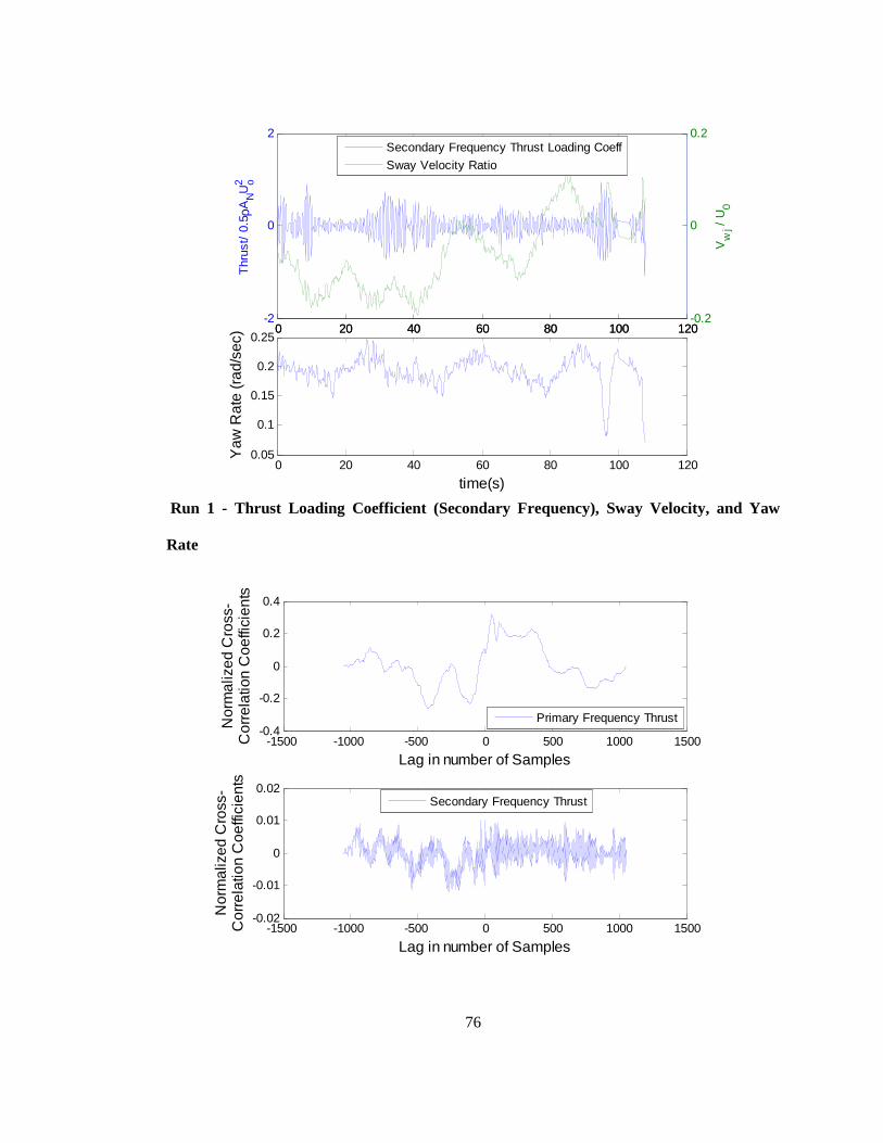
76
Run 1 - Thrust Loading Coefficient (Secondary Frequency), Sway Velocity, and Yaw
Rate
0 20 40 60 80 100 120-2
0
2
Thr
ust/
0.5
ρANU
o2
0 20 40 60 80 100 120-0.2
0
0.2
Vw
j / U
0
Secondary Frequency Thrust Loading Coeff
Sway Velocity Ratio
0 20 40 60 80 100 1200.05
0.1
0.15
0.2
0.25
time(s)
Yaw
Rat
e (r
ad/s
ec)
-1500 -1000 -500 0 500 1000 1500-0.4
-0.2
0
0.2
0.4
Lag in number of Samples
Nor
mal
ized
Cro
ss-
Cor
rela
tion
Coe
ffici
ents
Primary Frequency Thrust
-1500 -1000 -500 0 500 1000 1500-0.02
-0.01
0
0.01
0.02
Lag in number of Samples
Nor
mal
ized
Cro
ss-
Cor
rela
tion
Coe
ffici
ents
Secondary Frequency Thrust

77
Run 1 - Normalized Cross-Correlation Coefficients Between Thrust and Sway Velocity
Run 2
Target Radius: 10 m
Target Speed: 1.5 m/s
Run 2 - GPS Path
185 190 195 200 205 210 215
-10
-5
0
5
10
Meters E of Dock
Met
ers
Nor
th o
f Doc
k
Vehicle Path Waypoints

78
Run 2 - Primary and Secondary Components of Thrust
Run 2 - Vehicle and Local Waterjet Velocities
0 20 40 60 80 100 120 140-20
-10
0
10
20
30
40
50
Time (s)
For
ce (N
)
Primary Frequency Thrust Component
Secondary Frequency Thrust Component
0 20 40 60 80 100 120 140-0.5
0
0.5
1
1.5
2
2.5
time (s)
Vel
ocity
(m/s
)
Vehicle Surge
Vehicle Sway
Vehicle HeaveWaterjet Surge
Waterjet Sway
Waterjet Heave

79
Run 2 - Slip Angle
Run 2 - Thrust Loading Coefficient (Main Frequency), Sway Velocity, and Yaw Rate
0 20 40 60 80 100 120 140-6
-4
-2
0
2
4
6
8
10
12
14
Time (s)
Slip
Ang
le (d
egre
es)
0 20 40 60 80 100 120 140-10
0
10
20
30
Thr
ust/
0.5
ρANU
o2
0 20 40 60 80 100 120 140-0.2
-0.1
0
0.1
0.2
Vw
j / U
0
Primary Frequency Thrust Loading Coeff
Sway Velocity Ratio
0 20 40 60 80 100 120 140-0.2
0
0.2
0.4
0.6
time(s)
Yaw
Rat
e (r
ad/s
ec)

80
Run 2 - Thrust Loading Coefficient (Secondary Frequency), Sway Velocity, and Yaw Rate
Run 2 - Normalized Cross-Correlation Coefficients Between Thrust and Sway Velocity
0 20 40 60 80 100 120 140-2
-1
0
1
2
Thr
ust/
0.5
ρANU
o2
0 20 40 60 80 100 120 140-0.2
-0.1
0
0.1
0.2
Vw
j / U
0
Secondary Frequency Thrust Loading Coeff
Sway Velocity Ratio
0 20 40 60 80 100 120 140-0.2
0
0.2
0.4
0.6
time(s)
Yaw
Rat
e (r
ad/s
ec)
-1500 -1000 -500 0 500 1000 1500-0.4
-0.2
0
0.2
0.4
Lag in number of Samples
Nor
mal
ized
Cro
ss-
Cor
rela
tion
Coe
ffici
ents
Primary Frequency Thrust
-1500 -1000 -500 0 500 1000 1500-0.02
-0.01
0
0.01
0.02
Lag in number of Samples
Nor
mal
ized
Cro
ss-
Cor
rela
tion
Coe
ffici
ents
Secondary Frequency Thrust

81
Test Run 3
Target Radius: 10 m
Target Speed: 2.0 m/s
Run 3 - GPS Path
180 185 190 195 200 205 210 215 220 225
-20
-15
-10
-5
0
5
10
15
Meters E of Dock
Met
ers
Nor
th o
f Doc
k
Vehicle Path Waypoints

82
Run 3 - Primary and Secondary Components of Thrust
Run 3 - Vehicle and Local Waterjet Velocities
0 50 100 150 200 250 300 350-30
-20
-10
0
10
20
30
40
50
Time (s)
For
ce (N
)
Primary Frequency Thrust Component
Secondary Frequency Thrust Component
0 50 100 150 200 250 300 350-0.5
0
0.5
1
1.5
2
2.5
3
time (s)
Vel
ocity
(m/s
)
Vehicle Surge
Vehicle Sway
Vehicle HeaveWaterjet Surge
Waterjet Sway
Waterjet Heave

83
Run 3 - Slip Angle
Run 3 - Thrust Loading Coefficient (Main Frequency), Sway Velocity, and Yaw Rate
0 50 100 150 200 250 300 350-10
0
10
20
30
40
50
Time (s)
Slip
Ang
le (d
egre
es)
0 50 100 150 200 250 300 350-20
0
20
40
Thr
ust/
0.5
ρANU
o2
0 50 100 150 200 250 300 350-0.5
0
0.5
1
Vw
j / U
0
Primary Frequency Thrust Loading Coeff
Sway Velocity Ratio
0 50 100 150 200 250 300 350-0.2
0
0.2
0.4
0.6
time(s)
Yaw
Rat
e (r
ad/s
ec)

84
Run 3 - Thrust Loading Coefficient (Secondary Frequency), Sway Velocity, and Yaw Rate
Run 3 - Normalized Cross-Correlation Coefficients Between Thrust and Sway Velocity
0 50 100 150 200 250 300 350-5
-4
-3
-2
-1
0
1
2
3
4
5
Thr
ust/
0.5
ρANU
o2
0 50 100 150 200 250 300 350-0.2
-0.1
0
0.1
0.2
0.3
0.4
0.5
0.6
0.7
0.8
Vw
j / U
0
Secondary Frequency Thrust Loading Coeff
Sway Velocity Ratio
0 50 100 150 200 250 300 350-0.2
0
0.2
0.4
0.6
time(s)
Yaw
Rat
e (r
ad/s
ec)
-4000 -3000 -2000 -1000 0 1000 2000 3000 4000-0.4
-0.2
0
0.2
0.4
Lag in number of Samples
Nor
mal
ized
Cro
ss-
Cor
rela
tion
Coe
ffici
ents
Primary Frequency Thrust
-4000 -3000 -2000 -1000 0 1000 2000 3000 4000-0.1
-0.05
0
0.05
0.1
Lag in number of Samples
Nor
mal
ized
Cro
ss-
Cor
rela
tion
Coe
ffici
ents
Secondary Frequency Thrust
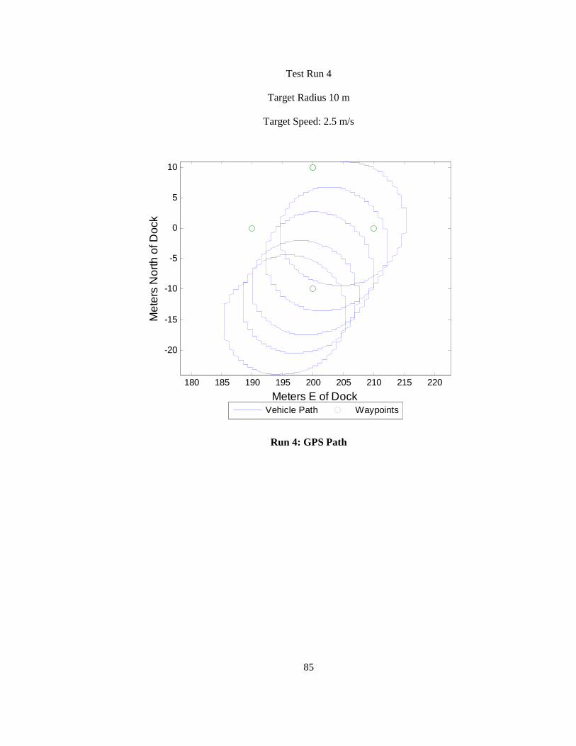
85
Test Run 4
Target Radius 10 m
Target Speed: 2.5 m/s
Run 4: GPS Path
180 185 190 195 200 205 210 215 220
-20
-15
-10
-5
0
5
10
Meters E of Dock
Met
ers
Nor
th o
f Doc
k
Vehicle Path Waypoints

86
Run 4 - Primary and Secondary Components of Thrust
Run 4 - Vehicle and Local Waterjet Velocities
0 20 40 60 80 100 120 140 160-30
-20
-10
0
10
20
30
40
50
Time (s)
For
ce (N
)
Primary Frequency Thrust Component
Secondary Frequency Thrust Component
0 20 40 60 80 100 120 140 160-0.5
0
0.5
1
1.5
2
2.5
time (s)
Vel
ocity
(m/s
)
Vehicle Surge
Vehicle Sway
Vehicle HeaveWaterjet Surge
Waterjet Sway
Waterjet Heave

87
Run 4 - Slip Angle
Run 4 - Thrust Loading Coefficient (Main Frequency), Sway Velocity, and Yaw Rate
0 20 40 60 80 100 120 140 160-10
-5
0
5
10
15
Time (s)
Slip
Ang
le (d
egre
es)
0 20 40 60 80 100 120 140 16010
15
20
25
Thr
ust/
0.5
ρANU
o2
0 20 40 60 80 100 120 140 160-0.4
-0.2
0
0.2
Vw
j / U
0Primary Frequency Thrust Loading Coeff
Sway Velocity Ratio
0 20 40 60 80 100 120 140 1600.1
0.15
0.2
0.25
time(s)
Yaw
Rat
e (r
ad/s
ec)

88
Run 4 - Thrust Loading Coefficient (Secondary Frequency), Sway Velocity, and Yaw Rate
Run 4 - Normalized Cross-Correlation Coefficients Between Thrust and Sway Velocity
0 20 40 60 80 100 120 140 160-2
0
2
Thr
ust/
0.5
ρANU
o2
0 20 40 60 80 100 120 140 160-0.5
0
0.5
Vw
j / U
0
Secondary Frequency Thrust Loading Coeff
Sway Velocity Ratio
0 20 40 60 80 100 120 140 1600.1
0.15
0.2
0.25
time(s)
Yaw
Rat
e (r
ad/s
ec)
-2000 -1500 -1000 -500 0 500 1000 1500 2000-0.5
0
0.5
1
Lag in number of Samples
Nor
mal
ized
Cro
ss-
Cor
rela
tion
Coe
ffici
ents
Primary Frequency Thrust
-2000 -1500 -1000 -500 0 500 1000 1500 2000-0.04
-0.02
0
0.02
0.04
Lag in number of Samples
Nor
mal
ized
Cro
ss-
Cor
rela
tion
Coe
ffici
ents
Secondary Frequency Thrust

89
Run 5
Target Radius: 15 m
Target Speed: 2.0 m/s
Run 5 - GPS Path
180 190 200 210 220 230
-25
-20
-15
-10
-5
0
5
10
15
Meters E of Dock
Met
ers
Nor
th o
f Doc
k
Vehicle Path Waypoints

90
Run 5 - Primary and Secondary Components of Thrust
Run 5 - Vehicle and Local Waterjet Velocities
0 20 40 60 80 100 120 140-20
-10
0
10
20
30
40
50
Time (s)
For
ce (N
)
Primary Frequency Thrust Component
Secondary Frequency Thrust Component
0 20 40 60 80 100 120 140-0.5
0
0.5
1
1.5
2
2.5
time (s)
Vel
ocity
(m/s
)
Vehicle Surge
Vehicle Sway
Vehicle HeaveWaterjet Surge
Waterjet Sway
Waterjet Heave
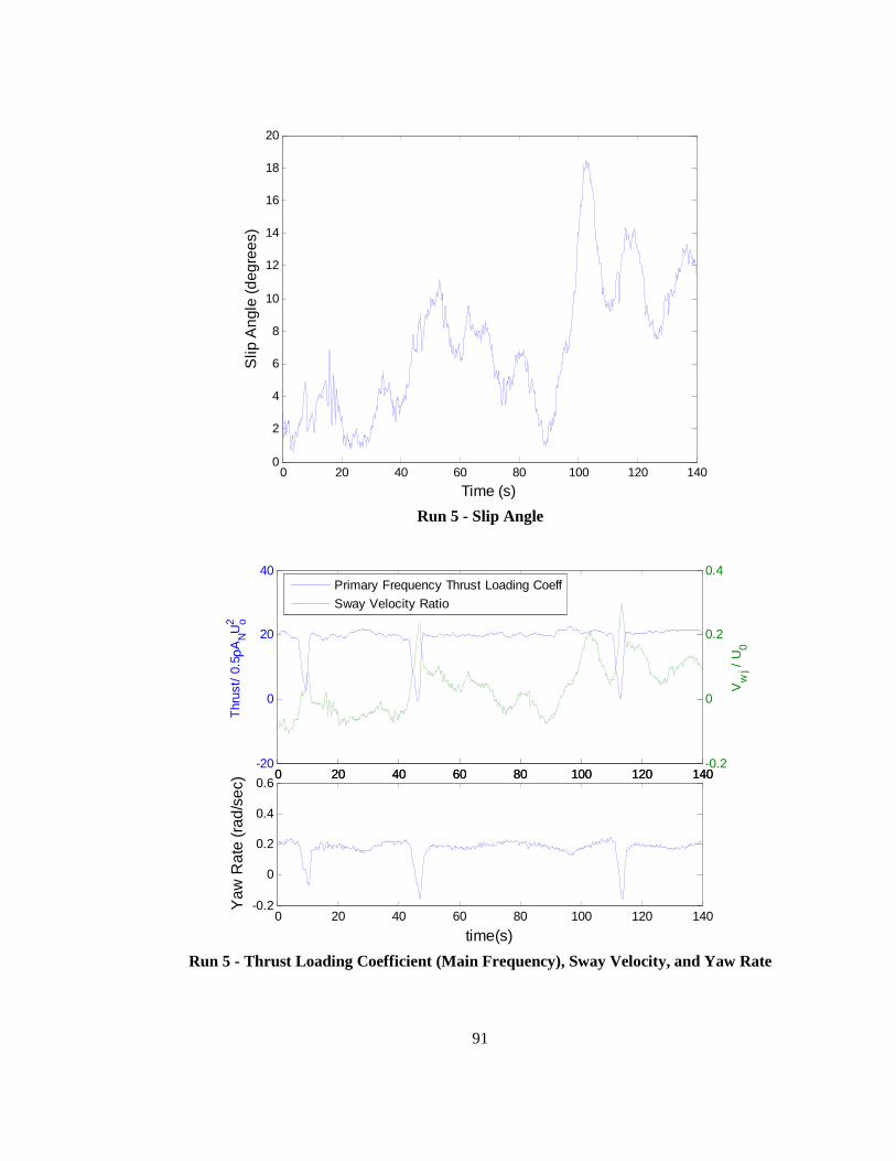
91
Run 5 - Slip Angle
Run 5 - Thrust Loading Coefficient (Main Frequency), Sway Velocity, and Yaw Rate
0 20 40 60 80 100 120 1400
2
4
6
8
10
12
14
16
18
20
Time (s)
Slip
Ang
le (d
egre
es)
0 20 40 60 80 100 120 140-20
0
20
40
Thr
ust/
0.5
ρANU
o2
0 20 40 60 80 100 120 140-0.2
0
0.2
0.4
Vw
j / U
0
Primary Frequency Thrust Loading Coeff
Sway Velocity Ratio
0 20 40 60 80 100 120 140-0.2
0
0.2
0.4
0.6
time(s)
Yaw
Rat
e (r
ad/s
ec)

92
Run 5 - Thrust Loading Coefficient (Secondary Frequency), Sway Velocity, and Yaw Rate
Run 5 - Normalized Cross-Correlation Coefficients Between Thrust and Sway Velocity-
0 20 40 60 80 100 120 140-1.5
-1
-0.5
0
0.5
1
Thr
ust/
0.5
ρANU
o2
0 20 40 60 80 100 120 140-0.2
-0.1
0
0.1
0.2
0.3
Vw
j / U
0
Secondary Frequency Thrust Loading Coeff
Sway Velocity Ratio
0 20 40 60 80 100 120 140-0.2
0
0.2
0.4
0.6
time(s)
Yaw
Rat
e (r
ad/s
ec)
-1500 -1000 -500 0 500 1000 1500-0.4
-0.2
0
0.2
0.4
Lag in number of Samples
Nor
mal
ized
Cro
ss-
Cor
rela
tion
Coe
ffici
ents
Primary Frequency Thrust
-1500 -1000 -500 0 500 1000 1500-0.04
-0.02
0
0.02
Lag in number of Samples
Nor
mal
ized
Cro
ss-
Cor
rela
tion
Coe
ffici
ents
Secondary Frequency Thrust

93
Run 6
Target Radius: 15 m
Target Speed: 2.5 m/s
Run 6 - GPS Path
180 185 190 195 200 205 210 215 220
-15
-10
-5
0
5
10
15
Meters E of Dock
Met
ers
Nor
th o
f Doc
k
Vehicle Path Waypoints

94
Run 6 - Primary and Secondary Components of Thrust
Run 6 - Vehicle and Local Waterjet Velocities
0 50 100 150-40
-20
0
20
40
60
80
Time (s)
For
ce (N
)
Primary Frequency Thrust Component
Secondary Frequency Thrust Component
0 50 100 150-0.5
0
0.5
1
1.5
2
2.5
time (s)
Vel
ocity
(m/s
)
Vehicle Surge
Vehicle Sway
Vehicle HeaveWaterjet Surge
Waterjet Sway
Waterjet Heave
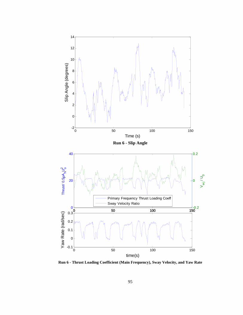
95
Run 6 - Slip Angle
Run 6 - Thrust Loading Coefficient (Main Frequency), Sway Velocity, and Yaw Rate
0 50 100 150-2
0
2
4
6
8
10
12
14
Time (s)
Slip
Ang
le (d
egre
es)
0 50 100 1500
20
40
Thr
ust/
0.5
ρANU
o2
0 50 100 150-0.2
0
0.2
Vw
j / U
0
Primary Frequency Thrust Loading Coeff
Sway Velocity Ratio
0 50 100 150-0.1
0
0.1
0.2
0.3
time(s)
Yaw
Rat
e (r
ad/s
ec)

96
Run 6 - Thrust Loading Coefficient (Secondary Frequency), Sway Velocity, and Yaw Rate
Run 6 - Normalized Cross-Correlation Coefficients Between Thrust and Sway Velocity
0 50 100 150-3
-2
-1
0
1
2
3
Thr
ust/
0.5
ρANU
o2
0 50 100 150-0.2
-0.1
0
0.1
0.2
Vw
j / U
0
Secondary Frequency Thrust Loading Coeff
Sway Velocity Ratio
0 50 100 150-0.1
0
0.1
0.2
0.3
time(s)
Yaw
Rat
e (r
ad/s
ec)
-1500 -1000 -500 0 500 1000 1500-0.5
0
0.5
Lag in number of Samples
Nor
mal
ized
Cro
ss-
Cor
rela
tion
Coe
ffici
ents
Primary Frequency Thrust
-1500 -1000 -500 0 500 1000 1500-0.1
-0.05
0
0.05
0.1
Lag in number of Samples
Nor
mal
ized
Cro
ss-
Cor
rela
tion
Coe
ffici
ents
Secondary Frequency Thrust

97
Run 7
Target Radius: 20 m
Target Speed: 2.0 m/s
Run 7 - GPS Path
180 190 200 210 220-20
-15
-10
-5
0
5
10
15
20
Meters E of Dock
Met
ers
Nor
th o
f Doc
k
Vehicle Path Waypoints

98
Run 7 - Primary and Secondary Components of Thrust
Run 7 - Vehicle and Local Waterjet Velocities
0 20 40 60 80 100 120 140 160 180 200-20
-10
0
10
20
30
40
50
60
Time (s)
For
ce (N
)
Primary Frequency Thrust Component
Secondary Frequency Thrust Component
0 20 40 60 80 100 120 140 160 180 200-0.5
0
0.5
1
1.5
2
2.5
time (s)
Vel
ocity
(m/s
)
Vehicle Surge
Vehicle Sway
Vehicle HeaveWaterjet Surge
Waterjet Sway
Waterjet Heave

99
Run 7 - Slip Angle
Run 7 - Thrust Loading Coefficient (Main Frequency), Sway Velocity, and Yaw Rate
0 20 40 60 80 100 120 140 160 180 200-4
-2
0
2
4
6
8
10
Time (s)
Slip
Ang
le (d
egre
es)
0 20 40 60 80 100 120 140 160 180 200-20
0
20
40
Thr
ust/
0.5
ρANU
o2
0 20 40 60 80 100 120 140 160 180 200-0.2
0
0.2
0.4
Vw
j / U
0
Primary Frequency Thrust Loading Coeff
Sway Velocity Ratio
0 20 40 60 80 100 120 140 160 180 200-0.2
0
0.2
0.4
0.6
time(s)
Yaw
Rat
e (r
ad/s
ec)

100
Run 7 - Thrust Loading Coefficient (Secondary Frequency), Sway Velocity, and Yaw Rate
Run 7 - Normalized Cross-Correlation Coefficients Between Thrust and Sway Velocity
0 20 40 60 80 100 120 140 160 180 200
0
Thr
ust/
0.5
ρANU
o2
0 20 40 60 80 100 120 140 160 180 200-0.5
0
0.5
Vw
j / U
0
Secondary Frequency Thrust Loading Coeff
Sway Velocity Ratio
0 20 40 60 80 100 120 140 160 180 200-0.2
-0.1
0
0.1
0.2
0.3
time(s)
Yaw
Rat
e (r
ad/s
ec)
-2000 -1500 -1000 -500 0 500 1000 1500 2000-1
-0.5
0
0.5
Lag in number of Samples
Nor
mal
ized
Cro
ss-
Cor
rela
tion
Coe
ffici
ents
Primary Frequency Thrust
-2000 -1500 -1000 -500 0 500 1000 1500 2000-0.1
-0.05
0
0.05
0.1
Lag in number of Samples
Nor
mal
ized
Cro
ss-
Cor
rela
tion
Coe
ffici
ents
Secondary Frequency Thrust

101
Run 8
Target Radius: 20 m
Target Speed: 2.5 m/s
Run 8 - GPS Path
180 190 200 210 220
-20
-15
-10
-5
0
5
10
15
20
Meters E of Dock
Met
ers
Nor
th o
f Doc
k
Vehicle Path Waypoints

102
Run 8 - Primary and Secondary Components of Thrust
Run 8 - Vehicle and Local Waterjet Velocities
0 20 40 60 80 100 120 140 160-20
-10
0
10
20
30
40
50
Time (s)
For
ce (N
)
Primary Frequency Thrust Component
Secondary Frequency Thrust Component
0 20 40 60 80 100 120 140 160-0.5
0
0.5
1
1.5
2
2.5
time (s)
Vel
ocity
(m/s
)
Vehicle Surge
Vehicle Sway
Vehicle HeaveWaterjet Surge
Waterjet Sway
Waterjet Heave

103
Run 8 - Slip Angle
Run 8 - Thrust Loading Coefficient (Main Frequency), Sway Velocity, and Yaw Rate
0 20 40 60 80 100 120 140 160-4
-2
0
2
4
6
8
10
Time (s)
Slip
Ang
le (d
egre
es)
0 20 40 60 80 100 120 140 1600
10
20
Thr
ust/
0.5
ρANU
o2
0 20 40 60 80 100 120 140 160-0.2
0
0.2
Vw
j / U
0Primary Frequency Thrust Loading Coeff
Sway Velocity Ratio
0 20 40 60 80 100 120 140 160-0.1
0
0.1
0.2
0.3
time(s)
Yaw
Rat
e (r
ad/s
ec)

104
Run 8 - Thrust Loading Coefficient (Secondary Frequency), Sway Velocity, and Yaw Rate
Run 8 - Normalized Cross-Correlation Coefficients Between Thrust and Sway Velocity
0 20 40 60 80 100 120 140 160-1
-0.5
0
0.5
1
Thr
ust/
0.5
ρANU
o2
0 20 40 60 80 100 120 140 160-0.2
-0.1
0
0.1
0.2
Vw
j / U
0
Secondary Frequency Thrust Loading Coeff
Sway Velocity Ratio
0 20 40 60 80 100 120 140 160-0.1
0
0.1
0.2
0.3
time(s)
Yaw
Rat
e (r
ad/s
ec)
-2000 -1500 -1000 -500 0 500 1000 1500 2000-0.5
0
0.5
Lag in number of Samples
Nor
mal
ized
Cro
ss-
Cor
rela
tion
Coe
ffici
ents
Primary Frequency Thrust
-2000 -1500 -1000 -500 0 500 1000 1500 2000-0.02
-0.01
0
0.01
0.02
Lag in number of Samples
Nor
mal
ized
Cro
ss-
Cor
rela
tion
Coe
ffici
ents
Secondary Frequency Thrust

105
Run 9
Target Radius: 25 m
Target Speed: 2.0 m/s
Run 9 - GPS Path
170 180 190 200 210 220 230
-20
-15
-10
-5
0
5
10
15
20
25
Meters E of Dock
Met
ers
Nor
th o
f Doc
k
Vehicle Path Waypoints

106
Run 9 - Primary and Secondary Components of Thrust
Run 9 - Vehicle and Local Waterjet Velocities
0 20 40 60 80 100 120 140-20
-10
0
10
20
30
40
50
60
Time (s)
For
ce (N
)
Primary Frequency Thrust Component
Secondary Frequency Thrust Component
0 20 40 60 80 100 120 140-0.5
0
0.5
1
1.5
2
2.5
time (s)
Vel
ocity
(m/s
)
Vehicle Surge
Vehicle Sway
Vehicle HeaveWaterjet Surge
Waterjet Sway
Waterjet Heave

107
Run 9 - Slip Angle
Run 9 - Thrust Loading Coefficient (Main Frequency), Sway Velocity, and Yaw Rate
0 20 40 60 80 100 120 140-6
-4
-2
0
2
4
6
8
Time (s)
Slip
Ang
le (d
egre
es)
0 20 40 60 80 100 120 140-20
0
20
40
Thr
ust/
0.5
ρANU
o2
0 20 40 60 80 100 120 140-0.1
0
0.1
0.2
Vw
j / U
0
Primary Frequency Thrust Loading Coeff
Sway Velocity Ratio
0 20 40 60 80 100 120 140-0.2
-0.1
0
0.1
0.2
time(s)
Yaw
Rat
e (r
ad/s
ec)

108
Run 9 - Thrust Loading Coefficient (Secondary Frequency), Sway Velocity, and Yaw Rate
Run 9 - Normalized Cross-Correlation Coefficients Between Thrust and Sway Velocity
0 20 40 60 80 100 120 140-2
0
2
Thr
ust/
0.5
ρANU
o2
0 20 40 60 80 100 120 140-0.2
0
0.2
Vw
j / U
0
Secondary Frequency Thrust Loading Coeff
Sway Velocity Ratio
0 20 40 60 80 100 120 140-0.2
-0.1
0
0.1
0.2
time(s)
Yaw
Rat
e (r
ad/s
ec)
-1500 -1000 -500 0 500 1000 1500-0.5
0
0.5
Lag in number of Samples
Nor
mal
ized
Cro
ss-
Cor
rela
tion
Coe
ffici
ents
Primary Frequency Thrust
-1500 -1000 -500 0 500 1000 1500-0.04
-0.02
0
0.02
0.04
Lag in number of Samples
Nor
mal
ized
Cro
ss-
Cor
rela
tion
Coe
ffici
ents
Secondary Frequency Thrust

109
Run 10
Target Radius: 25 m
Target Speed: 2.5 m/s
Run 10 - GPS Path
170 180 190 200 210 220 230-25
-20
-15
-10
-5
0
5
10
15
20
25
Meters E of Dock
Met
ers
Nor
th o
f Doc
k
Vehicle Path Waypoints

110
Run 10 -Primary and Secondary Frequency Thrust Components
Run 10 - Vehicle and Local Waterjet Velocities
0 20 40 60 80 100 120 140 160 180 200-10
0
10
20
30
40
50
Time (s)
For
ce (N
)
Primary Frequency Thrust Component
Secondary Frequency Thrust Component
0 20 40 60 80 100 120 140 160 180 200-0.5
0
0.5
1
1.5
2
2.5
time (s)
Vel
ocity
(m/s
)
Vehicle Surge
Vehicle Sway
Vehicle HeaveWaterjet Surge
Waterjet Sway
Waterjet Heave

111
Run 10 - Slip Angle
Run 10 - Thrust Loading Coefficient (Main Frequency), Sway Velocity, and Yaw Rate
0 20 40 60 80 100 120 140 160 180 200-4
-2
0
2
4
6
8
Time (s)
Slip
Ang
le (d
egre
es)
0 20 40 60 80 100 120 140 160 180 2005
10
15
20
Thr
ust/
0.5
ρANU
o2
0 20 40 60 80 100 120 140 160 180 200-0.2
-0.1
0
0.1
Vw
j / U
0Primary Frequency Thrust Loading Coeff
Sway Velocity Ratio
0 20 40 60 80 100 120 140 160 180 200-0.1
0
0.1
0.2
0.3
time(s)
Yaw
Rat
e (r
ad/s
ec)

112
Run 10 - Thrust Loading Coefficient (Secondary Frequency), Sway Velocity, and Yaw
Rate
Run 10 - Normalized Cross-Correlation Coefficients Between Thrust and Sway Velocity
0 20 40 60 80 100 120 140 160 180 200-1.5
-1
-0.5
0
0.5
1
1.5
Thr
ust/
0.5
ρANU
o2
0 20 40 60 80 100 120 140 160 180 200-0.2
-0.15
-0.1
-0.05
0
0.05
0.1
Vw
j / U
0
Secondary Frequency Thrust Loading Coeff
Sway Velocity Ratio
0 20 40 60 80 100 120 140 160 180 200-0.1
0
0.1
0.2
0.3
time(s)
Yaw
Rat
e (r
ad/s
ec)
-2000 -1500 -1000 -500 0 500 1000 1500 2000-0.5
0
0.5
Lag in number of Samples
Nor
mal
ized
Cro
ss-
Cor
rela
tion
Coe
ffici
ents
Primary Frequency Thrust
-2000 -1500 -1000 -500 0 500 1000 1500 2000-0.05
0
0.05
Lag in number of Samples
Nor
mal
ized
Cro
ss-
Cor
rela
tion
Coe
ffici
ents
Secondary Frequency Thrust

113
APPENDIX E - DESCRIPTION OF MOMENTUM FLUX METHOD
Figure E-1: Section Lines and Control Volume [5]
Figure E-1 above describes of the control volume designated by the ITTC for
use in momentum flux calculations and also defines several stations of interest. The
control volume is defined by the stream tube between station 1A and station 6. The
boundaries of the control volume consist primarily of the ducting of the jet, but also
includes the face of the nozzle (station 6), the capture area (Designated as A1 located at
station 1A), and the dividing stream line forward of the inlet opening which no mass
flow crosses (designated A2). The nozzle was used instead of the vena contracta
because the ITTC assumes that “in the vast majority of cases, the diameter of the vena
contracta is approximately the same as the nozzle diameter.” Additionally, the nozzle
diameter can be measured accurately while the vena contract is difficult to measure.
As stated in Newton's Second Law, the change in momentum flux over a control
volume equals the net forces acting on that control volume. In the case where the

114
nozzle is either completely immersed or completely ventilated this can be expressed as:
Equation 1
��� = ���� Using the given definitions for the boundaries of the control volume allows us to
define the change in momentum flux using stations 1A and 6.
Equation 2
Δ��� = ���� −����
The Momentum flux at station 6 can be obtained from a flow rate measurement
that has been calibrated to the thrust measured during a bollard pull experiment, which
is designated as the jet thrust.
Equation 3
���� = ���
The momentum flux ingested by the waterjet can be defined as the using the
velocity profile at the capture area A1.
Equation 4
���� =������
!�
This can also be determined by the flow rate and the ship velocity V0 using the
given relationship.
Equation 5
���� = �"�#$�%

115
Where #$� is defined as the momentum velocity coefficient at station 1 which
by definition is:
#$� = 1&'1 − �(�)"�%
* ���!��
And where �( is the local pressure coefficient.
�( = + − +0.5�%�
This is then enough information to calculate the net thrust of the waterjet
system. There are other thrust deduction coefficients involved which allow you to
compare this to the hull resistance and a series of efficiencies can be derived which
allow for the comparison between of models and prototypes.

116
APPENDIX F - WIRING DIAGRAMS
Cooling
Pump
60V 10A
Crydom
Solid State Relay3+ 4-
1+2-
Battery12V 1.2Ah
NiCad
+ -
KILL +
KILL -
Manual
Switch
+
-
Figure F-1 - Cooling System Wiring Diagram

117
From Electronics Box
Figure F-2 - Motor Circuit Wiring Diagram

118
APPENDIX G - CENTER OF GRAVITY CALCULATIONS AND
VERIFICATION
Preliminary estimates of the location of the center of gravity of the vehicle were
performed by recording the masses and centers for individual components and
identifying their location relative to a common reference point. For purposes of the
following calculations, the origin of the coordinate system is located at the intersection
of the centerline of the vehicle, the plane of the bottom of the pontoons, and the back
plane of the pontoons where the motor pods connect.

119
Vehicle Calculations
Vehicle
Weight
(lbs) LCG (in) VCG (in)
Bare Hull 90 36 13.21
Engine Pods 106 -18 4
Vehicle Total 196 6.80 8.23
Cargo Area Calculations
Cargo Area Components
Weight
(lbs) LCG (in) VCG (in)
Strobe Light
Light 1.5 -4.5 27
Mounting Bracket 3.9 0 25
Batteries 0 0 25
Strobe Light Total 5.4 -1.25 25.56
Control Box 30 26 26
Data Logging Box
Data Logging Box (empty) 8.25 39 31.5
Laptop 3 39 31
Force Transducer Amplifier 4.5 39 31
battery 1.6875 39 31
cDAQ 1.8125 39 31
Data Box Total 19.25 39 31.21
Cargo Area Total 54.65 27.89 27.80
Total Vehicle
Total
Weight
(lbs) LCG (in) VCG (in)
Vehicle Total 196 6.80 8.23
Cargo 54.65 27.89 27.80
TOTAL 250.65 11.40 12.50
Table G-1: Center of Gravity Estimation
After the estimation was performed, the location of the center of gravity was
confirmed by loading the vehicle with all equipment that would be mounted on the
vehicle for the actual experiments. The only exception to this was that the force

120
transducer was replaced with a blank of equal mass to prevent damage to the transducer.
During normal operation, the pods are held in an horizontal orientation by their
buoyancy and an elastic strap. To maintain the same orientation as during testing, a
rope loop was placed in place of the elastic strap.
The vehicle was then connected to the cable of a davit. Two different lifting
points were used and the angle that the vehicle made with respect to the cable. Using
the geometric relation between these two points, the center of gravity could then be
determined relative to the lifting points.
Figure G-1: Geometric Relation Between Two Lifting Points
and the Center of Gravity
Lifting Point 1
Lifting Point 2

121
The reference point for the hang test estimates for the center of gravity were
then compared to the reference point for the initial estimates. It was determined that the
initial estimates correlation well with the measured center of gravity of the vehicle.

122
REFERENCES
[1] ITTC, "Report of Specialist Committee on Validation of Waterjet Test
Procedures," 1999.
[2] J. Allison, "Marine Waterjet Propulsion," SNAME Transactions, pp. 275-335,
1993.
[3] O. M. Faltinsen, Hydrodynamics of High Speed Marine Vehicles, New York:
Cambridge University Press, 2005.
[4] ITTC Procedures, "Waterjets, Propulsive Performance Prediction (7.5-02-05-
03.1)," Recommended Procedures and Guidelines, 2005.
[5] ITTC, "Report of Specialist Committee on Validation of Waterjet Test
Procedures," in ITTC Proc of 24th ITTC, 2005.
[6] W.-G. Park, J. H. Jang, H. H. Chun and M. C. Kim, "Numerical flow and
performance analysis of waterjet propulsion system," Ocean Engineering, pp.
1740-1761, 2005.
[7] K. D. von Ellenrieder, "Free Running Tests of a Waterjet Propelled Unmanned
Surface Vehicle," Journal of Marine Engineering Technology, vol. 12, no. 1,
January 2013.
[8] K. von Ellenrieder, "Design and Instrumentation for Direct Thrust Measurements

123
from a Waterjet Propelled Unmanned Suface Vehicle," T-Craft Tools Review
Meeting, 2011.
[9] E. O. D. C. M. Albert S. Huang, "LCM: Lightweight Communications and
Marshalling," in Proc. Int. Conf. on Inteligent Robots and System (IROS), Taipei,
Taiwan, 2010.
[10] ITTC, "Report of Specialist Committee on Validation of Waterjet Test
Procedures," in ITTC Proc of 23rd ITTC, 2002.
[11] K. von Ellenrieder, "Experimental Testing of a Waterjet Propulsion System,"
TCraft Tools Review Meeting (Presenetation), 2012.
[12] T. I. Fossen, Guidance and Control of Ocean Vehicles, West Sussex, England:
John Wiley and Sons, Ltd, 1999.


