University of Illinois at Urbana-ChampaignBeckman Institute for Advanced Science and TechnologyTheoretical and Computational Biophysics Group

Simulation of WaterPermeation Through

Nanotubes

Jordi CohenFangqiang Zhu

Emad TajkhorshidCurrent editor:Zhijian Huang

February 2012

Please visit www.ks.uiuc.edu/Training/Tutorials/ to get the latest version of this

tutorial, to obtain more tutorials like this one, or to join the

tutorial-l@ks.uiuc.edu mailing list for additional help.

Contents

1 Initial Setup 3

2 Description of the system 3

3 Water diffusion and permeation through nanotubes 53.1 Submit your simulation . . . . . . . . . . . . . . . . . . . . . . . 63.2 Water diffusion in equilibrium . . . . . . . . . . . . . . . . . . . . 73.3 Simulation with induced pressure difference . . . . . . . . . . . . 83.4 Water properties in modified nanotubes . . . . . . . . . . . . . . 10

4 “Decorating” the nanotubes 114.1 Running a simulation with AutoIMD . . . . . . . . . . . . . . . . 114.2 Modifying the charges . . . . . . . . . . . . . . . . . . . . . . . . 144.3 Experimenting with different charge configurations . . . . . . . . 154.4 Modifying the VdW parameters . . . . . . . . . . . . . . . . . . . 164.5 Experimenting with VdW parameters . . . . . . . . . . . . . . . 18

2

1 Initial Setup

In order to complete this tutorial, you will be required to have up-to-date ver-sions of the following software, properly installed on your computer:

• VMD www.ks.uiuc.edu/Research/vmd/

– You will need to install VMD 1.8.4 or later.

• NAMD www.ks.uiuc.edu/Research/namd

• a text editor of your choice (we offer a few easy-to-use recommendations):

– UNIX: nedit (www.nedit.org)

– Windows XP: NotePad (included with OS)

– Mac OS X: TextEdit (included with OS)

• a command prompt, such as a terminal in UNIX, Terminal.app in Mac OS X,or the DOS command prompt (found under Accessories) in Windows.

If you downloaded the tutorial from the web, the files that you will be needingcan be found in a directory called files. If you got the files through a workshop,they can be found in the ∼/Workshop/nanotubes-tutorial directory. In therest of this tutorial, we will refer to this directory as the nanotubes-tutorialworking directory.

In a Terminal window, you can move to this directory by typing:

cd <path to nanotubes-tutorial working directory >

You can list the content of this directory, by using the command:

ls, in a UNIX or Mac OS X terminal, ordir, at the Windows command prompt.

2 Description of the system

In the following exercises, you will be investigating the permeation of waterthrough nanotubes, as a model for transmembrane permeation of substratesthrough channels. Before starting the simulations and analyzing them, let’shave a look at the system that you will be using for your exercises. For thesimulations you will be using a set of four nanotubes arranged side by side thatseparates two layers of water. This is, in fact, your unit cell, and in actualsimulations will be replicated in three dimensions using periodic boundary

3

conditions (PBC).

1. Start VMD, and load a new molecule with the files nanotubes.psf andnanotubes.pdb, located in the nanotubes-tutorial working directory. Youshould see four nanotubes arranged in a membrane with water on both sides.This is your unit cell. The dimensions of the unit cell are 24.07 by 20.85 by34.00 A3.

We now wish to see what the periodic system will look like (since the NAMDsimulation will be using periodic boundary conditions).

2. In VMD, open the TkCon console (from the Extensions menu), and set theperiodic cell dimensions by typing:

molinfo top set a 24.07molinfo top set b 20.85molinfo top set c 34.

a, b and c refer to the periodic cell dimensions in x, y and z, respectively. Theabove commands tell VMD the dimensions of the periodic cell that you are using.

3. Replace the current representation to only show the nanotubes. Open theRepresentations window and enter carbon for the text selection, and VdW forthe Drawing Method. Then choose the Display → Reset View menu item in theMain window. You should now see a top view of the nanotubes.

4. Now click on the Periodic tab in the Representation window. Making surethat your “carbon” representation is selected, click on the +X, -X, +Y and -Y checkboxes to display more unit cells. Your molecule should now resembleFig. 1.

Figure 1: The simulated nanotube array.

5. Now rotate the system sideways, uncheck all the ±X and ±Y checkboxes,and check the ±Z boxes instead.

4

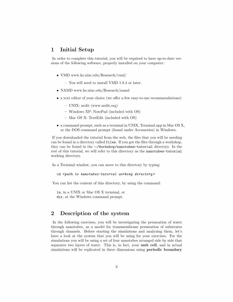
6. Add a water representation and make it periodic in Z as well, just like youpreviously did for the carbon nanotubes. Your molecule should now resembleFig. 2.

Figure 2: The layers of nanotubes and water in the simulation.

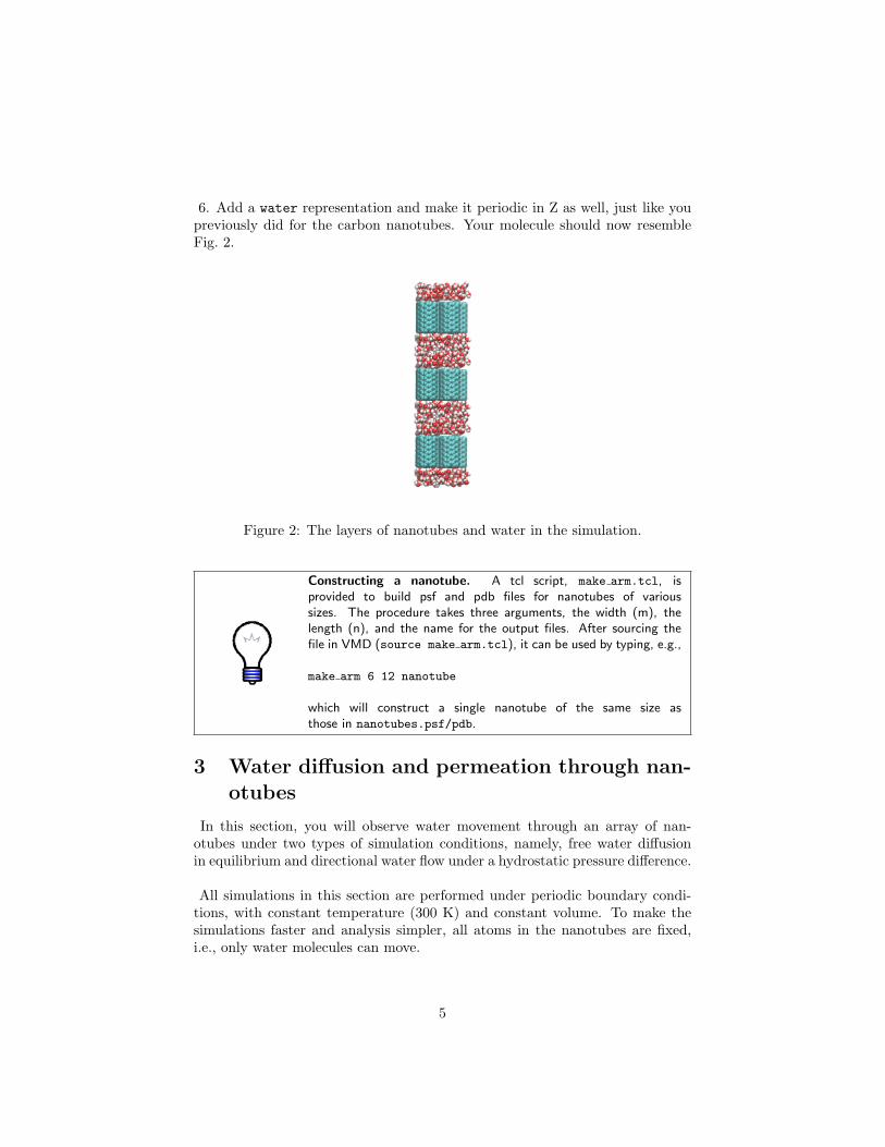
Constructing a nanotube. A tcl script, make arm.tcl, isprovided to build psf and pdb files for nanotubes of varioussizes. The procedure takes three arguments, the width (m), thelength (n), and the name for the output files. After sourcing thefile in VMD (source make arm.tcl), it can be used by typing, e.g.,

make arm 6 12 nanotube

which will construct a single nanotube of the same size asthose in nanotubes.psf/pdb.

3 Water diffusion and permeation through nan-otubes

In this section, you will observe water movement through an array of nan-otubes under two types of simulation conditions, namely, free water diffusionin equilibrium and directional water flow under a hydrostatic pressure difference.

All simulations in this section are performed under periodic boundary condi-tions, with constant temperature (300 K) and constant volume. To make thesimulations faster and analysis simpler, all atoms in the nanotubes are fixed,i.e., only water molecules can move.

5

For water diffusion, you will look at a 3 ns equilibrium MD simulation that hasbeen provided to you in the form of an already computed NAMD trajectory.Using this trajectory, you will look at water orientation in the nanotubes aswell as water diffusion through the nanotubes. Then you will perform anothertype of simulation, where a hydrostatic pressure difference is induced throughthe application of forces on some water molecules. In this simulation you willbe able to observe a directional water flow through the nanotubes. You willrun a short simulation (40 ps) of this type yourself, but we have also provided alonger trajectory (1 ns), which you can use for your analysis. Finally, you willlook at a 1 ns MD trajectory of modified nanotubes (with charges assigned to afew atoms), and find out whether the water in the nanotubes behaves differently.

3.1 Submit your simulation

Here, you will submit and start a simulation. The details of the simulation andhow you will analyze it will be explained in a later section. Since the simulationwill take some time to finish, you need to submit it now so that when you reachanalysis of the results, your simulation will be completed.

The following files will be used for your NAMD jobcnt.psfcnt.pdbpar all27 prot lipid.prminitial.coorinitial.velsim short.conf

1. Make sure you are in the nanotubes-tutorial working directory, using cdor dir in a terminal window.

2. Run the NAMD job. In the same terminal window, type:

namd2 sim short.conf

Windows users: Instead of typing “namd2”, you will need to specify the fullpath to NAMD, depending on where you installed it. For example, if you in-stalled namd2 in C:\NAMD\, you would type: C:\NAMD\namd2 sim short.conf

You should now see NAMD’s output indicating that the job is running. Nowlet’s move to the next section. You will come back to this job and analyze theresults after it has finished.

6

3.2 Water diffusion in equilibrium

Here, you will look closely at a long (3 ns) trajectory of an MD simulationin equilibrium, which shows free water diffusion through the nanotubes. Therespective simulation has been already computed and the results are providedto you in the nanotubes working directory.

1. In VMD, delete the molecule that you loaded in the previous section, andcreate a new molecule by loading the files cnt.psf and eq.dcd. Loading thetrajectory might take a minute or two.

2. Create different representations for nanotubes and water. You can use atomselections carbon and water, for nanotubes and water, respectively. Feel freeto choose your favorite Drawing Method and Coloring Method for these repre-sentations.

3. Observe water orientation inside the nanotubes. Also look at how the watermolecules are aligned. You should find that water molecules in the same nan-otube are all aligned along the same direction (i.e., either all with their O atomsup and H atoms down, or all with H atoms up and O atoms down). Think aboutwhy they prefer such a concerted alignment. Play the trajectory with the VMDanimation controls, and see whether the orientation remains stable during thesimulation. In particular, did you observe any flipping of their orientation? (Ifyes, how many times?)

4. Observe single file water diffusion. To identify individual water molecules,you can label a couple of them in a nanotube (choose Mouse → Label → Atomsin VMD). Now play the trajectory. How do water molecules move with respectto each other? Is any water molecule ever found to pass another one in the nan-otube? Otherwise do they always move in concert? Also look at the directionof the water movement in nanotubes. Does it move back and forth, just likeone-dimensional Brownian motion?

5. Observe permeation events. A permeation event is defined as a watermolecule entering from one end of a nanotube and leaving the other end, there-fore traversing the entire length of the nanotube. Can you find some of thepermeation events in the trajectory? Obviously, it is a tedious job to find allof them in a long trajectory. So we provide a script, permeation.tcl, to helpyou. To use the script in VMD, you should first make sure that the trajectoryto be analyzed is the “top” molecule. Then open the TkCon window in VMDand after making sure you are in the files directory, type into the window:

source permeation.tcl

NOTE: While the script is running, VMD may appear to freeze and not respondto other commands. Depending on your machine, this may take 10-30 seconds.

7

The script will list the resid number of all the water molecules permeatingthrough the nanotubes, the frame at which the permeation event completes,and its direction into the TKCon window. You can pick a few water moleculesfrom the list, and check whether they have indeed completed the permeationevent as reported by the script. In the last two lines of the output, the scriptalso tells you the total number of permeation events in each direction. Are thetwo numbers close to each other, as would be expected?

Some additional details: You won’t find any permeation events in the verybeginning (say, the first 200 ps) of the trajectory. This is because for watermolecules initially inside a nanotube, you don’t know from which end of thenanotube they had entered. Consequently, when they leave the nanotubes, nopermeation event can be counted. Therefore, for quantitative study, the begin-ning portion of the trajectory is usually excluded from statistics. In your case,the numbers of permeation events reported by the script permeation.tcl donot include those in the first 500 frames (500 ps), thus are actually for perme-ation events within the last 2.5 ns of the simulation.

6. After all of the above steps are done, delete the molecule from VMD, sinceit takes up a significant amount of memory in your machine.

3.3 Simulation with induced pressure difference

Now you will come back to the simulation that you submitted at the beginning.First, let’s learn something about the background and motivation for this typeof simulation.

In experiments, a typical method to study water channels is to set up differentconcentrations of (impermeable) solutes on the two sides of the channel, thusgiving rise to an osmotic pressure difference, and to measure the net directionalwater flux. Obviously, the relationship between the water flux and the osmoticpressure difference cannot be studied by equilibrium simulations.

It is known that an osmotic pressure is equivalent to a hydrostatic pressure.Therefore, if one can generate a hydrostatic pressure difference in MD simu-lations, one could mimic the experiments mentioned above. This can be doneby applying a constant force along the z direction on a layer of bulk watermolecules. The force will induce a pressure gradient in the bulk water layer,which results in a pressure difference on the two sides of the nanotubes due tothe periodic boundary conditions (refer to Fig. 2). One appealing feature of thismethod is that the amount of pressure difference can be easily calculated andtuned, thus the results can be compared to experiments quantitatively.

8

In the submitted simulation, a constant force of 0.4 Kcal/mol/A along the+z direction was applied to a 5.4 A-thick water layer. In every time step ofthe simulation, the force will be applied to the O atoms of water moleculeswhose coordinates (in the unit cell of the periodic system) satisfy z > 12.5A orz < −12.5A. This is a fairly large force, but it is needed to induce a very fastwater flux that can be observed in a very short simulation time (practically youcan only afford a 40 ps simulation for the purpose of this tutorial). You maytake a few moment to inspect the NAMD configuration file sim short.conf forthis simulation.

1. Check whether the simulation has already finished. If not, wait a few min-utes for it to finish (after 40,000 steps).

2. In VMD, create a new molecule with the files cnt.psf and sim short.dcd(the DCD file generated by your simulation).

3. Play the trajectory and observe the water flow. Since water molecules inthe nanotubes move concertedly, you can label any of them in a nanotube, andits movement will indicate the movement of the whole water chain. Did you ob-serve the drift of the water chains toward +z direction in the trajectory? Whatis the net water flow through the nanotubes during this simulation?

NOTE: The net water flow is in general different from the number of perme-ation events. For example, when each water molecule moves one step in thesingle file, effectively a water molecule is transferred, thus resulting in a netwater flow of one water molecule, although this move may not cause a perme-ation event. In the equilibrium simulation you looked at earlier, there was littlenet water flow, although you observed a lot of permeation events. In contrast,here in the present (short) trajectory, you might not see any individual watermolecule crossing all the way through the nanotubes, but you can observe a di-rectional water flow.

The trajectory of your simulation (40 ps) is too short for good statistics. There-fore, here we provide to you another trajectory, which was run at exactly thesame conditions as the simulation you ran, except that this one is longer (1 ns),which allows you to observe more water flow.

4. In VMD, delete all the frames of the current molecule (which should becnt.psf), by going to Molecule → Delete Frames → Delete. Then load into theDCD file sim.dcd, by first selecting the cnt.psf molecule and then calling theFile → Load Data Into Molecule... menu item.

5. Observe the water flow in the long trajectory. Since the total water flowis fairly large, it will be too tedious to count it by hand. Therefore, we haveprovided to you a script, flow.tcl, to count the water flow. In VMD, makesure that the 1 ns trajectory is the “top” molecule, and then type in the TKCon

9

window source flow.tcl. The script will report the amount of net water flowand its direction.

NOTE: While the script is running, VMD will freeze and will not respond toother commands. Depending on your machine, this may take 10-20 seconds.

Exercise: Can you calculate the hydrostatic pressure difference in this sim-ulation? The pressure difference is ∆P = nf/A. Here you know that f is0.4 Kcal/mol/A, the unit cell of the periodic system has dimensions of 23 A×19.9 A× 30.4 A, and n, the number of water molecules in the 5.4 A-thick layer(water molecules on which you are applying force), can be roughly estimatedby the volume of the layer and the molar volume of water (55.5 mol/l). Whatis your calculated pressure difference? How does it compare to one atmosphere(105 Pa)? Now you may realize how “hard” it is to induce a significant waterflow within 40 ps.

6. You may also look at water orientation in the nanotubes as water is beingconducted. Does the fast flow alter the water orientation that you had observedin the equilibrium case?

3.4 Water properties in modified nanotubes

So far, you have been looking at uncharged nanotubes. Now you will look atthe effect of modifications of the nanotubes.

Here is your new system: a positive charge (+1e) is assigned to the center ofthe nanotubes, and two negative charges (-0.5e each) are assigned to the edgesof the nanotubes. Other parts of the new system are exactly identical to yourprevious system. You will see later how you can do such a modification bychanging the psf file.

We ran a 1 ns simulation on this new system, with induced pressure differenceas described earlier. The simulation conditions were exactly the same as theprevious simulation of the unmodified nanotubes. The trajectory is providedto you in the form of the file sim mod.dcd available in the nanotubes workingdirectory.

1. In VMD, create a new molecule with the files cnt mod.psf and sim mod.dcd.

2. Visualize the charges of the modified nanotubes: highlight the charges,by adding a CPK representation of atom selection carbon and charge!=0 inVMD, and choose Charge in the Coloring Method.

3. Observe water orientation in the modified nanotubes. Does the water orien-tation in the nanotubes now look very different than what you observed before?

10

You should see a “bipolar” orientation here, in which the water molecules at thetop and bottom of the channels are oriented along opposite directions. Play thetrajectory. Is such a bipolar orientation well conserved during the simulation?You may want to pay particular attention to the water molecule in the centerof each nanotube and the positively charged atoms there. Do they seem to beinteracting strongly with each other?

4. Observe water permeation in modified nanotubes. Play the trajectory andlook at the movement of single water files inside the nanotubes. Do they seemto move as fast as what you observed before in the unmodified nanotubes? Nowcount the net water flow in this 1 ns trajectory (you can do this by hand, or byusing the script flow.tcl following earlier instructions). How does it compareto the water flow in the simulation of unmodified nanotubes (which were per-formed under the same conditions)? Now you may get an idea how much thepermeation property of the nanotubes can be altered by introduction of charges.Think about the reason for such a difference.

4 “Decorating” the nanotubes

4.1 Running a simulation with AutoIMD

Here, we describe a VMD extension called AutoIMD (where IMD stands forInteractive Molecular Dynamics). The purpose of this tool is to automaticallysetup a NAMD simulation that can be visualized in real-time in VMD. AutoIMDtakes care of generating all the necessary files (PDB/PSF/NAMD config) andof launching and connecting to a NAMD simulation. Once you have connectedVMD to a running simulation, you can see your molecule’s motion as it is beingcomputed!

1. In VMD and in the nanotubes working directory, load the files imdnanotube.psfand imdnanotube.pdb into a new molecule.

2. Create a new representation for the molecule in VMD. Select only atoms ofthe nanotube for the new representation by typing carbon into the atom selec-tion window. Choose the Charge Coloring Method. This will display differentcharges using different colors.

To get started with AutoIMD, follow these steps:

3. Open the AutoIMD window through the VMD Extensions→Simulation→AutoIMDmenu item.

4. In the AutoIMD window, select the Settings → Simulation Parameters...menu item. A new window should pop up (Fig. 3). In this new window, com-

11

pletely erase the contents of the text input field named CHARMM Params, andthen click on the Add... button. You will now need to locate the CHARMMparameter file called par nanotubes.inp in the nanotubes working directoryand click on Open. When you have specified the right parameter file, you candismiss the Simulation Parameters window (by clicking on its close box).

Figure 3: The AutoIMD Simulation Parameters dialog.

AutoIMD allows you to specify a region of your molecule that you wish tosimulate. To do this, it separates the molecule into three regions: a moltenregion, a fixed region and an excluded region. The molten region is the one thatwill be moving in the simulation. To hold the molten region in place, AutoIMDfinds all the atoms that surround it (this is the fixed region) and uses them asunmoving constraints for the molten region. Atoms that are very far from themolten region are not simulated in order to make the simulation faster; theyconstitute the excluded region.

5. In the AutoIMD window, in the molten selection text input box, enter sameresidue as water and (x*x + y*y < 16) . This corresponds to the cylinderof water of radius 4 A that we wish to simulate. The other atoms will becomepart of the “fixed” region.

6. Then, choose Local from the next menu in the window. This will make the

12

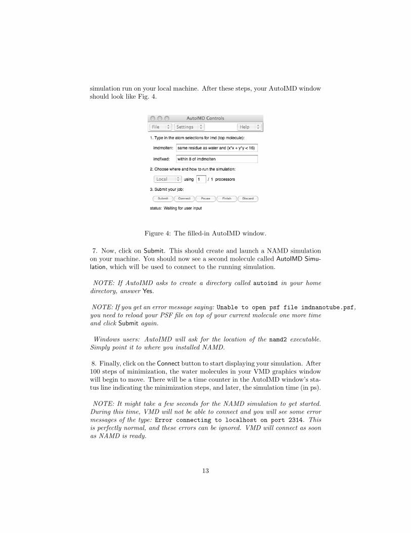
simulation run on your local machine. After these steps, your AutoIMD windowshould look like Fig. 4.

Figure 4: The filled-in AutoIMD window.

7. Now, click on Submit. This should create and launch a NAMD simulationon your machine. You should now see a second molecule called AutoIMD Simu-lation, which will be used to connect to the running simulation.

NOTE: If AutoIMD asks to create a directory called autoimd in your homedirectory, answer Yes.

NOTE: If you get an error message saying: Unable to open psf file imdnanotube.psf,you need to reload your PSF file on top of your current molecule one more timeand click Submit again.

Windows users: AutoIMD will ask for the location of the namd2 executable.Simply point it to where you installed NAMD.

8. Finally, click on the Connect button to start displaying your simulation. After100 steps of minimization, the water molecules in your VMD graphics windowwill begin to move. There will be a time counter in the AutoIMD window’s sta-tus line indicating the minimization steps, and later, the simulation time (in ps).

NOTE: It might take a few seconds for the NAMD simulation to get started.During this time, VMD will not be able to connect and you will see some errormessages of the type: Error connecting to localhost on port 2314. Thisis perfectly normal, and these errors can be ignored. VMD will connect as soonas NAMD is ready.

13

9. The nanotube will appear by default as bunch of chubby spheres. To seethe water through it, select the “imdhetero” representation in the AutoIMDmolecule, and change the drawing method from VdW to Bonds.

10. When you are done (after, say, 10 ps or more), click on the Discard button.This will halt the simulation and bring you back to the molecule as it was beforeyou started AutoIMD. If you had clicked on Finish instead, the final coordinatesof the simulation would have been saved into your initial molecule (overwritingthe old coordinates).

11. If you want to run a new simulation with different initial coordinates ormodified parameters (or simply to re-run your old simulation) you would nowonly need to repeat steps 8 to 10 (i.e., click on Submit, Connect and Discard).

4.2 Modifying the charges

Here, we will learn how to modify the electric charge of individual atoms, asthey appear in the NAMD simulation.

Exercise: We have seen that water permeates through the nanotubes in asingle file of oriented water molecules. We would like to modify the nanotubesuch that we get a bipolar configuration of water, such as the one seen in theglyceroaquaporin pore (i.e., the water oxygens at both ends of the pore pointtoward the center of the pore). One way to achieve this is to assign charges toa few carbon atoms in the nanotube. Think of a way that you can charge 3or more of the nanotube’s carbon atoms to achieve this. You will soon run asimulation using these charges to test your predictions.

The following instructions detail how to change the charge of an atom in a PSFfile (which in turn is used by NAMD simulations).

1. Make a copy of the imdnanotube.psf file (let’s call it mynanotube.psf, forexample) and open it in your favorite text editor. In the PSF file, you shouldsee a bunch of lines that look like:

64 NT22 1 ARM C063 CA 0.000000 12.0110 065 NT22 1 ARM C064 CA 0.000000 12.0110 066 NT22 1 ARM C065 CA 0.000000 12.0110 0

2. You want to change the charges of a few carbons in the nanotube, but firstyou need to identify these atoms by their unique index. Using the Mouse →Query mode in VMD and then clicking on atoms, get the indices of the carbonatoms whose charges you have decided to change (with the query mouse mode,you can read the atom indices in the console window or the Graphics → Labelswindow).

14

Note: VMD counts atoms starting from 0, while the PDB and PSF files startat 1. Thus, you need to add 1 to the index you get from VMD to get the atomindex in the PSF file.

3. In the PSF file (in the text editor), find the row corresponding to the atomindex that you are looking for (the atomic index is in the first column). Do notforget to add 1. Example: if you wish to change the charge of the atom withindex 65 in VMD, you need to edit the row starting with 66.

4. Now, change the column that says 0.000000 to a new number. This numbershould be a multiple or fraction of the electron charge e. Important: Make surenot to change the column alignment, as every space in the PSF file is important!For example, to assign a charge of -e/2 to the 65th (VMD’s index) atom, youwould substitute the line

66 NT22 1 ARM C065 CA 0.000000 12.0110 0

by

66 NT22 1 ARM C065 CA -0.500000 12.0110 0

5. Save your changes to the new PSF file.

6. Back in VMD, load your new PSF file (mynanotubes.psf) into your previ-ous molecule (by selecting it and choosing the File → Load Data Into Molecule...menu item, etc.). This will replace the charges that were previously there. Se-lect your nanotube (carbon) representation in the Graphical Representationswindow and click on the Apply button to redraw the nanotube with the correctcharge colors. You should now see different colors for different charges, as inFig. 5.

7. You can repeat this process as many times as you want, until you get thecharge distribution that you like to experiment with. Once you have a deco-rated nanotube, you are ready to run the simulation on your local machine withAutoIMD. Just follow instructions 8 to 10 from section 4.1 (i.e., click on Submit,Connect and Discard).

4.3 Experimenting with different charge configurations

Now that you know how to change the charges in a simulation, here are a fewnumerical experiments that you could do:

• Try placing a single large negative charge (i.e., -4e) at the center of thenanotube. Observe the simulation for about 10 ps. What happens tothe water file inside the nanotube? Can you explain what causes thisbehavior?

15

Figure 5: A decorated nanotube, showing a negatively charged carbon atom (inblue) near its center.

• What happens if you place instead a positive charge at the center?

• You may experiment with a few charge distributions of your choosing. Forexample, what happens if you reverse the charges that you have appliedin the previous section? What happens if all your charges are verticallyaligned along the nanotube, is it the same as if they were distributedsomewhere else around the tube? And finally, would the answer to thislast question remain the same if you inverted all the charges in the tube?

4.4 Modifying the VdW parameters

Here, you will learn how to modify the VdW radius of a certain type of atom ina NAMD simulation. you will significantly reduce the radius of the nanotube’scarbon. This will make the pore wider.

Question: Try to predict what will happen if you make the nanotube wider.As you will soon see, the answer to this will be quite surprising.

1. Make a copy of the par nanotubes.inp parameter file (let’s call it par mynanotubes.inp;it is very important that it starts with par and ends in .inp!) and open it ina text editor. Near the end of the file, you should see the following lines:

!atom ignored epsilon Rmin/2CA 0.000000 -0.070000 1.992400HT 0.000000 -0.046000 0.224500OT 0.000000 -0.152100 1.768200

16

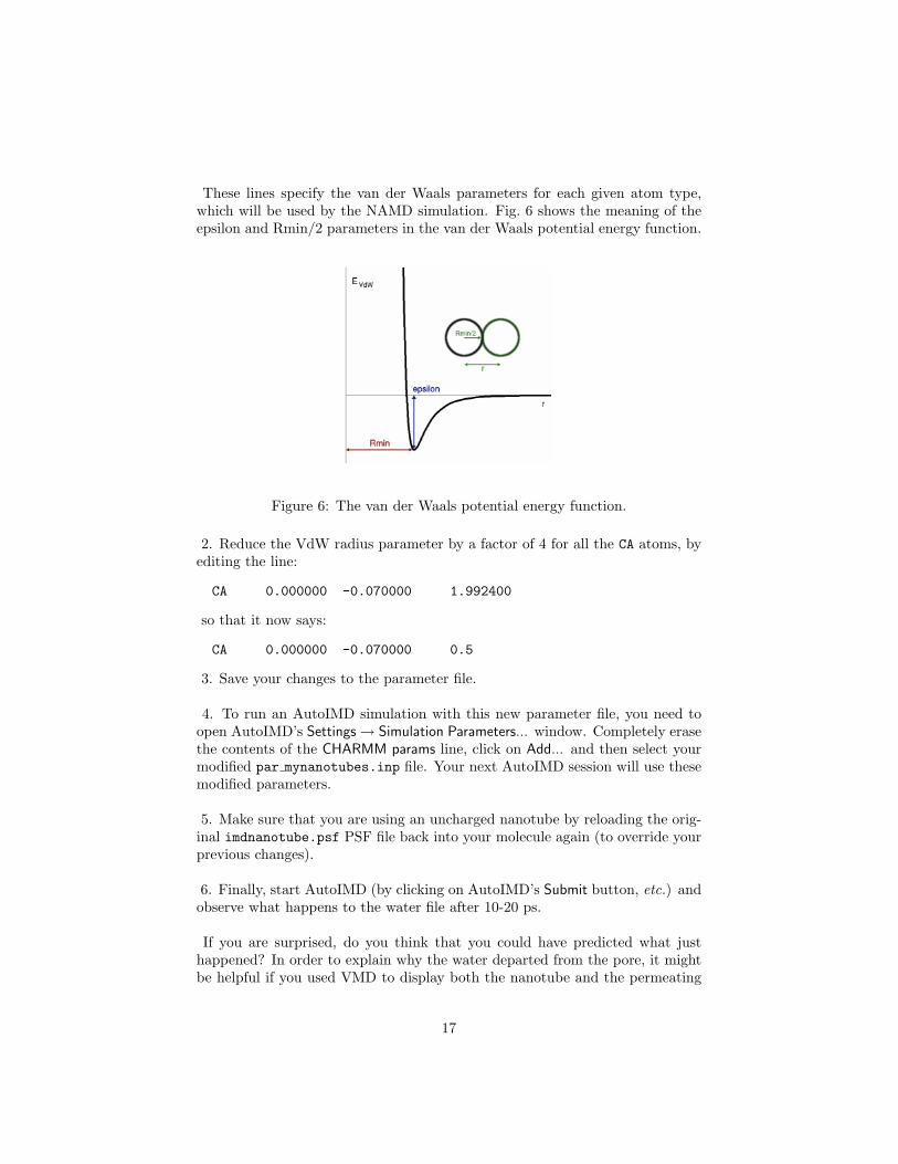
These lines specify the van der Waals parameters for each given atom type,which will be used by the NAMD simulation. Fig. 6 shows the meaning of theepsilon and Rmin/2 parameters in the van der Waals potential energy function.

Figure 6: The van der Waals potential energy function.

2. Reduce the VdW radius parameter by a factor of 4 for all the CA atoms, byediting the line:

CA 0.000000 -0.070000 1.992400

so that it now says:

CA 0.000000 -0.070000 0.5

3. Save your changes to the parameter file.

4. To run an AutoIMD simulation with this new parameter file, you need toopen AutoIMD’s Settings → Simulation Parameters... window. Completely erasethe contents of the CHARMM params line, click on Add... and then select yourmodified par mynanotubes.inp file. Your next AutoIMD session will use thesemodified parameters.

5. Make sure that you are using an uncharged nanotube by reloading the orig-inal imdnanotube.psf PSF file back into your molecule again (to override yourprevious changes).

6. Finally, start AutoIMD (by clicking on AutoIMD’s Submit button, etc.) andobserve what happens to the water file after 10-20 ps.

If you are surprised, do you think that you could have predicted what justhappened? In order to explain why the water departed from the pore, it mightbe helpful if you used VMD to display both the nanotube and the permeating

17

waters by using the VdW Draw Style. In order to display, the carbons’ approxi-mate size, you can shrink their VdW Sphere Radii (in the VMD Representationwindow) by a factor of 4 (i.e., Sphere Radius = 1.0/4 = 0.2-0.3). By inspection,what can you say about the water-nanotube interaction with the big and thesmall carbons. Remember that at the VdW radius (i.e. when the “spheres”touch) the VdW interaction is maximally attractive.

4.5 Experimenting with VdW parameters

Now that you know how to change the VdW parameter, here are a few moreexperiments that you can do.

• When you made the pore larger by reducing the carbons’ radii, you de-creased the surface of the favorable VdW interactions between the perme-ating water molecules and the nanotube. Instead of being surrounded bycarbon, the waters are now only attracted to one side, and therefore thewater-nanotube interaction is much smaller. Can you change the carbon’sVdW maximum binding energy (epsilon in the parameter file) so thatthe water file remains stable inside the pore (as opposed to leaving thepore as before), while still keeping a small carbon VdW radius parameterof 0.5? Make sure that epsilon is always negative or else the simulationwon’t run.

• Revert your changes by recopying the original parameter file. What hap-pens if you slightly increase the carbons’ VdW radius parameter so as toincrease the contact area with water? How can you observe this increasedinteraction in your water file? Can you find the optimal epsilon that willmaximize the number of water molecules in the pore?

Acknowledgments

Development of this tutorial was supported by the National Institutes of Health(P41-RR005969 - Resource for Macromolecular Modeling and Bioinformatics).

18