does your writing deceive you?
TRANSCRIPT

KENDRA OSBURN | 10-25-19 | IST 736 | HW4 | DECEPTION & SUBJECTIVITY KENDRA OSBURN | 11-10-19 | IST 736 | HW6 | Bernoulli Naive Bayes
DOES YOUR WRITING DECEIVE YOU?
Via @kuzelevdaniil
Introduction
Is it possible to tell when someone is lying? There are thousands of articles on Google
Scholar claiming that, yes, it is possible to tell when someone is lying. Everything from
someone’s temperature to pupil size to heart rate changes from truth to lie. But what about
words? Can the words people use give a hint to truthiness?
In the ever-expanding wild-west that is the internet, lie -- also referred to as fraud or
deception -- detection is more important than ever. When we, as a society, rely so heavily
on things like ratings or reviews, it’s imperative that we know we can trust these reviews.
However, just like spam snuck into our inboxes, fraud is sneaking into our rating systems.
And it’s not just bots! Humans are frequently paid to forge restaurant or product reviews.

What does this mean for both sellers and consumers? Is there any hope for truth in this
barren landscape?
Unfortunately for us researchers, there isn’t a whole lot of data out there actually labeled as
“fraudulent.” Other researchers have gone as far as paying Mechanical Turk workers to
author their own “fraud” and this likely points to reasons why our fraud-filter isn’t as
up-to-snuff as our spam-filter. With spam and email, we had/have an ever-growing dataset
that was conveniently being labeled for us already! We could simply look at the
user-labeled spam, the user-labeled not-spam and check differences. However, there is not
such an unintentionally-yet-actively maintained dataset for deception and since we’re
already starting out on a weaker footing, it’s hard to find the patterns we’d need to
accurately and intelligently make decisions about test sets when our training set is so very
small.
However, using the data she read about on the interwebs, one researcher took on this
monolithic task and tried to break it down as best she could. Despite referencing everything
from github to cornell whitepapers, the most she got was a sniff -- a whiff at a trail -- a hint
at a thread to pull -- and here is where you will read about her adventures.
Analysis & Models
ABOUT THE DATA
The researchers received the data as a semi-clean csv with three columns -- ‘lie’, ‘sentiment’
and ‘review’. Each row contained a review and a label if the review was a lie (t/f) and the
sentiment of the review (p/n). This semi-clean csv was imported and converted to a pandas
data frame with tab delimitation. The two columns of labels were separated into clean
columns and the reviews were cleaned of any rogue characters. A csv was exported.
Similarly, four separate corpuses were exported -- two for lie, two for sentiment. The final
corpuses were exported and then re-imported into the researcher’s pipelines.
See the appendix for Cleaning Code.
MODELS
2
NAIVE BAYES
What is Naive Bayes?
'We first segment the data by the class, and then compute the mean and variance of x in each
class.For example, the naive Bayes classifier will make the correct MAP decision rule classification so
long as the correct class is more probable than any other class.Like the multinomial model, this
model is popular for document classification tasks, where binary term occurrence features are used
rather than term frequencies.For example, suppose the training data contains a continuous
attribute.The discussion so far has derived the independent feature model, that is, the naive Bayes
probability model.'
This excerpt was created with the researcher’s own summarizer and wikipedia! Clearly, this is
evidence that the summarizer needs more work. See Appendix: Summarizer Code for current
summarizer code status.
Results
SENTIMENT
To get ‘results’ for this quick-and-dirty assignment, the researchers compared the
‘pastability data’ to past data sets in their ‘sentiment analysis’ pipeline to answer the
question -- does this newly cleaned data behave very similarly, slightly similarly or not at all
similarly to a cleaner dataset from the wild?
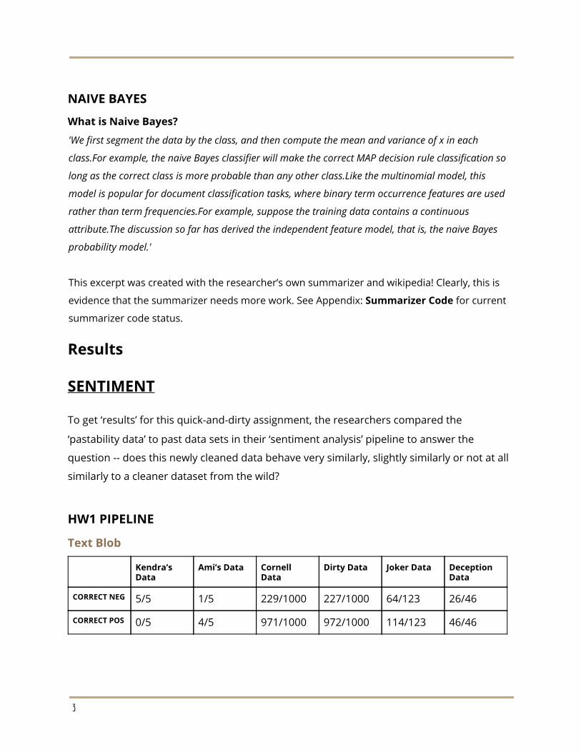
HW1 PIPELINE
Text Blob
Kendra’s Data
Ami’s Data Cornell Data
Dirty Data Joker Data Deception Data
CORRECT NEG 5/5 1/5 229/1000 227/1000 64/123 26/46
CORRECT POS 0/5 4/5 971/1000 972/1000 114/123 46/46
3

VADER
Kendra’s Data
Ami’s Data Cornell Data
Dirty Data Joker Data Deception Data
CORRECT NEG 2/5 3/5 445/1000 454/1000 64/123 26/46
CORRECT POS 5/5 3/5 828/1000 824/1000 114/123 45/46
NLTK
Kendra’s Data
Ami’s Data Cornell Data
Dirty Data Joker Data Deception Data
CORRECT NEG -- -- 89% 86% 81% 57%
CORRECT POS -- -- 74% 70% 35% 93%
ACCURACY -- -- 81% 77% 58% 75%
Without any additional cleaning, the sentiment is predicted fairly well. Looking at
Deception Data alone, it appears that positive sentiment is more frequently accurately
predicted than negative sentiment.
HW2 & HW3 PIPELINE
4

Naive Bayes Tests
SENTIMENT TESTS
GAUSSIAN
Vader Scores -- Gaussian Accuracy: 0.7777777777777778 Accuracy: 0.7777777777777778
5

Accuracy: 0.9259259259259259 Accuracy: 0.8888888888888888 Accuracy: 0.8888888888888888 AVERAGE ACCURACY: 0.8518518518518519
Vader Scores from Summary -- Gaussian Accuracy: 0.7777777777777778 Accuracy: 0.8518518518518519 Accuracy: 0.8888888888888888 Accuracy: 0.8518518518518519 Accuracy: 0.7777777777777778 AVERAGE ACCURACY: 0.8296296296296296
Vader Scores (original) and Vader Scores (summary) -- Gaussian Accuracy: 0.7777777777777778 Accuracy: 0.8518518518518519 Accuracy: 0.8888888888888888 Accuracy: 0.8518518518518519 Accuracy: 0.8518518518518519 AVERAGE ACCURACY: 0.8444444444444444
Vader Scores 50 most frequent filtered words -- Gaussian Accuracy: 0.8518518518518519 Accuracy: 0.7407407407407407 Accuracy: 0.9629629629629629 Accuracy: 0.8888888888888888 Accuracy: 0.7777777777777778 AVERAGE ACCURACY: 0.8444444444444444
BAG OF WORDS TESTS
GAUSSIAN MULTINOMIAL
Starting point -- Gaussian Accuracy: 0.8148148148148148 Accuracy: 0.7407407407407407 Accuracy: 0.8148148148148148 Accuracy: 0.7407407407407407 Accuracy: 0.8888888888888888 AVERAGE ACCURACY: 0.7999999999999999
Starting point -- Multinomial Accuracy: 0.7407407407407407 Accuracy: 0.7777777777777778 Accuracy: 0.9629629629629629 Accuracy: 0.8148148148148148 Accuracy: 0.9629629629629629 AVERAGE ACCURACY: 0.8518518518518519
DIY Cleaner Accuracy: 0.7777777777777778
DIY Cleaner -- Multinomial Accuracy: 0.9259259259259259
6
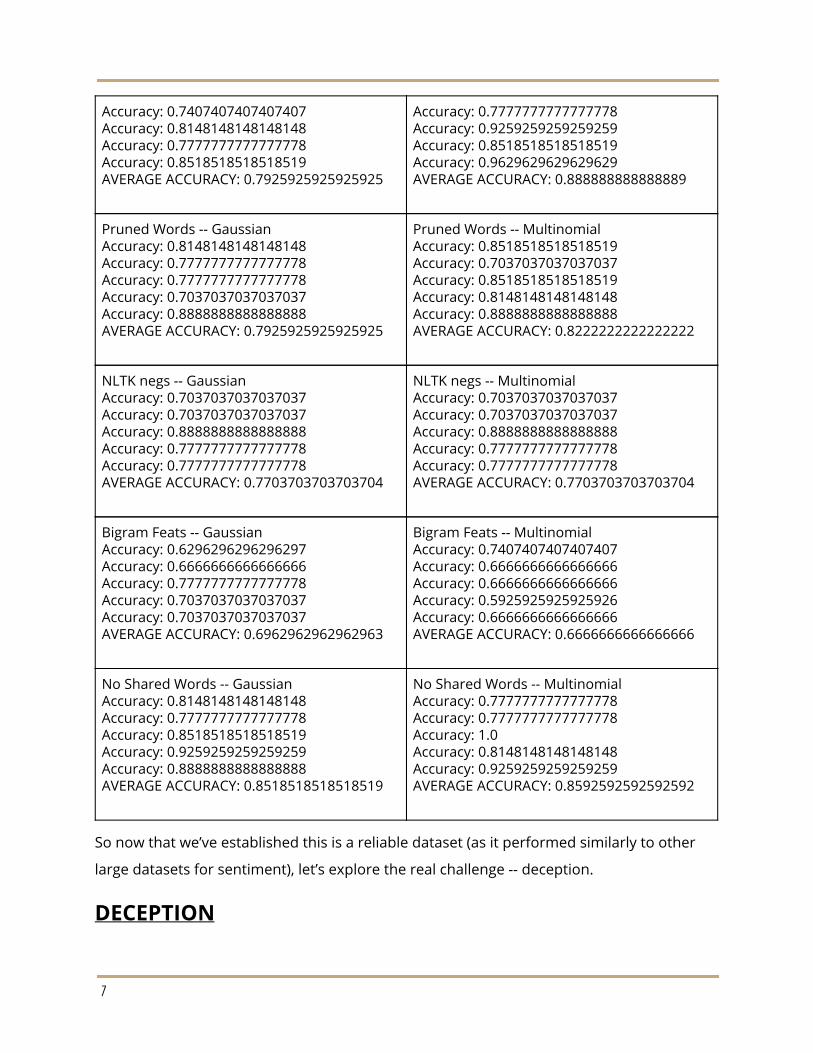
Accuracy: 0.7407407407407407 Accuracy: 0.8148148148148148 Accuracy: 0.7777777777777778 Accuracy: 0.8518518518518519 AVERAGE ACCURACY: 0.7925925925925925
Accuracy: 0.7777777777777778 Accuracy: 0.9259259259259259 Accuracy: 0.8518518518518519 Accuracy: 0.9629629629629629 AVERAGE ACCURACY: 0.888888888888889
Pruned Words -- Gaussian Accuracy: 0.8148148148148148 Accuracy: 0.7777777777777778 Accuracy: 0.7777777777777778 Accuracy: 0.7037037037037037 Accuracy: 0.8888888888888888 AVERAGE ACCURACY: 0.7925925925925925
Pruned Words -- Multinomial Accuracy: 0.8518518518518519 Accuracy: 0.7037037037037037 Accuracy: 0.8518518518518519 Accuracy: 0.8148148148148148 Accuracy: 0.8888888888888888 AVERAGE ACCURACY: 0.8222222222222222
NLTK negs -- Gaussian Accuracy: 0.7037037037037037 Accuracy: 0.7037037037037037 Accuracy: 0.8888888888888888 Accuracy: 0.7777777777777778 Accuracy: 0.7777777777777778 AVERAGE ACCURACY: 0.7703703703703704
NLTK negs -- Multinomial Accuracy: 0.7037037037037037 Accuracy: 0.7037037037037037 Accuracy: 0.8888888888888888 Accuracy: 0.7777777777777778 Accuracy: 0.7777777777777778 AVERAGE ACCURACY: 0.7703703703703704
Bigram Feats -- Gaussian Accuracy: 0.6296296296296297 Accuracy: 0.6666666666666666 Accuracy: 0.7777777777777778 Accuracy: 0.7037037037037037 Accuracy: 0.7037037037037037 AVERAGE ACCURACY: 0.6962962962962963
Bigram Feats -- Multinomial Accuracy: 0.7407407407407407 Accuracy: 0.6666666666666666 Accuracy: 0.6666666666666666 Accuracy: 0.5925925925925926 Accuracy: 0.6666666666666666 AVERAGE ACCURACY: 0.6666666666666666
No Shared Words -- Gaussian Accuracy: 0.8148148148148148 Accuracy: 0.7777777777777778 Accuracy: 0.8518518518518519 Accuracy: 0.9259259259259259 Accuracy: 0.8888888888888888 AVERAGE ACCURACY: 0.8518518518518519
No Shared Words -- Multinomial Accuracy: 0.7777777777777778 Accuracy: 0.7777777777777778 Accuracy: 1.0 Accuracy: 0.8148148148148148 Accuracy: 0.9259259259259259 AVERAGE ACCURACY: 0.8592592592592592
So now that we’ve established this is a reliable dataset (as it performed similarly to other
large datasets for sentiment), let’s explore the real challenge -- deception.
DECEPTION
7

Can sentiment be used to predict deception?
As the pipelines were already in place, the researchers ran the exact same “sentiment
pipelines” for the deception data. However, instead of attempting to predict “negative” and
“positive,” this time trying to predict “true” or “false.”
Text Blob
Deception Data (sentiment) Deception Data (deception)
CORRECT NEG 26/46 CORRECT FALSE 14/46
CORRECT POS 46/46 CORRECT TRUE 34/46
VADER
Deception Data (sentiment) Deception Data (deception)
CORRECT NEG 26/46 CORRECT FALSE 13/46
CORRECT POS 45/46 CORRECT TRUE 32/46
NLTK
Deception Data (sentiment) Deception Data (deception)
CORRECT NEG 57% CORRECT FALSE 57%
CORRECT POS 93% CORRECT TRUE 57%
ACCURACY 75% ACCURACY 57%
Clearly, with a 57% accuracy, sentiment is not the way to predict deception.
Can parts of speech be used to predict deception?
Quick EDA with bar graphs:
8

9

“NN” stands for “Noun, singular or mass” which matches up with our very first EDA
bar graphs. (To see what all the tags mean, please see Appendix) Initial EDA
suggests that there are similarities but also areas where we should definitely dig
further -- possibly, part of speech bigrams?
POS BIGRAMS
10

11

Not as helpful either.
Naive Bayes Tests
SENTIMENT TESTS
GAUSSIAN
Vader Scores -- Gaussian Accuracy: 0.4444444444444444 Accuracy: 0.4444444444444444 Accuracy: 0.4444444444444444 Accuracy: 0.48148148148148145 Accuracy: 0.4074074074074074 AVERAGE ACCURACY: 0.44444444444444436
Vader Scores from Summary -- Gaussian Accuracy: 0.5555555555555556 Accuracy: 0.6296296296296297 Accuracy: 0.5555555555555556 Accuracy: 0.48148148148148145 Accuracy: 0.48148148148148145 AVERAGE ACCURACY: 0.5407407407407407
12

Vader Scores (original) and Vader Scores (summary) -- Gaussian Accuracy: 0.48148148148148145 Accuracy: 0.6666666666666666 Accuracy: 0.5555555555555556 Accuracy: 0.5185185185185185 Accuracy: 0.4074074074074074 AVERAGE ACCURACY: 0.5259259259259259
Vader Scores 50 most frequent filtered words -- Gaussian Accuracy: 0.5555555555555556 Accuracy: 0.5925925925925926 Accuracy: 0.5555555555555556 Accuracy: 0.5185185185185185 Accuracy: 0.5925925925925926 AVERAGE ACCURACY: 0.562962962962963
BAG OF WORDS TESTS
GAUSSIAN MULTINOMIAL
Starting point -- Gaussian Accuracy: 0.5185185185185185 Accuracy: 0.5185185185185185 Accuracy: 0.5555555555555556 Accuracy: 0.5185185185185185 Accuracy: 0.5185185185185185 AVERAGE ACCURACY: 0.5259259259259259
Starting point -- Multinomial Accuracy: 0.4444444444444444 Accuracy: 0.48148148148148145 Accuracy: 0.48148148148148145 Accuracy: 0.6296296296296297 Accuracy: 0.5925925925925926 AVERAGE ACCURACY: 0.5259259259259259
DIY Cleaner Accuracy: 0.48148148148148145 Accuracy: 0.5185185185185185 Accuracy: 0.5925925925925926 Accuracy: 0.48148148148148145 Accuracy: 0.48148148148148145 AVERAGE ACCURACY: 0.5111111111111111
DIY Cleaner -- Multinomial Accuracy: 0.4074074074074074 Accuracy: 0.4444444444444444 Accuracy: 0.48148148148148145 Accuracy: 0.6296296296296297 Accuracy: 0.4444444444444444 AVERAGE ACCURACY: 0.4814814814814815
Pruned Words -- Gaussian Accuracy: 0.5555555555555556
Pruned Words -- Multinomial Accuracy: 0.5185185185185185
13

Accuracy: 0.48148148148148145 Accuracy: 0.5185185185185185 Accuracy: 0.48148148148148145 Accuracy: 0.5185185185185185 AVERAGE ACCURACY: 0.5111111111111111
Accuracy: 0.5185185185185185 Accuracy: 0.5925925925925926 Accuracy: 0.6296296296296297 Accuracy: 0.5555555555555556 AVERAGE ACCURACY: 0.562962962962963
NLTK negs -- Gaussian Accuracy: 0.5555555555555556 Accuracy: 0.5925925925925926 Accuracy: 0.4074074074074074 Accuracy: 0.4444444444444444 Accuracy: 0.48148148148148145 AVERAGE ACCURACY: 0.4962962962962963
NLTK negs -- Multinomial Accuracy: 0.5555555555555556 Accuracy: 0.5925925925925926 Accuracy: 0.4074074074074074 Accuracy: 0.4444444444444444 Accuracy: 0.48148148148148145 AVERAGE ACCURACY: 0.4962962962962963
Bigram Feats -- Gaussian Accuracy: 0.4074074074074074 Accuracy: 0.5185185185185185 Accuracy: 0.5555555555555556 Accuracy: 0.5555555555555556 Accuracy: 0.48148148148148145 AVERAGE ACCURACY: 0.5037037037037038
Bigram Feats -- Multinomial Accuracy: 0.5555555555555556 Accuracy: 0.5185185185185185 Accuracy: 0.5555555555555556 Accuracy: 0.6296296296296297 Accuracy: 0.6666666666666666 AVERAGE ACCURACY: 0.5851851851851851
No Shared Words -- Gaussian Accuracy: 0.5555555555555556 Accuracy: 0.7037037037037037 Accuracy: 0.5925925925925926 Accuracy: 0.6296296296296297 Accuracy: 0.6666666666666666 AVERAGE ACCURACY: 0.6296296296296295
No Shared Words -- Multinomial Accuracy: 0.5555555555555556 Accuracy: 0.6296296296296297 Accuracy: 0.6296296296296297 Accuracy: 0.7037037037037037 Accuracy: 0.6666666666666666 AVERAGE ACCURACY: 0.6370370370370371
HW6 Addition Now with Bernoulli
SENTIMENT DECEPTION
Starting point -- Bernoulli Accuracy: 0.7777777777777778
Starting point -- Bernoulli Accuracy: 0.4444444444444444
14
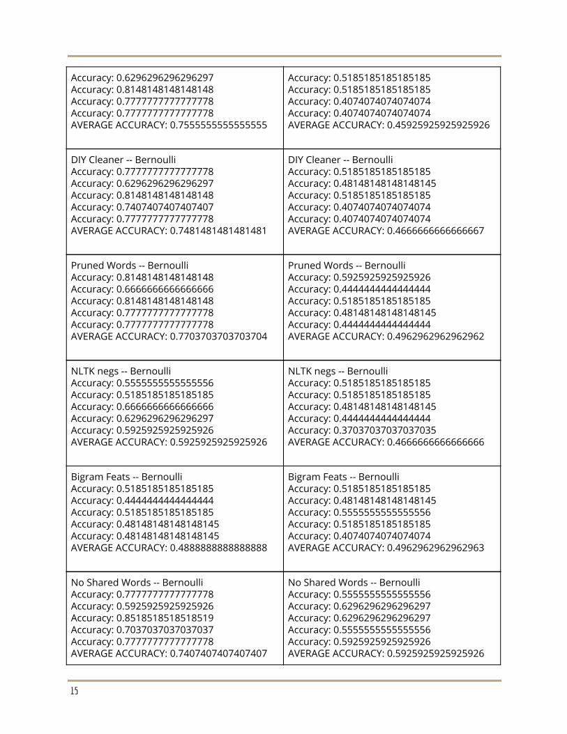
Accuracy: 0.6296296296296297 Accuracy: 0.8148148148148148 Accuracy: 0.7777777777777778 Accuracy: 0.7777777777777778 AVERAGE ACCURACY: 0.7555555555555555
Accuracy: 0.5185185185185185 Accuracy: 0.5185185185185185 Accuracy: 0.4074074074074074 Accuracy: 0.4074074074074074 AVERAGE ACCURACY: 0.45925925925925926
DIY Cleaner -- Bernoulli Accuracy: 0.7777777777777778 Accuracy: 0.6296296296296297 Accuracy: 0.8148148148148148 Accuracy: 0.7407407407407407 Accuracy: 0.7777777777777778 AVERAGE ACCURACY: 0.7481481481481481
DIY Cleaner -- Bernoulli Accuracy: 0.5185185185185185 Accuracy: 0.48148148148148145 Accuracy: 0.5185185185185185 Accuracy: 0.4074074074074074 Accuracy: 0.4074074074074074 AVERAGE ACCURACY: 0.4666666666666667
Pruned Words -- Bernoulli Accuracy: 0.8148148148148148 Accuracy: 0.6666666666666666 Accuracy: 0.8148148148148148 Accuracy: 0.7777777777777778 Accuracy: 0.7777777777777778 AVERAGE ACCURACY: 0.7703703703703704
Pruned Words -- Bernoulli Accuracy: 0.5925925925925926 Accuracy: 0.4444444444444444 Accuracy: 0.5185185185185185 Accuracy: 0.48148148148148145 Accuracy: 0.4444444444444444 AVERAGE ACCURACY: 0.4962962962962962
NLTK negs -- Bernoulli Accuracy: 0.5555555555555556 Accuracy: 0.5185185185185185 Accuracy: 0.6666666666666666 Accuracy: 0.6296296296296297 Accuracy: 0.5925925925925926 AVERAGE ACCURACY: 0.5925925925925926
NLTK negs -- Bernoulli Accuracy: 0.5185185185185185 Accuracy: 0.5185185185185185 Accuracy: 0.48148148148148145 Accuracy: 0.4444444444444444 Accuracy: 0.37037037037037035 AVERAGE ACCURACY: 0.4666666666666666
Bigram Feats -- Bernoulli Accuracy: 0.5185185185185185 Accuracy: 0.4444444444444444 Accuracy: 0.5185185185185185 Accuracy: 0.48148148148148145 Accuracy: 0.48148148148148145 AVERAGE ACCURACY: 0.4888888888888888
Bigram Feats -- Bernoulli Accuracy: 0.5185185185185185 Accuracy: 0.48148148148148145 Accuracy: 0.5555555555555556 Accuracy: 0.5185185185185185 Accuracy: 0.4074074074074074 AVERAGE ACCURACY: 0.4962962962962963
No Shared Words -- Bernoulli Accuracy: 0.7777777777777778 Accuracy: 0.5925925925925926 Accuracy: 0.8518518518518519 Accuracy: 0.7037037037037037 Accuracy: 0.7777777777777778 AVERAGE ACCURACY: 0.7407407407407407
No Shared Words -- Bernoulli Accuracy: 0.5555555555555556 Accuracy: 0.6296296296296297 Accuracy: 0.6296296296296297 Accuracy: 0.5555555555555556 Accuracy: 0.5925925925925926 AVERAGE ACCURACY: 0.5925925925925926
15

Sentiment classifications proved to be just as accurate as other datasets. This is likely due
to the many and varied ways we can look at and attempt to classify and label sentiment.
For example, if I gave five people a printout of tweets and asked them to label them as
positive or negative, this would likely be an easier task than identifying a false review. Why
is that? It likely means that the “packets of meaning” that can convey sentiment (words,
sometimes word order) are smaller and more easily distinguishable in analysis. If we as
humans still struggle with identifying the features that point out deception (in writing) than
how can we train a computer to do so? Additionally, how can we train a computer when we
don’t have as many labeled datasets?
Theoretically, we could employ Mechanical Turkers to write fake data for us. However,
without knowing the motivation behind the fake data (are they, the fake data creators out
in the wild, trying to overcorrect for a bad yelp review? Boost a movie’s score on IMDB?
Raise an Amazon Products star rating so it appears on the first page? Bash a hotel that
discriminated against a minority? Destroy a business because they inappropriately fired
someone?) we are inadvertently overcorrecting before we’ve even analyzed the data. We
would be creating a great model for predicting “Did a Mechanical Turker write this review.”
Which, while that might be the future, isn’t useful across the platforms where this model
would need to be used (filtering out fake reviews from all sources).
Conclusion
Classifying reviews based on sentiment alone proved to be a fairly easy exercise for a few
reasons. First, there is a large amount of labeled data in the field. Second, the “packets of
meaning” that convey sentiment can be something as small as a mneome or as large as a
sentence. In this paper, the packets of meaning were words, but that doesn’t mean they
couldn’t be other parts of the letters that make up the words that make up the sentences
16
that make up the reviews. In sentiment classification, we can look at these packets of
meaning from many different angles. We can look at the “valence” of a word (using an
external dictionary, something like Vader or TextBlob), we can look at the words that follow
negation words and we can look at all the words spread out together in a sparse matrix
and let the computer find patterns for itself.
Unfortunately, deception isn’t as easy of an exercise for a similarly long laundry list of
reasons. While sentiment has external dictionaries (both literally and figuratively -- if we
use the word “awesome” that goes to a dictionary in our mind that associates that word
with positive things, however, it’s fun to note that this word wasn’t always positive and if I
lived a couple of centuries ago, my internal dictionary would classify this word as negative)
to help the classification process along, there are no single words or collections of words
that scream “deception.”
Future study is going to center around topic modeling and comparison of the topics within
the review to the topic of the thing being reviewed. The researchers had high hopes that
there would be patterns within parts of speech but they were flummoxed by both the lack
of data and the inability of the data to conform to their hypotheses. How dare it. The
researchers couldn’t help but laugh as each of their attempts lead to lower and lower
accuracies, culminating in a personal best of low accuracy at 44%.
APPENDIX
Cleaning Code
#!/usr/bin/env python
# coding: utf-8
# # HW4 -- Sentiment and Lies
# ## STEP 1: Import the data
# NOTE: May need to change delimiter based on the data file
import pandas as pd df = pd.read_csv('deception_data_converted_final.csv', sep='\t') df[:5] # ## STEP 2: Pull out the labels
def get_labels(row): split_row = str(row).split(',') lie = split_row[0] sentiment = split_row[1] return [lie, sentiment, split_row[2:]] df['all'] = df.apply(lambda row: get_labels(row['lie,sentiment,review']), axis=1)
17

df[:5]
df['lie'] = df.apply(lambda row: row['all'][0][0], axis=1) df[:5]
df['sentiment'] = df.apply(lambda row: row['all'][1][0], axis=1) df[:5]
df['review'] = df.apply(lambda row: ''.join(row['all'][2]), axis=1) df[:5]
clean_df = df.copy()
clean_df.drop(['lie,sentiment,review', 'all'], axis=1, inplace=True)
clean_df
# ## STEP 3: Clean the data
def clean_rogue_characters(string): exclude = ['\\',"\'",'"'] string = ''.join(string.split('\\n')) string = ''.join(ch for ch in string if ch not in exclude) return string clean_df['review'] = clean_df['review'].apply( lambda x: clean_rogue_characters(x) ) clean_df['review'][0] # ## STEP 4: Export cleaned, formatted CSV
clean_df.to_csv('hw4_data.csv',index=False)
df = pd.read_csv('hw4_data.csv') df[:5] # ## STEP 5: Split df into data sets
# ### LIE DFs
lie_df_f = df[df['lie'] == 'f'] lie_df_t = df[df['lie'] == 't'] # ### SENTIMENT DFs
sent_df_n = df[df['sentiment'] == 'n'] sent_df_p = df[df['sentiment'] == 'p'] # ### STEP 5b: Export to Corpus to run on current pipelines
def print_to_file(rating, review, num, title): both = review
output_filename = str(rating) + '_'+ title +'_' + str(num) + '.txt' outfile = open(output_filename, 'w') outfile.write(both)
outfile.close()
def export_to_corpus(df, subj, title): for num,row in enumerate(df['review']): print_to_file(subj, row, num, title)
export_to_corpus(sent_df_n, 'neg', 'hw4_n') export_to_corpus(sent_df_p, 'pos', 'hw4_p')
export_to_corpus(lie_df_f, 'false', 'hw4_f')
18
export_to_corpus(lie_df_t, 'true', 'hw4_t')
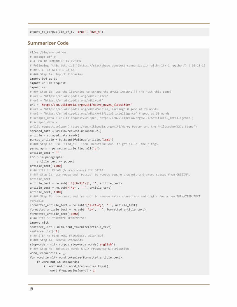
Summarizer Code
#!/usr/bin/env python
# coding: utf-8
# # HOW TO SUMMARIZE IN PYTHON
# Following [this tutorial!](https://stackabuse.com/text-summarization-with-nltk-in-python/) | 10-13-19
# ## STEP 1: GET THE DATA!!
# ### Step 1a: Import libraries
import bs4 as bs import urllib.request import re # ### Step 1b: Use the libraries to scrape the WHOLE INTERNET!! (jk just this page)
# url = 'https://en.wikipedia.org/wiki/Lizard'
# url = 'https://en.wikipedia.org/wiki/cat'
url = 'https://en.wikipedia.org/wiki/Naive_Bayes_classifier' # url = 'https://en.wikipedia.org/wiki/Machine_learning' # good at 20 words
# url = 'https://en.wikipedia.org/wiki/Artificial_intelligence' # good at 30 words
# scraped_data = urllib.request.urlopen('https://en.wikipedia.org/wiki/Artificial_intelligence')
# scraped_data =
urllib.request.urlopen('https://en.wikipedia.org/wiki/Harry_Potter_and_the_Philosopher%27s_Stone')
scraped_data = urllib.request.urlopen(url)
article = scraped_data.read()
parsed_article = bs.BeautifulSoup(article,'lxml') # ### Step 1c: Use `find_all` from `BeautifulSoup` to get all of the p tags
paragraphs = parsed_article.find_all('p') article_text = "" for p in paragraphs: article_text += p.text
article_text[:1000] # ## STEP 2: CLEAN (& preprocess) THE DATA!!
# ### Step 2a: Use regex and `re.sub` to remove square brackets and extra spaces from ORIGINAL
article_text
article_text = re.sub(r'\[[0-9]*\]', '', article_text) article_text = re.sub(r'\s+', ' ', article_text) article_text[:1000] # ### Step 2b: Use regex and `re.sub` to remove extra characters and digits for a new FORMATTED_TEXT
variable
formatted_article_text = re.sub('[^a-zA-Z]', ' ', article_text) formatted_article_text = re.sub(r'\s+', ' ', formatted_article_text) formatted_article_text[:1000] # ## STEP 3: TOKENIZE SENTENCES!!
import nltk sentence_list = nltk.sent_tokenize(article_text)
sentence_list[:5] # ## STEP 4: FIND WORD FREQUENCY, WEIGHTED!!
# ### Step 4a: Remove Stopwords
stopwords = nltk.corpus.stopwords.words('english') # ### Step 4b: Tokenize Words & DIY Frequency Distribution
word_frequencies = {}
for word in nltk.word_tokenize(formatted_article_text): if word not in stopwords: if word not in word_frequencies.keys(): word_frequencies[word] = 1
19

else: word_frequencies[word] += 1 # ### Step 4c: Calculate Weighted Frequency
max_frequency = max(word_frequencies.values())
for word in word_frequencies.keys(): word_frequencies[word] = (word_frequencies[word]/max_frequency)
# ## STEP 5: CALCULATE SENTENCE SCORES
## ILLUSTRATIVE EXAMPLE
## Nothing removed
for sent in sentence_list[:1]: for word in nltk.word_tokenize(sent.lower()): print(word)
## ILLUSTRATIVE EXAMPLE
## Stopwords etc. removed
## We are ONLY assigning values/weights to the words in the sentences that are inside our freq dist!
for sent in sentence_list[:1]: for word in nltk.word_tokenize(sent.lower()): if word in word_frequencies.keys(): print(word)
sentence_scores = {}
for sent in sentence_list: for word in nltk.word_tokenize(sent.lower())[:50]: if word in word_frequencies.keys(): if len(sent.split(' ')) < 30: if sent not in sentence_scores.keys(): sentence_scores[sent] = word_frequencies[word]
else: sentence_scores[sent] += word_frequencies[word]
sorted_sentences = sorted(sentence_scores.items(), key=lambda kv: kv[1], reverse=True) sorted_sentences[:10] summary = [sent[0] for sent in sorted_sentences[:5]] ''.join(summary) ''.join(summary).strip() summary_2 = [sent[0] for sent in sentence_scores.items() if sent[1] > 3] ''.join(summary_2).strip()
Parts of Speech (POS) Tags
20

21

22