1

DOES TOO MUCH FINANCE HARM GROWTH?:

PRE AND POST GLOBAL FINANCIAL CRISIS ANALYSIS

Elya Nabila Abdul Bahria,b,*, Abu Hassan Shaari Md Nora,

Tamat Sarmidia, Nor Hakimah Haji Mohd Norc

a Faculty of Economics and Management, Universiti Kebangsaan Malaysia 43600 Bangi, Selangor,

Malaysia b Faculty of Business, Finance and Hospitality, MAHSA University, Jalan SP 2, Bandar Saujana

Putra,

42610 Jenjarom, Selangor, Malaysia c Faculty of Management and Muamalah, Kolej Universiti Islam Antarabangsa Selangor Bandar Seri

Putra, 43000 Kajang, Selangor, Malaysia

*Corresponding author: elyanabila@gmail.com

ABSTRACT

The existing studies found that the relationship between financial development and economic

growth was nonlinear with an inverse U-shape, where financial development will harm the

economic growth after surpassed the threshold point. The objective of this study is to

investigate the nonlinear relationship between financial development and economic growth for

65 developing countries from 1980-2015 by using Generalized Method of Moment (GMM).

We split the sample into two regimes, 1980-2008 and 2009-2015, which is before and after

global economic crisis. Three financial indicators namely domestic credit, liquid liabilities, and

private credit are used in this study. The results from our study, however found that the findings

were contrasted from the past literature for 2009-2015 subsample. Based on the results from

second regime, interestingly, the relationship of financial development and economic growth

is nonlinear but U-shape for all indicators. It means that the financial development will

accelerate economic growth after reach the turning point. The results of the Sasabuchi-

LindMehlum test also confirmed the nonlinear mixture of inverse U-shape for first subsample

but U-shape for second subsample. It shows that the higher financial development will improve

better performance on economic growth for the recent economy. Thus, our results provide new

insight in recent literature and policy review.

Keywords: financial development, economic growth, nonlinear, U-shape

1. Introduction

There is a huge amount of the studies on investigated the relationship between financial

development and economic growth, for example, King and Levine (1993a, 1993b),

Demetriades and Hussein (1996), Levine (1997, 2003), Rajan and Zingales (1998), Levine et

al. (2000), Al-Yousif (2002), Beck and Levine (2004), Bertocco (20080), Hassan et al. (2009),

Jalil et al.(2010), Rahaman (2011), and Kendal (2012). The studies were found that the

financial development had a positive effect on economic growth, according to the pioneer work

2

by Schumpeter (1911), followed by King and Levine (1993a) who supported the ‘more finance,

more growth’ hypothesis. The study by Levine (1997), financial indicators enhance the

economic growth, by assisting allocate capital to be more benefited.

However, a number of studies show that the effect of financial development on

economic growth is conditional on many factors rather than itself. The performance of financial

development on economic growth is depends on threshold of other variables such as inflation,

government size, trade openness and income per capita (Yilmazkuday, 2011). The other

mediating variables such as financial sector policies (Abiad and Mody, 2005; Ang, 2008), legal

systems (La Porta et al., 1997, 1998), government ownership of bank (La Porta et al., 2002;

Andrianova et al., 2008), political institutions (Girma and Shortland, 2008; Roe and Siegel,

2011; Huang, 2010), culture (Stulz and Williamson, 2003), trade and financial openness (Rajan

and Zingales, 2003; Baltagi et al., 2009; Law, 2009), remittances (Aggarwal et al., 2011;

Demirguc-Kunt et al., 2011), institutions (Law and Azman-Saini, 2012; Law et al., 2013; Law

et al., 2017).

A number of studies show that the relationship between financial development and

growth depends on many qualifications. Beck and Levine (2004) and Ndikumana (2005)

investigated whether bank-based or market-based systems are more efficient in promoting

economic activity, concluding that both types of financial intermediation play a significant role.

In addition, Rousseau and Wachtel (2000) show that the increasing influence of stock markets

on economic activity holds for both developed and developing economies. Rousseau and

Wachtel (2002) also consider the role of inflation and find that there is an upper threshold

above which financial development ceases to have a positive effect on growth. While Aghion

et al. (2009) pointed out the importance of the level of financial development in understanding

the relationship between growth and exchange rate volatility.

In nonlinear properties, Deidda and Fattouh (2002) and Rioja and Valev (2004a) found

that the relationship between financial development and growth is not significant in low-

income countries, but it has positive and significant impact in high-income countries.

Furthermore, Rioja and Valev (2004b) highlighted the impact of financial development on

economic growth is positive only when it has achieved a certain level or threshold point. The

studies from Shen and Lee (2006), Ergungor (2008) and Hung (2009) also discovered patterns

on nonlinearity in the relationship between financial development and growth. Based on the

findings, all these papers suggested that a well-developed financial development to be increase

and supported the ‘more finance, more growth’ proposition.

However, the global financial crisis in 2007-2008 that hit the global economy has led

both academics and policymakers to reconsider their prior conclusions. The crisis has

illustrated the possibilities that malfunctioning financial systems can directly and indirectly

waste resources, discourage saving and encourage speculation, resulting in underinvestment

and a misallocation of scarce resources. Consequently, it may led to the economy stagnant,

increasing the unemployment and poverty is impaired. The drastic falls in real sector activity

during the crisis, due to adverse implications of financial turbulence, highlight the need for

economists and policy makers to question the optimal size of financial systems for sustainable

economic growth. In addition, the sub-prime mortgage crisis where the people who are

disqualified to borrow the money for buying house has been lending for second chances. The

second chances because of the moral hazard from the bankers to get the commission and also

to cover the house construction industry. When the borrowers unable to repay the money, the

non-performing loan increases. The global financial crisis is not only effect to Asian countries,

but the whole world economics which also reflect the developing countries. These conditions

implies the question: does finance is found to boost the economic growth regardless of the size

and growth of the financial sector? In the other words, does the size and growth of financial

sector should be limited?

3

Thus, the proposition of ‘more finance, more growth’ has been challenged with the

above questions. Moreover, the studies Arcand et al. (2012) Cechetti and Kharroubi (2012),

Law and Singh (2014), and Samargandi et al. (2015) highlighted the positive effect of financial

development is limited up to the certain point, but then the financial development will dampen

the economic growth after surpassed the threshold value. This implies that the relationship

between finance and growth is a non-linear with inverted U-shape or exist the economic

Kuznets curve. These studies suggested the ‘too much finance harm growth’ hypothesis. The

other example such as Huang and Lin (2009) pointed out that the positive effect between

financial development and growth is larger in low-income countries than in high–income

countries, that contrary with the findings from the study by Rioja and Valev (2004b). The

conflict between ‘too much finance’ hypotheses or ‘vanishing effect’ (Arcand et al., 2012;

Cechetti and Kharroubi, 2012, Law and Singh, 2014; Sarmargandi et al., 2015) contradict with

the hypothesis of ‘more finance, more growth’ by Levine (1993) and Schumpeter (1911). This

conflict implies a discussion on revealing the ambiguity of these mixed findings. Hence, the

nonlinearity relationship between financial development and economic growth is still in debate.

Understanding the relationship between financial development and economic growth is

important to the policy makers who are concerning the facts that surrounding around to the

particular issue to make a decision on regulation, controlling and monitoring the financial

intermediaries’ activities. Ang (2008) emphasized that an appropriate specification of the

functional form is critical in understanding the relationship between financial development and

growth since several studies have shown that the finance-growth nexus may be nonlinear, thus,

more research in this area is necessary.

Since these hypotheses are contradict, we create some doubt from the previous findings

by pointed out the question as highlighted by Law and Singh (2014) that, does the too much

finance harm growth permanently or temporarily? Thus, in this study, we extend the existing

literature to scrutinize the consistency of the ‘too much finance’ hypothesis by splitting the

sample of 65 developing countries into two regimes, with and without global financial crisis.

First regime is the period starting from 1980 through 2008 by considering the period global

financial crisis in 2007-2008 in our sample. While, second regime is the period after the global

financial crisis that covered from 2009 until the recent data of year 2015. The global financial

crisis in 2007-2008 has been chosen as defining moment in this study for two reasons, mainly

because of the recent economic crisis on our sample and the global financial crisis is more

affect the developing countries in our sample as compared to Asian financial crisis.

The purposed of this study are focused on two main objectives. First, the objective of

the study is attempted to examine the consistency of nonlinearity between financial

development and economic growth relationship of inverted U-shaped as found from the

previous study (Arcand et al., 2012; Cechetti and Kharroubi, 2012; Law and Singh, 2014;

Samargandi et al., 2015) by splitting our sample into the period until the global financial crisis

in 2008 that reflects the countries in our sample and after this Great Depression. Second, we

investigate whether there is the different of the threshold points of these two regimes which

entails to the discussion on the policy review, that extent to which the financial activities during

the soft-landing activities period.

This study is organized as follows. In the next section, the previous empirical studies

on the relationship between finance and growth are highlighted. Section 3 presents the data,

empirical model and the econometric methods applied in this study. The empirical results and

discussions are enclosed in Section 4. The last section provides a summary and conclusions.

4

2. Past Empirical Studies

Despite the recognition of financial intermediation’s crucial role in economic activity,

policymakers had not been proactive in promoting financial development prior to the 1970s.

In the early 1970s McKinnon (1973) and Shaw (1973) developed theoretical arguments

challenging the policies leading to financial repression. According to their study, financial

liberalisation would reduce the financial repression and would bring up the financial

development and spur the economic growth. Moreover, the liberalizing financial markets

would allow emerging economies to access international capital markets, allowing

consumption smoothing, risk sharing, and producing a virtuous circle between financial

development and efficient capital allocation.

The development of endogenous growth theory during the 1980s and 1990s

(Greenwood and Jovanovic, 1990; Bencivenga and Smith, 1991; King and Levine, 1993b;

Blackburn and Hung, 1998) led to the construction of several models that incorporated

financial institutions and described the mechanisms through which financial development

could affect growth. Capital accumulation channel and total factor productivity channel has

been identified as to how well-functioning financial systems would affect savings and

allocation decisions. The capital accumulation is channelled to the local and foreign

entrepreneurs who need funds in order to invest that led to widen the financial liberalisation.

Notwithstanding, in the early 2010s Broner and Ventura (2010) argue that the financial

liberalisation is not prolonged boost the economic growth due to the pro-cyclicality of the

financial system emerges as one of the main factors to the global financial crisis in 2008.

There is exist comovement between financial development and economic growth as

founded in the studies by Demetriades and Husein (1996), Arestis and Demetriades (1997),

Christopoulos and Tsionas (2004) and Apergis et al. (2007). The cointegration between these

two variables shows the long run relationship between financial development and economic

growth. Odedokun (1996), Beck et al. (2000), Benhabib and Spiegel (2000) and Henry (2000)

found that several measures of financial development are positively correlated with real per

capita GDP, TFP and the investment rate.

Finance-growth nexus has been proven in the causality analysis. Luintel and Khan

(1999), Shan et al. (2001), and Calderon and Liu (2003) found bi-directional causality between

financial development and economic growth. On the other hand, Ang and McKibbin (2007)

with focusing on the case of Malaysia, find that growth leads financial development. In

contrast, Neusser and Kugler (1998), Rousseau and Wachtel (1998), and Choe and Moosa

(1999) provide evidence that financial development leads economic growth. Graff (2005)

underlined the possibility of a causal relationship between financial development and economic

growth postulates three distinguish perspectives. First, the provision of an inexpensive and

reliable means of payment such as coins and later banking money, which historically came as

a by-product of fractional reserve banking (Kindleberger, 1993). Second, a volume effect,

where financial activity increases savings where the resources can be channelled into

investment and thirdly, an allocation effect which improves the allocation of resources devoted

to investment (Gurley and Shaw, 1960).

Cross-sectional studies tend to provide evidence supportive of the positive role of

financial sector development. For instance, using data from 90 countries King and Levine

(1993a) document strong and positive correlation between measures of financial development

and per capita output growth. This finding is further substantiated by King and Levine (1993b),

Levine and Zervos (1998), and Rajan and Zingales (1998). Xu (2000) further notes that “there

is strong evidence that financial development is important to economic growth both in the

short-term and in the long-term (p. 333) in his analysis of 41 developing countries. Moreover,

5

by examining five industrialized countries over the period 1870-1929, Rosseaul and Watchel

(1998) provide strong evidence for a unidirectional causality from finance to economic growth.

However, there is fragility of the relationship between financial development and

economic growth (Ibrahim, M., 2007). Financial development can reduce the real supply of

domestic firms as consumers may substitute loans from informal curd markets to formal

markets (Van Wijbergen 1983). This can lead to credit crunch and retard economic growth.

Further, some even argue that financial development may have adverse repercussion on

economic growth. The presence of financial instability decreases favourable macroeconomic

conditions for a strong economic growth. There are easy mobilization of productive savings,

efficient resource allocation, reduction of information asymmetry, and improvement of risk

management (Schumpeter, 1991).

This statement have been proven by looking the situation in the global financial crisis.

The global financial crisis in 2008 was marked clearly in the study by Calomiris (2009) with

the following events: the increase in subprime delinquency rates in the spring of 2007, the

ensuing liquidity crunch in late 2007, the liquidation of Bear Stearns in March 2008, and the

failure of Lehman Brothers in September 2008. The resulting decline in economic activity

came to full view in 2008, as the US economy officially slipped into a recession following the

peak in December 2007. The study from Claessens et al. (2010) found that there is not all

countries were affected at the same time or to the same extent. Some were impacted mainly

through rapid financial spillovers and others through the subsequent collapse in international

trade. The advanced countries such as Ireland and Iceland were affected first. Next were

countries with strong financial links with the United States, following several Western

European countries such as Estonia, Latvia and United. Most emerging markets were only

affected later, when the collapse in global demand led to a contraction in global trade. Thus,

the developing countries impacted by the subsequent collapse in open economies from the

crisis. For example, Thailand and Turkey affected in second quarter in 2008, following by

Bolivia, Brazil, China Colombia, Costa Rica, Malaysia, Peru, Philippines, Romania, Russia,

and South Africa in third quarter of year 2008.

The precipitating factor was a high default rate in the United States subprime home

mortgage sector. The expansion of this sector was encouraged by the Community Reinvestment

Act (CRA) a US federal law designed to help low- and moderate-income Americans get

mortgage loans. Many of these subprime (high risk) loans were then bundled and sold, finally

accruing to quasi-government agencies. The implicit guarantee by the US federal government

created a moral hazard and contributed to a glut of risky lending. Many of these loans were

also bundled together and formed into new financial instruments called mortgage-backed

securities, which could be sold as low-risk securities partly because they were often backed

by credit default swaps insurance. Because mortgage lenders could pass these mortgages on in

this way, they could and did adopt loose underwriting criteria, and some developed aggressive

lending practices. The accumulation and subsequent high default rate of these mortgages led

to the financial crisis and the consequent damage to the world economy. Low-quality

mortgage-backed securities backed by subprime mortgages in the United States caused a crisis

that played a major role in the end of 2007 global financial crisis.

Hence, the government respond to crises with bailouts that allow new expansions to

begin. As a result, financial markets have become ever larger and financial crises have become

more threatening to society, which forces governments to enact ever larger bailouts. This

process culminated in the current global financial crisis, which is so deeply rooted that even

unprecedented interventions by affected government. Therefore, the response to the subprime

crisis should not be to roll back the clock, and punish the technologies and markets that have

the future potential to reduce risk, improve economic equity and provide the foundation for a

sounder, fairer financial system. This crises are closely linked in the aftermath of financial

6

liberalization. The solution to the market failure lies in better and more liquid markets.

Henceforth, year 2008 has been chosen as defining moment in our study. By looking at the

performance of financial development after the global financial crisis, do the countries learnt

something from the crisis? Should we worry about the hypothesis of too much finance?

Therefore, the present study is interesting to investigate the nonlinearity of the

relationship between financial development and economic growth that attracted the

academicians and policy maker to identify the optimum level of financial development to spur

economic growth (see Table 1). The study by Deidda and Fattouh (2002) found the evidence

of a nonlinear relationship between financial development and economic growth. Financial

development has a positively significant impact on economic growth holds after a specific

threshold with high initial per capita income, whereas in countries with low initial per capita

income there seems to be no statistical significance. On the other hand, Ketteni et al. (2007)

found that the linearity of financial development and growth holds only when nonlinearities

between growth, initial income and human capital are taken into account. Based on the past

literature in nonlinearity between financial development and economic growth as shown in

Table 1, there is no study which covered the period of study from 1980 to 2015. In addition,

the studies did not covered the sample after the global financial crisis in 2007-2008. The studies

also combining the developed and developing countries, but not focus or splitting into

developed and developing countries.

Thus, our contribution focus on five main things. First, we split the sample of the period

from 1980 to 2015 into two regimes. The first regime is started from 1980 through 2008 with

considering the duration on global financial crisis, the second regime covers the period after

global financial crisis started from 2009 until 2015. By homogenizing the data for the case of

after the global financial crisis in the second regime, we can further investigate the recent

economic condition and also the efficiency of financial regulation had been taken after the

crisis. Second, we investigate whether there is exist nonlinear mixture between these two

regimes. Third, we examine the difference of threshold value between these two regimes,

which indicates the transition period of the economy. Thus, it implies further discussion on soft

landing policy during the transition period. Forth, we use the long time period until the recent

data covers from year 1980 to 2015. Fifth, we focus only for developing countries since the

financial development is more relevant in developing countries who depends on the financial

intermediaries to spur the economic growth as compared to developed countries.

By splitting the sample into two different regime, we would be to identify state the level

of financial development at which any further improvement would exert the economic impact

once again. This is important to policy makers because some of the policy makers may reduce

to extend the financial development after knowing that is harmful to growth. By identifying

two threshold level in our this study, we suggest to provide insight to policy makers how much

more the financial development should be improve after the financial crisis in order for it to

regain its strength in boosting economic growth once again.

7

Table 1: Summary of past studies in nonlinear relationship between financial development and economic growth

Authors Sample of study Type of data and

sample period Method Variables Findings

Deidda and

Fattouh (2002)

119 Developed and

developing

countries

Cross-sections

(1960-1989)

Hansen (2000) threshold

regression (two groups: high

and low income countries)

Liquid liabilities

(% of GDP)

Nonlinear relationship between finance and

growth. Finance is significant determinant of

growth in high-income countries but

insignificant in low-income countries

Rioja and Valev

(2004a)

74 Developed and

developing

countries

Panel data (1961-

1995) averaged

over 5-year

interval

Dynamic panel GMM (three

regions: low, intermediate and

high level of financial

development)

Private credit,

commercial central

bank, liquid

liabilities

Financial has large positive effect on growth

in intermediate financial development region.

It is positive but the effect is smaller in high

region, but insignificant in low region.

Graff (2005) 90 countries Panel data (1950-

2000)

Pooled OLS The share of the

labour force

employed in the

financial system,

the share of

financial system in

GDP, M2/GDP

Thresholds are delimiting regimes of higher

and lower marginal contribution of financial

activity to economic growth.

Shen and Lee

(2006)

48 Developed and

developing

countries

Panel data (1976-

2001)

Pooled OLS Private sector

credit, liquid

liabilities, interest

rate spread, ratio of

total stock traded

value, stock

turnover ratio

Nonlinear inverted U-shaped relationship

between finance (stock market variables) and

economic growth, however bank development

is better described as a weak inverted U-

shaped

Huang and Lin

(2009)

71 Countries of high

and low income

countries

Cross-sections

(average from

1960 to 1995)

Caner and Hansen (2004) IV

threshold regression (two

regimes: high and low income

countries)

Private credit,

commercial-central

bank, bank assets,

liquid liabilities.

Nonlinear positive relationship between

finance and growth. The positive effect is

more pronounced in the low-income countries

than in the high-income countries

Yilmazkuday

(2011)

84 countries Panel data

(average over 5-

year periods from

1965 to 2004)

2 stage least square Liquid liabilities

(% of GDP), the

ratio of M3 less

M1 to GDP

High inflation crowds out positive effects of

financial depth on long-run growth; small

government sizes hurt finance-growth nexus

in low-income countries, while large

government sizes hurt the finance-growth

nexus in high-income countries; low levels of

trade openness are sufficient for finance-

8

growth nexus in high-income countries, but

low-income countries need higher levels of

trade openness for finance-growth nexus;

finance-growth nexus are higher for moderate

per capita income levels.

Arcand et al.

(2012)

>100 developed and

developing

countries

Cross-sections

and panel data

(1960-2010)

Semi-parametric estimations Private sector

credit to deposit

money by banks

and other financial

institutions divided

by GDP

Finance starts having a negative effect on

output growth when credit to private sector

surpassed 100% of GDP. The results are

consistent with the ‘vanishing effect’

hypothesis

Cecchetti and

Kharroubi

(2012)

50 developed and

emerging countries

Panel data (5-year

non-overlapping

from 1980 to

2009)

Pooled OLS with robust

standard errors

Private sector

credit (% of GDP)

Financial sector has an inverted U-shaped on

productivity growth.

Law and Singh

(2014)

87 from developed

and developing

countries

Panel data (1980-

2010)

Dynamic panel threshold,

GMM

Private sector

credit (% of GDP),

liquid liabilities (%

of GDP), domestic

credit to private

sector (% of GDP)

Non-linear inverted U-shaped relationship

between finance (private credit, liquid

liabilities, domestic credit) and economic

growth. Threshold value: private credit,

Samargandi et

al. (2015)

52 middle income

countries (MIC)

Panel data (1980-

2008)

Pooled Mean Group (PMG),

Mean group (MG), Dynamic

Fixed Effect (DFE), U-test,

dynamic panel threshold

regression (three groups: all,

upper and low middle income

countries)

Liquid liabilities

(% of GDP), ratio

of commercial

bank assets to the

sum of commercial

bank assets and

central bank assets,

ratio of bank credit

to the private

sector to GDP

Non-monotonic inverted U-shape between

financial development index and economic

growth

Threshold value for MIC: PMG (), MG(),

DFE ()Dynamic panel threshold regression

(0.915)

Law et al.

(2016)

85 cross-country Cross-section

(1980-2008)

Caner and Hansen (2004) Private sector

credit (% of GDP),

commercial bank

assets (% of GDP),

liquid liabilities (%

of GDP)

Threshold effect in the finance-growth

relationship. The impact of finance on growth

is positive and significant only after a certain

threshold level of institutional development

has been attained.

Sources: Law and Singh (2014) and author’s compilation

9

3. Econometric Model and Data

An endogenous growth theory emphasized the capital concept in growth models. The

importance of capital in the production function of Y such as AK model adopted in Aghion and

Howitt (1998) is given by

𝑌𝑡 = 𝐴𝐾𝑡 (1)

where 𝑌 denotes the output, 𝐴 is a constant that reflects the level of technology in the economy

and is assumed to vary with time and 𝐾 is capital. According to Hicks (1937) following AK

model as applied by Jalil et al. (2010), a certain proportion of savings, the size of (1 − 𝜆) with

0 < 𝜆 < 1, is the cost of financial intermediation per unit of savings. Therefore, the smaller

the 𝜆, the more efficient is the financial system. To indicate the changes of capital stock changes

by �̇� from 𝑑𝐾/𝑑𝑡 explain by �̇� = 𝜆𝑠𝑌 − 𝛿𝐾. From Eq. (1), the growth rate of output per capita

𝑔𝑦 can be expressed as:

𝑔𝑦 = 𝑔𝐴 + 𝑔𝑘 (2)

where the growth rate of capital is

𝑔𝑘 = �̇�

𝐾=

𝜆𝑆

𝐾− 𝛿

by given 𝑠 =𝑆

𝑌=

𝑆

𝐴𝐾, therefore AK model can be written as:

�̇�

𝐾= 𝐴𝜆𝑠 − 𝛿

Eq. (2)-(3) expresses that economic growth per capita depends on the total factor

productivity (𝐴), the efficiency of financial intermediation (𝜆), and the rate of savings (𝑠).

When depreciation rate 𝛿 is assumed to be constant, economic growth depends on financial

development. The level of be 𝜆 is determined by the level of financial development while

𝑔𝑘 can be articulated as financial intermediation.

Translating the endogenous growth theory into baseline model by referring to Beck and

Levine (2004), the impact of financial development on economic growth can be expressed as

follows:

GROWTH = f (FINDEV, FDI, GFCF, CPI, HC) (4)

where, GROWTH indicates GDP per capita growth, FDI indicates foreign direct investment

inflows as a percentage to GDP, GFCF indicates gross fixed capital formation, CPI indicates

consumer price index, and HC indicates average years of schooling as a proxy for human

capital. While, FINDEV indicates financial development by using three indicators separately,

which include domestic credit to private sector, liquid liabilities and private credit to deposit

money.

In addition, the dynamic effect of economic growth has to be considered where the

economic growth in the current year depends on the economic growth in the previous year.

Thus, the model can be written in a dynamic panel data form as:

(3)

10

𝐺𝑅𝑂𝑊𝑇𝐻𝑖,𝑡 − 𝐺𝑅𝑂𝑊𝑇𝐻𝑖,𝑡−1 = (1 − 𝛼)𝐺𝑅𝑂𝑊𝑇𝐻𝑖,𝑡−1 + 𝛽1𝐹𝐼𝑁𝐷𝐸𝑉𝑖𝑡 + 𝛽′𝑋𝑖𝑡 + 𝜂𝑖 + 휀𝑖𝑡

(5)

Equivalently, Eq. (4) can be written as follows:

𝐺𝑅𝑂𝑊𝑇𝐻𝑖𝑡 = 𝛼𝐺𝑅𝑂𝑊𝑇𝐻𝑖,𝑡−1 + 𝛽1ln𝐹𝐼𝑁𝐷𝐸𝑉𝑖𝑡 + 𝛽′𝑋𝑖𝑡 + 𝜂𝑖 + 휀𝑖𝑡 (6)

where 𝐺𝑅𝑂𝑊𝑇𝐻 is GDP per capita growth, 𝐹𝐼𝑁𝐷𝐸𝑉 is financial development, 𝑋 is a vector

of control variables that are frequently used in the finance-growth literature comprising gross

fixed capital formation (CF), consumer price index (CPI), and human capital (HC) that effect

economic growth. The model using the semi log-linear specification in Eq. (6), cross-section

is denoted by subscript i (i = 1, 2, …, N) and time period by subscript t (t = 1, 2, …, T), 𝜂 is the

country specific effect and 휀 is the stochastic random term. The impacts of β1 is expected to

have a positive sign on the economic growth. The group of financial development includes

three proxies: domestic credit to private sector by banks as a percentage share of GDP (DCPS),

liquid liabilities as a percentage share of GDP (LL) and private sector credit to deposit money

by banks and other financial institutions as a percentage share of GDP (PCDM) are used as a

proxy for financial development (FINDEV), following Law and Singh (2014). All proxies are

tested by a separated model. The data are obtained from the World Databank Indicators,

UNCTAD Database, Financial Structure Dataset, and Barro and Lee website.

To investigate the ‘too much finance’ hypothesis, we employed the quadratic

polynomial model. The model specification which is broadly similar to the existing studies

(e.g., Checetti and Kharraoubi, 2012; Arcand et al., 2012; Law and Singh, 2014; Law et al.,

2017) by using financial development squared (𝐹𝐼𝑁𝐷𝐸𝑉2) to capture the non-linear effect of

finance and economic growth and determine the U-shaped or inverted U-shaped relationship.

By using semi-log model and quadratic polynomial model, the study further tailored Eq. (6)

with respect to the hypothesis of ‘too much finance’ can be written in a panel data form as:

𝐺𝑅𝑂𝑊𝑇𝐻𝑖𝑡 = 𝛼𝐺𝑅𝑂𝑊𝑇𝐻𝑖,𝑡−1 + 𝛽1ln𝐹𝐼𝑁𝐷𝐸𝑉𝑖𝑡 + 𝛽2ln𝐹𝐼𝑁𝐷𝐸𝑉𝑖𝑡2 + 𝛽3𝑋′𝑖𝑡 + 𝜂𝑖 + 휀𝑖𝑡 (7)

If the conjecture of Kuznets (1955) is correct, that is an inverted-U-shaped association between

financial development and economic growth, then the sign of the parameter 𝛽1 and 𝛽2

coefficients are positive and negative, respectively, and both are statistically significant, thus

the ‘too much finance’ or ‘finance curse’ hypothesis is supported. On the other hand, if 𝛽1 and

𝛽2 coefficients are negative and positive, respectively, and both are statistically significant, this

indicates a U-shaped relationship or anti-Kuznets, and the ‘finance curse’ hypothesis is not

supported, but it support the ‘more finance, more growth’ hypothesis. If the true relationship

between financial development and economic growth is non-monotone, models that do not

allow for non-monotonicity will lead to a downward bias in the estimated relationship between

financial development and economic growth.

To estimate the models, this study employs panel data of 65 developing (as listed in

Table 2) that covers a 36-year period from 1980 until 2015. The starting period of this study is

year 1980. This study follows the starting period from the study by Ergungor (2008), Checetti

and Kharroubi (2012), Law and Singh (2014), and Samargandi et al. (2015). However, the end

of period of this study until 2015 where the recent data is used. The choice of sample countries

is based on availability of data especially for financial development for developing countries.

11

Table 2: The list of selected developing countries

No. Country No. Country No. Country No. Country

1 Albania 18 Dominican Rep. 35 Mauritius 52 Senegal

2 Algeria 19 Ecuador 36 Mexico 53 Serbia

3 Armenia 20 Egypt 37 Moldova 54 Sierra Leone

4 Bangladesh 21 El Salvador 38 Mongolia 55 South Africa

5 Belize 22 Ghana 39 Morocco 56 Sri Lanka

6 Benin 23 Guatemala 40 Mozambique 57 Sudan

7 Bolivia 24 Guyana 41 Namibia 58 Tanzania

8 Botswana 25 Honduras 42 Nepal 59 Thailand

9 Brazil 26 India 43 Nicaragua 60 Togo

10 Burundi 27 Indonesia 44 Niger 61 Tunisia

11 Cambodia 28 Jordan 45 Pakistan 62 Turkey

12 Cameroon 29 Kazakhstan 46 Panama 63 Uganda

13 China 30 Kenya 47 Paraguay 64 Ukraine

14 Colombia 31 Lesotho 48 Peru 65 Vietnam

15 Congo, Dem. Rep. 32 Malawi 49 Philippines

16 Costa Rica 33 Malaysia 50 Romania

17 Cote d'Ivoire 34 Mali 51 Russia

Full sample of our data is covered the period from 1980 to 2015. The time period for

full sample is averaged into six-year intervals for a maximum of six observations per country.

The six observations span 1980-1985, 1986-1991, 1992-1997, 1998-2003, 2004-2009, and

2010-2015. Then data is split into two regime, namely before global financial crisis in the

duration of 1980 to 2008 and after global financial crisis in 2009 until 2015. The period of the

regime before global financial crisis is 29 years longer than after the global financial crisis

regime for 7 years. The time period is averaged into five-year intervals for a maximum of six

observations per country. The six observations span 1980-1984, 1985-1989, 1990-1994, 1995-

1999, 2000-2004, with the last observation covering a four-year span from 2005-2008. The

longer period of the first regime dataset is averaged to validate use of the GMM estimator,

which requires a large number of cross-section units (N) with a small number of time periods

(T). If we shorten the period, we may lose the information. But if we use the panel dataset

without averaging, the number of instruments tends to increase, which might proliferate the

instruments (Roodman, 2009). If the instrument problems still exist, the collapse technique of

lag length is used to control the instrument proliferation as proposed by Roodman (2009).

The selection of finance indicators is crucial to measure the financial development.

Many proxies for finance indicators has been used depends on the objectives of the studies.

Several papers including Beck, Levine, and Loayza (2000), Favara (2003) and Deidda and

Fattouh (2002) suggest to employ liquid liabilities, which is a less liquid monetary aggregate,

as a proxy for financial development. The liquid liabilities captures the amount of liquid

liabilities of the financial system, including the liabilities of banks, central banks and other

financial intermediaries, that reflects financial services (Demetriades & Hussein, 1996; Favara,

2003; King & Levine, 1993a, 1993b). The credit to private sector as a proportion of GDP also

most widely used as alternative measure of financial development (see Arcand et al., 2012;

Beck, Levine et al., 2000; Demetriades & Hussein, 1996; Favara, 2003; King & Levine, 1993a;

Liang & Teng, 2006). This indicator indicates the ability of the financial system to channel

funds from depositors to investors. This measure accounts for credit granted to the private

sector that enables the utilization of funds and their allocation to more efficient and productive

12

activities. It excludes credit issued by the central bank and thus is a more accurate measure of

the savings that financial intermediaries.

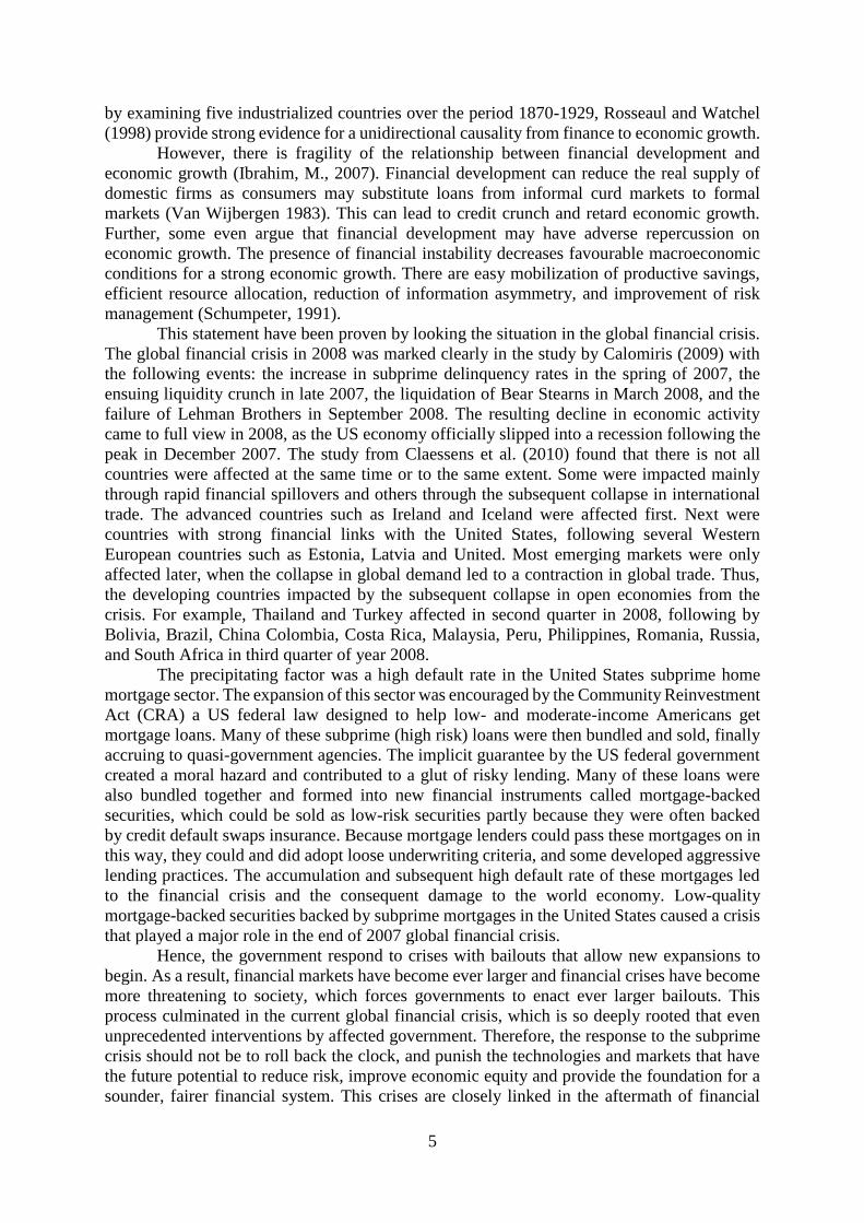
Table 3: Summary statistics

Minimum 10 %

quantile

25%

quantile

50%

quantile

75%

quantile

90%

quantile

Maximum

Full sample (1980-2015)

GROWTH -12.1584 -1.95999 0.284293 2.054874 3.611244 5.099898 10.6468

DCPS 0.507391 7.255853 14.41938 24.42315 39.51458 65.25134 147.1132

LL 0.00007 15.36658 21.94535 31.67114 48.04944 77.08999 175.2327

PCDM 2.38E-05 7.178998 13.0196 23.71132 39.18753 66.65384 145.4332

FDI -2.41406 0.098084 0.525568 1.556395 3.586591 5.86478 27.7441

FCAPITAL 5.287233 13.22195 16.7538 20.66417 25.31516 30.64452 67.94262

CPI 1.27E-11 5.68635 24.99292 57.67976 84.95159 113.6003 209.2374

HC 0.061667 0.415833 0.876667 1.556667 2.42 3.686667 6.758333

Regime 1: Period with the global financial crisis (1980-2008)

GROWTH -12.577 -2.25825 0 1.835465 3.700445 5.852173 12.40417

DCPS 0.624961 6.725534 12.82993 22.0526 35.90868 60.79381 148.9025

LL 0.00007 14.07986 20.45382 29.01117 45.17217 74.5094 140.1606

PCDM 2.38E-05 5.482951 11.7249 21.50451 33.65787 58.24547 145.3026

FDI -3.43271 0.082384 0.364901 1.336748 3.078573 5.326728 16.87215

FCAPITAL 3.958172 12.74261 16.60739 20.01761 24.42503 29.98878 65.93127

CPI 1.02E-11 3.281525 15.48634 45.94872 69.93418 81.84431 96.37586

HC 0.06 0.36 0.81 1.42 2.29 3.38 6.87

Regime 2: Period after the global financial crisis (2009-2015)

GROWTH -22.2913 -0.88995 0.853345 2.599571 4.24655 6.016117 18.06457

DCPS 3.92231 14.06665 22.7601 35.715 51.6572 84.6743 151.48

LL 6.700744 21.02809 30.67901 41.23619 61.80407 97.36151 182.7313

PCDM 2.785867 13.48744 21.97756 34.16426 50.57098 89.03164 149.3656

FDI -1.07525 0.873541 1.640418 3.057685 5.604434 9.022434 45.28993

FCAPITAL 8.95112 15.33145 19.11637 22.96524 27.33974 33.41376 50.77814

CPI 85.7374 96.56959 100 109.2717 120.2805 135.6614 348.9924

HC 0.19 0.59 1.46 2.27 3.34 4.58 6.87

Note: GROWTH = GDP per capita growth (%); DCPS = Domestic credit to private sector (% of GDP); LL =

Liquid liabilities (% of GDP); PCDM = Private credit to deposit money (% of GDP); FDI = Foreign direct

investment (% of GDP); FCAPITAL = Gross fixed capital formation (% of GDP); CPI = Consumer price index;

HC = Average years of schooling.

In general, the finance indicators that widely used in the literature are private credit to

deposit money as a percentage of GDP (Gregorio and Guidotti, 1995; Levine, 1999; Claessens

and Laeven, 2002; Loayza and Ranciere, 2002; Liu and Hsu, 2006; Shen and Lee, 2006;

Naceur and Ghazouani, 2007; Kemal et al., 2008; Barajas et al., 2010; Estrada et al., 2010;

Goaied and Sassi, 2010; Huang et al., 2010; Hassan et al., 2010; Leitao, 2010; Law and Singh,

2014; Samargandi et al., 2015), liquid liabilities as a percentage of GDP (Levine, 1999; Favara,

2003; Christopoulos and Tsionas, 2004; Liu and Hsu, 2006; Shen and Lee, 2006; Naceur and

Ghazouani, 2007; Kemal et al., 2008; Estrada et al., 2010; Goaied and Sassi, 2010; Huang et

13

al., 2010; Jalil et al., 2010; Hassan et al., 2011; Loayza and Ranciere, 2002; Lu and Yao, 2009,

Law and Singh, 2014) and domestic credit to private sector as a percentage of GDP (Hassan et

al., 2011; Law and Singh, 2014). Therefore, this study uses three financial indicators namely,

domestic credit to private sector, liquid liabilities and private credit to deposit money by banks

and other financial institutions. The source of these data is the 2017 version of World Bank’s

Dataset Indicators (WDI) and 2016 version of World Bank’s Financial Structure Dataset.

The summary statistics of the variables are shown in Table 3. The highest median for

financial indicators is liquid liabilities at 31.67 percent. The median for DCPS and PCDM is

24.42% and 23.71%, respectively. The summary statistics for second regime is higher than the

first regime. This entails the high degree of financial activities and also the increment of the

value due to increasing in inflation in the recent economy.

4. Methodology

4.1 Dynamic Panel Model: Generalized Method-of-Moment (GMM)

We estimate the quadratic polynomial model by using Generalized Method-of-Moments

(GMM). GMM is used to estimate the dynamic panel data model also allows for the lagged

level of economic growth. GMMs panel estimator was first proposed by Holtz-Eakin et al.

(1988) and this was subsequently extended by Arellano and Bond (1991), Arellano and Bover

(1995), and Blundell and Bond (1998). There are at least two reasons for choosing this

estimator. Firstly, to control for the country-specific effects, which cannot use country-specific

dummies due to the dynamic structure of the regression equation. Secondly, the estimator

controls for a simultaneity bias are caused by the possibility that some of the explanatory

variables may be endogenous. This method uses a set of instrumental variables to solve the

endogeneity problem of the regressors.

There are two types of GMM estimators (difference and system) and they can both be

alternatively considered in their one-step and two-step versions. However, the system-GMM

as proposed by Arellano and Bover (1995) only used in this study. The system-GMM estimator

(sys-GMM) includes not only the previous instruments but also the lagged values of the

dependent variable (Blundell and Bond, 1998). It helps solve the endogeneity problem arising

from the potential correlation between the independent variable and the error term in dynamic

panel data models (Topcu, 2013). It also permits to dealing with omitted dynamics in static

panel data models, owing to the ignorance of the impacts of lagged values of the dependent

variable (Bonds, 2002). Following Arellano and Bover (1995), the moment conditions for the

system-GMM are set as follows:

Ε[(𝑦𝑖,𝑡−𝑠 − 𝑦𝑖,𝑡−𝑠−1). (𝜂𝑖 + 휀𝑖,𝑡)] = 0 for 𝑠 = 1 (8)

Ε[(𝐹𝐼𝑁𝐷𝐸𝑉𝑖,𝑡−𝑠 − 𝐹𝐼𝑁𝐷𝐸𝑉𝑖,𝑡−𝑠−1). (𝜂𝑖 + 휀𝑖,𝑡)] = 0 for 𝑠 = 1 (9)

Ε[(𝑋′𝑖,𝑡−𝑠 − 𝑋𝑖,𝑡−𝑠−1). (𝜂𝑖 + 휀𝑖,𝑡)] = 0 for 𝑠 = 1 (10)

The consistency of the GMM estimator depends on two specification tests. The first is

Hansen’s (1982) J-test of over-identifying restrictions. Under the null of joint validity of all

instruments, the empirical moments have zero expectation, so the J statistic is distributed and

𝜒2 with degrees of freedom equal to the degree of over-identification. The second test examines

the hypothesis of no second-order serial correlation in the error term (Arellano and Bond,

1991). The failure to reject the null of both tests provides support to the estimated model.

14

The GMM estimators are typically applied in one-step and two-step variants (Arellano

& Bond, 1991). The one-step estimators use weighting matrices that are independent of

estimated parameters, whereas the two-step GMM estimator uses the so-called optimal

weighting matrices in which the moment conditions are weighted by a consistent estimate of

their covariance matrix. This makes the two-step estimator asymptotically more efficient than

the one-step estimator. However, the use of the two-step estimator in small samples has several

problems in terms of the estimation and diagnostics. These problems occur from the

instruments’ proliferation. If the number of instruments’ proliferation is more than the number

of groups, the estimation of parameter is inaccurate. To overcome this problem, we use the

collapse of lag length technique proposed by Roodman (2009) to get better results and achieve

the goodness of fit in the model.

4.1 Sasabuchi-Lind-Mehlum of U test

Even though most of the existing empirical studies claim that a U-shaped is identified if the

nonlinear term in quadratic model is significant, Lind and Mehlum (2010) demonstrated that

the true relationship is convex but monotone over relevant data values, it may spuriously

identify an extreme value and U-shaped properties.

To test for the presence of a U-shaped profile in more appropriate way, this study is

required to provide sufficiently strong evidence that the slope of the curve is positive at low

values of 𝐹𝑖𝑛𝐷𝑒𝑣 and negative at high values of 𝐹𝑖𝑛𝐷𝑒𝑣 to examine the existing of Kuznets

curve in ‘finance curse’ hypothesis. On the other hand, to investigate the existing of U-shape

or anti-Kuznets curve, the slope of the curve is negative at low values of 𝐹𝑖𝑛𝐷𝑒𝑣 and positive

at high values of 𝐹𝑖𝑛𝐷𝑒𝑣 to support the ‘more finance, more growth’ hypothesis. To confirm

our finding of an inverted U-shaped or U-shaped relationship between financial development

and economic growth, we conduct the U test of Sasabuchi (1980) which is extended by Lind

and Mehlum (2010). In the quadratic case in Eq. (7), the composite null with the joint

hypothesis is tested as follows:

𝐻0 ∶ (𝛽1 + 𝛽22𝐹𝑖𝑛𝐷𝑒𝑣𝑚𝑖𝑛 ⩽ 0) ∪ (𝛽1 + 𝛽22𝐹𝑖𝑛𝐷𝑒𝑣𝑚𝑎𝑥 ⩾ 0) (11)

against the alternative hypothesis:

𝐻1 ∶ (𝛽1 + 𝛽22𝐹𝑖𝑛𝑑𝐷𝑒𝑣𝑚𝑖𝑛 > 0) ∪ (𝛽1 + 𝛽22𝐹𝑖𝑛𝐷𝑒𝑣𝑚𝑎𝑥 < 0) (12)

where 𝐹𝑖𝑛𝐷𝑒𝑣𝑚𝑖𝑛 and 𝐹𝑖𝑛𝐷𝑒𝑣𝑚𝑎𝑥 represent the minimum and maximum values of financial

development, respectively. If the null hypothesis is rejected, this confirms the existence of an

inverted U-shape.

Particularly, the corresponding rejection is the convex cone:

𝑅𝛼 = (𝛽1, 𝛽2)𝛽1 + 𝛽2𝑓′(𝐹𝑖𝑛𝐷𝑒𝑣𝑚𝑖𝑛)

√𝑠11 + 2𝑓′(𝐹𝑖𝑛𝐷𝑒𝑣𝑚𝑖𝑛)𝑠12 + 𝑓′(𝐹𝑖𝑛𝐷𝑒𝑣𝑚𝑖𝑛)2𝑠22

< −𝑡𝛼

and 𝛽1 + 𝛽2(𝐹𝑖𝑛𝐷𝑒𝑣𝑚𝑎𝑥)

√𝑠11 + 2𝑓′(𝐹𝑖𝑛𝐷𝑒𝑣𝑚𝑎𝑥)𝑠12 + 𝑓′(𝐹𝑖𝑛𝐷𝑒𝑣𝑚𝑎𝑥)2𝑠22

> 𝑡𝛼

(13)

where 𝑠11, 𝑠22and 𝑠12 denote the estimated variances of 𝛽1 and 𝛽2 and the covariance between

𝛽1 and 𝛽2, respectively, and 𝑡𝛼 is the critical value with the appropriate degrees of freedom and

15

significance level α. Following Fieller (1954), Lind and Mehlum (2010) also provided the (1-

2α) confidence interval for the estimated extreme point, that is, -�̂�1/2�̂�2 in the quadratic case.

From the Eq. (7), the presence of a U-shape indicates that 𝛽1 + 𝛽22𝐹𝑖𝑛𝐷𝑒𝑣𝑚𝑖𝑛 < 0 and

𝛽1 + 𝛽22𝐹𝑖𝑛𝐷𝑒𝑣𝑚𝑎𝑥 > 0, whereas in the inverted U-shape means that 𝛽1 + 𝛽22𝐹𝑖𝑛𝐷𝑒𝑣𝑚𝑖𝑛 >0 and 𝛽1 + 𝛽22𝐹𝑖𝑛𝐷𝑒𝑣𝑚𝑎𝑥 < 0. Therefore the existing of U-shape can be tested as follows:

𝐻0 ∶ (𝛽1 + 𝛽22𝐹𝑖𝑛𝐷𝑒𝑣𝑚𝑖𝑛 ⩾ 0) ∪ (𝛽1 + 𝛽22𝐹𝑖𝑛𝐷𝑒𝑣𝑚𝑎𝑥 ⩽ 0) (14)

𝐻1 ∶ (𝛽1 + 𝛽22𝐹𝑖𝑛𝐷𝑒𝑣𝑚𝑖𝑛 < 0) ∪ (𝛽1 + 𝛽22𝐹𝑖𝑛𝐷𝑒𝑣𝑚𝑎𝑥 > 0) (15)

From Eq. (14) and Eq. (15), and if the null hypothesis is rejected, this confirms the existence

of U-shape in the nonlinearity relationship between financial development and economic

growth. Thus, the hypothesis of U test is depends on the quadratic model estimation from

system-GMM results in this study.

5. Empirical Findings and Discussions

Table 4 reports the results of system-GMM estimating Eq. (7) using three financial

development indicators in the quadratic polynomial model from Eq. (7). Meanwhile, the results

in Table 5 reports the existing of U-shape or inverted U-shape to confirm the nonlinearity either

anti-Kuznets or Kuznets curve in the results in Table 4. Finance indicators measure is domestic

credit to private sector (DCPS), liquid liabilities (LL) and private credit to deposit money

(PCDM).

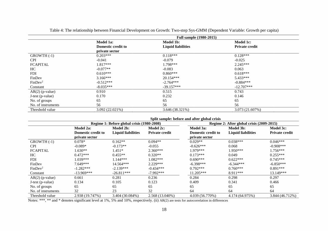
DCPS in full sample shows that the point estimate of the threshold value is 3.092 or

22.02% of GDP based on the first order condition (𝜕𝐺𝑅𝑂𝑊𝑇𝐻/𝜕𝐹𝐼𝑁𝐷𝐸𝑉). The result also

close with the threshold computed in Sasabuchi-Lind-Mehlum test (Table 5) of 3.091 or

22.00% of GDP with a corresponding 90% Fieller confidence interval [2.789, 3.267]. However,

the threshold percentage from our study is higher than the threshold of 2.295 or 9.924% of

GDP that calculated of the coefficient gain from GMM estimation studied by Law and Singh

(2014). The differences of the threshold point because two main reasons. First, our sample

focusing on developing countries, while the sample of study by Law and Singh (2014) covered

the developed and developing countries. Second, our period of study extended until 2015 data.

Nevertheless, we are not comparing the threshold point obtain from the dynamic panel

threshold in their study or other different methods. While, the threshold point of LL is 3.646 or

38.321% with 90% Fieller confidence interval [3.585, 3.709], and PCDM’s threshold point is

3.073 or 21.607% in the range of 90% Fieller confidence interval [2.914, 3.214]. The threshold

point for LL is higher as compared to the rest financial indicators. By using the period until the

recent data, these points also higher than the threshold points from the study by Law and Singh

(2014) at 2.28 and 2.21 for liquid liabilities and private sector credit, respectively.

However, the main things in this study is to investigate the nonlinearity of the

relationship between financial development and economic growth, whether there is exist U-

shape or inverted U-shape. The results from system-GMM estimation in Table 4 in full sample

(1980-2015 period) shows that the relationship between financial development and economic

growth is inverted U-shape or economic Kuznets curve indicated by the coefficient of 𝛽1 and

𝛽2 from the Eq. (7) is significant in positively and negatively sign, respectively. These results

are consistent with the findings by Arcand et al. (2012), Cecchetti and Kharroubi (2012), Law

and Singh (2014), and Samargandi et al. (2012). The financial development has positive impact

on economic growth until to the certain point, but after it reach the threshold point, financial

sector may cause the detrimental of economic growth. These results supported the ‘too much

16

finance harm growth’ hypothesis and ‘vanishing effect’. It is also supported by Sasabuchi-

Lind-Mehlum of U-test in Table 5 of exist the inverted U-shape relationship between financial

development and economic growth for all models. The slope of FINDEVmin is positive and

statistically significant, while FINDEVmax is negatively significant for all models, thus, the

results corresponding to the inverse U-shape in the relationship between financial development

and economic growth. This result of U-shape is consistent with the study by Samargandi et al.

(2015) that employed the same econometric technique.

Nonetheless, our interesting part is in splitting sample results. Our sample period in the

first regime is similar with the sample period of Samargandi et al. (2015), but the sample of

countries is different. The first regime prolonged with 29 years period consistent with the full

sample results that confirming the inverted U-shape for all models as shown in Model 2a-2c.

The U-test results in Model 5a-5c as shown in Table 5 also confirmed the economic Kuznets

curve or inverted U-shape. Thus, the results in the sample period in crises (Asian financial in

1997-1998 and global financial crisis in 2007-2008) supported the ‘too much finance harm

growth’ hypothesis. Similar with the full sample result, the financial development will dampen

the economic growth after it surpassed the threshold point due to the ‘vanishing effect’ as

highlighted by Arcand et al. (2012). Moreover, the threshold points in Model 2a-2c and also in

Model 5a-5c are slightly lower than the threshold points in the full sample. This is because the

financial development is increasing from year to year with including the recent data that

slightly higher (see Table 3), that inherit the threshold point to become higher in full sample.

Interestingly, the results for the second regime is contrast with the first regime and also

different with the full sample. The results from system-GMM estimation in Model 3a-3c (see

Table 4) in the second regime shows that the coefficient of 𝛽1 and 𝛽2 from the Eq. (7)

specification has negative and positive sign, respectively, and both are significant. These

indicates the relationship between financial development and economic growth is U-shape or

economic anti-Kuznets curve in all models for the Regime 2. These results are contrast with

the findings by Arcand et al. (2012), Cecchetti and Kharroubi (2012), Law and Singh (2014),

and Samargandi et al. (2012). For the case of second regime, the financial development can

boost the economic growth after it surpassed the threshold point. As a result, our findings had

challenging the hypothesis of ‘too much finance’, but supported the ‘more finance, more

growth’ as highlighted by Levine (1993). These results also supported by Sasabuchi-Lind-

Mehlum of U-test in Table 5 of U-shape relationship between financial development and

economic growth for all models. The slope of FINDEVmin is negative and statistically

significant, while FINDEVmax is positively significant for all models, thus, the results

conforming the U-shape in the relationship between financial development and economic

growth. The nonlinear mixture in the different regimes for all financial indicators also

illustrated in Figure 1. It seems like this group of country has been learnt from the global

financial crisis where these countries gone through the learning process. There is lesson to be

learnt from the global financial crisis. Consequently, there will focus more on tighten the

financial regulation with monitoring the liquid activities in the economy.

Rely on our results, it also supported Schumpeter (1911) where the important role of

financial development is still relevant in the recent economy. Our result denying the argument

from Asongu (2011) in his meta-analysis study, who claimed that the Schumpeter might be

wrong in the recent economy. The nonlinear mixture in our findings did not supported the meta

analysis study by Asongu (2011) who concern on endogeneity to be take into account that leads

the negative effect of finance and growth. He criticized the finance spillover has positive impact

on economic growth in Schumpeter hypothesis. Although the endogeneity problem has been

resolved in GMM technique, the impact of finance positively and negatively and both are

significant on growth was depends on the economic condition.

17

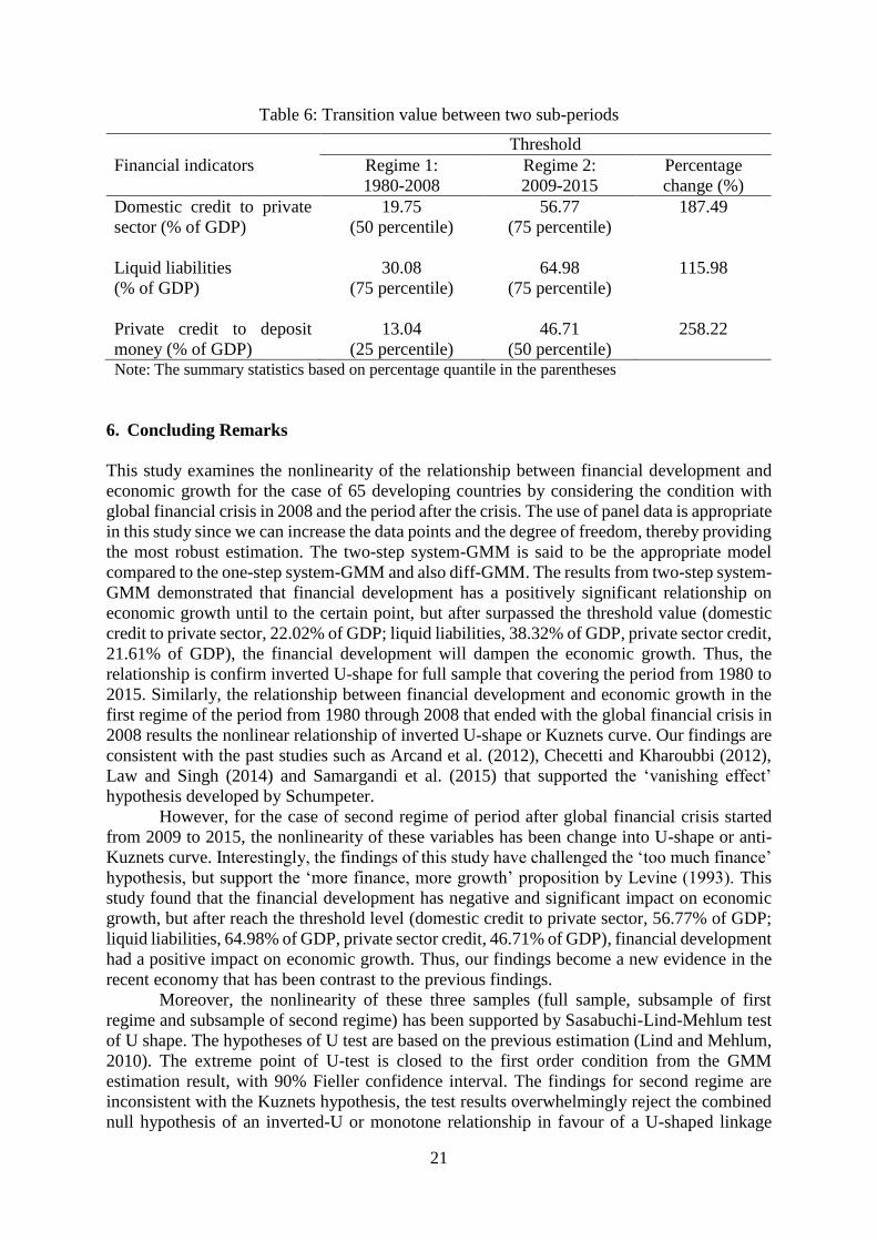
In further details, the threshold point of the second regime is higher than the threshold

point in the first regime. This is related to the statistical properties as shown in the Table 3 that

indicates the higher of financial development is necessary in the recent economy. Based on the

result in the Table 4, the threshold value for DCPS in first regime is 19.75% of GDP and the

size is increase in the second regime carry the threshold value up to 56.77%. This implies the

transition of threshold value in at least 25 percentile to Similarly to liquid liabilities and private

credit to deposit money where the threshold value increase 115.98% (from 30.08% of GDP to

64.98% of GDP) and 258.22% (from 13.04% of GDP to 46.71% of GDP), respectively. These

results infers the economy in transition period (See Table 6).

The threshold points are important to policy makers to set the appropriate financial cap

to control the financial activities. Having known that financial liberalisation may be harmful to

economic growth which requires further financial regulation control and activities, this tap does

not mean and immediate reduction of moral hazard in financial activities. Since the financial

sector is major contribution to growth through time, therefore, the central bank choose to imply

soft-landing policy. Soft-landing policy is not immediately reduce the finance curse, but it take

a longer period to be remedy. This may rise about another concern as to the duration of soft-

landing policy should be implemented where the country can benefit from it. For example,

when soft landing policy be fully materialised from 19.75% of GDP to 56.77% of GDP foresee

the continuous financial activities control. As a result, the central bank anticipated that the

amount of financial activities should be increase continuously during soft-landing period but

in the control manner. However, this aspect has not been studied previously, there is a gap to

be fill up in the present study.

18

Table 4: The relationship between Financial Development on Growth: Two-step Sys-GMM (Dependent Variable: Growth per capita)

Full sample (1980-2015)

Model 1a:

Domestic credit to

private sector

Model 1b:

Liquid liabilities

Model 1c:

Private credit

GROWTH (-1) 0.203*** 0.118*** 0.128***

CPI -0.041 -0.079 -0.025

FCAPITAL 1.817*** 1.798*** 2.245***

HC -0.077** -0.083 0.063

FDI 0.610*** 0.860*** 0.618***

FinDev 3.166*** 20.154*** 5.433***

FinDev2 -0.512*** -2.764*** -0.884***

Constant -8.035*** -39.157*** -12.707***

AR(2) (p-value) 0.910 0.515 0.743

J-test (p-value) 0.170 0.232 0.146

No. of groups 65 65 65

No. of instruments 56 56 56

Threshold value 3.092 (22.021%) 3.646 (38.321%) 3.073 (21.607%)

Split sample: before and after global crisis

Regime 1: Before global crisis (1980-2008) Regime 2: After global crisis (2009-2015)

Model 2a:

Domestic credit to

private sector

Model 2b:

Liquid liabilities

Model 2c:

Private credit

Model 3a:

Domestic credit to

private sector

Model 3b:

Liquid liabilities

Model 3c:

Private credit

GROWTH (-1) 0.078* 0.162** 0.094** 0.029** 0.038*** 0.046***

CPI -0.089* -0.173** -0.055 -0.626*** 0.068 -0.908***

FCAPITAL 1.630** 1.451* 2.360*** 1.979*** 1.950*** 1.756***

HC 0.472*** 0.455** 0.320** 0.173*** 0.049 0.255***

FDI 1.039*** 1.144*** 1.082*** 0.690*** 0.622*** 0.745***

FinDev 7.649*** 14.564*** 2.229*** -6.398*** -6.344*** -6.850***

FinDev2 -1.282*** -2.139*** -0.434*** 0.792*** 0.760*** 0.891***

Constant -13.969*** -26.811*** -7.992*** 11.205*** 8.911*** 13.149***

AR(2) (p-value) 0.661 0.281 0.236 0.284 0.298 0.297

J-test (p-value) 0.134 0.105 0.123 0.409 0.341 0.466

No. of groups 65 65 65 65 65 65

No. of instruments 32 23 32 64 64 64

Threshold value 2.938 (19.747%) 3.404 (30.084%) 2.568 (13.040%) 4.039 (56.770%) 4.174 (64.975%) 3.844 (46.712%)

Notes: ***, ** and * denotes significant level at 1%, 5% and 10%, respectively. (ii) AR(2) are tests for autocorrelation in differences

19

Table 5: Sasabuchi-Lind-Mehlum (SLM) test for U-shape

Full sample (1980-2015)

Model 4a:

Domestic credit to

private sector

Model 4b:

Liquid liabilities

Model 4c:

Private credit

Extreme point 3.091 3.646 3.072

95% Fieller interval [2.789, 3.267] [3.585, 3.709] [2.914, 3.214]

Slope at FINDEVmin 3.861***

(4.775)

73.043***

(10.256)

24.264***

(11.556)

Slope at FINDEVmax -1.946***

(-6.353)

-8.403***

(-9.872)

-3.375***

(-12.231)

Hypothesis test H0: U shape

H1: Inverted U shape

H0: U shape

H1: Inverted U shape

H0: U shape

H1: Inverted U shape

SLM test for U shape (t-value) 4.77*** 9.87*** 11.56***

p-value 0.000 0.000 0.000

Split sample: before and after global crisis

Regime 1: Before global crisis (1980-2008) Regime 2: After global crisis (2009-2015)

Model 5a:

Domestic credit to

private sector

Model 5b:

Liquid liabilities

Model 5c:

Private credit

Model 6a:

Domestic credit to

private sector

Model 6b:

Liquid liabilities

Model 6c:

Private credit

Extreme point 2.983 3.040 2.567 4.041 4.173 3.844

95% Fieller interval [2.616, 3.194] [3.222, 3.556] [2.145, 2.891] [3.919, 4.193] [3.933, 4.560] [3.690, 4.019]

Slope at FINDEVmin 8.854***

(3.312)

55.498***

(4.261)

11.472***

(4.908)

-4.234***

(-20.373)

-3.452***

(-8.438)

-5.024***

(-25.846)

Slope at FINDEVmax -5.178***

(-3.714)

-6.583***

(-4.339)

-2.094***

(-5.256)

1.551***

(7.727)

1.574***

(3.613)

2.072***

(9.067)

Hypothesis test H0: U-shape

H1: Inverted U-

shape

H0: U-shape

H1: Inverted U-

shape

H0: U-shape

H1: Inverted U-

shape

H0: Inverted U-

shape

H1: U-shape

H0: Inverted U-

shape

H1: U-shape

H0: Inverted U-

shape

H1: U-shape

SLM test for U shape (t-value) 3.31*** 4.26*** 4.91*** 7.73*** 3.61*** 9.07***

p-value 0.000 0.000 0.000 0.000 0.000 0.000

Notes: (i) *** denotes significant level at 1%. (ii) t-value in parentheses. (iii) The hypothesis testing is based on the SLM estimation

20

Figure 1: Nonlinear mixture on the relationship between financial development and economic growth

by splitting sample into two regimes

Domestic credit to private sector:

Before the global crisis (1980-2008) Domestic credit to private sector:

After the global crisis (2009-2015)

Liquid liabilities:

Before the global crisis (1980-2008) Liquid liabilities:

After the global crisis (2009-2015)

Private credit to deposit money:

Before the global crisis (1980-2008) Private credit to deposit money:

After the global crisis (2009-2015)

21

Table 6: Transition value between two sub-periods

Threshold

Financial indicators Regime 1:

1980-2008

Regime 2:

2009-2015

Percentage

change (%)

Domestic credit to private

sector (% of GDP)

19.75

(50 percentile)

56.77

(75 percentile)

187.49

Liquid liabilities

(% of GDP)

30.08

(75 percentile)

64.98

(75 percentile)

115.98

Private credit to deposit

money (% of GDP)

13.04

(25 percentile)

46.71

(50 percentile)

258.22

Note: The summary statistics based on percentage quantile in the parentheses

6. Concluding Remarks

This study examines the nonlinearity of the relationship between financial development and

economic growth for the case of 65 developing countries by considering the condition with

global financial crisis in 2008 and the period after the crisis. The use of panel data is appropriate

in this study since we can increase the data points and the degree of freedom, thereby providing

the most robust estimation. The two-step system-GMM is said to be the appropriate model

compared to the one-step system-GMM and also diff-GMM. The results from two-step system-

GMM demonstrated that financial development has a positively significant relationship on

economic growth until to the certain point, but after surpassed the threshold value (domestic

credit to private sector, 22.02% of GDP; liquid liabilities, 38.32% of GDP, private sector credit,

21.61% of GDP), the financial development will dampen the economic growth. Thus, the

relationship is confirm inverted U-shape for full sample that covering the period from 1980 to

2015. Similarly, the relationship between financial development and economic growth in the

first regime of the period from 1980 through 2008 that ended with the global financial crisis in

2008 results the nonlinear relationship of inverted U-shape or Kuznets curve. Our findings are

consistent with the past studies such as Arcand et al. (2012), Checetti and Kharoubbi (2012),

Law and Singh (2014) and Samargandi et al. (2015) that supported the ‘vanishing effect’

hypothesis developed by Schumpeter.

However, for the case of second regime of period after global financial crisis started

from 2009 to 2015, the nonlinearity of these variables has been change into U-shape or anti-

Kuznets curve. Interestingly, the findings of this study have challenged the ‘too much finance’

hypothesis, but support the ‘more finance, more growth’ proposition by Levine (1993). This

study found that the financial development has negative and significant impact on economic

growth, but after reach the threshold level (domestic credit to private sector, 56.77% of GDP;

liquid liabilities, 64.98% of GDP, private sector credit, 46.71% of GDP), financial development

had a positive impact on economic growth. Thus, our findings become a new evidence in the

recent economy that has been contrast to the previous findings.

Moreover, the nonlinearity of these three samples (full sample, subsample of first

regime and subsample of second regime) has been supported by Sasabuchi-Lind-Mehlum test

of U shape. The hypotheses of U test are based on the previous estimation (Lind and Mehlum,

2010). The extreme point of U-test is closed to the first order condition from the GMM

estimation result, with 90% Fieller confidence interval. The findings for second regime are

inconsistent with the Kuznets hypothesis, the test results overwhelmingly reject the combined

null hypothesis of an inverted-U or monotone relationship in favour of a U-shaped linkage

22

between financial development and economic growth for all finance indicators. Moreover, the

results are robust with Levine (1993) hypothesis of ‘more finance, more growth’. In addition,

the threshold point for the second regime are higher than the first regime. By considering the

linkages between these two regimes, the changes of the threshold point between regimes

indicates the transition period from cataclysm to remedy period before the financial

development boost the economic growth in the recent economies.

Our findings have contributed to enhancing the existing finance-growth literature in

two aspects. First, there exists nonlinear mixture of inverted U-shape and U-shape relationship

between financial development and economic growth when the relationship is studied in two

different regimes covering the period before and after global financial crisis – an approach less

attempted in the past. Second, this study has also proposed the transition period required in

investing for further financial development from the catastrophic period to the remedy period,

before the financial development regains its strength to boost economic growth once again.

This is made possible by identifying the two threshold points found our study. Thus, these

findings can be claimed as a new evidence to be contributed to the finance-growth literature.

In general, the policy makers should enhance the financial sector at least beyond the 90

percentile (refer to Table 2) to utilize the financial development in order to boost the economic

growth. In terms of policy implication, findings from the study suggest that policy makers

should not only expand on financial development in fostering economic growth but also

increase the quality of financial sector. This implies the concurrent expansion and tightening

of financial regulations with attendant control and monitoring of financial activities to ensure

the effectiveness of financial development on economic growth as well as to avoid the

‘vanishing effect’ that may lead to recurrence of economic crises in the future. In lieu of the

nonlinearity of the U-shaped profile in finance-growth relationship in our findings, does

financial regulation and its implementation, such as Basel III, positioned on the right track?

The financial policy as suggested by the previous studies need to be revised and to benefit from

the ‘more finance, more growth’ proposition. By take into account not only the quantity of

finance but also the quality, this study leads to ‘more and better finance, more growth’

proposition.

Despite, the nonlinearity of finance-growth relationship of U-shaped in our study

contradicted with the previous study in different time period indicate that the financial

development effect on economic growth may contingent on the economic situation. The study

also challenged the findings by Arcand et al. (2015) who suggested that the ‘vanishing effect’

was not influenced by output volatility and banking crises. In addition, the effect of financial

development on economic growth also depends on the level of macroeconomic variable and

economic regulation such as inflation (Yilmazkuday 2011), financial sector policies (Abiad &

Mody 2005), financial openness (Rajan & Zingales 2003) as a precondition, therefore this

dependency indicates the fragility of financial in boosting the economic growth. Hence, as

highlighted by Reinert (2012), which element should be controlled by policy makers, either to

save the financial economy or save the real economy? The paper suggests that policy makers

should control the financial mediating variables as well as the real economy instead only

expanding the financial sector development with contemporaneous banking quality to improve

the financial performance in promoting economic growth.

The findings also contribute to the finance-growth study to be extend and may lead to

feasibility study ties to reassess the nonlinearity of finance-growth based on different situations.

Research findings prior to the 2007-2008 Global Financial crisis produced the inverted U-

shaped profile while post-crisis research studies produced the U-shaped profile in finance-

growth relationship. For the future, is there the possibility of discovering a S-shaped

relationship? Such a profile, may likely postulate the transition period from catastrophic to

remedy period. The question may arise that, does the recent economy postulated as remedial

23

period? If S-shaped profile is possible then policy makers should be cautious that a regime-

switch trigger in the cycle of finance-growth may likely occur in the future. Hence, further

research is necessary to elucidate on this possibility.

Acknowledgement

This paper was supported financially by the Ministry of Higher Education, Malaysia through

the International Islamic University College Selangor under the Fundamental Research Grant

Scheme (FRGS) grant: FRGS/2/2014/SS05/KUIS/03/1.

References

Abiad, A and Mody, A (2005). Financial reform: what shakes it? What shapes it? American

Economic Review, 95(1), 63-88.

Aghion, P, Howitt, P and Mayer Foulkes, D (2005). The effect of financial development on

convergence: theory and evidence. Quarterly Journal of Economics 120, 173

Al-Yousif, Y. K. (2002). Financial development and economic growth: another look at the

evidence from developing countries. Review of Financial Economics, 11(2), 131-150.

Andrianova, S., Demetriades, P., & Shortland, A. (2008). Government ownership of

banks, institutions and financial development. Journal of Development

Economics 85 (1–2), 218–252.

Ang, J.B., 2008. Are financial sector policies effective in deepening the Malaysia

financial system. Contemporary Economic Policy 26 (4), 623–635.

Ang, J. B., & McKibbin, W. J. (2007). Financial liberalization, financial sector development

and growth: evidence from Malaysia. Journal of development economics, 84(1), 215-

233.

Apergis, N., Filippidis, I., & Economidou, C. (2007). Financial deepening and economic

growth linkages: a panel data analysis. Review of World Economics, 143(1), 179-198.

Arcand, J.L., Berkes, E., Panizza, U., 2012. Too Much Finance? IMF Working Paper 12/

161.

Arellano, M. & Bond, S. (1991). Some tests of specification for panel data: monte carlo

evidence with an application for employment equations. Review of Economic Studies, 58,

277–297.

Arellano, M., Bover, O. (1995). Another look at the instrumental-variable estimation of error-

components models. Journal of Econometrics, 68, 29–52.

Arestis, P., & Demetriades, P. (1997). Financial development and economic growth: assessing

the evidence. The Economic Journal, 107(442), 783-799.

Asongu, SA (2011). “Financial and Growth: Schumpeter might be wrong in our era. New

evidence from Meta-analysis”. MPRA No. 32559.

Barajas, A., Chami, R., & Yousefi, S. R., (2010). The Finance and Growth Nexus Re-

examined: Are There Cross-Region Differences? IMF Working Paper.

Basel Committee on Banking Supervision. (2010). Basel III: International framework for

liquidity risk measurement, standards and monitoring. Bank for International

Settlements.

Beck, T., & Levine, R. (2004). Stock markets, banks, and growth: Panel evidence. Journal of

Banking & Finance, 28(3), 423-442.

Beck, T., Levine, R. Loayza, N. (2000). Finance and the sources of growth. Journal of

Financial Economics 58(1-2), 261-300.

24

Beck T., Degryse, H., Kneer, C. (2012). Is More Finance Better? Disentangling Intermediation

and Size Effects of Financial Systems, Center for Economic Research, Discussion Paper

No. 2012-060, Tilburg University.

Bencivenga, V. R., & Smith, B. D. (1991). Financial intermediation and endogenous

growth. The Review of Economic Studies, 58(2), 195-209.

Benhabib, J., & Spiegel, M. M. (2000). The role of financial development in growth and

investment. Journal of economic growth, 5(4), 341-360.

Bertocco, G. (2008). Finance and development: Is Schumpeter’s analysis still

relevant?. Journal of Banking & Finance, 32(6), 1161-1175.

Blackburn, K., & Hung, V. T. (1998). A theory of growth, financial development and

trade. Economica, 65(257), 107-124.

Blundell, R., Bond, S. (1998). Initial conditions and moment restrictions in dynamic panel data

models. Journal of Econometrics 87(1), 115-143.

Bond, S. (2002). Dynamic panel data models: a guide to micro data methods and

practice. Portuguese economic journal, 1(2), 141-162.

Bowsher, C. (2002). On testing overidentifying restrictions in dynamic panel data models.

Economic Letters 77(2), 211-220.

Broner, F. A., & Ventura, J. (2010). Rethinking the effects of financial liberalization (No.

w16640). National Bureau of Economic Research.

Buckle, R. A., (2009). “Asia-Pacific growth before and after the global financial crisis”. Policy

Quarterly, 5(4): 36-45.

Cecchetti, G., Kharroubi, E (2012). Reassessing the Impact of Finance on Growth. BIS Working

Papers No. 381, Bank for International Settlements.

Christopoulos, D. K., & Tsionas, E. G., (2004). “Financial development and economic

growth:evidence from panel unit root and cointegration tests”. Journal of Development

Economics. 73: 55-74.

Claessens, S., & Laeven, L., (2002). “Financial Development, Property Rights and Growth”.

World Bank Policy Research Working Paper 2924

Crotty, J. (2009). Structural causes of the global financial crisis: a critical assessment of the

‘new financial architecture’. Cambridge journal of economics, 33(4), 563-580.

Demetriades, P. O., & Hussein, K. A. (1996). Does financial development cause economic

growth? Time-series evidence from 16 countries. Journal of Development

Economics, 51(2), 387-411.

Deidda, L. & Fattouh, B. (2002). Nonlinearity between finance and growth. Economics

Letters 74 (3), 339–345.

Demirgüç-Kunt, A., Córdova, E. L., Peria, M. S. M., & Woodruff, C. (2011). Remittances and

banking sector breadth and depth: Evidence from Mexico. Journal of Development

Economics, 95(2), 229-241.

Ergungor, O.E. (2008). Financial system structure and economic growth: structure

matters. International Review of Economics and Finance 17 (2), 292–305.

Favara, G., (2003). “An Empirical Reassessment of the Relationship between Finance and

Growth”. International Monetary Fund Working Paper 03/123.

Fieller, E. C. (1954). Some problems in interval estimation. Journal of the Royal Statistical

Society Series B 16, 175-185.

Gallagher, K.P., Tian, Y., Regulating capital flows in emerging markets: The IMF and the

global financial crisis. Review of Development Finance (2017),

http://dx.doi.org/10.1016/j.rdf.2017.05.002

Girma, S., & Shortland, A. (2008). The political economy of financial development.

Oxford Economics Papers 60 (4), 567–596.

25

Goaied, M., & Sassi, S., (2010). “Financial Development and Economic Growth in the MENA

Region: What about Islamic Banking Development”. Institut des Hautes Etudes

Commerciales, Carthage.

Greenwood, J., & Jovanovic, B. (1990). Financial development, growth, and the distribution

of income. Journal of political Economy, 98(5, Part 1), 1076-1107.

Gregorio, J., & Guidotti, P. E., (1995). “Financial Development and Economic Growth”. World

Development, 23(3): 433-448.

Gurley, J. G. S., Gurley, E. S. J. G., & Shaw, E. S. (1960). Money in a Theory of Finance (No.

332.4/G97m).

Hansen, L. P. (1982). Large Sample Properties of Generalized Method of Moments Estimators.

Econometrica 50(4): 1029-1054.

Hassan, K., Sanchez, B., & Yu, J., (2011). “Financial development and economic growth: new

evidence from panel data”. The Quarterly Review of Economics and Finance, 51: 88-

104.

Henry, P. B. (2000). Do stock market liberalizations cause investment booms?. Journal of

Financial economics, 58(1), 301-334.

Holtz-Eakin, D., Newey, W., Rosen, H., (1988). Estimating vector autoregressions with panel

data. Econometrica, 56, 1371–1395.

Huang, H.C., Lin, S.C. (2009). Non-linear finance-growth nexus. Economics of Transition 17,

439-466.

Huang, H., Lin, S., Kim, Dong. & Yeh, C., (2010). “Inflation and finance-growth nexus”.

Economic Modelling, 27: 229-236.

Hung, F.S. (2009). Explaining the nonlinear effects of financial development on economic

growth. Journal of Economics 97(1), 41-65.

Ibrahim, M. H. (2007). The role of the financial sector in economic development: the

Malaysian case, International Review Economics 54: 463-483.

Jalil, A., Wahid, A. N. M., & Shahbaz, M., (2010). “Financial Development and Growth: A

Positive, Monotonic Relationship? Empirical Evidences from South Africa”. MPRA No.

27668.

Kemal, A. R., Abdul, Q., & Hanif, M. N., (2008). “Financial Development and Economic

Growth: Evidence from Heterogeneous Panel of High Income Countries”. MPRA No.

10198.

Ketteni, E., Mamuneas, T., Savvides, A., & Stengos, T. (2007). Is the financial development

and economic growth relationship nonlinear?. Economics Bulletin, 15(14), 1-12.

King, G.R., Levine, R. (1993). Finance and growth: Schumpeter might be right. Quarterly

Journal of Economics 108(3), 717-737.

Kuznets, S. (1955). Economic growth and income inequality. The American economic

review, 45(1), 1-28.

La Porta, R., Lopez-de-Silane, F., Shleifer, A., Vishny, R.W. (1997). Legal determinants of

external finance. Journal of Finance 52(3), 1131-1150.

La Porta, R., Lopez-de-Silane, F., Shleifer, A., Vishny, R.W. (1998). Law and finance. Journal

of Political Economy 106(6), 1113-1155.

La Porta, R., Lopez-de-Silane, F., Shleifer, A. and Vishny, R.W. (2002). Government

ownership of banks. Journal of Finance LVII (1), 265–301.

Law, S.H. (2009). Trade openness, capital inflows and financial development in

developing countries. International Economic Journal 23 (3), 409–426.

Law, S.H. & Azman-Saini, W.N.W. (2012). Institutional quality, governance and

financial development. Economics of Governance 13 (3), 217–236.

Law, S.H., Azman-Saini, W.N.W., Ibrahim, M.H. (2013). Institutional quality, governance and

financial development. International Economic Journal 23(3), 217-236.

26

Law, S.H., Singh, N. (2014). Does too much finance harm economic growth? Journal of

Banking & Finance 41, 36-44.

Law, S.H., Kutan A.M., Naseem, N.A.M. (2017). The role of institutions in finance curse:

Evidence from international data. Journal of Comparative Economics (2017),

http://dx.doi.org/10.1016/j.jce.2017.04.001

Leitao, N., C., (2010). Financial Development and Economic Growth: A Panel Approach.

Theoretical and Applied Economics, 17(10:551): 15-24.

Levine, R. (1997). Financial development and economic growth: views and agenda. Journal of

Economic Literature 35(2), 688-726.

Levine, R. (2003). More on finance and growth: more finance, more growth? Federal Reserve

Bank of St. Louis Review 85 (July), 31-46.

Levine, R., Loayza, N., Beck, T. (2000). Financial intermediation and growth: causality and

causes. Journal of Monetary Economics 46(1), 31-77.

Levine, R., & Zervos, S. (1998). Stock markets, banks, and economic growth. American

economic review, 537-558.

Lind, J. T., & Mehlum, H. (2010). With or without U? The appropriate test for a U-shaped

relationship. Oxford Bulletin of Economics and Statistics, 72(1), 109-118.

Liu, W., & Hsu, C., (2006). “The role of financial development in economic growth: The

experience of Taiwan, Korea and Japan”, Journal of Asian Economics, 17: 667-690.

Loayza, N., & Ranciere, R., (2002). “Financial development, financial fragility and growth”,

Research Department of the Central Bank of Chile.

Luintel, K., & Khan, M., (1999). “A quantitative reassessment of the finance-growth nexus:

evidence from multivariate VAR”. Journal of Development Economics, 60: 381-405.

McKinnon, R. I. (1993). The order of economic liberalization: Financial control in the

transition to a market economy. JHU Press.

Naceur, S. B., & Ghazouani, S., (2007). “Stock markets, banks, and economic growth:

Empirical evidence from the MENA region”. Research in International Business and

Finance, 21: 297-315.

Ndikumana, L. (2005). Financial development, financial structure, and domestic investment:

International evidence. Journal of International Money and Finance, 24(4), 651-673.

Odedokun, M. O. (1996). Alternative econometric approaches for analysing the role of the

financial sector in economic growth: Time-series evidence from LDCs. Journal of

Development Economics, 50(1), 119-146.

Rahaman, M. M. (2011) Access to financing and firm growth. Journal of Banking and Finance

35, 79-723.

Rajan, R., Zingales, L. (1998). Financial dependence and growth. American Economic Review

88(3), 559-586.

Rajan, R., Zingales, L. (2003). The great reversals: the politics of financial development in the

twentieth century. Journal of Financial Economics 69(1), 5-50.

Reinert, E. S. 2012. Mechanisms of Financial Crises in Growth and Collapse: Hammurabi,

Schumpeter, Perez, and Minsky. Jurnal Ekonomi Malaysia 46(1): 85-100.

Rioja, F., Valev, N. (2004a). Does one size fit all? Are examination of the finance and growth

relationship. Journal of Development Economics 74(2), 429-447.

Rioja, F., Valev, N. (2004b). Finance and the sources of growth at various stages of economic

development. Economic Inquiry 42(1), 127-140.

Roe, M.J., Siegel, J.I. (2011). Political instability: effects on financial development, roots in

the severity of economic inequality. Journal of Comparative Economics 39(3), 279-309.

Roodman, D. (2009). A note on the theme of too many instruments. Oxford Bulletin of

Economics and Statistics 71(1), 135-158.

27

Rousseau, P. L., & Wachtel, P. (1998). Financial intermediation and economic performance:

historical evidence from five industrialized countries. Journal of money, credit and

banking, 657-678.

Rousseau, P. L., & Wachtel, P. (2000). Equity markets and growth: cross-country evidence on

timing and outcomes, 1980–1995. Journal of Banking & Finance, 24(12), 1933-1957.

Rousseau, P., & Wachtel, P., (2002), "Inflation thresholds and the finance-growth

nexus," Journal of International Money and Finance, 21(6), 777-793.

Rousseau, P., & Wachtel, P., (2011), "What is Happening to The Impact of

Financial Deepeneing on Economic Growth?" Economic Inquiry, 49, 276–288.

Samargandi, N., Fidrmuc, J., & Ghosh, S. (2015). Is the relationship between financial

development and economic growth monotonic? Evidence from a sample of middle-

income countries. World Development, 68, 66-81.

Sasabuchi, S. (1980). A test of a multivariate normal mean with composite hypotheses

determined by linear inequalities. Biometrika, 67(2), 429-439.

Schumpeter, J., (1911). The Theory of Economic Development, Cambridge, MA, Havard

University Press.

Shan, Z. J., Morris, A. G., & Sun, F. (2001). Financial development and economic growth: An

egg-and-chicken problem. Review of International Economics, 9(3), 443−454.

Shaw, E.S. (1973). Financial Deepening in Economic Development. Oxford University Press.

Shen, C.H. and Lee, C.C. (2006). Same financial development yet different economic growth

– why? Journal of Money, Credit and Banking 38(7), 1907-1994.

Stulz, R.M. & Williamson, R. (2003). Culture, openness and finance. Journal of Financial

Economics 70 (3), 313–349.

Xu, Z. (2000). Financial development, investment, and economic growth. Economic

Inquiry, 38(2), 331-344.

Yilmazkuday, H. (2011). Threshold in the Finance-Growth Nexus: A Cross-Country Analysis.

The World Bank Economic Review 25(2), 278-295.