does state fiscal relief during recessions a. first stage...

118

American Economic Journal: Economic Policy 2012, 4(3): 118–145 http://dx.doi.org/10.1257/pol.4.3.118

Does State Fiscal Relief During Recessions Increase Employment? Evidence from the American Recovery and Reinvestment Act†

By Gabriel Chodorow-Reich, Laura Feiveson, Zachary Liscow, and William Gui Woolston*

The American Recovery and Reinvestment Act (ARRA) of 2009 included $88 billion of aid to state governments administered through the Medicaid reimbursement process. We examine the effect of these transfers on states’ employment. Because state fiscal relief outlays are endogenous to a state’s economic environment, OLS results are biased downward. We address this problem by using a state’s pre-recession Medicaid spending level to instrument for ARRA state fiscal relief. In our preferred specification, a state’s receipt of a mar-ginal $100,000 in Medicaid outlays results in an additional 3.8 job-years, 3.2 of which are outside the government, health, and education sectors. (JEL H75, I18, I38, R23)

The federal government enacted the approximately $800 billion American Recovery and Reinvestment Act (ARRA) in February 2009 to provide a coun-

tercyclical impulse during the worst economic downturn in the United States in at least 60 years. At the same time, state governments, almost all of which have bal-anced budget requirements that restrict borrowing across fiscal years, had already begun to lay off employees, cut spending and transfer programs, and raise taxes. Rather than concentrate the stimulus in direct federal government purchases of output, the ARRA’s authors chose to mitigate this subnational contractionary fiscal impulse by routing roughly a third of the total through state and local governments. The largest of these programs was the increase in the federal match component of state Medicaid expenditures.

* Chodorow-Reich: UC Berkeley Department of Economics, 530 Evans Hall #3880, Berkeley, California 94720 (e-mail: [email protected]); Feiveson: MIT Department of Economics, 50 Memorial Drive E52-391, Cambridge, MA 02142 (e-mail: [email protected]); Liscow: UC Berkeley Department of Economics, 530 Evans Hall #3880, Berkeley, California 94720 (e-mail: [email protected]); Woolston: Stanford University Department of Economics, 579 Serra Mall, Stanford, CA, 94305 (e-mail: [email protected]). This paper bene-fited from discussions with Manuel Amador, Elizabeth Ananat, Alan Auerbach, Chris Carroll, Raj Chetty, Giacomo De Giorgi, Mark Duggan, Robert Hall, Caroline Hoxby, Pete Klenow, Pat Kline, Ilyana Kuziemko, Roy Mill, Enrico Moretti, John Pencavel, Jim Poterba, Christina Romer, David Romer, Jesse Rothstein, and Emmanuel Saez. In addition, we thank two anonymous referees for their helpful comments. All remaining errors are our own. Gabriel Chodorow-Reich acknowledges support from the National Science Foundation. Zachary Liscow acknowledges support from the Burch Center for Tax Policy and Public Finance and the Fisher Center for Real Estate and Urban Economics. William Gui Woolston acknowledges the support from the Stanford Graduate Fellowship Program.

† To comment on this article in the online discussion forum, or to view additional materials, visit the article page at http://dx.doi.org/10.1257/pol.4.3.118.

ContentsDoes State Fiscal Relief During Recessions Increase Employment? Evidence from the American Recovery and Reinvestment Act† 118

I. Institutional Details of the ARRA and Medicaid Grants 121II. Econometric Methodology and Baseline Specification 123A. Instrumental Variables Motivation 123B. Other Aspects of the Baseline Specification 123III. Data and Summary Statistics 125IV. Baseline Results 128A. First Stage 128B. Baseline Results through July 2009 130C. Timing Results 132V. Robustness Checks and Extensions 133A. Falsification Tests 133B. Other Robustness Checks 134VI. Discussion 137A. Job-Years 137B. Comparison to the Literature 138VII. Mechanism 139VIII. Conclusion 141Appendix 142A. Sources and Descriptions of Baseline Control Variables 142B. Description of Imputed Employment 143REFERENCES 143

mailto:[email protected]




http://dx.doi.org/10.1257/pol.4.3.118

VOL. 4 NO. 3 119chOdOROW-REIch ET AL.: STATE fIScAL RELIEf ANd EMPLOyMENT

Countercyclical intergovernmental transfers to support subnational budgets have occurred previously in the United States and in other countries around the world. Yet, this form of stimulus has received little attention in the academic literature, compared with the large number of studies of direct government purchases or tax reductions.1 A priori, transfers could have a small or zero immediate impact on economic outcomes if states simply use them to bolster their rainy day funds, effec-tively shifting money between government accounts without affecting the overall stance of the general government sector. On the other hand, states may use the money to reduce tax increases or avert budget cuts, allowing the money to enter the economy more quickly than direct federal purchases that require project selection and approval. Reflecting this theoretical uncertainty, views on the effectiveness of state aid prior to the ARRA’s passage ranged from then-House minority leader John Boehner, who predicted that “direct aid to the states is not going to do anything to stimulate our economy,” to the Obama administration, which predicted that the state relief would save or create more than 800,000 jobs in the fourth quarter of 2010.2 Even well after the ARRA’s passage, disagreement continued, with many Republicans and some economists claiming that no jobs had been created, while the White House continued claiming large job gains.3

This paper aims to fill the gap in our understanding of intergovernmental trans-fers by empirically assessing the impact of the ARRA’s Medicaid match program. The program has a number of features that make it attractive for study. First, the total amount of money distributed through this program is large enough to plausibly generate a detectable effect on employment. Out of a total of $88 billion dedicated to an increase in the Medicaid matching funds, states had received $61.2 billion by June 30, 2010, the end of our period of study. Second, because state Medicaid programs operate on a mandatory basis, increasing the federal share of costs effec-tively transfers money into state budgets that states can then use for any purpose they choose—the money is fungible. Indeed, many states reported that they had allocated the money quickly to areas that otherwise would have undergone deeper budget cuts (Government Accountability Office 2009; National Association of State Budget Officers 2009b). Third, the level of additional money received by states as of June 2010 per person aged 16 or older (16+) varied greatly, from a low of $103 in Utah to a high of $507 in DC, with an interquartile range of $114. This variation makes possible a cross-sectional econometric strategy. We focus our analysis on the effect on employment because the public debate on the effectiveness of the ARRA has centered largely on this outcome. Furthermore, high-quality monthly state level employment data makes it possible to obtain more precise estimates of fiscal multi-pliers than what is possible with the existing state-level income data.

1 There is a large literature on the extent to which federal grants crowd out local government spending which was spearheaded and summarized by Gramlich (1977).

2 See http://www.msnbc.msn.com/id/28841300/ns/meet_the_press/t/meet-press-transcript-jan/ and Romer and Bernstein (2009).

3 See http://www.factcheck.org/2010/09/did-the-stimulus-create-jobs/ for a list of quotes from Republicans claiming that the ARRA created no jobs. Also, a survey by the National Association for Business Economics showed that 69 percent of business economists they surveyed reported that the ARRA had no impact on employ-ment (http://www.jsonline.com/business/82657582.html).

http://www.msnbc.msn.com/id/28841300/ns/meet_the_press/t/meet-press-transcript-jan/

http://www.factcheck.org/2010/09/did-the-stimulus-create-jobs/

http://www.jsonline.com/business/82657582.html

120 AMERIcAN EcONOMIc JOuRNAL: EcONOMIc POLIcy AuguST 2012

The primary challenge to a cross-sectional study is that the amount of aid a state receives is endogenous to the state’s economic conditions. Because states that were in worse economic shape received more aid, the OLS relationship between the level of state fiscal transfers and changes in employment understates the true effect of state fiscal relief. We address this concern by using an instrument that isolates the component of the Medicaid transfers unrelated to changes in economic circum-stances. The ARRA increased the percentage of Medicaid expenditures that the fed-eral government pays for all states by 6.2 percentage points and increased the match rate by more for states that experienced especially large increases in unemployment. Thus, the level of ARRA Medicaid transfers to each state is the result of four factors: the amount of Medicaid spending in the state prior to the recession; the change in the number of beneficiaries during the recession; the change in the average spend-ing per beneficiary; and whether the state qualified for an additional match increase based on the change in the state’s unemployment rate. The heart of our identification strategy lies in exploiting only the cross-sectional variation from the first of these factors, that is, the variation in ARRA Medicaid transfers that results from variation in Medicaid programs from before the recession.

Another set of reasons why a state may have both received more Medicaid fund-ing and had different employment outcomes—omitted factors related to both state Medicaid program rules and economic changes—is not solved by the instrument. For example, more liberal coastal and Midwestern states both had larger downturns and have more generous Medicaid programs. We present several pieces of evidence that suggest that our results are not driven by underlying differences between high and low spending Medicaid states. First, to ensure that time-invariant differences between high and low Medicaid spending states are not driving our relationship, our empirical strategy considers changes, rather than levels, of employment. Second, in our baseline specification we exploit only differences in Medicaid spending within census divisions rather than between them, and include a number of variables that help predict how a state’s employment would have changed absent the ARRA. Finally, we present falsification tests by running our baseline specification on pre-ARRA data and show that in the decade before the ARRA passed, states with high and low Medicaid spending experienced similar employment outcomes.

An important caveat to our analysis is that a cross-state approach forces us to ignore general equilibrium effects, which could alter our interpretation of the overall effect of stimulus spending on jobs and prevents us from tying down the aggregate fiscal policy multiplier. For example, spending in one state may increase demand in other states, which would lead us to understate overall job increases.4 On the other hand, investment could decrease across the country in response to increased govern-ment borrowing, though this effect is likely to have been especially muted during the low policy interest rate environment of 2009–2010. Likewise, to the extent that people believe that their taxes will be raised in the future due to the increased gov-ernment borrowing, spending may decrease throughout the country.

4 Moretti (2010) notes that, through labor mobility, cross-state spillovers can also be negative. However, labor mobility is likely small over a period of time as short as that considered here.


With this caveat in mind, we find that the ARRA transfers to states had an eco-nomically large and statistically robust positive effect on employment. Assuming that employment does not persist beyond the time during which it is funded, our preferred specification suggests that a marginal $100,000 in Medicaid transfers resulted in 3.8 net job-years (i.e., one job that lasts for one year) of total employment through June 2010, of which 3.2 are outside the government, health, and education sectors. The effect is precisely estimated, and we can reject the null hypothesis that the spending had no effect on employment with a high degree of confidence. For this result to be economically plausible, states must have used the funds to avoid spending cuts or tax increases. Hence we also provide evidence that the transfers do not appear to have increased the states’ end of year balances. In connecting our estimates to the implicit changes in government spending or taxes, our paper also adds to the recent literature on the employment effects of state spending (e.g., Shoag 2011; Wilson forthcoming; Suarez-Serrato and Wingender 2011; Clemens and Miran 2012), as well as the fiscal effects of government spending generally (e.g., Nakamura and Steinsson 2011).

The paper proceeds as follows. In Section I, we describe the institutional details of Medicaid grants and the ARRA stimulus package. Section II contains our econo-metric methodology and describes our baseline specification. In Section III, we describe our data. Sections IV and V present our main results and robustness checks, respectively. Section VI provides an interpretation of our results and relates them to the existing literature. Section VII discusses evidence of a budgetary transmission mechanism, and Section VIII concludes.

I. Institutional Details of the ARRA and Medicaid Grants

The ARRA became law in February 2009 at an estimated 10-year cost of $787 bil-lion. Through December 2010, it had distributed $609 billion.5 As Cogan and Taylor (2010) point out, only $30 billion of this total got recorded in the national income accounts as federal government consumption or investment. A little more than half ($350 billion) went to individuals or business in the form of tax reductions or transfer payments. The rest, more than $200 billion, went through state and local governments, including $88 billion through the Medicaid match program designed especially to alleviate the strain on state budgets.6 State fiscal relief had the added advantage of getting out the door quickly: in the first quarter of 2009, more than three-fourths of total ARRA outlays and tax expenditures took the form of Medicaid outlays.

Medicaid is a state-run program that provides health insurance for certain individ-uals and families with low incomes and resources. Both the eligibility requirements and the scope of the insurance coverage vary across states. The federal government reimburses states for between 50 and 83 percent of their Medicaid expenditures, as determined by the Federal Medical Assistance Percentages (FMAP). Many states require that local governments share in financing the non-federal portion of

5 Data in this paragraph come from the Bureau of Economic Analysis Recovery Act data program at www.bea.gov/recovery.

6 Another $38 billion went through the State Fiscal Stabilization Fund (SFSF), part of a $48.6 billion appro-priation that apportioned the money according to a mix of population of persons aged 5–24 (61 percent) and total population (39 percent).


the program. Each federal fiscal year, states’ FMAPs are recalculated based on the three-year average of each state’s per capita personal income relative to the national average, with poorer states receiving higher reimbursement rates. Thus, states that have lower average incomes, more recipients of Medicaid per capita, or more gener-ous benefits receive larger per capita matching funds from the federal government.

The ARRA made three changes to the baseline FMAP calculation for October 2008 through December 2010. First, the baseline FMAP could not decrease. Second, the FMAP was increased by 6.2 percentage points above the baseline for every state.7 The additional match applied retroactively from passage in mid-February back to October 2008, making part of the transfer purely lump-sum. Finally, through December 2010, each state received a further increase in its FMAP based on the largest increase in its unemployment rate experienced between the trough three-month average since January 2006 and the most recently available three-month average.8 To qualify for the ARRA changes, states had to, at a minimum, maintain the eligibility standards, methodologies, and procedures of their Medicaid programs that existed on July 1, 2008. Program benefits could, however, change. The law also forbade states from increasing the share of the non-federally financed portion of Medicaid spending borne by local governments, in effect extending the fiscal relief to local governments as well.

There appear to have been two main rationales for the FMAP increases. First, unlike direct federal spending, state fiscal relief through changes to the FMAP could be implemented almost immediately; the first ARRA Medicaid reimburse-ments recorded by the Department of Health and Human Services occurred dur-ing the week ending on March 13, 2009, only a few weeks after the ARRA was signed into law. Second, the changes to FMAP were intended to boost the level of discretionary funds available to states, and not only to relieve Medicaid burdens. Because an increase in the FMAP reduces the state portion of mandatory payments, the additional funds are completely fungible—states can use them however they wish. Congress recognized the fungibility of the funds during the legislative debate. Indeed, the legislative text of the ARRA says that the first purpose of the section containing the FMAP increases is to “provide fiscal relief to States in a period of economic downturn.” Section VII discusses the empirical evidence on how states used the extra FMAP funds.

Congress began discussions with state governors on a stimulus bill that would include significant aid to state governments as early as December 2008.9 The House appropriation committee draft released on January 15, 2009 included an increase

7 Under the ARRA, the 0.83 cap on FMAP was also removed.8 In the fourth quarter of 2008 and the first quarter of 2009, the extra amount was actually based on the largest

increase between the trough three-month average unemployment rate since January 2006 and the average unem-ployment rate from October 2008 to December 2008. In the third and fourth quarters of 2010, the calculation was based on the difference between the same trough average rate and the larger average of the two three-consecutive month periods beginning with December 2009 and January 2010, respectively. Furthermore, there was a mainte-nance of status clause which legislated that any increase in FMAP made for a quarter on or after January 1, 2009, would be maintained through the second quarter of 2010.

9 For example, House speaker Nancy Pelosi met with a group of governors on December 1, 2008 to dis-cuss the contours of a stimulus bill that would include state aid. See Richard Cowan, “House to Push $500 Billion Stimulus Bill,” Reuters, December 1, 2008, accessed August 10, 2010. http://www.reuters.com/article/idUSTRE4B05QP20081201.

http://www.reuters.com/article/idUSTRE4B05QP20081201

http://www.reuters.com/article/idUSTRE4B05QP20081201


in the FMAP of 4.8 percentage points, and both the original House and Senate ver-sions, passed on January 28 and February 10, respectively, had the same $88 billion allocated to Medicaid as the final bill. Hence our analysis should begin no later than December 2008 if state governments incorporated the likelihood of additional fed-eral relief into their budget plans.

II. Econometric Methodology and Baseline Specification

A. Instrumental Variables Motivation

We begin with a simple framework that relates state fiscal relief to total employ-ment. The change in the ratio of employment to potential workers in a state, s, depends on the state fiscal relief that the state receives, a series of controls that cap-ture differential trends, and a state-specific shock:

(1) E 1 s − E 0

s _

N s = β 0 + β 1

Aid s _ N s

+ β 2 control s s + ε s ,

where E i s is the seasonally-adjusted employment in state s in period i, N s is the

16+ population in state s, β 0 is a national-level shock, Aid s is the state fiscal relief received by state s, control s s are state-level controls in state s, and ε s is a state-level mean-zero shock.

If the state fiscal relief per potential worker, Ai d s / N s , were uncorrelated with the error term, ε s , then (1) could be estimated with bivariate OLS. However, this assumption is almost certainly not valid. The ARRA Medicaid transfers to each state reflect four factors: the amount of Medicaid spending in the state prior to the reces-sion; the change in the number of beneficiaries during the recession; the change in the average spending per beneficiary; and whether the state qualified for the addi-tional match increase based on the change in the state’s unemployment rate. These last three factors, and especially the fourth, share the concern of reverse causality with respect to the outcome variable. Hence we use an instrument that restricts the cross-state variation to only that part of Medicaid transfers related to pre-recession Medicaid spending. Specifically, we implement a two-stage least squares estimation strategy, using 2007 Medicaid spending as an instrument for the FMAP transfers. We normalize all relevant variables by the number of individuals age 16+ in a state in 2008.

We also include a number of state-level controls that are potentially correlated with both 2007 Medicaid spending and changes in employment. These controls are detailed in Section III and include the lagged change in employment to capture pre-existing trends between high and low Medicaid spending states.

B. Other Aspects of the Baseline Specification

We focus on two primary outcome variables: change in seasonally adjusted total nonfarm employment and change in seasonally adjusted employment in the state and local government, health, and education sectors. We focus on total nonfarm


employment because it is the most comprehensive measure of employment avail-able in our primary data. We also consider government, health, and education work-ers since the direct effects of state spending are likely to be in these sectors, which contain state government employees, employees of local governments which may have received direct fiscal relief from lower required Medicaid payments and which depend heavily on state transfers for revenue, and employees of many of the private establishments that receive transfers or grants from state and local governments. To ensure that changes in federal employment are not driving our results, we exclude federal workers from this measure.

Although we show how our estimates evolve over time in Section IV, we focus on employment changes from December 2008 to July 2009 for our robustness checks and our summary statistics. We begin our period in December 2008 because, as described above, it is the last month before which the details of the ARRA, includ-ing the FMAP extension, became clear to the public. We end in July 2009 for three reasons. First, almost all states have fiscal years that run from July 1 to June 30.10 Thus, employment through the middle of July reflects any changes to government employment that occurred at the beginning of the first full fiscal year after the ARRA was passed. Second, employees in education tend to remain on the payroll through the end of the school year, so July is the first month that would fully reflect changes in the number of jobs in education. This is important because of the large fraction of state and local government spending that goes to education.

Historic aggregate time series confirm that employment changes are especially large in July. In regressions reported in an online Appendix, we compared the his-torical mean of the absolute value and square of state and local government employ-ment changes for each month.11 For both measures, the average July change was larger than that of every other month, and the difference was statistically significant for every month but September and October.

The third reason to end in July 2009 stems from efficiency considerations. For example, if the component of state employment orthogonal to our regressors is i.i.d. with variance σ 2 at a monthly frequency, then the residual variance in a regression with employment change taken over k months will equal k σ 2 . That is, standard errors may increase with the duration of the employment change. This is confirmed in Section IV where we explore how the effect evolves over time. To generate precise estimates for the baseline specification, it is therefore preferable to restrict the time-window to be as short as possible.

The endogenous variable in our baseline specification is total FMAP outlays to a state through June 30, 2010, normalized by a state’s 16+ population. This choice of endogenous variable is crucial to the interpretation of our results. If the state distribution of non-FMAP ARRA spending were correlated with the instrument, we would misestimate the true value of the coefficient on spending if we did not include the correlated component of spending in the endogenous variable. However,

10 All states other than Alabama, Michigan, New York, and Texas have fiscal years that begin on July 1. Alabama and Michigan’s start on October 1 (as does the federal fiscal year), New York’s fiscal year begins on April 1, and Texas’s fiscal year begins on September 1. See National Association of State Budget Officers (2008a).

11 Note that the employment data are seasonally adjusted, but only for levels, not higher-order moments.


a regression of all non-FMAP ARRA outlays to states against the instrument (both normalized by 16+ population) and our baseline controls cannot reject the null that the instrument is uncorrelated with other spending (p-value = 0.413).12

Our final decision concerns the time covered by the endogenous variable. Since states tend to budget in yearly cycles, Medicaid transfers from the federal govern-ment received during a fiscal year could have an effect on employment at any point within that year. Borrowing restrictions make transferring funds across fiscal years difficult. With these facts in mind, we set the endogenous variable equal to the total FMAP transfers through June 2010, which corresponds to the end of fiscal year 2010 for nearly all states. We use this endogenous variable in all of our timing regressions which cover employment changes between December 2008 and each month through June 2010. Because the amount of Medicaid spending in a state exhibits a high degree of serial correlation, the precise end date barely affects the statistical significance of our results.

III. Data and Summary Statistics

Outcome Variables.—Our primary outcome variables are derived from the sea-sonally adjusted state-level employment series available at a monthly frequency from the Current Employment Statistics (CES).13 For each state for which the CES has data, we obtained monthly data from January 2000 to June 2010 on employment in total nonfarm, government, health, education, and education and health (a series that is reported separately and is available for a wider group of states than either the health or education series). The latest available vintage of CES data contains bench-marks to unemployment insurance (UI) records through September 2010, meaning that employment for each month is based on data from the UI program (adjusted for coverage using other CES sources) and therefore contains minimal sampling error. We normalize employment by a state’s 16+ civilian noninstitutional population as estimated by the Bureau of Labor Statistics from US Census Bureau data.

Endogenous Variables.—Our primary endogenous variable is a state’s total ARRA FMAP outlays as of June 30, 2010, normalized by a state’s 16+ popula-tion. These data are available from recovery.gov (US Recovery Accountability and Transparency Board 2009–2010).14

12 The ARRA state outlays are from recovery.gov and exclude tax reductions.13 Because seasonal adjustment differs significantly across states, our baseline specification focuses on season-

ally adjusted data. However, in Table 5, we present year-over-year changes in employment using non-seasonally adjusted employment changes from the QCEW.

14 The agency Financial and Activity Reports available on Recovery.gov report outlays at the Treasury Account Financing Symbol (TAFS) level. The TAFS for FMAP is 750518. A payment to a state is recorded as an outlay when money is transferred from the US Treasury to the state as reimbursement for a Medicaid payment the state has already made. Our data exclude about $3 billion provided through application of the ARRA FMAP increase to state contributions for prescription drug costs for full-benefit dual eligible individuals enrolled in Medicare Part D because the Financial and Activity Reports do not show a state-by-state breakdown of this spending during our period of study.


Instrument.—The instrument is a state’s Medicaid spending in fiscal year 2007, normalized by the 16+ population.15,16 Figure 1 demonstrates the considerable cross-state variation in the instrument. To ease interpretation, the figure shows the instrument scaled by 6.2% because ARRA increased the FMAP by 6.2 percentage points, and inflated by 21/12 because from October 2008 (the month after which the FMAP increase was retroactively increased) through the end of June 2010 (the end of our sample), states received a cumulative 21 months of Medicaid reimburse-ments. Note that some states that are similar across many other dimensions have very different values; Medicaid spending is roughly twice as high in New York as in California, in Vermont as in New Hampshire, and in New Mexico as in Colorado.

control Variables.—Our choice of control variables is motivated primarily by the threat to identification that states that received different amounts of Medicaid fund-ing in 2007 were on different employment trends during the time period studied. Figure 2 shows on a map the value of the instrument, scaled as described above; states are grouped into six groups of spending per capita. One potential concern is there is substantial regional variation in Medicaid spending. For example, the map shows that New England has high Medicaid spending. Because the employment effects of the recession were distributed unevenly across regions, differences in employment between high and low Medicaid spending states could reflect regional differences in underlying economic conditions rather than the effect of state fiscal relief. To address this concern, in our preferred specification, we include categorical

15 Data on 2007 Medicaid spending by state are available from the Centers for Medicare and Medicaid Services (2008).

16 Per capita Medicaid spending is highly correlated over time. For example, the correlation between our instru-ment using 2007 Medicaid spending per capita and 2001 Medicaid spending per capita is 0.95.

0

50

100

150

200

250

300

350

AL

AK

AZ

AR

CA

CO CT

DE

DC FL

GA HI

ID IL IN IA KS

KY LA ME

MD

MA MI

MN

MS

MO

MT

NE

NV

NH NJ

NM NY

NC

ND

OH

OK

OR

PA RI

SC

SD

TN TX

UT

VT

VA

WA

WV WI

WY

Dollars, per person 16+

Figure 1. Value of the Scaled Instrument

Notes: The value of the scaled instrument is 0.062 × state’s fiscal year 2007 Medicaid spending × 21/12. See text for full details. Data are from the Center for Medicaid Services, data compendium, table VII.1.

Vol. 4 No. 3 127chodorow-reich et al.: state fiscal relief aNd employmeNt

variables for the nine census divisions, isolating the variation in the instrument that comes from within regions rather than between them.

In our preferred specification, we also control for preexisting economic condi-tions using lagged employment change (from May to December 2008, the seven months prior to the beginning of our sample period). Adding this control is poten-tially important because empirically, employment changes are highly persistent. Moreover, while we cannot reject the null that our instrument is uncorrelated with employment changes from May to December 2008, the point estimate for this correlation is nontrivial in magnitude, raising the possibility that high and low Medicaid spending states might have been on different employment trends prior to the ARRA.17 In Section V, we explore the robustness of our results to controlling for alternative measures of past economic conditions. In our baseline regression, we also control for GDP per potential worker and the employment manufacturing share.

To help address concerns about differential cyclicality of state spending related to the instrument through common political factors, we control for the 2007 share

17 The correlation between the change in per capita total nonfarm employment during the seven months prior to the beginning of our sample period (May and December 2008) and the instrument is 0.23 (p-value = 0.10). During this period, the correlation between the change in per capita government, health, and education employment and the instrument is −0.20 (p-value = 0.17). In contrast, during the main period of interest (December 2008 to July 2009), the correlation between the instrument and these outcome variables is larger and precisely estimated. For the change in employment, the correlation is 0.55 (p-value < 0.01), and for total nonfarm, the correlation is 0.40 for government, health, and education (p-value < 0.01).

Scaled instrument (dollars, per 16+)(188,310](157,188](136,157](120,136](104,120][67,104]



Figure 2. Value of the Scaled Instrument

Notes: The value of the scaled instrument is 0.062 × state’s fiscal year 2007 Medicaid spending (per person 16+) × 21/12. See text for full details.

source: Data are from the Center for Medicaid Services, data compendium, table VII.1.


of workers in a union and the vote share for Senator Kerry in the 2004 presidential election. If cyclicality differs between states with different amounts of Medicaid spending (in ways not captured by a lag) because more liberal or unionized states have more Medicaid spending, as well as stronger safety nets and weaker balanced budget requirements, these controls would alleviate that concern. Finally, we control for the 2008 state population. Further details are in the Appendix.

Table 1 presents summary statistics for the main variables used in the paper. All rel-evant variables are normalized by a state’s 16+ population. The average total ARRA outlay through June 2010 was approximately $1,000 per person age 16+ (excluding tax benefits and spending not tracked at the state level). Of this, approximately one-quarter came through FMAP outlays, and more than one-third came through FMAP outlays plus the other large state fiscal relief program, the State Fiscal Stabilization Fund. There is considerable variation in both total ARRA and FMAP outlays across states, with the coefficients of variation at 0.32 and 0.36 respectively. During the period considered, average total nonfarm employment changes were sharply nega-tive. However, there is also considerable cross-state variation in this pattern. For example, normalized employment changes were more than five times more nega-tive for the state at the fifth percentile of the total employment change distribution (Indiana) than the state at the 95th percentile (Alaska). There is broadly similar vari-ation in the change in employment in the government, health, and education sectors.

IV. Baseline Results

A. first Stage

In Table 2, we present results from several first-stage regressions. The outcome variable is total FMAP outlays as of June 30, 2010, normalized by a states’ 16+ population and measured in $100,000 increments.

Table 1—Summary Statistics

Mean SD Min. Median Max.

Outcome variables, per 1,000 people 16+ Δ total nonfarm employment, December 2008 → July 2009 −18.76 7.15 −38.84 −18.23 3.11 Δ govt, health, and education, December 2008 → July 2009 0.97 2.06 −2.13 0.53 9.11

Payout variables and instrument, per person 16+ Total ARRA outlays through June 2010 $1,002 $323 $586 $960 $2,940 Total FMAP outlays through June 2010 $250 $90 $103 $235 $507 Total FMAP and SFSF outlays through June 2010 $373 $88 $176 $358 $583 2007 Medicaid spending (instrument) $1,328 $454 $624 $1,227 $2,854

control variables Employment in manufacturing, percent 11.03 4.28 1.40 11.00 20.30 Vote share Kerry (2004), percent 46.52 10.38 26.00 47.02 89.18 Union share, percent 11.16 5.49 3.00 10.40 25.20 GDP per person 16+ ($1,000) 49.20 17.20 31.91 46.28 154.89 Population 16 and older (millions) 4.60 5.13 0.41 3.32 27.85 Δ total nonfarm employment, May 2008 → December 2008 −11.04 6.91 −33.42 −11.25 2.60 Δ govt, health, and education, May 2008 → December 2008 1.73 1.27 −1.44 1.75 6.30

Notes: See text and Appendix for sources. Note that “government” excludes federal government employees. All employment data are seasonally adjusted and reported per 1,000 people 16+.


To interpret Table 2, it is useful to divide the instrument coefficient by 0.062 to reflect the ARRA FMAP increase of 6.2 percentage points, and to further divide by 21/12 to adjust for the cumulative 21 months of Medicaid reimbursements through the end of June 2010 (the end of our sample), yielding a cumulative multiplicative scaling factor of 9.2. This scaled first stage coefficient would be 1 if the FMAP out-lays simply represented 6.2 percent of Medicaid spending at 2007 rates. However, there are two reasons why we would expect the scaled coefficient to be larger than 1. First, FMAP ARRA outlays are based on current Medicaid spending, not 2007 spending. Due to the rapid growth in nominal Medicaid expenditures since 2007, if all states’ Medicaid expenditures simply increased at the nominal national rate, we would expect a scaled coefficient substantially above 1.18 Second, as described above, FMAP outlays also include FMAP increases for states that experienced suf-ficiently large changes in their unemployment rate. If high and low Medicaid spend-ing states experienced identical changes in their unemployment rates, these FMAP expansions would mean that a larger number of dollars would flow to high Medicaid spending states, as a given FMAP increase translates into more dollars for these states. As a consequence, the average difference in Medicaid matching outlay for a high and low Medicaid spending state would be larger.

Model 1 presents a simple bivariate regression. The coefficient on our instrument is 0.18, and it is precisely estimated, with an f-statistic above 260. The instrument alone explains more than 80 percent of the variation in FMAP outlays. In Model 1, we can strongly reject the hypothesis that the scaled coefficient (0.18 divided by 0.062 and 21/12 = 1.68) is 1. Specifications 2–4 show that this positive and

18 The Centers for Medicare and Medicaid Services (CMS) reports that in 2008, Medicaid spending increased 4.7 percent. CMS projected that Medicaid spending would increase 9.9 percent in 2009. See http://www.cms.gov/NationalHealthExpendData/25_NHE_Fact_Sheet.asp.

Table 2—First Stage Regressions

(1) (2) (3) (4)2007 Medicaid spending (instrument) 0.18*** 0.15*** 0.16*** 0.15*** (0.01) (0.01) (0.01) (0.01)Region fixed effects? X X XVote share Kerry (2004) X X XUnion share X X XGDP per person 16+ X X XEmployment in manufacturing X X XState population X X XLagged total employment change May 2008 to Dec 2008 XLagged government, health, and education X employment change May 2008 to Dec 2008

Observations 51 51 51 51R2 0.84 0.93 0.93 0.93Mean of dependent variable 250.23 250.23 250.23 250.23

Notes: The outcome variable for each regression is total FMAP outlays per individual 16+ in a state, through June 30, 2010. The variable is measured in $100,000 per person 16+. See text and Appendix for sources. Note that “government” excludes federal government employees. Robust standard errors are in parentheses.

*** Significant at the 1 percent level. ** Significant at the 5 percent level. * Significant at the 10 percent level.

http://www.cms.gov/NationalHealthExpendData/25_NHE_Fact_Sheet.asp

http://www.cms.gov/NationalHealthExpendData/25_NHE_Fact_Sheet.asp


precisely estimated relationship between the instrument and our main endogenous variable is robust to including a large number of covariates. Model 2 includes our basic set of controls, including region fixed effects. Model 3 adds a control for lagged total employment change from May–December 2008,while Model 4 aug-ments (2) with lagged change in government, health, and education employment over the same period. Overall, the first stage is very strong.

B. Baseline Results through July 2009

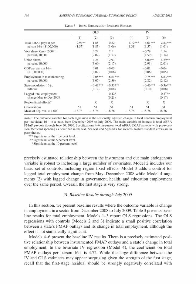
In this section, we present baseline results where the outcome variable is change in employment in a sector from December 2008 to July 2009. Table 3 presents base-line results for total employment. Models 1–3 report OLS regressions. The OLS regressions with controls (Models 2 and 3) indicate a small positive correlation between a state’s FMAP outlays and its change in total employment, although the effect is not statistically significant.

Models 4–6 present the baseline IV results. There is a precisely estimated posi-tive relationship between instrumented FMAP outlays and a state’s change in total employment. In the bivariate IV regression (Model 4), the coefficient on total FMAP outlays per person 16+ is 4.72. While the large difference between the IV and OLS estimates may appear surprising given the strength of the first stage, recall that the first-stage residual should be strongly negatively correlated with

Table 3—Total Employment Baseline Results

OLS IV

(1) (2) (3) (4) (5) (6)Total FMAP payout per 2.94** 1.88 0.82 4.72*** 4.61*** 2.83*** person 16+ ($100,000) (1.35) (1.83) (1.06) (1.31) (1.57) (1.01)Vote share Kerry (2004), 0.28 2.1 −0.79 1.14 percent/10,000 (2.02) (1.57) (1.59) (1.14)Union share, −4.26 −2.93 −6.00** −4.29** percent/10,000 (3.60) (2.17) (2.91) (2.01)GDP per person 16+ 0.01 −0.03 −0.01 −0.04 ($1,000,000) (0.07) (0.06) (0.06) (0.05)Employment in manufacturing, −10.05*** −6.61*** −9.75*** −6.83*** percent/10,000 (3.05) (2.39) (2.82) (2.12)State population 16+, −0.43*** −0.33*** −0.46*** −0.36*** billions (0.12) (0.08) (0.10) (0.08)Lagged total employment 0.42* 0.37** change May to Dec 2008 (0.21) (0.17)Region fixed effects? X X X X

Observations 51 51 51 51 51 51Mean of dep. var. × 1,000 −18.76 −18.76 −18.76 −18.76 −18.76 −18.76

Notes: The outcome variable for each regression is the seasonally adjusted change in total nonfarm employment per individual 16+ in a state, from December 2008 to July 2009. The main variable of interest is total ARRA FMAP payouts through June 30, 2010. Specifications 4–6 instrument total ARRA FMAP payouts with pre-reces-sion Medicaid spending as described in the text. See text and Appendix for sources. Robust standard errors are in parentheses.



employment growth due to the unemployment triggers in the FMAP increase, bias-ing the OLS results downward.

Adding a wide variety of control variables (Model 5) changes the estimate little. Including the lagged employment control (Model 6) reduces the point estimate by approximately 40 percent but has little effect on the statistical significance of the result, as the standard error also shrinks. The fact that adding a control for lagged employment influences the point estimate suggests that high and low Medicaid spending states were on different employment trends prior to the ARRA, a hypoth-esis that we explore in the robustness section.

The coefficient in (6), the preferred specification, suggests that for every $100,000 in FMAP outlays per individual 16+ that a state received by June 30, 2010, that states’ total employment increased by 2.83 per individual 16+ from December 2008 to July 2009. Section VI provides further discussion of how to interpret this magnitude.

Table 4 parallels the results from Table 3, using the change in government, health, and education employment as the outcome variable. The OLS coefficients (Models 1–3) are positive, relatively small in magnitude, and not statistically sig-nificant. The IV results (Models 4–6), in contrast, suggest a positive relation-ship between FMAP transfers and change in employment in these sectors. For

Table 4—State and Local Government, Health, and Education

OLS IV

(1) (2) (3) (4) (5) (6)Total FMAP payout per 0.43 0.34 0.30 0.99* 1.19*** 1.17*** person 16+ ($100,000) (0.53) (0.44) (0.40) (0.54) (0.37) (0.36)Vote share Kerry (2004) −0.76* −0.64 −1.10*** −1.01*** percent/10,000 (0.39) (0.39) (0.30) (0.32)Union share, 0.16 0.33 −0.38 −0.26 percent/10,000 (0.95) (0.96) 0.76 0.8

GDP per person 16+ 0.07*** 0.07*** 0.06*** 0.06*** ($1,000,000) (0.02) (0.02) (0.02) (0.02)Employment in manufacturing, −1.93** −1.84* −1.84** −1.77** percent/10,000 (0.89) (0.96) (0.84) (0.88)State population 16+, −0.11*** −0.10** −0.12*** −0.11*** billions (0.03) (0.04) (0.03) (0.03)Lagged total employment 0.18 0.14 change May to Dec 2008 (0.18) (0.17)Region fixed effects? X X X XObservations 51 51 51 51 51 51Mean of dep. var. × 1,000 0.97 0.97 0.97 0.97 0.97 0.97

Notes: The outcome variable for each regression is the seasonally adjusted change in total employment in state and local government, health, and education per individual 16+ in a state, from December 2008 to July 2009. The main variable of interest is total ARRA FMAP pay-outs through June 30, 2010. Specifications 4–6 instrument total ARRA FMAP payouts with pre-recession Medicaid spending as described in the text. See text and Appendix for sources. Note that “government” excludes federal government employees. Robust standard errors are in parentheses.



the IV specifications, the control variables have very little influence on the point estimates, but they do substantially reduce the standard errors. The coefficient on (6) suggests that for every $100,000 in FMAP outlays per individual 16+ that a state received by June 30, 2010, that states’ employment in the government, health, and education sectors increased by 1.17 per individual 16+ over the period considered.

The coefficients in Table 4 are less than half of the magnitude of those in Table 3, suggesting that the “indirect” employment gains in the nongovernment-related sec-tors were substantial. To see this more explicitly, we reestimate our preferred spec-ification, changing the dependent variable to be the change in total employment excluding the change in employment in the government, health, and education sec-tors. This regression yields a coefficient of 1.86 (95 percent CI: 0.32, 3.41).

C. Timing Results

The previous section presented results where the outcome variable was the change in employment from December 2008 until July 2009. This section explores how our estimates evolve as we change the month that marks the end of our sample. Specifically, we rerun the cross-sectional regression for changes in employment from December 2008 until every month from January 2009 to June 2010 and report the second stage coefficients on total FMAP outlays from our preferred specification with the full set of control variables. That is, we rerun the estimate from December 2008 to January 2009, December 2008 to February 2009, December 2008 to March 2009, etc. and report each of these 18 coefficients.

Figure 3 presents these results for total nonfarm employment. The solid line rep-resents the point estimate, and the dashed lines indicate the 95 percent confidence interval. These timing results suggest three main patterns. First, while there appears to be a positive relationship between FMAP outlays and change in employment before July 2009, the relationship is small and not precisely measured. Second, starting in July 2009, the coefficient jumps in magnitude, varying from a low of 2.16 (September 2009) to a high of 4.44 (February 2010). Finally, as expected, the standard errors tend to widen over time, although all of the coefficients remain sta-tistically significant at the 95 percent level.

Figure 4 parallels the results from Figure 3, using employment in the govern-ment, health, and education sectors. The broad patterns present in Figure 3 are also present in Figure 4. Again, the coefficient increases for July 2009, and the standard errors increase over time. However, the ratio of the standard errors to the point estimate is larger than for total employment. Comparing the magnitudes between the two timing figures shows that in all months, the estimates for total employment are larger than those for government employment, with the gap increasing through 2009 and peaking in early 2010. This pattern is consistent with the government employment results reflecting the relatively immediate direct effect of states and state-funded establishments not having to lay off workers, while the total employ-ment results include the lagging induced effects of households responding to higher disposable income.


V. Robustness Checks and Extensions

A. falsification Tests

Our identifying assumption is that, conditional on our control variables, states that had higher pre-recession Medicaid spending would not have experienced dif-ferent employment outcomes from states that were lower spenders in the absence of the increase in FMAP. One way of assessing this assumption is to consider if the effects we estimate are larger than the relationship between Medicaid spending and employment growth that existed prior to the period of interest.

Figure 5 reports the second stage coefficients for placebo tests using data that begin in January 2000 and end in December 2008. To parallel our baseline speci-fication, we consider seven-month changes in both total nonfarm employment and employment in government, health, and education. We then run our IV estimates on each overlapping seven-month period, for a total of 101 regressions. We rank the coefficients based on their magnitude and report the empirical CDF. For compari-son, we also show the second stage estimate run on the baseline period, December 2008 to July 2009, with a vertical line.

The results show two key patterns. First, the estimates are centered around 0; the empirical median of the estimate is 0.00 for total nonfarm and 0.11 for government,

0

2

4

6

8

Jan-

09

Feb

-09

Mar

-09

Apr

-09

May

-09

Jun-

09

Jul-0

9

Aug

-09

Sep

-09

Oct

-09

Nov

-09

Dec

-09

Jan-

10

Feb

-10

Mar

-10

Apr

-10

May

-10

Jun-

10

Value of coefficient on FMAP outlays

Figure 3. Total Nonfarm Second Stage Coefficients

Notes: This chart displays the second stage coefficient for regressions where the outcome variable is the change in seasonally adjusted employment between December 2008 and the month indicated on the x-axis. The variable of interest is total FMAP outlays. Regressions include the full set of controls. The 95 percent confidence interval, derived from robust standard errors, is plotted in dashed lines.


health and education. That is, in the years before the ARRA was passed, there is little evidence to suggest that high and low Medicaid spending states experienced systematically different employment trends. Second, our baseline estimates of both total nonfarm and government, health, and education employment are large relative to the coefficients in the period before the ARRA. For total employment, our result is larger than all but seven of the 101 pre-ARRA estimates. For government, health, and education, our estimate is larger than all but three of the pre-ARRA estimates. Both pieces of evidence increase our confidence that the estimates reported above are capturing the effect of the ARRA rather than underlying differences between high and low Medicaid spending states.

B. Other Robustness checks

Our baseline specification allows for the possibility that high and low Medicaid spending states were on different preexisting employment trends by controlling for a linear lag of the change in employment. This subsection addresses the con-cern that a linear lag may not be a sufficient statistic for preexisting employment trends. Specifically, we report results allowing for a more flexible preexisting trend and using a state’s pretreatment industry composition and the change in employ-ment by industry in other states to impute employment change during the treatment

−1

0

1

2

3

Jan-

09

Feb

-09

Mar

-09

Apr

-09

May

-09

Jun-

09

Jul-0

9

Aug

-09

Sep

-09

Oct

-09

Nov

-09

Dec

-09

Jan-

10

Feb

-10

Mar

-10

Apr

-10

May

-10

Jun-

10

Value of coefficient on FMAP outlays

Figure 4. Government, Health, and Education Second Stage Coefficients

Notes: This chart displays the second stage coefficient for regressions where the outcome variable is the change in seasonally adjusted employment between December 2008 and the month indicated on the x-axis. The variable of interest is total FMAP outlays. Regressions include the full set of controls. The 95 percent confidence interval, derived from robust standard errors, is plotted in dashed lines.


period, following Bartik (1991) and Blanchard and Katz (1992). The latter require detailed industry data from the QCEW, a dataset that is not available on a season-ally adjusted basis and that does not have representative coverage of the government sector. 19 We therefore present results for the change in total nonfarm employment, and for December 2008 to December 2009 in the specifications that use the imputed employment predictor. 20

Model 1 of Table 5 shows the second stage coefficient when we rerun our baseline specification, replacing the linear lag of employment change with an autoregressive model estimated using 18 years of data prior to the sample period to forecast a state’s employment change from December 2008 to July 2009.21 The second stage

19 According to Bureau of Labor Statistics (2008), 5 percent of total state and local government workers are not covered by the QCEW.

20 We perform the imputed employment calculation at the four-digit level because of disclosure limitations that eliminate observations at higher levels of detail.

21 Specifically, the logarithm of total employment was regressed against a time variable and nine monthly lags of itself. The coefficients were then used on data through December 2008 to forecast employment from January 2009

0

0.2

0.4

0.6

0.8

1

CD

F

−4 −2 0 2 4

Second stage coefficient

Total nonfarm

0

0.2

0.4

0.6

0.8

1

CD

F

−4 −2 0 2 4

Second stage coefficient

Government, health, and education

Figure 5. Placebo Results

Notes: Plots results of second stage regressions, where the outcome variable is seasonally adjusted change in employment for each overlapping seven month period, starting in January 2000 and ending in December 2008. All regressions include the full set of control variables. Coefficient from December 2008 to July 2009 is indicated with the vertical line. Note that government excludes federal government employment.


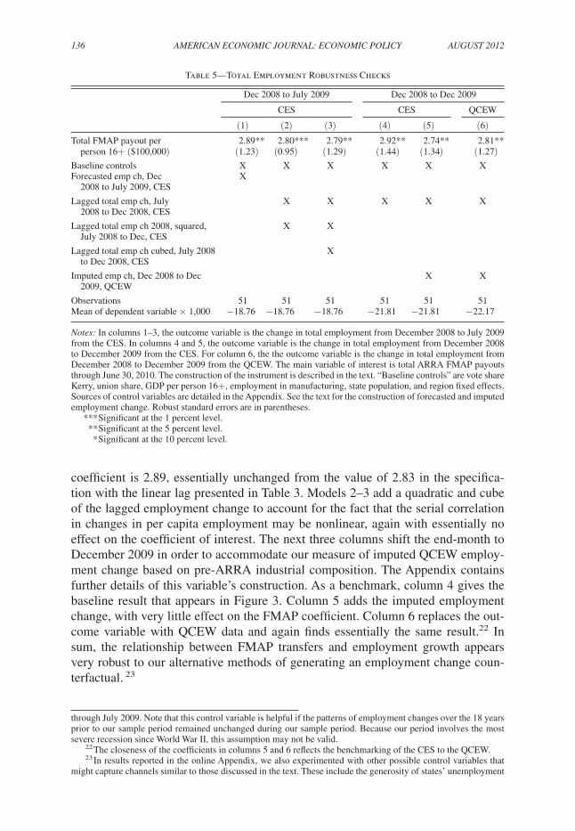
coefficient is 2.89, essentially unchanged from the value of 2.83 in the specifica-tion with the linear lag presented in Table 3. Models 2–3 add a quadratic and cube of the lagged employment change to account for the fact that the serial correlation in changes in per capita employment may be nonlinear, again with essentially no effect on the coefficient of interest. The next three columns shift the end-month to December 2009 in order to accommodate our measure of imputed QCEW employ-ment change based on pre-ARRA industrial composition. The Appendix contains further details of this variable’s construction. As a benchmark, column 4 gives the baseline result that appears in Figure 3. Column 5 adds the imputed employment change, with very little effect on the FMAP coefficient. Column 6 replaces the out-come variable with QCEW data and again finds essentially the same result.22 In sum, the relationship between FMAP transfers and employment growth appears very robust to our alternative methods of generating an employment change coun-terfactual. 23

through July 2009. Note that this control variable is helpful if the patterns of employment changes over the 18 years prior to our sample period remained unchanged during our sample period. Because our period involves the most severe recession since World War II, this assumption may not be valid.

22 The closeness of the coefficients in columns 5 and 6 reflects the benchmarking of the CES to the QCEW.23 In results reported in the online Appendix, we also experimented with other possible control variables that

might capture channels similar to those discussed in the text. These include the generosity of states’ unemployment

Table 5—Total Employment Robustness Checks

Dec 2008 to July 2009 Dec 2008 to Dec 2009

CES CES QCEW

(1) (2) (3) (4) (5) (6)Total FMAP payout per 2.89** 2.80*** 2.79** 2.92** 2.74** 2.81** person 16+ ($100,000) (1.23) (0.95) (1.29) (1.44) (1.34) (1.27)Baseline controls X X X X X XForecasted emp ch, Dec X 2008 to July 2009, CES

Lagged total emp ch, July X X X X X 2008 to Dec 2008, CES

Lagged total emp ch 2008, squared, X X July 2008 to Dec, CES

Lagged total emp ch cubed, July 2008 X to Dec 2008, CES

Imputed emp ch, Dec 2008 to Dec 2009, QCEW

X X

Observations 51 51 51 51 51 51Mean of dependent variable × 1,000 −18.76 −18.76 −18.76 −21.81 −21.81 −22.17

Notes: In columns 1–3, the outcome variable is the change in total employment from December 2008 to July 2009 from the CES. In columns 4 and 5, the outcome variable is the change in total employment from December 2008 to December 2009 from the CES. For column 6, the the outcome variable is the change in total employment from December 2008 to December 2009 from the QCEW. The main variable of interest is total ARRA FMAP payouts through June 30, 2010. The construction of the instrument is described in the text. “Baseline controls” are vote share Kerry, union share, GDP per person 16+, employment in manufacturing, state population, and region fixed effects. Sources of control variables are detailed in the Appendix. See the text for the construction of forecasted and imputed employment change. Robust standard errors are in parentheses.



VI. Discussion

A. Job-years

Our results indicate a positive and robust relationship between receiving FMAP transfers and relative employment outcomes. To interpret the magnitude of the esti-mates, we can translate the regression coefficients into the increase in job-years from $100,000 of marginal state fiscal relief. This requires two assumptions. First, we assume that FMAP outlays received through June 2010 have no employment effects beyond June 2010. If instead the employment effects linger beyond June 2010, then our estimate of job-years is a lower bound. Second, we assume that transfers to states after June 2010 do not influence employment changes before June 2010. This assumption is likely to be valid (at least for state employment) if states are unable to shift money across fiscal years.

Under these assumptions, the increase in job-years from $100,000 of FMAP out-lays can be calculated by taking the integral under the timing charts (Figures 3 and 4) and dividing by 12 to convert job-months to job-years. Our point estimates suggest that $100,000 of marginal state fiscal relief increases state employment by 3.8 job- years, 3.2 of which are outside the government, health, and education sectors. The associated p-value for this calculation is 0.018 for total employment, while the p-value for total employment excluding the government, health, and educa-tion sectors is 0.010. Dividing $100,000 by 3.8 job-years yields a cost per job of $26,000.

When considering the generalizability of the results, it is important to consider both the intended and apparently realized fungibility of the funds. As noted above, the text of the bill made clear that the funds were for general obligations, and states reported using them for this purpose. Indeed, results disaggregating the government, health, and education employment results suggest that only about a quarter of the increase in employment was in the health sector, with another quarter in education and the other half in state and local government.24

In the context of our broader understanding of the costs and benefits of fiscal stimulus, state fiscal relief, in particular, may be a particularly low-cost means of supporting employment during a recession. Furthermore, the jobs increases were rapid, perhaps because “shovel-ready” projects were often not necessary; in many cases, state and local governments only needed to avoid cuts.

insurance systems and the presence of a Democratic governor in February 2009 as proxies for political factors, an index of budget restrictiveness from the Advisory Committee on Intergovernmental Relations to address the con-cern that the 2007 Medicaid spending levels might be correlated with state budget rules, and the degree of house price appreciation during the mid-2000s as a proxy for economic conditions. The results reported in Tables 3 and 4 are robust to the inclusion of these additional controls.

24 When using the change from December 2008 to July 2009 in state and local government employment as the dependent variable in our baseline regression, we estimate a coefficient of 0.65 (SE = 0.26) on the FMAP transfers, while changes in health and education employment yield coefficients of 0.21 (SE = 0.10) and 0.29 (SE = 0.11) respectively.


B. comparison to the Literature

This paper contributes to a literature which uses cross-state variation to esti-mate fiscal multipliers. We do this using the most recently-available evidence in a context in which the parameter being estimated has direct relevance to a policy question: how much is employment increased by state fiscal relief during a reces-sion? Although estimated in quite different settings, Suarez-Serrato and Wingender (2011), and Shoag (2011) find estimates which are remarkably similar to our esti-mate of cost per job, at $30,000 and $35,000 per year respectively.25

While the political debate has focused on the effect of fiscal stimulus on employ-ment, the academic literature more commonly estimates the government purchases multiplier for output. Also using cross-state variation, Nakamura and Steinsson (2011) find an open-economy government purchases multiplier of 1.5, and Shoag (2011) finds an output multiplier of 2.1. Our findings are consistent with this range. We roughly map our results to an output multiplier as follows: in 2008 average com-pensation in both the total economy and state and local government was $56,000 per employee. If total compensation equals the marginal product of labor and work-ers affected by state fiscal relief have this same average compensation, this result would imply an output multiplier for a dollar of transfers of about 2.26 Given that the results from this cross-state approach do not incorporate general equilibrium effects, cross-state multipliers, or the response of a monetary authority, we interpret this multiplier as only suggestive of the national multiplier of policy interest.27

A few other papers have also studied parts of the ARRA. Wilson (forthcoming), and Feyrer and Sacerdote (2011) report costs per job of $114,312 and $170,000, respectively, but their numbers are not directly comparable to the 3.8 jobs per $100,000 reported above because they do not account for the timing of job cre-ation, and they cover other portions of the stimulus.28 Sahm, Shapiro, and Slemrod (forthcoming) find a relatively modest impact from the Making Work Pay tax cut. Mian and Sufi (forthcoming) find that the relatively small ($3 billion) “Cash for Clunkers” program (which was separate from the ARRA but implemented concur-rently during the summer of 2009) had little net effect on purchases.29

25 See also Neumann, Fishback, and Kantor (2010), and Fishback and Kachanovskaya (2010) for studies using cross-sectional variation during the Great Depression.

26 This calculation assumes that capital stays fixed. Data on average compensation per employee come from the Bureau of Economic Analysis GDP-by-Industry accounts. The output multiplier equals the jobs multiplier multi-plied by value-added per job (equivalent to a worker’s marginal product), or (3.8/$100,000) × $56,000 = 2.13.

27 Ramey (2011) surveys the literature on national output multipliers. Our estimate is at the upper end of her preferred range, consistent with recent empirical work on state-dependent output multipliers that finds higher mul-tipliers occur during depressed demand conditions such as prevailed during our period of study (Auerbach and Gorodnichenko 2012). Nakamura and Steinsson (2011), and Shoag (2011) explore the theoretical mapping from these estimates of local fiscal multipliers to the national multiplier in an open economy setting.

28 Wilson’s results for total job creation are closest to ours. This is not surprising, since his paper adopts our instrument, along with using simulated instruments for highway and education spending. The Feyrer-Sacerdote number corresponds only to “direct jobs” funded by the ARRA. Conley and Dupor (2011) find a positive effect of ARRA transfers on government employment, but no positive effect on employment outside of government.

29 The Obama administration (Council of Economic Advisers 2010), Congressional Budget Office (2010), and private forecasters and academics (Blinder and Zandi 2010) have all evaluated the ARRA using a multiplier model based on historical relationships between government spending, output and employment. These studies tend to find effects similar to or slightly smaller in magnitude than those in the current study for state fiscal relief. However,


VII. Mechanism

The ARRA transfers reached states in dire fiscal condition. During the 2009 fiscal year, 43 states faced budget gaps totaling more than $60 billion (National Conference of State Legislatures 2009). Almost all states have balanced budget requirements.30 Thus, the large budget gaps necessitated that they take action by cutting expenditures, raising revenues, or drawing from their “rainy day” funds or end of year balances, which are used to smooth revenue across years.31 Indeed, by December 2008, 22 states had made or announced cuts to their expenditures totaling $12 billion.32 By July 2009, 42 states had made cuts to their expenditures totaling more than $30 billion, and 30 states had increased taxes or fees to boost their revenues.33

There are essentially only three ways in which states could use the ARRA state fiscal relief funds: to alleviate program cuts, to prevent or lower tax and fee increases, or to contribute to their end of year balances (which include their rainy day funds). As long as the states did not respond to the federal transfers by completely siphoning them to their end of year balances, the observed employment responses could come from multipliers on the states’ spending or tax actions. The results in Section IV suggest that the ARRA funds were at least partially used to avoid program cuts, since a concentration of the employment effects appears to have occurred in sec-tors (government, health, and education) which are reliant on state funds. That total employment beyond those sectors is also affected positively by the federal fiscal relief suggests that there is a source of spillovers, arising from higher disposable income due to either the wages of the direct hires or lower net taxes because of fewer tax or fee increases.34

We can directly test the necessary condition that FMAP outlays affected spending or tax actions by regressing the change in end of year balances from 2008 to 2009 on instrumented FMAP outlays and controls. Models 1–3 of Table 6 summarize the results of these regressions. All else equal, if states that received more FMAP money decreased their balances less, we would expect a positive and significant coefficient on FMAP outlays, with the extreme case that if all of the money were saved we would expect a coefficient of 1. Instead, the estimates in columns 1–3 are small in magnitude, negative in all three of the specifications, and never significantly differ-ent from 0.35 Furthermore, the models allow us to reject the null that half of transfers

they are all calibrated models, whereas the current study uses empirical estimation. Council of Economic Advisers (2009) reported preliminary results of those in the current paper.

30 All states, except for Vermont, have some version of balanced budget requirements as reported by the National Association of State Budget Officers (2008a). Poterba (1994) gives an overview of the varying requirements.

31 From National Association of State Budget Officers (2008a). Kansas and Montana do not have budget sta-bilization (or “rainy day”) funds. However, they, like other states, may use surpluses from the prior fiscal year to cushion any fiscal difficulty in the next.

32 From National Association of State Budget Officers (2008b).33 Budget cuts from the National Association of State Budget Officers (2009a). The $32 billion figure refers

to the expenditure cuts in fiscal year 2009 alone. Tax increases from Johnson, Nicholas, and Pennington (2009).34 Several recent empirical studies have found a positive effect of lower taxes or higher transfers on economic

outcomes (Johnson, Parker, and Souleles 2006; Sahm, Shapiro, and Slemrod 2010; Romer and Romer 2010).35 We exclude Alaska, a state that experienced a per 16+ population decline in its end of year funds that was

more than ten times larger than that of the next largest states. When we include Alaska, we also cannot reject the that the coefficient on total FMAP outlays per person is equal to 0 (p-value for the bivariate IV regression is 0.435


were saved by states at the 99 percent confidence level for two regressions and at the 95 percent confidence level for the third, confirming that at least some of the funds were used to slow either budget cuts or tax increases. Models 4–6 of Table 6 repeat the same exercise, using the change in end of the year balances from 2009 to 2010 as the dependent variable, and yield similar results. 36 In summary, although the regres-sions have wide standard errors, the point estimates provide no evidence to suggest that states are retaining the transferred money in the form of end of year balances or rainy day funds.37

To determine if states that received more transfers cut their budgets less, we ran specifications that parallel those in Table 6 where the outcome variable was the change in expenditure (normalized by a state’s 16+ population) between 2008 and 2009 and between 2009 and 2010. Unfortunately, the results from this regression are quite noisy, and we can neither reject the that all of the money was spent on reduc-ing budget cuts (which would imply a coefficient of one) nor the null that none of the money was spent on reducing budget cuts (which would yield a coefficient of

for changes from 2008 to 2009 and is 0.311 for changes from 2009 to 2010). In addition, because the National Association of State Budget Officers does not provide data on DC, we exclude it from our regressions.

36 Poterba (1994) and Alt and Lowry (1994) examine how the states’ balanced budget rules affect their responses to deficits and find that, in response to a positive deficit shock, states cut expenditures or raise taxes within either the current or the following fiscal year. This is consistent with the findings that a federal transfer (a negative deficit shock) would impact expenditures or taxes.

37 These results contradict those of Cogan and Taylor (2010), who find using aggregate time-series data that ARRA Medicaid spending increased aggregate state net lending as measured in the National Income and Product Accounts. Given the unusual nature and length of the 2007–09 recession and its effect on state budgets, it is possible that aggregate time-series regressions misattribute the effect of the worsening recession and the eventual binding of state balanced budget requirements on net lending to the introduction of the FMAP expansion. Alternatively, it is possible that all states increased their saving in response to the FMAP transfers by the same dollar amount per capita, regardless of the amount of FMAP transfers actually received.

Table 6—Transmission Mechanism

Rainy day fund, change 2008 to 2009 (IV)

Rainy day fund, change 2009 to 2010 (IV)

(1) (2) (3) (4) (5) (6)

Total FMAP payout per −0.26 0.01 −0.14 −0.04 0.08 0.04 person 16+ ($100,000) (0.18) (0.23) (0.21) (0.09) (0.18) (0.17)Region fixed effects? X X X XIncludes lagged employment? X XExcludes Alaska? X X X X X XMissing Washington DC? X X X X X X

Observations 49 49 49 49 49 −17.84Mean of dep. var. (× 100,000) −29.22 −29.22 −29.22 −17.84 −17.84 −17.84

Notes: The outcome variable for columns 1–3 is change in a state’s rainy day fund, in $100,000, per person 16+, from fiscal year 2008 to fiscal year 2009. The outcome variable for columns 4–6 is the change in a state’s rainy day fund, in $100,000, per person 16+, from fiscal year 2009 to fiscal year 2010. Data are from the National Association of State Budget Officers (NASBO) Fiscal Survey of the States. The fiscal 2008 rainy day fund data come from the Fall 2009 Fiscal Survey, and the fiscal 2009 and 2010 rainy day fund data come from the Spring 2010 Fiscal Survey. All specifications exclude Washington, DC due to missing data. They also drop Alaska, an outlier in terms of the change in the state rainy day fund. Robust standard errors are in parentheses.



zero).38 Results using changes in a state’s revenue are similarly noisy, and thus do not provide conclusive evidence about the use of funds to reduce tax or fee increases. Further research into how states optimize over the margins of tax and spending when faced with an altered budget constraint would be a worthwhile area of future study.

VIII. Conclusion

This paper estimates the employment effects of a relatively unstudied form of government macroeconomic intervention that took center stage in the recent ARRA: fiscal relief to states during a downturn. We exploit cross-state variation in trans-fer receipts that comes from pre-recession differences in Medicaid spending. All else equal, states that spent more money on Medicaid before the recession received more money from the federal government. We confront the major threat to iden-tification—that states that spent more money on Medicaid may be on differential employment trends from states that spent less—in several ways, including adding regional fixed effects and other control variables as well as conducting placebo tests. Our baseline specifications suggest that $100,000 of marginal spending increased employment by 3.8 job-years, 3.2 of which are outside the government, health, and education sectors.

The fact that state fiscal relief may be an effective tool to cushion employment losses in recessions raises two questions. First, if the employment effects of state fiscal relief are substantial, should the federal government play a larger role in pro-viding revenue to states during recessions? When designing state fiscal relief, fed-eral planners face a tradeoff between providing relief to states experiencing critical budget situations and minimizing perverse incentives for state policy makers. If states expect to receive federal aid during recessions, they may not save sufficiently during boom times. This moral hazard is compounded if federal aid targets states with larger budget shortfalls, which might be desirable because aid distributed using a non-need-based formula would likely produce smaller employment effects. An important area of future research is to determine the extent to which these tradeoffs limit the potential for state fiscal relief to be an effective tool for cushioning job losses during recessions.

Second, why are states unable to save money during economic booms and use this savings during recessions? Because most states have adopted balanced budget legislation, states cannot borrow money during recessions to smooth fluctuations. As a substitute, most states have a “rainy day” fund that allows them to avoid the requirement of literally balancing their budget every fiscal year. However, political economy considerations make saving difficult for democratic governments (Alesina and Tabellini 1990; Amador 2003), and most states have essentially no restrictions on when they must contribute to their rainy day fund.39 For example, during the

38 Fiscal year 2008 expenditure data and the enacted tax and fee data are from the National Association of State Budget Officers (2009b). Fiscal year 2009 and 2010 expenditure data are from the National Association of State Budget Officers (2010).

39 The majority of states have requirements that they contribute to their rainy day funds only if the budget has a surplus. However, because states determine when they have a surplus by setting the level of taxes and spending, in


1990s economic boom, states increased spending and cut taxes rather than contrib-uting to their rainy day funds.40

To help solve these political economy problems, some states have considered adopting rules that would require the state to contribute to their rainy day fund dur-ing healthy economic times. For example, a state could be required to contribute to its fund when the unemployment rate in the state falls below a given threshold, and be permitted to tap into its fund when the unemployment rate rises to a sufficiently high level. These regulations have the advantage of constraining politicians, while helping to alleviate some of the fiscal strain induced by a recession. The evidence presented in this paper, though it concerns funding from the federal government, also informs the impact of additional state resources on state-level employment, and suggests that these and other rules may help states boost employment during reces-sions. Future research could focus on additional benefits, as well as costs, from state fiscal relief and state budgetary rules.

Appendix

A. Sources and descriptions of Baseline control Variables

Region Effects.—We include dummy variables for each of the nine census defined divisions. Definitions are given at http://www.census.gov/geo/www/us_regdiv.pdf.

Lagged change in Employment.—We control for the lagged value of the out-come variable. Specifically, if the outcome variable is change in total (government, health, and education) employment from month m to month m′, the lagged change in employment will be the change in total (government, health, and education) employ-ment from month m-7 to month m. In our baseline specification where the outcome variable is change in employment from December 2008 to July 2009, the lagged change in employment is the change in employment from May 2008 to December 2008. This 7 month lag was chosen to follow the 7 month period used for the out-come variable in our baseline specification.

gdP per Potential Worker.—We use a state’s 2008 GDP, normalized by a state’s 16+ population, from the Bureau of Economic Analysis.41

Employment Manufacturing Share.—From the Census Bureau, we also control for the share of the civilian employed population 16 years and older that is in the manufacturing sector. Data are from the American Community Survey and are aver-aged over 2005–2007 to reduce measurement error.

State 2008 Population and 2008 16+ Population.—Data are from the U.S. Census Bureau.

practice such requirements impose few restrictions on states’ contributions to their rainy day funds.40 See Zahradnik and Ribeiro (2003). 41 See http://www.bea.gov/newsreleases/regional/gdp_state/2009/pdf/gsp0609.pdf.

http://www.census.gov/geo/www/us_regdiv.pdf


2004 Kerry Share.—The state’s share of voters who cast ballots for Senator Kerry in the 2004 United States presidential election.

union Share.—Share of workers in a union, from the Bureau of Labor Statistics.42

B. description of Imputed Employment

As a robustness check, we control for a measure of imputed employment that uses information on the change in employment in each industry in the rest of the country and the initial industry distribution in each state to impute an expected employment change. Specifically, for state j and industry k define the percent change in employ-ment in industry k in all other states as:

(B1) %Δ E −j, k = Σ s≠j E t

s, k _

Σ s≠j E t−1 s, k

− 1

The imputed employment change for industry k in state j is then:

(B2) Δ E j, k = E t−1 j, k

∙ %Δ E −j, k

The total imputed employment change for state j is the sum over all industries:

(B3) Δ E j = Σ k Δ E j, k

We implement B1–B3 using the QCEW December 2008 and December 2009 state-level flat files.43 The QCEW provides employment by NAICS code and owner-ship status (private, federal government, state government, and local government). The QCEW suppresses output for state-industry-ownership rows where the number or concentration of firms does not surpass a minimum disclosure threshold. Letting o ∈ {private, federal, state, local} define ownership status, we set E t−1

j, k, o = 0 for any state-industry-ownership row with suppressed output. In practice, missing the dis-closure threshold correlates well with small size, so this assumption is quite mild. Nonetheless, we define industries using four digit rather than six digit NAICS codes in order to minimize disclosure limitations. Using six digit industries yields very similar results. Since we are interested in industry variation, we collapse the QCEW data on ownership status before implementing B1–B3.

REFERENCES

Alesina, Alberto, and Guido Tabellini. 1990. “A Positive Theory of Fiscal Deficits and Government Debt in Democracy.” Review of Economics Studies 57 (3): 403–14.

42 From http://www.bls.gov/news.release/pdf/union2.pdf.43 The files can be downloaded from ftp://ftp.bls.gov/pub/special.requests/cew/yyyy/state for yyyy={2008,2009}.

http://www.bls.gov/news.release/pdf/union2.pdf

ftp://ftp.bls.gov/pub/special.requests/cew/yyyy/state


Alt, James E., and Robert C. Lowry. 1994. “Divided Government, Fiscal Institutions, and Budget Defi-cits: Evidence from the States.” American Political Science Review 88 (4): 811–28.

Amador, Manuel. 2003. “Political Compromise and Savings.” http://www.stanford.com/~amador/sav-ings.pdf.

Auerbach, Alan J., and Yuriy Gorodnichenko. 2012. “Measuring the Output Responses to Fiscal Pol-icy.” American Economic Journal: Economic Policy 4 (2): 1–27.

Bartik, Timothy. 1991. Who Benefits from State and Local Economic development Policies? Kalama-zoo: W. E. Upjohn Institute for Employment Research.

Blanchard, Olivier Jean, and Lawrence Katz. 1992. “Regional Evolutions.” Brookings Paper on Eco-nomic Activity 23 (1): 1–75.

Blinder, Alan, and Mark Zandi. 2010. “How the Great Recession Was Brought to an End.” http://www.economy.com/mark-zandi/documents/End-of-Great-Recession.pdf.

Bureau of Labor Statistics. 1990–2010. “Current Employment Statistics: State Employment and Unemployment.” United States Department of Labor. ftp://ftp.bls.gov/pub/time.series/sm/.

Bureau of Labor Statistics. 2007–2009. “Quarterly Census of Employment and Wages.” United States Department of Labor. ftp://ftp.bls.gov/pub/special.requests/cew/.

Bureau of Labor Statistics. 2008. Employment and Wages, Annual Averages 2008. Government Print-ing Office.Washington, DC, December. http://www.bls.gov/cew/cewbultn08.htm.

Centers for Medicare and Medicaid Services. 2008. “Data Compendium 2008 Edition.” https://www.cms.gov/Research-Statistics-Data-and-Systems/Statistics-Trends-and-Reports/DataCompendium/16_2008DataCompendium.html.

Chodorow-Reich, Gabriel, Laura Feiveson, Zachary Liscow, and William Gui Woolston. 2012. “Does State Fiscal Relief During Recessions Increase Employment? Evidence from the American Recov-ery and Reinvestment Act: Dataset.” American Economic Journal: Economic Policy. http://dx.doi.org/10.1257/pol.4.3.118.

Clemens, Jeffrey, and Stephen Miran. 2012. “Fiscal Policy Multipliers on Subnational Government Spending.” American Economic Journal: Economic Policy 4 (2): 46–68.

Cogan, John, and John Taylor. 2010. “What the Government Purchases Multiplier Actually Multiplied in the 2009 Stimulus Package.” National Bureau of Economic Research (NBER) Working Paper 16505.

Congressional Budget Office. 2010. Estimated Impact of the American Recovery and Reinvestment Act on Employment and Economic Output from January 2010 through March 2010. Congressional Budget Office. Washington, DC, May.

Conley, Timothy, and Bill Dupor. 2011. “The American Recovery and Reinvestment Act: Public Jobs Saved, Private Sector Jobs Forestalled.” http://web.econ.ohio-state.edu/dupor/arra10_may11.pdf.

Council of Economic Advisers. 2009. The Effect of State fiscal Relief. Executive Office of the Presi-dent. Washington, DC, September.

Council of Economic Advisers. 2010. The Economic Impact of the American Recovery and Reinvestment Act of 2009: fourth Quarterly Report. Executive Office of the President. Washington, DC, July.

Fishback, Price V., and Valentina Kachanovskaya. 2010. “In Search of the Multiplier for Net Federal Spending in the States during the New Deal: A Preliminary Report.” National Bureau of Economic Research (NBER) Working Paper 16561.

Government Accountability Office. 2009. Recovery Act: States’ and Localities’ current and Planned uses of funds While facing fiscal Stresses. Congressional Committees. Washington, DC, July. http://www.gao.gov/new.items/d09829.pdf.

Gramlich, Edward. 1977. “Intergovernmental Grants: A Review of the Empirical Literature.” In The Political Economy of fiscal federalism, edited by Wallace E. Oates, 219–39. Lexington, MA: Lex-ington Books.

Johnson, David S., Jonathan A. Parker, and Nicholas S. Souleles. 2006. “Household Expenditure and the Income Tax Rebates of 2001.” American Economic Review 96 (5): 1589–1610.

Johnson, Nicholas, Andrew Nicholas, and Steven Pennington. 2009. Tax Measures help Balance State Budgets: A common and Reasonable Response to Shortfalls. Center on Budget and Policy Priori-ties. Washington, DC, July. http://www.cbpp.org/files/5-13-09sfp.pdf.

Nakamura, Emi, and Jon Steinsson. 2011. “Fiscal Stimulus in a Monetary Union: Evidence from US Regions.” http://www.columbia.edu/~en2198/papers/fiscal.pdf.

Mian, Atif, and Amir Sufi. Forthcoming. “The Effects of Fiscal Stimulus: Evidence from the 2009 ‘Cash for Clunkers’ Program.” Quarterly Journal of Economics.

Moretti, Enrico. 2010. “Local Multipliers.” American Economic Review 100 (2): 373–77.National Association of State Budget Officers. 2008a. Budget Processes in the States. National Gover-

nors Association. Washington, DC, Summer. http://www.nasbo.org/sites/default/files/BP_2008.pdf.

http://www.stanford.com/~amador/savings.pdf

http://www.stanford.com/~amador/savings.pdf

http://www.economy.com/mark-zandi/documents/End-of-Great-Recession.pdf

http://www.economy.com/mark-zandi/documents/End-of-Great-Recession.pdf

http://ftp://ftp.bls.gov/pub/time.series/sm/

http://ftp://ftp.bls.gov/pub/special.requests/cew/

http://www.bls.gov/cew/cewbultn08.htm

https://www.cms.gov/Research-Statistics-Data-and-Systems/Statistics-Trends-and-Reports/DataCompendium/16_2008DataCompendium.html





http://web.econ.ohio-state.edu/dupor/arra10_may11.pdf

http://www.gao.gov/new.items/d09829.pdf

http://www.cbpp.org/files/5-13-09sfp.pdf

http://www.columbia.edu/~en2198/papers/fiscal.pdf

http://www.nasbo.org/sites/default/files/BP_2008.pdf


National Association of State Budget Officers. 2008b. The fiscal Survey of States december 2008. National Governors Association. Washington, DC, December. http://www.nasbo.org/sites/default/files/fsfall2008.pdf.

National Association of State Budget Officers. 2009a. The fiscal Survey of States June 2009. National Governors Association. Washington, DC, June. http://www.nasbo.org/sites/default/files/fsspring2009.pdf.

National Association of State Budget Officers. 2009b. The fiscal Survey of States december 2009. National Governors Association. Washington, DC, December. http://www.nasbo.org/sites/default/files/fsfall2009.pdf.

National Association of State Budget Officers. 2010. The fiscal Survey of States June 2010. National Governors Association. Washington, DC, June. www.nga.org/files/live/sites/NGA/files/pdf/FSS1006.PDF.

National Conference of State Legislatures. 2009. State Budget update: April 2009. National Confer-ence of State Legislatures. Washington, DC, April. http://www.ncsl.org/?TabId=17080.

Neumann, Todd C., Price V. Fishback, and Shawn Kantor. 2010. “The Dynamics of Relief Spending and the Private Urban Labor Market during the New Deal.” Journal of Economic history 70 (1): 195–220.

Poterba, James M. 1994. “State Responses to Fiscal Crises: The Effects of Budgetary Institutions and Politics.” Journal of Political Economy 102 (4): 799–821.

Ramey, Valerie A. 2011. “Can Government Purchases Stimulate the Economy?” Journal of Economic Literature 49 (3): 673–85.

Romer, Christina, and Jared Bernstein. 2009. The Job Impact of the American Recovery and Reinvest-ment Plan. White House Council of Economic Advisers. Washington, DC, January.

Romer, Christina, and David Romer. 2010. “The Macroeconomic Effects of Tax Changes: Estimates Based on a New Measure of Fiscal Shocks.” American Economic Review 100 (3): 763–801.

Sahm, Claudia R., Matthew Shapiro, and Joel Slemrod. 2010. “Household Response to the 2008 Tax Rebates: Survey Evidence and Aggregate Implications.” In Tax Policy and the Economy, Vol. 24, edited by Jeffrey R. Brown, 69–110. Chicago: University of Chicago Press.

Sahm, Claudia, Matthew Shapiro, and Joel Slemrod. Forthcoming. “Check in the Mail or More in the Paycheck: Does the Effectiveness of Fiscal Stimulus Depend on How It Is Delivered?” American Eco-nomic Journal: Economic Policy.

Shoag, Daniel. 2011. “The Impact of Government Spending Shocks: Evidence on the Multiplier from State Pension Plan Returns.” http://www.people.fas.harvard.edu/~shoag/papers_files/shoag_jmp.pdf.

Suarez-Serrato, Juan Carlos, and Philippe Wingender. 2011. “Estimating Local Fiscal Multipliers.” http://www.jcsuarez.com/Files/Suarez_Serrato-JMP2.pdf.

US Recovery Accountability and Transparency Board. 2009–2010. Agency financial and Activity Reports. Department of Agriculture. Washington, DC.

Wilson, Daniel. Forthcoming. “Fiscal Spending Multipliers: Evidence from the 2009 American Recovery and Reinvestment Act.” American Economic Journal: Economic Policy.

Zahradnik, Bob, and Rose Ribeiro. 2003. heavy Weather: Are State Rainy day funds Working? Center on Budget and Policy Priorities. Washington, DC, May. http://www.cbpp.org/archiveSite/5-12-03sfp.pdf.

http://www.nasbo.org/sites/default/files/fsfall2008.pdf


http://www.nasbo.org/sites/default/files/fsspring2009.pdf

http://www.nasbo.org/sites/default/files/fsspring2009.pdf



http://www.nga.org/files/live/sites/NGA/files/pdf/FSS1006.PDF

http://www.nga.org/files/live/sites/NGA/files/pdf/FSS1006.PDF

http://www.ncsl.org/?TabId=17080

http://www.people.fas.harvard.edu/~shoag/papers_files/shoag_jmp.pdf

http://www.people.fas.harvard.edu/~shoag/papers_files/shoag_jmp.pdf

http://www.jcsuarez.com/Files/Suarez_Serrato-JMP2.pdf

http://www.cbpp.org/archiveSite/5-12-03sfp.pdf

http://www.cbpp.org/archiveSite/5-12-03sfp.pdf

This article has been cited by:

1. Benjamin D. Sommers, Donald Oellerich. 2013. The Poverty-Reducing Effect Of Medicaid.Journal of Health Economics . [CrossRef]

2. Daniel Shoag. 2013. Using State Pension Shocks to Estimate Fiscal Multipliers since the GreatRecession. American Economic Review 103:3, 121-124. [Abstract] [View PDF article] [PDF withlinks]

3. Alan J. Auerbach. 2012. The Fall and Rise of Keynesian Fiscal Policy. Asian Economic PolicyReview 7:2, 157-175. [CrossRef]

http://dx.doi.org/10.1016/j.jhealeco.2013.06.005

http://dx.doi.org/10.1257/aer.103.3.121

http://pubs.aeaweb.org/doi/pdf/10.1257/aer.103.3.121

http://pubs.aeaweb.org/doi/pdfplus/10.1257/aer.103.3.121

http://pubs.aeaweb.org/doi/pdfplus/10.1257/aer.103.3.121

http://dx.doi.org/10.1111/j.1748-3131.2012.01228.x

does state fiscal relief during recessions a. first stage...

Documents