The shadow of longevity - does social security reform reduce gains fromincreasing the retirement age?

Karolina Goraus 3 Krzysztof Makarski 1 2 Joanna Tyrowicz 1 3

1Narodowy Bank Polski

2Warsaw School of Economics

3Warsaw University

Agenta WorkshopJune 2015

1 / 32

Table of contents

1 Motivation and insights from literature

2 Model setup

3 Baseline and reform scenarios

4 Calibration

5 Results

2 / 32

Motivation and insights from literature

Motivation

Major issues in pension economics:

increasing old-age dependency ratio

majority of pension systems fail to assure actuarial fairness

in most countries people tend to retire as early as legally allowed

Typical reform proposals

switch to DC systems and strengthen the link between contributions and benefits

raise the social security contributions

cut government expenditure or ...

increasing minimum eligibility retirement age (MERA)

3 / 32

Motivation and insights from literature

Literature review

Two streams of literature:

1 Answering the question about optimal retirement age (Gruber and Wise (2007),Galasso (2008), Heijdra and Romp (2009))

2 Comparing different pensions system reforms: increasing retirement age vs. cut inbenefits/privatization of the system/... (Auerbach et al. (1989), Hviding andMarette (1998), Fehr (2000), Boersch-Supan and Ludwig (2010), Vogel et al.(2012))

Fehr (2000)

Macroeconomic effects of retirement age increase may depend on the existing relationbetween contributions and benefits

Remaining gaps in the literature

how the macroeconomic effects differ between various pension systems?

what happens to the welfare of each affected generation and why?

4 / 32

Motivation and insights from literature

Goals and expectations

Question

Can social security reform substitute for increasing the retirement age?

Goal

Compare macroeconomic and welfare implications of retirement age increase under DB(defined benefit), NDC (notionally defined contribution), and FDC (partially fundeddefined contribution) systems

Expectations

under DB: leisure ↓, taxes ↓, welfare?

under NDC: leisure ↓, pensions ↑, welfare?

under FDC: leisure ↓, pensions ↑, welfare?

Why a full model? → labor supply adjustments & general equilibrium effects...

5 / 32

Model setup

1 Motivation and insights from literature

2 Model setup

3 Baseline and reform scenarios

4 Calibration

5 Results

6 / 32

Model setup

Model structure - consumer I

”born” at age j = 1 (20) and lives up to J = 80 (100)

endogenous labor choice up to retirement age J̄ (forced to retire)

accidental bequests are spread equally to all cohorts

7 / 32

Model setup

Model structure - consumer II

Optimizes lifetime utility derived from leisure and consumption:

U0 =J∑

j=1

δj−1πj,t−1+juj(cj,t−1+j , lj,t−1+j) (1)

where

u(c, l) = φ log(c) + (1− φ) log(1− l), (2)

subject to the budget constraint

(1 + τc,t)cj,t + sj,t + Υt = (1− τl,t)(1− τ ιj,t)wj,t lj,t ← labor income (3)

+ (1 + rt(1− τk,t))sj,t−1 ← capital income

+ (1− τl,t)pj,t + bj,t ← pensions and bequests

8 / 32

Model setup

Model structure - producer

Standard firm optimization implies:

wt = (1− α)Kαt (ztLt)

−α

r kt = αKα−1t (ztLt)

1−α − d

9 / 32

Model setup

Model structure - government

collects social security contributions and pays out pensions of DB and NDC system

collects taxes (income, capital, consumption and lump sum)

spends fixed share of GDP on exogenous (unproductive) government expenditure

and wants to maintain long run debt/GDP ratio fixed

10 / 32

Model setup

Pension systems

Defined Benefit → constructed by imposing a mandatory exogenous contributionrate τ and an exogenous replacement rate ρ

pDBj,t =

{ρtwj−1,t−1, for j = J̄t

κDBt · pDB

j−1,t−1, for j > J̄t(4)

Defined Contribution → constructed by imposing a mandatory exogenouscontribution rate τ and individual accounts

Notional

pNDCj,t =

∑J̄t−1

i=1

[Πis=1(1+r It−i+s−1)

]τNDCJ̄t−i,t−i

wJ̄t−i,t−i lJ̄t−i,t−i∏Js=J̄t

πs,t, for j = J̄t

κDBt · pNDC

j−1,t−1, for j > J̄t

(5)

Funded

pFDCj,t =

∑J̄t−1

i=1

[Πis=1(1+rt−i+s−1)

]τFDCJ̄t−i,t−i

wJ̄t−i,t−i lJ̄t−i,t−i∏Js=J̄t

πs,t, for j = J̄t

(1 + rt)pFDCj−1,t−1, for j > J̄t

(6)

11 / 32

Model setup

Policy scenarios

What happens within each experiment?

1 Run the no policy change scenario ⇒ baseline

2 Run the policy change scenario ⇒ reform

3 For each cohort compare utility, compensate the losers from the winners

4 If net effect positive ⇒ reform efficient

Welfare analysis - LSRA like Nishiyama & Smetters (2007)

12 / 32

Baseline and reform scenarios

1 Motivation and insights from literature

2 Model setup

3 Baseline and reform scenarios

4 Calibration

5 Results

13 / 32

Baseline and reform scenarios

Reform of the systems

Three experiments:

1 DB with flat retirement age → DB with increasing retirement age

2 NDC with flat retirement age → NDC with increasing retirement age

3 FDC with flat retirement age → FDC with increasing retirement age

What is flat and what is increasing retirement age?

baseline reform

flat

14 / 32

Calibration

Age-productivity profile - flat or ...?

heterogeneity between cohorts due to age-specific productivity, wj,t = ωjwt

Deaton (1997) decomposition

15 / 32

Calibration

1 Motivation and insights from literature

2 Model setup

3 Baseline and reform scenarios

4 Calibration

5 Results

16 / 32

Calibration

Calibration to replicate 1999 economy of Poland

Preference for leisure (φ) chosen to match participation rate of 56.8%

Impatience (δ) chosen to match interest rate of 7.4%

Replacement rate (ρ) chosen to match benefits/GDP ratio of 5%

Contributions rate (τ) chosen to match SIF deficit/GDP ratio of 0.8%

Labor income tax (τl) set to 11% to match PIT/GDP ratio

Consumption tax (τl) set to match VAT/GDP ratio

Capital tax set de iure = de facto

17 / 32

Calibration

Final parameters

Table: Calibrated parameters

Age-productivity profileω - D97 ω = 1

α capital share 0.31 0.31τl labor tax 0.11 0.11φ preference for leisure 0.578 0.526δ discounting rate 0.998 0.979d depreciation rate 0.045 0.045τ total soc. security contr. 0.060 0.060ρ replacement rate 0.138 0.227

resulting∆kt investment rate 21 21r interest rate 7.4 7.4

18 / 32

Calibration

Exogenous processes in the model I

Demographics

Demographic projection until 2060, after that 80 years, and after that “new steadystate”

No of births (j=20) - from the projection, constant afterwards

Mortality rates - from the projection, constant afterwards

19 / 32

Calibration

Exogenous processes in the model II

Productivity growth

Labor augmenting productivity parameter

Data historically, projection from AWG, after that ”new steady state”, 1.7%

20 / 32

Results

1 Motivation and insights from literature

2 Model setup

3 Baseline and reform scenarios

4 Calibration

5 Results

21 / 32

Results

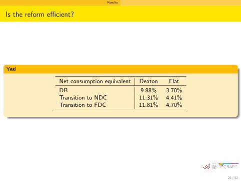
Is the reform efficient?

Yes!

Net consumption equivalent Deaton Flat

DB 9.88% 3.70%Transition to NDC 11.31% 4.41%Transition to FDC 11.81% 4.70%

22 / 32

Results

Who gains? Everybody!

23 / 32

Results

Why they gain? Pensions under DC systems ...

24 / 32

Results

... subsidies to pension system and taxes.

25 / 32

Results

Is there any behavioral response? Of course!

26 / 32

Results

Labor supply in the final steady state

Labor supply Labor supply with MERA increase(no reform) j < 60 j ≥ 60 Total

Average Average Aggregate Average Aggregate(baseline=100%) (baseline=100%)

DB 63.2% 59.6% 94.4% 71.8% 113.7%NDC 62.0% 58.8% 94.8% 72.3% 114.7%FDC 61.7% 59.0% 95.5% 72.2% 115.4%

27 / 32

Results

Aggregated labor supply (in mio of individuals)

28 / 32

Results

Capital (per effective unit of labor) decreases

29 / 32

Results

But mostly due to decrease in ‘’precautionary savings”

30 / 32

Results

Conclusions

extending the retirement age is universally welfare enhancing

some downward adjustment in individual labor supply, but the aggregated supplyincreases

surprisingly large effect on capital

31 / 32

Results

Questions or suggestions?

Thank you!

32 / 32