zaid & pat 3

1

Paper Title:

A Comparison of Logistic and Harvey Models for

Electricity Consumption in New Zealand

Authors : Zaid Mohamed1 and Pat Bodger*,2

Affiliations:

1. Mohamed, Z., B.E (Hons), is a Ph.D. student in the Department of Electrical and

Computer Engineering at the University of Canterbury, Christchurch, New

Zealand.

e-mail: [email protected]

2. Bodger, P.S, B.E (Hons), Ph.D., is Professor of Electric Power Engineering,

Department of Electrical and Computer Engineering

University of Canterbury, P.O Box 4800, Christchurch,

New Zealand,

Phone: (64)3642070, Fax: (64)3642761

e-mail: [email protected]

Running title: Harvey Model for New Zealand Electricity

* Corresponding author

2

Abstract

There have been a number of forecasting models based on various forms of the logistic

growth curve. This paper investigates the effectiveness of two forms of Harvey models

and a Logistic model for forecasting electricity consumption in New Zealand. The three

growth curve models are applied to the Domestic and Non-Domestic sectors and Total

electricity consumption in New Zealand. The developed models are compared using their

goodness of fit to historical data and forecasting accuracy over a period of 19 years. The

comparison revealed that the Harvey model is a very appropriate candidate for

forecasting electricity consumption in New Zealand. The developed models are also

compared with some available national forecasts.

Keywords: Forecasting; Energy; Growth curve models; Logistic growth

3

1. Introduction

Logistic models are attractive in situations where there is thought to be a saturation level

to a time series. A number of researchers have investigated the Logistic model either in

its simplest form or in a modified form, in studying various technological changes [1–10].

The Logistic model has also been successful in forecasting electricity consumption [11-

16].

The Logistic model [11,12] uses a Fibonacci search technique to determine the saturation

level. In that model, the saturation level needs to be estimated before the required

parameters of the logistic model may be estimated. It was found that the Logistic model

was very effective in describing the historical electricity consumption in New Zealand

but produced forecasts lower than the available national forecasts supporting the

perception that the logistic bias underestimates the final ceiling. This is mainly due to the

constraints imposed by the saturation level of the logistic growth curve. However,

underestimating the final ceiling is not always a characteristic of the logistic growth

model as applying it to the early growth data may lead to higher values. A time series

forecasting model based on the logistic curve was proposed by Harvey [17,18]. The

Harvey models do not require a saturation level to be estimated prior to estimation of the

parameters. However, the model approaches a saturation level with time. There are two

forms of Harvey models; a Harvey Logistic Model based on the general logistic model

and a Harvey Model based on general modified exponentials [17]. In general, the logistic

growth is growth in competition, while exponential growth represents a “population’

4

explosion typically encountered during the early phases of logistic growth. The Harvey

model constitutes an admixture of logistic and exponential growth. This paper

investigates the effectiveness of two forms of the Harvey models [17] for electricity

consumption in New Zealand and compares them with the previously developed Logistic

model [11,12].

2. Model Theory

2.1. Logistic and Harvey Logistic Model

Univariate time series models are often based on a local, rather than a global trend [17].

In local trend models, recent observations receive more weight when forecasting than

those in the more distant past. In global trend models, the time path of the data

concerned is regarded as following a deterministic function of time, upon which a

disturbance or error term is added.

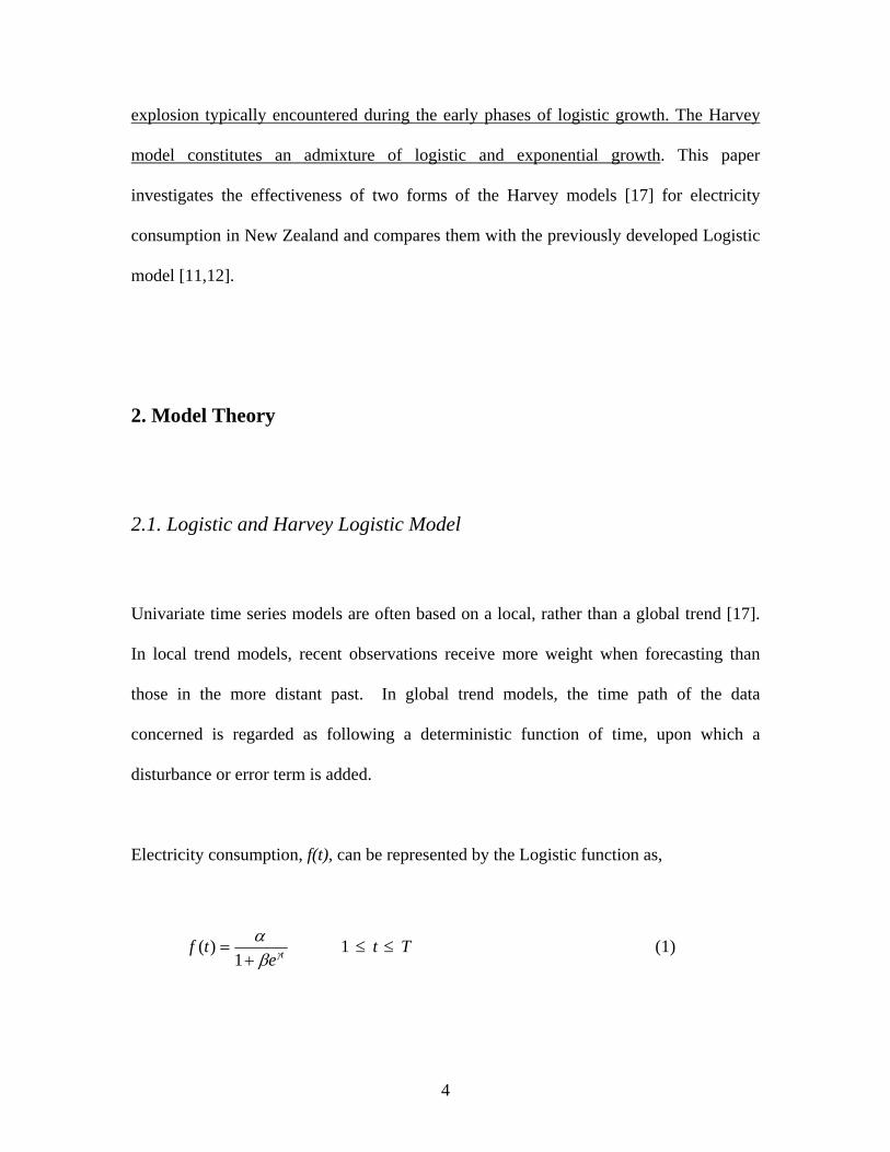
Electricity consumption, f(t), can be represented by the Logistic function as,

tetf γβ

α+

=1

)( 1 ≤ t ≤ T (1)

5

where, α is the saturation level

β and γ are parameters to be estimated

t is the time in years

In the Logistic model, α is estimated by a Fibonacci search technique [11, 12].

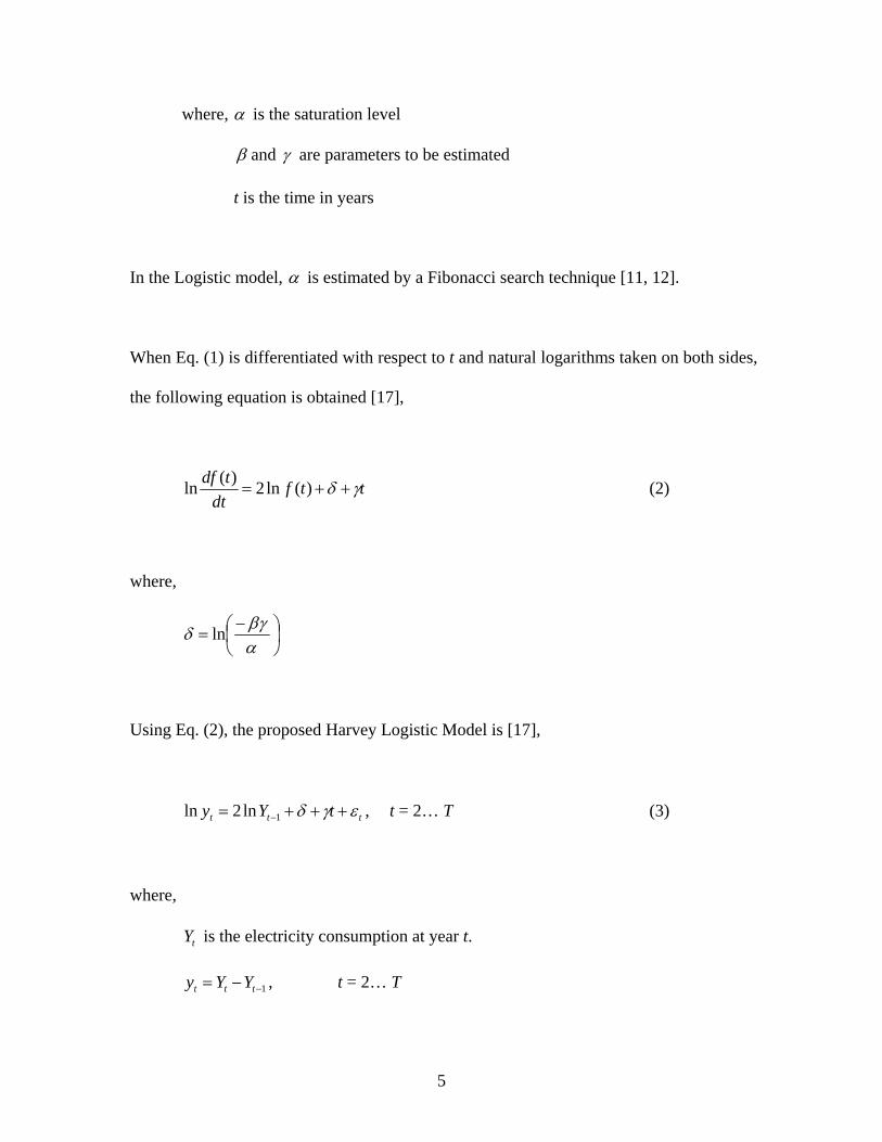
When Eq. (1) is differentiated with respect to t and natural logarithms taken on both sides,

the following equation is obtained [17],

ttfdt

tdf γδ ++= )(ln2)(ln (2)

where,

⎟⎠⎞

⎜⎝⎛ −=

αβγδ ln

Using Eq. (2), the proposed Harvey Logistic Model is [17],

ttt tYy εγδ +++= −1ln2ln , t = 2… T (3)

where,

tY is the electricity consumption at year t.

1−−= ttt YYy , t = 2… T

6

tε is a disturbance term with zero mean and constant variance

δ and γ are constants to be found by regression.

Eq. (3) is rearranged to give:

tt t

Yy

t

εγδ ++=⎟⎟⎠

⎞⎜⎜⎝

⎛

−2

1

ln (4)

The parameters δ and γ are found by regressing ⎟⎟⎠

⎞⎜⎜⎝

⎛

−21

lntYyt on t. Eq. (4) can be written as,

)(21

tt eYy t

γδ +−= (5)

It can be seen that Eq. (5) no longer contain the error term, tε . This is to simplify the

model. However, the residuals produced by ⎟⎟⎠

⎞⎜⎜⎝

⎛

−21

lntYyt on the regression line ( tγδ + ) are

studied using Durbin-Watson (DW) d-statistics [19]. Upon acceptable DW statistics, the

models are fitted to the data sets. More details can be found in Section 3.

Since 1−−= ttt YYy , then Eq. (5) can be written as,

)(21 1

ttt eYYY t

γδ +− −+= (6)

The h-step ahead forecasts of the electricity consumption, Y , can be made by using,

7

))((21 1

ˆˆˆ hththt eYYY ht

++−++ −++= γδ (7)

The forecast for electricity consumption takes the form of the Logistic curve and

gradually approaches the saturation level α .

2.2 Harvey Model

The general modified exponential function is of the form [17],

ktetf )1()( γβα += (8)

The value of k determines the form of the function f(t). When k = -1, f(t) is Logistic and

when k = 1 it is a simple modified exponential.

Differentiating and the taking natural logarithm as for the Logistic model, leads to the

Harvey model [17]:

ttt tYy εγδρ +++= −1lnln (9)

where,

k

k 1−=ρ

( )γβαδ kk /1ln=

8

ρ , β and γ are parameters to be estimated.

Forecasts are obtained using:

))((1 1

ˆˆˆ hththt eYYY ht

++−++ −++= γδρ (10)

Mean absolute percentage error (MAPE) and the Durbin-Watson statistic (DW) are used

in the comparison of the models [19]. MAPE gives an indication of the goodness of the

fit of the model to the historical data. MAPE is also used to compare the forecasting

accuracy of the models. The DW statistic tests whether the residuals of the fitted model

are independent. A DW statistic close to 2 indicates that there is no correlation in the

errors produced by the developed model.

3 Application to New Zealand Electricity Consumption

The annual electricity consumption data for New Zealand [20,21] from 1943 to 1999 are

modeled using the Harvey Logistic and Harvey Model. The models are applied separately

to each of the Domestic and the Non-Domestic sectors and to the Total consumption data.

Domestic and Non-domestic sectors are often studied separately because of their

perceived difference in contribution to society. The Domestic sector of residential

customers is primarily a goods and services consumption sector of society while the Non-

9

Domestic sector is the production of goods and services and hence that which gives rise

to the generation of economic wealth of a country. It never the less consumes electricity

(and other resources) in generating that wealth. The Total consumption is simply the

total electricity consumed and is the aggregate of the Domestic and the Non-Domestic

sector consumptions. In addition these are the sectors that the government has used for

electricity forecasting and are well accepted and published data sets.

Regressing ⎟⎟⎠

⎞⎜⎜⎝

⎛

−21

lntYyt over the time period 1943-1999 gives the following Harvey Logistic

models.

Domestic: tYy tt 083.086.150ln2ln 1 −+= − (11)

Non-Domestic: tYy tt 080.079.145ln2ln 1 −+= − (12)

Total: tYy tt 081.060.145ln2ln 1 −+= − (13)

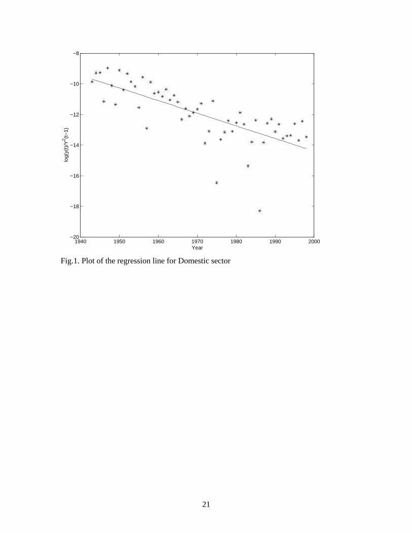
A plot of ⎟⎟⎠

⎞⎜⎜⎝

⎛

−21

lntYyt along with the fitted regression line for the Domestic sector is shown

in Fig. 1.

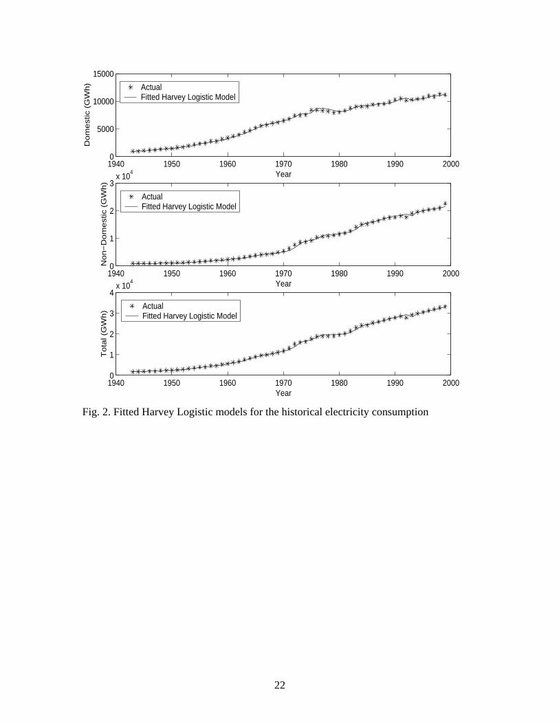
The residuals are very well behaved with a Durbin-Watson (DW) statistic of 2.0. The

residuals are also reasonably well behaved in the Non-Domestic sector and Total

consumption, with Durbin–Watson statistics of 1.1 and 1.5, although there is some

indication of serial correlation in the case of Non-Domestic data. Fig. 2 shows the fitted

Harvey Logistic models for the historical electricity consumption.

10

The Harvey Logistic models have produced very good fits of the historical electricity

consumption with MAPE values of 3.1 for Domestic, 3.3 for Non-Domestic and 2.6 for

Total consumption data.

Application of the electricity consumption data to the Harvey Model (Eq. 9) resulted in

the following models.

Domestic: tYy tt 018.044.35ln60.0ln 1 −+= − (14)

Non-Domestic: tYy tt 032.046.57ln29.1ln 1 −+= − (15)

Total: tYy tt 028.027.50ln08.1ln 1 −+= − (16)

Where, t is the time in years from 1944 to 1999.

These Harvey models also produced very good fits with MAPE values of 3.1 for

Domestic, 3.3 for Non-Domestic and 2.7 for Total consumption. These values are very

close to the Harvey Logistic model fits and thus the fitted Harvey models for the historic

periods of the Domestic and Non-Domestic sectors and Total consumption are very

similar to those shown in Fig. 2. However, the coefficients of 1−tY (Eqs. 14–16) are

significantly different from the 2 of those in the Harvey Logistic models (Eqs. 11-13).

These values indicate that the Harvey models are different from the Harvey Logistic

models.

11

4 Comparison of Forecasts

4.1. Comparison of the Harvey and Logistic Models

4.1.1. Goodness of Fit and Future Consumptions

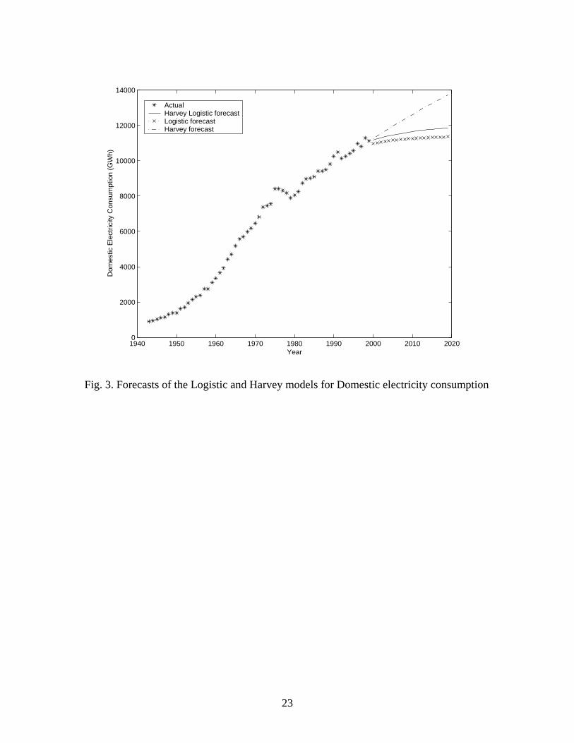
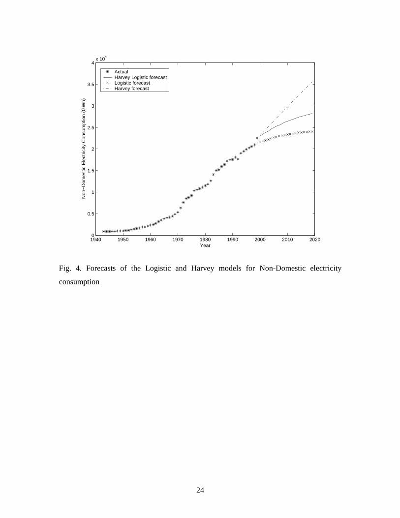
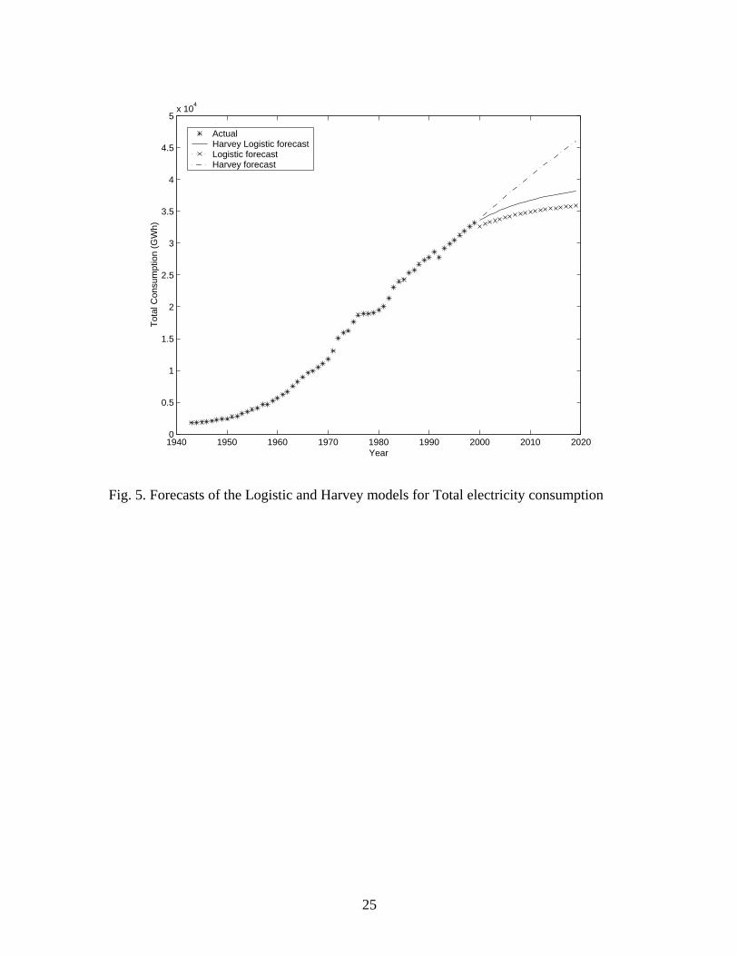
Forecasts produced by the Harvey models together with the forecasts of the Logistic

models for the Domestic, Non-Domestic and Total consumption are shown in Fig. 3, Fig.

4 and Fig. 5 respectively.

The forecasts for the Domestic and Non-Domestic sectors and Total consumptions are

increasing in an exponential nature for the three models. The Harvey model has given

rise to the highest forecasts for the three data sets considered. The Logistic model

forecasted the lowest consumptions for the three data sets. The Harvey Logistic model

gave forecasts somewhere in between the other two forecasts.

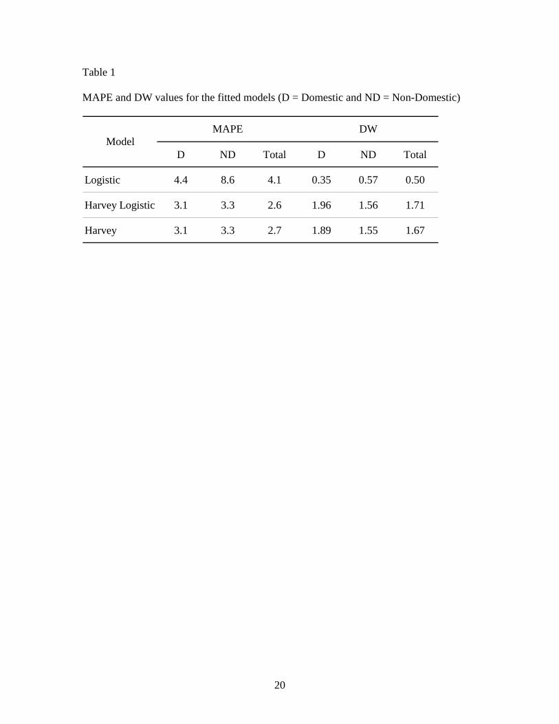
The MAPE and DW values of the fitted models from 1943 to 1999 for the Logistic,

Harvey Logistic and Harvey models are given in Table 1.

The MAPE values are very similar for the Harvey Logistic and Harvey models. In

addition, the lowest MAPE values are also recorded for these models. This indicates that

the Harvey models provide better fits of the historical data than the Logistic models. In

addition, the Durbin-Watson statistics are closer to 2 in the Harvey Logistic and Harvey

models. This indicates that the residuals are more reasonably well behaved in the Harvey

12

Logistic and Harvey models compared to the Logistic models. The DW values are much

smaller than 2 in the Logistic models indicating that there are some positive

autocorrelation in the residuals.

The resulting low predictions by the Logistic models are due to the constraints imposed

by the saturation level. In proposing the Logistic model [11,12] the saturation level is

obtained by the Fibonacci search technique prior to obtaining the constants by regression

analysis. In the Harvey Logistic model the asymptote is not approximated prior to the

regression analysis. As a result, the curve of the Harvey Logistic model gradually

approaches a saturation level. This has given rise to higher forecasts than the Logistic

model. The Harvey model is different from the other two in the sense that it has got one

extra parameter, ρ , to be estimated as a part of the regression analysis. It has been shown

that the parameter, ρ , calculated for each of the Domestic and Non-Domestic sectors and

Total consumption are significantly different from 2 showing that for these data, the

Harvey model is not equivalent to the Harvey Logistic model. However, with as good fits

to historical data as the Harvey Logistic model, the Harvey model has given rise to higher

consumption forecasts overall.

4.1.2 Forecasting Accuracy

The Logistic, Harvey Logistic and Harvey models are further analyzed for forecasting

accuracy. A number of actual consumption data points at the end of the series are held

out for comparison with the forecasts obtained by the developed models. The forecasts

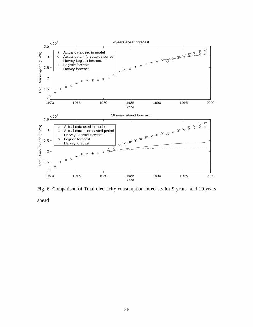
13

for the 9 years ahead and 19 years ahead, when the last 9 years and 19 years of data were

held out for the Total electricity consumption are shown in Fig. 6.

For the 9 years ahead forecasts the Harvey model gave forecasts that are closest to the

actual values while in the 19 years ahead forecasts, the Logistic model gave forecasts that

are very close to the actual Total consumption values. This suggests the choice of the best

model should not be made by just looking at the forecasts of the two chosen periods.

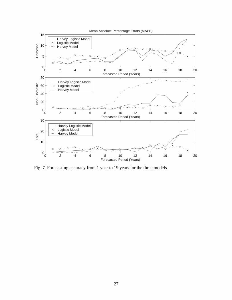
Therefore, forecasting models are obtained with data values held out from 1 year through

to 19 years for each of the three models. The average MAPE values of each of the

models using the actual values held out for each of the forecasted period from 1 year

through to 19 years are shown in Fig. 7, for the Domestic and Non-Domestic sectors and

Total consumption respectively.

For the Domestic sector, the Harvey model has given the lowest MAPE values from 1-

year through to 18-years ahead. The Harvey Logistic model gave very similar values to

the Harvey model with slightly larger errors. The Logistic model gave the highest error

values except at the 19-years ahead forecast. This indicates that the Harvey model is the

best among these three in forecasting the Domestic consumption for a period of up to 18

years ahead.

For the Non-Domestic sector, it is the Logistic model that gave the overall MAPE values

from 1-year ahead through to 18-years ahead forecasts. However, the Harvey Logistic

gave the lowest errors in the initial 6 years. The Harvey model also gave acceptable

14

results in the initial 8 years. Overall, the Logistic model is the best model for forecasting

electricity consumption in the Non-Domestic sector, especially for longer horizons up to

18 years ahead.

For the Total consumption, the errors are more comparable. However, the Harvey model

gave the lowest errors from 1-year ahead through to 14-years ahead forecasts while the

Logistic model performed better from 15-years through to 19-years ahead forecasts. The

Harvey Logistic model gave similar results to the Harvey model, but the errors are

slightly larger than for the Harvey model. These results indicate that the Harvey model is

the best to forecast Total electricity consumption for periods from 1 year through to 15

years ahead.

Young [15] studied nine different growth curve models including the Logistic and

Harvey models by comparing MAPE. The comparison revealed that the Harvey model

was one of the three proposed models for forecasting time series with an unknown upper

limit. The analysis in this section supports those results, indicating that the Harvey model

is an appropriate forecasting model for New Zealand electricity consumption.

A good forecasting model is often selected on the ability of the model to describe the

future data and not necessarily gives the best fit of the historical data [22]. The Harvey

model not only generated the best fit of the future data, but was also among the best in

fitting historical data. This strengthens the choice of the Harvey model in forecasting

electricity consumption in New Zealand.

15

4.2. Comparison with National Forecasts

The forecasts obtained by the Logistic, Harvey and Harvey Logistic models are compared

with the national forecasts available in New Zealand. They are CAE models [23] and

MED models [24]. The MED forecasts are made by the Ministry of Economic

Development, New Zealand, using its SADEM energy supply and demand model. The

SADEM model is a descriptive market equilibrium model focusing on the entire energy

sector. The model determines equilibrium in the energy market by projecting demands

for a given set of prices and comparing this with the modelled cost of supplying this level

of demand [24]. The CAE forecasts are modelled using an annual load growth of 1.8%.

Their study has used 1.8% as the baseline estimate, with 1.3% and 2.3 % growth used for

sensitivity analysis. This paper uses the 1.8% baseline estimate for comparison purposes.

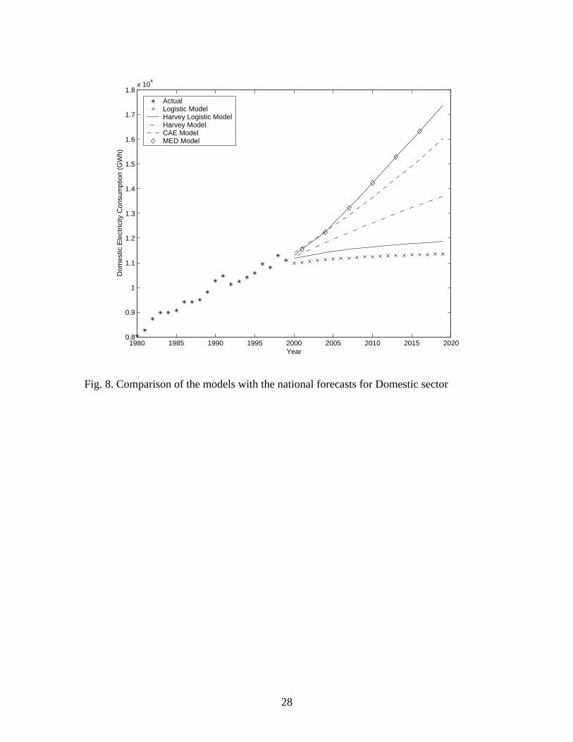
The forecasts obtained by these models for the Domestic and Non-Domestic sectors and

Total consumption are shown in Fig. 8, Fig. 9 and Fig. 10 respectively.

For the Domestic sector, the Logistic model forecasted the lowest consumption. The

Harvey model forecasts are also lower than the other models, but somewhere in between

the CAE and Harvey Logistic model forecasts. For the Non-Domestic sector, the

forecasts of the Harvey Logistic model are very close to the CAE and MED model

forecasts while the Harvey model forecasted the highest and the Logistic model

forecasted the lowest consumption.

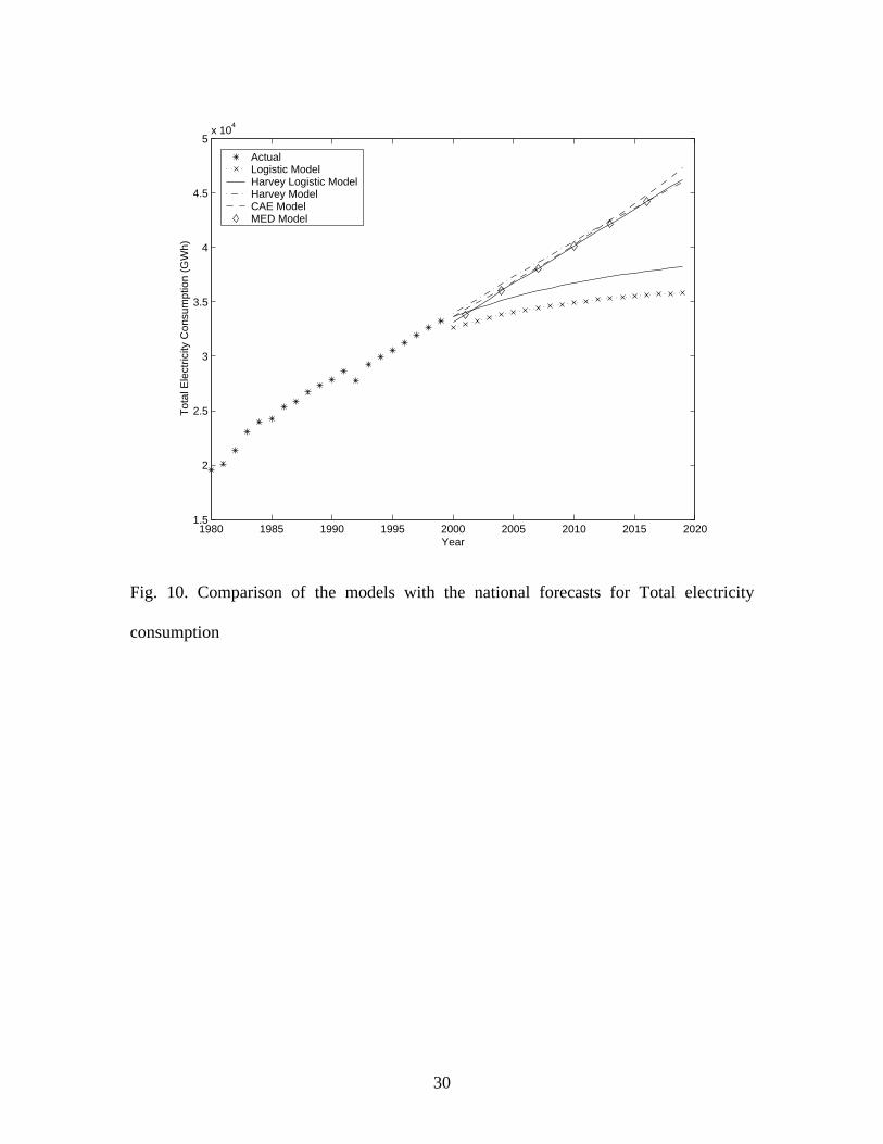
16

For the Total consumption, the Harvey model forecasted very similar forecasts to the

CAE and MED forecasts. The forecasts of the Logistic and Harvey Logistic models are

much lower. The forecasts by the Harvey model are virtually indistinguishable from the

CAE model and MED model forecasts. The fit to the historical data and forecasting

accuracy indicates that the Harvey model is an excellent candidate in forecasting New

Zealand electricity consumption.

5. Summary

This paper has investigated two forms of the Harvey models and compared them with a

previously developed Logistic model for forecasting electricity consumption in New

Zealand. It was found that the proposed models are generally appropriate in forecasting

electricity consumption New Zealand. However, the proposed Harvey model has

performed better than the Logistic model in most cases in terms of model fit to the

historical data and forecasting accuracy. The Harvey model forecasted higher

consumption comparable with national forecasts, especially for the Total consumption for

New Zealand. The good model fit and forecasting accuracy has indicated that the Harvey

model is a very suitable candidate in forecasting New Zealand electricity consumption.

17

Acknowledgements

The authors gratefully acknowledge the helpful suggestions of two anonymous reviewers

that enabled to improve the paper.

References:

[1] Carrillo, M., and Gonzalez, J.M.: A New Approach to modeling sigmoid curves,

Technological Forecasting and Social Change 69, 233-241 (2002).

[2] Bass, F.M.: A new product growth for model consumer durables, Management

Science 15(5), 215- 227 (1969).

[3] Jain, D.C., and Rao, R.C.: New concepts and applications in growth phenomena,

Journal of Applied Statistics 21(3), 161-190 (1994).

[4] Bhargava, S., Bhargava, R., and Jain, A.: Requirement of dimensional consistency

in model equations: Diffusion models incorporating price and their applications,


[5] Frank, L.D.: An analysis of the effect of the economic situation on modeling and

forecasting the diffusion of wireless communications in Finland, Technological

Forecasting and Social Change, ARTICLE IN PRESS, 1 –13 (2003).

[6] Bewley, R., and Fiebig, D.G.: A flexible logistic growth model with applications

in telecommunications, International Journal of Forecasting 4, 177-192 (1988).

18

[7] Meyer, P.S., and Ausubel, J.H.: Carrying capacity: A model with logistically

varying limits, Technological Forecasting and Social Change 61, 209-214 (1999).

[8] Giovanis, A.N., and Skiadas, C.H.: A stochastic logistic innovation diffusion

model studying the electricity consumption in Greece and the United States,

Technological Forecasting and Social Change 61, 235-246, (1999).

[9] Mar-Molineo.: Tractors in Spain: A logistic analysis, Journal of Operational

Research Society 31, 141-152 (1980).

[10] Oliver, F.R.: Tractors in Spain: A further logistic analysis, Journal of the

Operational Research Society 32, 499 – 502.

[11] Mohamed, Z., and Bodger, P.S.: Analysis of the Logistic model for Predicting

New Zealand Electricity Consumption, Proceedings of the Electricity

Engineer’s Association (EEA) New Zealand 2003 Conference, Christchurch,

New Zealand, Published in CD-ROM, 20-21 June (2003).

[12] Bodger, P.S., and Tay, H.S.: Logistic and Energy Substitution Models for

Electricity Forecasting: A Comparison Using New Zealand Consumption Data,


[13] Skiadas, C.H., Papayannakis L.L., and Mourelatos, A.G.: An Attempt to

Improve Forecasting Ability of Growth Functions: The Greek Electric System,

Technological Forecasting and Social Change 44, 391– 404 (1993).

[14] Sharp, J.A., and Price, H.R.: Experience Curve Models in the Electricity Supply

Industry, International Journal of Forecasting 6, 531–540 (1990).

[15] Young, P.: Technological Growth Curves: A Competition of Forecasting

Models, Technological Forecasting and Social Change 44, 375–389 (1993).

19

[16] Tingyan, X.: A Combined Growth Model for Trend Forecasts, Technological

Forecasting and Social Change 38, 175–186 (1990).

[17] Harvey, A.C.: Time series forecasting based on the logistic curve, Journal of the

Operational Research Society 35(7), 641-646 (1984).

[18] Harvey, A.C., Time Series Models. 2nd ed., The MIT Press, Cambridge,

Massachusetts, 1993, p.149-152.

[19] Makridakis, S., Weelwright S.C., and Hyndman R.J.: Forecasting: Methods

and Applications. Third ed., John Wiley and Sons, Inc., New York, 1998.

[20] Ministry of Energy.: Electricity Forecasting and Planning: A Background

Report to the 1984 Energy Plan, issues of 1982. –1984.

[21] Ministry of Economic Development.: New Zealand Energy Data File, July

2002.

[22] Martino, J.P.: A review of selected recent advances in technological forecasting,


[23] Sinclair Knight Merz and CAE (Centre for Advanced Engineering, University

of Canterbury, NZ).: Electricity Supply and Demand to 2015. Fifth Edition,

April 2000.

[24] Ministry of Economic Development, Modelling and Statistics Unit.: New

Zealand Energy Outlook to 2020, February 2000.

20

Table 1

MAPE and DW values for the fitted models (D = Domestic and ND = Non-Domestic)

D ND Total D ND Total

Logistic 4.4 8.6 4.1 0.35 0.57 0.50

Harvey Logistic 3.1 3.3 2.6 1.96 1.56 1.71

Harvey 3.1 3.3 2.7 1.89 1.55 1.67

DWMAPEModel

21

1940 1950 1960 1970 1980 1990 2000−20

−18

−16

−14

−12

−10

−8

Year

log(

y(t)

/Y2 (t

−1)

Fig.1. Plot of the regression line for Domestic sector

22

1940 1950 1960 1970 1980 1990 20000

5000

10000

15000

Year

Dom

est

ic (

GW

h) Actual

Fitted Harvey Logistic Model

1940 1950 1960 1970 1980 1990 20000

1

2

3x 10

4

Year

Non−

Dom

est

ic (

GW

h)

ActualFitted Harvey Logistic Model

1940 1950 1960 1970 1980 1990 20000

1

2

3

4x 10

4

Year

Tota

l (G

Wh)

ActualFitted Harvey Logistic Model

Fig. 2. Fitted Harvey Logistic models for the historical electricity consumption

23

1940 1950 1960 1970 1980 1990 2000 2010 20200

2000

4000

6000

8000

10000

12000

14000

Year

Dom

estic

Ele

ctric

ity C

onsu

mpt

ion

(GW

h)ActualHarvey Logistic forecastLogistic forecastHarvey forecast

Fig. 3. Forecasts of the Logistic and Harvey models for Domestic electricity consumption

24

1940 1950 1960 1970 1980 1990 2000 2010 20200

0.5

1

1.5

2

2.5

3

3.5

4x 10

4

Year

Non

−D

omes

tic E

lect

ricity

Con

sum

ptio

n (G

Wh)

ActualHarvey Logistic forecastLogistic forecastHarvey forecast

Fig. 4. Forecasts of the Logistic and Harvey models for Non-Domestic electricity

consumption

25

1940 1950 1960 1970 1980 1990 2000 2010 20200

0.5

1

1.5

2

2.5

3

3.5

4

4.5

5x 10

4

Year

Tot

al C

onsu

mpt

ion

(GW

h)

ActualHarvey Logistic forecastLogistic forecastHarvey forecast

Fig. 5. Forecasts of the Logistic and Harvey models for Total electricity consumption

26

1970 1975 1980 1985 1990 1995 20001

1.5

2

2.5

3

3.5x 10

4

Year

Tot

al C

onsu

mpt

ion

(GW

h) 9 years ahead forecast

Actual data used in model Actual data − forecasted periodHarvey Logistic forecastLogistic forecastHarvey forecast

1970 1975 1980 1985 1990 1995 20001

1.5

2

2.5

3

3.5x 10

4

Year

Tot

al C

onsu

mpt

ion

(GW

h)

19 years ahead forecast

Actual data used in model Actual data − forecasted periodHarvey Logistic forecastLogistic forecastHarvey forecast

Fig. 6. Comparison of Total electricity consumption forecasts for 9 years and 19 years

ahead

27

0 2 4 6 8 10 12 14 16 18 200

5

10

15D

omes

tic

Forecasted Period (Years)

Mean Absolute Percentage Errors (MAPE)

Harvey Logistic ModelLogistic ModelHarvey Model

0 2 4 6 8 10 12 14 16 18 200

20

40

60

80

Non

−D

omes

tic



0 2 4 6 8 10 12 14 16 18 200

10

20

30

Tot

al



Fig. 7. Forecasting accuracy from 1 year to 19 years for the three models.

28

1980 1985 1990 1995 2000 2005 2010 2015 20200.8

0.9

1

1.1

1.2

1.3

1.4

1.5

1.6

1.7

1.8x 10

4

Year

Dom

estic

Ele

ctric

ity C

onsu

mpt

ion

(GW

h)

ActualLogistic ModelHarvey Logistic ModelHarvey ModelCAE ModelMED Model

Fig. 8. Comparison of the models with the national forecasts for Domestic sector

29

1980 1985 1990 1995 2000 2005 2010 2015 20201

1.5

2

2.5

3

3.5

4x 10

4

Year

Non

−D

omes

tic E

lect

ricity

Con

sum

ptio

n (G

Wh)


Fig. 9. Comparison of the models with the national forecasts for Non-Domestic sector

30

1980 1985 1990 1995 2000 2005 2010 2015 20201.5

2

2.5

3

3.5

4

4.5

5x 10

4

Year

Tot

al E

lect

ricity

Con

sum

ptio

n (G

Wh)


Fig. 10. Comparison of the models with the national forecasts for Total electricity

consumption

zaid & pat 3

Documents