y-chromosome haplotype origins via biogeographical multilateration

Y-Chromosome Haplotype Origins via Biogeographical Multilateration Michael R. Maglio

Abstract

Current Y-chromosome migration maps only cover the broadest-brush strokes of the

highest-level haplogroups. Existing methods generalize geographic patterns based on large

population genetic frequency and diversity. New tools are required to illuminate our

nomadic, stationary and genealogical histories. Biogeographical Multilateration (BGM)

illustrates directional flow as well as chronological and physical origins at the individual

haplotype level.

Introduction

Traditional genealogy and its reliance on

paper records can only take us as far back as

records exist. This is perhaps 300 or 400

years. It could be as much as 1000 years if

we can connect to wealthy or royal families.

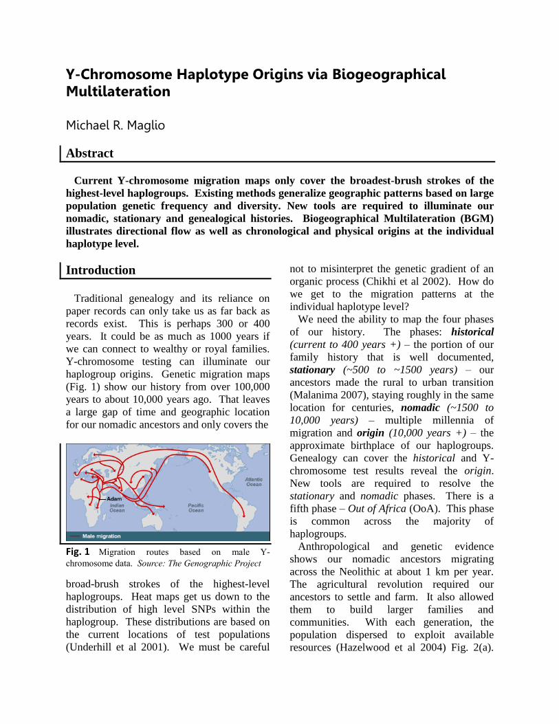
Y-chromosome testing can illuminate our

haplogroup origins. Genetic migration maps

(Fig. 1) show our history from over 100,000

years to about 10,000 years ago. That leaves

a large gap of time and geographic location

for our nomadic ancestors and only covers the

Fig. 1 Migration routes based on male Y-

chromosome data. Source: The Genographic Project

broad-brush strokes of the highest-level

haplogroups. Heat maps get us down to the

distribution of high level SNPs within the

haplogroup. These distributions are based on

the current locations of test populations

(Underhill et al 2001). We must be careful

not to misinterpret the genetic gradient of an

organic process (Chikhi et al 2002). How do

we get to the migration patterns at the

individual haplotype level?

We need the ability to map the four phases

of our history. The phases: historical

(current to 400 years +) – the portion of our

family history that is well documented,

stationary (~500 to ~1500 years) – our

ancestors made the rural to urban transition

(Malanima 2007), staying roughly in the same

location for centuries, nomadic (~1500 to

10,000 years) – multiple millennia of

migration and origin (10,000 years +) – the

approximate birthplace of our haplogroups.

Genealogy can cover the historical and Y-

chromosome test results reveal the origin.

New tools are required to resolve the

stationary and nomadic phases. There is a

fifth phase – Out of Africa (OoA). This phase

is common across the majority of

haplogroups.

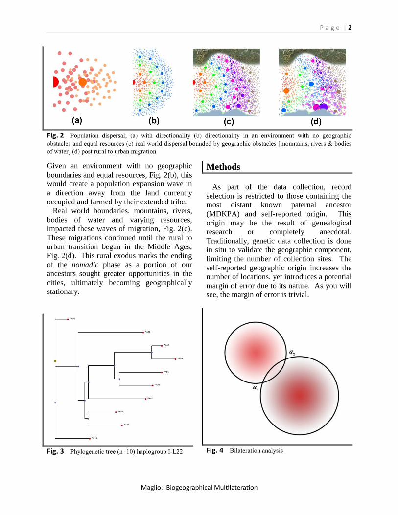
Anthropological and genetic evidence

shows our nomadic ancestors migrating

across the Neolithic at about 1 km per year.

The agricultural revolution required our

ancestors to settle and farm. It also allowed

them to build larger families and

communities. With each generation, the

population dispersed to exploit available

resources (Hazelwood et al 2004) Fig. 2(a).

P a g e | 2

Maglio: Biogeographical Multilateration

Fig. 2 Population dispersal; (a) with directionality (b) directionality in an environment with no geographic

obstacles and equal resources (c) real world dispersal bounded by geographic obstacles [mountains, rivers & bodies

of water] (d) post rural to urban migration

Given an environment with no geographic

boundaries and equal resources, Fig. 2(b), this

would create a population expansion wave in

a direction away from the land currently

occupied and farmed by their extended tribe.

Real world boundaries, mountains, rivers,

bodies of water and varying resources,

impacted these waves of migration, Fig. 2(c).

These migrations continued until the rural to

urban transition began in the Middle Ages,

Fig. 2(d). This rural exodus marks the ending

of the nomadic phase as a portion of our

ancestors sought greater opportunities in the

cities, ultimately becoming geographically

stationary.

Fig. 3 Phylogenetic tree (n=10) haplogroup I-L22

Methods

As part of the data collection, record

selection is restricted to those containing the

most distant known paternal ancestor

(MDKPA) and self-reported origin. This

origin may be the result of genealogical

research or completely anecdotal.

Traditionally, genetic data collection is done

in situ to validate the geographic component,

limiting the number of collection sites. The

self-reported geographic origin increases the

number of locations, yet introduces a potential

margin of error due to its nature. As you will

see, the margin of error is trivial.

Fig. 4 Bilateration analysis

P a g e | 3


Data sets consist of multiple records from a

37 STR marker haplotype and corresponding

SNP (YCC 2002). In this exercise, I-L22 is

used. Time to most recent common ancestor

(TMRCA) is generated to a 95% confidence

(Walsh 2001) using FTDNA derived mutation

rates. This output is then used by the

Neighbor-joining method, which is part of the

PHYLIP package for inferring phylogenetic

relationships. A phylogenetic tree, Fig. 3, and

chronological distances are produced for each

data set. Data points are mapped using

genealogical origin and a radius drawn on a

Mercator projection calculated using the

upper value of the Neolithic migration rate of

30 km per 25 years or 1.2km/yr (Cavalli-

Sforza 2002, Hazelwood et al 2004). The

resulting intersection between pairs, Fig. 4,

represents the approximate location of the

common ancestor. A Time Difference of

Arrival (TDoA) approach is used for

detecting the origin (Peter et al 2013).

Traditional TDoA uses two or more

“beacons” with known locations and a

measurement of the time it takes to receive a

signal from each. The time is converted to a

distance. A current location can then be

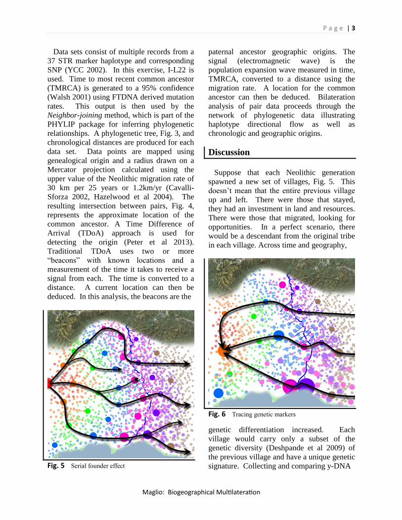
deduced. In this analysis, the beacons are the

Fig. 5 Serial founder effect

paternal ancestor geographic origins. The

signal (electromagnetic wave) is the

population expansion wave measured in time,

TMRCA, converted to a distance using the

migration rate. A location for the common

ancestor can then be deduced. Bilateration

analysis of pair data proceeds through the

network of phylogenetic data illustrating

haplotype directional flow as well as

chronologic and geographic origins.

Discussion

Suppose that each Neolithic generation

spawned a new set of villages, Fig. 5. This

doesn’t mean that the entire previous village

up and left. There were those that stayed,

they had an investment in land and resources.

There were those that migrated, looking for

opportunities. In a perfect scenario, there

would be a descendant from the original tribe

in each village. Across time and geography,

Fig. 6 Tracing genetic markers

genetic differentiation increased. Each

village would carry only a subset of the

genetic diversity (Deshpande et al 2009) of

the previous village and have a unique genetic

signature. Collecting and comparing y-DNA

P a g e | 4


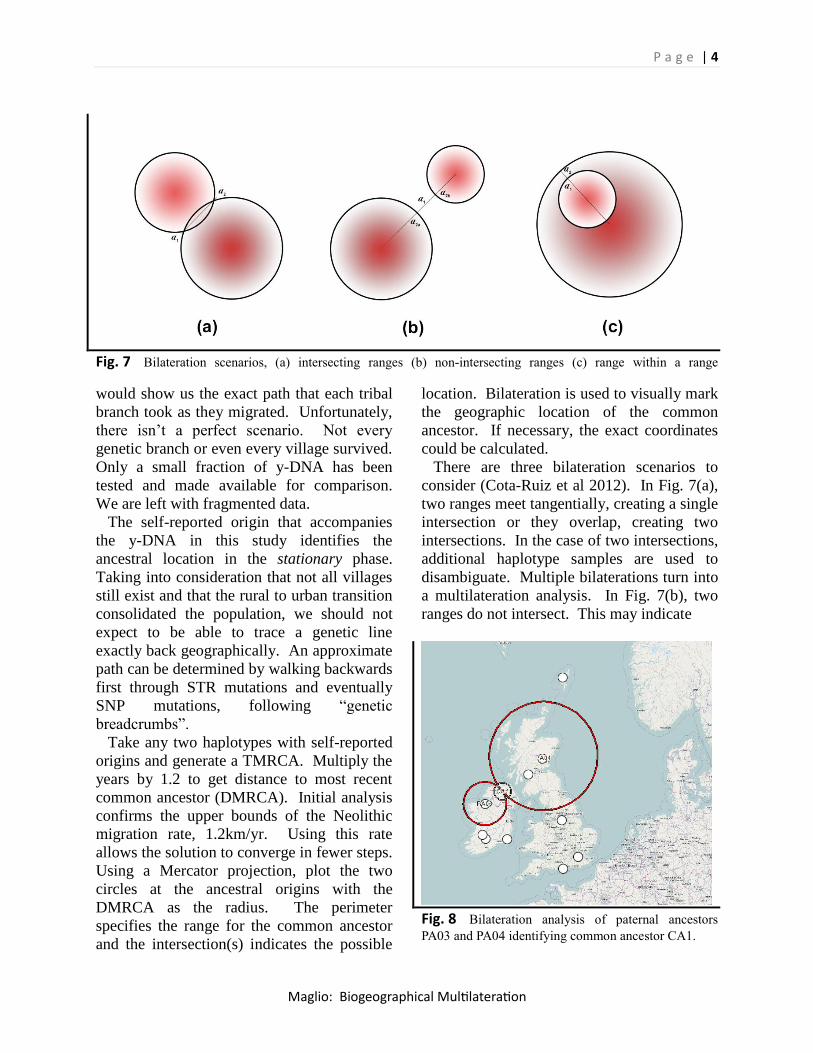
Fig. 7 Bilateration scenarios, (a) intersecting ranges (b) non-intersecting ranges (c) range within a range

would show us the exact path that each tribal

branch took as they migrated. Unfortunately,

there isn’t a perfect scenario. Not every

genetic branch or even every village survived.

Only a small fraction of y-DNA has been

tested and made available for comparison.

We are left with fragmented data.

The self-reported origin that accompanies

the y-DNA in this study identifies the

ancestral location in the stationary phase.

Taking into consideration that not all villages

still exist and that the rural to urban transition

consolidated the population, we should not

expect to be able to trace a genetic line

exactly back geographically. An approximate

path can be determined by walking backwards

first through STR mutations and eventually

SNP mutations, following “genetic

breadcrumbs”.

Take any two haplotypes with self-reported

origins and generate a TMRCA. Multiply the

years by 1.2 to get distance to most recent

common ancestor (DMRCA). Initial analysis

confirms the upper bounds of the Neolithic

migration rate, 1.2km/yr. Using this rate

allows the solution to converge in fewer steps.

Using a Mercator projection, plot the two

circles at the ancestral origins with the

DMRCA as the radius. The perimeter

specifies the range for the common ancestor

and the intersection(s) indicates the possible

location. Bilateration is used to visually mark

the geographic location of the common

ancestor. If necessary, the exact coordinates

could be calculated.

There are three bilateration scenarios to

consider (Cota-Ruiz et al 2012). In Fig. 7(a),

two ranges meet tangentially, creating a single

intersection or they overlap, creating two

intersections. In the case of two intersections,

additional haplotype samples are used to

disambiguate. Multiple bilaterations turn into

a multilateration analysis. In Fig. 7(b), two

ranges do not intersect. This may indicate

Fig. 8 Bilateration analysis of paternal ancestors

PA03 and PA04 identifying common ancestor CA1.

P a g e | 5


Table 1. Neighbor-joining branch lengths from Paternal Ancestors to Common Ancestor with corresponding distances (1.2 km/yr)

Paternal Ancestor

Common Ancestor TMRCA DMRCA (km)

PA01 2 137.1 165

PA02 5 695.6 835

PA03 1 106.8 128

PA04 1 253.1 304

PA05 3 453.7 545

PA06 3 356.2 428

PA07 6 612.5 735

PA08 8 297.2 357

PA09 8 362.8 435

PA10 2 372.8 447

Table 2. Neighbor-joining branch lengths from Common Ancestors to their Common Ancestor with corresponding distances (1.2 km/yr)

Common Ancestor

Common Ancestor TMRCA DMRCA (km)

1 4 402.7 483

3 4 54.7 66

4 6 276.2 332

5 2 249.4 299

6 7 38.4 46

7 5 70.3 84

8 7 34.7 42

that one or both migration rates were higher

than average. This is most common when a

body of water separates the two samples. It

may also indicate that one of the self-reported

origins is in error. In the case of a body of

water, the common ancestor has the potential

to exist on either coast, represented by points

a2a and a2b. Disambiguation, employing

additional bilaterations, is required. In Fig.

7(c), one migration range exists completely

within the second range. This suggests that

the migration rate of the sample with the

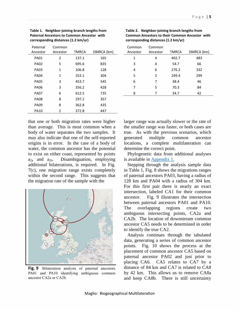
Fig. 9 Bilateration analysis of paternal ancestors

PA01 and PA10 identifying ambiguous common

ancestor CA2a or CA2b.

larger range was actually slower or the rate of

the smaller range was faster, or both cases are

true. As with the previous scenarios, which

generated multiple common ancestor

locations, a complete multilateration can

determine the correct point.

Phylogenetic data from additional analyses

is available in Appendix 1.

Stepping through the analysis sample data

in Table 1, Fig. 8 shows the migrations ranges

of paternal ancestors PA03, having a radius of

128 km and PA04 with a radius of 304 km.

For this first pair there is nearly an exact

intersection, labeled CA1 for their common

ancestor. Fig. 9 illustrates the intersection

between paternal ancestors PA01 and PA10.

The overlapping regions create two

ambiguous intersecting points, CA2a and

CA2b. The location of downstream common

ancestor CA5 needs to be determined in order

to identify the true CA2.

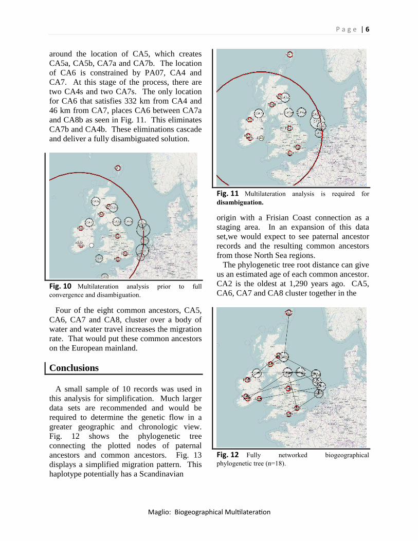
Analysis continues through the tabulated

data, generating a series of common ancestor

points. Fig. 10 shows the process at the

placement of common ancestor CA5 based on

paternal ancestor PA02 and just prior to

placing CA6. CA5 relates to CA7 by a

distance of 84 km and CA7 is related to CA8

by 42 km. This allows us to remove CA8a

and keep CA8b. There is still uncertainty

http://originhunters.com/content/bgm1.pdf

P a g e | 6


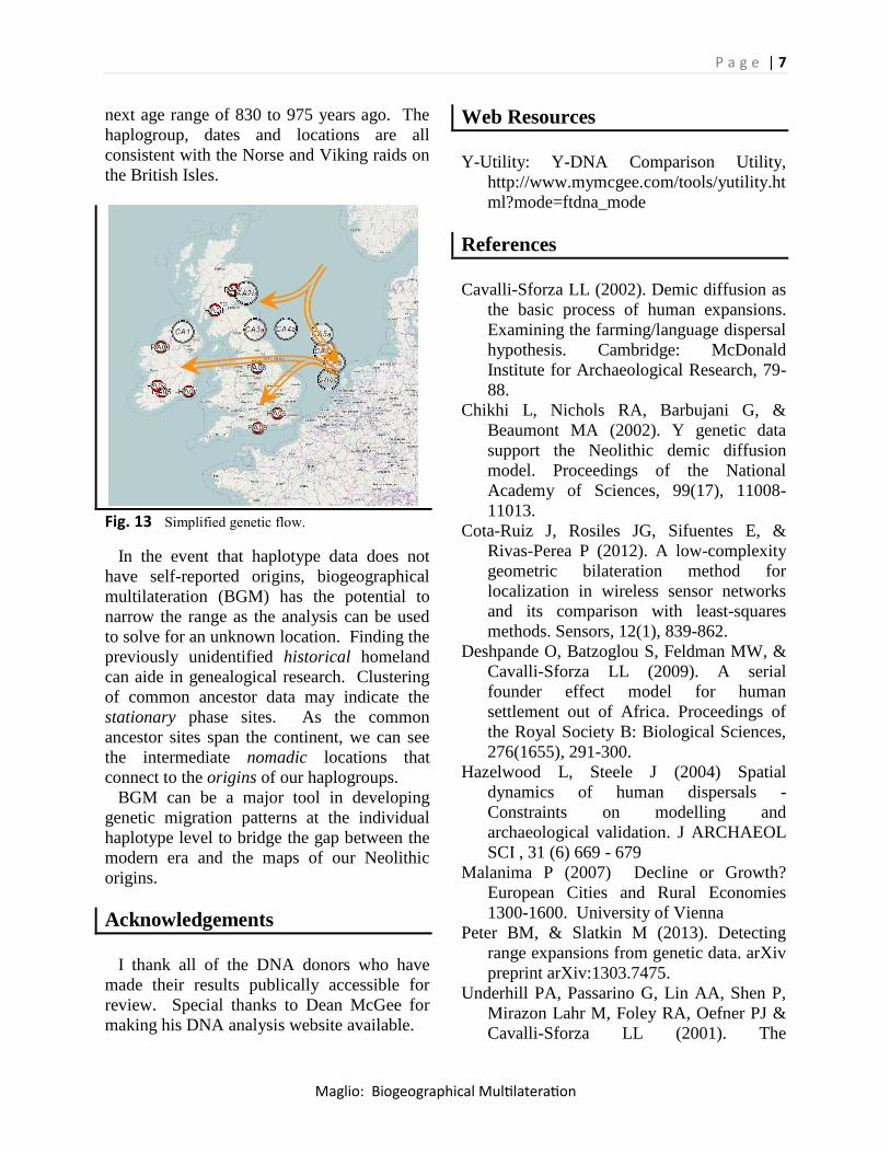
around the location of CA5, which creates

CA5a, CA5b, CA7a and CA7b. The location

of CA6 is constrained by PA07, CA4 and

CA7. At this stage of the process, there are

two CA4s and two CA7s. The only location

for CA6 that satisfies 332 km from CA4 and

46 km from CA7, places CA6 between CA7a

and CA8b as seen in Fig. 11. This eliminates

CA7b and CA4b. These eliminations cascade

and deliver a fully disambiguated solution.

Fig. 10 Multilateration analysis prior to full

convergence and disambiguation.

Four of the eight common ancestors, CA5,

CA6, CA7 and CA8, cluster over a body of

water and water travel increases the migration

rate. That would put these common ancestors

on the European mainland.

Conclusions

A small sample of 10 records was used in

this analysis for simplification. Much larger

data sets are recommended and would be

required to determine the genetic flow in a

greater geographic and chronologic view.

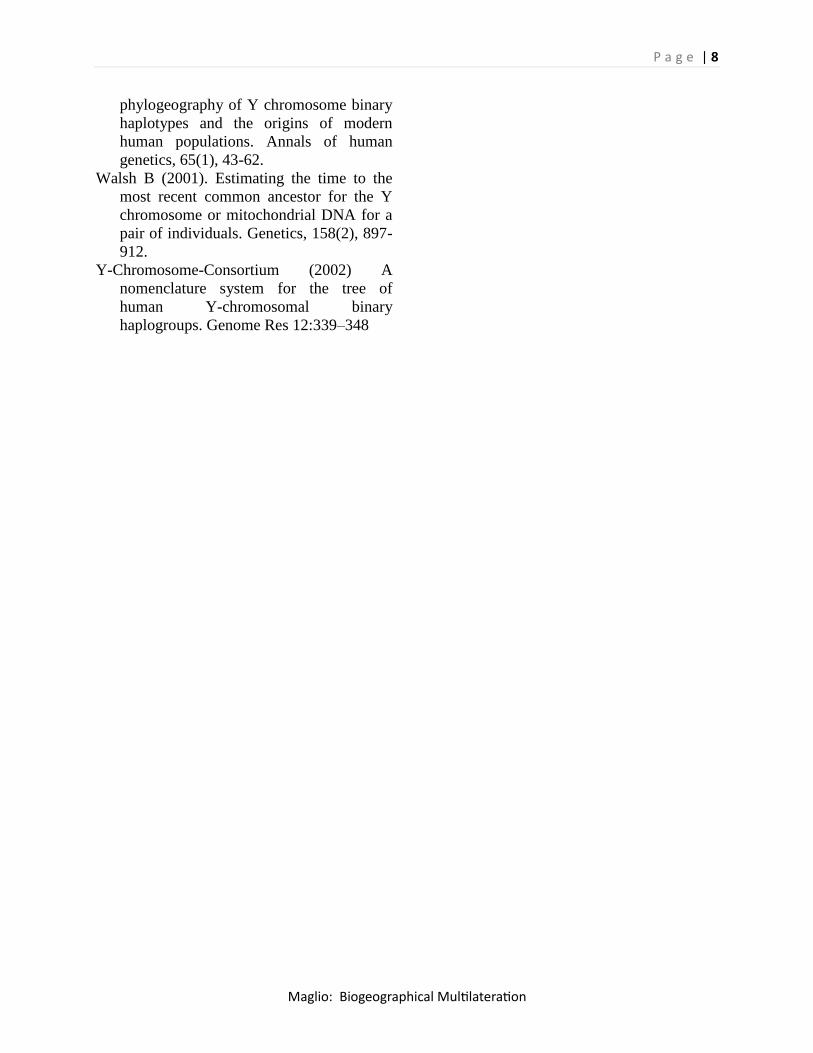
Fig. 12 shows the phylogenetic tree

connecting the plotted nodes of paternal

ancestors and common ancestors. Fig. 13

displays a simplified migration pattern. This

haplotype potentially has a Scandinavian

Fig. 11 Multilateration analysis is required for

disambiguation.

origin with a Frisian Coast connection as a

staging area. In an expansion of this data

set,we would expect to see paternal ancestor

records and the resulting common ancestors

from those North Sea regions.

The phylogenetic tree root distance can give

us an estimated age of each common ancestor.

CA2 is the oldest at 1,290 years ago. CA5,

CA6, CA7 and CA8 cluster together in the

Fig. 12 Fully networked biogeographical

phylogenetic tree (n=18).

P a g e | 7


next age range of 830 to 975 years ago. The

haplogroup, dates and locations are all

consistent with the Norse and Viking raids on

the British Isles.

Fig. 13 Simplified genetic flow.

In the event that haplotype data does not

have self-reported origins, biogeographical

multilateration (BGM) has the potential to

narrow the range as the analysis can be used

to solve for an unknown location. Finding the

previously unidentified historical homeland

can aide in genealogical research. Clustering

of common ancestor data may indicate the

stationary phase sites. As the common

ancestor sites span the continent, we can see

the intermediate nomadic locations that

connect to the origins of our haplogroups.

BGM can be a major tool in developing

genetic migration patterns at the individual

haplotype level to bridge the gap between the

modern era and the maps of our Neolithic

origins.

Acknowledgements

I thank all of the DNA donors who have

made their results publically accessible for

review. Special thanks to Dean McGee for

making his DNA analysis website available.

Web Resources

Y-Utility: Y-DNA Comparison Utility,

http://www.mymcgee.com/tools/yutility.ht

ml?mode=ftdna_mode

References

Cavalli-Sforza LL (2002). Demic diffusion as

the basic process of human expansions.

Examining the farming/language dispersal

hypothesis. Cambridge: McDonald

Institute for Archaeological Research, 79-

88.

Chikhi L, Nichols RA, Barbujani G, &

Beaumont MA (2002). Y genetic data

support the Neolithic demic diffusion

model. Proceedings of the National

Academy of Sciences, 99(17), 11008-

11013.

Cota-Ruiz J, Rosiles JG, Sifuentes E, &

Rivas-Perea P (2012). A low-complexity

geometric bilateration method for

localization in wireless sensor networks

and its comparison with least-squares

methods. Sensors, 12(1), 839-862.

Deshpande O, Batzoglou S, Feldman MW, &

Cavalli-Sforza LL (2009). A serial

founder effect model for human

settlement out of Africa. Proceedings of

the Royal Society B: Biological Sciences,

276(1655), 291-300.

Hazelwood L, Steele J (2004) Spatial

dynamics of human dispersals -

Constraints on modelling and

archaeological validation. J ARCHAEOL

SCI , 31 (6) 669 - 679

Malanima P (2007) Decline or Growth?

European Cities and Rural Economies

1300-1600. University of Vienna

Peter BM, & Slatkin M (2013). Detecting

range expansions from genetic data. arXiv

preprint arXiv:1303.7475.

Underhill PA, Passarino G, Lin AA, Shen P,

Mirazon Lahr M, Foley RA, Oefner PJ &

Cavalli-Sforza LL (2001). The

P a g e | 8


phylogeography of Y chromosome binary

haplotypes and the origins of modern

human populations. Annals of human

genetics, 65(1), 43-62.

Walsh B (2001). Estimating the time to the

most recent common ancestor for the Y

chromosome or mitochondrial DNA for a

pair of individuals. Genetics, 158(2), 897-

912.

Y-Chromosome-Consortium (2002) A

nomenclature system for the tree of

human Y-chromosomal binary

haplogroups. Genome Res 12:339–348

y-chromosome haplotype origins via biogeographical multilateration

Documents