Progress In Electromagnetics Research, PIER 64, 149–166, 2006

WIRE ANTENNA MODEL FOR TRANSIENTANALYSIS OF SIMPLE GROUNDINGSYSTEMS, PARTI: THE VERTICAL GROUNDING ELECTRODE

D. Poljak and V. Doric

Department of Electrical EngineeringUniversity of Split, Split, Croatia

Abstract—The paper deals with the transient impedance calculationfor simple grounding systems. The mathematical modelmodel isbased on the thin wire antenna theory. The formulation of theproblem is posed in the frequency domain, while the correspondingtransient response of the grounding system is obtained by meansof the inverse Fourier transform. The current distribution inducedalong the grounding system due to an injected current is governed bythe corresponding frequency domain Pocklington integro-differentialequation. The influence of a dissipative half-space is taken intoaccount via the reflection coefficient (RC) appearing within the integralequation kernel. The principal advantage of the RC approach versusrigorous Sommerfeld integral approach is simplicity of the formulationand significantly less computational cost.

The Pocklington integral equation is solved by the GalerkinBubnov indirect boundary element procedure thus providing thecurrent distribution flowing along the grounding system. The outlineof the Galerkin Bubnov indirect boundary element method is presentedin Part II of this work.

Expressing the electric field in terms of the current distributionalong the electrodes the feed point voltage is obtained by integratingthe normal field component from infinity to the electrode surface.

The frequency dependent input impedance is then obtained asa ratio of feed-point voltage and the value of the injected lightningcurrent. The frequency response of the grounding electrode is obtainedmultiplying the input impedance spectrum with Fourier transform ofthe injected current waveform.

Finally, the transient impedance of the grounding system iscalculated by means of the inverse Fourier transform. The verticaland horizontal grounding electrodes, as simple grounding systems, areanalyzed in this work. The Part I of this work is related to the vertical

150 Poljak and Doric

electrode, while Part II deals with a more demanding case of horizontalelectrode.

1. INTRODUCTION

Grounding systems, such as buried vertical or horizontal electrodesand large grounding grids are important part of safety and electricalequipment protection in industrial and power plants.

The principal task of such grounding systems is to ensurethe safety of personnel and prevent damage of installations andequipment, i.e., the configuration of grounding systems should avoidthe values of transient step and touch voltages which determines thehealth hazard. The secondary purpose of grounding systems is toprovide common reference voltage for all interconnected electrical andelectronic systems.

Local inequalities of this reference potential and disturbancesdistributed along the grounding systems are a source of malfunctionor even destruction of various components electrically connected withgrounding systems. In particular, the induced transient voltages maycause serious damage of electronic equipment with low-signal levelssensitive to various types of electromagnetic interfaces.

Consequently, the analysis of the space-time distribution oftransients along the grounding systems is necessary. One of themost important parameters arising from the transient analysis of agrounding system is the transient impedance.

In general, the transient response of any linear system couldbe obtained directly, by solving the time domain equations, or byfrequency domain approach and inverse Fourier transform. The formerapproach is valid as far as the soil ionization effect can be neglected.

While the stationary behaviour of grounding systems is wellinvestigated the transient analysis has been performed to a significantlyless extent. Until now, there have been some studies dealing with thetransient analysis of grounding systems based on analytical approaches,transmission line models and electromagnetic models [1–5].

Analytical approaches can be referred to as the network conceptbeing based on the empirical approach, and the lumped circuit theory,respectively. However, these models approaches in definitely sufferfrom too many approximations. In particular, the calculation ofthe equivalent electrical network parameters, due to conductive orinductive coupling is rather difficult, in particular for the groundingsystems of complex geometry.

A number of conventional approaches for transient analysis of

Progress In Electromagnetics Research, PIER 64, 2006 151

grounding systems are usually related to the transmission line method(TLM) [2, 3]. TLM approach is, however, valid for long horizontalconductors, but not convenient for modelling vertical and especiallyinterconected conductors. Moreover, the effect of the air-earthinterface has often been neglected assuming the conductors to be buriedat a very large depths [6]. Finally, TLM approach is not valid for lowvalues of ground conductivity and it also neglects the effect of mutualcoupling amoung the parts of the grounding system generating someerrors.

The rigorous electromagnetic field approach to the analysis of thegrounding system is based on wire antenna theory and is consideredto be the most accurate approach [4, 5, 7]. This model is based onsolving the corresponding thin electric field integral equation (EFIE)for half-space problems.

According to this approach the grounding system of interest isrepresented by a corresponding configuration of straight thin wireantennas buried in the surrounding soil. The soil is represented asa linear and homogeneous half-space characterized by its electricalparameters.

Through this rigorous approach the effect of an imperfectlyconducting half-space is taken into account by the Sommerfeldintegrals, appearing in the integral equation kernel. This approach,however, suffers from too long computational time for the evaluation ofbroadband frequency spectrum, consesquently, the rigorous approachis often regarded as too complex for practical applications, especiallyfor large grounding grids and it should be avoided wherever is possible[8]. A useful study on validity of quasistatic theory compared to fullwave theory was presented in [8]. One possible way of avoiding thecomputation of Sommerfeld integral is the use of modified image theory(MIT) [5, 9]. The MIT approach takes into account only the electricalproperties of the soil, but not the burial depth as a parameter and itis stated to be valid up to 1 MHz.

This work deals with the transient impedance calculation of thevertical and horizontal grounding electrode, respectively, as simplegrounding systems geometries. However, the approach can bereadily extended to more complex geometries related to more realisticgrounding systems.

The first part of this work deals with the vertical groundingelectrode, while consideration of a more demanding case of horizontalelectrode is taken up in Part II.

The analysis method presented in this paper is based on thePocklington integro-differential equation formulation [4, 7] arising fromthe antenna theory, and also proposes a simplified reflection coefficient

152 Poljak and Doric

approach for the treatment of the half-space problem (instead ofanalytically demanding and numerically time consuming Sommerfeldintegral approach [4, 5, 7–11]) is also proposed.

The current along the vertical grounding electrode is obtained bysolving the corresponding integro-differential equation via the indirectscheme of the Galerkin-Bubnov Boundary Element Method (GB-BEM)[7, 9–11] and some illustrative numerical results are presented.

Further contribution of this work is a convenient procedure forthe feed-point voltage evaluation. Firstly, the near electric field isexpressed in terms of the current induced along the vertical electrode.The feed point voltage can be obtained by integrating the normalelectric field from the electrode surface to infinity. The integrationis avoided by utilizing the weak formulation of the problem.

The input impedance of the grounding electrode, i.e., the transferfunction of the linear system, is defined as a ratio of evaluated voltageand injected lightning current at the feed point.

The frequency response of the grounding electrode is obtainedmultiplying the input impedance spectrum with Fourier transform ofthe lightning current waveform.

Finally, the transient impedance of the gounding electrode iscomputed by means of the inverse Fourier transform.

Some illustrative numerical results for the input impedancespectrum and transient impedance are presented in the paper.

2. INTEGRAL EQUATION FOR THE INDUCEDCURRENT ALONG THE ELECTRODE

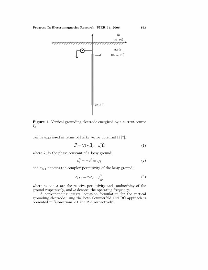
The geomatry of interest is a vertical straight wire of length L andradius a, buried in a lossy medium at depth d shown in Fig. 1. The wireis assumed to be perfectly conducting and the wire dimensions satisfythe well known thin wire approximation [4, 7, 8, 11], so the currentalong the wire is z-directed only.

The starting point in the mathematical model is the assessmentof the current distribution induced along the vertical electrode due toa time-harmonic excitation and for a number of frequencies within afrequency band of interest. This current distribution is goverened bythe Pocklington integro-differential equation. This integro-differentialequation can be derived by expressing the electric field in terms of theHertz vector potential and by satisfying the boundary conditions forthe tangential field components at the electrode surface.

The complete electric field induced in the vicinity of the straightthin wire of finite length buried in an imperfectly conducting half-space

Progress In Electromagnetics Research, PIER 64, 2006 153

air (ε0, µ0)

z=-d-L

z=-d

earth

(ε, µ0, σ )

I

Figure 1. Vertical grounding electrode energized by a current sourceIg.

can be expressed in terms of Hertz vector potential Π [7]:

E = ∇(∇Π) + k21Π (1)

where k1 is the phase constant of a lossy ground:

k21 = −ω2µεeff (2)

and εeff denotes the complex permitivity of the lossy ground:

εeff = εrε0 − jσ

ω(3)

where εr and σ are the relative permitivity and conductivity of theground respectively, and ω denotes the operating frequency.

A corresponding integral equation formulation for the verticalgrounding electrode using the both Sommerfeld and RC approach ispresented in Subsections 2.1 and 2.2, respectively.

154 Poljak and Doric

2.1. Sommerfeld Integral Approach

For the case of vertical grounding electrode energized by a currentsource Ig the vector equation (1) can be written as a set of two scalarequations for the normal x-component and tangential z-component ofthe electric field due to the vertical electrode:

EVx (x, z) =

∂2ΠVz

∂x∂z(4)

EVz (x, z) =

[∂2

∂z2+ k2

1

]ΠV

z (5)

where superscript V denotes the vertical electrode.The vector potential z-component is given by [7]:

ΠVz =

1j4πωµεeff

−d∫−d−L

[gV0 (x, z, z′) − gV

i (x, z, z′) + k22V11

]I(z′)dz′

(6)where I(z′) is the unknown current distribution along the verticalstraight wire, g0(x, z, z′) denotes the free space Green function of theform:

gV0 (x, z, z′) =

e−jkR1vI

R1v(7)

while gi(x, z, z′) arises from the image theory and is given by:

gVi (x, z, z′) =

e−jk2R2v

R2v(8)

where k2 is the phase constant of free space:

k22 = ω2µε0 (9)

and R1v and R2v are the distances from the wire in the ground andfrom its image in the air to the observation point in the lower medium,respectively.

The attenuation effect of the lossy ground is taken into accountby the Sommerfeld integral term V11 [4]:

V11 = 2∞∫0

e−µ1(h−z)

k22µ1 + k2

1µ2J0(λρ)λdλ (10)

where J0(λρ) is zero-order Bessel function of the first kind, while µ1, µ2

and ρ are given by:

µ1 =(λ2 − k2

1

)1/2, µ2 =

(λ2 − k2

2

)1/2, ρ = |z − z′| (11)

Progress In Electromagnetics Research, PIER 64, 2006 155

The Pocklington integro-differential equation for the vertical straightwire buried in a lossy ground can now be obtained by enforcing theboundary conditions for the tangential electric field components on theperfectly conducting (PEC) wire surface. The total tangential electricfield on the PEC wire surface at x = a vanishes, i.e.,

Eexc,Vz (a, z) + Esct,V

z (a, z) = 0 (12)

where Eexc,Vz denotes the excitation function and Esct,V

z is the scatteredfield along the electrode surface.

Combining the relations (5) to (12) leads to the Pocklingtonintegro-differential equation for the vertical grounding electrode:

Eexc,Vz = − 1

j4πωεeff

−d∫−d−L

[∂2

∂z2+ k2

1

]

·[g0(z, z′) − gi(z, z′) + k2

2V11

]I(z′)dz′ (13)

Solving the integral equation (13) the current distribution along theelectrode is obtained.

2.2. Reflection Coefficient Approach

The repeated evaluation of the Sommerfeld integral (10) at severalfrequencies, by which the earth-air attenuation effect is taken intoaccount, is rather difficult and time consuming task [4, 7–12].

Therefore, this work deals with a reflection coefficient (RC)approach which principal advantage versus rigorous Sommerfeldintegral approach is simplicity of the formulation and significantly lesscomputational cost.

For convenience, the integro-differential equation (13) can bewritten in the form:

Eexcz = − 1

j4πωεeff

−d∫−d−L

GV (z, z′)I(z, z′)dz′ (14)

where G(z, z′) is the total Green function given by:

GV (z, z′) =

[∂2

∂z2+ k2

1

] [gV0 (z, z′) − gV

i (z, z′) + k20V11

](15)

156 Poljak and Doric

According to the RC approximation [7] the rigorous Green functionsimplifies into:

GV (z, z′) =

[∂2

∂z2+ k2

1

] [g0(z, z′) + Γgi(z, z′)

]

=

[∂2

∂z2+ k2

1

]gv(z, z′) (16)

where Γ is the corresponding reflection coefficient [6] for the TMpolarization:

Γ =

1n−

√1n

1n

+

√1n

(17)

and n is given by:n =

εeff

ε0(18)

Finallly, the resulting Pocklington integro-differential equation for thevertical straight wire buried in a lossy half-space is given by:

Eexc,Vz = − 1

j4πωεeff

−d∫−d−L

[∂2

∂z2+ k2

1

] [gV0 (z, z′) + ΓgV

i (z, z′)I(z′)dz′]

(19)In this paper, the integro-differntial equation (19) is solved by means ofthe indirect Galerkin-Bubnov scheme of the Boundary Element method(GB-BEM). An outline of the applied numerical method is available inPart II of this work. Solving the integral equation (19) the equivalentcurrent distribution is obtained.

2.3. Imposed Boundary Conditions

In the analysis of the grounding electrodes, the excitation function isnot given in the form of electric field, as the wire is not illuminatedby the plane wave [4]. Thus, the left-hand side of the equation (19)vanishes along the perfectly conducting (PEC) wire surface, i.e.,

Eexcx = 0 (20)

and the integro-differential equation (19) becomes homogeneous.The vertical electrode is energized by the injection of an arbitrary

waveform current pulse produced by an ideal current generator with

Progress In Electromagnetics Research, PIER 64, 2006 157

one terminal connected to the grounding electrode and the other onein the remote soil.

Thus, the excitation is given in the form of the current flowing intothe electrode. This current source is included into the integral equationscheme through the simple boundary condition applied at the top ofthe electrode:

I(−d) = Ig (21)where Ig denotes the actual current generator.

In the frequency domain the unit current generator is alwayschosen, as its time domain counterpart is Dirac impulse.

3. THE EVALUATION OF THE INPUT IMPEDANCESPECTRUM

The calculation of the vertical electrode input impedance is moredemanding than in the antenna case, primarily because the inputterminals are placed between electrode point and remote soil, and thetedious integration on the infinite integral cannot be avoided.

By solving the integral equations (19) the equivalent currentdistribution along the vertical electrode is obtained and the inputimpedance can be computed. It is worth noting that this inputimpedance depends only on the grounding system geometry and onthe electrical properties of the surrounding soil.

The input impedance is simply defined by ratio [4]:

Zin =Vg

Ig(22)

where Vg and Ig are the values of the voltage and the current at thedriving point, respectively.

The feed-point voltage is obtained by integrating the normalelectric field component from the remote soil to the electrode surface,i.e.,

Vg = −a∫

∞

Eds (23)

Thus, the problem of obtaining the input impedance is related to thecalculation of the feed-point volatge. The spectrum of input impedanceis obtained by repeating this procedure in the wide frequency band.

For the given geometry of the vertical electrode integral (23)becomes:

Vg = −a∫

∞EV

x (x, z)dx (24)

158 Poljak and Doric

Since only the Πz component of the Hertz vector potential exists theEz component of the electric field is given by:

EVx (x, z) =

∂2ΠVz

∂x∂z=

1j4πωεeff

−d∫−d−L

I(z′)∂2gV (x, z, z′)

∂x∂zdz′ (25)

Numerical treatment of the expression (25) can be simplified byfeaturing the weak formulation of the problem [7, 9–11]. Namely,utilizing the property of Green functions for the source and imagewire, respectively:

∂gV0 (x, z, z′)∂z

= −∂gV0 (x, z, z′)∂z′

(26)

∂gVi (x, z, z′)∂z

=∂gV

i (x, z, z′)∂z′

(27)

and performing the integration by parts it follows:

EVx (x, z) = − 1

j4πωεeff

d

dx

I(z′)gV (x, z, z′)

∣∣∣∣∣z′=−d

z′=−d−L

−−d∫

−d−L

∂I(z′)∂z′

gV0 (x, z, z′)dz′ +

−d∫−d−L

∂I(z′)∂z′

ΓgVi (x, z, z′)dz′

(28)

Obviously, the mixed second-order differential operator is removedfrom the integral equation kernel GV .

Furthermore, substituting the equation (25) into (24) the followingexpression for the feed point voltage is obtained:

Vg = − 1j4πωεeff

∞∫a

d

dx

I(z′)gV (x, z, z′)

∣∣∣∣∣z′=−d

z′=−d−L

−−d∫

−d−L

∂I(z′)∂z′

gV0 (x, z, z′)dz′ +

−d∫−d−L

∂I(z′)∂z′

gVi (x, z, z′)dz′

dx

(29)

which simply leads to the expression:

Vg =1

j4πωεeff

I(−d)gV (x,−d, z) −

−d∫−d−L

∂I(z′)∂z′

gV0 (x, z, z′)dz′

Progress In Electromagnetics Research, PIER 64, 2006 159

+−d∫

−d−L

∂I(z′)∂z′

gVi (x, z, z′)dz′

∣∣∣∣∣x=∞

x=a

(30)

in which the tedious numerical integration over infinite domain isavoided.

The desired input impedance of the vertical grounding electrodeis finally defined by the relation:

Zin =1

j4πωεeffIg

I(−d)gV (x,−d, z) −

−d∫−d−L

∂I(z′)∂z′

gV0 (x, z, z′)dz′

+−d∫

−d−L

∂I(z′)∂z′

gVi (x, z, z′)dz

∣∣∣∣∣x=∞

x=a

(31)

Calculating this relation in a wide frequency range gives the frequencyspectrum of the input impedance.

4. CALCULATION OF THE TRANSIENT IMPEDANCE

The transient impedance, an essential parameter in grounding systemdesign, is defined as a ratio of time varying voltage and current at thedriving point [4]:

z(t) =v(t)i(t)

(32)

where i(t) represents the excitation function, i.e., the injected currentat a top of the vertical electrode, as shown in Fig. 1.

This injected current represents the lightning channel currentusually expressed by the double exponential function:

i(t) = I0 · (e−αt − e−βt), t ≥ 0 (33)

where pulse rise time is determined by constants α and β, while I0denotes the amplitude of the current waveform.

The Fourier transform of the excitation function is defined byintegral [13]:

I(f) =∞∫

−∞

i(t)e−j2πftdt (34)

160 Poljak and Doric

Integral (34) can be evaluated analytically [11]:

I(f) = I0 ·(

1α+ j2πf

− 1β + j2πf

)(35)

The frequency components up to few MHz are meaningfully presentin the lightning current Fourier spectrum with strong decreasingimportance from very low to highest frequencies.

Multiplying the excitation function I(f) with the input impedancespectrum Zinfj provides the frequency response of the groundingsystem:

V (f) = I(f)Zin(f) (36)Applying the Inverse Fourier Transform (IFT), a time domain voltagecounterpart is obtained. IFT of the function V (f) is defined by theintegral [13]:

v(t) =∞∫

−∞

V (f)ej2πftdω (37)

As the frequency response V (f) is represented by a discrete set of valuesthe integral (37) cannot be evaluated analytically and the DiscreteFourier transform, in this case the Fast Fourier Transform algorithm,is used, i.e.,

v(t) = IFFT(V (f)) (38)Implementation of this algorithm inevitably causes an error dueto discretization and truncation of essentially unlimited frequencyspectrum. The discrete set of the time domain voltage values is definedas [13]:

v(n∆t) = F ·N−1∑k=0

V (k∆f)ejk∆fn∆t (39)

where F is the highest frequency taken into account, N is the totalnumber of frequency samples, ∆f is sampling interval and ∆t is thetime step.

Finally, the transient impedance of the vertical groundingelectrode is computed from relation (32). The transient impedanceshould be recalculated for each excitation function while the inputimpedance spectrum depends only on geometry of the groundingsystem and on characteristics of the surrounding soil.

5. NUMERICAL RESULTS

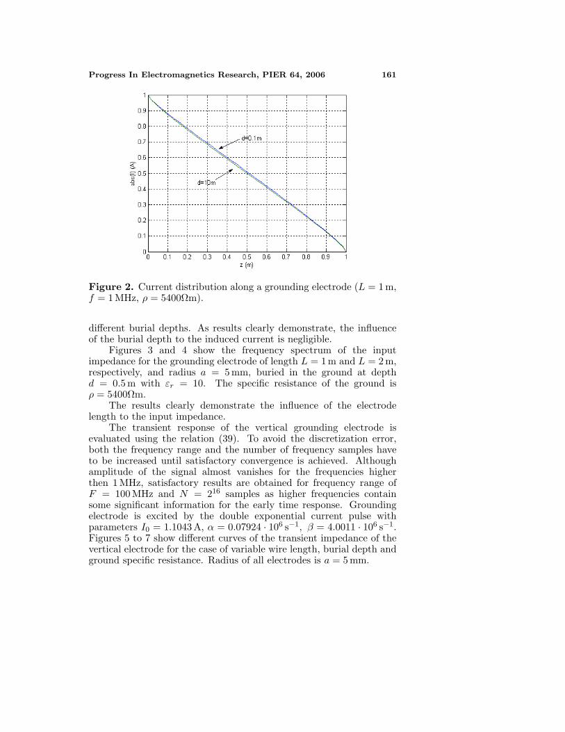
Figure 2 shows the current distribution induced along the groundingvertical electrode of length L = 1 m and radius a = 5 mm for two

Progress In Electromagnetics Research, PIER 64, 2006 161

Figure 2. Current distribution along a grounding electrode (L = 1 m,f = 1 MHz, ρ = 5400Ωm).

different burial depths. As results clearly demonstrate, the influenceof the burial depth to the induced current is negligible.

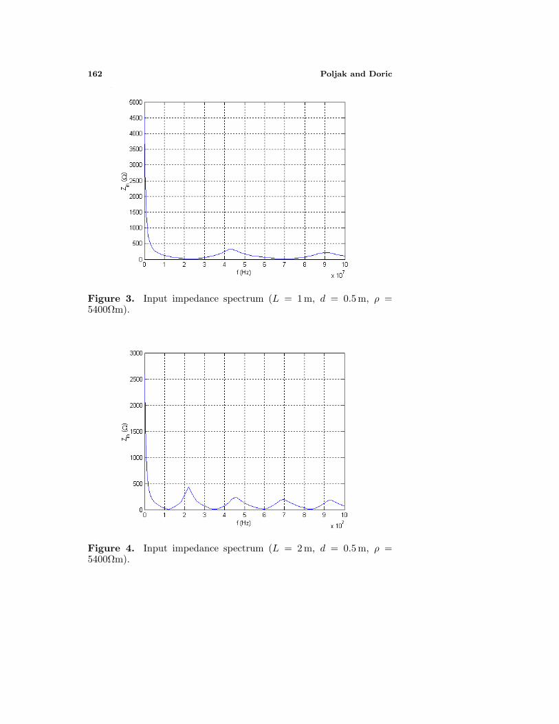
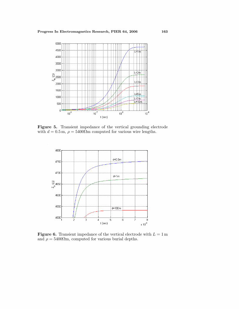
Figures 3 and 4 show the frequency spectrum of the inputimpedance for the grounding electrode of length L = 1 m and L = 2 m,respectively, and radius a = 5 mm, buried in the ground at depthd = 0.5 m with εr = 10. The specific resistance of the ground isρ = 5400Ωm.

The results clearly demonstrate the influence of the electrodelength to the input impedance.

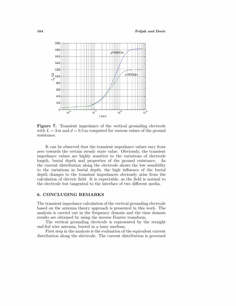
The transient response of the vertical grounding electrode isevaluated using the relation (39). To avoid the discretization error,both the frequency range and the number of frequency samples haveto be increased until satisfactory convergence is achieved. Althoughamplitude of the signal almost vanishes for the frequencies higherthen 1 MHz, satisfactory results are obtained for frequency range ofF = 100 MHz and N = 216 samples as higher frequencies containsome significant information for the early time response. Groundingelectrode is excited by the double exponential current pulse withparameters I0 = 1.1043 A, α = 0.07924 · 106 s−1, β = 4.0011 · 106 s−1.Figures 5 to 7 show different curves of the transient impedance of thevertical electrode for the case of variable wire length, burial depth andground specific resistance. Radius of all electrodes is a = 5 mm.

162 Poljak and Doric

Figure 3. Input impedance spectrum (L = 1 m, d = 0.5 m, ρ =5400Ωm).

Figure 4. Input impedance spectrum (L = 2 m, d = 0.5 m, ρ =5400Ωm).

Progress In Electromagnetics Research, PIER 64, 2006 163

Figure 5. Transient impedance of the vertical grounding electrodewith d = 0.5 m, ρ = 5400Ωm computed for various wire lengths.

Figure 6. Transient impedance of the vertical electrode with L = 1 mand ρ = 5400Ωm, computed for various burial depths.

164 Poljak and Doric

Figure 7. Transient impedance of the vertical grounding electrodewith L = 3 m and d = 0.5 m computed for various values of the groundresistance.

It can be observed that the transient impedance values vary fromzero towards the certain steady state value. Obviously, the transientimpedance values are highly sensitive to the variations of electrodelength, burial depth and properties of the ground resistance. Asthe current distribution along the electrode shows the low sensibilityto the variations in burial depth, the high influence of the burialdepth changes to the transient impedances obviously arise from thecalculation of electric field. It is expectable, as the field is normal tothe electrode but tangential to the interface of two different media.

6. CONCLUDING REMARKS

The transient impedance calculation of the vertical grounding electrodebased on the antenna theory approach is presented in this work. Theanalysis is carried out in the frequency domain and the time domainresults are obtained by using the inverse Fourier transform.

The vertical grounding electrode is represented by the straightend-fed wire antenna, buried in a lossy medium.

First step in the analysis is the evaluation of the equivalent currentdistribution along the electrode. The current distribution is governed

Progress In Electromagnetics Research, PIER 64, 2006 165

by the Pocklington integro-differential equation.The influence of the nearby air-earth interface is taken into

account by the reflection coefficient appearing within the integro-differential equation kernel. The integro-differential equation is solvedby the indirect Galerkin-Bubnov variant of the boundary elementmethod (GB-BEM).

Electric field components at an arbitrary point in the lossymedium can be in principle evaluated directly from the previouslycalculated current distribution. Input impedance is obtained byanalytically integrating the electrical field from the electrode surfaceto the infinity.

The frequency response of the grounding electrode is obtained bymultiplying the analytically evaluated Fourier transform of the currentpulse with the input impedance spectrum.

Finally, the transient impedance of the grounding wire iscomputed using the Inverse Fast Fourier Transform (IFFT). Obtainednumerical results show that the transient impedance of the verticalgrounding electrode is significantly influenced by the variation ofelectrode length, its burial depth and the specific resistance of theground.

This procedure shows some advantages over rigorous approachesbased on Sommerfeld integrals, primarily in simplicity and computa-tional efficiency. The method presented in this work for the case ofvertical grounding electrode is readily applicable to horizontal elec-trodes and complex grounding systems consisting of interconnectedconductors.

An extension of the reflection coefficient approach to the analysisof the horizontal grounding electrode is presented in Part II of thiswork.

REFERENCES

1. Velazquez, R. and D. Muhkedo, “Analytical modeling ofgrounding electrodes transient behaviour,” IEEE Trans. PowerAppar. Systems, Vol. PAS-103, 1314–1322, June 1984.

2. Liu, Y., M. Zitnik, and R. Thottappillil, “An improvedtransmission line model of grounding system,” IEEE Trans. EMC,Vol. 43, No. 3, 348–355, 2001.

3. Ala, G. and M. L. Di Silvestre, “A simulation model forelectromagnetic transients in lightning protection systems,” IEEETrans. EMC, Vol. 44, No. 4, 539–534, 2003.

4. Grcev, L. and F. Dawalibi, “An electromagnetic model for

166 Poljak and Doric

transients in grounding systems,” IEEE Trans. Power Delivery,No. 4, 1773–1781, Oct. 1990.

5. Grcev, L. D. and F. E. Menter, “Transient electro-magnetic fieldsnear large earthing systems,” IEEE Trans. Magnetics, Vol. 32,1525–1528, May 1996.

6. Bridges, G. E., “Transient plane wave coupling to bare andinsulated cables buried in a lossy half-space,” IEEE Trans. EMC,Vol. 37, No. 1, 62–70, Feb. 1995.

7. Poljak, D. and V. Roje, “The integral equation method for groundwire impedance,” Integral Methods in Science and Engineering,C. Constanda, J. Saranen, and S. Seikkala (eds.), Vol. I, 139–143,Longman, UK, 1997.

8. Olsen, R. G. and M.C. Willis, “A comparison of exact andquasi-static methods for evaluating grounding systems at highfrequencies,” IEEE Trans. Power Delivery, Vol. 11, No. 2, 1071–1081, April 1996.

9. Poljak, D., I. Gizdic, and V. Roje, “Plane wave coupling tofinite length cables buried in a lossy ground,” Eng. Analysis withBoundary Elements, Vol. 26, No. 1, 803–806, Jan. 2002.

10. Poljak, D. and V. Roje, “Boundary element approach tocalculation of wire antenna parameters in the presence ofdissipative half-space,” IEE Proc. Microw. Antennas Propag.,Vol. 142, No. 6, 435–440, Dec. 1995.

11. Poljak, D., Electromagnetic Modelling of Wire Antenna Struc-tures, WIT Press, Southampton, Boston, 2002.

12. Burke, G. J. and E. K. Miller, “Modeling antennas near to andpenetrating a lossy interface,” IEEE Trans. AP, Vol. 32, 1040–1049, 1984.

13. Ziemer, R. E. and W. H. Tranter, Principles of Communications,Houghton Mifflin Company, Boston, 1995.