A Model of Bridge Choice Across the Mississippi River1

in Minneapolis2

Carlos Carrion∗ David Levinson †3

May 15, 20114

Abstract5

On September 18th 2008, a replacement for the previously collapsed I-35W bridge opened6

to the public. Consequently, travelers were once again confronted with the opportunity to find7

better alternatives. The traffic pattern of the Minneapolis road network was likely to read-8

just, because of the new link addition. However, questions arise about the possible reasons (or9

components in the route choice process) that are likely to influence travelers crossing the Mis-10

sissippi, who had to choose among several bridge options, including the new I-35W bridge. A11

statistical model of bridge choice is specified and estimated employing weighted-least squares12

logit, and using Global Positioning System (GPS) data and web-based surveys collected both13

before and after the replacement bridge opened. In this way the proportion of I-35W trips can14

be estimated depending on the assigned values of the explanatory variables, which include:15

statistical measures of the travel time distribution experienced by the subjects, alternative di-16

versity, and others. The results showed that travel time savings and reliability were the main17

reasons for choosing the new I-35W bridge.18

Keywords: GPS, route choice, I-35W bridge, wls logit.19

∗Graduate Student, University of Minnesota, Department of Civil Engineering, carri149@umn.edu†RP Braun-CTS Chair of Transportation Engineering; Director of Network, Economics, and Urban Systems Re-

search Group; University of Minnesota, Department of Civil Engineering, 500 Pillsbury Drive SE, Minneapolis, MN55455 USA, dlevinson@umn.edu, http://nexus.umn.edu

1

1 Introduction1

In principle, travelers (if necessary) adapt to network changes (e.g. link closures, link additions)2

depending on their current acquired spatial information.Travelers’ responses may vary according3

to the temporal duration and spatial occupancy of network changes. For example, closure of a4

residential neighborhood street may not require travel behavior adjustments for most travelers, in5

contrast to the closure of a major highway section. Furthermore, potential travelers’ responses6

include:7

1. switching routes;8

2. canceling trips;9

3. rescheduling activities;10

4. using other travel modes;11

5. finding alternative location of activities; and others.12

Research on travelers’ behavioral responses to network changes due to large-scale disruption13

has been limited, and consequently not many studies exist because of their unusual nature (Giuliano14

and Golob, 1998). Typically, network disruptions can be divided in two categories: planned and15

unplanned. The former are generally due to road construction or maintenance work (e.g. 199916

closure of the Centre Street Bridge in Calgary (Hunt and Stefan, 2002)), transit strikes (e.g. 198117

and 1986 strikes in Orange County (Ferguson, 1992); 2003 strike in Los Angeles (Lo and Hall,18

2006); see van Exel and Rietveld (2001) for a review), major events (e.g. 2000 Olympic Games19

in Sydney (Hensher and Brewer, 2002); 2004 Olympic Games in Athens (Dimitriou et al., 2006)),20

and others. In contrast, the latter are usually attributed to natural disasters (e.g. 1989 Loma Prieta21

Earthquake (Tsuchida and Wilshusen, 1991); 1994 Northridge Earthquake (Wesemann et al. (1996)22

and Giuliano and Golob (1998)); 1995 Kobe Earthquake (Chang and Nojima, 2001)), structural23

failures (e.g. 2007 I-35W Bridge collapse in Minneapolis (Zhu et al., 2010)), and other severe24

non-recurrent events. Furthermore, this study focuses on the events after a network’s major link25

is removed suddenly, and later on restored. These events are the collapse of the I-35W Bridge on26

August 1st 2007 in Minneapolis, and the reopening of the new I-35W Bridge on September 18th27

2008. In the first case, travelers were forced to respond by exploring the network, and by adjusting28

their travel behavior according to their experience and other external information sources. In the29

second case, travelers were given another opportunity to explore new routes, and to decide if there30

are any benefits in switching to other alternatives. Consequently, the period of interest for this study31

is after the new I-35W bridge is open to the public, and the alternatives of interest are the bridges32

located along the Mississippi river near the city of Minneapolis.33

It is clear that the study of travel behavior during unforeseen disruptions is the main theme in34

this article. Therefore, a bridge choice model is built based on data collection efforts conducted35

during the period between August and December of 2008. These efforts included the collection36

of Global Positioning System (GPS) tracking data, and web-based surveys. In addition, the travel37

behavior process is studied from a bridge selection reference frame; this allows for studying solely38

the swapping behavior of travelers (i.e. choosing I-35W Bridge vs. Other alternatives) and the39

possible significant explanatory factors behind them (e.g. travel time). A review of the effects40

2

of the I-35W collapse can be found in Zhu et al. (2010). This study is organized as follows:1

A data section presents the data collection techniques, the analysis methodology employed, and2

descriptive statistics of the sample; the bridge choice model and its results are discussed in the3

subsequent section; and the last section concludes the article.4

2 Data5

2.1 Recruitment6

Subjects were recruited through announcements posted in different media including: Craigslist.org,7

and CityPages.com; the free local weekly newspaper City Pages; flyers at grocery stores; flyers8

at city libraries, postcards handed out in downtown parking ramps; flyers placed in downtown9

parking ramps; and emails to more than 7000 University of Minnesota staff (students and faculty10

were excluded). More than 900 subjects responded, and consequently they were randomly selected11

among those who satisfied the following requirements for their participation:12

1. Age between 25-65,13

2. Legal driver,14

3. Full-time job and follow a “regular” work schedule15

4. Travel by driving alone16

5. Likelihood of being affected by the reopening of the new I-35W Mississippi River bridge.17

The possible list of potential subjects was provided to Dr. Randall Guensler at the Georgia18

Institute of Technology and the subcontractor Vehicle Monitoring Technologies (VMTINC), who19

managed this field data collection effort. Also, a local subcontractor (MachONE) was employed20

to instrument the subjects’ vehicles with GPS devices two weeks before the new I-35W bridge re-21

opened. These GPS devices recorded the coordinates of the instrumented vehicle at every second22

between engine-on and engine-off events. The coordinates log collected by the GPS was transmit-23

ted to the server in real time through wireless communication. The subjects remained instrumented24

for 13 weeks without following any instructions with the exception of filling periodic surveys.25

In parallel, the authors and others affiliated with the University of Minnesota conducted an-26

other GPS-based data collection effort. Other potential subjects (randomly selected from the orig-27

inal pool) were instrumented with logging-type GPS devices (QSTARZ BT-Q1000p GPS Travel28

Recorder powered by DC output from in-vehicle cigarette lighter) also approximately two weeks29

before the replacement I-35W bridge opened to the public. These GPS devices recorded the posi-30

tion of the instrumented vehicle at a frequency of 25 meters per location point registered between31

engine-on and engine-off events. These subjects remained instrumented for 8 weeks, during this32

time period the subjects followed their usual commute pattern without any instruction from the33

researchers. In addition, at the end of the study period (i.e. 8 weeks or 13 weeks depending on the34

GPS study), subjects completed a comprehensive final web-based survey to evaluate the driving35

experience on routes using different bridges choices, provide socio-demographic information (see36

Section 3.1), and also answer some questions regarding route preferences.37

3

A total of approximately 143 (about 46 by VMTINC, and 97 by University of Minnesota)1

subjects had usable (complete day-to-day GPS information) data required for this analysis. For this2

study, only 46 subjects (25 from VMTINC, and 21 from University of Minnesota) had the required3

data according to the subsequent Section 2.2.4

2.2 Methodology5

The GPS data analysis process can be divided in three phases:6

1. Identification of commute trips per subject on the bridges of interest (see Figure 1);7

2. Information extraction (e.g. travel time) of commute trips per subject;8

3. Specification and estimation of a statistical model to determine the reasons for a subject to9

prefer the new I-35W bridge over other plausible alternatives.10

The first phase utilizes the coordinates of the trips per subject, and the TLG (defined in the sub-11

sequent paragraph) network in order to identify the trips crossing bridges, and the bridges crossed.12

This identification is done by spatial matching the coordinates of each bridge of interest to the co-13

ordinates of each set of trips for each subject. Also, subjects’ trips must start at their home/work14

and end at their work/home locations in order to be considered commute trips (or more precisely15

direct commute trips as in trips without chaining behavior). The distance tolerance between ori-16

gins (destinations) to home (work) locations was set to 600 m. The home and work locations are17

geocoded (transformed into point coordinates) from the actual addresses provided by the subjects18

on the web-based surveys. The origin and destination pair of each trip is obtained by mapping the19

coordinate points into trajectories of engine-on and engine-off events. Moreover, inaccurate points20

due to GPS “noise”, and out-of-town trips (e.g. during Thanksgiving) were excluded.21

The TLG network refers to a digital map maintained by the Metropolitan Council and The22

Lawrence Group (TLG). It covers the entire 7-county Twin Cities Metropolitan Area and is the23

most accurate GIS map of this network to date. The TLG network contains 290,231 links, and24

provides an accurate depiction of the entire Twin Cities network at the street level.25

The second phase extracts usable information from the identified trips including: statistics of26

travel time distribution of all trips (both average and standard deviation) for each subject; total27

number of trips observed for each subject; and the frequency of routes (i.e. bridges) used by each28

subject. This process is performed for each time period of travel (e.g. AM) , and for the period of29

interest (between September 18th and October 12th) . On September 18th, the new I-35W Bridge30

opened to the public at 5 AM. On October 12th, the I-94 lanes were re-stripped, and consequently31

eliminating a traffic restoration measure implemented by MnDOT to ameliorate the bride collapse32

effects.33

The third phase consists of fitting a statistical model to the data tabulated from the previous34

phases. The objective is to understand the factors behind the decision of commuters on whether35

to choose the new I-35W Bridge over other alternatives. This phase is described thoroughly in36

Section 4.37

4

3 Descriptive Statistics1

3.1 Socio-Demographics2

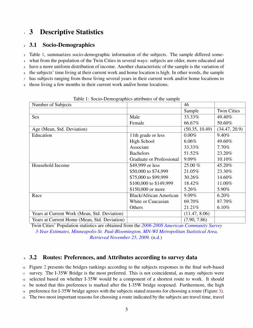
Table 1, summarizes socio-demographic information of the subjects. The sample differed some-3

what from the population of the Twin Cities in several ways: subjects are older, more educated and4

have a more uniform distribution of income. Another characteristic of the sample is the variation of5

the subjects’ time living at their current work and home location is high. In other words, the sample6

has subjects ranging from those living several years in their current work and/or home locations to7

those living a few months in their current work and/or home locations.8

Table 1: Socio-Demographics attributes of the sampleNumber of Subjects 46

Sample Twin CitiesSex Male 33.33% 49.40%

Female 66.67% 50.60%Age (Mean, Std. Deviation) (50.35, 10.49) (34.47, 20.9)Education 11th grade or less 0.00% 9.40%

High School 6.06% 49.60%Associate 33.33% 7.70%Bachelors 51.52% 23.20%Graduate or Professional 9.09% 10.10%

Household Income $49,999 or less 25.00 % 45.20%$50,000 to $74,999 21.05% 23.30%$75,000 to $99,999 30.26% 14.60%$100,000 to $149,999 18.42% 11.00%$150,000 or more 5.26% 5.90%

Race Black/African American 9.09% 6.20%White or Caucasian 69.70% 87.70%Others 21.21% 6.10%

Years at Current Work (Mean, Std. Deviation) (11.47, 8.06)Years at Current Home (Mean, Std. Deviation) (7.90, 7.86)Twin Cities’ Population statistics are obtained from the 2006-2008 American Community Survey

3-Year Estimates, Minneapolis-St. Paul-Bloomington, MN-WI Metropolitan Statistical Area,Retrieved November 25, 2009. (n.d.)

3.2 Routes: Preferences, and Attributes according to survey data9

Figure 2 presents the bridges rankings according to the subjects responses in the final web-based10

survey. The I-35W Bridge is the most preferred. This is not coincidental, as many subjects were11

selected based on whether I-35W would be a component of a shortest route to work. It should12

be noted that this preference is marked after the I-35W bridge reopened. Furthermore, the high13

preference for I-35W bridge agrees with the subjects stated reasons for choosing a route (Figure 3).14

The two most important reasons for choosing a route indicated by the subjects are travel time, travel15

5

time predictability, travel distance and other reasons unique to the subjects. The travel distance is1

an interesting reason as subjects are likely to drive to the bridges closer to their home and work2

location. Bridges that are farther might not attract subjects.3

3.3 Route Changing Behavior according to survey data4

In Tables 2 and 3, the subjects stated that they were prone to try alternative routes, and/or to5

change routes (if justified) after the I-35W Bridge reopened. The most cited (41%) reason the6

subject’s indicated for changing routes is that plausible alternatives have shorter travel times. In7

contrast, 45% of subjects who did not change routes considered that the alternatives were not better.8

This change of routes probably was required as many subjects did not reduce the number of river9

crossings according to Table 4, and thus alternatives to I-35W had to be found. In addition, it10

should be noted that subjects are asked whether they tried alternative routes irrespective to them11

changing routes, and vice versa.12

Table 2: Route changed after I-35W Bridge ReopenNumber of Subjects 46Usual route changed after I35W Bridge Reopening Yes 62.60%

No 37.50%Reasons for changing route Old route is more congested now. 9.09%

New route has a shorter travel distance. 9.09%New route has a shorter travel time. 40.91%The travel time of new route is more reliable 31.82%(predictable)Other 9.09%

Table 3: Alternative routes after I-35W Bridge ReopenNumber of Subjects 46Tried Alternative Routes other than usual routes Yes 63.64%after I35W Bridge Reopened No 36.36%Reasons for not changing route No alternative for my route to work. 20.00%

Apathetic about looking for alternatives. 0.00%The alternative routes are not likely to be better 45.00%off.The time and effort of trying alternatives 25.00%outweighs possible time savings.Other 10.00%

6

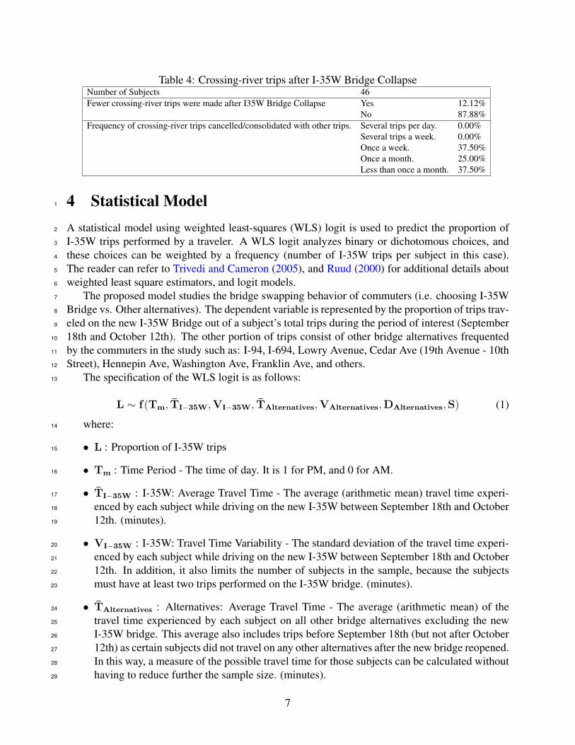
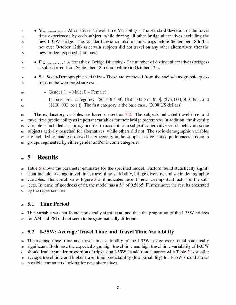
Table 4: Crossing-river trips after I-35W Bridge CollapseNumber of Subjects 46Fewer crossing-river trips were made after I35W Bridge Collapse Yes 12.12%

No 87.88%Frequency of crossing-river trips cancelled/consolidated with other trips. Several trips per day. 0.00%

Several trips a week. 0.00%Once a week. 37.50%Once a month. 25.00%Less than once a month. 37.50%

4 Statistical Model1

A statistical model using weighted least-squares (WLS) logit is used to predict the proportion of2

I-35W trips performed by a traveler. A WLS logit analyzes binary or dichotomous choices, and3

these choices can be weighted by a frequency (number of I-35W trips per subject in this case).4

The reader can refer to Trivedi and Cameron (2005), and Ruud (2000) for additional details about5

weighted least square estimators, and logit models.6

The proposed model studies the bridge swapping behavior of commuters (i.e. choosing I-35W7

Bridge vs. Other alternatives). The dependent variable is represented by the proportion of trips trav-8

eled on the new I-35W Bridge out of a subject’s total trips during the period of interest (September9

18th and October 12th). The other portion of trips consist of other bridge alternatives frequented10

by the commuters in the study such as: I-94, I-694, Lowry Avenue, Cedar Ave (19th Avenue - 10th11

Street), Hennepin Ave, Washington Ave, Franklin Ave, and others.12

The specification of the WLS logit is as follows:13

L ∼ f(Tm, T̄I−35W, VI−35W, T̄Alternatives, VAlternatives, DAlternatives, S) (1)

where:14

• L : Proportion of I-35W trips15

• Tm : Time Period - The time of day. It is 1 for PM, and 0 for AM.16

• T̄I−35W : I-35W: Average Travel Time - The average (arithmetic mean) travel time experi-17

enced by each subject while driving on the new I-35W between September 18th and October18

12th. (minutes).19

• VI−35W : I-35W: Travel Time Variability - The standard deviation of the travel time experi-20

enced by each subject while driving on the new I-35W between September 18th and October21

12th. In addition, it also limits the number of subjects in the sample, because the subjects22

must have at least two trips performed on the I-35W bridge. (minutes).23

• T̄Alternatives : Alternatives: Average Travel Time - The average (arithmetic mean) of the24

travel time experienced by each subject on all other bridge alternatives excluding the new25

I-35W bridge. This average also includes trips before September 18th (but not after October26

12th) as certain subjects did not travel on any other alternatives after the new bridge reopened.27

In this way, a measure of the possible travel time for those subjects can be calculated without28

having to reduce further the sample size. (minutes).29

7

• VAlternatives : Alternatives: Travel Time Variability - The standard deviation of the travel1

time experienced by each subject, while driving all other bridge alternatives excluding the2

new I-35W bridge. This standard deviation also includes trips before September 18th (but3

not over October 12th) as certain subjects did not travel on any other alternatives after the4

new bridge reopened. (minutes).5

• DAlternatives : Alternatives: Bridge Diversity - The number of distinct alternatives (bridges)6

a subject used from September 18th (and before) to October 12th.7

• S : Socio-Demographic variables - These are extracted from the socio-demographic ques-8

tions in the web-based surveys.9

– Gender (1 = Male; 0 = Female).10

– Income. Four categories: ($0, $49, 999], ($50, 000, $74, 999], ($75, 000, $99, 999], and11

($100, 000,∞+)]. The first category is the base case. (2008 US dollars).12

The explanatory variables are based on section 3.2. The subjects indicated travel time, and13

travel time predictability as important variables for their bridge preference. In addition, the diversity14

variable is included as a proxy in order to account for a subject’s alternative search behavior; some15

subjects actively searched for alternatives, while others did not. The socio-demographic variables16

are included to handle observed heterogeneity in the sample; bridge choice preferences unique to17

groups segmented by either gender and/or income categories.18

5 Results19

Table 5 shows the parameter estimates for the specified model. Factors found statistically signif-20

icant include: average travel time, travel time variability, bridge diversity, and socio-demographic21

variables. This corroborates Figure 3 as it indicates travel time as an important factor for the sub-22

jects. In terms of goodness of fit, the model has a R2 of 0.5865. Furthermore, the results presented23

by the regressors are:24

5.1 Time Period25

This variable was not found statistically significant, and thus the proportion of the I-35W bridges26

for AM and PM did not seem to be systematically different.27

5.2 I-35W: Average Travel Time and Travel Time Variability28

The average travel time and travel time variability of the I-35W bridge were found statistically29

significant. Both have the expected sign; high travel time and high travel time variability of I-35W30

should lead to smaller proportion of trips using I-35W. In addition, it agrees with Table 2 as smaller31

average travel time and higher travel time predictability (low variability) for I-35W should attract32

possible commuters looking for new alternatives.33

8

5.3 Alternatives: Average Travel Time and Travel Time Variability1

The average travel time and travel time variability of the alternative bridges (excluding I-35W) were2

found statistically significant. Both have the expected sign; high travel time and high travel time3

variability of alternatives to I-35W should lead to higher proportion of trips using I-35W. However,4

the travel time variability was less significant than its I-35W counterpart. This is perhaps product5

of the aggregations of different bridge alternatives.6

5.4 Alternatives: Bridge Diversity7

This variable was found statistically significant. It indicates that the more distinct alternatives a8

subject experience, the lower will be the subject’s proportion of trips on the I-35W bridge. A9

possible reason for this result is that travelers may still be in the process of searching for their best10

alternative (I-35W or other) according to their own criteria.11

5.5 Socio-Demographic variables12

Neither of the specified socio-demographic variables were found statistically significant. The13

choice situation tended to be dominated by the measures of the travel time distributions.14

Finally, other factors not included as pointed by the subjects in Table 3 may influence their15

preferred bridge choice, even if travel time benefits are present.16

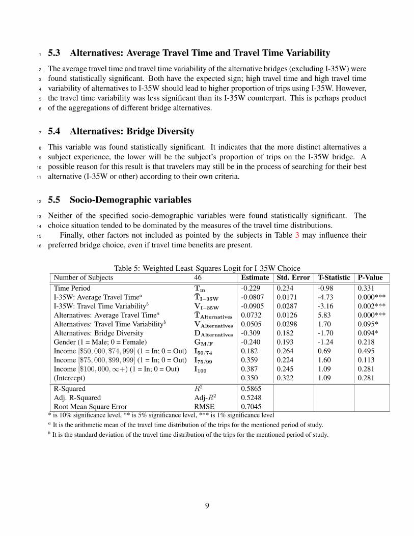
Table 5: Weighted Least-Squares Logit for I-35W ChoiceNumber of Subjects 46 Estimate Std. Error T-Statistic P-ValueTime Period Tm -0.229 0.234 -0.98 0.331I-35W: Average Travel Timea T̄I−35W -0.0807 0.0171 -4.73 0.000***I-35W: Travel Time Variabilityb VI−35W -0.0905 0.0287 -3.16 0.002***Alternatives: Average Travel Timea T̄Alternatives 0.0732 0.0126 5.83 0.000***Alternatives: Travel Time Variabilityb VAlternatives 0.0505 0.0298 1.70 0.095*Alternatives: Bridge Diversity DAlternatives -0.309 0.182 -1.70 0.094*Gender (1 = Male; 0 = Female) GM/F -0.240 0.193 -1.24 0.218Income [$50, 000, $74, 999] (1 = In; 0 = Out) I50/74 0.182 0.264 0.69 0.495Income [$75, 000, $99, 999] (1 = In; 0 = Out) I75/99 0.359 0.224 1.60 0.113Income [$100, 000,∞+) (1 = In; 0 = Out) I100 0.387 0.245 1.09 0.281(Intercept) 0.350 0.322 1.09 0.281R-Squared R2 0.5865Adj. R-Squared Adj-R2 0.5248Root Mean Square Error RMSE 0.7045

* is 10% significance level, ** is 5% significance level, *** is 1% significance levela It is the arithmetic mean of the travel time distribution of the trips for the mentioned period of study.b It is the standard deviation of the travel time distribution of the trips for the mentioned period of study.

9

6 Discussion and Limitations1

In summary, the main results (see section 5) of the model indicate that the average travel time, and2

the travel time variability are the key factors for bridge choice preference across subjects. These3

results should be understood from an aggregate level. The measures of centrality (average) and4

dispersion (standard deviation) of the travel time distributions for the I-35W bridge (i.e. all trips5

within the time period as defined in section 4) per subject, and the alternatives bridges (i.e. all6

trips within the time period as defined in section 4) per subject are significantly different per sub-7

ject (that is to say that each subject is a record in the dataset). This difference could be that some8

subjects for the whole travel time distribution (across the trips for the whole period) may have9

experienced on average higher travel time for I-35W in comparison to their plausible alternatives,10

or vice versa. Moreover, it means that it is assumed subjects at the aggregate level “settled” for a11

particular bridge choice. However, this has the side effect of neglecting that subjects are actually12

updating their decision most likely at a day to day level. In other words, subjects may have found13

better (worse) alternatives as soon as possible (early or late during the time period), and proceeded14

to change (stay) at their current choice. Therefore, the number of trips for either I-35W or the15

plausible alternatives may exhibit an state dependency effect (previous choices influence future16

choices; experience factor). Furthermore, this adaptation process (selecting choices from previous17

experience) is likely to happen regardless of whether a network disruption occurred, but a disrup-18

tion (depending on its temporal duration and its spatial occupancy) in principle will generate the19

traffic conditions (e.g. aggravate the differences across the choices’ travel times) that will motivate20

travelers to change and/or try new alternatives.21

Another important aspect is the searching behavior of the subjects (implied in the previous22

paragraph). The alternatives diversity variable was included to distinguish between subjects that23

tried alternative bridges vs. subjects that did not try any alternative bridges. Therefore, the variable24

acts as a “proxy” for search behavior. However, it is obvious that subjects with bridge diversity25

higher than zero will have less trips for the I-35W choice. This is because only direct commute26

trips are considered, and thus on regular working schedules (as those required for this study) the27

number of commute trips is likely to not change (2 commute trips per day) significantly from day28

to day. Therefore, the diversity variable has the correct sign and effect (higher values should reduce29

the number of I-35W trips), but it does not capture the feedback behavior (i.e. willingness and30

inertia to search for alternatives; see Table 3) of the subjects.31

Furthermore, the model benefits from the GPS data due to its detailed commute level informa-32

tion, despite that fact that the final sample’s characteristics differs from the Twin Cities’ character-33

istics. Thus, this limits the level of applicability of the model at the metropolitan level. In addition,34

other socio-demographic variables (e.g. household size) may indicate heterogeneity in the sample,35

despite the fact that such heterogeneity was not found at statistically significant levels.36

Finally, readers should be reminded of the exploratory nature of the study, and in this regard37

the model does identify the important factors of the bridge choice process, despite not taking into38

account state dependency (experience factor), search behavior, and other factors explicitly.39

10

7 Conclusion1

Network disruptions force travelers to adapt by changing to other modes, finding alternative routes,2

canceling/consolidating trips, rescheduling trips, and in severe cases look for new residential and/or3

work locations. However, questions arise about the effects after the disruption, and also about the4

influences of traffic restorations done by DOTs to the traffic patterns in the network. In the case5

of the I-35W Bridge collapse, MnDOT performed two major changes to the network: the opening6

of a new I-35W bridge, and the re-stripping of I-94 in order to have additional lanes. In this7

study, an exploratory analysis was performed focusing solely on the factors behind the travelers8

selection of the new I-35W bridge over their previously available alternatives after its collapse. A9

proposed model following (WLS logit) was formulated to identify the magnitude and direction of10

the contributions of elements such as travel time in the bridge choice process during this transition11

period.12

According to the survey data (Tables 2 and 3), subjects with at least two trips on the new I-35W13

bridge (the selected sample size) stated a high willingness to try new alternatives, and indicated that14

their usual route changed. Furthermore, travel time and travel time predictability (low variability)15

were selected as the main reasons for trading routes. This result also agreed with the bridge choice16

model fitted to the GPS data of the same subjects surveyed. Therefore, travel time savings and17

reliability were the key components regardless of their socio-demographic differences in explaining18

their swapping behavior (I-35W vs. Other alternatives). However, resistance (e.g. route constraints,19

high search costs) to choose the new I-35W bridge or other alternatives was also present as stated20

by the subjects.21

Future research is required as very few studies have extensively covered major disruptions,22

because naturally they are hard to predict, and thus data is not collected. In this case, the GPS23

data acquired is an invaluable scientific resource that allows further exploration with distinct model24

formulations. A possible path for new research is the development of models accounting for the25

experience factor (state dependency). This could be analyzed by considering the duration of mem-26

ory of travel times - how far back in time (1 week, 2 weeks, 3 weeks) travelers remember average27

travel times for a specific route they followed. This experiential model could be helpful, because it28

might identify the beginning of the bridge (or route) changing process.29

8 Acknowledgements30

This study is supported by the Oregon Transportation Research and Education Consortium (2008-31

130 Value of Reliability and 2009-248 Value of Reliability Phase II) and the Minnesota DOT project32

“Traffic Flow and Road User Impacts of the Collapse of the I-35W Bridge over the Mississippi33

River”. We would also like to thank Kathleen Harder, John Bloomfield, and Shanjiang Zhu.34

11

References1

2006-2008 American Community Survey 3-Year Estimates, Minneapolis-St. Paul-Bloomington,2

MN-WI Metropolitan Statistical Area, Retrieved November 25, 2009. (n.d.).3

URL: http://factfinder.census.gov/4

Chang, S. and Nojima, N. (2001), “Measuring post-disaster transportation system performance: the5

1995 kobe earthquake in comparative perspective”, Transportation Research Part A , Vol. 35,6

pp. 475–494.7

Dimitriou, D., Karlaftis, M., Kepaptsoglou, K. and Stathopoulos, M. (2006), Public transportation8

during the athens 2004 olympics: From planning to performance., in ‘Proceedings of the 85th9

Transportation Research Board Annual Meeting, Washington D.C., U.S.A.’.10

Ferguson, E. (1992), “Transit ridership, incident effects and public policy”, Transportation Re-11

search Part A , Vol. 26, pp. 393–407.12

Giuliano, G. and Golob, J. (1998), “Impacts of the northridge earthquake on transit and highway13

use”, Journal of Transportation and Statistics , Vol. 1, pp. 1–20.14

Hensher, D. and Brewer, A. (2002), “Going for gold at the sydney olympics: how did transport15

perform?”, Transport Reviews , Vol. 22, pp. 381–399.16

Hunt, J., B. A. and Stefan, K. (2002), “Responses to centre street bridge closure: Where the disap-17

pearing travelers went”, Transportation Research Record , Vol. 1807, pp. 51–58.18

Lo, S. and Hall, R. (2006), “Effects of the los angeles transit strike on highway congestion”, Trans-19

portation Research Part A , Vol. 40, pp. 903–917.20

Ruud, P. (2000), An introduction to classical econometric theory, Oxford University Press.21

Trivedi, P. K. and Cameron, A. C. (2005), Microeconometrics: Methods and Applications, Cam-22

bridge Univ. Press.23

Tsuchida, P. and Wilshusen, L. (1991), “Effects of the 1989 loma prieta earthquake on commute24

behavior in santa cruz county, california”, Transportation Research Board. , Vol. 1321, pp. 26–25

33.26

van Exel, N. and Rietveld, P. (2001), “Public transport strikes and traveller behaviour”, Transport27

Policy , Vol. 8, pp. 237–246.28

Wesemann, L., Hamilton, T., Tabaie, S. and Bare, G. (1996), “Cost-of-delay studies for freeway29

closures caused by northridge earthquake”, Transportation Research Record , Vol. 1559, pp. 67–30

75.31

Zhu, S., Levinson, D., Liu, H. and Harder, K. (2010), “The traffic and behavioral effects of the32

i-35w mississippi river bridge collapse”, Transportation Research part A , Vol. 44, pp. 771–784.33

12

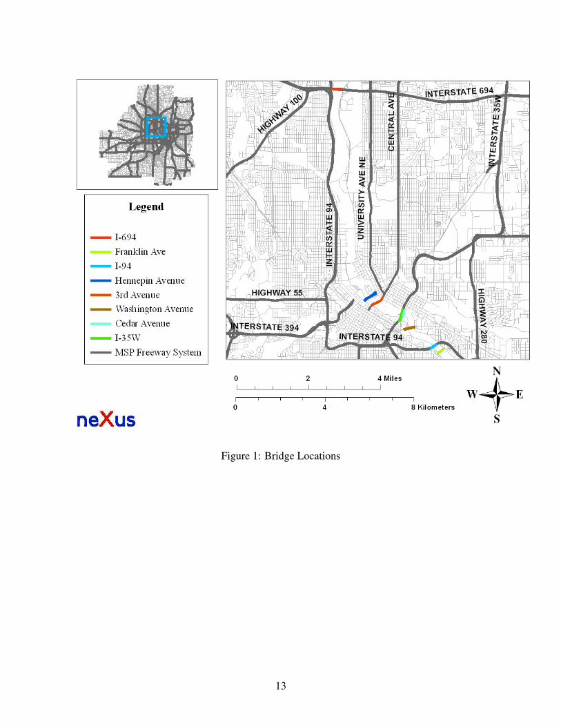
Figure 1: Bridge Locations

13

Figure 2: Routes Preference Top 3 Rank

14

Figure 3: Reason behind route preferences Top 3 Rank

15