weaving an ambiguous lexicon - isabelle dautriche
TRANSCRIPT
UNIVERSITÉ PARIS DESCARTES
École doctorale Frontière du Vivant (ED 474)
Laboratoire de Sciences Cognitives et PsycholinguistiqueDépartement d’Études Cognitives
École Normale Supérieure
Weaving an ambiguous lexicon
Par Isabelle DAUTRICHE
Thèse de doctorat de Sciences cognitives
Dirigée par Anne CHRISTOPHEand
co-encadrée par Benoît CRABBÉ
Présentée et soutenue publiquement le 18 septembre 2015
Devant un jury composé de :
Anne CHRISTOPHE [directeur] - Directrice de Recherche, CNRS, École Normale SupérieureBenoit CRABBÉ [co-encadrant] - Maître de Conférences, Université Paris DiderotPadraic MONAGHAN [rapporteur] - Professeur, University of LancasterJohn TRUESWELL [rapporteur] - Professeur, University of PennsylvaniaFrançois PELLEGRINO [examinateur] - Directeur de Recherche, CNRS, Université de Lyon 2Kim PLUNKETT [examinateur] - Professeur, University of Oxford

Abstract
Modern cognitive science of language concerns itself with (at least) two fundamental ques-tions: how do humans learn language? —the learning problem —and why do the world’slanguages exhibit some properties and not others? —the typology problem. Though therelation between language acquisition and typology is not necessarily one of equivalence,there are many points of contacts between these two domains. On the one hand, childrenwork on language through an extended period of time and their progression could plau-sibly reveal aspects of the cognitive blueprint for language. On the other hand, payingattention to the structural commonalities of languages can clue us in to what the humanlearning mechanism producing these preferences must look like. These questions, althoughcomplementary, represent different approaches of understanding the features of cognitionunderlying the language faculty and have often been dealt with separately by differentresearch communities.
In this dissertation, I attempt to link these two questions by looking at the lexicon, theset of word-forms and their associated meanings, and ask why do lexicons look the waythey are? And can the properties exhibited by the lexicon be (in part) explained by theway children learn their language? One striking observation is that the set of words in agiven language is highly ambiguous and confusable. Words may have multiple senses (e.g.,homonymy, polysemy) and are represented by an arrangement of a finite set of soundsthat potentially increase their confusability (e.g., minimal pairs). Lexicons bearing suchproperties present a problem for children learning their language who seem to have difficultylearning similar sounding words and resist learning words having multiple meanings. Usinglexical models and experimental methods in toddlers and adults, I present quantitativeevidence that lexicons are, indeed, more confusable than what would be expected by chancealone (Chapter 2). I then present empirical evidence suggesting that toddlers have thetools to bypass these problems given that ambiguous or confusable words are constrainedto appear in distinct context (Chapter 3). Finally, I submit that the study of ambiguouswords reveal factors that were currently missing from current accounts of word learning(Chapter 4). Taken together this research suggests that ambiguous and confusable words,while present in the language, may be restricted in their distribution in the lexicon andthat these restrictions reflect (in part) how children learn languages.
i

Résumé
Il y a (au moins) deux questions fondamentales que l’on est amené à se poser lorsqu’onétudie le langage: comment acquiert-on le langage? —le problème d’apprentissage —etpourquoi les langues du monde partagent certaines propriétés mais pas d’autres? —leproblème typologique. Bien que l’acquisition du langage n’explique pas directement latypologie des langues, et vice-versa, il existe de nombreux points de contacts entre cesdeux domaines. D’une part, la manière dont les enfants développent le langage peut êtreinformative sur les aspects cognitifs générant l’existence de telle ou telle propriété dans leslangues. D’autre part, étudier les propriétés qui sont communes à travers les langues peutnous éclairer sur les spécificités du mécanisme de l’apprentissage humain qui conduisent àl’existence de ces propriétés. Ces deux questions ont souvent été traitées séparément pardifférents groupes de recherche, bien qu’elles représentent une approche complémentaire àl’étude des caractéristiques cognitives qui sous-tendent la faculté du langage.
Dans cette thèse, j’entreprends de relier ces deux domaines en me focalisant sur le lex-ique, l’ensemble des mots de notre langue et leur sens associés, en posant les questionssuivantes: pourquoi le lexique est-il tel qu’il est? Et est-ce que les propriétés du lexiquepeuvent être (en partie) expliquées par la façon dont les enfants apprennent leur langue?Un des aspects les plus frappants du lexique est que les mots que nous utilisons sont am-bigus et peuvent être confondus facilement avec d’autres. En effet, les mots peuvent avoirplusieurs sens (par exemple, les homophones, comme "avocat") et sont représentés par unensemble limité de sons qui augmentent la possibilité qu’ils soient confondus (par exemple,les paires minimales, comme "bain"/"pain"). L’existence de ces mots semble présenter unproblème pour les enfants qui apprennent leur langue car il a été montré qu’ils ont desdifficultés à apprendre des mots dont les formes sonores sont proches et qu’ils résistent àl’apprentissage des mots ayant plusieurs sens. En combinant une approche computation-nelle et expérimentale, je montre, quantitativement, que les mots du lexique sont, en effet,plus similaires que ce qui serait attendu par chance (Chapitre 2), et expérimentalement,que les enfants n’ont aucun problème à apprendre ces mots à la condition qu’ils apparais-sent dans des contextes suffisamment distincts (Chapitre 3). Enfin, je propose que l’étudedes mots ambigus permet de révéler des éléments importants du mécanisme d’apprentissagedu langage qui sont actuellement absents des théories actuelles (Chapitre 4). Cet ensembled’études suggère que les mots ambigus et les mots similaires, bien que présents dans le
iii

Résumé
langage, n’apparaissent pas arbitrairement dans le langage et que leur organisation reflète(en partie) la façon dont les enfants apprennent leur langue.
iv
Acknowledgments
Here we are. This is the last page I write of my thesis, and perhaps the first that many ofyou will read. This is the page I’ve been dreaming of since some times already. And thisis the page to say thank you, to those who provided guidance, support, ideas, care or whowere simply there. And I am lucky to have so many persons to thank.
I am very grateful to have the chance to get feedback from such a great thesis committee– John Trueswell, Padraic Monaghan, François Pellegrino and Kim Plunkett – and I amlooking forward to discuss more with you four during my defense. I am particularly thankfulto my "rapporteurs", John Trueswell, for welcoming me in his lab for a few days andaccepting to come to Paris despite the vagaries of the French bureaucratie, and PadraicMonaghan, for his support on my post-doc candidature and his enthusiasm to read thisdissertation despite being unable to attend to my viva.
These three years have been particularly challenging at many levels and I think thiswouldn’t have been possible without Anne Christophe. Bien sur, on dit toujours ça deson directeur de thèse, mais j’ai l’impression d’avoir trouvé bien plus qu’un directeur dethèse, j’ai trouvé du soutien à tous les plans, personnel comme professionnel, de l’écoute,de la confiance. Bref, Anne, j’ai trouvé une personne magnifique. Je pense que tu m’asapporté bien plus que tu ne le penses, comme je te l’ai déjà dit, je ne sais pas encorecomment te remercier, toi et ta famille, pour tout ce que vous avez pu faire. Ce simplemot, "merci", semble bien peu matérialiser de ce que j’aimerais dire. Mais comme il n’y apas d’autre mot, je vais m’en contenter pour ces quelques lignes. Merci Anne.
J’ai eu la chance de collaborer avec de nombreuses personnes au LSCP comme à l’extérieur.A commencer par Emmanuel Chemla qui a eu le double jeu de tuteur et de collaborateuret qui a excellé dans ces deux rôles. S’il y a bien quelquechose que j’ai appris avec toi,c’est que collaborer est la clé et que ça permet de diversifier énormément ses travaux et definalement satisfaire sa propre curiosité. Sur le plan tuteur, les quelques discussions qu’ona eu m’ont toujours beaucoup apportées et rassurées sur beaucoup d’aspects. Encore unefois, j’ai eu la chance d’avoir sur ma route une personne qui sait jongler et intégrer sesqualités professionnelles et humaines dans son travail. Merci Emmanuel.
During my visit in Rochester in the beginning of my second year, I was puzzled to know that
v
Acknowledgments
another student was asking exactly the same questions as me using the same methodology.I discover through my own experience that one can gain much more by collaborating thanjust pursuing his own work independently. So I want to thank Kyle Mahowald, Ted Gibsonand Steven Piantadosi for sharing this spirit and acknowledge greatly their contributionto the first chapter of this thesis.
A big thank goes also to Daniel Swingley whose insights and experience benefited greatlythe second part of this thesis. I am curious to know what you think about the homophonepart with toddlers!
I thank also Alex Cristia, Cindy Fisher, Sylvia Yuan, Gabriel Synnaeve, Benjamin Boer-schinger, Mark Johnson, Emmanuel Dupoux, Ariel Gutman, Benoît Crabbé and Alex deCarvalho which whom I was happy to collaborate on a set of studies that is not presentedhere. In particular, I want to thank Alex Cristia for her patience: you were the first toread the first draft of my first paper and just for that it deserves an applause!
Merci aux membres de mon TAC: Benoît Crabbé, Judith Gervain et Jean-Pierre Nadal,pour votre temps durant ces trois ans et pour tous les conseils et remarques que vous avezpu formuler qui ont toujours été pertinents et ont permis à cette thèse de prendre la formequ’elle a aujourd’hui.
Je ne serai pas arrivée là si personne ne m’avait ouvert les portes du LSCP. Un grandmerci à Emmanuel Dupoux, qui m’a accueillie pour un premier stage en 2009 et qui m’aouvert les portes du Cogmaster en plein aout 2011. Le LSCP lui-même ne serait pas cequ’il est sans Isabelle Brunet, Anne-Caroline Fievet, Radhia Achheb, Vireack Ul et MichelDutat. Pour les grandes choses: le recrutement des bébés, la gestion administrative, ledéballage de l’eyetracker, les cabines bébés, et les plus petites (non moins importantes):les viennoiseries du vendredi matin, la rhubarbe et le rire. Merci à vous.
Au labo, j’ai eu aussi un gang incroyable en première année: Mathilde Fort, Irène Altarelli,Perrine Brusini et Gabriel Synnaeve qui ont tous contribué au bon démarrage de cettethèse, dans la bonne humeur. A chaque fois que l’un de vous est parti, ça m’a quandmême fait un petit vide. Heureusement, j’ai eu la chance de faire partie d’une promode thésards qui a fait explosé la densité de la population du LSCP et qui lui a donnéune sacrée personnalité, Mikael Bastian, Auréliane Pajani, Hernan Anllo, Léo Barbosa,Thomas Andrillon, Alex Cremers, Yue Sun, Abdellah Fourtassi, Louise Goupil et ThomasSchatz. Tous ont contribué d’une manière ou d’une autre à faire que ces trois années sedéroulent au mieux: pauses cafés, afterworks rue du pot de fer, rêves de voyage, partagede chocolat, discussions sur le futur/la recherche/la vie/la religion/le Maroc et pour finir,soutien pendant l’écriture de la dite thèse et rire. Merci à tous. There is also a specialthanks to give to Professor Van Heugten, better known under the name of Marieke. Notonly because you read parts of this thesis but because you have been always available
vi
to discuss through these three years, in and outside the lab. I don’t forget also SharonPepperkamp, qui a toujours été très attentionnée et Jérôme Sackur, pour son humour. Ungrand merci aux "petits", Alex de Carvalho, Alex Martin et Laia Fibla qui sont maintenantpresque tous grands et qui m’ont tous, beaucoup apporté.
Ma vie s’est un peu centrée sur ma thèse ces trois dernières années. Et j’ai eu la chanced’avoir des amis qui m’ont supportée et qui ont aussi supporté de me voir moins: OcéaneDubois, Mélodie Campiglia, Majka Baur, David Mercier. Ma famille a aussi joué unrôle essentiel, j’admire mes parents, Dominique Grandjean et Dominique Dautriche pourm’avoir vu changer d’orientation et de pays sans broncher. Je ne serai pas où j’en suis sansleur ouverture d’esprit et leur confiance. Je remercie aussi mes grands parents, Lucien etRégine Dautriche, qui ont toujours cru en moi depuis le premier mot. Je porte très hautleur fierté et même si mamie ne pourra pas venir, j’espère que toi papy, tu pourras assisterà ma thèse.
Finally, I want to thank the best collaborator in my life, Vijay Vikram Singh. Mujhe patahai ki aapke liye yeh teen saal assan nahin rahe the. Lekin aap yahein the. Isse se zyadaaccha mein aur nahi maang sakti thi.
vii

Contents
Abstract i
Résumé iii
Acknowledgments v
1 Introduction 11.1 Ambiguity in the lexicon . . . . . . . . . . . . . . . . . . . . . . . . . . . . . 3
1.1.1 The function of ambiguity in the lexicon . . . . . . . . . . . . . . . . 61.1.2 Ambiguity in language processing . . . . . . . . . . . . . . . . . . . . 8
1.2 Ambiguity: A challenge for language acquisition? . . . . . . . . . . . . . . . 101.2.1 The segmentation problem . . . . . . . . . . . . . . . . . . . . . . . . 111.2.2 The identification problem . . . . . . . . . . . . . . . . . . . . . . . . 121.2.3 The mapping problem . . . . . . . . . . . . . . . . . . . . . . . . . . 151.2.4 The extension problem . . . . . . . . . . . . . . . . . . . . . . . . . . 17
1.3 Summary . . . . . . . . . . . . . . . . . . . . . . . . . . . . . . . . . . . . . 19
2 Quantifying word form similarity in the lexicons of natural languages 212.1 Lexical clustering in an efficient language design . . . . . . . . . . . . . . . . 23
2.1.1 Method . . . . . . . . . . . . . . . . . . . . . . . . . . . . . . . . . . 272.1.2 Results: Overall similarity in the lexicon . . . . . . . . . . . . . . . . 312.1.3 Results: Finer-grained patterns of similarity in the lexicon . . . . . . 422.1.4 Conclusions . . . . . . . . . . . . . . . . . . . . . . . . . . . . . . . . 492.1.5 References . . . . . . . . . . . . . . . . . . . . . . . . . . . . . . . . . 53
2.2 Wordform similarity increases with semantic similarity: an analysis of 101languages . . . . . . . . . . . . . . . . . . . . . . . . . . . . . . . . . . . . . 582.2.1 Method . . . . . . . . . . . . . . . . . . . . . . . . . . . . . . . . . . 602.2.2 Results . . . . . . . . . . . . . . . . . . . . . . . . . . . . . . . . . . 622.2.3 Conclusions . . . . . . . . . . . . . . . . . . . . . . . . . . . . . . . . 682.2.4 References . . . . . . . . . . . . . . . . . . . . . . . . . . . . . . . . . 70
2.3 Summary and Discussion . . . . . . . . . . . . . . . . . . . . . . . . . . . . . 75
3 Learning confusable and ambiguous words 773.1 Learning phonological neighbors: Syntactic category matters . . . . . . . . . 79
3.1.1 Experiment 1 . . . . . . . . . . . . . . . . . . . . . . . . . . . . . . . 80
ix
Contents
3.1.2 Experiment 2 . . . . . . . . . . . . . . . . . . . . . . . . . . . . . . . 833.1.3 Experiment 3 . . . . . . . . . . . . . . . . . . . . . . . . . . . . . . . 843.1.4 Conlusions . . . . . . . . . . . . . . . . . . . . . . . . . . . . . . . . 863.1.5 References . . . . . . . . . . . . . . . . . . . . . . . . . . . . . . . . . 87
3.2 Learning homophones: syntactic and semantic contexts matter . . . . . . . 893.2.1 Experiment 1 - Manipulating the syntactic and semantic distance . . 913.2.2 Experiment 2 & 3 - Manipulating the semantic distance . . . . . . . 963.2.3 Experiment 4 - Manipulating the syntactic distance using gender . . 1063.2.4 Experiment 5 - Manipulating neighborhood density . . . . . . . . . . 1093.2.5 Conclusions . . . . . . . . . . . . . . . . . . . . . . . . . . . . . . . . 113
3.3 Similar-sounding words and homophones in the lexicon . . . . . . . . . . . . 1153.3.1 Minimal pairs in the lexicon . . . . . . . . . . . . . . . . . . . . . . . 1153.3.2 Homophones in the lexicon . . . . . . . . . . . . . . . . . . . . . . . 117
3.4 Summary and Discussion . . . . . . . . . . . . . . . . . . . . . . . . . . . . . 123
4 Theories of word learning and homophony: what is missing, what do we learn 1274.1 What homophones say about words . . . . . . . . . . . . . . . . . . . . . . . 129
4.1.1 Experiment 1: gap in conceptual space and structure of the lexicon . 1324.1.2 Experiment 2: linguistic manipulations . . . . . . . . . . . . . . . . . 1394.1.3 Conclusions . . . . . . . . . . . . . . . . . . . . . . . . . . . . . . . . 1454.1.4 References . . . . . . . . . . . . . . . . . . . . . . . . . . . . . . . . . 151
4.2 Word learning: homophony and the distribution of learning exemplars . . . 1534.2.1 Experiment 1 . . . . . . . . . . . . . . . . . . . . . . . . . . . . . . . 1564.2.2 Experiment 2 . . . . . . . . . . . . . . . . . . . . . . . . . . . . . . . 1634.2.3 Experiment 3 . . . . . . . . . . . . . . . . . . . . . . . . . . . . . . . 1674.2.4 Conclusions . . . . . . . . . . . . . . . . . . . . . . . . . . . . . . . . 1714.2.5 References . . . . . . . . . . . . . . . . . . . . . . . . . . . . . . . . . 173
4.3 Summary and Discussion . . . . . . . . . . . . . . . . . . . . . . . . . . . . . 181
5 General Discussion 1835.1 The lexicon: The arena of many functional constraints . . . . . . . . . . . . 1835.2 Ambiguity in context is not a challenge for language acquisition . . . . . . . 1855.3 How did the lexicon become the way it is? . . . . . . . . . . . . . . . . . . . 1885.4 The influence of external factors on the lexicon . . . . . . . . . . . . . . . . 1895.5 Insights into the link between language and mind . . . . . . . . . . . . . . . 1935.6 Conclusion . . . . . . . . . . . . . . . . . . . . . . . . . . . . . . . . . . . . . 195
References 197
A Word forms are structured for efficient use 213
B Cross-situational word learning in the right situations 231
x
1 Introduction
Language is such a common feature of our daily life that we rarely pause to think about it.It seems as natural for us to see children learn to speak as it is to see them learn to walk.Yet language may be more complex than one may think. While every child in the worldwalks in the same way, it is clearly the case that they do not speak in the same way: A childborn in North India will (likely) learn Hindi while a child born in France will (more thanlikely) learn French. More over, walking has not evolved much across generations: Thereare limited variations between the way children and their parents are walking. Languages,on the contrary, seem to vary without established limits, so fast, that within the span of ahuman life, one can see novel words and expressions coming into daily usage.
Languages are thus complex systems, that not only differ greatly from one another atevery level of description (sound, lexicon, grammar, meaning) but also evolve rapidly. Yet,children gain a good understanding of their native language even before they learn to dressthemselves alone or brush their teeth. Two-year-olds are capable of learning an averageof 10 new words per day without explicit training or feedback and can learn grammaticalrules for which there is only scarce evidence in their environment. Thus, it is not surprisingthat people have spent decades thinking about the learning problem: how do children learnlanguages, despite languages being implemented so differently across the world?
Certainly, the presence of fundamental differences between languages does not imply thatlanguages are unconstrained systems that vary freely. As several scholars have observed,languages also share important similarities. All languages are complex symbolic systemsthat combine the same units (phonemes, morphemes, words, sentences) to convey a po-tential infinity of meanings. These properties, inter alia, are listed as design features oflanguages (a term introduced by Hockett, 1969). Besides these core properties, languagesalso share important statistical tendencies in their surface patterns: properties that occurmore often than chance. For instance, subjects tend to precede objects in simple declarativesentences (Greenberg, 1966). Such universals, although not observed in all languages1, in-dicate that languages may not be random samples of properties, at least not at an abstractlevel. A resulting question thus concerns why languages share some properties and notothers. To date, this typology problem has received less attention than its corresponding
1Note that most "absolute universals", that is, properties that are universally represented in language,are contested (Evans & Levinson, 2009).
1
1 Introduction
what-question (i.e., what are the properties languages share) that is still heavily debated(e.g., Evans & Levinson, 2009).
The learning and typology problems discussed above are mutually informative of one an-other. On the one hand, paying attention to the structural commonalities between lan-guages would delineate necessary properties of human languages and thus characterize theconstraints on cognitive capacities that humans may bring into the learning problem. Onthe other hand, the study of language acquisition has to provide mechanisms that willallow children to learn any of the world’s language, and such general mechanisms couldplausibly reveal aspects of the cognitive blueprint for language.
A particularly interesting illustration of the interaction between learning and typologyis the distribution of grammatical encoding across languages. In order to interpret asentence, we need to determine the grammatical roles of the words to understand who didwhat to whom. There are two major ways in which languages signal syntactic relationshipsand grammatical roles: word order and case-marking. Slobin & Bever (1982) found thatTurkish, English, Italian and Serbo-Croatian children asked to act out transitive sentencesof the type "the squirrel scratches the dog" differed in their ability to perform this task.Turkish-speaking children as well as English and Italian-speaking children had no problemdetermining the meaning of these simple sentences, most likely because of the presence ofregular case-marking (in Turkish) and fixed word order (in English and Italian) indicatedreadily who is doing what to whom. In contrast, Serbo-Croatian children performed poorly,most likely because this language combines a flexible word order with a non-systematiccase-marking system. These results show that some properties are harder to learn thanothers in line with typological data: Most of the world’s languages display either a fixedword order or alternatively, a regular case-marking system. This suggests that languageproperties which are easily learnable proliferate, while others, not easily learnable, remainlimited or die out.
Certainly, learning and typology are not directly related (see Bowerman, 2011). Learningis dependent on the maturation of the brain and of other cognitive functions (executivefunctions, memory, etc) that may shape the learning progress. As such, learning difficultiesor learning facilities may not reflect solely cognitive constraints on the linguistic systembut also maturational constraints. Conversely, language patterns are not only influencedby learning but also by language usage in mature speakers and by external environmentalproperties inherent to human culture. In sum, while language acquisition and languagetypology have a lot of potential to be informative about one another, disentangling theirindividual contributions is a delicate problem by itself.
There are certain cases, however, where typology and learning can give us insight into oneanother. These are cases where we know that a given property exists in languages and wealso know that such a property is difficult to learn for children. Such cases are particularly
2
1.1 Ambiguity in the lexicon
interesting as one can examine what exactly enables children to learn such a property any-way, what the distribution of this property is, both within and across languages, whetherit correlates with children’s abilities, as well as what other processes this property couldaccount for. Thus, instead of trying to solely explain learning by typology, or typology bylearning, one could study both in a complementary approach to understand the featuresof cognition that underly the language faculty.
In this thesis, I take this complementary approach to look at the lexicon, the set of wordforms and their associated meanings, and concentrate on one puzzle of languages: the pres-ence of ambiguity. Ambiguity in the lexicon can arise in two different ways: First becausethe same phonological form can have multiple meanings (e.g., homophones, "bat" refersto both flying mammals and sport instruments); Second, because word forms may soundvery much alike (e.g., "sheep" and "ship") and can easily be confused during languageusage. This gives rise to the idea that phonological proximity is a concern. The purposeof this dissertation is to examine why lexicons are ambiguous. For this, I will attempt toanswer two-sub-questions: How prevalent are ambiguity and confusability in the lexicon?And how can children manage to learn such ambiguous and confusable words? I will thendiscuss whether the distribution of ambiguity in the lexicon can be (in part) explained bythe way children learn their language.
The plan of this introductory chapter is as follows. I start by describing what could bethe pros and the cons of an ambiguous lexicon and how this feature of lexicons impactslanguage processing (Section 1.1). I then turn to the domain of language acquisition andevaluate the impact of phonological proximity and phonological identity on different aspectsof learning as well as how these factors challenge current word learning accounts (Section1.2).
1.1 Ambiguity in the lexicon
Sganarelle: - Je veux vous parler de quelque chosePancrace: - Et de quelle langue voulez vous vous servir avec moi?Sganarelle: - De quelle langue?Pancrace: - Oui.Sganarelle: - Parbleu! De la langue que j’ai dans la bouche, je crois
que je n’irais pas emprunter celle de mon voisin.Pancrace: - Je vous dis de quel idiome, de quel langage?Sganarelle: - Ah!
— Molière, le mariage forcé
Everybody has once faced a situation where the meaning of an utterance or a word was
3
1 Introduction
uncertain. We may ask an interlocutor to specify her intended meaning because thereis an ambiguity about the meaning the speaker intended to convey (like Sgnararelle, wemay wonder whether langue means "tongue" or "language" in that context.). However,the frequency of such interventions is typically quite sparse, simply because most of thetime we are not aware of the ambiguity of our speech. Consider, for instance, the sentencein French "la grande ferme la porte" (The big girl closes the door), each word in thissentence can map onto several meanings: "grande" can refer both to a (big) girl and theadjective big, "ferme" can both mean the noun farm and the verb to close and "porte"could either mean the noun door or the verb to carry. Moreover, even a function word suchas "la" is ambiguous in French as it could be an article the, or an object clitic as in "Jela ferme" I close it. Yet despite the availability of several interpretations for each word inthis sentence, it is likely that French listeners processed the sentence without noticing anyambiguity. Keeping this in mind, paying attention to our own productions will cause us torealize that ambiguity is the norm rather than the exception; it is a pervasive property ofnatural language (Wasow, Perfors, & Beaver, 2005).
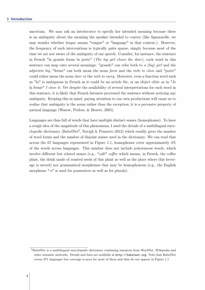
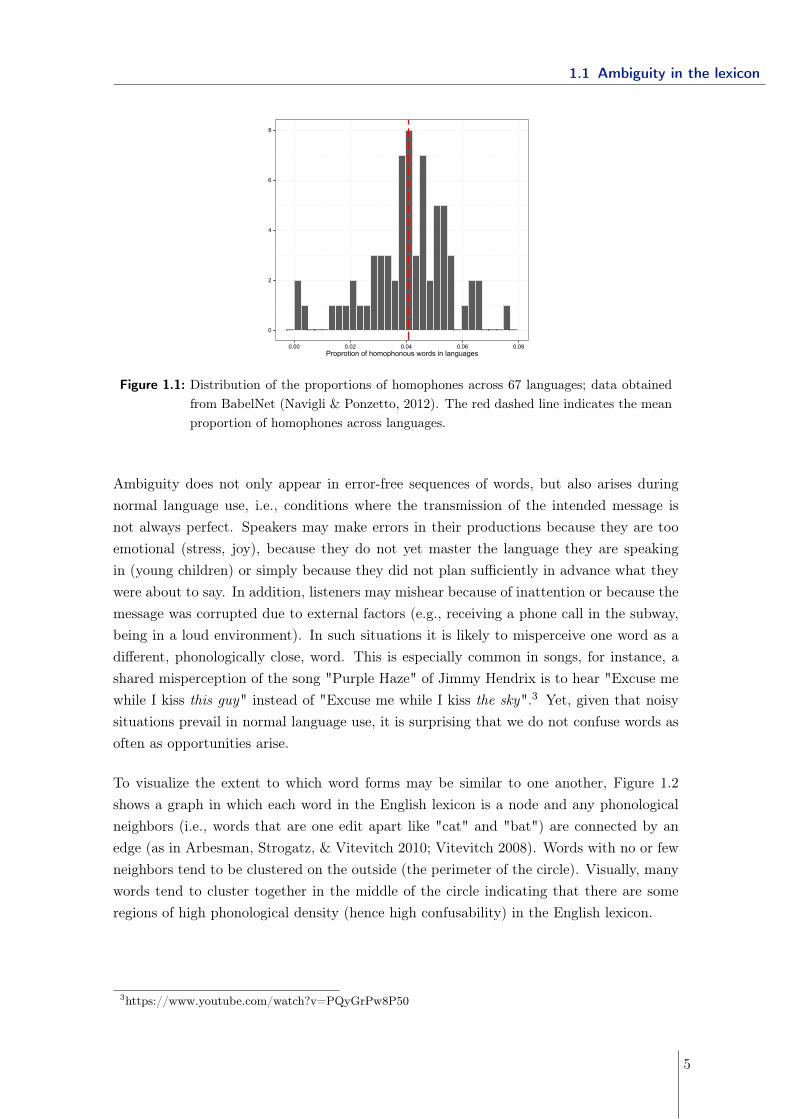
Languages are thus full of words that have multiple distinct senses (homophones). To havea rough idea of the magnitude of this phenomena, I used the details of a multilingual ency-clopedic dictionary (BabelNet2, Navigli & Ponzetto 2012) which readily gives the numberof word forms and the number of disjoint senses used in the dictionary. We can read thatacross the 67 languages represented in Figure 1.1, homophones cover approximately 4%of the words across languages. This number does not include polysemous words, whichinvolve different but related senses (e.g., "café" coffee which means, in French, the coffeeplant, the drink made of roasted seeds of this plant as well as the place where this bever-age is served) nor grammatical morphemes that may be homophonous (e.g., the Englishmorpheme "-s" is used for possessives as well as for plurals).
2BabelNet is a multilingual encyclopedic dictionary combining resources from WordNet, Wikipedia andother semantic networks. Details and data are available at http://babelnet.org. Note that BabelNetcovers 271 languages but coverage is poor for most of them and thus do not appear in Figure 1.1
4
1.1 Ambiguity in the lexicon
0
2
4
6
8
0.00 0.02 0.04 0.06 0.08Proprotion of homophonous words in languages
Figure 1.1: Distribution of the proportions of homophones across 67 languages; data obtainedfrom BabelNet (Navigli & Ponzetto, 2012). The red dashed line indicates the meanproportion of homophones across languages.
Ambiguity does not only appear in error-free sequences of words, but also arises duringnormal language use, i.e., conditions where the transmission of the intended message isnot always perfect. Speakers may make errors in their productions because they are tooemotional (stress, joy), because they do not yet master the language they are speakingin (young children) or simply because they did not plan sufficiently in advance what theywere about to say. In addition, listeners may mishear because of inattention or because themessage was corrupted due to external factors (e.g., receiving a phone call in the subway,being in a loud environment). In such situations it is likely to misperceive one word as adifferent, phonologically close, word. This is especially common in songs, for instance, ashared misperception of the song "Purple Haze" of Jimmy Hendrix is to hear "Excuse mewhile I kiss this guy" instead of "Excuse me while I kiss the sky".3 Yet, given that noisysituations prevail in normal language use, it is surprising that we do not confuse words asoften as opportunities arise.
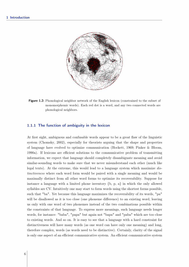
To visualize the extent to which word forms may be similar to one another, Figure 1.2shows a graph in which each word in the English lexicon is a node and any phonologicalneighbors (i.e., words that are one edit apart like "cat" and "bat") are connected by anedge (as in Arbesman, Strogatz, & Vitevitch 2010; Vitevitch 2008). Words with no or fewneighbors tend to be clustered on the outside (the perimeter of the circle). Visually, manywords tend to cluster together in the middle of the circle indicating that there are someregions of high phonological density (hence high confusability) in the English lexicon.
3https://www.youtube.com/watch?v=PQyGrPw8P50
5
1 Introduction
Figure 1.2: Phonological neighbor network of the English lexicon (constrained to the subset ofmonomorphemic words). Each red dot is a word, and any two connected words arephonological neighbors.
1.1.1 The function of ambiguity in the lexicon
At first sight, ambiguous and confusable words appear to be a great flaw of the linguisticsystem (Chomsky, 2002), especially for theorists arguing that the shape and propertiesof language have evolved to optimize communication (Hockett, 1969; Pinker & Bloom,1990a). If lexicons are efficient solutions to the communicative problem of transmittinginformation, we expect that language should completely disambiguate meaning and avoidsimilar-sounding words to make sure that we never misunderstand each other (much likelegal texts). At the extreme, this would lead to a language system which maximize dis-tinctiveness where each word form would be paired with a single meaning and would bemaximally distinct from all other word forms to optimize its recoverability. Suppose forinstance a language with a limited phone inventory {b, p, a} in which the only allowedsyllables are CV. Intuitively one may start to form words using the shortest forms possible,such that "ba". Yet because this language maximizes the recoverability of its words, "pa"will be disallowed as it is too close (one phoneme difference) to an existing word, leavingus only with one word of two phonemes instead of the two combinations possible withinthe constraints of that language. To express more meanings, such language needs longerwords, for instance: "baba", "papa" but again not "bapa" and "paba" which are too closeto existing words. And so on. It is easy to see that a language with a hard constraint fordistinctiveness will have many words (as one word can have only one meaning) and long,therefore complex, words (as words need to be distinctive). Certainly, clarity of the signalis only one aspect of an efficient communicative system. An efficient communicative system
6
1.1 Ambiguity in the lexicon
must also be composed of simple signals that are easily memorized, produced, processedand transmitted over generations of learners. Simple signals would be frequent, short andcomposed of common sound sequences. At its limit, the easiest language would be a lan-guage maximally compressible that uses only one simple word to express all meanings, suchas "ba". Certainly, natural languages neither seem to be fully compressible nor distinctiveand are likely to be situated on the scale of possible languages existing in-between thesetwo extremes.
The idea that there should be a balance between clarity and simplicity, or distinctivenessand compressibility, is not new (e.g., Piantadosi, Tily, & Gibson, 2012; Shannon, 1947;Zipf, 1949). Zipf formalized the principle of least effort which advances that languages area tradeoff between listeners’ and speakers’ interests. At the phonological level, listenerswant words to be distinctive, while speakers want simple words that minimize articulatoryeffort and maximize brevity and phonological reduction. At the lexical level, listenerswant a large vocabulary size such that each word maps onto a single meaning, whilespeakers want to reduce the size of the vocabulary to a limited list of simple words thatmap onto several meanings. This is, in essence, what Zipf’s law is about: If one lists allthe words of a language by how often they are used, the second most frequent word isabout half as frequent as the most frequent one, the third most frequent is about a thirdas frequent as the most frequent one, the fourth is a fourth as frequent and so on. Inaddition, frequent words tend also to have more meanings (Zipf, 1949) and to sound morealike (Mahowald, Dautriche, Gibson, & Piantadosi, submitted , see Appendix A) than lessfrequent words. Thus, Zipf’s law is consistent with a lexical tradeoff: when speakers tendto choose more frequent words this makes the listener’s task harder (as these words are themost ambiguous). By contrast, when listeners find it easier to determine a word’s meaning,this means that the speaker had to work harder (as these words will be less frequent andmore numerous). Additionally frequent words in languages are simpler than unfrequentwords: They tend to be short, predictable and phonotactically typical (Mahowald et al.,submitted ; Piantadosi, Tily, & Gibson, 2011; Zipf, 1949). Similarly, by assigning shorter andphonotactically simple forms to more frequent and predictable meanings, and longer andphonetically more complex forms to less frequent and less predictable meanings, languagesestablish a trade-off between the overall effort needed to produce words and the chancesof successful transmission of a message.
Previous quantitative analyses of the lexicon used word frequency as a tool to argue for thepresence of functional trade-offs. By showing that frequent words carry different proper-ties than less frequent words, they demonstrate that certain properties are non-uniformlydistributed across the words of the lexicon in a way that is consistent with communicativeoptimization principles. Yet much previous work has focused on simply measuring statisti-cal properties of natural language and interpreting the observed effects. This does not tellus whether the properties we observe are a by-product of chance or are really the manifes-
7
1 Introduction
tation of communicative principles or other cognitive principles associated with languageuse and language acquisition. If we want to understand the processes that give rise tothe observed structure of the lexicon, we need to simulate a range of possible processes toassess which aspects of natural language occur by chance and which are the result of con-straining forces. This can be done in (at least) two ways: 1) by simulating the emergenceof lexical structure in accelerated lab time (e.g., Kirby, Cornish, & Smith, 2008, using theiterated learning paradigm, I will discuss further this experimental method in the GeneralDiscussion) or 2) by using computing power to simulate the generation of lexical structurewith different constraints, structures, and biases. In this work, I focus on the latter.
In chapter 2.1, I propose to investigate whether the pattern of word form similarity inthe lexicon differs from chance and in what direction. As I outlined before, ambiguous andsimilar-sounding words may be a useful property of natural languages, simply because theyallow the re-use of words and sounds which are the most easily understood and produced(Juba, Kalai, Khanna, & Sudan, 2011; Piantadosi, Tily, & Gibson, 2012; Wasow et al.,2005). However, ambiguous and similar-sounding words may be harmful to communicationas they increase the chances of being misunderstood. The purpose of this chapter is thusto quantify where natural lexicons are situated along the continuum ranging from fullycompressible to fully distinctive lexicons and whether this differs from what we wouldexpect by chance alone.
1.1.2 Ambiguity in language processing
Il y a des verbes qui se conjuguent très irrégulièrement.Par exemple, le verbe "ouïr".Le verbe ouïr, au présent, ça fait : J’ois... j’ois...Si au lieu de dire "j’entends", je dis "j’ois",les gens vont penser que ce que j’entends est joyeuxalors que ce que j’entends peut être particulièrement triste.Il faudrait préciser: "Dieu, que ce que j’ois est triste !"
— Raymond Devos
In practice, ambiguous and similar-sounding words may not harm communication asstrongly as one might think. Indeed, words are rarely uttered in isolation but are partof the broader context in which they are used: the sentence in which they are pronounced,the discourse, the speakers involved, the register of language, the surroundings, etc. Inother words, if we are able to integrate other sources of information to constrain the pos-sible meaning of a word, then disambiguation may become (almost) free of cost.
Work on language processing supports this idea as many studies provided evidence thatadults use various kind of information to constrain lexical access: verb selectional re-
8
1.1 Ambiguity in the lexicon
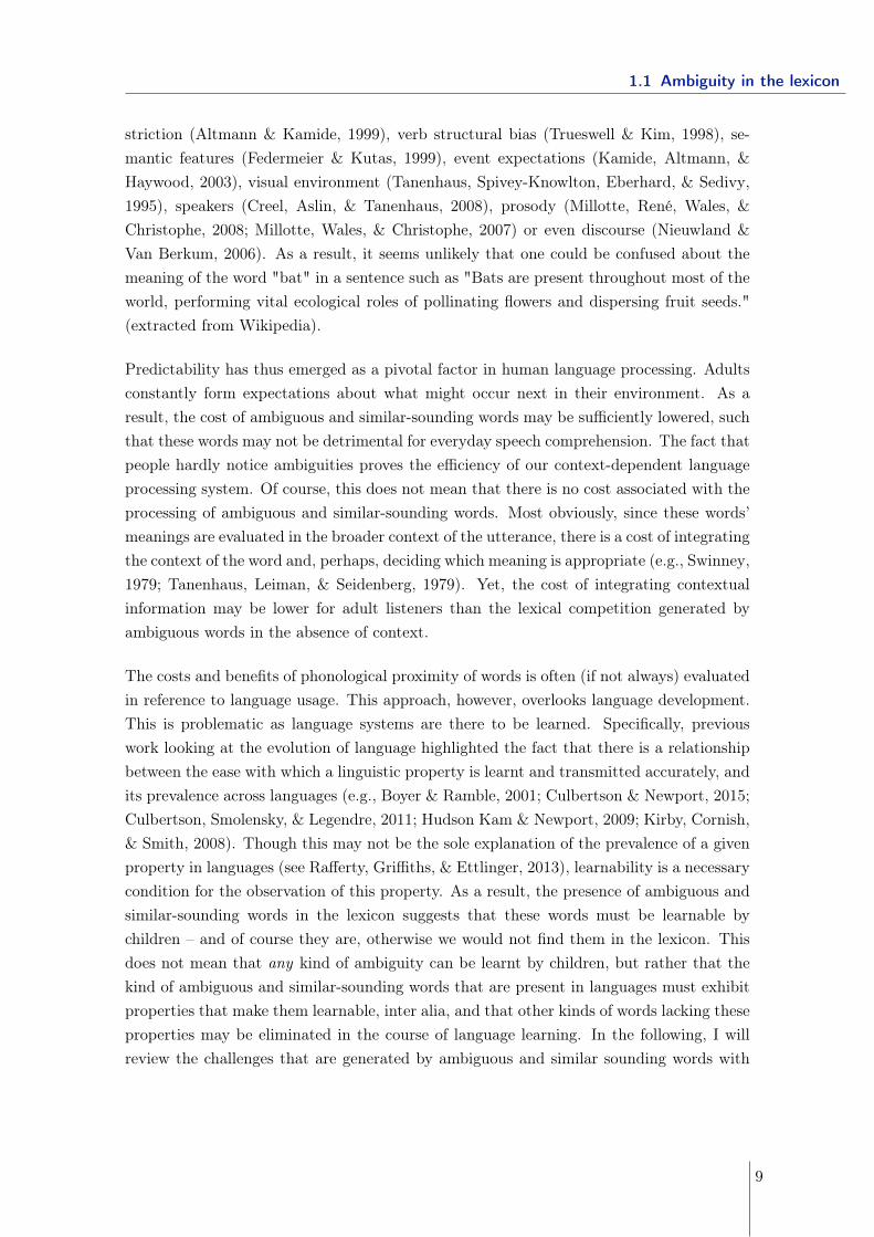
striction (Altmann & Kamide, 1999), verb structural bias (Trueswell & Kim, 1998), se-mantic features (Federmeier & Kutas, 1999), event expectations (Kamide, Altmann, &Haywood, 2003), visual environment (Tanenhaus, Spivey-Knowlton, Eberhard, & Sedivy,1995), speakers (Creel, Aslin, & Tanenhaus, 2008), prosody (Millotte, René, Wales, &Christophe, 2008; Millotte, Wales, & Christophe, 2007) or even discourse (Nieuwland &Van Berkum, 2006). As a result, it seems unlikely that one could be confused about themeaning of the word "bat" in a sentence such as "Bats are present throughout most of theworld, performing vital ecological roles of pollinating flowers and dispersing fruit seeds."(extracted from Wikipedia).
Predictability has thus emerged as a pivotal factor in human language processing. Adultsconstantly form expectations about what might occur next in their environment. As aresult, the cost of ambiguous and similar-sounding words may be sufficiently lowered, suchthat these words may not be detrimental for everyday speech comprehension. The fact thatpeople hardly notice ambiguities proves the efficiency of our context-dependent languageprocessing system. Of course, this does not mean that there is no cost associated with theprocessing of ambiguous and similar-sounding words. Most obviously, since these words’meanings are evaluated in the broader context of the utterance, there is a cost of integratingthe context of the word and, perhaps, deciding which meaning is appropriate (e.g., Swinney,1979; Tanenhaus, Leiman, & Seidenberg, 1979). Yet, the cost of integrating contextualinformation may be lower for adult listeners than the lexical competition generated byambiguous words in the absence of context.
The costs and benefits of phonological proximity of words is often (if not always) evaluatedin reference to language usage. This approach, however, overlooks language development.This is problematic as language systems are there to be learned. Specifically, previouswork looking at the evolution of language highlighted the fact that there is a relationshipbetween the ease with which a linguistic property is learnt and transmitted accurately, andits prevalence across languages (e.g., Boyer & Ramble, 2001; Culbertson & Newport, 2015;Culbertson, Smolensky, & Legendre, 2011; Hudson Kam & Newport, 2009; Kirby, Cornish,& Smith, 2008). Though this may not be the sole explanation of the prevalence of a givenproperty in languages (see Rafferty, Griffiths, & Ettlinger, 2013), learnability is a necessarycondition for the observation of this property. As a result, the presence of ambiguous andsimilar-sounding words in the lexicon suggests that these words must be learnable bychildren – and of course they are, otherwise we would not find them in the lexicon. Thisdoes not mean that any kind of ambiguity can be learnt by children, but rather that thekind of ambiguous and similar-sounding words that are present in languages must exhibitproperties that make them learnable, inter alia, and that other kinds of words lacking theseproperties may be eliminated in the course of language learning. In the following, I willreview the challenges that are generated by ambiguous and similar sounding words with
9
1 Introduction
regard to the word learning problem. I will also propose a few properties that would makesuch words easier to learn.
1.2 Ambiguity: A challenge for language acquisition?
Anyone who contemplates lexical acquisition will realize that ambiguous and similar-sounding words present a problem for children learning their language. Normally one canidentify a pair of homophonous words if they sound the same but have different meanings.Similarly, two words form a minimal pair if their word forms differ by a single phoneme,but they have different meanings. Of course, this is a relatively easy task for adults be-cause we already know which words are homophonous and which words sound similar toone another. By contrast, young language learners do not initially know which word formshave multiple meanings and which phonological elements are contrastive in their language:They must discover this during the course of language development. In order to examinewhat kind of challenge these words bring into the word learning game, we first need todefine what a word is, what aspects need to be acquired, and how this is done.
What’s in a word? By definition, a (content) word is composed of a phonological formthat is paired with a concept. For instance the word "cat" is composed of a sequence ofsounds, /kaet/, which is linked to the concept of CAT. Quite generally, the meaning of aword can be defined by its extension, that is the set of entities to which that word refers(e.g., the meaning of "cat" represents the set of all cats and only cats). Yet, we know muchmore about a word than its meaning: We know that "cat" is a noun, we also know thatthe meaning of "cat" is more similar to the meaning of "dog" than it is to the meaning of"chair" and we have stored information about contexts (linguistic and non linguistic) inwhich this word may occur. Thus the knowledge of a word also includes the knowledge ofits syntactic properties, its relations with other words in the lexicon and some other typesof non-linguistic knowledge, such as the situations in which that word typically occurs(e.g., Perfetti & Hart, 2002).
This brings us to the question of what aspects of words children learn when they "learnwords". Recent evidence has shown that as early as the first year of life, infants acquire themeanings of basic nouns and verbs in their language (Bergelson & Swingley, 2012, 2013;Tincoff & Jusczyk, 2012). It is, however, unlikely that all dimensions of word meaningsand all of their properties are in place this early on. For instance, it is only during thesecond year of life that toddlers start to realize how familiar and novel words are related toother words in their lexicon (Arias-Trejo & Plunkett, 2013; Wojcik & Saffran, 2013) andhave accumulated knowledge of the grammatical environment in which a word can appear(Bernal, Dehaene-Lambertz, Millotte, & Christophe, 2010). These studies and many othersprovide growing evidence that children do not fast-map a dictionary-like definition at the
10
1.2 Ambiguity: A challenge for language acquisition?
first encounter of a word (Carey, 1978a). Instead, word learning seems to be a slowprocess, gradually emerging through the accumulation of statistical, syntactic, semantic,and pragmatic fragmental evidence (e.g., Bion, Borovsky, & Fernald, 2013; Carey, 1978a;Gelman & Brandone, 2010; L. Smith & Yu, 2008).
How do children learn the meaning of words? There are, at least, four (non-sequential)problems that children must solve to in order to learn the meaning of words: extractingword forms from the speech signal (the segmentation problem), determining what countsas a novel word and what does not (the identification problem), determining what it refersto (the mapping problem) and determining the relevant concept to which it is associated(the extension problem). The fact that many phonological forms are alike or have severalmeanings potentially create a challenge at each level of the word learning process. I reviewthese challenges in turn below.
1.2.1 The segmentation problem
Because words are generally not uttered in isolation, one of the first tasks for infantslearning a language is to extract the words that make up the utterances they hear. This isnot a trivial task because there is typically no pause between words. Adults are known torely on their lexicon in order to segment continuous speech into words (e.g., Marslen-Wilson& Welsh, 1978). Because infants in their first year mostly lack such lexical knowledge,this procedure was thought to be unavailable to them, leading researchers to focus onalternative cues that can be recovered from the speech such as statistical regularities (e.g.,Saffran, Aslin, & Newport, 1996), phrasal prosody (Gout, Christophe, & Morgan, 2004),phonotactics (e.g., Jusczyk, Friederici, Wessels, Svenkerud, & Jusczyk, 1993), but alsoknowledge about the environment such as the broader context of the learning situation(see Synnaeve, Dautriche, Börschinger, Johnson, & Dupoux, 2014, for a computationalimplementation of this idea).4
Certainly lexical ambiguities, such as homophones, are not a challenge for the segmentationproblem since there is no ambiguity on the phonological form of the word. In fact, onecould even imagine that a highly compressible lexicon with a small vocabulary size (thuswith a lot of lexical ambiguities) would be easier to segment since all word forms wouldoccur frequently in speech making it easier to spot their word boundaries. Indeed, whenexposed to a stream of speech containing only 6 words (a rather compressible lexicon),
4Language occurs in context and is constrained by the events occurring in the daily life of the child. Forexample, during an eating event one is most likely to speak about food, while during a zoo-visit event,people are more likely to talk about the animals they see. These extra-linguistic contexts are readilyaccessible to very young children and could be used to boost the probability of specific vocabulariesand constrain the most plausible segmentation of an utterance (e.g., at meal times, you expect foodvocabulary).
11
1 Introduction
infants distinguish between words and non-words after only 2 min of exposure (Saffran etal., 1996), suggesting that a compressible lexicon is easy to segment.
Regarding similar-sounding words, it has been suggested that they can facilitate the seg-mentation process. Indeed, studies have shown that hearing familiar words in the speechsignal can help segmenting the speech into words: By 8 months of age, infants segmentwords more successfully when they are preceded by frequent functions words (Shi & Lep-age, 2008) or when they are preceded by a very familiar name such as "mommy" (Bortfeld,Morgan, Golinkoff, & Rathbun, 2005). Accordingly, it might be easier to isolate a novelword (e.g., "tog") from the speech stream when it sounds similar to a known word ("dog").Supporting that idea, Altvater-Mackensen & Mani (2013) showed that 7-month-old Ger-man infants familiarized with a word such as "Löffel" spoon in the lab had less difficultysegmenting novel words such as "Löckel" (similar in the onset) or "Nöffel" (similar in theoffset) than phonologically unrelated words such as "Sotte". Thus, phonological overlapwith a familiarized word may help infants recognize novel similar-sounding words in thespeech stream.
Taken together, this suggests that compressible lexicons with reduced vocabulary size and afair amount of phonological overlap may help infants in the segmentation process. Althoughthis issue will not be further addressed in the main body of this thesis, it is certainly aninteresting question to follow up for computational models of segmentation.5 At any rate,compressible lexicons may be functionally advantageous for speech segmentation.
1.2.2 The identification problem
To learn the meaning of a word, children must be able to identify a phonological form asa potential candidate for a novel entry into the lexicon. In the case of similar-soundingwords, they must identify that minimally different phonological forms (e.g., "sheep" and"ship") map onto two different meanings, and are not the by-product of the normal soundvariability of their language. Indeed, one difficulty for learners is that the same soundcategories are realized differently by different speakers of the same language (e.g., Labov,1966) and differ depending on the phonetic context they appear in (e.g., Holst & Nolan,1995). As a result, different instances of a given word do not all sound the same. Hence,children must learn to distinguish between the acceptable instances of a word and theinstances that do not correspond to that word.
Clearly, the presence of similar-sounding words adds an additional complexity to the word
5One can imagine creating two artificial corpora: one using a compressible lexicon and the other using adistinctive lexicon, keeping the number and frequency of words constant. The idea would be to evaluateon which corpus the same segmentation model (for instance, Adaptor Grammars, M. Johnson, Griffiths,& Goldwater, 2006) would give the best segmentation result.
12
1.2 Ambiguity: A challenge for language acquisition?
identification task. Indeed, several studies have shown that 14-month-old toddlers have ahard time differentiating between novel word forms that differ only in one phoneme (Pater,Stager, & Werker, 2004; Stager & Werker, 1997) (e.g., "bih" and "dih") despite beingperfectly able to distinguish the phonemic contrast (e.g., /b/ and /d/). Yet, the same agegroup can succeed when the novel word forms are presented in a more supportive context(Yoshida, Fennell, Swingley, & Werker, 2009), i.e. if they are embedded in a sentence(Fennell & Waxman, 2006) or if the objects onto which the words map are presented priorto the experiment (Fennell, 2012). This suggests that young toddlers need more supportto attend and encode minimally different forms. However, the presence of supportivecontext does not suffice in all conditions: Older 19-month-olds fail to use a single-featurephonological distinction to assign a novel meaning to a word form that sounds similar toa very familiar one (Swingley & Aslin, 2007) (e.g., learning a novel word such as "tog"when having "dog" in their lexicon). Again, perceptual discrimination between the familiarand the novel label was not an issue as children of the same age are able to distinguishfamiliar words from mispronounced variants (e.g., Mani & Plunkett, 2007; Swingley &Aslin, 2002). In sum, this suggests that young children have difficulty in attending to andencoding similar word forms compared to more distinct word forms.
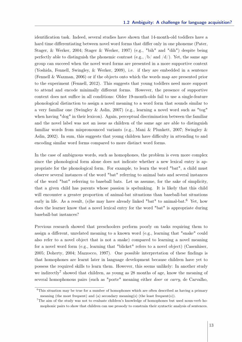
In the case of ambiguous words, such as homophones, the problem is even more complexsince the phonological form alone does not indicate whether a new lexical entry is ap-propriate for the phonological form. For example, to learn the word "bat", a child mustobserve several instances of the word "bat" referring to animal bats and several instancesof the word "bat" referring to baseball bats. Let us assume, for the sake of simplicity,that a given child has parents whose passion is spelunking. It is likely that this childwill encounter a greater proportion of animal-bat situations than baseball-bat situationsearly in life. As a result, (s)he may have already linked "bat" to animal-bat.6 Yet, howdoes the learner know that a novel lexical entry for the word "bat" is appropriate duringbaseball-bat instances?
Previous research showed that preschoolers perform poorly on tasks requiring them toassign a different, unrelated meaning to a known word (e.g., learning that "snake" couldalso refer to a novel object that is not a snake) compared to learning a novel meaningfor a novel word form (e.g., learning that "blicket" refers to a novel object) (Casenhiser,2005; Doherty, 2004; Mazzocco, 1997). One possible interpretation of these findings isthat homophones are learnt later in language development because children have yet topossess the required skills to learn them. However, this seems unlikely: In another studywe indirectly7 showed that children, as young as 28 months of age, know the meaning ofseveral homophonous pairs (such as "porte" meaning either door or carry, de Carvalho,
6This situation may be true for a number of homophones which are often described as having a primarymeaning (the most frequent) and (a) secondary meaning(s) (the least frequent(s)).
7The aim of the study was not to evaluate children’s knowledge of homophones but used noun-verb ho-mophonic pairs to show that children can use prosody to constrain their syntactic analysis of sentences.
13
1 Introduction
Dautriche, & Christophe, 2014, 2015). Another possibility is that children need moreevidence before accepting a new meaning for a known word than what is provided byexperimental protocols because they already possess an established meaning for the testedword form (e.g., "snake"). At any rate, this suggests that identifying whether a newmeaning is appropriate for a known word adds a degree of difficulty that children do notrun into when learning non-homophones.
Both similar-sounding and ambiguous words challenge learners with the same basic prob-lem: Identifying what counts as a novel word and what does not. In the case of similar-sounding words, children must not only be able to distinguish different phonological forms(e.g., "tog" vs. "dog") but they must also be able to interpret that such a phonologicaldistinction could be indicative of a novel word. In the case of homophones, the problemis even more complex since the same phonological form is used to label several meaningsand phonemic information thus cannot be used as a cue to distinguish them (see howeverConwell & Morgan, 2012; Gahl, 2008). So how do children eventually succeed at learningthese words? As I highlighted earlier, there are many important factors other than phonol-ogy in interpreting speech. Adults are sufficiently attuned to their language to attend tothe relevant context (i.e., linguistic, visual, pragmatic, etc.) for disambiguating ambiguouswords and minimizing the risk of confusing similar-sounding words. Yet, it is an openquestion whether children, like adults, also take a broader range of contextual informationinto consideration when judging the likelihood that a word form is attached to a novelmeaning.
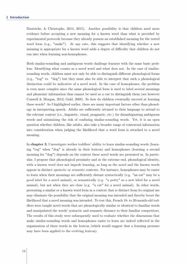
In chapter 3, I investigate wether toddlers’ ability to learn similar-sounding words (learn-ing "tog" when "dog" is already in their lexicon) and homophones (learning a secondmeaning for "dog") depends on the context these novel words are presented in. In partic-ular, I propose that phonological proximity and at the extreme end, phonological identity,with a known word does not impede learning, as long as the novel and the known wordsappear in distinct syntactic or semantic contexts. For instance, homophones may be easierto learn when their meanings are sufficiently distant syntactically (e.g. "an eat" may be agood label for a novel animal), or semantically (e.g. "a potty" as a new label for a novelanimal), but not when they are close (e.g. "a cat" for a novel animal). In other words,presenting a similar or a known word form in a context that is distinct from its original usemay eliminate the possibility that the original meaning was intended and thereby boost thelikelihood that a novel meaning was intended. To test this, French 18- to 20-month-old tod-dlers were taught novel words that are phonologically similar or identical to familiar wordsand manipulated the words’ syntactic and semantic distance to their familiar competitors.The results of this study were subsequently used to evaluate whether the dimensions thatmake similar-sounding words and homophones easier to learn are indeed reflected in theorganization of these words in the lexicon (which would suggest that a learning pressuremay have been applied to the evolving lexicon).
14
1.2 Ambiguity: A challenge for language acquisition?
1.2.3 The mapping problem
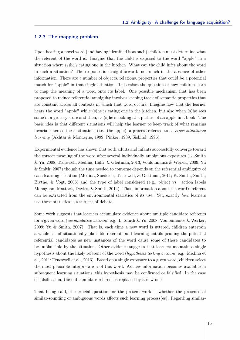
Upon hearing a novel word (and having identified it as such), children must determine whatthe referent of the word is. Imagine that the child is exposed to the word "apple" in asituation where (s)he’s eating one in the kitchen. What can the child infer about the wordin such a situation? The response is straightforward: not much in the absence of otherinformation. There are a number of objects, relations, properties that could be a potentialmatch for "apple" in that single situation. This raises the question of how children learnto map the meaning of a word onto its label. One possible mechanism that has beenproposed to reduce referential ambiguity involves keeping track of semantic properties thatare constant across all contexts in which that word occurs. Imagine now that the learnerhears the word "apple" while (s)he is eating one in the kitchen, but also when (s)he seessome in a grocery store and then, as (s)he’s looking at a picture of an apple in a book. Thebasic idea is that different situations will help the learner to keep track of what remainsinvariant across these situations (i.e., the apple), a process referred to as cross-situationallearning (Akhtar & Montague, 1999; Pinker, 1989; Siskind, 1996).
Experimental evidence has shown that both adults and infants successfully converge towardthe correct meaning of the word after several individually ambiguous exposures (L. Smith& Yu, 2008; Trueswell, Medina, Hafri, & Gleitman, 2013; Vouloumanos & Werker, 2009; Yu& Smith, 2007) though the time needed to converge depends on the referential ambiguity ofeach learning situation (Medina, Snedeker, Trueswell, & Gleitman, 2011; K. Smith, Smith,Blythe, & Vogt, 2006) and the type of label considered (e.g., object vs. action labelsMonaghan, Mattock, Davies, & Smith, 2014). Thus, information about the word’s referentcan be extracted from the environmental statistics of its use. Yet, exactly how learnersuse these statistics is a subject of debate.
Some work suggests that learners accumulate evidence about multiple candidate referentsfor a given word (accumulative account, e.g., L. Smith & Yu, 2008; Vouloumanos & Werker,2009; Yu & Smith, 2007). That is, each time a new word is uttered, children entertaina whole set of situationally plausible referents and learning entails pruning the potentialreferential candidates as new instances of the word cause some of these candidates tobe implausible by the situation. Other evidence suggests that learners maintain a singlehypothesis about the likely referent of the word (hypothesis testing account, e.g., Medina etal., 2011; Trueswell et al., 2013). Based on a single exposure to a given word, children selectthe most plausible interpretation of this word. As new information becomes available insubsequent learning situations, this hypothesis may be confirmed or falsified. In the caseof falsification, the old candidate referent is replaced by a new one.
That being said, the crucial question for the present work is whether the presence ofsimilar-sounding or ambiguous words affects such learning process(es). Regarding similar-
15
1 Introduction
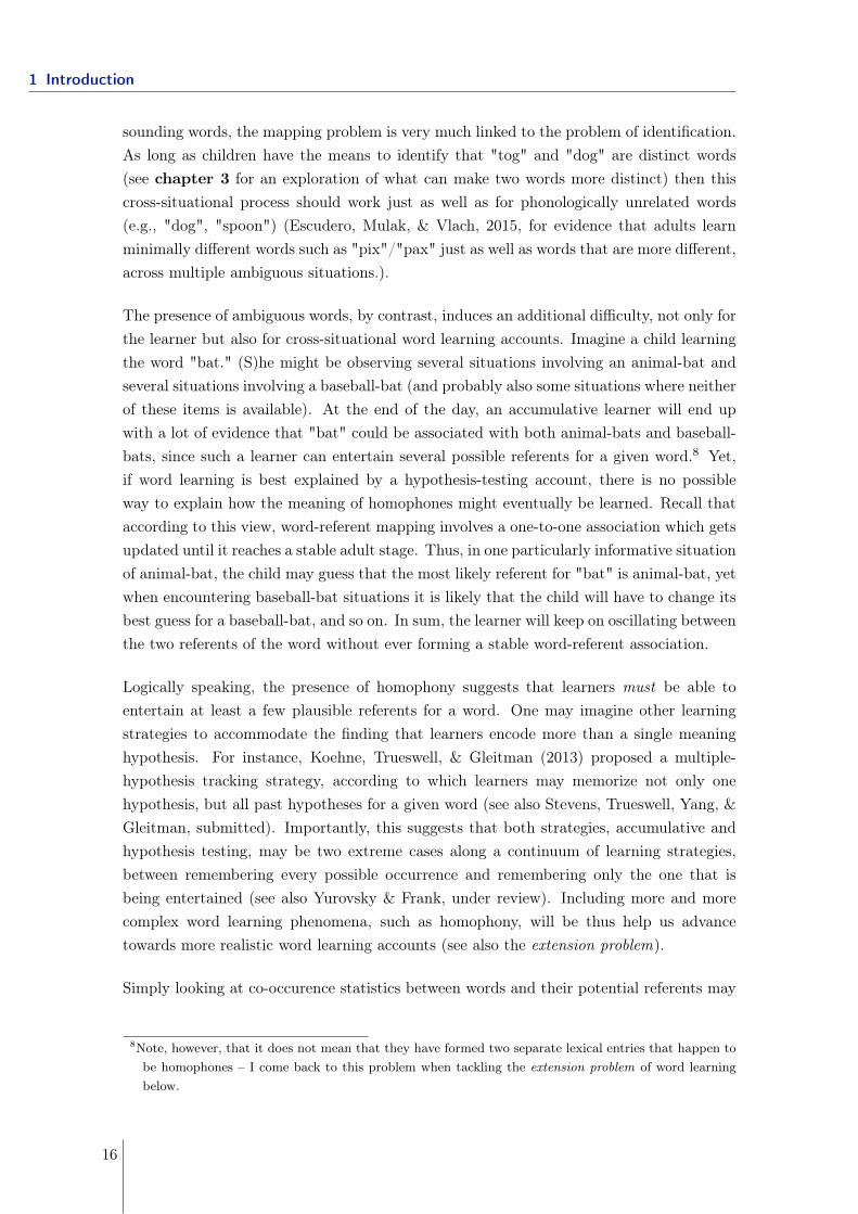
sounding words, the mapping problem is very much linked to the problem of identification.As long as children have the means to identify that "tog" and "dog" are distinct words(see chapter 3 for an exploration of what can make two words more distinct) then thiscross-situational process should work just as well as for phonologically unrelated words(e.g., "dog", "spoon") (Escudero, Mulak, & Vlach, 2015, for evidence that adults learnminimally different words such as "pix"/"pax" just as well as words that are more different,across multiple ambiguous situations.).
The presence of ambiguous words, by contrast, induces an additional difficulty, not only forthe learner but also for cross-situational word learning accounts. Imagine a child learningthe word "bat." (S)he might be observing several situations involving an animal-bat andseveral situations involving a baseball-bat (and probably also some situations where neitherof these items is available). At the end of the day, an accumulative learner will end upwith a lot of evidence that "bat" could be associated with both animal-bats and baseball-bats, since such a learner can entertain several possible referents for a given word.8 Yet,if word learning is best explained by a hypothesis-testing account, there is no possibleway to explain how the meaning of homophones might eventually be learned. Recall thataccording to this view, word-referent mapping involves a one-to-one association which getsupdated until it reaches a stable adult stage. Thus, in one particularly informative situationof animal-bat, the child may guess that the most likely referent for "bat" is animal-bat, yetwhen encountering baseball-bat situations it is likely that the child will have to change itsbest guess for a baseball-bat, and so on. In sum, the learner will keep on oscillating betweenthe two referents of the word without ever forming a stable word-referent association.
Logically speaking, the presence of homophony suggests that learners must be able toentertain at least a few plausible referents for a word. One may imagine other learningstrategies to accommodate the finding that learners encode more than a single meaninghypothesis. For instance, Koehne, Trueswell, & Gleitman (2013) proposed a multiple-hypothesis tracking strategy, according to which learners may memorize not only onehypothesis, but all past hypotheses for a given word (see also Stevens, Trueswell, Yang, &Gleitman, submitted). Importantly, this suggests that both strategies, accumulative andhypothesis testing, may be two extreme cases along a continuum of learning strategies,between remembering every possible occurrence and remembering only the one that isbeing entertained (see also Yurovsky & Frank, under review). Including more and morecomplex word learning phenomena, such as homophony, will be thus help us advancetowards more realistic word learning accounts (see also the extension problem).
Simply looking at co-occurence statistics between words and their potential referents may
8Note, however, that it does not mean that they have formed two separate lexical entries that happen tobe homophones – I come back to this problem when tackling the extension problem of word learningbelow.
16
1.2 Ambiguity: A challenge for language acquisition?
not be enough to account for homophony.9 As discussed before, learners must be able todistinguish between different meanings of the same word form (the identification problem).This might be possible if learners encode not only form-referent co-occurences but alsoother kinds of information. In previous work, I suggested that cross-situational learningis informed by the type of learning context (see Appendix B, Dautriche & Chemla, 2014).This idea rests on the observation that in the kitchen, one is more likely to speak about foodthan in the bathroom and the opposite holds for bath items. As such, the extra-linguisticcontext, which is naturally available to young children, may help learners in constrainingthe likely referent of the word in a given situation. If, as I suggested earlier, a sufficientlylarge semantic distance is a major characteristic of homophone pairs in language, then weexpect homophones to appear in clearly different contexts. For instance, animal-bats andbaseball-bats cover distant concepts, and it is likely that the situations in which animal-bats are mentioned (caving, garden at night) are quite different from the situations in whichbaseball-bats are mentioned (sport event). Thus, if learners retain contextual information,they may be able to "tag" different instances of the homophonous word, which may helpthem realize that they should track two separate referents instead of just a single one.
In sum, homophony challenges current word learning accounts on important grounds thatneed to be addressed to tackle more complex, and more ecologically valid, word learn-ing phenomena. For the learner, the presence of homophones, as well as similar-soundingwords, presents similar challenges for mapping as it does for identification: Finding thecorrect referent(s) of a word may be facilitated if learners are not overwhelmed by phono-logical identity, or proximity, and use other types of information, for instance the broadercontext of the learning situation, to constrain their word-referent hypotheses. Whetheror not the distribution of ambiguous and similar-sounding words in the lexicon allows forsuch distinction will be addressed in chapter 3.
1.2.4 The extension problem
At the same time as children determine the likely referent of a word, they must alsodetermine the relevant extension associated with the word (i.e. the subset of entities towhich a given word refers). In general, children will not observe all the entities that exhaustthe set of candidate exemplars, but will rather observe only a subset of those. Suppose forinstance, that the child observes that the word "cat" is used to refer to their pet. Ideally,the child should be able to extend the word to other cats, not just their own one. Yet, evenassuming that the child understood which object the word refers to, in that context (themapping problem), the meaning of "cat" is still underspecified after this single learning
9Nor for word learning in general. Recall that learning the meaning of a word is more than just establishinga link between a form and a referent, but also involves gaining knowledge about its syntactic propertiesand the situations in which this word may occur.
17
1 Introduction
situation (Quine, 1960). Certainly "cat" could refer to the set of all cats and only catsbut many other extensions are compatible with that one experience: Felix the cat, one ofits body parts, Felix the cat at 3pm in the kitchen, the set of all black cats, the set of allpets, the set of all animals and so on. In sum, the learner must decide between a numberof nested and overlapping possibilities.
Many theoretically plausible meanings can be ruled out simply because children do not,or cannot, consider them (e.g., Felix the cat at 3pm in the kitchen). Yet, many plausi-ble hypotheses still remain. This has led researchers to hypothesize that children comeequipped with constraints or biases about which hypotheses are more likely than others. Asensible way to characterize the constraints necessary for word learning is to observe howchildren extend words in controlled environments. In experiments testing this, children areusually shown several learning exemplars (e.g., "these are blickets") and asked whether theword could be extended to new objects (e.g., "which one of these is a blicket?"). Usingsuch a paradigm, it has been shown that children are more likely to treat novel labels asreferring to objects of the same kind (the taxonomy constraint, Markman & Hutchinson,1984), or of the same shape (the shape bias, Landau, Smith, & Jones, 1988). Moreover,even young infants of 10 months expect that a word labels a group objects that share acommon property (Plunkett, Hu, & Cohen, 2008). Accounts of word learning (associativelearning accounts, e.g., Regier, 2005; Yu & Smith, 2007; hypothesis elimination accounts,e.g., Pinker, 1989; Siskind, 1996; Bayesian accounts Frank, Goodman, & Tenenbaum, 2009;Piantadosi, Tenenbaum, & Goodman, 2012; Xu & Tenenbaum, 2007) accordingly presup-pose that the extension of a word is convex in conceptual space. That is, if two objectsA and B are both labelled by the word ”blicket”, then A and B are exemplars of a singleconcept whose members are contiguous in conceptual space (Gärdenfors, 2004).
However this approach will fail as soon as identity of form does not imply identity ofmeaning, that is when the language contains words that have multiple meanings such ashomophones. For example, if a child is learning the word "bat", (s)he might be observingseveral exemplars of animal-bats and several exemplars of baseball-bats. Thus, if bothanimal-bats and baseball-bats are thought to be exemplars of a single concept (the cate-gory including animal-bats and baseball-bats), then such a concept should encompass thecommon properties of both flying mammals and sport instruments, leading to very broadinterpretations such as "thing" or "stuff". Thus, reasoning across different exemplars basedon forms that are homophonous will lead to an overextension of the label, since all "things"are not "bats". Note that contrary to the mapping problem, here the issue is not aboutknowing that a word can apply to several referents but knowing that these referents belongsto distinct meanings and not a single one.
There are two possibilities that may explain why current word learning accounts have diffi-culty in dealing with homophony. The first possibility is that they simulate children’s priorknowledge: Children may start with an expectation that the structure of the language is
18
1.3 Summary
clear, that is, involving transparent, uniform mappings between forms and meanings, lead-ing to one-to-one correspondence across these domains (Slobin, 1973, 1975). The secondpossibility is that these priors reflect only what we know about very narrow word learningphenomena (learning unambiguous object labels) and cannot possibly explain the learn-ing of other phenomena, such as homophones. At any rate, the existence of homophonyin languages suggests that children must be able to entertain the possibility that otherform-meaning representations, besides a one-to-one correspondence between forms andmeanings, are possible.
In chapter 4, I provide the first careful examination of what homophones can tell usabout word learning from a theoretical and an experimental standpoint, using both anadults and a child population. On the experimental side, I explore the circumstancesunder which learners accept several meanings for the same word form. In particular, Iexplore whether a word is more likely to yield homophony when it is learnt from exem-plars clustered at two different positions in conceptual space than when exemplars forma uniform group. For instance, to learn "bat", learners will observe several exemplars ofanimal-bats and several exemplars of baseball-bats, but no non-bat exemplars. I hypoth-esize that such a distribution of learning exemplars will cue learners that they are in thepresence of a homophonous word. Note that if homophones cover distant concepts (seethe identification problem), we expect a significant gap in conceptual space between theexemplars of a homophone, which may increase the ease with which learners are able tolearn homophones. In essence, chapter 4 formalizes the intuition that distinctiveness inmeaning is an important factor for the discovery of homophony. On the theoretical side,I illustrate, with the example of homophony, how making the prior assumptions of wordlearning accounts explicit provides the best means to identify irreducible assumptions thelearning system may rely on.
1.3 Summary
The presence of ambiguity in languages is a problem at most levels of word learning (see,however, a potential advantage during the segmentation problem). At first sight, thismay be taken as a demonstration that languages are not influenced at all by children’slearning difficulties. Yet, as many have suggested, languages are a trade-off between severalfunctional pressures competing for opposite properties. This suggests two non-mutuallyexclusive explanations: 1) the presence of ambiguity in languages may be the consequenceof other functional pressures not related with the acquisition of words (e.g., cognitiveconstraint on word usage) and 2) the kind of ambiguity that is present in the lexicon islearnable; that is learning may exercise some more fine-grained influence on the distributionof ambiguity in the lexicon by keeping only ambiguous words of the learnable kind. I explorethese ideas by first quantifying the amount of word form similarity in the lexicon (chapter
19
1 Introduction
2). I then explore the question of what kind of ambiguity may be learnable by children(chapter 3), and I finish by formalizing how children can learn ambiguous words (chapter4).
20
2 Quantifying word form similarity in thelexicons of natural languages
An important question is whether language is designed such that it can be reduced toproperties of the cognitive system. Perceptual distinctiveness has been shown to play animportant role in shaping the phonology of languages. For instance, Wedel, Kaplan, &Jackson (2013) show that phoneme pairs that have been merged in the course of languagechange distinguished fewer minimal pairs than pairs of phonemes that remained contrastivein the language. This suggests that there are constraints favoring less confusable contrastsover more confusable contrasts. These constraints have been argued to derive from com-municative efficiency: successful transmission of a message requires listeners to be ableto recover what is being said, therefore the likelihood that two distinct words would beconfusable should be minimized.
The importance of perceptual distinctiveness in phonology has been widely reported (e.g.,Flemming, 2004; Graff, 2012; Lindblom, 1986; Wedel et al., 2013). Yet very few studieshave looked at 1) perceptual distinctiveness in the lexicon (i.e., at the word form level);2) the manifestation of other functional pressures, in particular those which are not onlybeneficial for the listener but also serve the interest of the speaker and 3) the interactionof phonological distinctiveness with other factors that are relevant for language processingand acquisition, such as semantic distinctiveness. Here we precisely tackle these threepoints and ask whether the structure of word form similarity in the lexicon is the resultof communicative and cognitive pressures associated with language acquisition and use.On one hand, one might expect that a well-designed lexicon should avoid confusable wordforms to satisfy communicative constraints. On the other hand, one might expect thata well-designed lexicon should favor word form similarity to make the lexicon easier toproduce, learn and remember.
section 2.1 proposes a new methodology to investigate whether the structure of wordform similarity in the lexicon differs from chance and in what direction. This methodologycompares real lexicons against "null" lexicons by creating random baselines that provide anull hypothesis for how the linguistic structure should be in the absence of communicativeand cognitive pressures. By simulating the generation of lexical structure without anycommunicative or cognitive constraint, it is thus possible to quantify whether there is
21
2 Quantifying word form similarity in the lexicons of natural languages
more or less word form similarity in the lexicons of natural languages compared to thechance level.
In section 2.2, I looked at the interaction of word form similarity and semantic similarityin relation with possible functional advantages. To date, with 101 languages in the sample,this is the largest cross-linguistic analysis that offers insight into the processes that governlanguage learning and use across languages.
22
Lexical clustering in efficient language design
Kyle Mahowald∗1, Isabelle Dautriche∗2, Edward Gibson1, Anne Christophe2 and Steven T.Piantadosi3
1Department of Brain and Cognitive Science, MIT2Laboratoire de Sciences Cognitives et Psycholinguistique (ENS, CNRS, EHESS), Ecole
Normale Supérieure, PSL Research University, Paris, France3Department of Brain and Cognitive Sciences, University of Rochester
Abstract
Recent evidence suggests that cognitive pressures associated with language acquisition anduse could affect the organization of the lexicon. On one hand, consistent with noisy channelmodels of language (e.g., Levy 2008), the phonological distance between wordforms should bemaximized to avoid perceptual confusability (a pressure for dispersion). On the other hand, alexicon with high phonetic regularity would be simpler to learn, remember and produce (e.g.,Monaghan et al., 2011) (a pressure for clumpiness). Here we investigate wordform similarity inthe lexicon, using measures of word distance (e.g., phonological neighborhood density) to askwhether there is evidence for dispersion or clumpiness of wordforms in the lexicon. We develop anovel method to compare lexicons to phonotactically-controlled baselines that provide a null hy-pothesis for how clumpy or sparse wordforms would be as the result of only phonotactics. Resultsfor four languages, Dutch, English, German and French, show that the space of monomorphemicwordforms is clumpier than what would be expected by the best chance model by a wide varietyof measures: minimal pairs, average Levenshtein distance and several network properties. Thissuggests a fundamental drive for regularity in the lexicon that conflicts with the pressure for wordsto be as phonetically distinct as possible.
Keywords: linguistics, lexical design, communication, phonotactics,
∗These authors contributed equally to this work. For correspondence, e-mail [email protected] [email protected]
2.1 Lexical clustering in an efficient language design
23
1 Introduction
de Saussure (1916) famously posited that the links between wordforms and their meanings are arbi-trary. As Hockett (1960) stated: “The word ‘salt’ is not salty, ‘dog’ is not canine, ‘whale’ is a smallword for a large object; ‘microorganism’ is the reverse.” Despite evidence for non-arbitrary struc-ture in the lexicon in terms of semantic and syntactic categories (Bloomfield, 1933; Monaghan et al.,2014), the fact remains that here is no systematic reason why we call a dog a ‘dog’ and a cat a ‘cat’ in-stead of the other way around, or instead of ‘chien’ and ‘chat.’ In fact, our ability to manipulate sucharbitrary symbolic representations is one of the hallmarks of human language and makes languagerichly communicative since it permits reference to arbitrary entities, not just those that have iconicrepresentations (Hockett, 1960).
Because of this arbitrariness, languages have many degrees of freedom in what wordforms theychoose and in how they carve up semantic space to assign these forms to meanings. Although themapping between forms and meanings is arbitrary, the particular sets of form-meaning mappingschosen by any given language may be constrained by a number of competing pressures and biasesassociated with learnability and communicative efficiency. For example, imagine a language thatuses the word ‘feb‘ to refer to the concept HOT, and that the language now needs a word for theconcept warm. If the language used the word ‘fep’ for WARM, it would be easy to confuse with ‘feb‘(HOT) since the two words differ only in the voicing of the final consonant and would often occurin similar contexts (i.e. when talking about temperature). However, the similarity of ‘feb‘ and ‘fep’could make it easier for a language learner to learn that those sound sequences are both associatedwith temperature, and the learner would not have to spend much time learning to articulate new soundsequences since ‘feb’ and ‘fep’ share most of their phonological structure. On the other hand, if thelanguage used the word ‘sooz’ for the concept WARM, it is unlikely to be phonetically confused with‘feb’ (HOT), but the learner might have to learn to articulate a new set of sounds and would need toremember two quite different sound sequences that refer to similar concepts.
Here, we investigate how communicative efficiency and learnability trade off in the large-scalestructure of natural languages. We have developed a set of statistical tools to characterize the large-scale statistical properties of the lexicons. Our analysis focuses on testing and distinguishing thesetwo pressures in natural lexicons: a pressure for dispersion (improved discriminability) versus a pres-sure for clumpiness (re-use of sound sequences). Below, we discuss each in more detail.
A pressure for dispersion of wordforms
Under the noisy channel model of communication (Gibson et al., 2013; Levy, 2008; Shannon,1948), there is always some chance that the linguistic signal will be misperceived as a result of errorsin production, errors in comprehension, inherent ambiguity, and other sources of uncertainty for theperceiver. A lexicon is maximally robust to noise when the expected phonetic distance among wordsis maximized (Flemming, 2004; Graff, 2012), an idea used in coding theory (Shannon, 1948). Such
2 Quantifying word form similarity in the lexicons of natural languages
24
dispersion has been observed in phonetic inventories (Flemming, 2002; Hockett & Voegelin, 1955) ina way that is sensitive to phonetic context (Steriade, 1997, 2001). The length and clarity of speakers’phonetic pronunciations are also sensitive to context predictability and frequency (Bell et al., 2003;Cohen Priva, 2008), such that potentially confusable words are pronounced more slowly and morecarefully. Applying this idea to the set of wordforms in a lexicon, one would expect wordforms to bemaximally dissimilar from each other, within the bounds of conciseness and the constraints on whatcan be easily and efficiently produced by the articulatory system. The pressure for dispersion can beillustrated by noting that languages avoid long but similar-sounding words. While English has wordslike ‘accordion’ and ‘encyclopedia’, it does not also have ‘accordiom’ and ‘encyclofedia.’ Indeed, alarge number of phonological neighbors (i.e., words that are one edit apart like ‘cat’ and ‘bat’) canimpede spoken word recognition (Luce, 1986; Luce & Pisoni, 1998), and the presence of lexical com-petitors can affect reading times (Magnuson et al., 2007).
A pressure for clumpiness of wordforms
Well-designed lexicons must also be easy to learn, remember, and produce. What would sucha lexicon look like? In the extreme case, one could imagine a language with only one wordform.Learning the entire lexicon would be as simple as learning to remember and pronounce one word.While this example is absurd, there are several cognitive advantages for processing words that aresimilar to other words in a speaker’s mental lexicon. There is evidence that adults and preschool-ers learn novel words occupying phonologically dense areas of the lexicon more readily than novelwords from sparser phonological spaces (Storkel et al., 2006). Also, words that have many similarsounding neighbors in the lexicon are easier to remember than words that are more phonologicallydistinct (Vitevitch et al., 2012) and facilitate production by reducing speech error rate (Stemberger,2004; Vitevitch & Sommers, 2003) and naming latencies (Vitevitch & Sommers, 2003) (but see Sadatet al. (2014) for a review of the sometimes conflicting literature on the effect of neighborhood densityon lexical production). Additionally, words with many phonological neighbors tend to be phoneti-cally reduced (shortened in duration and produced with more centralized vowels) in conversationalspeech (Gahl, 2015; Gahl et al., 2012).This result is expected if faster lexical retrieval is associatedwith greater phonetic reduction in conversational speech as it is assumed for highly predictable wordsand highly frequent words (Aylett & Turk, 2006; Bell et al., 2003). In sum, while words that partiallyoverlap with other words in the lexicon may be difficult to recognize (Luce, 1986; Luce & Pisoni,1998), they seem to have an advantage for learning, memory and lexical retrieval.
Another source of regularity in the lexicon comes from a correspondence between phonologyand semantic and/or syntactic factors. For example, there is evidence that children and adults have abias towards learning words for which the relationship between their semantics and phonology is notarbitrary (Imai & Kita, 2014; Imai et al., 2008; Monaghan et al., 2011, 2014; Nielsen & Rendall, 2012;Nygaard et al., 2009). Furthermore, it may be preferable for words of the same syntactic category toshare phonological features, such that nouns sound like nouns, verbs like verbs, and so on (Kelly et
2.1 Lexical clustering in an efficient language design
25
al., 1992). The presence of these natural clusters in semantic and syntactic space therefore result inthe presence of clusters in phonetic space. Imagine, for instance, that all words having to do withsight or seeing had to rhyme with ‘look’. A cluster of ‘-ook’ words would develop, and they wouldall be neighbors and share semantic meaning. One byproduct of these semantic and syntactic clusterswould be an apparent lack of sparsity among wordforms in the large-scale structure of the lexicon.
Another source of phonological regularity in the lexicon is phonotactics, the complex set of con-straints that govern the set of sounds and sound combinations allowed in a language (Hayes & Wilson,2008; Vitevitch & Luce, 1998). For instance, the word ‘blick’ is not a word in English but plausiblycould be, whereas the word ‘bnick’ is much less likely due to its implausible onset bn- (Chomsky& Halle, 1965).1 These constraints interact with the human articulatory system: easy-to-pronouncestrings like ‘ma’ and ‘ba’ are words in many human languages, whereas some strings, such as the lastname of Superman’s nemesis Mister Mxyzptlk, seem unpronounceable in any language. Neverthe-less, the phonotactic constraints of a language are often highly language-specific. While English doesnot allow words to begin with gn, French does. Phonotactic constraints provide an important sourceof regularity that aids production, lexical access, memory and learning. For instance, words thatare phonotactically probable in a given language (i.e., that make use of frequent transitions betweenphonemes) are recognized more quickly than less probable sequences (Vitevitch, 1999). Furthermore,infants and young children seem to learn phonotactically probable words before learning less prob-able words (Coady & Aslin, 2004; Storkel, 2004, 2009; Storkel & Hoover, 2010) and infants preferlistening to high-probability sequences of sounds compared to lower probability sequences (Jusczyk& Luce, 1994; Ngon et al., 2013).
The upshot of this regularity for the large-scale structure of the lexicon is to constrain the lexicalspace. For instance, imagine a language called Clumpish in which the only allowed syllables werethose that consist of a nasal consonant (like m or n) followed by the vowel a. Almost surely, thatlanguage would have the words ‘ma’, ‘na’, ‘mama’, ‘mana’, and so on since there are just not thatmany possible words to choose from. The lexical space would be highly constrained because mostpossible sound sequences are forbidden. From a communicative perspective, such a lexicon would bedisadvantageous since all the words would sound alike. The result would be very different from thelexicon of a hypothetical language called Sparsese in which there were no phonotactic or articulatoryconstraints at all and in which any phoneme was allowed. In a language like that, lexical neighborswould be few and far between since the word ‘ma’ would be just as good as ‘Mxyzptlk’.
1There are many existing models that attempt to capture these language-specific rules. A simple model is an n-grammodel over phones, whereby each sound in a word is conditioned on the previous n-1 sounds in that word. Such modelscan be extended to capture longer distance dependencies that arise within words (Gafos, 2014) as well as feature-basedconstraints such as a preference for sonorant consonants to come after less sonorant consonants (Albright, 2009; Goldsmith& Riggle, 2012; Hayes, 2012; Hayes & Wilson, 2008).
2 Quantifying word form similarity in the lexicons of natural languages
26
Assessing lexical structure
In this work, we ask whether the lexicon is clumpy or sparse. But, because of phonotactics andconstraints on the human articulatory system, a naive approach would quickly conclude that the lexi-con is clumpy. Natural languages look more like Clumpish than they do like Sparsese since any givenlanguage uses only a small portion of the phonetic space available to human language users.2 Wetherefore focus on the question of whether lexicons show evidence for clumpiness or sparsity aboveand beyond phonotactics in the overall (aggregate) structure of the lexicon.
The basic challenge with assessing whether a pressure for dispersion or clumpiness drives the or-ganization of wordform similarity in the lexicon is that it is difficult to know what statistical propertiesa lexicon should have in their absence. If we believe, for instance, that the wordforms chosen by En-glish are clumpy, we must be able to quantify clumpiness compared to some baseline. Such a baselinewould reflect the null hypothesis about how language may be structured in the absence of cognitiveforces. Indeed, our methods follow the logic of standard statistical hypothesis testing: we create asample of null lexicons according to a statistical baseline with no pressure for either clumpiness nordispersion. We then compute a test measure (e.g., string edit distance) and assess whether real lexi-cons have test measures that are far from what would be expected under the null lexicons. We presenta novel method to compare natural lexicons to phonotactically-controlled baselines that provide anull hypothesis for how clumpy or scattered wordforms would be as the result of only phonotactics.3
Across a variety of measures, we find that natural lexicons have the tendency to be clumpier thanexpected by chance (even when controlling for phonotactics). This reveals a fundamental drive forregularity in the lexicon that conflicts with the pressure for words to be as phonetically distinct aspossible.
2 Method
Assessing the extent to which the lexicons of natural languages are clumpy or sparse requires a modelof what wordforms should be expected in a lexicon in the absence of either force. Prior studies look-ing at the statistics of language—in particular Zipf’s law (Mandelbrot, 1958; Miller, 1957)—havemade use of a random typing model in which sub-linguistic units are generated at random, occasion-ally leading to a word boundary when a “space” character is emitted. However, this model makesunrealistic assumptions about the true generative processes of language (Howes, 1968; Piantadosi etal., 2013) as the sequences of sounds composing words are not generated randomly but follow com-plex constraints (Baayen, 1991; Hayes, 2012). To more accurately capture the phonotactic processes
2As an illustration, English has 44 phonemes so the number of possible unique 2-phone words is 442 = 1936, yet thereis only 225 unique 2-phone words in English, thus only 11% of the space possible for two -phone words is actually used inEnglish.
3Using a similar approach, Baayen (1991) studied wordform similarity in relation to words’ frequency by simulatinglexicons (see also Baayen (2001)’s implementation of the Simon-Mandelbrot model.)
2.1 Lexical clustering in an efficient language design
27
at play in real language, here we built several generative models of lexicons: ngrams over phones,ngrams over syllables, and a PCFG over syllables. After training, we evaluated each model on a held-out dataset to determine which most accurately captured each language. The best model was used asthe statistical baseline with which real lexicons are compared. We studied monomorphemes of Dutch,English, German and French. Because our baseline models capture effects of phonotactics, we areable to assess pressures for clumpiness or dispersion over and above phonotactic and morphologicalregularities.
2.1 Real Lexicons
We used the lexicons of languages for which we could obtain reliably marked morphological parses(i.e., whether a word is morphologically simple like ‘glad’ or complex like ‘dis-interest-ed-ness’).For Dutch, English and German we used CELEX pronunciations (Baayen et al., 1993) and restrictedthe lexicon to all lemmas which CELEX tags as monomorphemic. The monomorphemic words inCELEX were compiled by linguistic students and include all words that were judged to be nondecom-posed. For French, we used Lexique (New et al., 2004), and I.D. (a native French speaker) identifiedmonomorphemic words by hand. Note that, for Dutch, French and German, these monomorphemiclemmas include infinitival verb endings (-er in French, -en or -n in German and Dutch).4 Since it isnot clear how to separate homophones from polysemy, we chose to focus on surface phonemic forms:when two words with different spellings shared the same phonemic wordform (e.g., English ‘pair’ and‘pear’ are both pronounced /per/), we included that phonemic form only once. In order to focus on themost used parts of the lexicon and not on words that are not actually ever used by speakers, we usedonly those words that were assigned non-zero frequency in CELEX or Lexique, including these wordsin the simulation however, does not change the results observed. All three CELEX dictionaries weretransformed to turn diphthongs into 2-character strings in order to capture internal similarity amongdiphthongs and their component vowels. In each lexicon, we removed a small set of words containingforeign characters and removed stress marks. Note that since we removed all the stress marks in thelexicons, noun-verb pairs that differ in the position of stress were counted as a single wordform in ourlexicon (e.g., in English the wordform ‘desert’ is a noun when the stress in on the first vowel ‘désert’but is a verb when the stress is on the last vowel ‘desért’ but we use only the wordform /desert/ once).This resulted in a lexicon of 5343 words for Dutch, 6196 words for English, 4121 words for Germanand 6728 words for French.
2.2 Generative models of Lexicons
In order to evaluate each real lexicon against a plausible baseline, we defined a number of lexicalmodels. These models are all generative and commonly used in natural language processing (NLP)applications in computer science. The advantage of using generative models is that we can use the
4Removing these verb endings and running the same analysis on the roots did not change the results observed for these3 languages (but see section 4.2 for an analysis where verb endings matter)
2 Quantifying word form similarity in the lexicons of natural languages
28
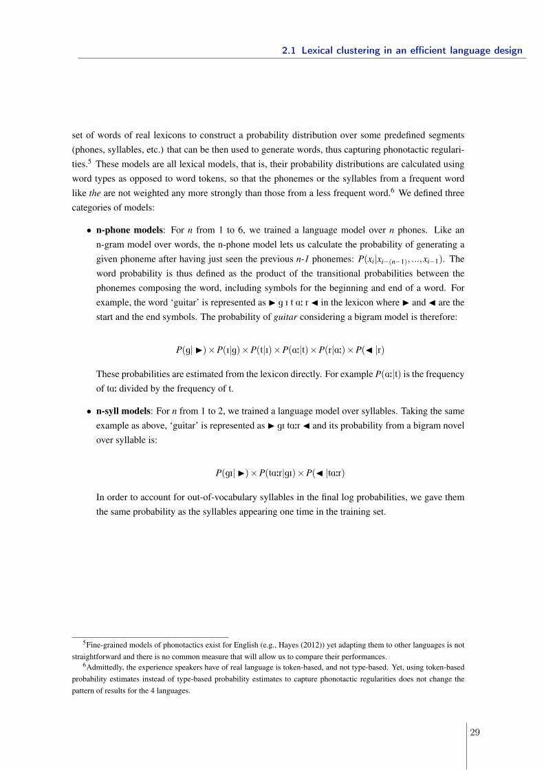
set of words of real lexicons to construct a probability distribution over some predefined segments(phones, syllables, etc.) that can be then used to generate words, thus capturing phonotactic regulari-ties.5 These models are all lexical models, that is, their probability distributions are calculated usingword types as opposed to word tokens, so that the phonemes or the syllables from a frequent wordlike the are not weighted any more strongly than those from a less frequent word.6 We defined threecategories of models:
• n-phone models: For n from 1 to 6, we trained a language model over n phones. Like ann-gram model over words, the n-phone model lets us calculate the probability of generating agiven phoneme after having just seen the previous n-1 phonemes: P(xi|xi−(n−1), ...,xi−1). Theword probability is thus defined as the product of the transitional probabilities between thephonemes composing the word, including symbols for the beginning and end of a word. Forexample, the word ‘guitar’ is represented as I g I t A: r J in the lexicon where I and J are thestart and the end symbols. The probability of guitar considering a bigram model is therefore:
P(g|I)×P(I|g)×P(t|I)×P(A:|t)×P(r|A:)×P(J |r)
These probabilities are estimated from the lexicon directly. For example P(A:|t) is the frequencyof tA: divided by the frequency of t.
• n-syll models: For n from 1 to 2, we trained a language model over syllables. Taking the sameexample as above, ‘guitar’ is represented as I gI tA:r J and its probability from a bigram novelover syllable is:
P(gI|I)×P(tA:r|gI)×P(J |tA:r)
In order to account for out-of-vocabulary syllables in the final log probabilities, we gave themthe same probability as the syllables appearing one time in the training set.
5Fine-grained models of phonotactics exist for English (e.g., Hayes (2012)) yet adapting them to other languages is notstraightforward and there is no common measure that will allow us to compare their performances.
6Admittedly, the experience speakers have of real language is token-based, and not type-based. Yet, using token-basedprobability estimates instead of type-based probability estimates to capture phonotactic regularities does not change thepattern of results for the 4 languages.
2.1 Lexical clustering in an efficient language design
29
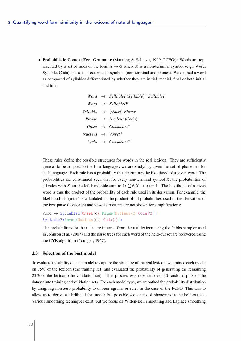
• Probabilistic Context Free Grammar (Manning & Schutze, 1999, PCFG;): Words are rep-resented by a set of rules of the form X → α where X is a non-terminal symbol (e.g., Word,Syllable, Coda) and α is a sequence of symbols (non-terminal and phones). We defined a wordas composed of syllables differentiated by whether they are initial, medial, final or both initialand final.
Word → SyllableI (Syllable)+ SyllableF
Word → SyllableIF
Syllable → (Onset) Rhyme
Rhyme → Nucleus (Coda)
Onset → Consonant+
Nucleus → Vowel+
Coda → Consonant+
These rules define the possible structures for words in the real lexicon. They are sufficientlygeneral to be adapted to the four languages we are studying, given the set of phonemes foreach language. Each rule has a probability that determines the likelihood of a given word. Theprobabilities are constrained such that for every non-terminal symbol X , the probabilities ofall rules with X on the left-hand side sum to 1: ∑P(X → α) = 1. The likelihood of a givenword is thus the product of the probability of each rule used in its derivation. For example, thelikelihood of ‘guitar’ is calculated as the product of all probabilities used in the derivation ofthe best parse (consonant and vowel structures are not shown for simplification):
Word → SyllableI(Onset(g) Rhyme(Nucleus(I) Coda(t)))
SyllableF(Rhyme(Nucleus(A:) Coda(r)))
The probabilities for the rules are inferred from the real lexicon using the Gibbs sampler usedin Johnson et al. (2007) and the parse trees for each word of the held-out set are recovered usingthe CYK algorithm (Younger, 1967).
2.3 Selection of the best model
To evaluate the ability of each model to capture the structure of the real lexicon, we trained each modelon 75% of the lexicon (the training set) and evaluated the probability of generating the remaining25% of the lexicon (the validation set). This process was repeated over 30 random splits of thedataset into training and validation sets. For each model type, we smoothed the probability distributionby assigning non-zero probability to unseen ngrams or rules in the case of the PCFG. This was toallow us to derive a likelihood for unseen but possible sequences of phonemes in the held-out set.Various smoothing techniques exist, but we focus on Witten-Bell smoothing and Laplace smoothing
2 Quantifying word form similarity in the lexicons of natural languages
30
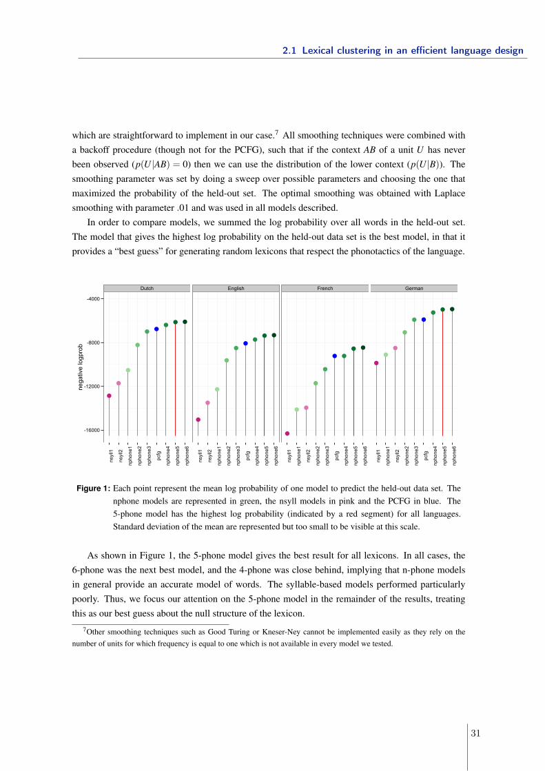
which are straightforward to implement in our case.7 All smoothing techniques were combined witha backoff procedure (though not for the PCFG), such that if the context AB of a unit U has neverbeen observed (p(U |AB) = 0) then we can use the distribution of the lower context (p(U |B)). Thesmoothing parameter was set by doing a sweep over possible parameters and choosing the one thatmaximized the probability of the held-out set. The optimal smoothing was obtained with Laplacesmoothing with parameter .01 and was used in all models described.
In order to compare models, we summed the log probability over all words in the held-out set.The model that gives the highest log probability on the held-out data set is the best model, in that itprovides a “best guess” for generating random lexicons that respect the phonotactics of the language.
Dutch English French German
-16000
-12000
-8000
-4000
nsyll1
nsyll2
nphone1
nphone2
nphone3
pcfg
nphone4
nphone5
nphone6
nsyll1
nsyll2
nphone1
nphone2
nphone3
pcfg
nphone4
nphone5
nphone6
nsyll1
nphone1
nsyll2
nphone2
nphone3
pcfg
nphone4
nphone5
nphone6
nsyll1
nphone1
nsyll2
nphone2
nphone3
pcfg
nphone4
nphone5
nphone6
nega
tive
logp
rob
Figure 1: Each point represent the mean log probability of one model to predict the held-out data set. Thenphone models are represented in green, the nsyll models in pink and the PCFG in blue. The5-phone model has the highest log probability (indicated by a red segment) for all languages.Standard deviation of the mean are represented but too small to be visible at this scale.
As shown in Figure 1, the 5-phone model gives the best result for all lexicons. In all cases, the6-phone was the next best model, and the 4-phone was close behind, implying that n-phone modelsin general provide an accurate model of words. The syllable-based models performed particularlypoorly. Thus, we focus our attention on the 5-phone model in the remainder of the results, treatingthis as our best guess about the null structure of the lexicon.
7Other smoothing techniques such as Good Turing or Kneser-Ney cannot be implemented easily as they rely on thenumber of units for which frequency is equal to one which is not available in every model we tested.
2.1 Lexical clustering in an efficient language design
31
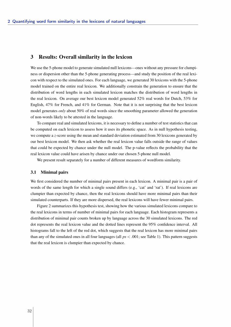
3 Results: Overall similarity in the lexicon
We use the 5-phone model to generate simulated null lexicons—ones without any pressure for clumpi-ness or dispersion other than the 5-phone generating process—and study the position of the real lexi-con with respect to the simulated ones. For each language, we generated 30 lexicons with the 5-phonemodel trained on the entire real lexicon. We additionally constrain the generation to ensure that thedistribution of word lengths in each simulated lexicon matches the distribution of word lengths inthe real lexicon. On average our best lexicon model generated 52% real words for Dutch, 53% forEnglish, 47% for French, and 41% for German. Note that it is not surprising that the best lexiconmodel generates only about 50% of real words since the smoothing parameter allowed the generationof non-words likely to be attested in the language.
To compare real and simulated lexicons, it is necessary to define a number of test statistics that canbe computed on each lexicon to assess how it uses its phonetic space. As in null hypothesis testing,we compute a z-score using the mean and standard deviation estimated from 30 lexicons generated byour best lexicon model. We then ask whether the real lexicon value falls outside the range of valuesthat could be expected by chance under the null model. The p-value reflects the probability that thereal lexicon value could have arisen by chance under our chosen 5-phone null model.
We present result separately for a number of different measures of wordform similarity.
3.1 Minimal pairs
We first considered the number of minimal pairs present in each lexicon. A minimal pair is a pair ofwords of the same length for which a single sound differs (e.g., ‘cat’ and ‘rat’). If real lexicons areclumpier than expected by chance, then the real lexicons should have more minimal pairs than theirsimulated counterparts. If they are more dispersed, the real lexicons will have fewer minimal pairs.
Figure 2 summarizes this hypothesis test, showing how the various simulated lexicons compare tothe real lexicons in terms of number of minimal pairs for each language. Each histogram represents adistribution of minimal pair counts broken up by language across the 30 simulated lexicons. The reddot represents the real lexicon value and the dotted lines represent the 95% confidence interval. Allhistograms fall to the left of the red dot, which suggests that the real lexicon has more minimal pairsthan any of the simulated ones in all four languages (all ps < .001; see Table 1). This pattern suggeststhat the real lexicon is clumpier than expected by chance.
2 Quantifying word form similarity in the lexicons of natural languages
32
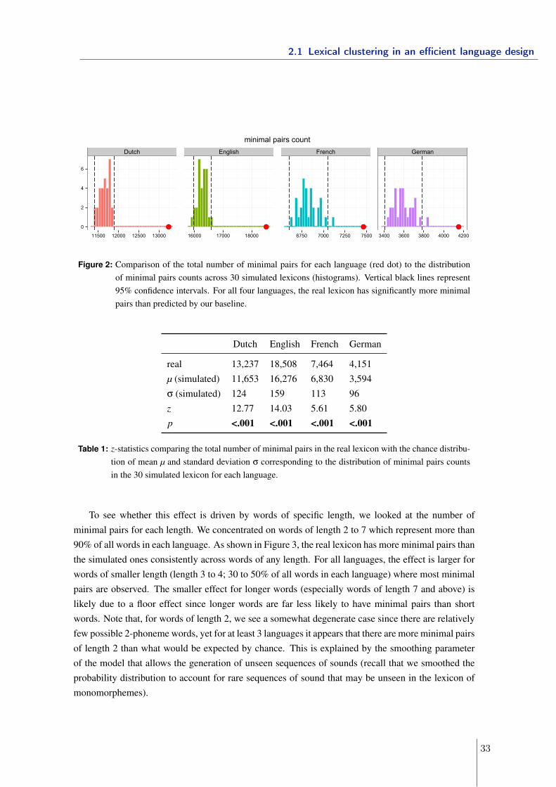
Dutch English French German
0
2
4
6
11500 12000 12500 13000 16000 17000 18000 6750 7000 7250 7500 3400 3600 3800 4000 4200
minimal pairs count
Figure 2: Comparison of the total number of minimal pairs for each language (red dot) to the distributionof minimal pairs counts across 30 simulated lexicons (histograms). Vertical black lines represent95% confidence intervals. For all four languages, the real lexicon has significantly more minimalpairs than predicted by our baseline.
Dutch English French German
real 13,237 18,508 7,464 4,151µ (simulated) 11,653 16,276 6,830 3,594σ (simulated) 124 159 113 96z 12.77 14.03 5.61 5.80p <.001 <.001 <.001 <.001
Table 1: z-statistics comparing the total number of minimal pairs in the real lexicon with the chance distribu-tion of mean µ and standard deviation σ corresponding to the distribution of minimal pairs countsin the 30 simulated lexicon for each language.
To see whether this effect is driven by words of specific length, we looked at the number ofminimal pairs for each length. We concentrated on words of length 2 to 7 which represent more than90% of all words in each language. As shown in Figure 3, the real lexicon has more minimal pairs thanthe simulated ones consistently across words of any length. For all languages, the effect is larger forwords of smaller length (length 3 to 4; 30 to 50% of all words in each language) where most minimalpairs are observed. The smaller effect for longer words (especially words of length 7 and above) islikely due to a floor effect since longer words are far less likely to have minimal pairs than shortwords. Note that, for words of length 2, we see a somewhat degenerate case since there are relativelyfew possible 2-phoneme words, yet for at least 3 languages it appears that there are more minimal pairsof length 2 than what would be expected by chance. This is explained by the smoothing parameterof the model that allows the generation of unseen sequences of sounds (recall that we smoothed theprobability distribution to account for rare sequences of sound that may be unseen in the lexicon ofmonomorphemes).
2.1 Lexical clustering in an efficient language design
33
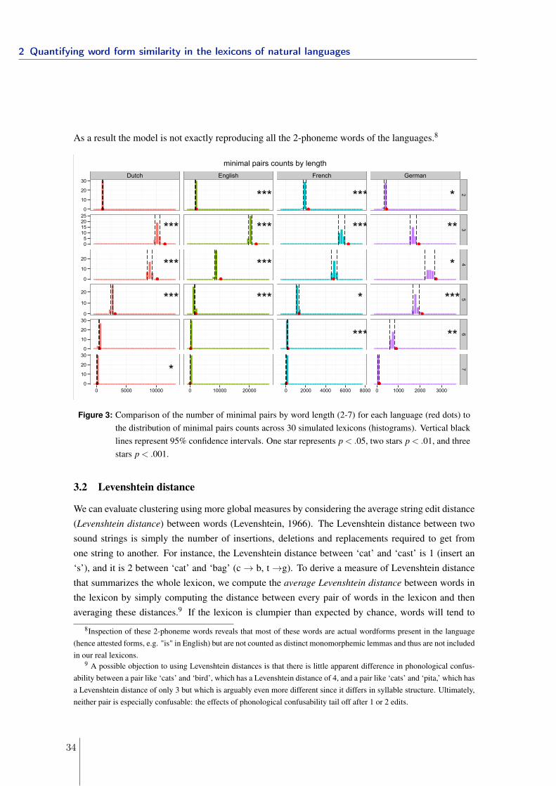
As a result the model is not exactly reproducing all the 2-phoneme words of the languages.8
Dutch English French German
***
***
***
*
***
***
***
***
***
***
*
***
*
**
*
***
**
0
10
20
30
0510152025
0
10
20
0
10
20
0
10
20
30
0
10
20
30
23
45
67
0 5000 10000 0 10000 20000 0 2000 4000 6000 8000 0 1000 2000 3000
minimal pairs counts by length
Figure 3: Comparison of the number of minimal pairs by word length (2-7) for each language (red dots) tothe distribution of minimal pairs counts across 30 simulated lexicons (histograms). Vertical blacklines represent 95% confidence intervals. One star represents p < .05, two stars p < .01, and threestars p < .001.
3.2 Levenshtein distance
We can evaluate clustering using more global measures by considering the average string edit distance(Levenshtein distance) between words (Levenshtein, 1966). The Levenshtein distance between twosound strings is simply the number of insertions, deletions and replacements required to get fromone string to another. For instance, the Levenshtein distance between ‘cat’ and ‘cast’ is 1 (insert an‘s’), and it is 2 between ‘cat’ and ‘bag’ (c→ b, t→g). To derive a measure of Levenshtein distancethat summarizes the whole lexicon, we compute the average Levenshtein distance between words inthe lexicon by simply computing the distance between every pair of words in the lexicon and thenaveraging these distances.9 If the lexicon is clumpier than expected by chance, words will tend to
8Inspection of these 2-phoneme words reveals that most of these words are actual wordforms present in the language(hence attested forms, e.g. "is" in English) but are not counted as distinct monomorphemic lemmas and thus are not includedin our real lexicons.
9 A possible objection to using Levenshtein distances is that there is little apparent difference in phonological confus-ability between a pair like ‘cats’ and ‘bird’, which has a Levenshtein distance of 4, and a pair like ‘cats’ and ‘pita,’ which hasa Levenshtein distance of only 3 but which is arguably even more different since it differs in syllable structure. Ultimately,neither pair is especially confusable: the effects of phonological confusability tail off after 1 or 2 edits.
2 Quantifying word form similarity in the lexicons of natural languages
34
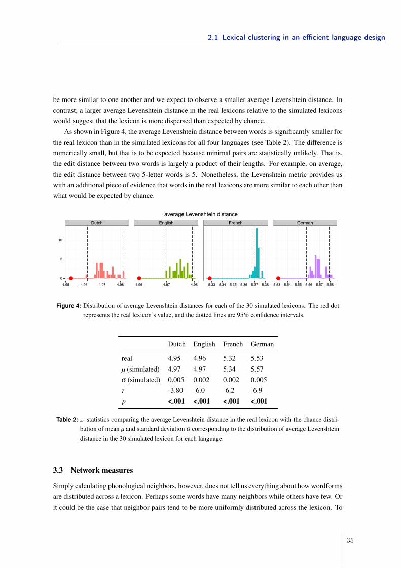
be more similar to one another and we expect to observe a smaller average Levenshtein distance. Incontrast, a larger average Levenshtein distance in the real lexicons relative to the simulated lexiconswould suggest that the lexicon is more dispersed than expected by chance.
As shown in Figure 4, the average Levenshtein distance between words is significantly smaller forthe real lexicon than in the simulated lexicons for all four languages (see Table 2). The difference isnumerically small, but that is to be expected because minimal pairs are statistically unlikely. That is,the edit distance between two words is largely a product of their lengths. For example, on average,the edit distance between two 5-letter words is 5. Nonetheless, the Levenshtein metric provides uswith an additional piece of evidence that words in the real lexicons are more similar to each other thanwhat would be expected by chance.
Dutch English French German
0
5
10
4.95 4.96 4.97 4.98 4.96 4.97 4.98 5.33 5.34 5.35 5.36 5.37 5.38 5.53 5.54 5.55 5.56 5.57 5.58
average Levenshtein distance
Figure 4: Distribution of average Levenshtein distances for each of the 30 simulated lexicons. The red dotrepresents the real lexicon’s value, and the dotted lines are 95% confidence intervals.
Dutch English French German
real 4.95 4.96 5.32 5.53µ (simulated) 4.97 4.97 5.34 5.57σ (simulated) 0.005 0.002 0.002 0.005z -3.80 -6.0 -6.2 -6.9p <.001 <.001 <.001 <.001
Table 2: z- statistics comparing the average Levenshtein distance in the real lexicon with the chance distri-bution of mean µ and standard deviation σ corresponding to the distribution of average Levenshteindistance in the 30 simulated lexicon for each language.
3.3 Network measures
Simply calculating phonological neighbors, however, does not tell us everything about how wordformsare distributed across a lexicon. Perhaps some words have many neighbors while others have few. Orit could be the case that neighbor pairs tend to be more uniformly distributed across the lexicon. To
2.1 Lexical clustering in an efficient language design
35
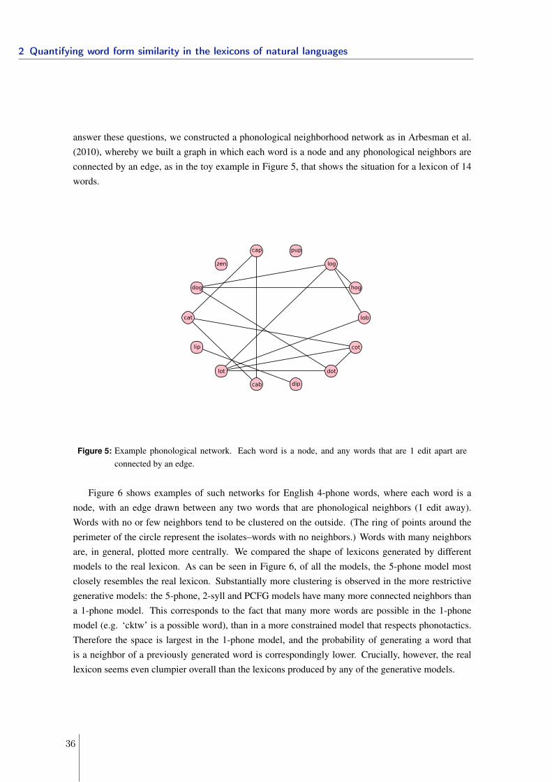
answer these questions, we constructed a phonological neighborhood network as in Arbesman et al.(2010), whereby we built a graph in which each word is a node and any phonological neighbors areconnected by an edge, as in the toy example in Figure 5, that shows the situation for a lexicon of 14words.
lob
hog
log
dip
cap
zen
dog
cat
lip
lot
cab
pup
dot
cot
Figure 5: Example phonological network. Each word is a node, and any words that are 1 edit apart areconnected by an edge.
Figure 6 shows examples of such networks for English 4-phone words, where each word is anode, with an edge drawn between any two words that are phonological neighbors (1 edit away).Words with no or few neighbors tend to be clustered on the outside. (The ring of points around theperimeter of the circle represent the isolates–words with no neighbors.) Words with many neighborsare, in general, plotted more centrally. We compared the shape of lexicons generated by differentmodels to the real lexicon. As can be seen in Figure 6, of all the models, the 5-phone model mostclosely resembles the real lexicon. Substantially more clustering is observed in the more restrictivegenerative models: the 5-phone, 2-syll and PCFG models have many more connected neighbors thana 1-phone model. This corresponds to the fact that many more words are possible in the 1-phonemodel (e.g. ‘cktw’ is a possible word), than in a more constrained model that respects phonotactics.Therefore the space is largest in the 1-phone model, and the probability of generating a word thatis a neighbor of a previously generated word is correspondingly lower. Crucially, however, the reallexicon seems even clumpier overall than the lexicons produced by any of the generative models.
2 Quantifying word form similarity in the lexicons of natural languages
36

Figure 6: Sampling of phonological neighbor network from the different generative models applied on all4-phone wordforms of the English lexicon. Each point is a word, and any two connected words arephonological neighbors. The simulated lexicons from less constrained generative models are lessclustered and have more isolates (words with no neighbors, plotted on the outside ring).
Using techniques from network analysis that have been fruitfully applied to describe social net-works and other complex systems (Barabási & Albert, 1999; Wasserman & Faust, 1994; Watts &Strogatz, 1998), we can quantitatively characterize the clustering behavior of the lexicon. We com-puted the transitivity, average clustering coefficient, and the percent of nodes in the giant component.All three of these measures can be used to evaluate how tightly clustered the words in the lexicon are.A graph’s transitivity is the ratio of the number of triangles (a set of 3 nodes in which each node in theset is connected to both other nodes in the set) to the number of triads (a set of 3 nodes in which at leasttwo of the nodes are connected). Thus, transitivity in effect asks, given that A is connected to B andB is connected to C, how likely is it that A is also connected to C? The average clustering coefficientis a closely related measure that finds the average clustering coefficient across all nodes, where theclustering coefficient of a node is defined as the fraction of possible triangles that could go throughthat node that actually do go through that node. Both values measure the extent to which nodes clustertogether. The largest cluster in a network is known as the giant component. A network with manyisolated nodes will have a relatively small giant component, whereas one in which nodes are tightlyclustered will have a large giant component. These measures give us some insight into the internalstructure of the lexicon, over and above those obtained by looking at more global measures such asthe number of minimal pairs and the average Levenshtein distance. If the real lexicon is clumpier thanexpected by chance, we predict that, relative to the simulated lexicons, the real lexicons will showhigher transitivity, higher average clustering coefficients, and a larger proportion of words in the giantcomponent.
2.1 Lexical clustering in an efficient language design
37
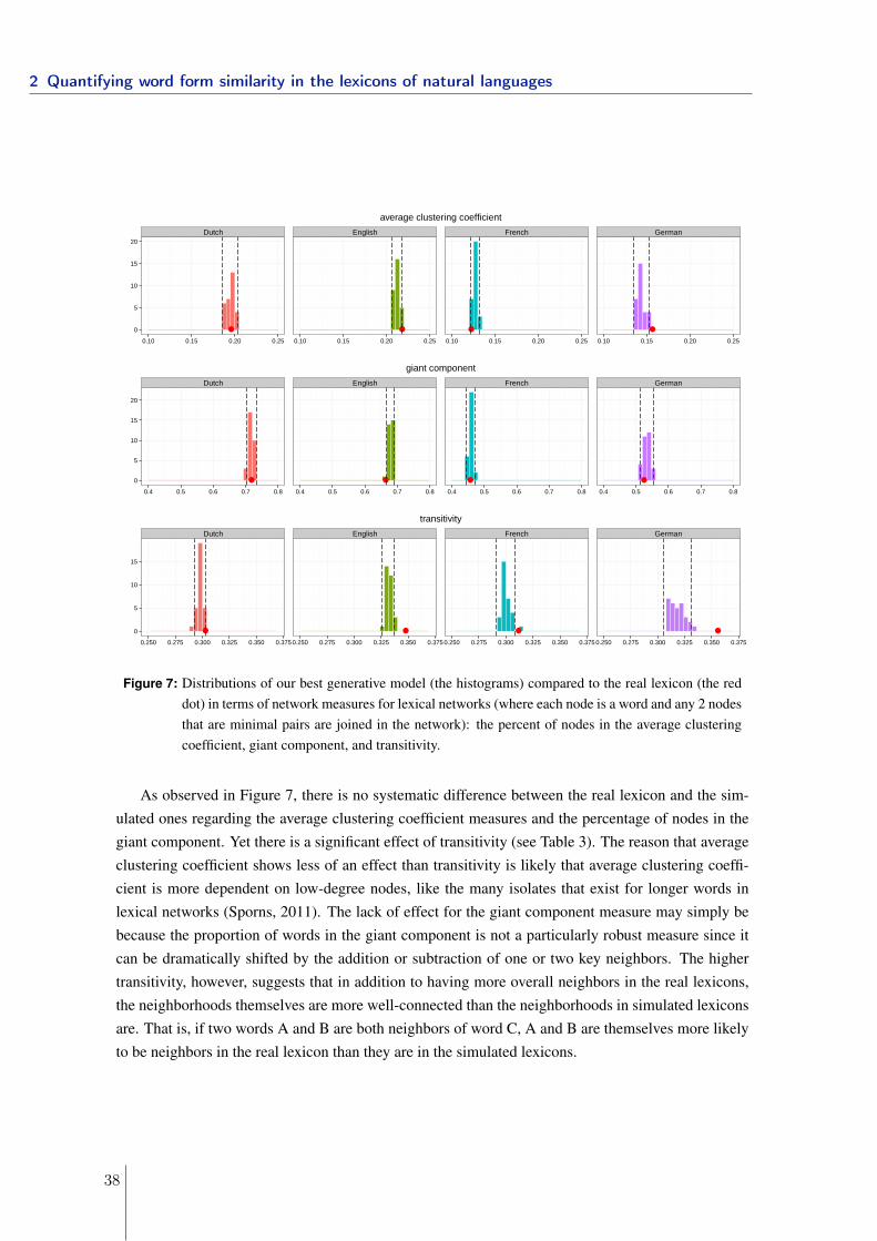
Dutch English French German
● ● ● ●0
5
10
15
20
0.10 0.15 0.20 0.25 0.10 0.15 0.20 0.25 0.10 0.15 0.20 0.25 0.10 0.15 0.20 0.25
average clustering coefficient
Dutch English French German
● ● ● ●0
5
10
15
20
0.4 0.5 0.6 0.7 0.8 0.4 0.5 0.6 0.7 0.8 0.4 0.5 0.6 0.7 0.8 0.4 0.5 0.6 0.7 0.8
giant component
Dutch English French German
● ● ● ●0
5
10
15
0.250 0.275 0.300 0.325 0.350 0.375 0.250 0.275 0.300 0.325 0.350 0.375 0.250 0.275 0.300 0.325 0.350 0.375 0.250 0.275 0.300 0.325 0.350 0.375
transitivity
Figure 7: Distributions of our best generative model (the histograms) compared to the real lexicon (the reddot) in terms of network measures for lexical networks (where each node is a word and any 2 nodesthat are minimal pairs are joined in the network): the percent of nodes in the average clusteringcoefficient, giant component, and transitivity.
As observed in Figure 7, there is no systematic difference between the real lexicon and the sim-ulated ones regarding the average clustering coefficient measures and the percentage of nodes in thegiant component. Yet there is a significant effect of transitivity (see Table 3). The reason that averageclustering coefficient shows less of an effect than transitivity is likely that average clustering coeffi-cient is more dependent on low-degree nodes, like the many isolates that exist for longer words inlexical networks (Sporns, 2011). The lack of effect for the giant component measure may simply bebecause the proportion of words in the giant component is not a particularly robust measure since itcan be dramatically shifted by the addition or subtraction of one or two key neighbors. The highertransitivity, however, suggests that in addition to having more overall neighbors in the real lexicons,the neighborhoods themselves are more well-connected than the neighborhoods in simulated lexiconsare. That is, if two words A and B are both neighbors of word C, A and B are themselves more likelyto be neighbors in the real lexicon than they are in the simulated lexicons.
2 Quantifying word form similarity in the lexicons of natural languages
38
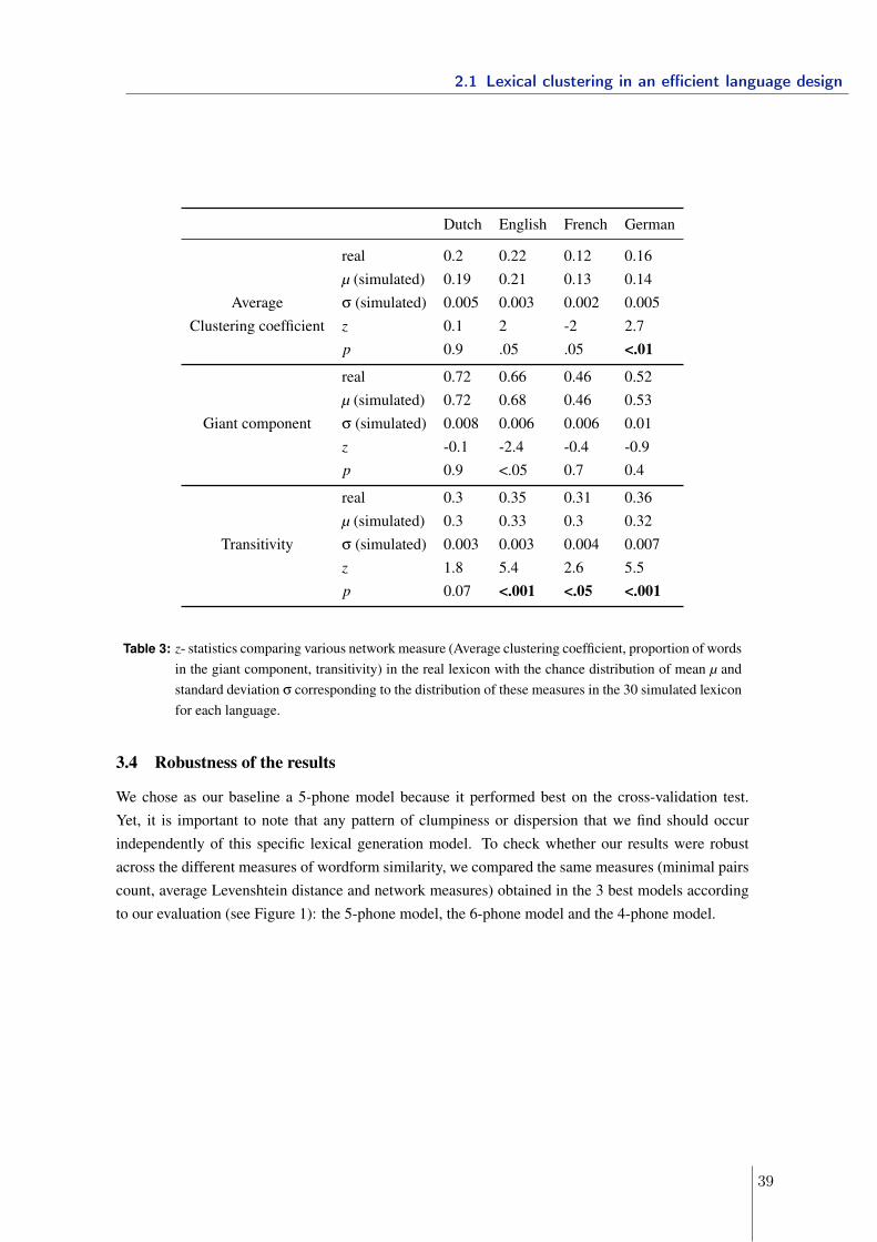
Dutch English French German
real 0.2 0.22 0.12 0.16µ (simulated) 0.19 0.21 0.13 0.14
Average σ (simulated) 0.005 0.003 0.002 0.005Clustering coefficient z 0.1 2 -2 2.7
p 0.9 .05 .05 <.01
real 0.72 0.66 0.46 0.52µ (simulated) 0.72 0.68 0.46 0.53
Giant component σ (simulated) 0.008 0.006 0.006 0.01z -0.1 -2.4 -0.4 -0.9p 0.9 <.05 0.7 0.4
real 0.3 0.35 0.31 0.36µ (simulated) 0.3 0.33 0.3 0.32
Transitivity σ (simulated) 0.003 0.003 0.004 0.007z 1.8 5.4 2.6 5.5p 0.07 <.001 <.05 <.001
Table 3: z- statistics comparing various network measure (Average clustering coefficient, proportion of wordsin the giant component, transitivity) in the real lexicon with the chance distribution of mean µ andstandard deviation σ corresponding to the distribution of these measures in the 30 simulated lexiconfor each language.
3.4 Robustness of the results
We chose as our baseline a 5-phone model because it performed best on the cross-validation test.Yet, it is important to note that any pattern of clumpiness or dispersion that we find should occurindependently of this specific lexical generation model. To check whether our results were robustacross the different measures of wordform similarity, we compared the same measures (minimal pairscount, average Levenshtein distance and network measures) obtained in the 3 best models accordingto our evaluation (see Figure 1): the 5-phone model, the 6-phone model and the 4-phone model.
2.1 Lexical clustering in an efficient language design
39
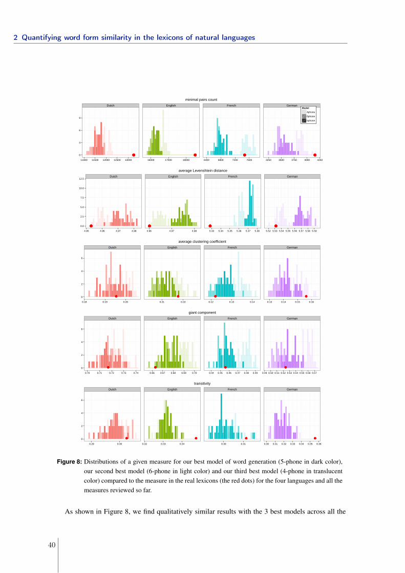
Dutch English French German
●●● ●●● ●●● ●●●0
3
6
9
11000 11500 12000 12500 13000 16000 17000 18000 6400 6800 7200 7600 3250 3500 3750 4000 4250
Model
4phone
6phone
5phone
minimal pairs count
Dutch English French German
●●● ●●● ●●● ●●●0.0
2.5
5.0
7.5
10.0
12.5
4.95 4.96 4.97 4.98 4.96 4.97 4.98 5.33 5.34 5.35 5.36 5.37 5.38 5.52 5.53 5.54 5.55 5.56 5.57 5.58 5.59
average Levenshtein distance
Dutch English French German
●●● ●●● ●●● ●●●0
2
4
6
0.18 0.19 0.20 0.21 0.22 0.12 0.13 0.14 0.13 0.14 0.15 0.16
average clustering coefficient
Dutch English French German
●●● ●●● ●●● ●●●0
2
4
6
0.70 0.71 0.72 0.73 0.74 0.66 0.67 0.68 0.69 0.70 0.44 0.45 0.46 0.47 0.48 0.49 0.49 0.50 0.51 0.52 0.53 0.54 0.55 0.56 0.57
giant component
Dutch English French German
●●● ●●● ●●● ●●●0
2
4
6
0.29 0.30 0.32 0.33 0.34 0.30 0.31 0.30 0.31 0.32 0.33 0.34 0.35 0.36
transitivity
Figure 8: Distributions of a given measure for our best model of word generation (5-phone in dark color),our second best model (6-phone in light color) and our third best model (4-phone in translucentcolor) compared to the measure in the real lexicons (the red dots) for the four languages and all themeasures reviewed so far.
As shown in Figure 8, we find qualitatively similar results with the 3 best models across all the
2 Quantifying word form similarity in the lexicons of natural languages
40
measures of wordform similarity previously introduced.10 In general, there were more minimal pairsand lower average Levenshtein distance in the real lexicons than across the three best models. As forthe 5-phone model, no conclusive results were obtained for the average clustering coefficient and thegiant component measures but the transitivity was higher in the real lexicons than in the three bestmodels of lexicons.
This is evidence that the pattern of clumpiness we found with the 5-phone model is robust acrosslexical generation models. A pressure for clumpiness is thus visible beyond the particular model ofphonotactic probability adopted by the best models produced here.
We also tested whether the German, Dutch, and French infinitival verb endings could be drivingclumpiness effects by redoing the analyses above using just root forms (i.e., by removing the infinitivalending from the verbs). One might imagine that, because most verbs end in -er in French, for instance,these words have fewer degrees of freedom and thus edit distances will be smaller across the lexicon.In our analysis using just root forms, however, the results were qualitatively the same as when we usedlemmas in their infinitive form, likely because the generative models already capture this regularity.That is, our baseline models too have a disproportionate number of words ending in -er in Frenchand -en in German and Dutch. Because the presence of these infinitival stems does not substantiallyalter the result, we chose to keep them in the main analysis so as to be consistent with the standarddatabases we used (CELEX and Lexique).
3.5 Interim summary
In general, these measures suggest that the lexicon is clumpy: words tend to be more phonologicallysimilar to each other than would be expected by chance. Word pairs in the real lexicon are more likelyto be minimal pairs and more likely to have a small edit distance compared to words in the “chance”simulated lexicons. The chance rate here was determined through a priori model comparison ofdifferent plausible generating models for words. This technique has allowed us to test for clumpinessvs. dispersion while still respecting the major phonotactic tendencies in each language. It is importantto emphasize that these results were computed on monomorphemes, so the results are not an artifactof morphology.
Crucially, the lexicon shows a tendency towards clumpiness above and beyond phonotactics. Aswe discussed earlier, phonotactic rules themselves can be thought of as a major source of clumpinessin the lexicon, insofar as phonotactics dramatically restricts the space of possible words. Yet, while ourbest lexical model controls for phonotactic regularity, we still observe clumpiness in the real lexiconcompared to this baseline. This suggests additional pressure for clustering beyond just phonotactics.
10The 3-phone model behaves somewhat differently and in fact shows more clustering than the 5-phone model. But,because its performance on the held-out data set is poor compared to the models shown here, we do not focus on this model.
2.1 Lexical clustering in an efficient language design
41
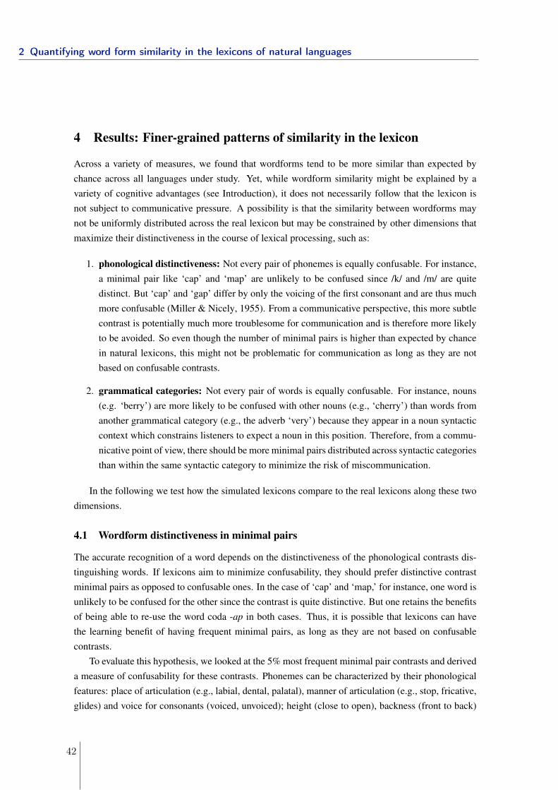
4 Results: Finer-grained patterns of similarity in the lexicon
Across a variety of measures, we found that wordforms tend to be more similar than expected bychance across all languages under study. Yet, while wordform similarity might be explained by avariety of cognitive advantages (see Introduction), it does not necessarily follow that the lexicon isnot subject to communicative pressure. A possibility is that the similarity between wordforms maynot be uniformly distributed across the real lexicon but may be constrained by other dimensions thatmaximize their distinctiveness in the course of lexical processing, such as:
1. phonological distinctiveness: Not every pair of phonemes is equally confusable. For instance,a minimal pair like ‘cap’ and ‘map’ are unlikely to be confused since /k/ and /m/ are quitedistinct. But ‘cap’ and ‘gap’ differ by only the voicing of the first consonant and are thus muchmore confusable (Miller & Nicely, 1955). From a communicative perspective, this more subtlecontrast is potentially much more troublesome for communication and is therefore more likelyto be avoided. So even though the number of minimal pairs is higher than expected by chancein natural lexicons, this might not be problematic for communication as long as they are notbased on confusable contrasts.
2. grammatical categories: Not every pair of words is equally confusable. For instance, nouns(e.g. ‘berry’) are more likely to be confused with other nouns (e.g., ‘cherry’) than words fromanother grammatical category (e.g., the adverb ‘very’) because they appear in a noun syntacticcontext which constrains listeners to expect a noun in this position. Therefore, from a commu-nicative point of view, there should be more minimal pairs distributed across syntactic categoriesthan within the same syntactic category to minimize the risk of miscommunication.
In the following we test how the simulated lexicons compare to the real lexicons along these twodimensions.
4.1 Wordform distinctiveness in minimal pairs
The accurate recognition of a word depends on the distinctiveness of the phonological contrasts dis-tinguishing words. If lexicons aim to minimize confusability, they should prefer distinctive contrastminimal pairs as opposed to confusable ones. In the case of ‘cap’ and ‘map,’ for instance, one word isunlikely to be confused for the other since the contrast is quite distinctive. But one retains the benefitsof being able to re-use the word coda -ap in both cases. Thus, it is possible that lexicons can havethe learning benefit of having frequent minimal pairs, as long as they are not based on confusablecontrasts.
To evaluate this hypothesis, we looked at the 5% most frequent minimal pair contrasts and deriveda measure of confusability for these contrasts. Phonemes can be characterized by their phonologicalfeatures: place of articulation (e.g., labial, dental, palatal), manner of articulation (e.g., stop, fricative,glides) and voice for consonants (voiced, unvoiced); height (close to open), backness (front to back)
2 Quantifying word form similarity in the lexicons of natural languages
42
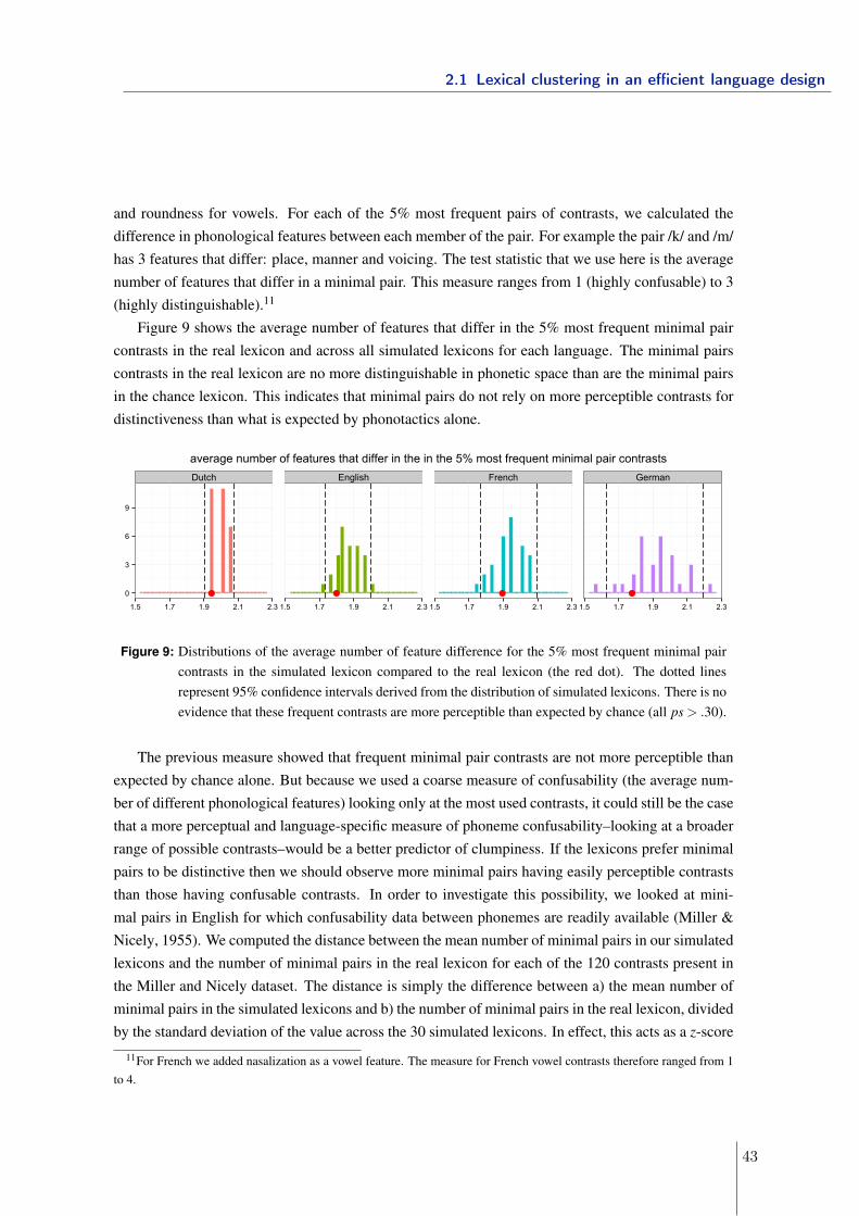
and roundness for vowels. For each of the 5% most frequent pairs of contrasts, we calculated thedifference in phonological features between each member of the pair. For example the pair /k/ and /m/has 3 features that differ: place, manner and voicing. The test statistic that we use here is the averagenumber of features that differ in a minimal pair. This measure ranges from 1 (highly confusable) to 3(highly distinguishable).11
Figure 9 shows the average number of features that differ in the 5% most frequent minimal paircontrasts in the real lexicon and across all simulated lexicons for each language. The minimal pairscontrasts in the real lexicon are no more distinguishable in phonetic space than are the minimal pairsin the chance lexicon. This indicates that minimal pairs do not rely on more perceptible contrasts fordistinctiveness than what is expected by phonotactics alone.
Dutch English French German
0
3
6
9
1.5 1.7 1.9 2.1 2.3 1.5 1.7 1.9 2.1 2.3 1.5 1.7 1.9 2.1 2.3 1.5 1.7 1.9 2.1 2.3
average number of features that differ in the in the 5% most frequent minimal pair contrasts
Figure 9: Distributions of the average number of feature difference for the 5% most frequent minimal paircontrasts in the simulated lexicon compared to the real lexicon (the red dot). The dotted linesrepresent 95% confidence intervals derived from the distribution of simulated lexicons. There is noevidence that these frequent contrasts are more perceptible than expected by chance (all ps > .30).
The previous measure showed that frequent minimal pair contrasts are not more perceptible thanexpected by chance alone. But because we used a coarse measure of confusability (the average num-ber of different phonological features) looking only at the most used contrasts, it could still be the casethat a more perceptual and language-specific measure of phoneme confusability–looking at a broaderrange of possible contrasts–would be a better predictor of clumpiness. If the lexicons prefer minimalpairs to be distinctive then we should observe more minimal pairs having easily perceptible contraststhan those having confusable contrasts. In order to investigate this possibility, we looked at mini-mal pairs in English for which confusability data between phonemes are readily available (Miller &Nicely, 1955). We computed the distance between the mean number of minimal pairs in our simulatedlexicons and the number of minimal pairs in the real lexicon for each of the 120 contrasts present inthe Miller and Nicely dataset. The distance is simply the difference between a) the mean number ofminimal pairs in the simulated lexicons and b) the number of minimal pairs in the real lexicon, dividedby the standard deviation of the value across the 30 simulated lexicons. In effect, this acts as a z-score
11For French we added nasalization as a vowel feature. The measure for French vowel contrasts therefore ranged from 1to 4.
2.1 Lexical clustering in an efficient language design
43
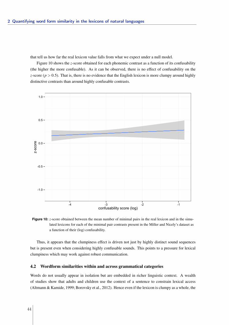
that tell us how far the real lexicon value falls from what we expect under a null model.Figure 10 shows the z-score obtained for each phonemic contrast as a function of its confusability
(the higher the more confusable). As it can be observed, there is no effect of confusability on thez-score (p > 0.5). That is, there is no evidence that the English lexicon is more clumpy around highlydistinctive contrasts than around highly confusable contrasts.
-1.0
-0.5
0.0
0.5
1.0
-4 -3 -2 -1confusability score (log)
z-score
Figure 10: z-score obtained between the mean number of minimal pairs in the real lexicon and in the simu-lated lexicons for each of the minimal pair contrasts present in the Miller and Nicely’s dataset asa function of their (log) confusability.
Thus, it appears that the clumpiness effect is driven not just by highly distinct sound sequencesbut is present even when considering highly confusable sounds. This points to a pressure for lexicalclumpiness which may work against robust communication.
4.2 Wordform similarities within and across grammatical categories
Words do not usually appear in isolation but are embedded in richer linguistic context. A wealthof studies show that adults and children use the context of a sentence to constrain lexical access(Altmann & Kamide, 1999; Borovsky et al., 2012). Hence even if the lexicon is clumpy as a whole, the
2 Quantifying word form similarity in the lexicons of natural languages
44
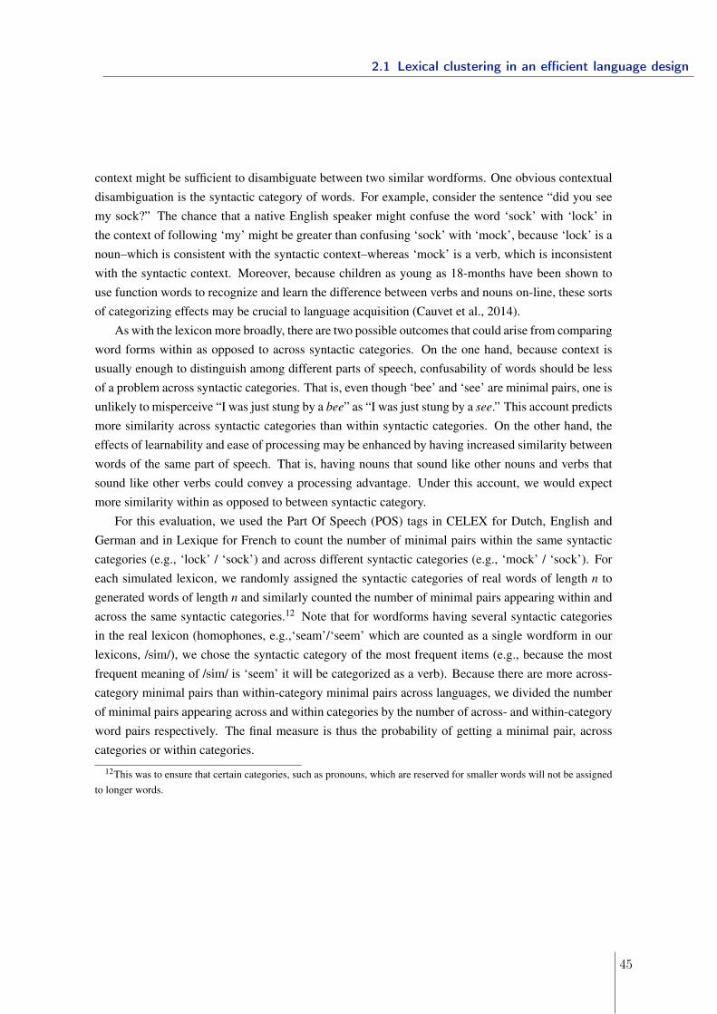
context might be sufficient to disambiguate between two similar wordforms. One obvious contextualdisambiguation is the syntactic category of words. For example, consider the sentence “did you seemy sock?” The chance that a native English speaker might confuse the word ‘sock’ with ‘lock’ inthe context of following ‘my’ might be greater than confusing ‘sock’ with ‘mock’, because ‘lock’ is anoun–which is consistent with the syntactic context–whereas ‘mock’ is a verb, which is inconsistentwith the syntactic context. Moreover, because children as young as 18-months have been shown touse function words to recognize and learn the difference between verbs and nouns on-line, these sortsof categorizing effects may be crucial to language acquisition (Cauvet et al., 2014).
As with the lexicon more broadly, there are two possible outcomes that could arise from comparingword forms within as opposed to across syntactic categories. On the one hand, because context isusually enough to distinguish among different parts of speech, confusability of words should be lessof a problem across syntactic categories. That is, even though ‘bee’ and ‘see’ are minimal pairs, one isunlikely to misperceive “I was just stung by a bee” as “I was just stung by a see.” This account predictsmore similarity across syntactic categories than within syntactic categories. On the other hand, theeffects of learnability and ease of processing may be enhanced by having increased similarity betweenwords of the same part of speech. That is, having nouns that sound like other nouns and verbs thatsound like other verbs could convey a processing advantage. Under this account, we would expectmore similarity within as opposed to between syntactic category.
For this evaluation, we used the Part Of Speech (POS) tags in CELEX for Dutch, English andGerman and in Lexique for French to count the number of minimal pairs within the same syntacticcategories (e.g., ‘lock’ / ‘sock’) and across different syntactic categories (e.g., ‘mock’ / ‘sock’). Foreach simulated lexicon, we randomly assigned the syntactic categories of real words of length n togenerated words of length n and similarly counted the number of minimal pairs appearing within andacross the same syntactic categories.12 Note that for wordforms having several syntactic categoriesin the real lexicon (homophones, e.g.,‘seam’/‘seem’ which are counted as a single wordform in ourlexicons, /sim/), we chose the syntactic category of the most frequent items (e.g., because the mostfrequent meaning of /sim/ is ‘seem’ it will be categorized as a verb). Because there are more across-category minimal pairs than within-category minimal pairs across languages, we divided the numberof minimal pairs appearing across and within categories by the number of across- and within-categoryword pairs respectively. The final measure is thus the probability of getting a minimal pair, acrosscategories or within categories.
12This was to ensure that certain categories, such as pronouns, which are reserved for smaller words will not be assignedto longer words.
2.1 Lexical clustering in an efficient language design
45
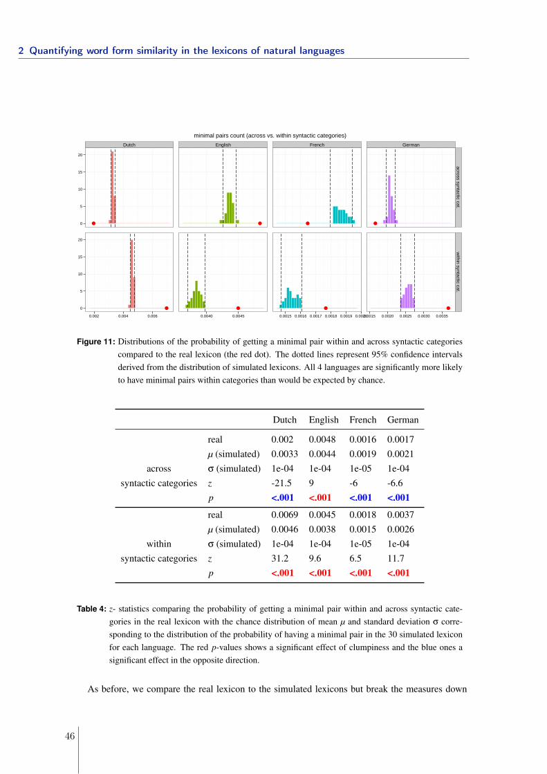
Dutch English French German
●
●
●
●
●
●
●
●
0
5
10
15
20
0
5
10
15
20
across syntactic cat.w
ithin syntactic cat.
0.002 0.004 0.006 0.0040 0.0045 0.0015 0.0016 0.0017 0.0018 0.0019 0.00200.0015 0.0020 0.0025 0.0030 0.0035
minimal pairs count (across vs. within syntactic categories)
Figure 11: Distributions of the probability of getting a minimal pair within and across syntactic categoriescompared to the real lexicon (the red dot). The dotted lines represent 95% confidence intervalsderived from the distribution of simulated lexicons. All 4 languages are significantly more likelyto have minimal pairs within categories than would be expected by chance.
Dutch English French German
real 0.002 0.0048 0.0016 0.0017µ (simulated) 0.0033 0.0044 0.0019 0.0021
across σ (simulated) 1e-04 1e-04 1e-05 1e-04syntactic categories z -21.5 9 -6 -6.6
p <.001 <.001 <.001 <.001
real 0.0069 0.0045 0.0018 0.0037µ (simulated) 0.0046 0.0038 0.0015 0.0026
within σ (simulated) 1e-04 1e-04 1e-05 1e-04syntactic categories z 31.2 9.6 6.5 11.7
p <.001 <.001 <.001 <.001
Table 4: z- statistics comparing the probability of getting a minimal pair within and across syntactic cate-gories in the real lexicon with the chance distribution of mean µ and standard deviation σ corre-sponding to the distribution of the probability of having a minimal pair in the 30 simulated lexiconfor each language. The red p-values shows a significant effect of clumpiness and the blue ones asignificant effect in the opposite direction.
As before, we compare the real lexicon to the simulated lexicons but break the measures down
2 Quantifying word form similarity in the lexicons of natural languages
46
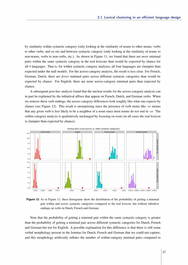
by similarity within syntactic category (only looking at the similarity of nouns to other nouns, verbsto other verbs, and so on) and between syntactic category (only looking at the similarity of nouns tonon-nouns, verbs to non-verbs, etc.). As shown in Figure 11, we found that there are more minimalpairs within the same syntactic category in the real lexicons than would be expected by chance forall 4 languages. That is, for within syntactic category analyses, all four languages are clumpier thanexpected under the null models. For the across-category analysis, the result is less clear. For French,German, Dutch, there are fewer minimal pairs across different syntactic categories than would beexpected by chance. For English, there are more across-category minimal pairs than expected bychance.
A subsequent post-hoc analysis found that the unclear results for the across-category analysis canin part be explained by the infinitival affixes that appear on French, Dutch, and German verbs. Whenwe remove these verb endings, the across-category differences look roughly like what one expects bychance (see Figure 12). This result is unsurprising since the presence of verb stems like -er meansthat any given verb is less likely to be a neighbor of a noun since most nouns do not end in -er. Thewithin-category analysis is qualitatively unchanged by focusing on roots (in all cases the real lexiconis clumpier than expected by chance).
Dutch (roots) English French (roots) German (roots)
●
●
●
●
●
●
●
●
0.0
2.5
5.0
7.5
10.0
12.5
0.0
2.5
5.0
7.5
10.0
12.5
across syntactic cat.w
ithin syntactic cat.
0.0055 0.0060 0.0065 0.0070 0.0040 0.0045 0.0016 0.0018 0.0020 0.0022 0.00275 0.00300 0.00325 0.00350 0.00375
minimal pairs count (across vs. within syntactic categories)
Figure 12: As in Figure 11, these histograms show the distribution of the probability of getting a minimalpair within and across syntactic categories compared to the real lexicon, but without infinitiveendings on verbs in Dutch, French and German.
Note that the probability of getting a minimal pair within the same syntactic category is greaterthan the probability of getting a minimal pair across different syntactic categories for Dutch, Frenchand German but not for English. A possible explanation for this difference is that there is still someverbal morphology present in the lemmas for Dutch, French and German that we could not capture,and this morphology artificially inflates the number of within-category minimal pairs compared to
2.1 Lexical clustering in an efficient language design
47
the number of across-category minimal pairs. For instance, in Dutch, verbs of motion systematicallydisplay phonaesthemes (typically a schwa followed by a sonorant) that are not analyzed as suffixes.Another possibility for this difference is that the probability of getting a minimal pair across andwithin syntactic categories may not be directly comparable because the length distributions for withincategory words and across categories words are different and may thus drive part of the differencefound here. As a result we prefer to concentrate on the comparison of the real lexicon with thesimulated lexicons.
4.3 Interim summary
To sum up, we did not find evidence that clumpiness is more likely among perceptible than confusablephonological contrasts. That is, it seems that confusable phoneme pairs like ‘m’ and ‘p’ are just aslikely to be the basis of minimal pairs as less confusable pairs. One possible explanation for this nullresult is that even highly confusable phoneme pairs like ‘b’ and ‘p’ are only confusable in certainspecific contexts, such as after vowels at the end of words as in ‘cab’ and ‘cap’ (Steriade, 1997). Eventhen, though, context might be enough to disambiguate the words such that the confusability is not anissue.
We found evidence for more clumpiness within syntactic category than across syntactic categories.This may potentially be the consequence of a more general pattern: words of the same syntactic cat-egory may share more phonological properties than with words of different classes (Kelly, 1992).For English words, it is also the case that we see more clustering across categories than expectedby chance. But that is not the case for French, German, or Dutch when we control for the presenceof infinitival markers. Therefore, at least for these languages, it may even be the case that this syn-tactic category effect drives the larger clumpiness effect observed across the lexicon. This would beconsistent with the findings of Monaghan et al. (2014) and Dautriche et al. (submitted), who show arelationship between semantic and phonological similarity.
5 General Discussion
We have shown that lexicons use their degrees of freedom in a systematic and interesting way. Whilewe can still characterize the relationship between wordforms and meanings as arbitrary, structureemerges when one considers the relationships within the space of possible wordforms. Across a widevariety of measures of phonological similarity, the real lexicons of natural languages show signifi-cantly more clustering than lexicons produced by the “best” generative model selected by our held-outmodel comparison procedure.
Because we focused on monomorphemic words, this effect cannot be a result of words sharingprefixes and suffixes. It is also not a product of any structure captured by sound-to-sound transitionprobabilities such as phonotactic regularities, since our models capture these patterns. This last pointis crucial: even though our model took away some clustering effect by capturing sound-to-sound
2 Quantifying word form similarity in the lexicons of natural languages
48
transition probabilities (compare the density of neighborhood between the network of the 1-phonemodel to the 5-phone model in Figure 6), there is still some clustering effect that is not explained byfrequency distribution of groups of phonemes.
Certainly, one explanation for the clumpiness in the lexicon is shared phonetic properties of se-mantically related words. Like ‘skirt’ and ‘shirt’, many words in the language share deep etymologicalroots. Moreover, the presence of sound symbolism in the lexicon is another source of structure in thelexicon not captured by our models. For instance, there is a tendency in English for gl- words to beassociated with light reflectance as in ‘glimmer’, ‘gleam’ and ‘glisten’ (Bergen, 2004; Bloomfield,1933). There are additionally cross-linguistic correspondences between form and meaning, such as atendency for words referring to smallness to contain high vowels (Hinton et al., 2006; Sapir, 1929).Interestingly, recent studies show that phonologically similar words tend to be more semantically sim-ilar across measures of wordform similarity over the whole English lexicon (Monaghan et al., 2014)but also in Dutch, French and German. This suggests that clumpiness in the lexicon cannot be at-tributed to small islands of sound symbolism. Rather, it reveals a fundamental drive for regularityin the lexicon, a drive that conflicts with the pressure for words to be as phonologically distinct aspossible.
One possible source of the lexicon’s clumpiness is that speakers preferentially re-use commonarticulatory sequences. That is, beyond just phonotactics and physical constraints, speakers find iteasier to articulate sounds that they already know. Recall our example of the language in which thereis only one word for a speaker to learn. She would quickly become an expert. Along those lines,the presence of any given sound sequence in the language makes it more likely that the sequencewill be re-used in a new word or a new pronunciation of an existing word. In that sense, the lexicon‘overfits’: any new word is deeply dependent on the existing words in the lexicon. Note that becauseour baseline used a lexical generation model, any pressure for re-use must occur over and above theobserved statistical trends (e.g., 5-phone sequences) in the language.
Relatedly, lexical clumpiness may be advantageous for word production. While words havingmany neighbors are challenging for word recognition (Luce, 1986; Luce & Pisoni, 1998), they maybe easy words to produce (Gahl et al., 2012). Previous studies suggest that listener-oriented modelof speech production– where speakers adjust their speech to ensure intelligibility of words that mightotherwise be difficult to understand (as could be words with many neighbors)– are limited by at-tentional demands and working memory in conversational speech (Arnold, 2008; Lane et al., 2006).However, speakers may produce words with many neighbors faster, because they are easier to accessand retrieve (Dell & Gordon, 2003; Gahl et al., 2012). Hence a clumpy lexicon would be beneficialfor a speaker-oriented model of speech production associated with rapid lexical access and retrieval.
A clumpy lexicon also may allow for easier compression of lexical knowledge. By having wordsthat share many parts, it may be possible to store words more easily. Though we concentrate hereon monomorphemic lemmas, these account only for one third of all the lemmas in the lexicon. Thefact that languages reuse words or parts of words in the remaining two thirds of the lemmas showsthat re-use of existing phonological material must be important. It may even be the case that, much
2.1 Lexical clustering in an efficient language design
49
as morphology allows the productive combination of word parts into novel words, there exist soundsequences below the level of the morpheme that also act as productive units of sound.
The interaction of these cognitive and articulatory constraints with the pressure for communicativeefficiency is complex. Despite the fact that one might expect the lexicon to be maximally dispersedfor communicative efficiency, these results strongly suggest that the lexicon is not nearly as sparse asit could be–even given various phonetic constraints. Thus, why does communicative efficiency notconflict with clumpiness in the lexicon?
One possibility is that clumpiness does not appear randomly in the lexicon but is organized alongdimensions that maximize wordform recoverability. We hypothesized that recoverability could beenhanced if similar wordforms such as minimal pairs were disambiguated by minimally confusablesounds. Our results provide no evidence that the lexicon is less clumpy for confusable sounds thanfor non-confusable sounds. Relatedly, lexical access might be faster in a lexicon where confusablewordforms span different syntactic categories. Yet we find that, if anything, wordforms are more sim-ilar within the same syntactic category than what would be expected by chance for all four languagesdespite the absence of morphology. This is in line with experimental evidence showing that phono-logical similarity might act as pointer to grammatical categories to facilitate learning (Monaghan etal., 2011).
Another possibility that would explain why communicative efficiency does not conflict with clumpi-ness in the lexicon is that contextual information outside the word pronunciation is usually enough todisambiguate words. Therefore it simply does not matter whether certain words are closer togetherin phonetic space than they might otherwise be. Piantadosi et al. (2012) showed that lexical am-biguity, such as dozens of meanings for short words like run, does not impede communication andin fact promotes it by allowing the re-use of short words. In a similar way, there may be a com-municative advantage from having not just identical words re-used but from re-using words that aremerely similar. In all cases, context may be enough to disambiguate the intended meaning and avoidconfusion–whether it be confusion between two competing meanings for the same word or confusionbetween two similar-sounding words.
Likewise, our analysis here concentrated on the phoneme representation of words ignoring thefact that speech contains a lot of fine phonetic details that listeners could use to disambiguate betweenwords. For instance, pairs of homophones such as ‘thyme’/‘time’ in English can be differentiatedbased on their duration (“gahl2008time”, n.d.), or on their stress pattern (e.g., ‘désert’ and ‘desért’).Kemps et al. (2005) show that English and Dutch listeners are sensitive to fine-grained durationaldifferences between a base word (‘run’) and the base word as it occurs in an inflected or derived word(‘runner’). Being sensitive to these cues may also be useful to disambiguate between words that soundsimilar such as minimal pairs.
The methodology used here, whereby the real lexicon is compared to a distribution of statisticallyplausible ‘null’ lexicons, could be generalized to answer other questions about the lexicon and humanlanguage more generally. While much previous work has focused on simply measuring statisticalproperties of natural language, modern computing power makes it possible to simulate thousands
2 Quantifying word form similarity in the lexicons of natural languages
50
of different languages with different constraints, structures, and biases. By comparing real naturallanguage to a range of simulated possibilities, it is possible to assess which aspects of natural languageoccur by chance and which exist for a reason.
Of course, we must keep in mind that the present work examines only a small number of Europeanlanguages. To know whether the effect generalizes would require a larger number of languages, andwe undertake exactly such a project in other work (Dautriche et al., submitted). Specifically, we usea corpus of 100+ languages from Wikipedia to show large-scale evidence for a) more frequent wordsto be more orthograhpically probable and have more minimal pairs than less frequent words and b)for semantically related words to be more phonetically similar than less related words. While theWikipedia corpus does not focus on monomorphemes and is therefore less controlled than the resultspresented here, it suggests that the clumpiness we observe in the lexicons of Dutch, English, German,and French likely generalizes to other languages as well.
In future work, it may be possible to test increasingly sophisticated models of phonotactics usingthis methodology. Perhaps our models of phonotactics are simply not good enough yet to capturethe rich structure of natural language. But the results here suggest that any “null” model that canapproximate natural language will need to account for not just the preferred sounds of a language butfor the entire space of existing words. That is, the goodness of ‘dax’ as an English word depends notjust on an underlying model of English sound structure but on the fact that ‘lax’ and ‘wax’ are words,that ‘bax’ is not, and on countless other properties of the existing lexicon.
Overall, we have shown that lexicons are more richly structured than previously thought. Thespace of wordforms for Dutch, English, German and French is clumpier than what would be expectedby the best chance model by a wide variety of measures: minimal pairs, average Levenshtein distanceand several network properties. The strongest evidence comes from minimal pairs, for which the effectsize was quite large. From this, we conclude that the clustered nature of the lexicon holds over andabove the patterns that are captured by a phonotactic model. Underlying the pressure for dispersionin the lexical system is a deep drive for regularity and re-use beyond standard levels of lexical andmorphological analysis.
Acknowledgement
We thank Benoit Crabbé, Emmanuel Dupoux and all members of Tedlab, the audience at AMLaP2014, and the audience at CUNY 2013 for helpful comments. This work was supported by ANR-10-LABX-0087, ANR-10-IDEX-0001-02, ANR-13-APPR-0012, as well as an NDSEG graduate fellow-ship and an NSF Doctoral Dissertation Improvement Grant in linguistics to KM and a PhD fellowshipfrom DGA to ID.
2.1 Lexical clustering in an efficient language design
51
References
(n.d.).
Albright, A. (2009). Feature-based generalisation as a source of gradient acceptability. Phonology,26(01), 9–41.
Altmann, G., & Kamide, Y. (1999). Incremental interpretation at verbs: Restricting the domain ofsubsequent reference. Cognition, 73(3), 247–264.
Arbesman, S., Strogatz, S. H., & Vitevitch, M. S. (2010). The structure of phonological networksacross multiple languages. International Journal of Bifurcation and Chaos, 20(03), 679–685. doi:10.1142/S021812741002596X
Arnold, J. (2008). Reference production: Production-internal and addressee-oriented processes.Language and cognitive processes, 23(4), 495–527.
Aylett, M., & Turk, A. (2006). Language redundancy predicts syllabic duration and the spectralcharacteristics of vocalic syllable nuclei. The Journal of the Acoustical Society of America, 119(5),3048–3058.
Baayen, R. (1991). A stochastic process for word frequency distributions. In Proceedings of the 29thannual meeting on association for computational linguistics (pp. 271–278).
Baayen, R. (2001). Word frequency distributions (Vol. 18). Springer Science & Business Media.
Baayen, R., Piepenbrock, R., & van H, R. (1993). The celex lexical data base on cd-rom. n.s.
Barabási, A.-L., & Albert, R. (1999). Emergence of scaling in random networks. science, 286(5439),509–512.
Bell, A., Jurafsky, D., Fosler-Lussier, E., Girand, C., Gregory, M., & Gildea, D. (2003). Effects ofdisfluencies, predictability, and utterance position on word form variation in english conversation.The Journal of the Acoustical Society of America, 113, 1001.
Bergen, B. K. (2004). The psychological reality of phonaesthemes. Language, 80(2), 290–311. doi:10.1353/lan.2004.0056
Bloomfield, L. (1933). Language. New York: Henry Holt.
Borovsky, A., Elman, J. L., & Fernald, A. (2012). Knowing a lot for one’s age: Vocabulary skill andnot age is associated with anticipatory incremental sentence interpretation in children and adults.Journal of Experimental Child Psychology, 112(4), 417–436. doi: 10.1016/j.jecp.2012.01.005
Cauvet, E., Limissuri, R., Millotte, S., Skoruppa, K., Cabrol, D., & Christophe, A. (2014). Func-tion words constrain on-line recognition of verbs and nouns in french 18-month-olds. LanguageLearning and Development, 10(1), 1–18.
2 Quantifying word form similarity in the lexicons of natural languages
52
Chomsky, N., & Halle, M. (1965). Some controversial questions in phonological theory. Journal ofLinguistics, 1, 97-138.
Coady, J. A., & Aslin, R. N. (2004). Young children’s sensitivity to probabilistic phonotactics inthe developing lexicon. Journal of Experimental Child Psychology, 89(3), 183–213. doi: 10.1016/j.jecp.2004.07.004
Cohen Priva, U. (2008). Using Information Content to Predict Phone Deletion. In Proceedings of the27th West Coast Conference on Formal Linguistics (p. 90).
Dautriche, I., Mahowald, K., Gibson, E., & Piantadosi, S. (submitted). Cross-linguistic effects ofsemantics on wordform similarity.
Dell, G. S., & Gordon, J. K. (2003). Neighbors in the lexicon: Friends or foes? Phonetics andPhonology in Language Comprehension and Production: Differences and Similarities, 6, 9.
de Saussure, F. (1916). Course in general linguistics. Open Court Publishing Company.
Flemming, E. (2002). Auditory representations in phonology. Routledge.
Flemming, E. (2004). Contrast and perceptual distinctiveness. In Phonetically based phonology (eds.bruce hayes, robert kirchner, donca steriade). Cambridge: Cambridge University Press.
Gafos, A. I. (2014). The articulatory basis of locality in phonology. Routledge.
Gahl, S. (2015). Lexical competition in vowel articulation revisited: Vowel dispersion in the easy/harddatabase. Journal of Phonetics, 49, 96–116.
Gahl, S., Yao, Y., & Johnson, K. (2012, May). Why reduce? phonological neighborhood density andphonetic reduction in spontaneous speech. Journal of Memory and Language, 66(4), 789–806. doi:10.1016/j.jml.2011.11.006
Gibson, E., Bergen, L., & Piantadosi, S. (2013). Rational integration of noisy evidence and priorsemantic expectations in sentence interpretation. Proceedings of the National Academy of Sciences.doi: 10.1073/pnas.1216438110
Goldsmith, J., & Riggle, J. (2012). Information theoretic approaches to phonological structure: thecase of finnish vowel harmony. Natural Language & Linguistic Theory, 30(3), 859–896. doi:10.1007/s11049-012-9169-1
Graff, P. (2012). Communicative efficiency in the lexicon (Unpublished doctoral dissertation). Mas-sachusetts Institute of Technology.
Hayes, B. (2012). BLICK - a phonotactic probability calculator.
2.1 Lexical clustering in an efficient language design
53
Hayes, B., & Wilson, C. (2008). A maximum entropy model of phonotactics and phonotactic learning.Linguistic Inquiry, 39(3), 379–440. doi: 10.1162/ling.2008.39.3.379
Hinton, L., Nichols, J., & Ohala, J. J. (2006). Sound symbolism. Cambridge University Press.
Hockett, C. (1960). The origin of language. Scientific American, 203(3), 88–96.
Hockett, C., & Voegelin, C. (1955). A manual of phonology (Vol. 21) (No. 4). Waverly PressBaltimore, MD.
Howes, D. (1968). Zipf’s law and miller’s random-monkey model. The American Journal of Psy-chology, 81(2), 269–272.
Imai, M., & Kita, S. (2014). The sound symbolism bootstrapping hypothesis for language acquisitionand language evolution. Philosophical Transactions of the Royal Society B: Biological Sciences,369(1651), 20130298–20130298. doi: 10.1098/rstb.2013.0298
Imai, M., Kita, S., Nagumo, M., & Okada, H. (2008). Sound symbolism facilitates early verb learning.Cognition, 109(1), 54–65. doi: 10.1016/j.cognition.2008.07.015
Johnson, M., Griffiths, T. L., & Goldwater, S. (2007). Bayesian inference for PCFGs via markovchain monte carlo. In HLT-NAACL (pp. 139–146).
Jusczyk, P., & Luce, P. (1994). Infants’ sensitivity to phonotactic patterns in the native language.Journal of Memory and Language, 33(5), 630–645. doi: 10.1006/jmla.1994.1030
Kelly, M. H. (1992). Using sound to solve syntactic problems: The role of phonology in grammaticalcategory assignments. Psychological Review, 99(2), 349–364. doi: 10.1037/0033-295X.99.2.349
Kelly, M. H., et al. (1992). Using sound to solve syntactic problems: The role of phonology ingrammatical category assignments. Psychological review, 99(2), 349–364.
Kemps, R. J., Wurm, L. H., Ernestus, M., Schreuder, R., & Baayen, H. (2005). Prosodic cues formorphological complexity in dutch and english. Language and Cognitive Processes, 20(1-2), 43–73.
Lane, L. W., Groisman, M., & Ferreira, V. S. (2006). Don’t talk about pink elephants! speakers’control over leaking private information during language production. Psychological science, 17(4),273–277.
Levenshtein, V. I. (1966). Binary codes capable of correcting deletions, insertions and reversals. InSoviet physics doklady (Vol. 10, p. 707).
Levy, R. (2008). Expectation-based syntactic comprehension. Cognition, 106(3), 1126–1177.
2 Quantifying word form similarity in the lexicons of natural languages
54
Luce, P. A. (1986). Neighborhoods of words in the mental lexicon. Research on Speech Perception.Technical Report No. 6..
Luce, P. A., & Pisoni, D. B. (1998). Recognizing spoken words: The neighborhood activation model.Ear and hearing, 19(1), 1.
Magnuson, J. S., Dixon, J. A., Tanenhaus, M. K., & Aslin, R. N. (2007). The dynamics of lexicalcompetition during spoken word recognition. Cognitive Science, 31(1), 133–156. doi: 10.1080/03640210709336987
Mandelbrot, B. (1958). An informational theory of the statistical structure of language. Communica-tion theory, 486–502.
Manning, C., & Schutze, H. (1999). Foundations of statistical natural language processing (Vol. 59).Cambridge, MA: MIT Press.
Miller, G. A. (1957). Some effects of intermittent silence. The American Journal of Psychology,311–314.
Miller, G. A., & Nicely, P. E. (1955). An analysis of perceptual confusions among some englishconsonants. The Journal of the Acoustical Society of America, 27(2), 338–352.
Monaghan, P., Christiansen, M. H., & Fitneva, S. A. (2011). The arbitrariness of the sign: Learningadvantages from the structure of the vocabulary. Journal of Experimental Psychology: General,140(3), 325–347. doi: 10.1037/a0022924
Monaghan, P., Shillcock, R. C., Christiansen, M. H., & Kirby, S. (2014). How arbitrary is language.Philosophical Transactions of the Royal Society B.
New, B., Pallier, C., Brysbaert, M., & Ferrand, L. (2004). Lexique 2: A new french lexical database.Behavior Research Methods, Instruments, & Computers, 36(3), 516–524.
Ngon, C., Martin, A., Dupoux, E., Cabrol, D., Dutat, M., & Peperkamp, S. (2013). (Non)words,(non)words, (non)words: evidence for a protolexicon during the first year of life. DevelopmentalScience, 16(1), 24–34.
Nielsen, A., & Rendall, D. (2012). The source and magnitude of sound-symbolic biases in processingartificial word material and their implications for language learning and transmission. Languageand Cognition, 4(02), 115–125. doi: 10.1515/langcog-2012-0007
Nygaard, L. C., Cook, A. E., & Namy, L. L. (2009). Sound to meaning correspondences facilitateword learning. Cognition, 112(1), 181–186. doi: 10.1016/j.cognition.2009.04.001
Piantadosi, S., Tily, H., & Gibson, E. (2012). The communicative function of ambiguity in language.Cognition, 122(3), 280–291. doi: 10.1016/j.cognition.2011.10.004
2.1 Lexical clustering in an efficient language design
55
Piantadosi, S., Tily, H., & Gibson, E. (2013). Information content versus word length in naturallanguage: A reply to ferrer-i-cancho and moscoso del prado martin [arXiv: 1209.1751]. arXivpreprint arXiv:1307.6726.
Sadat, J., Martin, C. D., Costa, A., & Alario, F.-X. (2014). Reconciling phonological neighborhoodeffects in speech production through single trial analysis. Cognitive psychology, 68, 33–58.
Sapir, E. (1929). A study in phonetic symbolism. Journal of experimental psychology, 12(3), 225.
Shannon, C. (1948). A Mathematical Theory of Communication. Bell System Technical Journal, 27,623–656.
Sporns, O. (2011). Networks of the brain. MIT Press.
Stemberger, J. P. (2004). Neighbourhood effects on error rates in speech production. Brain andLanguage, 90(1), 413–422.
Steriade, D. (1997). Phonetics in phonology: The case of laryngeal neutralization.
Steriade, D. (2001). Directional asymmetries in place assimilation: a perceptual account. In In humeand johnson.
Storkel, H. L. (2004). Do children acquire dense neighborhoods? an investigation of simi-larity neighborhoods in lexical acquisition. Applied Psycholinguistics, 25(02). doi: 10.1017/S0142716404001109
Storkel, H. L. (2009). Developmental differences in the effects of phonological, lexical and semanticvariables on word learning by infants. Journal of Child Language, 36(02), 291. doi: 10.1017/S030500090800891X
Storkel, H. L., Armbruster, J., & Hogan, T. P. (2006). Differentiating phonotactic probability andneighborhood density in adult word learning. Journal of Speech, Language, and Hearing Research,49(6), 1175–1192.
Storkel, H. L., & Hoover, J. R. (2010). An online calculator to compute phonotactic probability andneighborhood density on the basis of child corpora of spoken american english. Behavior ResearchMethods, 42(2), 497–506. doi: 10.3758/BRM.42.2.497
Vitevitch, M. S. (1999). Phonotactics, neighborhood activation, and lexical access for spoken words.Brain and Language, 68(1-2), 306–311. doi: 10.1006/brln.1999.2116
Vitevitch, M. S., Chan, K. Y., & Roodenrys, S. (2012). Complex network structure influences pro-cessing in long-term and short-term memory. Journal of memory and language, 67(1), 30–44.
Vitevitch, M. S., & Luce, P. A. (1998). When words compete: Levels of processing in perception ofspoken words. Psychological science, 9(4), 325–329.
2 Quantifying word form similarity in the lexicons of natural languages
56
Vitevitch, M. S., & Sommers, M. S. (2003). The facilitative influence of phonological similarity andneighborhood frequency in speech production in younger and older adults. Memory & Cognition,31(4), 491–504.
Wasserman, S., & Faust, K. (1994). Social network analysis: Methods and applications (Vol. 8).Cambridge university press.
Watts, D. J., & Strogatz, S. H. (1998). Collective dynamics of ‘small-world’ networks. Nature,393(6684), 440–442.
Younger, D. H. (1967). Recognition and parsing of context-free languages in time n3. Informationand control, 10(2), 189–208.
2.1 Lexical clustering in an efficient language design
57
Wordform similarity increases with semantic similarity: an
analysis of 101 languages
Isabelle Dautriche∗1, Kyle Mahowald2, Edward Gibson2, and Steven T. Piantadosi3
1Laboratoire de Sciences Cognitives et Psycholinguistique (ENS, CNRS, EHESS), EcoleNormale Supérieure, PSL Research University, Paris, France
2Department of Brain and Cognitive Science, MIT3Department of Brain and Cognitive Sciences, University of Rochester
Abstract
Although the mapping between form and meaning is often regarded as arbitrary, there are infact well-known constraints on wordforms which are the result of functional pressures associatedwith language use and its acquisition. In particular, languages have been shown to encode somemeaning distinction in their sound properties that are described to be important for language learn-ing. Here, we investigate the relationship between semantic distance and phonological distanceat the large-scale structure of the lexicon. We show evidence in 101 languages from a diverse ar-ray of language families that more semantically similar word pairs are also more phonologicallysimilar. We argue that there is a pervasive functional advantage for lexicons to have semanticallysimilar words be phonologically similar as well.
Keywords: lexicon, phonetics, semantics, lexical design
∗For correspondence, e-mail [email protected]
2 Quantifying word form similarity in the lexicons of natural languages
58
1 Introduction
Why do languages have the set of wordforms that they do? Although the mapping between form andmeaning is often regarded as arbitrary (de Saussure, 1916; Hockett, 1960), there are in fact well estab-lished regularities in lexical systems. The simplest of these involve correlations between word lengthand frequency (Zipf, 1949) or informativity (Piantadosi et al., 2011). Patterns can also be found inwhich specific wordforms are in a language, including the presence of clusters of phonological forms(over and above effects of phonotactics or morphology) (Mahowald, Dautriche, Gibson, Christophe,& Piantadosi, submitted), observed particularly in high-frequency words (Mahowald, Dautriche, Gib-son, & Piantadosi, submitted). Deeply semantic regularities are are also observed: sound symbolism,in which languages encode some meaning distinction in their sound properties,1 is one such form-meaning regularity and is present across many languages and cultures (e.g., Bremner et al., 2013;Childs, 1994; Hamano, 1998; Kim, 1977). For instance, adults intuitively pair ‘bouba’ with a pictureof a rounded object while they pair ‘kiki’ with a picture of a spiky object (the "bouba-kiki" effect,e.g., Bremner et al. 2013). Relatedly, certain sequences of sounds, called phonesthemes, tend to carrya certain semantic connotation. For instance, there is a tendency in English for gl- words to be asso-ciated with light reflectance as in ‘glitter’, ‘glimmer’, and ‘glisten’ (Bergen, 2004; Bloomfield, 1933)or words ending with -ack and -ash associated with abrupt contact (e.g., ‘smack’, ‘smash’, ‘crash’,‘mash’). Additionally, certain meaning distinctions are present in the phonological form of wordsmore transparently. For instance, semantic features, such as objects vs. actions, that are associatedwith grammatical distinctions may be marked morphologically (Monaghan & Christiansen, 2008;Pinker, 1984).
Several studies suggest that systematic form-meaning mappings may facilitate word learning (e.g.,Imai & Kita, 2014; Monaghan et al., 2011). The idea is that learning similarities among referents (andhence forming semantic categories) may be facilitated if these similarities appear also at the level ofthe wordform. For instance, it might be easier to learn the association of fep and feb to CAT and DOG
than to CAT and UMBRELLA. This advantage in learning may be a explanation for the observation ofsound-symbolism in languages and predicts that phonologically similar words would tend to be moresemantically similar. In this spirit, several studies have established that it is easier to learn languagesthat are compressible (Kemp & Regier, 2012). For instance, in the limit, the easiest language to learnis a language that uses only one word to express all meanings. More generally, it should be easier tolearn languages whose words tend to sound similar to each other, as fep and feb, because there is lessphonetic material to learn, remember or produce (Gahl et al., 2012; Stemberger, 2004; Storkel et al.,2006; Storkel & Lee, 2011; Vitevitch & Sommers, 2003).
Yet there may also be a functional disadvantage for form-meaning regularities. Another feature ofsemantically related words is that they are likely to occur in similar contexts. For instance, weatherwords like ‘rain’, ‘wind’, and ‘sun’ are all likely to occur in the same discourse contexts–namely
1Note that this is not specific to spoken languages, sign languages do also map meanings into visual sign (see Stricklandet al. in press)
2.2 Wordform similarity increases with semantic similarity: an analysis of 101 languages
59

when people are talking about the weather. As a result, one might imagine that context makes itmore difficult to distinguish between semantically similar words. If someone said, “Weather forecast:___ today and tomorrow” the missing word could plausibly have be ‘sun’ or ‘wind’, but it’s unlikelyto be ‘boat’ or ‘John’. Therefore, one would also predict that semantically related words should bemore distant in phonological space than semantically unrelated words, much like theories positingdispersion of phonemes in vowel space (e.g., Liljencrants & Lindblom, 1972).
In this work, we investigate the relationship between semantic distance and phonological dis-tance. If there is a positive correlation between semantic distance and phonological distance—i.e.,more similar wordforms are more semantically similar—then this would imply a pressure for phono-logical clustering that is tied specifically to meaning. On the other hand, if there is a negative corre-lation between semantic distance and phonological distance, there would be a pressure for dispersionfor words’ meanings to be more distinct relative to phonological distance, likely due to communica-tive pressures of confusability. Monaghan et al. (2014) previously examined the correlation betweensemantic distance and phonological distance in English. In this work, the authors found that phono-logically similar words tend to be more semantically similar. While this result is telling, the sampleof a single language does not indicate if form-meaning regularities in the lexicon are the product offunctional pressures that universally apply, or historical accidents of English.
In the present work, the existence of large-scale data sets in a large number of languages makes itpossible to investigate semantic and phonological relatedness across human language more generally.We use a dataset of 101 languages extracted from Wikipedia from a diverse array of language fami-lies. First, we performed several statistical tests to look at the correlation between semantic similarity(calculated using Latent Semantic Analysis over each Wikipedia corpus) and orthographic similar-ity: Pearson correlations and a mixed model analysis to ensure that the correlation observed does notdepend on a particular language family. Second, we probed the relation between semantic and phono-logical similarity by using a different measure looking at the interaction of semantic relatedness andthe likelihood of finding a minimal pair. Finally, we also used a subset of 4 languages to assess whetherthe correlation between semantic and phonological similarity still hold in a set of monomorphemicwords with phonemic representations. In sum, across all these languages we found that semanticallysimilar words tend to be phonologically similar, providing large-scale, cross-linguistic evidence forphonological clustering of semantically similar words.
2 Method
101 orthographic lexicons:
We extracted the lexicons of 101 languages from the Wikipedia database (as in Appendix A andMahowald, Dautriche, Gibson, & Piantadosi (submitted)). We define as the lexicon of these languagethe 5,000 most frequent wordforms in the Wikipedia corpus.2 Because a proper lemmatizer does not
2Since we calculated words’ semantic distance for all pairs of words of the same length, this restriction was to limit the
2 Quantifying word form similarity in the lexicons of natural languages
60
exist for most of these languages, all of the 5,000 most frequent wordforms were included regardlessof their morphemic status. In order to minimize the impact of semantic similarity due to morpholog-ical regularity (e.g., while comparing ‘cat’ and ‘cats’), we only compared words of the same length(Section 3.3 presents a more rigorous analysis looking at semantic distance in monomorphemic wordsin a smaller number of languages).
3 phonemic lexicons:
To assess whether a correlation between semantic similarity and phonological similarity holdsin a set of monomorphemic words with phonemic representations, we also used phonemic lexiconsderived from CELEX for Dutch, English and German (Baayen et al., 1995) and Lexique for French(New et al., 2004). The lexicons were restricted to include only monomorphemic lemmas (coded as"M" in CELEX; I.D. (a French native speaker) identified mono-morphemes by hand for French). Thatis, they contained neither inflectional affixes (like plural -s) nor derivational affixes like -ness. In orderto focus on the most used parts of the lexicon, we selected only words whose frequency in CELEX orin Lexique is strictly greater than 0. Since we used the surface phonemic form, when several wordsshared the same phonemic form (e.g., ‘bat’) we included this form only once.
All three CELEX dictionaries were transformed so that diphthongs were changed into 2-characterstrings. In each lexicon, we removed a small set of words containing foreign characters. This resultedin a lexicon of 5459 words for Dutch, 6512 words for English, 4219 words for German and 6782words for French.
Variables under consideration:
For each pair of words of the same length in each of the lexicons, we computed the pair’s:
• Orthographic/Phonological distance: we used the edit distance, or Levenshtein distance be-tween the two orthographic strings in the case of the 101 orthographic lexicons and phonemicstrings in the case of the 4 phonemic lexicons. The smaller the distance, the more similar word-forms are to each other. For example, the words ‘cat’ and ‘car’ are very similar, with an editdistance of 1.
• Semantic distance: we used Latent Semantic Analysis (LSA, Landauer & Dumais 1997), aclass of distributional semantic models that build on the hypothesis that words’ meanings canbe inferred from their context (Harris, 1954). Two words are expected to be semantically similarif their pattern of co-occurence in some observed text is similar. For example, ‘cat’ and ‘dog’will be more similar than ‘cat’ and ‘bottle’ because they are more likely to co-occur with thesame vocabulary (e.g., animal, domestic, pet, etc.). One advantage of using this technique as aproxy for semantics rather than hand-made lexical taxonomies such as WordNet (Miller, 1995) –which is only extensively developed in English – is that it can be adapted for any language given
number of possible calculations for each language.
2.2 Wordform similarity increases with semantic similarity: an analysis of 101 languages
61
a sufficiently large corpus. We note however that the results obtained from several measures ofword distance using WordNet provide the same results as an LSA model trained on English (seeAppendix B).
We applied LSA on Wikipedia for each language using the Gensim package (Rehurek & So-jka, 2010) in the R programming language (R Core Team, 2013). This model splits the wholeWikipedia corpus into documents consisting of n lines of text and constructs a word-documentmatrix where each row i is a word and each column j, a document. Each matrix cell ci j cor-responds to the frequency count of word i in document j. The matrix is then reduced to adimension d corresponding to the number of semantic dimensions of the model using SingularValue Decomposition. The semantic distance between two words is computed as 1 minus theabsolute value of the cosine of the angle between the two word vectors in the space of dimen-sion d. A value close to 0 indicates that two words are close in meaning, whereas values closeto 1 indicate that the meanings are not related.
For our purposes we defined a document as a Wikipedia article (number of documents perlanguage corpus: median = 42,989; min = 104 – Buginese; max = 36.6 billion – English) andd = 500 dimensions3 based on (Fourtassi & Dupoux, 2013; Rehurek & Sojka, 2010). We alsodiscarded words that appear in less than 20 documents and in more than 50% of the documentsto account for the fact that very common and very rare terms are weak predictors of semanticcontent (a procedure commonly used in Machine Learning; Luhn (1958)).
3 Results
3.1 Large-scale effects of semantics on 101 languages
3.1.1 Pearson correlations analysis
For each language, we computed Pearson correlations between the semantic distance of all pairs ofwords of the same length (focusing on words of length 3 to 7) and the pairs’ orthographic distance.The semantic distance was centered around the mean semantic distance for each length and eachlanguage and scaled by the standard deviation for each length and each language. To evaluate thecorrelation between semantic distance and orthographic distance, we need to compare it to a baselinethat reflects the chance correlation between form and meanings in the lexicon. We created such abaseline by randomly permuting the form/meaning mappings for words of a given length, randomlyreassigning every word meaning to a word of the same length. For example, the meaning of ‘car’could be reassigned to ‘cat’ and the meaning of ‘dog’ to ‘rat’. Under this permutation, the mappingbetween form and meaning (unlike in the real lexicon) is entirely arbitrary for words of a given length.For each language, we randomly reassigned meanings 30 times and computed Pearson correlations for
3For Buginese which was the only language having less documents than 500 (the number of dimensions), we took d = 20based on (Fourtassi & Dupoux, 2013).
2 Quantifying word form similarity in the lexicons of natural languages
62
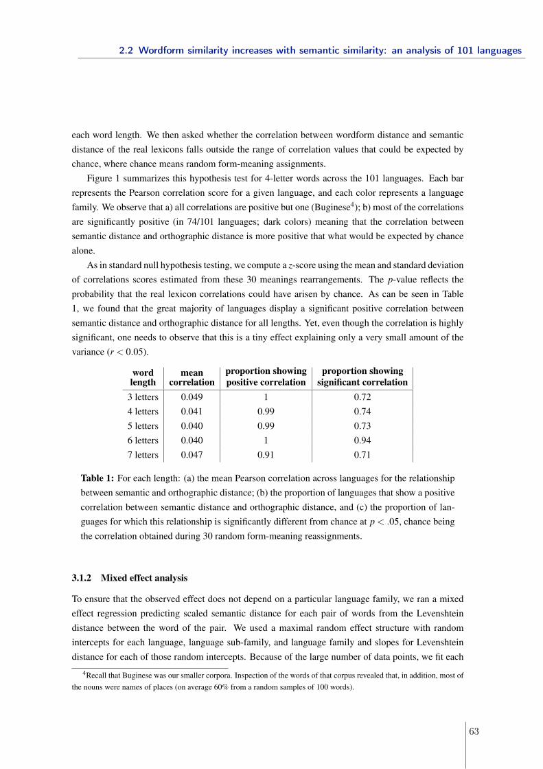
each word length. We then asked whether the correlation between wordform distance and semanticdistance of the real lexicons falls outside the range of correlation values that could be expected bychance, where chance means random form-meaning assignments.
Figure 1 summarizes this hypothesis test for 4-letter words across the 101 languages. Each barrepresents the Pearson correlation score for a given language, and each color represents a languagefamily. We observe that a) all correlations are positive but one (Buginese4); b) most of the correlationsare significantly positive (in 74/101 languages; dark colors) meaning that the correlation betweensemantic distance and orthographic distance is more positive that what would be expected by chancealone.
As in standard null hypothesis testing, we compute a z-score using the mean and standard deviationof correlations scores estimated from these 30 meanings rearrangements. The p-value reflects theprobability that the real lexicon correlations could have arisen by chance. As can be seen in Table1, we found that the great majority of languages display a significant positive correlation betweensemantic distance and orthographic distance for all lengths. Yet, even though the correlation is highlysignificant, one needs to observe that this is a tiny effect explaining only a very small amount of thevariance (r < 0.05).
wordlength
meancorrelation
proportion showingpositive correlation
proportion showingsignificant correlation
3 letters 0.049 1 0.724 letters 0.041 0.99 0.745 letters 0.040 0.99 0.736 letters 0.040 1 0.947 letters 0.047 0.91 0.71
Table 1: For each length: (a) the mean Pearson correlation across languages for the relationshipbetween semantic and orthographic distance; (b) the proportion of languages that show a positivecorrelation between semantic distance and orthographic distance, and (c) the proportion of lan-guages for which this relationship is significantly different from chance at p < .05, chance beingthe correlation obtained during 30 random form-meaning reassignments.
3.1.2 Mixed effect analysis
To ensure that the observed effect does not depend on a particular language family, we ran a mixedeffect regression predicting scaled semantic distance for each pair of words from the Levenshteindistance between the word of the pair. We used a maximal random effect structure with randomintercepts for each language, language sub-family, and language family and slopes for Levenshteindistance for each of those random intercepts. Because of the large number of data points, we fit each
4Recall that Buginese was our smaller corpora. Inspection of the words of that corpus revealed that, in addition, most ofthe nouns were names of places (on average 60% from a random samples of 100 words).
2.2 Wordform similarity increases with semantic similarity: an analysis of 101 languages
63
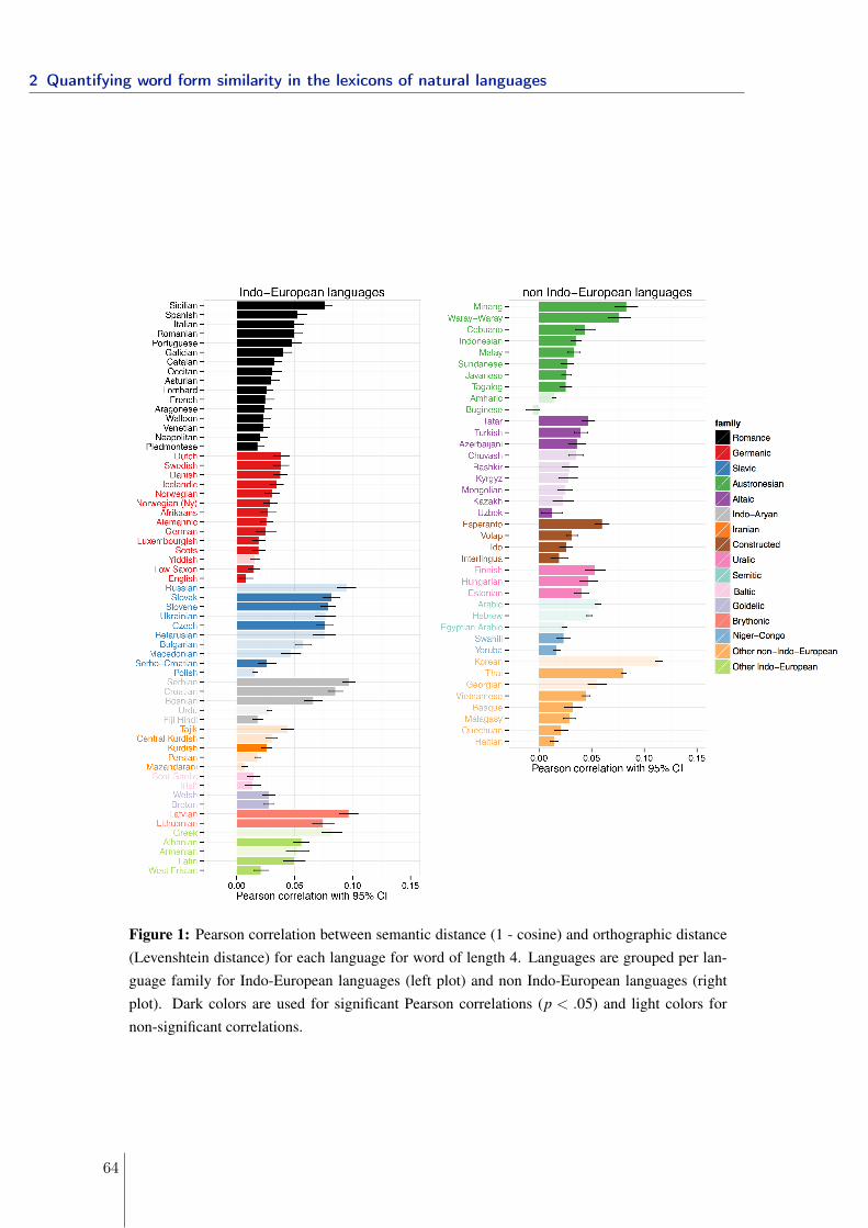
Figure 1: Pearson correlation between semantic distance (1 - cosine) and orthographic distance(Levenshtein distance) for each language for word of length 4. Languages are grouped per lan-guage family for Indo-European languages (left plot) and non Indo-European languages (rightplot). Dark colors are used for significant Pearson correlations (p < .05) and light colors fornon-significant correlations.
2 Quantifying word form similarity in the lexicons of natural languages
64
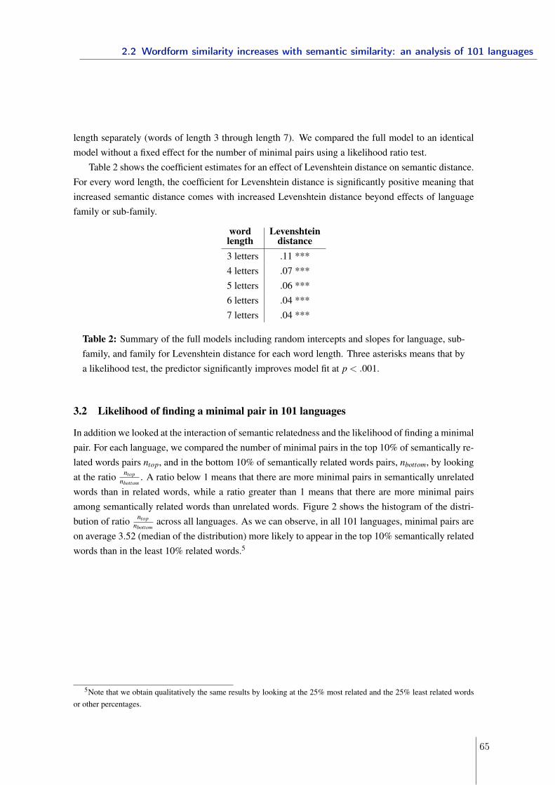
length separately (words of length 3 through length 7). We compared the full model to an identicalmodel without a fixed effect for the number of minimal pairs using a likelihood ratio test.
Table 2 shows the coefficient estimates for an effect of Levenshtein distance on semantic distance.For every word length, the coefficient for Levenshtein distance is significantly positive meaning thatincreased semantic distance comes with increased Levenshtein distance beyond effects of languagefamily or sub-family.
wordlength
Levenshteindistance
3 letters .11 ***4 letters .07 ***5 letters .06 ***6 letters .04 ***7 letters .04 ***
Table 2: Summary of the full models including random intercepts and slopes for language, sub-family, and family for Levenshtein distance for each word length. Three asterisks means that bya likelihood test, the predictor significantly improves model fit at p < .001.
3.2 Likelihood of finding a minimal pair in 101 languages
In addition we looked at the interaction of semantic relatedness and the likelihood of finding a minimalpair. For each language, we compared the number of minimal pairs in the top 10% of semantically re-lated words pairs ntop, and in the bottom 10% of semantically related words pairs, nbottom, by lookingat the ratio ntop
nbottom. A ratio below 1 means that there are more minimal pairs in semantically unrelated
words than in related words, while a ratio greater than 1 means that there are more minimal pairsamong semantically related words than unrelated words. Figure 2 shows the histogram of the distri-bution of ratio ntop
nbottomacross all languages. As we can observe, in all 101 languages, minimal pairs are
on average 3.52 (median of the distribution) more likely to appear in the top 10% semantically relatedwords than in the least 10% related words.5
5Note that we obtain qualitatively the same results by looking at the 25% most related and the 25% least related wordsor other percentages.
2.2 Wordform similarity increases with semantic similarity: an analysis of 101 languages
65
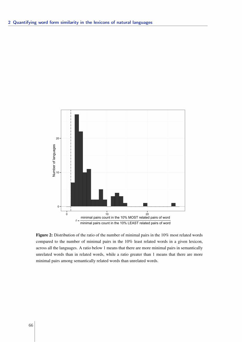
0
10
20
0 10 20
r =minimal pairs count in the 10% MOST related pairs of wordminimal pairs count in the 10% LEAST related pairs of word
Num
ber o
f lan
guag
es
Figure 2: Distribution of the ratio of the number of minimal pairs in the 10% most related wordscompared to the number of minimal pairs in the 10% least related words in a given lexicon,across all the languages. A ratio below 1 means that there are more minimal pairs in semanticallyunrelated words than in related words, while a ratio greater than 1 means that there are moreminimal pairs among semantically related words than unrelated words.
2 Quantifying word form similarity in the lexicons of natural languages
66
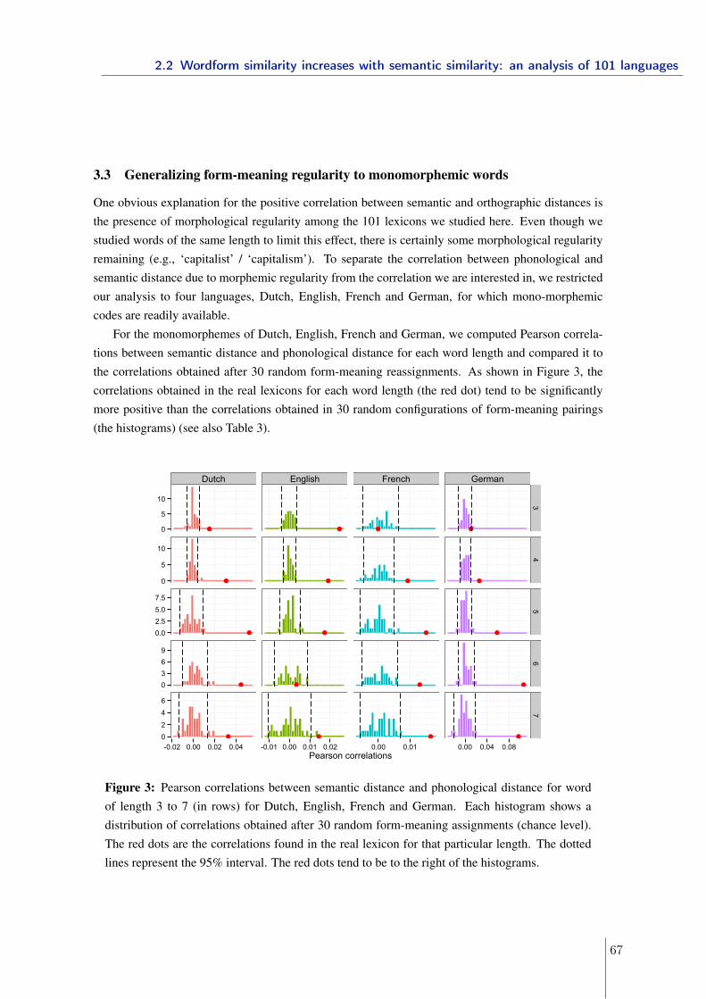
3.3 Generalizing form-meaning regularity to monomorphemic words
One obvious explanation for the positive correlation between semantic and orthographic distances isthe presence of morphological regularity among the 101 lexicons we studied here. Even though westudied words of the same length to limit this effect, there is certainly some morphological regularityremaining (e.g., ‘capitalist’ / ‘capitalism’). To separate the correlation between phonological andsemantic distance due to morphemic regularity from the correlation we are interested in, we restrictedour analysis to four languages, Dutch, English, French and German, for which mono-morphemiccodes are readily available.
For the monomorphemes of Dutch, English, French and German, we computed Pearson correla-tions between semantic distance and phonological distance for each word length and compared it tothe correlations obtained after 30 random form-meaning reassignments. As shown in Figure 3, thecorrelations obtained in the real lexicons for each word length (the red dot) tend to be significantlymore positive than the correlations obtained in 30 random configurations of form-meaning pairings(the histograms) (see also Table 3).
Dutch English French German
0
5
10
0
5
10
0.02.55.07.5
0369
0
2
4
6
34
56
7
-0.02 0.00 0.02 0.04 -0.01 0.00 0.01 0.02 0.00 0.01 0.00 0.04 0.08Pearson correlations
Figure 3: Pearson correlations between semantic distance and phonological distance for wordof length 3 to 7 (in rows) for Dutch, English, French and German. Each histogram shows adistribution of correlations obtained after 30 random form-meaning assignments (chance level).The red dots are the correlations found in the real lexicon for that particular length. The dottedlines represent the 95% interval. The red dots tend to be to the right of the histograms.
2.2 Wordform similarity increases with semantic similarity: an analysis of 101 languages
67
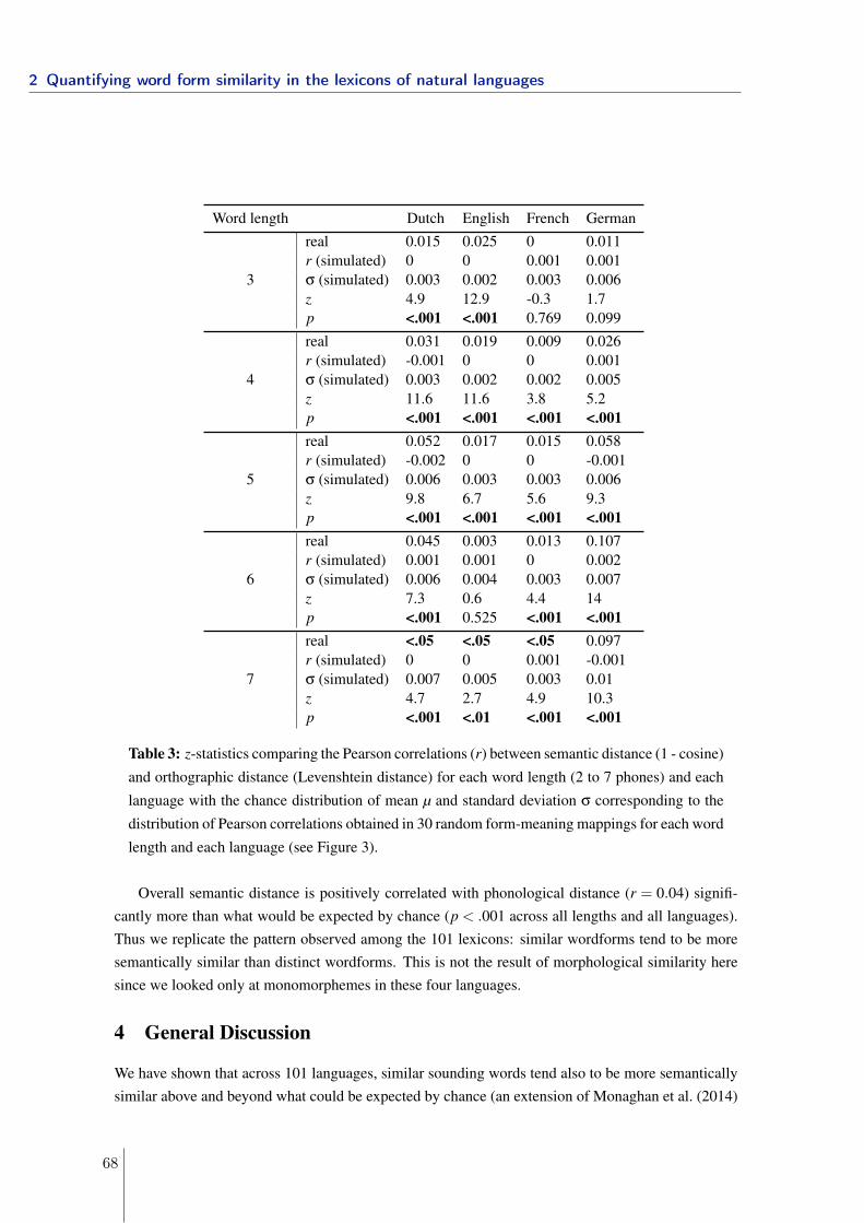
Word length Dutch English French Germanreal 0.015 0.025 0 0.011r (simulated) 0 0 0.001 0.001
3 σ (simulated) 0.003 0.002 0.003 0.006z 4.9 12.9 -0.3 1.7p <.001 <.001 0.769 0.099real 0.031 0.019 0.009 0.026r (simulated) -0.001 0 0 0.001
4 σ (simulated) 0.003 0.002 0.002 0.005z 11.6 11.6 3.8 5.2p <.001 <.001 <.001 <.001real 0.052 0.017 0.015 0.058r (simulated) -0.002 0 0 -0.001
5 σ (simulated) 0.006 0.003 0.003 0.006z 9.8 6.7 5.6 9.3p <.001 <.001 <.001 <.001real 0.045 0.003 0.013 0.107r (simulated) 0.001 0.001 0 0.002
6 σ (simulated) 0.006 0.004 0.003 0.007z 7.3 0.6 4.4 14p <.001 0.525 <.001 <.001real <.05 <.05 <.05 0.097r (simulated) 0 0 0.001 -0.001
7 σ (simulated) 0.007 0.005 0.003 0.01z 4.7 2.7 4.9 10.3p <.001 <.01 <.001 <.001
Table 3: z-statistics comparing the Pearson correlations (r) between semantic distance (1 - cosine)
and orthographic distance (Levenshtein distance) for each word length (2 to 7 phones) and each
language with the chance distribution of mean µ and standard deviation σ corresponding to the
distribution of Pearson correlations obtained in 30 random form-meaning mappings for each word
length and each language (see Figure 3).
Overall semantic distance is positively correlated with phonological distance (r = 0.04) signifi-cantly more than what would be expected by chance (p < .001 across all lengths and all languages).Thus we replicate the pattern observed among the 101 lexicons: similar wordforms tend to be moresemantically similar than distinct wordforms. This is not the result of morphological similarity heresince we looked only at monomorphemes in these four languages.
4 General Discussion
We have shown that across 101 languages, similar sounding words tend also to be more semanticallysimilar above and beyond what could be expected by chance (an extension of Monaghan et al. (2014)
2 Quantifying word form similarity in the lexicons of natural languages
68
in English). In order to remove the contribution of morphology from this correlation, we conductedthe same analysis on the set of monomorphemic lemmas of a restricted number of languages andfound exactly the same pattern of results. This suggests that the pattern of clumpiness in the lexiconmay be in part explained by form-meaning regularities, over and beyond morphological regularity,across a large range of typologically different languages.
What could be the reasons of form-meaning regularity in the lexicon? One possibility is thatform-meaning regularity is due to etymology. Etymology is an important source of regularity inform-meaning mappings: certain words are historically related or derived from other words in thelexicon (even when the lexicon is restricted to morphologically simple words). For example, ‘skirt’and ‘shirt’ are historically the Old Norse and Old English form of the same word, whose meaningshave since diverged. Similarly, the presence of local sound-symbolism (e.g., the phonesthemes gl- inEnglish) may drive the correlation. Yet, previous work showed that neither etymological roots norsmall clusters of sound symbolic words were sufficient to account for the pattern of systematicityobserved across the English lexicon (Monaghan et al., 2014). Though this needs to be confirmed forthe languages under study here, this suggests a global pattern of form-meaning systematicity acrossthe whole lexicon over and above etymological roots.
Another possibility is that form-meaning regularity is carried by the grammatical category of thewords. Even though we looked at monomorphemes, words from the same grammatical category sharephonological features (Cassidy & Kelly, 1991; Kelly, 1992), such that nouns sound more similar toother nouns and verbs to other verbs (see also Mahowald, Dautriche, Gibson, Christophe, & Piantadosi(submitted)), and are overall more semantically closer to words of the same grammatical category(e.g., verbs are more likely to map onto actions and nouns onto objects). Such systematic form-meaning mappings may be helpful during language learning to cue grammatical categories (Monaghanet al., 2011) and may be one of the outcomes of language transmission and evolution (Kirby et al.,2008) such that the optimal structure of the vocabulary may be one that incorporates form-meaningregularities at the large scale of the lexicon.
Still, the prevalence of wordform similarity in the lexicon conflicts in theory with communicativeefficiency. Imagine a language that displays an extreme pattern form-meaning regularity where similarand frequent concepts such as CAT and DOG will be associated with similar wordforms such as ‘feb’and ‘fep’ respectively. These words will be easily confused since their forms differ only from onephoneme and their meanings are similar. Nevertheless, we observed a correlation between semanticsimilarity and phonological distance. Perhaps, then, semantically similar words are not as confusableas one might suspect. Indeed, context is typically sufficient to disambiguate between meanings, sinceadult speakers use many cues when processing spoken sentences (e.g. prior linguistic context Altmann& Kamide (1999); visual information Tanenhaus et al. (1995); speaker Creel et al. (2008)). As aresult, finer-grained contextual information may be sufficient most of the time for adults’ listeners todistinguish between phonologically similar words.
To our knowledge, with 101 languages in the sample, this is the largest cross-linguistic analy-sis showing a correlation between semantic similarity and phonological similarity among monomor-
2.2 Wordform similarity increases with semantic similarity: an analysis of 101 languages
69

phemic words showing evidence of systematicity in form-meaning mappings beyond morphologicalregularity (at least for Dutch, English, French and German). Ultimately, the results here suggest afunctional advantage to having lexicons in which there is a positive correlation between phonetic andsemantic similarity.
References
Altmann, G., & Kamide, Y. (1999). Incremental interpretation at verbs: Restricting the domain ofsubsequent reference. Cognition, 73(3), 247–264.
Baayen, R., Piepenbrock, R., & Gulikers, L. (1995). The CELEX lexical database (release 2)[cd-rom].Philadelphia, PA: Linguistic Data Consortium, University of Pennsylvania [Distributor].
Bergen, B. K. (2004). The psychological reality of phonaesthemes. Language, 80(2), 290–311.
Bloomfield, L. (1933). Language. New York: Henry Holt.
Bremner, A. J., Caparos, S., Davidoff, J., de Fockert, J., Linnell, K. J., & Spence, C. (2013). “bouba”and “kiki” in namibia? a remote culture make similar shape–sound matches, but different shape–taste matches to westerners. Cognition, 126(2), 165–172.
Cassidy, K. W., & Kelly, M. H. (1991). Phonological information for grammatical category assign-ments. Journal of Memory and Language, 30(3), 348–369.
Childs, G. T. (1994). African ideophones. Sound symbolism, 178–204.
Creel, S. C., Aslin, R. N., & Tanenhaus, M. K. (2008). Heeding the voice of experience: The role oftalker variation in lexical access. Cognition, 106(2), 633–664.
de Saussure, F. (1916). Course in general linguistics. Open Court Publishing Company.
Fourtassi, A., & Dupoux, E. (2013). A corpus-based evaluation method for distributional semanticmodels. ACL 2013, 165.
Gahl, S., Yao, Y., & Johnson, K. (2012). Why reduce? phonological neighborhood density andphonetic reduction in spontaneous speech. Journal of Memory and Language, 66(4), 789–806.
Hamano, S. (1998). The sound-symbolic system of japanese. ERIC.
Harris, Z. S. (1954). Distributional structure. Word.
Hockett, C. (1960). The origin of speech. Scientific American, 203, 88–96.
Imai, M., & Kita, S. (2014). The sound symbolism bootstrapping hypothesis for language acquisitionand language evolution. Philosophical Transactions of the Royal Society B: Biological Sciences,369(1651), 20130298.
Kelly, M. H. (1992). Using sound to solve syntactic problems: The role of phonology in grammaticalcategory assignments. Psychological Review, 99(2), 349–364.
Kemp, C., & Regier, T. (2012). Kinship categories across languages reflect general communicativeprinciples. Science, 336(6084), 1049–1054.
2 Quantifying word form similarity in the lexicons of natural languages
70
Kim, K.-O. (1977). Sound symbolism in korean. Journal of Linguistics, 13(01), 67–75.
Kirby, S., Cornish, H., & Smith, K. (2008). Cumulative cultural evolution in the laboratory: Anexperimental approach to the origins of structure in human language. Proceedings of the NationalAcademy of Sciences, 105(31), 10681–10686.
Landauer, T., & Dumais, S. T. (1997). A solution to plato’s problem: The latent semantic analysistheory of acquisition, induction, and representation of knowledge. Psychological review, 104(2),211.
Liljencrants, J., & Lindblom, B. (1972). Numerical simulation of vowel quality systems: The role ofperceptual contrast. Language, 839–862.
Lin, D. (1998). An information-theoretic definition of similarity. In ICML (Vol. 98, pp. 296–304).
Luhn, H. P. (1958). The automatic creation of literature abstracts. IBM Journal of research anddevelopment, 2(2), 159–165.
Mahowald, K., Dautriche, I., Gibson, E., Christophe, A., & Piantadosi, S. (submitted). Lexicalclustering in efficient language design.
Mahowald, K., Dautriche, I., Gibson, E., & Piantadosi, S. (submitted). Cross-linguistic effects offrequency on wordform similarity.
Monaghan, P., & Christiansen, M. H. (2008). Integration of multiple probabilistic cues in syntaxacquisition. Corpora in language acquisition research: History, methods, perspectives, 139–164.
Monaghan, P., Christiansen, M. H., & Fitneva, S. A. (2011). The arbitrariness of the sign: Learningadvantages from the structure of the vocabulary. Journal of Experimental Psychology: General,140(3), 325–347.
Monaghan, P., Shillcock, R. C., Christiansen, M. H., & Kirby, S. (2014). How arbitrary is language.Philosophical Transactions of the Royal Society B.
New, B., Pallier, C., Brysbaert, M., & Ferrand, L. (2004). Lexique 2: A new french lexical database.Behavior Research Methods, Instruments, & Computers, 36(3), 516–524.
Piantadosi, S., Tily, H., & Gibson, E. (2011). Word lengths are optimized for efficient communication.Proceedings of the National Academy of Sciences, 108(9), 3526.
Pinker, S. (1984). Language learnability and language development. Cambridge, MA: HarvardUniversity Press.
R Core Team. (2013). R: A language and environment for statistical computing [Computer softwaremanual]. Vienna, Austria.
Rehurek, R., & Sojka, P. (2010). Software framework for topic modelling with large corpora.
Stemberger, J. P. (2004). Neighbourhood effects on error rates in speech production. Brain andLanguage, 90(1), 413–422.
Storkel, H. L., Armbruster, J., & Hogan, T. P. (2006). Differentiating phonotactic probability andneighborhood density in adult word learning. Journal of Speech, Language, and Hearing Research,49(6), 1175–1192.
2.2 Wordform similarity increases with semantic similarity: an analysis of 101 languages
71
Storkel, H. L., & Lee, S.-Y. (2011). The independent effects of phonotactic probability and neigh-bourhood density on lexical acquisition by preschool children. Language and Cognitive Processes,26(2), 191–211.
Strickland, B., Geraci, C., Chemla, E., Schlenker, P., Kelepir, M., & Pfau, R. (in press). Eventrepresentations constrain the structure of language: Sign language as a window into universallyaccessible linguistic biases. Proceedings of the National Academy of Sciences.
Tanenhaus, M., Spivey-Knowlton, M., Eberhard, K., & Sedivy, J. (1995). Integration of visual andlinguistic information in spoken language comprehension. Science, 268(5217), 1632.
Vitevitch, M. S., & Sommers, M. S. (2003). The facilitative influence of phonological similarity andneighborhood frequency in speech production in younger and older adults. Memory & Cognition,31(4), 491–504.
Zipf, G. (1949). Human Behavior and the Principle of Least Effort. New York: Addison-Wesley.
2 Quantifying word form similarity in the lexicons of natural languages
72
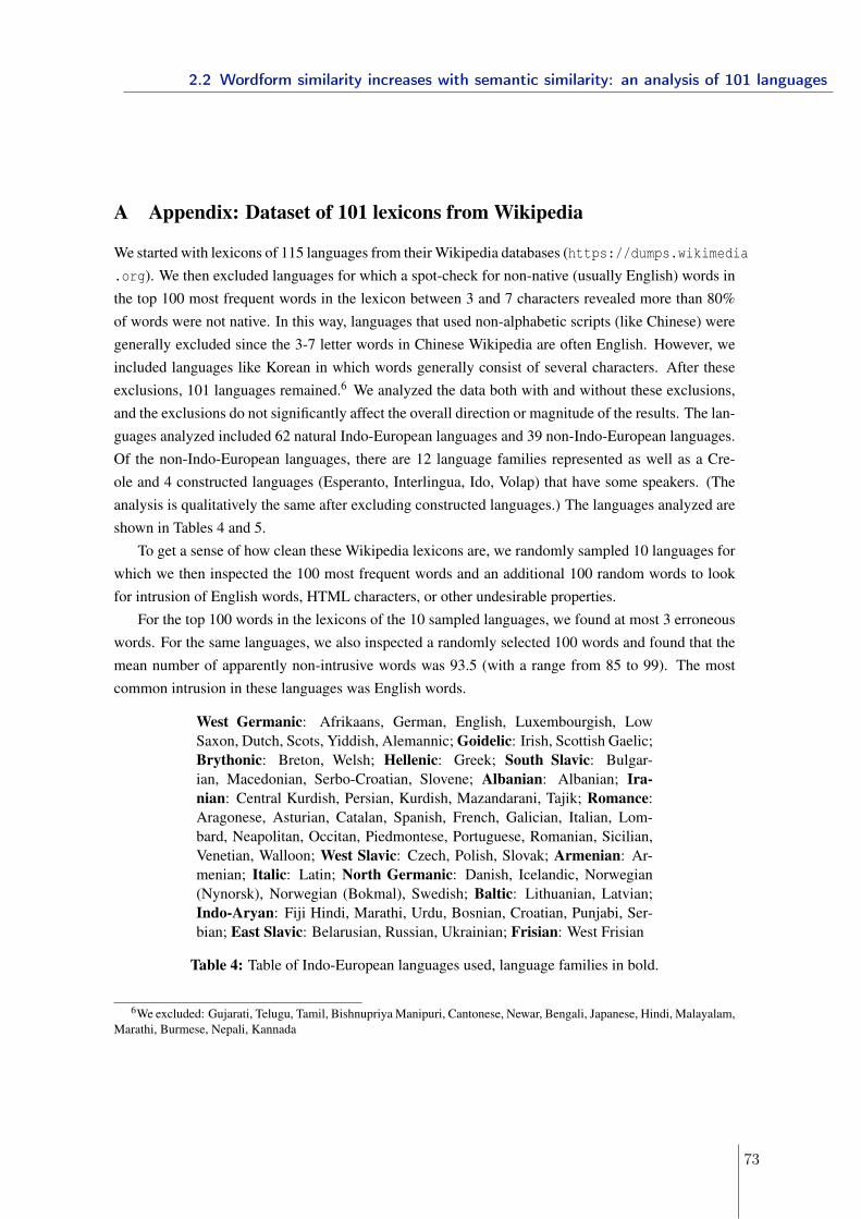
A Appendix: Dataset of 101 lexicons from Wikipedia
We started with lexicons of 115 languages from their Wikipedia databases (https://dumps.wikimedia.org). We then excluded languages for which a spot-check for non-native (usually English) words inthe top 100 most frequent words in the lexicon between 3 and 7 characters revealed more than 80%of words were not native. In this way, languages that used non-alphabetic scripts (like Chinese) weregenerally excluded since the 3-7 letter words in Chinese Wikipedia are often English. However, weincluded languages like Korean in which words generally consist of several characters. After theseexclusions, 101 languages remained.6 We analyzed the data both with and without these exclusions,and the exclusions do not significantly affect the overall direction or magnitude of the results. The lan-guages analyzed included 62 natural Indo-European languages and 39 non-Indo-European languages.Of the non-Indo-European languages, there are 12 language families represented as well as a Cre-ole and 4 constructed languages (Esperanto, Interlingua, Ido, Volap) that have some speakers. (Theanalysis is qualitatively the same after excluding constructed languages.) The languages analyzed areshown in Tables 4 and 5.
To get a sense of how clean these Wikipedia lexicons are, we randomly sampled 10 languages forwhich we then inspected the 100 most frequent words and an additional 100 random words to lookfor intrusion of English words, HTML characters, or other undesirable properties.
For the top 100 words in the lexicons of the 10 sampled languages, we found at most 3 erroneouswords. For the same languages, we also inspected a randomly selected 100 words and found that themean number of apparently non-intrusive words was 93.5 (with a range from 85 to 99). The mostcommon intrusion in these languages was English words.
West Germanic: Afrikaans, German, English, Luxembourgish, LowSaxon, Dutch, Scots, Yiddish, Alemannic; Goidelic: Irish, Scottish Gaelic;Brythonic: Breton, Welsh; Hellenic: Greek; South Slavic: Bulgar-ian, Macedonian, Serbo-Croatian, Slovene; Albanian: Albanian; Ira-nian: Central Kurdish, Persian, Kurdish, Mazandarani, Tajik; Romance:Aragonese, Asturian, Catalan, Spanish, French, Galician, Italian, Lom-bard, Neapolitan, Occitan, Piedmontese, Portuguese, Romanian, Sicilian,Venetian, Walloon; West Slavic: Czech, Polish, Slovak; Armenian: Ar-menian; Italic: Latin; North Germanic: Danish, Icelandic, Norwegian(Nynorsk), Norwegian (Bokmal), Swedish; Baltic: Lithuanian, Latvian;Indo-Aryan: Fiji Hindi, Marathi, Urdu, Bosnian, Croatian, Punjabi, Ser-bian; East Slavic: Belarusian, Russian, Ukrainian; Frisian: West Frisian
Table 4: Table of Indo-European languages used, language families in bold.
6We excluded: Gujarati, Telugu, Tamil, Bishnupriya Manipuri, Cantonese, Newar, Bengali, Japanese, Hindi, Malayalam,Marathi, Burmese, Nepali, Kannada
2.2 Wordform similarity increases with semantic similarity: an analysis of 101 languages
73
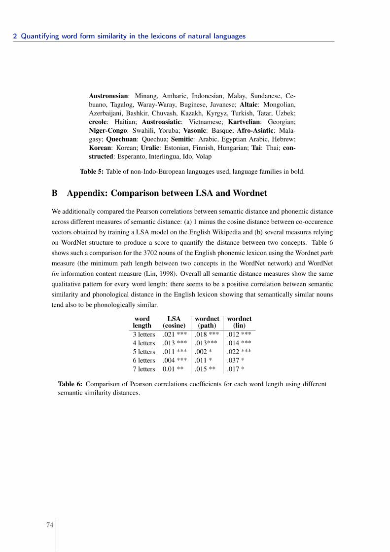
Austronesian: Minang, Amharic, Indonesian, Malay, Sundanese, Ce-buano, Tagalog, Waray-Waray, Buginese, Javanese; Altaic: Mongolian,Azerbaijani, Bashkir, Chuvash, Kazakh, Kyrgyz, Turkish, Tatar, Uzbek;creole: Haitian; Austroasiatic: Vietnamese; Kartvelian: Georgian;Niger-Congo: Swahili, Yoruba; Vasonic: Basque; Afro-Asiatic: Mala-gasy; Quechuan: Quechua; Semitic: Arabic, Egyptian Arabic, Hebrew;Korean: Korean; Uralic: Estonian, Finnish, Hungarian; Tai: Thai; con-structed: Esperanto, Interlingua, Ido, Volap
Table 5: Table of non-Indo-European languages used, language families in bold.
B Appendix: Comparison between LSA and Wordnet
We additionally compared the Pearson correlations between semantic distance and phonemic distanceacross different measures of semantic distance: (a) 1 minus the cosine distance between co-occurencevectors obtained by training a LSA model on the English Wikipedia and (b) several measures relyingon WordNet structure to produce a score to quantify the distance between two concepts. Table 6shows such a comparison for the 3702 nouns of the English phonemic lexicon using the Wordnet pathmeasure (the minimum path length between two concepts in the WordNet network) and WordNetlin information content measure (Lin, 1998). Overall all semantic distance measures show the samequalitative pattern for every word length: there seems to be a positive correlation between semanticsimilarity and phonological distance in the English lexicon showing that semantically similar nounstend also to be phonologically similar.
wordlength
LSA(cosine)
wordnet(path)
wordnet(lin)
3 letters .021 *** .018 *** .012 ***4 letters .013 *** .013*** .014 ***5 letters .011 *** .002 * .022 ***6 letters .004 *** .011 * .037 *7 letters 0.01 ** .015 ** .017 *
Table 6: Comparison of Pearson correlations coefficients for each word length using differentsemantic similarity distances.
2 Quantifying word form similarity in the lexicons of natural languages
74
2.3 Summary and Discussion
2.3 Summary and Discussion
Across languages and language families, I find that the structure of word form similarityin the lexicon is not arbitrary but is the result of functional pressures, such that 1) thereis more phonological similarity in the lexicon than expected by chance (section 2.1), and2) semantically related pairs of words are also orthographically related (section 2.2).
Null lexicons
The methodological contribution of this work is a new way of assessing linguistic structurethrough the creation of random baselines that provide a null hypothesis for how the lin-guistic structure should be in the absence of communicative and cognitive pressures. Thiscould be used to assess the distribution of other linguistic phenomena.
Note however that the chance level depends entirely on how we define it. Here our questionrequired us to model the phonotactics of the language sufficiently well in order to createnull lexicons that make plausible assumptions about the true generative process of words(contra a random typing model, Howes, 1968). Yet this is not to say that a n-gram modelon phones is the right way to think about words and certainly some better models ofphonotactics already exists (BLICK, Hayes, 2012) but their adaptation to other languagesthan English is not easy.10
In addition, the chance level I defined is language-specific, that is our best non-wordgenerative model was trained on a single language to generate non-words of that language.One could imagine that the chance level should be more general, i.e., trained across allpossible languages, since our primary question concerns the presence of general, thus nonlanguage-specific, cognitive pressures on the set of word forms. Yet, this may be unrealisticin practice. Since languages have different phonotactic constraints that may influence thespace of possible words for that language, comparing measures of word form similarity ina global random baseline to each individual languages may not be representative of theconstraints, in the absence of functional pressures, for that language.
Limitations
One limitation of this work is the use of orthographic corpora in section 2.2. Orthographyis often taken as an approximation for phonology, yet it would be useful to dispose of
10Note that at least for English, generating random baselines using non-words that are phonotactically"good" according to BLICK does not change the pattern of results obtained in section 2.1.
75
2 Quantifying word form similarity in the lexicons of natural languages
lexicons that are transcribed phonemically and are morphologically tagged. However since101 languages were used in this study, this, to some extent, takes away this concern.
Another perhaps more important limitation regarding the scope of this dissertation is thefocus on word form similarity alone. Indeed, we are still left with the question of how muchhomophony is present in languages? The methodology developed here, however, cannotgive a satisfying answer to that question. Recall that to compare word form similarity in agiven language to chance level, I focused on monomorphemes; but homophones are not onlylimited to the set of monomorphemes: for instance in French "porte" means both the noundoor and the verb to carry conjugated in the present tense singular. Thus, homophonymay arise in morphologically complex words (e.g., to carrypres.sing) that do not appear inthe list of monomorphemes. One could generate null lexicons for the set of word formsin a given language, encompassing thus all possible forms. Yet, this would go beyond theassumptions of our current generative model (a n-gram on phones), as it is not equippedwith a mechanism to generate morphologically complex words.
Conclusions
In sum, across a large range of measures, we showed that there is more phonologicalsimilarity in the lexicon than expected by chance and that these words tend to be correlatedwith greater semantic similarity. This suggests that there is a pressure for the lexicon tobe more clumpy, that is, to be more compressible. As we argued, such a pressure may bebeneficial not only for speakers, as it minimizes articulatory effort and relieves memory load(as less sound sequences are used), but also for learners at it may help them to learn someaspects of their language (as word form regularity may be helpful in segmenting words fromspeech and more systematic form-meaning mappings help category formation). However,such properties may be detrimental for some other aspects of learning as it suggests thatchildren may have a hard time differentiating these forms to attribute them meanings. Oneimportant question is thus: how do children manage to learn such a lexicon?
76
3 Learning confusable and ambiguouswords
Carey (1978b) has described word learning as starting with a process where children "flag"new word!" upon hearing a phonological sequence with no current lexical entry". Indeed,one feature of novel words is that they are often composed of unfamiliar sequences ofsounds. However, a new word can be phonologically similar or even identical to a wordthat already exists in the child’s lexicon and yet, be associated with a novel meaning. Forinstance, the child may already know the word "sheep" but needs to be able to identify that"ship", a minimally different word form, is a different word despite the phonetic variabilityof the speech signal. Similar-sounding words present thus learners with a challenging casewhere they need to find the right balance between phonological tolerance, to recognizeknown words, and phonological sensitivity, to be able to learn these new words.
Not only must children be able to identify novel word forms in the signal to consider themas candidate lexical entries, they also must be able to identify novel meanings even whenthe word form is identical to a form they already know, as in the case of homophones. Forinstance the child may already know that "bat" means bat-animals and be confronted witha sentence such as "aluminum bats are much easier to swing when compared to woodenbats". How does the child determine that "bat" is used here to refer to a baseball-batand not an animal-bat? Homophony thus presents learners with a unique word learningsituation where they cannot rely on the signal alone to determine whether a phonologicalform is a candidate for a novel entry in the lexicon as a new word.
In this chapter, I investigate whether 18- to 20-month-old toddlers take into account otherfactors than phonology when determining what counts as a new word. Specifically, insection 3.1, I test whether toddlers take into account the syntactic context to determinewhether a novel phonological neighbor of a word they know could be interpreted as a novelword (learning "tog" when "dog" is already in their lexicon). In section 3.2, I take theseresults further, and look whether children’s ability to learn homophones depends on thesyntactic or semantic context they are presented in. Finally in section 3.3, I evaluatewhether similar-sounding words and homophones that exhibit properties that make themlearnable by children are more represented in the lexicon of natural languages than similar-sounding words and homophones that are harder to learn.
77

3 Learning confusable and ambiguous words
skip
78

Learning novel phonological neighbors: Syntactic category matters
Isabelle Dautriche a,b,⇑, Daniel Swingley c, Anne Christophe a,b
a Laboratoire de Sciences Cognitives et Psycholinguistique (ENS, EHESS, CNRS), Département d’Études Cognitives (École Normale Supérieure – PSL Research University), Paris, Franceb Maternité Port-Royal, AP-HP, Faculté de Médecine Paris Descartes, Francec Department of Psychology and Institute for Research in Cognitive Science, University of Pennsylvania, United States
a r t i c l e i n f o
Article history:Received 14 December 2014Revised 3 June 2015Accepted 4 June 2015
Keywords:Word learningLexical accessPhonetic sensitivityLanguage acquisition
a b s t r a c t
Novel words (like tog) that sound like well-known words (dog) are hard for toddlers to learn, even thoughchildren can hear the difference between them (Swingley & Aslin, 2002, 2007). One possibility is thatphonological competition alone is the problem. Another is that a broader set of probabilistic considera-tions is responsible: toddlers may resist considering tog as a novel object label because its neighbor dog isalso an object. In three experiments, French 18-month-olds were taught novel words whose word formswere phonologically similar to familiar nouns (noun-neighbors), to familiar verbs (verb-neighbors) or tonothing (no-neighbors). Toddlers successfully learned the no-neighbors and verb-neighbors but failed tolearn the noun-neighbors, although both novel neighbors had a familiar phonological neighbor in the tod-dlers’ lexicon. We conclude that when creating a novel lexical entry, toddlers’ evaluation of similarity inthe lexicon is multidimensional, incorporating both phonological and semantic or syntactic features.
� 2015 Elsevier B.V. All rights reserved.
1. Introduction
Many of the words young children hear are not yet in theirvocabulary. As a result, in everyday conversation toddlers mustoften decide whether a given word-form corresponds to a wordthey already know, or to a word to be learned. In principle, childrencould accomplish this by checking to see if each utterance can beparsed entirely into a sequence of familiar words. If it cannot, per-haps the unidentified portions correspond to new words.
The problem, of course, is to define what counts as an instanceof a familiar word and what does not. Different instances of a givenword do not all sound the same. Talkers have different voices andvarying accents (e.g., Labov, 1966); words sound different depend-ing on the phonetic context they appear in (e.g., Holst & Nolan,1995), and speakers routinely blend sounds together or omit com-pletely entire sounds and even whole syllables of words (e.g.,Ernestus & Warner, 2011; Johnson, 2004). Such phenomena arepresent in the speech parents direct to their children (e.g., Bard &Anderson, 1983). Drawing the boundary between the set of accept-able instances of a word, and the instances that cannot correspondto that word, is complex.
Traditionally, it is said to be the role of the language’s phonol-ogy to define the set of phonetic differences that distinguish words,
to resolve these ambiguities. If words are represented as phonolog-ical descriptions adequate for maintaining contrast, and heardutterances are converted into phonological descriptions duringspeech comprehension, a simple comparison procedure should beadequate for identifying new words. If a word-form in the utter-ance fails to line up with any word-forms in the lexicon, this meansthat a new word has been heard.
This might not work for children, for several reasons. Children’sskills of phonetic categorization are inferior to adults’ and undergosubstantial refinement well into the school years, despite the rapidprogress toward language-specific perception made in infancy(e.g., Hazan & Barrett, 2000; Kuhl, 2004). In many cases childrenmay not successfully characterize utterances in phonologicalterms. And even when they can, it is not clear that children under-stand that phonological distinctions are meant to signal lexical dis-tinctions. Although children recognize words more easily when thewords are spoken with their canonical pronunciations than whenspoken with deviant pronunciations (e.g., Swingley, 2009), thisdoes not imply that the mispronunciations are interpreted as novelwords (e.g., White & Morgan, 2008). Toddlers do resist interpretingsome discriminable, but not phonological, differences as con-trastive (Dietrich, Swingley, & Werker, 2007; Quam & Swingley,2010), which suggests some sophistication in relating speech andthe lexicon. But being wary of interpreting a non-phonologicaldistinction as if it could distinguish words does not imply theinverse skill of readily interpreting phonological distinctions ascontrastive.
http://dx.doi.org/10.1016/j.cognition.2015.06.0030010-0277/� 2015 Elsevier B.V. All rights reserved.
⇑ Corresponding author at: Laboratoire de Sciences Cognitives et Psycholinguis-tique, École Normale Supérieure, 29 rue d’Ulm, P.J., 75005 Paris, France.
E-mail address: [email protected] (I. Dautriche).
Cognition 143 (2015) 77–86
Contents lists available at ScienceDirect
Cognition
journal homepage: www.elsevier .com/locate /COGNIT
3.1 Learning phonological neighbors: Syntactic category matters
79
One study tested whether toddlers could use a single-featurephonological distinction to assign a novel meaning to aword-form that sounded similar to a very familiar one (Swingley& Aslin, 2007). 19-month-olds were shown a novel object, whichwas repeatedly named using clear (hyperarticulated) speech. Insome cases the novel name given was similar to a familiar word(e.g., tog, similar to dog), and in some cases it was not (e.g., shang,not similar to any words children knew). Children were testedusing a fixation procedure in which pictures of two novel objectswere presented on a screen, and one of the pictures was labeledusing its novel name (e.g., ‘‘Look at the {tog, shang}’’. Fixation tothe named picture was used to index learning of the word. Intwo experiments, children were able to learn words that soundedvery different from the other words in their vocabularies (likeshang), but children did not learn the phonologically similar words(like tog). For some of the items tested, children of the same agehad previously shown discrimination of the nonce label and itsfamiliar counterpart, so perceptual discrimination per se wasapparently not at issue (e.g., Swingley & Aslin, 2002).
Why might this be? One possibility is that phonological compe-tition alone is the problem. The lexical entry of dog might be acti-vated by the phonologically neighboring form tog, interfering withchildren’s considering the possibility that a new word was beingoffered. This explanation of the experimental results is consistentwith a view that children first adopt a phonological criterion ofsimilarity, which apparently requires a greater difference thanthe single phonological feature tested in the experiment, and pro-ceed accordingly.
Another possibility is that a broader set of probabilistic consid-erations is responsible. Not only is tog phonologically similar to awell-entrenched word, but it is also syntactically and semanticallysimilar: both tog and dog are nouns referring to objects. Consideringthat the 18-month-old lexicon is relatively sparse in both phonol-ogy and semantics (Swingley & Aslin, 2007; but see Coady & Aslin,2003 for older children) the appearance of a novel word that isboth phonologically similar to, and somewhat semantically closeto, a familiar word, might seem implausible to children, leadingthem to suppose that the novel word might in fact be a ratherdubious instance of the familiar word.
Adults too may, in some conditions, fail to interpret aone-feature phonological change as lexically meaningful (e.g.,White, Yee, Blumstein, & Morgan, 2013). Under conditions inwhich the speech signal and the referential context are less clear(conditions which prevail quite generally in human communica-tion), adults can interpret phonologically novel word forms asinstances of known words (e.g., Cole, Jakimik, & Cooper, 1978).For example, upon hearing ‘‘this singer has a beautiful foice’’, lis-teners are more likely to misperceive foice as an instance of voice.In such a case, adults find it plausible that the word voice has beenuttered since both the syntactic and the semantic context con-strained their lexical search toward singing-related nouns.Although /f/ and /v/ are lexically contrastive in English, the differ-ence in voicing value may plausibly be interpreted as noise ratherthan indicating the presence of a new word in this particular con-text. In arriving at an analysis of spoken sentences, adults use adiverse array of sources of information: the physical context (e.g.,Tanenhaus, Spivey-Knowlton, Eberhard, & Sedivy, 1995); the priorlinguistic context (e.g., Altmann & Kamide, 1999); pragmaticexpectations supported by the discourse (e.g., Nieuwland & VanBerkum, 2006); and idiosyncrasies of the speaker (e.g., Creel,Aslin, & Tanenhaus, 2008). In a sense, all of these are neededwhile interpreting speech because speakers are aware that listen-ers have this information at their disposal, and frequently provideonly just enough phonetic information to allow the listener toresolve the intended meaning given the context (e.g., Hawkins,2003).
These findings with adults highlight the importance of factorsother than phonology in interpreting speech. Yet it is open to ques-tion whether toddlers identify words primarily using phonologicalcriteria, or whether, like adults, they take into consideration abroader range of probabilities in judging the likelihood that aphonological distinction implies a novel word. In support of thelatter, here we present evidence that toddlers evaluate other fac-tors than phonological features, such as syntactic or semantic fea-tures, when evaluating the possibility that a novel sequence ofsounds is a new word.
We started from Swingley and Aslin (2007)’s result that tod-dlers failed to learn new object labels that sounded similar tofamiliar object labels. In three experiments, French18-month-olds were taught object labels that were phonologicalneighbors of a familiar noun (a noun-neighbor, as tog was, fordog), neighbors of a familiar verb (a verb-neighbor, like teachingkiv, a neighbor of give) or no-neighbors (such as shang). Thenoun-neighbor and the verb-neighbor were both phonologicallysimilar to a familiar word in children’s lexicon. But only thenoun-neighbor was also semantically and syntactically similar toits neighbor; the verb-neighbor was not. If children take intoaccount semantic or syntactic likelihoods when interpreting novelneighbors, verb-neighbors should be perceived as sufficiently dis-tinct from any word in the lexicon to be easily assigned a novelobject meaning – just like no-neighbor words – whereasnoun-neighbors are expected to suffer from the competition withthe familiar noun and be hard to learn. In contrast, if children failto learn both noun-neighbors and verb-neighbors, this would indi-cate that children stake everything on phonological similarity indeciding whether a word-form is a new word.
2. Experiment 1
Experiment 1 sought to replicate Swingley and Aslin (2007)’sresults showing that phonological neighbors of a familiar noun(noun-neighbors) are hard for toddlers to learn. We taughtFrench 18-month-olds two novel object labels: a noun-neighbor(e.g., ‘‘ganard,’’ a neighbor of ‘‘canard’’ duck) and a no-neighbor(e.g., ‘‘torba’’). Word learning was then evaluated using alanguage-guided looking method (Fernald, Zangl, Portillo, &Marchman, 2008; Swingley, 2011). Children were presented withthe two novel objects and heard sentences that named one of thepictures (e.g., ‘‘il est où le ganard?’’ where is the ganard?). Anabove-chance proportion of looks toward the target picture afterword onset was taken as evidence that the word had been learned.
2.1. Method
2.1.1. ParticipantsSixteen French 18-month-olds participated in the study, rang-
ing in age from 17;19 (months; days) to 18;23, with a mean of18;13 (SD = 0;8; 7 girls). An additional 8 children were notincluded in the sample because they refused to wear the stickernecessary for eye-tracking (n = 3), fussiness during the experimentresulting in more than 50% of trials with missing eye tracking data(n = 3), no increase in average proportion of looks toward the targetduring familiar-word trials (n = 1)1 and hearing problems reportedby the parents (n = 1). The attrition rate was somewhat higher than
1 Following previous pilot experiments, before commencing testing here wedecided on an exclusion criterion of rejecting children who looked at the target onaverage less than 55% of the time (from word onset until the end of the trial) over the8 familiar-word trials. Individual time courses were inspected to be sure to not rejectchildren who only quickly looked toward the target instead of having a sustainedlook; there were no such cases. This criterion was applied blind to conditionperformance.
78 I. Dautriche et al. / Cognition 143 (2015) 77–86
3 Learning confusable and ambiguous words
80
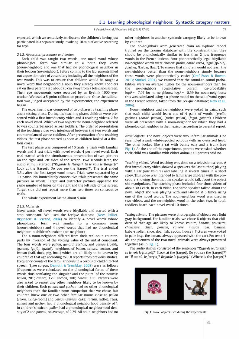
expected, which we tentatively attribute to the children’s having justparticipated in a separate study involving 10 min of active searchingfor toys.
2.1.2. Apparatus, procedure and designEach child was taught two words: one novel word whose
phonological form was similar to a noun they know(noun-neighbor) and one that had no phonological neighbor intheir lexicon (no-neighbor). Before coming to the lab, parents filledout a questionnaire of vocabulary including all the neighbors of thetest words. This was to ensure that children would be taught anovel word that neighbored a noun they already knew. Toddlerssat on their parent’s lap about 70 cm away from a television screen.Their eye movements were recorded by an Eyelink 1000 eye-tracker. We used a 5-point calibration procedure. Once the calibra-tion was judged acceptable by the experimenter, the experimentbegan.
The experiment was composed of two phases: a teaching phaseand a testing phase. During the teaching phase, children were pre-sented with a first introductory video and 4 teaching videos, 2 foreach novel word. Which of two objects the noun-neighbor referredto was counterbalanced across toddlers. The order of presentationof the teaching video was interleaved between the two words andcounterbalanced across toddlers. After presentation of the teachingvideos, the test phase started as soon as children looked at a fixa-tion cross.
The test phase was composed of 16 trials: 8 trials with familiarwords and 8 test trials with novel words, 4 per novel word. Eachtrial started with the simultaneous presentation of two pictureson the right and left sides of the screen. Two seconds later, theaudio stimuli started: (‘‘Regarde le [target], tu le vois le [target]?’’Look at the [target], Do you see the [target]?). The trial ended3.5 s after the first target word onset. Trials were separated by a1 s pause. No immediately consecutive trials presented the samepictures or words. Target and distractor pictures appeared thesame number of times on the right and the left side of the screen.Target side did not repeat more than two times on consecutivetrials.
The whole experiment lasted about 5 min.
2.1.3. MaterialsNovel words. All novel words were bisyllabic and started with astop consonant. We used the Lexique database (New, Pallier,Brysbaert, & Ferrand, 2004) to identify 4 novel words whosephonological form was similar to a common noun(noun-neighbors) and 4 novel words that had no phonologicalneighbor in children’s lexicon (no-neighbor).
The 4 noun-neighbors differed from their real-noun counter-parts by inversion of the voicing value of the initial consonant.The four words were pallon, ganard, gochon, and pateau (/palõ/,/gana�/, /goSõ/, /pato/), neighbors of ballon, canard, cochon, andbateau (ball, duck, pig, boat) which are all likely to be known bychildren of that age according to CDI reports from previous studies.Frequency counts of the familiar nouns in a corpus of child directedspeech (Lyon corpus, Demuth & Tremblay, 2008) were as follows(frequencies were calculated on the phonological forms of thesewords thus conflating the singular and the plural of the nouns):ballon, 201; canard, 179; cochon, 180; bateau, 105. Parents werealso asked to report any other neighbors likely to be known bytheir children. Both ganard and gochon had no other phonologicalneighbors than the familiar noun competitor that we chose, butchildren knew one or two other familiar nouns close to pallon(salon, living-room) and pateau (gateau, cake; rateau, rattle). Thus,ganard and gochon had a phonological neighborhood density of 1in children’s lexicon; pallon had a phonological neighborhood den-sity of 2 and pateau, on average, of 2.25. All noun-neighbors had no
other neighbors in another syntactic category likely to be knownby children.
The no-neighbors were generated from an n-phone modeltrained on the Lexique database with the constraint that theyshould be phonologically similar to less than 2 low frequencywords in the French lexicon. Four phonotactically legal bisyllabicno-neighbor words were chosen: prolin, barlié, torba, lagui (/p�ol~e/,/barljé/, /tOrba/, /lagi/). To ensure that children would not learn theno-neighbors better than the noun-neighbors simply becausethese words were phonotactically easier (Graf Estes & Bowen,2013; Storkel, 2001), we ensured that the sound-to-sound proba-bilities were on average higher for the noun-neighbors than forthe no-neighbors (cumulative bigram log-probabilitylogP = �7.07 for no-neighbors; logP = �5.59 for noun-neighbors;this was calculated using a n-phone model on the set of word typesin the French lexicon, taken from the Lexique database; New et al.,2004).
Noun-neighbors and no-neighbors were yoked in pairs, suchthat each child would learn one of 4 pairs of words: (prolin,gochon), (barlié, pateau), (torba, pallon), (lagui, ganard). Childrenwere all presented with a noun-neighbor for which they had aphonological neighbor in their lexicon according to parental report.
Novel objects. The novel objects were two unfamiliar animals. Oneresembled a pink white-spotted octopus with an oversized head.The other looked like a rat with bunny ears and a trunk (seeFig. 1). At the end of the experiment, parents were asked whethertheir child was familiar with either animal; all parents said no.
Teaching videos. Word teaching was done on a television screen. Afirst introductory video showed a speaker (the last author) playingwith a car (une voiture) and labeling it several times in a shortstory. This video was intended to familiarize children with the pro-cedure, showing them that the speaker would talk about the objectshe manipulates. The teaching phase included four short videos ofabout 30 s each. In each video, the same speaker talked about thenovel object she was playing with and labeled it 5 times usingone of the novel words. The noun-neighbor word was used intwo videos, and the no-neighbor word in the other two. In total,toddlers heard each novel word 10 times.
Testing stimuli. The pictures were photographs of objects on a lightgray background. For familiar trials, we chose 8 objects that chil-dren of that age are likely to know: voiture, banane, poussette,chaussure, chien, poisson, cuillère, maison (car, banana,baby-stroller, shoe, dog, fish, spoon, house). Pictures were yokedin pairs (e.g., the banana always appeared with the car). For test tri-als, the pictures of the two novel animals were always presentedtogether (as in Fig. 1).
The audio stimuli consisted of the sentences ‘‘Regarde le [target],tu le vois le [target]?’’ (Look at the [target], Do you see the [target]?)or ‘‘il est où, le [target]? Regarde le [target].’’ (Where is the [target]?
Fig. 1. Novel objects used during the experiments.
I. Dautriche et al. / Cognition 143 (2015) 77–86 79
3.1 Learning phonological neighbors: Syntactic category matters
81

Look at the [target]!) where [target] was the target word and waspronounced two times in a given trial. All sentences were recordedby the last author (the same speaker as in the videos). The averageduration of the novel words was 610 ms for the noun-neighborsand 598 ms for the no-neighbors.
2.1.4. Measurement and analysisGaze position on each trial was recorded via an eye-tracker with
a 2 ms sampling rate. We inspected the time course of eye move-ments from the onset of the first occurrence of the target word
(‘‘Look at the [target].’’) until the end of the trial. One recurrentproblem when analyzing continuous time series is the choice of awindow of analysis. Time can be made categorical by choosing aseries of consecutive time windows tailor-made to the data andthen performing separate analysis on each time window; or, morefrequently in the infant literature, by imposing a single, large win-dow to maximize the chances of observing a change in eye fixa-tions. While the first option leads to a problem of multiplecomparisons, the second often conflates response time and accu-racy, thus resulting in a loss of information (Swingley, 2011) andboth options are subject to biases inherent to window selection.Here, in order to test whether toddlers had learned each novelword we conducted a cluster-based permutation analysis (Maris& Oostenveld, 2007) to find a time window where we observed asignificant increase in looks toward the target picture. This typeof analysis, originally developed for EEG data, is free oftime-window biases, preserves the information available in thetime series and is able to cope well with multiple comparisons.2
The cluster-based analysis works as follows: at each time pointwe conducted a one-tailed3 t-test on fixations to the target com-pared to chance (0.5). All fixation proportions were transformedvia the arcsin square function to fit better the assumptions of thet-test. The means and variances were computed over subjects withinconditions. Adjacent time points with a significant effect (t > 2;p < .05) were grouped together into a cluster. Each cluster wasassigned a single numerical value measuring its size, and definedas the sum of all the t-values within the cluster (intuitively, a clusteris larger if it contains time-points for which the two conditions arevery significantly different, and if it spans a longer time-window).To obtain the probability of observing a cluster of that size bychance, we conducted 1000 simulations where conditions (novellabel, chance) were randomly assigned for each trial. For each simu-lation, we computed the size of the biggest cluster identified withthe same procedure that was used for the real data (sum of all thet-values within a cluster of significant t-values). Clusters in the chil-dren’s data were taken as significant if the probability of observing acluster of the same size or bigger in the randomized data was smallerthan 5% (that is, if a cluster that big was observed in less that 50cases over 1000), corresponding to a p-value of 0.05.
It is important to note that the criterion for including a time binin a cluster (t > 2 in our study) is independent of the process whichassesses cluster significance, so it does not affect the likelihood of afalse positive. Yet, it does have an influence on the size of the timewindow that one can find. If the threshold is low then the timewindow will be wider. However the same low threshold will beapplied to the randomized data as well, such that the chance of
getting a bigger cluster will also increase under the null hypothe-sis, thus maintaining the rate of false positive under 0.05.
In addition, to test whether there was a significant differencebetween conditions (whether children found the noun-neighborharder to learn than the no-neighbor), we conducted an additionalcluster-based permutation analysis in which clusters were formedon the basis of paired two-tailed t-tests comparing the looking pro-portions between conditions at each time point.
Thus in total, we conducted three cluster-based analyses: onefor each word condition (no-neighbor; noun-neighbor) comparingthe average proportion of looks toward the target picture for eachtest word to 50%, and one comparing the looking proportionsbetween conditions.
2.2. Results
Fig. 2 shows the average proportion of looks toward the targetpicture for familiar and test words (noun-neighbor andno-neighbor) from the onset of the first target word (Regarde le
[target], tu le vois le [target]? Look at the [target], do you see the[target]?) until the end of the trial.
Children showed recognition of the no-neighbor (green curve inFig. 2) but not the noun-neighbor (red curve in Fig. 2). Thecluster-based permutation analyses revealed that they fixated thecorrect picture above chance when asked to look at theno-neighbor (2178–2568 ms time-window, green-shaded area inFig. 2; p < .05) but stayed around chance level in the case of thenoun-neighbor (no significant time window found by thecluster-based permutation analysis). The difference between therecognition of the no-neighbor and the noun-neighbor was signif-icant in the time window ranging from 2044 to 2852 ms (p < .01,gray-shaded area in Fig. 2). Thus, children learned theno-neighbor but not the noun-neighbor (p = 0.19). We alsoobserved that the recognition of the no-neighbor occurred with adelay of about 900 ms compared to the recognition of familiarwords (gray curve in Fig. 2), a finding we will return to later in dis-cussing subsequent experiments.
2.3. Discussion
After a brief but intensive exposure to a pair of novel words,French 18-month-olds performed better when tested on a novelno-neighbor (e.g., ‘‘torba’’) than on a novel noun-neighbor (e.g.,‘‘ganard,’’ a novel neighbor of ‘‘canard,’’ duck) in a word recognitiontask. When presented with the two novel objects on the screen andhearing a sentence labeling one of them, children correctly recog-nized the no-neighbor but failed to recognize the noun-neighbor.This may be surprising given that children of that age can inferthe meaning of a word via mutual exclusivity (e.g., Markman &Wachtel, 1988). That is, if they learnt the no-neighbor then theyshould be able to infer the meaning of the noun-neighbor by pro-cess of elimination during the test phase. Yet several studies haveshown that mutual exclusivity effects seem to disappear whenchildren are confronted with a novel word that is phonologicallysimilar to a familiar word (e.g., Merriman, Marazita, & Jarvis,1995). When children heard ‘‘Regarde le pallon!’’ look at the pallon,they may start looking for a ‘‘ballon’’, the phonological competitor,and go back and forth between the two images to find the closestmatch.
This result replicates Swingley and Aslin’s (2007) findings withEnglish and Dutch 18-month-olds, showing that children of thatage find it hard to learn a phonological neighbor of a familiar noun.We will now test toddlers’ ability to learn a novel neighbor of afamiliar verb.
2 Following a reviewer’s suggestion, we also compared the results of this methodwith more traditional methods such as the salience-corrected fixations (see Swingley,2011, for a discussion of this measure) and the more recent growth curve analysismethod (Barr, 2008). Both methods of analysis lead to the same conclusion and areavailable upon request to the first author.
3 Note that we used one-tailed t-tests because our hypothesis was directional as weexpected a higher-than-chance looking proportion when the word was recognized,yet using two-tailed t-test did not change the pattern of results. In particular none ofthe clusters of fixations below chance level passed the permutation test.
80 I. Dautriche et al. / Cognition 143 (2015) 77–86
3 Learning confusable and ambiguous words
82
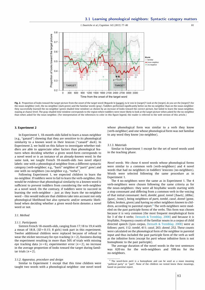
3. Experiment 2
In Experiment 1, 18-month-olds failed to learn a noun-neighbor(e.g., ‘‘ganard’’) showing that they are sensitive to its phonologicalsimilarity to a known word in their lexicon (‘‘canard’’ duck). InExperiment 2, we build on this failure to investigate whether tod-dlers are able to appreciate other factors than phonological fea-tures when deciding whether a given word-form corresponds toa novel word or is an instance of an already-known word. In thesame task, we taught French 18-month-olds two novel objectlabels: one with a phonological neighbor from a different syntacticcategory (verb-neighbor; e.g., ‘‘barti’’ neighbor of ‘‘parti’’ gone) andone with no neighbors (no-neighbor e.g., ‘‘torba’’).
Following Experiment 1, we expected children to learn theno-neighbor. If toddlers were to fail to learn the verb-neighbor, thiswould be evidence that phonological similarity to a known word issufficient to prevent toddlers from considering the verb-neighboras a novel word. On the contrary, if toddlers were to succeed inlearning the verb-neighbor – just as they learn the no-neighborword – this would indicate that children take into account not onlyphonological likelihood but also syntactic and/or semantic likeli-hood when deciding whether a given word-form denotes a novelword or not.
3.1. Method
3.1.1. ParticipantsSixteen French 18-month-olds, ranging from 17;18 to 19;4 with
a mean of 18;8, (SD = 0;15; 8 girls) took part in this experiment.Twelve additional children were replaced because of refusal towear the sticker necessary for eye-tracking (n = 2), fussiness duringthe experiment resulting in more than 50% of trials with missingeye tracking data (n = 6), experimenter error (n = 2), no increasein the average proportion of looks toward the target during famil-iar trials (n = 2).
3.1.2. Apparatus, procedure and designSimilar to Experiment 1 except that this time children were
taught two words with a phonological neighbor: one novel word
whose phonological form was similar to a verb they know(verb-neighbor) and one whose phonological form was not familiarto any word they know (no-neighbor).
3.1.3. MaterialsSimilar to Experiment 1 except for the set of novel words used
in the teaching phase.
Novel words. We chose 4 novel words whose phonological formswere similar to a common verb (verb-neighbors) and 4 novelwords that had no neighbors in toddlers’ lexicons (no-neighbors).Words were selected following the same procedure as inExperiment 1.
The 4 no-neighbors were the same as in Experiment 1. The 4verb-neighbors were chosen following the same criteria as forthe noun-neighbors: they were all bisyllabic words starting witha stop consonant and differing from a common verb in the voicingof that initial consonant: barti, dombé, gassé, tonné (/ba�ti/, /dõbe/,/gase/, /tone/), being neighbors of parti, tombé, cassé, donné (gone,fallen, broken, given) and having no other neighbors known to chil-dren, according to parental report.4 The verb-neighbors were mod-eled on the past participle forms of the verbs. This form was chosenbecause it is very common (the most frequent morphological formfor 3 of the 4 verbs; Demuth & Tremblay, 2008) and because it isbisyllabic, Frequency counts of the familiar nouns in a corpus of childdirected speech (Lyon corpus, Demuth & Tremblay, 2008) were asfollows: parti, 112; tombé, 411; cassé, 263; donné, 252. These countswere calculated on the phonological form of the neighbor in parentalinput and thus included the past participle form of the verb as wellas the infinitive form (except for parti whose infinitive form is nothomophonic to the past participle).
The average duration of the novel words in the test sentenceswas 620 ms for the verb-neighbors and 598 ms for theno-neighbors.
**p = 0.01*p = 0.04
TARGET TARGET
*************p = 0.01p === 00 101*p = 0.040p =
TARGET TARGETT R ETETE TARGETARGERT EE
0.2
0.3
0.4
0.5
0.6
0.7
0.8
0 300 600 900 1200 1500 1800 2100 2400 2700 3000 3300Time from the onset of the target word
Prop
ortio
n of
look
s to
war
d th
e ta
rget
pic
ture
Wordsfamiliarnoun-neighborno-neighbor
Fig. 2. Proportion of looks toward the target picture from the onset of the target word (Regarde le [target], tu le vois le [target]? Look at the [target], do you see the [target]?) forthe noun-neighbor (red), the no-neighbor (dark green) and the familiar words (gray). Toddlers performed significantly better on the no-neighbor than on the noun-neighbor:they successfully learned the no-neighbor (green shaded time window) as shown by an increase of looks toward the correct picture, but failed to learn the noun-neighbor,staying at chance level. The gray-shaded time window corresponds to the region where toddlers were more likely to look at the target picture when asked for the no-neighborthan when asked for the noun neighbor. (For interpretation of the references to color in this figure legend, the reader is referred to the web version of this article.)
4 The word-form parti is a homophone and can be used as a noun meaning‘‘political party’’ or ‘‘part’’. None of the children we tested knew these meanings,based on parental report.
I. Dautriche et al. / Cognition 143 (2015) 77–86 81
3.1 Learning phonological neighbors: Syntactic category matters
83
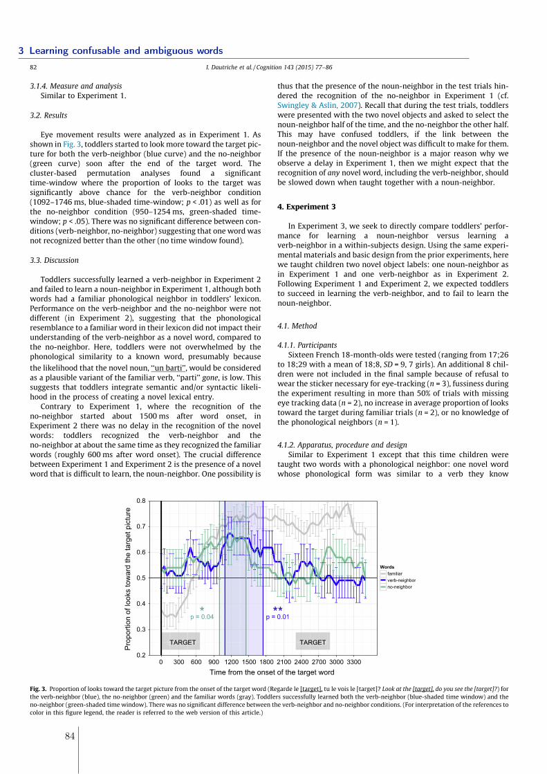
3.1.4. Measure and analysisSimilar to Experiment 1.
3.2. Results
Eye movement results were analyzed as in Experiment 1. Asshown in Fig. 3, toddlers started to look more toward the target pic-ture for both the verb-neighbor (blue curve) and the no-neighbor(green curve) soon after the end of the target word. Thecluster-based permutation analyses found a significanttime-window where the proportion of looks to the target wassignificantly above chance for the verb-neighbor condition(1092–1746 ms, blue-shaded time-window; p < .01) as well as forthe no-neighbor condition (950–1254 ms, green-shaded time-window; p < .05). There was no significant difference between con-ditions (verb-neighbor, no-neighbor) suggesting that one word wasnot recognized better than the other (no time window found).
3.3. Discussion
Toddlers successfully learned a verb-neighbor in Experiment 2and failed to learn a noun-neighbor in Experiment 1, although bothwords had a familiar phonological neighbor in toddlers’ lexicon.Performance on the verb-neighbor and the no-neighbor were notdifferent (in Experiment 2), suggesting that the phonologicalresemblance to a familiar word in their lexicon did not impact theirunderstanding of the verb-neighbor as a novel word, compared tothe no-neighbor. Here, toddlers were not overwhelmed by thephonological similarity to a known word, presumably because
the likelihood that the novel noun, ‘‘un barti’’, would be consideredas a plausible variant of the familiar verb, ‘‘parti’’ gone, is low. Thissuggests that toddlers integrate semantic and/or syntactic likeli-hood in the process of creating a novel lexical entry.
Contrary to Experiment 1, where the recognition of theno-neighbor started about 1500 ms after word onset, inExperiment 2 there was no delay in the recognition of the novelwords: toddlers recognized the verb-neighbor and theno-neighbor at about the same time as they recognized the familiarwords (roughly 600 ms after word onset). The crucial differencebetween Experiment 1 and Experiment 2 is the presence of a novelword that is difficult to learn, the noun-neighbor. One possibility is
thus that the presence of the noun-neighbor in the test trials hin-dered the recognition of the no-neighbor in Experiment 1 (cf.Swingley & Aslin, 2007). Recall that during the test trials, toddlerswere presented with the two novel objects and asked to select thenoun-neighbor half of the time, and the no-neighbor the other half.This may have confused toddlers, if the link between thenoun-neighbor and the novel object was difficult to make for them.If the presence of the noun-neighbor is a major reason why weobserve a delay in Experiment 1, then we might expect that therecognition of any novel word, including the verb-neighbor, shouldbe slowed down when taught together with a noun-neighbor.
4. Experiment 3
In Experiment 3, we seek to directly compare toddlers’ perfor-mance for learning a noun-neighbor versus learning averb-neighbor in a within-subjects design. Using the same experi-mental materials and basic design from the prior experiments, herewe taught children two novel object labels: one noun-neighbor asin Experiment 1 and one verb-neighbor as in Experiment 2.Following Experiment 1 and Experiment 2, we expected toddlersto succeed in learning the verb-neighbor, and to fail to learn thenoun-neighbor.
4.1. Method
4.1.1. ParticipantsSixteen French 18-month-olds were tested (ranging from 17;26
to 18;29 with a mean of 18;8, SD = 9, 7 girls). An additional 8 chil-dren were not included in the final sample because of refusal towear the sticker necessary for eye-tracking (n = 3), fussiness duringthe experiment resulting in more than 50% of trials with missingeye tracking data (n = 2), no increase in average proportion of lookstoward the target during familiar trials (n = 2), or no knowledge ofthe phonological neighbors (n = 1).
4.1.2. Apparatus, procedure and designSimilar to Experiment 1 except that this time children were
taught two words with a phonological neighbor: one novel wordwhose phonological form was similar to a verb they know
**p = 0.01*p = 0.04
TARGET TARGET
***p = 0.01p = 0 01= 0*p = 0.04p = 0 04=
TARGETTARGETT R TARGETTARGETRT E
0.2
0.3
0.4
0.5
0.6
0.7
0.8
0 300 600 900 1200 1500 1800 2100 2400 2700 3000 3300Time from the onset of the target word
Prop
ortio
n of
look
s to
war
d th
e ta
rget
pic
ture
Wordsfamiliarverb-neighborno-neighbor
Fig. 3. Proportion of looks toward the target picture from the onset of the target word (Regarde le [target], tu le vois le [target]? Look at the [target], do you see the [target]?) forthe verb-neighbor (blue), the no-neighbor (green) and the familiar words (gray). Toddlers successfully learned both the verb-neighbor (blue-shaded time window) and theno-neighbor (green-shaded time window). There was no significant difference between the verb-neighbor and no-neighbor conditions. (For interpretation of the references tocolor in this figure legend, the reader is referred to the web version of this article.)
82 I. Dautriche et al. / Cognition 143 (2015) 77–86
3 Learning confusable and ambiguous words
84
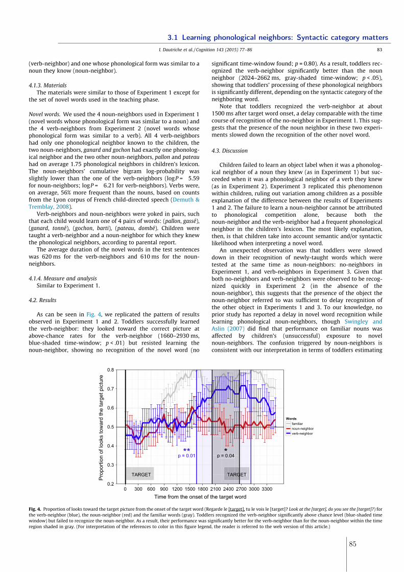
(verb-neighbor) and one whose phonological form was similar to anoun they know (noun-neighbor).
4.1.3. MaterialsThe materials were similar to those of Experiment 1 except for
the set of novel words used in the teaching phase.
Novel words. We used the 4 noun-neighbors used in Experiment 1(novel words whose phonological form was similar to a noun) andthe 4 verb-neighbors from Experiment 2 (novel words whosephonological form was similar to a verb). All 4 verb-neighborshad only one phonological neighbor known to the children, thetwo noun-neighbors, ganard and gochon had exactly one phonolog-ical neighbor and the two other noun-neighbors, pallon and pateauhad on average 1.75 phonological neighbors in children’s lexicon.The noun-neighbors’ cumulative bigram log-probability wasslightly lower than the one of the verb-neighbors (logP = �5.59for noun-neighbors; logP = �6.21 for verb-neighbors). Verbs were,on average, 56% more frequent than the nouns, based on countsfrom the Lyon corpus of French child-directed speech (Demuth &Tremblay, 2008).
Verb-neighbors and noun-neighbors were yoked in pairs, suchthat each child would learn one of 4 pairs of words: (pallon, gassé),(ganard, tonné), (gochon, barti), (pateau, dombé). Children weretaught a verb-neighbor and a noun-neighbor for which they knewthe phonological neighbors, according to parental report.
The average duration of the novel words in the test sentenceswas 620 ms for the verb-neighbors and 610 ms for the noun-neighbors.
4.1.4. Measure and analysisSimilar to Experiment 1.
4.2. Results
As can be seen in Fig. 4, we replicated the pattern of resultsobserved in Experiment 1 and 2. Toddlers successfully learnedthe verb-neighbor: they looked toward the correct picture atabove-chance rates for the verb-neighbor (1660–2930 ms,blue-shaded time-window; p < .01) but resisted learning thenoun-neighbor, showing no recognition of the novel word (no
significant time-window found; p = 0.80). As a result, toddlers rec-ognized the verb-neighbor significantly better than the nounneighbor (2024–2662 ms, gray-shaded time-window; p < .05),showing that toddlers’ processing of these phonological neighborsis significantly different, depending on the syntactic category of theneighboring word.
Note that toddlers recognized the verb-neighbor at about1500 ms after target word onset, a delay comparable with the timecourse of recognition of the no-neighbor in Experiment 1. This sug-gests that the presence of the noun neighbor in these two experi-ments slowed down the recognition of the other novel word.
4.3. Discussion
Children failed to learn an object label when it was a phonolog-ical neighbor of a noun they knew (as in Experiment 1) but suc-ceeded when it was a phonological neighbor of a verb they knew(as in Experiment 2). Experiment 3 replicated this phenomenonwithin children, ruling out variation among children as a possibleexplanation of the difference between the results of Experiments1 and 2. The failure to learn a noun-neighbor cannot be attributedto phonological competition alone, because both thenoun-neighbor and the verb-neighbor had a frequent phonologicalneighbor in the children’s lexicon. The most likely explanation,then, is that children take into account semantic and/or syntacticlikelihood when interpreting a novel word.
An unexpected observation was that toddlers were sloweddown in their recognition of newly-taught words which weretested at the same time as noun-neighbors: no-neighbors inExperiment 1, and verb-neighbors in Experiment 3. Given thatboth no-neighbors and verb-neighbors were observed to be recog-nized quickly in Experiment 2 (in the absence of thenoun-neighbor), this suggests that the presence of the object thenoun-neighbor referred to was sufficient to delay recognition ofthe other object in Experiments 1 and 3. To our knowledge, noprior study has reported a delay in novel word recognition whilelearning phonological noun-neighbors, though Swingley andAslin (2007) did find that performance on familiar nouns wasaffected by children’s (unsuccessful) exposure to novelnoun-neighbors. The confusion triggered by noun-neighbors isconsistent with our interpretation in terms of toddlers estimating
**p = 0.01 *p = 0.04
TARGET TARGET
****p = 0.01p = 0 01= . *p = 0.04p = 0 04= .
TARGETTARGETT GR GET GETEG TARGTARGRT GG
0.2
0.3
0.4
0.5
0.6
0.7
0.8
0 300 600 900 1200 1500 1800 2100 2400 2700 3000 3300Time from the onset of the target word
Prop
ortio
n of
look
s to
war
d th
e ta
rget
pic
ture
Wordsfamiliarnoun-neighborverb-neighbor
Fig. 4. Proportion of looks toward the target picture from the onset of the target word (Regarde le [target], tu le vois le [target]? Look at the [target], do you see the [target]?) forthe verb-neighbor (blue), the noun-neighbor (red) and the familiar words (gray). Toddlers recognized the verb-neighbor significantly above chance level (blue-shaded timewindow) but failed to recognize the noun-neighbor. As a result, their performance was significantly better for the verb-neighbor than for the noun-neighbor within the timeregion shaded in gray. (For interpretation of the references to color in this figure legend, the reader is referred to the web version of this article.)
I. Dautriche et al. / Cognition 143 (2015) 77–86 83
3.1 Learning phonological neighbors: Syntactic category matters
85
the likelihood that a given word-form corresponds to a novel lex-ical entry or an existing one: When the odds are against the cre-ation of a novel lexical entry – because the phonological andsemantic/syntactic similarity appear too great to be coincidental– children attempt to reconcile the deviant phonological form withthe existing lexical entry. This process might involve trying to fig-ure out in what circumstances the observed phonological changemay be licensed by the native language, as well as what extensionof the word’s meaning may encompass both the familiar referentand the novel referent. Whatever the exact nature of this process,it may contribute to the confusion that is observed.
5. General discussion
A simple rule for determining whether a spoken word corre-sponds to a word in the lexicon is to compare the phonologicalform of this word to the phonological forms in the lexicon. Whenthe forms match, the word’s identity is known; if the heard formmatches no known words, it may be a candidate for entry intothe lexicon as a new word. Part of the function of a phonologicalsystem is to ensure that this matching process can work, at leastwhen the signal itself is carefully produced and clearly heard.
Young children apparently have some difficulty in operatingwith their developing phonology in this way. For example, theyhave some trouble learning similar-sounding words (e.g., Stager& Werker, 1997). Swingley and Aslin’s (2007) finding, in whichthe proximity of a novel word like tog to the familiar word dogmade the novel word hard to learn, showed that lexical activationprocesses, whose function is to account for the sounds in an utter-ance in terms of the correct string of words (and possibly in spite ofmispronunciation or misperception), can conflict with word learn-ing processes. In that study, the novel object intended as the refer-ent for the novel word (e.g.) tog had no real resemblance to itsfamiliar counterpart (dog). Similarly in the present experiments,the plush pink octopus object labeled here as pateau is not a rea-sonable member of the category of boats (bateaux). Such consider-ations suggest that children’s difficulty might be purely a matter ofphonological proximity: tog (or pateau) is simply too close to afamiliar word to permit ready detection as a novel form.
The present work shows that this is not the case. In fact similar-ity of the novel referent to its competitor’s denotation matters. Thesimilarity of a pateau (plush octopus) to a bateau (boat) is not great,but it is greater than the similarity of the same octopus to themeaning of parti or cassé (gone, broken) because it shares the samesyntactic category (nouns) and the same broad semantic category(toys).
With the present data we cannot determine whether it is thesyntactic difference that is most important, or the semantic one, orboth; but to get some purchase on this question we looked forpotential item differences within the experiments. Recall that twoof our familiar nouns were animals (canard, duck, and cochon, pig)and two were artifacts (ballon, ball, and bateau, boat). Given howfundamental the distinction between animals and artifacts is, evento infants (e.g., Setoh, Wu, Baillargeon, & Gelman, 2013), our itemsganard and gochon (as plush animals) were probably semanticallymuch closer to their competitors canard and cochon than pateauor pallon (as plush animals) were to bateau or ballon. If semanticsimilarity were the main driving force behind our results, we wouldexpect children to learn pateau and pallon more easily than ganardand gochon. Indeed, inspection of the results revealed a nonsignifi-cant trend toward better performance on pateau and pallon thanganard and gochon for participants in Experiment 1 and 3. It couldbe interesting to vary this similarity systematically with moreitems; here, there are confounding features of the words, such asuneven phonotactic probability and neighborhood density, that
make interpreting this trend difficult. At any rate, although the pre-sent result cannot tells us whether the semantic or the syntactic dif-ference between the neighbors and their familiar competitors playa role, it is clear that 18-month-olds take more into considerationthan the sounds alone.
Might some unmeasured difference between our noun and verbneighbors be responsible for our effects? For example, frequentwords are generally recognized more readily than infrequentwords (e.g., Solomon & Postman, 1952). Could it be that the inter-fering effect of noun neighbors derives from stronger activation ofthose words, and not from the direct consequences of semantic orsyntactic distance from the novel objects? This might happen if thephonological form of nouns were more strongly established in chil-dren’s lexicons than the phonological form of verbs: indeed, verbsin French occur in more varied phonological forms than nouns, dueto morphology. However, as we reported, the exact phonologicalforms of the verbs we used were, on average, 56% more frequentthan the nouns in parental input, and as frequent as the nouns inchildren’s production, based on counts from the Lyon corpus ofFrench child-directed speech (Demuth & Tremblay, 2008), and par-ents in each experiment reported that their children knew theneighboring words.
Another possibility is that independently of frequency, themeanings of the noun neighbors were better entrenched in chil-dren’s lexicons than the meanings of the verb neighbors, leadingto greater interference. Yet if more entrenched representationslead to greater interference, we would also expect thatverb-neighbors should lead to more interference than a word withno neighbor. That’s not what we observe: children learntverb-neighbors just as well as no-neighbors in Experiment 2. Sowhile we cannot dismiss the possibility that more entrenched rep-resentations of the familiar nouns over the familiar verbs plays arole in children’s interpretation of novel neighbors, our data pro-vide little support for this hypothesis. Thus our main point wouldstill hold, namely that semantic or syntactic similarity plays a rolein children’s interpretation of novel neighbors.
Thus, we propose that young toddlers’ evaluation of similarityin the lexicon in the context of word learning is multidimensional,incorporating both phonological and semantic and/or syntacticfeatures. The plausibility of a syntactic contribution to the resultsis supported by prior studies showing that children, like adults,use the sentence context to build on-line expectations about thesyntactic category of an upcoming word (e.g., Bernal,Dehaene-Lambertz, Millotte, & Christophe, 2010). Toddlers asyoung as 14 to 18 months expect a noun to follow a determinerand expect a verb after a personal pronoun (Cauvet et al., 2014;He & Lidz, 2014; Kedar, Casasola, & Lust, 2006; Shi & Melancon,2010; Zangl & Fernald, 2007). For instance, Cauvet et al. (2014)showed that French 18-month-old toddlers trained to turn theirhead for a known target noun (‘‘la balle’’ the ball), responded moreoften to the word ‘‘balle’’ when it appeared in a noun context (‘‘uneballe’’ a ball) than when it appeared (incorrectly) in a verb context(‘‘on balle’’ they ball). In fact, in that last case, they did not turntheir head more often than for control sentences which did notcontain the target word at all. In our study, when children wereprocessing the syntactic context of our sentences, they should haveexpected a noun at the point where the verb-neighbor, barti, washeard. Since barti occurred in a context where the familiar verbparti was not expected, one possibility is that children did notaccess the familiar verb parti at all, and therefore that they didnot even notice the similarity with a word present in their lexicon.Another possibility is that children may have accessed parti despitethe nominal context because the integration of contextual cues islimited by toddlers’ developing executive function abilities (e.g.,Khanna & Boland, 2010, but see Rabagliati, Pylkkänen, & Marcus,2013) Yet the presence of additional cues provided by the learning
84 I. Dautriche et al. / Cognition 143 (2015) 77–86
3 Learning confusable and ambiguous words
86
situation (i.e., repetition of the verb-neighbor in a noun context,presence of a novel object and contingent gaze cues from thespeaker whenever the verb-neighbor was used) may render thepossibility that the verb-neighbor barti is a novel word a moreplausible alternative than for the noun-neighbor.
Children process words in context, just as adults do. In particu-lar, the linguistic context plays a prominent role in constraininglexical access and thus in estimating the likelihood that a novelphonological word-form is a novel lexical entry rather than a vari-ant of a known word. Manipulating the linguistic context by plac-ing a verb-neighbor in a noun syntactic frame indicated to childrenthat a new meaning was appropriate for the novel word-form. Wewould expect the same result to be found using other syntacticframes (e.g., pronouns) or by doing the symmetric manipulation(i.e., presenting a noun-neighbor in a verb syntactic frame). Thissuggests also that the linguistic context may play a role in learningseveral meanings for perfectly identical word-forms (homophones;see also Casenhiser, 2005), a possibility that we are currentlyexploring.
Learning neighbors of familiar words is difficult for toddlers, butas we showed, this difficulty disappears when the novel wordsappear in contexts that are sufficiently different from their knownneighbors (either syntactically or semantically or both). If learn-ability influences language changes, then this constraint on earlylexical acquisition might have a long-lasting impact on the overallstructure of the lexicon. Do lexicons avoid similar-soundingwords? And when similar-sounding words do occur, are they pref-erentially distributed across syntactic or semantic categories toimprove their learnability (and their recoverability)? Recent stud-ies observed that not only do mature lexicons contain manysimilar-sounding words, perhaps even more than would beexpected by chance (Dautriche et al., 2014), but there is also a ten-dency for phonologically similar words to be more semanticallysimilar than phonologically distinct words (Monaghan, Shillcock,Christiansen, & Kirby, 2014; Dautriche et al., 2014). In sum, lexi-cons appear to favor similar-sounding words which are semanti-cally related.
At first sight this might appear at odds with the present study,yet there are two ways to resolve this apparent inconsistency.First, a rich literature suggests that similar-sounding words displaya range of advantages for language use: they are easier to remem-ber, produce and process for adults (e.g., Vitevitch, 2002;Vitevitch, Chan, & Roodenrys, 2012; Vitevitch & Stamer, 2006)and preschoolers (e.g., Storkel & Lee, 2011; Storkel & Morrisette,2002). Also, greater systematicity of form-to-meaning mappingscould facilitate the grouping of words into categories (PadraicMonaghan, Christiansen, & Fitneva, 2011). Overall, the processingbenefits for similar-sounding words might outweigh an initiallearning disadvantage. Second, an early disadvantage for learningsimilar-sounding words may not actively exert a selective pressurefor words that are more phonologically dissimilar because childrenmay eventually manage to learn neighbors through repeated expo-sure. Thus, instead of being reflected in the static organization ofthe lexicon, the constraint we uncovered may be reflected in thedynamics of early lexical growth: early in children’s lexical devel-opment, novel words may preferably be added whenever they canbe easily distinguished from already existing words along at leastone dimension (phonological, syntactic, and/or semantic).Previous work looking at the growth of the lexicon focused onhow either phonological similarity or semantic similarity influ-ences word learning, but not on potential interactions between sev-eral dimensions (Carlson, Sonderegger, & Bane, 2014; Hills,Maouene, Maouene, Sheya, & Smith, 2009; Steyvers &Tenenbaum, 2005; but see Regier et al., 2001).
In sum, our work shows that 18-month-old children processwords in context, using multiple sources of information.
Phonological similarity alone does not serve as a kind of filter thatcollapses phonological neighbors in advance of meaningful analy-sis. Rather, 18-month-olds appear to evaluate simultaneously thephonological, syntactic and/or semantic likelihood of this sequenceof sounds being a new word.
Acknowledgements
This work was funded by grants from the Région IIe-de-France,Fondation de France, LabEx IEC (ANR-10-LABX-0087), IdEx PSL(ANR-10-IDEX-0001-02), the ANR ‘Apprentissages’ (ANR-13-APPR-0012) to AC, NIH grant R01-HD049681 to DS, and a PhDfellowship from DGA to ID.
References
Altmann, G., & Kamide, Y. (1999). Incremental interpretation at verbs: Restrictingthe domain of subsequent reference. Cognition, 73(3), 247–264.
Bard, E. G., & Anderson, A. H. (1983). The unintelligibility of speech to children.Journal of Child Language, 10(02), 265–292.
Barr, D. J. (2008). Analyzing ‘‘visual world’’ eyetracking data using multilevel logisticregression. Journal of Memory and Language, 59(4), 457–474.
Bernal, S., Dehaene-Lambertz, G., Millotte, S., & Christophe, A. (2010). Two-year-oldscompute syntactic structure on-line. Developmental Science, 13(1), 69–76.
Carlson, M. T., Sonderegger, M., & Bane, M. (2014). How children explore thephonological network in child-directed speech: A survival analysis of children’sfirst word productions. Journal of Memory and Language, 75, 159–180.
Casenhiser, D. M. (2005). Children’s resistance to homonymy: An experimentalstudy of pseudohomonyms. Journal of Child Language, 32(2), 319–343.
Cauvet, E., Limissuri, R., Millotte, S., Skoruppa, K., Cabrol, D., & Christophe, A. (2014).Function words constrain on-line recognition of verbs and nouns in French 18-month-olds. Language Learning and Development, 10(1), 1–18.
Coady, J. A., & Aslin, R. N. (2003). Phonological neighbourhoods in the developinglexicon. Journal of Child Language, 30(2), 441–469.
Cole, R. A., Jakimik, J., & Cooper, W. E. (1978). Perceptibility of phonetic features influent speech. The Journal of the Acoustical Society of America, 64(1), 44–56.
Creel, S. C., Aslin, R. N., & Tanenhaus, M. K. (2008). Heeding the voice of experience:The role of talker variation in lexical access. Cognition, 106(2), 633–664.
Dautriche, I., Mahowald, K., Gibson, E., Christophe, A., & Piantadosi S. T. (2014).Lexical clustering in efficient language design. Oral presentation in AMLaP.Edinburgh, Scotland.
Demuth, K., & Tremblay, A. (2008). Prosodically-conditioned variability in children’sproduction of French determiners. Journal of Child Language, 35(1), 99.
Dietrich, C., Swingley, D., & Werker, J. F. (2007). Native language governsinterpretation of salient speech sound differences at 18 months. Proceedingsof the National Academy of Sciences, 104(41), 16027–16031.
Ernestus, M., & Warner, N. (2011). An introduction to reduced pronunciationvariants. Journal of Phonetics, 39(3), 253–260.
Fernald, A., Zangl, R., Portillo, A. L., & Marchman, V. A. (2008). Looking whilelistening: Using eye movements to monitor spoken language. DevelopmentalPsycholinguistics: On-Line Methods in Children’s Language Processing, 113–132.
Graf Estes, K., & Bowen, S. (2013). Learning about sounds contributes to learningabout words: Effects of prosody and phonotactics on infant word learning.Journal of Experimental Child Psychology, 114(3), 405–417.
Hawkins, S. (2003). Roles and representations of systematic fine phonetic detail inspeech understanding. Journal of Phonetics, 31(3), 373–405.
Hazan, V., & Barrett, S. (2000). The development of phonemic categorization inchildren aged 6–12. Journal of Phonetics, 28(4), 377–396.
He, A. X., & Lidz, J. (2014). Development of the verb-event link between 14 and 18months. Paper presentation accepted for the 39th Boston University Conference onLanguage Development (BUCLD). Boston, MA: Boston University.
Hills, T. T., Maouene, M., Maouene, J., Sheya, A., & Smith, L. (2009). Longitudinalanalysis of early semantic networks preferential attachment or preferentialacquisition? Psychological Science, 20(6), 729–739.
Holst, T., & Nolan, F. (1995). The influence of syntactic structure on [s] to [S]assimilation. Papers in Laboratory Phonology, IV, 315–3333.
Johnson, K. (2004). Massive reduction in conversational American English. InSpontaneous speech: Data and analysis. Proceedings of the 1st session of the 10thinternational symposium (pp. 29–54).
Kedar, Y., Casasola, M., & Lust, B. (2006). Getting there faster: 18-and 24-month-oldinfants’ use of function words to determine reference. Child Development, 77(2),325–338.
Khanna, M. M., & Boland, J. E. (2010). Children’s use of language context in lexicalambiguity resolution. The Quarterly Journal of Experimental Psychology, 63(1),160–193.
Kuhl, P. K. (2004). Early language acquisition: cracking the speech code. NatureReviews Neuroscience, 5(11), 831–843.
Labov, W. (1966). The social stratification of English in New York city. CambridgeUniversity Press.
Maris, E., & Oostenveld, R. (2007). Nonparametric statistical testing of EEG-andMEG-data. Journal of Neuroscience Methods, 164(1), 177–190.
I. Dautriche et al. / Cognition 143 (2015) 77–86 85
3.1 Learning phonological neighbors: Syntactic category matters
87
Markman, E. M., & Wachtel, G. F. (1988). Children’s use of mutual exclusivity toconstrain the meanings of words. Cognitive Psychology, 20(2), 121–157.
Merriman, W. E., Marazita, J., & Jarvis, L. (1995). Children’s disposition to map newwords onto new referents. Beyond Names for Things: Young Children’s Acquisitionof Verbs, 147–183.
Monaghan, P., Christiansen, M. H., & Fitneva, S. A. (2011). The arbitrariness of thesign: Learning advantages from the structure of the vocabulary. Journal ofExperimental Psychology: General, 140(3), 325–347.
Monaghan, P., Shillcock, R. C., Christiansen, M. H., & Kirby, S. (2014). How arbitraryis language? Philosophical Transactions of the Royal Society B: Biological Sciences,369(1651). 20130299–20130299.
New, B., Pallier, C., Brysbaert, M., & Ferrand, L. (2004). Lexique 2: A new Frenchlexical database. Behavior Research Methods, Instruments, & Computers, 36(3),516–524.
Nieuwland, M. S., & Van Berkum, J. J. (2006). When peanuts fall in love: N400evidence for the power of discourse. Journal of Cognitive Neuroscience, 18(7),1098–1111.
Quam, C., & Swingley, D. (2010). Phonological knowledge guides 2-year-olds’ andadults’ interpretation of salient pitch contours in word learning. Journal ofMemory and Language, 62(2), 135–150.
Rabagliati, H., Pylkkänen, L., & Marcus, G. F. (2013). Top-down influence in youngchildren’s linguistic ambiguity resolution. Developmental Psychology, 49(6),1076–1089.
Regier, T., Corrigan, B., Cabasaan, R., Woodward, A., Gasser, M., & Smith, L. (2001).The emergence of words. In Proceedings of the 23rd annual conference of thecognitive science society (pp. 815–820).
Setoh, P., Wu, D., Baillargeon, R., & Gelman, R. (2013). Young infants have biologicalexpectations about animals. Proceedings of the National Academy of Sciences,110(40), 15937–15942.
Shi, R., & Melancon, A. (2010). Syntactic categorization in French-learning infants.Infancy, 15(5), 517–533.
Solomon, R. L., & Postman, L. (1952). Frequency of usage as a determinant ofrecognition thresholds for words. Journal of Experimental Psychology, 43(3), 195.
Stager, C. L., & Werker, J. F. (1997). Infants listen for more phonetic detail in speechperception than in word-learning tasks. Nature, 388(6640), 381–382.
Steyvers, M., & Tenenbaum, J. B. (2005). The large-scale structure of semanticnetworks: Statistical analyses and a model of semantic growth. CognitiveScience, 29(1), 41–78.
Storkel, H. L. (2001). Learning new words phonotactic probability in languagedevelopment. Journal of Speech, Language, and Hearing Research, 44(6),1321–1337.
Storkel, H. L., & Lee, S.-Y. (2011). The independent effects of phonotactic probabilityand neighbourhood density on lexical acquisition by preschool children.Language and Cognitive Processes, 26(2), 191–211.
Storkel, H. L., & Morrisette, M. L. (2002). The Lexicon and Phonology: Interactions inLanguage Acquisition. Language, Speech, and Hearing Services in Schools, 33(1),24–37.
Swingley, D. (2009). Contributions of infant word learning to languagedevelopment. Philosophical Transactions of the Royal Society B: BiologicalSciences, 364(1536), 3617–3632.
Swingley, D. (2011). The looking-while-listening procedure. Research Methods inChild Language: A Practical Guide, 29–42.
Swingley, D., & Aslin, R. N. (2002). Lexical neighborhoods and the word-formrepresentations of 14-month-olds. Psychological Science, 13(5), 480–484.
Swingley, D., & Aslin, R. N. (2007). Lexical competition in young children’s wordlearning. Cognitive Psychology, 54(2), 99.
Tanenhaus, M. K., Spivey-Knowlton, M. J., Eberhard, K. M., & Sedivy, J. C. (1995).Integration of visual and linguistic information in spoken languagecomprehension. Science, 268(5217), 1632–1634.
Vitevitch, M. S. (2002). The influence of phonological similarity neighborhoods onspeech production. Journal of Experimental Psychology: Learning, Memory, andCognition, 28(4), 735–747.
Vitevitch, M. S., Chan, K. Y., & Roodenrys, S. (2012). Complex network structureinfluences processing in long-term and short-term memory. Journal of Memoryand Language, 67(1), 30–44.
Vitevitch, M. S., & Stamer, M. K. (2006). The curious case of competition in Spanishspeech production. Language and Cognitive Processes, 21(6), 760–770.
White, K. S., & Morgan, J. L. (2008). Sub-segmental detail in early lexicalrepresentations. Journal of Memory and Language, 59(1), 114–132.
White, K. S., Yee, E., Blumstein, S. E., & Morgan, J. L. (2013). Adults show lesssensitivity to phonetic detail in unfamiliar words, too. Journal of Memory andLanguage, 68(4), 362–378.
Zangl, R., & Fernald, A. (2007). Increasing flexibility in children’s online processingof grammatical and nonce determiners in fluent speech. Language Learning andDevelopment, 3(3), 199–231.
86 I. Dautriche et al. / Cognition 143 (2015) 77–86
3 Learning confusable and ambiguous words
88
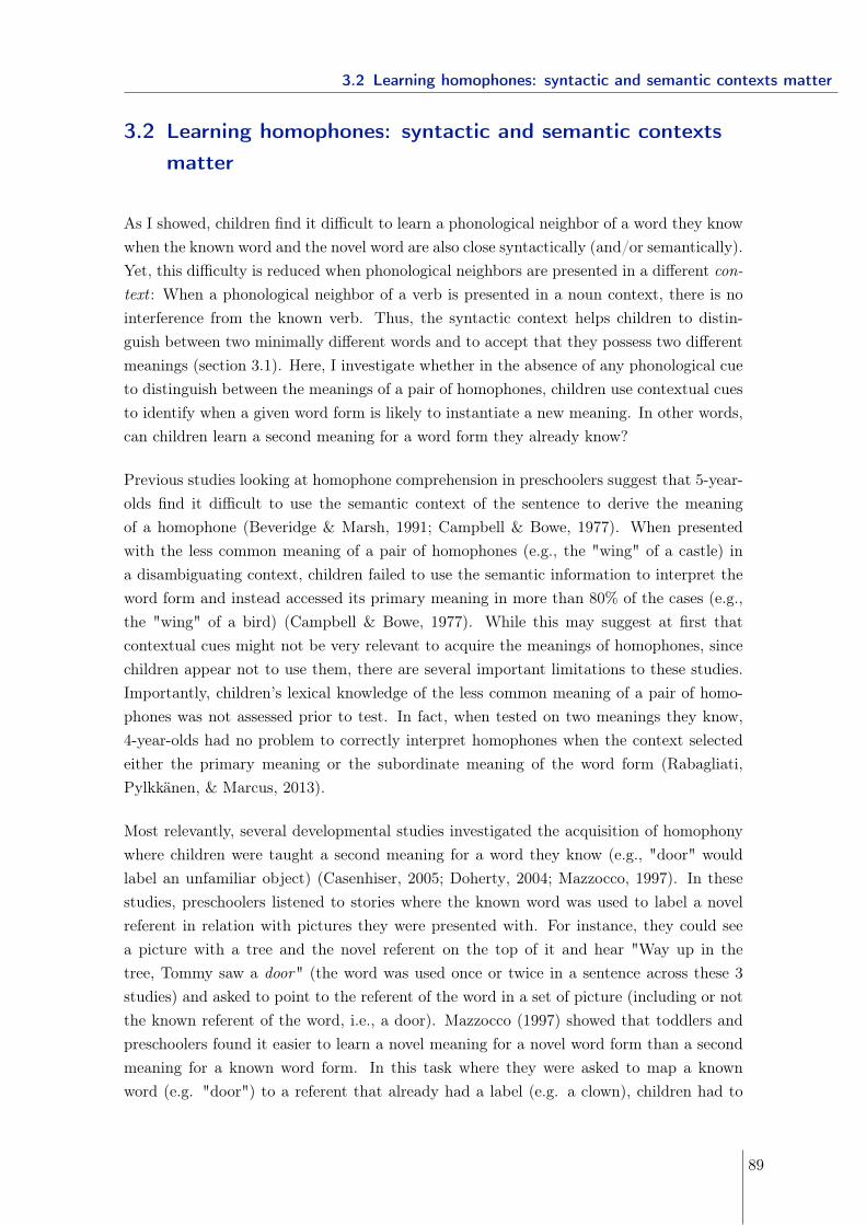
3.2 Learning homophones: syntactic and semantic contexts matter
3.2 Learning homophones: syntactic and semantic contextsmatter
As I showed, children find it difficult to learn a phonological neighbor of a word they knowwhen the known word and the novel word are also close syntactically (and/or semantically).Yet, this difficulty is reduced when phonological neighbors are presented in a different con-text : When a phonological neighbor of a verb is presented in a noun context, there is nointerference from the known verb. Thus, the syntactic context helps children to distin-guish between two minimally different words and to accept that they possess two differentmeanings (section 3.1). Here, I investigate whether in the absence of any phonological cueto distinguish between the meanings of a pair of homophones, children use contextual cuesto identify when a given word form is likely to instantiate a new meaning. In other words,can children learn a second meaning for a word form they already know?
Previous studies looking at homophone comprehension in preschoolers suggest that 5-year-olds find it difficult to use the semantic context of the sentence to derive the meaningof a homophone (Beveridge & Marsh, 1991; Campbell & Bowe, 1977). When presentedwith the less common meaning of a pair of homophones (e.g., the "wing" of a castle) ina disambiguating context, children failed to use the semantic information to interpret theword form and instead accessed its primary meaning in more than 80% of the cases (e.g.,the "wing" of a bird) (Campbell & Bowe, 1977). While this may suggest at first thatcontextual cues might not be very relevant to acquire the meanings of homophones, sincechildren appear not to use them, there are several important limitations to these studies.Importantly, children’s lexical knowledge of the less common meaning of a pair of homo-phones was not assessed prior to test. In fact, when tested on two meanings they know,4-year-olds had no problem to correctly interpret homophones when the context selectedeither the primary meaning or the subordinate meaning of the word form (Rabagliati,Pylkkänen, & Marcus, 2013).
Most relevantly, several developmental studies investigated the acquisition of homophonywhere children were taught a second meaning for a word they know (e.g., "door" wouldlabel an unfamiliar object) (Casenhiser, 2005; Doherty, 2004; Mazzocco, 1997). In thesestudies, preschoolers listened to stories where the known word was used to label a novelreferent in relation with pictures they were presented with. For instance, they could seea picture with a tree and the novel referent on the top of it and hear "Way up in thetree, Tommy saw a door" (the word was used once or twice in a sentence across these 3studies) and asked to point to the referent of the word in a set of picture (including or notthe known referent of the word, i.e., a door). Mazzocco (1997) showed that toddlers andpreschoolers found it easier to learn a novel meaning for a novel word form than a secondmeaning for a known word form. In this task where they were asked to map a knownword (e.g. "door") to a referent that already had a label (e.g. a clown), children had to
89
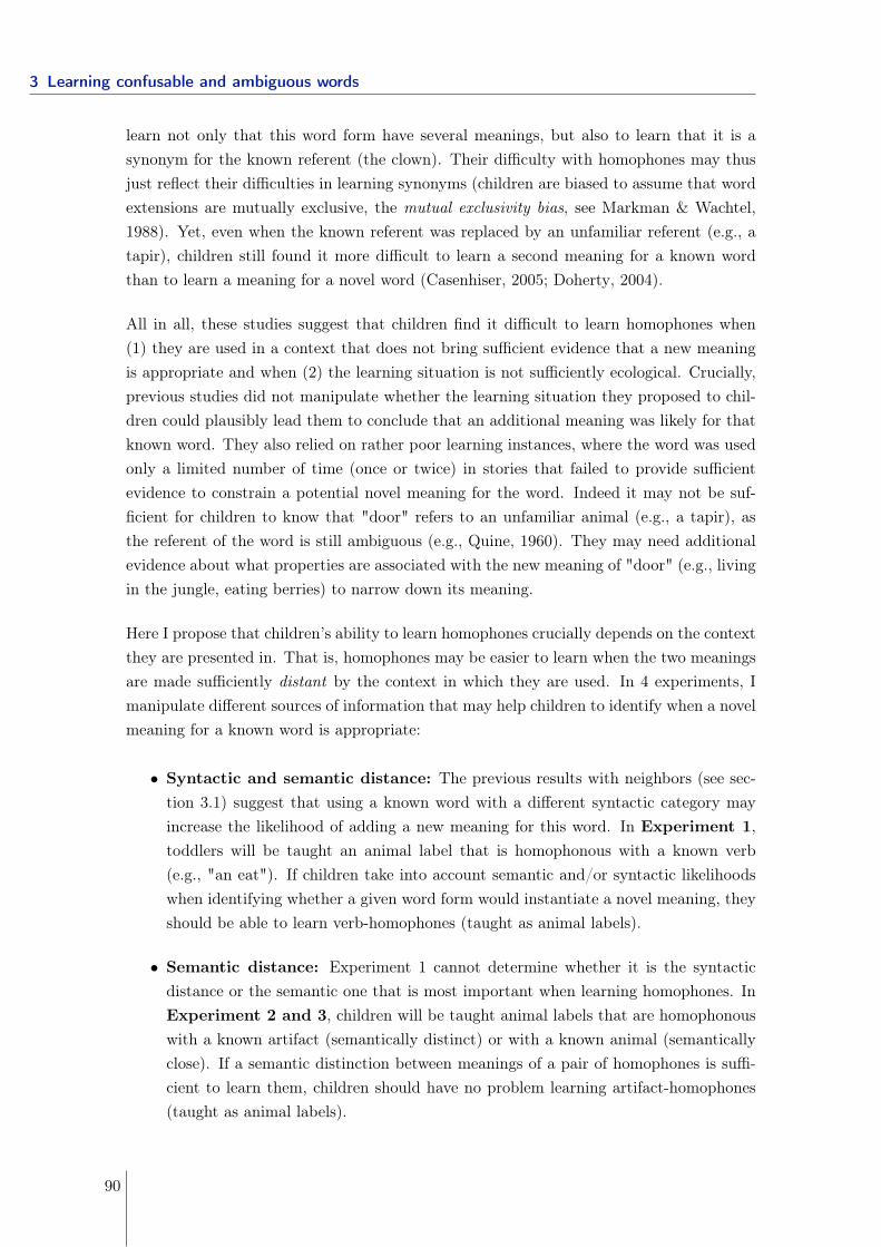
3 Learning confusable and ambiguous words
learn not only that this word form have several meanings, but also to learn that it is asynonym for the known referent (the clown). Their difficulty with homophones may thusjust reflect their difficulties in learning synonyms (children are biased to assume that wordextensions are mutually exclusive, the mutual exclusivity bias, see Markman & Wachtel,1988). Yet, even when the known referent was replaced by an unfamiliar referent (e.g., atapir), children still found it more difficult to learn a second meaning for a known wordthan to learn a meaning for a novel word (Casenhiser, 2005; Doherty, 2004).
All in all, these studies suggest that children find it difficult to learn homophones when(1) they are used in a context that does not bring sufficient evidence that a new meaningis appropriate and when (2) the learning situation is not sufficiently ecological. Crucially,previous studies did not manipulate whether the learning situation they proposed to chil-dren could plausibly lead them to conclude that an additional meaning was likely for thatknown word. They also relied on rather poor learning instances, where the word was usedonly a limited number of time (once or twice) in stories that failed to provide sufficientevidence to constrain a potential novel meaning for the word. Indeed it may not be suf-ficient for children to know that "door" refers to an unfamiliar animal (e.g., a tapir), asthe referent of the word is still ambiguous (e.g., Quine, 1960). They may need additionalevidence about what properties are associated with the new meaning of "door" (e.g., livingin the jungle, eating berries) to narrow down its meaning.
Here I propose that children’s ability to learn homophones crucially depends on the contextthey are presented in. That is, homophones may be easier to learn when the two meaningsare made sufficiently distant by the context in which they are used. In 4 experiments, Imanipulate different sources of information that may help children to identify when a novelmeaning for a known word is appropriate:
• Syntactic and semantic distance: The previous results with neighbors (see sec-tion 3.1) suggest that using a known word with a different syntactic category mayincrease the likelihood of adding a new meaning for this word. In Experiment 1,toddlers will be taught an animal label that is homophonous with a known verb(e.g., "an eat"). If children take into account semantic and/or syntactic likelihoodswhen identifying whether a given word form would instantiate a novel meaning, theyshould be able to learn verb-homophones (taught as animal labels).
• Semantic distance: Experiment 1 cannot determine whether it is the syntacticdistance or the semantic one that is most important when learning homophones. InExperiment 2 and 3, children will be taught animal labels that are homophonouswith a known artifact (semantically distinct) or with a known animal (semanticallyclose). If a semantic distinction between meanings of a pair of homophones is suffi-cient to learn them, children should have no problem learning artifact-homophones(taught as animal labels).
90
3.2 Learning homophones: syntactic and semantic contexts matter
• Syntactic distance: Similarly, the syntactic distance alone may be sufficient tolearn homophones. In Experiment 4, children will be taught animal labels that arehomophonous with a known animal (e.g., "unmasculine chat", a cat) but associatedwith a different gender (e.g., "unefeminine chat"). Since grammatical gender is nota semantic property in French, it can thus be used to test the effect of syntacticdistance independently from semantic distance.
• Neighborhood density: Besides syntax and semantics, another important factorin language learning and processing is the phonological context of the word in thelexicon. Dense neighborhoods slow down lexical retrieval in adults compared to sparseneighborhoods (Vitevitch & Luce, 1998), hence it may be easier to learn a secondarymeaning for a word form with high phonological neighborhood density than for aword form with low phonological neighborhood density simply because the primarymeaning of the word would be less accessible. In Experiment 5, children will betaught an animal label that is homophonous with the label of a known artifact whichhas no neighbor in children’s lexicon. If neighborhood density has an influence, suchsparse artifact-homophones should be more difficult to learn than dense artifact-homophones.
In these experiments, I will test 20-month-olds, thus younger children than in previousstudies (Casenhiser, 2005; Doherty, 2004; Mazzocco, 1997), for several reasons: (1) toddlersof this age already use the different sources of information that I propose to investigatehere during lexical processing (noun vs. verb, e.g., Cauvet et al., 2014; semantic relations,e.g., Arias-Trejo & Plunkett, 2013; gender cues, e.g., Van Heugten & Christophe, in press;neighborhood density, e.g., Newman, Samuelson, & Gupta, 2008) and (2) they may alreadyhave acquired a certain number of homophone pairs (de Carvalho et al., 2014) suggestingthat learning lexical ambiguities should be possible at this young age. In these experiments,toddlers will be taught homophones in the word learning task used in section 3.1, whichhas the advantage of presenting novel words in a richer context than in previous studieson preschoolers.
3.2.1 Experiment 1 - Manipulating the syntactic and semantic distance
Experiment 1 investigated whether the syntactic and/or semantic context would be suffi-cient to signal that a novel meaning for a known word was appropriate. Most relevantly,Casenhiser (2005) found that 4-year-olds find it easier to learn an additional meaning fora known word when used in a disambiguating linguistic context. As in section 3.1, I ma-nipulate the syntactic and/or the semantic context by placing a known verb in a nounframe to label a novel animal (a verb-homophone; e.g., "an eat"). In such a case, bothmeanings are used in distinct syntactic contexts ("to eat" is a verb while "an eat" is a
91
3 Learning confusable and ambiguous words
noun) and they are also semantically distinct ("to eat" refers to an action and "an eat"refers to an animal). If toddlers evaluate the syntactic and/or semantic features of wordswhen identifying novel words, verb-homophones should be perceived as sufficiently distinctfrom the known verb to be assigned a novel meaning.
Method
Participants. Thirty-two French 20-month-olds, ranging from 19;1 to 20;9 with a meanage of 20;3, (SD = 0;5; 13 boys) took part in this experiment. Five additional childrenwere replaced because of fussiness during the experiment resulting in more than 50% oftrials with missing eye tracking data (n = 3), experimenter error (n = 1), born at less than37 weeks’ gestation (n = 1).
Apparatus, procedure and design. Similar to the Experiments of section 3.1 exceptthat this time toddlers were taught one novel word that was homophonous with a verb(a verb-homophone) and a novel word that did not resemble any word in the children’slexicons (a non-homophone).
Material. Similar to the Experiments of section 3.1 except for the set of novel words usedin the teaching phase.
Novel words. I chose 4 phonological word forms of verbs that toddlers of that age are likelyto know (according to the CDI of previous studies) and the 4 novel word forms used inExperiments of section 3.1.
The 4 non-homophones were all bisyllabic: "prolin", "barlier", "torba", "lagui" (/pKole/,/barljé, /tOKba/, /lagi/) and had no phonological neighbors with words that toddlers knew.The 4 verb-homophones were also all bisyllabic words: "manger", "tomber", "casser","cacher" (/mãZe/, /tõbe/, /kase/, /kaSe/) meaning: eat, fall, break and hide. The verb-homophones were the infinitive and the past participle forms of the known verbs. Theseforms were used because they were bisyllabic and they are very common (the most frequentmorphological form for all 4 verbs; Demuth & Tremblay, 2008). The average duration ofthe novel words in the test sentences was 640ms for the verb-homophones and 622ms forthe non-homophones.
Measure and Analysis. Similar to the Experiments of section 3.1.
92
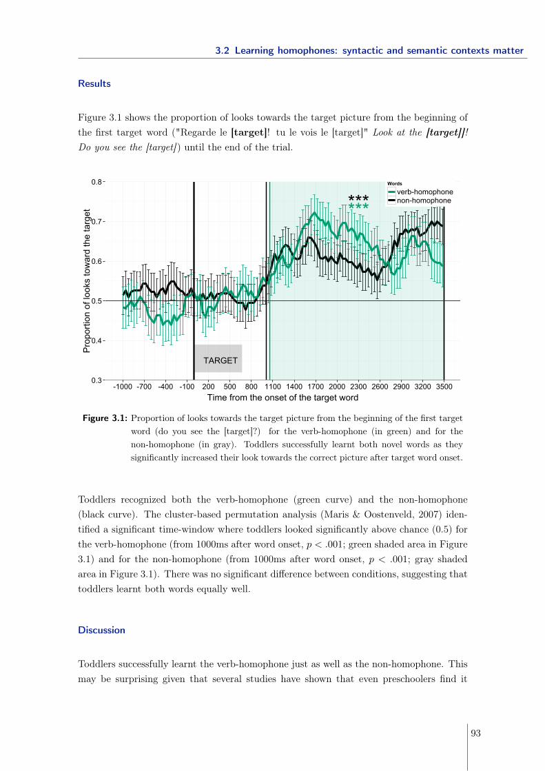
3.2 Learning homophones: syntactic and semantic contexts matter
Results
Figure 3.1 shows the proportion of looks towards the target picture from the beginning ofthe first target word ("Regarde le [target]! tu le vois le [target]" Look at the [target]]!Do you see the [target]) until the end of the trial.
TARGET
******
0.3
0.4
0.5
0.6
0.7
0.8
-1000 -700 -400 -100 200 500 800 1100 1400 1700 2000 2300 2600 2900 3200 3500Time from the onset of the target word
Pro
porti
on o
f loo
ks to
war
d th
e ta
rget
Words
verb-homophonenon-homophone
Figure 3.1: Proportion of looks towards the target picture from the beginning of the first targetword (do you see the [target]?) for the verb-homophone (in green) and for thenon-homophone (in gray). Toddlers successfully learnt both novel words as theysignificantly increased their look towards the correct picture after target word onset.
Toddlers recognized both the verb-homophone (green curve) and the non-homophone(black curve). The cluster-based permutation analysis (Maris & Oostenveld, 2007) iden-tified a significant time-window where toddlers looked significantly above chance (0.5) forthe verb-homophone (from 1000ms after word onset, p < .001; green shaded area in Figure3.1) and for the non-homophone (from 1000ms after word onset, p < .001; gray shadedarea in Figure 3.1). There was no significant difference between conditions, suggesting thattoddlers learnt both words equally well.
Discussion
Toddlers successfully learnt the verb-homophone just as well as the non-homophone. Thismay be surprising given that several studies have shown that even preschoolers find it
93
3 Learning confusable and ambiguous words
difficult to associate a novel meaning to a known word (Casenhiser, 2005; Doherty, 2004;Mazzocco, 1997). Yet contrary to previous studies, toddlers may not have been disturbedby the re-use of a known verb, as the syntactic context, a noun frame, decreased thelikelihood that the speaker could possibly be using the known meaning of the verb (seealso Casenhiser, 2005). This suggests that children can use the syntactic context to identifywhether a novel meaning is appropriate for a word, even when the word is already associatedto a meaning.
One possibility is that toddlers did not even notice that a familiar verb was used in thisexperiment. Indeed, toddlers use the syntactic context to constrain lexical access: Forinstance they expect a noun after a determiner and a verb after a pronoun (e.g., Cauvetet al., 2014; Shi & Melancon, 2010; Zangl & Fernald, 2007). Thus, when presented witha noun phrase such as "C’est un manger!" (this an eat! ), toddlers may simply not haveaccessed the familiar verb and this made it very easy to link an additional meaning to theword, just as easy as for the non-homophone.
Yet another possibility is that toddlers initially noticed that the verb they knew was usedin an incorrect frame. Indeed, two-year-old children display an early left-lateralized brainresponse when an expected noun is incorrectly replaced by a verb (e.g., "je prends lamange" I take the eat, Bernal et al., 2010). Relevantly, ERP studies looking at adults’processing of lexical ambiguities in reading tasks found that the syntactic context alonewas insufficient to constrain lexical access in the case of noun/verb homographs (e.g., thepark/to park) as evidenced by a frontal negativity compared to unambiguous words (e.g.,Lee & Federmeier, 2012). Yet additional semantic constraints on the meaning of the wordseliminated the frontal negativity (e.g., Lee & Federmeier, 2009). Such a frontal compo-nent has been suggested to reflect the recruitment of frontally mediated meaning selectionmechanisms needed to disambiguate noun-verb homographs in the absence of constrainingsemantics (e.g., Novick, Trueswell, & Thompson-Schill, 2010) suggesting that the syntac-tic context alone may be insufficient to suppress totally the inappropriate meaning of theword. Yet, in our experiment, because the verb is never used to convey its initial mean-ing (thus the verb meaning is never pre-activated) but repetitively used in a noun framewith a visual support (i.e., the novel referent), social support (i.e., the speaker lookingcontingently to the referent each time she uses the verb-homophone) and supplementedwith information about its novel meaning (e.g., "Un manger, ca a des grandes oreillles"Eats have big ears), this may have increased the likelihood that the known meaning of theverb was inappropriate in that context and supported the identification of an additionalmeaning for the known verb form.
At any rate, the present results show that children have no problem learning noun-verbhomophones in a supportive context. This has important consequences for theories ofsyntactic development looking at the acquisition of syntactic categories. One commonassumption is that children may start grouping words into categories by observing their
94
3.2 Learning homophones: syntactic and semantic contexts matter
distributional context: For instance, all words X appearing in the context [you X the] arelikely to be verbs. To obtain adult-like categories (nouns, verbs, etc), learners would needto merge these context-based categories, possibly by grouping together the categories thatshare a portion of their categorized words (Mintz, 2003). For instance, [you X the] and [heX the] would be grouped together since words such as "drink", "eat", "give" would appearin both contexts. Yet words that appear in multiple categories should make distributionalcues to category less effective. Learners could conflate distributions and create a singlecategory that contains both nouns and verbs. In fact, noun/verb homophones have beencited as evidence against the logical possibility of learning grammatical categories fromtheir distributions (Pinker, Lebeaux, & Frost, 1987). To get around this problem, twosolutions have been proposed.
The first solution suggests that children may be sensitive to a (small) perceptual distinc-tion between nouns and verbs such that they would be able to maintain two phonologicallydistinct representations of the same word form (e.g., park-NOUN and park-VERB Conwell,2015; Conwell & Morgan, 2012). This is supported by several sources of evidence showingthat there are prosodic differences between noun and verb homophones, such that nountokens are longer than verb tokens (Conwell & Morgan, 2012; Shi & Moisan, 2008).11 Fol-lowing this hypothesis, learners would use this sensitivity to tackle the ambiguity problem,such that words that appear in more than one lexical category should not pose a problemfor children.
The second solution suggests that children could start building syntactic categories bygrouping words together according to their semantic category as soon as they start toknow the meaning of basic words (from 9 months of age, Bergelson & Swingley, 2012,2013) (Brusini, 2012; Gutman, Dautriche, Crabbé, & Christophe, 2014). For example,they could start grouping together "toy", "car", and "spoon" because they all refer toconcrete objects, and "drink", "eat", and "give" because they all refer to actions. Theknowledge of a few content words may allow learners to discover the distributional contextin which they appear: They could notice that nouns/objects appear most of the timepreceded by determiners and verbs/actions by pronouns or auxiliary, and subsequently usethis information to categorize new words. Following this hypothesis, children rely on thecontext to attribute a category (or a meaning) to novel words.
Certainly, these two solutions are not mutually exclusive. What I showed here is thatat 20 months of age, children are not confused by noun/verb homophones because they11This is, however, not surprising given that nouns may be more likely than verbs to appear at the end
of a prosodic phrase as in [the kids’ brush] [is on the table] (where brackets indicate prosodic phraseboundaries) and thus is typically lengthened compared to verbs that are more likely to appear phrase-internally as in [the kids] [brush their teeth] (Delais-Roussarie, 1995). Thus, these prosodic differencesmay not be part of the phonological form of the word but depend on the position of the word in thesentence: Both nouns and verbs homophones appear to have the same duration when they are situatedin the same position in the sentence (Sorensen, Cooper, & Paccia, 1978).
95
3 Learning confusable and ambiguous words
already process words in context, suggesting that noun/verb homophones may not bea major problem for syntactic development. Interestingly, similarly to toddlers in thisstudy, several computational (Bayesian) models of syntactic category acquisition are ableto deal well with noun-verb ambiguity (e.g., Goldwater & Griffiths, 2007; Parisien, Fazly,& Stevenson, 2008). Yet these models find it difficult to identify the syntactic categoryof a noun when there is a strong lexical bias in favor of the verb of the homophone pair(Parisien et al., 2008) while toddlers, as I just showed, have no problem in such cases.
Importantly, here, I concentrated on learning noun/verb homophones, yet one interestingfollowing question is how does that relate to the acquisition of noun/verb polysemes thatshare the same form and have related meanings (e.g., a kiss/to kiss). I showed that childrenare sensitive to the syntactic context in which a known word is used to decide whetherthe word may instantiate a new meaning. Yet the existence of polysemes suggests thatnoun/verb distributional cues do not necessarily trigger the formation of a novel distinctlexical entry. Indeed noun/verb polysemes share not only a common phonological form butalso the same lexical representational base (e.g., Caramazza & Grober, 1976). Oshima-Takane, Barner, Elsabbagh, & Guerriero (2001) propose that children can learn the cross-categorical use of these words not only by paying attention to the distributional cues ofthe noun/verb pair but also, by using the semantic information of the words, noting forinstance that the same word could be used for an artifact and its function (e.g., brush) (seealso Lippeveld & Oshima-Takane, 2014). Thus paying attention to the semantic relationbetween the meanings of a word may help children to differentiate between noun/verbhomophones and noun/verb polysemes.
To conclude, I started by noting that learning homophones may be easier when theirmeanings are made sufficiently distinct by the context in which they are used. When averb form referring to an action was used as a noun to label a novel object, children hadno problem to learn it. Yet the present result cannot tell whether the syntactic distance(verb/noun) or the semantic distance (action/object) mattered here. In Experiment 2, Iinvestigate the effect of semantic distance alone on learning noun-noun homophones.
3.2.2 Experiment 2 & 3 - Manipulating the semantic distance
Learning homophones may be easier when the semantic distance between their meaningsis large. For example, "bat" is likely to be unambiguous in a context where one speaksabout sport, as we do not expect the bat-animal meaning in this context. Intuitively,homophones seem to map onto clearly distinct meanings (e.g., animal-bat/baseball-bat,flour/flower, mussel/muscle, etc.) suggesting an advantage for homophones that are se-mantically distinct over semantically close (I come back to this idea in section 3.3).
In Experiment 2, toddlers were taught either a novel animal noun that was homophonous
96
3.2 Learning homophones: syntactic and semantic contexts matter
with a noun referring to an artifact (an artifact-homophone, syntactically identical, butsemantically distant; e.g., "un pot", a potty) or a novel animal noun that was homophonouswith a noun referring to an animal (an animal-homophone, both syntactically and se-mantically close; e.g., "un chat", a cat). Contrary to Experiment 1, a non-homophone wasnot taught, so as to minimize task difficulty, since learning a second meaning for a knownnoun may be more challenging that learning a second meaning for a known verb. Yet be-cause children were taught a single word, I also controlled that a potential learning effectwould not be due to a preference for looking at the only labeled animal, namely toddlersmight look more towards the labeled animal during the test phase not because they asso-ciated the novel label to this animal but because this animal is the only one that has beennamed during the teaching phase. Therefore, during the test phase toddlers were testedboth on the homophone (the artifact-homophone condition or the animal-homophone con-dition), and on an untaught non-homophone (the non-homophone condition). If toddlersin the non-homophone condition looked more towards the unlabeled animal (or at least be-haved differently from the homophone conditions; the mutual exclusivity effect), this wouldsuggest that toddlers formed a form-meaning association between the artifact-homophone,or the animal-homophone, and its animal referent.
Experiment 2
Method
Participants. Thirty-two French 20-month-olds took part in this experiment, sixteenlearnt an artifact-homophone (range = 19;2 months to 20;8 months, mean = 19;8, SD =0;6, 8 boys) and sixteen learnt an animal-homophone (range = 19;4 months to 20;9 months,mean = 20;2, SD = 0;4, 6 boys). Sixteen additional children were replaced because oftechnical problem (n = 7)12, fussiness during the experiment resulting in more than 50%of trials with missing eye tracking data (n = 6), refusal to wear the sticker necessary foreye-tracking (n = 2) and not knowing any of the test words according to their parents’report (n = 1).
Apparatus, procedure and design. Similar to Experiment 1 except that this timetoddlers were taught a single novel word that was homophonous with a known noun re-ferring to an artifact (an artifact-homophone) or a known noun referring to an animal (ananimal-homophone). The other plush animal was still presented, for a video of the sameduration, with the same movements and story line, but without any label (only pronounswere used – "do you see this one? It has big ears..."). During the test phase, toddlers had
12For Experiments 2 and 3, the position of the eye-tracker relative to the screen was improperly centeredresulting in a loss of data when children were looking towards one side of the screen.
97
3 Learning confusable and ambiguous words
4 test trials on the homophone label (the artifact- or the animal-homophone) and 4 testtrials on the non-homophone label (the non-homophone condition).
Material. Similar to Experiment 1 except for the set of novel words used in the teachingphase.
Novel words. I chose 4 phonological word forms of nouns labeling artifacts that toddlersof that age are likely to know, 4 phonological word forms of nouns labeling animals thattoddlers of that age are likely to know (according to the CDI of previous studies) and 4novel non-homophones.
The 4 artifact-homophones were all monosyllabic words: "verre", "pot", "pull", "bain"(/vEK/, /po/, /pyl/, /be/) meaning: glass, potty, sweater and bath. On average, thesewords had a phonological neighborhood density of 3.8 (irrespective of the syntactic categoryof the word) and an average frequency count of 152 in a corpus of child directed speech(the Lyon corpus, Demuth & Tremblay, 2008).
The 4 animal-homophones were also all monosyllabic words: "chat", "loup", "poule","mouche" (/Sa/, /lu/, /pul/, /muS/) meaning: cat, wolf, hen and fly. These words hadan average phonological neighborhood density of 3.1 (irrespective of the syntactic categoryof the word) and a frequency count of 157 in a corpus of child directed speech (the Lyoncorpus, Demuth & Tremblay, 2008).
The 4 novel non-homophones were identical to those used in Experiment 1.
The average duration of the novel words in the test sentences was 455ms for the artifact-homophones, 517ms for the animal-homophones and 622ms for the non-homophones.
Measure and Analysis. Similar to Experiment 1, except that this time the dependentvariable was the proportion of looks towards the plush animal labeled during the learningphase (in order to compare any potential difference in behavior between the test trials onthe homophone label and the mutual exclusivity trials on the non-homophone label). Thecluster analysis was this time run from -1500ms before target word onset until the end ofthe trial.
Results
Artifact-homophone group
Figure 3.2 shows the proportion of looks towards the referent of the artifact-homophone(the labelled animal during the learning phase) from -1000ms before the beginning of the
98
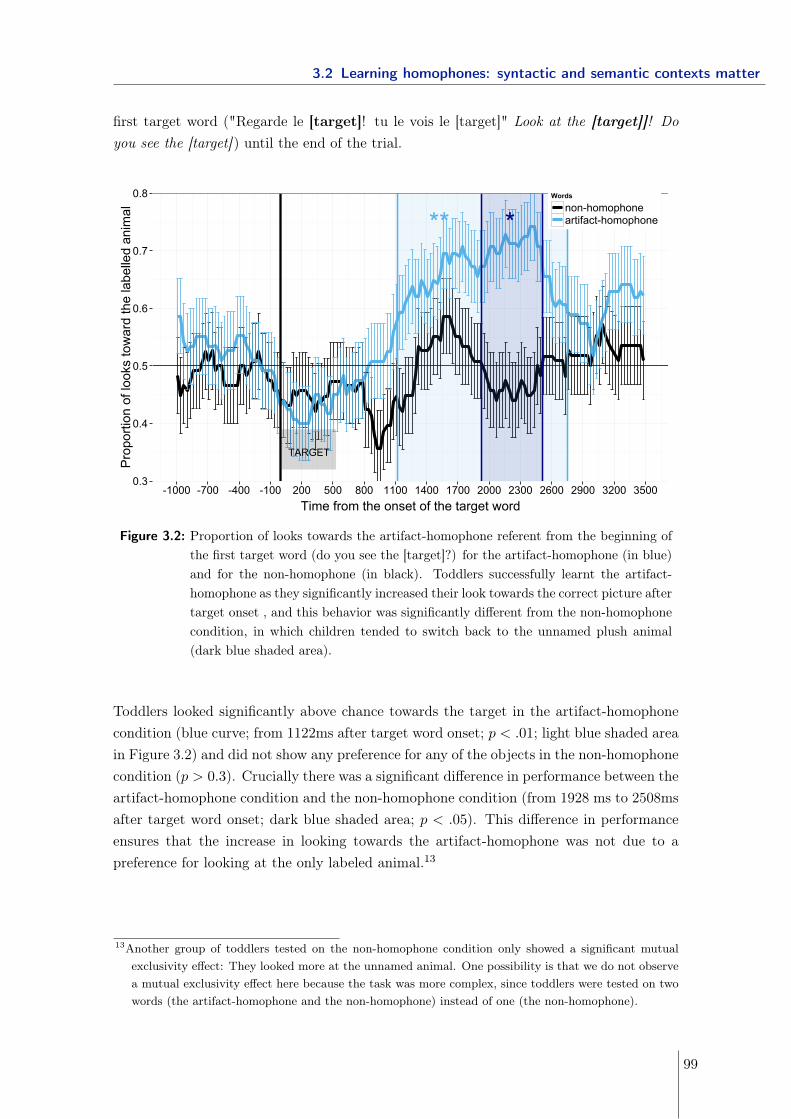
3.2 Learning homophones: syntactic and semantic contexts matter
first target word ("Regarde le [target]! tu le vois le [target]" Look at the [target]]! Doyou see the [target]) until the end of the trial.
TARGET
** *
0.3
0.4
0.5
0.6
0.7
0.8
-1000 -700 -400 -100 200 500 800 1100 1400 1700 2000 2300 2600 2900 3200 3500Time from the onset of the target word
Pro
porti
on o
f loo
ks to
war
d th
e la
belle
d an
imal
Words
non-homophoneartifact-homophone
Figure 3.2: Proportion of looks towards the artifact-homophone referent from the beginning ofthe first target word (do you see the [target]?) for the artifact-homophone (in blue)and for the non-homophone (in black). Toddlers successfully learnt the artifact-homophone as they significantly increased their look towards the correct picture aftertarget onset , and this behavior was significantly different from the non-homophonecondition, in which children tended to switch back to the unnamed plush animal(dark blue shaded area).
Toddlers looked significantly above chance towards the target in the artifact-homophonecondition (blue curve; from 1122ms after target word onset; p < .01; light blue shaded areain Figure 3.2) and did not show any preference for any of the objects in the non-homophonecondition (p > 0.3). Crucially there was a significant difference in performance between theartifact-homophone condition and the non-homophone condition (from 1928 ms to 2508msafter target word onset; dark blue shaded area; p < .05). This difference in performanceensures that the increase in looking towards the artifact-homophone was not due to apreference for looking at the only labeled animal.13
13Another group of toddlers tested on the non-homophone condition only showed a significant mutualexclusivity effect: They looked more at the unnamed animal. One possibility is that we do not observea mutual exclusivity effect here because the task was more complex, since toddlers were tested on twowords (the artifact-homophone and the non-homophone) instead of one (the non-homophone).
99
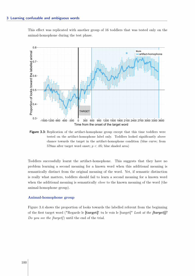
3 Learning confusable and ambiguous words
This effect was replicated with another group of 16 toddlers that was tested only on theanimal-homophone during the test phase.
TARGET
*
0.3
0.4
0.5
0.6
0.7
0.8
-1500-1200 -900 -600 -300 0 300 600 900 1200 1500 1800 2100 2400 2700 3000 3300 3600Time from the onset of the target word
Pro
porti
on o
f loo
ks to
war
d th
e la
belle
d an
imal Words
artifact-homophone
Figure 3.3: Replication of the artifact-homophone group except that this time toddlers weretested on the artifact-homophone label only. Toddlers looked significantly abovechance towards the target in the artifact-homophone condition (blue curve; from578ms after target word onset; p < .05; blue shaded area)
Toddlers successfully learnt the artifact-homophone. This suggests that they have noproblem learning a second meaning for a known word when this additional meaning issemantically distinct from the original meaning of the word. Yet, if semantic distinctionis really what matters, toddlers should fail to learn a second meaning for a known wordwhen the additional meaning is semantically close to the known meaning of the word (theanimal-homophone group).
Animal-homophone group
Figure 3.4 shows the proportion of looks towards the labelled referent from the beginningof the first target word ("Regarde le [target]! tu le vois le [target]" Look at the [target]]!Do you see the [target]) until the end of the trial.
100
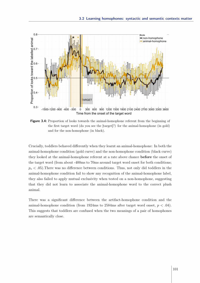
3.2 Learning homophones: syntactic and semantic contexts matter
TARGET
* .
0.3
0.4
0.5
0.6
0.7
0.8
-1500-1200 -900 -600 -300 0 300 600 900 1200 1500 1800 2100 2400 2700 3000 3300 3600Time from the onset of the target word
Pro
porti
on o
f loo
ks to
war
d th
e la
belle
d an
imal
Words
non-homophoneanimal-homophone
Figure 3.4: Proportion of looks towards the animal-homophone referent from the beginning ofthe first target word (do you see the [target]?) for the animal-homophone (in gold)and for the non-homophone (in black).
Crucially, toddlers behaved differently when they learnt an animal-homophone: In both theanimal-homophone condition (gold curve) and the non-homophone condition (black curve)they looked at the animal-homophone referent at a rate above chance before the onset ofthe target word (from about -400ms to 70ms around target word onset for both conditions;ps < .05).There was no difference between conditions. Thus, not only did toddlers in theanimal-homophone condition fail to show any recognition of the animal-homophone label,they also failed to apply mutual exclusivity when tested on a non-homophone, suggestingthat they did not learn to associate the animal-homophone word to the correct plushanimal.
There was a significant difference between the artifact-homophone condition and theanimal-homophone condition (from 1924ms to 2584ms after target word onset, p < .04).This suggests that toddlers are confused when the two meanings of a pair of homophonesare semantically close.
101
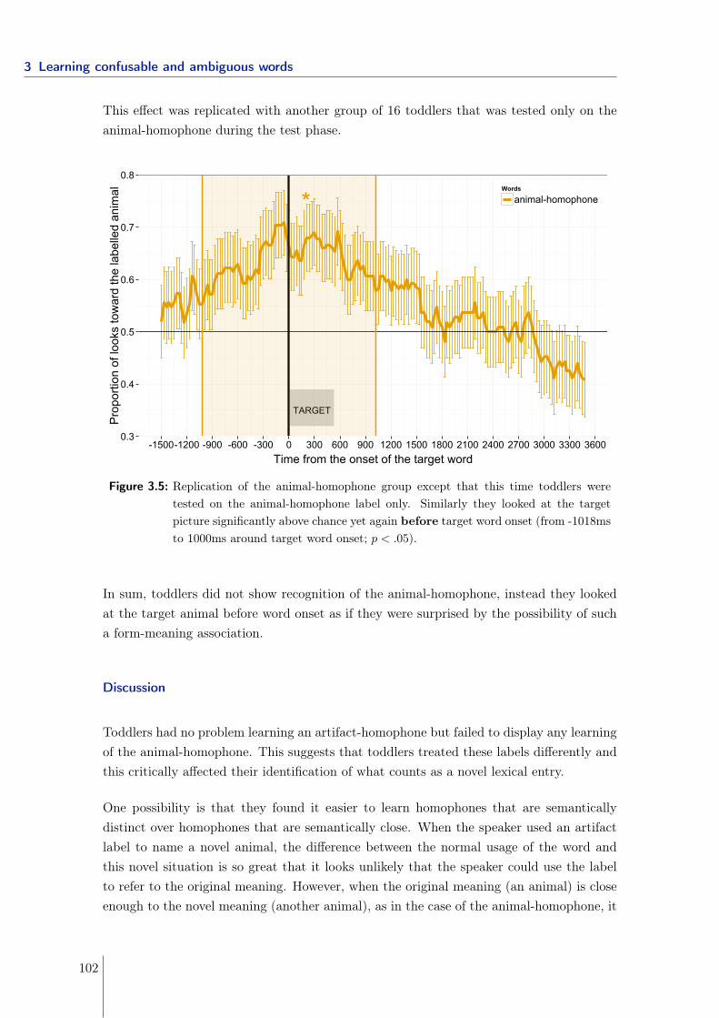
3 Learning confusable and ambiguous words
This effect was replicated with another group of 16 toddlers that was tested only on theanimal-homophone during the test phase.
TARGET
*
0.3
0.4
0.5
0.6
0.7
0.8
-1500-1200 -900 -600 -300 0 300 600 900 1200 1500 1800 2100 2400 2700 3000 3300 3600Time from the onset of the target word
Pro
porti
on o
f loo
ks to
war
d th
e la
belle
d an
imal Words
animal-homophone
Figure 3.5: Replication of the animal-homophone group except that this time toddlers weretested on the animal-homophone label only. Similarly they looked at the targetpicture significantly above chance yet again before target word onset (from -1018msto 1000ms around target word onset; p < .05).
In sum, toddlers did not show recognition of the animal-homophone, instead they lookedat the target animal before word onset as if they were surprised by the possibility of sucha form-meaning association.
Discussion
Toddlers had no problem learning an artifact-homophone but failed to display any learningof the animal-homophone. This suggests that toddlers treated these labels differently andthis critically affected their identification of what counts as a novel lexical entry.
One possibility is that they found it easier to learn homophones that are semanticallydistinct over homophones that are semantically close. When the speaker used an artifactlabel to name a novel animal, the difference between the normal usage of the word andthis novel situation is so great that it looks unlikely that the speaker could use the labelto refer to the original meaning. However, when the original meaning (an animal) is closeenough to the novel meaning (another animal), as in the case of the animal-homophone, it
102
3.2 Learning homophones: syntactic and semantic contexts matter
may be more difficult for toddlers to differentiate between a less prototypical member ofthe original meaning of the label and a novel meaning instance.
Another possibility is that some unmeasured difference between the set of artifact labels andthe set of animal labels was responsible for the observed effect. While both sets of wordswere matched for frequency, neighborhood density in toddlers’ lexicon and phonotacticprobability, toddlers may have a better lexical representation for the animal labels thanthe artifact labels used in this study, leading to greater interference (e.g., McKenna &Parry, 1994; Setoh, Wu, Baillargeon, & Gelman, 2013, for some evidence that animals mayhave a special status). Thus, toddlers may find it more difficult to learn a second meaningfor an animal-label than for an artifact-label not because the semantic distance betweenthe two meanings is greater for the artifact-homophones but because toddlers may havegreater difficulty in suppressing the primary meaning of the animal-homophones. The nextexperiment disentangles between these two possibilities.
Experiment 3
Experiment 3 was similar to Experiment 2, except that this time toddlers were taughtthat the animal-homophone labels used in Experiment 2 could label a novel artifact (e.g.,"un chat", a cat, was used to label a novel music instrument). Thus, the set of animal-homophone labels was identical to Experiment 2 but, crucially, the semantic distancebetween the two meanings of the label increased. If semantic distance between meaningsof a pair of homophones is a major reason why learning an artifact-homophone is easierthan learning a animal-homophone in Experiment 2, then toddlers should have no problemlearning an animal-homophone when the novel meaning is sufficiently distant semanticallyfrom the animal category. On the contrary if better lexical representations for the animal-labels used in Experiment 2 led to the observed effect, then toddlers should still fail tolearn an animal-homophone even though its second meaning is semantically distinct fromits original meaning.
Method
Participants. Fourteen14 French 20-month-olds took part in this experiment. 14 ad-ditional children were replaced because of technical problem (n = 10; see footnote 12),refusal to wear the sticker necessary for eye-tracking (n = 2), because the parent took outthe earphones during the experiment (n = 1) and because the child did not know any ofthe target words (n = 1).
14This experiment is on-going.
103
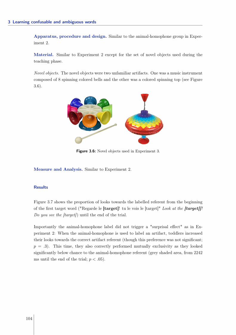
3 Learning confusable and ambiguous words
Apparatus, procedure and design. Similar to the animal-homophone group in Exper-iment 2.
Material. Similar to Experiment 2 except for the set of novel objects used during theteaching phase.
Novel objects. The novel objects were two unfamiliar artifacts. One was a music instrumentcomposed of 8 spinning colored bells and the other was a colored spinning top (see Figure3.6).
Figure 3.6: Novel objects used in Experiment 3.
Measure and Analysis. Similar to Experiment 2.
Results
Figure 3.7 shows the proportion of looks towards the labelled referent from the beginningof the first target word ("Regarde le [target]! tu le vois le [target]" Look at the [target]]!Do you see the [target]) until the end of the trial.
Importantly the animal-homophone label did not trigger a "surprisal effect" as in Ex-periment 2: When the animal-homophone is used to label an artifact, toddlers increasedtheir looks towards the correct artifact referent (though this preference was not significant;p = .3). This time, they also correctly performed mutually exclusivity as they lookedsignificantly below chance to the animal-homophone referent (grey shaded area, from 2242ms until the end of the trial; p < .05).
104
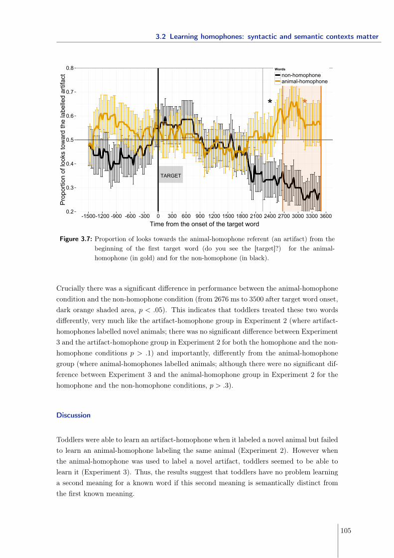
3.2 Learning homophones: syntactic and semantic contexts matter
TARGET
* *
0.2
0.3
0.4
0.5
0.6
0.7
0.8
-1500-1200 -900 -600 -300 0 300 600 900 1200 1500 1800 2100 2400 2700 3000 3300 3600Time from the onset of the target word
Pro
porti
on o
f loo
ks to
war
d th
e la
belle
d ar
tifac
tWords
non-homophoneanimal-homophone
Figure 3.7: Proportion of looks towards the animal-homophone referent (an artifact) from thebeginning of the first target word (do you see the [target]?) for the animal-homophone (in gold) and for the non-homophone (in black).
Crucially there was a significant difference in performance between the animal-homophonecondition and the non-homophone condition (from 2676 ms to 3500 after target word onset,dark orange shaded area, p < .05). This indicates that toddlers treated these two wordsdifferently, very much like the artifact-homophone group in Experiment 2 (where artifact-homophones labelled novel animals; there was no significant difference between Experiment3 and the artifact-homophone group in Experiment 2 for both the homophone and the non-homophone conditions p > .1) and importantly, differently from the animal-homophonegroup (where animal-homophones labelled animals; although there were no significant dif-ference between Experiment 3 and the animal-homophone group in Experiment 2 for thehomophone and the non-homophone conditions, p > .3).
Discussion
Toddlers were able to learn an artifact-homophone when it labeled a novel animal but failedto learn an animal-homophone labeling the same animal (Experiment 2). However whenthe animal-homophone was used to label a novel artifact, toddlers seemed to be able tolearn it (Experiment 3). Thus, the results suggest that toddlers have no problem learninga second meaning for a known word if this second meaning is semantically distinct fromthe first known meaning.
105
3 Learning confusable and ambiguous words
However, while toddlers’ performance in Experiment 3 did not differ from the artifact-homophone group in Experiment 2, it seems that toddlers were not as successful to learnan animal-homophone as an artifact-homophone even when the semantic distance betweenthe novel and the primary meaning is kept the same. There may be two possibilities toaccount for this observation: First, there may be a small effect of animal labels vs. artifactlabels: It could be the case that lexical representations for animals are more entrenchedthan the lexical representations of the artifacts chosen in this set of experiments and thusinterfere more with the creation of a novel lexical entry; Second, the stories of Experiment3 and Experiment 2 are different and involve different sets of objects. Thus it may bethe case that the stories used in Experiment 3 are more complicated for toddlers than thestories of Experiment 2. In particular because they involve more complicated vocabulary(e.g., for artifacts: "button", "playing music", "bell", "spinning" vs. for animals: "ear","nose", "legs", "jumping") that may be less known to toddlers of that age. Future work willcontrol for that possibility by teaching toddlers non-homophones for these novel artifactsto check whether these stories generally make word learning more challenging.
In sum, in Experiment 1 showed that toddlers had no problem to learn a second meaningfor a known word when this second meaning was syntactically and semantically distinctfrom the known meaning. Experiment 2 showed that a semantic distinction between themeanings of a pair of homophones was sufficient to learn them. One question that remainsis whether a syntactic distinction between the members of a homophone pair may besufficient to learn two meanings for the same word form. I investigate this question inExperiment 4.
3.2.3 Experiment 4 - Manipulating the syntactic distance using gender
Experiment 4 investigated whether solely increasing the syntactic distance between themeanings of a pair of homophones may facilitate the acquisition of these meanings. To iso-late the effect of syntax from semantic, I focused on grammatical gender. Crucially, gram-matical gender is a lexical property, as opposed to a semantic property in languages wheregender categories are not clearly defined in semantic terms (as it is the case in French).In gender-marking languages, the gender of the noun determines the form of associateddeterminers and adjectives. In French, feminine nouns are preceded by a gender-markeddefinite article "la" or indefinite "une" and masculine nouns by the gender-marked definitearticle "le" or the indefinite "un" when used in their singular form. Such gender cueshave been shown to constrain lexical access in adults (e.g., Dahan, Swingley, Tanenhaus,& Magnuson, 2000; Spinelli & Alario, 2002) but also in young children (E. K. Johnson,2005; Lew-Williams & Fernald, 2007; Van Heugten & Shi, 2009). Interestingly for thecurrent study, adults use such gender-marked context to selectively access the meaning ofhomophones (Spinelli & Alario, 2002). For instance, in French, /sEl/ means both saddle
106
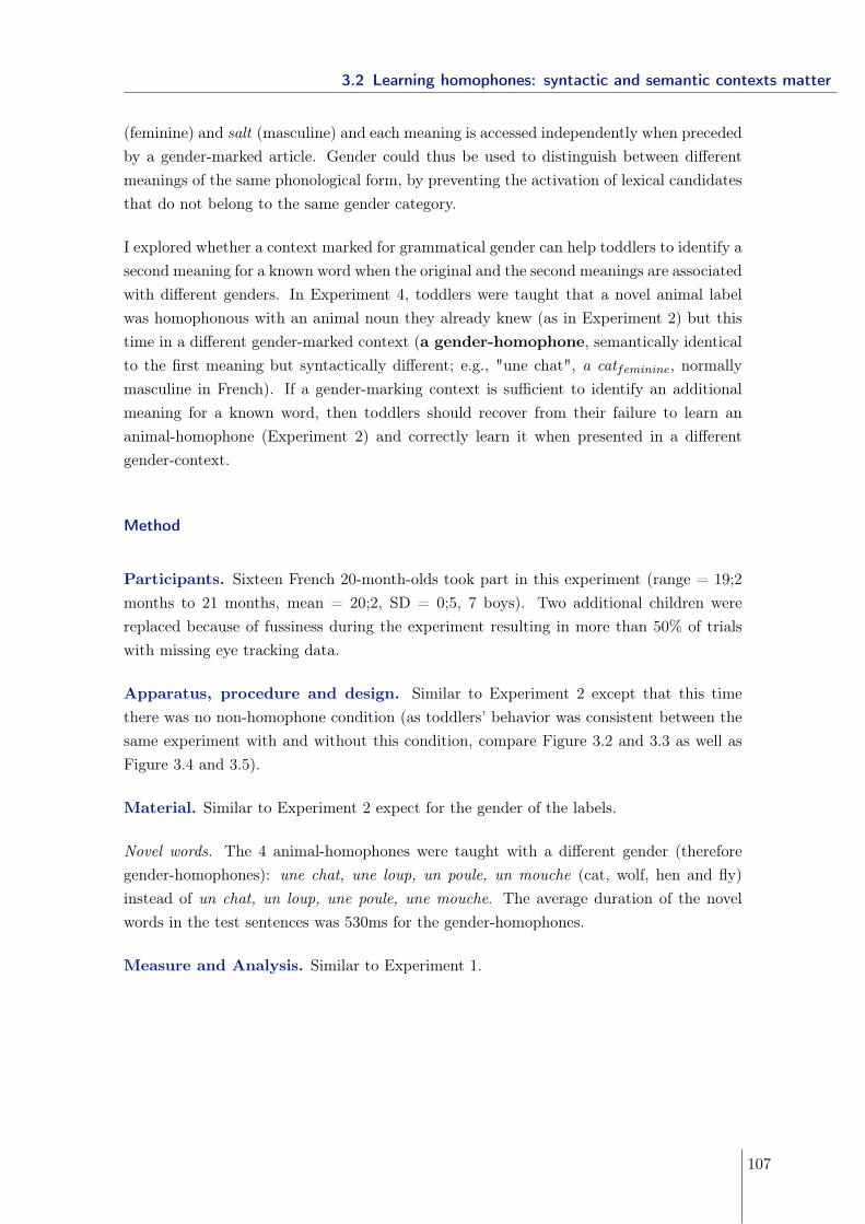
3.2 Learning homophones: syntactic and semantic contexts matter
(feminine) and salt (masculine) and each meaning is accessed independently when precededby a gender-marked article. Gender could thus be used to distinguish between differentmeanings of the same phonological form, by preventing the activation of lexical candidatesthat do not belong to the same gender category.
I explored whether a context marked for grammatical gender can help toddlers to identify asecond meaning for a known word when the original and the second meanings are associatedwith different genders. In Experiment 4, toddlers were taught that a novel animal labelwas homophonous with an animal noun they already knew (as in Experiment 2) but thistime in a different gender-marked context (a gender-homophone, semantically identicalto the first meaning but syntactically different; e.g., "une chat", a catfeminine, normallymasculine in French). If a gender-marking context is sufficient to identify an additionalmeaning for a known word, then toddlers should recover from their failure to learn ananimal-homophone (Experiment 2) and correctly learn it when presented in a differentgender-context.
Method
Participants. Sixteen French 20-month-olds took part in this experiment (range = 19;2months to 21 months, mean = 20;2, SD = 0;5, 7 boys). Two additional children werereplaced because of fussiness during the experiment resulting in more than 50% of trialswith missing eye tracking data.
Apparatus, procedure and design. Similar to Experiment 2 except that this timethere was no non-homophone condition (as toddlers’ behavior was consistent between thesame experiment with and without this condition, compare Figure 3.2 and 3.3 as well asFigure 3.4 and 3.5).
Material. Similar to Experiment 2 expect for the gender of the labels.
Novel words. The 4 animal-homophones were taught with a different gender (thereforegender-homophones): une chat, une loup, un poule, un mouche (cat, wolf, hen and fly)instead of un chat, un loup, une poule, une mouche. The average duration of the novelwords in the test sentences was 530ms for the gender-homophones.
Measure and Analysis. Similar to Experiment 1.
107
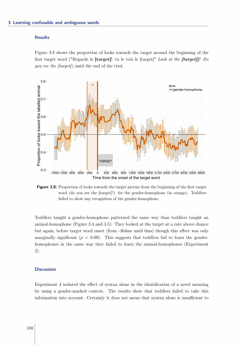
3 Learning confusable and ambiguous words
Results
Figure 3.8 shows the proportion of looks towards the target around the beginning of thefirst target word ("Regarde le [target]! tu le vois le [target]" Look at the [target]]! Doyou see the [target]) until the end of the trial.
TARGET
.
0.3
0.4
0.5
0.6
0.7
0.8
-1500-1200 -900 -600 -300 0 300 600 900 1200 1500 1800 2100 2400 2700 3000 3300 3600Time from the onset of the target word
Pro
porti
on o
f loo
ks to
war
d th
e la
belle
d an
imal Words
gender-homophone
Figure 3.8: Proportion of looks towards the target picture from the beginning of the first targetword (do you see the [target]?) for the gender-homophone (in orange). Toddlersfailed to show any recognition of the gender-homophone.
Toddlers taught a gender-homophone patterned the same way than toddlers taught ananimal-homophone (Figure 3.4 and 3.5): They looked at the target at a rate above chancebut again, before target word onset (from -364ms until 0ms) though this effect was onlymarginally significant (p = 0.09). This suggests that toddlers fail to learn the gender-homophones in the same way they failed to learn the animal-homophones (Experiment2).
Discussion
Experiment 4 isolated the effect of syntax alone in the identification of a novel meaningby using a gender-marked context. The results show that toddlers failed to take thisinformation into account. Certainly it does not mean that syntax alone is insufficient to
108
3.2 Learning homophones: syntactic and semantic contexts matter
distinguish between meanings of a pair of homophones, but that gender may not provideenough evidence for toddlers that a novel meaning is intended in that situation.
Yet there may be several others interpretations for toddlers’ failure. One possibility is thatFrench 20-month-olds do not yet use gender when processing spoken language. However, Ibelieve this possibility to be unlikely: A recent study shows that 18-month-old toddlers cantrack the statistical dependencies between gender-marked articles and nouns (Van Heugten& Christophe, in press). Toddlers prefer to listen to article-noun sequences in which thegender-marked article matched with the gender of the noun (e.g., "lafem poussettefem",the stroller) than when the gender-marked article mismatched with the gender of thenoun (e.g.,"lemasc poussettefem"). This suggests that toddlers of that age may already besensitive to gender cues when processing speech.
Another possibility is that gender information may not bring convincing evidence that anovel meaning is intended when used to label animals. Indeed, gender marking for ananimal-label corresponds to the male and female individuals of the specie (e.g., "unmasc
chat" /Sa/ refers to the male cat and "unefem chatte" /Sat/ to the female cat). Accordinglyif toddlers already know that animals may have different biological genders and understandthat female individuals are often preceded by a feminine article (e.g., "la") and male in-dividuals by a masculine article (e.g., "le"), they may have considered that the originalmeaning was intended when presented with the novel animal, as in Experiment 2, despitebeing preceded by contradictory gender information. Thus, if gender-marking helps todistinguish an additional meaning for a known word form, such information may be avail-able only when labeling non-biological entities. In order to test this hypothesis, the sameexperiment could be conducted on artifact-labels instead of animal-labels.15
At any rate, while toddlers of that age use gender cues when processing speech, such cuesmay not constitute systematic evidence to identify that a word form could map onto severalmeanings (as I discussed in the case of animal labels) and accordingly toddlers may failto use it as I show here. If this is correct, this suggests that learning should not exert apressure for across-genders homophones to be more represented than chance in the lexicon,I come back to this hypothesis in section 3.3.
3.2.4 Experiment 5 - Manipulating neighborhood density
The previous experiments manipulated the distance (semantic and syntactic; semanticalone; syntactic alone) between a known first meaning and a novel second meaning. Exper-iment 5 investigated whether the phonological context of the word in the lexicon (whether
15Though, one would need to find a condition where children fail on artifact-labels first.
109
3 Learning confusable and ambiguous words
it belongs to a dense vs. sparse phonological neighborhood) modulates the conditions inwhich toddlers accept a secondary meaning for a known word.
Phonological neighborhood density for a word is the number of words that differ by oneaddition, one deletion or one substitution (Luce, 1986). For instance, neighbors of "cat"include words such as "cap", "hat", "fat", "rat", "at", "catch", etc. Some words are saidto live in a dense neighborhood when they have many neighbors and some words live in asparse neighborhood because they have only a few neighbors. Importantly, neighborhooddensity has been shown to play a critical role in speech processing: Adults recognize wordsfaster when they live in sparse neighborhoods than when they live in dense neighborhoods(Luce & Pisoni, 1998a; Magnuson, Dixon, Tanenhaus, & Aslin, 2007). Such an inhibitoryeffect may also help toddlers to learn homophones as I explain below.
In previous experiments, toddlers were taught a novel meaning for a known word formwith a high phonological neighborhood density in toddlers’ lexicon. Indeed, on averagethe animal-homophones had a phonological neighborhood density of 3.1 and the artifact-homophone of 3.8, which is rather high considering that an average French 20-month-oldtoddler comprehends about 200 words (according to measures using the French CDI inprevious experiments, Kern, 2007). One possibility is that learning an artifact-homophonewas possible in Experiment 2 because of the semantic distance between the original meaning(an artifact) and the novel meaning (an animal) of the word. Yet, another non-mutuallyexclusive possibility for their success, is the use of word forms with high phonologicalneighborhood density in this experiment (e.g., "bain" bath) which may have activatedothers words in toddlers’ lexicon (e.g., "pain" bread, "main" hand), thus inhibiting stronglythe known meaning and favoring the possibility of a novel meaning in these conditions.
Experiment 5 explored whether neighborhood density modulates the learning effect ob-served in Experiment 2. Toddlers were taught that a novel animal label was homophonouswith an artifact noun they already know (as in Experiment 2) but this time the labelwas from a sparse phonological neighborhood in toddlers’ lexicon (a sparse-homophone:Semantically distinct from the original meaning but whose word form has a low phonolog-ical neighborhood density; e.g., "un livre", a book). If phonological neighborhood densityhelped toddlers to learn the artifact-homophones in Experiment 2, then toddlers shouldfail to learn the sparse-homophones. On the reverse, if toddlers are able to learn the sparse-homophones as well as the artifact-homophones in Experiment 2, this would suggest thatincreasing the semantic distance between the meanings of a pair of homophones is enoughto learn these meanings, independently of the phonological neighborhood density of theword form.
110
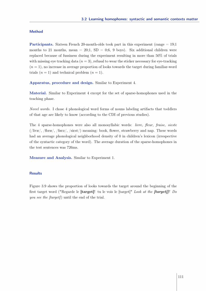
3.2 Learning homophones: syntactic and semantic contexts matter
Method
Participants. Sixteen French 20-month-olds took part in this experiment (range = 19;1months to 21 months, mean = 20;1, SD = 0;6, 9 boys). Six additional children werereplaced because of fussiness during the experiment resulting in more than 50% of trialswith missing eye tracking data (n = 3), refusal to wear the sticker necessary for eye-tracking(n = 1), no increase in average proportion of looks towards the target during familiar-wordtrials (n = 1) and technical problem (n = 1).
Apparatus, procedure and design. Similar to Experiment 4.
Material. Similar to Experiment 4 except for the set of sparse-homophones used in theteaching phase.
Novel words. I chose 4 phonological word forms of nouns labeling artifacts that toddlersof that age are likely to know (according to the CDI of previous studies).
The 4 sparse-homophones were also all monosyllabic words: livre, fleur, fraise, sieste(/livK/, /flœK/, /fKEz/, /siEst/) meaning: book, flower, strawberry and nap. These wordshad an average phonological neighborhood density of 0 in children’s lexicon (irrespectiveof the syntactic category of the word). The average duration of the sparse-homophones inthe test sentences was 726ms.
Measure and Analysis. Similar to Experiment 1.
Results
Figure 3.9 shows the proportion of looks towards the target around the beginning of thefirst target word ("Regarde le [target]! tu le vois le [target]" Look at the [target]]! Doyou see the [target]) until the end of the trial.
111
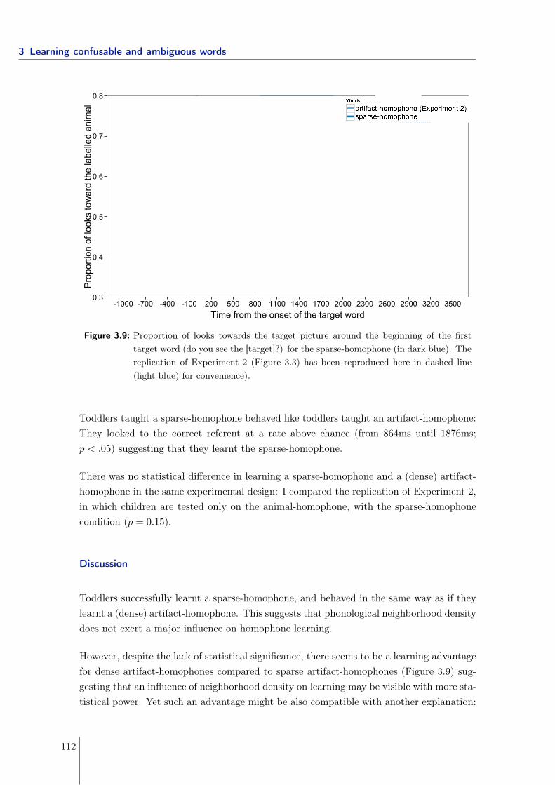
3 Learning confusable and ambiguous words
TARGET
*
0.3
0.4
0.5
0.6
0.7
0.8
-1000 -700 -400 -100 200 500 800 1100 1400 1700 2000 2300 2600 2900 3200 3500Time from the onset of the target word
Pro
porti
on o
f loo
ks to
war
d th
e la
belle
d an
imal
sparse-homophone
exp
sparseunrelated
Figure 3.9: Proportion of looks towards the target picture around the beginning of the firsttarget word (do you see the [target]?) for the sparse-homophone (in dark blue). Thereplication of Experiment 2 (Figure 3.3) has been reproduced here in dashed line(light blue) for convenience).
Toddlers taught a sparse-homophone behaved like toddlers taught an artifact-homophone:They looked to the correct referent at a rate above chance (from 864ms until 1876ms;p < .05) suggesting that they learnt the sparse-homophone.
There was no statistical difference in learning a sparse-homophone and a (dense) artifact-homophone in the same experimental design: I compared the replication of Experiment 2,in which children are tested only on the animal-homophone, with the sparse-homophonecondition (p = 0.15).
Discussion
Toddlers successfully learnt a sparse-homophone, and behaved in the same way as if theylearnt a (dense) artifact-homophone. This suggests that phonological neighborhood densitydoes not exert a major influence on homophone learning.
However, despite the lack of statistical significance, there seems to be a learning advantagefor dense artifact-homophones compared to sparse artifact-homophones (Figure 3.9) sug-gesting that an influence of neighborhood density on learning may be visible with more sta-tistical power. Yet such an advantage might be also compatible with another explanation:
112

3.2 Learning homophones: syntactic and semantic contexts matter
Dense artifact-homophones are composed of more frequent sound sequences than sparseartifact-homophones (cumulative bigram log-probability logP = −3.38 for dense artifact-homophones; logP = −5.69 for sparse artifact-homophones16) and there is evidence thattoddlers and children find it easier to learn words composed of frequent segments thanwords composed of infrequent segments (Graf Estes & Bowen, 2013; Storkel & Maekawa,2005).
At any rate, the present results suggest that the effect of phonological neighborhood densityis smaller than the effect of semantic distance.
3.2.5 Conclusions
An important part of the word learning process requires children to identify what counts asa novel word and what does not. This is especially a challenge when learning homophones,where the same phonological form is used to refer to several distinct meanings. Here, Iinvestigated different sources of information that may help children to identify when a novelmeaning for a known word is appropriate. Specifically I manipulated 1) both the syntacticand the semantic distance between the novel word and its familiar homophone acrossexperiments (Experiment 1-4) and 2) the position of the word form in the phonologicalnetwork of the mental lexicon (Experiment 5).
Experiment 1 showed that toddlers had no problem learning homophones when their mean-ings are realized in different syntactic categories: "an eat" was a good label for a novelanimal despite children knowing the meaning of the verb "to eat". Yet, this does not tell uswhether the syntactic distinction (noun/verb) or the semantic distinction (object/action)between the two meanings was important to learn homophones. Experiment 2 and 3showed that a semantic distinction between the two meanings of a pair of homophones wassufficient to trigger learning: Toddlers learnt easily that "a potty" could also label a novelanimal but failed in a condition where the novel animal was labelled "a cat". However,Experiment 4 failed to show that the syntactic context alone, when different meanings ofa homophone are cued by different genders, is sufficient to learn a second meaning for aknown noun: Toddlers failed to learn that a novel animal could be called "unefem chat"a cat despite the existence of the article "unefem" that indicates that "chat" (a masculinenoun in French) may not be used in its known meaning. Finally, Experiment 5 suggeststhat the phonological density of the word form of the homophone does not have a majorinfluence on establishing that this word form maps onto several meanings.
The word learning process, thus, does not seem to exclusively rely on identifying those wordforms that have no lexical entry and associate them a meaning (e.g., Carey, 1978b). As I16This was calculated using a ngram model on the set of word types in the French lexicon, taken from the
Lexique database; (New, Pallier, Brysbaert, & Ferrand, 2004)
113
3 Learning confusable and ambiguous words
showed were, deciding what counts as novel word or not depends on the context in whichthe word form appears, even when this word form already has a lexical entry in children’slexicon. In particular, the linguistic context plays a prominent role in constraining lexicalaccess to the existing word and thus impacting the likelihood that this word form couldconvey a novel meaning in that context. Similarly, when the two meanings of the sameword form are semantically distinct, it makes it easier to identify that a novel meaning isintended.
Taken as a whole, this set of studies suggests that learning homophones is less challengingfor toddlers than one might think: When the two meanings of a pair of homophones appearin contexts that are sufficiently distinct, they are learnt as easily as non-homophones. Iconclude that creating a novel lexical entry depends on multiple sources of informationcoming from the lexicon and the parsing system.
114
3.3 Similar-sounding words and homophones in the lexicon
3.3 Similar-sounding words and homophones in the lexicon
The results obtained in both section 3.1 and 3.2 suggest that the process of creating anovel lexical entry is mediated by multiple sources of information coming from the lexicon(e.g., lexical-semantic relationships) and the parsing system (e.g., expecting a noun or averb in a given linguistic context). As a result, minimal pairs of words and homophonepairs are less challenging for children than previous studies suggested, at least whenevereach member of the pair appears in distinct syntactic or semantic contexts. One importantquestion is whether the structure of the lexicon reflects these constrains on learning: Is itthe case that members of a homophone pair, or a minimal pair, are more distant from oneanother than would be expected by chance alone? Such a result would suggest that thelexicon might be shaped by learning constraints.
3.3.1 Minimal pairs in the lexicon
Learning neighbors of familiar words is difficult for toddlers, but as I showed, this diffi-culty disappears when the novel words appear in contexts that are sufficiently differentfrom their known neighbors (either syntactically or semantically or both) (section 3.1). Iflearnability influences language changes, then this constraint on early lexical acquisitionmight have a long-lasting impact on the overall structure of the lexicon. Do lexicons avoidsimilar-sounding words? And when similar-sounding words do occur, are they preferen-tially distributed across syntactic or semantic categories to improve their learnability (andtheir recoverability)?
The quantitative analyses of the lexicon done in section 2.1 suggest that natural lexiconscontain many similar sounding words, more than what would be expected by phonotacticsand morphological regularity. In addition, lexicons display a small but significant tendencyfor similar sounding words to be also more semantically similar (section 2.2, Monaghan,Shillcock, Christiansen, & Kirby, 2014). Relevant to the results with toddlers, in section2.1, I also looked at whether lexicons favor similar-soundings words (i.e., minimal pairs)to appear across syntactic categories rather than within the same syntactic category (seeFigure 3.10 copied below for convenience). These results show that all 4 languages (Dutch,English, French and German) have more minimal pairs within categories than would beexpected by chance. In sum, lexicons show an advantage for similar sounding words thatare closely related.
115
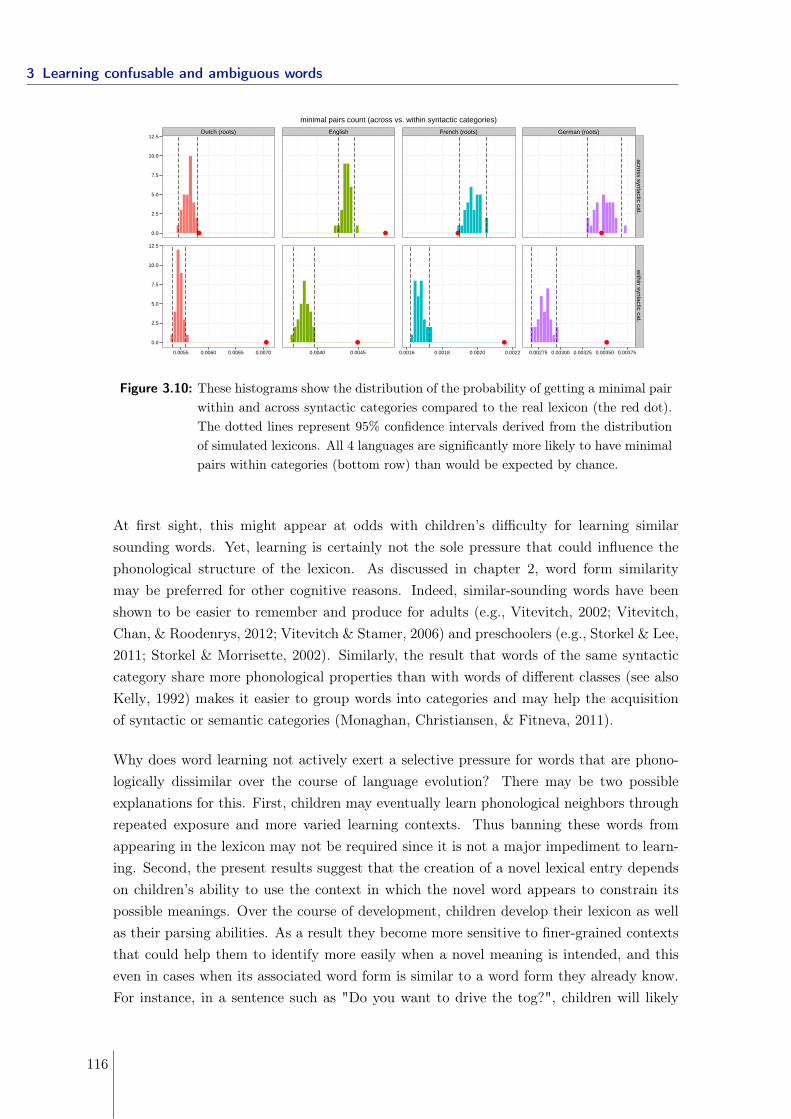
3 Learning confusable and ambiguous words
Dutch (roots) English French (roots) German (roots)
●
●
●
●
●
●
●
●
0.0
2.5
5.0
7.5
10.0
12.5
0.0
2.5
5.0
7.5
10.0
12.5
across syntactic cat.w
ithin syntactic cat.
0.0055 0.0060 0.0065 0.0070 0.0040 0.0045 0.0016 0.0018 0.0020 0.0022 0.00275 0.00300 0.00325 0.00350 0.00375
minimal pairs count (across vs. within syntactic categories)
Figure 3.10: These histograms show the distribution of the probability of getting a minimal pairwithin and across syntactic categories compared to the real lexicon (the red dot).The dotted lines represent 95% confidence intervals derived from the distributionof simulated lexicons. All 4 languages are significantly more likely to have minimalpairs within categories (bottom row) than would be expected by chance.
At first sight, this might appear at odds with children’s difficulty for learning similarsounding words. Yet, learning is certainly not the sole pressure that could influence thephonological structure of the lexicon. As discussed in chapter 2, word form similaritymay be preferred for other cognitive reasons. Indeed, similar-sounding words have beenshown to be easier to remember and produce for adults (e.g., Vitevitch, 2002; Vitevitch,Chan, & Roodenrys, 2012; Vitevitch & Stamer, 2006) and preschoolers (e.g., Storkel & Lee,2011; Storkel & Morrisette, 2002). Similarly, the result that words of the same syntacticcategory share more phonological properties than with words of different classes (see alsoKelly, 1992) makes it easier to group words into categories and may help the acquisitionof syntactic or semantic categories (Monaghan, Christiansen, & Fitneva, 2011).
Why does word learning not actively exert a selective pressure for words that are phono-logically dissimilar over the course of language evolution? There may be two possibleexplanations for this. First, children may eventually learn phonological neighbors throughrepeated exposure and more varied learning contexts. Thus banning these words fromappearing in the lexicon may not be required since it is not a major impediment to learn-ing. Second, the present results suggest that the creation of a novel lexical entry dependson children’s ability to use the context in which the novel word appears to constrain itspossible meanings. Over the course of development, children develop their lexicon as wellas their parsing abilities. As a result they become more sensitive to finer-grained contextsthat could help them to identify more easily when a novel meaning is intended, and thiseven in cases when its associated word form is similar to a word form they already know.For instance, in a sentence such as "Do you want to drive the tog?", children will likely
116
3.3 Similar-sounding words and homophones in the lexicon
interpret "tog" as a type of vehicle since they could use its immediate context (i.e., "drive")to attribute properties ("could be driven") to the novel word that makes it unlikely to beconfused with "dog".
Importantly, the observation that difficulties in learning phonological neighbors do notscale up to the overall structure of the lexicon does not mean that learning does not exertan influence at all. Yet its influence may be less critical than the other cognitive pressuresmentioned above for this particular phenomenon. While learning difficulties may not bevisible in the static structure of the lexicon, they may be reflected in the dynamics of earlylexical growth: Novel words may preferably be added along dimensions that allow themto be easily distinguishable from already existing words. Previous work looking at thedynamic growth of the lexicon only focused on how phonological similarity or semanticsimilarity of single words to other words in the rest of the lexicon may separately influenceword learning (Carlson, Sonderegger, & Bane, 2014; Hills, Maouene, Maouene, Sheya, &Smith, 2009; Steyvers & Tenenbaum, 2005, but see Regier 2005). For instance, Hills etal. (2009) show that the order of acquisition of nouns depends on the semantic or thephonological connectivity to other words in the lexicon: The more connected the word, theearlier it is acquired. Yet as we have seen, looking at a single dimension independently ofthe others may not account for the learning pattern observed here. Thus, it remains opento question whether the growing lexicon reflects the influence of the learning system.
3.3.2 Homophones in the lexicon
Learning homophones may be difficult even for preschoolers (Casenhiser, 2005; Doherty,2004; Mazzocco, 1997), yet as I showed this difficulty is reduced when both meanings ofa pair of homophones have different syntactic categories or cover distinct concepts. Oneinteresting question is thus whether these learnability advantages translate into the overallstructure of the lexicon: Are there more homophones from different syntactic categoriesthan same-category homophones in lexicons? Similarly, are members of a homophonepair more likely to be semantically distant in languages? Interestingly the present resultsalso suggest that grammatical gender and neighborhood density do not help toddlers toidentify whether a given word form maps onto several meanings. Following the same idea,this suggests that these factors might not exert a major influence on the organization ofhomophony within the lexicon.
To investigate these questions, I extracted the pairs of homophones in the lexicon of 4 lan-guages (Dutch, English, French and German) and looked at their distributions in both thesyntactic (grammatical categories and gender) and semantic spaces. I then compared these
117
3 Learning confusable and ambiguous words
distributions to random baselines that simulate how homophone pairs should be distributedunder random conditions if there were no cognitive pressure (including learning).17
Method
Lexicons. I used the phonemic lexicons of 4 languages: Dutch, English, German (ex-tracted from CELEX, Baayen, Piepenbrock, & van H, 1993) and French (extracted fromLexique, New et al., 2004). For each language, I defined a lexicon as the set of the most10,000 frequent word forms.
To identify homophone pairs in each lexicon, I took all the pairs of words that share thesame phonological form but are from different lemmas according to their lemma code inCELEX and Lexique. This procedure eliminated homophones coming from the same rootbut instantiated by different categories (e.g., to fight/a fight) or where one of the formshas a silent morphological marker (e.g., chien/chiens dog/dogs, which are pronounced inthe same way in French).
Measures.
Syntactic category. I used the Part Of Speech (POS) tags in CELEX for Dutch, English andGerman and in Lexique for French to count the number of homophones within the samesyntactic category (e.g., animal-"bat"/baseball-"bat") and the number of homophonesacross different categories (e.g., a park/to park).
Gender. I used the gender information tags provided in CELEX for Dutch and Germanand in Lexique for French to count the number of noun-noun homophones within the samegender (e.g., "avocat" meaning avocadomasc or lawyermasc) and across different genders(e.g., mur/mûre, wallmasc/blackberryfem). Note that there are 3 grammatical genders inDutch and German (feminine, masculine, neutral) and 2 in French (feminine, masculine).English was not concerned by this measure as it is not a gender-marked language.
Semantic Similarity. I applied Latent Semantic Analysis (LSA, Landauer & Dumais 1997)on Wikipedia for each language using the Gensim package (Rehurek, Sojka, & others, 2010)(see section 2.2). Thus, each word of the Wikipedia corpus was modeled as a vector ina multidimensional space. The semantic similarity between two words is the cosine ofthe angle between the two word vectors. A value close to 1 indicates that two words areclose in meaning, whereas values close to 0 indicate that the meanings are not related.
17Note that I did not study (yet) the influence of neighborhood density on homophones. However oneprevious study suggests that shorter words and more phonotactically probable words (which also havemore phonological neighbors, see Mahowald, Dautriche, Gibson, & Piantadosi submitted) have moremeanings than longer and less phonetically likely words (Piantadosi, Tily, & Gibson, 2012). Yet, afuture study should examine whether there is an influence of phonological neighborhood density on thenumber of meanings beyond confounding factors such as frequency, phonotactic probability and length.
118
3.3 Similar-sounding words and homophones in the lexicon
I computed the semantic similarity between the two members of homophone pairs thatshared their syntactic category (excluding across-categories homophones). Yet, becauseLSA is computed over an orthographic corpus, only homophones that are written differentlycan be distinguished with this measure, therefore I looked only at these homophones thathave different orthography (between 200 and 400 pairs for the 4 languages under study).
Random baselines.
Syntactic category. For each language, I shuffled the syntactic categories within each wordlength. I then evaluated the number of pairs of homophones that fell across categories forthis random configuration.
Gender. For each language, I extracted the subset of nouns from the lexicon and shuffledtheir grammatical gender within each word length. I then evaluated the number of pairsof homophones that have a different gender for this random configuration.
Semantic similarity. Similarly, I randomly shuffled the LSA vectors within all words ofthe same length and computed the average cosine similarity of this configuration of form-meaning mappings for all pairs of homophones.
Each random baseline was repeated 30 times in order to obtain a chance distribution forthe given measure.
Results
Across-categories homophones in the lexicon
I first considered the proportion of homophone pairs that are distributed across syntacticcategories. If there are more homophones across syntactic categories than expected bychance, the proportion of across-categories homophones should be greater in the lexiconsthan in the random baselines.
Figure 3.11 shows how the random baselines (the histograms) compare to the lexicons(the red dots). Crucially, all histograms fall to the left of the red dot, which meansthat all lexicons have more across-categories homophones than expected by chance (allps < .001). Note that the proportion of across-categories homophones (ranging from 0.8to 0.9 across the 4 languages) is greater than the proportion of same-category homophones(the complementary proportion). This suggests that there is a pressure for homophonesto be distributed across syntactic categories rather than within.
119
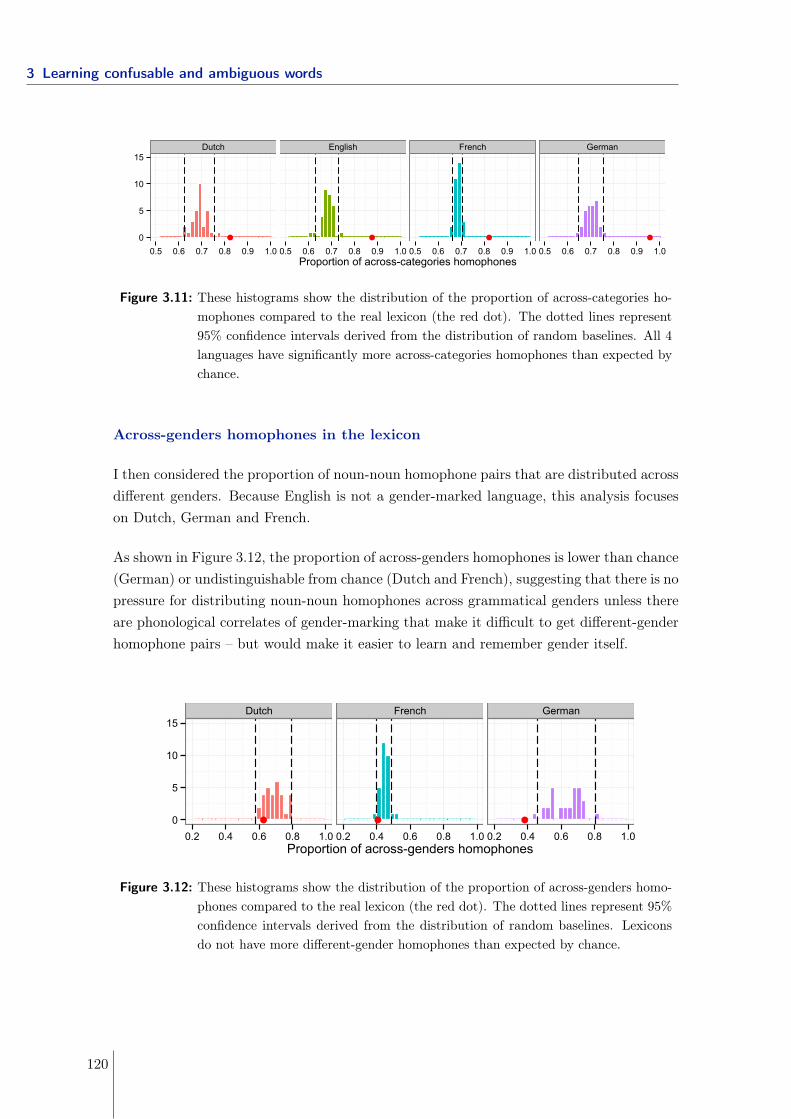
3 Learning confusable and ambiguous words
Dutch English French German
0
5
10
15
0.5 0.6 0.7 0.8 0.9 1.0 0.5 0.6 0.7 0.8 0.9 1.0 0.5 0.6 0.7 0.8 0.9 1.0 0.5 0.6 0.7 0.8 0.9 1.0Proportion of across-categories homophones
Figure 3.11: These histograms show the distribution of the proportion of across-categories ho-mophones compared to the real lexicon (the red dot). The dotted lines represent95% confidence intervals derived from the distribution of random baselines. All 4languages have significantly more across-categories homophones than expected bychance.
Across-genders homophones in the lexicon
I then considered the proportion of noun-noun homophone pairs that are distributed acrossdifferent genders. Because English is not a gender-marked language, this analysis focuseson Dutch, German and French.
As shown in Figure 3.12, the proportion of across-genders homophones is lower than chance(German) or undistinguishable from chance (Dutch and French), suggesting that there is nopressure for distributing noun-noun homophones across grammatical genders unless thereare phonological correlates of gender-marking that make it difficult to get different-genderhomophone pairs – but would make it easier to learn and remember gender itself.
Dutch French German
0
5
10
15
0.2 0.4 0.6 0.8 1.0 0.2 0.4 0.6 0.8 1.0 0.2 0.4 0.6 0.8 1.0Proportion of across-genders homophones
Figure 3.12: These histograms show the distribution of the proportion of across-genders homo-phones compared to the real lexicon (the red dot). The dotted lines represent 95%confidence intervals derived from the distribution of random baselines. Lexiconsdo not have more different-gender homophones than expected by chance.
120
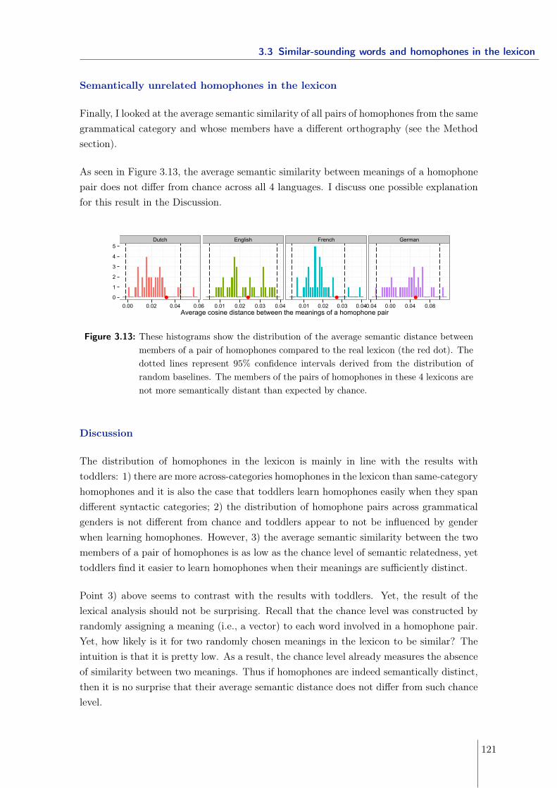
3.3 Similar-sounding words and homophones in the lexicon
Semantically unrelated homophones in the lexicon
Finally, I looked at the average semantic similarity of all pairs of homophones from the samegrammatical category and whose members have a different orthography (see the Methodsection).
As seen in Figure 3.13, the average semantic similarity between meanings of a homophonepair does not differ from chance across all 4 languages. I discuss one possible explanationfor this result in the Discussion.
Dutch English French German
0
1
2
3
4
5
0.00 0.02 0.04 0.06 0.01 0.02 0.03 0.04 0.01 0.02 0.03 0.04-0.04 0.00 0.04 0.08Average cosine distance between the meanings of a homophone pair
Figure 3.13: These histograms show the distribution of the average semantic distance betweenmembers of a pair of homophones compared to the real lexicon (the red dot). Thedotted lines represent 95% confidence intervals derived from the distribution ofrandom baselines. The members of the pairs of homophones in these 4 lexicons arenot more semantically distant than expected by chance.
Discussion
The distribution of homophones in the lexicon is mainly in line with the results withtoddlers: 1) there are more across-categories homophones in the lexicon than same-categoryhomophones and it is also the case that toddlers learn homophones easily when they spandifferent syntactic categories; 2) the distribution of homophone pairs across grammaticalgenders is not different from chance and toddlers appear to not be influenced by genderwhen learning homophones. However, 3) the average semantic similarity between the twomembers of a pair of homophones is as low as the chance level of semantic relatedness, yettoddlers find it easier to learn homophones when their meanings are sufficiently distinct.
Point 3) above seems to contrast with the results with toddlers. Yet, the result of thelexical analysis should not be surprising. Recall that the chance level was constructed byrandomly assigning a meaning (i.e., a vector) to each word involved in a homophone pair.Yet, how likely is it for two randomly chosen meanings in the lexicon to be similar? Theintuition is that it is pretty low. As a result, the chance level already measures the absenceof similarity between two meanings. Thus if homophones are indeed semantically distinct,then it is no surprise that their average semantic distance does not differ from such chancelevel.
121
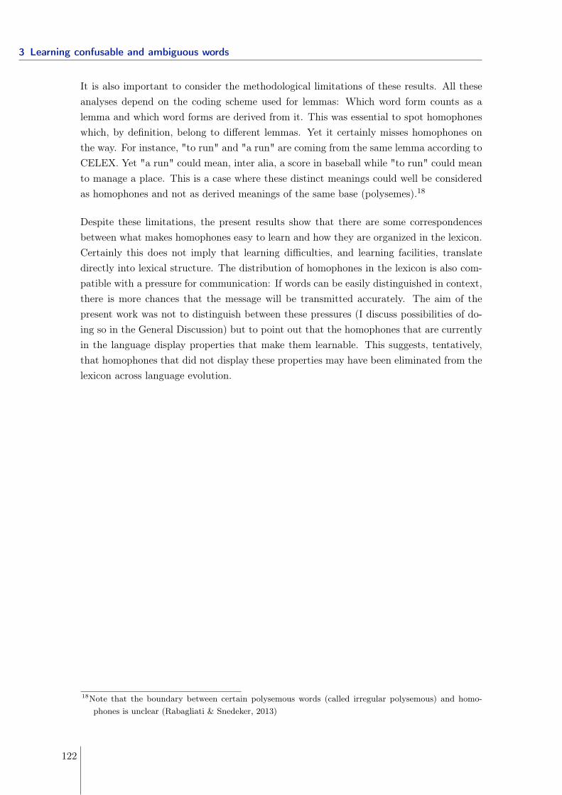
3 Learning confusable and ambiguous words
It is also important to consider the methodological limitations of these results. All theseanalyses depend on the coding scheme used for lemmas: Which word form counts as alemma and which word forms are derived from it. This was essential to spot homophoneswhich, by definition, belong to different lemmas. Yet it certainly misses homophones onthe way. For instance, "to run" and "a run" are coming from the same lemma according toCELEX. Yet "a run" could mean, inter alia, a score in baseball while "to run" could meanto manage a place. This is a case where these distinct meanings could well be consideredas homophones and not as derived meanings of the same base (polysemes).18
Despite these limitations, the present results show that there are some correspondencesbetween what makes homophones easy to learn and how they are organized in the lexicon.Certainly this does not imply that learning difficulties, and learning facilities, translatedirectly into lexical structure. The distribution of homophones in the lexicon is also com-patible with a pressure for communication: If words can be easily distinguished in context,there is more chances that the message will be transmitted accurately. The aim of thepresent work was not to distinguish between these pressures (I discuss possibilities of do-ing so in the General Discussion) but to point out that the homophones that are currentlyin the language display properties that make them learnable. This suggests, tentatively,that homophones that did not display these properties may have been eliminated from thelexicon across language evolution.
18Note that the boundary between certain polysemous words (called irregular polysemous) and homo-phones is unclear (Rabagliati & Snedeker, 2013)
122
3.4 Summary and Discussion
3.4 Summary and Discussion
At the beginning of this chapter I laid out that similar-sounding words and ambiguouswords were a challenge for children who need to determine what counts as a novel wordand what does not (the identification problem).
In section 3.1, I revisited children’s failure to learn similar-sounding words (learning"tog" when "dog" is already in their lexicon Swingley & Aslin, 2007). I proposed thattoddlers may resist considering "tog" as a novel object label because its neighbor "dog"is also an object, such that both words share too many commonalities between them. Toincrease the likelihood that a novel form such as "tog" could be interpreted as a novelword, I manipulated the syntactic context of the form. In particular, 18-month-olds weretaught object labels that were phonological neighbors of a familiar noun (as "tog" was,for "dog"), or neighbors of a familiar verb (like teaching "kiv", a neighbor of "give").Children successfully learnt the verb-neighbors but failed to learn the noun-neighbors.Thus, manipulating the linguistic context by placing a verb-neighbor in a noun syntacticframe indicated to children that a new meaning was appropriate for the novel word form.Learning neighbors of familiar words is difficult for toddlers, but this difficulty disappearswhen the novel words appear in contexts that are sufficiently different from their knownneighbors.
In section 3.2, I investigated whether children’s ability to learn homophones dependsalso on the context these words are presented in. I showed that 20-month-olds are willingto learn a second meaning for a word they know, provided that the two homophones aresufficiently distant syntactically (e.g. "an eat" is a good label for a novel animal), orsemantically (e.g. "a sweater" for a novel animal), but not when they are close (e.g. "acat" for a novel animal). This suggests that when the two members of a homophone pairappear in contexts that are sufficiently distinct (either syntactically or semantically) theyare learnt as easily as non-homophones.
As the present results suggest, minimal pairs and homophones may be less problematic thanpreviously thought, at least when each member of the pair appears in different syntacticor semantic contexts that indicate to children that a meaning distinction is necessary.
In section 3.3, I evaluated whether similar-sounding words and homophones are dis-tributed in the lexicon in a way that makes them more distinctive, thus more learnable.Interestingly enough, my results show that despite being more learnable, there is no pres-sure for minimal pairs to appear across distinct syntactic categories in the lexicon and to besemantically distinct (see section 2.2). In contrast, such a pressure exists for homophones,that is, there are more across-categories homophones than expected by chance and thathomophones were as semantically dissimilar as any random pair of words in the lexicon.
123
3 Learning confusable and ambiguous words
Note that this trend was observed for all 4 languages under study (Dutch, English, Frenchand German) suggesting that these results are robust cross-linguistically (though furtherinvestigation with more language families needs to be done in order to confirm this).
How can we explain that minimal-pairs and homophones are distributed differently inthe lexicon? I suggest that these differences reflect the influence of different functionalpressures associated with language acquisition and language use. There may be a greateradvantage for minimal pairs to be more semantically similar and clustered within thesame syntactic category than for homophones. I suggested that a compressible lexicon,or clumpy lexicon, would be advantageous for speech production (i.e., re-use of commonarticulatory sequences), memory (i.e., less sound sequences to remember) and learningcategories (i.e., phonological similarity may facilitate the identification of syntactic andsemantic classes). Additionally such a clumpy lexicon would also be advantageous tosegment speech into words (see the Introduction 1.2.1, Altvater-Mackensen & Mani, 2013).A pressure for clumpiness would prevail over a pressure for distinctiveness because adults,and children as I showed here, are able to use fine-grained contextual cues to access therelevant meaning of the word successfully (see the relevant discussion in section 3.3). Onthe contrary, homophones show an advantage of distinctiveness over clumpiness, suggestingthat because of form-identity, there is no choice but for these words to be distinctive inmeaning in order to be learnable and transmitted with accuracy.
In sum, the lexicon is the theater of functional tradeoffs: Several pressures seem to be atplay in the lexicon and influence differently the set of word forms present in the languageand how they associate to meanings. An important future direction for this work willbe to determine exactly how such functional tradeoffs arise in the course of language useand its acquisition depending on the phenomenon (e.g., minimal pairs, homophones) understudy.
124

3.4 Summary and Discussion
w
125

4 Theories of word learning andhomophony: what is missing, what dowe learn
Learning the meaning of a word is not an easy task, though children make it appearsthis way. Certainly, after a few presentations children are able to correctly identify theappropriate referent of a novel word they just have been taught (see Chapter 3). Yet, it isunclear what exactly they have "learned" about the word and which lexical representationthey have formed. Suppose that a speaker uses "banana" to refer to the fruit the child iseating, what can the child infer about the word "banana"? At this point, even assumingthat the child understood which object is referred to by the word in context (a non obviousproblem, see section 1.2.3), the meaning of "banana" is still undetermined (Quine, 1960).Certainly "banana" could refer to the set of all bananas and only bananas but many othersmeanings are consistent with that one experience: the set of all fruits, the set of all yellowobjects and so on.
Existing theories of word learning have stressed the importance of prior knowledge or con-straints about possible word meanings to constrain the learning problem faced by the child(e.g., Bloom, 2001; Goodman, 1955; Markman, 1989). For instance, children assume thatnovel labels refer to whole objects rather than parts of the object (the whole object con-straint, Markman, 1991), to objects of the same type (the taxonomic constraint, Markman& Hutchinson, 1984) and to unnamed objects (the mutual exclusivity constraint, Mark-man & Wachtel, 1988). These constraints on word learning have specifically addressed theproblem of learning unambiguous words where a single form is used to refer to a singlemeaning.
I propose that current accounts of word learning face massive challenges which can berevealed by trying to incorporate more word learning phenomena into the picture. In thischapter, I focus in particular on the role of homophony: what are the factors that leadlanguage learners to postulate homophony for a new word? and what does homophonyreveal about the word learning algorithm? Specifically, in Section 4.1, I investigatewhether observing a "gap" in conceptual space between the learning exemplars for a givenword or the intervention of other lexical items in that gap, lead adult learners to postulate
127
4 Theories of word learning and homophony: what is missing, what do we learn
homophony for a word. In Section 4.2, I take this results further by looking at children’sacquisition of homophones.
128
What homophones say about words
Dautriche Isabelle
Chemla Emmanuel
Laboratoire de Sciences Cognitives et Psycholinguistique, (DEC-ENS/EHESS/CNRS), Paris,
France
Acknowledgements
Funding: the European Research Council under FP/2007-2013-ERC n°313610, ANR-
10-IDEX-0001-02, ANR-10-LABX-0087, Direction Générale de l’Armement (PhD program
Frontières du Vivant). We thank Anne Christophe, Paul Egré, Jean-Rémy Hochmann,
Alexander Martin, Philippe Schlenker, Benjamin Spector, Brent Strickland
Abstract
Homophones are word forms associated with two separate meanings. Two sets of
experiments documented two factors that lead adults to postulate homophony for newly
learned words: the gap in conceptual space between the learning exemplars for a given word
and the intervention of other lexical items in that gap (Experiment 1). These effects were
modulated by zeugmas, linguistic manipulations coherent with the presence/absence of
homophony (Experiment 2). We show how homophony yields a challenge to current
accounts of word learning, which share, explicitly or implicitly, a “convexity constraint”:
learners seek to associate a given phonological form with a single meaning, whose extension
is convex in conceptual space. Homophones, however, cover disconnected areas in
conceptual space and therefore call for an explicit way to integrate them into current models
of word learning.
Keywords: word learning; concepts; word meaning; lexical representation; homophony;
psycholinguistics
4.1 What homophones say about words
129
!
!
Learning the word “cat” implies associating the sequence of sounds /kaet/ to the set
of all cats and only cats. Quite generally one description of the meaning of a content word is
its “extension”, i.e. the set of all entities to which that word refers (an idea discussed in detail
in the tradition of formal semantics at least since Frege, 1892). But language learners need
to infer the extension of a word based on a set of exemplars that surely do not exhaust that
extension. The underlying inference problem would be unsolvable without prior knowledge,
most notably some that could constrain the hypothesis space, which is the set of potential
meanings for words (e.g., Bloom, 2001; Goodman, 1955; Keil, 1989; Markman, 1989; and
Mitchell, 1980 for a formal proof).
Such priors have been described over different forms of conceptual structure (e.g.,
Tenenbaum, Kemp, Griffiths, & Goodman, 2011) in association with different models of
meaning inference (e.g., Bayesian inference, Xu & Tenenbaum, 2007; Hypothesis
elimination, Siskind, 1996; Associative learning, Regier, 2005). Irrespective of these
differences, all current accounts assume that those concepts that happen to have word forms
associated with them are convex, that is, they form a coherent cluster in conceptual space
(e.g., Gardenfors, 2004). For instance, an arbitrarily motivated concept such as DOG OR
TABLE is not a possible concept because it does not form a coherent class of objects (see
Murphy & Medin, 1985 for the idea of “conceptual coherence”). Crucially, all current accounts
of word learning transpose the idea of concept convexity into an explicit or implicit “convexity
constraint” on words: learners seek to associate a given phonological form with a convex
extension. That is, if A and B can be labeled using the sound /kaet/, then all objects falling in
between A and B in conceptual space can also be labeled with the word /kaet/.
There is evidence suggesting that language learners may start with a convexity
constraint. For instance, toddlers and preschoolers prefer to extend a novel word (e.g.,
“blicket” designing a dog) to an object of the same kind (e.g., a cat) rather than to an object
of a different kind (e.g., a bone) (e.g., Markman & Hutchinson, 1984; Waxman & Gelman,
1986; see also the “shape bias”, showing that infants extend a label on the basis of the
shape, Landau, Smith, & Jones, 1988). Hence, children seem to expect that the extension of
a given label groups together objects that share a common property. If such a property is
prioritized in the way we organize the world (we discuss the importance of some properties
over others to define conceptual spaces further in the General Discussion), then it follows
that extensions of words should follow a convexity constraint.
Our goal is to study how homophones fit into this picture, because they present a
challenge to the convexity constraint. Indeed, words do not have to point to individual
4 Theories of word learning and homophony: what is missing, what do we learn
130
!
!
concepts. A homophone is a phonological form associated arbitrarily with several meanings
(contrary to polysemy, see e.g., Rabagliati & Snedeker, 2013; Rabagliati, Marcus, &
Pylkkänen, 2010), which together form a discontinuous set in conceptual space. For
instance, the English word “bat” applies both to the convex concept of ANIMAL BATS and to
the convex concept of BASEBALL BATS, but, regardless of how the conceptual space is
constructed, not all intervening objects sharing a common property of animal bats and
baseball bats count as bats. However, all current approaches implement the convexity
constraint to reduce the hypothesis space and therefore mechanically predict that when
encountering this word form that applies to animal bats and baseball bats, English learners
should conclude that bat applies to any intervening object, as would words that apply very
broadly, such as “thing” or “stuff”. The very existence of homophony in human languages
thus shows that learners do not adhere blindly to a convexity constraint. This challenges the
details of any account that rely on the convexity constraint to reduce the hypothesis space.
Concretely, our point of departure will be work by Xu and Tenenbaum (2007). One
advantage of their study is that it implements the convexity constraint in a predictive model,
but it also provides the means to test it in a non-circular way. To do so, they first gathered
similarity judgments between pairs of objects, and inferred a tree-structure over the whole
set. This tree structure represents the taxonomy between the objects: different dogs are
close together and form a subtree, mammals form a (bigger) subtree, etc. Such a hypothesis
space reflects the taxonomic assumption (Markman, 1989) that requires words to label the
nodes of a tree-structured hierarchy of natural concepts, in line with developmental data
(e.g., Keil, 1989; Markman & Hutchinson, 1984; Markman, 1989; Waxman & Gelman, 1986).
Crucially, Xu and Tenenbaum used this structured conceptual space to test a model of word
learning according to which the extension inferred for a given word label should be a set of
objects with no gap in conceptual space and which minimally includes all exemplars.
Accordingly, they demonstrate that, when exposed to a set of learning exemplars,
participants generalize the extension of the exemplars’ label to the smallest subtree that
contains all these exemplars (their convex hull). In other words, participants pick the smallest
generalization that satisfies the convexity constraint.
The present study explores the situations that lead language learners to postulate
homophony for a new word using the word learning paradigm used by Xu and Tenenbaum.
In Experiment 1, we manipulate two factors that should invite learners to favor a homophone
interpretation of a novel label:
a) The size of the gap, in conceptual space, that separates different learning
exemplars of a given word. To learn a homophone, language learners are exposed to a
4.1 What homophones say about words
131
!
!
discrete set of learning exemplars. For instance, for the word bat, they would observe several
animal-bats and several baseball bats. However if the underlying true concept were the
broad category that encompasses animal-bats, baseball-bats and all intervening objects
(e.g., “thing”), then presumably learners would not observe exemplars confined to two
corners of this set. Rather, they would observe a set of learning exemplars randomly
(uniformly) sampled from the broad category. Observing exemplars clustered at two distant
positions in the hypothesis space, i.e., observing a large gap between the exemplars may
boost the likelihood that the exemplars are sampled from two independent categories,
favoring a homophone interpretation.
b) The intervention of other lexical items in that gap. Evidence for homophony may
also come from other words in the lexicon. There has been much evidence that words and
their underlying concepts mutually constrain each other. For instance, language learners
assume that words do not overlap in meaning (the “mutual exclusivity effect”; e.g., Markman
& Wachtel, 1988). Having evidence that an additional label point towards an intervening
region of the conceptual space (e.g., between animal-bat and baseball bats) may help
learners discover more subtle configurations about how words map onto meanings.
Our results show that participants refrain from associating a label to a broad concept
encompassing all the exemplars. Yet it does not entail that learners postulate homophony in
these cases. We address this question more directly in Experiment 2. All in all, our results
suggest that the effects documented in Experiment 1 are the footprints of homophony. This
shows that current accounts of word learning face new challenges when incorporating
homophony into the picture and that homophony can reveal (some of) the existing
constraints on how words are associated with concepts in general.
Experiment 1: gap in conceptual space and overall structure of the lexicon
We used a word learning paradigm à la Xu and Tenenbaum (2007): participants were
exposed to a new label through a couple of learning exemplars and asked whether the label
should be extended to test items. We introduced a) a large gap in conceptual space between
learning exemplars b) an intervening exemplar with a different label in that gap. We predicted
that these two manipulations would lead to a breaking point after which participants would
violate the convexity constraint, i.e., exclude items in the gap from the extension of the label.
Method
Participants. One hundred and five adults were recruited through Amazon’s
Mechanical Turk (45 females; M = 33 years; 102 native speakers of English) and
4 Theories of word learning and homophony: what is missing, what do we learn
132
!
!
compensated $0.50 for their participation. We excluded participants for lack of engagement
in the task (criterion: participants who selected no test item in more than 50% of the
“attractive” trials, in which at least 3 items should have been selected, see below; n = 0 in
Experiment 1A, n =16 in Experiment 1B) and participated in both versions of the experiment
or in a previous pilot version (n = 3 and 5). This resulted in 41 participants in Experiment 1A
and 40 participants in Experiment 1B. Data collection was stopped when each of the
experiment had at least 40 participants. The number of participants was established before
data collection began.
Procedure and display. Participants were tested online. They were instructed that
they would be exposed to words from an alien language and would have to select images
that correspond to those words. In the instructions, participants were shown an example of a
trial with pictures and a label that would not appear during the test. In each trial, participants
first saw 3 or 4 learning exemplars, presented as the combination of a picture and a
sentence. The first three learning exemplars (referred to as LE1, LE2 and LE3 below) were
presented in random order and labeled with a novel word, e.g., blicket, via a prompt of the
form “This is a blicket” underneath each of them. The fourth learning exemplar (LEX below), if
present, was labeled with another novel word highlighted in red, as in e.g., “This is a bosa”
and was always the right-most exemplar. Once participants pressed a button “Show”, they
would see a set of 4 pictures below the learning exemplars and be asked to select from
these test items which one(s) could be labeled with the first novel word: “Do you see any
other blicket(s)?” (see Figure 1.1). They responded by clicking to select none, one or multiple
test items. When a picture was selected, its frame became green. Participants could unselect
their choice by clicking on it again. Once a response was validated, the set of selected
pictures was recorded and the test continued to the next trial.
4.1 What homophones say about words
133
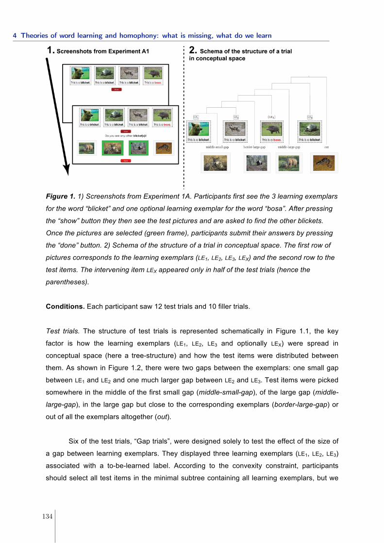
!
!
Figure 1. 1) Screenshots from Experiment 1A. Participants first see the 3 learning exemplars
for the word “blicket” and one optional learning exemplar for the word “bosa”. After pressing
the “show” button they then see the test pictures and are asked to find the other blickets.
Once the pictures are selected (green frame), participants submit their answers by pressing
the “done” button. 2) Schema of the structure of a trial in conceptual space. The first row of
pictures corresponds to the learning exemplars (LE1, LE2, LE3, LEX) and the second row to the
test items. The intervening item LEX appeared only in half of the test trials (hence the
parentheses).
Conditions. Each participant saw 12 test trials and 10 filler trials.
Test trials. The structure of test trials is represented schematically in Figure 1.1, the key
factor is how the learning exemplars (LE1, LE2, LE3 and optionally LEX) were spread in
conceptual space (here a tree-structure) and how the test items were distributed between
them. As shown in Figure 1.2, there were two gaps between the exemplars: one small gap
between LE1 and LE2 and one much larger gap between LE2 and LE3. Test items were picked
somewhere in the middle of the first small gap (middle-small-gap), of the large gap (middle-
large-gap), in the large gap but close to the corresponding exemplars (border-large-gap) or
out of all the exemplars altogether (out).
Six of the test trials, “Gap trials”, were designed solely to test the effect of the size of
a gap between learning exemplars. They displayed three learning exemplars (LE1, LE2, LE3)
associated with a to-be-learned label. According to the convexity constraint, participants
should select all test items in the minimal subtree containing all learning exemplars, but we
4 Theories of word learning and homophony: what is missing, what do we learn
134
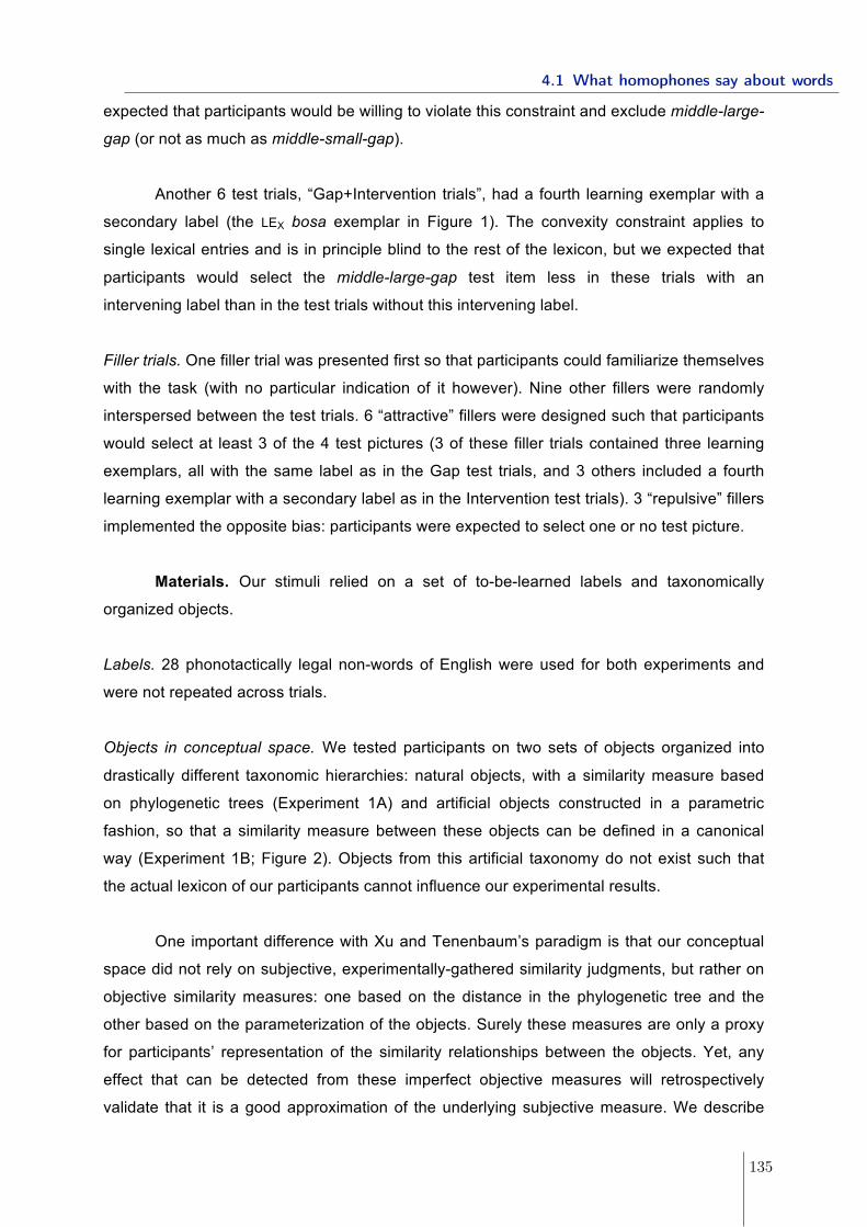
!
!
expected that participants would be willing to violate this constraint and exclude middle-large-
gap (or not as much as middle-small-gap).
Another 6 test trials, “Gap+Intervention trials”, had a fourth learning exemplar with a
secondary label (the LEX bosa exemplar in Figure 1). The convexity constraint applies to
single lexical entries and is in principle blind to the rest of the lexicon, but we expected that
participants would select the middle-large-gap test item less in these trials with an
intervening label than in the test trials without this intervening label.
Filler trials. One filler trial was presented first so that participants could familiarize themselves
with the task (with no particular indication of it however). Nine other fillers were randomly
interspersed between the test trials. 6 “attractive” fillers were designed such that participants
would select at least 3 of the 4 test pictures (3 of these filler trials contained three learning
exemplars, all with the same label as in the Gap test trials, and 3 others included a fourth
learning exemplar with a secondary label as in the Intervention test trials). 3 “repulsive” fillers
implemented the opposite bias: participants were expected to select one or no test picture.
Materials. Our stimuli relied on a set of to-be-learned labels and taxonomically
organized objects.
Labels. 28 phonotactically legal non-words of English were used for both experiments and
were not repeated across trials.
Objects in conceptual space. We tested participants on two sets of objects organized into
drastically different taxonomic hierarchies: natural objects, with a similarity measure based
on phylogenetic trees (Experiment 1A) and artificial objects constructed in a parametric
fashion, so that a similarity measure between these objects can be defined in a canonical
way (Experiment 1B; Figure 2). Objects from this artificial taxonomy do not exist such that
the actual lexicon of our participants cannot influence our experimental results.
One important difference with Xu and Tenenbaum’s paradigm is that our conceptual
space did not rely on subjective, experimentally-gathered similarity judgments, but rather on
objective similarity measures: one based on the distance in the phylogenetic tree and the
other based on the parameterization of the objects. Surely these measures are only a proxy
for participants’ representation of the similarity relationships between the objects. Yet, any
effect that can be detected from these imperfect objective measures will retrospectively
validate that it is a good approximation of the underlying subjective measure. We describe
4.1 What homophones say about words
135
!
!
the two sets of objects at the basis of Experiments 1A and 1B, their structure, and how our
experimental conditions were obtained in each case in the Supplemental Material. The
experimental material for both experiments is available at
https://osf.io/u473e/?view_only=33576a1ac18746b08d7e3fcc96e10e9a
Figure 2. Examples of the artificial stimuli used in Experiment 1B, out of a set of 1024
possible unique combinations obtained from 5 parameters (core pattern, core pattern
occurrences, size of the core pattern, number of radial lines, number of bumps in the radial
lines) with 4 levels each.
Presentation and trial generation. The order of the trials as well as the pairing
between the labels and the set of learning exemplars was fully randomized and differed for
each participant. All trials were generated automatically following the algorithmic constraints
described in the Supplemental Material for each stimuli type.
Statistical analysis. In a mixed logit regression (Jaeger, 2008), we modeled the
selection of a test item (coded as 0 or 1) for each experiment (natural or artificial stimuli).
Both models included two categorical predictors with their interaction: Test Item (middle-
small-gap, border-large-gap, middle-large-gap, out) and Trial Type (Gap vs.
Gap+Intervention) as well as a random intercept and random slopes for both Test Item and
Trial Type for participants. We coded our predictors such that selection of middle-large-gap
for Gap trials served as a baseline (unless otherwise mentioned) against which we compared
a) responses to the other test items, b) the responses to middle-large-gap in
Gap+Intervention trials.
4 Theories of word learning and homophony: what is missing, what do we learn
136
!
!
All analyses were conducted using the lme4 package (Bates & Sarkar, 2004) of R.
Ceiling effects (both in the choice of middle-small-gap and out, see Figure 2) impacted the
log-estimation behind the logit models such that even obvious effects revealed by mere
visual inspection of the data were not captured by the analysis. To get rid of these ceiling
effects in a highly conservative way we introduced random noise: we ran the same analysis
on a modified dataset where we randomly changed 5% of the responses within each Trial
Type and each Test Item.
Results
Figure 3 reports the average proportion of selection of each test item by Trial Type
(Gap vs. Gap+Intervention trials) and Experiment (1A or 1B).
For Gap trials (Figures 3.1a and 3.2a), we replicate the minimal category effect seen
in previous results (i.e., Xu & Tenenbaum, 2007) showing that participants are more likely to
select a test item belonging to the category which is minimally consistent with the exemplars
(middle-small-gap, border-large-gap, middle-large-gap) than a test item outside of this
category (out), both for Experiment 1A (β = -1.56, z = -8.80, p < .001) and Experiment 1B (β
= -5.17, z = -11.46, p < .001)1. Crucially, the size of the gap between learning exemplars
modulated the convexity constraint. That is, participants selected middle-small-gap items
more than middle-large-gap items both in Experiment 1A (Mmiddle-large-gap = 0.59, Mmiddle-small-gap
= 0.98; β = 0.83, z = 3.85, p < .001) and in Experiment 1B (Mmiddle-large-gap = 0.44, Mmiddle-small-gap
= 0.94; β = 3.04, z = 9.55, p < .001). Participants were sensitive to the distribution of the
learning exemplars with natural stimuli but also with unfamiliar stimuli. This latter case shows
that familiarity with the categories (e.g., mammals, carnivores, animals) and possible existing
labels for them cannot fully explain the results.
For Intervention trials (Figures 3.1b and 3.2b), we first replicate the effect described
above: participants were sensitive to the size of the gap between the exemplars, that is, they
selected middle-small-gap more than middle-large-gap in Experiments 1A (Mmiddle-large-gap =
0.43, Mmiddle-small-gap = 0.97; β = 3.82, z = 9.75, p < .001) and in Experiment 1B (Mmiddle-large-gap =
0.32; Mmiddle-small-gap = 0.82; β = 2.70, z = 10.32, p < .001). Crucially, we expected that the
!!!!!!!!!!!!!!!!!!!!!!!!!!!!!!!!!!!!!!!!!!!!!!!!!!!!!!!!1!We Helmert-coded the predictor Test Item to compare the choice of out to the choice of the rest of the test items as a group.!
4.1 What homophones say about words
137
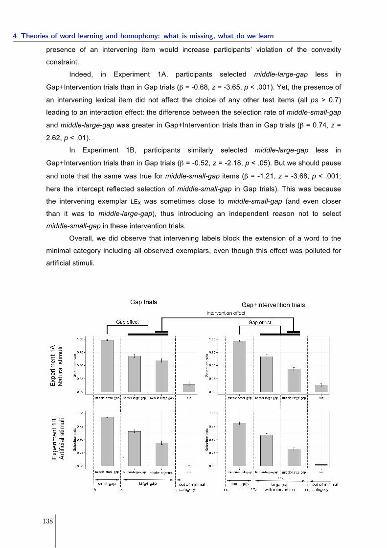
!
!
presence of an intervening item would increase participants’ violation of the convexity
constraint.
Indeed, in Experiment 1A, participants selected middle-large-gap less in
Gap+Intervention trials than in Gap trials (β = -0.68, z = -3.65, p < .001). Yet, the presence of
an intervening lexical item did not affect the choice of any other test items (all ps > 0.7)
leading to an interaction effect: the difference between the selection rate of middle-small-gap
and middle-large-gap was greater in Gap+Intervention trials than in Gap trials (β = 0.74, z =
2.62, p < .01).
In Experiment 1B, participants similarly selected middle-large-gap less in
Gap+Intervention trials than in Gap trials (β = -0.52, z = -2.18, p < .05). But we should pause
and note that the same was true for middle-small-gap items (β = -1.21, z = -3.68, p < .001;
here the intercept reflected selection of middle-small-gap in Gap trials). This was because
the intervening exemplar LEX was sometimes close to middle-small-gap (and even closer
than it was to middle-large-gap), thus introducing an independent reason not to select
middle-small-gap in these intervention trials.
Overall, we did observe that intervening labels block the extension of a word to the
minimal category including all observed exemplars, even though this effect was polluted for
artificial stimuli.
4 Theories of word learning and homophony: what is missing, what do we learn
138
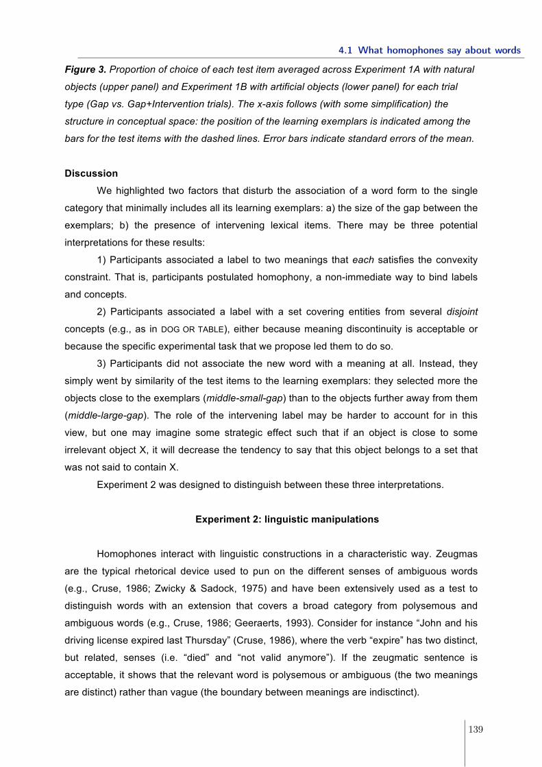
!
!
Figure 3. Proportion of choice of each test item averaged across Experiment 1A with natural
objects (upper panel) and Experiment 1B with artificial objects (lower panel) for each trial
type (Gap vs. Gap+Intervention trials). The x-axis follows (with some simplification) the
structure in conceptual space: the position of the learning exemplars is indicated among the
bars for the test items with the dashed lines. Error bars indicate standard errors of the mean.
Discussion
We highlighted two factors that disturb the association of a word form to the single
category that minimally includes all its learning exemplars: a) the size of the gap between the
exemplars; b) the presence of intervening lexical items. There may be three potential
interpretations for these results:
1) Participants associated a label to two meanings that each satisfies the convexity
constraint. That is, participants postulated homophony, a non-immediate way to bind labels
and concepts.
2) Participants associated a label with a set covering entities from several disjoint
concepts (e.g., as in DOG OR TABLE), either because meaning discontinuity is acceptable or
because the specific experimental task that we propose led them to do so.
3) Participants did not associate the new word with a meaning at all. Instead, they
simply went by similarity of the test items to the learning exemplars: they selected more the
objects close to the exemplars (middle-small-gap) than to the objects further away from them
(middle-large-gap). The role of the intervening label may be harder to account for in this
view, but one may imagine some strategic effect such that if an object is close to some
irrelevant object X, it will decrease the tendency to say that this object belongs to a set that
was not said to contain X.
Experiment 2 was designed to distinguish between these three interpretations.
Experiment 2: linguistic manipulations
Homophones interact with linguistic constructions in a characteristic way. Zeugmas
are the typical rhetorical device used to pun on the different senses of ambiguous words
(e.g., Cruse, 1986; Zwicky & Sadock, 1975) and have been extensively used as a test to
distinguish words with an extension that covers a broad category from polysemous and
ambiguous words (e.g., Cruse, 1986; Geeraerts, 1993). Consider for instance “John and his
driving license expired last Thursday” (Cruse, 1986), where the verb “expire” has two distinct,
but related, senses (i.e. “died” and “not valid anymore”). If the zeugmatic sentence is
acceptable, it shows that the relevant word is polysemous or ambiguous (the two meanings
are distinct) rather than vague (the boundary between meanings are indisctinct).
4.1 What homophones say about words
139
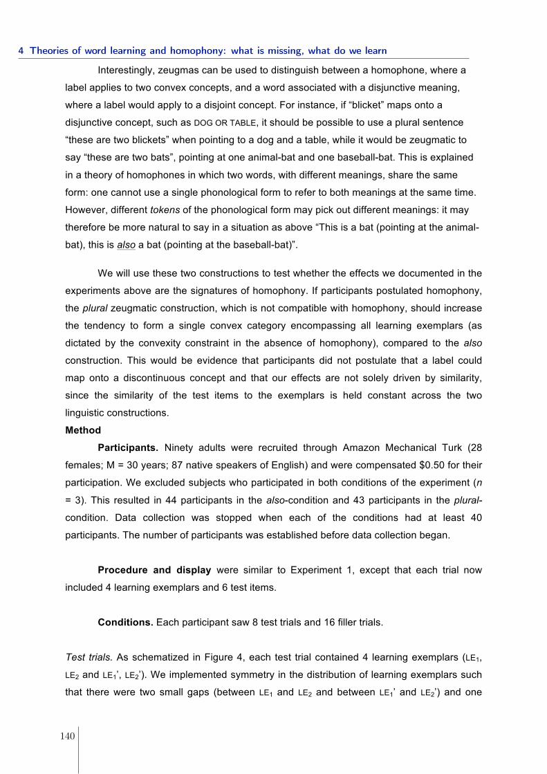
!
!
Interestingly, zeugmas can be used to distinguish between a homophone, where a
label applies to two convex concepts, and a word associated with a disjunctive meaning,
where a label would apply to a disjoint concept. For instance, if “blicket” maps onto a
disjunctive concept, such as DOG OR TABLE, it should be possible to use a plural sentence
“these are two blickets” when pointing to a dog and a table, while it would be zeugmatic to
say “these are two bats”, pointing at one animal-bat and one baseball-bat. This is explained
in a theory of homophones in which two words, with different meanings, share the same
form: one cannot use a single phonological form to refer to both meanings at the same time.
However, different tokens of the phonological form may pick out different meanings: it may
therefore be more natural to say in a situation as above “This is a bat (pointing at the animal-
bat), this is also a bat (pointing at the baseball-bat)”.
We will use these two constructions to test whether the effects we documented in the
experiments above are the signatures of homophony. If participants postulated homophony,
the plural zeugmatic construction, which is not compatible with homophony, should increase
the tendency to form a single convex category encompassing all learning exemplars (as
dictated by the convexity constraint in the absence of homophony), compared to the also
construction. This would be evidence that participants did not postulate that a label could
map onto a discontinuous concept and that our effects are not solely driven by similarity,
since the similarity of the test items to the exemplars is held constant across the two
linguistic constructions.
Method
Participants. Ninety adults were recruited through Amazon Mechanical Turk (28
females; M = 30 years; 87 native speakers of English) and were compensated $0.50 for their
participation. We excluded subjects who participated in both conditions of the experiment (n
= 3). This resulted in 44 participants in the also-condition and 43 participants in the plural-
condition. Data collection was stopped when each of the conditions had at least 40
participants. The number of participants was established before data collection began.
Procedure and display were similar to Experiment 1, except that each trial now
included 4 learning exemplars and 6 test items.
Conditions. Each participant saw 8 test trials and 16 filler trials.
Test trials. As schematized in Figure 4, each test trial contained 4 learning exemplars (LE1,
LE2 and LE1’, LE2’). We implemented symmetry in the distribution of learning exemplars such
that there were two small gaps (between LE1 and LE2 and between LE1’ and LE2’) and one
4 Theories of word learning and homophony: what is missing, what do we learn
140
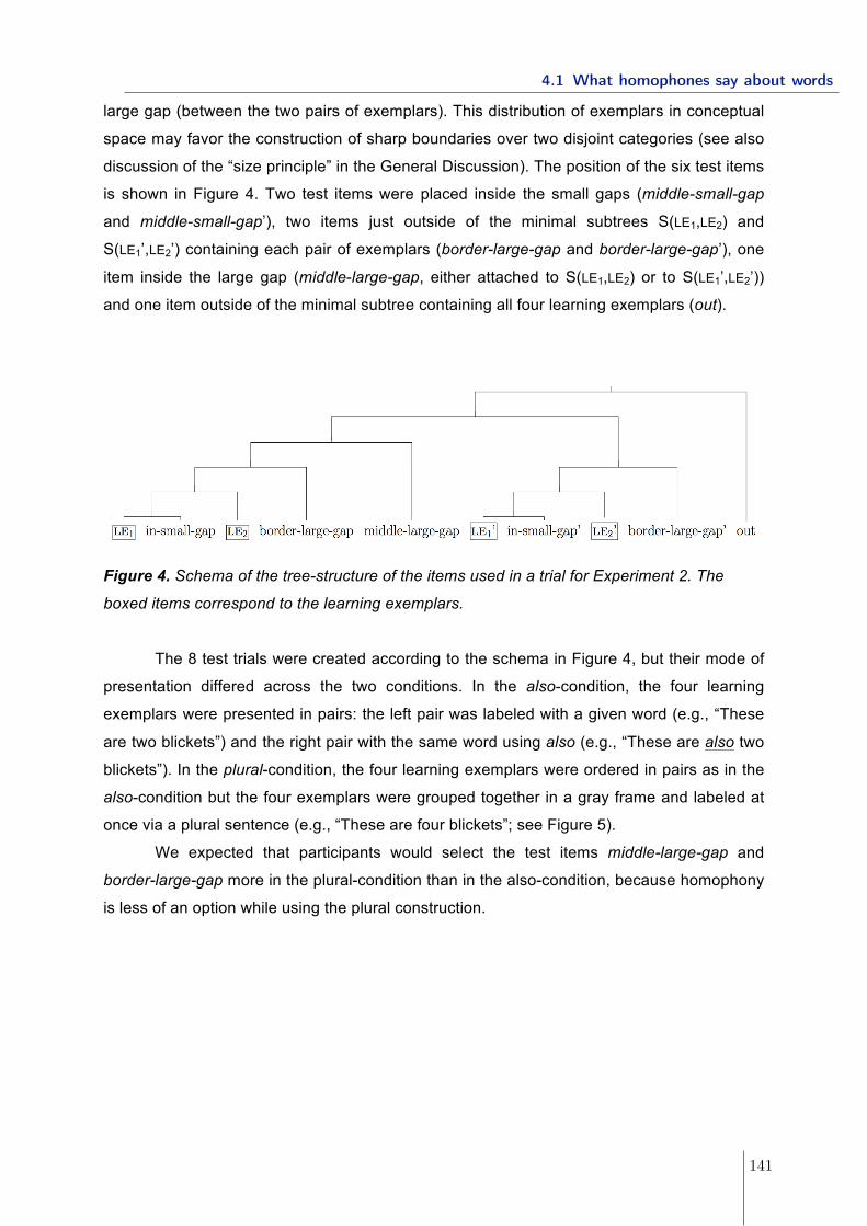
!
!
large gap (between the two pairs of exemplars). This distribution of exemplars in conceptual
space may favor the construction of sharp boundaries over two disjoint categories (see also
discussion of the “size principle” in the General Discussion). The position of the six test items
is shown in Figure 4. Two test items were placed inside the small gaps (middle-small-gap
and middle-small-gap’), two items just outside of the minimal subtrees S(LE1,LE2) and
S(LE1’,LE2’) containing each pair of exemplars (border-large-gap and border-large-gap’), one
item inside the large gap (middle-large-gap, either attached to S(LE1,LE2) or to S(LE1’,LE2’))
and one item outside of the minimal subtree containing all four learning exemplars (out).
Figure 4. Schema of the tree-structure of the items used in a trial for Experiment 2. The
boxed items correspond to the learning exemplars.
The 8 test trials were created according to the schema in Figure 4, but their mode of
presentation differed across the two conditions. In the also-condition, the four learning
exemplars were presented in pairs: the left pair was labeled with a given word (e.g., “These
are two blickets”) and the right pair with the same word using also (e.g., “These are also two
blickets”). In the plural-condition, the four learning exemplars were ordered in pairs as in the
also-condition but the four exemplars were grouped together in a gray frame and labeled at
once via a plural sentence (e.g., “These are four blickets”; see Figure 5).
We expected that participants would select the test items middle-large-gap and
border-large-gap more in the plural-condition than in the also-condition, because homophony
is less of an option while using the plural construction.
4.1 What homophones say about words
141
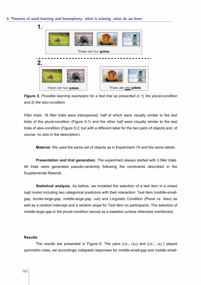
!
!
Figure 5. Possible learning exemplars for a test trial as presented in 1) the plural-condition
and 2) the also-condition.
Filler trials. 16 filler trials were interspersed, half of which were visually similar to the test
trials of the plural-condition (Figure 5.1) and the other half were visually similar to the test
trials of also-condition (Figure 5.2; but with a different label for the two pairs of objects and, of
course, no also in the description).
Material. We used the same set of objects as in Experiment 1A and the same labels.
Presentation and trial generation. The experiment always started with 3 filler trials.
All trials were generated pseudo-randomly following the constraints described in the
Supplemental Material.
Statistical analysis. As before, we modeled the selection of a test item in a mixed
logit model including two categorical predictors with their interaction: Test Item (middle-small-
gap, border-large-gap, middle-large-gap, out) and Linguistic Condition (Plural vs. Also) as
well as a random intercept and a random slope for Test Item on participants. The selection of
middle-large-gap in the plural-condition served as a baseline (unless otherwise mentioned).
Results
The results are presented in Figure 6. The pairs (LE1, LE2) and (LE1’, LE2’) played
symmetric roles, we accordingly collapsed responses for middle-small-gap and middle-small-
4 Theories of word learning and homophony: what is missing, what do we learn
142
!
!
gap’ and responses for border-small-gap and border-small-gap’ (practically ignoring the
prime sign in the report).
First, the results confirm the existence of a gap effect. Participants showed sensitivity
to the sampling distribution of the exemplars, in that they selected more middle-small-gap
than middle-large-gap in both the also-condition (β = 2.20, z = 11.26, p < .001) and the
plural-condition (β = 1.70, z = 8.59, p < .001).
Interestingly, the minimum path (in terms of number of branches) between the
learning exemplars LE1 and LE2 was smaller in Experiment 1A (mean for d(LE1, LE2) = 3.65),
compared both to (LE1, LE2) and (LE1’, LE2’) in Experiment 2 (mean for d(LE1,LE2) = 7.16) (see
Supplemental material). Accordingly, we found a cross-experiment gap effect such that
middle-small-gap was less selected in Experiment 2 (M = 0.75) than in Experiment 1A (M =
0.95).
Our critical expectation concerned the comparison between linguistic presentations.
Test items in the gap between (LE1, LE2) and (LE1’, LE2’) were selected more often in the
plural-condition than in the also-condition: this was true both for middle-large-gap (β = 0.73, z
= 2.24, p < .05) and border-large-gap (β = 0.64, z = 2.13, p < .05), resulting in an interaction
effect: the difference between the selection rate of middle-small-gap (serving as a baseline)
and the combined selection rate of middle-large-gap and border-large-gap was greater in the
plural-condition than in in the also-condition (β = 0.46, z = 2.02, p < .05).2
!!!!!!!!!!!!!!!!!!!!!!!!!!!!!!!!!!!!!!!!!!!!!!!!!!!!!!!!2!We Helmert coded the predictor Test Item to compare the choice of middle-small-gap to the choice of the middle-large-gap and border-large-gap as a group.!
4.1 What homophones say about words
143
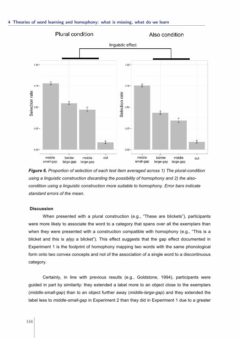
!
!
Figure 6. Proportion of selection of each test item averaged across 1) The plural-condition
using a linguistic construction discarding the possibility of homophony and 2) the also-
condition using a linguistic construction more suitable to homophony. Error bars indicate
standard errors of the mean.
Discussion
When presented with a plural construction (e.g., “These are blickets”), participants
were more likely to associate the word to a category that spans over all the exemplars than
when they were presented with a construction compatible with homophony (e.g., “This is a
blicket and this is also a blicket”). This effect suggests that the gap effect documented in
Experiment 1 is the footprint of homophony mapping two words with the same phonological
form onto two convex concepts and not of the association of a single word to a discontinuous
category.
Certainly, in line with previous results (e.g., Goldstone, 1994), participants were
guided in part by similarity: they extended a label more to an object close to the exemplars
(middle-small-gap) than to an object further away (middle-large-gap) and they extended the
label less to middle-small-gap in Experiment 2 than they did in Experiment 1 due to a greater
4 Theories of word learning and homophony: what is missing, what do we learn
144
!
!
distance between the learning exemplars in Experiment 2.3 Yet, such similarity effects cannot
explain the main result of Experiment 2 since the linguistic manipulation is realized holding
constant similarity relations among learning exemplars and test items. The amount of
similarity-driven generalization in participants’ responses could be quantified (see Xu and
Tenenbaum for a model comparison of rule- vs. similarity-based model), but it is sufficient for
our purposes to note that it cannot account for the entirety of the present effects, which are
driven by linguistic manipulations alone in Experiment 2.4
One may also ask whether the plural/also effect is linked to the very specific linguistic
constructions involved or whether it is merely driven by the visual, two-part presentation that
co-varies with these constructions in our experiments. Importantly, a visual effect (i.e., a
visual “zeugma”) would make the same point as a more specific linguistic construction effect:
all that matters for our argument is that there is room for two tokens of the same phonological
form, either because two tokens are indeed present, or simply because the presentation
introduces different labeling events.
General Discussion
We documented two factors that reduce the tendency to map a phonological form
onto a single, convex extension, an explicit or implicit assumption about learners in all
current accounts of word learning: a) the size of the gap in conceptual space between
learning exemplars; b) the presence of an intervening label for entities in that gap. These
effects were modulated by linguistic manipulations coherent with the presence/absence of
homophony. We submit that when encountering novel words in such situations, learners
prefer to postulate homophony to preserve concept convexity, whereby a label applies to two
convex concepts, rather than accepting that a label applies to a single discontinuous
concept.
In the following we first come back to the very idea of a conceptual space, how to
access such an abstract construct. Second, we move to the level of words and show how the
current study of homophony is relevant to current accounts of word learning broadly, and
why other phenomena should be subjected to the same scrutiny. Finally, our results are
!!!!!!!!!!!!!!!!!!!!!!!!!!!!!!!!!!!!!!!!!!!!!!!!!!!!!!!!3!Note that this is also compatible with the size principle documented by Xu and Tenenbaum (2007): since the boundaries of the categories defined by the pairs of exemplars (LE1, LE2) and (LE1’, LE2’) were less sharp than in Experiment 1A, the correct level of generalization was more uncertain in Experiment 2 than in Experiment 1A.!4!While we demonstrate that participants are sensitive to the linguistic constructions in which the words enter, we cannot tell whether the also construction alters the results in one direction (towards homophony), or whether the also construction pushes in the opposite direction (against homophony), or both.!
4.1 What homophones say about words
145
!
!
based on adult data only and we discuss their relevance for children in the process of
learning their native language.
How to work with concepts
A provocative question at this point is whether the notion of conceptual space is
useful. One worry is that there may not be a stable metric between abstract entities across
contexts (Tversky, 1977), such that two entities can be made arbitrarily similar by changing
the dimension under consideration. For instance, one may consider that a Ferrari and a VW
Beatle are closer to one another than a Ferrari and a diamond, but this similarity relation may
reverse if the context involves paying attention to the value of entities. However, we submit
that some dimensions are privileged: they are more stable across contexts, by default, and
infants are biased to pay more attention to them (e.g., Poulin-Dubois, Lepage, & Ferland,
1996). For instance, animacy may be a property that is privileged in that sense, over say
color, to categorize objects. It does not always have to be the case, but on average this will
create the basis for a stable set of privileged features to (partly) provide a structure for
conceptual space (see also Barsalou, 1983 for the notion of ad hoc categories and Keil,
1981; Osherson, 1978 for the idea of concept naturalness).
The next worry then is to decide how one can objectively assess what the actual,
“privileged” metric in conceptual space is. Xu and Tenembaum (2007) gathered subjective
judgments of similarities, independently from the categorization task. In our studies, we
decided on a structure of conceptual space prior to using it for our test. Specifically, our
notion of convexity relied on phylogenetic trees and on an arbitrary metric over a multi-
dimensional space of visual features. The hope was that there would be a sufficiently good
matching between these idealized conceptual spaces and what participants would actually
take to be the relations between the relevant entities. Since participants had access to the
entities only through visual representations, one may worry that we over-evaluated the
chances that perceptual features could determine concepts. Perceptual features as such
may not be the determinant of conceptual structure, since concepts may be defined by non-
observable properties. Several developmental studies show that, indeed, children prefer to
draw inferences based on category membership than inferences based on perceptual
appearances (e.g., Gelman & Coley, 1990; Gelman & Markman, 1987; Graham, Kilbreath, &
Welder, 2004). Nevertheless, we use perceptual similarity as a proxy to reflect conceptual
structure and follow previous work in that respect (see Medin & Schaffer, 1978; Nosofsky,
1986; Shepard, 1964; Smith & Medin, 1981; Xu & Tenenbaum, 2007). Interestingly, we note
that young children may also use such a proxy in their earliest word meaning inferences
(Graham & Poulin-Dubois, 1999; Landau et al., 1988).
4 Theories of word learning and homophony: what is missing, what do we learn
146
!
!
The current inquiry was based on the hope that conceptual space could be
approximately circumscribed by objective or scientifically based properties (e.g., phylogenetic
trees). There surely has to be some correlation between such an objectively based
categorization and actual, subjective categorization (e.g., Atran, 1998). Most importantly, the
fact that our results come out the right way suggests a posteriori that our simplifying
hypotheses are acceptable to a sufficient degree: our results could not be obtained if our
assumptions to approximate the underlying conceptual structure were inappropriate.
Challenges for accounts of word learning
The above discussion only refers to concepts, not to words. A natural assumption is
that one word would map to one concept, but it does not have to be so. For instance, a word
could map onto a set of concepts, as if there was a word meaning DOG OR TABLE (where DOG
and TABLE here are supposed to be disjoint concepts). Our study of homophones shows that
this does not happen. Instead, when a word could potentially have such a disjunctive,
discontinuous meaning, a homophone is created. As a result, the convexity condition of
concepts invades the level of words, but this comes at the cost of the existence of
homophones, which constrains the learning device, as we will now discuss.
All current accounts of word learning presuppose a convexity constraint whereby
word forms map onto a single meaning that ought to be convex in conceptual space. But this
assumption bans homophony from the system. Specifically, it seems that incorporating
homophony in the best current views of word learning (i.e., Bayesian approaches of word
learning, Xu & Tenenbaum, 2007) requires that the learning system allows for this from the
start: children would come to the world with a learning mechanism able to learn non-
homophones, just like the modern models of word learning, but there would have to be a
different learning mechanism to track and learn homophones, one part of the system that is
not currently described. If the architecture of the learning system were such that it separated
homophones and non-homophones so sharply, it would be a very strong prior that amounts
to saying that children know, innately, that their to-be-learnt language will include
homophones. If this prior cannot be eliminated (by tweaking the learning inference
component, see our proposition regarding the possibility of a sampling effect below), the
innate expectation of homophony would be a striking example of innate linguistic knowledge.
The problem is more general. Current models of word learning incorporate built-in
constraints to reduce the hypothesis space. Sometimes these constraints not only reduce the
hypothesis space, but also ban phenomena that are outside of the reduced hypothesis
space. This is the situation we revealed for the convexity constraint and homophony. In
principle, there are two solutions to this problem: one could hope that later refinements will
4.1 What homophones say about words
147
!
!
be able to get rid of the constraint or, if this is not obtained, one could take this difficulty at
face value and postulate that the system implement independent learning modules (e.g., one
for homophones and one for non-homophones), implying that the distinction between
homophones and non-homophones is at least innately “expected”. Let us illustrate with
another example. Xu and Tenenbaum (2007) propose a rational use of co-occurrences of
words and objects to learn content words. Function words, however, occur in all sorts of
contexts and may co-occur with all possible objects, in principle. Hence, the model predicts
that words like “the” or “and” mean the same as “thing” or “stuff”, which also co-occur with
any kind of object. Arguably, learners deploy a different strategy to learn content words and
function words (see relatedly Piantadosi, Tenenbaum, & Goodman, 2012 for the use of a
different strategy for learning numerical concepts). Yet before separating hypothesis spaces
for content words and hypothesis spaces for function words, one would need to propose a
mechanism that separates function and content words for rational reasons (see, e.g.,
Hochmann, 2013 for empirical facts that could support this rational mechanism). But the fact
that this separation is triggered in the first place may have to be implemented in the prior part
of the learning system, thus making it an innate component that languages contain both
function words and content words.
In sum, current word learning accounts break the learning problem into manageable
pieces of the puzzle, studying object labels, ambiguous words, functions words or numerical
concepts separately. A reconciliation of these pieces into a single solution may be technically
easy; one could say that the system “expects” these differences. But it has rich
consequences because in the absence of a more complete picture, it amounts to postulating
that subtle and quite specific phenomena such as the distinction between function words and
content words or the existence of homophony have an innate basis.
Early language acquisition
Through the study of homophones, our studies uncover several factors that play an
important role in revealing the existing constraints on how words associate with concepts in
general. An important open question is whether these factors influence word learning during
the earliest stages of word acquisition. While studying adults may inform us about the
general strategies involved in word learning (Markson & Bloom, 1997), children have
different cognitive resources and biases and may consequently use different strategies. We
detail four relevant factors that could lead to the emergence of homophony in children and
leave their study open for future research:
1) Concept convexity. Adults refrain from associating a label to a broad concept when
positive evidence is missing for a large gap within the concept. The observation that a label
4 Theories of word learning and homophony: what is missing, what do we learn
148
!
!
applies to a discontinuous extension triggers the formation of novel word representations that
are compatible with the convexity constraint. Do children also expect words to refer to
coherent and convex concepts and, if so, what representation do they adopt when the
convexity constraint is not met? Plunkett, Hu, and Cohen (2008) offer a relevant study in
which they presented 10-month-old infants with exemplars of a word forming a gap in
conceptual space: the presence of a similar label was enough for children to extend the label
to all intervening items in that gap. Yet, they only tested rather small gaps, which may very
well be before the breaking point of the convexity constraint.
2) Sampling effect. Xu and Tenenbaum (2007) document a “size principle” according to
which the sharpness of a concept is a function of the number of learning exemplars, for both
children and adults. We showed an effect of the distribution of the learning exemplars in
conceptual space: observing exemplars clustered at two distant positions in the hypothesis
space boosted the likelihood that the exemplars were sampled from two independent
categories. Children are sensitive to the size principle; they may also show sensitivity to such
a “distribution principle”, a possibility that we are currently exploring.
3) The structure of the semantic lexicon. When confronted with a new word, adults consider
the existence of other (potentially unknown) words. Specifically, they generalize a word A
less to a new object if this new object comes in the vicinity of a concept labeled by a word B.
This demonstrates that learners have expectations about the structure of the semantic
lexicon as a whole and priors about how words may share the conceptual space. This new
kind of evidence against individual word-by-word learning is coherent with simpler, so-called
“mutual exclusivity effects” (Markman & Wachtel, 1988), according to which a new word
should not occupy the same conceptual space as a known word. Interestingly, this effect has
to be modulated by other factors, since some words surely overlap in conceptual space (e.g.,
compare cat and animal). To our knowledge, priors over the whole lexicon are missing from
current word learning computational models – and their implementation raises immediate
challenges.
4) Linguistic factors: Adults’ generalization was modulated by the linguistic construction in
which words were presented. While we used linguistic constructions as a linguistic test for
homophony, these constructions may also be used to discover homophony (noting that
homophones never appear in plural constructions but may appear in some more appropriate
constructions such as the also construction we documented). Whether children are able to
pick up on this is an empirical question, both because they may not be sensitive to these
linguistic factors (effectively this would otherwise be a case of linguistic bootstrapping of
homophony) or because the relevant facts may be too sparse in their input, e.g., if
homophones cover distant concepts, it is unlikely that these two concepts will be mentioned
within the same learning situation.
4.1 What homophones say about words
149
!
!
Summary
In this work, we showed that a word is more likely to yield homophony if: (a) it is learnt
from exemplars leaving an important gap between them (in conceptual space), (b) this gap in
conceptual space is occupied by other words. We submit that encountering novel words in
such situations may trigger forms of word representations which comply with concept
convexity. More generally, we argue that incorporating homophony and other challenging
word learning phenomena into current word learning accounts, will provide a better
understanding of learners’ implicit knowledge and assumptions about how word forms map
onto meanings.
References
Atran, S. (1998). Folk biology and the anthropology of science: Cognitive
universals and cultural particulars. Behavioral and Brain Sciences, 21(04), 547–569.
Barsalou, L. W. (1983). Ad hoc categories. Memory & Cognition, 11(3), 211–227.
Bates, D., & Sarkar, D. (2004). Ime4 library. Accessed.
Bloom, P. (2001). Précis of How children learn the meanings of words.
Behavioral and Brain Sciences, 24(06), 1095–1103.
Cruse, D. A. (1986). Lexical semantics. Cambridge University Press.
Frege, G. (1892). Ueber Begriff und Gegenstand. Vierteljahreszeitschrift Fuer
Wissenschaftliche Philosophie, 16, 192–205.
Gardenfors, P. (2004). Conceptual spaces as a framework for knowledge
representation. Mind and Matter, 2(2), 9–27.
Geeraerts, D. (1993). Vagueness’s puzzles, polysemy’s vagaries. Cognitive
Linguistics (includes Cognitive Linguistic Bibliography), 4(3), 223–272.
Gelman, S. A., & Coley, J. D. (1990). The importance of knowing a dodo is a bird:
Categories and inferences in 2-year-old children. Developmental Psychology, 26(5), 796.
Gelman, S. A., & Markman, E. M. (1987). Young children’s inductions from
natural kinds: The role of categories and appearances. Child Development, 1532–1541.
Goldstone, R. L. (1994). Arguments for the Insufficiency of Similarity for
Grounding Categorization.
Goodman, N. (1955). Fact, fiction, and forecast. Harvard University Press.
Graham, S. A., Kilbreath, C. S., & Welder, A. N. (2004). Thirteen-Month-Olds
Rely on Shared Labels and Shape Similarity for Inductive Inferences. Child Development,
75(2), 409–427.
Graham, S. A., & Poulin-Dubois, D. (1999). Infants’ reliance on shape to
4 Theories of word learning and homophony: what is missing, what do we learn
150
!
!
generalize novel labels to animate and inanimate objects. Journal of Child Language, 26(02),
295–320.
Hochmann, J.-R. (2013). Word frequency, function words and the second
gavagai problem. Cognition, 128(1), 13–25.
Jaeger, T. F. (2008). Categorical data analysis: Away from ANOVAs
(transformation or not) and towards logit mixed models. Journal of Memory and Language,
59(4), 434–446.
Keil, F. C. (1981). Constraints on knowledge and cognitive development.
Psychological Review, 88(3), 197–227.
Keil, F. C. (1989). Concepts, kinds, and cognitive development. MIT Press.
Landau, B., Smith, L. B., & Jones, S. S. (1988). The importance of shape in early
lexical learning. Cognitive Development, 3(3), 299–321.
Markman, E. M. (1989). Categorization and naming in children: Problems of
induction. Mit Press.
Markman, E. M., & Hutchinson, J. E. (1984). Children’s sensitivity to constraints
on word meaning: Taxonomic versus thematic relations. Cognitive Psychology, 16(1), 1–27.
Markman, E. M., & Wachtel, G. F. (1988). Children’s use of mutual exclusivity to
constrain the meanings of words. Cognitive Psychology, 20(2), 121–157.
Markson, L., & Bloom, P. (1997). Evidence against a dedicated system for word
learning in children. Nature, 385(6619), 813–815.
Medin, D. L., & Schaffer, M. M. (1978). Context theory of classification learning.
Psychological Review, 85(3), 207.
Mitchell, T. M. (1980). The need for biases in learning generalizations.
Department of Computer Science, Laboratory for Computer Science Research, Rutgers
Univ.
Murphy, G. L., & Medin, D. L. (1985). The role of theories in conceptual
coherence. Psychological Review, 92(3), 289.
Nosofsky, R. M. (1986). Attention, similarity, and the identification–categorization
relationship. Journal of Experimental Psychology: General, 115(1), 39.
Osherson, D. N. (1978). Three conditions on conceptual naturalness. Cognition,
6(4), 263–289.
Piantadosi, S. T., Tenenbaum, J. B., & Goodman, N. D. (2012). Bootstrapping in
a language of thought: A formal model of numerical concept learning. Cognition, 123(2),
199–217.
Plunkett, K., Hu, J.-F., & Cohen, L. B. (2008). Labels can override perceptual
categories in early infancy. Cognition, 106(2), 665–681.
Poulin-Dubois, D., Lepage, A., & Ferland, D. (1996). Infants’ concept of animacy.
4.1 What homophones say about words
151
!
!
Cognitive Development, 11(1), 19–36.
Rabagliati, H., Marcus, G. F., & Pylkkänen, L. (2010). Shifting senses in lexical
semantic development. Cognition, 117(1), 17–37.
Rabagliati, H., & Snedeker, J. (2013). The Truth About Chickens and Bats:
Ambiguity Avoidance Distinguishes Types of Polysemy. Psychological Science.
Regier, T. (2005). The emergence of words: Attentional learning in form and
meaning. Cognitive Science, 29(6), 819–865.
Shepard, R. N. (1964). Attention and the metric structure of the stimulus space.
Journal of Mathematical Psychology, 1(1), 54–87.
Siskind, J. M. (1996). A computational study of cross-situational techniques for
learning word-to-meaning mappings. Cognition, 61(1), 39–91.
Smith, E. E., & Medin, D. L. (1981). Categories and concepts. Harvard University
Press Cambridge, MA.
Tenenbaum, J. B., Kemp, C., Griffiths, T. L., & Goodman, N. D. (2011). How to
grow a mind: Statistics, structure, and abstraction. Science, 331(6022), 1279–1285.
Tversky, A. (1977). Similarity features. Psychological Review, 84, 327–352.
Waxman, S., & Gelman, R. (1986). Preschoolers’ use of superordinate relations
in classification and language. Cognitive Development, 1(2), 139–156.
Xu, F., & Tenenbaum, J. B. (2007). Word learning as Bayesian inference.
Psychological Review, 114(2), 245–272.
Zwicky, A., & Sadock, J. (1975). Ambiguity tests and how to fail them. Syntax and
Semantics, 4(1), 1–36.
4 Theories of word learning and homophony: what is missing, what do we learn
152
Word learning:
homophony and the distribution of learning exemplars
Isabelle Dautriche∗, Emmanuel Chemla, and Anne Christophe
Laboratoire de Sciences Cognitives et Psycholinguistique (ENS, CNRS, EHESS), EcoleNormale Superieure, PSL Research University, Paris, France
Acknowledgements
This work was funded by grants from the European Research Council (FP/2007-2013-ERC n◦313610),the Region IIe-de-France, the Fondation de France, LabEx IEC (ANR-10-LABX-0087), IdEx PSL (ANR-10-IDEX-0001-02), the ANR ‘Apprentissages’ (ANR-13- APPR-0012), and a PhD fellowship from Di-rection Generale de l’Armement (DGA). We thank Anne-Caroline Fievet and the language group of theLSCP.
Abstract
How do children infer the meaning of a word? Current accounts of word learning assume that chil-dren expect a word to map onto exactly one concept whose members form a coherent category. If thisassumption was strictly true, children should infer that a homophone, such as ”bat”, refers to a singlesuperordinate category that encompasses both animal-bats and baseball-bats. The current study exploresthe situations that lead children to postulate that a single word-form maps onto several distinct mean-ings, rather than a single superordinate meaning. Three experiments showed that adults and 5-year-oldFrench children use information about the sampling of learning exemplars (and in particular the factthat they can be regrouped in two distinct clusters in conceptual space) to postulate homophony. Thisunexplored sensitivity and the very possibility of homophony are critically missing from current wordlearning accounts.
Keywords: word learning; homophony; concepts; constraints
∗Correspondence concerning this article should be addressed to Isabelle Dautriche, Laboratoire de Sciences Cognitives et Psy-cholinguistique, Ecole Normale Superieure, 29 rue d’Ulm – P.J., 75005 Paris – France. E-mail: [email protected]
4.2 Word learning: homophony and the distribution of learning exemplars
153
Introduction
To learn a word, language learners must draw a link in their mental lexicon between a phonological formand its meaning. While many words conform with a one-to-one mapping between form and meaning, this isnot always the case: a homophone is a phonological form associated arbitrarily with several meanings, eachof which corresponds to a concept. For instance, the word form “bat” applies both to the concept ANIMAL
BAT and to the concept BASEBALL BAT. Hence, homophones present children with a non-standard wordlearning situation, for which they need to discover that there is a decoupling between linguistic signals andconcepts.
In order to examine what kind of challenge homophony brings into the word learning task, let us con-sider a typical word learning situation. Children do not observe associations between words and concepts;rather, they observe the co-occurrences of word forms and exemplars of their associated concepts. Thus,one major problem for the learner is to infer the meaning of the word from a set of exemplars that is con-sistent with an unbounded number of possible meanings (Quine, 1960). Existing theories of word learninghave stressed the importance of prior knowledge to constrain the learning problem faced by the child (e.g.,Bloom, 2001; Goodman, 1955; Markman, 1989). Such priors have been described at the level of concepts(what are the possible concepts our mind is ready to entertain) and at the level of word forms (what are theconstraints on possible form-concept configurations).
All current accounts of word learning (associative learning accounts, e.g., Regier 2005; Yu & Smith2007; hypothesis elimination accounts, e.g., Pinker 1989; Siskind 1996; Bayesian accounts, e.g., Frank etal. 2009; Piantadosi et al. 2012; Xu & Tenenbaum 2007) assume that learners rest on two main assumptions:First, the structure of the language is clear, that is, involves transparent, uniform mappings between formsand concepts, leading to one-to-one correspondence across these domains (a constraint at the level of wordforms). Second, those concepts are convex (a constraint at the level of concepts), that is, whose membersform a group that share a common set of properties that holds them to be contiguous in conceptual space(see further the notion of concept convexity in Gardenfors, 2004; and the related notion of conceptualcoherence in Murphy & Medin, 1985). For instance, a concept such as CAR OR WATER, is not a propercandidate for a concept because its members would be drawn from two disjoint sets which do not form aconvex cluster of entities in conceptual space. Yet there is a sense in which this convexity constraint doesnot translate at the level of word forms: if a phonological form is used to refer to two objects A and B,it does not imply that all objects between A and B in conceptual space can also be labeled by the sameform, as in the case of homophones (see discussion in Dautriche & Chemla, submitted). In other words,the extension of the meaning(s) of a word form is not necessarily convex.
Evidence for a convexity constraint at the level of concepts comes from several experimental studies(Dautriche & Chemla, submitted; Xu & Tenenbaum, 2007). In these studies, the conceptual space is de-fined over a tree-structured representation of entities by clustering a set of entities based on their similarity.Subtrees correspond to categories that words could label at different levels of granularity (e.g., cat, fe-line, mammal, animal). When exposed to a set of learning exemplars uniformly sampled from a category,adults extend the label to the minimal subtree including all the exemplars (Xu & Tenenbaum, 2007). Forexample, when presented with three “feps” labeling three Dalmatians, adults readily extend “fep” to theset of all Dalmatians, would they be presented with a Dalmatian, a Labrador and a German-shepherd theywould extend the label to the set of all dogs. Yet, when presented with exemplars clustered at two distantpositions in conceptual space, such as {two primates, one mushroom}, adults did not extend the label to
4 Theories of word learning and homophony: what is missing, what do we learn
154
all objects falling within a convex category encompassing all exemplars (i.e. LIVING BEINGS), rather, theypreferred to restrict the label to members of two disjoint subcategories (i.e. PRIMATE and MUSHROOM).Furthermore, this effect is strengthened by the manipulation of specific linguistic evidence that signals orbans homophony, such that the occurrence in some particular constructions (so called zeugmas, Zwicky &Sadock 1975). The interpretation is the following. When encountering novel words, adults are first guidedby the idea of a one-to-one mapping between words and concepts, and convexity of concepts thus yieldsword forms with convex extensions. Yet, when observing evidence against the convexity of the set of enti-ties that may be labelled by a given word form (i.e. the presence of two distinct convex clusters of learningexemplars in conceptual space), adults postulate homophony, that is they prioritize concept convexity overthe possibility that a word form maps onto a single concept (Dautriche & Chemla, submitted).
An important question is whether concept convexity influences word learning during language devel-opment. Do children also expect word forms to refer to convex concepts? In case this seems untenable, dothey also know about the backup strategy, homophony? Much developmental work suggests that childrenstart with the assumption that one word form maps onto exactly one concept (Slobin, 1973, 1975) and thatthey follow some convexity constraint in that they expect concepts to group objects that share a commonproperty. For instance, once children have mapped one form to an object, they will extend it to other objectsthat share the same ontological kind (the taxonomic constraint, Markman & Hutchinson, 1984), or the sameshape (the shape bias, Landau et al., 1988). Yet, it remains open to question how children react to caseswhere concept convexity is challenged (see however Plunkett et al., 2008), i.e. when there is evidence thatthe extension of a word form is not convex: do they postulate homophony to maintain concept convexity(an important assumption to form concepts in the first place), do they prioritize sticking to a one-to-onemapping assumption between word form and meaning (an important assumption to learn words), or do theysimply ignore the presence of two smaller convex clusters of exemplars and save their prior assumptionsabout both word forms and concepts by simply postulating a broad meaning for the word in question?
Relevantly, it has been experimentally demonstrated that 3- to 9-year-old children have difficulty inlearning homophones (Casenhiser, 2005; Doherty, 2004; Mazzocco, 1997). In particular they find it moredifficult to learn a second meaning for a word they know (thus a homophone, e.g., learning that the familiarword form ”door” also labels an unfamiliar object) than to learn a completely novel word (e.g., learning that”blick” labels an unfamiliar object). This suggests that children are slower to learn secondary meanings ofhomophones than to learn novel words, consistent with the idea that children prefer to preserve a one-to-onemapping between forms and meanings. Yet another possibility is that homophone learning is difficult inthese conditions because the homophones are chosen such that one meaning is already available to childrenand thus interferes with their ability to learn a novel meaning for the same word form. Indeed even whenboth meanings of a pair of homophones are known to children before the experiment, they find it difficultto retrieve the less frequent meaning of the pair when the most frequent meaning is activated, but haveless trouble to do so when the task provides greater contextual support for the less frequent interpretation(Beveridge & Marsh, 1991; Campbell & Bowe, 1977; Rabagliati et al., 2013). That is, in experiments wherea second meaning novel meaning is taught for a known word form, the competition between the knownfirst meaning and the novel secondary meaning may mask children’s ability to consider homophones as apossible option.
The present study addresses exactly this key problem by testing the simultaneous acquisition of twomeanings for a single word form. When learning a homophone, such as “bat”, learners will observe severalexemplars of animal-bats and several exemplars of baseball-bats, all linked to the same word form “bat”.
4.2 Word learning: homophony and the distribution of learning exemplars
155

In such a case, if learners hypothesize that this word form applies to a single, convex concept, as most wordforms do, they would never discover homophony. Instead, they could consistently postulate that “bat”refers to some superordinate, coherent category encompassing both animal bats and baseball bats, just likea word like “thing” does. However, if “bat” was indeed linked to such a broad category, it is likely thatlearners would have observed many things that are called ”bat” but are neither animal bats nor baseball bats(a uniform distribution of exemplars drawn from the superordinate category of “things”) rather than havingobserved only animal bats and baseball bats (a bimodal distribution of exemplars within the superordinatecategory).
We thus ask whether children capitalize on the sampling distribution of the learning exemplars to postu-late homophony. To our knowledge, this is the first study that looks at the acquisition of multiple meaningsfor a new word by children. In Experiment 1, we combined two tests (inspired from Srinivasan & Snedeker,2011 and Xu & Tenenbaum, 2007) to replicate previous results with adult participants, circumscribing thesituations in which homophony emerges. In Experiment 2, we exported our experimental procedure withchildren, showing that they also refrained from associating a label to a broad set of entities encompassingall learning exemplars when they form two distinct convex clusters. Experiment 3 provides a control withadults to discard the possibility of a superficial explanation for part of our effect. Altogether, our resultssuggest that children by the age of 5 use information about the sampling distribution of learning exemplarsto discover whether a novel word form is associated with one or several meanings. Just like adults, childrenexpect that words, but not word forms, refer to convex concepts and form lexical representations that followthis constraint, in essence showing early awareness that homophony is a possibility in natural languages.
Experiment 1
The experiment consisted of two testing phases: the extension test and the representation test. The ex-tension test was similar to Xu & Tenenbaum (2007) and Dautriche & Chemla (submitted): participantswere taught novels labels from an alien language (e.g., “blicket”) for animal categories and were asked toextend this label to test items. We manipulated whether the set of exemplars they observed formed either auniform or a bimodal distribution of the minimal superordinate category encompassing all the exemplars.If participants are sensitive to this sampling information, we predicted that they should be less likely toextend the label to all objects that are in the superordinate category when the exemplars form a bimodaldistribution compared to when they form a uniform distribution.
During the representation test, we tested whether participants represented the meaning(s) of the wordthey have just been taught as two separate lexical entries (i.e. homophony) or as a single lexical entry.The procedure was similar to Srinivasan & Snedeker (2011): participants were taught that a subset of theexamples previously shown were wrongly labelled and are in fact labelled by another word in that language(the corrected label, e.g., “these are not blickets, these are feps”). When the exemplars formed a bimodaldistribution (as in the case of homophones, e.g., two animal-bats and two baseball-bats), the correctedlabel corresponded to one of the meanings of the initial word (e.g., “fep” labelled the two animal-bats).When the exemplars formed a uniform distribution (e.g., one animal-bat, one tree, one car, one-baseballbat), the corrected label applied to two of the exemplars (e.g., “fep” labelled one animal-bat and one car).Participants were then tested on their extension of the corrected label. If a bimodal distribution of exemplarsis sufficient to trigger homophony, and assuming that participants can rely on the independence of the twomeanings of a homophone, they should restrict the corrected label to the subcategory for which they have
4 Theories of word learning and homophony: what is missing, what do we learn
156
evidence (e.g., “fep” refers to animal-bats) and not extend it to the broader category (e.g., exclude baseball-bats). On the opposite, if participants readily extend the corrected label to the unattested meaning (or atleast as much as in the uniform condition), this would suggest that they interpreted the initial word asreferring to a broad category, and not as a homophone.
Method
Participants
Nineteen adults were recruited from Amazon Mechanical Turk (6 Females; M = 37 years; all native speak-ers of English) and were compensated $0.4 for their participation. One additional participant was excludedbecause he did not provide any answer.
Procedure and display
Adults were tested online. They saw the pictures of two aliens, one blue and one red, both coming fromthe same planet. They were instructed that they would be exposed to words from their language and wouldhave to select images that correspond to those words. In the instructions, they saw an example of a trialwith the pictures and the label used for the training trial.
The trials followed the time course schematically represented in Figure 1. In the learning phase, 4learning exemplars were displayed as a combination of a picture and a prompt underneath each of them(e.g., “This is a blicket”), allegedly pronounced by the blue alien who was pictured at the bottom of thescreen.
The extension test started as soon as adults pressed a “Go to test” button placed below the exemplars.Participants were presented with 12 test pictures displayed one-by-one below the 4 learning exemplars andasked whether this test item could be labelled by the novel word (e.g.,“Is this also a blicket?”). Participantscould answer by clicking on a “yes” or “no” button on the screen. When the response was “yes”, thepicture frame became green, if it was “no”, the picture frame became red. Once the response was validatedby participants by pressing a “Done” button, the test continued to the next test picture.
In the last two test trials, the extension test was followed by a representation test. On the left side ofthe screen, participants saw 2 of the 4 learning exemplars, highlighted in a green frame, with the red alienappearing with the prompt “What are you saying these are not blickets, these are feps!”.1 Once participantspressed the “I got that” button, the blue alien re-appeared on the right side of the screen recognizing hismistake and asking whether the corrected label could apply to 3 novel test pictures presented one-by-one(e.g., “Ooooh you are right! I made a mistake, Is this a fep too?”). Participants validated their answer bypressing a “Done” button before moving to the next test picture.
At the end of the experiment, there was a final questionnaire asking participants about their age, nativelanguage and country.
1We chose to rename two of the learning exemplars instead of one following a pilot study conducted with adults. When a singleexemplar was re-labelled, adults were confused whether the corrected label applied only to this specific instance or to the wholecategory of the initial label.
4.2 Word learning: homophony and the distribution of learning exemplars
157
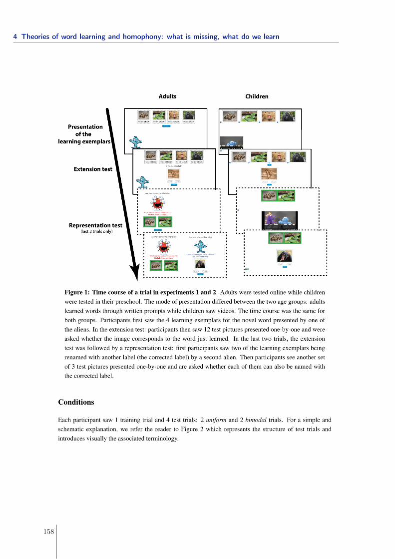
Figure 1: Time course of a trial in experiments 1 and 2. Adults were tested online while childrenwere tested in their preschool. The mode of presentation differed between the two age groups: adultslearned words through written prompts while children saw videos. The time course was the same forboth groups. Participants first saw the 4 learning exemplars for the novel word presented by one ofthe aliens. In the extension test: participants then saw 12 test pictures presented one-by-one and wereasked whether the image corresponds to the word just learned. In the last two trials, the extensiontest was followed by a representation test: first participants saw two of the learning exemplars beingrenamed with another label (the corrected label) by a second alien. Then participants see another setof 3 test pictures presented one-by-one and are asked whether each of them can also be named withthe corrected label.
Conditions
Each participant saw 1 training trial and 4 test trials: 2 uniform and 2 bimodal trials. For a simple andschematic explanation, we refer the reader to Figure 2 which represents the structure of test trials andintroduces visually the associated terminology.
4 Theories of word learning and homophony: what is missing, what do we learn
158
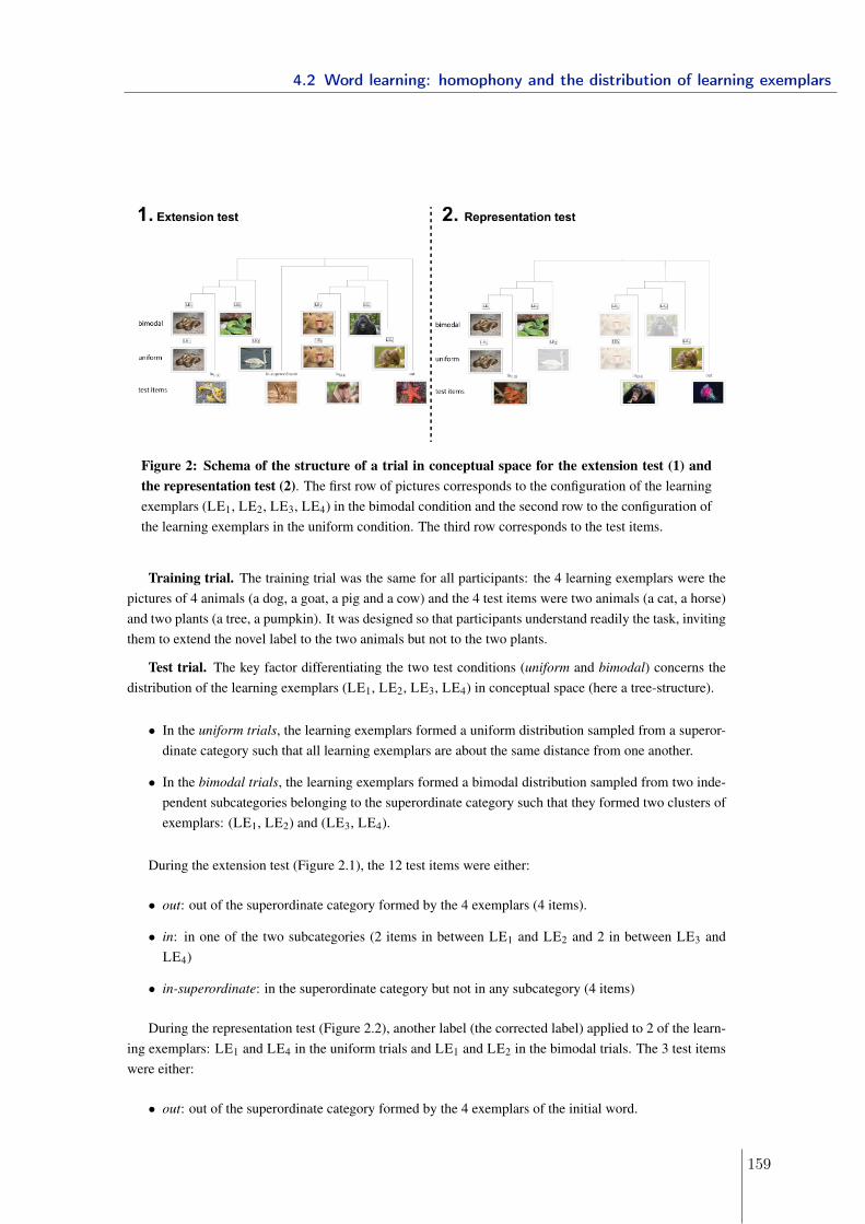
Figure 2: Schema of the structure of a trial in conceptual space for the extension test (1) andthe representation test (2). The first row of pictures corresponds to the configuration of the learningexemplars (LE1, LE2, LE3, LE4) in the bimodal condition and the second row to the configuration ofthe learning exemplars in the uniform condition. The third row corresponds to the test items.
Training trial. The training trial was the same for all participants: the 4 learning exemplars were thepictures of 4 animals (a dog, a goat, a pig and a cow) and the 4 test items were two animals (a cat, a horse)and two plants (a tree, a pumpkin). It was designed so that participants understand readily the task, invitingthem to extend the novel label to the two animals but not to the two plants.
Test trial. The key factor differentiating the two test conditions (uniform and bimodal) concerns thedistribution of the learning exemplars (LE1, LE2, LE3, LE4) in conceptual space (here a tree-structure).
• In the uniform trials, the learning exemplars formed a uniform distribution sampled from a superor-dinate category such that all learning exemplars are about the same distance from one another.
• In the bimodal trials, the learning exemplars formed a bimodal distribution sampled from two inde-pendent subcategories belonging to the superordinate category such that they formed two clusters ofexemplars: (LE1, LE2) and (LE3, LE4).
During the extension test (Figure 2.1), the 12 test items were either:
• out: out of the superordinate category formed by the 4 exemplars (4 items).
• in: in one of the two subcategories (2 items in between LE1 and LE2 and 2 in between LE3 andLE4)
• in-superordinate: in the superordinate category but not in any subcategory (4 items)
During the representation test (Figure 2.2), another label (the corrected label) applied to 2 of the learn-ing exemplars: LE1 and LE4 in the uniform trials and LE1 and LE2 in the bimodal trials. The 3 test itemswere either:
• out: out of the superordinate category formed by the 4 exemplars of the initial word.
4.2 Word learning: homophony and the distribution of learning exemplars
159
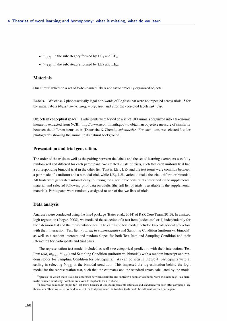
• in(1,2): in the subcategory formed by LE1 and LE2.
• in(3,4): in the subcategory formed by LE3 and LE4.
Materials
Our stimuli relied on a set of to-be-learned labels and taxonomically organized objects.
Labels. We chose 7 phonotactically legal non-words of English that were not repeated across trials: 5 forthe initial labels blicket, smirk, zorg, moop, tupa and 2 for the corrected labels kaki, fep.
Objects in conceptual space. Participants were tested on a set of 100 animals organized into a taxonomichierarchy extracted from NCBI (http://www.ncbi.nlm.nih.gov) to obtain an objective measure of similaritybetween the different items as in (Dautriche & Chemla, submitted).2 For each item, we selected 3 colorphotographs showing the animal in its natural background.
Presentation and trial generation.
The order of the trials as well as the pairing between the labels and the set of learning exemplars was fullyrandomized and differed for each participant. We created 2 lists of trials, such that each uniform trial hada corresponding bimodal trial in the other list. That is LE1, LE3 and the test items were common betweena pair made of a uniform and a bimodal trial, while LE2, LE4 varied to make the trial uniform or bimodal.All trials were generated automatically following the algorithmic constraints described in the supplementalmaterial and selected following pilot data on adults (the full list of trials is available is the supplementalmaterial). Participants were randomly assigned to one of the two lists of trials.
Data analysis
Analyses were conducted using the lme4 package (Bates et al., 2014) of R (R Core Team, 2013). In a mixedlogit regression (Jaeger, 2008), we modeled the selection of a test item (coded as 0 or 1) independently forthe extension test and the representation test. The extension test model included two categorical predictorswith their interaction: Test Item (out, in, in-superordinate) and Sampling Condition (uniform vs. bimodal)as well as a random intercept and random slopes for both Test Item and Sampling Condition and theirinteraction for participants and trial pairs.
The representation test model included as well two categorical predictors with their interaction: TestItem (out, in(1,2), in(3,4)) and Sampling Condition (uniform vs. bimodal) with a random intercept and ran-dom slopes for Sampling Condition for participants.3 As can be seen in Figure 4, participants were atceiling in selecting in(1,2) in the bimodal condition. This impacted the log-estimation behind the logitmodel for the representation test, such that the estimates and the standard errors calculated by the model
2Species for which there is a clear difference between scientific and subjective popular taxonomy were excluded (e.g., sea mam-mals: counter-intuitively, dolphins are closer to elephants than to sharks).
3There was no random slopes for Test Items because it leads to implausible estimates and standard error even after correction (seethereafter). There was also no random effect for trial pairs since the two last trials could be different for each participant.
4 Theories of word learning and homophony: what is missing, what do we learn
160
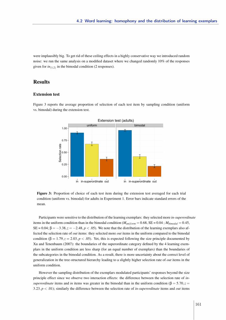
were implausibly big. To get rid of these ceiling effects in a highly conservative way we introduced randomnoise: we run the same analysis on a modified dataset where we changed randomly 10% of the responsesgiven for in(1,2) in the bimodal condition (2 responses).
Results
Extension test
Figure 3 reports the average proportion of selection of each test item by sampling condition (uniformvs. bimodal) during the extension test.
uniform bimodal
0.00
0.25
0.50
0.75
1.00
in in-superordinate out in in-superordinate out
Sel
ectio
n ra
te
Extension test (adults)
Figure 3: Proportion of choice of each test item during the extension test averaged for each trialcondition (uniform vs. bimodal) for adults in Experiment 1. Error bars indicate standard errors of themean.
Participants were sensitive to the distribution of the learning exemplars: they selected more in-superordinateitems in the uniform condition than in the bimodal condition (Muni f orm = 0.68, SE = 0.04 ; Mbimodal = 0.45,SE = 0.04; β =−3.38,z =−2.48, p < .05). We note that the distribution of the learning exemplars also af-fected the selection rate of out items: they selected more out items in the uniform compared to the bimodalcondition (β = 1.79,z = 2.03, p < .05). Yet, this is expected following the size principle documented byXu and Tenenbaum (2007): the boundaries of the superordinate category defined by the 4 learning exem-plars in the uniform condition are less sharp (for an equal number of exemplars) than the boundaries ofthe subcategories in the bimodal condition. As a result, there is more uncertainty about the correct level ofgeneralization in the tree-structured hierarchy leading to a slightly higher selection rate of out items in theuniform condition.
However the sampling distribution of the exemplars modulated participants’ responses beyond the sizeprinciple effect since we observe two interaction effects: the difference between the selection rate of in-superordinate items and in items was greater in the bimodal than in the uniform condition (β = 5.70,z =3.23, p < .01); similarly the difference between the selection rate of in-superordinate items and out items
4.2 Word learning: homophony and the distribution of learning exemplars
161
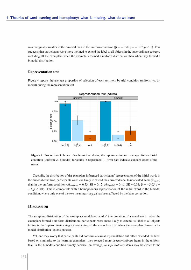
was marginally smaller in the bimodal than in the uniform condition (β =−1.58,z =−1.67, p < .1). Thissuggests that participants were more inclined to extend the label to all objects in the superordinate categoryincluding all the exemplars when the exemplars formed a uniform distribution than when they formed abimodal distribution.
Representation test
Figure 4 reports the average proportion of selection of each test item by trial condition (uniform vs. bi-modal) during the representation test.
uniform bimodal
0.00
0.25
0.50
0.75
1.00
in(1,2) in(3,4) out in(1,2) in(3,4) out
Sel
ectio
n ra
te
Representation test (adults)
Figure 4: Proportion of choice of each test item during the representation test averaged for each trialcondition (uniform vs. bimodal) for adults in Experiment 1. Error bars indicate standard errors of themean.
Crucially, the distribution of the exemplars influenced participants’ representation of the initial word: inthe bimodal condition, participants were less likely to extend the corrected label to unattested items (in(3,4))than in the uniform condition (Muni f orm = 0.53, SE = 0.12; Mbimodal = 0.16, SE = 0.08; β = −5.05,z =−3, p < .01). This is compatible with a homophonous representation of the initial word in the bimodalcondition, where only one of the two meanings (in(3,4)) has been affected by the later correction.
Discussion
The sampling distribution of the exemplars modulated adults’ interpretation of a novel word: when theexemplars formed a uniform distribution, participants were more likely to extend its label to all objectsfalling in the superordinate category containing all the exemplars than when the exemplars formed a bi-modal distribution (extension test).
Yet, one may worry that participants did not form a lexical representation but rather extended the labelbased on similarity to the learning exemplars: they selected more in-superordinate items in the uniformthan in the bimodal condition simply because, on average, in-superordinate items may be closer to the
4 Theories of word learning and homophony: what is missing, what do we learn
162
learning exemplars in the uniform than in the bimodal condition. Yet that’s not the case: recall that inour similarity space (Figure 2), the common ancestor of in-superordinate items with any pair of learningexemplars, i.e. (LE1, LE2) or (LE3, LE4), is the same in the uniform and the bimodal condition. Certainlyparticipants’ responses were in part guided by similarity of the test items to the learning exemplars: in thebimodal condition during the extension test, adults selected in-superordinate items at a higher rate than outitems (β =−2.30,z =−1.99, p < .05). Yet it is sufficient for our purpose to note that this does not accountfor the entirety of our effect.4
An interesting question is whether observing the exemplars in a bimodal distribution was sufficient forparticipants to form homophonous form-meaning representations. Indeed, there may be two interpretationsof the results of the extension test:
1. Participants formed words’ representations that respect concept convexity. In the bimodal condition,participants postulated homophony: they associated the novel word with two independent meanings,each corresponding to a convex concept (e.g., PRIMATE and SNAKE).
2. Participants accepted that a word’s meaning could be a set of disconnected concepts: in the bimodalcondition they associated the novel word to a single, disjoint concept (e.g., PRIMATE OR SNAKE).
The results of the representation test favor the first possibility. When presented with a bimodal distributionof exemplars (e.g., 2 primates and 2 snakes) labelled by a single word “blicket”, participants interpretedthe corrected label based on its taught meaning alone (e.g., the 2 snakes but not the 2 primates) suggestingthat they preferentially understood “blicket” as a word form associated with two homophonic words, ratherthan as a single word with a single discontinuous meaning.
All in all, we replicate previous results (Dautriche & Chemla, submitted) showing that the distribu-tion of learning exemplars interacts with constraints on concept convexity to form different form-meaningrepresentations. When the exemplars form a uniform distribution, participants are more likely to asso-ciate the word to a single convex meaning that encompasses all the learning exemplars (and every entityin between them). Yet, when the exemplars form a bimodal distribution, participants prefer to postulatehomophony such that the novel word is associated to two convex meanings, rather than to a single, broadconvex meaning or to a single discontinuous meaning. The critical question then, is, do children also postu-late homophony when there is evidence that the exemplars of a word are distributed in two convex clustersin conceptual space? Experiment 2 investigated this question by adapting the design of Experiment 1 toFrench preschoolers.
4Note that similarity to the exemplars also played a role in the representation test, in which participants selected more in(1,2) itemsthan in(3,4) items in the uniform condition (β = −4.01,z = −2.61, p < .01) simply because in the tree structure for uniform trials(Figure 2), in(1,2) is closer to LE1 than in(3,4) to LE4, thus more likely to be selected as an instance of the corrected label.
4.2 Word learning: homophony and the distribution of learning exemplars
163
Experiment 2
Method
Participants
Twenty-one 5-year-old monolingual French speaking children (5;1 to 6;1, Mage = 5;6, 10 girls) were testedin a public preschool in Paris. Their parents signed an informed consent form. Three additional childrenwere tested but not included in the analysis because they systematically responded yes (n = 1) or no (n = 2)without even looking at the test pictures or responding before they appeared on the screen.
Procedure and display
The experiment was identical to Experiment 1 except that we used videos instead of written prompts withchildren (see Figure 1).
Children were tested individually in a quiet room in their preschool. During the experiment, childrensat next to the experimenter, in front of a computer and wore headphones to listen to the stimuli. Beforethe experiment began, children watched a video where two alien puppets introduced them with the task.The two puppets presented themselves as Boba and Zap, and told the children that they were coming fromanother planet where they speak a different language, so they would teach the children words of theirlanguage. Once a child demonstrated to the experimenter that (s)he understood the task, the experimentstarted. In each trial, children saw 4 learning exemplars, presented one-by-one as the combination of apicture and a video of Boba labeling the picture with a non-word “Ca, on appelle ca une bamoule!” This,we call it a bamoule. Each learning exemplar was displayed on the screen when the experimenter clickedon a button. Once children saw all 4 learning exemplars, they saw a last video where Boba asked them torepeat the word. This was to ensure that children were on task and for the experimenter to know whichword was used by the puppet (as the words were randomly assigned to a set of learning exemplars and theexperimenter could not hear the stimuli).
During the extension test, children were presented with the 12 test pictures displayed one-by-one belowthe 4 learning exemplars. For each of them, the experimenter asked: “Est ce que tu penses que ca s’appelleune bamoule?” Do you think it is called a bamoule?. When the child answered, the experimenter clickedaccordingly on the “yes” or “no” button on the screen. Children could change their mind if they wantedwithin a few seconds after their answer or longer if the experimenter saw that they were still hesitating.Once a response was validated by the experimenter, the test continued to the next test picture.
In the last two test trials, the extension test was followed by a representation test. Children saw 2 ofthe 4 learning exemplars grouped in a frame together with a video where the second puppet, Zap, scoldedthe first one, Boba, for using the wrong word for the two exemplars displayed “C’est pas des bamoules ca!C’est des torbas!” These are not bamoules! These are torbas (the whole script for this video can be foundin the supplemental material). Boba then, aknowledged his mistake. During the dialogue, the frame of thepictures was blinking in green. At the end of the video, the experimenter asked the child what happened andreplayed the video if the child did not understand the video or did not remember the novel word. Childrenwere then tested whether the corrected label could apply to 3 novel test pictures. Each of the test picture
4 Theories of word learning and homophony: what is missing, what do we learn
164
was displayed below the two learning exemplars and the child was asked by the experimenter “Est ce quetu penses que ca, ca s’appelle un torba?” Do you think that this is called a torba?.
At the end of the experiment, there was a final video where the two puppets said good-bye to the child.The whole Experiment lasted about 15 min. All sessions were audiotaped.
Conditions, Materials, Presentation and trial generation, Data analysis.
Everything was similar to Experiment 1, except that the experiment was in French and hence the set of non-words consisted of 9 phonotactically legal non-words of French: bamoule was always used in the trainingtrial. From the remaining 8 non-words that were used in the test trials, half of them were bisyllabic andwere used as the initial label (toupa, fimo, lagui, yoshi), the other half were trisyllabic and were used asthe corrected labels (midori, cramoucho, didolu, baboocha). The difference in the number of syllables wasintroduced to make it easier for children to distinguish between the initial and the corrected labels.
Results
Extension test
As shown in Figure 5, children and adults behaved in the same way: children selected more in-superordinateitems in the uniform condition than in the bimodal condition (Muni f orm = 0.61, SE = 0.04 ; Mbimodal = 0.28,SE = 0.04; β =−2.56,z =−3.73, p < .001). The distribution of the learning exemplars did not affect anyother test items for children (all ps> 0.7) resulting in two interaction effects: the difference between the se-lection rate of in-superordinate items and in items, was greater in the bimodal than in the uniform condition(β = 2.79,z = 2.30, p < .05); similarly the difference between the selection rate of in-superordinate itemsand out items, was smaller in the bimodal than in the uniform condition (β=−3.28,z=−4, p< .001). Thissuggests that children were more likely to extend the label to all objects in the minimal subtree containingall the exemplars in the uniform condition compared to the bimodal condition.
4.2 Word learning: homophony and the distribution of learning exemplars
165
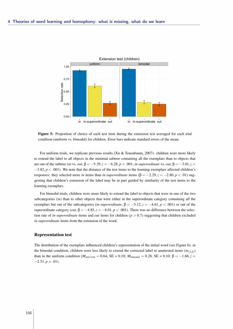
uniform bimodal
0.00
0.25
0.50
0.75
1.00
in in-superordinate out in in-superordinate out
Sel
ectio
n ra
teExtension test (children)
Figure 5: Proportion of choice of each test item during the extension test averaged for each trialcondition (uniform vs. bimodal) for children. Error bars indicate standard errors of the mean.
For uniform trials, we replicate previous results (Xu & Tenenbaum, 2007): children were more likelyto extend the label to all objects in the minimal subtree containing all the exemplars than to objects thatare out of the subtree (in vs. out, β =−5.39,z =−6.28, p < .001; in-superordinate vs. out, β =−3.01,z =−3.82, p < .001). We note that the distance of the test items to the learning exemplars affected children’sresponses: they selected more in items than in-superordinate items (β = −2.29,z = −2.80, p < .01) sug-gesting that children’s extension of the label may be in part guided by similarity of the test items to thelearning exemplars.
For bimodal trials, children were more likely to extend the label to objects that were in one of the twosubcategories (in) than to other objects that were either in the superordinate category containing all theexemplars but out of the subcategories (in-superordinate, β = −5.12,z = −4.61, p < .001) or out of thesuperordinate category (out, β =−4.85,z =−8.01, p < .001). There was no difference between the selec-tion rate of in-superordinate items and out items for children (p > 0.7) suggesting that children excludedin-superordinate items from the extension of the word.
Representation test
The distribution of the exemplars influenced children’s representation of the initial word (see Figure 6): inthe bimodal condition, children were less likely to extend the corrected label to unattested items (in(3,4))than in the uniform condition (Muni f orm = 0.64, SE = 0.10; Mbimodal = 0.28, SE = 0.10; β = −1.66,z =−2.51, p = .01).
4 Theories of word learning and homophony: what is missing, what do we learn
166
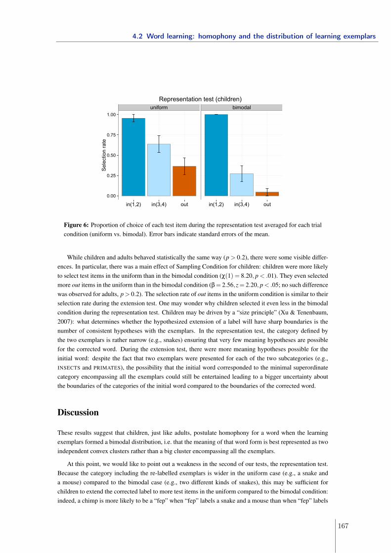
uniform bimodal
0.00
0.25
0.50
0.75
1.00
in(1,2) in(3,4) out in(1,2) in(3,4) out
Sel
ectio
n ra
teRepresentation test (children)
Figure 6: Proportion of choice of each test item during the representation test averaged for each trialcondition (uniform vs. bimodal). Error bars indicate standard errors of the mean.
While children and adults behaved statistically the same way (p > 0.2), there were some visible differ-ences. In particular, there was a main effect of Sampling Condition for children: children were more likelyto select test items in the uniform than in the bimodal condition (χ(1) = 8.20, p < .01). They even selectedmore out items in the uniform than in the bimodal condition (β= 2.56,z= 2.20, p< .05; no such differencewas observed for adults, p > 0.2). The selection rate of out items in the uniform condition is similar to theirselection rate during the extension test. One may wonder why children selected it even less in the bimodalcondition during the representation test. Children may be driven by a “size principle” (Xu & Tenenbaum,2007): what determines whether the hypothesized extension of a label will have sharp boundaries is thenumber of consistent hypotheses with the exemplars. In the representation test, the category defined bythe two exemplars is rather narrow (e.g., snakes) ensuring that very few meaning hypotheses are possiblefor the corrected word. During the extension test, there were more meaning hypotheses possible for theinitial word: despite the fact that two exemplars were presented for each of the two subcategories (e.g.,INSECTS and PRIMATES), the possibility that the initial word corresponded to the minimal superordinatecategory encompassing all the exemplars could still be entertained leading to a bigger uncertainty aboutthe boundaries of the categories of the initial word compared to the boundaries of the corrected word.
Discussion
These results suggest that children, just like adults, postulate homophony for a word when the learningexemplars formed a bimodal distribution, i.e. that the meaning of that word form is best represented as twoindependent convex clusters rather than a big cluster encompassing all the exemplars.
At this point, we would like to point out a weakness in the second of our tests, the representation test.Because the category including the re-labelled exemplars is wider in the uniform case (e.g., a snake anda mouse) compared to the bimodal case (e.g., two different kinds of snakes), this may be sufficient forchildren to extend the corrected label to more test items in the uniform compared to the bimodal condition:indeed, a chimp is more likely to be a “fep” when “fep” labels a snake and a mouse than when “fep” labels
4.2 Word learning: homophony and the distribution of learning exemplars
167
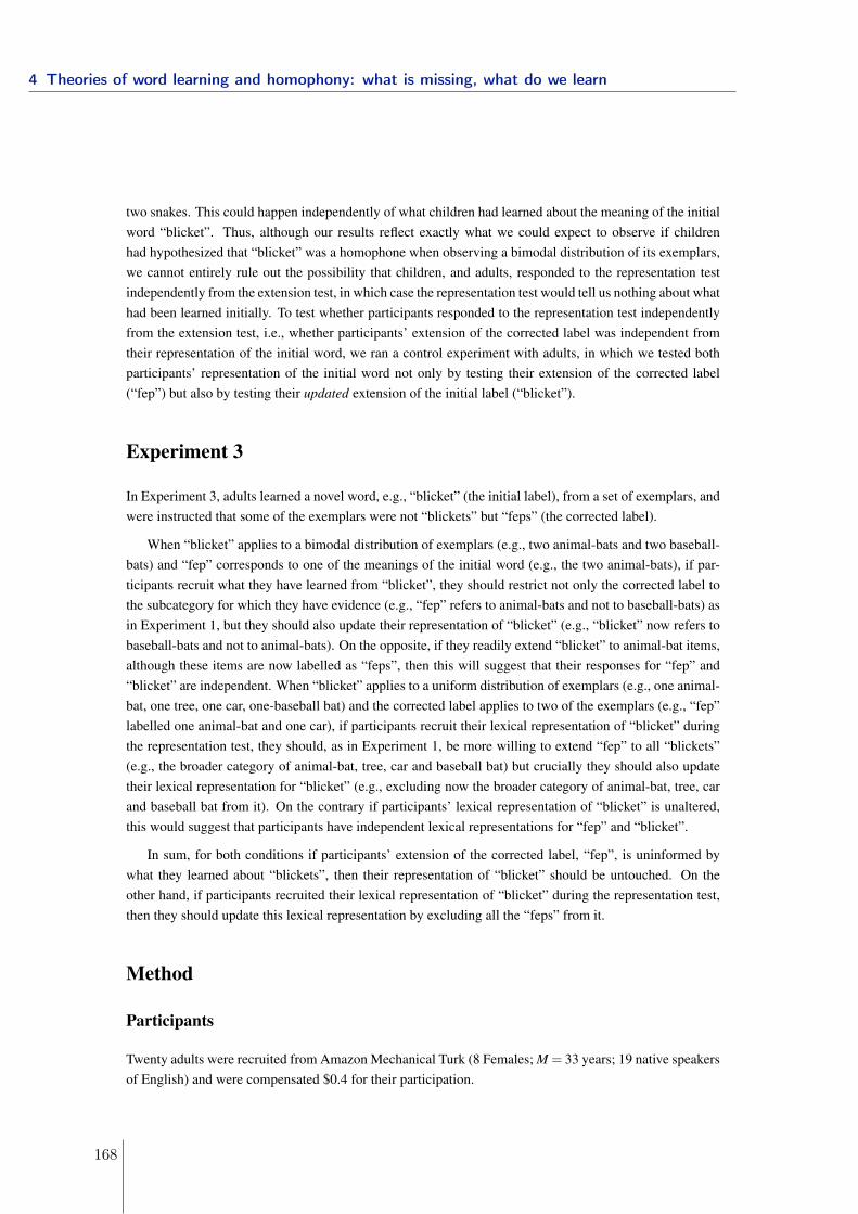
two snakes. This could happen independently of what children had learned about the meaning of the initialword “blicket”. Thus, although our results reflect exactly what we could expect to observe if childrenhad hypothesized that “blicket” was a homophone when observing a bimodal distribution of its exemplars,we cannot entirely rule out the possibility that children, and adults, responded to the representation testindependently from the extension test, in which case the representation test would tell us nothing about whathad been learned initially. To test whether participants responded to the representation test independentlyfrom the extension test, i.e., whether participants’ extension of the corrected label was independent fromtheir representation of the initial word, we ran a control experiment with adults, in which we tested bothparticipants’ representation of the initial word not only by testing their extension of the corrected label(“fep”) but also by testing their updated extension of the initial label (“blicket”).
Experiment 3
In Experiment 3, adults learned a novel word, e.g., “blicket” (the initial label), from a set of exemplars, andwere instructed that some of the exemplars were not “blickets” but “feps” (the corrected label).
When “blicket” applies to a bimodal distribution of exemplars (e.g., two animal-bats and two baseball-bats) and “fep” corresponds to one of the meanings of the initial word (e.g., the two animal-bats), if par-ticipants recruit what they have learned from “blicket”, they should restrict not only the corrected label tothe subcategory for which they have evidence (e.g., “fep” refers to animal-bats and not to baseball-bats) asin Experiment 1, but they should also update their representation of “blicket” (e.g., “blicket” now refers tobaseball-bats and not to animal-bats). On the opposite, if they readily extend “blicket” to animal-bat items,although these items are now labelled as “feps”, then this will suggest that their responses for “fep” and“blicket” are independent. When “blicket” applies to a uniform distribution of exemplars (e.g., one animal-bat, one tree, one car, one-baseball bat) and the corrected label applies to two of the exemplars (e.g., “fep”labelled one animal-bat and one car), if participants recruit their lexical representation of “blicket” duringthe representation test, they should, as in Experiment 1, be more willing to extend “fep” to all “blickets”(e.g., the broader category of animal-bat, tree, car and baseball bat) but crucially they should also updatetheir lexical representation for “blicket” (e.g., excluding now the broader category of animal-bat, tree, carand baseball bat from it). On the contrary if participants’ lexical representation of “blicket” is unaltered,this would suggest that participants have independent lexical representations for “fep” and “blicket”.
In sum, for both conditions if participants’ extension of the corrected label, “fep”, is uninformed bywhat they learned about “blickets”, then their representation of “blicket” should be untouched. On theother hand, if participants recruited their lexical representation of “blicket” during the representation test,then they should update this lexical representation by excluding all the “feps” from it.
Method
Participants
Twenty adults were recruited from Amazon Mechanical Turk (8 Females; M = 33 years; 19 native speakersof English) and were compensated $0.4 for their participation.
4 Theories of word learning and homophony: what is missing, what do we learn
168
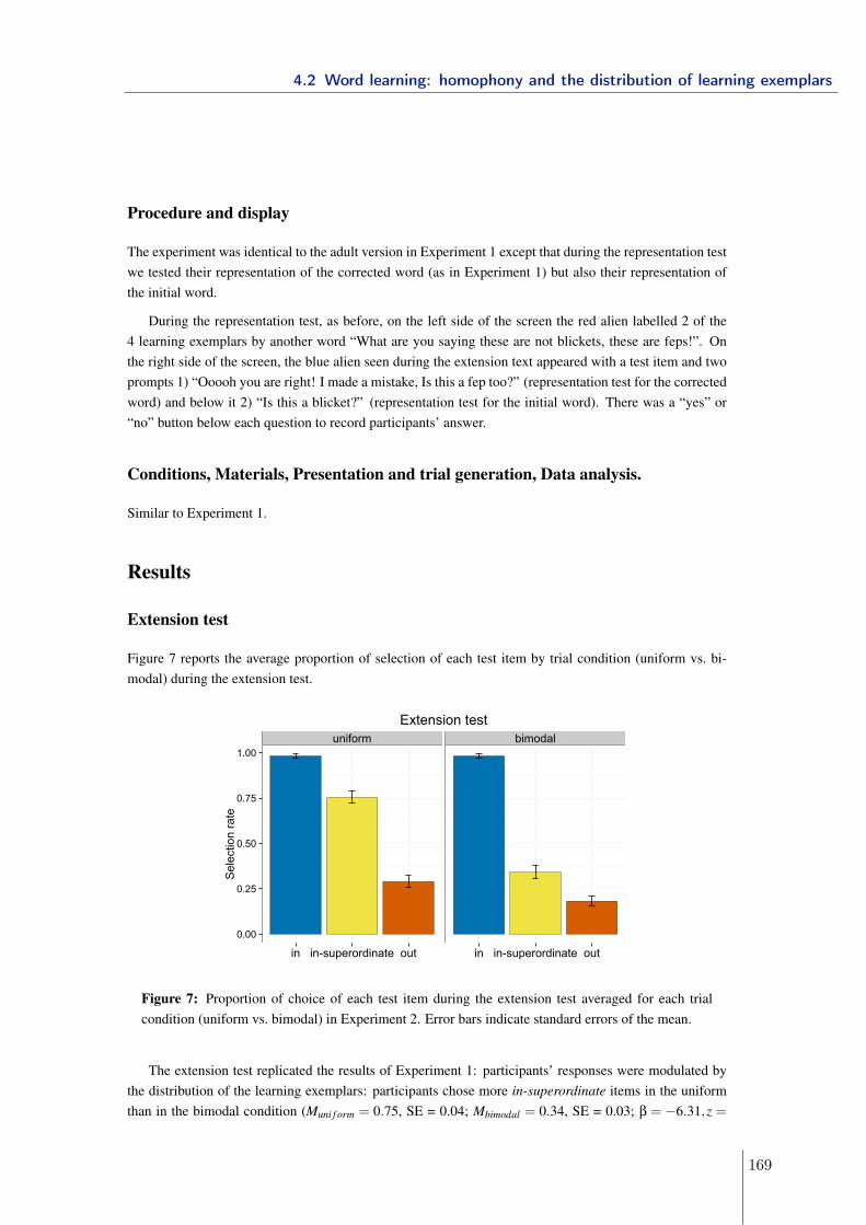
Procedure and display
The experiment was identical to the adult version in Experiment 1 except that during the representation testwe tested their representation of the corrected word (as in Experiment 1) but also their representation ofthe initial word.
During the representation test, as before, on the left side of the screen the red alien labelled 2 of the4 learning exemplars by another word “What are you saying these are not blickets, these are feps!”. Onthe right side of the screen, the blue alien seen during the extension text appeared with a test item and twoprompts 1) “Ooooh you are right! I made a mistake, Is this a fep too?” (representation test for the correctedword) and below it 2) “Is this a blicket?” (representation test for the initial word). There was a “yes” or“no” button below each question to record participants’ answer.
Conditions, Materials, Presentation and trial generation, Data analysis.
Similar to Experiment 1.
Results
Extension test
Figure 7 reports the average proportion of selection of each test item by trial condition (uniform vs. bi-modal) during the extension test.
uniform bimodal
0.00
0.25
0.50
0.75
1.00
in in-superordinate out in in-superordinate out
Sel
ectio
n ra
te
Extension test
Figure 7: Proportion of choice of each test item during the extension test averaged for each trialcondition (uniform vs. bimodal) in Experiment 2. Error bars indicate standard errors of the mean.
The extension test replicated the results of Experiment 1: participants’ responses were modulated bythe distribution of the learning exemplars: participants chose more in-superordinate items in the uniformthan in the bimodal condition (Muni f orm = 0.75, SE = 0.04; Mbimodal = 0.34, SE = 0.03; β = −6.31,z =
4.2 Word learning: homophony and the distribution of learning exemplars
169
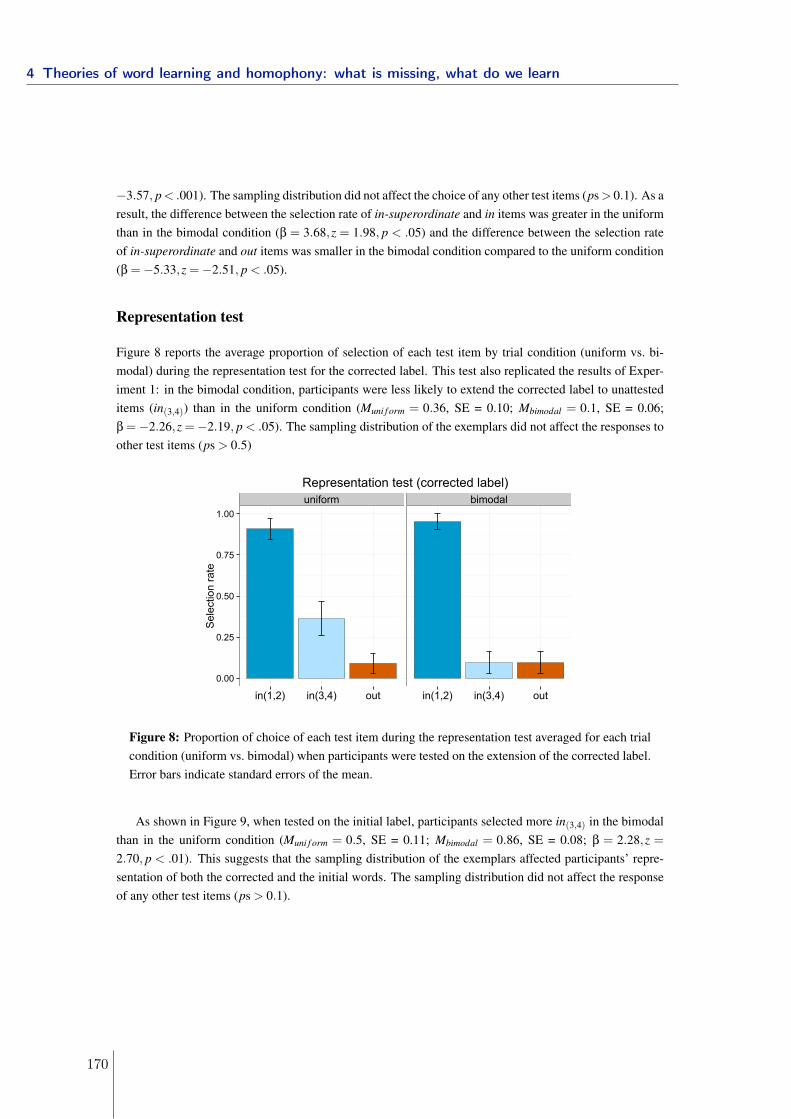
−3.57, p< .001). The sampling distribution did not affect the choice of any other test items (ps> 0.1). As aresult, the difference between the selection rate of in-superordinate and in items was greater in the uniformthan in the bimodal condition (β = 3.68,z = 1.98, p < .05) and the difference between the selection rateof in-superordinate and out items was smaller in the bimodal condition compared to the uniform condition(β =−5.33,z =−2.51, p < .05).
Representation test
Figure 8 reports the average proportion of selection of each test item by trial condition (uniform vs. bi-modal) during the representation test for the corrected label. This test also replicated the results of Exper-iment 1: in the bimodal condition, participants were less likely to extend the corrected label to unattesteditems (in(3,4)) than in the uniform condition (Muni f orm = 0.36, SE = 0.10; Mbimodal = 0.1, SE = 0.06;β =−2.26,z =−2.19, p < .05). The sampling distribution of the exemplars did not affect the responses toother test items (ps > 0.5)
uniform bimodal
0.00
0.25
0.50
0.75
1.00
in(1,2) in(3,4) out in(1,2) in(3,4) out
Sel
ectio
n ra
te
Representation test (corrected label)
Figure 8: Proportion of choice of each test item during the representation test averaged for each trialcondition (uniform vs. bimodal) when participants were tested on the extension of the corrected label.Error bars indicate standard errors of the mean.
As shown in Figure 9, when tested on the initial label, participants selected more in(3,4) in the bimodalthan in the uniform condition (Muni f orm = 0.5, SE = 0.11; Mbimodal = 0.86, SE = 0.08; β = 2.28,z =2.70, p < .01). This suggests that the sampling distribution of the exemplars affected participants’ repre-sentation of both the corrected and the initial words. The sampling distribution did not affect the responseof any other test items (ps > 0.1).
4 Theories of word learning and homophony: what is missing, what do we learn
170
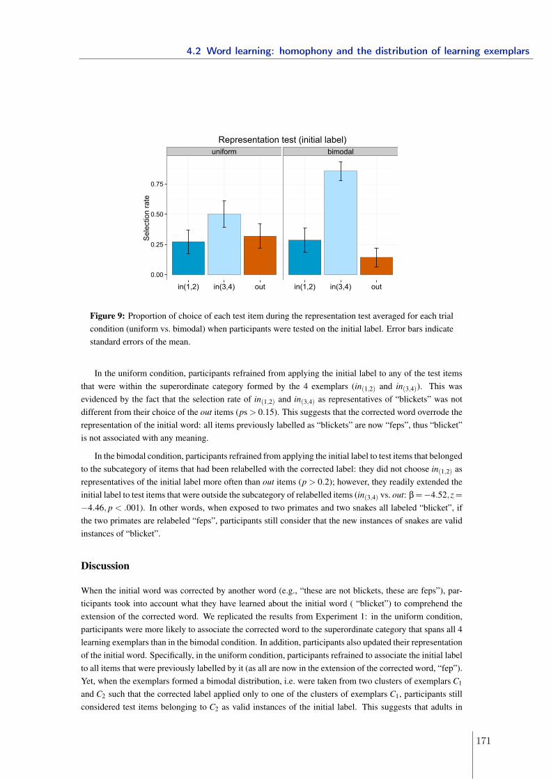
uniform bimodal
0.00
0.25
0.50
0.75
in(1,2) in(3,4) out in(1,2) in(3,4) out
Sel
ectio
n ra
teRepresentation test (initial label)
Figure 9: Proportion of choice of each test item during the representation test averaged for each trialcondition (uniform vs. bimodal) when participants were tested on the initial label. Error bars indicatestandard errors of the mean.
In the uniform condition, participants refrained from applying the initial label to any of the test itemsthat were within the superordinate category formed by the 4 exemplars (in(1,2) and in(3,4)). This wasevidenced by the fact that the selection rate of in(1,2) and in(3,4) as representatives of “blickets” was notdifferent from their choice of the out items (ps > 0.15). This suggests that the corrected word overrode therepresentation of the initial word: all items previously labelled as “blickets” are now “feps”, thus “blicket”is not associated with any meaning.
In the bimodal condition, participants refrained from applying the initial label to test items that belongedto the subcategory of items that had been relabelled with the corrected label: they did not choose in(1,2) asrepresentatives of the initial label more often than out items (p > 0.2); however, they readily extended theinitial label to test items that were outside the subcategory of relabelled items (in(3,4) vs. out: β=−4.52,z=−4.46, p < .001). In other words, when exposed to two primates and two snakes all labeled “blicket”, ifthe two primates are relabeled “feps”, participants still consider that the new instances of snakes are validinstances of “blicket”.
Discussion
When the initial word was corrected by another word (e.g., “these are not blickets, these are feps”), par-ticipants took into account what they have learned about the initial word ( “blicket”) to comprehend theextension of the corrected word. We replicated the results from Experiment 1: in the uniform condition,participants were more likely to associate the corrected word to the superordinate category that spans all 4learning exemplars than in the bimodal condition. In addition, participants also updated their representationof the initial word. Specifically, in the uniform condition, participants refrained to associate the initial labelto all items that were previously labelled by it (as all are now in the extension of the corrected word, “fep”).Yet, when the exemplars formed a bimodal distribution, i.e. were taken from two clusters of exemplars C1
and C2 such that the corrected label applied only to one of the clusters of exemplars C1, participants stillconsidered test items belonging to C2 as valid instances of the initial label. This suggests that adults in
4.2 Word learning: homophony and the distribution of learning exemplars
171
Experiment 1 recruited the representation of the initial word during the representation test.
However, the alternative explanation, i.e., that the representation of the corrected label “fep” is com-puted on the basis of the learning exemplars for “fep” only (independently of the representation of the initiallabel “blicket”), cannot be entirely ruled out. Participants could have extended the corrected label “fep”according to the distribution of its exemplars in the representation test (i.e., extend it to more test itemsin the uniform condition than in the bimodal condition simply because the category covered by the twoexemplars in the representation test is wider in the uniform case) and then used this information to decidehow “blicket” should be extended. Clearly if participants decide that a given item I is an instance of “fep”,they will be more willing to exclude it from the extension of “blicket” and this independently of how theydecided that I is a “fep”. However, it should be noted that out items are excluded both from the extensionof “fep” and the extension of “blicket”, suggesting that when responding to “blicket” in the representationtest, participants are still influenced by their responses for “blicket” during the extension test (where theyalso excluded out items from the extension of the word). So this would suggest that, while participants maynot recruit their initial representation of “blicket” to extend “fep” to test items in the representation test,they still recruit it (together with what they have learned about “fep”) to find the extension of “blicket” inthe representation test. While we cannot entirely dismiss the possibility that participants would selectivelyattend to their initial representation of “blicket” in the representation test when responding to “blicket” butnot to “fep”, our data provide little support for this hypothesis.
We conclude thus that the most likely interpretation of our results in Experiment 1 is that adults re-cruited the representation of the initial word during the representation test. Adults preferred, in the firstphase, to postulate that the novel word carries homophony when it is learned from exemplars in a bimodaldistribution. Given the similarity of the results between Experiments 1 and 2, one would be tempted toextend this interpretation to the children results from Experiment 2. At this point, however, a note of cau-tion is necessary. One limitation of the present data is that we used our conclusion with adults to rule out apossible confound for Experiment 1 and 2 with adults and children. Yet we cannot exclude the possibilitythat this very explanation may still underly children’s response pattern. We leave it for future research toestablish a more direct argument to explain both children’s and adults’ performance in these experiments.
General Discussion
Children are sensitive to the sampling distribution of the learning exemplars when learning words (as in Xu& Tenenbaum, 2007). Yet, we demonstrate that this interacts with the kind of form-meaning representationchildren are ready to entertain. Observing a bimodal distribution of learning exemplars for a novel wordindicated to our participants that the word was likely to have several meanings. Importantly, our resultssuggest that these meanings were stored separately, suggesting that children’s representation of the novelword in these conditions is very much similar to homophony (Srinivasan & Snedeker, 2011). This extendsprevious results from adults (Dautriche & Chemla, submitted) and suggests that when observing a bimodaldistribution of exemplars for the same word form, children generate form-meaning representations, suchas homophony, that respect concept convexity.
Current word learning accounts have documented and modeled paradigmatic cases of word acquisition,where a single form is associated with a single meaning. We pursued that enterprise by showing that lessstandard situations, such as homophony, can help highlight the key role of factors such as the sampling
4 Theories of word learning and homophony: what is missing, what do we learn
172
distribution of exemplars. It also helps better understand the priors that may constrain and guide wordacquisition, as we detail below.
Missing factors in word learning accounts
Previous studies have shown that children are sensitive to sampling principles when learning words. Xu& Tenenbaum (2007) describe a size principle: children’s confidence in the boundary of the set of entitiesassociated with a word increases as they observe more learning exemplars, even if they are all identical.Here we showed that children were sensitive to the distribution of learning exemplars in conceptual space,another statistical principle presumably following from the assumption that the exemplars of a word aresampled randomly from the underlying category (c.f Xu & Tenenbaum, 2007). Intuitively, in the case ofhomophones, we expect the label to occur with a set of exemplars S drawn from two distinct subcategoriesX1 and X2. Thus, S would take the form of a bimodal distribution within the single superordinate categoryX encompassing the two subcategories (i.e. X is the minimal well-formed category such that X1∪X2 ⊂ X).Yet if the word were to be associated with the whole X , we would expect the exemplars that are associatedwith the label (i.e., S) to be uniformly distributed within X . Our results suggest that children can use suchsampling considerations to decide whether a word is associated with one category (standard case) or severalcategories (homophone), even when exposed to very few exemplars.5
There are other factors, not documented here, that may interact with the expectation that concepts areconvex and could help children to identify that a word has several meanings. First, evidence for homophonymay come from other words in the lexicon. Adults are less likely to extend a label (e.g., “blicket”) to anentity, even if this entity falls right between the learning exemplars for the label, when this entity also fallsclose to some entity labelled by another word (e.g., “fep”) (Dautriche & Chemla, submitted). Intuitively,the interfering label provides further evidence for the presence of two distinct clusters of exemplars inconceptual space, that are separated by another concept labelled by another word (“fep” in the example).This suggests that learners have expectations not only about how words occupy the conceptual space,but also about how they share the conceptual space. Similarly, children assume that word extensions aremutually exclusive (Markman & Wachtel, 1988), and may thus possibly use the presence of other wordsin their lexicon together with a constraint on concept convexity to discover that a word is likely to haveseveral meanings.
Second, some linguistic constructions may be helpful to discover homophony (or the absence of ho-mophony). For instance, children could notice that words mapping to a single meaning commonly appearin some plural sentences where homophones never appear (e.g., “These are two bats” pointing at onebaseball-bat and one animal-bat). And this is so for reasons one can understand: a single phonologicalform cannot be used to refer to two words at the same time, even if the two words are homophonic.6 Adultshave been shown to use such constructions to assess homophony (Dautriche & Chemla, submitted), andchildren may also be sensitive to such linguistic evidence.
These factors may help learners to identify words with multiple meanings. Yet, they also raise im-mediate challenges for current word learning accounts. For instance, we assumed until now that childrenunderstood which object is referred to by the word in context. Yet, in the real world, the label is uttered
5One may argue that the low number of exemplars was not a limitation in our task because it could be compensated by pragmaticconsiderations: participants may expect that the learning exemplars were not drawn at random by the aliens, but rather that the aliensin our stories were trying to be informative about the meaning of the words and chose their exemplars optimally.
6Note that such a sentence is not agrammatical but zeugmatic (Zwicky & Sadock, 1975).
4.2 Word learning: homophony and the distribution of learning exemplars
173
in a complex visual environment where the true referent is likely to be confounded with other possiblereferents present at the same time (the mapping problem, Quine, 1960). Thus it is likely that the set ofexemplars for a label contains outliers, i.e. items that are outside of the true extension of the word, becausethe child would have failed to narrow down the true referent of the word. As a result, the set of exemplarswould certainly form a multimodal distribution (e.g., a set of banana exemplars along with a dog exemplar– that happened to eat a banana during one of the learning event). The challenge for the learner is thus todistinguish between outliers of the true meaning of the word and representative examples of a new wordmeaning. General principles such as the convexity of concepts and one-to-one mapping between wordforms and concepts may help discard noise of this type. However, if these general principles allow excep-tions, as our study of homophony reveals, they may hardly help disentangle signal (of homophony) fromnoise.
Missing priors in word learning accounts
Our results suggest that children expect meanings to be convex, and are willing to postulate homophonyrather than breaking this constraint (postulating a disjoint meaning) or than enforcing that convexity con-straint at all cost (postulating a broad lexical entry for problematic words).
This contradicts current word learning accounts which, technically, transpose the notion of convexityfrom the level of concepts to the level of word forms, assuming that word forms link to concepts in aone-to-one fashion. Accordingly, none of the current accounts allow for the possibility that children canassociate word forms with multiple meanings. As a matter of fact, many developmental studies have doc-umented that preschoolers have notable difficulties in learning homophones (Casenhiser, 2005; Doherty,2004; Mazzocco, 1997). In these studies, the encounter of the second meaning of a homophone is simu-lated by using familiar words (e.g., “snake”) to refer to novel referents (e.g., an unfamiliar object). Yet,we suggest that children’s failure in these studies does not reflect an excessive reliance on a one-to-onemapping between form and meaning, but rather insufficient executive skills for such a task; as the currentresults show, children have no problem learning homophones when they have to learn the two meaningssimultaneously. Learning homophones in our study may be easier than learning a second meaning for aknown word because children do not have to inhibit a highly active word representation for one of the mean-ings (Khanna & Boland 2010, see also Choi & Trueswell 2010; Novick, Trueswell, & Thompson-Schill2010). This suggests that children’s difficulty in learning homophones may have been previously over-rated and that endowing the learning system with a strict one-to-one form-meaning mapping constraintcannot solely account for the mechanism underlying the acquisition of homophones. Certainly it may stillbe possible that a one-to-one form-meaning mapping constraint is guiding word learning at earlier stagesof language development, as 5-year-olds may already have learned to relax this constraint to accommo-date more challenging form-meaning mappings, such as homophony. Yet, if this is the case, current wordlearning accounts should be able to explain how children depart from this default assumption.
The present work thus has important implications for current word learning accounts. When a labelseems to apply to a disjoint set of objects, the learner has two options: 1) postulate homophony (i.e. thepossibility that a word form maps onto two distinct meanings) or 2) follow a one-to-one form-meaningmapping constraint and postulate that the label is a single word that applies to a larger set of objects (thecategory that covers all the positive instances of the label). Most accounts predict that 2) is the default, butthis has to be refined since children eventually learn homophones (e.g., it is likely that English preschoolers
4 Theories of word learning and homophony: what is missing, what do we learn
174
know both meanings of the word form “bat”; see also de Carvalho et al. 2015 for evidence that French 3-year-olds have acquired a certain number of homophone pairs). An important open issue then is to equipthe learning system with the right built-in constraints. At this point it seems that word learning is guidedby a) learners’ expectations that concepts are convex, always; b) learners’ expectation that word formsare linked to one meaning, in general; and c) the possibility that a word form maps onto several distinctmeanings if a) is challenged. While a) helps to constrain the possible concepts one can entertain, b) helpsto constrain the number of hypotheses children need to consider when learning words (especially whileused in combination with a)). Note that this would constitute very specific priors for a general learningsystem: it presupposes that children already know that an essential feature of their to-be-learnt lexiconis to be composed of form-meaning mappings of very specific kinds. The present study contributes topoint c) above: children can entertain the possibility that a word maps onto several distinct meanings toaccommodate apparent violations of a) concept convexity at the detriment of b) a one-to-one mappingbetween forms and meanings. This suggests that children are able to selectively trigger or silence b) asa function of the learning situation (and we documented that this could be made possible by observingthe sampling distribution of the learning exemplars). One possibility for current word learning accountswould be thus to implement these three built-in constraints directly in the learning system and tweak thelearning inference component to accommodate the sampling effect we document. Yet this would be a ratherstrong assumption that amounts to saying that the learning system expects the existence of a phenomenonas specific as homophony, from the start.
Because current word learning accounts specialized into fairly simple word leaning phenomena (i.e.,one form associated with a single meaning), they equipped the learner with specialized built-in constraints(e.g., a one-to-one form-meaning mapping constraint) that cannot explain learning of other more complexphenomena, such as homophony. Incorporating homophony, and potentially other less trivial word learningsituations, will allow these accounts to delineate the more general priors that children bring into the wordlearning task. Yet, although adding different built-in constraints to these accounts may be technically easy,this may be theoretically challenging as we described above, as one would need to explain how the learningsystem is capable of juggling between different priors to appropriately learn different types of words.
Conclusion
Homophony presents a challenge to word learners: it requires children to discover that word forms andconcepts are not always in a one-to-one relation, an otherwise important assumption to restrict the searchspace for word meanings. The present study showed that children use information about the samplingdistribution of learning exemplars (and in particular the fact that they form two distinct convex clusters inconceptual space) to infer homophony for a novel label. We argue that this unexplored sensitivity and thevery possibility of homophony should be incorporated into future accounts of word learning.
References
Bates, D., Maechler, M., Bolker, B., & Walker, S. (2014). lme4: Linear mixed-effects models using eigenand s4 [Computer software manual]. (R package version 1.1-2)
4.2 Word learning: homophony and the distribution of learning exemplars
175
Beveridge, M., & Marsh, L. (1991). The influence of linguistic context on young children’s understandingof homophonic words. Journal of Child Language, 18(02), 459–467.
Bloom, P. (2001). Precis of How children learn the meanings of words. Behavioral and Brain Sciences,24(06), 1095–1103.
Campbell, R. N., & Bowe, T. (1977). Functional asymmetry in early language understanding. SalzbergerBeitrage fur Linguistik, 3.
Casenhiser, D. M. (2005). Children’s resistance to homonymy: an experimental study of pseudohomonyms.Journal of Child Language, 32(2), 319–343.
Choi, Y., & Trueswell, J. C. (2010). Children’s (in) ability to recover from garden paths in a verb-final language: Evidence for developing control in sentence processing. Journal of Experimental ChildPsychology, 106(1), 41–61.
Dautriche, I., & Chemla, E. (submitted). What homophones way about words.
de Carvalho, A., Dautriche, I., & Christophe, A. (2015). Preschoolers use phrasal prosody online toconstrain syntactic analysis. Developmental science.
Doherty, M. J. (2004). Childrens difficulty in learning homonyms. Journal of Child Language, 31(1),203–214.
Frank, M. C., Goodman, N. D., & Tenenbaum, J. B. (2009). Using speakers’ referential intentions to modelearly cross-situational word learning. Psychological Science, 20(5), 578–585.
Goodman, N. (1955). Fact, fiction, and forecast. Harvard University Press.
Gardenfors, P. (2004). Conceptual spaces: The geometry of thought. MIT press.
Jaeger, T. F. (2008). Categorical data analysis: Away from ANOVAs (transformation or not) and towardslogit mixed models. Journal of Memory and Language, 59(4), 434–446.
Khanna, M. M., & Boland, J. E. (2010). Children’s use of language context in lexical ambiguity resolution.The Quarterly Journal of Experimental Psychology, 63(1), 160–193.
Landau, B., Smith, L. B., & Jones, S. S. (1988). The importance of shape in early lexical learning.Cognitive development, 3(3), 299–321.
Markman, E. M. (1989). Categorization and naming in children: Problems of induction. Mit Press.
Markman, E. M., & Hutchinson, J. E. (1984). Children’s sensitivity to constraints on word meaning:Taxonomic versus thematic relations. Cognitive psychology, 16(1), 1–27.
Markman, E. M., & Wachtel, G. F. (1988). Children’s use of mutual exclusivity to constrain the meaningsof words. Cognitive psychology, 20(2), 121–157.
Mazzocco, M. M. (1997). Children’s interpretations of homonyms: a developmental study. Journal ofChild Language, 24(02), 441–467.
Murphy, G. L., & Medin, D. L. (1985). The role of theories in conceptual coherence. Psychological review,92(3), 289.
4 Theories of word learning and homophony: what is missing, what do we learn
176
Novick, J. M., Trueswell, J. C., & Thompson-Schill, S. L. (2010). Broca’s area and language processing:Evidence for the cognitive control connection. Language and Linguistics Compass, 4(10), 906–924.
Piantadosi, S. T., Tenenbaum, J. B., & Goodman, N. D. (2012). Bootstrapping in a language of thought: Aformal model of numerical concept learning. Cognition, 123(2), 199–217.
Pinker, S. (1989). Learnability and cognition: The acquisition of argument structure. The MIT Press.
Plunkett, K., Hu, J.-F., & Cohen, L. B. (2008). Labels can override perceptual categories in early infancy.Cognition, 106(2), 665–681.
Quine, W. V. O. (1960). Word and Object. MIT Press.
R Core Team. (2013). R: A language and environment for statistical computing [Computer softwaremanual]. Vienna, Austria.
Rabagliati, H., Pylkkanen, L., & Marcus, G. F. (2013). Top-down influence in young children’s linguisticambiguity resolution. Developmental Psychology, 49(6), 1076–1089.
Regier, T. (2005). The emergence of words: Attentional learning in form and meaning. Cognitive science,29(6), 819–865.
Siskind, J. M. (1996). A computational study of cross-situational techniques for learning word-to-meaningmappings. Cognition, 61(1), 39–91.
Slobin, D. I. (1973). Cognitive prerequisites for the development of grammar. Studies of child languagedevelopment, 1, 75–208.
Slobin, D. I. (1975). Language change in childhood and in history. Language Behavior Research Labora-tory, University of California.
Srinivasan, M., & Snedeker, J. (2011). Judging a book by its cover and its contents: The representationof polysemous and homophonous meanings in four-year-old children. Cognitive Psychology, 62(4),245–272.
Xu, F., & Tenenbaum, J. B. (2007). Word learning as Bayesian inference. Psychological Review, 114(2),245–272.
Yu, C., & Smith, L. B. (2007). Rapid word learning under uncertainty via cross-situational statistics.Psychological Science, 18(5), 414–420.
Zwicky, A., & Sadock, J. (1975). Ambiguity tests and how to fail them. Syntax and semantics, 4(1), 1–36.
4.2 Word learning: homophony and the distribution of learning exemplars
177
Supplemental material
Trial generation
We define S(A, B) the minimal, well-formed subtree containing A and B.
In the bimodal condition, the learning exemplars (LE1, LE2, LE3, LE4) were chosen such that (LE1,
LE2) have at least 3 more common ancestors than (LE1, LE3). LE2 and LE4 were chosen such that S(LE1,
LE2), respectively S(LE3, LE4), was the first subtree which contained at least 4 animals.
The uniform condition was defined from the bimodal distribution. LE1 and LE3 were kept the same
but LE2 and LE4 were chosen such that S(LE1, LEbimodal2 ) ⊂ S(LE1, LEuni f orm
2 ) and S(LE3, LEbimodal4 ) ⊂
S(LE3, LEuni f orm4 ) such that LE1, LE2, LE3 and LE4 were about the same distance (in number of branches)
from one another.
The test items (in, in-superordinate, out) were chosen such that:
1. 2 in items belonged to the smallest subtree containing LE1, LE2, S(LE1, LE2) and 2 in items be-
longed to the smallest subtree containing LE3, LE4.
2. in-superordinate items were not in S(LE1, LE2), neither in S(LE3, LE4) but it was in S(LE1, LE2,
LE3, LE4).
3. out items were not in S(LE1, LE2, LE3, LE4).
The test trials chosen for the present set of experiments were chosen after piloting with adults and
selecting the trials that maximized our chances of observing an effect with children.
List of trials
List of learning exemplars for each trial in each list. Note that within a list, participants were not asked
to learn two words with the same target meaning. Target meanings for the uniform condition are defined
according to the out items used for each trial. Note that all target meanings may not have a word in
children’s lexicon. Yet this is not a problem: we do not expect children to map these novel words on words
they already know.
1
4 Theories of word learning and homophony: what is missing, what do we learn
178
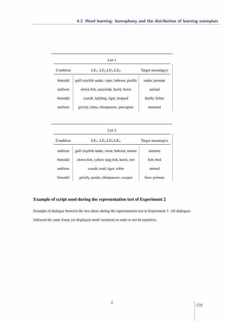
List 1
Condition LE1, LE2,LE3,LE4 Target meaning(s)
bimodal gulf crayfish snake, viper, baboon, gorilla snake; primate
uniform clown fish, anaconda, hawk, horse animal
bimodal scarab, ladybug, tiger, leopard beetle; feline
uniform grizzly, chita, chimpanzee, porcupine mammal
List 2
Condition LE1, LE2,LE3,LE4 Target meaning(s)
uniform gulf crayfish snake, swan, baboon, mouse amniote
bimodal clown fish, yellow tang fish, hawk, owl fish; bird
uniform scarab, toad, tiger, robin animal
bimodal grizzly, panda, chimpanzee, cacajao bear; primate
Example of script used during the representation test of Experiment 2
Example of dialogue between the two aliens during the representation test in Experiment 2. All dialogues
followed the same frame yet displayed small variations in order to not be repetitive.
2
4.2 Word learning: homophony and the distribution of learning exemplars
179
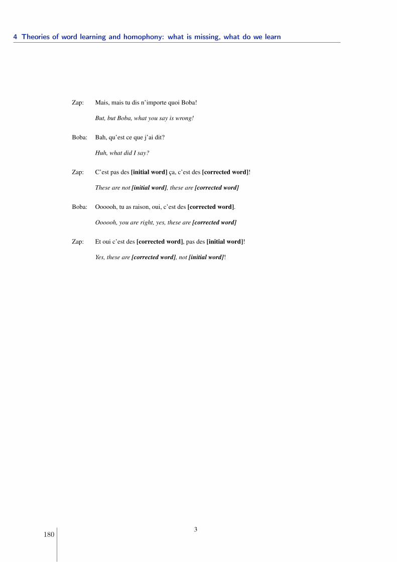
Zap: Mais, mais tu dis n’importe quoi Boba!
But, but Boba, what you say is wrong!
Boba: Bah, qu’est ce que j’ai dit?
Huh, what did I say?
Zap: C’est pas des [initial word] ca, c’est des [corrected word]!
These are not [initial word], these are [corrected word]
Boba: Oooooh, tu as raison, oui, c’est des [corrected word].
Oooooh, you are right, yes, these are [corrected word]
Zap: Et oui c’est des [corrected word], pas des [initial word]!
Yes, these are [corrected word], not [initial word]!
3
4 Theories of word learning and homophony: what is missing, what do we learn
180
4.3 Summary and Discussion
4.3 Summary and Discussion
What is missing, what do we learn
One piece of all current word learning models that make them succeed is that they presup-pose that word forms map onto a single meaning that ought to be "convex" in conceptualspace. This assumption simplifies both the research question and the learning task; yet insome versions of it, it also bans homophony from the system entirely.
In this chapter, I provided the first careful look at what homophones have to say about wordlearning, from a theoretical and an experimental standpoint both with adults (Section4.1) and with children (Section 4.2). On the experimental side, I showed that a wordis more likely to yield homophony if: (a) it is learnt from exemplars leaving an importantgap between them (in conceptual space), (b) this gap in conceptual space is occupied byother words. These results lead to conclusions beyond homophony, and about the existingconstraints on how words associate with concepts in general. For instance, (b) abovedemonstrates that words compete with each other to occupy the conceptual space so thatword learning has to be thought about as a global process over the lexicon, rather than aone-word at a time mechanism.
One of the main contribution of the present set of studies is that currently, learning in dif-ferent domains (object labels, function words including functional morphemes, numericalconcepts) involves different prior hypotheses on the hypothesis space of meanings (and howwords maps onto concepts). Yet, this assumes implicitly that learners are already able todistinguish between several word "domains" in the first place, e.g., they are able to triggerdifferent learning algorithm when facing function words vs. content words. Accordingly,word learning algorithm, even those that are argued to emerge from domain-general mech-anisms (as in Bayesian models), are more specialized than they look like. I come back tothis point further in the General Discussion.
Learning homophones
This was the first set of studies looking at the simultaneous acquisition of the meanings ofa pair of homophones and testing their representations. Recall that in section 3.2, I foundthat learning a secondary meaning for a known word is easier when the second meaning issemantically distinct from the original meaning of the word. To some extent this is compa-rable to one of the factors I uncovered here: observing a gap in conceptual space betweenlearning exemplars increases the likelihood that we are in the presence of homophones. Yetthe studies reported in section 3.2 did not look at the representation of the words: childrenwere taught that "bath" could label a novel animal and could recognize it during the test
181
4 Theories of word learning and homophony: what is missing, what do we learn
phase, yet it is unclear what kind of representation they entertained for "bath". Did theyform another lexical entry to accommodate the novel meaning ("bath" is a homophone)?Did they broaden the original meaning of "bath" to include the novel one ("bath" would bea very broad category encompassing animals, bath items, and everything "in between")?Or did they simply considered that the word could label a set of disconnected concepts("bath" meaning bath or pink octopus)? The present set of studies suggests thattoddlers are more likely to postulate homophony when there is evidence for an importantgap in conceptual space between two learning exemplars of the same word form. Yet wecannot exclude the possibility that younger toddlers may lack the metalinguistic skills todissociate the level of words from the level of concepts and would thus prefer to associate asingle meaning for a given form. Clearly, the children tested in the present study (5.5 years)possess the metalinguistic abilities to conceive the relationship between form and meaning(Backscheider & Gelman, 1995; Peters & Zaidel, 1980). An interesting open question isthus whether younger children, who have not yet been proven to possess this ability arenevertheless able to build lexical representations that conform with homophony.
182
5 General Discussion
Children start learning their first words within their first year of life and by the time theyreach adulthood, they will know approximately 60,000 words (Bloom, 2001). Words aregenerally acquired without any training or feedback: It seems that whatever inferencemechanism children use to learn the meanings of words, they eventually get it right, evenwhen the evidence is scarce or noisy. This may suggest a tight connexion between themechanisms that children employ when acquiring their lexicon and the way the lexicon isstructured and used.
Yet, the presence of ambiguity in the lexicon challenges this view. Indeed, words canhave multiple senses (e.g., homophones) and are represented by an arrangement of a finiteset of phonemes that potentially increases their confusability (e.g., minimal pairs). Giventhat children initially appear to experience difficulty learning similar-sounding words (e.g.,Stager & Werker, 1997; Swingley & Aslin, 2007) and resist learning homophones (e.g.,Casenhiser, 2005; Mazzocco, 1997), lexicons containing many confusable word pairs likelypresent a problem for children. The fit between lexicon structure and lexical learningabilities may hence not be as good as common intuition may suggest.
Motivated by this apparent discrepancy between learning abilities and typological patternwith respect to ambiguity in the lexicon, this dissertation addresses the link between thesetwo factors. In particular, I addressed the possibility that there may be no paradox betweenchildren’s learning abilities and the presence of ambiguity in the lexicon: On the one handthe presence of ambiguity in languages may be the consequence of other functional pressuresnot related with the acquisition of words. On the other hand, the kind of ambiguity that ispresent in the lexicon is learnable; that is learning may exercise some finer-grained influenceon the distribution of ambiguity in the lexicon by keeping only ambiguous words of thelearnable kind. I summarize below the results obtained along these two (non-mutuallyexclusive) lines of work.
5.1 The lexicon: The arena of many functional constraints
Languages have to simultaneously satisfy constraints concerning expressive power and easeof learning and processing (in production and in comprehension). Expressive power will
183
5 General Discussion
lead to languages that are more complex, while ease of learning and processing tends tomaximize simplicity of the linguistic code. Yet importantly, the constraints for ease ofprocessing and learning may conflict: Speakers want many words that are easier to say,thus a more regular and compressible lexicon that maximizes the re-use of word formsand parts of word forms, while listeners and learners want many words that can be easilyidentified, thus a more distinctive lexicon that maximize the phonological distance betweenwords. However, no quantitative study to date has investigated whether lexicons are morelikely to be compressible or more distinctive than chance levels, where chance would bewhat the lexicon would look like in the absence of functional pressures.
In chapter 2, I provided such a methodology for quantifying the amount of phonologicalclustering present in the lexicon. My results show that natural lexicons (at least for the fourlanguages under study) have more similar-sounding words than what would be expectedbased on chance alone. In addition, I show that greater phonological clustering in thelexicon may be explained (in part) by semantic factors: Across a large corpus of 101languages, similar-sounding words tend to be semantically closer than expected by chance.This reveals a fundamental drive for compressibility in the lexicon that conflicts with thepressure for words to be as phonetically distinct as possible.
The prevalence of ambiguous words was not measured using this methodology (see thediscussion in section 2.3). Yet, previous studies have shown that short, frequent andphonotactically probable words are likely to have more meanings than other, more complexand unfrequent words (Piantadosi, Tily, & Gibson, 2012). Thus, all factors that facilitatelexical processing (word length, frequency, phonotactic likelihood) predict, independently,an increase of ambiguity (see for an identical pattern for similar-sounding words, Mahowaldet al., submitted , Appendix A). This suggests that the frequency distribution of words isstructured in a non-arbitrary way, which results in a maximization of the use of ambiguousand similar-sounding words.
Taken together, these results reveals two important tendencies: First, lexicons may beorganized less arbitrarily than previously proposed (de Saussure, 1916; Hockett, 1969) –at least when considering the distribution of similar-sounding words and their mappingsto meanings. Second, just like Zipfian distributions can be interpreted as the result of afunctional trade-off between speakers’ and listeners’ interests regarding word length andword forms, the distribution of word form similarity in the lexicon appears to be explainedby cognitive pressures: Phonological proximity benefits word production (e.g., Dell &Gordon, 2003) but is detrimental for word recognition (e.g., Luce & Pisoni, 1998b) andword learning (e.g., Casenhiser, 2005; Swingley & Aslin, 2007). By assigning similar-sounding and ambiguous word forms to more frequent and predictable meanings, and lesssimilar forms to less frequent and less predictable meanings, languages establish a trade-off between the overall effort needed to produce words and the probability of successfultransmission of a message, and thus, of successful learning of the language.
184

5.2 Ambiguity in context is not a challenge for language acquisition
In sum, the above-chance presence of similar-sounding words in the lexicon illustrates thepresence of multiple functional pressures that compete in the lexicon to minimize the globalcost of the language: Similar-sounding words aid speech production (and memory) beyondthe cost of perceptual confusion of these words. In other words, ease of production mayweigh more heavily on the presence of similar-sounding words than ease of comprehensionor learning, resulting in more compressible lexicons.
5.2 Ambiguity in context is not a challenge for languageacquisition
Even within the learning system, phonological proximity may display at the same time somefunctional advantages and some functional disadvantages. To form a novel lexical entry intheir lexicon, children must be able to extract a word form and associate it to a meaning. Intheory, a compressible lexicon may be advantageous for learning as it reduces the amountof new information that must be represented in the lexicon. For instance, to learn a novelword such as "blick", children need to create a novel phonological representation /blIk/that needs to be associated to a novel semantic representation. Learning several meaningsfor the same phonological form (or re-using parts of a phonological form) may be moreefficient because children only need to learn a novel semantic representation that they canassociate with an already existing phonological representation (Storkel & Maekawa, 2005;Storkel, Maekawa, & Aschenbrenner, 2012). Thus, compressible lexicons may display afunctional advantage as it minimizes the amount of phonological information that must belearnt and remembered. Yet, compressible lexicons may, at the same time, be functionallychallenging for learning as it requires learners to create a new semantic representation whenfew or no phonological cues can be used to signal that a new meaning is intended (see alsosection 1.2).
In chapter 3, I showed that French 18- to 20-month-old toddlers had no problem learningobject labels that were phonological neighbors of a familiar verb (e.g., learning "kiv",a neighbor of "give") but did find it difficult to map neighbors of a familiar noun ontoa novel object (e.g., learning "tog", a neighbor of "dog"). This suggests that toddlersare not confused by phonological similarity per se when learning words. In fact, evenin cases where the novel word is phonologically identical to a word in toddlers’ lexicons(i.e., a homophone), toddlers correctly learnt the novel meaning, provided that the twohomophones are sufficiently distant syntactically (e.g. "an eat" is a good name for anovel animal) or semantically (e.g. "a potty" for a novel animal). When the homophoneswere close on both dimensions (e.g. "a cat" for a novel animal), however, no learningwas observed. These results show that toddlers recruit multiple sources of informationto infer whether or not a given word form is likely to instantiate a novel meaning. More
185
5 General Discussion
generally, the process of creating a lexical entry seems to be mediated by toddlers’ existinglexicon and their parsing abilities. This suggests that the functional disadvantage of havingsimilar-sounding and homophonous word pairs in the lexicon may be reduced when themeanings of these words appear in contexts that can be recognized as distinct by children’sdeveloping parsing system.
Chapter 4 formalized this conclusion for current word learning accounts, circumscribingthe conditions in which homophonous word representations can emerge. Intuitively, in thecase of homophones, we expect the label to occur with a set of exemplars S drawn from twodistinct subcategories X1 and X2. Thus, S would take the form of a bimodal distributionwithin the single superordinate category X encompassing the two subcategories (i.e. X isthe minimal well-formed category such that X1 ∪ X2 ⊂ X). Yet if the word were to beassociated with the whole X, we would expect the exemplars that are associated with thelabel (i.e., S) to be uniformly distributed within X. My results suggest that children andadults can use such sampling considerations to decide whether a word is associated withone category (standard case) or several categories (homophone), even when exposed to veryfew exemplars. In particular, I showed that a word is more likely to be considered as ahomophone when its exemplars are sampled from semantic categories leaving an importantgap between them in conceptual space. Yet, this kind of sampling information may beinformative beyond cases of semantic distance between meanings: When the members ofa pair of homophones are not from the same syntactic category, the sampling distributionof the syntactic context of the label would thus be bimodal and help learners to postulatehomophony.
Interestingly, in chapter 4, I also proposed that the learning system is equipped withbuilt-in constraints that allow for the existence of homophony. This is important becausecontrary to similar-sounding words, homophony presents an additional challenge for wordlearners: It requires them to discover that there is no one-to-one correspondence betweenword forms and the associated concepts (as discussed in the Introduction, section 1.2).Certainly, word learning is guided by a set of built-in constraints regarding the possibleconcepts and form-meaning configurations. This set of experiments makes the followingconstraints explicit: Learners 1) always expect concepts to be convex, that is, to con-sist of groups of contiguous entities in conceptual space; 2) generally expect words tobe associated with a single meaning; 3) entertain the possibility that a word maps ontoseveral meanings if concept convexity is challenged. These constraints show that, albeitdispreferred, homophony can be a possible outcome of our learning system.
Certainly, the requirements to learn similar-sounding words and homophones are differ-ent. While pairs of similar-sounding words can be distinguished at the word form level,homophones cannot: The only way for homophones to be recognized as such is to havesufficiently distinct meanings. Meaning distinctiveness is thus fundamental for these wordsto be learnt and to remain in the language. Interestingly, Bloomfield (1962) reports that in
186
5.2 Ambiguity in context is not a challenge for language acquisition
a dialect of Southwestern France, when the Latin forms "gallus" rooster and "cattus" catwere in danger of merging into one form, "gat", another novel word acquired the meaningrooster, suggesting that the use of the same label for cat and rooster was unwanted andcaused speakers to remap a new form onto one of these meanings. This illustrates thatpairs of homophones that belong to the same semantic field tend to be eliminated duringthe course of language evolution. Conversely, while pairs of similar-sounding words may beeasier to learn when they have distinct meanings, this is not a mandatory property for thesewords to be correctly recognized. In addition, while homophones require that learners formlexical representations that dissociate linguistic signals from concepts (i.e., one word formassociated with several meanings), similar-sounding words do not. Meaning distinctivenessmay thus be a prerequisite for children to form more complex lexical representations, suchas homophony, that depart from an intuitive bias to map each phonological form to a sin-gle meaning. Yet meaning distinctiveness may be unnecessary for similar-sounding words,that still conform to a one-to-one mapping between forms and meanings.
While lexicons are compressible at the word form level, are they constrained by other di-mensions that maximize meaning distinctiveness? Chapter 3 showed that while membersof a pair of homophones appear to be distinctive, i.e., homophones preferentially appearacross syntactic categories rather than within and their meanings are semantically distinct,this does not seem the case for similar-sounding words, i.e., minimal pairs are more likelyto appear within the same syntactic category and to be semantically related. Thus ho-mophones show an advantage for meaning distinctiveness, but similar-sounding words donot. Yet as chapters 3 and 4 suggest, this functional disadvantage may be reduced whenthe meanings of similar-sounding words and homophones can be distinguished in context.This suggests that toddlers’ learning abilities impact the way in which homophones aredistributed in the lexicon, but not by the way similar-sounding words are organized.
Importantly, this does not mean that there is no functional disadvantage associated withthe presence of similar-sounding words that are also more syntactically and semanticallysimilar: As I showed, learning novel words in these conditions is difficult. Yet, this dis-advantage may be outweighed by other learning advantages: (a) similar-sounding wordsmay be easier to spot in the speech stream (Altvater-Mackensen & Mani, 2013, see alsosection 1.2.1); (b) similar-sounding words sharing the same grammatical category may helpchildren group words into categories (i.e., nouns, verbs) (Cassidy & Kelly, 1991; Monaghanet al., 2011); but also other processing advantages: (c) similar-sounding words are easierto produce and to memorize. In sum, the distribution of similar words in the lexicon,both at the word form level and at the syntax/semantic level, may simply reflect a greaterfunctional advantage rather than the absence of functional cost.
The empirical evidence presented in chapters 3 and 4 suggests that the learning system ofyoung children is equipped with constraints and mechanisms that allow them to successfullylearn ambiguous and similar-sounding words as long as these words can be distinguished in
187
5 General Discussion
a context that children can capitalize on. Thus, children can deal with ambiguity as long asdistinctiveness along other dimensions that are relevant for them is maximized. In addition,I suggest that learning exercises a finer-grained influence on the distribution of ambiguityin the lexicon by selecting ambiguous words whose meaning can be easily disambiguatedby the context in which they occur, while pruning out ambiguous words which are notdistinguishable through their context, which makes them both hard to learn and prone totriggering misunderstandings. Interestingly the distribution of similar-sounding words inthe lexicon did not seem to be affected by children learning difficulties potentially becausethey confer a greater advantage for speech production and memory (see chapter 2). Ipropose that the difference between the distribution of ambiguous and similar-soundingwords illustrates the presence of multiple functional pressures that compete in the lexicon,and that the end result is a trade-off that minimizes the global cost for language users.Yet, while we can probably get an idea of the weight of different functional pressures fromobserving the structure of the lexicon (and of languages more generally), we cannot tellwhether they actually explain why lexicons look the way they are. In the set of studiespresented in this thesis, I examine the connexions between learning and processing abilitiesand lexicon structure, but this work does not provide evidence about whether there is adirectional and causal relation between the way our mind is working and language. I turnto this point in the following sections.
5.3 How did the lexicon become the way it is?
Language is transmitted culturally from one generation to the next: First-generation speak-ers produce sentences, which second-generation learners use in order to infer the propertiesof the language. These cycles of production and inference are crucial in understanding howlanguage has developed and evolved into the structure we observe now.
Iterated learning provides a framework to study the emergence of a linguistic systemthrough cultural transmission. Iterated learning is the process by which individuals learna language produced by a previous individual, who learnt it in the same way (Kirby etal., 2008; Kirby, Griffiths, & Smith, 2014; K. Smith, Kirby, & Brighton, 2003), and can besimulated using computational models or experiments with human participants in the lab.Kirby, Tamariz, Cornish, & Smith (2015) show that the languages that emerge from iter-ated learning are shaped by the processes of both cross-generation transmission (languagelearning) and within-generation communication (language use). Iterated learning can thusbe used to isolate effects of learning (i.e., where a participant learns a language and thentries to recall it) and the effects of communication (i.e., where participants interact withone another).
Work using this paradigm has consistently shown that individuals will preferentially dis-
188

5.4 The influence of external factors on the lexicon
card forms and structures that are disadvantageous in favor of other, more advantageouswords and phrases (e.g., Reali & Griffiths, 2009; K. Smith & Wonnacott, 2010). For in-stance, Reali & Griffiths (2009) show that over repeated episodes of learning, a lexicon withmultiple labels for objects (synonyms or many-to-one form-meaning mappings) evolves intoa lexicon that associates each label with a unique object. This is consistent with the obser-vation that there is a historical tendency for languages to lose many-to-one mappings overtime and that children display a bias against many-to-one mappings (Markman & Wachtel,1988). Note that to date, no work exists investigating in such a paradigm whether lexiconsevolve to be more phonologically similar and start tolerating the existence of homophonesover time.
Iterated learning thus offers a promising venue for future research to understand howfunctional pressures from both language learning and language usage combine to producethe particular distribution of ambiguous and confusable words found in human languages.Imagine that individuals are taught an artificial lexicon that contains pairs of similar-sounding words and pairs of homophones that vary in their meaning distinctiveness. Ourresults with child learners predict that the degree to which members of homophone orminimal pairs are distinct may influence participants’ learning abilities, thus affecting thetransmission of these words to the next generation of learners. We might expect that,across generations, pairs of homophones which cannot be distinguished by their seman-tic or syntactic context will disappear from the language, while pairs of minimal pairswill tend to stay and be easier to learn if they facilitate syntactic or semantic grouping.This may provide direct evidence that 1) functional processes directly influence the dis-tribution of those words in the lexicon, for instance by looking at whether phonologicalproximity tends to decrease or increase during learning and/or during communication; 2)the different patterns of distribution found for ambiguous and confusable words stem fromdifferent functional pressures that weigh differently in the process of language usage andtransmission.
While looking at language evolution in accelerated lab time provides us with an impressionof which functional pressures give rise to a particular structure, functional pressures maynot be the only determinant of structure. Certainly, languages must adapt to constraintsexternal to the human mind.
5.4 The influence of external factors on the lexicon
Several studies have previously demonstrated that the cultural process of transmitting alanguage, in combination with the constraints and biases of language learners and users,offers an explanation for language structure (e.g., Kirby, 1999). For example, composi-tional languages (i.e., languages in which the meaning of an expression is determined by
189

5 General Discussion
the meaning of its constituent expressions) emerge from unstructured languages throughrepeated transmission through a learning bottleneck (e.g., Brighton, 2002; Brighton, Smith,& Kirby, 2005; Vogt, 2005). Because language learners need to infer the whole languagefrom limited evidence (the "bottleneck"), compositionality appears as a natural solutionfor language since it is the only way for learners to infer the properties of a large linguis-tic system with limited evidence.Thus, the process of transmission itself may give rise tostructure because it constrains the kind of inferences that learners can entertain. In par-ticular, the size of the "bottleneck" influences whether the resulting language will reflectthe inductive biases or constraints of the learning system: The smaller the bottleneck thefaster it will converge to the priors of the learner (e.g., Griffiths, Christian, & Kalish, 2008;Griffiths & Kalish, 2007; Kirby, Dowman, & Griffiths, 2007; Reali & Griffiths, 2009), yetwhen the bottleneck is large (a large amount of information is available to the learner), thelanguage will be a combination of the learner’s priors with the distribution of events in theworld (the posterior, in Bayesian terms) (Perfors & Navarro, 2014). Thus, the transmissionprocess by itself is a mediating force in the shaping of languages.19
These results are particularly interesting in relation to the distribution of homophonesin languages. Many have suggested that learners expect words to be associated with asingle convex meaning (a one-to-one form-meaning mapping bias). Yet, as we showed inchapter 4, learners offset this constraint when they are given evidence that the meaningonto which the word would map is not convex, allowing for the formation of homophones.Thus, when the evidence is fairly limited (hence the bottleneck is small), learners will morereadily follow the more general constraint that one word should be associated to a singlemeaning. For instance, if learners are provided with only a small number of exemplars,revealing that the word "bat" is associated to two baseball-bats and one animal-bat, theywill be likely to infer that "bat" means baseball-bat and discard the animal-bat exemplar.This may be especially true when one of the two meanings of a pair of homophones isvery infrequent. Conversely, if the bottleneck is large, that is, if learners observe manyexemplars for each meaning of the homophone pair, learners will have more evidence thatconcept convexity is not met and will postulate homophony. As such, the amount ofhomophony that remains in the language should depend on how easy it is for the learnerto identify the two meanings (chapters 3 and 4) but may also depend on the size of thebottleneck – how much evidence the learner is given to observe. Similarly, languages mayhave evolved to impose greater phonological overlap to words that are semantically andsyntactically related (chapter 4) such that learners would quickly group words accordingto their relevant syntactic or semantic categories even when the size of the bottleneck issmall.
The structure of the world also interacts with learners and users of a language and influences
19Note however that it does not preclude the possibility that the type of response our mind is adopting tothe bottleneck problem, i.e., in this example compositionality, may be grounded in human cognition.
190
5.4 The influence of external factors on the lexicon
the resulting structure. For instance, the population size has an influence on language com-plexity: Languages spoken by larger groups have larger signal inventories (this is true evenin animal communicative systems, Freeberg, Dunbar, & Ord, 2012) but simpler morphol-ogy than languages spoken in smaller communities, both in real world languages (Lupyan& Dale, 2010; Nettle, 2012) and in artificial learning experiments (Atkinson, Kirby, &Smith, 2015). In addition, the structure of the environment influences the structure ofthe language: If entities in the world are grouped along a single dimension (e.g., objectsare naturally grouped according to their size), the languages of iterated learning exper-iments evolve to reflect that structure independently of the dimension chosen (i.e., size,color, etc) and independently of the language the first generation has to learn (Perfors &Navarro, 2014).20 Similarly, the situational context is an important driver of the space ofmeanings: If a meaning dimension (e.g., color, shape, motion) is made not relevant duringword learning (because it does not help to infer an intended meaning), then languages willnot encode this particular meaning dimension (Silvey, Kirby, & Smith, 2014). Others havereported the importance of frequency of use as an explanation of language structure (e.g.,Bybee, 2006): High frequency patterns are learnt easily, independently of their regularityin the language, while low-frequency patterns are difficult to learn when they are irregularand thus, may disappear from the language. The classical example is the acquisition ofEnglish past tense. Irregular past forms (e.g., go→ went) are more likely to be frequent inthe language and when they are not frequent, they are more likely to show some regularityin their past forms (e.g, breed → bred; bleed → bled; meet → met).
Frequency may be an important factor to explain the existence of similar-sounding wordsand homophones in the lexicon. Recall that ambiguity and confusability is more likely toappear on frequent forms than on infrequent forms (Mahowald et al., submitted ; Piantadosi,Tily, & Gibson, 2012; Zipf, 1949). As discussed in chapter 2, words with higher frequenciesare beneficial for speakers. Yet, in addition, it could also be an advantage for learners: Ashomophones and similar-sounding words are frequent, this will provide them with enoughevidence through the learning bottleneck to learn the meanings of those words, allowingthus for a greater likelihood that these words are transmitted to the next generation andremain in the language. Certainly this also imposes constraints on which homophones aremost likely to stay in the languages: Homophones whose meanings occur frequently will bemore likely to be transmitted than homophones with unbalanced frequencies where onlythe most frequent meaning will go through.
Maturational constraints can also impact the structure of language. For instance, whenadults and 5-year-olds were exposed to a language with an inconsistent grammar, childrenregularized the language – their output was more consistent than their input, while adults
20Certainly, the way we structure the world may, to some extent, also depend on the language we use.For instance, the way that languages partition the color spectrum into labeled categories affects colorsimilarity judgments, memory, and discrimination (e.g., Regier & Kay, 2009; Roberson, Davies, &Davidoff, 2000; Winawer et al., 2007).
191
5 General Discussion
reproduced only what they heard (Hudson Kam & Newport, 2009). Hudson Kam &Newport (2009) hypothesized that children’s restricted memory capacities limit their abilityto store complex forms (see also Newport, 1990), and are thus more likely to impact thestructure of language compared to adults. This aligns nicely with the case of similar-sounding and ambiguous words. Maturational constraints linked to memory constraintsmay limit the appearance of maximally distinctive lexicons since it would be more difficultfor children to learn them, as they would need to remember more phonological formsand more sound sequences, and favor compressible lexicons that have a certain amount ofphonological overlap.
In the case of homophones, an additional maturational constraint seems critical for chil-dren: The ability to conceive the relationship between form and meaning. Metalinguisticawareness of that sort seems to appear between 3 and 4 years of age (Doherty, 2000). Forinstance, here is the quote of 4-year-old French kid, well aware of homophones (in French/vEK/ means, inter alia, either the color, green; the material, glass; something to drinkfrom, a glass; or an animal, a worm):
C’est /vEK/ mais c’est pas en /vEK/, enfin c’est en /vEK/, mais c’est pas DU /vEK/This is [green] but it is not [glass], well it is in [green], but it is not made of [glass]
If metalinguistic awareness develops late in younger children, this may limit their abilities tolearn homophones. However, it is unclear exactly when this metalinguistic ability develops.Certainly children younger than 3 years of age know a few pairs of homophones (de Carvalhoet al., 2014) and can readily attach a second meaning to a known word form in certainconditions (chapter 3). Yet, very little is known about the lexical representations ofthese words at that age and how children reflect about them. One possibility is thatlearning homophones may not have to be metalinguistic at its earliest stages: Toddlersmay start building two separate lexical entries for the same word form because the contextin which each meaning is used fully prevents them from accessing the other meaning(s) ofthe same form. Then, only later, children may realize that the mapping between forms andmeanings is ambiguous. According to this view, it is crucial that the meanings of a pair ofhomophones are distinct for homophones to be able to remain in the language. Anotherpossibility is that children have these metalinguistic skills from the start. Interestinglysome toddlers appear to initially use certain word forms to refer to multiple referents (e.g.,Vihman, 1981). For instance "cat" could be used in reference to a cat but also in referenceto a dog or any object. One interesting question is whether their representation of "cat"is simply greatly underspecified or whether they are aware that the true meaning of "cat"is the set of cats and only cats, and use this word because they do not possess a betteralternative in their lexicon. If the latter case is true, this would suggest that childrenhave the ability to distinguish between words and concepts early on and may be able toentertain homophony.21
21Certainly this is not the only way to test whether children know that words and concepts are not related
192
5.5 Insights into the link between language and mind
Taken together, as I reviewed above, there are many factors, determined by functionalconsiderations and the external world, that could explain part of the amount and theparticular distribution of homophones and similar-sounding words in the lexicon. In myfuture work, I will continue pursuing these directions. In particular, I will investigatethe role of frequency in the transmission of ambiguous and similar-sounding words inthe iterative learning paradigm with adults, and I will extend the study of one-to-manyform-meaning mappings to younger children, in order to gain an understanding of thematurational constraints underlying the representation of homophonous meanings.
5.5 Insights into the link between language and mind
I started this thesis by noting that there is a connection between the mechanisms by whichwe acquire and process languages on the one hand and the structure of languages on theother hand. Yet the origin of such a relationship is the topic of a long-standing (but im-portant) debate (Chomsky, 1986; Christiansen & Chater, 2008; Evans & Levinson, 2009;Pinker & Bloom, 1990b). One view argues that this relationship has occurred becauseof specialized biological machinery that embodies the principles that govern natural lan-guages (e.g., Chomsky, 1986). As such, these principles do not need to be determined byfunctional considerations since they are hard-wired in the learning system. A second viewholds that the structure of language has evolved to fit domain-general learning and process-ing constraints (e.g., Christiansen & Chater, 2008). From this perspective, the learner’scognitive constraints are likely to be helpful in learning the target language because thelanguage has evolved to conform to these biases. Both views agree that languages areshaped by the mind but differ in whether this occurs through language-specific or domain-general mechanisms. The present work does not aim to disentangle between these viewsbut rather provides some interesting insights into these ideas that will need to be furtherexplored.
For a long time, the presence of ambiguity has challenged the view that language is de-signed to fit our learning and processing needs. Yet, much evidence (e.g., Piantadosi, Tily,& Gibson, 2012; Wasow et al., 2005), including the data presented in the body of thisthesis, proposes that the existence of ambiguity and confusability may find an explana-tion when one is considering the competing needs of learners, listeners and speakers of thelanguage. The studies in that dissertation started to address this question by looking ata few languages and study child learners and provide an interesting starting point sug-gesting that ambiguity, and the way it is distributed in the lexicon, may be functionallymotivated. Certainly, future work should expand this investigation further: Indeed, mostof the languages studied here are historically related (thus share some of their properties)
in a one-to-one fashion. Yet this also relates directly to children metalinguistic abilities and providesan interesting framework to study the representation of words in early vocabularies.
193
5 General Discussion
and most language acquisition studies are restricted to a few languages. In future work,I plan to overcome the scarcity of data by taking advantage of the existence of big cor-pora (see chapter 2) and simulate language evolution in the lab (e.g., iterated learning)to study different learning and communicative configurations and supplement children’slearning data. This will be a crucial component for disentangling the impact of differentfunctional pressures, and understand why/how they weigh differently for different aspectsof language.
Does word learning emerge from innately constrained cognitive mechanisms or from moredomain-general mechanisms? Bayesian approaches are often called for to reduce learningto domain-general mechanisms. Yet, a careful look at the literature reveals that currentmodels of word learning, including Bayesian models, assume very strong built-in constraintsfor the learning algorithm. These models do not take into account certain word learningphenomenon, such as homophony, when describing word learning. I suggest that this isdue to a specialization of the individual word learning algorithms put forth by researchers:One algorithm can learn object labels, another one can learn function words, yet anothercan learn number words, etc. Yet none of these algorithms can be used to learn all kindsof words. This may not be a problem by itself, but while focusing on learning a singleword type, current word learning accounts implicitly incorporate built-in assumptions thatmay or may not be justified. For instance, the existence of several learning algorithmsrests on the assumption that learners already know to distinguish between different wordtypes (e.g., function words and content words or words having several meanings versuswords having only one) so that they can apply the relevant learning algorithm in a givensituation. One possibility is that these accounts assume that word distinction is an innateproperty of the learning system. Another possibility is that children use a domain-generalmechanism to distinguish between these words: For instance, infants have been shownto use word frequency as a cue to distinguish between function words and content words(Hochmann, Endress, & Mehler, 2010)22. Also, it has been shown that infants distinguishbetween function and content words at birth, likely based on acoustical cues only (Shi,Werker, & Morgan, 1999). At any rate, these implicit priors, and their origin, need to bespecified and studied. As I have shown, one way of doing so is to look at more diverseword learning phenomena within the same word learning model to reveal and understandwhat may count as a an actual cognitive constraint and what is merely a simplification ofthe learning algorithm.
In addition, this thesis provided evidence that the lexicon is strongly constrained by thekinds of representations our mind is willing to entertain. As we showed, learners expectconcepts to be convex. That is, they expect its members to form a coherent cluster in
22Though whether this is domain-general or domain-specific is still debatable. On the one hand, therecould be an innate constraint saying that frequent morphemes are functional. On the other hand, therecould be a general appreciation of frequency: if a given word is too frequent, then it is unlikely to referto a concrete object and therefore must be used for some other (functional) purposes.
194
5.6 Conclusion
conceptual space. Yet while this constraint is certainly not language-specific, it seems thatlearners assume that their to-be-learnt lexicon is composed of form-meaning mappings ofa very specific kind: They expect words to be mapped onto a single concept. This seemsa rather specific assumption on the language they are about to learn, yet this does notnecessarily imply that this is a language-specific constraint: Learners have been shownto have a preference for simplicity across a wide range of cognitive processes (Chater &Vitányi, 2003), including language learning. Accordingly, learners may expect that formsand meanings come in a one-to-one relation because that may be the simplest representa-tion that learners could possibly find (see also Slobin, 1973, 1975, for the argument thatexpecting clarity between signals and their functions is an important driving principle).However, one important finding reported in the present work was that learners can enter-tain more complex meaning representations (homophony) in cases where there is no clearmapping between a word form and a single meaning, but only in the "right" contexts. Thisis a very specific built-in constraint for a general learning system that seems to expect thata linguistic phenomenon as specific as homophony may be a possibility from the start.Certainly, this calls for further investigation and leaves several open questions for futureresearch, regarding the hierarchy of the constraints of the learning system (as I showed con-cept convexity seems to be prioritized over forming a one-to-one mapping between formsand meanings), and the possibility of the existence of some very specific constraints on themapping between forms and meanings in the learning system.
5.6 Conclusion
This work investigated why lexicons are ambiguous. A prominent feature of this thesishas been the combined use of lexical models to quantify the amount of ambiguity in thelexicon and experimental methods in toddlers and adults to investigate what exactly en-ables children to learn ambiguous and confusable words. Taken together, this researchsuggests that ambiguous and confusable words, while present in the language, may be re-stricted in their distribution in the lexicon and that these restrictions reflect (in part) howchildren learn languages, and (in part) the existence of several other constraints on thelexicon. Taken together, this dissertation provides the basis for a research program ded-icated to understanding how cognitive constraints coming from language acquisition andlanguage use combine to produce the lexicons found in human languages through culturaltransmission.
195

References
Akhtar, N., & Montague, L. (1999). Early lexical acquisition: The role of cross-situationallearning. First Language, 19 (57), 347–358.
Altmann, G., & Kamide, Y. (1999). Incremental interpretation at verbs: Restricting thedomain of subsequent reference. Cognition, 73 (3), 247–264.
Altvater-Mackensen, N., & Mani, N. (2013). Word-form familiarity bootstraps infantspeech segmentation. Developmental science, 16 (6), 980–990.
Arbesman, S., Strogatz, S. H., & Vitevitch, M. S. (2010). The structure of phonologicalnetworks across multiple languages. International Journal of Bifurcation and Chaos,20 (03), 679–685.
Arias-Trejo, N., & Plunkett, K. (2013). What’s in a link: Associative and taxonomicpriming effects in the infant lexicon. Cognition, 128 (2), 214–227.
Atkinson, M., Kirby, S., & Smith, K. (2015). Speaker input variability does not explainwhy larger populations have simpler languages. PloS one, 10 (6), e0129463.
Baayen, R. H., Piepenbrock, R., & van H, R. (1993). The celex lexical data base oncd-rom.
Backscheider, A. G., & Gelman, S. A. (1995). Children’s understanding of homonyms.Journal of Child Language, 22 (01), 107–127.
Bergelson, E., & Swingley, D. (2012). At 6-9 months, human infants know the meaningsof many common nouns. Proceedings of the National Academy of Sciences, 109 (9),3253–3258.
Bergelson, E., & Swingley, D. (2013). The acquisition of abstract words by young infants.Cognition, 127 (3), 391–397.
Bernal, S., Dehaene-Lambertz, G., Millotte, S., & Christophe, A. (2010). Two-year-oldscompute syntactic structure on-line. Developmental science, 13 (1), 69–76.
197
References
Beveridge, M., & Marsh, L. (1991). The influence of linguistic context on young children’sunderstanding of homophonic words. Journal of Child Language, 18 (02), 459–467.
Bion, R. A., Borovsky, A., & Fernald, A. (2013). Fast mapping, slow learning: Disam-biguation of novel word–object mappings in relation to vocabulary learning at 18, 24,and 30months. Cognition, 126 (1), 39–53.
Bloom, P. (2001). Précis of How children learn the meanings of words. Behavioral andBrain Sciences, 24 (06), 1095–1103.
Bloomfield, L. (1962). Language. 1933. Holt, New York .
Bortfeld, H., Morgan, J. L., Golinkoff, R. M., & Rathbun, K. (2005). Mommy andme familiar names help launch babies into speech-stream segmentation. PsychologicalScience, 16 (4), 298–304.
Bowerman, M. (2011). Linguistic typology and first language acquisition. Oxford UniversityPress.
Boyer, P., & Ramble, C. (2001). Cognitive templates for religious concepts: Cross-culturalevidence for recall of counter-intuitive representations. Cognitive Science, 25 (4), 535–564.
Brighton, H. (2002). Compositional syntax from cultural transmission. Artificial life, 8 (1),25–54.
Brighton, H., Smith, K., & Kirby, S. (2005). Language as an evolutionary system. Physicsof Life Reviews, 2 (3), 177–226.
Brusini, P. (2012). Découvrir les noms et les verbes: Quand les classes sémantiquesinitialisent les catégories syntaxiques (Unpublished doctoral dissertation). UniversitéPierre et Marie Curie.
Bybee, J. (2006). Frequency of use and the organization of language.
Campbell, R. N., & Bowe, T. (1977). Functional asymmetry in early language understand-ing. Salzberger Beitrage für Linguistik , 3 .
Caramazza, A., & Grober, E. (1976). Polysemy and the structure of the subjective lexicon.Georgetown University roundtable on languages and linguistics. Semantics: Theory andapplication, 181–206.
Carey, S. (1978a). The child as word learner.
198
References
Carey, S. (1978b). The child as word learner.
Carlson, M. T., Sonderegger, M., & Bane, M. (2014). How children explore the phonologicalnetwork in child-directed speech: A survival analysis of children’s first word productions.Journal of Memory and Language, 75 , 159–180.
Casenhiser, D. M. (2005). Children’s resistance to homonymy: an experimental study ofpseudohomonyms. Journal of Child Language, 32 (2), 319–343.
Cassidy, K. W., & Kelly, M. H. (1991). Phonological information for grammatical categoryassignments. Journal of Memory and Language, 30 (3), 348–369.
Cauvet, E., Limissuri, R., Millotte, S., Skoruppa, K., Cabrol, D., & Christophe, A. (2014).Function words constrain on-line recognition of verbs and nouns in French 18-month-olds. Language Learning and Development , 10 (1), 1–18.
Chater, N., & Vitányi, P. (2003). Simplicity: a unifying principle in cognitive science?Trends in cognitive sciences, 7 (1), 19–22.
Chomsky, N. (1986). Knowledge of language: Its nature, origin, and use. Praeger Pub-lishers.
Chomsky, N. (2002). An interview on minimalism. N. Chomsky, On Nature and Language,92–161.
Christiansen, M. H., & Chater, N. (2008). Language as shaped by the brain. Behavioraland Brain Sciences, 31 (05).
Conwell, E. (2015). Neural responses to category ambiguous words. Neuropsychologia, 69 ,85–92.
Conwell, E., & Morgan, J. L. (2012). Is it a noun or is it a verb? resolving the ambicate-goricality problem. Language Learning and Development , 8 (2), 87–112.
Creel, S. C., Aslin, R. N., & Tanenhaus, M. K. (2008). Heeding the voice of experience:The role of talker variation in lexical access. Cognition, 106 (2), 633–664.
Culbertson, J., & Newport, E. L. (2015). Harmonic biases in child learners: In support oflanguage universals. Cognition, 139 , 71–82.
Culbertson, J., Smolensky, P., & Legendre, G. (2011). Learning biases predict a wordorder universal. Cognition.
199
References
Dahan, D., Swingley, D., Tanenhaus, M. K., & Magnuson, J. S. (2000). Linguistic genderand spoken-word recognition in french. Journal of memory and Language, 42 (4), 465–480.
Dautriche, I., & Chemla, E. (2014). Cross-situational word learning in the right situations.Journal of Experimental Psychology: Learning, Memory, and Cognition, 40 (3), 892.
de Carvalho, A., Dautriche, I., & Christophe, A. (2014). Phrasal prosody constrainsonline syntactic analysis in two-year-old children. 39th Boston University Conferenceon Language Development - Boston, MA - USA.
de Carvalho, A., Dautriche, I., & Christophe, A. (2015). Preschoolers use phrasal prosodyonline to constrain syntactic analysis. Developmental science.
Delais-Roussarie, E. (1995). Pour une approche parallele de la structure prosodique:Etude de lõorganisation prosodique et rythmique de la phrase française [for a parallelapproach of prosodic structure: A study of the prosodic and rhythmic organisation of thefrench sentence]. Unpublished Ph. D. thesis. Toulouse, France: Université de Toulouse-LeMirail .
Dell, G. S., & Gordon, J. K. (2003). Neighbors in the lexicon: Friends or foes? Phoneticsand phonology in language comprehension and production: Differences and similarities,6 , 9.
Demuth, K., & Tremblay, A. (2008). Prosodically-conditioned variability in children’sproduction of French determiners. Journal of Child Language, 35 (1), 99.
de Saussure, F. (1916). Course in general linguistics. Columbia University Press.
Doherty, M. J. (2000). Children’s understanding of homonymy: metalinguistic awarenessand false belief. Journal of Child Language, 27 (02), 367–392.
Doherty, M. J. (2004). Childrens difficulty in learning homonyms. Journal of ChildLanguage, 31 (1), 203–214.
Escudero, P., Mulak, K. E., & Vlach, H. A. (2015). Cross-situational learning of minimalword pairs. Cognitive science.
Evans, N., & Levinson, S. C. (2009). The myth of language universals: Language diversityand its importance for cognitive science. Behavioral and Brain Sciences, 32 (05), 429.
Federmeier, K. D., & Kutas, M. (1999). A rose by any other name: Long-term memorystructure and sentence processing. Journal of memory and Language, 41 (4), 469–495.
200
References
Fennell, C. T. (2012). Object Familiarity Enhances Infants’ Use of Phonetic Detail inNovel Words. Infancy , 17 (3), 339–353.
Fennell, C. T., & Waxman, S. (2006). Infants of 14 months use phonetic detail in novelwords embedded in naming phrases. In Proceedings of the 30th annual boston universityconference on language development (pp. 178–189).
Flemming, E. (2004). Contrast and perceptual distinctiveness. Phonetically based phonol-ogy , 232–276.
Frank, M. C., Goodman, N. D., & Tenenbaum, J. B. (2009). Using speakers’ referentialintentions to model early cross-situational word learning. Psychological Science, 20 (5),578–585.
Freeberg, T. M., Dunbar, R. I., & Ord, T. J. (2012). Social complexity as a proximate andultimate factor in communicative complexity. Philosophical Transactions of the RoyalSociety B: Biological Sciences, 367 (1597), 1785–1801.
Gahl, S. (2008). Time and thyme are not homophones: The effect of lemma frequency onword durations in spontaneous speech. Language, 84 (3), 474–496.
Gelman, S. A., & Brandone, A. C. (2010). Fast-mapping placeholders: Using words totalk about kinds. Language Learning and Development , 6 (3), 223–240.
Goldwater, S., & Griffiths, T. (2007). A fully bayesian approach to unsupervised part-of-speech tagging. In Annual meeting-association for computational linguistics (Vol. 45,p. 744).
Goodman, N. (1955). Fact, fiction, and forecast. Harvard University Press.
Gout, A., Christophe, A., & Morgan, J. L. (2004). Phonological phrase boundaries con-strain lexical access II. Infant data. Journal of Memory and Language, 51 (4), 548–567.
Graf Estes, K., & Bowen, S. (2013). Learning about sounds contributes to learningabout words: Effects of prosody and phonotactics on infant word learning. Journal ofExperimental Child Psychology , 114 (3), 405–417.
Graff, P. N. H. M. (2012). Communicative efficiency in the lexicon (Unpublished doctoraldissertation). Massachusetts Institute of Technology.
Greenberg, J. H. (1966). Universals of language .
201
References
Griffiths, T. L., Christian, B. R., & Kalish, M. L. (2008). Using category structures to testiterated learning as a method for identifying inductive biases. Cognitive Science, 32 (1),68–107.
Griffiths, T. L., & Kalish, M. L. (2007). Language evolution by iterated learning withBayesian agents. Cognitive Science, 31 (3), 441–480.
Gutman, A., Dautriche, I., Crabbé, B., & Christophe, A. (2014). Bootstrapping the Syn-tactic Bootstrapper: Probabilistic Labeling of Prosodic Phrases. Language Acquisition,1–25.
Gärdenfors, P. (2004). Conceptual spaces: The geometry of thought. MIT press.
Hayes, B. (2012). BLICK - a phonotactic probability calculator.
Hills, T. T., Maouene, M., Maouene, J., Sheya, A., & Smith, L. (2009). Longitudinalanalysis of early semantic networks preferential attachment or preferential acquisition?Psychological Science, 20 (6), 729–739.
Hochmann, J. R., Endress, A. D., & Mehler, J. (2010). Word frequency as a cue foridentifying function words in infancy. Cognition, 115 (3), 444.
Hockett, C. F. (1969). The origin of speech. Sci. Am, 203 , 88–111.
Holst, T., & Nolan, F. (1995). The influence of syntactic structure on [s] to [S] assimilation.Papers in Laboratory Phonology, IV , 315–3333.
Howes, D. (1968). Zipf’s law and miller’s random-monkey model. The American Journalof Psychology , 81 (2), 269–272.
Hudson Kam, C. L., & Newport, E. L. (2009). Getting it right by getting it wrong: Whenlearners change languages. Cognitive Psychology , 59 (1), 30–66.
Johnson, E. K. (2005). Grammatical gender and early word recognition in dutch. InProceedings of the 29th annual boston university conference on language development(Vol. 1, pp. 320–330).
Johnson, M., Griffiths, T. L., & Goldwater, S. (2006). Adaptor grammars: A frameworkfor specifying compositional nonparametric bayesian models. In Advances in neuralinformation processing systems (pp. 641–648).
Juba, B., Kalai, A. T., Khanna, S., & Sudan, M. (2011). Compression without a commonprior: an information-theoretic justification for ambiguity in language.
202
References
Jusczyk, P. W., Friederici, A. D., Wessels, J. M., Svenkerud, V. Y., & Jusczyk, A. M.(1993). Infants’ sensitivity to the sound patterns of native. Journal of memory andlanguage, 32 (3), 402–420.
Kamide, Y., Altmann, G., & Haywood, S. L. (2003). The time-course of prediction inincremental sentence processing: Evidence from anticipatory eye movements. Journal ofMemory and Language, 49 (1), 133–156.
Kelly, M. H. (1992). Using sound to solve syntactic problems: The role of phonology ingrammatical category assignments. Psychological Review , 99 (2), 349–364.
Kern, S. (2007). Lexicon development in french-speaking infants. First Language, 27 (3),227–250.
Kirby, S. (1999). Function, selection, and innateness: The emergence of language univer-sals. Oxford University Press.
Kirby, S., Cornish, H., & Smith, K. (2008). Cumulative cultural evolution in the laboratory:An experimental approach to the origins of structure in human language. Proceedingsof the National Academy of Sciences, 105 (31), 10681–10686.
Kirby, S., Dowman, M., & Griffiths, T. L. (2007). Innateness and culture in the evolutionof language. Proceedings of the National Academy of Sciences, 104 (12), 5241–5245.
Kirby, S., Griffiths, T., & Smith, K. (2014). Iterated learning and the evolution of language.Current Opinion in Neurobiology , 28 , 108–114.
Kirby, S., Tamariz, M., Cornish, H., & Smith, K. (2015). Compression and communicationin the cultural evolution of linguistic structure. Cognition, 141 , 87–102.
Koehne, J., Trueswell, J. C., & Gleitman, L. R. (2013). Multiple proposal memory inobservational word learning. In Proceedings of the 35th annual meeting of the cognitivescience society. austin, tx: Cognitive science society.
Labov, W. (1966). The social stratification of English in New York city. CambridgeUniversity Press.
Landau, B., Smith, L. B., & Jones, S. S. (1988). The importance of shape in early lexicallearning. Cognitive development , 3 (3), 299–321.
Landauer, T. K., & Dumais, S. T. (1997). A solution to Plato’s problem: The latentsemantic analysis theory of acquisition, induction, and representation of knowledge.Psychological review , 104 (2), 211.
203
References
Lee, C.-l., & Federmeier, K. D. (2009). Wave-ering: An erp study of syntactic and semanticcontext effects on ambiguity resolution for noun/verb homographs. Journal of Memoryand Language, 61 (4), 538–555.
Lee, C.-l., & Federmeier, K. D. (2012). Ambiguity’s aftermath: How age differences inresolving lexical ambiguity affect subsequent comprehension. Neuropsychologia, 50 (5),869–879.
Lew-Williams, C., & Fernald, A. (2007). Young children learning spanish make rapid use ofgrammatical gender in spoken word recognition. Psychological Science, 18 (3), 193–198.
Lindblom, B. (1986). Phonetic universals in vowel systems. Experimental phonology ,13–44.
Lippeveld, M., & Oshima-Takane, Y. (2014). The effect of input on children’s cross-categorical use of polysemous noun-verb pairs. Language Acquisition(ahead-of-print),1–31.
Luce, P. A. (1986). Neighborhoods of words in the mental lexicon. Research on SpeechPerception. Technical Report No. 6..
Luce, P. A., & Pisoni, D. B. (1998a). Recognizing spoken words: The neighborhoodactivation model. Ear and hearing , 19 (1), 1.
Luce, P. A., & Pisoni, D. B. (1998b). Recognizing spoken words: The neighborhoodactivation model. Ear and hearing , 19 (1), 1.
Lupyan, G., & Dale, R. (2010). Language structure is partly determined by social structure.PloS one, 5 (1), e8559.
Magnuson, J. S., Dixon, J. A., Tanenhaus, M. K., & Aslin, R. N. (2007). The dynamics oflexical competition during spoken word recognition. Cognitive Science, 31 (1), 133–156.
Mahowald, K., Dautriche, I., Gibson, E., & Piantadosi, S. (submitted). Word forms arestructured for efficient use.
Mani, N., & Plunkett, K. (2007). Phonological specificity of vowels and consonants inearly lexical representations. Journal of Memory and Language, 57 (2), 252–272.
Maris, E., & Oostenveld, R. (2007). Nonparametric statistical testing of EEG-and MEG-data. Journal of neuroscience methods, 164 (1), 177–190.
204
References
Markman, E. M. (1989). Categorization and naming in children: Problems of induction.Mit Press.
Markman, E. M. (1991). The whole-object, taxonomic, and mutual exclusivity assump-tions as initial constraints on word meanings. Perspectives on language and thought:Interrelations in development , 72–106.
Markman, E. M., & Hutchinson, J. E. (1984). Children’s sensitivity to constraints on wordmeaning: Taxonomic versus thematic relations. Cognitive psychology , 16 (1), 1–27.
Markman, E. M., &Wachtel, G. F. (1988). Children’s use of mutual exclusivity to constrainthe meanings of words. Cognitive psychology , 20 (2), 121–157.
Marslen-Wilson, W. D., & Welsh, A. (1978). Processing interactions and lexical accessduring word recognition in continuous speech. Cognitive psychology , 10 (1), 29–63.
Mazzocco, M. M. (1997). Children’s interpretations of homonyms: a developmental study.Journal of Child Language, 24 (02), 441–467.
McKenna, P., & Parry, R. (1994). Category specificity in the naming of natural andman-made objects: Normative data from adults and children. Neuropsychological Reha-bilitation, 4 (3), 255–281.
Medina, T. N., Snedeker, J., Trueswell, J. C., & Gleitman, L. R. (2011). How words canand cannot be learned by observation. Proceedings of the National Academy of Sciences,108 (22), 9014–9019.
Millotte, S., René, A., Wales, R., & Christophe, A. (2008). Phonological phrase boundariesconstrain the online syntactic analysis of spoken sentences. Journal of ExperimentalPsychology: Learning, Memory, and Cognition, 34 (4), 874.
Millotte, S., Wales, R., & Christophe, A. (2007). Phrasal prosody disambiguates syntax.Language and Cognitive Processes, 22 (6), 898–909.
Mintz, T. H. (2003). Frequent frames as a cue for grammatical categories in child directedspeech. Cognition, 90 (1), 91–117.
Monaghan, P., Christiansen, M. H., & Fitneva, S. A. (2011). The arbitrariness of the sign:Learning advantages from the structure of the vocabulary. Journal of ExperimentalPsychology: General , 140 (3), 325–347.
Monaghan, P., Mattock, K., Davies, R. A., & Smith, A. C. (2014). Gavagai is as gavagaidoes: Learning nouns and verbs from cross-situational statistics. Cognitive science.
205
References
Monaghan, P., Shillcock, R. C., Christiansen, M. H., & Kirby, S. (2014). How arbitraryis language? Philosophical Transactions of the Royal Society B: Biological Sciences,369 (1651), 20130299–20130299.
Navigli, R., & Ponzetto, S. P. (2012). BabelNet: The automatic construction, evaluationand application of a wide-coverage multilingual semantic network. Artificial Intelligence,193 , 217-250.
Nettle, D. (2012). Social scale and structural complexity in human languages. PhilosophicalTransactions of the Royal Society B: Biological Sciences, 367 (1597), 1829–1836.
New, B., Pallier, C., Brysbaert, M., & Ferrand, L. (2004). Lexique 2: A new French lexicaldatabase. Behavior Research Methods, Instruments, & Computers, 36 (3), 516–524.
Newman, R., Samuelson, L., & Gupta, P. (2008). Learning Novel Neighbors: Distributedmappings help children and connectionist models. In 30th annual meeting of the cognitivescience society.
Newport, E. L. (1990). Maturational constraints on language learning. Cognitive science,14 (1), 11–28.
Nieuwland, M. S., & Van Berkum, J. J. (2006). When peanuts fall in love: N400 evidencefor the power of discourse. Journal of Cognitive Neuroscience, 18 (7), 1098–1111.
Novick, J. M., Trueswell, J. C., & Thompson-Schill, S. L. (2010). Broca’s area and languageprocessing: Evidence for the cognitive control connection. Language and LinguisticsCompass, 4 (10), 906–924.
Oshima-Takane, Y., Barner, D., Elsabbagh, M., & Guerriero, A. S. (2001). Learning ofdeverbal nouns. In Proceedings of the 8th conference of the international association forthe study of child language (pp. 1154–1170).
Parisien, C., Fazly, A., & Stevenson, S. (2008). An incremental bayesian model for learningsyntactic categories. In Proceedings of the twelfth conference on computational naturallanguage learning (pp. 89–96).
Pater, J., Stager, C., & Werker, J. (2004). The perceptual acquisition of phonologicalcontrasts. Language, 384–402.
Perfetti, C. A., & Hart, L. (2002). The lexical quality hypothesis. Precursors of functionalliteracy , 11 , 67–86.
206
References
Perfors, A., & Navarro, D. J. (2014). Language evolution can be shaped by the structureof the world. Cognitive science, 38 (4), 775–793.
Peters, A. M., & Zaidel, E. (1980). The acquisition of homonymy. Cognition, 8 (2),187–207.
Piantadosi, S. T., Tenenbaum, J. B., & Goodman, N. D. (2012). Bootstrapping in alanguage of thought: A formal model of numerical concept learning. Cognition.
Piantadosi, S. T., Tily, H., & Gibson, E. (2011). Word lengths are optimized for efficientcommunication. Proceedings of the National Academy of Sciences, 108 (9), 3526–3529.
Piantadosi, S. T., Tily, H., & Gibson, E. (2012). The communicative function of ambiguityin language. Cognition, 122 (3), 280–291.
Pinker, S. (1989). Learnability and cognition: The acquisition of argument structure. TheMIT Press.
Pinker, S., & Bloom, P. (1990a). Natural language and natural selection. Behavioral andbrain sciences, 13 (04), 707–727.
Pinker, S., & Bloom, P. (1990b). Natural selection and natural language. Behavioral andBrain Sciences, 13 (4), 707–784.
Pinker, S., Lebeaux, D. S., & Frost, L. A. (1987). Productivity and constraints in theacquisition of the passive. Cognition, 26 (3), 195–267.
Plunkett, K., Hu, J.-F., & Cohen, L. B. (2008). Labels can override perceptual categoriesin early infancy. Cognition, 106 (2), 665–681.
Quine, W. V. O. (1960). Word and Object. MIT Press.
Rabagliati, H., Pylkkänen, L., & Marcus, G. F. (2013). Top-down influence in youngchildren’s linguistic ambiguity resolution. Developmental Psychology , 49 (6), 1076–1089.
Rabagliati, H., & Snedeker, J. (2013). The Truth About Chickens and Bats: AmbiguityAvoidance Distinguishes Types of Polysemy. Psychological Science.
Rafferty, A. N., Griffiths, T. L., & Ettlinger, M. (2013). Greater learnability is not sufficientto produce cultural universals. Cognition, 129 (1), 70–87.
Reali, F., & Griffiths, T. L. (2009). The evolution of frequency distributions: Relatingregularization to inductive biases through iterated learning. Cognition, 111 (3), 317–328.
207
References
Regier, T. (2005). The emergence of words: Attentional learning in form and meaning.Cognitive science, 29 (6), 819–865.
Regier, T., & Kay, P. (2009). Language, thought, and color: Whorf was half right. Trendsin cognitive sciences, 13 (10), 439–446.
Rehurek, R., Sojka, P., & others. (2010). Software framework for topic modelling withlarge corpora.
Roberson, D., Davies, I., & Davidoff, J. (2000). Color categories are not universal: repli-cations and new evidence from a stone-age culture. Journal of Experimental Psychology:General , 129 (3), 369.
Saffran, J. R., Aslin, R. N., & Newport, E. L. (1996). Statistical learning by 8-month-oldinfants.
Setoh, P., Wu, D., Baillargeon, R., & Gelman, R. (2013). Young infants have biologicalexpectations about animals. Proceedings of the National Academy of Sciences, 110 (40),15937–15942.
Shannon, C. E. (1947). A mathematical theory of communication. ACM SIGMOBILEMobile Computing and Communications Review , 5 (1), 3–55.
Shi, R., & Lepage, M. (2008). The effect of functional morphemes on word segmentationin preverbal infants. Developmental Science, 11 (3), 407–413.
Shi, R., & Melancon, A. (2010). Syntactic Categorization in French-Learning Infants.Infancy , 15 (5), 517–533.
Shi, R., & Moisan, A. (2008). Prosodic cues to noun and verb categories in infant-directedspeech. In Bucld 32: Proceedings of the 32th annual boston university conference onlanguage development (Vol. 2, pp. 450–461).
Shi, R., Werker, J. F., & Morgan, J. L. (1999). Newborn infants’ sensitivity to perceptualcues to lexical and grammatical words. Cognition, 72 (2), B11–B21.
Silvey, C., Kirby, S., & Smith, K. (2014). Word Meanings Evolve to Selectively PreserveDistinctions on Salient Dimensions. Cognitive Science, n/a–n/a.
Siskind, J. M. (1996). A computational study of cross-situational techniques for learningword-to-meaning mappings. Cognition, 61 (1), 39–91.
208
References
Slobin, D. I. (1973). Cognitive prerequisites for the development of grammar. Studies ofchild language development , 1 , 75–208.
Slobin, D. I. (1975). Language change in childhood and in history. Language BehaviorResearch Laboratory, University of California.
Slobin, D. I., & Bever, T. G. (1982). Children use canonical sentence schemas: A crosslin-guistic study of word order and inflections. Cognition, 12 (3), 229–265.
Smith, K., Kirby, S., & Brighton, H. (2003). Iterated learning: a framework for theemergence of language. Artificial life, 9 (4), 371–386.
Smith, K., Smith, A., Blythe, R., & Vogt, P. (2006). Cross-situational learning: a mathe-matical approach. Symbol grounding and beyond , 31–44.
Smith, K., & Wonnacott, E. (2010). Eliminating unpredictable variation through iteratedlearning. Cognition, 116 (3), 444–449.
Smith, L., & Yu, C. (2008). Infants rapidly learn word-referent mappings via cross-situational statistics. Cognition, 106 (3), 1558–1568.
Sorensen, J. M., Cooper, W. E., & Paccia, J. M. (1978). Speech timing of grammaticalcategories. Cognition, 6 (2), 135–153.
Spinelli, E., & Alario, F.-X. (2002). Gender context effects on homophone words. Languageand Cognitive Processes, 17 (5), 457–469.
Stager, C. L., & Werker, J. F. (1997). Infants listen for more phonetic detail in speechperception than in word-learning tasks. Nature, 388 (6640), 381–382.
Stevens, J., Trueswell, J., Yang, C., & Gleitman, L. (submitted). The pursuit of wordmeanings.
Steyvers, M., & Tenenbaum, J. B. (2005). The Large-Scale Structure of Semantic Networks:Statistical Analyses and a Model of Semantic Growth. Cognitive science, 29 (1), 41–78.
Storkel, H. L., & Lee, S.-Y. (2011). The independent effects of phonotactic probabilityand neighbourhood density on lexical acquisition by preschool children. Language andCognitive Processes, 26 (2), 191–211.
Storkel, H. L., & Maekawa, J. (2005). A comparison of homonym and novel word learning:The role of phonotactic probability and word frequency. Journal of child language, 32 (4),827.
209
References
Storkel, H. L., Maekawa, J., & Aschenbrenner, A. J. (2012). The Effect of Homonymyon Learning Correctly Articulated Versus Misarticulated Words. Journal of Speech,Language, and Hearing Research, 56 (2), 694–707.
Storkel, H. L., & Morrisette, M. L. (2002). The Lexicon and PhonologyInteractions inLanguage Acquisition. Language, Speech, and Hearing Services in Schools, 33 (1), 24–37.
Swingley, D., & Aslin, R. N. (2002). Lexical neighborhoods and the word-form represen-tations of 14-month-olds. Psychological Science, 13 (5), 480–484.
Swingley, D., & Aslin, R. N. (2007). Lexical competition in young children’s word learning.Cognitive psychology , 54 (2), 99.
Swinney, D. A. (1979). Lexical access during sentence comprehension:(re) considerationof context effects. Journal of verbal learning and verbal behavior , 18 (6), 645–659.
Synnaeve, G., Dautriche, I., Börschinger, B., Johnson, M., & Dupoux, E. (2014). Unsu-pervised word segmentation in context.
Tanenhaus, M. K., Leiman, J. M., & Seidenberg, M. S. (1979). Evidence for multiplestages in the processing of ambiguous words in syntactic contexts. Journal of verballearning and verbal behavior , 18 (4), 427–440.
Tanenhaus, M. K., Spivey-Knowlton, M. J., Eberhard, K. M., & Sedivy, J. C. (1995). Inte-gration of visual and linguistic information in spoken language comprehension. Science,268 (5217), 1632–1634.
Tincoff, R., & Jusczyk, P. W. (2012). Six-Month-Olds Comprehend Words That Refer toParts of the Body. Infancy , 17 (4), 432–444.
Trueswell, J. C., & Kim, A. E. (1998). How to prune a garden path by nipping it in thebud: Fast priming of verb argument structure. Journal of memory and language, 39 (1),102–123.
Trueswell, J. C., Medina, T. N., Hafri, A., & Gleitman, L. R. (2013). Propose but verify:Fast mapping meets cross-situational word learning. Cognitive Psychology , 66 (1), 126–156.
Van Heugten, M., & Christophe, A. (in press). Infants’ acquisition of grammatical genderdependencies. Infancy .
210

References
Van Heugten, M., & Shi, R. (2009). French-learning toddlers use gender information ondeterminers during word recognition. Developmental Science, 12 (3), 419–425.
Vihman, M. M. (1981). Phonology and the development of the lexicon: Evidence fromchildren’s errors. Journal of Child Language, 8 (02), 239–264.
Vitevitch, M. S. (2002). The influence of phonological similarity neighborhoods on speechproduction. Journal of Experimental Psychology: Learning, Memory, and Cognition,28 (4), 735–747.
Vitevitch, M. S. (2008). What can graph theory tell us about word learning and lexicalretrieval? Journal of Speech, Language, and Hearing Research, 51 (2), 408–422.
Vitevitch, M. S., Chan, K. Y., & Roodenrys, S. (2012). Complex network structureinfluences processing in long-term and short-term memory. Journal of Memory andLanguage, 67 (1), 30–44.
Vitevitch, M. S., & Luce, P. A. (1998). When words compete: Levels of processing inperception of spoken words. Psychological science, 9 (4), 325–329.
Vitevitch, M. S., & Stamer, M. K. (2006). The curious case of competition in Spanishspeech production. Language and cognitive processes, 21 (6), 760–770.
Vogt, P. (2005). The emergence of compositional structures in perceptually groundedlanguage games. Artificial intelligence, 167 (1), 206–242.
Vouloumanos, A., & Werker, J. F. (2009). Infants’ learning of novel words in a stochasticenvironment. Developmental Psychology , 45 (6), 1611–1617.
Wasow, T., Perfors, A., & Beaver, D. (2005). The puzzle of ambiguity. Morphology andthe Web of grammar: Essays in memory of Steven G. Lapointe. CSLI Publications.
Wedel, A., Kaplan, A., & Jackson, S. (2013). High functional load inhibits phonologicalcontrast loss: A corpus study. Cognition, 128 (2), 179–186.
Winawer, J., Witthoft, N., Frank, M. C., Wu, L., Wade, A. R., & Boroditsky, L. (2007).Russian blues reveal effects of language on color discrimination. Proceedings of theNational Academy of Sciences, 104 (19), 7780–7785.
Wojcik, E. H., & Saffran, J. R. (2013). The Ontogeny of Lexical Networks: ToddlersEncode the Relationships Among Referents When Learning Novel Words. PsychologicalScience.
211
References
Xu, F., & Tenenbaum, J. B. (2007). Word learning as Bayesian inference. PsychologicalReview , 114 (2), 245–272.
Yoshida, K. A., Fennell, C. T., Swingley, D., & Werker, J. F. (2009). Fourteen-month-oldinfants learn similar-sounding words. Developmental Science, 12 (3), 412–418.
Yu, C., & Smith, L. B. (2007). Rapid word learning under uncertainty via cross-situationalstatistics. Psychological Science, 18 (5), 414–420.
Yurovsky, D., & Frank, M. C. (under review). An integrative account of constraints oncross-situational word learning.
Zangl, R., & Fernald, A. (2007). Increasing flexibility in children’s online processing ofgrammatical and nonce determiners in fluent speech. Language Learning and Develop-ment , 3 (3), 199–231.
Zipf, G. (1949). Human behavior and the principle of least effort.
212
Word forms are structured for efficient use
Kyle Mahowald∗1, Isabelle Dautriche2, Edward Gibson1, and Steven T. Piantadosi3
1Laboratoire de Sciences Cognitives et Psycholinguistique (ENS, CNRS, EHESS),Ecole Normale Supérieure, PSL Research University, Paris, France
2Department of Brain and Cognitive Science, MIT3Department of Brain and Cognitive Sciences, University of Rochester
June 24, 2015
Keywords: lexicon, word frequency, phonetics, communication, efficiency
Abstract
If natural language lexicons are structured for ease of production, the easiest-to-produce words willbe used more often than words that have higher production costs. This account conflicts with predictionsfrom noisy channel theories, which predict that the most frequent words in a language should be themost phonetically distinct in order to avoid perceptual confusion. We test these competing hypothesesusing corpora of 101 languages from Wikipedia. We find that, across a variety of languages and languagefamilies, the most frequent forms in a language tend to be more phonotactically well-formed and havemore phonological neighbors than less frequent forms.
1 Introduction
Zipf famously observed that frequent words tend to be shorter than infrequent words. (Zipf, 1935). Thisinverse relationship between word length and word frequency, and a closely related inverse relationshipbetween word length and predictability in context (Piantadosi et al., 2011), has since been found acrossa variety of languages. These statistical patterns in the lexicon are most likely a functional product oflanguage use (Piantadosi, 2014; Zipf, 1949): from an information-theoretic perspective (Shannon, 1948),it is more efficient for the most predictable, most frequently used codes to be short. By assigning shorterforms to more frequent and predictable meanings and longer forms to less frequent and less predictablemeanings, languages establish a trade-off between the overall effort needed to produce words and thechances of successful transmission of a message. It would be onerous and slow to have to re-use longwords over and over when the content is predictable. But when the content is unpredictable, longer wordsare likely to be more robust to noise and allow for information to be transmitted at a rate at which themessage will be understood (Aylett & Turk, 2004; Levy & Jaeger, 2007; van Son & Pols, 2003).
Besides length, one important dimension by which words can vary is their phonological form. Inaddition to theorizing about length, Zipf (1935) also claimed that the Principle of Least Effort predicts thateasily articulated sounds should be used more often in language than more difficult sounds. In this work,
∗For correspondence, e-mail [email protected]
213
we operationalize this idea in terms of phonotactic probability. Some words, like cat, are composed ofsequences that are easy to pronounce. Other words in the language, like dwarf, are harder to pronouncebecause they have more unusual phoneme sequences. A side effect of phonotactic probability is that wordswith higher phonotactic probability tend to be more phonologically similar to one another. Phonologicalneighborhood density is a measure of the number of words in the lexicon that are phonologically similarto a given target word (Luce, 1986; Vitevitch & Luce, 1998). For instance, phonological neighbors ofcat include cast, bat, and at. Critically, words with high phonotactic probability are likely to have higherphonological neighborhood density than words with lower phonotactic probability since highly probablewords are likely close in phonetic space to other phonotactically probable words.
Both phonotactic probability and neighborhood density have been shown to play a critical role in lan-guage processing and acquisition, as we discuss below in more detail.
Phonotactic probability
Phonotactic probability is a measure of the well-formedness of a string in a given language. For instance, inEnglish, the word drop is phonotactically quite probable, dwop is less probable but still allowed, and dsophas, essentially, no probability. In this work, we will use orthographic probability, as measured by an n-gram model, as a proxy for phonotactic probability. Under a bigram model of orthographic probability, forinstance, the probability of a string like drop would depend on the probability of the two-letter sequencesthat make up the word: dr, ro, and rp.
Phonotactic probability is likely related to articulatory constraints as well as other factors, and there iscompelling evidence that phonotactically probably words are easier to produce and understand in languageuse. For instance, it has been claimed that the phonetics of languages evolve to enable easy articulationand perception (Lindblom, 1983, 1990, 1992) and the patterns of sounds observed across languages reflectarticulatory constraints (Kawasaki & Ohala, 1980). Therefore, a language whose most frequent words arephonotactically probable likely requires less production effort than a language organized such that the mostfrequent strings are not phonotactically likely.
Less obviously, the same may also be true of comprehension and learning: phonotactically probablewords are more easily recognized than less probable words (Vitevitch, 1999). And there appears to be alearning advantage for probable strings: probable strings are learned more easily by infants and children(Coady & Aslin, 2004; Storkel, 2004, 2009; Storkel & Hoover, 2010) and infants prefer high-probabilitysequences of sounds compared to lower probability sequences (Jusczyk & Luce, 1994; Ngon et al., 2013).All of this evidence suggests a functional advantage to using phonotactically probable words. Here, wewill think of a word’s phonotactic probability as a proxy for the cost of using that particular word.
Phonological neighborhood density
Phonological neighborhood density of a word w is the number of words that differ from word w by oneinsertion, deletion, or substitution (Luce, 1986; Vitevitch & Luce, 1998). On one hand, words with manyneighbors have an inhibitory effect on lexical access in perception (Luce, 1986; Vitevitch & Luce, 1998)and elicit lexical competition that slows down word learning in toddlers (Swingley & Aslin, 2007). More-over, Magnuson et al. (2007) shows that high-density word onsets inhibit reading times. However, phono-logical similarity (a) facilitates the ease with which people produce words (Gahl et al., 2012; Stemberger,2004; Vitevitch & Sommers, 2003); (b) supports novel word representation in working memory (Storkel& Lee, 2011) and (c) boosts word learnability in adults (Storkel et al., 2006). As Dell & Gordon (2003)
A Word forms are structured for efficient use
214
demonstrate in their model, phonological similarity in the lexicon challenges word recognition yet bene-fits word production.1 This asymmetry between the effect of phonological similarity in word recognitionand word production provides a window into the functional pressures that act on wordform similarity andmakes competing predictions as to whether the most frequent words in a language should have more orfewer phonological neighbors than less frequent words.
The present study
What we know about neighborhood density and phonotactic probability (which are highly correlated witheach other) leads to two possible predictions about the functional organization of the lexicon. On one hand,following a noisy channel setting (Gibson et al., 2013; Levy, 2008; P. Smith, 1970) where a speaker istransmitting a message to a receiver with some probability of error along the way, one wants to make surethat the most frequent words are most perceptually distinct from each other in order to minimize the numberof errors made. On the other hand, if speakers prefer to re-use common articulatory sound sequences, oneshould structure the lexicon such that the most frequent words consist of phonotactically likely strings.That way, the infrequent and hard-to-pronounce words only rarely need to be used.
To evaluate the extent to which the phonological forms of words may be explained by word usage,we investigated whether (a) wordforms that are orthographically probable (as measured over word types)are likely to be more frequent (by token) than wordforms that are less orthographically probable and (b)whether wordforms that are orthographically similar to other words are likely to be more frequent thanphonologically more unique wordforms.
If we observe a positive correlation between frequency and orthographic probability and between fre-quency and phonological density, it would indicate that lexicons are structured so that the most commonlyused words are easy to produce. In contrast, a negative correlation would indicate that highly-frequentwords are more subject to a pressure for dispersion of word forms. Note that, because we train the phono-tactic model and measure neighbors using unique word forms and then correlate those measures with thetoken frequency of those word forms, we avoid any circularity in this analysis. That is, the estimates ofphonotactic probability and neighborhood density do not depend on the frequency of the word forms.
This kind of correlation has been examined in the literature before, but only for a small number oflanguages. Landauer & Streeter (1973) performed a similar analysis for English, and Frauenfelder et al.(1993) for English and Dutch. All found that the most frequent words in the language have higher phono-tactic probability and more phonological neighbors than more infrequent words. While these results aresuggestive, it is difficult to draw conclusions based on a small set of related languages. In the current study,we used orthographic lexicons from 101 typologically diverse languages downloaded from Wikipedia inorder to investigate whether the relationship between phonotactic probability, neighborhood density, andfrequency reflect functional constraints. We found that frequent wordforms tend to be phonotacticallylikely and have more neighbors than less frequent wordforms, suggesting that there is a functional pressureassociated with word usage for languages to prefer phonotactically probable strings that are phonologically
1Sadat et al. (2014), however, find that phonological neighborhood density actually causes longer naming latencies in productionand therefore has an inhibitory effect–but that there are also facilitative effects of neighborhood density in lexical access. Vitevitch& Stamer (2006) (like Sadat et al. (2014)) argue that morphologically rich languages like Spanish and French typically show aninhibitory effect for words with many neighbors in naming tasks. Chen & Mirman (2012) present a model showing that, whether ornot neighborhood effects in general are facilitative or inhibitory may be task dependent. While the literature on the topic is large andcomplex, for our purposes, it is sufficient to acknowledge that there is at least some facilitative effect in language production associatedwith having an easy-to-pronounce string with many neighbors relative to a difficult-to-pronounce string with few neighbors. Languageproduction would be inhibited if speakers had to rely mostly on difficult-to-pronounce wordforms.
215
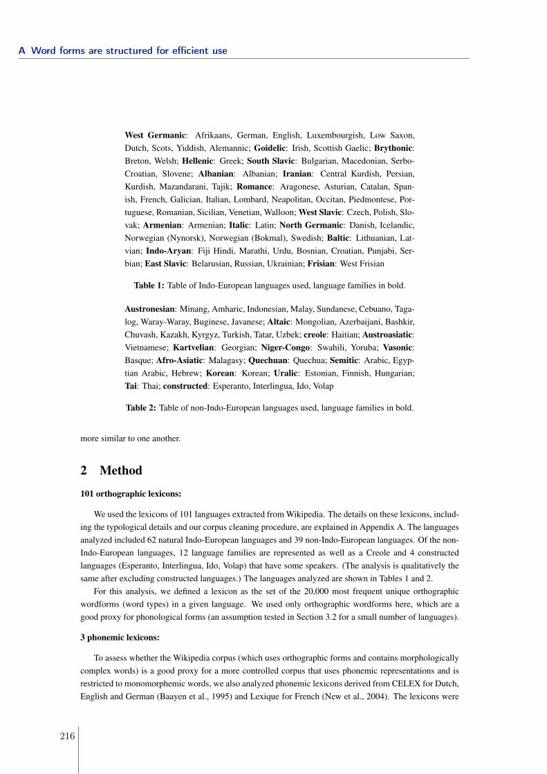
West Germanic: Afrikaans, German, English, Luxembourgish, Low Saxon,Dutch, Scots, Yiddish, Alemannic; Goidelic: Irish, Scottish Gaelic; Brythonic:Breton, Welsh; Hellenic: Greek; South Slavic: Bulgarian, Macedonian, Serbo-Croatian, Slovene; Albanian: Albanian; Iranian: Central Kurdish, Persian,Kurdish, Mazandarani, Tajik; Romance: Aragonese, Asturian, Catalan, Span-ish, French, Galician, Italian, Lombard, Neapolitan, Occitan, Piedmontese, Por-tuguese, Romanian, Sicilian, Venetian, Walloon; West Slavic: Czech, Polish, Slo-vak; Armenian: Armenian; Italic: Latin; North Germanic: Danish, Icelandic,Norwegian (Nynorsk), Norwegian (Bokmal), Swedish; Baltic: Lithuanian, Lat-vian; Indo-Aryan: Fiji Hindi, Marathi, Urdu, Bosnian, Croatian, Punjabi, Ser-bian; East Slavic: Belarusian, Russian, Ukrainian; Frisian: West Frisian
Table 1: Table of Indo-European languages used, language families in bold.
Austronesian: Minang, Amharic, Indonesian, Malay, Sundanese, Cebuano, Taga-log, Waray-Waray, Buginese, Javanese; Altaic: Mongolian, Azerbaijani, Bashkir,Chuvash, Kazakh, Kyrgyz, Turkish, Tatar, Uzbek; creole: Haitian; Austroasiatic:Vietnamese; Kartvelian: Georgian; Niger-Congo: Swahili, Yoruba; Vasonic:Basque; Afro-Asiatic: Malagasy; Quechuan: Quechua; Semitic: Arabic, Egyp-tian Arabic, Hebrew; Korean: Korean; Uralic: Estonian, Finnish, Hungarian;Tai: Thai; constructed: Esperanto, Interlingua, Ido, Volap
Table 2: Table of non-Indo-European languages used, language families in bold.
more similar to one another.
2 Method
101 orthographic lexicons:
We used the lexicons of 101 languages extracted from Wikipedia. The details on these lexicons, includ-ing the typological details and our corpus cleaning procedure, are explained in Appendix A. The languagesanalyzed included 62 natural Indo-European languages and 39 non-Indo-European languages. Of the non-Indo-European languages, 12 language families are represented as well as a Creole and 4 constructedlanguages (Esperanto, Interlingua, Ido, Volap) that have some speakers. (The analysis is qualitatively thesame after excluding constructed languages.) The languages analyzed are shown in Tables 1 and 2.
For this analysis, we defined a lexicon as the set of the 20,000 most frequent unique orthographicwordforms (word types) in a given language. We used only orthographic wordforms here, which are agood proxy for phonological forms (an assumption tested in Section 3.2 for a small number of languages).
3 phonemic lexicons:
To assess whether the Wikipedia corpus (which uses orthographic forms and contains morphologicallycomplex words) is a good proxy for a more controlled corpus that uses phonemic representations and isrestricted to monomorphemic words, we also analyzed phonemic lexicons derived from CELEX for Dutch,English and German (Baayen et al., 1995) and Lexique for French (New et al., 2004). The lexicons were
A Word forms are structured for efficient use
216
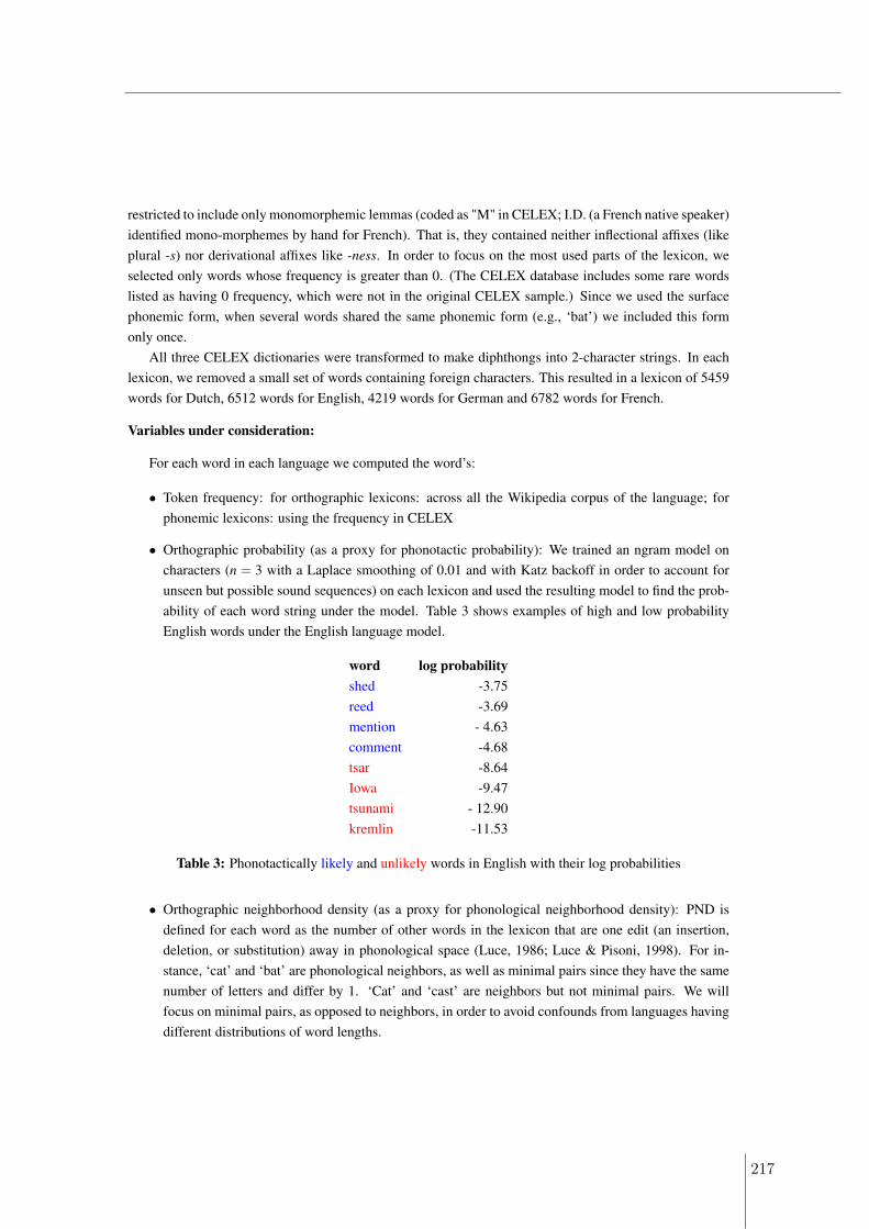
restricted to include only monomorphemic lemmas (coded as "M" in CELEX; I.D. (a French native speaker)identified mono-morphemes by hand for French). That is, they contained neither inflectional affixes (likeplural -s) nor derivational affixes like -ness. In order to focus on the most used parts of the lexicon, weselected only words whose frequency is greater than 0. (The CELEX database includes some rare wordslisted as having 0 frequency, which were not in the original CELEX sample.) Since we used the surfacephonemic form, when several words shared the same phonemic form (e.g., ‘bat’) we included this formonly once.
All three CELEX dictionaries were transformed to make diphthongs into 2-character strings. In eachlexicon, we removed a small set of words containing foreign characters. This resulted in a lexicon of 5459words for Dutch, 6512 words for English, 4219 words for German and 6782 words for French.
Variables under consideration:
For each word in each language we computed the word’s:
• Token frequency: for orthographic lexicons: across all the Wikipedia corpus of the language; forphonemic lexicons: using the frequency in CELEX
• Orthographic probability (as a proxy for phonotactic probability): We trained an ngram model oncharacters (n = 3 with a Laplace smoothing of 0.01 and with Katz backoff in order to account forunseen but possible sound sequences) on each lexicon and used the resulting model to find the prob-ability of each word string under the model. Table 3 shows examples of high and low probabilityEnglish words under the English language model.
word log probabilityshed -3.75reed -3.69mention - 4.63comment -4.68tsar -8.64Iowa -9.47tsunami - 12.90kremlin -11.53
Table 3: Phonotactically likely and unlikely words in English with their log probabilities
• Orthographic neighborhood density (as a proxy for phonological neighborhood density): PND isdefined for each word as the number of other words in the lexicon that are one edit (an insertion,deletion, or substitution) away in phonological space (Luce, 1986; Luce & Pisoni, 1998). For in-stance, ‘cat’ and ‘bat’ are phonological neighbors, as well as minimal pairs since they have the samenumber of letters and differ by 1. ‘Cat’ and ‘cast’ are neighbors but not minimal pairs. We willfocus on minimal pairs, as opposed to neighbors, in order to avoid confounds from languages havingdifferent distributions of word lengths.
217
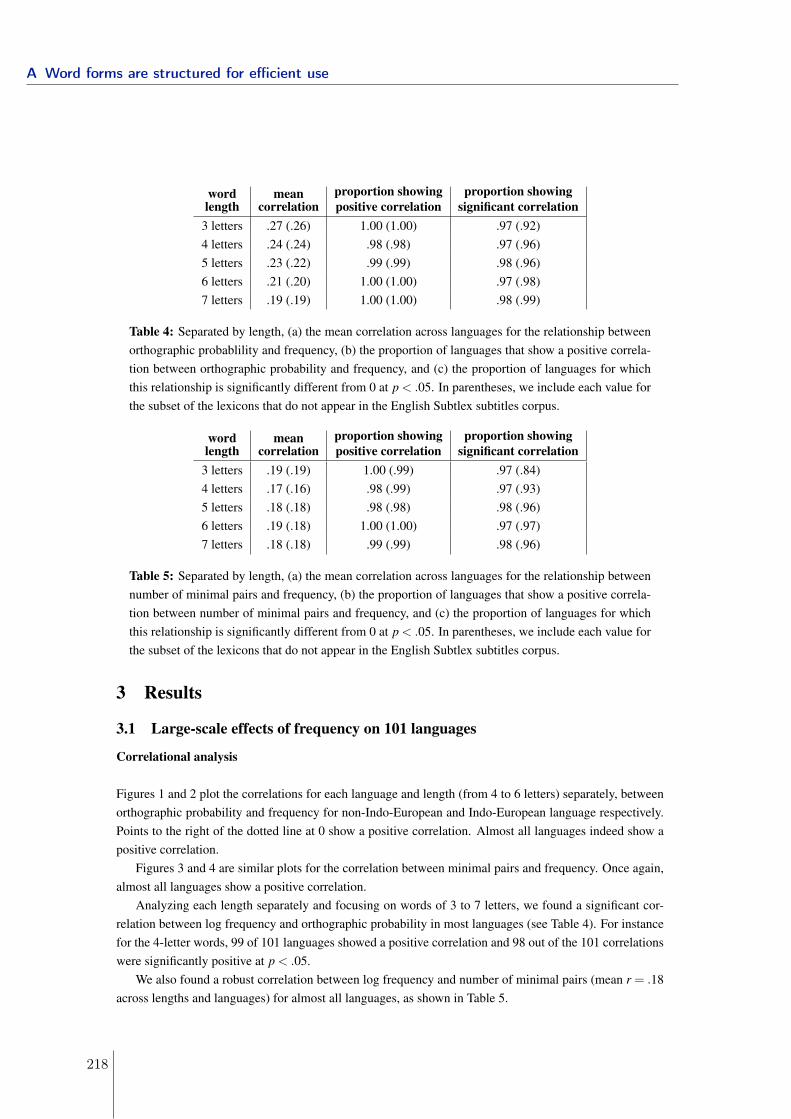
wordlength
meancorrelation
proportion showingpositive correlation
proportion showingsignificant correlation
3 letters .27 (.26) 1.00 (1.00) .97 (.92)4 letters .24 (.24) .98 (.98) .97 (.96)5 letters .23 (.22) .99 (.99) .98 (.96)6 letters .21 (.20) 1.00 (1.00) .97 (.98)7 letters .19 (.19) 1.00 (1.00) .98 (.99)
Table 4: Separated by length, (a) the mean correlation across languages for the relationship betweenorthographic probablility and frequency, (b) the proportion of languages that show a positive correla-tion between orthographic probability and frequency, and (c) the proportion of languages for whichthis relationship is significantly different from 0 at p < .05. In parentheses, we include each value forthe subset of the lexicons that do not appear in the English Subtlex subtitles corpus.
wordlength
meancorrelation
proportion showingpositive correlation
proportion showingsignificant correlation
3 letters .19 (.19) 1.00 (.99) .97 (.84)4 letters .17 (.16) .98 (.99) .97 (.93)5 letters .18 (.18) .98 (.98) .98 (.96)6 letters .19 (.18) 1.00 (1.00) .97 (.97)7 letters .18 (.18) .99 (.99) .98 (.96)
Table 5: Separated by length, (a) the mean correlation across languages for the relationship betweennumber of minimal pairs and frequency, (b) the proportion of languages that show a positive correla-tion between number of minimal pairs and frequency, and (c) the proportion of languages for whichthis relationship is significantly different from 0 at p < .05. In parentheses, we include each value forthe subset of the lexicons that do not appear in the English Subtlex subtitles corpus.
3 Results
3.1 Large-scale effects of frequency on 101 languages
Correlational analysis
Figures 1 and 2 plot the correlations for each language and length (from 4 to 6 letters) separately, betweenorthographic probability and frequency for non-Indo-European and Indo-European language respectively.Points to the right of the dotted line at 0 show a positive correlation. Almost all languages indeed show apositive correlation.
Figures 3 and 4 are similar plots for the correlation between minimal pairs and frequency. Once again,almost all languages show a positive correlation.
Analyzing each length separately and focusing on words of 3 to 7 letters, we found a significant cor-relation between log frequency and orthographic probability in most languages (see Table 4). For instancefor the 4-letter words, 99 of 101 languages showed a positive correlation and 98 out of the 101 correlationswere significantly positive at p < .05.
We also found a robust correlation between log frequency and number of minimal pairs (mean r = .18across lengths and languages) for almost all languages, as shown in Table 5.
A Word forms are structured for efficient use
218
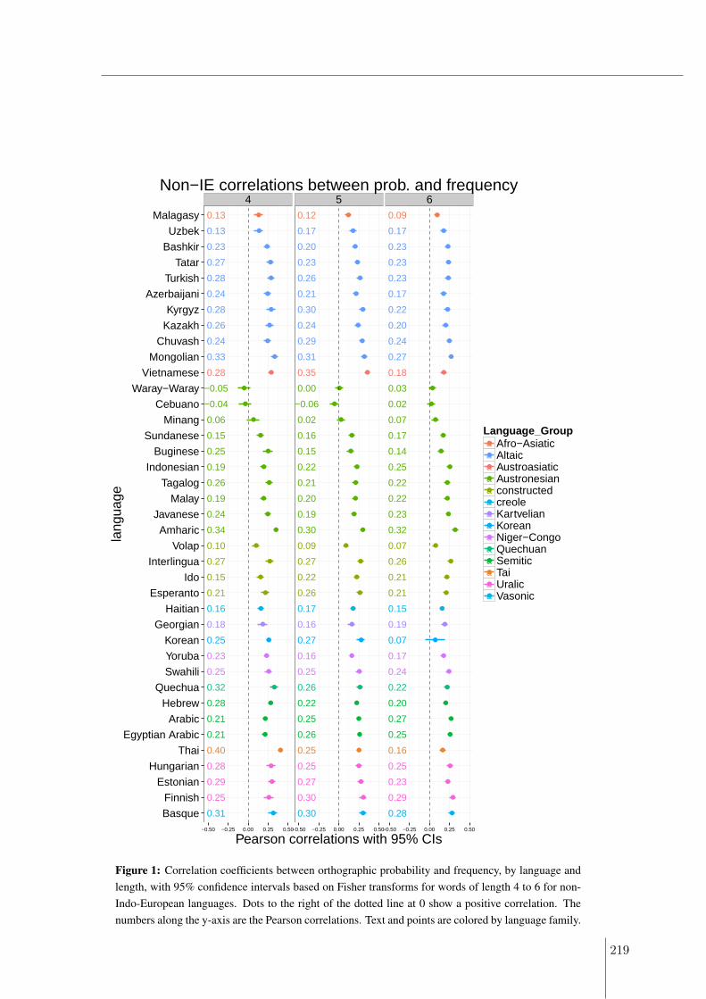
4 5 6●
●
●
●
●
●
●
●
●
●
●
●
●
●
●
●
●
●
●
●
●
●
●
●
●
●
●
●
●
●
●
●
●
●
●
●
●
●
●
0.13
0.13
0.28
0.23
0.27
0.24
0.28
0.24
0.26
0.33
0.28
−0.05
−0.04
0.06
0.15
0.25
0.19
0.26
0.19
0.24
0.34
0.10
0.27
0.15
0.21
0.16
0.18
0.25
0.23
0.25
0.32
0.21
0.28
0.21
0.40
0.28
0.29
0.25
0.31
●
●
●
●
●
●
●
●
●
●
●
●
●
●
●
●
●
●
●
●
●
●
●
●
●
●
●
●
●
●
●
●
●
●
●
●
●
●
●
0.12
0.20
0.23
0.17
0.21
0.26
0.24
0.30
0.29
0.31
0.35
−0.06
0.00
0.02
0.15
0.16
0.21
0.22
0.20
0.19
0.30
0.09
0.27
0.26
0.22
0.17
0.16
0.27
0.16
0.25
0.26
0.22
0.25
0.26
0.25
0.25
0.27
0.30
0.30
●
●
●
●
●
●
●
●
●
●
●
●
●
●
●
●
●
●
●
●
●
●
●
●
●
●
●
●
●
●
●
●
●
●
●
●
●
●
●
0.09
0.17
0.23
0.22
0.17
0.23
0.23
0.20
0.27
0.24
0.18
0.02
0.03
0.07
0.14
0.17
0.25
0.22
0.22
0.23
0.32
0.07
0.26
0.21
0.21
0.15
0.19
0.07
0.24
0.17
0.22
0.20
0.27
0.25
0.16
0.25
0.29
0.23
0.28Basque
Finnish
Estonian
Hungarian
Thai
Egyptian Arabic
Arabic
Hebrew
Quechua
Swahili
Yoruba
Korean
Georgian
Haitian
Esperanto
Ido
Interlingua
Volap
Amharic
Javanese
Malay
Tagalog
Indonesian
Buginese
Sundanese
Minang
Cebuano
Waray−Waray
Vietnamese
Mongolian
Chuvash
Kazakh
Kyrgyz
Azerbaijani
Turkish
Tatar
Bashkir
Uzbek
Malagasy
−0.50 −0.25 0.00 0.25 0.50−0.50 −0.25 0.00 0.25 0.50−0.50 −0.25 0.00 0.25 0.50
Pearson correlations with 95% CIs
lang
uage
Language_Group●a●a●a●a●a●a●a●a●a●a●a●a●a●a
Afro−AsiaticAltaicAustroasiaticAustronesianconstructedcreoleKartvelianKoreanNiger−CongoQuechuanSemiticTaiUralicVasonic
Non−IE correlations between prob. and frequency
Figure 1: Correlation coefficients between orthographic probability and frequency, by language andlength, with 95% confidence intervals based on Fisher transforms for words of length 4 to 6 for non-Indo-European languages. Dots to the right of the dotted line at 0 show a positive correlation. Thenumbers along the y-axis are the Pearson correlations. Text and points are colored by language family.
219
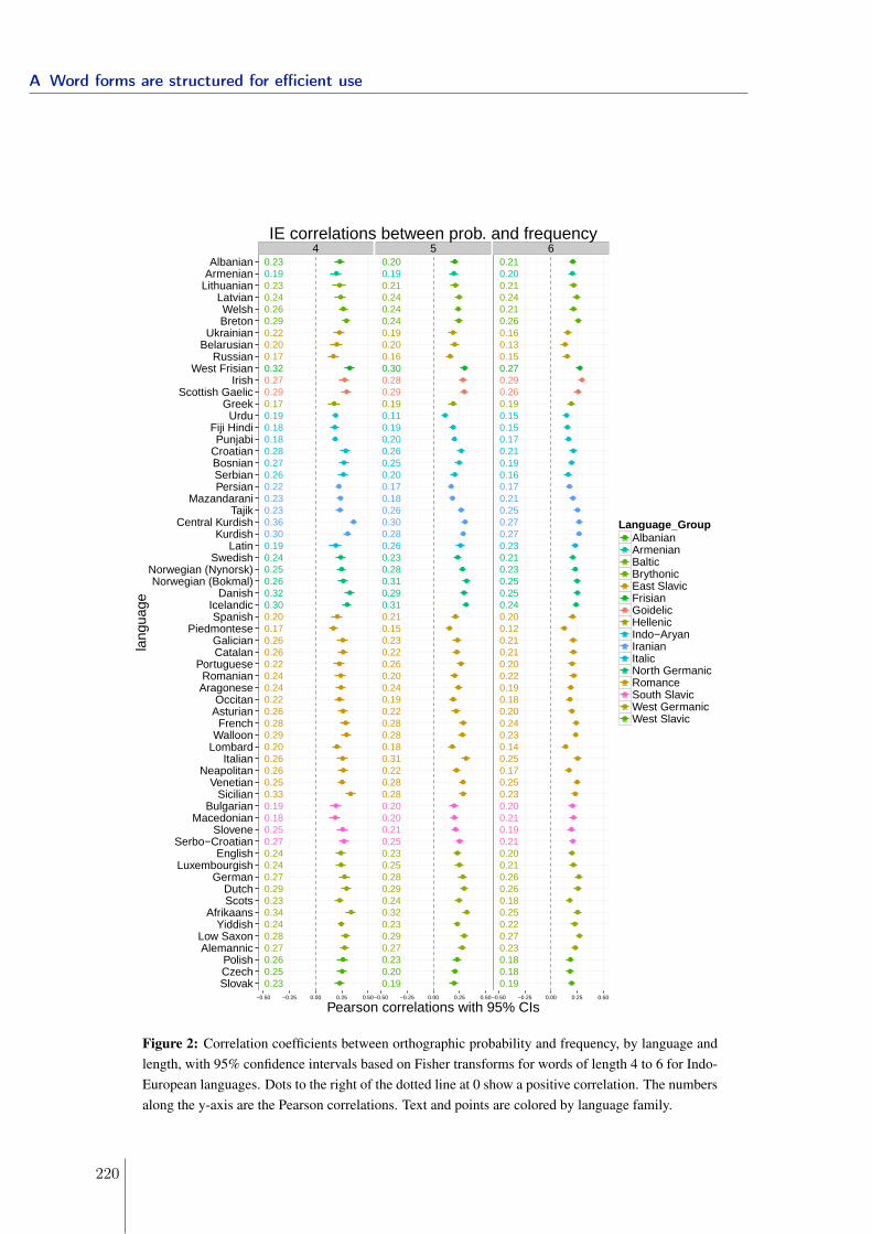
4 5 6●
●
●
●
●
●
●
●
●
●
●
●
●
●
●
●
●
●
●
●
●
●
●
●
●
●
●
●
●
●
●
●
●
●
●
●
●
●
●
●
●
●
●
●
●
●
●
●
●
●
●
●
●
●
●
●
●
●
●
●
●
●
0.230.190.230.240.260.29
0.200.17
0.22
0.320.270.290.170.19
0.280.27
0.180.18
0.260.22
0.230.23
0.300.36
0.190.240.250.260.320.30
0.170.20
0.240.22
0.24
0.26
0.26
0.26
0.20
0.28
0.26
0.22
0.25
0.29
0.26
0.330.19
0.270.250.18
0.27
0.24
0.29
0.24
0.23
0.24
0.34
0.280.270.260.250.23
●
●
●
●
●
●
●
●
●
●
●
●
●
●
●
●
●
●
●
●
●
●
●
●
●
●
●
●
●
●
●
●
●
●
●
●
●
●
●
●
●
●
●
●
●
●
●
●
●
●
●
●
●
●
●
●
●
●
●
●
●
●
0.200.190.210.240.240.240.190.200.160.300.280.290.190.110.19
0.260.25
0.20
0.200.170.180.260.300.280.260.23
0.29
0.280.31
0.310.21
0.230.22
0.19
0.15
0.22
0.200.24
0.26
0.280.280.18
0.220.31
0.280.28
0.200.21
0.20
0.250.230.25
0.32
0.290.24
0.28
0.230.290.270.23
0.190.20
●
●
●
●
●
●
●
●
●
●
●
●
●
●
●
●
●
●
●
●
●
●
●
●
●
●
●
●
●
●
●
●
●
●
●
●
●
●
●
●
●
●
●
●
●
●
●
●
●
●
●
●
●
●
●
●
●
●
●
●
●
●
0.210.200.210.240.210.260.160.130.150.270.290.260.19
0.150.15
0.17
0.16
0.210.19
0.170.210.250.270.270.23
0.230.21
0.250.25
0.24
0.210.21
0.20
0.20
0.18
0.12
0.23
0.22
0.24
0.19
0.20
0.250.17
0.14
0.250.230.200.210.190.210.20
0.26
0.21
0.180.25
0.26
0.270.22
0.230.180.180.19Slovak
CzechPolish
AlemannicLow Saxon
YiddishAfrikaans
ScotsDutch
GermanLuxembourgish
EnglishSerbo−Croatian
SloveneMacedonian
BulgarianSicilian
VenetianNeapolitan
ItalianLombardWalloonFrench
AsturianOccitan
AragoneseRomanian
PortugueseCatalanGalician
PiedmonteseSpanish
IcelandicDanish
Norwegian (Bokmal)Norwegian (Nynorsk)
SwedishLatin
KurdishCentral Kurdish
TajikMazandarani
PersianSerbianBosnianCroatianPunjabi
Fiji HindiUrdu
GreekScottish Gaelic
IrishWest Frisian
RussianBelarusianUkrainian
BretonWelsh
LatvianLithuanianArmenianAlbanian
−0.50 −0.25 0.00 0.25 0.50−0.50 −0.25 0.00 0.25 0.50−0.50 −0.25 0.00 0.25 0.50
Pearson correlations with 95% CIs
lang
uage
Language_Group●a●a●a●a●a●a●a●a●a●a●a●a●a●a●a●a
AlbanianArmenianBalticBrythonicEast SlavicFrisianGoidelicHellenicIndo−AryanIranianItalicNorth GermanicRomanceSouth SlavicWest GermanicWest Slavic
IE correlations between prob. and frequency
Figure 2: Correlation coefficients between orthographic probability and frequency, by language andlength, with 95% confidence intervals based on Fisher transforms for words of length 4 to 6 for Indo-European languages. Dots to the right of the dotted line at 0 show a positive correlation. The numbersalong the y-axis are the Pearson correlations. Text and points are colored by language family.
A Word forms are structured for efficient use
220
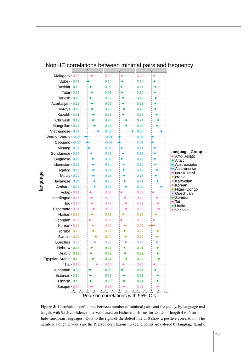
4 5 6●
●
●
●
●
●
●
●
●
●
●
●
●
●
●
●
●
●
●
●
●
●
●
●
●
●
●
●
●
●
●
●
●
●
●
●
●
●
●
0.15
0.02
0.10
0.10
0.15
0.15
0.16
0.19
0.21
0.25
0.37
−0.05
−0.00
0.04
0.13
0.19
0.19
0.19
0.20
0.24
0.25
0.11
0.14
0.16
0.21
0.15
0.08
0.18
0.20
0.29
0.26
0.12
0.15
0.19
0.33
0.09
0.10
0.10
0.14
●
●
●
●
●
●
●
●
●
●
●
●
●
●
●
●
●
●
●
●
●
●
●
●
●
●
●
●
●
●
●
●
●
●
●
●
●
●
●
0.09
0.06
0.09
0.10
0.12
0.12
0.13
0.16
0.23
0.23
0.46
−0.02
−0.01
0.07
0.07
0.12
0.14
0.14
0.15
0.18
0.23
0.06
0.19
0.23
0.23
0.13
0.05
0.20
0.17
0.22
0.22
0.17
0.19
0.24
0.14
0.09
0.15
0.15
0.15
●
●
●
●
●
●
●
●
●
●
●
●
●
●
●
●
●
●
●
●
●
●
●
●
●
●
●
●
●
●
●
●
●
●
●
●
●
●
●
0.09
0.10
0.12
0.13
0.13
0.14
0.15
0.18
0.20
0.24
0.35
0.03
0.04
0.11
0.12
0.12
0.14
0.15
0.19
0.21
0.34
0.05
0.19
0.23
0.26
0.15
0.08
0.02
0.19
0.22
0.19
0.21
0.22
0.25
0.10
0.14
0.21
0.21
0.21Basque
Finnish
Estonian
Hungarian
Thai
Egyptian Arabic
Arabic
Hebrew
Quechua
Swahili
Yoruba
Korean
Georgian
Haitian
Esperanto
Ido
Interlingua
Volap
Amharic
Javanese
Malay
Tagalog
Indonesian
Buginese
Sundanese
Minang
Cebuano
Waray−Waray
Vietnamese
Mongolian
Chuvash
Kazakh
Kyrgyz
Azerbaijani
Turkish
Tatar
Bashkir
Uzbek
Malagasy
−0.50 −0.25 0.00 0.25 0.50−0.50 −0.25 0.00 0.25 0.50−0.50 −0.25 0.00 0.25 0.50
Pearson correlations with 95% CIs
lang
uage
Language_Group●a●a●a●a●a●a●a●a●a●a●a●a●a●a
Afro−AsiaticAltaicAustroasiaticAustronesianconstructedcreoleKartvelianKoreanNiger−CongoQuechuanSemiticTaiUralicVasonic
Non−IE correlations between minimal pairs and frequency
Figure 3: Correlation coefficients between number of minimal pairs and frequency, by language andlength, with 95% confidence intervals based on Fisher transforms for words of length 4 to 6 for non-Indo-European languages. Dots to the right of the dotted line at 0 show a positive correlation. Thenumbers along the y-axis are the Pearson correlations. Text and points are colored by language family.
221
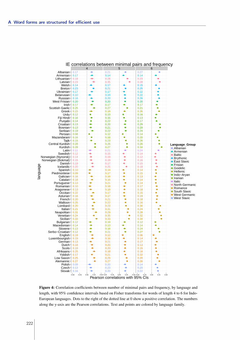
4 5 6●
●
●
●
●
●
●
●
●
●
●
●
●
●
●
●
●
●
●
●
●
●
●
●
●
●
●
●
●
●
●
●
●
●
●
●
●
●
●
●
●
●
●
●
●
●
●
●
●
●
●
●
●
●
●
●
●
●
●
●
●
●
0.170.170.180.230.140.23
0.100.16
0.17
0.200.170.250.150.12
0.130.13
0.140.16
0.190.08
0.150.16
0.280.28
0.110.120.140.150.190.20
0.090.10
0.100.13
0.13
0.16
0.16
0.18
0.20
0.20
0.21
0.22
0.24
0.25
0.31
0.330.12
0.120.130.14
0.13
0.17
0.18
0.19
0.19
0.19
0.25
0.250.270.090.130.16
●
●
●
●
●
●
●
●
●
●
●
●
●
●
●
●
●
●
●
●
●
●
●
●
●
●
●
●
●
●
●
●
●
●
●
●
●
●
●
●
●
●
●
●
●
●
●
●
●
●
●
●
●
●
●
●
●
●
●
●
●
●
0.210.140.280.350.170.210.170.190.200.200.170.270.180.130.16
0.200.21
0.22
0.220.120.180.230.260.270.210.15
0.17
0.190.19
0.250.14
0.160.16
0.17
0.17
0.17
0.180.18
0.21
0.210.220.23
0.290.31
0.330.35
0.130.18
0.19
0.210.120.16
0.18
0.200.20
0.21
0.210.250.270.20
0.200.23
●
●
●
●
●
●
●
●
●
●
●
●
●
●
●
●
●
●
●
●
●
●
●
●
●
●
●
●
●
●
●
●
●
●
●
●
●
●
●
●
●
●
●
●
●
●
●
●
●
●
●
●
●
●
●
●
●
●
●
●
●
●
0.270.140.230.280.150.250.220.220.260.200.170.210.26
0.130.16
0.17
0.24
0.290.29
0.140.200.260.260.340.24
0.120.14
0.150.16
0.18
0.130.14
0.14
0.14
0.15
0.15
0.16
0.17
0.18
0.18
0.19
0.240.28
0.30
0.320.340.120.140.240.270.06
0.13
0.14
0.150.16
0.17
0.200.22
0.260.140.200.22Slovak
CzechPolish
AlemannicLow Saxon
YiddishAfrikaans
ScotsDutch
GermanLuxembourgish
EnglishSerbo−Croatian
SloveneMacedonian
BulgarianSicilian
VenetianNeapolitan
ItalianLombardWalloonFrench
AsturianOccitan
AragoneseRomanian
PortugueseCatalanGalician
PiedmonteseSpanish
IcelandicDanish
Norwegian (Bokmal)Norwegian (Nynorsk)
SwedishLatin
KurdishCentral Kurdish
TajikMazandarani
PersianSerbianBosnianCroatianPunjabi
Fiji HindiUrdu
GreekScottish Gaelic
IrishWest Frisian
RussianBelarusianUkrainian
BretonWelsh
LatvianLithuanianArmenianAlbanian
−0.50 −0.25 0.00 0.25 0.50−0.50 −0.25 0.00 0.25 0.50−0.50 −0.25 0.00 0.25 0.50
Pearson correlations with 95% CIs
lang
uage
Language_Group●a●a●a●a●a●a●a●a●a●a●a●a●a●a●a●a
AlbanianArmenianBalticBrythonicEast SlavicFrisianGoidelicHellenicIndo−AryanIranianItalicNorth GermanicRomanceSouth SlavicWest GermanicWest Slavic
IE correlations between minimal pairs and frequency
Figure 4: Correlation coefficients between number of minimal pairs and frequency, by language andlength, with 95% confidence intervals based on Fisher transforms for words of length 4 to 6 for Indo-European languages. Dots to the right of the dotted line at 0 show a positive correlation. The numbersalong the y-axis are the Pearson correlations. Text and points are colored by language family.
A Word forms are structured for efficient use
222
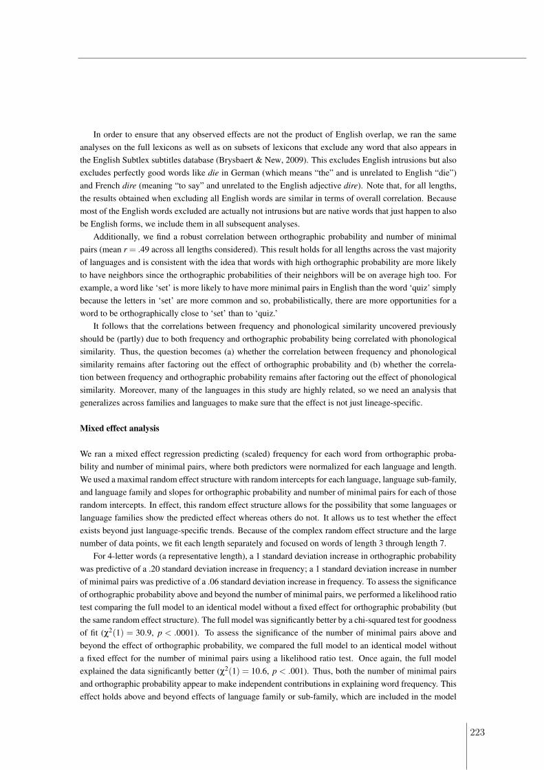
In order to ensure that any observed effects are not the product of English overlap, we ran the sameanalyses on the full lexicons as well as on subsets of lexicons that exclude any word that also appears inthe English Subtlex subtitles database (Brysbaert & New, 2009). This excludes English intrusions but alsoexcludes perfectly good words like die in German (which means “the” and is unrelated to English “die”)and French dire (meaning “to say” and unrelated to the English adjective dire). Note that, for all lengths,the results obtained when excluding all English words are similar in terms of overall correlation. Becausemost of the English words excluded are actually not intrusions but are native words that just happen to alsobe English forms, we include them in all subsequent analyses.
Additionally, we find a robust correlation between orthographic probability and number of minimalpairs (mean r = .49 across all lengths considered). This result holds for all lengths across the vast majorityof languages and is consistent with the idea that words with high orthographic probability are more likelyto have neighbors since the orthographic probabilities of their neighbors will be on average high too. Forexample, a word like ‘set’ is more likely to have more minimal pairs in English than the word ‘quiz’ simplybecause the letters in ‘set’ are more common and so, probabilistically, there are more opportunities for aword to be orthographically close to ‘set’ than to ‘quiz.’
It follows that the correlations between frequency and phonological similarity uncovered previouslyshould be (partly) due to both frequency and orthographic probability being correlated with phonologicalsimilarity. Thus, the question becomes (a) whether the correlation between frequency and phonologicalsimilarity remains after factoring out the effect of orthographic probability and (b) whether the correla-tion between frequency and orthographic probability remains after factoring out the effect of phonologicalsimilarity. Moreover, many of the languages in this study are highly related, so we need an analysis thatgeneralizes across families and languages to make sure that the effect is not just lineage-specific.
Mixed effect analysis
We ran a mixed effect regression predicting (scaled) frequency for each word from orthographic proba-bility and number of minimal pairs, where both predictors were normalized for each language and length.We used a maximal random effect structure with random intercepts for each language, language sub-family,and language family and slopes for orthographic probability and number of minimal pairs for each of thoserandom intercepts. In effect, this random effect structure allows for the possibility that some languages orlanguage families show the predicted effect whereas others do not. It allows us to test whether the effectexists beyond just language-specific trends. Because of the complex random effect structure and the largenumber of data points, we fit each length separately and focused on words of length 3 through length 7.
For 4-letter words (a representative length), a 1 standard deviation increase in orthographic probabilitywas predictive of a .20 standard deviation increase in frequency; a 1 standard deviation increase in numberof minimal pairs was predictive of a .06 standard deviation increase in frequency. To assess the significanceof orthographic probability above and beyond the number of minimal pairs, we performed a likelihood ratiotest comparing the full model to an identical model without a fixed effect for orthographic probability (butthe same random effect structure). The full model was significantly better by a chi-squared test for goodnessof fit (χ2(1) = 30.9, p < .0001). To assess the significance of the number of minimal pairs above andbeyond the effect of orthographic probability, we compared the full model to an identical model withouta fixed effect for the number of minimal pairs using a likelihood ratio test. Once again, the full modelexplained the data significantly better (χ2(1) = 10.6, p < .001). Thus, both the number of minimal pairsand orthographic probability appear to make independent contributions in explaining word frequency. Thiseffect holds above and beyond effects of language family or sub-family, which are included in the model
223
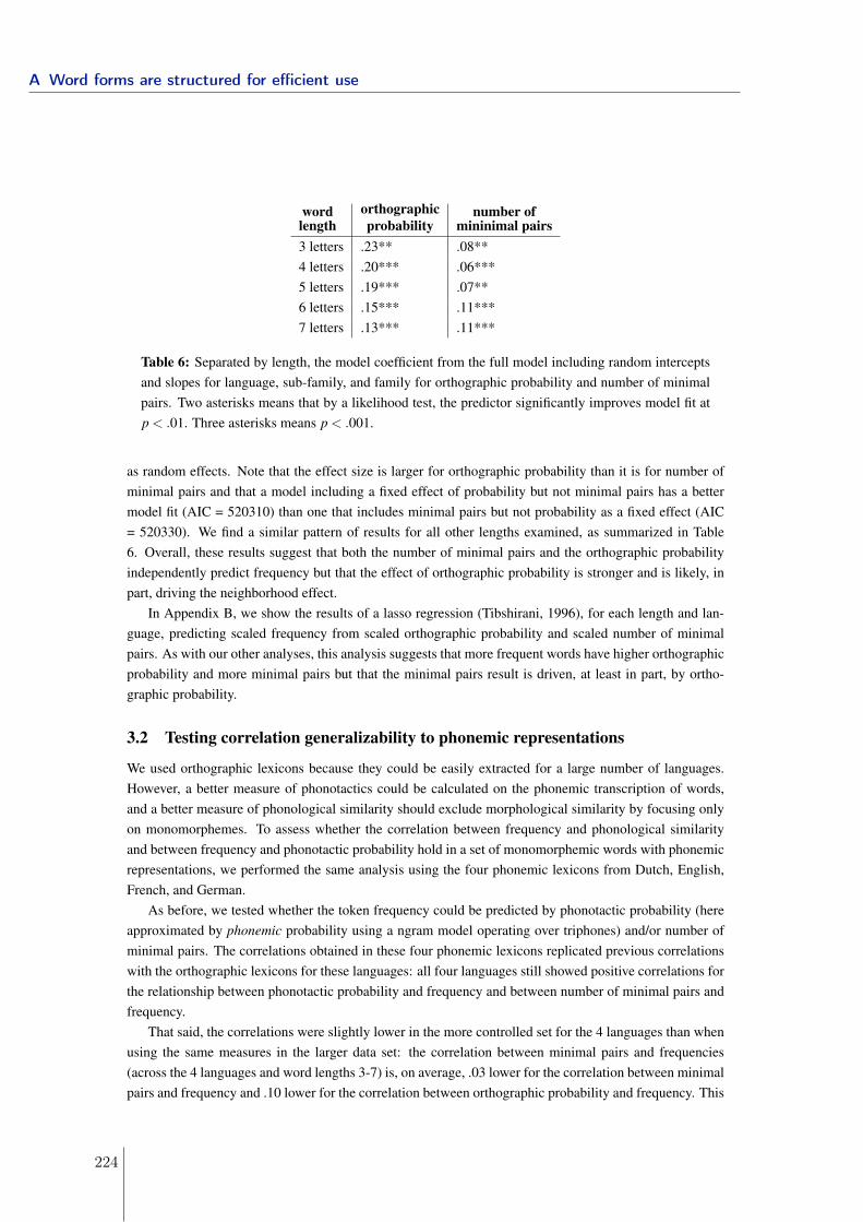
wordlength
orthographicprobability
number ofmininimal pairs
3 letters .23** .08**4 letters .20*** .06***5 letters .19*** .07**6 letters .15*** .11***7 letters .13*** .11***
Table 6: Separated by length, the model coefficient from the full model including random interceptsand slopes for language, sub-family, and family for orthographic probability and number of minimalpairs. Two asterisks means that by a likelihood test, the predictor significantly improves model fit atp < .01. Three asterisks means p < .001.
as random effects. Note that the effect size is larger for orthographic probability than it is for number ofminimal pairs and that a model including a fixed effect of probability but not minimal pairs has a bettermodel fit (AIC = 520310) than one that includes minimal pairs but not probability as a fixed effect (AIC= 520330). We find a similar pattern of results for all other lengths examined, as summarized in Table6. Overall, these results suggest that both the number of minimal pairs and the orthographic probabilityindependently predict frequency but that the effect of orthographic probability is stronger and is likely, inpart, driving the neighborhood effect.
In Appendix B, we show the results of a lasso regression (Tibshirani, 1996), for each length and lan-guage, predicting scaled frequency from scaled orthographic probability and scaled number of minimalpairs. As with our other analyses, this analysis suggests that more frequent words have higher orthographicprobability and more minimal pairs but that the minimal pairs result is driven, at least in part, by ortho-graphic probability.
3.2 Testing correlation generalizability to phonemic representations
We used orthographic lexicons because they could be easily extracted for a large number of languages.However, a better measure of phonotactics could be calculated on the phonemic transcription of words,and a better measure of phonological similarity should exclude morphological similarity by focusing onlyon monomorphemes. To assess whether the correlation between frequency and phonological similarityand between frequency and phonotactic probability hold in a set of monomorphemic words with phonemicrepresentations, we performed the same analysis using the four phonemic lexicons from Dutch, English,French, and German.
As before, we tested whether the token frequency could be predicted by phonotactic probability (hereapproximated by phonemic probability using a ngram model operating over triphones) and/or number ofminimal pairs. The correlations obtained in these four phonemic lexicons replicated previous correlationswith the orthographic lexicons for these languages: all four languages still showed positive correlations forthe relationship between phonotactic probability and frequency and between number of minimal pairs andfrequency.
That said, the correlations were slightly lower in the more controlled set for the 4 languages than whenusing the same measures in the larger data set: the correlation between minimal pairs and frequencies(across the 4 languages and word lengths 3-7) is, on average, .03 lower for the correlation between minimalpairs and frequency and .10 lower for the correlation between orthographic probability and frequency. This
A Word forms are structured for efficient use
224
suggests that part of the effect could be driven by morphology–which is absent in the controlled phonemiclexicons but present in the Wikipedia corpus.
4 Discussion
We found that frequent wordforms are more likely to be similar to other wordforms and composed ofmore likely sequence of phonemes than infrequent ones. These correlations were robustly present acrossa large number and wide variety of typologically different languages. Just as the Zipfian word frequencydistribution allows for functional optimization of word lengths(Piantadosi, 2014; Piantadosi et al., 2011)and word forms (Piantadosi et al., 2012), this work shows that the frequency profile of even words of thesame length is structured in a non-arbitrary way so as to maximize the use of “good” word forms.
Note that, form a noisy channel perspective, there is a tradeoff in structuring the lexicon this way. Ina language where phonotactically probable strings in dense neighborhoods are the most frequent words,there may be an increased chance of perceptual confusion. On the other hand, it is possible that in everydayspeech, noise conditions may not be extreme enough that perceptual confusion would be an issue. Or maybethe cost of perceptual confusion–asking an interlocutor to repeat a phrase or getting the information someother way–is typically not high enough to offset the cost that would come with structuring the lexicon suchthat the most frequent word forms were phonetically odd.
We do not believe that the main result of this paper is purely a result of morphological regularity sincethe same analyses run on monomorphemic words in a subset of languages show the same pattern of results.Moreover, although phonotactic constraints are an obvious and major source of regularity in the lexicon, itis important to note that these results are not likely just the result of phonotactic constraints since the resultshold even after controlling for the influence of phonotactic probability, at least in the analyses reflectingthe influence of word usage. In a companion study (Mahowald et al., submitted) in which we constructed aphonotactically-controlled baseline for lexicons, we provided compelling evidence that natural lexicons aremore tightly clustered in phonetic space than would be expected by chance, over and above the constraintsimposed by phonotactics. This, taken together with the present results, suggests that languages tend tofavor wordform similarity in the lexicon.
In this study, we addressed the issue of why wordform similarity in lexicons diverges from what canbe expected by chance alone, but we leave it to future work to investigate how it got to be that way. Onepromising body of work in that vein concerns language evolution. Indeed, there has been much experimen-tal work studying the evolution of language showing that language users will preferentially discard formsand structures that are disadvantageous in favor of other, fitter words and phrases (Fedzechkina et al., 2012;K. Smith et al., 2003). Thus, one plausible mechanism for the effects described here is that generations oflearners improve on the lexicon, honing it over time by avoiding words that are too strange, complex, orthat otherwise don’t fit with the rest of the words in the lexicon.
References
Aylett, M., & Turk, A. (2004). The smooth signal redundancy hypothesis: A functional explanation forrelationships between redundancy, prosodic prominence, and duration in spontaneous speech. Languageand Speech, 47(1), 31âAS56.
Baayen, R., Piepenbrock, R., & Gulikers, L. (1995). The CELEX lexical database (release 2)[cd-rom].Philadelphia, PA: Linguistic Data Consortium, University of Pennsylvania [Distributor].
225
Brysbaert, M., & New, B. (2009). Moving beyond Kucera and Francis: A critical evaluation of currentword frequency norms and the introduction of a new and improved word frequency measure for americanenglish. Behavior Research Methods, 41(4), 977–990.
Chen, Q., & Mirman, D. (2012). Competition and cooperation among similar representations: toward aunified account of facilitative and inhibitory effects of lexical neighbors. Psychological review, 119(2),417.
Coady, J. A., & Aslin, R. N. (2004). Young children’s sensitivity to probabilistic phonotactics in thedeveloping lexicon. Journal of Experimental Child Psychology, 89(3), 183–213.
Dell, G. S., & Gordon, J. K. (2003). Neighbors in the lexicon: Friends or foes? Phonetics and Phonologyin Language Comprehension and Production: Differences and Similarities, 6, 9.
Efron, B., Hastie, T., Johnstone, I., Tibshirani, R., et al. (2004). Least angle regression. The Annals ofstatistics, 32(2), 407–499.
Fedzechkina, M., Jaeger, T. F., & Newport, E. L. (2012). Language learners restructure their input tofacilitate efficient communication. Proceedings of the National Academy of Sciences, 109(44), 17897–17902.
Frauenfelder, U., Baayen, R., & Hellwig, F. (1993). Neighborhood density and frequency across languagesand modalities. Journal of Memory and Language, 32(6), 781–804.
Gahl, S., Yao, Y., & Johnson, K. (2012). Why reduce? phonological neighborhood density and phoneticreduction in spontaneous speech. Journal of Memory and Language, 66(4), 789–806.
Gibson, E., Bergen, L., & Piantadosi, S. (2013). Rational integration of noisy evidence and prior semanticexpectations in sentence interpretation. Proceedings of the National Academy of Sciences.
Jusczyk, P., & Luce, P. (1994). Infants’ sensitivity to phonotactic patterns in the native language. Journalof Memory and Language, 33(5), 630–645.
Kawasaki, H., & Ohala, J. J. (1980). Acoustic basis for universal constraints on sound sequences. TheJournal of the Acoustical Society of America, 68(S1), S33–S33.
Landauer, T., & Streeter, L. (1973). Structural differences between common and rare words: Failureof equivalence assumptions for theories of word recognition. Journal of Verbal Learning and VerbalBehavior, 12(2), 119–131.
Levy, R. (2008). A noisy-channel model of rational human sentence comprehension under uncertain input.In Proceedings of the conference on empirical methods in natural language processing (p. 234âAS243).
Levy, R., & Jaeger, T. (2007). Speakers optimize information density through syntactic reduction. InH. T. SchÃulkopf B Platt J (Ed.), (pp. 849–856). Cambridge, MA: MIT Press.
Lindblom, B. (1983). Economy of speech gestures. Springer.
Lindblom, B. (1990). Explaining phonetic variation: A sketch of the h&h theory. In Speech productionand speech modelling (pp. 403–439). Springer.
Lindblom, B. (1992). Phonological units as adaptive emergents of lexical development. Phonologicaldevelopment: Models, research, implications, 131âAS163.
A Word forms are structured for efficient use
226
Luce, P. A. (1986). Neighborhoods of words in the mental lexicon. Research on Speech Perception.Technical Report No. 6..
Luce, P. A., & Pisoni, D. B. (1998). Recognizing spoken words: The neighborhood activation model. Earand hearing, 19(1), 1.
Magnuson, J. S., Dixon, J. A., Tanenhaus, M. K., & Aslin, R. N. (2007). The dynamics of lexical compe-tition during spoken word recognition. Cognitive Science, 31(1), 133–156.
New, B., Pallier, C., Brysbaert, M., & Ferrand, L. (2004). Lexique 2: A new french lexical database.Behavior Research Methods, Instruments, & Computers, 36(3), 516–524.
Ngon, C., Martin, A., Dupoux, E., Cabrol, D., Dutat, M., & Peperkamp, S. (2013). (Non)words,(non)words, (non)words: evidence for a protolexicon during the first year of life. Developmental Science,16(1), 24–34.
Piantadosi, S. (2014). Zipf’s word frequency law in natural language: A critical review and future direc-tions. Psychonomic Bulletin & Review, 21(5), 1112–1130.
Piantadosi, S., Tily, H., & Gibson, E. (2011). Word lengths are optimized for efficient communication.Proceedings of the National Academy of Sciences, 108(9), 3526.
Piantadosi, S., Tily, H., & Gibson, E. (2012). The communicative function of ambiguity in language.Cognition, 122(3), 280–291.
Sadat, J., Martin, C. D., Costa, A., & Alario, F.-X. (2014). Reconciling phonological neighborhood effectsin speech production through single trial analysis. Cognitive psychology, 68, 33–58.
Shannon, C. (1948). A Mathematical Theory of Communication. Bell System Technical Journal, 27,623–656.
Smith, K., Kirby, S., & Brighton, H. (2003). Iterated learning: A framework for the emergence of language.Artificial Life, 9(4), 371–386.
Smith, P. (1970). Communication over noisy channels: Applications to the statistical structure of english.British Journal of Psychology, 61(2), 197–206.
Stemberger, J. P. (2004). Neighbourhood effects on error rates in speech production. Brain and Language,90(1), 413–422.
Storkel, H. L. (2004). Do children acquire dense neighborhoods? an investigation of similarity neighbor-hoods in lexical acquisition. Applied Psycholinguistics, 25(02).
Storkel, H. L. (2009). Developmental differences in the effects of phonological, lexical and semanticvariables on word learning by infants. Journal of Child Language, 36(02), 291.
Storkel, H. L., Armbruster, J., & Hogan, T. P. (2006). Differentiating phonotactic probability and neigh-borhood density in adult word learning. Journal of Speech, Language, and Hearing Research, 49(6),1175–1192.
Storkel, H. L., & Hoover, J. R. (2010). An online calculator to compute phonotactic probability andneighborhood density on the basis of child corpora of spoken american english. Behavior ResearchMethods, 42(2), 497–506.
227
Storkel, H. L., & Lee, S.-Y. (2011). The independent effects of phonotactic probability and neighbourhooddensity on lexical acquisition by preschool children. Language and Cognitive Processes, 26(2), 191–211.
Swingley, D., & Aslin, R. N. (2007). Lexical competition in young children’s word learning. Cognitivepsychology, 54(2), 99.
Tibshirani, R. (1996). Regression shrinkage and selection via the lasso. Journal of the Royal StatisticalSociety. Series B (Methodological), 267–288.
van Son, R., & Pols, L. (2003). How efficient is speech? Proceedings Institute of Phonetic Sciences,University of Amsterdam, 25, 171âAS184.
Vitevitch, M. S. (1999). Phonotactics, neighborhood activation, and lexical access for spoken words. Brainand Language, 68(1-2), 306–311.
Vitevitch, M. S., & Luce, P. A. (1998). When words compete: Levels of processing in perception of spokenwords. Psychological science, 9(4), 325–329.
Vitevitch, M. S., & Sommers, M. S. (2003). The facilitative influence of phonological similarity andneighborhood frequency in speech production in younger and older adults. Memory & Cognition, 31(4),491–504.
Vitevitch, M. S., & Stamer, M. K. (2006). The curious case of competition in spanish speech production.Language and cognitive processes, 21(6), 760–770.
Zipf, G. (1935). The psychology of language. NY Houghton-Mifflin.
Zipf, G. (1949). Human behavior and the principle of least effort.
A Word forms are structured for efficient use
228
A Appendix: Dataset of 101 lexicons from Wikipedia
We started with lexicons of 115 languages from their Wikipedia databases (https://dumps.wikimedia.org). We then excluded languages for which a spot-check for non-native (usually English) words in thetop 100 most frequent words in the lexicon between 3 and 7 characters revealed more than 80% of wordswere not native. In this way, languages that used non-alphabetic scripts (like Chinese) were generally ex-cluded since the 3-7 letter words in Chinese Wikipedia are often English. However, we included languageslike Korean in which words generally consist of several characters. After these exclusions, 101 languagesremained.2 We analyzed the data both with and without these exclusions, and the exclusions do not sig-nificantly affect the overall direction or magnitude of the results. The final languages included 62 naturalIndo-European languages and 39 non-Indo-European languages. Of the non-Indo-European languages,there are 12 language families represented as well as a Creole and 4 constructed languages (Esperanto,Interlingua, Ido, Volap) that have some speakers. (The analysis is qualitatively the same after excludingconstructed languages.)
To get a sense of how clean these Wikipedia lexicons are, we randomly sampled 10 languages for whichwe then inspected the 100 most frequent words and an additional 100 random words to look for intrusionof English words, HTML characters, or other undesirable properties.
For the top 100 words in the lexicons of the 10 sampled languages, we found at most 3 erroneous words.For the same languages, we also inspected a randomly selected 100 words and found that the mean numberof apparently non-intrusive words was 93.5 (with a range from 85 to 99). The most common intrusion inthese languages was English words.
B Appendix: Lasso regression analysis
Lasso analysis
We fit separate lasso regressions (Tibshirani, 1996) for each length and language predicting scaled fre-quency from scaled orthographic probability and scaled number of minimal pairs. The lasso regressionputs a constraint on the sum of the absolute value of the regression coefficients (L1-regularization) andthus effectively pushes some coefficients to 0 if they are not needed. We set the value of the lasso parame-ter using cross-validation to minimize the out-of-sample error and used the lars software package (Efronet al., 2004) in R.
In Figure 5, for each language, we plot the coefficient for scaled number of minimal pairs on the x-axisagainst the coefficient for scaled orthographic probability on the y-axis. If both predictors show robusteffects, we would predict the points to cluster in the upper right quadrant. If both predictors showed littleeffect, the points would cluster around 0.
Although the lasso regression drives some of these coefficients to 0, the plot clearly shows effects ofboth minimal pairs and orthographic probability (with larger coefficients in general for orthographic prob-ability). Specifically, for 4 and 5 letter words, only 2 languages show negative coefficients for orthographicprobability and none for 6 and 7 letter words.
Thus, it appears that more frequent words also have higher orthographic probability as well as moreminimal pairs, although the minimal pairs effect is driven in part by orthographic probability.
2We excluded: Gujarati, Telugu, Tamil, Bishnupriya Manipuri, Cantonese, Newar, Bengali, Japanese, Hindi, Malayalam, Marathi,Burmese, Nepali, Kannada
229
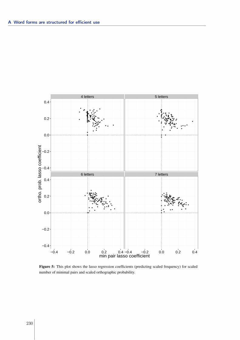
4 letters 5 letters
6 letters 7 letters
−0.4
−0.2
0.0
0.2
0.4
−0.4
−0.2
0.0
0.2
0.4
−0.4 −0.2 0.0 0.2 0.4 −0.4 −0.2 0.0 0.2 0.4min pair lasso coefficient
orth
o. p
rob.
lass
o co
effic
ient
Figure 5: This plot shows the lasso regression coefficients (predicting scaled frequency) for scalednumber of minimal pairs and scaled orthographic probability.
A Word forms are structured for efficient use
230
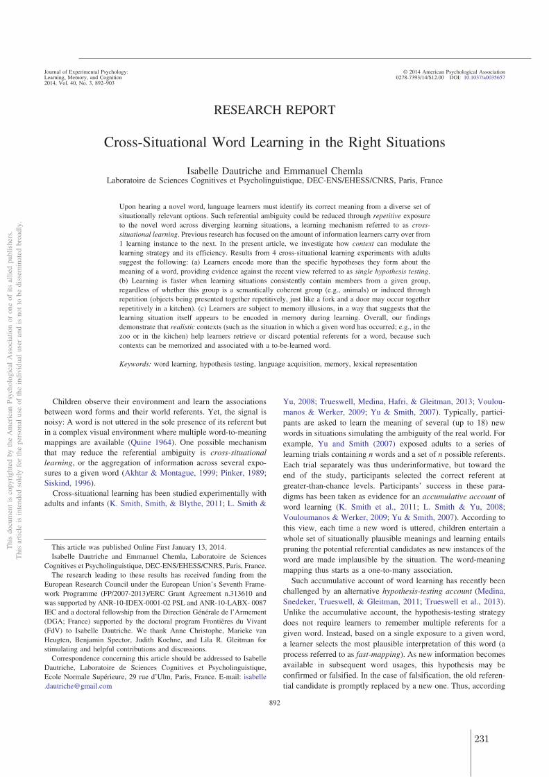
RESEARCH REPORT
Cross-Situational Word Learning in the Right Situations
Isabelle Dautriche and Emmanuel ChemlaLaboratoire de Sciences Cognitives et Psycholinguistique, DEC-ENS/EHESS/CNRS, Paris, France
Upon hearing a novel word, language learners must identify its correct meaning from a diverse set ofsituationally relevant options. Such referential ambiguity could be reduced through repetitive exposureto the novel word across diverging learning situations, a learning mechanism referred to as cross-situational learning. Previous research has focused on the amount of information learners carry over from1 learning instance to the next. In the present article, we investigate how context can modulate thelearning strategy and its efficiency. Results from 4 cross-situational learning experiments with adultssuggest the following: (a) Learners encode more than the specific hypotheses they form about themeaning of a word, providing evidence against the recent view referred to as single hypothesis testing.(b) Learning is faster when learning situations consistently contain members from a given group,regardless of whether this group is a semantically coherent group (e.g., animals) or induced throughrepetition (objects being presented together repetitively, just like a fork and a door may occur togetherrepetitively in a kitchen). (c) Learners are subject to memory illusions, in a way that suggests that thelearning situation itself appears to be encoded in memory during learning. Overall, our findingsdemonstrate that realistic contexts (such as the situation in which a given word has occurred; e.g., in thezoo or in the kitchen) help learners retrieve or discard potential referents for a word, because suchcontexts can be memorized and associated with a to-be-learned word.
Keywords: word learning, hypothesis testing, language acquisition, memory, lexical representation
Children observe their environment and learn the associationsbetween word forms and their world referents. Yet, the signal isnoisy: A word is not uttered in the sole presence of its referent butin a complex visual environment where multiple word-to-meaningmappings are available (Quine 1964). One possible mechanismthat may reduce the referential ambiguity is cross-situationallearning, or the aggregation of information across several expo-sures to a given word (Akhtar & Montague, 1999; Pinker, 1989;Siskind, 1996).
Cross-situational learning has been studied experimentally withadults and infants (K. Smith, Smith, & Blythe, 2011; L. Smith &
Yu, 2008; Trueswell, Medina, Hafri, & Gleitman, 2013; Voulou-manos & Werker, 2009; Yu & Smith, 2007). Typically, partici-pants are asked to learn the meaning of several (up to 18) newwords in situations simulating the ambiguity of the real world. Forexample, Yu and Smith (2007) exposed adults to a series oflearning trials containing n words and a set of n possible referents.Each trial separately was thus underinformative, but toward theend of the study, participants selected the correct referent atgreater-than-chance levels. Participants’ success in these para-digms has been taken as evidence for an accumulative account ofword learning (K. Smith et al., 2011; L. Smith & Yu, 2008;Vouloumanos & Werker, 2009; Yu & Smith, 2007). According tothis view, each time a new word is uttered, children entertain awhole set of situationally plausible meanings and learning entailspruning the potential referential candidates as new instances of theword are made implausible by the situation. The word-meaningmapping thus starts as a one-to-many association.
Such accumulative account of word learning has recently beenchallenged by an alternative hypothesis-testing account (Medina,Snedeker, Trueswell, & Gleitman, 2011; Trueswell et al., 2013).Unlike the accumulative account, the hypothesis-testing strategydoes not require learners to remember multiple referents for agiven word. Instead, based on a single exposure to a given word,a learner selects the most plausible interpretation of this word (aprocess referred to as fast-mapping). As new information becomesavailable in subsequent word usages, this hypothesis may beconfirmed or falsified. In the case of falsification, the old referen-tial candidate is promptly replaced by a new one. Thus, according
This article was published Online First January 13, 2014.Isabelle Dautriche and Emmanuel Chemla, Laboratoire de Sciences
Cognitives et Psycholinguistique, DEC-ENS/EHESS/CNRS, Paris, France.The research leading to these results has received funding from the
European Research Council under the European Union’s Seventh Frame-work Programme (FP/2007-2013)/ERC Grant Agreement n.313610 andwas supported by ANR-10-IDEX-0001-02 PSL and ANR-10-LABX- 0087IEC and a doctoral fellowship from the Direction Générale de l’Armement(DGA; France) supported by the doctoral program Frontières du Vivant(FdV) to Isabelle Dautriche. We thank Anne Christophe, Marieke vanHeugten, Benjamin Spector, Judith Koehne, and Lila R. Gleitman forstimulating and helpful contributions and discussions.
Correspondence concerning this article should be addressed to IsabelleDautriche, Laboratoire de Sciences Cognitives et Psycholinguistique,Ecole Normale Supérieure, 29 rue d’Ulm, Paris, France. E-mail: [email protected]
Thi
sdo
cum
ent
isco
pyri
ghte
dby
the
Am
eric
anPs
ycho
logi
cal
Ass
ocia
tion
oron
eof
itsal
lied
publ
ishe
rs.
Thi
sar
ticle
isin
tend
edso
lely
for
the
pers
onal
use
ofth
ein
divi
dual
user
and
isno
tto
bedi
ssem
inat
edbr
oadl
y.
Journal of Experimental Psychology:Learning, Memory, and Cognition
© 2014 American Psychological Association
2014, Vol. 40, No. 3, 892–9030278-7393/14/$12.00 DOI: 10.1037/a0035657
892
231
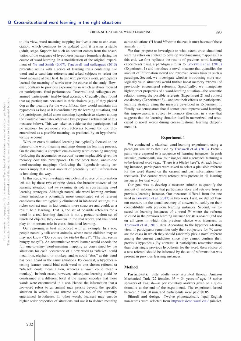
to this view, word-meaning mapping involves a one-to-one asso-ciation, which continues to be updated until it reaches a stable(adult) stage. Support for such an account comes from the obser-vation of the sequence of hypotheses learners formulate during thecourse of word learning. In a modification of the original experi-ment of Yu and Smith (2007), Trueswell and colleagues (2013)presented adults with a series of learning trials containing oneword and n candidate referents and asked subjects to select theword meaning at each trial. In line with previous work, participantslearned the meaning of words over the course of the study. How-ever, contrary to previous experiments in which analyses focusedon participants’ final performance, Trueswell and colleagues ex-amined participants’ trial-by-trial accuracy. Crucially, they foundthat (a) participants persisted in their choices (e.g., if they pickeddog as the meaning for the word blicket, they would maintain thishypothesis as long as it is confirmed by the learning situation), and(b) participants picked a new meaning hypothesis at chance amongthe available candidates otherwise (we propose a refinement of thismeasure below). This was taken as evidence that participants hadno memory for previously seen referents beyond the one theyentertained as a possible meaning, as predicted by an hypothesis-testing account.
Work on cross-situational learning has typically focused on thenature of the word-meaning mappings during the learning process.On the one hand, a complete one-to-many word-meaning mapping(following the accumulative account) seems implausible given thememory cost this presupposes. On the other hand, one-to-oneword-meaning mappings (following the hypothesis-testing ac-count) imply that a vast amount of potentially useful informationis lost along the way.
In this study, we investigate one potential source of informationleft out by these two extreme views, the broader context of thelearning situation, and we examine its role in constraining wordlearning strategies. Although naturalistic word learning environ-ments introduce a potentially more complicated set of referentcandidates that are typically eliminated in lab-based settings, thisricher context may in fact contain more structure and could, as aresult, help learning. That is, the set of possible referents for aword in a real learning situation is not a pseudo-random set ofunrelated objects; they co-occur in the real world, and this couldplay an important role in cross-situational learning.
Our reasoning is best introduced with an example. In a zoo,people naturally talk about animals, whose name children may ormay not know (“Do you see the blicket there?”; “The dax seemshungry today!”). An accumulative word learner would encode thefull one-to-many word-meaning mapping as constrained by thesituations for each occurrence of a new word (a “blicket” couldmean lion, elephant, or monkey, and so could “dax,” as this wordhas been heard in the same situation). By contrast, a hypothesis-testing learner would bind each word to one chosen referent (a“blicket” could mean a lion, whereas a “dax” could mean amonkey). In both cases, however, subsequent learning could beconstrained at a different level if the learner encodes that thesewords were encountered in a zoo. Hence, the information that azoo-word refers to an animal may persist beyond the specificsituation in which it was uttered and on top of the currentlyentertained hypotheses. In other words, learners may encodehigher order properties of situations and use it to deduce meaning
across situations (“I heard blicket in the zoo, it must be one of theseanimals . . . ”).
We thus propose to investigate to what extent cross-situationallearning relies on context to develop word-meaning mappings. Tothis end, we first replicate the results of previous word learningexperiments using a paradigm similar to Trueswell et al. (2013)(Experiment 1) and introduce a novel measure that quantifies theamount of information stored and retrieved across trials in such aparadigm. Second, we investigate whether introducing more eco-logically valid situations would further boost memory retrieval ofpreviously encountered referents. Specifically, we manipulatehigher order properties of a word-learning situation—the semanticrelation among the possible referents (Experiment 2) and contextconsistency (Experiment 3)—and test their effects on participants’learning strategy using the measure developed in Experiment 1.Finally, we demonstrate that if context can improve word learning,this improvement is subject to memory illusions, in a way thatsuggests that the learning situation itself is memorized and asso-ciated to novel words during cross-situational learning (Experi-ment 4).
Experiment 1
We conducted a classical word-learning experiment using aparadigm similar to that used by Trueswell et al. (2013). Partici-pants were exposed to a sequence of learning instances. In eachinstance, participants saw four images and a sentence featuring ato-be-learned word (e.g., “There is a blicket here”). At each learn-ing instance, participants were asked to select a plausible referentfor the word (based on the current and past information theyreceived). The correct word referent was present in all learninginstances for that word.
Our goal was to develop a measure suitable to quantify theamount of information that participants store and retrieve from aprevious learning instance. Our measures differed from the oneused in Trueswell et al. (2013) in two ways. First, we did not baseour measure on the actual accuracy of answers but solely on theircompatibility with previous learning instances. Second, we fo-cused on learning instances of a word W where the referentselected in the previous learning instance for W is absent (and noton all cases in which this previous choice was incorrect, asTrueswell et al., 2013, did). According to the hypothesis-testingview, if participants remember only their conjecture for W, theseare the cases in which they should randomly pick a novel referentamong the current candidates since they cannot confirm theirprevious hypothesis. By contrast, if participants remember morethan their single previous hypothesis for the word, their choice ofa new referent should be informed by the set of referents that waspresent in previous learning instances.
Method
Participants. Fifty adults were recruited through AmazonMechanical Turk (22 females, M � 34 years of age, 48 nativespeakers of English—as per voluntary answers given on a ques-tionnaire at the end of the experiment). The experiment lastedbetween 5 and 10 min, and participants were paid $0.85.
Stimuli and design. Twelve phonotactically legal Englishnon-words were selected from http://elexicon.wustl.edu/ (blicket,
Thi
sdo
cum
ent
isco
pyri
ghte
dby
the
Am
eric
anPs
ycho
logi
cal
Ass
ocia
tion
oron
eof
itsal
lied
publ
ishe
rs.
Thi
sar
ticle
isin
tend
edso
lely
for
the
pers
onal
use
ofth
ein
divi
dual
user
and
isno
tto
bedi
ssem
inat
edbr
oadl
y.
893CROSS-SITUATIONAL WORD LEARNING
B Cross-situational word learning in the right situations
232
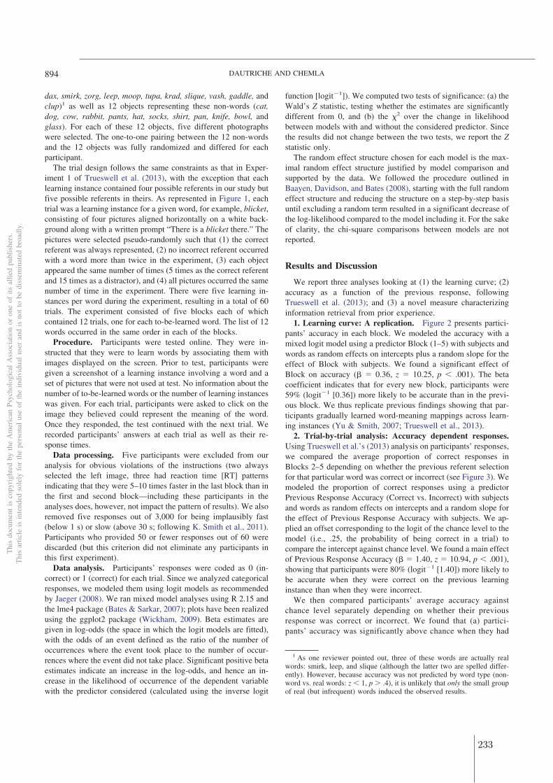
dax, smirk, zorg, leep, moop, tupa, krad, slique, vash, gaddle, andclup)1 as well as 12 objects representing these non-words (cat,dog, cow, rabbit, pants, hat, socks, shirt, pan, knife, bowl, andglass). For each of these 12 objects, five different photographswere selected. The one-to-one pairing between the 12 non-wordsand the 12 objects was fully randomized and differed for eachparticipant.
The trial design follows the same constraints as that in Exper-iment 1 of Trueswell et al. (2013), with the exception that eachlearning instance contained four possible referents in our study butfive possible referents in theirs. As represented in Figure 1, eachtrial was a learning instance for a given word, for example, blicket,consisting of four pictures aligned horizontally on a white back-ground along with a written prompt “There is a blicket there.” Thepictures were selected pseudo-randomly such that (1) the correctreferent was always represented, (2) no incorrect referent occurredwith a word more than twice in the experiment, (3) each objectappeared the same number of times (5 times as the correct referentand 15 times as a distractor), and (4) all pictures occurred the samenumber of time in the experiment. There were five learning in-stances per word during the experiment, resulting in a total of 60trials. The experiment consisted of five blocks each of whichcontained 12 trials, one for each to-be-learned word. The list of 12words occurred in the same order in each of the blocks.
Procedure. Participants were tested online. They were in-structed that they were to learn words by associating them withimages displayed on the screen. Prior to test, participants weregiven a screenshot of a learning instance involving a word and aset of pictures that were not used at test. No information about thenumber of to-be-learned words or the number of learning instanceswas given. For each trial, participants were asked to click on theimage they believed could represent the meaning of the word.Once they responded, the test continued with the next trial. Werecorded participants’ answers at each trial as well as their re-sponse times.
Data processing. Five participants were excluded from ouranalysis for obvious violations of the instructions (two alwaysselected the left image, three had reaction time [RT] patternsindicating that they were 5–10 times faster in the last block than inthe first and second block—including these participants in theanalyses does, however, not impact the pattern of results). We alsoremoved five responses out of 3,000 for being implausibly fast(below 1 s) or slow (above 30 s; following K. Smith et al., 2011).Participants who provided 50 or fewer responses out of 60 werediscarded (but this criterion did not eliminate any participants inthis first experiment).
Data analysis. Participants’ responses were coded as 0 (in-correct) or 1 (correct) for each trial. Since we analyzed categoricalresponses, we modeled them using logit models as recommendedby Jaeger (2008). We ran mixed model analyses using R 2.15 andthe lme4 package (Bates & Sarkar, 2007); plots have been realizedusing the ggplot2 package (Wickham, 2009). Beta estimates aregiven in log-odds (the space in which the logit models are fitted),with the odds of an event defined as the ratio of the number ofoccurrences where the event took place to the number of occur-rences where the event did not take place. Significant positive betaestimates indicate an increase in the log-odds, and hence an in-crease in the likelihood of occurrence of the dependent variablewith the predictor considered (calculated using the inverse logit
function [logit�1]). We computed two tests of significance: (a) theWald’s Z statistic, testing whether the estimates are significantlydifferent from 0, and (b) the �2 over the change in likelihoodbetween models with and without the considered predictor. Sincethe results did not change between the two tests, we report the Zstatistic only.
The random effect structure chosen for each model is the max-imal random effect structure justified by model comparison andsupported by the data. We followed the procedure outlined inBaayen, Davidson, and Bates (2008), starting with the full randomeffect structure and reducing the structure on a step-by-step basisuntil excluding a random term resulted in a significant decrease ofthe log-likelihood compared to the model including it. For the sakeof clarity, the chi-square comparisons between models are notreported.
Results and Discussion
We report three analyses looking at (1) the learning curve; (2)accuracy as a function of the previous response, followingTrueswell et al. (2013); and (3) a novel measure characterizinginformation retrieval from prior experience.
1. Learning curve: A replication. Figure 2 presents partici-pants’ accuracy in each block. We modeled the accuracy with amixed logit model using a predictor Block (1–5) with subjects andwords as random effects on intercepts plus a random slope for theeffect of Block with subjects. We found a significant effect ofBlock on accuracy (� � 0.36, z � 10.25, p � .001). The betacoefficient indicates that for every new block, participants were59% (logit�1 [0.36]) more likely to be accurate than in the previ-ous block. We thus replicate previous findings showing that par-ticipants gradually learned word-meaning mappings across learn-ing instances (Yu & Smith, 2007; Trueswell et al., 2013).
2. Trial-by-trial analysis: Accuracy dependent responses.Using Trueswell et al.’s (2013) analysis on participants’ responses,we compared the average proportion of correct responses inBlocks 2–5 depending on whether the previous referent selectionfor that particular word was correct or incorrect (see Figure 3). Wemodeled the proportion of correct responses using a predictorPrevious Response Accuracy (Correct vs. Incorrect) with subjectsand words as random effects on intercepts and a random slope forthe effect of Previous Response Accuracy with subjects. We ap-plied an offset corresponding to the logit of the chance level to themodel (i.e., .25, the probability of being correct in a trial) tocompare the intercept against chance level. We found a main effectof Previous Response Accuracy (� � 1.40, z � 10.94, p � .001),showing that participants were 80% (logit�1 [1.40]) more likely tobe accurate when they were correct on the previous learninginstance than when they were incorrect.
We then compared participants’ average accuracy againstchance level separately depending on whether their previousresponse was correct or incorrect. We found that (a) partici-pants’ accuracy was significantly above chance when they had
1 As one reviewer pointed out, three of these words are actually realwords: smirk, leep, and slique (although the latter two are spelled differ-ently). However, because accuracy was not predicted by word type (non-word vs. real words: z � 1, p � .4), it is unlikely that only the small groupof real (but infrequent) words induced the observed results.
Thi
sdo
cum
ent
isco
pyri
ghte
dby
the
Am
eric
anPs
ycho
logi
cal
Ass
ocia
tion
oron
eof
itsal
lied
publ
ishe
rs.
Thi
sar
ticle
isin
tend
edso
lely
for
the
pers
onal
use
ofth
ein
divi
dual
user
and
isno
tto
bedi
ssem
inat
edbr
oadl
y.
894 DAUTRICHE AND CHEMLA
233
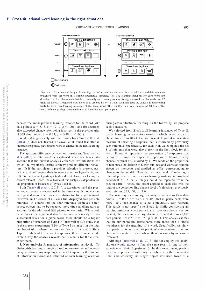
been correct in the previous learning instance for that word (789data points; � � 3.13, z � 12.10, p � .001), and (b) accuracyalso exceeded chance after being incorrect in the previous trial(1,339 data points; � � 0.33, z � 3.48, p � .001).
While (a) aligns nicely with the results from Trueswell et al.(2013), (b) does not. Instead, Trueswell et al. found that after anincorrect response, participants were at chance in the next learninginstance.
The apparent difference between our results and Trueswell etal.’s (2013) results could be explained when one takes intoaccount that the current analysis collapses two situations forwhich the hypothesis-testing strategy predicts different behav-iors: (I) if the participant’s previous selection is present, par-ticipants should repeat their incorrect previous hypothesis, and(II) if is it not present, participants should be at chance in selecting thecorrect referent. Hence, the outcome of this analysis is dependent onthe proportion of instances of Types I and II.
Both Trueswell et al.’s (2013) first experiment and the pres-ent experiment are constrained in the same way: No object canbe repeated more than twice as a distractor for a given word.However, in Trueswell et al., each trial displayed five possiblereferents (in contrast to the four referents displayed here);hence, objects had to be repeated more often as distractors toaccount for the additional fifth picture on each trial. While bothoccurrences for a given distractor are not necessarily in twosubsequent trials for a given word, there should be a higherproportion of instances of Type I in Trueswell et al.’s study thanin the present experiment (12% of Type I instances on the totalnumber of trials where the previous choice is incorrect). SinceType I trials lead to incorrect responses, this difference couldexplain why the analysis reveals better results for the currentexperiment.
3. New analysis: A measure of information retrieval. Todistinguish learning strategies based on one-to-one and one-to-many word-meaning mappings, we need to quantify the amountof information stored and retrieved at each learning occasion
during cross-situational learning. In the following, we proposesuch a measure.
We selected from Block 2 all learning instances of Type II,that is, learning instances for a word x in which the participant’schoice for x from Block 1 is not present. Figure 4 represents ameasure of selecting a response that is informed by previouslyseen referents. Specifically, for each trial, we computed the setS of referents that were also present in the first block for thisword. Figure 4 represents the proportion of responses thatbelong to S minus the expected proportion of falling in S bychance (cardinal of S divided by 4). We modeled the proportionof responses that belong to S with subjects and words as randomeffects on intercepts and applied an offset corresponding tochance to the model. Note that chance level of selecting areferent present in the previous learning instance is now trialdependent (1, 2, or 3 images could be repeated from theprevious trial); hence, the offset applied to each trial was thelogit of the corresponding chance level of selecting a previouslyseen referent (.25, .50, or .75).
The resulting measure significantly exceeds zero (336 datapoints; � � 0.27, z � 2.28, p � .05); that is, participants weremore likely than chance to select a previously seen referent.This result is not specific to Block 2: While considering alllearning instances where participants’ previous choice was notpresent, the measure also significantly exceeded zero (1,172data points; � � 0.27, z � 3.77, p � .001). This analysis showsthat in our paradigm, participants store more than a singlehypothesis for the meaning of a word. Specifically, we showthat participants resorted to previously encountered, but notchosen, referents in cases where their previous hypothesis isirrelevant.
Although Trueswell et al. (2013) did not employ this analy-sis, one would expect to find the same result in one of theirexperiments: their Experiment 3. In this experiment, partici-pants were presented with only two objects on the screen at atime, and, crucially, no single object was used twice as a
Figure 1. Experimental design. A learning trial of a to-be-learned word is a set of four candidate referentspresented with the word in a simple declarative sentence. The five learning instances for each word aredistributed in five blocks such that there is exactly one learning instance for a given word per block—hence, 12trials per block. As depicted, each block is an ordered list of 12 trials, such that there are exactly 11 interveningtrials between two learning instances of the same word. This resulted in a total number of 60 trials. Theword–referent pairings were randomly assigned for each participant.
Thi
sdo
cum
ent
isco
pyri
ghte
dby
the
Am
eric
anPs
ycho
logi
cal
Ass
ocia
tion
oron
eof
itsal
lied
publ
ishe
rs.
Thi
sar
ticle
isin
tend
edso
lely
for
the
pers
onal
use
ofth
ein
divi
dual
user
and
isno
tto
bedi
ssem
inat
edbr
oadl
y.
895CROSS-SITUATIONAL WORD LEARNING
B Cross-situational word learning in the right situations
234
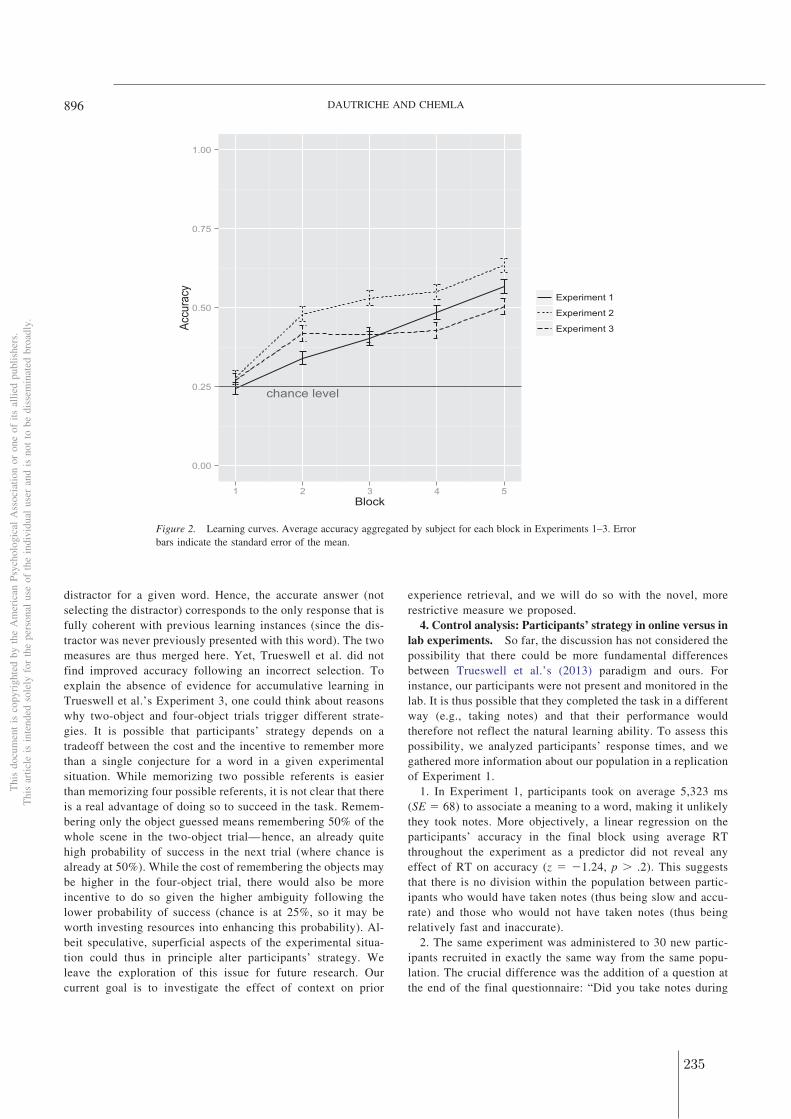
distractor for a given word. Hence, the accurate answer (notselecting the distractor) corresponds to the only response that isfully coherent with previous learning instances (since the dis-tractor was never previously presented with this word). The twomeasures are thus merged here. Yet, Trueswell et al. did notfind improved accuracy following an incorrect selection. Toexplain the absence of evidence for accumulative learning inTrueswell et al.’s Experiment 3, one could think about reasonswhy two-object and four-object trials trigger different strate-gies. It is possible that participants’ strategy depends on atradeoff between the cost and the incentive to remember morethan a single conjecture for a word in a given experimentalsituation. While memorizing two possible referents is easierthan memorizing four possible referents, it is not clear that thereis a real advantage of doing so to succeed in the task. Remem-bering only the object guessed means remembering 50% of thewhole scene in the two-object trial— hence, an already quitehigh probability of success in the next trial (where chance isalready at 50%). While the cost of remembering the objects maybe higher in the four-object trial, there would also be moreincentive to do so given the higher ambiguity following thelower probability of success (chance is at 25%, so it may beworth investing resources into enhancing this probability). Al-beit speculative, superficial aspects of the experimental situa-tion could thus in principle alter participants’ strategy. Weleave the exploration of this issue for future research. Ourcurrent goal is to investigate the effect of context on prior
experience retrieval, and we will do so with the novel, morerestrictive measure we proposed.
4. Control analysis: Participants’ strategy in online versus inlab experiments. So far, the discussion has not considered thepossibility that there could be more fundamental differencesbetween Trueswell et al.’s (2013) paradigm and ours. Forinstance, our participants were not present and monitored in thelab. It is thus possible that they completed the task in a differentway (e.g., taking notes) and that their performance wouldtherefore not reflect the natural learning ability. To assess thispossibility, we analyzed participants’ response times, and wegathered more information about our population in a replicationof Experiment 1.
1. In Experiment 1, participants took on average 5,323 ms(SE � 68) to associate a meaning to a word, making it unlikelythey took notes. More objectively, a linear regression on theparticipants’ accuracy in the final block using average RTthroughout the experiment as a predictor did not reveal anyeffect of RT on accuracy (z � �1.24, p � .2). This suggeststhat there is no division within the population between partic-ipants who would have taken notes (thus being slow and accu-rate) and those who would not have taken notes (thus beingrelatively fast and inaccurate).
2. The same experiment was administered to 30 new partic-ipants recruited in exactly the same way from the same popu-lation. The crucial difference was the addition of a question atthe end of the final questionnaire: “Did you take notes during
chance level
0.00
0.25
0.50
0.75
1.00
1 2 3 4 5Block
Accu
racy Experiment 1
Experiment 2
Experiment 3
Figure 2. Learning curves. Average accuracy aggregated by subject for each block in Experiments 1–3. Errorbars indicate the standard error of the mean.
Thi
sdo
cum
ent
isco
pyri
ghte
dby
the
Am
eric
anPs
ycho
logi
cal
Ass
ocia
tion
oron
eof
itsal
lied
publ
ishe
rs.
Thi
sar
ticle
isin
tend
edso
lely
for
the
pers
onal
use
ofth
ein
divi
dual
user
and
isno
tto
bedi
ssem
inat
edbr
oadl
y.
896 DAUTRICHE AND CHEMLA
235
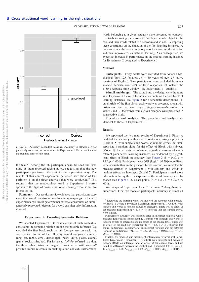
the task?” Among the 28 participants who finished the task,none of them reported taking notes, suggesting that the newparticipants performed the task in the appropriate way. Theresults of this control experiment patterned with those of Ex-periment 1 on the three analyses that were conducted.2 Thissuggests that the methodology used in Experiment 1 corre-sponds to the type of cross-situational learning exercise we areinterested in.
Summary. Our results provide evidence that participants storemore than simple one-to-one word-meaning mappings. In the nextexperiments, we investigate whether external constraints on simul-taneously presented referents for a word can alter prior informationretrieval.
Experiment 2: Encoding Semantic Relation
We adapted Experiment 1 to evaluate one of such contextualconstraint: the semantic relation among the possible referents. Wemodified the first block such that all four pictures on each trialcorresponded to one of the following natural categories: animals(dog, cat, rabbit, cow), dishes (pan, bowl, knife, glass), clothes(pants, socks, shirt, hat). For instance, if blicket referred to a dog,the three other distractor images it co-occurred with were allpossible animal referents, mimicking a zoo-context. Furthermore,
words belonging to a given category were presented on consecu-tive trials (allowing the learner to first learn words related to thezoo, and then words related to a bedroom and so on). By imposingthese constraints on the situation of the first learning instance, wehope to reduce the overall memory cost for encoding the situationand thus improve cross-situational learning. As a consequence, weexpect an increase in performance in the second learning instancefor Experiment 2 compared to Experiment 1.
Method
Participants. Forty adults were recruited from Amazon Me-chanical Turk (25 females, M � 40 years of age, 37 nativespeakers of English). Two participants were excluded from ouranalysis because over 20% of their responses fell outside the1–30-s response time window (see Experiment 1—Analysis).
Stimuli and design. The stimuli and the design were the sameas in Experiment 1 except for new constraints on the first block oflearning instances (see Figure 5 for a schematic description): (1)on all trials of the first block, each word was presented along withdistractors from the target object category (animals, clothes, ordishes), and (2) the words from a given category were presented inconsecutive trials.
Procedure and analysis. The procedure and analysis areidentical to those in Experiment 1.
Results
We replicated the two main results of Experiment 1. First, wemodeled the accuracy with a mixed logit model using a predictorBlock (1–5) with subjects and words as random effects on inter-cepts and a random slope for the effect of Block with subjects(Model 1). Participants demonstrated a gradual learning of word-referent pairs across learning instances, as evidenced by a signif-icant effect of Block on accuracy (see Figure 2; � � 0.39, z �7.12, p � .001). Participants were 60% (logit�1 [0.39]) more likelyto be accurate than in the previous block. Second, we modeled themeasure defined in Experiment 1 with subjects and words asrandom effects on intercepts (Model 2). Participants stored moreinformation during the first exposure of the word than expected bychance (see Figure 4; 223 data points; � � 1.20, z � 6.37, p �.001).
We compared Experiment 1 and Experiment 2 along these twodimensions. First, we modeled participants’ accuracy in Blocks 1
2 Regarding the learning curve, we modeled the accuracy with a predic-tor Block (1–5) and a predictor Experiment (Experiment 1, Control) withsubjects and words as random effects on intercepts. There was no effect ofthe predictor Experiment (z � 1, p � .4), showing that the learning curveswere similar.
Furthermore, accuracy was modeled after an incorrect response with apredictor Experiment (Experiment 1, Control) with subjects and words asrandom effects on intercepts and an offset of the chance level. There wasno effect of the predictor Experiment (z � �1.5, p � .1), showing thatcontrol participants’ accuracy after an incorrect response was not differentfrom earlier participants’ (MControl � 0.32, SEControl � 0.02; MExp.1 � 0.31,SEExp.1 � 0.02).
Finally, we modeled our measure of information retrieval with a pre-dictor Experiment (Experiment 1, Control) with subjects and words asrandom effects on intercepts and an offset of the chance level, and wefound no difference between the Control and Experiment 1 (z � 0.2, p �.8; MControl � 0.06, SEControl � 0.02; MExp.1 � 0.06, SEExp.1 � 0.01).
Figure 3. Accuracy dependent measure. Accuracy in Blocks 2–5 forpreviously correct or incorrect words in Experiment 1. Error bars indicatethe standard error of the mean.
Thi
sdo
cum
ent
isco
pyri
ghte
dby
the
Am
eric
anPs
ycho
logi
cal
Ass
ocia
tion
oron
eof
itsal
lied
publ
ishe
rs.
Thi
sar
ticle
isin
tend
edso
lely
for
the
pers
onal
use
ofth
ein
divi
dual
user
and
isno
tto
bedi
ssem
inat
edbr
oadl
y.
897CROSS-SITUATIONAL WORD LEARNING
B Cross-situational word learning in the right situations
236
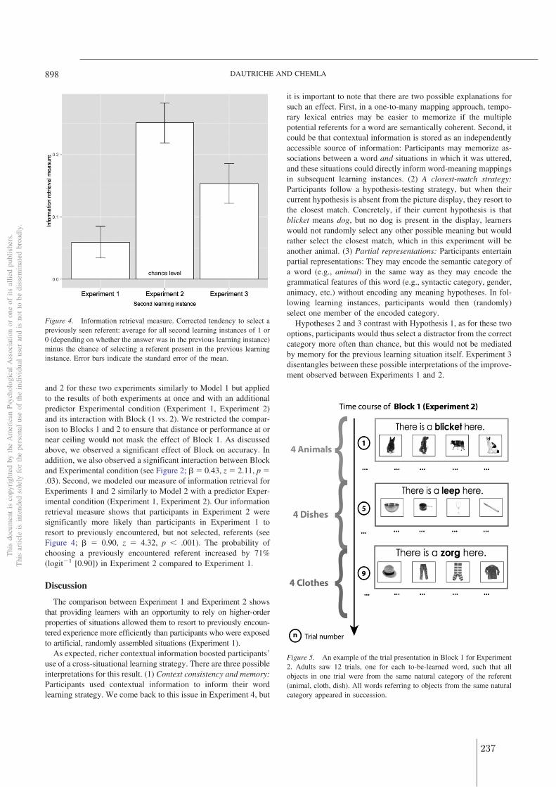
and 2 for these two experiments similarly to Model 1 but appliedto the results of both experiments at once and with an additionalpredictor Experimental condition (Experiment 1, Experiment 2)and its interaction with Block (1 vs. 2). We restricted the compar-ison to Blocks 1 and 2 to ensure that distance or performance at ornear ceiling would not mask the effect of Block 1. As discussedabove, we observed a significant effect of Block on accuracy. Inaddition, we also observed a significant interaction between Blockand Experimental condition (see Figure 2; � � 0.43, z � 2.11, p �.03). Second, we modeled our measure of information retrieval forExperiments 1 and 2 similarly to Model 2 with a predictor Exper-imental condition (Experiment 1, Experiment 2). Our informationretrieval measure shows that participants in Experiment 2 weresignificantly more likely than participants in Experiment 1 toresort to previously encountered, but not selected, referents (seeFigure 4; � � 0.90, z � 4.32, p � .001). The probability ofchoosing a previously encountered referent increased by 71%(logit�1 [0.90]) in Experiment 2 compared to Experiment 1.
Discussion
The comparison between Experiment 1 and Experiment 2 showsthat providing learners with an opportunity to rely on higher-orderproperties of situations allowed them to resort to previously encoun-tered experience more efficiently than participants who were exposedto artificial, randomly assembled situations (Experiment 1).
As expected, richer contextual information boosted participants’use of a cross-situational learning strategy. There are three possibleinterpretations for this result. (1) Context consistency and memory:Participants used contextual information to inform their wordlearning strategy. We come back to this issue in Experiment 4, but
it is important to note that there are two possible explanations forsuch an effect. First, in a one-to-many mapping approach, tempo-rary lexical entries may be easier to memorize if the multiplepotential referents for a word are semantically coherent. Second, itcould be that contextual information is stored as an independentlyaccessible source of information: Participants may memorize as-sociations between a word and situations in which it was uttered,and these situations could directly inform word-meaning mappingsin subsequent learning instances. (2) A closest-match strategy:Participants follow a hypothesis-testing strategy, but when theircurrent hypothesis is absent from the picture display, they resort tothe closest match. Concretely, if their current hypothesis is thatblicket means dog, but no dog is present in the display, learnerswould not randomly select any other possible meaning but wouldrather select the closest match, which in this experiment will beanother animal. (3) Partial representations: Participants entertainpartial representations: They may encode the semantic category ofa word (e.g., animal) in the same way as they may encode thegrammatical features of this word (e.g., syntactic category, gender,animacy, etc.) without encoding any meaning hypotheses. In fol-lowing learning instances, participants would then (randomly)select one member of the encoded category.
Hypotheses 2 and 3 contrast with Hypothesis 1, as for these twooptions, participants would thus select a distractor from the correctcategory more often than chance, but this would not be mediatedby memory for the previous learning situation itself. Experiment 3disentangles between these possible interpretations of the improve-ment observed between Experiments 1 and 2.
Figure 4. Information retrieval measure. Corrected tendency to select apreviously seen referent: average for all second learning instances of 1 or0 (depending on whether the answer was in the previous learning instance)minus the chance of selecting a referent present in the previous learninginstance. Error bars indicate the standard error of the mean.
Figure 5. An example of the trial presentation in Block 1 for Experiment2. Adults saw 12 trials, one for each to-be-learned word, such that allobjects in one trial were from the same natural category of the referent(animal, cloth, dish). All words referring to objects from the same naturalcategory appeared in succession.
Thi
sdo
cum
ent
isco
pyri
ghte
dby
the
Am
eric
anPs
ycho
logi
cal
Ass
ocia
tion
oron
eof
itsal
lied
publ
ishe
rs.
Thi
sar
ticle
isin
tend
edso
lely
for
the
pers
onal
use
ofth
ein
divi
dual
user
and
isno
tto
bedi
ssem
inat
edbr
oadl
y.
898 DAUTRICHE AND CHEMLA
237
Experiment 3: Encoding Context Consistency
Experiment 3 was set up to replicate Experiment 2 with threeartificial categories of objects with no a priori coherence (e.g.,{apple, dog, flower, hat}) instead of “natural” categories. Note thatdespite the lack of semantic coherence among these objects, cat-egories could nonetheless emerge here due to the repeated andconsecutive co-occurrence of the four objects that constitute eachof them.
Although these categories are clearly artificially induced, theprocess of category induction may in fact not be unnatural. Spe-cifically, under the right circumstances, many sets of objects,however unrelated they may appear to be, can co-occur. Forexample, in the kitchen, you may simultaneously see an apple, adog, a vase with flowers, and a hat hung on the wall. These itemsare not transparently related, but all of them may be simultane-ously found in the kitchen, possibly for quite different reasons.Thus, in the absence of semantic relations between the objects ofan artificial category in Experiment 3, the coherence may beinduced by their co-occurrence on four consecutive trials (once foreach of the word that refers to them). The consistent display hereplays the role of the kitchen in the example above.
If participants fail to use this contextual consistency, then theyshould behave like participants in Experiment 1, where none of theobjects within a trial was semantically related to the other. Thiswould favor Hypotheses 2 and 3, which attribute the improvementobserved in Experiment 2 to semantic consistency. By contrast, ifthe artificial categories improve cross-situational learning com-pared to Experiment 1, this would favor Hypothesis 1, which relieson consistency in general and not on a tendency to resort to asemantically close selection (as of Hypothesis 2) or on partialrepresentations (remembering “animal” instead of specific ani-mals; as per Hypothesis 3).
Method
Participants. Forty adults were recruited from Amazon Me-chanical Turk (12 females, M � 34 years of age, 39 nativespeakers of English). Four participants were excluded from ouranalysis because over 20% of their responses felt outside the1–30-s response time window (see Experiment 1—Analysis) (n �2) or because they participated in previous experiments (n � 2).
Stimuli and design. The design was similar to Experiment 2.We used a novel set of objects in order to minimize the potentialsemantic associations among them within each of the three artifi-cial categories. Categories were defined as follows: {apple, dog,flower, hat}, {pants, chair, pan, teddy bear}, and {leaf, snake,watch, book}.
The first block follows the same design as in Experiment 2, butthe position on the screen for each object within the trials of thesame category was fixed. For example, considering the set {apple,dog, flower, hat}, these objects appeared in the same position(albeit with different images) on the screen in all four learninginstances for the four target words associated with them. Thisshould raise the awareness that the situation is constant. Thus, adog might be the left-most object for four consecutive trials, butthe image used on each trial will change.
Procedure and analysis. The procedure and analysis areidentical to those in Experiments 1 and 2.
Results
We replicated the two main results of Experiments 1 and 2.First, we modeled participants’ accuracy in Experiment 3 with amixed logit model using a predictor Block (1–5) with subjects andwords as random effects on intercepts and a random slope for theeffect of Block with subjects (Model 1). Participants demonstrateda gradual learning of word-referent pairs across learning instancesas evidenced by a significant effect of Block on accuracy (seeFigure 2; � � 0.20, z � 3.48, p � .001). Second, we modeled ourmeasure of information retrieval in Block 2 with subjects andwords as random effects on intercepts (Model 2). Participantsretrieved more information from the first exposure to a word thanexpected by chance (see Figure 4; 231 data points; � � 0.68, z �4.68, p � .001).
We compared the three experiments along these two dimen-sions. First, we modeled participants’ accuracy in Blocks 1 and 2for the three experiments with the predictor Block (1 vs. 2) used inModel 1 and an additional predictor Experimental condition (Ex-periment 1, Experiment 2, Experiment 3) and its interaction withBlock. There was no significant interaction between Block andExperimental condition (Experiment 3 vs. Experiment 1:� � �0.20, z � �1.02, p � .3; Experiment 3 vs. Experiment 2:� � 0.21, z � 1.02, p � .3; see Figure 2). Second, we modeled ourinformation retrieval measure in Block 2 for the three experimentssimilarly to Model 2 with a predictor Experimental condition(Experiment 1, Experiment 2, Experiment 3). Participants in Ex-periment 3 were significantly less likely to choose a previouslyseen, but not selected, referent than participants in Experiment 2(� � 0.47, z � 2.14, p � .05), but they were significantly morelikely to do so than participants in Experiment 1 (� � �0.42,z � �2.11, p � .05; see Figure 4).
Overall, these results demonstrate that participants in this ex-periment retrieved the systematic co-occurrence of seemingly un-related objects to degree intermediate between participants inExperiments 1 and 2. This shows that participants use contextualinformation from consistent contexts to inform word learning, andthey do so to a greater extent if contexts furthermore share asemantic relation.
Discussion
Participants used the artificial categories presented in the firstlearning instance to guide their choice of the word’s referent insubsequent instances. Crucially, this effect was preserved eventhough none of the objects presented in the first learning instanceshared a “natural” property. This rules out the possibility that theresults from the previous experiment could be due entirely to anunder-specification of a selection (e.g., animal instead of dog) orto a tendency to resort to a semantically close choice (e.g., fromdog to cat) when the previously hypothesized referent was notavailable. Instead, our results favor the hypothesis that contextualconsistency helps encoding situations in both Experiments 2 and 3.
Nonetheless, participants in Experiment 3 were less likely toresort to previously encountered referents than participants inExperiment 2. One reasonable explanation may be that encodingan artificial relation is more demanding than encoding a naturalrelation: While participants in Experiment 2 could remember alabel readily available to characterize the relation among objects(“animal,” “clothes,” or “dishes”), participants in Experiment 3
Thi
sdo
cum
ent
isco
pyri
ghte
dby
the
Am
eric
anPs
ycho
logi
cal
Ass
ocia
tion
oron
eof
itsal
lied
publ
ishe
rs.
Thi
sar
ticle
isin
tend
edso
lely
for
the
pers
onal
use
ofth
ein
divi
dual
user
and
isno
tto
bedi
ssem
inat
edbr
oadl
y.
899CROSS-SITUATIONAL WORD LEARNING
B Cross-situational word learning in the right situations
238
had to encode the category as a plain list of objects. Hence,learners may have encoded contextual information in both exper-iments, but the format of the relevant information varies from oneexperiment to the other, and this could recruit different memoryresources.
Experiment 3 showed that contextual consistency, and not onlysemantic consistency, helped learners resort to possible wordmeaning hypotheses. However this effect could be explained bytwo possible representations of context in memory. (a) Internal toword-meaning mappings: One-to-many word-meaning mappingsmay be more or less easier to remember, and a coherence betweenthe possible meanings may indirectly boost an active memory forthese mappings. As a result, multiple hypotheses for a word arebetter remembered when these hypotheses form a coherent group,but context is not necessarily stored in memory as such. (b)External to word-meaning mappings: Contextual informationcould be directly accessible as an independent source of informa-tion, that is, learners could remember the situation in which theyheard a word in addition to the single or multiple hypotheses theyentertain for this word. In this case, contextual information can beused actively to constrain subsequent learning instances.
Experiment 3 did not distinguish between an internal versus anexternal representation of context since contextual representationwas confounded with word-meaning representations. In Experi-ment 4, we propose to disentangle these two possibilities andassess whether context is represented per se in memory.
Experiment 4: Context Representation in Memory
Experiment 4 investigates whether the effect of context ob-served in Experiments 2 and 3 is the result of an internal or anexternal representation of context. Much like Experiments 2 and 3,objects in the first block of this experiment were grouped into threesets. Two of these sets contained objects from a single naturalcategory (animals and clothes) as in Experiment 2, henceforth,“natural sets.” By contrast, the third set was hybrid: It containedtwo (new) animals and two (new) pieces of clothes. For a wordwhose referent belongs to a natural set, participants could encodea natural category (e.g., animal), as in Experiment 2. However,some objects from this natural category occurred in the hybrid setand should not be considered possible referents for this word afterthe first learning instance (contrary to Experiment 2).
We propose to reproduce a memory illusion effect identified inearlier work (Roediger & McDermott, 1995) showing that partic-ipants asked to remember a list of words are likely to mis-report aword as being part of this list if there is a natural relation betweenthe word and the list. For example, participants incorrectly recallthe word sleep as a member of a list such as bed, pillow, night.Applied to our word learning task, lists can be thought of as setsof objects seen in the first block (e.g., dog, cat, snake, cow). Ifcontext is encoded as an additional source of information (Hypoth-esis b), participants are in the same situation as in the memoryillusion experiment, and we expect to reproduce the same illusion.Participants should be more likely to map a target word in thenatural sets onto a distractor object from the appropriate naturalcategory than from the other category. However, crucially, thisbias for the appropriate category should be observed even when wecompare only distractors from the hybrid set, which had neverappeared with the target word before. If context is not encoded
independently and the effect occurs at the level of the lexicon(Hypothesis a), then there is no immediate expectation with respectto this illusion.
Method
Participants. A total of 119 adults were recruited from Am-azon Mechanical Turk (47 females, M � 36 years of age, 116native speakers of English). Twenty-four participants were ex-cluded from our analysis because they participated in previousexperiments (n � 14), because they indicated that they took notesduring the task (n � 4), or because their RT patterns were highlyirregular, in a fashion similar to participants who indicated thatthey took notes (e.g., 5–10 times faster from one block to another;n � 6).
Stimuli and design. The design was similar to Experiment 2.We formed two natural sets—animals {cat, cow, snake, rabbit},and clothes {pants, tie, hat, socks}—and one hybrid set of imagesmixing objects from each natural category: {dog, rat, shirt, shoe}.The hybrid set served as a reservoir of objects that could reveal theillusion when used as distractors. The hybrid set was alwayspresented first.
We generated the learning trials following the constraintsdescribed in Experiment 1. However, our planed analysis fo-cused on responses in the second block such that the targetwould be from one of the natural sets but responses would be adistractor from the hybrid set H. Hence, in order to have moredata points of interest, we assigned the learning instance withthe maximal number of distractors belonging to H (among thefour learning instances otherwise distributed randomly inBlocks 2–5) to the second block. To limit the frequency ofobjects from H in Block 2, we did this for target objects innatural sets, but the opposite for target objects in H (which trialswere not of interest). As a result, participants saw on averagefive instances of the objects in the hybrid set during Block 2(instead of four instances before).
Procedure and analysis. The procedure and analysis areidentical to those in Experiment 1, 2, and 3.
Results
We selected learning instances from Block 2 for words belong-ing to the two natural sets of objects. We looked at the artificial setof objects to compare the proportion of responses that belong tothe set S of distractors from the same category and to the set D ofdistractors from a different category. Figure 6 shows the propor-tion of responses in S and D minus the probability of selectingthem by chance (the cardinal of S and D divided by 4). Note thatwe selected trials where neither set S nor set D were empty (482data points; chance level for S or D was either .25 or .50).
We modeled the proportion of responses in the artificial set ofobjects by a predictor Distractor type (Same category vs. Differentcategory). Observations of the results led us to add a predictorSemantic category (Animals vs. Clothes) to the model, as well asits interaction with Distractor type. The random structure includedsubjects and words as random effects on intercepts and no randomslope was justified. We applied an offset corresponding to chanceto the model.
We observe a main effect of Distractor type (� � 0.45, z � 2.7,p � .01), showing that participants were 61% (logit�1 [0.45])
Thi
sdo
cum
ent
isco
pyri
ghte
dby
the
Am
eric
anPs
ycho
logi
cal
Ass
ocia
tion
oron
eof
itsal
lied
publ
ishe
rs.
Thi
sar
ticle
isin
tend
edso
lely
for
the
pers
onal
use
ofth
ein
divi
dual
user
and
isno
tto
bedi
ssem
inat
edbr
oadl
y.
900 DAUTRICHE AND CHEMLA
239
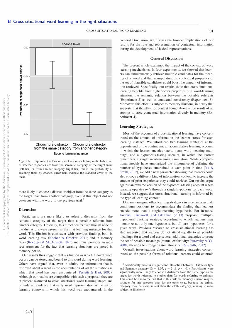
more likely to choose a distractor object from the same category asthe target than from another category, even if this object did notco-occur with the word in the previous trial.3
Discussion
Participants are more likely to select a distractor from thesemantic category of the target than a possible referent fromanother category. Crucially, this effect occurs even though none ofthe distractors were present in the first learning instance for thatword. This illusion is consistent with previous findings both inword learning task (Koehne & Crocker, 2011) and in memorytasks (Roediger & McDermott, 1995) and, thus, provides an indi-rect argument for the fact that learning situations are stored inmemory per se.
Our results thus suggest that a situation in which a novel wordoccurs can be stored and bound to this word during word learning.Others have argued that, even in adults, the information that isretrieved about a word is the accumulation of all the situations inwhich that word has been encountered (Perfetti & Hart, 2002).Although our results are compatible with such a proposal, they areat present restricted to cross-situational word learning stages andprovide no evidence that early word representation is the set oflearning contexts in which this word was encountered. In the
General Discussion, we discuss the broader implications of ourresults for the role and representation of contextual informationduring the development of lexical representations.
General Discussion
The present article examined the impact of the context on wordlearning mechanisms. In four experiments, we showed that learn-ers can simultaneously retrieve multiple candidates for the mean-ing of a word and that manipulating the contextual properties ofthe set of plausible candidates could boost the amount of informa-tion retrieved. Specifically, our results show that cross-situationallearning benefits from higher-order properties of a word-learningsituation: the semantic relation between the possible referents(Experiment 2) as well as contextual consistency (Experiment 3).Moreover, this effect is subject to memory illusions, in a way thatsuggests that the effect of context found above is the result of anattempt to store contextual information directly in memory (Ex-periment 4).
Learning Strategies
Most of the accounts of cross-situational learning have concen-trated on the amount of information the learner stores for eachlearning instance. We introduced two learning strategies at theopposite end of the continuum: an accumulative learning account,in which the learner encodes one-to-many word-meaning map-pings, and a hypothesis-testing account, in which the learnerremembers a single word-meaning association. While computa-tional models have emphasized the importance of defining thenumber of hypotheses entertained at each point in time (Yu &Smith, 2012), we add a new parameter showing that learners couldalso encode a different kind of information, context, to increase theamount of prior experience they could retrieve. Our results argueagainst an extreme version of the hypothesis-testing account wherelearning operates only through a single hypothesis for each word.Instead, we suggest that cross-situational learning is informed bythe type of learning context.
One may imagine other learning strategies in more intermediatecontinuum positions to accommodate the finding that learnersencode more than a single meaning hypothesis. For instance,Koehne, Trueswell, and Gleitman (2013) proposed multiple-hypothesis tracking strategy, according to which learners maymemorize not only one hypothesis, but all past hypotheses for agiven word. Previous research on cross-situational learning hasalso suggested that learners do not attend equally to all possiblemeanings for a word and use several additional strategies to prunethe set of possible meanings (mutual exclusivity: Yurovsky & Yu,2008; attention to stronger associations: Yu & Smith, 2012).
Overall, investigations about word learning strategies concen-trated on the possible forms of relations learners could entertain
3 Additionally there is a significant interaction between Distractor typeand Semantic category (� � 1.07, z � 3.19, p � .01). Participants weresignificantly more likely to choose a distractor from the same type as thetarget for words referring to clothes than for words referring to animals.This could be due to the fact that in this task the memory illusion may bestronger for one category than for the other (e.g., because the animalcategory may be more salient than the cloth category, making it moresubject to illusions).
Figure 6. Experiment 4. Proportion of responses falling in the hybrid setas whether responses are from the semantic category of the target word(left bar) or from another category (right bar) minus the probability ofselecting them by chance. Error bars indicate the standard error of themean.
Thi
sdo
cum
ent
isco
pyri
ghte
dby
the
Am
eric
anPs
ycho
logi
cal
Ass
ocia
tion
oron
eof
itsal
lied
publ
ishe
rs.
Thi
sar
ticle
isin
tend
edso
lely
for
the
pers
onal
use
ofth
ein
divi
dual
user
and
isno
tto
bedi
ssem
inat
edbr
oadl
y.
901CROSS-SITUATIONAL WORD LEARNING
B Cross-situational word learning in the right situations
240
between a word and possible referents. Here, we propose that somecontextual information is memorized and can boost word learningin realistic situations.
Implications for Learning Words in the Real World
Learners relied on previously experienced information moreefficiently when this information was packaged conveniently. Thatis, cross-situational learning was improved not only by a naturalrelation between possible referents (Experiment 2) but also by anartificial relation between objects solely induced by their repeti-tively joint presentation (Experiment 3). Of course, real-life situ-ations are much more complex learning environments than thesituations in the word-learning paradigm we used in Experiment 1(Medina et al., 2011): Here, the level of referential ambiguity isrelatively low (four possible referents), only one word is presentedat a time, and the true referent is always present in all wordoccurrences. Further simplification of the task may hence seeminappropriate. However, the specific simplifications we introducedin Experiments 2 and 3 in fact make the task more ecologicallyvalid. In daily life, learners navigate through situations they maybe interested in and find coherent. This could help them remembervarious properties of these situations (a kitchen, a zoo, a pantry,etc.). In Experiments 2 and 3, we introduced such coherence andshowed that it has a specific impact on their strategy and perfor-mance for learning new words.
Interestingly, a recent computational approach looking at envi-ronment regularities showed that coherent activity contexts such aseating, bathing or other regular activities could help simplify thelearning problem (Roy, Frank, & Roy, 2012). Our results alignwith this view, showing that more complex information from thebroader context in which a word has been uttered is part of thelearning problem faced by the child. The role of the learningenvironment on word learning requires attention in future research.
The Representation of Lexical Meaning DuringLearning
One important issue in the acquisition of word meaning involvesthe kind of representations children form about words. In otherwords, what do learners encode about a word when they first hearit? The full understanding of a word requires that learners not onlyknow its word form, its meaning, and its syntactic properties butalso information about contexts in which this word may occur.Recent evidence has shown that even infants in the first year of lifehave already acquired some knowledge for basics words (Bergel-son & Swingley, 2012, 2013). However, there is growing evidencethat children do not fast-map a dictionary-like definition at the firstencounter of the word. Instead, word learning, including verblearning, seems to be a slow process gradually emerging throughthe accumulation of syntactic, semantic, and pragmatic fragmentalevidence (Bion, Borovsky, & Fernald, 2013; Gelman & Brandone,2010; Yuan & Fisher, 2009). However it is currently unclear whatthis partial knowledge might be. The present results suggest that,alongside linguistic features (e.g., phonological form, syntacticcategory), non-linguistic features such as semantic category (Ex-periment 2) and situations in which the word occurred (Experi-ments 3 and 4) may be encoded and part of an early wordrepresentation. Non-linguistic relations between words are a cru-
cial component of the organization of the lexicon. Work on lexicalpriming has evidenced that young 21-month-olds already possessa structured knowledge of familiar words based on non-linguisticinformation such as semantic and associative relations (Arias-Trejo & Plunkett, 2013). As models of lexical development sug-gest (Steyvers & Tenenbaum, 2005), such a semantic organizationof the lexicon is the product of the mechanisms by which word-meaning associations are constructed throughout learning. Thissuggests that semantic and contextual relations may be encodedfrom the earliest step of lexical acquisition (see Wojcik & Saffran,2013, for evidence that toddlers can encode similarities amongreferents when learning words).
However, to our knowledge, no cross-situational study investi-gated the role of the learning context in word learning. Suchstudies could not only shape our understanding of early wordrepresentation but also shed light on the content and structure ofadults’ mature lexical entries.
Summary
Overall, our findings suggest that learners store in memory thelearning situation in which they hear a novel word and use thisinformation to constrain their word-meaning hypotheses. We firstproposed a new way to analyze classical word learning experi-ments through an information retrieval measure. We then modifiedthe classical word learning paradigm to evaluate whether realisticfeatures of the world could inform word learning strategies. Ourresults show that prior experience is better used when it consists ofcoherent contexts, and real-world situations may well be coherentcontexts in the relevant sense. We conclude that such paradigms,however simple, could and should be used to further study thestructure, richness, and poverty of the representations that consti-tute the early developing lexicon.
References
Akhtar, N., & Montague, L. (1999). Early lexical acquisition: The role ofcross-situational learning. First Language, 19, 347–358. doi:10.1177/014272379901905703
Arias-Trejo, N., & Plunkett, K. (2013). What’s in a link: Associative andtaxonomic priming effects in the infant lexicon. Cognition, 128, 214–227. doi:10.1016/j.cognition.2013.03.008
Baayen, R. H., Davidson, D. J., & Bates, D. M. (2008). Mixed-effectsmodeling with crossed random effects for subjects and items. Journal ofMemory and Language, 59, 390–412. doi:10.1016/j.jml.2007.12.005
Bates, D., & Sarkar, D. (2007). lme4: Linear mixed-effects models usingS4 classes (R package Version 0.99875-6) [Computer software]. Avail-able at http://cran.r-project.org/web/packages/lme4/index.html
Bergelson, E., & Swingley, D. (2012). At 6 to 9 months, human infantsknow the meanings of many common nouns. Proceedings of the Na-tional Academy of Sciences, USA, 109, 3253–3258. doi:10.1073/pnas.1113380109
Bergelson, E., & Swingley, D. (2013). The acquisition of abstract words byyoung infants. Cognition, 127, 391–397. doi:10.1016/j.cognition.2013.02.011
Bion, R. A. H., Borovsky, A., & Fernald, A. (2013). Fast mapping, slowlearning: Disambiguation of novel word–object mappings in relation tovocabulary learning at 18, 24, and 30 months. Cognition, 126, 39–53.doi:10.1016/j.cognition.2012.08.008
Gelman, S. A., & Brandone, A. C. (2010). Fast-mapping placeholders:Using words to talk about kinds. Language Learning and Development,6, 223–240. doi:10.1080/15475441.2010.484413
Thi
sdo
cum
ent
isco
pyri
ghte
dby
the
Am
eric
anPs
ycho
logi
cal
Ass
ocia
tion
oron
eof
itsal
lied
publ
ishe
rs.
Thi
sar
ticle
isin
tend
edso
lely
for
the
pers
onal
use
ofth
ein
divi
dual
user
and
isno
tto
bedi
ssem
inat
edbr
oadl
y.
902 DAUTRICHE AND CHEMLA
241
Jaeger, T. F. (2008). Categorical data analysis: Away from ANOVAs(transformation or not) and towards logit mixed models. Journal ofMemory and Language, 59, 434–446. doi:10.1016/j.jml.2007.11.007
Koehne, J., & Crocker, M. W. (2011). The interplay of multiple mecha-nisms in word learning. In L. Carlson, C. Hoelscher, & T. F. Shipley(Eds.), Proceedings of the 33rd Annual Meeting of the Cognitive ScienceSociety (pp. 1930–1936). Austin, TX: Cognitive Science Society.
Koehne, J., Trueswell, J. C., & Gleitman, L. R. (2013). Multiple proposalmemory in observational word learning. In M. Knauff, M. Pauen, N.Sebanz, & I. Wachsmuth (Eds.), Proceedings of the 35th Annual Con-ference of the Cognitive Science Society (pp. 805–810). Austin, TX:Cognitive Science Society.
Medina, T. N., Snedeker, J., Trueswell, J. C., & Gleitman, L. R. (2011).How words can and cannot be learned by observation. Proceedings ofthe National Academy of Sciences, USA, 108, 9014–9019. doi:10.1073/pnas.1105040108
Perfetti, C. A., & Hart, L. (2002). The lexical quality hypothesis. In L.Vehoeven, C. Elbro, & P. Reitsma (Eds.), Precursors of functionalliteracy (pp. 189–213). Amsterdam, the Netherlands: John Benjamins.
Pinker, S. (1989). Learnability and cognition: The acquisition of argumentstructure. Cambridge, MA: MIT Press.
Quine, W. V. O. (1964). Word and object (Vol. 4). Cambridge, MA: MITPress.
Roediger, H. L., & McDermott, K. B. (1995). Creating false memories:Remembering words not presented in lists. Journal of Experimental Psy-chology: Learning, Memory, and Cognition, 21, 803–814. doi:10.1037/0278–7393.21.4.803
Roy, B. C., Frank, M. C., & Roy, D. (2012). Relating activity contexts toearly word learning in dense longitudinal data. In Proceedings of the34th Annual Meeting of the Cognitive Science Society. Austin, TX:Cognitive Science Society.
Siskind, J. M. (1996). A computational study of cross-situational tech-niques for learning word-to-meaning mappings. Cognition, 61, 39–91.doi:10.1016/S0010–0277(96)00728-7
Smith, K., Smith, A. D. M., & Blythe, R. A. (2011). Cross-situationallearning: An experimental study of word-learning mechanisms. Cogni-tive Science, 35, 480–498. doi:10.1111/j.1551-6709.2010.01158.x
Smith, L., & Yu, C. (2008). Infants rapidly learn word-referent mappingsvia cross-situational statistics. Cognition, 106, 1558–1568. doi:10.1016/j.cognition.2007.06.010
Steyvers, M., & Tenenbaum, J. B. (2005). The large-scale structure ofsemantic networks: Statistical analyses and a model of semantic growth.Cognitive Science, 29, 41–78. doi:10.1207/s15516709cog2901_3
Trueswell, J. C., Medina, T. N., Hafri, A., & Gleitman, L. R. (2013).Propose but verify: Fast mapping meets cross-situational word learning.Cognitive Psychology, 66, 126–156. doi:10.1016/j.cogpsych.2012.10.001
Vouloumanos, A., & Werker, J. F. (2009). Infants’ learning of novel wordsin a stochastic environment. Developmental Psychology, 45, 1611–1617.doi:10.1037/a0016134
Wickham, H. (2009). ggplot2: Elegant graphics for data analysis. NewYork, NY: Springer.
Wojcik, E. H., & Saffran, J. R. (2013, August 12). The ontogeny of lexicalnetworks: Toddlers encode the relationships among referents whenlearning novel words. Psychological Science. Advance online publica-tion. doi:10.1177/0956797613478198
Yu, C., & Smith, L. B. (2007). Rapid word learning under uncertainty viacross-situational statistics.PsychologicalScience,18,414–420.doi:10.1111/j.1467-9280.2007.01915.x
Yu, C., & Smith, L. B. (2012). Modeling cross-situational word–referentlearning: Prior questions. Psychological Review, 119, 21–39. doi:10.1037/a0026182
Yuan, S., & Fisher, C. (2009). “Really? She blicked the baby?” Two-year-olds learn combinatorial facts about verbs by listening. PsychologicalScience, 20, 619–626. doi:10.1111/j.1467-9280.2009.02341.x
Yurovsky, D., & Yu, C. (2008). Mutual exclusivity in cross-situationalstatistical learning. In B. C. Love, K. McRae, & V. M. Sloutsky (Eds.),Proceedings of the 30th Annual Conference of the Cognitive ScienceSociety (pp. 715–720). Austin, TX: Cognitive Science Society.
Received May 26, 2013Revision received November 20, 2013
Accepted November 25, 2013 �
Thi
sdo
cum
ent
isco
pyri
ghte
dby
the
Am
eric
anPs
ycho
logi
cal
Ass
ocia
tion
oron
eof
itsal
lied
publ
ishe
rs.
Thi
sar
ticle
isin
tend
edso
lely
for
the
pers
onal
use
ofth
ein
divi
dual
user
and
isno
tto
bedi
ssem
inat
edbr
oadl
y.
903CROSS-SITUATIONAL WORD LEARNING
B Cross-situational word learning in the right situations
242