formalising ordinal partition relations using isabelle/hol
TRANSCRIPT
HAL Id: hal-03203361https://hal.archives-ouvertes.fr/hal-03203361
Submitted on 20 Apr 2021
HAL is a multi-disciplinary open accessarchive for the deposit and dissemination of sci-entific research documents, whether they are pub-lished or not. The documents may come fromteaching and research institutions in France orabroad, or from public or private research centers.
L’archive ouverte pluridisciplinaire HAL, estdestinée au dépôt et à la diffusion de documentsscientifiques de niveau recherche, publiés ou non,émanant des établissements d’enseignement et derecherche français ou étrangers, des laboratoirespublics ou privés.
Formalising Ordinal Partition Relations UsingIsabelle/HOL
Mirna Džamonja, Lawrence Paulson, Angeliki Koutsoukou-Argyraki
To cite this version:Mirna Džamonja, Lawrence Paulson, Angeliki Koutsoukou-Argyraki. Formalising Ordinal PartitionRelations Using Isabelle/HOL. Experimental Mathematics, Taylor & Francis, In press. �hal-03203361�
Formalising Ordinal Partition RelationsUsing Isabelle/HOL
Mirna Džamonja ([email protected])IRIF
CNRS-Université de Paris6 Rue Nicole-Reine Lepaute
75013 Paris, France
Angeliki Koutsoukou-Argyraki ([email protected])and Lawrence C. Paulson FRS ([email protected])Computer Laboratory, University of Cambridge
15 JJ Thomson Avenue, Cambridge CB3 0FD, UK
April 20, 2021
Abstract
This is an overview of a formalisation project in the proof assistantIsabelle/HOL of a number of research results in infinitary combina-torics and set theory (more specifically in ordinal partition relations)by Erdős–Milner, Specker, Larson and Nash-Williams, leading to Lar-son’s proof of the unpublished result by E.C. Milner asserting thatfor all m ∈ N, ωω −→ (ωω,m). This material has been recently for-malised by Paulson and is available on the Archive of Formal Proofs;here we discuss some of the most challenging aspects of the formali-sation process. This project is also a demonstration of working withZermelo–Fraenkel set theory in higher-order logic.
Keywords : ordinal partition relations, set theory, interactive theoremproving, Isabelle, proof assistants.
AMS 2020 subject classes : 03E02, 03E05, 03E10, 03B35, 68V20, 68V35.
1
1 IntroductionHigher-order logic theorem proving was originally intended for proving thecorrectness of digital circuit designs. The focus at first was bits and inte-gers. But in 1994, a bug in the Pentium floating point division unit costIntel nearly half a billion dollars [32], and verification tools suddenly neededa theory of the real numbers. The formal analysis of more advanced numeri-cal algorithms, e.g. for the exponential function [20], required derivatives,limits, series and other mathematical topics. Later, the desire to verifyprobabilistic algorithms required a treatment of probability, and thereforeof Lebesgue measure and all of its prerequisites [23]. The more verificationengineers wanted to deal with real-world phenomena, the more mathematicsthey needed to formalise. And it was the spirit of the field to reduce every-thing to a minimal foundational core rather than working on an axiomaticbasis. So a great body of mathematics came to be formalised in higher-orderlogic, including advanced results such as the central limit theorem [1], theprime number theorem [21], the Jordan curve theorem [19] and the proof ofthe Kepler conjecture [18].
The material we have formalised for this case study [12, 28, 45] comesfrom the second half of the 20th century and concerns an entirely unexam-ined field: infinitary combinatorics and more specifically, ordinal partitionrelations. This field deals with generalisations of Ramsey’s theorem to trans-finite ordinals. It was of special interest to the legendary Paul Erdős, andit is particularly lacking in intuition, to such an extent that even he couldmake many errors [13]. Moreover, because our example requires ordinals suchas ωω, it is a demonstration of working with Zermelo-Fraenkel set theory inhigher-order logic.
From a mathematical point of view, this work has the ambitious aim tobe more than a case study of formalisation. We hope that it is a first step ina programme of finding ordinal partition relations by new methods, using thetechniques developed in the formalisation. The reader familiar with Ramseytheory on cardinal numbers, including the encyclopaedic book by Paul Erdőset al. [11] or more recent works on the use of partition relations in topol-ogy and other celebrated applications, e.g. by Stevo Todorčević [43, 44, 45],might be doubtful about the need for new methods in discovering partitionrelations. But none of the powerful set-theoretic methods for studying car-dinal partition relations apply to ordinal partition relations. The difficultyis that in addition to the requirement on the monochromatic set to have a
2
given size, which we would ask of a cardinal partition relation, the ordinalcase also has the requirement of preserving the order structure through hav-ing a fixed order type. In fact, the difference between the order structureversus an unstructured set shows up already in the case of addition: the ad-dition of infinite cardinals is trivial, whereas with ordinals we don’t even have1 + α = α+ 1. Ordinal partition relations are the first instance of structuralRamsey theory, which is a growing and complex area of combinatorics.
The fact is that everything we know about ordinal partition relations—which is short enough to be reviewed in our §2—has been proven painfullyand laboriously. Ingenious constructions by several authors since the 1950shave chipped the edges off the most important problem in the subject, whichis to characterise the countable ordinals α such that α −→ (α,m) for a givennatural number m (for the notation see §2). The simplest nontrivial case ofm = 3 is the subject of a $1000 open problem of Erdős, posed back in 1987,see §2.
We may ask why it is that modern set theory is so silent on the subjectof ordinal partitions. Perhaps it is the case of the chicken and the egg. Inthe case of cardinal numbers, whose study has been at the heart of almosteverything done in set theory since the time of Cantor, one of the first impor-tant advances was exactly the understanding of partition relations. They arethe backbone of infinite combinatorics: many theorems in set theory can beformulated in terms of partitions, an attitude well supported by the work ofTodorčević cited above. So to better understand the ordinals, we first haveto understand their partition properties, rather than expecting that powerfulgeneral methods will be developed first and then yield an understanding ofordinal partitions. The most interesting problems about ordinal partitionsare about countable ordinals, while modern combinatorial set theory reallyonly starts at the first uncountable cardinal. Even the popular method ofusing countable elementary submodels is only useful if one applies it to car-dinals, since the intersection of a countable elementary submodel M with theordinals is a countable highly indecomposable limit δ, such that δ is actuallya subset of M and δ = ωM
1 . So M reflects everything about ordinals below δand nothing about the ones above, not giving any room for reflection argu-ments that elementary submodels are used for. Consequently, it cannot beused to argue about countable ordinals, as much as it can be used to argueabout ω1.
The notation in the paper is quite standard, while every new notion isexplained in the relevant part of the paper. Throughout we use the identifi-
3
cation of the ordinal ω with the set of natural numbers and of each naturalnumber n > 0 with the set of its predecessors {0, 1, . . . , n}. This is also equalto ω \ (n+ 1).
The plan of this paper is as follows: in the next section we give a shortbut comprehensive introduction to ordinal partition relations; in Section 3, wepresent the material formalised including brief sketches of Larson’s proofs ofpartition theorems for ω2 and ωω; in Section 4, we give a more detailed expo-sition on the Nash-Williams partition theorem including two different proofs;in Section 5, we present an introduction to the Isabelle/HOL theorem prover;Section 6 presents our formalisation of the Nash-Williams theorem; Section 7discusses the formalisation of Larson’s proofs; finally, Section 8 summariseswhat we learned from this project.
2 Ordinal partition relationsAs a side lemma in his work on decidability, Frank Ramsey [39] in 1929proved what we now call Ramsey’s theorem. It states that for any twonatural numbers m and n, if we divide the unordered m-tuples of an infiniteset A into n pieces, there will be an infinite subset B of A whose all unorderedm-tuples are in the same piece of the division. This theorem has since beengeneralised in many directions and Ramsey theory now forms an importantpart of combinatorics, both in the finite and in the infinite case. We shallonly discuss Ramsey theory of cardinal and ordinal numbers, although avast theory exists extending Ramsey theory to various structures, see forexample the work of Todorčević [44, 45]. Also, we shall only be interested inpartitions of pairs of ordinals, as it already proves to be quite challenging.In this section we review what is known about such ordinal partitions.
It is convenient to introduce the notation coming from Erdős and hisschool, for example in Combinatorial Set Theory [11]. Writing
α −→ (β, γ) (1)
means that for every partition of the set [α]2 of unordered pairs of elementsof α into two parts (called colours, say 0 and 1), there is either a subset Bof α of order type β whose pairs are all coloured by 0, or a subset C of αof order type γ whose pairs are all coloured by 1. Such a B is said to be0-monochromatic, while C is 1-monochromatic. The notation implies that
4
the situation is trivial unless β, γ ≤ α, as we shall assume. Note also thatfor all ordinals, the following rules of monotonicity hold:
if α −→ (β, γ) then α′ −→ (β′, γ′) for α′ ≥ α, β′ ≤ β, γ′ ≤ γ.
Some authors, such as Larson [28], use the notation α −→ (β, γ)2 to em-phasise that it is pairs that are coloured, but since we shall only ever workwith pairs, we omit the superscript. The negation of α −→ (β, γ) is writtenα ∕−→ (β, γ).
It turns out that finding the triples α, β, γ for which the relation (1) holdsis highly non-trivial. It is even non-trivial when all of the ordinals α, β, γ arecountable, which is the case to which we shall restrict our attention. On theother hand, for α ≤ ω the situation is already understood by the classicalRamsey theorem, so we shall assume α > ω. We should also assume that γ isfinite [17, p.177] (note that all arithmetic in the paper is ordinal arithmetic):
Observation 2.1 For any ordinal α > ω we have α ∕−→ (|α|+ 1,ω).
By definition we have α −→ (α, 2) for any α, so the first nontrivial case isthe following question, to which Erdős attached a prize of $1000 in 1987 [9]:
Erdős’s problem Characterise the set of all countable ordinals α such thatα −→ (α, 3).
This problem is still very much open. In fact, the more general problem ofcharacterising countable ordinals α and natural numbers m such that
α −→ (α,m)
holds was asked already by Erdős and Richard Rado in 1956 [10] and it wasthe slow progress on it that made Erdős reiterate the simplest case of thisproblem in his 1987 problem list [9].
The first progress towards solving Erdős’s problem came from ErnstSpecker [42], whose results were continued by Chen-Chung Chang [5]. Changgave a very involved proof of ωω −→ (ωω, 3) and gained $250 from Erdős. Inan unpublished manuscript, Eric Milner improved Chang’s result to say that
ωω −→ (ωω,m)
for all natural numbers m. The main proof that we have formalised is JeanLarson’s proof of Milner’s result. Comparing her paper [28] with earlier
5
proofs explains why the paper is called ‘A short proof . . . ’, but it is not ashort proof and formalising it was a challenge.
It turns out that the behaviour of countable ordinals with respect topartition relations is influenced by their Cantor Normal Form, so we take theopportunity to remind the reader of that concept.
Theorem 2.1 (Cantor Normal Form) Every ordinal number can be writ-ten in a unique way as an ordinal sum of the form
ωβ0 ·m0 + ωβ1 ·m1 + . . .ωβn ·mn,
where n is non-negative integer, as are the mi for i ≤ n, and β0 > β1 >. . . βn ≥ 0 are ordinals.
The state of the art regarding the known positive instances of Erdős’sproblem is the following theorem of Rene Schipperrus from his 1999 Ph.D.thesis [40], published many years later, in 2010, as a journal paper [41]:
Theorem 2.2 (Schipperus 1999) Suppose that β is a countable ordinalwhose Cantor Normal Form has at most two summands. Then
ωωβ −→ (ωωβ
, 3).
The delay between the thesis and the paper is indicative of the difficulty ofthe proof and the process of checking its correctness. A sketch of Schipperus’proof, divided in seven subsections, is given on pages 188–209 of the excellentsurvey article [17] by András Hajnal and Larson. The reason that Schipperusfocused on ordinals of the type ωωβ is that if the ordinal α is not a power ofω then it cannot satisfy α −→ (α, 3), as shown in the following Observation2.2. Hence, only the powers of ω are of interest. Fred Galvin showed [14]that for an ordinal of the form α = ωβ where β ≥ 2 is not itself a power of ω,we have α ∕−→ (α, 3). Hence Schipperus’ choice of ordinals. Still open is thecase of α = ωωβ where β has at least three summands in its Cantor NormalForm.
Observation 2.2 Suppose that α is an ordinal which is not a power of ω.Then α ∕−→ (α, 3).
6
Proof. It follows from the Cantor Normal Form that any α which is not apower of ω is additively decomposable: there exist ordinals β, γ < α suchthat α = β+γ. Fixing such β and γ, we define c on [α]2 by letting c(x, y) = 0if either x, y < β or x, y ≥ β. Otherwise, we let c(x, y) = 1.
Then it suffices to note that any 0-monochromatic subset of α is eithercontained in β or in [β, β+γ) and hence has the order type at most max(β, γ),which is strictly less than α. On the other hand, if we have distinct x, y,z < α, at least two of them will be < β or at least two of them will be ≥ βand in either case, the set they form will get mapped to 0 by c. Hence theset {x, y, z} is not 1-monochromatic. !2.2
In this section, we have mostly concentrated on the result we formalisedand Erdős’s problem. Information on some additional instances of α −→(α,m) for m > 3 can be found in the Hajnal-Larson paper [17].
3 Theorems formalisedThe ultimate objective of the project was to formalise Larson’s proof [28] ofthe following unpublished result by E.C. Milner:
Theorem 3.1 For all m ∈ N, ωω −→ (ωω,m).
While working towards that objective, many set-theoretic prerequisites hadto be formalised, notably Cantor Normal Form, indecomposable ordinals andmany elementary properties of order types. Her paper contains, as a simplerexample of the methods she employed, a proof of Specker’s theorem [42]:
Theorem 3.2 (Specker) For all m < ω, ω2 −→ (ω2,m)
Although not strictly necessary, the proof of Theorem 3.2 was formalised asa warmup exercise, as it is structured similarly to the proof of Theorem 3.1.The project also required the formalisation of a short but difficult (and errorfilled) proof by Erdős and Milner [13]:
Theorem 3.3 (Erdős-Milner) For all n < ω and for all α < ω1,
ω1+α·n −→ (ω1+α, 2n).
7
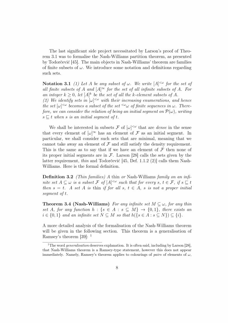
The last significant side project necessitated by Larson’s proof of Theo-rem 3.1 was to formalise the Nash-Williams partition theorem, as presentedby Todorčević [45]. The main objects in Nash-Williams’ theorem are familiesof finite subsets of ω. We introduce some notation and definitions regardingsuch sets.
Notation 3.1 (1) Let A be any subset of ω. We write [A]<ω for the set ofall finite subsets of A and [A]∞ for the set of all infinite subsets of A. Foran integer k ≥ 0, let [A]k be the set of all the k-element subsets of A.(2) We identify sets in [ω]<ω with their increasing enumerations, and hencethe set [ω]<ω becomes a subset of the set <ωω of finite sequences in ω. There-fore, we can consider the relation of being an initial segment on P(ω), writings ⊑ t when s is an initial segment of t.
We shall be interested in subsets F of [ω]<ω that are dense in the sensethat every element of [ω]∞ has an element of F as an initial segment. Inparticular, we shall consider such sets that are minimal, meaning that wecannot take away an element of F and still satisfy the density requirement.This is the same as to say that if we have an element of F then none ofits proper initial segments are in F . Larson [28] calls the sets given by thelatter requirement, thin and Todorčević [45, Def. 1.1.2 (2)] calls them Nash-Williams. Here is the formal definition.
Definition 3.2 (Thin families) A thin or Nash-Williams family on an infi-nite set A ⊆ ω is a subset F of [A]<ω such that for every s, t ∈ F , if s ⊑ tthen s = t. A set A is thin if for all s, t ∈ A, s is not a proper initialsegment of t.
Theorem 3.4 (Nash-Williams) For any infinite set M ⊆ ω, for any thinset A, for any function h : {s ∈ A : s ⊆ M} → {0, 1}, there exists ani ∈ {0, 1} and an infinite set N ⊆ M so that h({s ∈ A : s ⊆ N}) ⊆ {i}.
A more detailed analysis of the formalisation of the Nash-Williams theoremwill be given in the following section. This theorem is a generalisation ofRamsey’s theorem [39]: 1
1The word generalisation deserves explanation. It is often said, including by Larson [28],that Nash-Williams theorem is a Ramsey-type statement, however this does not appearimmediately. Namely, Ramsey’s theorem applies to colourings of pairs of elements of ω,
8
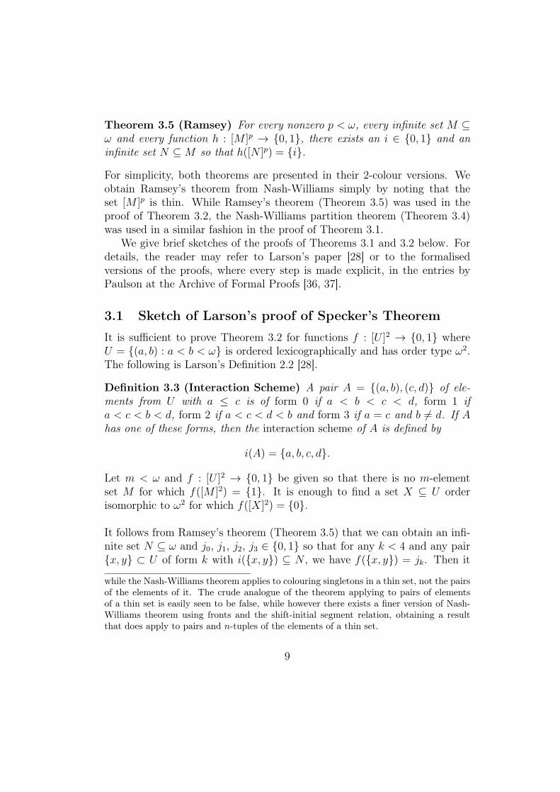
Theorem 3.5 (Ramsey) For every nonzero p < ω, every infinite set M ⊆ω and every function h : [M ]p → {0, 1}, there exists an i ∈ {0, 1} and aninfinite set N ⊆ M so that h([N ]p) = {i}.
For simplicity, both theorems are presented in their 2-colour versions. Weobtain Ramsey’s theorem from Nash-Williams simply by noting that theset [M ]p is thin. While Ramsey’s theorem (Theorem 3.5) was used in theproof of Theorem 3.2, the Nash-Williams partition theorem (Theorem 3.4)was used in a similar fashion in the proof of Theorem 3.1.
We give brief sketches of the proofs of Theorems 3.1 and 3.2 below. Fordetails, the reader may refer to Larson’s paper [28] or to the formalisedversions of the proofs, where every step is made explicit, in the entries byPaulson at the Archive of Formal Proofs [36, 37].
3.1 Sketch of Larson’s proof of Specker’s Theorem
It is sufficient to prove Theorem 3.2 for functions f : [U ]2 → {0, 1} whereU = {(a, b) : a < b < ω} is ordered lexicographically and has order type ω2.The following is Larson’s Definition 2.2 [28].
Definition 3.3 (Interaction Scheme) A pair A = {(a, b), (c, d)} of ele-ments from U with a ≤ c is of form 0 if a < b < c < d, form 1 ifa < c < b < d, form 2 if a < c < d < b and form 3 if a = c and b ∕= d. If Ahas one of these forms, then the interaction scheme of A is defined by
i(A) = {a, b, c, d}.
Let m < ω and f : [U ]2 → {0, 1} be given so that there is no m-elementset M for which f([M ]2) = {1}. It is enough to find a set X ⊆ U orderisomorphic to ω2 for which f([X]2) = {0}.
It follows from Ramsey’s theorem (Theorem 3.5) that we can obtain an infi-nite set N ⊆ ω and j0, j1, j2, j3 ∈ {0, 1} so that for any k < 4 and any pair{x, y} ⊂ U of form k with i({x, y}) ⊆ N , we have f({x, y}) = jk. Then it
while the Nash-Williams theorem applies to colouring singletons in a thin set, not the pairsof the elements of it. The crude analogue of the theorem applying to pairs of elementsof a thin set is easily seen to be false, while however there exists a finer version of Nash-Williams theorem using fronts and the shift-initial segment relation, obtaining a resultthat does apply to pairs and n-tuples of the elements of a thin set.
9
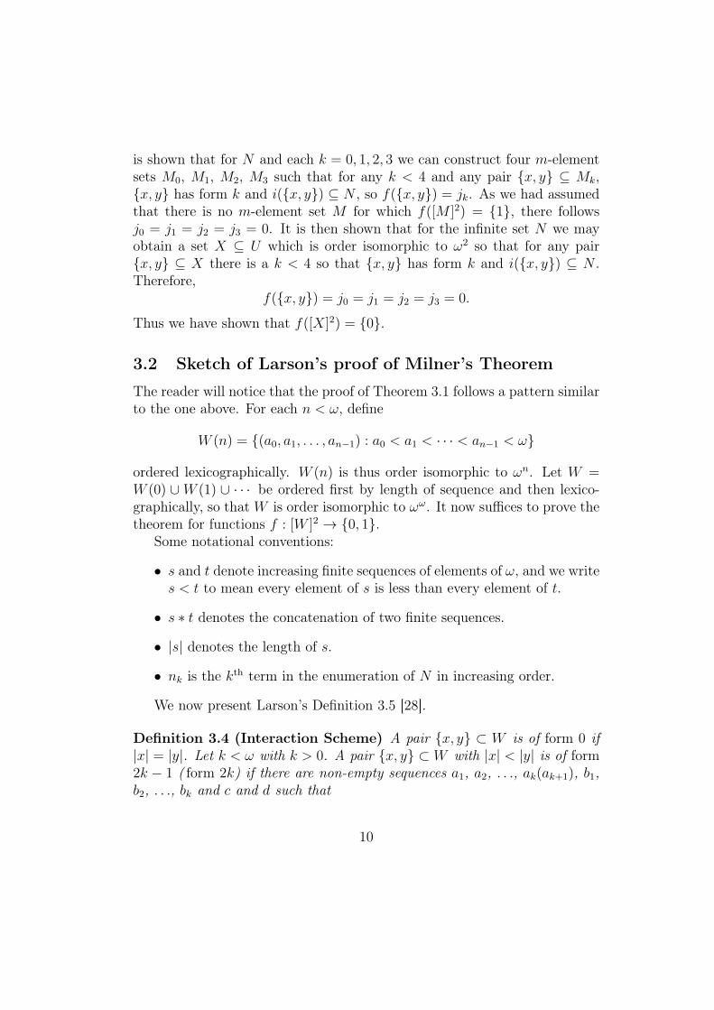
is shown that for N and each k = 0, 1, 2, 3 we can construct four m-elementsets M0, M1, M2, M3 such that for any k < 4 and any pair {x, y} ⊆ Mk,{x, y} has form k and i({x, y}) ⊆ N , so f({x, y}) = jk. As we had assumedthat there is no m-element set M for which f([M ]2) = {1}, there followsj0 = j1 = j2 = j3 = 0. It is then shown that for the infinite set N we mayobtain a set X ⊆ U which is order isomorphic to ω2 so that for any pair{x, y} ⊆ X there is a k < 4 so that {x, y} has form k and i({x, y}) ⊆ N .Therefore,
f({x, y}) = j0 = j1 = j2 = j3 = 0.
Thus we have shown that f([X]2) = {0}.
3.2 Sketch of Larson’s proof of Milner’s Theorem
The reader will notice that the proof of Theorem 3.1 follows a pattern similarto the one above. For each n < ω, define
W (n) = {(a0, a1, . . . , an−1) : a0 < a1 < · · · < an−1 < ω}
ordered lexicographically. W (n) is thus order isomorphic to ωn. Let W =W (0) ∪ W (1) ∪ · · · be ordered first by length of sequence and then lexico-graphically, so that W is order isomorphic to ωω. It now suffices to prove thetheorem for functions f : [W ]2 → {0, 1}.
Some notational conventions:
• s and t denote increasing finite sequences of elements of ω, and we writes < t to mean every element of s is less than every element of t.
• s ∗ t denotes the concatenation of two finite sequences.
• |s| denotes the length of s.
• nk is the kth term in the enumeration of N in increasing order.
We now present Larson’s Definition 3.5 [28].
Definition 3.4 (Interaction Scheme) A pair {x, y} ⊂ W is of form 0 if|x| = |y|. Let k < ω with k > 0. A pair {x, y} ⊂ W with |x| < |y| is of form2k − 1 ( form 2k) if there are non-empty sequences a1, a2, . . ., ak(ak+1), b1,b2, . . ., bk and c and d such that
10
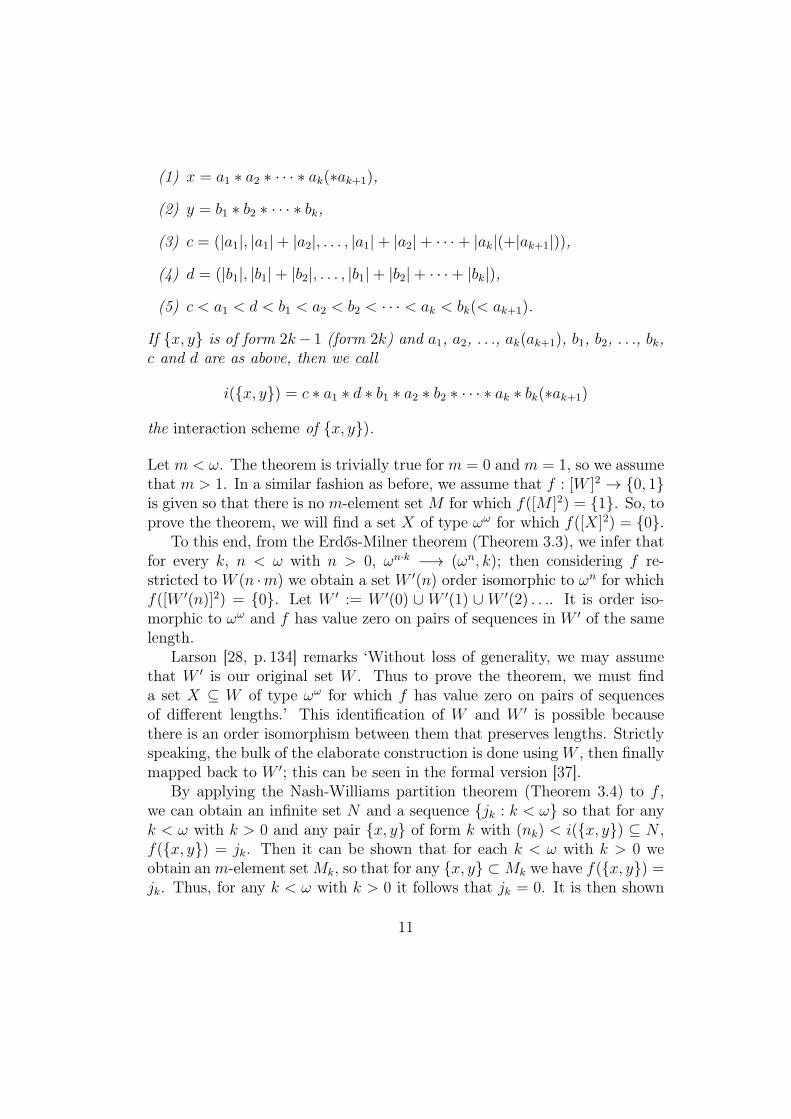
(1) x = a1 ∗ a2 ∗ · · · ∗ ak(∗ak+1),
(2) y = b1 ∗ b2 ∗ · · · ∗ bk,
(3) c = (|a1|, |a1|+ |a2|, . . . , |a1|+ |a2|+ · · ·+ |ak|(+|ak+1|)),
(4) d = (|b1|, |b1|+ |b2|, . . . , |b1|+ |b2|+ · · ·+ |bk|),
(5) c < a1 < d < b1 < a2 < b2 < · · · < ak < bk(< ak+1).
If {x, y} is of form 2k− 1 (form 2k) and a1, a2, . . ., ak(ak+1), b1, b2, . . ., bk,c and d are as above, then we call
i({x, y}) = c ∗ a1 ∗ d ∗ b1 ∗ a2 ∗ b2 ∗ · · · ∗ ak ∗ bk(∗ak+1)
the interaction scheme of {x, y}).
Let m < ω. The theorem is trivially true for m = 0 and m = 1, so we assumethat m > 1. In a similar fashion as before, we assume that f : [W ]2 → {0, 1}is given so that there is no m-element set M for which f([M ]2) = {1}. So, toprove the theorem, we will find a set X of type ωω for which f([X]2) = {0}.
To this end, from the Erdős-Milner theorem (Theorem 3.3), we infer thatfor every k, n < ω with n > 0, ωn·k −→ (ωn, k); then considering f re-stricted to W (n ·m) we obtain a set W ′(n) order isomorphic to ωn for whichf([W ′(n)]2) = {0}. Let W ′ := W ′(0) ∪ W ′(1) ∪ W ′(2) . . .. It is order iso-morphic to ωω and f has value zero on pairs of sequences in W ′ of the samelength.
Larson [28, p. 134] remarks ‘Without loss of generality, we may assumethat W ′ is our original set W . Thus to prove the theorem, we must finda set X ⊆ W of type ωω for which f has value zero on pairs of sequencesof different lengths.’ This identification of W and W ′ is possible becausethere is an order isomorphism between them that preserves lengths. Strictlyspeaking, the bulk of the elaborate construction is done using W , then finallymapped back to W ′; this can be seen in the formal version [37].
By applying the Nash-Williams partition theorem (Theorem 3.4) to f ,we can obtain an infinite set N and a sequence {jk : k < ω} so that for anyk < ω with k > 0 and any pair {x, y} of form k with (nk) < i({x, y}) ⊆ N ,f({x, y}) = jk. Then it can be shown that for each k < ω with k > 0 weobtain an m-element set Mk, so that for any {x, y} ⊂ Mk we have f({x, y}) =jk. Thus, for any k < ω with k > 0 it follows that jk = 0. It is then shown
11
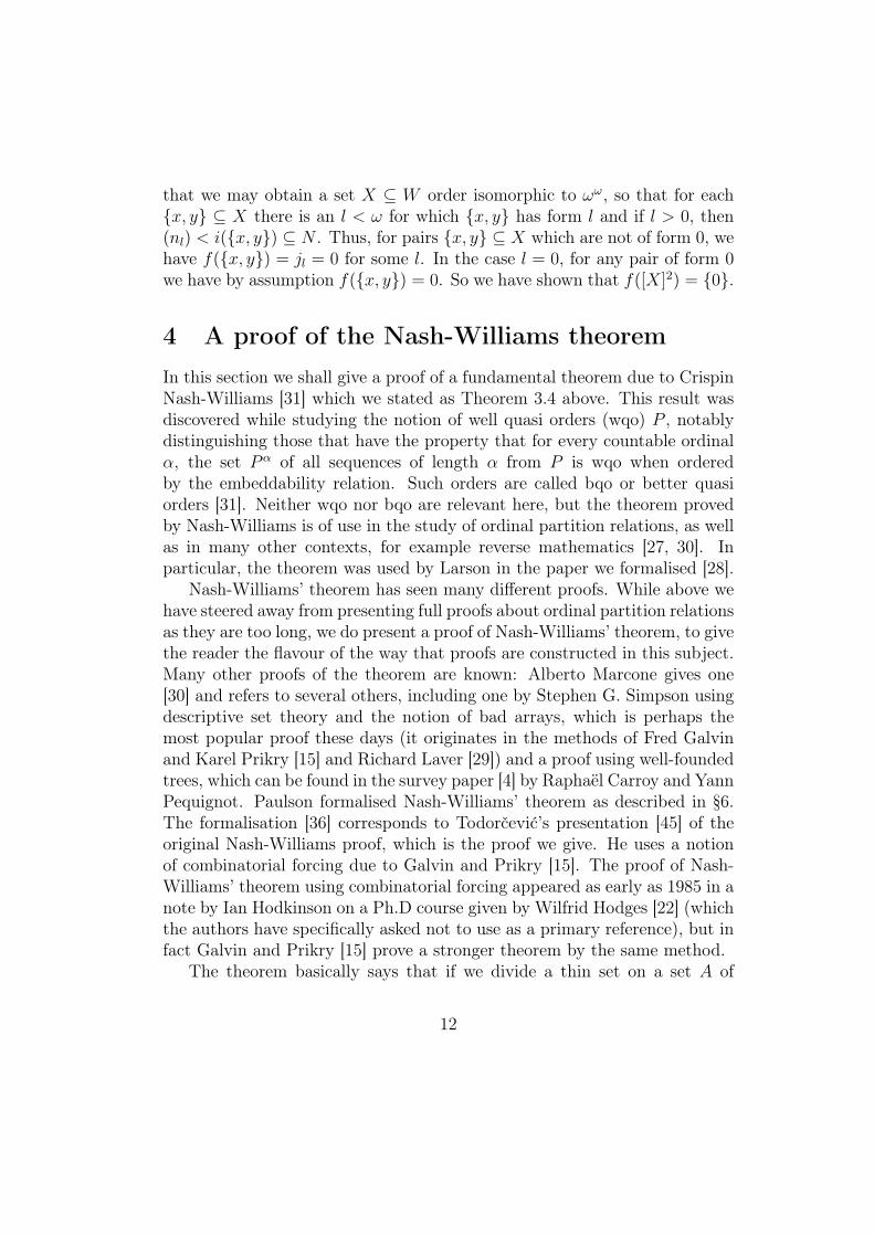
that we may obtain a set X ⊆ W order isomorphic to ωω, so that for each{x, y} ⊆ X there is an l < ω for which {x, y} has form l and if l > 0, then(nl) < i({x, y}) ⊆ N . Thus, for pairs {x, y} ⊆ X which are not of form 0, wehave f({x, y}) = jl = 0 for some l. In the case l = 0, for any pair of form 0we have by assumption f({x, y}) = 0. So we have shown that f([X]2) = {0}.
4 A proof of the Nash-Williams theoremIn this section we shall give a proof of a fundamental theorem due to CrispinNash-Williams [31] which we stated as Theorem 3.4 above. This result wasdiscovered while studying the notion of well quasi orders (wqo) P , notablydistinguishing those that have the property that for every countable ordinalα, the set Pα of all sequences of length α from P is wqo when orderedby the embeddability relation. Such orders are called bqo or better quasiorders [31]. Neither wqo nor bqo are relevant here, but the theorem provedby Nash-Williams is of use in the study of ordinal partition relations, as wellas in many other contexts, for example reverse mathematics [27, 30]. Inparticular, the theorem was used by Larson in the paper we formalised [28].
Nash-Williams’ theorem has seen many different proofs. While above wehave steered away from presenting full proofs about ordinal partition relationsas they are too long, we do present a proof of Nash-Williams’ theorem, to givethe reader the flavour of the way that proofs are constructed in this subject.Many other proofs of the theorem are known: Alberto Marcone gives one[30] and refers to several others, including one by Stephen G. Simpson usingdescriptive set theory and the notion of bad arrays, which is perhaps themost popular proof these days (it originates in the methods of Fred Galvinand Karel Prikry [15] and Richard Laver [29]) and a proof using well-foundedtrees, which can be found in the survey paper [4] by Raphaël Carroy and YannPequignot. Paulson formalised Nash-Williams’ theorem as described in §6.The formalisation [36] corresponds to Todorčević’s presentation [45] of theoriginal Nash-Williams proof, which is the proof we give. He uses a notionof combinatorial forcing due to Galvin and Prikry [15]. The proof of Nash-Williams’ theorem using combinatorial forcing appeared as early as 1985 in anote by Ian Hodkinson on a Ph.D course given by Wilfrid Hodges [22] (whichthe authors have specifically asked not to use as a primary reference), but infact Galvin and Prikry [15] prove a stronger theorem by the same method.
The theorem basically says that if we divide a thin set on a set A of
12
natural numbers into a finite number of pieces, then one of them will containa thin set on some infinite subset A′ of A. This is the analogue of the versionof the pigeonhole principle which says that if an infinite set is divided into afinite number of pieces, then one of the pieces is infinite. Notice that Theorem3.4 yields this by applying the theorem finitely many times.
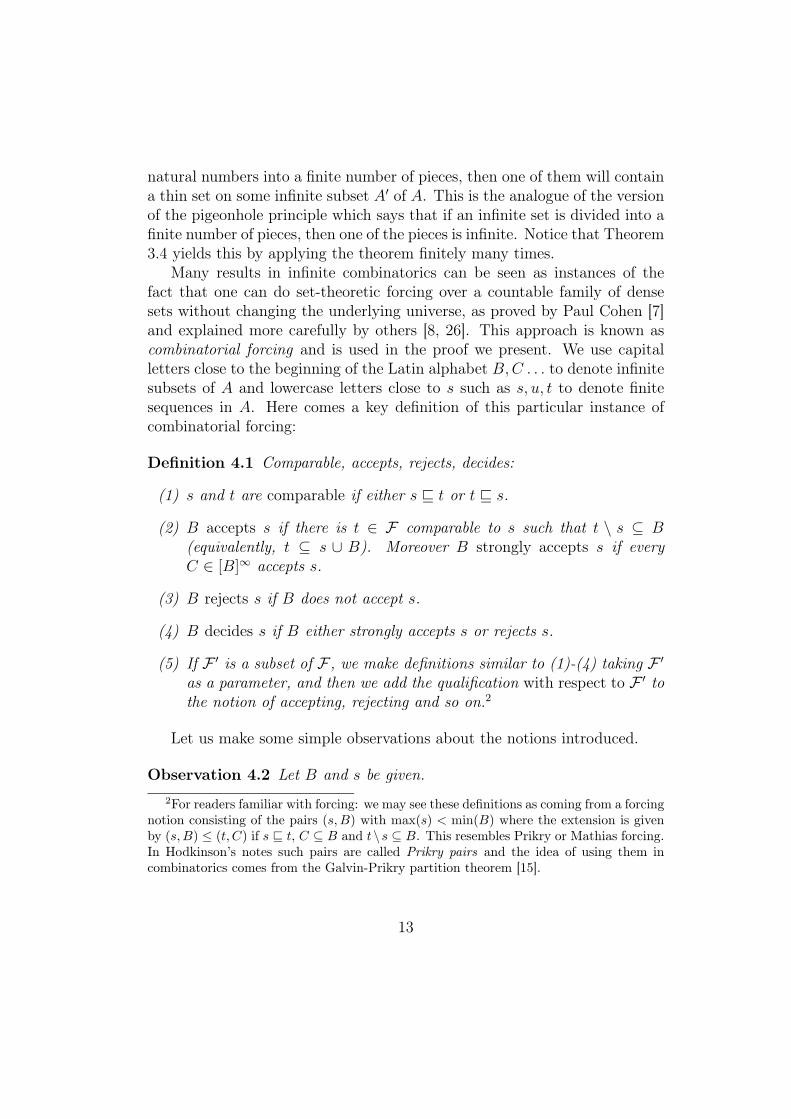
Many results in infinite combinatorics can be seen as instances of thefact that one can do set-theoretic forcing over a countable family of densesets without changing the underlying universe, as proved by Paul Cohen [7]and explained more carefully by others [8, 26]. This approach is known ascombinatorial forcing and is used in the proof we present. We use capitalletters close to the beginning of the Latin alphabet B,C . . . to denote infinitesubsets of A and lowercase letters close to s such as s, u, t to denote finitesequences in A. Here comes a key definition of this particular instance ofcombinatorial forcing:
Definition 4.1 Comparable, accepts, rejects, decides:
(1) s and t are comparable if either s ⊑ t or t ⊑ s.
(2) B accepts s if there is t ∈ F comparable to s such that t \ s ⊆ B(equivalently, t ⊆ s ∪ B). Moreover B strongly accepts s if everyC ∈ [B]∞ accepts s.
(3) B rejects s if B does not accept s.
(4) B decides s if B either strongly accepts s or rejects s.
(5) If F ′ is a subset of F , we make definitions similar to (1)-(4) taking F ′
as a parameter, and then we add the qualification with respect to F ′ tothe notion of accepting, rejecting and so on.2
Let us make some simple observations about the notions introduced.
Observation 4.2 Let B and s be given.2For readers familiar with forcing: we may see these definitions as coming from a forcing
notion consisting of the pairs (s,B) with max(s) < min(B) where the extension is givenby (s,B) ≤ (t, C) if s ⊑ t, C ⊆ B and t\s ⊆ B. This resembles Prikry or Mathias forcing.In Hodkinson’s notes such pairs are called Prikry pairs and the idea of using them incombinatorics comes from the Galvin-Prikry partition theorem [15].
13
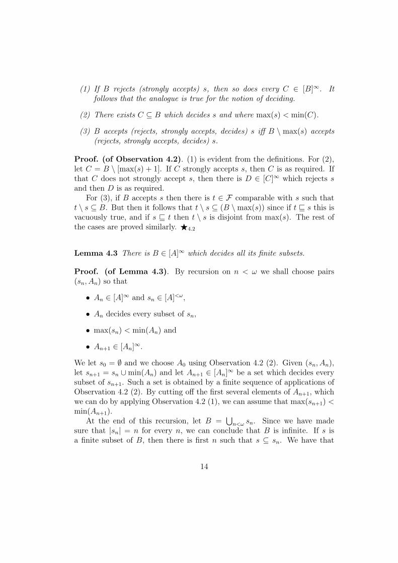
(1) If B rejects (strongly accepts) s, then so does every C ∈ [B]∞. Itfollows that the analogue is true for the notion of deciding.
(2) There exists C ⊆ B which decides s and where max(s) < min(C).
(3) B accepts (rejects, strongly accepts, decides) s iff B \ max(s) accepts(rejects, strongly accepts, decides) s.
Proof. (of Observation 4.2). (1) is evident from the definitions. For (2),let C = B \ [max(s) + 1]. If C strongly accepts s, then C is as required. Ifthat C does not strongly accept s, then there is D ∈ [C]∞ which rejects sand then D is as required.
For (3), if B accepts s then there is t ∈ F comparable with s such thatt \ s ⊆ B. But then it follows that t \ s ⊆ (B \max(s)) since if t ⊑ s this isvacuously true, and if s ⊑ t then t \ s is disjoint from max(s). The rest ofthe cases are proved similarly. !4.2
Lemma 4.3 There is B ∈ [A]∞ which decides all its finite subsets.
Proof. (of Lemma 4.3). By recursion on n < ω we shall choose pairs(sn, An) so that
• An ∈ [A]∞ and sn ∈ [A]<ω,
• An decides every subset of sn,
• max(sn) < min(An) and
• An+1 ∈ [An]∞.
We let s0 = ∅ and we choose A0 using Observation 4.2 (2). Given (sn, An),let sn+1 = sn ∪min(An) and let An+1 ∈ [An]
∞ be a set which decides everysubset of sn+1. Such a set is obtained by a finite sequence of applications ofObservation 4.2 (2). By cutting off the first several elements of An+1, whichwe can do by applying Observation 4.2 (1), we can assume that max(sn+1) <min(An+1).
At the end of this recursion, let B =!
n<ω sn. Since we have madesure that |sn| = n for every n, we can conclude that B is infinite. If s isa finite subset of B, then there is first n such that s ⊆ sn. We have that
14
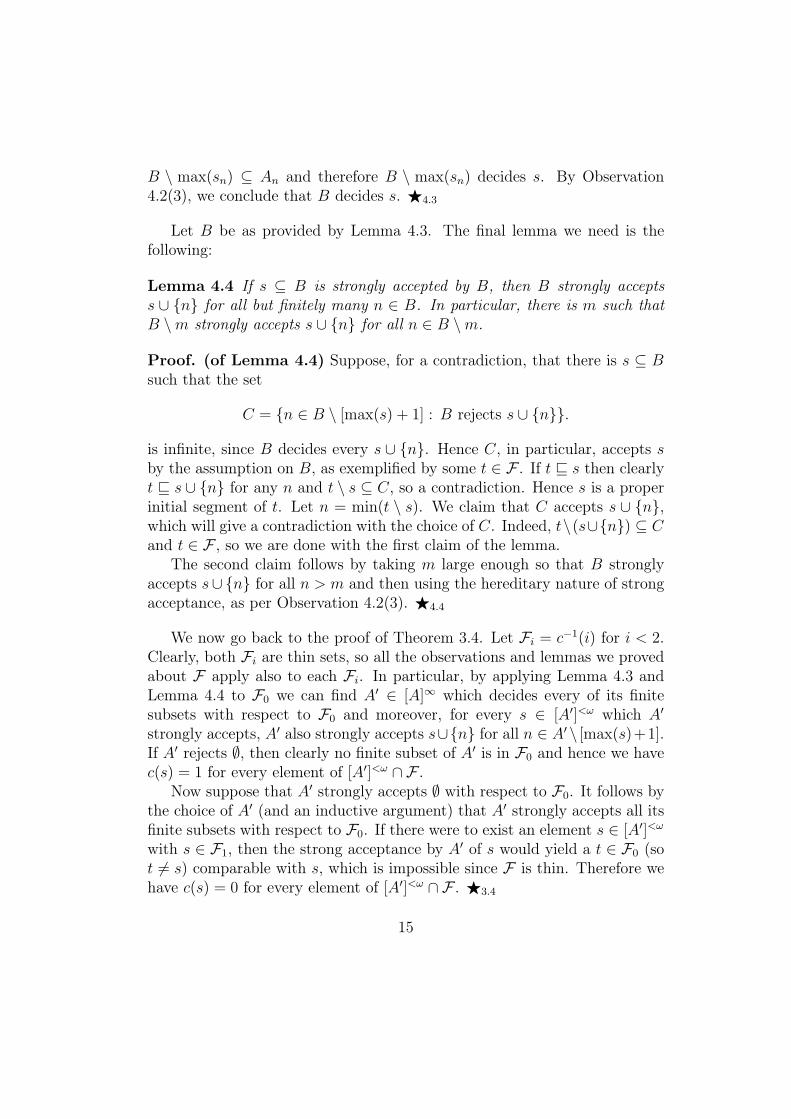
B \ max(sn) ⊆ An and therefore B \ max(sn) decides s. By Observation4.2(3), we conclude that B decides s. !4.3
Let B be as provided by Lemma 4.3. The final lemma we need is thefollowing:
Lemma 4.4 If s ⊆ B is strongly accepted by B, then B strongly acceptss ∪ {n} for all but finitely many n ∈ B. In particular, there is m such thatB \m strongly accepts s ∪ {n} for all n ∈ B \m.
Proof. (of Lemma 4.4) Suppose, for a contradiction, that there is s ⊆ Bsuch that the set
C = {n ∈ B \ [max(s) + 1] : B rejects s ∪ {n}}.
is infinite, since B decides every s ∪ {n}. Hence C, in particular, accepts sby the assumption on B, as exemplified by some t ∈ F . If t ⊑ s then clearlyt ⊑ s ∪ {n} for any n and t \ s ⊆ C, so a contradiction. Hence s is a properinitial segment of t. Let n = min(t \ s). We claim that C accepts s ∪ {n},which will give a contradiction with the choice of C. Indeed, t\(s∪{n}) ⊆ Cand t ∈ F , so we are done with the first claim of the lemma.
The second claim follows by taking m large enough so that B stronglyaccepts s∪ {n} for all n > m and then using the hereditary nature of strongacceptance, as per Observation 4.2(3). !4.4
We now go back to the proof of Theorem 3.4. Let Fi = c−1(i) for i < 2.Clearly, both Fi are thin sets, so all the observations and lemmas we provedabout F apply also to each Fi. In particular, by applying Lemma 4.3 andLemma 4.4 to F0 we can find A′ ∈ [A]∞ which decides every of its finitesubsets with respect to F0 and moreover, for every s ∈ [A′]<ω which A′
strongly accepts, A′ also strongly accepts s∪{n} for all n ∈ A′ \ [max(s)+1].If A′ rejects ∅, then clearly no finite subset of A′ is in F0 and hence we havec(s) = 1 for every element of [A′]<ω ∩ F .
Now suppose that A′ strongly accepts ∅ with respect to F0. It follows bythe choice of A′ (and an inductive argument) that A′ strongly accepts all itsfinite subsets with respect to F0. If there were to exist an element s ∈ [A′]<ω
with s ∈ F1, then the strong acceptance by A′ of s would yield a t ∈ F0 (sot ∕= s) comparable with s, which is impossible since F is thin. Therefore wehave c(s) = 0 for every element of [A′]<ω ∩ F . !3.4
15
5 Introduction to IsabelleIsabelle is an interactive theorem prover originally developed in the 1980swith the aim of supporting multiple logical formalisms. These include first-order logic (intuitionistic as well as classical) and higher-order logic as well asZermelo Fraenkel set theory. However, the 1990s saw higher-order logic takea dominant role in the field of interactive theorem proving, particularly inhardware verification [20, 25, 34]. While Isabelle/ZF and Isabelle/HOL sharethe entire Isabelle code base (basic inference procedures, a sophisticated userinterface, etc.), Isabelle/HOL [33] has much additional automation: so muchso that it’s the best choice even for set theory.
Unlike proof assistants based on constructive type theories, Isabelle/HOLimplements simple type theory. Types can take types as parameters but notintegers for example. The type of finite sequences (known as lists) takesthe component type as a parameter, but there is no type of n-element lists.Logical predicates form the basis of a basic typed set theory, where anydesired set can be expressed by comprehension over a formula. We can definethe set of n-element lists where the elements are drawn from some other set.Thus, the simple framework given by types can be refined through the useof sets.
There are always trade-offs between expressiveness of a formalism andease of automation. Reliance on a simple classical formalism frees us fromthe many technical difficulties which seem to plague constructive type the-ories, such as intensional equality, difficulties with the concept of set, andperformance issues in space and time.
Isabelle employs the time-honoured LCF approach [16]. This architectureensures soundness through the use of a small proof kernel that implementsthe rules of inference and has the sole right to declare a statement to bea theorem. Upon this foundation, Isabelle/HOL provides many forms ofpowerful automation [38]:
• Simplification, i.e., systematic directed rewriting using identities.
• Sophisticated logical reasoning even with quantifiers.
• Sledgehammer: strong integration with external theorem provers.
• Automatic counterexample finding for many problem domains.
16
We found that some of this automation works effectively with Larson’s elab-orate constructions on sequences.
5.1 Simple type theory in Isabelle/HOL
Isabelle’s higher-order logic is closely based on Church’s simple type the-ory [6]. It includes the following elements:
• Types and type operators, for example int (the type of integers), orα⇒β (the type of functions from α to β), or α list (the type of finitesequences whose elements have type α). Note the postfix syntax: (intlist) set is the type of sets of lists of integers.
• Terms built of constants, variables, λ-abstractions, and function appli-cations.
• Formulas : terms of the truth value type, bool (Church’s o), with theusual logical connectives and quantifiers.
• The axiom of choice (AC) for all types via Hilbert’s operator εx.φ,denoting some a such that φ(a) if such exists.3 The Isabelle syntax isSOME x. P x.
The typed set theory essentially identifies sets with predicates, with typeα set essentially the same as α⇒bool. On this foundation, recursive def-initions of types, functions and predicates/sets are provided through pro-grammed procedures that reduce such definitions to primitive constructionsand automatically prove the essential properties. This basis is expressiveenough for the formalisation of the numerous advanced results mentioned inthe introduction.
5.2 ZFC in simple type theory
Since the set type operator can be iterated only finitely many times, simpletype theory turns out to be weaker than Zermelo set theory (let alone ZF). Forwork requiring the full power of ZFC, it is convenient to assume some versionof the ZF axioms within Isabelle/HOL. The approach adopted here [35] seeks
3An undefined value is simply regarded as underspecified. It has the expected type,and we always have (εx.φ) = (εx.φ) for example.
17
a smooth integration between ZFC and simple type theory. We introduce atype V (the type of all ZF sets) and then V set is the type of classes. OurZF axioms characterise the small classes, those that can be embedded intoelements of V . The axiom of choice is inherited from Isabelle/HOL. On thisbasis it is straightforward to define the usual elements of Cantor’s paradise,including ordinals, cardinals, alephs and order types. We borrow large formaldevelopments from the existing Isabelle/HOL framework: recursion on ∈ isjust an instance of well-founded recursion, and it’s easy to deduce that thetype real corresponds to some element of V without redoing the constructionof the real numbers.
We define order types on wellorderings only (yielding ordinals). Thesewellorderings can be defined on any Isabelle/HOL type: we can considerorderings defined on type nat rather than on the equivalent ordinal, ω. Westarted with a small library of facts about order types, which grew and grewin accordance with the demands of the case study.
The point of adopting Isabelle/HOL over Isabelle/ZF is the possibilityof making use of its aforementioned automation (Sledgehammer) and thecounterexample-finding tools (Nitpick [2] and Quickcheck [3]). The maindrawback of doing set theory in Isabelle/HOL is the impossibility of workingwithout AC: the axiom is inherently part of the framework. That drawbackhas no bearing on the present project, however.
6 Formalising the Nash-Williams theoremAlthough the Nash-Williams partition theorem is only a minor part of theproject, it’s a key result and its formalisation is brief enough to present inreasonable detail. In the next section, we’ll turn to Larson’s paper.
6.1 Preliminaries
As we saw in Sect. 4 above, the theorem is concerned with sets of naturalnumbers. Finite sets of natural numbers can be identified with ascendingfinite sequences; typical treatments of Nash-Williams use sets, while Larsonuses sequences. For sets S and T , we write S < T to express that everyelement of S is less than every element of T (it holds vacuously if either setis empty). This is essentially the same statement as the s < t mentioned inthe previous section. Our formalisation [36] follows Todorčević [45] as in the
18
proof in Sect. 4.S is an initial segment of T if T can be written in the form S ∪ S ′ such
that S < S ′, written S ≪ S’ in Isabelle syntax.
definition init_segment :: "nat set ⇒ nat set ⇒ bool"where "init_segment S T ≡ ∃ S’. T = S ∪ S’ ∧ S ≪ S’"
The Ramsey property expresses the conclusion of the theorem for thegeneral case of r components. Its definition for a family F of sets F and aninteger r is straightforward. A partition of F into r disjoint sets is expressedas a map f : F → {0, . . . , r − 1}. Partition j is expressed as the inverseimage f−1(j), written f -‘ {j} in Isabelle syntax.
Now the Ramsey property for F and r holds if for every partition map fand every infinite set M , there exists an infinite N ⊆ M and i < r such thatfor all j < r, if j ∕= i then partition j does not contain any subsets of N .(Pow N is the powerset of N .)
definition Ramsey :: "[nat set set, nat] ⇒ bool"where "Ramsey F r ≡
∀ f ∈ F → {..<r}. ∀ M. infinite M −→(∃ N i. N ⊆ M ∧ infinite N ∧ i<r ∧(∀ j<r. j ∕=i −→ f -‘ {j} ∩ F ∩ Pow N = {}))"
Recall that a family F of sets is thin provided every element of F is finite(expressed as F ⊆ {X. finite X}) and it does not contain distinct elementsS and T where one is an initial segment of the other (see Definition 3.2).
definition thin_set :: "nat set set ⇒ bool"where "thin_set F ≡
F ⊆ {X. finite X} ∧ (∀ S∈F. ∀ T∈F. init_segment S T −→ S=T)"
These definitions provide the necessary vocabulary to state the theorem,although its proof appears at the end of the development after those of allprerequisite lemmas.
theorem Nash_Williams:assumes F: "thin_set F" "r > 0" shows "Ramsey F r"
We now formalise the concepts of rejecting, strongly accepting and decid-ing a set, as described in Sect. 4. We regard F as fixed and say M decides S,etc. Note that the identification of ‘M accepts S’ with ‘M does not reject S’is formalised as an abbreviation rather than a definition, a distinction thataffects proof procedures but makes no difference mathematically.
19
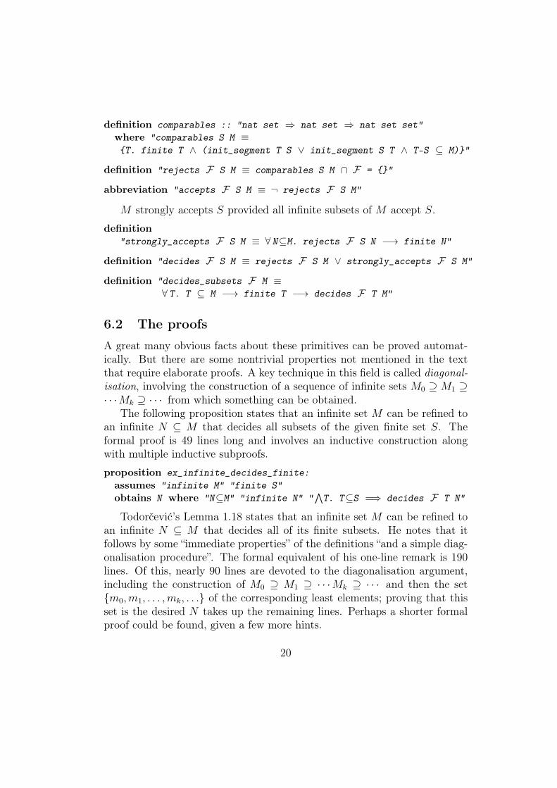
definition comparables :: "nat set ⇒ nat set ⇒ nat set set"where "comparables S M ≡{T. finite T ∧ (init_segment T S ∨ init_segment S T ∧ T-S ⊆ M)}"
definition "rejects F S M ≡ comparables S M ∩ F = {}"
abbreviation "accepts F S M ≡ ¬ rejects F S M"
M strongly accepts S provided all infinite subsets of M accept S.
definition"strongly_accepts F S M ≡ ∀ N⊆M. rejects F S N −→ finite N"
definition "decides F S M ≡ rejects F S M ∨ strongly_accepts F S M"
definition "decides_subsets F M ≡∀ T. T ⊆ M −→ finite T −→ decides F T M"
6.2 The proofs
A great many obvious facts about these primitives can be proved automat-ically. But there are some nontrivial properties not mentioned in the textthat require elaborate proofs. A key technique in this field is called diagonal-isation, involving the construction of a sequence of infinite sets M0 ⊇ M1 ⊇· · ·Mk ⊇ · · · from which something can be obtained.
The following proposition states that an infinite set M can be refined toan infinite N ⊆ M that decides all subsets of the given finite set S. Theformal proof is 49 lines long and involves an inductive construction alongwith multiple inductive subproofs.
proposition ex_infinite_decides_finite:assumes "infinite M" "finite S"obtains N where "N⊆M" "infinite N" "
!T. T⊆S =⇒ decides F T N"
Todorčević’s Lemma 1.18 states that an infinite set M can be refined toan infinite N ⊆ M that decides all of its finite subsets. He notes that itfollows by some “immediate properties” of the definitions “and a simple diag-onalisation procedure”. The formal equivalent of his one-line remark is 190lines. Of this, nearly 90 lines are devoted to the diagonalisation argument,including the construction of M0 ⊇ M1 ⊇ · · ·Mk ⊇ · · · and then the set{m0,m1, . . . ,mk, . . .} of the corresponding least elements; proving that thisset is the desired N takes up the remaining lines. Perhaps a shorter formalproof could be found, given a few more hints.
20
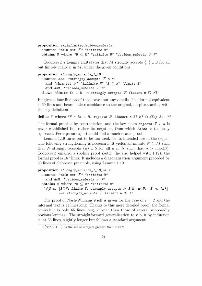
proposition ex_infinite_decides_subsets:assumes "thin_set F" "infinite M"obtains N where "N ⊆ M" "infinite N" "decides_subsets F N"
Todorčević’s Lemma 1.19 states that M strongly accepts {n} ∪ S for allbut finitely many n in M , under the given conditions.
proposition strongly_accepts_1_19:assumes acc: "strongly_accepts F S M"
and "thin_set F" "infinite M" "S ⊆ M" "finite S"and dsM: "decides_subsets F M"
shows "finite {n ∈ M. ¬ strongly_accepts F (insert n S) M}"
He gives a four-line proof that leaves out any details. The formal equivalentis 69 lines and bears little resemblance to the original, despite starting withthe key definition4
define N where "N = {n ∈ M. rejects F (insert n S) M} ∩ {Sup S<..}"
The formal proof is by contradiction, and the key claim rejects F S N isnever established but rather its negation, from which False is tediouslysqueezed. Perhaps an expert could find a much neater proof.
Lemma 1.19 turns out to be too weak for its intended use in the sequel.The following strengthening is necessary. It yields an infinite N ⊆ M suchthat N strongly accepts {n} ∪ S for all n in N such that n > max(S).Todorčević emailed a six-line proof sketch (he also helped with 1.19); theformal proof is 167 lines. It includes a diagonalisation argument preceded by50 lines of elaborate preamble, using Lemma 1.19.
proposition strongly_accepts_1_19_plus:assumes "thin_set F" "infinite M"
and dsM: "decides_subsets F M"obtains N where "N ⊆ M" "infinite N""!S n. [[S⊆N; finite S; strongly_accepts F S N; n∈N; S ≪ {n} ]]
=⇒ strongly_accepts F (insert n S) N"
The proof of Nash-Williams itself is given for the case of r = 2 and theinformal text is 11 lines long. Thanks to this more detailed proof, the formalequivalent is only 65 lines long, shorter than those of several supposedlyobvious lemmas. The straightforward generalisation to r > 0 by inductionis, at 66 lines, slightly longer but follows a standard argument.
4{Sup S<..} is the set of integers greater than maxS
21
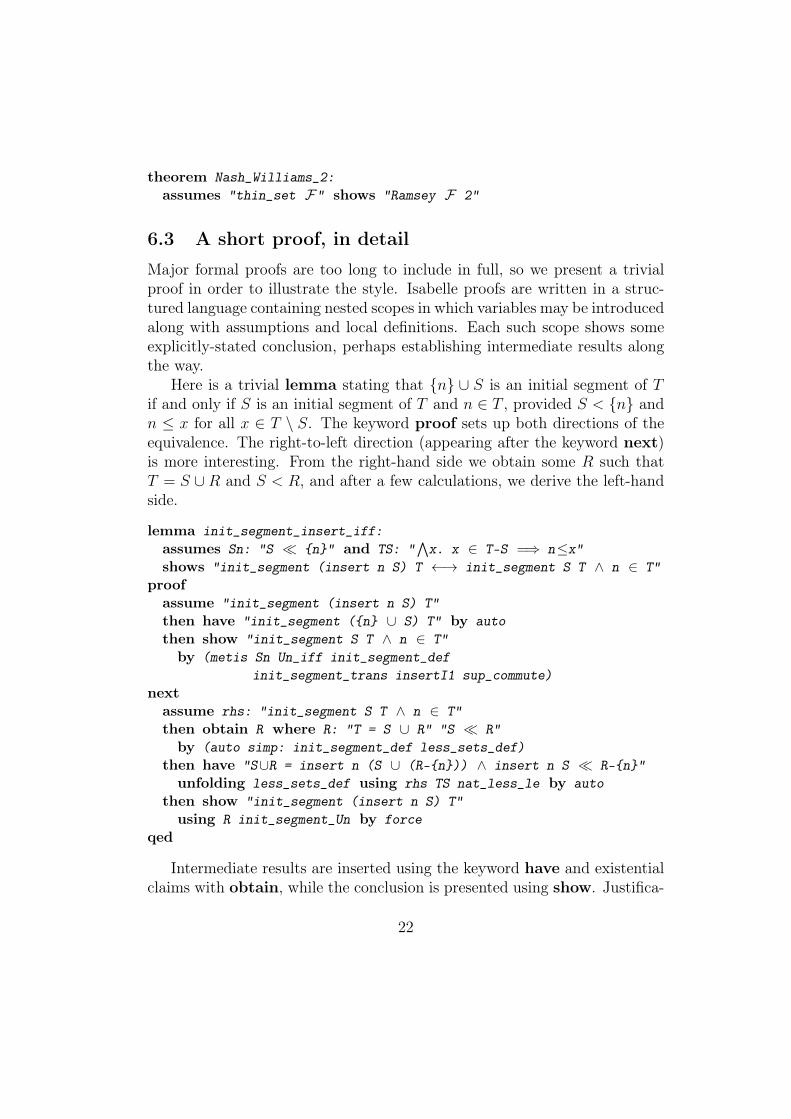
theorem Nash_Williams_2:assumes "thin_set F" shows "Ramsey F 2"
6.3 A short proof, in detail
Major formal proofs are too long to include in full, so we present a trivialproof in order to illustrate the style. Isabelle proofs are written in a struc-tured language containing nested scopes in which variables may be introducedalong with assumptions and local definitions. Each such scope shows someexplicitly-stated conclusion, perhaps establishing intermediate results alongthe way.
Here is a trivial lemma stating that {n} ∪ S is an initial segment of Tif and only if S is an initial segment of T and n ∈ T , provided S < {n} andn ≤ x for all x ∈ T \ S. The keyword proof sets up both directions of theequivalence. The right-to-left direction (appearing after the keyword next)is more interesting. From the right-hand side we obtain some R such thatT = S ∪ R and S < R, and after a few calculations, we derive the left-handside.
lemma init_segment_insert_iff:assumes Sn: "S ≪ {n}" and TS: "
!x. x ∈ T-S =⇒ n≤x"
shows "init_segment (insert n S) T ←→ init_segment S T ∧ n ∈ T"proof
assume "init_segment (insert n S) T"then have "init_segment ({n} ∪ S) T" by autothen show "init_segment S T ∧ n ∈ T"
by (metis Sn Un_iff init_segment_definit_segment_trans insertI1 sup_commute)
nextassume rhs: "init_segment S T ∧ n ∈ T"then obtain R where R: "T = S ∪ R" "S ≪ R"
by (auto simp: init_segment_def less_sets_def)then have "S∪R = insert n (S ∪ (R-{n})) ∧ insert n S ≪ R-{n}"
unfolding less_sets_def using rhs TS nat_less_le by autothen show "init_segment (insert n S) T"
using R init_segment_Un by forceqed
Intermediate results are inserted using the keyword have and existentialclaims with obtain, while the conclusion is presented using show. Justifica-
22
tions are introduced with by. A justification can consist of a proof methodsuch as auto, or a series of proof methods, or a full proof structure enclosedwithin the brackets proof and qed. Thus the various proof elements (thereare many others) can be nested to any depth.
Because proofs in Isabelle’s Isar language are structured, they can be muchmore readable than proofs in other theorem provers. Explicit statementsof the assumptions and conclusions make structured proofs more verbosethan the tactic-style proofs that predominate with other proof assistants,but infinitely more legible. The ideal is not merely to formalise mathematicalresults but to create a document that makes the proof clear to the reader,where—without having to trust the software—a knowledgeable reader coulddecide for herself whether the claims follow from the assumptions. A humanmathematician would not like to see an incomprehensible ‘black box’ proof.The possibility to recreate a ‘traditional’ proof from Isabelle code does helpthe user feel more at ease.
6.4 On the length of formal proofs
The de Bruijn factor [46] is defined as the ratio of the size of the formalmathematics to the size of the corresponding mathematical exposition. Itcan be regarded as measuring the cost of formalisation.
Unfortunately, it’s highly inexact. Mathematical writing varies greatly inits level of detail. The first ever de Bruijn factor was calculated for Jutting’stranslation of Landau’s Grundlagen der Analysis—on the construction of thecomplex numbers—into AUTOMATH.
An aspect which has not been mentioned so far is the ratiobetween the length of pieces of AUT-QE text and the length of thecorresponding German texts. Our claim at the outset was thatthis ratio can be kept constant. . . . As a measure of the lengths thenumber of stored AUT-QE expressions . . . and (rough estimatesof) the number of German words. [24, p. 46]
The highest ratio, 6.4, is obtained for the translation of Landau’s Chapter4, in which the real numbers are constructed from the positive real numbers(in the form of Dedekind cuts, which had been defined in Chapter 3). Butthis is a book that devotes 173 pages to the development of complex numberarithmetic from logic. The proof that a/b = c/d ⇐⇒ ad = bc includes
23
two references to previous theorems about complex arithmetic. The materialcould be covered in 10% of the space.
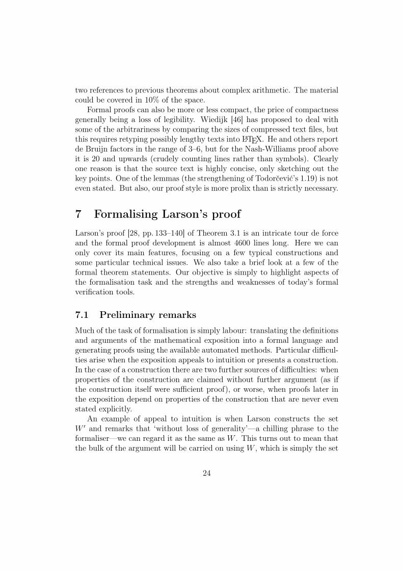
Formal proofs can also be more or less compact, the price of compactnessgenerally being a loss of legibility. Wiedijk [46] has proposed to deal withsome of the arbitrariness by comparing the sizes of compressed text files, butthis requires retyping possibly lengthy texts into LATEX. He and others reportde Bruijn factors in the range of 3–6, but for the Nash-Williams proof aboveit is 20 and upwards (crudely counting lines rather than symbols). Clearlyone reason is that the source text is highly concise, only sketching out thekey points. One of the lemmas (the strengthening of Todorčević’s 1.19) is noteven stated. But also, our proof style is more prolix than is strictly necessary.
7 Formalising Larson’s proofLarson’s proof [28, pp. 133–140] of Theorem 3.1 is an intricate tour de forceand the formal proof development is almost 4600 lines long. Here we canonly cover its main features, focusing on a few typical constructions andsome particular technical issues. We also take a brief look at a few of theformal theorem statements. Our objective is simply to highlight aspects ofthe formalisation task and the strengths and weaknesses of today’s formalverification tools.
7.1 Preliminary remarks
Much of the task of formalisation is simply labour: translating the definitionsand arguments of the mathematical exposition into a formal language andgenerating proofs using the available automated methods. Particular difficul-ties arise when the exposition appeals to intuition or presents a construction.In the case of a construction there are two further sources of difficulties: whenproperties of the construction are claimed without further argument (as ifthe construction itself were sufficient proof), or worse, when proofs later inthe exposition depend on properties of the construction that are never evenstated explicitly.
An example of appeal to intuition is when Larson constructs the setW ′ and remarks that ‘without loss of generality’—a chilling phrase to theformaliser—we can regard it as the same as W . This turns out to mean thatthe bulk of the argument will be carried on using W , which is simply the set
24
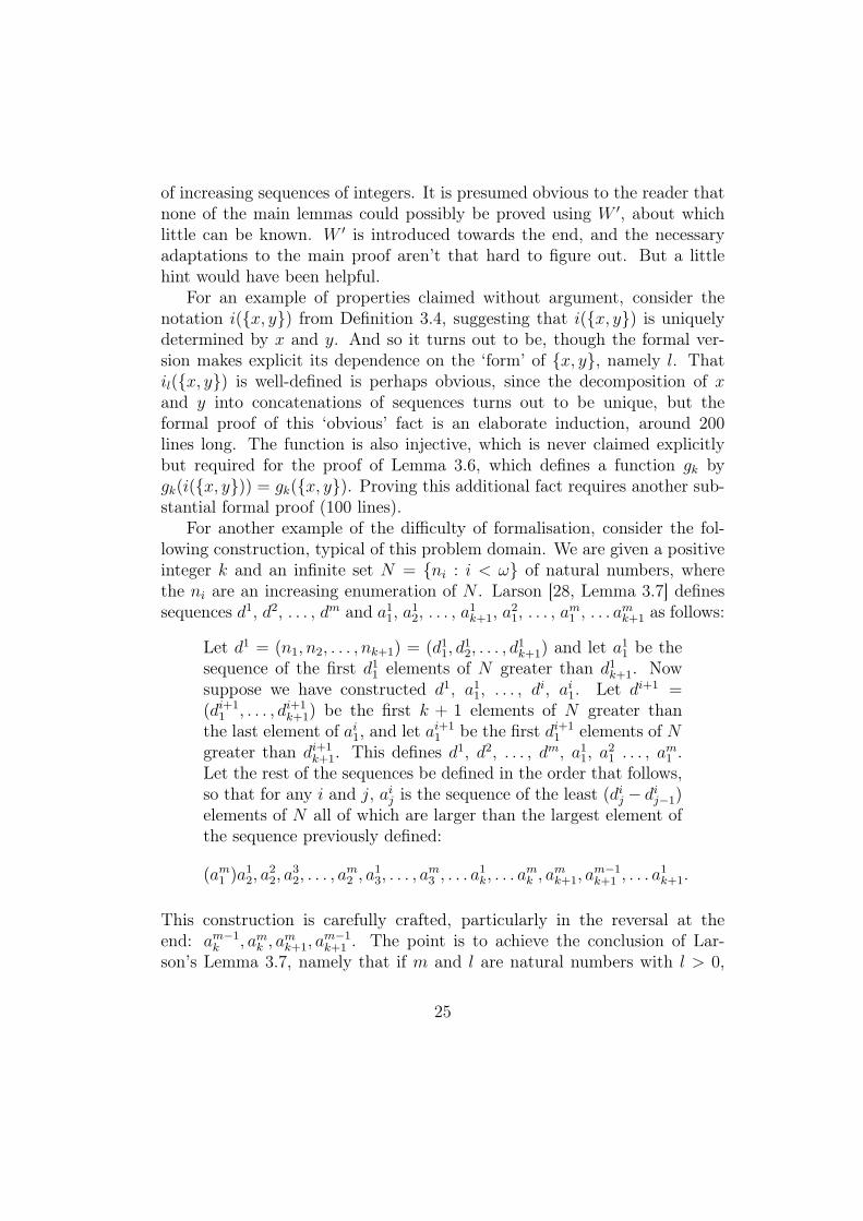
of increasing sequences of integers. It is presumed obvious to the reader thatnone of the main lemmas could possibly be proved using W ′, about whichlittle can be known. W ′ is introduced towards the end, and the necessaryadaptations to the main proof aren’t that hard to figure out. But a littlehint would have been helpful.
For an example of properties claimed without argument, consider thenotation i({x, y}) from Definition 3.4, suggesting that i({x, y}) is uniquelydetermined by x and y. And so it turns out to be, though the formal ver-sion makes explicit its dependence on the ‘form’ of {x, y}, namely l. Thatil({x, y}) is well-defined is perhaps obvious, since the decomposition of xand y into concatenations of sequences turns out to be unique, but theformal proof of this ‘obvious’ fact is an elaborate induction, around 200lines long. The function is also injective, which is never claimed explicitlybut required for the proof of Lemma 3.6, which defines a function gk bygk(i({x, y})) = gk({x, y}). Proving this additional fact requires another sub-stantial formal proof (100 lines).
For another example of the difficulty of formalisation, consider the fol-lowing construction, typical of this problem domain. We are given a positiveinteger k and an infinite set N = {ni : i < ω} of natural numbers, wherethe ni are an increasing enumeration of N . Larson [28, Lemma 3.7] definessequences d1, d2, . . . , dm and a11, a12, . . . , a1k+1, a21, . . . , am1 , . . . amk+1 as follows:
Let d1 = (n1, n2, . . . , nk+1) = (d11, d12, . . . , d
1k+1) and let a11 be the
sequence of the first d11 elements of N greater than d1k+1. Nowsuppose we have constructed d1, a11, . . . , di, ai1. Let di+1 =(di+1
1 , . . . , di+1k+1) be the first k + 1 elements of N greater than
the last element of ai1, and let ai+11 be the first di+1
1 elements of Ngreater than di+1
k+1. This defines d1, d2, . . . , dm, a11, a21 . . . , am1 .Let the rest of the sequences be defined in the order that follows,so that for any i and j, aij is the sequence of the least (dij − dij−1)elements of N all of which are larger than the largest element ofthe sequence previously defined:
(am1 )a12, a
22, a
32, . . . , a
m2 , a
13, . . . , a
m3 , . . . a
1k, . . . a
mk , a
mk+1, a
m−1k+1 , . . . a
1k+1.
This construction is carefully crafted, particularly in the reversal at theend: am−1
k , amk , amk+1, a
m−1k+1 . The point is to achieve the conclusion of Lar-
son’s Lemma 3.7, namely that if m and l are natural numbers with l > 0,
25
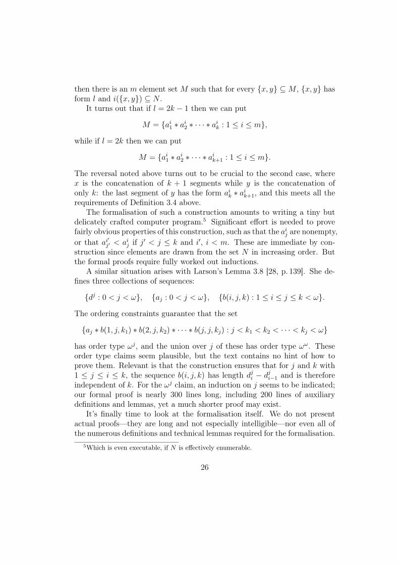
then there is an m element set M such that for every {x, y} ⊆ M , {x, y} hasform l and i({x, y}) ⊆ N .
It turns out that if l = 2k − 1 then we can put
M = {ai1 ∗ ai2 ∗ · · · ∗ aik : 1 ≤ i ≤ m},
while if l = 2k then we can put
M = {ai1 ∗ ai2 ∗ · · · ∗ aik+1 : 1 ≤ i ≤ m}.
The reversal noted above turns out to be crucial to the second case, wherex is the concatenation of k + 1 segments while y is the concatenation ofonly k: the last segment of y has the form aik ∗ aik+1, and this meets all therequirements of Definition 3.4 above.
The formalisation of such a construction amounts to writing a tiny butdelicately crafted computer program.5 Significant effort is needed to provefairly obvious properties of this construction, such as that the aij are nonempty,or that ai
′j′ < aij if j′ < j ≤ k and i′, i < m. These are immediate by con-
struction since elements are drawn from the set N in increasing order. Butthe formal proofs require fully worked out inductions.
A similar situation arises with Larson’s Lemma 3.8 [28, p. 139]. She de-fines three collections of sequences:
{dj : 0 < j < ω}, {aj : 0 < j < ω}, {b(i, j, k) : 1 ≤ i ≤ j ≤ k < ω}.
The ordering constraints guarantee that the set
{aj ∗ b(1, j, k1) ∗ b(2, j, k2) ∗ · · · ∗ b(j, j, kj) : j < k1 < k2 < · · · < kj < ω}
has order type ωj, and the union over j of these has order type ωω. Theseorder type claims seem plausible, but the text contains no hint of how toprove them. Relevant is that the construction ensures that for j and k with1 ≤ j ≤ i ≤ k, the sequence b(i, j, k) has length dji − dji−1 and is thereforeindependent of k. For the ωj claim, an induction on j seems to be indicated;our formal proof is nearly 300 lines long, including 200 lines of auxiliarydefinitions and lemmas, yet a much shorter proof may exist.
It’s finally time to look at the formalisation itself. We do not presentactual proofs—they are long and not especially intelligible—nor even all ofthe numerous definitions and technical lemmas required for the formalisation.
5Which is even executable, if N is effectively enumerable.
26
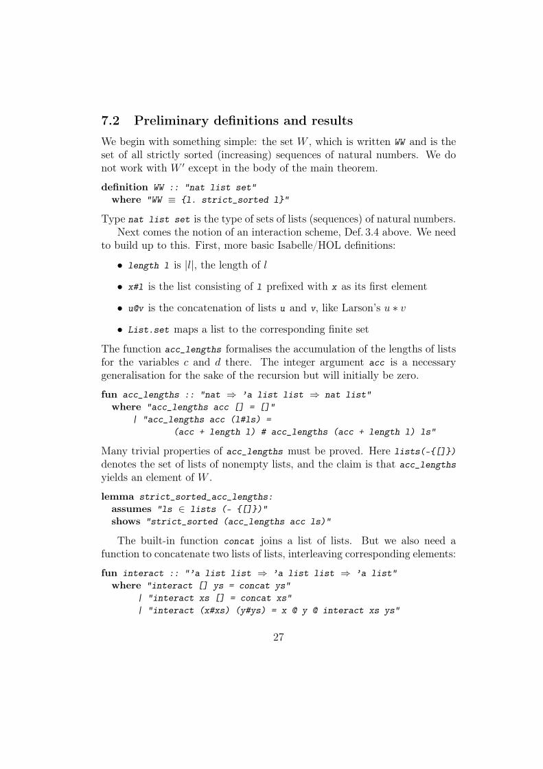
7.2 Preliminary definitions and results
We begin with something simple: the set W , which is written WW and is theset of all strictly sorted (increasing) sequences of natural numbers. We donot work with W ′ except in the body of the main theorem.
definition WW :: "nat list set"where "WW ≡ {l. strict_sorted l}"
Type nat list set is the type of sets of lists (sequences) of natural numbers.Next comes the notion of an interaction scheme, Def. 3.4 above. We need
to build up to this. First, more basic Isabelle/HOL definitions:
• length l is |l|, the length of l
• x#l is the list consisting of l prefixed with x as its first element
• u@v is the concatenation of lists u and v, like Larson’s u ∗ v
• List.set maps a list to the corresponding finite set
The function acc_lengths formalises the accumulation of the lengths of listsfor the variables c and d there. The integer argument acc is a necessarygeneralisation for the sake of the recursion but will initially be zero.
fun acc_lengths :: "nat ⇒ ’a list list ⇒ nat list"where "acc_lengths acc [] = []"
| "acc_lengths acc (l#ls) =(acc + length l) # acc_lengths (acc + length l) ls"
Many trivial properties of acc_lengths must be proved. Here lists(-{[]})denotes the set of lists of nonempty lists, and the claim is that acc_lengthsyields an element of W .
lemma strict_sorted_acc_lengths:assumes "ls ∈ lists (- {[]})"shows "strict_sorted (acc_lengths acc ls)"
The built-in function concat joins a list of lists. But we also need afunction to concatenate two lists of lists, interleaving corresponding elements:
fun interact :: "’a list list ⇒ ’a list list ⇒ ’a list"where "interact [] ys = concat ys"
| "interact xs [] = concat xs"| "interact (x#xs) (y#ys) = x @ y @ interact xs ys"
27
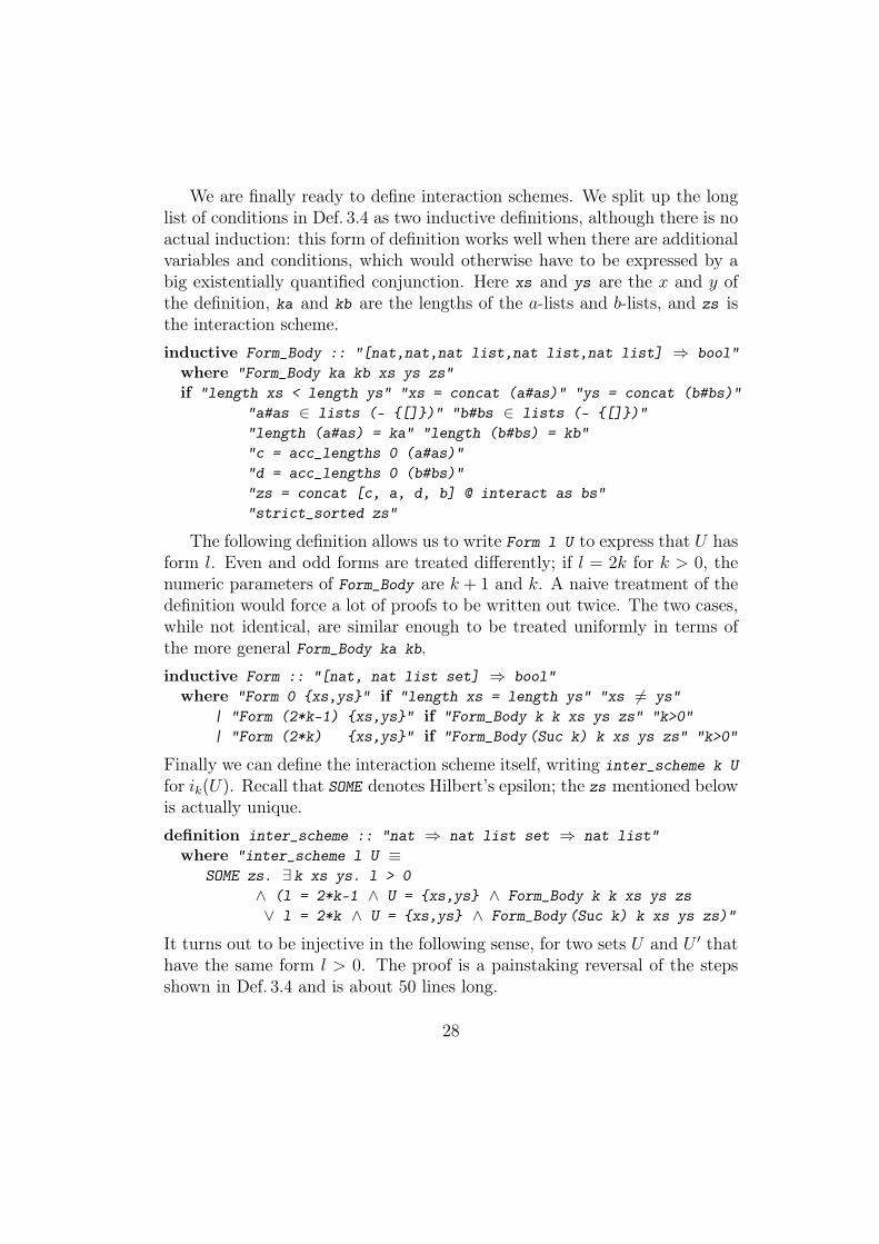
We are finally ready to define interaction schemes. We split up the longlist of conditions in Def. 3.4 as two inductive definitions, although there is noactual induction: this form of definition works well when there are additionalvariables and conditions, which would otherwise have to be expressed by abig existentially quantified conjunction. Here xs and ys are the x and y ofthe definition, ka and kb are the lengths of the a-lists and b-lists, and zs isthe interaction scheme.inductive Form_Body :: "[nat,nat,nat list,nat list,nat list] ⇒ bool"
where "Form_Body ka kb xs ys zs"if "length xs < length ys" "xs = concat (a#as)" "ys = concat (b#bs)"
"a#as ∈ lists (- {[]})" "b#bs ∈ lists (- {[]})""length (a#as) = ka" "length (b#bs) = kb""c = acc_lengths 0 (a#as)""d = acc_lengths 0 (b#bs)""zs = concat [c, a, d, b] @ interact as bs""strict_sorted zs"
The following definition allows us to write Form l U to express that U hasform l. Even and odd forms are treated differently; if l = 2k for k > 0, thenumeric parameters of Form_Body are k + 1 and k. A naive treatment of thedefinition would force a lot of proofs to be written out twice. The two cases,while not identical, are similar enough to be treated uniformly in terms ofthe more general Form_Body ka kb.inductive Form :: "[nat, nat list set] ⇒ bool"
where "Form 0 {xs,ys}" if "length xs = length ys" "xs ∕= ys"| "Form (2*k-1) {xs,ys}" if "Form_Body k k xs ys zs" "k>0"| "Form (2*k) {xs,ys}" if "Form_Body (Suc k) k xs ys zs" "k>0"
Finally we can define the interaction scheme itself, writing inter_scheme k Ufor ik(U). Recall that SOME denotes Hilbert’s epsilon; the zs mentioned belowis actually unique.definition inter_scheme :: "nat ⇒ nat list set ⇒ nat list"
where "inter_scheme l U ≡SOME zs. ∃ k xs ys. l > 0
∧ (l = 2*k-1 ∧ U = {xs,ys} ∧ Form_Body k k xs ys zs∨ l = 2*k ∧ U = {xs,ys} ∧ Form_Body (Suc k) k xs ys zs)"
It turns out to be injective in the following sense, for two sets U and U ′ thathave the same form l > 0. The proof is a painstaking reversal of the stepsshown in Def. 3.4 and is about 50 lines long.
28
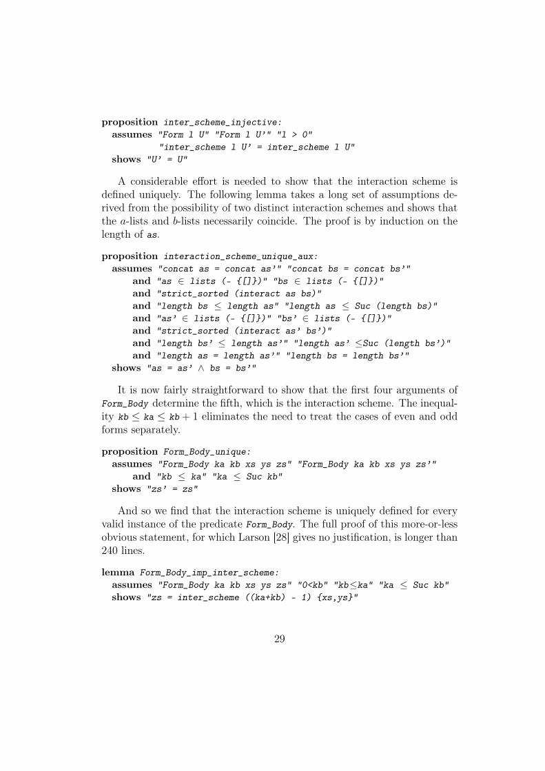
proposition inter_scheme_injective:assumes "Form l U" "Form l U’" "l > 0"
"inter_scheme l U’ = inter_scheme l U"shows "U’ = U"
A considerable effort is needed to show that the interaction scheme isdefined uniquely. The following lemma takes a long set of assumptions de-rived from the possibility of two distinct interaction schemes and shows thatthe a-lists and b-lists necessarily coincide. The proof is by induction on thelength of as.
proposition interaction_scheme_unique_aux:assumes "concat as = concat as’" "concat bs = concat bs’"
and "as ∈ lists (- {[]})" "bs ∈ lists (- {[]})"and "strict_sorted (interact as bs)"and "length bs ≤ length as" "length as ≤ Suc (length bs)"and "as’ ∈ lists (- {[]})" "bs’ ∈ lists (- {[]})"and "strict_sorted (interact as’ bs’)"and "length bs’ ≤ length as’" "length as’ ≤Suc (length bs’)"and "length as = length as’" "length bs = length bs’"
shows "as = as’ ∧ bs = bs’"
It is now fairly straightforward to show that the first four arguments ofForm_Body determine the fifth, which is the interaction scheme. The inequal-ity kb ≤ ka ≤ kb + 1 eliminates the need to treat the cases of even and oddforms separately.
proposition Form_Body_unique:assumes "Form_Body ka kb xs ys zs" "Form_Body ka kb xs ys zs’"
and "kb ≤ ka" "ka ≤ Suc kb"shows "zs’ = zs"
And so we find that the interaction scheme is uniquely defined for everyvalid instance of the predicate Form_Body. The full proof of this more-or-lessobvious statement, for which Larson [28] gives no justification, is longer than240 lines.
lemma Form_Body_imp_inter_scheme:assumes "Form_Body ka kb xs ys zs" "0<kb" "kb≤ka" "ka ≤ Suc kb"shows "zs = inter_scheme ((ka+kb) - 1) {xs,ys}"
29
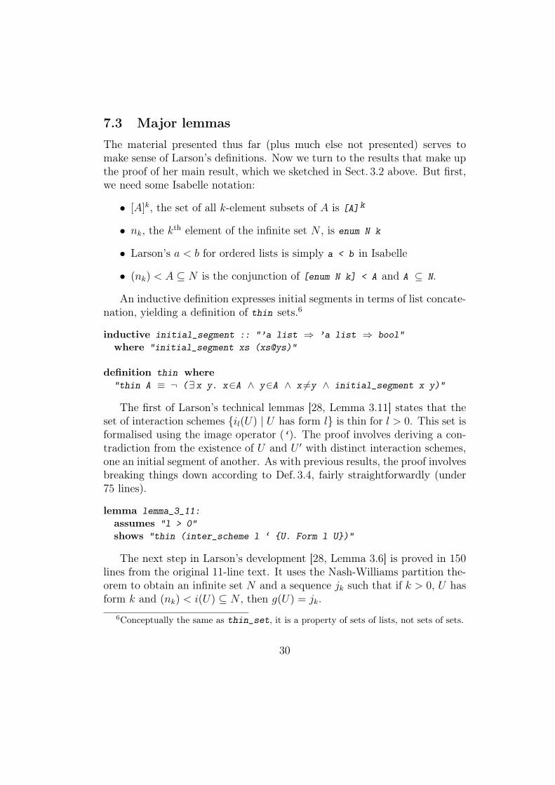
7.3 Major lemmas
The material presented thus far (plus much else not presented) serves tomake sense of Larson’s definitions. Now we turn to the results that make upthe proof of her main result, which we sketched in Sect. 3.2 above. But first,we need some Isabelle notation:
• [A]k, the set of all k-element subsets of A is [A]k
• nk, the kth element of the infinite set N , is enum N k
• Larson’s a < b for ordered lists is simply a < b in Isabelle
• (nk) < A ⊆ N is the conjunction of [enum N k] < A and A ⊆ N.
An inductive definition expresses initial segments in terms of list concate-nation, yielding a definition of thin sets.6
inductive initial_segment :: "’a list ⇒ ’a list ⇒ bool"where "initial_segment xs (xs@ys)"
definition thin where"thin A ≡ ¬ (∃ x y. x∈A ∧ y∈A ∧ x ∕=y ∧ initial_segment x y)"
The first of Larson’s technical lemmas [28, Lemma 3.11] states that theset of interaction schemes {il(U) | U has form l} is thin for l > 0. This set isformalised using the image operator (‘). The proof involves deriving a con-tradiction from the existence of U and U ′ with distinct interaction schemes,one an initial segment of another. As with previous results, the proof involvesbreaking things down according to Def. 3.4, fairly straightforwardly (under75 lines).
lemma lemma_3_11:assumes "l > 0"shows "thin (inter_scheme l ‘ {U. Form l U})"
The next step in Larson’s development [28, Lemma 3.6] is proved in 150lines from the original 11-line text. It uses the Nash-Williams partition the-orem to obtain an infinite set N and a sequence jk such that if k > 0, U hasform k and (nk) < i(U) ⊆ N , then g(U) = jk.
6Conceptually the same as thin_set, it is a property of sets of lists, not sets of sets.
30
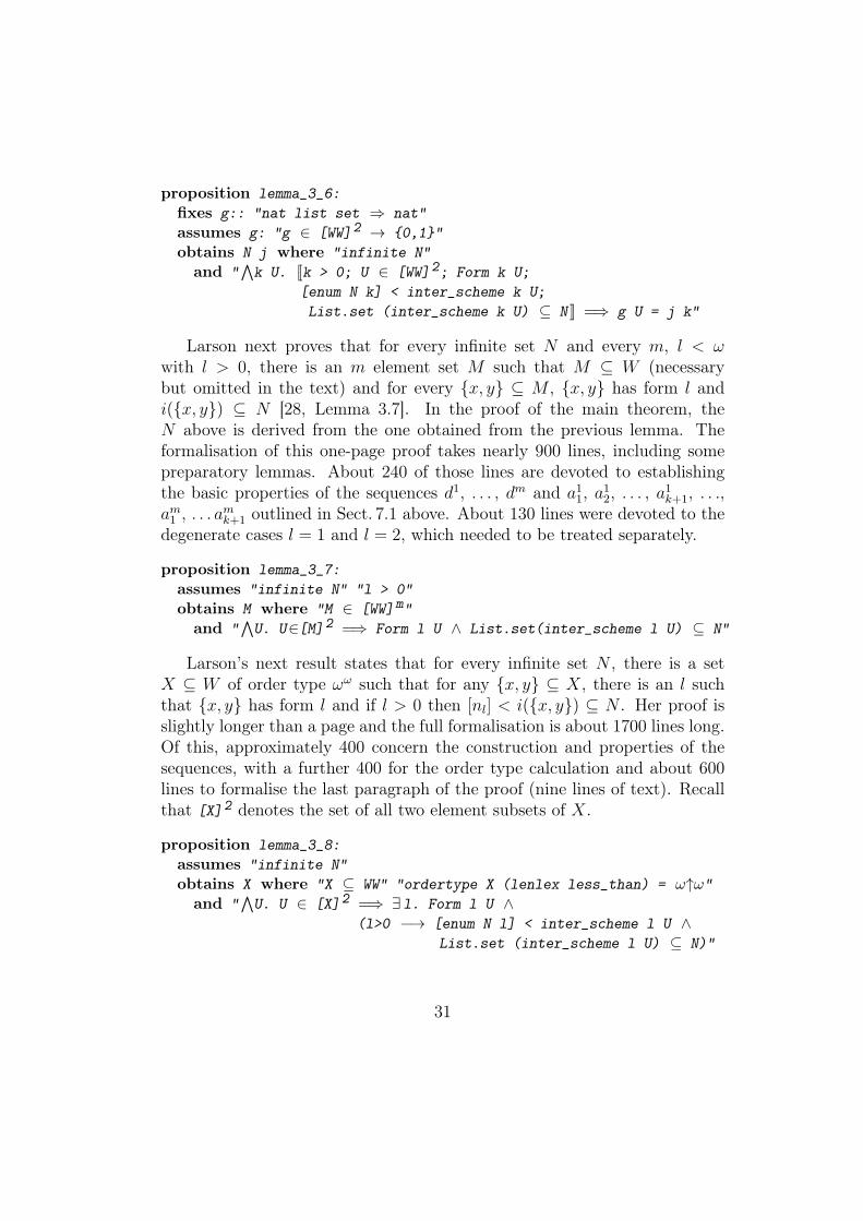
proposition lemma_3_6:fixes g:: "nat list set ⇒ nat"assumes g: "g ∈ [WW]2 → {0,1}"obtains N j where "infinite N"
and "!k U. [[k > 0; U ∈ [WW]2; Form k U;
[enum N k] < inter_scheme k U;List.set (inter_scheme k U) ⊆ N ]] =⇒ g U = j k"
Larson next proves that for every infinite set N and every m, l < ωwith l > 0, there is an m element set M such that M ⊆ W (necessarybut omitted in the text) and for every {x, y} ⊆ M , {x, y} has form l andi({x, y}) ⊆ N [28, Lemma 3.7]. In the proof of the main theorem, theN above is derived from the one obtained from the previous lemma. Theformalisation of this one-page proof takes nearly 900 lines, including somepreparatory lemmas. About 240 of those lines are devoted to establishingthe basic properties of the sequences d1, . . . , dm and a11, a12, . . . , a1k+1, . . .,am1 , . . . amk+1 outlined in Sect. 7.1 above. About 130 lines were devoted to thedegenerate cases l = 1 and l = 2, which needed to be treated separately.
proposition lemma_3_7:assumes "infinite N" "l > 0"obtains M where "M ∈ [WW]m"
and "!U. U∈[M]2 =⇒ Form l U ∧ List.set(inter_scheme l U) ⊆ N"
Larson’s next result states that for every infinite set N , there is a setX ⊆ W of order type ωω such that for any {x, y} ⊆ X, there is an l suchthat {x, y} has form l and if l > 0 then [nl] < i({x, y}) ⊆ N . Her proof isslightly longer than a page and the full formalisation is about 1700 lines long.Of this, approximately 400 concern the construction and properties of thesequences, with a further 400 for the order type calculation and about 600lines to formalise the last paragraph of the proof (nine lines of text). Recallthat [X]2 denotes the set of all two element subsets of X.
proposition lemma_3_8:assumes "infinite N"obtains X where "X ⊆ WW" "ordertype X (lenlex less_than) = ω↑ω"
and "!U. U ∈ [X]2 =⇒ ∃ l. Form l U ∧
(l>0 −→ [enum N l] < inter_scheme l U ∧List.set (inter_scheme l U) ⊆ N)"
31
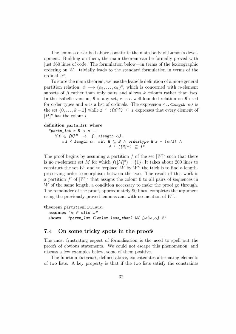
The lemmas described above constitute the main body of Larson’s devel-opment. Building on them, the main theorem can be formally proved withjust 360 lines of code. The formulation below—in terms of the lexicographicordering on W—trivially leads to the standard formulation in terms of theordinal ωω.
To state the main theorem, we use the Isabelle definition of a more generalpartition relation, β −→ (α1, . . . ,αk)
n, which is concerned with n-elementsubsets of β rather than only pairs and allows k colours rather than two.In the Isabelle version, B is any set, r is a well-founded relation on B usedfor order types and α is a list of ordinals. The expression {..<length α} isthe set {0, . . . , k− 1} while f ‘ ([H]n) ⊆ i expresses that every element of[H]n has the colour i.
definition partn_lst where"partn_lst r B α n ≡
∀ f ∈ [B]n → {..<length α}.∃ i < length α. ∃ H. H ⊆ B ∧ ordertype H r = (α!i) ∧
f ‘ ([H]n) ⊆ i"
The proof begins by assuming a partition f of the set [W ]2 such that thereis no m-element set M for which f([M ]2) = {1}. It takes about 200 lines toconstruct the set W ′ and to ‘replace’ W by W ′; the trick is to find a length-preserving order isomorphism between the two. The result of this work isa partition f ′ of [W ]2 that assigns the colour 0 to all pairs of sequences inW of the same length, a condition necessary to make the proof go through.The remainder of the proof, approximately 90 lines, completes the argumentusing the previously-proved lemmas and with no mention of W ′.
theorem partition_ωω_aux:assumes "α ∈ elts ω"shows "partn_lst (lenlex less_than) WW [ω↑ω,α] 2"
7.4 On some tricky spots in the proofs
The most frustrating aspect of formalisation is the need to spell out theproofs of obvious statements. We could not escape this phenomenon, anddiscuss a few examples below, some of them positive.
The function interact, defined above, concatenates alternating elementsof two lists. A key property is that if the two lists satisfy the constraints
32
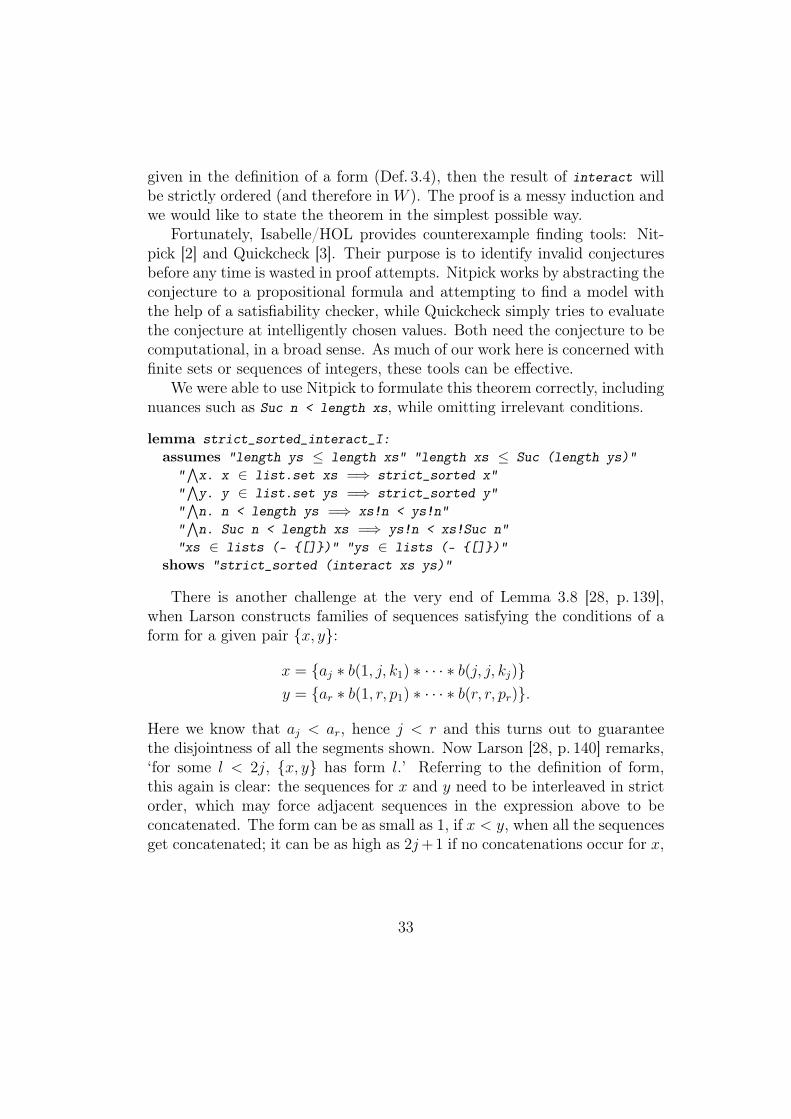
given in the definition of a form (Def. 3.4), then the result of interact willbe strictly ordered (and therefore in W ). The proof is a messy induction andwe would like to state the theorem in the simplest possible way.
Fortunately, Isabelle/HOL provides counterexample finding tools: Nit-pick [2] and Quickcheck [3]. Their purpose is to identify invalid conjecturesbefore any time is wasted in proof attempts. Nitpick works by abstracting theconjecture to a propositional formula and attempting to find a model withthe help of a satisfiability checker, while Quickcheck simply tries to evaluatethe conjecture at intelligently chosen values. Both need the conjecture to becomputational, in a broad sense. As much of our work here is concerned withfinite sets or sequences of integers, these tools can be effective.
We were able to use Nitpick to formulate this theorem correctly, includingnuances such as Suc n < length xs, while omitting irrelevant conditions.
lemma strict_sorted_interact_I:assumes "length ys ≤ length xs" "length xs ≤ Suc (length ys)"
"!x. x ∈ list.set xs =⇒ strict_sorted x"
"!y. y ∈ list.set ys =⇒ strict_sorted y"
"!n. n < length ys =⇒ xs!n < ys!n"
"!n. Suc n < length xs =⇒ ys!n < xs!Suc n"
"xs ∈ lists (- {[]})" "ys ∈ lists (- {[]})"shows "strict_sorted (interact xs ys)"
There is another challenge at the very end of Lemma 3.8 [28, p. 139],when Larson constructs families of sequences satisfying the conditions of aform for a given pair {x, y}:
x = {aj ∗ b(1, j, k1) ∗ · · · ∗ b(j, j, kj)}y = {ar ∗ b(1, r, p1) ∗ · · · ∗ b(r, r, pr)}.
Here we know that aj < ar, hence j < r and this turns out to guaranteethe disjointness of all the segments shown. Now Larson [28, p. 140] remarks,‘for some l < 2j, {x, y} has form l.’ Referring to the definition of form,this again is clear: the sequences for x and y need to be interleaved in strictorder, which may force adjacent sequences in the expression above to beconcatenated. The form can be as small as 1, if x < y, when all the sequencesget concatenated; it can be as high as 2j+1 if no concatenations occur for x,
33
as in this example:7
aj < ar < b(1, j, k1) < b(1, r, p1) < b(2, j, k2) < · · · < b(j, r, pj)∗· · ·∗b(r, r, pr).
To ask for a justification of this obvious claim would be unreasonable. Andyet to formalise the process of examining the interleavings of these sequencesand arranging them so as to satisfy the conditions of Definition 3.4—so thatthose conditions can be proved—turned out to require weeks of work.
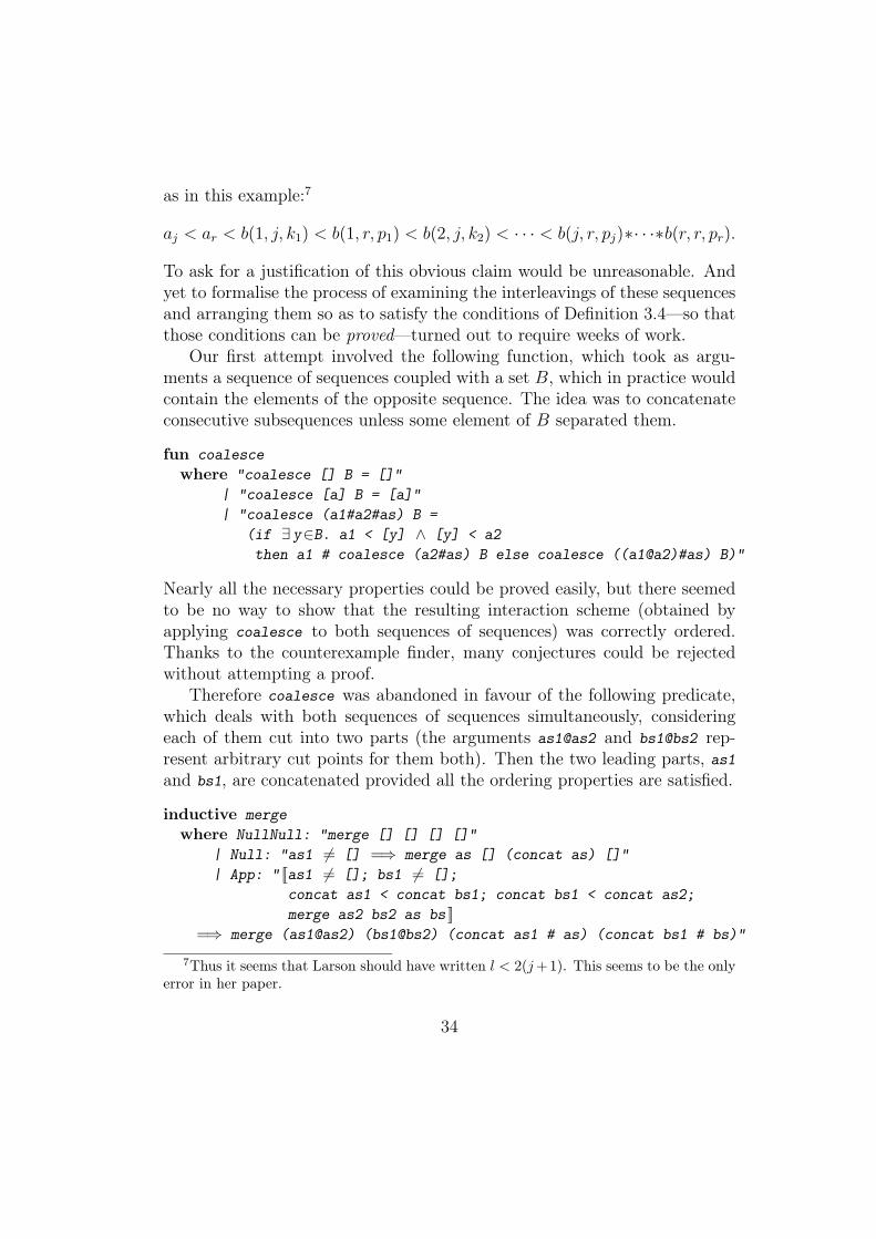
Our first attempt involved the following function, which took as argu-ments a sequence of sequences coupled with a set B, which in practice wouldcontain the elements of the opposite sequence. The idea was to concatenateconsecutive subsequences unless some element of B separated them.
fun coalescewhere "coalesce [] B = []"
| "coalesce [a] B = [a]"| "coalesce (a1#a2#as) B =
(if ∃ y∈B. a1 < [y] ∧ [y] < a2then a1 # coalesce (a2#as) B else coalesce ((a1@a2)#as) B)"
Nearly all the necessary properties could be proved easily, but there seemedto be no way to show that the resulting interaction scheme (obtained byapplying coalesce to both sequences of sequences) was correctly ordered.Thanks to the counterexample finder, many conjectures could be rejectedwithout attempting a proof.
Therefore coalesce was abandoned in favour of the following predicate,which deals with both sequences of sequences simultaneously, consideringeach of them cut into two parts (the arguments as1@as2 and bs1@bs2 rep-resent arbitrary cut points for them both). Then the two leading parts, as1and bs1, are concatenated provided all the ordering properties are satisfied.
inductive mergewhere NullNull: "merge [] [] [] []"
| Null: "as1 ∕= [] =⇒ merge as [] (concat as) []"| App: " [[as1 ∕= []; bs1 ∕= [];
concat as1 < concat bs1; concat bs1 < concat as2;merge as2 bs2 as bs ]]
=⇒ merge (as1@as2) (bs1@bs2) (concat as1 # as) (concat bs1 # bs)"
7Thus it seems that Larson should have written l < 2(j+1). This seems to be the onlyerror in her paper.
34
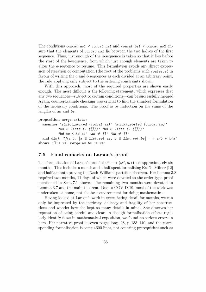
The conditions concat as1 < concat bs1 and concat bs1 < concat as2 en-sure that the elements of concat bs1 lie between the two halves of the firstsequence. Thus, just enough of the a-sequence is taken so that it lies beforethe start of the b-sequence, from which just enough elements are taken toallow the a-sequence to resume. This formulation avoids any direct expres-sion of iteration or computation (the root of the problems with coalesce) infavour of writing the a and b-sequences as each divided at an arbitrary point,the rule applying only subject to the ordering constraints shown.
With this approach, most of the required properties are shown easilyenough. The most difficult is the following statement, which expresses thatany two sequences—subject to certain conditions—can be successfully merged.Again, counterexample checking was crucial to find the simplest formulationof the necessary conditions. The proof is by induction on the sums of thelengths of as and bs.
proposition merge_exists:assumes "strict_sorted (concat as)" "strict_sorted (concat bs)"
"as ∈ lists (- {[]})" "bs ∈ lists (- {[]})""hd as < hd bs" "as ∕= []" "bs ∕= []"
and disj: "!a b. [[a ∈ list.set as; b ∈ list.set bs ]] =⇒ a<b ∨ b<a"
shows "∃ us vs. merge as bs us vs"
7.5 Final remarks on Larson’s proof
The formalisation of Larson’s proof of ωω −→ (ωω,m) took approximately sixmonths. This includes a month and a half spent formalising Erdős–Milner [12]and half a month proving the Nash-Williams partition theorem. Her Lemma 3.8required two months, 11 days of which were devoted to the order type proofmentioned in Sect. 7.1 above. The remaining two months were devoted toLemma 3.7 and the main theorem. Due to COVID-19, most of the work wasundertaken at home, not the best environment for doing mathematics.
Having looked at Larson’s work in excruciating detail for months, we canonly be impressed by the intricacy, delicacy and fragility of her construc-tions and wonder how she kept so many details in mind. She deserves herreputation of being careful and clear. Although formalisation efforts regu-larly identify flaws in mathematical exposition, we found no serious errors inhers. Her narrative proof is seven pages long [28, p. 133–140] and the corre-sponding formalisation is some 4600 lines, not counting prerequisites such as
35
Nash-Williams and Erdős–Milner, which are proved elsewhere. Estimating30 lines per page, this suggests a de Bruijn factor of roughly 23.
8 ConclusionOur work shows that ordinal partition theory is clearly formalisable withinIsabelle/HOL augmented with a straightforward axiomatisation of ZFC. Wehave found no serious errors in the original mathematical material, and al-though we struggled in some places it is quite hard to fault Larson’s expo-sition [28] beyond noting that a few hints here and there could have savedus quite a bit of effort. The reader of a mathematical proof is expected toinvest much thought.
As usual, a concern is the disproportionate effort needed to prove somesimple observations. The inductive constructions of sequences that appear inLarson’s Lemmas 3.7 and 3.8 [28] must surely be regarded as straightforwardand yet we struggled to find the right language in which to express themand derive their obvious properties. The same can be said of the order typecalculation in 3.8. It’s also unfortunate that the degenerate cases l = 1 andl = 2 in 3.7 required so much work. However, given the inherent complexityof the subject matter, it’s reassuring to know that the entire development hasbeen checked formally, with a proof text [37] that is available for inspectionor automated analysis.
This case study also demonstrates the diversity of mathematical topicsthat can be formalised in Isabelle/HOL: we have formalised material that islight years away from what is usually formalised.
Ordinal partition relations seem to be at the same time formalisable inIsabelle/HOL and at a point of their mathematical development where hu-man advances seem rare and not forthcoming. None of the high power tech-niques of set theory and model theory such as large cardinals, forcing, pcfor elementary submodes seem to be relevant. Therefore, we hope that someadvances in this subject might be obtained by automatisation. However,we remain with a humble conviction that doing enough preparatory workwith Isabelle to be able to produce such results will require a considerableintellectual effort.
Acknowledgements. Angeliki Koutsoukou-Argyraki and Lawrence C. Paul-son thank the ERC for their support through the Advanced Grant ALEXAN-
36
DRIA (Project GA 742178). Mirna Džamonja’s research was supported bythe GAČR project EXPRO 20-31529X and RVO: 67985840 at the CzechAcademy of Sciences; she received funding from the European’s Union Hori-zon 2020 research and innovation programme under the Maria Skołodowska-Curie grant agreement No 1010232. All three authors thank the LondonMathematical Society for support through their Grant SC7-1920-11. Thanksto Stevo Todorčević for advice and to the anonymous reviewers for theirhelpful feedback on the first submitted version of this paper.
References[1] Jeremy Avigad, Johannes Hölzl, and Luke Serafin. A formally verified
proof of the central limit theorem. Journal of Automated Reasoning,59(4):389–423, December 2017.
[2] Jasmin Christian Blanchette and Tobias Nipkow. Nitpick: A counterex-ample generator for higher-order logic based on a relational model finder.In Matt Kaufmann and Lawrence C. Paulson, editors, Interactive Theo-rem Proving, volume 6172 of Lecture Notes in Computer Science, pages131–146. Springer, 2010.
[3] Lukas Bulwahn. The new Quickcheck for Isabelle. In Chris Hawblitzeland Dale Miller, editors, Certified Programs and Proofs, LNCS 7679,pages 92–108. Springer, 2012.
[4] Raphaël Carroy and Yann Pequignot. Well, better and in-between.In Monika Seisenberger Peter Schuster and Andreas Weiermann, edi-tors, Well Quasi-orders in Computation, Logic, Language and Reason-ing, pages 1–27. Springer, 2020.
[5] Chen-Chung Chang. A partition theorem for the complete graph on ωω.Journal of Combinatorial Theory (A), 12:396–452, 1972.
[6] Alonzo Church. A formulation of the simple theory of types. Journal ofSymbolic Logic, 5:56–68, 1940.
[7] Paul Cohen. Set Theory and the Continuum Hypothesis. Benjamin, NewYork, 1966.
37
[8] Mirna Džamonja. Fast Track to Forcing. Cambridge University Press,2020.
[9] P. Erdős. Some problems on finite and infinite graphs. In Logic andcombinatorics (Arcata, Calif., 1985), volume 65 of Contemp. Math.,pages 223–228. Amer. Math. Soc., Providence, RI, 1987.
[10] Paul Erdős and Richard Rado. A partition calculus in set theory. Bull.Amer. Math. Soc., 62(427-489), 1956.
[11] Paul Erdös, András Hajnal, Atilla Mate, and Richard Rado. Combina-torial Set Theory: Partition Relations for Cardinals. Studies in Logicand the Foundations of Mathematics 106. Elsevier Science Ltd, 1984.
[12] Paul Erdős and E. C. Milner. A theorem in the partition calculus.Canadian Mathematical Bulletin, 15(4):501–505, December 1972.
[13] Paul Erdős and E. C. Milner. A theorem in the partition calculus cor-rigendum. Canadian Mathematical Bulletin, 17(2):305, June 1974.
[14] Fred Galvin and Jean A. Larson. Pinning countable ordinals. Funda-menta Mathematicae, 82:357–361, 1974.
[15] Fred Galvin and Karel L. Prikry. Borel sets and Ramsey’s theorem.Journal of Symbolic Logic, 38:192–198, 1973.
[16] M. J. C. Gordon. Tactics for mechanized reasoning: A commentary onMilner (1984) ‘The use of machines to assist in rigorous proof’. Philo-sophical Transactions of the Royal Society of London A: Mathematical,Physical and Engineering Sciences, 373(2039), 2015.
[17] András Hajnal and Jean A. Larson. Partition relations. In MatthewForeman and Akihiro Kanamori, editors, Handbook of Set Theory, vol-ume 1, pages 120–213. Springer, 2010.
[18] Thomas Hales, Mark Adams, Gertrud Bauer, Tat Dat Dang, John Harri-son, Le Truong Hoang, Cezary Kaliszyk, Victor Magron, Sean Mclaugh-lin, Tat Thang Nguyen, et al. A formal proof of the Kepler conjecture.Forum of Mathematics, Pi, 5:e2, 2017.
[19] Thomas C. Hales. The Jordan curve theorem, formally and informally.The American Mathematical Monthly, 114(10):882–894, 2007.
38
[20] John Harrison. Floating point verification in HOL Light: the exponentialfunction. Formal Methods in System Design, 16:271–305, 2000.
[21] John Harrison. Formalizing an analytic proof of the prime number the-orem. Journal of Automated Reasoning, 43(3):243–261, 2009.
[22] Ian Hodkinson. Kruskal’s theorem and Nash-Williams theory, after Wil-frid Hodges. version 3.6 online at www.doc.ic.ac.uk/~imh/papers/bar.pdf, February 2003.
[23] Johannes Hölzl and Armin Heller. Three chapters of measure theoryin Isabelle/HOL. In Marko Eekelen, Herman Geuvers, Julien Schmaltz,and Freek Wiedijk, editors, Interactive Theorem Proving — Second In-ternational Conference, LNCS 6898, pages 135–151. Springer, 2011.
[24] L.S. van Benthem Jutting. Checking Landau’s “Grundlagen” in the AU-TOMATH System. PhD thesis, Eindhoven University of Technology,1977. https://doi.org/10.6100/IR23183.
[25] Sara Kalvala. HOL around the world. In M. Archer, J. J. Joyce, K. N.Levitt, and P. J. Windley, editors, International Workshop on the HOLTheorem Proving System and its Applications, pages 4–12. IEEE Com-puter Society, 1991.
[26] Kenneth Kunen. Set Theory, volume 102 of Studies in Logic and theFoundations of Mathematics. North-Holland, 1980.
[27] Igor Kříž and Robin Thomas. Analyzing Nash-Williams’ partition the-orem by means of ordinal types. Discrete Math., 95(1-3):135–167,1991. Directions in infinite graph theory and combinatorics (Cambridge,1989).
[28] Jean A. Larson. A short proof of a partition theorem for the ordinal ωω.Annals of Mathematical Logic, 6:129–145, 1973.
[29] Richard Laver. On Fraïssé’s order type conjecture. Annals of Mathe-matics, 93(1):89–111, January 1971.
[30] Alberto Marcone. On the logical strength of Nash-Williams’ theoremon transfinite sequences. In Logic: from foundations to applications(Staffordshire, 1993), Oxford Sci. Publ., pages 327–351. Oxford Univ.Press, New York, 1996.
39
[31] C. St. J. A. Nash-Williams. On well-quasi-ordering transfinite sequences.Proc. Cambridge Philos. Soc., 61:33–39, 1965.
[32] Thomas R. Nicely. Pentium FDIV flaw, 2011. FAQ page online athttps://faculty.lynchburg.edu/~nicely/pentbug/pentbug.html.
[33] Tobias Nipkow, Lawrence C. Paulson, and Markus Wenzel. Isa-belle/HOL: A Proof Assistant for Higher-Order Logic. Springer,2002. Online at http://isabelle.in.tum.de/dist/Isabelle/doc/tutorial.pdf.
[34] S. Owre, S. Rajan, J.M. Rushby, N. Shankar, and M.K. Srivas. PVS:Combining specification, proof checking, and model checking. In RajeevAlur and Thomas A. Henzinger, editors, Computer Aided Verification:8th International Conference, CAV ’96, LNCS 1102, pages 411–414.Springer, 1996.
[35] Lawrence C. Paulson. Zermelo Fraenkel set theory in higher-orderlogic. Archive of Formal Proofs, October 2019. http://isa-afp.org/entries/ZFC_in_HOL.html, Formal proof development.
[36] Lawrence C. Paulson. The Nash-Williams partition theorem. Archiveof Formal Proofs, May 2020. http://isa-afp.org/entries/Nash_Williams.html, Formal proof development.
[37] Lawrence C. Paulson. Ordinal partitions. Archive of Formal Proofs,August 2020. http://isa-afp.org/entries/Ordinal_Partitions.html, Formal proof development.
[38] Lawrence C. Paulson, Tobias Nipkow, and Makarius Wenzel. From LCFto Isabelle/HOL. Formal Aspects of Computing, 31(6):675–698, 2019.
[39] F. P. Ramsey. On a Problem of Formal Logic. Proc. London Math. Soc.(2), 30(4):264–286, 1929.
[40] Rene Schipperus. Countable partition ordinals. PhD thesis, Universityof Colorado-Boulder, 1999.
[41] Rene Schipperus. Countable partition ordinals. Ann. Pure Appl. Log.,161(10):1195–1215, 2010.
40
[42] Ernst Specker. Teilmengen von Mengen mit Relationen. Commenta-tiones Mathematicae Helvetia, 31:302–314, 1956.
[43] Stevo Todorčević. Partitioning pairs of countable ordinals. Acta Math.,159(3-4):261–294, 1987.
[44] Stevo Todorčević. Partition Problems in Topology. Amer. Math. Soc.,Providence, Rhode Island, 1989.
[45] Stevo Todorcevic. Introduction to Ramsey spaces, volume 174 of Annalsof Mathematics Studies. Princeton University Press, Princeton, NJ,2010.
[46] Freek Wiedijk. The De Bruijn factor. Technical report, Departmentof Computer Science Nijmegen University, P.O. Box 9010, 6500 GL Ni-jmegen, Netherlands, 2000. Online at http://www.cs.ru.nl/~freek/factor/.
41