water cycle, mine blast and improved mine blast algorithms for discrete sizing optimization of truss...

Computers and Structures 149 (2015) 1–16

Contents lists available at ScienceDirect

Computers and Structures

journal homepage: www.elsevier .com/locate /compstruc

Water cycle, mine blast and improved mine blast algorithms for discretesizing optimization of truss structures

http://dx.doi.org/10.1016/j.compstruc.2014.12.0030045-7949/� 2014 Elsevier Ltd. All rights reserved.

⇑ Corresponding author. Tel.: +673 897 5723.E-mail address: [email protected] (A. Bahreininejad).

Ali Sadollah a, Hadi Eskandar b, Ardeshir Bahreininejad c,⇑, Joong Hoon Kim a

a School of Civil, Environmental and Architectural Engineering, Korea University, 136-713 Seoul, South Koreab Faculty of Engineering, Semnan University, Semnan, Iranc Faculty of Engineering, Institut Teknologi Brunei, Bandar Seri Begawan, Brunei

a r t i c l e i n f o

Article history:Received 18 August 2013Accepted 1 December 2014

Keywords:Mine blast algorithmWater cycle algorithmTruss structuresDiscrete variablesSizing optimization

a b s t r a c t

This paper presents the applications of the mine blast algorithm (MBA) and the water cycle algorithm(WCA), in addition to an improved version of MBA for weight minimization of truss structures includingdiscrete sizing variables. The MBA mimics the explosion of landmines, while the WCA is inspired by theobservation of water cycle process. An improved version of MBA (IMBA), is also presented. The efficiencyof the three optimization algorithms is tested using classical benchmark discrete truss design problems.Optimization results show that MBA, IMBA, and WCA offer a good degree of competitiveness againstother state-of-the-art metaheuristic techniques.

� 2014 Elsevier Ltd. All rights reserved.

1. Introduction

Over the last decades, various algorithms have been used fortruss optimization problems which are very popular in the fieldof structural optimization. Metaheuristic methods such as geneticalgorithms (GAs), harmony search (HS), and particle swarm opti-mization (PSO) can efficiently be used in truss design optimizationproblems including discrete variables. GAs [1] mimic the processesof natural selection leading to the survival of the fittest.

For instance, Goldberg and Samtani [2] and Rajeev and Krishna-moorthy [3] performed sizing optimization of truss structures.Krishnamoorthy et al. [4] used GAs to optimize space truss struc-tures in the context of an object-oriented framework. Sivakumaret al. [5] optimized steel lattice towers. Gero et al. [6] used GAsfor design optimization of 3D steel structures.

Geem et al. [7] developed the HS that reproduces the musicalprocess of searching for a perfect state of harmony. The harmonyin music is analogous to the optimum design, and the musicians’improvisation is analogous to local/global search schemes [8].The HS was successfully applied to truss optimization problemsusing discrete and continuous variables [9,10].

The PSO is a population-based algorithm developed by Kennedyand Eberhart [11]. Li et al. [12] developed an efficient heuristic PSO

(HPSO) for truss structures which outperformed hybrid PSO withpassive congregation (PSOPC) [13] and standard PSO.

The PSOPC was also combined with ant colony optimization(ACO) and HS by Kaveh and Talatahari [14] to form an efficientalgorithm for truss optimization, called discrete heuristic particleswarm ant colony optimization (DHPSACO). Comprehensivereviews for applications of metaheuristic algorithms on skeletalstructures have been presented in the literature [15,16].

Sadollah et al. [17] recently developed the mine blast algorithm(MBA) which mimics the explosion of landmines. The MBA wassuccessfully applied to discrete sizing optimization of truss struc-tures [17]. Furthermore, Eskandar et al. [18] proposed anothermetaheuristic algorithm, reproducing the water cycle process.The water cycle algorithm (WCA) was tested in mathematicaland engineering problems [18]. The MBA and WCA algorithmswere found to be superior over other optimization methods interms of convergence rate and quality of optimized designs[17,18].

In this study, MBA is improved and its operators are enhancedin terms of efficiency so called improved MBA (IMBA). The relativeperformance of the MBA, IMBA and WCA algorithms in discreteoptimization problems of truss structures are investigated in thisresearch. Furthermore, the efficiency of three algorithms is com-pared with the results extracted in the literature.

The paper is organized as follows: the formulation of the dis-crete optimization problem is presented in Section 2. The IMBAand WCA algorithms and their constraint handling strategies are

http://crossmark.crossref.org/dialog/?doi=10.1016/j.compstruc.2014.12.003&domain=pdf

http://dx.doi.org/10.1016/j.compstruc.2014.12.003

mailto:[email protected]

http://dx.doi.org/10.1016/j.compstruc.2014.12.003

http://www.sciencedirect.com/science/journal/00457949

http://www.elsevier.com/locate/compstruc

2 A. Sadollah et al. / Computers and Structures 149 (2015) 1–16

described in detail in Section 3. Section 4 discusses the optimiza-tion results comparing the developed algorithms with the litera-ture. Section 5 presents a sensitivity analysis on the effect ofalgorithms internal parameters set by the user on the overall con-vergence behavior; the analysis is carried out for some of the testproblems considered in this study. Finally, Section 6 summarizesthe findings of this study.

2. Discrete structural optimization problems

In discrete sizing optimization problems of truss structures, theobjective usually is to minimize the weight of the structure yetsatisfying nonlinear constraints on element stresses, nodal dis-placements, critical loads, etc. The optimization problem can beformulated as follows:

min WðXÞ; X ¼ ½x1; x2; x3; . . . ; xN �; ð1Þ

subject to:

gjðx1; x2; . . . ; xNÞ 6 0 j ¼ 1;2; . . . ; k; ð2Þ

xd 2 Sd ¼ fX1;X2; . . . ;Xpg; ð3Þ

where W(X) is the cost function corresponding to the structuralweight; N and k are the number of design variables and inequalityconstraint functions, respectively. Each design variable can be cho-sen from a discrete set Sd (X1, X2, . . . ,Xp) of P available cross-sectionsaccording to production standards.

3. Applied metaheuristic algorithms

3.1. Improved mine blast algorithm

MBA algorithm is inspired by the process of landmines explo-sion; shrapnel pieces are thrown away and collide with othermines in the vicinity of the explosion area causing further explo-sions. Consider a landmine field where the goal is to clear land-mines. To clear all the mines, the position of the most explosivemine must be located. This position corresponds to the optimaldesign.

Landmines of different sizes and explosive power are plantedunder the ground. Landmine explosions cause many pieces ofshrapnel to be propelled in the air. The casualties of each pieceof shrapnel are evaluated using a cost function (fitness function)and, then, related to the presence of other landmines with differentexplosive power [17].

Often times, pieces of shrapnel collide with other mines andtrigger more mine explosions. This behavior is helpful for findingthe most explosive landmine. MBA algorithm was developed tofind the most explosive landmine (i.e., the landmine with the mostcasualties). Table 1 lists nomenclature of MBA parameters.

The MBA algorithm requires an initial population of individuals,similar to several other metaheuristic methods. The population is

Table 1Nomenclature of MBA (IMBA) parameters.

Parameter Definition Parame

Rand Uniformly distributed random number between 0 and1(vector)

XBest�1

Randn Normally distributed random number (vector) D

X0 Generated first shot point (initial solution, vector) Xe

d0 Initial distance of shrapnel pieces (vector) lLB Lower bounds of design variables (vector) tUB Upper bounds of design variables (vector) hm Number of design variables (scalar) aXBest Best obtained solution (current improved solution, vector) Ns (Npo

generated from a first shot explosion that produces a number ofindividuals (shrapnel pieces). The size of initial population (Npop)is taken as the number of shrapnel pieces (Ns). The MBA algorithminitially uses the lower and upper bounds of design variables and,then, randomly creates the first shot point as follows:

~X0 ¼ L~Bþ frandg � fU~B� L~Bg: ð4Þ

Vector quantities are denoted by over sign. Assume X is the cur-rent location of a landmine; that is,

~X ¼ ½x1; x2; x3; . . . ; xm�: ð5Þ

Design variables (x1, x2, . . . ,xm) can take real values in continu-ous optimization problems or they can be selected from a prede-fined set of discrete values. We assume that the first shot point(X0) is the best solution (XBest = X0). For performing any optimiza-tion method, exploration and exploitation are considered as twocritical steps.

The difference between the exploration and exploitation phasesis how they influence the whole search process in finding the opti-mal solution. Similar to other metaheuristic algorithms, MBA algo-rithm starts with the exploration phase, which is responsible forcomprehensively exploring the search space.

The exploration factor (l) serves to explore different regions ofdesign space. This parameter, used in the early iterations of MBA, iscompared with an iteration number index (t): exploration takesplace if l is greater than t. The exploration phase of MBA is gov-erned by the following equations [17]:

~Xe ¼ ~dt�1

n o� frandn2g � cos h t ¼ 1;2; . . . ;l; ð6Þ

~Xe ¼ ~XBest þ~Xe t 6 l; ð7Þ

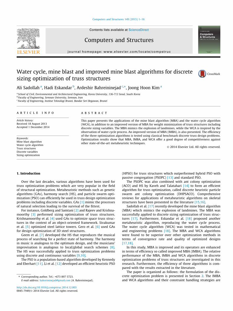
where the dt�1 vector includes the shrapnel distance for explodedmines with respect to each coordinate direction. Fig. 1 demon-strates the concept and performance of Eq. (6) from a schematicpoint of view.

By taking the square of a normally distributed random number,better exploration is achieved at the beginning of the optimizationprocess (see Eq. (6)). The value of l determines the intensity of theexploration. For example, increasing l makes it possible to exploremore remote regions of design space. The shrapnel angle of inci-dence, denoted by h in Eq. (6), is given by:

h ¼ k� D k ¼ 0;1;2; . . . ;Ns � 1; ð8Þ

where D = 360/Ns. The value of h ranges from 0 to 360; the resultingvalue of cos(h) ranges between �1 and 1. The initial distance of eachpiece of shrapnel is d0 = (UB–LB); thus, the best solution is in therange [LB, UB]. For example, the LB and UB of a four design variableproblem are [�30–20�10–5] and [3020105], respectively. Then,the initial distance, d0 (dt�1 when t = 1), is the vector of shrapneldistances [60402010].

Improved MBA (IMBA) modifies the exploitation phase in MBAand distance reduction of each shrapnel pieces. For the exploitation

ter Definition

Previous best obtained solution (previous improved solution, vector)

Euclidean distance between the current and previous best solutions(scalar)Location of exploded mine (vector)Exploration factor (scalar)Iteration index number (scalar)Shrapnel angle of incidence (scalar)Reduction factor (scalar)

p) Number of shrapnel pieces (number of population, scalar)

Fig. 1. Schematic view of generating a new solution using the MBA explorationphase given in Eq. (6).

A. Sadollah et al. / Computers and Structures 149 (2015) 1–16 3

phase, IMBA focuses on the solution closest to the current bestsolution. The location of an exploding landmine Xe in the exploita-tion phase is defined as follows [17]:

~Xe ¼ ~dt�1

n o�frandng� cosðhÞ t ¼ lþ1; . . . ;Max Iteration; ð9Þ

~Xe ¼ ~XBest þ~Xe t > l ð10Þ

therefore, the updated formulation of the exploitation phase inIMBA is suggested as follows:

~Xe ¼ ~Xe þ exp �ffiffiffiffi1D

r !� frandg � ~XBest �~XBest�1

n o; t > l: ð11Þ

We compare IMBA to MBA [17] with a few modifications. Theconcept of direction in MBA is adapted to a two dimensional opti-mization problem. When an optimization problem with more thanthree decision variables is considered, determining the direction ofeach piece of shrapnel is difficult or impossible.

For IMBA, we modify the exploitation equations to avoid prob-lems with the dimension of the search space. Indeed, the percep-tion of direction is replaced by moving to the best solutions.

The exponential term in Eq. (11) (when t > l in the exploitationphase) improves the obtained exploded point by including infor-mation from current and previous best solutions (XBest and XBest�1)and their Euclidean distances. The Euclidean distance between thecurrent and previous best landmines in m dimensions is given by:

D ¼Xm

i¼1

XiBest � XiðBest�1Þ� �2

" #1=2

: ð12Þ

It can be seen from Eq. (11) that when the distance betweenXBest and XBest�1 approaches 0 (i.e., in the final cycles of the optimi-zation process), the exponential term contained in that equationvanishes. Eq. (13) allows locations of shrapnel pieces to be updatedin both exploration and exploitation phases in the IMBA as follows:

~Xe ¼

~dt�1

n o� randn2n o

� cos h t 6 l

~dt�1

n o� frandng � cosðhÞ þ exp �

ffiffiffi1D

q� �� frandg

� ~XBest �~XBest�1

n ot � l

8>>>><>>>>:

:

ð13Þ

To improve IMBA’s global search ability, the initial distance ofshrapnel pieces (d0) is gradually reduced at each iteration toquickly detect the near location of the most explosive landmine.During the optimization process, the distance of each shrapnelpiece at each dimension adaptively decrease as follows:

~dt ¼~dt�1

eðt=aÞt ¼ 1;2;3; . . . ;Max Iteration; ð14Þ

where a is the reduction factor, a user-defined parameter, whichdepends on the complexity of the optimization problem. At theend of the optimization process, shrapnel distances are close tozero. It is worth mentioning that in IMBA, unlike MBA, the shrapneldistances are reduced if there are no changes in cost function in thecurrent iteration. Conversely, if the cost function decreases, there isno need to reduce the value of shrapnel distances. This approachhelps to have more exploration improving cost in each iteration.

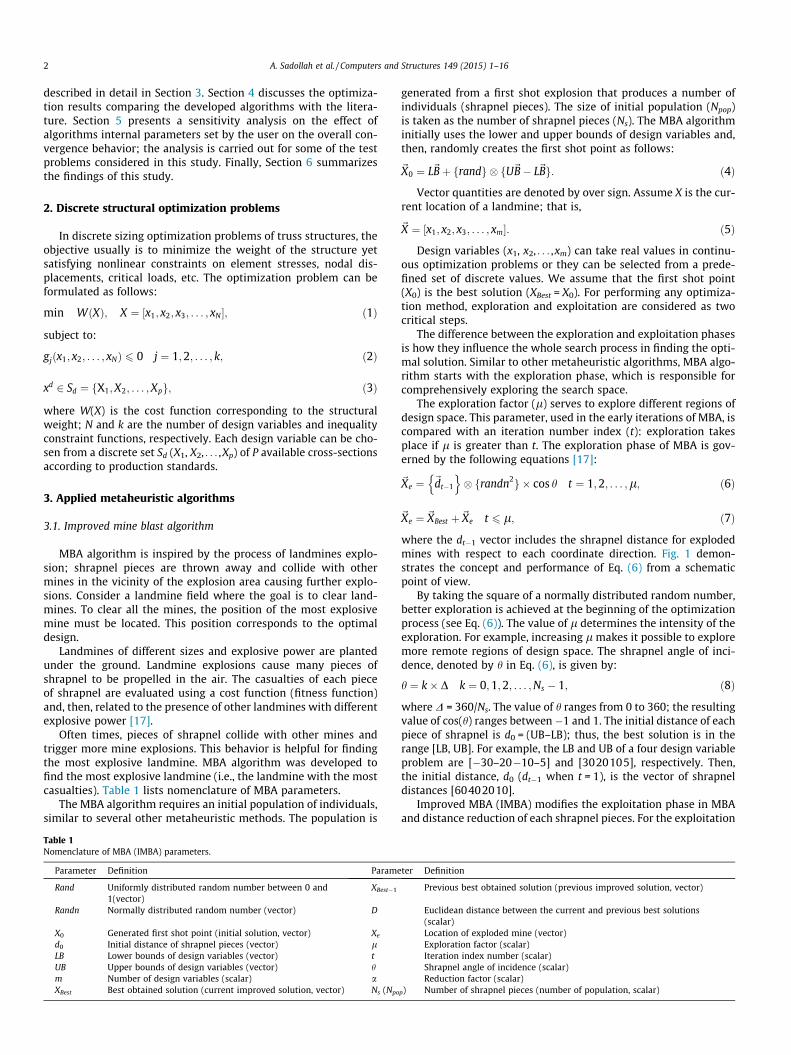
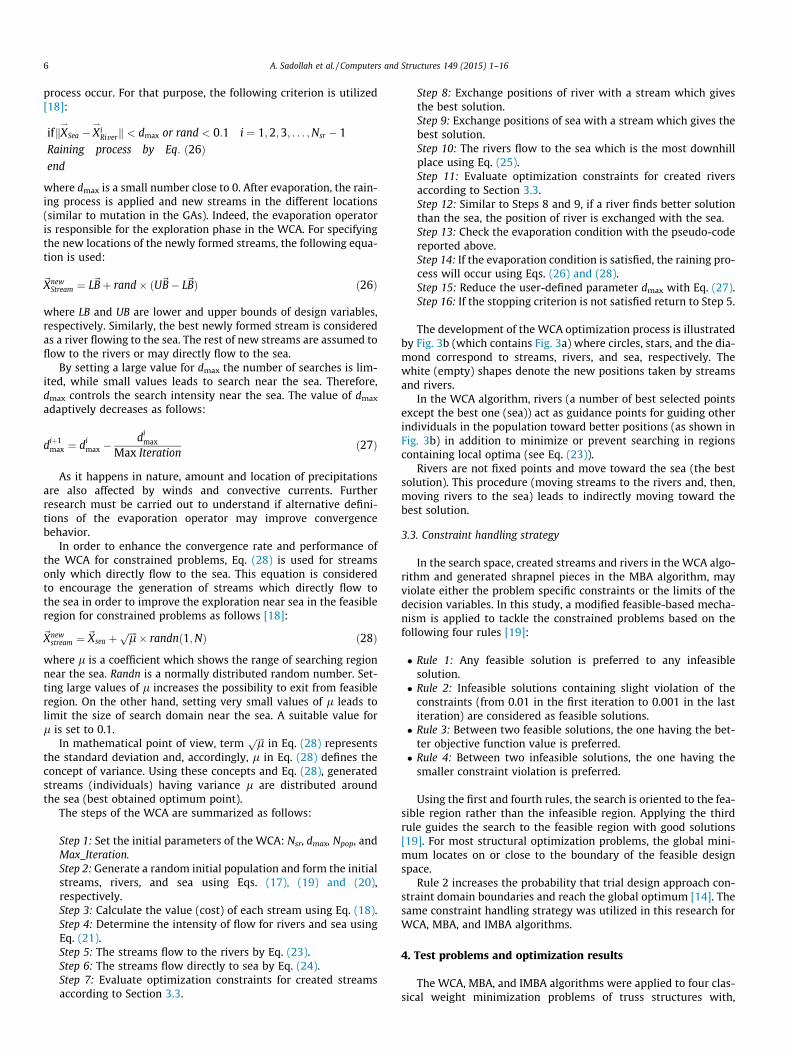
Fig. 2 summarizes the IMBA search process. The explorationphase is represented by the dashed area, and the exploitationphase is represented by the solid area. The black and white circles(exploded mines) correspond to locations of improved (the smallerthe objective function value, the better the mine for minimizationproblem) and non-improved shrapnel pieces, respectively. Weassume there are five shrapnel pieces (population size = 5), andl = 2, which means there are two iterations for the explorationphase.

With respect to the exploitation process, IMBA converges to theglobal optimal solution using Eqs. (9) and (10). The distance ofshrapnel pieces is reduced adaptively using Eq. (14) in both theexploitation and exploration processes. Pseudo-code for the explo-ration and exploitation processes of IMBA is given in detail inTable 2.

The IMBA algorithm includes the following steps:

Step 1: Set the internal parameters of MBA: a, Ns (Npop), andMax_Iteration.Step 2: Check the condition of the exploration factor (l).Step 3: If t 6 l, calculate distances of shrapnel pieces and theirlocations for exploded mines with Eqs. (6) and (7), respectively,and go Step 7. Otherwise, go to Step 4.Step 4: Calculate the locations of exploded landmines in theexploitation phase using Eqs. (9) and (10).Step 5: Calculate the Euclidian distance between current andprevious best solutions using Eq. (12).Step 6: Generate the updated landmines and compute theirimproved locations using Eq. (11).Step 7: Check constraints for generated shrapnel pieces (seeconstraint handling strategy outlined in Section 3.3).Step 8: Save the best shrapnel piece as the current best record.Step 9: Does the shrapnel piece improve cost with respect to thecurrent best record?Step 10: If the above occurs, exchange the position of the shrap-nel piece with the current best record.Step 11: Reduce adaptively the distance of the shrapnel pieceswith Eq. (14).Step 12: If the stopping criterion is not satisfied return to Step 2.

3.1.1. Setting initial parameters of IMBAPoor choices of algorithm parameters may result in a low con-

vergence rate, convergence to a local minimum, or undesired solu-tions. The following guidelines are designed to fine tune theinternal parameters.

The reduction factor (a) depends on the complexity of the prob-lem and the number of decision variables. The optimal value of arelies on the value of the maximum iteration. As explained earlier

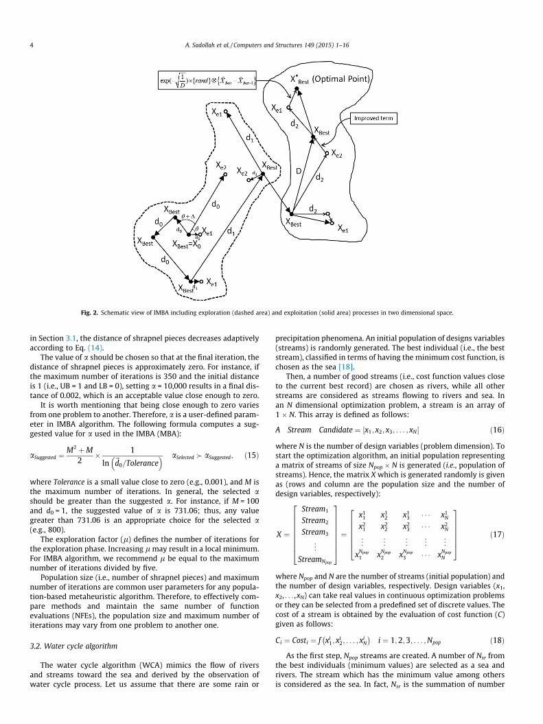
Fig. 2. Schematic view of IMBA including exploration (dashed area) and exploitation (solid area) processes in two dimensional space.


in Section 3.1, the distance of shrapnel pieces decreases adaptivelyaccording to Eq. (14).

The value of a should be chosen so that at the final iteration, thedistance of shrapnel pieces is approximately zero. For instance, ifthe maximum number of iterations is 350 and the initial distanceis 1 (i.e., UB = 1 and LB = 0), setting a = 10,000 results in a final dis-tance of 0.002, which is an acceptable value close enough to zero.

It is worth mentioning that being close enough to zero variesfrom one problem to another. Therefore, a is a user-defined param-eter in IMBA algorithm. The following formula computes a sug-gested value for a used in the IMBA (MBA):

aSuggested ¼M2 þM

2� 1

ln ~d0=Tolerance� � aSelected � aSuggested; ð15Þ

where Tolerance is a small value close to zero (e.g., 0.001), and M isthe maximum number of iterations. In general, the selected ashould be greater than the suggested a. For instance, if M = 100and d0 = 1, the suggested value of a is 731.06; thus, any valuegreater than 731.06 is an appropriate choice for the selected a(e.g., 800).

The exploration factor (l) defines the number of iterations forthe exploration phase. Increasing l may result in a local minimum.For IMBA algorithm, we recommend l be equal to the maximumnumber of iterations divided by five.

Population size (i.e., number of shrapnel pieces) and maximumnumber of iterations are common user parameters for any popula-tion-based metaheuristic algorithm. Therefore, to effectively com-pare methods and maintain the same number of functionevaluations (NFEs), the population size and maximum number ofiterations may vary from one problem to another one.

3.2. Water cycle algorithm

The water cycle algorithm (WCA) mimics the flow of riversand streams toward the sea and derived by the observation ofwater cycle process. Let us assume that there are some rain or

precipitation phenomena. An initial population of designs variables(streams) is randomly generated. The best individual (i.e., the beststream), classified in terms of having the minimum cost function, ischosen as the sea [18].

Then, a number of good streams (i.e., cost function values closeto the current best record) are chosen as rivers, while all otherstreams are considered as streams flowing to rivers and sea. Inan N dimensional optimization problem, a stream is an array of1 � N. This array is defined as follows:

A Stream Candidate ¼ ½x1; x2; x3; . . . ; xN� ð16Þ

where N is the number of design variables (problem dimension). Tostart the optimization algorithm, an initial population representinga matrix of streams of size Npop � N is generated (i.e., population ofstreams). Hence, the matrix X which is generated randomly is givenas (rows and column are the population size and the number ofdesign variables, respectively):

X ¼

Stream1

Stream2

Stream3

..

.

StreamNpop

266666664

377777775¼

x11 x1

2 x13 � � � x1

N

x21 x2

2 x23 � � � x2

N

..

. ... ..

. ... ..

.

xNpop1 xNpop

2 xNpop3 � � � xNpop

N

2666664

3777775 ð17Þ

where Npop and N are the number of streams (initial population) andthe number of design variables, respectively. Design variables (x1,x2, . . . ,xN) can take real values in continuous optimization problemsor they can be selected from a predefined set of discrete values. Thecost of a stream is obtained by the evaluation of cost function (C)given as follows:

Ci ¼ Costi ¼ f xi1; x

i2; . . . ; xi

N

� �i ¼ 1;2;3; . . . ;Npop ð18Þ

As the first step, Npop streams are created. A number of Nsr fromthe best individuals (minimum values) are selected as a sea andrivers. The stream which has the minimum value among othersis considered as the sea. In fact, Nsr is the summation of number

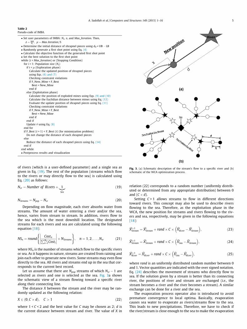
Table 2Pseudo-code of IMBA.

� Set user parameters of IMBA: Ns, a, and Max_Iteration. Then,D ¼ 360

Ns; l ¼ Max Iteration=5

� Determine the initial distance of shrapnel pieces using d0 = UB � LB� Randomly generate a first shot point using Eq. (4)� Calculate the objective function of the generated first shot point� Set the best solution to the first shot pointwhile (t < Max_Iteration) or (Stopping Condition)

for i = 1: Population size (Ns)if t < l (Exploration phase)

Calculate the updated position of shrapnel piecesusing Eqs. (6) and (7)Checking constraint violationsif F_New_Mine < F_Best

Best = New_Mineend if

else (Exploitation phase)Calculate the position of exploded mines using Eqs. (9) and (10)Calculate the Euclidian distance between mines using Eq. (12)Evaluate the update position of shrapnel pieces using Eq. (11)Checking constraint violationsif F_New_Mine < F_Best

Best = New_Mineend if

end ifUpdate h using Eq. (8)

end forif F_Best (t + 1) < F_Best (t) (for minimization problem)

Do not change the distance of each shrapnel pieceselse

Reduce the distance of each shrapnel pieces using Eq. (14)end if

end while� Postprocess results and visualization

Fig. 3. (a) Schematic description of the stream’s flow to a specific river and (b)schematic of the WCA optimization process.


of rivers (which is a user-defined parameter) and a single sea asgiven in Eq. (19). The rest of the population (streams which flowto the rivers or may directly flow to the sea) is calculated usingEq. (20) as follows:

Nsr ¼ Number of Riversþ 1|{z}Sea

ð19Þ

NStreams ¼ Npop � Nsr ð20Þ

Depending on flow magnitude, each river absorbs water fromstreams. The amount of water entering a river and/or the sea,hence, varies from stream to stream. In addition, rivers flow tothe sea which is the most downhill location. The designatedstreams for each rivers and sea are calculated using the followingequation [18]:

NSn ¼ roundCostnPNsri¼1Costi

�� NStreams

( ); n ¼ 1;2; . . . ;Nsr ð21Þ

where NSn is the number of streams which flow to the specific riversor sea. As it happens in nature, streams are created from raining andjoin each other to generate new rivers. Some streams may even flowdirectly to the sea. All rivers and streams end up in the sea that cor-responds to the current best record.

Let us assume that there are Npop streams of which Nsr � 1 areselected as rivers and one is selected as the sea. Fig. 3a showsthe schematic view of a stream flowing toward a specific riveralong their connecting line.

The distance X between the stream and the river may be ran-domly updated as the following relation:

X 2 ð0;C � dÞ; C > 1 ð22Þ

where 1 < C < 2 and the best value for C may be chosen as 2; d isthe current distance between stream and river. The value of X in

relation (22) corresponds to a random number (uniformly distrib-uted or determined from any appropriate distribution) between 0and (C � d).

Setting C > 1 allows streams to flow in different directionstoward rivers. This concept may also be used to describe riversflowing to the sea. Therefore, as the exploitation phase in theWCA, the new position for streams and rivers flowing to the riv-ers and sea, respectively, may be given in the following equations[18]:

~Xiþ1Stream ¼ ~Xi

Stream þ rand� C � ~XiRiver �~Xi

Stream

� �; ð23Þ

~Xiþ1Stream ¼ ~Xi

Stream þ rand� C � ~XiSea �~Xi

Stream

� �; ð24Þ

~Xiþ1River ¼ ~Xi

River þ rand� C � ~XiSea �~Xi

River

� �; ð25Þ

where rand is an uniformly distributed random number between 0and 1. Vector quantities are indicated with the over signed notation.Eq. (24) describes the movement of streams who directly flow tosea. If the solution given by a stream is better than its connectingriver, the positions of river and stream are exchanged (i.e., thestream becomes a river and the river becomes a stream). A similarexchange can be done for a river and the sea.

The evaporation process operator also is introduced to avoidpremature convergence to local optima. Basically, evaporationcauses sea water to evaporate as rivers/streams flow to the sea.This leads to new precipitations. Therefore, we have to check ifthe river/stream is close enough to the sea to make the evaporation


process occur. For that purpose, the following criterion is utilized[18]:

ifkX!

Sea � X!

iRiverk < dmax or rand < 0:1 i ¼ 1;2;3; . . . ;Nsr � 1

Raining process by Eq: ð26Þend

where dmax is a small number close to 0. After evaporation, the rain-ing process is applied and new streams in the different locations(similar to mutation in the GAs). Indeed, the evaporation operatoris responsible for the exploration phase in the WCA. For specifyingthe new locations of the newly formed streams, the following equa-tion is used:

~XnewStream ¼ L~Bþ rand� ðU~B� L~BÞ ð26Þ

where LB and UB are lower and upper bounds of design variables,respectively. Similarly, the best newly formed stream is consideredas a river flowing to the sea. The rest of new streams are assumed toflow to the rivers or may directly flow to the sea.

By setting a large value for dmax the number of searches is lim-ited, while small values leads to search near the sea. Therefore,dmax controls the search intensity near the sea. The value of dmax

adaptively decreases as follows:

diþ1max ¼ di

max �di

max

Max Iterationð27Þ

As it happens in nature, amount and location of precipitationsare also affected by winds and convective currents. Furtherresearch must be carried out to understand if alternative defini-tions of the evaporation operator may improve convergencebehavior.

In order to enhance the convergence rate and performance ofthe WCA for constrained problems, Eq. (28) is used for streamsonly which directly flow to the sea. This equation is consideredto encourage the generation of streams which directly flow tothe sea in order to improve the exploration near sea in the feasibleregion for constrained problems as follows [18]:

~Xnewstream ¼ ~Xsea þ

ffiffiffiffilp � randnð1;NÞ ð28Þ

where l is a coefficient which shows the range of searching regionnear the sea. Randn is a normally distributed random number. Set-ting large values of l increases the possibility to exit from feasibleregion. On the other hand, setting very small values of l leads tolimit the size of search domain near the sea. A suitable value forl is set to 0.1.

In mathematical point of view, termffiffiffiffilp in Eq. (28) represents

the standard deviation and, accordingly, l in Eq. (28) defines theconcept of variance. Using these concepts and Eq. (28), generatedstreams (individuals) having variance l are distributed aroundthe sea (best obtained optimum point).

The steps of the WCA are summarized as follows:

Step 1: Set the initial parameters of the WCA: Nsr, dmax, Npop, andMax_Iteration.Step 2: Generate a random initial population and form the initialstreams, rivers, and sea using Eqs. (17), (19) and (20),respectively.Step 3: Calculate the value (cost) of each stream using Eq. (18).Step 4: Determine the intensity of flow for rivers and sea usingEq. (21).Step 5: The streams flow to the rivers by Eq. (23).Step 6: The streams flow directly to sea by Eq. (24).Step 7: Evaluate optimization constraints for created streamsaccording to Section 3.3.

Step 8: Exchange positions of river with a stream which givesthe best solution.Step 9: Exchange positions of sea with a stream which gives thebest solution.Step 10: The rivers flow to the sea which is the most downhillplace using Eq. (25).Step 11: Evaluate optimization constraints for created riversaccording to Section 3.3.Step 12: Similar to Steps 8 and 9, if a river finds better solutionthan the sea, the position of river is exchanged with the sea.Step 13: Check the evaporation condition with the pseudo-codereported above.Step 14: If the evaporation condition is satisfied, the raining pro-cess will occur using Eqs. (26) and (28).Step 15: Reduce the user-defined parameter dmax with Eq. (27).Step 16: If the stopping criterion is not satisfied return to Step 5.

The development of the WCA optimization process is illustratedby Fig. 3b (which contains Fig. 3a) where circles, stars, and the dia-mond correspond to streams, rivers, and sea, respectively. Thewhite (empty) shapes denote the new positions taken by streamsand rivers.

In the WCA algorithm, rivers (a number of best selected pointsexcept the best one (sea)) act as guidance points for guiding otherindividuals in the population toward better positions (as shown inFig. 3b) in addition to minimize or prevent searching in regionscontaining local optima (see Eq. (23)).

Rivers are not fixed points and move toward the sea (the bestsolution). This procedure (moving streams to the rivers and, then,moving rivers to the sea) leads to indirectly moving toward thebest solution.

3.3. Constraint handling strategy

In the search space, created streams and rivers in the WCA algo-rithm and generated shrapnel pieces in the MBA algorithm, mayviolate either the problem specific constraints or the limits of thedecision variables. In this study, a modified feasible-based mecha-nism is applied to tackle the constrained problems based on thefollowing four rules [19]:

� Rule 1: Any feasible solution is preferred to any infeasiblesolution.� Rule 2: Infeasible solutions containing slight violation of the

constraints (from 0.01 in the first iteration to 0.001 in the lastiteration) are considered as feasible solutions.� Rule 3: Between two feasible solutions, the one having the bet-

ter objective function value is preferred.� Rule 4: Between two infeasible solutions, the one having the

smaller constraint violation is preferred.

Using the first and fourth rules, the search is oriented to the fea-sible region rather than the infeasible region. Applying the thirdrule guides the search to the feasible region with good solutions[19]. For most structural optimization problems, the global mini-mum locates on or close to the boundary of the feasible designspace.

Rule 2 increases the probability that trial design approach con-straint domain boundaries and reach the global optimum [14]. Thesame constraint handling strategy was utilized in this research forWCA, MBA, and IMBA algorithms.

4. Test problems and optimization results

The WCA, MBA, and IMBA algorithms were applied to four clas-sical weight minimization problems of truss structures with,

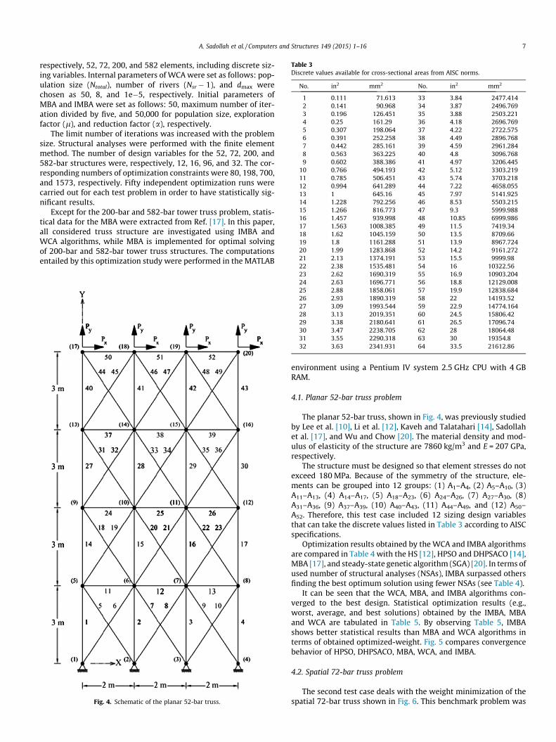
Table 3Discrete values available for cross-sectional areas from AISC norms.

No. in2 mm2 No. in2 mm2

1 0.111 71.613 33 3.84 2477.4142 0.141 90.968 34 3.87 2496.7693 0.196 126.451 35 3.88 2503.2214 0.25 161.29 36 4.18 2696.7695 0.307 198.064 37 4.22 2722.5756 0.391 252.258 38 4.49 2896.7687 0.442 285.161 39 4.59 2961.2848 0.563 363.225 40 4.8 3096.7689 0.602 388.386 41 4.97 3206.445

10 0.766 494.193 42 5.12 3303.21911 0.785 506.451 43 5.74 3703.21812 0.994 641.289 44 7.22 4658.05513 1 645.16 45 7.97 5141.92514 1.228 792.256 46 8.53 5503.21515 1.266 816.773 47 9.3 5999.98816 1.457 939.998 48 10.85 6999.98617 1.563 1008.385 49 11.5 7419.3418 1.62 1045.159 50 13.5 8709.6619 1.8 1161.288 51 13.9 8967.72420 1.99 1283.868 52 14.2 9161.27221 2.13 1374.191 53 15.5 9999.9822 2.38 1535.481 54 16 10322.56


respectively, 52, 72, 200, and 582 elements, including discrete siz-ing variables. Internal parameters of WCA were set as follows: pop-ulation size (Ntotal), number of rivers (Nsr � 1), and dmax werechosen as 50, 8, and 1e�5, respectively. Initial parameters ofMBA and IMBA were set as follows: 50, maximum number of iter-ation divided by five, and 50,000 for population size, explorationfactor (l), and reduction factor (a), respectively.

The limit number of iterations was increased with the problemsize. Structural analyses were performed with the finite elementmethod. The number of design variables for the 52, 72, 200, and582-bar structures were, respectively, 12, 16, 96, and 32. The cor-responding numbers of optimization constraints were 80, 198, 700,and 1573, respectively. Fifty independent optimization runs werecarried out for each test problem in order to have statistically sig-nificant results.

Except for the 200-bar and 582-bar tower truss problem, statis-tical data for the MBA were extracted from Ref. [17]. In this paper,all considered truss structure are investigated using IMBA andWCA algorithms, while MBA is implemented for optimal solvingof 200-bar and 582-bar tower truss structures. The computationsentailed by this optimization study were performed in the MATLAB

Fig. 4. Schematic of the planar 52-bar truss.

23 2.62 1690.319 55 16.9 10903.20424 2.63 1696.771 56 18.8 12129.00825 2.88 1858.061 57 19.9 12838.68426 2.93 1890.319 58 22 14193.5227 3.09 1993.544 59 22.9 14774.16428 3.13 2019.351 60 24.5 15806.4229 3.38 2180.641 61 26.5 17096.7430 3.47 2238.705 62 28 18064.4831 3.55 2290.318 63 30 19354.832 3.63 2341.931 64 33.5 21612.86

environment using a Pentium IV system 2.5 GHz CPU with 4 GBRAM.

4.1. Planar 52-bar truss problem

The planar 52-bar truss, shown in Fig. 4, was previously studiedby Lee et al. [10], Li et al. [12], Kaveh and Talatahari [14], Sadollahet al. [17], and Wu and Chow [20]. The material density and mod-ulus of elasticity of the structure are 7860 kg/m3 and E = 207 GPa,respectively.

The structure must be designed so that element stresses do notexceed 180 MPa. Because of the symmetry of the structure, ele-ments can be grouped into 12 groups: (1) A1–A4, (2) A5–A10, (3)A11–A13, (4) A14–A17, (5) A18–A23, (6) A24–A26, (7) A27–A30, (8)A31–A36, (9) A37–A39, (10) A40–A43, (11) A44–A49, and (12) A50–A52. Therefore, this test case included 12 sizing design variablesthat can take the discrete values listed in Table 3 according to AISCspecifications.

Optimization results obtained by the WCA and IMBA algorithmsare compared in Table 4 with the HS [12], HPSO and DHPSACO [14],MBA [17], and steady-state genetic algorithm (SGA) [20]. In terms ofused number of structural analyses (NSAs), IMBA surpassed othersfinding the best optimum solution using fewer NSAs (see Table 4).

It can be seen that the WCA, MBA, and IMBA algorithms con-verged to the best design. Statistical optimization results (e.g.,worst, average, and best solutions) obtained by the IMBA, MBAand WCA are tabulated in Table 5. By observing Table 5, IMBAshows better statistical results than MBA and WCA algorithms interms of obtained optimized-weight. Fig. 5 compares convergencebehavior of HPSO, DHPSACO, MBA, WCA, and IMBA.

4.2. Spatial 72-bar truss problem

The second test case deals with the weight minimization of thespatial 72-bar truss shown in Fig. 6. This benchmark problem was

Table 452-bar truss problem: comparison of WCA, MBA and IMBA optimization results with the literature.

Variables (mm2) SGA [20] HS [12] HPSO [12] DHPSACO [14] MBA [17] WCA IMBA

A1–A4 4658.055 4658.055 4658.055 4658.055 4658.055 4658.055 4658.055A5–A10 1161.288 1161.288 1161.288 1161.288 1161.288 1161.288 1161.288A11–A13 645.160 506.451 363.225 494.193 494.193 494.193 494.193A14–A17 3303.219 3303.219 3303.219 3303.219 3303.219 3303.219 3303.219A18–A23 1045.159 940.000 940.000 1008.385 940.000 940.000 940.000A24–A26 494.193 494.193 494.193 285.161 494.193 494.193 494.193A27–A30 2477.414 2290.318 2238.705 2290.318 2283.705 2283.705 2283.705A31–A36 1045.159 1008.385 1008.385 1008.385 1008.385 1008.385 1008.385A37–A39 285.161 2290.318 388.386 388.386 494.193 494.193 494.193A40–A43 1696.771 1535.481 1283.868 1283.868 1283.868 1283.868 1283.868A44–A49 1045.159 1045.159 1161.288 1161.288 1161.288 1161.288 1161.288A50–A52 641.289 506.451 729.256 506.451 494.193 494.193 494.193

Weight (kg) 1970.142 1906.76 1905.495 1904.83 1902.605 1902.605 1902.605Number of structural analyses N/Aa N/A 105,000 11,100 5450 7100 4750

a Not available.

Table 5Statistical optimization results obtained from WCA, MBA, and IMBA for the 52-bar truss problem.

Methods Best optimized weight (kg) Average optimized weight (kg) Worst optimized weight (kg) Standard deviation on weight (kg)

WCA 1902.605 1909.856 1912.646 7.09MBA 1902.605 1906.076 1912.646 4.09IMBA 1902.605 1903.076 1904.83 1.13

Fig. 5. Comparison of convergence curves recorded for the 52-bar truss problem.


previously studied by Lee et al. [10], Li et al. [12], Kaveh and Tala-tahari [14], Sadollah et al. [17], and Wu and Chow [20]. The mate-rial density and the modulus of elasticity of the truss structure are0.1 lb/in3 (2767.99 kg/m3) and E = 10 Msi (68.95 GPa), respectively.

The maximum stress developed in the elements must notexceed 25,000 psi (172.4 MPa). The top nodes are subjected to dis-placement limits of 0.25 in (6.35 mm) in coordinate directions xand y. Because of the symmetry of the structure, the 72 elementscan be grouped into 16 groups: (1) A1–A4, (2) A5–A12, (3) A13–A16, (4) A17–A18, (5) A19–A22, (6) A23–A30, (7) A31–A34, (8) A35–A36, (9) A37–A40, (10) A41–A48, (11) A49–A52, (12) A53–A54, (13)A55–A58, (14) A59–A66 (15) A67–A70, and (16) A71–A72.

Two variants were considered for this optimization problem: (i)Case 1, where values of cross-sectional areas could be selectedfrom the discrete set D = [0.1, 0.2, 0.3, 0.4, 0.5, 0.6, 0.7, 0.8, 0.9,1.0, 1.1, 1.2, 1.3, 1.4, 1.5, 1.6, 1.7, 1.8, 1.9, 2.0, 2.1, 2.2, 2.3, 2.4,2.5, 2.6, 2.7, 2.8, 2.9, 3.0, 3.1,3.2] (in2); (ii) Case 2, where valuesof cross-sectional areas could be selected from the discrete set ofTable 3. The structure is subject to two independent load casesdescribed in Table 6.

The maximum number of optimization iterations was set as1000 for all problem variants. Statistical results obtained by theWCA, MBA, and IMBA algorithms are compared in Table 7. All algo-rithms converged to the best weight of 385.54 lb in the case of

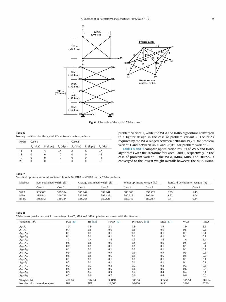
Fig. 6. Schematic of the spatial 72-bar truss.

Table 6Loading conditions for the spatial 72-bar truss structure problem.

Nodes Case 1 Case 2

Px (kips) Py (kips) Pz (kips) Px (kips) Py (kips) Pz (kips)

17 5 5 �5 0 0 �518 0 0 0 0 0 �519 0 0 0 0 0 �520 0 0 0 0 0 �5

Table 7Statistical optimization results obtained from MBA, IMBA, and WCA for the 72-bar proble

Methods Best optimized weight (lb) Average optimized weight (lb)

Case 1 Case 2 Case 1 Case 2

WCA 385.542 389.334 385.842 389.941MBA 385.542 390.739 387.665 395.432IMBA 385.542 389.334 385.765 389.823

Table 872-bar truss problem variant 1: comparison of WCA, MBA and IMBA optimization results

Variables (in2) SGA [20] HS [12] HPSO [1

A1–A4 1.5 1.9 2.1A5–A12 0.7 0.5 0.6A13–A16 0.1 0.1 0.1A17–A18 0.1 0.1 0.1A19–A22 1.3 1.4 1.4A23–A30 0.5 0.6 0.5A31–A34 0.2 0.1 0.1A35–A36 0.1 0.1 0.1A37–A40 0.5 0.6 0.5A41–A48 0.5 0.5 0.5A49–A52 0.1 0.1 0.1A53–A54 0.2 0.1 0.1A55–A58 0.2 0.2 0.2A59–A66 0.5 0.5 0.5A67–A70 0.5 0.4 0.3A71–A72 0.7 0.6 0.7

Weight (lb) 400.66 387.94 388.94Number of structural analyses N/A N/A 12,500


problem variant 1, while the WCA and IMBA algorithms convergedto a lighter design in the case of problem variant 2. The NSAsrequired by the WCA ranged between 3200 and 19,750 for problemvariant 1 and between 4600 and 26,050 for problem variant 2.

Tables 8 and 9 compare optimization results of WCA and IMBAalgorithms with the literature for Cases 1 and 2, respectively. In thecase of problem variant 1, the WCA, IMBA, MBA, and DHPSACOconverged to the lowest weight overall; however, the MBA, IMBA,

m.

Worst optimized weight (lb) Standard deviation on weight (lb)

Case 1 Case 2 Case 1 Case 2

386.800 393.778 0.55 1.43390.615 399.49 1.62 3.04387.942 389.457 0.41 0.84

with the literature.

2] DHPSACO [14] MBA [17] WCA IMBA

1.9 1.9 1.9 1.90.5 0.5 0.5 0.50.1 0.1 0.1 0.10.1 0.1 0.1 0.11.3 1.4 1.4 1.40.5 0.5 0.5 0.50.1 0.1 0.1 0.10.1 0.1 0.1 0.10.6 0.5 0.5 0.50.5 0.5 0.5 0.50.1 0.1 0.1 0.10.1 0.1 0.1 0.10.2 0.2 0.2 0.20.6 0.6 0.6 0.60.4 0.4 0.4 0.40.6 0.6 0.6 0.6

385.54 385.54 385.54 385.5410,650 9450 3200 5750

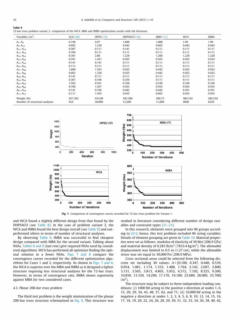
Table 972-bar truss problem variant 2: comparison of the WCA, MBA and IMBA optimization results with the literature.

Variables (in2) SGA [20] HPSO [12] DHPSACO [14] MBA [17] WCA IMBA

A1–A4 0.196 4.97 1.800 1.800 1.99 1.99A5–A12 0.602 1.228 0.442 0.602 0.442 0.442A13–A16 0.307 0.111 0.141 0.111 0.111 0.111A17–A18 0.766 0.111 0.111 0.111 0.111 0.111A19–A22 0.391 2.88 1.228 1.266 1.228 1.228A23–A30 0.391 1.457 0.563 0.563 0.563 0.563A31–A34 0.141 0.141 0.111 0.111 0.111 0.111A35–A36 0.111 0.111 0.111 0.111 0.111 0.111A37–A40 1.800 1.563 0.563 0.442 0.563 0.563A41–A48 0.602 1.228 0.563 0.442 0.563 0.563A49–A52 0.141 0.111 0.111 0.111 0.111 0.111A53–A54 0.307 0.196 0.250 0.111 0.111 0.111A55–A58 1.563 0.391 0.196 0.196 0.196 0.196A59–A66 0.766 1.457 0.563 0.563 0.563 0.563A67–A70 0.141 0.766 0.442 0.442 0.391 0.391A71–A72 0.111 1.563 0.563 0.602 0.563 0.563

Weight (lb) 427.203 933.09 393.380 390.73 389.334 389.334Number of structural analyses N/A 50,000 12,500 11,600 4600 6250

Fig. 7. Comparison of convergence curves recorded for 72-bar truss problem for Variant 1.


and WCA found a slightly different design from that found by theDHPSACO (see Table 8). In the case of problem variant 2, theWCA and IMBA found the best design overall (see Table 9) and out-performed others in terms of number of structural analyses.

By observing Table 9, IMBA was successful to find cheapestdesign compared with MBA for the second variant. Talking aboutNSAs, Tables 8 and 9 (last row) give required NSAs used by consid-ered algorithms. WCA has performed all optimizer finding the opti-mal solution in a fewer NSAs. Figs. 7 and 8 compare theconvergence curves recorded for the different optimization algo-rithms for Cases 1 and 2, respectively. As shown in Figs. 7 and 8,the WCA is superior over the MBA and IMBA as it designed a lighterstructure requiring less structural analyses for the 72-bar truss.However, in terms of convergence rate, IMBA shows superiorityagainst MBA for two considered cases.

4.3. Planar 200-bar truss problem

The third test problem is the weight minimization of the planar200-bar truss structure schematized in Fig. 9. This structure was

studied in literature considering different number of design vari-ables and constraint types [21–23].

In this research, elements were grouped into 96 groups accord-ing to [21]; hence, this test problem included 96 sizing variables.Details of element grouping are given in Table 10. Material proper-ties were set as follows: modulus of elasticity of 30 Msi (206.9 GPa)and material density of 0.283 lb/in3 (7833.4 kg/m3). The allowabledisplacement was limited to 0.5 in (1.27 cm), while the allowablestress was set equal to 30,000 Psi (206.9 MPa).

Cross sectional areas could be selected from the following dis-crete set including 30 values: A = [0.100, 0.347, 0.440, 0.539,0.954, 1.081, 1.174, 1.333, 1.488, 1.764, 2.142, 2.697, 2.800,3.131, 3.565, 3.813, 4.805, 5.952, 6.572, 7.192, 8.525, 9.300,10.850, 13.330, 14.290, 17.170, 19.180, 23.680, 28.080, 33.700](in2).

The structure may be subject to three independent loading con-ditions: (i) 1000 lbf acting in the positive x direction at nodes 1, 6,15, 20, 29, 34, 43, 48, 57, 62, and 71; (ii) 10,000 lbf acting in thenegative y direction at nodes 1, 2, 3, 4, 5, 6, 8, 10, 12, 14, 15, 16,17, 18, 19, 20, 22, 24, 26, 28, 29, 30, 31, 32, 33, 34, 36, 38, 40, 42,

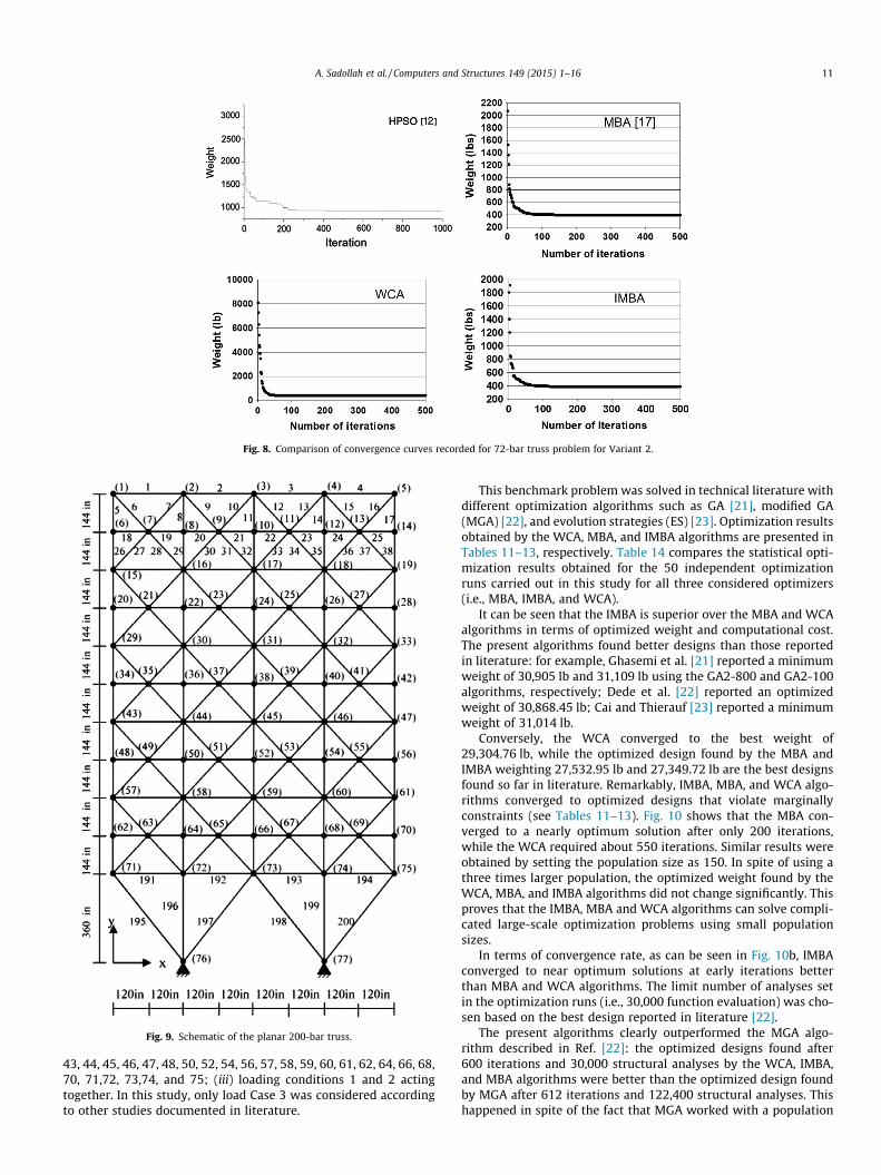
Fig. 8. Comparison of convergence curves recorded for 72-bar truss problem for Variant 2.

Fig. 9. Schematic of the planar 200-bar truss.


43, 44, 45, 46, 47, 48, 50, 52, 54, 56, 57, 58, 59, 60, 61, 62, 64, 66, 68,70, 71,72, 73,74, and 75; (iii) loading conditions 1 and 2 actingtogether. In this study, only load Case 3 was considered accordingto other studies documented in literature.

This benchmark problem was solved in technical literature withdifferent optimization algorithms such as GA [21], modified GA(MGA) [22], and evolution strategies (ES) [23]. Optimization resultsobtained by the WCA, MBA, and IMBA algorithms are presented inTables 11–13, respectively. Table 14 compares the statistical opti-mization results obtained for the 50 independent optimizationruns carried out in this study for all three considered optimizers(i.e., MBA, IMBA, and WCA).

It can be seen that the IMBA is superior over the MBA and WCAalgorithms in terms of optimized weight and computational cost.The present algorithms found better designs than those reportedin literature: for example, Ghasemi et al. [21] reported a minimumweight of 30,905 lb and 31,109 lb using the GA2-800 and GA2-100algorithms, respectively; Dede et al. [22] reported an optimizedweight of 30,868.45 lb; Cai and Thierauf [23] reported a minimumweight of 31,014 lb.

Conversely, the WCA converged to the best weight of29,304.76 lb, while the optimized design found by the MBA andIMBA weighting 27,532.95 lb and 27,349.72 lb are the best designsfound so far in literature. Remarkably, IMBA, MBA, and WCA algo-rithms converged to optimized designs that violate marginallyconstraints (see Tables 11–13). Fig. 10 shows that the MBA con-verged to a nearly optimum solution after only 200 iterations,while the WCA required about 550 iterations. Similar results wereobtained by setting the population size as 150. In spite of using athree times larger population, the optimized weight found by theWCA, MBA, and IMBA algorithms did not change significantly. Thisproves that the IMBA, MBA and WCA algorithms can solve compli-cated large-scale optimization problems using small populationsizes.

In terms of convergence rate, as can be seen in Fig. 10b, IMBAconverged to near optimum solutions at early iterations betterthan MBA and WCA algorithms. The limit number of analyses setin the optimization runs (i.e., 30,000 function evaluation) was cho-sen based on the best design reported in literature [22].

The present algorithms clearly outperformed the MGA algo-rithm described in Ref. [22]: the optimized designs found after600 iterations and 30,000 structural analyses by the WCA, IMBA,and MBA algorithms were better than the optimized design foundby MGA after 612 iterations and 122,400 structural analyses. Thishappened in spite of the fact that MGA worked with a population

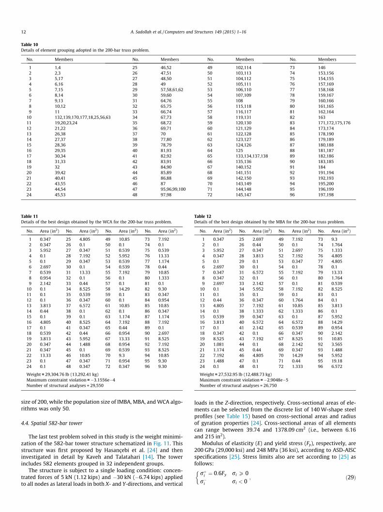
Table 10Details of element grouping adopted in the 200-bar truss problem.

No. Members No. Members No. Members No. Members

1 1,4 25 46,52 49 102,114 73 1462 2,3 26 47,51 50 103,113 74 153,1563 5,17 27 48,50 51 104,112 75 154,1554 6,16 28 49 52 105,111 76 157,1695 7,15 29 57,58,61,62 53 106,110 77 158,1686 8,14 30 59,60 54 107,109 78 159,1677 9,13 31 64,76 55 108 79 160,1668 10,12 32 65,75 56 115,118 80 161,1659 11 33 66,74 57 116,117 81 162,164

10 132,139,170,177,18,25,56,63 34 67,73 58 119,131 82 16311 19,20,23,24 35 68,72 59 120,130 83 171,172,175,17612 21,22 36 69,71 60 121,129 84 173,17413 26,38 37 70 61 122,128 85 178,19014 27,37 38 77,80 62 123,127 86 179,18915 28,36 39 78,79 63 124,126 87 180,18816 29,35 40 81,93 64 125 88 181,18717 30,34 41 82,92 65 133,134,137,138 89 182,18618 31,33 42 83,91 66 135,136 90 183,18519 32 43 84,90 67 140,152 91 18420 39,42 44 85,89 68 141,151 92 191,19421 40,41 45 86,88 69 142,150 93 192,19322 43,55 46 87 70 143,149 94 195,20023 44,54 47 95,96,99,100 71 144,148 95 196,19924 45,53 48 97,98 72 145,147 96 197,198

Table 11Details of the best design obtained by the WCA for the 200-bar truss problem.

No. Area (in2) No. Area (in2) No. Area (in2) No. Area (in2)

1 0.347 25 4.805 49 10.85 73 7.1922 0.347 26 0.1 50 0.1 74 0.13 5.952 27 0.347 51 0.539 75 0.5394 0.1 28 7.192 52 5.952 76 13.335 0.1 29 0.347 53 0.539 77 1.1746 2.697 30 0.1 54 0.539 78 0.447 0.539 31 13.33 55 7.192 79 10.858 0.954 32 0.1 56 0.1 80 1.3339 2.142 33 0.44 57 0.1 81 0.1

10 0.1 34 8.525 58 14.29 82 9.3011 0.1 35 0.539 59 0.1 83 0.34712 0.1 36 0.347 60 0.1 84 0.95413 3.813 37 6.572 61 10.85 85 10.8514 0.44 38 0.1 62 0.1 86 0.34715 0.1 39 0.1 63 1.174 87 1.17416 4.805 40 8.525 64 7.192 88 7.19217 0.1 41 0.347 65 0.44 89 0.118 0.539 42 0.44 66 0.954 90 2.69719 3.813 43 5.952 67 13.33 91 8.52520 0.347 44 1.488 68 0.954 92 7.19221 0.347 45 0.1 69 0.539 93 8.52522 13.33 46 10.85 70 9.3 94 10.8523 0.1 47 0.347 71 0.954 95 9.3024 0.1 48 0.347 72 0.347 96 9.30

Weight = 29,304.76 lb (13,292.41 kg)Maximum constraint violation = �3.1556e�4Number of structural analyses = 29,550

Table 12Details of the best design obtained by the MBA for the 200-bar truss problem.


1 0.347 25 2.697 49 7.192 73 9.32 0.1 26 0.44 50 0.1 74 1.7643 5.952 27 0.347 51 2.697 75 1.3334 0.347 28 3.813 52 7.192 76 4.8055 0.1 29 0.1 53 0.347 77 4.8056 2.697 30 0.1 54 0.1 78 0.17 0.347 31 6.572 55 7.192 79 13.338 0.347 32 0.1 56 0.1 80 1.7649 2.697 33 2.142 57 0.1 81 0.539

10 0.1 34 5.952 58 7.192 82 8.52511 0.1 35 0.1 59 0.1 83 0.112 0.44 36 0.347 60 1.764 84 0.113 4.805 37 7.192 61 10.85 85 3.81314 0.1 38 1.333 62 1.333 86 0.115 0.539 39 0.347 63 0.1 87 5.95216 3.813 40 6.572 64 6.572 88 14.2917 0.1 41 2.142 65 0.539 89 0.95418 0.347 42 0.1 66 0.347 90 2.14219 8.525 43 7.192 67 8.525 91 10.8520 1.081 44 0.1 68 2.142 92 3.56521 1.174 45 0.44 69 0.347 93 1.48822 7.192 46 4.805 70 14.29 94 5.95223 1.488 47 0.1 71 0.44 95 19.1824 0.1 48 0.1 72 1.333 96 6.572



size of 200, while the population size of IMBA, MBA, and WCA algo-rithms was only 50.

4.4. Spatial 582-bar tower

The last test problem solved in this study is the weight minimi-zation of the 582-bar tower structure schematized in Fig. 11. Thisstructure was first proposed by Hasançebi et al. [24] and theninvestigated in detail by Kaveh and Talatahari [14]. The towerincludes 582 elements grouped in 32 independent groups.

The structure is subject to a single loading condition: concen-trated forces of 5 kN (1.12 kips) and �30 kN (�6.74 kips) appliedto all nodes as lateral loads in both X- and Y-directions, and vertical

loads in the Z-direction, respectively. Cross-sectional areas of ele-ments can be selected from the discrete list of 140 W-shape steelprofiles (see Table 15) based on cross-sectional areas and radiusof gyration properties [24]. Cross-sectional areas of all elementscan range between 39.74 and 1378.09 cm2 (i.e., between 6.16and 215 in2).

Modulus of elasticity (E) and yield stress (Fy), respectively, are200 GPa (29,000 ksi) and 248 MPa (36 ksi), according to ASD-AISCspecifications [25]. Stress limits also are set according to [25] asfollows:

rþi ¼ 0:6Fy ri P 0r�i ri < 0

�; ð29Þ

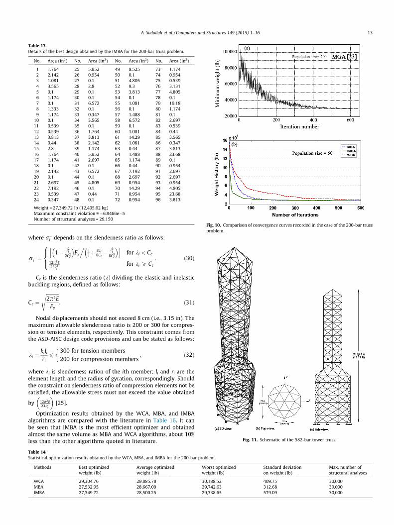
Table 13Details of the best design obtained by the IMBA for the 200-bar truss problem.


1 1.764 25 5.952 49 8.525 73 1.1742 2.142 26 0.954 50 0.1 74 0.9543 1.081 27 0.1 51 4.805 75 0.5394 3.565 28 2.8 52 9.3 76 3.1315 0.1 29 0.1 53 3.813 77 4.8056 1.174 30 0.1 54 0.1 78 0.17 0.1 31 6.572 55 1.081 79 19.188 1.333 32 0.1 56 0.1 80 1.1749 1.174 33 0.347 57 1.488 81 0.1

10 0.1 34 3.565 58 6.572 82 2.69711 0.539 35 0.1 59 0.1 83 0.53912 0.539 36 1.764 60 1.081 84 0.4413 3.813 37 3.813 61 14.29 85 3.56514 0.44 38 2.142 62 1.081 86 0.34715 2.8 39 1.174 63 0.44 87 3.81316 1.764 40 5.952 64 1.488 88 23.6817 1.174 41 2.697 65 1.174 89 0.118 0.1 42 0.1 66 0.44 90 0.95419 2.142 43 6.572 67 7.192 91 2.69720 0.1 44 0.1 68 2.697 92 2.69721 2.697 45 4.805 69 0.954 93 0.95422 7.192 46 0.1 70 14.29 94 4.80523 0.539 47 0.44 71 0.954 95 23.6824 0.347 48 0.1 72 0.954 96 3.813


Fig. 10. Comparison of convergence curves recorded in the case of the 200-bar trussproblem.

Fig. 11. Schematic of the 582-bar tower truss.


where r�i depends on the slenderness ratio as follows:

r�i ¼1� k2

i

2C2c

� �Fy

.53þ

3ki8Cc� k3

i

8C3c

� �h ifor ki < Cc

12p2E23k2

ifor ki P Cc

8><>: : ð30Þ

Cc is the slenderness ratio (k) dividing the elastic and inelasticbuckling regions, defined as follows:

Cc ¼ffiffiffiffiffiffiffiffiffiffiffi2p2E

Fy

s: ð31Þ

Nodal displacements should not exceed 8 cm (i.e., 3.15 in). Themaximum allowable slenderness ratio is 200 or 300 for compres-sion or tension elements, respectively. This constraint comes fromthe ASD-AISC design code provisions and can be stated as follows:

ki ¼kili

ri6

300 for tension members200 for compression members

�; ð32Þ

where ki is slenderness ration of the ith member; li and ri are theelement length and the radius of gyration, correspondingly. Shouldthe constraint on slenderness ratio of compression elements not besatisfied, the allowable stress must not exceed the value obtained

by 12p2E23k2

i

[25].

Optimization results obtained by the WCA, MBA, and IMBAalgorithms are compared with the literature in Table 16. It canbe seen that IMBA is the most efficient optimizer and obtainedalmost the same volume as MBA and WCA algorithms, about 10%less than the other algorithms quoted in literature.

Table 14Statistical optimization results obtained by the WCA, MBA, and IMBA for the 200-bar problem.

Methods Best optimizedweight (lb)

Average optimizedweight (lb)

Worst optimizedweight (lb)

Standard deviationon weight (lb)

Max. number ofstructural analyses

WCA 29,304.76 29,885.78 30,188.52 409.75 30,000MBA 27,532.95 28,667.09 29,742.63 312.68 30,000IMBA 27,349.72 28,500.25 29,338.65 579.09 30,000

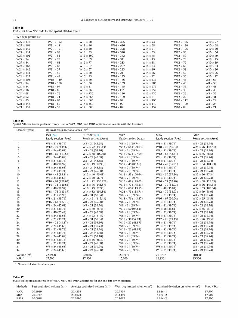
Table 15Profile list from AISC code for the spatial 582-bar tower.

W-shape profile list

W27 � 178 W21 � 122 W18 � 50 W14 � 455 W14 � 74 W12 � 136 W10 � 77W27 � 161 W21 � 111 W18 � 46 W14 � 426 W14 � 68 W12 � 120 W10 � 68W27 � 146 W21 � 101 W18 � 40 W14 � 398 W14 � 61 W12 � 106 W10 � 60W27 � 114 W21 � 93 W18 � 35 W14 � 370 W14 � 53 W12 � 96 W10 � 54W27 � 102 W21 � 83 W16 � 100 W14 � 342 W14 � 48 W12 � 87 W10 � 49W27 � 94 W21 � 73 W16 � 89 W14 � 311 W14 � 43 W12 � 79 W10 � 45W27 � 84 W21 � 68 W16 � 77 W14 � 283 W14 � 38 W12 � 72 W10 � 39W24 � 162 W21 � 62 W16 � 67 W14 � 257 W14 � 34 W12 � 65 W10 � 33W24 � 146 W21 � 57 W16 � 57 W14 � 233 W14 � 30 W12 � 58 W10 � 30W24 � 131 W21 � 50 W16 � 50 W14 � 211 W14 � 26 W12 � 53 W10 � 26W24 � 117 W21 � 44 W16 � 45 W14 � 193 W14 � 22 W12 � 50 W10 � 22W24 � 104 W18 � 119 W16 � 40 W14 � 176 W12 � 336 W12 � 45 W8 � 67W24 � 94 W18 � 106 W16 � 36 W14 � 159 W12 � 305 W12 � 40 W8 � 58W24 � 84 W18 � 97 W16 � 31 W14 � 145 W12 � 279 W12 � 35 W8 � 48W24 � 76 W18 � 86 W16 � 26 W14 � I32 W12 � 252 W12 � 30 W8 � 40W24 � 68 W18 � 76 W14 � 730 W14 � 120 W12 � 230 W12 � 26 W8 � 35W24 � 62 W18 � 71 W14 � 665 W14 � 109 W12 � 210 W12 � 22 W8 � 31W24 � 55 W18 � 65 W14 � 605 W14 � 99 W12 � 190 W10 � 112 W8 � 28W21 � 147 W18 � 60 W14 � 550 W14 � 90 W12 � 170 W10 � 100 W8 � 24W21 � 132 W18 � 55 W14 � 500 W14 � 82 W12 � 152 W10 � 88 W8 � 21

Table 16Spatial 582-bar tower problem: comparison of WCA, MBA, and IMBA optimization results with the literature.

Element group Optimal cross-sectional areas (cm2)

PSO [24] DHPSACO [14] WCA MBA IMBAReady section (Area) Ready section (Area) Ready section (Area) Ready section (Area) Ready section (Area)

1 W8 � 21 (39.74) W8 � 24 (45.68) W8 � 21 (39.74) W8 � 21 (39.74) W8 � 21 (39.74)2 W12 � 79 (149.68) W12 � 72 (136.13) W14 � 68 (129.03) W18 � 76 (56.64) W24 � 76 (144.51)3 W8 � 24 (45.68) W8 � 28 (53.16) W8 � 21 (39.74) W8 � 21 (39.74) W8 � 21 (39.74)4 W10 � 60 (113.55) W12 � 58 (109.68) W16 � 67 (127.09) W12 � 65 (48.51) W12 � 65 (48.51)5 W8 � 24 (45.68) W8 � 24 (45.68) W8 � 21 (39.74) W8 � 21 (39.74) W8 � 21 (39.74)6 W8 � 21 (39.74) W8 � 24 (45.68) W8 � 21 (39.74) W8 � 21 (39.74) W8 � 21 (39.74)7 W8 � 48 (90.97) W10 � 49 (92.90) W12 � 45 (85.16) W14 � 48 (35.81) W10 � 54 (101.93)8 W8 � 24 (45.68) W8 � 24 (45.68) W8 � 21 (39.74) W8 � 21 (39.74) W8 � 21 (39.74)9 W8 � 21 (39.74) W8 � 24 (45.68) W8 � 21 (39.74) W8 � 21 (39.74) W8 � 21 (39.74)

10 W10 � 45 (85.81) W12 � 40 (75.48) W12 � 53 (100.64) W12 � 50 (37.34) W12 � 50 (37.34)11 W8 � 24 (45.68) W12 � 30 (56.71) W8 � 21 (39.74) W8 � 21 (39.74) W8 � 21 (39.74)12 W10 � 68 (129.03) W12 � 72 (136.129) W10 � 68 (129.03) W16 � 77 (57.40) W10 � 68 (129.03)13 W14 � 74 (140.65) W18 � 76 (143.87) W16 � 77 (145.81) W12 � 79 (58.93) W24 � 76 (144.51)14 W8 � 48 (90.97) W10 � 49 (92.90) W10 � 60 (113.55) W8 � 48 (35.81) W14 � 53 (100.64)15 W18 � 76 (143.87) W14 � 82 (154.84) W21 � 73 (138.71) W12 � 79 (58.93) W12 � 79 (58.93)16 W8 � 31 (55.90) W8 � 31 (58.84) W8 � 21 (39.74) W8 � 21 (39.74) W8 � 21 (39.74)17 W8 � 21 (39.74) W14 � 61 (115.48) W18 � 76 (143.87) W16 � 67 (50.04) W12 � 65 (48.51)18 W16 � 67 (127.10) W8 � 24 (45.68) W8 � 21 (39.74) W8 � 21 (39.74) W8 � 21 (39.74)19 W8 � 24 (45.68) W8 � 21 (39.74) W8 � 21 (39.74) W8 � 21 (39.74) W8 � 21 (39.74)20 W8 � 21 (39.74) W12 � 40 (75.48) W16 � 50 (94.84) W8 � 48 (35.81) W12 � 45 (85.16)21 W8 � 40 (75.48) W8 � 24 (45.68) W8 � 21 (39.74) W8 � 21 (39.74) W8 � 21 (39.74)22 W8 � 24 (45.68) W14 � 22 (41.87) W8 � 21 (39.74) W8 � 21 (39.74) W8 � 21 (39.74)23 W8 � 21 (39.74) W8 � 31 (58.84) W10 � 30 (57.03) W12 � 26 (19.43) W16 � 26 (49.54)24 W10 � 22 (41.87) W8 � 28 (53.16) W10 � 22 (41.87) W8 � 21 (39.74) W8 � 21 (39.74)25 W8 � 24 (45.68) W8 � 21 (39.74) W8 � 21 (39.74) W8 � 21 (39.74) W8 � 21 (39.74)26 W8 � 21 (39.74) W8 � 21 (39.74) W14 � 22 (41.87) W8 � 21 (39.74) W8 � 21 (39.74)27 W8 � 21 (39.74) W8 � 24 (45.68) W8 � 21 (39.74) W8 � 21 (39.74) W8 � 21 (39.74)28 W8 � 24 (45.68) W8 � 28 (53.16) W8 � 21 (39.74) W8 � 21 (39.74) W8 � 21 (39.74)29 W8 � 21 (39.74) W16 � 36 (68.39) W8 � 21 (39.74) W8 � 21 (39.74) W8 � 21 (39.74)30 W8 � 21 (39.74) W8 � 24 (45.68) W8 � 21 (39.74) W8 � 21 (39.74) W8 � 21 (39.74)31 W8 � 24 (45.68) W8 � 21 (39.74) W8 � 21 (39.74) W8 � 21 (39.74) W8 � 21 (39.74)32 W8 � 24 (45.68) W8 � 24 (45.68) W8 � 21 (39.74) W8 � 21 (39.74) W8 � 21 (39.74)

Volume (m3) 22.3958 22.0607 20.1919 20.0737 20.0688NSAsa 17,500 17,500 15,600 14,850 15,300

a Number of structural analyses.

Table 17Statistical optimization results of WCA, MBA, and IMBA algorithms for the 582-bar tower problem.

Methods Best optimized volume (m3) Average optimized volume (m3) Worst optimized volume (m3) Standard deviation on volume (m3) Max. NSAs

WCA 20.1919 20.4253 20.7339 1.92e�1 17,500MBA 20.0737 20.1023 20.1489 4.07e�2 17,500IMBA 20.0688 20.0990 20.1027 2.01e�2 17,500


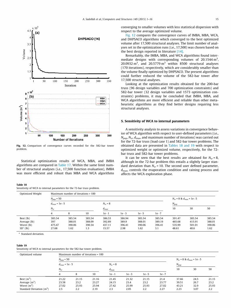
Fig. 12. Comparison of convergence curves recorded for the 582-bar towerproblem.


Statistical optimization results of WCA, MBA, and IMBAalgorithms are compared in Table 17. Within the same limit num-ber of structural analyses (i.e., 17,500 function evaluation), IMBAwas more efficient and robust than MBA and WCA algorithms

Table 18Sensitivity of WCA to internal parameters for the 72-bar truss problem.

Optimized Weight Maximum number of iterations = 100

Npop = 50

dmax = 1e�5 Nsr = 8

Nsr dmax

4 8 10 1e�1

Best (lb) 385.54 385.54 385.54 386.53Average (lb) 397 388.01 388.09 392.89Worst (lb) 475.47 390.06 390.34 437.11SDa (lb) 27.68 1.62 1.3 15.57

a Standard deviation.

Table 19Sensitivity of WCA to internal parameters for the 582-bar tower problem.

Optimized volume Maximum number of iterations = 100

Npop = 50

dmax = 1e�5 Nsr = 8

Nsr dmax

4 8 10 1e�1

Best (m3) 21.22 21.15 21.16 21.45Average (m3) 23.58 23.2 23.27 24.15Worst (m3) 27.02 25.93 25.94 27.42Standard Deviation (m3) 2.5 2.2 2.19 2.3

converging to smaller volumes with less statistical dispersion withrespect to the average optimized volume.

Fig. 12 compares the convergence curves of IMBA, MBA, WCA,and DHPSACO algorithms which converged to the best optimizedvolume after 17,500 structural analyses. The limit number of anal-yses set in the optimization runs (i.e., 17,500) was chosen based onthe best design reported in literature [14].

Remarkably, the IMBA, MBA, and WCA algorithms found inter-mediate designs with corresponding volumes of 20.1544 m3,20.0932 m3, and 20.5779 m3 within 8500 structural analyses(170 iterations), respectively, which are considerably smaller thanthe volume finally optimized by DHPSACO. The present algorithmscould further reduced the volume of the 582-bar tower after17,500 structural analyses.

Looking at the optimization results obtained for the 200-bartruss (96 design variables and 700 optimization constraints) and582-bar tower (32 design variables and 1573 optimization con-straints) problems, it may be concluded that IMBA, MBA, andWCA algorithms are more efficient and reliable than other meta-heuristic algorithms as they find better designs requiring lessstructural analyses.

5. Sensitivity of WCA to internal parameters

A sensitivity analysis to assess variations in convergence behav-ior of WCA algorithm with respect to user-defined parameters (i.e.,Npop, Nsr, dmax, and maximum number of iterations) was carried outfor the 72-bar truss (load case 1) and 582-bar tower problems. Theobtained data are presented in Tables 18 and 19 with respect tooptimized weight or optimized volume, respectively, for the 72-bar truss and 582-bar tower problems.

It can be seen that the best results are obtained for Nsr = 8,although in the 72-bar problem this entails a slightly larger stan-dard deviation than Nsr = 10. The second user defined parameter,dmax, controls the evaporation condition and raining process andaffects the WCA exploration phase.

Nsr = 8 & dmax = 1e�5

Npop

10 30 50

1e�3 1e�5 1e�7

386.94 385.54 385.54 391.47 385.54 385.54389.9 388.01 389.19 465.68 415.91 388.01396.41 390.06 396.41 535.99 501.01 390.062.98 1.62 3.1 48.61 40.6 1.62

Nsr = 8 & dmax = 1e�5

Npop

10 30 50

1e�3 1e�5 1e�7

21.32 21.15 21.4 37.66 24.5 21.1523.4 23.2 23.77 39.51 26.7 23.225.99 25.93 27.02 43.21 32.9 25.932.05 2.2 2.27 2.23 3.07 2.2


In general, setting dmax as a large value reduces the exploitationcapability, while setting small values of dmax reduces the explora-tion capability. This is confirmed by the sensitivity analysis datareported in Tables 18 and 19. The worst designs were obtainedfor the very large value dmax = 1e�1 and for the very small valuedmax = 1e�7 that also entailed the largest standard deviations (SD).

The last parameter affecting performance of WCA is the size ofinitial population (Npop). It should be noted that Npop is a commoninput parameter for most metaheuristic algorithms. In general,Npop should be considerably larger than Nsr. In the WCA case, ifNsr = 8 and Npop = 10, some rivers are generated without havingany streams moving toward them. This has a detrimental effecton optimization results. In particular, if Nsr = 8, the worst and bestperformance of the WCA algorithm occur for Npop = 10 andNpop = 50, respectively.

In summary, the best value for dmax is in the range [1e�5,1e�3],while the value of Nsr should be selected based on the value of Npop

(looking at sensitivity analysis data, Nsr should be about one sixthof Npop). By increasing the number of iterations, WCA as well asother metaheuristic algorithms will have more chances to findthe best solution and explore the design space. For example, byincreasing the number of iterations to 500, WCA could reach thebest solution for both test problems.

Talking about MBA and IMBA internal parameters, the sug-gested value of l is the maximum iteration number divided by fiverecommended in Section 3.1.1. The exploration factor (l) gives thealgorithm more freedom to search a wider range, which results inbetter detection of solutions. However, increasing the value of thisparameter more than the predefined value may diverge the resultsand prevent further exploitation near the best obtained solutions.

The reduction factor (a) divides the distance of shrapnel piecesinto a interval distances, which enables searching within thereduced intervals at each iteration. Searching smaller intervals isbetter and more efficient than searching in large intervals.

Higher values of a increase the probability of finding the globaloptimal solution; however, increasing a more than the suitablevalue may inhibit searching regions near the optimal solution dur-ing the final iterations. The user specified parameter sensitivity forthe MBA for solving truss structures is given in [26] which can alsobe extend for weight/volume minimization problems of complextruss structures.

6. Conclusions

This paper presented some applications of two recently devel-oped optimization techniques, the mine blast algorithm (MBA)and water cycle algorithm (WCA) to discrete sizing optimizationproblems of truss structures. The WCA and MBA are inspired byobservation of water cycle process and explosion of landmines,respectively. The MBA was improved and applied to solve bench-mark problems, so called improved MBA (IMBA).

The efficiency and performance of IMBA, WCA, and MBA wasexamined using four truss structures. The improvements made toMBA are as follows: the distance of each shrapnel piece was chan-ged by the value of the objective function (i.e., it was reduced whenthere were no improvements to the obtained solution). The per-ception of direction was replaced with the concept of moving tothe best solutions.

Optimization results obtained for four benchmark truss prob-lems including a number of sizing variables ranging between 12and 96 seem to prove that the IMBA, WCA, and MBA algorithmsare highly competitive with other metaheuristic algorithms pre-sented in the literature in terms of optimized weight and numberof structural analyses required by the optimization process.

The IMBA slightly outperformed the MBA and WCA algorithmsin the large scale truss problems in this paper. Hybridization of theWCA with MBA and/or other optimizers may lead to furtherimprove convergence behavior and is certainly a topic to be inves-tigated in future research.

Acknowledgments

This work was supported by a National Research Foundation ofKorea (NRF) Grant funded by the Korean government (MSIP) (NRF-2013R1A2A1A01013886).

References

[1] Holland J. Adaptation in natural and artificial systems. Ann Arbor(MI): University of Michigan Press; 1975.

[2] Goldberg DE, Samtani MP. Engineering optimization via genetic algorithms. In:Proc of the ninth conference on electronic computations, ASCE. Birmingham,Alabama; 1986. p. 471–82.

[3] Rajeev S, Krishnamoorthy CS. Discrete optimization of structures using geneticalgorithms. J Struct Eng 1992;118(5):1233–50.

[4] Krishnamoorthy CS, Venkatesh PP, Sudarshan R. Object-oriented frameworkfor genetic algorithms with application to space truss optimization. J ComputCiv Eng 2002;16:66–75.

[5] Sivakumar P, Rajaraman A, Natajan K, Samuel KGM. Artificial intelligencetechniques for optimization of steel lattice towers, recent developments instructural engineering. In: Proc structural engineering convention; 2001. p.435–45.

[6] Gero MBP, Garcia AB, Diaz JJDC. Design optimization of 3D steel structures:genetic algorithms vs. classical techniques. J Constr Steel Res 2006;62:1303–9.

[7] Geem Z, Kim J, Loganathan GV. A new heuristic optimization algorithm:harmony search. Simulation 2001;76:60–8.

[8] Lee KS, Geem ZW. A new meta-heuristic algorithm for continuous engineeringoptimization: harmony search theory and practice. Comput Method ApplMech 2005;194:3902–33.

[9] Lee KS, Geem ZW. A new structural optimization method based on theharmony search algorithm. Comput Struct 2004;82:781–98.

[10] Lee KS, Geem ZW, Lee SH, Bae KW. The harmony search heuristic algorithm fordiscrete structural optimization. Eng Optim 2005;37(7):663–84.

[11] Kennedy J, Eberhart R. Particle swarm optimization. In: Proc IEEE IJCNN. Perth,Australia; 1995. p. 1942–48.

[12] Li LJ, Huang ZB, Liu F. A heuristic particle swarm optimization method for trussstructures with discrete variables. Comput Struct 2009;87:435–43.

[13] He S, Wu QH, Wen JY, Saunders JR, Paton RC. A particle swarm optimizer withpassive congregation. Biosystems 2004;78:135–47.

[14] Kaveh A, Talatahari S. A particle swarm ant colony optimization for trussstructures with discrete variables. J Constr Steel Res 2009;65:1558–68.

[15] Lamberti L, Pappalettere C. Metaheuristic design optimization of skeletalstructures: a review. Comput Technol Rev 2011;4:1–32.

[16] Saka MP. Optimum design of skeletal structures: a review. In: Topping BHV,editor. Progress in civil and structural engineering computing. Stirlingshire(UK): Saxe-Coburg Publications; 2003. p. 237–84. http://dx.doi.org/10.4203/csets.10.10 [chapter 10].

[17] Sadollah A, Bahreininejad A, Eskandar H, Hamdi M. Mine blast algorithm foroptimization of truss structures with discrete variables. Comput Struct2012;102–103:49–63.

[18] Eskandar H, Sadollah A, Bahreininejad A, Hamdi M. Water cycle algorithm – anovel metaheuristic optimization method for solving constrained engineeringoptimization problems. Comput Struct 2012;110–111:151–66.

[19] Montes EM, Coello CAC. An empirical study about the usefulness of evolutionstrategies to solve constrained optimization problems. Int J Gen Syst2008;37:443–73.

[20] Wu SJ, Chow PT. Steady-state genetic algorithms for discrete optimization oftrusses. Comput Struct 1995;56:979–91.

[21] Ghasemi MR, Hinton E, Wood RD. Optimization of trusses using geneticalgorithms for discrete and continuous variables. Eng Comput 1999;16–3:272–301.

[22] Dede T, Bekiroglub S, Ayvazc Y. Weight minimization of trusses with geneticalgorithm. Appl Soft Comput 2011;11:2565–75.

[23] Cai J, Thierauf G. Discrete structural optimization using evolution strategies.In: Topping BHV, Khan AI, editors. Neural networks and combinatorialoptimization in civil and structural engineering, civil-comp, Edinburg. p. 95–100. doi: http://dx.doi.org/10.4203/ccp.16.6.11993.

[24] Hasançebi O, Çarbas S, Dogan E, Erdal F, Saka MP. Performance evaluation ofmetaheuristic search techniques in the optimum design of real size pin jointedstructures. Comput Struct 2009;87(5–6):284–302.

[25] American Institute of Steel Construction (AISC). Manual of steel constructionallowable stress design. 9th ed. Chicago (IL); 1989.

[26] Sadollah A, Bahreininejad A, Eskandar H, Hamdi M. Mine blast algorithm: anew population based algorithm for solving constrained engineeringoptimization problems. Appl Soft Comput 2013;13:2592–612.

http://refhub.elsevier.com/S0045-7949(14)00281-8/h0005


























http://dx.doi.org/10.4203/csets.10.10

http://dx.doi.org/10.4203/csets.10.10

















http://dx.doi.org/10.4203/ccp.16.6.11993







water cycle, mine blast and improved mine blast algorithms for discrete sizing optimization of truss...

Documents