water contaminants of the lake erie watershed
TRANSCRIPT

1
Water Contaminants of the Lake Erie Watershed
Dissertation
Presented in Partial Fulfillment of the Requirements for the Degree Doctor of Philosophy
in the Graduate School of The Ohio State University
By
Michael Robert Brooker
Graduate Program in Environmental Science
The Ohio State University
2018
Dissertation Committee
Dr. Paula Mouser, Co-advisor
Dr. Jon Witter, Co-advisor
Dr. Gil Bohrer
Dr. Virginia Rich

2
Copyrighted by
Michael Robert Brooker
2018

ii
Abstract
Streams and rivers act as conduits, transporting pollutants from their sources to
downstream drainage basins. The Lake Erie watershed is dominated by agricultural land
use. As a result, there are many concerns over pollution sourced from upstream
agroecosystems. Among the principle issues in the region, phosphorus and other nutrient
pollutants have been faulted for stimulating and/or supporting the frequency and
magnitude of recurrent harmful algal blooms occurring in the western Lake Erie basin.
Phosphorus pollution originates from a variety of point and nonpoint sources, however
specific estimates of source contributions have proven elusive due to wide variations
between members of the same sources. Better distinguishing between the sources of
pollution, as well as an improved ability to track transport through the watershed is
essential for managing nutrient loads. One promising and new approach to elucidating
source contaminants is the organic phosphorus fraction of dissolved organic matter
(DOM). Point and nonpoint sources may exhibit unique DOM or dissolved organic
phosphorus (DOP) signatures, that allows for the differentiation between sources, either
through signature analysis or the application of marker molecules. Here, electrospray
ionization Fourier-transform mass spectrometry (ESI FT-ICR-MS) was used to analyze
the DOM and DOP signatures from nutrient pollution sources in the Lake Erie watershed.
Three marker compounds were distinct to sources were proposed for use in tracking the

iii
presence of source contamination. From this source signature analysis, differences in
DOM was next evaluated along a mixing profile for a Lake Erie tributary. The ability to
detect DOM formulae upstream to downstream sites was assessed. Compounds detected
in higher abundance upstream were more likely to be detected at downstream locations.
The mass spectra signals of merging branches appeared to be mixed linearly into several
confluence points.
In addition to nutrient sources influencing Lake Erie water quality, there are
concerns over the introduction of antibiotics to the drainage basin from use in regional
agricultural operations. Metals and antibiotics are known to co-select for antibiotic
resistance genes in agroecosystems, suggesting two possible causes in the development of
resistant microbial communities. Here, sediments from agricultural dominated channels
were analyzed for antibiotics, metals, and relevant functional microbial genes. Although
few antibiotics were detected in the sediments, some metals were found at elevated
levels. Antibiotic resistance genes were among the most abundant and diverse set of
genes detected using an environmental microbial functional microarray technology,
GeoChip. Metal homeostasis genes and the intI integrase gene, indicative of the potential
for horizonal gene transfer, were also abundant across samples. These results highlight
the prevalence of antibiotic resistant genes in sediments draining to the Lake Erie
ecosystem, with implications for downstream transport from agricultural sources.
iv
Acknowledgments
Thank you to everyone who helped support me on my way into and through graduate
school. That starts with my wife, Molly, and my family. It has been a long and difficult
path. Without Molly, I doubt that I would have ever considered going back to school. Her
encouragement is the biggest reason this document exists. Her support has gotten me
through the most difficult times. I must also thank all the faculty who guided me as my
advisors, committee members, or for giving me numerous opportunities. Dr. Paula
Mouser was my advisor for three graduate degrees, and without her I may never have
entered graduate school. She has been an inspiration and model for my own career. Dr.
Gil Bohrer and Dr. Jon Witter both have served as co-advisors on at least one of my
degrees. All three of these committee members, and my other committee member Dr.
Virginia Rich, took me under their wings and taught me the foundations of how to
conduct research, present that research, and teach courses. Their feedback on my research
and writing was crucial to my success. I am also grateful for them being understanding
during my moments of crazed panic, of which there were many. I would like to recognize
that all faculty members of my department gave me many opportunities along the way.
There are far too many people who helped me along my way to put into this section here.
Please know that I will always appreciate all you have done for me.
v
Vita
2003................................................................Northwest High School
2007................................................................B.S. Microbiology, The Ohio State
University
2013................................................................M.S. Environmental Science, The Ohio
State University
2011 to present ..............................................Graduate Teach and Research Assistant,
Department of Civil, Environmental, and
Geodetic Engineering, The Ohio State
University
Fields of Study
Major Field: Environmental Science

vi
Table of Contents
Abstract ............................................................................................................................... ii
Acknowledgments.............................................................................................................. iv
Vita ...................................................................................................................................... v
List of Tables ................................................................................................................... viii
List of Figures .................................................................................................................... ix
Preface ................................................................................................................................ xi
Chapter 1: Discrete Organic Phosphorus Signatures are Evident in Pollutant Sources
within a Lake Erie Tributary ............................................................................................... 1
Introduction ..................................................................................................................... 1
Methods........................................................................................................................... 5
Site Description and Sample Collection ..................................................................... 5
Sample Processing ...................................................................................................... 7
ESI FT-ICR-MS Data Analysis .................................................................................. 8
Results ............................................................................................................................. 9
Discussion ..................................................................................................................... 17
Chapter 2: Dissolved Organic Matter Transport and Mixing in the Portage River .......... 22
Introduction ................................................................................................................... 22
Methods......................................................................................................................... 26
Sampling Locations and Collection .......................................................................... 26
Sample Processing .................................................................................................... 28
ESI FT-ICR-MS Data Analysis ................................................................................ 29
Results ........................................................................................................................... 31
Discussion ..................................................................................................................... 45
Chapter 3: The Emerging Concern of Antibiotic Resistance Genes in Agricultural
Sediments .......................................................................................................................... 52
Introduction ................................................................................................................... 52
vii
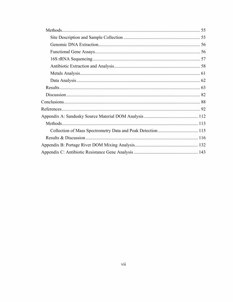
Methods......................................................................................................................... 55
Site Description and Sample Collection ................................................................... 55
Genomic DNA Extraction......................................................................................... 56
Functional Gene Assays ............................................................................................ 56
16S rRNA Sequencing .............................................................................................. 57
Antibiotic Extraction and Analysis ........................................................................... 58
Metals Analysis ......................................................................................................... 61
Data Analysis ............................................................................................................ 62
Results ........................................................................................................................... 63
Discussion ..................................................................................................................... 82
Conclusions ....................................................................................................................... 88
References ......................................................................................................................... 92
Appendix A: Sandusky Source Material DOM Analysis ............................................... 112
Methods....................................................................................................................... 113
Collection of Mass Spectrometry Data and Peak Detection ................................... 115
Results & Discussion .................................................................................................. 116
Appendix B: Portage River DOM Mixing Analysis ....................................................... 132
Appendix C: Antibiotic Resistance Gene Analysis ........................................................ 143
viii
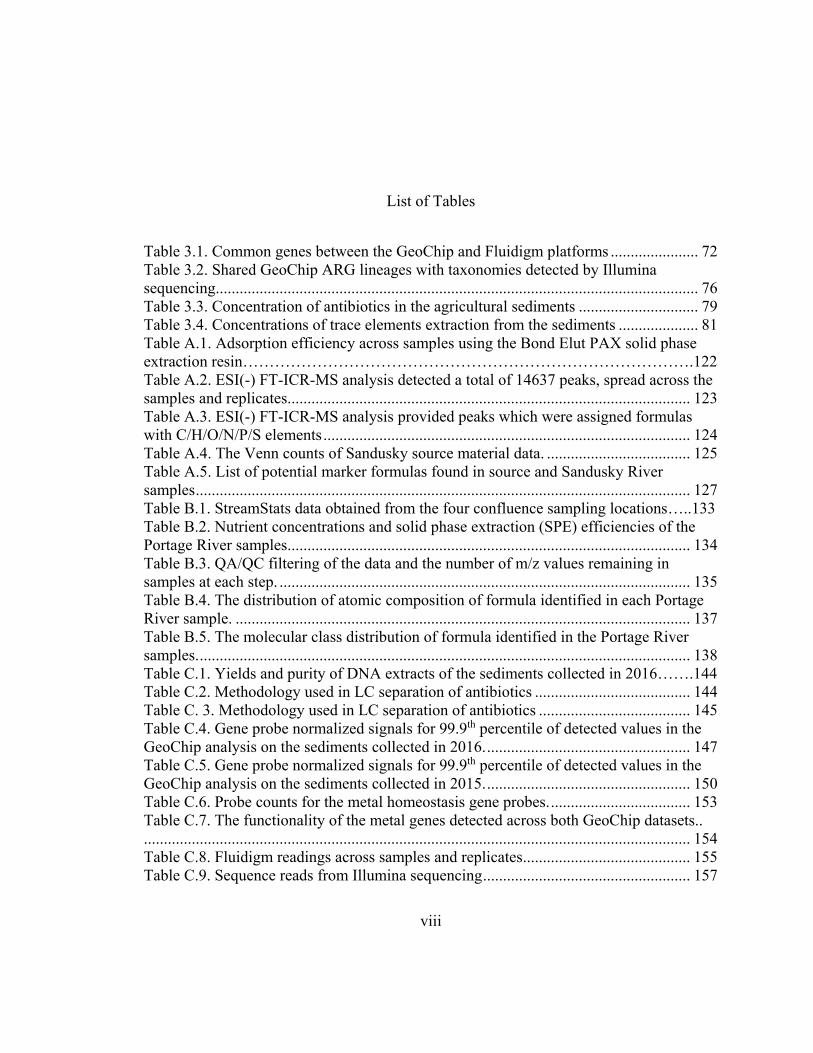
List of Tables
Table 3.1. Common genes between the GeoChip and Fluidigm platforms ...................... 72
Table 3.2. Shared GeoChip ARG lineages with taxonomies detected by Illumina
sequencing......................................................................................................................... 76
Table 3.3. Concentration of antibiotics in the agricultural sediments .............................. 79
Table 3.4. Concentrations of trace elements extraction from the sediments .................... 81
Table A.1. Adsorption efficiency across samples using the Bond Elut PAX solid phase
extraction resin………………………………………………………………………….122
Table A.2. ESI(-) FT-ICR-MS analysis detected a total of 14637 peaks, spread across the
samples and replicates. .................................................................................................... 123
Table A.3. ESI(-) FT-ICR-MS analysis provided peaks which were assigned formulas
with C/H/O/N/P/S elements ............................................................................................ 124
Table A.4. The Venn counts of Sandusky source material data. .................................... 125
Table A.5. List of potential marker formulas found in source and Sandusky River
samples ............................................................................................................................ 127
Table B.1. StreamStats data obtained from the four confluence sampling locations…..133
Table B.2. Nutrient concentrations and solid phase extraction (SPE) efficiencies of the
Portage River samples..................................................................................................... 134
Table B.3. QA/QC filtering of the data and the number of m/z values remaining in
samples at each step. ....................................................................................................... 135
Table B.4. The distribution of atomic composition of formula identified in each Portage
River sample. .................................................................................................................. 137
Table B.5. The molecular class distribution of formula identified in the Portage River
samples. ........................................................................................................................... 138
Table C.1. Yields and purity of DNA extracts of the sediments collected in 2016…….144
Table C.2. Methodology used in LC separation of antibiotics ....................................... 144
Table C. 3. Methodology used in LC separation of antibiotics ...................................... 145
Table C.4. Gene probe normalized signals for 99.9th percentile of detected values in the
GeoChip analysis on the sediments collected in 2016. ................................................... 147
Table C.5. Gene probe normalized signals for 99.9th percentile of detected values in the
GeoChip analysis on the sediments collected in 2015. ................................................... 150
Table C.6. Probe counts for the metal homeostasis gene probes. ................................... 153
Table C.7. The functionality of the metal genes detected across both GeoChip datasets..
......................................................................................................................................... 154
Table C.8. Fluidigm readings across samples and replicates .......................................... 155
Table C.9. Sequence reads from Illumina sequencing .................................................... 157
ix
List of Figures
Figure 1.1. Description of sampling location and watershed. ............................................. 6
Figure 1.2. Summary of atomic composition and mass to charge values by samples ...... 11
Figure 1.3. Van Krevelen diagrams of each sample, and the molecular classes of
identified formulae ............................................................................................................ 13
Figure 1.4. Comparison of samples by binary Jaccard distance matrices. ....................... 15
Figure 1.5. Relative peak heights for potential markers for detecting or tracking source-
derived DOP nutrients shared uniquely by the Sandusky River and either the (1) three
manures, (2) WWTP effluent, or (3) edge of field samples. ............................................. 17
Figure 2.1. Sampling locations in the Portage River ........................................................ 28
Figure 2.2. DOC, TDN, and TDP concentrations measured in Portage River samples ... 33
Figure 2.3. Van Krevelen plots of the 16 samples in this study ....................................... 36
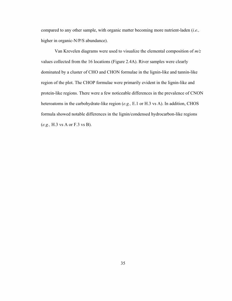
Figure 2.4. Summary of elemental composition and molecular classes of assigned
formula .............................................................................................................................. 38
Figure 2.5. Percentage of shared and unique formulae between samples at the confluence
sampling locations ............................................................................................................ 39
Figure 2.6. Clustering analysis of m/z values ................................................................... 41
Figure 2.7. Quantiles of the peak heights for observed m/z values ................................... 43
Figure 2.8. Comparisons between the StreamStats and DOM mixing model contribution
estimates ............................................................................................................................ 45
Figure 3.1. Summary of the gene probe abundance and signals for functional categories
and antibiotic resistance .................................................................................................... 67
Figure 3.2. Dendrograms of the GeoChip and antibiotic resistance gene hierarchal
clustering ........................................................................................................................... 70
Figure 3.3. Fluidigm results and comparison to GeoChip observations ........................... 73
Figure 3.4. Illumina sequencing on the v4 region of the 16S rRNA gene was performed
on sediment DNA. ............................................................................................................ 75
Figure 3.5. Distribution of unmatched taxa between GeoChip lineages and taxonomies
detected by Illumina sequencing. ...................................................................................... 78
Figure A.1. Retention of carbon, nitrogen, and phosphorus by solid phase extraction
columns ………………………………………………………………………………...117
Figure A.2. Recovery of known phosphorus standards .................................................. 119
Figure A.3. Carbon, nitrogen, and phosphorus concentration of samples in Sandusky
River watershed .............................................................................................................. 121
Figure A.4. The distribution of NOSC values by molecular classes. ............................. 122
Figure A.5. Spectra captured from ESI(-) FT-ICR-MS analysis of all sample replicates
and blanks. ...................................................................................................................... 131
Figure B.1. Spectra collected by ESI(-) FT-ICR-MS analysis…………………………136
Figure B.2. Correlations between nitrogen and phosphorus concentrations and elemental
compositions ................................................................................................................... 139
Figure B.3. Hierarchal clustered dendrogram and heatmap based off the Canberra
distance matrix. ............................................................................................................... 140

x
Figure B.4. Hierarchal clustering of the binary Jaccard distance matrix between samples
collected in both Chapter 1 and Chapter 2. ..................................................................... 141
Figure B.5. The relative change in peak heights between upstream-downstream samples
in the upper reaches of the Portage River (A through E.2). ............................................ 142
xi
Preface
Agriculture dominates the Lake Erie watershed, with sources of pollution from
agroecosystems a significant concern. Nutrient pollution, primarily phosphorus and
nitrogen are loaded into Lake Erie with much of the blame on nonpoint – largely
agricultural – sources. There is a need to better understand the contributions of nonpoint
and point sources, including phosphorus loads and other emerging health threats, such as
antibiotic resistance to the region. This dissertation builds on two chapters of research in
my dual-degree Master of Science Thesis in Civil Engineering (completed October 2017)
through the detailed evaluation of pollutants in contaminant sources, sediments, and
waters of Lake Erie tributaries. The dissertation is structured with three stand-alone
chapters that are intended to be submitted directly for peer review in relevant
environmental engineering or science journals. As chapters are intended to meet the word
limit requirement for the intended journal, supplemental information for each chapter (i.e.
detailed methods, raw data, etc.) is provided in a corresponding Appendix. A short
conclusions chapter is provided after Chapter 3 to highlight significant findings and
present future research needs in this field. The following paragraphs summarize the
topics discussed in Chapters 1 through 3.
In Chapter 1, DOM signatures were described for five point and nonpoint sources
of nutrient pollution in a Lake Erie watershed. These signatures were proposed as a
means to detect the presence of phosphorus, or other nutrient pollutants, derived from
specific source materials. Chapter 1 focused on the fraction of organic phosphorus within
the DOM. Divergent DOP signatures were observed between several manures and other

xii
source materials. A high degree of similarity was detected between the Sandusky River
and edge of field runoff (from a synthetically fertilized crop field). Several marker
compounds were proposed for use in detecting and tracking source contributions through
this and other Lake Erie tributaries.
The objective of Chapter 2 was to build on the findings of Chapter 1 through a
broader analysis (in terms of geography and total number of samples) of DOM and DOP
along a second river transect draining to Lake Erie. Samples were collected along 50
linear miles from upstream tributaries through the mouth of the Portage River, with a
mixing analysis conducted at four confluence points. Samples were compared based on
their mass spectral diversity and abundance, the similarity of their organic matter
features, and their overall nutrient concentration. Apparent changes in heteroatom and
molecular classifications were observed between upstream to downstream reaches, with
CHON formulae becoming more abundant closer to the mouth of the river. The most
prominent DOM features persisted from upstream reaches to downstream locations,
suggesting a DOM mixing model analysis may provide a tool for tracking source
contributions along the watershed.
In Chapter 3, a genomic analysis of sediments accumulating in drainage ditches
from agricultural headwaters revealed a diversity and prevalence of antibiotic resistance
genes. Additionally, metal homeostasis genes were abundant. These two gene categories
are commonly co-selected in the environment. Although few antibiotics were detected
that might contribute to the prevalence of antibiotic resistant organisms, many metals
were detected at elevated levels. The data suggests that the ARGs of these sediments is

xiii
maintained through the co-selection of antibiotic resistance genes with metal homeostasis
genes.

1
Chapter 1: Discrete Organic Phosphorus Signatures are Evident in Pollutant Sources
within a Lake Erie Tributary
This chapter was submitted to the journal Environmental Science & Technology on
November 14 under the title: Discrete Organic Phosphorus Signatures are Evident in
Pollutant Sources within a Lake Erie Tributary by Michael R. Brooker, Krista
Longnecker, Elizabeth B. Kujawinski, Mary H. Evert, Paula J. Mouser. It is currently
under review.
Introduction
Freshwater lakes, such as the Great Lakes in North America, provide numerous
economic opportunities to shoreline communities in the form of tourism, recreation,
fisheries, manufacturing, and the transportation of goods across local and international
boundaries. Lake Erie is one of five Great Lakes in the United States and Canada, and as
with many freshwater resources worldwide, it has experienced recurrent harmful algal
blooms that are believed to be propagated from anthropogenically-sourced nutrients from
within its drainage basins (Conley et al., 2009; Conroy et al., 2011). Primary productivity
in freshwater systems is most often limited by phosphorus or nitrogen (Conley et al.,
2009; Conroy et al., 2011), therefore changes in the abundance and form of these
nutrients from upstream sources can have a profound effect on the ecosystem. Since the
early 2000s, increased nutrient loads have led to recurrent toxic cyanobacterial blooms
along the southern coastline of the western Lake Erie basin, while hypoxia has developed
in the hypolimnion of the central basin in the lake (Conroy et al., 2011; Michalak et al.,
2013; Steffen et al., 2017).

2
The magnitude of Lake Erie algae blooms in a given year is most strongly
correlated to spring (May-June) phosphorus loads from its tributaries (Stumpf et al.,
2012), with small blooms sometimes inflicting severe damage to the ecosystem. For
example, although it was smaller in size compared to years past, the Microcystis bloom at
the Toledo water treatment facility intake pipe in 2014 had a major impact on the
shoreline community (Steffen et al., 2017). Microcystin concentrations in the treated
water were twice as high as state guidelines (currently 1.6 μg/l in Ohio), causing the
shutdown of the drinking water treatment plant serving over 400,000 Toledo residents
and resulting in $65 million in economic damages to property values, tourism, recreation,
and emergency water handling (Steffen et al., 2017). The impact of this and other
phytoplankton blooms on the local economy has served as a call-to-action for Ohio
legislators to improve our understanding of nutrient pollutants contributing to this
problem and develop best management practices to minimize discharge.
Phosphorus pollution in drainage basins is derived from both point (e.g.,
municipal/industrial wastewater effluents or combined sewer overflows) and nonpoint
sources (sewage leaks, urban area runoff, or agricultural runoff/tile drainage) (D. B.
Baker et al., 2014; Ohio Lake Erie Phosphorus Task Force, 2013), making individual
pollutant sources difficult to isolate and manage. An extensive sampling network has
been established in select Lake Erie tributaries to monitor loads to the lake (D. B. Baker
et al., 2014), with an emphasis on reactive and total phosphorus. Reactive phosphorus, a
term used interchangeably with orthophosphate (PO43-), is readily assimilated by algae
and simple to measure (D. B. Baker et al., 2014; Baldwin, 1998). Total phosphorus has

3
been useful in forecasting harmful algal bloom severity (Stumpf et al., 2012). Models
have helped fill in the gaps between discrete sampling locations by considering local land
usage to estimate spatial contributions (D. Baker, 2011; Michalak et al., 2013). However,
despite efforts made toward monitoring and modeling source contributions to Lake Erie,
distinguishing between specific pollutant sources to mitigate the most impactful loads to
the lake has proven difficult.
In order to gain further insight into pollutant sources and phosphorus pool
dynamics, researchers are applying new mass spectrometry tools. One method, analysis
of oxygen isotopic fractionation, has allowed for partial source tracking of phosphate
entering Lake Erie from its tributaries (Elsbury et al., 2009). Isotopic fractionation arises,
in part, from the enzymatic hydrolysis of dissolved organic phosphorus (DOP). The
results of this isotopic analysis in Lake Erie suggested a non-riverine source of phosphate
was supplying the algal bloom, but could not establish whether DOP was the source of
this phosphorus (Elsbury et al., 2009). DOP is rarely analyzed on environmental samples
because (1) concentrations are low and are indirectly quantified (Baldwin, 1998;
Monaghan, E. J., Ruttenberg,K.C., 1999; Ruttenberg KC, 2012), and (2) the low
elemental abundance of phosphorus within dissolved organic matter (DOM) makes
detection using mass spectrometry difficult (Cooper et al., 2005; D. M. Karl, 2014; Kruse
et al., 2015). Analysis of DOP has been disregarded in favor of measuring total dissolved
phosphorus (TDP), as TDP effectively defines bioavailable phosphorus (Ohio Lake Erie
Phosphorus Task Force, 2013; Ruttenberg and Dyhrman, 2005). However, TDP obscures
the diversity of DOP formulae elucidated through mass spectrometry (Cooper et al.,
4
2005; Minor et al., 2012) which may aid in source identification and provide a better
understanding of biogeochemical controls in the system.
Electrospray ionization Fourier-transform ion cyclotron resonance mass
spectrometry (ESI FT-ICR-MS) can provide new insight into the molecular composition
of environmental samples through non-target identification of phosphorus in dissolved
organic matter (DOM). To date, ESI FT-ICR-MS has rarely been used to investigate
DOP, and, in some cases, phosphorus has been excluded from these (Kujawinski and
Behn, 2006; Kujawinski et al., 2009) due in part to a low elemental abundance of
phosphorus (~0.3%) in organic matter. However, organophosphorus compounds can be
concentrated for mass spectrometry analysis with solid phase extraction (SPE), which
removes background interferences (i.e., desalts) while retaining organic constituents that
resemble the original sample (Ohno and Ohno, 2013; Raeke et al., 2016). Even in the
absence of selective concentration, ESI FT-ICR-MS analysis revealed an abundance of
organic phosphorus-containing compounds in Lake Superior and its tributaries (Minor et
al., 2012). Based on the frequency of harmful algal blooms, we expected Lake Erie would
be replete in unique organic phosphorus compounds that could be related to tributary
sources.
The objective of this study was to characterize organic-bound phosphorus from
select point and nonpoint pollutant sources in a Lake Erie tributary. We analyzed organic
matter and organophosphorus signatures in three different nonpoint source fertilizer
materials (hog, chicken, and dairy manures), runoff from the edge of a synthetically
fertilized agricultural field, a point source discharge location from a municipal
5
wastewater treatment plant (WWTP), and the Sandusky River using ultrahigh resolution
ESI FT-ICR-MS. Molecular masses, molecular classes, sample similarity and unique
marker formulae were identified in these samples. Our analysis identified a diverse
organic phosphorus pool that is obscured by the single phosphorus measurement typically
used to represent these sources. These data provide signatures of pollutant that can used
to monitor their movement through tributaries, and gives consideration to the
understudied pool of organic phosphorus.
Methods
Site Description and Sample Collection
Sampling was performed in the Sandusky River tributary system, which drains
into the Western Lake Erie Basin at Sandusky Bay. The Sandusky River is dominated by
nonpoint phosphorus pollution (90%) with smaller contributions from point (9%) and
atmospheric (1%) sources (Figure 1.1A) (Ohio Lake Erie Phosphorus Task Force, 2010).
The primary land use in the watershed is agricultural, with the vast majority of fertilizer
application derived from inorganic (66%) forms rather than manure (27%) or biosolids
(7%) (Ohio Lake Erie Phosphorus Task Force, 2010). Most of the manure applied in the
Lake Erie basin originates from cattle (50%), hog (34%), and poultry (5%) sources
(Figure 1.1B) (Ohio Lake Erie Phosphorus Task Force, 2010). Sampling was conducted
on March 14, 2016 following a precipitation event (Figure 1.1C). At the time of
collection, flows were high (>90th percentile) and corresponded with a high total
phosphorus load (www.heidelberg.edu/NCWQR) (D. B. Baker et al., 2014). Six samples
were collected from the Sandusky River tributary network (Figure1.1D), including (1) an

6
edge of field site, (2) hog manure, (3) chicken (poultry) manure, (4) dairy (cattle) manure,
and (5) wastewater treatment plant (WWTP) effluent. Downstream of these sampling
locations, another sample was collected from the (6) Sandusky River.
Figure 1.1. Description of sampling location and watershed. (A) The Ohio Lake Erie
Phosphorus Task Force has estimated the nonpoint contribution from point and nonpoint
sources for the Sandusky River (Ohio Lake Erie Phosphorus Task Force, 2010). (B) This
group has also detailed the contributions of various manures, as elemental P, to the
Western Lake Erie basin (Ohio Lake Erie Phosphorus Task Force, 2010). (C) Flow, total
phosphorus, and soluble reactive phosphorus were reported in the 2015-2016 water year
by Heidelberg University (www.heidelberg.edu/NCWQR) (D. B. Baker et al., 2014). The
arrow shows the flow conditions at the time of sampling. (D) Six samples were collected
from the Sandusky River watershed situated in north-central Ohio. The chicken and hog
samples were collected on the same property.
Sampling equipment was pre-conditioned by triple rinsing sampling devices and
storage containers with Milli-Q water. The chicken manure sample was retrieved from
the center of an open-air stockpile following excavation by landowner equipment. The
7
hog manure sample was sampled from a hog manure pit using a PVC sampling device.
Dairy manure was collected from a secondary lagoon using the PVC sampling device. An
edge of field sample was collected from the mouth of a tile drainage pipe flowing into the
connected stream. Wastewater effluent was collected following chlorination but prior to
discharge from the Tiffin Water Pollution Control Center. Finally, the Sandusky River
sample was collected from the faucet of the USGS station (USGS 04198000). All
samples were collected in pre-rinsed (DI water) polyethylene containers, transported on
ice to the OSU Environmental Biotechnology Laboratory, and held at 4°C. Wet samples
were processed within 24 hours.
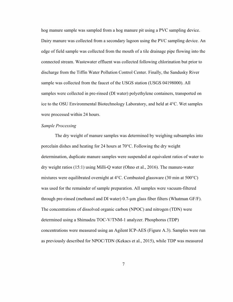
Sample Processing
The dry weight of manure samples was determined by weighing subsamples into
porcelain dishes and heating for 24 hours at 70°C. Following the dry weight
determination, duplicate manure samples were suspended at equivalent ratios of water to
dry weight ratios (15:1) using Milli-Q water (Ohno et al., 2016). The manure-water
mixtures were equilibrated overnight at 4°C. Combusted glassware (30 min at 500°C)
was used for the remainder of sample preparation. All samples were vacuum-filtered
through pre-rinsed (methanol and DI water) 0.7-µm glass fiber filters (Whatman GF/F).
The concentrations of dissolved organic carbon (NPOC) and nitrogen (TDN) were
determined using a Shimadzu TOC-V/TNM-1 analyzer. Phosphorus (TDP)
concentrations were measured using an Agilent ICP-AES (Figure A.3). Samples were run
as previously described for NPOC/TDN (Kekacs et al., 2015), while TDP was measured

8
at wavelength 213.648nm (Bartos et al., 2014). Each sample was prepared in duplicate at
a concentration of 6.5 mg L-1 NPOC in preparation for solid-phase extraction.
We previously determined that the Plexa-PAX solid phase extraction columns
were most efficient at retaining organic phosphorus compounds used as laboratory
standards (Appendix A). Thus, Plexa-PAX SPE columns were used for the concentration
of DOM. The 6 samples we collected were prepared in duplicate along with two
reference standards (Pony Lake Fulvic Acid [PLFA], Suwanee River Fulvic Acid
[SRFA]) for a total of 14 samples. Briefly, columns were prepared by wetting with 3 mL
100% HPLC grade methanol, and were then rinsed with 2L DI water. While still wet,
275mL of each sample were gravity filtered through the conditioned SPE columns to
collect and concentration the organic contents. The binding efficiency of samples (C/N/P)
was calculated from the concentrations measured before and after SPE filtration (Table
A.1).
Samples were eluted from the columns with 5mL of HPLC grade methanol,
followed by 5 mL of methanol+ 5% formic acid. These elutions were combined into
amber glassware and stored at -20°C. The samples were shipped on dry ice to the Woods
Hole Oceanographic Institution for ESI (-) FT-ICR MS analysis.
ESI FT-ICR-MS Data Analysis
Mass spectrometry data was collected as previously described (Appendix A)
(Minor et al., 2012). Peaks were detected in the range of 200-1000 Da. Molecular
formulae assignments were made with the Compound Identification Algorithm
(Kujawinski and Behn, 2006; Kujawinski et al., 2009). A total of 14,637 unique peaks

9
were detected under this analysis. Quality controls were used to quality filter the dataset:
peaks observed in DI water or solvent blanks, and singletons were removed (Table A.2).
Only m/z values with an assigned formula were considered for further analysis.
Additional data analyses were performed using R Statistics (version 3.1.1). The
distributions of peak heights and m/z values were compared among replicates and
samples. Then the peak heights were normalized to the sum of peaks for each replicate.
Replicates were combined through averaging of these normalized peak heights. Sample
similarity was compared based on presence/absence of the formulae using Venn Euler
diagrams, and based on relative peak heights using a Bray-Curtis dissimilarity matrix
generated by the ‘vegan’ package (Oksanen et al., 2015). A list of organic phosphorus
formulae, shared between the Sandusky River and at least one source material, were
filtered as a subset from the data. Putative tracers were further screened from this list with
the stipulation that the maximum relative peak height was observed in a source sample.
Results
The amount of carbon, nitrogen, and phosphorus varied across samples (Figure
A.3), with manure-extracted DOM having considerably higher concentrations relative to
other aqueous samples. The manure samples had nutrient concentrations in the range of
30-76 mg C L-1, 12-60 mg N L-1, and 4.8-9.6 mg P L-1 as compared to WWTP effluent,
edge of field, and Sandusky River samples (6.5-8.8 mg C L-1, 2.6-11mg N L-1, and <0.03-
0.09 mg P L-1). The influent and effluent concentrations for these samples were measured
to estimate the amounts that were retained by PAX columns. PAX extraction efficiency
varied considerably, with 8-44% C, 6-41%N, and <0-100% P retained by the columns

10
(Table A.1). At the low P concentrations observed in several of our samples, extraction
efficiencies were near our analytical quantitation limits and reported as estimates.
ESI FT-ICR-MS analysis was used to characterize the molecular properties of
organic matter isolated from the six sample materials. A total of 7250 formulae were
identified in the dataset following quality filtering and formulae assignment (Table A.2).
Reproducibility between replicates were generally high (>80% shared formulae) for all
six samples (Table A.2), which allowed for a combination of replicate data by averaging
the normalized signal between duplicates as well as include any detected formulae in the
final representative sample (Table A.3). The number of identified formulae ranged from
1803 to 4522 across the samples (Figure 1.2A and Table A.3). Within these data, the
number of formulae containing a P atom ranged from 132 to 313 for these six samples,
representing between 3.3% and 12.8% of detected formulae (Figure 1.2B). The manure
samples contained the greatest proportion of DOP formulae (10.9% to 12.8%), double to
triple what was detected in the edge of field, WWTP effluent, and Sandusky River
samples (3.3% to 5.3%). Manure samples also had a greater abundance of formulae with
N or S atoms compared to the other samples, with CHON representing 30-40% of the
manure formulae versus 16-21% in the other three samples.

11
Figure 1.2. Summary of atomic composition and mass to charge values by samples. (A)
The number of assigned formulae representing DOM (full bar) and DOP (red bar) varied
across the six watershed samples. Actual values are printed within their respective bars,
with the total noted above. Note that any formulae containing a P atom was considered to
be DOP. (B) The proportional distribution of major atom classes for each sample shown
with pie charts, with percentages indicating the total proportion of DOP. The distribution
of (C) DOM and (D) DOP m/z values were visualized using kernel-based cumulative
density plots (violin plots). The width of each band indicates the kernel-based density of
m/z values relative to total number, with white bands representing sample quartiles.

12
The manure samples were composed of a greater number of low molecular mass
formulae compared to the other samples (Figure 1.2C). Specifically, the median
molecular mass of observed m/z values for hog (420 Da), chicken (387 Da), and dairy
(419 Da) manures were on average 70 Da lower than that of the WWTP effluent (474
Da), edge of field (485 Da) and Sandusky River (481 Da). DOP formulae generally
followed this trend, with the chicken (341 Da) and dairy (355 Da) manures having a
lower median mass than the WWTP effluent (414 Da), edge of field (412 Da), and
Sandusky River (404 Da) samples (Figure 1.2C). The hog manure sample had the highest
median molecular mass of DOP m/z values (424 Da). Furthermore, unlike the other 5
samples, which were shifted toward lower molecular mass of DOP relative to DOM, the
hog manure DOP molecular mass distribution resembled that of its overall DOM.
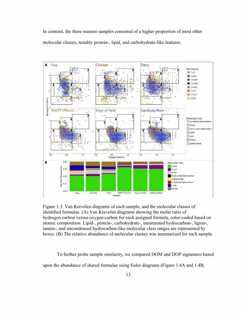
Sample signatures were visualized using Van Krevelen diagrams, which relate the
C:H to the O:C molar ratios for all observed formulae (Figure 1.3A). The relative
placement of each formulae provides an estimation of molecular class, which we refer to
as “–like” types. The overall scatter had apparent differences, with manure samples
exhibiting a greater diversity of molecular type classes (i.e., more scatter) compared to
the Sandusky River, edge of field, and WWTP effluent samples which more tightly
clustered around the lignin-like features. To further highlight these differences in overall
scatter, we tallied the relative abundance of formulae in each of 7 different molecular
classes (Figure 1.3B). Although the majority of formulae across all samples were lignin-
like (51-80%), the WWTP effluent, edge of field, and Sandusky River samples were
especially dominated by lignin- and tannin-like features (86-88%) compared to manures.
13
In contrast, the three manure samples consisted of a higher proportion of most other
molecular classes, notably protein-, lipid, and carbohydrate-like features.
Figure 1.3. Van Krevelen diagrams of each sample, and the molecular classes of
identified formulae. (A) Van Krevelen diagrams showing the molar ratio of
hydrogen:carbon versus oxygen:carbon for each assigned formula, color-coded based on
atomic composition. Lipid-, protein-, carbohydrate-, unsaturated hydrocarbon-, lignin-,
tannin-, and uncondensed hydrocarbon-like molecular class ranges are represented by
boxes. (B) The relative abundance of molecular classes was summarized for each sample.
To further probe sample similarity, we compared DOM and DOP signatures based
upon the abundance of shared formulae using Euler diagrams (Figure 1.4A and 1.4B,

14
respectively). Although they were collected from 12 to 41 miles apart, the WWTP
effluent, edge of field, and Sandusky River samples shared 54% of all assigned DOM
formulae. When we calculated the intersection between the Sandusky River and either the
WWTP effluent or the edge of field sample, over 84% of assigned formulae were shared
for both data sets. This level of similarity is comparable to our replicates (81-90% shared
formulae, Table A.2). Interestingly, the edge of field sample shared a considerably
greater number (124) and percentage (75%) of DOP formulae with the Sandusky River as
compared to the WWTP effluent sample (98, 59%).

15
Figure 1.4. Comparison of samples by binary Jaccard distance matrices. Sample
similarity based on presence/absence data visualized using Euler diagrams for (A) DOM
and (B) DOP. The centroid is marked by a small circle with numbers indicating the
number of formulae shared within an intersection. Not all numbers are indicated but may
be found in Table A.4. The number of unique formulae for each sample is color-coded
and placed adjacent to that sample’s ring. Hierarchal clustering dendrograms for (C)
DOM and (D) DOP prepared from Bray-Curtis dissimilarity matrices generated from
relative peak heights for assigned formulae. Numbers along the top reflect the level of
dissimilarity between samples at the branch point.
Across the three manure samples, only 33% of the m/z values were shared with
the Sandusky River. In pairwise comparisons, the intersection between the Sandusky
River and individual manures ranged from 31-36%. Moreover, these shared formulae
were not unique among manures and the Sandusky River; all but one was also present in

16
the WWTP effluent and edge of field runoff samples. Only five m/z values were uniquely
shared between the manures and Sandusky River sample.
We expanded our analysis to also consider the similarity of two NOM standards
(PLFA and SRFA) based on relative peak heights of all assigned formulae using
hierarchal clustering analysis to visualize relationships between all eight samples (Figure
1.4C-D). Dendrogram clustering patterns for DOM (Figure 1.4C) reaffirmed the
similarities between the Sandusky River, edge of field, and WWTP effluent samples also
based on presence/absence analysis (Figure 1.4A). These three samples and the NOM
standards formed a separate branch from the manure samples, which exhibited greater
dissimilarity between one another and the rest of the samples (Figure 1.4C). When
considering only DOP formulae, dissimilarity grew between all samples, although the
two major branches remained the same (Figure 1.4D). We found that the SRFA clustered
among our samples for DOM, yet when we only considered DOP, both SRFA and PLFA
were separated from the WWTP effluent, edge of field, and Sandusky River samples.
These NOM standards are primarily derived from a terrestrial origin, with the Pony Lake
(Antarctica) more geographically remote and less anthropogenically-impacted then the
Suwanee River (Georgia, USA).
In an effort to identify phosphorus formulae originating from our point source
(WWTP effluent) and nonpoint sources (all others) in the Sandusky River, we generated
a list of DOP formulae present in at least one sample and the Sandusky River. The list
was further screened to remove formulae that increased in peak abundance from the
source to the Sandusky River, as this could indicate origination of these m/z values within

17
the river. Our filtering resulted in 72 formulae, which we propose could serve as markers
for detecting or tracking source-derived nutrients (Table A.5). We next identified
formulae from this list that were unique to the (1) edge of field, (2) WWTP effluent, or
(3) the three manure samples (Figure 1.5). The relative peak height for the manure
marker was an order of magnitude higher than was observed in the Sandusky River,
while peak heights for edge of field and WWTP effluent markers were comparable
between the source and Sandusky River sample.
Figure 1.5. Relative peak heights for potential markers for detecting or tracking source-
derived DOP nutrients shared uniquely by the Sandusky River and either the (1) three
manures, (2) WWTP effluent, or (3) edge of field samples.
Discussion
Regulatory agencies and research institutions in the Great Lakes region are
collectively working to understand the sources and sinks of nutrient pollution associated
with eutrophication-induced hypoxia and reduce the recurrence of harmful algal blooms
through nutrient management strategies. In Lake Erie tributaries where land use is
dominated by agriculture, the majority of phosphorus is thought to be derived from
inorganic fertilizer applied to fields (D. B. Baker et al., 2014; Ohio Lake Erie Phosphorus

18
Task Force, 2010; Ohio Lake Erie Phosphorus Task Force, 2013). However, this finding
relies upon models which have considered bulk phosphorus analyses of total or dissolved
reactive P, measurements that cannot be used to discriminate between point and nonpoint
pollution sources within the watershed. Our ultrahigh resolution MS analysis showed that
DOM and DOP signatures collected from drainage tiles at the edge of an agricultural
field in the Sandusky River were highly similar (84% DOM, 75% DOP) to that of the
river itself collected 41 miles downstream. This level of similarity is remarkable
considering Sandusky River replicates shared 85% of m/z values. Closer in hydrologic
proximity (12 miles between sampling locations), the Sandusky River and WWTP
effluent sample also had similar DOM (84% shared formulae), but were more dissimilar
in their DOP (59% shared m/z values). It is notable that the edge of field and Sandusky
River are most alike in their DOP character, as this finding is consistent with the type of
nutrient pollution, primary land use, and fertilizer form previously reported for the
Sandusky River (Ohio Lake Erie Phosphorus Task Force, 2010).
The signatures of the three manure samples were vastly different from all of the
other samples. Manures account for 27% of total P applied as fertilizer to agricultural
systems for the Lake Erie basin (Ohio Lake Erie Phosphorus Task Force, 2010) serving
as a rich source of natural fertilizer despite challenges associated with their handling. Our
analysis shows manure samples are abundant in N- (> 30%) and P- (>10%) containing
organic molecules that are easily liberated from the solids by water. The DOM that was
extracted from these manures in our labs had higher relative phosphorus and nitrogen
concentrations than our other samples, and this can likely explain the high abundance of

19
DOP formulae. Manure DOM also consisted of lower molecular mass m/z values, relative
to the other samples, which may represent more labile compounds that are easily
assimilated into the landscape (Ohno et al., 2007). Future studies should consider the
signatures associated with manure-applied field runoff.
DOP and DOM signatures from point and nonpoint sources would be altered by
abiotic (i.e., photodegradation) or biotic (i.e., biodegradation) processes in soils,
groundwater and surface waters as it moves through the watershed. In particular, the
transport of biosolids and manure derived organic compounds through porous media into
the water column could be retarded by adsorption to solid materials (Dodd and Sharpley,
2015; Sharma et al., 2017). Sorption affinity of phosphorus is specific to each compound
and is also affected by soil type (Berg and Joern, 2006) therefore we would expect
hydrophilic compounds to be more prominent in manure-derived runoff. Although the
molecular masses in our analysis provide little information about hydrophobicity, the
extraction method we used to obtain our manure DOM was likely to have selected for the
more hydrophilic compounds
Inorganic phosphate can be readily assimilated by most plants and organisms,
while organic phosphorus requires enzymatic cleavage (D. M. Karl, 2014). Natural
organic phosphorus exists in the P(V) (organophosphates) or P(III) state
(organophosphonates), with the latter requiring enzymatic oxidation to phosphate
following liberation of the phosphonate groups (D. M. Karl, 2014; Pasek et al., 2014).
Conversely, organophosphates are directly hydrolyzed into inorganic phosphate by
enzymes such as alkaline phosphatase (D. M. Karl, 2014; Ruttenberg and Dyhrman,

20
2005). Organophosphonates therefore require a greater investment of activation energy
that has been found to slow microbial growth, leading to a buildup of these compounds in
natural systems (Adams et al., 2008; D. M. Karl, 2014). Organophosphorus can be
utilized concurrently with inorganic P, but its nutrient value is greater when total
phosphorus supplies are limited (Bjorkman and Karl, 2003; Ruttenberg and Dyhrman,
2005). The Lake Erie tributary network has relatively high phosphate concentrations
compared to other aquatic systems suggesting organic phosphorus turnover will be
slower relative to inorganic forms in its rivers and streams (D. Baker, 2011; D. B. Baker
et al., 2014). Whether these compounds persist and accumulate in the lake remains to be
seen.
Certain organic molecules in these samples are more susceptible to chemical
transformations and would be more readily assimilated by microorganisms. The WWTP
effluent sample was enriched with microbial-derived (e.g., lipid- and protein-like)
features from the activated sludge process while the edge of field and Sandusky River,
like the SRFA standard, were greatly dominated by lignin. Tannin- and lignin-like
features are regarded to have a terrestrial (plant-derived) origin compared to protein-,
carbohydrate-, and lipid-like features which instead originate from endogenous
microorganisms (Feng et al., 2016; Minor et al., 2012). In addition to indicating the
source material, these molecular classes also correlate to the nominal oxidation state of
carbon (NOSC, Figure A.4), which describes the redox potential of the formulae.
Specifically, tannin-like features are oxidized; lipid-like features are reduced; and lignin-
like features have an average oxidation state around zero (Boye et al., 2017). This
21
suggests that the reduced lipid- and protein-like features more common to the manure
formulae can be expected to oxidize during the transport in aerobic surface waters. We
would therefore expect manure derived DOM to undergo the greatest amount of signature
change relative to other samples. A targeted analysis of similar samples (e.g., using LC
MS/MS of authentic standards to validate these proposed compounds) would be useful in
elucidating these structures of m/z values shared between our samples, which would
provide greater insights to their molecular properties (Lee and Kerns, 1999).
The similarity between edge of field sample and Sandusky River supports the
previously reported data that nutrient loads are predominantly sourced from agricultural
fields in this Lake Erie tributary. However, the edge of field, WWTP effluent, and
Sandusky River samples are hydrologically connected and would be expected to share
some background DOM signature received from rainwater, runoff, and/or groundwater in
the watershed. Still, the DOP signatures were highly divergent between manures and
other source materials, which should allow us to detect the presence of these nonpoint
and point sources in the tributary network. Formulae shared by the Sandusky River and
other samples were identified, and could serve as source markers in the watershed.
Additionally, we elucidated unique DOM and DOP signatures which could be used by
regulatory agencies to detect and monitor the presence of nutrient pollutant sources in the
tributaries.
22
Chapter 2: Dissolved Organic Matter Transport and Mixing in the Portage River
This chapter is currently being prepared for submission to the Journal of Great Lakes
Research with authors and title to be determined.
Introduction
Among the Great Lakes, Lake Erie has experienced the greatest degree of
eutrophication. Nitrogen and phosphorus loads from Lake Erie tributaries have
contributed to recurrent harmful algal blooms in the lake for much of the last half century
(D. Baker, 2010; Steffen et al., 2017). Since the early 2000s, increased nutrient loads
have led to recurrent toxic cyanobacterial blooms along the southern coastline of the
western Lake Erie basin, while hypoxia has developed in the hypolimnion of the lake's
central basin (Conroy et al., 2011; Michalak et al., 2013; Steffen et al., 2017). This
nutrient pollution is derived from both point (e.g., municipal/industrial wastewater
effluents or combined sewer overflows) and nonpoint sources (sewage leaks, urban area
runoff, or agricultural runoff/tile drainage) (D. B. Baker et al., 2014; Ohio Lake Erie
Phosphorus Task Force, 2013), with the loads from nonpoint sources being particularly
difficult to manage. The magnitude of the algal bloom for a given year is most strongly
correlated to spring (May-June) phosphorus loads from its tributaries (Stumpf et al.,
2012). Eutrophication became a crisis when, in 2014, microcystin remained in the
finished water of the Toledo water treatment plant, disrupting the service of residents and
incurring millions in economic losses (Steffen et al., 2017). These impacts have catalyzed
23
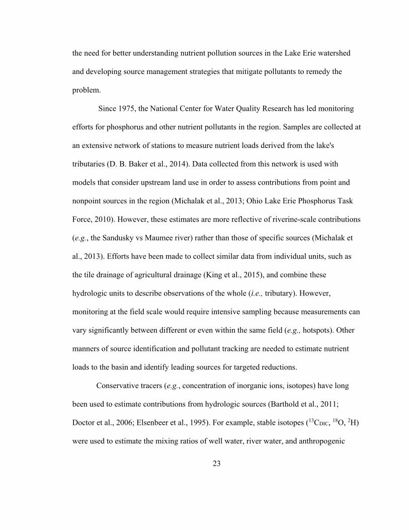
the need for better understanding nutrient pollution sources in the Lake Erie watershed
and developing source management strategies that mitigate pollutants to remedy the
problem.
Since 1975, the National Center for Water Quality Research has led monitoring
efforts for phosphorus and other nutrient pollutants in the region. Samples are collected at
an extensive network of stations to measure nutrient loads derived from the lake's
tributaries (D. B. Baker et al., 2014). Data collected from this network is used with
models that consider upstream land use in order to assess contributions from point and
nonpoint sources in the region (Michalak et al., 2013; Ohio Lake Erie Phosphorus Task
Force, 2010). However, these estimates are more reflective of riverine-scale contributions
(e.g., the Sandusky vs Maumee river) rather than those of specific sources (Michalak et
al., 2013). Efforts have been made to collect similar data from individual units, such as
the tile drainage of agricultural drainage (King et al., 2015), and combine these
hydrologic units to describe observations of the whole (i.e., tributary). However,
monitoring at the field scale would require intensive sampling because measurements can
vary significantly between different or even within the same field (e.g., hotspots). Other
manners of source identification and pollutant tracking are needed to estimate nutrient
loads to the basin and identify leading sources for targeted reductions.
Conservative tracers (e.g., concentration of inorganic ions, isotopes) have long
been used to estimate contributions from hydrologic sources (Barthold et al., 2011;
Doctor et al., 2006; Elsenbeer et al., 1995). For example, stable isotopes (13CDIC, 18O, 2H)
were used to estimate the mixing ratios of well water, river water, and anthropogenic

24
sourced waters at the border of Italy and Slovenia (Doctor et al., 2006). However,
isotopic fractionation does not always provide sufficient resolution for distinguishing
between point and nonpoint sources in watersheds. To this end, signatures of DOM
generated from fluorescent emission spectroscopy (Larsen et al., 2015; L. Yang et al.,
2015) or electrospray ionization Fourier-transform ion cyclotron resonance mass
spectrometry (ESI FT-ICR-MS) (Arnold et al., 2014; Kujawinski et al., 2009), have
proven useful in differentiating between distinct sources in some environments. For
example, indicator species of terrestrial and marine DOM were identified in surface water
of Atlantic Ocean samples, allowing for the discrimination between terrigenous and
autogenously produced organic carbon materials (Kujawinski et al., 2009). ESI FT-ICR-
MS has also been used to differentiate between forest or pasture-dominated headwaters
for a freshwater system (Lu et al., 2015). In addition to the two studies described above
which examine broad signatures of DOM, other, end member mixing analysis - using a
variety of inorganic tracers (isotopes, salinity, silica, potential temperature, etc.) - has
been used to model DOM components from mixtures of several sources (Hudson et al.,
2007; Medeiros et al., 2015; Wilson and Xenopoulos, 2009; L. Yang et al., 2015). For
example, end member mixing analysis was capable of modelling ESI FT-ICR mass
spectra of northern Atlantic Ocean samples from their four major sources of water
(Hansman et al., 2015). Conversely, several properties of DOM, elucidated through
electron emission spectroscopy, were found to be capable of acting as tracers in end
member mixing analysis (L. Yang et al., 2015). In other words, some conserved features
of DOM may be suitable as tracers in end member mixing analysis. Identifying conserved

25
components of DOM is crucial in any effort to use it for source tracking during transport
and mixing.
Changes during hydrologic transport complicates our ability to identify and track
DOM sources during as it moves downstream toward Lake Erie. DOM is susceptible to
changes from biological processing, photolysis, and abiotic reactions (e.g., hydrolysis or
oxidation) during transport. Its signature may also change from the autogenous
production of similar or unique compounds in the water column (Kellerman et al., 2015;
Medeiros et al., 2015; Stubbins et al., 2010). Certain, more calcitrant components of
DOM are more likely to persist along a river flow path. If these compounds are unique to
pollutant sources, they represent possible tracers in the hydrologic system. For example,
as much as 60% of DOM from marine samples could be attributed to DOM introduced
from the Amazon River. The terrestrial DOM remained present after mixing along the
continental shelf (Medeiros et al., 2015). In Swedish lakes, many N-containing DOM
formulae identified using ESI-FT-ICR-MS persisted in the water column, with minor
changes in peak abundance over time (Kellerman et al., 2015), suggesting limited
biological processing of N-containing features in the cold, submerged system.
Understanding how mass spectra change during transport from mixing, dilution, and
internal processing is critical to understanding the fate of DOM features.
Given the need to expand the tools available to assess nutrient pollutant source
loading to Lake Erie, the objective of this study was to evaluate how complex signatures
of dissolved organic matter change along a tributary due to branch mixing and other
hydrologic controls. Samples collected from upstream reaches to the mouth of the
26
Portage River were analyzed using ultrahigh resolution ESI FT-ICR-MS, which allows
for non-target analysis of dissolved organic matter. ESI FT-ICR MS is capable of
resolving thousands of DOM features to their elemental composition. The characteristics
of the assigned molecular formulae were compared between samples, with a focus on
shared and unique DOM features at confluence points. Linear mixing models were
applied to mass spectra data to test whether expected mixing ratios were conserved in
DOM signatures. The analysis showed that DOM is highly similar throughout the Portage
River, with some evidence that the similarities are due to the downstream transport of
DOM and linear mixing at merging branches. Organic matter originating from pollutant
sources could be monitored by watershed managers at downstream locations to detect the
presence of key pollutant sources in the watershed.
Methods
Sampling Locations and Collection
Samples were collected from 16 locations in the Portage River on April 6-7, 2017
using a Teflon-coated sample container attached to a rope (Figure 2.1A). Among the
Lake Erie tributaries, the drainage area of the Portage River accounts for 973 mi2 of the
nearly 14,000 mi2 total drainage area for Lake Erie (approximately 7%) (Ohio Lake Erie
Phosphorus Task Force, 2010). As it is among the smaller tributaries in the drainage
basin, it was selected for the ease of sample collection. Due the size of the watershed,
only one USGS gauge (#04195500) is used to collected real time water data. This gauge
is also the sampling site monitored by the Center for National Water Quality Research
(D. B. Baker et al., 2014). Therefore, significant gaps exist for the source of nutrient

27
loads and the contributions of flows from the upper reaches. The majority of the land use
in the watershed is dedicated to agriculture (76%), but with contributions from urban
(13%) and natural sources (11%) (Ohio Lake Erie Phosphorus Task Force, 2010). The
container was conditioned at each site by rinsing several times. A sample was collected
into HDPE containers for initial elemental (C/N/P) analyses. Acid-rinsed amber
glassware was baked at 550°C overnight to remove residual organic matter. This
glassware was used to collect the samples for mass spectrometric analysis. Duplicates
were collected at two locations, to confirm reproducibility. All samples were stored on
ice during collection and subsequently stored at 4°C until processing within 14 days.
Following sampling, Milli-Q water, and Suwannee River Fulvic Acid (SRFA) dissolved
organic matter standards were prepared and processed with the samples as
methodological controls.
In addition to the collection of water samples, hydrologic data, including drainage
area and predicted recurrent intervals for storm water flows was gathered for ungauged
sites using USGS StreamStats version 4 (Ries III et al., 2017). Return interval flows were
used to estimate volumetric flows originating from upstream tributaries at the four
confluence sampling points. The contributions from these tributaries were calculated
using the 2-year return interval (Figure 2.1B).
28
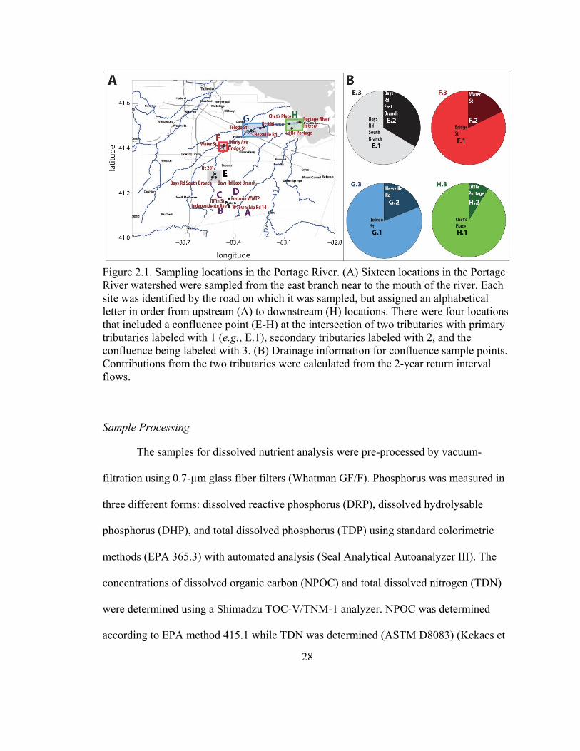
Figure 2.1. Sampling locations in the Portage River. (A) Sixteen locations in the Portage
River watershed were sampled from the east branch near to the mouth of the river. Each
site was identified by the road on which it was sampled, but assigned an alphabetical
letter in order from upstream (A) to downstream (H) locations. There were four locations
that included a confluence point (E-H) at the intersection of two tributaries with primary
tributaries labeled with 1 (e.g., E.1), secondary tributaries labeled with 2, and the
confluence being labeled with 3. (B) Drainage information for confluence sample points.
Contributions from the two tributaries were calculated from the 2-year return interval
flows.
Sample Processing
The samples for dissolved nutrient analysis were pre-processed by vacuum-
filtration using 0.7-µm glass fiber filters (Whatman GF/F). Phosphorus was measured in
three different forms: dissolved reactive phosphorus (DRP), dissolved hydrolysable
phosphorus (DHP), and total dissolved phosphorus (TDP) using standard colorimetric
methods (EPA 365.3) with automated analysis (Seal Analytical Autoanalyzer III). The
concentrations of dissolved organic carbon (NPOC) and total dissolved nitrogen (TDN)
were determined using a Shimadzu TOC-V/TNM-1 analyzer. NPOC was determined
according to EPA method 415.1 while TDN was determined (ASTM D8083) (Kekacs et
29
al., 2015). Calibration curves were generated between 3-20 mg C/N L-1 using potassium
hydrogen phthalate or potassium nitrate, respectively, with limits of detection at 2 mg C
L-1 and 0.01 mg N L-1. In order to estimate solid phase extraction efficiency, TDP was
measured on an Agilent ICP-OES at 213.648 nm according to EPA method 3051 (Bartos
et al., 2014).
Combusted glassware (30 min at 550°C) was used for mass spectrometric
analysis. All samples were vacuum-filtered through pre-rinsed (methanol and DI water)
0.7-µm glass fiber filters (Whatman GF/F). Solid phase extraction was performed with
Plexa-PAX columns using 325 mL of undiluted samples adjusted to pH 10 with sodium
hydroxide. Initial NPOC concentrations ranged between 6-14 mg C L-1 (Table B.1).
Readings of NPOC, TDN, and TDP were made on solid phase extraction influent and
effluent samples to estimate the amount retained by PAX columns (Table B.1). PAX
columns were primed using Milli-Q water and methanol per the manufacturer’s
instructions. DOM was eluted from SPE columns using 10 mL of HPLC-grade methanol,
followed by 10 mL of HPLC-grade methanol +5% formic acid. The elutions were
combined and stored at -20°C for ESI FT-ICR-MS analysis at Woods Hole
Oceanographic Institute.
ESI FT-ICR-MS Data Analysis
Mass spectrometry data was collected as has been previously described
(Appendix A) (Minor et al., 2012). The samples were analyzed with electrospray
ionization under the negative ionization mode on a 7T FTICR mass spectrometer
(Thermo Fisher Scientific, Waltham, MA USA). The instrument settings were optimized

30
by tuning on the SRFA standard. The samples were infused into the ESI interface at 4 μL
min-1, and the instrumental and spray parameters were optimized for each sample. The
capillary temperature was set at 250°C, and the spray voltage was between 3.7 and 4 kV.
For each sample, 200 scans were collected spanning the 150-1000 Da m/z range.
Molecular formula assignments were made using the Compound Identification Algorithm
with an error of 1 ppm (Kujawinski and Behn, 2006; Kujawinski et al., 2009). A total of
29,273 unique peaks were detected. Two quality control measures were used to filter the
dataset (1) peaks observed in DI water or solvent blanks were removed from all samples,
and (2) any singletons were removed from the dataset (Table B.3). Additionally, only m/z
values with an assigned formula were considered in further analysis.
Data analyses were performed using R Statistics (version 3.1.1). Samples were
compared based on (1) presence or absence and (2) relative peak height. For relative peak
height comparisons, peak abundances were normalized to maximum peak height for each
sample. Cluster analysis was performed using the ‘vegan’ package distance methods,
with the Jaccard method used for analysis of presence/absence data and Canberra method
used with relative peak heights (Oksanen et al., 2015).
We considered the potential of downstream transport as the detection of the same
m/z value between upstream and downstream samples. The more prominent peaks, or
those with the greatest height, were expected to be detected in downstream samples. The
m/z values were binned by peak height working in 0.01th quantile intervals. The
probability of positive detection in the nearest downstream neighbor was calculated for
each of those quantile bins. End member mixing analysis models were developed using
31
the ‘quadprog’ package to reveal whether the DOM spectra were linearly mixed at the
expected ratios according to the StreamStats estimates. The model considered the m/z all
m/z values detected in the confluence and at least one of the branch samples. The
solve.QP command was used to develop models for the confluence according to:
𝐶𝑜𝑛𝑓𝑙𝑢𝑒𝑛𝑐𝑒 = 𝑎 × 𝑇𝑟𝑖𝑏𝑢𝑡𝑎𝑟𝑦1 + 𝑏 × 𝑇𝑟𝑖𝑏𝑢𝑡𝑎𝑟𝑦 2
where a>0, b>0, and a+b=1. Peak heights we m/z values were used to solve the equation
across the factorized (Cholesky decomposition method) set to account for covariance
between variables. A random sample of 500 m/z values were used to solve the mixing
equation. Bootstrapping (n=1,000) was used to generate a 95% confidence interval for the
estimated mean contribution of each branch to its confluence with the assumption that
predictions followed a normal distribution.
Results
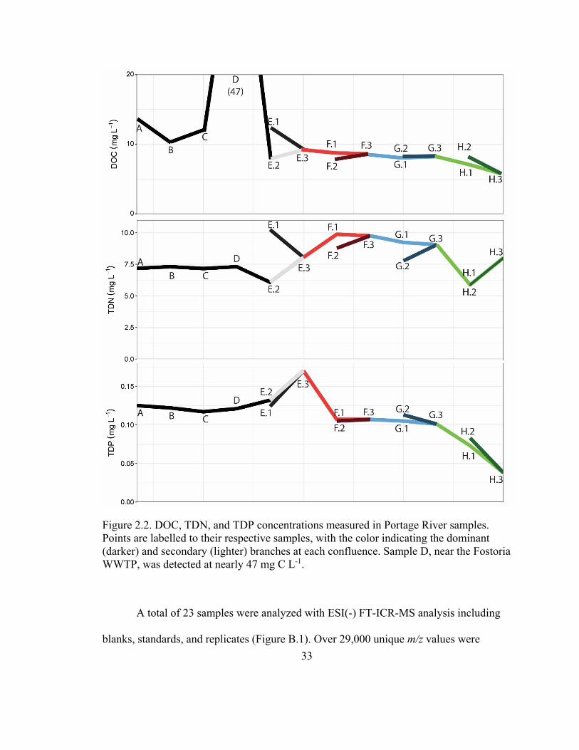
Carbon, nitrogen, and phosphorus concentrations varied across the Portage River
Table B.1, Figure 2.2). NPOC ranged between 6 and 47 mg C L-1 with the highest value
observed near the Fostoria WWTP collection site (Location D). The NPOC measured at
the WWTP site were more than 3-fold higher than all other samples, which were <12.6
mg C L-1. Carbon concentrations were higher in the upper reaches of the east branch
where all five samples were measured at >10.3 mg C L-1. The south branch and all
samples downstream of the first confluence sampling area (Location E) were measured at
<10 mg C L-1. The TDN concentrations of the samples ranged between 5.9 and 10.2 mg
N L-1. The concentrations in the east branch were between 7.2 and 7.4 mg N L-1 until the
first confluence point (Location E.2) which showed the highest measured N levels (10.2
32
mg N L-1). Concentrations dropped to 8.0 mg N L-1 or less after this sample location.
TDP ranged between 124 and 132 μg P L-1 in the upper reaches (A-E), dropping to
between 101 and 113 μg P L-1 leading up to the final mixing area (F-G). Toward the
mouth of the river (H), the concentration fell to 83 μg P L-1 or less as the river reached
Lake Erie. On the order of 87-94% total phosphorus was measured as DHP, while 71-
86% was measured as DRP. Generally, DRP and DHP accounted for a lower proportion
of TDP as samples moved downstream (A through H).
33
Figure 2.2. DOC, TDN, and TDP concentrations measured in Portage River samples.
Points are labelled to their respective samples, with the color indicating the dominant
(darker) and secondary (lighter) branches at each confluence. Sample D, near the Fostoria
WWTP, was detected at nearly 47 mg C L-1.
A total of 23 samples were analyzed with ESI(-) FT-ICR-MS analysis including
blanks, standards, and replicates (Figure B.1). Over 29,000 unique m/z values were
34
observed across the set. Following quality filtering, a total of 11,344 m/z values remained
in the dataset between the mass range of 150-1000 Da (Table B.3). While these
preprocessing steps removed 72% of detected values, at least 74% of the detected m/z
values were retained for each sample. Almost all these m/z values were assigned a
formula (11,064, 99%), and these data were then normalized and used for all analyses
described in the following sections.
The data were summarized based on elemental composition of assigned formulae
(Figure 2.4A, Table B.4). The CHO compounds dominated all samples (57% to 73%),
but there was also an abundance (22.6-36.2%) of CHON compounds throughout the river
(Table B.3). The lowest abundance of CHON was observed in the upstream reaches of
the east branch (A-C), near Fostoria, Ohio, while the highest abundances were detected in
the samples near the mouth of the Portage River (H.3). However, this patttern was not
reflected across the range of TDN concentrations and CHON% values (p=0.28, Figure
B.2A). A noticeable spike in the percentage of CHON formulae wasdetected near the
Fostoria WWTP (D), yet increased organic nitrogen diversity was not manifested as an
increase in TDN concentrations. Throughout the hydrologic system, the percentage of
CHON formulae fluctuated substantially, and usually this corresponded to the change in
CHO formulae. Despite an overall reduction in TDP from upstream to downstream
locations, the relative abundance of phosphorus containing formula also increased from
upstream reaches toward the mouth of the Portage River (Figure B.2B). The sample
closest to the mouth of the river (H.3) had the lowest abundance of CHO formulae
35
compared to any other sample, with organic matter becoming more nutrient-laden (i.e.,
higher in organic-N/P/S abundance).
Van Krevelen diagrams were used to visualize the elemental composition of m/z
values collected from the 16 locations (Figure 2.4A). River samples were clearly
dominated by a cluster of CHO and CHON formulae in the lignin-like and tannin-like
region of the plot. The CHOP formulae were primarily evident in the lignin-like and
protein-like regions. There were a few noticeable differences in the prevalence of CNON
heteroatoms in the carbohydrate-like region (e.g., E.1 or H.3 vs A). In addition, CHOS
formula showed notable differences in the lignin/condensed hydrocarbon-like regions
(e.g., H.3 vs A or F.3 vs B).

36
Figure 2.3. Van Krevelen plots of the 16 samples in this study. The hydrogen:carbon molar ratio is plotted against the oxygen:carbon
molar ratio for each formula identified in the sample. The seven boxes indicate the molecular class features of each individual
formula.

37
Next, we summarized the data according to the molecular classifications of m/z
values indicated by their molar ratios to compare the sample similarities based on
molecular features. All samples were dominated by lignin-like features (≥73%, Table
B.5, Figure 2.4B). In general, tannin-, protein-, and lipid-like features were the next most
abundant features for many of the samples. Again, a major shift was observed between
samples C and D, near the Fostoria WWTP as tannin-like features increased and lignin-
like features decreased in relative abundance. There were similarities between the
samples A through C with protein-like features becoming more abundant (7.1-8.3%)
largely at the expense of lignin-like features (80.3-79.3%). In sample D, the shift became
more dramatic with lignin-like features decreasing by nearly 4% (75.6%), but in this case
tannin-like features became more predominant. However, the nearest downstream sample
(E.2) did not share these characteristics, and sample D in fact shared more similarities
with the other branch (E.1) at the confluence E. Thus, the effects from the WWTP
effluent may have diminished during downstream transport. Carbohydrate-like features
ranged from 0.5-2.3%, and these were highest in the H.2 and H.3 samples that were
collected near the mouth of the river. Again, the samples nearest to the mouth had
striking differences with the upstream samples in that lignin-like features were much less
abundant and tannin-like and unclassified (‘other’) features became more prominent.
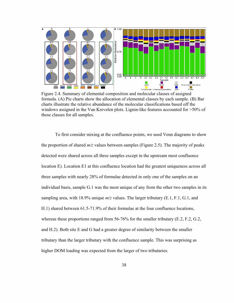
38
Figure 2.4. Summary of elemental composition and molecular classes of assigned
formula. (A) Pie charts show the allocation of elemental classes by each sample. (B) Bar
charts illustrate the relative abundance of the molecular classifications based off the
windows assigned in the Van Krevelen plots. Lignin-like features accounted for >50% of
these classes for all samples.
To first consider mixing at the confluence points, we used Venn diagrams to show
the proportion of shared m/z values between samples (Figure 2.5). The majority of peaks
detected were shared across all three samples except in the upstream most confluence
location E). Location E1 at this confluence location had the greatest uniqueness across all
three samples with nearly 28% of formulae detected in only one of the samples on an
individual basis, sample G.1 was the most unique of any from the other two samples in its
sampling area, with 18.9% unique m/z values. The larger tributary (E.1, F.1, G.1, and
H.1) shared between 61.5-71.9% of their formulae at the four confluence locations,
whereas these proportions ranged from 56-76% for the smaller tributary (E.2, F.2, G.2,
and H.2). Both site E and G had a greater degree of similarity between the smaller
tributary than the larger tributary with the confluence sample. This was surprising as
higher DOM loading was expected from the larger of two tributaries.
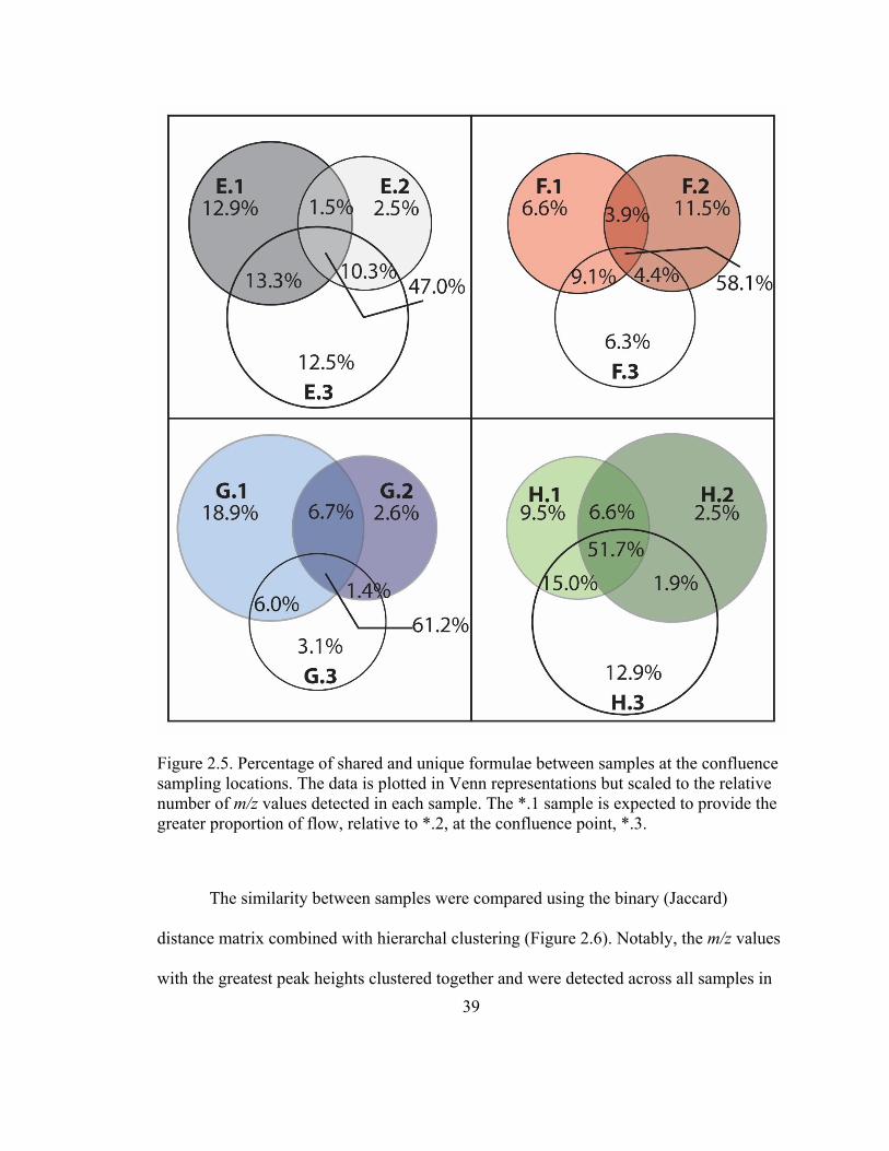
39
Figure 2.5. Percentage of shared and unique formulae between samples at the confluence
sampling locations. The data is plotted in Venn representations but scaled to the relative
number of m/z values detected in each sample. The *.1 sample is expected to provide the
greater proportion of flow, relative to *.2, at the confluence point, *.3.
The similarity between samples were compared using the binary (Jaccard)
distance matrix combined with hierarchal clustering (Figure 2.6). Notably, the m/z values
with the greatest peak heights clustered together and were detected across all samples in

40
this study. Between confluence samples, F.1 clustered closely to F.3, and G.2 clustered
with G.3. Alternatively, there was greater separation between the samples from
confluence E, and even greater separation between confluence H samples. One of the far
downstream sites, H.1, clustered with sample D, near the Fostoria WWTP. Outside
sample D, the upstream samples collected around the outskirts of Fostoria were all
clustered closely together, suggesting that there was a substantial change to the DOM
signature near the Fostoria WWTP. Hierarchal clustering was also performed using the
Canberra distance matrix (using noramlized peak heights). This analysis resulted in
improved clustering between the confluences and their two tributaries (Figure B.3),
suggesting low abundant peaks represent noise in the dataset. Additionally, cluster
analysis using Canberra distances resulted in more similarity in transects closer in
distance (e.g., D and E.1), rather than similarity to samples collected further downstream
(D and H.1). Otherwise, there were few differences in the clustering of samples using
presence/absence as compared with normalized peak heights.
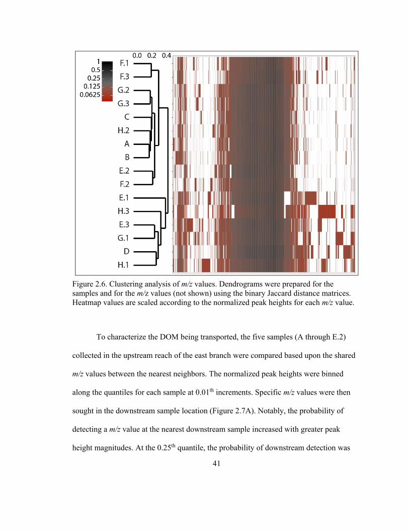
41
Figure 2.6. Clustering analysis of m/z values. Dendrograms were prepared for the
samples and for the m/z values (not shown) using the binary Jaccard distance matrices.
Heatmap values are scaled according to the normalized peak heights for each m/z value.
To characterize the DOM being transported, the five samples (A through E.2)
collected in the upstream reach of the east branch were compared based upon the shared
m/z values between the nearest neighbors. The normalized peak heights were binned
along the quantiles for each sample at 0.01th increments. Specific m/z values were then
sought in the downstream sample location (Figure 2.7A). Notably, the probability of
detecting a m/z value at the nearest downstream sample increased with greater peak
height magnitudes. At the 0.25th quantile, the probability of downstream detection was
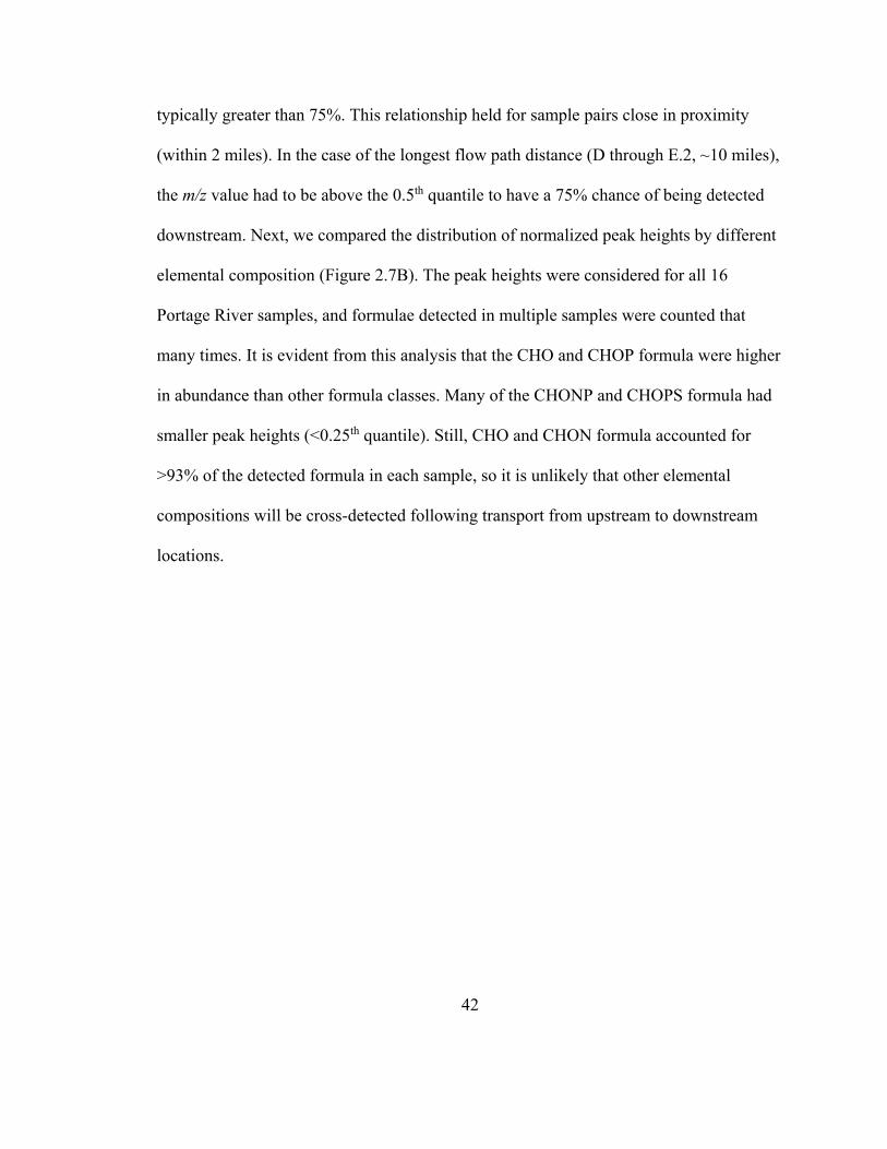
42
typically greater than 75%. This relationship held for sample pairs close in proximity
(within 2 miles). In the case of the longest flow path distance (D through E.2, ~10 miles),
the m/z value had to be above the 0.5th quantile to have a 75% chance of being detected
downstream. Next, we compared the distribution of normalized peak heights by different
elemental composition (Figure 2.7B). The peak heights were considered for all 16
Portage River samples, and formulae detected in multiple samples were counted that
many times. It is evident from this analysis that the CHO and CHOP formula were higher
in abundance than other formula classes. Many of the CHONP and CHOPS formula had
smaller peak heights (<0.25th quantile). Still, CHO and CHON formula accounted for
>93% of the detected formula in each sample, so it is unlikely that other elemental
compositions will be cross-detected following transport from upstream to downstream
locations.
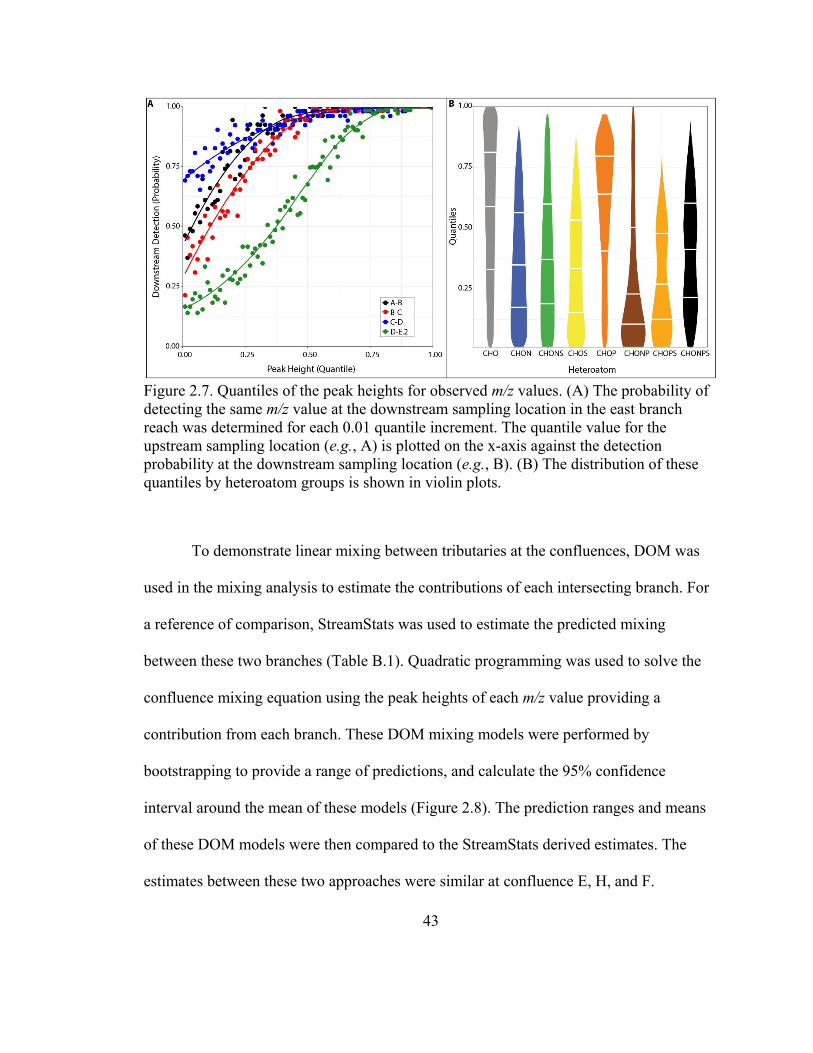
43
Figure 2.7. Quantiles of the peak heights for observed m/z values. (A) The probability of
detecting the same m/z value at the downstream sampling location in the east branch
reach was determined for each 0.01 quantile increment. The quantile value for the
upstream sampling location (e.g., A) is plotted on the x-axis against the detection
probability at the downstream sampling location (e.g., B). (B) The distribution of these
quantiles by heteroatom groups is shown in violin plots.
To demonstrate linear mixing between tributaries at the confluences, DOM was
used in the mixing analysis to estimate the contributions of each intersecting branch. For
a reference of comparison, StreamStats was used to estimate the predicted mixing
between these two branches (Table B.1). Quadratic programming was used to solve the
confluence mixing equation using the peak heights of each m/z value providing a
contribution from each branch. These DOM mixing models were performed by
bootstrapping to provide a range of predictions, and calculate the 95% confidence
interval around the mean of these models (Figure 2.8). The prediction ranges and means
of these DOM models were then compared to the StreamStats derived estimates. The
estimates between these two approaches were similar at confluence E, H, and F.

44
Although there was no overlap between the 95% confidence interval and the StreamStats
estimate, the prediction range did include the StreamStats estimates at these sites. Most
notably, the estimated contributions at confluence E were ±3% of each other. Confluence
G samples had the greatest disagreement between StreamStats and our mixing model
estimates, but this confluence also had the greatest variation from the DOM mixing
models. Notably, of the samples collected in this study, G.1 and G.2 were the furthest
distance away from their respective confluence point. Based on the similarity between the
DOM mixing model and StreamStats estimates, these results suggest that DOM mass
spectra signals mix linearly within the watershed.
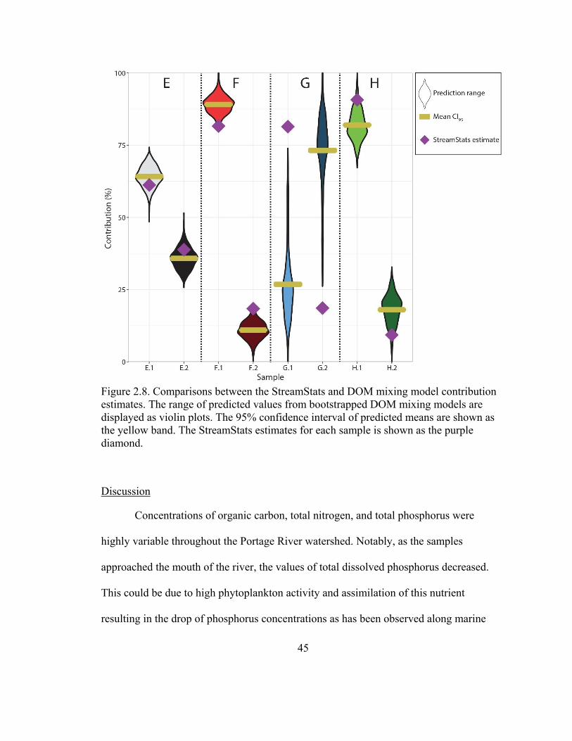
45
Figure 2.8. Comparisons between the StreamStats and DOM mixing model contribution
estimates. The range of predicted values from bootstrapped DOM mixing models are
displayed as violin plots. The 95% confidence interval of predicted means are shown as
the yellow band. The StreamStats estimates for each sample is shown as the purple
diamond.
Discussion
Concentrations of organic carbon, total nitrogen, and total phosphorus were
highly variable throughout the Portage River watershed. Notably, as the samples
approached the mouth of the river, the values of total dissolved phosphorus decreased.
This could be due to high phytoplankton activity and assimilation of this nutrient
resulting in the drop of phosphorus concentrations as has been observed along marine
46
coastlines (Ruttenberg and Dyhrman, 2005). It could also be related to the loss of
phosphorus due to particulate adsorption. Corresponding with this decrease in TDP, the
relative proportion of P-formulae increased in those samples, possibly indicating an
enrichment of DOP at these locations. However, with the use of PAX-SPE we expected
to concentrate DOP, so these two variables are not directly comparable. While the
amount of DOP (TDP-DHP) was not higher at these locations, the proportion of DOP of
the TDP was measured at the highest ratio in the sample closest to the mouth and higher
at these marginal locations. Phytoplankton has a general preference for the inorganic
forms of phosphorus which does seem to enhance the proportion of DOP relative to TDP
in coastal sites (Monaghan, E. J., Ruttenberg,K.C., 1999; Ruttenberg KC, 2012).
Throughout the Portage River, the percentage of P- and N-formulae fluctuated between
samples. We expected this to relate to the concentrations of both total nitrogen and
phosphorus, but only found a negative correlation between total dissolved phosphorus
and percentage of CHOP* formulae.
The Portage River drains to the western Lake Erie Basin, and has 76% of its
watershed area is dedicated to agricultural land use (Ohio Lake Erie Phosphorus Task
Force, 2010). In that sense, the Portage River is similar to the Sandusky River with
slightly more area dedicated to urban land use (13% vs 10%) (Ohio Lake Erie
Phosphorus Task Force, 2010). The samples collected between these two watersheds
were compared to determine the similarity of source signatures to the samples collected
throughout the Portage River. Comparisons were made between the two sets of DOM
data using shared molecular formulae. Many of the formulae (4567, 63%) identified in

47
the Sandusky dataset were also detected in the Portage River dataset. Of those shared
formula, only 26 included a phosphorus atom, meaning <4% of the DOP formula
identified in the Sandusky dataset were also detected in the Portage River. Additionally,
four of our proposed markers were detected within the Portage River: C10H23O3N4P,
C17H25O9P, C18H23O9P, and C17H21O9P. However, the Portage River samples were
collected during a high flow event. Possibly, the proposed markers were diluted and
obscured from detection due to diffuse, background DOM. Such background DOM could
also explain the high degree of similarity between the 16 Portage River samples.
The Portage River samples were dominated by lignin-like and tannin-like
features, similar to the Sandusky River sample analyzed in the previous set. However,
there were a greater number of carbohydrate-, protein-, and lipid-like features with the
Portage River samples compared to the Sandusky River. A greater number of CHON
formula were detected in the Portage River samples compared to the Sandusky River
(>23.8% vs 20.8%). Although CHON were in greater abundance in Portage River
samples, the number of P-containing formula were lower in all but three of the samples:
Bridge St (3.7%), Chet’s Place (3.5%), and Portage River Retreat (3.6%); while Bierly
Ave (3.1%) was within the range of P formula detected in the Sandusky River (3.3%).
Our dataset was also relative enriched in CHON content, but lower in P containing
formula then samples collected in the tributaries of Lake Superior (Minor et al., 2012).
Compared to an urban (3% agriculture) and mixed-land use (28% agriculture) stream in
Florida, our samples were also more enriched in CHON formula (Lusk and Toor, 2016).
In fact, the relative abundance of CHON formulae was twice as high as that of the mixed-

48
land use stream (11.6%) (Lusk and Toor, 2016).. Another potential source of CHON
formula, however, is sewage (e.g., septic contaminated groundwater) which also has high
CHON content (Arnold et al., 2014). Treated wastewater effluent may also be enriched in
sulfur formulae (Gonsior et al., 2011). Our sample (D) collected nearest to the Fostoria
WWTP had a notable increase in N- (25 to 35%) and S-formulae (2.1 to 2.4%) from the
sample upstream, location C. Both S- and N-formulae (3.6 and 37%) became more
enriched in the DOM spectra of the samples closest to the mouth reaching proportions
that exceeded those next to the WWTP. The character of the Portage River samples
appeared similar to other natural riverine systems, in terms of lignin-like features, but had
a relatively high abundance of CHON compound.
The samples from the Portage River clustered together often in relation to their
physical proximity to one another. Notably, the dominant peaks detected in this study
were present in most if not all samples, and normalized peak heights were nearly the
same as well. For example, the upper reach samples of locations A through C cluster
together in Jaccard and Canberra distance matrices. However, the next nearest site to
these, location D sampled by the WWTP, clustered near other samples further
downstream. We hypothesize that this may reflect DOM influenced by sewage from
WWTP or septic inputs (Maizel and Remucal, 2017). Hierarchal clustering analysis
between the Portage River and Sandusky watershed samples was also performed on
Jaccard distances using only the formula that were cross-detected (Figure B.3). While we
expected the Fostoria WWTP sample (D) to cluster closely to the WWTP effluent sample
collected in the Sandusky sampling set, this did not turn out to be the case. This
49
difference though may be on account of differences between the final treatment processes
used at the Tiffin (chlorination) and Fostoria (UV irradiation) wastewater treatment
plants. Wastewater treatment plants expose influent organic matter to physical (e.g.
filtration), biological (e.g. activated sludge), and chemical (e.g. chlorination) processes
that affect the organic matter as it proceeds through these treatment processes (Maizel
and Remucal, 2017). The biological processes at one such facility was associated with an
increased production of CHON, CHOS, and CHOP formulae (Maizel and Remucal,
2017). The observed increase of these features near the Fostoria WWTP may highlight
their ability to detect sewage contamination. Further, their abundance at the mouth of the
Portage River may highlight the amount of contamination originating from sewage
sources in this watershed.
Changes to the DOM through production or degradation does not stop with the
discharge from point and nonpoint sources to riverine systems. Rather, internal riverine
processing continues within the waterways due to indigenous biota, photolysis, and
exposure to abiotic elements (Mesfioui et al., 2012; Stubbins et al., 2010). Therefore, we
sought to identify the compounds which persisted during their transport through the east
branch of the Portage River. The samples collected from the upstream reaches of the
east branch of the Portage River were used to elucidate the downstream transport of m/z
values. We found that the probability of detecting a m/z value corresponded to the
magnitude of its peaks. In other words, the most prominent peaks may be the most
reliable markers for tracking sources of pollution. As DOM is transported, it may have
been diluted due to unaccounted headwaters merging with our stem of the Portage River

50
between sampling locations (Medeiros et al., 2015). These inputs may also have
contributed to relatively stable levels of certain m/z values, especially if these
components are originating from diffuse sources.
Another consideration in the transport of the m/z values is the molecular class
features which may affect biodegradability. For example, bioassays looked at the
susceptibility of N containing formula and found that protein- and lipid-like features were
more reactive than lignin-like features (Lusk and Toor, 2016; Mesfioui et al., 2012). Still,
there may not be dramatic changes as only 5-7% of the DON was removed during a five-
day bioassay (Lusk and Toor, 2016). Thus, at the upper reach sampling locations, we also
considered the change in peak heights of m/z values as a function of their molecular
classification (Figure B.4). We found that many of lignin-like features were less likely to
change between our sampling points (i.e. median change for these features was 0 between
upstream and downstream neighbors). Like the CHON bioassay studies, the peak heights
of the protein- and lipid-like features were more likely to decrease in the corresponding
downstream sample. While we did not further consider this factor, it may be worthwhile
to select for only those features which show limited degrees of change in peak heights
over the course of downstream transport, as these may serve as more robust markers to
track sources of pollution.
The constrained, linear mixing models developed from DOM spectra were in
good agreement with the estimates we calculated using StreamStats predicted flows. Only
the third confluence point (G) yielded poor results, whereas the other confluence models
performed well with differences of <9%. An important note is that sample G.1 was
51
sampled just upstream of the local WWTP and was also the furthest distance from its
confluence sample (G.3) of any sample collected. If, as we hypothesize, WWTP effluent
has a significant impact on DOM, the WWTP situated between G.1 and G.3 sampling
locations may partially explain the failure of this model. To our knowledge, ESI FT-ICR-
MS has not been used within end member mixing analysis to provide source
contributions. However, mixing analysis has been used to reproduce the ESI FT-ICR-MS
spectra from the Atlantic Ocean from several riverine sources (Hansman et al., 2015).
Additionally, this technique was used to track the loading of DOM from the Amazon
River into the Atlantic Ocean finding that many of m/z values persisted and were diluted
from mixing with autogenous DOM (Medeiros et al., 2015). These studies suggest that
the mass spectra elucidated with ESI FT-ICR-MS, specifically the more conserved or
recalcitrant features may follow a linear mixing model in certain hydrologic systems. As
ionization efficiencies of different compounds can vary considerably and the inability to
acquire standards limits the quantification of individual compounds, non-target ESI-FT-
ICR-MS methods are semi-quantitative at best. However, recent studies support the
notion that relative peak heights provide an indication of relative abundance for m/z
values (Banerjee and Mazumdar, 2012; Kamga et al., 2014; Lu et al., 2015). The
feasibility of using DOM for source tracking or within end member mixing analysis relies
on better defining the quantification limits of ESI FT-ICR-MS. Our results suggest that
there is some potential for DOM to be used in end member mixing analysis pending
further evaluation.

52
Chapter 3: The Emerging Concern of Antibiotic Resistance Genes in Agricultural
Sediments
This chapter will be submitted under the title: The Prevalence of Antibiotic Resistance
Genes in Agricultural Channel Sediments by Michael R. Brooker, Julia Beni, Timothy
LaPara, Jill Kerrigan, Bill Arnold, Paula J. Mouser. This manuscript will be submitted to
Water Research. This work was supported by the National Integrated Water Quality
Program Award Number 2012-51130-20255 from the USDA National Institute of Food
and Agriculture.
Introduction
In the Midwestern United States, agricultural drainage is managed by constructing
trapezoidal ditches optimized to remove excess water from the field. Recently, there have
been efforts to restore these ditches to resemble more natural streams by incorporating
floodplains by widening the drainage corridor (Powell et al., 2007). This practice of two-
stage channel construction captures sediments and establishes macrophyte communities
which support a productive microbial habitat. Such microbial communities provide
ecosystem services, for instance, these floodplains are strongly associated with
denitrification thus attenuating downstream eutrophication (Rabalais et al., 2002; Roley
et al., 2012). Due to the novelty of this two-stage practice, there has been minimal
characterization of the microbial ecology where much of the emphasis has been on
ecosystem services provided (e.g. denitrification) (Arango et al., 2007; Roley et al.,
2012). Additionally, the microbial ecosystems of floodplains have been recognized for
their role in treating other agricultural pollutants like herbicides and pesticides (Douglass
et al., 2015; Vymazal and Březinová, 2015). Microbial characterization of two-stage
channels must be performed to fully understand the potential benefits and drawbacks of
this practice.
53
One method for assessing the functional potential of uncultivated microorganisms
in these systems is through metagenomic techniques. The GeoChip microarray is a
metagenomic tool with the capability to semi-quantitatively detect thousands of
environmentally relevant functional genes equally across samples (Zhou et al., 2010).
These genes span a range of categories, but notably include those involved in nutrient
cycling (i.e. organic remediation) or aiding in microbial stress (i.e. antibiotic resistance or
metal homeostasis). This technique has been used to characterize the microbial
ecosystems of many environments; wastewater treatment, grasslands, forests, and riverine
sediments (Cong et al., 2015; Low et al., 2016; Sun et al., 2016; Y. Yang et al., 2014).
Among the many systems characterized by the GeoChip, a relatively high
abundance of antibiotic resistance genes (ARGs) were noted in urban watershed
sediments (Low et al., 2016). The ARGs in these urban sediments were predominantly
efflux pumps, which may confer multidrug resistance (Low et al., 2016). However, these
efflux pumps can provide resistance to other toxins, may be co-selected for with metal
resistance, or used in intercellular signaling (Baker-Austin et al., 2006; Low et al., 2016).
ARGs are maintained or proliferated through in situ selection by antibiotics or other
toxins, microbial migration, or horizontal gene transfer (HGT) (Niehus et al., 2015). In
HGT, mobile genetic elements (i.e., integrons, transposons) may be transmitted through
plasmids, and integrons were implicated in the enrichment of ARGs in agricultural soils
amended with hog manure (Johnson et al., 2016). ARGs have been detected in
groundwater, tile drainage, and downstream watersheds connected to agricultural fields
54
(Frey et al., 2015; Storteboom et al., 2010). Their presence would be expected in the
sediments collecting within drainage corridors.
Antibiotic resistance is a naturally occurring phenomenon that occurs
ubiquitously across all environments. In recent times, the use of antibiotics for medical
and agricultural purposes has increased the prevalence of this functionality in
anthropogenically-impacted environments (Hobman and Crossman, 2015; Martinez,
2009). In the United States, a majority of antibiotic usage is dedicated to agricultural
operations (Center for Disease Dynamics, Economics & Policy, 2015). Thus, there are
emerging concerns over the prevalence and persistence of antibiotic resistance genes
(ARGs) in agroecosystems (Rothrock et al., 2016). Antibiotic resistance in agricultural
fields occurs through several routes of exposure, for instance manure spreading (Ghosh
and LaPara, 2007; McManus et al., 2002; Munir et al., 2011; Negreanu et al., 2012;
Schmitt et al., 2006; Udikovic-Kolic et al., 2014). Antibiotic resistant organisms are not
confined to these fields, but are rather transported through ground and surface water
flows (Chee-Sanford et al., 2001; Chee-Sanford et al., 2009; Frey et al., 2015). While the
presence of ARGs at agricultural sites and their downstream transport in surface water
flows have been studied, little is known about these genes in agricultural channel
sediments.
Agricultural channels, with natural floodplains developing within their banks
(Powell et al., 2007), were selected for our analysis. Three sites located in the Western
Lake Erie Basin (WLEB) were selected to characterize microbial ecosystem services and
taxonomy. Our previous research had determined that the chemical and physical

55
properties of these sites were strongly associated with their designated Ecoregion
(Brooker, 2018). Due to the variations in soil properties, we hypothesized that the
microbial communities would be diverse from one another across these sites. We used the
GeoChip 5.0 to assess the functional genomic diversity, while 16S rRNA gene
sequencing was used for taxonomic analysis. Specific classes of functional genes were
also assessed using Fluidigm quantitative PCR (qPCR). Our results identified ARGs,
metal homeostasis genes, organic remediation genes, and an integrase gene to be
prevalent in the sediments of Lake Erie drainage corridors that indicates these sediments
are a considerable reservoir for antibiotic resistance in the environment.
Methods
Site Description and Sample Collection
Sampling locations were chosen in three U.S. EPA defined Ecoregions of the
Western Lake Erie Basin: Clayey, High-Lime Till Plains (CHLP), Oak Openings (OO),
and Paulding Plains (PP) (Omernik, 1986). Criteria included in the site selection included
1) the presence of self-formed floodplains, 2) adjacency to agricultural row crop fields,
and 3) greater than 70% agriculture land use in the watershed. Samples were collected on
October 1, 2015 and again on October 18, 2016 to assess ecosystem services using
GeoChip and 16S rRNA gene sequencing. The samples collected in 2016 were further
analyzed using Fluidigm qPCR as well as assessed for a suite of common antibiotics and
metals.
Sediment cores were extracted from the surface (0-20cm) of floodplains using a
soggy bottom sampler device with sterilized PVC liners (AMS). The dry weights for

56
sediments were calculated after drying more than 10g of sediment at 70°C until no further
changes in weight were observed (approximately 24 hours). For quantification of
antibiotic concentrations, samples were collected in combusted glassware (450°C, 2
hours) using ceramic spoons. Samples were transported on ice to the laboratory where
they were stored at -20°C overnight. Samples used for antibiotic quantification were
freeze-dried over the course of a week, while DNA extracts commenced on the day
following sampling.
Genomic DNA Extraction
Community DNA was extracted using the MoBio PowerSoil DNA extraction kit
as previously described (Brooker et al., 2014). For the 2015 samples, duplicate cores
were collected from each sampling location. Each core was homogenized separately, and
two 0.5-mg (wet weight) aliquots were taken from each core for extraction (n=12). After
extraction, DNA was pooled for each core (n=2), resulting in six total samples for
analysis (duplicates from three different sampling locations, n=6). In 2016, DNA was
extracted using 0.25-mg (wet weight) of homogenized sediment from triplicate cores at
each sampling location, resulting in nine total samples for analysis. Triplicate cores were
pooled by site for GeoChip and 16S rRNA gene sequencing (n=3). All replicates were
analyzed using Fluidigm qPCR (n=9). DNA was stored at -80°C until shipment on dry
ice to sequencing and analysis facilities.
Functional Gene Assays
The GeoChip 5.0 analysis was performed at Glomics, Inc. (Norman, OK) and has
been described in detail (Cong et al., 2015) The GeoChip 5.0 microarray consists of
57
167,044 probes covering about 1500 gene families of functional genes commonly
observed in the environment. Briefly, purified DNA was labelled with Cy3 fluorescent
dye with a random priming method and hybridized to the GeoChip 5.0 array slide. Slides
were washed and scanned at 633nm using a laser with a NimbleGen MS200 Microarray
Scanner. Data was preprocessed by the microarray analysis by removal of poor quality
spots (SNR <2.0).
A combination of antibiotic resistance, metal homeostasis, and integrase genes
were selected for qPCR analysis using an integrated fluidic circuit (Fluidigm
Corporation, San Francisco, CA) (Johnson et al., 2016). Briefly, 48 primer sets and nine
samples (2016) were input into a 48.48 Access Array. EvaGreen dye was used at the
fluorescent marker, which allowed for real-time quantification of amplification products.
The amplicon pool was prepared by the Fluidigm FL1 and FL2 workflow. Several genes
were targeted with multiple primer sets, and these were annotated with a gene suffix (e.g.,
aadA and aadA5), and primer sets used can be found in Johnson et al. (2016). Threshold
cycle values were quality checked by Fluidigm software. Standard curves for each gene
were used to estimate the number of copies detected in each sample. The number of gene
copies per gram of sediment (dry weight) was calculated using the amount of eluent
applied in DNA extraction and the amount of sediment added to the extraction tube
(Table C.1).
16S rRNA Gene Sequencing
PCR amplicon libraries targeting the 16S rRNA gene were produced using a
barcoded primer set adapted for the Illumina platform (Caporaso et al., 2012). Each 25

58
µL PCR reaction contained 9.5 µL of MO BIO PCR Water (Certified DNA-Free), 12.5
µL of QuantaBio’s AccuStart II PCR ToughMix (2x concentration, 1x final), 1 µL
Forward Primer (5 µM concentration, 200 pM final), 1 µL Golay barcode tagged Reverse
Primer (5 µM concentration, 200 pM final), and 1 µL of template DNA. The conditions
for PCR were as follows: 94 °C for 3 minutes to denature the DNA, with 35 cycles at 94
°C for 45 s, 50 °C for 60 s, and 72 °C for 90 s; with a final extension of 10 min at 72°C to
ensure complete amplification. Amplicons were then quantified using PicoGreen
(Invitrogen) and a plate reader (Infinite 200 PRO, Tecan). Once quantified, volumes of
each of the products were pooled in equimolar amounts, cleaned up using AMPure XP
Beads (Beckman Coulter), and quantified using a fluorometer (Qubit, Invitrogen). After
quantification, the molarity of the pool is determined and diluted to 2 nM, denatured, and
then diluted to a final concentration of 6.75 pM with a 10% PhiX spike for sequencing on
the Illumina MiSeq. Amplicons were sequenced on a 151bp x 12bp x 151bp MiSeq run
using customized sequencing primers and procedures (Caporaso et al., 2012). The
sequencing was performed at the Joint Genome Institute (San Francisco) or Argonne
National Laboratories (Chicago, IL) for the 2015 and 2016 sets, respectively.
Antibiotic Extraction and Analysis
Antibiotic extraction and quantification was carried out according to Kerrigan et
al. (2017). All glassware was triple-rinsed with a dilute Alconox solution, tap water, and
DI water before being baked at 550°C for more than 5 hours to remove organic matter.
Labware unable to be baked was triple-rinsed with acetonitrile, ethyl acetate, and
methanol following the DI wash. Stainless steel accelerated solvent extraction cells were

59
cleaned using the non-baking approach. Endcaps were rinsed without the use of Alconox,
and then disassembled. The frit, cap insert, and snap fitting were soaked in a water bath
and then sonicated in an acetone bath for 10 min. Following re-assembly, the organic
solvent rinses were repeated.
Freeze-dried sediments were thawed and sieved prior to the extraction of
antibiotics. Sediments (1 g) were spiked with surrogates (20 ng nalidixic acid and 100 ng
13C6-sulfamethazine) in a methanol solution prior to ASE extraction. The ASE cells were
assembled with 2 glass fiber filters, a thin layer of Ottawa sand, the sediment sample,
filled with Ottawa sand, and covered with another glass fiber filter. A 50:50 methanol to
50 mM phosphate buffer (pH=7) was applied at 100°C for 5 min, allowed to sit for 5 min,
with the process repeated twice and using a rinse volume of 150%. Methanol was
removed from the ASE extract using a rotary evaporator in a 35°C water bath.
Solid phase extraction (SPE) was adapted from Meyer et al. (2000). Oasis HLB (6
mL, 200 mg, 30 µm) and MCX (6 mL, 150 mg, 30 µm) columns were used in tandem,
with the HLB column stacked on top of the MCX. Both columns were preconditioned
with 10 mL of methanol and ultrapure water. Samples were loaded and passed through
the column under a vacuum (<15 mm Hg). The HLB column was washed with 6 mL of
40:60 methanol:water while MCX was washed with water (ultrapure). Antibiotics were
eluted from the columns in tandem; first applying 3-mL of the extracts to the HLB
column, and then applying 2x5 mL methanol to the MCX stacked on the HLB column.
An addition elution of 3 mL 5% ammonium acetate in methanol was applied separately to
the MCX column. The elution was initiated with a vacuum manifold, but allowed to drip

60
by gravity once started with the eluent collected in a 15-mL glass centrifuge tube.
Internal standards (100 ng each of clinafloxacin, 13C2-erythromycin, 13C2-erythromycin-
H2O, simeton, and 13C6-sulfomethoxazole) in methanol were spiked into the eluent. The
eluents were dried under industrial grade N2 in a 40°C water bath. Samples were
dissolved into 200 µL of 20 mM ammonium acetate, and syringe-filtered (GHP, 0.4 µm)
to remove suspended particles prior to liquid chromatography tandem mass spectrometry
analysis.
Samples were analyzed on a Thermo Dionex ultimate 3000 RSLCnano system
equipped with a Thermo TSQ Vantage triple quadrupole tandem mass spectrometer
(MS/MS) in positive electrospray ionization mode. Separation of antibiotics (8 µL
injection volume) were achieved with a XSelect CSH C18 (3.5 µm, 130 Å, 50 × 2.1 mm)
column at a flow rate of 0.5 mL/min and temperature of 35 °C. The elution buffer
consisted of 0.1% formic acid in water or methanol and were applied at two gradients
(Table C.2). From 0 to 1.5 min and 5.5 to 20 min, flow was diverted to waste. Due to the
number of analytes included in the study, each sample was analyzed by three LC-MS/MS
methods that monitored for: (1) sulfonamides, 13C6-sulfamethazine, and others; (2)
tetracyclines, fluoroquinolones, and nalidixic acid; and (3) macrolides.
Analytes were detected and quantified using single reaction monitoring (SRM)
transitions (Table C.3). Confirmation SRMs were used to corroborate the identity of
quantified peaks. The mass spectrometer sensitivity varied between analyses, and thus
parameters were optimized with the infusion of 5µM simeton in 50:50 20 mM
ammonium acetate:methanol prior to each analysis. Typical values for mass spectrometer

61
parameters were: scan time 0.02 sec; scan width: 0.15; Q1/Q3: 0.7; spray voltage: 3300 V;
sheath gas pressure: 18 psi; capillary temperature: 300°C; collision pressure: 1.5 mTorr;
declustering voltage: -9 V; and tube lens: 95.
Several quality assurance and control measures were taken to assure the precision
of reported antibiotic concentrations. Antibiotic extraction efficiency from sediment was
determined for each collection site. This was achieved by spiking a methanolic solution
of antibiotics (100 ng) onto the sediment prior to ASE and calculating the mass loss due
to the extraction process. Method blanks (comprised of Ottawa sand spiked with
surrogates) were subjected to the entire extraction process and were extracted at least
every eight samples to monitor for any carryover contamination. Limits of quantification
(LOQs) and detection (LODs) were defined as S/N ratio of 10 and 3, respectively.
Antibiotic concentrations above LOQ were calculated using internal standard
methodology and were corrected according to percent recovery. Reported LOQs and
LODs were also corrected according to percent recovery.
Metals Analysis
Sediments were shipped to the Service Testing and Research Laboratory
(Wooster, Ohio) for metals testing. Microwave-assisted acid extraction (EPA 3051A) was
used with acid to extract the metals from air dried soil. Briefly, approximately 0.5 g of
the sediment was weighed into a vessel and 10 mL of 3:1 nitric to hydrochloric acid was
added. The solution was microwaved to 175°C and digested at this temperature for 10
min. Elemental analysis was conducted on the digest using an Agilent 5110 inductively
coupled plasma optical emission spectrometry (ICP-OES).

62
Data Analysis
Analysis of 16S rRNA gene sequences was performed using the QIIME pipeline
(Caporaso et al., 2010). For Illumina sequencing, paired ends were joined using the EA
utils toolkit (Aronesty, 2013). OTUs were picked at a 97% similarity using the BLAST
algorithm against the Greengenes database (version 13_5), with all taxonomic
assignments made using this database (Altschul et al., 1990; DeSantis et al., 2006).
While the GeoChip utilizes species-specific probes, the propensity of these genes
for mobilization make these assignments unreliable. To determine whether the organisms
assigned to of the GeoChip 5.0 ARG probes were present, an in-silico 16S rRNA dataset
was generated from the detected species. The unique set of organisms were filtered into a
list for each GeoChip sample (n=6). These organisms were searched for within the
SILVA SSU database (release 128) (Yilmaz et al., 2013). To remove unknown species
(e.g. ‘uncultured archaeon’ or ‘sediment metagenome’), any organism which generated
over 100 hits in the SILVA database was not included. QIIME was used to filter the
SILVA fasta file, separating out one sequence for each of the organisms. Sequences
within these files were truncated between the 515F (5’-GTGCCAGCMGCCGCGGTAA-
3’) and 806F (5’-ATTAGAWACCCBNGTAGTCC-3’) primer positions (~291 bp)
corresponding to the sequences obtained by our actual 16S rRNA sequencing runs.
Sequences with no match for either of these primers were removed from the set. The
PhyloToAST toolkit was used to identify the shared and unique OTUs related to the in-
silico ARG sequences compared with Illumina 16S rRNA gene sequences (Dabdoub et
63
al., 2016). An OTU-level biom file was prepared and used for all other analysis of the
Illumina sequences.
Further data analysis was completed using R Statistics (3.1.1) and its packages.
The normalized signals from sample replicates were averaged across individual gene
probes. Relative signals were determined as the proportion of the signal for each gene
family per the mean of the signals for all gene families of each sample. Following a brief
comparison, the duplicates included in the 2015 GeoChip set were combined by
averaging the signals detected in each sample. Relative abundance of probes was
calculated for each gene probe detected belonging to gene families and their categorical
assignments. Mean signals were calculated across the three samples. Clustering analysis
was performed using the binary Jaccard dissimilarity method in the ‘vegan’ package
(Oksanen et al., 2015). Fluidigm values were averaged across the triplicate readings for
each sediment sample. The values determined for probes common to the Fluidigm and
GeoChip were correlated (Pearson) to one another considering probe counts, mean
signals, and sum of signals (count × mean). The results from 16S rRNA analysis were
compared to the in-silico GeoChip 16S rRNA results. The number of taxa (species) and
OTUs (species clustered to a 97% similarity) that were not detected in the Illumina set
were calculated. Further, we identified the organisms which had a genus-member in the
Illumina set, but were not detected themselves.
Results
We used the GeoChip 5.0 microarray to characterize the functional metagenomes
of sediments collected from agricultural drainage channels in three Ecoregions of the

64
Western Lake Erie Basin. Two measures of site homogeneity were used in GeoChip
analysis: (1) replicates were compared for individual sites in 2015, and (2) sites were
compared in 2016. In the duplicate cores, 67-92% of probes were shared, suggesting a
high measure of similarity at specific sample locations. Once duplicates were combined,
81-88% probes were shared across sampling locations analyzed in 2015. These combined
replicates were used for all further analysis. When comparing across sites without the use
of replicates in 2016, 72-75% probes were shared. Combined, these data suggest a high
degree of functional similarity across agricultural drainage channels and that site
replicates may not be necessary to capture variations in functional diversity for this
system.
Probes detected in the carbon cycling, nitrogen cycling, metal homeostasis, and
antibiotic resistance categories were among the most abundant (Figure 3.1, Table 3.1).
The number of probes detected, and the patterns between the categories of genes
remained consistent between years and across the samples ranging from 48,762-60,564
probes. Metal homeostasis genes were the most commonly detected category, followed
by stress and carbon cycling genes. However, these patterns closely followed the number
of gene probes which are included for those gene categories. Therefore, the abundance of
gene probes may be more reflective of the GeoChip arrangement than a property of the
microbial ecosystem. Antibiotic resistance genes accounted for 12-13% (whereas
antibiotic resistance gene probes account for 9% of a GeoChip plate) of the detected
probes in all samples for both years, and these probes had some of the highest signals in
the array (Tables C.4 and C.5). The major facilitator superfamily (MFS) of antibiotic

65
transporters were prominent in both our datasets, with 12-13 of these probes having a
signal above the 99.9th percentile. In fact, eight of those probes had signals in the 99.9th
percentile for both years. Between 2015 and 2016, though, the MFS antibiotic
transporters continued to have the greatest number of detected gene probes while the
signal intensities became lower relative to other ARGs (Figure 3.1). The patterns of gene
category diversity remained relatively unchanged, indicating a continued presence of
antibiotic resistance in these sediments.
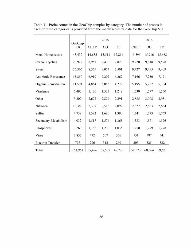
66
Table 3.1.Probe counts in the GeoChip samples by category. The number of probes in
each of these categories is provided from the manufacturer’s data for the GeoChip 5.0
GeoChip
5.0
2015 2016
CHLP OO PP CHLP OO PP
Metal Homeostasis 43,432 14,655 15,511 12,814 15,595 15,916 15,668
Carbon Cycling 26,922 8,951 9,430 7,820 9,720 9,818 9,578
Stress 26,306 8,569 9,073 7,501 9,427 9,495 9,409
Antibiotic Resistance 15,850 6,919 7,202 6,262 7,166 7,250 7,171
Organic Remediation 11,591 4,854 5,085 4,272 5,195 5,282 5,184
Virulence 6,493 1,430 1,523 1,248 1,530 1,577 1,550
Other 5,302 2,672 2,824 2,291 2,885 3,008 2,931
Nitrogen 10,380 2,397 2,516 2,092 2,627 2,663 2,634
Sulfur 4,739 1,582 1,680 1,390 1,741 1,773 1,769
Secondary Metabolism 4,032 1,517 1,574 1,365 1,583 1,571 1,576
Phosphorus 3,260 1,182 1,270 1,035 1,250 1,299 1,278
Virus 2,857 472 507 376 551 587 541
Electron Transfer 797 296 312 260 303 325 332
Total 161,961 55,496 58,507 48,726 59,573 60,564 59,621

67
Figure 3.1. Summary of the gene probe abundance and signals for functional categories
and antibiotic resistance. Relative abundance of the GeoChip categories were based off
the number of probes detected for that category divided by the total number of probes in
each sample (left). The number of probes detected in these categories were summarized
and compared across the two years of sampling (right). We further analyzed these probes
by comparing the mean signal intensities for the gene families across the two years
(inset). Error bars represent the standard deviation for the samples collected from our
three sites.
Metal homeostasis outnumbered the next most abundant gene category, carbon
cycling, by at least 5,000 probes in each sample, about 1.5-fold higher than carbon
cycling. Among these, iron and nickel gene probes were the most abundant (Table C.6).
Notably, genes associated with zinc, arsenic, copper, chromium, mercury, and silver
regulation were also abundant. The majority of metal genes were associated with
transport (either uni- or bi-directional), but with considerable numbers of detoxification
genes (Table C.7). There were few examples of metals genes used for storage or
sequestration in the data. Detoxification genes were only detected for arsenic, copper,
tellurium, chromium, and mercury. The transport genes for metals, however, may also
play a role in regulating the toxicity of metals depending on the concentrations within the

68
cytoplasm. The functional use of the metals in these communities specifically cannot be
inferred simply from their abundance.
Across both years, many similar probes yielded signals which were in the 99.9th
percentile of the data. For example, gene probes for ompR, which is involved in
osmoregulation, yielded some of the highest signals. Additionally, a single fnr gene
associated with oxygen limitation yielded a high signal in the dataset for each year.
Within the stress category, high-affinity phosphorus transporters (pst) showed high
signals for 2015 samples, but not in 2016 samples. In the carbon cycling gene category, a
pectin lyase (pel Cdeg) gene probe yielded one of the higher signals in 2015, while amyA
(amylase) and mcrA (methanogenesis) showed higher signals in 2016. Between the years,
the most prominent metal homeostasis genes changed considerably. The nikA gene
(nickel) had several probes in the 99.9th percentile of signals in 2015 samples, but these
signals were not as rich in 2016 samples. Rather, genes were present for tellurium,
potassium, manganese, and chromium. While all ARGs in the 99.9th percentile of the
2015 samples were MFS transporters, some MATE, Mex, and β-lactamase genes also
yielded high signals in the 2016 sample set. Many of these probes with the high signals
were detected between both years, but rarely were the signals as enriched in both sets.

69
The other families of antibiotic transporters were also highly abundant compared
to the MFS transporters The Mex (RND), ABC transporters, and SMR probes accounted
for the next greatest number of antibiotic resistant probes detected. MATE transporters
were also abundant, but less so than two of the β-lactamase resistance genes. The average
signals of these other transport families were also considerably high relative to many
other genes in the GeoChip. Although few probes were detected, Tet, Van, and the β-
lactamase resistance genes yielded high signals. This likely indicates low diversity, but
high abundance of these genes. However, the evidence suggests that the major
mechanism of antibiotic resistance in the sediments was from efflux-mediated protection.
Like ARGs, nearly half of the organic remediation probes included with the
GeoChip 5.0 were detected across the samples. A vast majority of these probes are
associated with the remediation of aromatic compounds (Figure C.1). Within the
aromatics group, probes were most abundant in the nitroaromatics, carboxylic acid, and
other subgroups. Outside of aromatics, probes were also abundant for the degradation of
herbicide related compounds and chlorinated compounds. Fewer probes were detected for
the pesticide related compounds, but this could also be reflective of the fact that there are
fewer probes for that subcategory. Few notable differences emerged between samples
collected from the two years in terms of the number and type of organic remediation
probes detected. The general trend showed that more probes were detected in 2016
samples in category, which is the opposite of what was observed for antibiotic resistance.
Hierarchal clustering analysis of GeoChip data revealed samples grouped by the
year in which they were collected, not by Ecoregion location (Figure 3.2). This suggests

70
temporal changes dominated differences in ecosystem services as opposed to site
differences, which is remarkable based on expected variation in physical and biotic
features between EcoRegions. In order to assess whether this trend was shared for
individual gene groups, a similar analysis was conducted on ARGs. Of the 9182 total
ARG probes in this analysis, 6689 ARGs were detected across the two years of sampling.
Within the ARGs, 85-91% of probes were shared for 2015 samples; 89-90% were shared
for 2016 samples; while 80-86% were shared by the same site across the two years. Like
the whole microarray analysis, hierarchal clustering of ARG-designated probes revealed
samples clustered by collection year, not location (Figure 3.2). This high degree of
similarity suggests the persistence of many species-specific ARGs in agricultural
drainage channel sediments.
Figure 3.2. Dendrograms of the GeoChip and antibiotic resistance gene hierarchal
clustering. Hierarchal clustering of our samples was performed based on the binary
Jaccard distance matrix for the GeoChip analysis. Clustering was performed based on the

71
entire GeoChip set (black) and with only the ARG probes (red). The relative level of
dissimilarity is printed above the dendrogram.
DNA extracted from 2016 samples were split and analyzed more in-depth by
applying the qPCR Fluidigm platform. Our Fluidigm array successfully quantified 22
genes belonging to antibiotic resistance or metal homeostasis mechanisms (Table C.8).
Gene abundance was expressed per gram of dry sediment per the amount of wet sediment
used for extraction and the volume of elution (Table C.1). The most abundant gene
detected by Fluidigm was the integrase I gene, a marker of mobile genomic elements that
commonly feature ARGs. This gene was present at more than 105 genes per gram of
sediment for each site (Figure 3.3A). Not all the genes detected by GeoChip were
included in the Fluidigm or vice versa, and integrase I was one example which was not
included in the GeoChip. The abundance of genes varied slightly across the set; for
instance, a greater abundance of blaOXA (class D), tetA, and aacA genes was detected in
the PP samples. These represent resistance to three major class of antibiotics – β-lactams,
tetracyclines, and aminoglycosides. However, there were also eight genes detected in the
OO and CHLP samples which were not detected for the PP sample. The merA gene,
providing mercury resistance, was the most abundant of metal homeostasis genes
detected with the Fluidigm analysis.
Also abundant in the Fluidigm set were the mexB and blaSHV (β-lactamase class
A) genes. While the high abundance of mexB is in agreement with the GeoChip data in
terms of probe counts and average signal intensities, the blaSHV appeared consistent with
the signal intensity of β-lactamase A. Several other genes quantified by the Fluidigm were
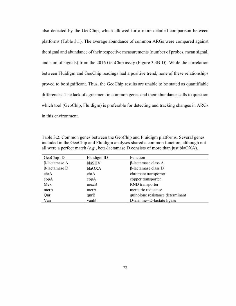
72
also detected by the GeoChip, which allowed for a more detailed comparison between
platforms (Table 3.1). The average abundance of common ARGs were compared against
the signal and abundance of their respective measurements (number of probes, mean signal,
and sum of signals) from the 2016 GeoChip assay (Figure 3.3B-D). While the correlation
between Fluidigm and GeoChip readings had a positive trend, none of these relationships
proved to be significant. Thus, the GeoChip results are unable to be stated as quantifiable
differences. The lack of agreement in common genes and their abundance calls to question
which tool (GeoChip, Fluidigm) is preferable for detecting and tracking changes in ARGs
in this environment.
Table 3.2. Common genes between the GeoChip and Fluidigm platforms. Several genes
included in the GeoChip and Fluidigm analyses shared a common function, although not
all were a perfect match (e.g., beta-lactamase D consists of more than just blaOXA).
GeoChip ID Fluidigm ID Function
β-lactamase A blaSHV β-lactamase class A
β-lactamase D blaOXA β-lactamase class D
chrA chrA chromate transporter
copA copA copper transporter
Mex mexB RND transporter
merA merA mercuric reductase
Qnr qnrB quinolone resistance determinant
Van vanB D-alanine--D-lactate ligase
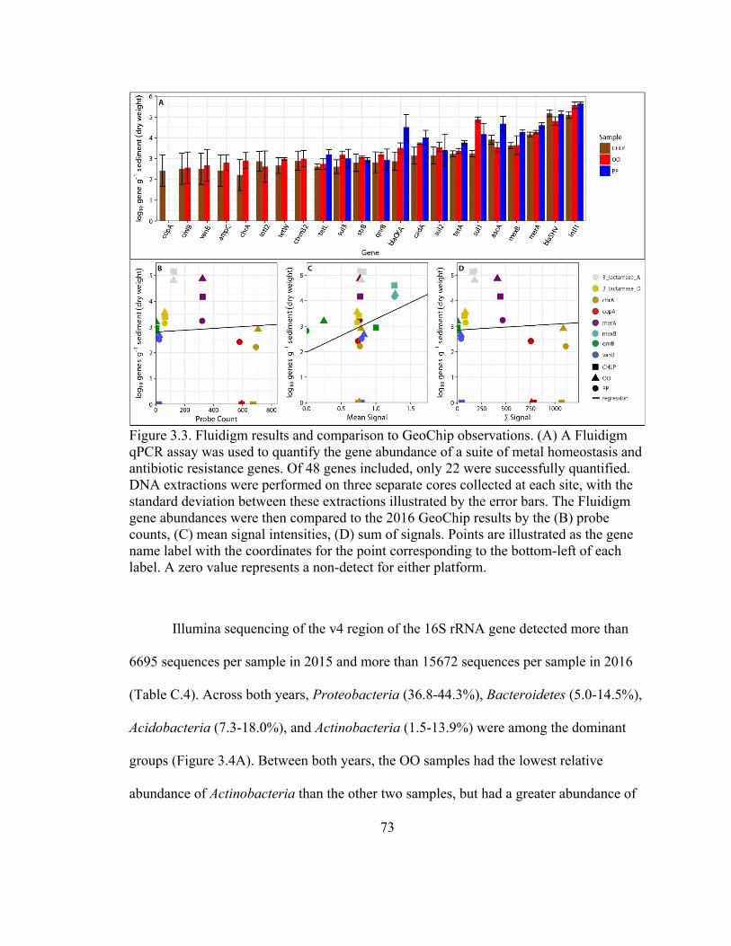
73
Figure 3.3. Fluidigm results and comparison to GeoChip observations. (A) A Fluidigm
qPCR assay was used to quantify the gene abundance of a suite of metal homeostasis and
antibiotic resistance genes. Of 48 genes included, only 22 were successfully quantified.
DNA extractions were performed on three separate cores collected at each site, with the
standard deviation between these extractions illustrated by the error bars. The Fluidigm
gene abundances were then compared to the 2016 GeoChip results by the (B) probe
counts, (C) mean signal intensities, (D) sum of signals. Points are illustrated as the gene
name label with the coordinates for the point corresponding to the bottom-left of each
label. A zero value represents a non-detect for either platform.
Illumina sequencing of the v4 region of the 16S rRNA gene detected more than
6695 sequences per sample in 2015 and more than 15672 sequences per sample in 2016
(Table C.4). Across both years, Proteobacteria (36.8-44.3%), Bacteroidetes (5.0-14.5%),
Acidobacteria (7.3-18.0%), and Actinobacteria (1.5-13.9%) were among the dominant
groups (Figure 3.4A). Between both years, the OO samples had the lowest relative
abundance of Actinobacteria than the other two samples, but had a greater abundance of

74
other, minority phyla. Within their respective years, the OO samples also had a slightly
higher abundance of β-proteobacteria and Nitrospirae than the other samples.
Alternatively, the α-proteobacteria were more prevalent in the CHLP samples, while the
Chloroflexi were more dominant in the PP samples.
Despite the greater number of sequences in 2016, 5377 OTUs were assigned for
the 2016 set compared to 6235 OTUs for 2015. Only 41% (3363/8249) of the OTUs were
shared among years. Either this indicates a dramatic shift in communities between the
years, or is a result of using different sequencing facilities. Sample β-diversity was
compared using Jaccard matrices and hierarchal clustering, revealing 2016 samples
clustered closely together with greater dissimilarity in 2015 microbial community
structure (Figure 3.4B). The lower number of sequence may partially explain this pattern
reads in 2015. There were also differences between these data in terms of the relative
abundance of dominant OTUs (Figure 3.4C). Notably, the more dominant OTUs in the
2016 set were detected at a higher relative abundance compared with the 2015 set. Based
on the number of OTUs compared to sequences detected (Table C.9), the 2015 set did not
reach a sufficient sampling depth to detect all species present in the microbiome. Still,
there were many similarities between the phylum-level structure detected between years
at the same sampling site.

75
Figure 3.4. Illumina sequencing on the v4 region of the 16S rRNA gene was performed
on sediment DNA. (A) The taxonomic composition of the samples was compared at the
phyla level, differentiating between the subphyla of the Proteobacteria. (B) Hierarchal
clustering of these sequences was performed using the binary Jaccard distance matrix
with the relative dissimilarity shown above the dendrogram. (C) A rank abundance curve
was generated with the average abundance and standard deviation of the ranks for the
three samples collected from each year of sampling.
The GeoChip uses species-specific probes that revealed phylogenetic information
about detected ARGs. This allowed for an in-silico comparison between resistant taxa
detected in GeoChip and 16S rRNA gene analyses. The number of organisms ranged
between 1,175-1,301 per GeoChip sample (Table 3.3). However, the in-silico sets of
these organisms were condensed down to 743-795 OTUs clustered at 97% similarity. In

76
other words, many of the species included in the GeoChip could not be differentiated
between related member at the OTU97 level. By number of organisms in these ARG sets,
~17% had a matching OTU in the 2015 16S samples, while ~29% had a matching OTU
in the 2016 16S samples. However, only 10% or 19% of the ARG OTUs corresponded to
a 16S rRNA gene sequence OTU in the 2015 and 2016 samples, respectively. In other
words, many of the organisms tagged to the GeoChip ARG probes were not detected by
16S rRNA gene sequencing. Most of those community members detected through
targeting the 16S rRNA gene analysis could account for multiple probes in the GeoChip
data. Or in other words, multiple species included in the GeoChip are classified to the
same OTU at a 97% similarity.
Table 3.3. Shared GeoChip ARG lineages with taxonomies detected by Illumina
sequencing. The number of GeoChip taxa associated with the ARGs, having a match in
the SILVA database, are shown. An in-silico sequence file was developed for each
sample. The number of taxa with a match to the Illumina set for each sample was
calculated, as well as the percent of those with a match. Many of these taxa were
clustered into the same OTU, and again the number of matched OTUs were calculated.
2015 2016
CHLP OO PP CHLP OO PP
GeoChip Taxa 1230 1258 1175 1279 1301 1268
Match in 16S rRNA gene 213 216 206 372 368 371
Percent Matched 17% 17% 18% 29% 28% 29%
GeoChip OTU97 778 795 743 763 781 766
Match in 16S rRNA gene OTU97 77 78 76 146 148 148
Percent Matched 10% 10% 10% 19% 19% 19%

77
Many of the unmatched taxa belonged to genera that were detected by Illumina
sequencing. Between 41.5-43% of the unmatched OTUs in 2015 samples and 28.8-30.0%
in 2016 were related to a genus present in the Illumina set. The abundance of unmatched
taxa was predominantly found in the Gammaproteobacteria, Alphaproteobacteria,
Actinobacteria, Betaproteobacteria, and Deltaproteobacteria (Figure 3.5). Many of these
groups were better represented in the more deeply sequenced 2016 sample set, which
may explain the drop in unmatched taxa. The fact that many of these taxa had a related
genus member detected in the Illumina sequences makes it surprising that they
themselves were not detected, although this discrepancy may also have been imparted
from amplification and sequencing errors leading to the assignment of closely-related
genera.
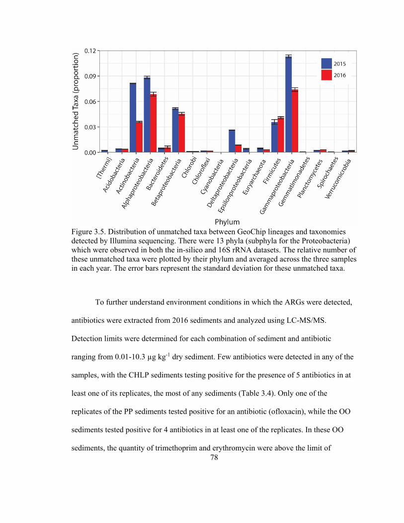
78
Figure 3.5. Distribution of unmatched taxa between GeoChip lineages and taxonomies
detected by Illumina sequencing. There were 13 phyla (subphyla for the Proteobacteria)
which were observed in both the in-silico and 16S rRNA datasets. The relative number of
these unmatched taxa were plotted by their phylum and averaged across the three samples
in each year. The error bars represent the standard deviation for these unmatched taxa.
To further understand environment conditions in which the ARGs were detected,
antibiotics were extracted from 2016 sediments and analyzed using LC-MS/MS.
Detection limits were determined for each combination of sediment and antibiotic
ranging from 0.01-10.3 µg kg-1 dry sediment. Few antibiotics were detected in any of the
samples, with the CHLP sediments testing positive for the presence of 5 antibiotics in at
least one of its replicates, the most of any sediments (Table 3.4). Only one of the
replicates of the PP sediments tested positive for an antibiotic (ofloxacin), while the OO
sediments tested positive for 4 antibiotics in at least one of the replicates. In these OO
sediments, the quantity of trimethoprim and erythromycin were above the limit of
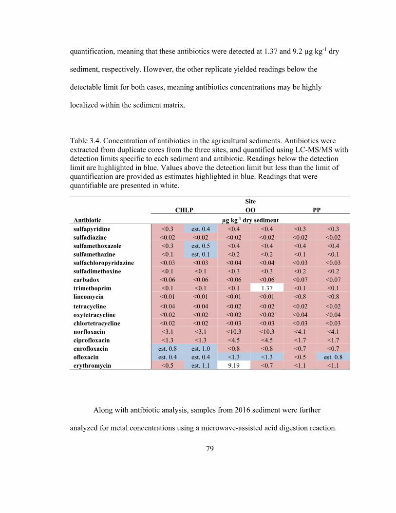
79
quantification, meaning that these antibiotics were detected at 1.37 and 9.2 µg kg-1 dry
sediment, respectively. However, the other replicate yielded readings below the
detectable limit for both cases, meaning antibiotics concentrations may be highly
localized within the sediment matrix.
Table 3.4. Concentration of antibiotics in the agricultural sediments. Antibiotics were
extracted from duplicate cores from the three sites, and quantified using LC-MS/MS with
detection limits specific to each sediment and antibiotic. Readings below the detection
limit are highlighted in blue. Values above the detection limit but less than the limit of
quantification are provided as estimates highlighted in blue. Readings that were
quantifiable are presented in white.
Antibiotic
Site
CHLP OO PP
µg kg-1 dry sediment
sulfapyridine <0.3 est. 0.4 <0.4 <0.4 <0.3 <0.3
sulfadiazine <0.02 <0.02 <0.02 <0.02 <0.02 <0.02
sulfamethoxazole <0.3 est. 0.5 <0.4 <0.4 <0.4 <0.4
sulfamethazine <0.1 est. 0.1 <0.2 <0.2 <0.1 <0.1
sulfachloropyridazine <0.03 <0.03 <0.04 <0.04 <0.03 <0.03
sulfadimethoxine <0.1 <0.1 <0.3 <0.3 <0.2 <0.2
carbadox <0.06 <0.06 <0.06 <0.06 <0.07 <0.07
trimethoprim <0.1 <0.1 <0.1 1.37 <0.1 <0.1
lincomycin <0.01 <0.01 <0.01 <0.01 <0.8 <0.8
tetracycline <0.04 <0.04 <0.02 <0.02 <0.02 <0.02
oxytetracycline <0.02 <0.02 <0.02 <0.02 <0.04 <0.04
chlortetracycline <0.02 <0.02 <0.03 <0.03 <0.03 <0.03
norfloxacin <3.1 <3.1 <10.3 <10.3 <4.1 <4.1
ciprofloxacin <1.3 <1.3 <4.5 <4.5 <1.7 <1.7
enrofloxacin est. 0.8 est. 1.0 <0.8 <0.8 <0.7 <0.7
ofloxacin est. 0.4 est. 0.4 <1.3 <1.3 <0.5 est. 0.8
erythromycin <0.5 est. 1.1 9.19 <0.7 <1.1 <1.1
Along with antibiotic analysis, samples from 2016 sediment were further
analyzed for metal concentrations using a microwave-assisted acid digestion reaction.

80
ICP-OES analysis was performed to quantify the concentration of 28 metal/metalloids
(Table 3.4). Nine of these elements were present at the order of g kg-1 dry sediment,
while the others were in the range mg kg-1 dry sediment. Several of the analyzed elements
harbor some known level of toxicity to microorganisms (e.g. Zn, Ni, Chromium, etc.).
Genes involved in the detoxification or transport of these metals, as well as some that
were not quantified (e.g. Hg and Ag), were detected by the GeoChip (Table C.3). Direct
detoxification, or the transport of these metals out of cell could provide resistance to
these toxic effects. Notably, the concentrations of nickel, zinc, chromium, and copper
were relatively elevated compared to the other metals, while the number of probe counts
specific to the detoxification/transports of these metals were similarly high (Figure C.2).
Detoxification genes were detected for arsenic, copper, tellurium, chromium, and
mercury, with the highest number detected in arsenic, tellurium, and mercury. While
these metals had a low concentration, and mercury was not detected by our analysis, the
abundance of detoxification genes could indicate that these are toxic levels for those
metals.

81
Table 3.5. Concentrations of trace elements extraction from the sediments. Sediments
from each site were run in duplicate and readings were performed using ICP-OES
following microwave-assisted digestion. Values below the detection limit are presented
as <DL, and values below the limit of quantification are listed as estimated values.
Analyte
Site
CHLP OO PP
g kg-1 dry sediment
Ca 60.6 81.4 22.9 22.5 31.3 29.4
Al 18.2 17.3 26.0 24.9 32.6 34.2
Fe 18.6 16.6 22.9 22.4 23.2 23.7
Mg 22.7 30.5 11.4 11.3 12.2 12.0
K 6.5 6.6 5.6 5.4 12.3 13.0
Si 1.6 1.5 1.6 1.4 1.7 1.6
Mn 0.6 0.6 1.8 1.6 0.7 0.7
P 0.5 0.6 1.5 1.4 0.7 0.7
S 0.5 0.6 1.4 1.4 0.4 0.4
mg kg-1 dry sediment
Na 249.4 295.3 228.0 238.1 382.1 405.0
Ba 115.1 130.9 251.6 241.4 171.3 181.1
Zn 67.6 93.0 131.2 125.2 69.9 72.2
Sr 112.8 129.6 55.9 54.6 65.1 65.0
V 45.7 42.2 57.7 56.2 70.0 72.6
Cr 20.9 19.9 33.1 32.1 37.0 38.6
Ni 24.5 23.9 27.3 26.2 34.9 35.9
Cu 20.4 43.6 27.8 26.9 26.2 22.8
Li 19.5 19.7 25.7 24.6 36.3 38.2
B 17.0 25.6 14.1 13.2 44.0 47.4
Pb 15.2 13.6 20.5 20.7 13.9 14.0
Co 10.9 9.0 11.4 10.9 14.7 15.5
As 10.6 7.9 9.1 8.9 7.0 7.4
Mo 7.0 6.0 2.1 2.4 5.1 4.6
Se 2.0 1.8 3.0 3.5 <0.9 <0.9
Tl est. 1.0 2.3 4.6 1.8 <0.05 1.2
Cd 1.7 1.5 2.5 2.4 1.9 1.9
Sb est. 0.7 est. 0.8 est. 0.7 <0.4 est. 1.0 1.5
Be <0.9 <0.9 <0.9 <0.9 <0.9 <0.9
82
Discussion
Agricultural drainage channels frequently fail due to the accumulation of
sediments that impede hydrological flows necessary for productive crop yields. The
formation of floodplains by these sediments have been envisioned as the basis for
reengineering drainage channels that incorporates these floodplains by widening of the
channel. The benefits from these two-stage channels include microbial processes, like
denitrification, that help to attenuate nutrient loads (Roley et al., 2012). We characterized
the functional potential of these microbial ecosystems more thoroughly using the
GeoChip 5.0 microarray, which has been used to broadly characterize the diversity of
functional genes in many environments, including urban/forested rivers (Low et al.,
2016) and wastewater bioreactors (Sun et al., 2016). It should be noted that in both of the
above-mentioned environments, the antibiotic resistance genes had many positive gene
probes and relatively high signals that made them the focus of their respective studies
(Low et al., 2016; Sun et al., 2016). The similarities between our results and those of Low
et al. (2016) are striking in that MFS antibiotic resistance genes were the most diverse
probe in the array. While Low et al. (2016) observed 4887 MFS probes (6.6% relative
abundance), we observed 4077 (6.9% relative abundance) and 3911 (6.4% relative
abundance) for our 2015 and 2016 datasets, respectively. This shows a high degree of
similarity between the ARGs of agricultural drainage sediments in Ohio with the river
sediments of the urban and forested environment of Singapore. Our GeoChip analysis
revealed that the sediments of agricultural drainage floodplains host a high diversity of
antibiotic resistance, primarily related to MFS transporters.

83
Antibiotic resistance can be propagated through migration and horizontal gene
transfer in addition to selective pressure (Niehus et al., 2015). ARGs are notorious for
being transferred, mediated through conjugation or phage, or carried on plasmids with
metal homeostasis genes (Li et al., 2015; Niehus et al., 2015). The persistence of ARGs at
the study sites described in this chapter as well as the potential for their spread to
downstream locations can be better understood through future exploration into the
mechanisms of selection, horizontal gene transfer, and migration of ARGs in sediments.
Not only were ARGs detected in sediments for three EcoRegions draining to Lake
Erie, but they remained present the year following their initial detection. In many cases,
the same ARG probes were detected in both years, indicating a persistence of these genes
at specific sampling locations. Yet, despite recurring detection of ARGs, there was little
evidence of antibiotics accumulated in sediment samples. Antibiotics detected in one or
more sediment samples (e.g. ofloxacin, enrofloxacin) were often below the limit of
quantification, on the order of 1 g/kg. Therefore, we cannot ascribe persistence of ARGs
to active selective pressure by antibiotics across the three sites. However, antibiotic
resistance can be co-selected with metal homeostasis genes, which were also highly
abundant in our sediments (Baker-Austin et al., 2006). Therefore, selection might be due
to the presence of metals in the sediment which led to co-selection of these ARGs.
In our survey of metals and metalloids in these sediments, several were detected
in all three sampling sites at concentrations approaching toxic levels for soil
microorganisms (Giller et al., 1998). For example, case studies have found cadmium,
zinc, lead, and nickel to exert some measurable toxicity (i.e., depressed soil respiration) at

84
levels of ≥ 10 mg kg-1 dry soil (Giller et al., 1998). Zinc, lead, and nickel were all well
above this level in the site sediments. In the case of zinc, concentrations were 6 to 13-fold
higher than levels know to exhibit measurable toxicity, suggesting considerable metal
toxicity may exist in these sediments. Gene probes for nickel, copper, and zinc
detoxification/transport, capable of providing resistance to metal toxicity in soil
microorganisms (Akhtar et al., 2013), were abundant in the dataset. Similarly, arsenic and
silver detoxification/transport genes were also abundant, although it is hard to define the
toxicity of these compounds without further distinguishing the forms of these elements
(e.g., redox of As; particle size of Ag) (Akhtar et al., 2013; Schlich et al., 2013). The
quantity of the metals, and the presence of detoxification/transport genes combine to
support the notion that metals could be one reason for the selection for antibiotic
resistance genes in the microbial community.
Combining our analysis of metals with antibiotics, the internal pressure within the
system for ARG selection may be applied by the metals. While antibiotics have been
shown to quickly degrade in soils, metals persist as there is no manner to remove them
from the system (Chee-Sanford et al., 2009; Hu et al., 2016). A common pathway in
which ARGs are introduced to agroecosystems is through manure application (Davies
and Davies, 2010; Udikovic-Kolic et al., 2014). To our knowledge, the fields adjacent to
our streams were not using manure-based fertilizers making this pathway dubious.
However, since metals may be introduced through inorganic fertilizers or pesticides
(Gimeno-García et al., 1996), the detected concentrations of metals are a much more
likely explanation for the abundance of ARGs in our samples. Recently, Hu et al. (2016)

85
demonstrated that nickel additions to agricultural soils resulted in the enrichment of
ARGs, including multidrug resistant genes, in fields which had no known contact with
organic fertilizers. Notably, the nickel concentrations applied in that experiment far
exceeded the concentrations of nickel measured in our sediments (>50 compared to <40
mg Ni kg-1 soil). Thus, further evaluation is needed to elucidate the toxicity levels of
metals in regard to selecting for ARGs.
In addition to metals and antibiotics, other organic compounds may be responsible
for the selection of antibiotic resistance. Organic residues may act as biocides for some
microorganisms, with antibiotic resistant organisms holding some advantage to
susceptible organisms (Pal et al., 2015; Romero et al., 2017). Recently, the mutation of
bacteria with a pesticide degrading gene revealed the selection of multidrug resistant
organisms following the exposure of soils to toxic levels of pesticides (Rangasamy et al.,
2017). Although in this case the degradation gene provided resistance to the
microorganisms, it could still be rationally argued that transport genes may have the
potential to interact with toxic levels of pesticides or other organic residues (Pal et al.,
2015; Romero et al., 2017). The abundance of organic remediation probes detected by the
GeoChip may also indicate regular exposure to these compounds in the sediments. Like
metals, the organic components of our sediments should be studied in more detail to
elucidate their potential to co-select for antibiotic resistant organisms.
While selection may be occurring, there is also evidence that could support the
case for horizontal gene transfer of the ARGs. Specifically, the intlI gene was detected at
the highest abundance of all genes included in the Fluidigm qPCR analysis. Class I

86
integrases provide the functionality for recombination for ARGs carried by plasmids or
other mobile genomic elements (Goldstein et al., 2001). Thus, there should be some
concern over the spread of ARGs within the agricultural floodplains. Due to this high
abundance of intlI, it was important to determine whether the organisms identified by the
GeoChip would be also be detected by 16S rRNA sequencing.
The same DNA extracts used in the GeoChip and Fluidigm analyses were also
used for lllumina sequencing of the 16S rRNA gene sequencing for both years. Notably,
analysis of the 16S gene sequences revealed a much more disparate community compared
to the GeoChip microarray. In other words, the functionality between our sampling
locations and between years were much more similar to one another than the community
members revealed by Illumina sequencing. To compare the phylogenetic information
contained in the GeoChip to the 16S analysis we first had to generate an in-silico set of
16S DNA from the SILVA database and process that through QIIME to account for the
0.97 clustering of our reference database used to pick OTUs. Through this simulation,
less than 30% of the GeoChip taxa were identified in the actual 16S analysis results, a
rather poor overlap. Eighteen phyla (including subphyla for Proteobacteria) were shared
between both the 16S and GeoChip OTUs. Notably, three Proteobacteria subphyla (α-/β-
/γ-), Actinobacteria, and Firmicutes were the phyla which contained the greatest number
of unexplained taxa matched between the GeoChip and 16S data. Known biases have
found the v4 region – covered by our sequencing primers - to limit the detection of
Actinobacteria and Verrucomicrobia through our Illumina sequencing method (Guo et
al., 2015). While we could account for the lack of matches in Actinobacteria from primer
87
bias, we are unable to explain the lack of matches for the other phyla. Since ARGs are
known to be highly mobile, the lack of matches between Illumina sequences and the in-
silico GeoChip set may be accounted for due to other organisms harboring these genes
than those that are assigned to the probes. Combining the abundance of intI with the lack
of matches between the 16S community members and GeoChip taxa may reveal that
ARGs were highly mobilized in these sediments or the ecosystem from which the
sediments originated. Therefore, future analyses should consider screening the cultivable
microbial community to identify those which demonstrate antibiotic resistance.
The presence, persistence, and fate of ARGs in our agricultural drainage ways is
of major concern because of the threat that antibiotic resistance poses as a health concern
to downstream human communities. However, it is important to also consider that the
majority of the ARGs exposed by our analysis were the MFS transport systems. Efflux-
mediated resistance does not necessarily mean that an organism has resistance to
antibiotic at a clinical level, but in these systems, can provide resistance to a greater range
of compounds (Kumar et al., 2013). Cultivation methods could be applied to decipher the
level of resistance of the organisms in our sediments, such as was performed by Low et
al. (2016). Another important fact to consider is that the development of two-stage
channels is to attenuate the sediment loads reaching downstream waters (Jayakaran et al.,
2010). Perhaps then these systems could limit the transport of ARGs to downstream
waters, if they are capturing antibiotic resistant organisms attached to sediments. The
continued presence of ARGs at these sites, though, also means that these sediments could
act as a reservoir of these genes in the environment.

88
Conclusions
The purpose of the research covered by this dissertation was to gain a better
understanding of pollutants in the Lake Erie watershed. Although the drainage basins
sampled in this dissertation represent a minor fraction draining into this important Great
Lake, the data and analyses performed here have applicability to world issues and could
be used in other watersheds experiencing eutrophication and harmful algal bloom issues.
Agricultural pollution is a problem across the world and the issues presented here are not
isolated to Lake Erie or North America.
The objective of Chapters 1 and 2 was to examine develop a protocol that could
be used to distinguish between sources of nutrient pollution and monitor for their
presence in the Lake Erie watershed. New information is need by regional managers to
identify the leading sources so that management practices can be targeted at the leading
sources. In Chapter 1, disparate organic matter and organic phosphorus signatures were
characterized for several point and nonpoint sources. Marker m/z values were proposed to
help discriminate between these sources. In Chapter 2, we analyzed the transport of DOM
through the tributary network. DOM was highly similar throughout the watershed,
although broad characteristics changed considerably. We found that the most prominent
features were more consistently detected during their transport from upstream to
downstream samples. Additionally, the DOM spectra appeared to mix linearly at several
confluence points. The data from these chapters suggest that DOM can differentiate the
source of its origin. However, we discovered that the most prominent m/z values were
reliably detected through its transport. Since the original markers proposed for tracking

89
pollutant sources were typically detected with low peak magnitudes, tour selection
process of markers should be reevaluated to seek marker DOM more likely to be detected
throughout the watershed during transport. Marker compounds could be expanded to
include compounds other than just DOP, which should provide more options through the
inclusion of the abundant CHO and CHON formulae.
In Chapter 3, sediments collected from agricultural floodplains developing within
drainage channels contained many ARGs. It is difficult to define the abundance of these
genes as different technologies showed a disagreement between each other. It appears
that there is a high diversity of MFS antibiotic transport genes in these sediments. There
must be further work to elucidate the abundance of these genes, but that will require
greater research into the interpretation of results obtained through different technologies.
The presence of integrase genes suggested the potential for HGT or mobilization of
ARGs in our floodplains, and the lack of matching taxa in the 16S to GeoChip datasets
suggests these genes have already been transferred to other microbial community
members. Few antibiotics were detected in our sediments, and so we argue that selection
must be occurring through some other mechanism. It is reasonable to believe that MFS
transporters may instead be co-selected for due to the presence of metals at putatively
toxic concentrations. Seemingly high abundance of metal resistance genes further
supports this theory. Concern should be given to the presence of these ARGs in
agricultural channels, but we must gain a better understanding over how these genes
arrived at these sediments, why they may persist, and how they may be transported
further downstream.

90
Our analyses were used to better define a well-known and established issue
focused on the eutrophication of Lake Erie through nutrient loads, but also may have
exposed that the tributaries may act as conduits for antibiotic resistance. The analysis of
DOM shows some promise in being able to identify the presence of source
contamination. Continued development of this approach could hold value to the Lake
Erie watershed, but also to coastal areas like the Gulf of Mexico or Chesapeake Bay
when distinguishing sources of nutrient pollution is necessary. Alternatively, we present
evidence that antibiotic resistance must be monitored for its transport through waterways
as these genes present a rising health concern.
Future research needs to improve upon the results and conclusions drawn from the
research presented here. In terms of the mass spectrometric analysis, the signatures were
characterized for only a few of the many sources in the regions. The analysis could be
expanded to include other sources of concern (CSOs, septic tanks, lawns, etc.) and runoff
from manure-fertilized fields. This research could improve our knowledge over the
signatures to look for in this, or other nutrient-impaired waterways. Additionally, the
understanding of transport and mixing of DOM could be improved through controlled
laboratory and field experiments. For example, direct mixing of sample could be
performed in the laboratory while organic nitrogen and phosphorus compounds could be
added as tracers in the natural environment. For antibiotic resistance, value would be
added from the cultivation and phenotyping of the microorganisms in the sediments.
Specifically, antibiotic resistant pathogens should be targeted as they pose the greatest
threat to human health. Finally, the origin, transport, and fate of antibiotic resistance in
91
agricultural waters should be studied more in depth. For example, while we demonstrate
that the sediments in the channels were enriched with antibiotic resistance we do not
know whether this is acting as a sink or source for further downstream transport. Field
studies should be designed to answer whether these systems are removing antibiotic
resistant organisms from downstream transport, the localized selection for or against
antibiotic resistance within the sediments, and the potential for antibiotic resistance to be
dispersed during flow events. My future research will explore many of these areas under
the common theme of exploring agricultural contaminants.

92
References
Adams M.M., M.R. Gomez-Garcia, A.R. Grossman and D. Bhaya. 2008. Phosphorus
deprivation responses and phosphonate utilization in a thermophilic Synechococcus
sp. from microbial mats. J. Bacteriol. 190:8171-84.
Akhtar M.S., B. Chali and T. Azam. 2013. Bioremediation of arsenic and lead by plants
and microbes from contaminated soil. Research in Plant Sciences 1:68-73.
Altschul S.F., W. Gish, W. Miller, E.W. Myers and D.J. Lipman. 1990. Basic local
alignment search tool. J. Mol. Biol. 215:403-10.
Arango C.P., J.L. Tank, J.L. Schaller, T.V. Royer, M.J. Bernot and M.B. David. 2007.
Benthic organic carbon influences denitrification in streams with high nitrate
concentration. Freshwat. Biol. 52:1210-1222.
Arnold W.A., K. Longnecker, K.D. Kroeger and E.B. Kujawinski. 2014. Molecular
signature of organic nitrogen in septic-impacted groundwater. Environ. Sci. :
Processes Impacts2400.
Aronesty E. 2013. Comparison of sequencing utility programs. The Open Bioinformatics
Journal 7:.
93
Baker D. 2011. The sources and transport of bioavailable phosphorus to lake erie. 1-30.
Baker D. 2010. Trends in bioavailable phosphorus loading to lake erie. 1-21.
Baker D.B., R. Confesor, D.E. Ewing, L.T. Johnson, J.W. Kramer and B.J. Merryfield.
2014. Phosphorus loading to lake erie from the maumee, sandusky and cuyahoga
rivers: The importance of bioavailability. J. Great Lakes Res. 40:502-517.
Baker-Austin C., M.S. Wright, R. Stepanauskas and J.V. McArthur. 2006. Co-selection
of antibiotic and metal resistance. Trends Microbiol. 14:176-182.
Baldwin D.S. 1998. Reactive “organic” phosphorus revisited. Water Res. 32:2265-2270.
Banerjee S. and S. Mazumdar. 2012. Electrospray ionization mass spectrometry: A
technique to access the information beyond the molecular weight of the analyte.
International Journal of Analytical Chemistry 2012:.
Barthold F.K., C. Tyralla, K. Schneider, K.B. Vaché, H. Frede and L. Breuer. 2011. How
many tracers do we need for end member mixing analysis (EMMA)? A sensitivity
analysis. Water Resour. Res. 47:.
Bartos J.M., B.L. Boggs, J.H. Falls and S.A. Siegel. 2014. Determination of phosphorus
and potassium in commercial inorganic fertilizers by inductively coupled plasma-
optical emission spectrometry: Single-laboratory validation. J. AOAC Int. 97:.

94
Berg A.S. and B.C. Joern. 2006. Sorption dynamics of organic and inorganic phosphorus
compounds in soil. J. Environ. Qual. 35:.
Bhatia M.P., S.B. Das, K. Longnecker, M.A. Charette and E.B. Kujawinski. 2010.
Molecular characterization of dissolved organic matter associated with the greenland
ice sheet. Geochim. Cosmochim. Acta 74:3768-3784.
Bjorkman K.M. and D.M. Karl. 2003. Bioavailability of dissolved organic phosphorus in
the euphotic zone at station ALOHA, north pacific subtropical gyre. Limnology and
Oceanography 48:1049-1057.
Boye K., V. Noel, S.E. Bone, J.R. Bargar, K. Boye, S. Fendorf, M.M. Tfaily and K.H.
Williams. 2017. Thermodynamically controlled preservation of organic carbon in
floodplains. Nature Geoscience 10:415-419.
Brooker M.R., G. Bohrer and P.J. Mouser. 2014. Variations in potential CH4 flux and
CO2 respiration from freshwater wetland sediments that differ by microsite location,
depth and temperature. Ecological Engineering 72:84-94.
Brooker M.R. 2018. Physical and chemical characterization of self-developing
agricultural floodplains. The Ohio State University, .
Caporaso J.G., C.L. Lauber, W.A. Walters, D. Berg-Lyons, J. Huntley, N. Fierer, S.M.
Owens, J. Betley, L. Fraser, M. Bauer, N. Gormley, J.A. Gilbert, G. Smith and R.
95
Knight. 2012. Ultra-high-throughput microbial community analysis on the illumina
HiSeq and MiSeq platforms. Isme 6:.
Caporaso J.G., J. Kuczynski, J. Stombaugh, K. Bittinger, F.D. Bushman, E.K. Costello,
N. Fierer, A.G. Pena, J.K. Goodrich, J.I. Gordon, G.A. Huttley, S.T. Kelley, D.
Knights, J.E. Koenig, R.E. Ley, C.A. Lozupone, D. McDonald, B.D. Muegge, M.
Pirrung, J. Reeder, J.R. Sevinsky, P.J. Tumbaugh, W.A. Walters, J. Widmann, T.
Yatsunenko, J. Zaneveld and R. Knight. 2010. QIIME allows analysis of high-
throughput community sequencing data. Nature Methods 7:.
Center for Disease Dynamics, Economics & Policy. 2015. State of the world’s
antibiotics. CDDEP, Washington, D.C.
Chee-Sanford J.C., R.I. Aminov, I.J. Krapac, N. Garrigues-Jeanjean and R.I. Mackie.
2001. Occurrence and diversity of tetracycline resistance genes in lagoons and
groundwater underlying two swine production facilities. Appl. Environ. Microbiol.
67:1494-1502.
Chee-Sanford J.C., R.I. Mackie, S. Koike, I.G. Krapac, Y.F. Lin, A.C. Yannarell, S.
Maxwell and R.I. Aminov. 2009. Fate and transport of antibiotic residues and
antibiotic resistance genes following land application of manure waste. J. Environ.
Qual. 38:.

96
Cong J., H. Lu, D. Li, Y. Zhang, J. Cong, X. Liu, H. Xu, Y. Li and Y. Deng. 2015.
Analyses of the influencing factors of soil microbial functional gene diversity in
tropical rainforest based on GeoChip 5.0. Genomics Data 5:397-398.
Conley D.J., H.W. Paerl, R.W. Howarth, D.F. Boesch, S.P. Seitzinger, K.E. Havens, C.
Lancelot and G.E. Likens. 2009. Controlling eutrophication: Nitrogen and
phosphorus. Science 123:1014-1015.
Conroy J.D., L. Boegman, H. Zhang, W.J. Edwards and D.A. Culver. 2011. "Dead zone"
dynamics in lake erie: The importance of weather and sampling intensity for
calculated hypolimnetic oxygen depletion rates. Aquat. Sci. 73:289-304.
Cooper W.T., J.M. Llewelyn, G.L. Bennett and V.J.M. Salters. 2005. Mass spectrometry
of natural organic phosphorus. Talanta 66:348-358.
Dabdoub S.M., M.L. Fellows, A.D. Paropkari, M.R. Mason, S.S. Huja, A.A. Tsigarida
and P.S. Kumar. 2016. PhyloToAST: Bioinformatics tools for species-level analysis
and visualization of complex microbial datasets. Scientific Reports 6:29123.
Davies J. and D. Davies. 2010. Origins and evolution of antibiotic resistance. Microbiol.
Mol. Biol. Rev. 74:417-433.
DeSantis T.Z., P. Hugenholtz, N. Larsen, M. Rojas, E.L. Brodie, K. Keller, T. Huber, D.
Dalevi, P. Hu and G.L. Andersen. 2006. Greengenes, a chimera-checked 16S rRNA
97
gene database and workbench compatible with ARB. Appl. Environ. Microbiol.
72:5069-72.
Doctor D.H., E.C. Alexander, M. Petrič, J. Kogovšek, J. Urbanc, S. Lojen and W.
Stichler. 2006. Quantification of karst aquifer discharge components during storm
events through end-member mixing analysis using natural chemistry and stable
isotopes as tracers. Hydrogeol. J. 14:1171-1191.
Dodd R.J. and A.N. Sharpley. 2015. Recognizing the role of soil organic phosphorus in
soil fertility and water quality. Resources, Conservation and Recycling 105:282-293.
Douglass J.F., M. Radosevich and O.H. Tuovinen. 2015. Molecular analysis of atrazine-
degrading bacteria and catabolic genes in the water column and sediment of a
created wetland in an agricultural/urban watershed. Ecol. Eng. 83:405-412.
Elsbury K.E., A. Paytan, N.E. Ostrom, C. Kendall, M.B. Young, K. McLaughlin, M.E.
Rollog and S. Watson. 2009. Using oxygen isotopes of phosphate to trace
phosphorus sources and cycling in lake erie. Environ. Sci. Technol. 43:3108-14.
Elsenbeer H., D. Lorieri and M. Bonell. 1995. Mixing model approaches to estimate
storm flow sources in an overland flow‐dominated tropical rain forest catchment.
Water Resour. Res. 31:2267-2278.
Feng L., J. Xu, S. Kang, X. Li, Y. Li, B. Jiang and Q. Shi. 2016. Chemical composition
of microbe-derived dissolved organic matter in cryoconite in tibetan plateau glaciers:

98
Insights from fourier transform ion cyclotron resonance mass spectrometry analysis.
Environ. Sci. Technol. 50:13215-13223.
Frey S.K., E. Topp, I.U. Khan, B.R. Ball, M. Edwards, N. Gottschall, M. Sunohara and
D.R. Lapen. 2015. Quantitative campylobacter spp., antibiotic resistance genes, and
veterinary antibiotics in surface and ground water following manure application:
Influence of tile drainage control. Sci. Total Environ. 532:138-153.
Ghosh S. and T.M. LaPara. 2007. The effects of subtherapeutic antibiotic use in farm
animals on the proliferation and persistence of antibiotic resistance among soil
bacteria. ISME Journal 1:191-203.
Giller K.E., E. Witter and S.P. Mcgrath. 1998. Toxicity of heavy metals to
microorganisms and microbial processes in agricultural soils: A review. Soil Biol.
Biochem. 30:1389-1414.
Gimeno-García E., V. Andreu and R. Boluda. 1996. Heavy metals incidence in the
application of inorganic fertilizers and pesticides to rice farming soils.
Environmental Pollution 92:19-25.
Goldstein C., M.D. Lee, S. Sanchez, C. Hudson, B. Phillips, B. Register, M. Grady, C.
Liebert, A.O. Summers, D.G. White and J.J. Maurer. 2001. Incidence of class 1 and
2 integrases in clinical and commensal bacteria from livestock, companion animals,
and exotics. Antimicrob. Agents Chemother. 45:723-726.
99
Gonsior M., M. Zwartjes, W.J. Cooper, W. Song, K.P. Ishida, L.Y. Tseng, M.K. Jeung,
D. Rosso, N. Hertkorn and P. Schmitt-Kopplin. 2011. Molecular characterization of
effluent organic matter identified by ultrahigh resolution mass spectrometry. Water
Res. 45:2943-2953.
Guo J., J.R. Cole, Q. Zhang, C.T. Brown and J.M. Tiedje. 2015. Microbial community
analysis with ribosomal gene fragments from shotgun metagenomes. Appl. Environ.
Microbiol. 82:157-166.
Hansman R.L., T. Dittmar and G.J. Herndl. 2015. Conservation of dissolved organic
matter molecular composition during mixing of the deep water masses of the
northeast atlantic ocean. Mar. Chem. 177:288-297.
Hobman J.L. and L.C. Crossman. 2015. Bacterial antimicrobial metal ion resistance. J.
Med. Microbiol. 64:471-497.
Hu H., J. Wang, J. Li, X. Shi, Y. Ma, D. Chen and J. He. 2016. Long-term nickel
contamination increases the occurrence of antibiotic resistance genes in agricultural
soils. Environ. Sci. Technol. 51:790-800.
Hudson N., A. Baker and D. Reynolds. 2007. Fluorescence analysis of dissolved organic
matter in natural, waste and polluted waters—a review. River Research and
Applications 23:631-649.

100
Jayakaran A.D., D.E. Mecklenburg, J.D. . Witter, A.D. Ward and G.E. and Powell. 2010.
Fluvial processes in agricultural ditches inthe north central region of the united states
and implica-tions for their management. p. 195-222. In M.T. Moore and R. and
Kroger (eds.) Agricultural DrainageDitches: Mitigation wetlands for the 21st
century. Research Signpost, Karala, India.
Johnson T.A., R.D. Stedtfeld, Q. Wang, J.R. Cole, S.A. Hashsham, T. Looft, Y.G. Zhu
and J.M. Tiedje. 2016. Clusters of antibiotic resistance genes enriched together stay
together in swine agriculture. mBio 7:02214-15.
Kamga A.W., F. Behar and P.G. Hatcher. 2014. Quantitative analysis of long chain fatty
acids present in a type I kerogen using electrospray ionization fourier transform ion
cyclotron resonance mass spectrometry: Compared with BF3/MeOH
methylation/GC-FID. Journal of the American Society for Mass Spectrometry
25:880-890.
Karl D.M. 2014. Microbially mediated transformations of phosphorus in the sea: New
views of an old cycle. Annual Review of Marine Science 6:279-337.
Karl, David M.,Tien, Georgia,. 1992. MAGIC: A sensitive and precise method for
measuring dissolved phosphorus in aquatic environments. LNO Limnology and
Oceanography 37:105-116.
101
Kekacs D., B.D. Drollette, M.R. Brooker, D.L. Plata and P.J. Mouser. 2015. Aerobic
biodegradation of organic compounds in hydraulic fracturing fluids. Biodegradation
26:271-87.
Kellerman A.M., D.N. Kothawala, T. Dittmar and L.J. Tranvik. 2015. Persistence of
dissolved organic matter in lakes related to its molecular characteristics. Nature
Geoscience 8:454.
Kerrigan J.F., K.D. Sandberg, D.R. Engstrom, T.M. LaPara and W.A. Arnold. 2017.
Sedimentary record of antibiotic accumulation in minnesota lakes. Science of the
Total Environment.
King K.W., M.R. Williams and N.R. Fausey. 2015. Contributions of systematic tile
drainage to watershed-scale phosphorus transport. J. Environ. Qual. 44:486-494.
Kruse J., M. Abraham, W. Amelung, C. Baum, R. Bol, O. Kuhn, H. Lewandowski, J.
Niederberger, Y. Oelmann, C. Ruger, J. Santner, M. Siebers, N. Siebers, M. Spohn,
J. Vestergren, A. Vogts and P. Leinweber. 2015. Innovative methods in soil
phosphorus research: A review. Journal of Plant Nutrition and Soil Science 178:43-
88.
Kujawinski E.B. and M.D. Behn. 2006. Automated analysis of electrospray ionization
fourier transform ion cyclotron resonance mass spectra of natural organic matter.
Anal. Chem. 78:4363-4373.

102
Kujawinski E.B., K. Longnecker, N.V. Blough, R. Del Vecchio, L. Finlay, J.B. Kitner
and S.J. Giovannoni. 2009. Identification of possible source markers in marine
dissolved organic matter using ultrahigh resolution mass spectrometry. Geochim.
Cosmochim. Acta 73:4384-4399.
Kumar S., M.M. Mukherjee and M.F. Varela. 2013. Modulation of bacterial multidrug
resistance efflux pumps of the major facilitator superfamily. International Journal of
Bacteriology 2013:1-15.
Larsen L., J. Harvey, K. Skalak and M. Goodman. 2015. Fluorescence‐based source
tracking of organic sediment in restored and unrestored urban streams. Limnol.
Oceanogr. 60:1439-1461.
Lee M.S. and E.H. Kerns. 1999. LC/MS applications in drug development. Mass
Spectrom. Rev. 18:187-279.
Li A.D., L.G. Li and T. Zhang. 2015. Exploring antibiotic resistance genes and metal
resistance genes in plasmid metagenomes from wastewater treatment plants. Front.
Microbiol. 6:1025.
Low A., C. Ng and J. He. 2016. Identification of antibiotic resistant bacteria community
and a GeoChip based study of resistome in urban watersheds. Water Res. 106:330-
338.
103
Lu Y.H., X. Li, R. Mesfioui, J.E. Bauer, R.M. Chambers, E.A. Canuel and P.G. Hatcher.
2015. Use of ESI-FTICR-MS to characterize dissolved organic matter in headwater
streams draining forest-dominated and pasture-dominated watersheds. PloS One
10:e0145639.
Lusk M.G. and G.S. Toor. 2016. Dissolved organic nitrogen in urban streams:
Biodegradability and molecular composition studies. Water Res. 96:225-235.
Maizel A.C. and C.K. Remucal. 2017. The effect of advanced secondary municipal
wastewater treatment on the molecular composition of dissolved organic matter.
Water Research 122:42-52.
Mantini D., F. Petrucci, D. Pieragostino, P. Del Boccio, M. Di Nicola, C. Di Ilio, G.
Federici, P. Sacchetta, S. Comani and A. Urbani. 2007. LIMPIC: A computational
method for the separation of protein MALDI-TOF-MS signals from noise. BMC
Bioinformatics 8:1.
Martinez J.L. 2009. Environmental pollution by antibiotics and by antibiotic resistance
determinants. Environmental Pollution 157:2893-2902.
McManus P.S., V.O. Stockwell, G.W. Sundin and A.L. Jones. 2002. Antibiotic use in
plant agriculture. Annu. Rev. Phytopathol. 40:443-465.
Medeiros P.M., M. Seidel, N.D. Ward, E.J. Carpenter, H.R. Gomes, J. Niggemann, A.V.
Krusche, J.E. Richey, P.L. Yager and T. Dittmar. 2015. Fate of the amazon river
104
dissolved organic matter in the tropical atlantic ocean. Global Biogeochem. Cycles
29:677-690.
Mesfioui R., N.G. Love, D.A. Bronk, M.R. Mulholland and P.G. Hatcher. 2012.
Reactivity and chemical characterization of effluent organic nitrogen from
wastewater treatment plants determined by fourier transform ion cyclotron resonance
mass spectrometry. Water Research 46:622-634.
Meyer M.T., J.E. Bumgarner, J.L. Varns, J.V. Daughtridge, E.M. Thurman and K.A.
Hostetler. 2000. Use of radioimmunoassay as a screen for antibiotics in confined
animal feeding operations and confirmation by liquid chromatography/mass
spectrometry. Science of the Total Environment 248:181-187.
Michalak A.M., E.J. Anderson, D. Beletsky, S. Boland, N.S. Bosch, T.B. Bridgeman,
J.D. Chaffin, K. Cho, R. Confesor, I. Daloglu, J.V. Depinto, M.A. Evans, G.L.
Fahnenstiel, L. He, J.C. Ho, L. Jenkins, T.H. Johengen, K.C. Kuo, E. Laporte, X.
Liu, M.R. McWilliams, M.R. Moore, D.J. Posselt, R.P. Richards, D. Scavia, A.L.
Steiner, E. Verhamme, D.M. Wright and M.A. Zagorski. 2013. Record-setting algal
bloom in lake erie caused by agricultural and meteorological trends consistent with
expected future conditions. Proc. Natl. Acad. Sci. U. S. A. 110:6448-52.
Minor E.C., C.J. Steinbring, K. Longnecker and E.B. Kujawinski. 2012. Characterization
of dissolved organic matter in lake superior and its watershed using ultrahigh
resolution mass spectrometry. Org. Geochem. 43:1-11.

105
Monaghan, E. J., Ruttenberg,K.C.,. 1999. Dissolved organic phosphorus in the coastal
ocean: Reassessment of available methods and seasonal phosphorus profiles from
the eel river shelf. LNO Limnology and Oceanography 44:1702-1714.
Munir M., K. Wong and I. Xagoraraki. 2011. Release of antibiotic resistant bacteria and
genes in the effluent and biosolids of five wastewater utilities in michigan. WR
Water Research 45:681-693.
Negreanu Y., Z. Pasternak, E. Jurkevitch and E. Cytryn. 2012. Impact of treated
wastewater irrigation on antibiotic resistance in agricultural soils. Environ. Sci.
Technol. 46:4800-4808.
Niehus R., S. Mitri, A.G. Fletcher and K.R. Foster. 2015. Migration and horizontal gene
transfer divide microbial genomes into multiple niches. Nature Communications 6:.
Ohio Lake Erie Phosphorus Task Force. 2013. Final report II. Ohio EPA, .
Ohio Lake Erie Phosphorus Task Force. 2010. Final report I. Ohio Environmental
Protection Agency, Division of Surface Water, Columbus.
Ohno T. and P.E. Ohno. 2013. Influence of heteroatom pre-selection on the molecular
formula assignment of soil organic matter components determined by ultrahigh
resolution mass spectrometry. Analytical and Bioanalytical Chemistry 405:3299-
3306.

106
Ohno T., R.L. Sleighter and P.G. Hatcher. 2016. Comparative study of organic matter
chemical characterization using negative and positive mode electrospray ionization
ultrahigh-resolution mass spectrometry. Analytical and Bioanalytical Chemistry
408:2497-2504.
Ohno T., J. Chorover, A. Omoike and J. Hunt. 2007. Molecular weight and humification
index as predictors of adsorption for plant- and manure-derived dissolved organic
matter to goethite. European Journal of Soil Science 58:125-132.
Oksanen J., F.G. Blanchet, R. Kindt, P. Legendre, P.R. Minchin, R. O’hara, G.L.
Simpson, P. Solymos, M. Stevens and H. Wagner. 2015. Vegan: Community
ecology package. R package version 2.0-10. 2013. There is no Corresponding
Record for this Reference.
Omernik J.M. 1986. Ecoregions of the conterminous united states.
Pal C., J. Bengtsson-Palme, E. Kristiansson and D.J. Larsson. 2015. Co-occurrence of
resistance genes to antibiotics, biocides and metals reveals novel insights into their
co-selection potential. BMC Genomics 16:964.
Pasek M.A., J.M. Sampson and Z. Atlas. 2014. Redox chemistry in the phosphorus
biogeochemical cycle. Proc. Natl. Acad. Sci. U. S. A. 111:.
107
Powell G.E., A.D. Ward, D.E. Mecklenburg, J. Draper and W. Word. 2007. Special
section: Drainage ditches - two-stage channel systems: Part 2, case studies. Journal
of Soil and Water Conservation. 62:286.
Rabalais N.N., R.E. Turner and W.J. Wiseman. 2002. Gulf of mexico hypoxia, aka "the
dead zone". Annu. Rev. Ecol. Syst. 33:235-263.
Raeke J., O.J. Lechtenfeld, M. Wagner, P. Herzsprung and T. Reemtsma. 2016.
Selectivity of solid phase extraction of freshwater dissolved organic matter and its
effect on ultrahigh resolution mass spectra. Environmental Science: Processes &
Impacts 18:918-927.
Rangasamy K., M. Athiappan, N. Devarajan and J.A. Parray. 2017. Emergence of multi
drug resistance among soil bacteria exposing to insecticides. Microbial Pathogenesis
105:153-165.
Ries III K.G., J.K. Newson, M.J. Smith, J.D. Guthrie, P.A. Steeves, T.L. Haluska, K.R.
Kolb, R.F. Thompson, R.D. Santoro and H.W. Vraga. 2017. StreamStats, Version 4.
Roley S.S., J.L. Tank and M.A. Williams. 2012. Hydrologic connectivity increases
denitrification in the hyporheic zone and restored floodplains of an agricultural
stream. Journal of Geophysical Research. 117:.
Romero J.L., M.J. Grande Burgos, R. Pérez-Pulido, A. Gálvez and R. Lucas. 2017.
Resistance to antibiotics, biocides, preservatives and metals in bacteria isolated from
108
seafoods: Co-selection of strains resistant or tolerant to different classes of
compounds. Frontiers in Microbiology 8:1650.
Rothrock M.J., P.L. Keen, K.L. Cook, L.M. Durso, A.M. Franklin and R.S. Dungan.
2016. How should we be determining background and baseline antibiotic resistance
levels in agroecosystem research? Journal of Environment Quality 45:420-431.
Ruttenberg KC D.S. 2012. Dissolved organic phosphorus production during simulated
phytoplankton blooms in a coastal upwelling system. Frontiers in Microbiology 3:.
Ruttenberg K.C. and S.T. Dyhrman. 2005. Temporal and spatial variability of dissolved
organic and inorganic phosphorus, and metrics of phosphorus bioavailability in an
upwelling-dominated coastal system. Journal of Geophysical Research: Oceans 110:.
Schlich K., T. Klawonn, K. Terytze and K. Hund-Rinke. 2013. Hazard assessment of a
silver nanoparticle in soil applied via sewage sludge. Environmental Sciences
Europe 25:17.
Schmitt H., K. Stoob, G. Hamscher, E. Smit and W. Seinen. 2006. Tetracyclines and
tetracycline resistance in agricultural soils: Microcosm and field studies. Microb.
Ecol. 51:267-276.
Sharma R., R.W. Bella and M.T.F. Wong. 2017. Dissolved reactive phosphorus played a
limited role in phosphorus transport via runoff, throughflow and leaching on
contrasting cropping soils from southwest australia. Sci. Total Environ. 577:33-44.
109
Southam A.D., T.G. Payne, H.J. Cooper, T.N. Arvanitis and M.R. Viant. 2007. Dynamic
range and mass accuracy of wide-scan direct infusion nanoelectrospray fourier
transform ion cyclotron resonance mass spectrometry-based metabolomics increased
by the spectral stitching method. Anal. Chem. 79:4595-4602.
Steffen M.M., T.W. Davis, R.M.L. McKay, G.S. Bullerjahn, L.E. Krausfeldt, J.M.A.
Stough, M.L. Neitzey, N.E. Gilbert, G.L. Boyer, T.H. Johengen, D.C. Gossiaux,
A.M. Burtner, D. Palladino, M.D. Rowe, G.J. Dick, K.A. Meyer, S. Levy, B.E.
Boone, R.P. Stumpf, T.T. Wynne, P.V. Zimba, D. Gutierrez and S.W. Wilhelm.
2017. Ecophysiological examination of the lake erie microcystis bloom in 2014:
Linkages between biology and the water supply shutdown of toledo, OH. Environ.
Sci. Technol.
Storteboom H., M. Arabi, J.G. Davis, B. Crimi and A. Pruden. 2010. Tracking antibiotic
resistance genes in the south platte river basin using molecular signatures of urban,
agricultural, and pristine sources. Environ. Sci. Technol. 44:7397-7404.
Stubbins A., R.G.M. Spencer, H. Chen, P.G. Hatcher, K. Mopper, P.J. Hernes, V.L.
Mwamba, A.M. Mangangu, J.N. Wabakanghanzi and J. Six. 2010. Illuminated
darkness: Molecular signatures of congo river dissolved organic matter and its
photochemical alteration as revealed by ultrahigh precision mass spectrometry.
Limnol. Oceanogr. 55:1467-1477.

110
Stumpf R.P., T.T. Wynne, D.B. Baker and G.L. Fahnenstiel. 2012. Interannual variability
of cyanobacterial blooms in lake erie. PloS One 7:e42444.
Sun Y., Y. Shen, P. Liang, J. Zhou, Y. Yang and X. Huang. 2016. Multiple antibiotic
resistance genes distribution in ten large-scale membrane bioreactors for municipal
wastewater treatment. Bioresour. Technol. 222:100-106.
Udikovic-Kolic N., F. Wichmann, N.A. Broderick and J. Handelsman. 2014. Bloom of
resident antibiotic-resistant bacteria in soil following manure fertilization. Proc. Natl.
Acad. Sci. U. S. A. 111:15202-15207.
Vymazal J. and T. Březinová. 2015. The use of constructed wetlands for removal of
pesticides from agricultural runoff and drainage: A review. Environment
International 75:11-20.
Wilson H.F. and M.A. Xenopoulos. 2009. Effects of agricultural land use on the
composition of fluvial dissolved organic matter. Nature Geoscience 2:37.
Yang L., S. Chang, H. Shin and J. Hur. 2015. Tracking the evolution of stream DOM
source during storm events using end member mixing analysis based on DOM
quality. Journal of Hydrology 523:333-341.
Yang Y., G. Y., D. Xu, L. Wu, J. Zhou, S. Wang, H. Yu, Z. He, Y. Deng, Q. Lin, Y. Hu
and X. Li. 2014. The microbial gene diversity along an elevation gradient of the
tibetan grassland. ISME J.ISME Journal 8:430-440.
111
Yilmaz P., L.W. Parfrey, P. Yarza, J. Gerken, E. Pruesse, C.S. Quast T., J. Peplies, W.
Ludwig and F.O. Glockner. 2013. The SILVA and “all-species living tree project
(LTP)" taxonomic frameworks. Nucleic Acids Res. 42:D643-D648.
Zhou J., Y. Deng, Z. He, L. Wu and J.D. Van Nostrand. 2010. Applying GeoChip
analysis to disparate microbial communities. Microbe Magazine 5:60-65.

112
Appendix A: Sandusky Source Material DOM Analysis

113
Methods
Prior to ESI(-) FT-ICR MS analysis, the protocols used for organic matter
collection were tested to determine their ability to isolate organic phosphorus compounds.
Several organic phosphorus compounds were purchased to be used as reference
compounds: 2-aminoethyl phosphonate (2-AEP); fosfomycin (FOM); n-hexylphosphonic
acid (HexP); glucose-6-phosphate (G6P); phenyl phosphate (PhP); nicotinamide
dinucleotide phosphate (reduced, NADH); monopotassium phosphate (PO4); and sodium
pyrophosphate (P2O7). Each standard was prepared as a stock 1 mg L-1 P solution in DI
water. A sample of primary clarifier water was collected from the Southerly Wastewater
Plant (Columbus, OH) following the methods described in the manuscript. An initial
experiment was designed to determine the carbon, nitrogen, and phosphorus retention
efficiency of four SPE column types (Agilent Bond Elut): functionalized styrene
divinylbenzene (PPL); hydrophobic, bonded silica (C18); polymer anionic exchange
(PAX); strong anionic exchange (SAX). While the manufacturer instructions call for the
adjustment of samples to a pH 2 for the PPL and C18 columns, the PAX and SAX
columns recommend adjusting the sample to a pH 10. The primary clarifier water was
used to determine the retention of phosphorus by all four columns, both at pH 2 and pH
10 with duplicates for each column (n=16). Following the determination of pH
adjustments, a mixture of the reference organic phosphorus compounds was used to
determine the retention of these compounds for each filter at pH 10 using duplicate
columns. However, due to observed desorption, the SAX columns were excluded from
this subsequent analysis (n=6).
114
Primary clarifier water was passed through the SPE columns using the methods
described in the manuscript. The amount of carbon applied to each column type was
determined to meet the maximum sorptive capacity. The effluent from the columns was
collected into combusted glassware. The retention efficiency of NPOC and TDN were
determined by the change in concentration between the influent and effluent samples
measured with the Shimadzu TOC-V/TN. The retention efficiency of TDP was
determined by the change in concentration between the influent and effluent samples
using an Agilent ICP-OES.
A 7.5 mg L-1 P concentration mixture using equal parts (0.9375 mg L-1 P) of the
eight phosphorus reference compounds – six organic, and two inorganic – was prepared
for further analysis of the SPE columns. The mixture was analyzed using ion
chromatography with an AS-11HC column on a Dionex ICS-2100 ion chromatograph
(Dionex Corporation, Sunnyvale, CA). The flow rate was set at 1.5 mL/min for 15 min a
sample, eluted in a 1-60 mM gradient of KOH at 30°C. This method allowed for the
detection of seven out of the eight compounds, with the lone exception being 2-AEP.
These samples were made basic (pH 10) using KOH and gravity filtered through three
SPE column types in duplicate (n=6). The effluent was collected in combusted glassware
and ion chromatography analysis was used to visually detect the presence/absence of the
compounds. TOC/TDN/TDP concentrations were measured on the influent and effluent
samples to determine the retention efficiency.

115
Collection of Mass Spectrometry Data and Peak Detection
The samples were analyzed with electrospray ionization under the negative
ionization mode on a 7T FTICR mass spectrometer (Thermo Fisher Scientific, Waltham,
MA USA). The instrument settings were optimized by tuning on the SRFA standard. The
samples were infused into the ESI interface at 4 μL min-1, and the instrumental and spray
parameters were optimized for each sample. The capillary temperature was set at 250°C,
and the spray voltage was between 3.7 and 4 kV. For each sample, 200 scans were
collected spanning the 200-1000 m/z range. An external calibration mixture (Thermo
Calibration Mix; Thermo Fisher Scientific) was used to calibrate the mass accuracy to
<1.5 ppm. The processed spectra were internally calibrated resulting in a mass accuracy
of <1 ppm (Bhatia et al., 2010). The target average resolving power was 400,000 at m/z
400 (where resolving power is defined as m/Δm 50% where Δm is the width at half-
height of peak m).
Individual transients as well as a combined raw file were collected using xCalibur
2.0 (Thermo Fisher Scientific). Transients were co-added and processed with custom-
written MATLAB code (Southam et al., 2007). Only transients with a total ion current
>20% of the maximum value observed in each sample were added, processed with
Hanning apodization, and zero-filled prior to fast Fourier transformation. All m/z values
with a signal:noise ratio > 10 were retained. Spectra were internally re-calibrated using a
list of m/z values present in the majority of samples. Individual sample peak lists were
then aligned in MATLAB (Mantini et al., 2007). Formula assignments were made
through the custom-built Compound Identification Algorithm at the Wood Hole
116
Oceanographic Institution, as previously described (Kujawinski and Behn, 2006;
Kujawinski et al., 2009).
The nominal oxidation state of carbon (NOSC) for each identified formula was
calculated according to the equation of Koye et al. (2016). The equation is based on the
count of individual atom counts according to equation 1. The distribution of the NOSC
values were considered for each molecular classification, using only unique formula (no
duplicates between 12C and 13C isotopologues).
𝑁𝑂𝑆𝐶 = 4 −4𝐶+𝐻−2𝑂−3𝑁−2𝑆+5𝑃
𝐶 (equation 1)
Results & Discussion
The selection of SPE materials has been principally chosen so that the resulting
sample best reproduces the signature that would be observed in the original sample.
Previous research has used PPL filters for its broad selectivity of carbon (Ohno and
Ohno, 2013). However, phosphorus represents a minor portion of dissolved organic
matter pool. Selective concentration of organic phosphorus compounds enhances their
detectability in the organic matter spectrum (Cooper et al., 2005) Our objective was to
determine which SPE material and methodology would best suit our needs to retain
organic phosphorus compounds. The retention efficiencies of the all four SPE materials
had enhanced P recovery when samples were adjusted to a pH 10 (Figure A.1). Carbon
retention displayed some differences using this method with increased recovery for the
PAX column, but a reduction in the carbon recovery for the other three columns. Most
notably, the SAX column had an increased carbon concentration in the effluent, and
therefore was removed from subsequent analyses. As the majority of phosphorus may
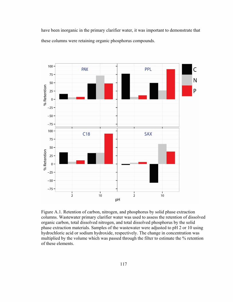
117
have been inorganic in the primary clarifier water, it was important to demonstrate that
these columns were retaining organic phosphorus compounds.
Figure A.1. Retention of carbon, nitrogen, and phosphorus by solid phase extraction
columns. Wastewater primary clarifier water was used to assess the retention of dissolved
organic carbon, total dissolved nitrogen, and total dissolved phosphorus by the solid
phase extraction materials. Samples of the wastewater were adjusted to pH 2 or 10 using
hydrochloric acid or sodium hydroxide, respectively. The change in concentration was
multiplied by the volume which was passed through the filter to estimate the % retention
of these elements.

118
The primary clarifier water was likely to contain minerals that could interfere with
the interpretation of our results. For instance, the presence of magnesium in the water
combined with the pH adjustment could lead to the precipitation of inorganic phosphates
(Karl, David M.,Tien, Georgia, 1992). In fact, precipitates were visually observed in the
samples prior to filtration. Therefore, using the laboratory phosphorus standards allowed
us to detect their retention in the absence of interfering chemicals. Rather than
quantifying the change in concentrations, the ion chromatographs were used to identify
changes to the presence of the standard compounds before and after SPE filtration
(Figure A.2A). The PAX column nearly lacked four of the compounds in its effluent
chromatograph: HexP, PhP, NADH, and P2O7. These represented three organic and one
inorganic compound. Notably, there was a near complete recovery of nitrogen – as
determined by TDN analysis – that could indicate the recovery of the 2-AEP compound
(Figure A.2B). The determined recovery percent of nitrogen and phosphorus matched the
results expected presuming complete recovery of 2-AEP, PhP, NADH, and P2O7. These
results confirmed that the PAX column and methodology was adequate for organic
phosphorus retention, and therefore this solid phase extraction resin was selected for
future analyses.
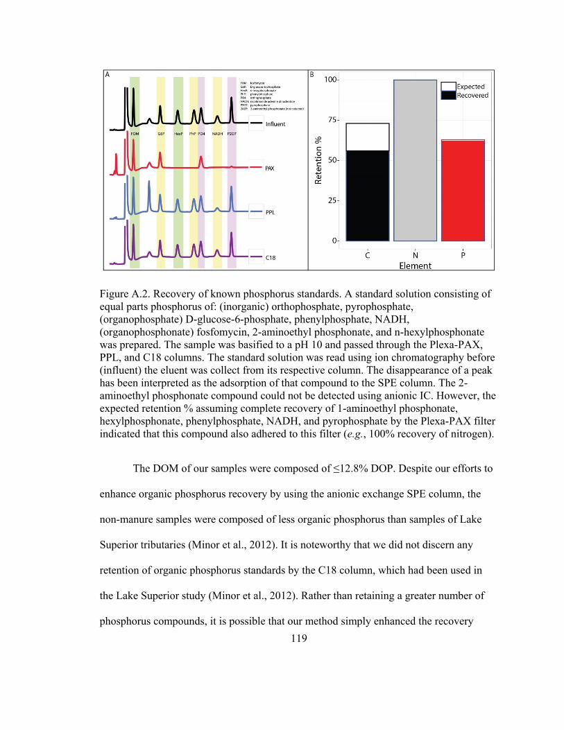
119
Figure A.2. Recovery of known phosphorus standards. A standard solution consisting of
equal parts phosphorus of: (inorganic) orthophosphate, pyrophosphate,
(organophosphate) D-glucose-6-phosphate, phenylphosphate, NADH,
(organophosphonate) fosfomycin, 2-aminoethyl phosphonate, and n-hexylphosphonate
was prepared. The sample was basified to a pH 10 and passed through the Plexa-PAX,
PPL, and C18 columns. The standard solution was read using ion chromatography before
(influent) the eluent was collect from its respective column. The disappearance of a peak
has been interpreted as the adsorption of that compound to the SPE column. The 2-
aminoethyl phosphonate compound could not be detected using anionic IC. However, the
expected retention % assuming complete recovery of 1-aminoethyl phosphonate,
hexylphosphonate, phenylphosphate, NADH, and pyrophosphate by the Plexa-PAX filter
indicated that this compound also adhered to this filter (e.g., 100% recovery of nitrogen).
The DOM of our samples were composed of ≤12.8% DOP. Despite our efforts to
enhance organic phosphorus recovery by using the anionic exchange SPE column, the
non-manure samples were composed of less organic phosphorus than samples of Lake
Superior tributaries (Minor et al., 2012). It is noteworthy that we did not discern any
retention of organic phosphorus standards by the C18 column, which had been used in
the Lake Superior study (Minor et al., 2012). Rather than retaining a greater number of
phosphorus compounds, it is possible that our method simply enhanced the recovery
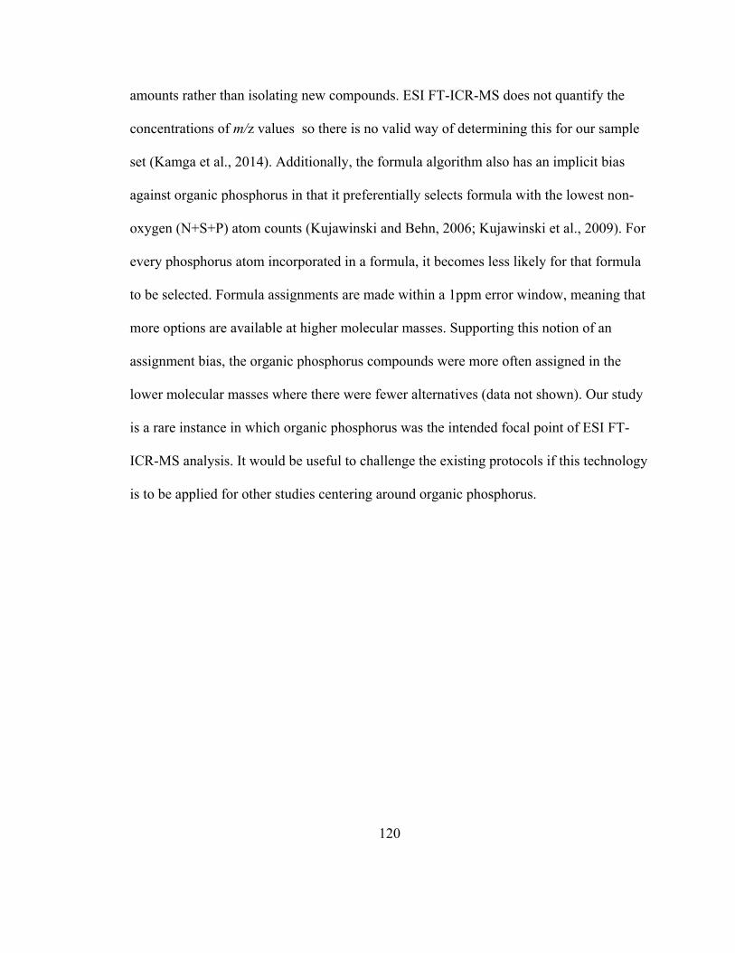
120
amounts rather than isolating new compounds. ESI FT-ICR-MS does not quantify the
concentrations of m/z values so there is no valid way of determining this for our sample
set (Kamga et al., 2014). Additionally, the formula algorithm also has an implicit bias
against organic phosphorus in that it preferentially selects formula with the lowest non-
oxygen (N+S+P) atom counts (Kujawinski and Behn, 2006; Kujawinski et al., 2009). For
every phosphorus atom incorporated in a formula, it becomes less likely for that formula
to be selected. Formula assignments are made within a 1ppm error window, meaning that
more options are available at higher molecular masses. Supporting this notion of an
assignment bias, the organic phosphorus compounds were more often assigned in the
lower molecular masses where there were fewer alternatives (data not shown). Our study
is a rare instance in which organic phosphorus was the intended focal point of ESI FT-
ICR-MS analysis. It would be useful to challenge the existing protocols if this technology
is to be applied for other studies centering around organic phosphorus.

121
Figure A.3. Carbon, nitrogen, and phosphorus concentration of samples in Sandusky
River watershed. (A) The carbon, nitrogen and phosphorus concentrations were measured
as non-purgeable carbon (NPOC), total dissolved nitrogen (TDN); and total dissolved
phosphorus (TDP). The detection limit (DL) for N was 0.01 mg N L-1, while it was 0.03
mg P L-1 leading to a lower limit of quantification (LOQ) of 0.1 mg P L-1. Concentrations
were diluted prior to solid phase extraction.

122
Figure A.4. The distribution of NOSC values by molecular classes.
Table A.1. Adsorption efficiency across samples using the Bond Elut PAX solid phase
extraction resin. Carbon was measured using non-purgeable organic carbon, while
nitrogen and phosphorus were measured as the change in concentrations following
sample dilution and after passing through the solid phase extraction columns. Values
below the limit of quantification (10 µg N L-1, 100 µg P L-1) are reported as estimates.
Where effluent values were above influent, values are reported as <0%.
Sample Replicate C N P
Chicken replicate 1 18% 26% <0%
replicate 2 19% 28% 15%
Dairy replicate 1 20% 13% 6.4%
replicate 2 8% 31% 5.2%
Hog replicate 1 10% 41% <0%
replicate 2 19% 41% <0%
WWTP Effluent replicate 1 44% 32% est. 100%
replicate 2 12% 32% est. 97%
Edge of Field replicate 1 21% 6% est. 17%
replicate 2 16% 7% est. 9.1%
Sandusky River replicate 1 36% 25% est. 59%
replicate 2 28% 33% est. 76%
SRFA - 41% BDL BDL
PLFA - 42% BDL BDL

123
Table A.2. ESI(-) FT-ICR-MS analysis detected a total of 14637 peaks, spread across the samples and replicates. The data was quality
filtered by removing peaks detected in the DI procedural blank; the extraction solvent; singletons (detected in only 1 sample of the
entire dataset); and peaks which had no assigned formula. The reproducibility was determined between sample replicates
(shared#/mean#).
Hog Chicken Dairy Wastewater Edge of field
Sandusky
River NOM
Processing Total DI Solvent 1 2 1 2 1 2 1 2 1 2 1 2 PLFA SRFA
All
Detected
Peaks
14637 3014 534 2497 2352 3452 2493 3519 1626 2388 3602 4449 4702 4169 3154 3412 3707
Remove
Peaks in
Blank
11633 - 377 2094 2053 3219 2312 3215 1232 2245 3341 4338 4483 3983 3023 3262 3415
Remove
Peaks in
Solvent
11246 - - 1983 1931 3098 2200 3070 1128 2171 3270 4260 4396 3895 2939 3146 3325
Removed
Singleton
Peaks
7438 - - 1673 1700 2364 2072 2476 995 2070 3096 3979 4254 3853 2815 2630 3027
Assigned
Formula 7250 - - 1590 1625 2315 2021 2444 964 2046 3071 3974 4220 3846 2798 2622 3021
Reproducibility between sample replicates 88% 88% 68% 81% 90% 85% -

124
Table A.3. ESI(-) FT-ICR-MS analysis provided peaks which were assigned formulas with C/H/O/N/P/S elements. The distribution of
the m/z values detected in each sample were distributed across 8 formula classes. The numbers of formula are printed for each sample
replicate with the number in bold indicating the total number detected in the combined samples. I think the data in this figure are fine,
but it is a little hard to separate the different formula classes without some additional lines or perhaps presenting the data in a figure.
Hog Chicken Dairy WWTP Effluent Edge of field Sandusky River NOM
Total 1 2 1 2 1 2 1 2 1 2 1 2 PLFA SRFA
CHO 3981 772 857 824 801 1139 475 1700 2374 3037 3190 2913 2154
1749 2727 906 908 1144 2413 3356 2924
CHON 2198 502 466 1047 814 923 276 239 479 732 827 769 549
751 119 550 1064 927 488 903 811
CHOP 394 111 99 172 150 203 112 57 126 117 117 109 75
70 78 119 179 207 129 132 111
CHOS 254 62 68 75 69 89 37 7 40 68 35 21 2
38 74 72 82 93 40 75 22
CHONP 147 50 44 81 79 30 23 9 19 7 18 12 6
3 5 53 83 35 19 18 13
CHONS 149 39 46 66 61 37 20 22 19 10 19 15 9
8 12 47 69 40 28 22 16
CHOPS 62 30 24 24 23 18 14 2 5 0 3 2 0
1 2 30 25 18 5 3 2
CHONPS 65 24 21 26 24 5 7 10 9 3 11 5 3
2 4 26 26 9 14 13 6
Total 7250 1590 1625 2315 2021 2444 964 2046 3071 3974 4220 3846 2798
2622 3021 1803 2436 2473 3136 4522 3905
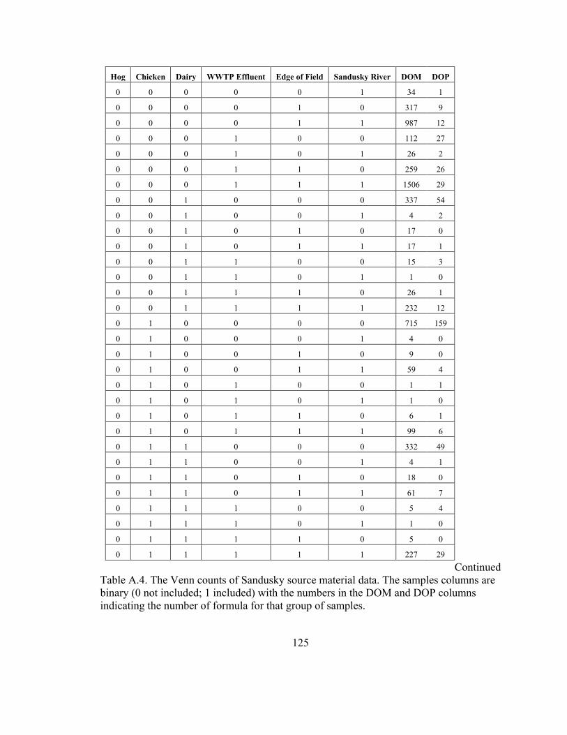
125
Hog Chicken Dairy WWTP Effluent Edge of Field Sandusky River DOM DOP
0 0 0 0 0 1 34 1
0 0 0 0 1 0 317 9
0 0 0 0 1 1 987 12
0 0 0 1 0 0 112 27
0 0 0 1 0 1 26 2
0 0 0 1 1 0 259 26
0 0 0 1 1 1 1506 29
0 0 1 0 0 0 337 54
0 0 1 0 0 1 4 2
0 0 1 0 1 0 17 0
0 0 1 0 1 1 17 1
0 0 1 1 0 0 15 3
0 0 1 1 0 1 1 0
0 0 1 1 1 0 26 1
0 0 1 1 1 1 232 12
0 1 0 0 0 0 715 159
0 1 0 0 0 1 4 0
0 1 0 0 1 0 9 0
0 1 0 0 1 1 59 4
0 1 0 1 0 0 1 1
0 1 0 1 0 1 1 0
0 1 0 1 1 0 6 1
0 1 0 1 1 1 99 6
0 1 1 0 0 0 332 49
0 1 1 0 0 1 4 1
0 1 1 0 1 0 18 0
0 1 1 0 1 1 61 7
0 1 1 1 0 0 5 4
0 1 1 1 0 1 1 0
0 1 1 1 1 0 5 0
0 1 1 1 1 1 227 29
Continued
Table A.4. The Venn counts of Sandusky source material data. The samples columns are
binary (0 not included; 1 included) with the numbers in the DOM and DOP columns
indicating the number of formula for that group of samples.

126
Table A.4 Continued
Hog Chicken Dairy WWTP Effluent Edge of Field Sandusky River DOM
1 0 0 0 0 0 445 100
1 0 0 0 0 1 3 1
1 0 0 0 1 0 8 1
1 0 0 0 1 1 3 0
1 0 0 1 0 0 5 1
1 0 0 1 0 1 0 0
1 0 0 1 1 0 9 3
1 0 0 1 1 1 35 8
1 0 1 0 0 0 326 57
1 0 1 0 0 1 1 0
1 0 1 0 1 0 8 0
1 0 1 0 1 1 1 0
1 0 1 1 0 0 7 1
1 0 1 1 0 1 0 0
1 0 1 1 1 0 11 0
1 0 1 1 1 1 52 4
1 1 0 0 0 0 69 7
1 1 0 0 0 1 1 0
1 1 0 0 1 0 1 1
1 1 0 0 1 1 6 0
1 1 0 1 0 0 1 0
1 1 0 1 0 1 1 0
1 1 0 1 1 0 0 0
1 1 0 1 1 1 45 0
1 1 1 0 0 0 237 30
1 1 1 0 0 1 17 1
1 1 1 0 1 0 14 0
1 1 1 0 1 1 49 4
1 1 1 1 0 0 12 1
1 1 1 1 0 1 1 0
1 1 1 1 1 0 8 0
1 1 1 1 1 1 427 8
127
m/z Formula C13 Hog Chicken Dairy WWTP Effluent Edge of field Sandusky River
432.0675772 C20H20O6NPS - - - 2.14E-04 - - 6.62E-05
464.1477252 C22H28O8NP - - - 3.78E-04 - - 8.25E-05
277.1433072 C10H23O3N4P - - 1.10E-04 4.24E-04 - - 3.39E-05
276.0724817 C11H17O6P 1 2.54E-04 6.89E-04 8.44E-04 - - 4.09E-05
408.2239451 C19H37O7P 1 - - - 7.22E-05 - 5.76E-05
376.0885573 C15H21O9P 1 - - - - 1.13E-04 6.34E-05
420.0783553 C16H21O11P 1 - - - - 9.02E-05 4.77E-05
420.1147941 C17H25O10P 1 - - - - 8.38E-05 5.16E-05
430.0779524 C21H19O8P 1 - - - - 9.68E-05 5.18E-05
434.0940188 C17H23O11P 1 - - - - 8.76E-05 5.08E-05
502.1565882 C22H31O11P 1 - - - - 8.25E-05 5.05E-05
406.135515 C17H27O9P 1 - - 7.44E-05 - 8.54E-05 4.73E-05
332.0623426 C13H17O8P 1 - 2.05E-04 - - 9.30E-05 4.94E-05
392.0834377 C15H21O10P 1 - 2.02E-04 - - 7.88E-05 4.62E-05
302.0881438 C13H19O6P 1 - 2.59E-04 4.41E-04 - 8.02E-05 4.26E-05
304.0674032 C12H17O7P 1 - 5.06E-04 4.50E-04 - 7.36E-05 4.10E-05
318.0830637 C13H19O7P 1 - 5.92E-04 1.91E-04 - 8.09E-05 4.78E-05
330.0830667 C14H19O7P 1 - 2.01E-04 1.47E-04 - 1.36E-04 1.38E-04
Continued
Table A.5. List of potential marker formulas found in source and Sandusky River samples. The mass to charge (m/z) ratios were used
to identify a molecular formula. C13 indicates the presence (1) or absence (0) of a single 13C isotope in the formula. The relative peak
height for the m/z values in the samples is provided, and - signifies that the m/z value was not detected for that sample.

128
Table A.5 Continued
m/z Formula C13 Hog Chicken Dairy WWTP Effluent Edge of field Sandusky River
332.0987091 C14H21O7P 1 - 2.57E-04 1.13E-04 - 9.82E-05 4.42E-05
362.1092918 C15H23O8P 1 - 6.35E-05 7.52E-05 - 9.24E-05 4.80E-05
275.0260021 C9H13O4N2PS - 4.46E-04 1.31E-04 7.34E-04 - 4.33E-05 8.45E-05
294.0619326 C14H15O5P 1 3.39E-04 4.22E-04 6.09E-04 - 9.19E-05 1.27E-04
320.0775812 C16H17O5P 1 3.64E-04 1.78E-04 4.03E-04 - 4.06E-05 4.53E-05
421.236256 C20H39O7P - 3.57E-04 1.97E-04 1.33E-03 - 3.64E-05 7.27E-05
372.1664215 C18H29O6P 1 - - - 3.03E-04 1.33E-04 1.76E-04
386.1820806 C19H31O6P 1 - - - 2.22E-04 9.86E-05 1.10E-04
388.1613368 C18H29O7P 1 - - - 2.70E-04 1.54E-04 1.69E-04
402.1769532 C19H31O7P 1 - - - 2.09E-04 1.05E-04 1.38E-04
403.1165379 C17H25O9P - - - - 1.00E-04 9.28E-05 4.57E-05
413.100923 C18H23O9P - - - - 1.10E-04 8.84E-05 3.93E-05
416.1926161 C20H33O7P 1 - - - 1.74E-04 1.04E-04 1.08E-04
417.095797 C17H23O10P - - - - 9.12E-05 4.37E-05 4.11E-05
418.0990897 C17H23O10P 1 - - - 7.87E-05 1.75E-04 1.74E-04
418.1718666 C19H31O8P 1 - - - 7.17E-05 9.78E-05 5.75E-05
429.1322172 C19H27O9P - - - - 1.18E-04 7.46E-05 3.66E-05
488.1773569 C22H33O10P 1 - - - 5.45E-05 8.69E-05 4.83E-05
344.1351164 C16H25O6P 1 - - 8.28E-05 2.60E-04 1.41E-04 1.60E-04
370.1507808 C18H27O6P 1 - - 9.10E-05 3.58E-04 1.57E-04 2.28E-04
372.1300277 C17H25O7P 1 - - 9.49E-05 3.00E-04 2.15E-04 2.31E-04
Continued

129
Table A.5 Continued
m/z Formula C13 Hog Chicken Dairy WWTP Effluent Edge of field Sandusky River
382.1507627 C19H27O6P 1 - - 1.11E-04 3.36E-04 2.01E-04 2.34E-04
384.166397 C19H29O6P 1 - - 9.51E-05 2.90E-04 1.77E-04 2.08E-04
399.0852169 C17H21O9P - - - 4.55E-04 7.87E-05 8.40E-05 3.89E-05
414.176966 C20H31O7P 1 - - 7.62E-05 3.70E-04 2.13E-04 2.34E-04
458.1668009 C21H31O9P 1 - - 7.86E-05 2.57E-04 1.63E-04 1.92E-04
484.1824486 C23H33O9P 1 - - 7.72E-05 2.19E-04 1.65E-04 2.03E-04
360.130038 C16H25O7P 1 - 7.45E-05 - 2.13E-04 1.59E-04 1.88E-04
456.1147265 C20H25O10P 1 - 7.61E-05 - 2.90E-04 2.52E-04 2.77E-04
342.1194474 C16H23O6P 1 - 1.67E-04 1.17E-04 3.47E-04 1.65E-04 2.11E-04
344.0987134 C15H21O7P 1 - 1.87E-04 1.48E-04 8.20E-05 1.40E-04 1.73E-04
350.0881719 C17H19O6P 1 - 2.26E-04 4.02E-04 2.42E-04 1.37E-04 1.56E-04
354.0830662 C16H19O7P 1 - 3.05E-04 1.23E-04 2.32E-04 2.25E-04 2.50E-04
356.0623315 C15H17O8P 1 - 3.92E-04 1.82E-04 6.87E-05 2.34E-04 2.79E-04
356.1351082 C17H25O6P 1 - 6.45E-05 1.11E-04 2.68E-04 1.47E-04 1.73E-04
358.1143977 C16H23O7P 1 - 6.54E-05 1.13E-04 2.56E-04 2.25E-04 2.31E-04
368.0987153 C17H21O7P 1 - 2.04E-04 1.38E-04 3.00E-04 2.26E-04 2.86E-04
370.1143768 C17H23O7P 1 - 1.06E-04 1.22E-04 2.99E-04 2.25E-04 2.70E-04
380.098741 C18H21O7P 1 - 1.02E-04 3.92E-04 3.54E-04 2.54E-04 3.08E-04
382.1143594 C18H23O7P 1 - 2.00E-04 1.27E-04 3.69E-04 2.99E-04 3.32E-04
396.1300303 C19H25O7P 1 - 2.24E-04 1.46E-04 4.39E-04 3.31E-04 3.48E-04
398.1456726 C19H27O7P 1 - 2.14E-04 1.23E-04 4.31E-04 3.05E-04 3.31E-04
Continued

130
Table A.5 Continued
m/z Formula C13 Hog Chicken Dairy WWTP Effluent Edge of field Sandusky River
410.109275 C19H23O8P 1 - 1.94E-04 1.33E-04 4.50E-04 3.60E-04 4.13E-04
410.145669 C20H27O7P 1 - 2.18E-04 1.17E-04 4.47E-04 2.96E-04 3.49E-04
412.1613237 C20H29O7P 1 - 1.75E-04 1.18E-04 4.35E-04 2.96E-04 3.38E-04
430.1354991 C19H27O9P 1 - 6.31E-05 1.10E-04 2.77E-04 2.47E-04 2.50E-04
440.119842 C20H25O9P 1 - 1.73E-04 9.72E-05 3.63E-04 3.13E-04 3.41E-04
440.1562514 C21H29O8P 1 - 1.85E-04 1.13E-04 3.42E-04 2.81E-04 3.06E-04
426.067739 C18H19O10P 1 3.78E-04 - 1.20E-03 2.03E-04 2.97E-04 3.55E-04
296.0775853 C14H17O5P 1 2.26E-04 5.66E-04 4.98E-04 5.81E-05 1.02E-04 6.58E-05
322.0932496 C16H19O5P 1 5.06E-04 2.23E-04 8.40E-04 7.76E-05 1.00E-04 1.61E-04
336.1088903 C17H21O5P 1 1.91E-04 2.01E-04 1.31E-04 2.15E-04 9.13E-05 1.17E-04
366.0830953 C17H19O7P 1 6.32E-04 2.19E-04 1.42E-03 2.65E-04 1.95E-04 2.55E-04
384.0936035 C17H21O8P 1 2.21E-04 3.47E-04 8.02E-04 2.89E-04 3.47E-04 3.64E-04

131
Figure A.5. Spectra captured from ESI(-) FT-ICR-MS analysis of all sample replicates and blanks.

132
Appendix B: Portage River DOM Mixing Analysis

133
Table B.1. StreamStats data obtained from the four confluence sampling locations. The
contribution of the two tributaries were estimated from their relative 2-year recurrenc
interval flows. The USGS guage station at Woodville was monitored to estimate the
flows during the time of sampling.
Confluence Location
Drainage
Area
(mi2) Latitude Longitude
Slope
(%)
Forest
(%)
2-year
Return
Interval
(cfs)
Contribution
(%)
E
1. Bays Rd
South
Branch
53.9 41.26807 -83.52579 6.7 4.47 1280 61%
2. Bays Rd
East Branch 35.3 41.26807 -83.50652 5.98 5.09 826 39%
3. Rt 281 91.7 41.2826 -83.50993 6.23 4.87 1840
F
1. Bridge St 348 41.40916 -83.45708 4.16 4.27 4940 82%
2. Water St 57.3 41.41011 -83.45848 1.8 4 1120 18%
3. Bierly
Ave 406 41.41254 -83.45453 4.13 4.23 5580
G
1. Toledo St 426 41.4772 -83.29551 3.57 4.44 5620 82%
2. Hessville
Rd 63 41.48674 -83.24105 4.25 8.78 1250 18%
3. Rt 590 493 41.49145 -83.2215 3.74 5 6300
H
1. Chet's
Place 536 41.50562 -83.06928 3.39 5.06 6510 91%
2. Little
Portage 29.9 41.48656 -83.05353 4.82 7.55 649 9%
3. Portage
River
Retreat
579 41.51377 -83.00750 2.84 5.22 6410
Woodville
(USGS
gauge)
421 41.44935 -83.35808 3.79 4.33 5620

134
Table B.2. Nutrient concentrations and solid phase extraction (SPE) efficiencies of the Portage River samples. Phosphorus was
measured using colorimetric methods and via ICP-OES for estimating SPE efficiencies.
Colorimetric
NPOC (mg L-1) TDN (mg L-1) TDP (mg L-1) NPOCSPE (%) TDNSPE (%) TDPSPE (est. %) Sample ID DRP DHP TDP
A. W Township Rd 14 0.099 0.117 0.125 13.73 7.179 0.16 42% 4% 0%
B. Independence Ave 0.102 0.114 0.122 10.31 7.309 0.16 42% 6% 6%
Independence Ave (rep) - - - 10.53 7.417 0.16 27% 6% 13%
C. Tiffin St 0.098 0.109 0.117 12.07 7.165 0.17 37% 4% 6%
D. Fostoria WWTP 0.100 0.112 0.121 46.67 7.309 0.10 34% 5% <0%
E.1. Bays Rd South 0.105 0.119 0.132 8.106 6.078 est. 0.09 51% 1% <0%
E.2. Bays Rd East 0.107 0.116 0.124 12.57 10.24 0.24 40% 10% 8%
E.3. Rt 281 - - - 9.413 8.048 0.17 40% 9% 6%
F.1. Bridge St 0.087 0.098 0.107 8.929 9.876 0.10 34% 3% 20%
Bridge St (rep) - - - 9.807 9.958 0.11 25% 9% 45%
F.2. Water St 0.087 0.096 0.105 8.061 8.773 <0.03 45% 5% BDL
F.3. Bierly Ave 0.086 0.097 0.107 8.808 9.756 est. 0.06 26% 4% 33%
G.1. Toledo St 0.085 0.094 0.105 8.333 9.231 est. 0.06 33% 2% 0%
G.2. Hessville Rd 0.092 0.104 0.113 8.432 7.773 est. 0.03 30% 6% 67%
G.3. Rt 590 0.082 0.094 0.101 8.505 9.05 0.05 41% 7% 20%
H.1. Chet's Place 0.059 0.066 0.073 7.339 5.876 <0.03 24% 9% BDL
H.2. Little Portage 0.064 0.073 0.083 8.441 5.885 est. 0.04 37% 10% 0%
H.3. Portage River Retreat 0.027 0.033 0.038 5.985 8.013 <0.03 41% 7% BDL
SRFA-B (Method) - - - 7.569 0.119 <0.03 32% 15% BDL
DI-B (Blank) - - - BDL BDL <0.03 BDL BDL BDL
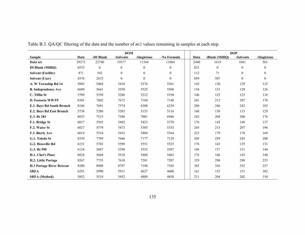
135
Table B.3. QA/QC filtering of the data and the number of m/z values remaining in samples at each step.
DOM DOP
Sample Data -DI Blank -Solvents -Singletons -No Formula Data -Blank (MilliQ) -Solvents -Singletons
Data set 29273 22740 19577 11344 11064 2440 1619 1041 501
DI Blank (MilliQ) 6533 0 0 0 0 821 0 0 0
Solvent (Facility) 871 542 0 0 0 112 71 0 0
Solvent (User) 4376 2633 0 0 0 859 507 0 0
A. W Township Rd 14 5885 5484 5410 5376 5361 145 130 129 125
B. Independence Ave 6049 5641 5558 5525 5508 154 131 128 126
C. Tiffin St 5789 5358 5286 5212 5194 146 125 123 118
D. Fostoria WWTP 8301 7802 7672 7184 7148 241 212 207 178
E.1. Bays Rd South Branch 8186 7691 7574 6308 6239 280 246 242 183
E.2. Bays Rd East Branch 5738 5280 5203 5153 5116 168 138 133 129
E.3. Rt 281 8033 7515 7380 7001 6946 243 204 200 176
F.1. Bridge St 6017 5565 5492 5423 5370 176 145 140 137
F.2. Water St 6027 5579 5473 5385 5353 245 215 207 196
F.3. Bierly Ave 6014 5534 5432 5404 5364 223 179 170 169
G.1. Toledo St 8339 7789 7646 7177 7129 305 259 245 208
G.2. Hessville Rd 6151 5703 5599 5551 5525 176 143 135 131
G.3. Rt 590 6124 5687 5598 5552 5507 186 157 151 144
H.1. Chet's Place 6024 5604 5518 5488 5461 176 146 143 140
H.2. Little Portage 8267 7755 7618 7281 7207 329 298 290 255
H.3 Portage River Retreat 9280 8908 8797 7188 7103 385 356 352 257
SRFA 6291 5990 5911 4627 4606 161 153 151 102
SRFA (Method) 5852 5518 5452 4889 4858 211 204 202 154

136
Figure B.1. Spectra collected by ESI(-) FT-ICR-MS analysis. All samples and replicates (rep) are shown. Replicates were used as a
check, and then removed from the analysis. Solvent blanks were run from the analytical facility as well as from the user. The
methodological SRFA sample was run through the solid phase extraction process while the SRFA sample was prepared directly in the
user solvent.

137
Table B.4. The distribution of atomic composition of formula identified in each Portage
River sample.
Sample ID CHO CHON CHONP CHONPS CHONS CHOP CHOPS CHOS
A. W Township Rd 14 70.66% 25.57% 0.24% 0.43% 0.88% 1.66% 0.00% 0.56%
B. Independence Ave 70.41% 26.00% 0.33% 0.33% 0.82% 1.63% 0.00% 0.49%
C. Tiffin St 73.47% 22.62% 0.33% 0.39% 1.14% 1.50% 0.06% 0.50%
D. Fostoria WWTP 62.66% 32.88% 0.53% 0.41% 1.22% 1.51% 0.04% 0.76%
E.2. Bays Rd East
Branch 72.46% 23.79% 0.53% 0.27% 0.80% 1.68% 0.04% 0.43%
E.1. Bays Rd South
Branch 60.35% 34.46% 0.79% 0.30% 1.17% 1.75% 0.10% 1.09%
E.3. Rt 281 65.52% 30.16% 0.62% 0.40% 1.02% 1.43% 0.09% 0.76%
F.1. Bridge St 65.96% 28.04% 0.49% 0.47% 1.05% 2.67% 0.04% 1.29%
F.2. Water St 71.34% 24.34% 0.32% 0.52% 1.23% 1.60% 0.11% 0.54%
F.3. Bierly Ave 66.52% 28.06% 0.39% 0.54% 1.21% 2.14% 0.07% 1.06%
G.1. Toledo St 63.22% 31.80% 0.69% 0.48% 1.29% 1.68% 0.07% 0.77%
G.2. Hessville Rd 71.19% 25.29% 0.29% 0.34% 0.69% 1.65% 0.09% 0.47%
G.3. Rt 590 70.31% 25.71% 0.42% 0.31% 0.94% 1.73% 0.16% 0.42%
H.1. Chet's Place 61.80% 31.94% 0.92% 0.51% 1.35% 2.08% 0.03% 1.37%
H.2. Little Portage 70.85% 25.07% 0.31% 0.48% 0.81% 1.74% 0.04% 0.71%
H.3. Portage River
Retreat 57.43% 36.21% 0.96% 0.61% 1.34% 2.00% 0.06% 1.41%

138
Table B.5. The molecular class distribution of formula identified in the Portage River
samples.
Sample Carbohydrate
Condensed
hydrocarbon Lignin Lipid Other Protein Tannin
Unsaturated
hydrocarbon
A. W
Township Rd
14
0.8% 0.6% 80.3% 2.5% 1.7% 7.1% 6.1% 0.9%
B.
Independence
Ave
0.8% 0.5% 79.4% 2.9% 1.8% 7.8% 6.0% 0.8%
C. Tiffin St 0.5% 0.5% 79.3% 3.7% 1.6% 8.3% 5.1% 1.0%
D. Fostoria
WWTP 1.5% 1.2% 75.6% 2.8% 2.5% 7.9% 7.4% 1.1%
E.1. Bays Rd
South Branch 2.2% 0.9% 73.0% 3.1% 3.3% 8.8% 7.3% 1.3%
E.2. Bays Rd
East Branch 0.7% 0.5% 80.9% 3.7% 1.1% 8.9% 3.4% 0.9%
E.3. Rt 281 1.6% 0.9% 75.9% 3.5% 2.4% 8.4% 6.2% 1.1%
F.1. Bridge St 1.0% 0.3% 78.0% 2.4% 2.7% 8.4% 6.3% 0.9%
F.2. Water St 0.9% 0.3% 80.8% 3.8% 1.4% 8.1% 3.4% 1.3%
F.3. Bierly
Ave 1.0% 0.3% 77.4% 2.5% 2.7% 8.0% 7.2% 0.9%
G.1. Toledo
St 1.9% 0.7% 77.8% 3.7% 1.9% 8.2% 4.4% 1.3%
G.2. Hessville
Rd 0.6% 0.5% 81.5% 3.1% 1.3% 7.6% 4.7% 0.8%
G.3. Rt 590 0.8% 0.3% 81.0% 2.8% 1.4% 7.7% 5.0% 1.0%
H.1. Chet's
Place 1.8% 1.0% 73.9% 2.6% 3.6% 8.0% 7.8% 1.3%
H.2. Little
Portage 0.9% 0.5% 79.4% 3.0% 1.6% 7.9% 5.7% 0.9%
H.3. Portage
River Retreat 2.3% 0.9% 73.5% 2.5% 4.0% 7.8% 7.6% 1.4%

139
Figure B.2. Correlations between nitrogen and phosphorus concentrations and elemental
compositions. (A) The correlation between total dissolved nitrogen and CHON* formula
was found to not be significant (Pearson correlation, line). (B) The correlation between
total dissolved phosphorus and TDP was significant (Pearson correlation, line).
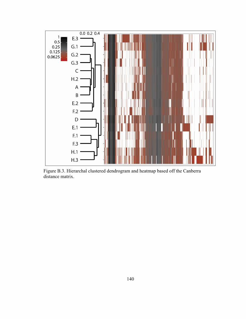
140
Figure B.3. Hierarchal clustered dendrogram and heatmap based off the Canberra
distance matrix.
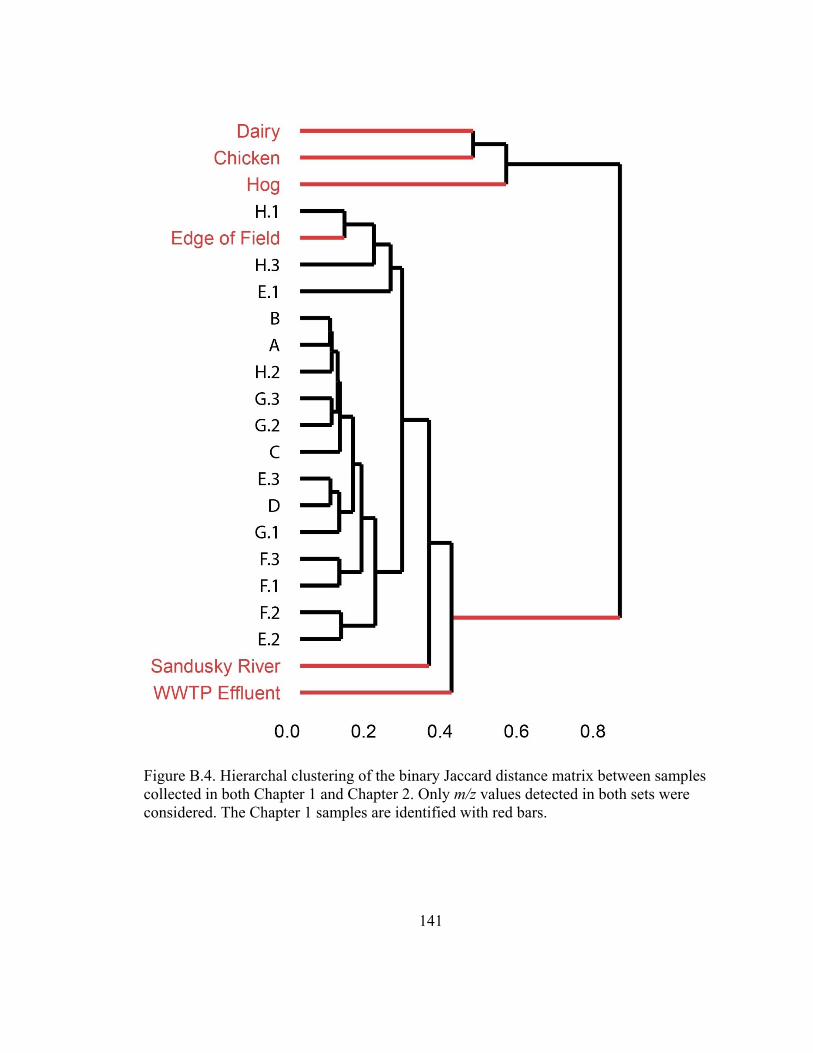
141
Figure B.4. Hierarchal clustering of the binary Jaccard distance matrix between samples
collected in both Chapter 1 and Chapter 2. Only m/z values detected in both sets were
considered. The Chapter 1 samples are identified with red bars.

142
Figure B.5. The relative change in peak heights between upstream-downstream samples
in the upper reaches of the Portage River (A through E.2). The distributions were
compiled for all pairs and examined based upon molecular class types assigned based on
their position in the van Krevelen diagrams.

143
Appendix C: Antibiotic Resistance Gene Analysis

144
Table C.1. Yields and purity of DNA extracts of the sediments collected in 2016. Values
were used to calculate gene abundance in sediment g-1 dry weight.
Sample Replicate
DNA concentration
(ng/µl) 260:280 260:230
Sediment
(g dry weight)
CHLP
1 19.3 1.88 1.08 0.60
2 19.7 1.91 1.25 0.33
3 18.8 1.67 1.19 0.41
OO
1 20.6 1.86 1.69 0.30
2 18.9 1.9 1.77 0.27
3 20.2 1.88 1.67 0.33
PP
1 9.5 1.87 1.05 0.35
2 11.4 1.79 1.82 0.35
3 13.7 1.82 1.39 0.39
Table C.2. Methodology used in LC separation of antibiotics. Gradient elution of 0.1%
formic acid in methanol (% B) with respect to time (min) on Waters XSelect CSH C18
column that separated sulfonamides, macrolides, and others via method 1 and
fluoroquinolones and tetracyclines via method 2.
Method 1 Method 2
Time (min) % B Time (min) % B
0.0 0 0.0 0
5.5 100 0.5 0
7.5 100 4.0 40
8.0 0 7.0 100
20.0 0 9.0 100
-- -- 10.0 0
-- -- 20.0 0

145
Analyte Parent Ion Product Ion CE Quantification or
(m/z) (m/z) (V) Confirmation
Sulfonamides
sulfapyridine 250.10 156.00 17 quantification
250.10 108.05 25 confirmation
sulfadiazine 251.05 156.00 15 quantification
251.05 108.05 24 confirmation
sulfamethoxazole 254.05 92.10 29 quantification
254.05 108.00 24 confirmation
sulfamethazine 279.05 186.00 17 quantification
279.05 156.00 20 confirmation
sulfachloropyridazine 285.00 156.06 15 quantification
285.00 92.05 35 confirmation
sulfadimethoxine 311.10 156.06 21 quantification
311.10 92.05 35 confirmation
13C6-sulfamethoxazole 260.05 98.10 32 quantification
(internal standard) 260.05 114.10 27 confirmation
13C6-sulfamethazine 285.05 186.00 22 quantification
(surrogate) 285.05 123.00 20 confirmation
Fluoroquinolones
norfloxacin 320.10 276.10 17 quantification
320.10 302.10 21 confirmation
ciprofloxacin 332.10 231.05 35 quantification
332.10 314.10 21 confirmation
enrofloxacin 360.10 245.10 25 quantification
360.10 316.15 19 confirmation
ofloxacin 362.10 261.10 28 quantification
362.10 318.10 19 confirmation
clinafloxacin 366.10 348.00 20 confirmation
(internal standard) 366.10 305.00 22 quantification
nalidixic acid 233.15 187.00 27 confirmation
(surrogate) 233.15 104.05 40 quantification
Continued
Table C. 3. Methodology used in LC separation of antibiotics. Gradient elution of 0.1%
formic acid in methanol (% B) with respect to time (min) on Waters XSelect CSH C18
column that separated sulfonamides, macrolides, and others via method 1 and
fluoroquinolones and tetracyclines via method 2.

146
Table C.3 Continued
Analyte Parent Ion Product Ion CE Quantification or
(m/z) (m/z) (V) Confirmation
Tetracyclines Tetracycline 445.10 410.10 19 quantification
445.10 427.05 11 confirmation
doxycycline 445.10 321.05 31 quantification
445.10 428.15 18 confirmation
oxytetracycline 461.10 426.10 17 quantification
461.10 443.10 12 Confirmation
chlortetracycline 479.05 462.10 20 quantification
& degradation products 479.05 444.10 17 Confirmation
481.05 464.10 20 quantification
481.05 446.10 30 Confirmation
demeclocycline 465.10 448.05 20 quantification
(surrogate) 465.10 430.05 17 Confirmation
Macrolides erythromycin 734.4 158.15 35 quantification
734.4 576.35 15 Confirmation
erythromycin-H2O 716.45 158.15 35 quantification
716.45 558.35 15 Confirmation
roxithromycin 837.45 158.10 35 quantification
837.45 679.45 20 confirmation
Tylosin 916.45 174.10 40 quantification
916.45 772.45 30 confirmation 13C2-erythromycin 736.40 160.15 35 quantification
736.40 578.35 20 confirmation
13C2-erythromycin-H2O
718.40 160.15 35 quantification
718.40 560.35 20 confirmation
Non-categorized Carbadox 263.10 130.05 22 quantification
263.10 231.05 13 confirmation
trimethoprim 291.10 230.10 23 quantification
291.10 123.05 24 confirmation
Lincomycin 407.30 126.10 35 quantification
407.30 359.20 18 confirmation
Simeton 198.20 68.10 33 quantification
(internal standard) 198.20 100.10 27 confirmation

147
Genbank ID Gene Gene category
2015 2016
CHLP OO PP CHLP OO PP
302407215 pel Cdeg Carbon Cycling 168.6 91.4 122.8 24.8 31.3 20.6
284165967 phytoene synthase Secondary metabolism 141.9 88.1 121.5 26.2 32.2 19.9
327480404 MFS antibiotic Antibiotic resistance 128.8 88.5 108.4 25.6 32.3 21.3
89069932 ompR Stress 129.7 78.0 104.1 18.5 25.3 18.6
196259193 fnr Stress 120.3 79.3 104.6 24.8 32.4 23.0
91802036 ompR Stress 127.4 75.6 95.6 22.9 29.9 21.3
50954857 gdh Nitrogen 132.2 67.1 99.0 18.7 29.1 16.3
329118461 nikA Metal Homeostasis 126.4 73.5 98.2 21.2 31.1 18.2
390569537 MFS antibiotic Antibiotic resistance 104.6 77.5 113.9 24.6 36.7 23.3
153962580 sqr Sulfur 123.0 74.8 97.0 20.2 29.8 17.5
315603069 nikA Metal Homeostasis 109.3 81.0 103.2 25.4 30.3 21.6
325265934 nitroreductase b Organic Remediation 128.8 67.0 97.4 18.2 26.3 15.8
148273451 nhaA Metal Homeostasis 106.6 80.1 105.1 19.7 26.4 19.3
335036555 znuC Metal Homeostasis 117.0 72.9 101.2 0.0 0.0 0.0
120605943 merT Metal Homeostasis 105.6 80.1 104.3 0.0 0.0 0.0
127514333 MFS antibiotic Antibiotic resistance 116.0 76.8 96.8 23.9 31.2 21.8
170738862 arsB Metal Homeostasis 118.1 71.8 97.8 19.6 28.7 16.7
345010049 corA Metal Homeostasis 100.1 94.4 93.0 30.2 36.9 24.9
178465870 MFS antibiotic Antibiotic resistance 118.9 71.3 96.9 18.1 26.7 17.2
323276022 MFS antibiotic Antibiotic resistance 116.4 67.6 101.0 18.1 28.0 16.6
334103082 nikA Metal Homeostasis 115.2 71.6 97.9 21.7 31.4 22.0
283786071 CsoS1 CcmK Carbon Cycling 114.3 71.5 96.8 17.2 22.8 16.7
345013283 MFS antibiotic Antibiotic resistance 117.9 67.2 95.6 18.5 26.4 16.9
311112862 MFS antibiotic Antibiotic resistance 94.0 79.0 103.5 21.8 33.0 21.5
83838314 pstB Stress 108.6 72.7 93.0 18.0 25.3 16.4
171472824 sod FeMn secondary metabolism 110.3 68.3 94.8 19.6 28.0 17.4
254388596 pstA Stress 95.5 80.6 96.7 26.2 26.1 19.8
42627732 catechol Organic Remediation 109.4 69.0 94.4 19.1 28.7 16.7
238059362 arsB Metal Homeostasis 92.0 79.0 100.9 21.8 23.2 19.7
238757841 spiC virulence 96.8 70.9 98.6 19.4 30.7 16.8
Continued
Table C.4. Gene probe normalized signals for 99.9th percentile of detected values in the
GeoChip analysis on the sediments collected in 2016.

148
Table C.4 Continued
Genbank
ID Gene Gene category
2015 2016
CHLP OO PP CHLP OO PP
83950262 ompR Stress 95.4 73.7 97.1 17.6 23.3 17.3
292675888 Mex
Antibiotic
resistance 96.8 68.5 99.7 18.4 27.4 15.7
339611386 MATE antibiotic
Antibiotic
resistance 91.6 85.8 87.4 26.2 32.6 22.5
221723831 catechol b
Organic
Remediation 92.9 74.5 97.2 27.3 34.2 21.6
91978835 ompR Stress 95.5 71.7 93.9 22.2 29.9 20.4
367038109 Ara Carbon Cycling 93.8 72.1 92.9 0.0 0.0 0.0
285019189 kup Metal Homeostasis 91.8 81.5 85.4 0.0 0.0 0.0
167561665 mdla
Organic
Remediation 89.7 77.4 91.1 24.0 31.6 20.7
297193687 phytase Phosphorus 84.6 77.6 94.7 19.6 28.9 17.3
299134974 TIM Carbon Cycling 82.4 84.9 85.6 28.0 32.8 23.3
84388610 tktA Carbon Cycling 89.9 74.9 88.1 22.2 30.0 19.1
377807676 vana Carbon Cycling 90.3 74.3 86.2 0.0 0.0 0.0
29832895 TerD Metal Homeostasis 82.7 71.1 95.8 17.1 25.1 16.2
205363968
lycopene beta
cyclase
Secondary
metabolism 86.0 69.1 93.0 17.5 25.6 16.4
356639591 one ring 23diox
Organic
Remediation 91.9 69.8 85.5 20.1 29.0 17.7
294629873 MFS antibiotic
Antibiotic
resistance 87.7 66.8 91.0 17.6 23.0 16.4
336321746 MFS antibiotic
Antibiotic
resistance 88.8 74.5 81.0 22.2 29.9 19.1
148257018 Fnr Stress 87.1 75.1 79.0 29.2 35.8 22.4
292815360 mntH Nramp Metal Homeostasis 86.4 67.9 86.3 24.1 27.5 22.6
356882203 Mex
Antibiotic
resistance 84.8 72.9 82.7 21.7 29.5 18.6
74318372 ompR Stress 86.2 74.0 79.8 0.0 0.0 0.0
70728315 degP Stress 78.4 75.3 84.5 22.0 27.2 20.5
315500429 Mex
Antibiotic
resistance 81.5 67.6 87.7 18.1 27.3 16.5
380766219 mcra Carbon Cycling 82.5 67.9 85.9 17.5 25.7 16.7
209959496 b lactamase
Antibiotic
resistance 87.3 66.0 82.7 17.5 25.8 16.7
357408389 amyA Carbon Cycling 85.5 68.0 79.2 18.5 25.0 17.9
340360549 amyA Carbon Cycling 76.8 68.5 83.6 19.0 26.8 17.3
182411857 mannanase Carbon Cycling 78.5 66.7 77.6 17.9 25.1 16.5
331021446 sodA Stress 80.1 63.6 78.6 19.0 6.5 16.0
116104071 Cas6e Other 78.5 65.5 78.1 26.2 32.2 19.9
326315542 ChrA Metal Homeostasis 78.9 64.7 75.9 21.6 30.6 18.1
295690051 Mex
Antibiotic
resistance 67.6 68.9 81.5 20.2 22.8 19.7
Continued
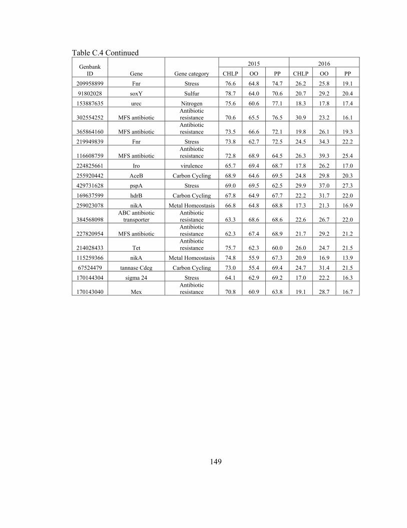
149
Table C.4 Continued
Genbank
ID Gene Gene category
2015 2016
CHLP OO PP CHLP OO PP
209958899 Fnr Stress 76.6 64.8 74.7 26.2 25.8 19.1
91802028 soxY Sulfur 78.7 64.0 70.6 20.7 29.2 20.4
153887635 urec Nitrogen 75.6 60.6 77.1 18.3 17.8 17.4
302554252 MFS antibiotic
Antibiotic
resistance 70.6 65.5 76.5 30.9 23.2 16.1
365864160 MFS antibiotic
Antibiotic
resistance 73.5 66.6 72.1 19.8 26.1 19.3
219949839 Fnr Stress 73.8 62.7 72.5 24.5 34.3 22.2
116608759 MFS antibiotic
Antibiotic
resistance 72.8 68.9 64.5 26.3 39.3 25.4
224825661 Iro virulence 65.7 69.4 68.7 17.8 26.2 17.0
255920442 AceB Carbon Cycling 68.9 64.6 69.5 24.8 29.8 20.3
429731628 pspA Stress 69.0 69.5 62.5 29.9 37.0 27.3
169637599 hdrB Carbon Cycling 67.8 64.9 67.7 22.2 31.7 22.0
259023078 nikA Metal Homeostasis 66.8 64.8 68.8 17.3 21.3 16.9
384568098
ABC antibiotic
transporter
Antibiotic
resistance 63.3 68.6 68.6 22.6 26.7 22.0
227820954 MFS antibiotic
Antibiotic
resistance 62.3 67.4 68.9 21.7 29.2 21.2
214028433 Tet
Antibiotic
resistance 75.7 62.3 60.0 26.0 24.7 21.5
115259366 nikA Metal Homeostasis 74.8 55.9 67.3 20.9 16.9 13.9
67524479 tannase Cdeg Carbon Cycling 73.0 55.4 69.4 24.7 31.4 21.5
170144304 sigma 24 Stress 64.1 62.9 69.2 17.0 22.2 16.3
170143040 Mex
Antibiotic
resistance 70.8 60.9 63.8 19.1 28.7 16.7
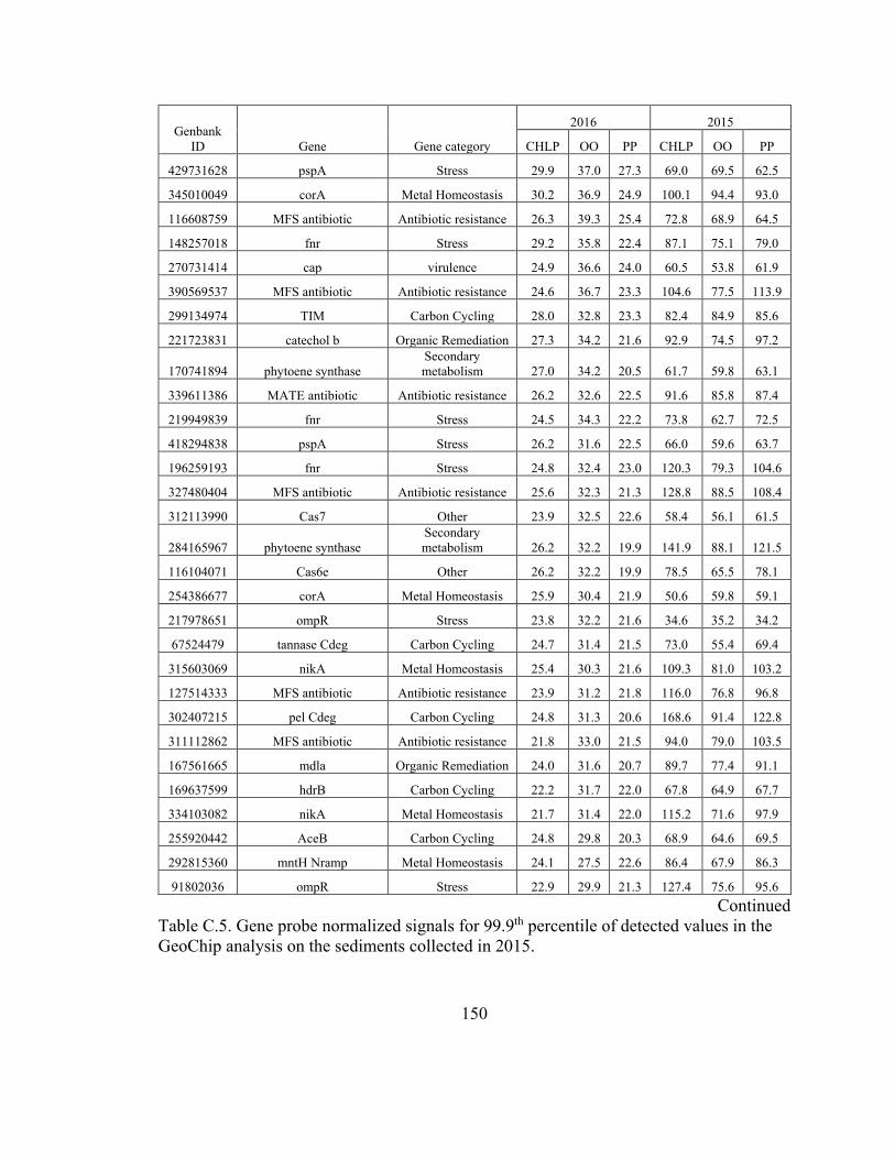
150
Genbank
ID Gene Gene category
2016 2015
CHLP OO PP CHLP OO PP
429731628 pspA Stress 29.9 37.0 27.3 69.0 69.5 62.5
345010049 corA Metal Homeostasis 30.2 36.9 24.9 100.1 94.4 93.0
116608759 MFS antibiotic Antibiotic resistance 26.3 39.3 25.4 72.8 68.9 64.5
148257018 fnr Stress 29.2 35.8 22.4 87.1 75.1 79.0
270731414 cap virulence 24.9 36.6 24.0 60.5 53.8 61.9
390569537 MFS antibiotic Antibiotic resistance 24.6 36.7 23.3 104.6 77.5 113.9
299134974 TIM Carbon Cycling 28.0 32.8 23.3 82.4 84.9 85.6
221723831 catechol b Organic Remediation 27.3 34.2 21.6 92.9 74.5 97.2
170741894 phytoene synthase
Secondary
metabolism 27.0 34.2 20.5 61.7 59.8 63.1
339611386 MATE antibiotic Antibiotic resistance 26.2 32.6 22.5 91.6 85.8 87.4
219949839 fnr Stress 24.5 34.3 22.2 73.8 62.7 72.5
418294838 pspA Stress 26.2 31.6 22.5 66.0 59.6 63.7
196259193 fnr Stress 24.8 32.4 23.0 120.3 79.3 104.6
327480404 MFS antibiotic Antibiotic resistance 25.6 32.3 21.3 128.8 88.5 108.4
312113990 Cas7 Other 23.9 32.5 22.6 58.4 56.1 61.5
284165967 phytoene synthase
Secondary
metabolism 26.2 32.2 19.9 141.9 88.1 121.5
116104071 Cas6e Other 26.2 32.2 19.9 78.5 65.5 78.1
254386677 corA Metal Homeostasis 25.9 30.4 21.9 50.6 59.8 59.1
217978651 ompR Stress 23.8 32.2 21.6 34.6 35.2 34.2
67524479 tannase Cdeg Carbon Cycling 24.7 31.4 21.5 73.0 55.4 69.4
315603069 nikA Metal Homeostasis 25.4 30.3 21.6 109.3 81.0 103.2
127514333 MFS antibiotic Antibiotic resistance 23.9 31.2 21.8 116.0 76.8 96.8
302407215 pel Cdeg Carbon Cycling 24.8 31.3 20.6 168.6 91.4 122.8
311112862 MFS antibiotic Antibiotic resistance 21.8 33.0 21.5 94.0 79.0 103.5
167561665 mdla Organic Remediation 24.0 31.6 20.7 89.7 77.4 91.1
169637599 hdrB Carbon Cycling 22.2 31.7 22.0 67.8 64.9 67.7
334103082 nikA Metal Homeostasis 21.7 31.4 22.0 115.2 71.6 97.9
255920442 AceB Carbon Cycling 24.8 29.8 20.3 68.9 64.6 69.5
292815360 mntH Nramp Metal Homeostasis 24.1 27.5 22.6 86.4 67.9 86.3
91802036 ompR Stress 22.9 29.9 21.3 127.4 75.6 95.6
Continued
Table C.5. Gene probe normalized signals for 99.9th percentile of detected values in the
GeoChip analysis on the sediments collected in 2015.

151
Genbank
ID Gene Gene category
2016 2015
CHLP OO PP CHLP OO PP
91978835 ompR Stress 22.2 29.9 20.4 95.5 71.7 93.9
214028433 Tet Antibiotic resistance 26.0 24.7 21.5 75.7 62.3 60.0
254388596 pstA Stress 26.2 26.1 19.8 95.5 80.6 96.7
227820954 MFS antibiotic Antibiotic resistance 21.7 29.2 21.2 62.3 67.4 68.9
330828074 Mex Antibiotic resistance 23.9 30.9 17.0 31.7 30.6 29.8
384568098
ABC antibiotic
transporter Antibiotic resistance 22.6 26.7 22.0 63.3 68.6 68.6
84388610 tktA Carbon Cycling 22.2 30.0 19.1 89.9 74.9 88.1
336321746 MFS antibiotic Antibiotic resistance 22.2 29.9 19.1 88.8 74.5 81.0
326772217 nikA Metal Homeostasis 23.0 26.4 21.8 49.8 46.8 56.7
209958899 fnr Stress 26.2 25.8 19.1 76.6 64.8 74.7
399074437 MFS antibiotic Antibiotic resistance 22.2 27.3 21.5 56.9 59.9 61.4
329118461 nikA Metal Homeostasis 21.2 31.1 18.2 126.4 73.5 98.2
297151115 MFS antibiotic Antibiotic resistance 28.5 21.9 20.0 60.3 61.4 69.6
91802028 soxY Sulfur 20.7 29.2 20.4 78.7 64.0 70.6
326315542 ChrA Metal Homeostasis 21.6 30.6 18.1 78.9 64.7 75.9
302554252 MFS antibiotic Antibiotic resistance 30.9 23.2 16.1 70.6 65.5 76.5
356882203 Mex Antibiotic resistance 21.7 29.5 18.6 84.8 72.9 82.7
70728315 degP Stress 22.0 27.2 20.5 78.4 75.3 84.5
114776318 sigma 38 Stress 22.5 24.5 22.1 36.3 39.1 34.9
170782088 SMR antibiotics Antibiotic resistance 24.7 22.6 21.5 33.6 28.8 28.9
61678850 pectinase (pectate lyase) Carbon Cycling 26.6 22.2 19.9 30.0 26.2 31.0
217969666 ompR Stress 26.2 21.5 20.9 54.5 44.1 43.5
309813148 cadBD Metal Homeostasis 22.4 22.4 23.4 23.3 27.9 26.3
260576032 nikA Metal Homeostasis 20.9 30.2 17.0 54.4 49.4 52.1
88807717 LPOR
Secondary
metabolism 21.8 26.2 19.9 55.9 48.8 57.3
153962580 sqr Sulfur 20.2 29.8 17.5 123.0 74.8 97.0
258520125 nirk Nitrogen 31.1 17.8 18.5 28.9 33.4 27.4
156972415 oxyR Stress 22.0 25.0 20.4 54.2 46.3 69.1
398070662 hrcA Stress 24.9 21.0 21.3 63.0 60.8 63.1
372476560 natB Metal Homeostasis 21.2 27.5 18.2 50.9 46.4 46.0
238757841 spiC virulence 19.4 30.7 16.8 96.8 70.9 98.6
356639591 one ring 23diox
Organic
Remediation 20.1 29.0 17.7 91.9 69.8 85.5
Continued
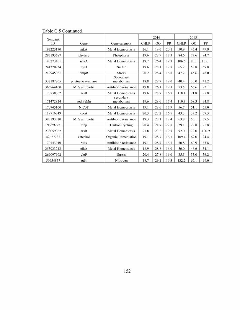
152
Table C.5 Continued
Genbank
ID Gene Gene category
2016 2015
CHLP OO PP CHLP OO PP
193223170 nikA Metal Homeostasis 26.1 19.6 20.1 50.9 45.4 49.9
297193687 phytase Phosphorus 19.6 28.9 17.3 84.6 77.6 94.7
148273451 nhaA Metal Homeostasis 19.7 26.4 19.3 106.6 80.1 105.1
241320734 cysJ Sulfur 19.6 28.1 17.8 65.2 58.8 59.8
219945981 ompR Stress 20.2 28.4 16.8 47.2 45.6 48.0
332187265 phytoene synthase
Secondary
metabolism 18.8 28.7 18.0 40.4 35.0 41.2
365864160 MFS antibiotic Antibiotic resistance 19.8 26.1 19.3 73.5 66.6 72.1
170738862 arsB Metal Homeostasis 19.6 28.7 16.7 118.1 71.8 97.8
171472824 sod FeMn
secondary
metabolism 19.6 28.0 17.4 110.3 68.3 94.8
170745160 NiCoT Metal Homeostasis 19.1 28.0 17.9 56.7 51.1 55.0
119716849 corA Metal Homeostasis 20.3 28.2 16.5 43.3 37.2 39.3
398193010 MFS antibiotic Antibiotic resistance 19.3 28.1 17.4 63.8 55.1 59.5
21929222 mnp Carbon Cycling 20.4 21.7 22.8 29.1 29.8 25.8
238059362 arsB Metal Homeostasis 21.8 23.2 19.7 92.0 79.0 100.9
42627732 catechol Organic Remediation 19.1 28.7 16.7 109.4 69.0 94.4
170143040 Mex Antibiotic resistance 19.1 28.7 16.7 70.8 60.9 63.8
255923242 nikA Metal Homeostasis 18.9 28.8 16.9 56.0 46.6 54.1
269097992 clpP Stress 20.4 27.8 16.0 35.5 35.0 36.2
50954857 gdh Nitrogen 18.7 29.1 16.3 132.2 67.1 99.0

153
Table C.6. Probe counts for the metal homeostasis gene probes. Probes are summarized
by their associated metal foe the samples collected across the two years.
CHLP OO PP
2015 2016 2015 2016 2015 2016
Iron 2011 2228 2165 2283 1768 2237
Nickel 1406 1461 1493 1503 1262 1476
Potassium 1290 1431 1409 1453 1094 1410
Sodium 1105 1169 1181 1235 958 1190
Magnesium 994 1102 1075 1130 869 1116
Zinc 948 1004 999 1021 835 989
Arsenic 900 970 945 972 795 960
Copper 856 912 898 910 735 904
Tellurium 844 869 881 892 743 897
Chromium 686 685 731 720 625 706
Mercury 489 484 492 496 426 494
Silver 461 464 477 461 397 474
Manganese 440 480 467 474 377 477
Cadmium 399 406 411 412 346 402
Calcium 71 71 73 77 63 74
Aluminum 59 69 67 70 51 73
Cobalt 58 68 59 64 50 67
Lead 21 17 20 19 17 21
Silicon 9 12 9 13 7 10
Boron 1 5 2 2 0 4
Selenium 1 1 2 1 1 1
Magnesium Cobalt 654 692 675 671 578 673
Zinc Cadmium Cobalt 477 496 496 508 413 509
Multiple metals 450 477 458 501 384 478
Nickel Cobalt 25 22 26 28 20 26

154
Table C.7. The functionality of the metal genes detected across both GeoChip datasets.
Any positive probe detected across the samples was counted once.
Metal Transport Detoxification Sequestration Storage Biosynthesis Total
Iron 1906 0 0 360 0 2266
Nickel 1539 0 0 0 0 1539
Potassium 1471 0 0 0 0 1471
Sodium 1237 0 0 0 0 1237
Magnesium 1127 0 0 0 0 1127
Zinc 1034 0 0 0 0 1034
Arsenic 405 580 0 0 0 985
Copper 917 21 0 0 0 938
Tellurium 424 495 0 0 0 919
Chromium 736 15 0 0 0 751
Cobalt Magnesium 705 0 0 0 0 705
Cadmium Cobalt
Zinc 517 0 0 0 0 517
Mercury 131 385 0 0 0 516
Silver 497 0 0 0 0 497
Manganese 496 0 0 0 0 496
Multiple metals 478 0 15 0 0 493
Cadmium 430 0 0 0 0 430
Calcium 76 0 0 0 0 76
Aluminum 69 0 0 0 0 69
Cobalt 64 0 0 0 0 64
Cobalt Nickel 27 0 0 0 0 27
Lead 22 0 0 0 0 22
Silicon 8 0 0 0 1 9
Selenium 0 2 0 0 0 2
Boron 2 0 0 0 0 2
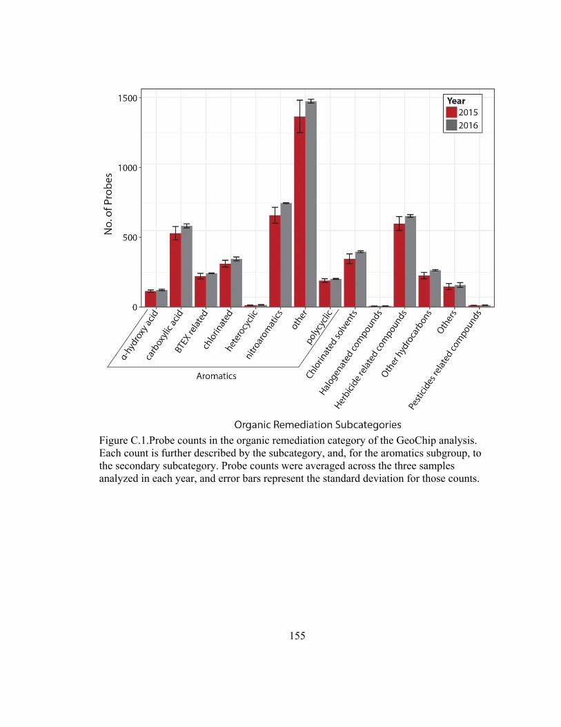
155
Figure C.1.Probe counts in the organic remediation category of the GeoChip analysis.
Each count is further described by the subcategory, and, for the aromatics subgroup, to
the secondary subcategory. Probe counts were averaged across the three samples
analyzed in each year, and error bars represent the standard deviation for those counts.
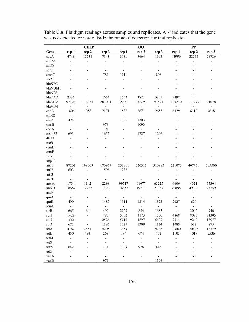
156
Table C.8. Fluidigm readings across samples and replicates. A’-‘ indicates that the gene
was not detected or was outside the range of detection for that replicate.
CHLP OO PP
Gene rep 1 rep 2 rep 3 rep 1 rep 2 rep 3 rep 1 rep 2 rep 3
aacA 4748 12531 7143 3131 5664 1695 91999 22555 26726
aadA5 - - - - - - - - -
aadD - - - - - - - - -
acrD - - - - - - - - -
ampC - - 781 1011 - 898 - - -
arr2 - - - - - - - - -
blaKPC - - - - - - - - -
blaNDM1 - - - - - - - - -
blaNPS - - - - - - - - -
blaOXA 2536 - 1654 1552 3821 5325 7497 - -
blaSHV 97124 138334 203061 35451 60575 94571 180270 141975 94078
blaVIM - - - - - - - - -
cadA 1806 1058 2171 1536 2671 2655 6829 6110 4618
catB8 - - - - - - - - -
chrA 494 - - 1106 1303 - - - -
cmlB - - 978 - 1093 - - - -
copA - - 791 - - - - - -
ctxm32 693 - 1652 - 1727 1206 - - -
dfr13 - - - - - - - - -
ereB - - - - - - - - -
ermB - - - - - - - - -
ermF - - - - - - - - -
floR - - - - - - - - -
imp13 - - - - - - - - -
intI1 87262 109009 176937 256811 320315 510983 521073 407451 385500
intI2 603 - 1596 1236 - - - - -
intI3 - - - - - - - - -
mefE - - - - - - - - -
merA 1734 1142 2298 99717 61077 63225 4606 4321 35304
mexB 18684 12285 12362 14657 19711 21337 40898 49303 28259
qacF - - - - - - - - -
qnrA - - - - - - - - -
qnrB 499 - 1487 1914 1314 1523 2027 620 -
rcnA - - - - - - - - -
strB 665 64 490 2029 854 1685 - 2042 946
sul1 1428 - 780 5102 3173 1530 4868 8085 84305
sul2 1566 - 2526 5019 4897 5632 2614 9240 18977
sul3 671 - 1193 1125 1308 1114 1089 662 875
tetA 4762 2581 5205 3959 - 9236 22800 20428 12379
tetL 450 493 269 184 674 772 1103 1018 2536
tetM - - - - - - - - -
tetS - - - - - - - - -
tetW 642 - 734 1109 926 846 - - -
tetX - - - - - - - - -
vanA - - - - - - - - -
vanB - - 971 - - 1396 - - -

157
Table C.9. Sequence reads from Illumina sequencing
Sample Sequences OTU97 Berger
Parker Shannon
PD Whole
Tree
2015
CHLP 6,695 1687 0.003 7.36 88.5
OO 2,348 1531 0.005 7.19 83
PP 1,990 1578 0.007 7.26 85.6
2016
CHLP 16,953 890 0.021 6.31 50.8
OO 34,333 971 0.015 6.45 56.5
PP 16,951 955 0.023 6.43 53.4
Figure C..2 The number of gene probes related to metal homeostasis and concentrations
measured for those metals. The number of probes were determined for the entire number
measured across the 2016 GeoChip set, while the concentration of the metal was the
average value detected in the three sediments collected that same year. Error bars
represent the standard deviation for the three sediments, following the averaging of
replicates between sites. The abundance of gene probes for multiple metals were not
accounted for in their respective metal groups.