visualizing in polar coordinates with the geogebra
TRANSCRIPT
21
Visualizing in polar coordinates with the Geogebra
Francisco Regis Vieira Alves Instituto Federal de Educação, Ciência e Tecnologia do Estado do Ceará – IFCE.
Brazil
ABSTRACT: In this article we discuss and describe some
examples of application of the integrals in polar coordinates. We
see that the software Geogebra provides means to describe
complex regions in the plane. Moreover, explore and manipulate
the graphic-geometric construction with the purpose to indicate
the convenient definite integral. Finally, with some examples we
show strategies of solution that not emphasize only the
analytical standard approach in the teaching process of the
integral Calculus.
KEYWORDS: Visualization, Polar Coordinates, Integral
Calculus, Software Geogebra.
1 Introduction
Admittedly, the notion of polar coordinates has a prominent place in the
teaching of Calculus in Brazil. While we recognize your relevance, we can
not overlook some negatives elements. First, we observe that the hegemonic
standard style of discussion by the book’s authors is the analytical approach.
Second, we must note that many complex constructions in polar coordinates
become impossible without the computer’s help.
In this perspective, we elaborated tree situations linked with the notion
of polar coordinates and we demonstrate that description of one
understanding’s scenarios for the pupils is invaluable, when we do not use
the technological instruments. Moreover, we can discuss the elements
originated by the perception and visualization of the graphics provided by the
22
computer environment. In this way, we intend reduce the emphasis of the
analytical and formal arguments in despite of final resolution in each
problem situation.
The mathematical model is described by 2
1
2
1 2 ( )A d , where
the function f is continuous and positive in the considered region of the
plane and each point P is determined by a distance from a fixed point O
and a angle from a fixed direction . So, we will show a way to extract and
indicate the integrals directly from de graph provided by the software.
2 Visualizing regions in polar coordinates with Geogebra
We present some problem situations involved the notion of polar
coordinates. We emphasize that these structured situation was thought in the
way that promote the visualization and perception of the properties in the
first stage of strategy’s solution.
Situation I: Describe the region determined by the two curves in the
fig.1 and indicate the definite integral corresponding.
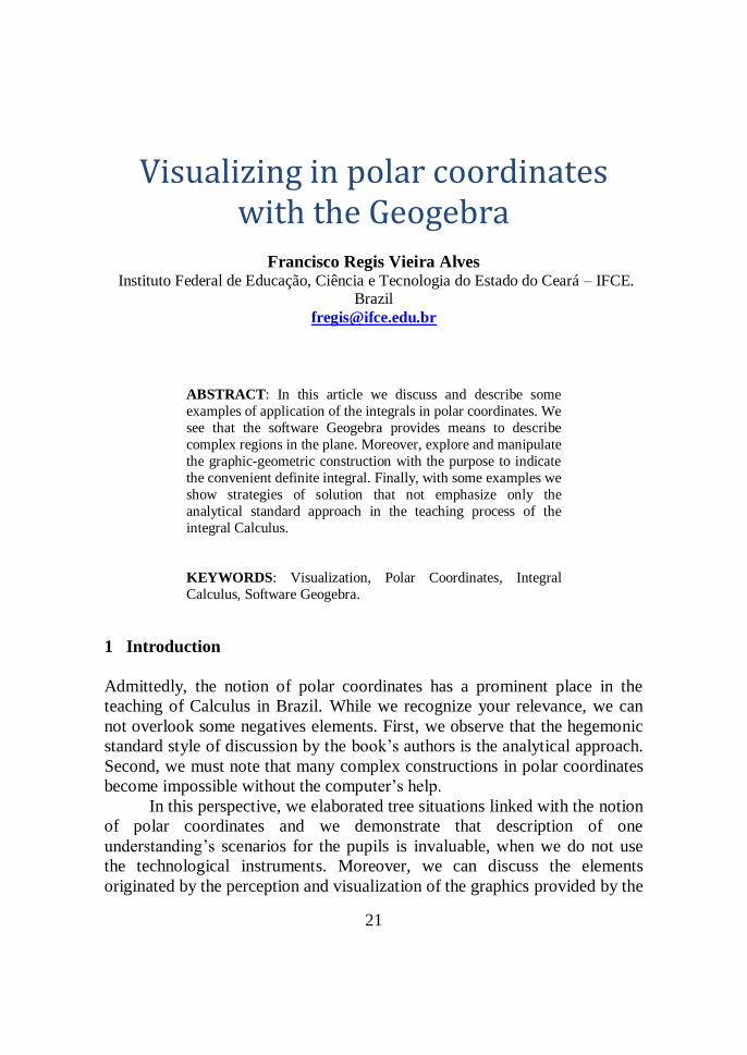
Comments: We see in the fig. 1 the equations 1 and 2cos(2 ) .
In the fig. 1-I we perceive that are intersection points determinate by these
curves in the polar plane. However, we wish to describe some regions of the
symmetry. So, we explore the construction (fig. 1-II) and we can identify two
lines. Quickly, we determine the points from the conditions 2cos(2 ) 1.
Observing the fig. 1-II, we indicate the lines y x et 33
y x . We still
observe that others regions can be obtained by the symmetry properties in the
figure below. In any case, we will restrain our preliminary analysis to 1º
quadrant of the polar plane.
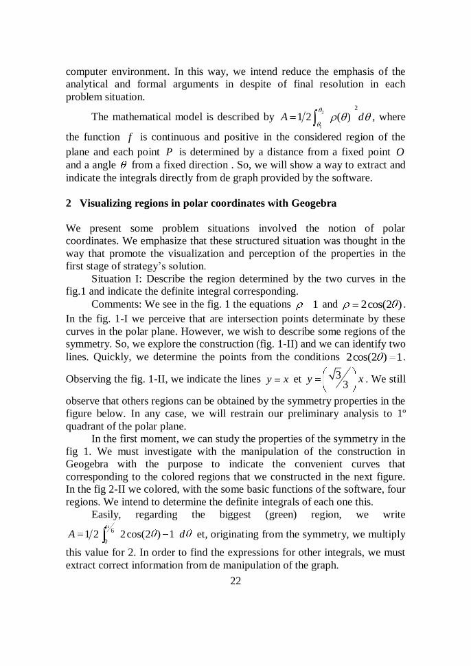
In the first moment, we can study the properties of the symmetry in the
fig 1. We must investigate with the manipulation of the construction in
Geogebra with the purpose to indicate the convenient curves that
corresponding to the colored regions that we constructed in the next figure.
In the fig 2-II we colored, with the some basic functions of the software, four
regions. We intend to determine the definite integrals of each one this.
Easily, regarding the biggest (green) region, we write
6
01 2 2cos(2 ) 1A d et, originating from the symmetry, we multiply
this value for 2. In order to find the expressions for other integrals, we must
extract correct information from de manipulation of the graph.
23
Fig. 1. We identify the regions of symmetry with the help of the software Geogebra
Fig. 2. Discriminating the regions of the simmetry with the purpose to
elaborate the polar coordinates integral
24
In the fig. 2-II, we can write that 4
6
1 2 2cos(2 )A d relatively
the smallest region (purple) limited by these curves. On the other hand, with
the aim to calculate the rose (and the light green) region indicated in the
same figure, we will establish that 4 4
6 6
1 11 2cos(2 )
2 2d d
correspondently to the light green region between the two lines. At the end,
we can effectively determine the other region (in pink), from the symmetry
again by multiplying by 2.
Indeed, we finalize with the expression
4 4
6 6
1 12 1 2cos(2 )
2 2d d correspondently the symmetry (fig. 2-
II) that express the area of the pink and light green regions.
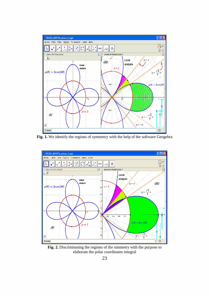
Situation II: Describe the region determined by the two curves in the
fig.3 and indicate the definite integral corresponding.
Comments: We will consider the equations 1 and 2 cos(2 ) .
In the first stage, we suggest the students realize a global visualization. We
view in the fig 3-I the two considered curves. In these circumstances, we
conclude that exist limited regions between these two plane curves. This
scene allows producing the preliminary perceptions.
Fig. 3. The software allows explore the construction with the aim that
find geometric and graph properties
25
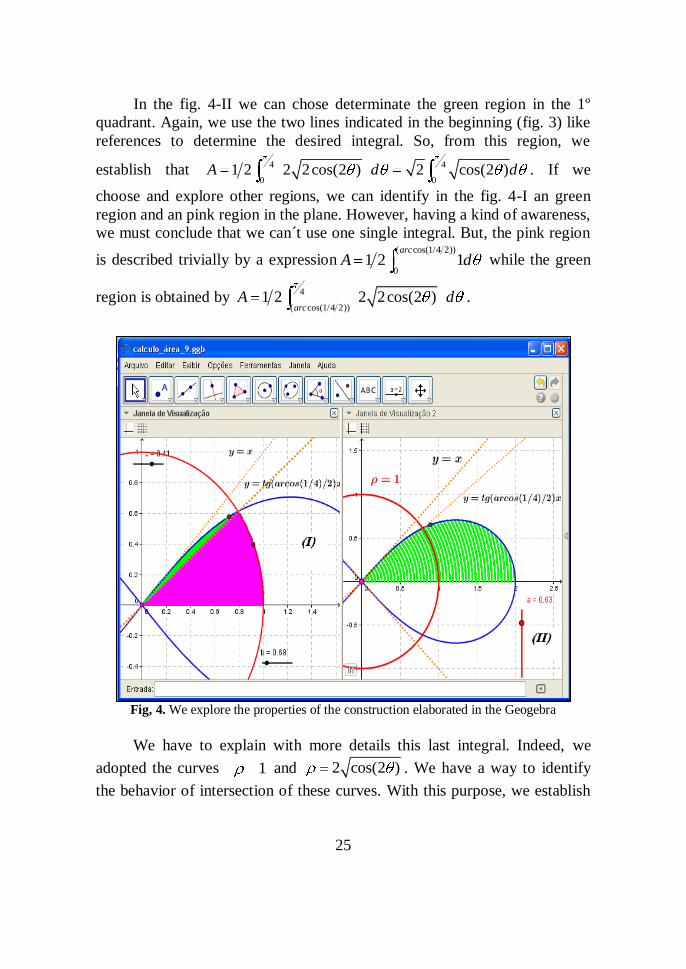
In the fig. 4-II we can chose determinate the green region in the 1º
quadrant. Again, we use the two lines indicated in the beginning (fig. 3) like
references to determine the desired integral. So, from this region, we
establish that 4 4
0 01 2 2 2cos(2 ) 2 cos(2 )A d d . If we
choose and explore other regions, we can identify in the fig. 4-I an green
region and an pink region in the plane. However, having a kind of awareness,
we must conclude that we can´t use one single integral. But, the pink region
is described trivially by a expression( cos(1/4 2))
01 2 1
arc
A d while the green
region is obtained by 4
( cos(1/4 2))1 2 2 2cos(2 )
arcA d .
Fig, 4. We explore the properties of the construction elaborated in the Geogebra
We have to explain with more details this last integral. Indeed, we
adopted the curves 1 and 2 cos(2 ) . We have a way to identify
the behavior of intersection of these curves. With this purpose, we establish
26
12 cos(2 ) 1 cos(2 )
4. Finally, we find arccos(1 8) . We notice
that some basic commands of the software, like Curva[s(t) cos(t), s(t)
sen(t), t, 0, 6.28319].
We can color various regions in the scenario of the fig. 3. The next
situation was structured in other to develop a precise analysis and elaborated
perception directly to the graphs. Without the software, may be it seems
difficult to elaborate such graphs. (see fig. 5-I)
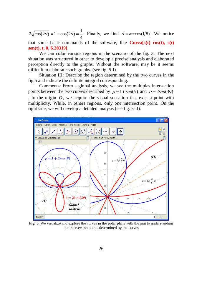
Situation III: Describe the region determined by the two curves in the
fig.5 and indicate the definite integral corresponding.
Comments: From a global analysis, we see the multiples intersection
points between the two curves described by 1 ( )sen and 2 (3 )sen
. In the origin O , we acquire the visual sensation that exist a point with
multiplicity. While, in others regions, only one intersection point. On the
right side, we will develop a detailed analysis (see fig. 5-II).
Fig. 5. We visualize and explore the curves in the polar plane with the aim to understanding
the intersection points determined by the curves
27
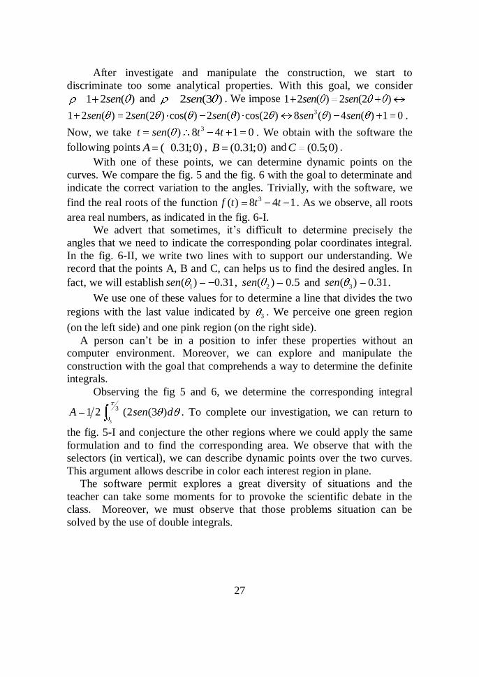
After investigate and manipulate the construction, we start to
discriminate too some analytical properties. With this goal, we consider
1 2 ( )sen and 2 (3 )sen . We impose 1 2 ( ) 2 (2 )sen sen 31 2 ( ) 2 (2 ) cos( ) 2 ( ) cos(2 ) 8 ( ) 4 ( ) 1 0sen sen sen sen sen .
Now, we take 3( ) 8 4 1 0t sen t t . We obtain with the software the
following points ( 0.31;0)A , (0.31;0)B and (0.5;0)C .
With one of these points, we can determine dynamic points on the
curves. We compare the fig. 5 and the fig. 6 with the goal to determinate and
indicate the correct variation to the angles. Trivially, with the software, we
find the real roots of the function 3( ) 8 4 1f t t t . As we observe, all roots
area real numbers, as indicated in the fig. 6-I.
We advert that sometimes, it’s difficult to determine precisely the
angles that we need to indicate the corresponding polar coordinates integral.
In the fig. 6-II, we write two lines with to support our understanding. We
record that the points A, B and C, can helps us to find the desired angles. In
fact, we will establish 1( ) 0.31sen , 2( ) 0.5sen and 3( ) 0.31sen .
We use one of these values for to determine a line that divides the two
regions with the last value indicated by 3 . We perceive one green region
(on the left side) and one pink region (on the right side).
A person can’t be in a position to infer these properties without an
computer environment. Moreover, we can explore and manipulate the
construction with the goal that comprehends a way to determine the definite
integrals.
Observing the fig 5 and 6, we determine the corresponding integral
3
31 2 (2 (3 )A sen d . To complete our investigation, we can return to
the fig. 5-I and conjecture the other regions where we could apply the same
formulation and to find the corresponding area. We observe that with the
selectors (in vertical), we can describe dynamic points over the two curves.
This argument allows describe in color each interest region in plane.
The software permit explores a great diversity of situations and the
teacher can take some moments for to provoke the scientific debate in the
class. Moreover, we must observe that those problems situation can be
solved by the use of double integrals.
28
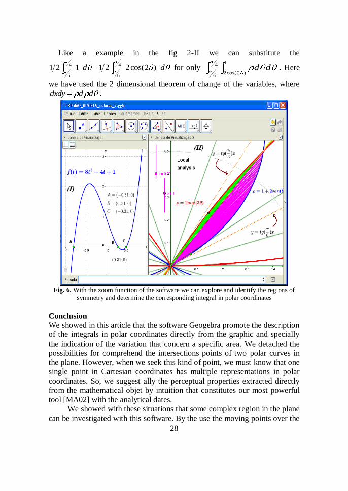
Like a example in the fig 2-II we can substitute the
4 4
6 6
1 2 1 1 2 2cos(2 )d d for only 1
4
2cos(2 )6
d d . Here
we have used the 2 dimensional theorem of change of the variables, where
dxdy d d .
Fig. 6. With the zoom function of the software we can explore and identify the regions of
symmetry and determine the corresponding integral in polar coordinates
Conclusion
We showed in this article that the software Geogebra promote the description
of the integrals in polar coordinates directly from the graphic and specially
the indication of the variation that concern a specific area. We detached the
possibilities for comprehend the intersections points of two polar curves in
the plane. However, when we seek this kind of point, we must know that one
single point in Cartesian coordinates has multiple representations in polar
coordinates. So, we suggest ally the perceptual properties extracted directly
from the mathematical objet by intuition that constitutes our most powerful
tool [MA02] with the analytical dates.
We showed with these situations that some complex region in the plane
can be investigated with this software. By the use the moving points over the
29
trajectories, we can color a specific region and after employ the analytical
model for compare the final dates. Moreover, it is possible to solve these
problems by double integrals. In such way, we can establish relevant
conceptual relationships in the teaching of Calculus [FRV11].
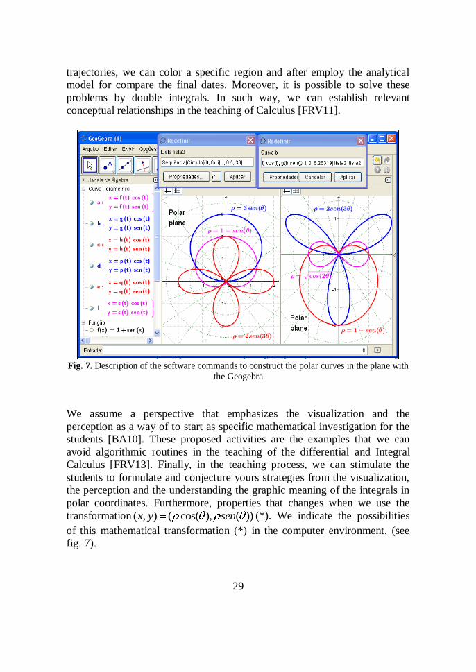
Fig. 7. Description of the software commands to construct the polar curves in the plane with
the Geogebra
We assume a perspective that emphasizes the visualization and the
perception as a way of to start as specific mathematical investigation for the
students [BA10]. These proposed activities are the examples that we can
avoid algorithmic routines in the teaching of the differential and Integral
Calculus [FRV13]. Finally, in the teaching process, we can stimulate the
students to formulate and conjecture yours strategies from the visualization,
the perception and the understanding the graphic meaning of the integrals in
polar coordinates. Furthermore, properties that changes when we use the
transformation ( , ) ( cos( ), ( ))x y sen (*). We indicate the possibilities
of this mathematical transformation (*) in the computer environment. (see
fig. 7).
30
References
[Alv13] F. R. V. Alves – Local analysis for the construction for
parameterized curves, in Proceedings of VII CIBEN, Uruguay,
2013.
[Alv11] F. R. V. Alves – Intuitive categories in the teaching of the
Calculus in several variables: application of the Sequence
Fedathi, Phd Thesis, Fortaleza-Brazil, 2011.
[BA10] I. Bayazit and Y. Aksoy – Connecting Representations and
Mathematical Ideas with GeoGebra, Geogebra Internation
Romani, vol. 1, nº1: 93-106, 2010.
[Ati02] M. Atiyah – Mathematics in the 20TH Century, Bulletin London
Math, vol. 34: 1-15, 2002.