Visual representation in the determination of saliency

Neil D. B. Bruce, Xun Shi, Evgueni Simine and John K. TsotsosDepartment of Computer Science and Engineering

York UniversityToronto, Canada

Email: {neil,shixun,eugene,tsotsos}@cse.yorku.ca

Abstract—In this paper, we consider the role that visualrepresentation plays in determining the behavior of a genericmodel of visual salience. There are a variety of differentrepresentations that have been employed to form an earlyvisual representation of image structure. The experimentspresented demonstrate that the choice of representation hasan appreciable effect on the system behavior. The reasons forthese differences are discussed, and generalized to implicationsfor vision systems in general. In instances where a design choiceis arbitrary, we look to the properties of visual representationin early visual processing in humans for answers. The resultsas a whole demonstrate the importance of filter choice andhighlight some desirable properties of log-Gabor filters.

Keywords-saliency; salience; linear filtering; Gabor filters;visual representation

I. INTRODUCTION

Fast determination of visually salient targets may presentan advantageous component of a combined attention andrecognition system. The processing hardware involved inmodels that seek to characterize visual salience typicallyinvolve units that model local oriented structure in the scene.This may additionally include units sensitive to intensity,color, local contrast, edge content and a variety of otherpossibilities. A common element to most models that char-acterize saliency in some manner is a representation oforiented intensity gradients. This generally comes in theform of a bank of filters each selective for a particularcombination of orientation and spatial frequency. There exista variety of different means of constructing a representationof this form that are all similar in their nature but thatdiffer in their precise details. It is apparent that spectralsampling may present a very important factor in determiningsalience. One might expect then, that the predictions ofvisually salient regions of a scene to depend on the preciserepresentation used to model local oriented structure in thescene. To this end, we explore the extent to which this isthe case, towards determining an optimal representation fora visual surveillance task. This is investigated in the contextof the AIM model of visual saliency [1,2]. There exists priorefforts that define optimality according to a specific objectivefunction [3,4,5]. In this case, the definition of optimalityis in consideration to achieving even spectral coverage andinsofar as it supports the estimation of salience in a visualsurveillance task. While some specifics of parameterization

are discussed, the emphasis is on the comparison of differentclasses of early Gabor-like visual filters.

The paper is formatted as follows: In section 2, a numberof alternatives for representing local oriented structure arepresented. This includes a look at the role that parame-terization plays in dictating the nature of the filter banksin question. In section 3, experiments conducted based onvisual surveillance scenarios are presented to demonstratehow the various representations differ in their ability tosignal targets of potential interest to a recognition system.Finally, section 4 summarizes these results and discussesimplications of the work that generalize to the modeling ofsalience at large.

II. EARLY VISUAL REPRESENTATION

A variety of linear filters have been proposed as means ofrepresenting local frequency structure of an image. Gaborfilters are ubiquitous in the modeling literature offeringsimultaneous localization of local structure in space and fre-quency. Starting with this definition, a variety of alternativesare described in this section with general practical issues thatpertain to each choice being highlighted.

A. Gabor filters

Gabor filters are ubiquitous in the computer vision andimage processing literature. They also figure prominentlyin modeling early visual representation in humans. Gaborfilters produce a representation corresponding to a localizedregion of space and a specific spatial frequency band andorientation. The definition of a Gabor filter is as follows:

g(x, y;λ, θ, ψ, σ, γ) = exp

(x′2 + γ2y′2

−2σ2

)cos

(2πx′

λ+ ψ

)with x′ = x cos θ + y sin θ and y′ = −x sin θ + y cos θ.

The aforementioned equation depicts only the real part ofthe filter with the cos becoming a sin in the imaginary coun-terpart. The parameters are as follows: λ is the wavelengthof the sinusoidal component, θ dictates the orientation, ψis the phase offset, σ controls the extent of the Gaussianenvelope, and γ controls the aspect ratio.

2011 Canadian Conference on Computer and Robot Vision

978-0-7695-4362-8/11 $26.00 © 2011 IEEE

DOI 10.1109/CRV.2011.39

242

B. log-Gabor filters

The log-Gabor function is an alternative to the Gaborfunction proposed in [6]. Log-Gabor filters differ fromGabor filters in that they have a transfer function that issymmetric on a log frequency scale. For this reason, onecannot directly write the definition of log-Gabor filters inthe spatial domain. Instead, log-Gabor filters are constructedin the frequency domain according to the definition:

G(w) = exp{−[log(w/wo)]2/2[log(k/wo)]

2}

with wo the filters center frequency. k is chosen such thatk/wo is constant for varying choices of wo. k/wo effectivelycontrols the filter bandwidth. The precise placement ofbands then depends on the bandwidth and center frequencieschosen. This issue is discussed further at the end of thissection.

The structure of natural images is such that the spectralpower falls off as a function of 1/f with f being the radialfrequency. This implies that a standard Gabor filter is biasedin its sampling, with a higher likelihood of the filter beingdriven by lower spatial frequency content. In using a log-Gabor filter, one compensates for this bias resulting in arepresentation that is arguably a better encoding of visualcontent. It is interesting to note that the representation thatappears in the early areas of human visual cortex is moreconsistent with a Gabor like representation that has a transferfunction that is symmetric on a log scale [7]. This lendscredence to the claim that log-Gabor filters are optimalin some sense as a representation of angular and radialfrequency.

C. Difference of Gaussians

Inspired by the human visual system, a Difference ofGaussians based representation provides an alternative filterapproach to extract oriented features. It has been shown [8,9]that the spatial organization of lateral geniculate nucleus(LGN) receptive fields accounts for orientation selectivityof V1 simple cells. Generally, a simple cell responds to aspecific orientation from elongated patterns of convergingsymmetric LGN filters, which takes the form of an orientedDifference of Gaussians filter.

The center-surround receptive fields of LGN have re-sponse patterns that can be described as a Difference-of-Gaussian filter [10] given by:

flgn(x, y) =1

2πσ2c

exp {−(x2 + y2)

2σ2c

}

− 1

2πσ2s

exp {−(x2 + y2)

2σ2s

}(1)

where σc and σs are the bandwidth (standard deviation)for the center and surround Gaussian function respectively.

Through image convolution, signals containing spatial fre-quency confined to σc and σs are selected, which can betuned for either magnocellular or parvocellular cells.

Orientation selectivity of a V1 simple cell can be repre-sented by Oriented Difference of Gaussians (O-DOG) filter,which accumulates strengths over a group of LGN center-surround filters (DOGs) towards the desired orientation. TheO-DOG filter is therefore defined as:

fv1(x, y) =∑∆x

∑∆y

flgn(x+ xθ, y + yθ) · fG(x, y) (2)

where ∆x and ∆y denote the range of V1 receptive fieldwith respect to number of LGN receptive fields in Cartesiancoordinates. The orientation is governed by xθ = ∆x cos θ+∆y sin θ and yθ = −∆x sin θ + ∆y cos θ.

Gaussian function fG(x, y) is used in (2) to attenuateresponses that are far from the center of the filter, whichis given by:

fG(x, y) = exp {−(x2θ

2σ2x

+y2θ

2σ2y

)} (3)

where σx and σy are the bandwidth (standard deviation) ofthe simple cell towards x and y axis respectively. The shapeof the Gaussian profile is chosen to have the same orientationas the DOGs, which is governed by xθ = x cos θ + y sin θand yθ = −x sin θ + y cos θ.

D. Independent Component Analysis

Rather than a functional form, one can also learn arepresentation by optimizing an objective function

Independent Component Analysis (ICA) is one meansof producing a filter set for which the response of theconstituent units are as independent as possible. ICA isa form of projection pursuit that seeks basis filters thatoptimize an objective function. The objective is chosen toguide the algorithm towards the most independent basisset possible. This typically involves considering informationtheoretic quantities [11], or higher order statistics [12]. Inthe case of images, choosing random patches and seekinga set of basis filters to encode the patches in a mannerin which the constituent filters exhibit responses that aremutually independent, results in a basis set of Gabor-likefilters [13]. In the experiments considered in this paper, thebasis sets are learned using a variety of algorithms using21x21 random patches from RGB images. The details aredescribed in the section on experimentation.

Existing instances of AIM have employed independentcomponents towards a likelihood estimate formulated as aproduct of 1D marginal likelihood estimates

E. Filter banks and parameterization

One facet of the filter bank based representation producedby parametric models, that has not yet been discussed, is therole of parameters. The specific nature of the function that

243

characterizes content in a local neighbourhood has alreadybeen established in the preceding discussion. Also importantis the set of parameters chosen to construct a filter bank. Itis this set of parameters that dictates the spectral samplingincluding the precision of angular and radial frequencylocalization. The following discusses briefly steps towardsachieving a sensible set of parameters for the filter banks tobe used in the experimentation.

The possible space of parameters in characterizing Gaborand log-Gabor filters is large. A sensible guide for choosingthese variables may correspond to values correspondingapproximately to Gabor-like cells appearing in the earlyvisual cortex of primates. This representation arguably hassome optimality built into it that corresponds to the structureof the natural world [6].

The following considerations establish in short a set ofconstraints that define an idealized filter bank consistent withthe visual representation appearing in early visual cortex ofprimates (referred to as V1 from hereon). Parameters tiedto Gabor filtering that are discussed in the following aredescribed in [14]. For further detail, readers may wish torefer to this work.

Beginning with Gabor filters, one might state the follow-ing:

• The half-magnitude frequency bandwidth is 1.4 cpd forall filters. In V1, the bandwidth of cells varies from 1.7for cells that respond to low spatial frequencies to 1.2for cells that correspond to high spatial frequencies.Choosing 1.4 then is a good compromise withoutthe added complexity of representing a variable half-magnitude bandwidth.

• The half-magnitude orientation bandwidth is 40 de-grees. Here the variability in visual cortex is largeranging from 10 degrees to 60 degrees depending on thecell under consideration. Again, 40 degrees is a goodcompromise to avoid the added complexity of variableorientation bandwidths.

• One may derive the fact that the filters have an aspectratio of 1.24 from the above. Setting the half-magnitudecontour of one frequency band to the lower contour ofthe following frequency band ensures even coverage.

The structure of log-Gabor filters lends itself naturally todesigning a filter bank according to practical considerations.For a deep discussion of these considerations, see [15]. Asummary of considerations that contribute to the design ofa log-Gabor filter bank follow:

• For broad bandwidth log-Gabor filters, the tails may beextended to a significant degree in the spatial domain.One might then consider the bandwidth that requiresthe minimum spatial filter width to ensure good spatiallocalization. In practice this is in the range of 1 to 3octaves and 2.1 octaves was used in our experiments.This determination derives from considering the width

needed to represent 99% of the filter’s absolute area.• The Nyquist wavelength of 2 pixels defines the mini-

mum filter wavelength. In practice, choosing 3 preventsstrong aliasing effects. [15]

• The maximum wavelength is determined by an up-per limit chosen by the number of frequency bandsrepresented. This may be defined implicitly based ona chosen number of scales, and the smallest filterwavelength.

• Filter bandwidth is determined by the ratio of thestandard deviation of the log-Gabor’s transfer functionto the filter centre frequency. A value between 1 and2 octaves is sensible and setting the ratio to 0.65 isa good practical choice. Note that 0.55 correspondsapproximately to 2 octaves and 0.75 to approximately1 octave.

• There is a tradeoff between even spectral coverageand correlation between filters. The scaling factor thatachieves even spectral coverage may be determinedempirically and 2.1 does so for the ratio of 0.65mentioned previously.

• The representation of angular frequency is determinedby the spread of each filter and the number of orien-tations considered. Even coverage and correlation be-tween filters again comes into play. By setting the ratioof the interval between orientations and the standarddeviation of the angular Gaussian to 1.5 one achieveseven spectral coverage.

Defining a rigorous set of criteria for the Difference ofGaussian based filters is a challenging issue. For this reason,the representation considered is crafted to maintain coverageas even as possible across the frequency plane.

This section has gone to significant lengths to outlinethe issues that come into play in designing a filter bankrepresentation of the image. It is clear that there are manyfactors at play and one needs to be careful to ensure that theset of features produces a representation of image contentthat is adequate for the task at hand. In the followingsections, experimentation and discussion pertaining to theimpact of representation on task performance is presented.

F. Summary of early visual representations

In this section we have discussed a variety of different op-tions for producing similar representations of local orientedintensity variation in an image. In the experimentation thatfollows, the set of operations that are considered includes:A bank of Gabor filters, A bank of log-Gabor filters, AHierarchical Gabor based representation (fixed Gabor filterswith varying image scale), Filters derived through ICA withRGB patches as input, Filters derived through ICA basedon a YCbCr color space, and filters based on a spatiallyoriented sum over numerous circular symmetric DoG filtersas described.

244

In the section that follows, the result of experiments arepresented in which each of the aforementioned options formsthe early visual representation used to derive a measure ofvisual salience based on the model described in [1,2].

III. EXPERIMENTAL EVALUATION

Data employed in experimentation was collected from anumber of elevated vantage points using a variety of camerasand varied imaging and environmental conditions. Addi-tionally, data from aerial vehicles from a variety of publicsources was used in evaluation. Qualitative evaluation wascarried out on the entirety of the aformentioned data, whilequantitative evaluation was performed on a representativesubset of these videos for which ground truth was available.The ground truth for this data consisted of a set of boundingboxes for each frame of the video indicating the locationsof pedestrians and vehicles in the video sequence. Theintention of this labeling was to indicate targets that are nota fixed item or person (i.e. not part of the background). Theevaluation then measures the extent to which the choice ofvisual representation impacts on the determination of salienttargets (defined as people and vehicles) in this context.Labeling was carried out using the SimpleLabel labelingsoftware developed as part of this assessment [16]. All ofthe results presented correspond to the output of the AIMalgorithm [1,2], while varying the visual representation onwhich this definition is applied. The definition of saliencycomputed by AIM is as follows:

For a given local neighborhood of the image, one hasa representation w corresponding to filters w1, w2, ..., wnthat comprise a Gabor-like visual representation of localcontent. One may define the saliency according to thedefinition appearing in [1,2], as the −log(p(w1 = v1, w2 =v2, ..., wn = vn)) which quantifies the negative log like-lihood of observing the local response vector with valuesv1, ..., vn within a particular context. The presumed indepen-dence of the filter responses (originally inspired by the ICArepresentation) means that p(w1 = v1, w2 = v2, ..., wn =vn) =

∏ni=1 p(wi = vi). Thus, a sparse representation

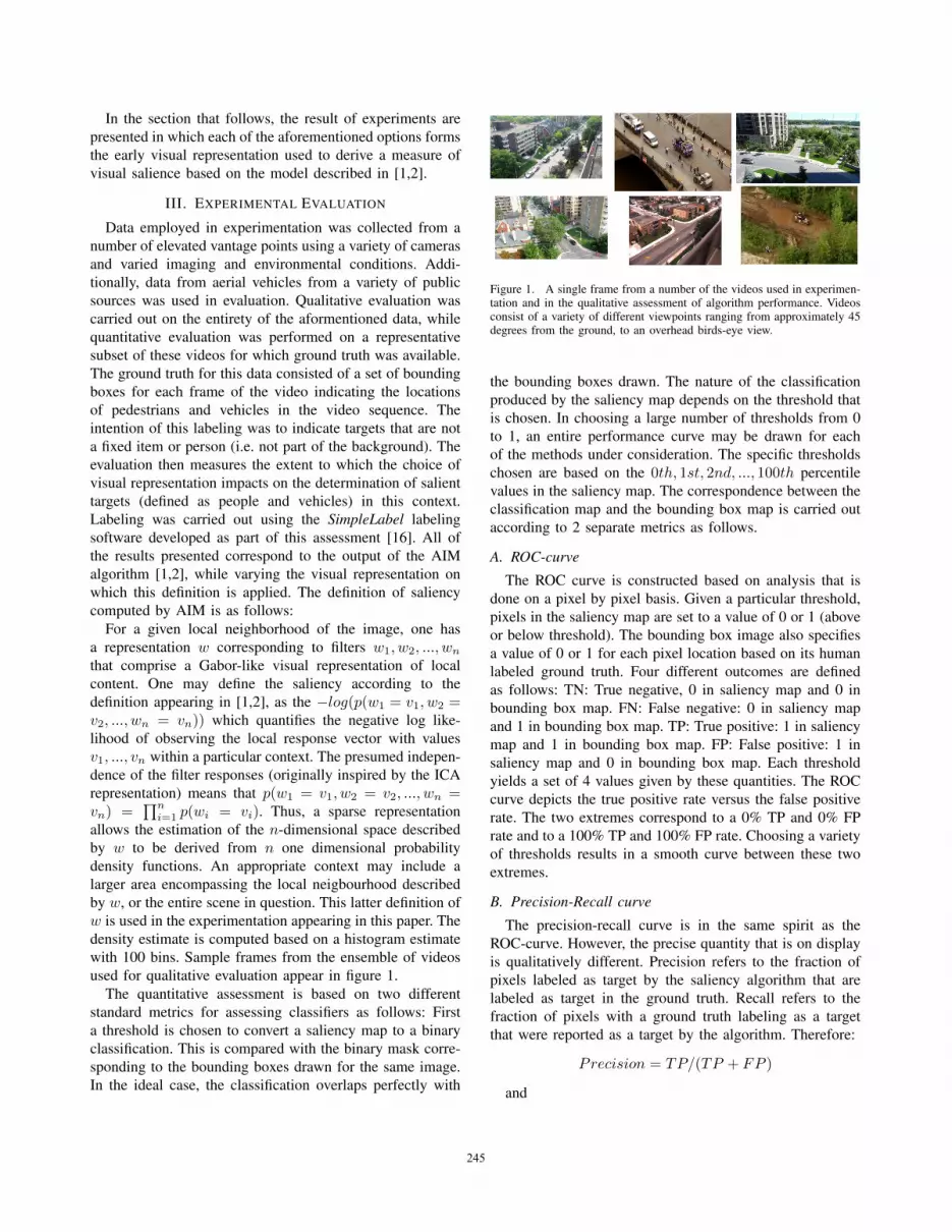
allows the estimation of the n-dimensional space describedby w to be derived from n one dimensional probabilitydensity functions. An appropriate context may include alarger area encompassing the local neigbourhood describedby w, or the entire scene in question. This latter definition ofw is used in the experimentation appearing in this paper. Thedensity estimate is computed based on a histogram estimatewith 100 bins. Sample frames from the ensemble of videosused for qualitative evaluation appear in figure 1.

The quantitative assessment is based on two differentstandard metrics for assessing classifiers as follows: Firsta threshold is chosen to convert a saliency map to a binaryclassification. This is compared with the binary mask corre-sponding to the bounding boxes drawn for the same image.In the ideal case, the classification overlaps perfectly with

Figure 1. A single frame from a number of the videos used in experimen-tation and in the qualitative assessment of algorithm performance. Videosconsist of a variety of different viewpoints ranging from approximately 45degrees from the ground, to an overhead birds-eye view.

the bounding boxes drawn. The nature of the classificationproduced by the saliency map depends on the threshold thatis chosen. In choosing a large number of thresholds from 0to 1, an entire performance curve may be drawn for eachof the methods under consideration. The specific thresholdschosen are based on the 0th, 1st, 2nd, ..., 100th percentilevalues in the saliency map. The correspondence between theclassification map and the bounding box map is carried outaccording to 2 separate metrics as follows.

A. ROC-curve

The ROC curve is constructed based on analysis that isdone on a pixel by pixel basis. Given a particular threshold,pixels in the saliency map are set to a value of 0 or 1 (aboveor below threshold). The bounding box image also specifiesa value of 0 or 1 for each pixel location based on its humanlabeled ground truth. Four different outcomes are definedas follows: TN: True negative, 0 in saliency map and 0 inbounding box map. FN: False negative: 0 in saliency mapand 1 in bounding box map. TP: True positive: 1 in saliencymap and 1 in bounding box map. FP: False positive: 1 insaliency map and 0 in bounding box map. Each thresholdyields a set of 4 values given by these quantities. The ROCcurve depicts the true positive rate versus the false positiverate. The two extremes correspond to a 0% TP and 0% FPrate and to a 100% TP and 100% FP rate. Choosing a varietyof thresholds results in a smooth curve between these twoextremes.

B. Precision-Recall curve

The precision-recall curve is in the same spirit as theROC-curve. However, the precise quantity that is on displayis qualitatively different. Precision refers to the fraction ofpixels labeled as target by the saliency algorithm that arelabeled as target in the ground truth. Recall refers to thefraction of pixels with a ground truth labeling as a targetthat were reported as a target by the algorithm. Therefore:

Precision = TP/(TP + FP )

and

245

Figure 2. A depiction of the algorithmic determination of saliency attributed to the representation corresponding to the different choices of filters. Theextent to which a region is suppressed indicates its determined salience by AIM. Also shown (bottom middle and bottom right) is the output of analternative algorithm [17] for comparison. Regions that are non-salient are made to appear closer to white resulting in a cloudy or foggy appearance fornon-salient regions. Labels are as follows: jadeRGB: ICA based filters learned using the Jade algorithm [12], infomaxRGB: ICA based filters learned usingthe extended infomax algorithm [11], Flat Gabor: A filter bank based on a standard Gabor based representation, Hierarchical Gabor: A filter bank based ona hierarchical Gabor wavelet decomposition, log-Gabor: A filter bank constructed using log-Gabor filters, DoG: A filter bank built as the sum of circularDifference of Gaussian filters arranged in an oriented pattern, infomaxTran: ICA based filters using the extended infomax algorithm on an alternativecolorspace (YCbCr).

Recall = TP/(TP + FN)

This measure reflects the tradeoff between relevance andthe proportion of positive cases retrieved.

Figure 2 depicts a representation of the saliency attributedto different regions of a frame from one of the sequencesconsidered. The areas deemed non-salient by the algorithmare less transparent and in effect are closer to white. Thisthen provides a depiction of the algorithms predictionslocalized on the image under consideration. One can seequickly from this image, that the qualitative differencesbetween the output of the algorithms under consideration aresignificant. Each of the frames in figure 2 is labeled in yellowwith the algorithm that depicted output corresponds to. Notshown is the output of the fasticaTran algorithm which isvery similar to the infomaxTran output. At first inspection, itappears that the log-Gabor filters produce clearer localizationof people and vehicles in the scene and also that spatiallocalization is much better than say the ICA based output. Inother high contrast regions (e.g. road markings) there is alsoqualitative variability in the degree of attributed salience.

The DoG based filters also produce output that is appealingfrom a qualitative perspective. A closer view of a region ofthis frame is depicted in figure 3. The qualitative observationof output corresponding to the complete set of aerial andsurveillance videos is in agreement with these observations.

To verify that these qualitative conclusions concerningthe filter outputs are correct, it is necessary to examinequantitatively the extent to which the regions deemed salientcorrespond to the people and cars labeled in the groundtruth. An example of the ground truth for one frame of theevaluation appears in figure 4. To perform this quantitativeevaluation, a representative video was selected for eachof an approximately 45 degree view of the ground (asshown in figure 2), as well as a birds-eye view from above.Figure 5 demonstrates the ROC and Precision-Recall basedcomparisons of the various filter bank choices across severalhundred frames of the video sequence. The algorithms arelabeled as follows:

1) jadeRGB: ICA based filters learned using the Jadealgorithm [15].

2) infomaxRGB: ICA based filters learned using the

246

Figure 3. A depiction of the algorithmic determination of saliency attributed to the representation corresponding to the different choices of filters. Theextent to which a region is transparent indicates its determined salience by AIM. Regions heavily obscured by white are deemed non-salient by thealgorithm. Labels are as in figure 2.

Figure 4. A depiction of the ground truth used in the quantitative assessment for one frame of the 45 degrees test video sequence. Boxed areas indicateareas where regions deemed as salient are present.

extended infomax algorithm [1].3) Flat Gabor: A filter bank based on a standard Gabor

based representation.4) Hierarchical Gabor: A filter bank based on a hierar-

chical Gabor wavelet decomposition.5) Log-Gabor: A filter bank constructed using log-Gabor

filters.

6) DoG: A filter bank built as the sum of circularDifference of Gaussian filters arranged in an orientedpattern.

7) infomaxTran: ICA based filters using the extendedinfomax algorithm on an alternative colorspace(YCbCr).

8) fasticaTran: ICA based filters using the fastICA algo-

247

0 0.1 0.2 0.3 0.4 0.5 0.6 0.7 0.8 0.9 10

0.1

0.2

0.3

0.4

0.5

0.6

0.7

0.8

0.9

1

False Accept Rate

Fal

se R

ejec

t Rat

e

jadeRGB

infomaxRGBFlat Gabor

Hierarchical Gabor

log-Gabor

DoGinfomaxTran

fasticaTran

jadeRGB

infomaxRGBFlat Gabor

Hierarchical Gabor

log-Gabor

DoGinfomaxTran

fasticaTranjadeRGB

infomaxRGBFlat Gabor

Hierarchical Gabor

log-Gabor

DoGinfomaxTran

fasticaTran

45 degrees

Birds-eye view

Figure 5. Top: Curves for the quantitative evaluation corresponding to the 45 degree angle intersection video sequence. Bottom: Curves correspondingto the birds-eye view video sequence. Left: ROC curves depicting the relative performance of the different algorithms. Right: Precision-Recall curvesdepicting the relative performance of the algorithms under consideration. Labels are the same as those listed in figure 2.

rithm [18] on an alternative colorspace (YCbCr).

The top row of figure 5 corresponds to the 45 degreeangled video and the bottom row to the aerial view. Onthe left of each column is the ROC curve for the videounder consideration and on the right is the Precision-Recallcurve. As can be seen, the representation under considerationcan appreciably affect algorithm performance. In general thequantitative assessment agrees with the intuition drawn fromthe qualitative assessment. As a whole, the log-Gabor filtersare the best option for their simplistic parametric nature,and the quality of their output in the context of the algorithmunder consideration. This is perhaps not surprising consider-ing that cells in the visual cortex of humans appear to havea profile akin to log-Gabors and this conceivably yields amore even sampling of the spectral domain. It is interesting

to note the apparently poor performance attributed to thestandard flat Gabor filters here. This is apparently due tostrong selectivity for certain frequency bands, notably onthe higher spatial frequency end in this case. It is alsoconceivable that the performance difference might be smallerusing masks that are a more precise fit to the boundariesof target items (i.e. not based on bounding boxes). In thecase of the ICA based filters, the form, and also spatiallocalization can be poor. This is due in part to the fact thatthese filters have steeper boundaries when compared to thosewith a smoother Gaussian envelope that forms the spatiallylocalized component of the filter definitions.

IV. DISCUSSION

It is apparent from the results that the nature of earlyvisual filtering has an appreciable impact on the deter-

248

mination of saliency. The intuition that derives from ourextensive qualitative experimentation suggests that the natureof spectral sampling has a very important role in the determi-nation of salient targets. From a system design perspective,representation based on independent component analysis(ICA) can be convenient since it allows the treatment ofintensity variations as well as chromatic content to be dealtwith using a single unified set of filters. On the other hand, inthe absence of a parametric form describing the interpretiveunits involved in the system, it can be impossible to performcertain operations (e.g. suppressing a specific frequencyband) without doing some further analysis first.

Owing to the 1/f structure of natural scenes, it is apparentthat the sampling produced by standard Gabor filters isbiased to certain radial frequencies determined by the filterparameters. When coupled with postprocessing that is highlynon-linear, this bias can become exaggerated and lead tosignificant performance differences; this is apparently thecase for the experimentation presented here. The resultscorresponding to log-Gabor filters appear to correspondmore closely to targets of interest in a qualitative sense andthis may be verified quantitatively based on the performanceevaluation presented in this paper. Moreover, the fact thatlog-Gabor filters arguably provide a better fit for visualcomputation in the primate brain suggests that they mayhave some especially desirable properties.

The non-linear postprocessing that is performed by themodel corresponds to a likelihood estimate based on aGeneralized Gaussian distribution (GGD) followed by alogarithmic non-linearity. The probability density functioncorresponding to the response of any Gabor-like filter is fitwell by a GGD. This implies that the strong sensitivity toany weak frequency bias (in the standard Gabor as opposedto the log-Gabor) is not isolated to the model at hand, butwill likely arise in any model for which there is a likelihoodestimate based on the response of a Gabor-like or bankof Gabor-like filters. The implication of this is that all ofthe issues discussed in this paper including the conclusionsdrawn are not system specific, but rather are issues that aredeserving of close consideration in building any system thatinvolves that analysis of outputs of Gabor or similar filters.

REFERENCES

[1] Bruce, N.D.B., Tsotsos, J.K., Saliency Based on InformationMaximization. Advances in Neural Information ProcessingSystems, 18, pp. 155-162, June 2006.

[2] Bruce, N.D.B., Tsotsos, J.K., Saliency, Attention, and Vi-sual Search: An Information Theoretic Approach, Journalof Vision 9:3, p1-24, 2009, http://journalofvision.org/9/3/5/,doi:10.1167/9.3.5.

[3] Dunn, D.F. and Higgins, W.E., Optimal Gabor-filter designfor texture segmentation. ICASSP 0-7803-0946-4 (1993), pp.v37v40.

[4] D.A. Clausi and M.Ed Jernigan, Designing Gabor filters foroptimal texture separability. Pattern Recognition 33 11 (2000),pp. 18351849.

[5] Lunscher, W.H.H.J and Beddoes, M.P., Optimal edge detectordesign I: parameter selection and noise effects, IEEE Trans.Pattern Analysis Mach. Intell. 8 (1986), pp. 164177.

[6] Field DJ. (1987). ”Relations Between the Statistics of NaturalImages and the Response Profiles of Cortical Cells”. Journalof the Optical Society of America A, 4, 2379-2394.

[7] Parker, A. J. and Hawken, M. J. ”Two-dimensional spatialstructure of receptive fields in monkey striate cortex,” J. Opt.Soc. Am. A 5, 598-605. 1988.

[8] Lampl, I., Anderson, J.S., Gillespie, D.C. and Ferster, D.,Prediction of Orientation Selectivity from Receptive FieldArchitecture in Simple Cells of Cat Visual Cortex, Neuron,30:1, 263–274, 2001.

[9] Somers, D.C., Nelson, S.B. and Sur, M., An emergent model oforientation selectivity in cat visual cortical simple cells, Journalof Neuroscience, 15:8, 5448-5465, 1995.

[10] Kaplan, E. and Marcus, S. and So, Y.T., Effects of darkadaptation on spatial and temporal properties of receptive fieldsin cat lateral geniculate nucleus, Journal of Physiology, 294:1,561-580, 1979.

[11] Lee, T.-W., Girolami, M., Bell, A. J., Sejnowski, T. J., AUnifying Information-Theoretic Framework for IndependentComponent Analysis, Computers and Mathematics with Ap-plications, 39, 1-21, 2000.

[12] Cardoso, J-F., High-order contrasts for independent compo-nent analysis, Neural Computation, 11:1, 157–192, 1999.

[13] Olshausen BA, and Field DJ. (1996). Emergence of Simple-Cell Receptive Field Properties by Learning a Sparse Code forNatural Images. Nature, 381: 607-609.

[14] Movellan, J. R., Tutorial on Gabor Filters. Technical Report,2002.

[15] Kovesi, P.D., MATLAB and Octave Functions for ComputerVision and Image Processing, Centre for Exploration Targeting,School of Earth and Environment, The University of WesternAustralia, http://www.csse.uwa.edu.au/ pk/research/matlabfns/

[16] Simine, E., SimpleLabel software package, Lab forActive and Attentive Vision, York University, 2010.http://www.cse.yorku.ca/LAAV/software/index.html

[17] Itti, L.,Koch, C., Niebur, E., A Model of Saliency-BasedVisual Attention for Rapid Scene Analysis, IEEE Transactionson Pattern Analysis and Machine Intelligence, Vol. 20, No. 11,pp. 1254-1259, 1998.

[18] Hyvarinen, A. and Oja, E., A Fast Fixed-Point Algorithmfor Independent Component Analysis, Neural Computation,9(7):1483-1492, 1997.

249