validation of odin/osiris stratospheric no 2 profiles

Validation of Odin/OSIRIS stratospheric NO2 profiles

Samuel M. Brohede,1 Craig S. Haley,2 Chris A. McLinden,3 Christopher E. Sioris,3,4

Donal P. Murtagh,1 Svetlana V. Petelina,4 Edward J. Llewellyn,4 Ariane Bazureau,5

Florence Goutail,5 Cora E. Randall,6 Jerry D. Lumpe,7 Ghassan Taha,8

Larry W. Thomasson,9 and Larry L. Gordley10

Received 31 May 2006; revised 25 October 2006; accepted 20 November 2006; published 12 April 2007.

[1] This paper presents the validation study of stratospheric NO2 profiles retrieved fromOdin/OSIRIS measurements of limb-scattered sunlight (version 2.4). The OpticalSpectrograph and Infrared Imager System (OSIRIS) NO2 data set is compared tocoincident solar occultation measurements by the Halogen Occultation Experiment(HALOE), Stratospheric Aerosol and Gas Experiment (SAGE) II, SAGE III, and PolarOzone and Aerosol Measurement (POAM) III during the 2002–2004 period.Comparisons with seven Systeme d’Analyse par Observation Zenithal (SAOZ) balloonmeasurements are also presented. All comparisons show good agreement, withdifferences, both random and systematic, of less than 20% between 25 km and 35 km.Inconsistencies with SAGE III below 25 km are found to be caused primarily by diurnaleffects from varying NO2 concentrations along the SAGE III line-of-sight. On thebasis of the differences, the OSIRIS random uncertainty is estimated to be 16% between15 km and 25 km, 6% between 25 km and 35 km, and 9% between 35 km and 40 km.The estimated systematic uncertainty is about 22% between 15 and 25 km, 11–21%between 25 km and 35 km, and 11–31% between 35 km and 40 km. The uncertaintiesfor AM (sunrise) profiles are generally largest and systematic deviations are found to belarger at equatorial latitudes. The results of this validation study show that the OSIRISNO2 profiles are well behaved, with reasonable uncertainty estimates between 15 kmand 40 km. This unique NO2 data set, with more than hemispheric coverage andhigh vertical resolution will be of particular interest for studies of nitrogen chemistry in themiddle atmosphere, which is closely linked to ozone depletion.

Citation: Brohede, S. M., et al. (2007), Validation of Odin/OSIRIS stratospheric NO2 profiles, J. Geophys. Res., 112, D07310,

doi:10.1029/2006JD007586.

1. Introduction

[2] A number of satellite instruments have been launchedrecently that measure limb-scattered sunlight radiances withthe goal of deriving vertical profiles of stratospheric minorspecies. These instruments include OSIRIS (Optical Spec-trograph and Infrared Imager System) on the Odin satellite

[Warshaw et al., 1998; Llewellyn et al., 2004] and SCIA-MACHY (Scanning Imaging Absorption Spectrometer forAtmospheric Chartography) on Envisat [Bovensmann et al.,1999]. GOMOS (Global Ozone Measurement by Occulta-tion of Stars) on Envisat [Bertaux et al., 1991] and SAGE(Stratospheric Aerosol and Gas Experiment) III on theMeteor-3M spacecraft [McCormick et al., 1991] are primar-ily occultation instruments that also have limb-scatter mea-surement capabilities.[3] The interest in the limb-scatter technique lies in a

demand for atmospheric information with both globalcoverage and relatively high vertical resolution. The tradi-tional sources of global stratospheric minor species infor-mation have largely been limited to either poor or novertical information (nadir mapping instruments) or restrictedspatial coverage (solar occultation instruments). The advan-tage of the limb-scatter technique is the provision of verticalprofiles of stratospheric and mesospheric minor constituentswith high vertical resolution (1–3 km) and near globalcoverage. A limitation to the technique is that only themeasurements from the sunlit portion of each orbit can beutilized (i.e., daytime only). Passive emission instruments

JOURNAL OF GEOPHYSICAL RESEARCH, VOL. 112, D07310, doi:10.1029/2006JD007586, 2007

1Department of Radio and Space Science, Chalmers University ofTechnology, Goteborg, Sweden.

2Centre for Research in Earth and Space Science, York University,Toronto, Ontario, Canada.

3Environment Canada, Toronto, Ontario, Canada.4Department of Physics and Engineering Physics, University of

Saskatchewan, Saskatoon, Saskatchewan, Canada.5Service d’Aeronomie, Centre National de la Recherche Scientifique,

Verrieres le Buisson, France.6Laboratory for Atmospheric and Space Physics and Department of

Atmospheric and Oceanic Science, University of Colorado, Boulder, USA.7Computational Physics Inc., Springfield, Virginia, USA.8Science Systems and Applications Inc., Lanham, Maryland, USA.9NASA Langley Research Center, Hampton, Virginia, USA.10GATS Inc., Newport News, Virginia, USA.

Copyright 2007 by the American Geophysical Union.0148-0227/07/2006JD007586

D07310 1 of 22

provide similar benefits as the limb-scatter technique andare not limited to measuring the sunlit atmosphere. TheMichelson Interferometer for Passive Atmospheric Sound-ing (MIPAS) on Envisat [Fischer and Oelhaf, 1996] pro-vides NO2 profiles with a vertical resolution of about 4 km,but the retrievals require extensive non-LTE (Local Ther-modynamic Equilibrium) calculations [Funke et al., 2005].[4] Haley et al. [2004] describe how NO2 and O3 can be

successfully retrieved from OSIRIS limb-scatter measure-ments in the stratosphere using a combination of Differen-tial Optical Absorption Spectroscopy (DOAS) [Platt, 1994]and Optimal Estimation (OE) [Rodgers, 2000]. OSIRISprovides a unique data set of NO2 with a slightly morethan hemispheric coverage and a vertical resolution of about2 km between 15 and 40 km. A detailed error analysis wascarried out by Haley et al. [2004] and the major sources ofuncertainty were identified as pointing offset (tangent heightregistration), aerosols and cloud and concluded that theOSIRIS NO2 profiles have an accuracy of 10% at the peakof the profiles.[5] The purpose of this study is to validate the OSIRIS

NO2 product (version 2.4) and determine the systematic andrandom uncertainties. Four solar occultation instruments,HALOE (Halogen Occultation Experiment), POAM (PolarOzone and Aerosol Measurement) III, SAGE (StratosphericAerosol and Gas Experiment) II, and SAGE III, are used forcomparisons with coincident OSIRIS NO2 measurementsfrom 2002 to 2004. OSIRIS NO2 profiles are also comparedwith SAOZ (Systeme d’Analyse par Observation Zenithale)balloon instrument measurements. Stratospheric NO2 is animportant species to measure because it is part of the NOx

chemistry, which is closely linked to ozone depletion; seesection 2.[6] Section 2 gives a brief description of nitrogen chem-

istry in the stratosphere and is followed by a brief overviewof each instrument in section 3 and a short description of theOSIRIS retrieval process in section 4. Thereafter the vali-dation process is described (section 5) and the results arepresented (section 6). An analysis of the results is presentedin section 7, followed by major conclusions and suggestedfuture work in section 8.

2. Stratospheric NOx Chemistry

[7] This section gives a brief introduction to stratosphericNOx chemistry based on Brasseur and Solomon [1986] andreferences therein. The term NOx refers to the sum of NOand NO2 and is used due to the strong interaction betweenthese species according to reactions (1) to (3) below. Theterm NOy is reserved for all reactive nitrogen oxides,including NO, N2O, NO2, NO3, N2O5, and HNO3.

NO2 þ hn ! NOþ O ð1Þ

NO2 þ O ! NOþ O2 ð2Þ

NOþ O3 ! NO2 þ O2 ð3Þ

[8] The lifetime of NOx is too short for it to cross thetropopause barrier in any significant amount, and the

dominant sources of NOx in the stratosphere are rather themore inert N2O crossing the tropopause and to a smallextent the polar winter descent of NOy created by auroralprocesses.[9] NOx species are photochemically active, and the

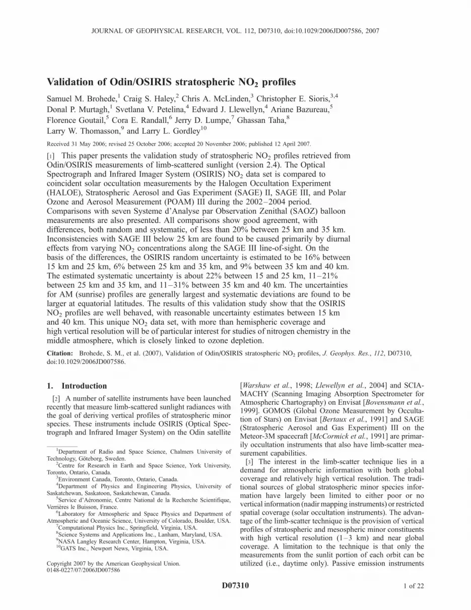
availability of solar radiation determines the relative abun-dance of NO and NO2 as seen in reaction (1). Duringdaytime conditions, the NOx equilibrium is pushed towardNO. As the Sun sets the NO2 concentration rapidlyincreases at the cost of NO (see Figure 1). In the nighttimechemistry an additional, but slower, processes take place,converting NOx into NOy:

NO2 þ O3 ! NO3 þ O2 ð4Þ

NO2 þ NO3 þM ! N2O5 þM ð5Þ

The NO3 and N2O5 are photolyzed during the daytime,creating NOx again. The NO3 concentration drops rapidly atsunrise, while N2O5 is more slowly photolyzed at strato-spheric temperatures, which explains the positive NO2

gradient during the day in Figure 1.[10] NOx chemistry is crucial to many stratospheric

processes, including ozone depletion. Ozone (odd oxygen)is catalytically destroyed through the reaction cycle (2) and(3). In fact, photochemical loss of O3 is dominated by NOx

between 25 km and 40 km altitude [Dessler, 2000].In addition, NOx is an important factor in the formation ofreservoir species and in the creation of HNO3-richPSC (Polar Stratospheric Cloud) particles. The mostimportant sink of stratospheric nitrogen inside the polarvortex is deposition of these particles to the troposphere(denitrification).

3. Instrument Descriptions

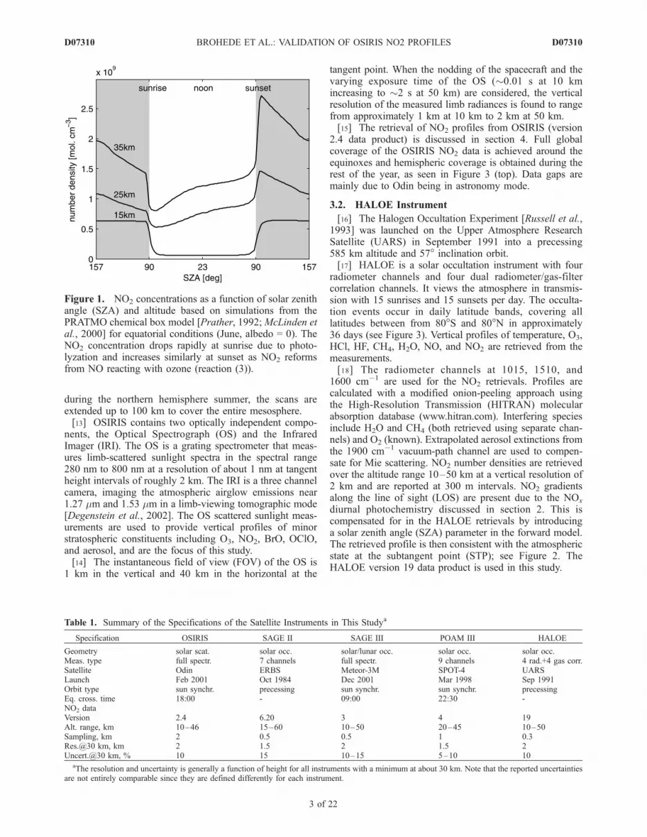
[11] Brief descriptions of the satellite orbit, instrumentparameters, NO2 retrieval method, and error estimation foreach of the instruments are found below. An overview of theimportant parameters is found in Table 1. The viewinggeometries of solar occultation and solar scattering instru-ments are illustrated in Figure 2.

3.1. OSIRIS Instrument

[12] The Optical Spectrograph and Infrared ImagerSystem [Llewellyn et al., 2004] is one of two instrumentson board the Odin satellite [Nordh et al., 2003]. Odin waslaunched in February 2001 into a 600 km circular Sun-synchronous near-terminator orbit with a 97.8� inclinationand the ascending node at 1800 hours LST (Local SolarTime). Odin is a combination of astronomy and aeronomymissions with equal time disposition. OSIRIS is dedicatedto aeronomy studies [Murtagh et al., 2002] and a secondinstrument, the Submillimeter and Millimeter Radiometer(SMR) [Frisk et al., 2003] carries out both aeronomy andastronomy studies. The instruments are coaligned and scanthe limb of the atmosphere over a tangent height range 7 kmto 70 km in approximately 85 seconds during normalstratospheric operations through controlled nodding of thesatellite. Every 8th day in general and every 1–3 days

D07310 BROHEDE ET AL.: VALIDATION OF OSIRIS NO2 PROFILES

2 of 22

D07310

during the northern hemisphere summer, the scans areextended up to 100 km to cover the entire mesosphere.[13] OSIRIS contains two optically independent compo-

nents, the Optical Spectrograph (OS) and the InfraredImager (IRI). The OS is a grating spectrometer that meas-ures limb-scattered sunlight spectra in the spectral range280 nm to 800 nm at a resolution of about 1 nm at tangentheight intervals of roughly 2 km. The IRI is a three channelcamera, imaging the atmospheric airglow emissions near1.27 mm and 1.53 mm in a limb-viewing tomographic mode[Degenstein et al., 2002]. The OS scattered sunlight meas-urements are used to provide vertical profiles of minorstratospheric constituents including O3, NO2, BrO, OClO,and aerosol, and are the focus of this study.[14] The instantaneous field of view (FOV) of the OS is

1 km in the vertical and 40 km in the horizontal at the

tangent point. When the nodding of the spacecraft and thevarying exposure time of the OS (�0.01 s at 10 kmincreasing to �2 s at 50 km) are considered, the verticalresolution of the measured limb radiances is found to rangefrom approximately 1 km at 10 km to 2 km at 50 km.[15] The retrieval of NO2 profiles from OSIRIS (version

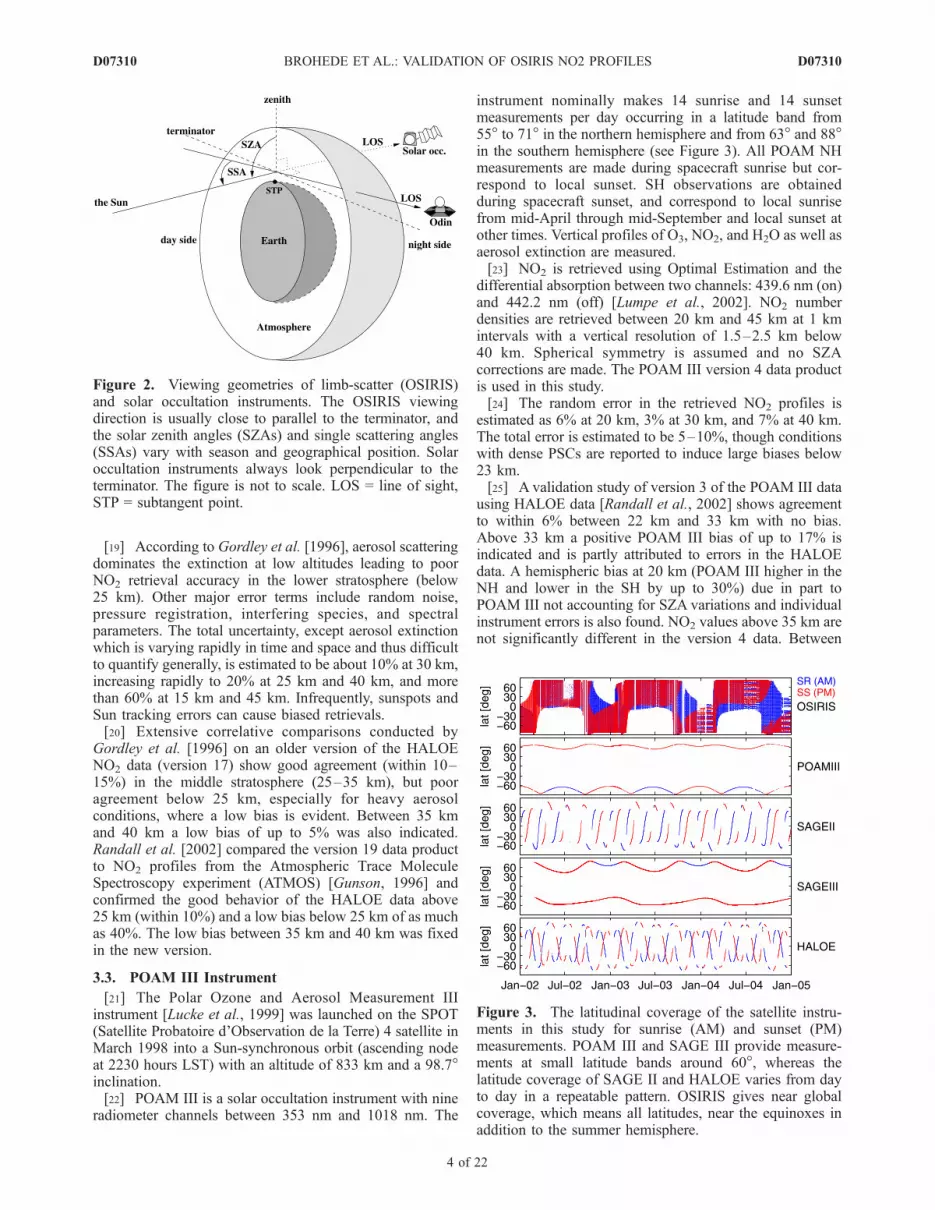
2.4 data product) is discussed in section 4. Full globalcoverage of the OSIRIS NO2 data is achieved around theequinoxes and hemispheric coverage is obtained during therest of the year, as seen in Figure 3 (top). Data gaps aremainly due to Odin being in astronomy mode.

3.2. HALOE Instrument

[16] The Halogen Occultation Experiment [Russell et al.,1993] was launched on the Upper Atmosphere ResearchSatellite (UARS) in September 1991 into a precessing585 km altitude and 57� inclination orbit.[17] HALOE is a solar occultation instrument with four

radiometer channels and four dual radiometer/gas-filtercorrelation channels. It views the atmosphere in transmis-sion with 15 sunrises and 15 sunsets per day. The occulta-tion events occur in daily latitude bands, covering alllatitudes between from 80�S and 80�N in approximately36 days (see Figure 3). Vertical profiles of temperature, O3,HCl, HF, CH4, H2O, NO, and NO2 are retrieved from themeasurements.[18] The radiometer channels at 1015, 1510, and

1600 cm�1 are used for the NO2 retrievals. Profiles arecalculated with a modified onion-peeling approach usingthe High-Resolution Transmission (HITRAN) molecularabsorption database (www.hitran.com). Interfering speciesinclude H2O and CH4 (both retrieved using separate chan-nels) and O2 (known). Extrapolated aerosol extinctions fromthe 1900 cm�1 vacuum-path channel are used to compen-sate for Mie scattering. NO2 number densities are retrievedover the altitude range 10–50 km at a vertical resolution of2 km and are reported at 300 m intervals. NO2 gradientsalong the line of sight (LOS) are present due to the NOx

diurnal photochemistry discussed in section 2. This iscompensated for in the HALOE retrievals by introducinga solar zenith angle (SZA) parameter in the forward model.The retrieved profile is then consistent with the atmosphericstate at the subtangent point (STP); see Figure 2. TheHALOE version 19 data product is used in this study.

Figure 1. NO2 concentrations as a function of solar zenithangle (SZA) and altitude based on simulations from thePRATMO chemical box model [Prather, 1992;McLinden etal., 2000] for equatorial conditions (June, albedo = 0). TheNO2 concentration drops rapidly at sunrise due to photo-lyzation and increases similarly at sunset as NO2 reformsfrom NO reacting with ozone (reaction (3)).

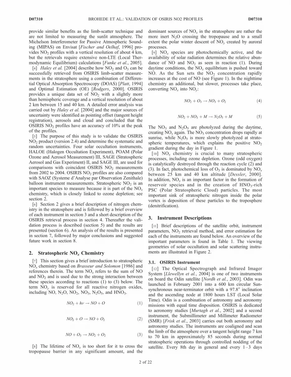
Table 1. Summary of the Specifications of the Satellite Instruments in This Studya

Specification OSIRIS SAGE II SAGE III POAM III HALOE

Geometry solar scat. solar occ. solar/lunar occ. solar occ. solar occ.Meas. type full spectr. 7 channels full spectr. 9 channels 4 rad.+4 gas corr.Satellite Odin ERBS Meteor-3M SPOT-4 UARSLaunch Feb 2001 Oct 1984 Dec 2001 Mar 1998 Sep 1991Orbit type sun synchr. precessing sun synchr. sun synchr. precessingEq. cross. time 18:00 - 09:00 22:30 -NO2 dataVersion 2.4 6.20 3 4 19Alt. range, km 10–46 15–60 10–50 20–45 10–50Sampling, km 2 0.5 0.5 1 0.3Res.@30 km, km 2 1.5 2 1.5 2Uncert.@30 km, % 10 15 10–15 5–10 10

aThe resolution and uncertainty is generally a function of height for all instruments with a minimum at about 30 km. Note that the reported uncertaintiesare not entirely comparable since they are defined differently for each instrument.


3 of 22

D07310

[19] According to Gordley et al. [1996], aerosol scatteringdominates the extinction at low altitudes leading to poorNO2 retrieval accuracy in the lower stratosphere (below25 km). Other major error terms include random noise,pressure registration, interfering species, and spectralparameters. The total uncertainty, except aerosol extinctionwhich is varying rapidly in time and space and thus difficultto quantify generally, is estimated to be about 10% at 30 km,increasing rapidly to 20% at 25 km and 40 km, and morethan 60% at 15 km and 45 km. Infrequently, sunspots andSun tracking errors can cause biased retrievals.[20] Extensive correlative comparisons conducted by

Gordley et al. [1996] on an older version of the HALOENO2 data (version 17) show good agreement (within 10–15%) in the middle stratosphere (25–35 km), but pooragreement below 25 km, especially for heavy aerosolconditions, where a low bias is evident. Between 35 kmand 40 km a low bias of up to 5% was also indicated.Randall et al. [2002] compared the version 19 data productto NO2 profiles from the Atmospheric Trace MoleculeSpectroscopy experiment (ATMOS) [Gunson, 1996] andconfirmed the good behavior of the HALOE data above25 km (within 10%) and a low bias below 25 km of as muchas 40%. The low bias between 35 km and 40 km was fixedin the new version.

3.3. POAM III Instrument

[21] The Polar Ozone and Aerosol Measurement IIIinstrument [Lucke et al., 1999] was launched on the SPOT(Satellite Probatoire d’Observation de la Terre) 4 satellite inMarch 1998 into a Sun-synchronous orbit (ascending nodeat 2230 hours LST) with an altitude of 833 km and a 98.7�inclination.[22] POAM III is a solar occultation instrument with nine

radiometer channels between 353 nm and 1018 nm. The

instrument nominally makes 14 sunrise and 14 sunsetmeasurements per day occurring in a latitude band from55� to 71� in the northern hemisphere and from 63� and 88�in the southern hemisphere (see Figure 3). All POAM NHmeasurements are made during spacecraft sunrise but cor-respond to local sunset. SH observations are obtainedduring spacecraft sunset, and correspond to local sunrisefrom mid-April through mid-September and local sunset atother times. Vertical profiles of O3, NO2, and H2O as well asaerosol extinction are measured.[23] NO2 is retrieved using Optimal Estimation and the

differential absorption between two channels: 439.6 nm (on)and 442.2 nm (off) [Lumpe et al., 2002]. NO2 numberdensities are retrieved between 20 km and 45 km at 1 kmintervals with a vertical resolution of 1.5–2.5 km below40 km. Spherical symmetry is assumed and no SZAcorrections are made. The POAM III version 4 data productis used in this study.[24] The random error in the retrieved NO2 profiles is

estimated as 6% at 20 km, 3% at 30 km, and 7% at 40 km.The total error is estimated to be 5–10%, though conditionswith dense PSCs are reported to induce large biases below23 km.[25] A validation study of version 3 of the POAM III data

using HALOE data [Randall et al., 2002] shows agreementto within 6% between 22 km and 33 km with no bias.Above 33 km a positive POAM III bias of up to 17% isindicated and is partly attributed to errors in the HALOEdata. A hemispheric bias at 20 km (POAM III higher in theNH and lower in the SH by up to 30%) due in part toPOAM III not accounting for SZA variations and individualinstrument errors is also found. NO2 values above 35 km arenot significantly different in the version 4 data. Between

Figure 2. Viewing geometries of limb-scatter (OSIRIS)and solar occultation instruments. The OSIRIS viewingdirection is usually close to parallel to the terminator, andthe solar zenith angles (SZAs) and single scattering angles(SSAs) vary with season and geographical position. Solaroccultation instruments always look perpendicular to theterminator. The figure is not to scale. LOS = line of sight,STP = subtangent point.

Figure 3. The latitudinal coverage of the satellite instru-ments in this study for sunrise (AM) and sunset (PM)measurements. POAM III and SAGE III provide measure-ments at small latitude bands around 60�, whereas thelatitude coverage of SAGE II and HALOE varies from dayto day in a repeatable pattern. OSIRIS gives near globalcoverage, which means all latitudes, near the equinoxes inaddition to the summer hemisphere.


4 of 22

D07310

27 km and 33 km the values in version 4 are about 5–15%lower than in version 3. Below 25 km the version 4 data aresignificantly larger than in version 3, varying from 5% orless in the summer to up to 50% in the winter, where theNO2 abundances are small (C. E. Randall et al., Comparisonof solar occultation NO2 measurements, manuscript inpreparation, 2007).

3.4. SAGE II Instrument

[26] The Stratospheric Aerosol and Gas Experiment IIinstrument [Mauldin et al., 1985] was launched on boardthe Earth Radiation Budget Satellite (ERBS) in October1984 into a precessing orbit with an altitude of 610 km anda 56� inclination.[27] SAGE II is a solar occultation photometer with a

holographic grating and 7 channels between 385 nm and1020 nm. The latitude coverage of SAGE II varies from dayto day in a 1-year repeatable pattern, similar to HALOE,extending from approximately 70�S to 70�N (see Figure 3).SAGE II produces vertical profiles of aerosols, O3, NO2,and H2O.[28] Slant columns of NO2 are calculated from the 448 nm

and 453 nm channels using a differential technique [Chuand McCormick, 1989]. Vertical profiles are then retrievedbetween 15 km and 60 km using an onion peeling proce-dure, where the NO2 slant columns are smoothed prior topeeling. The altitude sampling is 1 km and the verticalresolution for NO2 is about 1.5 km below 39 km and 5 kmabove 39 km. As with POAM III, spherical symmetry isassumed and no SZA correction is applied. The SAGE IIversion 6.20 data product is used in this study, and com-pensates for the slight drift in the NO2 channels after launch.[29] The random error associated with the NO2 retrievals

between 27 km and 36 km is approximately 5%. The overallaccuracy is estimated to be 15%, with the increase mostlydue to NO2 cross section uncertainties. Difficulties inseparating NO2, O3, and aerosols below 23 km makemeasurements in that region highly uncertain.[30] A validation study carried out by Cunnold et al.

[1991] on an older version of data found the SAGE II NO2

to be in agreement with balloon instruments to within 10%between 23 km and 32 km. Comparisons between SAGE IIand HALOE by Gordley et al. [1996], also using an olderversion of data, indicated a significant bias in the SAGE IIdata due to aerosol contamination below 27 km, goodagreement (10%) from 27 km to 33 km, and a negativebias of up to 25% above 33 km. Taha et al. [2004] analyzedthe version 6.20 data product and found that the agreementwith SAGE III NO2 is within 5–9% in the altitude range20–36 km.

3.5. SAGE III Instrument

[31] The Stratospheric Aerosol and Gas Experiment IIIinstrument [Thomason and Taha, 2003] was launched onboard the Russian Meteor-3M platform in December 2001into a Sun-synchronous orbit with ascending node at0900 hours LST. It is primarily designed to make solarand lunar occultation measurements but also has a limb-scatter measurement capability.[32] The SAGE III instrument is a spectrometer covering

wavelengths from 280 nm to 1040 nm with a 1–2 nmspectral resolution. An additional photodetector at 1550 nm

is included. SAGE III provides 30 measurement events perday, 15 sunrises at high northern latitudes (45–80�N) and15 sunsets at southern midlatitudes (25–60�S). All satellitesunrise measurements are at local sunset, while observationsobtained during satellite sunset are also at local sunsetexcept from mid-September through February, as seen inFigure 3. SAGE III measures O3, NO2, aerosol extinction,H2O, NO3 (lunar), OClO, cloud information, pressure, andtemperature.[33] Profiles of NO2 are derived using a multiple linear

regression (MLR) technique for two spectral channels(433–450 nm and 563–622 nm) [NASA Langley ResearchCenter, 2002]. MLR simultaneously solves for O3 and NO2,which absorb significantly in both spectral regions. Theuncertainty is estimated to be 10–15% (systematic) and10–15% (random). Smoothing is applied to the NO2 slantcolumns, giving an effective vertical resolution of about2 km throughout the 10–50 km retrieval range (for otherproducts the resolution is about 1 km). Number densities arereported at 0.5 km intervals and no SZA correction isapplied. The SAGE III version 3 data product is used inthis study.[34] According to Taha et al. [2004], the agreement with

SAGE II NO2 is within 5–9% in the altitude range 20–36 km. Agreement with POAM III is within 10% above22 km and with HALOE is within 5% between 25 km and34 km. Large differences between SAGE III and HALOEbelow 25 km (up to 60%) are found and are likely due toSAGE III not accounting for SZA variations.

3.6. SAOZ Instrument

[35] The SAOZ (Systeme d’Analyse par ObservationZenithale) UV/visible spectrometer makes solar occultationmeasurements during the ascent/descent of the balloon andduring sunset/sunrise from float. The balloon version of theSAOZ instrument is very similar to the one used for ground-based measurements of total ozone and NO2 [Pommereauand Goutail, 1988]. Measurements are recorded between290 nm and 640 nm with an average spectral resolution of0.8 nm. Using an onion peeling method, SAOZ provides thevertical distribution of O3, NO2, and atmospheric extinctionat a vertical resolution of 1.4 km with accuracies of betterthan 3% for O3 and 10% for NO2 [Pommereau andPiquard, 1994].[36] The SAOZ NO2 profiles are reported to agree to

within 20% with POAM III from 23 km to 27 km, whereSAOZ has a negative bias at 27 km and a positive positivebias at 23 km [Randall et al., 2002]. At 20 km the meandifference is larger (50%). The SAOZ NO2 data used in thisstudy have not been corrected for diurnal variations alongthe line of sight.

4. OSIRIS NO2 Retrievals

[37] A thorough description of the OSIRIS NO2 retrievalscan be found in the work of Haley et al. [2004]. Only asimplified description is given here.

4.1. DOAS Step

[38] Instead of retrieving NO2 vertical profiles directlyfrom the OSIRIS limb-scattered radiance measurements, anintermediate step is applied where effective column densities,


5 of 22

D07310

ECD, (sometimes referred to as slant column densities) arecalculated using Differential Optical Absorption Spectros-copy (DOAS) [Platt, 1994]. The DOAS step is performed toreduce the sensitivity to phenomena that vary slowly withwavelength such as aerosol (Mie) scattering.[39] The wavelength region used for retrieving NO2 is

435–451 nm, where the absorption is large compared withO3 and strong Fraunhofer lines are avoided. An average ofspectra measured between 46 km and 65 km tangent heightfrom each limb scan is used as the reference spectrum,effectively reducing any Ring-effect and Fraunhofer signa-tures. O3 and O4 are included together with NO2 in thenonlinear, least-squares fit, and the I0-effect, wavelengthshifts, and different trending in the reference and themeasurement spectra (tilt-effect) are compensated for. TheNO2 absorption cross sections from Vandaele et al. [1998]are used.

4.2. Forward Model

[40] The pseudo-spherical multiple scattering radiativetransfer model LIMBTRAN [Griffoen and Oikarinen,2000] is used to invert ECD as a function of tangent heightto number density as a function of height. Temperature andpressure information used in LIMBTRAN is from theEuropean Centre for Medium-Range Weather Forecasts(ECMWF) analysis fields. Aerosol information is alsoincluded and consists of the stratospheric aerosol extinctionclimatology for 1999 from Bauman et al. [2003a, 2003b]and a Heney-Greenstein phase function (asymmetryparameter 0.7). The surface albedo is taken fromKoelemeijeret al. [2003].[41] LIMBTRAN assumes horizontal homogeneity with-

in its vertical layers, and the retrieved profile is assigned to

the location of the STP; see Figure 2. This can lead to errorsin the retrieved profiles at times when horizontal variationsin the true NO2 distribution exists. Such variations exist inthe NO2 distribution near the terminator due to photochem-istry and can affect the retrieved profiles, as will bediscussed in section 4.5.

4.3. Inversion Process

[42] The inversion algorithm used to deduce verticalprofiles of NO2 from ECDs is Optimal Estimation (OE)or more specifically the nonlinear Maximum A Posteriori(MAP) estimator from Rodgers [2000], solved in a Gauss-Newton iterative manner. MAP is a Bayesian estimatorgiving the most probable solution based on the measure-ments and a priori information and the associated covarian-ces. A positive constraint is applied to the retrievals byinverting in logarithm space. Profiles that have not con-verged after eight iterations or have converged with a highc2-value are discarded.[43] A fixed retrieval grid is chosen, stretching from 10 to

46 km at 2 km intervals. It was found that the weightingfunctions can be calculated using only two wavelengths,single scattering, and no aerosol without significantlyreducing accuracy. Good response (>0.75), i.e., low a prioricontamination, is usually found between 15 km and 40 kmand the resolution at 30 km is about 2 km, but this variesslightly from profile to profile depending on the measure-ment conditions.[44] The NO2 a priori information is taken from precal-

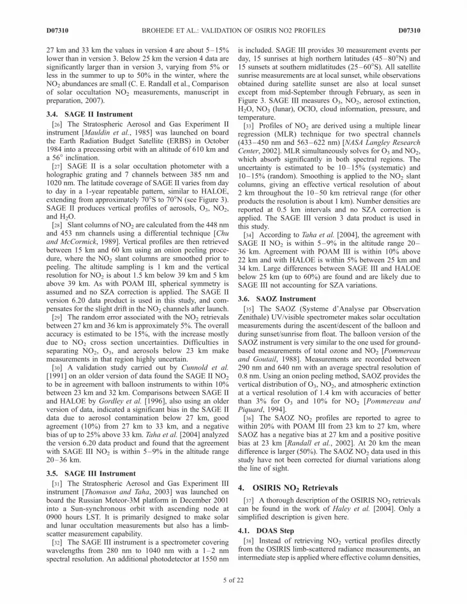
culated look-up tables constructed using a photochemicalbox model [Prather, 1992; McLinden et al., 2000], initial-ized with input fields derived from climatology (O3, T,aerosol surface area), three-dimensional model output (NO2,NOy), and tracer correlations (CH4, HO2, Cly, Bry). The apriori profile is chosen to be the nearest neighbor based onprofiles tabulated bimonthly and every 2.5� in latitude andthen interpolated in SZA to the value at the OSIRIS scanlocation. The covariance matrix of the a priori state is alsorequired for the retrievals. NO2 is assumed to follow a log-normal distribution, with standard deviations for the diag-onal components of 60% and an exponential off-diagonalcorrelation length of 4 km. The measurement covariancematrix is a diagonal matrix with the variance of thepropagated measurement noise in the diagonal. Measure-ments from different tangent altitudes are assumed uncor-related. A sample NO2 number density profile retrievedfrom a modeled noise-free OSIRIS limb scan is shown inFigure 4.

4.4. Error Budget

[45] The error estimation of the retrieved profiles is thecrucial part of any inversion technique. As described byRodgers [2000], four sources of error can be identified:(1) smoothing error, (2) retrieval noise, (3) forward modelerror, (4) forward model parameter error. The smoothingerror and measurement noise components of the totalretrieval error are easily calculated. However, the forwardmodel and forward model parameter errors are more diffi-cult to evaluate.[46] The smoothing error arises due to the limited vertical

resolution of the retrieval compared to the true atmosphericstate. If the retrieved profile is said to represent a smoothed

Figure 4. Typical NO2 retrieval characteristics for amodeled, noise-free OSIRIS midlatitude limb scan (SZA =85�, SSA = 90�). (a) The true, a priori (66% of the true), andretrieved profiles and the absolute difference between thetrue and retrieved profiles, (b) the averaging kernels (solidlines) and the measurement response (dashed line), and(c) the vertical resolution (‘‘spread’’) are shown. Highresponse (> 0.75) is usually found between 15 km and 40 kmand the vertical resolution is about 2 km near 30 km.


6 of 22

D07310

version on the true state, this error term can be ignored.Furthermore, when comparing retrieved profiles to profilesfrom another instrument with similar vertical resolution, thesmoothing error becomes irrelevant. Henceforth, the OSI-RIS smoothing error will not be included in the error budgetfor this validation study, where the vertical resolution of thevarious instruments only differs by a factor of two at most(see Table 1).[47] Retrieval noise is the measurement noise propagated

through the inversion process. This is a pure random errorwhich is easily computed and verified.[48] The forward model error is estimated by analyzing

the impact of various approximations on the retrievals. Thetotal forward model error for OSIRIS NO2 retrievals wasassessed by Haley et al. [2004] and found to be small(<5%), between 15 and 40 km, and generally independentof the measurement conditions. This type of error is mostlysystematic. Note that no attempt was made to estimate theerror introduced by the use of a pseudo-spherical forwardmodel.

[49] The forward model parameter error concerns theuncertainty in input parameters to the forward model suchas aerosol, neutral density, temperature, surface albedo,instrument spectral resolution, absorption cross sections,and the tangent height registration. Haley et al. [2004]studied these errors by treating them as independent errorsources, each with an assumed uncertainty. The errors wereestimated by performing perturbations of one standarddeviation to a number of forward model parameters abouta midlatitude atmosphere with surface albedo 0.3. In addi-tion to the above error sources, the impact of cloud on theretrievals is estimated in a preliminary way by perturbingthe surface albedo to a value of 1.0. Though crude, thisgives a sense of the impact that can be expected when cloudis present in the measurements (below the FOV of thelowest measurement) but is not taken into account in theretrievals. An additional error that was not considered byHaley et al. [2004] was the impact of nonretrieved species(i.e., O3), but this has now been included and has beenfound to be small (<1%). Assuming that each of the errorsare independent and that vertical correlations can beignored, the total forward model parameter error is givenby the square root of the sum of the error variances ofthe individual errors. Note that no attempt was made toestimate the error introduced by the assumption of sphericalhomogeneity.[50] Each of the forward model parameter error sources

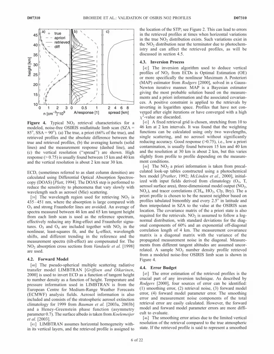
and the total are shown in Figure 5 for high-Sun (SZA =60�) and for both cloudy and cloud-free conditions. Errorsfor low-Sun conditions (SZA � 90�) are comparable tothose of high-Sun cloud-free conditions and are not signif-icantly sensitive to clouds. As the figure shows, tangentheight registration (pointing) uncertainty is the largestsource of error, potentially introducing errors of about15% away from the peak. Clouds (albedo) can also havea large effect on the retrievals, leading to errors of about15% below 20 km. Note that the tangent height registrationuncertainty in the OS measurements is difficult to deter-mine, but for this analysis it was estimated that the correctedtangent heights are accurate to 500 m (see section 4.6). Theerror due to cloud is also difficult to assess since theeffective albedo of cloud depends on the characteristics ofthe cloud (e.g., thickness and patchiness) and on the solarconditions. The analysis here is essentially a worst-casescenario.[51] If the three different error sources can be treated

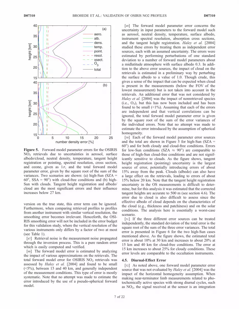
independently, the standard deviation of the total error is thesquare root of the sum of the three error variances. The totalerror is presented in Figure 6 for the two high-Sun casesmentioned above. As the figure shows, the estimated totalerror is about 10% at 30 km and increases to about 20% at15 km and 40 km for cloud-free conditions. The error at15 km increases to about 25% for cloudy conditions. Theseerror levels are comparable to the occultation instruments.

4.5. Diurnal-Effect Error

[52] As noted above, one forward model parameter errorsource that was not evaluated by Haley et al. [2004] was theimpact of the horizontal homogeneity assumption. Whenmaking near-terminator limb measurements related to pho-tochemically active species with strong diurnal cycles, suchas NO2, the signal received at the sensor is an integration

Figure 5. Forward model parameter errors for the OSIRISNO2 retrievals due to uncertainties in aerosol, surfacealbedo/cloud, neutral density, temperature, tangent heightregistration or pointing, spectral resolution, cross section,and ozone, given as 1s, and the total forward modelparameter error, given by the square root of the sum of thevariances. Two scenarios are shown: (a) high-Sun (SZA =60�, SSA = 90�) with cloud-free conditions and (b) high-Sun with clouds. Tangent height registration and albedo/cloud are the most significant errors and their influenceincreases below 27 km.


7 of 22

D07310

over a range of SZAs representing different atmosphericstates with a potentially large variation in the numberdensity of the target species. This so-called ‘‘diurnal effect’’is not accounted for in the OSIRIS retrievals, wherespherical homogeneity is assumed.[53] The error introduced by not accounting for the

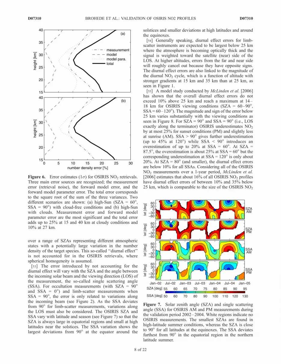
diurnal effect will vary with the SZA and the angle betweenthe incoming solar beam and the viewing direction (LOS) ofthe measurement, the so-called single scattering angle(SSA). For occultation measurements (with SZA = 90�and SSA = 0�) and limb-scatter measurements whenSSA = 90�, the error is only related to variations alongthe incoming beam (see Figure 2). As the SSA deviatesfrom 90� for limb-scatter measurements, variations alongthe LOS must also be considered. The OSIRIS SZA andSSA vary with latitude and season (see Figure 7) so that theSZA is always large in equatorial regions and small at highlatitudes near the solstices. The SSA variation shows thelargest deviations from 90� at the equator around the

solstices and smaller deviations at high latitudes and aroundthe equinoxes.[54] Generally speaking, diurnal effect errors for limb-

scatter instruments are expected to be largest below 25 kmwhere the atmosphere is becoming optically thick and thesignal is weighted toward the satellite (near) side of theLOS. At higher altitudes, errors from the far and near sidewill roughly cancel out because they have opposite signs.The diurnal effect errors are also linked to the magnitude ofthe diurnal NO2 cycle, which is a function of altitude withstronger gradients at 15 km and 35 km than at 25 km, asseen in Figure 1.[55] A model study conducted by McLinden et al. [2006]

has shown that the overall diurnal effect errors do notexceed 10% above 25 km and reach a maximum at 14–18 km for OSIRIS viewing conditions (SZA = 60–90�,SSA= 60–120�). The magnitude and sign of the error below25 km varies substantially with the viewing conditions asseen in Figure 8. For SZA = 90� and SSA = 90� (i.e., LOSexactly along the terminator) OSIRIS underestimates NO2

by at most 25% for sunset conditions (PM) and slightly lessat sunrise (AM). SSA > 90� gives further underestimation(up to 45% at 120�) while SSA < 90� introduces anoverestimation of up to 20% at SSA = 60�. At SZA =87.5�, the overestimation is about 25% at SSA = 60� but thecorresponding underestimation at SSA = 120� is only about20%. At SZA = 80� (and smaller), the diurnal effect errorsare below 10% for all SSAs. Considering all of the OSIRISNO2 measurements over a 1-year period, McLinden et al.[2006] estimates that about 16% of all OSIRIS NO2 profileshave diurnal effect errors of between 10% and 35% below25 km, which is comparable to the size of the OSIRIS NO2

Figure 6. Error estimates (1s) for OSIRIS NO2 retrievals.Three main error sources are recognized; the measurementerror (retrieval noise), the forward model error, and theforward model parameter error. The total error correspondsto the square root of the sum of the three variances. Twodifferent scenarios are shown: (a) high-Sun (SZA = 60�,SSA = 90�) with cloud-free conditions and (b) high-Sunwith clouds. Measurement error and forward modelparameter error are the most significant and the total erroradds up to 25% at 15 and 40 km at cloudy conditions and10% at 27 km.

Figure 7. Solar zenith angle (SZA) and single scatteringangle (SSA) for OSIRIS AM and PM measurements duringthe validation period 2002–2004. White regions indicate noOSIRIS measurements. The smallest SZAs are found inhigh-latitude summer conditions, whereas the SZA is closeto 90� for all latitudes at the equinoxes. The SSA deviatesfurthest from 90� in the equatorial region in the northernlatitude summer.


8 of 22

D07310

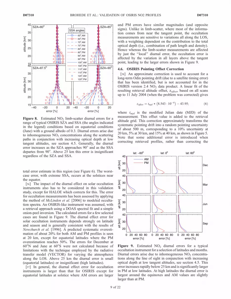
total error estimate in this region (see Figure 6). The worst-case error, with extreme SSA, occurs at the solstices nearthe equator.[56] The impact of the diurnal effect on solar occultation

instruments also has to be considered in this validationstudy, except for HALOE which corrects for this. The errorfor occultation measurements has been assessed by applyingthe method of McLinden et al. [2006] to modeled occulta-tion spectra. An OSIRIS-like instrument was assumed, witha retrieval approach using a DOAS spectral fit and a simpleonion-peel inversion. The calculated errors for a few selectedcases are found in Figure 9. The diurnal effect error forsolar occultation instruments depends strongly on latitudeand season and is generally consistent with the results ofNewchurch et al. [1996]. A predicted systematic overesti-mation of about 20% for both AM and PM profiles is seenat 20 km, except for equatorial latitudes where the PMoverestimation reaches 50%. The errors for December at60�N and June at 60�S were not calculated because oflimitations with the technique employed by the radiativetransfer model (VECTOR) for varying the atmospheresalong the LOS. Above 25 km the diurnal error is small(equatorial latitudes) or insignificant (high latitudes).[57] In general, the diurnal effect error for occultation

instruments is larger than that for OSIRIS except forequatorial latitudes at solstice where AM errors are larger

and PM errors have similar magnitudes (and oppositesigns). Unlike in limb-scatter, where most of the informa-tion comes from near the tangent point, the occultationmeasurements are sensitive to variations all along the LOS,with a weighting dependent on the contribution to the totaloptical depth (i.e., combination of path length and density).Hence whereas the limb-scatter measurements are affectedby just the ‘‘local’’ diurnal error, the occultation error isaffected by the variation in all layers above the tangentpoint, leading to the larger errors shown in Figure 9.

4.6. OSIRIS Pointing Offset Correction

[58] An approximate correction is used to account for along-term Odin pointing drift (due to a satellite timing error)that has been identified, but is not accounted for in theOSIRIS version 2.4 NO2 data product. A linear fit of theresulting retrieval altitude offset, zoffset, based on all scansup to 11 July 2004 (when the problem was corrected) gives

zoffset ¼ tmjd * 8:543 10�4� �

� 43:95; ð6Þ

where tmjd is the modified Julian date (MJD) of themeasurement. This offset value is added to the retrievalaltitude grid. This correction approximately transforms thesystematic pointing drift into a random pointing uncertaintyof about 500 m, corresponding to a 10% uncertainty at20 km, 5% at 30 km, and 15% at 40 km, as shown in Figure 5.Note that some additional error is introduced whencorrecting retrieved profiles, rather than correcting the

Figure 8. Estimated NO2 limb-scatter diurnal errors for arange of typical OSIRIS SZA and SSA (the angles indicatedin the legend) conditions based on equatorial conditions(June) with a ground albedo of 0.3. Diurnal errors arise dueto inhomogeneous NO2 concentrations along the scatteringpaths in conjunction with increasing optical depth at lowtangent altitudes, see section 4.5. Generally, the diurnalerror increases as the SZA approaches 90� and as the SSAdepartes from 90�. Above 25 km this error is insignificantregardless of the SZA and SSA.

Figure 9. Estimated NO2 diurnal errors for a typicaloccultation instrument for a selection of latitudes andmonths.Diurnal errors arise due to inhomogeneous NO2 concentra-tions along the line of sight in conjunction with increasingoptical depth at low tangent altitudes, see section 4.5. Thiserror increases rapidly below 25 km and is significantly largerin PM at low latitudes. At high latitudes the diurnal error islargest around the equinoxes and AM values are slightlylarger than at PM.


9 of 22

D07310

OSIRIS measurements prior to the retrieval process, due tononlinearities.

5. Intercomparison Methodology

[59] When comparing limb-scattered sunlight measure-ments to solar occultation measurements, it is important toremember that the viewing geometries are quite different, asis seen in Figure 2, and can lead to differences even formeasurements in which the STPs are colocated in time andspace. Also, any deviation in the LST and location of themeasurements can make the result difficult to interpret. Thisis particularly true for NO2, which has a short atmosphericlifetime and strong variations between daytime and night-time chemistry, enhanced by Odin’s near-terminator orbit.An approach to compensate for different LSTs is describedin section 5.2.

5.1. Finding Coincidences

[60] The validation period in this study stretches fromJanuary 2002 to December 2004, avoiding the first monthsof the Odin mission where there were satellite pointingproblems, and excluding the more recent period whereOdin’s orbit has deviated significantly from the initial1800 hour ascending node.[61] A distance tolerance of 500 km is used in this study.

This tolerance is loose enough to give a sufficient number ofcoincidences for an extensive statistical analysis, but tightenough to not impact significantly on the results of theanalysis. The time tolerance is selected to be 2 hours UT.Owing to the diurnal variation of NO2, a small timetolerance is needed, although 2 hours is not nearly smallenough without SZA scaling (as described in section 5.2).Also, the different chemistry during sunrise (AM) andsunset (PM) necessitates that these categories are treatedseparately. For the SAOZ balloon comparisons, the distancetolerance was relaxed to 1000 km and the time tolerancewas relaxed to 6 hours due to the small SAOZ data set.When more than one coincidence is found within thetolerances, the one which is closest in time (UT) is selected.[62] All coincidences are further divided into three latitude

bands: southern latitudes (�90 lat <�30), equatorial latitudes(�30 lat 30), and northern latitudes (30 < lat 90).This division is done to limit the impact of differentatmospheric conditions on the comparisons, includingcloudiness and tropopause height. In addition, the data isdivided into four seasons: November–December–January(NDJ), February–March (FM), April–May–June–July–August (AMJJA), and September-October (SO). This divisionis logical when considering the OSIRIS latitude coverage overthe year, where the northern hemisphere is covered betweenApril and August, the southern hemisphere is covered fromNovember to January, and full global coverage is achievedonly close to the equinoxes (September/October and February/March) (see Figure 3).[63] When interpreting the results, the altitudes have been

divided into three regimes; high altitudes (35–40 km),midaltitudes (25–35 km), and low altitudes (15–25 km).The low-altitude regime is characterized by large uncertain-ties, including diurnal effect errors, SZA scaling biases, OStangent height registration errors, cloud, aerosol, albedo,and a priori contamination. In the high-altitude regime, the

signal to noise ratio for all instruments is generally declin-ing and there is potential a priori contamination, dependingon the retrieval technique. The midaltitude regime is pre-sumed to contain the highest data quality for all instruments.[64] The OSIRIS data are filtered based on measurement

response (only >0.75 accepted) and vertical resolution (only<5 km accepted) to ensure that the a priori contamination isminimized. The other instrument data are filtered based onavailable data flags (any flagged data points are removed)and error estimate (any data points with an error estimate>100% are removed). To calculate differences, the OSIRISdata is interpolated to the altitude grid of the solar occul-tation instrument.[65] To be entirely consistent, the vertical resolution of

the instruments must be similar. If not, the resolution of oneinstrument must be transformed to the resolution of theother. This is omitted in this study since the resolution of allof the instruments is similar, only varying between 1 and2 km (see Table 1), and resulting differences would onlyproduce small errors that do not justify the effort of andpotential errors introduced by the transformation.

5.2. SZA Scaling

[66] Owing to the sharp concentration gradients of NO2

around sunset and sunrise (see Figure 1), even smalldeviations in SZA (or equivalently LST) of the coincidentmeasurements can have a large impact on the results. Nearthe terminator, a SZA difference of a few degrees can leadto a change in the NO2 concentration by a factor of 2 or 3due to only photochemistry. Since the intention is to studydifferences in the general NO2 field, meaningful compar-isons can demand a very small SZA (or LST) tolerance,perhaps within a degree or a few minutes. Such strictrequirements would reduce the number of coincidencesdramatically, making a statistical analysis impossible.[67] One solution to this problem is to use a photochemical

model to scale the OSIRIS profile to the SZA of the otherinstrument, as is discussed by Bracher et al. [2005]. Atabulated photochemical box model (PRATMO) [Prather,1992;McLinden et al., 2000], driven by climatological ozoneand temperatures, is used for this purpose. The look-up tablesare given as a function of latitude (2.5� increments), time(2-week increments), altitude (2 km increments from 10 to58 km), and SZA (up to 34 per day).[68] The OSIRIS number density profiles at 90� SZA,

nOS(90, z), are estimated by multiplying the profiles at themeasured SZA, nOS(qOS, z), by the model-based scalingfactor sq;

nOS 90; zð Þ ¼ nmod 90; zð Þnmod qOS ; zð Þ|fflfflfflfflfflfflfflffl{zfflfflfflfflfflfflfflffl}

sq

nOS qOS ; zð Þ; ð7Þ

where z is the altitude and nmod are the model profilesobtained from the look-up tables. Points where sq is greaterthan 2 or less than 2/3 are discarded since the scaling isbelieved to lose accuracy at the extremes.[69] Uncertainties in the SZA scaling for OSIRIS mea-

surement conditions are shown in Figure 10 and have beenestimated by repeating the calculation of sq after varyingone of the assumed geophysical parameters by estimate ofits uncertainty. The parameters considered (and their


10 of 22

D07310

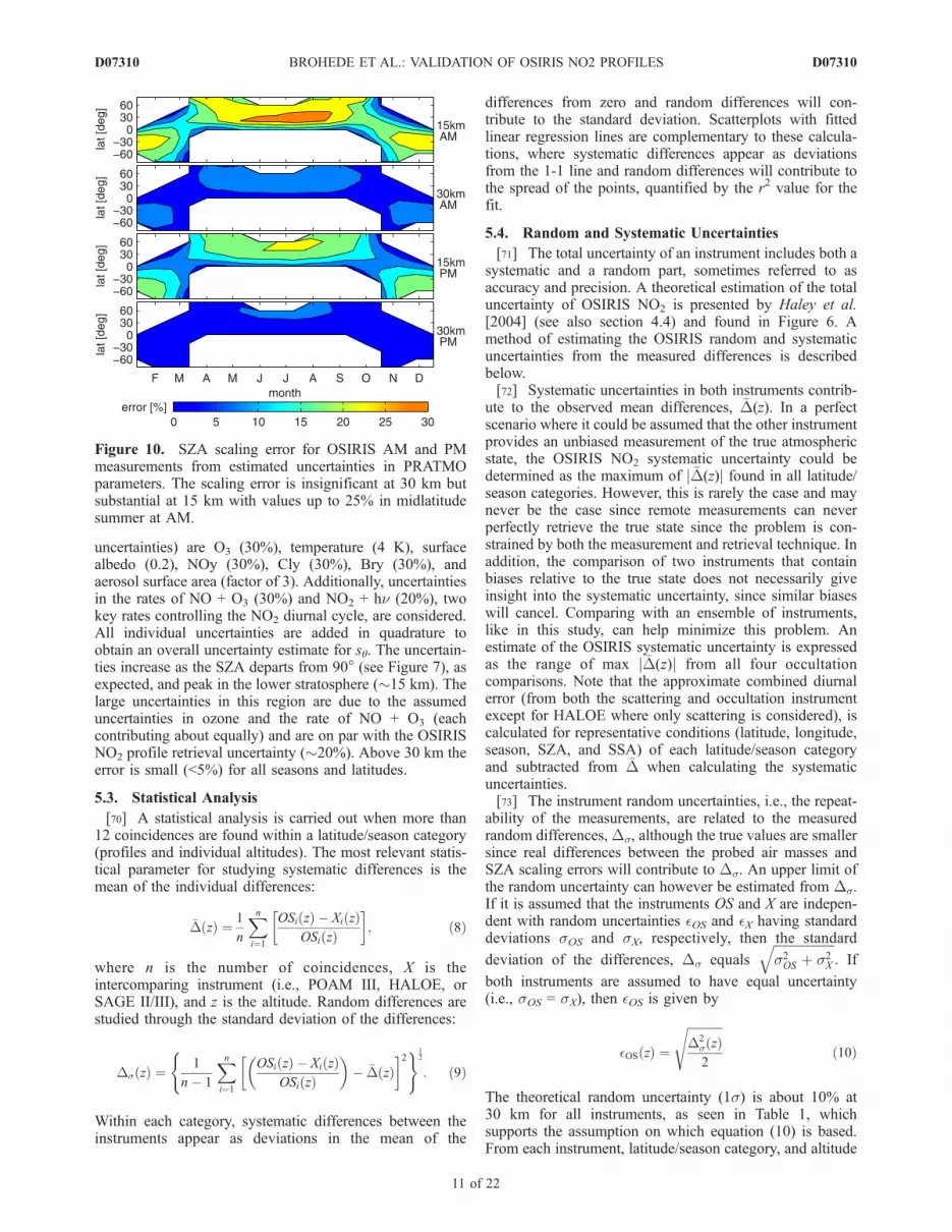
uncertainties) are O3 (30%), temperature (4 K), surfacealbedo (0.2), NOy (30%), Cly (30%), Bry (30%), andaerosol surface area (factor of 3). Additionally, uncertaintiesin the rates of NO + O3 (30%) and NO2 + hn (20%), twokey rates controlling the NO2 diurnal cycle, are considered.All individual uncertainties are added in quadrature toobtain an overall uncertainty estimate for sq. The uncertain-ties increase as the SZA departs from 90� (see Figure 7), asexpected, and peak in the lower stratosphere (�15 km). Thelarge uncertainties in this region are due to the assumeduncertainties in ozone and the rate of NO + O3 (eachcontributing about equally) and are on par with the OSIRISNO2 profile retrieval uncertainty (�20%). Above 30 km theerror is small (<5%) for all seasons and latitudes.

5.3. Statistical Analysis

[70] A statistical analysis is carried out when more than12 coincidences are found within a latitude/season category(profiles and individual altitudes). The most relevant statis-tical parameter for studying systematic differences is themean of the individual differences:

�D zð Þ ¼ 1

n

Xni¼1

OSi zð Þ � Xi zð ÞOSi zð Þ

; ð8Þ

where n is the number of coincidences, X is theintercomparing instrument (i.e., POAM III, HALOE, orSAGE II/III), and z is the altitude. Random differences arestudied through the standard deviation of the differences:

Ds zð Þ ¼ 1

n� 1

Xni¼1

OSi zð Þ � Xi zð ÞOSi zð Þ

� �� D zð Þ

2( )12

: ð9Þ

Within each category, systematic differences between theinstruments appear as deviations in the mean of the

differences from zero and random differences will con-tribute to the standard deviation. Scatterplots with fittedlinear regression lines are complementary to these calcula-tions, where systematic differences appear as deviationsfrom the 1-1 line and random differences will contribute tothe spread of the points, quantified by the r2 value for thefit.

5.4. Random and Systematic Uncertainties

[71] The total uncertainty of an instrument includes both asystematic and a random part, sometimes referred to asaccuracy and precision. A theoretical estimation of the totaluncertainty of OSIRIS NO2 is presented by Haley et al.[2004] (see also section 4.4) and found in Figure 6. Amethod of estimating the OSIRIS random and systematicuncertainties from the measured differences is describedbelow.[72] Systematic uncertainties in both instruments contrib-

ute to the observed mean differences, �D(z). In a perfectscenario where it could be assumed that the other instrumentprovides an unbiased measurement of the true atmosphericstate, the OSIRIS NO2 systematic uncertainty could bedetermined as the maximum of j �D(z)j found in all latitude/season categories. However, this is rarely the case and maynever be the case since remote measurements can neverperfectly retrieve the true state since the problem is con-strained by both the measurement and retrieval technique. Inaddition, the comparison of two instruments that containbiases relative to the true state does not necessarily giveinsight into the systematic uncertainty, since similar biaseswill cancel. Comparing with an ensemble of instruments,like in this study, can help minimize this problem. Anestimate of the OSIRIS systematic uncertainty is expressedas the range of max j �D(z)j from all four occultationcomparisons. Note that the approximate combined diurnalerror (from both the scattering and occultation instrumentexcept for HALOE where only scattering is considered), iscalculated for representative conditions (latitude, longitude,season, SZA, and SSA) of each latitude/season categoryand subtracted from �D when calculating the systematicuncertainties.[73] The instrument random uncertainties, i.e., the repeat-

ability of the measurements, are related to the measuredrandom differences,Ds, although the true values are smallersince real differences between the probed air masses andSZA scaling errors will contribute to Ds. An upper limit ofthe random uncertainty can however be estimated from Ds.If it is assumed that the instruments OS and X are indepen-dent with random uncertainties �OS and �X having standarddeviations sOS and sX, respectively, then the standard

deviation of the differences, Ds equalsffiffiffiffiffiffiffiffiffiffiffiffiffiffiffiffiffiffiffis2OS þ s2

X

q. If

both instruments are assumed to have equal uncertainty(i.e., sOS = sX), then �OS is given by

�OS zð Þ ¼

ffiffiffiffiffiffiffiffiffiffiffiffiD2

s zð Þ2

sð10Þ

The theoretical random uncertainty (1s) is about 10% at30 km for all instruments, as seen in Table 1, whichsupports the assumption on which equation (10) is based.From each instrument, latitude/season category, and altitude

Figure 10. SZA scaling error for OSIRIS AM and PMmeasurements from estimated uncertainties in PRATMOparameters. The scaling error is insignificant at 30 km butsubstantial at 15 km with values up to 25% in midlatitudesummer at AM.


11 of 22

D07310

Figure 11


12 of 22

D07310

range, a value of �OS is calculated. The best estimate of thetrue instrument random uncertainty of OSIRIS is assumedto be the lowest value since this emanates from a categorywith the smallest atmospheric variation and the occultationinstrument with lowest random uncertainty.

6. Results

[74] The intercomparison methodology presented in theprevious section results in 7711 coincidences betweenOSIRIS and the other four satellite instruments. Figures 11to 14 show the mean differences and the 1s standarddeviation of the mean differences for the four intercompar-isons in each of the twelve categories, while Figure 15shows scatter plots for all coincidences with each of thefour instruments at five altitudes. Figure 16 showsadditional comparisons between OSIRIS and four SAOZballoon flights.[75] Also shown in Figures 11 to 14 is the estimated

diurnal effect error for each category. The diurnal effecterror was simulated as discussed in section 4.5 and includesboth the limb-scatter and the occultation components exceptfor the HALOE comparisons, where only the limb-scattercomponent is shown since the HALOE retrievals include adiurnal effect correction. The error was simulated for therepresentative conditions in each category (average SZA,SSA, latitude, and day of year of the coincidences). Theoccultation component generally dominates this error in theconditions studied here.[76] Detailed results from each instrument intercompari-

son are presented in the following sections and are summa-rized in Table 2. The results are given in three differentaltitude regions: high altitudes (35–40 km), midaltitudes(25–35 km), and low altitudes (15–25 km). Ds values referto one standard deviation (1s). Results for individual yearsare not shown, but are consistent with the results from thefull 3-year comparison period.

6.1. HALOE

[77] Altogether 830 sunrise (AM) and 687 sunset (PM)coincidences are found for OSIRIS and HALOE during thevalidation period. The results of these comparisons areshown in Figure 11. Coincidences are found in all latitude/season categories except for southern latitudes in AMJJA.The HALOE coincidences in the northern hemisphere inNDJ are the only coincidences for high latitudes around thewinter solstice in the entire study.[78] The Ds for PM categories varies from 22–33% at

low altitudes, 12–17% at midaltitudes, and 12–18% at highaltitudes. The systematic differences, �D, are within 70% atlow altitudes, 11% at midaltitudes, and 20% at high alti-tudes, if equatorial categories, where the systematic differ-ence increases rapidly below 30 km, are excluded. Allcategories show similar patterns, where OSIRIS is increas-ingly larger than HALOE below 20 km. The systematic

differences below 25 km are not consistent with the esti-mated limb-scatter diurnal error.[79] For AM profiles, Ds varies from 24–60% at low

altitudes, 13–35% at midaltitudes, and 14–20% at highaltitudes, if the large values (>100%) at equatorial latitudesin NDJ are excluded. Northern latitudes in NDJ andequatorial latitudes in NDJ and SO tend to have the largestvalues. The systematic differences, �D are within 60% at lowaltitudes, 23% at midaltitudes, and 18% at high altitudes,again if the equatorial categories, where the difference islarger, are excluded. The OSIRIS NO2 densities are signif-icantly larger than HALOE at the lower altitudes for almostall categories. The equatorial region in NDJ in the AM is aclear exception, showing OSIRIS values that are smaller bymore than 100%. The diurnal error estimates do notcorrelate with the AM systematic differences.[80] The HALOE/OSIRIS scatter plots (Figure 15a) show

very close fits to the 1-1 line (high r2) at 25 km and 30 km,while OSIRIS shows larger NO2 densities at 35 km and40 km. The 15 km and 20 km plots show many outliers. Thecorrelations are higher for PM comparisons at all altitudes.[81] HALOE mean profiles and their corresponding stan-

dard deviations are not presented, but show very significantincreases in NO2 concentration and variability below 18 km,particularly for equatorial categories and in the AM. Thispattern is not visible in the OSIRIS data set, the OSIRIS apriori data, or in the other instrument data sets except forSAGE II.

6.2. SAGE II

[82] For the OSIRIS and SAGE II data sets, 860 AM and386 PM coincidences are found. The results of thesecomparisons are shown in Figure 12. The coincidencescover all latitude/season categories except southern latitudesin AMJJA and northern latitudes in NDJ.[83] The PMDs varies from 17–86% at low altitudes, 9–

17% at midaltitudes, and 15–22% at high altitudes, ifequatorial latitudes and southern latitudes in FM, wherethe magnitudes reach several hundred percent at low alti-tudes, are excluded. The OSIRIS NO2 densities are lowerthan SAGE II for most categories and the systematicdifferences ( �D) are within 26% at low altitudes, 17% atmidaltitudes, and 31% at high altitudes, again if the equa-torial latitudes and southern latitudes in FM are excluded.Southern latitudes have the smallest systematic differencesand equatorial regions have the largest. The systematicdifferences are to some extent consistent with the estimateddiurnal error in shape and sign, although the magnitudeseems incorrect, especially for the equatorial regions.[84] For AM coincidences, Ds varies from 23–47% at

low altitudes, 13–23% at midaltitudes, and 20–26% at highaltitudes. The systematic differences, �D, are within 56% atlow altitudes, 21% at midaltitudes, and 25% at high alti-tudes, if the low-altitude range is constrained to 18–25 km,since values below 18 km deviate considerably. All

Figure 11. Results from OSIRIS and HALOE coincidences in 2002–2004, divided into 12 latitude/season categories andexpressed as the mean (solid line) and 1s standard deviation (error bars) of the differences. Sunrise (AM) and sunsetprofiles (PM) profiles are treated and plotted separately. The average solar zenith angle (SZA) and solar scattering angle(SSA) are given together with the number of coincidences (n) in each category. Estimated diurnal error biases (sum ofoccultation and limb-scatter) are plotted as dashed lines.


13 of 22

D07310

Figure 12. Same as Figure 11, but for SAGE II.


14 of 22

D07310

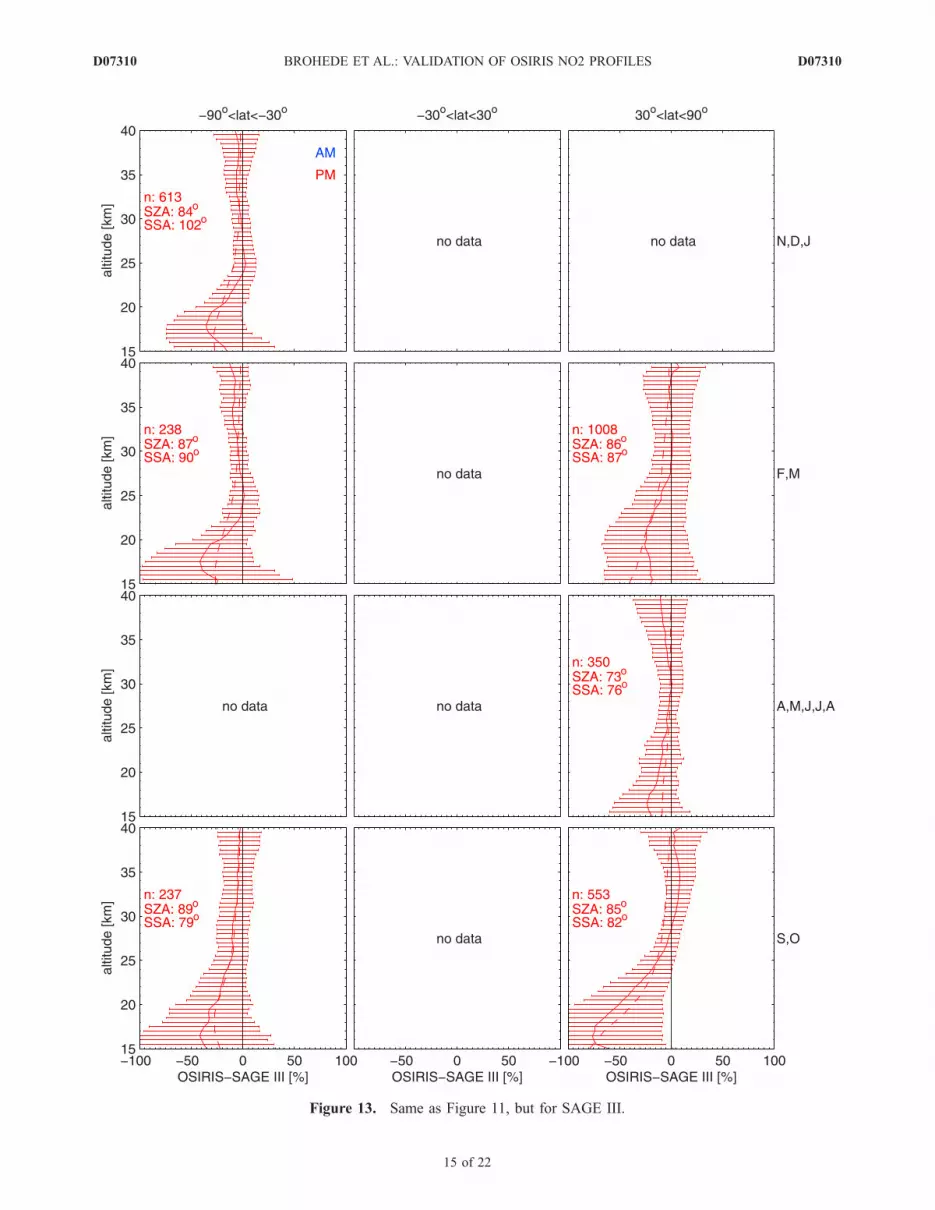
Figure 13. Same as Figure 11, but for SAGE III.


15 of 22

D07310

Figure 14. Same as Figure 11, but for POAM III.


16 of 22

D07310

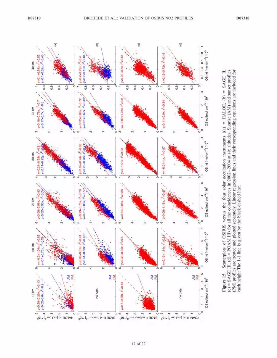
Figure

15.

Scatterplots

ofOSIRIS

versusthefoursolaroccultation

instruments

((a)

=HALOE,(b)=

SAGE

II,

(c)=SAGEIII,(d)=POAM

III)forallthecoincidencesin

2002–2004at

sixaltitudes.Sunrise

(AM)andsunsetprofiles

(PM)profilesaretreatedandplotted

separately.Linearregressionlines

andtheircorrespondingequationsareincluded

for

each

heightThe1-1

lineisgiven

bytheblack

dashed

line.


17 of 22

D07310

categories show large negative systematic differences below20 km, reaching up to several hundred percent at 15 km atequatorial latitudes. The estimated diurnal effect bias doesnot correlate with the measured AM bias at low altitudes.[85] The SAGE II/OSIRIS scatterplots (Figure 15b) show

close fits to the 1-1 line, with few extreme outliers, from25 km to 35 km except for an OSIRIS high bias in the 35 kmAM points. The fits at 20 km and 40 km are poor with alarge number of outliers. PM comparisons show generally

higher correlations, especially at the highest and lowestaltitudes.[86] The SAGE II mean profiles and their corresponding

standard deviations are not presented but show a verysignificant increase in NO2 concentration and variabilitybelow 20 km, especially for midlatitude categories and inthe AM, similar to what is seen in the HALOE data.[87] There seems to be a significant systematic difference

between SAGE II SR and SS measurements at around20 km for many categories, even though it is smaller thanexpected from the observed bias between SAGE II satelliteSR and SS events [Randall et al., 2005]. Note that forSAGE II and OSIRIS coincidences, local sunrisecorresponds to satellite sunrise, except for a few cases innorthern latitudes in NDJ.

6.3. SAGE III

[88] Owing to the latitude coverage of the Sun-synchro-nous orbits of SAGE III and OSIRIS, close coincidences intime and space only occur in southern and northern latitudesalmost entirely at local sunset (PM). Altogether 3005coincidences are found of which only six are in the AM,too few to make any statistical analysis. The coincidencesappear in the northern and southern latitudes in all seasonsexcept the winter solstices, as seen in Figure 13.[89] All available latitude/season categories show similar

patterns with a Ds of 22–45% at low altitudes, 9–19% atmidaltitudes, and 14–25% at high altitudes. Northern lat-itudes in FM stand out with significantly larger Ds atmiddle and high altitudes. OSIRIS is systematically lowby about 50%, peaking between 15 km and 20 km, whichcorresponds very well to the estimated diurnal errors in bothmagnitude and shape. If the estimated diurnal error issubtracted, the �D is within 21% at low altitudes, 12% atmidaltitudes, and 11% at high altitudes.[90] The SAGE III/OSIRIS scatterplots (Figure 15c)

show generally good fits to the 1-1 line from 20 km to35 km and a reasonable fit at 40 km, particularly at smallerconcentrations. At 15 km, the fit is poor. The SAGE IIImean profiles and corresponding standard deviations are notpresented but are consistent with OSIRIS and do not showthe low-altitude features seen in the HALOE and SAGE IIdata sets.

6.4. POAM III

[91] For OSIRIS and POAM III, close coincidences onlyoccur in the southern and northern latitude regions, almostentirely at local sunset (PM). A total of 1943 coincidencesare found of which only 10 are AM coincidences (again toofew to make any statistical analysis). The categories aroundthe winter solstices contain no coincidences due to the lackof OSIRIS data, as seen in Figure 14.[92] The mean Ds varies from 18–40% at low altitudes,

10–19% at midaltitudes, and 16–27% at high altitudes, ifthe southern latitude category in SO, which shows signif-icantly larger Ds, is excluded. Systematic differences, �D,after the diurnal error is subtracted, are within 40% at lowaltitudes, 21% at midaltitudes, and 14% at high altitudes,again if the southern latitudes in SO are excluded. OSIRIShas systematically lower values by about 40% for southernlatitudes and 50% for northern latitudes, peaking at about22 km. The only exception is the southern latitudes in SO,

Figure 16. Comparisons of OSIRIS NO2 profiles (solidand dotted lines) with results from four SAOZ flights(crosses). The closest coincidences in time and space forascent (asc.) and occultation (occ.) are shown, with (solidlined with 1s standard deviation uncertainties) and without(dotted lines) photochemical scaling of the OSIRIS profilesto the solar zenith angle of the respective SAOZ measure-ment. (a) NO2 profiles retrieved from OSIRIS measure-ments on 1 October 2002 (scan:8745004, lat:39.2�N,lon:10�W, 1817 UT) and data from a SAOZ sonde launchedat Aire sur l’Adour, France (PM ascent: lat:43.8�N,lon:0.1�W, 1700 UT, PM occultation: lat:43.7�N,lon:3.9�W, 1754 UT). (b) OSIRIS measurements on31 January 2004 (scan:16011044, lat:24.6�S, lon:58.7�W,2220 UT) and data from a SAOZ sonde launched at Bauru,Brazil (PM ascent: lat:22.4�S, lon:49�W, 2118 UT, PMoccultation: lat:23.5�S, lon:53.4�W, 2206 UT). (c) OSIRISmeasurements on 24 August 2001 (scan:2743015,lat:63.9�S, lon:29.5�W, 0508 UT) and data from a SAOZsonde launched at Kiruna, Sweden (AM occultation:lat:67.9�N, lon:23.5�E, 0230 UT). (d) OSIRIS measure-ments on 16 March 2003 (scan:11218006, lat:66.1�N,lon:10.6�E, 16:12 UT, scan:11219007, lat:71.0�N,lon:4.9�E, 1614 UT) and data from a SAOZ sonde launchedat Kiruna, Sweden (PM ascent: lat:67.5�N, lon:22.0�E,1548 UT, PM occultation: lat:67.3�N, lon:14.3�E,1654 UT).


18 of 22

D07310

where OSIRIS is lower by above 80%. The OSIRIS sys-tematic low peak does not correspond to the estimateddiurnal error.[93] The scatterplots of POAM III/OSIRIS (Figure 15d)

show a good fit to the 1-1 line only at 30 km and 35 km.Below 30 km, OSIRIS are clearly lower than POAM III,especially at high concentrations. At 20 km and 40 km thefit is fair due to many outlayers.[94] The mean profiles of POAM III are not presented but

show a typical sharp peak or double peak at 20 km, whichroughly corresponds to the atmospheric NO2 maximum.The OSIRIS mean NO2 peak is smaller and much smoother.The sharp peak structure appears in almost all POAM IIIprofiles and is not due to a few outliers in the data set. Thisbehavior is not seen in any of the other instruments.

6.5. SAOZ

[95] Only four coincidences between OSIRIS and SAOZballoon flights are found, even with the relaxed coincidencetolerances; hence no statistical analysis can be performed.However, as is shown in Figure 16, the four profilesgenerally agree to within the combined OSIRIS and SAOZerror bars (SAOZ error bars are not plotted for clarity) downto 15 km for most occasions except for the SAOZ PMoccultation during the 31 January 2004 Bauru flight ataltitudes above 20 km, where the OSIRIS SZA scalingcorrection appears to lead to an overestimate of the NO2

concentrations, and for the PM ascent during the 1 October2002 Aire sur l’Adour flight, where the SZA scalingappears to lead to an underestimation.

6.6. OSIRIS Uncertainties

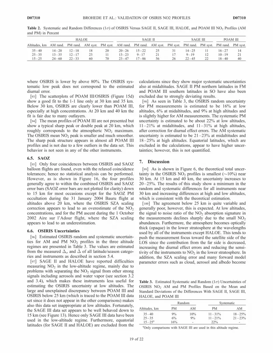
[96] Estimated OSIRIS random and systematic uncertain-ties for AM and PM NO2 profiles in the three altituderegimes are presented in Table 3. The values are estimatedfrom the measured Ds and �D of all latitude/season catego-ries and instruments as described in section 5.4.[97] SAGE II and HALOE have reported difficulties

measuring NO2 in the low-altitude regime, mainly due toproblems with separating the NO2 signal from other strongsignals including aerosols and water vapor (see section 3.2and 3.4), which makes these instruments less useful forestimating the OSIRIS uncertainty at low altitudes. Thelarge and unexplained discrepancy between POAM III andOSIRIS below 25 km (which is traced to the POAM III dataset since it does not appear in the other comparisons) makesalso this data set inappropriate at low altitudes. Fortunately,the SAGE III data set appears to be well behaved down to15 km (see Figure 13). Hence only SAGE III data have beenused in the low-altitude regime. Furthermore, equatoriallatitudes (for SAGE II and HALOE) are excluded from the

calculations since they show major systematic uncertaintiesalso at midaltitudes. SAGE II PM northern latitudes in FMand POAM III southern latitudes in SO have also beenexcluded due to strongly deviating results.[98] As seen in Table 3, the OSIRIS random uncertainty

for PM measurements is estimated to be 16% at lowaltitudes, 6% at midaltitudes, and 9% at high altitudes andis slightly higher for AM measurements. The systematic PMuncertainty is estimated to be about 22% at low altitudes,11–21% at midaltitudes, and 11–31% at high altitudes,after correction for diurnal effect errors. The AM systematicuncertainty is estimated to be 21–23% at midaltitudes and18–25% at high altitudes. Equatorial latitudes, which areexcluded in the calculations, appear to have higher uncer-tainties; however, this is not quantified.

7. Discussion

[99] As is shown in Figure 6, the theoretical total uncer-tainty in the OSIRIS NO2 profiles is smallest (�10%) near30 km. At 15 km and 40 km, the uncertainty increases to20–25%. The results of this study show a minimum in therandom and systematic differences for all instruments near30 km and increasing differences at high and low altitudes,which is consistent with the theoretical estimation.[100] The agreement below 25 km is quite variable and

generally poor, however, this is expected. At low altitudes,the signal to noise ratio of the NO2 absorption signature inthe measurements declines sharply due to the small NO2

abundances. Furthermore, the atmosphere becomes opticallythick (opaque) in the lower stratosphere at the wavelengthsused by all of the instruments except HALOE. This tends topush the measurement focus toward the satellite side of theLOS since the contribution from the far side is decreased,increasing the diurnal effect errors and reducing the sensi-tivity of the instruments to NO2 in the lower stratosphere. Inaddition, the SZA scaling error and many forward modelparameter errors such as cloud, aerosol and albedo become

Table 2. Systematic and Random Differences (1s) of OSIRIS Versus SAGE II, SAGE III, HALOE, and POAM III NO2 Profiles (AM

and PM) in Percent

Altitudes, km

HALOE SAGE II SAGE III POAM III

AM rand. PM rand. AM syst. PM syst. AM rand. PM rand. AM syst. PM syst. PM rand. PM syst. PM rand. PM syst.

35–40 14–20 12–18 18 20 20–26 15–22 25 31 14–25 11 16–27 1425–35 13–35 12–17 23 11 13–23 9–17 21 17 9–19 12 10–19 2115–25 24–60 22–33 60 70 23–47 17–86 56 26 22–45 22 18–40 40

Table 3. Estimated Systematic and Random (1s) Uncertainties ofOSIRIS NO2 AM and PM Profiles Based on the Mean and

Standard Deviations of the Differences With SAGE II, SAGE III,

HALOE, and POAM III

Altitudes, km

Random Systematic

PM AM PM AM

35–40 9% 10% 11–31% 18–25%25–35 6% 9% 11–21% 21–23%15–25a 16% - 22% -aOnly comparisons with SAGE III are used in this altitude regime.


19 of 22

D07310

important below 20 km. Decreasing signal to noise andpossibly increasing pointing offset errors are the mainreasons for the worse agreement at high altitudes (above35 km). The generally larger random uncertainties for AMprofiles are likely related to the small AM NO2 abundances(as compared to PM profiles).[101] One thing to notice is that solar scattering and solar

occultation techniques probe different air masses even if ameasurement corresponds to the very same STP. Solaroccultation instruments sample NO2 along the solar beam,but the scattering instruments sample partly along the solarbeam and partly along the instrument LOS (consideringsingle scattering only, the multiple scattering component ofthe signal further complicates the picture). If the atmosphericNO2 concentration is truly spherically homogeneous, as isassumed in the retrievals, this is not a problem. The trueconcentration can, however, vary horizontally, due to photo-chemistry and near the vortex edge, for example. The twodifferent techniques, then, should not be expected to giveexactly the same result even if the measurements are perfectwith no noise or other errors. However, a large number ofcoincidences will tend tominimize this problem (in terms of asystematic effect).[102] As was mentioned in section 5.3, random uncertain-

ties in the various instruments will contribute to theobserved Ds. In a perfect scenario, where no other sourcesof error contribute and where both instrument have exactlyequal uncertainties, the real OSIRIS NO2 random uncer-tainty can be calculated. However, coincidence issues,random errors in the SZA scaling factor, OSIRIS pointingerror, vertical/horizontal resolution differences, a prioricontamination and any other nonretrieved parameters thatcan affect the retrievals in a random way within eachcategory (i.e., cloud, aerosols, and albedo) will potentiallylead to an overestimation of the random uncertainty. This isparticularly true at low altitudes where the various contri-butions are generally most significant. Nevertheless, theestimated OSIRIS random uncertainty, as seen in Table 3, isconsistent with the theoretical measurement error (Figure 6).This indicates that the potential overestimation is small (orthat the theoretical measurement error is underestimated).[103] OSIRIS SZA scaling errors could possibly explain

some of the differences at altitudes below 25 km. FromFigure 10, the error should be more pronounced in thesummer solstice periods (i.e., NH in AMJJA and SH inNDJ) and less significant around the time of the equinoxeswhere the SZA is close to 90� (i.e., in FM and SO). Inaddition, AM profiles should be more affected. However,nothing in the results indicates that the SZA scaling is amajor random error source. To confirm this, the compar-isons were repeated while limiting the included OSIRISmeasurements to those where the SZAwas within 2� of 90�,thus making the SZA scaling factor negligible). Very similarpatterns to those presented in the previous section werefound, indicating that indeed the SZA scaling is not a majorsource of the observed differences.[104] OSIRIS uses a climatological albedo in the NO2

retrievals (assuming no clouds) which may introduce sys-tematic errors of up to 15% at 15 km for high Sunconditions (SZA = 60�) in the presence of clouds, as seenin Figure 5, and small errors in low Sun conditions. Thelargest albedo errors (due to the presence of clouds) are then

expected in the summer high latitudes. However, thispattern is not evident in the comparisons.[105] Systematic and random differences may also be

related to aerosols since OSIRIS has some sensitivity tothe accuracy of the aerosol climatology used in the retriev-als, and the other instruments (HALOE, SAGE II, andPOAM III in particular) are known to have significantaerosol-related errors at low altitudes. This error shouldgenerally be largest in the equatorial region. Peaks at thelowest altitudes in the NO2 mean profiles exist in theHALOE and SAGE II data but not in SAGE III and POAMIII data. Such peaks also do not exist in the OSIRIS NO2

profiles or the aerosol climatology used in the OSIRISretrievals. These peaks in the lower altitudes are likely thecause of the large mean difference values and are likely dueto, for example, the LOS passing directly through clouds.This should mostly occur in the tropical region wheretropical convective clouds may extend into the lowerstratosphere or in regions of polar stratospheric clouds.[106] The ad hoc OSIRIS tangent height registration

correction that has been applied to the NO2 data could alsobe a source of the systematic differences at low altitudessince in this region a simple shift of the retrieved profiles inheight can lead to large errors due to a priori contaminationand nonlinearities in the retrievals. However, this would beexpected to impact the comparisons with all instruments.The remaining OSIRIS pointing uncertainty of approxi-mately 500 m is expected to introduce random errors ofabout 10% at 20 km, 5% at 30 km, and 15% at 40 km and islikely contributing to the observed standard deviations ofthe differences.[107] The combined diurnal effect error (both occultation

and scattering) explains most of the systematic differencesbetween OSIRIS and SAGE III at low altitudes. Both themagnitude and the shape of the error is consistent with thedifferences in all of the categories. In the POAM III andSAGE II PM data the diurnal effect error may explain partof the observed differences at low altitudes. For the othercomparisons the contribution of the diurnal error to theobserved systematic differences at low altitudes remainsunclear. The approximation of the combined diurnal errorfor representative conditions (as plotted in the resultFigures 11 to 14) are believed to be more accurate forPOAM III and SAGE III where the latitudes are restricted toa small latitude band. A more accurate approach is tosimulate the diurnal error for each profile within a category,not just for a representative case. However, this involvesextensive computer runs and is left for future studies.[108] It is difficult to make any quantitative assessment of

the OSIRIS data quality based on the SAOZ comparisonsdue to the small number of coincidences and since thedistance and time criteria are large. However, it can be saidthat the results are consistent and that no obvious biasesexist.[109] The assumption of independence made in the cal-

culation of the random uncertainties can be questioned sincethe same NO2 cross sections, and atmospheric parameterssuch as temperature and pressure are sometimes used in theretrievals for the various instruments. However, since theviewing geometries and the retrieval techniques are funda-mentally different (except for OSIRIS and POAM III, whichboth useOE) themeasurements should be largely independent.


20 of 22

D07310

Furthermore, HALOE measurements are made in the infra-red and are consistent with OSIRIS measurements in thevisible.

8. Conclusions

[110] Stratospheric NO2 profiles retrieved from OSIRISlimb-scatter measurements (version 2.4) have been com-pared with NO2 profiles measured with the HALOE,SAGE II, SAGE III, and POAM III satellite occultationinstruments. All together 7711 coincidences were foundwithin 2 hours and 500 km tolerances, between 1 January2002 and 31 December 2004. Comparisons were also madewith the SAOZ balloon occultation instrument.[111] The agreement between OSIRIS and the satellite

instruments is excellent between 25 km and 35 km, whereboth the random and systematic differences are within20%. This is true for all instruments, seasons, and lati-tudes, except for a few exceptional cases. From 35 km to40 km, the agreement is within 30%. The systematicagreement is slightly better for high latitudes than forequatorial latitudes. Below 25 km only OSIRIS andSAGE III are consistent. Model simulations indicate thatthe systematic difference between OSIRIS and SAGE IIIat low altitudes to a large extent can be attributed todiurnal effects in the SAGE III measurements from varyingNO2 concentrations along the line of sight. The SAOZcomparisons, though limited in number, show good agree-ment with OSIRIS down to 15 km, which further indicateshigh-quality OSIRIS measurements throughout the entirealtitude range (15–40 km).[112] On the basis of on the measured differences, the

OSIRIS random uncertainty (�precision) is estimated to be9% from 35 km to 40 km, 6% from 25 km to 35 km, and16% from 15 km to 25 km. The systematic uncertainty(�accuracy) is estimated to be 11–31% from 35 km to40 km, 11–21% from 25 km to 35 km, and around 22%from 15 km to 25 km. The AM uncertainties are found to beslightly higher than the PM uncertainties. These resultscorrespond well to the theoretical uncertainties.[113] Given the results of this validation study, the

OSIRIS NO2 profiles are well behaved, with reasonableuncertainty estimates throughout the entire retrieval range of15–40 km. This unique NO2 data set, with more thanhemispheric coverage and high vertical resolution will beof particular interest for studies of nitrogen chemistry inthe middle atmosphere, which is closely linked to ozonedepletion.

[114] Acknowledgments. This work is supported by the NaturalSciences and Engineering Research Council (Canada), the Canadian SpaceAgency, the Swedish National Space Board, and Chalmers University ofTechnology. Odin is a Swedish-led satellite project, funded jointly bySweden (SNSB), Canada (CSA), Finland (Tekes), and France (CNES).POAM III analyses are supported by the NASA data buy program and bythe NASA Solar Occultation Satellite Science Team program. The SAGE II,SAGE III, and POAM III data were obtained from the NASA LangleyResearch Center EOSDIS Distributed Active Archive Center. Thanks alsogoes to the HALOE and SAOZ teams for providing data and support.

ReferencesBauman, J. J., P. B. Russell, M. A. Geller, and P. Hamill (2003a), A strato-spheric aerosol climatology from SAGE II and CLAES measurements:1. Methodology, J. Geophys. Res., 108(D13), 4382, doi:10.1029/2002JD002992.

Bauman, J. J., P. B. Russell, M. A. Geller, and P. Hamill (2003b), A strato-spheric aerosol climatology from SAGE II and CLAES measurements:2. Results and comparisons, 1984–1999, J. Geophys. Res., 108(D13),4383, doi:10.1029/2002JD002993.

Bertaux, J., G. Megie, T. Widemann, E. Chassefie, R. Pellinen, E. Kyrola,S. Korpela, and P. Simon (1991), Monitoring of ozone trend by stellaroccultations: The GOMOS instrument, Adv. Space. Res., 11, 237–242.

Bovensmann, H., J. P. Burrows, M. Buchwitz, J. Frerick, S. Noel, V. V.Rozanov, K. V. Chance, and A. P. H. Goede (1999), SCIAMACHY:Mission objectives and measurement modes, J. Atmos. Sci., 56, 127–150.

Bracher, A., M. Sinnhuber, A. Rozanov, and J. P. Burrows (2005), Using aphotochemical model for the validation of NO2 satellite measurements atdifferent solar zenith angles, Atmos. Chem. Phys., 5, 393–408.

Brasseur, G., and S. Solomon (1986), Aeronomy of the Middle Atmosphere,2nd ed., Springer, New York.

Chu, W. P., and M. P. McCormick (1989), SAGE II inversion algorithm,J. Geophys. Res., 94, 8339–8351.

Cunnold, D. M., et al. (1991), Validation of SAGE II NO2 measurements,J. Geophys. Res., 96, 12,913–12,925.

Degenstein, D. A., E. J. Llewellyn, and N. D. Lloyd (2002), Volume emis-sion rate tomography from a satellite platform, Appl. Opt., 42(8), 1441–1450.

Dessler, A. E. (2000), The Chemistry and Physics of Stratospheric Ozone,Elsevier, New York.

Fischer, H., and H. Oelhaf (1996), Remote sensing of vertical profiles ofatmospheric trace constituents with MIPAS limb emission spectrometers,Appl. Opt., 35, 2787–2796.

Frisk, U., et al. (2003), The Odin satellite I. Radiometer design and test,Astron. Astrophys., 402, L27–L34, doi:10.1051/0004-6361:20030335.

Funke, B., et al. (2005), Retrieval of stratospheric NOx from 5.3 and6.2 Mm nonlocal thermodynamic equilibrium emissions measured byMichelson Interferometer for Passive Atmospheric Sounding (MIPAS)on Envisat, J. Geophys. Res., 110, D09302, doi:10.1029/2004JD005225.

Gordley, L. L., et al. (1996), Validation of nitric oxide and nitrogen dioxidemeasurements made by the halogen occulation experiment for uarsplatform, J. Geophys. Res., 101, 10,241–10,266.

Griffoen, E., and L. Oikarinen (2000), LIMBTRAN: A pseudo three-dimensional radiative transfer model for the limb-viewing imagerOSIRIS on the Odin satellite, J. Geophys. Res., 105, 29,717–29,730.

Gunson, M. R. (1996), The atmospheric trace molecule spectroscopy(ATMOS) experiment: Deployment on the ATLAS space shuttle mis-sions, Geophys. Res. Lett., 23, 2333–2336.

Haley, C. S., et al. (2004), Retrievals of stratospheric O3 and NO2 profilesfrom Odin Optical Spectrograph and InfraRed Imager System (OSIRIS)limb-scattered sunlight measurements, J. Geophys. Res., 109, D16303,doi:10.1029/2004JD004588.

Koelemeijer, R. B. A., J. F. de Haan, and P. Stammes (2003), A database ofspectral surface reflectivity in the range 335–772 nm derived from5.5 years of GOME observations, J. Geophys. Res., 108(D2), 4070,doi:10.1029/2002JD002429.

Llewellyn, E. J., et al. (2004), The OSIRIS instrument on the Odin space-craft, Can. J. Phys., 82, 411–422.

Lucke, R. L., et al. (1999), The polar ozone and aerosol measurement(POAM) III instrument and early validation results, J. Geophys. Res.,104, 18,785–18,799.

Lumpe, J. D., R. M. Bevilacqua, K. W. Hoppel, and C. E. Randall (2002),POAM III retrieval algorithm and error analysis, J. Geophys. Res.,107(D21), 4575, doi:10.1029/2002JD002137.

Mauldin, L. E., III, N. H. Zaun, M. P. McCormick, J. H. Guy, and W. R.Vaughn (1985), Stratospheric aerosol and gas experiment II instrument: Afunctional description, Opt. Eng., 34, 307–312.

McCormick, M. P., W. P. Chu, J. M. Zawodny, L. E. Mauldin III, and L. R.McMaster (1991), Stratospheric aerosol and gas experiment III(SAGE III) aerosol and trace gas measurements for earth observing sys-tem (EOS), Proc. SPIE Int. Soc. Opt. Eng., 1491, 125–141.

McLinden, C. A., S. Olsen, B. Hannegan, O. Wild, M. J. Prather, andJ. Sundet (2000), Stratospheric ozone in 3-D models: A simple chemistryand the cross-tropopause flux, J. Geophys. Res., 105, 14,653–14,665.

McLinden, C. A., C. S. Haley, and C. E. Sioris (2006), Diurnal effects inlimb scatter observations, J. Geophys. Res., 111, D14302, doi:10.1029/2005JD006628.

Murtagh, D., et al. (2002), An overview of the Odin atmospheric mission,Can. J. Phys., 80, 309–319.

NASA Langley Research Center (2002), SAGE III algorithm theoreticalbasis document (ATBD) solar and lunar algorithm, Tech. Rep. LaRC-475-00-109, Version 2.1, Hampton, Va.

Newchurch, M. J., et al. (1996), Stratospheric NO and NO2 abundancesfrom atmos solar-occultation measurements, J. Geophys. Res., 23, 2373–2376.


21 of 22

D07310

Nordh, H. L., et al. (2003), The Odin orbital observatory, Astron. Astro-phys., 402, L21–L25, doi:10.1051/0004-6361:20030334.

Platt, U. (1994), Differential optical absorption spectroscopy (DOAS), inAir Monitoring by Spectroscopic Techiques, edited by M. Sigrist, pp. 27–84, John Wiley, Hoboken, N. J.

Pommereau, J. P., and F. Goutail (1988), O3 and NO2 ground-based mea-surements by visible spectrometry during arctic winter and spring 1988,Geophys. Res. Lett., 15, 891–894.

Pommereau, J. P., and J. Piquard (1994), Ozone, nitrogen dioxide andaerosol vertical distribution by UV-visible solar occultation from bal-loons, Geophys. Res. Lett., 21, 1227–1230.

Prather, M. J. (1992), Catastrophic loss of stratospheric ozone in densevolcanic clouds, J. Geophys. Res., 97, 10,187–10,191.

Randall, C. E., et al. (2002), Validation of POAM III NO2 measurements,J. Geophys. Res., 107(D20), 4432, doi:10.1029/2001JD001520.

Randall, C. E., et al. (2005), Update on the SOSST Unified Data Base andOccultation Intercomparisons, paper presented at Solar OccultationSatellite Science Team Meeting, NASA, Washington, D. C.

Rodgers, C. D. (2000), Inverse Methods for Atmospheric Sounding: Theoryand Practise, 1st ed., World Sci., Tokyo.

Russell, J. M., et al. (1993), The halogen occultation experiment, J. Geo-phys. Res., 98, 10,777–10,797.

Taha, G., L. W. Thomason, C. R. Trepte, and W. P. Chu (2004), Validationof SAGE III data products version 3.0, paper presented at QuadrennialOzone Symposium, Int. Ozone Comm., Kos, Greece. (Available at http://ioc.atmos.uiuc.edu)

Thomason, L. W., and G. Taha (2003), SAGE III aerosol extinction mea-surements: Initial results, Geophys. Res. Lett., 30(12), 1631, doi:10.1029/2003GL017317.

Vandaele, A., et al. (1998), Measurements of the NO2 absorption cross-section from 42000 cm�1 to 10000 cm�1 (238–1000 nm) at 220 K and294 K, J. Quant. Spectrosc. Radiat. Transfer, 59, 171–184.

Warshaw, G., D. Desaulniers, and D. Degenstein (1998), Optical design andperformance of the Odin UV/visible spectrograph and infrared imagerinstrument, paper presented at 10th Annual Conference on Small Satellites,

Am. Inst. of Aeronaut. and Astronaut., Logan, Utah. (Available at http://www.smallsat.org/proceedings)

��A. Bazureau and F. Goutail, Service d’Aeronomie-Centre National de la

Recherche Scientifique, Reduit de Verrieres-BP3, 91371 Verrieres leBuisson Cedex, France. ([email protected]; [email protected])S. M. Brohede and D. Murtagh, Department of Radio and Space Science,

Chalmers University of Technology, SE-412 96 Goteborg, Sweden.([email protected]; [email protected])L. Gordley, GATS Inc., 11864 Canon Boulevard, Suite 101, Newport

News, VA 23606, USA. ([email protected])C. Haley, Centre for Research in Earth and Space Science, York

University, 4700 Keele Street, Toronto, Ontario, M3J 1P3, Canada.([email protected])J. Lumpe, Computational Physics Inc., 1650 38th Street, Suite 105,

Boulder, CO 80301, USA. ([email protected])C. McLinden and C. Sioris, Environment Canada, 4905 Dufferin Street,

Toronto, Ontario, M3H 5T4, Canada. ([email protected]; [email protected])S. Petelina and E. Llewellyn, Department of Physics and Engineering

Physics, 116 Science Place, University of Saskatchewan, Saskatoon,Saskatchewan, S7N 5E2, Canada. ([email protected]; [email protected])C. Randall, Laboratory for Atmospheric and Space Physics, University of

Colorado, Boulder, CO 80309-0392, USA. ([email protected])G. Taha, Science Systems and Applications Inc., 10210 Greenbelt Road,

Suite 400, Lanham, MD 20706, USA. ([email protected])L. Thomasson, Science Directorate, NASA Langley Research Center,

Mail Stop 475, Hampton, VA 23681-2199, USA. ([email protected])


22 of 22

D07310

validation of odin/osiris stratospheric no 2 profiles

Documents