validation and application of empirical shear wave velocity models based on standard penetration

Online version is available on http://research.guilan.ac.ir/cmce

Comp. Meth. Civil Eng., Vol.4 No.1 (2013) 25-41©Copyright by the University of Guilan, Printed in I.R. Iran

Validation and application of empirical Shear wave velocity models basedon standard penetration test

I. Shooshpashaa,*, H. Mola-Abasia, A. Jamalianb, Ü. Dikmenc, M. Salahib

aDepartment of Civil Engineering, Babol University of Technology, IranbDepartment of Applied Mathematics, Faculty of Mathematical Sciences, University of Guilan, Iran

cDepartment of Geophysical Engineering, Faculty of Engineering, Ankara University,06100 Ankara, Turkey

Received 22 December 2012; accepted in revised form 28 October 2013

Abstract

Shear wave velocity is a basic engineering tool required to define dynamic properties of soils. In manyinstances it may be preferable to determine Vs indirectly by common in-situ tests, such as the StandardPenetration Test. Many empirical correlations based on the Standard Penetration Test are broadlyclassified as regression techniques. However, no rigorous procedure has been published for choosing themodels. This paper provides 1) a quantitative comparison of the predictive performance of empiricalcorrelations; 2) a reproducible method for choosing the coefficients of previous empirical methods basedon the particle swarm optimization and 3) taking into account the polynomial correlation, a new modelproposed. Different empirical correlations are compared with different validation criteria. The bestperforming empirical correlationsresult in a new modeland the unique coefficient associated determined byparticle swarm optimization concluded. The more recent correlation only marginally improves predictionaccuracy; thus, efforts should focus on improving data collection.

Keywords: Shear wave velocity; Standard penetration test; Least squares; Particle swarm optimization;Validation.

1. Introduction

Shear wave velocity (Vs) is a principal geotechnical soil property for site responseanalysis. It is helpful for estimating an earthquake site response, liquefaction potential, soildensity, site and soil classification since the dynamic soil modulus at small shear strain levelsis directly related to Vs. In many cases, difficulties in soil sampling, and high costs ofrepresentative undisturbed specimens, in-situ investigations (e.g. seismic measurements) inlieu of laboratory element testing are preferred to determine Vs directly. Using seismicmeasurement techniques, a shear wave velocity profile can be established without boring andpenetration [1]. These non-destructive and non-intrusive features make Vs-based approach a

* Corresponding author. Tel: +98 1113232071; Fax: +98 111323107.E-mail address: [email protected] (I. Shooshpasha).

CMCEComputational Methods in Civil Engineering

Issa Shooshpasha, Hossein Mola-Abasi, Ali Jamalian, Ünal Dikmen, Maziar Salahi/ Comp. Meth. Civil Eng. 1 (2013) 25-41

26

potentially attractive alternative for characterizing liquefaction susceptibility in sandy soils[2]. However, seismic in-situ tests are not always feasible, especially in urban areas due tospace constraints and noise level limits. Therefore, it is necessary to determine Vs indirectlythrough methods such as the Standard Penetration Test (SPT) or the Cone Penetration Test(CPT), which are commonly used for conventional geotechnical site investigations. Ingeotechnical engineering, many soil parameters are associated with the Standard PenetrationTest blow counts (NSPT).

The interdependency of factors involved in such problems prevents the use of regressionanalysis and demands a more extensive and sophisticated method resulted empiricalcorrelations (ECs). The particle swarm optimization (PSO) can be used to evaluate ECscoefficients more accurate.In recent years, PSO has been used successfully in geotechnicalpractices (e.g. Zhangetal.,[3], Khajehzadehet al., [4]).

This paper aims to 1) evaluate previous model coefficients; 2) quantify modelimprovement and 3) examine a new and more reliable model. The outline of this paper asfollows,first reviews previous efforts in correlating NSPT and Vs, then a brief explanation ofthe case histories under consideration. The phenomena of modeling with PSO are presentedandfinally the developed model is described and its accuracy is assessed through validationanalysis.

2. Background to previously proposed correlations

Some researchers have proposed correlations mostly between NSPT and Vs for differentsoils, e.g. sand, silt and clay (Ohba and Toriuma, [5], Fujiwara, [6], Ohsaki and Iwasaki, [7],Imai et al., [8], Seed and Idriss, [9], Imai and Tonouchi, [10], Jinan, [11], Athanasopoulos,[12], Iyisan, [13]). Among of them, Imai and Yoshimura [14] studied 192 specimens andproposed empirical relationships between Vs and soil index properties. Sykora and Stokoe[15] asserted that geological age and soil type have little influence in predicting Vs. Jafarietal., [16] presented a detailed historical review on statistical correlations between NSPT and Vsfor fine grained soils. Hasancebi and Ulusay [17] reported statistical correlations for sandsand clays. Ulugergerli and Uyanık [18] investigated statistical correlations using 327 samplesand delimited empirically a range for Vs values. Dikmen [19] investigated uncorrected SPTdata and presented a correlation for all soil types and more recently, Akın et al., [20] reportedstatistical correlation between Vs and NSPT and proposed a site specific correlation as afunction of depth and NSPT valid up to a depth of 25 meters for alluvial and Pliocene typesoils.Others have developed correlations accounting for stress-corrected Vs, energy-correctedNSPT (e.g. Pitilakiset al., [21], Kikuet al., [22]), NSPTand depth (e.g. Yoshida et al., [23],Jamiolkowskiet al., [24]), fines content (e.g., Ohta and Goto [25]) and vertical effectivestress (’v) (e.g. Brandenberget al., [26]). The Vs can also provide estimates of effectivestress (σ ) for clayey soils as suggested by Mayne and Martin[27]. Mayne [28] presented arelationship for the total unit weight (γ) of saturated soils in terms of Vs and depth. Althoughalmost all of the foregoing studies have focused on relationships between uncorrected NSPT

and Vs, the effect of fines content in order to restrict the disadvantage of SPT usage in claysoil type has been considered in this study. Presently existing20 empiricalrelationshipsbetween Vs and NSPTfor all soil types in the literature is shown in Table 1.

3. Overview of database and case histories

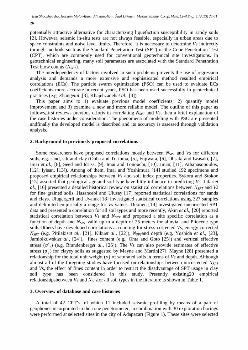
A total of 42 CPT’s, of which 11 included seismic profiling by means of a pair ofgeophones incorporated in the cone penetrometer, in combination with 30 exploration boringswere performed at selected sites in the city of Adapazarı (Figure 1). These sites were selected

Issa Shooshpasha,, Hossein Mola-Abasi, Ali Jamalian, Ünal Dikmen, Maziar Salahi/ Comp. Meth. Civil Eng. 1 (2013) 25-41

27

based on their performance after the devastating earthquake (Mw=7.4) occurred in August17, 1999 in Kocaeli (Turkey) [29].

Table 1. Inventory of proposed correlations between uncorrected NSPT and Vs

Author(s) Proposed correlationOhba and Toriuma (1970) Vs = 84N0.31

Fujiwara (1972) Vs = 92.1N0.337

Ohsaki and Iwasaki (1973) Vs = 91.4N0.39

Imai and Yoshimura (1975) Vs = 76N0.33

Imai et al (1975) Vs = 89.9N0.341

Ohta and Goto (1978) Vs = 85.35N0.348

Seed and Idriss (1981) Vs = 61.4N0.5

Imai and Tonouchi (1982) Vs = 96.9N0.314

Sykora and Stokoe (1983) Vs = 100.5N0.29

Jinan (1987) Vs = 116.1(N+0.3185)0.202

Yoshida et al (1988) Vs = 83N0.25Z0.14 (Gravel type)Jamiolkowski et al (1988) Vs = 69Z0.2N0.17(clay type)Athanasopoulos (1995) Vs = 107.6N0.36

Iyisan (1996) Vs = 51.5N0.516

Kiku et al (2001) Vs= 68.3 N0.292

Jafari et al (2002) Vs= 27 N0.73 (clay type)Hasancebi and Ulusay (2006) Vs = 90N0.309

Ulugergerli and Uyanık (2007) VSU = 23.291Ln(N)+ 405.61 (upper bound)VSL = 52.9e−0.011N (lower bound)

Dikmen (2009) Vs = 58N0.39

Akın et al (2011) Vs = 59.44N0.109Z0.426

Figure 1. Location of in-situ tests in Adapazarı, Turkey [29]


27




Fujiwara (1972) Vs = 92.1N0.337



Imai et al (1975) Vs = 89.9N0.341

Ohta and Goto (1978) Vs = 85.35N0.348




Jinan (1987) Vs = 116.1(N+0.3185)0.202


Iyisan (1996) Vs = 51.5N0.516

Kiku et al (2001) Vs= 68.3 N0.292



Dikmen (2009) Vs = 58N0.39

Akın et al (2011) Vs = 59.44N0.109Z0.426



27




Fujiwara (1972) Vs = 92.1N0.337



Imai et al (1975) Vs = 89.9N0.341

Ohta and Goto (1978) Vs = 85.35N0.348




Jinan (1987) Vs = 116.1(N+0.3185)0.202


Iyisan (1996) Vs = 51.5N0.516

Kiku et al (2001) Vs= 68.3 N0.292



Dikmen (2009) Vs = 58N0.39

Akın et al (2011) Vs = 59.44N0.109Z0.426



28

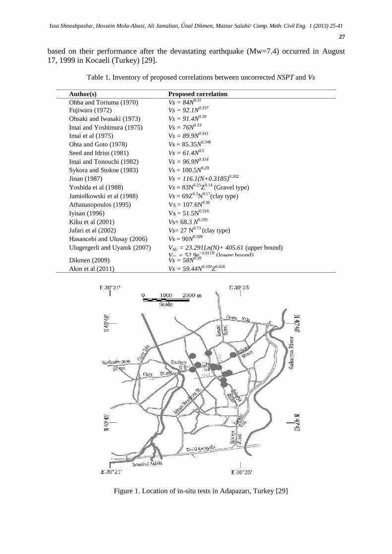
The epicenter was located near the city of Izmit, and fault rupture was physically visiblethrough most of the seismically impacted area (Marmara region); from Karamürsel toAkyazı. In the vicinity of Adapazarı, with peak ground accelerations recorded atapproximately 0.4 g, as much as 70% of the buildings were subjected to large groundsettlements, liquefaction, or subsidence and sea water inundation [30]. As illustrated inFigure 2, the southern shores of Izmit Bay are covered by Holocene deposits, these areprincipally fine-grained sandy sediments which become finer (more silty and clayey)northwards into the depths of Izmit Bay. Detailed geological and geotechnical properties ofthe site isavailable in PEER [29].

Figure 2. Simplified geological map of Armutlu peninsula (after Goncuoglu [30])

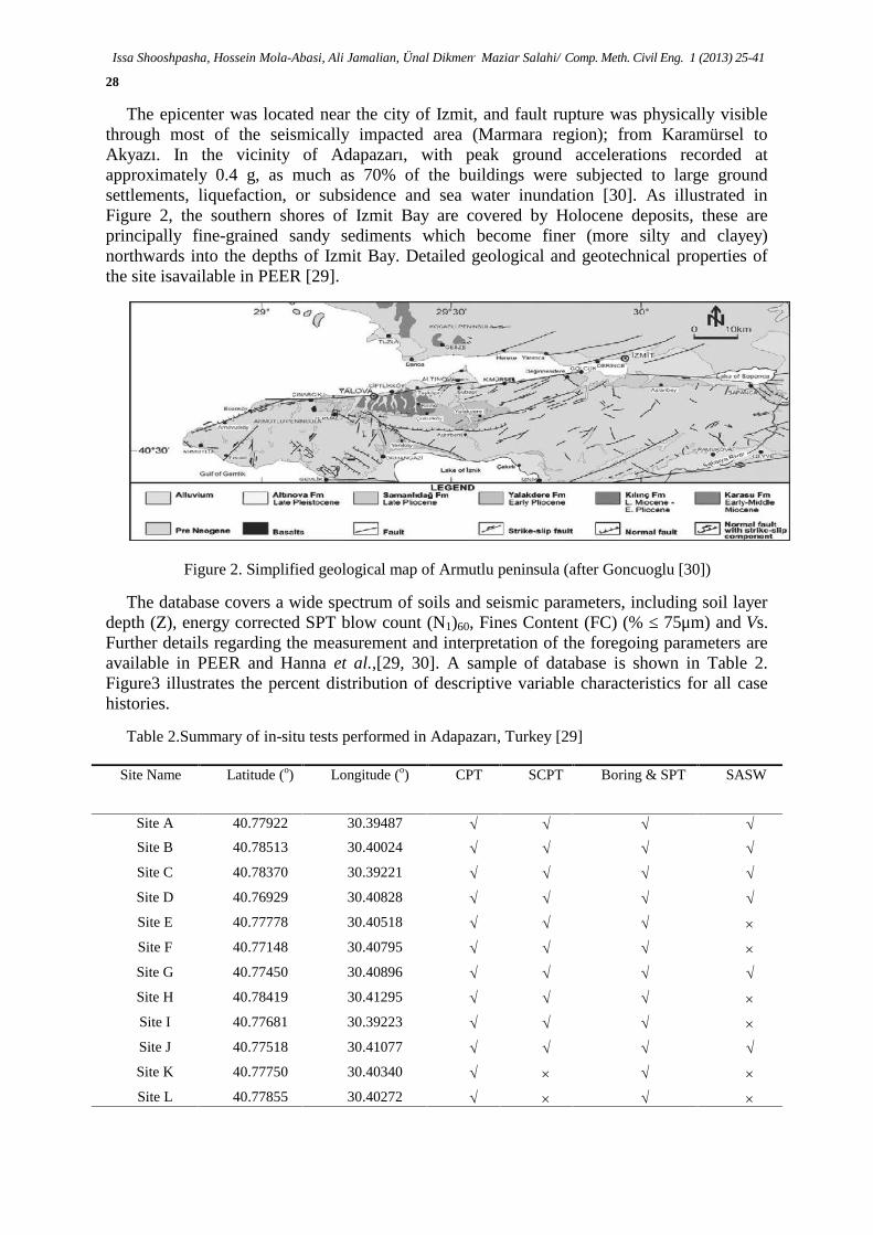
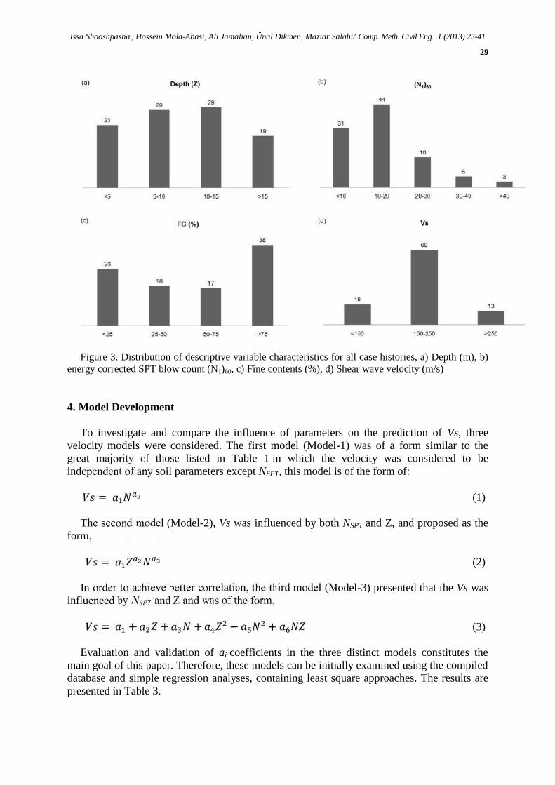
The database covers a wide spectrum of soils and seismic parameters, including soil layerdepth (Z), energy corrected SPT blow count (N1)60, Fines Content (FC) (% ≤ 75μm) and Vs.Further details regarding the measurement and interpretation of the foregoing parameters areavailable in PEER and Hanna et al.,[29, 30]. A sample of database is shown in Table 2.Figure3 illustrates the percent distribution of descriptive variable characteristics for all casehistories.

Table 2.Summary of in-situ tests performed in Adapazarı, Turkey [29]

Site Name Latitude (o) Longitude (o) CPT SCPT Boring & SPT SASW

Site A 40.77922 30.39487

Site B 40.78513 30.40024

Site C 40.78370 30.39221

Site D 40.76929 30.40828

Site E 40.77778 30.40518

Site F 40.77148 30.40795

Site G 40.77450 30.40896

Site H 40.78419 30.41295

Site I 40.77681 30.39223

Site J 40.77518 30.41077

Site K 40.77750 30.40340

Site L 40.77855 30.40272


29

Figure 3. Distribution of descriptive variable characteristics for all case histories, a) Depth (m), b)energy corrected SPT blow count (N1)60, c) Fine contents (%), d) Shear wave velocity (m/s)

4. Model Development

To investigate and compare the influence of parameters on the prediction of Vs, threevelocity models were considered. The first model (Model-1) was of a form similar to thegreat majority of those listed in Table 1 in which the velocity was considered to beindependent of any soil parameters except NSPT, this model is of the form of:= (1)

The second model (Model-2), Vs was influenced by both NSPT and Z, and proposed as theform, = (2)

In order to achieve better correlation, the third model (Model-3) presented that the Vs wasinfluenced by NSPT and Z and was of the form,= + + + + + (3)

Evaluation and validation of ai coefficients in the three distinct models constitutes themain goal of this paper. Therefore, these models can be initially examined using the compileddatabase and simple regression analyses, containing least square approaches. The results arepresented in Table 3.


30

Table 3. Correlation coefficients for three distinct models

Model a1 a2 a3 a4 a5 a6

Model-1 108.5675 0.19849 - - - -Model-2 95.7194 0.18281 0.10063 - - -Model-3 116.8281 5.7117 1.0228 -0.0733 -0.0085 0.0575

5. Principles of modeling by using particle swarm optimization

In this section, the PSO method ofKennedy and Eberhart[31] reviewed and discussed itsmain properties. Consider a special class of problems with bounded variables in the form ofmin ( ) , . . ≤ ≤ , = 1,2, … , .

Particle swarm optimizers are optimization algorithms which are inspired of the behaviorsof social models like bird flocking or fish schooling. It is introduced by Kennedy andEberhart [31] as an optimization method for continuous nonlinear functions. Later, it hasbeen applied to wide range of problems due to its simple concepts and easy implementation.

PSO is a stochastic and population-based optimization technique where individuals,referred to as particles are grouped into a swarm. Each particle has a position and velocityvector. Particles can initially be positioned randomly or to predetermined locations. Theposition of a particle is a candidate solution to the optimization problem. In a PSO system,each particle is moved through the multi-dimensional search space, adjusting its position insearch space according to its own experience and that of neighboring particles. A particletherefore makes use of its neighbors to position itself toward an optimal solution. The effectis that particles move toward a minimum, while still searching a wide area around the bestsolution. The performance of each particle (i.e. the ‘‘closeness’’ of a particle to the globaloptimum) is measured using a predefined fitness function which encapsulates thecharacteristics of the optimization problem.Each particle in the swarm maintains the currentposition, current velocity and the personal best position. The personal best position associatedwith a particle i is the best position that the particle has visited, i.e. a position that yielded thehighest fitness value for that particle. If f denotes the objective function then the personal bestof a particle at a time step,t is updated as follows:( + 1) = ( ) , ( ( + 1)) ≥ ( ( ))( + 1) , ( ( + 1)) < ( ( )) (4)

Two main approaches to PSO exist, namely lbest and gbest, where the difference is in theneighborhood topology used to exchange experience among particles. For the gbest model,the best particle is determined from the entire swarm. If the position of the best particle isdenoted by the vector , then( ) ∈ { , ,⋯ , } = ( ) , ( ) ,⋯ , ( ( )) (5)

wheres is the total number of particles in the swarm. For the lbest model, a swarm isdivided into overlapping neighborhoods of particles. For each neighborhood, , a bestparticle is determined with position . This best particle is referred to as the neighborhoodbest particle defined as= { ( ), ( ),⋯ , ( ), ( ), ( ),⋯ , ( ), ( )} (6)( + 1) ∈ | ( + 1) = { ( )} ∀ ∈


31

wherej stands for the number of neighborhood in the entire swarm. Neighborhoods areusually determined using particle indices [32], although topological neighborhoods have alsobeen used [33]. The gbest PSO is a special case of lbest while l=s, that is, the neighborhoodis the entire swarm. In the gbest PSO algorithm, the velocity, vi and the position,xi of aparticle in the swarm are updated at the end of each iteration as follows:( + 1) = ( ) + [ ( ) − ( )] + [ ( ) − ( )] (7a)( + 1) = ( ) + ( + 1) (7b)

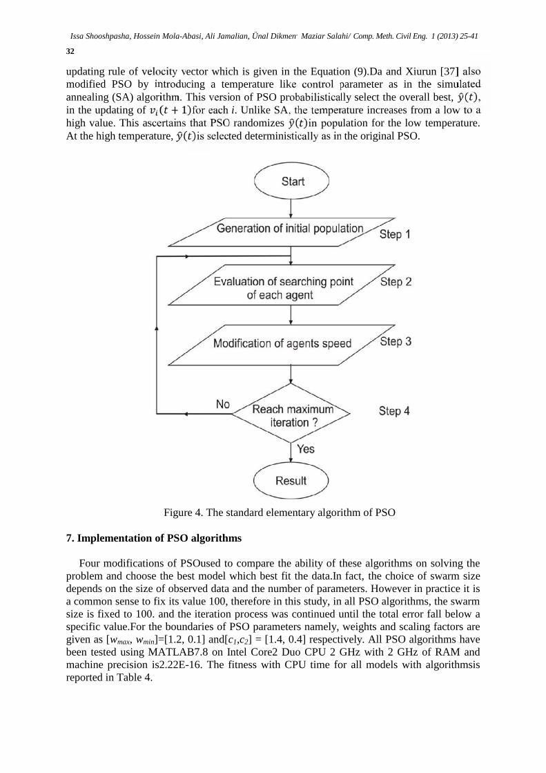
wherer1 andr2 are uniformly distributed random numbers [31], c1 andc2are the learningfactors (weights)that controls the personal and global best respectively. Therefore, the secondand the third terms in the right site ofequation (7a) show personal and global(social)influences respectively. For the lbest version of PSO, ( )is replaced by, i.e. thecorresponding neighborhood best particle.The PSO algorithm performs repeated applicationsof the updated equations above until a specified number of iterations have been exceeded oruntil velocity updates are close to zero. Figure 4 shows the original canonical PSO algorithm.

6. Improved PSO algorithms

Since the PSO method introduced by Kennedy and Eberhart [31], many techniques wereproposed to refine and/or complement the standard elementary structure of the PSOalgorithm, namely regarding its tuning parameters. A number of modifications to PSO havebeen introduced in the literature. The first modification was done by Shi and Eberhart [34].They proposed a constant inertia weight,wwhich controls how much a particle tends to followits direction as compared to the memorized personal best position (pbest), ( ) and the globalbest position (gbest), ( ). This version is referred to as PSO with constant inertia or PSO-CI.Hence, in PSO-CI, velocity update is given as( + 1) = ( ) + [ ( ) − ( )] + [ ( ) − ( )] (8)

where the values ofr1 andr2 are realized component-wise.Shi and Eberhart [35] alsoproposed a linearly varying inertia weight during the searching process. The inertia weight islinearly reduced during the search. This entails a more globally search during the initialstages and a more locally search during the final stages. This version is referred to as PSOwith linear inertia or PSO-LI. Also, a linearly varying scaling factors, (c1, c2) of PSOduringthe search has been proposed. These factors are linearly reduced during the search. Thisversion is referred to as PSO with linear acceleration weights or PSO-LA.Clerc and Kennedy[36] introduced another interesting modification to PSO in the form of a constrictioncoefficient K, which controls all the three components in velocity update rule (7a). This hasan effect of reducing the velocity as the search progresses. In this modification, the velocityupdate is given as( + 1) = ( ( ) + [ ( ) − ( )] + [ ( ) − ( )]) (9)

whereviis the velocity vector of ith person of population in time,t and K is given as= 2/ 2 − − − 4 , = + > 4 (10)

This version is referred to as PSO with constriction or CPSO. The structure of CPSOalgorithm is similar to the structure of PSO algorithm (Figure 4) and the only difference is the


32

updating rule of velocity vector which is given in the Equation (9).Da and Xiurun [37] alsomodified PSO by introducing a temperature like control parameter as in the simulatedannealing (SA) algorithm. This version of PSO probabilistically select the overall best, ( ),in the updating of ( + 1)for each i. Unlike SA, the temperature increases from a low to ahigh value. This ascertains that PSO randomizes ( )in population for the low temperature.At the high temperature, ( )is selected deterministically as in the original PSO.

Figure 4. The standard elementary algorithm of PSO

7. Implementation of PSO algorithms

Four modifications of PSOused to compare the ability of these algorithms on solving theproblem and choose the best model which best fit the data.In fact, the choice of swarm sizedepends on the size of observed data and the number of parameters. However in practice it isa common sense to fix its value 100, therefore in this study, in all PSO algorithms, the swarmsize is fixed to 100. and the iteration process was continued until the total error fall below aspecific value.For the boundaries of PSO parameters namely, weights and scaling factors aregiven as [wmax, wmin]=[1.2, 0.1] and[c1,c2] = [1.4, 0.4] respectively. All PSO algorithms havebeen tested using MATLAB7.8 on Intel Core2 Duo CPU 2 GHz with 2 GHz of RAM andmachine precision is2.22E-16. The fitness with CPU time for all models with algorithmsisreported in Table 4.


33

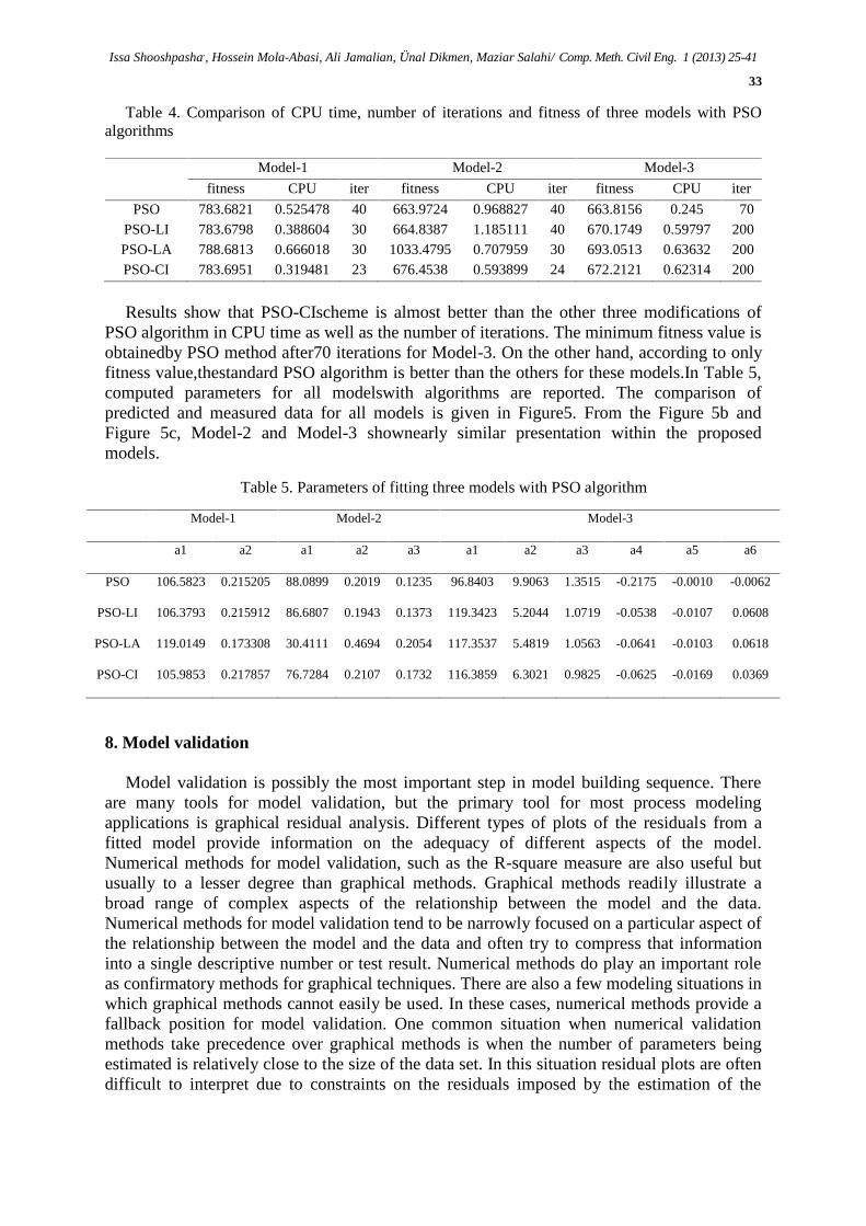
Table 4. Comparison of CPU time, number of iterations and fitness of three models with PSOalgorithms

Model-1 Model-2 Model-3

fitness CPU iter fitness CPU iter fitness CPU iter

PSO 783.6821 0.525478 40 663.9724 0.968827 40 663.8156 0.245 70PSO-LI 783.6798 0.388604 30 664.8387 1.185111 40 670.1749 0.59797 200PSO-LA 788.6813 0.666018 30 1033.4795 0.707959 30 693.0513 0.63632 200PSO-CI 783.6951 0.319481 23 676.4538 0.593899 24 672.2121 0.62314 200

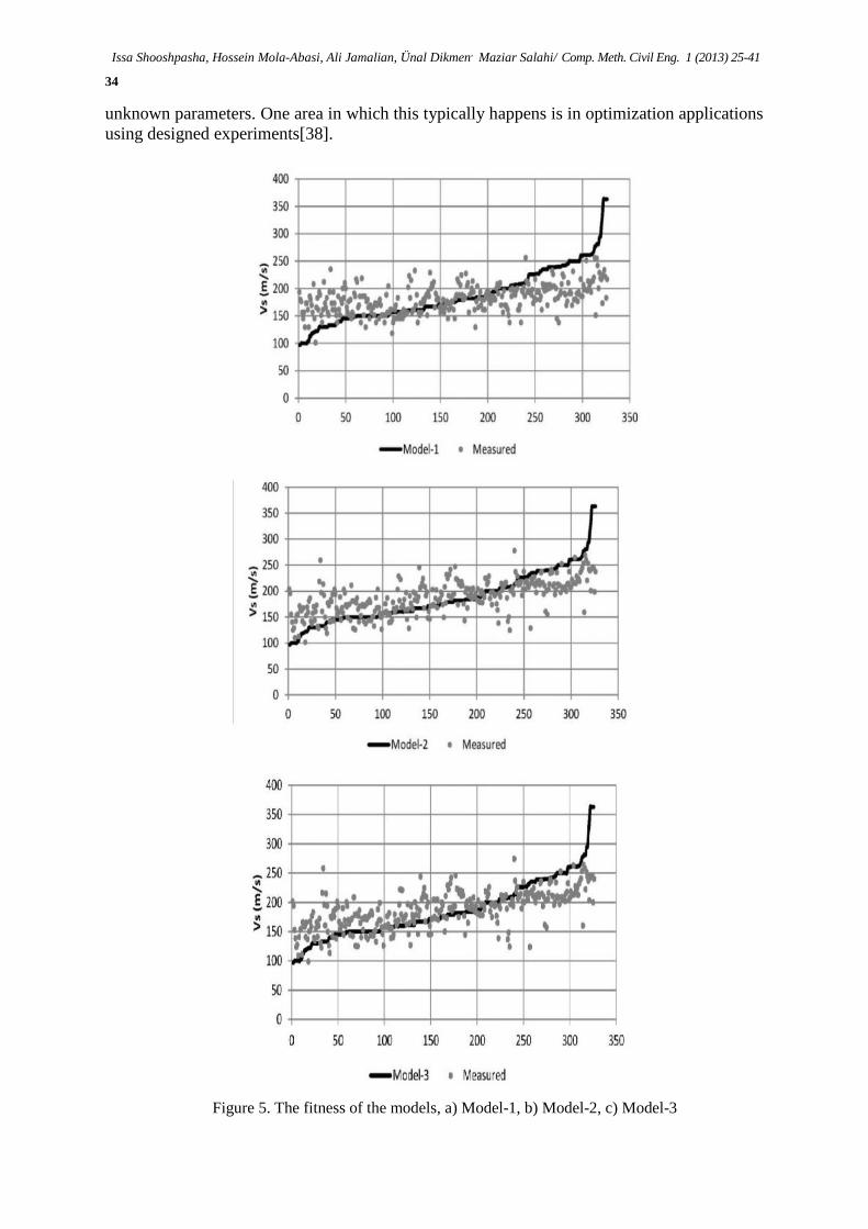
Results show that PSO-CIscheme is almost better than the other three modifications ofPSO algorithm in CPU time as well as the number of iterations. The minimum fitness value isobtainedby PSO method after70 iterations for Model-3. On the other hand, according to onlyfitness value,thestandard PSO algorithm is better than the others for these models.In Table 5,computed parameters for all modelswith algorithms are reported. The comparison ofpredicted and measured data for all models is given in Figure5. From the Figure 5b andFigure 5c, Model-2 and Model-3 shownearly similar presentation within the proposedmodels.

Table 5. Parameters of fitting three models with PSO algorithm

Model-1 Model-2 Model-3

a1 a2 a1 a2 a3 a1 a2 a3 a4 a5 a6

PSO 106.5823 0.215205 88.0899 0.2019 0.1235 96.8403 9.9063 1.3515 -0.2175 -0.0010 -0.0062

PSO-LI 106.3793 0.215912 86.6807 0.1943 0.1373 119.3423 5.2044 1.0719 -0.0538 -0.0107 0.0608

PSO-LA 119.0149 0.173308 30.4111 0.4694 0.2054 117.3537 5.4819 1.0563 -0.0641 -0.0103 0.0618

PSO-CI 105.9853 0.217857 76.7284 0.2107 0.1732 116.3859 6.3021 0.9825 -0.0625 -0.0169 0.0369

8. Model validation

Model validation is possibly the most important step in model building sequence. Thereare many tools for model validation, but the primary tool for most process modelingapplications is graphical residual analysis. Different types of plots of the residuals from afitted model provide information on the adequacy of different aspects of the model.Numerical methods for model validation, such as the R-square measure are also useful butusually to a lesser degree than graphical methods. Graphical methods readily illustrate abroad range of complex aspects of the relationship between the model and the data.Numerical methods for model validation tend to be narrowly focused on a particular aspect ofthe relationship between the model and the data and often try to compress that informationinto a single descriptive number or test result. Numerical methods do play an important roleas confirmatory methods for graphical techniques. There are also a few modeling situations inwhich graphical methods cannot easily be used. In these cases, numerical methods provide afallback position for model validation. One common situation when numerical validationmethods take precedence over graphical methods is when the number of parameters beingestimated is relatively close to the size of the data set. In this situation residual plots are oftendifficult to interpret due to constraints on the residuals imposed by the estimation of the


34

unknown parameters. One area in which this typically happens is in optimization applicationsusing designed experiments[38].

Figure 5. The fitness of the models, a) Model-1, b) Model-2, c) Model-3


35

Goodness of fit of a model describes how well it fits a set of observations. Measures ofgoodness of fit typically summarize the discrepancy between observed values and the valuesexpected under the model in question. Before the comparison of the developed models, briefinformation of basic formulas of error measuresgiven.Some goodnessoffit measures forparametric models are following [39,40]:

Sum of squares of error (SSE) R-square Degrees of freedom adjusted R-square Chi-square Reduced Chi-square Weighting methods

Sum of Squares of Error

This measure measures the total deviation of the response values from the fit to theresponse values. It is also called the summed square of residuals and is usually labeled asSSE and defined as= ∑ ( − ) (11)

whereyi and denote measured andestimated values respectively. In this measure, a valuecloser to zero indicates that the model has a smaller random error component and that the fitwill be more useful for prediction.

R-Square

This statistic measures how successful the fit is in explaining the variation of the data. Putanother way, R-square is the square of the correlation between the measured and predictedvalues. It is also called the square of the multiple correlation coefficients and the coefficientof multiple determinations. R-square is defined as the ratio of the sum of squares of theregression (SSR) and the total sum of squares (SST). SSR is defined as= ∑ ( − ) (12)

SST is also called the sum of squares about the mean, and is defined as= ∑ ( − ) (13)

where, SST = SSR + SSE. Given the last two definitions for SSR and SST, R-square isexpressed as:− = = 1 − (14)

R-square can take on any value between 0 and 1, with a value closer to 1 indicating that agreater proportion of variance is accounted for by the model. When the number ofcoefficients in model is increased, the R-square increases although the fit may not improve in


36

a practical sense. To avoid this situation, the degrees of freedom adjusted R-square statisticwhich described below is needed.

Degrees of freedom adjusted R-Square

This measure uses the R-square measure defined above and adjusts it based on the residualdegrees of freedom. The residual degrees of freedom is defined as the number of responsevalues n minus the number of fitted coefficients m estimated from the response values.= −where,v indicates the number of independent pieces of information involving the n datapoints that are required to calculate the sum of squares.

Chi-square

One way in which goodness of fit of a model can be measured, in the case where thevariance of the measurement error is known, is to construct a weighted sum of squared errors:= ∑ ( )

(15)

whereσ2 is the known variance of the observation, O and E stand for observed andestimated data respectively.

ReducedChi-square

The reduced Chi-squared measure is simply the Chi-square divided by the number ofdegrees of freedom [38, 39, 40]:= = ∑ ( )

(16)

whereν is the number of degrees of freedom, usually given by N − n − 1, where N is thenumber of observations, and n is the number of fitted parameters, assuming that the meanvalue is an additional fitted parameter. The advantage of the reduced Chi-square is that italready normalizes for the number of data points and model complexity.As a rule of thumb, alarge indicates a poor model fit. However < 1 indicates that the model is over-fitting the data. A > 1 indicates that the fit has not fully captured the data. In principle,a value of = 1 indicates that the extent of the match between observations and estimatesare in accord with the error variance.

Weighting methods

Nonlinear regression is commonly done without weighting. If there is a similar trendbetween experimental and estimation, we can weight points differentially.There are tworelative weighting methods:

weighting by 1/y2

weighting by 1/y


37

Weighting by1/y2

This method minimizes the sum-of-squares of the relative distances of the data from thecurve. The method is appropriate when we expect the average distance of the points from thecurve to be higher when y is higher, but the relative distance (distance divided by y) to be aconstant. In this common situation, minimizing the sum-of-squares is inappropriate becausepoints with high y values will have a large influence on the sum-of-squares value while pointswith smaller y values will have little influence. Minimizing the sum of the square of therelative distances restores equal weighting to all points.

Weighting by 1/y

Weighting by 1/yis a compromise between minimizing the actual distance squared andminimizing the relative distance squared. The selection of the weighting methods in generaldepends on the distribution of data.

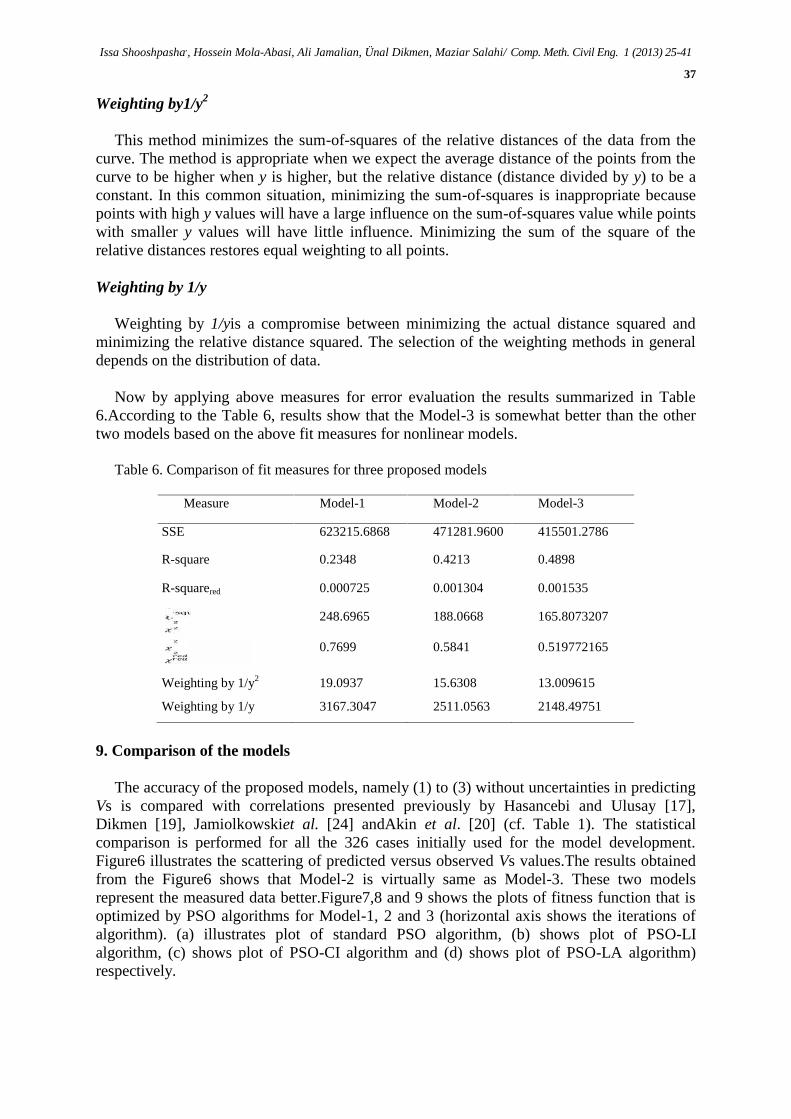
Now by applying above measures for error evaluation the results summarized in Table6.According to the Table 6, results show that the Model-3 is somewhat better than the othertwo models based on the above fit measures for nonlinear models.

Table 6. Comparison of fit measures for three proposed models

Measure Model-1 Model-2 Model-3

SSE 623215.6868 471281.9600 415501.2786

R-square 0.2348 0.4213 0.4898

R-squarered 0.000725 0.001304 0.001535

248.6965 188.0668 165.8073207

0.7699 0.5841 0.519772165

Weighting by 1/y2 19.0937 15.6308 13.009615

Weighting by 1/y 3167.3047 2511.0563 2148.49751

9. Comparison of the models

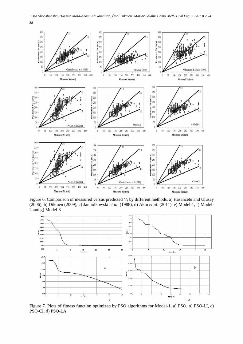
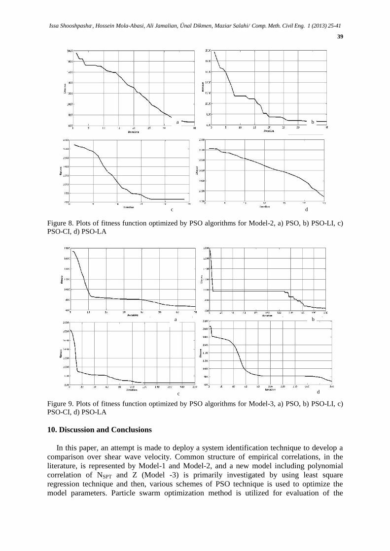
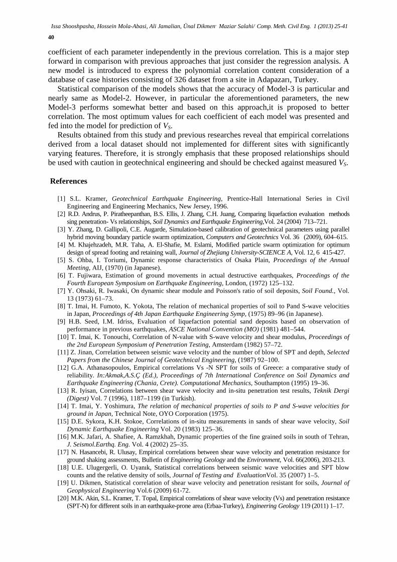
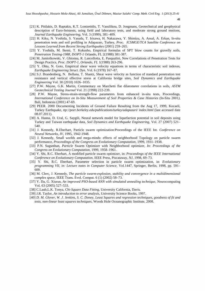
The accuracy of the proposed models, namely (1) to (3) without uncertainties in predictingVs is compared with correlations presented previously by Hasancebi and Ulusay [17],Dikmen [19], Jamiolkowskiet al. [24] andAkin et al. [20] (cf. Table 1). The statisticalcomparison is performed for all the 326 cases initially used for the model development.Figure6 illustrates the scattering of predicted versus observed Vs values.The results obtainedfrom the Figure6 shows that Model-2 is virtually same as Model-3. These two modelsrepresent the measured data better.Figure7,8 and 9 shows the plots of fitness function that isoptimized by PSO algorithms for Model-1, 2 and 3 (horizontal axis shows the iterations ofalgorithm). (a) illustrates plot of standard PSO algorithm, (b) shows plot of PSO-LIalgorithm, (c) shows plot of PSO-CI algorithm and (d) shows plot of PSO-LA algorithm)respectively.


38

Figure 6. Comparison of measured versus predicted VS by different methods, a) Hasancebi and Ulusay(2006), b) Dikmen (2009), c) Jamiolkowski et al. (1988), d) Akin et al. (2011), e) Model-1, f) Model-2 and g) Model-3

Figure 7. Plots of fitness function optimized by PSO algorithms for Model-1, a) PSO, b) PSO-LI, c)PSO-CI, d) PSO-LA

a b

c d


39



10. Discussion and Conclusions

In this paper, an attempt is made to deploy a system identification technique to develop acomparison over shear wave velocity. Common structure of empirical correlations, in theliterature, is represented by Model-1 and Model-2, and a new model including polynomialcorrelation of NSPT and Z (Model -3) is primarily investigated by using least squareregression technique and then, various schemes of PSO technique is used to optimize themodel parameters. Particle swarm optimization method is utilized for evaluation of the

a

a b

c d

b

c d


40

coefficient of each parameter independently in the previous correlation. This is a major stepforward in comparison with previous approaches that just consider the regression analysis. Anew model is introduced to express the polynomial correlation content consideration of adatabase of case histories consisting of 326 dataset from a site in Adapazarı, Turkey.

Statistical comparison of the models shows that the accuracy of Model-3 is particular andnearly same as Model-2. However, in particular the aforementioned parameters, the newModel-3 performs somewhat better and based on this approach,it is proposed to bettercorrelation. The most optimum values for each coefficient of each model was presented andfed into the model for prediction of VS.

Results obtained from this study and previous researches reveal that empirical correlationsderived from a local dataset should not implemented for different sites with significantlyvarying features. Therefore, it is strongly emphasis that these proposed relationships shouldbe used with caution in geotechnical engineering and should be checked against measured VS.

References

[1] S.L. Kramer, Geotechnical Earthquake Engineering, Prentice-Hall International Series in CivilEngineering and Engineering Mechanics, New Jersey, 1996.

[2] R.D. Andrus, P. Piratheepanthan, B.S. Ellis, J. Zhang, C.H. Juang, Comparing liquefaction evaluation methodssing penetration- Vs relationships, Soil Dynamics and Earthquake Engineering,Vol. 24 (2004) 713–721.

[3] Y. Zhang, D. Gallipoli, C.E. Augarde, Simulation-based calibration of geotechnical parameters using parallelhybrid moving boundary particle swarm optimization, Computers and Geotechnics Vol. 36 (2009), 604–615.

[4] M. Khajehzadeh, M.R. Taha, A. El-Shafie, M. Eslami, Modified particle swarm optimization for optimumdesign of spread footing and retaining wall, Journal of Zhejiang University-SCIENCE A, Vol. 12, 6 415-427.

[5] S. Ohba, I. Toriumi, Dynamic response characteristics of Osaka Plain, Proceedings of the AnnualMeeting, AIJ, (1970) (in Japanese).

[6] T. Fujiwara, Estimation of ground movements in actual destructive earthquakes, Proceedings of theFourth European Symposium on Earthquake Engineering, London, (1972) 125–132.

[7] Y. Ohsaki, R. Iwasaki, On dynamic shear module and Poisson's ratio of soil deposits, Soil Found., Vol.13 (1973) 61–73.

[8] T. Imai, H. Fumoto, K. Yokota, The relation of mechanical properties of soil to Pand S-wave velocitiesin Japan, Proceedings of 4th Japan Earthquake Engineering Symp, (1975) 89–96 (in Japanese).

[9] H.B. Seed, I.M. Idriss, Evaluation of liquefaction potential sand deposits based on observation ofperformance in previous earthquakes, ASCE National Convention (MO) (1981) 481–544.

[10] T. Imai, K. Tonouchi, Correlation of N-value with S-wave velocity and shear modulus, Proceedings ofthe 2nd European Symposium of Penetration Testing, Amsterdam (1982) 57–72.

[11] Z. Jinan, Correlation between seismic wave velocity and the number of blow of SPT and depth, SelectedPapers from the Chinese Journal of Geotechnical Engineering, (1987) 92–100.

[12] G.A. Athanasopoulos, Empirical correlations Vs -N SPT for soils of Greece: a comparative study ofreliability. In:Akmak,A.S.Ç (Ed.), Proceedings of 7th International Conference on Soil Dynamics andEarthquake Engineering (Chania, Crete). Computational Mechanics, Southampton (1995) 19–36.

[13] R. Iyisan, Correlations between shear wave velocity and in-situ penetration test results, Teknik Dergi(Digest) Vol. 7 (1996), 1187–1199 (in Turkish).

[14] T. Imai, Y. Yoshimura, The relation of mechanical properties of soils to P and S-wave velocities forground in Japan, Technical Note, OYO Corporation (1975).

[15] D.E. Sykora, K.H. Stokoe, Correlations of in-situ measurements in sands of shear wave velocity, SoilDynamic Earthquake Engineering Vol. 20 (1983) 125–36.

[16] M.K. Jafari, A. Shafiee, A. Ramzkhah, Dynamic properties of the fine grained soils in south of Tehran,J. Seismol.Earthq. Eng. Vol. 4 (2002) 25–35.

[17] N. Hasancebi, R. Ulusay, Empirical correlations between shear wave velocity and penetration resistance forground shaking assessments, Bulletin of Engineering Geology and the Environment, Vol. 66(2006), 203 -213.

[18] U.E. Ulugergerli, O. Uyanık, Statistical correlations between seismic wave velocities and SPT blowcounts and the relative density of soils, Journal of Testing and EvaluationVol. 35 (2007) 1–5.

[19] U. Dikmen, Statistical correlation of shear wave velocity and penetration resistant for soils, Journal ofGeophysical Engineering Vol.6 (2009) 61-72.

[20] M.K. Akin, S.L. Kramer, T. Topal, Empirical correlations of shear wave velocity (Vs) and penetration resistance(SPT-N) for different soils in an earthquake-prone area (Erbaa-Turkey), Engineering Geology 119 (2011) 1–17.


41

[21] K. Pitilakis, D. Raptakis, K.T. Lontzetidis, T. Vassilikou, D. Jongmans, Geotechnical and geophysicaldescription of Euro-Seistests, using field and laboratory tests, and moderate strong ground motions,Journal Earthquake Engineering, Vol. 3 (1999), 381–409.

[22] H. Kiku, N. Yoshida, S. Yasuda, T. Irisawa, H. Nakazawa, Y. Shimizu, A. Ansal, A. Erkan, In-situpenetration tests and soil profiling in Adapazarı, Turkey, Proc. ICSMGE/TC4 Satellite Conference onLessons Learned from Recent Strong Earthquakes (2001) 259–265.

[23] Y. Yoshida, M. Ikemi, T. Kokusho, Empirical formulas of SPT blow counts for gravelly soils,Penetration Testing-1988, ISOPT-1 Orlando, FL 2(1988) 381-387.

[24] M. Jamiolkowski, V. Ghionna, R. Lancellotta, E. Pasqualini, New Correlations of Penetration Tests forDesign Practice, Proc. ISOPT-1, Orlando, FL 1(1988) 263-296.

[25] Y. Ohta, N. Goto, Empirical shear wave velocity equations in terms of characteristic soil indexes,Earthquake Engineering Struct. Dyn. Vol. 6 (1978) 167–87.

[26] S.J. Brandenberg, N. Bellana, T. Shantz, Shear wave velocity as function of standard penetration testresistance and vertical effective stress at California bridge sites, Soil Dynamics and EarthquakeEngineering Vol. 30 (2010) 1026–1035.

[27] P.W. Mayne, G.K. Martin, Commentary on Marchetti flat dilatometer correlations in soils, ASTMGeotechnical Testing Journal Vol. 21 (1998) 222-239.

[28] P.W. Mayne, Stress-strain-strength-flow parameters from enhanced in-situ tests, Proceedings,International Conference on In-Situ Measurement of Soil Properties & Case Histories (In-Situ 2001),Bali, Indonesia (2001) 47-69.

[29] PEER. 2000 Documenting Incidents of Ground Failure Resulting from the Aug 17, 1999, Kocaeli,Turkey Earthquake, ttp://peer.berkeley.edu/publications/turkey/adapazari/ index.html (last accessed date08.07.2011).

[30] A. Hanna, D. Ural, G. Saygili, Neural network model for liquefaction potential in soil deposits usingTurkey and Taiwan earthquake data, Soil Dynamics and Earthquake Engineering, Vol. 27 (2007) 521–540.

[31] J. Kennedy, R.Eberhart, Particle swarm optimization:Proceedings of the IEEE Int. Conference onNeural Networks, IV, 1995, 1942-1948.

[32] J. Kennedy, Small worlds and mega-minds: effects of neighborhood Topology on particle swarmperformance, Proceedings of the Congress on Evolutionary Computation, 1999, 1931–1938.

[33] P.N. Sugsnthan, Particle Swarm Optimizer with Neighborhood optimizer, In: Proceedings of theCongress on Evolutionary Computation, 1999, 1958–1961.

[34] Y. Shi, R.C. Eberhart, A modified particle swarm optimizer, in: Proceedings of the IEEE InternationalConference on Evolutionary Computation, IEEE Press, Piscataway, NJ, 1998, 69–73.

[35] Y. Shi, R.C. Eberhart, Parameter selection in particle swarm optimization, in: Evolutionaryprogramming VII, in: Lecture notes in Computer Science, Vol.1447, Springer, Berlin, 1998, pp. 591–600.

[36] M. Clerc, J. Kennedy, The particle swarm-explosion, stability and convergence in a multidimensionalcomplex space, IEEE Trans. Evol. Comput. 6 (1) (2002) 58–73.

[37] Y. Da, G. Xiurun, An improved PSO-based ANN with simulated annealing technique, NeurocomputingVol. 63 (2005) 527–533.

[38] C.Laub,L.K. Tonya, Chi-Square Data Fitting, University California, Davis.[39] J.R. Taylor, An introduction to error analysis, University Science Books, 1997.[40] D. M. Glover, W. J. Jenkins, S. C. Doney, Least Squares and regression techniques, goodness of fit and

tests, non-linear least squares techniques, Woods Hole Oceanographic Institute, 2008.

validation and application of empirical shear wave velocity models based on standard penetration

Documents