uwe t. bornscheuer matthias höhne editors

Protein Engineering

Uwe T. BornscheuerMatthias Höhne Editors

Methods and Protocols

Methods in Molecular Biology 1685

ME T H O D S I N MO L E C U L A R B I O L O G Y

Series EditorJohn M. Walker

School of Life and Medical SciencesUniversity of Hertfordshire

Hatfield, Hertfordshire, AL10 9AB, UK

For further volumes:http://www.springer.com/series/7651

http://www.springer.com/series/7651

http://www.springer.com/series/7651

Protein Engineering

Methods and Protocols

Edited by

Uwe T. Bornscheuer

Department of Biotechnology and Enzyme Catalysis, Institute of Biochemistry, Greifswald University,Greifswald, Germany

Matthias Höhne

Protein Biochemistry, Institute of Biochemistry, Greifswald University, Greifswald, Germany

EditorsUwe T. BornscheuerDepartment of Biotechnologyand Enzyme Catalysis

Institute of BiochemistryGreifswald UniversityGreifswald, Germany

Matthias HohneProtein BiochemistryInstitute of BiochemistryGreifswald UniversityGreifswald, Germany

ISSN 1064-3745 ISSN 1940-6029 (electronic)Methods in Molecular BiologyISBN 978-1-4939-7364-4 ISBN 978-1-4939-7366-8 (eBook)DOI 10.1007/978-1-4939-7366-8

Library of Congress Control Number: 2017953803

© Springer Science+Business Media LLC 2018This work is subject to copyright. All rights are reserved by the Publisher, whether the whole or part of the material isconcerned, specifically the rights of translation, reprinting, reuse of illustrations, recitation, broadcasting, reproductionon microfilms or in any other physical way, and transmission or information storage and retrieval, electronic adaptation,computer software, or by similar or dissimilar methodology now known or hereafter developed.The use of general descriptive names, registered names, trademarks, service marks, etc. in this publication does not imply,even in the absence of a specific statement, that such names are exempt from the relevant protective laws and regulationsand therefore free for general use.The publisher, the authors and the editors are safe to assume that the advice and information in this book are believed tobe true and accurate at the date of publication. Neither the publisher nor the authors or the editors give a warranty,express or implied, with respect to the material contained herein or for any errors or omissions that may have been made.The publisher remains neutral with regard to jurisdictional claims in published maps and institutional affiliations.

Printed on acid-free paper

This Humana Press imprint is published by Springer NatureThe registered company is Springer Science+Business Media, LLCThe registered company address is: 233 Spring Street, New York, NY 10013, U.S.A.

Preface

Since the discovery of proteins and their numerous roles in life, scientists are fascinated tostudy the molecular basis of how proteins function. It is amazing to see the plethora ofprotein structures and mechanisms that appeared during evolution, and the creativity, whichis operating in nature’s continuing process of tailoring and fine-tuning proteins and, thus,life itself.

Proteins, especially enzymes, are also the key players of biocatalysis and biotechnologyand thus they are linked to the wealth of our modern society. Besides deepening basicunderstanding, scientists are attracted by the possibility of knowledge-guided tailoring ofproteins to suit the needs of biotechnological applications (rational protein design) or tocreate novel protein functions. As an alternative to this rationally inspired approach, scien-tists mimic the process of evolution by introducing random mutations in the laboratory(directed evolution). Although we are far away from understanding and reliably predictingprotein folding and function de novo, there are remarkable success stories in the field ofprotein engineering: Enzymes were created that catalyze reactions not observed in nature,they were highly stabilized for robustness in industrial processes, and proteins havingsuperior pharmacological profiles have been successfully created. Hence, protein engineer-ing has become an indispensable tool for pharmaceutical and industrial biotechnology.

Protein engineering is a complex and versatile process. With this book we aim to collectbasic and advanced protocols for both stages of protein engineering: (i) the library designphase and (ii) the identification of improved variants by screening and selection. The focus ofthe book lies on enzyme engineering using rational and semirational approaches. Librarycreation protocols for random mutagenesis and recombining methods are a very diversefield, and a collection of protocols for this approach has been published recently in theexcellent volume Directed Evolution Library Creation of this series. Hence, this area is notcovered in this edition.

As an introduction, Chapter 1 presents a general introduction into protein engineering.The book is then structured into three parts: Part I describes computational protocols forrational protein engineering with the aid of case studies. A review (Chapter 2) summarizesdifferent design approaches and methodologies. Protein tunnel inspection and basic steps ofmolecular modeling are exemplified using the user-friendly software packages CAVER(Chapter 3) and YASARA (Chapter 4). Chapter 5 demonstrates how to use the FRESCOalgorithm to stabilize proteins. The presented guide allows to follow this more complex, butvery powerful computational engineering protocol. To study structure–function relation-ships, one useful experimental approach is to study the so-called mutability landscape of aprotein. By characterizing every possible single variant of each amino acid position of aprotein, beneficial substitutions and nonmutable residues can be identified. Chapter 6presents a laboratory protocol for an efficient way how to construct and analyze such alibrary.

Part II focuses on the high-throughput expression of libraries and summarizes commonsolutions for various problems (Chapters 7 and 8). As a more advanced technique,Chapter 9 presents the split-GFP complementation assay. This approach allows determiningthe amount of the desired protein via fluorescence measurements in the presence of theentire host proteins. Activity data can then be normalized to the amount of total proteins

v

without the need of enzyme purification. Chapter 10 covers expression and functionalstudies of membrane proteins using E. coli and insect cell-free expression systems.

High-throughput screening and selection assays are covered in Part III of this book.This is a very broad research area. Consequently, only exemplary screening protocols can begiven as an inspiration for the development of alternative screening assays. An introductoryreview (Chapter 11) provides an overview of currently existing approaches. The followingchapters deal with microplate assays: Chapter 12 describes the design of photometricscreening protocols with emphasis on hydrolytic enzymes. Exemplary protocols for screen-ing transaminases, laccases, and β-glucosidase are presented in Chapters 13–15. As screeningcampaigns have to be well planned and need an efficient way to collect, process, and visualizethe data, Chapter 16 describes an open-source software solution that aids experimentalplanning, but especially data processing and visualization.

The last protocols present solutions for screening and selection procedures. This part ofthe book covers techniques like solid phase agar plate assays (Chapter 17), droplet sorting(Chapter 18), selection by FACS (Chapter 19), and a growth assays for active and thermo-stable variants (Chapter 20).

We very much hope that this compilation of concepts, methods, and protocols will helpreaders to facilitate the planning and performance of their experiments, but most impor-tantly, that they will easily create and discover the desired improved proteins or enzymes. Wekeep our fingers crossed for success!

Greifswald, Germany Matthias HohneUwe T. Bornscheuer

vi Preface

Contents

Preface . . . . . . . . . . . . . . . . . . . . . . . . . . . . . . . . . . . . . . . . . . . . . . . . . . . . . . . . . . . . . . . . . . . . . vContributors. . . . . . . . . . . . . . . . . . . . . . . . . . . . . . . . . . . . . . . . . . . . . . . . . . . . . . . . . . . . . . . . . ix

1 Protein Engineering: Past, Present, and Future . . . . . . . . . . . . . . . . . . . . . . . . . . . . . 1Stefan Lutz and Samantha M. Iamurri

PART I COMPUTATIONAL PROTOCOLS

2 Rational and Semirational Protein Design . . . . . . . . . . . . . . . . . . . . . . . . . . . . . . . . . . 15Ivan V. Korendovych

3 Computational Analysis of Protein Tunnels and Channels. . . . . . . . . . . . . . . . . . . . 25Jan Brezovsky, Barbora Kozlikova, and Jiri Damborsky

4 YASARA: A Tool to Obtain Structural Guidance in BiocatalyticInvestigations. . . . . . . . . . . . . . . . . . . . . . . . . . . . . . . . . . . . . . . . . . . . . . . . . . . . . . . . . . . 43Henrik Land and Maria Svedendahl Humble

5 A Computational Library Design Protocol for RapidImprovement of Protein Stability: FRESCO. . . . . . . . . . . . . . . . . . . . . . . . . . . . . . . . 69Hein J. Wijma, Maximilian J. L. J. F€urst, and Dick B. Janssen

6 Directed Evolution of Proteins Based on Mutational Scanning . . . . . . . . . . . . . . . 87Carlos G. Acevedo-Rocha, Matteo Ferla, and Manfred T. Reetz

PART II PROTEIN LIBRARY EXPRESSION

7 A Brief Guide to the High-Throughput Expression of DirectedEvolution Libraries. . . . . . . . . . . . . . . . . . . . . . . . . . . . . . . . . . . . . . . . . . . . . . . . . . . . . . 131Ana Luısa Ribeiro, Mario Mencıa, and Aurelio Hidalgo

8 Library Growth and Protein Expression: Optimal and ReproducibleMicrotiter Plate Expression of Recombinant Enzymes in E. coliUsing MTP Shakers . . . . . . . . . . . . . . . . . . . . . . . . . . . . . . . . . . . . . . . . . . . . . . . . . . . . . 145Sandy Schmidt, Mark Dorr, and Uwe T. Bornscheuer

9 Normalized Screening of Protein Engineering Librariesby Split-GFP Crude Cell Extract Quantification . . . . . . . . . . . . . . . . . . . . . . . . . . . . 157Javier Santos-Aberturas, Mark Dorr, and Uwe T. Bornscheuer

10 Functional Analysis of Membrane Proteins Producedby Cell-Free Translation . . . . . . . . . . . . . . . . . . . . . . . . . . . . . . . . . . . . . . . . . . . . . . . . . 171Srujan Kumar Dondapati, Doreen A. W€ustenhagen, and Stefan Kubick

vii

PART III SCREENING AND SELECTION ASSAYS

11 Practical Considerations Regarding the Choice of the BestHigh-Throughput Assay . . . . . . . . . . . . . . . . . . . . . . . . . . . . . . . . . . . . . . . . . . . . . . . . . 189Carolin M€ugge and Robert Kourist

12 High-Throughput Screening Assays for Lipolytic Enzymes . . . . . . . . . . . . . . . . . . 209Alexander Fulton, Marc R. Hayes, Ulrich Schwaneberg,Jorg Pietruszka, and Karl-Erich Jaeger

13 Continuous High-Throughput Colorimetric Assays for α-Transaminases . . . . . . 233Egon Heuson, Jean-Louis Petit, Franck Charmantray,Veronique de Berardinis, and Thierry Gefflaut

14 Colorimetric High-Throughput Screening Assays for the DirectedEvolution of Fungal Laccases. . . . . . . . . . . . . . . . . . . . . . . . . . . . . . . . . . . . . . . . . . . . . 247Isabel Pardo and Susana Camarero

15 Directed Coevolution of Two Cellulosic Enzymes in Escherichia coliBased on Their Synergistic Reactions . . . . . . . . . . . . . . . . . . . . . . . . . . . . . . . . . . . . . . 255Min Liu, Lidan Ye, and Hongwei Yu

16 Program-Guided Design of High-Throughput Enzyme ScreeningExperiments and Automated Data Analysis/Evaluation. . . . . . . . . . . . . . . . . . . . . . 269Mark Dorr and Uwe T. Bornscheuer

17 Solid-Phase Agar Plate Assay for Screening Amine Transaminases . . . . . . . . . . . . . 283Martin S. Weiß, Uwe T. Bornscheuer, and Matthias Hohne

18 Ultrahigh-Throughput Screening of Single-Cell Lysates for DirectedEvolution and Functional Metagenomics . . . . . . . . . . . . . . . . . . . . . . . . . . . . . . . . . . 297Fabrice Gielen, Pierre-Yves Colin, Philip Mair, and Florian Hollfelder

19 Isolation of pH-Sensitive Antibody Fragments by Fluorescence-ActivatedCell Sorting and Yeast Surface Display. . . . . . . . . . . . . . . . . . . . . . . . . . . . . . . . . . . . . 311Christian Schroter, Simon Krah, Jan Beck, Doreen Konning, JuliusGrzeschik, Bernhard Valldorf, Stefan Zielonka, and Harald Kolmar

20 Library Generation and Auxotrophic Selection Assays in Escherichia coliand Thermus thermophilus . . . . . . . . . . . . . . . . . . . . . . . . . . . . . . . . . . . . . . . . . . . . . . . . 333Jorg Claren, Thomas Schwab, and Reinhard Sterner

Index . . . . . . . . . . . . . . . . . . . . . . . . . . . . . . . . . . . . . . . . . . . . . . . . . . . . . . . . . . . . . . . . . . . . . . 347

viii Contents

Contributors

CARLOS G. ACEVEDO-ROCHA � Department of Biocatalysis, Max-Planck-Institut f€urKohlenforschung, M€ulheim an der Ruhr, Germany; Department of Chemistry, Philipps-Universit€at Marburg, Marburg, Germany; Biosyntia ApS, Copenhagen, Denmark

VERONIQUE DE BERARDINIS � CEA, DSV, IG, Genoscope, Evry, France; CNRS-UMR8030,Evry, France; Universite d’Evry Val d’Essonne, Evry, France

JAN BECK � Institute for Organic Chemistry and Biochemistry, Technische Universit€atDarmstadt, Darmstadt, Germany; Protein Engineering and Antibody Technologies,Merck-Serono, Merck KGaA, Darmstadt, Germany

UWE T. BORNSCHEUER � Department of Biotechnology and Enzyme Catalysis, Institute ofBiochemistry, Greifswald University, Greifswald, Germany

JAN BREZOVSKY � Loschmidt Laboratories, Department of Experimental Biology, ResearchCentre for Toxic Compounds in the Environment RECETOX, Faculty of Science, MasarykUniversity, Brno, Czech Republic

SUSANA CAMARERO � Centro de Investigaciones Biologicas, CSIC, Madrid, SpainFRANCK CHARMANTRAY � Institut de Chimie de Clermont-Ferrand, Clermont Universite,

Universite Blaise Pascal, Clermont-Ferrand, France; CNRS, UMR6296, ICCF, Aubiere,France

JORG CLAREN � Clariant Produkte (Deutschland) GmbH, Planegg, GermanyPIERRE-YVES COLIN � Department of Biochemistry, University of Cambridge, Cambridge,

UK; Department of Biochemical Engineering, University College London, London, UKMARK DORR � Department of Biotechnology and Enzyme Catalysis, Institute of Biochemistry,

Greifswald University, Greifswald, GermanyJIRI DAMBORSKY � Loschmidt Laboratories, Department of Experimental Biology, Research

Centre for Toxic Compounds in the Environment RECETOX, Faculty of Science, MasarykUniversity, Brno, Czech Republic

SRUJAN KUMAR DONDAPATI � Branch Bioanalytics and Bioprocesses (IZI-BB), FraunhoferInstitute for Cell Therapy and Immunology (IZI), Potsdam, Germany

MAXIMILIAN J. L. J. F€uRST � Groningen Biomolecular Sciences and Biotechnology Institute,University of Groningen, Groningen, The Netherlands

MATTEO FERLA � Department of Biochemistry, Oxford University, Oxford, UKALEXANDER FULTON � Institute of Molecular Enzyme Technology, Heinrich-Heine –

Universit€at D€usseldorf, Forschungszentrum J€ulich, J€ulich, Germany; Novozymes A/S,Bagsvaerd, Denmark

THIERRY GEFFLAUT � Institut de Chimie de Clermont-Ferrand, Clermont Universite,Universite Blaise Pascal, Clermont-Ferrand, France; CNRS, UMR6296, ICCF, Aubiere,France

FABRICE GIELEN � Department of Biochemistry, University of Cambridge, Cambridge, UK;Living Systems Institute, University of Exeter, Exeter, UK

JULIUS GRZESCHIK � Institute for Organic Chemistry and Biochemistry, TechnischeUniversit€at Darmstadt, Darmstadt, Germany

MATTHIAS HOHNE � Protein Biochemistry, Institute of Biochemistry, Greifswald University,Greifswald, Germany

ix

MARC R. HAYES � Institute of Bioorganic Chemistry, Heinrich-Heine - Universit€atD€usseldorf, Forschungszentrum J€ulich, J€ulich, Germany

EGON HEUSON � Institut de Chimie de Clermont-Ferrand, Clermont Universite, UniversiteBlaise Pascal, Clermont-Ferrand, France; CNRS, UMR6296, ICCF, Aubiere, France

AURELIO HIDALGO � Department of Molecular Biology, Center for Molecular Biology “SeveroOchoa” (UAM-CSIC), Universidad Autonoma de Madrid, Madrid, Spain

FLORIAN HOLLFELDER � Department of Biochemistry, University of Cambridge, Cambridge,UK

MARIA SVEDENDAHL HUMBLE � School of Biotechnology, Industrial Biotechnology, KTH RoyalInstitute of Technology, AlbaNova University Center, Stockholm, Sweden; Pharem BiotechAB, Biovation Park, Sodert€alje, Sweden

SAMANTHA M. IAMURRI � Department of Chemistry, Emory University, Atlanta, GA, USAKARL-ERICH JAEGER � Institute of Molecular Enzyme Technology, Heinrich-Heine -

Universit€at D€usseldorf, , Forschungszentrum J€ulich, J€ulich, Germany; Institute of Bio- andGeosciences IBG-1: Biotechnology, Forschungszentrum J€ulich GmbH, 52428 J€ulich,Germany

DICK B. JANSSEN � Groningen Biomolecular Sciences and Biotechnology Institute, Universityof Groningen, Groningen, The Netherlands

DOREEN KONNING � Institute for Organic Chemistry and Biochemistry, TechnischeUniversit€at Darmstadt, Darmstadt, Germany

HARALD KOLMAR � Institute for Organic Chemistry and Biochemistry, Technische Universit€atDarmstadt, Darmstadt, Germany

IVAN V. KORENDOVYCH � Department of Chemistry, Syracuse University, Syracuse, NY, USAROBERT KOURIST � Institute of Molecular Biotechnology, TU Graz, Graz, AustriaBARBORA KOZLIKOVA � Human Computer Interaction Laboratory, Faculty of Informatics,

Masaryk University, Brno, Czech RepublicSIMON KRAH � Institute for Organic Chemistry and Biochemistry, Technische Universit€at

Darmstadt, Darmstadt, Germany; Protein Engineering and Antibody Technologies,Merck-Serono, Merck KGaA, Darmstadt, Germany

STEFAN KUBICK � Branch Bioanalytics and Bioprocesses (IZI-BB), Fraunhofer Institute forCell Therapy and Immunology (IZI), Potsdam, Germany

HENRIK LAND � School of Biotechnology, Industrial Biotechnology, KTH Royal Institute ofTechnology, AlbaNova University Center, Stockholm, Sweden; Angstrom Laboratory,Department of Chemistry, Molecular Biomimetics, Uppsala University, Uppsala, Sweden

MIN LIU � State Key Laboratory of Bioreactor Engineering, Newworld Institute ofBiotechnology, East China University of Science and Technology, Shanghai, People’sRepublic of China

STEFAN LUTZ � Department of Chemistry, Emory University, Atlanta, GA, USACAROLIN M€uGGE � Junior Research Group for Microbial Biotechnology, Ruhr-University

Bochum, Bochum, GermanyPHILIP MAIR � Department of Biochemistry, University of Cambridge, Cambridge, UKMARIO MENCIA � Department of Molecular Biology, Center for Molecular Biology “Severo

Ochoa” (UAM-CSIC), Universidad Autonoma de Madrid, Madrid, SpainISABEL PARDO � Centro de Investigaciones Biologicas, CSIC, Madrid, SpainJEAN-LOUIS PETIT � CEA, DSV, IG, Genoscope, Evry, France; CNRS-UMR8030, Evry,

France; Universite d’Evry Val d’Essonne, Evry, France

x Contributors

JORG PIETRUSZKA � Institute of Bioorganic Chemistry, Heinrich-Heine - Universit€atD€usseldorf, Forschungszentrum J€ulich, J€ulich, Germany; Institute of Bio- and GeosciencesIBG-1: Biotechnology, Forschungszentrum J€ulich GmbH, J€ulich, Germany

MANFRED T. REETZ � Department of Biocatalysis, Max-Planck-Institut f€ur Kohlenforschung,M€ulheim an der Ruhr, Germany; Department of Chemistry, Philipps-Universit€atMarburg, Marburg, Germany

ANA LUISA RIBEIRO � Department of Molecular Biology, Center for Molecular Biology “SeveroOchoa” (UAM-CSIC), Universidad Autonoma de Madrid, Madrid, Spain

JAVIER SANTOS-ABERTURAS � Department of Molecular Microbiology, John Innes Centre,Norwich, UK

SANDY SCHMIDT � Institute of Molecular Biotechnology, TU Graz, Graz, AustriaCHRISTIAN SCHROTER � Institute for Organic Chemistry and Biochemistry, Technische

Universit€at Darmstadt, Darmstadt, Germany; Protein Engineering and AntibodyTechnologies, Merck-Serono, Merck KGaA, Darmstadt, Germany

THOMAS SCHWAB � Boehringer Ingelheim Pharma GmbH & Co. KG, Biberach, GermanyULRICH SCHWANEBERG � Lehrstuhl f€ur Biotechnologie, RWTH Aachen University, Aachen,

Germany; DWI Leibniz-Institute for Interactive Materials, RWTH Aachen University,Aachen, Germany

REINHARD STERNER � Institute of Biophysics and Physical Biochemistry, University ofRegensburg, Regensburg, Germany

BERNHARD VALLDORF � Institute for Organic Chemistry and Biochemistry, TechnischeUniversit€at Darmstadt, Darmstadt, Germany

DOREEN A. W€uSTENHAGEN � Branch Bioanalytics and Bioprocesses (IZI-BB), FraunhoferInstitute for Cell Therapy and Immunology (IZI), Potsdam, Germany

MARTIN S. WEIß � Department of Biotechnology and Enzyme Catalysis, Institute ofBiochemistry, Greifswald University, Greifswald, Germany

HEIN J. WIJMA � Groningen Biomolecular Sciences and Biotechnology Institute, University ofGroningen, Groningen, The Netherlands

LIDAN YE � Department of Chemical and Biology Engineering, Institute of Bioengineeringand State Key Laboratory of Chemical Engineering, Zhejiang University, Hangzhou,People’s Republic of China

HONGWEI YU � Department of Chemical and Biology Engineering, Institute ofBioengineering and State Key Laboratory of Chemical Engineering, Zhejiang University,Hangzhou, People’s Republic of China

STEFAN ZIELONKA � Institute for Organic Chemistry and Biochemistry, TechnischeUniversit€at Darmstadt, Darmstadt, Germany

Contributors xi

Chapter 1

Protein Engineering: Past, Present, and Future

Stefan Lutz and Samantha M. Iamurri

Abstract

The last decade has seen a dramatic increase in the utilization of enzymes as green and sustainable (bio)catalysts in pharmaceutical and industrial applications. This trend has to a significant degree been fueled byadvances in scientists’ and engineers’ ability to customize native enzymes by protein engineering. A reviewof the literature quickly reveals the tremendous success of this approach; protein engineering has generatedenzyme variants with improved catalytic activity, broadened or altered substrate specificity, as well as raisedor reversed stereoselectivity. Enzymes have been tailored to retain activity at elevated temperatures and tofunction in the presence of organic solvents, salts and pH values far from physiological conditions.However, readers unfamiliar with the field will soon encounter the confusingly large number of experi-mental techniques that have been employed to accomplish these engineering feats. Herein, we use historyto guide a brief overview of the major strategies for protein engineering—past, present, and future.

Key words Protein engineering, Protein design, Rational design, Directed evolution, Biocatalysis

1 Introduction

Enzymes represent nature’s solution to drive chemical processes ata timescale and under conditions relevant for cellular life. Byexploiting elements of classic thermodynamics, macromoleculardynamics, and quantum mechanics, enzymes can accelerate chemi-cal reactions by up to seventeen orders of magnitude. Moreover,these (bio)catalysts can reach such rate accelerations while main-taining exquisite chemoselectivity, stereoselectivity, and regioselec-tivity in aqueous environments, ambient temperature, andatmospheric pressure. Recognizing these highly desirable func-tional properties, scientists have been exploiting native enzymes asbiocatalysts in the chemical laboratory for well over 100 years [1].While some enzymes from natural sources remain highly relevanttoday, their broader application at the bench, in therapeutics andindustrial processes is inherently limited as high specificity andselectivity often restrict an enzyme’s use beyond its natural sub-strates. To adapt enzymes for unnatural substrates, reaction envir-onments and novel chemistries, the ability to either remodel

Uwe T. Bornscheuer and Matthias Hohne (eds.), Protein Engineering: Methods and Protocols, Methods in Molecular Biology,vol. 1685, DOI 10.1007/978-1-4939-7366-8_1, © Springer Science+Business Media LLC 2018

1

existing natural enzymes or, more recently, to design entirely newbiocatalysts has become both a challenge and an opportunity forprotein engineers (see Fig. 1).

2 The First Step: Site-Specific Mutagenesis by Rational Design

The first successful attempts to remodel native enzymes in a con-trolled and reproducible fashion were reported in the early 1980s.These efforts were made possible by then recent advances in molec-ular biology, which introduced methods for oligonucleotide syn-thesis, DNA amplification by the polymerase chain reaction, site-specific cutting and pasting with restriction endonucleases andligases, as well as techniques for extended DNA sequences analysis.Together, the new recombinant tools enabled scientists to deliber-ately and precisely substitute specific amino acid residues, replacingthem with one of the other 19 natural amino acids [2, 3]. Suddenly,such rational protein modifications allowed for a hypothesis-drivenapproach toward answering fundamental questions related to indi-vidual amino acids’ roles in protein structure and function. Beyondits application as an investigative tool for studying basic enzymefunction, protein engineering soon found use for synthetic pur-poses as well. In a landmark paper published in 1985, Estell andcoworkers modified subtilisin by rational protein engineering,replacing Met222, which had been identified as a site sensitive tooxidative damage [4]. While substitution ofMet222 with Ser or Ala

Fig. 1 Advances in protein engineering for tailoring biocatalysts. (a) A century ago, Rosenthaler used a crudeenzyme preparation from almonds to convert benzaldehyde to mandelonitrile. (b) In the 1980s, advances inmolecular biology and the introduction of directed evolution enabled generation of customized proteins asexemplified by an aldolase engineered for high selectivity and substrate tolerance in the synthesis of theatorvastatin side chain. (c) Semirational and computer-guided engineering offers new and effective strategiesto tailor biocatalyts as demonstrated with transaminases for the asymmetric synthesis of sitagliptin. (d) Mostrecent protein engineering efforts focus on adopting biocatalysts for novel chemistry such as cyclopropanationreactions

2 Stefan Lutz and Samantha M. Iamurri

led to a reduction in catalytic activity to 30–50% of the nativeenzyme, both variants concurrently became resistant to 1 M hydro-gen peroxide. As such, the authors not only experimentally verifiedthe location of oxidative damage in the wild-type enzyme, but theyalso deliberately tailored the biocatalyst toward effectivelyoperating in the desired reaction environment. This seminal subtil-isin work, as well as subsequent site-specific mutagenesis studies ofother enzymes, were largely guided by crystallographic informa-tion. While early successes by such rational design highlighted thepotential of protein engineering, there was also plenty of anecdotalevidence for failed rational engineering attempts; a reflection of ourlimited understanding of enzymes’ true structural and functionalcomplexity.

3 Learning from Nature: Directed Evolution

In searching for more effective strategies for tailoring proteins inthe laboratory, one can take cues from nature. Faced with the samechallenge of functional complexity, nature’s solution is Darwinianevolution: an iterative process consisting of (a) diversificationthrough random variations in a parental gene sequence, followedby (b) selection for superior functional performance of thecorresponding protein variant based on host cell fitness. Overtime, this process represents an effective search algorithm to samplethe vast array of possible protein sequences in order to repurposeexisting proteins. Powerful demonstrations exemplifying the effec-tiveness of evolutionary mechanisms are the rapid emergence andresistance to antibiotics or of metabolic pathways for xenobioticsincluding herbicides, pesticides and synthetic polymers [5–8].

Protocols designed to harness Darwinian evolution for proteinengineering at the bench first emerged in the late 80s. Early meth-ods mostly relied on random mutagenesis for gene sequence diver-sification, generating multimillion member libraries via PCR withlow fidelity DNA polymerases and suboptimal reaction conditions[9, 10]. Following the cloning of these libraries into a DNA vectorand transformation into an expression host, the correspondingprotein variants could be evaluated for “fitness” via selection inauxotrophic strains using agar plate or microtiter plate-basedscreening. Repeated over a dozen or more cycles, improved variantsemerged as beneficial mutations accumulated with each round[11–14]. Nevertheless, the accumulation of beneficial mutationsby random mutagenesis is complicated by the fact that each librarymember represents a distinct (clonal or asexual) evolutionary line-age. Beneficial amino acid substitutions can not be shared but mustbe found independently by each lineage. While the low probabilityfor such an event could in theory be compensated for throughmore iterative cycles, in practice such a strategy is problematic due

Protein Engineering 3

to simultaneous acquisition of neutral and, more importantly, dele-terious amino acid changes. The introduction of DNA shuffling(also known as sexual DNA shuffling) by Stemmer and coworkersoffered an elegant and effective approach to address the shortfalls ofrandom mutagenesis [15, 16]. During each round of directedevolution by DNA shuffling, the genes of library members arefragmented into oligonucleotides and reassembled via homologousrecombination, providing a mechanism to share (beneficial) andeliminate (deleterious) mutations laterally. In subsequent years, avariety of alternate experimental protocols have emerged, addres-sing potential technical problems [17, 18] and broadening thescope of parental sequences [19–22], without significant concep-tual deviation from the original idea of in vitro recombination.Over two decades, DNA shuffling has remained a key method inprotein engineering and likely will continue to play a central role inthe field.

Despite many successful examples of directed enzyme evolu-tion, random mutagenesis and DNA shuffling face a number ofpractical limitations which can greatly influence the outcome of aprotein engineering experiment. For example, determining theoptimal mutation frequency per gene sequence can prove tricky astoo few nucleotide changes restricts the searchable sequence space(which represents all possible sequence variations for a given pro-tein or gene sequence) [23]. On the other hand, function isthought to be sparse within sequence space, so too many mutationsdramatically increase the chance for library members to lose allfunction.

The number of mutations per gene also determines library size.While directed evolution libraries with up to 1015 sequence variantshave been reported, even they are insufficient to cover all possiblevariations if the average mutation frequency exceeds as few as twoor three changes in a 1000-bp gene sequence [10, 24]. Worse still,gene libraries are routinely transformed into host organisms forexpression of the corresponding protein variants. At maximumtransformation efficiencies of 1010 colony-forming units for E.coli, the most common expression host, the creation of largergene libraries becomes somewhat futile. Last but not least, eachround of directed evolution must be concluded by functionallyevaluating its members via either selection or screening methods.Again, library size is critical as the capacity to assess millions ofvariants is limited to methods such as in vivo complementation ofauxotrophic host strains or fluorescence activated cell sorting(FACS) [25]. In light of the functional constraints of these meth-ods, a majority of library analyses continues to be performed viascreening in microtiter plates instead. Even with the help of high-end automated systems, microtiter plate screening is usually limitedto no more than 104 library members [26]. Given the sparsity ofprotein function in sequence space, sampling such a small


percentage of library members greatly increases the risk of failure tocapture variants with improved properties, thus compromising thesuccess of the entire experiment.

Confronted with the experimental challenges of library size andanalysis, more recent efforts on the technology side of proteinengineering have shifted toward new library design strategies thatallow for small, focused sequence pools with higher functionalcontent. Additionally, more cost-effective and versatile high-throughput screening methods have concurrently emerged to aidwith library analysis.

4 Does Size Really Matter? Small and Smart Focused Libraries

Departing from traditional directed evolution methods, an excitingnew trend in protein engineering consists of semirationalapproaches [27]. Semirational approaches capitalize on informa-tion from ever-growing protein sequence and structure databases,as well as advanced computational and machine-learning algo-rithms, to guide the design of smaller, more focused libraries ofprotein variants. These smaller sequence pools not only offerpotential time savings, but also reduce the dependency on high-throughput screening methods.

Briefly, the simplest semirational approaches utilize multiplesequence alignments to determine the degree of evolutionary varia-bility of amino acids at each position in a protein sequence. Capi-talizing on such information, Reetz and coworkers focused onamino acid residues in or near the active site (synonymous withtheir importance for enzyme function) to limit the number ofresidues targeted by randomization (CASTing). When applied iter-atively, the multisite saturation mutagenesis approach dramaticallyreduced library size, yet proved highly effective for tailoringenzyme function [28–33]. Separately, information of entire enzymesuperfamilies have been organized in searchable databases such as3DM to effectively guide protein engineering [34, 35]. The inte-gration of protein sequence, structure and functional data for nativeand engineered variants within an enzyme superfamily provides thebasis for a comprehensive analysis of structure–function relation-ships, and has been shown to greatly facilitate the identification ofbeneficial positions to be targeted by protein engineering.

Rather than relying on experimental and sequencing data forguidance, the impact of amino acid substitutions on protein struc-ture and function can also be presampled by computational meth-ods. In silico tools such as the Rosetta Design software, YASARAand FoldX [36–38] utilize structural information and in conjunc-tion with free energy state calculations and molecular dynamicssimulations to predict the impact of amino acid substitutions,


thereby dramatically reducing the number of variants that must begenerated to identify improved enzymes [39–41].

Finally, another emerging strategy within semirational proteinengineering constitutes the use of design-of-experiment methodo-logies, which employ smaller, functionally rich libraries to optimizeamino acid sequences for arbitrary functions. These approachesalgorithmically derive sequence-to-function relationships frompools of homologous protein sequences or experimental data andidentify superior enzyme variants by systematic recombination ofamino acid substitutions. With an explicit focus on efficiency andspeed, methods such as ProSAR and ProteinGPS have successfullyevolved enzyme variants by harboring up to 30 amino acid sub-stitutions to meet a variety of design criteria, yet require preparationand functional evaluation of only a few hundred variants to achievesuch functional gains [42–45].

5 “You Get What You Select For”: Library Selection and Screening

Paralleling advances in smarter library design, and the developmentof highly efficient library analysis tools has also been an area ofactive research. Although established strategies including,library analysis by auxotrophic selection and microtiter plate-based screening, remain highly relevant, exciting new develop-ments in robotics and microfluidics have introduced powerfulnew strategies for functional assessment of protein variants. Criticalto both old and new methods, two fundamental aspects remainrelevant for library analysis: (a) the need to link a library member’sgenotype with its phenotype and (b) the rule that “you get what youselect for” [23, 46].

The necessity to maintain a tight connection between genotypeand phenotype emerges from the fact that library diversity is typi-cally introduced through modifications at the genetic level, i.e.,mutations. Meanwhile, the functional consequences of these mod-ifications must be evaluated at the protein level. By far, the simplestand most common way to establish such genotype–phenotypelinkage is through transformation of the (DNA)-library into anexpression host. In the presence of the appropriate selection mar-kers, each host cell will maintain a single library variant and alsofacilitate the translation of the genetic information into protein[47]. While functional evaluation via auxotrophic complementa-tion can be performed in bulk, it is far more common for individualhost colonies to be grown and evaluated in isolation. Often assisted byrobotic equipment and performed in microtiter plates, suchapproaches offer greater flexibility in the type of library analysis assaythat can be performed. Yet as pointed out earlier, the throughput of


such screening methods is limited and reaction volumes in the tensto hundreds of microliters per sample can drive up reagent costs. Inaddition, functional assays of the engineered protein with specificligands or substrates can be problematic as the reagents must beeffectively transported across the host cell membrane. Finally,endogenous host proteins can interfere with functional assays.

A clever strategy to circumvent membrane transport limitationsand minimize host protein interference has been the developmentof surface-display systems [48–52]. Using host membrane proteinsas fusion partners, engineered proteins have be effectively exportedto the extracellular surface of viruses, bacteria, and yeast cells, yetremain covalently linked to the host cell containing their geneticinformation. While cell surface-display is extremely effective for theidentification of high affinity binding proteins, which can be cap-tured via column-immobilized ligands, the isolation of enzymevariants can be more challenging, as multiple catalytic turnoverconditions often result in product diffusion and hence loss of aclear selection criterion.

A real paradigm shift in the methodology to analyze largeprotein libraries was the development of in vitro compartmentali-zation by Griffiths and Tawfik [53]. The creation of picoliter reac-tion vessels via a water-in-oil emulsion offered a simple, yet effectivemethod to establish an artificial genotype–phenotype linkage.Subsequent studies demonstrated the tremendous versatility ofin vitro compartmentalization to screen large protein engineeringlibraries and isolate variants with desired properties [54, 55]. Moreimportantly, in vitro compartmentalization combined with micro-fluidics has now become one of the major technologies for high-throughput screening of protein engineering libraries [56–60].

Beyond the many established and emerging strategies to main-tain a linkage of genotype and phenotype, a well-tested and provenaspect of library analysis is captured in the phrase “you get what youselect for.” Too often, experimentalists rely on proxy substrates ordo not pay close attention to all parameters that will factor intotheir functional assay, such as sample preparation conditions, buffercomposition, changes in pH, and temperature. Inadvertently, suchapproximations and experimental oversight can result in the isola-tion of variants with undesirable properties or, in extreme cases, inengineered enzymes that do not display any of the targeted func-tional improvements. These factors are particularly important asscreening throughput increases and reaction volumes decrease.Avoidance of proxy substrates, careful experimental design, andassay validation are critical aspects for planning the analysis oflarge combinatorial libraries.


6 Putting It All Together: New Tools, New Biocatalysts, New Challenges

Herein we have reviewed the progression of protein engineeringtechniques over the past two decades. When comparing thesetechniques retrospectively, a logical progression of engineeringcan be seen. Previously, this progression was classified as a seriesof waves by Bornscheuer et al., with each wave introducing a higherdegree of engineering sophistication over the proceeding waves[61]. The first wave consisted of isolating enzymes from natureand utilizing them for their native activities. The second waveintroduced two schools of thought: rational design versus directedevolution. The third wave incorporated structural data to createsemirationally designed libraries. Recently, we have seen the emer-gence of a fourth wave.

Beyond improving existing properties, engineered variants areemerging that have novel activities not previously seen in nature[62]. The idea of creating novel catalysts for specific processes is nota new concept, but thus far has been limited to organic chemistryand small molecule catalysts. Protein engineering has advanced ourunderstanding of basic protein function, elucidating new detailsregarding enzyme dynamics and affording new perspectives withrespect to active site architecture. Together, these advances intechnology and fundamental knowledge have set the stage for thenext, fourth wave of biocatalysis, which utilizes the methods ofdirected evolution, rational and computational design to designnovel enzymes possessing nonnative activities. Specifically, wehave seen the application of these techniques toward the develop-ment of enzymes with nonnative activities for synthetic purposes.

Inspiration for these novel enzymes is derived from organicchemistry, specifically reactions that involve metal catalysts and aretargeting processes that have not been previously discovered innature. Enzymes are known for their efficiency, selectivity, andspecificity while also being evolvable, a helpful trait when develop-ing a new catalyst [62]. Arnold and Fasan have led the field byexploring the full capacity of heme proteins. Both groups have beenable to completely expand the reaction scope of both cytochromeP450 BM3 and sperm whale myoglobin. Specifically, the Arnoldgroup has worked with P450 BM3 extensively and has a directedevolution library of P450 BM3 variants [63]. From this library,roughly 100 variants were screened and the top variants were thensubjected to further mutation in order to increase activity and alterstereoselectivity. Likewise, Fasan was able to design a myoglobinvariant also capable of catalyzing the cyclopropanation of styreneand ethyl diazo acetate with high activity and enantioselectivity[64]. Conversely, his approach relied on the power of rationaldesign: three active site residues were chosen based on their prox-imity to the distal face of the heme. While engineering heme


proteins relies on the natural metallocofactors, others like Lewisand Ward have designed novel enzymes by creating artificial metal-loenzymes (ArM) through cofactor insertion [65, 66]. By insertinga metal catalyst into a protein scaffold Lewis and Ward have beenable to create ArMs also capable of performing C-H activation.Lewis was able to develop an ArM capable of olefin cyclopropana-tion from propyl oligopeptidase by covalently linking a dirhodiummetal complex into the active site through the use of unnaturalamino acids [66]. Rational design was instituted when decidingwhere the unnatural amino acid would be located and which resi-dues needed to be mutated in order to expand the active site. Withthis method he was able to create an ArM with comparable activityand enantioselectivity to enzymes designed by Arnold and Fasan.Ward also relied on the power of rational design; more specifically,he used the computing power of Rosetta to identify residues ofcarbonic anhydrase II which would allow for tighter binding of theiridium metal complex [65]. Rosetta was able to identify a variantthat bound the metal complex 64 times tighter than the wild-typeenzyme and with increased activity and enantioselectivity.

Another good example of merging the latest technology forlibrary design and analysis is the work by Baker, Hilvert and co-workers [67, 68]. They were able to explore the power of Rosetta-Match and Rosetta Design to find a protein scaffold that couldsupport the desired active site shape. Once the scaffold wasdesigned, Rosetta was used again to identify specific residues thatwould increase activity. The next round of optimization wasachieved by multiple rounds of directed evolution. This combina-torial approach was repeated and produced a retro-aldolase with atotal turnover number (TTN) 14-fold higher than the best com-mercially available aldolase antibody [68].

Though protein engineering has come a long way, there is stillsignificant room for improvement, as evidenced by the fact thatTTN values for laboratory designed enzymes still fall short of thosepresented by natural enzyme catalysts [62, 68]. Computationaldesign can provide a good starting point for the laboratory basedmethods of rational design and directed evolution. As we ride thefourth wave of protein engineering, directed evolution, rational,and computational design will be utilized together to create betterand focused smart libraries.

Acknowledgments

We thank the members of the Lutz lab for helpful comments andsuggestions on the manuscript. Financial support in part by the USNational Science Foundation (CBET-1159434 & CBET-1546790) is gratefully acknowledged.


References

1. Rosenthaler L (1908) Durch Enzyme bewirkteasymmetrische Synthese. Biochem Z14:238–253

2. Winter G et al (1982) Redesigning enzymestructure by site-directed mutagenesis: tyrosyltRNA synthetase and ATP binding. Nature299:756–758

3. Wilkinson AJ et al (1983) Site-directed muta-genesis as a probe of enzyme structure andcatalysis: tyrosyl-tRNA synthetase cysteine-35to glycine-35 mutation. Biochemistry22:3581–3586

4. Estell DA, Graycar TP, Wells JA (1985) Engi-neering an enzyme by site-directed mutagene-sis to be resistant to chemical oxidation. J BiolChem 260:6518–6521

5. Gorontzy T et al (1994) Microbial degradationof explosives and related compounds. Crit RevMicrobiol 20:265–284

6. Singh BK, Walker A (2006) Microbial degra-dation of organophosphorus compounds.FEMS Microbiol Rev 30:428–471

7. Davies J, Davies D (2010) Origins and evolu-tion of antibiotic resistance. Microbiol MolBiol Rev 74:417–433

8. Iredell J, Brown J, Tagg K (2016) Antibioticresistance in Enterobacteriaceae: mechanismsand clinical implications. BMJ 352:h6420

9. Cadwell RC, Joyce GF (1992) Randomizationof genes by PCR mutagenesis. Genome Res2:28–33

10. Firth AE, Patrick WM (2005) Statistics of pro-tein library construction. Bioinformatics21:3314–3315

11. Arnold FH (1990) Engineering enzymes fornon-aqueous solvents. Trends Biotechnol8:244–249

12. Dube DK et al (1991) Artificial mutants gen-erated by the insertion of random oligonucleo-tides into the putative nucleoside binding siteof the HSV-1 thymidine kinase gene. Biochem-istry 30:11760–11767

13. Chen KQ, Arnold FH (1993) Tuning the activ-ity of an enzyme for unusual environments–se-quential random mutagenesis of subtilisin-Efor catalysis in dimethylformamide. Proc NatAcad Sci USA 90:5618–5622

14. Moore JC, Arnold FH (1996) Directed evolu-tion of a para-nitrobenzyl esterase for aqueous-organic solvents. Nat Biotechnol 14:458–467

15. Stemmer WP (1994) DNA shuffling by ran-dom fragmentation and reassembly: in vitrorecombination for molecular evolution. ProcNatl Acad Sci U S A 91:10747–10751

16. Stemmer WP (1994) Rapid evolution of a pro-tein in vitro by DNA shuffling. Nature370:389–391

17. Zhao H, Giver L, Shao Z et al (1998) Molecu-lar evolution by staggered extension process(StEP) in vitro recombination. Nat Biotechnol16:258–261

18. M€uller KM, Stebel SC, Knall S et al (2005)Nucleotide exchange and excision technology(NExT) DNA shuffling: a robust method forDNA fragmentation and directed evolution.Nucleic Acids Res 33:e117

19. Crameri A, Raillard SA, Bermudez E et al(1998) DNA shuffling of a family of genesfrom diverse species accelerates directed evolu-tion. Nature 391:288–291

20. Ness JE, Welch M, Giver L et al (1999) DNAshuffling of subgenomic sequences of subtili-sin. Nat Biotechnol 17:893–896

21. Kolkman JA, Stemmer WP (2001) Directedevolution of proteins by exon shuffling. NatBiotechnol 19:423–428

22. Patnaik R, Louie S, Gavrilovic V et al (2002)Genome shuffling of Lactobacillus forimproved acid tolerance. Nat Biotechnol20:707–712

23. Romero PA, Arnold FA (2009) Exploring pro-tein fitness landscapes by directed evolution.Nat Rev Mol Cell Biol 10:866–876

24. Patrick WM, Firth AE, Blackburn JM (2003)User-friendly algorithms for estimating com-pleteness and diversity in randomized protein-encoding libraries. Protein Eng 16:451–457

25. Acevedo-Rocha CG, Agudo R, Reetz MT(2014) Directed evolution of stereoselectiveenzymes based on genetic selection as opposedto screening systems. J Biotechnol 191:3–10

26. Martis EA, Badve RR (2011) High-throughput screening: the hits and leads ofdrug discovery–an overview. J Appl Pharm Sci1:2–10

27. Lutz S (2010) Beyond directed evolution–-semi-rational protein engineering and design.Curr Opin Biotechnol 21:734–743

28. Clouthier CM, Kayser MM, Reetz MT (2006)Designing new Baeyer-Villiger monooxy-genases using restricted CASTing. J OrgChem 71:8431–8437

29. Reetz MT, Carballeira JD, Peyralans J et al(2006) Expanding the substrate scope ofenzymes: combining mutations obtained byCASTing. Chem Eur J 12:6031–6038

30. Reetz MT, Wang LW, Bocola M (2006)Directed evolution of enantioselective


enzymes: iterative cycles of CASTing for prob-ing protein-sequence space. Angew Chem IntEd 45:1236–1241

31. Agudo R, Roiban GD, Reetz MT (2012)Achieving regio- and enantioselectivity ofP450-catalyzed oxidative CH activation ofsmall functionalized molecules by structure-guided directed evolution. ChemBioChem13:1465–1473

32. Gumulya Y, Sanchis J, Reetz MT (2012) Manypathways in laboratory evolution can lead toimproved enzymes: how to escape from localminima. ChemBioChem 13:1060–1066

33. Parra LP, Agudo R, Reetz MT (2013) Directedevolution by using iterative saturation muta-genesis based on multiresidue sites. ChemBio-Chem 14:2301–2309

34. Kourist R, Jochens H, Bartsch S et al (2010)The α/β-hydrolase fold 3DM database(ABHDB) as a tool for protein engineering.ChemBioChem 11:1635–1643

35. Kuipers RK, Joosten HJ, van Berkel WJ et al(2010) 3DM: systematic analysis of heteroge-neous superfamily data to discover proteinfunctionalities. Proteins 78:2101–2113

36. Krieger E, Koraimann G, Vriend G (2002)Increasing the precision of comparative modelswith YASARA NOVA–a self-parameterizingforce field. Proteins 47:393–402

37. Das R, Baker D (2008) Macromolecular mod-eling with Rosetta. Annu Rev Biochem77:363–382

38. Richter F, Leaver-Fay A, Khare SD et al (2011)De novo enzyme design using Rosetta3. PLoSOne 6:e19230

39. Bartsch S, Wybenga GG, Jansen M et al (2013)Redesign of a phenylalanine aminomutase intoa phenylalanine ammonia lyase. Chem-CatChem 5:1797–1802

40. Floor RJ, Wijma HJ, Colpa DI et al (2014)Computational library design for increasinghaloalkane dehalogenase stability. ChemBio-Chem 15:1660–1672

41. Wijma HJ, Floor HJ, Jekel PA et al (2014)Computationally designed libraries for rapidenzyme stabilization. Protein Eng Des Sel27:49–58

42. Liao J, Warmuth MK, Govindarajan S et al(2007) Engineering proteinase K usingmachine learning and synthetic genes. BMCBiotechnol 7:16

43. Ehren J, Govindarajan S, Moron B et al (2008)Protein engineering of improved prolyl endo-peptidases for celiac sprue therapy. Protein EngDes Sel 21:699–707

44. Midelfort KS, Kumar R, Han S et al (2013)Redesigning and characterizing the substrate

specificity and activity of Vibrio fluvialis amino-transferase for the synthesis of imagabalin. Pro-tein Eng Des Sel 26:25–33

45. Govindarajan S, Mannervik B, Silverman JAet al (2015) Mapping of amino acid substitu-tions conferring herbicide resistance in wheatglutathione transferase. ACS Synth Biol4:221–227

46. Lutz S, Patrick WM (2004) Novel methods fordirected evolution of enzymes: quality, notquantity. Curr Opin Biotechnol 15:291–297

47. Lodish H, Berk A, Zipursky SL et al (2000)Molecular cell biology, 4th edn. W. H. Free-man, New York, Section 7.1, DNA cloningwith plasmid vectors. Available from: https://www.ncbi.nlm.nih.gov/books/NBK21498/

48. Boder ET, Wittrup KD (1997) Yeast surfacedisplay for screening combinatorial polypeptidelibraries. Nat Biotechnol 15:553–557

49. Chao G, Lau WL, Hackel BJ et al (2006) Iso-lating and engineering human antibodies usingyeast surface display. Nat Protocols 1:755–768

50. Bratkovic T (2009) Progress in phage display:evolution of the technique and its applications.Cell Mol Life Sci 67:749–767

51. Celik E, Fischer AC, Guarino C et al (2010) Afilamentous phage display system for N-linkedglycoproteins. Protein Sci 19:2006–2013

52. Karlsson AJ, Lim HK, Xu H et al (2012) Engi-neering antibody fitness and function usingmembrane-anchored display of correctly foldedproteins. J Mol Biol 416:94–107

53. Tawfik DS, Griffiths AD (1998) Man-madecell-like compartments for molecular evolu-tion. Nat Biotechnol 16:652–656

54. Bernath K, Hai M, Mastrobattista E et al(2004) In vitro compartmentalization by dou-ble emulsions: sorting and gene enrichment byfluorescence activated cell sorting. Anal Bio-chem 325:151–157

55. Aharoni A, Griffiths AD, Tawfik DS (2005)High-throughput screens and selections ofenzyme-encoding genes. Curr Opin ChemBiol 9:210–216

56. Agresti JJ, Antipov E, Abate AR et al (2010)Ultrahigh-throughput screening in drop-basedmicrofluidics for directed evolution. Proc NatlAcad Sci U S A 107:4004–4009

57. Fischlechner M, Shaerli Y, Mohamed MF et al(2014) Evolution of enzyme catalysts caged inbiomimetic gel-shell beads. Nat Chem6:791–796

58. Ostafe R, Prodanovic R, Nazor J et al (2014)Ultra-high-throughput screening method forthe directed evolution of glucose oxidase.Chem Biol 21:414–421


https://www.ncbi.nlm.nih.gov/books/NBK21498/

https://www.ncbi.nlm.nih.gov/books/NBK21498/

59. Zinchenko A, Devenish SRA, Kintses B et al(2014) One in a million: flow cytometric sort-ing of single cell-lysate assays in monodispersepicolitre double emulsion droplets for directedevolution. Anal Chem 86:2526–2533

60. Romero PA, Tran TM, Abate AR (2015) Dis-secting enzyme function with microfluidic-based deep mutational scanning. Proc NatlAcad Sci U S A 112:7159–7164

61. Bornscheuer UT, Huisman GW, Kazlauskas RJet al (2012) Engineering the third wave ofbiocatalysis. Nature 485:185–194

62. Prier CK, Arnold FH (2015) Chemomimeticbiocatalysis: exploiting the synthetic potentialof cofactor-dependent enzymes to create newcatalysts. J Am Chem Soc 137:13992–14006

63. Coelho PS, Brustad EM, Kannan A et al (2013)Olefin cyclopropanation via carbene transfercatalyzed by engineered cytochrome P450enzymes. Science 339:307–310

64. Bordeaux M, Tyagi V, Fasan R (2015) Highlydiastereoselective and enantioselective olefincyclopropanation using engineeredmyoglobin-based catalysts. Angew Chem IntEd 54:1744–1748

65. Heinisch T, Pellizzoni M, D€urrenberger Met al (2015) Improving the catalytic perfor-mance of an artificial metalloenzyme bycomputational design. J Am Chem Soc137:10414–10419

66. Srivastava P, Yang H, Ellis-Guardiola K et al(2015) Engineering a dirhodium artificialmetalloenzyme for selective olefin cyclopropa-nation. Nat Commun 6:7789

67. Althoff EA, Wang L, Jiang L et al (2012)Robust design and optimization of retroaldolenzymes. Protein Sci 21:717–726

68. Giger L, Caner S, Obexer R et al (2013) Evo-lution of a designed retro-aldolase leads tocomplete active site remodeling. Nat ChemBiol 9:494–498


Part I

Computational Protocols

Chapter 2

Rational and Semirational Protein Design

Ivan V. Korendovych

Abstract

This mini review gives an overview over different design approaches and methodologies applied in rationaland semirational enzyme engineering. The underlying principles for engineering novel activities, enantio-selectivity, substrate specificity, stability, and pH optimum are summarized.

Key words Rational protein design, Computational enzyme design, De novo enzyme design, Mole-cular dynamics, Molecular docking, Enantioselectivity, Substrate specificity, Thermostability, pHoptimum

The ability to produce desired molecules in a direct, inexpensiveand efficient fashion is the ultimate goal of applied chemistry.Despite the abundance of easy and inexpensive sources of energy(e.g., heat, electricity, and light) the complex task of taking availablechemical building blocks to drive thermodynamically allowed pro-cesses in one particular direction is far from solved. Nature hasfound many ways to accomplish this task through enzymatic catal-ysis, promoted by proteins and nucleic acids. Thus, it is hardlysurprising that ever since the discovery of the first enzyme chemistsattempt to replicate their amazing efficiency by creating proteinscapable of producing chemicals of industrial relevance. Many dif-ferent approaches have been explored with various degrees of suc-cess (Table 1). Existing catalysts were repurposed to change thesubstrate scope and reactions specificity. Proteins that have noenzymatic function adopted new catalytic functions. Catalystshave been prepared from protein scaffolds not present in natureand proteins that have no observable enzymatic activity for thereaction of interest—this I refer to as de novo design. Finally,catalysts for reactions that were not observed in nature until nowcould be created in protein scaffolds by mutagenesis: novel activ-ities were designed by a careful placement of chemical functional-ities that are provided by nature’s menu of amino acids to stabilizetransition states, enable proton transfers, facilitate the interaction of


15

the substrate with the active site or with cofactors present in theprotein, or modulate the chemical reactivity of natural cofactors.The spectrum of catalysis was further extended by introducingartificial cofactors or unnatural amino acids [28]. Table 1 givesexamples for this large spectrum of design approaches.

Table 1Representative examples of proteins designed using various approaches

Design principles, methodsa Parameters introduced/optimizedRepresentativecitations

Substitution of amino acids by rational design

Visual inspection, Docking, ISM Substrate specificityStereoselectivity

[1]

CAVER,ISM

Activity,Stabiliy

[3, 4]

B-Fit, ISM Thermostability [5]

MD-simulations Enantioselectivity [6, 7]

Prediction of pKa pH Optimum [8–11]

Computational design

FRESCO Thermostability [12]

CASCO Rosetta Design Enantioselectivity [13]

Rosetta Design/Rosetta match Introducing new chemical activities [14–17]

Minimalist design Introducing new chemical activities [18–20]

De novo design of protein folds

Semiempirical computation Introducing catalysis [21]

Introduction of noncanonical amino acids

Rational, substrate docking Introducing new chemical activities [22]

Rosetta Protein–peptide interface, metalcofactor binding

[23, 24]

Redesign of the existing or introduction of new cofactors

Introducing metal cofactors into proteins [25]

Substitution of metal ions in existingcofactors

Introducing new chemical activities [26]

Transition metal complexes anchored bybiotin conjugation

[27]

aNote the list is by no means exhaustive

ISM iterative saturation mutagenesis, MD molecular dynamics, FRESCO framework for rapid enzyme stabilization by

computational libraries, CASCO catalytic selectivity by computational design

16 Ivan V. Korendovych

Design tools have been very diverse: ranging from purely com-binatorial [29] to highly rational [30]. Combinatorial methods(relying on randommutagenesis) have been successful in repurpos-ing of existing proteins to adopt new functions and creation of newcatalytic function from random sequences [29, 31, 32]. However,the enormity of sequence space to be explored in a design problemmeans that in practical terms some degree of rational input has tobe made to limit the search space to a manageable size. Thus, a clearline between rational and combinatorial approaches is hard, if notimpossible, to draw. One crucial requirement in rational design isthe necessity to understand the molecular basis of the protein’sproperty that is the subject of the design study (structure–functionrelationship). Table 1 lists specific rational design techniques andhow they are used to modify a well-defined property of an enzyme.

Many application-oriented enzyme-engineering projects focuson creating or adapting the substrate scope of an enzyme to gainaccess to (a class of) compounds of interest. This often also involvestuning enantioselectivity or regioselectivity in the desired direction.Increasing the stability of the biocatalyst under process conditionsis an equally important goal. For all these questions, a rationalunderstanding has become available during the past few decades.

1 Semirational Tools for Engineering Substrate Specificity and Enantioselectivity

Certain features of catalysts can be modified relatively easily: Sub-strate specificity and enantioselectivity are often governed by stericfactors of the active site [33]. Thus, the easiest approach to guide asemirational design is to use structural visualization to identify hotspot residues that are then targeted in a site-saturation mutagenesisexperiment. The active site must be shape-complementary to thetransition state of the reaction to accelerate formation of the desiredproduct [34]. A well-defined geometry allows the preferred bind-ing and positioning of one enantiomeric form of the substrate, orthe preferred creation of one configuration of the chiral product.On the contrary, binding poses that lead to undesired regio orstereo isomers have to be blocked. Additionally, selectivity towardsdifferent substrates is affected during their passage of the entrancetunnel of the enzyme: modifications of tunnel residues influencethe access of different compounds to the active site and thus induceselectivity [35].

Rational redesign of the active site is often easily possible, e.g.,by blocking the productive binding of the undesired enantiomer byintroducing a bulky residue. However, as enzymes are often morecomplex than it is apparent from the structural models, manyeffects cannot be predicted (due to protein dynamics or effects onprotein folding). The more detailed the available information and

(Semi)rational Protein Design 17

knowledge of catalysis is, the better. While detailed structural infor-mation on the intermediates in the catalytic cycle can be obtained,most of X-ray and NMR structures present in the Protein DataBank represent the structure without direct information about howsubstrate binds or is turned over. Additional studies that requirecrystallization of the enzyme with an appropriate inhibitor mayrequire a long time without any definitive guarantee of success.Fortunately, several very successful algorithms have been developedto identify the location and possible poses of the substrate in theenzyme [36]. Cavity search and docking techniques give hints howand where the substrate might be bound. Even low-resolutioninformation about how the substrate associates with the protein isoften sufficient to make educated guesses in which positions muta-genesis needs to be done to achieve maximum desired effect.Especially when the active site or the substrate is large and canadopt multiple conformations, or when binding is based mainlyon hydrophobic interactions, reliable predictions are not yet possi-ble. Partial or complete randomization of identified hot spots istherefore an efficient approach, which often leads to success. Itera-tive site saturation mutagenesis has become a very popular engi-neering tool [37].

The CAVER software is an easy to handle tool for identificationand analysis of tunnels and channels in protein structures [38].CAVER is used as a plugin in Pymol, a program, which is employedfrequently for protein visualizing [39]. It predicts the location of“hot spot” residues, which can be mutated to enhance enzymeactivity, stability, specificity, and enantioselectivity. Another com-monly used program YASARA [39] provides the user with agraphic, user-friendly interface to detect hotspots and to performmolecular mechanics based simulations for rational protein engi-neering. If no structure is available for the protein of interest,YASARA has a tool for the computer-aided construction of ahomology model. Some structural information, although the accu-racy of the model might be limited, can be obtained from relatedproteins with sequence identities as low as 30%. On the other hand,if a reliable structure is available, computational docking–which isalso integrated in YASARA–has shown enormous predictive powerin identifying residues to be modified in order to alter the selectivityand improve the reactivity of the existing proteins. However, muchcare has to be taken when interpreting results of docking experi-ments that rely on homology models.

It is universally accepted that enzymes are far from static andrely on concerted movement of amino acids to achieve function[40]. Semiempirical molecular dynamics, (MD) approaches havebeen extremely useful in deciphering the intricate details of protein-catalyzed chemical reactions [41]. Owing to the continuousimprovement of computational hardware MD techniques arebecoming more and more available to solve protein design


problems [42]. MD simulations have been useful in improving theenzyme activity and enantioselectivity. This is the most difficult andtime consuming aspect of rational design and much needs to belearned before our methods are efficient and accurate enough toreliably predict mutations that are likely to improve enzymaticefficiency.

MD simulations generate an ensemble of possible conforma-tions and conformational transitions, as compared to a static pictureprovided by X-ray crystallography. Combined with knowledge ofthe reaction mechanism (e.g., from quantum mechanical model-ing), MD simulations determine how frequently geometries thatwill promote catalysis according to the model are observed, ascompared to “unproductive conformations” [43]. MD simulationsare also used to identify dynamic, flexible regions of a protein.Changes in these regions can affect protein stability and activity,because catalysis requires certain flexibility of critical residues orparts of the protein. Loop flexibility can also determine reactionspecificity, as was demonstrated by reengineering a phenylalaninemutase into a phenylalanine ammonia lyase by introducing a singlemutation in a loop near the active site [44].

2 Advanced Computational Engineering for Optimizing Enantioselectivityand Thermostability

Computational engineering creates large virtual libraries of variantsin silico. Designs are then evaluated and ranked automatically, e.g.,by energy scoring functions or geometric restraints, and only a fewhits (ten to some hundreds) are manually inspected and tested inthe lab [30]. Different tools that often introduce several mutationsat once are used for the creation of the libraries. Computationalenzyme design allows for engineering highly enantioselective cata-lysts for a particular chemical transformation already catalyzed bythe enzyme, complete redesign of active sites to fit substrate struc-tures that are very different from the natural ones, and de novodesign of enzymes, i.e., proteins catalyzing nonnatural reactions.

In the first step, optimal geometries of possible active siteresidues that stabilize the transition state of the reaction are pre-dicted using QM simulations. The resulting arrangements of aminoacid residues, called theozymes, are placed in suitable protein scaf-folds identified by RosettaMatch. Finally, RosettaDesign optimizesthe complete active site pocket to allow the precise positioning ofthe catalytic residues and the transition state. Designs are thenevaluated and ranked in silico, and only a few (ten to somehundreds) are manually inspected and tested in the lab. This strat-egy was used for de novo engineering Kemp eliminases, retro-aldolase, Diels-Alderases, but also to generate highly


enantioselective epoxide hydrolases [13–17]. For the latter study,in silico variants were screened using high-throughput multipleindependent MD simulations [45], a technique that leads to amore complete sampling of protein conformational space in ashorter time (compared to long single-run MD simulations) andshowed an improved correlation between predicted and observedenantioselectivity. This helped to reduce library size that had to beactually screened. Moreover, computational approaches can assistin improving enzymes using directed evolution: semirationallydeveloped libraries produced up to 4–5-fold higher hit rate ascompared to a full coverage libraries thus greatly limiting effort toidentify productive mutations [46]. While many programs havebeen developed and successfully used for performing MD simula-tions, YASARA provides a user-friendly interface for a beginner.

A second very important engineering target is enzyme thermo-stability. It became clear early on that practical applicability (andevolvability!) of an enzymatic catalyst is related to its stability [47].Enzymes from thermophilic organisms are commonly used in manydifferent applications, but what if the catalyst to be repurposed/improved has no obvious thermophilic analog? Homology model-ing and rational evaluation of the structure has been very produc-tive in identification of mutations to improve stability. Thissometimes also leads to improvement in the yield of recombinantexpression of soluble enzymes, although the evidence is somewhatanecdotal.

Several approaches have been successfully used to predict andimprove thermostability [42, 48–50]. Most often protein stabilityis increased by rigidification of flexible sites. Analysis of B-factors incrystal structures (B-Fit Method) [5], high temperature unfoldingMD simulations, and comparative MD simulations of homologousproteins from mesophilic and thermophilic organisms at differenttemperatures unravel flexible regions of the protein that are suscep-tible to unfolding to guide reengineering [42].

Alternatively, protein stability can be increased by improvinghydrophobic packing of the protein core [51] and/or creating afavorable network of positive and negative charges at the proteinsurface [52]. Scoring of variants is then performed by evaluatingdifferences in the free energy of folding using specifically parame-terized energy functions [49, 53] such as one included in the FoldXsuite. Finally, stabilizing disulfide bridges can be engineered intothe protein using the FRESCO algorithm in YASARA.

In summary, the path to developing the ability to create func-tional proteins for a particular purpose has been long, windy, andfull of obstacles. Decades of research in biochemistry, enzymology,and biotechnology produced a number of exciting discoveries thatadvance our understanding of enzymatic catalysis, nonetheless westill fall short from being able to create a single unique tool that willallow us to create efficient protein catalysts from scratch [54].


Despite the disappointment with the overall progress of the field,fueled in part by the overzealous promises that could not be ful-filled thrown around so easily, many amazing stories of success thatapply rational principles to (re)design of proteins have emergedthrough the years [55–59]. Advances in computation led to anexplosive growth of structural information and the developmentof robust tools for building protein structures of predefined fold.Creating a crucial link between a (re)designed well-defined struc-ture and catalytic function is the next major milestone for the field.

References

1. Ghislieri D, Green AP, Pontini M et al (2013)Engineering an enantioselective amine oxidasefor the synthesis of pharmaceutical buildingblocks and alkaloid natural products. J AmChem Soc 135:10863–10869

2. Kille S, Zilly FE, Acevedo JP et al (2011)Regio- and stereoselectivity of P450-catalysedhydroxylation of steroids controlled by labora-tory evolution. Nat Chem 3:738–743

3. Liskova V, Bednar D, Prudnikova T et al(2015) Balancing the stability-activity trade-off by fine-tuning dehalogenase access tunnels.ChemCatChem 7:648–659

4. Pavlova M, Klvana M, Prokop Z et al (2009)Redesigning dehalogenase access tunnels as astrategy for degrading an anthropogenic sub-strate. Nat Chem Biol 5:727–733

5. Reetz MT, Carballeira JD, Vogel A (2006)Iterative saturation mutagenesis on the basisof B factors as a strategy for increasing proteinthermostability. Angew Chem Int Ed45:7745–7751

6. Raza S, Fransson L, Hult K (2001) Enantios-electivity in Candida antarctica lipase B: amolecular dynamics study. Protein Sci10:329–338

7. Rotticci D, Rotticci-Mulder JC, Denman Set al (2001) Improved enantioselectivity of alipase by rational protein engineering. Chem-BioChem 2:766–770

8. Tynan-Connolly BM, Nielsen JE (2007) Rede-signing protein pK(a) values. Protein Sci16:239–249

9. Pokhrel S, Joo JC, Yoo YJ (2013) Shifting theoptimum pH of Bacillus circulans xylanasetowards acidic side by introducing arginine.Biotechnol Bioprocess Eng 18:35–42

10. Pokhrel S, Joo JC, Kim YH et al (2012) Ratio-nal design of a Bacillus circulans xylanase byintroducing charged residue to shift the pHoptimum. Process Biochem 47:2487–2493

11. Xu H, Zhang F, Shang H et al (2013) Alkalo-philic adaptation of XynB endoxylanase fromAspergillus niger via rational design of pKa ofcatalytic residues. J Biosci Bioeng115:618–622

12. Wijma HJ, Floor RJ, Jekel PA et al (2014)Computationally designed libraries for rapidenzyme stabilization. Protein Eng Des Sel27:49–58

13. Wijma HJ, Floor RJ, Bjelic S et al (2015) Enan-tioselective enzymes by computational designand in silico screening. Angew Chem Int Ed54: 3726–3730

14. Rothlisberger D, Khersonsky O, Wollacott AMet al (2008) Kemp elimination catalysts bycomputational enzyme design. Nature453:190–195

15. Siegel JB, Zanghellini A, Lovick HM et al(2010) Computational design of an enzymecatalyst for a stereoselective bimolecular Diels-Alder reaction. Science 329:309–313

16. Blomberg R, Kries H, Pinkas DM et al (2013)Precision is essential for efficient catalysis in anevolved Kemp eliminase. Nature 503:418–421

17. Jiang L, Althoff EA, Clemente FR et al (2008)De novo computational design of retro-aldolenzymes. Science 319:1387–1391

18. Korendovych IV, Kulp DW, Wu Y et al (2011)Design of a switchable eliminase. Proc NatlAcad Sci U S A 108:6823–6827

19. Moroz YS, Dunston TT, Makhlynets OV et al(2015) New tricks for old proteins: singlemutations in a nonenzymatic protein give riseto various enzymatic activities. J Am Chem Soc137:14905–14911

20. Raymond EA, Mack KL, Yoon JH et al (2015)Design of an allosterically regulated retroaldo-lase. Protein Sci 24:561–570

21. Burton AJ, Thomson AR, Dawson WM et al(2016) Installing hydrolytic activity into acompletely de novo protein framework. NatChem 8:837–844


22. Pan T, Liu Y, Si C et al (2017) Construction ofATP-switched allosteric antioxidant selenoen-zyme. ACS Catalysis 7(3):1875–1879

23. Renfrew PD, Choi EJ, Bonneau R et al (2012)Incorporation of noncanonical amino acidsinto Rosetta and use in computationalprotein-peptide interface design. PLoS One 7:e32637

24. Mills JH, Khare SD, Bolduc JM et al (2013)Computational design of an unnatural aminoacid dependent metalloprotein with atomiclevel accuracy. J Am Chem Soc135:13393–13399

25. Reetz MT, Jiao N (2006) Copper–phthalocya-nine conjugates of serum albumins as enantio-selective catalysts in Diels–Alder reactions.Angew Chem Int Ed 45:2416–2419

26. Key HM, Dydio P, Clark DS et al (2016) Abi-ological catalysis by artificial haem proteinscontaining noble metals in place of iron.Nature 534:534–537

27. Lo C, Ringenberg MR, Gnandt D et al (2011)Artificial metalloenzymes for olefin metathesisbased on the biotin-(strept)avidin technology.Chem Commun 47:12065–12067


29. Seelig B, Szostak JW (2007) Selection and evo-lution of enzymes from a partially randomizednon-catalytic scaffold. Nature 448:828–831

30. Kiss G, Celebi-Olcum N, Moretti R et al(2013) Computational enzyme design.Angew Chem Int Ed 52:5700–5725

31. Reetz MT (2013) Biocatalysis in organic chem-istry and biotechnology: past, present andfuture. J Am Chem Soc 135:12480–12496

32. Reetz MT (2011) Laboratory evolution ofstereoselective enzymes: a prolific source ofcatalysts for asymmetric reactions. AngewChem Int Ed 50:138–174

33. Reetz MT (2004) Controlling the enantios-electivity of enzymes by directed evolution:practical and theoretical ramifications. ProcNatl Acad Sci U S A 101:5716–5722

34. Schramm VL (2005) Enzymatic transitionstates: thermodynamics, dynamics and ana-logue design. Arch Biochem Biophys433:13–26

35. Butler CF, Peet C, Mason AE et al (2013) Keymutations alter the cytochrome P450 BM3conformational landscape and remove inherentsubstrate bias. J Biol Chem 288:25387–25399

36. Sousa SF, Fernandes PA, Ramos MJ (2006)Protein–ligand docking: current status andfuture challenges. Proteins Struct Funct Bioinf65:15–26

37. Gumulya Y, Sanchis J, Reetz MT (2012) Manypathways in laboratory evolution can lead toimproved enzymes: how to escape from localminima. ChemBioChem 13:1060–1066

38. Chovancova E, Pavelka A, Benes P et al (2012)CAVER 3.0: a tool for the analysis of transportpathways in dynamic protein structures. PLoSComput Biol 8:e1002708

39. Available from: http://www.pymol.org

40. Eisenmesser EZ, Bosco DA, Akke M et al(2002) Enzyme dynamics during catalysis. Sci-ence 295:1520–1523

41. Adcock SA, McCammon JA (2006) Moleculardynamics: survey of methods for simulating theactivity of proteins. ChemRev 106:1589–1615

42. Childers MC, Daggett V (2017) Insights frommolecular dynamics simulations for computa-tional protein design. Mol Sys Des Eng 2:9–33

43. Wijma HJ, Floor RJ, Janssen DB (2013) Struc-ture- and sequence-analysis inspired engineer-ing of proteins for enhanced thermostability.Curr Opin Struct Biol 23:588–594

44. Bartsch S, Wybenga GG, Jansen M et al (2013)Redesign of a phenylalanine aminomutase intoa phenylalanine ammonia lyase. Chem-CatChem 5:1797–1802

45. Wijma HJ, Marrink SJ, Janssen DB (2014)Computationally efficient and accurate enan-tioselectivity modeling by clusters of moleculardynamics simulations. J Chem Inf Model54:2079–2092

46. Chen MMY, Snow CD, Vizcarra CL et al(2012) Comparison of random mutagenesisand semi-rational designed libraries forimproved cytochrome P450 BM3-catalyzedhydroxylation of small alkanes. Protein EngDes Sel 25:171–178

47. Bloom JD, Labthavikul ST, Otey CR et al(2006) Protein stability promotes evolvability.Proc Nat Acad Sci U S A 103:5869–6874

48. Reetz MT, Soni P, Fernandez L (2009)Knowledge-guided laboratory evolution ofprotein thermolability. Biotechnol Bioeng102:1712–1717

49. Seeliger D, de Groot BL (2010) Protein ther-mostability calculations using alchemical freeenergy simulations. Biophys J 98:2309–2316

50. Zeiske T, Stafford KA, Palmer AG (2016)Thermostability of enzymes from moleculardynamics simulations. J Chem Theory Comput12:2489–2492

51. Borgo B, Havranek JJ (2012) Automatedselection of stabilizing mutations in designedand natural proteins. Proc Nat Acad Sci U S A109:1494–1499


http://www.pymol.org

52. Gribenko AV, Patel MM, Liu J et al (2009)Rational stabilization of enzymes by computa-tional redesign of surface charge–charge inter-actions. Proc Natl Acad Sci U S A106:2601–2606

53. Van Durme J, Delgado J, Stricher F et al(2011) A graphical interface for the FoldX for-cefield. Bioinformatics 27:1711–1712

54. Korendovych IV, DeGrado WF (2014) Cata-lytic effciency of designed catalytic proteins.Curr Opin Struct Biol 27:113–121

55. Wijma HJ, Janssen DB (2013) Computationaldesign gains momentum in enzyme catalysisengineering. FEBS J 280:2948–2960

56. Yeung N, Lin YW, Gao YG et al (2009) Ratio-nal design of a structural and functional nitricoxide reductase. Nature 462:1079–1082

57. Kazlauskas RJ, Bornscheuer UT (2009)Finding better protein engineering strategies.Nat Chem Biol 5:526–529

58. Hohne M, Sch€atzle S, Jochens H et al (2010)Rational assignment of key motifs for functionguides in silico enzyme identification. NatChem Biol 6:807–813

59. Yin H, Slusky JS, Berger BW et al (2007)Computational design of peptides that targettransmembrane helices. Science315:1817–1822


Chapter 3

Computational Analysis of Protein Tunnels and Channels

Jan Brezovsky, Barbora Kozlikova, and Jiri Damborsky

Abstract

Protein tunnels connecting the functional buried cavities with bulk solvent and protein channels, enablingthe transport through biological membranes, represent the structural features that govern the exchangerates of ligands, ions, and water solvent. Tunnels and channels are present in a vast number of knownproteins and provide control over their function. Modification of these structural features by proteinengineering frequently provides proteins with improved properties. Here we present a detailed computa-tional protocol employing the CAVER software that is applicable for: (1) the analysis of tunnels andchannels in protein structures, and (2) the selection of hot-spot residues in tunnels or channels that canbe mutagenized for improved activity, specificity, enantioselectivity, or stability.

Key words Binding, Protein, Tunnel, Channel, Gate, Rational design, Software, CAVER, Transport

1 Introduction

All biomolecules contain a complex system of voids—cavities, chan-nels, tunnels, or grooves of various shapes and sizes (Fig. 1a).Cavities often host a site of functional importance, but in manycases, also tunnels and channels have functional roles. They securethe transport of ligands between different regions, e.g., connectburied cavities with the surface, different cavities, or even differentcellular compartments, such as in membrane proteins. The pres-ence of tunnels was already reported for numerous enzymes fromall six Enzyme Commission classes as well as all main structuralclasses [1, 2]. The geometry, physicochemical properties, anddynamics of tunnels have been shown to determine the exchangerates of ligands between the active sites and a bulk solvent. Addi-tional functions are often secured by the tunnels: (1) enabling theaccess of preferred substrates, while denying the access of nonpre-ferred ones and thus preventing the formation of nonproductivecomplexes, (2) avoiding the damage of the enzymes dependent oncofactors containing the transition metals by their poisoning, (3)preventing the damage to the cell by releasing toxic intermediates,


25

(4) enabling reactions that require the absence of water, and (5)synchronizing reactions that require the contact of a large numberof substrates, intermediates, or cofactors [1, 3]. Recognizing theimportance of transport processes for enzymatic catalysis, the key–-lock–keyhole model has recently been proposed [1] and experi-mentally validated by a number of protein engineering studies.These studies successfully exploited the tunnel modification forimproving enzyme activity [4, 5], specificity [6], enantioselectivity[7], and stability [8, 9]. Identification of tunnels and channels inthe complex voids present in protein structures is not a trivial task,and many software tools have recently been developed for thispurpose, e.g., CAVER [10], MOLE [11], MolAxis [12], ChExVis[13], or BetaCavityWeb [14]. All these tools are based on compu-tational geometry methods employing the Voronoi diagrams.These methods identify the pathways connecting a starting pointin a buried cavity to a bulk solvent in the target protein structure(Fig. 1b). The starting point is defined by several atoms or residuessurrounding an empty space of the occluded protein cavity. As themain output, the tools provide geometry of the tunnels, which havetheir minimal radius wider than the radius specified by the user. Thetunnels’ geometry is supplemented by the information about theircharacteristics, profiles, the tunnel-lining residues, and the residuesforming the tunnel bottleneck, i.e., the narrowest part of the accesstunnel [15]. The bottleneck residues represent particularly suitablehot-spots for the modification of tunnels’ geometry since their

Fig. 1 (a) Schematic representation of complex voids in protein structures. Channel (1), tunnel (2), buriedcavities (3), and surface groove (4) are in light gray. Channel and tunnel entrance is in gray. Channel andtunnel centerlines are shown as dashed lines, bottlenecks are indicated by black arrows, and bottleneck-liningresidues are in bold. The gray star in the buried cavity represents the starting point for the tunnel calculation.Cavity-, channel-, and tunnel-lining residues are in black lines, while bottleneck residues are in black sticks.(b) Schematic representation of Voronoi diagram. Atoms are represented by gray circles, edges by lines, astarting point of tunnel by a gray star, a tunnel exit by an arrow, a tunnel surface by a thick black contour

26 Jan Brezovsky et al.

substitutions often have substantial impact on the function orstability of the protein [1, 3].

The software tools outlined in the previous paragraph enablefast identification of permanent tunnels in a single structure andprovide information about their characteristics. The main limita-tion of such analysis is that protein dynamics is neglected and thetransient tunnels are missed. In other words, only the tunnels thatare open in the analyzed structure are identified, while the transientgated tunnels, which are temporarily closed in the investigatedstructure, can be overlooked [10, 16]. Additionally, it is oftendifficult to distinguish biologically relevant tunnels using the analy-sis of a single static structure [10, 16]. Both pitfalls can be over-come by analyzing the tunnels in an ensemble of proteinconformations. These conformations can be obtained from: (1)NMR ensemble, (2) set of crystal structures, or (3) moleculardynamics simulations (see Note 1). From the aforementionedtools, only CAVER was designed for comprehensive analysis oftunnels in molecular ensembles and includes essential tunnel clus-tering [15]. However, setting up molecular dynamics simulationsrequires considerable expertise and knowledge of a studied protein.Hence, the description of molecular dynamics and the analysis oftunnels over an ensemble is beyond the scope of this chapter (seeNote 2).

2 Overview of Implementations of CAVER 3.0

CAVER is a software tool widely used for the identification andanalysis of transport tunnels in macromolecular structures. It isavailable in several implementations that provide various sets offeatures (Table 1), addressing needs of users with different level ofexperience and expectations: (1) a command-line application foranalysis of both static and dynamic structures, (2) a PyMOL pluginfor the analysis of static structures, and (3) a graphical user interfaceCAVER Analyst [17] for the analysis of both static and dynamicstructures as well as the visualization of detected tunnels. Addition-ally, CAVER is also integrated into two web services: (4) CAVERWeb (under preparation), (5) HotSpot Wizard [18] and (6) Caver-Dock (under preparation). These interactive web tools are accessi-ble via the site: http://loschmidt.chemi.muni.cz/peg/software.

1. CAVER Command-line application is suited for advancedusers who aim to analyze large ensembles of structures, typi-cally counting thousands or tens of thousands of snapshots.The larger number of structures may require the use of super-computers. Moreover, the command-line application isemployed as tunnel analysis engine in all other implementa-tions. The setting of the tunnel calculation is performed via a

Analysis of Tunnels and Channels 27

http://loschmidt.chemi.muni.cz/peg/software

configuration file, and the visualization of the tunnels isenabled by scripts for PyMOL and VMD programs, or byusing CAVER Analyst. Detailed information about the tunnels,the residues, and the atoms surrounding these tunnels, and thebottleneck residues are provided in the text files. The softwareis freely available at www.caver.cz.

2. CAVERPyMOLplugin is suited for unexperienced users whoneed a simple exploration of tunnels or channels in their

Table 1Main features of various implementations of CAVER 3.0

Feature

CAVERcommand-line

CAVER PyMOLplugin CAVER Analyst

CAVERWeb

HotSpotWizard

Input format PDB Formats supportedby PyMOL

PDB, mdcrd,xtc, and dcd

PDB PDB

Analysis of ensembles + � + � �Assistance duringpreparation of inputstructure

� � + + +

Manipulation of proteinstructure

� + + � �

Additional analyses ofprotein structure

� + + � �

Advanced settings ofcalculation

+ + + � �

Start from–user-definedpoint

+ + + + �

Start from–buried cavity � � + + +

Start from–catalytic residues � � + + +

Direct visualization oftunnels

� + + + +

Interactive GUI � � + + �Interactive exploration ofoutput statistics

� � + + �

Advanced visualization � � + � �Detailed information abouttunnels properties

+ + + + �

Physicochemical propertiesof tunnels

� � + + �

Evolutionary conservation � � � + +


http://www.caver.cz

biomolecular structures from crystallographic or NMR ana-lyses. The plugin provides a graphical interface for setting upthe calculation and interactive visualization of results (Figs. 2and 3). The starting point position can be specified by usingany PyMOL selection or alternatively by its coordinates. Thecalculation can be performed for any structure loaded intoPyMOL. Similarly to the command-line application, additionalinformation is available from the text files. The software is freelyavailable at www.caver.cz.

3. CAVER Analyst provides the users with the interactive multi-platform environment for a comprehensive analysis on bothstatic and dynamic structures (Fig. 4a). It allows interactiveexploration of tunnels computed either by the command-lineversion or directly from the CAVER Analyst interface. It con-tains additional features for evaluation of the biological rele-vance of tunnels (calculation of physicochemical properties,

Fig. 2 Input form of CAVER plugin for PyMOL. Individual sections described in theprotocol are numbered. 1–output directories, 2–tunnel calculation parameters,3–number of approximating balls, 4–list of input model for analysis, 5–inputatoms, 6–selection defining a starting point, 7–coordinates of the starting point,8–parameters for the starting point optimization


http://www.caver.cz

filtering of tunnels by their parameters, etc.) and for compara-tive analysis of tunnels in homologous structures. The setup ofthe calculation is facilitated by cavity calculations and queryingdatabases for functionally relevant residues. It accepts ensem-bles in Protein data bank (PDB) format, as well as formats ofseveral molecular dynamics programs: mdcrd of AMBER [19],xtc of GROMACS [20], and dcd of CHARMM [21]. Thesoftware is freely available at www.caver.cz.

4. CAVER Web is a web server providing intuitive, straightfor-ward, and fast analysis of tunnels for inexperienced users(Fig. 4b). The user is guided through the preparation of theinput structure and setting of the tunnel calculations in a step-by-step manner, maximizing the biological relevance ofobtained results with minimal effort. The visualization of tun-nel geometry using JSMOL is provided along with several basictables and graphs summarizing the most important propertiesof the identified tunnels. The full version is freely available at:http://loschmidt.chemi.muni.cz/caverweb.

Fig. 3 Visualization of the tunnels in the haloalkane dehalogenase DhaA by the CAVER plugin for PyMOL. Theprotein is shown as gray cartoon and individual tunnels as colored spheres. The tunnels are available asseparate PyMOL objects labeled as 4e46_tX, where X represents the tunnel ID, and are ordered accordingly totheir throughputs


http://www.caver.cz

http://loschmidt.chemi.muni.cz/caverweb

5. HotSpot Wizard is a web server focused on automated pre-diction of hot-spot residues for mutagenesis that are likely toalter enzyme activity, selectivity, or stability. Within its work-flow, tunnels are calculated from the automatically identified

Fig. 4 Graphical user interfaces of CAVER for interactive analysis of tunnels and channels. (a) CAVER Analystand (b) CAVER Web


active site cavity. Tunnels are visualized with their basic para-meters, e.g., bottleneck radius and length, and the identity oftunnel-forming residues is provided. Additionally, the informa-tion on the evolutionary conservation of the tunnel-formingresidues is provided. The server is freely available at: http://loschmidt.chemi.muni.cz/hotspotwizard.

6. CAVER Dock is a software tool for rapid analysis of transportprocesses in proteins. It models the transportation of a ligandfrom outside environment into the protein active or bindingsite and vice versa. The input is a protein structure in PDBformat and a ligand structure in the PDBQ format. The out-puts are ligand’s trajectory and energetic profile. CAVER Dockimplements a novel algorithm which is based on moleculardocking and is able to produce contiguous ligand trajectoryand estimation of a binding energy along the pathway. It usesCAVER for pathway identification and heavily modifiedAUTODOCK VINA as a docking engine. The tool is muchfaster than molecular dynamic simulations (2-20 min per job).The software is easy to use as it requires in its minimalisticconfiguration the setup for AUTODOCKVINA and geometryof the tunnel. The tool is freely available at: http://loschmidt.chemi.muni.cz/caverdock.

3 Protocol for Analysis of Tunnels by CAVER

In this example, we will analyze tunnels in a crystal structure ofhaloalkane dehalogenase DhaA (PDB-ID 4e46) using the CAVERplugin for PyMOL. The aim of this analysis is to: (1) find all tunnelspresent in the structure, (2) select the most functionally relevanttunnels, and (3) identify residues forming these tunnels and theirbottlenecks as the most promising targets for protein engineering.

3.1 Calculation

Setup

1. In the PDB database, select a protein structure, ideally withhigh resolution, without missing atoms or residues and with abiologically relevant quaternary structure (see Note 3). Thestructure of the haloalkane dehalogenase DhaA with PDB-ID4e46 determined to the resolution 1.26 A by protein crystal-lography is a suitable choice.

2. In PyMOL, use Plugin ! PDB Loader Service ! 4e46 todownload the PDB file of the haloalkane dehalogenase DhaAfrom RCSB PDB. Alternatively, use File ! Open to load thePDB file from the local computer (see Note 4).


http://loschmidt.chemi.muni.cz/hotspotwizard

http://loschmidt.chemi.muni.cz/hotspotwizard

http://loschmidt.chemi.muni.cz/caverdock

http://loschmidt.chemi.muni.cz/caverdock

3. Use Plugin ! Caver 3.0.x to invoke the CAVER plugin forcalculation of tunnels (Fig. 2). In case the plugin is not avail-able, see Note 5 for further instructions.

4. In the Output directories field specify the path to the directorywhere the results of the CAVER analysis should be stored.

5. Set the parameters for calculation of tunnels:

(a) Maximum Java heap size—specifies the maximum mem-ory allocated for computation (see Note 6). The defaultvalue of 6000 MB is more than enough to enable theanalysis of the 4e46 structure, however this structure canbe processed even with as little as 500 MB of the memory.

(b) Minimum probe radius—defines the minimum radius ofthe identified tunnels. For permanently opened tunnels,this parameter should approximately correspond to thedimension of the transported ligands. However, smallerradii may be more appropriate for transient/gated tunnelsto emulate missing protein dynamics. For discussion ondrawbacks of using smaller probe, seeNote 7. In our case,the default value of 0.9 A will be sufficient to disclose allmain ligand pathways.

(c) Shell radius and Shell depth parameters—define the mole-cular surface of the protein and ultimately the endpointsof the identified tunnels. The protein surface is delineatedby rolling a probe of the Shell radius over the proteinstructure. Smaller Shell radius provides less approximatedescription of the protein surface, but it could also disal-low the identification of the appropriate tunnels (seeNote8). The Shell depth parameter disables the branching oftunnels within a given depth from the protein surface,defined by the Shell radius. Suitable values for these twoparameters significantly differ between individual proteinsand need to be optimized for each case (see Note 8). Thedefault values (Shell depth 4 A and Shell radius 3 A) aresuitable for our example.

(d) Clustering threshold—defines the level of details for tunnelbranches. The smaller the Clustering threshold, the morebranches will be provided. A very small value can result inthe identification of many nearly identical tunnelbranches. The default value of 3.5 is suitable for ourexample.

(e) Number of approximating balls—specifies the number ofballs that are employed to represent individual atoms inthe input structure of protein to enable the constructionof an ordinary Voronoi diagram. Using a high number ofballs increases the accuracy of results, but also the


computational time and memory demands. For most ofthe cases, the usage of default 12 balls provides acceptableprecision.

6. Select 4e46 as the Input model out of a list of input modelsavailable to perform the tunnel analysis of this structure.

7. In the Input atoms section, choose only the relevant atomsbelonging to the macromolecule to be employed in the analysis(see Note 9). In this example, use 20 standard amino acidresidues (20_AA) as the only atoms included in the calculation.Remaining ligands named ACT, CL, and IPA have to be dese-lected. Water molecules (HOH) are excluded automatically.

8. Specify the starting point for the tunnel calculation. The start-ing point is initially placed in the center of mass of the residuesor atoms specified by PyMOL selection. Residues suitable forthe creation of such a selection are: (1) residues forming therelevant cavity, (2) catalytic residues in the cavity, or (3) ligandsin the cavity (see Note 10). It is important to stress that anappropriate starting point has to be located in an empty spaceof the cavity and cannot intersect with any protein atoms (seeNote 11). In our example, select the ligand with residue nameIPA, which is conveniently located at the center of the activesite (see Note 12). Once a suitable selection is created inPyMOL, the user has to input the name of this selection intothe Specify selection field and press the Convert to x, y, z button.This will show the initial location of the starting point as awhite cross. At this stage, the user has to check if the point islocated inside the empty space within the protein structure. If itis not, the user can either manually modify the position of thestarting point by changing the absolute coordinates, or rely onthe automatic optimization of the position that is controlled bythe Maximum distance and Desired radius parameters. Thisoptimization will relocate the starting point to the emptysphere of the Desired radius up to the Maximum distancefrom its initial position (see Note 13).

9. Press Compute tunnels button to start calculation of tunnels inthe structure of the haloalkane dehalogenase DhaA.

3.2 Interpretation

of Results

1. Explore the tunnels identified in the context of the haloalkanedehalogenase DhaA structure (Fig. 3). The identified tunnelsbecome available as separate PyMOL objects labeled as4e46_tX, where X represents tunnel IDs, and ordered accord-ingly to the tunnel throughput, i.e., a metrics combining thelength and width of the tunnel. The throughput reflectsthe predicted ability of a tunnel to transport small molecules.Individual tunnels can be shown/hidden and their visualiza-tion style modified by using the right control panel of PyMOL.


2. Extract the main geometric parameters of the identified tunnelsfrom the summary.txt file, which is located in the Outputdirectories (see Note 14). The most important parameters ofeach tunnel are the bottleneck radius (Avg_BR), the tunnellength (Avg_L), the tunnel curvature (Avg_C), and the tunnelthroughput (Avg_throughput) (Table 2).

3. Combining the visualization of the tunnels with the informa-tion about their parameters, the relevance of each tunnel withrespect to protein function can be estimated (see Note 15). Inour case, the first tunnel (4e46_t001), with the bottleneckradius of nearly 1.6 A, is the only tunnel wide enough to enablethe transport of any molecule without a need for conforma-tional changes in the protein structure. Therefore, this tunnelwill be in focus of our further analyses. Note that two auxiliarytunnels could still represent the suitable targets forengineering—especially of protein stability [8] and activity [5].

4. Perform an analysis of the tunnel profile by plotting the tunnelradius against the tunnel length. This enables identification oftunnel bottlenecks. For this purpose, use the data from thecaver_output/calculation_id/analysis/tunnel_profiles.csv file,located in the previously defined Output directories (see Note14). Focusing on the tunnel cluster 1, plot R versus lengthparameters (Fig. 5a). One can easily identify the location of thetunnel bottleneck 5.5 A from the starting point from this graph(see Note 16).

5. Identify the tunnel- and the bottleneck-forming residues repre-senting the potential hot-spots for mutagenesis (see Note 17).Open the caver_output/calculation_id/analysis/residues.txt filefrom the Output directories (see Note 14). There are 22 resi-dues lining the tunnel 1 (Fig. 5b). Out of these, 18 residuescontribute to the formation of the tunnel by their side chains,while the remaining four residues participate only by backbonewith their side chains oriented outward the tunnel. The formerresidues represent good hot-spots for modulation of the

Table 2Main geometric parameters of the tunnels identified in the haloalkane dehalogenase DhaA

ID Avg_BR [A] Avg_L [A] Avg_C Avg_throughput

1 1.57 9.18 1.13 0.76

2 1.28 16.11 1.49 0.62

3 1.06 10.69 1.25 0.59

Avg_BR average bottleneck radius, Avg_L average tunnel length, Avg_C average tunnel curvature, Avg_throughputaverage tunnel throughput. Please note that in the case of static protein structure, these values are averaged over a single

tunnel, i.e., these parameters correspond directly to the bottleneck radius, tunnel length, and curvature of a particular

tunnel


properties of the tunnel by substitutions. However, one has tobe careful since some of these residues form also the wall of theburied cavity, and thus are often involved in other proteinfunctions, such as ligand binding and catalysis. These indis-pensable residues must be excluded from further considera-tions to provide a viable design (see Note 18). A saferalternative is to focus on the bottleneck residues that are lessfrequently overlapping with the catalytic or ligand bindingresidues. At the same time, their modification has higher prob-ability to alter the tunnel properties [10]. The list of residuesforming the tunnel bottleneck is available in the file caver_out-put/calculation_id/analysis/bottlenecks.csv, located in the Out-put directories (see Note 14). In our case, there are eightbottleneck residues (Fig. 5b): Trp141, Phe144, Ala145,Thr148, Phe149, Ala172, Cys176, and Val245. Referring tothe residues.txt file, the user can verify that all these residuescontribute to the tunnel by their side chain, and thus could beconsidered as proper hot-spots.

4 Notes

1. Individual structures of the ensemble must be aligned to aselected reference structure, located in a single directory, andin the case of time-dependent ensemble also consecutivelynumbered in a computer-recognized order (e.g., the structure“10” could come before “2” thus it is necessary to number the

Fig. 5 Analysis of the main tunnel of the haloalkane dehalogenase DhaA. (a) Profile of the main tunnel. Theposition of the bottleneck is represented by the red diamond in the profile. The dashed-line illustrates thefurther widening of the pathway at the protein surface. (b) Tunnel-lining and bottleneck residues identified byCAVER. Residues are shown as white (tunnel-lining) and yellow (bottleneck) sticks


structures as “02” and “10” instead). For NMR structuresavailable from the PDB database, the individual models presentin the PDB file must be split into separate files. The detailedprotocol for the analysis of ensemble data is described in theUser guides of CAVER 3.0 and CAVER Analyst 1.0.

2. The molecular dynamics trajectories of some proteins could beprocured from databases like MoDEL—http://mmb.pcb.ub.es/MoDEL [22].

3. The PDB file of the analyzed protein has to be of sound quality,hence special attention should be devoted to its resolution,information on missing atoms or residues, and its biologicalunit. Structures with resolution below 2 A are preferred for theanalysis. However, beware of the alternative conformation ofresidues that are frequently present in high-resolution struc-tures, as CAVER retains only those conformations with thehighest occupancy by default. Missing atoms or residuescould lead to the identification of artificial tunnels. Using anasymmetric unit instead of a proper biological unit of theprotein could also be a source of errors: (1) artificial tunnelsare identified that lead through a space that is occupied byanother protein chain of the biological unit, and (2) somerelevant tunnels may not be identified because their openingsat the surface can be blocked by other protein chain, that wouldnot be present in the biological unit.

4. Aside from the PDB format supported by the CAVER pluginand the CAVER command-line application, additional inputformats from molecular dynamics trajectories are supported inCAVER Analyst (AMBER—mdcrd, GROMACS—xtc, andCHARMM—dcd).

5. The caver_3.0_plugin.zip file containing CAVER plugin forPyMOL and the user guide with instructions for the installa-tion procedure can be obtained from the download section athttp://www.caver.cz.

6. Maximum Java heap size parameter should be increased in thecase when the out of memory error is encountered. When only alimited memory is available, the requirements can be reducedby decreasing the number of approximating balls parameter.

7. Using too small probe radius results in the identification ofmany artificial tunnels since narrow tunnels can be identifiednearly everywhere in the protein structure. Due to a largenumber of such tunnels, the time required for their analysisincreases notably. It is therefore preferred to analyze transienttunnels from molecular dynamics simulation using a probe ofmore realistic radius.

8. Shell depth and Shell radius parameters need to be optimized toavoid artificial tunnels (Fig. 6a). While the smaller Shell radius


http://mmb.pcb.ub.es/MoDEL

http://mmb.pcb.ub.es/MoDEL

http://www.caver.cz

provides more realistic surface, it should also be larger than themaximum radius of the individual tunnels and must be largerthan the bottleneck radius of each tunnel. Otherwise no tun-nels or artificially shortened tunnels will be identified, since insuch a case the protein interior or its part will be considered asbulk solvent (Fig. 6b). The user should increase the Shell radius

Fig. 6 Effect of different settings of the shell radius and shell depth parameterson tunnels of the haloalkane dehalogenase DhaA. (a) Optimal tunnels obtained byusing the most suitable parameters. (b) Short tunnels poorly describing the reallength due to too small Shell radius. (c) Artificial tunnels slithering on the proteinsurface due to too small Shell depth. The protein is shown as grey surface,individual tunnels as colored spheres, and the starting point is depicted as ablack star


whenever the obtained tunnels are ending prematurely beforereaching the protein surface. A hallmark of too large Shellradius and too small Shell depth is the presence of many tunnelsthat seem to be slithering on the protein surface (Fig. 6c). Incase the Shell radius cannot be further decreased and manyslithering tunnels are still identified, the user should increasethe Shell depth instead. Since the Shell depth prohibits branchingof tunnels, it is necessary to check that all important tunnelbranches are identified under such settings. Conversely, if someimportant tunnel or some important tunnel branch is missing,the Shell depth should be decreased.

9. In general, only atoms of the investigated biomolecules, i.e.,amino acid residues or nucleotides, should be included in theanalysis, as the ligand moieties present in the structures couldocclude the tunnels and disallow their identification. However,special care has to be taken with covalently bound atoms ofmodified residues, cofactors, or metals that should be includedin the analysis as integral components of the biomolecule.

10. Automatic identification of catalytic residues and occludedcavities can be performed by CAVER Analyst, CAVER Web,or Hotspot Wizard. Alternatively, the user can perform amanual analysis of cavities and important residues. There aremany tools serving for the identification and analysis of pocketsin protein structure [23, 24]. Some of these tools, e.g., CASTp[25], MetaPocket 2.0 [26], or Fpocket [27], are available aseasy-to-use web servers, providing a list of residues formingeach identified pocket. To recognize the relevant pockets, theuser can employ the information on catalytic residues inCASTp, a consensus prediction of several tools in MetaPocket2.0, or a druggability score provided by Fpocket. If no relevantpocket can be unambiguously selected, the information onfunctional or catalytic residues from UniProtKB [28] or Cata-lytic Site Atlas 2.0 [29] databases can be employed for specify-ing the functional pocket in which these residues are localized.

11. When using the protein residues to define the starting point,more than one residue from the protein is often required forthe optimal placement of the point into an empty space. Byclicking on three residues around a cavity, PyMOL will createthe selection named “sele“. Atoms included in this selectionwill be used by CAVER to calculate a starting point as theirgeometric center upon pressing the Convert to x, y, z button.The readers may want to try this approach, e.g., by selectingAsp106, Leu209 and Phe168 residues.

12. It is important to note that defining the starting point by theligand IPA will work only in the case that the atoms of the


ligand were excluded from the analysis during the step 7, asexemplified by our protocol.

13. Increasing the Desired radius parameter will place the startingpoint in the center of the closest empty space large enough toharbor a sphere of at leastDesired radius, within theMaximumdistance. The potential pitfall of setting both Maximum dis-tance and Desired radius parameters to relatively high values isthat such settings could displace the calculation starting pointoutside the protein structure or to a different cavity, and thusno tunnels will be identified. After the completion of thetunnel calculation, the position of the optimized startingpoint will be available in the output folder (see Note 14) asthe PyMOL object 4e46_v_origins.

14. Individual output files with details about the CAVER analysisare located in the Output directories specified during the fourthstep of the calculation setup, in the folder caver_output/calcu-lation_id. Calculation_id subfolder with the highest numbercorresponds to the latest analysis.

15. The properties that may account for higher functional rele-vance of the tunnels are larger width, shorter length, and lesscurved trajectory [10]. The relevant tunnels are often com-posed of residues with physicochemical properties complemen-tary to their cognate ligands [30]. The bottleneck residues areoften flexible to enable a tunnel gating [16].

16. In some cases, the tunnel bottleneck may be detected at thebeginning of the tunnel, which indicates that the starting pointwas incorrectly placed too close to the protein atoms. Suchproblem can be solved by moving the starting point into anempty space either manually or by adjusting the Maximumdistance and the Desired radius parameters.

17. Both the tunnel-lining and the bottleneck-forming residues areidentified by a predefined distance from the tunnel surface (3 Aby default). This approach may also provide false positiveresults, i.e., residues in the second shell of the tunnel or bottle-neck. Therefore, without filtering over an ensemble of proteinstructures, the location and orientation of the identified resi-dues should be visualized to verify their role in the tunnel orbottleneck formation.

18. The residues forming the walls of ligand-binding or catalyticpockets, as well as catalytic residues, can be identified by thetools discussed (see Note 10). The residues in a contact withbound ligands present in the structure could be identified byLigPlotþ [31], PoseView [32], or LPC [33]. Alternatively,users can employ an integrative analysis by HotSpot Wizard[18]. A detailed discussion on the construction of smartlibraries can be found in the book chapter by Sebestova et al.in the recent Methods in Molecular Biology series [34].


Acknowledgments

The authors would like to express their thanks to Sergio Marquesand David Bednar (Masaryk University, Brno) and to the editorsUwe Bornscheuer and Matthias Hohne (University Greifswald,Greifswald) for critical reading of the manuscript. MetaCentrumand CERIT-SC are acknowledged for providing access to super-computing facilities (LM2015042 and LM2015085). The CzechMinistry of Education is acknowledged for funding (LQ1605,LO1214, LM2015051, LM2015047 and LM2015055). Fundinghas been also received from the European Union Horizon 2020research and innovation program under the grant agreement No.676559.

References

1. Prokop Z, Gora A, Brezovsky J et al (2012)Engineering of protein tunnels: keyhole-lock-key model for catalysis by the enzymes withburied active sites. In: Lutz S, BornscheuerUT (eds) Protein engineering handbook.Wiley-VCH, Weinheim, pp 421–464

2. Gora A, Brezovsky J, Damborsky J (2013)Gates of enzymes. Chem Rev 113:5871–5923

3. Kingsley LJ, Lill MA (2015) Substrate tunnelsin enzymes: structure-function relationshipsand computational methodology. Proteins83:599–611

4. Biedermannova L, Prokop Z, Gora A et al(2012) A single mutation in a tunnel to theactive site changes the mechanism and kineticsof product release in haloalkane dehalogenaseLinB. J Biol Chem 287:29062–29074

5. Pavlova M, Klvana M, Prokop Z et al (2009)Redesigning dehalogenase access tunnels as astrategy for degrading an anthropogenic sub-strate. Nat Chem Biol 5:727–733

6. Chaloupkova R, Sykorova J, Prokop Z et al(2003) Modification of activity and specificityof haloalkane dehalogenase from Sphingomonaspaucimobilis UT26 by engineering of itsentrance tunnel. J Biol Chem278:52622–52628

7. Prokop Z, Sato Y, Brezovsky J et al (2010)Enantioselectivity of haloalkane dehalogenasesand its modulation by surface loop engineer-ing. Angew Chem Int Ed 49:6111–6115

8. Koudelakova T, Chaloupkova R, Brezovsky Jet al (2013) Engineering enzyme stability andresistance to an organic cosolvent by modifica-tion of residues in the access tunnel. AngewChem Int Ed 52:1959–1963

9. Liskova V, Bednar D, Prudnikova T et al(2015) Balancing the stability–activity trade-off by fine-tuning dehalogenase access tunnels.ChemCatChem 7:648–659

10. Chovancova E, Pavelka A, Benes P et al (2012)CAVER 3.0: a tool for the analysis of transportpathways in dynamic protein structures. PLoSComput Biol 8:e1002708

11. Sehnal D, Svobodova Varekova R, Berka K et al(2013) MOLE 2.0: advanced approach foranalysis of biomacromolecular channels. J Che-minform 5:39

12. Yaffe E, Fishelovitch D, Wolfson HJ et al(2008) MolAxis: efficient and accurate identifi-cation of channels in macromolecules. Proteins73:72–86

13. Masood TB, Sandhya S, Chandra N et al(2015) CHEXVIS: a tool for molecular chan-nel extraction and visualization. BMC Bioin-formatics 16:119

14. Kim J-K, Cho Y, Lee M et al (2015) BetaCavi-tyWeb: a webserver for molecular voids andchannels. Nucleic Acids Res 43:W413–W418

15. Brezovsky J, Chovancova E, Gora A et al(2013) Software tools for identification, visual-ization and analysis of protein tunnels andchannels. Biotechnol Adv 31:38–49

16. Kingsley LJ, Lill MA (2014) Ensemble genera-tion and the influence of protein flexibility ongeometric tunnel prediction in cytochromeP450 enzymes. PLoS One 9:e99408

17. Kozlikova B, Sebestova E, Sustr V et al (2014)CAVER analyst 1.0: graphic tool for interactivevisualization and analysis of tunnels and chan-nels in protein structures. Bioinformatics30:2684–2685


18. Pavelka A, Chovancova E, Damborsky J (2009)HotSpot wizard: a web server for identificationof hot spots in protein engineering. NucleicAcids Res 37:W376–W383

19. Case DA, Cheatham TE, Darden Tet al (2005)The Amber biomolecular simulation programs.J Comput Chem 26:1668–1688

20. Berendsen HJC, van der Spoel D, van DrunenR (1995) GROMACS: a message-passing par-allel molecular dynamics implementation.Comput Phys Commun 91:43–56

21. Brooks BR, Bruccoleri RE, Olafson BD et al(1983) CHARMM: a program for macromo-lecular energy, minimization, and dynamics cal-culations. J Comput Chem 4:187–217

22. Meyer T, D’Abramo M, Hospital A et al(2010)MoDEL (molecular dynamics extendedlibrary): a database of atomistic moleculardynamics trajectories. Structure18:1399–1409

23. Henrich S, Salo-Ahen OMH, Huang B et al(2010) Computational approaches to identify-ing and characterizing protein binding sites forligand design. J Mol Recognit 23:209–219

24. Perot S, Sperandio O, Miteva MA et al (2010)Druggable pockets and binding site centricchemical space: a paradigm shift in drug discov-ery. Drug Discov Today 15:656–667

25. Dundas J, Ouyang Z, Tseng J et al (2006)CASTp: computed atlas of surface topographyof proteins with structural and topographicalmapping of functionally annotated residues.Nucleic Acids Res 34:W116–W118

26. Zhang Z, Li Y, Lin B et al (2011) Identifica-tion of cavities on protein surface using multi-ple computational approaches for drugbinding site prediction. Bioinformatics27:2083–2088

27. Schmidtke P, Le Guilloux V, Maupetit J et al(2010) Fpocket: online tools for proteinensemble pocket detection and tracking.Nucleic Acids Res 38:W582–W589

28. UniProt Consortium (2015) UniProt: a hubfor protein information. Nucleic Acids Res 43:D204–D212

29. Furnham N, Holliday GL, de Beer TAP et al(2014) The catalytic site atlas 2.0: catalogingcatalytic sites and residues identified inenzymes. Nucleic Acids Res 42:D485–D489

30. Pravda L, Berka K, Svobodova Varekova R et al(2014) Anatomy of enzyme channels. BMCBioinformatics 15:379

31. Laskowski RA, Swindells MB (2011)LigPlotþ: multiple ligand-protein interactiondiagrams for drug discovery. J Chem InfModel 51:2778–2786

32. Stierand K, Rarey M (2010) Drawing the PDB:protein-ligand complexes in two dimensions.ACS Med Chem Lett 1:540–545

33. Sobolev V, Sorokine A, Prilusky J et al(1999) Automated analysis of interatomiccontacts in proteins. Bioinformatics15:327–332

34. Sebestova E, Bendl J, Brezovsky J et al (2014)Computational tools for designing smartlibraries. Methods Mol Biol 1179:291–314


Chapter 4

YASARA: A Tool to Obtain Structural Guidancein Biocatalytic Investigations

Henrik Land and Maria Svedendahl Humble

Abstract

In biocatalysis, structural knowledge regarding an enzyme and its substrate interactions complements andguides experimental investigations. Structural knowledge regarding an enzyme or a biocatalytic reactionsystem can be generated through computational techniques, such as homology- or molecular modeling.For this type of computational work, a computer program developed for molecular modeling of proteins isrequired. Here, we describe the use of the program YASARA Structure. Protocols for two specific biocata-lytic applications, including both homology modeling and molecular modeling such as energy minimiza-tion, molecular docking simulations and molecular dynamics simulations, are shown. The applications arechosen to give realistic examples showing how structural knowledge through homology and molecularmodeling is used to guide biocatalytic investigations and protein engineering studies.

Key words Biocatalysis, Enzyme, Energy minimization, Homology modeling, Molecular modeling,Molecular docking simulations, Molecular dynamics simulations, Protein engineering

1 Introduction

In Biocatalysis, enzymes are applied as catalysts to enhance thereaction rate as well as to control the reaction- and substrate speci-ficity of a chemical transformation [1]. Enzymes are nature’s owncatalysts developed through evolution to perform chemical trans-formations fulfilling the native host requirement. The native hostenvironmental conditions most often differ from those reactionconditions applied in biocatalytic syntheses. This limits the applica-tion of enzymes in their native form [2]. Generally, an effectivebiocatalytic process requires the enzyme to be stable, soluble andeasy to produce [3]. Depending on the specific enzyme and thetype of chemical reaction to be performed, substrate specificity aswell as temperature and/or solvent stability of a native enzymemight not match the desired parameters. Hence, protein engineer-ing is often applied to overcome these hurdles. In protein engineer-ing, an enzyme is modified at the gene level.


43

Numerous papers have described protein engineering as a suc-cessful method to improve enzymes for specific biocatalytic applica-tions. For protein engineering, three main experimental methodshave been developed: directed evolution, semirational design, andrational design [4–11]. Directed evolution does not require struc-tural knowledge and is based on iterative creation of gene librariesby a random mutagenesis method in combination with a suitablescreening method to search through a large pool of created enzymevariants. Selected enzyme variants are chosen as templates for thenext round of random mutagenesis followed by screening. Bothsemirational and rational design use structural information to guidethe mutagenesis work. In semirational design, the amino acid resi-dues to be altered by random or semi-random mutagenesis meth-ods are generally determined using structural information.Knowledge regarding enzyme substrate interactions is often bene-ficial. A successful protein engineering study by (semi)rationaldesign requires (1) knowledge about reaction mechanism, (2) aprotein 3D structure, (3) a computer with a software to visualizethe protein 3D structure, and (4) knowledge on how to interpretthe structural information. Computational techniques can prefera-bly be applied to complement practical laboratory experiments.Most often, theoretical experiments are less expensive and lesstime consuming than practical laboratory experiments.

Structural information requires a protein 3D structure, whichmay be found in the PDB protein data bank [12, 13]. If nostructure of the specific enzyme is deposited in the protein databank, a new structure can be experimentally determined by X-raycrystallography or nuclear magnetic resonance (NMR) techniques.Then, the precise arrangement of each atom in the protein struc-ture may be determined. To harbor these two experimental tech-niques, the specific knowledge of a crystallographer or acomputational biology scientist is demanded. X-ray crystallographyis the most commonly applied technique, which is also shown bythe number of solved structures: In August 2017, close to 111,000X-ray protein crystal structures were deposited to the protein databank [12], which is tenfold more than the number of proteinstructures solved by NMR-techniques. When no protein 3D struc-ture is available and solving the specific 3D structure by the above-mentioned techniques is not an alternative, homology modelingcan be applied. Homology modeling is a theoretical method topredict a protein’s 3D structure using structural information froma related protein. This is theoretically possible, since the structuralarrangement of atoms in a protein is known to depend on its aminoacid sequence.

A computer program is required to visualize a protein 3Dstructure or to perform molecular modeling. There are variousprograms available for this purpose. Some programs only allowprotein structure visualization, while others allow the user to doadvanced molecular modeling.

44 Henrik Land and Maria Svedendahl Humble

Molecular modeling is the general technique to modify and sim-ulate a protein structure in silico by computational techniques. Mole-cular modeling can give theoretical knowledge regarding an enzyme,specific enzyme substrate interactions to guide protein-engineeringwork or to support theoretical explanations to results received experi-mentally in the laboratory. The most commonly applied molecularmodeling techniques within biocatalytic investigations are (1) homo-logy modeling, (2) energy minimization, (3) molecular dockingsimulations, and (4) molecular dynamic simulations.

Homology modeling is a computational technique to predictand generate a protein 3D structure using protein sequence infor-mation and one or several related protein structures. The goal inhomology modeling is to create a protein 3D structure that is ofcomparable quality to those high-resolution structures made byexperimental techniques, such as X-ray or NMR. Still, to predict aprotein’s 3D structure using exclusively protein sequence informa-tion remains an unsolved challenge. Homology modeling is basedon the observations that the folding of a protein structure is deter-mined by its amino acid sequence [14, 15] and that evolution oftenhas conserved the overall fold of amino acid sequences sharing acertain similarity [16, 17]. The latter observation has shown thatthis is depending on the number of aligned residues and the pres-ence of identical residues [18]. In homology modeling, the enzymeto create a 3D-model structure of is called query or target. A relatedhomologous protein with known 3D structure of high-resolutionin pdb file format is called template. Templates are commonlyfound by simple alignments comparing sequence identity. Typically,higher sequence identity results in higher quality of the resultingmodel. As a rule of thumb, similarities of target and templateprotein should be >30% (better: >40%).

Homology modeling is a multistep process that commonlyinvolves (1) finding a template to the target by initial sequencealignment, (2) alignment correction, (3) generation of the targetprotein backbone, (4) modeling of loops and side-chains, (5) opti-mization of the generated model, and (6) validation of the homo-logy model to detect structural errors and iteration (if the structureis not satisfying enough) [19–21]. However, the use of a homologystructure depends on the quality of the final structure.

Energy minimization is often applied in molecular modeling ofprotein systems to create or refine the hydrogen bond network,remove unfavorable contacts and lower the overall system energy.However, an energy minimization does not necessarily result in astructure that is closer to the native structure compared to thestarting structure [20]. Systems can be trapped in a local minimumand consequently not reach the global energy minimum. To over-come this problem, molecular dynamics simulations can be applied.Molecular dynamics gives information regarding different motionsin a system, such as intra- and intermolecular motions, over time.Each atom in a protein has a potential energy, which can be

Molecular Modeling with YASARA 45

computed by Newton’s second law of motion. The movement ofparticles in a system is then calculated in small time steps. For this, aforce field needs to be applied. The use of force fields (molecularmechanics) is a simplification of quantum mechanics where elec-tronic motions are ignored. The energy of the system is onlydescribed as a function of the nuclear positions [22].

Molecular docking simulations can be applied to explore andpredict substrate binding modes or substrate coordination in anenzyme. This computational technique is often used within drugdiscovery for hit identification. In a docking simulation, the sub-strate is called ligand and the enzyme is called receptor. The ligandis commonly built manually or taken from a crystal structure. Thedocking of the ligand often starts from a random position outsidethe enzyme and may allow both ligand and receptor flexibility.Resulting binding modes of the ligand in the receptor are exploredand the resulting binding energy can be calculated.

YASARA is a computer program with no specific systemrequirements for simple to advanced molecular modeling applica-tions [23, 24]. The program is available in four different packages:YASARAView, YASARAModel, YASARADynamics, and YASARAStructure. The simplest version, YASARA View, is available foronline download and is suitable for molecular graphics and analysis.For molecular modeling and molecular dynamics, more advancedversions are required: YASARA Model or YASARA Dynamics.YASARA Structure is required for homology modeling and molec-ular docking simulations. The more advanced program packagesinclude all functions of the less advanced program packages includ-ing additional modeling tools.

This chapter is focusing on how to use YASARA Structure as atool to gain important structural enzyme information for use inbiocatalytic investigations. YASARA Structure contains a range ofsuitable features to aid the modeling work, such as (1) a graphicalinterface, (2) a user-friendly tutorial including learning movies andpremade scripts. However, the user has to be alert and validate theobtained modeling results carefully. Minor mistakes during amethod set up can result in major errors and misinterpretations.Therefore, critical usage and knowledge regarding the modelinglimits are important.

2 Materials

A computer with internet connection and the YASARA Structureprogram.

YASARA runs on Linux, Microsoft Windows, and MacOS. Ofcourse, a faster CPU decreases the calculation time. Further accel-eration can be obtained if a suitable GPU card is available. Forrecommendations, please have a look at http://yasara.org/gpu.htm.


http://yasara.org/gpu.htm

3 Methods

In this chapter, protocols for (1) homology modeling, (2) substratebuilding, (3) energy minimizations, (4) molecular docking simula-tions and (5) molecular dynamics simulations using the YASARAStructure program are given. These protocols will be described withinthe workflow of two specific research applications (Subheadings 3.1and 3.2) to illustrate the use of YASARA Structure as a tool to gainstructural information to complement biocatalytic investigations.

3.1 Create a 3D

Model of an Amine

Transaminase by

Homology Modeling

3.1.1 Find the Gene of

Interest

The gene encoding a class III aminotransferase from Bacillus sp.Soil768D1 was found in the NCBI GenBank® database [25, 26].

>gi|950170211|ref|WP_057219702.1| aminotransferase class III[Bacillus sp. Soil768D1]

MSLTVQKINWEQVKEWDRKYLMRTFSTQNEYQPVPIESTEGDYLIMPDGTRLLDFFNQLYCVNLGQKNPKVNAAIKEALDRYGFVWDTYSTDYKAKAAKIIIEDILGDEDWPGKVRFVSTGSEAVETALNIARLYTNRPLVVTREHDYHGWTGGAATVTRLRSYRSGLVGENSESFSAQIPGSSYNSAVLMAPSPNMFQDSNGNCLKDENGELLSVKYTRRMIENYGPEQVAAVITEVSQGAGSAMPPYEYIPQIRKMTKELGVLWITDEVLTGFGRTGKWFGYQHYGVQPDIITMGKGLSSSSLPAGAVLVSKEIAEFMDRHRWESVSTYAGHPVAMAAVCANLEVMMEENFVEQAKNSGEYIRSKLELLQEKHKSIGNFDGYGLLWIVDIVNAKTKTPYVKLDRNFTHGMNPNQIPTQIIMKKALEKGVLIGGVMPNTMRIGASLNVSREDIDKAMDALDYALDYLESGEWQQS

3.1.2 Homology

Modeling

1. Open the YASARA Structure program. To set your workingfolder (“Your working directory”):

Go to Options > Working directory

From now on, all newly created files will be saved in thisfolder. Also, save your amino acid sequence (ex. ATSoil768D1.fasta), from which you want to build a homology model, in the“Your working directory” folder.

2. Prepare to start a homology modeling experiment “the easyway” (see Note 1).

Go to Options > Macro & Movie > Set target

The target is your fasta sequence file saved in the “Yourworking directory” folder.

All premade scripts or macros are found in the YASARAfolder > mcr or at www.yasara.org. For the homology model-ing “the easy way”, use the macro “hm_build.mcr” [27]. Alldefault parameters are already set in the macro and modifica-tions of those can be made before the experiment is started.The “hm_build.mcr“ macro will create a tetrameric structure.


Here, a dimeric structure is preferred for the aminotransferase.Consequently, the script requires a modification to create adimer instead of a tetramer (see Note 2).

3. Start the homology modeling experiment “the easy way”:

Go toOptions>Macro&Movie> Playmacro> hm_build.mcr

The homology modeling experiment starts as soon as themacro is played.

4. Inspect the results: In the end of the homology modelingexperiment, a report is created. It includes the following infor-mation: (1) the homology modeling target, (2) the homologymodeling parameters, (3) the homology modeling templates,(4) the secondary structure prediction, (5) the target sequenceprofile, (6) the initial homology models, (7) the model ranking,and (8) the hybrid model.

YASARA is performing the homology modeling in several steps.Firstly, YASARA identifies the homology modeling target and mod-eling parameters set by the macro. Then, the program searches formodeling templates by sequence alignments using PSI-BLAST [28].For the class III aminotransferase from Bacillus sp. Soil768D1, fivehomology modeling templates (as were set by the macro) wereselected based on a sequence alignment total score (Table 1).

To refine the alignments and support loop modeling, a second-ary structure prediction is made using PSI-BLAST [28] and the

Table 1YASARA runs a sequence alignment to identify possible templates. Based on the highest total scorea

number, five templates (PDB ID) of 112 hits, were found by three PSI-BLAST iterations made toextract a position specific scoring matrix (PSSM) from UniRef90

No PDB IDSequenceidentity (%)

Sequencecover (%)

BLASTE-value

Resolution(A) Total scorea

1 4AH3-A 29 91 4e�130 1.57b 185.67

2 3HMU-B 27 92 3e�139 2.10c 172.68

3 3N5M-A 28 89 7e�131 2.05 169.08

4 3GJU-A 28 90 1e�125 1.55 167.35

5 4OKS-A 27 90 4e�122 1.80d 158.74

aThe total score is the product of the BLASTalignment score, theWHAT_CHECK [29] quality score in the PDBFinder2

database and the sequence coveragebYASARA downloaded this structure from PDB_REDO (www.cmbi.ru.nl/pdb_redo), since re-refinement improved the

structure quality Z-score by 0.434cYASARA downloaded this structure from PDB_REDO (www.cmbi.ru.nl/pdb_redo), since re-refinement improved the

structure quality Z-score by 0.122dYASARA downloaded this structure from PDB_REDO (www.cmbi.ru.nl/pdb_redo), since re-refinement improved the

structure quality Z-score by 0.112


PSI-Pred secondary structure prediction algorithm [30]. PSI-BLAST will create a target sequence profile based on a multiplesequence alignment using UniRef90 sequences. The targetsequence profile is made to improve alignment of the target tothe template and the result will indicate the probability for thethree secondary structure conformations: coil, helix, or strand.

Models are built for the target using the template structures.The number of models built on each template is depending on thequality of the alignment. For the class III aminotransferase fromBacillus sp. Soil768D1, five models were built per template giving atotal number of 25 models. In addition, a number of loops neededto be modeled. As an example, in homology model 1/25 (based ontemplate 4AH3, alignment variant 01) about 83% (394 of 476) ofthe target amino acid residues are aligned to template residues. Thesequence identity is 29% and the sequence similarity is 50%. Twelveloops had to be modeled.

Each created model is refined in two steps, as all amino acidresidues are built, optimized and fine-tuned. The newly modeledloops are refined by a combined steepest descent and simulatedannealing minimization keeping the backbone atoms fixed. There-after, a full unrestrained simulated annealing minimization is per-formed on the half-refined model. After refinements, the quality ofthe model is evaluated by Check (seeNote 3) and shown in Table 2.

As all models are generated and refined, a ranking of all modelsbased on the overall quality Z-score is made. In the end, the bestparts of all 25 models are combined to create one hybrid model.The hybrid model may score worse than the best model. However,since the hybrid model is based on all models it often has largeramino acid coverage, which may be preferred.

Table 2The quality of the homology model 1/25 (based on template 4AH3, alignment variant 01) afterrefinement in two steps

After half-refinementa After full-refinementb

Check typec Z-scored Commente Z-score Comment

Dihedrals �1.014 Satisfactory �0.357 Good

Packing 1D �2.385 Poor �2.065 Poor

Packing 3D �2.326 Poor �2.118 Poor

Overall quality �2.159 Poor �1.842 Satisfactory

aHalf-refinement by a combined steepest descent and simulated annealing minimization keeping the backbone atoms

fixedbRefinement by a full unrestrained simulated annealing minimization performed on the half-refined modela

cSee Note 3.dThe quality Z-score is calculated as the weighted sum of: 0.145 � “Dihedrals” þ 0.390 � “Packing1D” þ 0.465 �“Packing3D”eThe correlation between Z-score and comment is shown in Note 4


3.1.3 Validate the

Homology Modeling

Experiment

1. View the homology modeling result:

Open YourModel.html saved in “Your working directoryfolder”.

Quality data for all models including the hybrid model isshown in the resulting report. However, the user should alsovalidate the 3D models manually. This could be done by asimple comparison of the Check reports for one or severalmodels to the corresponding data achieved using a crystalstructure (Table 3).

2. Start the validation procedure by setting the force field:

Simulation > Force field > YASARA2

Then, go to:

Analyze > Check > Dihedrals/Packing1D/Packing3D/Model quality (see Note 3).

A manual structural comparison by structural alignment torelated enzymes (in terms of overall structure RMDS values,location of the important amino acid residues for inhibitor,substrate, and cofactor hydrogen bond coordination as well asthe position of catalytically active amino acid residues) shouldbe made to validate the 3D-model applicability.

3. For a structural alignment in YASARA, start by loading yourfiles. Load yob files from “Your working directory” and selectthe pdb files from the internet:

File > Load > yob file from “Your working directory”File > Load > Pdb file from internet

Table 3Structural quality comparison between the crystal structure 4ah3.pdb (used as template 1, moleculeA and C), the homology model 1/25 (based on template 4AH3, alignment variant 01) after refinement,and the hybrid model using Check Object (force field YASARA2)

Structures 4ah3_AC Homology model 1/25a Hybrid model

Check typeb Z-scorec Commentd Z-score Comment Z-score Comment

Dihedrals �0.570 Good �0.357 Good �0.157 Good

Packing 1D 0.289 Optimal �2.065 Poor �1.070 Satisfactory

Packing 3D �0.989 Good �2.118 Poor �2.179 Poor

Overall �0.575 Good �1.842 Satisfactory �1.453 Satisfactory

aHomology model 1/25 (based on template 4AH3, alignment variant 01 after refinement)bSee Note 3cThe quality Z-score is calculated as the weighted sum of: 0.145 � “Dihedrals” þ 0.390 � “Packing1D” þ 0.465 � “

Packing3D”dThe correlation between Z-score and comment is shown in Note 4


To align the structures [31]:

Analyze > Align > Objects with MUSTANG.

The resulting data received from the structural alignmentsof the homology model 1/25, based on template 4AH3, align-ment variant 01, and the five templates to the hybrid model isshown in Table 4. In Fig. 1, the structural alignment of thehomology model 1/25 (based on template 4AH3, alignmentvariant 01) to 4AH3_AC to the hybrid model is shown. In aclose-up view of the active site, the amino acid residuesresponsible for the cofactor, pyridoxal-50-phosphate (PLP),coordination is correctly positioned. By showing the hydrogenbond pattern the important hydrogen bond coordinationbetween Asp269 to the PLP pyridine nitrogen hydrogen andthe phosphate anchor to “the phosphate group binding cup”[32] is verified:

View > Show interactions > Hydrogen bonds of > All >Extend selection to include hydrogen bond partners, showingall hydrogen bonds involving the selection.

A close up view of one active site of the hybrid model isshown in Fig. 2.

Table 4Structural comparison of the hybrid model to the homology model 1/25 (based on template 4AH3,alignment variant 01) and the five templates. The RMSDa, the number of aligned residuesb, and thesequence identity are shown

Structure RMSDa (A) Number of aligned residuesb Sequence identity (%)

Homology model 1/25 1.376 851 100

4AH3_ACc 1.464 804 26.6

3HMUd 1.543 795 26.4

3N5Me 1.692 739 31.7

3GJUf 1.531 386g 29.8

3OKSh 1.702 717 27.8

aRMSD means the Root Mean Standard DeviationbThe target monomer contains 476 amino acid residues (the dimer contains 952)cCrystal structure (455 residues) of a holo omega-transaminase from Chromobacterium violaceum [33]dCrystal structure (460 residues) of a class III aminotransferase from Silicibacter pomeroyi (unpublished)eCrystal structure (452 residues) of a Bacillus anthracis aminotransferase (unpublished)fCrystal structure (458 residues) of a putative aminotransferase (Mll7127) from Mesorhizobium loti Maff303099

(unpublished)gMonomerhCrystal structure (444 residues) of a 4-aminobutyrate transaminase from Mycobacterium smegmatis [34]


Fig. 1 Structural alignment of 4AH3_AC (magenta) to the hybrid model. The twosubunits of the hybrid dimer are shown as ribbon in green and blue color,respectively, and PLP is shown in element colors

Fig. 2 A close-up view on one of two active sites of the hybrid model. The twosubunits of the hybrid dimer are shown as ribbon in grey color. The cofactor,PLP, is coordinated to the catalytic lysine, K298, as an internal aldimine shownby balls-and-sticks in element colors. An aspartate, Asp269, is coordinating tothe PLP pyridine nitrogen hydrogen. The phosphate group of PLP is coordinatinginto “the phosphate group binding cup” [32]. The hydrogen bond coordinationsare shown by yellow dashes


3.2 Explore Enzyme

Substrate Interactions

by Investigating the

Role of Arg417 in the

Dual-Specificity of an

Amine Transaminase

3.2.1 Prepare Protein

Structure

Usually, protein X-ray structures obtained from the PDB databank[12] are not optimized in terms of energy and positioning of aminoacid side chains. Cofactor-dependent enzymes do not always containthe specific cofactor. Other cofactor substitutes, in the form of inhi-bitors or different ions, can be present. Therefore, pdb-files need tobe cleaned up and prepared before any modeling can be performed.

In this protocol, molecular docking simulations of pro-(S)-quinonoid complexes to a class III aminotransferase from Silicibac-ter pomeroyiwill be performed. This common reaction intermediateof PLP-dependent enzymes arises after the condensation of anamino substrate to the cofactor PLP and abstraction of the hydro-gen at the α-C atom by the catalytic base. However, the crystalstructure (3HMU.pdb) of this aminotransferase contains twomolecules of SO4

2� instead of the cofactor PLP. The two ionsneed to be replaced by two PLP molecules. If the apo enzymedoes not undergo significant structural changes during binding ofthe cofactor, and if a holo enzyme (with bound cofactor) from thissuperfamily is known, the coordinates for the cofactor can beobtained from this homologous structure. In this case, the struc-ture 3FCR.pdb contains PLP and will be used for this purpose.After the addition of PLP, a series of steps to clean up and energyminimize the resulting structure will be performed before the dock-ing simulations.

1. Download the two crystal structures, 3HMU.pdb and 3FCR.pdb, from the PDB databank and open them in YASARA.

File > Load > PDB file > 3HMU.pdb

File > Load > PDB file > 3FCR.pdb

2. The command ”Clean” will add all missing hydrogen atomsand identify residues having several conformations.

Edit > Clean > All

Only one of the multiple conformations will be kept. Itmight be necessary to manually check, which of the conforma-tions were deleted. If one does not agree with the choice of theprogram, it is also possible to delete a conformation manuallyby clicking successively on each of the atoms of the undesiredside chain conformation followed by the ‘del’ key.

3. To save space, some pdb-files of biologically active multimericproteins are saved as monomers. If a pdb-file contains a“REMARK 350”, YASARA can use this data to build a multi-meric protein structure. By using the command ”Oligomer-ize”, YASARA creates the second subunit of 3FCR. The secondsubunit (monomer) is created as a separate object. The twosubunits need to be joined as one object.

Edit > Oligomerize > Object > 3FCR

Edit > Join > Object > 3FCR_2 > 3FCR


4. Adopt the coordinates of PLP from the dimeric FCR to3HMU by a structural alignment.

Analyze > Align > Objects with MUSTANG > 3FCR >3HMU

The 3FCR object contains several molecules. The objectneeds to be split in order to separate PLP from the rest of theobject. This turns all molecules in the previous 3FCR objectinto their own objects. PLP can then be joined to 3HMU.

Edit > Split > Object > 3FCR

Locate PLP in both subunits (3FCRA Atom 23062-23085and 3FCRB Atom 31050-31073) and join them to 3HMU:

Edit > Join > Object > Select Object 4 and 13 > ClickOK > 3HMU

Delete all remaining parts of 3FCR that are not joined to3HMU:

Edit > Delete > Object > Name > Select 3FCRA and3FCRB > Click OK

5. The PLP molecules are now included in the 3HMU object.However, all molecules (SO4

2� and H2O) that occupy the samepart of the active site as the newPLPmolecules need to be deleted.

Delete the two SO42� molecules bumping on PLP:

Edit > Delete > Residue > Name: SO4

Delete the seven H2O molecules bumping on PLP:

Edit > Delete > Residue > Name: Hoh > and this manualselection: 517 634 652 672 724 742 767 > OK

6. The PLP molecules need to be in the correct protonation statefor catalysis (Fig. 3).

Add a hydrogen atom to the pyridine nitrogen of PLP:

Right click on the PLP pyridine nitrogen > Add > hydrogensto: Atom > 1 hydrogen > OK

7. In order to perform a simulation in YASARA, a simulation cellis required. The simulation cell is a boundary that limits theprogram to only perform calculations inside it.

Simulation > Define simulation cell > Set size automatically:Extend 5.0 A > around all atoms

Simulation > Cell boundaries > Periodic

Simulation > Fill cell with. . . > Water > OK

8. In YASARA, there are several force fields to choose from. Theforce field should be chosen carefully to suit the application. Inthis application, AMBER03 is chosen as force field.

Simulation > Force field > Select AMBER03 > OK, and if aforce field is selected above, also set its default parameters


9. Now, the structure is cleaned and a simulation cell is set up. Anenergy minimization will be performed to optimize the hydro-gen bonding network and position amino acid residues toobtain as low energy in the system as possible.

Options > Choose experiment > Energy minimization

When the energy minimization is completed, YASARA canvisualize hydrogen bonds to see if PLP is correctly positioned(e.g., that the phosphate group of PLP is hydrogen bonded tothe phosphate binding cup (Ser124 and Thr322) and that thepyridine nitrogen is hydrogen bonded to Asp261). To showthe hydrogen bonding network:

Right click anywhere on PLP > Show > Hydrogenbonds > Residue > Extend selection to include hydrogenbonding partners, showing all hydrogen bonds involving theselection. > OK

10. As the protein structure is energy minimized the preparationsfor the docking can begin. All H2O molecules occupying theactive site may prevent productive docking and consequentlyneeds to be removed.

Delete H2O molecules blocking the binding pocket in sub-unit A:

Edit > Delete > Residue > Name: Hoh > Belongs to or has:Mol A > and this manual selection: 528 644 656 906

Fig. 3 One PLP molecule originated from 3FCR.pdb. The atoms are colored inelement color: cyan—carbon, red—oxygen, yellow—phosphorus, blue—nitrogen, and white—hydrogen. The atoms are named and numberedaccording to YASARA. The chemical bonds, connecting the atoms in PLP, areassigned and shown in different colors: grey for single bond; magenta forresonance bond of order 1.33, red for resonance bond of order 1.5, and yellowfor a double bond


Delete H2O molecules blocking the binding pocket insubunit B:

Edit > Delete > Residue > Name: Hoh > Belongs to or has:Mol B > and this manual selection: 539 591 644 671Edit > Delete > Object > Sequence: 3 Water > OK

Now, the structure can be saved.

File > Save as > YASARA Scene > Filename: structure.sce > OK

11. When the active site of an enzyme is known, the simulation cellcan be redefined to only include that part in the dockingexperiment. This will reduce the time of the experiment, asless computational power is used. The following steps (11and 12) will be performed separately for both subunits (pro-tein chains).

Define new simulation cell around the active site ofsubunit A:

Simulation > Define simulation cell > Set size automatically:Extend 10.0 A > around selected atoms > and this manualselection: 16025 (aldehyde carbon of PLP)

12. As the simulation cell is set, the PLP molecules can beremoved. But, before both PLP molecules are deleted, one ofthem is saved as a YASARA Object for later use in ligandpreparation.

Edit > Split > Object > 3HMU > OK

Save PLP as YASARA Object (this only has to be per-formed for one subunit):

File> Save as> YASARAObject>Object: 8 3HMUA (Or theobject corresponding to PLP in subunit A) > Filename: PLP.yob > OK

Now, the protein without PLP is prepared and saved.

Edit > Delete > Object > Sequence: 8 3HMUA > OKEdit > Join > Object > Sequence: Select Objects 3-9 >OK > Sequence: Select Object 1 > OKFile > Save as > YASARA Scene > Filename: subunit_a_recep-tor.sce > OK

Repeat the last two steps (11 and 12) but for subunit B.

3.2.2 Prepare Ligand The two substrates L-alanine (Ala) and (S)-1-phenylethylamine(PEA) will be built, separately, based on the PLP molecule object(Fig. 3) to form two planar pro-(S)-quinonoid complexes (calledPLP_ALA and PLP_PEA) (Figs. 4 and 5). The quinonoid struc-tures should correspond to the first planar reaction intermediate inthe proposed reaction mechanism [35]. The completed ligands willlater be used for docking simulations. Building small molecules is


Fig. 4 The ligand PLP_Ala in planar pro-(S)-quinonoid structure conformationbased on the PLP molecule (Fig. 3). The atoms are colored in element color:cyan—carbon, red—oxygen, yellow—phosphorus, blue—nitrogen, andwhite—hydrogen. The atoms are named and numbered according to YASARA.The chemical bonds, connecting the atoms in PLP, are assigned and shown indifferent colors: grey for single bond; magenta for resonance bond of order 1.33,red for resonance bond of order 1.5, and yellow for a double bond. The atomsC4, C4A, N7, and C are shown in yellow despite the different atom types to showthat the geometry of this dihedral bond is fixed

Fig. 5 The ligand PLP_PEA in planar pro-(S)-quinonoid structure based on theligand PLP_Ala (Fig. 4). The atoms are colored in element color: cyan—carbon,red—oxygen, yellow—phosphorus, blue—nitrogen, and white—hydrogen. Theatoms are named and numbered according to YASARA. The chemical bonds,connecting the atoms in PLP, are assigned and shown in different colors: grey forsingle bond; magenta for resonance bond of order 1.33, red for resonance bondof order 1.5, and yellow for a double bond. The atoms C4, C4A, N7, and C areshown in yellow despite the different atom types to show that the geometry ofthis dihedral bond is fixed


straightforward with YASARA. We recommend viewing the inter-active tutorial video on building:

Help > Play help movie > 4.1 Building small molecules

With this knowledge and the structures given in Figs. 3, 4,and 5, you should be able to easily add the missing atoms to PLP,and to swap the bonds into the correct bond order (single/doublebond). For displaying the bond order, press the F2 key—differentbonds will be displayed in different colors. Usually, the final geo-metry will be optimized by an energy minimization step. This isespecially important if cyclized molecules have been built or if manyhetero atoms are included.

(a) PLP_Ala

1. Open the previously saved PLP Object:

File>Load>YASARAObject>Browse: PLP.yob>OK(Fig. 3)

2. In the first steps, the bond orders of PLP will be adjustedproperly. Select atoms N1 and C2 (multiple atoms can beselected by holding the ctrl-key).

Right click on the first atom (with the white cir-cle) > Swap > Bond > Single bond > OK

Repeat for bonds N1-C6, C4-C5, C3-C4 and C4A-O4A: Press and hold the Tab or the Alt key, then the lastaction will be repeated: The program prompts you toclick on the first, then on the second atom, and the bondwill be swapped into a double bond.

3. Select atoms C2 and C3.

Right click > Swap > Bond > Double bond > OK

Repeat for bonds C5-C6 and C4-C4A.

4. Now, the quinoid intermediate will be built. The PLPaldehyde oxygen atom has to be changed to a nitrogen:

Select atomO4A.Right click> Swap>Atom>Element:Nitrogen > OK

5. To further extend the molecule with additional atoms,existing hydrogen atoms are selected and swapped intocarbon or other hetero atoms. After adjusting the bondorder, new hydrogen atoms will appear at the introducedcarbon atom, which can be further changed into carbonatoms. Note that the bond order of the carbon skeletonwill determine the geometry of the newly built molecule.

Select the hydrogen atom pointing upwards fromN7 (Fig. 4).

Right click > Swap > Atom > Element: Carbon > OK

6. Select atoms C and N7.

Right click > Swap > Bond > Double bond > OK


7. Select atom N7.

Right click > Add > hydrogens to: Atom > 1hydrogen > OK

8. Select one hydrogen atom on C.


Repeat for the other hydrogen atom on C.

9. Select one hydrogen atom on C9.

Right click > Swap > Atom > Element: Oxygen > OK

10. Select atoms C9 and O9.

Right click > Swap > Bond > Resonance bond of order1.50 > OK

11. Select the remaining hydrogen atom on C9.

Right click > Swap > Atom > Element: Oxygen > OK

The bond should automatically swap to a resonancebond of order 1.50. If not, repeat step 10 for atoms C9and O10.

12. Now, the geometry of the built molecule will be opti-mized in a small energy minimization. As the ring of thePLP has not been changed, the atoms can be fixed andthus excluded from movements. Select C4.

Right click > Fix > Atom

Repeat on all atoms in the ring and on the substitu-ents of atoms C2, C3 and C5. Tip: Hold Alt or Tab afterC4 is fixed and click all other atoms that are to be fixed.This repeats the last action performed.

13. Perform energy minimization to optimize the orienta-tion of the substrate part of the molecule.

Options > Choose experiment > Energy minimization

14. Select any fixed atom.

Right click > Free > Object

15. Lock the PLP molecule in a planar conformation. Selectatoms C4, C4A, N7 and C.

Right click > Geometry > Dihedral > 180 > OKSelect C4.Right click > Fix > Atom

Repeat on atoms C4A, N7 and C.

16. Save the finished ligand (Fig. 4)

File> Save as> YASARAObject>Object: 1 PLP> File-name: PLP_Ala.yob > OK.


(b) PLP_PEA1. Repeat steps 1–8 from PLP_Ala

2. Select any hydrogen atom on C9.


This action forms atom C10.


Right click > Swap > Bond > Resonance bond of order1.50 > OK

4. The Alt button can be used to repeat the previous com-mand. In case two commands are to be performed atonce (atom swap and bond swap) the command needs tobe repeated manually twice before it can be repeated bythe use of the Alt button.

Select any hydrogen atom on C10.


The bond should automatically be swapped to aresonance bond of order 1.50.

5. Hold Alt and click any hydrogen atom on C11. Repeatfor C12 and C13.


Right click > Add > Bond > Resonance bond of order1.50 > OK

This action will close the aromatic ring of thesubstrate.

7. Repeat steps 12–16 from PLP_Ala.

8. Save the finished ligand (Fig. 5).

File> Save as> YASARAObject>Object: 1 PLP> File-name: PLP_PEA.yob > OK

3.2.3 Molecular Docking

Simulations

Docking simulations will be performed using the previouslyprepared ligands, PLP_Ala and PLP_PEA (Figs. 4 and 5), to thereceptor structure.

The molecular docking simulations are performed using a pre-made script for molecular docking simulations in YASARA. Thescript (dock_run.mcr) [36] is found in the main YASARA folder.Here, this script (dock_run.mcr) requires a minor modificationbefore start (see Note 5). All files involved in the docking experi-ment must be named as written in the script and saved in the same“Your working directory” folder. It is recommended to create anew folder for every docking experiment, e.g., create a foldernamed PLP_Ala_a. In this folder, the ligand and receptor of thedocking experiment is saved. The filename for the ligand should


end with the tail “_ligand.yob” and the receptor filename shouldend with the tail “_receptor.sce.”

1. Open the previously saved “PLP_Ala.yob”:

File > Load > YASARA Object > Filename: PLP_Ala.yob> OK

2. Save the Object with a new filename in the correct folder:

File > Save as > YASARA Object > Object: 1 PLP_Ala >Browse: PLP_Ala_a> Filename: PLP_Ala_a_ligand.yob> OK

3. Load the previously saved “subunit_a_receptor.sce”:

File> Load> YASARA Scene> subunit_a_receptor.sce> OK

Loading a YASARA Scene automatically closes anythingthat was open before so closing the YASARA Object beforeloading the YASARA Scene is not necessary.

4. Save the Scene with a new filename in the correct folder:

File > Save as > YASARA Scene > Browse: PLP_Ala_a > File-name: PLP_Ala_a_receptor.sce > OK

5. Set the receptor structure as target for the docking experiment:

Options > Macro & Movie > Set target > Browse: PLP_A-la_a_receptor.sce > Filename: Since the YASARA Scene wasselected in the previous action the name of the file should nowbe in the Filename box. Delete the tail “_receptor.sce” of thefilename. > OK

6. Start the docking simulation.

Options > Macro & Movie > Play macro > dock_run.mcr > OK

As the docking simulation is completed, all generated fileshave been saved in “Your working directory” folder. Theresults of the docking simulation can be visualized interactivelyby running the script dock_play.mcr [37] found in the mainYASARA folder.

7. The analysis of the docking simulation can be performed byvarious methods depending on the aim of the experiment.Here, the docking result is firstly visualized by opening thescene “PLP_Ala_a.sce”:

File> Load> YASARA Scene> Browse: PLP_Ala_a.sce>OK

In the scene file “PLP_Ala_a.sce”, all 50 docked ligands arepresented as 50 separate molecules in one single object called“Ligand”. The molecules are listed in the file “PLP-Ala_a.log”under “Bind.energy” by binding energies; ranging from highto low values. One could compare the binding energies calcu-lated by YASARA for each docked ligand. A higher positivebinding energy value indicates a stronger binding, while a


negative energy means no binding. However, the values of thebinding energy do not say anything about productive ligandpositioning for catalysis (productive binding mode). Here, thefour docked ligands with the lowest binding energy still haverather high binding energies compared to the highest ones, butthey are docked upside down.

8. Another common method to analyze docking results is tocompare predefined properties of every docked ligand or touse a productive binding mode definition. For the docked pro-(S)-quinonoid complexes, the distance between an aspartateresidue (Asp261 in 3HMU.pdb) and the hydrogen atom ofthe pyridine nitrogen (N1) can be evaluated [38–41]. Forcatalysis, the proton on the N1 atom should be coordinatedby a hydrogen bond (<3 A) to the carboxylate group of anaspartic residue.

Select the hydrogen atom (atom 16040 in the ligand withthe highest binding energy) bound to the N1 atom and one ofthe two oxygen atoms in the carboxylate of Asp261. Whenboth atoms are selected, the distance between them will belisted under “Atom Properties” in the top left corner of thewindow as “Marked Distance”.

As the docking simulation experiment to 3HMU_A (subunitA) is finished, all steps in this section is repeated for the secondsubunit as well as for the second ligand PLP_PEA.

3.2.4 Molecular

Dynamics Simulations

Molecular dynamics (MD) simulations can be performed in orderto visualize possible interactions between enzyme and substrate(ligand). This is a complex task, but since YASARA includes pre-made MD-scripts the task is simplified. In this protocol, MD-simulations are used to visualize the hydrogen bonding interactionbetween the carboxylate group of the substrate alanine and theamino acid residue Arg417.

1. First, a starting structure needs to be prepared using the previ-ously created YASARA Scene file containing 50 docked ligands:Open the previously saved “PLP_Ala_b.sce”:

File > Load > YASARA Scene > Browse: PLP_Ala_b.sce >OK

2. To run the MD-simulation, only one of the docked ligands isrequired. A suitable candidate should suit the criteria from thedocking experiment. Here, the first of the 50 docked ligands ischosen. To join the chosen ligand to the enzyme structure, thefollowing steps need to be performed:

Edit > Split > Object > Sequence: 3 Ligand > OK

Edit > Join > Object > Sequence: 3 LigandA > OK >Sequence: 1 Receptor > OK


The ligand is now joined to the enzyme and the completestructure can be saved as a PDB file. Make sure that the file issaved in a new folder dedicated to the MD simulation.

File> Save as> PDB file> Sequence: 1 Receptor>OK> File-name: PLP_Ala_b_MD.pdb > OK

3. Before the MD simulation can begin the script needs to beprepared. Locate the folder named mcr in the main YASARAfolder and open the file md_run.mcr [42] using a text editor. Inthe beginning of the script there are settings that may requiremodification, e.g., pH, temperature, force field, and duration.In this protocol, the duration is set to 1 ns (see Note 6). Theactual time that the simulation will take depends on the com-puter to be applied.

4. The structure does not need further preparations. The scriptwill make a simulation cell, fill it with water and perform anenergy minimization before the MD simulation starts. To startthe script, open the previously saved PDB file “PLP_A-la_b_MD.pdb” in a new YASARA window:

File> Load> PDB file> Browse: PLP_Ala_b_MD.pdb> OK

Options > Macro & Movie > Set target > Browse: PLP_A-la_b_MD.pdb > OK

Options > Macro & Movie > Play macro > Browse: md_run.mcr > OK

5. During the MD simulation a series of snapshots will be saved inthe folder where the target structure is located. They will benamed “PLP_Ala_b_MD00000.sim” and so on. These snap-shots can be visualized by running the script md_play.mcr [43].To be able to run this script, the scene file created by theprevious script (md_run.mcr) needs to be set as target. Opena new YASARA window and follow these steps:

Options > Macro & Movie > Set target > PLP_Ala_b_MD.sce > OK

Options > Macro & Movie > Play macro > md_play.mcr > OK

This script adds a user interface to the YASARA window andmakes it possible to click through each snapshot to visualize howthe MD simulation proceeded. As can be seen in Fig. 6, the aminoacid residue Arg417 moved towards the substrate Ala and formedhydrogen bond coordinations.


4 Notes

1. Learnabout homologymodeling inYASARA:Go toHelp> ShowDocumentation, on Query write “Homology modeling” andlearn how to: Build a homology model, useful homology mod-eling hints, how YASARA builds homology models, homologymodeling the easy way and refine a homology model.

Fig. 6 Screenshots of the molecular dynamics simulation after 0 ps (a), 250 ps (b), 500 ps (c) and 1000 ps (d).The atoms are colored in element color: cyan—carbon, red—oxygen, yellow—phosphorus, blue—nitrogen,and white—hydrogen. The protein secondary structure in ribbon is colored gray. The hydrogen bondcoordinations are shown by yellow dashes


2. The script hm_build.mcr written by Elmar Krieger [27] wasmodified (oligostate¼4 changed to oligostate¼2, according tobelow), saved and used for the further homology modelingexperiment.

# Maximum oligomerization state, build a dimeric modeloligostate¼2

3. Validation of model structure: Analyze>Check. The followingchecks can be made to validate the quality of a homologystructure:

l Detect cis-peptide bonds or unusual amino acid residues.

l Detect D-amino acid residues or mirrored side chain residuesof Thr and Ile.

l Verify naming conventions.

l Detect flipped side chain residues of Val and Leu.

l Detect incorrect or not normal water positions.

l Detect the normality of bond lengths, angles, or dihedralangles (Dihedrals) according to the current force field.Ignores hydrogen atoms.

l Detect the normality of combined Coulomb and VdWinteractions, according to the current force field.

l Detect the normality of 1D distance-dependent packinginteractions (Packing1D) and 3D direction-dependentpacking interactions (Packing3D), according to theYASARA2 force field.

l Detect the model quality (ModelQuality) by the followingcalculation: The weighted sum of 0.145 � ‘Dihedrals’,0.390 � ‘Packing1D’, and 0.465 � ‘Packing3D’ to yield asingle model quality score.

4. The correlation between the Z-score and the comment (descrip-tion) used by YASARA is given in Table 5. The description of theZ-score is based on the numbers that “perfect” or “misfolded”proteins show. Perfectly folded proteins give positive values,while proteins “with serious errors” give low negative values.

5. The script dock_run.mcr written by Elmar Krieger [36] wasmodified (according to below), saved and used for the molec-ular docking simulation experiment.

# Docking method, either AutoDockLGA or VINAmethod¼’AutoDockLGA’# Number of docking runs (maximally 999, each run can takeup to an hour)runs¼50


6. The script md_run.mcr written by Elmar Krieger [42] wasmodified (according to below), saved and used for the molec-ular dynamics simulation experiment.

# Duration of the simulation, alternatively use for exampleduration¼5000 to simulate for 5000 picosecondsduration¼1000

Acknowledgment

This work was funded by KTH Royal Institute of Technology.

References

1. Faber K (2011) Biotransformations in organicchemistry: a textbook, 6th edn. Springer,Heidelberg

2. Luetz S, Giver L, Lalonde J (2008) Engineeredenzymes for chemical production. BiotechnolBioeng 101:647–653

3. Widmann M, Pleiss J, Samland AK (2012)Computational tools for rational protein engi-neering of aldolases. Comput Struct Biotech-nol J 2:e201209016

4. Chen R (2001) Enzyme engineering: rationalredesign versus directed evolution. Trends Bio-technol 19:13–15

5. Chica RA, Doucet N, Pelletier JN (2005)Semi-rational approaches to engineeringenzyme activity: combining the benefits of

directed evolution and rational redesign. CurrOpin Biotechnol 16:378–384

6. Turner NJ (2009) Directed evolution drivesthe next generation of biocatalysts. Nat ChemBiol 5:567–573

7. Otten LG, Hollmann F, Arends IWCE (2009)Enzyme engineering for enantioselectivity:from trial-and-error to rational design? TrendsBiotechnol 28:46–54

8. Lutz S (2010) Beyond directed evolution -semi-rational protein engineering and design.Curr Opin Biotechnol 6:734–743

9. Bommarius AS, Blum JK, Abrahamson MJ(2011) Status of protein engineering for bio-catalysts: how to design an industrially usefulbiocatalyst. Curr Opin Chem Biol 15:194–200

Table 5Interpretation of the Z-score

Z-scorea Commentb

<�5 Disgusting

<�4 Terrible

<�3 Bad

<�2 Poor

<�1 Satisfactory

<0 Good

>0 Optimal

aThe definition and calculation of the Z-score can be found at www.Applications/

YASARA.app/yasara/doc/CheckAtomResObjAll.htmlbThe description of the Z-score is based on the numbers that “perfect” or “misfolded”proteins shows. Perfectly folded proteins give positive values, while proteins “with

serious errors” give low negative values



11. Steiner K, Schwab H (2012) Recent advancesin rational approaches for enzyme engineering.Comput Struct Biotechnol J 2:e201209010

12. The Protein Data Bank http://www.rcsb.org/pdb/home/home.do

13. Bergman HM, Henrick K, Nakamura H(2003) Announcing the world-wide ProteinData Bank. Nat Struct Biol 10:980

14. Epstain CJ, Goldberger RF, Anfinsen CB(1963) The genetic control of tertiary proteinstructure: studies with model systems. ColdSpring Harb Symp Quant Biol 28:439–449

15. Epstain CJ (1964)Relation of protein evolutionto tertiary structure. Nature 203:1350–1352

16. Chothia C, Lesk AM (1986) The relationbetween the divergence of sequence and struc-ture in proteins. EMBO J 5:823–836

17. Sander C, Schneider R (1991) Database ofhomology-derived protein structures and thestructural meaning of sequence alignment.Proteins 9:56–68

18. Rost B (1999) Twilight zone of proteinsequence alignments. Protein Eng 12:85–94

19. Krieger E, Nabuurs SB, Vriend G (2003)Homology modeling. In: Bourne PE, WeissigH (eds) Structural bioinformatics. John Wiley& Sons, Hoboken, NJ

20. Tramontano A (2006) Protein structure pre-diction. Concepts and applications. Wiley-VCH, Weinheim

21. Venselaar H, Joosten RP, Vroling B et al(2010) Homology modeling and spectroscopy,a never ending love story. Eur Biophys J39:551–563

22. Leach AR (2001) Molecular modelling – prin-ciples and applications, 2nd edn. Dorset Press,Dorchester

23. Information regarding the YASARA programproducts www.yasara.org/products.html

24. Krieger E, Vriend G (2014) YASARA View -molecular graphics for all devices - from smart-phones to workstations. Bioinformatics30:2981–2982

25. The NCBI GenBank: www.ncbi.nlm.nih.gov

26. BensonDA, CavanaughM, Clark K et al (2013)GeneBank. Nucleic Acids Res 41:D36–D42

27. Pre-made script in YASARA for homologymodeling simulations http://www.yasara.org/hm_build.mcr

28. Altschul SF, Madden TL, Sch€affer AA et al(1997) Gapped BLAST and PSI-BLAST: a

new generation of protein database search pro-grams. Nucleic Acids Res 25:3389–3402

29. Hooft RW, Vriend G, Sander C et al (1996)Errors in protein structures. Nature 381:272

30. Jones DT (1999) Protein secondary structureprediction based on position-specific scoringmatrices. J Mol Biol 292:195–202

31. Konagurthu AS, Whisstock JC, Stuckey PJ et al(2006) MUSTANG: a multiple structuralalignment algorithm. Proteins 64:559–574

32. Denesyuk AI, Denessiouk KA, Korpela T et al(2002) Functional attributes of the phosphategroup binding cup of pyridoxal phosphate-dependent enzymes. J Mol Biol 316:155–172

33. Sayer C, Isupov MN, Westlake A et al (2013)Structural studies with Pseudomonas and Chro-mobacterium [omega]-aminotransferases pro-vide insights into their differing substratespecificity. Acta Crystallogr Sect D 69:564–576

34. Baugh L, Phan I, Begley DW et al (2015)Increasing the structural coverage of tubercu-losis drug targets. Tuberculosis 95:142–148

35. Silverman RB (2002) The organic chemistry ofenzyme-catalysed reactions, 2nd edn. Aca-demic Press, London, pp 388–390

36. Pre-made script in YASARA written by ElmarKrieger for molecular docking simulationshttp://www.yasara.org/dock_run.mcr

37. Pre-made script in YASARA written by ElmarKrieger to visualize (play up) a molecular dock-ing simulation http://www.yasara.org/dock_-play.mcr

38. Svedendahl M, Branneby C, Lindberg L et al(2010) Reversed enantiopreference of an ω-transaminase by a single-point mutation.ChemCatChem 2:976–980

39. Svedendahl Humble M, Engelmark CassimjeeK, Abedi Vet al (2012) Key amino acid residuesfor reversed or improved enantiospecificity of anω-transaminase. ChemCatChem 4:1167–1172

40. Steffen-Munsberg F, Vickers C, Thontowi Aet al (2013) Connecting unexplored proteincrystal structures to enzymatic function.ChemCatChem 5:150–153

41. Steffen-Munsberg F, Vickers C, Thontowi Aet al (2013) Revealing the structural basis ofpromiscuous amine transaminase activity.ChemCatChem 5:154–157

42. Pre-made script in YASARA written by ElmarKrieger for molecular dynamics simulationhttp://www.yasara.org/md_run.mcr

43. Pre-made script in YASARA written by ElmarKrieger to visualize (play up) amolecular dynam-ics simulation http://www.yasara.org/md_play.mcr


http://www.ncbi.nlm.nih.gov/

http://www.yasara.org/md_play.mcr

http://www.yasara.org/md_play.mcr

Chapter 5

A Computational Library Design Protocol for RapidImprovement of Protein Stability: FRESCO

Hein J. Wijma, Maximilian J.L.J. F€urst, and Dick B. Janssen

Abstract

The ability to stabilize enzymes and other proteins has wide-ranging applications. Most protocols forenhancing enzyme stability require multiple rounds of high-throughput screening of mutant libraries andprovide only modest improvements of stability. Here, we describe a computational library design protocolthat can increase enzyme stability by 20–35 �C with little experimental screening, typically fewer than 200variants. This protocol, termed FRESCO, scans the entire protein structure to identify stabilizing disulfidebonds and point mutations, explores their effect by molecular dynamics simulations, and provides mutantlibraries with variants that have a good chance (>10%) to exhibit enhanced stability. After experimentalverification, the most effective mutations are combined to produce highly robust enzymes.

Key words Stabilization, Thermostability, Protein engineering, Biocatalysis, Biotransformation,Directed evolution, Mutant design strategy, Smart library, Computational design, In silico screening

1 Introduction

Thermostable enzymes are important for applications in research,analytics, diagnostics, and industry [1–4]. For many enzyme classesno thermostable variants are available from nature. With mostprotein engineering techniques, the reported increases in apparentmelting temperature (TM) are in the range of 2–15 �C [2]. Theseare small increases compared to the differences between naturallyoccurring thermostable enzymes (TM > 80 �C) and mesostableenzymes (TM approximately 50 �C) [5]. To obtain larger stabilityimprovements, the FRESCO workflow was developed. FRESCOuses the computational library design approach—(sets of) muta-tions are prescreened in silico. The result is a small high-qualitylibrary that can be experimentally screened in a short time. Theresults hitherto obtained with four enzymes showed promising TM

improvements of 20–35 �C [6–9].A challenge in thermostability engineering is related to the

large size of most enzymes and their irreversible denaturation.


69

Whereas small proteins often unfold reversibly in a single step(Fig. 1a), larger ones mostly aggregate irreversibly following theinitial unfolding of certain regions (Fig. 1b) [4]. In case of rever-sible one-step unfolding, mutations at all positions are expected tohave an effect on TM since interactions of all amino acids change inthe unfolding step. For larger proteins, mutations outside the earlyunfolding region have a much smaller or a negligible effect [4, 11,12] and the spots where mutations can improve stability may behard to find.

The FRESCO workflow addresses this challenge by in silicoscreening for diverse types of potentially stabilizing mutationsthroughout the enzyme [6, 7]. Selecting a small subset of theFRESCO generated mutations bears the risk that mutations stabi-lizing early unfolding regions are missed. The most stabilizingmutations generated by FRESCO were found both in flexible andin rigid (low B-factor) stretches of the protein sequence [7, 9]. Ifthe target protein is well expressed in an easy to transform hostorganism like Escherichia coli, the complete FRESCO library can beexperimentally screened in a few weeks and will produce enoughstabilizing mutations to be combined into a highly robust finalvariant.

Below, the entire FRESCO [6, 7] protocol is described in detailfor experimentalists in a way that requires no prior experience withUnix(-like) systems, which are required for running the protocol.The protocol is implemented for the user-friendly Mac OS Xoperating system but can be modified to be used under Linux (seeNote 1). Possibly the protocol can also be implemented under theLinux bash shell that recently became available under Windows 10,or other Unix-like environments. The underlying algorithms are

Fig. 1 Thermally induced inactivation of small versus large proteins. (a) For small proteins (�20 kDa, [10]), it ismost common that the entire protein unfolds in a single reversible step and that the unfolded protein remainssoluble. (b) In large proteins, there is often a specific region (indicated with a red circle) that unfolds first. Thispartial unfolding often triggers irreversible aggregation [10]

70 Hein J. Wijma et al.

described elsewhere [7, 13–15]. The example that is described inthe protocol, the stabilization of the enzyme limonene epoxidehydrolase (LEH) [7], enables the users to verify that all the installedsoftware works properly. The workflow is shown in Fig. 2.

2 Materials

The FRESCO workflow consists of executables, scripts, and para-meter files for running the three software packages that identify thestabilizing mutations. FoldX and Rosetta are employed to predictstabilizing point mutations [13, 14]. YASARA is used for moleculargraphics, for designing disulfide bonds, and for MD simulations

Fig. 2 Framework for rapid enzyme stabilization by computational library design(FRESCO). The numbers refer to the sections in this protocol. The protocol differsslightly from the initial approach [7], in which chemically unreasonablemutations were filtered out (Subheading 3.8) prior to the MD simulations(Subheading 3.7). The current protocol is faster as each mutant only needs tobe inspected once

Improving Protein Stability with FRESCO 71

[15]. The FRESCO specific software is made available via https://groups.google.com/forum/#!forum/fresco-stabilization-of-proteins. Via this forum, it is also possible to ask questions aboutthe protocol to other FRESCO users. A short introduction to usethe command line (unixIntroduction.pdf, with short exercises forpeople without command line experience) and instructions forobtaining and installing the other software are provided there aswell. The procedure described below assumes that all software hasbeen installed as described in “installationInstructions.pdf”.YASARA Dynamics (YASARA View lacks the required functional-ities), Rosetta, and FoldX require licenses. Below, differently col-ored layouts distinguish UNIX command line input andYASARA command line input

Hardware requirements—The only part of FRESCO that needsa large amount of calculation power is the MD simulation of themutants (Subheading 3.7), for which a computer cluster may beneeded. The calculation time of these MD simulations increasesroughly with the square of protein size but also depends on proteinshape. Accordingly, it depends on the target protein whether or nota computer cluster is required (see Note 2). The MD simulationsfor LEH (32 kDa) took <45 min per variant on a desktop com-puter (Intel Core i5, 4 cores, 3.2 GHz). Thus, testing 500 mutantsby MD would take 10 days. On a computer cluster, this could bedone in a few hours. To test the protocol on the LEH example asshown below, only a few selected MD simulations are required.

3 Methods

3.1 Setting Up a

Directory Structure

and Preparing the

Target Protein

In this section, defects to the pdb file, such as missing hydrogenatoms, are repaired. The resulting structure, which should berepresentative for the protein in solution, will be used for the restof the procedure.

1. Create a design directory and subdirectories for each step of theprocedure, e.g., in your home folder (which can be abbreviatedwith ~):

mkdir ~/frescoLEH

cd ~/frescoLEH

mkdir disulfides foldx rosetta designsMD finalVariants

2. Obtain a pdb file of the protein of interest. Best are crystalstructures of high resolution and with a low Rfree (<0.25).Structures obtained through homology modeling are probablytoo inaccurate. For training purposes, download the LEHstructure 1NWW.pdb.


https://groups.google.com/forum/#!forum/fresco-stabilization-of-proteins



3. Move the downloaded 1NWW.pdb to ~/frescoLEH. In thisdirectory, type yasara 1NWW.pdb& (& opens the process in thebackground, so the console can still be used while YASARA isrunning).

4. In YASARA, delete buffer, ligand, and any other nonstructuralmolecules (see Note 3). For 1NWW, this can be done by typingDelRes MES HPN (MES andHPN are the names of the buffer andligand molecules). For other proteins, possible ligands or buffermolecules have to be identified by visual inspection withYASARA. Usually, they are displayed in the amino acid sequencepanel in the bottom of the YASARA window. Cofactors, such asheme or NADP, should not be deleted at this stage.

5. Use the YASARA commands CleanAll and OptHydAll to obtainreasonable protonation states for most residues. For each pro-tein, one should carefully check by visual inspection that theprotein structure is realistic (see Note 4).

6. Save the structure as a pdb file: SavePdb OBJ 1, 1NWW_cleaned

3.2 Running an MD

Simulation for

Dynamic Disulfide

Discovery

To explore possible protein conformations for disulfide bonddesign, an MD simulation of the wild-type enzyme is carried out.The result will be a series of snapshots that provide samples of thepossible protein conformations. These conformations are usedunder Subheading 3.5 for designing disulfide bonds (Fig. 2).

1. Within the disulfides directory, make a subdirectory:mkdir disulfides/trajectoryMD

2. Enter this directory (cd disulfides/trajectoryMD/) and copythe cleaned pdb file to this directory:cp ../../1NWW_cleaned.pdb .

3. To run the MD simulation, type (as a single command):

yasara -txt ~/frescoSoft/FRESCO/MDSimulBackboneSampl.mcr “MacroTarget = ‘1NWW_cleaned’” > LOG_MD&

This will start the macro (.mcr) file that contains all neces-sary specifications for the simulation.

4. Verify that the MD simulation started. The command ls –rlt

should reveal new files being created and top –o cpu (seeNote 1)should reveal the processes running (exit top with q). It shouldtake several hours or even days before this simulation is finished.One can already start with sections 3.3 and 3.4.

3.3 Predicting

Stabilizing Point

Mutations with FoldX

This section starts the FoldX calculations, which predict theΔΔGfold for individual mutations. These results will be used toselect stabilizing point mutations (Fig. 2).

1. In the frescoLEH directory (cd ~/frescoLEH), create a table file(.tab) that lists the protein residues that are allowed to mutateby executing the following command, type:


yasara -txt ~/frescoSoft/FRESCO/FarEnoughZone.mcr "MacroTarget = '1NWW'" "AvoidResidue = 'HPN'" "AvoidDistance = 5"

For other proteins, replace “HPN” with the PDBabbreviation of either an active site ligand, or cofactor. The“AvoidDistance” is the minimal distance that residues shouldhave from the “AvoidResidue” to be allowed to mutate (seeNote 5). If the entire protein should be allowed to mutate, use‘XXX’.

2. This should result in a new file (ls –rtl) named 1NWW_Mor-eThan5AngstromFromHPN.tab.

3. Go to the FoldX directory (cd foldx) and copy the rotabase.txtfile (cp ~/frescoSoft/FoldX_2017/rotabase.txt .).

4. Set up the FoldX calculations using (the text in between <X>should be replaced, including the brackets themselves):

~/frescoSoft/FRESCO/DistributeFoldX Phase1 1NWW_cleaned 2 A B ../1NWW_MoreThan<X>AngstromFrom<AvoidedResidue>.tab 1000~/frescoSoft/FoldX_2017/foldx<version>

A short explanation will appear on the command linedescribing what DistributeFoldX does. This explanation willalso provide guidance when setting up the calculation for one’sown protein of interest. Write down the number of mutationsthat will be analyzed by FoldX.

5. Start the calculations by running the todolist file: ./todolist&.

6. Verify that no error messages appear and check whether thecalculations are indeed running (top -o cpu). Type tail */LOG

to verify that no problems were encountered (see Note 6). Itmay take a day for the calculations to finish. One can estimatehow much time the calculations will take, based on the infor-mation provided by the command ls -rlt Subdirectory*.

3.4 Predicting

Stabilizing Point

Mutations Through

Rosetta

This is essentially the same procedure as described for FoldX inSubheading 3.3.

1. Enter the Rosetta directory (cd ~/frescoLEH/rosetta) andcopy the necessary parameter file FLAGrow3 into this directory(cp ~/frescoSoft/FRESCO/FLAGrow3 .).

2. Open this file FLAGrow3 using a plain text editor(open –e FlAGrow3) and adapt the Rosetta database location,behind “–database”, to match that in your own computer (seeNote 1). Alternatively, for manual editing you might use Perl:

perl -pi -e "s,-database.*,-database ~/frescoSoft/rosetta_bin_<version>_bundle/main/database/,g" FLAGrow3

3. The Rosetta_ddg application is parameterized for implicitwater and has not (yet) been programmed to accept multimericproteins. Therefore, explicit water molecules have to be


deleted. If the pdb file of the protein contains more than onechain, residues and chain IDs have to be renamed. For exampleif there are two chains—A and B having 400 amino acidseach—residues of chain B have to be renumbered to401–800, and Rosetta will accept this as a “monomeric” pro-tein. Use YASARA to adapt the earlier cleaned pdb file: ForLEH type: yasara ../1NWW_cleaned.pdb&. Then, remove allwater molecules (DelRes HOH) (see Note 3), remove an aminoacid that occurs only in one of the LEH subunits (DelRes 4),rename subunit B to A (RenameMol B, A) and ensure the soft-ware forgets that the protein are two different chains with(JoinRes protein). Ensure consecutive residue numbering,without shifting the original positions in the first subunit,with RenumberRes protein, 5 and save the file in the currentdirectory (SavePdb OBJ 1, 1NWW_forRosetta).

4. Set up the calculations by typing (use Tab-completion):

~/frescoSoft/FRESCO/DistributeRosettaddg Phase1 ../1NWW_MoreThan5AngstromFromHPN.tab 2 A 5 B 150 1NWW_forRosetta.pdb 4000 FLAGrow3 ~/frescoSoft/rosetta_bin_<version>_bundle/main/source/bin/ddg_monomer.macosclangrelease

5. Start the calculations (./todolist&)

6. Again, verify that these calculations are running correctly(top -o cpu, ls -rlt ,Subdirectory*, tail */LOG, seeNote6).

3.5 Predicting

Stabilizing Disulfide

Bonds Through

Dynamic Disulfide

Discovery

The snapshots created under Subheading 3.2 are now used todesign disulfide bonds.

1. Verify the snapshot files exist in the disulfides directory:

cd ~/frescoLEH/disulfides withls trajectoryMD/*pdb

The files have names ending with for example 1000ps.pdb,where ps stands for picoseconds.

2. In the disulfides directory, make a new subdirectorymkdir all_designs and copy both the cleaned pdb file(cp ../1NWW_cleaned.pdb all_designs/) and the snapshotsfrom the MD trajectory in therecp trajectoryMD/*ps.pdb all_designs/

3. Go into this new directory (cd all_designs/)

4. If desired, the minimum number of residues spanning betweena disulfide bond can be increased by editing ~/frescoSoft/FRESCO/DisulfideDiscovery.mcr. However, this is unneces-sary for thermostability engineering [16].

5. Type

chmod +x ~/frescoSoft/FRESCO/commandRunningDisulfideDesign


and ~/frescoSoft/FRESCO/commandRunningDisulfideDesign togenerate a todolist file. Inspect the todolist: less todolist.

6. Start the calculations with ./todolist&. Verify with top thatYASARA started. The calculations may take several hours tofinish on a desktop computer.

7. Type tail LOG to verify no errors were encountered. Type

ls disulfideBonds_1NWW_cleaned__1NWW_MoreThan<X>AngstromFrom<avoidResidue>/*pdb | wc –l

This command counts the number of pdb files in the direc-tory with disulfide bonds. For the LEH example, this should be27 once the calculation has finished. This includes multipleconformations of the same disulfide bond.

8. Use the appropriate script to create an overview of all the disulfidebonds (~/frescoSoft/FRESCO/OverviewDisulfides) and inspectthe result (less BestEnergyUniqueDisulfideBonds.tab). TheUniqueDisulfides should now contain the pdb files of the disulfidebonds structures with the best energy, as well as their templates.

3.6 Selecting

Computationally

Designed Variants for

MD Simulation

In this section, mutations that are predicted to be stabilizing byFoldX and Rosetta are identified. The predicted 3D structures ofthe mutants, and those of the disulfide bond mutants, are collectedto carry out MD simulations (see section 3.7).

1. Go to the all_designs directory and copy theUniqueDisulfides folderto designsMD (cp –r UniqueDisulfides ../../designsMD/).Also copy the list with structures there

(cp BestEnergyUniqueDisulfideBonds.tab ../../designsMD)

2. Go to the Rosetta folder (cd ../../rosetta). Select all muta-tions that are predicted to have a more than 5 kJ/mol improve-ment of ΔΔGfoldpredicted (see Note 7):

~/frescoSoft/FRESCO/DistributeRosettaddg Phase2 ../1NWW_MoreThan5AngstromFromHPN.tab 2 A 5 B 150 1NWW_forRosetta 4000 -5

Use the resulting command line output to verify that indeedall targeted mutations were screened.

3. In the FoldX folder (cd ../foldx), type:

~/frescoSoft/FRESCO/DistributeFoldX Phase2 1NWW_cleaned 2 A B ../1NWW_MoreThan5AngstromFromHPN.tab 1000 -5

Again, verify that the planned number of mutations hasindeed been screened.


4. Make a list of all the mutations that are predicted to be stabiliz-ing, by either FoldX or Rosetta, by entering (using Tab-completion):

cat ../rosetta/MutationsEnergies_BelowCutOff.tab > list_SelectedMutations.tab && tail -n +2 MutationsEnergies_BelowCutOff.tab >> list_SelectedMutations.tab

5. Before doingMD simulations, re-add the water molecules (andpossibly the cofactors) to the pdb files of the designs. Do thisby running the HydrateDesigns script:

yasara -txt ~/frescoSoft/FRESCO/HydrateDesigns.mcr > log_conversion &

A few lines of this short script need to be altered if any other proteinthan LEH is targeted, as indicated in the script itself.

6. Look at the resulting directory (ls –rlt NamedPdbFiles/).Verify that there are indeed pdb files in the generated sub-directories. With top and tail -f log_conversion one cancheck whether YASARA has already finished.

7. For a selected target protein, use YASARA to open one of thepdb files with waters added to verify that the structure is realis-tic, e.g., with all cofactors present (see Note 8).

8. Once finished, copy the subdirectory with pdb files of thehydrated structures to the designsMD folder(cp -r NamedPdbFiles ../designsMD/; there should not be a/ behind NamedPdbFiles) as well as the list of selected mutations(cp list_SelectedMutations.tab ../designsMD/).

3.7 MD Simulations

of Mutants

For each of the mutants, MD simulations are carried out. This isdone to predict their flexibility.

1. Go to the MD directory cd ~/frescoLEH/designsMD. Oneshould see (ls) two directories named UniqueDisulfides andNamedPdbFiles.

2. Run the script to set up the MD simulations~/frescoSoft/FRESCO/commandRunningMDsimulations (if one istargeting another protein than the LEH example, this fileshould be modified using a text editor according to the instruc-tions in the file itself). After that, run the resulting todolist./todolist&. Verify that YASARA is running with top –o cpu.

3. For the LEH example, it will probably take several hours forthis step to finish, as only a few selected designs will be sub-jected to an MD simulation. For any other protein than LEH,after a few MD simulations have finished on a desktop com-puter do a visual inspection (section 3.8) and verify there arestill no problems with the protein structure (such as missingcofactors, see Note 8). After careful inspection of a few struc-tures, the remaining MD simulations can be done withoutrisking that a large amount of CPU time is wasted.


4. Also determine howmuch time it takes for the MD simulationsof a single mutant to finish (ls –rlt */*/*yob). If the pace ofMD simulations is too slow for all selected variants to finish in areasonable time, obtain an account at a computer cluster andcarry out the calculations there (see Note 9).

3.8 Visual Inspection Those mutations that are computationally predicted to be stabiliz-ing will often have one or more identifiable biophysical errors dueto simplifications in the energy functions and incomplete confor-mational sampling [7, 17]. With visual inspection, such variants areeliminated (see Notes 10 and 11). This further improves the qual-ity of the library that will be screened experimentally, and thusreduces the screening effort that is required.

1. Copy the YASARA plugin file in the appropriate folder:

cp ~/frescoSoft/FRESCO/MutantInspectPlugin.py ~/frescoSoft/YASARA.app/yasara/plg/

2. Enter the MD directory (cd ~/frescoLEH/designsMD) and runYASARA with yasara 1NWW_cleaned.pdb&. In the menu bar, goto Analyze ! FRESCO ! Prepare Excel file from Mutationslist. Wait until the file is created, open it and copy/paste thetext into a blank sheet of your favorite spreadsheet application.To this list of mutations, the user should add his or her ownobservations and a final judgment whether to keep or discardthe mutation. Start the visual inspection in YASARA by clickingAnalyze ! FRESCO ! Start Inspection of Mutants. Theplugin will load the mutations showing the static structures ofwild type and mutant in a panel called main and the MDsimulations of mutant and wild type in two other panels (seeNote 12).

3. Optionally, set YASARA to stereo vision (Stereo CrossEyed orStereo Parallel ) (see Notes 3 and 13).

Carry out visual inspections for all mutations in the sequenceof steps 4–10 (seeNote 14). Variants can be eliminated as soonas they fail an inspection step. Usually, about 40–50% of themutations will be eliminated both during inspection for bio-physical credibility (steps 4–6) and during inspection for con-served rigidity (steps 7–10). Thus, about 25–35% of themutations usually survive the visual inspection. Some informa-tion for practicing visual inspection skills on example mutationsof LEH are provided in Note 10.

4. Eliminate mutations that result in unusual solvent exposure ofhydrophobic side chains. Inspect the structure of both wild typeand mutant around the mutated residue to see whether theintroduced (hydrophobic) side chain atoms becomes unusuallywater exposed (Fig. 3a). The inspection can be done both for thestatic structure and for the structures from the MD simulation.


Visually inspect howmanywatermolecules can contact hydropho-bic atoms in the side-chain andevaluatewhether this is still normal.In case of doubt, make a comparison by looking at the sametype of residue elsewhere in the enzyme (e.g., for phenylalanines,type ShowRes Phe, ColorAtom Res Phe element C, red,ShowRes res with distance < 5 from res Phe). For trainedeyes, the identification of this common problem is very fast,leading to elimination of mutants within seconds.

5. If the number of unsatisfied H-bond donors/acceptors increasesdue to the mutation, eliminate the mutant. This is the secondmost common reason for elimination. Count the number ofunsatisfied H-bond donors and acceptors around the mutation(Figs. 3b and 4, see Note 15). H-bond acceptors and donorsthat are only involved in one three-centered H-bond interac-tion (Fig. 4c) are counted as half unsaturated [18].

6. Verify that the mutations do not violate other biophysical criteria.With most proteins, for one or a few positions almost all sub-stitutions are predicted to be stabilizing, which probablyreflects a systematic error in the energy calculations (see Note16). In such cases, only accept the mutations if the wild-typeprotein features structural problems (unsatisfied H-bonds, cav-ities) that are repaired by the proposed mutations. Further, noprolines should be introduced in an α-helix. In case of a disul-fide bond mutation, eliminate the proposed mutations if thesecreate a large cavity in the protein interior.

Fig. 3 Examples of the most common structural errors encountered amongst top-ranked point mutations. Bothmutations belong to the example set of LEH (see Note 10). The visualization is as provided by the YASARAFRESCO plugin. (a) Introduction of a hydrophobic residue that is solvent exposed. F48 is surrounded by watermolecules. (b) A mutation that results in an unsatisfied H-bond donor (the backbone amide) and an unsatisfiedH-bond acceptor (the water oxygen). In the native structure, S12 makes an H-bond to the backbone amidewhile there is room for an additional water molecule to make an H-bond to the now unsatisfied water


7. Make the most different MD structures invisible for both wild typeand mutant. It is often found that one of the MD simulationssamples a different conformation than all the others (Fig. 5)and thus behaves as an outlier. If the results of these MDsimulations were evaluated in an identical manner, the differ-ences between mutant and wild type would be randomly exag-gerated. To prevent this, always remove the most differentstructures. Click on the visibility button in the HUD displayone by one for the structures while watching the screen. Thepicture will change most when hiding the most differentstructure.

8. Eliminate the mutant if the introduced side chain is unusuallyflexible. Flexibility depends on the nature of the side chain. Forexample, high flexibility would be normal for a lysine but notfor a tryptophan. When in doubt, compare with similar wild-type residues (for example, type ShowRes Trp).

9. Eliminate the mutation if the backbone at the mutation site, or inthe flanking regions, becomes significantly more flexible (Fig. 6).

10. Eliminate the mutant if the overall structure becomes signifi-cantly more flexible. This rarely occurs by introduction of singlepoint mutations.

3.9 Experimental

Verification of the

Selected Variants

The variants that survive visual inspection should be screenedexperimentally. The protocols for genetic engineering and thermo-stability assays are widely used and are therefore only briefly sum-marized here. Genetic engineering can be done rapidly andinexpensively using 15 μL scale QuikChange reactions (AgilentTechnologies) in 96-well plates. The reactions should be veryreliable, we find mostly only a single clone needs to be sequenced.The TM of the variants can be determined with the Thermofluor

Fig. 4 Schematic examples of saturated, unsaturated, and partially unsaturated H-bond networks. (a) All H-bond donors and acceptors are saturated. (b) The hydroxyl oxygen, a good H-bond acceptor, is unsaturated. (c)Both carbonyl oxygens are half-unsaturated since they share a single H-bond donor, forming a 3-center H-bond


method [19, 20] after a small-scale purification (from 1 to 5 mL ofculture). The mutants with improved thermostability should alsobe tested for preserved catalytic activity. Additional details havebeen described elsewhere [6, 7].

Fig. 5 Example of identifying an outlier. From the averaged structures of five independent MD simulations, thestructure that differs most from the other four is removed. For clarity, only the part of the protein with thelargest differences is shown

Fig. 6 Example of a mutation that is predicted to increase local backbone flexibility. R9P is one of the LEHexample mutations (see Note 10). Parts of the backbone that show significant increase of flexibility aremarked with red. MD-averaged structures (see caption Fig. 5) of the wild type are shown in sea green whilethe corresponding structures of the mutant are shown in orange. The mutated residue is in magenta


3.10 Combination of

Stabilizing Mutations

to a Hyperstable Final

Variant

1. Enter the finalCombinations directory:cd frescoLEH/finalCombinations.

2. Combine all compatible stabilizing mutations that do notdecrease catalytic activity. Predict the structure of the proposedfinal variant(s) using the ~/frescoSoft/FRESCO/Combine-Mutations.mcr. This script contains instructions for how togenerate a table file listing the mutations that should be com-bined. The protein structure as generated under Subheading3.1, step 6 should be used as a template.

3. The generated pdb file(s), which already contain(s) the crystalwaters, should then be used as starting point(s) for MD simu-lation as described under Subheading 3.7.

4. The resulting structures should be inspected as described underSubheading 3.8.

5. If the combination fails these inspection steps, identify possible(combinations of) mutations that cause problems and repeatsteps 2–4 while omitting these mutations.

6. Prepare the final variant(s) using consecutive QuikChangereactions (see Subheading 3.9). Determine the TM of all inter-mediate mutants as well. This allows experimental identifica-tion of incompatible mutations.

4 Notes

1. This protocol could be adapted for any Unix(-like) system onwhich one can install the required software. Typical challengesthen are finding the correct graphic drivers that YASARA needsto run smooth molecular graphics, compiling Rosetta if theprecompiled binaries do not work for that particular Linuxdistribution, and Linux distribution specific differences in thecommands that need to be given. For example, top –o cpu

does not work under Linux but top does. It is possible to runthe visual inspection under Windows.

2. The increase of calculation time with the square of the proteinlength is due both to the increasing number of mutants thatwill be screened as well as the increase in computation time perMD simulation.

3. For more information about the YASARA commands and theirsyntax, use the SearchDoc function within YASARA. For exam-ple SearchDoc AddBond.

4. For other proteins, common problems encountered are:unusual numbering of the amino acids in the pdb file, gaps inthe protein sequence, unusual residues, unusual protonationstates, cofactors that need to be manually adapted to ensure the


simulated state is physically relevant, etc. Careful inspectionand editing solves such problems.

5. Both FoldX and Rosetta_ddg were not parameterized for usewith cofactors. Thus, the predicted ΔΔGFold for residues closeto cofactors would be unreliable.

6. Input files or commands often cause problems due to (small)abnormalities in the formatting or errors in spelling and punc-tuation. If Rosetta, FoldX, or YASARA do not work asexpected, it is best to first examine whether the log files containerror messages. This can be done by entering tail log if theoutput of the failing program was redirected to a file called log.

7. The cutoff of�5 kJ/mol can be made less strict (e.g.,�2.5 kJ/mol) to increase the number of stabilizing mutations that canbe discovered.

8. The HydrateDesigns.mcr script ought to put cofactors backtogether with the crystallographic water molecules. This scripthas been tested for several cofactors but may fail for others. Ifcofactors or covalent bonds are missing, or other errors occur,the user needs to adapt the HydrateDesigns.mcr script (seeNote 3) and rerun it.

9. To log in to a cluster, ssh can be used after one obtains a username. Only YASARA will need to be installed at the cluster.The most useful command to transfer a large number of files toand from a computer (cluster) is rsync –avu <origin> <destiny>.To start the calculations, cluster specific scripts will be neededthat can normally be obtained via the cluster’s website.

10. For the LEH example, Q7M, E68L, A48F, and S111M intro-duce highly surface-exposed hydrophobic side chains. Muta-tions S12M, T22D, and G129S introduce unsatisfied H-bonddonors or acceptors while E49P, Y96W, and R9P cause localflexibility which is larger than that of the template structure. Allother variants, both those that solve structural problems(T85V) and those that merely lack clear biophysical errors(E45K, E124D) should be selected for experimental testing.

11. Visual inspection is a standard step in computational designand molecular modeling and is therefore often not mentionedin the materials and methods sections of publications.

12. The plugin automatically finds the files used for the visual inspec-tion but it requires the above provided standard file and foldernames to function properly. In a directory called designsMD therehave to be two subdirectories: NamedPdbFiles and UniqueDisul-fides. The pdb and yob files in subdirectories of these directoriesshould bear a name of the type<anything>_cleaned<name of themutations><furtherExtensions>.


13. Cross-eyed or parallel stereo needs to be learned by the user.This will take a few hours. See the YASARA website for theavailable other forms of stereo. Some users prefer to manuallyrotate the structures for 3D depth perception.

14. Experienced protein designers can inspect more than 120 var-iants per day while beginners should aim at 30–50 variants perday. The fastest method for inspecting is to follow thedescribed sequence of steps, in which mutants are initiallyeliminated based on common and fast to analyze problems.

15. The algorithms used in molecular modeling are poor at asses-sing whether an H-bond is made. They typically use some kindof distance cutoff and use surface accessibility to predictwhether water can form an H-bond. For this reason, alsodistrust the H-bonds as displayed by YASARA. There couldbe additional H-bonds that are not visualized. Visual inspec-tion is needed to eliminate cases where the computer over-estimates the feasibility of water H-bonds or fails to identifythe three-center H-bonds, which are energetically unfavorable[18].

16. The calculated energy of the wild-type structure is subtractedfrom those of the mutants to predict ΔΔGFold. If almost allmutations are predicted to be stabilizing at a particular posi-tion, this suggests an error in the energy calculation of thewild-type structure.

Acknowledgments

This research was supported by the European Union Seventhframework project Kyrobio (KBBE-2011-5, 289646), by the Euro-pean Union Horizon 2020 program (project LEIT-BIO-2014-1,635734) by NWO (Netherlands Organization for ScientificResearch) through an ECHO grant, and by the Dutch Ministryof Economic Affairs through BE-Basic (www.be-basic.org).

References

1. Tokuriki N, Tawfik DS (2009) Stability effectsof mutations and protein evolvability. CurrOpin Struct Biol 19:596–604

2. Wijma HJ, Floor RJ, Janssen DB (2013) Struc-ture- and sequence-analysis inspired engineer-ing of proteins for enhanced thermostability.Curr Opin Struct Biol 23:588–594

3. Bommarius AS, Paye MF (2013) Stabilizingbiocatalysts. Chem Soc Rev 42:6534–6565

4. Eijsink V, Bjork A, Gaseidnes S et al (2004)Rational engineering of enzyme stability. J Bio-technol 113:105–120

5. Haki GD, Rakshit SK (2003) Developments inindustrially important thermostable enzymes: areview. Bioresour Technol 89:17–34

6. Floor RJ, Wijma HJ, Colpa DI et al (2014)Computational library design for increasinghaloalkane dehalogenase stability. ChemBio-Chem 15:1659–1671


7. Wijma HJ, Floor RJ, Jekel PA et al (2014)Computationally designed libraries for rapidenzyme stabilization. Protein Eng Des Sel27:49–58

8. Wu B, Wijma HJ, Song L et al (2016) Versatilepeptide C-terminal functionalization via acomputationally engineered peptide amidase.ACS Catal 6:5405–5414

9. Arabnejad H, Dal Lago M, Jekel PA et al(2017) A robust cosolvent-compatible halohy-drin dehalogenase by computational librarydesign. Protein Eng Des Sel 30:173. doi:10.1093/protein/gzw068

10. Wijma HJ (2016) In silico screening of enzymevariants by molecular dynamics simulation. In:Svendsen AS (ed) Understanding enzymes;function, design, engineering and analysis.Pan Stanford, Singapore, pp 805–833

11. Eijsink V, Gaseidnes S, Borchert T et al (2005)Directed evolution of enzyme stability. BiomolEng 22:21–30

12. Veltman O, Vriend G, Hardy F et al (1997)Mutational analysis of a surface area that iscritical for the thermal stability ofthermolysin-like proteases. Eur J Biochem248:433–440

13. Kellogg EH, Leaver-Fay A, Baker D (2011)Role of conformational sampling in computingmutation-induced changes in protein structure

and stability. Protein Struct Funct Bioinform79:830–838

14. Guerois R, Nielsen J, Serrano L (2002) Pre-dicting changes in the stability of proteins andprotein complexes: a study of more than 1000mutations. J Mol Biol 320:369–387

15. Krieger E, Vriend G (2015) New ways to boostmolecular dynamics simulations. J ComputChem 36:996–1007

16. van Beek HL, Wijma HJ, Fromont L et al(2014) Stabilization of cyclohexanone mono-oxygenase by a computationally designed disul-fide bond spanning only one residue. FEBSOpen Bio 4:168–174

17. Wijma HJ, Janssen DB (2013) Computationaldesign gains momentum in enzyme catalysisengineering. FEBS J 280:2948–2960

18. Feldblum ES, Arkin IT (2014) Strength of abifurcated H bond. Proc Natl Acad Sci U S A111:4085–4090

19. Lavinder JJ, Hari SB, Sullivan BJ et al (2009)High-throughput thermal scanning: a general,rapid dye-binding thermal shift screen for pro-tein engineering. J Am Chem Soc131:3794–3795

20. Ericsson UB, Hallberg BM, DeTitta GT et al(2006) Thermofluor-based high-throughputstability optimization of proteins for structuralstudies. Anal Biochem 357:289–298


https://doi.org/10.1093/protein/gzw068

https://doi.org/10.1093/protein/gzw068

Chapter 6

Directed Evolution of Proteins Based on MutationalScanning

Carlos G. Acevedo-Rocha, Matteo Ferla, and Manfred T. Reetz

Abstract

Directed evolution has emerged as one of the most effective protein engineering methods in basic researchas well as in applications in synthetic organic chemistry and biotechnology. The successful engineering ofprotein activity, allostery, binding affinity, expression, folding, fluorescence, solubility, substrate scope,selectivity (enantio-, stereo-, and regioselectivity), and/or stability (temperature, organic solvents, pH) isjust limited by the throughput of the genetic selection, display, or screening system that is available for agiven protein. Sometimes it is possible to analyze millions of protein variants from combinatorial librariesper day. In other cases, however, only a few hundred variants can be screened in a single day, and thus thecreation of smaller yet smarter libraries is needed. Different strategies have been developed to create theselibraries. One approach is to perform mutational scanning or to construct “mutability landscapes” in orderto understand sequence–function relationships that can guide the actual directed evolution process. Hereinwe provide a protocol for economically constructing scanning mutagenesis libraries using a cytochromeP450 enzyme in a high-throughput manner. The goal is to engineer activity, regioselectivity, and stereo-selectivity in the oxidative hydroxylation of a steroid, a challenging reaction in synthetic organic chemistry.Libraries based on mutability landscapes can be used to engineer any fitness trait of interest. The protocol isalso useful for constructing gene libraries for deep mutational scanning experiments.

Key words Synthetic biology, Directed evolution, Protein engineering, Site-directed mutagenesis,Saturation mutagenesis, Scanning mutagenesis, Mutability landscapes, Deep mutational scanning,Cytochrome P450 monooxygenase, Stereoselectivity

1 Introduction

Directed evolution has emerged as one of the most effective proteinengineering methods in basic research [1] as well as in applicationsin synthetic organic chemistry and biotechnology [2–10]. Traitsthat can be improved by this method include, inter alia, proteinactivity, allostery, binding affinity, expression, folding, fluorescence,solubility, substrate scope, selectivity (enantio-, stereo-, and regio-selectivity) as well as stability (temperature, organic solvents, andpH). Directed evolution consists of repetitive cycles of random orfocused gene mutagenesis, expression, screening or selection, and


87

amplification of the fittest variant. To create diversity, various meth-ods can be used, the most common ones being error-prone PCR(epPCR), homologous recombination-based methods (e.g., DNAshuffling) and saturation mutagenesis (SM). The former ones usu-ally target partial or complete gene sequences randomly, whereasthe latter can be directed to practically any gene position or region.

Depending on the setup, combinatorial libraries bearing largenumbers of enzyme variants in the range of 108–1012 can behandled in a single experiment provided high-throughput settingsare available such as genetic selection systems [11, 12], displaysystems (plasmid, SNAP, phage, mRNA, ribosome, liposome, bac-teria, and yeast) [1, 11–13], fluorescence-based systems (e.g.,FACS) [14], or in vitro compartmentalization (e.g., water-in-oilemulsions) [15] systems. The implementation of these systems,however, is hampered by the nature of the protein trait that has tobe optimized. For example, it is very difficult to devise reliablegenetic selection or display systems for engineering stereoselectiveenzymes [16], which are important biocatalysts in the synthesis ofstereoisomers and/or regioisomers in organic chemistry [5, 8]. Inconsequence, medium (104–105) to low (102–103) throughputscreening of enzyme libraries becomes the only option available.To increase the speed of analysis, screening can be automatizedusing chromatographic systems based on HPLC, GC, NMR, orUV-Vis absorbance, with the most common format being a micro-titer plate (MTP) of 96 or 384 wells for library assaying. Singlecolonies from a library are inoculated manually or automaticallyusing a liquid-handling robot into each MTP well. The cells aregrown, followed by protein expression and functional analysis.Thereafter, the best mutant is chosen and the process is iterateduntil the desired biocatalyst has been evolved. The faster that anenzyme can be engineered, the better it is for both practical andeconomical reasons.

Although the most common methods in directed evolution arerandom epPCR and DNA shuffling [17], semirational approacheshave emerged as superior ones because the same or better resultscan be achieved with less effort, for example, when engineeringselectivity and stability [5, 8]. One of these methods relies onIterative Saturation Mutagenesis (ISM), in which careful librarydesign is crucial for success: To increase the activity, substratescope as well as stereoselectivity and/or regioselectivity, aminoacids lining or near the substrate binding pocket are grouped andrandomized using the Combinatorial Active-site Saturation Test(CAST) [18, 19]. If the goal is to increase the tolerance againstchemical (organic solvents) and thermal denaturation, the mostflexible residues analyzed from crystallographic data are chosenfor ISM via the B-Factor Iterative Test (B-FIT) [18, 19]. Forexample, using CAST-based ISM, our group reported the

88 Carlos G. Acevedo-Rocha et al.

evolution of the cytochrome monooxygenase P450BM3 for theefficient regioselective and stereoselective hydroxylation of steroids[20]. It is also possible to combine CAST and B-FIT to engineermultiple protein fitness traits simultaneously [21].

An unresolved challenge in ISM, however, is the selection andgrouping of residues involved in phenotype (or fitness) and thechoice of the optimal amino acid alphabet (AAA) for randomiza-tion. For example, in small binding pockets of many hydrolases(e.g., esterases, lipases, or epoxide hydrolases) there can be up toten first-sphere residues that can serve as targets for mutagenesis,but in larger binding pockets such as P450s, there can be more than40 potential target residues. Obviously, this difference increases thelibrary complexity and difficulty for improving one or more enzymetraits depending on the protein family. Furthermore, targetingsecond-sphere residues [22] as well as distant residues from theactive site [22] can help in controlling allostery and selectivity. Forthese reasons, it is often difficult to predict what are the bestresidues for mutagenesis. Fortunately, strategies have been devel-oped for selecting the optimal AAAs:

1.1 Bioinformatics

and Computational

Methods

Multiple-sequence alignments (MSAs) can be used to identifyconsensus-like sequences [23] based on the assumption that natu-rally occurring amino acids are less likely to cause deleterious effects[24–26]. This strategy is particular helpful in enzymes that share ahigh degree of sequence homology because fewer residues willchange across protein family members, thus allowing to have smal-ler libraries depending on the number of sequence alignments.Computational methods that also gain information from MSAs,gene or protein 3D structure databases have emergedmore recentlyas valuable tools to guide the selection of suitable AAAs [27].

1.2 RandomMethods In early protein engineering studies, the degenerate codon NNN(64 codons) was used for SM, but soon it was realized that NNK/Sdegeneracy is better to reduce redundancy because 20 amino acidsare encoded by 32 codons. To further reduce the genetic coderedundancy, the methodology evolved to make use of the degener-ate codon NDT (12 codons), which encodes 12 amino acids bear-ing a balanced mixture of physicochemical properties [28]. Thiscodon was been used successfully in many different settings [29].More recently, smaller AAAs have been successfully used includingfive [30], four [31, 32] or two [33, 34] members of differentphysicochemical properties. Theoretically, small randomizationalphabets are better than large ones because the total number ofvariants using small AAAs is still low compared to 12 codons(Table 1). Practically, however, overly small randomization alpha-bets may prove to be useless if these fail to contain sequences thatare needed to code for a properly folded and improved biocatalyst.

High-Throughput Mutational Scanning 89

This phenomenon has been seen even in the simplest case (binaryalphabet), in which one of two residues (the wild type and anotheramino acid) was used randomly as building block [33].

1.3 Rational Methods These rational design methods are based on sequence–functionrelationships from previous mutagenesis studies to derive beneficialmutations that can increase fitness while avoiding deleterious ones.Several non-combinatorial scanning mutagenesis techniques haveemerged to explore genotype-to-phenotype relationships by intro-ducing all 20 canonical amino acids at a handful sites, partialregions or even complete proteins. In vitro scanning mutagenesis[36], codon-based mutagenesis [37], and shotgun mutagenesis[38] were essentially developed to scan antibody binding affinity,which can be applied in a high-throughput manner thanks tophage-display [39]. More recently, all-codon scanning [40], deep-mutational scanning [41], and massively parallel single-amino-acidmutagenesis [42] have emerged as powerful high-throughput scan-ning approaches, yet their potential is limited to genetic selection,display, and high-throughput colorimetric or fluorescent systems[43] that can handle large protein library sizes (106–1012 variants).Since the function of many proteins, for example stereoselectiveenzymes [16], can only be analyzed using screening-based systems

Table 1The numbers problem in directed evolution focusing on the number of codons as a function of thereduced amino acid alphabet (AAA)

Residues NDT 6-AAA 4-AAA 3-AAA 2-AAA

1 12 6 4 3 2

2 144 36 16 9 4

3 1728 216 64 27 8

4 20,736 1296 256 81 16

5 248,832 7776 1024 243 32

6 2.9 � 106 46,656 4096 729 64

7 3.5 � 107 279,936 16,384 2187 128

8 4.3 � 108 1.6 � 106 65,536 6561 256

9 5.1 � 109 1.0 � 107 262,144 19,683 512

10 6.2 � 1010 6.0 � 107 1.0 � 106 59,049 1024

11 7.4 � 1011 3.6 � 108 4.2 � 106 1.8 � 105 2048

12 8.9 � 1012 2.2 � 109 1.6 � 107 5.3 � 105 4096

The number of variants increases exponentially as the number of target residues and amino acid alphabet increases. The

screening effort for a given library coverage needs to be computed as well, which goes from ~3 to ~10 oversampling for

95–100%, respectively, without library bias. The library sizes were computed with TopLib [35]


in a small to medium-throughput manner (103–105), other scan-ning strategies are required. Three scanning techniques with differ-ent names but same principle are site-saturation mutagenesis (SSM)[44], gene-site saturation mutagenesis (GSSM) [45], and single-site saturation mutagenesis (SSSM) [46], all employing conven-tional degenerate, doped, spiked, or contaminated oligonucleo-tides for the randomization of individual codons based on SM.The potential of these technologies has been shown for completeenzymes including nitrilase [45], DNA polymerase [46], haloalk-ane dehydrogenase [47], phytase [48], lipase [49], and two xyla-nases [50, 51]. In all these studies, degenerate nucleotides such asNNN [44, 46, 50, 51] (N ¼ A/T/G/C) or NNK [45, 47–49](K ¼ G/T) have been used, assuming a uniform randomization oftarget sequences that usually are oversampled with 95% librarycoverage or more, resulting in the screening of one MTP of 96wells or up to four, which corresponds to 96–384 samples peramino acid position. This setup represents a formidable screeningeffort.

However, there is accumulating evidence showing that therandomization of target codons does not occur uniformly [52,53]. For example, strong hybridization of the parental codon tothe wild-type (WT) sequence can occur, regardless of whetherNNK or nonredundant combinations of codons are used [52].Likewise, recent work by our lab also indicates that library biasand thus library yield and quality also depends on primer purityand source, with oligos from some suppliers being excellent andothers poor regardless of purity [52]. To ensure that the yield of thelibrary is maximal, it is usually recommended to perform oversam-pling, according to the Patrick and Firth [54, 55] algorithm. Forexample, an oversampling factor of ~3 is needed to ensure 95%library coverage, which corresponds to about 96, 66 and 60 trans-formants, respectively, when NNK (32 codons), 22-Trick (22codons) [56] or Tang (20 codons) [57] randomization is used asAAA at one single site (Fig. 1). Typically, it is assumed that libraryyield is 100%, i.e., that there is no bias during library creation andthat each variant has the same probability to be created. However,this is not always the case as shown in different enzyme systems bystandard DNA sequencing [52, 53, 58, 59]. Thus, amino acidsimportant for the fitness trait under quest (e.g., activity or selectiv-ity) can be missed because these were either not sampled, or notcreated during the mutagenesis process regardless of libraryoversampling.

To reduce library bias, library creation at each target codonshould be optimized in terms of primer length, melting tempera-ture, overlapping region (if using Quik-Change), PCR conditionsincluding annealing temperature and number of cycles, DNA tem-plate amount, and transformation conditions. Another way toreduce bias is to reduce library redundancy by using specific


degenerate/nondegenerate mixtures of three [56] or four [57]primers specific for 22 (i.e., Trick-22c) or 20 (i.e., Tang-20c)codons encoding the 20 canonical amino acids, respectively. How-ever, we have observed that bias can be also introduced by usingthese special primer mixtures [52]. Furthermore, the disadvantageof using the Trick-22c or Tang-20c method is that six or eightprimers, respectively, are needed per randomization site if a Quik-Change-like protocol is used, as it is done in most SM experiments[17]. On the other hand, only two primers are needed in the case ofNNK/S-based libraries; thus, the Trick22c and Tang-20c strategyis three and four times more expensive than using NNK/S, espe-cially when large regions or complete proteins are targets formutagenesis.

For this reason, statistically, the most economical strategy toobtain all 19 point mutants per target site is to perform first a roundof SM using NNK/S degeneracy, then sequence a portion of theresulting library and finally create in a second round the remainingmutants using site-directed mutagenesis (SDM) [60]. Although itmight be too expensive to sequence many variants at each aminoacid site of a large region or full protein, the costs of library creationversus library screening have to be balanced. For example, in somecases HPLC or GS screening might be too expensive (<100 sam-ples per day). Thus, if the step of library screening is more expensivethan library creation, it might be even cheaper to create each of the19 variants [52] using emergent SDM approaches [61]. As indi-cated above, performing NNK/S at each residue of a target codonis nothing new regardless of the technique used for that purpose

Fig. 1 Oversampling factor for screening single-site saturation mutagenesis libraries. For 95% librarycoverage, traditional NNK/S (32 codons) requires the screening of ca. 90 transformants, whereas 66 and60 samples are needed when the Trick (22 codons) or Tang (20 codons) methods are employed


(i.e., SSM, GSSM, or SSSM). In most of the studies using thesetechniques, however, the creation of diversity was not assessed, witha few exceptions of a limited number of sampled residues [45, 51].Verification by sequencing that all mutants are actually createdwould be ideal. This strategy, also dubbed “mutability landscapes”[62–64], has been reported for various protein classes in whichsome regions or the full-length protein has been entirely mutated(Table 2).

Once all mutants have been created and sequenced, each possi-ble variant is known and can be placed in a unique MTP well afterDNA sequencing. This information is valuable because it can beused to learn structure–function relationships of multiple substrateswith the lowest screening effort since no variant duplicates aregenerated (for five residues, each with 19 variants, a 96-well MTPsuffices). Importantly, this strategy replaces completely other dif-ferent noncombinatorial methods including alanine [67], cysteine[68], tryptophan [69], glycine [70], serine [71], proline [72],tyrosine [73], and lysine [74] scanning. Furthermore, these“smart libraries” differ from typical libraries in directed evolution(SSM, GSSM, and SSSM), which are stored and then used to screennew substrates because these procedures increase expenses andproduction of waste, especially when most of the wells containredundant variants.

We envision that gene sequencing will be replaced by ultrahigh-throughput gene synthesis in the near future, but the cost of suchlibraries (in which all variants are synthesized) will remain too high

Table 2Mutability landscapes studies of proteins and enzymes

Protein/enzymeTargetresidues

Randomizationcodon

Number ofvariants created Reference

26–10monoclonalantibody

6 Nondegeneratecodons

114 Burks et al. [36]

Abscisic acidreceptor

39 NNN 741 Mosquna et al. [65]

Abscisic acidreceptor

25 NNK 475 Park et al. [66]

Lipase 181 NNS 3439 Frauenkron-Machedjou et al. [58]and Fulton et al. [59]

Tautomerase 62 Unknown At least 930 van der Meer et al. [64]

P450BM3 34 Nondegeneratecodons

646 Acevedo-Rocha et al. (inpreparation)

The target variants have been created and sequence-verified for binding or screening assays (excluding genetic selection

and fluorescence-based studies)


SCM / CBM / SHM

Plasmid libraries

Template digestion

Protein expression

Nosequencing

Deepsequencing

Sangersequencing

LT to HT screening,selection, FACS, display

LT to HT screening

Mutability landscape

Protein engineering & directed evolution

Transformation

GSSM / SSM / SSSM

Fig. 2 Rational approaches based on saturation mutagenesis commonly used in protein engineering anddirected evolution. The region of a protein or a complete protein can be scanned using PCR. The promoter andribosome binding site (RBS) are shown upstream of the target gene in which five codons (yellow) are targets ofmutagenesis. A downstream terminator is also shown. These sequences are important to consider whenrandomizing the initial and terminal codons of a whole gene. All PCR methods are based on the QuikChangeprotocol that uses completely overlapping oligonucleotides. Other protocols use a pair of partially overlappingnucleotides, as shown for five sets of sense (FW) and antisense (RV) primers P1–5. In each primer, it ispossible to introduce degenerate (e.g., NNK or NNS), nondegenerate codons or combinations thereof (e.g., 22cand 20c refer to a mixture of three and four codons, respectively). To create diversity at each codon, differentmethodologies with the same principle but different names can be recalled: Scanning Mutagenesis (SCM),codon-based mutagenesis (CBM), shotgun mutagenesis (SHM), Site-Saturation Mutagenesis (SSM), Gene-SiteSaturation Mutagenesis (GSSM), and Single-Site Saturation Mutagenesis (SSSM). The resulting libraries are


for many labs with modest budgets. For this reason, practical andeconomical alternatives are necessary. In this chapter, we provide ageneral protocol for scanning mutagenesis in which all pointmutants of a protein region (or complete proteins) can be obtainedin an economical and efficient manner using PCR as well as suitableequipment and reagents. This means that all 19 amino acid variantsper residue site have to be generated and sequence-verified (Fig. 2).The resulting mutants are arranged in a standard MTP of 96-wells(or 384), which are ready for screening by, for instance, GC orHPLC. There are several advantages of sequencing and obtainingall mutants for constructing mutability landscapes vs. typicallydoing NNK randomization: (1) Detailed knowledge about sequen-ce–function relationships. In NNK randomization, only the “win-ners” are sequenced and nothing else can be learned from the study,for example, the identity of neutral and deleterious mutations.Gaining insights about the protein system is important forsubsequent iterative rounds of mutagenesis and for optimizingmachine learning systems. (2) Reliable and bias-free library design.NNK randomization assumes a uniform creation of the 32 variants;however, this might not be the case, as it has been shown in severalcases [52, 53, 58, 59]. Thus, rare beneficial mutations that areimportant for the desired fitness trait might not be created duringmutagenesis due to bias. Mutability landscapes do not haveassumptions and, thus, are reliable. (3) Economics and versatility.If the screening step is too expensive (e.g., a few dozens of samplescan be screened per day per fitness trait per substrate), in the long-term the cost of creating the mutability landscape could be cheaperthan using NNK randomization. Because the mutability landscapecan be screened relatively fast and with the minimal screeningeffort, in principle, any fitness trait can be explored with varioussubstrates and in different environments, thus accelerating theengineering process.

It is also possible to use the current protocol for creatinglibraries that do not require low-throughput screening like indeep mutational scanning coupled to genetic selection [41] orfluorescence-readouts [75]. In contrast to new approaches likenicking mutagenesis [76], we believe that our method can decrease

�

Fig. 2 (Continued) transformed into a suitable host upon eliminating the template and protein expression isinduced. Typically, most libraries are usually not sequenced and used directly for blind screening in a low (LT)to high-throughput (HT) setting (left panel). If the libraries are sequenced using deep or next generation(middle panel) and Sanger (right panel) sequencing, it is possible to construct “mutability landscapes” in orderto learn insightful sequence–function relationships that can guide more rationally the protein engineering ordirected evolution process. Deep Mutational Scanning (DMS) libraries are deep-sequenced prior and aftergenetic selection or Fluorescence-Activated Cell Sorting (FACS). For proteins where genetic selection systems,display or fluorescence-based methods are difficult or not possible to devise, screening is the only methodavailable, which can be in low- (LT) or high-throughput (HT) mode


significantly the costs for scanning even whole proteins because itdoes not require ligase, phosphorylated oligos as well as manydifferent restriction sites and nucleases. Last but not least, ourmethod is exemplified for protein-coding sequences, but any genesequence or element (promoters, RBSs, linkers, etc.) can be stud-ied as well.

2 Materials

2.1 Databases 1. The nucleotide sequence of interest obtained from a suitabledatabase, e.g., GenBank https://www.ncbi.nlm.nih.gov/genbank/ [77].

2.2 Reagents 1. Target gene cloned into or assembled to a suitable vector (seeNote 1).

2. Oligonucleotides of good quality preferentially resuspended at2–5 μM in ultra-pure water or suitable buffer (see Note 2).

3. DNA polymerase for PCR (see Note 3).

4. PCR Master mix including buffer, dNTPs, and polymerase (seeNote 4).

5. DpnI restriction enzyme (see Note 5).

6. E. coli BL21(DE3)Gold, or another suitable expression host(see Note 6).

7. SOC medium: 20 g/L tryptone, 5 g/L yeast extract, 10 mMNaCl, 2.5 mM KCl, 10 mM MgCl2, and 10 mM MgSO4.Sterilize by autoclaving, then add glucose to 20 mM using a2 M sterile stock solution (see Note 7).

8. LB medium and LB agar plates.

9. Suitable antibiotic stock solution(s) (1000�) according to theused plasmid.

10. Plasmid miniprep, midiprep, and/or maxiprep kit (seeNote 8).

2.3 Equipment 1. Gradient thermocycler suitable for 96-well microtiter plates(MTPs).

2. Equipment for high-throughput (HT) DNA electrophoresis(see Note 9).

3. Incubator with shaker for MTPs.

4. Incubator with shaker for Eppendorf tubes.

5. Centrifuge for MTPs and Eppendorf tubes.

6. Spectrophotometer for determining DNA concentration.

7. Multichannel pipettes (8 or 12 channels).


https://www.ncbi.nlm.nih.gov/genbank/

https://www.ncbi.nlm.nih.gov/genbank/

2.4 Materials 1. Standard plastic ware (PCR tubes, 1.5 and 2.0 mL plasticreaction tubes, 15 and 50 mL falcon tubes, petri dishes of 10and 15 cm diameter).

2. 96-Well MTPs for PCR (see Note 10).

3. Agarose gels for HT DNA electrophoresis (see Note 11).

4. Standard 14 mL round-bottom tubes for cell culturing.

5. 2.2 mL deep-well 96-well MTPs with paper or metal lids.

6. 6-/12-Well multidish plates with flat-bottom well design (seeNote 12).

7. Glass beads of ca. 3 mm diameter.

8. Wood toothpicks.

2.5 Services 1. A company providing service for HT DNA plasmid extractionand sequencing in MTP format (see Note 13).

2.6 Software and

Servers

1. Programs for designing primers in HT format:

(a) Deepscan is a program currently in development thatallows introducing degenerate or non-degenerate codonsinto partially overlapping primers alike to QuikChangemutagenesis for gene segments or complete genes (seeNote 14).

(b) AAscan [78] was primarily created to find optimal primersfor alanine scanning using a QuikChange-like protocol[79].

(c) MegaWHOP [80] is based on the MegaPrimer [81]method.

2. Software for aligning and processing multiple DNA sequencingfiles (see Note 15).

3. Software to measure base peak heights from DNA chromato-grams (see Note 16).

4. An online program to calculate library screening effort (seeNote 17):

(a) TopLib [35]: http://stat.haifa.ac.il/~yuval/toplib/

(b) GLUE-IT [55]: http://guinevere.otago.ac.nz/cgi-bin/aef/glue-IT.pl

3 Methods

The stages of this protocol are summarized in Fig. 3. It has beenapplied to a cytochrome P450 monooxygenase as described belowin the case study. However, it can be applied to any other proteinand even non-coding regions that are part of a plasmid.


http://stat.haifa.ac.il/~yuval/toplib/

http://guinevere.otago.ac.nz/cgi-bin/aef/glue-IT.pl

http://guinevere.otago.ac.nz/cgi-bin/aef/glue-IT.pl

3.1 Library Design

In Silico

1. Choose a suitable system as starting point: It is advisable toknow the performance of the gene/enzyme in the cloned/assembled plasmid before starting high-throughput muta-genesis experiments (see Note 1). Also, it may not be neces-sary to start mutating the WT gene as model system: a single,double or triple mutant that is sufficiently active and stable orexhibits, for instance, high activity, selectivity, or fluorescencecan be a good starting point. This means that some interest-ing mutations for optimizing the target fitness trait could betested and added to theWT gene before embarking on a morethorough mutational scanning project.

2. Choose target region: Before starting primer design, it is veryimportant to define the region of interest to be scanneddepending on the budget allocated to the project. Of course,scanning a whole gene is a great scientific endeavor forlearning insightful sequence–function relationships, but it isextremely costly, especially if a bottleneck in the screeningprocedure exists (i.e., no genetic selection, display, or fluores-cent system is available). If this is the case and the goal is toengineer substrate scope and selectivity, for instance, thebinding pocket of a protein could be scanned firstly. If thegoal is to increase thermal and chemical stability, residuesexhibiting the highest B-Factors based on X-ray crystallogra-phy (or homology models) can be the targets for mutagenesis.The selection of either set of residues via CAST-/B-FIT-basedISM can be done following a suitable protocol reported

Fig. 3 Protocol overview. The flowchart describes the most critical steps for the generation and construction ofmutability landscapes. QQC quick quality control, MTP microtiter plate, HT high throughput


elsewhere [18]. If the purpose of the study is to optimizeother fitness traits such as protein activity, allostery, fluores-cence, or product inhibition, there are still no general rules asto what residues to mutate. Nevertheless, some statisticalapproaches based on amino acid coevolution can providesome insight in some protein families [63], which are worthconsidering when no guideline is available and the budget is alimitation.

3. Design of oligonucleotides: Upon choosing targets for muta-genesis, oligonucleotides have to be designed either manuallyor automatically, for example, using NNK degeneracy per site.In previous studies, we designed oligos manually until wefound the program AAscan, which seems to be very convenientas it takes into account primer melting temperature, overalllength, length of overlap regions, and presence of GC clamps atthe 30 end [78]. Other researchers have used this softwaresuccessfully to scan large protein regions to a limited set ofresidues [82, 83]. Still, since there is no program dedicated toprovide oligos with degenerate codons at any gene sequence,we are developing a server for this purpose (Ferla et al. inpreparation). Regardless of the design approach, we prefer toinclude partially overlapping oligonucleotides for saturation(SM) and site-directed mutagenesis (SDM) to reduce the for-mation of dsDNA homoduplexes. With this setting we haveobserved lesser primer misinsertions but the primers shouldhave an optimal overlapping region. Xia et al. found that threeout of seven high-fidelity polymerases were not able to amplifya target plasmid using completely overlapping oligos, includingPhusion polymerase [79]. Nevertheless, with Phusion it ispossible to amplify the target vector when the primer-overlapping region entails 12–24 nucleotides (but not more).Based on these findings, we have used Phusion successfully toamplify vectors with an optimal overlapping region of 16–20nucleotides (see Note 3). It is also important to mention thatthe quality of the oligos has to be good otherwise the libraryquality will be compromised and the project will become moreexpensive (see Note 2).

3.2 Optimizing

Conditions for Library

Creation

1. Transform your target vector in a Dam/Dcm+ E. coli strain toobtain methylated template using chemical-based transforma-tion according to standard procedures (see Note 18).

2. Purify the vector using the miniprep kit and dissolve it inultrapure water.

3. Determine concentration of template.


4. Find optimal conditions for heat-shock transformation (seeNote 19) as well as parental template digestion (see Note 20).

5. Choose optimal DNA template concentration for PCR.

6. Order a small set of oligo pairs with NNK degeneracy anddilute them to 5 μM for testing PCR efficiency at differentregions of the target gene (see Note 21).

7. Mix 2 μL of each oligo with 1 μL template and 5 μL 2� PCRMaster Mix. The final reaction volume of the PCR is 10 μL.

8. Perform gradient PCR in tubes (see Note 22).

9. Run 1–2 μL of samples in appropriate agarose gel.

10. Determine DNA concentrations and yields using 1–2 μL.11. Digest parent template with DpnI at the optimal conditions

previously found by adding the enzyme directly to the samePCR buffer.

12. Have ready a 14 mL round-bottom polypropylene round-bottom tube with 1 mL SOC medium or equivalent pre-warmed at 37 �C.

13. Add 1–5 μL of DNA at the optimal amount to 10–50 μL hoststrain and transform according to the optimal conditions pre-viously found (see Note 19). The transformation can be donein a standard PCR tube using the thermocycler or water bath.After heat-shock, place samples on ice for 1–2 min.

14. Transfer the cells to the 14 mL prewarmed tube containingSOC broth.

15. Incubate samples at 37 �C for 40–60 min (or longer) andvigorous shaking.

16. Plate for example 1/100th (10 μL) and 1/20th (50 μL) of the1-mL cell suspension onto selective LB agar plates.

17. Incubate the plates in the oven at 37 �C for 16–20 h.

18. Add 1 mL of LB þ 1 mL of LB having 2� the antibioticsconcentration to the tube containing the remaining cells andincubate it in a shaker at 37 �C for 16–20 h. The final volume is2 mL but this volume can be scaled up depending on theplasmid yield.

19. The next day count the colonies on the agar plates and deter-mine transformation efficiency in CFU per microgram DNA.

20. Transfer 2 mL from the 14 mL tubes to 2 mL Eppendorf tubesfor extracting and sequencing the pooled plasmids using theminiprep kit (see Note 13).

21. Send libraries for sequencing with a suitable primer for thetarget codon(s).


3.3 Evaluation of

Preliminary Libraries

1. Open a suitable program for processing ab1 files (seeNote 15).

2. Measure the height of each peak (see Note 16).

3. Perform a Quick Quality Control (QQC) and calculate theQpool-values [52, 53] (see Note 23).

4. If the libraries show the desired properties (i.e., no or little bias thatcorrelateswith a highQpool-value), proceed toorder oligos of goodquality dissolved at an appropriate concentration (e.g., 5 μM),withan optimal melting temperature (e.g., 55–60 �C) and length (e.g.,18–60 bases) for HT library creation (seeNote 2).

3.4 Library Creation 1. Transform your target vector in a Dam/Dcm+ E. coli strain toobtain methylated template by chemical transformationaccording to standard procedures (see Note 18) and in anappropriate amount according to the total number of reactionsexpected to be performed (see below).

2. Purify vector using miniprep, midiprep or maxiprep kitdepending on the expected plasmid yield and dissolve it inultrapure water that is sufficient for the number of reactionsthat you need (see Note 24).

3. Determine concentration of template.

4. Using a multichannel pipette, mix in a new MTP 2 μL of eacholigo, 1 μL template and 5 μL 2� PCR Master Mix. Close theplate with a lid or several PCR lid-stripes, vortex the samplesand spin down.

5. Perform PCR in 96-well MTP using the optimal conditionsdetermined previously.

6. Run 1–2 μL of samples in 96-well agarose gel.

7. Determine if there is a DNA band at the expected plasmid size(see Note 25).

8. Digest parent template with DpnI at the optimal conditionspreviously found by adding 1 μL enzyme directly to the PCRbuffer (see Note 5).

9. Have ready a deep-well MTP with 450 mL SOC medium orequivalent broth incubated at 37 �C.

10. Add 1–5 μL of PCR mixture previously digested to 50 μLfreshly cultured host strain and transform according to theoptimal conditions previously found (see Note 18). The trans-formation can be done using the thermocycler or a water bath.After heat-shock, place samples on ice for 1–2 min.

11. Transfer the cells to the prewarmed deep-well MTP containing450 mL recovery broth and close it with a lid (e.g., adhesivepaper foil with pores for oxygen transfer).


12. Incubate samples at 37 �C for 40–60 min or longer withvigorous shaking, for example, 200–250 rpm of a standardMTP shaker.

13. Plate optimal amount of culture previously found onto selec-tive LB agar plates in standard petri dishes so that colonies canbe easily picked.

14. Incubate plates in the oven at 37 �C for 16–20 h.

15. The next day, count the colonies on the agar plates and deter-mine transformation efficiency in CFU per microgram DNA.

16. Pick up 32–48 colonies per randomization site into 200 μL ofLB broth in a deep-well MTP and incubate the plate in a shakerat 37 �C and 220 rpm for 16–20 h (see Note 26).

17. The next day, transfer 100 μL of preculture to MTPs contain-ing 50 μL of 70% glycerol (final conc. ca. 20% glycerol) and5–10 μL preculture to a well of a 96-well MTPs containingselective LB agar provided by the sequencing provider.

18. Dry the plates under sterile conditions for 20–30 min.

19. Send the plates for sequencing with a suitable primer thattargets the randomized codon (see Note 27).

20. Store the glycerol plates at �80 �C until further use.

3.5 Library

Evaluation

1. Open a suitable program for processing ab1 files (see Note15).

2. Align sequencing reads using a suitable algorithm (see belowcase study) and discard sequences containing primer misinser-tions and unexpected gene mutations.

3. If gene variants are missed, order the corresponding primerpairs and repeat the procedure above until obtaining thedesired mutants. In other cases, you can also increase over-sampling to 48–96 samples per MTP but this strategy is alsoexpensive if many codons are mutated.

4. Once all variants have been created, take a deep-well MTP andplace each unique variant in a well (see Note 28) to prepare a“Master plate.” Take out all those glycerol stock plates con-taining 95 mutants, for example, 19 mutants of five targetsites. Scratch the surface of the plates with a toothpick andtransfer it to 200 μL of LB broth in a deep-well MTP. Incu-bate the plate in a shaker at 37 �C and 220 rpm for 16–20 h.

5. The next day, transfer 100 μL of preculture to MTPs contain-ing 50 μL of 70% glycerol (final conc. ca. 20% glycerol) andstore the glycerol plates at �80 �C until further use.


3.6 Investigating

Sequence–Function

Relationships

1. Transfer an aliquot of your master plate to an expression plate.Grow and harvest cells and assay your enzyme using appro-priate protocols.

2. Export the data to a suitable format. The data is normallyobtained in a table matrix, but the best way to analyze it is bymaking visual representations of it. A way to do this is byarranging all amino acids according to their physicochemicalproperties, as shown in Fig. 4. This can be done relativelyquickly in programs such as Excel.

3. The arranged data can now be depicted using bar charts orheat-maps, which helps to quickly identified patterns of thefitness trait in quest (e.g., activity, selectivity, or stability) whenit increases or decreases across a large set of data (see below casestudy).

Fig. 4 Amino acid side chains sorted by physicochemical properties. The 20nonpolar and polar amino acids are respectively highlighted in black and whitebackground. Each residue is classified upon four different properties of the side-chains according to Pommie et al. [84]: Top left. Chemical type: (1) Aromatic; (2)Sulfur-containing; (3) Aliphatic; (4) Hydroxyl; (5) Basic; (6) Acidic; (7) Amide. Topright. Volume (A3): (I) Very small (60–90); (II) Small (108–117); (III) Medium(138–154); (IV) Large (162–174); (V) Very large (189–228). Bottom left.Hydropathy: Hydrophobic (l), neutral (

J), hydrophilic (◯). Bottom right.

Polarity: Positively charged (þ), uncharged (�), and negatively charged (�).Amino acids are abbreviated in one-letter code


4. Alternatively, the data can be analyzed a more advanced soft-ware such as Matlab. In either case, analyze the data andidentify what are the most important residues involved in thefitness trait under study by comparing the activity of the wild-type protein to that of the mutants.

5. After the hotspot mutations are identified, it is possible tocombine these by recombination methods. The experimentalprotocols for employing these methods have been publishedelsewhere recently including DNA Shuffling [85], Assembly ofDesigned Oligonucleotides [18] and gene assembly [86].

3.7 Case Study:

Controlling

Regioselectivity and

Stereoselectivity of

Steroids Using

P450BM3

1. Choose a suitable system as starting point: We chose the cyto-chrome P450 monooxygenase P450BM3 from Bacilllus mega-terium because it is perhaps the most active P450 known to date[87]. However, the WT enzyme does not display significantactivity toward large nonnatural substrates. This is the reasonwhy we started with the mutant F87A as template. The genelength of P450BM3 is 3147 bp, which is translated in 1049 aminoacid residues. The gene coding for BM3 was previously cloned inthe pMET11 vector, a low-copy number plasmid of ca. 9 kb [20].

2. Choose target region: The active site of P450BM3 is very large,with more than 20 residues surrounding the heme prostheticgroup, which could serve as potential targets for mutagenesis(Fig. 5). We previously found that mutating residues R47, T49,Y51, V78, and A82 enables the discovery of two highly activemutants capable of hydroxylating the steroidal substrate testos-terone (1) with high stereoselectivity and regioselectivitytoward positions 2β or 15β, which are very challenging reac-tions in synthetic organic chemistry [20].

In a separate study, we scanned the same five residues ofmutant F87A to construct a mutability landscape, finding thatsome hotspot-mutants are regioselective toward 2β- (2), 15β-(3), or 16β- (4) hydroxytestosterone (Fig. 6). Interestingly,variant A82M/F87A is the most active and 3-selective oneexhibiting 78% conversion of 1 and 78% 3-regioselectivity,respectively (Acevedo-Rocha et al., in preparation). To furtherstudy the evolution of the fitness landscape of 3, we chosemutant A82M/F87A as template for scanning the remainingfour residues R47, T49, Y41, and V78 and construct a muta-bility landscape with 19 � 4 ¼ 76 newly created mutants.

3. Design of oligonucleotides: For PCR, we used at that time aQuikChange-like protocol based on the KOD polymerase inwhich the primers overlap completely. The oligos weredesigned manually including nondegenerate codons encodingall 19 amino acids (Table 3) according to E. coli codon usage. Itis important to order high-quality primers in resuspended form(e.g., water) to increase speed. We usually order oligos at a final


Fig. 5 Model enzyme. The P450BM3 heme domain is seen in the left panel. The right panel zooms into theactive site. The double mutant parental enzyme is F87A/A82M. Mutational scanning was performed atresidues R47, T49, Y51, and V78. The image was created using PYMOL based on PDB 1JPZ [88]. Manyother residues are potential targets for mutagenesis

Fig. 6Model reaction. Testosterone (1) can be hydroxylated at position 2-beta (2), 15-beta (3) or 16-beta (4) byP450BM3F87A-derived mutants

Table 3Oligos used for scanning four active site residues of P450BM3

Name Sequence (50 ! 30)

R47_FW CGCCTGGTXXXGTAACGCG

R47_RV CGCGTTACYYYACCAGGCG

T49_FW CTGGTCGTGTAXXXCGCTACTTATC

T49_RV GATAAGTAGCGYYYTACACGACCAG

Y51_FW GTAACGCGCXXXTTATCAAGTCAGC

Y51_RV GCTGACTTGATAAYYYGCGCGTTAC

V78_FW CAAGCGCTTAAATTTXXXCGTGATTTTATGG

V78_RV CCATAAAATCACGYYYAAATTTAAGCGCTTG

XXX/YYY ¼ FW/RV codon used for each amino acid: ATG/CAT (M), ATC/GAT (I), ACA/TGT (T), AAA/TTT

(K), AAC/GTT (N), TCC/GGA (S), CGT/ACG (R), GGA/TCC (G), GAC/GTC (D), GAA/TTC (E), GCA/TGC

(A), GTA/TAC (V), CAC/GTG (H), CAA/TTG (Q), CCA/TGG (P), CTC/GAG (L), TTC/GAA (F), TAC/GTA(Y), TGC/GCA (C), TGG/CCA (W)


concentration of 2–5 μM in desalted form from one of the bestsuppliers (see Note 2).

4. Library creation. We did not perform PCR optimization testsfor creating the four gene libraries using the P450BM3 templateA82M/F87A, as protocols for this gene are well established inour lab. We set up four PCR using 0.1 μL parental plasmid(20 ng), 5 μL of 2 μM of each primer pair (Table 3) and 10 μLKOD 2� PCR Master Mix in a total volume of 20 μL. ThePCR program entails 95 �C for 3 min, 30 cycles of 95 �C for30 s, 55 �C for 20 s, 72 �C for 6 min; 72 �C for 10 min,followed by sample cooling. Upon checking the presence ofbands in DNA gel electrophoresis, the reactions were purifiedusing the Qiagen miniprep kit with elution in 45 μL water andtreated with 1 μL DpnI for 16–20 h in the supplier’s buffer.Thereafter, samples were dialyzed in 50 mL water and 2 μLwere used for transforming electrocompetent E. coli BL21(DE3)-Gold cells (see Note 19). The cells were recoveredwith LB broth at 37 �C for 60 min and 100 � g in an Eppen-dorf thermo-shaker. Afterward, 100 μL of cells was plated ontoLB agar KanR plates. The plates were placed in an incubator at37 �C for 16–20 h. The next day, 200–300 colonies appearedonto each agar plate, of which 96 were picked up in 200 μL ofLB KanR broth in a 2.2 mL MTP with 96 wells. The cells werecultured for 16–20 h. The next day, using a liquid-handlingrobot (Tecan, Maennedorf, Switzerland), 10 μL were inocu-lated on 96-well MTPs containing LB agar KanR provided bythe sequencing provider. The plates were left to dry inside alaminar flow hood for 30 min and where sent for sequencingwith a primer specific for the T7 promoter. Using the same tips,100 μL of the overnight culture were mixed with 50 μL of 70%glycerol (final conc. ca. 20% glycerol) and the plates were storedat �80 �C until further use.

5. Library evaluation. The first step is to download the data filesfrom the sequence provider. Some providers provide a goodoverview of the sequencing results (Fig. 7). Interestingly, notall 96 samples sent to the provider came back with a legiblesequence. In some cases, the sequencing may have been poorlyperformed, but the supplier usually includes quality controlsand if the service is not performed properly, the analysis isusually repeated one more time. If a large number of samplesare not sequenced, it is likely related to a bad quality librarypreparation. In these cases, additional unexpected sequencesupstream or downstream of the target codon can be introduced(e.g., primer misinsertions), which would impair a correctligation of the plasmid. Furthermore, not all obtainedsequences are of good quality. Some of them will have shorteror longer reads, which increases the chances of getting lesser


sequences correctly aligned. For example, in library A82/F87Atargeting residue R47, even though 1 out of 95 sequences werenot delivered, about 11 samples have lengths of <500 bpwhereas the remaining 85 samples are >800 bp long (Fig. 7a).

All sequences were downloaded and stored in a suitablefolder. Files with ab1 extension are required for the alignmentand peak assessment. For illustrative purposes, we show thealignment of files from the first library (R47). The 95 files wereopened in MegAlign (enter sequences option) and alignedusing the Clustal V algorithm. A screenshot of the resultingalignment is shown in Fig. 8.

In total, we found 26 primer misinsertions, which decreasethe number of useful sequences from 95 to 69. All those ‘bad’sequences having primer insertions were removed from thealignment to proceed. The remaining files are aligned againusing the Clustal V algorithm. A screenshot of the alignment isshown in Fig. 9.

Fig. 7 Exemplary overview of 96-well sequencing results of four target residues. Green fields indicatesuccessful sequencing runs, whereas red fields code for nonsuccessful sequencings. Clearly, there is morebias during library construction at residues T49 and Y51 than R47 or V78. This demonstrates the need forchecking quality of the different libraries. Top left: Residue R47 yielded 95 out of 96 sequencing reads (99%)of which 85 have lengths of >700 bp (88%). Top right: Residue T49 yielded 82 out of 96 sequencing reads(86%) of which 82 have lengths of >700 bp (85%). Bottom left: Residue Y51 yielded 71 out of 96 sequencingreads (74%) of which 68 have lengths of >700 bp (71%). Bottom right: Residue V78 yielded 50 out of 51sequencing reads (99%) of which 50 have lengths of >700 bp (99%). In all cases 96 samples were sent forsequencing, except for residue V78 in which 51 samples were delivered (wells A1 to E3)


Subsequently, 14 sequences showing additional mutationswere removed from the alignment and the remaining 55 fileswere realigned using the Clustal V algorithm. Overall, 55sequences were translated in the corresponding amino acids.A summary of the results for the R47 and the other libraries isshown in Table 4. In general, the success or yield of samplerandomization lies between 57% and 71%, whichmeans that for95% library coverage, 79–99 colonies had to be sequenced. It isgenerally assumed that randomization efficiency is 100%, butthis is not the case in the present examples.

Table 5 shows amino acid distributions for the libraries ofresidues R47, T49, Y51, and V78. As discussed above, somelibraries show bias: the template should not be present, but itappears several times in the library R47 (10) and Y51 (6). Thismeans that DpnI overnight digestion was suboptimal in thesecases, but not in the libraries T49 and Y78 that showed parentaltemplate in just one case. Also, it is unexpected to find a stopcodon in R47 library, as only 19 sense and 19 antisense primerswere mixed for creating these libraries. Still, all target aminoacids were found in library T49, but 1 (Ala), 2 (Cys, Asp) and 3(Met, Gly, Lys) amino acids were missed in libraries R47, Y51and V78, respectively. In the latter cases, the 6 remainingresidues were created using SDM as described in the experi-mental section. For each case, four colonies were harvestedafter PCR and transformation, followed by plasmid extraction

Fig. 8 Alignment of 95 sequencing reads of the R47 library using MegAlign software. There are several primermisinsertions of different length upstream and downstream of the target codon (marked by the red arrows).The target codon CGT is represented with the blue bases CXC (in the red rectangle)


and sequencing (seeNote 28). In this way, all target 76mutantswere created, but it should be noticed that, contrary to expec-tations, amino acid distributions are not uniform, with residuesbeing represented as many as 8 (R47 and T49 libraries) or 14(W in Y51 library) times versus once (N in libraries R47, Y51,and V78). It is important to consider these findings when

Fig. 9 Alignment of 69 sequencing reads of R47 library using MegAlign software. There are mutations in red inseveral cases downstream of the target codon CGT, which has bases AGC as consensus sequence (blue)within the red rectangle. The screenshot shows about 53 aligned sequences. Interestingly, even though thesequencing reads are of good quality and sequences showing primer misinsertions have been removed, thereare still several point mutations and frameshift mutations that affect the open reading frame (indicated by thered arrows). These effects are usually present in libraries that have not been optimized. However, they canalso be found in optimized libraries. This example shows how difficult it is to randomize a given gene at acertain location without bias. The success is affected by many factors, such as GC content, secondarystructures, primer melting temperature as well as annealing temperature, polymerase, number of cycles of thePCR


Table 4Sequencing results of single-site saturation mutagenesis libraries at four residues

Samples R47 T49 Y51 V78

Sent for sequencing 96 (100%) 96 (100%) 96 (100%) 51 (100%)

Failed sequencing 1 (1%) 14 (15%) 24 (25%) 1 (2%)

Primer misinsertions 26 (27%) 15 (16%) 6 (6%) 8 (16%)

Other mutations 14 (15%) 1 (1%) 9 (10%) 6 (12%)

In-frame sequences 55 (57%) 66 (69%) 57 (59%) 36 (71%)

Oversampling for 95% library coverage basedon real yield (correct sequences)

99 85 95 79

Oversampling for 95% library coverage basedon 100% theoretical yield

56 56 56 56

The oversampling factor was calculated using the TopLib server [35]

Table 5Amino acid distributions determined in site-saturation mutagenesis libraries of the four targetresidues

AA (codon) R47 (CGT) T49 (ACG) Y51 (TAC) V78 (GTA)W (TGG) 4 1 14 2F (TTC) 3 2 2 3

M (ATG) 2 6 1 0L (CTC) 2 4 6 2I (ATC) 8 5 1 4V (GTA) 2 8 5 1A (GCA) 0 4 3 2C (TGC) 2 1 0 1G (GGA) 2 2 2 0P (CCA) 1 3 3 2S (TCC) 3 4 0 4T (ACA) 3 1 3 4Y (TAC) 1 3 6 0H (CAC) 2 3 2 2K (AAA) 1 4 2 0R (CGT) 10 2 1 1D (GAC) 3 1 0 4E (GAA) 3 2 1 2Q (CAA) 1 3 4 1N (AAC) 1 7 1 1

Stop (TAA) 1 0 0 0Total 55 66 57 36

WT residue is highlighted in black


building mutability landscapes that required the careful controlof regioselectivity and stereoselectivity, at least in the case ofsteroid hydroxylation (see Note 29).

6. Investigating sequence–function relationships. Upon identifica-tion of correct mutants and creation of remaining ones, atoothpick was used to scratch the surface of the frozen glyceroland placed into a deep-well MTPs containing 800 μL of LBKanR broth. Cells were placed in the incubator at 37 �C for16–20 h. The next day, 100 μL preculture were transferredwith the liquid handling robot to a deep-well MTP containingTB KanR with additives including 100 μM IPTG for inducingprotein expression, as reported elsewhere [20]. After 24 h, cellswere centrifuged at 4000 rpm for 10 min at 4 �C and washedonce with 100 mM potassium phosphate buffer at pH 8.0. Thecells were frozen twice with liquid nitrogen and suspended in600 μL reaction mixture containing potassium phosphatebuffer, 100 mM NADH with a recycling system based on10% glucose and 1 U/mL glucose dehydrogenase and 1 mMtestosterone (dissolved in 1% dimethylformamide as cosol-vent). The reaction was stopped after 24 h by adding 350 μLethyl acetate (EA). The organic phase was extracted and trans-ferred to a 96-well MTP of 250 μL suitable for HPLC analysis.The EA was left to dry and the steroid was dissolved in 150 μLacetonitrile. The samples were processed in the HPLC asdescribed elsewhere (Acevedo-Rocha et al. submitted). Screen-ing data of steroid hydroxylation was processed in triplicatesand analyzed with Microsoft Excel. Table 6 shows the screen-ing data of 1 with the created mutants. However, the dataarranged in this way lacks visual power, so it should be repre-sented visually to understand sequence–function relationships,which can be displayed in different ways. One strategy is to usebar charts where the genotype and phenotype or fitness arelinked in a 3D matrix. This can be done fairly easy in MicrosoftExcel (Fig. 10).

Interestingly, half of the mutations at position R47 confer anincrease of ca. 10% conversion without losing selectivity(Fig. 10a/c). At position T49, a smaller amount of mutantsexhibited similar patterns. On the other hand, mutations atposition Y51 lose 3- in favor of 2-selectivity, which can benicely seen in Fig. 10b. Finally, residue V78 shows the mostactive and 3-selective mutants whenM, L or I are introduced aswell as some mutants that are 4-selective (Fig. 10c/d).

The disadvantage of bar charts, however, is that they occupylarge space so that these can be used for analyzing a smallnumber of variants. If a large dataset is generated, it is moresuitable to use heat-maps (Fig. 11). This visual representationcan be also generated in Excel.


Table 6Fitness analysis of all possible single steps of parent mutant A82M/F87A at residues R47, T49, Y51,and V78 using resting cells

Entry Mutant 1 Conversion (%) Selectivity (%)2 3 4 Others a

1 ----M 78.7 ± 0.7 14.5 ± 0.8 78.4 ± 0.1 2.9 ± 0.2 4.2 ± 0.32 W---M 80.8 ± 1.4 14.4 ± 0.2 76.7 ± 1.5 3.7 ± 1.8 5.3 ± 1.83 F---M 91.0 ± 1.2 5.6 ± 0.3 81.5 ± 1.2 0.7 ± 0.7 12.2 ± 1.14 M---M 87.5 ± 2.6 7.5 ± 0.5 81.1 ± 2.4 0.8 ± 0.6 10.7 ± 1.75 L---M 89.7 ± 0.7 7.4 ± 0.7 80.8 ± 0.7 0.8 ± 0.7 11.0 ± 1.16 I---M 88.2 ± 1.5 7.3 ± 0.6 80.8 ± 1.1 0.8 ± 0.7 11.1 ± 0.87 V---M 85.2 ± 4.7 6.6 ± 0.9 79.9 ± 4.1 1.1 ± 0.9 12.3 ± 1.18 A---M 87.0 ± 1.5 7.1 ± 0.6 80.7 ± 1.6 0.9 ± 0.9 11.2 ± 1.39 C---M 91.2 ± 2.3 8.0 ± 0.4 80.2 ± 2.1 0.9 ± 0.6 10.9 ± 1.010 G---M 87.9 ± 3.0 7.8 ± 1.1 80.9 ± 2.1 1.7 ± 0.9 9.6 ± 0.811 P---M 68.4 ± 3.3 14.9 ± 0.4 78.3 ± 4.0 0.9 ± 0.6 5.9 ± 1.012 S---M 88.3 ± 2.5 7.6 ± 0.8 81.3 ± 2.1 1.1 ± 1.0 9.9 ± 1.213 T---M 84.8 ± 1.6 8.0 ± 0.4 80.8 ± 1.9 1.2 ± 1.0 10.1 ± 1.514 Y---M 88.3 ± 1.2 5.5 ± 0.7 80.5 ± 1.1 0.8 ± 0.7 13.2 ± 1.915 H---M 88.0 ± 1.2 8.8 ± 0.7 81.9 ± 0.9 0.9 ± 0.8 8.4 ± 0.816 K---M 78.1 ± 2.4 13.0 ± 0.5 80.1 ± 3.3 0.7 ± 0.6 6.2 ± 0.917 D---M 88.3 ± 2.1 8.6 ± 0.4 80.9 ± 1.9 0.8 ± 0.8 9.7 ± 1.518 E---M 86.5 ± 2.4 8.2 ± 0.3 79.2 ± 2.6 0.8 ± 0.6 11.8 ± 1.119 Q---M 82.9 ± 2.3 9.9 ± 0.8 81.0 ± 2.2 1.1 ± 0.9 8.0 ± 0.920 N---M 17.8 ± 1.7 13.8 ± 1.8 81.9 ± 8.2 0.4 ± 0.1 3.9 ± 0.721 -W--M 73.7 ± 4.5 11.7 ± 0.6 82.0 ± 5.6 0.7 ± 0.4 5.6 ± 0.522 -F--M 69.9 ± 1.1 13.0 ± 0.2 80.9 ± 1.1 0.8 ± 0.5 5.3 ± 0.423 -M--M 86.9 ± 2.7 11.0 ± 0.5 79.8 ± 2.8 2.5 ± 1.0 6.7 ± 0.924 -L--M 76.6 ± 0.1 12.0 ± 0.4 82.5 ± 0.0 1.6 ± 1.3 4.0 ± 0.325 -II--M 78.2 ± 2.9 11.2 ± 0.5 80.3 ± 3.7 2.0 ± 0.9 6.5 ± 1.126 -V--M 82.2 ± 0.6 10.0 ± 0.6 80.6 ± 0.7 2.4 ± 0.9 7.0 ± 1.427 -A--M 69.6 ± 1.7 11.9 ± 1.0 80.4 ± 1.4 2.2 ± 0.8 5.5 ± 1.228 -C--M 85.0 ± 1.8 16.5 ± 0.7 74.6 ± 2.2 2.1 ± 0.8 6.8 ± 0.729 -G--M 80.7 ± 3.0 14.2 ± 0.2 78.9 ± 3.3 1.4 ± 0.5 5.5 ± 0.730 -P--M 45.6 ± 1.9 12.8 ± 0.2 82.4 ± 3.9 1.4 ± 0.5 3.5 ± 0.531 -S--M 84.6 ± 2.3 12.6 ± 0.3 78.4 ± 2.1 1.1 ± 0.9 7.9 ± 0.832 -Y--M 86.1 ± 1.2 9.2 ± 0.4 81.7 ± 1.4 2.6 ± 1.0 6.4 ± 1.133 -H--M 78.1 ± 1.8 13.0 ± 0.8 80.3 ± 1.8 1.3 ± 0.4 5.4 ± 0.234 -K--M 72.1 ± 2.1 19.1 ± 1.0 72.3 ± 2.1 1.4 ± 0.7 7.2 ± 0.735 -R--M 46.5 ± 2.4 14.7 ± 0.7 80.4 ± 4.1 0.6 ± 0.4 4.2 ± 0.236 -D--M 87.0 ± 1.7 9.7 ± 0.4 79.6 ± 1.9 0.5 ± 0.4 10.2 ± 0.837 -E--M 86.6 ± 1.8 11.4 ± 0.2 72.2 ± 2.3 0.5 ± 0.2 15.9 ± 0.938 -Q--M 85.6 ± 2.1 6.7 ± 0.3 84.5 ± 2.3 2.1 ± 0.8 6.7 ± 0.639 -N--M 72.5 ± 0.7 11.9 ± 0.5 81.2 ± 0.8 3.0 ± 0.1 4.0 ± 0.440 --W-M 89.1 ± 3.0 10.2 ± 0.3 82.5 ± 2.4 1.6 ± 0.2 5.6 ± 0.841 --F-M 89.9 ± 2.1 17.4 ± 0.4 74.7 ± 1.6 1.1 ± 0.5 6.8 ± 0.342 --M-M 87.6 ± 1.9 25.2 ± 0.5 68.2 ± 1.8 0.8 ± 0.2 5.8 ± 0.543 --L-M 84.4 ± 3.0 25.8 ± 1.4 66.9 ± 2.0 0.7 ± 0.2 6.6 ± 0.444 --I-M 86.7 ± 1.6 33.5 ± 0.4 59.5 ± 2.0 0.6 ± 0.2 6.4 ± 0.845 --V-M 71.7 ± 0.7 36.8 ± 0.3 56.5 ± 0.5 0.5 ± 0.2 6.2 ± 0.446 --A-M 34.7 ± 1.7 34.9 ± 1.7 60.6 ± 3.1 0.7 ± 0.2 3.8 ± 1.047 --C-M 52.3 ± 0.2 34.5 ± 1.1 59.9 ± 0.9 0.7 ± 0.2 5.0 ± 0.148 --G-M 40.0 ± 4.1 25.3 ± 2.6 70.2 ± 7.9 0.8 ± 0.3 3.6 ± 0.549 --P-M 52.1 ± 2.8 36.8 ± 1.7 58.1 ± 3.2 0.9 ± 0.5 4.3 ± 0.550 --S-M 54.5 ± 4.0 35.4 ± 2.6 59.7 ± 4.2 0.6 ± 0.2 4.2 ± 0.451 --T-M 76.6 ± 2.2 34.9 ± 0.7 58.8 ± 1.3 0.3 ± 0.2 6.0 ± 0.852 --H-M 85.9 ± 2.9 16.2 ± 0.2 76.2 ± 2.4 1.5 ± 0.7 6.1 ± 0.753 --K-M 77.6 ± 3.1 25.8 ± 0.8 67.8 ± 2.8 1.1 ± 0.6 5.2 ± 0.854 --R-M 12.9 ± 0.7 17.4 ± 1.9 72.4 ± 5.3 2.7 ± 0.6 7.6 ± 1.455 --D-M 21.4 ± 3.6 23.0 ± 3.6 72.8 ± 11.8 0.7 ± 0.7 3.6 ± 0.956 --E-M 51.9 ± 5.4 18.0 ± 1.9 75.5 ± 7.6 1.2 ± 0.7 5.3 ± 0.357 --Q-M 63.7 ± 3.1 20.2 ± 1.2 74.1 ± 3.8 1.6 ± 0.6 4.1 ± 0.858 --N-M 70.7 ± 4.3 22.2 ± 0.8 70.9 ± 4.0 0.9 ± 0.5 6.1 ± 1.359 ---WM 10.7 ± 0.8 8.8 ± 1.7 69.9 ± 4.3 6.9 ± 2.6 14.4 ± 4.960 ---FM 19.5 ± 2.3 13.2 ± 1.5 80.3 ± 9.5 1.0 ± 0.9 5.4 ± 2.161 ---MM 83.0 ± 2.4 5.2 ± 0.4 83.9 ± 2.6 1.7 ± 1.7 9.3 ± 1.962 ---LM 91.5 ± 1.7 7.7 ± 0.3 81.0 ± 1.4 0.6 ± 0.2 10.7 ± 0.363 --IM 88.4 ± 1.4 6.4 ± 0.7 84.2 ± 1.5 0.5 ± 0.4 8.9 ± 0.964 ---AM 58.1 ± 2.4 6.9 ± 0.3 82.4 ± 4.2 4.2 ± 2.1 6.5 ± 2.165 ---CM 69.9 ± 2.7 15.3 ± 0.8 77.6 ± 2.9 1.8 ± 0.8 5.3 ± 1.066 ---GM 19.5 ± 1.1 9.4 ± 0.8 85.9 ± 5.4 1.1 ± 0.8 3.6 ± 0.867 ---PM 15.5 ± 0.4 9.3 ± 0.8 83.5 ± 1.9 1.8 ± 0.6 5.3 ± 1.368 ---SM 31.3 ± 1.7 8.6 ± 0.2 85.5 ± 4.8 1.1 ± 1.1 4.9 ± 1.469 ---TM 56.3 ± 1.9 10.5 ± 0.7 82.1 ± 2.1 1.2 ± 1.1 6.3 ± 1.070 ---YM 12.5 ± 2.2 15.7 ± 2.7 77.0 ± 12.4 1.1 ± 0.2 6.3 ± 2.271 ---HM 2.0 ± 0.1 6.5 ± 6.5 52.8 ± 1.2 3.3 ± 1.7 37.5 ± 12.172 ---KM 2.1 ± 0.4 4.1 ± 4.1 50.2 ± 9.8 10.0 ± 1.2 35.7 ± 8.673 ---RM 1.6 ± 0.3 0.0 ± 0.0 5.9 ± 5.9 14.2 ± 2.7 79.9 ± 24.574 ---DM 6.8 ± 0.8 12.5 ± 1.9 72.3 ± 9.5 3.4 ± 0.5 11.8 ± 1.675 ---EM 1.5 ± 0.0 0.0 ± 0.0 42.6 ± 5.1 17.5 ± 2.3 39.9 ± 8.476 ---QM 1.5 ± 0.2 3.4 ± 3.4 47.9 ± 3.1 10.0 ± 1.0 38.6 ± 12.877 ---NM 13.4 ± 0.8 14.9 ± 1.3 76.5 ± 5.5 2.5 ± 0.8 6.0 ± 2.2

Mutant A82M/F87A (——M) was used as template to create all single mutants at positions R47 (_—M), T49 (-_–M),

Y51 (–_-M), and V78 (—_M). Values shown in green/red are above/below those of the parent mutantaOther oxidation sites occur at positions 19, 1β and unknown products

Screening values are the average of three experiments displaying the standard error mean (n ¼ 3)

Microsoft Excel is useful for representing scanning data, but itis limited in statistical analyses that can be performed. Alterna-tively, other programs such as Matlab or R can be used. For

0

1

2

3

4

5

4S

elec

tvity

rel.

to --

--M

(%)

0

2

4

6

8

10

3S

elec

tvity

rel.

to --

--M

(%)

0

10

20

30

40

50

2S

elec

tvity

rel.

to --

--M

(%)

R47T49

Y51V78

R47T49

Y51V78

R47T49

Y51V78

R47T49

Y51V78

0

5

10

15

20

25

W F M L I V A C G P S T Y H K R D E Q N




1 C

onve

rsio

n R

el. t

o --

--M

(%)

a

d

b

c

Fig. 10 Mutability landscapes of P450BM3 mutant A82M/F87A (M) in 3D bars format created with MicrosoftExcel. The traits are (a) conversion of 1 toward (b) 2, (c) 3, and (d) 4. Data represent the %HPLC averagevalues normalized to the respective parent mutant based on three independent experiments (n ¼ 3). Aminoacids are arranged according to their physicochemical parameters (Fig. 3). M means that the parent mutantA82M/F87A is used to create the mutability landscape at four residues represented by the hyphens


example, heatmaps can be even combined in one image(Fig. 12) and it is also possible to build histograms (Fig. 13)and ternary plots (Fig. 14) to identify the critical mutations fora determined fitness trait (see Notes 30–32).

This case study was developed to study how evolution pro-ceeds at single mutation steps, a fascinating topic related tofitness landscapes, epistasis, protein evolution, directed evolu-tion and protein engineering in general [89].

4 Notes

1. As any other well-planned scientific project, it is important totest what is the optimal plasmid for overexpressing a targetprotein. Plasmids with different inducible and non-induciblepromoters, ribosomal binding sites (RBSs) sequences, termi-nators, replication origins, and markers are available frommanysuppliers (DNA 2.0 provides a series of custom vectors for

Fig. 11 Mutability landscapes of P450BM3 mutant A82M/F87A (M) in heat-map format. The color code wasgenerated using Microsoft Excel. The traits shown are (a) conversion of 1 (first panel) toward (b) 2 (secondpanel), (c) 3 (third panel), and (d) 4 (fourth panel). The data represent the %HPLC average values based onthree independent experiments (n ¼ 3). Amino acids are arranged according to their physicochemicalparameters (Fig. 4)


Fig. 13 Mutability landscapes of P450BM3 mutant A82M/F87A (M) in ternary plot format generated withMatlab. The datapoints are color-coded based on the activity relative to wild type (see Note 31)

Fig. 12 Mutability landscapes of P450BM3 mutant A82M/F87A (——M) in heatmap format with colorscorrected to show diversity. The figure was generated by using Matlab (see Note 30). In the upper fourlanes, larger conversions are indicated by a black color. The lower four lanes code for selectivity: the degree ofred, green, and blue color codes for hydroxylation in position 2 (formation of 2), position 15 (formation of 3),and position 16 (formation of 4)

various hosts including E. coli). If the target codons for muta-genesis are not located close upstream or downstream of theopen reading frame (ORF), the oligos can be used for muta-genesis regardless of the plasmid. Also consider the possibilityof optimizing the codon usage according to the host if it isintended to maximize protein expression and solubility. Impor-tantly, the gene chosen for mutagenesis should display a rea-sonable output (e.g., measurable activity or fluorescence)because the distribution of hotpots mutations is usually verylow (probably below 0.1–1%), which means that most muta-tions will be neutral or deleterious and just a few beneficial.Thus, there is a risk of losing some important hotspot-mutations if the activity of the gene is too low. Sometimes theWT gene may not exhibit the desired activity toward a nonnat-ural substrate. If this is the case, a set of variants should betested first and the best mutant can be chosen as the parentalgene.

2. Although there are many different suppliers of oligonucleo-tides, it is advisable to get the best quality oligos for the lowestcost. That means that HPLC-purified is prohibited and onlycolumn-purified (desalted) oligos had to be considered in the

Fig. 14 Clustered mutability landscapes of P450BM3 mutant A82M/F87A (M) in bar chart format with a partiallycollapsed dendrogram. The figure was generated by using Matlab (see Note 32). Some nodes were clusteredtogether, namely, cluster #1 (V78Y, V78N), #2 (R47N, V78F), #3 (V78G, V78P), #4 (R47W/F/M/L/I/V/A/C/G/S/T/Y/H/K/D/E/Q, T49W/M/L/I/V/A/G/H/K/E/N, Y51W/F/H, V78M/L/I), #5 (R47P/R, T49C/P/S/T, Y51Y, V78V/C), #6(T49D, Y51N), #7 (Y51M/L), #8 (Y51V/K), #9 (Y51C/P/S), #10 (V78K/Q)


present case. We have tested three different suppliers findingthat oligos from IDT (Leuven, Belgium) show the same qualityregardless of purification (desalted vs. HPLC) [52]. Further-more, in IDT the cost per base can go as low as USD 0.10 byordering more than 288 oligos of 15–60 bases in MTP formatof 96 or 384 wells (“500 picomole DNA Plate Oligo”), whichrepresents the lowest cost compared to any other provider. IDTthus fulfills oligos without purification of highest quality, low-est price, and fastest turnaround times. In addition, the oligoscan be normalized to a specific concentration in water or suit-able buffer without additional or minor costs. In our lab aconcentration of 2 μM works fine but 5 μM is ideal to decreasevolume and hence minimize PCR costs. Also, it is advisable tobear in mind that buying two oligos with NNK degeneracy ischeaper than 38 oligos per site (if using QuikChange) from theeconomical perspective. This is why it is recommened to firstperform NNK/S mutagenesis, followed by the creation of themissing mutants (60). Lastly, it is possible to ask the provider tomix the oligos without additional costs.

3. It is important to choose a polymerase whose PCR buffer iscompatible with the buffer of the DpnI restriction enzyme toensure complete removal of the methylated and hemimethy-lated parental plasmid when obtained from a strain containingmethyl transferases (Dam or Dcm) without additional purifica-tion steps, which would otherwise increase the cost of librarypreparation. The polymerase that fulfils this requirement isPhusion (New England Biolabs, Ipswick, USA). It generatesblunt-ended PCR products and its buffer is compatible withDpnI enzyme from the same supplier. However, there might beother enzymes with buffers that should be compatible. In thiscase, testing is essential.

4. It is more practical and convenient to mix the template DNAand primers with a PCR master mix (generally 2�) so that theprocess can be automatized or done manually in a high-throughput fashion and with minimal errors. Obviously, thechoice of the PCR master mix depends on the polymerasechosen (see Note 3). In the case of our preferred enzyme,Phusion, there are two types of PCR Master Mixes (HG vs.GC buffers according to high fidelity vs. high GC content inthe parental plasmid). Either buffer works, but if your targetgene contains a high GC content, it is advisable to use the latterbuffer. Either buffer can be obtained in two versions allowingfor 100 or 500 reactions of 50 μL each (25 μL of 2� MasterMix are needed per reaction), however, the PCR volume can beminimized to 10 μL to decrease costs by using 5 μL of PCRMaster Mix (see below).


5. It is advisable to choose a DpnI restriction enzyme that is fastand whose buffer is compatible with the polymerase (see Note4). We have routinely used the enzyme from New EnglandBiolabs, but others should work as well.

6. Creating a large number of libraries is not only expensive, butalso time-consuming. Thus, the less number of steps per-formed, the more efficient the procedure becomes. If subclon-ing or retransformation steps can be avoided, it is certainlyadvantageous. Instead of starting with a common cloningstrain (E. coli Top10, D5H-alpha, XL1-Blue, etc.), it is advis-able to use directly the expression host, if possible. It is ofcourse important to test its transformation efficiency beforecreating all the libraries. We have successfully used E. coliBL21(DE3)Gold (Novagen, Merck-Millipore, Darmstadt,Germany), which allows for both convenient DNA preparationand protein expression.

7. It is also possible to use typical LB or 2�YT broth, but SOCmay be more suitable for some host strains. If necessary, it isadvisable to test first different media for cell recovery beforeperforming high-throughput experiments.

8. There are many miniprep plasmid DNA kits available fromdifferent suppliers (Qiagen, New England Biolabs, Sigma, Pro-mega, Thermo Fisher Scientific, Macherey Nagel, etc.). Wehave found that “Zyppy™ Plasmid Miniprep Kit” from ZymoResearch (Irvine, USA) offers the fastest protocol and lowestcost for isolation good-quality plasmid DNA preparations. Inthe case of midiprep or maxiprep kits, we have only experiencewith Qiagen, but there should be no big difference comparedto other suppliers. If the plasmid copy number is low, loweryields will be obtained. Therefore, it is more convenient in suchcases to choose a midiprep or maxiprep kit. The midiprep kitcan be used to prepare several reactions in parallel (e.g., twocolumns), whereas the maxiprep can be used to do at once a bigreaction. If the plasmid copy number is high, it may suffice toprepare several miniprep tubes in parallel (e.g., 6–8). Regard-less of the plasmid copy number, it is advisable to use a “fresh”plasmid stock (maximum 2 weeks after preparation) to increasemutagenesis performance and parental template elimination.

9. It is advisable to have a DNA electrophoresis system suitable forhigh-throughput (HT) sample processing in which gels of 96wells can be used to apply samples fromMTPs upon PCR usinga multichannel pipette. Companies such as Thermo Fisher Sci-entific (Waltham, USA), Labnet International (Edison, USA),and Embi Tec (San Diego, USA) offer such kind of systems. The“E-Base™ Integrated Power System” from the former companyworks very well with precasted gels (see Note 11).


10. Be sure to have PCR MTPs in which the lids can seal properlythe wells. If small volumes are used, relatively volatile samplewill evaporate quickly if the seal is suboptimal.

11. Precasted gels for HTP electrophoresis are commercially avail-able, but it should be also possible to prepare homemade gels[90]. We have used successfully the “E-Gel® 96 1% AgaroseGels” from Thermo Fisher Scientific, as 96 samples can beprocessed and analyzed in <20 min.

12. Multidish plates of 6 or 12 wells are excellent tools whenaiming to a small number of colonies. In these plates, LB agarcan be economized because the volume needed for a 6- or 12-well plate is ca. 4 mL or 2 mL, respectively which correspondsin either case to a total volume of 24 mL. In the 6-well format,20–40 colonies can be easily isolated. This format could beeven useful for plating the NNK libraries if a low number ofsamples are chosen for DNA sequencing. In the 12-well for-mat, about 10–20 colonies can be isolated. This format may bemore suitable for SDM of a few gene variants. In either case,the volume for cell plating has to be optimized depending onthe transformation efficiency and amount of cells. In eitherformat, the fastest way to culture the cells is by adding 2–3glass beads using a sterile metal spoon of small size. We haveused successfully plates from Corning, Thermo Fischer Scien-tific and Merck-Millipore.

13. If many samples are processed in parallel for sequencing, it ischeaper to send directly an inoculum of the cultures in 96-wellLB agar plates with the right antibiotic provided by a sequenc-ing company. The service provider will perform plasmid extrac-tion and sequencing. It is advisable to negotiate with thecompany for a reasonable price if many MTPS are planned tobe sequenced, as a discount of even 50% on the overall cost maywell be granted.

14. Deepscan generates a list of partially overlapping QuikChange-based primers aimed at constructing mutability landscapesusing PCR. It iterates across a DNA sequence, codon bycodon and generates a primer pair that employs the partiallyoverlapping primer pair strategy [79]. Namely, the primers in apair will have an user-defined overlap length (e.g., 22 bp)centred around the codon to mutate and will have a 30 over-hand long enough to allow the region beyond the mutagen-ized codon to anneal with the template above a given meltingtemperature, while taking into account terminal GC clamp. Itis available as both a Python 3 script (https://github.com/matteoferla/mutational_scanning) and as a web app (http://deepscan.matteoferla.com/).


https://github.com/matteoferla/mutational_scanning

https://github.com/matteoferla/mutational_scanning

http://deepscan.matteoferla.com/

http://deepscan.matteoferla.com/

15. We have used successfully the MegAlign program from DNA-star (Madison, Wisconsin, US) to quickly align DNA sequences(using the Clustal V algorithm) and translate them directly intoamino acid sequences. This program requires a one-timelicense that is not so expensive compared to other softwarefor analyzing DNA sequences. Other suitable software thatcan be used is CLC Main Workbench (Qiagen), which is anexcellent program but the license is considerably more expen-sive. Both programs are compatible with Windows and Macoperating systems.

16. There are various software programmes available but we findfour peaks (http://nucleobytes.com/4peaks/) very useful.This is freeware software for measuring quickly the peakheights, which is needed to calculate theQpool-values for deter-mining the quick quality control (QQC) at each codon. Theprogram can be installed in both Windows and Mac operatingsystems.

17. TopLib is a newer server that can calculate oversampling inlibraries in which up to 12 codons are randomized, whereasGLUE-IT is limited to six codons.

18. The following protocol for preparing chemically competentcells works in our hands: (a) Cool centrifuges and all solutions.(b) Inoculate 100 mL LB/2�YT medium with 1 mL of freshovernight culture. (c) Add 10mMMgSO4 and 10mMMgCl2.(d) Check OD600 every hour and harvest cells at OD600 ¼ 0.4.(e) Place the cells on ice for 15 min. (f) Centrifuge at 3500 � gfor 8 min at 4 �C and remove the supernatant. (g) Resuspendcell pellet in 50 mL of RF1 solution at pH 5.8 (100 mM RbCl,50 mM MnCl2 · 4H2O, 30 mM CH3CO2K, 10 mMCaCl2 · 2H2O, and 15% glycerol) and incubate 15 min onice. (h) Centrifuge at 3500 � g for 8 min at 4 �C and removethe supernatant. (i) Resuspend cell pellet in 5 mL of RF2solution at pH 5.8 (10 mM RbCl, 10 mM MOPS, 75 mMCaCl2 · 2H2O, and 15% glycerol) and incubate 15 min on ice.(j) Using a multichannel pipette, transfer 25 μL aliquots perwell in two MTPs. (k) Transform immediately or store at�80 �C until further use. Always check transformationefficiency.

19. To find optimal transformation conditions, it is best to harvestcells when OD600 ¼ 0.3–0.4. The cells have to be cooled alltimes and treated gently (no vortex and gentle pipetting). Ifcombinatorial libraries are needed, electroporation is recom-mended. In this case, cells are harvested and washed carefullytwo or three times with either ultra-pure water or 10% glycerol(each wash requires 3500 � g at 4 �C for 8 min). The finalOD600 has to be determined as well. A final OD600 ¼ 100/mLshould be concentrated in 50 or 100 μL cells for optimal


http://nucleobytes.com/4peaks/

efficiency. There should be also an optimal amount of DNAused, which is 1–100 ng depending on the vector. In the caseof transformations in which a few colonies or small libraries of<10,000 members are needed, the heat-shock protocol isrecommended. The final OD600 has to be adjusted dependingon the strain by diluting the final cell suspension to differentODs such as 1, 10 or more ODs/mL concentrated in 25 or50 μL so that material and effort can be saved. DNA amountsof 1–100 ng could be also tested. It is advisable to test optimalconditions according to the host and protocol fortransformation.

20. Old DpnI enzymes were not so efficient as modern ones.Suppliers now typically recommend digesting template DNAin <60 min. While this protocol depends on the nature of theDNA and optimal buffer conditions, it is advisable to test first aseries of digestions using the target vector only. For example,10 and 100 ng of vector can beDpnI digested in 10 μL for 1, 4,and 16 h. The reactions can then be dialyzed using filter disksof 0.022 μM pore diameter (Merck-Millipore): Add 30 mLdeionized water in a typical petri dish, place the filter on thewater surface using tweezers and pipette carefully the digestionreactions. It is possible to use one filter for up to six reactionseach of 50 μL or up to ten reactions of 10 μL. Dialyze samplesfor 15–30 min (this time can be optimized as well). Use 1–5 μLof digested samples to host strain via electroporation. After cellrecovery in SOC broth as usually performed, centrifuge cellsfor 3 min at 6000 rpm in a Benchtop centrifuge. Removesupernatant and suspend cells in 100 μL of suitable mediumand plate all the suspension on selective agar plates. Incubatethe plates at 37 �C in the oven for 16–20 h. The next day countthe colonies and determine optimal digestion conditions. Donot forget to include positive controls where samples are alsodialyzed but without DpnI enzyme treatment.

21. For example, if your scanning region consists of 35 amino acidresidues, which corresponds to 105 bases, you can choosearbitrarily a codon at the first (bases 1–3), second (bases30–33), third (bases 60–63), and fourth (bases 90–93) quarterof the gene. Ideally, you target four codons every 100 nucleo-tides. For each target codon order a primer pair (if usingQuikChange format).

22. To reduce the workload, two annealing temperatures with adifference of 5–10 �C can be tested. If the Tm of the pri-mers ¼ 60 �C, you can test 55 and 60 �C. At this point, it isalso advisable to optimize the number of cycles needed for yourPCR. It may suffice with 20 cycles, so you could try both 20and 30 cycles of template denaturation, primer annealing andpolymerase extension. Thus there can be up to four different


conditions for each target site. If four sites are chosen fortesting, you will end up with 16 samples. Also, depending onthe polymerase chosen (seeNote 3), the extension temperatureand speed (e.g., kb/s) can differ. Use the settings provided bythe supplier to reduce time and thus increase efficiency.

23. The QQC is a single sequencing reaction from pooled plasmidsthat can be obtained from a solid-agar plate or from liquidculture [52]. The QQC tells whether diversity has been intro-duced at the target codon, but it does not tell if all amino acidshave been found. The QQC is qualitative, but the Qpool-valueswere introduced by Stewart and colleagues to convert the QQCin a quantitative score [53]. The closer the Qpool-value is to 1.0,the more efficient the randomization is. The calculation of theQ-value is cumbersome if done for many different codons atmany different PCR conditions. To avoid this, we have imple-mented a server that allows obtaining Qpool-values from DNAelectropherograms (Ferla et al., in preparation). This serverallows the automation of the Qpool-values calculations. Wehave provided two MatLab scripts to do so, in QQC_auto-mated.m (https://raw.githubusercontent.com/matteoferla/mutational_scanning/master/QQC_fully_automated.m) awhole folder of alignments is processed, in QQC_manual.m(https://raw.githubusercontent.com/matteoferla/mutational_scanning/master/QQC_manual.m) only one alignment, butwith extra detail. These operate thanks to the inbuilt functionscfread, which reads the alignment files. Once the spancorresponding to the mutated codon is identified on the chro-matogram, themaximumheight of each of the four channels canbe obtained. In the case of sequences mutated with multiplecodons a rough estimate of the contribution of each can beobtained by optimizing the function in Eq. 1.

argminx∈ 0;1½ �

X4, 3i¼1;j¼1

paxi, j ,aai, j þ pbxi, j ,bbi, j þ pcxi, j , cci, j �mi, j

�� ð1Þ

where p is a vector of the proportions of the three primers (A, B,C), a, b, c, and d are matrices of dimensions 4 � 3 of theproportion of bases in each position (columns) either expectedfor the three primers (a, b, and c) or empirical values of themixture (m), the tensor x of dimensions 4 � 3 � 3 to beoptimised is a scaling factor for each of the bases at each positionfor each codon. The component-wise multiplication of xA with agives the predicted proportion of the bases for primer A. Thesum of the predicted frequency of the bases in each position maydiffer from one as the proportion of that primer may differ fromthe expected proportion (pA); however, the sums of the pre-dicted base frequencies for each position in a primer mix should


https://raw.githubusercontent.com/matteoferla/mutational_scanning/master/QQC_fully_automated.m

https://raw.githubusercontent.com/matteoferla/mutational_scanning/master/QQC_fully_automated.m

https://raw.githubusercontent.com/matteoferla/mutational_scanning/master/QQC_manual.m)

https://raw.githubusercontent.com/matteoferla/mutational_scanning/master/QQC_manual.m)

be the same, therefore making it a good indicator of the accuracyof the fit. Finally the predicted proportion of amino acids can bealso predicted. This is done first by calculating the frequency ofeach codon assuming no covariance. Namely, the codon propor-tion is found by multiplying the base frequencies at each positionwith each other, or more technically two tensor productsbetween the three vectors of base frequencies (e.g., a1 in thedeconvolution problem above) arranged as horizontal, vertical,and stacked, resulting in a 4 � 4 � 4 tensor. Lastly, the frequen-cies of codons encoding the same amino acid are summedtogether. One caveat is that this calculation assumes no covari-ance, that is, the neighboring positions are independent on eachother, which may not be overly correct.

24. For example, if four MTPs are used for HT PCR and 1 μLtemplate (e.g., 10 ng) is used per well, it means that you need400 μL (4 μg) of template.

25. If bands are detected, proceed with template digestion. If not,PCR may require optimization by changing annealing temper-ature and/or number of cycles, among other potential factors.

26. It is important to optimize PCR conditions (at least from a setof samples) to reduce bias during library creation. The less biasintroduced, the more variants will be found. The most expen-sive part of creating mutability landscapes is to sequence manyvariants until finding 19 unique sequences per randomizedcodon. In one MTP, libraries from two to three codons couldbe included for DNA sequencing. In the former case, 48colonies could be analyzed, whereas 32 would suffice in thelatter format. About 10–19 mutants could be likely found ineither scenario. While this might not be desired in some pro-jects, in others it might be sufficient. Experience tells that atleast ten variants can be found in the first 30–48 samplesanalyzed.

27. If the gene is too long to cover it with a single primer, anothersequencing primer could be included if it is necessary. If theparameter in quest increases significantly, e.g., tenfold activity,the result could be the introduction of an additional mutation ata distal site within or even outside the gene. In such cases, it isimportant to confirm that only a single mutation is responsibleof the effect observed to avoid making wrong conclusions.

28. Once all the target variants are found, each one can be placed ina unique well to explore sequence–function relationships withthe lowest screening effort. If 19 variants are created for each offive codons, all can be arranged in 95 wells, living one for thecontrol template without mutations if using 96-well MTPs.

29. We have found that for controlling regio- and diastereoselec-tive hydroxylation of steroids, it is important to find the right


amino acid at the right position. In some cases, having equiva-lent amino acids is useful (e.g., M vs. L, F vs. W, E vs. D, and Svs. T). However, in other cases it appears that only a particularside chain is necessary to improve the fitness trait under study.For this reason, we find important to construct mutabilitylandscapes when subtle changes in sequence have a profoundchange in selectivity and/or activity.

30. The selectivity toward the predominant product in the wild-type enzyme (15-β-hydroxytestosterone) dominates over theothers in most variants, and therefore in order to accentuatethe differences between the mutants the data was scaled,shifted, and gamma-corrected so that the minimum value, themedian, and the maximum were converted to 0, 0.5, and 1,respectively, using Eq. 2. The Matlab script for Figs. 12, 13,and 14 can be found at: https://raw.githubusercontent.com/matteoferla/mutational_scanning/master/P450_analysis.m

ξ ¼ x�min xð Þmax xð Þ �min xð Þ

� �γ

where γ ¼ log 0:5ð Þlog median xð Þð Þ ð2Þ

31. A ternary plot is a barycentric plot where each sample isrepresented by three variables which sum to 1. If there wereonly two different enzymatic products, a 1D plot could beused (akin to a timeline), but generally a 2D plot would beused, such as a scatter plot with selectivity against activity.When there are three possible different products a ternaryplot can be used. If there were four different products, itcould either be plotted on a tetrahedral plot, which is the3D extension of a ternary plot, or on a 2D plot with square-shaped axes. Beyond that, collapsing dimensions is the onlyalternative. Additional dimensions can be encoded with data-point size or color (as done in this example).

32. Many possible clustering schemes are commonly used toreduce the size of large datasets. k-means clustering groupsthe data into a specified number (k) of different groups basedon the distance from the centroid of each group, while adendrogram is based on the pairwise distance between eachelement and in this network the lower branches can begrouped (“collapsed”).

References

1. Molina-Espeja P, Vina-Gonzalez J, Gomez-Fernandez BJ et al (2016) Beyond the outerlimits of nature by directed evolution. Biotech-nol Adv 34:754–767

2. Bommarius AS (2015) Biocatalysis: a statusreport. Annu Rev Chem Biomol Eng6:319–345


https://raw.githubusercontent.com/matteoferla/mutational_scanning/master/P450_analysis.m

https://raw.githubusercontent.com/matteoferla/mutational_scanning/master/P450_analysis.m

3. Denard CA, Ren H, Zhao H (2015) Improv-ing and repurposing biocatalysts via directedevolution. Curr Opin Chem Biol 25:55–64

4. Nestl BM, Hammer SC, Nebel BA et al (2014)New generation of biocatalysts for organic syn-thesis. Angew Chem Int Ed 53:3070–3095

5. ReetzMT (2013) Biocatalysis in organic chem-istry and biotechnology: past, present, andfuture. J Am Chem Soc 135:12480–12496

6. Goldsmith M, Tawfik DS (2012) Directedenzyme evolution: beyond the low-hangingfruit. Curr Opin Struct Biol 22:406–412


8. Reetz MT (2011) Laboratory evolution ofstereoselective enzymes: a prolific source ofcatalysts for asymmetric reactions. AngewChem Int Ed 50:138–174

9. Turner NJ (2009) Directed evolution drivesthe next generation of biocatalysts. Nat ChemBiol 5:567–573

10. Jackel C, Kast P, Hilvert D (2008) Proteindesign by directed evolution. Annu Rev Bio-phys 37:153–173

11. Xiao H, Bao Z, Zhao H (2015) High through-put screening and selection methods fordirected enzyme evolution. Ind Eng ChemRes 54:4011–4020

12. Tizei PA, Csibra E, Torres L et al (2016) Selec-tion platforms for directed evolution in syn-thetic biology. Biochem Soc Trans44:1165–1175

13. Baker M (2011) Protein engineering: navigat-ing between chance and reason. Nat Methods8:623–626

14. Yang G, Withers SG (2009) Ultrahigh-throughput FACS-based screening for directedenzyme evolution. ChemBioChem10:2704–2715

15. Aharoni A, Griffiths AD, Tawfik DS (2005)High-throughput screens and selections ofenzyme-encoding genes. Curr Opin ChemBiol 9:210–216


17. Tee KL, Wong TS (2013) Polishing the craft ofgenetic diversity creation in directed evolution.Biotechnol Adv 31:1707–1721

18. Acevedo-Rocha CG, Hoebenreich S, ReetzMT (2014) Iterative saturation mutagenesis: apowerful approach to engineer proteins by sys-tematically simulating Darwinian evolution.Methods Mol Biol 1179:103–128

19. Reetz MT, Carballeira JD (2007) Iterative sat-uration mutagenesis (ISM) for rapid directedevolution of functional enzymes. Nat Protoc2:891–903

20. Kille S, Zilly FE, Acevedo JP et al (2011)Regio- and stereoselectivity of P450-catalysedhydroxylation of steroids controlled by labora-tory evolution. Nat Chem 3:738–743

21. Li G, Zhang H, Sun Z et al (2016) Multipa-rameter optimization in directed evolution:engineering thermostability, enantioselectivity,and activity of an epoxide hydrolase. ACS Catal6:3679–3687

22. Wu S, Acevedo JP, Reetz MT (2010) Inducedallostery in the directed evolution of an enan-tioselective Baeyer-Villiger monooxygenase.Proc Natl Acad Sci U S A 107:2775–2780

23. Steipe B, Schiller B, Pluckthun A et al (1994)Sequence statistics reliably predict stabilizingmutations in a protein domain. J Mol Biol240:188–192

24. Jochens H, Bornscheuer UT (2010) Naturaldiversity to guide focused directed evolution.ChemBioChem 11:1861–1866

25. Steffen-Munsberg F, Vickers C, Kohls H et al(2015) Bioinformatic analysis of a PLP-dependent enzyme superfamily suitable forbiocatalytic applications. Biotechnol Adv33:566–604


27. Sebestova E, Bendl J, Brezovsky J et al (2014)Computational tools for designing smartlibraries. Methods Mol Biol 1179:291–314

28. Reetz MT, Kahakeaw D, Lohmer R (2008)Addressing the numbers problem in directedevolution. ChemBioChem 9:1797–1804

29. Acevedo-Rocha CG, Reetz MT (2014) Assem-bly of designed oligonucleotides: a useful toolin synthetic biology for creating high-qualitycombinatorial DNA libraries. Methods MolBiol 1179:189–206

30. Parra LP, Agudo R, Reetz MT (2013) Directedevolution by using iterative saturation muta-genesis based on multiresidue sites. ChemBio-Chem 14:2301–2309

31. Sun Z, Lonsdale R, Ilie A et al (2016) Catalyticasymmetric reduction of difficult-to-reduceketones: triple-code saturation mutagenesis ofan alcohol dehydrogenase. ACS Catal6:1598–1605

32. Sun Z, Lonsdale R, Wu L et al (2016)Structure-guided triple-code saturation muta-genesis: efficient tuning of the stereoselectivity


of an epoxide hydrolase. ACS Catal6:1590–1597

33. Sun Z, Lonsdale R, Kong XD et al (2015)Reshaping an enzyme binding pocket forenhanced and inverted stereoselectivity: use ofsmallest amino acid alphabets in directed evo-lution. Angew Chem Int Ed 54:12410–12415

34. Sun Z, Wikmark Y, Backvall JE et al (2016)New concepts for increasing the efficiency indirected evolution of stereoselective enzymes.Chemistry 22:5046–5054

35. Nov Y (2012) When second best is goodenough: another probabilistic look at satura-tion mutagenesis. Appl Environ Microbiol78:258–262

36. Burks EA, Chen G, Georgiou G et al (1997) Invitro scanning saturation mutagenesis of anantibody binding pocket. Proc Natl Acad SciU S A 94:412–417

37. WuH, Beuerlein G, Nie Y et al (1998) Stepwisein vitro affinity maturation of Vitaxin, an αvβ3-specific humanized mAb. Proc Natl Acad Sci US A 95:6037–6042

38. Davidson E, Doranz BJ (2014) A high-throughput shotgun mutagenesis approach tomapping B-cell antibody epitopes. Immunol-ogy 143:13–20

39. Rojas G, Tundidor Y, Infante YC (2014) Highthroughput functional epitope mapping: revi-siting phage display platform to scan targetantigen surface. MAbs 6:1368–1376

40. Baronio R, Danziger SA, Hall LV et al (2010)All-codon scanning identifies p53 cancer rescuemutations. Nucleic Acids Res 38:7079–7088

41. Fowler DM, Fields S (2014) Deep mutationalscanning: a new style of protein science. NatMethods 11:801–807

42. Kitzman JO, Starita LM, Lo RS et al (2015)Massively parallel single-amino-acid mutagene-sis. Nat Methods 12:203–206

43. Dietrich JA, McKee AE, Keasling JD (2010)High-throughput metabolic engineering:advances in small-molecule screening andselection. Annu Rev Biochem 79:563–590

44. O’Donohue MJ, Kneale GG (1996) A methodfor introducing site-specific mutations usingoligonucleotide primers and its application tosite-saturation mutagenesis. Mol Biotechnol6:179–189

45. DeSantis G, Wong K, Farwell B et al (2003)Creation of a productive, highly enantioselec-tive nitrilase through gene site saturation muta-genesis (GSSM). J Am Chem Soc125:11476–11477

46. Steffens DL, Williams JG (2007) Efficient site-directed saturation mutagenesis using

degenerate oligonucleotides. J Biomol Tech18:147–149

47. Gray KA, Richardson TH, Kretz K et al (2001)Rapid evolution of reversible denaturation andelevated melting temperature in a microbialhaloalkane dehalogenase. Adv Synth Catal343:607–617

48. Garrett JB, Kretz KA, O’Donoghue E et al(2004) Enhancing the thermal tolerance andgastric performance of a microbial phytase foruse as a phosphate-mobilizing monogastric-feed supplement. Appl Environ Microbiol70:3041–3046

49. Eggert T, Funke SA, Andexer JN et al (2008)Evolution of enantioselective Bacillus subtilislipase. In: Lutz S, Bornscheuer UT (eds) Pro-tein engineering handbook. Wiley-VCH,Weinheim

50. Palackal N, Brennan Y, Callen WN et al (2004)An evolutionary route to xylanase process fit-ness. Protein Sci 13:494–503

51. Dumon C, Varvak A, Wall MA et al (2008)Engineering hyperthermostability into aGH11 xylanase is mediated by subtle changesto protein structure. J Biol Chem283:22557–22564

52. Acevedo-Rocha CG, Reetz MT, Nov Y (2015)Economical analysis of saturation mutagenesisexperiments. Sci Rep 5:10654

53. Sullivan B, Walton AZ, Stewart JD (2013)Library construction and evaluation for sitesaturation mutagenesis. Enzyme Microb Tech-nol 53:70–77

54. Patrick WM, Firth AE (2005) Strategies andcomputational tools for improving randomizedprotein libraries. Biomol Eng 22:105–112

55. Firth AE, Patrick WM (2008) GLUE-IT andPEDEL-AA: new programmes for analyzingprotein diversity in randomized libraries.Nucleic Acids Res 36:W281–W285

56. Kille S, Acevedo-Rocha CG, Parra LP et al(2013) Reducing codon redundancy andscreening effort of combinatorial proteinlibraries created by saturation mutagenesis.ACS Synth Biol 2:83–92

57. Tang L, Gao H, Zhu X et al (2012) Construc-tion of “small-intelligent” focused mutagenesislibraries using well-designed combinatorialdegenerate primers. Biotechniques52:149–158

58. Frauenkron-Machedjou VJ, Fulton A, Zhu Let al (2015) Towards understanding directedevolution: more than half of all amino acidpositions contribute to ionic liquid resistanceof Bacillus subtilis lipase A. ChemBioChem16:937–945


59. Fulton A, Frauenkron-Machedjou VJ, Skoc-zinski P et al (2015) Exploring the proteinstability landscape: Bacillus subtilis lipase A asa model for detergent tolerance. ChemBio-Chem 16:930–936

60. Nov Y, Fulton A, Jaeger KE (2013) Optimalscanning of all single-point mutants of a pro-tein. J Comput Biol 20:990–997

61. Mingo J, Erramuzpe A, Luna S et al (2016)One-tube-only standardized site-directedmutagenesis: an alternative approach to gener-ate amino acid substitution collections. PLoSOne 11:e0160972

62. van der Meer JY, Biewenga L, Poelarends GJ(2016) The generation and exploitation of pro-tein mutability landscapes for enzyme engi-neering. ChemBioChem 17:1792–1799

63. Hecht M, Bromberg Y, Rost B (2013) Newsfrom the protein mutability landscape. J MolBiol 425:3937–3948

64. van der Meer JY, Poddar H, Baas BJ et al(2016) Using mutability landscapes of a pro-miscuous tautomerase to guide the engineer-ing of enantioselective Michaelases. NatCommun 7:10911

65. Mosquna A, Peterson FC, Park SY et al (2011)Potent and selective activation of abscisic acidreceptors in vivo by mutational stabilization oftheir agonist-bound conformation. Proc NatlAcad Sci U S A 108:20838–20843

66. Park SY, Peterson FC, Mosquna A et al (2015)Agrochemical control of plant water use usingengineered abscisic acid receptors. Nature520:545–548

67. Cunningham BC, Wells JA (1989) High-resolution epitope mapping of hGH-receptorinteractions by alanine-scanning mutagenesis.Science 244:1081–1085

68. Kanaya E, Kanaya S, Kikuchi M (1990) Intro-duction of a non-native disulfide bridge tohuman lysozyme by cysteine scanning muta-genesis. Biochem Biophys Res Commun173:1194–1199

69. Sharp LL, Zhou J, Blair DF (1995) Features ofMotA proton channel structure revealed bytryptophan-scanning mutagenesis. Proc NatlAcad Sci U S A 92:7946–7950

70. Weinglass AB, Smirnova IN, Kaback HR(2001) Engineering conformational flexibilityin the lactose permease of Escherichia coli: useof glycine-scanning mutagenesis to rescuemutant Glu325–>Asp. Biochemistry40:769–776

71. Weis R, Gaisberger R, Gruber K et al (2007)Serine scanning: a tool to prove the conse-quences of N-glycosylation of proteins. J Bio-technol 129:50–61

72. Schulman BA, Kim PS (1996) Proline scanningmutagenesis of a molten globule reveals non-cooperative formation of a protein’s overalltopology. Nat Struct Biol 3:682–687

73. Kuhn DM, Sadidi M, Liu X et al (2002)Peroxynitrite-induced nitration of tyrosinehydroxylase: identification of tyrosines 423,428, and 432 as sites of modification bymatrix-assisted laser desorption ionizationtime-of-flight mass spectrometry and tyrosine-scanning mutagenesis. J Biol Chem277:14336–14342

74. Leitolf H, Tong KP, GrossmannM et al (2000)Bioengineering of human thyrotropin superac-tive analogs by site-directed “lysine-scanning”mutagenesis. Cooperative effects betweenperipheral loops. J Biol Chem275:27457–27465

75. Romero PA, Tran TM, Abate AR (2015) Dis-secting enzyme function with microfluidic-based deep mutational scanning. Proc NatlAcad Sci U S A 112:7159–7164

76. Wrenbeck EE, Klesmith JR, Stapleton JA et al(2016) Plasmid-based one-pot saturationmutagenesis. Nat Methods 13:928–930

77. Benson DA, Karsch-Mizrachi I, Lipman DJet al (2008) GenBank. Nucleic Acids Res 36:D25–D30

78. Sun D, Ostermaier MK, Heydenreich FM et al(2013) AAscan, PCRdesign and MutantCh-ecker: a suite of programs for primer designand sequence analysis for high-throughputscanning mutagenesis. PLoS One 8:e78878

79. Xia Y, Chu W, Qi Q et al (2015) New insightsinto the QuikChange process guide the use ofPhusion DNA polymerase for site-directedmutagenesis. Nucleic Acids Res 43:e12

80. Krauss U, Jaeger KE, Eggert T (2010) Rapidsequence scanning mutagenesis using in silicooligo design and the Megaprimer PCR ofwhole plasmid method (MegaWHOP). Meth-ods Mol Biol 634:127–135

81. Sanchis J, Fernandez L, Carballeira JD et al(2008) Improved PCRmethod for the creationof saturation mutagenesis libraries in directedevolution: application to difficult-to-amplifytemplates. Appl Microbiol Biotechnol81:387–397

82. Ostermaier MK, Peterhans C, Jaussi R et al(2014) Functional map of arrestin-1 at singleamino acid resolution. Proc Natl Acad Sci U SA 111:1825–1830

83. Sun D, Flock T, Deupi X et al (2015) ProbingGalphai1 protein activation at single-aminoacid resolution. Nat Struct Mol Biol22:686–694


84. Pommie C, Levadoux S, Sabatier R et al (2004)IMGT standardized criteria for statistical anal-ysis of immunoglobulin V-REGION aminoacid properties. J Mol Recognit 17:17–32

85. Behrendorff JB, Johnston WA, Gillam EM(2014) Restriction enzyme-mediated DNAfamily shuffling. Methods Mol Biol1179:175–187

86. Currin A, Swainston N, Day PJ et al (2017)SpeedyGenes: exploiting an improved genesynthesis method for the efficient productionof synthetic protein libraries for directed evolu-tion. Methods Mol Biol 1472:63–78

87. Whitehouse CJ, Bell SG, Wong LL (2012)P450(BM3) (CYP102A1): connecting thedots. Chem Soc Rev 41:1218–1260

88. Haines DC, Hegde A, Chen B et al (2011) Asingle active-site mutation of P450BM-3 dra-matically enhances substrate binding and rateof product formation. Biochemistry50:8333–8341

89. Reetz MT (2013) The importance of additiveand non-additive mutational effects in proteinengineering. Angew Chem Int Ed52:2658–2666

90. Gaunt TR, Hinks LJ, Rassoulian H et al (2003)Manual 768 or 384 well microplate gel ‘dry’electrophoresis for PCR checking and SNPgenotyping. Nucleic Acids Res 31:e48


Part II

Protein Library Expression

Chapter 7

A Brief Guide to the High-Throughput Expression of DirectedEvolution Libraries

Ana Luısa Ribeiro, Mario Mencıa, and Aurelio Hidalgo

Abstract

The process of protein production optimization requires time and labor, constituting one of the mainbottlenecks for the downstream utilization of the proteins. However, once through this bottleneck, theprotein production process can be easily standardized and multiplexed to find the fittest variants in largelibraries created by random mutagenesis. In this chapter, we present an overview of the most importantchoices to achieve homogeneous and functional expression of directed evolution libraries in microplateformat: (1) choice of induction system and host strain, (2) choice of media and growth conditions, and (3)modifications to the genetic sequence.

Key words High-throughput recombinant expression, E. coli, Host strains, Autoinduction medium,Solubilization tags, Affinity purification

1 Introduction

Directed evolution is often described as an iterative algorithm con-sisting of alternating phases of genetic diversification and selectionor screening of the fittest individuals. However, the most carefullydesigned library and directed evolution campaign may fail to findthe fittest individual if the library members are not functionallyexpressed in soluble form. Consequently, time and labor must bededicated to the process of protein production optimization for theparental enzyme, to ensure an easy standardization and implemen-tation in high-throughput format.

This chapter does not pretend to give an infallible and universalmethod for functional expression, as there is none. However, it isintended as an overview of the most important factors that mayhamper functional expression and their corresponding fixes. Fur-thermore, we focus on the practical case of achieving homogeneousexpression in microplate (MTP) format of the maximal number ofvariants instead of traditional flask cultivation, which may alsocondition some of our suggestions.


131

For practical purposes, we cover three possible strategies toimprove functional expression of proteins using Escherichia coli ashost, ranging from the macroscopic to the genetic level: (1) choiceof induction system and host strain, (2) choice of media and growthconditions, and (3) modifications to the genetic sequence.

1.1 Choice of

Induction System

and Host Strain

While, in principle, a protein should be ideally expressed in itsnatural host organism for maximal activity, the gold standardfrom economical and practical points of view is the expression inthe bacteria E. coli [1, 2]. This does not imply that the expression inmany other systems is not possible, but the facts simply remain thatE. coli is the best known organism, easy, fast and cheap to grow, easyto lyse, and with streamlined genetic manipulation methods. How-ever, despite, all these advantages, the major drawbacks of E. coli asan expression system include the inability to perform many of thepost-translational modifications found in eukaryotic proteins, thelack of a secretionmechanism for the efficient release of protein intothe culture medium, and the limited ability to facilitate extensivedisulfide bond formation [3].

Expression vectors should incorporate specific features for pro-tein production in the selected host, i.e., transcriptional promoters,replicon, or antibiotic-resistance markers. The protein purificationstrategy should also be kept in mind when selecting the vector sincesolubility and/or affinity fusion tags, and sequences to direct theprotein synthesis to the cytoplasm or periplasm might be necessary[4, 5]. From the many E. coli promoters tested for induced proteinexpression, the Φ10 promoter of the T7 bacteriophage is the mostwidely used, because it can be tightly controlled as it is solely readby the RNA polymerase of that bacteriophage and not by the E. coliRNA polymerase. This system requires that the T7 RNA polymer-ase gene is expressed in turn from an IPTG inducible cellularpromoter, normally inserted in the genome. Expression systemsbased on pET vectors [6, 7] are by far the most commonly usedfor recombinant expression in E. coli. Aiming to provide a parallelcloning of the target gene and an easy protein purification method,all the generated vectors should contain the same T7 promotorsequence, insertion site and antibiotic resistance. Affinity tags witha protease cleavage site are fused to all proteins to facilitate theirpurification or capture.

Considering the above-mentioned shortcomings of E. coli andassuming the use of the T7 promoter for recombinant expression,Table 1 compiles possible fixes for almost every situation usingvariant strains of E. coli developed to optimize the expression orfolding of different types of protein of interest.

132 Ana Luısa Ribeiro et al.

Table 1Overview of the most frequently used E. coli expression strains

E. coli strain Use when. . . Characteristics Ref

BL21(DE3)(Novagen)

General use l T7 RNA polymerase is encoded in the genome [8]l Deletion mutant of the Lon and Omp

proteases to increase the yield of recombinantprotein. However, producing high levels ofexpressed protein can lead to toxicity and/orinsolubility

BL21(DE3)pLysS/pLysE(Novagen)

Recombinant protein is toxic l Plasmids pLysS or pLysE express the phage T7lysozyme upon induction, which inhibits thebasally expressed T7 RNA polymerase, so theprotein of interest is only obtained after fullinduction of the system

[9]

Lemo (NEB) l Two independent regulations: arabinose for theT7 RNA polymerase and IPTG for the promoterof the protein of interest

[10]

KRX (Promega) l Two independent regulations: rhamnose for theT7 RNA polymerase and IPTG for the promoterof the protein of interest

BL21(DE3)Tuner(Novagen)

The amount of induced proteinneeds to be finely adjusted

l Entrance of IPTG into the cell has beenenhanced to prove proportional induction to theIPTG added within a given range

BL21(DE3)C41, C43

Recombinant protein is amembrane protein or has lowsolubility

l The cytoplasmic membrane shows involutionsand foldings to accommodate membraneproteins produced with the T7 system

[11]

BL21(DE3)Rosetta(Novagen)

Codon usage of the originalsource is very different fromthat of E. coli

l Plasmid pRARE carrying tRNA genes to read 10codons has been engineered and included in thisstrain

[12]

BL21(DE3)Origami(Novagen)

Recombinant protein containsdisulfide bridges importantfor protein foldingor function

l Thioredoxin reductase (trxB) and glutathionereductase (gor) genes are mutated to achieveoxidizing cytoplasm

[13]

l Also available with pRARE as Rosetta-gamiSHuffle l DsbC is overexpressed

SoluBL21(DE3)(Gelantis)

Recombinant protein needs to beexpressed at temperaturesbelow 37 �C

l Specifically selected, after random mutagenesis,for high expression of low solubility proteins

l Growth in M9 minimal medium isrecommended to maximize the solubility ofproteins

Arctic ExpressDE3(Agilent).

l Produces the Cpn10 and Cpn60 chaperoninsfrom Oleispira antarctica

[14]

l Growth in M9 minimal medium isrecommended to maximize the solubility ofproteins

High-Throughput Expression of Variant Libraries 133

1.2 Choice of

Medium and Growth

Conditions

Once the issues of post-translational modifications, codon usageand disulfide bonds have been addressed (Table 1), “only” the issueof proper folding remains. However, whereas all other difficultiescan be rationalized and subsequently countered, protein foldinglargely remains a black box, subject to empirical test. The physio-logical parameters of native protein production are exacerbatedwhen the cell machinery is “hijacked” and a recombinant proteinis expressed under the control of a strong promoter, producingproteins at a much faster rate than the native. As a result, this excessof protein may not be able to fold quickly enough, and it will eitherbe degraded or it will aggregate to reach a more thermodynamicallyfavored conformation (inclusion bodies), which shields hydropho-bic areas from being exposed to a hydrophilic medium [15], andneither of the two outcomes is desired.

Misfolding of recombinantly expressed proteins will be miti-gated if the rate of synthesis is decreased, and this is mostly achievedthrough lowering the cultivation temperature to 12–25 �C. Underthese conditions, the rate of protein synthesis will decrease notablywhile the rate of protein folding is hypothesized to be affected onlyslightly. This will provide sufficient time for protein folding, yield-ing active proteins and avoiding the formation of inactive proteinaggregates. One further advantage of cold production is the con-comitant synthesis of a cold-shock protein, which is usually betterthan heat-shock proteins to promote folding. However, one disad-vantage of cold induction is that longer times will be needed inorder to achieve yields similar to those obtained at 37 �C.

Differences in lag time or growth rate, such as those seen incultivation in microplate format, typically generate a situationwhere different cultures will be ready for induction at differenttimes. Even if cultures could be read simultaneously in a platereader, considerable effort would be required to follow growthand add inducer to each culture at the proper time. If all of thecultures were collected at once, choosing a collection time when allhad been induced to optimal levels and none had suffered over-growth by cells incapable of expressing target protein might bedifficult or impossible [16]. Autoinduction media solve this prob-lem because the uptake of the inducer depends on the metabolicstate of bacteria.

Autoinduction media take advantage of diauxic growth phe-nomena: this is the ability to prioritize one carbon source overanother, due to the fact that utilization of the preferred carbonsource represses transcription of the machinery needed to utilizethe secondary source. Two of the most popular promoters, Placand Para, are based on utilization of secondary carbon sources andcan be successfully repressed by the presence of glucose, while othercarbon sources, e.g., glycerol have no effect [16]. Autoinductionmedia are supplemented with sugars to achieve higher cell densities,Mg2+ and phosphate and sometimes succinate is included to buffer


the acid metabolites produced. In further detail, autoinductionmedium contains glucose, lactose and glycerol as carbon sources,which will be used sequentially. Glucose is used as a preferentialcarbon source during the initial growth period, keeping recombi-nant expression low due to catabolite repression of the lac or araoperons. When glucose is depleted, catabolite repression is liftedand a small amount of lactose may enter through constitutivelyexpressed transporter molecules [17], converted into allolactose,which in turn induces the lac operon, while growth proceeds onlactose and glycerol.

From the perspective of high-throughput protein productionfor structural genomics or directed evolution, autoinduction ismore convenient than IPTG induction because the expressionstrain is simply inoculated into autoinducing medium and grownto saturation without the need to follow culture growth and addinducer at the proper time. Furthermore, the culture density andconcentration of target protein per volume of culture are typicallyconsiderably higher concentrations of target protein per mL ofculture. This stability of autoinduced cultures at or near saturation,together with the relative uniformity of the inoculating culturesgrown to saturation in non-inducing media, makes autoinducingmedia very convenient for enhancing solubility and uniformity inhigh-throughput expression setups.

1.3 Modifications in

the Genetic Sequence

When all of the above strategies fail to achieve soluble expression,the gene sequence itself may be modified to improve yield andsolubility through three different strategies: adjusting the codonusage, improving stability of the transcript and appending addi-tional sequences to promote solubilization (and streamlinepurification).

With decreasing prices, custom gene synthesis has becomeaffordable for many laboratories. Among the services available,companies offer sequence optimization to address codon bias byusing synonymous codons, easily adapting the codon usage of theoriginal organism to the codon usage of the recombinant host ofchoice, usually E. coli. Thus, this strategy is equivalent if not betterthan the use of rare tRNA-encoding strains, such as Rosetta orCodonPlus (Table 1).

At the same time that codon usage is optimized, the resultingsequence aims to improve the secondary structure of the mRNA,which contributes to stability and half-life of the messenger, andtherefore increases the yield of recombinant protein. A number ofother important factors, such as splicing sites, mRNA destabilizingmotifs, and repeats play a crucial role in sequence optimization aswell. Therefore, the companies providing this kind of service useadvanced multiobjective optimization algorithms to improve allrelevant features of a given sequence, thus maximizing proteinexpression.


The expression of a stretch of amino acids (peptide tag) or alarge polypeptide (fusion partner) in tandem with the desired pro-tein can be exploited to improve protein solubility and folding,facilitating protein purification or downstream processing and toincrease production yields [18, 19]. Table 2 provides an overviewon the most frequently used and interesting tag-protein fusionsystems.

The exact mechanism(s) by which solubility enhancing fusiontags transfer that property to their partners remain unclear. Manyresearchers hypothesize that fusion proteins attract chaperones orhave an intrinsic chaperone-like activity. It was also proposed thatthey could form micelle-like structures or inhibit protein aggrega-tion by electrostatic repulsion [25, 44, 48–52]. When selectingwhich tag to use, one is faced with an enormous number of possi-bilities [18]. In most cases, the identification of an optimal tag for agiven experiment requires significant trial and error [20], as fusionpartners do not function equally with all target proteins, and eachtarget protein can be differentially affected by several fusion tags[53]. Furthermore, when these tags are removed, the final solubil-ity of the desired product is unpredictable [53].

Affinity tags display different size ranges from a single aminoacid to entire proteins, and allow their partner to be selectivelycaptured and purified through association with a tag-specific affin-ity resin [20]. They allow for the purification of virtually anyprotein without any prior knowledge of its biochemical properties.In fact, HTS would not be feasible if specific purification proce-dures were to be developed for each individual protein. The use ofaffinity tags enables different proteins to be purifed using a com-mon method as opposed to highly customized procedures used inconventional chromatographic purification [54].

Affinity and solubility enhancing tags may represent a disadvan-tage for the projected application of the protein [54, 55]. Theremoval of fusion partners is usually made by specific proteasesites included between the fusion tag and the target protein. Byplacing an affinity tag at the N terminus of the fusion partner,cleavage can be conducted either in solution, following purifica-tion, or immediately after enzyme capture, on the chromatographyresin itself (in situ) [56]. Many different protease cleavage enzymesare commercially available, such as enterokinase, factor Xa, throm-bin, PreScission™ protease, and tobacco etch virus (TEV) protease,among others [57]. The main limitations in the use of proteases arerelated to the tag incompatibility under certain cleavage conditions(e.g., buffers and temperature), thus influencing its operation, andaccessibility to the cleavage site [58]. For many groups PreScis-sion™ and TEV appear to offer the best solutions with regard tominimal non-specific secondary effects [56].


Table 2Overview of the most frequently used tag-protein fusion systems

Tag Use for. . . Characteristics Ref

His-Tag Affinity purification l Consists of 6–10 histidines in tandem and canreversibly interact with positively chargedmetal ions (most commonly Ni2+ or Co2+)immobilized in a metal chelate matrix

[20–22]

l Tendency for contaminant proteins withexternal histidine residues to co-purify withHis-tagged targets

l Tolerance to N- or C-terminal insertionmust be determined experimentally

Strep-TagII (Strep-Tactin)

Affinity purification l Formed by eight amino acids (WSHPQFEK) [23, 24]l Exhibits intrinsic affinity towards anengineered variant of streptavidin(streptactin)

l Optimal for the purification of intact proteincomplexes, even if only one subunit carriesthe tag

l More efficient with two tandem copies ofthe tag

MBP (maltose-binding protein)

Solubilityenhancement andaffinity purification

l MBP is a 42 kDa periplasmic and highlysoluble protein of E. coli engaged in thetransport of maltose and maltodextrins acrossthe cytoplasmic membrane

[25–28]

l Promotes target protein solubility byshowing intrinsic chaperone activity

l MBP fusion proteins can bind strongly tocross-linked amylose resins, and elution canbe carried out under mild conditions withfree maltose

GST (glutathione-S-transferase)

Solubilityenhancement andaffinity purification

l GST is a 26 kDa protein from Schistosomajaponicum and catalyzes the reaction betweena nucleophile, reduced glutathione, andelectrophilic compounds

[29–34]

l GST tag can bind tightly to glutathioneresins, and reduced glutathione can beemployed as a competitive agent for elution

l Reducing conditions must be guaranteed toavoid oxidative aggregation due to theexistence of four cysteine residues exposedat the surface of the GST tag

l In many cases, the target protein precipitatesafter cleavage of the fusion

Trx (ThioredoxinA)

Solubilityenhancement

l Trx is a small 12 kDa E. coli thermostableoxidoreductase that facilitates the reductionof other proteins

[35–39]

l trxA translates very efficiently andcontributes to high yields of soluble protein

l The fusion partner Trx is more effective atthe N-terminus

(continued)


2 Materials

2.1 Biological

Agents, Chemicals,

and Labware

l Competent E. coli BL21(DE3) or any other suitable strain fromTable 1.

l Directed evolution library cloned in vector under the control ofthe T7 RNA polymerase promoter.

l SOC medium: 0.5% yeast extract, 2% tryptone, 10 mM NaCl,2.5 mM KCl, 10 mM MgSO4, 10 mM MgCl2 and 20 mMglucose. Prepare a solution containing the first four reagents,autoclave and let it cool down. Add MgCl2 and glucose previ-ously sterilized by passing it through a 0.2 μm filter.

l Sterile toothpicks.

l 96-Well microplates, sterile (ranging from 300 to 2000 μLcapacity/well).

l Breathable adhesive film, e.g., Breathable Sealing Tape(Corning).

l Luria–Bertani lysogeny broth (LB): dissolve 10 g tryptone, 5 gyeast extract, and 10 g NaCl in ~950 mL ultrapure water. Adjustthe pH of the medium to 7.0 using 2 M NaOH. Set the volumeto 1 L with water. Dispense into bottles and autoclave.

l LB agar: Add 15 g of agar to 1 L of LB medium before auto-claving. Preparation of agar plates: after autoclaving allow theLB agar bottles to cool to approximately 45 �C. Add therequired antibiotics and mix well. Pour onto plates immediately.

Table 2(continued)

Tag Use for. . . Characteristics Ref

NusA (N-utilizationsubstance A)


l NusA is a 55 kDa transcription elongationand anti-termination factor of E. coli

[40–43]

l It is intrinsically soluble and slows downtranslation at the transcriptional pauses,offering more time for protein folding

SUMO (smallubiquitin-likemodifier protein)


l SUMO is a yeast protein involved in post-translational modification

[41,44–47]

l It promotes the proper folding andsolubility of its target proteins possibly byexerting chaperoning effects in a similarmechanism to the described for itsstructural homolog ubiquitin

l It generates a native N-terminus for thetarget protein after cleavage with theSUMO protease


l Autoinduction medium: 928 mL ZY medium, 500 μL 2 MMgSO4, 20 mL 50� 5052, 50 mL 20� NPS, in that order.

l ZY medium: dissolve 10 g of N-Z-amine AS (or any trypticdigest of casein, e.g., tryptone) and 5 g of yeast extract in925 mL of water and autoclave.

l 2 MMgSO4 stock: dissolve 49.3 g of MgSO4·7H2O in water toa final volume of 100 mL. Autoclave.

l 5052 50� stock: in a beaker place 250 g of glycerol. Then, add730 mL water, and while stirring, add 25 g of glucose and 100 gof α-lactose. Lactose dissolves slowly; stirring over low heat willfasten the process. Autoclave once dissolved.

l NPS 20� stock: to 900 mL of water, add (in the followingorder) 66 g of (NH4)2SO4, 136 g of KH2PO4, and 142 g ofNa2HPO4. Stir until dissolved, then autoclave.

2.2 Equipment l Microplate incubator (e.g., Titramax, Heidolph, Germany).

l Multichannel pipettes (e.g., Eppendorf, Germany).

l Benchtop centrifuge with capacity for microplates (e.g., 5810-R, Eppendorf Germany).

l Thermoshaker (e.g., Thermomixer Comfort, Eppendorf,Germany).

3 Methods

3.1 Transformation

of Libraries

1. Thaw a number of aliquots of chemically competent BL21(DE3) strain (or appropriate derivative, see Table 1) on ice.

2. Supplement with β-mercaptoethanol if required by the manu-facturer’s instructions.

3. Carefully pipette the adequate amount of DNA (following themanufacturer’s instructions) on the surface of the cell suspen-sion, tap the Eppendorf tube and incubate on ice for 30 min.

4. Heat shock for 30 s on a water bath or thermoshaker at 42 ˚C.

5. Incubate on ice for 5 min.

6. Add 500 μL of preheated SOC medium and transfer to a10 mL tube.

7. Incubate in an orbital shaker for 1 h at 37 ˚C, or as directed bythe manufacturer depending on the antibiotic used for trans-formant selection.

8. Plate a suitable amount of cell suspension on LB-agar platessupplemented with the required antibiotic for transformantselection.

9. Incubate overnight at 37 ˚C.


3.2 Preinoculum 1. Fill the microplates to half the capacity with LB medium sup-plemented with the required antibiotic.

2. Using sterile toothpicks, pick single colonies and deposit eachone in a separate well.

3. Close the microplate with a sterile lid or a breathable adhesivefilm and incubate for 24 h at 37 ˚C in a microplate shaker (oruntil saturation).

3.3 Recombinant

Expression

1. Fill each well of the production microplates to half the capacitywith autoinduction medium supplemented with the requiredantibiotic (see Notes 1–3).

2. Using multichannel pipettes, transfer 1/100 of the total vol-ume from the preinoculum plate to the production plate.

3. Close the microplate with a sterile lid and incubate for 24–36 hat 20 ˚C in a microplate shaker at 200 rpm (see Note 4).

4. Supplement the remainder of the preinoculum plate with 85%v/v glycerol to a final concentration of 20% v/v. Mix thor-oughly and store at �80 ˚C as a master plate.

5. After 24–36 h centrifuge the productionmicroplate for 10min at3000�g and 4 �C.Discard the supernatant by vigorously invert-ing the plate and freeze the pellet at �20 ˚C until further use.

4 Notes

1. The cell density at which autoinduction occurs can be effec-tively regulated through the concentration of glucose. Addi-tionally, the cell density obtained at the end of that phase willinfluence the duration of the autoinduction period, as higherdensities will consume lactose faster [59].

2. Oxygen concentration exerts an effect on the diauxic growthpattern depending on the promoter used, to the point ofreverting the order of utilization of glycerol and lactose, thusdelaying induction even further [59]. It is advisable to checkthat the recombinant protein was correctly expressed in suffi-cient amount by SDS-PAGE analysis of randomly selectedwells.

3. In general, it is advisable to apply filling volumes of half the wellcapacity with regard to optimize the oxygen transfer. However,larger filling volumes may be applied in order to ensure thatsufficient protein is obtained for further analysis. The resultingoxygen limitation can be mitigated by increasing incubationtime [60]. Nevertheless, the concentration of 0.2% lactosechosen for autoinducing media seems likely to be high enoughto induce full expression of target protein at almost any rate ofaeration likely to be encountered [16].


4. It is important to note that autoinduction and saturation oftenoccur at considerably higher density at 20 �C than at 37 �C(perhaps due to the higher solubility of oxygen at the lowertemperature). Higher saturation densities combined withslower growth at 20 �C means that cultures may be quitedense after overnight incubation but not yet be induced, socare must be taken not to collect low-temperature culturesbefore they have saturated. The incubation time can be short-ened by incubating at 37 �C for a few hours, until culturesbecome lightly turbid, and then transferring to 20 �C forautoinduction [16].

References

1. Graslund S, Nordlund P, Weigelt J et al (2008)Protein production and purification. NatMethods 5:135–146

2. Demain AL, Vaishnav P (2009) Production ofrecombinant proteins by microbes and higherorganisms. Biotechnol Adv 27:297–306

3. Makrides SC (1996) Strategies for achievinghigh-level expression of genes in Escherichiacoli. Microbiol Rev 60:512–538

4. Sørensen HP,Mortensen KK (2005) Advancedgenetic strategies for recombinant proteinexpression in Escherichia coli. J Biotechnol115:113–128

5. Costa S, Almeida A, Castro A et al (2014)Fusion tags for protein solubility, purificationand immunogenicity in Escherichia coli: thenovel Fh8 system. Front Microbiol 5:63

6. Studier FW, Rosenberg AH, Dunn JJ et al(1990) Use of T7 RNA polymerase to directexpression of cloned genes. Methods Enzymol185:60–89

7. Dubendorff JW, Studier FW (1991)Controlling basal expression in an inducibleT7 expression system by blocking the targetT7 promoter with lac repressor. J Mol Biol219:45–59

8. Studier FW, Moffatt BA (1986) Use of bacteri-ophage T7 RNA polymerase to direct selectivehigh-level expression of cloned genes. J MolBiol 189:113–130

9. Zhang X, Studier FW (1997) Mechanism ofinhibition of bacteriophage T7 RNA polymer-ase by T7 lysozyme. J Mol Biol 269:10–27

10. Wagner S, Klepsch MM, Schlegel S et al (2008)Tuning Escherichia coli for membrane proteinoverexpression. Proc Natl Acad Sci U S A105:14371–14376

11. Miroux B, Walker JE (1996) Over-productionof proteins in Escherichia coli: mutant hosts thatallow synthesis of some membrane proteins

and globular proteins at high levels. J MolBiol 260:289–298

12. Novy R, Drott D, Yaeger K et al (2001) Over-coming the codon bias of E. coli for enhancedprotein expression. Innov 12:1–3

13. Prinz WA, Aslund F, Holmgren A et al (1997)The role of the thioredoxin and glutaredoxinpathways in reducing protein disulfide bonds inthe Escherichia coli cytoplasm. J Biol Chem272:15661–15667

14. Ferrer M, Chernikova TN, Timmis KN, Goly-shin PN (2004) Expression of a temperature-sensitive esterase in a novel chaperone-basedEscherichia coli strain. Appl Environ Microbiol70:4499–4504

15. Baneyx F, Mujacic M (2004) Recombinantprotein folding and misfolding in Escherichiacoli. Nat Biotechnol 22:1399–1408

16. Studier FW (2005) Protein production byauto-induction in high density shaking cul-tures. Protein Expr Purif 41:207–234

17. Deutscher J (2008) The mechanisms of carboncatabolite repression in bacteria. Curr OpinMicrobiol 11:87–93

18. Correa A, Oppezzo P (2011) Tuning differentexpression parameters to achieve solublerecombinant proteins in E. coli: advantages ofhigh-throughput screening. Biotechnol J6:715–730

19. Nilsson J, Stahl S, Lundeberg J et al (1997)Affinity fusion strategies for detection, purifica-tion, and immobilization of recombinant pro-teins. Protein Expr Purif 11:1–16

20. Wood DW (2014) New trends and affinity tagdesigns for recombinant protein purification.Curr Opin Struct Biol 26:54–61

21. Correa A, Oppezzo P (2015) Overcoming thesolubility problem in E. coli: availableapproaches for recombinant protein produc-tion. Methods Mol Biol 1258:27–44


22. Bolanos-Garcia VM, Davies OR (2006) Struc-tural analysis and classification of native pro-teins from E. coli commonly co-purified byimmobilised metal affinity chromatography.Biochim Biophys Acta 1760:1304–1313

23. Schmidt TG, Skerra A (2007) The Strep-tagsystem for one-step purification and high-affinity detection or capturing of proteins. NatProtoc 2:1528–1535

24. Skerra A, Schmidt TG (2000) Use of the Strep-Tag and streptavidin for detection and purifica-tion of recombinant proteins. Methods Enzy-mol 326:271–304

25. Kapust RB, Waugh DS (1999) Escherichia colimaltose-binding protein is uncommonly effec-tive at promoting the solubility of polypeptidesto which it is fused. Protein Sci 8:1668–1674

26. Kellermann OK, Ferenci T (1982) Maltose-binding protein from Escherichia coli. MethodsEnzymol 90:459–463

27. Nikaido H (1994) Maltose transport system ofEscherichia coli: an ABC-type transporter.FEBS Lett 346:55–58

28. Bach H, Mazor Y, Shaky S et al (2001) Escher-ichia coli maltose-binding protein as a molecu-lar chaperone for recombinant intracellularcytoplasmic single-chain antibodies. J MolBiol 312:79–93

29. Smith DB, Johnson KS (1988) Single-steppurification of polypeptides expressed inEscherichia coli as fusions with glutathione S-transferase. Gene 67:31–40

30. Kaplan W, Husler P, KlumpH, Erhardt J, Sluis-Cremer N, Dirr H (1997) Conformational sta-bility of pGEX-expressed Schistosoma japoni-cum glutathione S-transferase: a detoxificationenzyme and fusion-protein affinity tag. ProteinSci 6:399–406

31. Malhotra A (2009) Tagging for protein expres-sion. Methods Enzymol 463:239–258

32. HammarstromM, Hellgren N, van Den Berg Set al (2002) Rapid screening for improved sol-ubility of small human proteins produced asfusion proteins in Escherichia coli. Protein Sci11:313–321

33. Dyson MR, Shadbolt SP, Vincent KJ et al(2004) Production of soluble mammalian pro-teins in Escherichia coli: identification of pro-tein features that correlate with successfulexpression. BMC Biotechnol 4:32

34. Boyer TD (1989) The glutathione S-transferases: an update. Hepatology9:486–496

35. LaVallie ER, DiBlasio EA, Kovacic S et al(1993) A thioredoxin gene fusion expressionsystem that circumvents inclusion body

formation in the E. coli cytoplasm. Nat Bio-technol 11:187–193

36. LaVallie ER, Lu Z, Diblasio-Smith EA et al(2000) Thioredoxin as a fusion partner forproduction of soluble recombinant proteins inEscherichia coli. Methods Enzymol326:322–340

37. Kim S, Lee SB (2008) Soluble expression ofarchaeal proteins in Escherichia coli by usingfusion-partners. Protein Expr Purif62:116–119

38. Terpe K (2003) Overview of tag proteinfusions: from molecular and biochemical fun-damentals to commercial systems. Appl Micro-biol Biotechnol 60:523–533

39. Dummler A, Lawrence AM, de Marco A(2005) Simplified screening for the detectionof soluble fusion constructs expressed in E. coliusing a modular set of vectors. Microb CellFact 4:34

40. Gusarov I, Nudler E (2001) Control of intrin-sic transcription termination by N and NusA:the basic mechanisms. Cell 107:437–449

41. Marblestone JG, Edavettal SC, Lim Y et al(2006) Comparison of SUMO fusion technol-ogy with traditional gene fusion systems:enhanced expression and solubility withSUMO. Protein Sci 15:182–189

42. De Marco V, Stier G, Blandin S et al (2004)The solubility and stability of recombinant pro-teins are increased by their fusion to NusA.Biochem Biophys Res Commun 322:766–771

43. Davis GD, Elisee C, Newham DM et al (1999)New fusion protein systems designed to givesoluble expression in Escherichia coli. Biotech-nol Bioeng 65:382–388

44. Butt TR, Edavettal SC, Hall JP (2005) SUMOfusion technology for difficult-to-express pro-teins. Protein Expr Purif 43:1–9

45. Li SJ, Hochstrasser M (1999) A new proteaserequired for cell-cycle progression in yeast.Nature 398:246–251

46. Khorasanizadeh S, Peters ID, Roder H (1996)Evidence for a three-state model of proteinfolding from kinetic analysis of ubiquitin var-iants with altered core residues. Nat Struct Biol3:193–205

47. Malakhov MP, Mattern MR, Malakhova OAet al (2004) SUMO fusions and SUMO-specific protease for efficient expression andpurification of proteins. J Struct Funct Geno-mics 5:75–86

48. Nallamsetty S, Waugh DS (2007) Mutationsthat alter the equilibrium between open andclosed conformations of Escherichia colimaltose-binding protein impede its ability to


enhance the solubility of passenger proteins.Biochem Biophys Res Commun 364:639–644

49. Douette P, Navet R, Gerkens P et al (2005)Escherichia coli fusion carrier proteins act assolubilizing agents for recombinant uncou-pling protein 1 through interactions withGroEL. Biochem Biophys Res Commun333:686–693

50. Fox JD, Kapust RB, Waugh DS (2001) Singleamino acid substitutions on the surface ofEscherichia coli maltose-binding protein canhave a profound impact on the solubility offusion proteins. Protein Sci 10:622–630

51. Zhang YB, Howitt J, McCorkle S et al (2004)Protein aggregation during overexpressionlimited by peptide extensions with large netnegative charge. Protein Expr Purif36:207–216

52. Su Y, Zou Z, Feng S et al (2007) The acidity ofprotein fusion partners predominantly deter-mines the efficacy to improve the solubility ofthe target proteins expressed in Escherichia coli.J Biotechnol 129:373–382

53. Esposito D, Chatterjee DK (2006) Enhance-ment of soluble protein expression through theuse of fusion tags. Curr Opin Biotechnol17:353–358

54. Arnau J, Lauritzen C, Petersen GE, Pedersen J(2006) Current strategies for the use of affinitytags and tag removal for the purification of

recombinant proteins. Protein Expr Purif48:1–13

55. Pina AS, Lowe CR, Roque AC (2014) Chal-lenges and opportunities in the purification ofrecombinant tagged proteins. Biotechnol Adv32:366–381

56. Koehn J, Hunt I (2009) High-throughputprotein production (HTPP): a review ofenabling technologies to expedite protein pro-duction. Methods Mol Biol 498:1–18

57. Young CL, Britton ZT, Robinson AS (2012)Recombinant protein expression and purifica-tion: a comprehensive review of affinity tagsand microbial applications. Biotechnol J7:620–634

58. Waugh DS (2011) An overview of enzymaticreagents for the removal of affinity tags. Pro-tein Expr Purif 80:283–293

59. Blommel PG, Becker KJ, Duvnjak P et al(2007) Enhanced bacterial protein expressionduring auto-induction obtained by alterationof lac repressor dosage and medium composi-tion. Biotechnol Prog 23:585–598

60. Kensy F, Engelbrecht C, B€uchs J (2009) Scale-up from microtiter plate to laboratory fermen-ter: evaluation by online monitoring techni-ques of growth and protein expression inEscherichia coli and Hansenula polymorpha fer-mentations. Microb Cell Fact 8:68


Chapter 8

Library Growth and Protein Expression: Optimal andReproducible Microtiter Plate Expression of RecombinantEnzymes in E. coli Using MTP Shakers

Sandy Schmidt, Mark Dorr, and Uwe T. Bornscheuer

Abstract

Escherichia coli (E. coli) as heterologous host enables the recombinant expression of the desired protein inhigh amounts. Nevertheless, the expression in such a host, especially by utilizing a strong induction system,can result in insoluble and/or inactive protein fractions (inclusion bodies). Furthermore, the expression ofdifferent enzyme variants often leads to a diverse growth behavior of the E. coli clones resulting in theidentification of false-positives when screening a mutant library. Thus, we developed a protocol for anoptimal and reproducible protein expression in microtiter plates showcased for the expression of thecyclohexanone monooxygenase (CHMO) from Acinetobacter sp. NCIMB 9871. By emerging this proto-col, several parameters concerning the expression medium, the cultivation temperatures, shaking conditionsas well as time and induction periods for CHMO were investigated. We employed a microtiter plate shakerwith humidity and temperature control (Cytomat™) (integrated in a robotic platform) to obtain an evengrowth and expression over the plates. Our optimized protocol provides a comprehensive overview of thekey factors influencing a reproducible protein expression and this should serve as basis for the adaptation toother enzyme classes.

Key words Reproducible protein expression, Microtiter plates, Escherichia coli, High-throughput,Screening, Library growth, Baeyer-Villiger monooxygenase, CHMO

1 Introduction

The reproducible expression of recombinant proteins, e.g., Baeyer-Villiger monooxygenases (BVMOs) and all other biotechnologi-cally relevant enzymes has become a standard method, but stillcomprises challenging issue. This is not only highly important forthe increased interest of such enzymes in the growing field ofapplications, but particular for the evolvement of the enzymes’properties using directed-evolution methods [1]. On the onehand, millions of gene sequences are constantly discovered, result-ing also in numerous new protein families as recently shown [2].These yet uncharacterized proteins potentially provide unexplored


145

enzymes harboring new activities, which can serve as valuable bio-catalysts for “green” production processes for the synthesis of bulkchemicals, pharmaceutical building blocks, new materials or nanos-tructured materials [3–6]. A mandatory prerequisite for the screen-ing of such rich protein archives toward new enzymatic activities is aworking expression system leading to high amounts of solubleprotein for the functional characterization of the respective newactivity. On the other hand, such enzymes can be altered andimproved, respectively, by protein engineering concerning forexample substrate specificity and stereoselectivity. Moreover, suchapproaches can also address the stability or product inhibition issueof already known and well-characterized enzymes to finally adaptthese biocatalysts for industrial purposes [5, 7]. Such directedevolution experiments generate even more enzyme variants,which are often less solubly expressable than the wild-type counter-part. Thus, a high demand for reliable protein expression methodsfor mutant libraries arises too. To lower the screening effort and,most importantly, the expenditure of time to investigate such(often huge) libraries, the protein expression in 96-well microtiterplates (MTPs) is usually the method of choice. The protein expres-sion in MTPs is often challenging relating to the investigated classof enzyme and the warranty of an equal expression level of eachenzyme variant. Otherwise the unequal amount of enzyme can leadto an apparent higher activity, which is not due to the betterperformance of the enzyme variant, but a result of a varied (better)expression. Consequently this leads to the identification of false-positives, which are then only discovered and discarded after labo-rious follow-up experiments (expression on larger scale, purifica-tion, biochemical assays). When performing and comparingvariations in different growth and expression experiments, wefound that using a microtiter plate shaker with humidity and tem-perature control (Cytomat™) gave most reproducible results withsmallest variations within one or multiple microtiter plates.Although such a device is an investment, we recommend itsusage, especially for larger screening campaigns. It significantlyhelps to get uniform and reproducible expression pattern, as itprovides a well-controlled environment for 32 standard 96-wellplates regarding humidity, temperature, and shaking behavior.The protocol we describe in this chapter is designed for using thisautomated Cytomat™ shakers. They are included in our roboticplatform [7], but can in principle also be operated separately.

We have chosen the cyclohexanone monooxygenase (CHMO)from Acinetobacter sp. NCIMB 9871 as “not-easy to handle”model enzyme concerning the expression level and stability. How-ever, this enzyme is well characterized in terms of substrate speci-ficity, analysis of substrate and product inhibition, comparison ofdifferent expression hosts, stability, analysis of oxygen supply,kinetic data and the analysis of different microscale processing

146 Sandy Schmidt et al.

techniques [8–17]. These studies pointed out the importance ofthe expression host as well as the chosen expression system. Bothmust be efficient but are known to be strongly influenced bydifferent factors such as the expression temperature, time of induc-tion, and total cultivation time. Although valuable, these studies donot always provide a clear, general and easy reproducible methodfor the optimal library growth and expression of the CHMOdue tothe variety of the investigated expression hosts, the different expres-sion systems and the overall conditions used. Furthermore, most ofthe reported results were focused on the improvement of biotrans-formation for the conversion of a respective substrate based on E.coli whole-cells harboring overexpressed enzyme.

2 Materials

In general, most of the materials needed are commonly requiredreagents and solutions for enzyme library screening. The media andthe solution for induction should be prepared under sterile condi-tions whereas it is not necessary to prepare the cell lysis solutionsterile.

2.1 Chemicals,

Solutions and

Materials

1. Agar plates containing the clones from a transformed mutantlibrary in E. coli (see Notes 1 and 2).

2. Lysogeny broth (LB) medium: 0.5% (w/v) yeast extract (5 g/L), 1% (w/v) tryptone (10 g/L), 1% (w/v) NaCl (10 g/L),sterilized by autoclaving.

3. Terrific broth (TB) medium: 2.4% (w/v) yeast extract (24 g/L), 1.2% (w/v) peptone/tryptone (12 g/L), 0.8% glycerol(8 g/L). Prepare separately 10� TB-salts: 0.72 M K2HPO4�3 H2O (164.4 g/L), 0.17 M KH2PO4 (23.2 g/L), both themedium and the salts are sterilized by autoclaving. For use add100 mL of autoclaved 10� TB-salts to 900 mL of autoclavedTB medium.

4. Auto-induction medium (ZYP-5052) [18]: mixture of 20�ZYP salts, 20� ZYP sugars and ZYP medium. For 0.4 LZYP salts: 54 g KH2PO4 (1 M, MW 136.09 g/mol), 143 gNa2HPO4 (1 M, MW 358 g/mol), 26.4 g (NH4)2SO4

(0.5 M). For 0.4 L 20� ZYP sugars: 40 g glycerol (1.08 M,10%), 4.4 g D-glucose-monohydrate (55.5 mM 1%), 16 g lac-tose X M (4%). For 50 mL 100� MgSO4: 2.46 g MgSO4

(200 mM). For 712 mL ZYP medium: 8 g tryptone, 4 gyeast extract. Every solution must be sterilized by autoclaving.Finally add 40 mL 20� ZYP salts, 40 mL 20� ZYP sugars and8 mL 100� MgSO4 to the 712 mL prepared medium.

5. 1000x Antibiotics stock solutions: 50 mg/mL kanamycin.

Cultivation in MTP Shakers 147

6. 1000x Inducer stock solution: Dissolve 2.62 g of isopropyl-beta-D-thiogalactoside (IPTG) (see Note 1) in 8 mL of Aq.dest. Adjust volume to 10 mL with Aq. dest to get a final IPTGconcentration of 1.1 M. Filter sterilize with a 0.22 μm syringefilter.

7. Assay buffer: 50mMsodiumphosphate buffer, pH8 (seeNote3).

8. Assay solution: 0.56 mMNADPH, 1.11 mM cyclohexanone inassay buffer. Add cyclohexanone as a 100� stock solution(10.9 mg/mL in DMF).

9. Cell lysis buffer: 1 mg/mL lysozyme, 1 μL/mL DNase I (froma 10 mg/mL stock solution) in assay buffer (see Note 4).

10. 60% Glycerol solution in distilled water (sterile).

11. 96-Well clear microtiter plates (flat bottom, with lid), sterile ortreated for 5 min by UV.

12. AeraSeal™ Sealing Films for sealing 96-well MTPs.

13. Toothpicks (sterilized by autoclaving).

2.2 Equipment 1. Absorbance microplate reader with computer control and thecorresponding software.

2. 96-Channel pipetting robot (if possible with a cooled station).

3. Handheld multichannel pipette (if possible with electroniccontrol, capable of accurate multiple deliveries in μL range).

4. Autoclavable solution basin (sterile).

5. Microtiter plate shaker with humidity and temperature control(ideal: Cytomat™ 24 C Automated Incubator, Thermo FisherScientific, Waltham, Massachusetts, USA, see Note 5).

6. Centrifuge with rotor designed to spin 96-well plates.

7. 96-pin plate replicator, a 70% ethanol bath and a Bunsenburner or the like.

8. If available: a colony-picking robot instead of a 96-pin platereplicator.

3 Methods

When optimizing the enzyme expression in MTPs, important vari-ables have to be considered including the growth conditions, lysisprocedures, and concentrations and volumes of each used compo-nent (e.g., medium, inducer, and lysis solution). Thereby it shouldbe taken into account for the assay used to determine the enzymeactivities (kinetics or end-point, colorimetric assay, etc.), becausethis can influence the parameters for the enzyme expression proto-col (see Note 3).


Before starting the screening of a mutant library, the suitableenzyme expression conditions should be determined in prescreensusing 1–6 MTPs containing just the wild-type enzyme and blanks(Subheading 3.1).

The preparation of libraries for screening concerning the pro-tein expression and cell lysis/protein extraction is described in theSubheadings 3.2 and 3.3 (see also Fig. 2).

3.1 Determining

Suitable Expression

Conditions

To determine suitable conditions for the best expression of therespective enzymes (in our case the CHMO), 1–6MTPs containingjust the wild-type enzyme (positive control) and negative controlsshould be tested with different media and inducer concentrations.As “good” negative controls serves the empty vector transformedin the respective E. coli strain and wells containing just the medium(blanks). Figure 1 recommends the distribution of the controls in a96-well MTP (seeNote 6). Also in the prescreens, enzyme activitiesshould be measured for each plate and checked for reproducibilityand cross contaminations. When starting with the establishment ofthe CHMO library screening using the standard expression proto-col, nearly no enzyme activity was measurable. Although the cellsshowed a really good growth (during the bacterial growth as well asafter induction), nearly no band corresponding to the CHMOcould be detected in the SDS-PAGE analysis, which was madeafter cell lysis with lysozyme. In accordance with the low enzymeamount, no activity was measurable in the obtained cell lysate.Thus, it was necessary to improve the expression protocol for

Fig. 1 Representative scheme of a microtiter plate showing a suggestion for thedistribution of the blanks (B, medium), negative controls (NC, empty vector) andpositive controls (PC, wild-type enzyme). When screening a library of at least 5MTPs, the “hiking” of the controls is indicated by the given arrows to cover eachposition of the plate


CHMO. Similar to the expression optimization, which is normallyperformed in shaking flasks for such not well expressing enzymes,the expression optimization of CHMO in MTPs was investigatedby changing to TB medium (in contrast to LB medium) and usingsmaller amounts of IPTG for induction of protein expression(0.1 mM instead of 1.0 mM). Moreover, the time for growth ofthe E. coli cells and the protein expression was prolonged to ensurea slow, but soluble enzyme expression. Additionally, the washingstep after harvest of the cells was omitted to avoid that cells get lost.

For the determination of appropriate expression conditionsfollow these steps:

1. Prepare 6 MTPs (already sterile or treat them for 5 min underUV light) with LB, TB, and auto-induction medium (contain-ing the respective antibiotic, see Note 7). In each case two

TransformedE. coli cells

Mutant library onagar plate(s)

Transfer of colonies into MTPCultivation

Addition of glycerol

Master plate

Production plate

Production plate

Induction of protein expressionEnzyme production for 16 h at 20ºC

Replica platingGrowth for 9h at 37ºC

Cell harvesting/centrifugationCell lysis with Lysozyme/DNase I

Transfer to assay plate

Improved enzyme variants

Measurement of activity

Assay plate

Fig. 2 Illustration of a typical library screening round. After transformation, the clones were plated and grownon LB agar plates. The colonies were transferred using sterile toothpicks (or a colony-picking robot) to apreculture MTP and cultured to saturation. Glycerol is added resulting in the master plate serving as storedback-up of the library (at �80 �C). A new MTP is inoculated from the master plate(s) using a 96-pin replicatorand grown at 37 �C for 9 h. Protein expression is then induced by addition of the induction solution and furthergrown under the determined optimal conditions (e.g., at 20 �C for 16 h). Afterward, cells were harvested bycentrifugation and lysed. The cell lysate in the appropriate amount is then transferred into an assay plate andenzyme activity is measured, resulting in the identification of improved enzyme variants


plates were filled with 180 μL LB, 180 μL TB, and 200 μLautoinduction medium. Follow the procedure for preparing alibrary for protein expression (Subheading 3.2) but inoculateyour wells by picking wild-type enzyme from freshly trans-formed LB agar plates instead of the mutant library.

2. Seal the plates with AeraSeal™ Sealing Films and let the cul-tures grow at 37 �C for 9 h. When using auto-inductionmedium, let cultures grow for 20–24 h (see Note 8).

3. Prepare two different inducer solutions in the respectivemedium under sterile conditions, e.g., 11 mM or 1.1 mMIPTG in LB/TB by diluting the 1000� IPTG stock solutionwith LB or TB medium 1:100 and 1:1000.

4. After growth of the cultures for 9 h, add 20 μL of the respectiveinducer solution to the plates containing the LB/TB medium,respectively. One plate containing LB/TB, respectively, is thaninduced using a final IPTG concentration of 1 mM, whereasthe other plate with LB/TB medium is induced with 0.1 mMIPTG.

5. After further growth/protein expression for 16 h cultures wereharvested as described in Subheading 3.2.

6. Cell pellets are usually washed with buffer to get rid of remain-ing medium. This step can be omitted when recognizing agreat loss of cells (check if remaining medium not disturbsthe enzyme activity measurement).

7. Follow the procedure given in Subheading 3.3 for cell lysis.

8. Transfer all solutions necessary for the activity assay into a freshplate, preferentially by using a pipetting robot (final volume inone well should be not more than 200 μL). For CHMO assay,mix 180 μL of assay solution with 20 μL of cell lysate andmeasure activities in the microplate reader. (see Note 9).

9. If the cell lysate contains too much enzyme for the respectiveactivity measurement, e.g., when applying NADPH assay incase of CHMO, always consider a predilution of the lysate (seeNote 10). Determine a suitable volume of lysate to use forscreening activity.

10. Perform the initial activity assay of the entire wild-type enzymecontaining plates using the adapted lysate volume/dilution (seeNote 11).

11. Perform a SDS-PAGE analysis using two (or more) samplesfrom each plate.

12. The best identified condition concerning the medium and theIPTG concentration leading to the highest amount of solubleenzyme should be used for investigation of further improve-ments by a prolonged growth/expression time and/or of the


cell lysis procedure using BugBuster® as described in Subhead-ing 3.2 (if further improvements are necessary).

3.2 Preparation of

Libraries for

Screening—Protein

Expression

1. By using sterile toothpicks (or if available a colony picker), pickcolonies from your transformed mutant library into 96-wellmaster culture plates. When using an E. coli expression system,the master plate is typically prepared with LB medium (e.g.,200 μL per well) supplemented by the respective antibiotic.Follow the distribution of the controls as depicted in Fig. 1 (seeNote 6).

2. The master plate cultures were grown to saturation (until thestationary phase is reached, determined by OD600 measure-ments) in a humidified shaker. With a 96-pin plate replicator,these cultures are then used to inoculate another set of platesused for expression of the mutant library (see Note 12).

3. The master plates are stored in 20% glycerol at �80 �C toensure a recovery of those mutants with improved properties(see Note 13).

4. The new set of cultures containing the library are grown andinduced for protein expression using the best-identified condi-tions in the prescreen (e.g., enzyme production at 20 �C for16–20 h).

5. After expression, pellet the cells by centrifugation for 10 min at2200 � g and 4 �C (see Note 14).

6. After centrifugation, the cell pellet is normally washed with200 μL assay buffer (the buffer, which is also used for preparingthe lysis solution, e.g., sodium phosphate buffer). Therefore,the cell pellets are resuspended by pipetting the solution tentimes up and down using either a multichannel pipette or bythe pipetting robot and centrifuged again for 10 min at2200 � g and 4 �C. If remaining medium does not disturbthe activity assay, it is recommended to waive this step.

3.3 Preparation of

Libraries for

Screening—Cell Lysis/

Protein Extraction

The cell lysis can be accomplished in a number of possible ways. Acommon detergent is the BugBuster® Protein Extraction Reagent(Novagen), which releases the protein of interest by disrupting thebacterial cell wall. The manufacturer’s protocol can be applied tomicroliter-scale suitable for disruption of cells in MTPs. However,it should be considered that a high amount of BugBuster® isnecessary to screen large mutant libraries. In our hands, we couldreduce the suggested amount of the BugBuster® reagent from 10%(v/v) to 1% (v/v) without losing lysis efficiency to save costs (For90 € around 100 plates can be screened when using 100 μL lysisbuffer with 1% BugBuster®). Secondly, such detergents can beharmful to the assay system (e.g., formation of bubbles can disturbabsorbance measurements, see Note 15). Freeze-thaw cycles are


also often used for disruption of cells. Nevertheless, for screeninglarge mutant libraries we recommend using cell disruption bylysozyme/DNase I in terms of handling, costs, and effectiveness.The following protocol describes how to use lysozyme to disruptthe cell pellets from 96-well plate (also suitable for deep-well plates)cultures:

1. The pelleted cells (Subheading 3.2) can be frozen at �20 �C(see Note 16).

2. The cell pellets are resuspended in 100–200 μL of lysis bufferby a 96-channel pipetting robot.

3. Cell pellets are lysed for 3 h at 30 �C with gentle agitation.

4. After lysis, MTPs are centrifuged for 10–15 min at 2200 � g topellet the cell debris and clarify the lysate. If possible, the usageof a cooled centrifuge (4 �C) is recommended.

5. The lysates should be kept cooled (on ice) and stored at 4 �C,but should be assayed as fast as possible to avoid enzymeinactivation.

4 Notes

1. In our study, we used a CHMO gene inserted in the pET28a(þ) plasmid [5]. The plasmid contains a T7 promoter; geneexpression can be induced with IPTG. Cells harboring theplasmid are selected by using kanamycin (50 μg/mL). In caseyou use other plasmids, adopt the antibiotic or inducer.

2. Typically, E. coli BL21 (DE3) as efficient expression strain isused. If it is necessary to screen a library for 95% coverage ofevery single amino acid substitution in saturation mutagenesis,it is recommended to transform the library by electrotransfor-mation to achieve a high number of clones. Furthermore, alsoalternative E. coli strains should always be considered for theexpression of the protein of interest, e.g., E. coli BL21 Star™(DE3) pLysS (high mRNA stability results in increased proteinyield, and therefore it is ideal for use with high copy numberbased T7 promoter plasmids showing low background expres-sion in uninduced cells).

3. If you adapt this protocol for enzymes other then CHMO,choose a suitable assay buffer. Pay attention that in the assaybuffer must be compatible with the conditions of the cell lysisstep. DNase I requires divalent metal cations for activity. Nor-mally, the metal ions present in the cell lysate are apparentlysufficient to activate the DNaseI. Additional salts (e.g., MgCl2)can be added to the lysis solution, but depending on the


applied assay after cell lysis this may cause complications in thescreening.

4. We recommend using dialyzed and purified lysozyme andDNase I, respectively, to avoid contaminations by proteases.The lysis buffer should be freshly prepared in the assay buffer,which is later used for the enzymes’ activity assay and stored at4 �C (or on ice) until use.

5. It is very important that a sufficient humidity is ensured toprevent evaporation and thus dehydration of the cultures. Fur-thermore, the water in cultures in wells close to the edge ofeach plate evaporates faster than cultures in the center of theplates. This causes variations in the enzyme concentrationacross each plate resulting in a lowered reproducibility andincreased identification of false-positives during the screen.Therefore, we highly recommend using a Cytomat™ due tothe regulation capabilities in terms of temperature, humidityand stable CO2 conditions. When using a microtiter plateshaker without humidity control, insert (if possible) the platesin a plastic box (or the like) with enough wet tissues andadditionally put beakers with water inside of the shaker. Other-wise evaporation will be a huge problem.

6. It is highly recommended that these negative controls shouldbe distributed over the 96-well MTP in a way that they statisti-cally occur in each well of the plate when screening a wholelibrary. For instance, when screening �5 MTPs, the blanks arehiking from well A1 in the first plate to well B2 in the secondplate and so on. This is also true for the negative control(empty vector) as well as the positive control (wild type).Such controls are important to follow cross-contaminations,differences in the growth, which derives from the position onthe plate and to control the activity assay.

7. When using auto-induction medium, adjust the final antibioticconcentration as following: kanamycin 100 μg/mL (highphosphate induces Kanamycin resistance, 100 μg/mL is suffi-cient when using media described in Subheading 2.1), ampicil-lin 50 μg/mL and chloramphenicol 35 μg/mL.

8. Auto-induction is a result of lactose in the medium. Glucoseprevents induction by lactose. Adjusting glucose/lactose levelsin the medium can regulate autoinduction. Suitable E. colistrains are: BL21 (DE3) (T7 polymerase present in chromo-some), also compatible with B834 (DE3) and C41 (DE3). Notrecommended are cell types expressing lysozyme (e.g., pLysS).

9. Each pipetting step (whether by hand or by using a pipettingrobot) should be performed very carefully to avoid bubbleformation as this can disturb the activity assay. Moreover, it isrecommended to perform a shaking step after all reaction


components were mixed together (30–60 s, many photometerssuitable for MTPs are able to shake). This can additionally beuseful to get rid of formed bubbles.

10. When using the NAD(P)H assay to determine monooxygenaseactivity, the consumption of NAD(P)H (decrease in absorp-tion) might be too fast leading to no analyzable slopes. In somecases, it is necessary to decrease the amount of cell lysate toobtain evaluable slopes. This can be done by predilution of thecell lysate and then subjection to the NAD(P)H assay using thesame amounts and concentrations of buffer, substrate andNAD(P)H.

11. Make sure that the wild-type activity is consistent across thewhole plate. The standard deviation in activity should be notmore than 10–15% across the entire plate when using a Cyto-matTM. Check also the controls (blank and empty vector) if noactivities are detectable.

12. Depending on the results of the expression optimization, youmay have to use deep-well plates (1 mL or 2 mL total volume)for an increased culture volume (up to 1 mL).

13. The glycerol should be added by hand using a multichannelpipette. For an easier pipetting you can cut off a small part fromthe tip (around 3–4 mm) for a wider opening of the tip. In asterile solution basin the sterile glycerol solution is filled (undera sterile bench). Ensure short distances from the wells on theMTP you would like to fill and the solution basin (the glyceroldrops out of the tip).

14. Make sure that your centrifuge is suitable for the spinning ofMTPs. Follow the manufacturer’s specifications for the centri-fuge and the used plates to avoid cracking the plates. In case ofdoubt, centrifuge in steps of 5 min at�2200� g and check thepellet formation in between.

15. The performance can be enhanced using Benzonase® nucleaseand rLysozyme™ (Merck Millipore, Darmstadt, Germany) ifnecessary. Using the BugBuster® protocol, resuspension isproblematic due to the repeated pipetting steps. This detergentwill create air bubbles, thereby hindering the following assayprocedure (absorbance-based as well as fluorescence-basedassays). Therefore, repeating pipetting steps are not recom-mended for 96-well plate cultures. Resuspension can beachieved by shaking of the MTPs and/or by stirring the cellextract with the metal tips from the 96-pin replicator (do notforget the sterilization by 70% ethanol and heat in betweeneach plate to avoid cross-contaminations).

16. Freezing the cell pellet first enhances the cell disruptionefficiency.


References


2. Venter JC, Remington K, Heidelberg JF et al(2004) Environmental genome shotgunsequencing of the Sargasso Sea. Science304:66–74

3. Woodley JM (2008) New opportunities forbiocatalysis: making pharmaceutical processesgreener. Trends Biotechnol 26:321–327

4. Tao JH, Xu JH (2009) Biocatalysis in develop-ment of green pharmaceutical processes. CurrOpin Chem Biol 13:43–50

5. Schmidt S, Scherkus C, Muschiol J et al (2015)An enzyme cascade synthesis of ε-caprolactoneand its oligomers. Angew Chem Int Ed54:2784–2787

6. Sattler JH, Fuchs M, Mutti FG et al (2014)Introducing an in situ capping strategy in sys-tems biocatalysis to access 6-aminohexanoicacid. Angew Chem Int Ed 53:14153–14157

7. Dorr M, Fibinger MPC, Last D et al (2016)Fully automatized high-throughput enzymelibrary screening using a robotic platform. Bio-technol Bioeng 113:1421–1432

8. Barclay SS, Woodley JM, Lilly MD et al (2001)Production of cyclohexanone monooxygenasefrom Acinetobacter calcoaceticus for large scaleBaeyer-Villiger monooxygenase reactions. Bio-technol Lett 23:385–388

9. Doig SD, O’Sullivan LM, Patel S et al (2001)Large scale production of cyclohexanonemonooxygenase from Escherichia coli TOP10pQR239. EnzymMicrob Technol 28:265–274

10. Staudt S, Bornscheuer UT, Menyes U et al(2013) Direct biocatalytic one-pot-transforma-tion of cyclohexanol with molecular oxygeninto ε-caprolactone. Enzym Microb Technol53:288–292

11. Walton AZ, Stewart JD (2002) An efficientenzymatic Baeyer-Villiger oxidation by engi-neered Escherichia coli cells under non-growingconditions. Biotechnol Prog 18:262–268

12. Walton AZ, Stewart JD (2004) Understandingand improving NADPH-dependent reactionsby nongrowing Escherichia coli cells. Biotech-nol Prog 20:403–411

13. Lee WH, Park JB, Park K et al (2007)Enhanced production of epsilon-caprolactoneby overexpression of NADPH-regeneratingglucose 6-phosphate dehydrogenase in recom-binant Escherichia coli harboring cyclohexa-none monooxygenase gene. Appl MicrobiolBiotechnol 76:329–338

14. Baldwin CVF, Woodley JM (2006) On oxygenlimitation in a whole cell biocatalytic Baeyer–-Villiger oxidation process. Biotechnol Bioeng95:362–369

15. Ferreira-Torres C, Micheletti M, Lye GJ(2005) Microscale process evaluation ofrecombinant biocatalyst libraries: applicationto Baeyer–Villiger monooxygenase catalysedlactone synthesis. Bioprocess Biosyst Eng28:83–93

16. Doig SD, Pickering SCR, Lye GJ et al (2002)The use of microscale processing technologiesfor quantification of biocatalytic Baeyer-Villiger oxidation kinetics. Biotechnol Bioeng80:42–49

17. Doig SD, Avenell PJ, Bird PA et al (2002)Reactor operation and scale-up of whole cellBaeyer-Villiger catalyzed lactone synthesis.Biotechnol Prog 18:1039–1046

18. Studier F (2005) Protein production by auto-induction in high density shaking cultures.Protein Expr Purif 41:207–234


Chapter 9

Normalized Screening of Protein Engineering Libraries bySplit-GFP Crude Cell Extract Quantification

Javier Santos-Aberturas, Mark Dorr, and Uwe T. Bornscheuer

Abstract

The different expression level and solubility showed by each protein variant represents an importantchallenge during screening campaigns: Usually, the total activity measurement constitutes the only criterionfor identifying improved variants. This hampers the chances of finding interesting mutants, especially if theaim is to improve activity: On the one hand, interesting but poorly soluble variants will remain undetect-able. On the other hand, a mutation might not increase activity, but improve expression level or solubility.The split-GFP technology offers an affordable and technically simple manner for overcoming that con-straints, making protein library screening more efficient through the normalization of the detectedenzymatic activities in relation to the quantified protein contents responsible for them.

Key words High-throughput screening, Directed evolution, Protein engineering, Data normaliza-tion, Split-GFP, Protein solubility, Mutant library

1 Introduction

The screening of large protein engineering libraries in the search forimprovedmutants usually ignores the big variations in the solubilityof the different protein variants across the explored mutationallandscape. As proteins normally have evolved as marginally solublemacromolecules, a vast majority of the individual amino-acid sub-stitutions affect negatively their solubility (in other words, theireffective expression level) [1, 2]. That fact substantially hampersprotein library screening campaigns, because many interesting butpoorly soluble protein variants remain undetectable, as normallyonly total protein activity is employed to evaluate them. Thus, amethodology enabling the exploration of mutant libraries in anormalized way, taking into account the quantity of protein respon-sible for the observed activity in each individual case, would providea highly informative, clearer, and more realistic view of the proper-ties of the generated mutants. Such approach would allow the


157

researchers to rescue interesting mutants invisible during ordinaryscreening campaigns.

Given that the purification of each individual protein variant atlarge library scales constitutes an expensive and highly time-consuming process (to which a quantification step should beadded), this approach is not an option in the case of large screeningsrequiring high-throughput standards. Similarly, protein quantifica-tion based on antibody blot only provides very limited screeningcapacity. Thus, the ideal normalization tool should enable thequantification of the expression level of each mutant without itspurification and directly from the cell crude extract. A number ofchimeric systems have been developed to quantify the expressionlevel of the protein of interest through the detection of the fluores-cent or catalytic properties of a second protein fused to it [3].However, in many cases the big size of that label leads to substantialand unpredictable disturbances in both the solubility and the activ-ity of the protein of interest, constraining the usefulness of thosechimeric systems to particular experimental cases.

The split-GFP technology [4, 5] offers an excellent alternativeto solve all those issues in an affordable and technically simplemanner. This system is based on the reconstitution of the GreenFluorescent Protein (GFP) fluorescence signal when a GFPtruncated form (GFP 1–10) self-assembles with a small GFP frag-ment (GFP 11, also known as S11), consisting in a 16 amino acidstag (RDHMVLHEYVNAAGIT) fused to the protein of interestthrough a flexible linker. Compared to large fusion tags, this smallfragment has a much lower probability to affect the folding or thesolubility of the protein of interest, and can be fused both to the N-terminal or C-terminal ends of the protein (or inserted into flexibleloops in any region along the protein). In the presence of a suffi-cient excess of GFP 1–10, the generated fluorescence is propor-tional to the amount of tagged protein, thus providing astraightforward tool for its quantification from cell crude extracts(Fig. 1). The coefficient between the enzymatic activity measuredfor each individual variants during the library screening and theamount of protein responsible for it (Ra/f ratio) can then be calcu-lated, and employed for a realistic comparison of the variantsrespect to the original scaffold protein.

Even when originally conceived to be employed in the contextof E. coli heterologous protein expression, the split-GFP screeningnormalization system can potentially be adapted to any otherexpression system and to any conceivable screening scale, fromsingle-position saturation mutagenesis to large random mutagene-sis libraries for directed evolution.

In this chapter, we provide the general information required forthe application of the split-GFP normalization principle to thescreening of a protein variants library [6]. It must be taken intoaccount that the particular conditions employed in the screening of

158 Javier Santos-Aberturas et al.

a given enzyme (culture conditions of the library clones, require-ments for the induction of the heterologous protein, enzymaticassay for the detection of the activity) as well as the methodemployed for the generation of the library (error-prone PCR,QuikChange™ or gene shuffling, for example) must be decidedby the researcher according to the requirements of every individualexperimental plan. Luckily, a generous amount of literature is avail-able to be interrogated about all that issues [7, 8].

Even when this protocol is oriented to the optimization of thescreening of protein engineering libraries based on industriallyrelevant enzymes, the same principles are applicable to any kind ofprotein activity, as far as its activity measurement is compatible within vitro microtiter plate screenings.

2 Materials

Unless otherwise indicated, prepare all the solutions employingultrapure water as solvent (prepared by purifying deionized waterto attain 18 MΩ of resistance at 25 �C) and analytical gradereagents. Ordinary laboratory glassware and plastic material (1.5,

Fig. 1 General overview of the split GFP normalized screening workflow. The normalized enzyme screeningrequires the separated measurement of the enzymatic activity for each variant (a) and the amount of solublesplit GFP-tagged protein in each well via the addition of purified GFP 1–10 (b). The calculated activity ratiobetween the observed activity and the fluorescence (Ra/f) permits a more realistic comparison of each variantin relation to the starting scaffold (wt) and allows the detection of previously overlooked hits (c), which shouldbe finally collected in a new plate for confirmation through a repetition of the normalized screening (d)

Spit-GFP Assay 159

10, and 50mL tubes, micropipette tips, syringes, syringe filters, andpetri dishes) will be required during different steps of the protocoland should be available.

2.1 Cloning and

Expression

1. High-fidelity PCR purification kit (e.g., a Pfu polymerase-based kit).

2. PCR product purification kit.

3. Plasmid DNA purification kit.

4. Expression vector for the cloning of the gene of interest (e.g.,pET11a and pET22a) (see Note 1).

5. Restriction enzymes and buffers.

6. T4 DNA ligase and buffer.

7. Chemically competent DH5α and BL21 (DE3) E. coli cellsfrom a commercial supplier, or prepared following a standardprotocol (i.e., rubidium chloride method) [9].

8. Lysogenic Broth (LB) medium: 0.5% (w/v) yeast extract (5 g/L), 1% (w/v) tryptone (10 g/L), 1% (w/v) NaCl (10 g/L),sterilized by autoclaving.

9. Lysogeny Broth (LB) ampicillin agar plates: LB medium with1.5% (w/v) agar. Before pouring the plates, add the antibioticstock solution (1 mL/L medium) (see Note 1).

10. 1000� Antibiotic stock solution: 50 mg/mL ampicillin. Ster-ilize by filtration (see Note 1).

11. Inducer solution: 1 M IPTG. Sterilize by filtration (seeNote 1).

12. Microtiter plates (96 round wells, flat bottom).

13. Lysis buffer: 1 mg/mL lysozyme, 1 μg/mL DNAse in salinebuffer.

14. Saline buffer: 50 mM Tris–HCl, pH 7.5, 300 mM NaCl.

2.2 Enzymatic

Activity Screening

The choice of the reagents for activity screening depends entirelyon the studied enzymatic activity in each particular screening. Oneof the big advantages of the split-GFP normalization is its compati-bility with most activity assays, as protein quantification is per-formed independently of activity measurement.

2.3 Expression and

Purification of the GFP

1–10 Reporter Protein

1. Plasmid encoding the GFP 1–10 reporter protein: pET GFP1–10 [6] (see Note 2).

2. Chemically competent BL21 (DE3) E. coli cells.

3. LB kanamycin medium: 50 mg/L kanamycin in LB medium.

4. BugBuster™ (Novagen) or an alternative protein extractionreagent.


5. TNG Buffer: 100 mM Tris–HCl, 150 mM NaCl, 10% (v/v)glycerol. Dissolve 12.1 g of Tris in 800 mL of water, adjustthe pH to 7.4 with HCl, add 8.76 g of NaCl and after dissolu-tion add 100 mL of glycerol. Transfer to a 1 L cylinder andadjust the volume up to 1 L with water.

6. 9 M Urea: 545.4 g/L urea.

7. 1 M DTT: 154 mg/mL dithiothreitol.

2.4 Equipment 1. Microcentrifuge.

2. Thermal cycler.

3. Orbital shaking incubator for flasks.

4. Centrifuge (including 50mL tubes and 96-well plate adapters).

5. Ultracentrifuge.

6. Probe sonicator.

7. Microtiter plate shaking incubator (preferably including airhumidity control).

8. Microtiter plate reader (should be able to measure fluorescenceand absorbance).

9. Ideally, a pipetting robot for 96-well plates would be perfect forthe handling of the solutions, but for small or medium screen-ing efforts, multichannel pipettes (preferably electronic) can beemployed.

10. The colonies to be screened can be picked manually into the96-well plates, but for large screening campaigns the employ-ment of an automated colony picker would be highlyrecommendable.

3 Methodology

3.1 Cloning of the

GFP 11-Tagged Gene

of Interest

The GFP 11 fused fragment can be placed both to the N-terminalor C-terminal of the protein. Of course it is possible to order asynthetic construct including the GFP 11 tagging. In this section,we describe the general steps for the PCR-based tagging of theoriginal gene of interest and its cloning into any conceivable E. coli-expression vector.

3.1.1 Primer Design 1. The total length of the GFP 11 tag added to the gene ofinterest consists of the tag itself (16 residues RDHMVLHEYV-NAAGIT) plus a flexible linker required to connect the tag withthe protein of interest. Any flexible linker could be useful, butwe have regularly employed the one indicated by Cabantousand Waldo [5], consisting of the 14 amino acidsLIGSDGGSGGGSTS. Thus, the primer requires (1) 48 ntencoding the GFP 11 fragment, (2) 42 nucleotides encoding

Spit-GFP Assay 161

the linker, (3) nucleotides required for a translation start (orend, in the case of C-terminal tagging) codon, and (4) theaddition of the restriction site required for the cloning of thePCR product (ca. 12 nucleotides), and around 20 nucleotidesannealing inside of the template. This sums up to a totalnumber of ca. 120 nucleotides in a single primer.

2. We recommend ordering this sequence as a gene string (smallsynthetic DNA), though we have used a two-PCR strategy togenerate the desired construct. For doing so, the nucleotidesequence to be attached is split into two overlapping forwardprimers (or two overlapping reverse primers, in the case of theC-terminal tagging). Figure 2 illustrates the general taggingPCR strategy. For recommendations on the tag positioning, seeNote 3.

3.1.2 PCR Amplification

and Cloning into the

Expression Vector

1. First PCR: In the case of N-terminal tagging of the gene ofinterest, the first fragment of the desired tag, correspondingmainly to the flexible linker, will be added to the gene ofinterest employing the first forward primer (F1) and the reverseprimer (R). Ideally, the gene of interest would have been previ-ously cloned (i.e., into an expression vector and fused to apurification tag). Amplification from any other DNA template(as genomic DNA) is also possible, but could require additionaloptimization of the PCR conditions. In the case of C-terminaltagging of the gene of interest, that first step will employ for thePCR the forward primer (F) and the first reverse primer (R1).

Fig. 2 PCR strategy for connecting the GFP11 tag to the target gene at the N terminus (a) or C terminus (b).Two overlapping primers are used in two consecutive PCRs against a fixed opposite primer


2. Perform a standard agarose gel electrophoresis in order toseparate the desired PCR product from possible unspecificamplifications, together with a proper DNA ladder. AfterDNA-staining (employing for example ethidium bromide),visualize the gel and check it for the presence of the desiredamplicon size. Extract the amplified band with a scalpel.

3. Purify the desired PCR product from the agarose gel employ-ing a PCR-purification kit, preferably eluting the DNA with20–25 μL of hot water (ca. 65 �C).

4. Quantify the purified PCR product (for example with a Nano-Drop™ spectrophotometer).

5. Perform the second PCR, using 30–50 ng of the previouslypurified PCR-product as template. In that case, the secondreverse primers (F2) should be employed together with the Rprimer, completing the GFP 11 tag and adding at the sametime the restriction site required for the cloning of the GFP 11-tagged gene into the chosen expression vector. In the case ofthe C-terminal tagging of the gene of interest, this PCR reac-tion would employ the primer F and the reverse primer 2 (R2).

6. Perform a standard agarose gel electrophoresis in order toseparate and purify the final PCR product, as described insteps 4 and 5.

7. Quantify the purified DNA of the second PCR.

8. Digest the GFP 11-tagged gene of interest (insert) and theexpression vector with the chosen restriction enzymes (if pos-sible, that enzymes should be suitable for double digestion). Inprinciple, we would recommend to digest 5–6 μg of the vectorovernight in a final volume of 50 μL, employing 10 units ofeach restriction enzyme. The double digested, linearized vectormust undergo agarose electrophoresis and be purified from thegel, eluting from the purification column with 30 μL of hotwater (65 �C). Finally, the purified DNA should be quantified.In the case of the insert, we recommend the digestion of500–1000 ng in a final volume of 15–20 μL for 2 h in thepresence of 5 units of each restriction enzyme. If possible,perform a heat inactivation after the digestion. Otherwise, werecommend to freeze the digestion mixture at�20 �C andmeltit again just before its ligation into the expression vector (seeNote 4).

9. Ligate the GFP 11-tagged gene of interest into the chosenexpression vector. We recommend the usage of a T4 DNAligase provided together with a polyethyleneglycol containingbuffer, as this additive improves substantially the reaction effi-ciency. Adjust the reaction mixture to a final volume of 10 μLcontaining 20–50 ng of digested vector, a 4–6 fold molarexcess of insert (without representing more than 4 μL in the

Spit-GFP Assay 163

final mixture) and 1 unit of T4 DNA ligase. Incubate thereaction for 2–3 h at 16–20 �C.

10. Employ 10 μL of the ligation mixture for the transformation of100 μL of E. coliDH5α chemically competent cells, following astandard heat-shock based method: (a) melt a chemically com-petent cells vial in ice, (b) add the 10 μL of ligation mixture tothe cells and mix gently by pipetting, (c) incubate in ice for20min, (d) perform a 45 s heat shock by introducing the vial ofcells into a 42 �C water bath, (e) incubate on ice for 2 min, (f)add 700 μL of room temperature LB medium (without anti-biotics) to the cells and place it in a shaker at 37 �C during40 min. Finally, (g) spread the cells on LB ampicillin plates (seeNote 1) and (h) incubate the agar plates at 37 �C for 12 h.

11. Check some (10–20) of the antibiotic-resistant clones bycolony-PCR or by restriction analysis after plasmid purifica-tion. Select 1–3 positive clones and sequence their inserts toverify the absence of undesired mutations and the correct GFP11-tagging of the gene of interest.

3.2 Preparation of

the GFP 1–10 Reporter

Protein Solution

This protocol is only slightly modified from the original one pro-posed by Cabantous and Waldo [5].

1. Transform 1 μL of pET GFP 1–10 expression vector into 50 μLof E. coli BL21 (DE3) chemically competent cells following themethod previously described (Subheading 3.1.2, step 10).

2. Select a few (1–5) antibiotic-resistant clones and check them bycolony PCR. Select one of the positive clones for proteinexpression.

3. Employ the selected clone to inoculate 10 mL preculture of LBmedium supplemented with the kanamycin and incubate over-night at 37 �C in an orbital shaker.

4. Inoculate 500 mL of LB kanamycin medium with 5 mL of thepreculture, and grow it at 37 �C in an orbital shaker (250 rpm)until the culture reaches OD600 ¼ 0.6.

5. Induce the expression of GFP 1–10 by adding 0.5 mL of IPTGstock solution and continue the incubation of the culture at37 �C in an orbital shaker (250 rpm) for 3 h. Under theseconditions, a substantial amount of the GFP 1–10 will bedirected to inclusion bodies, which will be employed for thepurification of the reporter protein.

6. Centrifuge the culture in a refrigerated centrifuge (4 �C) at4000 � g, for 10 min and discard the supernatant.

7. Resuspend the cells in 20 mL of cold TNG buffer, transferthem to a preweighted 50 mL Falcon tube, and sonicatethem on ice for 10 min (50% working/resting cycle, 50%power).


8. Centrifuge the suspension to recover the inclusion bodies (inthe pellet) at 30,000 � g for 30 min, and discard thesupernatant.

9. Add 10 mL of Bugbuster 1� (or employ an alternative proteinextraction reagent) and sonicate for 2 min in order to resus-pend the inclusion bodies (if additional resuspension isrequired, repeat the sonication step). Centrifuge at30,000 � g for 30 min and discard the supernatant. Repeatthis step three times.

10. Add 10 mL of cold TNG Buffer and sonicate for 2 min forresuspension and detergent removal. Centrifuge at 30,000 � gfor 30 min and discard the supernatant. Repeat this step twotimes.

11. Calculate the weight of the washed inclusion bodies pellet.

12. Calculate the volume required to reach a final concentration of75 mg inclusion bodies/mL of TNG buffer, add that volumeof TNG buffer and resuspend the pellet by sonication.

13. Split the resuspended inclusion bodies into 1 mL aliquots in1.5 mL tubes, and centrifuge them at 16,000� g for 10 min ina micro centrifuge, and discard the supernatant. The pellets canbe frozen at �80 �C until use up to 6 months.

14. Dissolve the pellet contained in one tube in 1 mL of 9 M ureacontaining 5 mM DTT. Resuspend by pipetting and incubateat 37 �C until the complete dissolution of the inclusion bodies.

15. Centrifuge the tube for 1 min at 16,000 � g in a microcen-trifugue in order to precipitate any GFP 1–10 misfoldedaggregates.

16. Transfer 1 mL of the GFP 1–10 urea-dissolved GFP 1–10 to a50-mL Falcon tube and add 25 mL of TNG buffer. Mix gentlyby inversion and pass the solution through a 0.2 μm filter to anew tube. This will be the reporter solution employed for thesplit-GFP protein quantification assays required for the nor-malization of the protein library screenings. It is ready to useand can be stored up to 2 weeks at �20 �C, or up to 2 monthsat �80 �C.

3.3 Performance of

the Normalized Library

Screening

3.3.1 Generation of the

Library

1. Create the library of protein variants by your method of choice(employing the GFP 11-tagged gene of interest as startingscaffold) and introduce the created library into an E. coli strainsuitable for heterologous expression of proteins, like E. coliBL21 (DE3). If you intend to use an expression system differ-ent from E. coli, please see Note 5.

3.3.2 Preparation of

Crude Cell Extracts in MTP

1. Pipette 200 μL of LB ampicillin medium into the wells of each96-welll microtiter plate.

Spit-GFP Assay 165

2. Pick one colony from the library into each well, keeping fourwells for the GFP 11-tagged wild type (that will serve as areference during the screening), four for the expression straincarrying the empty expression plasmid (that will serve for thecalculation of the background enzymatic activity and fluorescerequired for statistic subtractions) and keep another four wellswithout inoculation, just with medium (preferably in the innerregion of the plate, in order to control possible cross contam-inations due to the plate shaking).

3. Grow the inoculated 96-well plates shaking overnight at 37 �Cand 700 rpm.

4. Replicate the overnight grown 96-well microtiter plates (thatwill serve as library backup) into new 96-well plates containingexpression medium (normally LB or TB, supplemented withthe required antibiotics), using a 96-well replicator or a roboticcolony picker. These plates will be the expression plates for thescreening.

5. Grow the expression plates for 4–6 h until OD600 reaches avalue of 0.5 (controlling the average OD600 of the wells can beuseful to establish the required time) under shaking and triggerthe protein expression adding IPTG. Shaking frequency, timeof induction and inducer concentration has to be optimized foreach protein of interest.

6. Incubate the induced expression plates shaking them overnightat the optimal temperature required for the expression of theprotein of interest.

7. Centrifuge the expression plates for 20 min at 4000 � g topellet the cells and eliminate the supernatant (by decantation orwith the help of a pipetting robot).

8. Wash the cell pellets once by resuspending them in salinebuffer. Centrifuge the 96-well plates once again (4000 � g,20 min) and discard the supernatant.

9. For cell lysis, resuspend the cell pellets in 200 μL of lysis bufferand incubate the 96-well plates shaking at 700 rpm for 2 h.

10. Centrifuge the 96-well plates for 20 min at 4000 � g, andtransfer the supernatants to a new 96-well plate, in which thatcell crude extracts will be preserved at 4 �C until usage.

3.3.3 Split-GFP Protein

Quantification and Activity

Assays

1. In a 96-well microtiter plate, pipette for each well (including allthe control wells) 20 μL of crude extract and 180 μL of theGFP 1–10 superfolder reporter protein solution obtained inthe Subheading 3.2, step 16.

2. Incubate the protein quantification assays overnight at 4 �C (seeNote 6) and measure fluorescence generated by the reconsti-tuted split-GFP (λex ¼ 488 nm/λem ¼ 530 nm). The


fluorescence value will later be used for normalizing the activ-ities. However, it is also possible to calibrate the assay and todetermine specific activities directly from the crude extracts (seeNote 7).

3. The enzymatic activity assay depends on the particular studiedprotein of interest. Perform your assay method of choice in anewmicrotiter plate using the cell crude extracts containing thestudied GFP 11-tagged enzyme variants prepared in Subhead-ing 3.3.2, step 10.

3.3.4 Data Analysis 1. The data analysis is based simply on the calculation of the ratiobetween the observed enzymatic activity and the fluorescentsignal (Ra/f) and its comparison with the values obtained forthe four wild-type control wells present in the plate. Once theRa/f ratio has been calculated for every clone, different condi-tions can be established in the statistical analysis in order toidentify positive hits with different levels of stringency. A vari-ant will be considered as a hit if it shows a certain level improve-ment of Ra/f compared to the wild type. This threshold has tobe set wisely (see Note 8).

2. As manual calculations are very time consuming, we recom-mend to apply automated data analysis. A useful R-code forsplit-GFP screening of protein engineering libraries data analy-sis is available, and can be inspiring for the design of additionaltools [6].

3.3.5 Confirmation of Hit

Clones

1. To confirm the putative hit clones identified in the first roundof quantitative screening, a confirmation 96-well plate shouldbe prepared starting from the original clones preserved in thelibrary backup plates (see Subheading 3.3.2, step 4). A usefulexperimental design for the confirmation plate will includeonce again four replicates of the reference/positive control(the GFP11-tagged wild-type protein of interest), four nega-tive controls for background subtractions and cross-contamination controls. In addition to that, this plate shouldinclude four replicates of each putative hit identified during thedata analysis of the original normalized screening. The confir-mation plate must be processed and analysed exactly in thesame way than the plates of the original screening, startingfrom Subheading 3.3.2, step 5.

4 Notes

1. Any suitable vector can be employed for the expression of yourgene of choice. Inducer and antibiotic must be adaptedaccordingly.

Spit-GFP Assay 167

2. The sequence of the GFP 1–10 reporter protein is:MSKGEELFTGVVPILVELDGDVNGHKFSVRGEGEGDA-TIGKLTLKFICTTGKLPVPWPTLVTTLTYGVQCFSRYPD-HMKRHDFFKSAMPEGYVQERTISFKDDGKYKTRAVVK-FEGDTLVNRIELKGTDFKEDGNILGHKLEYNFNSHNV-YITADKQKNGIKANFTVRHNVEDGSVQLADHYQQNT-PIGDGPVLLPDNHYLSTQTVLSKDPNEK (214 aminoacids). A gene encoding this amino acid sequence can becloned in other suitable vectors. In this protocol, we wouldassume that the expression system employed is inducible bythe addition of IPTG. Adapt the inducer and antibiotic toyour system.

3. The GFP 11 tag can theoretically be placed at any position inthe protein (even inserted into loops), given that the activity ofthe protein is not disturbed while being accessible for the GFP1–10 truncated reporter. Usually, placing the tag in one of theterminal ends of the protein of interest is technically easier andmore feasible. As most of the times the proteins employed asscaffolds for protein engineering are fused to terminal affinitytags, the most pragmatic decision would be to simply place theGFP 11 tag before the affinity tag (in N-terminal affinity taggedproteins) or after it (in C-terminal affinity tagged proteins). Inany case, every available structural data about the protein ofinterest would be valuable in order to make the right decision.In principle, the small size of the GFP 11 tag usually does notaffect significantly the expression level, solubility or folding ofthe protein of interest, but before starting a resource-consuming screening, it is necessary to verify that the GFP11-tagged protein has similar properties like the untaggedstarting protein in terms of activity and expression. This shouldbe done preferably after the purification of both proteins byaffinity chromatography, but evaluation from crude extractscould be possible if the intention is only to detect the activityunder the usual expression conditions for the protein of inter-est. Similarly, the generation of fluorescence after the additionof the GFP 1–10 reporter must be verified, in order to ensurethe accessibility of the GFP 11 for the split GFP reconstitution.The ideal sample for that should be a cell crude extractobtained under the conditions that will be employed in thescreening (culture medium, volume, protein expression induc-tion), in order to test the efficiency of the method at that scale.

4. The purification of the digested DNA directly from the diges-tion mixture using a DNA-purification kit (like the oneemployed for previous purifications from agarose gels alongthis protocol) could be another option, as well as the phenol-chloroform extraction and ethanol precipitation, but thoseprocedures normally lead to a considerable decrease of the


final insert yield. In our experience, the direct usage of a certainamount of the digestion mixture (not exceding 40% of the finalligation reaction volume) usually ensures a successful DNAligation reaction.

5. E. coli protein expression strains are by far the most widely usedfor the screening of protein engineering libraries (especially inthe case of enzymatic activity screenings). However, the expres-sion of certain proteins must be performed in different organ-isms (i.e., Pichia pastoris or other yeast systems). The onlyrecommendable modifications in these cases would be thecodon optimization of the GFP 11 tag according to therequirements of the specific expression host and the utilizationof an adequate cell disruption protocol. In case that the proteinof interest has to be secreted to the culture medium, the GFP11 tag should not constitute a problem, as it is very flexible, andhas been shown to be fully compatible with translocation sys-tems in the past [10].

6. The time for reaching the maximum fluorescence varies. Usu-ally, incubation over night ensures that reconstitution of thefull GFP has completed, but in some cases this process mighttake a longer time. For the first assays we recommend toperform additional fluorescence measurements after 24 and48 h incubation, in order to establish the incubation timerequired for the generation of the maximal fluorescent signalin a particular screening.

7. During the description of the normalized screening procedure,we have shown how hidden hits can be rescued from proteinvariant libraries by the relative comparison of the Ra/f values ofthe mutants and the wild-type reference clones. However, thesplit-GFP principle allows the precise quantification of solubleprotein amounts, and can be employed for the calculation ofthe specific activity for every single protein variant directly fromcell crude extracts. For that, an affinity purification tag must beavailable in addition to the GFP 11 tag, and employed for theisolation of the GFP 11-tagged protein. Purity should beassessed by standard SDS-PAGE. The concentration of a dilu-tion series of the purified protein (from the original solution toa 1024-fold diluted sample, by a ten times twofold dilutionseries, for example) must then be calculated by a standardprotein quantification method (i.e., Bradford- or Biuret-basedprotocols), employing BSA for the generation of a standardcurve. Each diluted sample should then be employed in a split-GFP reconstitution assay, as described in Subheading 3.3. Therelationship between the calculated protein concentration andthe fluorescent signal generated by each dilution in the split-GFP assay is linear within a wide range of protein concentra-tions [4]. Thus, the fluorescence value for each protein variant

Spit-GFP Assay 169

can be employed for the calculation of protein content duringthe screening, making it possible to calculate the specific activ-ity values for each protein variant without its purification. Anexcellent guideline about how to perform in vitro molar calcu-lations for the protein content employing the split-GFP tech-nology is provided by Cabantous and Waldo [5].

8. In general, it is more reliable to consider as hits the variantswhich show an Ra/f value higher than any of the wild-type wells,not only bigger than the average of them. However, in order toincrease the chance of finding actually improved mutants,being simply better than any of the wild-type replicates is notenough. Establishing a certain threshold (a Ra/f 20–30% betterthan any of the wild-type replicates, for example) helps toreduce substantially the number of false positives. The fluores-cence value by itself is also an interesting feature that canindicate the presence of mutations favoring the solubility ofthe protein of interest, and can be considered for an indepen-dent analysis based on similar threshold improvement criteriathan the Ra/f.

References

1. Taverna DM, Goldstein RA (2002) Why areproteins marginally stable. Proteins46:105–109

2. Romero PA, Arnold FH (2009) Exploring pro-tein landscapes by directed evolution. Nat RevMoll Cell Biol 10:866–876

3. Waldo GS (2003) Genetic screens and directedevolution for protein solubility. Curr OpinChem Biol 7:33–38

4. Cabantous S, Terwilliger TC, Waldo GS(2005) Protein tagging and detection withengineered self-assembling fragments of greenfluorescent protein. Nat Biotechnol23:102–107

5. Cabantous S, Waldo GS (2006) In vivo andin vitro protein solubility assays using splitGFP. Nat Methods 3:845–854

6. Santos-Aberturas J, Dorr M, Waldo GS et al(2015) In-depth high-throughput screening of

protein engineering libraries by split-GFPdirect crude cell extract data normalization.Chem Biol 22:1406–1414

7. Gillam EMJ, Copp JN, Ackerley DF (eds)(2014) Directed evolution library creation:methods and protocols, 2nd edn. New York,Humana Press

8. Ruff AJ, Dennig A, Schwaneberg U (2013) Toget what we aim for–progress in diversity gen-eration methods. FEBS J 280:2961–2978

9. Green R, Rogers EJ (2013) Chemical transfor-mation of E. coli. Methods Enzymol529:329–336

10. Hyun SI, Maruri-Avidal L, Moss B (2015)Topology of endoplasmic reticulum-associatedcellular and viral proteins determined withsplit-GFP. Traffic 16:787–795


Chapter 10

Functional Analysis of Membrane Proteins Producedby Cell-Free Translation

Srujan Kumar Dondapati, Doreen A. W€ustenhagen, and Stefan Kubick

Abstract

Cell-free production is a valuable and alternative method for the synthesis of membrane proteins. Thissystem offers openness allowing the researchers to modify the reaction conditions without any boundaries.Additionally, the cell-free reactions are scalable from 20 μL up to several mL, faster and suitable for thehigh-throughput protein production. Here, we present two cell-free systems derived from Escherichia coli(E. coli) and Spodoptera frugiperda (Sf21) lysates. In the case of the E. coli cell-free system, nanodiscs areused for the solubilization and purification of membrane proteins. In the case of the Sf21 system, endoge-nous microsomes with an active translocon complex are present within the lysates which facilitate theincorporation of the bacterial potassium channel KcsA within the microsomal membranes. Following cell-free synthesis, these microsomes are directly used for the functional analysis of membrane proteins.

Key words Cell-free protein synthesis, Sf21, E. coli, Nanodiscs, Lipid bilayers, Membrane proteins,Proteoliposomes

1 Introduction

Membrane proteins (MPs) represent one third of the total proteinsencoded by the human genome. These include receptors, ionchannels, transporters, and porins. They play an important role ina wide range of biological processes like cell-to-cell communica-tion, extracellular and intracellular ligand recognition, signal trans-duction, ion-channel conductance, and transport of a range ofsubstrates across the membranes which are vital for survival of anyorganism. Any functional defect in the MPs could affect the cellularactivities which could often lead to a wide range of diseases likeAlzheimer’s disease, cystic fibrosis, epilepsy, cardia arrhythmia, andmigraine [1–3]. Due to their medical importance, MPs havebecome more than 50% of the total drug targets from pharmaceu-tical companies. However, despite their significance in cellularphysiology, complete structural information is only known for asmall percentage of MPs. This is due to the lack of methods to


171

synthesize high quality MPs essential for structural and functionalanalysis. Functional synthesis of MPs in vivo is challenging due tolow yields, solubilization and purification problems, and overex-pression often leads to toxicity. Having a flexible approach andfaster synthesis method are crucial for synthesizing a wide rangeof high quality MPs which might help the researchers and drugcompanies to develop functional assays and to design new thera-peutics. For more detailed understanding of the protein function,one needs to have an open isolated system where one can vary theparameters regulating the protein expression systematically. Cell-free system offers all the conveniences required for proper synthesisof MPs. This method offers a high degree of controllability andprovides a completely open system allowing direct manipulation ofthe reaction conditions to optimize protein folding, disulfide bondformation, incorporation of noncanonical amino acids and thesynthesis of toxic proteins [4–9]. In comparison to conventionalcell-based systems, cell-free systems offer rapid protein synthesis,purification and functional analysis. One of the most widely usedcell-free systems is based on E. coli extracts. This system is widelyused for synthesis of MPs in the presence of membrane solubiliza-tion supplements in the form of nanodiscs, detergents, proteolipo-somes etc. added externally into the cell-free reaction [5, 10].Nanodiscs are synthetic discoidal nanoparticles consisting of aphospholipid bilayer surrounded by two copies of membrane scaf-fold proteins (MSPs). MSPs are modified apolipoproteins consist-ing of a hydrophobic part toward the lipid bilayer and a hydrophilicpart outside thus providing stability to the nanodiscs and makethem soluble without any detergents [8]. These nanoparticles canbe added directly into the cell-free reaction system. Another exist-ing cell-free system derived from insect (Spodoptera frugiperdaSf21) extracts is also used for synthesizing MPs. This eukaryoticcell-free system offers additional advantages in the form of native,ER-derived endogenous microsomes. Such microsomes containthe entire translocon machinery responsible for proper folding ofMPs [8–13]. Recently, the potassium channel KcsA was synthesizedsuccessfully in this system [13]. The synthesized MP showed tetra-meric configuration and exhibited single-channel activity character-istic to the protein.

In this chapter, we will present a general method for measuringthe functionality of MPs derived from E. coli and insect-based cell-free systems. The expression and analysis will be shown exemplarywith the proteins bacteriorhodopsin (BR) and mannitol permease(MtlA) using the E. coli cell-free system (Subheading 3.2), whereasthe insect cell-free system will be used to produce the potassiumchannel protein KcsA (Subheading 3.3). We recommend usingthese proteins as positive controls when establishing the describedprotocols for your proteins of interest. The methodology we pres-ent here is also suitable for functional analysis of MPs synthesized

172 Srujan Kumar Dondapati et al.

by additional cell-free systems not discussed in this chapter. Themain objective of this chapter is to propose two simple methods forthe functional analysis of MPs derived from cell-free systems. Theseprotocols can also be applied for screening protein variants.

2 Materials

2.1 Preparation of

Nanodiscs

1. Membrane scaffold protein (MSP) (MSP1D1) (Sigma-Aldrich).

2. Dimyristoyl phosphatidylcholine (DMPC) (Avanti PolarLipids).

3. 1,2-dioleoyl-3-trimethylammonium-propane (DOTAP).

4. 1,2-dioleoyl-sn-glycero-3-phospho-(10-rac-glycerol) (DOPG).

5. Biobeads SM-2 (Bio-Rad).

6. Purified water (Milli-Q system).

7. Cholate buffer: 100 mM sodium cholate, 20 mM Tris,100 mM NaCl, pH 7.4.

2.2 Prokaryotic Cell-

Free Synthesis

1. E. coli lysate and reaction buffer (EasyXpress E. coli kit,BR1402001) (Biotechrabbit GmbH, Germany).

2. 14C-labeled leucine (PerkinElmer) (100 dpm/pmol).

3. Genes encoding proteins bacteriorhodopsin (BR) and manni-tol permease (MtlA) cloned in the pIX3.0 plasmid (100 nMstock solutions).

4. Ni-NTA magnetic beads (Qiagen).

2.3 Synthesis of MPs

in the Insect Cell-Free

System

1. Transcription reaction mixture containing 80 mM HEPES–-KOHbuffer, pH 7.6, 15mMMgCl2, 3.75mMNTPs, 0.5 mMm7G(50)ppp(50)G-CAP analog, and 1 U/μL T7 RNApolymerase.

2. DyeEx spin columns (Qiagen).

3. Insect (Spodoptera frugiperda Sf21) lysates used for the cell-freereaction have to be prepared as described [5–7] (see Note 1).

4. Translation mixture containing 25% (v/v) Sf21 lysate, 30 mMHEPES–KOH, pH 7.6, 2.5 mM Mg(OAc)2, 75 mM KOAc,0.25 mM spermidine, 200 μM amino acids and energy regen-eration components 20 mM creatine phosphate, 1.75 mMATP, and 0.45 mM GTP.

5. Genes encoding the protein KcsA cloned in the pIX3.0plasmid.

Cell-Free Production of Membrane Proteins 173

2.4 Preparation of

Proteoliposomes and

Lipid Bilayers

1. 2.5 mM Puromycin (Sigma-Aldrich) dissolved in 500 mMKCl.

2. 1,2-diphytanoyl-sn-glycero-3-phosphocholine (DPhPC)(Avanti Polar Lipids).

3. Octane.

4. Multi electrode cavity arrays (MECA) chips (Nanion GmbH,Germany).

5. 0.1 M phosphate buffered saline (PBS) pH 7.0.

2.5 Analysis of

Synthesized Proteins

1. Trichloroacetic acid.

2. Filter paper (MN GF-3, Macherey-Nagel).

3. Scintillation tubes (Zinsser Analytic).

4. Scintillation cocktail (Quicksafe A, Zinsser Analytic).

5. NuPAGE® LDS Sample Buffer (Invitrogen).

6. Precast SDS-PAGE gels (NuPAGE 10% Bis–Tris Gel with MESSDS buffer) (Invitrogen).

2.6 Instrumentation

and Software

1. Thermomixer comfort.

2. NanoDrop 2000c.

3. Vacuum filtration system.

4. Orbital shaker.

5. Unigeldryer.

6. Size measurements are done by using dynamic light scatteringmeasurements, e.g., using the Zetasizer Nano ZS instrument(Malvern, UK).

7. The functionality of MPs is analyzed with the Port-a-Patchsystem using borosilicate glass chips with an aperture diameterof approximately 1 μm and chip-based, parallel bilayer record-ing setup Orbit 16 System (Nanion Technologies GmbH,Munich, Germany) with multi-electrode-cavity-array (MECA)chips (Ionera Technologies). This also requires a single channelamplifier (EPC-10, HEKA Electronic Dr. Schulze GmbH,Lambrecht, Germany) and the data acquisition software Patch-master (HEKA).

8. Electrophysiology recordings are analyzed by Clampfit 10.7software (Molecular devices, Sunnyvale, California, USA).

9. For quality control of the synthesized proteins, typical radio-nucleotide laboratory equipment is required, including forexample a LS6500 Multi-Purpose scintillation counter (Beck-man Coulter) and a phosphorimager system (TyphoonTRIO + Imager, GE Healthcare).


3 Methods

3.1 Preparation of

Nanodiscs (NDs)

1. First prepare 5 mg/mL of MSP protein solution (200 μM)containing 20 mM Tris, pH 7.4, with 0.1 MNaCl and 0.5 mMEDTA.

2. Dissolve DMPC, DOTAP and DOPG lipids in cholate bufferat a concentration of 15 mM (see Note 2).

3. Set up the reactions: mix the lipid solutions (seeNotes 3 and 4)with MSP as indicated in Table 1.

4. Incubate the reactions at 25 �C for 30 min. Then, biobeadsSM-2 are added almost to 80 vol % of the Lipid-MSP mixturesand left to react at 25 �C for 45 min and then centrifuged at1000 � g for 1 min. Remove the upper supernatants.

5. For each reaction, add a second set of 80 vol % biobeads-SM2and incubate for 15 min. After centrifugation at 1000 � g for1 min at RT, recollect the top solution. The finally recoveredsolution is further centrifuged at 5000 � g for 5 min and justthe top solution (leaving the lower 5 μL volume) is recollectedand analyzed by zetasizer.

6. Place 20 μL of the recovered solution in a zeta sizer cuvette andmeasure the size intensity of the particles present in the solu-tion. Figure 1 shows an exemplary measurement: the presenceof a strong peak with maximum intensity at around 11.5 nmindicates the presence of NDs.

3.2 Membrane

Protein Synthesis in

Prokaryotic Cell-Free

Systems

1. BR and MtlA proteins are synthesized in cell-free systems usingE. coli lysates. A typical 50 μL standard reaction comprises 35%(v/v) E. coli lysate containing T7 RNA-polymerase, 40% reac-tion buffer containing the complete amino acid mix (1.2 mM

Table 1Pipetting scheme for reaction setup of NDs

ReactionDMPC (15 mM)(μL)

DOTAP (15 mM)(μL)

DOPG (15 mM)(μL)

MSP (200 μM)(μL)

Total(μL)

1 40 10 50 100

2 25 25 50 100

3 50 50 100

4 50 50 100

5 50 50 100

6 40 10 50 100

7 25 25 50 100


each), 25 � XE-solution (EasyXpress E. coli kit), 1 μL of therespective plasmid (0.75 μg/mL) and 14C-labeled leucine, finalconcentration: 50 μM; 4 DPM/pmol) (see Note 5), and 10%(v/v) of the prepared ND. Set up the following reactions andcontrols (without NDs) (Table 2).

2. Perform the protein synthesis in a thermomixer with shaking at500 rpm and 37 �C for 90 min.

3. Once the reaction is completed, all the qualitative and quanti-tative measurements are done by SDS-PAGE combined withautoradiography and TCA precipitation using 14C-leucine.Initially 2 � 5 μL of the reaction mixture (suspension) iscollected for TCA precipitation and 1 � 5 μL for SDS-PAGEanalysis. Next, centrifuge the remaining reaction mixture at16,000 � g for 10 min at 4 �C.

4. Collect the supernatant into a separate Eppendorf tube.2 � 5 μL of the supernatant is collected for TCA precipitationand 1 � 5 μL for SDS-PAGE analysis.

5. For TCA precipitation, mix 5 μL aliquots (both suspension andsupernatant) with 3 mL trichloroacetic acid (TCA) and incu-bate the mixture in a water bath at 80 �C for 15 min. After-ward, keep the reaction vessel on ice for 30 min.

Membrane ScaffoldProtein (MSP)

Lipids dissolved indetergent

Empty Nanodisc with sizecontrolled by MSP

14

12

Size Distribution by Intensity

His His

His

10

8

64

2

00.1 1 10 100

Size (d.nm)

Inte

nsity

(%

)

1000 10000

Fig. 1 Scheme depicting the preparation of NDs by detergent based reconstitution. Zetasizer measurementsshowing the presence of a single significant peak at around 11.5 nm indicating the presence of nanodiscs


6. Filter the solution using the vacuum filtration system to retainthe radiolabeled proteins on the surface of the filter paper.Wash proteins twice with TCA and twice with acetone, drythe filter papers for some minutes under the hood.

7. Transfer the dried protein-enriched filter papers to scintillationtubes (Zinsser Analytic), overlay with 3 mL of scintillationcocktail and let it shake on the orbital shaker for at least 1 h.Measure the incorporation of 14C-leucine by liquid scintillationcounting using the scintillation counter.

8. For SDS-PAGE analysis, precipitate 5 μL aliquots (both sus-pension and supernatant) of the cell-free reaction mixtures bycold acetone precipitation: Add 45 μL of the water and 150 μLof ice cold acetone to the 5 μL aliquot and incubate on ice for15 min. Next, centrifuge the mixture at 16,000 � g for 10 minat 4 �C. Discard the supernatant containing the acetone.

9. Resuspend the pellets in 20 μL of NuPAGE® LDS SampleBuffer and load the samples on precast SDS-PAGE gels. Runthe gel at 200 V for 35 min. After drying the gels for 70 min at70 �C using the Unigeldryer, visualize radioactively labeledproteins with the phosphorimager.

10. BR in the presence of NDs is folded in a correct form andshows a purple color due to the conversion of all-trans retinalto 11-cis retinal (Fig. 2). Confirm this by analyzing the super-natant samples of BR (Subheading 3.2, step 4) by UV-Visiblespectroscopy for measuring the BR-specific peak.

An absorbance peak at around 550 nm corresponds to thepurple color of the BR protein. Supernatants from the controlreaction (without NDs) should neither produce a purple colornor show an absorbance peak at 550 nm. This indicates that NDshelp in correct folding of the BR. Figure 3 shows the synthesis offunctional BR in the presence of NDs with saturated DMPC lipidsdoped with cationic (DOTAP) and anionic lipids (DOPG) (Reac-tions 1 and 6, Table 1). The intensity of the purple color, whichindicates the presence of functional BR, varies with lipid

Table 2Setup of the E. coli based cell-free synthesis of BR and MtlA proteins in the presence of NDs

ProteinE. coli lysate(μL)

Reaction buffer(μL)

14C-Leucine(μL)

Plasmid (5 nM)(μL)

NDs(μL)

Water(μL)

Total(μL)

BR 17.5 20 1.25 2.5 5 3.75 50

MtlA 17.5 20 1.25 2.5 5 3.75 50

BR 17.5 20 1.25 2.5 0 8.75 50

MtlA 17.5 20 1.25 2.5 0 8.75 50


composition with higher intensity in the presence of DOPG lipids.This clearly shows that doping of DOPG lipids along with DMPChelps in a better folding of the BR compared to DOTAP lipids.These results suggest that ND with different lipids can have influ-ence on the functionality of the protein [14].

Fig. 3 (a) Reaction tubes showing the BR synthesized in the presence of nanodiscs containing different lipidcomposition by using E. coli based cell-free system. (b) UV-visible absorbance peak of BR synthesized in thepresence of nanodiscs with different lipid compositions at 550 nm

Reaction mixture containing

E.coli cell-free extract

supplemented with empty

nanodiscs

Suspension Suspension Suspension (CE)

14

28

38

62

98

Supernatant Supernatant Supernatant

Nanodisc with a self-assembled

membrane protein

37°C for 2h at 500rpm

400

350

300

250

200

150

100

prot

ein

(µg

/ ml)

50

0

His

His

kDa

62493828

1714

M

ND0,05

0,04

0,03

0,02

0,01

0,00450 500 550

wavelength (nm)

abso

rban

ce (

AU

)

600 650 700

ND

A)

B)C C

E M E

His-tag purificationMtla

MSP MSPBR

Eg., Bacteriorhodopsin

Fig. 2 (a) E. coli based cell-free synthesis of MPs in the presence of NDs. Proteins solubilized in NDs can bepurified by using the His-tag available on the MSP. The SDS-PAGE gel (right) shows the presence of two bandscorresponding to the MSP and the synthesized protein (MtlA and BR). (b) Quantification of de novo synthesizedBR based on TCA-precipitation. The cell-free system shows the recovery of the synthesized BR MP only in thepresence of NDs in the supernatant fraction. SDS-PAGE combined with autoradiography shows the presenceof bands corresponding to the synthesized BR protein in the supernatant fraction only in the presence of NDs.UV-Visible measurements showing the presence of a peak around 550 nm corresponding to the presence ofBR. Inset shows the purple color formation corresponding to the BR incorporated in the NDs


3.3 Membrane

Protein Synthesis in

Eukaryotic Cell-Free

Systems

Cell-free protein synthesis is performed in the linked reaction modeby performing transcription and translation individually (see Notes5 and 6). Details can be found in Refs. [4, 7]:

1. In the first step, mRNA is generated by transcription from theplasmid DNA (plasmid encoding the KcsA protein, final con-centration: 60 μg/mL) or E-PCR product (final concentration:8 μg/mL) and is incubated for 2 h at 37 �C. The reaction isperformed with 80 mMHEPES–KOH buffer, pH 7.6, 15 mMMgCl2, 3.75 mM NTPs, 0.5 mM m7G(ppp)G-CAP analogand 1 U/μL T7 RNA polymerase.

2. Once the reaction is completed, purify the mRNA using DyeExspin columns according to the manufacturer’s instructions.

3. Quantify the purified mRNA using the NanoDrop 2000c.After estimating the concentration, mRNA is used for proteinsynthesis.

4. In the second step, translation is performed by adding mRNAat a final concentration of 260 μg/mL. To monitor proteinquality and quantity, add 14C-labeled leucine to the translationreaction mixture to yield a final concentration of 60 μM. Thetranslation mixture is incubated for 90 min at 27 �C.

5. Quantification of the synthesized protein is done by hot tri-chloroacetic acid (TCA) precipitation followed by radioactivitymeasurements as described in Subheading 3.2, steps 4–7. Toanalyze homogeneity and molecular weight of in vitro trans-lated proteins, take 5 μL aliquots of radiolabeled cell-freetranslation reaction mixtures for SDS-PAGE analysis usingprecast gels as explained in Subheading 3.2, step 8 and inRefs. [4–7].

6. KcsA forms a stable tetramer as seen in Fig. 4a. A prolongedtime of translation leads to an increase in the intensity of thetetramer band in the vesicular fraction (VF). These observa-tions correlate with the protein yields for different time periods(Fig. 4b).

3.4 Preparation of

Proteoliposomes

Once the protein is synthesized, the vesicular fraction (VF) harbor-ing the synthesized protein of interest is used for functional analy-sis. One can add either the translation reaction mixture harboringthe microsomes and synthesized proteins directly onto the lipidbilayer or prepare proteoliposomes for a faster fusion, as describedin the following steps:

1. 50 μL of the cell-free translation mixture (TM) is centrifuged at16,000 � g for 10 min at 4 �C. Supernatant (SN) is separatedfrom the pellet (VF). VF contains the microsomes incorporat-ing the MP of interest.


2. Resuspend the VF in 0.1 M PBS pH 7.0 by pipetting up anddown. Repeat the centrifugation step. After the second centri-fugation, separate the SN from the VF. The VF contains thewashed microsomes.

3. Dissolve the washed VF in 50 μL of the cholate buffer. Resus-pend vigorously.

4. Mix 50 μL of the detergent resuspended microsomal fractionwith 50 μL of the 15 mM lipid solution of choice (DOPG inour case) and keep the solution for rotation at 300 rpm at 4 �Cfor 1 h (see Note 3).

5. Add Biobeads-SM2 up to 80 vol% of the lipid mixture andincubate further overnight (ON) at 4 �C.

6. After ON incubation at 4 �C, spin down all the Biobeads-SM2by using a short centrifugation step for few seconds and collectthe supernatant from the top. The proteoliposomes can bestored at 4 �C for few days when measured continuously (seeNote 7).

7. For measuring the activity of the native translocon sec61 porenaturally present in the microsomes, add 30 μL of 2.5 mMpuromycin dissolved in 500 mM KCl to the vesicular fractionand incubate on ice for 45 min (VF from step 1 in this section)to get a final concentration of 250 μM in 500 mM KCl.Puromycin combined with high salt concentration unplugsthe ribosome from the microsomes and opens the sec61pore [18].

Fig. 4 Cell-free synthesis of KcsA. (a) Time course analysis of KcsA assembly during cell-free translation.Products of the cell-free reaction mixture were separated in a 10% SDS polyacrylamide gel. De novosynthesized proteins were labeled with 14C-leucine and visualized by autoradiography showing the KcsAtetramer band at approximately 49 kDa. (b) Time course analysis of protein yields in different fractions.Quantification is performed by hot TCA precipitation of 14C-leucine labeled KcsA. Translation mixture (TM) isseparated by centrifugation into supernatant (SN) and vesicular fractions (VF)


8. Centrifuge the microsomal fraction once again at 16,000 � gfor 10 min at 4 �C and remove the SN. Prepare the proteolipo-somes by repeating the steps 2–6 in this section.

3.5 Formation of

Lipid Bilayers

1. Lipids of interest are dissolved in octane at a concentration of2 mg/mL. All the stocks of lipids are stored at �20 �C.

2. Lipid bilayers are formed on MECA array chips mounted onthe Orbit 16 System [16].

3. Lipid bilayers are formed as described in [16, 17]: Briefly,200 μL of electrolyte solution is added to the measurementchamber containing the MECA chip. Once the buffer is added,all the electrodes will be in open (seal resistance of few MΩ).

4. For the automated bilayer formation on the 16 cavities inparallel, a small amount of approx. 0.1 μL of DPhPC at2 mg/mL in octane is pipetted on to the chip surface andpainted with the help of a magnetic bar lying on the MECAchip [16]. Following pipetting of lipids, the bar is moved acrossthe apertures in a circuitious fashion by performing one slow(45–180�/s) rotation of a counter magnet positioned belowthe chip with the help of the electromotor.

5. Lipid bilayer formation will be indicated by the change inresistance from MΩ to GΩ (for confirmation of lipid bilayerformation, see Notes 8 and 9).

3.6 Functional

Assessment of MPs

1. Once the lipid bilayer is formed, add 4 μL of the proteolipo-somes prepared from the puromycin treated native microsomes(no protein synthesized) directly into the buffer chamber con-taining the lipid bilayers and wait for fusion.

2. After incubating the lipid bilayer with the proteoliposomes,measure activity from the voltage-clamped lipid bilayers of thesec61 pore by a single channel amplifier single channel amplifier(EPC-10) and the data acquisition software Patchmasterconnected to the multiplexer electronics port of the Orbit16system [14–16]. Recordings are done at a sampling rate of50 kHz with a 10 kHz Bessel filter (see Subheading 2.6, step7). Unitary currents are recorded from the voltage-clampedlipid bilayers.

3. Analyze data: Parameters like voltage ramps for monitoringcurrents are measured by using Patchmaster software and ana-lyzed by the Clampfit software version 10.7.

3.7 Case Study:

Exemplary Data for

sec61 and KcsA

Proteins

Figure 5 shows the functional analysis of native endogenous trans-locon sec61 protein activity from the microsomal membranes. Thediagram shows the typical voltage-gating behavior of native sec61translocon pore typically present in the microsomes obtained afterfusion to the planar lipid bilayer. At lower voltages of �20 and


�40 mV, the channel is open without any subconductance states.When the potential is increased to �60, �80, and �100 mV, onecan notice the subconductance states. The probability of the chan-nel to be either closed or in one of its open states was constantlyreduced at larger potentials. From these activity studies, weobserved that the rate of fusion of the protein to the lipid bilayeris increased with modified microsomes (proteoliposomes) whencompared to the unmodified. This also shows us the efficiency ofthe fusion of microsomal proteoliposomes to the lipid bilayer. FromFig. 5a, we can see that with increase in the holding potential, theprobability of the channel to be open continuously is reduced [18].

The next step was to prove that this observation is applicable tothe newly expressed proteins into the microsomes. The results ofthe activity measurements of KcsA synthesized in the eukaryoticcell-free system are presented in Fig. 6. After the synthesis reaction,steps 1 and 2 in the Subheading 3.4 were repeated and the micro-somes were extracted and used for the functionality measurements.Electrophysiology measurements were recorded and analyzed asshown in Subheading 3.6, steps 2 and 3. KcsA present in themicrosomes showed the functional activity after fusion with thelipid bilayer. Parameters like single-channel conductance events(in the case of KcsA), all point histograms (see Note 10) weremeasured and analyzed. The protein exhibits a typical single-channel gating characteristic of KcsA at a transmembrane voltageof +60 mV, with a varying mean open time of few ms followed bythe closure of the channel (inactivation) [13] (see Note 11).

Fig. 5 Measurement of native endogenous translocon activity from the proteoliposomes formed from PG andmicrosomal lipids derived from the insect cell-free system. (a) Two Voltage ramp traces (shown in black andgrey) showing the translocon currents (�100 mV to +100 mV). (b) Current voltage relationship of a single sec61channel unit from the microsomal proteoliposomes at different negative voltages (�100 mV shown in black andother voltages shown in different colors) (observe the sub conductance states at larger potentials)


4 Notes

1. Preparation of Sf21 lysate: Fall army worm (Spodoptera frugi-perda 21, Sf21) cells which were grown exponentially in well-controlled fermenters at 27 �C in an animal component freeinsect cell medium (Sf21: Insect-XPRESS medium, Lonza)were harvested at a density of approximately 4 � 106 cells/mL. Sf21 cells were collected by centrifugation at 200 � g for10 min, washed and resuspended with a HEPES-based [4-(2-hydroxyethyl)-1-piperazineethanesulfonic acid] buffer consist-ing of 40 mMHEPES–KOH (pH 7.5), 100 mMKOAc, 4 mMDTT to reach a final cell density of approximately 2 � 108

cells/mL. Sf21 cells were disrupted mechanically by passing thecell suspension through a 20-gauge needle or by high-pressurehomogenization followed by centrifugation at 10,000 � g for10 min to remove the nuclei and cell debris. The supernatantwas applied to a Sephadex G-25 column (GE Healthcare, Frei-burg, Germany), equilibrated with the above mentioned resus-pension buffer, and the fractions with the highest RNA

Fig. 6 (a) Electrophysiological characterization of KcsA demonstrating the single-channel activity. All theelectrophysiology measurements were done in symmetrical 10 mM Tris, 200 mM KCl solutions withasymmetric pHs 4.0 and 7.0 on either side of the lipid bilayer. The closed state of the channel is markedwith a red arrow indicating a baseline. Single-channel KcsA trace obtained at +60 mV. Zoomed-in view of the1 s current trace obtained at +60 mV (pointed by blue arrow). (b) All-point histograms of the current traceplotted as amplitudes (pA) of the KcsA currents against counts of current amplitudes at +60 mV


content, as measured by absorbance at 260 nm, were pooled.Cell lysates were treated with micrococcal nuclease (S7) inorder to degrade residual mRNA. Finally, aliquots of the celllysate were immediately shock-frozen in liquid nitrogen andstored at �80 �C to preserve maximum activity.

2. Always aliquot the samples (lysates, cell-free components,NDs, proteoliposomes etc) to avoid repeated freeze thawcycles.

3. The choice of using the lipids is flexible and can be changedaccording to the protein of interest. Some proteins, especiallyvoltage-gated ion channels, are sensitive to the lipid composi-tion [19]. The above-explained strategy can be modified withdifferent lipids to improve the activity of the protein.

4. NDs can be prepared with different lipids and the proteinsfunctionality can be improved by carefully adjusting the lipidcomposition. BR is shown as an example as it emits purple colorwhen folded correctly but the NDs protocol can be applied toany type of MP.

5. Wait until all samples are completely thawed and fully dissolvedbefore use. Do not keep the cell-free components outside onice for longer periods. Once the cell-free components aremixed, it is recommended to shock-freeze them immediatelyin liquid N2 and store at �80 �C.

6. In order to increase the protein yields, plasmids can bedesigned with additional regulatory elements such as CrPVIRES etc. [6].

7. For longer storages we recommend to store them by shockfreezing in liquid N2 at �80 �C. Always thaw the proteolipo-somes or microsomes on ice when taken from �80 �C.

8. Once we notice the formation of Gigaseals indicating the for-mation of lipid bilayers, it is better to confirm by applying theZAP pulse button (900 mV for 200 ms) to the underlyingmicroelectrode cavities. Application of ZAP pulse clearly breaksthe lipid bilayer (Resistance changes from GΩ to few MΩ). Ifthere is no effect on the seal current, it indicates the clogging ofMEC by the solvent or formation of multiple layers of lipids.

9. If there is an indication of clogging, it is recommended to turnthe magnet multiple times until we notice the lipid bilayerpresence (ZAP function test).

10. All point histograms presents the total number of opening andclosing events within a defined time scale.

11. This lipid bilayer reconstitution protocol for studying the func-tionality of the synthesized proteins is applicable only withproteoliposomes or microsomes. In the case of soluble proteins(e. g., porins), one can directly add the purified protein overthe lipid bilayer.


Acknowledgment

This work is supported by the European Regional DevelopmentFund (EFRE) and the GermanMinistry of Education and Research(BMBF, No. 031B0078A).

References

1. Bear CE, Li CH, Kartner N et al (1992) Purifi-cation and functional reconstitution of the cys-tic fibrosis transmembrane conductanceregulator (CFTR). Cell 68:809–818

2. Caterina MJ, Schumacher MA, Tominaga Met al (1997) The capsaicin receptor: a heat-activated ion channel in the pain pathway.Nature 389:816–824

3. Sanguinetti MC, Tristani-Firouzi M (2006)hERG potassium channels and cardiac arrhyth-mia. Nature 440:463–469

4. Sachse R, W€ustenhagen D, Samalıkova M et al(2012) Synthesis of membrane proteins ineukaryotic cell-free systems. Eng Life Sci13:39–48

5. Brodel AK, Raymond JA, Duman JG et al(2013) Functional evaluation of candidate icestructuring proteins using cell-free expressionsystems. J Biotechnol 163:301–310

6. Brodel AK, Sonnabend A, Roberts LO et al(2013) IRES-mediated translation of mem-brane proteins and glycoproteins in eukaryoticcell-free systems. PLoS One 8:e82234

7. Zeng A, Stech M, Broedel AK et al (2013)Cell-free systems: functional modules for syn-thetic and chemical biology. Adv Biochem EngBiotechnol 137:67–102

8. Sachse R, Dondapati SK, Fenz SF et al (2014)Membrane protein synthesis in cell-free sys-tems: from bio-mimetic systems to bio-membranes. FEBS Lett 588:2774–2781

9. Quast RB, Kortt O, Henkel J et al (2015)Automated production of functional mem-brane proteins using eukaryotic cell-free trans-lation systems. J Biotechnol 203:45–53

10. Bechlars S, W€ustenhagen DA, Dr€agert K et al(2013) Cell-free synthesis of functional ther-mostable direct hemolysins of Vibrio parahae-molyticus. Toxicon 76:132–142

11. Quast RB, Claussnitzer I, Merk H et al (2014)Synthesis and site-directed fluorescence

labeling of azido proteins using eukaryoticcell-free orthogonal translation systems. AnalBiochem 451:4–9

12. Quast RB, Mrusek D, Hoffmeister C et al(2015) Cotranslational incorporation of non-standard amino acids using cell-free proteinsynthesis. FEBS Lett 589:1703–1712

13. Dondapati SK, Kreir M, Quast RB et al (2014)Membrane assembly of the functional KcsApotassium channel in a vesicle-based eukaryoticcell-free translation system. Biosens Bioelec-tron 59:174–183

14. Cappuccio JA, Blanchette CD, Sulchek TA et al(2008) Cell-free co-expression of functionalmembrane proteins and apolipoprotein, form-ing soluble nanolipoprotein particles. Mol CellProteomics 7:2246–2253

15. Baaken G, Ankri N, Schuler AK et al (2011)Nanopore-based single-molecule mass spec-trometry on a lipid membrane microarray.ACS Nano 5:8080–8088

16. Baaken G, Halimeh I, Bacri L et al (2015)High-resolution size-discrimination of singlenonionic synthetic polymers with a highlycharged biological nanopore. ACS Nano9:6443–6449

17. del Rio Martinez JM, Zaitseva E, Petersen Set al (2015) Automated formation of lipidmembrane microarrays for ionic single-molecule sensing with protein nanopores.Small 11:119–125

18. Erdmann F, Jung M, Maurer P et al (2010)The mammalian and yeast translocon com-plexes comprise a characteristic Sec61 channel.Biochem Biophys Res Commun 396:714–720

19. Lee SY, Lee A, Chen J et al (2005) Structure ofthe KvAP voltage-dependent K+ channel andits dependence on the lipid membrane. ProcNatl Acad Sci U S A 102:15441–15446


Part III

Screening and Selection Assays

Chapter 11

Practical Considerations Regarding the Choice of the BestHigh-Throughput Assay

Carolin M€ugge and Robert Kourist

Abstract

All protein engineering studies include the stage of identifying and characterizing variants within a mutantlibrary by employing a suitable assay or selection method. A large variety of different assay approaches fordifferent enzymes have been developed in the last few decades, and the throughput performance of theseassays vary considerably. Thus, the concept of a protein engineering study must be adapted to the availableassay methods. This introductory review chapter describes different assay concepts on selected examples,including selection and screening approaches, detection of pH and cosubstrate changes, coupled enzymeassays, methods using surrogate substrates and selective derivatization. The given examples should guideand inspire the reader when choosing and developing own high-throughput screening approaches.

Key words Protein engineering, High-throughput screening, Selection, pH assay, Selective derivati-zation, Surrogate substrates

1 Introduction

Since the first successful directed evolution studies in the 1990s,experience has shown that the success of protein engineering for anenzyme of interest mainly depends on the extent of knowledge ofits structure–function relationships and the ability to characterize asufficiently large number of enzyme variants [1]. A good under-standing of the catalytic property that lies in the focus of theengineering project makes it possible to achieve the desiredimprovements with very few amino acid exchanges. In contrast, apowerful assay makes it possible to extend the number of investi-gated variants and thus to increase the likelihood to find animproved variant, especially in cases where details of the catalyticmechanism are poorly or not understood. A typical example is thebacterial arylmalonate decarboxylase, which is able to decarboxylatearylmethyl malonic acids in an enantiospecific manner [2]. A validhypothesis on the mechanistic basis of enantioselectivity made itpossible to invert the enzyme’s enantioselectivity from 99%eeR to


189

99%eeS with two simultaneous amino acid exchanges [3]. How-ever, structure–function relationships regarding the activity of theenzyme were less understood, and it took the screening of severalthousand variants to create S-selective decarboxylase variants hav-ing an activity comparable to the wild type [4, 5]. In his history ofthe elucidation of the protein biosynthesis machinery, Hans-JorgRheinberger pointed out that many unexpected discoveries do notso much depend from mere chance, but rather from the ability ofthe scientists to positively interpret results they had not anticipated[6]. Often, a tedious proceeding with numerous and systematiccontrol reactions plays a crucial role in order to be able to “see” thepotential in an unexpected finding. An efficient high-throughputscreening method is an important prerequisite to develop truly“open” experimental systems, i.e., systems without fixed expecta-tions on the results, for the identification of enzyme variants thatcannot be anticipated or accurately predicted with the availableknowledge.

The decisive criteria for such high-throughput screening (HTS)systems are the number of variants to be screened, the signal-to-noiseratio, the reproducibility and the practical effort needed to realizethe screening [7]. All these technical parameters summarize ourability to break down a complex chemical reaction to a change ofone single property that can be easily measured. In the following, afew practical considerations regarding the expression of enzymes inmicrotiter plates are discussed. Then, different measurement princi-ples are presented.

2 High-Throughput Cultivation and Screening

Figure 1 shows the typical procedure of a high-throughput screen-ing. The first crucial step is the transformation of the DNA libraryinto a suitable expression strain. As some expression strains such asthe derivatives of E. coli BL21 show a poor DNA uptake aftermutagenesis, an intermediary transformation of a highly competentstrain is often recommended [8]. The cells are then used for theinoculation of a master plate, which is often stored as glycerol stockfor backup purposes. After inoculation of the production plate, theexpression of the enzyme is induced (often by using timesavingautoinduction media) and the cells are harvested after a few hours.After lysis, parts of the cell-free extracts are transferred to the assayplate. In this step, knowing the concentration of the active enzymeis important for further dilution. Undiluted cell-free extracts areprone to cause background reactions and would thus reduce thesignal-to-noise ratio. Purification in microtiter plates of enzymesbearing a polyhistidine tag is in principle possible, but tedious.

A first—often overlooked—requirement for a successful high-throughput screening is an efficient expression of the target enzyme

190 Carolin M€ugge and Robert Kourist

in microtiter plates. The majority of technically used enzymes canbe expressed in E. coli. Due to its ease of manipulation and the richavailability of tools, this is the ideal host for microtiter expression.However, the soluble expression of a considerable number of bio-catalysts is very challenging in E. coli. As the amount of solublyexpressed enzyme is a crucial factor for a HTS assay, the optimiza-tion of cultivation conditions is often tedious, but decisive for thesuccess of the experiment. In cases where the expression in bacteriais difficult, fungal expression systems are often an effective alterna-tive [9]. A typical case is the expression of fungal lipases such as thewidely applied lipases from the yeastCandida antarctica. While thetechnical production in fungal expression systems is straightfor-ward, the production of lipases in microtiter plates is often chal-lenging. Table 1 compares three approaches for the microtiterexpression of the lipase A from the yeast C. antarctica (CAL-A).The first two tried to solve expression problems in E. coli, while thethird chose the yeast Pichia pastoris as expression system.

The presence of several disulfide bonds made the solubleexpression in the reductive cytosol from E. coli challenging. A firstapproach used the strain E. coli Origami, in which a deficientglutathione reductase system avoids the reduction of cystins to

Fig. 1 Typical procedure of a high-throughput screening [7, 22]

High-Throughput Screening Assays 191

cysteins [10]. In a second approach, fusing the lipase to a signal tagallowed the export of the peptide in the periplasm [11]. Theoxidative environment of the periplasm of gram-negative bacteriafacilitates the soluble expression of enzymes containing disulfidebonds. A third approach avoided the disadvantages of the bacterialexpression system by using the yeast Pichia pastoris as expressionhost. Key to success was the use of an autonomously replicatingplasmid [12] instead of an insertion into the yeast genome, whichgreatly facilitated the handling of the system [9]. As the periplasmicexpression in E. coli and the expression in yeast were both success-fully applied for the directed evolution of the enzyme, it is difficultto judge which system is more suitable. As a rule of thumb, thegenetic modification of E. coli is usually easier, while the betterexpression of lipases in yeasts makes the actual high-throughputscreening easier. In cases where the expression of enzymes in bacte-ria or yeast cells fails, cell-free expression systems are a perhapsexpensive, but efficient solution [13].

Table 1Comparison of different problem-solving approaches for the difficult expression of lipase A fromCanidida antarctica (CAL-A) in microtiter plates

Cytoplasmic expression ingram-negative bacteria

Periplasmicexpression ingram-negativebacteria Expression in yeast cells

Expressionsystem

E. coli Origami E. coli CR41 P. pastoris

Optimizationtools

Fusion with thioredoxin tag;coexpression of chaperones;expression at 15 �C undercontrol of a cold-shockpromoter

Expression intheperiplasmausing thepelB-tag

Use autonomously replicatingepisomal plasmid; export ofthe lipase using N-terminalfusion with the S. cerevisiae α-mating factor.

Expressionefficiency

Low Low High

Transformationefficiency

High High Very low; requires intermediarytransformation of libraries toE. coli

Directedevolution ofCAL-A

Not successful Successful Successful

Reference Pfeffer et al. [10] Brundiek et al.[11]

Sandstrom et al. [9]


3 Role of Active Biocatalyst Concentration

In many cases, particularly when the activity of an enzyme toward asubstrate is of interest, it is imperative that the enzyme concentra-tion in all wells of a microtiter plate is the same, or that theconcentration of the enzyme is known in order to relate themeasured activity to the actual concentration of the catalyst. Differ-ent growth in the high-throughput cultivation format and differentsoluble expression introduces variation in the amounts of activeenzyme. The optical density or the total protein concentration isoften used as an indicator for the enzyme concentration but oflimited value since the expression rate of the cells may differ. His-tag purification and subsequent spectroscopic quantification of theprotein is possible in microtiter plates, but often not practical. Theuse of reference reactions, e.g., the conversion of a second substrate[14] or the comparison of two enantiomers [15] avoids the neces-sity to quantify the catalyst amount in each single well as thedifferent enzyme concentrations in the wells can be normalized.This makes the measurement of selectivity often a more gratifyingtask than that of actual enzyme activity.

Fusion of the enzyme to the green-fluorescent protein (GFP) isa powerful method to quantify enzyme concentration and is possi-ble even in the presence of other fluorophores [16]. Fusion withGFP might lead to folding problems, but variants such as superfolder GFP (sfGFP) cause less problems [17]. The decrease of theexpressed enzyme’s specific activity is usually reasonable. A problemhere is the tendency of N-terminally fused GFP constructs to leadto fragments of free GFP from premature termination of transla-tion. This bears the risk that the fluorescence signal may not corre-late with the amount of correctly folded enzyme. Recently, split-GFP has been introduced to overcome this limitation [18]. Here,the enzyme of interest is fused to a fragment of GFP that reassem-bles with core GFP after expression and only then induces fluores-cence, thus ensuring that only properly fused and folded enzymeconstructs contribute to the measured fluorescence intensity.

4 Screening or Selection?

Selection and screening are alternative strategies for the characteri-zation of a library of enzyme variants [19]. For a comparison ofboth approaches, Fig. 1 shows two recently developed assays for theidentification of variants of N-acyl amino acid racemase (NAAAR)variants with higher racemizing activity. When coupled to enantio-selectiveN-acyl amino acid acylases, NAAAR can be applied for thedynamic kinetic resolution of optically pure amino acids. However,the low activity of NAAAR represents a bottleneck for industrial


applications. The determination of racemizing activity usuallyrequires chiral analytics, which is not easy to perform in high-throughput-scale.

In growth assay selection assays, an enzymatic reaction is cou-pled to a growth advantage of a microorganism. By deletion ofpathways leading to L-methione (Fig. 2a), an auxotrophic E. colistrain was generated [7]. While auxotrophes usually grow fast oncomplex media, they grow much slower on miminal media lackingan L-methionine source. By supplying N-acyl-D-methionine, onlyclones with the ability to racemize this compound are selected. Onthe one hand, the generation of an auxotrophic strain is not trivial,as it requires the deletion of endogenous pathways (often bacteriahave more than one pathway leading to an important metabolite)and the presence of a suitable transporter for the complementationof the nutrient. On the other hand, once it is established, a selectionstrain is a powerful tool that allows the characterization of vastlibraries with up to 109 clones with very simple means. The mainlimitation of selection approaches is that the target reaction must becoupled to the metabolism of the cell. In the example of NAAAR,the strain can be used for the directed evolution of the activitytoward conversion of N-acyl-methionine, but not for any otheramino acid. The development of selection assays for non-naturalsubstrates is particularly challenging. Another disadvantage is thatbeyond a certain threshold concentration, a metabolite ceases to bea limiting factor, which makes it sometimes difficult to increase anenzymatic activity above a certain level. Selection assays are there-fore highly suitable to improve a poor biocatalyst, but an activityincrease of an already active and well-expressed enzyme is quitedifficult to achieve. While selection assays often rely on simpleexperimental means such as agar plate assays, the use of a fluores-cence-activated cell sorter (FACS) allows a vast throughput com-bined with a more accurate characterization of the individual clones[20]. Notably, FACS can be used both for screening and selection.

In order to be able to engineer NAAAR for the conversion of awider spectrum of non-proteinogenic N-acyl amino acids, anenzyme-coupled screening assay was developed in which the race-mization induces downstream formation of hydrogen peroxide viaa cascade, which can then easily be detected by adding horseradishperoxidase and a chromogenic substrate (Fig. 2b) [21]. This assaycan be applied to any amino acid that is converted by the amino acidacylase and amino acid oxidase, which increases the flexibility of theassay considerably. Moreover, the assay can also be used for thedetermination of kinetic parameters [22]. On the downside, thecultivation of the cells in microtiter plates and the addition of allenzymes and co-reagents for this screening method has a muchhigher requirement for consumables, handling, and automationthan the selection assay described above, which can basically bedone on agar plates. This reduces the throughput and hence the


combinatorial diversity that can be screened. Tables 2 and 3 exem-plarily list screening assays for different type of enzyme reactionsand screening methods.

Albeit the limitations of selection and screening methods, acombination of both can lead to a reasonable reduction of experi-mental efforts. Libraries that vary catalytically relevant amino acidsoften contain a considerable number of inactive clones. Sorting outthese clones with a rapid preselection can efficiently reduce theoverall screening effort. Therefore, rather than being the actualscreening tool, selection assays can be coupled to high-throughputscreenings for an efficient preselection of active clones.

Fig. 2 Comparison of (a) a selection [17] and (b) a screening assay [18] for the characterization of N-acylamino acid racemases [21, 49]. NAAAR N-Acetyl amino acid racemase, L-AOx L-amino acid oxidase,HRP horseradish peroxidase


5 Instrumental Analytics

Particularly for emerging and novel enzyme classes, often no satis-factory HTS method is available. Moreover, several reactions aredifficult to monitor due to the absence of suitable markers orcharacteristics that can be measured directly. This holds true forexample for the composition of a mixture of sesquiterpenes that allhave similar physical and chemical properties. So far, the availabletrue high-throughput screens for terpenes are specific for selectedproducts and not generally applicable [23]. Gas chromatographyis here a tedious but reliable tool for medium-throughput screen-ings [24].

Another notoriously challenging parameter for screening is theoptical purity of compounds and hence the enantioselectivity ofenzymes. While the enantioselectivity in kinetic resolutions canconveniently be determined by measuring the conversion of thepure enantiomers in separate wells [15], an asymmetric synthesis or

Table 2Examples for typical colorimetric assays for known enzyme classes

Enzyme EC class Method Reference

Dehydrogenases EC 1(Oxidoreductases)

NADPH-detection [36]

P450 monooxygenases EC 1(Oxidoreductases)

CO-spectra; p-nitrophenyl ethers [44]

Amino acid oxidases EC 1(Oxidoreductases)

Detection of hydrogen peroxide [39]

Alcohol oxidases EC 1(Oxidoreductases)

Detection of hydrogen peroxide [23]

Amine transaminases EC 2 (Transferases) UV-detection of acetophenone [54]

Lipases, esterases EC 3 (Hydrolases) p-nitrophenyl esters (for acyl substrates) [11]

Lipases, esterases EC 3 (Hydrolases) pH shift, Acetate assay [15, 34]

Amidases EC 3 (Hydrolases) p-Nitroanilide derivatives [43]

Proteases EC 3 (Hydrolases) p-Nitroanilide derivatives [55]

Hydroxynitrile lyases EC 4 (Lyases) Detection of the cyanide ion [40]

Arylmalonatedecarboxylases

EC 4 (Lyases) Detection of pH shift [56]

Amino aciddecarboxylase

EC 4 (Lyases) Derivatization of prim-amine function [51]

Racemase EC 5 (Isomerases) Use of a L-methionine auxotroph selectionstrain

[49]


a racemization reaction requires the measurement of the enantio-meric excess of a large number of samples. Use of selectivelyisotope-labeled racemates and prochiral compounds, usuallyreferred to as “pseudoracemates” or “pseudoprochiral molecules,”allows to detect optical purity by mass spectrometry (Fig. 3) [25].

Similarly, an enzymatic racemization can be followed by in situNMR bymonitoring the exchange of the proton at the stereocenterwith a deuteron (Fig. 3c) [26]. However, an efficient HTS methodrequires screening formats that ideally enable the cultivation andanalysis of many samples at the same time, e.g., by scaling eachindividual experiment down to microtiter plate level. The down-scaling and automation of MS-based assays usually requires mucheffort, and often an appropriate device is not available. Assays usingdetector enzymes (vide infra) are very useful for such a problem,but are restricted by the availability of detectable enzymes with anappropriate substrate spectrum and selectivity. Gas and liquid chro-matography (GC [24, 27] and HPLC [28]) have been successfullyapplied in some cases for medium-throughput screens. While being

Table 3Different methods available for the screening of enzymatic activity in the racemization of opticallypure compounds

Method Enzyme CommentWeeklythroughput Reference

Polarimetry Glutamate racemasefrom B. subtilis

Requires purification of racemase n.d. [31]

Polarimetry Mandelate racemase Medium throughput <100 [32, 33]

In situNMR

Arylpropionateracemase AMDaseG74C

Limited by availability of NMRmeasurement time and intensivehandling

<10 [26]

ChiralHPLC

Arylpropionateracemase AMDaseG74C

Feasible with cell-free extracts; varioussubstrates

1000 [28]

Coupledenzymeassay

Alanin racemase Requires purification of racemase <100 [47]

Coupledenzymeassay

Lactate racemase <500 [48]

Coupledenzymeassay

N-Acetylamino acidracemases

Feasible with cell-free extracts; varioussubstrates

[21]

Selection N-Acetylamino acidracemases

Limited to methionine [49]


quite expensive, these robust and reliable methods can be opti-mized for the measurement of several hundred samples per week.As these devices are widely available, GC and HPLC methods areusually the benchmark for the practicability of a high-throughputassay. A successful HTS should have a higher throughput or ahigher cost–benefit ratio than instrumental analytics. A typicalcase is the optimization of the enoate reductase YqjM [8]. Whilethe enzyme is NADPH-dependent, decoupling (i.e., the oxidationof NADPH without product formation) under aerobic conditionsmakes it difficult to use the consumption of NADPH as indicatorfor the conversion. GC-analysis of the formed product is here thepreferred option. Instrumental analysis therefore presents a perhapstedious, but often practical approach for the screening of medium-sized libraries. Pooling techniques [8] or preselection approaches[29] can be successfully used to decrease the sample number whilestill being able to monitor several thousand clones.

H3CH2CO

O

OCD2CD3

O

OBn

PLEH3CH2CO

O

OH

O

OBn

HO

O

OCD2CD3

O

OBn

pseudo-enantiomeric productsmass spectrometry: M = 5

'pseudoprochiral' substrate

Ar COOX

R HAMDaseracemase

D2Obuffer

Ar COOX

R D Activity monitoring by 1H NMR:Loss of -H signal due to H-D exchange

b) Use of selectively deuterated substrates for mass spectrometric screening

c) NMR monitoring of racemization via deuteration level

Ph

O

Ph

OCH3

O

CD3

O

Ph

OH

Ph

OH

HO HOCH3

O

CD3

O

'pseudoracemate' substrate isotope homologuesmass spectrometry: M = 3

+++

enantiomeric products

+

a) Use of enantiopure isotope homologues for mass spectrometric sreening

+

lipase

Fig. 3 Examples of typical approaches to use instrumental analytics for enantioselective conversions. (a)Enantioselective ester hydrolysis with enantiopure isotope homologues for product determination with massspectrometry [53]. (b) Enantioselecitive ester hydrolysis monitored by selectively deuterated substrates [53].(c) Racemization activity monitored as H-D exchange by in situ NMR [26]. PLE pig liver esterase, AMDasearylmalonate decarboxylase


As many enzymatic reactions lead to a change of the pH value,monitoring the pH value with a pH indicator is an easy and widelyapplicable measurement principle. It is possible to detect anincrease or a decrease of the pH. Figure 4 shows an acidificationof the reaction medium by an enzymatic hydrolysis and a basifica-tion by cleavage of carboxyl groups through a decarboxylase.Despite the simplicity of the measurement principle, the practicalperformance of such an assay is often challenging. Measuring thepH usually requires working at low buffer concentrations in ordernot to suppress the pH changes induced by the monitored reaction.It is difficult to deduce quantitative conversions from the colorchange of the indicator because the reaction needs to overcompen-sate the buffer capacity. In addition to the pH value, also otherproperties such as the conductivity [30] or the rotation of plane-polarized light (with optically pure substrates) [31–33] can beefficiently used for screening purposes.

Measuring the change of a physical or chemical property of thereaction usually has to cope with an often very low sensitivity. Thisis a particular challenging problem in the case of low enzymeactivities. Consequently, lipases and esterases are usually screenedusing chromogenic surrogate substrates [9] or coupled detectorenzymes [15] (vide infra). If no alternative option is available,repetition of pH screens for the samples and the control reactioncan increase the reproducibility, but drastically reduce the through-put [4]. Nevertheless, with a sufficiently high quantity of the bio-catalyst available, pH changes are an excellent tool for theprescreening of libraries or enzyme collections [34, 35]. Thegreat advantage is that pH screens are completely independentfrom the substrate and do not require the application of “surro-gate” substrates.

6 Detection of a Coreagent or Side Product

The detection of coproducts that are formed in the enzymaticreaction bears the advantage that all enzymes of a class can beutilized and the true substrate (as opposed to surrogate substrates,

Fig. 4 Monitoring of reactions by following (a) acidification and (b) basification. The change of the pH value ismade visible by suitable pH indicators. AMDase arylmalonate decarboxylase


vide infra) can be used for high-throughput screening. The perhapsmost prominent example is the detection of the reduced forms ofthe nicotinamide cofactors NADPH and NADH by absorption orfluorescence (Fig. 5a). While this is a robust and widely appliedapproach, a few practical considerations should be kept in mind.The cell-free extracts of the expression host contain small amountsof cofactors and several NAD(P)H-dependent enzymes that mightlead to a strong noise. It is therefore important to dilute the cell-free extracts after cultivation. An important requirement for thedetection of nicotinamide cofactors is thus a high expression yieldthat allows several dilution steps. Using undiluted cell-free extractsrequires a careful handling and numerous control reactions [36].Moreover, in case of a low enzymatic activity it is easier to detectNAD(P)H formation than a decrease of the NAD(P)H concentra-tion. Reversing the reaction for screening purposes is therefore

Fig. 5 Detection of side products that are inherently formed from all substrates of the enzyme class. Unlikeassays using surrogate substrates, the shown assays are applicable for all substrates of an enzyme class. (a)Monitoring the concentration of the coreagents NAD(P)H and NAD(P)+ by absorption or fluorescence [36]; (b)detection of hydrogen peroxide by hydrogen peroxidase [39]; (c) detection of cyanide through a chromophoricassay [40]. DH dehydrogenase, AOx alcohol oxidase, HRP horseradish peroxidase, HNL hydroxynitrile lyase


often an efficient option. The same holds true for the equilibriumof the reaction. Here it is advisable to conduct the reaction in thedirection of a favourable equilibrium. While monitoring the reac-tion of alcohol dehydrogenases is straightforward, several NAD(P)H-dependent enzymes (such as enoate reductases, vide supra) showdecoupling. In such a case, the quantification of side productsmight not be the method of choice (vide supra).

Another widely used side product is hydrogen peroxide [37],that can be conveniently detected by using horseradish peroxidase(HRP) [38]. This is perhaps one of the most widely used enzymaticassays [39] and can be coupled to any enzyme that generateshydrogen peroxide as side product (Fig. 5b) [23]. In this case,the formed hydrogen peroxide is used by HRP to convert anadditional substrate such as luminol, 10-acetyl-3,7-dihydroxyphe-noxazine (AmplexRed or Ampliflu), or 3,5,30,50-tetramethylbenzi-dine (TMB) into a chromophoric product which can then easily bemonitored by spectrophotometry or fluorescence spectroscopy[38].

Also less frequent side products like cyanide can be efficientlydetected in colorimetric HTS assays (Fig. 5c) [40]. Again, themethod relies on the selective conversion of an assay substrate bythe formed side product, here cyanide, to give a chromophoricproduct that can easily be detected using spectrophotometricmethods.

7 Chromophoric Surrogate Substrates

Assays using chromophoric surrogate substrates stand out for theirhigh sensitivity and favourable signal-to-noise ratio [41]. However,the model substrate is usually too expensive to be used for produc-tion purposes. Usually, surrogate substates are applied for proteinengineering only. Then the improved variants are characterizedwith the target substrate of the desired process. A typical examplefor the use of surrogate substrates is the screening of esterases andlipases, where the p-nitrophenyl group allows a simple screening ofsubtrates with different acyl groups. Hydrolysis of p-nitrophenylesters releases p-nitrophenol, which is brightly yellow. Its anion, thep-nitrophenolate, shows strong absorption around 400 nm, whichcan easily be monitored spectrophotometrically (Fig. 6). Numerousp-nitrophenyl esters are commercially available and the synthesis ofp-nitrophenylesters and p-nitrophenyl anilides is simple, whichmakes this a flexible and widely applicable assay. Consequently,numerous studies have applied this assay for the investigation oflipase activity [13], enantioselectivity [9, 42], cis-trans-selectivity(Fig. 6a) [11], and chemoselectivity [43]. Interestingly, severalalcohols with a strong chromophore are available for the screeningof esters with different acids, but in reverse, there are no useful acids


that bear a suitable chromophore to be used in the screening ofdifferent alcohols. Studies on the directed evolution of hydrolasesfor the conversion of alcohols have therefore mainly relied on pH-shift [34] or coupled enzyme assays [15] (vide infra). Anotherdisadvantage of the p-nitrophenyl group is its low thermostability,and thus similar surrogate substrates with higher stability have beendeveloped [41].

Reaction principles leading to the formation or release of chro-mophores can often be transferred to other enzyme classes. Aninteresting example is the measurement of P450 monooxygenasesthat hydroxylate fatty acids in (ω-1)-position. Using ω-bound p-nitrophenyl ethers, the hydroxylation of these surrogate substratesleads to a hemiacetal, which undergoes spontaneous decomposi-tion and thus releases p-nitrophenol (Fig. 6b) [44].

Fig. 6 Application of the chromophore of p-nitrophenol for high-throughput screening. (a) The hydrolysis of p-nitrophenyl fatty acid esters leads to the release of p-nitrophenol. By measuring the reaction rate of lipase Afrom Candida antarctica toward different isomers in separate wells, the enzyme’s trans-selectivity could beincreased [11]; (b) the hydroxylation of terminal p-nitrophenyl ethers of fatty acids by P450 monooxygenasesleads to the release of p-nitrophenol [44]


Optimizing an enzyme for a surrogate substrate bears the riskthat the results cannot be transferred to the real target compoundof interest. In an early example, directed evolution of the p-nitro-benzyl esterase from B. subtilis for the conversion of a derivative ofthe antibiotic compound loracarbef using a surrogate p-nitrophenylester instead of the “true substrate,” a p-nitrobenzyl ester, yieldedvariants with up to 24-fold increased activity [45]. In the conver-sion of the true substrate, however, the best improvement obtainedfrom this approach was 4-fold. This example underlines the risk ofusing surrogate substrates. A second limitation is the availability ofmodel compounds for a given reaction. Here, commercially andinexpensive screening substrates are preferred.

8 Coupled Enzyme Assays and Selective Derivatization

While the combination of an investigated reaction with a secondenzymatic step adds complexity, the high selectivity of enzymes canbe utilized to selectively monitor a specific enzymatic reaction. Themain advantages of coupled enzyme assays is the often outstandingselectivity of enzymes, and the fact that they are very efficient forthe detection of frequent coproducts such as hydrogen peroxide(Fig. 5b) [23]. Combining two enzymatic reactions requires acareful optimization of the reaction conditions, and often makesit necessary to conduct the assay as end-point method. The mainstrength of coupled enzyme assays lies in the high selectivity ofenzymes and the fact that enzymes from different organisms canbe very efficiently combined to multienzyme one-pot reactions[46]. In the case of amino acid racemization (vide supra), a deter-mination of enzymatic activity requires the measurement of theoptical purity of a compound. While this is very difficult in microti-ter scale, nature offers several enzymes that can easily distinguishbetween the substrate and product of a racemization. It is thereforenot surprising that coupled enzyme assays [21, 47, 48] and selec-tion methods [49, 50] are often applied for the characterization ofracemases (Fig. 2). When enantioselective reactions can be moni-tored from enantiopure starting materials, as shown for the esteraseactivity screen in Fig. 7a, also kinetic resolutions can be measuredwithout the need of actual chiral analytics [15]. In this case, theenzyme’s substrate activity is determined by detection of formedacetate via an acetate assay and the activities in two separate wellstoward the (R)-and (S)-enantiomer are compared.

A similar approach is the selective derivatization of analytes[51]. For instance, the decarboxylation of amino acids to theircorresponding amines can be elegantly determined by derivatiza-tion. o-Phthalaldehyde (OPA) is a standard reagent for the conver-sion of amines and amino groups into fluorogenic derivatives.While OPA converts amines and amino acids with similar efficiency,


ketones such as o-diacetylbenzene (DAB) can discriminate effi-ciently between both. Notably, it is in principle also possible todetect the pH shift of the decarboxylation (Fig. 4). For amino aciddecarboxylases however, the fluorescence assay is the preferredoption due to its much higher sensitivity. Due to the aforemen-tioned drawbacks, pH screenings are usually only used if no alter-native is available.

Obviously, every step for the incubation of samples with thederivative agents and their subsequent quenching or removal is anadditional source of error. The use of automated pipetting devices istherefore highly recommended in order to increase the assay’saccuracy. A more serious setback however, is that the reactionconditions of derivatizations are often not compatible with thoseof the enzymatic reactions. Quenching the reaction, though, eithermakes it necessary to withdraw samples at certain time points,resulting in multiple derivatization incidents per reaction moni-tored, or to conduct the assays as the so-called endpoint assays.

Fig. 7 (a) Kinetic resolution monitoring of ester hydrolysis by conversion of pure enantiomers [15]. (b) HTSassay for amino acid decarboxylases using a chemoselective derivatization with o-diacetylbenzene (o-DAB)


Endpoint assays give much less information than a continuous assaywhere the development of a reaction can be monitored [7].

9 Quality Assessment of Screens

Once a suitable expression system and an assay reaction have beenestablished, the quality of the assay is crucial for the identification ofdesired variants. Here it is very helpful to compare differentenzymes or enzyme variants in order to see if their different proper-ties are reflected in the assay. It is advisable to use purified enzymeswhen establishing a new assay in order to define the best sampletime, enzyme concentration, substrate concentration, addition ofcosolvents, and other parameters. Use of cell-free extracts fromcultivations in shake-flasks then gives the first hint on the robust-ness of the assay regarding possible interference with the metabo-lism of the expression hosts. Here, the dilution factor is a criticalparameter. In the choice of end-point and kinetic assays, the latter isusually the preferred option as it gives more information and makesproblems easier to detect. The final test is the cultivation in micro-titer plates combined with high-throughput screening. For all thesestages, the Z-factor is a viable parameter to assess the quality of anassay [52]. It is calculated using the mean value μ of a positive (μp)and negative control (μn) and the corresponding standard devia-tions σn and σp. A Z-factor of 1 is ideal, and a value higher than 0.5is considered meaningful. Assays with Z-factors below 0.5 may beused successfully for medium-throughput screens, but are difficultfor automation since they require numerous controls andrepetition.

Z ‐factor ¼ 1� 3 σp þ σn� �

μp � μn

��

Before conducting a comprehensive screening of a mutantcollection with several thousand clones, it is advisable to make aprescreening of one plate containing the wild type and one singlemutant plate, the so-called “wild-type” and “mutant” landscapes ofa library. The amount of inactive clones depends largely on themutagenesis strategy. Error-prone PCR (epPCR) causes the crea-tion of stop-codons, and iterative saturation mutagenesis or simul-taneous saturation mutagenesis of the active site usually generates aconsiderable number of inactive clones. The prescreening ofselected microtiter plates should therefore yield a considerablenumber (5–20%) of inactive clones, confirming that that the muta-genesis strategy creates diversity. A library containing exclusivelyactive clones usually stems from an unsuccessful mutagenesis ortargets a neutral site of the enzyme. Once the Z-factor and theprescreens are satisfactory, the actual screening can start.


References

1. Bornscheuer U, Huisman G, Kazlauskas R et al(2012) Engineering the third wave of biocatal-ysis. Nature 485:185–194

2. Miyamoto K, Ohta H (1990) Enzyme-mediated asymmetric decarboxylation ofdisubstituted malonic acids. J Am Chem Soc112:4077–4078

3. Terao Y, Ijima Y, Miyamoto K et al (2007)Inversion of enantioselectivity of arylmalonatedecarboxylase via site-directed mutation basedon the proposed reaction mechanism. J MolCatal B Enzym 45:15–20

4. Yoshida S, Enoki J, Kourist R et al (2015)Engineered hydrophobic pocket of (S)-selec-tive arylmalonate decarboxylase variant bysimultaneous saturation mutagenesis toimprove catalytic performance. Biosci Biotech-nol Biochem 79:1965–1971

5. Gassmeyer S, Wetzig J, M€ugge C et al (2016)Arylmalonate decarboxylase-catalyzed asym-metric synthesis of both enantiomers of opti-cally pure flurbiprofen. ChemCatChem8:916–921

6. Rheinberger HJ (2001) Experimentalsystemeund epistemische Dinge. Wallstein, Gottingen

7. Acker MG, Auld DS (2014) Considerations forthe design and reporting of enzyme assays inhigh-throughput screening applications. PerspSci 1:56–73

8. Bougioukou DJ, Kille S, Taglieber A et al(2009) Directed evolution of an enantioselec-tive enoate-reductase: testing the utility of iter-ative saturation mutagenesis. Adv Synth Catal351:3287–3305

9. Sandstrom AG, Wikmark Y, Engstrom K et al(2012) Combinatorial reshaping of the Can-dida antarctica lipase A substrate pocket forenantioselectivity using an extremelycondensed library. Proc Natl Acad Sci U S A109:78–83

10. Pfeffer J, Rusnak M, Hansen CE et al (2007)Functional expression of lipase A from Can-dida antarctica in Escherichia coli—a prerequi-site for high-throughput screening anddirected evolution. J Mol Catal B Enzym45:62–67

11. Brundiek H, Evitt AS, Kourist R, BornscheuerUT (2012) Creation of a highly trans fatty acidselective lipase by protein engineering. AngewChem Int Ed 51:412–414

12. Sandstrom AG, Engstrom K, Jyhlen J et al(2009) Directed evolution of Candida antarc-tica lipase A using an episomaly replicatingyeast plasmid. Protein Eng Des Sel22:413–420

13. Koga Y, Kato K, Nakano H et al (2003) Invert-ing enantioselectivity of Burkholderia cepaciaKWI-56 lipase by combinatorial mutation andhigh-throughput screening using single-molecule PCR and in vitro expression. J MolBiol 331:585–592

14. Janes LE, Kazlauskas RJ (1997) Quick E: a fastspectrophotometric method to measure theenantioselectivity of hydrolases. J Org Chem62:4560–4561

15. Bartsch S, Kourist R, Bornscheuer UT (2008)Complete inversion of enantioselectivitytowards acetylated tertiary alcohols by a doublemutant of a Bacillus subtilis esterase. AngewChem Int Ed 47:1508–1511

16. Bartsch M, Gassmeyer SK, Igarashi K et al(2015) Expression of enantioselective enzymesin cyanobacteria. Microb Cell Factories 14:53

17. Pedelacq J-D, Cabantous S, Tran T et al (2006)Engineering and characterization of a super-folder green fluorescent protein. Nat Biotech-nol 24:79–88

18. Santos-Aberturas J, Dorr M, Waldo GS et al(2015) In-depth high-throughput screening ofprotein engineering libraries by split-GFPdirect crude cell extract data normalization.Chem Biol 22:1406–1414


20. Fernandez-Alvaro E, Snajdrova R, Jochens Het al (2011) A combination of in vivo selectionand cell sorting for the identification of enan-tioselective biocatalysts. Ang Chem Int Ed50:8584–8587

21. Sanchez-Carron G, Fleming T, Holt-Tiffin KEet al (2015) Continuous colorimetric assay thatenables high-throughput screening of N-acet-ylamino acid racemases. Anal Chem87:3923–3928

22. Bottcher D, Bornscheuer UT (2006) High-throughput screening of activity and enantios-electivity of esterases. Nat Protoc1:2340–2343

23. Lauchli R, Rabe KS, Kalbarczyk KZ et al(2013) High-throughput screening for ter-pene-synthase-cyclization activity and directedevolution of a terpene synthase. Angew ChemInt Ed 52:5649

24. Yoshikuni Y, Ferrin TE, Keasling JD (2006)Designed divergent evolution of enzyme func-tion. Nature 440:1078–1082

25. Masterson DS, Rosado DA, Nabors C (2009)Development of a practical mass spectrometry


based assay for determining enantiomericexcess. A fast and convenient method for theoptimization of PLE-catalyzed hydrolysis ofprochiral disubstituted malonates. TetrahedronAsymmetry 20:1476–1486

26. Kourist R, Miyauchi Y, Uemura D, MiyamotoK (2011) Engineering the promiscuous race-mase activity of arylmalonate decarboxylase.Chem Eur J 17:557–563

27. Rabe P, Dickschat JS (2013) Rapid chemicalcharacterization of bacterial terpene synthases.Angew Chem Int Ed 52:1810–1812

28. Gassmeyer SK, Yoshikawa H, Enoki J et al(2015) STD-NMR-based protein engineeringof the unique arylpropionate racemaseAMDase G74C. Chembiochem16:1943–1949

29. Yoshikuni Y, Martin VJ, Ferrin TE et al (2006)Engineering cotton (+)-delta-cadinenesynthase to an altered function: germacreneD-4-ol synthase. Chem Biol 13:91–98


31. Schonfeld DL, Bornscheuer UT (2004) Polar-imetric assay for the medium-throughputdetermination of α-amino acid racemase activ-ity. Anal Chem 76:1184–1188

32. Gu J, Liu M, Guo F et al (2014) Virtual screen-ing of mandelate racemase mutants withenhanced activity based on binding energy inthe transition state. Enzym Microb Technol55:121–127

33. Stecher H, Hermetter A, Faber K (1998) Man-delate racemase assayed by polarimetry. Bio-technol Tech 12:257–261

34. Kourist R, Nguyen GS, Str€ubing D et al (2008)Hydrolase-catalyzed stereoselective prepara-tion of protected α,α-dialkyl-α-hydroxycar-boxylic acids. Tetrahedron Asymmetry19:1839–1843

35. Nguyen GS, Kourist R, Paravidino M et al(2010) An enzymatic toolbox for the kineticresolution of 2-(pyridinyl)but-3-yn-2-ols andtertiary cyanohydrins. Eur J Org Chem2010:2753–2758

36. Steffler F, Guterl JK, Sieber V (2013) Improve-ment of thermostable aldehyde dehydrogenaseby directed evolution for application in syn-thetic cascade biomanufacturing. EnzymMicrob Technol 53:307–314

37. Rhee SG, Chang TS, Jeong W et al (2010)Methods for detection and measurement ofhydrogen peroxide inside and outside of cells.Mol Cells 29:539–549

38. Veitch NC (2004) Horseradish peroxidase: amodern view of a classic enzyme. Phytochem-istry 65:249–259

39. Beyzavi K, Hampton S, Kwasowski P et al(1987) Comparison of horseradish peroxidaseand alkaline phosphatase-labelled antibodies inenzyme immunoassays. Ann Clin Biochem24:145–152

40. Andexer J, Guterl JK, Pohl M et al (2006) Ahigh-throughput screening assay for hydroxy-nitrile lyase activity. ChemCommun:4201–4203

41. Reymond JL (2008) Colorimetric and fluores-cence based screening. In: Lutz S, BornscheuerUT (eds) Protein engineering handbook.Wiley-VCH, Weinheim

42. Reetz MT, Wilensek S, Zha D et al (2001)Directed evolution of an enantioselectiveenzyme through combinatorial multiple-cassette mutagenesis. Angew Chem Int Ed40:3589–3591

43. Kourist R, Bartsch S, Fransson L et al (2008)Understanding promiscuous amidase activityof an esterase from Bacillus subtilis. Chembio-chem 9:67–69

44. Otey CR, Landwehr M, Endelman JB et al(2006) Structure-guided recombination cre-ates an artificial family of cytochromes P450.PLoS Biol 4:e112

45. Moore JC, Arnold FH (1996) Directed evolu-tion of a para-nitrobenzyl esterase for aqueous-organic solvents. Nat Biotechnol 14:458–467

46. Enoki J, Meisborn J, M€uller A et al (2016) Amulti-enzymatic cascade reaction for thestereoselective production of γ-oxyfunctiona-lyzed amino acids. Front Microbiol 7:425

47. Cassimjee KE, Trummer M, Branneby C et al(2008) Silica-immobilized His(6)-taggedenzyme: alanine racemase in hydrophobic sol-vent. Biotechnol Bioeng 99:712–716

48. Desguin B, Goffin P, Viaene E et al (2014)Lactate racemase is a nickel-dependent enzymeactivated by a widespread maturation system.Nat Commun 5:3615

49. Baxter S, Royer S, Grogan G et al (2012) Animproved racemase/acylase biotransformationfor the preparation of enantiomerically pureamino acids. J Am Chem Soc134:19310–19313

50. Chen IC, Lin WD, Hsu SK et al (2009) Isola-tion and characterization of a novel lysine race-mase from a soil metagenomic library. ApplEnviron Microbiol 75:5161–5166

51. Medici R, de Marıa PD, Otten LG et al (2011)A high-throughput screening assay for aminoacid decarboxylase activity. Adv Synth Catal353:2369–2376


52. Zhang J-H, Chung TD, Oldenburg KR (1999)A simple statistical parameter for use in evalua-tion and validation of high-throughput screen-ing assays. J Biom Screen 4:67–73

53. Reetz MT, Becker MH, Klein HW et al (1999)A method for high-throughput screening ofenantioselective catalysts. Ang Chem Int Ed38:1758–1761

54. Baud D, Ladkau N, Moody T et al (2015) Arapid, sensitive colorimetric assay for the high-throughput screening of transaminases in

liquid or solid-phase. Chem Commun51:17225–17228

55. Pinto MR, Schanze KS (2004) Amplified fluo-rescence sensing of protease activity with con-jugated polyelectrolytes. Proc Natl Acad Sci US A 101:7505–7510

56. Miyauchi Y, Kourist R, Uemura D et al (2011)Dramatically improved catalytic activity of anartificial (S)-selective arylmalonate decarboxyl-ase by structure-guided directed evolution.Chem Commun 47:7503–7505


Chapter 12

High-Throughput Screening Assays for Lipolytic Enzymes

Alexander Fulton, Marc R. Hayes, Ulrich Schwaneberg,Jorg Pietruszka, and Karl-Erich Jaeger

Abstract

Screening is defined as the identification of hits within a large library of variants of an enzyme or proteinwith a predefined property. In theory, each variant present in the respective library needs to be assayed;however, to save time and consumables, many screening regimes involve a primary round to identify clonesproducing active enzymes. Such primary or prescreenings for lipolytic enzyme activity are often carried outon agar plates containing pH indicators or substrates as triolein or tributyrin. Subsequently, high-throughput screening assays are usually performed in microtiter plate (MTP) format using chromogenicor fluorogenic substrates and, if available, automated liquid handling robotics. Here, we describe differentassay systems to determine the activity and enantioselectivity of lipases and esterases as well as the synthesisof several substrates. We also report on the construction of a complete site saturation library derived fromlipase A of Bacillus subtilis and its testing for detergent tolerance. This approach allows for the identificationof amino acids affecting sensitivity or resistance against different detergents.

Key words Screening, Lipase, Esterase, Spectrophotometric assays, Fluorimetric assays, Enantioselec-tivity, Complete site saturation library, Detergent tolerance

1 Introduction

In biotechnology, screening describes the method used to identifyan enzyme or protein with a predefined property within a largelibrary of variants. Theoretically, this is done by testing every singlevariant present in the library, but in practice, only a small part of agiven library will be tested. As the screening throughput can varygreatly, we distinguish medium—(approx. 100–1000 samples)from high—(104–105 samples) and ultrahigh—(>106 samples)throughput screening methods. In most cases, these assays areperformed in a microtiter plate (MTP) format, for which experi-mental errors are commonly around 10% [1, 2]. Major considera-tions have to go into the design of a screening assay to ensure (1) ahigh signal-to-noise ratio, (2) a high significance of the results; and(3) reasonable assay costs. The main cost factors are the MTP


209

needed for cultivation, for dilutions, and for the activity assay(s),along with the reagents, e.g., chromogenic substrates for activitymeasurements, and the necessary equipment for automated liquidhandling and measurement. In many cases, screenings will result ina high number of false-positive hits, depending on the sensitivity ofthe assay. False positives are partially sorted out during rounds ofrescreening, with more replicates, or by subsequent more elaborateassays once the number of potential candidates is reduced by pre-screening. Many screening regimes involve a primary screeninground to identify the general property or activity searched for.Such primary screenings are often carried out on agar plates con-taining some sort of indicator, e.g., clones expressing a gene-encoding an esterase can be identified by halo formation on agarplates containing the esterase substrate tributyrin; additional exam-ples include screens for organic solvent tolerance and low tempera-ture stability [3, 4]. Ultrahigh throughput can be achieved if thedesired property can be linked to a fluorescence signal inside a cell,or an artificial compartment, which can be assayed using fluores-cence-activated cell sorting (FACS). Examples include the directedevolution of sialyltransferases and monitoring the formation ofsialosides in intact Escherichia coli cells by selectively trapping thefluorescently labeled products [5] and the identification of enantio-selective hydrolases using a cell surface display method [6].

In this chapter, we describe three experimental protocols asexamples for high-throughput screening methods to identifylipases and esterases.

1.1 High-Throughput

Screening for Lipases

and Esterases

Screening assays for different enzymes may involve (1) the directdetection of a reaction product or (2) its analysis after consecutivefollow-up reactions or addition of indicators. Hence, a screeningassay devised to detect enzyme activities in a metagenomic librarywould differ strongly from an assay set up to find optimal reactionconditions or to determine enantioselectivities. In the followingpart, we will discuss high-throughput screening methods devel-oped to identify and characterize biotechnologically relevanthydrolytic enzymes belonging to the family of lipases and esterases.However, the general strategy outlined below is also applicable for avariety of other enzymes.

The identification of new enzymes with novel properties usu-ally requires the screening of large libraries consisting of severalthousands to hundred thousands of clones which all carry DNAfragments derived from genomes of existing (micro)organisms orenvironmental DNA isolated by metagenomics approaches [7]. Forscreening of such large libraries, high-throughput methods todetect enzymatic activity are needed. Agar plates supplementedwith substrates such as tributyrin or olive oil and rhodamine Bserve as fast and simple assay methods to screen for the presence

210 Alexander Fulton et al.

of lipases and esterases [8, 9]. Similarly, utilizing a halo formation asan output for enzymatic activity, engineered cellulases can bescreened on agar plates supplemented with Azo-CM-Cellulase[1]. Glycosidases can be identified with substrates such as X-Galor X-Glc turning colonies producing galactosidase or glucosidaseactivity, respectively, blue for simple identification [10]. This solidphase method can also be implemented using pH indicators if therespective enzymatic activity causes a shift in pH over time (demon-strated for example for lipases and glycosynthases) [11]. Further-more, agar plates can be used for selection when supplemented withcompounds which release a sole carbon source upon enzymatichydrolysis, as shown for example for identification of lypolyticactivity [12, 13]. Subsequently, colonies showing enzymatic activitycan be transferred into a deep-well MTP, grown and subjected tofurther quantitative screening methods. The most widely usedassays for screening of enzymatic activity are based on colorimetricand fluorimetric detection methods [14]. These assays can mostoften be carried out in microtiter or microarray plates allowing forhigh-throughput analysis. The assays are usually based on surrogatesubstrates, which release a fluorescent or colored product uponhydrolysis of the substrate. Glycosides, ethers, or esters containingan umbelliferyl or 4-nitrophenyl moiety are the most widely usedsubstrates for glycosidase, monooxygenase, and esterase/lipaseactivity, respectively [15, 16]. Further chromogenic and fluoro-genic moieties exhibiting different absorption and emission proper-ties are resorufin, fluorescein, and 7-hydroxy-9H-(1,3-dichloro-9,9-dimethylacridine) [14, 17, 18]. Even though these substratesare relatively simple to synthesize and well-characterized, somedrawbacks exist. The stability, in particular of the esters, can oftenbe low, due to the low pK value of the leaving group (umbelliferyl/nitrophenolate ion), leading to a high rate of autohydrolysis [19]. Ifbulky moieties are coupled in close vicinity to the bond to behydrolyzed, the activity of the respective enzyme might be nega-tively influenced as compared to the natural substrate. In order toovercome such disadvantages various substrate derivatives such asesters with self-immolative chemical functionalities such as mixedcarbamates and acyloxymethylethers were synthesized, which uponhydrolysis of the ester spontaneously form carbon dioxide or form-aldehyde, respectively, together with chromophore/fluorophore[19–21]. Reymond and coworkers developed an ester-linker,which releases a 1,2-diol moiety after enzymatic hydrolysis [22].The umbelliferone is subsequently released by β-elimination cata-lyzed by BSA after cleavage of the diol using sodium periodate. Thehigher stability of these esters enabled the development of a low-volume assay on solid support by impregnating silica gel plates withthe fluorogenic substrates [23]. This allowed the amount ofenzyme solution needed for each reaction to be reduced to 1 μLor less. A diverse array of p-nitrophenyl- and umbelliferyl-esters are

Screening of Lipolytic Enzymes 211

commercially available or can be synthesized making them attrac-tive substrates for fingerprinting of lipase/esterase activities(Table 1).

Such in-depth characterizations can be carried out in MTPswith each well containing a different ester leading to a map ofactivities (fingerprint) indicating for example selectivity or enantios-electivity, which can be compared with other lipase fingerprints [23,24]. This method has been further extended to the use of singlesubstrate cocktails reducing the amount of stock solutions [25].The cocktail is analyzed after the enzymatic reaction via HPLC in asingle run. In order to avoid the use of surrogate substrates, whichmight not reflect activities toward real substrates, many indirectassays have been developed such as those using pH indicators[26–28]. Molecules, as for example p-nitrophenol or bromothymolblue, are added to follow the shift in pH during hydrolysis of thetargeted natural substrate resulting in a change of their colorimetricproperties. This type of assay can be carried out in MTP or as solidphase assay on agar plates. It is prerequisite, however, for the pKa ofthe indicator to be in the same range as the chosen buffers pKa

which can limit the range of screenable conditions [29]. A similarmethod was developed utilizing the pH-dependent fluorescencequenching of fluorescein [26]. Another approach trying to avoidthe use of unnatural bulky groups is the use of an enzymaticcoupled reaction. Baumann et al. introduced a method in whichthe conversion of acetate esters was followed by further convertingthe produced acetate in an enzymatic cascade [30]. The cascade inturn results in the reduction of NAD+ to NADH, which can bequantified by photometric methods without the need to use sub-strates containing bulky chromogenic groups. Recently, a novelmethod was described to determine lipase activity based on fluores-cence resonance energy transfer (FRET) [31]. This method used anatural-like triglyceride substrate containing an EDANS fluoro-phore and a DABCYL quencher at the end of two of the fattyacid chains of the triglyceride. The intact triglyceride does notshow fluorescence, but hydrolysis by a lipase removes either thefluorophore or the quencher from the triglyceride thus changingthe FRET signal.

When considering enzymes for the use in synthesis of finechemicals or pharmaceuticals, activity and chemoselectivity areimportant, but enantioselectivity is also an absolute prerequisite[32]. Screening methods determining the enantioselectivity (usu-ally described by the E-value) are mostly carried out by a preparativescale kinetic resolution and lengthy analysis methods such as GC[33], HPLC [34], MS [35], or NMR [36] measurements, whichraise the cost and lower the throughput of the screening method.The MTP assays mentioned above can also be used for screening ofenantioselectivity with high throughput when using chiral sub-strates. Most of the mentioned assays are, however, limited to the


Table 1A selection of commercially available substrates suitable for activity measurement of lipases

Commercially available substrates Analytical method

Absorption; λmax ¼ 410 nm



Fluorescence; λex ¼ 385 nm, λem ¼ 502 nm

Absorption/Fluorescence; λex ¼ 571 nm,λem ¼ 585 nm

Absorption/Fluorescence; λex ¼ 571 nm,λem ¼ 585 nm

(continued)


screening of enantioselectivity towards chiral acids, as the alcoholicmoiety is usually an achiral chromophore/fluorophore. In thesecases, the enantiomers are tested in separate reactions and the E-value is determined by comparison of both initial reaction rates [37,38]. This E-value represents an apparent approximation as compe-tition between the enantiomers in the active site of the enzyme isneglected. An extension of this method is the Quick E methoddeveloped by Janes and Kazlauskas [28, 39]. The group introducedan achiral reference compound (resorufin ester) during the conver-sion of a specific enantiomer to simulate a competition in the activesite. The E-values determined by this method showed closer simi-larity to the determined true E-values than the apparent E-valuecalculated by conversion of the single enantiomers. The Quick Emethodology has been recently extended even further to the Quickee by Lima et al. for a closer approximation of the ee-value [40].

The first protocol of this chapter (Subheading 3.1) describesthe general synthesis of p-nitrophenylester via the Steglich esterifi-cation method, giving easy access to a variety of structurally differ-ing esters for lipase activity measurements. The method activatesthe carboxylic acid toward a nucleophilic attack in a reaction withEDC·HCl and 4-DMAP. The synthesis is carried out in one stepand purified by simple column chromatography, leading to pureproduct in good yields. The described carboxylic acids vary in chainlength, degree of branching, and also structure (alkyl vs. aryl),allowing for the use of these p-nitrophenyl esters for a detailedcharacterization of esterases (fingerprinting assay).

The second protocol (Subheading 3.2) utilizes the synthesizedp-nitrophenylesters for an activity-fingerprinting assay to character-ize the lipases in respect to chemoselectivity (chain length, degreeof branching, and arylic substituents) and also allowing determina-tion of the apparent enantioselectivity. As described above, p-nitro-phenyl esters are common surrogate substrates for enzyme activityassays. The liberated p-nitrophenolate ion is simply detected by

Table 1(continued)

Commercially available substrates Analytical method

Fluorescence; λex ¼ 490 nm, λex ¼ 515 nm


measurement of the absorption at 410 nm. Essential condition forthe absorption measurements is a buffer pH value above pH 7 toensure the deprotonation of pNP as the sensitivity of the assay islowered strongly when carried out below a pH of 7. A slightdisadvantage of these esters is their low stability and often lowsolubility of the compounds. Due to the instability, caused by thelow pKa value of the nitrophenolate ion, the measurement requirescontrol reactions without addition of enzyme in order to determinethe rate of autohydrolysis. The low solubility of the esters can becircumvented by the use of cosolvents such as acetonitrile orDMSO. The content of cosolvent should not exceed a concentra-tion of 10% in order to avoid an influence on the enzymatic activity.

The third protocol (Subheading 3.3) describes a variation ofthe assay method to screen the influence of every possible singleamino acid substitution in the Bacillus subtilis lipase A towards achange in tolerance against different surfactants based on the loss ofactivity after 2 h incubation. For this particular study we havecreated a high-quality mutant library, which was fully sequencedto ensure the complete coverage of all possible single amino acidsubstitutions at every amino acid positions of the protein.

2 Materials

2.1 Synthesis of

Colorimetric Assay

Substrates

(p-Nitrophenyl Esters)

1. The ester synthesis requires a carboxylic acid. We suggest tosynthesize esters using the following acids: Propanoic acid,butyric acid, caprilyc acid, lauric acid, palmitic acid, dimethyl-propanoic acid (pivalic acid), and 2-methylpropanoic acid (iso-butyric acid).

(R)- and (S)-2-Metyldecanoic acid (see Note 1).

(S)- and (R,S)-2-(4-(2-Methylpropyl)phenyl)propanoic acid(ibuprofen).

(-)-(R)- and (+)-(S)-2-(6-Methoxynaphthalen-2-yl) propanoicacid (naproxen).

2. 4-Dimethylaminopyridine (4-DMAP).

3. Ethylcarbodiimide hydrochloride (EDC HCl).

4. p-Nitrophenol (pNP).

5. Organic solvents: dichloromethane (DCM), petroleum ether(PE), and ethyl acetate (EA) (see Note 2).

6. Saturated sodium bicarbonate solution.

7. Silica gel for chromatography (Silica 60, 0.040–0.063 mm,230–400 mesh).

8. Anhydrous magnesium sulfate.

9. Funnel with Celite™ filter material.


10. Glassware and Equipment: Schlenk-flask with magnetic stirrerand rubber septum, Schlenk-line providing dry nitrogen atmo-sphere and vacuum, Erlenmeyer- and round bottom flasks,separation funnel, chromatography column, magnetic stirrer,ice bath (0 �C), thermometer, and heat gun.

2.2 Colourimetric

Fingerprinting Assay

1. Substrate stock solution: 20 mM p-nitrophenyl ester in aceto-nitrile (see Note 3).

2. Assay buffer: 50 mM KH2PO4, 50 mM K2HPO4, adjust to pH8 using NaOH.

3. p-nitrophenol stock solution: 10 mM p-nitrophenol inacetonitrile.

4. Enzyme solution in assay buffer.

5. Microtiter plates (flat bottom, clear, nonsterile, without lid).

2.3 HTS for

Detergent Tolerance

1. Gene encoding the lipolytic enzyme and mutant library, clonedin pET22 or pET28 plasmid (see Notes 4 and 5). Prepare thelibraries in 96-well MTP before the start of the screening andstore theMTP at�80 �C for convenient use once the screeningis under way (see Note 6).

2. E. coli strains BL21(DE3), Tuner(DE3), and JM109(DE3).

3. Antibiotic stock solutions: 50 mg/mL ampicillin or kanamycinin aq. dest. Store at �20 �C.

4. LB medium: 10 g tryptone, 10 g NaCl, 5 g yeast extract, ad1000 mL aq. dest., adjust pH to 7.5 with NaOH, autoclave at121 �C, 20 min and store at RT (see Note 7).

5. 1.25� TBmedium: 12 g casein, 24 g yeast extract, 5 g glycerol,ad 800 mL aq. dest., autoclave at 121 �C, 20 min and store atRT.

6. Autoinducingmedium: 800mLTB-medium (1.25�), 100mLlactose (20 g/L), 90 mL potassium phosphate buffer pH 7(1M), and 10 mL glucose (50 g/L), store at 4 �C (seeNote 8).

7. LB agar: 15 g agar, ad 1000mL LBmedium (seeNote 9). Afterautoclaving allow the LB agar bottles to cool to approximately45 �C. Add the required amount of 1000� antibiotic stocksolution and mix well. Pour onto plates immediately.

8. KPi buffer (50 mM, pH 7): 39 mL KH2PO4 solution (0.5 M),61 mL K2HPO4 solution (0.5 M), ad 1000 mL aq. dest.,autoclave at 121 �C, 20 min and store at RT.

9. Tris–HCl buffer (1 M, pH 8): 1 M Tris base, adjust to pH8 with HCl.

10. Sørensen buffer: 42.5 mL Na2HPO4 (8.9 g/L), 2.5 mLKH2PO4 (6.8 g/L).


11. 2� pNPB substrate solution: 17.2 μL pNP-butyrate, 5 mLacetonitrile, and 45 mL Sørensen buffer (see Note 10).

12. 2� pNPP substrate solution: 30 mg pNP-palmitate, 5 mL 2-propanol, 45 mL Sørensen buffer, 103.5 mg sodium deoxy-cholate, and 50 mg gum arabic (see Note 11).

13. Surfactant solution: 0.01–0.03% (w/v) surfactant, 50 mMTris–HCl pH 8 (see Note 12).

14. Pipetting tips for multichannel pipettes: epTips 1200 μL (blue)and 300 μL (yellow) (see Note 13).

15. Disposable reagent reservoirs (see Note 14).

16. Disposable polystyrene weighing dishes.

17. Microtiter plates: 96-well flat bottom (clear, nonsterile, with-out lid), 96-well flat buttom (any color, sterile, with lid), 96 V-well (any color, sterile, with lid).

2.4 Equipment 1. Xplorer plus (Eppendorf, Germany) 8-channel automaticpipette 100–1200 μL.

2. Xplorer plus (Eppendorf, Germany) 12-channel automaticpipette 5–100 μL.

3. 96-Pin steel replicator and ethanol bath.

4. Spectramax 250 (Molecular Devices, USA) microtiter platereader for absorbance, and Infinite M1000pro (Tecan, Switzer-land) microplate reader for absorbance and fluorescencemeasurements.

5. Rotanta 460 R centrifuge equipped with a 5264 Rotor(4 � 1 kg) for four microtiter plates (Andreas Hettich GmbH& Co. KG, Germany).

6. TiMix5 with RCS-550 microtiter plate shaker and incubationchamber with cooling option (LTF Labortechnik GmbH&CoKG., Germany).

7. Freedom EVO 200 (Tecan, Switzerland) for automated liquidhandling.

3 Methods

3.1 Synthesis of

p-Nitrophenyl Esters

1. Connect the Schlenk-flask (containing a magnetic stirrer andclosed with a rubber septum) to the Schlenk-line in order toprepare the flask for the reaction under inert conditions. Theevacuated flask is heated carefully using a heat gun whileattached to the vacuum. After cooling down to room tempera-ture, the flask is then flushed with dry nitrogen. This process ofevacuating, heating and flushing is repeated twice again (seeNote 15).


2. While flushing the Schlenk-flask with dry nitrogen, p-nitrophe-nol (1 eq, 1 mmol, 139 mg), 4-DMAP (0.1 eq, 0.1 mmol,12.2 mg) and the chosen acid (1 eq, 1 mmol, see Table 2 foramount) are added to the inert flask and dissolved in drydichloromethane (5 mL/mmol acid) (see Note 16).

3. Cool the reaction mixture to 0 �C using an ice bath.

4. While keeping the temperature at 0 �C, add EDC·HCl (1.2 eq,1.2 mmol, 230 mg) to the reaction while flushing with drynitrogen.

5. Stir the reaction for 1 h at 0 �C and further 12 h at roomtemperature (see Note 17).

6. Quench the reaction by addition of distilled water (in excess)and vigorous stirring (see Note 18).

7. Transfer the reaction mixture into a separation funnel andseparate the aqueous phase from the organic phase. Wash theorganic phase using first an aqueous sodium bicarbonate solu-tion and secondly distilled water (see Note 19).

8. The organic phase is then dried by addition of anhydrousmagnesium sulfate (see Note 20) and filtered through a funnelwith Celite™ into a round bottom flask.

9. The solvent is evaporated under reduced pressure using a rota-tory evaporator yielding the crude product.

10. Purify the crude product by column chromatography withsilica gel using a mixture of PE–EA in a ratio of 90:10 (seeNote 21). Fractions containing the desired ester are combined

Table 2Required weight of carboxylic acid for 1 mmol product

Carboxylic acid Weight [mg]/(1 mmol)

Propanoic acid 74.1

Butyric acid 88.1

Caprylic acid 144.2

Lauric acid 200.3

Palmitic acid 256.4

Pivalic acid 102.1

Isobutyric acid 88.1

(S)-/(RS)-2-(4-(2-Methylpropyl)phenyl) propanoic acid 206.3

(-)-(R)-/(+)-(S)-2-(6-Methoxynaphthalen-2-yl) propionic acid 230.3

(S)-/(R)-/(RS)-2-Methyldecanoic acid 186.3


and the solvent removed under reduced pressure resulting ineither a colorless oil or solid as the final product.

11. For identification of the product and determination of thecompounds purity, analytical data such as NMR, IR, and GC-MS should be measured. For exemplary data of 2-(R)-methyl-decanoic acid and literature refs. 41–47 for further compoundssee Note 22.

3.2 Colourimetric

Fingerprinting Assay

1. For calibration, a dilution series of 8–10 pNP solutions inacetonitrile in the range of 0.1–5 mM is created by dilutingthe stock solution. Vortex each solution for 1–2 min.

2. Pipette 135 μL assay buffer for each dilution into a MTP andadd 15 μL of the calibration sample. Measure the absorption atλ ¼ 410 nm in a microtiter plate reader. Plot each measuredabsorption [mAu] against the correlating concentration of eachpNP solution [mM] in order to receive a calibration curve (seeNote 23).

3. Create a master mix solution of assay buffer containing thesubstrate in a concentration of 0.25 mM and 10% acetonitrileusing the substrate stock solution (see Note 24).

4. 120 μL master mix solution of each pNP-ester is pipetted intoan MTP.

5. Add 30 μL of enzyme solution to each well containing the assaymaster mixand mix well by repeated pipetting (see Note 25).Blank reactions for determination of the autohydrolysis rate areprepared for each substrate by adding 30 μL assay buffer.

6. The absorption of the reaction is measured at 410 nm after2–5 min reaction time in a microtiter plate reader (seeNote 26)(Fig. 1).

7. For the activity fingerprint: Subtract the blank values (repre-senting the autohydrolysis) from the measured absorptionvalues of each reaction and calculate the enzymatic activityusing the slope of the calibration curve (Volumetric activity:Eq. 1; Specific activity: Eq. 2). Each activity can then beassigned a color-intensity in order to create the fingerprintpixel diagram.

U vol:μmol

min�mL

� �¼

Abs mAu½ �εCalib:

mAumM½ �

� �� 5

t min½ � ð1Þ

Abs ¼ Absorption [mAu] of reaction

εCalib. ¼ Slope of calibration curve [mAu/mM]

t ¼ Time of enzymatic reaction


U spec:μmol

min�mg

� �¼

U vol:μmol

min�mL

h ic mg

mL

� � ð2Þ

c ¼ Protein concentration [mg/mL] of enzyme sample

8. For determination of apparent enantioselectivity Eapp: Deter-mine the hydrolytic reaction rates of the separate enantiomersof a single chiral compound (e.g., (S)- and (R)-2-methyldeca-noic p-nitrophenyl ester) to determine Eapp using Eq. 3 (seeNote 27).

Eapp ¼ Conversion ratefast enantiomer

Conversion rateslow enantiomerð3Þ

3.3 HTS for

Detergent Tolerance

3.3.1 Optimization of the

Expression System

1. Transform commercially available E. coli strains BL21(DE3),Tuner(DE3), and JM109(DE3) with the plasmids encodingthe wild-type hydrolase enzyme and incubate over night onselective LB agar plates containing either 50 μg/mL kanamycin(pET28 derivatives) or 100 μg/mL ampicillin (pET22derivatives).

2. Prepare a sterile flat-bottom MTP with 150 μL selective LBmedium in each well using a 8-channel pipette and a sterilereagent reservoir.

3. Pick eight clones from each agar plate into 150 μL LB mediumusing a tooth pick, close the lid and seal the MTP with tape.Incubate overnight at 37 �C and 900 rpm with 3 mm shakingdiameter (see Note 28).

Fig. 1 Chemoselectivity and enantioselectivity screening of lipases from T. lanuginosus and B. cepacia usingp-nitrophenyl ester a–n. The reaction was run for 5 min at room temperature (25 �C). Control reactions werecarried out by adding buffer without enzyme in order to determine the rate of autohydrolysis


4. The following day prepare three sterile V-well MTPs with120 μL selective TB autoinducing medium in each well usinga 8-channel pipette.

5. Use a 96 pin steel replicator to transfer a few microliter of eachculture and make three copies of the preculture in TB auto-inducing medium. Incubate one of each plate for 16 h at 25 �C,30 �C, or 37 �C, respectively (see Note 29).

6. After incubation, centrifuge for 30 min at 1500 � g to pelletthe cells.

7. Transfer 10 μL of the supernatant into a nonsterile flat-bottomMTP and dilute with 90 μL of 50 mM Tris–HCl pH 8 and add100 μL of 2� pNPP Substrate solution

8. Monitor the increase of OD410 using a microtiter plate reader(see Note 30).

9. Use the slope of each well to calculate the amount of activelipase and the variation between the eight biological replicates.Data analysis will reveal the most suitable cultivation conditions(see Note 31).

3.3.2 Choosing

Appropriate Detergent

Concentrations

1. Prepare a benchmarking plate for the assay development. Pick92 clones of the selected wild-type plasmid and expressionstrain combination into a sterile flat-bottom MTP togetherwith four clones of cells transformed with the empty vectorwithout the lipA gene to measure the experimental back-ground (see Note 32).

2. Incubate the MTP containing the benchmarking variants over-night at 37 �C, 900 rpm in 150 μL of selective LBmedium, addglycerol or DMSO, seal the plate with an adhesive foil and storeat �80 �C (see Note 33).

3. Thaw the frozen benchmark microtiter plates (MTPs) and copythe plate into a sterile flat-bottom preculture MTP filled with150 μL LB medium per well using a 96-pin steel replicator andincubate over night at 37 �C, 900 rpm. Store the benchmarkMTP again at �80 �C in case you will need to repeat thisprocess.

4. Transfer the fresh culture into a sterile V-well microtiter platecontaining 120 μL autoinducing medium for target geneexpression. Incubate 16 h at the previously determined optimalcultivation temperature, e.g., 30 �C in our case.

5. Collect the supernatant after 30min centrifugation at 1500� gand dilute if necessary.

6. Transfer 10 μL of the diluted culture supernatant to a nonster-ile flat-bottom MTP and add 90 μL of various surfactants inconcentrations ranging from 0% (w/v) to 0.1% (w/v), incubatefor 2 h at room temperature (see Note 34).


7. After the incubation the activity is measured as describedabove, but using pNPB as substrate instead (see Note 35).

8. Calculate residual activity by first subtracting the activitymeasured in the empty vector controls to remove the back-ground rate of activity. Then calculate the relative change inactivity in each surfactant-containing reaction compared to theactivity of the sample with buffer only. Based on the results,select the most appropriate surfactants (see Note 36).

9. Repeat the process and only use the chosen concentration(s) ofthe surfactants, instead of the gradient, to estimate the experi-mental error using all the available replicates on the MTP.

3.3.3 Screening of the

Bacillus subtilis Lipase A

Library

1. Prepare 60 mL of LB (100 μg/mL ampicillin for bla expressingE. coli) und transfer it into a sterile reagent reservoir for multi-channel pipettes.

2. Thaw four microtiter plate libraries plates (�80 �C) on ice (seeNote 37).

3. Fill four sterile flat-bottom MTPs with 150 μL of LB (100 μg/mL ampicillin) with a 8-channel automatic pipette (seeNote 38).

4. Use a 96-pin steel replicator to copy the master plates into theplates from step 3, sterilize the replicator in 70% (v/v) ethanolbetween the different plates, and let it dry before inserting itinto the next culture.

5. Close the plates and use tape to seal the plate by tapingtogether the lid and the plate along the outside of the MTP.

6. Incubate overnight at 37 �C and 900 rpm.

7. Remove the preculture from the incubator and store at roomtemperature until inoculation of the main culture (seeNote 39).

8. Prepare 60 mL of TB autoinduction medium (100 μg/mLampicillin) and transfer it into a sterile reagent reservoir formultichannel pipettes.

9. Fill four sterile V-well bottom MTPs by adding 120 μL of TBautoinduction medium (100 μg/mL ampicillin).

10. Use a 96-pin steel replicator to copy the preculture into theplates from step 9, sterilize the replicator in 70% (v/v) ethanolbetween the different plates, let it dry before inserting it intothe next culture.

11. Close the plates and use tape to seal the plates completely bytaping together the lid and the plate along the outside of it (seeNote 40).

12. Incubate for 16 h at 30 �C 900 rpm.

13. Separate the supernatant by centrifugation, 30 min 1500 � g(see Note 41).


14. Transfer 100 μL of the supernatant into a new nonsterile F-bottom MTP and dilute with 100 μL of 50 mM Tris–HCl pH8.

15. Prepare five nonsterile F-bottom MTPs (four detergents andone buffer control) for each library plate (e.g., 20 plates if fourlibrary plates are screened in parallel with four different deter-gents in one concentration, or 52 to test at three differentconcentrations as in our screening) and label MTPs accord-ingly (see Note 42).

16. Prepare reagent reservoirs with the different detergents, set the8-channel pipette to dispense 12 times 90 μL.

17. Transfer 10 μL of the diluted supernatant into each of theplates using a 12-channel pipette set to dispense 5 times with10 μL, so that you will end up with MTPs which match thelayout of your library (see Note 43).

18. Start the 2 h incubation by adding 90 μL of detergent solutioninto each well, set the start of each incubation apart by approx-imately 2 min and write the time on the plate (see Note 44).

19. After 2 h incubation, freshly prepare the pNPB substrate solu-tion (see Note 10) by mixing 13.5 mL of assay buffer and1.5 mL of pNPB in acetonitrile, briefly vortex, and pour itinto a reagent reservoir. Pipette 100 μL of the substrate solu-tion onto the 100 μL in the incubation MTP and measure theincrease in OD410 and rinse the reagent reservoir. Repeat theprocess until all plates have been measured.

20. Export the data in a *.csv or *.xlx format and analyze theresidual activity of each variant (Fig. 2) (see Note 45).

4 Notes

1. For stereoselective synthesis of this compound see ref. 16.

2. Beware; dichloromethane is toxic and suspected of causingcancer!

3. Caution when pipetting organic solvents. Due to the low den-sity of acetonitrile the solvent can drip out of the tip of thepipette. Repeated pipetting of the solvent beforehand can min-imize this effect.

4. The library in our study was composed of ~19,500 clonescontaining 3439 single amino acid variants [48]. We havefound that a typical site-saturation mutagenesis (SSM) with aNNS codon (32 possible codons coding for all amino acids andone stop codon) on the lipA gene has a mean yield of 90%meaning that the library will contain 10% of wild-type clones orclones in which the Quikchange mutagenesis method failed


Fig.

2Relativechange

ofresidual

LipA

activity

comparedto

thewild-typeenzymein

thepresence

of0.35

mM

SDS.Thedata

areshow

nas

aheat

map

representation.Aminoacidpositions

beginningattheN-terminus

areplottedalongtheX-axis(activesiteresidues

arelabeled).Therespectiveam

inoacidinthe

variantisgivenintheY-axis.R

edcolorationindicatesadecrease

andgreencolorationindicatesan

increase

inresistance

ascomparedtothewild-typeenzyme.

Whitecoloredvariantscouldnotbe

measuredduetoloss

ofactivity


and resulted in multiple insertions of the mutagenesis primer,as also observed in other studies [49]. We have devised a twostage method which is statistically the most efficient, in whichwe sequence 92 clones from a site-saturation mutagenesis andlater add all missing variants by a second round of site-directedmutagenesis. The setup depends on oligonucleotide costs,yield of the SSM and costs of sequencing. The calculation ofthe optimal variant numbers for the SSM is described by Novet al. [50]

5. In our study, the enzyme was secreted into the periplasm ofE. coli BL21(DE3) and subsequently released into the culturesupernatant thus avoiding a dedicated lysis step. To find theoptimal conditions, the lipA gene was inserted into the multi-ple cloning sites of plasmids pET22b and pET28a (Novagen,USA) with and without fusion of the PelB signal to the N-terminus of the protein and compared in different E. coliexpression host strains.

6. The MTPs for the frozen libraries contained 92 different var-iants, three wild-type clones in wells A1, E7, and H12, and oneempty vector clone in D6 as internal control. In addition, ourlibrary creation approach resulted in about ten additional wild-type clones randomly distributed in the plates, which were alsolater used to measure the assay quality and experimental error.

7. To our experience, adding one NaOH pellet should give youconsistent results. Refrain from using premixed ready to usemedia due to high variations from batch to batch.

8. Prepare separate stock solutions and combine afterwards, oth-erwise it will precipitate, store at 4 �C.

9. Add agar to individual blue cap flasks, then add LB mediumand a stirring bar, take out of autoclave after sterilizing and mixbriefly, this will greatly help when heating up again at a latertime. Just before pouring the plates, add the required amountof the 1000� antibiotics stock solution.

10. Dissolve pNPB in acetonitrile and prepare the buffer separately.Combine only as much as needed for each individual measure-ment directly before the measurement. pNPB has a very highautohydrolysis rate and will turn yellow within a few minutesafter dilution in buffer.

11. Weigh in pNPP in a 15 mL tube, resuspend in 2-propanol untilcompletely dissolved. Weigh in sodium deoxycholate and gumarabic in a 50 mL tube, add Sørensen buffer, and vortex. Letboth solutions agitate at 25 or 37 �C to facilitate solvation.Slowly add pNPP/2-propanol to the buffer to form the sub-strate emulsion. The solution should be turbid with a white tofaintly yellow color. In case of a completely yellow color, mostlikely causes are a wrong pH of the buffer, or high water


content in your substrate stock from many freeze-thaw cycles,which can cause autohydrolysis of pNPP over time.

12. Weigh in surfactant on a very small disposable tray, fill a flaskwith the appropiate amount of buffer and add the whole trayand a magnetic stirring bar into the flask and stir. This ensuresthat the full amount is added; most of the surfactants mayotherwise stick to the tray. Remove the tray later with tweezers.Measure and adjust the pH, since many surfactants will impactthe pH. Solutions are used for up to a week, they can be usedlonger if they are stored in the dark and cool. However, forma-tion of peroxides may be a problem over time.

13. Generic tips may also fit and are significantly cheaper; this isespecially relevant for the tips used on the automated liquidhandling platform.

14. Can also be reused, but the reservoirs used for the substrateshould be marked and only used for this purpose to ensure thatno residual enzymes cause a high background by hydrolysis inthe reagent reservoir.

15. Do not, in any case, heat a closed flask due to the danger ofexplosion!

16. Make sure to always wear safety equipment when handlingchemicals! 4-DMAP is toxic and may be fatal in contact withskin.

17. Check the reaction for full conversion before quenching byusing thin-layer chromatography with a solvent mixture of90:10 PE:EA.

18. Add enough equivalents of water to fully quench the EDCHClin case of an incomplete conversion.

19. Caution when washing with sodium bicarbonate solution. Theacidic reaction medium will cause the production of carbondioxide. Release the pressure in the separation funnel aftershaking.

20. If the solvent still contains traces of water, the magnesiumsulfate will clump. Add to the organic phase until the magne-sium sulfate keeps a powder form in the solvent.

21. This mixture should be adequate for purification of each esterdescribed in this protocol. More polar mixtures up to 70:30PE–EA are also possible. The separation of the compoundsshould always be checked by thin layer chromatography beforepurification.

22. This set of analytical data of the (R)-enantiomer is identical to the(S)-enantiomer. 1H-NMR (600 MHz, CDCl3) δ [ppm] ¼ 0.88(t, 3J10,9¼ 6.9Hz, 3H, 10-H), 1.31 (d, 3J2-Me¼ 7.0Hz, 3H,2-CH3), 1.22–1.46 (m, 6 � CH2), 1.52–1.62 (m, 1 H, 3-Ha),


1.75–1.86 (m, 1 H, 3-Hb), 2.72 (ddq, 3J2,3a ¼ 7.0 Hz, 3J2,2-Me ¼ 7.0 Hz, 1 H, 2-H), 7.24–7.29 (m, 2 H), 8.25–8.29 (m,2 H); 13C NMR (151 MHz, CDCl3) δ [ppm] ¼ 14.10, 16.68,22.67, 27.20, 29.24, 29.44, 29.48, 31.85, 33.63, 39.72,122.42, 125.18, 145.24, 155.69, 174.39; GC-MS (EI,70 eV):m/z (%) ¼ 195 (18), 169 (80), 139 (25), 109 (43), 85(90), 71 (75), 57 (100); IR (ATR film): v ¼ 3120, 3080, 2925,2855, 1763, 1615, 1593, 1523, 1490, 1462, 1378, 1345, 1206,1159, 1097, 1012, 882, 861, 746, 723, 689, 658. For analyticaldata of other p-nitrophenyl esters see the following literature:Propanoic-[41], butyric- [42], caprilyc- [43], lauric- [44], pal-mitic- [44], (RS)- 2-(4-(2-methylpropyl) phenyl) propanoic-[45], (+)-(S)-2-(6-methoxynaphthalen-2-yl) propanoic- [45],dimethylpropanoic [46], and 2-methylpropanoic-p-nitrophenylester [47].

23. The pNP stock solutions are diluted tenfold in the MTP wells.Beware of this when plotting the calibration curve.

24. The effect of cosolvents on the stability of the esters shouldalways be tested before carrying out the enzymatic assay. Insome cases, DMSO has been found to catalyze the autohydro-lysis of the p-nitrophenyl esters.

25. When pipetting multiple rows of reactions make sure to usefresh pipette tips in order to avoid contamination with othersubstrates.

26. The reaction time depends on the activity of the enzyme. If thesignal is too low or exceeds the detection limit, the reactiontime should be lengthened or shortened, respectively. In caseof very short reaction times, adapt the protein content of theenzyme solution by dilution.

27. The E-value is only an estimated value, due to the neglectingcompetition effects of the enantiomers when measuring thesein separate reactions.

28. Completely seal by taping along the entire outside of the MTPto close any gaps between the lid and the plate. This is impor-tant to reduce edging effects.

29. Vary these parameters with your own system according to yourneeds, e.g., different cultivation lengths or precultures at 37 �Cfor 3 h with a subsequent shift to 15 �C. In our case, 16 h werechosen as incubation time as this was later more convenientduring screening.

30. The remaining supernatant and cell pellet can optionally beused for SDS PAGE analysis. Further dilution may be necessaryif the supernatants contain a lot of active enzyme.

31. In our case, incubation at 30 �C is chosen as the activity is stillquite high. The supernatant was diluted by adding 100 μL KPi


buffer pH 8, which resulted in an activity of about 0.2 OD/min at 410 nm using pNPB as the substrate. This moderateactivity was chosen for easy handling since the screeningrequires the addition of substrate to 96 wells and very activeclones might otherwise already reach an OD410nm > 1 beforethe MTP is inserted into the microtiter plate reader.

32. Depending on the assay that is being developed, it might beuseful to also replace some of the wild-type clones with addi-tional references or already available variants to benchmark theoverall performance.

33. The plate should be handled exactly the same way as the platesthat contain the variants used for screening so that the resultsare comparable.

34. Variation of temperature and shaking of the plate during theincubation can be used to increase the stress if needed.

35. The pNPB substrate solution is not an emulsion and thus willnot contain sodium deoxycholate and gum arabic, which couldinterfere with the surfactants present from the incubation.

36. We selected the most appropriate surfactants based on thecharge of the hydrophilic head group, so that one detergentof each category (anionic, cationic, nonionic, and zwitterionic)is used for screening. The concentrations are chosen to result ina residual activity of about 30–50% compared to the incubationin buffer. This way, variants can later have an equal, higher orlower residual activity compared to the wild type.

37. Number of libraries plates that can be handled in paralleldepends on the number of assays, available centrifuges, andmicrotiterplate readers.

38. Do not set the pipette to aspirate the maximum volume of thepipette to avoid carry over, instead set it to aspirate one lessthan the maximum, e.g., set to dispense 7 times 150 μL, anddiscard the first dispense.

39. Start this inoculation with 16 h incubation in mind, e.g., inocu-late at 5 pm, plates will be ready the following day at 9 am.

40. The main reason to seal the plates is to avoid evaporation of thesample in the outer wells of the microtiter plate. If the platesare not sealed tightly, this leads to a concentration of thesupernatant in the outer wells and subsequently to inconsistentresults. A reduced cultivation temperature (30 �C) and a tightsealing solved this problem and resulted in a uniform perfor-mance in the assay reactions from inner and outer wells of themicrotiterplate.

41. Depending on whether or not your target protein is releasedinto the supernatant. If it is not released you will need to addadditional steps for lysis of the cells.


42. During the screening, labeling can take a lot of time, so preparethe MTPs beforehand or print out labels.

43. This step can be done beforehand; the 10 μL supernatant willnot dry out if you stack the plates and directly continue withthe following step.

44. The timing depends on the number of plates, the length of theactivity measurement and the number of available microplatereaders that will be used for parallel measurements. It is oftenpossible to optimize the assay for 384-well plates by cutting thevolumes in half (5 μL supernatant, 45 μL surfactant solution,and 50 μL substrate per well). However, you will need toconsider that in the 384-well reading mode the plate readerwill only be able to measure each well once every 40–60 sdepending on the speed of the MTP reader.

45. Use the mean or median value of the residual activity of theintentional wild-type clones, as well as the random wild-typeclones, which are the result of the 90% yield of the mutagenesis.These residual activities can be used to calculate the true exper-imental error during the assay across different days using sev-eral thousand replicates. We have used three times the standarddeviation (3 sigma) as a threshold to identify a significantincrease of % relative activity caused by a single amino acidsubstitution. The measured residual activity of the wild-typeclones in each plate can also be used to check the quality of themeasurement. If these values are too far off, most likely therewas an error somewhere and it is better to repeat the respectiveexperiment with this plate.

References

1. Lehmann C, Sibilla F, Maugeri Z et al (2012)Reengineering CelA2 cellulase for hydrolysis inaqueous solutions of deep eutectic solvents andconcentrated seawater. Green Chem14:2719–2726

2. Wong TS, Roccatano D, Schwaneberg U(2007) Steering directed protein evolution:strategies to manage combinatorial complexityof mutant libraries. Environ Microbiol9:2645–2659

3. Kumar V, Yedavalli P, Gupta V et al (2014)Engineering lipase A from mesophilic Bacillussubtilis for activity at low temperatures. ProteinEng Des Sel 27:73–82

4. Yedavalli P, Rao NM (2013) Engineering theloops in a lipase for stability in DMSO. ProteinEng Des Sel 26:317–324

5. Aharoni A, Thieme K, Chiu CP et al (2006)High-throughput screening methodology forthe directed evolution of glycosyltransferases.Nat Methods 3:609–614

6. Becker S, Hobenreich H, Vogel A et al (2008)Single-cell high-throughput screening to iden-tify enantioselective hydrolytic enzymes.Angew Chem Int Ed 47:5085–5088

7. Liebl W, Angelov A, Juergensen J et al (2014)Alternative hosts for functional (meta)genomeanalysis. Appl Microbiol Biotechnol98:8099–8109

8. Chow J, Kovacic F, Dall Antonia Y et al (2012)The metagenome-derived enzymes LipS andLipT increase the diversity of known lipases.PLoS One 7:e47665


9. Cardenas F, Alvarez E, Castro-Alvarez MS et al(2001) Screening and catalytic activity inorganic synthesis of novel fungal and yeastlipases. J Mol Catal B: Enzym 14:111–123

10. Pearson B, Wolf PL, Vazquez J (1963) A com-parative study of a series of new indolyl com-pounds to localize beta-galactosidase in tissues.Lab Invest 12:1249–1259

11. Ben-David A, Shoham G, Shoham Y (2008) Auniversal screening assay for glycosynthases:directed evolution of glycosynthase XynB2(E335G) suggests a general path to enhanceactivity. Chem Biol 15:546–551

12. Leis B, Angelov A, Mientus M et al (2015)Identification of novel esterase-active enzymesfrom hot environments by use of the host bac-terium Thermus thermophilus. Front Microbiol6:275

13. Fernandez-Alvaro E, Snajdrova R, Jochens Het al (2011) A combination of in vivo selectionand cell sorting for the identification of enan-tioselective biocatalysts. Angew Chem Int Ed50:8584–8587

14. Wahler D, Reymond JL (2001) High-throughput screening for biocatalysts. CurrOpin Biotechnol 12:535–544

15. Reymond JL, Fluxa VS, Maillard N (2009)Enzyme assays. Chem Commun 2009:34–46

16. Lauinger B (2016) Kolorimetrische und fluori-metrische Assays – auf der Jagd nach neuen Bio-katalysatoren f€ur die Synthesechemie.Dissertation, Heinrich-Heine-University,D€usseldorf

17. Schmidt M, Bornscheuer UT (2005) High-throughput assays for lipases and esterases. Bio-mol Eng 22:51–56

18. Tallman KR, Beatty KE (2015) Far-red fluoro-genic probes for esterase and lipase detection.ChemBioChem 16:70–75

19. Leroy E, Bensel N, Reymond JL (2003) A lowbackground high-throughput screening (HTS)fluorescence assay for lipases and esterasesusing acyloxymethylethers of umbelliferone.Bioorg Med Chem Lett 13:2105–2108

20. Lavis LD, Chao TY, Raines RT (2011) Synthe-sis and utility of fluorogenic acetoxymethylethers. Chem Sci 2:521–530

21. Zadlo A, Koszelewski D, Borys F et al (2015)Mixed carbonates as useful substrates for afluorogenic assay for lipases and esterases.ChemBioChem 16:677–682

22. Nyfeler E, Grognux J, Wahler D et al (2016) Asensitive and selective high-throughput screen-ing fluorescence assay for lipases and esterases.Helv Chim Acta 86:2919–2927

23. Babiak P, Reymond JL (2005) A high-throughput, low-volume enzyme assay onsolid support. Anal Chem 77:373–377

24. Reymond JL (2008) Substrate arrays forfluorescence-based enzyme fingerprinting andhigh-throughput screening. Ann N Y Acad Sci1130:12–20

25. Maillard N, Babiak P, Syed S et al (2011) Five-substrate cocktail as a sensor array for measur-ing enzyme activity fingerprints of lipases andesterases. Anal Chem 83:1437–1442

26. Wang B, Tang X, Ren G et al (2009) A newhigh-throughput screening method for deter-mining active and enantioselective hydrolases.Biochem Eng J 46:345–349

27. Rachinskiy K, Schultze H, Boy M et al (2009)Enzyme test bench: a high-throughput enzymecharacterization technique including the long-term stability. Biotechnol Bioeng103:305–322

28. Liu AMF, Somers NA, Kazlauskas RJ et al(2001) Mapping the substrate selectivity ofnew hydrolases using colorimetric screening:lipases from Bacillus thermocatenulatus andOphiostoma piliferum, esterases from Pseudo-monas fluorescens and Streptomyces diastatochro-mogenes. Tetrahedron: Asymmetr 12:545–556

29. Franken B, Jaeger KE, Pietruszka J (2016)Screening for enantioselective enzymes. Springer,Berlin

30. Baumann M, St€urmer R, Bornscheuer UT(2001) A high-throughput‐screening methodfor the identification of active and enantiose-lective hydrolases. Angew Chem Int Ed40:4201–4204

31. Andersen RJ, Brask J (2016) Synthesis andevaluation of fluorogenic triglycerides as lipaseassay substrates. Chem Phys Lipids 198:72–79

32. Trapp O (2007) Boosting the throughput ofseparation techniques by “multiplexing”.Angew Chem Int Ed 46:5609–5613

33. Reetz M, K€uhling KM, Wilensek S (2001) AGC-based method for high-throughputscreening of enantioselective catalysts. CatalToday 67:389–396

34. Reetz MT, Kuhling KM, Hinrichs H (2000)Circular dichroism as a detection method in thescreening of enantioselective catalysts. Chirality12:479–482

35. Schrader W, Eipper A, Pugh DJ (2002)Second-generation MS-based high-throughput screening system for enantioselec-tive catalysts and biocatalysts. Can J Chem80:626–632


36. Reetz MT, Eipper A, Tielmann P et al (2016) Apractical NMR-based high-throughput assayfor screening enantioselective catalysts and bio-catalysts. Adv Synth Catal 344:1008–1016

37. Henke E, Bornscheuer UT (1999) Directedevolution of an esterase from Pseudomonasfluorescens. Random mutagenesis by error-prone PCR or a mutator strain and identifica-tion of mutants showing enhanced enantios-electivity by a resorufin-based fluorescenceassay. Biol Chem 380:1029–1033

38. Engstrom K, Nyhlen J, Sandstrom AG (2010)Directed evolution of an enantioselective lipasewith broad substrate scope for hydrolysis ofalpha- substituted esters. J Am Chem Soc132:7038–7042

39. Janes LE, Kazlauskas RJ (1997) Quick E. A fastspectrophotometric method to measure theenantioselectivity of hydrolases. J Org Chem62:4560–4561

40. Lima MLSO, Goncalves CCS, Barreiro JC et al(2015) High-throughput enzymatic enantio-meric excess: Quick-ee. J Braz Chem Soc26:319–324

41. Ke D, Zhan C, Li X et al (2009) The urea-dipeptides show stronger H-bonding propen-sity to nucleate β-sheetlike assembly than natu-ral sequence. Tetrahedron 65:8269–8276

42. Qian L, Liu JY, Liu JY et al (2011) Fingerprintlipolytic enzymes with chromogenic p-nitro-phenyl esters of structurally diverse carboxylicacids. J Mol Catal B: Enzym 73:22–26

43. Jin C, Li J, Su W (2009) Ytterbium triflatecatalysed Friedel–Crafts reaction using carbox-ylic acids as acylating reagents under solvent-free conditions. J Chem Res 2009:607–611

44. Kobayashi S, Matsubara R, Nakamura Y et al(2003) Catalytic, asymmetric Mannich-typereactions of N-acylimino esters: reactivity, dia-stereo- and enantioselectivity, and applicationto synthesis of N-acylated amino acid deriva-tives. J Am Chem Soc 125:2507–2515

45. Bongen P (2014) ChemoenzymatischeSynthesen - Hydrolasen in Methodik undAnwendung. Dissertation, Heinrich-Heine-University, D€usseldorf

46. Liu Z, Ma Q, Liu Y et al (2013) 4-(N,N-Dimethylamino)pyridine hydrochloride as arecyclable catalyst for acylation of inert alco-hols: substrate scope and reaction mechanism.Org Lett 16:236–239

47. Lu N, Chang WH, Tu WH et al (2011) A saltmade of 4-N,N-dimethylaminopyridine(DMAP) and saccharin as an efficient recyclableacylation catalyst: a new bridge between het-erogeneous and homogeneous catalysis. ChemCommun 47:7227–7229

48. Fulton A, Frauenkron-Machedjou VJ, Skoc-zinski P et al (2015) Exploring the proteinstability landscape: Bacillus subtilis lipase A asa model for detergent tolerance. ChemBio-Chem 16:930–936

49. Edelheit O, Hanukoglu A, Hanukoglu I(2009) Simple and efficient site-directed muta-genesis using two single-primer reactions inparallel to generate mutants for proteinstructure-function studies. BMC Biotechnol9:61

50. Nov Y, Fulton A, Jaeger KE (2013) Optimalscanning of all single-point mutants of a pro-tein. J Comput Biol 20:990–997


Chapter 13

Continuous High-Throughput Colorimetric Assaysfor α-Transaminases

Egon Heuson, Jean-Louis Petit, Franck Charmantray,Veronique de Berardinis, and Thierry Gefflaut

Abstract

Transaminases are efficient tools for the stereoselective conversion of prochiral ketones into valuable chiralamines. Notably, the diversity of naturally occurring α-transaminases offers access to a wide range of L- andD-α-amino acids. We describe here two continuous colorimetric assays for the quantification of transamina-tion activities between a keto acid and a standard donor substrate (L- or D-Glutamic acid or cysteine sulfinicacid). These assays are helpful for kinetic studies as well as for high-throughput screening of enzymecollections.

Key words Transaminase, Amino acids, Screening assay, Cysteine sulfinic acid, High-throughputscreening

1 Introduction

Transaminases (TA) offer an efficient access to chiral amines, whichare found in numerous pharmaceuticals, and therefore have gainedconsiderable attention in the past few years [1–3]. Notably, α-transaminases (α-TA) catalyze the conversion of α-keto acids intoα-amino acids of both L- or D-series. Many L- or D-selective TA havealready proven useful for the preparation of a range of rare ornonnatural amino acids with high stereoselectivity, which are keybuilding blocks for biologically active peptides or pseudopeptides.With the aim of mining biodiversity to identify new useful biocata-lysts within the α-TA family, we have developed two continuouscolorimetric assays to monitor transamination reactions [4]. Asshown in Fig. 1, these assays are based on the use of L- or D-cysteinesulfinic acid (CSA) as irreversible amino donor. In the direct assay,L- or D-CSA is used as unique amino donor substrate and leadsupon transamination to the release of sulfur dioxide, readily con-verted into sulfite ions by hydration. Subsequently, the nucleophilic


233

sulfite specifically reacts with Ellman’s reagent (5,50-dithiobis-(2-nitrobenzoic acid), DTNB) to give a yellow thiolate anion(λ ¼ 412 nm, ε ¼ 14,150 M�1 cm�1) [5, 6]. Noteworthy, theuse of L-or D-CSA offers the opportunity to identify TA withcomplementary stereoselectivities opening access to α-amino acidsof the L- or D-series from a wide range of keto acids tested asacceptor substrates. In the coupled assay, L- or D-Glu is used asprimary amino donor and gives upon transamination ketoglutaricacid (KG), which is converted back to L-Glu using aspartate trans-aminase (AspTA) as an auxiliary enzyme and L-CSA as secondaryamino donor. The first enzymatic transamination reaction cantherefore be monitored by colorimetric sulfite titration in the pres-ence of Ellman’s reagent DTNB, as described above for the directassay. Considering that Glu is a preferred substrate for most α-TA,

Fig. 1 Principle of direct and coupled assays. In the direct assay, L-CSA or D-CSA must be accepted by thetransaminase of interest. CSA conversion yields the instable beta keto sulfonic acid. SO2 is then formed in aspontaneous decomposition and detected via a dye-forming reaction. Coupled assay: If the transaminasedoesn’t convert CSA, Asp-TA is employed as a shuttling enzyme that facilitates CSA conversion

234 Egon Heuson et al.

this coupled assay thus allows for identifying a large variety ofvaluable TA.

With dynamic ranges of 0.05–80 mU/mL and 0.25–80 mU/mL for the direct and coupled assays respectively [4], these two newcomplementary assays can be used for high-throughput screeningof large collections of TA, as well as for kinetic studies of a variety ofenzymes accepting L/D-CSA or L/D-Glu as amino donor substrate.We describe here, as application examples, the determination ofkinetic parameters of the two E. coli enzymes AspTA and branchedchain transaminase (BCTA) as well as the screening protocol of anα-TA library to detect new enzymes for the stereoselective synthesisof amino acids from the corresponding keto acids. Using these newassays for screening a library of 232 α-TA from biodiversity, wecould identify new valuable biocatalysts for the synthesis of L- andD-homophenylalanine [4].

2 Materials

2.1 Chemical

Synthesis

of L- and D-CSA

Use chemicals and solvents of reagent or analytical grade.

1. 95% Formic acid.

2. 37% Hydrochloric acid.

3. 30% Hydrogen peroxide.

4. 30% Ammonia.

5. L-/D-Cystine (C6H12N2O4S).

6. 1 M Formic acid.

7. 1 M Acetic acid (AcOH).

8. Sulfonic acid resin column: pour 250 mL Amberlite® IR120Nain a glass column (4 cm diameter, 30 cm length) equipped witha Teflon stopcock and a cotton piece to retain the resin. Washthe column with 2 M HCl (1 L) and then with water, untilneutrality (typically 2 L).

9. Basic resin column (AcO� form): pour 200 mL Dowex® 1�8(200–400 mesh, Cl� form) in a glass column (4 cm diameter,30 cm length) equipped with a Teflon stopcock and a cottonpiece to retain the resin. Wash the column with 1 M NaOH(1 L), with water until neutrality of the effluent (approx.400 mL), with 1 M AcOH until acidity (approx. 400 mL)and finally with H2O until neutrality (approx. 400 mL).

10. Thin-layer chromatography (TLC): use silica gel 60F254 alu-minum plates (Merck HX093822); elute with n-propa-nol–H2O (7:3); reveal by immersion in 2 g/L ninhydrine inEtOH, followed by heating at 200 �C with a heat-gun (Rf ofCSA ¼ 0.5).

α-Transaminase Colorimetric Assays 235

2.2 Enzyme

Production and

Purification

Use chemicals and solvents of reagent or analytical grade (>98%).Prepare all solutions using deionized water. Store buffers at 4 �Cunless otherwise specified.

1. AspTA and BCTA from E. coli are produced from transformedE. coli BL21(DE3) strains. The plasmid pET22b_AspTA con-tains the AspC gene (Uniprot Acc. No. P00509) coding forAspTA. Plasmid pET22b_BCTA contains the ilvE gene (Uni-prot Acc. No. P0AB80) coding for E. coli BCTA. Both plas-mids also contain a gene for ampicillin resistance for selectionof transformed cells. A sequence coding for a His-tag wasadded to the AspC and IlvE genes, for enzyme purification byimmobilized metal affinity chromatography (IMAC). Storestocks of transformed cells at �80 �C in LB medium (3 mL)supplemented with glycerol (10%).

2. Ampicillin stock solution: 200 mg/mL ampicillin in water.

3. IPTG solution: 50 mM isopropyl β-D-1-thiogalactopyranoside.4. Luria-Bertani (LB)-ampicillin medium: 10 g/L tryptone, 5 g/

L yeast extract, 10 g/L NaCl, 100 mg/L ampicillin. In a 2 Lbeaker equipped with a stir bar, dissolve 50 g of solid LBmixture (Difco 244610) composed of tryptone (20 g), yeastextract (10 g) and NaCl (20 g) in 1.9 L water. Fill up to 2 L in acylinder. Pour 200 mL of this solution in each of ten 0.5 Lflasks equipped with a cotton stopper coated with an aluminumsheet and sterilize in an autoclave for 20 min at 121 �C. In eachflask, add 0.1 mL ampicillin solution passed through 0.2 μMsterile syringe filters (Whatman FP30/0.2 CA-S).

5. 50 mM Phosphate buffer, pH 7.5: in a 0.5 L beaker, equippedwith a stir bar, dissolve 6.80 g KH2PO4 in 900 mL water.Adjust pH with 5 M KOH (approx. 10 mL). Fill up to 1 L ina cylinder.

6. Lysis buffer: 50 mM potassium phosphate, 300 mM KCl,10 mM imidazole, pH 8. In a 1 L beaker equipped with a stirbar, dissolve 6.80 g KH2PO4, 22.3 g KCl, and 0.68 g imidazolein 900 mL water. Adjust pH with 5 M KOH (approx. 10 mL).Fill up to 1 L in a cylinder.

7. Washing buffer: 50 mM potassium phosphate, 300 mM KCl,20 mM imidazole, pH 8. Prepare as described for lysis bufferwith 1.36 g imidazole.

8. Elution buffer: 50 mM potassium phosphate, 300 mM KCl,250 mM imidazole, pH 8. Prepare as described for lysis bufferwith 17.0 g imidazole.

9. Cleaning buffer: 50 mM potassium phosphate, 300 mM KCl,500 mM imidazole, pH 9. Prepare as described for lysis bufferwith 34.0 g imidazole.


10. Dialysis buffer: 50 mM potassium phosphate, 3 M(NH4)2SO4, pH 7.5. In a 1 L beaker equipped with a stirbar, dissolve 6.80 g KH2PO4 and 396.4 g (NH4)2SO4 in600 mL water. Adjust pH with 5 M KOH (approx. 10 mL).Fill up to 1 L in a cylinder.

11. IMAC column: Ni-NTA Agarose (Qiagen). Prepare a 15 mLcolumn and wash it with water (100 mL) and lysis buffer(100 mL). Between two purifications, use cleaning buffer(100 mL) and equilibrate with water (100 mL) and lysis buffer(100 mL). For storage, equilibrate with 20% EtOH (200 mL).

12. Dialysis membranes: 33 mm dialysis tubing cellulose mem-brane (Sigma-Aldrich).

2.3 Enzyme Assays,

Kinetics, and

Screening

Prepare all solutions using deionized water. Store buffers at 4 �Cunless otherwise specified. Use chemicals and solvents of reagent oranalytical grade (>98%).

1. Substrate and cofactor solutions: Prepare the various solutionslisted below as follows: in a 50 mL beaker equipped with a stirbar, dissolve 0.34 g KH2PO4 and the appropriate amount ofsubstrate (see below) in 40 mL water. Adjust pH to 7.5 with1–5 M KOH (<5 mL) and bring to 50 mL in a cylinder.Concentrations and amounts of different substrates:

KG solution, 20 mM: 0.15 g 2-ketoglutaric acid.

MOPA solution, 20 mM: 0.15 g 4-methyl-2-oxopentanoicacid sodium salt.

L-Glu solution, 200 mM: 1.48 g L-glutamic acid (see Notes 1and 2).

L-Asp solution, 200 mM: 1.33 g L-aspartic acid, (see Note 1).L-CSA solution, 200 mM: 1.53 g L-cysteine sulfinic acid (see

Notes 1 and 2).

Ammonium sulfate solution, 0.5 M: 3.30 g (NH4)2SO4.

DTNB solution, 10 mM: 0.198 g 5,50-dithiobis(2-nitroben-zoic acid) previously dissolved in 5 mL EtOH.

PLP stock solution, 10 mM: 0.133 g pyridoxal phosphatemonohydrate.

PLP solution, 0.5 mM: dilute 2.5 mL of 10 mM PLP-solutionto 50 mL in a cylinder.

NADH solution, 8.5 mM: 6 mg β-nicotinamide adenine dinu-cleotide reduced, disodium salt in 1 mL phosphate bufferjust before use.

Keto acid solution, 20 mM: For screening substrate specificity,prepare 20 mM solutions of various keto acids of yourchoice in phosphate buffer.


2. Glutamate dehydrogenase (GDH) from bovine liver (40 U/mg) and malate dehydrogenase (MDH) from bovine heart(3000 U/mg) are commercially available as suspensions in3 M ammonium sulfate (Sigma-Aldrich). Prepare enzyme solu-tions just before use: in a 1.5 mL microcentrifuge tube, centri-fuge the appropriate volume of suspension at 14,000 � g for5 min. Discard the supernatant and gently dissolve the pellet inthe appropriate volume of phosphate buffer, in order to reachthe desired final concentration.

3. Bradford reagent (Bio-Rad).

4. BSA solutions, 0.01–0.1 mg/mL: prepare by serial dilution ofbovine serum albumin (BSA) in phosphate buffer.

5. 96-Well microtiter plates, clear, flat bottom.

6. For screening tansaminase collections, enzyme solutionsshould be available as cell-free extracts, e.g., after cultivationand cell-disruption of recombinant E. coli clones in 96-wellmicrotiter plates.

2.4 Equipment 1. Microplate reader.

3 Methods

3.1 Chemical

Synthesis

of L- or D-CSA

L- and D-CSA are prepared from commercially available L- and D-cystine following a modified procedure including oxidation of thedisulfide bond of cystine with H2O2, followed by dismutation ofthe intermediate using ammonia [7]. A simple purification on anion exchange column provides highly pure L- or D-CSA. Alterna-tively, L-CSA can be purchased from commercial sources.

1. In a 3-necked round bottom flask equipped with a stir bar and athermometer, suspend cystine (20 g, 83.3 mmol) in 95% for-mic acid (417 mL).

2. Add to the suspension conc. HCl (15 mL, 174 mmol).

3. Add 30% H2O2 (20 mL, 200 mmol) dropwise, while keepingthe temperature of the solution at 20 � 3 �C using an ice bathand vigorous stirring. Stir then the mixture for 16 h at roomtemperature.

4. Concentrate the solution to dryness under reduced pressure(see Note 3) to obtain a yellow oil. Dissolve this oil in water(50 mL) and concentrate it again to dryness under reducedpressure. Repeat this step to completely remove formic acid byazeotropic distillation.

5. Dissolve the residue in water (200 mL) and adjust the pH valueto 3.5 with 30% ammonia (approx. 5 mL). Cool the solution to4 �C for 16 h. Filter the precipitate, and wash it three timeswith cold water (3 � 20 mL).


6. Suspend the precipitate in water (45 mL) and add 30% ammo-nia (45 mL). Stir the mixture for 2 h at room temperature.

7. Concentrate the mixture under reduced pressure to dryness.Dilute the residue in water (50 mL) and concentrate again todryness under reduced pressure. Repeat this last step two timesto completely remove ammonia. Suspend the residue in water(90 mL). Remove the precipitated cystine by filtration andwash it with cold water (10 mL). Concentrate the combinedsolution to approx. 20 mL under reduced pressure.

8. Pour the solution on the Amberlite® IR120 column (H+ form,250 mL). Elute with water and collect 25 mL fractions. Followthe product elution by TLC. Combine the CSA containingfractions and reduce the solution to approx. 20 mL underreduced pressure.

9. Pour the solution on the Dowex® 1X8 column (AcO� form,200 mL). Wash successively with water (500 mL) and 1 MAcOH (500 mL), and elute with 1 M formic acid. Collect25 mL fractions and follow CSA elution by TLC. Combinethe CSA containing fractions and concentrate the solutionunder reduced pressure. Dilute the residue in H2O (20 mL)and concentrate again to dryness under reduced pressure.Repeat this operation two times to completely remove formicacid. Typically, CSA is isolated as a white solid in 75% yield (seeNote 4).

3.2 Production of

AspTA from

Escherichia coli

We describe here the cell culture conditions and the purification ofAspTA (see Note 5).

1. Preculture: in a sterilized 0.5 L flask, add a 3 mL stock sampleof AspC recombinant cells to 100 mL of LB-ampicillinmedium. Stir at 200 rpm for 24 h at 37 �C.

2. In each of five sterilized 0.5 L flasks containing 200 mL of LB-ampicillin medium, add 4 mL of preculture suspension and stirat 200 rpm at 37 �C until OD at λ ¼ 600 nm reaches approx.0.7.

3. To each flask, add 2 mL of a 50 mM IPTG solution and stir at200 rpm for 24 h at 30 �C.

4. Centrifuge the culture broth at 8000 � g for 15 min, combineand resuspend the cell pellets in lysis buffer (20 mL) andcentrifuge at 8000 � g for 15 min. Repeat this washing stepwith lysis buffer three times. Usually, approx. 3 g of wet cellsare obtained per liter of culture medium.

5. Suspend the cells in 20 mL of lysis buffer and disrupt cell wallsby sonication at 4 �C (seeNote 6). Centrifuge at 25,000� g for30 min at 4 �C to remove cell debris.

6. Adjust the lysate volume to 28.5 mL and add 1.5 mL of 10 mMPLP.


7. Measure AspTA activity (see Note 7): In a 0.3 mL well, add20 μL of the lysate diluted 100 times (see Note 8), 20 μL of10 U/mL MDH, 20 μL of PLP solution, 20 μL of NADHsolution, 20 μL of KG solution, 50 μL of phosphate buffer, andinitiate the reaction by adding 50 μL of L-asp solution. Recordthe OD linear decay at 340 nm. The activity (U/mL ¼ μmol/(min·mL) of AspTA in the supernatant is calculated from theslope (min�1) as follows: Activity ¼ ((slope/6220)/0.59)�2·10�4�50�106 (see Note 9). Usually a total activity of25,000 U is found in the crude extract from 1 L culture.

8. Pour the cell lysate on a 15 mL IMAC column. Wash thecolumn with the 150 mL of washing buffer and elute AspTAwith 50 mL of elution buffer while collecting 5 mL fractions.Measure AspTA activity as described above and pool theAspTA-containing fractions. Usually the protein is obtainedin fractions 3–5.

9. Fill a dialysis tubing with the AspTA solution, immerge in200 mL dialysis buffer and stir slowly at 4 �C for 24 h. Refreshdialysis buffer (200 mL) two times after 8 and 16 h. Afterdialysis, remove the protein suspension from the tubing andstore at 4 �C. Measure AspTA activity as described above.Usually around 10 mL of AspTA suspension is obtained withan activity of approx. 1500 U/mL. The suspension can bestored for months without loss of activity.

3.3 Production of

BCTA from Escherichia

coli

We describe here the recombinant production and purification ofBCTA (see Note 10).

1. Prepare BCTA-containing cell lysate as described above forAspTA.

2. Measure BCTA activity as follows (see Note 7): In a 0.3 mLwell, add 20 μL of cell lysate diluted ten times (see Note 8),20 μL of 10 U/mL GluDH, 20 μL of PLP solution, 20 μL ofNADH solution, 20 μL of ammonium sulfate solution, 20 μLof MOPA solution, 30 μL of phosphate buffer, and initiate thereaction with 50 μL of L-Glu solution. Record the OD lineardecay. BCTA activity in the cell lysate is calculated as describedabove for AspTA. Usually a total activity of 2500 U is found inthe crude extract from 1 L culture.

3. Purify BCTA by IMAC and dialyze as described for AspTA.Usually around 10 mL of BCTA suspension is obtained with anactivity of approx. 100 U/mL. The suspension can be storedfor months without loss of activity.

3.4 Enzyme Kinetics

Using the Direct Assay

AspTA was chosen as a model of CSA-accepting enzyme to imple-ment kinetic studies using the direct assay. All the measurements aredone in triplicate for statistical reliability.


1. Measure the protein concentration of the purified AspTA sus-pension with the Bradford quantification method [8]. To getthe calibration curve, add 20 μL of 0.01–0.1 mg/mL BSAsolutions or phosphate buffer as a blank in different wells of a96-well plate and add 180 μL of Bradford reagent. Incubate theplate at 30 �C for 15 min and measure OD at 595 nm. Plot ODas a function of BSA concentration. In a 1.5 mL microcentri-fuge tube, centrifuge 20 μL of AspTA suspension in 3 M(NH4)2SO4 at 14,000 � g for 5 min. Discard the supernatantand dissolve the pellet in phosphate buffer (1 mL). Dilute100 μL of this solution to 1 mL. In a well, add the preparedAspTA solution (20 μL) and 180 μL of Bradford reagent (seeNote 11). Incubate the mixture at 30 �C for 15 min andmeasure OD at 595 nm. Finally, determine AspTA concentra-tion using the calibration curve obtained with BSA solutions.

2. Prepare a 0.1 U/mL AspTA solution: In a 1.5 mL microcen-trifuge tube, centrifuge 10 μL of AspTA suspension producedin Subheading 3.2 at 14,000 � g during 5 min. Discard thesupernatant and dissolve gently the pellet in 1 mL phosphatebuffer. Dilute this solution to obtain a final activity of 0.1 U/mL (see Note 12).

3. Prepare by serial dilutions 16, 8, 4, 2, and 1 mM KG and 64,32, 16, 8, 4, and 1 mM L-CSA solutions from 20 mM KG and200 mM L-CSA solutions respectively.

4. Measure the activity of AspTA at various substrate concentra-tions (see Note 7): In a 0.3 mL well, introduce 0.1 U/mLAspTA (20 μL), 20 μL of PLP solution, 20 of μL DTNBsolution, 20 μL of KG solution (various concentrations),70 μL of phosphate buffer, and initiate the reaction with50 μL of L-CSA solution (various concentrations) (see Note13). Record the OD variation at 412 nm over 30 min and usethe slope (in min�1) to calculate the initial velocity of AspTAfrom the linear part of the curve as follows: Vi (inmU) ¼ ((slope/14150)/0.59)�2.10�4 (see Note 9).

5. Use a ping-pong bi-bi model to calculate the kinetic parametersof AspTA [9]. In our case, KM values of 10 � 0.5 mM and1 � 0.1 mM were found for L-CSA and KG, respectively, and akcat of 13,700 � 700 min�1 was determined from measuredVmax and protein concentration (see Note 14).

3.5 Enzyme Kinetics

Using the Coupled

Assay

BCTA is chosen as a model for enzymes accepting Glu as aminodonor substrate and devoid of activity toward CSA. All the mea-surements are done in triplicate for statistical reliability.

1. Measure the protein concentration of the purified BCTA sus-pension as described above for AspTA (see Note 15).


2. Prepare as described above, a 10 U/mL AspTA solution and a0.1 U/mL BCTA solution (see Note 16).

3. Prepare by serial dilutions 20, 15, 10, 8, 4, and 2 mM MOPAsolutions from the 20 mM MOPA solution. Prepare 25 mM l-CSA by diluting 125 μL of 200 mM l-CSA to 1 mL.

4. Measure BCTA activity at various MOPA concentrations and50mM l-Glu (apparent KM) (seeNote 7): In a 0.3 mLwell, add20 μL of 0.1 U/mL BCTA, 20 μL of 10 U/mL AspTA, 20 μLof PLP solution, 20 μL of DTNB solution, 20 μL of MOPAsolution (various concentrations), and 50 μL of 25 mM l-CSA,and initiate the reaction with 50 μL of l-Glu solution. Recordthe OD variation, calculate the initial velocities and determinethe kinetic parameters as described above for AspTA. In ourcase an apparent KM value of 0.33� 0.02 mM for MOPA and akcat value of 268 � 5 min�1 were found (see Note 14).

3.6 Screening of a TA

Collection Using the

Direct Assay

Both the direct and coupled assays are suitable for screeningenzyme collections. In our study, we screened a library of putativetransaminase genes from biodiversity, which were overexpressed inrecombinant E. coli strains. 232 well-expressed TA were producedin 96-well microplates and screening with various keto acid sub-strates were performed on cell lysates after cell disruption by soni-cation [4].

1. Prepare the direct assay mixtures (MixD) for 100 assays: foreach tested keto acid, mix 2 mL of L-CSA solution (seeNote 2),2 mL of DTNB solution, 100 μL of PLP stock solution, 2 mLof the desired keto acid solution, and 3.9 mL of phosphatebuffer. The MixD can be stored at 4 �C for 12 h.

2. Dilute the cell lysates in order to allow measurement of TAactivities within the assay dynamic range (see Note 17).

3. In each 0.3 mL well of a microtiter plate, add 20 μL of thevarious diluted cell-lysates and 80 μL of phosphate buffer, andinitiate the reaction by adding 100 μL of MixD.

4. Monitor OD variation at 412 nm over 30min (seeNote 7), andcalculate initial velocity from the slope (in min�1) of the linearpart of the curve: Vi (in mU) ¼ (slope/14,150)/0.59)�2.10�4.

3.7 Screening of a TA

Collection Using the

Coupled Assay

1. Prepare the coupled assay mixture (MixC) for 100 assays: foreach tested keto acid, mix 2 mL of L-CSA solution, 2 mL of L-Glu solution (see Note 2), 2 mL of DTNB solution, 100 μL ofPLP stock solution, 2 mL of keto acid solution and 1.9 mL ofphosphate buffer. The MixC can be stored at 4 �C for 12 h.


2. Dilute the cell lysates in order to allow measurement of TAactivities within the assay dynamic range (see Note 17).

3. In each 0.3 mL well of a 96-well microtiter plate, add 20 μL ofvarious diluted cell-lysates, 80 μL of 0.25 U/mL AspTA (seeNote 18), and initiate the reaction by adding 100 μL of MixC.

4. Monitor OD variation and calculate initial velocities asdescribed above for the direct assay.

4 Notes

1. As acidic amino acids (Glu, Asp, and CSA) are poorly soluble inwater in their neutral form, a suspension is first obtained.Solubilization is observed during pH adjustment and is com-plete at pH 7.5.

2. This chapter describes screening protocols for L-specific trans-aminases. If you want to assay D-specific transaminases, D-CSAmust be used in the direct assay instead of L-CSA. In thecoupled assay, d-glutamate has to be employed instead ofL-glutamate, but keep in mind that the aspartate transaminase(reporter enzyme) needs L-CSA in the coupled reaction!

3. The absence of residual peroxides should be checked by usingtest sticks before the concentration. In our case we used Quan-tofix® peroxide 25 and never evidenced any remaining peroxidein the solution.

4. The structure and purity of CSA can be checked by the follow-ing analyses: Melting point: 160 �C; [α]25D ¼ +28� (c 1, 1 MHCl, L-enantiomer); 1H and 13CNMR (5mg in 0.5 mLD2O):1H NMR (400 MHz) δ (ppm) 4.50 (1H, dd, J ¼ 3.8, and9.0 Hz), 2.99 (1H, dd, J ¼ 3.8, and 14.2 Hz), 2.82 (1H, dd,J ¼ 9.0, and 14.2 Hz); 13C NMR (100 MHz, D2O) δ (ppm)179.6, 174.6, 138.0, 128.9, 128.3, 127.8, 59.9, 44.1, 40.3.

5. AspTA is also available from various organisms and commercialsources. Commercial enzyme preparations can also be used toimplement the present colorimetric assays.

6. We used a Bandelin sonopuls sonicator, alternating 8 s on and15 s off, for 60 min at 50% amplitude. The cell suspension iscooled by immersion in a water-ice bath during the sonicationto avoid protein degradation.

7. Enzyme assays were automated on a Tecan Freedom EVO™robotic platform. The workstation includes a multimodemicroplate reader (Safire™ II, Tecan) for UV/Vis absorbancemeasurement. All the experiments were performed in Greiner®

96-well plates incubated at 30 � 2 �C and stirred 90 s beforemeasurement.


8. If the measured activity is too high or too low, adjust thedilution of the supernatant to measure an enzyme activity of1–4 mU/well.

9. The factor 0.59 is the calculated optical length of a well filledwith 200 μL water.

10. As alternative to expression and protein purification, BCTAfrom various organisms and commercial sources can be usedto implement the present colorimetric assay.

11. In our condition, the protein concentration of the purifiedAspTA suspension was about 16 mg/mL. The final proteinconcentration in the prepared solution (after centrifugationand 500-times dilution) was therefore around 0.03 mg/mL.This ensured that it was in the linear range of the calibrationcurve. If necessary, adjust the suspension dilution.

12. In our case, considering a starting activity of approx. 1500 U/mL for the AspTA suspension, 66 μL of AspTA solution werediluted to 1 mL to get a final mother solution of 0.1 U/mL.

13. All combinations of various KG and L-CSA concentrations areassayed.

14. Close values were measured using classical NADH assays basedon reduction of pyruvate formed from CSA in the presence oflactate dehydrogenase, or on the reductive amination of KGformed from Glu in the presence of glutamate dehydrogenase.

15. In our condition, the protein concentration of the purifiedBCTA suspension was about 8 mg/mL. The final proteinconcentration in the prepared solution (after centrifugationand 200-times dilution) was then close to 0.04 mg/mL. Ifnecessary, adjust the suspension dilution in order to be withinthe linear range of the calibration curve.

16. In our case, considering a starting activity of approx. 100 U/mL for the BCTA suspension, the pellet was dissolved in0.5 mL before dilution of 50 μL of the solution to 1 mL.

17. In our case, lysates were diluted to get 0.1–0.5 mg/mL ofprotein.

18. The reference AspTA activity must be measured in the screen-ing conditions (20 mM L-CSA, 2 mM KG, 1 mM DTNB, and50 μM PLP) using the direct assay.


References

1. Koszelewski D, Tauber K, Faber K et al (2010)Omega-transaminases for the synthesis of non-racemic alpha-chiral primary amines. TrendsBiotechnol 28:324–332

2. Hwang BY, Cho BK, Yun H et al (2005) Revisitof aminotransferase in the genomic era and itsapplication to biocatalysis. J Mol Catal B Enzym37:47–55

3. Taylor PP, Pantaleone DP, Senkpeil RF et al(1998) Novel biosynthetic approaches to theproduction of unnatural amino acids using trans-aminases. Trends Biotechnol 16:412–418

4. Heuson E, Petit JL, Debard A et al (2016) Con-tinuous colorimetric screening assays for thedetection of specific L- or D-α-amino acid trans-aminases in enzyme libraries. Appl MicrobiolBiotechnol 100:387–408

5. Ellman GL (1959) Tissue sulfhydryl groups.Arch Biochem Biophys 82:70–77

6. Humphrey RE, Ward MH, Hinze W (1970)Spectrophotometric determination of sulfitewith 4,40-dithio-dipyridine and 5,50-dithiobis(2-nitrobenzoic acid). Anal Chem 42:698–702

7. Emilliozzi R, Pichat L (1959) A simple methodfor the preparation of cysteinesulfinic acid. ActaChem Scand 10:1887–1888

8. Bradford MM (1976) A rapid and sensitivemethod for the quantitation of microgramquantities of protein utilizing the principle ofprotein-dye binding. Anal Biochem 72:248–254

9. Segel IH (1975) Enzyme kinetics: behavior andanalysis of rapid equilibrium and steady stateenzyme systems. John Wiley & Sons, New York


Chapter 14

Colorimetric High-Throughput Screening Assays for theDirected Evolution of Fungal Laccases

Isabel Pardo and Susana Camarero

Abstract

In this chapter we describe several high-throughput screening assays for the evaluation of mutant librariesfor the directed evolution of fungal laccases in the yeast Saccharomyces cerevisiae. The assays are based on thedirect oxidation of three syringyl-type phenols derived from lignin (sinapic acid, acetosyringone, andsyringaldehyde), an artificial laccase mediator (violuric acid), and three organic synthetic dyes (MethylOrange, Evans Blue, and Remazol Brilliant Blue). While the assays with the natural phenols can be used forlaccases with low redox potential, the rest are exclusive for high-redox potential laccases. In fact, the violuricacid assay is devised as a method to ascertain that the high-redox potential of laccase is not lost duringdirected evolution.

Key words Laccase, Directed evolution, High-throughput screening, Mutant libraries, Colorimetricassays, Syringyl-type phenols, Violuric acid, Synthetic organic dyes

1 Introduction

Laccases are multicopper oxidases capable of oxidizing a wide rangeof compounds, mainly substituted phenols and aromatic amines,using only oxygen from air. Their oxidative capabilities are limitedby the redox potential at the catalytic T1 copper site, according towhich laccases can be classified as of low- (up to +0.5 V), medium-(up to +0.7 V), and high-redox potential (up to +0.8 V). Laccasesare considered green catalysts of great biotechnological potential,finding application in different industrial processes (pulp and paper,textile, biofuels production, organic synthesis, etc.) and in biore-mediation (pollutants removal from soil and residual waters). Forthis reason, many efforts have been made to engineer theseenzymes in order to obtain laccases with enhanced activity overdifferent substrates and/or increased tolerance to adverse condi-tions, using both rational design and directed evolution approaches[1]. In this chapter we describe several colorimetric assays devisedfor the high-throughput screening of mutant laccase libraries,


247

which we have used for the directed evolution of high-redoxpotential laccases in the lab [2].

The first group of assays is based on the oxidation of sinapicacid, syringaldehyde, and acetosyringone (Fig. 1a–c), threesyringyl-type phenols released during lignin biodegradation bywood-rotting fungi (the main producers of high-redox potentiallaccases in nature). These compounds have been described as effi-cient laccase redox mediators, acting as diffusible electron shuttlesbetween the enzyme and the substrate and extending the oxidativecapabilities of laccases [3]. As opposed to the more extensivelystudied artificial mediators such as 2,20-azino-bis-(3-ethylben-zothiazoline-6-sulfonic acid) (ABTS), 1-hydroxybenzotriazole(HBT), and violuric acid, these S-type phenols have the advantagesthat (1) they can be easily obtained at low-cost from lignocellulosicresidues; (2) they are environmentally friendly; and (3) due to theirlower E0 (~0.5 V), they can be oxidized by laccases of low andmedium redox potential from bacteria and fungi.

Next, we describe an assay with violuric acid (Fig. 1d), whichhas been commonly used as a synthetic laccase mediator. With aredox potential of +1.1 V, this compound can only be directlyoxidized by high-redox potential laccases. For this reason, we

Fig. 1 Chemical structures of the substrates used in the assays: (a) sinapic acid, (b) syringaldehyde, (c)acetosyringone, (d) violuric acid, (e) Evans Blue, (f) Methyl Orange, (g) Remazol Brilliant Blue

248 Isabel Pardo and Susana Camarero

devised this assay as a tool to assure that the laccase redox potentialwas not diminished throughout the directed evolution pathway.

Finally, we describe another three activity assays for high-redoxpotential laccases based on the degradation of three synthetic dyes(Fig. 1e–g): two azoic dyes (Evans Blue and Methyl Orange) andone anthraquinoid (Remazol Brilliant Blue) dye. These dyes wereselected for their chemical structures (azo dyes are the most com-monly used in the textile industry) and because they gave a solubleand quantifiable response. These assays are useful for engineeringlaccases for the treatment of industrial dye-stuff effluents [4].

2 Materials

2.1 Biological

Materials

1. Saccharomyces cerevisiae strain BJ5465 (protease deficient) forthe heterologous expression of laccase.

2. Shuttle expression vector with the laccase coding sequencefused to an appropriate secretion signal peptide. In our casewe used the pJRoC30 plasmid, with the GAL10 promoter andselection markers for S. cerevisiae (uracil) and Escherichia coli(ampicilin), containing a high-redox potential laccase CDSfused to an engineered alpha factor pre-proleader.

2.2 Culture Media,

Buffers, and Solutions

1. Yeast transformation kit (Sigma).

2. Synthetic complete (SC) drop-out medium: 20 g/L glucose,6.7 g/L Yeast Nitrogen Base (BD), 1.92 g/L yeast syntheticdrop-out medium supplements without uracil (Sigma),25 mg/L chloramphenicol, and 20 g/L agar.

3. Minimal medium: 20 g/L raffinose, 6.7 g/L Yeast NitrogenBase, 1.92 g/L yeast synthetic drop-out medium supplementswithout uracil, 25 mg/L chloramphenicol.

4. Expression medium: 20 g/L galactose, 20 g/L peptone, 10 g/L yeast extract, 60 mM phosphate buffer (pH 6.0), 2 mMCuSO4, 25 g/L ethanol, and 25 mg/mL chloramphenicol.

5. Sodium tartrate buffer, 100 mM, pH 4.0.

6. Sinapic acid stock solution: 25 mM in absolute ethanol.

7. Acetosyringone and syringaldehyde stock solutions: 20 mM in20% ethanol.

8. Violuric acid stock solution: 200 mM in 20% ethanol.

9. Methyl Orange and Evans Blue stock solutions: 500 μM inwater.

10. Remazol Brilliant Blue stock solution: 2 mM in water.

2.3 Equipment 1. Orbital shaker with humidity control.

2. 8-channel pipette.

Laccase Libraries HTS Assays 249

3. 96-well flat-bottom polystyrene plates.

4. Automatic liquid handler, in the example Quadra 96–320 Liq-uid Handler (Tomtec).

5. UV-Vis plate reader, in the example SPECTRAMax Plus 384(Molecular Devices).

3 Methods

3.1 Microcultures of

S. cerevisiae Cells

Expressing Laccase

The protocol used for the construction and expression of laccasemutant libraries in S. cerevisiae microcultures is described in detailin previous volumes [5, 6]. Here we briefly describe the conditionswe used for cell growth and laccase expression for library screening,with slight modifications respecting those mentioned beforehand.

1. Transform an aliquot of competent yeast cells with the mutantDNA library and another with the parent gene. Grow on SC-dropout plates at 30 �C for 2–3 days.

2. Pick individual colonies and transfer to sterile 96-well platescontaining 50 μL of minimal medium. In each plate, one well isleft without inoculating as negative control, while a wholecolumn is inoculated with yeast cells expressing the parenttype as reference.

3. Cover plates, seal with Parafilm to avoid evaporation, andincubate for 2 days at 30 �C, with controlled humidity andagitation (200 rpm). Then, add 160 μL of expression mediumto the 96-well plates and incubate for three more days (seeNote1).

4. Centrifuge plates at 2200 g for 15 min, at 4 �C. With the helpof the automatic liquid-handler, transfer 30 μL of supernatantto new 96-well plates (not necessarily sterile). Up to threereplica plates can be prepared for a multisubstrate screeningwith these volumes.

3.2 Laccase Activity

High-Throughput

Screening Assays

3.2.1 Oxidation of S-Type

Phenols

1. In order to avoid spontaneous oxidation of the substrates, it isadvisable to dilute the stock solutions in tartrate buffer rightbefore performing the screening assay. The final concentrationof the substrate solutions is 2 mM for acetosyringone andsyringaldehyde, and 250 μM for sinapic acid (see Note 2).

2. With the help of the automatic liquid handler, add 220 μL ofsubstrate solution to the 96-well plates containing the laccasesample.

3. As soon as the substrate is added, measure the initial absor-bance in the plate reader at 370 nm for syringaldehyde, 520 nmfor acetosyringone and 512 nm for sinapic acid.


4. Incubate the plates at room temperature, preferably in dark-ness, and read the increase in absorbance regularly at thecorresponding wavelength once the color starts to develop:syringaldehyde should turn yellow, acetosyringone will initiallybecome yellow but then should turn red, and sinapic acidshould turn pink (Fig. 2) (see Notes 3 and 4).

5. In our conditions, end-point is reached after 6–8 h for aceto-syringone and syringaldehyde and 1–2 h for sinapic acid. Cal-culate relative activities with respect to the parent reference ineach plate (see Notes 5 and 6).

3.2.2 Oxidation of

Violuric Acid to Assess

Redox Potential

1. Dilute violuric acid stock solution in tartrate buffer to a finalconcentration of 20 mM (see Note 7).

2. Add 220 μL of violuric acid working solution to the 96-wellplates containing the laccase sample.

3. As soon as the substrate is added, measure the initial absor-bance in the plate reader at 515 nm (see Note 8).

4. Incubate the plates at room temperature, preferably in dark-ness, and read increase in absorbance at 515 nm regularly oncethe color starts to change to red.

5. In our conditions, end-point is reached after 6–8 h (see Note5). Calculate relative activities with respect to the parent refer-ence in each plate.

Fig. 2 Colored response of the activity assays with increasing volumes ofsupernatants from S. cerevisiae microcultures for (a) sinapic acid (SI),acetosyringone (AS), and syringaldehyde (SA); (b) violuric acid (VIO, the bottomrow shows the color change due to copper chelation with a non-inoculated control);and (c) Evans Blue (EB), Methyl Orange (MO), and Remazol Brilliant Blue (RBB)


3.2.3 Decolorization of

Synthetic Organic Dyes

1. Dilute stock solutions in tartrate buffer to a final concentrationof 50 μM for Methyl Orange and Evans Blue and 200 μM forRemazol Brilliant Blue (see Note 9).

2. Add 220 μL of substrate solutions to the 96-well plates con-taining the laccase sample.

3. As soon as the substrate is added, measure the initial absor-bance in the plate reader at 470 nm for methyl orange, 605 nmfor Evans Blue, and 640 nm for Remazol Brilliant Blue.

4. Incubate the plates at room temperature, preferably in dark-ness, and read decrease in absorbance regularly at thecorresponding wavelength.

5. In our conditions, end-point is reached after 6–8 h for EvansBlue and Remazol Brilliant Blue and 20 h for Methyl Orange(see Note 5). Calculate relative activities with respect to theparent reference in each plate.

4 Notes

1. The optimal expression medium and incubation times can varydepending on the expressed laccase and should be adjusted foreach case.

2. Due to the limited solubility in water of sinapic acid, syringalde-hyde, and acetosyringone, stock solutions are prepared in abso-lute ethanol or in a 1:4 (ethanol:water) solution. Stock solutionsof higher concentration may be prepared in absolute ethanol.The only important consideration is that the final concentrationof ethanol in the reaction mix should be as low as possible(preferably <5%, in the conditions given it is below 2%), as thepresence of organic solvents can affect laccase activity.

3. While the colored response is quite stable for syringaldehydeand acetosyringone, after some time the pink color of sinapicacid will change to yellow-orange, as the absorbance spectrumpeak shifts from 512 nm to around 420 nm.

4. The development of the colored response from the oxidationof sinapic acid is pH-dependent. For this reason, the colorimet-ric assay should be validated if it is performed at a different pH.

5. Under the microculture conditions described, the high-redoxpotential laccase we used for the validation of the assays pro-duces up to 120 mU/mL, measured with 3 mM ABTS(ε418 ¼ 36,000 M�1 cm�1). Using this activity as reference,the detection limit is of 0.15 mU in the well for all the assays atthe indicated end-point times, except in the case of sinapic acid,which has a detection limit of 1 mU (seeNote 6). Nevertheless,lower laccase activity can be detected with longer reactiontimes.


6. Upon oxidation of sinapic acid by laccase, the phenoxy radicalsundergo a fast β-β0 coupling rendering dimeric intermediates[7]. The colored response obtained in the assay is the result ofthe oxidation of the aforementioned intermediates. This pro-duces an initial lag phase followed by a rapid increase at512 nm. For this reason, it may be difficult to calculate relativeactivities accurately based on end-point measures when oneclone has reached maximum absorbance at 512 nm and theparent reference has not yet developed any color. In our expe-rience, 2 to 3-fold increases in activity can be measured withcertainty (Fig. 3).

7. In order to dissolve the substrate, the stock solution should beprepared with mild heating (<50 �C) immediately before dilut-ing in the reaction buffer, as violuric acid will precipitate withtime. Due to its low solubility, the violuric acid concentrationused in this assay is not saturating for laccase activity. Never-theless, it is sufficient to see substrate oxidation and to assurethe high redox potential of laccase.

8. Violuric acid acts as a chelant of metal ions [8] and can there-fore coordinate Cu(II) present in the expression medium. Theviolurate-Cu(II) complex presents an orange color with anabsorbance peak at 420 nm that, however, does not interferewith the increase in absorbance measured at 515 nm (Fig. 4).

9. The high initial absorbance of the three dyes limited their use athigher concentrations, considering the plate reader’s absor-bance detection limit. Therefore, the concentrations used inthe assays are not saturating for laccase activity, although theygave a measurable and linear response.

Fig. 3 Absorbance at 512 nm for the end-point assay with sinapic acid after 1 hof reaction with increasing volumes of microculture supernatant


Acknowledgments

This work was supported by the INDOX (KBBE-2013-613549)EU project and the NOESIS (BIO2014-56388-R) project of theSpanish Ministry of Economy and Competitiveness (MINECO).

References

1. Pardo I, Camarero S (2015) Laccase engineeringby rational and evolutionary design. Cell MolLife Sci 72:897–910

2. Pardo I, Chanaga X, Vicente AI et al (2013)New colorimetric screening assays for thedirected evolution of fungal laccases to improvethe conversion of plant biomass. BMC Biotech-nol 13:90

3. Camarero S, Ibarra D, Martinez MJ et al (2005)Lignin-derived compounds as efficient laccasemediators for decolorization of different typesof recalcitrant dyes. Appl Environ Microbiol71:1775–1784

4. Husain Q (2007) Potential applications of theoxidoreductive enzymes in the decolorizationand detoxification of textile and other synthetic

dyes from polluted water: a review. Crit RevBiotechnol 26:201–221

5. Bulter T, Sieber V, Alcalde M (2003) Screeningmutant libraries in Saccharomyces cerevisiae.Methods Mol Biol 230:99–107

6. Bulter T, Alcalde M (2003) Preparing libraries inSaccharomyces cerevisiae. Methods Mol Biol231:17–22

7. Lacki K, Duvnjak Z (1998) Transformation of3,5-dimethoxy,4-hydroxy cinnamic acid bypolyphenol oxidase from the fungus Trametesversicolor: product elucidation studies. Biotech-nol Bioeng 57:694–703

8. Leermakers PA, Hoffman WA (1958) Chelatesof violuric acid. J Am Chem Soc 80:5663–5667

Fig. 4 Changes in the visible spectrum of violuric acid after 20 h oxidation with30 μL of microculture supernatant. Inset shows the oxidation by a commercialhigh-redox potential laccase where the peak for the violurate complex of Cu(II) isnot observed. Inital spectra are shown in dashed lines


Chapter 15

Directed Coevolution of Two Cellulosic Enzymes inEscherichia coli Based on Their Synergistic Reactions

Min Liu, Lidan Ye, and Hongwei Yu

Abstract

Directed evolution is a widely used technique for improving enzymatic properties. The development of anefficient high-throughput screening method is a key procedure, which is however often unavailable formany enzyme reactions, including the cellulase-catalyzed cellulose hydrolysis. Here, we describe a high-throughput screening assay for directed coevolution of two cellulases (an endoglucanase and a β-glucosi-dase) in form of a bicistronic operon based on their synergistic reactions. Insoluble filter paper is used as thereal cellulose substrate to screen for positive enzyme variants, facilitated by the colorimetric assay coupled toglucose liberated from cellulose under catalysis of endoglucanase and β-glucosidase. Directed coevolutionsaves the labor and time required for two independent directed evolution cycles, which might providereference for the engineering of other cellulosic enzymes or multienzyme systems.

Key words High-throughput screening, Directed evolution, Cellulose, Cellulase, Coexpression,Endoglucanase, β-glucosidase

1 Introduction

Cellulose is the most abundant renewable natural biologicalresource in the world. The production of biofuels and other bio-materials from cellulosic materials is critical for sustainable develop-ment. Generally, the widely accepted mechanism for hydrolyzingcellulose to the fermentable glucose involves synergistic actions ofvarious cellulases including endoglucanase, exoglucanase, and β-glucosidase. Until recently, the cellulases still comprise a major costin the economics of cellulosic industry [1–4]. Improving the cellu-lase activity by protein engineering and thus decreasing the cellulaseamount required is one of the potential approaches to reduceproduction cost.

Directed evolution, independent of enzyme structure and theinteraction between enzyme and substrate, is a widely used tech-nique for improving enzymatic properties. An efficient high-throughput screening method is the key to successful directed


255

evolution, which is however often unavailable for enzyme reactionswithout visible color change or easily detectable features, with thecellulase-catalyzed cellulose degradation as an example. Developingefficient screening methods for cellulosic enzymes, especially usingthe exact substrate of cellulose rather than cellulose analogs orchromogenic and fluorogenic substrates, is imperative for theirdirected evolution, with the ultimate goal of “you get what youscreen for” [4, 5].

Endoglucanase and β-glucosidase are two key enzymes in cel-lulose degradation. Endoglucanases catalyze the hydrolysis of inter-nal β-1,4-glucosidic bonds of amorphous cellulose, generatingoligosaccharides of various lengths, many of which can be hydro-lyzed by β-glucosidase to liberate glucose [3]. Based on this princi-ple, we constructed a bicistronic operon coexpressing a cocktailmixture containing both endoglucanase and β-glucosidase, thegenes of which were connected by the internal ribosome bindingsite (IRBS) sequence originated from pET30a introduced upstreamof the β-glucosidase encoding gene [6–8], as depicted in Fig. 1.This cocktail mixture would directly hydrolyze cellulose to glucose,the fermentable sugar readily detectable in a high-throughputmanner [6]. The bicistronic operon was constructed based on theT7 promoter for transcriptional regulation and expressed in an E.coli strain harboring the DE3 prophage. For directed coevolution,the mutant library was constructed using error-prone PCR bytreating the endoglucanase and β-glucosidase encoding genestogether with the IRBS as an integral construct (Fig. 2). The 7-mm diameter Whatman No. 1 filter paper was used as a modelcellulose substrate for screening and the glucose liberated fromcellulose was detected colorimetrically by a coupled reaction ofglucose oxidase and peroxidase [6, 9].

2 Materials

2.1 Biological and

Chemical Materials

Prepare all solutions using analytical grade reagents and ultrapurewater prepared by purifying deionized water to a sensitivity of18 MΩ cm at 25 �C.

1. Cellulomonas fimi (ATCC 484).

2. Trichoderma reesei QM 9414 (ATCC 26921).

3. E. coli BL21 (DE3).

4. Plasmid pET30a.

5. Oligonucleotides:

Primer 1:ATTCGAAGCTCCCGGCTGCCGCGTCGACTAC.(Underlined:NspV recognition sequence).

256 Min Liu et al.

Fig. 1 Principle for the directed coevolution strategy of endoglucanase and β-glucosidase. (a) Construction ofa bicistronic operon for coexpression of CenA and BGL based on the backbone of pET30a plasmid. BGL canhydrolyze oligosaccharides liberated by CenA to glucose, which can be easily detected by a glucose oxidaseand peroxidase assay-coupled kit. (b) Targeting the genes of cenA, bgl, and the internal ribosome binding siteas an integral structure for mutagenesis (named cenA-IRBS-bgl). The mutant library is constructed byintroduction of the cenA-IRBS-bgl mutants generated by error-prone PCR into plasmid pET30a. RBS: ribosomebinding site of pET30a; IRBS: internal ribosome binding site introduced by primer design

Fig. 2 Procedures for construction of the mutant library of CenA-BGL. Random mutations are introduced intothe cenA-IRBS-bgl gene via error-prone PCR (with 0.05 mM Mn2+) using primers T7 and T7ter

Coevolution of Endoglucanase and β-glucosidase 257

Primer 2: CGGGGTACCTCAATGGTGGTGATGATGGT GCCACCTGGCGTTG. (Underlined: KpnI recognitionsequence).

Primer 3: GGAATTCGGTACCTTGCCCAAGGACTTTCAGTGGGGGTTCGCCACGGCTGCCTACCAGATCGAGGGCGCCGTC. (Underlined:KpnI recognition sequence)

Primer 4: CCGGAATTCTCAATGGTGGTGATGATGGTGCGCCGCCGCAATCAGCT. (Underlined: EcoRI recognitionsequence).

Primer 5: CGGGGTACCAATAATTTTGTTTAACTTTAA-GAAGGAGATATACATATGTTGCCCAAGGACTTT-CAG (Underlined: KpnI recognition sequence).

Primer T7: TAATACGACTCACTATAGGG

Primer T7ter: TGCTAGTTATTGCTCAGCGG.

Prepare 10 μM solutions of each oligonucleotide.

6. LB medium: 10 g/L tryptone, 5 g/L yeast extract, 10 g/LNaCl. Adjust pH to 7.2 and sterilize by autoclaving at 121 �Cfor 20 min.

7. LB agar plates: 1.5% (w/v) agar in LB medium.

8. LB kanamycin plates: 1.5% (w/v) agar in LB medium, 50 μg/mL kanamycin.

9. Cellulose inducing medium: 3 g/L peptone, 2 g/L(NH4)2SO4, 0.5 g/L yeast extract, 4 g/L KH2SO4, 0.3 g/LCaCl2·2H2O, 0.3 g/L MgSO4·7H2O, 0.02% (w/v) Tween80, 20 g/L Avicel PH-101 (Sigma, USA). Sterilize byautoclaving.

10. Basal medium: 1 g/L NaNO3, 1 g/L K2HPO4, 0.5 g/L KCl,0.5 g/L yeast extract, 0.5 g/L MgSO4·7H2O, 1 g/L AvicelPH-101. Sterilize by autoclaving.

11. PBS buffer: 8 g/L NaCl, 0.2 g/L KCl, 3.63 g/L Na2H-PO4·12H2O, 0.24 g/L KH2PO4. Adjust pH to 7.4.

12. Tris–HCl buffer (50 mM, pH 8.0): 6.06 g/L Tris. Adjust pHto about 8.0 by HCl.

13. CaCl2 buffer (60 mM, pH 7.2): 8.82 g/L CaCl2·2H2O, 15%(v/v) glycerol. Adjust pH to 7.2. Sterilize by autoclaving andstore at 4 �C.

14. NaAc buffer (50mM, pH 4.8): 4.1 g/L sodium acetate. AdjustpH to 4.8.

15. Inoue buffer: Dissolve 15.1 g PIPES in 80 mL distilled water.Adjust pH to 6.7 using 5 M KOH and dilute to 100 mL withwater (store at �20 �C). Mix 10.9 g MnCl2·4H2O (55 mM),2.2 g CaCl2·2H2O (15 mM), and 18.6 g KCl (250 mM) with

258 Min Liu et al.

20 mL 0.5 M PIPES buffer, and dilute to 1000 mL with water.Sterilize by filtration through 0.2 μm filter and store at 4 �C.

16. Cell lysis buffer: Add 0.48 g MgCl2·6H2O (5 mM), 250 mglysozyme, 1000 UDNase I to 500 mL of Tris–HCl buffer, mixwell and store at 4 �C.

17. Whatman No. 1 filter paper (Sigma, USA): Cut the WhatmanNo. 1 filter paper (φ ¼ 9 cm) into plates with a diameter of7.0 mm using an office paper punch for the 96-well microplateassays.

18. IPTG solution (1 mM): Dissolve 2.38 g IPTG in 10 mL water,sterilize by filtration through 0.2 μm Millipore filter and storeat �20 �C..

19. Binding buffer: 7.6 g/L Na3PO4·12H2O, 29.2 g/L NaCl,1.36 g/L imidazole. Adjust pH to 7.4. Sterilize by filtration.

20. Elution buffer: 7.6 g/L Na3PO4·12H2O, 29.2 g/L NaCl,34 g/L imidazole. Adjust pH to 7.4. Sterilize by filtration.

21. Stripping buffer: 7.6 g/L Na3PO4·12H2O, 29.2 g/L NaCl,14.6 g/L EDTA. Adjust pH to 7.4. Sterilize by filtration.

22. NaCl solution (1.5 M): 87.7 g/L NaCl. Sterilize by filtration.

23. NaOH solution (1 M): 40 g/L. Sterilize by filtration.

24. NiSO4 solution (0.1 M): 26.3 g/L NiSO4. Sterilize byfiltration.

25. Bradford reagent.

26. Sterile 96-well microtiter plates with lid, flat bottom, clear.

27. Kits and enzymes:

Genome extraction kits for bacteria and fungi.

T4 DNA Ligase.

FastDigest restriction enzymes (NspV/KpnI/EcoRI).

Glucose detection kit (Rsbio, China).

PrimeSTAR HS DNA polymerase (TaKaRa, Japan).

TaKaRa LA Taq (TaKaRa, Japan).

2.2 Equipment UV-VIS microplate reader.

Microplate shaking incubator.

Equipment for standard molecular biology operations (gel electro-phoresis, incubators, PCR machine).

3 Methods

3.1 Cloning of cenA

Gene

1. CultivateC. fimi (ATCC 484) in the basal medium at 30 �C for2 days. Extract the genome of C. fimi using a bacterial genomeextraction kit.


2. Amplify the cenA (Uniprot: P07984) gene from C. fimi geno-mic DNA using primer 1 and primer 2 and PrimeSTAR HSDNA polymerase according to the manufacturer’s instruction.

3. Digest the cenA gene with NspV/KpnI in a 40 μL reactionsystem containing 34 μL of purified cenA gene, 1 μL of NspV,1 μL of KpnI, and 4 μL of 10 � FastDigest buffer at 37 �C for1 h.

4. Introduce the NspV/KpnI-digested cenA gene into pET30adigested with the same restriction enzymes to obtain plasmidpET30a-cenA by ligation using T4 DNA ligase at 22 �C for30 min.

3.2 Cloning of bgl

Gene

1. Cultivate T. reesei QM 9414 (ATCC 26921) in the celluloseinducing medium at 28 �C for 5 days. Extract the genome of T.reesei using a fungal genome extraction kit.

2. Amplify the bgl (Uniprot: O93785) gene from T. reesei geno-mic DNA using primer 3 and primer 4 and PrimeSTAR HSDNA polymerase according to manufacturer’s instruction (seeNote 1).

3. Digest the bgl gene withKpnI/EcoRI in a 40 μL reaction systemcontaining 34 μL of purified bgl gene, 1 μL of KpnI, 1 μL ofEcoRI, and 4 μL of 10� FastDigest buffer at 37 �C for 1 h.

4. Introduce the KpnI/EcoRI-digested bgl gene into pET30adigested with the same restriction enzymes to obtain plasmidpET30a-bgl by ligation using T4 DNA ligase at 22 �C for30 min.

3.3 Construction of

Bicistronic Plasmid

pcenA-bgl

1. Introduce the IRBS sequence (AATAATTTTGTTTAACTT-TAAGAAGGAGATATACAT, 36 nt, see Note 2) upstream ofthe bgl gene using primer 5 and primer 4 to obtain the IRBS-bgl gene, using plasmid pET30a-bgl as the template and Pri-meSTAR HS DNA polymerase according to the manufac-turer’s instruction.

2. Digest IRBS-bgl gene with KpnI/EcoRI in a 40 μL reactionsystem containing 34 μL of purified IRBS-bgl gene, 1 μL ofKpnI, 1 μL of EcoRI, and 4 μL of 10 � FastDigest buffer at37 �C for 1 h.

3. Introduce the KpnI/EcoRI-digested IRBS-bgl into plasmidpET30a-cenA digested with the same restriction enzymes byligation at 22 �C for 30 min using T4 DNA ligase to obtain theplasmid pcenA-bgl (see Note 3).

3.4 Error-Prone PCR

for Generation of

cenA-IRBS-bgl

Mutants

1. Mix 25 μL of 2 � GC buffer I (Mg2+ plus), 8 μL of dNTPs(2.5 mM each), 0.5 μL of TakaraLA Taq (5 U/μL), 0.05 mMMn2+ (see Note 4), 1 μL of primer T7, 1 μL primer T7ter,10 ng template plasmid pcenA-bgl, and top up to a finalvolume of 50 μL using water.

260 Min Liu et al.

2. Prepare the PCR product (cenA-IRBS-bgl) according to man-ufacturer’s recommendations of LA Taq DNA polymeraseusing the following cycles: 1 min at 94 �C for denaturation,30 cycles of 30 s at 94 �C for denaturation, 30 s at 54 �C forannealing and 2.5 min at 72 �C for extension.

3. Purify the PCR product of cenA-IRBS-bgl using a DNAcleanup kit according to the manufacturer’s instruction.

3.5 Digestion for

Mutant Library

Construction

1. To digest the cenA-IRBS-bgl fragment, mix 34 μL of purifiedPCR product of cenA-IRBS-bgl with 4 μL of 10 � FastDigestbuffer, 1 μL of NspV, and 1 μL of EcoRI and incubate at 37 �Cfor 1 h.

2. To digest the vector, mix 34 μL of pET30a plasmid with 4 μLof 10� FastDigest buffer, 1 μL ofNspV, and 1 μL of EcoRI andincubate at 37 �C for 1 h.

3. Purify the digested cenA-IRBS-bgl gene and pET30a plasmidusing a DNA clean up kit according to the manufacturer’sinstruction.

3.6 Preparation of E.

coli BL21 (DE3)

Competent Cells

1. Pick a single colony from LB plate (cultured at 37 �C for12–16 h) and inoculate it into 25 mL LB, followed by incuba-tion at 37 �C for 6–8 h (250 rpm).

2. Transfer 0.5 mL, 1 mL, and 2 mL of the culture into 500 mLconical flasks containing 125 mL LB, respectively, and incubateat 18 �C overnight.

3. Measure the OD600 values of the three cultures the next morn-ing. Cool the culture with an OD600 of 0.55 in an ice bath anddiscard the other two cultures.

4. Centrifuge the culture for 10 min at 4 �C (2000� g), and gentlysuspend the precipitate with 40 mL of cold Inoue buffer. Thencentrifuge again and resuspend with 10 mL of cold Inoue buffer.

5. Add 0.75 mL DMSO, blend gently, and put on ice for 10 min.

6. Aliquot the cell suspension in volumes of 100 μL or 200 μL andstore at �80 �C after briefly immersed in liquid nitrogen.

3.7 Construction of

the Mutant Library

1. Ligate the NspV/EcoRI double-digested cenA-IRBS-bgl frag-ment and pET30a by mixing at a ratio of 3:1–5:1 (seeNote 5),and incubating with T4 DNA ligase in a 20 μL reaction at22 �C for 30 min.

2. Transform the ligation system into 200 μL E. coli BL21 (DE3)component cells using a heat pulse method (42 �C for 90 s) andincubate the cells on LB kanamycin plates at 37 �C overnight.

3. Create about 3000 colonies in each round of screening(Fig. 2).


3.8 High-Throughput

Screening Protocol

1. Select and transfer the colonies to 96-well microplates (con-taining 200 μL of LB medium in each well) one by one withsterilized toothpicks. Incubate at 37 �C overnight in a micro-plate shaker. These plates are called the mother plates (seeNote6).

2. Transfer 10 μL of cultures (see Note 7) from each well of themother plate to the corresponding fresh wells in another 96-well microplate (containing 200 μL of LBmedium in each well,called daughter plate) and incubate at 37 �C in a microplateshaker for 2–3 h.

3. Add 20 μL of IPTG solution into each well of the daughterplate to induce protein expression, and continue growth foranother 4 h.

4. Collect the cells by centrifugation at 4000 � g for 10 min andfreeze at �80 �C overnight (see Note 8), then lyse with lysisbuffer at 37 �C for 1 h.

5. Centrifuge the microplates at 2000 g for 5 min (4 �C) to obtainthe crude enzyme.

6. Store the mother plates at �80 �C by adding 15% glycerol.

3.9 Enzyme Activity

Assay for High-

Throughput Screening

1. Add appropriate amount of crude enzyme (see Note 9) fromwells of the daughter plate into a new 96-well microplate witheach well containing 0.05 M NaAc buffer and a disk(φ ¼ 7 mm) of Whatman No. 1 filter paper in a 60 μL assayreaction.

2. Incubate the reaction mixture at 40 �C for 30 min.

3. Measure the final product of glucose with a coupled glucoseoxidase and peroxidase assay kit (Rsbio, China). Transfer100 μL (mixture of 50 μL buffer A and 50 μL buffer B) ofreaction solution into each well of the reaction microplateabove, incubate at 37 �C for 10 min, and assay at 505 nmusing a microplate spectrophotometer (see Note 10).

3.10 Preparation of

Ni-NTA Column for

Enzyme Purification by

In Situ Cleaning and

Regeneration

1. Strip the resin by washing with 5–10 resin volumes of strippingbuffer (see Note 11).

2. Wash the column with 5–10 resin volumes of 1.5 M NaCl and10 resin volumes of water.

3. Wash the column with 1 M NaOH for 1–2 h, followed by 10resin volumes of binding buffer and 10 resin volumes of water.

4. Wash the column with 5–10 resin volumes of 30% isopropanoland 10 resin volumes of water to complete in situ cleaning ofthe Ni-NTA column.

5. Strip the resin by washing with 5–10 resin volumes of strippingbuffer.

262 Min Liu et al.

6. Wash the column with 5–10 resin volumes of binding bufferand 10 resin volumes of water.

7. Recharge the water-washed column by loading 2.5 mL of0.1 M NiSO4.

8. Wash the column with 5 resin volumes of water and 5 resinvolumes of binding buffer.

9. Wash the column with 5 resin volumes of 20% ethanol andstore the column in 20% ethanol. The column is now ready foruse.

3.11 Purification of

the His-Tagged Protein

1. Install the Ni-NTA column on the AKTA purifier FPLC purifi-cation system.

2. Wash the column with 3–5 resin volumes of water.

3. Equilibrate the column with 5 resin volumes of binding bufferat a flow rate of 5 mL/min.

4. Charge the cell lysate to the column at a flow rate of 5mL/min.

5. Wash the column with 6 resin volumes of binding buffer.

6. Wash the column with 4 resin volumes of elution buffer untilthe protein peak occurs and collect the protein.

7. Wash the column with 5 resin volumes of binding buffer andstore the column with 20% ethanol.

3.12 Determination

of Relative Activity and

Specific Activity of the

Wild-Type Strain and

Positive Mutants

1. Inoculate the wild-type strain and positive mutants into 5 mLof LB medium (supplemented with 50 μg/mL kanamycin),and let grow overnight.

2. In the morning of the next day, dilute the culture into 50 mL ofLB medium (containing 50 μg/mL kanamycin) and incubateat 37 �C until OD600 reaches 0.6–0.8.

3. Add 0.1mM IPTG and further incubate at 16 �C overnight (seeNote 12).

4. Harvest the cells, wash with PBS buffer, resuspend in Tris–HClbuffer, and lyse by sonication.

5. Purify the supernatant using AKTA purifier FPLC purificationsystem equipped with the HisTrapTM HP column (GE Health-care, Sweden).

6. Measure the protein concentration by the method of Bradford.

7. Determine the relative activity using the crude enzyme and thespecific activity using the purified enzyme (see Note 13).

3.13 Directed

Coevolution

Usually, several rounds of screenings are conducted to select posi-tive mutants with higher activities than the wild-type enzyme. Inour study, we conducted three rounds of mutagenesis and subse-quently combined the most active variants of both enzymes to yield


the final bicistronic plasmid (Fig. 3). At this point, the mutagenesisstrategy (number of screening rounds, combination of beneficialmutations and genes) can be adapted to individual needs.

1. Use the wild-type plasmid of pcenA-bgl as the template and thewild-type strain as the positive control to perform the firstround of error-prone PCR (see Note 14).

2. Select the best variant with improved activity, prepare plasmid,and send it for sequencing.

3. Subclone the genes from the improved variant into pET30a,send for sequencing and investigate its characteristics (Fig. 3).

4. Use the plasmid of the improved variant as the template and asthe positive control in the second round of error-prone PCR.

5. Conduct subsequent rounds of error-prone PCR and screen-ing. Use one or a few variants as starting points for furthermutagenesis (Fig. 3) (see Note 15).

3.14 Combination of

Positive Mutations

1. Combine the mutant genes of the most active variants togenerate a final mutant bicistronic operon (Fig. 3).

2. Determine its activity and compare it to those of the wild-typeand other mutant strains (see Notes 16 and 17).

Fig. 3 Description of the multiple-round screening and the display of color variation among crude enzymes ofthe wild type (WT, CenA-BGL) and six positive variants

264 Min Liu et al.

4 Notes

1. There is only one intron in the bgl gene, thus over-lap exten-sion PCR is more convenient than reverse transcription PCR(RT-PCR) for cloning of the bgl gene. For target genes withtwo or more introns, it would be better to use RT-PCR.

2. The ribosome binding site (RBS) and its surrounding mRNAsequences are important factors for determining the expressionlevel of proteins [6], which are therefore often optimized anddemonstrated with effectiveness in many commercial vectors,including pET30a. In this work, the sequence downstream ofthe T7 promoter and upstream of the initiation codon (ATG)was used as the internal RBS for expression of the downstreambgl gene.

3. The gene order significantly affects enzyme expression in thecoexpression process. In general, the bicistronic constructunder control of a single promoter often leads to poor expres-sion of the downstream gene. Moreover, locating the gene withshorter coding sequence in the upstream and the gene withlonger coding sequence in the downstream might result inhigher expression level of the downstream protein than thereverse order. This might be ascribed to the more complexstructure of the longer coding sequence which negativelyaffects gene expression [8].

4. Optimization of Mn2+ concentration (0.01 mM, 0.05 mM,0.1 mM, and 0.15 mM were tested here) is often required foradapting the mutation frequency in the error-prone PCR. Inour case, DNA sequencing analysis of nine randomly pickedmutants generated with 0.05 mM Mn2+ revealed an averagemutation frequency of 2.4 base pairs/cenA-bgl operon, indi-cating alteration of 1 or 2 amino acids in the CenA-BGLenzyme cascade in average, which was deemed as appropriatemutation rate for finding positive colonies.

5. A ratio of 3:1–5:1 between the mutant cenA-IRBS-bgl frag-ment and the plasmid can guarantee the efficiency of ligationand thus creation of effective colonies in the mutant library.

6. It is important to store the mother plates. In each round ofscreening, when positive colonies were found in the high-throughput screening process, the colonies were transferredfrom corresponding mother plates to new microplates forrescreening. If the enhancement of glucose production isrepeatable, the corresponding colonies are cultivated in flasksand characterized.


7. In the high-throughput screening process, it is necessary toguarantee exactly the same inoculum concentration amongeach well in the microplate.

8. The cells from the daughter plate are frozen at �80 �C over-night before cell disruption with lysis buffer at 37 �C next day.Improvement of the lysis efficiency is expected after freezing at�80 �C overnight because of the thermal expansionphenomenon.

9. The color difference between different colonies would be diffi-cult to distinguish if the glucose concentration is too high ortoo low. Thus, adjustment of the enzyme addition amount inthe high-throughput reaction system is necessary.

10. The final product glucose was measured with a coupled glucoseoxidase and peroxidase assay kit. The detection principle of thiskit is as follows: Gluconic acid and hydrogen peroxide aregenerated from glucose under the catalysis of glucose oxidase;subsequently, the coexistence of hydrogen peroxide, 4-aminoantipyrine, and phenol leads to the formation of qui-nones that can be detected at 505 nm using a microplatespectrophotometer.

11. When significant contamination of the resin is observed, acleaning procedure is required to restore column performance,whereas stripping and recharging of Ni-NTA column is notalways necessary. However, if the performance is still not satis-factory after in situ cleaning, the Ni-NTA resin in the columnshould be stripped and recharged.

12. Low-temperature induction (at 16 �C overnight) with IPTGwas used to enhance the soluble expression of CenA and BGLin flask cultures and characterization of positive colonies. In thehigh-throughput screening process, the CenA and BGL wereinduced at 37 �C for 4 h instead of the overnight low-temperature induction at 16 �C, in order to save the screeningtime.

13. The relative activity was determined with crude enzyme andexpressed as unit/volume, in order to evaluate both theenzyme expression level and the enzyme activity of mutantcolonies.

14. At least three wells should be incubated for each positivecontrol to enhance the effectiveness of high-throughputscreening in each round.

15. For further improvement of activity, mixed plasmids of 2-A4and 2-F6 were used as templates in the third round of screen-ing due to their comparable activity in glucose production. Aseffective controls, at least three wells for 2-A4 and three wellsfor 2-F6 should be set in each screening microplate.

266 Min Liu et al.

16. All CenA and BGL mutants were separately subcloned andcharacterized from the CenA-BGL mutants obtained in eachround of screening. After that, the CenA and BGL mutantswith the highest activities (3-A12-CenA and 3-H1-BGL,Fig. 3) were combined to generate a new CenA-BGL mutant,which showed the highest activity in glucose production.

17. This coengineering approach based on bicistronic operon canalso be applied for the directed evolution of an individualexoglucanase, which could be achieved by ligating the mutantexoglucanase gene with plasmid containing a wild-type gene ofβ-glucosidase to facilitate the screening. β-glucosidase canhydrolyze the cellobiose generated by exoglucanase to glucose.The catalytic efficiency of exoglucanase can be evaluated indi-rectly by measuring the glucose generated fom the synergeticaction of β-glucosidase. Further, the engineered exoglucosi-dase together with the engineered endoglucanase and β-gluco-sidase can be combined into a single plasmid to construct awhole engineered cellulase system in E. coli for enhancedhydrolysis of cellulose.

Acknowledgment

This work was financially supported by the Natural Science Foun-dation of China (Grant No. 21176215), and National High Tech-nology Research and Development Program of China (Grant No.SS2015AA020601).

References

1. Banerjee G, Scott-Craig JS, Walton JD (2010)Improving enzymes for biomass conversion: abasic research perspective. Bioenergy Res3:82–92

2. Klein-Marcuschamer D, Oleskowicz-Popiel P,Simmons BA et al (2012) The challenge ofenzyme cost in the production of lignocellulosicbiofuels. Biotechnol Bioeng 109:1083–1087

3. Lynd LR, Weimer PJ, van Zyl WH et al (2002)Microbial cellulose utilization: fundamentalsand biotechnology. Microbiol Mol Biol Rev66:506–577

4. Zhang YHP, Himmel ME, Mielenz JR (2006)Outlook for cellulase improvement: screeningand selection strategies. Biotechnol Adv24:452–481

5. Cobb RE, Chao R, Zhao HM (2013) Directedevolution: past, present, and future. AICHE J59:1432–1440

6. Liu M, Gu J, Xie W et al (2013) Directed co-evolution of an endoglucanase and a beta-glucosidase in Escherichia coli by a novel high-throughput screening method. Chem Commun49:7219–7221

7. Liu M, Yu HW (2012) Cocktail production ofan endo-beta-xylanase and a beta-glucosidasefrom Trichoderma reeseiQM 9414 in Escherichiacoli. Biochem Eng J 68:1–6

8. Smolke CD, Keasling JD (2002) Effect of genelocation, mRNA secondary structures, andRNase sites on expression of two genes in anengineered operon. Biotechnol Bioeng80:762–776

9. Xiao ZZ, Storms R, Tsang A (2004) Microplate-based filter paper assay to measure total cellulaseactivity. Biotechnol Bioeng 88:832–837


Chapter 16

Program-Guided Design of High-Throughput EnzymeScreening Experiments and Automated DataAnalysis/Evaluation

Mark Dorr and Uwe T. Bornscheuer

Abstract

The open source LARA software suite is designed for guiding manual or automated high-throughputscreening experiments. Process planning, data reading, analysis, and visualization are herein explained in astep-by-step guide using exemplary dataset.

Key words High-throughput enzyme screening, Robotics, Process planning, Evaluation, Automateddata analysis, Data visualization, Python, R

1 Introduction to the Challenges of High-Throughput Enzyme Screening

Manual and automated high-throughput enzyme screening [1–4]requires a well-planned and organized working schedule to (1)efficiently and reproducibly grow and harvest cells, (2) lyse cellsto obtain a sufficient protein concentration, and finally (3) performthe most informative assays to determine enzyme activity, stabilityor other enzyme characteristics, e.g., kinetic constants, pH opti-mum, and solvent tolerance. For this purpose a widely applicableopen source software suite LARA has been developed (lara.uni-greifswald.de) [5]. LARA supports its user with planning, design-ing, and scheduling the different phases of high-throughputscreening experiments. A constantly updated overview of allrequired materials for running the process is visualized on a surveypage during the design process. This includes chemicals; containerslike microtiter plates, deep well blocks, and reagent reservoirs; anddevices as well as an approximate schedule of the whole experiment.This helps to foresee and circumvent bottleneck steps and to pre-dict the amounts of consumables and the time point at which theyare required. The LARA suite uses only software that is freely andopenly available.


269

The software is written platform-independent and should prin-cipally run under all common operating systems (LINUX, AppleOSX and alsoMS-Windows), but it has been developed and tested ina LINUX environment, so this is best supported (recommendeddistribution: Ubuntu 16.04 LTS)—for the database version aLinux-based server is recommended.

Please make sure that Python (currently version 2.7), Python-Qt4, and R (ver. >3.3) are installed on your computer. For conve-nience, we recommend R-Studio from rstudio.org.

2 Installation of the Components

The latest download instructions and release notes can be found atlara.uni-greifswald.de (or the corresponding GitHub reposi-tory: https://github.com/LARAsuite).

The following summary of the installation procedure isdescribed for a Linux system; for OSX and Microsoft Windowsinstallation, please refer to the file INSTALL_OSX.rst orINSTALL_MSWIN.rst respectively—please note that software forclosed source operation systems are not actively supported by theLARA developers. Alternatively, it is possible to use a virtualmachine, like VirtualBox (virtualbox.org) to install a LINUX dis-tribution and the LARA suite. Please always use the latest installa-tion procedure described in the source code repositories.

The LARA software suite currently consists of three majorparts: The LARA planning tool, which provides a graphical userinterface (GUI) to plan screenings and robotic processes. This toolis a Python based application that needs to be started from a termi-nal (LINUX command line) as described in the README file. Touse LARA, only basic knowledge of opening a command-line andchanging to the right directory is necessary. For writing furtherprocess plug-ins, code generators for new robotic platforms etc.,intermediate knowledge of Python and QT4 is necessary. The sec-ond part is called LARA-R and consists of R packages for datareading, evaluation and visualization libraries. To use thesepackages basic knowledge of R is required (we recommend toadditionally install R-Studio for easier handling). For expandingthe code, intermediate to advanced R knowledge is needed. Thethird part, LARA-django, is a Python and Python-django (s. www.djangoproject.com) based collection of applications and libraries,which contain modules for data organization and database basedstorage (any Python supported database), and powerful web-basedvisualization. The evaluation modules use parts of the LARA-Rpackages. These need to be installed on the system to use allevaluation features. Since the source code of all modules isprovided, the authors highly encourage the user to expand thegiven code according to their needs.

The LARA suite requires some additional software packages.To install these, please follow the instructions in the README file.

270 Mark Dorr and Uwe T. Bornscheuer

http://rstudio.org

https://github.com/LARAsuite

http://virtualbox.org

http://www.djangoproject.com

http://www.djangoproject.com

3 LARA Software Overview

The LARA suite is an integrated, open and flexible solution forplanning and evaluation of for example high-throughput screeningexperiments. In contrast to proprietary reader software solutionsand manual evaluation with spreadsheets it follows a differentparadigm (Fig. 1): It accompanies all phases of the experiment,i.e., the planning phase, the performance of the experiments andthe evaluation and visualization of the data generated (and ifrequired, even data storage). All processes are implemented asmodifiable and lightweight scripts to achieve highest flexibilityand speed. The GUI based project planner was kept lean and easyto use. This is also a difference to large process evaluation packageslike KNIME (www.knime.org) and Orange bioinformatics (orange.biolab.si). LARA is designed to use only a minimum of dependen-cies to special packages/libraries to avoid a sudden interruption ofsupport if one of these software dependencies cannot be fulfilled.

Each step of the LARA support process is now described in thefollowing chapters.

3.1 Design and

Planning-Phase

LARA supports the scientist in the high-throughput experiment-planning phase with its intuitive graphical user interface. TheLARA project planner follows the protein engineering work-flowparadigm, offering modules for example for cellular growth andprotein expression, lysis, and analysis. Each of the modules can begraphically aligned in the process view (Fig. 2). New modules canbe added as Python/Qt4 plug-ins, using process abstraction classesand classes for GUI elements (a minimal sample code for a plug-inis provided in the repository). Every change in the process view willaffect the process summary view. This process summary preview(Fig. 3) informs the user about the required chemicals, consum-ables and gives a rough estimate of the required durations of acertain step. Each module has an optional field where the user canset the starting time manually (currently this feature is used forplanning only and will not affect a possible robotic process). Thisalready helps to find bottlenecks of a process.

3.2 Example

Procedure

A very common process in protein engineering is to grow cells,induce protein expression with, e.g., IPTG, harvest and lyse thecells and perform some assay with the crude cell extract. How cansuch a process be planned with the LARA software?

1. Open a terminal and change to the LARA directory. Then startLARA by typing. /lara.py.

Automated Data Analysis 271

http://www.knime.org

http://orange.biolab.si

http://orange.biolab.si

2. Press the “New Process” button and begin to drag your pro-cess modules onto the process editor surface—this will gener-ate a new process view tab, a process overview tab and thecorresponding LARA xml (.lml) file, containing the processsteps.

3. Provide a process name (when a name is provided, the applica-tion can be closed at any time of design without the need of anexplicit saving step—every change is saved when the applicationis closed and additionally after every 10 min).

4. Add more modules if required.

5. Adjust parameters like growth temperature and duration foreach module, if required, in the project modules.

6. Finally, make sure that the last step is connected to the endprocess symbol (or double click on the end process symbol).

7. Inspect the results in the related process overview tab.

Each individual process step has a default value of containers(e.g., microtiter plates) that are associated with this step. Thisnumber can be changed by double-clicking the module icon. Ona change of container numbers, the total amount of required con-tainers will automatically be reevaluated. It should be kept in mindthat some devices, e.g., centrifuges, require a defined number ofcontainers to operate properly or have restrictions on the amountand type of containers that can be used.

planning experiment evaluation

a/n

visualization

Fig. 1 LARA workflow paradigm

Fig. 2 LARA process planner


During the whole design process one can always switch tothe corresponding overview tab of the process to get an ideaabout the tentative scheduling and amount of consumablesrequired (see Fig. 3).

For manual processing, user-defined timing can be set in thesettings and timing tab of each module, which contain an input for

Fig. 3 LARA process summary preview


the start time and duration of a certain step. Additionally a pausemodule is available in the process flow section, which can be addedto plan, e.g., an overnight pause of the manual process.

If it is intended to address a certain robotic system, thecorresponding control code for the robotic system can be gener-ated (compiled) by pressing the “generate” button (gears symbol)or by selecting the corresponding menu). The details of theaddressed machine are manifested in the process steps. Currentlyonly text based outputs (for script based target devices, like Java-Script, ThermoMomentum code, EpiMotion code, TECAN Gem-ini code, SiLA xml) are implemented, but binary output formats arealso conceivable if the target output format is known and docu-mented. The generated output programs can then be transferred tothe target robot system, loaded and executed without modifica-tions. New devices can be supported, by adding a generator moduleinto the LARA/generators folder.

Leaving the LARA process planner/designer will automati-cally save every value and setting as an XML based LARA processfile (.lml) that will automatically be reopened when the LARAprocess planner is started. Additionally, the process overview infor-mation of each open process is automatically generated as an htmloutput file. This html overview file can be viewed by any web-browser or imported into common text processing programs, likeLibreOffice. The print version of the process overview has check-marks that can be used to keep track of the current step processed.

3.3 Screening Phase After planning all steps with the LARA process planner, the auto-matically generated html overview document can be used to guidethe experimenter through the screening process or, if a robot ispresent in the laboratory, the generated process script code forindividual devices can be loaded into the robot’s control software.According to the list generated, consumables should be placed atthe correct positions and the process can be executed.

After finishing this screening process in the laboratory, thereceived raw data files need to be read and processed.

3.4 Primary Data

Analysis

To provide initial information about the measured data, theLARA-R modules contain scripts for fast evaluation and preview-ing. For this processing it is recommended to prepare a containerlayout description file as exemplified in the template directory(LARA-R/laraDataReader/plate_layout_templates). This layoutdescription file has a simple, but versatile comma separated values(csv) structure that is used to describe each well and providesfurther details of the experiments, e.g., per well volume, addedsubstrate, substrate concentration, and cofactor and/or enzymeconcentration. The geometry of the container or plate is arbitrarilydefinable in the header line of the layout file. The informationprovided here are then automatically read during the evaluation


process. In the layout file each sample is assigned a sample class,e.g., sample (S), reference (R), positive control (pCtrl), negativecontrol (nCtrl), blank (BL), and a small description separated by acolon. The sample class is used to define which wells are used, e.g.,for blank subtraction or comparison of the samples to an internalreference. The short description is used to tag and memorize eachindividual sample. This description can be plotted in each outputgraph to label the graph and generates the automatic graph filename. The definition of the container layout is therefore a key stepfor the evaluation, since the evaluation module uses this informa-tion about the samples to group and relate the measurements. Thisalso allows averaging multiple repeats of an experiment just byusing the same description. The syntax details are explained in thelayout templates. Important: please currently avoid special charac-ters, like umlauts and commas in your entries.

After defining the layout, the raw data can be read by thelaraDataReader R modules. For manual evaluation it is recom-mended to install R and R-studio as a working environment. Forlarger data volumes an automatic data processing pipeline with adatabase connection and web presentation is also provided. The filereader modules (located in laraDataReader/R/) are written in Rand support a set of plate readers (e.g., from BMG, TECAN andThermo) and HPLC ASCII outputs. More file formats can bespecified in the import data module and can be added with inter-mediate programming skills. The files “import modules” are allderived from the LA_ImportData base class and share a commonparameter set. The class of the file name (as assigned by the struc-ture method) defines which module is chosen to read the data (seedemo session in Subheading 4). The file name can either be a singlefile name or a regular expression pattern to select multiple filenames.

For long-term data storage, proprietary binary file formats anddatabases should be avoided. Simple text outputs in structuredformats like JSON, XML or csv are preferable. It is highly recom-mended to store information about the used measurement condi-tions, like wavelengths, number of data points, temperature,number of repeated reads, time units, starting time, recordingduration, and well information within these files. Commonly, themethod editor of a measuring device allows for adjusting the out-put format and information saved. These generated files shouldhave names according to the LARA file name convention (seeSubheading 5).

The next step after reading the raw data is its processing. Forthis purpose the following modules currently exist:

l Combining multiple measurement files to one single kinetics foreach well.

l Baseline subtraction.


l Detection of the longest linear region with calculation of slopeand intercept.

l Calculation of the initial slope.

l Best n evaluation (depending on given criterion and number n).

l splitGFP evaluation (combination of linear activity measure-ments with single-point fluorescence measurements) [6].

l Michaelis–Menten kinetics.

For special evaluations of enzyme assays, please find individualmodules in the/LARA_dataworkflow/LARAEvalVis/R folder.

Finally, the processed data can be visualized by laraEvalVis-modules (/LARA-R/laraEvalVis/) for common plots, like kineticplots, chromatogram plots, histogram plots, well overview plotsand spectral plots. Once the data is read, their visualization can beachieved through one common plot command (LA_plot) with astandard set of parameters, but depending on the class of theplotting data LA_plot triggers the right plotting routine. Thismakes the plotting routines very powerful since they rely only onone common data structure; this is illustrated in the examplessection below.

3.5 Higher Order

Data Analysis

Utilizing the LARA-database (part of LARA-django), it is alsopossible to extend the evaluation of only one single experiment.LARA-django provides mechanisms to combine data from severalexperiments, e.g., different measurements of the same sample, oreven multiple projects—to extract for example the ten best mutantsof multiple, independent screening rounds. Please refer to theLARA-django demo data to explore these features.

4 Demo Session for Primary Data Analysis

How can these libraries now be used practically? This small demosession should illustrate the simplicity and power of the LARAlibraries. With four simple commands, it reads kinetic UV-visabsorption data of a transaminase acetophenone assay performedin a standard SBS 96-well microtiter plate, generated by a platereader and plots the best linear fit for each individual well into onesingle high-resolution image. This and more demos can also befound in laraEvalVis/demo. After installing the R libraries asdescribed in the LARA documentation, one can open a new,empty R file, e.g., in R-studio, and enter (the #-sign denotes com-ments that are not executed):


library("LARADataReader")

library("LARAEvalVis")

setwd("./")

# reading multiple single point absorption measurement files generated

# by a Thermo Varioskan microtiter plate reader with two wavelengths (600nm and

# 660nm)

# and corresponding plate layout information (layout¼TRUE) and path length

# correction (PLC)

# the import method further specifies, how the data is interpreted during the

# reading phase.

vs_assay_df ¼ LA_ImportData(structure("BC_4480_20150611.*varioskan_SPabs.*",

class¼"varioskan"), method¼’KINabs’, layout¼TRUE, PLC¼TRUE)

# find best linear models for each individual well

best_lin_mod_df ¼ selectBestLinModel(kin_data_df¼vs_assay_df, wavelength¼340)

# plotting all the data as kinetics data

class(vs_assay_df) <- "kinetics"

LA_Plot( plot_data_df¼vs_assay_df, slopes_df¼best_lin_mod_df, ylim¼c(0.3,1.1),

xlim¼c(0, 10.0), markBest¼TRUE, bestNegSlope¼TRUE, plotBestLinMod¼TRUE,

description¼TRUE)

This short demo script consists of four lines of code to read,evaluate and plot the data. If no parameters are supplied, defaultvalues are assigned as shown in the documentation. For each mod-ule the documentation of its purpose and parameters can be viewedby writing help(“[command-name]”) into the R console, or veryuser friendly inR-studio by moving the cursor on the method namean pressing F1.

4.1 Examples of

Evaluation and Data

Visualisation

To visualize the growth curves of E. coli cells measured at approx.2 h time intervals by individual absorption measurements at600 nm (see Fig. 4).

# growth plot demo

growth_df ¼ LA_ImportData(structure("BC_4693.*omega_SPabs.*", class¼"omega"),

method¼’SPabs’, layout¼TRUE, PLC¼TRUE)

class(growth_df) <- "kineticsPlate"

LA_Plot( plot_data_df¼growth_df, ylim¼c(0.0,5.5), xlim¼c(0, 180000.0),

xlab¼"time / s", description¼T )

A kinetic plot can be obtained from the information in theabove plots by the following four commands (Fig. 5):

# kinetic plot demo

tecan_assay_df ¼ LA_ImportData(structure("0316_racemase_daao_vanillicacid.xlsx",

class¼"tecanXLSX"), method¼’KINabs’, barcode¼"0316", layout¼TRUE,

PLC¼TRUE)

# fast best model

best_lin_mod_df ¼ selectBestLinModel(kin_data_df¼tecan_assay_df)


Fig. 4 Bacterial growth curve. Blue circles denote absorption during growth phase; red circles representabsorption after inducer addition

Fig. 5 Exemplary activity plots from two wells of an MTP showing an active (left) and inactive (right) variant inthe screening. The well number, sample type, and description are given in the left upper corner. A thick redframe highlights the best variant. The colored circle graphically represents overall relative activity. Originalraw data (black circles); best linear fit (red solid line); activity range of wild-type control reactions (rose area);average wild-type activity (white line in rose area); two sigma deviation (grey area); best linear range(perpendicular dotted lines)


class(tecan_assay_df) <- "kinetics"

LA_Plot(plot_data_df¼tecan_assay_df, slopes_df¼lin_mod, ylim¼c(0.0,6.5),

xlim¼c(0, 3000.0), description¼TRUE, filename¼"_kinPlot_lin_mod_1")

The same data can be plotted as color encoded plate overviewof the activities in well plot format (Fig. 6) and as a “top 15” plot(Fig. 7) by the following commands:

class(tecan_assay_df) <- "wellplot"



# or as top 15 plot (s. Figure 7)

class(tecan_assay_df) <- "top15"



For more complex examples, like splitGFP evaluation [6] andMichaelis–Menten kinetic plots, please refer to the package demofiles. It is also possible to read and plot chromatograms fromHPLCor GC data. Examples of complete automated protein activityscreenings are described in [5] and at lara.uni-greifswald.de.

Fig. 6 Per-well activity plot of the same data


4.2 User

Adjustments

to the Scripts

There are two common cases where adjustments to the scripts arerequired. The first case is the addition or fine tuning of an assayevaluation, the second the addition of a new data input format froman unsupported device.

A new assay evaluation can be defined within modules in thelaraEvalVis/R/folder. To add a new assay evaluation, see the codein, e.g., enzymeAssays.R.

In case a new, unknown output format needs to be read, such asa new microtiter plate reader or a high-throughput GC/MS deviceetc., a new data input method needs to be written. The folderlaraDataReader/R/ contains a collection of input methods forcommon device classes. All import methods are derived from thebase class LA_ImportData, which is defined in the module import-Data.R. To write a new module it is in most cases sufficient to selectand copy the most similar one, adjust its name and change themethod according to the requirements of the format that shouldbe imported by the module.

Important: Whenever a change in one of the modules wasmade, the packages need to be recompiled and installed by thefollowing commands to make them available for the user processingscript:

Fig. 7 Plot of 15 best candidates. The red solid line represents the average wild-type activity, dashed lines theminimum and the maximum of the wild-type activity, the grey lines two standard deviations of the wild-typereferences


# Change to the root directory of the scripts

# (the directory that contains the folders LARADataReader and LARAEvalVis),

# start R and type (remember that the devtools R package is installed):

library("devtools") # this will provide to tools for package compilation

document("LARADataReader") # this will compile and document the module

install("LARADataReader") # this will install the new module

For further adjustments, refer to the LARA web page or lookinside the well-documented script code.

5 LARA File Naming Scheme Convention

On many lab device computers in the world it is not uncommon tofind files named “test measurement1.dat”, “prot1 kinetics.txt” etc.Within weeks it is impossible to assign such names to a certainexperiment. Therefore it is highly recommended to use a standar-dized output file name scheme, including a unique identifier, like acontainer barcode to connect the measured data with the measuredcontainer, the date and time of the measurement, the device, themethod, and some user defined tags to make the file human identi-fiable. LARA, especially the automatic evaluation part, relies onstandardized file names.

LARA file name scheme:

UID_YYMMDD_HHmmss_DEVICE_METHOD_USERSTRING.file_type

Example:

1234_160528_122457_varioskan_SPabs_kemp_activity.csv

6 Summary

The LARA software suite supports high-throughput screeningefforts beyond common spreadsheet evaluation. It guides theresearcher in planning, evaluation, and visualization. The evalua-tions can be performed on many levels from the initial data proces-sing (pathlength correction, baseline subtraction, smoothing) toproject wide interpretation of results. Every module is designed tobe very lean, but powerful. Its application ranges from manualscreening to robot-assisted processes and data evaluation ofmedium-sized robotic platforms. The code is designed to bequickly adjustable to the individual needs of a scientist, given thatbasic programming skills are present.


References

1. Romero PA, Arnold FH (2009) Exploring pro-tein fitness landscapes by directed evolution. NatRev Mol Cell Biol 10:866–876

2. Hertzberg RP, Pope AJ (2000) High-throughput screening: new technology for the21st century. Curr Opin Chem Biol 4:445–451

3. Goddard JP, Reymond JL (2004) Enzyme assaysfor high-throughput screening. Curr Opin Bio-technol 15:314–322

4. Bisswanger H (2014) Enzyme assays. PerspectSci 1:41–55

5. Dorr M, Fibinger MPC, Last D et al (2016)Fully automatized high-throughput enzymelibrary screening using a robotic platform. Bio-technol Bioeng 113:1421–1432

6. Santos-Aberturas J, Dorr M, Waldo GS et al(2015) In-depth high-throughput screening ofprotein engineering libraries by split-GFP directcrude cell extract data normalization. Chem Biol22:1406–1414


Chapter 17

Solid-Phase Agar Plate Assay for Screening AmineTransaminases

Martin S. Weiß, Uwe T. Bornscheuer, and Matthias Hohne

Abstract

Agar plate assays represent a useful method for high-throughput prescreening of larger enzyme librariesderived from for example error-prone PCR or multiple site-saturation mutagenesis to decrease screeningeffort by separating promising variants from less active, inactive, or neutral variants. In order to do so,colonies are directly applied for enzyme expression and screening on adsorbent and microporous mem-branes instead of elaborately preparing cell lysates in 96-well plates. This way, 400–800 enzyme variants canbe prescreened on a single membrane, 10,000–20,000 variants per week and per single researcher respec-tively (25 membranes per week).The following chapter gives a detailed protocol of how to screen transaminase libraries in solid phase, but

it also intends to provide inspiration to establish a direct or coupled agar plate assay for screening variableenzymatic activities by interchanging assay enzymes and adapting assay conditions to individual needs.

Key words Agar plate assay, Solid-phase assay, High-throughput screening assay, Directed evolution,Transaminase, Horseradish peroxidase, Glycine oxidase

1 Introduction

Random mutagenesis and multiple site-saturation mutagenesis stillrepresent key methods for evolving biocatalysts to fit the desiredprocess conditions such as high solvent, substrate and product titersor elevated temperatures [1]. In most of the cases random muta-genesis methods are applied to improve an already existing enzymeproperty by mimicking nature’s evolution process and simplyscreening a large number of random variants [2]. To reduce thescreening effort by sorting out less active or inactive variants and tofocus only on the promising ones, various assay systems with differ-ent throughput levels are available. Among those, 96-well microti-ter plate assays are commonly used, and allow for growth of theexpression host, and expression and screening of the variants. Inthis way the screening throughput is more or less restricted to


283

screening not significantly more than 1000 variants per week perresearcher (without any robotic support) [2].

Solid-phase assay screening intends to increase the throughputby circumventing the laborious inoculation of single variants fromagar plates in microtiter plates. Instead, colonies carrying the plas-mids with the mutated genes are directly transferred from themaster agar plate to microporous membranes. Placing themembranes—colonies facing up—on different agar plates (contain-ing appropriate inducer and assay substances) allows expression andscreening of the enzyme variants by diffusion of the assay com-pounds from the agar into the membrane. In general, agar plateassays comprise the same principle steps as microtiter plate assaysdo: (1) Transfer of the colonies to a microporous membrane, (2)enzyme expression on an induction plate, (3) cell permeabilization,e.g., by chloroform treatment, and (4) finally assaying the desiredreaction by placing the membrane on an assay plate containing allthe reagents necessary for the detection of the desired activity.Thus, up to ~800 colonies can be prescreened on a single mem-brane and as handling of the membranes does not involve any time-consuming and elaborate processing steps, such as centrifugation ofmicrotiter plates after cell disruption, it is easily feasible to prescreen25 membranes representing 10,000–20,000 different variants perweek per researcher. However, not only the throughput is relevantfor efficient catalyst evolution, but also a well-prepared library,which should provide a suitable mutation frequency without com-prising too many wild-type sequences. Using an agar plate assayallows preparation and investigation of several different libraries inparallel. Observation of the ratio of active to inactive variants on amembrane can help to adjust the mutation frequency to the indi-vidual’s needs or can help to select one of the investigated librariesfor further screening.

There are various interchangeable assay reactions available thatallow translation of the desired enzyme activity into a detectablesignal, most frequently by formation of a dye to visualize coloniescontaining the desired enzyme variants on agar plates or mem-branes (see Table 1) [14].

For coupled assay systems, coexpression of one or more assayenzymes together with the variant of interest allows efficientscreening in solid-phase without any need to apply purifiedenzymes and taking advantage of very close proximity of allinvolved assay enzymes [12, 13]. Application of externally appliedpurified assay enzymes may lead to diffuse color formation due todiffusion of the intermediate products before its local concentra-tions are high enough to allow fast subsequent conversion by theassay enzymes in situ, if the activity of the assay enzymes is insuffi-cient [12, 13]. For coexpression of multiple enzymes on differentplasmids, subcloning in compatible plasmids exhibiting indepen-dently regulated plasmid replication origins is required [15].

284 Martin S. Weiß et al.

Horseradish peroxidase-coupled assays allow screening of avariety of different enzymatic activities by detection of hydrogenperoxide and subsequent formation of a dye [8–13]. There areseveral chromogenic substrates for horseradish peroxidases thatlead to soluble or insoluble products. However, the pH workingrange is different for each substrate due to changes in the absor-bance spectra, altered stability or specific reactivities leading to theproper formation of the dye at different pH values (see Table 2).

The following chapter intends to provide general inspiration toestablish a direct or coupled agar plate assay for screening variableenzymatic activities. Thus, we exemplarily describe a glycine oxi-dase and horseradish peroxidase double-coupled agar plate assay fordetection of transaminase activities toward amines by following theformation of the by-product glycine, which is oxidized in situ,generating hydrogen peroxide and finally leading to the formationof a red quinone imine dye (see Fig. 1) [12].

The solid-phase assay screening procedure consists of severalconsecutive steps depicted in Fig. 2. E. coli BL21 (DE3) carryingthe plasmid coding for glycine oxidase (Fig. 2a) is transformed withthe plasmid mixture obtained from the mutagenesis experiment.

Table 1Selected exemplary literature using the most commonly used assay principles in agar plate screening

Enzyme activity Principle References

Hydrolases, decarboxylases, kinases, andglycosyltransferases

Detection of pH change [3]

Transaminases Direct formation of a colored product [4–6]

Glycosynthase Coupled assay using chromogenicsubstrates

[7]

Oxidases Direct detection of hydrogenperoxide

[8–11]

Racemases and transaminases Coupled assays detecting hydrogenperoxide

[12, 13]

Table 2Suitable horseradish peroxidase substrates for agar plate screenings at different pH working ranges

Compound name pH-working range Dye solubility

3-Amino-9-ethylcarbazole (AEC) <6.0 Insoluble

4-Chloro-1-naphthol (4-CN) 7.0–8.0 Insoluble

3,30-Diaminobenzidine (DAB) 7.0–7.6 Insoluble

4-Aminoantipyrine (4-AAP) and vanillic acid or phenol >8.0 Soluble

Plate Assays 285

Transformed cells are spread out on agar plates and are incubatedovernight for colony growth on the plates (Fig. 2b). Transfer of thecolonies on a microporous membrane (Fig. 2c) allows induction ofthe colonies on agar plates containing suitable inducers (Fig. 2d),while the original plate is kept to serve as a master plate. Afterexpression, the membrane is treated with chloroform for cell per-meabilization (Fig. 2e). To reduce possible background reactionsthe membrane is placed on dialysis plates overnight allowing lowmolecular weight compounds to diffuse into the dialysis agar(Fig. 2e). Finally, incubation of the membranes on assay platescontaining all the substrates and reagents for the assay reactionallows screening of the library of interest by selecting most coloredcolonies for further investigation (Fig. 2f). In Table 3, we suggest apossible timetable for the assay procedure for screening 25 agarplates per week.

2 Materials

1. E. coli BL21 (DE3) expression strain harboring the plasmidpCDF-1b encoding the glycine oxidase gene (see Note 1).

R1 R2

NH2+

O

OH

(R )- or (S )-TA

Glycine Oxidase

OGlyoxylate

R1 R2

O+

O

OHNH2

Glycine

O2 , H2ONH3, H2O2

HRP

NNO

N

O

OH

O

O

3 H2O

NN

ONH2

2 H2O2

Fig. 1 Application of glyoxylate as amino acceptor substrate allows screening foractivity toward different amines by either (R)- or (S)-selective transaminases.Production of achiral glycine is then followed by oxidation and hydrogen peroxideformation leading to the formation of a red quinone imine dye [12]. Toxic phenolcan be substituted by vanillic acid [12]. Figure reproduced from [12], http://pubs.acs.org/doi/pdf/10.1021/ac503445y


http://pubs.acs.org/doi/pdf/10.1021/ac503445y


3. Colony Transfer on Nitrocellulose Membrane

5. Cell Permeabilization in Chloroform Vapor

(Desiccator)

2. Colony Growth on LB Agar Plate (Antibiotics)

4. Protein Expression on Induction Plate

(IPTG, Antibiotics)

6. Removal of Background Noise on Dialysis Plate

7. Screening for Active Variants on Assay Plate

TA

1. Plasmid Transformation into E. coli (GO)

GO

Fig. 2 General procedure of the solid-phase assay. E. coli BL21(DE3) cells are transformed with both plasmidscoding for glycine oxidase and the transaminase library of interest (a) and colonies are grown on dual selectionLB agar plates (b). Afterward, colonies are transferred to nitrocellulose membranes (c) that are placed—colonies facing up—on induction plates containing IPTG for expression of the proteins (d). Then, cells arepermeabilized by chloroform treatment (e). To eliminate false-positive background color formation, permea-bilized cell colonies are dialyzed overnight by placing the membranes on dialysis plates (f). Finally, screeningis conducted by incubation of the membranes on assay plates (g). Figure reproduced from [12], http://pubs.acs.org/doi/pdf/10.1021/ac503445y



2.1 Biological and

Chemical Materials

2. A transaminase of interest and a transaminase mutant librarysubcloned in a compatible plasmid, such as pET22b(þ) asdescribed in [16] (see Notes 1 and 2).

3. 10% glycerol (autoclaved).

4. Ampicillin stock solution: 100 mg/mL ampicillin in deionizedwater. Sterilize by filtration (0.2 μm pore size filter).

5. Spectinomycin stock solution: 50 mg/mL spectinomycin indeionized water. Sterilize by filtration.

6. IPTG stock solution: 238 mg/mL IPTG in deionized water.Sterilize by filtration.

7. Tris–HCl buffer, 30 mM, pH 8.5.

8. CHES buffer, 50 mM, pH 9.5. Adjust the pH with NaOH.

9. 1 M Glyoxylate stock solution: 92 g/L glyoxylic acid in deio-nized water. Store at 4 �C.

Table 3Suggested schedule for solid-phase assaying

Monday Tuesday Wednesday Thursday Friday

Preparation ofagar plates,inductionplates, dialysisplates, buffersand stocksolutions

Transformationof the librariesand plating out75 plates forincubationovernight

If no suitable colonydensity on the plateswas achieved, repeatthe program ofyesterday

Preparation of freshassay plates

Reserved forrepetitionsandorganizationof the nextweek’sexperiments

Preparation of 1%agarose inscreeningbuffer andstorage at60 �C

Labeling of 25membranes,transfer of thecolonies to themembranes,induction andregrowth of thecolonies on themaster plates

Screening of themembranes: 45 mintime-delayed forevery five or tenmembranes

After at least 6 h ofexpression oninduction plateschloroformtreatment andovernight dialysis

Following colorformation of thecolonies andselection of the mostcolored colonies onthe master plates

Arrangement of a hitplate


10. 4-AAP stock solution: 0.3 g/mL 4-aminoantipyrine in pureethanol. Store at room temperature.

11. Vanillic acid stock solution: 0.13 g/mL vanillic acid in metha-nol. Store at room temperature.

12. Amine donor stock solution: 1 M (S)-1-phenylethylamine inpure ethanol. Pipette 263 μL of (S)-(�)-1-phenylethylamine,add 1737 μL of pure ethanol, mix and store at roomtemperature.

13. HRP solution: Carefully dissolve 3000 U horseradish peroxi-dase lyophilisate in 2.5 mL ultrapure water. Keep on ice and donot store the solution longer than necessary. Always prepare itfresh directly before use.

14. LB medium: 0.5% (w/v) yeast extract, 1.0% (w/v) NaCl, 1.0%(w/v) tryptone. Sterilize by autoclaving.

15. SOC medium: 20 g/L tryptone, 5 g/L yeast extract, 10 mMNaCl, 2.5 mM KCl, 20 mM glucose. Add glucose as sterile-filtered 1 M stock solution to the autoclaved solution contain-ing the remaining components.

16. Selection plates: 0.5% (w/v) yeast extract, 1.0% (w/v) NaCl,1.0% (w/v) tryptone, 1.5% (w/v) agar-agar, 100 mg/L ampi-cillin, 35 mg/L spectinomycin. Add 12 g of agar-agar to800 mL of LB medium and autoclave the mixture. Cooldown to �45 �C while stirring. For the simultaneous selectionof cells that harbor both plasmids (encoding the glycine oxi-dase and the transaminase variant) add 800 μL of ampicillinstock solution and 800 μL of spectinomycin stock solution (seeNote 1). After mixing, aliquot the solution in sterile Petridishes (30–35 plates at 20–25 mL) and store them at 4 �Cafter solidification.

17. Induction plates: 0.5% (w/v) yeast extract, 1.0% (w/v) NaCl,1.0% (w/v) tryptone, 1.5% (w/v) agar-agar, 100 mg/L ampi-cillin, 35 mg/L spectinomycin, 1 mM IPTG. Prepare in thesame way as the selection plates, but additionally add 800 μL ofIPTG stock solution before pouring the plates.

18. Dialysis plates: 30 mM Tris–HCl, pH 8.5, 0.4% (w/v) agarose,0.1 mMPLP, 10 μMFAD. Suspend 3.2 g of agarose in 800mLof Tris–HCl buffer and boil the suspension by microwaveheating or on a hot plate until the agarose is completely dis-solved. Cool the solution down to 38 �C while stirring. Add19.77 mg PLP and 6.28 mg FAD. Aliquot the homogeneoussolution into petri dishes (30–35 plates at 20–25 mL) and (seeNote 2).

19. Assay plates: 50 mM CHES pH 9.5, 1% (w/v) agarose, 3 g/L4-aminoantipyrine, 0.65 g/L vanillic acid, 0.92 g/L glyoxylicacid, 10 mM amino donor. Suspend 2 g of agarose in 200 mL

Plate Assays 289

CHES buffer and boil the suspension until the agarose iscompletely dissolved. Cool down the solution to 40 �C whilestirring. Add 160 μL of 4-AAP stock solution, 1 mL of vanillicacid stock solution, 2 mL of glyoxylic acid stock solution and2 mL of amine donor stock solution (seeNote 3). Horseradishperoxidase application on the assay plates takes place rightbefore the membranes are applied as described in the methodssection.

20. Control plates: Same ingredients as assay plates but glyoxylicacid is omitted.

21. Nitrocellulose membranes: Binding capacity for proteins>200 μg/cm2, pore size 0.2 μm, membrane strength0.15 mm � 0.05 mm.

2.2 Equipment 1. Electroporator.

2. Desiccator: Fill up a desiccator with chloroform to 1 cm height,close the lid and store it for at least 5 h at room temperature.

3. Sieve: A usual steel strainer used in the kitchen, remove thehandle in order to fit it in the desiccator.

3 Methods

1. Thaw a sample of electrocompetent cells containing plasmidsnecessary for the assay on ice for 5–10 min. Add 0.5 μL ofplasmid DNA from your library of interest having a plasmidDNA concentration of around 20 ng/μL (seeNote 4). Add thealiquot containing the DNA in a precooled 0.2 mm electropo-ration cuvette and pulse with 1.8 kV (see Note 5).

2. Immediately afterward, add 1 mL of LB-SOC medium andcarefully transfer the suspension in a sterile 1.5 mL tube.Cure the cells for 1 h at 37 �C and 180 rpm. To achieve suitablecolony numbers on the plates, plate out 10, 20, 30, 40, and50 μL of the suspension on selection plates (room temperature)containing ampicillin and spectinomycin. Incubate the plates at30 �C overnight.

3. In the same way, transform and plate cells with the plasmidharboring the gene of the wild-type transaminase (or the start-ing transaminase mutant used for the mutagenesis). This platewill be used as a control to investigate background colorformation.

4. The nextmorning, incubate theplates at 37 �C, if the colonies arenot big enough, until the desired size is obtained (seeNote 6).

5. Use a waterproof pen to label the nitrocellulose membraneswith a membrane number and the current date. Additionally,


put three different check marks on the margin of each mem-brane (ideally in a triangle), to be able to document the orien-tation of the membrane on the agar plate.

6. Place one labeled nitrocellulose membrane, labeling facingdown, on an agar plate covered with colonies of reasonablesize (see Note 7). Make sure the membrane has contact to theassay agar over the whole plate. Use a waterproof pen to labelthe agar plate with the same check marks in the same orienta-tion, plate number and date. One nitrocellulose membranewith colonies is required for a negative control.

7. Take the membrane off the agar plate using tweezers and placeit, colonies facing up, on an induction plate. Make sure that themembrane is in contact with the induction medium over thewhole plate. For coexpression of the variants of interest and theassay enzymes, incubate the membrane for 6–7 h at 30 �C (seeNote 8).

8. The selection plates, where the colonies were transferred from,are incubated for 6 h at 37 �C for regrowth of the colonies. Bydoing so, an exact copy of the colonies on the membranes isgenerated that can serve as master plates for further investiga-tion of the interesting variants. Seal the master plates and storethem at 4 �C.

9. After expression, the membranes are placed on a mesh in thedesiccator (saturated with chloroform vapor) for 60 s at roomtemperature (seeNote 9) to permeabilize the cells (Figs. 3 and 4).

10. After cell permeabilization place the membranes on precooleddialysis plates and store them overnight at 4 �C (see Note 10).

11. Spread 100 μL of horseradish peroxidase solution on an assayplate (see Note 11). Immediately afterward place a membranecovered with chloroform-treated and dialyzed colonies, colo-nies facing up, on the assay plate with horseradish peroxidase. Ifnecessary strip remaining liquid of the membrane at the lid ofthe petri dish. Make sure the whole membrane is in contactwith the assay agarose. Incubate the assay plates at 37 �C andmonitor color formation for up to 6 h (see Note 12).

12. Select the most colored colonies on each membrane and locatethem on the corresponding master plate for regrowth on a hit-agar plate or for rescreening in microtiter plates, depending onthe number of interesting variants for further investigation (seeNote 13).

Plate Assays 291

4 Notes

1. The transaminase gene can be subcloned in pET22b asdescribed in [16], but in principle, other plasmids can be usedtoo. However, it is important that the plasmid encoding theglycine oxidase is compatible with the one containing thetransaminase. The two plasmids should contain different anti-biotic selection markers. In our hands, a codon-optimizedglycine oxidase gene [12] subcloned in the compatible vectorpCDF-1b worked well. In this case, selection for two plasmidsis carried out by ampicillin (transaminase of interest) and spec-tinomycin (glycine oxidase, assay enzyme). Substitute these

Fig. 4 Chloroform vapor treatment of membranes in a desiccator filled withchloroform to 1 cm of height

Fig. 3 Arrangement of the membranes on a mesh prior to cell permeabilizationby chloroform vapor


antibiotics according to your needs. For three or more differ-ent plasmids, reduce the amount of each antibiotic.

To create the mutant library expression strain harboring bothplasmids, transform competent E. coli cells with pCDF-1b(glycine oxidase). The obtained transformants are made com-petent again to achieve high transformation efficiencies formultiple plasmid transformations. Transform again. Repeatthe protocol for the preparation of electrocompetent cells.Do not forget to add the corresponding antibiotics to theculture media.

2. Do not dry the dialysis plates after aliquoting. They are sup-posed to be wet enough to facilitate diffusion during the dialy-sis step.

3. Do not stir the assay agar too strongly, to avoid air intake andair bubble formation. The amount of substrate for the enzymeof interest (here transaminases) depends on the activity of yourtemplate and the cost of the amine substrates. We recommendconcentrations of 1–10 mM. For higher amine substrate con-centrations it is important to check, whether the buffer capacityis sufficient or whether the pH has to be adjusted. For otherassay systems substitute all reagents to assay your reaction ofinterest. Be advised: Depending on both the substrates andyour protein of interest the choice of buffer compound andthe adjusted pH value is crucial. For transaminases even pH 9.0instead of pH 9.5 will dramatically affect the signal strength.Make sure that all assay enzymes (here glycine oxidase andhorseradish peroxidase) at least tolerate or are compatible theconditions required by your enzyme of interest. Make sure touse chromogenic dyes that are suitable for the desired pH valueof the assay agar. Besides the desired assay reaction, a back-ground color formation might occur, which often also has acertain pH optimum. Do not store the assay plates for morethan a few hours to avoid auto-oxidation or other sidereactions.

4. Please consult further literature for preparation of randommutagenesis libraries or saturation libraries [17, 18], as itwould go beyond the scope of this chapter to discuss this indetail.

5. In our hands, transformation by electroporation provided thehighest and quite reproducible transformation efficiencies.Both properties are crucial for efficient screening of largelibraries. However, despite all efforts, transformation efficiencyvaries. Less than 800 colonies should be plated out per mem-brane, in order to get separated colonies on the membrane andto be able to identify hit colonies on the master plates. Too fewcolonies per membrane are not worth the screening effort. The

Plate Assays 293

amount of colonies obtained is very dependent on the amountof DNA added. Try to always add the same amount of DNA(e.g., 20 ng) and determine the individual transformation effi-ciency for each batch of competent cells. With some experienceit is easily possible to get the ideal numbers of colonies.

6. Do not grow the plates too long, as too large colonies cannotbe discriminated form each other. This will decrease the screen-ing efficiency. Too small colonies are difficult to transfer to themembrane and later on are more difficult to locate on themaster plate, when interesting colonies are supposed to beselected for further investigation. Consider that during expres-sion the colonies still continue to grow. For these reasonscolonies should not be larger than the head of a pin (<1 mmdiameter) when they are transferred to the nitrocellulosemembrane.

7. Whenever possible try to implement a positive control on eachmembrane. In best cases the template already shows initialactivity against the target substrate. This way properly workingassay reagents and procedure can be monitored for each mem-brane. It is also possible to apply a positive control from adifferent plate. To do so cut out a piece of agar from a platecovered with colonies carrying wild-type or reference plasmidsand transfer the colonies to the membrane before placing themembrane on the plate with the target library. However, thispositive control will not exactly behave as the colonies obtainedfrom placing the membrane on the agar containing the coloniesof the library of interest as cell material will remain on themaster plate.

8. Expression conditions such as temperature, duration, kind ofinducer and inducer concentration need to be adapted to theneeds of both your assay enzymes and your protein of interest,as well as to your expression system. We recommend elaborat-ing the expression conditions for the assay enzymes in a firststep (in this case expression of cells containing only glycineoxidase and incubation on glycine containing assay agar). Inparallel, expression conditions for the protein of interest can beinvestigated in shake flasks to get an idea where to start. Inevery case a good compromise needs to be made for allenzymes involved in the assay reaction. Investigation of thewhole enzymatic setup is possible by application of character-ized wild-type proteins (here transamiases) and application ofdifferent substrates being accepted with different activities.Thus, determine the limit of detection for your individualassay conditions.

9. In our hands, cell permeabilization using chloroform was moststraightforward. Close and incubate the desiccator for a few


minutes to ensure a chloroform-saturated atmosphere. Free-ze–thaw cycles or liquid nitrogen might be possible as well, butwe observed that the nitrocellulose membranes broke intopieces and we did not put further effort in optimizing theseapproaches. Membranes from different suppliers might behavedifferently.

10. In every case a negative control experiment employing assayplates without the substrate of interest (in this case 1-phenylethylamine) is required to investigate if any compoundsin the cell lysate lead to a false-positive signal in the assay. In ourexemplary case a background signal could arise from intracel-lular glycine, or other amino acids that are converted to glycineby the transaminase. Incubating the membranes in a dialysisstep helped to remove most of the background signal.

11. Make sure to apply the membrane immediately after applica-tion of horseradish peroxidase solution in order to avoid diffu-sion into the assay agarose and to allow the membrane to soakin the solution. Make sure that there is not too much liquidbetween the membrane and the assay agar. The amount ofhumidity should be enough for the substrates to diffuse intothe nitrocellulose membrane when placed on the agar but lowenough to avoid any easy diffusion of reaction products.

12. Too long incubation of the plates leads to color formation thatis potentially not correlated to the desired enzyme activity.Also, diffusion of the dye plays a bigger role for longer incuba-tions. Investigate the maximum duration of incubation byapplication of positive and negative controls. We recommendapplication of insoluble dyes for long-term incubations.

13. According to our experience, variants with more than fivefoldincreased activity compared to the reference can be discrimi-nated in solid phase on a hit plate. For more accurate investi-gation, most colored colonies should be expressed in deep-wellblocks followed by the screening of the crude lysates. Formultiple plasmids in the cells, add all antibiotics and expressall cascade enzymes. As a reference, apply E. coli BL21 (DE3)cells transformed as well with all the plasmids necessary for theassay cascade and the protein of interest to guaranteecomparability.

References


2. Leemhuis H, Kelly RM, Dijkhuizen L (2009)Directed evolution of enzymes: library screen-ing strategies. IUBMB Life 61:222–228

3. Bornscheuer UT, Altenbuchner J, Meyer HH(1998) Directed evolution of an esterase forthe stereoselective resolution of a key interme-diate in the synthesis of epothilones. Biotech-nol Bioeng 58:554–559

Plate Assays 295

4. Green AP, Turner NJ, O’Reilly E (2014) Chiralamine synthesis using ω-transaminases: anamine donor that displaces equilibria andenables high-throughput screening. AngewChem Int Ed 53:10714–10717

5. Martin AR, DiSanto R, Plotnikov I et al (2007)Improved activity and thermostability of (S)-aminotransferase by error-prone polymerasechain reaction for the production of a chiralamine. Biochem Eng J 37:246–255

6. Hailes H, Baud D, Ladkau N et al (2015) Arapid, sensitive colorimetric assay for the high-throughput screening of transaminases in liq-uid or solid-phase. Chem Commun51:17225–17228

7. Mayer C, Jakeman DL, Mah M et al (2001)Directed evolution of new glycosynthases fromAgrobacterium β-glucosidase: a general screento detect enzymes for oligosaccharide synthe-sis. Chem Biol 8:437–443

8. Delagrave S, Murphy DJ, Pruss JL et al (2001)Application of a very high-throughput digitalimaging screen to evolve the enzyme galactoseoxidase. Protein Eng 14:261–267

9. Escalettes F, Turner NJ (2008) Directed evo-lution of galactose oxidase: generation of enan-tioselective secondary alcohol oxidases.ChemBioChem 9:857–860

10. Alexeeva M, Enright A, Dawson MJ (2002)Deracemization of α-methylbenzylamineusing an enzyme obtained by in vitro evolu-tion. Angew Chem Int Ed 41:3177–3180

11. Rowles I, Malone KJ, Etchells LL et al (2012)Directed evolution of the enzyme monoami-neoxidase (MAO-N): highly efficient chemo-enzymatic deracemisation of the alkaloid (�)-crispine A. ChemCatChem 4:1259–1261

12. Weiß MS, Pavlidis IV, Vickers C et al (2014)Glycine oxidase based high-throughput solid-phase assay for substrate profiling and directedevolution of (R)- and (S)-selective amine trans-aminases. Anal Chem 86:11847–11853

13. Willies SC, White JL, Turner NJ (2012) Devel-opment of a high-throughput screeningmethod for racemase activity and its applicationto the identification of alanine racemase var-iants with activity towards L-arginine. Tetrahe-dron 68:7564–7567

14. Reymond JL (2006) Enzyme assays. Wiley-VCH, Weinheim

15. Tolia NH, Joshua-Tor L (2006) Strategies forprotein coexpression in Escherichia coli. NatMethods 3:55–64

16. Steffen-Munsberg F, Vickers C, Thontowi Aet al (2013) Connecting unexplored proteincrystal structures to enzymatic function.ChemCatChem 5:150–153

17. Tee KL, Wong TS (2013) Polishing the craft ofgenetic diversity creation in directed evolution.Biotechnol Adv 31:1707–1721

18. Gillam EMJ, Copp JN, Ackerley DF (eds)(2014) Directed evolution library creation:methods and protocols. Springer, New York


Chapter 18

Ultrahigh-Throughput Screening of Single-Cell Lysatesfor Directed Evolution and Functional Metagenomics

Fabrice Gielen, Pierre-Yves Colin, Philip Mair, and Florian Hollfelder

Abstract

The success of ultrahigh-throughput screening experiments in directed evolution or functional metage-nomics strongly depends on the availability of efficient technologies for the quantitative testing of a largenumber of variants. With advanced robotics, libraries of up to 105 clones can be screened per day as colonieson agar plates or cell lysates in microwell plates, albeit at high cost of capital, manpower and consumables.These cost considerations and the general need for high-throughput make miniaturization of assay volumesattractive. To provide a general solution to maintain genotype–phenotype linkage, biochemical assays havebeen compartmentalized into water-in-oil droplets. This chapter presents a microfluidic workflow thattranslates a frequently used screening procedure consisting of cytoplasmic/periplasmic protein expressionand cell lysis to the single cell level in water-in-oil droplet compartments. These droplets are sorted based onreaction progress by fluorescence measurements at the picoliter scale.

Key words Directed evolution, Ultrahigh-throughput screening, Single-cell, Microfluidic droplets,Assay miniaturization, In vitro compartmentalization, Hydrolase, Microfluidics, Functionalmetagenomics

1 Introduction

The selection of enzyme variants, e.g., in directed evolution experi-ments or from metagenomic libraries, is crucially dependent onscreening large numbers of library members in high-quality quan-titative enzyme assays [1]. Screening at the single cell level byfluorescence-activated cell sorting (FACS) allows analysis of up to108 mutants per day, but is only possible for reactions in which alink between the genotype, i.e., the gene coding for the enzyme ofinterest, and the phenotype, e.g., the reaction product, is main-tained [2–4]. Biomimetic compartments [5] provide a generalsolution for genotype–phenotype linkage and enable the recoveryof the identity of enzyme variants. Additionally, these compart-ments drive down experimental cost a million fold over classicalformats with reaction volumes at the picoliter to femtoliter scale


297

[6]. Microfluidic devices allow production of large numbers of suchcompartments in monodisperse form [7, 8].

Several enzymatic assays have been successfully miniaturized indroplet compartments [1, 9]. Here, we focus on the single celllysate assay [10], a well-established format for the high-throughputscreening of enzymes. This assay can be carried out in differentcompartmentalized formats such as agarose beads [11] or doubleemulsions [12], but this chapter outlines procedures employed forwork in water-in-oil droplets [1]. Instead of expressing the proteinof interest in E. coli, in vitro expression can also be used [13–16].

The miniaturized single cell lysate assay requires the use ofthree microfluidic operation units [17]. Picoliter droplets are gen-erated in a flow-focusing device, incubated (“in line” or off-chip),and subsequently sorted on chip based on a fluorescence readoutindicating reaction progress. This approach proved highly effectivein recovering improved variants of a promiscuous sulfatase/phos-phonate hydrolase from 107 sequences, which were randomlydiversified [10]. It was also instrumental in identifying rare enzymesvia their promiscuous activity in the screening of a million-membered metagenomic library [18]. In both cases, 106–107 com-partments containing single variants were screened, overcomingthe screening capacity of microtiter plates by two- to three ordersof magnitude, thanks to the sorting of droplets at kHz frequencieson chip. Figure 1 summarizes the different operations of a platformtechnology in which miniaturized single cell lysate assays areemployed for the screening of enzymes in directed evolutionrounds or in functional metagenomics.

The following protocol has been implemented for dropletswith a typical diameter of 15 μm (corresponding to a volume of2 pL) using substrates that use fluorescein as a leaving group whichserves as an optical reporter of reaction progress.

2 Materials

2.1 Preparation of

Microfluidic Devices

1. SU-8 photoresist (see Note 1).

2. Polydimethylsiloxane (PDMS) Sylgard 184 kit (DowCorning).

3. Desiccator.

4. Oven.

5. Biopsy punch of 1 mm diameter.

6. Glass coverslips with 1 mm and 0.13 mm thickness.

7. An oxygen plasma generator (Femto, Diener Electronics).

8. Trichloro(1H,1H,2H,2H–perfluorooctyl)silane (PFOTS) 1%v/v in the fluorous oil HFE 7500 (3 M).

9. Indium wire (51 In/32.5 Bi/16.5 Sn; Indium Corporationand electrical wiring (multicore, diameter 0.75 mm RS).

298 Fabrice Gielen et al.

2.2 Preparation of

Bacterial Suspensions

Prior to Droplet

Encapsulation

1. Competent E. coli cells to transform the DNA library (e.g., E.cloni 10G Elite; Lucigen).

2. Library cloned into a high-copy plasmid (e.g., pZero-2, Invi-trogen, or pRSFDuet-1, Novagen).

3. Screening buffer: 100mMMOPS, 115mMNaCl, 100 μg/mLkanamycin (or other suitable antibiotic depending on the vec-tor used), complete EDTA-free protease inhibitor: one tablet/50 mL, Percoll (25%, v/v; Sigma-Aldrich). Adjust pH to 8.0.

4. Syringe filters (pore size: 0.22 μm and 5 μm; Sartorius).

2.3 Generation,

Incubation, and

Sorting of Microfluidic

Droplets

1. Fluorinated oil HFE-7500 (3 M) with fluorosurfactant: 1%(w/w) PicoSurf1 (Dolomite) in HFE-7500 (3 M) (see Note2).

2. Lysis buffer: 20% (v/v) BugBuster®, 30 kU/mL lysozyme, andthe fluorogenic substrate (typically in the μM range), 50 mMMOPS, pH 7.5.

3. Syringe pumps (Nemesys, Cetoni), syringes (BD plastic and gastight glass syringes (SGE)) and PTE tubing (Smiths Medical)to operate the microfluidic chip.

4. A fluorescence microscope, e.g., Olympus IX73 equipped witha 40� objective (NA 0.60), 488 nm laser source, dichroic filter,and photodetector (PMT, Hamamatsu).

Fig. 1 Miniaturized cell lysate assay using microfluidic droplets. (a) Single cell lysis in a droplet compartment.Single E. coli cells are encapsulated in monodisperse water-in-oil droplets using a microfluidic chip togetherwith a fluorogenic substrate (S) and lysis reagents. After droplet formation, the cell is lysed and thecytoplasmic enzymes are released inside the compartment and can now encounter and process the substrate.Hydrolysis of the fluorogenic substrate generates a fluorescent product P. The droplet maintains the linkbetween the genotype (i.e., plasmids encoding the enzyme) and the phenotype (i.e., the fluorescent product).(b) The unit operations used for the miniaturized single cell lysate assay. (i) Cells transformed by the genelibrary (1) are mixed with substrate and lysis reagents (2) and emulsified by fluorous oil containing surfactant(3). The arrow 4 shows the direction of the droplets. (ii) Droplets are incubated off-chip in a syringe (shown byarrow 5). (iii) Droplets are reinjected into the sorting chip (the arrow 4 shows the direction of the flow). Positivedroplets are selected by dielectrophoresis induced by the electrodes designated by the arrow 6. Scale bars:40 μm

Enzyme Screening in Microdroplets 299

5. A pulse generator (TGP110, Thurlby Thandar Instruments)and a high-voltage amplifier (610E, Trek) to select dropletsthat have a signal above a set voltage threshold.

6. A high-speed camera (Miro C110, Phantom Research) tomonitor the physical selection of single droplets.

7. A differential voltage comparator (based on LM339, STMi-croelectronics) to trigger the high-speed camera and pulsegenerator when the observed signal exceeds the set voltagethreshold (see Note 3).

2.4 Recovery of DNA

and Transformation

l 1H,1H,2H,2H–perfluorooctanol (Sigma-Aldrich) to break thedroplet emulsion prior to recovering the DNA.

l DNA Clean & Concentrator-5 (Zymo Research) to purify theplasmid DNA.

l Nontransformable DNA (e.g., linear salmon sperm DNA, LifeTechnologies).

l Competent E. coli cells to transform the DNA library (e.g., E.cloni 10G Elite; Lucigen).

3 Methods

3.1 Preparation of

Microfluidic Devices

[19]

1. PDMS is used to cast the fluidic master and produce cheapreplicates (see Note 1). Mix the PDMS elastomer and thecuring agent thoroughly in a 10:1 (v:v) ratio.

2. Degas the mixture in a desiccator under vacuum for about30 min until all air bubbles have disappeared.

3. Pour PDMS onto SU-8 mould and cure in the convection ovenat 65 �C for at least 4 h.

4. Peel the PDMS off the SU-8 mould and punch holes to formthe inlets/outlets with a biopsy punch (see Fig. 2).

5. Bond the PDMS chips to a glass coverslip (thickness: 1 mm forflow-focusing chip, 0.13 mm for sorting chip) using the oxy-gen plasma generator [20].

6. Treat the channels by flushing a freshly prepared solution of 1%v/v PFOTS in HFE-7500 through the channels.

7. Cure the devices in the convection oven at 65 �C for another20 min, remove from the oven, and store at room temperature.

8. Place the chip on a hot plate (set at 145 �C) and insert lowmelting-point indium composite solder into the electrodechannel entrance holes to melt the metal (see Note 4).

9. Connect electrical wiring (length, 2 cm) by introducing it intothe still molten indium composite solder.


3.2 Preparation of

the Cell Suspension

and Poisson

Distribution

1. Transform competent E. coli cells with the plasmid library andplate on agar plates containing the appropriate antibiotic.

2. Grow bacterial cells at 37 �C and incubate in adequate condi-tions to achieve optimal protein expression.

3. Centrifuge the culture (4 min, 2000 � g), resuspend the pelletin buffer, repeat twice, filter through a syringe filter (pore size:5 μm) and record the optical density OD600 of the filtrate at600 nm.

4. To achieve a given cell occupancy, dilute the cells in buffer toachieve the corresponding initial cell concentration (Fig. 3).

Given that an OD600 of 1 corresponds to a concentration ofabout 5·108 cells/mL and using droplets with a diameter of15 μm, for a cell occupancy of 0.1, a value of OD600 of 0.15 willresult in 9% of droplets containing a single cell and 1% contain-ing 2 or more cells.

Steps 1-3 Step 4 Step 5 Step 6 Steps 7-9

Fig. 2 Preparation of microfluidic devices. Cartoon representation of the cross section of a microfluidic deviceat the different steps described in Subheading 3.1. Color coding: light-grey—SU-8 mould; light-blue—PDMS;dark-blue—glass-cover slide; orange—PFOTS solution and resulting hydrophobic coating; dark-grey—metalelectrode

0.0

0.2

0.4

0.6

0.8

1.0

0 2 4 6 8 10

P (x

)

x

= 0.1

= 0.5

= 1

= 2

= 3

Fig. 3 Poisson Distribution. Probability distribution P(x) to encapsulate x entitiesin a droplet as a function of occupancy λ, assuming a droplet size of 2 pL(Ø:15 μm). The figure shows the percentage of droplets containing x entities atdifferent occupancies λ


5. Filter all solutions before compartmentalization using syringefilters to avoid clogging of microfluidic channels. Use a filterpore size of 5 μm for the cell suspension and 0.22 μm for allother solutions.

3.3 Generation,

Incubation, and

Sorting of the

Microdroplets

1. Place the microfluidic device on the stage of the invertedmicroscope. Fill two 1 mL gas-tight syringes with the cellsuspension and the solution containing the substrate and lysisagent, respectively. Fill a 5 mL syringe with the oil–surfactantmix (seeNote 2). Connect the syringes to PTE tubes, which aresufficiently long to reach the microfluidic inlets. Fix the syrin-ges tightly on the syringe pumps and connect the tubes to theappropriate inlets of the chip (Fig. 4a, flow-focusing design).

2. Start the syringe pumps in order to initiate the generation ofmonodisperse droplets. Set flow rates for the aqueous and theoil phases to 50 μL/h and 500 μL/h, respectively. Wait for

1

2

3

4

47

5

66

a b

8

8

Fig. 4 Designs of microfluidic devices. (a) Flow-focusing device for the generation of monodisperse water-in-oil droplets. The two aqueous solutions, containing the substrate and the cells are injected from inlet 2 and 3,respectively. Inlet 1 is used for the oil–surfactant mixture. Droplets are collected from the outlet 4. (b) Sortingdevice for the fluorescence-based screening of droplets. The emulsion is reinjected into the device using theinlet 5. Droplets are respaced by extra fluorous oil injected by the two inlets 6. Laser-induced fluorescence isrecorded and used as a selection signal to sort droplets into the outlet 4. Positive droplets are deflected bydielectrophoresis induced by the electrodes 8. Droplets that do not satisfy the user-defined fluorescencethreshold flow into the waste channel 7


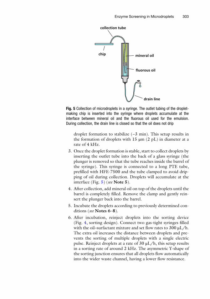
droplet formation to stabilize (~3 min). This setup results inthe formation of droplets with 15 μm (2 pL) in diameter at arate of 4 kHz.

3. Once the droplet formation is stable, start to collect droplets byinserting the outlet tube into the back of a glass syringe (theplunger is removed so that the tube reaches inside the barrel ofthe syringe). This syringe is connected to a long PTE tube,prefilled with HFE-7500 and the tube clamped to avoid drip-ping of oil during collection. Droplets will accumulate at theinterface (Fig. 5) (see Note 5).

4. After collection, add mineral oil on top of the droplets until thebarrel is completely filled. Remove the clamp and gently rein-sert the plunger back into the barrel.

5. Incubate the droplets according to previously determined con-ditions (see Notes 6–8).

6. After incubation, reinject droplets into the sorting device(Fig. 4, sorting design). Connect two gas-tight syringes filledwith the oil–surfactant mixture and set flow rates to 300 μL/h.The extra oil increases the distance between droplets and pre-vents the sorting of multiple droplets with a single electricpulse. Reinject droplets at a rate of 30 μL/h, this setup resultsin a sorting rate of around 2 kHz. The asymmetric Y-shape ofthe sorting junction ensures that all droplets flow automaticallyinto the wider waste channel, having a lower flow resistance.

collection tube

mineral oil

fluorous oil

drain line

chip

Fig. 5 Collection of microdroplets in a syringe. The outlet tubing of the droplet-making chip is inserted into the syringe where droplets accumulate at theinterface between mineral oil and the fluorous oil used for the emulsion.During collection, the drain line is closed so that the oil does not drip


7. Focus the laser beam about 180 μm upstream of the sortingjunction through a 40� microscope objective (refer to Fig. 6).

8. Connect the photomultiplier tube (PMT) to the pulse genera-tor. The differential voltage comparator inputs are the PMTsignal (Vsig) and a user-defined reference voltage (Vref) thatcorresponds to the threshold product concentration (see Note7). Wire the output of the comparator to the trigger input of thepulse generator. When Vsig exceeds Vref, a square pulse (0.5 ms)is triggered. Amplify the generated pulse 1000-fold to between0.6 and 0.8 kV (seeNote 9) with the high-voltage amplifier andapply to the electrodes of the sorting device (Fig. 7) (see Note10).

9. Use an Eppendorf tube to collect sorted droplets. Being lighterthan the fluorous oil carrier phase, the sorted droplets accumu-late at the air–oil interface of the collection vessel and can beconveniently harvested despite their small volume.

3.4 Recovery of DNA

and Transformation

1. Add 100 μL water into the collecting Eppendorf tube afterhaving rinsed the connecting tubing (from outlet to tube) withHFE-7500 oil (to make sure no droplets are left inside thetubing).

2. Gently add 200 μL of perfluorooctanol to the Eppendorf tubecontaining the microdroplets, making sure it rinses the tube’swalls.

3. Remove the aqueous phase and add ~100 ng of non-transformable DNA (typically ~1 nM final concentration) toprevent loss of selected plasmids during DNA recovery. Purifyand concentrate using a spin column. Elute into 7 μL milliQwater.

Fig. 6 Snapshot of the droplet sorting device. In the absence of electric pulsing, droplets flow to the bottom(waste) channel. Whenever a fluorescence read-out exceeds a freely set threshold, the electric pulse isactivated, dielectrophoretically attracting a single droplet (indicated by an arrow) to the sorting channel. Scalebar: 60 μm


4. Transform plasmid DNA into electro-competent E. coli cells.

5. Plate out transformed bacteria on petri dishes containing LB-agar and appropriate antibiotics. Incubate plates overnight at37 �C.

6. Samples from individual colonies are re-grown in deep 96-wellplates and their activity confirmed in cell lysates (see Notes 11and 12).

7. Colonies are re-grown and their DNA is extracted (using aplasmid DNA extraction kit) and sequenced.

4 Notes

1. The master mould of the microfluidic device is made out ofSU-8 2015 photoresist (MicroChem) using standard

Vref

Fig. 7 Microscopy and sorting setup. The microfluidic chip is illuminated by the microscope light source (BF)using a band-pass filter (F1, 593/25 nm) to prevent green illumination light from reaching the detector. Thelaser beam (488 nm) passes a dichroic mirror (DC1, 495 nm) and is focused through a 40� objective (OL),about 180 μm upstream of the sorting junction (inset and Fig. 6). The induced fluorescence is directed to asecond dichroic mirror (DC2, 555 nm), which allows the red light to be captured by a high-speed camera(CAM) for imaging of the chip. Lower wavelengths are directed to a band-pass filter (F2, 516–530 nm) beforereaching the photomultiplier tube (PMT) for detection. The PMT output voltage (Vsig) is connected to a voltagecomparator. If an operator-defined threshold (Vref) is exceeded, the comparator sets its output voltage (Vtrig) tohigh, thereby triggering the pulse generator (PG) and image acquisition by the high-speed camera (CAM). Thegenerated pulse is amplified (AMP) and applied to the electrodes, which are embedded in the microfluidic chipfinally causing the fluorescent droplet to be dielectrophoretically pulled into the collection channel


photolithographic techniques [21] with the flow-focusing anddroplet sorting designs (e.g., those deposited at http://openwetware.org/wiki/DropBase).

2. Alternatively, the surfactant 008-fluorosurfactant (Ran Bio-technologies) can be employed. Similar surfactants canbe synthesized following published protocols [12, 19]. Theoil–surfactant mixture has to be optimized for several aspects:stability of the droplets to prevent progressive coarsening of theemulsion, small molecule transfers between compartments oruptake of these small molecules by the oil and also proteinstability and activity in the presence of a two-phase system[22]. A given reaction time frame will depend on how longthe reaction products can be retained in the droplets. Additionof BSA [23] or small molecules (e.g., cyclodextrins) [24] to theaqueous phase, adjustment of pH, variation of the surfactantconcentrations and choice of the fluorous carrier oil are para-meters that can improve the retention of fluorophores by sev-eral orders of magnitude. Alternatively, chemical modificationof the substrate, e.g., by introduction of a polar functionalgroup, can increase product retention [25]. A simple methodenabling the quantification of fluorescent molecules in micro-droplets facilitates the analysis of the effects of oil–surfactantmixtures on enzyme activity as well as those of additives on theretention of fluorescent molecules within the compartment[22].

3. The implementation of the electronic trigger module using adifferential comparator is the simplest and cheapest option.Other methods use microprocessors to make comparisonsbetween measured optical signal and trigger threshold (e.g.,an open source Arduino board [26] or more sophisticated FieldProgrammable Gate Array logic [27]).

4. Alternatively, sodium chloride electrodes have recently beenused [28]: prepare two syringes with a solution of 5 M NaClin water, connect them to a metallic needle and fit a plastictubing onto the needles. Then, fill the channels with the NaClsolution.

5. Droplets collected immediately after their formation form apacked emulsion layer within the collection syringe. In orderto avoid possible coalescence during passage through a metallicneedle, flow rates have to be kept low during this transit (i.e.,around 100 μL/h). Coalescence within the tubing can alsooccur whenever the pressure is too high within the microfluidicchip: for instance, as a consequence of the inlet becomingclogged by dust or debris. Monitoring whether the chipremains in a pristine state over time helps to address problemsquickly by immediate intervention for troubleshooting. The


http://openwetware.org/wiki/DropBase

http://openwetware.org/wiki/DropBase

fluidics operation is otherwise well optimized and should, iffiltered solutions are used, consistently run for several hours.Alternative setups for storing droplets include glass vials [27]or long tubing [26].

6. The sensitivity of the optical setup has to be determined foreach analyte to assess the minimum number of enzymatic turn-overs needed to detect a signal. Typically, a few thousandmolecules can be readily detected using laser sources and sensi-tive detectors. Current FACS instruments can detect 4000fluorescein molecules. The minimal incubation time for thedroplets can then be inferred assuming catalytic rates andexpression levels are known.

7. For directed evolution, the fluorescence signal brought aboutby the parental or wild-type enzyme has to be determined inorder to set up a selection threshold for screening of the library.

8. Background reaction resulting from other enzymes containedin E. coli and buffer-catalyzed hydrolysis have to be evaluated tomake sure fluorescent signals arise from the protein of interest.This threshold can be empirically measured by measuring themean fluorescence of cells bearing a plasmid expressing anunrelated protein without relevant activity.

9. To drive the selected droplets into the collection channel, therequired pulse settings may be varied (e.g., length or ampli-tude), depending on droplet frequency, flow rates, and dropletsize: the bigger the droplets and higher flow rates, the strongerthe pulses required. However, the higher flow rates also requireshorter pulses (at least below the period between two droplets)to ensure that only single droplets are selected. Typical settingsfor the procedures described in this chapter are a single pulse at600 V of 500 μs width. The settings are adjusted before eachsorting experiment to achieve optimal performance, which isverified by monitoring the sorting process by visual inspectionof a movie taken by the high-speed camera.

10. When using salt electrodes, connect the output of the amplifierto the metallic needles of the syringes loaded with the saltsolution.

11. Encapsulation of multiple cells and phenotypic variation willinfluence the apparent product formation rates, so that the tailof a fluorescence histogram will include false positives.Depending on the width of the selection window (and thesensitivity of the threshold set by the operator) between lessthan 1% and 90% false positives have been typically observed.

12. If hits are rare, we recommend accepting even a majority offalse positives (e.g., as a consequence of high background thatmakes distinguishing positives difficult). True positives can be


verified in a subsequent microtiter plate screen, provided it isavailable, or by repeated droplet selections. We also recom-mend oversampling the library screened by a factor of 10 sothat all hits can be recovered.

References

1. Colin PY, Zinchenko A, Hollfelder F (2015)Enzyme engineering in biomimetic compart-ments. Curr Opin Struct Biol 33:42–51

2. Leemhuis H, Stein V, Griffiths AD et al (2005)New genotype-phenotype linkages for directedevolution of functional proteins. Curr OpinStruct Biol 15:472–478

3. Yang G, Withers SG (2009) Ultrahigh-throughput FACS-based screening for directedenzyme evolution. ChemBioChem10:2704–2715

4. Schaerli Y, Wootton RC, Robinson T et al(2009) Continuous-flow polymerase chainreaction of single-copy DNA in microfluidicmicrodroplets. Anal Chem 81:302–306

5. van Vliet LD, Colin PY, Hollfelder F (2015)Bioinspired genotype-phenotype linkages:mimicking cellular compartmentalization forthe engineering of functional proteins. Inter-face Focus 5:20150035

6. Agresti JJ, Antipov E, Abate AR et al (2010)Ultrahigh-throughput screening in drop-basedmicrofluidics for directed evolution. Proc NatlAcad Sci U S A 107:4004–4009

7. Theberge AB, Courtois F, Schaerli Y et al(2010) Microdroplets in microfluidics: an evol-ving platform for discoveries in chemistry andbiology. Angew Chem Int Ed 49:5846–5868

8. Huebner A, Sharma S, Srisa-Art M et al (2008)Microdroplets: a sea of applications? Lab Chip8:1244–1254

9. Mair P, Gielen F, Hollfelder F (2017) Explor-ing sequence space in search of functionalenzymes using microfluidic droplets. CurrOpin Chem Biol 37:137–144. doi:10.1016/j.cbpa.2017.02.018

10. Kintses B, Hein C, Mohamed MF et al (2012)Picoliter cell lysate assays in microfluidic drop-let compartments for directed enzyme evolu-tion. Chem Biol 19:1001–1009

11. Fischlechner M, Schaerli Y, Mohamed MF et al(2014) Evolution of enzyme catalysts caged inbiomimetic gel-shell beads. Nat Chem6:791–796

12. Zinchenko A, Devenish SRA, Kintses B et al(2014) One in a million: flow cytometric sort-ing of single cell-lysate assays in monodisperse

picolitre double emulsion droplets for directedevolution. Anal Chem 86:2526–2533

13. Courtois F, Olguin LF, Whyte G et al (2008)An integrated device for monitoring time-dependent in vitro expression from singlegenes in picolitre droplets. ChemBioChem9:439–446

14. Houlihan G, Gatti-Lafranconi P, KaltenbachMet al (2014) An experimental framework forimproved selection of binding proteins usingSNAP display. J Immunol Methods 405:47–56

15. Diamante L, Gatti-Lafranconi P, Schaerli Y et al(2013) In vitro affinity screening of protein andpeptide binders by megavalent bead surfacedisplay. Protein Eng Des Sel 26:713–724

16. Mankowska SA, Gatti-Lafranconi P, ChodorgeM et al (2016) A shorter route to antibodybinders via quantitative in vitro bead-displayscreening and consensus analysis. Sci Rep6:36391

17. Kintses B, van Vliet LD, Devenish SRA et al(2010) Microfluidic droplets: new integratedworkflows for biological experiments. CurrOpinChem Biol 14:548–555

18. Colin PY, Kintses B, Gielen F et al (2015)Ultrahigh-throughput discovery of promiscu-ous enzymes by picodroplet functional meta-genomics. Nat Commun 6:10008

19. Kotz K, Cheng X, Toner M (2007) PDMSdevice fabrication and surface modification. JVis Exp 8:319

20. Eddings MA, Johnson MA, Gale BK (2008)Determining the optimal PDMS-PDMS bond-ing technique for microfluidic devices. J Micro-mech Microeng 18:067001

21. McDonald JC, Duffy DC, Anderson JR et al(2000) Fabrication of microfluidic systems inpoly(dimethylsiloxane). Electrophoresis21:27–40

22. Kaltenbach M, Devenish SR, Hollfelder F(2012) A simple method to evaluate the bio-chemical compatibility of oil/surfactant mix-tures for experiments in microdroplets. LabChip 12:4185–4192

23. Courtois F, Olguin LF, Whyte G et al (2009)Controlling the retention of small molecules inemulsion microdroplets for use in cell-basedassays. Anal Chem 81:3008–3016


https://doi.org/10.1016/j.cbpa.2017.02.018

https://doi.org/10.1016/j.cbpa.2017.02.018

24. Zinchenko A, Devenish SR, Hollfelder F(2017) Rapid quantitative assessment of leak-age of assay components from microdroplet totest the suitability of oil/surfactant combina-tions. Submitted

25. Woronoff G, El Harrak A, Mayot E et al (2011)New generation of amino coumarin methylsulfonate-based fluorogenic substrates for ami-dase assays in droplet-based microfluidic appli-cations. Anal Chem 83:2852–2857

26. Gielen F, Hours R, Emond S et al (2016)Ultrahigh-throughput-directed enzyme

evolution by absorbance-activated dropletsorting (AADS). Proc Natl Acad Sci U S A113:E7383–E7389

27. Beneyton T, Coldren F, Baret JC et al (2014)CotA laccase: high-throughput manipulationand analysis of recombinant enzyme librariesexpressed in E. coli using droplet-based micro-fluidics. Analyst 139:3314–3323

28. Sciambi A, Abate AR (2015) Accurate micro-fluidic sorting of droplets at 30 kHz. Lab Chip15:47–51


Chapter 19

Isolation of pH-Sensitive Antibody Fragmentsby Fluorescence-Activated Cell Sorting and YeastSurface Display

Christian Schroter, Simon Krah, Jan Beck, Doreen Konning,Julius Grzeschik, Bernhard Valldorf, Stefan Zielonka,and Harald Kolmar

Abstract

Fluorescence-activated cell sorting (FACS) in combination with yeast surface display (YSD) has proven tobe a valuable tool for the engineering of antibodies. It enables the fast and robust identification andisolation of candidates with prescribed characteristics from combinatorial libraries. A novel application forFACS and YSD that has recently evolved addresses the engineering of antibodies toward pH-switchableantigen binding, aiming at reduced binding at acidic pH, compared to neutral pH. Therefore, we giveguidance for the incorporation of such pH switches into antibody variable domains using combinatorialhistidine scanning libraries. The protocol describes a flow cytometric sorting technique for the enrichmentof antigen-specific molecules. Moreover, we provide information on how to screen the obtained antibodypools from initial sorting to isolate and characterize pH-sensitive variants.

Key words Fluorescence-activated cell sorting (FACS), Yeast surface display, Fab display, Antibodyengineering, Protein engineering, pH-dependent antigen binding, pH-switch engineering

1 Introduction

Monoclonal antibodies have emerged as one of the most promisingand hence rapidly growing class of therapeutics for various indica-tions, such as inflammatory diseases and cancer [1, 2]. The genera-tion of antibodies comprising desired properties is yet challengingand often requires antibody engineering toward affinity, specificity,or enhanced biophysical stability [3].

In order to improve the performance of therapeutic antibodies,engineering approaches have emerged to incorporate pH sensitivityinto the antigen-binding site of antibodies exhibiting reduced


Christian Schroter, Simon Krah and Jan Beck contributed equally to this work.

311

antigen binding at acidic pH (pH 6.0), compared to physiologicalpH (pH 7.4). Upon internalization, antibody–antigen complexescan enter the endosomal pathway, where pH-dependent antigenbinding allows dissociation of the complex in the acidified endo-some (pH ~6.0). As a consequence, released antigen can enter thedegradative pathway whereas the free antibody is recycled to the cellsurface via its interaction with the neonatal Fc-receptor (FcRn) [4].The reuse of antibodies can result in enhanced antigen clearancethat may enable less frequent or lower antibody dosing [5].Decrease in affinity over a modest pH drop from pH 7.4 to pH6.0 can be achieved through insertion of histidine residues into thecomplementary determining regions of the variable domains of anantibody. It has been shown that the number of histidine residues,the synergistic interplay of multiple histidine residues as well as themagnitude of pKa changes upon antibody binding affect pH sensi-tivity [6].

Fluorescence-activated cell sorting (FACS) in combinationwith yeast surface display (YSD) (Fig. 1) has become one of themost valuable tools for the engineering of antibodies affording thebenefit of rapid isolation of hit candidates with predefined charac-teristics from combinatorial libraries [7–9]. One of the main advan-tageous features of YSD lies in the fact that the eukaryoticexpression machinery of yeast ensures proper protein folding ofhuman antibody-derived fragments. In combination with FACS, asensitive and quantitative analysis of each library variant can beperformed by real-time and online data analysis [10]. Furthermore,libraries exceeding a diversity of 109 transformants can easily becreated by homologous recombinations and antibody heavy andlight chain repertoires can be combined by yeast mating technology[11, 12]. These features have been acknowledged by several suc-cessful protein engineering approaches, wherein protein variantswith pH-dependent antigen binding were isolated from combina-torial libraries using FACS and YSD [13, 14]. In this regard, werecently published a novel approach that comprehensively consid-ered the combinatorial effects of multiple histidine substitutions[14]. Synthesis of the variable regions of a parental antibody Fabfragment allowed incorporation of histidines within all three com-plementarity determining regions (CDRs) of the variable regions ofheavy and light chain (VH and VL) with average mutation rates of2–3 histidine per variant. Moreover, a novel screening strategyenabled the efficient screening of the antibody Fab histidine scan-ning libraries and isolation of antibody variants that revealed sharp,reversible pH-dependent binding profiles. A general outline of theprocedure for isolating pH-dependent antibodies is given in Fig. 2.

312 Christian Schroter et al.

2 Materials

2.1 Strains,

Plasmids, and

Libraries

1. S. cerevisiae strain EBY100 (MATa) (Invitrogen)

(URA3-52 trp1 leu2Δ1 his3Δ200 pep4::HIS3 prb1Δ1.6Rcan1 GAL) (pIU211:URA3).

2. S. cerevisiae strain BJ5464 (MATα) (American Type CultureCollection, ATCC)

(URA3-52 trp1 leu2Δ1his3Δ200 pep4::HIS3 prb1Δ1.6Rcan1 GAL).

3. E. coli strain Top10 (Invitrogen)

(F- mcrA Δ(mrr-hsdRMS-mcrBC) Φ80lacZΔM15 ΔlacX74recA1 araD139 Δ(ara leu) 7697 galU galK rpsL (StrR)endA1 nupG).

4. Plasmids: Two derivatives of pYD1 vectors (Invitrogen) areused for cell surface display of heterodimeric antibody Fab

Fig. 1 Schematic illustration of the yeast surface display system as described byBoder and Wittrup for antibody Fab fragment expression [15]. The heavy chain ofthe Fab fragment is fused to the a-agglutinin yeast adhesion receptor proteinAga2p, which assembles with the coexpressed Aga1p forming two disulfidebonds. Aga1p in turn is covalently linked to β-glucan of the extracellular yeastcell matrix and thereby anchors the protein assembly to the yeast cell wall. Twosingle copy E. coli yeast shuttle plasmids encode for heavy and light chains,which include TRP or LEU auxotrophic markers for selection in yeast andampicillin or kanamycin markers for E. coli selection, respectively. The heavychain fusion protein includes a His6-tag for detection of Fab expression. Thesystem requires the chromosomally encoded AGA1 in yeast (e.g., EBY100).Expression of AGA1 as well as shuttle plasmid encoded proteins are undercontrol of the inducible galactose 1 promotors

FACS-based Antibody pH-switch Engineering 313

fragments encoding for the heavy chain fusion protein (Xpress-tag-(G4S)-VH-CH1-(G4S)-His6-(G4S)3-Aga2p) and the lightchain protein. In case of the light chain vector, the aMFpp8leader sequence is followed by VL-Cλ or VK-Cκ which resultsin soluble expression of the light chain [16]. In addition, bothplasmids encode different auxotrophic markers allowing yeastgrowth in tryptophan or leucine deficient media and ampicillinor kanamycin resistance genes for selection in E. coli.

5. A detailed protocol for the generation of yeast libraries is notgiven at this point, but has been described in detail elsewhere[11]. However, we provide a brief outline of the histidinemutagenesis procedure in this section: Combinatorial histidinesubstitution libraries can be commercially obtained (GeneArt,Life Technologies or EllaBiotech). Gene synthesis of the vari-able regions of the parental Fab fragment allows combinatorial

Fig. 2 General workflow for the generation of pH-sensitive antibody fragments by YSD and FACS. Gap repaircloning is applied to generate separate heavy chain and light chain combinatorial histidine-scanning librariesvia homologous recombination that are derived from a parental antibody. Subsequently, heavy and light chaindiversities can be combined with corresponding parental chains or shuffled in order to introduce additionaldiversity by mating. Resulting libraries are initially screened by FACS to isolate functional antigen-specificvariants, followed by 3–5 consecutive rounds of FACS for identification and isolation of pH-sensitivecandidates. After successful enrichment of pH-sensitive variants, isolated single clones are sequenced,allowing for the identification of antibody domains that are further characterized by flow cytometry


histidine substitutions within all three CDRs of the VH and VLregions (CDR H1-H3 and CDR L1-L3) (see Note 1). Theoccurrence of a histidine codon at defined positions is adjustedto 10%. Theoretical diversities are calculated as previouslydescribed [17]. VH and VL gene libraries are amplified withspecific oligonucleotides using PCR and cloned into yeastshuttle vectors by gap repair cloning following the protocolof Benatuil and colleagues to generate two separate libraries inEBY100 and BJ5464 cells, respectively [11]. Considering thediversities that can be covered by magnetic activated cell sort-ing (MACS; see Note 2) and FACS in combination with YSD,heavy and light chain repertoires are either combined or pairedwith corresponding parental chains using yeast mating technol-ogy [12]. After mating, cells are cultivated in Trp and Leudeficient media. These libraries represent the starting materialfor flow cytometric sorting (Fig. 2).

2.2 Media and

Reagents

1. SD �Trp/�Leu medium: Dissolve 26.7 g minimal SD-Base(Clontech) in deionized H2O and adjust volume to 900 mL.Sterilize by autoclaving. Dissolve 8.56 g NaH2PO4 · H2O,5.4 g Na2HPO4 and 0.64 g Dropout-mix �Trp/�Leu (Clon-tech) in deionized H2O and adjust the volume to 100 mL.Sterilize by autoclaving. Combine both solutions, add 10 mLof Penicillin–Streptomycin (Gibco, 10,000 U/mL) andremove any particles by filter sterilization using a 0.22 μmbottle top filter.

2. SD �Trp/�Leu plates: Dissolve 26.7 g of minimal SD-Agar(Clontech) in deionized H2O and adjust volume to 900 mL.Sterilize by autoclaving. Dissolve 8.56 g of NaH2PO4 · H2O,5.4 g of Na2HPO4 and 0.64 g Dropout-mix �Trp/�Leu(Clontech) in deionized H2O and adjust the volume to100 mL. Sterilize by autoclaving. Combine both solutionsand prepare plates.

3. SG �Trp/�Leu medium: Dissolve 37 g of minimal SD-Base + Gal/Raf (Clontech) in deionized H2O and adjust vol-ume to 500 mL. Dissolve 8.56 g of NaH2PO4 · H2O, 5.4 g ofNa2HPO4 and 0.64 g Dropout-mix �Trp/�Leu (Clontech)in deionized H2O and adjust the volume to 100 mL. Dissolve110 g of PEG8000 in deionized H2O and adjust the volume to400 mL. Sterilize by autoclaving and combine all three solu-tions. Add 10 mL of Penicillin-Streptomycin (Gibco,10,000 U/mL) and remove any particles by filter sterilizationusing a 0.22 μm bottle top filter (Merck Millipore).

4. SD Low �Trp/�Leu medium: Dissolve 5 g dextrose, 6.7 gyeast nitrogen base in deionized H2O and adjust volume to900 mL. Sterilize by autoclaving. Dissolve 8.56 gNaH2PO4 · H2O, 5.4 g Na2HPO4, and 0.64 g Dropout-mix


�Trp/�Leu (Clontech) in deionized H2O and adjust thevolume to 100 mL. Sterilize by autoclaving. Combine bothsolutions, add 10 mL of Penicillin-Streptomycin (Gibco,10,000 U/mL) and remove any particles by filter sterilizationusing a 0.22 μm bottle top filter (Merck Millipore).

5. LB Amp medium: Dissolve 10 g NaCl, 10 g tryptone, and 5 gyeast extract in 1 L deionized H2O. Sterilize by autoclaving.Once the medium has chilled (to approximately 50 �C), add1 mL of sterile filtered ampicillin solution (100 mg/mL indeionized H2O).

6. LB Amp plates: Dissolve 10 g NaCl, 10 g tryptone, 5 g yeastextract, and 15 g agar to a volume of 1 L in deionized water.Sterilize by autoclaving. When medium is chilled off (toapproximately 50 �C), add 1 mL of sterile filtrated ampicillinsolution (100 mg/mL in deionized H2O) and prepare plates.

7. LB Kana medium: Dissolve 10 g NaCl, 10 g tryptone, and 5 gyeast extract in 1 L deionized water. Sterilize by autoclaving.Once the medium has cooled down (to approximately 50 �C),add 1 mL of sterile filtered kanamycin sulfate solution (30 mg/mL in deionized H2O).

8. LB Kana plates: Dissolve 10 g NaCl, 10 g tryptone, 5 g yeastextract, and 15 g agar in 1 L deionized water. Sterilize byautoclaving. Once the medium has cooled down (to approxi-mately 50 �C), add 1 mL of sterile filtered kanamycin sulfatesolution (30 mg/mL in deionized H2O) and prepare plates.

9. Yeast library freezing solution: Dissolve 2 g of glycerol and0.67 g of yeast nitrogen base in a volume of 100 mLDulbecco’sPhosphate-Buffered Saline (DPBS). Sterile-filter the solution.

2.3 Selection

Reagents for FACS

1. Alexa Fluor 647 labeled mouse anti-His IgG antibody,0.2 mg/mL (Qiagen).

2. 1 mg/mL Streptavidin, R-phycoerythrin conjugate(Invitrogen).

3. Target proteins devoid of a His-tag (His-tag is present in theYSD heavy chain fusion protein).

4. EZ-Link Sulfo-NHS-Biotin (Thermo Scientific).

5. Pierce™ Biotin Quantitation Kit (Life technologies).

6. Dulbecco’s Phosphate-Buffered Saline (DPBS) (Gibco).

7. PBS-1: adjust DPBS to pH 7.4 with 1 M NaOH.

8. PBS-2: adjust DPBS to pH 6.0 with 1 M HCl.

2.4 Equipment 1. Cryogenic vials.

2. Freezing container.

3. 0.22 μM Steriflip and Steritop filtration units.


4. Yeast plasmid preparation kit.

5. E. coli plasmid miniprep kit.

6. Shaking incubator (20 and 30 �C).

7. Flow cytometry device.

3 Methods

In the following sections, all centrifugation steps to pellet yeast cellsare performed at 3000 � g for 3 min. Ensure that fluorophores areshielded from light and perform incubation steps on ice.

3.1 Target Protein

Preparation

For labeling of antigen, a plethora of different tags and fluoro-phores are commercially available (see Note 3). Nevertheless, werecommend the application of the EZ-Link™Sulfo-NHS-Biotin(Thermo Scientific) according to the manufacturer’s protocol.Herein, biotin is linked to N-terminally accessible primary amines(NH2) or to surface exposed lysine residues. Since antigen labelingwith biotin may affect antigen functionality, consider assessing thequality of conjugated antigen by yeast surface display (Subheading3.4.1) (see Notes 4 and 5). Furthermore, biotinylated antigensrequire secondary labeling using fluorophore-conjugated streptavi-din that allows signal amplification.

3.2 Yeast Library

Preparation for the

Expression and

Display of Antibody

Fragments

1. Thaw an aliquot of the frozen library at room temperature andresuspend cells in SD �Trp/�Leu medium, yielding a finalOD600 of 0.1–0.5. An absorbance value of 1 at 600 nm corre-sponds to approximately 1 � 107 cells/mL. The total numberof cells in the starting culture should exceed the calculatedlibrary diversity at least ten times.

2. Expand the culture overnight at 30 �C and 225 rpm untilstationary phase is reached (OD600 of approximately 4–6). Atthis point, storage of cells is possible for up to 4 weeks at 4 �C.

3. Harvest at least the number of cells corresponding to a tenfoldexcess of the library diversity by centrifugation and resuspendcells in SG �Trp/�Leu medium to an initiate OD600 of 1.Cultivate cells for 24–48 h at 20 �C and 225 rpm for expressionof antibody fragments.

3.3 Yeast Library

Cryoconservation for

Long-Term Storage

1. Harvest cells from a freshly grown SD�Trp/�Leu culture andpellet the cells by centrifugation.

2. Inoculate SD Low �Trp/�Leu medium to an initiate OD600

of 0.5–1 and cultivate the cells for 48–72 h at 30 �C and225 rpm. Library diversity should be oversampled at least tentimes.

3. Harvest cells by centrifugation and remove the supernatant


4. Resuspend the cells in yeast library freezing solution with finalcell concentrations of approximately 1 � 1010 cells/mL andtransfer suspensions into cryogenic vials, followed by incuba-tion at room temperature for 5–10 min.

5. Freeze vials at �70 �C.

3.4 Labeling of

Library Yeast Cells for

Flow Cytometric

Analysis

All samples should be handled in parallel reactions. Cell washing isperformed by centrifugation of cell suspension, followed by aspira-tion of the supernatant and resuspension of the cell pellet in 0.5 mLPBS-1 per 1 � 107 cells. A second centrifugation step yields thewashed cell pellet.

3.4.1 Assessment of

Saturating Antigen

Concentrations

For determination of appropriate antigen concentrations and toevaluate the quality of biotinylated antigen, binding signals onyeast cells are analyzed by FACS using streptavidin,R-phycoerythrin conjugate (SA-PE) (see Note 6).

1. For this, yeast cells (displaying antigen-specific antibody frag-ments as control and/or library cells) are induced for antibodyexpression. Next, split 5 � 107 cells into 1.5 mL tubes with1 � 107 cells per tube.

2. Wash cells and resuspend the pellets in 20 μL PBS-1 containingdifferent antigen concentrations of biotinylated antigen (typi-cal serial dilutions range from 62.5 nM to 1 μM) in PBS-1(20 μL/1 � 107 cells) and incubate the cells on ice for 30 min(see Note 7).

3. Afterward, wash the cells, followed by secondary labeling(20 μL/1 � 107 cells) with SA-PE (diluted 1:20 in PBS-1)and subsequent FACS analysis.

4. In FACS histograms, antigen binding signals can be quantifiedand the sample that exhibits a relative fluorescence intensityconverging with the measured value obtained from cells stainedwith a higher antigen concentration can be considered assaturated. If the above outlined concentrations do not yieldsaturating antigen binding signals, use higher antigenconcentrations.

3.4.2 Isolation of

Displayed Antibody

Fragments that Exhibit

Antigen Binding

The initial round of flow cytometry sorting allows for the isolationof binders that successfully display the antibody fragments andsimultaneously bind the antigen of interest. Therefore, cells areincubated with biotinylated antigen (Subheading 3.1), followedby labeling with SA-PE as wells as Alexa Fluor 647 conjugatedanti-Penta-His antibody for detection surface expressed antibodyFab fragments.


Overview of samples to be prepared:

Sort Sample (steps 1–3): Primary labeling with biotinylated anti-gen, secondary labeling with SA-PE and Alexa Fluor 647 con-jugated anti-Penta-His antibody.

Target Binding Control (steps 4–6): Primary labeling with bioti-nylated antigen, secondary labeling with SA-PE.

Fab Display Control (steps 7 and 8): Alexa Fluor 647 conjugatedanti-Penta-His antibody and SA-PE.

The following protocol is given for handling 107 cells and canbe up-scaled according to the cell number used (see Note 8). Thenumber of cells for sorting should exceed the theoretical diversityby at least ten times. By increasing the numbers of cells, volumesand amounts of labeling reagents should be increasedproportionally.

1. For preparing the Sort Sample, harvest the induced yeast cellsby centrifugation (1 � 107 cells) and remove the supernatantby aspiration. Wash the cells and resuspend the cell pellet in20 μL PBS-1 containing a saturating antigen concentration (seeSubheading 3.4.1) and incubate the cells on ice for 30 min.

2. Wash and resuspend the cells in 20 μL PBS-1 containing AlexaFluor 647 conjugated anti-Penta-His antibody (diluted 1:20)and SA-PE (diluted 1:20), followed by incubation on ice for30 min.

3. Wash the cells and resuspend the cell pellet in 0.5 mL PBS-1and keep on ice shielded from light until sorting.

4. For preparing the Target Binding Control, pellet cell suspen-sion (1 � 107 cells) by centrifugation and remove the superna-tant by aspiration. Wash the cells and resuspend the cell pelletin 20 μL PBS-1 containing a saturating antigen concentration(see Subheading 3.4.1) and incubate the cells on ice for 30 min.

5. Wash the cells and perform secondary labeling by resuspensionof the cell pellet in 20 μL PBS-1 containing SA-PE (diluted1:20), followed by incubation on ice for 30 min.

6. Wash the cells and resuspend the cell pellet in 0.5 mL PBS-1and keep on ice shielded from light until FACS analysis.

7. For preparing the Fab Display Control, pellet cell suspension(1 � 107 cells) by centrifugation and remove the supernatantby aspiration. Wash the cells and resuspend the cell pellet in20 μL PBS-1 and incubate cells on ice for 30 min.

8. Wash and resuspend the cells in 20 μL PBS-1 containing AlexaFluor 647 conjugated anti-Penta-His antibody (diluted 1:20)and SA-PE (diluted 1:20), followed by incubation on ice for30 min.



3.4.3 Labeling Strategy

for the Isolation of pH-

Sensitive Antibody

Fragments

A labeling strategy for the enrichment of pH-sensitive variants isdescribed in this section. Cells are initially incubated with unlabeledantigen at pH 7.4 (PBS-1), which allows saturation of antigen-specific antibody variants (Subheading 3.4.1). Afterward, cells arewashed and incubated at pH 6.0 (PBS-2), enabling pH-sensitivevariants to release unlabeled antigen. As a control, cells are incu-bated at pH 7.4 (PBS-1) instead of pH 6.0 (PBS-2) to estimate thefraction of pH-sensitive variants. Subsequently, cells are washed andincubated with labeled antigen at pH 7.4 (PBS-1). The rebindingof labeled antigen allows for discrimination of pH-sensitive variantsand variants that are still occupied by unlabeled antigen. An exem-plary FACS analysis is shown in Fig. 3.


Sort Sample pH 6.0 (steps 1–5): Primary labeling with biotinylatedantigen, secondary labeling with SA-PE and Alexa Fluor 647conjugated anti-Penta-His antibody. Includes incubation stepat pH 6.0.

Fig. 3 Initial library screenings for isolation of antigen specific variants at pH 7.4 using FACS. (a) Sort Sample:Yeast cells expressing library variants are labeled with biotinylated antigen in PBS-1, followed by labeling withSA-PE and Alexa Fluor 647 conjugated anti-Penta-His antibody in PBS-1. (b) Fab Display Control: Cells arelabeled in PBS-1 with Alexa Fluor 647 conjugated anti-Penta-His antibody and SA-PE. (c) Target BindingControl: Cells are labeled in PBS-1 with biotinylated antigen, followed by labeling with SA-PE


Sample Control pH 7.4 (steps 6–10): Primary labeling with bioti-nylated antigen, secondary labeling with SA-PE and AlexaFluor 647 conjugated anti-Penta-His antibody. Includes incu-bation step at pH 7.4 instead of pH 6.0.

FAB Display Control at pH 6.0 (steps 11–15): Alexa Fluor 647conjugated anti-Penta-His antibody and SA-PE. Incubationstep at pH 6.0.

Target Binding Control at pH 6.0 (steps 16–20): Primary labelingwith biotinylated antigen, secondary labeling with SA-PE.Incubation step at pH 6.0.

The following protocol is given for handling 107 cells and canbe upscaled according to the cell number used (see Note 8). Thenumber of cells for sorting should exceed the theoretical diversityby at least ten times. By increasing the numbers of cells, volumesand amounts of labeling reagents should be increasedproportionally.

1. For preparing the Sort Sample pH 6.0, harvest the induced yeastcells by centrifugation (1 � 107 cells) and remove supernatantby aspiration. Wash cells and resuspend the cell pellet in 20 μLPBS-1 containing a saturating concentration of unlabeled anti-gen and incubate cells on ice for 30 min.

2. Wash the cells and resuspend the pellet in PBS-2 (0.5 mL/1� 107 cells) and incubate the cells on ice for 30 min (seeNote9).

3. Centrifuge the cells, and resuspend the pellet in 20 μL PBS-1containing a saturating concentration of biotinylated antigen(see Subheading 3.4.1) and incubate the cells on ice for 30 min.

4. Afterward, wash the cells and resuspend the pellet in 20 μLPBS-1 containing Alexa Fluor 647 conjugated anti-Penta-Hisantibody (diluted 1:20) and SA-PE (diluted 1:20), followed byincubation on ice for 30 min.

5. Wash the cells and resuspend the cell pellet in 0.5 mL PBS-1and keep on ice shielded from light until sorting.

6. For preparing the Sample Control pH 7.4, harvest the inducedyeast cells by centrifugation (1 � 107 cells) and remove super-natant by aspiration. Wash the cells and resuspend the cell pelletin 20 μL PBS-1 containing a saturating concentration of unla-beled antigen and incubate cells on ice for 30 min.

7. Wash the cells and resuspend the pellet in PBS-1 (0.5 mL/1 � 107 cells) and incubate the cells on ice for 30 min.





11. For preparing the FAB Display Control at pH 6.0, harvest theinduced yeast cells by centrifugation (1 � 107 cells) andremove supernatant by aspiration. Wash the cells and resuspendthe cell pellet in 20 μL PBS-1 containing a saturating concen-tration of unlabeled antigen and incubate cells on ice for30 min.

12. Wash the cells and resuspend the pellet in PBS-2 (0.5 mL/1 � 107 cells) and incubate cells on ice for 30 min.

13. Centrifuge the cells, and resuspend the pellet in 20 μL PBS-1and incubate cells on ice for 30 min.



16. For preparing the Target Binding Control at pH 6.0, harvestthe induced yeast cells by centrifugation (1 � 107 cells) andremove supernatant by aspiration. Wash cells and resuspend thecell pellet in 20 μL PBS-1 containing a saturating concentra-tion of unlabeled antigen and incubate cells on ice for 30 min.



19. Afterward, wash the cells and resuspend the pellet in 20 μLPBS-1 containing SA-PE (diluted 1:20), followed by incuba-tion on ice for 30 min.


3.5 Fluorescence-

Activated Cell Sorting

Once the labeling procedure is completed, cells can directly be usedfor sorting. It is important to note that fluorophores with over-lapping emission spectra (e.g., phycoerythrin (PE) and fluorescein(FITC)), require proper compensation of the flow cytometer foradequate data interpretation. Furthermore, aggregated yeast cellsand debris can be removed by initial gating on forward and side


scatter channels. For sorting using a MoFlo cell sorter device,parameters can be set as follows: Side scatter—LOG mode: 650;Forward scatter—LIN mode: 570; FL8—LOG mode (Alexa-Fluor647): 600; FL2—LOG mode (PE): 400; Trigger parameter:side scatter. The sample flow rate is adjusted to an event rate ofapproximately 10,000–15,000 s�1. The first round of sortingshould be done on an enrich mode whereas subsequent roundscan be performed using the purify mode. If other cell sorters areused, settings have to be adjusted.

3.5.1 Sorting of Antigen-

Specific Fab Clones

In order to discard variants that do not bind the antigen, cells areincubated with labeled antigen at pH 7.4 (labeling procedure seeSubheading 3.3, step 2), followed by identification and isolation ofantigen-specific variants by FACS.

1. Prepare a yeast library (see Subheading 3.2) and label the cellsincluding controls according to Subheading 3.4.2.

2. Define a suitable sorting gate that includes the upper rightquadrant to isolate all cells that are positive for Fab fragmentexpression and antigen binding (Fig. 3a). In this step it isimportant to include great fractions of double positive cells toguarantee full sampling of functional diversity prior to sortingfor pH-dependent antigen binding. Gating is performedaccording to the Fab Display Control and Target Binding Con-trol samples (Fig. 3b, c). The number of cells analyzed duringthe sort should exceed at least ten times the theoretical librarydiversity.

3. Transfer sorted yeast cells to about 10 mL SD -Trp/-Leumedium and expand culture at 30 �C and 225 rpm for24–72 h. For further sorting, inoculate harvested cells in SG -Trp/-Leu medium followed by 24–48 h of cultivation at 20 �Cand 225 rpm (see Subheading 3.2). Alternatively, inoculate cellsin SD Low -Trp/-Leu medium and apply the procedure forcryoconservation of yeast cells. Consider tenfold oversamplingof sorted cells for storage (see Subheading 3.3).

3.5.2 Sorting Strategy for

the Isolation of pH-

Sensitive Fab Clones

This subsection describes the isolation of pH-sensitive variants withhigh-affinity antigen binding at pH 7.4 and reduced binding at pH6.0.

1. Label the cell population that have been enriched for targetprotein binders by consecutive rounds of labeling and FACS asdescribed in Subheadings 3.4.2 and 3.5.1. Consider at leasttenfold oversampling of previously sorted cell numbers.

2. Draw an appropriate sorting gate around the double positivecells in the upper right quadrant of the Sort Sample pH 6.0(Fig. 4a). The negative gating borders should be alignedaccording to the FAB Display Control pH 6.0 (Fig. 4c) and


the Target Binding Control pH 6.0 (Fig. 4d). In addition, theSample Control pH 7.4 (Fig. 4b) is used to precisely quantifycell fractions that refer to variants with pH-sensitive binding(compare Fig. 4a, b). Usually, a less stringent sorting gate canbe applied that includes 0.1–5% of cells, thereby reducing theprobability of loosing unique clones. The amount of cells thatis labeled for sorting should exceed the number of isolated cellsfrom the previous sorting round by a factor of 10 (at least).

3. Regrow selected yeast cells in 10 mL SD -Trp/-Leu medium at30 �C and 225 rpm for 24–72 h.

4. For further sorting, harvest yeast cells by centrifugation andremove supernatant by aspiration. Herein, cell numbers shouldexceed the numbers of selected cells from previous sortinground at least tenfold.

Fig. 4 Dot plots illustrating the selection of pH-sensitive Fab fragments. (a) Sort Sample pH 6.0: Yeast cells areincubated with unlabeled antigen, transferred to PBS-2 (pH 6.0), followed by staining with biotinylated antigen,SA-PE and Alexa Fluor 647 conjugated anti-Penta-His antibody for simultaneous detection of antigen binding(X-axis) and surface display (Y-axis). (b) Sample Control pH 7.4: Yeast cells, which are incubated in PBS-1 (pH7.4) instead of PBS-2 (pH 6.0). (c) FAB Display Control at pH 6.0: Yeast cells, which are stained with AlexaFluor 647 conjugated anti-Penta-His antibody. (d) Target Binding Control at pH 6.0: Yeast cells, which arestained with biotinylated antigen and SA-PE


5. Resuspend the pellet in SG -Trp/-Leu medium, followed by24–48 h of cultivation at 20 �C and 225 rpm. Alternatively,inoculate cells in SD Low -Trp/-Leu medium and apply theprocedure for cryoconservation of yeast cells (see Subheading3.3). Consider tenfold oversampling of sorted cells for storage.

6. Repeat steps 1–5 until the enrichment of a population withpH-sensitive binding behavior is observable. This usuallyrequires 3–5 rounds of sorting (see Notes 10 and 11).

7. It is advisable to plate single clones onto selective SD platesduring each sort (usually up to 100 single clones) by flowsorting for subsequent characterization (see Subheading 3.4).Colonies are grown on plates by incubation at 30 �C for48–72 h and grown colonies can be stored for up to 6 weeksat 4 �C. Single clones can also be obtained by plating of serialdilutions from regrown sorted cells onto selective SD plates.

3.6 Characterization

of Enriched Clones

Apart from monitoring the phenotype of the yeast populationthroughout 3–4 rounds of sorting, it is advisable to verify desiredproperties for enriched library variants by single clone analysis (seeNote 12). Selection of enriched clones can be performed uponsequencing of the Fab coding sequence from single yeast coloniesto estimate the diversity of the sorted population. Subsequentcharacterization of selected single clones by flow cytometric analysisassess specificity as well as pH sensitivity of displayed antibodyfragments.

3.6.1 Sequencing of

Plasmids from Yeast Cells

1. After flow sorting, single colonies are characterized bysequence analysis. For this, 10–20 randomly picked clones areused to inoculate individually 4 mL of SD -Trp/-Leu medium,followed by 24–48 h cultivation at 30 �C and 225 rpm. Subse-quently, heavy and light chain encoding plasmids are isolatedfrom stationary cultures using the RPM plasmid isolation kit(MP Biomedicals) following the manufacturer’s protocol.

2. Electrocompetent E. coli Top10 cells (Invitrogen) are trans-formed with heavy and light chain plasmids carrying the ampi-cillin and kanamycin resistance markers, respectively.

3. Cells are separated by plating on selective agar platescorresponding to the heavy or light chain resistance genes.

4. Furthermore, plasmid DNA is extracted from E. coli cells usingany commercially available kit and can be used for sequenceanalysis. Sequence information can be used to identify uniqueantibody variants for further characterization

3.6.2 Analysis of Single

Clones Using Flow

Cytometry

This section describes a labeling strategy to validate pH sensitivityof antibody fragments on selected yeast single clones with respectto different off-rates at pH 7.4 and pH 6.0 and also addresses cross-specificity with labeling reagents. In order to avoid the analysis of


redundant single clones, identification of unique variants bysequencing should be performed prior to flow cytometricexperiments.


Reference pH 6.0 (steps 1–4): Primary labeling with biotinylatedantigen, incubation step at pH 6.0, secondary labeling with SA-PE and Alexa Fluor 647 conjugated anti-Penta-His antibody.

Reference pH 7.4 (steps 5–8): Primary labeling with biotinylatedantigen, incubation step at pH 7.4, secondary labeling with SA-PE and Alexa Fluor 647 conjugated anti-Penta-His antibody.

FABDisplay Control at pH 6.0 (steps 9–12): Incubation step at pH6.0, Alexa Fluor 647 conjugated anti-Penta-His antibody andSA-PE.

Target Binding Control at pH 6.0 (steps 13–16): Primary labelingwith biotinylated antigen, incubation step at pH 6.0, secondarylabeling with SA-PE.

For the induction of Fab surface expression, inoculate 4 mL SG-Trp/-Leu medium at an initiate OD600 of 1 with a freshly grownsingle clone in SD -Trp/-Leu culture and cultivate for 24–48 h at20 �C and 225 rpm.

1. For preparing the Reference pH 6.0, harvest the induced yeastcells by centrifugation (1 � 107 cells) and remove supernatantby aspiration. Wash the cells and resuspend the cell pellet in20 μL PBS-1 containing a saturating concentration of labeledantigen (Subheading 3.4.1) and incubate cells on ice for30 min.

2. Wash the cells, resuspend the pellet in PBS-2 (0.5 mL/1 � 107 cells), and incubate the cells on ice for 30 min.

3. Centrifuge the cells and resuspend the pellet in 20 μL PBS-1containing Alexa Fluor 647 conjugated anti-Penta-His anti-body (diluted 1:20) and SA-PE (diluted 1:20), followed byincubation on ice for 30 min.

4. Wash the cells and resuspend the cell pellet in 0.5 mL PBS-1and keep on ice shielded from light until FACS analysis

5. For preparing the Reference pH 7.4, harvest the induced yeastcells by centrifugation (1 � 107 cells) and remove supernatantby aspiration. Wash the cells and resuspend the cell pellet in20 μL PBS-1 containing a saturating concentration of labeledantigen (Subheading 3.4.1) and incubate cells on ice for30 min.

6. Wash the cells and resuspend the pellet in PBS-1 (0.5 mL/1 � 107 cells) and incubate cells on ice for 30 min.




9. For preparing the FAB Display Control at pH 6.0, harvest theinduced yeast cells by centrifugation (1� 107 cells) and removesupernatant by aspiration. Wash the cells and resuspend the cellpellet in 20 μL PBS-1 and incubate cells on ice for 30 min.




13. For preparing the Target Binding Control at pH 6.0, harvestthe induced yeast cells by centrifugation (1 � 107 cells) andremove the supernatant by aspiration. Wash the cells and resus-pend the cell pellet in 20 μL PBS-1 containing a saturatingconcentration of labeled antigen (Subheading 3.4.1) and incu-bate the cells on ice for 30 min.


15. Centrifuge the cells and resuspend the pellet in 20 μL PBS-1containing SA-PE (diluted 1:20), followed by incubation onice for 30 min.


During FACS analysis, gating on double positive cells in theupper right quadrant should be done according to FAB DisplayControl at pH 6 (Fig. 5c) and Target Binding Control at pH 6.0(Fig. 5d). Double positive cell fractions of Reference pH 7.4(Fig. 5a) and Reference pH 6.0 (Fig. 5b) are analyzed to access themean fluorescence intensity (MFI) of antigen-binding signals, nor-malized to display signals. In addition, calculating the MFI ratios ofReference pH 7.4 andReference pH 6.0 allows qualitative estimationof pH sensitivity: The higher the ratio, the faster the off-rate at pH6.0, compared to pH 7.4 and hence the more pronounced is thepH-sensitive binding (see Note 13).


4 Notes

1. With respect to the antibody library design it needs to bementioned that the engineering of pH sensitivity into an exist-ing antibody might not always be achieved upon introducinghistidine mutations into the complementary determiningregions only. Framework residues can be considered as muta-tional spots as well. However, our suggestion to address inter-face residues is not limiting for the positioning of histidineresidues, since there is a plethora of possible mechanismsinvolving protonable histidine residues leading to

Fig. 5 Single clones analysis for pH-dependent antigen binding. (a) Reference pH 7.4: Yeast cells areincubated with biotinylated antigen, transferred to PBS-1 (pH 7.4), followed by staining with SA-PE andAlexa Fluor 647 conjugated anti-Penta-His antibody for simultaneous detection of antigen binding (X-axis) andsurface display (Y-axis). (b) Reference pH 6.0: Cells are incubated with biotinylated antigen, transferred toPBS-2 (pH 6.0), followed by staining with SA-PE and Alexa Fluor 647 conjugated anti-Penta-His antibody. (c)FAB Display Control at pH 6.0: Cells are incubated in PBS-2 (pH 6.0), followed by staining with SA-PE andAlexa Fluor 647 conjugated anti-Penta-His antibody. (d) Target Binding Control at pH 6.0: Cells are incubatedwith biotinylated antigen, transferred to PBS-2 (pH 6.0), followed by staining with SA-PE. Gated cell numbersand mean fluorescence intensities for antigen binding signals are indicated for (a) and (b)


protein–protein complex destabilization. Hence, mechanismsthat are responsible for pH-dependent interactions can differfrom case to case.

2. If the library diversity exceeds the maximum capacity of FACS,magnetic activated cell sorting (MACS) should be appliedbefore cells are subjected to flow cytometric sorting. Thisprocess allows the rapid isolation of a large number of cells[18] in a relatively short period of time.

3. A variety of labeling reagents are commercially available anddifferent combinations of fluorescent dyes and detectionreagents can be used. With respect to fluorophore selection, itshould be considered that excitation and emission spectrashould not overlap (guidance is given for example on the BDhomepage (bdbiosciences.com)). Appropriate labeling reagentconcentrations should be assessed in titrating experiments (ifno recommendation is given by the manufacturer).

4. It is advisable to test the stability of the antigen at pH 6.0 aswell as the intrinsic pH sensitivity of the parental antibody priorto any other experiment.

5. Antigen labeling with 2–3 biotin molecules per protein mole-cule is sufficient for signal detection using streptavidin–fluor-ophore conjugates. Higher ratios of biotin/protein enhancesthe risk for “overbiotinylation,” which results in a decreasedfraction of functional protein.

6. For FACS analysis and screening, it is helpful to include wildtype antibody displaying yeast cells as a control in order toassess binding signals of labeling reagent.

7. Incubation times of about 20–30 min are usually sufficient togain adequate detection signals, however they can be set up in away that binding equilibrium between antibody and antigen isachieved. Detailed information is provided by Gera et al. [19].

8. The incubation steps described in this protocol are performedin a volume of 20 μL/1 � 107 cells, which allows yeast cells tostay in suspension. At a defined concentration, increasedvolumes can be used, consequently increasing antigen con-sumption. In general, variations of volumes (incubation andwashing steps) should be adjusted proportionally for controlsamples.

9. During the labeling procedure for the isolation of pH-sensitivevariants, different off-rate stringencies can be applied by vary-ing the incubation time at pH 6.0 (e.g., from 30 to 10 min).When the incubation time at pH 6.0 is decreased, only variantsthat are able to release the unlabeled antigen in a shortenedperiod of time can rebind the labeled antigen in the followingincubation step (increased off-rate stringency, fast off-rate).


10. Different labeling reagents should be alternated in successivescreening rounds to avoid the enrichment of antibody frag-ments that bind to labeling reagents. However, screenings ofcombinatorial histidine scanning libraries are usually less proneto enrichment of reagent binders, as most of the library variantsshare high similarity and specificity with the parental antibody.

11. Throughout subsequent sorting rounds, the concentration forantigen labeling can be reduced to enhance the selection strin-gency which favors selection of high affinity target bindingvariants. However antigen concentrations should always allowsufficient signal detection during FACS. Details about theoptimal antigen concentration for screening are given in [20].

12. Affinity at pH 7.4 and/or pH 6.0 can be easily determined bylabeling yeast single clones with varying antigen concentra-tions. A detailed protocol can be found in [21].

13. Detailed analysis of binding kinetics can be obtained withsoluble antibodies by using biolayer interferometry (BLI) orsurface plasmon resonance (SPR). For this, antibodies have tobe formatted for soluble expression. During binding analysis,binding affinity (KD), association rate (ka), and dissociationrate constants (kd) can be analyzed and dissociation rate con-stants at pH 6.0 can be measured to assess pH sensitivity.Guidance is provided in [14].

References

1. Chan AC, Carter PJ (2010) Therapeutic anti-bodies for autoimmunity and inflammation.Nat Rev Immunol 10:301–316

2. Scott AM, Wolchok JD, Old LJ (2012) Anti-body therapy of cancer. Nat Rev Cancer12:278–287

3. Hudson PJ, Souriau C (2003) Engineeredantibodies. Nat Med 9:129–134

4. Igawa T, Mimoto F, Hattori K (2014) pH-dependent antigen-binding antibodies as anovel therapeutic modality. Biochim BiophysActa 1844:1943–1950

5. Igawa T, Ishii S, Tachibana T et al (2010)Antibody recycling by engineered pH-dependent antigen binding improves the dura-tion of antigen neutralization. Nat Biotechnol28:1203–1207

6. Murtaugh ML, Fanning SW, Sharma TM et al(2011) A combinatorial histidine scanninglibrary approach to engineer highly pH-dependent protein switches. Protein Sci20:1619–1631

7. Rhiel L, Krah S, Gunther R et al (2014) REAL-Select: full-length antibody display and library

screening by surface capture on yeast cells.PLoS One 9:e114887

8. Boder ET, Midelfort KS, Wittrup KD (2000)Directed evolution of antibody fragments withmonovalent femtomolar antigen-binding affin-ity. Proc Natl Acad Sci U S A 97:10701–10705

9. Tillotson BJ, de Larrinoa IF, Skinner CA et al(2013) Antibody affinity maturation usingyeast display with detergent-solubilized mem-brane proteins as antigen sources. Protein EngDes Sel 26:101–112

10. Doerner A, Rhiel L, Zielonka S et al (2014)Therapeutic antibody engineering by high effi-ciency cell screening. FEBS Lett 588:278–287

11. Benatuil L, Perez JM, Belk J et al (2010) Animproved yeast transformation method for thegeneration of very large human antibodylibraries. Protein Eng Des Sel 23:155–159

12. Weaver-Feldhaus JM, Lou J, Coleman JR et al(2004) Yeast mating for combinatorial Fablibrary generation and surface display. FEBSLett 564:24–34

13. Traxlmayr MW, Lobner E, Hasenhindl C et al(2014) Construction of pH-sensitive Her2-


binding IgG1-Fc by directed evolution. Bio-technol J 9:1013–1022

14. Schroeter C, Gunther R, Rhiel L et al (2015) Ageneric approach to engineer antibody pH-switches using combinatorial histidine scan-ning libraries and yeast display. MAbs7:138–151

15. Boder ET, Wittrup KD (1997) Yeast surfacedisplay for screening combinatorial polypeptidelibraries. Nat Biotechnol 15:553–557

16. Rakestraw JA, Sazinsky SL, Piatesi A et al(2009) Directed evolution of a secretory leaderfor the improved expression of heterologousproteins and full-length antibodies in Saccharo-myces cerevisiae. Biotechnol Bioeng103:1192–1201

17. Arnold FH (1996) Directed evolution: creat-ing biocatalystsfor the future. Chem Eng Sci51:5091–5102

18. Mattanovich D, Borth N (2006) Applicationsof cell sorting in biotechnology. Microb CellFact 5:12

19. Gera N, Hussain M, Rao BM (2013) Proteinselection using yeast surface display. Methods60:15–26

20. Boder ET, Wittrup KD (1998) Optimalscreening of surface-displayed polypeptidelibraries. Biotechnol Prog 14:55–62

21. Chao G, Lau WL, Hackel BJ et al (2006) Iso-lating and engineering human antibodies usingyeast surface display. Nat Protoc 1:755–768


Chapter 20

Library Generation and Auxotrophic Selection Assaysin Escherichia coli and Thermus thermophilus

Jorg Claren, Thomas Schwab, and Reinhard Sterner

Abstract

The selection of optimized enzymes from gene libraries is important, both for basic and applied research.Here, we first describe the generation of plasmid-borne libraries using error-prone PCR and highlycompetent Escherichia coli cells. We then provide protocols for the use of these libraries for auxotrophicselection assays with E. coli and the extremely thermophilic bacterium Thermus thermophilus as hosts.

Key words Auxotrophic selection, Error-prone PCR, Enzyme optimization, Gene libraries, Thermusthermophilus

1 Introduction

The optimization of enzymes with respect to stability and activity isof utmost importance for both basic and applied research. Twodifferent strategies are available for the generation of tailoredenzymes, rational design and directed evolution. Traditional ratio-nal enzyme design uses site-directed mutagenesis to introducespecific amino acid exchanges that are planned on the basis of thevisual inspection of high-resolution crystal structures [1]. Modernrational design strategies use sophisticated knowledge-basedcomputational tools, which have allowed to optimize enzymaticactivities and even to tweak protein scaffolds such that they cancatalyze nonnatural reactions [2]. A directed evolution experimentrequires much less information than is necessary for rational design.Here, the gene for the target enzyme is locally or globally rando-mized, for example by error-prone PCR. The resulting ensemble ofmutated genes is then cloned into a plasmid and used to transformthe carrier Escherichia coli. The plated carrier cells, each containinga plasmid with a specific gene variant, are then collected and pro-pagated, followed by the preparation of the mixture of plasmidDNA molecules. This plasmid-encoded gene library is used to


333

transform an appropriate host organism, which is subjected to oneor more rounds of high-throughput screening or selection thatallow for the isolation of beneficial variants [3]. Screening assays,which are generally based on the spectroscopically monitored con-version of substrate into product, are highly versatile but can beinfrastructure-intensive and time-consuming. Moreover, albeit spe-cific screening techniques such as fluorescence-activated cell-sorting allow for the throughput of up to 108 variants, the numberof variants that can be screened with maintainable effort is generallylimited to about 104 [4]. Selection assays based on metaboliccomplementation of auxotrophic cells are not as generally applica-ble as screening techniques, because they require that beneficialamino acid exchanges can be coupled to the (better) survival ofthe host organism. However, metabolic selection allows for a veryhigh throughput of up to 1010 variants [4]. The most commonhost organism both for screening and selection is E. coli, due to itseasy handling and high transformation efficiency. However, othergenetically manipulable microorganisms have also been used formetabolic selection. For example, stabilized variants of a metabolicenzyme have been isolated with the help of the extremely thermo-philic bacterium Thermus thermophillus as host organism [5].

This chapter is devoted to the use of selection assays in directedevolution experiments. We first describe how error-prone PCR canbe used to construct plasmid-based gene libraries with E. coli as acarrier. We then show how these libraries can be used for theoptimization of enzymes by metabolic selection in E. coli or T.thermophilus as hosts.

2 Materials

2.1 Generation of a

Gene Library in E. coli

1. Template DNA encoding the gene of interest.

2. A suitable vector for cloning and expression of the target gene(see Note 1).

3. Enzymes for conducting PCR, restriction and ligation reac-tions: Taq polymerase, suitable restriction endonucleases, T4-DNA ligase.

4. Antibiotic stock solution (1000�) (see Note 1).

5. Plasmid preparation kit (for E. coli).

6. Gel extraction kit.

7. SOB medium: 20 g/L tryptone, 5 g/L yeast extract, 0.5 g/LNaCl, 0.186 g/L KCl, 2.4 g/L MgSO4 [6] (see Note 2).

8. SOC medium: 20 g/L tryptone, 5 g/L yeast extract, 2.4 g/LMgSO4, 0.5 g/L NaCl, 0.186 g/L KCl, 3.603 g/L glucose(see Note 2).

334 Jorg Claren et al.

9. SOC agar plates: SOC medium containing 1.5% (w/v) Bactoagar. Autoclave 3 � 1 L of SOB medium containing 1.5% (w/v) Bacto agar. Add 20 mL of 1 M sterile-filtered glucose (endconcentration: 20 mM) and 1 mL of 1000� antibiotic stocksolution. 3 L medium is sufficient to spill 40 large (Ø14.5 cm)and 20 small (Ø 8.5 cm) agar dishes.

10. LB medium: 0.5% (w/v) yeast extract, 1.0% (w/v) NaCl, 1.0%(w/v) tryptone.

11. Millipore water, sterile.

12. Thermocycler.

13. Electroporator and electroporation cuvettes with a gap size of2 mm.

14. Equipment for agarose gel electrophoresis.

2.2 Auxotrophic

Selection in E. coli

1. Auxotrophic E. coli strain.

2. 1% (w/v) NaCl solution, sterile.

3. SOC medium.

4. M9� minimal selection medium: Mix 780 mL sterile A. dest.,200 mL of 5�M9 salts, 20 mL of 20% (w/v) glucose, 2 mL of1 M MgSO4, 0.1 mL of 1 M CaCl2, 1 mL of antibiotic stocksolution. Glucose and salt solutions are sterilized by filtration inadvance.

M9 salts: 64 g/L Na2HPO4 · 7H2O, 15 g/L KH2PO4, 2.5 g/L NaCl, 5 g/L NH4Cl. Sterilize by autoclaving.

5. M9� selection plates: Mix 780 mL sterile A. dest., 200 mL of5�M9 salts, 15 g Bacto agar and autoclave the suspension. Letcool it down to 50 �C, add 20 mL of 20% (w/v) glucose, 2 mLof 1 M MgSO4, 0.1 mL of 1 M CaCl2, and 1 mL of antibioticstock solution.

6. LB agar plates: 0.5% (w/v) yeast extract, 1.0% (w/v) NaCl,1.0% (w/v) tryptone, 1.5% (w/v) Bacto agar. Add 1 mL anti-biotic stock solution per L medium before pouring the plates.

7. M9� positive control medium: M9� selection medium plus theselection product. Use a final concentration of 20 μg/mL asorientation.

2.3 Auxotrophic

Selection in

T. thermophilus

1. Auxotrophic T. thermophilus strain.

2. Terrific broth (TB) medium: 2.4% (w/v) yeast extract (24 g/L), 1.2% (w/v) peptone/tryptone (12 g/L), 0.8% glycerol(8 g/L). Prepare separately 10� TB-salts: 0.72 MK2HPO4 · 3H2O (164.4 g/L), 0.17 M KH2PO4 (23.2 g/L),both the medium and the salts are sterilized by autoclaving. Foruse add 100 mL of autoclaved 10� TB-salts to 900 mL ofautoclaved TB-medium.

Auxotrophic Selection in E. coli and T. thermophilus 335

3. TB kanamycin agar plates: TB-medium containing 1.5% (w/v)Bacto agar, 50 mg/L kanamycin (see Note 1).

4. Synthetic minimal medium (SH�) [7]: Mix 900 mL of solutionA, 100 mL of solution B, 0.1 mL of solution C, 1 mL ofsolution D.

Solution A: In 400 mL A. dest., dissolve 20 g of sucrose, 20 gof sodium glutamate, 0.5 g of K2HPO4, 0.25 g of KH2PO4,2 g of NaCl, and 0.5 g of (NH4)2SO4. Adjust pH to 7.0–7.2and adjust volume to 500 mL with A. dest. Add 100 mL of12 g/L NaMoO2 · H2O, 100 mL of 1 g/L VOSO4 · xH2O,100 mL of 5 g/L MnCl2 · 4H2O (dissolved in 0.01 M HCl),60 mg ZnSO4 · 7H2O + 15 mg CuSO4 · 5H2O (dissolved in100 mL A. dest.). Final volume: 900 mL. Sterilize byautoclaving.SolutionB: 1.25 g/LMgCL2 · 6H2O, 0.25 g/LCaCl2 · 2H2O.Dissolve in A. dest., sterilize by autoclaving.Solution C: 60 g/L FeSO4 · 7H2O, 8 g/L CoCl2 · 6H2O,0.2 g/L NiCl2 · 6H2O. Dissolve in 5 mM H2SO4, sterilize byfiltration.Solution D: 0.1 mg/mL biotin, 1 mg/mL thiamin, sterilize byfiltration.

5. SH� agar plates: SH� medium containing 1.5% (w/v) agar,50 mg/L kanamycin.

6. Shaking and plate incubators with a temperature range of up to80 �C. Plates should be wrapped by plastic bags to deceleratethe dehydration process.

3 Methods

3.1 Generation of a

Gene Library in E. coli

Day 1

1. Prepare the error-prone (ep) PCR to amplify the library frag-ment (seeNote 3). Make sure to perform sufficient PCRs to getenough of the desired amplification fragment. Three PCRapproaches with 50 μL each are best practice.

2. Purify amplification fragment by preparative gel electrophoresisfollowed by a gel extraction (see Note 4).

3. Digest the PCR fragment and the desired plasmid with appro-priate restriction enzymes (see Note 5). For later auxotrophicselection in T. thermophilus, an E. coli–T. thermophilus shuttleplasmid must be used in this step (see Note 1).

4. Purify digested PCR fragment and vector by preparative gelelectrophoresis followed by a gel extraction (see Note 6).

5. Setup ligation reactions with 1 U of T4-DNA Ligase at 16 �Cover night (see Note 7).


6. Inoculate a suitable E. coli strain for preparing the library in a50 mL over night preculture (see Note 8).

Day 2

7. Inoculate the 200 mL SOB medium with the E. coli preculturefrom step 6 to OD600 ¼ 0.1. Harvest the cells at OD600 ¼ 0.6to make fresh electrocompetent cells (see Note 9).

8. Dialyze the nine ligation preparations on small dialysis mem-branes against water for 60 min (see Note 10).

9. Transform E. coli cells with ligation preparations in electropo-ration cuvettes with the electroporator. Use the recommendedelectric pulse settings, which are for E. coli normally 2500 V,25 μF, and 200 Ω. Use 6 μL of ligation approach per 100 μL ofcompetent E. coli cells (see Note 11). To wash transformed E.coli cells out of the electroporation cuvette, use 3 � 500 μLSOC medium and transfer the cells into a 50 mL Falcon tube.In one 50 mL Falcon tube, 10–15 electrotransformation reac-tions can be pooled. Regenerate the cells for 1 h at 37 �C on ashaking platform (200 rpm). To determine the transformationefficiency of freshly prepared cells, transform 100 μL of cellswith 100 ng of undigested empty vector, but handle this trans-formation strictly separate from library transformations.Regenerate the vector transformation in a 15 mL Falcon tube.

10. After cell regeneration, centrifuge the transformed cells at3200 � g, 10 min, at 25 �C, and resuspend the cells in 8 mLSOC medium.

11. Use large petri dishes (Ø14.5 cm) with SOC agar to plate200 μL of the library on each dish (40 dishes in total). Todetermine the size of the library and the transformation effi-ciency, plate the library and the empty vector control on smallSOC agar dishes in the following dilutions, prepared withSOC-medium: 1:10–1:107. Incubate the agar plates at 37 �C,over night.

Day 3

12. Determine transformation efficiency of freshly prepared E. colicells by counting the colonies of the empty vector transforma-tion and determine the size of the library by counting thecolonies, both on the small SOC agar dishes. Perform a colonyPCR with 20 randomly picked clones from the small disheswith the library to determine the ligation efficiency (see Notes12 and 13).

13. Scratch colonies from large agar dishes with a sterile spatulaand liquid LB-medium (5–10 mL per plate are sufficient) andcollect the cells in 50 mL Falcon tubes.


14. Extract plasmid DNA with a suitable commercial kit along theprotocol of supplier.

15. Determine DNA concentration via UV absorption at 260 nmand store the plasmid-encoded library at�20 �C. This library isready to use for subsequent selection experiments with E. colior T. thermophilus.

3.2 Auxotrophic

Selection in E. coli

1. Use the desired auxotrophic E. coli strain for the complemen-tation assay. In order to obtain high transformation efficiencies,the use of freshly prepared competent cells is recommended (seeNote 9 for a convenient protocol). Alternatively, stored cells at�80 �C can be used (see Note 14).

2. Do the electroporation of the auxotrophic E. coli cells with theplasmid-encoded gene library and at least two negative controls(empty plasmid and plasmid with starting construct) and onepositive control (plasmid with a gene coding for the desiredfunction of library variants; see Note 15). Use 100 ng ofplasmid DNA for each transformation; if necessary, do severaltransformations. Wash the transformed E. coli cells with3� 500 μL of SOCmedium out of the electroporation cuvetteand transfer the cells in 15 mL Falcon tubes. Incubate thetransformed cells for 1 h at 37 �C on a shaking platform torevitalize the cells.

3. After revitalization of cells, transfer them into 2 mL reactionvessels, centrifuge them at 1500� g for 1 min at room temper-ature, and wash the cell pellet with 1 mL of 1% (w/v) NaCl toremove residual rich SOC medium by resuspending the cellswith a pipette. Repeat this step for additional two times.

4. Use the prepared large agar dishes (Ø14.5 cm) with M9�

medium for plating the cells transformed with the plasmid-encoded gene library and with the controls. Plate on eachlarge agar dish approximately 200 μL of the transformed cells.Divide two M9� selection plates in four equally large sectors,by adding a cross on the backside of the petri dish with awaterproof pen. Label each sector with the desired control,and plate afterward in each sector 50 μL of the two negativecontrols, the positive control, and the cells transformed withthe plasmid-encoded library. Plate the controls in differentsectors of a M9� selection plate in two dilutions—undilutedand 1:100 diluted. Additionally, plate 200 μL undiluted cells ofthe negative controls on a M9� selection plate per control.Plate four M9� selection plates with 200 μL of the undilutedcells transformed with the plasmid-encoded library; optionally,plate several 1:5 or 1:10 dilutions. Start incubation of platesafter finishing the plating procedure at 37 �C in an incubator.


To determine the transformation efficiency, plate the con-trols and the cells transformed with the plasmid-encodedlibrary on plates containing LB agar medium, or on M9�

medium plus the selection product.

5. Optionally, a selection assay can additionally be performed inliquid M9� medium in a shake flask [8]. To this aim, use100 mL shake flasks filled with 50 mL M9� liquid mediumsupplemented with antibiotic stock solution and inoculate themedium to OD600 < 0.1. Use 500 μL of 1:10 dilution ofpositive and negative control and 500 μL of cells transformedwith the plasmid-encoded library undiluted and 1:10 diluted.

6. To follow colony growth, do a visible inspection of each plateand mark grown colonies with date and time. To follow ODincrease in case of a liquid complementation assay, take 800 μLsamples out of each shaking flask, do an OD600 measurementand document the values.

7. To analyze the nucleotide sequence of the relevant gene ofgrown colonies, pick each grown colony of the library platesand inoculate 5 mL LB medium supplemented with antibioticstock solution with this colony. Do a DNA preparation andanalyze the sequence of the grown variant. To analyze therelevant gene sequence of cells grown in liquid medium, take100 μL out of the library culture, do different dilutions, platethem on LB agar plates. After overnight incubation, inoculatewith at least three colonies from each library culture 5 mL LBliquid medium for a DNA preparation. Afterward, analyze theDNA by sequencing (see Note 16).

8. To compare the isolated variants directly to each other, a sec-ond complementation assay should be performed by trans-forming the auxotrophic E. coli cells with the variants. Theprocedure is the same for this rescreen of the variants as inthe initial screen. Plate the variants in 1:100 and 1:1000 dilu-tions on M9� agar plates and in at least one suitable dilution(1:100) on LB agar plates as transformation control. With thissecond complementation assay a first estimation should bepossible, which variants should be in focus.

3.3 Auxotrophic

Selection in

T. thermophilus

1. Use the desired auxotrophic T. thermophilus strain for thecomplementation assay. A glycerol stock culture is applied forinoculation of 5 mL TB medium and cultivated overnight at70 �C. This preculture is used to seed TB medium, which iscultivated to an OD600¼ 0.7 at 70 �C. Then 0.5mL of the cellsare transferred to a new cultivation tube and diluted with0.5 mL of fresh TB medium.

2. After 1 h storage at 70 �C the plasmid-encoded gene librarythat has been generated in E. coli is added to the cultivation


tube, and the mixture is incubated for another 1 h at 70 �C (seeNote 17). Use 2 μg of plasmid DNA for each transformation of1 mL cells; if necessary, do several transformations with theplasmid-encoded gene library or scale up the respective cultiva-tion volume. Additionally transform the T. thermophilus cellswith a negative control (plasmid with starting construct). Therealization of a positive control (transformation with a plasmidcontaining a gene coding for the desired function of libraryvariants) is not recommended due to the potential risk forcross-contamination of the selection plates (see Note 18).

3. After the incubation, centrifuge the tubes at 1500 � g for3 min at room temperature. Wash the cell pellet with 1 mL of1% (w/v) NaCl to remove residual rich TB medium by resus-pending the cells with a pipette. Repeat this step for additionaltwo times.

4. Use the prepared large agar dishes (Ø14.5 cm) with SH�

medium for plating the cells transformed with the plasmid-encoded gene library. As a control, SH� medium plates plusthe selection product can be applied and tested if available.Plate on each large agar dish approximately 200 μL of thecells transformed with the plasmid-encoded gene library orthe negative control; optionally, plate several 1:5 or 1:10 dilu-tions. Start incubation of plates after finishing the plating pro-cedure at 55–79 �C in an incubator (see Note 19). Thetemperature range for selection needs to be assessed based onthe thermal stability of the enzyme of interest and the assumedpotential of improving its thermal stability by randommutagenesis.

To determine the transformation efficiency, plate the con-trols and the cells transformed with the plasmid-encoded genelibrary on plates containing TB kanamycin agar medium, or onSH� medium plus the selection product.

5. To follow colony growth, do a visible inspection of each plateand mark grown colonies with date and time.

6. To analyze the plasmid sequence of the relevant gene of growncolonies, pick each grown colony of the library plates andinoculate 5 mL TB kanamycin medium with this colony. Do aDNA preparation and analyze the sequence of the grown vari-ant (see Note 20).

7. To compare the isolated variants directly to each other, a sec-ond complementation assay should be performed by trans-forming the auxotrophic T. thermophilus cells with theisolated variants. The procedure is the same for this rescreenof the variants as in the initial screen. Plate the variants inundiluted and 1:10 dilutions on SH� agar plates and in atleast one suitable dilution (1:10) on TB kanamycin agar plates


as transformation control. With this second complementationassay a first estimation should be possible, which variantsshould be in focus.

4 Notes

1. If it is intended to perform selection in T. thermophilus, thelibrary should be prepared with an E. coli–T. thermophilusshuttle vector, such as pMK18 [5, 9]. This shuttle vector con-tains a kanamycin resistance selection marker. For selectionexperiments in E. coli, any suitable expression plasmid can beemployed. Please adopt the required antibiotic throughout thisprotocol.

2. To increase the competency of E. coli cells, use as cultivationvolume a maximum of 200 mL SOB medium. Larger volumesresult in decreased competency of cells.

SOB medium is also available commercially (e.g., from Sigma-Aldrich). Add sterile-filtered 1 M glucose (end concentration20 mM) to autoclaved SOB to create SOC medium.

3. In case of an epPCR, the following protocol with an unbal-anced ratio of deoxyribonucleotides and MnCl2 is an approvedmethod [10–12]: 25 ng DNA template, 1 μM of each primer,0.35 mM dATP, 0.4 mM dCTP, 0.2 mM dGTP, 1.35 mMdTTP (unbalanced dNTP ratio makes sure to get a broaderspectrum of transitions and transversions), various concentra-tions of MnCl2 (in the range of 0.3–0.75 mM; determines theexchange rate—more exchanges with higher concentrations),1 mM MgCl2, reaction buffer (contains additional 1.5 mMMgCl2) 5 U of Taq DNA-Polymerase, add water to 50 μLtotal reaction volume.

4. To increase the quality of the amplified PCR fragment after gelextraction, incubate the column with the bound DNA for1 min at 50 �C to evaporate remained ethanol and elute theDNA afterward with 40 μL of preheated water (50 �C).

5. Use 2 μg of your desired plasmid and digest it in one digestionreaction. Do three separate digestion reactions for the threePCR. Total volume for each approach is 50 μL. Time fordigestion is 2–4 h, or overnight, or follow the recommendationof restriction enzyme supplier. Critical step: Use highly efficientrestriction enzymes for production of a gene library. Highlysuitable is the combination SphI/HindIII (fast digestionwithin 2–4 h, low amount of vector religation).

6. Deviating from Note 3, use only 30 μL of preheated water forelution of the digested plasmid and for each of the three PCRfragment digestions. After this step, 20–25 μL of digested


plasmid is available (lower volume due to the dead volume ofthe column after ethanol evaporation) and 50–60 μL ofdigested PCR fragment.

7. Digested epPCR product is sufficient for ~9 ligationapproaches. Best practice is to use 6 μL of insert, 2 μL ofdigested plasmid, 2 μL of 10� ligation buffer, 1 μL T4-DNAligase, and 9 μL water to a total volume of 20 μL. Prepare theligations on ice and incubate the ligation mixtures at 16 �Covernight. After ligation, a heat inactivation step is possibledepending on the ligase, which increases transformationefficiency.

8. Highly important is to use an E. coli strain, which shows hightransformation efficiency. Transformation efficiency of the usedstrain should be higher than 108 cfu/μg with the used plasmid.(Check transformation efficiency of the strain by transformingthe undigested vector as control.) A suitable strain is E. coli XL1Blue MRF0, for example. Another important aspect of this stepis relevant for subsequent selection experiments for enzymefunctions with are present within E. coli. To avoid contamina-tion of the primary library with E. coli wild-type genes, use inthis step directly the auxotrophic E. coli deletion strain. For thisover night preculture, 50 mL LB are suitable. Use either asingle colony from agar plate for this preculture or scratchsome cells from a glycerol stock stored at �80 �C.

9. A convenient lab protocol to produce electrocompetent cells isas follows: Inoculate 200 mL SOBmedium to an OD600 of 0.1from an overnight preculture and incubate the culture at 37 �Cand 220 rpm to a final OD600 of 0.6. Cool the culture down onice for 30 min and transfer the 200 mL in four 50 mL falcontubes. Centrifuge the tubes at 4 �C, 1500 � g for 10 min.Resuspend the pelleted cells in 50 mL, ice-cold sterile water,store the falcons 15 min on ice. Repeat this step with 25 mLand 10 mL of ice-cold sterile water. Concentrate the freshlyproduced electrocompetent cells in the last step with the ice-cold sterile water to the required volume of cells for transfor-mation. Aliquot the cells in 1.5 mL reaction tubes with 100 μLper tube.

10. Important for dialysis is to put the ligation approaches fordialysis on the glossy side of the membrane and to use onemembrane for each ligation approach. A possibility is to putthree dialysis membranes in one petri dish filled with water(room temperature). To avoid contamination, wear glovesand use a tweezer to put the membrane on the water. Put thepetri dish cap on the dish for dialysis.

11. During dialysis, approximately 15–20% of ligation volume getslost (i.e., nine ligation approaches with 20 μL for each


approach—in total 180 μL; dialysis on nine membranes;pooled volume after dialysis approximately 150 μL). Mix6 μL of ligation approach with 100 μL of E. coli cells in one1.5 mL reaction tube. In case of 150 μL ligation volume, 25transformation reactions are required to transform all plasmids.

12. After overnight incubation of agar plates at 37 �C, determinethe transformation efficiency with the transformant colonies ofthe empty vector control. Use formula 1 to determine thetransformation efficiency. Critical step: Be aware to calculatethe dilution factor correctly.

T E ¼ n � fmDNA

Formula 1: Calculation of transformation efficiency

TE: Transformation efficiency (cfu per microgram DNA); n:number of colonies; f: dilution factor; mDNA: applied DNA[μg]To determine the size of the library, use the small dilution

plates and count the colonies. Determine the amount oftransformed cells with formula 2:

nT ¼ nC � f � V

Formula 2: Calculation of amount of transformed cells

nT: amount of transformed cells; nC: amount of colonies ondilution plate; f: dilution factor; V: Volume factor (factor tothe total plated volume).

To correct the size of the library with the ligation efficiency, doa colony PCR with 20 randomly selected colonies andcalculate the ligation efficiency with formula 3:

L ¼ nf

nt� 100

Formula 3: Calculation of ligation efficiency in percent

L: ligation efficiency; nf: amount of colonies with full lengthconstruct; nt: total amount of analyzed colonies.

The total size of the libraryG is calculated as a product nT and L(formula 4):


G ¼ nT � L

100

Formula 4: Calculation of the size of a library.

13. With this protocol, library sizes of 106–107 independent var-iants are possible. This protocol can relatively easy be adapted tothe demand of larger or smaller libraries by up- and downscalethe amount of transformations (and consequently the prepara-tion works prior and after transformation). Especially insubsequent screening assays where the throughput is limitedby screening capacity, a smaller library size reduces the effort togenerate the library.

14. In general, it is recommended to use fresh competent cells forelectroporation due to higher transformation efficiencies ofthese cells. With stored cells at �80 �C, transformation effi-ciency may become a limiting factor to display the whole size ofthe library in the complementation test.

15. Obviously, it is highly important to keep the positive controlstrictly separate from the negative controls and from the library,otherwise, the complementation assay gets contaminated withthis positive control.

Critical step for insoluble enzymes in E. coli: If a comple-mentation assay should be done with a library of a gene whichproduces an insoluble gene product, it could be nearly impossi-ble to identify positive variants, because the hurdle of enzymesolubility has to be overcome first. This can be achieved bydoing a fusion construct with the maltose binding protein(MBP) as solubility enhancer. In this case, the gene library iscloned at the C-terminus of MBP [8].In general, weak constitutive promoters have been proven to bewell suitable for complementation assays like the E. coli pro-moter of the tryptophanase operon [13].

16. The advantage of a complementation assay in liquid mediumcould be that growth conditions are better for cells comparedon agar plates and therefore also weak activities appear. If severalcells contain an active gene variant, a mixed culture of differentvariants could grow, which may produce unclear results. But allgained variants can be reevaluated in a second complementationassay, where the gained variants are plated on M9� medium onlarge agar dishes to get a better impression for the bestperforming variants.


17. Unlike E. coli, T. thermophilus is a naturally competent bacterialsystem, which is able to take up DNA without specific prepara-tion [14].

18. It has turned out difficult to keep the positive control strictlyseparate from the negative controls and from the library, forunknown reasons. As a consequence, cross-contamination hasbeen observed. Thus, as an additional safety margin the reali-zation of a positive control (plasmid with a gene coding for thedesired function of library variants) is not recommended.

19. The plates applied for auxotrophic selection at 55–79 �Cshould be packed in plastic foil including some manuallyadded holes enabling circulation. This packaging step enablesincubation processes for several days and prevents dehydrationof the plates at the elevated temperatures. The incubation atelevated temperatures and the increased evaporation processcompared to 37 �C is furthermore the reason to not recom-mend to apply the selection in liquid medium in a shake flask asfor auxotrophic selection in E. coli.

20. Isolation of plasmid DNA from T. thermophilus is as for E. colicells.

References

1. van den Burg B, Eijsink VG (2002) Selection ofmutations for increased protein stability. CurrOpin Biotechnol 13:333–337

2. Hilvert D (2013) Design of protein catalysts.Annu Rev Biochem 82:447–470

3. Bershtein S, Tawfik DS (2008) Advances inlaboratory evolution of enzymes. Curr OpinChem Biol 12:151–158

4. Packer MS, Liu DR (2015) Methods for thedirected evolution of proteins. Nat Rev Genet16:379–394

5. Schwab T, Sterner R (2011) Stabilization of ametabolic enzyme by library selection in Ther-mus thermophilus. ChemBioChem12:1581–1588

6. Sambrook J, Fritsch EE, Maniatis T (1989)Molecular cloning: a laboratory manual. ColdSpring Harbor Laboratory, Cold Spring Har-bor, NY

7. Tanaka T, Kawano N, Oshima T (1981) Clon-ing of 3-isopropylmalate dehydrogenase geneof an extreme thermophile and partial purifica-tion of the gene product. J Biochem89:677–682

8. Claren J, Malisi C, Hocker B et al (2009)Establishing wild-type levels of catalytic activity

on natural and artificial (βα)8-barrel proteinscaffolds. Proc Natl Acad Sci U S A106:3704–3709

9. de Grado M, Castan P, Berenguer J (1999) Ahigh-transformation-efficiency cloning vectorfor Thermus thermophilus. Plasmid42:241–245

10. Drummond DA, Iverson BL, Georgiou G et al(2005) Why high-error-rate random mutagen-esis libraries are enriched in functional andimproved proteins. J Mol Biol 350:806–816

11. Fromant M, Blanquet S, Plateau P (1995)Direct random mutagenesis of gene-sizedDNA fragments using polymerase chain reac-tion. Anal Biochem 224:347–353

12. Vanhercke T, Ampe C, Tirry L et al (2005)Reducing mutational bias in random proteinlibraries. Anal Biochem 339:9–14

13. Merz A, Yee MC, Szadkowski H et al (2000)Improving the catalytic activity of a thermo-philic enzyme at low temperatures. Biochemis-try 39:880–889

14. Koyama Y, Hoshino T, Tomizuka N et al(1986) Genetic transformation of the extremethermophile Thermus thermophilus and ofother Thermus spp. J Bacteriol 166:338–340


INDEX

A

Agar plate assays ........194, 283–286, 288, 289, 291–295

Aldolase................................................................... 2, 9, 19

AMBER ........................................................................... 30

Amino acid racemase .................................. 193, 195, 203

Aminotransferase. See Transaminase

Antibody engineering ...................................................311

Artificial metalloenzymes (ArM) ...................................... 9

Arylmalonate decarboxylase ....................... 189, 196, 198

Assay miniaturization ........................................... 298, 299

Assays

agar plate ........................ 91, 99, 106, 119, 121, 122,

138, 139, 147, 150, 151, 160, 164, 194, 210,

212, 220, 283–286, 288, 289, 291–295, 301,

324, 335–337, 339, 340, 342–344

chromophoric ................................................. 200–202

fluorophoric............................................................. 212

high-throughput .................. 189–199, 201–203, 205

pH-based ............................................... 148, 199, 215

solid-phase ........................... 211, 212, 283–286, 288,

289, 291–295

spectrophotometric ................................................. 217

Atorvastatin ..................................................................... 22

Autoinduction medium ......................135, 139, 140, 222

Automated data analysis ............ 167, 269–272, 274–281

Auxotrophic

cell ............................................................................ 334

selection ...................................................... 6, 333–345

selection assays ............................................... 333–345

2,20-Azino-bis-(3-ethylbenzothiazoline-6-sulfonic acid)(ABTS) ...................................................... 248, 252

B

Bacteriorhodopsin (BR) ............................ 172, 173, 175,

177, 178, 184

Baeyer-Villiger monooxygenase (BVMOs) .................145

BCTA (Branched chain transaminase). See Transaminase

BetaCavityWeb ................................................................ 26

B-factors....................................................... 20, 70, 88, 98

B-Fit methods ....................................................20, 88, 98

BLAST .......................................................................48, 49

C

CASCO............................................................................ 16

CASTing ............................................................................ 5

CAVER .............................. 16, 18, 27–33, 36, 37, 39, 40

Cavities..............................18, 25, 26, 28, 30, 32, 34, 36,

39, 40, 79, 174, 180, 184

Cell-free translation.................... 171–178, 180, 182–184

Cellulases .............................................211, 255, 256, 267

Channels ..................................18, 25–30, 32–37, 39, 40,

91, 122, 148, 171, 172, 174, 180, 182–184, 217,

221, 223, 249, 300, 302, 304–307, 323

CHARMM ................................................................30, 37

ChExVis........................................................................... 26

Chromophoric substrates .................................... 200–202

CodonPlus strains .........................................................135

Coevolution.......................................................... 255–267

Colony-picking robot .......................................... 148, 150

Colorimetric assays..................................... 148, 211, 216,

233–244, 247, 252

Compartments .....................................25, 210, 297–299,

302, 306

Computational enzyme design....................................... 19

Computational library design......................69–79, 81–84

Computational tools. See Software

Cyclohexanone monooxygenase (CHMO)................146,

147, 149, 151, 153

Cytoplasmic expression.................................................192

Cyclopropanation......................................................2, 8, 9

D

Darwinian evolution ......................................................... 3

Data normalization ......................................158–160, 165

Data visualisation ................................................. 277, 279

De novo enzyme design............................. 15, 16, 19, 178

Detergent tolerance ............................216, 217, 220–223

Diels-Alderases ................................................................ 19

Directed evolution ...........................2–5, 8, 9, 20, 44, 87,

90, 92–94, 98, 105, 108, 110, 113, 115, 116,

131–141, 145, 146, 189, 192, 194, 202, 203,

210, 247–253, 255, 256, 267, 297–307, 333, 334

Display methods........... 210. See also Yeast surface display

Disulfide bonds ....................................71, 73, 75, 76, 79,

132, 134, 172, 191, 238

DNA shuffling ....................................................4, 88, 104

Droplet encapsulation...................................................299

Droplet sorting .................................................... 304, 306

DTNB. See Ellman’s reagent

Uwe T. Bornscheuer and Matthias Hohne (eds.), Protein Engineering: Methods and Protocols, Methods in Molecular Biology,vol. 1685, DOI 10.1007/978-1-4939-7366-8, © Springer Science+Business Media LLC 2018

347

E

Ellman’s reagent............................................................234

Enantioselectivity .............................8, 9, 16–20, 26, 189,

196, 201, 210, 212, 214, 220

Endoglucanase .............................................255–257, 267

Energy minimization ..................... 45, 47, 55, 58, 59, 63

Enoate reductases................................................. 198, 201

Enzyme engineering ....................................................... 17

Enzyme purification............................................. 236, 262

Enzymes

arylmalonate decarboxylase ..........189, 196, 198, 199

cellulase..........................................211, 255, 256, 267

cyclohexanone monooxygenase (CHMO).. 146, 147,

149, 151, 153

Diels-Alderases .......................................................... 19

endoglucanase ........................................255–257, 267

enoate reductase...................................................... 198

epoxide hydrolase......................................... 20, 71, 89

esterase.................................196, 198, 199, 201, 203,

210–212, 214

glucosidase..............................................255–257, 267

glycine oxidase.......................................285–287, 289,

292–294

glycosidase ............................................................... 211

haloalkane dehalogenase........................30, 32–36, 38

horseradish-peroxidase (HRP) ............ 195, 201, 285,

289–291, 293, 295

Kemp-eliminase ......................................................... 19

laccase ............................................................. 247–254

lipolytic enzymes ............................................ 209–229

mannitol permease (MtlA) .................. 172, 173, 175,

177, 178

P450 BM3................................................................... 8

P450 monooxygenase................ 8, 97, 104, 196, 202

phenylalanine ammonia lyase ................................... 19

subtilisin................................................................... 2, 3

transaminase .............................47–49, 53–56, 58–61,

63, 233–244, 275, 283–286, 288, 289, 291–295

Epoxide hydrolase ..............................................20, 71, 89

Error-prone PCR (epPCR) ........................ 205, 340, 342

Esterase ............................... 89, 196, 198, 199, 201, 203,

210–212, 214

Expression conditions .........................149, 150, 168, 294

F

Fluorescence ..............................4, 87, 88, 93, 95, 98, 99,

116, 158, 159, 161, 166, 169, 170, 193, 194,

200, 201, 204, 210, 212, 213, 217, 297–299,

302, 304, 305, 307, 311–314, 316–319,

321–324, 326, 327, 329, 330, 334

Fluorescence-activated cell sorting (FACS)..............4, 88,

95, 194, 210, 297, 307, 311–314, 316–319,

321–324, 326, 327, 329, 330

Fluorimetric assay..........................................................211

Focused libraries............................................................5, 6

FoldX .................................................5, 20, 71–74, 76, 83

Fpocket ............................................................................ 39

FRESCO................................................ 16, 69–79, 81–84

Functional metagenomics.................................... 297–307

G

Gene libraries................................... 4, 44, 106, 299, 315,

333–337, 339, 340, 344

Genotype–phenotype linkage.............................. 6, 7, 297

Glucosidase...................................................255–257, 267

Glycine oxidase........................... 285–287, 289, 292–294

Glycosidase ....................................................................211

GROMACS ...............................................................30, 37

Growth assay .................................................................194

Growth conditions ..............................132, 134, 148, 344

H

Haloalkane dehalogenase.............................30, 32–36, 38

High-throughput

assay ...................................... 189–199, 201–203, 205

expression ....................................................... 131–141

screening.............................. 5, 7, 190–192, 195, 196,

200, 202, 205, 209–229, 235, 247–255, 262,

265, 266, 269, 271, 281, 298, 334

High-throughput screening (HTS) .......... 136, 190–192,

195, 196, 200, 202, 205, 216, 217, 220–223

Homology modeling ...........................18, 20, 44–48, 64,

65, 72, 98

Horseradish-peroxidase (HRP).......................... 195, 201,

285, 289–291, 293, 295

I

In vitro compartmentalization ...................................7, 88

Inclusion bodies .......................................... 134, 163, 165

Iterative Saturation Mutagenesis (ISM) .... 16, 88, 89, 98

J

JSMOL ............................................................................ 30

K

Kemp-eliminase ............................................................... 19

L

Laccase .................................................................. 247–254

LARA software suite ....................................269–275, 281

Library

creation ...............................91, 92, 99, 106, 123, 225

evaluation........................................................ 102, 106

growth ........................................... 145–151, 153–155

348PROTEIN ENGINEERING: METHODS AND PROTOCOLSIndex

screening.................................. 92, 97, 147, 149, 150,

157, 158, 165, 250, 308

size .................................................................... 4, 5, 90

Lipases.............................89, 91, 93, 191, 192, 196, 199,

201, 202, 210–212, 214, 215, 220–223

Lipid bilayers ..................... 172, 174, 176, 180, 182–184

Lipolytic enzymes................................................. 209–229

M

Mannitol permease (MtlA)........................ 172, 173, 175,

177, 178

Matlab................................104, 113, 115, 116, 122, 124

MD simulations.......................16, 18–20, 61, 63, 71–73,

76–78, 80–82

MegAlign......................................................107–109, 120

MegaWHOP ................................................................... 97

Membrane proteins (MPs) ...............................7, 25, 133,

171–178, 180, 182–184

Metagenomics ..............................................210, 297–307

MetaPocket...................................................................... 39

Microdroplets ....................................................... 303, 306

Microfluidics............................... 6, 7, 298–302, 305, 306

Microtiter plate (MTPs) ............................ 3, 4, 6, 88, 91,

93, 95, 97–99, 102, 106, 111, 117–120, 123,

145–151, 153–155, 159–161, 165–167,

190–194, 197, 205, 209, 211, 212, 216, 218,

220–223, 225, 227–229, 238, 242, 243, 269,

272, 275, 278, 280, 283, 284, 298, 308

MolAxis............................................................................ 26

MOLE ............................................................................. 26

Molecular docking

simulations....................................... 45–47, 53, 58, 65

Molecular dynamics (MD)

simulations......................... 16, 18–20, 61, 63, 71–73,

76–78, 80–82

Molecular modeling.................................... 45, 46, 83, 84

MTPs. See Microtiter plates

Multiple sequence alignments (MSA) ................ 5, 49, 89

Mutability landscapes...................... 93, 95, 98, 104, 111,

113–116, 119, 123, 124

Mutagenesis

epPCR.......................................................88, 340, 342

QuikChange .............................. 92, 94, 97, 104, 119,

121, 159, 223

random .................................... 3, 4, 17, 44, 133, 158,

283, 293, 340

scanning ........................................................ 90, 94, 95

site saturation (SSM) .......................5, 18, 91, 93, 94,

110, 225, 283

site-specific............................................................... 2, 3

Mutant libraries ..................................146, 147, 149–151,

157, 215, 216, 250, 256, 257, 261, 265, 288, 293

Mutational scanning ............................87, 90, 92–94, 98,

105, 108, 110, 113, 115, 116

N

Nanodiscs (NDs)........................ 172, 173, 175–178, 184

Nuclear magnetic resonance (NMR)...............18, 27, 29,

37, 44, 45, 88, 198, 212, 219, 226, 243

P

P450 BM3......................................................................... 8

P450 monooxygenase...97, 104, 196, 202. See also P450

BM3

PDB. See Protein data bank

Periplasmic expression ..................................................192

pH-assay ...................................................... 148, 199, 215

Phenylalanine ammonia lyase ......................................... 19

Phospholipid bilayer .....................................................172

pH optimum ........................................................ 269, 293

pH-sensitive antibody fragments ....................... 311–314,

316–319, 321–324, 326, 327, 329, 330

p-nitrophenyl ester(s)........................ 196, 201, 203, 211,

214, 216, 217, 220, 227

Primary data analysis ....................................272, 275–277

Primer design .................................................98, 161, 257

Program(mes). See Software

Programs........................................................................274

ProSAR .............................................................................. 6

Protein

engineering............................ 1–9, 18, 69, 87, 89, 94,

95, 114, 146, 157–170, 189, 201, 255, 271, 312

expression ............................ 132, 145–151, 153–155,

158, 163, 166, 168, 169, 172, 262, 271, 301

fusion ....................................................................... 137

solubility ...................... 136, 137, 157, 158, 168, 170

tunnels .......................................25–30, 32–37, 39, 40

Protein data bank (PDB)........................... 28, 30, 32, 37,

44, 48, 53, 63, 74

Protein expression.......................... 88, 95, 111, 116, 118

ProteinGPS........................................................................ 6

Proteoliposomes................ 172, 174, 176, 180–182, 184

Pymol................................. 18, 27–30, 32–34, 37, 39, 40

Python .................................................................. 119, 270

Q

QuikChange ................................79, 82, 92, 94, 97, 104,

119, 121, 159, 223

R

Random mutagenesis.............................3, 4, 17, 44, 133,

158, 283, 293, 340

Rational approaches ........................................................ 94

Rational design.....................................3, 8, 9, 16, 17, 19,

44, 247, 333

Rational methods. See Rational design

Recombinant expression.......................20, 132, 135, 140

PROTEIN ENGINEERING: METHODS AND PROTOCOLSIndex 349

Robotic .......................................... 6, 146, 166, 243, 270,

271, 274, 281, 284

Rosetta E. coli strain......................................................133

RosettaMatch ..............................................................9, 19

S

Scanning mutagenesis ........................................90, 94, 95

Screening substrate .......................................................237

Selection assay. See Growth assay

Selective derivatization......................................... 203, 204

Semi-rational

approaches .............................................................5, 88

design......................................................................... 44

protein design......................................................15–20

Sequence-function relationships ................. 6, 17, 90, 93,

95, 98, 103, 104, 111, 123, 189

Sexual PCR. See DNA shuffling

Shell depth.......................................................... 33, 37–39

Shell radius ......................................................... 33, 37–39

Single-cell ............................................................. 297–307

Sitagliptin........................................................................... 2

Site saturation mutagenesis (SSM) .................... 5, 18, 91,

93, 94, 110, 225, 283

Site-directed mutagenesis (SDM) ..................92, 99, 108,

119, 225, 333

Smart libraries ...................................................... 9, 40, 93

Software

AMBER ..................................................................... 30

BetaCavityWeb .......................................................... 26

B-Fit .............................................................. 20, 88, 98

BLAST .................................................................48, 49

CASCO...................................................................... 16

CHARMM ..........................................................30, 37

ChExVis..................................................................... 26

esterase....................................................................... 89

FoldX .....................................................................5, 20

Fpocket ...................................................................... 39

FRESCO.......................................... 16, 69–79, 81–84

GROMACS .........................................................30, 37

JSMOL ...................................................................... 30

LARA ......................................................269–275, 281

MegAlign................................................107–109, 120

MetaPocket................................................................ 39

MolAxis...................................................................... 26

MOLE ....................................................................... 26

ProSAR ........................................................................ 6

ProteinGPS.................................................................. 6

Pymol............................18, 27–30, 32–34, 37, 39, 40

Python ............................................................ 119, 270

RosettaMatch ........................................................9, 19

YASARA............................... 5, 18, 20, 46–48, 53–59,

61, 63–65, 71–73, 75–79, 82–84

Solid phase assay......................... 211, 284–289, 291–295

Solubilization tags................................................ 136, 138

Spectrophotometric assay .............................................212

Split-GFP.............................................................. 157–170

Stability ....................................17–20, 26, 27, 31, 35, 43,

69–79, 81–84, 87, 88, 98, 103, 135, 146, 153,

172, 210, 211, 227, 269, 306, 311, 329, 333, 340

Structure-function relationships......................5, 189, 190

Substrate specificity ................................... 16–19, 43, 146

Subtilisin ........................................................................2, 3

Surface-display........................................ 7, 210, 311–314,

316–319, 321–324, 326, 327, 329, 330

Surrogate substrates ................... 199–202, 211, 212, 214

T

Thermostability ..................... 16, 19, 20, 69, 75, 79, 202

Transaminase ..................................47–49, 53–56, 58–61,

63, 233–244, 275, 283–286, 288, 289, 291–295

U

Ultrahigh-throughput screening........209, 210, 297–307

V

Voronoi diagram .......................................................26, 33

W

Water-in-oil droplets ...............................7, 298, 299, 302

X

X-ray crystallography .................................. 19, 44, 45, 53

Y

YASARA..................................... 5, 18, 20, 46–48, 53–59,

61, 63–65, 71–73, 75–79, 82–84

Yeast surface display ...........................311–314, 316–319,

321–324, 326, 327, 329, 330

Z

Z-score .......................................................................49, 65

350PROTEIN ENGINEERING: METHODS AND PROTOCOLSIndex

uwe t. bornscheuer matthias höhne editors

Documents