PLEASE SCROLL DOWN FOR ARTICLE

This article was downloaded by: [USDA National Agricultural Library]On: 20 November 2009Access details: Access Details: [subscription number 908592676]Publisher RoutledgeInforma Ltd Registered in England and Wales Registered Number: 1072954 Registered office: Mortimer House, 37-41 Mortimer Street, London W1T 3JH, UK

Society & Natural ResourcesPublication details, including instructions for authors and subscription information:http://www.informaworld.com/smpp/title~content=t713667234

Using Extant Data to Determine Management Direction in Family ForestsIndrajit Majumdar a; Lawrence D. Teeter b; Brett J. Butler c

a Forest Business & Economics Section, Industry Relations Branch, Ministry of Natural Resources, SaultSte. Marie, Ontario, Canada b School of Forestry and Wildlife Sciences, Auburn University, Auburn,Alabama, USA c USDA Forest Service, Northern Research Station, Amherst, Massachusetts, USA

To cite this Article Majumdar, Indrajit, Teeter, Lawrence D. and Butler, Brett J.'Using Extant Data to DetermineManagement Direction in Family Forests', Society & Natural Resources, 22: 10, 867 — 883To link to this Article: DOI: 10.1080/08941920802064687URL: http://dx.doi.org/10.1080/08941920802064687

Full terms and conditions of use: http://www.informaworld.com/terms-and-conditions-of-access.pdf

This article may be used for research, teaching and private study purposes. Any substantial orsystematic reproduction, re-distribution, re-selling, loan or sub-licensing, systematic supply ordistribution in any form to anyone is expressly forbidden.

The publisher does not give any warranty express or implied or make any representation that the contentswill be complete or accurate or up to date. The accuracy of any instructions, formulae and drug dosesshould be independently verified with primary sources. The publisher shall not be liable for any loss,actions, claims, proceedings, demand or costs or damages whatsoever or howsoever caused arising directlyor indirectly in connection with or arising out of the use of this material.

Articles

Using Extant Data to Determine ManagementDirection in Family Forests

INDRAJIT MAJUMDAR

Forest Business & Economics Section, Industry Relations Branch,Ministry of Natural Resources, Sault Ste. Marie, Ontario, Canada

LAWRENCE D. TEETER

School of Forestry and Wildlife Sciences, Auburn University, Auburn,Alabama, USA

BRETT J. BUTLER

USDA Forest Service, Northern Research Station, Amherst,Massachusetts, USA

This study investigated the differences between multiple-objective-, timber-, andnon-timber-motivated family forest landowner groups in the southeastern states ofAlabama, Georgia, and South Carolina. Our focus was primarily to develop aclassification scheme using easily available location-specific secondary dataassociated with family forest owners such that we may be able to identify the likelymanagement direction for particular parcels of forestland in the future. Usingnonparametric discriminatory analysis procedures we found that the biophysical,socioeconomic, and demographic factors best differentiated the landowner groups.With all the variables used to develop the classification scheme in this study known,a priori—that is, before the landowner on a Forest Inventory and Analysis (FIA)plot location is contacted for the National Woodland Owner Survey (NWOS)—itmay be possible to predict the motivational membership type of a future landownerwith known woodlot (FIA) and demographic (Census) attributes.

Keywords discriminant analysis, family forest, K-Nearest Neighbor, landowner

Received 16 July 2007; accepted 7 December 2007.This research was supported by the US Forest Service, through a cooperative agreement

(06-JV-11231300-100) with the School of Forestry & Wildlife Sciences, Auburn University.The authors wish to thank Yaoqi Zhang, David Laband, Laura Robinson and Wayde Morsefor their comments, the Forest Policy Center at Auburn University, and three anonymousreviewers for their valuable input. All errors are the responsibility of the authors.

Address correspondence to Indrajit Majumdar, Economics Specialist-Forest Bioeconomy,Forest Business & Economics Section, Industry Relations Branch, Ministry of NaturalResources, 70 Foster Drive, Suite 400, Sault Ste. Marie, Ontario P6A 6V5, Canada. E-mail:indrajit.majumdar@ontario.ca

Society and Natural Resources, 22:867–883Copyright # 2009 Taylor & Francis Group, LLCISSN: 0894-1920 print=1521-0723 onlineDOI: 10.1080/08941920802064687

867

Downloaded By: [USDA National Agricultural Library] At: 12:11 20 November 2009

Forestland ownership patterns have changed dramatically in the southern UnitedStates over the last 20 years, with forest industry (FI) selling most of its holdingsto timber investment management organizations (TIMOs), real estate investmenttrusts (REITs), and private individuals, parceling their holdings to more, smallerownerships. Within the last decade, while forest industry was divesting itself of itsforest holdings, the number of family forest owners nationwide rose by 11%, from9.3 million to 10.3 million, and these owners now own 42% of the nation’s forestland(Butler and Leatherberry 2004). Family forests are defined to ‘‘include lands that areat least 1 acre in size, 10% stocked, and owned by individuals, married couples, familyestates and trusts, or other groups of individuals who are not incorporated or other-wise associated as a legal entity’’ (Butler and Leatherberry 2004). Given their largenumbers and the expectation that their numbers will continue to increase, a closer lookat family forest owners and their motivations and reasons for owning forestland iswarranted. Previous research has documented that family forest owners are heteroge-neous in their motivations and has emphasized the importance of understanding theseowners to gauge how they might manage their forests in the future.

Traditionally the two most widely researched aspects of family forest ownershave been their harvest and reforestation behaviors. Recently however, with theincreasing trend of small forest owners (Mehmood and Zhang 2001) with multipleand=or different objectives, the research focus has shifted attention to issues of forestparcelization and fragmentation and how landowner motivations are related to thesephenomena. While fragmented landscapes might be beneficial to some species suchas deer, wild turkeys, skunks, and raccoons (Dijak and Thompson 2000; Kays et al.1999), they can have negative impacts on other species of plants and animals(Wilcove 1990), ecological processes (Zipperer et al. 1997), and the economic viabi-lity of timber management in forests divided among smaller and smaller tracts(Hill et al. 1998). It is necessary to understand the changing landowner attitudestoward the nature of fragmented landscapes, as powerful social and demographicforces drive forest fragmentation (Sampson and DeCoster 2000).

Because family forest owners are diverse in terms of the nature of the forestproperties they hold, their economic and social surroundings, and their personalhistories and characteristics, it is likely that segmenting family forest owners intomultiple groups with similar objectives could help communicate new ideas to ownersfor maintaining the health of their forests. Also, ‘‘diversity of landownership islinked with economic, social, and ecological diversity, and thus with ruralwell-being’’ (Bliss et al. 1998, 408) such that understanding what keeps the diversefamily forest as forests may be critical to promoting rural community development.Based on the stated objectives for owning forestland, family forest owners in theSoutheast were classified into three motivational types, namely, timber-oriented,multiple-objective-oriented, and non-timber-oriented owners (Majumdar et al.2008). A plurality of family forest owners (49.1%) formed the multiple-objectivegroup, with owners of this group strongly motivated by both consumptive (hunting,timber harvest) use values and nonconsumptive (aesthetic beauty, biodiversity) usevalues. The timber-motivated owners (29.4%) owned the largest tracts of land andwere mostly motivated by profit from timber sales and forestland as a lucrativeinvestment option. The non-timber owners formed the smallest cluster (21.4%),owned the smallest parcels, and were the least active forest managers.

Using the landowner typology result from the study previously cited (Majumdar et al.2008), wheremanagement objectiveswere known for each type of landowner, our goalwas

868 I. Majumdar et al.

Downloaded By: [USDA National Agricultural Library] At: 12:11 20 November 2009

to predict the same management objectives of landowners but instead of using primarysurvey data we used easily available land cover and Census demographic characteristics.

A number of studies1 have examined the family forest owners’ varied motivationsfor owning forestland and have explored the presence of owner typologies (Butler2005; Finley et al. 2006; Gramann et al. 1985; Kendra and Hull 2005; Kluenderand Walkingstick 2000; Kuuluvainen et al. 1996). Apart from characterizing thelandowner groups, few of the studies have actually characterized the differencesbetween landowner groups based on their social and economic environment.

Multivariate discriminant function (DF) analysis has been recently used in anumber of studies related to private forest landowner behavior. For example, Aranoet al. (2004) in their study of 829 Mississippi forest landowners consisting of twogroups, non-regenerators (402) and regenerators (427), used canonical discriminantfunction analysis to classify the owner groups based on ownership characteristicsand ownership size, attitudes toward timber investment, awareness of assistanceprograms, and attendance in educational programs.

Finley et al. (2006) used multiple discriminant analysis to rank the strength ofthe association of forestland ownership reasons, attitudes, and forest managementactions and perceived barriers to cooperation for three groups of Massachusetts pri-vate landowners, namely, general cooperators, conservation cooperators, and neutr-alists and non-cooperators, that they segmented based on their level of interest inproposed cooperative activities. Though the studies mentioned earlier help in identi-fying factors or variables that best differentiate between the private landowner typol-ogies identified, they depend on primary survey data, which are not always available.

Greene and Blatner (1986) successfully classified nearly 80% of the respondentsin a study of Arkansas private forest landowner groups, as timber managers andnonmanagers, based on a set of 47 variables related to reasons for owning forestland,owner characteristics, forest characteristics, and onwer attitudes toward forestmanagement. This study is an example of one of the first uses of multivariate discri-minant analysis to analyze woodland owners and reveals the importance of usingdemographic, historical, and attitudinal characteristics of private landowners indistinguishing timber managers from nonmanagers.

The focal point of this article is first to identify such exogenous variables (fromexisting data) that can differentiate the three family forest landowner groups, timber,multiple-objective, and non-timber, classified using cluster analysis for landownersin Alabama, Georgia, and South Carolina (Majumdar et al. 2008), and then to fol-low that with a test to determine the accuracy levels of the classification. In this studywe not only identify the demographic and land cover characteristics that explainwhether a forest parcel is likely to be owned by a timber, non-timber, or multiple-objective motivated owner but also quantify and evaluate the influence of thosecharacteristics on different motivational types using logistic regression. With thisinformation we can model the anticipated management direction for land parcelswithout regard to the specific owner (and his or her motivations) of the parcel.

Data and Methods

This article involves multivariate discrimination procedures of three predeterminedfamily forest owner types, multiple-objective (765 respondents), non-timber (292 respon-dents) and timber (459 respondents). This grouping of family forest owners in Alabama,Georgia and South Carolina is based on responses to the National Woodland Owner

Management Direction in Family Forests 869

Downloaded By: [USDA National Agricultural Library] At: 12:11 20 November 2009

Survey2 (NWOS) obtained during the period 2002–2004. Although NWOS surveys allprivate landowners, our data set and our focus include only ‘‘family forest owners’’and exclude all industrial, TIMO, and REIT owners from the NWOS sample. The land-owner clusters were based on the importance they assigned to various reasons for owningforestland (question 9 of the NWOS3), ranging from timber and investment objectives tonon-timber objectives such as biodiversity, aesthetics, hunting, and recreation.

Data

The data consist of information on the sociodemographic characteristics, economicsurroundings, and biophysical characteristics of the land holdings for each land-owner belonging to one of the three family forest ownership motivation types andwas taken from various sources. The biophysical data4 came from the Forest Inven-tory and Analysis (FIA) program of the U.S. Department of Agriculture (USDA)Forest Service (USFS). The FIA forest resources inventory collects forest resourcesdata annually from a sample of standard plots each representing roughly 6,000 acresin the East. The social counterpart of the FIA forest resource inventories is theNWOS, which is conducted on a sample of private forest owners of FIA plotsalready surveyed for the biophysical data. In other words, the people identified bythe FIA forest inventory as private forest landowners form the sample frame forthe NWOS (Butler et al. 2005, 13). We matched the NWOS owners of known moti-vational types (from the study by Majumdar et al. 2008) with the FIA plot-basedbiophysical information associated with their specific forest properties. Biologicaland physical characteristics of the forestland set the constraints on what a foreststand is and what it is capable of, and these characteristics reveal to some extentlandowner preferences and their type. For example, landowners whose primarymotive is timber production are likely to focus on maximizing timber value per acre,to be associated with better quality land (higher site class), and sites with flatterterrain for efficient harvesting operations, when compared to a landowner who isprimarily driven by the nonmarket, amenity values of forests. Social and demo-graphic factors are also likely to be important indicators of the type of landownerlikely to own a piece of forestland. For example, it is reasonable to assume thattimber managers are likely to own their land in rural settings, as opposed to exurbanareas with high demands for non-timber amenity values (Xu et al. 2003) and wheretimber harvest operations are less popular. A study carried out in Mississippi andAlabama reported that most measures of urbanization like proximity to develop-ment and higher population density lead to lower timber harvesting rates, possiblydue to increased non-timber values (Barlow et al. 1998). Munn et al. (2002) investi-gated the impact of urbanization on intermediate and final timber harvests andfound urbanization to be negatively related with timber harvesting; they concludedthat ‘‘active forest management is curtailed far beyond the urban boundary.’’

Inventory data on the forest plots owned and managed by the family forestowners included variables such as slope (SLOPE), average stand age (AGE), volumeper acre (VOL), average diameter (DIA), distance to the nearest paved road (DIST),forest type (PINE) (dummy variable where pine¼ 1 and other¼ 0), site quality(SITE), physiography (PHYSIO), and tree biodiversity indices (Shannon’s index,Simpson’s index, and species richness) characterizing forest management heterogene-ity among the owner types. The sociodemographic and economic data were incorpo-rated in the study from linkages of the Census Bureau data with the FIA plots. To

870 I. Majumdar et al.

Downloaded By: [USDA National Agricultural Library] At: 12:11 20 November 2009

represent the decision environment related to economic and sociodemographicfactors, the variables included were real median household county income (INC),population gravity index (PGI),5 pulpmills gravity index (MGI),6 and county popu-lation density (PD). The SAS (SAS Institute, Inc. 2004) procedure STEPDISC wasused to select the variables that best discriminated the three groups of landowners.The variables selected were PGI, INC, and PD (sociodemographic characteristics),and AGE, SLOPE, DIST, SITE, and PINE (biophysical characteristics). Thesources and the descriptions of all the variables used are given in Table 1.

Discriminant Analysis

Discriminant analysis (DA) is a statistical technique that allows the researcher tostudy the differences between two or more groups of objects with respect to severalvariables simultaneously (Johnson and Wichern 2002; Klecka 1988). The goals ofDA are to classify cases into one of the several mutually exclusive groups on thebasis of various characteristics, to establish which characteristics are important fordistinguishing among the groups, and to evaluate the accuracy of the classification.Our aim in this study was to investigate the accuracy of classifying a landowner intoeither a multiple-objective- or a non-timber- or a timber-motivated group. The two

Table 1. Data sources and their descriptive statistics

Variable Description Source Mean SD

PGI Number of persons=km2

around each FIA plotwithin a 100-km radius

FIA plot andCensus Bureau

522.34 1432.23

INC Median household incomeby county in $$

EconomicResearchServices (ERS)unit of USDA

32852.98 7164.54

PD Number of persons persquare mile of countyland area

Census Bureau 106.96 179.34

DIST Euclidean distance fromFIA plot center to thenearest improved road

FIA plot 4.22 1.44

SLOPE Angle of slope in percent FIA Cond 6.69 9.26PINE Forest type dummy with

value of 1 for pine and 0for for all other types

FIA Cond 0.42 0.49

AGE Average stand age FIA Cond 31.87 23.86SITE Site productivity class code

taking values from 1 to 6,with 6 representing thebest site

FIA Cond 4.41 0.90

Note. FIACond represents the multiple conditions and is defined by heterogeneity in reservedstatus, owner group, forest type, stand-size class, regeneration status, and stand density withinFIA plots (for details on FIA data description and collection methods see Alerich et al. 2004).

Management Direction in Family Forests 871

Downloaded By: [USDA National Agricultural Library] At: 12:11 20 November 2009

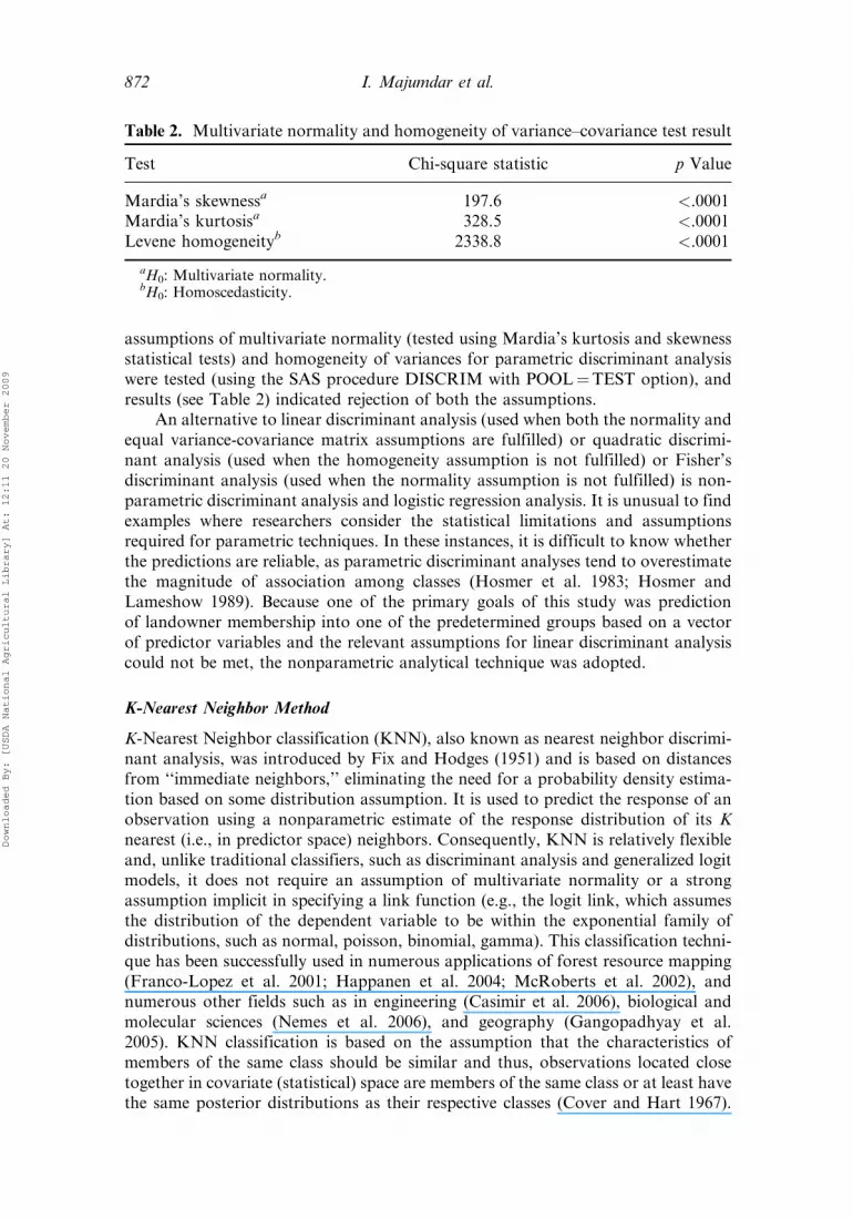
assumptions of multivariate normality (tested using Mardia’s kurtosis and skewnessstatistical tests) and homogeneity of variances for parametric discriminant analysiswere tested (using the SAS procedure DISCRIM with POOL¼TEST option), andresults (see Table 2) indicated rejection of both the assumptions.

An alternative to linear discriminant analysis (used when both the normality andequal variance-covariance matrix assumptions are fulfilled) or quadratic discrimi-nant analysis (used when the homogeneity assumption is not fulfilled) or Fisher’sdiscriminant analysis (used when the normality assumption is not fulfilled) is non-parametric discriminant analysis and logistic regression analysis. It is unusual to findexamples where researchers consider the statistical limitations and assumptionsrequired for parametric techniques. In these instances, it is difficult to know whetherthe predictions are reliable, as parametric discriminant analyses tend to overestimatethe magnitude of association among classes (Hosmer et al. 1983; Hosmer andLameshow 1989). Because one of the primary goals of this study was predictionof landowner membership into one of the predetermined groups based on a vectorof predictor variables and the relevant assumptions for linear discriminant analysiscould not be met, the nonparametric analytical technique was adopted.

K-Nearest Neighbor Method

K-Nearest Neighbor classification (KNN), also known as nearest neighbor discrimi-nant analysis, was introduced by Fix and Hodges (1951) and is based on distancesfrom ‘‘immediate neighbors,’’ eliminating the need for a probability density estima-tion based on some distribution assumption. It is used to predict the response of anobservation using a nonparametric estimate of the response distribution of its Knearest (i.e., in predictor space) neighbors. Consequently, KNN is relatively flexibleand, unlike traditional classifiers, such as discriminant analysis and generalized logitmodels, it does not require an assumption of multivariate normality or a strongassumption implicit in specifying a link function (e.g., the logit link, which assumesthe distribution of the dependent variable to be within the exponential family ofdistributions, such as normal, poisson, binomial, gamma). This classification techni-que has been successfully used in numerous applications of forest resource mapping(Franco-Lopez et al. 2001; Happanen et al. 2004; McRoberts et al. 2002), andnumerous other fields such as in engineering (Casimir et al. 2006), biological andmolecular sciences (Nemes et al. 2006), and geography (Gangopadhyay et al.2005). KNN classification is based on the assumption that the characteristics ofmembers of the same class should be similar and thus, observations located closetogether in covariate (statistical) space are members of the same class or at least havethe same posterior distributions as their respective classes (Cover and Hart 1967).

Table 2. Multivariate normality and homogeneity of variance–covariance test result

Test Chi-square statistic p Value

Mardia’s skewnessa 197.6 <.0001Mardia’s kurtosisa 328.5 <.0001Levene homogeneityb 2338.8 <.0001

aH0: Multivariate normality.bH0: Homoscedasticity.

872 I. Majumdar et al.

Downloaded By: [USDA National Agricultural Library] At: 12:11 20 November 2009

To decide which group a test case belongs to, SAS calculates the squared distance(Mahalanobis distance) between the test observation and each remaining memberof the training dataset and classifies based on majority of classes for the nearest(shortest distance) K-neighbors. To illustrate the point suppose an observation(landowner) whose group membership is not known a-priori has attribute vector xand x1, x2, x3, x4 . . . xn are the attribute vectors of ‘n’ landowners who are alreadyassigned to a group ‘i.’ The Mahalanobis squared distance between any two observa-tions can be estimated as

d2i ðx;x1Þ ¼ ðx� x1Þ0V�1

t ðx� x1Þ ðDistance between the observation vectors x and x1Þ

where V�1t denotes the inverse covariance matrix between x and x1.

It is necessary to note that Mahalanobis distance is a metric measure and cannotbe calculated with categorical variables. In order to include the SITE and PINE cate-gorical variables the following transformation was made. The two variables SITEand PINE were broken down into a set of 7 (6 for the six classes of SITE and 1as PINE dummy) dummy variables which were then subjected to Multiple Corre-spondence Analysis (MCA) (Greenacre 1984; Saporta and Niang 2006) using SASprocedure CORRESP to extract the dimensions (comparable to the principalcomponents of Principal Components Analysis) that explained a majority of varia-tion in these variables. The 4-Inertias (Inertia refers to variance in the context ofCorrespondence Analysis) that explained a variation of 72.5% in the two variableswere retained for calculating the Mahalanobis distance for KNN classification.Based on the squared distance defined above and the specified parameter ‘k,’ a posi-tive integer, which denotes the number of nearest neighbors to be considered, ‘k’observations that are closest to x are identified and x is assigned to the group thatthe majority of the ‘k’ nearest neighbors belong to. For example, in Figure 1 below,a new member ‘X’ will be classified as a white ball when k¼ 1, black ball when k¼ 5and cannot be classified based on majority votes when k¼ 10.

While KNN classification can help in measuring the accuracy of classificationit cannot establish relationships between landowner preferences and the predictorvariables (KNN is a classification method and cannot be used as a regression methodto describe the relationship between explanatory variables and the responsevariable). We used logistic regression analysis to assess the relationship of the inde-pendent variables with the categorical dependent variable denoting motivationaltype of landowner. Logistic regression does not require that the data displaymultivariate normality and can also accommodate the independent variables onany measurement scale (KNN does not support categorical variables).

Figure 1. K-Nearest Neighbor classification based on k¼ 1, k¼ 5, or k¼ 10.

Management Direction in Family Forests 873

Downloaded By: [USDA National Agricultural Library] At: 12:11 20 November 2009

Results

This study focuses on whether it is possible to predict group membership of familyforest owners in the southeast using variables which are not collected using a surveyof landowners. In other words, is it possible to assign a new landowner to a broadergroup based on management objectives ex-ante to acquiring primary data from thelandowners? The summary statistics of the variables selected as discriminators (usingstep-wise selection SAS procedure STEPDISC) between the three landowner groupsnamely, multiple-objective, non-timber and timber according to their preference forproducing either both, non-timber or timber is given is Table 1. The socioeconomic(INC, DIST), demographic (PGI, PD) and biophysical characteristics (SLOPE,SITE, AGE and PINE) describing the three groups of landowners can be used toclassify a new (previously unclassified) landowner into one of the groups. KNN clas-sification performance is evaluated using two accuracy measures generated as part ofthe output from running the SAS procedure DISCRIM. These are referred to as theapparent error rate and the cross-validation error rate. Percentage of correct classi-fication within each group (cluster) and the whole population based on predictionsof KNN classification are reported in Table 3 and results suggest an optimal choiceof K as 2, since the classification accuracy peaked within each ownership group whentwo nearest neighbors were considered (see Table 3). Since in this case the same inputdata is used to define and evaluate the classification criterion, the resulting error-count estimate has an optimistic bias (SAS Institute, Inc. 2004, p. 1163). One wayto reduce the bias is use the one-leave-one cross-validation option (Lachenbruchand Mickey 1968) to classify each observation based on the discriminant functioncomputed from all other observations. Cross-validation results corroborated thatat k¼ 2 the percent of accurate classification was highest across all the three groups.Results show (Table 3) that while the average accuracy of prediction across all thelandowner groups was 83.4%, it was 86.5%, 78% and 81.6% for multiple-objective,non-timber and timber owners respectively.

Accuracy measures can be calculated in more than one way as advocated byCongalton (1991) who presented two methods as users accuracy and producers accu-racy. Users accuracy calculates correctly classed from the trace variable over the rowtotal and provides an indication of errors of case omission. Similarly producers accu-racy is the calculation of correctly classed from the trace value over the column total.Producers accuracy gives an indication of the accuracy of what the model was able to

Table 3. Classification results for the apparent-error-rate KNN method

k Multiple-objective Non-timber Timber Total

Percentage correct2 86.5 78.0 81.6 83.43 74.0 60.0 59.4 66.94 68.2 50.7 54.0 60.55 76.7 51.3 59.0 66.56 75.3 47.7 52.3 63.07 75.4 46.7 54.0 63.48 74.9 42.7 48.4 60.69 77.3 37.3 45.8 60.1

874 I. Majumdar et al.

Downloaded By: [USDA National Agricultural Library] At: 12:11 20 November 2009

itself predict, whereas users accuracy relates how well the training data wasdiscerned. Table 4 presents the results of users accuracy and producers accuracycalculated from the one-leave-one cross validation results of KNN classification(k¼ 2).

Paired Logistic Comparisons

Three binary logistic models to investigate the relationship of the discriminatoryvariables on landowner motivations were evaluated. The likelihood ratio tests sug-gest that all the explanatory variables in the three models are jointly significant inexplaining the heterogeneity of landowner motivations as indicated by their member-ship in either the non-timber-, multiple-objective- or timber-motivated owner group.The likelihood ratio test statistics for the logistic models explain the differences inlandowner motivation, Timber Vs. Non-timber (136.78), Non-timber Vs. Multiple-objective (108.33), Timber Vs. Multiple-objective (38.69), and indicate that timber-motivated owners were most separated from non-timber-motivated owners whilethe timber- and multiple-objective-motivated owners were the most overlapping.

Timber Vs. Non-Timber

Except for median household income (INC), distance to the nearest paved road(DIST) and stand age (AGE), the two sociodemographic variables (populationgravity index [PGI] and county population density [PD]) and the three biophysicalvariables (forest type [PINE], SLOPE and SITE) were significant (Table 5). Asexpected the two sociodemographic variables had a negative coefficient indicatingthat forest plots close to population centers or in counties with high population den-sity are less likely to be attractive to timber motivated owners relative to non-timbermotivated owners. For every addition of 1000 units to the PGI, the probability of alandowner likely to be classified as timber relative to non-timber would decrease by20%. The SLOPE variable was negative indicating that an increase in slope of 10%reduces the likelihood that the forest plot would be owned by a timber-motivatedrelative to non-timber-objective owner by 8% (Table 5).

As expected the positive sign on the coefficient for PINE and SITE indicate thatfast growing pine stands and productive better quality lands are more likely to beowned by a timber relative to a non-timber objective owner. Results further suggestthat for a unit increase in site quality (for example, from site class 1 to 2), the

Table 4. Producers and users accuracy for one-leave-one cross-validation method(k¼ 2)

Producers accuracy Users accuracy

ClassedColumntotal

Accuracy(%) Classed

Rowtotal

Accuracy(%)

Multiple-objective 575 793 72.5 575 777 74.0Non-timber 180 286 62.9 180 300 60.0Timber 275 450 61.1 275 463 59.4

Management Direction in Family Forests 875

Downloaded By: [USDA National Agricultural Library] At: 12:11 20 November 2009

likelihood that the owner would belong to the timber group relative to non-timberincreases by 7%. Similarly there is an 18% greater likelihood of a pine stand to bemanaged by the timber group relative to non-timber motivated owners.

Non-Timber Vs. Multiple-Objective

Excluding population density (PD) all the variables were statistically significant indiscriminating non-timber motivated owners from multiple-objective motivatedowners (Table 6). The positive coefficient on population gravity index (PGI) andmedian household income (INC) suggests that landowners near population centersor in richer counties with higher median household incomes are more likely to belongto the non-timber group relative to multiple-use. On average for every addition of1000 units to the PGI and for every increase in median household income by$1,000, the probability that a landowner will likely to be grouped as non-timberrelative to multiple-use would increase by 5% and 0.6% respectively. The positivecoefficient on SLOPE indicates that steeper terrain stands are likely to be ownedby non-timber motivated owners relative to multiple-use management owners. Otherthings remaining the same, for every 10% increase in slope there is a 9% increased

Table 5. Timber vs. non-timber

Variable Estimate Marginal effects

Intercept �0.799 �0.195(0.627) (0.154)

PGI �0.0007a �0.0002(0.0002) (0.00005)

INC 0.000023 0.000006(0.00001) (0.000004)

PD �0.005a �0.001(0.001) (0.0003)

DIST 0.001 0.0002(0.0007) (0.0002)

SLOPE �0.0313a �0.008(0.008) (0.002)

PINE 0.768a 0.183(0.183) (0.042)

AGE 0.003 0.0007(0.004) (0.0009)

SITE 0.277a 0.068(0.093) (0.023)

Log-likelihood function �439.6Restricted log likelihood �513.2Chi-squarea 147.1Number of observations 765Percent correct 68.1

Note. Standard errors in parentheses.aSignificant at .01.

876 I. Majumdar et al.

Downloaded By: [USDA National Agricultural Library] At: 12:11 20 November 2009

likelihood of that land being classified as owned by a non-timber motivated ownerrelative to a multiple-objective owner.

As expected the coefficient of forest type (PINE) is negative indicating thatthe commercially profitable softwood stands are less appealing to the non-timber-motivated owners relative to the multiple-objective-motivated owners. The negativecoefficients on AGE suggest that mature stands are less likely to be owned bynon-timber motivated owners relative to the multiple-use objective owners whilethe negative sign on SITE suggest that less productive poor quality lands are likelyto be owned by non-timber relative to multiple-objective-motivated owners. Ceterisparibus (other things remaining the same), for an unit increase in site quality thelikelihood that landowners would be classed into non-timber relative to multiple-objective decreases by 3.2%. Similarly there is a 15% decrease in likelihood fornon-timber-motivated owners to manage pine stands relative to multiple-objectivegroup of owners. Contrary to our expectation that non-timber owners are likelyto own older stands with higher amenity values we found that for a 10-year increasein stand age the likelihood that landowners would be grouped as non-timber-motivated relative to being driven by multiple-objective decreases by 1.5%.

Table 6. Non-timber vs. multiple-objective

Variable Estimate Marginal effects

Intercept �1.1426a �0.2212(0.460) (0.088)

PGI 0.0002a 0.00005(0.00007) (0.00001)

INC 0.00003a 0.000006(0.00001) (0.000002)

PD �0.0005 �0.00009(0.0004) (0.00009)

DIST �0.00097b �0.0002(0.0004) (0.00009)

SLOPE 0.0474a 0.0092(0.008) (0.001)

PINE �0.8083a �0.1504(0.163) (0.029)

AGE �0.0078a �0.0015(0.003) (0.0006)

SITE �0.1633b �0.03162(0.071) (0.014)

Log-likelihood function �585.04Restricted log likelihood �640.99Chi-squarea 111.9Number of observations 1083Percent Correct 75

Note. Standard errors in parentheses.aSignificant at .01.bSignificant at .05.

Management Direction in Family Forests 877

Downloaded By: [USDA National Agricultural Library] At: 12:11 20 November 2009

Timber Vs. Multiple-Objective

Population density (PD), local site characteristics SLOPE and SITE significantlydiscriminated the timber owners from the multiple-objective group of forest owners(Table 7). Population gravity index (PGI), median household income (INC) andforest type (PINE) did not significantly contribute to the classification of timber-objective versus the multiple-objective owners. The negative coefficient on countypopulation density indicates that forest plots in counties with high populationdensity are less likely to be owned by a timber-objective owner relative to a multiple-use motivated owner. For every 100 unit increase in county population density thereis a decrease in likelihood of landowners within that county to be motivated bytimber production relative to multiple-use by 6%. The positive coefficient on SITEindicates that high quality forest stands are more likely to be owned by timber-motivated relative to multiple-use owners. AGE has a negative coefficient indicatingthat younger stands are more likely to be managed by timber motivated relative tomultiple-use owners. The positive coefficient on the SLOPE variable indicates thatsteeper physiography is more likely to be owned by a timber-motivated relative tomultiple-use owner which is contrary to our expectation.

Table 7. Timber vs. multiple-objective

Variable Estimate Marginal effects

Intercept �1.49a �0.345(0.45) (0.103)

PGI �0.00005 �0.000013(0.0001) (0.00003)

INC 0.00002 0.000004(0.00001) (0.000003)

PD �0.003a �0.0006(0.0009) (0.0002)

DIST 0.0006 0.0001(0.0006) (0.0001)

SLOPE 0.014b 0.0033(0.007) (0.0017)

PINE �0.067 �0.015(0.13) (0.029)

AGE �0.006b �0.0014(0.003) (0.0006)

SITE 0.182a 0.042(0.066) (0.015)

Log-likelihood function �803.1Restricted log likelihood �821.2Chi–squarea 36.1Number of observations 1244Percent correct 63.3

Note. Standard errors in parentheses.aSignificant at .01.bSignificant at .05.

878 I. Majumdar et al.

Downloaded By: [USDA National Agricultural Library] At: 12:11 20 November 2009

Conclusion

The majority of the forests in the south are owned by individuals and families whopose a challenge to the forestry community because of their continuously increasingnumbers (DeCoster 1998) and diversity of desires for their land (Kittredge 2004). Tosuccessfully direct educational efforts, we need to identify the important variablesthat can help differentiate diversely motivated groups of landowners. Our study indi-cates that landowners can be accurately classified into heterogeneous motivationalgroups (multiple-objective, non-timber, and timber) using predetermined demo-graphic (from Census) and woodlot (from FIA) variables using the KNN technique.

Examples of the use of discriminant analysis in landowner studies are sparse andhave concentrated on searching for variables that discriminate owner groups, forexample, timber managers versus non-managers (Greene and Blatner 1986), regen-erators versus non-regenerators (Arano et al. 2004), and cross-boundary cooperatorsversus non-cooperators (Finley et al. 2006). These studies provide valuable insightsto identifying the variables that define different landowner groups based on detailedanalysis of landowner survey questions. An ex-ante assignment of non-surveyedlandowners into different groups was not a goal of their work. Our classificationscheme based on variables known a-priori, that is, before landowners on a FIA plotlocation are contacted for the NWOS, suggests that it may be possible to predictmanagement direction for a specified parcel without asking the landowner abouthis intentions. Given the increasing number of family forest owners and the increas-ing proportion of timberland they own and manage as an ownership class, this studycan effectively help in estimating the different adjustment factors for diversely moti-vated landowner groups in order to more accurately project future supplies of timberand other forest related non-timber products. Finally, this piece of information canalso help design new features for the NWOS survey that focus on issues of interest tolandowners and may help improve communications and development of effectiveoutreach and educational programs.

To our knowledge KNN classification has not been used to study landownerbehavior though the technique is relatively simple to implement, especially sincethere is no need to meet the statistical assumptions inherent in parametric classifica-tion methods (e.g., variables characterizing the difference between the landownergroups must have multivariate normal distributions and equal variance-covariancematrix). Our study also extends research on ways to understand landowner behaviorin the future by taking into consideration their diverse set of motivations andattitudes toward forest management instead of treating the family forest owners asa single homogeneous group.

We find consistently that with increases in population pressure (near developedareas) a family forest owner is likely to be motivated by non-timber consumption offorest amenities compared to timber production, a result consistent with past studies(e.g., Brunson et al. 1997; Ribe and Matteson 2002; Tremblay and Dunlap 1978; Xuet al. 2003). This indicates that forestland closer to developed land (populationcenters) may be subjected to a high opportunity cost for timber production and islikely to be owned by individuals who value the aesthetic and recreational valuesof forests. On the other hand, rural areas with little development are more conduciveto timber production and are likely to be owned and managed by timber producerswith the intent to produce timber for profit. Results also show that better quality andflatter sites are preferred for timber production and are more likely to be owned by a

Management Direction in Family Forests 879

Downloaded By: [USDA National Agricultural Library] At: 12:11 20 November 2009

timber producer with a profit motive. Kuuluvainen et al. (1996) reported that themean percentage growth that reflects the site quality of woodlot parcels is signifi-cantly positively related to single objective owners (that includes the monetarilymotivated timber owners) while being insignificant in explaining the multiple-objective-motivated landowners.

This paper is an example of the large body of recent research focusing on under-standing family forest owners’ motivations, attitudes, their future managementintentions and ways to communicate effectively with them. Research on ways todifferentiate and understand these owners better may be critical to insure futuresustainable supplies of timber, environmental services, and amenities from familyforests at current or enhanced levels.

Notes

1. As noted by one of the external reviewers, our definition of family forest owners may differfrom past researchers who were not nearly as explicit about the type of family ownershipsthat they surveyed. They reported they surveyed families, but did not elaborate on theirdefinitions of what constituted a family. Though our definitions may differ we have noway of determining the extent of the differences based on their published work.

2. For details on the NWOS survey design, implementation and analysis methods see Butleret al. (2005).

3. Question# 9 of the NWOS: People own woodland for many reasons. How important arethe following reasons for why you own woodland?

. To enjoy beauty or scenery

. To protect nature and biologic diversity

. For land investment

. As part of my home, vacation home, farm or ranch

. For privacy

. To pass land on to my children or other heirs

. For cultivation=collection of non-timber forest products

. For production of firewood biofuel (energy)

. For production of sawlogs, pulpwood or other timber products

. For hunting or fishing

. For recreation, other than hunting or fishing

4. Since the predictors were based on FIA plot and condition data and the link to NWOS wasbased only on FIA plots landowners who had multiple conditions in their plot wererepresented multiple times and so each observation was weighted by the proportion of plotthat the condition represented in the analysis.

5. PGI was calculated by linking landowner forest parcel location with the census demo-graphic data on populated places as:

PGIK ¼X

p

Pp

D2kp

8P : Dkp � 100 km

Where Pp is the population of census populated place p and Dkp is the distance betweenFIA plot k and populated place p.

6. MGI was calculated by linking the FIA plot to the pulpmills located within the radius of200 km around the forest plot and was calculated as:

MGIk ¼X

m

Mm

D2km

8M : Dkm � 200 km

880 I. Majumdar et al.

Downloaded By: [USDA National Agricultural Library] At: 12:11 20 November 2009

WhereMm is the pulping capacity in millions of cords at pulpmillM and Dkm is the distancebetween FIA plot k and pulpmill m.

References

Alerich, C. L., L. Klevgard, C. Liff, and P. D. Miles. 2004. The Forest Inventory and AnalysisDatabase: Database Description and Users Guide Version 1.7. http://www.ncrs2.fs.fed.us/4801/fiadb/fiadb_documentation/FIADB_v17_122104.pdf (accessed 7 May 2006).

Arano, K. G., I. A. Munn, J. E. Gunter, S. H. Bullard, and M. L. Doolittle. 2004. Comparisonbetween regenerators and non-regenerators in Mississippi: A discriminant analysis.Southern Journal of Applied Forestry 28(4):189–195.

Barlow, S. A., I. A. Munn, D. A. Cleaves, and D. L. Evans. 1998. The effect of urban sprawlon timber harvesting: A look at two southern states. Journal of Forestry 96(12):10–14.

Bliss, J. C., M. L. Sisock, and T. W. Birch. 1998. Ownership matters: Forestland concentrationin rural Alabama. Society and Natural Resources 11(4):401–410.

Brunson, M. W., B. Shindler, and B. S. Steel. 1997. Consensus and dissention among rural andurban publics concerning forest management in the Pacific Northwest. In Public landsmanagement in the West: Citizens, interest groups, and values, ed. B. Steel, 83–94.Westport, CT: Praeger.

Butler, B. J. 2005. The timber harvesting behavior of family forest owners. PhD dissertation,Department of Forest Science, Oregon State University, Corvallis, OR.

Butler, B. J. and E. C. Leatherberry. 2004. America’s family forest owners. Journal of Forestry102(7):4–9.

Butler, B. J., E. C. Leatherberry, and M. S. Williams. 2005. Design, implementation, andanalysis methods for the National Woodland Owner Survey. United States Departmentof Agriculture Forest Service, Northeastern Research Station, General Technical ReportNE-336. http://www.treesearch.fs.fed.us/pubs/20830 (accessed 16 October 2006).

Casimir, R., E. Boutleux, G. Clerc, and A. Yahoui. 2006. The use of features selection andnearest neighbors rule for faults diagnostic in induction motors. Engineering Applicationsof Artificial Intelligence 19:169–177.

Congalton, R. G. 1991. A review of assessing the accuracy of classifications of remotely senseddata. Remote Sensing of Environment 37(1):35–46.

Cover, T. M. and P. E. Hart. 1967. Nearest neighbor pattern classification. Transactions onInformation Theory 13:21–27.

DeCoster, L. A. 1998. The boom in forest owners—A bust for forestry? Journal of Forestry96(5):25–28.

Dijak, W. D. and F. R. Thompson. 2000. Landscape and edge effects on the distribution ofmammalian predators in Missouri. Journal of Wildlife Management 64:209–216.

Finley, A. O., D. B. Kittredge, T. H. Stevens, C. M. Schweik, and D. C. Dennis. 2006. Interestin cross-boundary cooperation: Identification of distinct type of forest owners. ForestScience 52(1):10–23.

Fix, E. and J. Hodges. 1951. Discriminatory analysis, nonparametric discrimination: Consis-tency properties. Technical Report, Randolph Field, Texas: USAF School of AviationMedicine.

Franco-Lopez, H., A. R. Ek, and M. E. Bauer. 2001. Estimation and mapping of forest standdensity, volume, and cover type using the k-nearest neighbor method. Remote Sensing ofEnvironment 77:251–274.

Gangopadhyay, S., M. Clark, and B. Rajagopalan. 2005. Statistical downscaling usingK-nearest neighbors. Water Resources Research 41 W02024:1–23.

Gramann, J. H., T. D. Marty, andW. B. Kurtz. 1985. A logistic analysis of the effects of beliefsand past experience on management plans for nonindustrial private forests. Journal ofEnvironmental Management 20:347–356.

Management Direction in Family Forests 881

Downloaded By: [USDA National Agricultural Library] At: 12:11 20 November 2009

Greenacre, M. J. 1984. Theory and applications of Correspondence Analysis. London:Academic press.

Greene, J. L. and K. A. Blatner. 1986. Identifying woodland owner characteristics associatedwith timber management. Forest Science 32(1):135–146.

Happanen, R., A. R. Ek, M. E. Bauer, and A. O. Finley. 2004. Delineation of forest=nonforestland use classes using nearest neighbor methods. Remote Sensing of Environment89:265–271.

Hill, L., R. Cooksey, J. McConnell, K. O’Connell, J. Michaels, D. Raimo, J. Garner, J. Grace,and J. Mallow. 1998. Forest fragmentation in the Chesapeake Bay watershed: Ecological,economic, policy and law impacts. United States Department of Agriculture Forest Ser-vice and Society of American Foresters, Report. http://www.safnet.org/policyandpress/frag6.cfm (accessed 31 October 2006).

Hosmer, D. W. and S. Lameshow. 1989. Applied logistic regression. New York: Wiley-Interscience.

Hosmer, T., D. W. Hosmer, and L. L. Fisher. 1983. A comparison of maximum likelihood anddiscriminant function estimators of the coefficients of logistic regression model for mixedcontinuous and discrete variables. Communications in Statistics B 12:577–593.

Johnson, R. A. and D. W. Wichern. 2002. Applied multivariate statistical data analysis, 5th ed.Prentice Hall: Upper Saddle River, NJ.

Kays, J., V. M. Schultz, and P. Townsend. 1999. Forest landowners in a fragmentedlandscape. Branching Out: Maryland’s Forest Stewardship Educator 7(2):1–3. http://www.naturalresources.umd.edu/BranchingOut.cfm (accessed 21 November 2006).

Kendra, A. and R. B. Hull. 2005. Motivations and behaviors of new forest owners in Virginia.Forest Science 51(2):142–154.

Kittredge, D. B. 2004. Extensionnoutreach implications for America’s family forest owners.Journal of Forestry 102(7):15–18.

Klecka, W. R. 1988. Discriminant Analysis. Sage University Paper series on QuantitativeApplications in the Social Sciences, series no. 07-019. Beverly Hills, CA, and London:Sage Publications.

Kluender, R. A. and T. L. Walkingstick. 2000. Rethinking how nonindustrial landowners viewtheir lands. Southern Journal of Applied Forestry 24(3):150–158.

Kuuluvainen, J., H. Karpppinen, and V. Ovaskainen. 1996. Landowner objectives and non-industrial private timber supply. Forest Science 42(3):300–309.

Lachenbruch, P. A. and M. R. Mickey. 1968. Estimation of Error Rates in DiscriminantAnalysis. Technometrics 10:1–11.

Majumdar, I., L. D. Teeter, and B. J. Butler. 2008. Characterizing family forest owners: Acluster analysis approach. Forest Science 54(2):176–184.

McRoberts, R. E., M. D. Nelson, and D. G. Wendt. 2002. Stratified estimation of forest areausing satellite imagery, inventory data, and the K-Nearest Neighbors technique. RemoteSensing of Environment 82:457–468.

Mehmood, S. R. and D. Zhang. 2001. Forest parcelization in the United States: A study ofcontributing factors. Journal of Forestry 99(4):30–34.

Munn, I. A., S. A. Barlow, D. L. Evans, and D. Cleaves. 2002. Urbanization’s impact ontimber harvesting in the south central United States. Journal of Environmental Manage-ment 64(1):65–76.

Nemes, A., W. J. Rawls, and Y. A. Pachepsky. 2006. Use of nonparametric nearest neighborapproach to estimate soil hydraulic properties. Soil Science Society of America Journal70:327–336.

Ribe, R. and M. Matteson. 2002. Views of old forestry and new among reference groups in thePacific Northwest. Western Journal of Applied Forestry 17(4):173–182.

Sampson, N. and L. DeCoster. 2000. Forest fragmentation: Implications for sustainableprivate forests. Journal of Forestry 98(3):4–8.

882 I. Majumdar et al.

Downloaded By: [USDA National Agricultural Library] At: 12:11 20 November 2009

Saporta, G. and N. Niang. 2006. Correspondence analysis and classification. In Multiple cor-respondence analysis and related methods, eds. M. J. Greenacre and J. Blasius, 372–392.London: Chapman & Hall=CRC.

SAS Institute Inc. 2004. SAS=STAT 9.1 User’s Guide. Cary, NC: SAS Institute Inc.Tremblay, K. R. and R. Dunlap. 1978. Rural–urban residence and concern with environmen-

tal quality. Rural Sociology 43:474–491.Wilcove, D. S. 1990. Forest fragmentation as a wildlife management issue in the eastern

United States. United States Department of Agriculture Forest Service, NortheasternForest Experiment Station, General Technical Report NE-140. http://www.treesearch.fs.fed.us/pubs/4191 (accessed 7 December 2006).

Xu, W., B. R. Lippke, and J. Perez-Garcia. 2003. Valuing biodiversity, aesthetics, and joblosses associated with ecosystem management using stated preferences. Forest Science49(2):247–257.

Zipperer, W. C., S. M. Sisinni, R. V. Pouyat, and T. W. Foresman. 1997. Urban tree cover: Anecological perspective. Urban Ecosystems 1:229–246.

Management Direction in Family Forests 883

Downloaded By: [USDA National Agricultural Library] At: 12:11 20 November 2009