Use of Exchangeable Pairs in the Analysis of Simulations

Charles Stein withPersi Diaconis, Susan Holmes, Gesine Reinert

March 2002

AbstractThe method of exchangeable pairs has emerged as an important tool in proving limittheorems for Poisson, normal and other classical approximations. Here the method is usedin a simulation context. We estimate transition probabilitites from the simulations and usethese to reduce variances. Exchangeable pairs are used as control variates.

Finally, a general approximation theorem is developed that can be complemented bysimulations to provide actual estimates of approximation errors.

1 Introduction

A basic computational problem of the theory of probability may be formulated in thefollowing way. Let X and W be two finite sets and let ω be a function on X to W. Weknow (except possibility for the normalizing factor) the distribution of a random variable Xtaking values in X , and want to study the distribution of the random variable W = ω(X),perhaps to evaluate or approximate the expectation Ef(W ) with f a given real-valuedfunction on W. Often X is a space of functions (in particular sequences or graphs) andW is a subset of RP . In typical situations, X is so large and complicated that directcomputation of Ef(W ) is intractable. An example to keep in mind is the classical Isingmodel on an N × N × N size grid. Here X is the space of 2N

3labelings of the grid by

{±1}. If W = ω(X) is the sum of all the grid labels (the so-called magnetization), director theoretical evaluation of EW is impossible e.g. when N = 10.

These problems can be studied by simulation methods such as Markov chain MonteCarlo. This paper discusses three techniques which can be used in conjunction with stan-dard simulation procedures to get increased accuracy. The techniques are all based oncreating exchangeable pairs (X,X ′). These pairs give rise to classes of identities whichsuggest new estimators.

In Section 2, exchangeable pairs are introduced. The relation with reversible Markovchains is recalled. A basic identity for an exchangeable pair (W,W ′), as given in Proposition

1

2 is :

p(w′)p(w)

=p(w′|w)p(w|w′)

.

This suggests that the ratios p(w′)p(w) can be estimated by counting w → w′ transitions in a

sequence of pairs. In the Markov chain context this is the transition matrix Monte Carlotechnique of Wang et al. [29]. The technique is illustrated on two examples in Section 3:the distribution of the number of ones in Poisson-binomial trials and the Ising model. Itworks well in the first example and modestly in the second example.

Section 4 uses exchangeable pairs (X,X ′) to make control variates EX(W ′) for W . Thisis used to improve the naive estimate 1

N

∑Ni=1Wi of EW , obtained by N simulations of W .

New estimates of Var(W ) are also suggested.

Section 5 uses exchangeable pairs to derive a closed form expression for the error of aclassical approximation (e.g. normal or Poisson) for the distribution of W . The error isan explicit function of (W,W ′). It can thus be estimated from a sequence of such pairsand used to correct the classical approximation. A normal example is worked through indetail. A general approximation theorem for an essentially arbitrary limit is also derivedand used to suggest non-parametric alternate estimators.

Exchangeable pairs have been used to derive a class of limiting approximations viaversions of “Stein’s method”. The basic ratio identities of Section 4 were used to deriveapproximations to the number of Latin rectangles (Stein [23]) and to derive combinatorialformulae for balls and boxes and cycle lengths in random permutations (Stein [27], Chapter5). The idea is that the ratios p(w′|w)

p(w|w′) may be much easier to work with than p(w′)p(w) . In Section

4 we find versions of these ratios which are easily computible. The explicit remainder termsof Section 5 appear in the earliest versions of Stein’s method. In previous work, calculusand probability estimates were used to bound the remainders, giving Berry-Esseen likeerrors. Here the emphasis will be on applications to the output of a simulation.

2 Exchangeable pairs

We first define exchangeable pairs and give examples and a basic ratio identity. Then theconnection with reversible Markov chains is given.

2.1 Definitions

An ordered pair (X,X ′) of random variables taking values in the finite set X is defined tobe exchangeable if, for all x1 and x2 in X ,

P{X = x1 and X ′ = x2} = P{X = x2 and X ′ = x1}. (1)

2

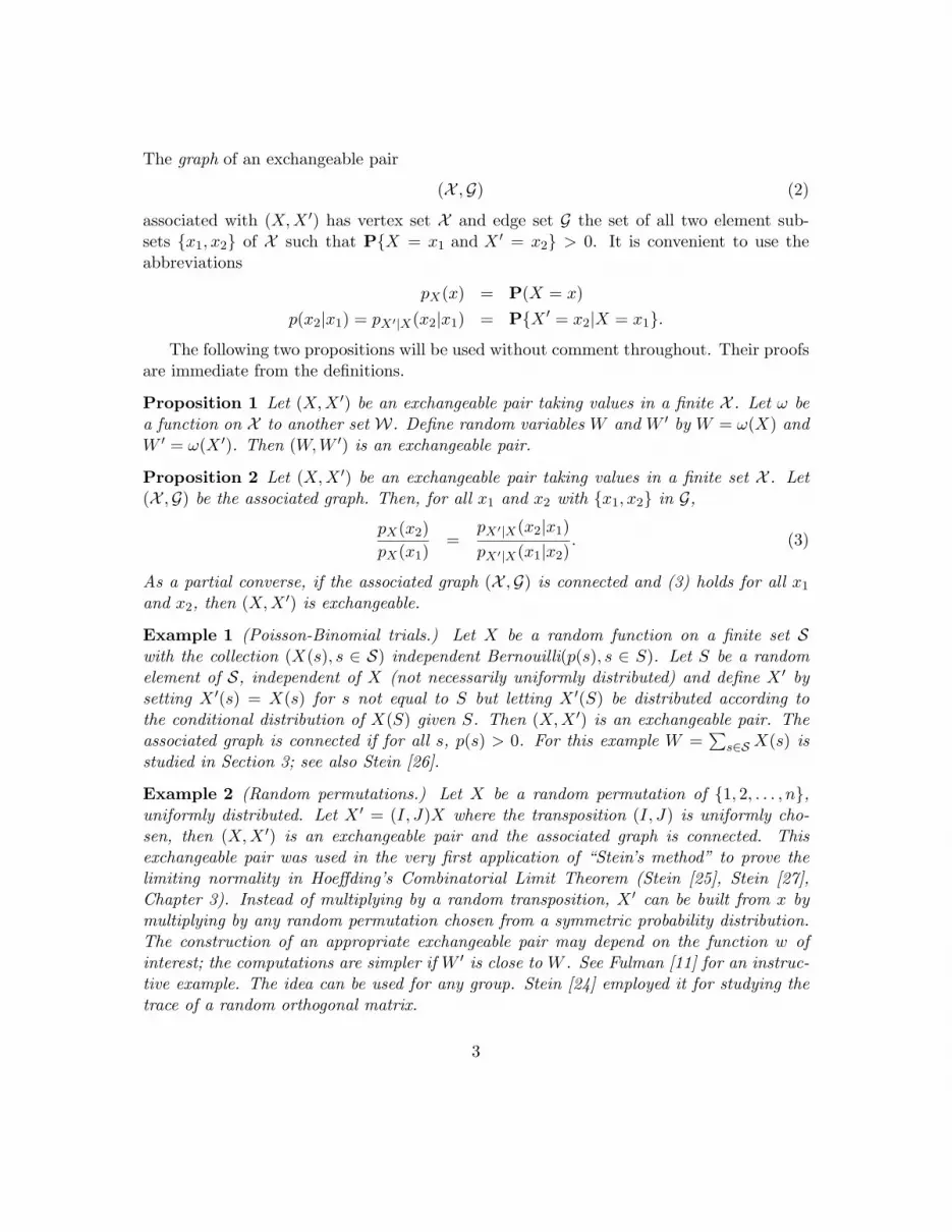
The graph of an exchangeable pair

(X ,G) (2)

associated with (X,X ′) has vertex set X and edge set G the set of all two element sub-sets {x1, x2} of X such that P{X = x1 and X ′ = x2} > 0. It is convenient to use theabbreviations

pX(x) = P(X = x)p(x2|x1) = pX′|X(x2|x1) = P{X ′ = x2|X = x1}.

The following two propositions will be used without comment throughout. Their proofsare immediate from the definitions.

Proposition 1 Let (X,X ′) be an exchangeable pair taking values in a finite X . Let ω bea function on X to another set W. Define random variables W and W ′ by W = ω(X) andW ′ = ω(X ′). Then (W,W ′) is an exchangeable pair.

Proposition 2 Let (X,X ′) be an exchangeable pair taking values in a finite set X . Let(X ,G) be the associated graph. Then, for all x1 and x2 with {x1, x2} in G,

pX(x2)pX(x1)

=pX′|X(x2|x1)pX′|X(x1|x2)

. (3)

As a partial converse, if the associated graph (X ,G) is connected and (3) holds for all x1

and x2, then (X,X ′) is exchangeable.

Example 1 (Poisson-Binomial trials.) Let X be a random function on a finite set Swith the collection (X(s), s ∈ S) independent Bernouilli(p(s), s ∈ S). Let S be a randomelement of S, independent of X (not necessarily uniformly distributed) and define X ′ bysetting X ′(s) = X(s) for s not equal to S but letting X ′(S) be distributed according tothe conditional distribution of X(S) given S. Then (X,X ′) is an exchangeable pair. Theassociated graph is connected if for all s, p(s) > 0. For this example W =

∑s∈S X(s) is

studied in Section 3; see also Stein [26].

Example 2 (Random permutations.) Let X be a random permutation of {1, 2, . . . , n},uniformly distributed. Let X ′ = (I, J)X where the transposition (I, J) is uniformly cho-sen, then (X,X ′) is an exchangeable pair and the associated graph is connected. Thisexchangeable pair was used in the very first application of “Stein’s method” to prove thelimiting normality in Hoeffding’s Combinatorial Limit Theorem (Stein [25], Stein [27],Chapter 3). Instead of multiplying by a random transposition, X ′ can be built from x bymultiplying by any random permutation chosen from a symmetric probability distribution.The construction of an appropriate exchangeable pair may depend on the function w ofinterest; the computations are simpler if W ′ is close to W . See Fulman [11] for an instruc-tive example. The idea can be used for any group. Stein [24] employed it for studying thetrace of a random orthogonal matrix.

3

Many further examples are given in Section 2.2. There is a large literature on ex-changeability. Informative treatments are in Kingman [16], Aldous [1], Diaconis [6]. Mostof this literature deals with potentially infinite exchangeable sequences and is not relevantfor present purposes.

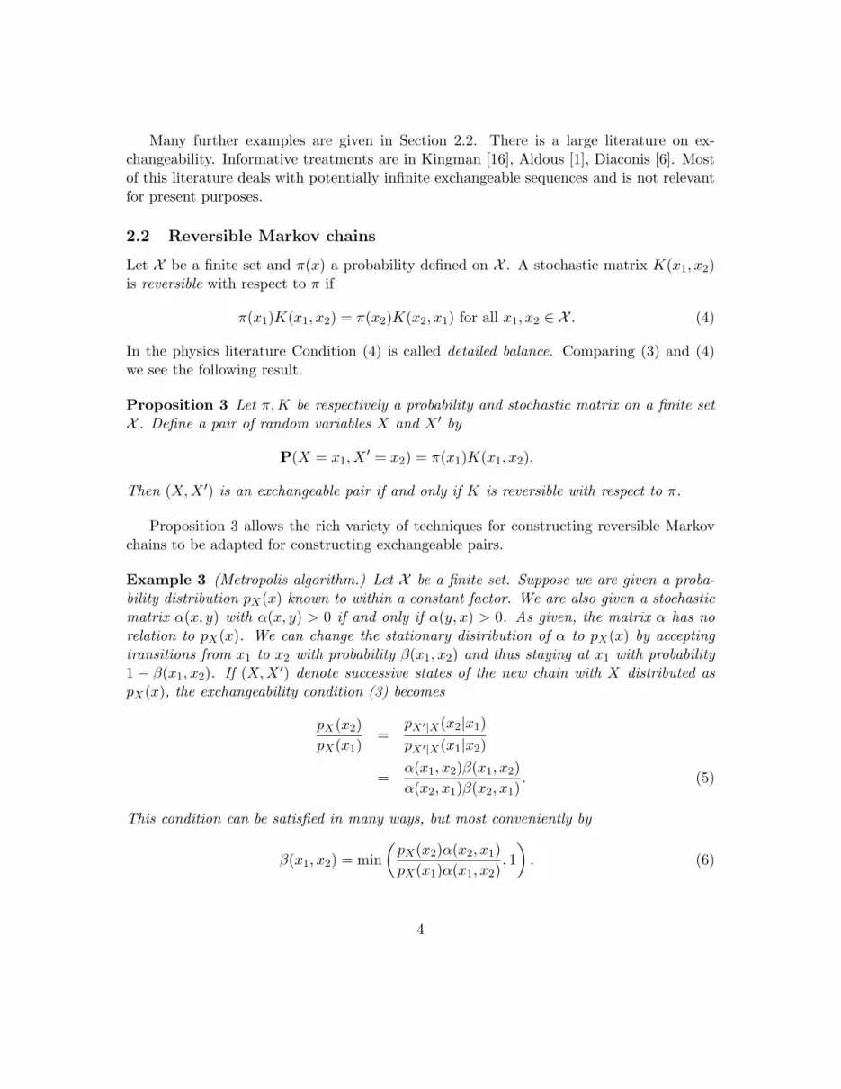
2.2 Reversible Markov chains

Let X be a finite set and π(x) a probability defined on X . A stochastic matrix K(x1, x2)is reversible with respect to π if

π(x1)K(x1, x2) = π(x2)K(x2, x1) for all x1, x2 ∈ X . (4)

In the physics literature Condition (4) is called detailed balance. Comparing (3) and (4)we see the following result.

Proposition 3 Let π,K be respectively a probability and stochastic matrix on a finite setX . Define a pair of random variables X and X ′ by

P(X = x1, X′ = x2) = π(x1)K(x1, x2).

Then (X,X ′) is an exchangeable pair if and only if K is reversible with respect to π.

Proposition 3 allows the rich variety of techniques for constructing reversible Markovchains to be adapted for constructing exchangeable pairs.

Example 3 (Metropolis algorithm.) Let X be a finite set. Suppose we are given a proba-bility distribution pX(x) known to within a constant factor. We are also given a stochasticmatrix α(x, y) with α(x, y) > 0 if and only if α(y, x) > 0. As given, the matrix α has norelation to pX(x). We can change the stationary distribution of α to pX(x) by acceptingtransitions from x1 to x2 with probability β(x1, x2) and thus staying at x1 with probability1 − β(x1, x2). If (X,X ′) denote successive states of the new chain with X distributed aspX(x), the exchangeability condition (3) becomes

pX(x2)pX(x1)

=pX′|X(x2|x1)pX′|X(x1|x2)

=α(x1, x2)β(x1, x2)α(x2, x1)β(x2, x1)

. (5)

This condition can be satisfied in many ways, but most conveniently by

β(x1, x2) = min(pX(x2)α(x2, x1)pX(x1)α(x1, x2)

, 1). (6)

4

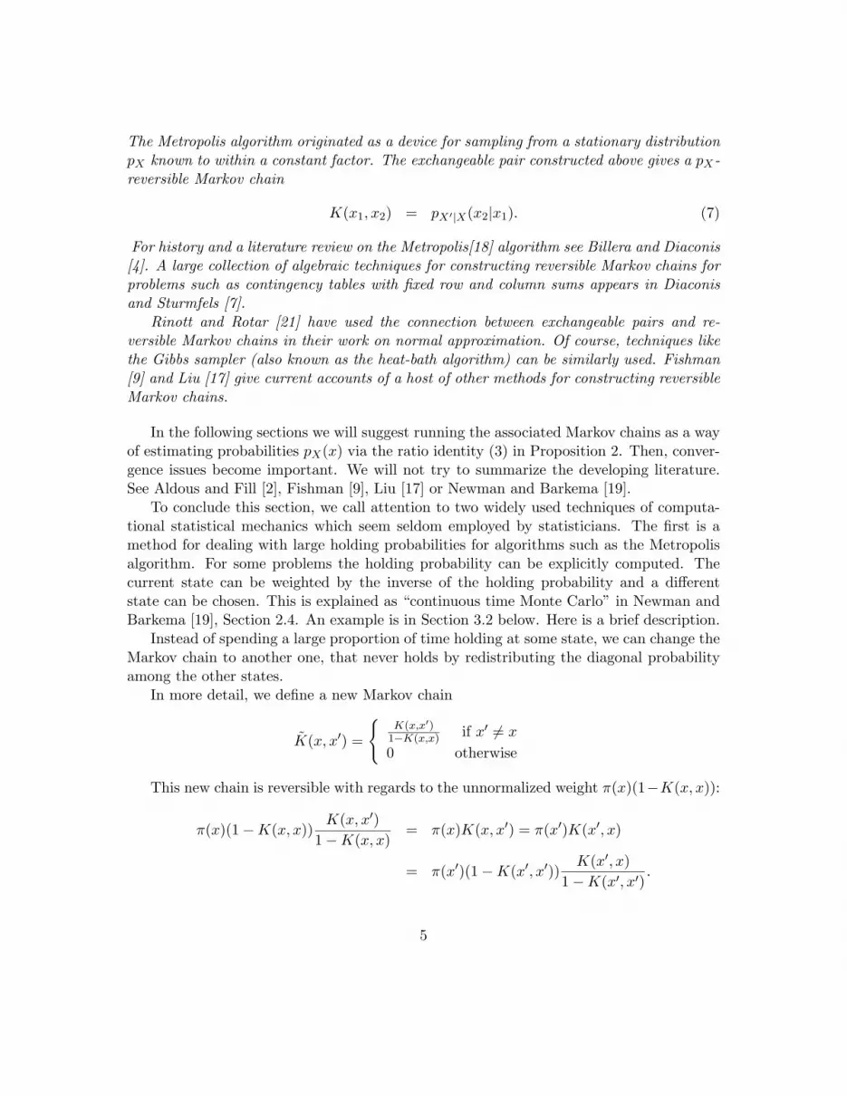
The Metropolis algorithm originated as a device for sampling from a stationary distributionpX known to within a constant factor. The exchangeable pair constructed above gives a pX-reversible Markov chain

K(x1, x2) = pX′|X(x2|x1). (7)

For history and a literature review on the Metropolis[18] algorithm see Billera and Diaconis[4]. A large collection of algebraic techniques for constructing reversible Markov chains forproblems such as contingency tables with fixed row and column sums appears in Diaconisand Sturmfels [7].

Rinott and Rotar [21] have used the connection between exchangeable pairs and re-versible Markov chains in their work on normal approximation. Of course, techniques likethe Gibbs sampler (also known as the heat-bath algorithm) can be similarly used. Fishman[9] and Liu [17] give current accounts of a host of other methods for constructing reversibleMarkov chains.

In the following sections we will suggest running the associated Markov chains as a wayof estimating probabilities pX(x) via the ratio identity (3) in Proposition 2. Then, conver-gence issues become important. We will not try to summarize the developing literature.See Aldous and Fill [2], Fishman [9], Liu [17] or Newman and Barkema [19].

To conclude this section, we call attention to two widely used techniques of computa-tional statistical mechanics which seem seldom employed by statisticians. The first is amethod for dealing with large holding probabilities for algorithms such as the Metropolisalgorithm. For some problems the holding probability can be explicitly computed. Thecurrent state can be weighted by the inverse of the holding probability and a differentstate can be chosen. This is explained as “continuous time Monte Carlo” in Newman andBarkema [19], Section 2.4. An example is in Section 3.2 below. Here is a brief description.

Instead of spending a large proportion of time holding at some state, we can change theMarkov chain to another one, that never holds by redistributing the diagonal probabilityamong the other states.

In more detail, we define a new Markov chain

K(x, x′) =

{K(x,x′)

1−K(x,x) if x′ 6= x

0 otherwise

This new chain is reversible with regards to the unnormalized weight π(x)(1−K(x, x)):

π(x)(1−K(x, x))K(x, x′)

1−K(x, x)= π(x)K(x, x′) = π(x′)K(x′, x)

= π(x′)(1−K(x′, x′))K(x′, x)

1−K(x′, x′).

5

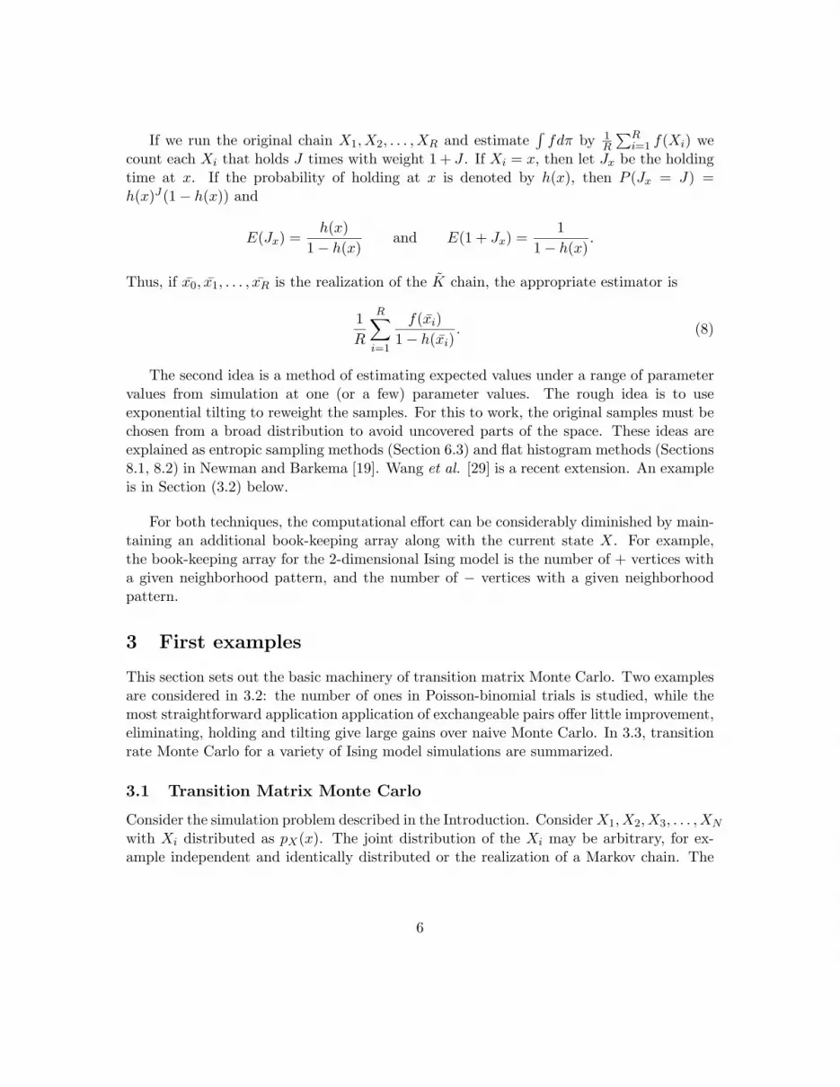
If we run the original chain X1, X2, . . . , XR and estimate∫fdπ by 1

R

∑Ri=1 f(Xi) we

count each Xi that holds J times with weight 1 + J . If Xi = x, then let Jx be the holdingtime at x. If the probability of holding at x is denoted by h(x), then P (Jx = J) =h(x)J(1− h(x)) and

E(Jx) =h(x)

1− h(x)and E(1 + Jx) =

11− h(x)

.

Thus, if x0, x1, . . . , xR is the realization of the K chain, the appropriate estimator is

1R

R∑i=1

f(xi)1− h(xi)

. (8)

The second idea is a method of estimating expected values under a range of parametervalues from simulation at one (or a few) parameter values. The rough idea is to useexponential tilting to reweight the samples. For this to work, the original samples must bechosen from a broad distribution to avoid uncovered parts of the space. These ideas areexplained as entropic sampling methods (Section 6.3) and flat histogram methods (Sections8.1, 8.2) in Newman and Barkema [19]. Wang et al. [29] is a recent extension. An exampleis in Section (3.2) below.

For both techniques, the computational effort can be considerably diminished by main-taining an additional book-keeping array along with the current state X. For example,the book-keeping array for the 2-dimensional Ising model is the number of + vertices witha given neighborhood pattern, and the number of − vertices with a given neighborhoodpattern.

3 First examples

This section sets out the basic machinery of transition matrix Monte Carlo. Two examplesare considered in 3.2: the number of ones in Poisson-binomial trials is studied, while themost straightforward application application of exchangeable pairs offer little improvement,eliminating, holding and tilting give large gains over naive Monte Carlo. In 3.3, transitionrate Monte Carlo for a variety of Ising model simulations are summarized.

3.1 Transition Matrix Monte Carlo

Consider the simulation problem described in the Introduction. ConsiderX1, X2, X3, . . . , XN

with Xi distributed as pX(x). The joint distribution of the Xi may be arbitrary, for ex-ample independent and identically distributed or the realization of a Markov chain. The

6

naive estimate of Ef(W ) is

1N

N∑i=1

f(ω(Xi)). (9)

Suppose we construct an exchangeable pair (X,X ′) as described in Section 1.2 above andcan calculate PX(W ′ = w) with W ′ = ω(X ′). Then as an estimate of pW ′|W (w2|w1),abbreviated by p(w2|w1), we can use

p(w2|w1) =∑N

i=1 δWi=w1PXi(W ′i = w2)∑N

i=1 δWi=w1

. (10)

Then, for all w1 and w2 for which both p(w2|w1) and p(w1|w2) are positive we estimatethe ratio P(W=w2)

P(W=w1) by

p(w2|w1)p(w1|w2)

.

From these ratio estimates all ratios of all probabilities, and so all probabilities, can beestimated, provided the sample is large enough for the connectedness of the graph (2) tobe reflected in the sample. We assume throughout that the graph of the exchangeable pairis connected

To go from ratios to probabilities, form a matrix with rows and columns indexed by Whaving (w,w′) entry

p(w′|w)p(w|w′)

.

In applications, this is often a sparse matrix. For example, for W a birth and death chain,the matrix is tridiagonal. For (w,w′) with zero entry in the matrix there may be manypaths in the graph giving estimates of p(w′)

p(w) .Fitzgerald et al. [10] have suggested reconciling these various estimates by least squares.

Treat p(w) as parameters in

p(w)p(w′)

=p(w|w′)p(w′|w)

.

Take logarithms on both sides

`(w)− `(w′) = `(w|w′)− `(w′|w)

and solve for `(w) by minimizing∑(`(w)− `(w′)− `(w|w′) + `(w′|w)

)27

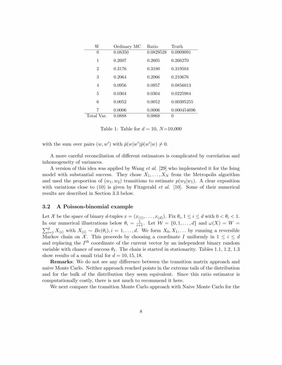
W Ordinary MC Ratio Truth0 0.08350 0.0829528 0.0909091

1 0.2607 0.2605 0.266270

2 0.3176 0.3180 0.319504

3 0.2064 0.2066 0.210676

4 0.0956 0.0957 0.0856013

5 0.0304 0.0304 0.0225984

6 0.0052 0.0052 0.00395255

7 0.0006 0.0006 0.000454696Total Var. 0.0888 0.0868 0

Table 1: Table for d = 10, N=10,000

with the sum over pairs (w,w′) with p(w|w′)p(w′|w) 6= 0.

A more careful reconciliation of different estimators is complicated by correlation andinhomogeneity of variances.

A version of this idea was applied by Wang et al. [29] who implemented it for the Isingmodel with substantial success. They chose X1, . . . , XN from the Metropolis algorithmand used the proportion of (w1, w2) transitions to estimate p(w2|w1). A clear expositionwith variations close to (10) is given by Fitzgerald et al. [10]. Some of their numericalresults are described in Section 3.3 below.

3.2 A Poisson-binomial example

Let X be the space of binary d-tuples x = (x(1), . . . , x(d)). Fix θi, 1 ≤ i ≤ d with 0 < θi < 1.In our numerical illustrations below θi = 1

i+1 . Let W = {0, 1, . . . , d} and ω(X) = W =∑di=1X(i) with X(i) ∼ Be(θi), i = 1, . . . , d. We form X0, X1, . . . by running a reversible

Markov chain on X . This proceeds by choosing a coordinate I uniformly in 1 ≤ i ≤ dand replacing the Ith coordinate of the current vector by an independent binary randomvariable with chance of success θI . The chain is started in stationarity. Tables 1.1, 1.2, 1.3show results of a small trial for d = 10, 15, 18.

Remarks: We do not see any difference between the transition matrix approach andnaive Monte Carlo. Neither approach reached points in the extreme tails of the distributionand for the bulk of the distribution they seem equivalent. Since this ratio estimator iscomputationally costly, there is not much to recommend it here.

We next compare the transition Monte Carlo approach with Naive Monte Carlo for the

8

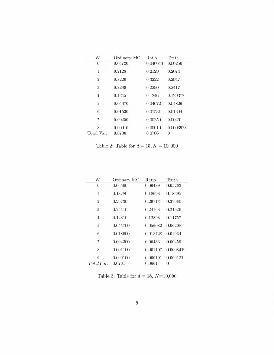
W Ordinary MC Ratio Truth0 0.04720 0.046644 0.06250

1 0.2128 0.2129 0.2074

2 0.3220 0.3222 0.2947

3 0.2289 0.2290 0.2417

4 0.1245 0.1246 0.129372

5 0.04670 0.04672 0.04826

6 0.01530 0.01531 0.01304

7 0.00250 0.00250 0.00261

8 0.00010 0.00010 0.0003923Total Var. 0.0700 0.0706 0

Table 2: Table for d = 15, N = 10, 000

W Ordinary MC Ratio Truth0 0.06590 0.06489 0.05263

1 0.18780 0.18698 0.18395

2 0.29730 0.29713 0.27960

3 0.24110 0.24168 0.24926

4 0.12810 0.12898 0.14757

5 0.055700 0.056082 0.06208

6 0.018600 0.018728 0.01934

7 0.004300 0.00433 0.00459

8 0.001100 0.001107 0.0008419

9 0.000100 0.000101 0.000121TotalV ar. 0.0701 0.0661 0

Table 3: Table for d = 18, N=10,000

9

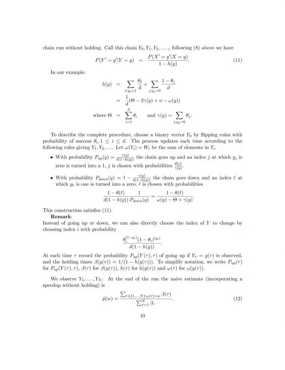
chain run without holding. Call this chain Y0, Y1, Y2, . . . ,, following (8) above we have

P (Y ′ = y′|Y = y) =P (X ′ = y′|X = y)

1− h(y). (11)

In our example:

h(y) =∑`:y`=1

θ`d

+∑j:yj=0

1− θjd

=1d

(Θ− 2γ(y) + n− ω(y))

where Θ =d∑i=1

θi and γ(y) =∑j:yj=0

θj .

To describe the complete procedure, choose a binary vector Y0 by flipping coins withprobability of success θi, 1 ≤ i ≤ d. The process updates each time according to thefollowing rules giving Y1, Y2, . . .. Let ω(Yi) = Wi be the sum of elements in Yi.

• With probability Pup(y) = γ(y)d(1−h(y)) the chain goes up and an index j at which yj is

zero is turned into a 1, j is chosen with probabilities θ(j)γ(y) .

• With probability Pdown(y) = 1 − γ(y)d(1−h(y)) the chain goes down and an index ` at

which y` is one is turned into a zero, ` is chosen with probabilities

1− θ(`)d(1− h(y))

1Pdown(y)

=1− θ(`)

ω(y)−Θ + γ(y).

This construction satisfies (11).Remark:

Instead of going up or down, we can also directly choose the index of Y to change bychoosing index i with probability

θ(1−yi)i (1− θi)(yi)

d(1− h(y)).

At each time τ record the probability Pup(Y (τ), τ) of going up if Yτ = y(τ) is observed,and the holding times β(y(τ)) = 1/(1 − h(y(τ))). To simplify notation, we write Pup(τ)for Pup(Y (τ), τ), β(τ) for β(y(τ)), h(τ) for h(y(τ)) and ω(τ) for ω(y(τ)).

We observe Y1, . . . , YN . At the end of the run the naive estimate (incorporating aspeedup without holding) is

p(w) =

∑τ∈{1,...,N}:ω(τ)=w β(τ)∑N

τ=1 βτ. (12)

10

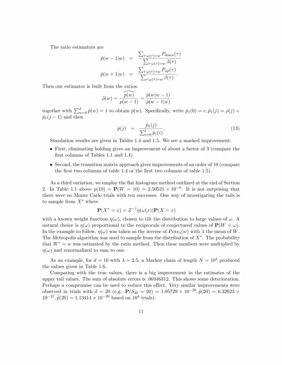
The ratio estimators are

p(w − 1|w) =

∑τ :ω(τ)=w Pdown(τ)∑τ :ω(τ)=w β(τ)

p(w + 1|w) =

∑τ :ω(τ)=w Pup(τ)∑τ :ω(τ)=w β(τ)

.

Then our estimator is built from the ratios:

ρ(w) =p(w)

p(w − 1)=p(w|w − 1)p(w − 1|w)

together with∑d

w=0 p(w) = 1 to obtain p(w). Specifically, write p1(0) = c, p1(j) = ρ(j)×p1(j − 1) and then

p(j) =p1(j)∑li=0 p1(i)

. (13)

Simulation results are given in Tables 1.4 and 1.5. We see a marked improvement:

• First, eliminating holding gives an improvement of about a factor of 3 (compare thefirst columns of Tables 1.1 and 1.4).

• Second, the transition matrix approach gives improvements of an order of 10 (comparethe first two columns of table 1.4 or the first two columns of table 1.5).

As a third variation, we employ the flat histogram method outlined at the end of Section2. In Table 1.1 above p(10) = P(W = 10) .= 2.50521 × 10−8. It is not surprising thatthere were no Monte Carlo trials with ten successes. One way of investigating the tails isto sample from X∗ where

P(X∗ = x) = Z−1η(ω(x))P(X = x)

with a known weight function η(ω), chosen to tilt the distribution to large values of ω. Anatural choice is η(ω) proportional to the reciprocals of conjectured values of P(W = ω).In the example to follow, η(ω) was taken as the inverse of Poisλ(w) with λ the mean of W .The Metropolis algorithm was used to sample from the distribution of X∗. The probabilitythat W ∗ = w was estimated by the ratio method. Then these numbers were multiplied byη(ω) and renormalized to sum to one.

As an example, for d = 10 with λ = 2.5, a Markov chain of length N = 104 producedthe values given in Table 1.6.

Comparing with the true values, there is a big improvement in the estimates of theupper tail values. The sum of absolute errors is .00346312. This shows some deterioration.Perhaps a compromise can be used to reduce this effect. Very similar improvements wereobserved in trials with d = 20 (e.g. P(S20 = 20) = 1.95729 × 10−20, p(20) = 6.32623 ×10−21, ˆp(20) = 1.13414× 10−20 based on 104 trials).

11

W No-hold MC Ratio Truth0 0.089593 0.090624 0.090909

1 0.26896 0.26621 0.26627

2 0.31977 0.32032 0.31950

3 0.20793 0.21047 0.21068

4 0.086466 0.085350 0.085601

5 0.023173 0.022639 0.022598

6 0.0037734 0.0039319 0.0039525

7 0.00034131 0.00045885 0.00045470

8 . . 0.00003306878307

9 . . 0.00000137786596

10 . . 0.00000002505211Total Var. 0.013190217 0.001309314 0

Table 4: Table for d = 10, N = 10, 000

W No-hold MC Hold-Ratio Truth0 0.055758 0.053261 0.052632

1.0 0.17837 0.18409 0.18395

2.0 0.27270 0.27890 0.27960

3.0 0.24988 0.24883 0.24926

4.0 0.15004 0.14743 0.14757

5.0 0.066245 0.062305 0.062078

6.0 0.021428 0.019493 0.019344

7.0 0.0047119 0.0046758 0.0045865

8.0 0.00082380 0.00089075 0.00084194

9.0 0.000044097 0.00012792 0.00012093Total Var. 0.0294353652 0.0018954746 0

Table 5: Table for d = 18, N=10,000

12

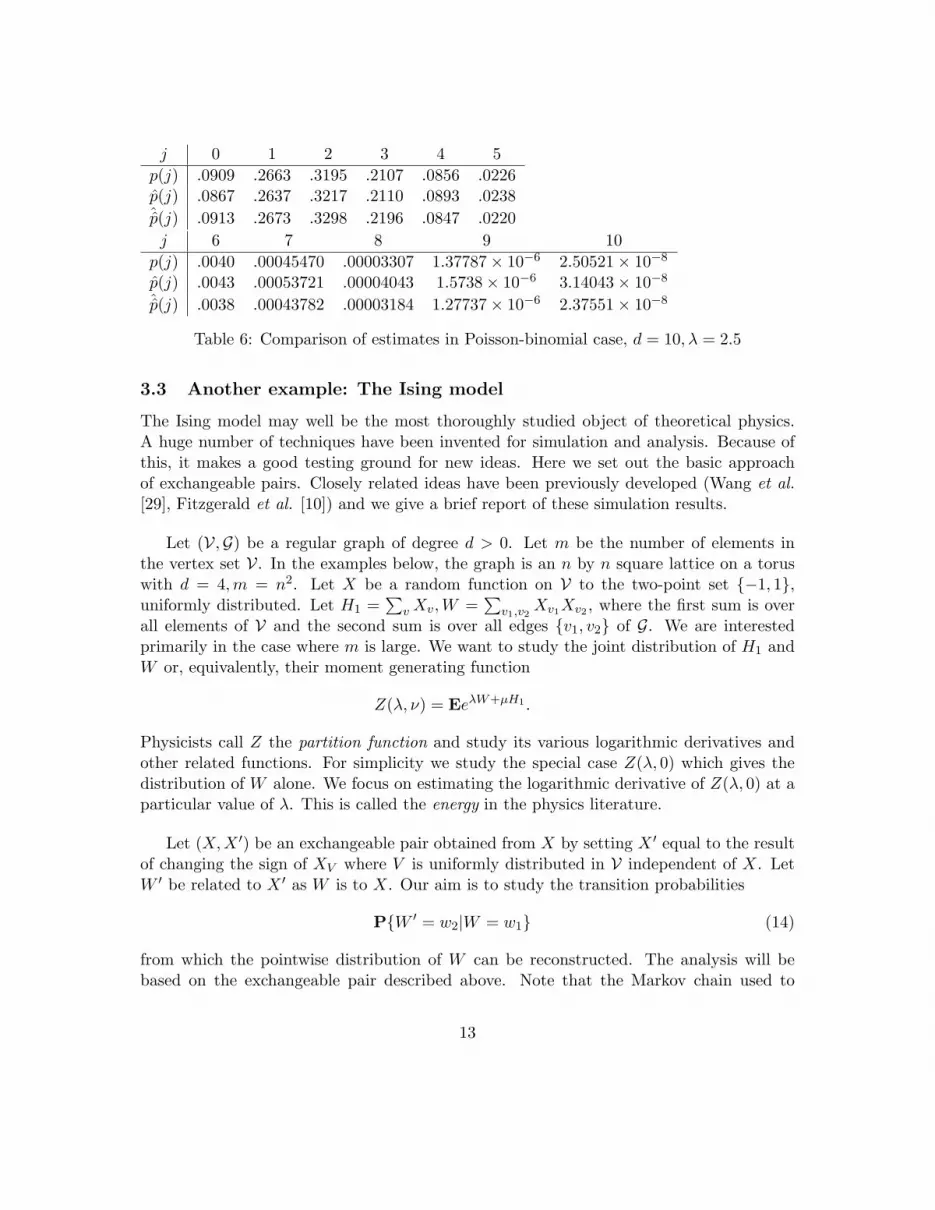
j 0 1 2 3 4 5p(j) .0909 .2663 .3195 .2107 .0856 .0226p(j) .0867 .2637 .3217 .2110 .0893 .0238ˆp(j) .0913 .2673 .3298 .2196 .0847 .0220j 6 7 8 9 10p(j) .0040 .00045470 .00003307 1.37787× 10−6 2.50521× 10−8

p(j) .0043 .00053721 .00004043 1.5738× 10−6 3.14043× 10−8

ˆp(j) .0038 .00043782 .00003184 1.27737× 10−6 2.37551× 10−8

Table 6: Comparison of estimates in Poisson-binomial case, d = 10, λ = 2.5

3.3 Another example: The Ising model

The Ising model may well be the most thoroughly studied object of theoretical physics.A huge number of techniques have been invented for simulation and analysis. Because ofthis, it makes a good testing ground for new ideas. Here we set out the basic approachof exchangeable pairs. Closely related ideas have been previously developed (Wang et al.[29], Fitzgerald et al. [10]) and we give a brief report of these simulation results.

Let (V,G) be a regular graph of degree d > 0. Let m be the number of elements inthe vertex set V. In the examples below, the graph is an n by n square lattice on a toruswith d = 4,m = n2. Let X be a random function on V to the two-point set {−1, 1},uniformly distributed. Let H1 =

∑vXv,W =

∑v1,v2

Xv1Xv2 , where the first sum is overall elements of V and the second sum is over all edges {v1, v2} of G. We are interestedprimarily in the case where m is large. We want to study the joint distribution of H1 andW or, equivalently, their moment generating function

Z(λ, ν) = EeλW+µH1 .

Physicists call Z the partition function and study its various logarithmic derivatives andother related functions. For simplicity we study the special case Z(λ, 0) which gives thedistribution of W alone. We focus on estimating the logarithmic derivative of Z(λ, 0) at aparticular value of λ. This is called the energy in the physics literature.

Let (X,X ′) be an exchangeable pair obtained from X by setting X ′ equal to the resultof changing the sign of XV where V is uniformly distributed in V independent of X. LetW ′ be related to X ′ as W is to X. Our aim is to study the transition probabilities

P{W ′ = w2|W = w1} (14)

from which the pointwise distribution of W can be reconstructed. The analysis will bebased on the exchangeable pair described above. Note that the Markov chain used to

13

simulate realizations may be very different from the single site dynamics which underlyour exchangeable pair. Thus the Markov chain may be generated by the Swendsen-Wangalgorithm or, in the case of a bipartite graph (V,G) by an alternating (checkerboard)algorithm. To compute an estimate of (14) consider the random variables

Yv =∑

v′:(v,v′)neighbors

Xv′δv,v′(G)

W =12

∑v

XvYv.

Then

W ′ −W = ω(X ′)− ω(X) = −XvYv.

Thus the conditional distribution of W ′−W given X is given by PX{W ′−W = d} = s(d,x)m ,

where s(d, x) = |{v : XvYv = −d}|. This gives the needed ingredients to take the outputof a Markov chain X∗0 , X

∗1 , . . ., where

P{X∗i = x} = Z−1(λ, 0)eλω(x)P(X = x).

Then, the procedure outlined in Sections 2.1, 2.2 can be used. This first derives estimatesof ratios in (14) and then of P(W = w). These may be used to estimate Z′

Z by∑w we

λwpW (w)∑w e

λwpW (w).

(Here Z ′ denotes the derivative.)A version of this approach has been implemented by Fitzgerald et al. [10]. They

carried out a large simulation to assess the improvement in mean-square error due to theirversion of the transition density method. They studied the expected value of H2

1 (magneticsusceptibility) when λ = .42 and µ = 0. This is just slightly above the critical temperature.Their Markov chain was the result of a single sweep through the 900 sites. In this case thetrue expectation is known. They chose N = 5 × 106 sweeps and repeated the entire run500 times. They calculated the average error for t = 1, . . . , 5× 106. They found relativelysmooth decrease of the mean-squared error in t. The transition density method improvedmean-squared error over the naive estimator by about 25 %.

They carried out a similar experiment for another functional (specific heat) and foundan improvement of about 7 %.

Fitzgerald et al. [10] report a more naive method of estimating p(w′|w) based oncounting the proportion of w to w′ transitions in a chain generated by single site updatesshowed no improvement over the naive estimator. We hope to try adjusting for holdingtimes in later work.

14

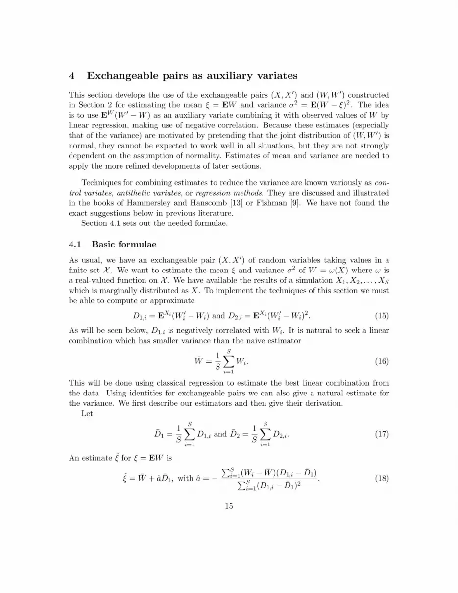
4 Exchangeable pairs as auxiliary variates

This section develops the use of the exchangeable pairs (X,X ′) and (W,W ′) constructedin Section 2 for estimating the mean ξ = EW and variance σ2 = E(W − ξ)2. The ideais to use EW (W ′ −W ) as an auxiliary variate combining it with observed values of W bylinear regression, making use of negative correlation. Because these estimates (especiallythat of the variance) are motivated by pretending that the joint distribution of (W,W ′) isnormal, they cannot be expected to work well in all situations, but they are not stronglydependent on the assumption of normality. Estimates of mean and variance are needed toapply the more refined developments of later sections.

Techniques for combining estimates to reduce the variance are known variously as con-trol variates, antithetic variates, or regression methods. They are discussed and illustratedin the books of Hammersley and Hanscomb [13] or Fishman [9]. We have not found theexact suggestions below in previous literature.

Section 4.1 sets out the needed formulae.

4.1 Basic formulae

As usual, we have an exchangeable pair (X,X ′) of random variables taking values in afinite set X . We want to estimate the mean ξ and variance σ2 of W = ω(X) where ω isa real-valued function on X . We have available the results of a simulation X1, X2, . . . , XS

which is marginally distributed as X. To implement the techniques of this section we mustbe able to compute or approximate

D1,i = EXi(W ′i −Wi) and D2,i = EXi(W ′i −Wi)2. (15)

As will be seen below, D1,i is negatively correlated with Wi. It is natural to seek a linearcombination which has smaller variance than the naive estimator

W =1S

S∑i=1

Wi. (16)

This will be done using classical regression to estimate the best linear combination fromthe data. Using identities for exchangeable pairs we can also give a natural estimate forthe variance. We first describe our estimators and then give their derivation.

Let

D1 =1S

S∑i=1

D1,i and D2 =1S

S∑i=1

D2,i. (17)

An estimate ξ for ξ = EW is

ξ = W + aD1, with a = −∑S

i=1(Wi − W )(D1,i − D1)∑Si=1(D1,i − D1)2

. (18)

15

An estimate σ2 for σ2 = VarW is

σ2 = − 12S

(∑Si=1D2,i

)(∑Si=1(Wi − W )2

)∑S

i=1(Wi − W )(D1,i − D1). (19)

To begin, let us show that W and EX(W ′−W ) are negatively correlated. For this assumewithout loss of generality that the mean ξ = 0. First, (W ′ + W )(W ′ − W ) is an anti-symmetric function of (W,W ′), so that E(W ′ +W )(W ′ −W ) = 0 = EW ′2 − EW 2. ThusEW ′2 = EW 2. Then

E(W ′ −W )2 = E(W ′)2 + EW 2 − 2EWW ′

= 2EW 2 − 2EWW ′ = −2E(W (W ′ −W ))= −2E(WEX(W ′ −W )).

It follows that E(WEX(W ′ −W )) ≤ 0, with strict inequality unless W = W ′.

To motivate the estimate ξ of (18) observe that both W and W + D1 are unbiasedestimates of ξ = EW . It is reasonable to estimate ξ by a linear combination of thesewith coefficients adding to 1 determined from the data in the same way as a regressioncoefficient. This leads to

ξa = a(W + D1) + (1− a)W = W + aD1,

with a given in (18).

This is related to the problem of finding the best linear predictor of W using EX(W ′−W ).Indeed, writing

W = ξ + aEX(W ′ −W ) +R (20)

with ER = 0,ERW = 0, the coefficient yielding the smallest variance between observedand predicted is

a =Cov(W,EX(W ′ −W ))

Var(EX(W ′ −W )).

Estimating a leads to (18). Note that estimating

ξ = W − aEX(W ′ −W ), (21)

we obtain

Var(ξ) = VarW (1− Corr2(W,EX(W ′ −W ))).

16

Note that this quantity is smaller than VarW , and thus improves on the standard estimateof estimating ξ by W .

To understand this approach better, we now focus on the perfect case. Suppose we havean exchangeable pair (W,W ′) and a constant λ, 0 < λ < 1, such that

EW (W ′ −W ) = −λ(W − ξ). (22)

There are many examples when (22) is satisfied, see [27]. Because w′ − w is an antisym-metric function in (w,w′) we have

EEW (W ′ −W ) = 0 = −λE(W − ξ),

yielding ξ = EW . Note that ξ can also be written as

ξ = W +1λEW (W ′ −W ). (23)

We see this as the sum of two antithetic random variables because

E(W ′ −W )2 = −2EWEW (W ′ −W ),

thus EWEW (W ′−W ) < 0, so W and EW (W ′−W ) are negatively correlated. Under (22),we have

E(W ′ −W )2 = −2λEW (W − ξ) = −2λ(EW 2 − ξ2) = −2λVarW,

so that the two components have covariance

Cov(W,

1λEW (W ′ −W )

)=

1λEWEW (W ′ −W ) = −VarW.

We also remark that given (22) we know that

λ =12E(W ′ −W )2

VarW.

We estimate λ using the regression approach :

λ =∑

i(D1,i − D1)(Wi − W )∑i(Wi − W )2

and

σ2 =E(W ′ −W )2

2λ

2λ = −∑

iD2,i∑′

i(W′i − W )2

2S∑

i(D1,i − D1)(Wi − W ).

This leads to (19).

17

Approximate case

Suppose now that

EW (W ′ −W ) = −λ(W − ξ) +R. (24)

Here, (24) and exchangeability imply that if EW = ξ then ER = 0 and conversely ifER = 0 then EW = ξ.If we want to estimate ξ we can write

ξ = W +1λEW (W ′ −W )− 1

λR.

The right hand side leads to the antithetic variables W − 1λR and 1

λEW (W ′ −W ):

Cov(W − 1λR,

1λEW (W ′ −W )) =

= E(W − 1

λR− ξ, 1

λEW (W ′ −W )

)= −E[(W − 1

λR− ξ)(W − 1

λR− ξ)]

= −Var(W − 1λR) < 0.

As to the estimate of variance; if R is small, it can be effectively neglected and calculationsfor the perfect case above are in force; yet a further justification for σ is given next.

As a regression problem

Write ξ = W − β(EWW ′−W ), this is an unbiased estimate of ξ. For all β to minimize itsvariance:

Var(ξ) = VarW − 2βCov(W,EWW ′ −W ) + β2Var(EWW ′ −W )

Choose β =Cov(W,EWW ′ −W )

Var(EWW ′ −W )In fact, with our perfect case notation

λ = − 1β

= − VarEWW ′ −WCov(W,EWW ′ −W )

.

This can be estimated by:

λ = −∑

i(Di,1 −D1)2∑(Wi − W )(Di,1 − D1)

.

Another extension is the following. To simplify we have been conditioning on the valuesof Wi = ω(Xi). It is also possible to rewrite all the above conditioning on the larger stateXi; this is what is suggested in practice.

18

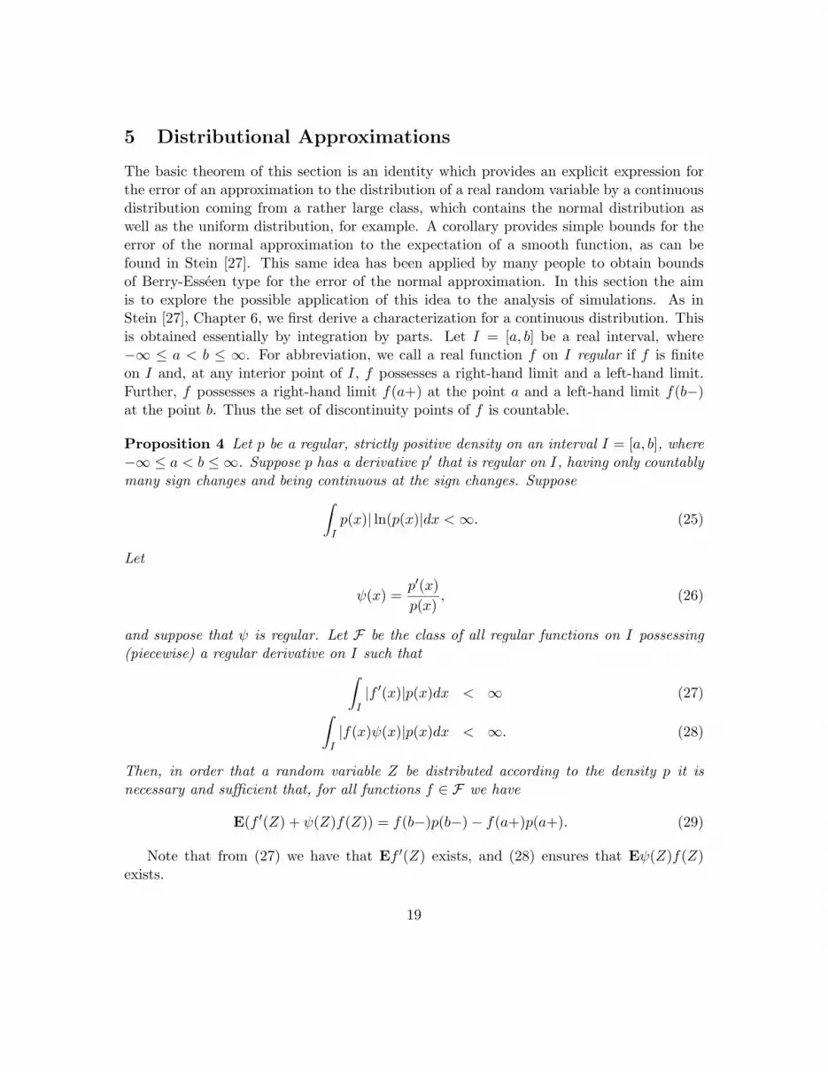
5 Distributional Approximations

The basic theorem of this section is an identity which provides an explicit expression forthe error of an approximation to the distribution of a real random variable by a continuousdistribution coming from a rather large class, which contains the normal distribution aswell as the uniform distribution, for example. A corollary provides simple bounds for theerror of the normal approximation to the expectation of a smooth function, as can befound in Stein [27]. This same idea has been applied by many people to obtain boundsof Berry-Esseen type for the error of the normal approximation. In this section the aimis to explore the possible application of this idea to the analysis of simulations. As inStein [27], Chapter 6, we first derive a characterization for a continuous distribution. Thisis obtained essentially by integration by parts. Let I = [a, b] be a real interval, where−∞ ≤ a < b ≤ ∞. For abbreviation, we call a real function f on I regular if f is finiteon I and, at any interior point of I, f possesses a right-hand limit and a left-hand limit.Further, f possesses a right-hand limit f(a+) at the point a and a left-hand limit f(b−)at the point b. Thus the set of discontinuity points of f is countable.

Proposition 4 Let p be a regular, strictly positive density on an interval I = [a, b], where−∞ ≤ a < b ≤ ∞. Suppose p has a derivative p′ that is regular on I, having only countablymany sign changes and being continuous at the sign changes. Suppose∫

Ip(x)| ln(p(x)|dx <∞. (25)

Let

ψ(x) =p′(x)p(x)

, (26)

and suppose that ψ is regular. Let F be the class of all regular functions on I possessing(piecewise) a regular derivative on I such that∫

I|f ′(x)|p(x)dx < ∞ (27)∫

I|f(x)ψ(x)|p(x)dx < ∞. (28)

Then, in order that a random variable Z be distributed according to the density p it isnecessary and sufficient that, for all functions f ∈ F we have

E(f ′(Z) + ψ(Z)f(Z)) = f(b−)p(b−)− f(a+)p(a+). (29)

Note that from (27) we have that Ef ′(Z) exists, and (28) ensures that Eψ(Z)f(Z)exists.

19

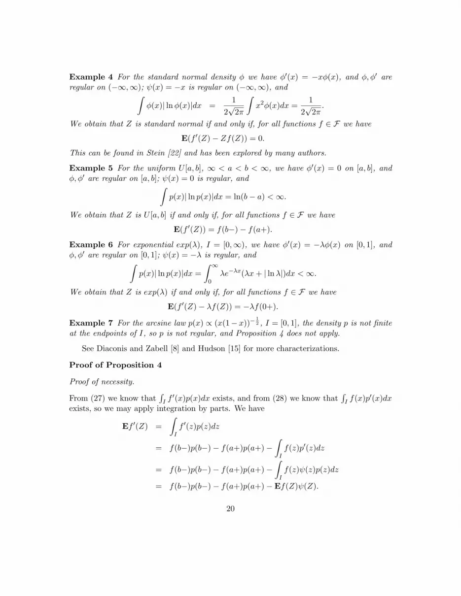
Example 4 For the standard normal density φ we have φ′(x) = −xφ(x), and φ, φ′ areregular on (−∞,∞); ψ(x) = −x is regular on (−∞,∞), and∫

φ(x)| lnφ(x)|dx =1

2√

2π

∫x2φ(x)dx =

12√

2π.

We obtain that Z is standard normal if and only if, for all functions f ∈ F we have

E(f ′(Z)− Zf(Z)) = 0.

This can be found in Stein [22] and has been explored by many authors.

Example 5 For the uniform U [a, b], ∞ < a < b < ∞, we have φ′(x) = 0 on [a, b], andφ, φ′ are regular on [a, b]; ψ(x) = 0 is regular, and∫

p(x)| ln p(x)|dx = ln(b− a) <∞.

We obtain that Z is U [a, b] if and only if, for all functions f ∈ F we have

E(f ′(Z)) = f(b−)− f(a+).

Example 6 For exponential exp(λ), I = [0,∞), we have φ′(x) = −λφ(x) on [0, 1], andφ, φ′ are regular on [0, 1]; ψ(x) = −λ is regular, and∫

p(x)| ln p(x)|dx =∫ ∞

0λe−λx(λx+ | lnλ|)dx <∞.

We obtain that Z is exp(λ) if and only if, for all functions f ∈ F we have

E(f ′(Z)− λf(Z)) = −λf(0+).

Example 7 For the arcsine law p(x) ∝ (x(1− x))−12 , I = [0, 1], the density p is not finite

at the endpoints of I, so p is not regular, and Proposition 4 does not apply.

See Diaconis and Zabell [8] and Hudson [15] for more characterizations.

Proof of Proposition 4

Proof of necessity.

From (27) we know that∫I f′(x)p(x)dx exists, and from (28) we know that

∫I f(x)p′(x)dx

exists, so we may apply integration by parts. We have

Ef ′(Z) =∫If ′(z)p(z)dz

= f(b−)p(b−)− f(a+)p(a+)−∫If(z)p′(z)dz

= f(b−)p(b−)− f(a+)p(a+)−∫If(z)ψ(z)p(z)dz

= f(b−)p(b−)− f(a+)p(a+)−Ef(Z)ψ(Z).

20

Proof of sufficiency.

Let Z be a real random variable such that, for all functions f ∈ F , (29) holds, and let hbe an arbitrary measurable function for which∫

I|h(z)|p(z)dz <∞. (30)

Let f be the particular solution of the differential equation

f ′(z) + ψ(z)f(z) = h(z)− Ph (31)

given by

f(z) =

∫ za (h(x)− Ph)p(x)dx

p(z), (32)

where

Ph =∫Ih(z)p(z)dz.

We want to show that f ∈ F , for then, (29) holds, yielding

0 = E(f ′(Z) + ψ(Z)f(Z))− f(b−)p(b−) + f(a+)p(a+)= Eh(Z)− Ph.

As the class of all measurable regular functions h satisfying (30) contains the indicatorfunctions of Borel sets and hence is is measure-determining for p, this would prove that Zhas density p.

From (32) we have that f is regular and f(b−)p(b−) = f(a+)p(a+) = 0 and∫I|f ′(z)|p(z)dz ≤

∫I|h(z)|p(z)dz + Ph+

∫I|f(z)ψ(z)|p(z)dz,

so that it suffices to prove that (28) holds. We have∫I|f(z)ψ(z)|p(z)dz =

∫I|f(z)p′(z)|dz

≤∫I

|p′(z)|p(z)

∫ b

z|h(x)− Ph|p(x)dxdz.

Denote by c1 < c2 < · · · the sign change points of p′ and hence of φ, and note that dueto the continuity assumption ψ(ci) = 0, i = 1, 2, . . .. Let Ai = (ai1 , ai2), i = 1, 2, . . . be the

21

intervals where ψ > 0 and let Bj = (bj1 , bj2), j = 1, 2, . . . be the intervals where ψ ≤ 0.Then ∫

I

|p′(z)|p(z)

∫ b

z|h(x)− Ph|p(x)dxdz

=∞∑i=1

∫Ai

ψ(z)∫ b

z|h(x)− Ph|p(x)dxdz

−∞∑j=1

∫Bj

ψ(z)∫ b

z|h(x)− Ph|p(x)dxdz.

Note that ψ(z) = (ln p(z))′ and ln p(z) is regular, so we can apply integration by partsagain to obtain that the above equals

∞∑i=1

{∫Ai

|h(x)− Ph|p(x) ln(p(x))dx−[|h(x)− Ph|p′(x)

]ai2ai1

}dxdz

−∞∑j=1

∫Bj

{|h(x)− Ph|p(x) ln(p(x))dx−

[|h(x)− Ph|p′(x)

]bj2bj1

}dxdz

≤∫I|h(x)− Ph|p(x) ln(p(x))dx

+|h(b−)− Ph|p′(b−) + |h(a+)− Ph|p′(a+)< ∞,

due to (25).

Proposition 4 will be used to obtain a general approximation theorem. Under the assump-tion of Proposition 4, let for convenience

φ(x) = −ψ(x). (33)

Note that, from (29),

Eψ(Z) = p(b−)− p(a+)

and

Eψ(Z)Z = bp(b−)− ap(a+)− 1.

We will often have the case that

Eφ(Z) ≈ 0, Eφ(Z)Z ≈ 1.

22

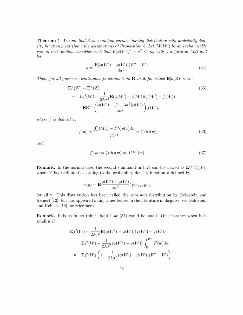
Theorem 1 Assume that Z is a random variable having distribution with probability den-sity function p satisfying the assumptions of Proposition 4. Let (W,W ′) be an exchangeablepair of real random variables such that E(φ(W ))2 = σ2 < ∞, with φ defined at (33) andlet

λ =E(φ(W ′)− φ(W ))(W ′ −W )

2σ2. (34)

Then, for all piecewise continuous functions h on R to R for which E|h(Z)| <∞,

Eh(W )−Eh(Z) (35)

= Ef ′(W )− 12λσ2

E(φ(W ′)− φ(W ))(f(W ′)− f(W ))

−EEW

(φ(W ′)− (1− λσ2)φ(W )

λσ2

)f(W ),

where f is defined by

f(w) =

∫ za (h(x)− Ph)p(x)dx

p(z)= (Uh)(w) (36)

and

f ′(w) = (V h)(w) = (Uh)′(w). (37)

Remark. In the normal case, the second summand in (37) can be viewed as E(V h)(Y ),where Y is distributed according to the probability density function π defined by

π(y) = Eφ(W ′)− φ(W )

λσ2δ{W<y<W ′}.

for all y. This distribution has been called the zero bias distribution by Goldstein andReinert [12], but has appeared many times before in the literature in disguise; see Goldsteinand Reinert [12] for references.

Remark. It is useful to think about how (35) could be small. One instance when it issmall is if

Ef ′(W )− 12λσ2

E(φ(W ′)− φ(W ))(f(W ′)− f(W ))

= Ef ′(W )− 12λσ2

(φ(W ′)− φ(W ))∫ W ′

Wf ′(w)dw

≈ Ef ′(W )(

1− 12λσ2

(φ(W ′)− φ(W ))(W ′ −W )).

23

From (34) we have that

12λσ2

E(φ(W ′)− φ(W ))(W ′ −W ) = 1,

so that

Ef ′(W )− 12λσ2

E(φ(W ′)− φ(W ))(f(W ′)− f(W )) ≈ 0.

Moreover, if

EWφ(W ′) = (1− λσ2)φ(W )

then

EEW

(φ(W ′)− (1− λσ2)φ(W )

λσ2

)f(W ) = 0

relating to Condition (22).

Proof of Theorem 1

Let f ∈ F be a function on I to R, where F is as in Proposition 4. For any antisymmetricfunction F on R2 to R,

EF (W,W ′) = 0. (38)

Applying this to the function F defined by

F (w1, w2) =(φ(w2)− φ(w1))(f(w1) + f(w2))

2λσ2

=φ(w2)− φ(w1)

λσ2f(w1)

+φ(w2)− φ(w1)

2λσ2(f(w2)− f(w1)),

we obtain

E[φ(W ′)− φ(W )

λσ2f(W )− φ(W ′)− φ(W )

2λσ2(f(W ′)− f(W ))

]= 0.

This can be rewritten in the form

E[−φ(W )f(W ) +

φ(W ′)− (1− λσ2)φ(W )λσ2

f(W )

+φ(W ′)− φ(W )

2λσ2

∫ W ′

Wf ′(w)dw

]= 0.

24

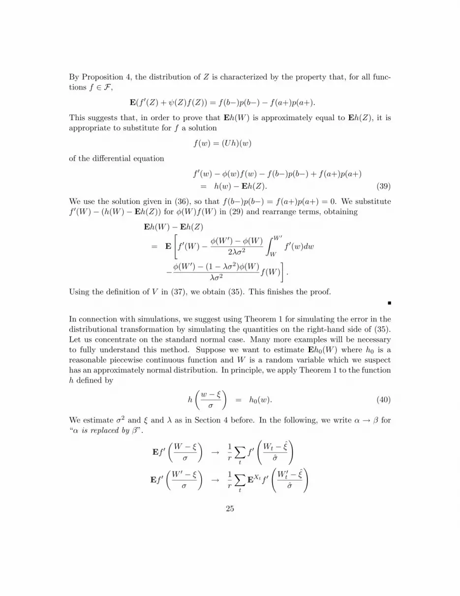
By Proposition 4, the distribution of Z is characterized by the property that, for all func-tions f ∈ F ,

E(f ′(Z) + ψ(Z)f(Z)) = f(b−)p(b−)− f(a+)p(a+).

This suggests that, in order to prove that Eh(W ) is approximately equal to Eh(Z), it isappropriate to substitute for f a solution

f(w) = (Uh)(w)

of the differential equation

f ′(w)− φ(w)f(w)− f(b−)p(b−) + f(a+)p(a+)= h(w)−Eh(Z). (39)

We use the solution given in (36), so that f(b−)p(b−) = f(a+)p(a+) = 0. We substitutef ′(W )− (h(W )−Eh(Z)) for φ(W )f(W ) in (29) and rearrange terms, obtaining

Eh(W )−Eh(Z)

= E

[f ′(W )− φ(W ′)− φ(W )

2λσ2

∫ W ′

Wf ′(w)dw

−φ(W ′)− (1− λσ2)φ(W )λσ2

f(W )].

Using the definition of V in (37), we obtain (35). This finishes the proof.

In connection with simulations, we suggest using Theorem 1 for simulating the error in thedistributional transformation by simulating the quantities on the right-hand side of (35).Let us concentrate on the standard normal case. Many more examples will be necessaryto fully understand this method. Suppose we want to estimate Eh0(W ) where h0 is areasonable piecewise continuous function and W is a random variable which we suspecthas an approximately normal distribution. In principle, we apply Theorem 1 to the functionh defined by

h

(w − ξσ

)= h0(w). (40)

We estimate σ2 and ξ and λ as in Section 4 before. In the following, we write α → β for“α is replaced by β”.

Ef ′(W − ξσ

)→ 1

r

∑t

f ′

(Wt − ξσ

)

Ef ′(W ′ − ξσ

)→ 1

r

∑t

EXtf ′

(W ′t − ξσ

)

25

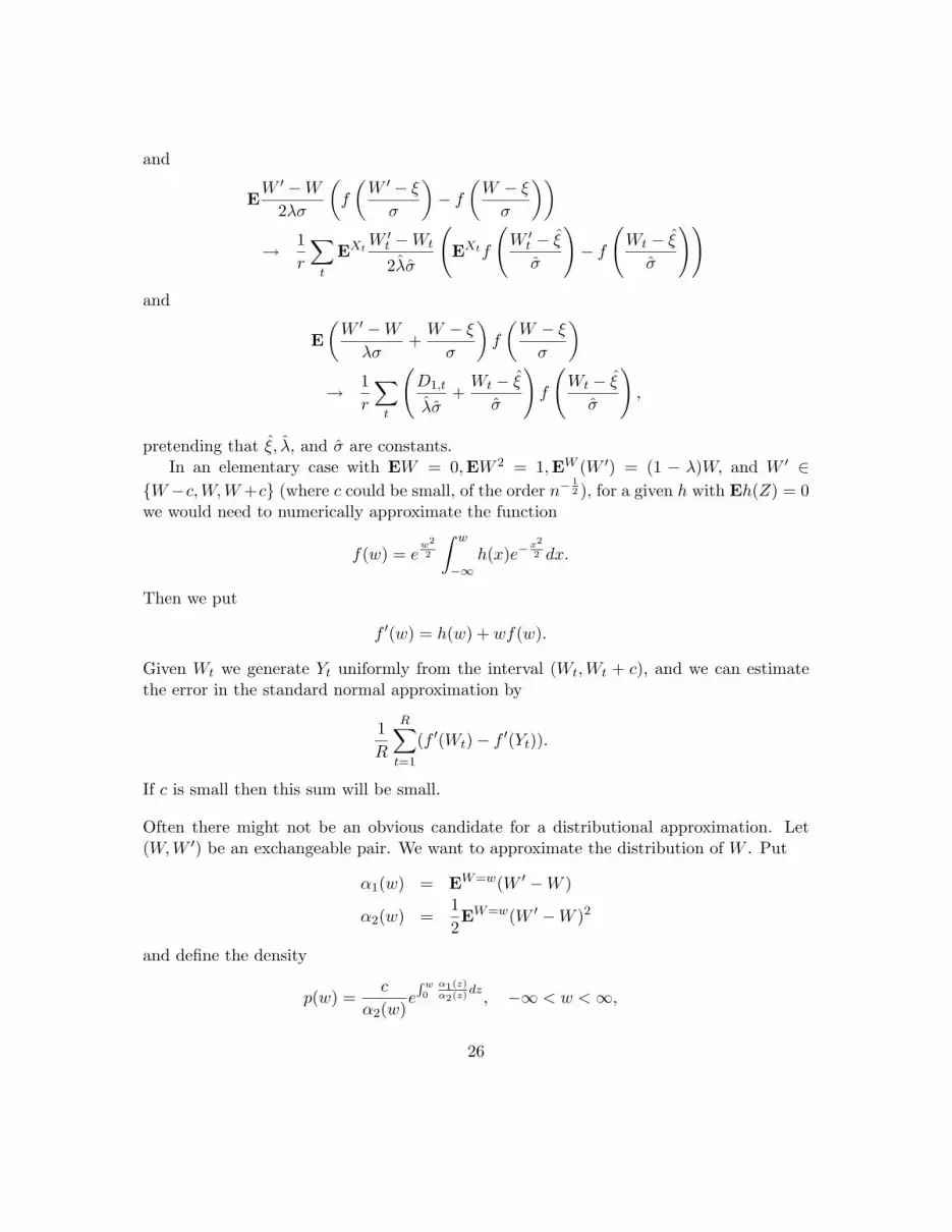
and

EW ′ −W

2λσ

(f

(W ′ − ξσ

)− f

(W − ξσ

))→ 1

r

∑t

EXtW′t −Wt

2λσ

(EXtf

(W ′t − ξσ

)− f

(Wt − ξσ

))and

E(W ′ −Wλσ

+W − ξσ

)f

(W − ξσ

)→ 1

r

∑t

(D1,t

λσ+Wt − ξσ

)f

(Wt − ξσ

),

pretending that ξ, λ, and σ are constants.In an elementary case with EW = 0,EW 2 = 1,EW (W ′) = (1 − λ)W, and W ′ ∈

{W−c,W,W+c} (where c could be small, of the order n−12 ), for a given h with Eh(Z) = 0

we would need to numerically approximate the function

f(w) = ew2

2

∫ w

−∞h(x)e−

x2

2 dx.

Then we put

f ′(w) = h(w) + wf(w).

Given Wt we generate Yt uniformly from the interval (Wt,Wt + c), and we can estimatethe error in the standard normal approximation by

1R

R∑t=1

(f ′(Wt)− f ′(Yt)).

If c is small then this sum will be small.

Often there might not be an obvious candidate for a distributional approximation. Let(W,W ′) be an exchangeable pair. We want to approximate the distribution of W . Put

α1(w) = EW=w(W ′ −W )

α2(w) =12EW=w(W ′ −W )2

and define the density

p(w) =c

α2(w)e

R w0

α1(z)α2(z)

dz, −∞ < w <∞,

26

where c is determined by the condition that∫p(w)dw = 1. Note that

ψ(w) =p′(w)p(w)

=α1(w)− α′2(w)

α2(w)

is of Pearson type. If p satisfies the assumptions of Proposition 4 with p(−∞) = p(∞) = 0,then any random variable Z has density p if and only if, for all f ∈ F ,

Ef ′(Z) + φ(Z)f(Z) = 0.

Theorem 2 In the above situation, let Z have density p defined by (41). Then, for allregular functions h such that

∫|h(x)|p(x)dx <∞ we have

Eh(W ) = Eh(Z) = −E{R1

(g

α2

)(W,W ′)

},

where

R1 (f) (w,w′) =12

(w′ − w)(f(w′)− f(w))

−14

(w′ − w)2(f ′(w′)− f(w)) (41)

and

g(z) =1p(z)

∫ z

−∞(h(x)− Ph)p(x)dx. (42)

Proof of Theorem 2

We use the antisymmetric function

F (w,w′) =12

(w′ − w)(f(w′) + f(w))

= (w′ − w)f(w) +12

(w′ − w)(f(w′)− f(w))

= (w′ − w)f(w) +12

(w′ − w)2f(w′) + f(w)

2

+12

(w′ − w)(f(w′)− f(w))− 14

(w′ − w)2(f(w′) + f(w))

= (w′ − w)f(w) +12

(w′ − w)2f(w′) + f(w)

2+R1(f)(w,w′),

where R1(f)(w,w′) is given in (41). Thus, from (38),

0 = EF (W,W ′)

27

giving

0 = EEW (W ′ −W )f(W ) +12EEW (W ′ −W )2

f(W ′) + f(W )2

+ER1(f)(W,W ′).

Put g(w) = α2(w)f(w), so that

f ′(w) =g′(w)α2(w)

− g(w)α′2(w)

(α2(w))2.

We obtain

ER1(f)(W,W ′) = E{R1

(g

α2

)(W,W ′)

}= E

{α1(W )α2(W )

g(W ) +α2(W )g′(W )− g(W )α′2(W )

α2(W )

}= E

{α1(W )− α′2(W )

α2(W )g(W ) + g′(W )

}= Eψ(W )g(W ) + g′(W )= Eh(W )−Eh(Z).

Here, h and g are related through g given in 42.

In particular,

Eh(W ) = Eh(Z) + EEWR1

(g

α2

)(W,W ′)

= Eh(Z) + ER2(g)(W ),

where

R2(g)(w) = EW=wR1

(g

α2

)(W,W ′).

Thus, from R observations we can estimate

Eh(W ) = Eh(Z) +1R

R∑t=1

EXtR1

(g

α2

)(Wt,W

′t).

28

References

[1] D.J. Aldous (1981). Representations for Partially Exchangeable Arrays of Ran-dom Variables. J. Multivariate Anal. 11, 581-598.

[2] D. Aldous and J.A. Fill (2003) Markov Chains, book available on the webat: http://www.stat.berkeley.edu/~aldous/.

[3] H.J. Arnold, B.D. Bucher, H.F. Trotter, and J.W. Tukey (1956).Monte Carlo techniques in a complex problem about normal samples. Sympo-sium on Monte Carlo methods. H.A. Meyer, ed., Wiley, New York; 80–88.

[4] L.J. Billera and P. Diaconis (2001). A geometric interpretation of theMetropolis-Hastings algorithm. Statistical Science, vol. 16, no 4, pages 335–339.

[5] P. Diaconis (1989). An example for Stein’s method. in this volume, chapter 2.

[6] P. Diaconis (1988). Recent progress in de Finetti’s notions of exchangeability.In Bayesian Statistics vol. 3, J. Bernardo et al. (eds), Oxford Press, Oxford, 111-125

[7] P. Diaconis and Sturmfels (1998). Algebraic Algorithms for Sampling fromConditional Distributions. Ann. Statist. 26, 363–397.

[8] P. Diaconis and S. Zabell (1991). Closed form summation for classical dis-tributions: Variations on a theme of de Moivre Statistical Science 6, 284–302.

[9] G.S. Fishman (1996). Monte Carlo : Concepts, Algorithms, and Applications.Springer, New York etc.

[10] M. Fitzgerald, R.R. Picard, and R.N. Silver (2000). Monte Carlo tran-sition dynamics and variance reduction. J. Statist. Phys. 98, 321–345.

[11] J. Fulman (2001). A Stein’s method proof of the asymptotic normality ofdescents and inversions in the symmetric group. In this volume, chapter 4.

[12] L. Goldstein and G. Reinert (1997). Stein’s method and the zero biastransformation with application to simple random sampling. Ann. Appl. Probab.7, 935–952.

[13] J.M. Hammersley and D.C. Hanscomb (1965). Monte Carlo Methods.Methuen, London.

[14] M. Huber and G. Reinert (2000). The stationary distribution in the antivotermodel: exact sampling and approximations. In this volume, chapter 5.

29

[15] H.M. Hudson (1978). A natural identity for exponential families with applica-tions in multiparameter estimation. Ann. Statist. 6, 473–484.

[16] J.C.F. Kingman (1978). Uses of exchangeability. Ann. Probab. 6, 183–197.

[17] J.S. Liu (2001). Monte Carlo Strategies in Scientific Computing. Springer, NewYork.

[18] N. Metropolis, A.W. Rosenbluth, M.N. Rosenbluth, A.H. Teller, andE. Teller (1953). Equations of state calculations by fast computing machines.J. Chem. Phys. 21, 1087–1092.

[19] M.E.J. Newman and G.T. Barkema (1999) Monte Carlo Methods in Statis-tical Physics. Clarendon Press, Oxford.

[20] P.M.C. de Oliveira, T.J.P. Penna, and H.J. Herrmann (1998). Broadhistogram Monte Carlo. Eur. Phys. J. B 1, 205–208.

[21] Y. Rinott and V. Rotar (1997). On coupling constructions and rates inthe clt for dependent summands with applications to the anti-voter model andweighted U-statistics. Ann. Applied Probability 7, 1080–1105.

[22] C. Stein (1972). A bound for the error in the normal approximation to thedistribution of a sum of dependent random variables. Proc. Sixth Berkeley Symp.Math. Statist. Probab. 2, 583–602. Univ. California Press, Berkeley.

[23] C. Stein (1978). Asymptotic evaluation of the number of Latin rectangles. J.Combinat. Theory A 25, 38–49.

[24] C. Stein (1996). Trace of random matrix, Stanford Statistics Dept, TechnicalReport, 1996.

[25] C. Stein (1967). Class notes from course taught at Stanford, notes taken byLincoln Moses.

[26] C. Stein (1988). Application of Newton’s identities to a generalized birthdayproblem and to the Poisson binomial distribution. Stanford, Technical Report.

[27] C. Stein (1986). Approximate Computation of Expectations. IMS, Hayward,California.

[28] H.F. Trotter and J.W. Tukey (1956). Conditional Monte Carlo for normalsamples. Symposium on Monte Carlo methods. H.A. Meyer, ed., Wiley, New York;64–79.

[29] J.S. Wang, T.K. Tay, and R.H. Swendsen (1999). Transition matrix MonteCarlo reweighting and dynamics. Phys. Rev. Lett. 82, 476–479.

30