Citation: Moon, J.; Lee, J.; Lee, S.;

Yun, H. Urban River Dissolved

Oxygen Prediction Model Using

Machine Learning. Water 2022, 14,

1899. https://doi.org/10.3390/

w14121899

Academic Editors: Celestine Iwendi

and Thippa Reddy Gadekallu

Received: 3 May 2022

Accepted: 9 June 2022

Published: 13 June 2022

Publisher’s Note: MDPI stays neutral

with regard to jurisdictional claims in

published maps and institutional affil-

iations.

Copyright: © 2022 by the authors.

Licensee MDPI, Basel, Switzerland.

This article is an open access article

distributed under the terms and

conditions of the Creative Commons

Attribution (CC BY) license (https://

creativecommons.org/licenses/by/

4.0/).

water

Article

Urban River Dissolved Oxygen Prediction Model UsingMachine LearningJuhwan Moon 1, Jaejoon Lee 1 , Sangwon Lee 1 and Hongsik Yun 2,*

1 Interdisciplinary Program in Crisis, Disaster and Risk Management, Sungkyunkwan University,Seoul 03063, Korea; moonjuhwan@skku.edu (J.M.); lunevocal@naver.com (J.L.); swl230@korea.kr (S.L.)

2 School of Civil, Architectural Engineering & Landscape Architecture, Sungkyunkwan University,Seoul 03063, Korea

* Correspondence: yoonhs@skku.edu; Tel.: +82-31-290-7534

Abstract: This study outlines the preliminary stages of the development of an algorithm to predictthe optimal WQ of the Hwanggujicheon Stream. In the first stages, we used the AdaBoost algorithmmodel to predict the state of WQ, using data from the open artificial intelligence (AI) hub. TheAdaBoost algorithm has excellent predictive performance and model suitability and was selectedfor random forest and gradient boosting (GB)-based boosting models. To predict the optimizedWQ, we selected pH, SS, water temperature, total nitrogen(TN), dissolved total phosphorus(DTP),NH3-N, chemical oxygen demand (COD), dissolved total nitrogen (DTN), and NO3-N as the inputvariables of the AdaBoost model. Dissolved oxygen (DO) was used as the target variable. Third, analgorithm showing excellent predictive power was selected by analyzing the prediction accuracyaccording to the input variable by using the random forest or GB series algorithm in the initial model.Finally, the performance evaluation of the ultimately developed predictive model demonstrated thatRMS was 0.015, MAE was 0.009, and R2 was 0.912. The coefficient of the variation of the root meansquare error (CVRMSE) was 17.404. R2 0.912 and CVRMSE were 17.404, indicating that the predictivemodel developed meets the criteria of ASHRAE Guideline 14. It is imperative that government andadministrative agencies have access to effective tools to assess WQ and pollution levels in their localbodies of water.

Keywords: artificial intelligence; prediction; dissolved oxygen; water

1. Introduction

Due to urbanization and population growth in metropolitan areas, water quality (WQ)changes in urban rivers, including water pollution, because WQ accidents occur frequentlyaround the globe [1–3]. Despite the river maintenance project, the WQ of downtownrivers is deteriorating. Dissolved oxygen (DO) is among the WQ elements of downtownrivers that are worsening due to water pollution [4], and as a result, various WQ accidentsoccur frequently. According to the Seoul Institute of Health and Environment (2018), overthe past 13 years (2005–2017), there have been about 50 WQ accidents in Seoul. For thisreason, it is necessary to intensively manage the WQ and aquatic ecosystem of the city’surban rivers [5].

The importance of monitoring WQ in urban rivers is only increasing, as WQ deterio-rates and WQ accidents occur more frequently in urban rivers, due to the concentrationof populations in large cities [6,7]. Since 1990, Seoul has been operating an automatic WQmeasurement network system that measures WQ on an hourly or daily basis in order tochange the WQ of urban rivers [5]. These efforts made it possible to analyze quantitativeand sophisticated predictive model algorithms for WQ changes in urban rivers due topopulation concentrations in large cities [8,9].

The current study sought to predict changes in the WQ of urban rivers in large citiesby using traditional time series modeling of data from various automatic WQ measurement

Water 2022, 14, 1899. https://doi.org/10.3390/w14121899 https://www.mdpi.com/journal/water

Water 2022, 14, 1899 2 of 19

network systems from the past to the present [10,11]. Recently, the scale of measurementdata has become vast and the measurement period of data has been shortened, due to thedevelopment of internet-of-things (IoT) technology. This makes it difficult to process itwith the existing time series model [12]; it showed a non-linear relationship between thevariables measured first. Additionally, since the covariance between the time series movingaverage and the observed value does not change with time, it is difficult to reflect long-termchanges. Finally, there is also a difficulty in learning about discontinuous time series data.

Since prediction is performed based on input data, machine learning algorithmsdeveloped to be universally applied to data analysis and image analysis can be usedflexibly in various fields; the use of machine learning models is also rapidly increasing inthe WQ field. The ensemble model, which uses a method to improve the performance of amodel by combining the results of several models among various machine learning models,is relatively uncomplicated and has excellent predictive performance compared to deeplearning models. For this reason, it has been used in various fields until recently [13–17].

Recently, however, there has been an increasing number of studies using machinelearning techniques to process and model massive data [17,18]. For efficient WQ manage-ment, it is necessary to check the current status of WQ and predict changes that are likelyto occur. For this purpose, various WQ prediction models based on WQ, environmentalconditions, hydrometeorological factors, etc. have been developed and utilized [11,19–21].

Therefore, in this study, the accident caused by the deterioration of the WQ of theabove urban rivers, the degree of deterioration of the urban river WQ, and the changein the water environment data were determined as three tasks to predict the WQ of theurban river.

2. Materials and Methods

As for the scope of this study, a model was developed to predict dissolved oxygen,which is a source of water pollution, and the predictive performance evaluation wasinvestigated. There were three main processes, which are as follows: (i) initial modeldevelopment, (ii) model optimization, and (iii) performance evaluation.

This study intends to implement an algorithm for predicting WQ using a machinelearning algorithm based on data provided by a state agency. The machine learningmodel can improve the performance of the model by selecting various input variablesin consideration of the characteristics of the items to be predicted, and can increase thepractical applicability. In addition, by utilizing the boosting technique among machinelearning techniques, frequent urban river WQ problems can be prevented by predicting thedeterioration of urban river WQ and changes in water environment data.

Using machine learning techniques, it is possible to first model a non-linear relation-ship between variables, and then observe a correlation between the training variables.Second, the long-term correlation of time series data is reflected in learning. The thirddata segment is used for learning, and it has shown good performance in learning andpredicting discontinuous time series data, and is currently being actively used as a WQprediction model [22–25].

In this study, we follow the process of first building an initial model centered on thegradient boosting (GB) model and random forest, which are representative algorithms ofthe ensemble model, and then optimizing it as a model with excellent predictive power.In particular, we attempted to increase the predictive power and learning speed of theimplementation algorithm by using appropriate parameters through Grid Search to buildthe optimization model and adjust the loss function and learning rate that the user mustspecify. Using AdaBoost, one of the most widely used GB algorithms, a model was builtto predict the WQ concentration of the Hwanggujicheon in Korea. In addition, we triedto figure out how the input data, used for building the model, affect the outcomes ofthe analyses.

Additionally, the scalability of the machine learning-based urban river DO predic-tion model was also considered by using the commercial computing language Python

Water 2022, 14, 1899 3 of 19

(python 3.6) and the open-source libraries Keras and Orange 3 for model developmentand validation. In addition, we proposed a new WQ prediction model by adapting tothe changes in the urban river WQ prediction model technique that changes from thetraditional time series model to a machine learning-based prediction model.

The optimization process for the initial prediction model for each measurement pointto predict the DO amount was carried out; the final prediction model was developedthrough the prediction performance evaluation. After that, the driving algorithm wasdeveloped to derive the optimal system control variable set value, and finally, the predictivepower was confirmed by applying the simulation and actual data.

In addition, the predictive performance and reliability are identified through researchevaluation. In order to understand the predictive performance and reliability of the de-veloped algorithm, R2 was >0.8, which is the correlation standard between the measuredvalues and the predicted values, presented in ASHRAE (American Society of Heating, Re-frigeration and Air-Conditioning Engineers) Guideline 14, and the coefficient of variationof the root mean square error. The prediction accuracy and reliability of the AdaBoostmodel algorithm implemented in this study were evaluated using CVRMSE < 30% [21].

2.1. Literature Review2.1.1. Overview of Gradient Boosting and Research Cases

The GB model is one of the ensemble models of decision trees, and unlike the randomforest bagging algorithm, the tree is created in a way that compensates for the error of theprevious tree. The GB model has no randomness and builds trees, the depth of which doesnot exceed five per tree. Therefore, the GB modeling method can be said to connect asmany shallow trees as possible [26]. Friedman’s (2001) GB algorithm is as follows [5,27].

F0(x) = argminγ

n

∑i=1

L(yi, γ) (1)

γim = −[

∂L(yi, F(xi))

∂F(xi)

](F(x)=Fm−1(x))

(2)

x is an explanatory variable, y is a dependent variable, L(y, F(x)) is a differentiable lossfunction, and as in Equation (3), similar residuals are calculated by repeating m times.

Fm(x) = Fm−1(x) + γmhm(x) (3)

After fitting hm(x), the base learner, to the calculated similar residuals, the processof calculating γm and updating the residuals is repeated m times. The loss functionquantifies the error of the prediction model, and in order to find the parameters in themodel that minimize the loss function value, general machine learning models use thegradient descent method.

GB performs this parameter loss function minimization process in the model function( fi) space, and differentiates the loss function into the tree model function learned sofar according to Equation (4), not the model parameter. In Equation (4) below, ρ is thelearning rate.

GB performs this parameter loss function minimization process in the model function( fi) space. In addition, this differentiates the loss function into the tree model functiontrained so far. The process is done via Equation (4). In Equation (4) below, ρ is thetraining rate.

fi+1 = fi − ρδJδ fi

(4)

That is, in the GB model, the tree model function derivative serves to indicate theweakness of the model trained so far. Furthermore, when fitting the next tree model, thederivative is used to compensate for the weakness to boost performance [28]. The GBalgorithm was created for classification purposes for different classes of logistic likelihood

Water 2022, 14, 1899 4 of 19

and for the regression of the fewest absolute deviation loss functions, Huber-M, and thefewest squares [29]. It provides a very powerful and competitive environment for miningregression and classification problems, especially with fewer clean data sets.

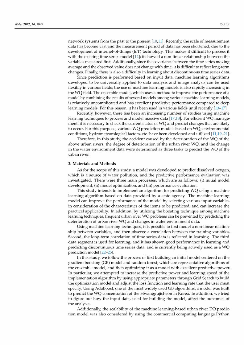
GB makes a forward stepwise additive approach through gradient descent in thefunction space. In addition, we sequentially construct various regression trees for eachfeature in a fully distributed manner. GB involves the following three basic factors: the lossfunction must be adjusted, the weak learner model must produce predictions, and finally,the additive model must merge all weak learners to reduce the overall loss function value.The basic structure of the GB machine algorithm is shown in Figure 1 [30].

Water 2022, 14, x FOR PEER REVIEW 4 of 20

trained so far. The process is done via Equation (4). In Equation (4) below, ρ is the train-ing rate.

1i+ ii

δJf = f ρδf

− (4)

That is, in the GB model, the tree model function derivative serves to indicate the weakness of the model trained so far. Furthermore, when fitting the next tree model, the derivative is used to compensate for the weakness to boost performance [28]. The GB al-gorithm was created for classification purposes for different classes of logistic likelihood and for the regression of the fewest absolute deviation loss functions, Huber-M, and the fewest squares [29]. It provides a very powerful and competitive environment for mining regression and classification problems, especially with fewer clean data sets.

GB makes a forward stepwise additive approach through gradient descent in the function space. In addition, we sequentially construct various regression trees for each feature in a fully distributed manner. GB involves the following three basic factors: the loss function must be adjusted, the weak learner model must produce predictions, and finally, the additive model must merge all weak learners to reduce the overall loss func-tion value. The basic structure of the GB machine algorithm is shown in Figure 1 [30].

Figure 1. Model of gradient boosting.

The advantage is that, as is the case with other tree-based models, it works well on datasets with a mix of scales between features and nominal and numeric variables. The disadvantage is that it is sensitive to parameters and the training time is long. In addition, it is known that the performance is poor on very high-dimensional data sets [28].

Next, looking at AdaBoost, Freund’s AdaBoost algorithm is the most widely used boosting algorithm [30]. AdaBoost is a high-accuracy model that uses a decision tree as a base model.

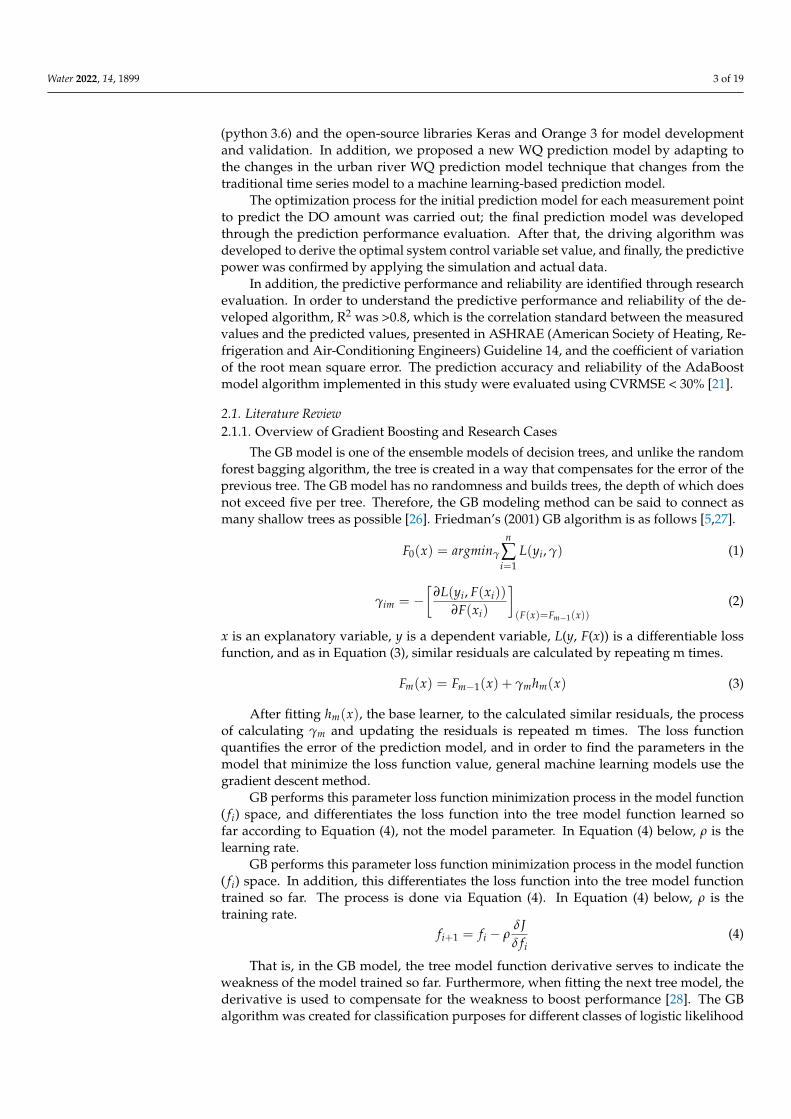
Therefore, we train based on the updated weights and the aggregated results ob-tained from multiple decision trees. In particular, the advantage of AdaBoost is that the number of predicted parameters is small compared to other learning methods. In addi-tion, when boosting learning is performed in terms of false positives, a cascade classifica-tion model can be easily constructed in stages, with a positive error rate below a certain standard. Moreover, by selecting one specific dimension through a weak classifier at each step, it can be applied to the aspect of feature selection.

AdaBoost is a learning technique that generates a strong classifier by repeatedly learning a weak classifier using samples from two classes. Figure 2 shows the basic model of AdaBoost. X is given as an input and output pair (xi , yi ), and the weak learner classifier is given the same weight Wm

i for all the data. When the training of the first classifier is

completed, the weight of the data to be applied to the second classifier is modified accord-ing to the result.

Figure 1. Model of gradient boosting.

The advantage is that, as is the case with other tree-based models, it works well ondatasets with a mix of scales between features and nominal and numeric variables. Thedisadvantage is that it is sensitive to parameters and the training time is long. In addition,it is known that the performance is poor on very high-dimensional data sets [28].

Next, looking at AdaBoost, Freund’s AdaBoost algorithm is the most widely usedboosting algorithm [30]. AdaBoost is a high-accuracy model that uses a decision tree as abase model.

Therefore, we train based on the updated weights and the aggregated results obtainedfrom multiple decision trees. In particular, the advantage of AdaBoost is that the numberof predicted parameters is small compared to other learning methods. In addition, whenboosting learning is performed in terms of false positives, a cascade classification modelcan be easily constructed in stages, with a positive error rate below a certain standard.Moreover, by selecting one specific dimension through a weak classifier at each step, it canbe applied to the aspect of feature selection.

AdaBoost is a learning technique that generates a strong classifier by repeatedlylearning a weak classifier using samples from two classes. Figure 2 shows the basic modelof AdaBoost. X is given as an input and output pair (xi, yi), and the weak learner classifieris given the same weight Wi

m for all the data. When the training of the first classifieris completed, the weight of the data to be applied to the second classifier is modifiedaccording to the result.

Water 2022, 14, x FOR PEER REVIEW 5 of 20

Figure 2. AdaBoost classifier model.

At this time, the value of the weight decreases if there is no error, and if there is an error, the value of the weight increases. The AdaBoost algorithm focuses on erroneous (highly weighted) data. This process is performed m times.

Each classifier is trained using the adjusted weights, and in the final combining step, the value of ai, which was used for training, is applied so that the classifier with a small error rate can play a more important role in judgment [31].

The AdaBoost classifier can be obtained using the following steps. First, we obtain the training data, D= (x1, y1),(x2 , y2) ,... ,(xn , yn) . In the k-th step

(k = 1, 2, ..., T), probability p(n)( ) is used to restore and extract from the training data Dk to generate new training data. A classifier Ck is generated using the generated training data, and if the n-th observation is improperly classified, d(n) = 1, and if the nth obser-vation is properly classified, d(n) = 0.

The error kE is defined as the following equation:

kn

E = p (5)

1 kk

k

Eγ =E−

(6)

The (k + 1)-th probability to be updated is as follows: p(n)( ) = p(n)( )γ ( )∑ p (n)( )γ ( ) (7)

Repeat this process m times. After completing the m-th step, C1,C2 , ... ,Cm are combined into one classifier by the classifier Ck with weight log(γm) to create a final classifier [26].

The advantage is that AdaBoost is adaptive because instances misclassified by previ-ous classifiers are reconstructed into subsequent classifiers. A disadvantage is that Ada-Boost is sensitive to noise data and outliers [32].

The AdaBoost model optimizes the model to minimize a loss function (L: loss func-tion) that calculates the difference between the measured value (y ) of the item to be pre-dicted and the predicted value (y ) of the model and an objective function composed of a regulation function (Ω), which is a function of the individual DT (decision tree) model (f k ) [33–35].

In this study, the optimal prediction algorithm is implemented using the AdaBoost algorithm. WQ measurement data were used as an independent variable to predict the

Figure 2. AdaBoost classifier model.

Water 2022, 14, 1899 5 of 19

At this time, the value of the weight decreases if there is no error, and if there is anerror, the value of the weight increases. The AdaBoost algorithm focuses on erroneous(highly weighted) data. This process is performed m times.

Each classifier is trained using the adjusted weights, and in the final combining step,the value of ai, which was used for training, is applied so that the classifier with a smallerror rate can play a more important role in judgment [31].

The AdaBoost classifier can be obtained using the following steps.First, we obtain the training data, D = (x1, y1), (x2, y2), . . . , (xn, yn). In the k-th step

(k = 1, 2, . . . , T), probability p(n)(k) is used to restore and extract from the training data Dkto generate new training data. A classifier Ck is generated using the generated training data,and if the n-th observation is improperly classified, d(n) = 1, and if the nth observation isproperly classified, d(n) = 0.

The error Ek is defined as the following equation:

Ek = ∑n

p (5)

γk =1− Ek

Ek(6)

The (k + 1)-th probability to be updated is as follows:

p(n)(k+1) =p(n)(k)γk

d(n)

∑n p(n)(k)γkd(n)

(7)

Repeat this process m times. After completing the m-th step, C1, C2, . . . , Cm arecombined into one classifier by the classifier Ck with weight log(γm) to create a finalclassifier [26].

The advantage is that AdaBoost is adaptive because instances misclassified by previousclassifiers are reconstructed into subsequent classifiers. A disadvantage is that AdaBoost issensitive to noise data and outliers [32].

The AdaBoost model optimizes the model to minimize a loss function (L: loss function)that calculates the difference between the measured value (yi) of the item to be predictedand the predicted value (yi) of the model and an objective function composed of a regulationfunction (Ω), which is a function of the individual DT (decision tree) model ( fk) [33–35].

In this study, the optimal prediction algorithm is implemented using the AdaBoostalgorithm. WQ measurement data were used as an independent variable to predict thedependent variable DO. The grid search method was used to optimize the model, andcross-validation was performed by dividing the input data into 10 sets. Model constructionand optimization were performed using Python open-source [36].

2.1.2. Prior Research

Changes in river WQ have been predicted through traditional time series modelingfor various forms of water pollution [10,37], and the amount of research being conducted ison the rise [23,38], as the size of the data has grown and the limitations of the traditionaltime series model have been revealed. As an alternative to this, a deep learning-based ormachine-learning-based prediction model is emerging [12].

In the case of WQ prediction based on deep learning, Lim and An (2018) describedrecurrent neural networks (RNN) and a long short-term memory (LSTM) algorithm wasused to predict the pollution load [19].

A machine-learning algorithm [11] presented a model for predicting Chl-a concen-tration using artificial neural networks (ANN) and support vector machine (SVM), whichare representative machine learning algorithms, and Kwon et al. (2018) predicted Chl-aconcentration using ANN and SVM algorithms and satellite image data [39]. Lee et al.(2020) used random forest (RF) and gradient boosting decision tree (GBDT), which are

Water 2022, 14, 1899 6 of 19

representative ensemble machine-learning algorithms that use a method to improve theperformance of models by combining the results of several models. A model for predictionwas built. In addition, research for predicting WQ changes using a machine-learningmodel based on advanced data analysis technology is also active, and until recently, ithas been used in various fields [13,14,19]. In some cases, studies were performed withLightGBM [16,33,35,40–42].

Looking at previous studies as target variables, PM concentration prediction [22],Chl-a concentration prediction [11,39], pollution-load prediction [19,43], prediction of othervariables [44], and image recognition [45] can be obtained.

In summary, a number of prior studies on WQ prediction use deep learning techniques.However, as in this case, no previous study developed a model for predicting unit-DOconcentration in urban rivers using the GB-based boosting algorithm. No concentrationwas predicted. There was no algorithm to predict the DO concentration in urban riversdownstream using the GB series AdaBoost, which shows high predictive power.

2.2. GB Series Prediction Model Development2.2.1. Data Sources

Data to be used in this study were provided from https://aihub.or.kr (accessed on23 March 2022). AI Hub is an AI integrated platform operated by the Korea Intelligent In-formation Society Agency. As part of the 2017 AI learning data building and disseminationproject, it aims to provide one-stop AI data, software, computing resources, and materialinformation essential for AI technology and service development [46].

The data for AI learning in this study were the WQ measurement data of the water envi-ronment measurement network, including WQ/automatic/total amount/sediment/radioactivematerial/KRF, etc., concerning the related measurement data. Detailed data sources forwater-quality-related fields are the National Institute of Environmental Sciences of theMinistry of Environment and the Korea Water Resources Corporation [46].

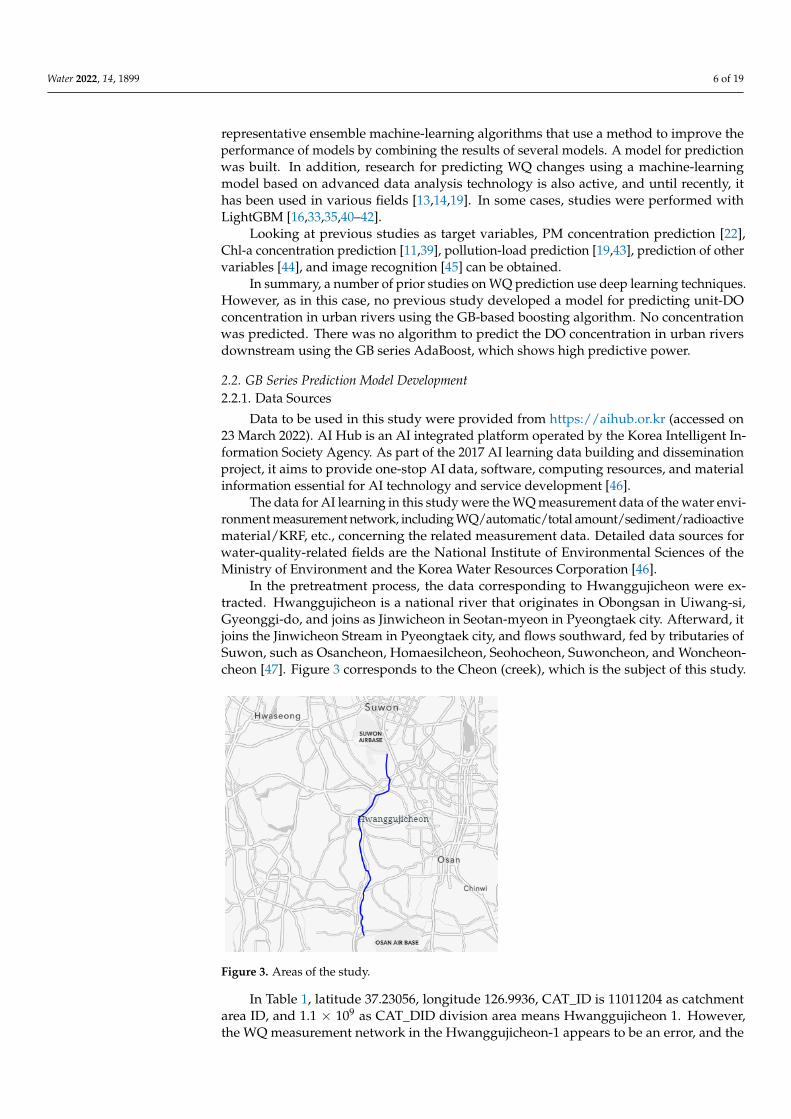
In the pretreatment process, the data corresponding to Hwanggujicheon were ex-tracted. Hwanggujicheon is a national river that originates in Obongsan in Uiwang-si,Gyeonggi-do, and joins as Jinwicheon in Seotan-myeon in Pyeongtaek city. Afterward, itjoins the Jinwicheon Stream in Pyeongtaek city, and flows southward, fed by tributaries ofSuwon, such as Osancheon, Homaesilcheon, Seohocheon, Suwoncheon, and Woncheon-cheon [47]. Figure 3 corresponds to the Cheon (creek), which is the subject of this study.

Water 2022, 14, x FOR PEER REVIEW 7 of 20

Figure 3. Areas of the study.

Table 1. Latitude and longitude of the area of research.

WQ Network Compound Latitude Longitude Cat_Id Cat_Did Hwanggujicheon1 Ammonia Nitrogen (NH₃-N) 37.23056 126.9936 11011204 1.1 × 109 Hwanggujicheon-1 Ammonia Nitrogen (NH₃-N) 37.32086 127.9486 10060601 1.01 × 109 Hwanggujicheon1-1 Ammonia Nitrogen (NH₃-N) 37.20347 127.0255 11011304 1.1 × 109 Hwanggujicheon2 Ammonia Nitrogen (NH₃-N) 37.18372 127.0093 11011305 1.1 × 109 Hwanggujicheon-2 Ammonia Nitrogen (NH₃-N) 37.29789 126.9462 11011201 1.1 × 109 Hwanggujicheon3 Ammonia Nitrogen (NH₃-N) 37.11886 127.0014 11011308 1.1 × 109

In Table 1, latitude 37.23056, longitude 126.9936, CAT_ID is 11011204 as catchment area ID, and 1.1 × 109 as CAT_DID division area means Hwanggujicheon 1. However, the WQ measurement network in the Hwanggujicheon-1 appears to be an error, and the lo-cation indicated by the above longitude corresponds to a different area. It was, therefore, excluded from this study. Figure 3 is the relevant area for the estimation of water pollution in this study.

It also provides the name and value of the data measurement item and whether the item has been refined. A total of 20 items, such as measurement date, flow rate, water temperature, flow rate (m3/sec), water temperature (°C), pH, DO (mg/L), BOD (mg/L), COD (mg/L), SS (mg)/L), EC (μS/cm), T-N (mg/L), DTN (mg/L), NO₃-N (mg/L), NH₃-N (mg/L), T-P (mg/L), -DTP (mg/L), PO₄-P (mg/L), chlorophyll-a, and TOC (mg/L), are pro-vided.

Table 2. Items to check.

Items Index Notation Values pH pH 7.1

Suspended Solids (SS) SS 35 Mercury Mercury 3

Total Nitrogen (T-N) TN 3.624 Dissolved Total Phosphorus (DTP) DTP

NH₃-N NHN

Figure 3. Areas of the study.

In Table 1, latitude 37.23056, longitude 126.9936, CAT_ID is 11011204 as catchmentarea ID, and 1.1 × 109 as CAT_DID division area means Hwanggujicheon 1. However,the WQ measurement network in the Hwanggujicheon-1 appears to be an error, and the

Water 2022, 14, 1899 7 of 19

location indicated by the above longitude corresponds to a different area. It was, therefore,excluded from this study. Figure 3 is the relevant area for the estimation of water pollutionin this study.

Table 1. Latitude and longitude of the area of research.

WQ Network Compound Latitude Longitude Cat_Id Cat_Did

Hwanggujicheon1 Ammonia Nitrogen (NH3-N) 37.23056 126.9936 11011204 1.1 × 109

Hwanggujicheon-1 Ammonia Nitrogen (NH3-N) 37.32086 127.9486 10060601 1.01 × 109

Hwanggujicheon1-1 Ammonia Nitrogen (NH3-N) 37.20347 127.0255 11011304 1.1 × 109

Hwanggujicheon2 Ammonia Nitrogen (NH3-N) 37.18372 127.0093 11011305 1.1 × 109

Hwanggujicheon-2 Ammonia Nitrogen (NH3-N) 37.29789 126.9462 11011201 1.1 × 109

Hwanggujicheon3 Ammonia Nitrogen (NH3-N) 37.11886 127.0014 11011308 1.1 × 109

It also provides the name and value of the data measurement item and whetherthe item has been refined. A total of 20 items, such as measurement date, flow rate,water temperature, flow rate (m3/s), water temperature (C), pH, DO (mg/L), BOD(mg/L), COD (mg/L), SS (mg)/L), EC (µS/cm), T-N (mg/L), DTN (mg/L), NO3-N(mg/L), NH3-N (mg/L), T-P (mg/L), -DTP (mg/L), PO4-P (mg/L), chlorophyll-a, andTOC (mg/L), are provided.

In Table 2, electrical conductivity (EC), total phosphorus (T-P), chlorophyll-a, flowrate, phosphate (PO4-P), and total organic carbon (TOC) were excluded due to missingvalues. Monthly data were used from January 2008 to December 2020 for the usage dataperiod. The data in this study did not show a time series. There is a lack of regularityin the measurement period of the data, and there are parts where monthly data for aspecific year are omitted. In addition, parts with many missing values were deleted. Forexample, measurements of items such as chlorophyll-a only have recent results, and dataprior to 2020 do not have values. Looking at the number of data collection cases, the waterenvironment field was 264,147,400, and the data related to the WQ of HwanggujicheonStream were extracted from it.

Table 2. Items to check.

Items Index Notation Values

pH pH 7.1

Suspended Solids (SS) SS 35

Mercury Mercury 3

Total Nitrogen (T-N) TN 3.624

Dissolved Total Phosphorus (DTP) DTP

NH3-N NHN

COD COD 42

DO DO 8.6

Dissolved Total Nitrogen (DTN) DTN

NO3-N NON

Electrical Conductivity (EC) EC

BOD BOD 42

Total Phosphorus (T-P) TP 0.837

Chlorophyll-a Chlorophyll-a

Flow Rate Flow Rate

Phosphate Phosphorus (PO4-P) PO4-P

Total Organic Carbon (TOC) TOC

Water 2022, 14, 1899 8 of 19

The data used in this study were source data collected from the National Institute ofEnvironmental Sciences, Statistics Korea, and the Korea Meteorological Administration,and the data were primarily refined based on related laws, such as the announcement ofthe water environment monitoring network operation plan. As for the type of refinement,outliers were identified and removed by determining whether they were included withinthe confidence interval in the removal of outliers. In addition, cross-validation withdata construction institutions and inspection institutions was performed by designatinga dedicated inspection team among participating institutions, and an expert inspectionwas performed by designating a national organization consultative body composed ofwater-quality experts from the National Academy of Environmental Sciences [46].

In this study, MinMaxScaler() was used for scaling after data preprocessing. Thenormalization method used in the DO prediction model used min-max scaling as a methodto make the range the same for all input variable characteristics. The min–max scalingmethod of normalizing used variables to values between 0 and 1. The smallest value isconverted to 0, the largest value is converted to 1, and all properties have the range (0–1).Many missing values were deleted.

In this study, the number of instances extracted through preprocessing to build amodel for predicting DO in Hwanggujicheon, the research target area, is 761. The measuredperiod is from 2008 to 2020. It corresponds to the number in which the part due to missingvalues or data errors is removed.

Each element and sub-item were selected through the literature search and priorresearch, and unused sub-items were those that were not properly learned or parts withmany missing values and were removed when constructing the DO prediction model. Asthe modeling optimization factor, nine features of the DO prediction model were used.Looking at the model variables used in this study, the data of DO, a WQ item of theWQ measurement network, is used as the dependent variable of the boosting-based DOprediction model. The data of nine WQ items from the automatic WQ measurementnetwork were used for the independent variable (input variable) of the boosting-based DOprediction model.

The criteria for selecting the learning data in this study were the literature search,previous studies, and the living environment criteria items of rivers and lakes. Thiswas based on Article 12 (2) of the Framework Act on Environmental Policy (setting ofenvironmental standards) and the environmental standards of the enforcement decree ofthe same law. However, the total organic carbon content (TOC) was excluded from thestudy because there were many missing values and there were too many unmeasuredareas. Biochemical oxygen demand (BOD) was excluded because it was measured from theamount of DO.

In the boosting-based DO prediction model, an algorithm was applied to each mea-surement point, but sufficient results were not obtained due to limited regional data.Therefore, the current study used the whole part of Hwanggujicheon. Data partitioningwas set to 80:20. A 10-fold cross-validation method was used. In addition, a simulationwas performed using the latest data to evaluate the prediction algorithm, but the numberof instances was insufficient and the predictive power was minimal.

2.2.2. Statistical Data and Its Visualization

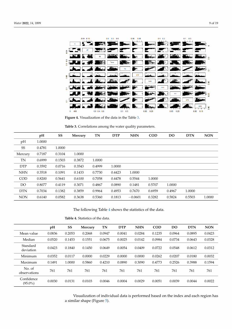
The correlations of the data used in this study are as follows.Figure 4 below shows the plot for the data in Table 3.

Water 2022, 14, 1899 9 of 19

Water 2022, 14, x FOR PEER REVIEW 9 of 20

based on Article 12 (2) of the Framework Act on Environmental Policy (setting of environ-mental standards) and the environmental standards of the enforcement decree of the same law. However, the total organic carbon content (TOC) was excluded from the study be-cause there were many missing values and there were too many unmeasured areas. Bio-chemical oxygen demand (BOD) was excluded because it was measured from the amount of DO.

In the boosting-based DO prediction model, an algorithm was applied to each meas-urement point, but sufficient results were not obtained due to limited regional data. There-fore, the current study used the whole part of Hwanggujicheon. Data partitioning was set to 80:20. A 10-fold cross-validation method was used. In addition, a simulation was per-formed using the latest data to evaluate the prediction algorithm, but the number of in-stances was insufficient and the predictive power was minimal.

2.2.2. Statistical Data and Its Visualization The correlations of the data used in this study are as follows. Figure 4 below shows the plot for the data in Table 3.

Table 3. Correlations among the water quality parameters.

pH SS Mercury TN DTP NHN COD DO DTN NON pH 1.0000 SS 0.4781 1.0000

Mer-cury

0.7187 0.3104 1.0000

TN 0.6999 0.1503 0.3872 1.0000 DTP 0.3592 0.0716 0.3543 0.4999 1.0000

NHN 0.3518 0.1091 0.1433 0.7730 0.4423 1.0000 COD 0.8200 0.5641 0.6100 0.7058 0.4478 0.5544 1.0000 DO 0.8077 0.4119 0.3071 0.4867 0.0890 0.1481 0.5707 1.0000

DTN 0.7034 0.1382 0.3859 0.9964 0.4953 0.7670 0.6959 0.4967 1.0000 NON 0.6140 0.0582 0.3638 0.5360 0.1813 −0.0601 0.3282 0.5824 0.5503 1.0000

Figure 4. Visualization of the data in the Table 3.

The following Table 4 shows the statistics of the data.

Table 4. Statistics of the data.

Figure 4. Visualization of the data in the Table 3.

Table 3. Correlations among the water quality parameters.

pH SS Mercury TN DTP NHN COD DO DTN NON

pH 1.0000

SS 0.4781 1.0000

Mercury 0.7187 0.3104 1.0000

TN 0.6999 0.1503 0.3872 1.0000

DTP 0.3592 0.0716 0.3543 0.4999 1.0000

NHN 0.3518 0.1091 0.1433 0.7730 0.4423 1.0000

COD 0.8200 0.5641 0.6100 0.7058 0.4478 0.5544 1.0000

DO 0.8077 0.4119 0.3071 0.4867 0.0890 0.1481 0.5707 1.0000

DTN 0.7034 0.1382 0.3859 0.9964 0.4953 0.7670 0.6959 0.4967 1.0000

NON 0.6140 0.0582 0.3638 0.5360 0.1813 −0.0601 0.3282 0.5824 0.5503 1.0000

The following Table 4 shows the statistics of the data.

Table 4. Statistics of the data.

pH SS Mercury TN DTP NHN COD DO DTN NON

Mean value 0.0836 0.2053 0.2068 0.0947 0.0041 0.0284 0.1235 0.0964 0.0895 0.0423

Median 0.0520 0.1453 0.1551 0.0675 0.0025 0.0142 0.0984 0.0734 0.0643 0.0328

Standarddeviation 0.0423 0.1840 0.1450 0.0649 0.0054 0.0409 0.0722 0.0548 0.0612 0.0312

Minimum 0.0352 0.0117 0.0000 0.0229 0.0000 0.0000 0.0262 0.0207 0.0180 0.0032

Maximum 0.1491 1.0000 0.5860 0.4210 0.0890 0.3090 0.4773 0.2526 0.3988 0.1594

No. ofobservations 761 761 761 761 761 761 761 761 761 761

Confidence(95.0%) 0.0030 0.0131 0.0103 0.0046 0.0004 0.0029 0.0051 0.0039 0.0044 0.0022

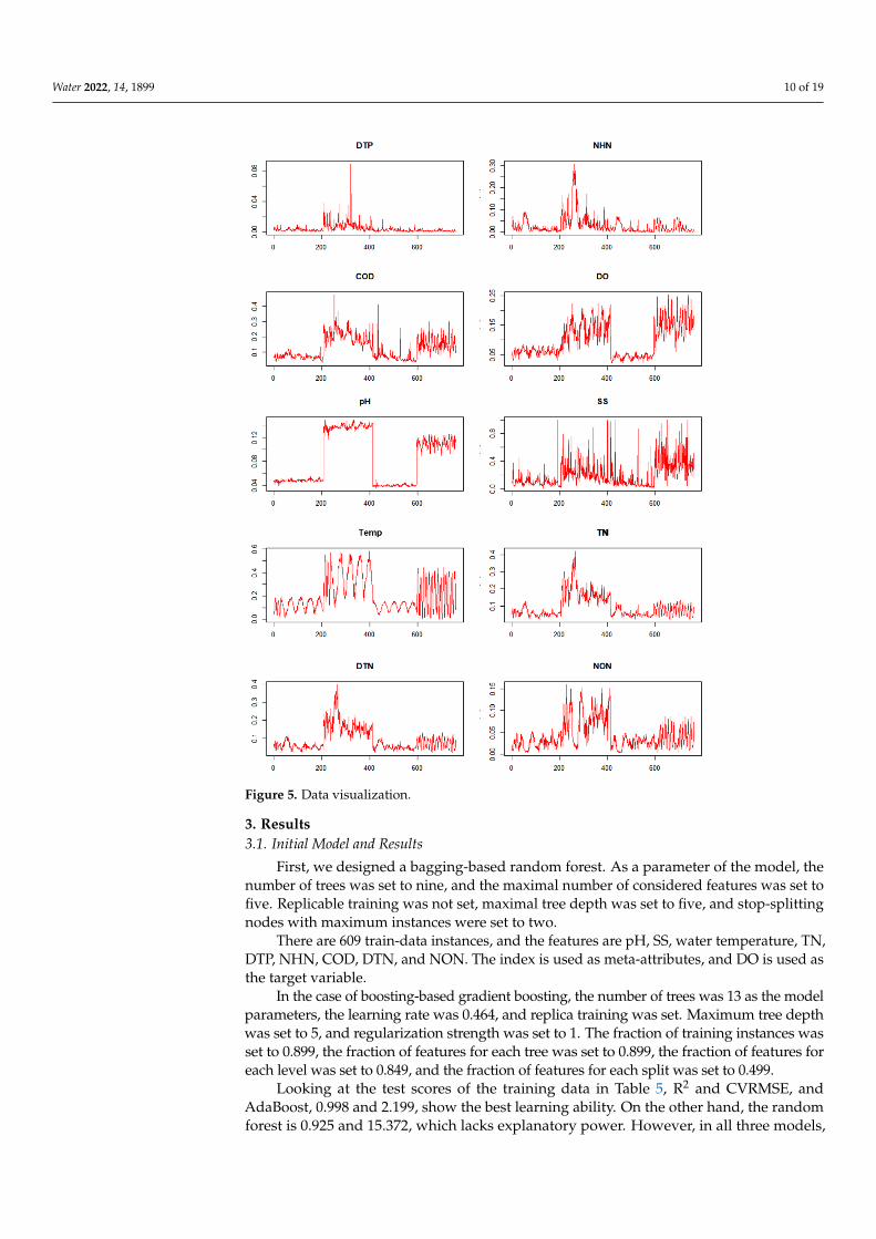
Visualization of individual data is performed based on the index and each region hasa similar shape (Figure 5).

Water 2022, 14, 1899 10 of 19

Water 2022, 14, x FOR PEER REVIEW 10 of 20

pH SS Mercury TN DTP NHN COD DO DTN NON Mean value 0.0836 0.2053 0.2068 0.0947 0.0041 0.0284 0.1235 0.0964 0.0895 0.0423

Median 0.0520 0.1453 0.1551 0.0675 0.0025 0.0142 0.0984 0.0734 0.0643 0.0328 Standard deviation 0.0423 0.1840 0.1450 0.0649 0.0054 0.0409 0.0722 0.0548 0.0612 0.0312

Minimum 0.0352 0.0117 0.0000 0.0229 0.0000 0.0000 0.0262 0.0207 0.0180 0.0032 Maximum 0.1491 1.0000 0.5860 0.4210 0.0890 0.3090 0.4773 0.2526 0.3988 0.1594

No. of obser-vations

761 761 761 761 761 761 761 761 761 761

Confidence (95.0%)

0.0030 0.0131 0.0103 0.0046 0.0004 0.0029 0.0051 0.0039 0.0044 0.0022

Visualization of individual data is performed based on the index and each region has a similar shape (Figure 5).

Figure 5. Data visualization. Figure 5. Data visualization.

3. Results3.1. Initial Model and Results

First, we designed a bagging-based random forest. As a parameter of the model, thenumber of trees was set to nine, and the maximal number of considered features was set tofive. Replicable training was not set, maximal tree depth was set to five, and stop-splittingnodes with maximum instances were set to two.

There are 609 train-data instances, and the features are pH, SS, water temperature, TN,DTP, NHN, COD, DTN, and NON. The index is used as meta-attributes, and DO is used asthe target variable.

In the case of boosting-based gradient boosting, the number of trees was 13 as the modelparameters, the learning rate was 0.464, and replica training was set. Maximum tree depthwas set to 5, and regularization strength was set to 1. The fraction of training instances wasset to 0.899, the fraction of features for each tree was set to 0.899, the fraction of features foreach level was set to 0.849, and the fraction of features for each split was set to 0.499.

Looking at the test scores of the training data in Table 5, R2 and CVRMSE, andAdaBoost, 0.998 and 2.199, show the best learning ability. On the other hand, the randomforest is 0.925 and 15.372, which lacks explanatory power. However, in all three models,

Water 2022, 14, 1899 11 of 19

MSE is 0.000, but there is a difference between RMSE and MAE, as well as a difference inrunning time.

Table 5. Score in training data.

Score on Training Data

Model Train Time (s) Test Time (s) MSE RMSE MAE R2 CVRMSE

Random Forest 0.432 0.005 0.000 0.015 0.011 0.925 15.372

Gradient Boosting 0.076 0.007 0.000 0.022 0.015 0.845 22.157

AdaBoost 0.202 0.019 0.000 0.002 0.001 0.998 2.199

Table 6 is the result value that is learned by 10-fold cross-validation. R2 and CVRMSE,AdaBoost, 0.896 and 18.082, show the best learning ability. On the other hand, randomforest has relatively poor explanatory power with 0.887 and 18.874. In addition, althoughMSE is 0.000, there is a difference between RMSE and MAE.

Table 6. 10-fold cross-validation.

10-Fold Cross-Validation

Model Train Time (s) Test Time (s) MSE RMSE MAE R2 CVRMSE

Random Forest 0.871 0.062 0.000 0.019 0.013 0.887 18.874

Gradient Boosting 0.825 0.169 0.001 0.025 0.018 0.790 25.770

AdaBoost 0.709 0.040 0.000 0.018 0.011 0.896 18.082

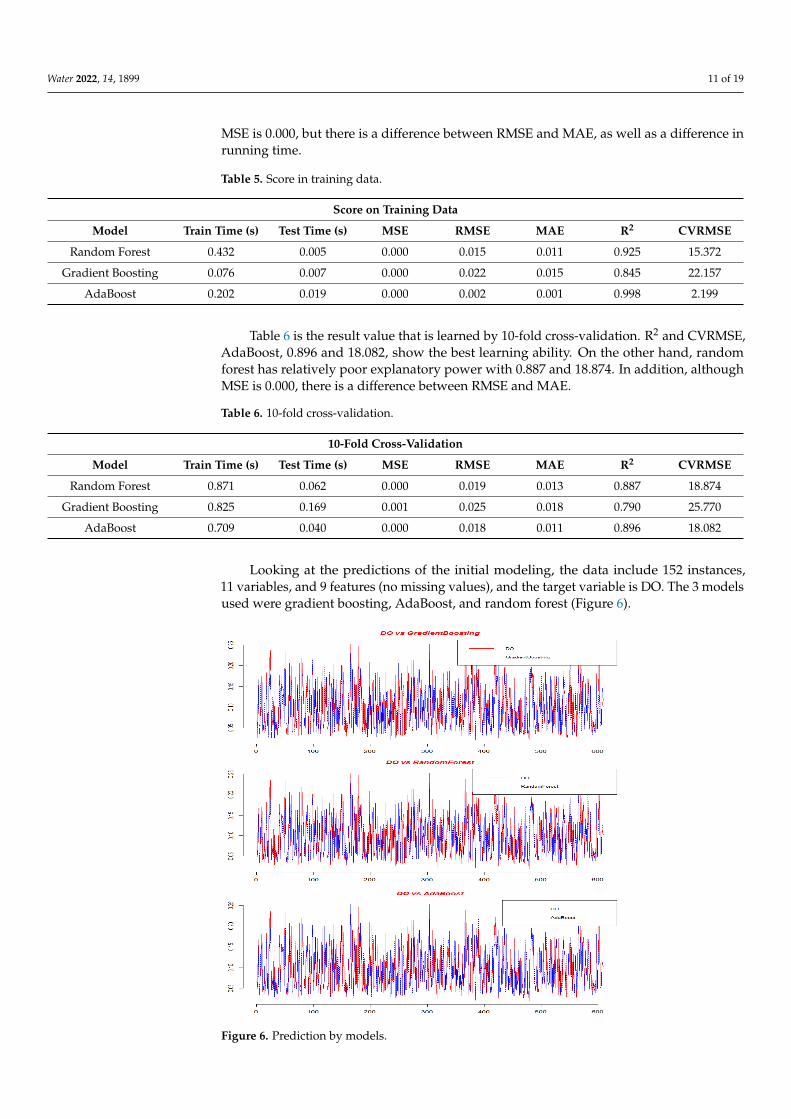
Looking at the predictions of the initial modeling, the data include 152 instances,11 variables, and 9 features (no missing values), and the target variable is DO. The 3 modelsused were gradient boosting, AdaBoost, and random forest (Figure 6).

Water 2022, 14, x FOR PEER REVIEW 12 of 20

Figure 6. Prediction by models.

Table 7 corresponds to the prediction results. It also shows the same predictive power as the previous results. In the overall evaluation index, AdaBoost is excellent. Similar to the results of the training process, the MSE is the same, but there are differences in RMSE, MAE, R2, and CVRMSE. AdaBoost’s RMSE is 0.016, which is relatively close to 0, and R2 is 0.901, which is closer to 1. CVRMSE is relatively low at 18.435, which satisfies all eval-uation criteria of R2 and CVRMSE.

Table 7. Prediction by models.

Prediction Scores Model Train Time (s) Test Time (s) MSE RMSE MAE R2 CVRMSE

Gradient Boosting N/A N/A 0.001 0.024 0.016 0.79 26.824 AdaBoost N/A N/A 0 0.016 0.009 0.901 18.4354

Random Forest N/A N/A 0 0.017 0.012 0.886 19.752

3.2. Optimal Model and Design While designing an optimized model, AdaBoost’s learning ability and predictive

ability were superior to that of random forest of bagging or GB-based XGBoost, so it was selected as an optimized model. In addition, we want to design a design that improves prediction performance by adjusting the basic parameters.

AdaBoosting is used as the model parameters, the base estimator is tree and the num-ber of estimators is seven. The learning rate is 0.500. The reproducibility of the experiment was set as the fixed seed for the random generator was set to 155. There are 609 data in-stances of data, and the features are pH, SS, water temperature, TN, DTP, NHN, COD, DTN, and NON. As meta-attributes, they are indexed as Feature 1. The target was set to DO.

Figure 6. Prediction by models.

Water 2022, 14, 1899 12 of 19

Table 7 corresponds to the prediction results. It also shows the same predictive poweras the previous results. In the overall evaluation index, AdaBoost is excellent. Similar tothe results of the training process, the MSE is the same, but there are differences in RMSE,MAE, R2, and CVRMSE. AdaBoost’s RMSE is 0.016, which is relatively close to 0, and R2 is0.901, which is closer to 1. CVRMSE is relatively low at 18.435, which satisfies all evaluationcriteria of R2 and CVRMSE.

Table 7. Prediction by models.

Prediction Scores

Model Train Time (s) Test Time (s) MSE RMSE MAE R2 CVRMSE

Gradient Boosting N/A N/A 0.001 0.024 0.016 0.79 26.824

AdaBoost N/A N/A 0 0.016 0.009 0.901 18.4354

Random Forest N/A N/A 0 0.017 0.012 0.886 19.752

3.2. Optimal Model and Design

While designing an optimized model, AdaBoost’s learning ability and predictiveability were superior to that of random forest of bagging or GB-based XGBoost, so it wasselected as an optimized model. In addition, we want to design a design that improvesprediction performance by adjusting the basic parameters.

AdaBoosting is used as the model parameters, the base estimator is tree and thenumber of estimators is seven. The learning rate is 0.500. The reproducibility of theexperiment was set as the fixed seed for the random generator was set to 155. There are609 data instances of data, and the features are pH, SS, water temperature, TN, DTP, NHN,COD, DTN, and NON. As meta-attributes, they are indexed as Feature 1. The target wasset to DO.

In Table 8, there is a difference in the evaluation index according to the shape of theloss function. Comparing R2 and CVRMSE, R2 shows 0.999 in the same way for linearand exponential functions. However, in CVRMSE, linear is 2.066 and exponential is 1.463,which is close to 0, indicating good learning ability. In this study, the exponential functionwas first selected as the loss function and the same parameters were set to estimate thepredictive ability. Next, the predictive ability was compared by applying the linear andsquare loss functions.

Table 8. Optimal model.

Model Train Time (s) Test Time (s) MSE RMSE MAE R2 CVRMSE

Random Forest 0.111 0.004 0.000 0.015 0.011 0.923 15.636

Gradient Boosting 0.246 0.006 0.000 0.022 0.015 0.845 22.157

AdaBoost0.074 0.003 0.000 0.002 0.001 0.998 2.199

Loss: Square

AdaBoost0.081 0.006 0.000 0.002 0.000 0.999 2.066

Loss: Linear

AdaBoost0.076 0.008 0.000 0.001 0.000 0.999 1.463

Loss: Exponential

3.3. Predictive Performance Evaluation

Considering the indices for evaluating the performance prediction of machine learningmodels, various indices, including RMSE (root mean square error), MAE (mean absoluteerror), MSE, R2, and CVRMSE, are used. For the evaluation of DO prediction performanceusing the AdaBoost model constructed in this study, root mean square error (RMSE),

Water 2022, 14, 1899 13 of 19

MSE, MAE, CVRMSE, R2, and running time were used. The latter two indices, R2 andCVRMSE, were mainly used in this paper. MAE and MSE often show the same value,and predictive performance cannot be properly evaluated in many cases. Meanwhile,RMSE is an index that compares the absolute value of the difference between the predictedvalue and the measured value. Among the evaluation indicators, the closer to 0, thebetter the performance of MSE, MAE, RMSE, and CVRMSE. The closer to 1, the better theperformance of R2.

RSME =

√∑n

i=1 (yi − yi)2

n

It is a value rooted in the MSE, and the error-index is converted back to a unit similarto the actual value, which makes interpretation somewhat easier.

MSE =1n

n

∑i=1

(yi − yi )2

MSE is the main loss function of the regression model, and it is defined as the meansquare of the errors, which is the difference between the predicted value and the actualvalue. Because it is squared, it is sensitive to outliers. MAE is the mean of the absolutevalues of errors, which is the difference between the actual value and the predicted valueand is less sensitive to outliers than the MSE.

MAE =1n

n

∑i=1

( |yi − yi| )2

R2 (coefficient of determination) is a variance-based prediction performance evaluationindex. Other indicators, such as MAE and MSE, have different values depending on thescale of the data, but R2 can intuitively judge the relative performance. That is, the R2 scorecoefficient of determination is an index that measures the accuracy performance of dataprediction by calculating the variance in the predicted value compared to the variance inthe actual observation.

It is expressed as a number from 0 to 1; the better the linear regression fits the data,the closer the value of R2 is to 1. The R2 value is obtained by dividing the sum of squares ofresiduals by the sum of squared residuals with respect to the average value as follows:

R 2 = 1 − ∑ni=1 (yi − yi)

2

∑ni=1 (yi − y)2

where yi is the fitted value and y is the mean value.The coefficient of variation of the standard error (CVRMSE: coefficient of variation

of the RMSE) is a measured value suggested by ASHRAE (American Society of Heating,Refrigeration and Air-Conditioning Engineers) Guideline 14 to understand the predictiveperformance and reliability of the optimized AdaBoost model.

CVRMSE =1y[∑n

i=1 ( yi − yi )2

n − p]0.5

The prediction accuracy of the AdaBoost model was evaluated using the correlationcriterion (R2 > 0.8) and the root mean square error coefficient of variation (CVRMSE) [21].

To analyze the predictive performance and reliability of the AdaBoost model, actualwater pollution data and predicted results were compared. At this time, ASHRAE providesstatistical criteria for comparing and evaluating the measured data and simulation results,and the predictive performance of the AdaBoost model was mainly evaluated with the R2

value and CVRMSE. R2, representing the model explanatory diagram, is a measure of themagnitude of the explanatory power of the input variables for the variation in the outputvariables of data, and the correlation was judged to be appropriate when the ASHRAE

Water 2022, 14, 1899 14 of 19

standard was 0.8 or higher. CVRMSE is the coefficient of variation (CV) of the root meansquare error (RMSE), and was used as a measure to determine the difference between theactual value and the predicted value.

4. Discussion

It shows the learning power according to the loss function by setting the hyperparam-eter obtained by Grid Search. Train time is 0.074–0.081, and test time is 0.003–0.008. MSEshows the same value according to the loss function.

For RMSE, loss: square is 0.002, loss: exponential is 0.001, and the exponential lossfunction is close to 0. In addition, MAE is 0.001 and 0.000, so loss: exponential is close to 0.Similarly for R2, loss: exponential is 0.999 and 0.998, which is closer to 1 than loss: square.In addition, since R2 is 80% or more, all loss functions are suitable for the determinationof fitness. In CVRMSE, 2.199 has the highest loss: square, 2.066, and 1.463, all suggestingappropriate values of less than 30%.

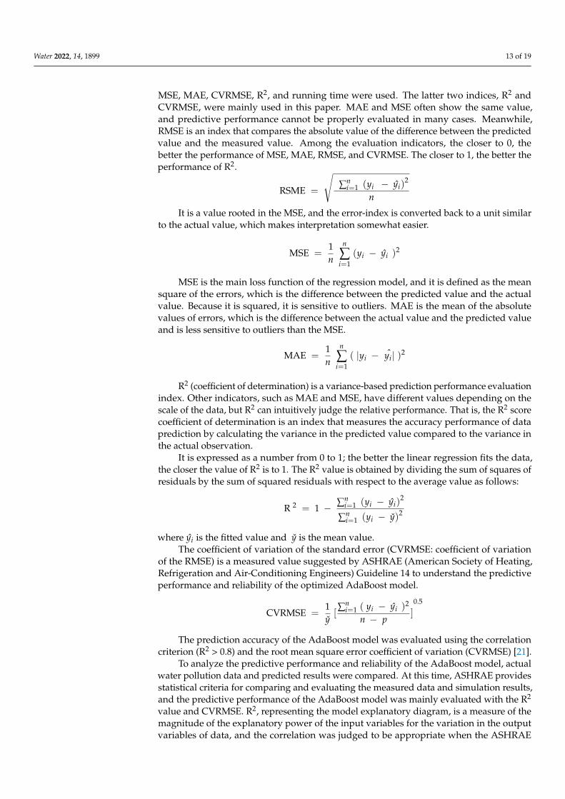
Figure 7 corresponds to the part learned by AdaBoost’s loss function loss: square. Asshown in Table 9, the learning ability is close to 1. The reason that the loss function wasselected as loss: square in this study is because it shows better predictive power than theother loss functions in the prediction output of Table 10.

Water 2022, 14, x FOR PEER REVIEW 15 of 20

AdaBoost 0.076 0.008 0.000 0.001 0.000 0.999 1.463

Loss: Exponential

Figure 7. Train score (AdaBoost).

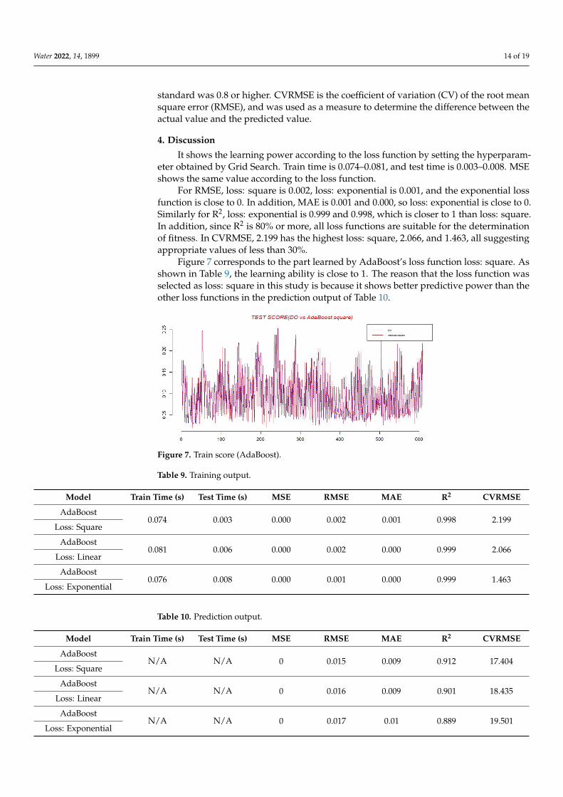
Figure 8 corresponds to a line plot of the training output and shows the distribution of values for each variable.

Figure 8. Train output line plot.

Table 10 shows the performance evaluation according to the loss function. It can be found that the loss functions loss: linear and loss: exponential have relative overfitting in comparison to loss: square. The MSE of all loss functions is equally 0, and in RMASE and MAE, loss: square is the closest to 0. However, in MAE, loss: exponential is relatively closer to 0 than the two loss functions.

Table 10. Prediction output.

Model Train Time (s) Test Time (s) MSE RMSE MAE R2 CVRMSE AdaBoost

N/A N/A 0 0.015 0.009 0.912 17.404 Loss: Square

AdaBoost N/A N/A 0 0.016 0.009 0.901 18.435

Loss: Linear

Figure 7. Train score (AdaBoost).

Table 9. Training output.

Model Train Time (s) Test Time (s) MSE RMSE MAE R2 CVRMSE

AdaBoost0.074 0.003 0.000 0.002 0.001 0.998 2.199

Loss: Square

AdaBoost0.081 0.006 0.000 0.002 0.000 0.999 2.066

Loss: Linear

AdaBoost0.076 0.008 0.000 0.001 0.000 0.999 1.463

Loss: Exponential

Table 10. Prediction output.

Model Train Time (s) Test Time (s) MSE RMSE MAE R2 CVRMSE

AdaBoostN/A N/A 0 0.015 0.009 0.912 17.404

Loss: Square

AdaBoostN/A N/A 0 0.016 0.009 0.901 18.435

Loss: Linear

AdaBoostN/A N/A 0 0.017 0.01 0.889 19.501

Loss: Exponential

Water 2022, 14, 1899 15 of 19

Figure 8 corresponds to a line plot of the training output and shows the distribution ofvalues for each variable.

Water 2022, 14, x FOR PEER REVIEW 15 of 20

AdaBoost 0.076 0.008 0.000 0.001 0.000 0.999 1.463

Loss: Exponential

Figure 7. Train score (AdaBoost).

Figure 8 corresponds to a line plot of the training output and shows the distribution of values for each variable.

Figure 8. Train output line plot.

Table 10 shows the performance evaluation according to the loss function. It can be found that the loss functions loss: linear and loss: exponential have relative overfitting in comparison to loss: square. The MSE of all loss functions is equally 0, and in RMASE and MAE, loss: square is the closest to 0. However, in MAE, loss: exponential is relatively closer to 0 than the two loss functions.

Table 10. Prediction output.

Model Train Time (s) Test Time (s) MSE RMSE MAE R2 CVRMSE AdaBoost

N/A N/A 0 0.015 0.009 0.912 17.404 Loss: Square

AdaBoost N/A N/A 0 0.016 0.009 0.901 18.435

Loss: Linear

Figure 8. Train output line plot.

Table 10 shows the performance evaluation according to the loss function. It can befound that the loss functions loss: linear and loss: exponential have relative overfitting incomparison to loss: square. The MSE of all loss functions is equally 0, and in RMASE andMAE, loss: square is the closest to 0. However, in MAE, loss: exponential is relatively closerto 0 than the two loss functions.

This is probably because the MAE is calculated as the average of the absolute valuesof the errors, which is the difference between the actual value and the predicted value,and it is less sensitive to outliers. For R2, loss: square is 0.912, loss: linear is 0.901, loss:exponential is 0.889, and loss: square is closer to 1. Unlike train score, loss: linear and loss:exponential are closer to loss: square than 1, and it shows that the model predictive poweris high. Loss: linear also shows better explanatory power than loss: exponential.

In CVRMSE, loss: square is 17.404, loss: linear is 18.435, loss: exponential is 19.501,loss: square is closer to 0, the reliability of the model is high, and the model evaluation ismore valid.

Therefore, when the model is evaluated based on R2 and CVRMSE, loss: square showsa higher model fit and predictive power than loss: linear and loss: exponential. All caseswhere R2 is 0.8 or more and CVRMSE is less than 30 are accepted. AdaBoost’s loss functionloss: square showed higher predictive power than other loss functions loss: linear and loss:exponential.

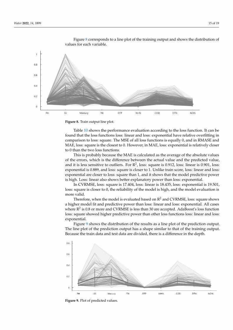
Figure 9 shows the distribution of the results as a line plot of the prediction output.The line plot of the prediction output has a shape similar to that of the training output.Because the train data and test data are divided, there is a difference in the depth.

Water 2022, 14, x FOR PEER REVIEW 16 of 20

AdaBoost N/A N/A 0 0.017 0.01 0.889 19.501

Loss: Exponential

This is probably because the MAE is calculated as the average of the absolute values of the errors, which is the difference between the actual value and the predicted value, and it is less sensitive to outliers. For R2, loss: square is 0.912, loss: linear is 0.901, loss: exponential is 0.889, and loss: square is closer to 1. Unlike train score, loss: linear and loss: exponential are closer to loss: square than 1, and it shows that the model predictive power is high. Loss: linear also shows better explanatory power than loss: exponential.

In CVRMSE, loss: square is 17.404, loss: linear is 18.435, loss: exponential is 19.501, loss: square is closer to 0, the reliability of the model is high, and the model evaluation is more valid.

Therefore, when the model is evaluated based on R2 and CVRMSE, loss: square shows a higher model fit and predictive power than loss: linear and loss: exponential. All cases where R2 is 0.8 or more and CVRMSE is less than 30 are accepted. AdaBoost’s loss function loss: square showed higher predictive power than other loss functions loss: linear and loss: exponential.

Figure 9 shows the distribution of the results as a line plot of the prediction output. The line plot of the prediction output has a shape similar to that of the training output. Because the train data and test data are divided, there is a difference in the depth.

Figure 9. Plot of predicted values.

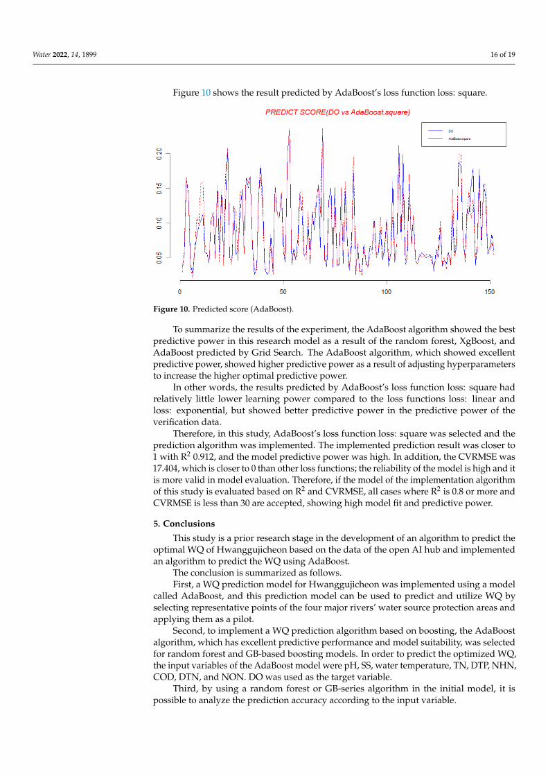
Figure 10 shows the result predicted by AdaBoost’s loss function loss: square. To summarize the results of the experiment, the AdaBoost algorithm showed the best

predictive power in this research model as a result of the random forest, XgBoost, and AdaBoost predicted by Grid Search. The AdaBoost algorithm, which showed excellent predictive power, showed higher predictive power as a result of adjusting hyperparame-ters to increase the higher optimal predictive power.

Figure 9. Plot of predicted values.

Water 2022, 14, 1899 16 of 19

Figure 10 shows the result predicted by AdaBoost’s loss function loss: square.

Water 2022, 14, x FOR PEER REVIEW 17 of 20

Figure 10. Predicted score (AdaBoost).

In other words, the results predicted by AdaBoost’s loss function loss: square had relatively little lower learning power compared to the loss functions loss: linear and loss: exponential, but showed better predictive power in the predictive power of the verifica-tion data.

Therefore, in this study, AdaBoost’s loss function loss: square was selected and the prediction algorithm was implemented. The implemented prediction result was closer to 1 with R2 0.912, and the model predictive power was high. In addition, the CVRMSE was 17.404, which is closer to 0 than other loss functions; the reliability of the model is high and it is more valid in model evaluation. Therefore, if the model of the implementation algorithm of this study is evaluated based on R2 and CVRMSE, all cases where R2 is 0.8 or more and CVRMSE is less than 30 are accepted, showing high model fit and predictive power.

Figure 10. Predicted score (AdaBoost).

To summarize the results of the experiment, the AdaBoost algorithm showed the bestpredictive power in this research model as a result of the random forest, XgBoost, andAdaBoost predicted by Grid Search. The AdaBoost algorithm, which showed excellentpredictive power, showed higher predictive power as a result of adjusting hyperparametersto increase the higher optimal predictive power.

In other words, the results predicted by AdaBoost’s loss function loss: square hadrelatively little lower learning power compared to the loss functions loss: linear andloss: exponential, but showed better predictive power in the predictive power of theverification data.

Therefore, in this study, AdaBoost’s loss function loss: square was selected and theprediction algorithm was implemented. The implemented prediction result was closer to1 with R2 0.912, and the model predictive power was high. In addition, the CVRMSE was17.404, which is closer to 0 than other loss functions; the reliability of the model is high and itis more valid in model evaluation. Therefore, if the model of the implementation algorithmof this study is evaluated based on R2 and CVRMSE, all cases where R2 is 0.8 or more andCVRMSE is less than 30 are accepted, showing high model fit and predictive power.

5. Conclusions

This study is a prior research stage in the development of an algorithm to predict theoptimal WQ of Hwanggujicheon based on the data of the open AI hub and implementedan algorithm to predict the WQ using AdaBoost.

The conclusion is summarized as follows.First, a WQ prediction model for Hwanggujicheon was implemented using a model

called AdaBoost, and this prediction model can be used to predict and utilize WQ byselecting representative points of the four major rivers’ water source protection areas andapplying them as a pilot.

Second, to implement a WQ prediction algorithm based on boosting, the AdaBoostalgorithm, which has excellent predictive performance and model suitability, was selectedfor random forest and GB-based boosting models. In order to predict the optimized WQ,the input variables of the AdaBoost model were pH, SS, water temperature, TN, DTP, NHN,COD, DTN, and NON. DO was used as the target variable.

Third, by using a random forest or GB-series algorithm in the initial model, it ispossible to analyze the prediction accuracy according to the input variable.

Water 2022, 14, 1899 17 of 19

Algorithms with excellent predictive power were selected. After the optimizationprocess, when the loss function was square, the model evaluation and reliability criteria ofthe training data, R2 and CVRMSE, were low, but R2 and CVRMSE were selected as thecriteria in the predict score.

Fourth, as a result of the performance evaluation of the finally developed predictivemodel, RMSE was 0.015, MAE was 0.009, and R2 was 0.912. CVRMSE was 17.404. R2 0.912and CVRMSE were 17.404, indicating that the predictive model that was developed meetsthe criteria of ASHRAE Guideline 14.

The WQ measurement algorithm of this study can be used as a policy suggestion. In thepolicy field, WQ prediction can be carried out by referring to data and models for WQ mea-surement and pollution source prediction of environmental pollution artificial intelligencedata during WQ prediction model evaluation and development by national/administrativeagencies, such as the Environmental Technology Institute and Korea Water Resources Cor-poration. It can also support decision-making regarding environmental and urban policy.

Future directions for this study include developing an operating algorithm for the WQprediction system, controlling the set values and variables of each system, and applying itto simulation and actual WQ prediction. In addition, it is necessary to predict WQ so thatWQ accidents, such as fish death, can be prevented in advance.

Author Contributions: Conceptualization, J.M. and H.Y.; methodology, J.M. and H.Y.; software,J.M. and J.L.; validation, J.M. and H.Y.; formal analysis, J.M. and S.L.; investigation, J.M. and H.Y.;resources, J.M.; writing—original draft preparation, J.M. and J.L.; writing—review and editing, J.M.and S.L.; visualization, J.M.; supervision, H.Y.; project administration, H.Y.; funding acquisition, H.Y.All authors have read and agreed to the published version of the manuscript.

Funding: This research was supported by a grant (2021-MOIS61-02-01010100-2021) of Developmentof location oriented virus safety map, funded by the Ministry of Interior and Safety (MOIS, Korea).

Institutional Review Board Statement: Not applicable.

Informed Consent Statement: Not applicable.

Data Availability Statement: Not applicable.

Acknowledgments: This work was supported by the Ministry of Interior and Safety (MOIS, Korea).

Conflicts of Interest: The authors declare no conflict of interest.

References1. Chang, H. Spatial and temporal variations of WQ in the Han River and its tributaries, Seoul, Korea, 1993–2002. Water Air Soil

Pollut. 2005, 161, 267–284. [CrossRef]2. Liu, P.; Wang, J.; Sangaiah, A.K.; Xie, Y.; Yin, X. Analysis and Prediction of WQ Using LSTM Deep Neural Networks in IoT

Environment. Sustainability 2019, 11, 2058. [CrossRef]3. Amit, K.; Taxak, A.K.; Saurabh, M.; Rajiv, P. Long term trend analysis and suitability of water quality of River Ganga at Himalayan

hills of Uttarakhand, India. Environ. Technol. Innov. 2021, 22, 101405.4. Lee, J.Y.; Lee, K.Y.; Lee, S.; Choi, J.; Lee, S.J.; Jung, S.; Jung, M.S.; Kim, B. Recovery of Fish Community and WQ in Streams Where

Fish Kills have Occurred. KJEE 2013, 46, 154–165. [CrossRef]5. Kim, E.M. Learning of Housing Tenure and Decision-Making Comparison of Prediction Models Using Machine on Housing Sales

in the Korean Housing Market. Ph.D. Dissertation, The Graduate School of Hansung University, Seoul, Korea, 2020.6. He, H.; Zhou, J.; Wu, Y.; Zhang, W.; Xie, X. Modelling the response of surface WQ to the urbanization in Xi’an, China. J. Environ.

Manag. 2008, 86, 731–749. [CrossRef]7. Vigiak, O.; Grizzetti, B.; Udias-Moinelo, A.; Zanni, M.; Dorati, C.; Bouraoui, F.; Pistocchi, A. Predicting biochemical oxygen

demand in European freshwater bodies. Sci. Total Environ. 2019, 666, 1089–1105. [CrossRef]8. Herzfeld, M.; Hamilton, D.P.; Douglas, G.B. Comparison of a mechanistic sediment model and a water column model for

hindcasting oxygen decay in benthic chambers. Ecol. Model. 2001, 136, 255–267. [CrossRef]9. Grizzetti, B.; Liquete, C.; Antunes, P.; Carvalho, L.; Geamănă, N.; Giucă, R.; Leone, M.; McConnell, S.; Preda, E.; Santos, R.; et al.

Ecosystem services for water policy: Insights across Europe. Environ. Sci. Policy 2016, 66, 179–190. [CrossRef]10. Cho, S.; Lim, B.; Jung, J.; Kim, S.; Chae, H.; Park, J.; Park, S.; Park, J.K. Factors affecting algal blooms in a man-made lake and

prediction using an artificial neural network. Measurement 2014, 53, 224–233. [CrossRef]

Water 2022, 14, 1899 18 of 19

11. Park, Y.; Cho, K.H.; Park, J.; Cha, S.M.; Kim, J.H. Development of early-warning protocol for predicting chlorophyll-a concentrationusing machine learning models in freshwater and estuarine reservoirs, Korea. Sci. Total Environ. 2015, 502, 31–41. [CrossRef]

12. Chatterjee, S.; Gusyev, M.A.; Sinha, U.K.; Mohokar, H.V.; Dash, A. Understanding water circulation with tritium tracer in theTural-Rajwadi geothermal area, India. Appl. Geochem. 2019, 109, 104373. [CrossRef]

13. Belgiu, M.; Drăgut, L. Random forest in remote sensing: A review of applications and future directions. ISPRS J. Photogramm.Remote Sens. 2016, 114, 24–31. [CrossRef]

14. Dietterich, T.G. Ensemble Methods in Machine Learning. In Multiple Classifier Systems. MCS 2000. Lecture Notes in ComputerScience; Springer: Berlin/Heidelberg, Germany, 2000; Volume 1857. [CrossRef]

15. Zhou, Z.H. Ensemble Learning. Available online: https://cs.nju.edu.cn/zhouzh/zhouzh.files/publication/springerEBR09.pdf(accessed on 30 April 2022).

16. Rezaei, K.; Vadiati, M. A comparative study of artificial intelligence models for predicting monthly river suspended sedimentload. J. Water Land Dev. 2020, 45, 107–118.

17. Effat, E.; Hossein, M.; Hamidreza, N.; Meysam, V.; Alireza, M.; Ozgur, K. Delineation of isotopic and hydrochemical evolution ofkarstic aquifers with different cluster-based (HCA, KM, FCM and GKM) methods. J. Hydrol. 2022, 609, 127706.

18. Su, Y.; Zhao, Y. Prediction of Downstream BOD based on Light Gradient Boosting Machine Method. In Proceedings of the2020 International Conference on Communications, Information System and Computer Engineering (CISCE), Kuala Lumpur,Malaysia, 3–5 July 2020; pp. 127–130. [CrossRef]

19. Lim, H.; An, H. Prediction of pollution loads in Geum River using machine learning. In Proceedings of the Korea Water ResourcesAssociation Conference, Gwangju, Korea, 24–25 May 2018; p. 445.

20. Lee, S.M.; Park, K.D.; Kim, I.K. Comparison of machine learning algorithms for Chl-a prediction in the middle of Nakdong River(focusing on WQ and quantity factors). J. Korean Soc. Water Wastewater 2020, 34, 275–286. [CrossRef]

21. Amit, K.; Saurabh, M.; Taxak, A.K.; Rajiv, P.; Yu, Z.-G. Nature rejuvenation: Long-term (1989–2016) vs short-term memoryapproach based appraisal of water quality of the upper part of Ganga River, India. Environ. Technol. Innov. 2020, 20, 101164.

22. Zhang, S.; Zhang, C.; Yang, Q. Data preparation for data mining. Appl. Artif. Intell. 2003, 17, 375–381. [CrossRef]23. Singh, K.P.; Basant, A.; Malik, A.; Jain, G. Artificial neural network modeling of the river WQ—A case study. Ecol. Model. 2009,

220, 888–895. [CrossRef]24. Elmasdotter, A.; Nyströmer, C. A Comparative Study between LSTM and ARIMA for Sales Forecasting in Retail. Bachelor’s

Thesis, KTH Royal Institute Of Technology School Of Electrical Engineering And Computer Science, Stockholm, Sweden,6 June 2018.

25. Hargan, M.R. ASHRAE Guideline 14-2002, Measurement of Energy and Demand Savings. Available online: http://www.eeperformance.org/uploads/8/6/5/0/8650231/ashrae_guideline_14-2002_measurement_of_energy_and_demand_saving.pdf(accessed on 30 April 2022).

26. Jung, J.H.; Min, D.K. The study of foreign exchange trading revenue model using decision tree and gradient boosting. J. KoreanData Inf. Sci. Soc. 2013, 24, 161–170.

27. Friedman, J.H. Greedy function approximation: A gradient boosting machine. Ann. Statist. 2001, 29, 1189–1232. [CrossRef]28. Heo, J.S.; Kwon, D.H.; Kim, J.B.; Han, Y.H.; An, C.H. Prediction of Cryptocurrency Price Trend Using Gradient Boosting. KIPS

Trans. Softw. Data Eng. 2018, 7, 387–396.29. Saqlain, M. A Convolutional Neural Network Model for Wafer Map Defect Identification in Semiconductor Manufacturing

Process. Ph.D. Dissertation, Chungbuk National University, Cheongju, Korea, 2021.30. Freund, Y.; Schapire, R.E. A Decision-Theoretic Generalization of On-Line Learning and an Application to Boosting. J. Comput.

Syst. Sci. 1997, 55, 119–139. [CrossRef]31. Lee, S.M.; Yeon, J.S.; Kim, J.S.; Kim, S.S. Semisupervised Learning Using the AdaBoost Algorithm with SVM-KNN. Trans. Korean

Inst. Elect. Eng. 2012, 61, 1336–1339.32. Korada, N.K.; Kuma, N.S.P.; Deekshitulu, Y.V.N.H. Implementation of Naive Bayesian Classifier and Ada-Boost Algorithm Using

Maize Expert System. 2012. Available online: https://ssrn.com/abstract=3878606 (accessed on 23 March 2022).33. Chen, T.; Guestrin, C. XGBoost: A Scalable Tree Boosting System. In Proceedings of the 22nd ACM SIGKDD International

Conference on Knowledge Discovery and Data Mining, San Francisco, CA, USA, 13–17 August 2016; Association for ComputingMachinery: New York, NY, USA, 2016; pp. 785–794.

34. Shin, C.M.; Min, J.H.; Park, S.Y.; Choi, J.; Park, J.H.; Song, Y.S.; Kim, K. Operational WQ Forecast for the Yeongsan River UsingEFDC Model. J. Korean Soc. Water Environ. 2017, 33, 219–229.

35. Zhang, D.; Qian, L.; Mao, B.; Huang, C.; Huang, B.; Si, Y. A Data-Driven Design for Fault Detection of Wind Turbines UsingRandom Forests and XGboost. IEEE Access 2018, 6, 21020–21031. [CrossRef]

36. Pedregosa, F.; Varoquaux, G.; Gramfort, A.; Michel, V.; Thirion, B.; Grisel, O.; Blondel, M.; Prettenhofer, P.; Weiss, R.; Dubourg, V.Scikit-learn: Machine learning in Python. J. Mach. Learn. Res. 2011, 12, 2825–2830.

37. Park, J.; Moon, M.; Lee, H.; Kim, K. A Study on Characteristics of WQ using Multivariate Analysis in Sumjin River Basin. J.Korean Soc. Water Environ. 2014, 30, 119–127. [CrossRef]

38. Liang, C.; Li, H.; Lei, M.; Du, Q. Dongting Lake Water Level Forecast and Its Relationship with the Three Gorges Dam Based on aLong Short-Term Memory Network. Water 2018, 10, 1389. [CrossRef]

Water 2022, 14, 1899 19 of 19

39. Kwon, Y.S.; Baek, S.H.; Lim, Y.K.; Pyo, J.; Ligaray, M.; Park, Y.; Cho, K.H. Monitoring Coastal Chlorophyll-a Concentrations inCoastal Areas Using Machine Learning Models. Water 2018, 10, 1020. [CrossRef]

40. Ke, G.; Meng, Q.; Finley, T.; Wang, T.; Chen, W.; Ma, W.; Ye, Q.; Liu, T.Y. LightGBM: A highly efficient gradient boosting decisiontree. In Proceedings of the 31st International Conference on Neural Information Processing Systems (NIPS’17), Long Beach, CA,USA, 4–9 December 2017; Curran Associates Inc.: Red Hook, NY, USA, 2017; pp. 3149–3157.

41. Ma, X.; Sha, J.; Wang, D.; Yu, Y.; Yang, Q.; Niu, X. Study on a prediction of P2P network loan default based on the machinelearning LightGBM and XGboost algorithms according to different high dimensional data cleaning. Electron. Commer. Res. Appl.2018, 31, 24–39. [CrossRef]

42. Oh, H.R.; Son, A.L.; Lee, Z.K. Occupational accident prediction modeling and analysis using SHAP. J. Digit. Contents Soc. 2021, 22,1115–1123. [CrossRef]

43. Géron, A. Hands-on Machine Learning with Scikit-Learn, Keras, and Tensorflow: Concepts, Tools, and Techniques to Build IntelligentSystems; O’Reilly Media, Inc.: Sebastopol, CA, USA, 2019.

44. Tongal, H.; Booij, M.J. Simulation and forecasting of streamflows using machine learning models coupled with base flowseparation. J. Hydrol. 2018, 564, 266–282. [CrossRef]

45. Yim, I.; Shin, J.; Lee, H.; Park, S.; Nam, G.; Kang, T.; Cho, K.H.; Cha, Y.K. Deep learning-based retrieval of cyanobacteria pigmentin inland water for in-situ and airborne hyperspectral data. Ecol. Indic. 2020, 110, 105879. [CrossRef]

46. AI Hhub. Guidelines for Building and Using Artificial Intelligence Data. Available online: https://aihub.or.kr/sites/default/files/2021-10/020 (accessed on 23 March 2022).

47. Hwanggujicheon. Available online: https://kr.geoview.info/hwanggujicheon_hwanggujicheon,55056228w (accessed on 30 April 2022).