unveiling protostellar disk formation
TRANSCRIPT

Unveiling Protostellar Disk Formationaround Low-Mass Stars


Unveiling Protostellar Disk Formationaround Low-Mass Stars
Proefschrift
ter verkrijging vande graad van Doctor aan de Universiteit Leiden,
op gezag van de Rector Magnificus prof. mr. C. J. J. M. Stolker,volgens besluit van het College voor Promotieste verdedigen op woensdag 24 september 2014
klokke 10.00 uur
door
Daniel Santoso Harsono
geboren te Sumenep, Indonesiein 1985
Promotiecommissie
Promotor: Prof. dr. E. F. van Dishoeck
Co-promotor: Dr. S. Bruderer Max-Planck-Institut Fur Extraterrestrische Physik
Overige leden: Dr. M. R. HogerheijdeProf. dr. H. RottgeringProf. dr. F. F. S. van der Tak Space Research Organization Netherlands,
and RUGProf. dr. L. Hartmann University of MichiganProf. dr. Z.-Y. Li University of VirginiaDr. J. K. Jørgensen University of Copenhagen

To those who travel far and wide

Front cover: Photographs by Thibaut Prod’homme and author.
Table of contents vii
Table of contentsPage
Chapter 1. Introduction 11.1 Star and planet formation . . . . . . . . . . . . . . . . . . . . . . . . . . . . . . . . 11.2 Disk formation: energy and momentum conservation . . . . . . . . . . . . . . . . 61.3 Simplified models of star formation . . . . . . . . . . . . . . . . . . . . . . . . . . . 81.4 Bridging theory and observations . . . . . . . . . . . . . . . . . . . . . . . . . . . . 121.5 This thesis and outlook . . . . . . . . . . . . . . . . . . . . . . . . . . . . . . . . . . 16
Chapter 2. Discriminating protostellar disk formation models with continuum andspectral line observations 192.1 Introduction . . . . . . . . . . . . . . . . . . . . . . . . . . . . . . . . . . . . . . . . 192.2 Numerical simulations and radiative transfer . . . . . . . . . . . . . . . . . . . . . 212.3 Continuum . . . . . . . . . . . . . . . . . . . . . . . . . . . . . . . . . . . . . . . . . 252.4 Molecular lines . . . . . . . . . . . . . . . . . . . . . . . . . . . . . . . . . . . . . . . 272.5 Discussion . . . . . . . . . . . . . . . . . . . . . . . . . . . . . . . . . . . . . . . . . 342.6 Summary and conclusions . . . . . . . . . . . . . . . . . . . . . . . . . . . . . . . . 39
Chapter 3. Global Gravitational Instabilities in Discs with Infall 413.1 Introduction . . . . . . . . . . . . . . . . . . . . . . . . . . . . . . . . . . . . . . . . 413.2 Numerical Method . . . . . . . . . . . . . . . . . . . . . . . . . . . . . . . . . . . . 423.3 Results . . . . . . . . . . . . . . . . . . . . . . . . . . . . . . . . . . . . . . . . . . . 453.4 Discussion . . . . . . . . . . . . . . . . . . . . . . . . . . . . . . . . . . . . . . . . . 533.5 Summary . . . . . . . . . . . . . . . . . . . . . . . . . . . . . . . . . . . . . . . . . . 56
Chapter 4. Evolution of CO lines in time-dependent models of protostellar disk for-mation 574.1 Introduction . . . . . . . . . . . . . . . . . . . . . . . . . . . . . . . . . . . . . . . . 574.2 Method . . . . . . . . . . . . . . . . . . . . . . . . . . . . . . . . . . . . . . . . . . . 594.3 FIR and submm CO evolution . . . . . . . . . . . . . . . . . . . . . . . . . . . . . . 624.4 NIR CO absorption lines . . . . . . . . . . . . . . . . . . . . . . . . . . . . . . . . . 684.5 Discussion . . . . . . . . . . . . . . . . . . . . . . . . . . . . . . . . . . . . . . . . . 714.6 Summary and conclusions . . . . . . . . . . . . . . . . . . . . . . . . . . . . . . . . 744.A Two dimensional RT grid . . . . . . . . . . . . . . . . . . . . . . . . . . . . . . . . . 754.B FIR and submm lines . . . . . . . . . . . . . . . . . . . . . . . . . . . . . . . . . . . 764.C NIR molecular lines . . . . . . . . . . . . . . . . . . . . . . . . . . . . . . . . . . . . 77
Chapter 5. Rotationally-supported disks around Class I sources in Taurus: disk for-mation constraints 815.1 Introduction . . . . . . . . . . . . . . . . . . . . . . . . . . . . . . . . . . . . . . . . 815.2 Observations . . . . . . . . . . . . . . . . . . . . . . . . . . . . . . . . . . . . . . . . 835.3 Results . . . . . . . . . . . . . . . . . . . . . . . . . . . . . . . . . . . . . . . . . . . 845.4 Analysis . . . . . . . . . . . . . . . . . . . . . . . . . . . . . . . . . . . . . . . . . . . 875.5 Discussion . . . . . . . . . . . . . . . . . . . . . . . . . . . . . . . . . . . . . . . . . 99
viii Table of contents
5.6 Conclusions . . . . . . . . . . . . . . . . . . . . . . . . . . . . . . . . . . . . . . . . 1035.A Observational data . . . . . . . . . . . . . . . . . . . . . . . . . . . . . . . . . . . . 1045.B Large-scale structure . . . . . . . . . . . . . . . . . . . . . . . . . . . . . . . . . . . 1045.C WideX data . . . . . . . . . . . . . . . . . . . . . . . . . . . . . . . . . . . . . . . . . 1045.D L1536 . . . . . . . . . . . . . . . . . . . . . . . . . . . . . . . . . . . . . . . . . . . . 105
Chapter 6. Volatile snowlines in embedded disks around low-mass protostars 1096.1 Introduction . . . . . . . . . . . . . . . . . . . . . . . . . . . . . . . . . . . . . . . . 1096.2 Physical and chemical structures . . . . . . . . . . . . . . . . . . . . . . . . . . . . 1116.3 Results . . . . . . . . . . . . . . . . . . . . . . . . . . . . . . . . . . . . . . . . . . . 1156.4 Discussion . . . . . . . . . . . . . . . . . . . . . . . . . . . . . . . . . . . . . . . . . 1206.5 Summary and conclusions . . . . . . . . . . . . . . . . . . . . . . . . . . . . . . . . 1236.A Snowline test . . . . . . . . . . . . . . . . . . . . . . . . . . . . . . . . . . . . . . . . 1256.B CO2 and CO gas fraction . . . . . . . . . . . . . . . . . . . . . . . . . . . . . . . . . 125
Bibliography 127
Nederlandse samenvatting 131
Ringkasan 139
Curriculum vitae 145
Acknowledgements 147
Chapter 1Introduction
AT least one planet is orbiting every star (Batalha et al. 2013). Planets are formed withinthe accretion disk that is an important part of star formation. Most of the stellar mass is
transported and processed by the disk while the left-over gas and dust become the buildingblocks of the planetary system. The processing within the disk alters the chemical structure ofthe gas and dust during the formation and evolution of disks up to their dissipation. Whilethese two stages (formation and dissipation) are crucial, they are not well understood. Oneof the big questions in astronomy is how these changes in the physical and chemical structureduring the early stages of star formation affect the planet formation process and the emergenceof life.
The majority of chemical elements essential for life (SPONCH) as we know it are producedinside the stars. In the early universe, only chemical elements up to Lithium are synthesized(Galli & Palla 2013). The life-cycle of stars enriches the interstellar medium (ISM) by fusingelements to produce heavier elements up to iron (Fe) in the core through nuclear burning. Themass of the element that is synthesized in the stellar core is related to the mass of the star: onlythe more massive stars can produce Fe in their cores. Over time, more of these heavier elementsare produced and incorporated into the next generation(s) of star and planet formation. Theseelements are then integrated into molecules, both simple and complex, during the star andplanet formation process.
Star and planet formation are intimately linked through the disk. Disks have been proposedby Kant and Laplace in the 18th century. Yet, it took another 2 centuries for the direct observa-tional evidence of disks. The formation and evolution of disks dictate the amount of materialdelivered onto the star and of that what remains to form planets. This thesis focuses on thephysical and chemical processes in the early stages of disk formation and evolution.
1.1 Star and planet formation
Stars form out of cold (∼ 10− 20 K) dense molecular clouds (Bergin & Tafalla 2007) composedmostly of H2 gas with 1% by mass in dust (Tielens 2005). With recent high sensitivity obser-vations using the Herschel Space Observatory, it is known that these molecular clouds and starformation are located along filaments (Andre et al. 2010; Kennicutt & Evans 2012). Withinthese filaments, there are a variety of sizes and masses of molecular clouds. The more mas-sive of these, especially at the point where filaments merge, will form star clusters (Schneideret al. 2012). There are small dense cores (≤ 0.1 pc, n ∼ 104–105 cm−3) along the filament whichwill form low-mass stars such as our Sun. Significant progress has been made recently in un-derstanding the formation of these filaments and molecular clouds within them (Hennebelle &Falgarone 2012; Andre et al. 2014). Supersonic turbulence in the ISM causes the gas to compressinto sheets and filaments. As a molecular cloud accumulates mass, gravity starts to become thedominant force and the cloud collapses to form cores that will form each individual star. In

2 Chapter 1. Introduction
addition, magnetic fields also control the flow of material on different physical scales.The central protostar is a hot luminous ball of gas powered by the energy released by accre-
tion in the protostellar phase and by nuclear reactions in its center at later stages. The stages oflow-mass star formation (M ≤ 2 M) are relatively well understood compared to their highermass counterparts but still several aspects remain unclear. While massive stars are luminousand easier to observe, low mass stars are more common. The study of the physical processesthat take place during their formation provides insight into how our planetary system formedand on the emergence of life on Earth.
As the collapse proceeds, some material forms a disk as a consequence of energy andmomentum conservation. Theoretical studies of disk properties did not start until the 1970s(Shakura & Sunyaev 1973). Early indirect evidence of disks has been found through optical po-larization and spectra (Hartmann & Kenyon 1985, 1987) and mm-wave velocity fields (Sargent& Beckwith 1987). However, it is not until Strom et al. (1989) that the first statistical studiesof disks emerged through the characterization of their spectral energy distributions (SEDs),thanks to the Infrared Astronomical Satellite (IRAS). A follow-up survey of millimeter contin-uum emission by Beckwith et al. (1990) provided early mass estimates of disks around youngstars. The key evidence was the first direct image of disks in 1994 using the Hubble Space Tele-scope (O’Dell & Wen 1994). Now, it is known that an accretion disk is present around everyyoung star and it is a crucial part of star and planet formation (see Dullemond & Monnier 2010,Williams & Cieza 2011 and Luhman 2012 for recent reviews). This disk is usually called a cir-cumstellar or protoplanetary disk (see Evans et al. 2009a for nomenclature). During the earlystages of its evolution, the disk contains substantial amounts of gas, which is essential for theformation of gas-rich giants such as Jupiter.
Within these disks, planets eventually will form. Currently, there are over 1000 confirmedplanets around other stars and more than 3000 candidates1. The current favorite scenario isthat these planets are formed through coagulation of small dust particles to form larger bodies(Safronov 1969; Hayashi 1981; Pollack et al. 1996). It is expected that larger grains (>cm radius)move at larger velocities with respect to the gas. The drift velocity is maximal for 1 meter sizebodies. At such velocities, the dust can either collide and fragment or drift inward onto the starbefore they grow to planetesimal size. This theoretical problem in planet formation is called themeter-size barrier. One possible solution is that these grains are covered by ices as proposed byEddington (1937) and, finally, detected by Gillett & Forrest (1973). Over recent years followingmany surveys using ground-based telescopes and space observatories, it is clear that water isthe main constituent of these ices as molecules freeze out and form on cold dust grains (e.g.,Gibb et al. 2004; Oberg et al. 2011a). The growth of particles may well be enhanced in regionsof the circumstellar disk where these ices remain on the dust grains (Stevenson & Lunine 1988;Ros & Johansen 2013). The main difference between the mechanisms proposed by Safronov(1969) and the Kyoto model (Hayashi 1981) is that the latter focuses on the importance of gasdynamics.
To illustrate the stages of star formation leading toward planet formation, it is simplest topresent the general sequence of the formation of an isolated low-mass star (see Figure 1.1).Isolated here means that it is formed out of a gravitationally collapsing spherical ball of gasand dust without the presence of any stars near enough such that they provide disturbances.The general sequence of star formation can be split into four ‘Stages’ that describe the transferof mass from the large-scale envelope (Menv) to the star (M?) (Robitaille et al. 2006; Dunhamet al. 2014).
1see exoplanets.org for updated values

Section 1.1. Star and planet formation 3
Star
Figure 1.1 — Top: A sketch of low-mass star and planet formation. a: The embedded stage is indicated by the redbox. Gravitational contraction occurs during Stage 0 on scales of 1 pc. b: A rotationally supported disk is presentby Stage I embedded inside an envelope up to 0.1 pc. Jets and winds (thin blue arrows) launched from the innerregions create bipolar outflows and carve out a cavity. c: The envelope has dissipated away by Stage II and a ∼ 200AU radius disk surrounds the pre-main sequence star (blue object). d: A planetary system has formed by Stage III.Bottom: Spectral energy distribution (SED) at each stage of evolution (energy as a function of wavelength increasingto the right). The different colors highlight the different components: the cold envelope is indicated by the browncolor (far left), the warm disk/envelope emission is the red color, and the star is depicted by the blue color.
• Stage 0 – Envelope mass is much greater than the central or protostellar mass(Menv M?). The dust thermal emission during this stage indicates a cold outer enve-lope. Highly collimated bipolar outflows are typically observed toward such objects (e.g.,Bachiller & Tafalla 1999; Arce et al. 2007). This phase proceeds for ∼ 105 years.• Stage I – The central protostellar mass is greater than the envelope mass (M? > Menv).
The star and a possible disk contribution to the thermal emission is visible indicating awarm dust component. A weaker outflow component is typically associated with sourcesin this stage. The phase lasts ∼ 105−6 years.• Stage II – The envelope is largely dispersed and the central star is surrounded by a cir-
cumstellar disk. The sources in this stage are called classical T-Tauri stars. The emissionat short wavelengths is dominated by the central protostar while the disk dominates theemission at longer wavelengths. The phase lasts ∼ 106−7 years.• Stage III – At this stage, the protostar is surrounded by a gas poor circumstellar disk
(debris disk, see Wyatt 2008 and Matthews et al. 2014 for recent reviews). Planet(s) andasteroid belts must already be formed by this stage.
Stages 0 and I represent the embedded phase of star formation where a substantial massstill resides within the large-scale envelope as depicted in Fig. 1.1. This thesis focuses on thephysical processes that act during this particular time, ∼ 105 years after the gravitational col-lapse of a pre-stellar core. It is well accepted that planets form inside disks and that disks areimportant in the formation and evolution of stars. Planet formation is generally consideredwithin disks in Stage II, but could start as early as Stage 0 and I if the conditions are favorable.Disk formation and its early evolution are not at all yet understood (e.g., Bodenheimer 1995;Williams & Cieza 2011; Li et al. 2014a). The main questions of this thesis are as follows:
4 Chapter 1. Introduction
• Do disks like those observed around pre-main sequence stars exist in the embeddedphase of star formation?• Are they observable and how can they be differentiated from the infalling rotating enve-
lope?• Are their physical and chemical structure consistent with the current models of disk for-
mation?• How stable are embedded disks and can they sustain a high infall rate from their enve-
lope?• How much does the embedded disk contribute to the observed molecular lines?
1.1.1 Radiation: dust and gas
Inferring the properties of young stellar objects (YSOs) is typically done through the dust con-tinuum radiation in images and spectral energy distribution (SED, see Fig. 1.1). The peak of theSED determines the dominant dust temperature of the system. Dust warms up by reprocess-ing the stellar radiation from high-energy (short wavelengths) to lower-energy photons (longwavelengths). The dust temperature structure is determined by the protostellar luminosity (L?)and the dust properties, through absorption and re-emission of photons. The widely adopteddust opacities for YSOs are given by Ossenkopf & Henning (1994). Furthermore, the bulk dom-inant dust sizes and mineralogy of dust grains are found to be similar in disks across differentstar-forming regions (e.g., Oliveira et al. 2010, 2011). The warm dust in the inner disk emitsin the infrared. However, during the embedded phase of star formation, the cold massive en-velope surrounds the disk and re-radiates the disk emission. For a given physical structure, acomplete SED and image(s) at different wavelengths can be simulated using radiative transfertools to interpret observations in continuum (Dullemond et al. 2007) and in lines (van der Tak2011).
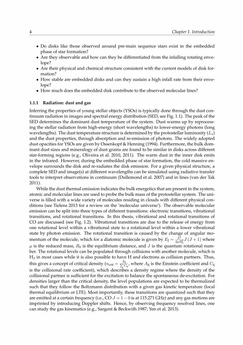
While the dust thermal emission indicates the bulk energetics that are present in the system,atomic and molecular lines are used to probe the bulk mass of the protostellar system. The uni-verse is filled with a wide variety of molecules residing in clouds with different physical con-ditions (see Tielens 2013 for a review on the ’molecular universe’). The observable molecularemission can be split into three types of different transitions: electronic transitions, vibrationaltransitions, and rotational transitions. In this thesis, vibrational and rotational transitions ofCO are discussed (see Fig. 1.2). Vibrational transitions are due to the release of energy fromone rotational level within a vibrational state to a rotational level within a lower vibrationalstate by photon emission. The rotational transition is caused by the change of angular mo-mentum of the molecule, which for a diatomic molecule is given by EJ = ~2
2µR20J (J + 1) where
µ is the reduced mass, R0 is the equilibrium distance, and J is the quantum rotational num-ber. The rotational levels can be populated through collisions with another molecule, which isH2 in most cases while it is also possible to have H and electrons as collision partners. Thus,this gives a concept of critical density (ncrit =
Aij∑Cij
, where Aij is the Einstein coefficient and Cij
is the collisional rate coefficient), which describes a density regime where the density of thecollisional partner is sufficient for the excitation to balance the spontaneous de-excitation. Fordensities larger than the critical density, the level populations are expected to be thermalizedsuch that they follow the Boltzmann distribution with a given gas kinetic temperature (localthermal equilibrium or LTE). Most importantly, these transitions are quantized such that theyare emitted at a certain frequency (i.e., CO J = 1− 0 is at 115.271 GHz) and any gas motions areimprinted by introducing Doppler shifts. Hence, by observing frequency resolved lines, onecan study the gas kinematics (e.g., Sargent & Beckwith 1987; Yen et al. 2013).
Section 1.1. Star and planet formation 5
Figure 1.2 — Top left: The vibrational and rotational levels of 12CO up to v = 2 and J = 40. Bottom left: Azoom in of the rotational transitions up to Ju = 10. A cartoon depicting the molecular line excitation and radiationpropagation from an envelope to the observed line profile. The low J levels are populated in the low densityand low temperature regimes while higher rotational levels are populated in dense warm gas. The excitation ofmolecular levels include collisions with H2 (sometimes with H, He, and electrons) and radiation from dust, otherCO molecules if sufficiently optically thick, and the cosmic microwave background at 2.7 K. Adapted from Bruderer2010.
1.1.2 Observational tools
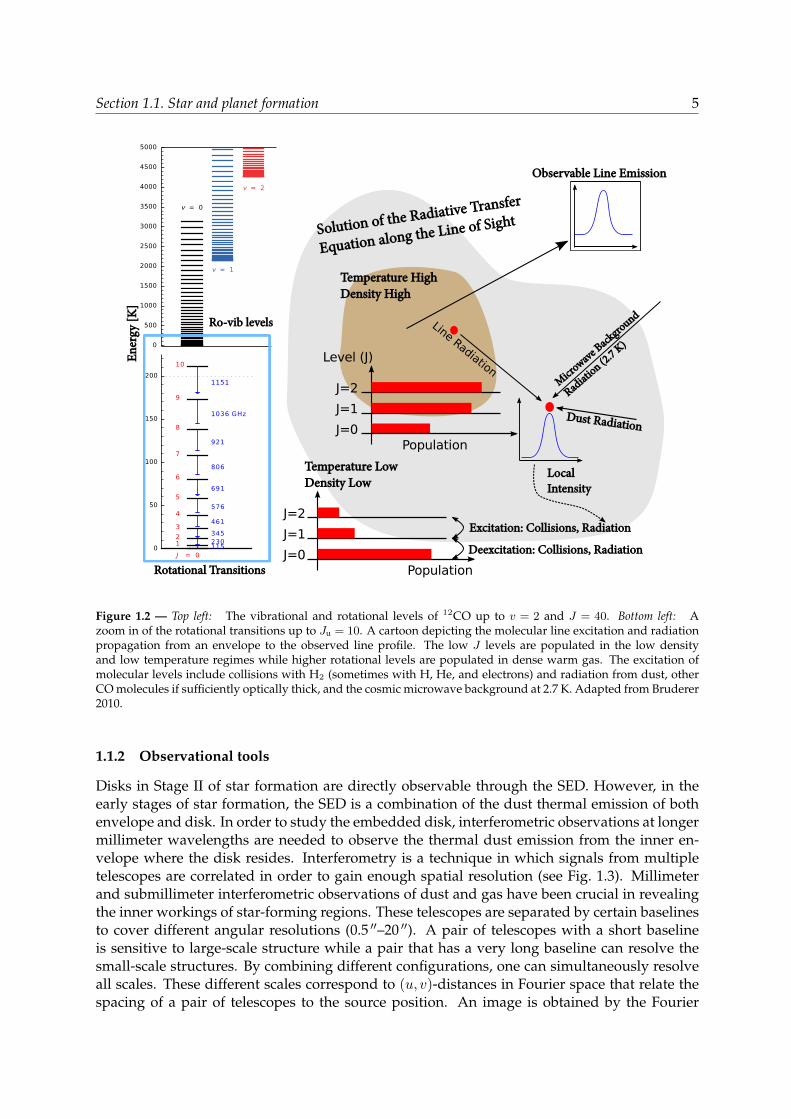
Disks in Stage II of star formation are directly observable through the SED. However, in theearly stages of star formation, the SED is a combination of the dust thermal emission of bothenvelope and disk. In order to study the embedded disk, interferometric observations at longermillimeter wavelengths are needed to observe the thermal dust emission from the inner en-velope where the disk resides. Interferometry is a technique in which signals from multipletelescopes are correlated in order to gain enough spatial resolution (see Fig. 1.3). Millimeterand submillimeter interferometric observations of dust and gas have been crucial in revealingthe inner workings of star-forming regions. These telescopes are separated by certain baselinesto cover different angular resolutions (0.5 ′′–20 ′′). A pair of telescopes with a short baselineis sensitive to large-scale structure while a pair that has a very long baseline can resolve thesmall-scale structures. By combining different configurations, one can simultaneously resolveall scales. These different scales correspond to (u, v)-distances in Fourier space that relate thespacing of a pair of telescopes to the source position. An image is obtained by the Fourier
6 Chapter 1. Introduction
Figure 1.3 — Left: Sketch of how interferometry probes the physical structure of an embedded disk. A shortbaseline (blue) and a long baseline (red) are indicated. Right: The correlated flux as function of baseline length interms of u, v distance is shown by the black dashed line. The expected contribution of the envelope and the disk areshown in orange and red, respectively. The single dish flux is indicated by the circle on top which could be largerthan the correlated flux at short baselines.
transform of a collection of (u, v) points. By utilizing the Earth’s rotation, a more complete(u, v) coverage can be obtained which greatly increases the image quality. On the other hand,the largest physical scale that one probes is defined by the shortest baseline. Consequently,emission from the large scale is always filtered out due to the missing short spacings since thetelescopes cannot be placed infinitely close together. Beckwith et al. (1984) demonstrated thepower of such observations when they revealed the compact structure of gas and dust aroundHL Tau. With the availability of the Plateau de Bure Interferometer (PdBI, 7 telescopes) andAtacama Large Millimeter Array (ALMA, 66 telescopes), such observations can be routinelydone with much better sensitivity than before to reveal faint structures. Furthermore, the jumpfrom 6 to 66 telescopes will provide unprecedented imaging capabilities at submillimeter wave-lengths. The full ALMA will provide an angular resolution< 0.1 ′′ or< 14 AU spatial resolutionat typical distances of 140 pc, which is sufficient to study the disk formation process.
1.2 Disk formation: energy and momentum conservation
Significant theoretical work has gone into studying the disk formation process. Current ob-servations provide the spatial resolution and sensitivity to test these theoretical models. Thestar formation process is very complex with dynamical processes occurring at physical scalesranging from a few stellar radii of ∼0.1 AU to envelope scales of 104 AU and densities of 104
cm−3 to 1015 cm−3. The disk forms out of conservation of energy and momentum as the corecollapses from the large-scale molecular cloud. This section introduces the basic idea of howthis proceeds and the problems with current theories.
1.2.1 Large scale: envelope
The physical processes that control the collapse of a large scale protostellar core include turbu-lence, gravity, thermal pressure, rotation, and magnetic field. Turbulence is an important aspectof galactic dynamics as a whole. It is defined by chaotic, non-linear changes to density, veloc-ity, temperature and magnetic field during energy transfer from large scale to smaller scales.
Section 1.2. Disk formation: energy and momentum conservation 7
Recent major advances in theoretical models of star formation have focused on the role of tur-bulence in star and disk formation simulations (Mac Low & Klessen 2004; McKee & Ostriker2007). Gravity takes over once there is substantial mass within a sufficiently small volume. Inthe presence of gravity alone, the gas and dust simply stream toward the center. The presenceof rotation changes the trajectory of the gas and dust as they spiral toward the growing proto-star. In general, the dynamics at large scale are unchanged by rotation, however the densitiesand velocities are changed at small scales. Finally, magnetic fields permeate the galaxy andregulate the star-formation process (see e.g., McKee et al. 1993; Crutcher 2012). Its origin andhow it is regulated is still debated. In reality, all of these forces act together during the dynam-ical evolution of the forming star and disk system. Fast and reliable computer programs arerequired to investigate the combined effects of all these forces.
Envelope rotation has been observed by Goodman et al. (1993) by mapping N2H+ emissionon scales of ∼0.1 pc. The typical rotational rates of 10−13–10−15 Hz seem to be consistent withthat expected from turbulent cloud simulations by Burkert & Bodenheimer (2000). However,recent three-dimensional simulations by Dib et al. (2010) suggest that the inferred rotation ratesfrom observations could be up to one order of magnitude higher than the true specific angularmomentum of the core.
The strength of the magnetic fields toward molecular cloud cores has been inferred throughstatistical analysis of observations of the Zeeman effect (see e.g., Crutcher 2012). Sufficientmagnetic pressure can prevent gravitational collapse when its mass is subcritical such thatM <MφB = πR2B
2π√G
for a slab of gas and a uniform magnetic field B (Nakano & Nakamura 1978;McKee et al. 1993). In the supercritical case (M > MφB ), the core simply collapses to form astar. The interesting case for a subcritical cloud is that the magnetic field prevents the ionizedgas and dust from collapsing, but the neutral material can proceed to form a star (ambipolardiffusion, Zweibel 1988). More important for the disk formation and the trajectory of materialis the fact that the presence of a magnetic field can remove angular momentum due to thetwisted magnetic field lines. This strongly affects the formation of disks at scales R < 1000 AUas rotation dominates the motion on smaller scales than the magnetic fields.
1.2.2 Small scale: star and disk
The flow of material from the large-scale structure (> 1000 AU) to small scales (< 1000 AU) isdetermined by the angular momentum conservation and evolution. The sun’s specific angularmomentum is ∼ 1015 cm2 s−1 (Pinto et al. 2011). For comparison, the typical specific angularmomentum of molecular cloud cores is ∼ 1021−22 cm2 s−1 (Goodman et al. 1993), so > 6 or-ders of magnitude need to be removed. This problem was first recognized by Mestel & Spitzer(1956). Perhaps, some of the angular momentum has already been lost either before or duringthe gravitational collapse such as described above through magnetic fields. Since angular mo-mentum is strictly conserved in equations of motion, it needs to be transferred to other bodiesor removed by other mechanism(s).
The infalling matter with excess angular momentum will form a flattened structure or arotationally supported disk. Disks are found to have a typical specific angular momentumof ∼ 1019−21 cm2 s−1, which are lower than their envelope but still higher than the growingstar (Williams & Cieza 2011; Belloche 2013). Consequently, the disk must further remove theangular momentum excess. It does so either by launching a wind/jet or by viscous transport.For the purpose of this thesis, viscous transport will be discussed. Viscosity can arise eitherfrom the collisions between gas molecules or the mixing of fluid elements through turbulence.The latter is the most commonly used viscosity parameter to describe the viscous evolution

8 Chapter 1. Introduction
of disks while molecular collisions are unimportant. The most commonly used viscous diskevolution model is that of the alpha-disk (α prescription) as described by Shakura & Sunyaev(1973). It is assumed that the energy loss and momentum transfer occurs locally within a lengthscale that corresponds to the disk’s scale height (Hdisk). From such models, a constant α ∼10−2 is found to be a good description of the observed disk evolution and physical structure(Hartmann et al. 1998; Hughes et al. 2011).
1.2.3 Infall and accretion
The embedded phase of star formation is the period in which both of the physics at large scaleand at small scales are intertwined and affect each other. The trajectory of the infalling mat-ter from the large scale dictates the distribution of matter that forms the disk. The physicalstructure of the disk is crucial in determining its accretion properties. Infall describes the gen-eral trajectory of gas and dust from the envelope to the disk or star. Accretion is the transportof material inward through the disk onto the star. In the embedded phase of low-mass starformation, the dominant heating comes from the combination of infall and accretion since theprotostar is still growing. Hence, the dust temperature structure that affects the physical andchemical structure of the disk and the inner envelope (< 1000 AU) relies on the understandingof the rate at which the material is being transported onto the star. This process does not haveto be continuous, but it is likely episodic to avoid the luminosity problem (e.g., Evans et al.2009b; Dunham et al. 2014). The ‘luminosity problem’ describes the discrepancy between theobserved luminosities of embedded protostellar systems and the luminosity produced by theaccretion process at a steady rate needed to build up a solar mass star (see Kenyon & Hartmann1990).
1.3 Simplified models of star formation
As described in previous sections, star formation involves a wide range of physical processesat both large scale (∼ 0.1 pc) and small scale (< 100 AU). However, simplified models of starformation that only look at one or two physical processes, in general, capture the physical struc-ture of the large-scale envelope and the disk. These physical structures are used to interpretthe observational data. There are two types of simplified models of star formation: analyticalmodels and hydrodynamic simulations.
1.3.1 Analytical models
A subset of these simplified models can be solved analytically to describe the general sequenceof star formation (Shu 1977). A significant fraction of our understanding of star formation isobtained through investigation of how different, separated physical processes independentlyaffect the collapse and disk formation. A few of the simplifications are presented here with anincreasing level of complexity. The following sections introduce analytical models of disk andenvelope around protostars.
1.3.1.1 Large-scale envelope
The simplest model of the large-scale envelope is a spherically symmetric power law model:ρ ∝ r−p where ρ is the total (gas+dust) density, r is the spherical radius, and p is the power-lawslope. Such a power-law model stems from earlier studies such as the collapse of a singularisothermal sphere (Larson 1969). The exact density profile may change depending on the poly-tropic equation of the gas (P ∝ ργ , see Ogino et al. 1999 for detailed discussion). Furthermore,the presence of magnetic fields slows down the contraction process that will eventually lead

Section 1.3. Simplified models of star formation 9
100 AU
Protoplanetary DiskStage II
Warm surface layer
100 AU
Embedded DiskStage 0/I
Outow cavity
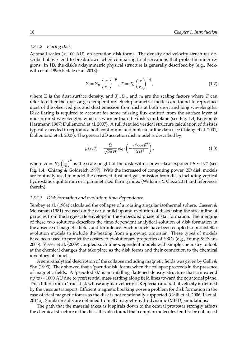
Figure 1.4 — Schematic of the 2D protoplanetary disk (left) and an embedded disk (right) physical structure inspherical coordinates (r, θ). The scale height of the disk H(r) is indicated along with the warm surface layer thatemits most of the IR irradiation. The outflow cavity and centrifugal radius rcen are indicated in the embedded diskmodel.
to the isothermal solution as shown by Shu (1977). The temperature structure of such a modelcan be determined by assuming a central protostar with a temperature of ∼ 5000 K. Such amodel has been shown to reproduce the observed properties (SED and continuum images) ofprotostellar envelopes (e.g., Kenyon et al. 1993; Jørgensen et al. 2002).
The effects of rotation on the collapse process of the envelope were investigated in theearly 70s using two- and three-dimensions with imposed axisymmetry (Larson 1972; Wood-ward 1978). Ulrich (1976) calculated the density structure of the envelope by imposing angularmomentum conservation as the parcels of gas and dust fall toward the center. From theseassumptions, the 2D density structure is described by the following equation:
ρ (r,µ) = ρ0
(r
rcen
)−3/2(1 +
µ
µ0
)−1/2( µ
µ0+
2rcen
rµ2
0
)−1
, (1.1)
where µ ≡ cosθ, rcen is the centrifugal radius where the infalling material is stopped by cen-trifugal force, and finally µ0, θ0 is the solution to the streamline at r and θ from θ0 (see Fig. 1.4,Cassen & Moosman 1981, Whitney & Hartmann 1993). The scaling factor ρ0 could be a freeparameter or connected to the infall rate from the envelope. Compared with the sphericallysymmetric power-law models, this particular model in 2D is similar at large scale (> 1000 AU)while the inner regions are flattened (disk-like). The flattened region is determined by the rcenparameter which describes the regime in which the material starts to enter the disk, and, con-sequently, can be larger than the extent of the rotationally supported disk where the azimuthalvelocities are Keplerian. Such a simple two-dimensional model has been used to model the ob-served properties of both dust and gas toward YSOs (e.g., Whitney & Hartmann 1993; Eisner2012; Yen et al. 2013).
10 Chapter 1. Introduction
1.3.1.2 Flaring disk
At small scales (< 100 AU), an accretion disk forms. The density and velocity structures de-scribed above tend to break down when comparing to observations that probe the inner re-gions. In 1D, the disk’s axisymmetric physical structure is generally described by (e.g., Beck-with et al. 1990; Fedele et al. 2013):
Σ = Σ0
(r
r0
)−p, T = T0
(r
r0
)−q, (1.2)
where Σ is the dust surface density, and T0,Σ0, and r0 are the scaling factors where T canrefer to either the dust or gas temperature. Such parametric models are found to reproducemost of the observed gas and dust emission from disks at both short and long wavelengths.Disk flaring is required to account for some missing flux emitted from the surface layer atmid-infrared wavelengths which is warmer than the disk’s midplane (see Fig. 1.4, Kenyon &Hartmann 1987; Dullemond et al. 2007). A full detailed vertical structure calculation of disks istypically needed to reproduce both continuum and molecular line data (see Chiang et al. 2001;Dullemond et al. 2007). The general 2D accretion disk model is described by
ρ (r, θ) =Σ√2πH
exp
(−r
2 cosθ2
2H2
), (1.3)
where H = H0
(rr0
)his the scale height of the disk with a power-law exponent h ∼ 9/7 (see
Fig. 1.4, Chiang & Goldreich 1997). With the increased of computing power, 2D disk modelsare routinely used to model the observed dust and gas emission from disks including verticalhydrostatic equilibrium or a parametrized flaring index (Williams & Cieza 2011 and referencestherein).
1.3.1.3 Disk formation and evolution: time-dependence
Terebey et al. (1984) calculated the collapse of a rotating singular isothermal sphere. Cassen &Moosman (1981) focused on the early build up and evolution of disks using the streamline ofparticles from the large-scale envelope in the embedded phase of star formation. The mergingof these two solutions describes the time-dependent analytical solution of disk formation inthe absence of magnetic fields and turbulence. Such models have been coupled to protostellarevolution models to include the heating from a growing protostar. These types of modelshave been used to predict the observed evolutionary properties of YSOs (e.g., Young & Evans2005). Visser et al. (2009) coupled such time-dependent models with simple chemistry to lookat the chemical changes that take place as the disk forms and their connection to the chemicalinventory of comets.
A semi-analytical description of the collapse including magnetic fields was given by Galli &Shu (1993). They showed that a ‘pseudodisk’ forms when the collapse proceeds in the presenceof magnetic fields. A ‘pseudodisk’ is an infalling flattened density structure that can extendup to∼ 1000 AU due to preferential mass settling along field lines toward the equatorial plane.This differs from a ‘true’ disk whose angular velocity is Keplerian and radial velocity is definedby the viscous transport. Efficient magnetic breaking poses a problem for disk formation in thecase of ideal magnetic forces as the disk is not rotationally supported (Galli et al. 2006; Li et al.2014a). Similar results are obtained from 3D magneto-hydrodynamic (MHD) simulations.
The path that the material takes as it spirals down to the central protostar strongly affectsthe chemical structure of the disk. It is also found that complex molecules tend to be enhanced
Section 1.3. Simplified models of star formation 11
if a rotationally supported disk is present instead of a pseudodisk. This occurs due to the lackof photodissociating photons coupled with a sufficiently warm disk for complex molecules toform. Therefore, continuum and molecular line observables that can differentiate between thetwo modes of disk formation are required to connect the physical and chemical changes duringthe early stages of star formation to our Solar System.
1.3.2 Numerical hydrodynamic simulations
Recent progress in numerical simulations of star formation has been made due to advancesin computing. While analytical solutions can describe the general features of star formation,hydrodynamic simulations can investigate the non-linear effects of the different physical pro-cesses at once. However, one should be cautious of the numerical artefacts that are inherent inthese simulations. In general, there are three types of numerical simulations that one can adopt:smoothed particle hydrodynamics (SPH), grid-based, and moving mesh. The two most testedand benchmarked of these are SPH and grid-based. There are indeed fundamental differencesin the two methods as described in Agertz et al. (2007) and Tasker et al. (2008). In this thesis,SPH and grid-based codes are used.
1.3.2.1 Smoothed Particle Hydrodynamics (SPH)
This method solves the equations of fluid dynamics by interpolation (smoothed) between manydynamic particles. The implementation was started roughly 40 years ago by Lucy (1977) andGingold & Monaghan (1977). In recent years, the treatment of different physical processesincluding magnetic fields has been added which are reviewed in Springel (2010) (see also Mon-aghan 1992 for an introduction to SPH). Any physical properties such as density (ρ), temper-ature described by sound speed cs, and velocities are calculated through kernel W smoothingsuch that
ρ (r) =
∫ρ (r)W
(δr, hSPH
)dr′ =
∑
i
ρiW(δri, hSPH
)(1.4)
with r the position of the particle i and hSPH the smoothing length. Most current codes adopt acubic smoothing kernel based on the distance normalized by the smoothing hSPH. This methodfollows the particles as they move through space and time (Lagrangian method), which ensuresthe conservation of energy and momentum. SPH has been used to simulate star formation,stellar encounters, planet formation, and disk evolution.
1.3.2.2 Grid methods and AMR
Grid-based codes fix the number of resolution elements in which the fluid equations are solved.Thus, the equations of motions are solved within a set of boundary conditions and information(transfer of mass, energy, and momentum) must be propagated to adjacent grids (Eulerian)through numerical schemes. Adaptive-mesh refinement (AMR) splits up or refines certaingrid(s) that satisfy a few pre-defined conditions in order to resolve the physics within thatregion. Different methods have been used to propagate information from one cell to nearbycells such as those (and variations of them) in van Leer (1979), Woodward & Colella (1984),and Stone & Norman (1992). In particular, Fleming et al. (2000) introduced methods to solvenon-ideal magneto-hydrodynamics (MHD) equations. In the ideal MHD limit, the magneticfield is always frozen to the fluid element, while in the non-ideal case, the field is allowed nu-merically to diffuse and reconnect. Non-ideal MHD treatment is found to allow for rotationallysupported disk formation, although not conclusively.
12 Chapter 1. Introduction
Physicalmodel
Dust temperature
Molecular abundance+
Excitation
Spectral cubes
Interferometricvisibilities
1D analytical,
2D/3D simulations
RADMC-3D, analytical
Parametric functionor simple chemistry
ALI or escape probability
Emission at x, y, and
velocity v
Simulation, analytical
Intensity prole
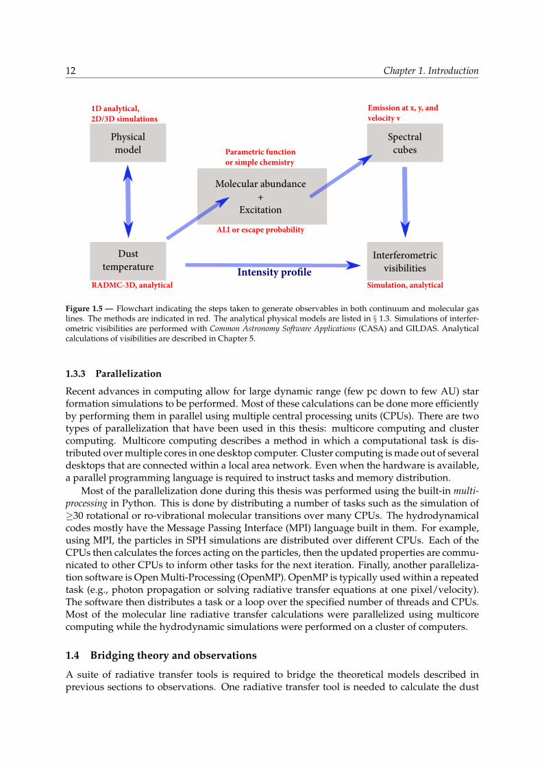
Figure 1.5 — Flowchart indicating the steps taken to generate observables in both continuum and molecular gaslines. The methods are indicated in red. The analytical physical models are listed in § 1.3. Simulations of interfer-ometric visibilities are performed with Common Astronomy Software Applications (CASA) and GILDAS. Analyticalcalculations of visibilities are described in Chapter 5.
1.3.3 Parallelization
Recent advances in computing allow for large dynamic range (few pc down to few AU) starformation simulations to be performed. Most of these calculations can be done more efficientlyby performing them in parallel using multiple central processing units (CPUs). There are twotypes of parallelization that have been used in this thesis: multicore computing and clustercomputing. Multicore computing describes a method in which a computational task is dis-tributed over multiple cores in one desktop computer. Cluster computing is made out of severaldesktops that are connected within a local area network. Even when the hardware is available,a parallel programming language is required to instruct tasks and memory distribution.
Most of the parallelization done during this thesis was performed using the built-in multi-processing in Python. This is done by distributing a number of tasks such as the simulation of≥30 rotational or ro-vibrational molecular transitions over many CPUs. The hydrodynamicalcodes mostly have the Message Passing Interface (MPI) language built in them. For example,using MPI, the particles in SPH simulations are distributed over different CPUs. Each of theCPUs then calculates the forces acting on the particles, then the updated properties are commu-nicated to other CPUs to inform other tasks for the next iteration. Finally, another paralleliza-tion software is Open Multi-Processing (OpenMP). OpenMP is typically used within a repeatedtask (e.g., photon propagation or solving radiative transfer equations at one pixel/velocity).The software then distributes a task or a loop over the specified number of threads and CPUs.Most of the molecular line radiative transfer calculations were parallelized using multicorecomputing while the hydrodynamic simulations were performed on a cluster of computers.
1.4 Bridging theory and observations
A suite of radiative transfer tools is required to bridge the theoretical models described inprevious sections to observations. One radiative transfer tool is needed to calculate the dust

Section 1.4. Bridging theory and observations 13
temperature structure by simulating the photon propagation through dusty media. Anotherset of radiative transfer tools is required to simulate the molecular line emission. In most cases,these two tools are completely independent of each other. The typical flow of modelling theobservables is illustrated in Fig. 1.5.
1.4.1 Radiative transfer: dust and masses
Dust makes up about 1% of the total mass. For a given central heating and mass distributionas in § 1.3, dust continuum radiative transfer simulates the propagation of photons as they areabsorbed or scattered and re-emited by dust. The most common method is the Monte Carlo(MC) approach (Bjorkman & Wood 2001) where photon packages with energy L?/Nphotons arelaunched from the central source. Through the absorption and re-emission of these photonpackages, the dust temperature structure can be obtained. The amount of energy that the dustabsorbs depends on the dust optical properties.
The photon propagation is easy computationally for optically thin radiation. In this thesis,a few tricks are used to efficiently compute the dust temperature structure of optically thick(τ ≥ 106) embedded disks. Computationally, regions are taken as optically thick, when theopacity towards the star is larger than a few 1000 at the peak wavelength of the star. In gen-eral, a higher number of photons (∼ 107) are required to obtain a smooth dust temperaturestructure. The exact number of photons depends on the number of grids. The propagation ofa photon through an optically thick region is modified such that it is not trapped within onecomputational cell (see Min et al. 2009). An additional source of heating such as accretion heat-ing can be added. There are two ways to add such a term, either by depositing the energy thateach cell has or by launching another set of photons from the disk. Furthermore, the diffusionapproximation (∇∇T 4
3ρκP= 0, where κP is the Planck opacity) is used to smooth the midplane’s
temperature structure. The diffusion approximation is valid in the highly optically thick region(τ0.1 µm >> 1) since the radiation field is in thermal equilibrium such that the source functionis the Planck function. A smooth dust temperature structure is crucial in the determination ofmolecular abundances in embedded disks.
The dust thermal emission can be simulated by solving the radiative transfer equation alonga line of sight similar to that depicted in Fig. 1.2. One generally finds that the emission at longwavelengths is optically thin and, consequently, it is a direct measure of the dust mass. Diskand envelope masses have been obtained through such assumptions. The simplest envelopemodel is by assuming spherical symmetry (ρ ∝ r−p). Through dust continuum radiative trans-fer programs such as DUSTY (Ivezic & Elitzur 1997), the thermal structure can be obtainedand its SED compared to observation. Jørgensen et al. (2002) and Kristensen et al. (2012) usedsuch a method to constrain the large-scale envelope structure. In order to determine the diskmass, Jørgensen et al. (2009) explored the contribution of such a model to interferometric dustthermal emission. Thus, by accounting for the large-scale contribution, the disk emission canbe extracted and, in turn, their masses (see also Looney et al. 2003; Enoch et al. 2011). More so-phisticated tools such as RADMC (Dullemond & Dominik 2004), RADMC-3D, and Hyperion(Robitaille 2011) are required to build 2D and 3D physical models. Recent developments in 3Dradiative transfer tools are reviewed by Steinacker et al. (2013).
1.4.2 Chemical abundances
To simulate the observed molecular lines, the gas phase molecular abundances are needed.A simple gas phase abundance can be obtained by considering the adsorption and thermaldesorption of molecules on the dust grains. In addition, a lower abundance is expected along

14 Chapter 1. Introduction
the warm surface layers close to the star (see Fig. 1.4) where molecules can be photodissociatedby absorption of energetic ultraviolet (UV) photons (see van Dishoeck et al. 2006). Ices couldalso be photodesorbed from the grain if they are not well shielded from energetic UV photons(e.g., Oberg et al. 2009; Fayolle et al. 2011). This thesis limits the chemistry to adsorption andthermal desorption of molecules on the dust grains. The adsorption rate is the rate at whichices of species X accumulate on the dust grain given the gas temperature and size of the dust(∼ 0.1 µm). A molecular species X also has a binding energy that describes how strongly it isbound on the grain surface. The binding energies of well known ice species such as H2O andCO have been inferred through controlled laboratory experiments (e.g., Bisschop et al. 2006;Burke & Brown 2010). At steady state, the adsorption rate kads is balanced by the thermaldesorption rate kthdes. Using such a balance, one finds that CO is in the gas phase forTdust > 20 K while it is 100 K for H2O. The temperature of this transition is pressure dependentsuch that it can be up to 160 K for H2O at high densities (nH ∼ 1016 cm−3). This is not necessarilyvalid at low densities such as those found in the large-scale envelope since the adsorptiontimescale is longer than the lifetime of the residing material. The physical processes such asinfall tend to occur on timescales much shorter than the chemical timescales for the embeddedphase of star formation. However, for most of the purposes of this thesis, steady state chemistryis appropriate to simulate the observables from theoretical models.
1.4.3 Molecular emission as a probe of physical structure
The dust physical structure is the first step in the determination of molecular abundances to-ward YSOs (e.g., Hogerheijde et al. 1998; Yıldız et al. 2013). While the low-J transitions ofCO can be treated in local thermal equilibrium (LTE or thermalized) due to their low criticaldensities, higher-J lines tend not to be in LTE. Non-LTE population levels are calculated byconsidering different excitation and de-excitation mechanisms (van der Tak et al. 2007):
ni
N∑
i
Pij =N∑
j6=i
njPji, (1.5)
where ni,j are the populations of levels i and j, respectively, N is the total number of levels,and Pij indicate the rate of transition between level i and j. The rates take into account theprobability of spontaneous emission given by Einstein Aij coefficient, probability of stimulatedemission Bij
⟨Jij⟩, and collisional rates.
Thanks to many years of primarily theoretical studies in determination of potential energysurfaces and the subsequent collision dynamics on these surfaces, these properties are knownand tabulated in the Leiden Atomic and Molecular Database (LAMDA Schoier et al. 2005) forwell-known molecules. Theoretical calculations of collisional rate coefficients typically employthe close coupling (CC), coupled-states (CS) and infinite order sudden (IOS) approximations.While CC is exact, the CS approximation assumes that the angular momentum is conserved andthe IOS approximation assumes that the molecules do not rotate during collision (see Schoieret al. 2005; Roueff & Lique 2013). Most recent calculations employ the CC method, which solvesthe nuclear Schrodinger equation exactly given the detailed potential energy surfaces (Roueff& Lique 2013). Most of the molecular databases only contain collisional rate coefficients for therotational levels within the vibrational ground state. For example, Yang et al. (2010) calculatedthe CO collisional rate coefficients up to J = 40. To reproduce recent observations of high-JCO molecular lines (J > 40), extrapolations are needed as used in Chapter 4 to calculate thepopulation levels of J > 40 (see also Neufeld 2012). For a simple rigid rotor such as CO, theextrapolation considers the cross section of a linear molecule with an atom as described by a
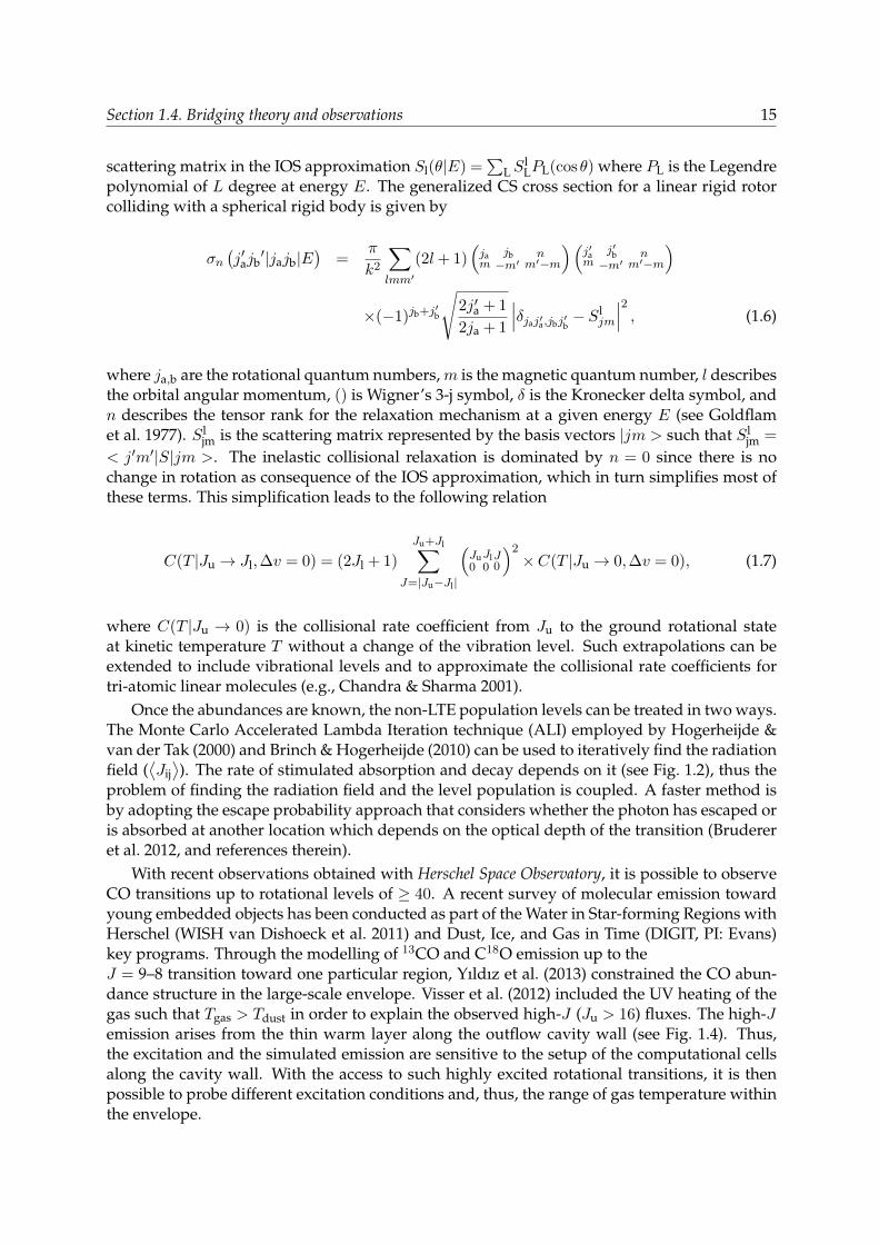
Section 1.4. Bridging theory and observations 15
scattering matrix in the IOS approximation Sl(θ|E) =∑
L SlLPL(cosθ) where PL is the Legendre
polynomial of L degree at energy E. The generalized CS cross section for a linear rigid rotorcolliding with a spherical rigid body is given by
σn(j′ajb
′|jajb|E)
=π
k2
∑
lmm′
(2l+ 1)(jam
jb−m′
nm′−m
)(j′am
j′b−m′
nm′−m
)
×(−1)jb+j′b
√2j′a + 1
2ja + 1
∣∣∣δjaj′a,jbj′b− Sl
jm
∣∣∣2, (1.6)
where ja,b are the rotational quantum numbers,m is the magnetic quantum number, l describesthe orbital angular momentum, () is Wigner’s 3-j symbol, δ is the Kronecker delta symbol, andn describes the tensor rank for the relaxation mechanism at a given energy E (see Goldflamet al. 1977). Sl
jm is the scattering matrix represented by the basis vectors |jm > such that Sljm =
< j′m′|S|jm >. The inelastic collisional relaxation is dominated by n = 0 since there is nochange in rotation as consequence of the IOS approximation, which in turn simplifies most ofthese terms. This simplification leads to the following relation
C(T |Ju→ Jl,∆v = 0) = (2Jl + 1)
Ju+Jl∑
J=|Ju−Jl|
(Ju0Jl0J0
)2×C(T |Ju→ 0,∆v = 0), (1.7)
where C(T |Ju → 0) is the collisional rate coefficient from Ju to the ground rotational stateat kinetic temperature T without a change of the vibration level. Such extrapolations can beextended to include vibrational levels and to approximate the collisional rate coefficients fortri-atomic linear molecules (e.g., Chandra & Sharma 2001).
Once the abundances are known, the non-LTE population levels can be treated in two ways.The Monte Carlo Accelerated Lambda Iteration technique (ALI) employed by Hogerheijde &van der Tak (2000) and Brinch & Hogerheijde (2010) can be used to iteratively find the radiationfield (
⟨Jij⟩). The rate of stimulated absorption and decay depends on it (see Fig. 1.2), thus the
problem of finding the radiation field and the level population is coupled. A faster method isby adopting the escape probability approach that considers whether the photon has escaped oris absorbed at another location which depends on the optical depth of the transition (Brudereret al. 2012, and references therein).
With recent observations obtained with Herschel Space Observatory, it is possible to observeCO transitions up to rotational levels of ≥ 40. A recent survey of molecular emission towardyoung embedded objects has been conducted as part of the Water in Star-forming Regions withHerschel (WISH van Dishoeck et al. 2011) and Dust, Ice, and Gas in Time (DIGIT, PI: Evans)key programs. Through the modelling of 13CO and C18O emission up to theJ = 9–8 transition toward one particular region, Yıldız et al. (2013) constrained the CO abun-dance structure in the large-scale envelope. Visser et al. (2012) included the UV heating of thegas such that Tgas > Tdust in order to explain the observed high-J (Ju > 16) fluxes. The high-Jemission arises from the thin warm layer along the outflow cavity wall (see Fig. 1.4). Thus,the excitation and the simulated emission are sensitive to the setup of the computational cellsalong the cavity wall. With the access to such highly excited rotational transitions, it is thenpossible to probe different excitation conditions and, thus, the range of gas temperature withinthe envelope.
16 Chapter 1. Introduction
1.5 This thesis and outlook
This thesis explores both the theoretical and observational aspects of disk formation during theembedded stage of star formation. Semi-analytical and numerical hydrodynamic models havebeen coupled to dust continuum and line radiative transfer tool(s) as depicted in Fig. 1.5. Thepredicted spectrally resolved rotational transitions of CO isotopologs are simulated for compar-ison with observations. These simulations and predictions are accompanied by spatially andspectrally resolved observations of optically thin CO emission toward less embedded (moreevolved Stage I) young stellar objects. The observations were carried out with the Plateau deBure Interferometer (PdBI) located in France. The following list outlines the results of thisthesis.
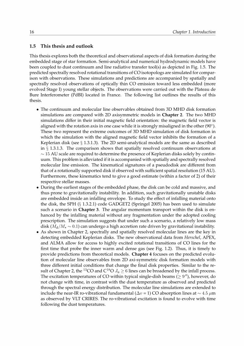
• The continuum and molecular line observables obtained from 3D MHD disk formationsimulations are compared with 2D axisymmetric models in Chapter 2. The two MHDsimulations differ in their initial magnetic field orientation: the magnetic field vector isaligned with the rotation axis in one case while it is strongly misaligned in the other (90).These two represent the extreme outcomes of 3D MHD simulation of disk formation inwhich the simulation with the aligned magnetic field vector inhibits the formation of aKeplerian disk (see § 1.3.1.3). The 2D semi-analytical models are the same as describedin § 1.3.1.3. The comparison shows that spatially resolved continuum observations at∼ 15 AU scale are required to determine the presence of Keplerian disks solely by contin-uum. This problem is alleviated if it is accompanied with spatially and spectrally resolvedmolecular line emission. The kinematical signatures of a pseudodisk are different fromthat of a rotationally supported disk if observed with sufficient spatial resolution (15 AU).Furthermore, these kinematics tend to give a good estimate (within a factor of 2) of theirrespective stellar masses.• During the earliest stages of the embedded phase, the disk can be cold and massive, and
thus prone to gravitationally instability. In addition, such gravitationally unstable disksare embedded inside an infalling envelope. To study the effect of infalling material ontothe disk, the SPH (§ 1.3.2.1) code GADGET2 (Springel 2005) has been used to simulatesuch a scenario in Chapter 3. The angular momentum transport within the disk is en-hanced by the infalling material without any fragmentation under the adopted coolingprescription. The simulation suggests that under such a scenario, a relatively low massdisk (Md/M? ∼ 0.1) can undergo a high accretion rate driven by gravitational instability.• As shown in Chapter 2, spectrally and spatially resolved molecular lines are the key in
detecting embedded Keplerian disks. The new observational data from Herschel, APEX,and ALMA allow for access to highly excited rotational transitions of CO lines for thefirst time that probe the inner warm and dense gas (see Fig. 1.2). Thus, it is timely toprovide predictions from theoretical models. Chapter 4 focuses on the predicted evolu-tion of molecular line observables from 2D axi-symmetric disk formation models withthree different initial conditions that change the final disk properties. Similar to the re-sult of Chapter 2, the 13CO and C18O Ju ≥ 6 lines can be broadened by the infall process.The excitation temperatures of CO within typical single-dish beams (≥ 9 ′′), however, donot change with time, in contrast with the dust temperature as observed and predictedthrough the spectral energy distribution. The molecular line simulations are extended toinclude the near-IR ro-vibrational fundamental (∆v = 1) CO absorption lines at ∼ 4.5 µmas observed by VLT CRIRES. The ro-vibrational excitation is found to evolve with timefollowing the dust temperatures.
Section 1.5. This thesis and outlook 17
• Chapters 2 and 4 suggest that the deeply embedded disk is easily revealed by spatiallyand spectrally resolved molecular line observations. Furthermore, the disk’s contributionto the integrated optically thin CO line is predicted to be high during the later phase ofthe embedded stages of star formation. Chapter 5 presents the spatially and spectrallyresolved 13CO and C18O 2–1 lines toward four well-known Stage I embedded objects inthe nearby Taurus molecular cloud (d=140 pc). At a spatial resolution of ≤ 0.8 ′′ (∼ 110AU diameter), three out of the four targeted sources have ∼ 100 AU radius Kepleriandisks as traced by the C18O 2–1 line. The properties of the claimed embedded disks inthe literature combined with the sources studied in this chapter are compared with the2D disk formation models of Chapter 4. This comparison suggests that the models withinitial rotation of Ω = 10−14 Hz and slow sound speeds match well with the observeddisks.• As a consequence of an actively accreting disk, the energy dissipated away during the
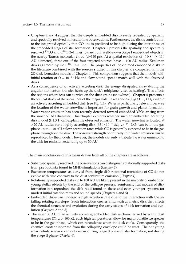
angular momentum transfer heats up the disk’s midplane (viscous heating). This affectsthe regions where ices can survive on the dust grains (snowlines). Chapter 6 presents atheoretical study of the snowlines of the major volatile ice species (H2O, CO, CO2) withinan actively accreting embedded disk (see Fig. 1.4). Water is particularly relevant becausethe location of the water snowline is important for grain growth and planet formation.Water vapor emission has been recently detected toward embedded YSOs arising fromthe inner 50 AU diameter. This chapter explores whether such an embedded accretingdisk model (§ 1.3.1) can explain the observed emission. The water snowline is located at>20 AU radius for a highly accreting disk (M ≥ 10−5 M yr−1). CO2 can be in the gasphase up to∼ 40 AU at low accretion rates while CO is generally expected to be in the gasphase throughout the disk. The observed strength of optically thin water emission can bereproduced by the models. However, the models can only attribute the water emission tothe disk for emission extending up to 30 AU.
The main conclusions of this thesis drawn from all of the chapters are as follows:
• Subarcsec spatially resolved line observations can distinguish rotationally supported disksfrom pseudodisks found in MHD simulations (Chapter 2).• Excitation temperatures as derived from single-dish rotational transitions of CO do not
evolve with time contrary to the dust continuum emission (Chapter 4).• Rotationally supported disks up to 100 AU are likely present in the majority of embedded
young stellar objects by the end of the collapse process. Semi-analytical models of diskformation can reproduce the disk radii found in these and even younger systems formodest initial rotation rates and sound speeds (Chapters 4 and 5).• Embedded disks can undergo a high accretion rate due to the interaction with the in-
falling rotating envelope. Such interaction creates a non-axisymmetric disk that affectsthe chemical structure and evolution during the early stages of disk formation and evo-lution (Chapters 2 and 3)• The inner 30 AU of an actively accreting embedded disk is characterized by warm dust
temperatures (Tdust > 100 K). Such high temperatures allow for major volatile ice speciesto be in the gas phase, which can recondense when the disk cools. Consequently, thechemical content inherited from the collapsing envelope could be reset. The hot youngsolar nebula scenario can only occur during Stage 0 phase of star formation, not duringthe Stage II phase (Chapter 6).

18 Chapter 1. Introduction
Future outlook Current observations have revealed the presence of rotationally supporteddisks in the inner few 100 AU toward a couple of embedded protostars (Tobin et al. 2012;Murillo et al. 2013), which are compared with disk formation models. However, to furtherstudy the details of the disk formation and evolution process in the earliest stages of star for-mation, the spatial resolution and sensitivity of ALMA down to scales of 10 AU is required.The higher spatial and spectral resolution observations of molecular lines can differentiate theKeplerian disk from the infalling envelope. The temperature structure of the disk, which iscrucial to investigate the heating processes, requires two different molecular transitions of amolecule to investigate their excitation conditions. Furthermore, high sensitivity observationsare necessary to study the velocity structure of the disk since the molecular emission at highvelocities is much weaker than at line center. This will be easier done in the future to revealthe kinematics at small scales and allow disk tomography in radial and vertical direction. Inaddition, the combination of short and long baselines that ALMA can deliver will reveal thekinematics of the gas as it falls onto the disk.
This thesis employs steady-state accretion models of disk formation to investigate the molec-ular excitation. It is known that the accretion process is episodic during the early stages of starformation (Vorobyov et al. 2013; Dunham et al. 2014). The processes within the disk and themovement of the gas and dust during this phase has direct consequences for the physical andchemical structure of an evolving embedded disk (Visser & Bergin 2012; Jørgensen et al. 2013).The main challenge is to couple these simulations that include the disk’s vertical structure withradiative transfer tools and chemical models to compare with observations.
Time dependence is needed to investigate the true gas and ice abundances that are presentwithin the Keplerian disk. Time dependent radiative transfer and chemical models such as thatapplied to the 2D models need to be coupled with MHD simulations of disk formation. Fur-thermore, the comparison between the disk formation scenarios with and without turbulenceis still an unexplored territory. The different scenarios also predict different protostellar forma-tion histories that dictate the heating events during the early stages of star formation and, thus,the temperature structure of the newly formed disk. The predicted observables from the hotgas in the inner envelope and disk can be compared with observations that will be taken bythe James Webb Space Telescope (JWST). The synergy between ALMA, VLT CRIRES, JWST, andultimately E-ELT METIS will reveal the physical and chemical structure of the young disk atall scales, including the planet forming zones.

Chapter 2Discriminating protostellar disk
formation models with continuum andspectral line observations
Abstract. Context. Recent simulations have explored different ways to form accretion disks around low-mass stars. However, it has been difficult to differentiate between the proposed mechanisms because ofa lack of observable predictions from these numerical studies.Aims. We aim to present observables that can differentiate a rotationally supported disk from an infallingrotating envelope toward deeply embedded young stellar objects (Menv >Mdisk) and infer their massesand sizes.Methods. Two 3D MHD disk formation simulations of Li and collaborators are studied, with a rotation-ally supported disk (RSD) forming in one but not the other (where a pseudo-disk is formed instead),together with the 2D semi-analytical model. The dust temperature structure is determined throughcontinuum radiative transfer RADMC3D modelling. A simple temperature dependent CO abundancestructure is adopted and synthetic spectrally resolved submm rotational molecular lines up to Ju = 10are compared with existing data to provide predictions for future ALMA observations.Results. 3D MHD simulations and 2D semi-analytical model predict similar compact components incontinuum if observed at the spatial resolutions of 0.5–1 ′′ typical of the observations to date. A spatialresolution of ∼14 AU and high dynamic range (> 1000) are required in order to differentiate betweenRSD and pseudo-disk formation scenarios in the continuum. The moment one maps of the molecularlines show a blue- to red-shifted velocity gradient along the major axis of the flattened structure in thecase of RSD formation, as expected, whereas it is along the minor axis in the case of pseudo-disk. Thepeak-position velocity diagrams indicate that the pseudo-disk shows a flatter velocity profile with ra-dius than an RSD. On larger-scales, the CO isotopolog line profiles within large (> 9 ′′) beams are similarand are narrower than the observed line widths of low-J (2–1 and 3–2) lines, indicating significant tur-bulence in the large-scale envelopes. However a forming RSD can provide the observed line widths ofhigh-J (6–5, 9–8, and 10–9) lines. Thus, either RSDs are common or a higher level of turbulence (b ∼ 0.8km s−1) is required in the inner envelope compared with the outer part (0.4 km s−1).Conclusions. Spatially and spectrally resolved molecular line observations can differentiate between thepseudo-disk and the RSD much better than continuum data. The continuum data give a better estimateon disk masses whereas the disk sizes can be estimated from the spatially resolved molecular lines ob-servations. The general observable trends are similar between the 2D semi-analytical models and 3DMHD RSD simulations.
D. Harsono, E. F. van Dishoeck, S. Bruderer, Z. Y. Li, J. K. Jørgensensubmitted
2.1 Introduction
THE formation of stars and their planetary systems is linked through the formation and evo-lution of accretion disks. In the standard star formation picture, the infalling material forms
20 Chapter 2. Protostellar disk formation models
an accretion disk simply from angular momentum conservation (e.g., Lin & Pringle 1990; Bo-denheimer 1995; Belloche 2013). However, magnetic field strengths observed toward molecularcores (see Crutcher 2012,for a recent review) are expected theoretically to be sufficient in affect-ing the formation and evolution of disks around low-mass stars (e.g., Galli et al. 2006; Joos et al.2012; Krumholz et al. 2013; Li et al. 2013, 2014a). Recent advances in both observational andtheoretical studies give an opportunity to test the star formation process at small-scales (< 1000AU).
It has been known for a long time that the presence of magnetic fields can drastically changethe flow dynamics around low-mass stars (e.g., Galli & Shu 1993) and potentially suppressesdisk formation (e.g., Galli et al. 2006). The latter is due to catastrophic magnetic braking whereessentially all of the angular momentum of the accreting material is removed by twisted fieldlines. Recently, Li et al. (2011) investigate the collapse and disk formation from a uniform cloudwhile Joos et al. (2012) and Machida & Matsumoto (2011) performed simulations starting witha steep density profile and a Bonnor-Ebert sphere, respectively. They found that rotationallysupported disks (RSDs) do not form out of uniform and non-uniform cores under strong mag-netic fields unless the field is misaligned with respect to the rotation axis (Hennebelle & Ciardi2009). Turbulence has also been shown to help with disk formation (Santos-Lima et al. 2012;Seifried et al. 2012; Myers et al. 2013; Joos et al. 2013; Li et al. 2014b).
In spite of a number of disk formation and evolution simulations, only a few observableshave been presented so far. The expected observables in the continuum (spectral energy distri-bution or SED) from 1D and 2D disk formation models have been presented in Young & Evans(2005) and Dunham et al. (2010). Continuum observables out of 2D hydrodynamics simula-tions with a thin disk approximation have been shown by Dunham & Vorobyov (2012) andVorobyov et al. (2013). However, only a handful of synthetic observables from 3D magnetohy-drodynamics (MHD) simulations have been presented in the literature (e.g., Commercon et al.2012a,b).
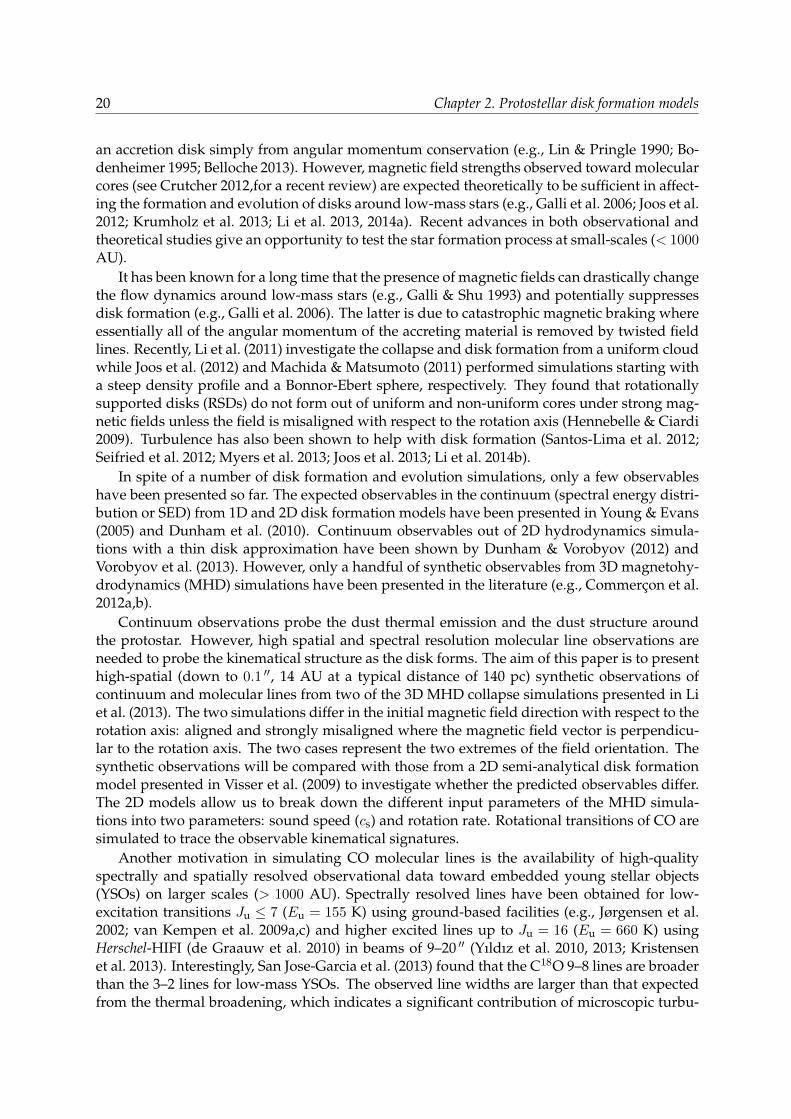
Continuum observations probe the dust thermal emission and the dust structure aroundthe protostar. However, high spatial and spectral resolution molecular line observations areneeded to probe the kinematical structure as the disk forms. The aim of this paper is to presenthigh-spatial (down to 0.1 ′′, 14 AU at a typical distance of 140 pc) synthetic observations ofcontinuum and molecular lines from two of the 3D MHD collapse simulations presented in Liet al. (2013). The two simulations differ in the initial magnetic field direction with respect to therotation axis: aligned and strongly misaligned where the magnetic field vector is perpendicu-lar to the rotation axis. The two cases represent the two extremes of the field orientation. Thesynthetic observations will be compared with those from a 2D semi-analytical disk formationmodel presented in Visser et al. (2009) to investigate whether the predicted observables differ.The 2D models allow us to break down the different input parameters of the MHD simula-tions into two parameters: sound speed (cs) and rotation rate. Rotational transitions of CO aresimulated to trace the observable kinematical signatures.
Another motivation in simulating CO molecular lines is the availability of high-qualityspectrally and spatially resolved observational data toward embedded young stellar objects(YSOs) on larger scales (> 1000 AU). Spectrally resolved lines have been obtained for low-excitation transitions Ju ≤ 7 (Eu = 155 K) using ground-based facilities (e.g., Jørgensen et al.2002; van Kempen et al. 2009a,c) and higher excited lines up to Ju = 16 (Eu = 660 K) usingHerschel-HIFI (de Graauw et al. 2010) in beams of 9–20 ′′ (Yıldız et al. 2010, 2013; Kristensenet al. 2013). Interestingly, San Jose-Garcia et al. (2013) found that the C18O 9–8 lines are broaderthan the 3–2 lines for low-mass YSOs. The observed line widths are larger than that expectedfrom the thermal broadening, which indicates a significant contribution of microscopic turbu-

Section 2.2. Numerical simulations and radiative transfer 21
Table 2.1 — Stellar (M?), envelope (Menv), and disk (Md) masses for the three simulations. Rd is the extent of therotationally supported disk for each simulation.
Model M? Menv Md Rd[M] [M] [M] [AU]
3D MHD RSD 0.38 0.29 0.06 250–3003D MHD No RSD 0.24 0.35 0.13∗ ...2D RSD 0.35 0.32 0.04 65
∗ Mass of pseudo-disk is the sum of the regions with number densities nH2 > 107.5 cm−3; noradius is tabulated for this case.
lence or some other forms of motion, such as rotation and infall. Through the characterizationof spectrally resolved molecular lines on such physical scales, we aim to test the kinematicspredicted in various star and disk formation models.
Another key test of star formation models is to compare the predicted mass evolution fromthe envelope to the star with observations (e.g., Jørgensen et al. 2009; Li et al. 2014a). Inferringthese properties toward embedded YSOs are not straightforward due to confusion betweendisk and envelope. The mass evolution of the disk and envelope can be deduced from millime-ter surveys combining both aperture synthesis and single dish observations (Keene & Masson1990; Terebey et al. 1993; Looney et al. 2003; Jørgensen et al. 2009; Enoch et al. 2011). However,precise determination of stellar masses requires spatially and spectrally resolved molecular lineobservations of the velocity gradient in the inner regions of embedded YSOs (Sargent & Beck-with 1987; Ohashi et al. 1997a; Brinch et al. 2007a; Lommen et al. 2008; Jørgensen et al. 2009;Takakuwa et al. 2012; Yen et al. 2013). Here we apply a similar analysis on the synthetic con-tinuum and molecular line data as performed on the observations to test the reliability of theinferred masses.
This paper is structured as follows. Section 6.2 describes the simulations and the radiativetransfer method that are used. The synthetic continuum images are presented in Section 2.3.Section 2.4 presents the synthetic CO moment maps and line profiles for the different simula-tions. The results are then discussed in Section 6.4 and summarized in Section 6.5.
2.2 Numerical simulations and radiative transfer
2.2.1 Magneto-hydrodynamical simulations
We utilize the 3D MHD simulations of the collapse of a 1 M uniform, spherical envelope asdescribed in Li et al. (2013). The envelope initially has a density of ρ0 = 4.77× 10⁻¹⁹ g cm−3,a solid-body rotation of Ω0 = 10−13 Hz, and a relatively weak, uniform magnetic field of B0 =11 µG. The details of the simulations can be found in Li et al. (2013).
A snapshot of two simulations at t = 3.9× 10¹² s = 1.24× 10⁵ years is used. This corre-sponds to near the end of the Stage 0 phase of star formation where almost one half of theinitial core mass has collapsed onto the star (Robitaille et al. 2006; Dunham et al. 2014). Thedifference between the two simulations is the tilt angle between the rotation axis and the direc-tion of initial magnetic field vector, θ0. One simulation starts with an initial tilt angle θ0 = 0 inwhich a pseudo-disk forms but not an RSD. The other simulation starts with an initial tilt angleof θ0 = 90 in which an RSD forms (see Fig. 2.1 and Figure 1 in Li et al. 2013).
The RSD simulation (left) forms a flattened structure with number gas densities nH2 > 107.5
cm−3 in the inner 300 AU radius. In the region r > 100 AU, the magnitude of the radial andangular velocities are within a factor of 2 of each other. The radial velocities nearly vanish in
22 Chapter 2. Protostellar disk formation models
−150
0
150
25
40
5 6 7 8 9 10 11 12Log n(H2) [cm−3]
RSD
25
40
15 23 35 54 84 129 199 306Tdust [K]
−150
0
150
25
40
No RSD
25
40
−150 0 150
R [AU]
−150
0
150
z[A
U]
40
−150 0 150
2D Model
40
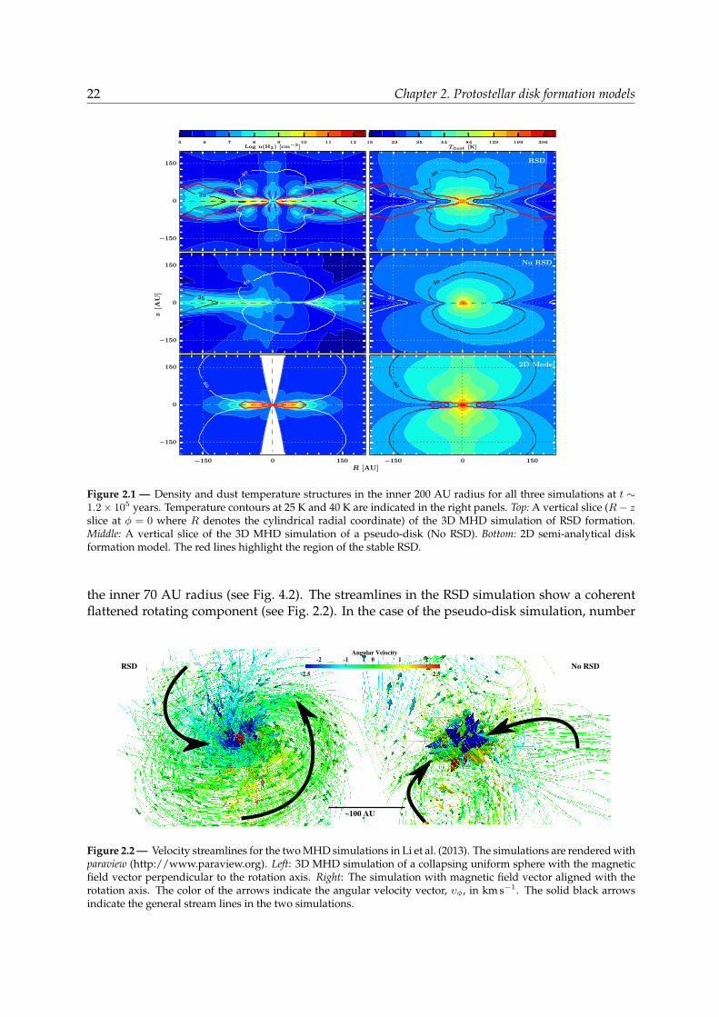
Figure 2.1 — Density and dust temperature structures in the inner 200 AU radius for all three simulations at t ∼1.2× 10⁵ years. Temperature contours at 25 K and 40 K are indicated in the right panels. Top: A vertical slice (R− zslice at φ = 0 where R denotes the cylindrical radial coordinate) of the 3D MHD simulation of RSD formation.Middle: A vertical slice of the 3D MHD simulation of a pseudo-disk (No RSD). Bottom: 2D semi-analytical diskformation model. The red lines highlight the region of the stable RSD.
the inner 70 AU radius (see Fig. 4.2). The streamlines in the RSD simulation show a coherentflattened rotating component (see Fig. 2.2). In the case of the pseudo-disk simulation, number
~100 AU
No RSDRSD-2 -1 0 1 2
Angular Velocity
-2.5 2.5
Figure 2.2 — Velocity streamlines for the two MHD simulations in Li et al. (2013). The simulations are rendered withparaview (http://www.paraview.org). Left: 3D MHD simulation of a collapsing uniform sphere with the magneticfield vector perpendicular to the rotation axis. Right: The simulation with magnetic field vector aligned with therotation axis. The color of the arrows indicate the angular velocity vector, υφ, in km s−1. The solid black arrowsindicate the general stream lines in the two simulations.
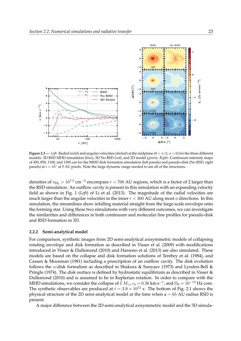
Section 2.2. Numerical simulations and radiative transfer 23
10 100 1000
r [AU]
−4
−2
0
2
4
6
8
υ[k
ms−
1]
RSD
No RSD
2D Model
υφ
υr
−2
0
2
450
RSD No RSD
−2
0
2
850
−2
0
2
1100
−2 0 2
∆RA [”]
−2
0
2
∆D
EC
[”]
1300
−2 0 2
−3
−1
0
1
Iν
[Jy
arcse
c−
2]
Figure 2.3 — Left: Radial (solid) and angular velocities (dashed) at the midplane (θ= π/2, φ= 0) for the three differentmodels: 3D RSD MHD simulation (blue), 3D No RSD (red), and 2D model (green). Right: Continuum intensity mapsof 450, 850, 1100, and 1300 µm for the MHD disk formation simulation (left panels) and pseudo-disk (No RSD, rightpanels) at i = 45 at 5 AU pixels. Note the large dynamic range needed to see all of the structures.
densities of nH2 > 107.5 cm−3 encompass r < 700 AU regions, which is a factor of 2 larger thanthe RSD simulation. An outflow cavity is present in this simulation with an expanding velocityfield as shown in Fig. 1 (Left) of Li et al. (2013). The magnitude of the radial velocities aremuch larger than the angular velocities in the inner r < 300 AU along most φ directions. In thissimulation, the streamlines show infalling material straight from the large-scale envelope ontothe forming star. Using these two simulations with very different outcomes, we can investigatethe similarities and differences in both continuum and molecular line profiles for pseudo-diskand RSD formation in 3D.
2.2.2 Semi-analytical model
For comparison, synthetic images from 2D semi-analytical axisymmetric models of collapsingrotating envelope and disk formation as described in Visser et al. (2009) with modificationsintroduced in Visser & Dullemond (2010) and Harsono et al. (2013) are also simulated. Thesemodels are based on the collapse and disk formation solutions of Terebey et al. (1984), andCassen & Moosman (1981) including a prescription of an outflow cavity. The disk evolutionfollows the α-disk formalism as described in Shakura & Sunyaev (1973) and Lynden-Bell &Pringle (1974). The disk surface is defined by hydrostatic equilibrium as described in Visser &Dullemond (2010) and is assumed to be in Keplerian rotation. In order to compare with theMHD simulations, we consider the collapse of 1 M, cs = 0.26 km s−1, and Ω0 = 10−13 Hz core.The synthetic observables are produced at t = 3.9× 10¹² s. The bottom of Fig. 2.1 shows thephysical structure of the 2D semi-analytical model at the time when a ∼ 65 AU radius RSD ispresent.
A major difference between the 2D semi-analytical axisymmetric model and the 3D simula-
24 Chapter 2. Protostellar disk formation models
tions is the outflow cavity. The photon propagation is still treated in 3D. Although outflowinggas is present in the pseudo-disk simulation (No RSD), the cavity remains filled with high num-ber density (105 cm−3) gas while lower density (102−3 cm−3) gas occupies the cavity in the 2Dmodel. The outflowing gas in the pseudo-disk model has relatively low velocities such that itdoes not clear out the cavity. As a result, the dust temperature structure along the cavity wallis higher in the 2D model due to the direct illumination of the central star. This is readily seenin the 40 K contour in Fig. 2.1 where it is elongated in the z direction in the 2D case.
2.2.3 Rotationally supported disk sizes and masses
The extent of the RSD in the 2D semi-analytical model is defined by hydrostatic equilibrium.Using these properties, the RSD is a region with densities > 107.5 cm−3 and angular velocitiesυφ > 1.2 km s−1. The disk evolution in 2D follows the alpha-disk formalism with α = 10−2,which in turns define the radial velocities as υr/υφ ∼ α(H/R)2 ∼ 10−3 where H is the disk’sscale height. Similar criteria are used to extract the extent of the RSD in the 3D simulation withthe additional constraint of vφ > vr. Note that we apply the criteria from the 2D models to definethe RSD from the 3D simulations, thus the RSD is not necessarily in hydrostatic equilibrium.Using these criteria, an RSD up to 260 AU is found in the mis-aligned simulation.
The extent of the 3D RSD is 300 AU if vφ > 1 km s−1 is used. With the former criterion, thedisk masses contained within such a region are 0.06 M for the 3D RSD and 0.04 M for the 2DRSD surrounding 0.38M and 0.35M stars, respectively (see Table 6.1). As Fig. 4.2 shows, theradial velocity component of the pseudodisk is a significant fraction of the Keplerian velocity.Due to such high radial velocities, the surface density of the pseudodisk remains low. However,the total mass of the high density regions (nH2 > 107.5 cm−3) is a factor of 2 higher than the RSDmass.
2.2.4 Observables and radiative transfer
The first step before producing observables is the calculation of the dust temperature structure,which is critical for the molecular abundances since it controls the freeze-out from the gas ontothe dust. The dust temperature is computed using the 3D continuum radiative transfer codeRADMC3D1 with a central temperature of 5000 K, which is the typical central temperature inthe 2D semi-analytical models at around the end of Stage 0 phase. The central luminosity isfixed at 3.5 L for all models. The dust opacities used are those corresponding to a mix ofsilicates and graphite grains covered by ice mantles (Crapsi et al. 2008). The luminosity is fixedat 3.5 L. The same opacities and central temperature are adopted for all simulations in orderto focus on the general features of the observables. The gas temperatures are assumed to beequal to the dust temperatures, which is valid for the optically thin lines simulated here thattrace the bulk mass where Tgas ∼ Tdust (Doty et al. 2002; Doty et al. 2004).
CO abundance. In this paper, we concentrate on simulating CO molecular lines of J = 2–1, 3–2, 6–5, and 9–8. For simplicity, the 12CO abundance is set to a constant value of 10−4
with respect to H2 except in regions with Tdust < 25 K, where it is reduced by a factor of 20to mimic freeze-out (Jørgensen et al. 2005b; Yıldız et al. 2013). We adopt constant isotopicratios of 12C/13C= 70, 16O/18O= 540, and 18O/17O= 3.6 (Wilson & Rood 1994) to compute theabundance structures of the isotopologs.
1http://www.ita.uni-heidelberg.de/ dullemond/software/radmc-3d
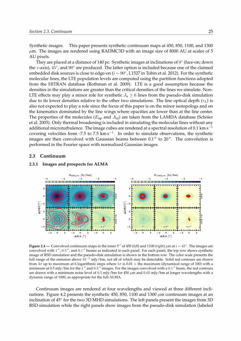
Section 2.3. Continuum 25
Synthetic images. This paper presents synthetic continuum maps at 450, 850, 1100, and 1300µm. The images are rendered using RADMC3D with an image size of 8000 AU at scales of 5AU pixels.
They are placed at a distance of 140 pc. Synthetic images at inclinations of 0 (face-on; downthe z-axis), 45, and 90 are produced. The latter option is included because one of the claimedembedded disk sources is close to edge-on (i∼ 90, L1527 in Tobin et al. 2012). For the syntheticmolecular lines, the LTE population levels are computed using the partition functions adoptedfrom the HITRAN database (Rothman et al. 2009). LTE is a good assumption because thedensities in the simulations are greater than the critical densities of the lines we simulate. Non-LTE effects may play a minor role for synthetic Ju ≥ 6 lines from the pseudo-disk simulationdue to its lower densities relative to the other two simulations. The line optical depth (τL) isalso not expected to play a role since the focus of this paper is on the minor isotopologs and onthe kinematics dominated by the line wings where opacities are lower than at the line center.The properties of the molecules (Eup and Aul) are taken from the LAMDA database (Schoieret al. 2005). Only thermal broadening is included in simulating the molecular lines without anyadditional microturbulence. The image cubes are rendered at a spectral resolution of 0.1 km s−1
covering velocities from -7.5 to 7.5 km s−1. In order to simulate observations, the syntheticimages are then convolved with Gaussian beams between 0.1 ′′ to 20 ′′. The convolution isperformed in the Fourier space with normalized Gaussian images.
2.3 Continuum
2.3.1 Images and prospects for ALMA
−2
0
2
−2 0 2
∆RA [”]
−2
0
2
∆D
EC
[”]
1′′
−2 0 2
0.5′′
RSD
−2 0 2
0.1′′
No
RSD
−5 −4 −3 −2 −1
S450µm [Jy/bm]
−2
0
2
−2 0 2
∆RA [”]
−2
0
2
∆D
EC
[”]
1′′
−2 0 2
0.5′′
RSD
−2 0 2
0.1′′
No
RSD
−5 −4 −3 −2 −1
S1100µm [Jy/bm]
Figure 2.4 — Convolved continuum maps in the inner 5 ′′ of 450 (left) and 1100 (right) µm at i= 45. The images areconvolved with 1 ′′, 0.5 ′′, and 0.1 ′′ beams as indicated in each panel. For each panel, the top row shows syntheticimage of RSD simulation and the pseudo-disk simulation is shown in the bottom row. The color scale presents thefull range of the emission above 10−2 mJy/bm, not all of which may be detectable. Solid red contours are drawnfrom 3σ up to maximum at 6 logarithmic steps where 1σ is 0.01 × the maximum (dynamical range of 100) with aminimum at 0.5 mJy/bm for the 1 ′′ and 0.5 ′′ images. For the images convolved with a 0.1 ′′ beam, the red contoursare drawn with a minimum noise level of 0.5 mJy/bm for 450 µm and 0.05 mJy/bm at longer wavelengths with adynamic range of 1000, as appropriate for the full ALMA.
Continuum images are rendered at four wavelengths and viewed at three different incli-nations. Figure 4.2 presents the synthetic 450, 850, 1100 and 1300 µm continuum images at aninclination of 45 for the two 3D MHD simulations. The left panels present the images from 3DRSD simulation while the right panels show images from the pseudo-disk simulation (labeled
26 Chapter 2. Protostellar disk formation models
as No RSD). The features produced during the collapse are clearly visible in the 450 µm map;most of them are two orders of magnitude fainter at 1300 µm. The spiral structure in the 450µm image is due to magnetically channelled, supersonically collapsing material on its way tothe RSD, rather than a feature of the RSD itself.
One of the aims of this paper is to investigate whether these features are observable withcurrent observational limits and what is possible with future Atacama Large Millimeter/sub-millimeter Array (ALMA) data. With the full ALMA, a sensitivity of σ=0.5 mJy bm−1 (bm =beam) at∼ 450 µm and 0.05 mJy bm−1 at 1100 µm can be achieved at spatial resolutions≤ 0.1 ′′
for 30 minutes of integration (1.8 GHz bandwidth). In addition, a high dynamic range of> 1000(σ = 0.001× Speak) can also be achieved. Figure 2.4 presents the images convolved with a 0.1 ′′
beam for the two 3D MHD simulations (right-most panels). The color scale indicates the fullrange of emission, while the red solid lines show the region above 3σ where σ is either dynam-ically limited to 1000 or to the σ values listed above. This simply means that the solid red linesindicate the detectable features. With a combination of high dynamic range and sensitivity,the features of the collapse are observable and distinguishable in both 450 µm and 1100 µmcontinuum maps. At a spatial resolution of 0.1 ′′, most of the emission at 1100 µm is due to therotationally supported disk with little contribution from the surrounding envelope.
As Figs. 4.2 and 2.4 show, both the strength of the features and their extent change withwavelength, as indicated by the red line contours. With a resolution of 0.1 ′′, the extent of thedetectable emission decreases from 1.5 ′′ at 450 µm to < 1 ′′ at 1100 µm for the RSD case. Atlong wavelengths, the dust emission is given by Iν ∼ Tdustν
2 × (1 − e−τdust). Since the dustemission is optically thin at long wavelengths, the intensity is ∝ Tdustν
2τdust. The variablesthat depend on position are Tdust and τdust ∝ ρdustκν . The frequency dependence of the opacityis κν ∝ ν1.5 for the adopted opacity table. The extent of the detectable emission depends onthese quantities. At one particular position, the ratio of the emission at the two wavelengths issimply I450µm/I1100µm ∝ ν3.5. Thus, the predicted difference in size at the two wavelengths isdue to the frequency dependence of the emission.
For ALMA early science observations (cycles 0 and I), the capabilities provided a dynamicrange only up to 100 at a spatial resolution of ∼ 0.5 ′′. Figure 2.4 presents the synthetic 50 and1100 µm images convolved with 1 ′′ and 0.5 ′′ beams, compared with the 0.1 ′′ beam images. Thecolor scale again indicates the full range of emission, while the red solid lines now show theregion above 3σ where the noise level, σ, is dynamically limited to 100 with a minimum of 0.5mJy/beam at both wavelengths. The red lines again present the emission that is observable.The 450 µm images convolved with a 1 ′′ beam show an elongated flattened structure for bothRSD and pseudo-disk simulations and are therefore indistinguishable. Most of the emissionat 1100 µm and longer wavelengths is not detectable at the assumed noise level of 0.5 mJybm−1. A similar result is found after convolution with a 0.5 ′′ beam. Although the syntheticobservations from the pseudodisk indicate a ‘cometary’ structure, this may be affected by thepresence of outflow cavity which is absent in the case of RSD. Thus, the full ALMA capabilitiesare needed to distinguish models based on continuum data only.
2.3.2 Inclination effects
The images for a face-on system (i = 0) are similar to those of the moderately inclined system(i = 45) presented in Fig. 2.4. For low inclinations between 0 to 45, the continuum imagesonly change slightly in terms of absolute flux density and show a small elongation due toorientation.
In contrast, the two simulations rendered at edge-on (i ∼ 90) geometry exhibit similarcompact components even at the highest angular resolution (Fig. 2.5). They both show an
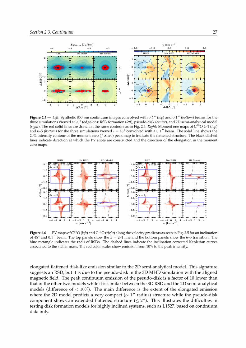
Section 2.3. Continuum 27
−2
0
2
RSD
−2 0 2∆RA [”]
−2
0
2
∆D
EC
[”]
No RSD
−2 0 2
0.5 ′′
2D model
−2 0 2
0.1 ′′
−4 −4 −3 −2
S850µm [Jy/bm]
−1
0
1 Ju = 2
RSD
−1 0 1∆RA [”]
−1
0
1
∆D
EC
[”]
Ju = 6
No RSD
−1 0 1
2D Model
−1 0 1
−2.0 −1.0 0.0 1.0 2.0
υ [km s−1]
Figure 2.5 — Left: Synthetic 850 µm continuum images convolved with 0.5 ′′ (top) and 0.1 ′′ (bottom) beams for thethree simulations viewed at 90 (edge-on): RSD formation (left), pseudo-disk (center), and 2D semi-analytical model(right). The red solid lines are drawn at the same contours as in Fig. 2.4. Right: Moment one maps of C18O 2–1 (top)and 6–5 (bottom) for the three simulations viewed i = 45 convolved with a 0.1 ′′ beam. The solid line shows the20% intensity contour of the moment zero (
∫Sυdυ) peak map to indicate the flattened structure. The black dashed
lines indicate direction at which the PV slices are constructed and the direction of the elongation in the momentzero maps.
−3.0
−1.5
0.0
1.5
3.0Ju = 2C18O i = 45
RSD
−4 −2 0 2 4
υ [km s−1]
−3.0
−1.5
0.0
1.5
3.0
Off
set
[”]
Ju = 6
No RSD
−4 −2 0 2 4
2D Model
−4 −2 0 2 4
−3.0
−1.5
0.0
1.5
3.0Ju = 2C17O i = 45
RSD
−4 −2 0 2 4
υ [km s−1]
−3.0
−1.5
0.0
1.5
3.0
Off
set
[”]
Ju = 6
No RSD
−4 −2 0 2 4
2D Model
−4 −2 0 2 4
Figure 2.6 — PV maps of C18O (left) and C17O (right) along the velocity gradients as seen in Fig. 2.5 for an inclinationof 45 and 0.1 ′′ beam. The top panels show the J = 2–1 line and the bottom panels show the 6–5 transition. Theblue rectangle indicates the radii of RSDs. The dashed lines indicate the inclination corrected Keplerian curvesassociated to the stellar mass. The red color scales show emission from 10% to the peak intensity.
elongated flattened disk-like emission similar to the 2D semi-analytical model. This signaturesuggests an RSD, but it is due to the pseudo-disk in the 3D MHD simulation with the alignedmagnetic field. The peak continuum emission of the pseudo-disk is a factor of 10 lower thanthat of the other two models while it is similar between the 3D RSD and the 2D semi-analyticalmodels (difference of < 10%). The main difference is the extent of the elongated emissionwhere the 2D model predicts a very compact (∼ 1 ′′ radius) structure while the pseudo-diskcomponent shows an extended flattened structure (≤ 2 ′′). This illustrates the difficulties intesting disk formation models for highly inclined systems, such as L1527, based on continuumdata only.
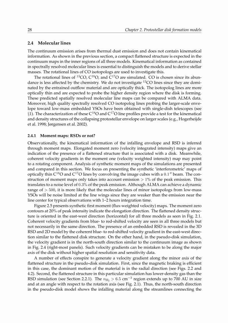
28 Chapter 2. Protostellar disk formation models
2.4 Molecular lines
The continuum emission arises from thermal dust emission and does not contain kinematicalinformation. As shown in the previous section, a compact flattened structure is expected in thecontinuum maps in the inner regions of all three models. Kinematical information as containedin spectrally resolved molecular lines is essential to distinguish the models and to derive stellarmasses. The rotational lines of CO isotopologs are used to investigate this.
The rotational lines of 13CO, C18O, and C17O are simulated. CO is chosen since its abun-dance is less affected by the chemistry. We do not investigate 12CO lines since they are domi-nated by the entrained outflow material and are optically thick. The isotopolog lines are moreoptically thin and are expected to probe the higher density region where the disk is forming.These predicted spatially resolved molecular line maps can be compared with ALMA data.Moreover, high quality spectrally resolved CO isotopolog lines probing the larger-scale enve-lope toward low-mass embedded YSOs have been obtained with single-dish telescopes (see§1). The characterization of these C18O and C17O line profiles provide a test for the kinematicaland density structures of the collapsing protostellar envelope on larger scales (e.g., Hogerheijdeet al. 1998; Jørgensen et al. 2002).
2.4.1 Moment maps: RSDs or not?
Observationally, the kinematical information of the infalling envelope and RSD is inferredthrough moment maps. Elongated moment zero (velocity integrated intensity) maps give anindication of the presence of a flattened structure that is associated with a disk. Meanwhile,coherent velocity gradients in the moment one (velocity weighted intensity) map may pointto a rotating component. Analysis of synthetic moment maps of the simulations are presentedand compared in this section. We focus on presenting the synthetic ‘interferometric’ maps ofoptically thin C18O and C17O lines by convolving the image cubes with a 0.1 ′′ beam. The con-struction of moment maps only takes into account emission > 1% of the peak emission. Thistranslates to a noise level of 0.3% of the peak emission. Although ALMA can achieve a dynamicrange of > 500, it is more likely that the molecular lines of minor isotopologs from low-massYSOs will be noise limited at the line wings since they are weaker than the emission near theline center for typical observations with 1–2 hours integration time.
Figure 2.5 presents synthetic first moment (flux-weighted velocity) maps. The moment zerocontours at 20% of peak intensity indicate the elongation direction. The flattened density struc-ture is oriented in the east-west direction (horizontal) for all three models as seen in Fig. 2.1.Coherent velocity gradients from blue- to red-shifted velocity are seen in all three models butnot necessarily in the same direction. The presence of an embedded RSD is revealed in the 3DRSD and 2D model by the coherent blue- to red-shifted velocity gradient in the east-west direc-tion similar to the flattened disk structure. On the other hand, in the pseudo-disk simulation,the velocity gradient is in the north-south direction similar to the continuum image as shownin Fig. 2.4 (right-most panels). Such velocity gradients can be mistaken to be along the majoraxis of the disk without higher spatial resolution and sensitivity data.
A number of effects conspire to generate a velocity gradient along the minor axis of theflattened structure in the pseudo-disk simulation. First, since the magnetic braking is efficientin this case, the dominant motion of the material is in the radial direction (see Figs. 2.2 and4.2). Second, the flattened structure in this particular simulation has lower-density gas than theRSD simulation (see Section 2.2.1). The nH2 > 6.5 cm−3 region extends up to 700 AU in sizeand at an angle with respect to the rotation axis (see Fig. 2.1). Thus, the north-south directionin the pseudo-disk model shows the infalling material along the streamlines connecting the

Section 2.4. Molecular lines 29
large-scale envelope and the central star.At moderate inclinations, the pseudo-disk simulation therefore shows a coherent velocity
gradient in a more-or-less straight north-south line. The velocity gradient changes to an east-west direction at high inclinations. At high inclinations, the observer has a direct line of sighton the high density region shown in Fig. 2.1 and therefore the line emissions pick up the ro-tational motions of the flattened structure similar to the RSD simulations. Furthermore, theskewness that is present in the moment one maps of RSD simulations largely disappears athigh inclinations for the same reason. Thus, it is difficult to separate the envelope from the diskfor high inclinations from moment one map alone.
2.4.2 Velocity profiles
2.4.2.1 PV cuts
Observationally, the presence of embedded Keplerian disks is often established by construct-ing position velocity (PV) diagrams along the major axis of the system as seen in moment zeromaps. In theory, the PV analysis is straight-forward. It is symmetric in both position and veloc-ity space (4 quadrants are occupied) if the system is infall dominated (e.g., Ohashi et al. 1997a;Brinch et al. 2008). The symmetry is broken if rotation is present and the emission peaks areshifted to larger offsets corresponding to the strength of the rotational velocities (2 quadrantsare occupied).
Figure 2.6 presents synthetic PV diagrams along the major axis of the disk where it corre-sponds to the direction of the blue- to red-shifted velocity gradient. For the images in Fig. 2.5,an east-west slice (horizontal) is taken for the RSD simulations, while a north-south (vertical)slice is adopted for the case of the simulation without an RSD. These slices are not exactly themajor axis of the moment zero map, however these directions pick up most of the velocity gra-dient present in the inner 1 ′′. Both C18O and C17O lines are simulated. Interestingly, the PVslices suggest that rotational motions are present regardless of whether an RSD is present ornot. This is most readily seen in the C17O PV maps (right of Fig. 2.6) in which only 2 of the4 quadrants are occupied by molecular emissions for all three models at i = 45. This showsthat C17O emission readily picks up the rotational motion at small-scales but also that infallingmotion can be confused with rotation if the wrong direction for the PV cut is chosen (No RSDmodel).
The C18O PV maps indicate contributions from the infalling envelope since the maps aremore symmetric than those in C17O. The C18O PV slices of the pseudo-disk simulations indicatean infall-dominated structure in which the 4 quadrants are occupied. On the other hand, thereis a clear indication of a rotating component for the two RSD simulations in which only 2 of the4 quadrants are filled at small radii. This suggests that spatially and spectrally resolved C18Olines can distinguish between a pseudo-disk and an RSD.
Figures 2.6 compares the PV maps of the 2–1 and 6–5 transitions. Most of the emission in the6–5 transition occupies only 2 of the 4 quadrants indicating signatures of rotational motions,whereas the 2–1 lines also show some emission in the other 2 quadrants from larger scales. Thisis a clear indication that the 6–5 line is a better probe of the rotational motions in the inner 100AU than the 2–1 line.
2.4.2.2 Peak position-velocity diagrams
While it is clear that there is indeed a rotating component for some models, the question iswhether the extent of the Keplerian structure can be extracted from such an analysis. A Kep-lerian rotating flattened structure exhibits a velocity profile υ ∝ r−0.5, where r is the distance

30 Chapter 2. Protostellar disk formation models
10 100
1υ
[km
s−1] M? = 0.31M
RSDC18O 6 - 5
10 100
Distance from center [AU]
No RSDM? = 0.12M
10 100
2D ModelM? = 0.68M
∝ r−1
∝ r−0.5
10 100
1
υ[k
ms−
1] M? = 0.28M
RSDC17O 2 - 1
10 100
Distance from center [AU]
No RSDM? = 0.13M
10 100
2D ModelM? = 0.37M
∝ r−1
∝ r−0.5
Figure 2.7 — Peak position-velocity diagrams of C18O 6–5 (top) and C17O 2–1 (bottom) at i = 45 after convolutionwith a 0.1 ′′ beam. The red and blue symbols correspond to the red- and blue-shifted velocity components, respec-tively. The different panels present the PPV for the different simulations. Vertical solid lines show the disk radiiextracted for the three models and dashed lines show the steep velocity profile (υ ∝ r−1) while the solid cyan linesindicate the Keplerian curves. The stellar masses are indicated in the top right of each panel. The offset betweenblue- and red-shifted points are due to the limited spatial and spectral resolution at the high velocities.
from the central source. These positions are either determined from fitting interferometric visi-bilities of each velocity channel (Lommen et al. 2008; Jørgensen et al. 2009) or determination ofthe peak positions in the image space (Tobin et al. 2012; Yen et al. 2013). We here determine thepeak positions directly in the image space to assess whether a velocity profile is visible in thesynthetic molecular lines.
Peak positions are determined for each of the velocity channel maps for each molecularline for the red and blue-shifted components separately taking into account channels whosepeak flux density (Sν in Jy bm−1) are > 1% of Smax. They are subsequently rotated accordingto the direction of the velocity gradient. If an RSD is present, the peak positions of both red-and blue-shifted velocities are expected to follow the Keplerian velocity profile (υ ∝ r−0.5).The combination of infalling rotating envelope and RSD, which exhibits a skewness in themoment one map, is expected to show a steeper velocity profile (υ ∝ r−1) (Lin et al. 1994).However, at high velocities, the peak positions of the red- and blue-shifted velocities can bemisaligned at scales of 5 AU due to the limited spatial resolution. The disk radius is determinedby minimizing the difference (∼ 10%) between the best-fit stellar mass inside and at the diskradius.
The peak position-velocity diagrams (PPVs) for C18O 6–5 and C17O 2–1 are shown in Fig. 2.7.These lines are chosen because they represent two observational extremes in terms of excitationand optical depth. There is a clear distinction between the RSD simulations and a pseudo-disk.The velocity profile of the pseudo-disk is much flatter than that expected from an RSD. Thus,spatially and spectrally resolved molecular lines observations can clearly differentiate betweenan RSD and a pseudo-disk.
All three PPVs indicate a velocity profile close to υ ∝ r−0.5 (for the pseudo-disk see C17O2–1 PPV in the inner 20 AU). This reflects the fact that the inner 300 AU of the models isdominated by velocity structure that is proportional to r−0.5, which is both the radial veloc-
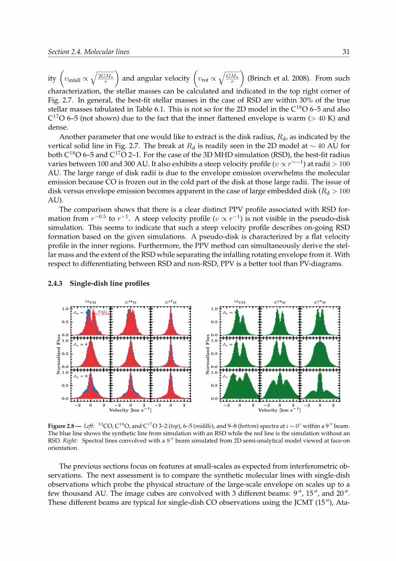
Section 2.4. Molecular lines 31
ity(υinfall ∝
√2GM?r
)and angular velocity
(υrot ∝
√GM?r
)(Brinch et al. 2008). From such
characterization, the stellar masses can be calculated and indicated in the top right corner ofFig. 2.7. In general, the best-fit stellar masses in the case of RSD are within 30% of the truestellar masses tabulated in Table 6.1. This is not so for the 2D model in the C18O 6–5 and alsoC17O 6–5 (not shown) due to the fact that the inner flattened envelope is warm (> 40 K) anddense.
Another parameter that one would like to extract is the disk radius, Rd, as indicated by thevertical solid line in Fig. 2.7. The break at Rd is readily seen in the 2D model at ∼ 40 AU forboth C18O 6–5 and C17O 2–1. For the case of the 3D MHD simulation (RSD), the best-fit radiusvaries between 100 and 300 AU. It also exhibits a steep velocity profile (υ ∝ r∼−1) at radii> 100AU. The large range of disk radii is due to the envelope emission overwhelms the molecularemission because CO is frozen out in the cold part of the disk at those large radii. The issue ofdisk versus envelope emission becomes apparent in the case of large embedded disk (Rd > 100AU).
The comparison shows that there is a clear distinct PPV profile associated with RSD for-mation from r−0.5 to r−1. A steep velocity profile (υ ∝ r−1) is not visible in the pseudo-disksimulation. This seems to indicate that such a steep velocity profile describes on-going RSDformation based on the given simulations. A pseudo-disk is characterized by a flat velocityprofile in the inner regions. Furthermore, the PPV method can simultaneously derive the stel-lar mass and the extent of the RSD while separating the infalling rotating envelope from it. Withrespect to differentiating between RSD and non-RSD, PPV is a better tool than PV-diagrams.
2.4.3 Single-dish line profiles
0.0
0.5
1.0Ju = 3 RSD
No RSD
13CO C18O C17O
0.0
0.5
1.0Ju = 6
−2 0 2
Velocity [km s−1]
0.0
0.5
1.0Norm
alized
Flu
x
Ju = 9
−2 0 2 −2 0 2
0.0
0.5
1.0Ju = 3
13CO C18O C17O
0.0
0.5
1.0Ju = 6
−2 0 2
Velocity [km s−1]
0.0
0.5
1.0Norm
alized
Flu
x
Ju = 9
−2 0 2 −2 0 2
Figure 2.8 — Left: 13CO, C18O, and C17O 3–2 (top), 6–5 (middle), and 9–8 (bottom) spectra at i∼ 0 within a 9 ′′ beam.The blue line shows the synthetic line from simulation with an RSD while the red line is the simulation without anRSD. Right: Spectral lines convolved with a 9 ′′ beam simulated from 2D semi-analytical model viewed at face-onorientation.
The previous sections focus on features at small-scales as expected from interferometric ob-servations. The next assessment is to compare the synthetic molecular lines with single-dishobservations which probe the physical structure of the large-scale envelope on scales up to afew thousand AU. The image cubes are convolved with 3 different beams: 9 ′′, 15 ′′, and 20 ′′.These different beams are typical for single-dish CO observations using the JCMT (15 ′′), Ata-
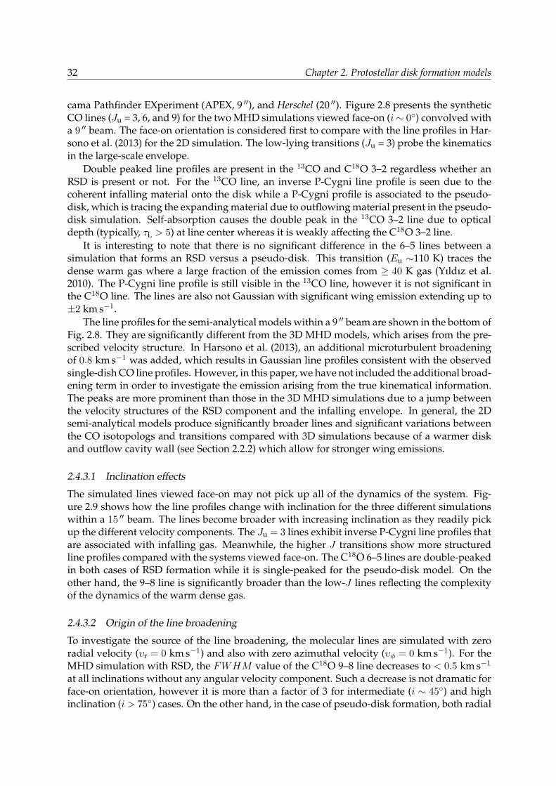
32 Chapter 2. Protostellar disk formation models
cama Pathfinder EXperiment (APEX, 9 ′′), and Herschel (20 ′′). Figure 2.8 presents the syntheticCO lines (Ju = 3, 6, and 9) for the two MHD simulations viewed face-on (i∼ 0) convolved witha 9 ′′ beam. The face-on orientation is considered first to compare with the line profiles in Har-sono et al. (2013) for the 2D simulation. The low-lying transitions (Ju = 3) probe the kinematicsin the large-scale envelope.
Double peaked line profiles are present in the 13CO and C18O 3–2 regardless whether anRSD is present or not. For the 13CO line, an inverse P-Cygni line profile is seen due to thecoherent infalling material onto the disk while a P-Cygni profile is associated to the pseudo-disk, which is tracing the expanding material due to outflowing material present in the pseudo-disk simulation. Self-absorption causes the double peak in the 13CO 3–2 line due to opticaldepth (typically, τL > 5) at line center whereas it is weakly affecting the C18O 3–2 line.
It is interesting to note that there is no significant difference in the 6–5 lines between asimulation that forms an RSD versus a pseudo-disk. This transition (Eu ∼110 K) traces thedense warm gas where a large fraction of the emission comes from ≥ 40 K gas (Yıldız et al.2010). The P-Cygni line profile is still visible in the 13CO line, however it is not significant inthe C18O line. The lines are also not Gaussian with significant wing emission extending up to±2 km s−1.
The line profiles for the semi-analytical models within a 9 ′′ beam are shown in the bottom ofFig. 2.8. They are significantly different from the 3D MHD models, which arises from the pre-scribed velocity structure. In Harsono et al. (2013), an additional microturbulent broadeningof 0.8 km s−1 was added, which results in Gaussian line profiles consistent with the observedsingle-dish CO line profiles. However, in this paper, we have not included the additional broad-ening term in order to investigate the emission arising from the true kinematical information.The peaks are more prominent than those in the 3D MHD simulations due to a jump betweenthe velocity structures of the RSD component and the infalling envelope. In general, the 2Dsemi-analytical models produce significantly broader lines and significant variations betweenthe CO isotopologs and transitions compared with 3D simulations because of a warmer diskand outflow cavity wall (see Section 2.2.2) which allow for stronger wing emissions.
2.4.3.1 Inclination effects
The simulated lines viewed face-on may not pick up all of the dynamics of the system. Fig-ure 2.9 shows how the line profiles change with inclination for the three different simulationswithin a 15 ′′ beam. The lines become broader with increasing inclination as they readily pickup the different velocity components. The Ju = 3 lines exhibit inverse P-Cygni line profiles thatare associated with infalling gas. Meanwhile, the higher J transitions show more structuredline profiles compared with the systems viewed face-on. The C18O 6–5 lines are double-peakedin both cases of RSD formation while it is single-peaked for the pseudo-disk model. On theother hand, the 9–8 line is significantly broader than the low-J lines reflecting the complexityof the dynamics of the warm dense gas.
2.4.3.2 Origin of the line broadening
To investigate the source of the line broadening, the molecular lines are simulated with zeroradial velocity (υr = 0 km s−1) and also with zero azimuthal velocity (υφ = 0 km s−1). For theMHD simulation with RSD, the FWHM value of the C18O 9–8 line decreases to < 0.5 km s−1
at all inclinations without any angular velocity component. Such a decrease is not dramatic forface-on orientation, however it is more than a factor of 3 for intermediate (i ∼ 45) and highinclination (i > 75) cases. On the other hand, in the case of pseudo-disk formation, both radial
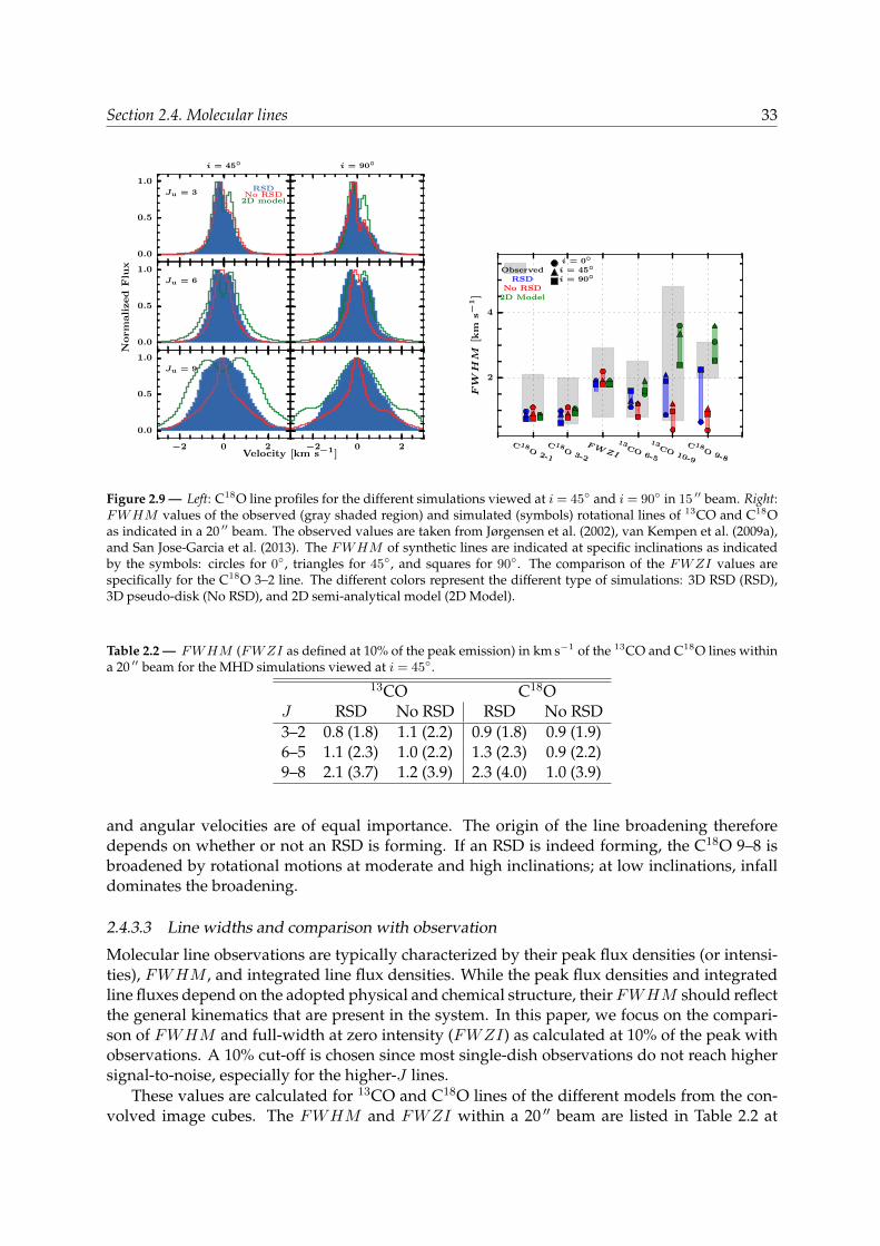
Section 2.4. Molecular lines 33
0.0
0.5
1.0Ju = 3 RSD
No RSD2D model
i = 45 i = 90
0.0
0.5
1.0Ju = 6
−2 0 2Velocity [km s−1]
0.0
0.5
1.0
Norm
alized
Flu
x
Ju = 9
−2 0 2 C18O
2-1
C18O
3-2
FWZI
13CO
6-5
13CO
10-9
C18O
9-8
2
4
FWHM
[km
s−1]
RSDNo RSD
2D Model
Observedi = 0i = 45i = 90
Figure 2.9 — Left: C18O line profiles for the different simulations viewed at i = 45 and i = 90 in 15 ′′ beam. Right:FWHM values of the observed (gray shaded region) and simulated (symbols) rotational lines of 13CO and C18Oas indicated in a 20 ′′ beam. The observed values are taken from Jørgensen et al. (2002), van Kempen et al. (2009a),and San Jose-Garcia et al. (2013). The FWHM of synthetic lines are indicated at specific inclinations as indicatedby the symbols: circles for 0, triangles for 45, and squares for 90. The comparison of the FWZI values arespecifically for the C18O 3–2 line. The different colors represent the different type of simulations: 3D RSD (RSD),3D pseudo-disk (No RSD), and 2D semi-analytical model (2D Model).
Table 2.2 — FWHM (FWZI as defined at 10% of the peak emission) in km s−1 of the 13CO and C18O lines withina 20 ′′ beam for the MHD simulations viewed at i = 45.
13CO C18OJ RSD No RSD RSD No RSD3–2 0.8 (1.8) 1.1 (2.2) 0.9 (1.8) 0.9 (1.9)6–5 1.1 (2.3) 1.0 (2.2) 1.3 (2.3) 0.9 (2.2)9–8 2.1 (3.7) 1.2 (3.9) 2.3 (4.0) 1.0 (3.9)
and angular velocities are of equal importance. The origin of the line broadening thereforedepends on whether or not an RSD is forming. If an RSD is indeed forming, the C18O 9–8 isbroadened by rotational motions at moderate and high inclinations; at low inclinations, infalldominates the broadening.
2.4.3.3 Line widths and comparison with observation
Molecular line observations are typically characterized by their peak flux densities (or intensi-ties), FWHM , and integrated line flux densities. While the peak flux densities and integratedline fluxes depend on the adopted physical and chemical structure, their FWHM should reflectthe general kinematics that are present in the system. In this paper, we focus on the compari-son of FWHM and full-width at zero intensity (FWZI) as calculated at 10% of the peak withobservations. A 10% cut-off is chosen since most single-dish observations do not reach highersignal-to-noise, especially for the higher-J lines.
These values are calculated for 13CO and C18O lines of the different models from the con-volved image cubes. The FWHM and FWZI within a 20 ′′ beam are listed in Table 2.2 at
34 Chapter 2. Protostellar disk formation models
moderate inclination (i = 45) comparing the two 3D MHD simulations. Within such a largebeam, their values for 13CO and C18O are similar. The FWHM values do not necessarily in-crease between Ju =3 and 6, in contrast with the FWZI values (see Fig. 2.9). This is expectedsince the wing emissions are much lower than the peak because the emitting region is muchsmaller than the beam (beam dilution).
Considering all inclinations (0, 45, and 90), the FWHM values of the low-J CO linesare similar between the 3D simulations and 2D semi-analytical models. On the other hand, theline widths of the high-J lines differ significantly. This is expected since most of the 2–1 and3–2 emission originates from the large-scale envelope, which is similar in terms of kinematicsin the three simulations. However, the high-J lines originate from the warm inner regions inwhich the three simulations show different velocity structures.
Figure 2.9 presents the comparison between the simulated and observed lines. The ob-served line widths toward low-mass YSOs are taken from Jørgensen et al. (2002), van Kempenet al. (2009a), and San Jose-Garcia et al. (2013,FWHMN for the narrow component). Sourceswith known confusion in their line profiles from other nearby sources have been excluded. Itis clear that the observed line widths of the low-J lines (Ju = 2 and 3) are significantly greaterthan the model simulations, by a factor of 2. Since these lines probe the large-scale quiescentenvelope, the discrepancy between the predicted and observed line widths suggests that thelarge-scale envelope is turbulent with FWHM ≈ 1 km s−1 or a Doppler b of ∼ 0.4 km s−1, i.e.,more than what is included in the current simulations that could be due to an interaction withfast outflow, at least in part. The comparison of the FWZI values also supports this conclusion.
For the dense and warm gas probed by the higher Ju ≥ 6 lines, the predicted line widths areconsistent with observations. Moreover, the pseudo-disk (No RSD) simulations predict muchsmaller line widths than those observed. This line originates from the inner warm parts that arerotationally supported. Thus, this comparison may suggest that the large observed line widthsof C18O 9–8 line indicate that most of the low-mass embedded YSOs have or are forming anRSD. Alternatively, a turbulence with FWHM = 2 km s−1 would be required in the inner partsif RSDs are absent.
2.5 Discussion
2.5.1 Variations with viewing angles
This paper presents synthetic continuum maps and CO isotopolog lines from 3D MHD simula-tions and 2D semi-analytical disk formation models out of collapsing rotating envelopes. Theaim is to present signatures that can differentiate between embedded rotationally supporteddisks (RSDs) and a pseudo-disk. Thus far, we have analyzed the continuum and syntheticmolecular lines with respect to one viewing angle in the azimuthal direction with φ = 0. Asshown previously by Smith et al. (2012), the line profiles may change with different viewingangles since the collapse process is not spherically symmetric.
In order to look at the general trend with viewing angles, synthetic images at 4 differentinclinations (i) from 15 to 150 and 8 azimuthal angles from 8 to 315 are generated. Weconcentrate the analysis on 850 µm, 1100 µm, C18O, and C17O images. Figure 2.10 presentsthe continuum and molecular lines at a few viewing angles for the two 3D MHD simulations.The 3D RSD formation predicts an observable spiral feature at near face-on (i ≈ 0) with highdynamic range (1000). As mentioned earlier, this is due to the infalling material on its way tothe disk.
In terms of kinematical signatures, the moment one maps of the C18O 2–1 line are com-pared for the two cases. Both the RSD and pseudo-disk simulations predict a coherent velocity

Section 2.5. Discussion 35
850μm 1100μm Moment1 C18O9−8
i=0o
ϕ=0o
i=30oϕ=45o
i=90o
ϕ=0o
i=130o
ϕ=200o
i=160o
ϕ=150o
Figure 2.10 — Comparison of synthetic 850 µm, 1100 µm, C18O 2–1 moment one maps and normalized C18O 9–8spectra for the 3D RSD (left) and pseudo-disk (right) MHD simulations viewed at a few orientations. The imagesand image cubes are convolved with a 0.1 ′′ beam. The maps sizes are 5 ′′ across similar to Fig. 2.4. The color scalesand line contours are defined in Figs. 2.4 and 2.5. The normalized C18O 9–8 spectra refer to a 15 ′′ beam on the samescale as Fig. 2.9. The inclination and rotation values are representative only and not exact.
gradient in the inner 300 AU. However, the velocity gradient is more robust if an RSD is form-ing. The pseudo-disk simulation shows a velocity gradient that is not necessarily along thedisk major axis (see Fig. 2.1 and Section 2.4.1). Such a direction corresponds to the streamlinesof the infalling material from the large-scale envelope to the central star. At high inclinations(i > 75), this direction of the velocity gradient shifts to east-west direction similar to the RSDsimulation, because the moment one map is dominated by the rotational motions which are inthe east-west direction.
To assess the general predictions for the large-scale envelope, C18O 9–8 spectra within a 15 ′′
beam are compared. The low-J lines (Ju = 2 and 3) exhibit inverse P-Cygni profiles indicat-ing infalling material in both RSD and pseudo-disk simulations. For the high-J lines, the 3DRSD simulation predicts a broader line than the pseudo-disk simulation in most orientationsconsistent with Fig. 2.9.
In summary, the results that are presented in previous sections are robust and do not de-pend on the viewing angles. A pseudo-disk shows more distinct features in the kinematics inthe moment one maps that are different from an RSD. A coherent blue- to red-shifted velocitygradient in the inner 1 arcseconds aligned with the major axis is most likely a signature of anRSD or on-going RSD formation. Although these lines are simulated assuming LTE conditions,non-LTE effects generally decrease the strength of the emission but do not alter the results ofthe kinematics derived from the molecular limes.
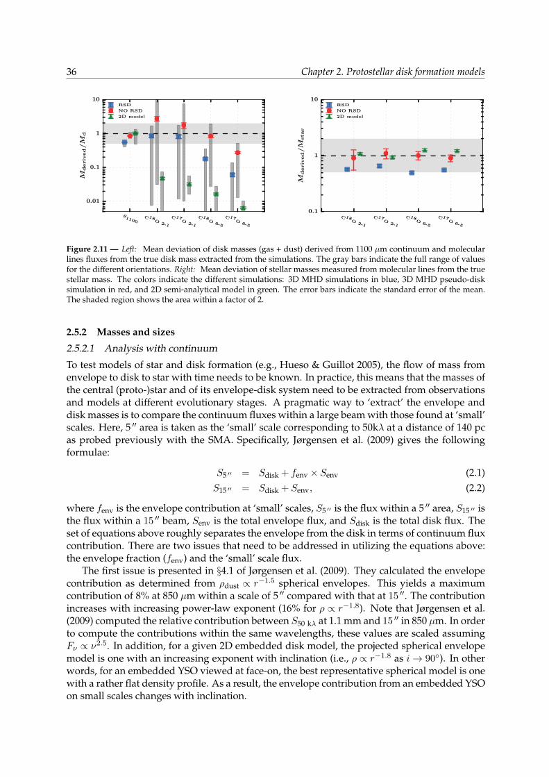
36 Chapter 2. Protostellar disk formation models
S1100
C18O
2-1
C17O
2-1
C18O
6-5
C17O
6-5
0.01
0.1
1
10
Mderiv
ed/M
d
RSD
NO RSD
2D model
C18O
2-1
C17O
2-1
C18O
6-5
C17O
6-5
0.1
1
10
Mderiv
ed/M
star
RSD
NO RSD
2D model
Figure 2.11 — Left: Mean deviation of disk masses (gas + dust) derived from 1100 µm continuum and molecularlines fluxes from the true disk mass extracted from the simulations. The gray bars indicate the full range of valuesfor the different orientations. Right: Mean deviation of stellar masses measured from molecular lines from the truestellar mass. The colors indicate the different simulations: 3D MHD simulations in blue, 3D MHD pseudo-disksimulation in red, and 2D semi-analytical model in green. The error bars indicate the standard error of the mean.The shaded region shows the area within a factor of 2.
2.5.2 Masses and sizes
2.5.2.1 Analysis with continuum
To test models of star and disk formation (e.g., Hueso & Guillot 2005), the flow of mass fromenvelope to disk to star with time needs to be known. In practice, this means that the masses ofthe central (proto-)star and of its envelope-disk system need to be extracted from observationsand models at different evolutionary stages. A pragmatic way to ‘extract’ the envelope anddisk masses is to compare the continuum fluxes within a large beam with those found at ‘small’scales. Here, 5 ′′ area is taken as the ‘small’ scale corresponding to 50kλ at a distance of 140 pcas probed previously with the SMA. Specifically, Jørgensen et al. (2009) gives the followingformulae:
S5 ′′ = Sdisk + fenv × Senv (2.1)S15 ′′ = Sdisk + Senv, (2.2)
where fenv is the envelope contribution at ‘small’ scales, S5 ′′ is the flux within a 5 ′′ area, S15 ′′ isthe flux within a 15 ′′ beam, Senv is the total envelope flux, and Sdisk is the total disk flux. Theset of equations above roughly separates the envelope from the disk in terms of continuum fluxcontribution. There are two issues that need to be addressed in utilizing the equations above:the envelope fraction (fenv) and the ‘small’ scale flux.
The first issue is presented in §4.1 of Jørgensen et al. (2009). They calculated the envelopecontribution as determined from ρdust ∝ r−1.5 spherical envelopes. This yields a maximumcontribution of 8% at 850 µm within a scale of 5 ′′ compared with that at 15 ′′. The contributionincreases with increasing power-law exponent (16% for ρ ∝ r−1.8). Note that Jørgensen et al.(2009) computed the relative contribution between S50 kλ at 1.1 mm and 15 ′′ in 850 µm. In orderto compute the contributions within the same wavelengths, these values are scaled assumingFν ∝ ν2.5. In addition, for a given 2D embedded disk model, the projected spherical envelopemodel is one with an increasing exponent with inclination (i.e., ρ ∝ r−1.8 as i→ 90). In otherwords, for an embedded YSO viewed at face-on, the best representative spherical model is onewith a rather flat density profile. As a result, the envelope contribution from an embedded YSOon small scales changes with inclination.

Section 2.5. Discussion 37
Another issue is the ‘small’ scale flux at which to determine the envelope contribution. Ifthe size is too small (i.e., 1 ′′), the envelope contribution is naturally negligible and it is easy toextract the disk flux. However, the disk flux can be underestimated within such a small scale.Furthermore, the flux that is measured at each pixel is always a combination of the envelopeand the disk. Thus, it is more intuitive to calculate the envelope’s contribution at scales largerthan the disk (∼ 5 ′′, 700 AU at 140 pc) in order to obtain all of the disk’s flux.
For this purpose, following the method in the literature, the envelope and disk massesare determined from comparing the fluxes within a 15 ′′ beam and a 5 ′′ area. This procedureis performed on the images rendered at the 32 different viewing angles as described in theprevious paragraphs. A typical constant envelope fraction of 8% at 850 µm (2% at 1100 µm)is adopted to see how well such a simple estimation based on spherically symmetric envelopemodel can extract the disk properties of the 2D and 3D simulations.
Once the disk and envelope fluxes at 850 µm have been obtained, the conversion to dustmass follows Jørgensen et al. (2009), Eq. (1), which takes into account the fact that there is a dis-tribution of temperatures in the envelope set by the luminosity of the protostar. The envelopemass therefore scales both with distance and bolometric luminosity (Lbol). For the disk, a dusttemperature of 30 K is adopted to calculate its mass as it is done in observations. These valuesare compared to the masses of different components in the simulations (Table 6.1). The diskmass in the simulation is defined by the velocity structure as described in Section 2.2.3. Theleft-over material within the computational box is the envelope mass.
Figure 2.11 presents the ratio of disk masses derived from synthetic continuum observationsto the true masses tabulated in Table 6.1. In the case of the pseudo-disk, the disk mass is takento be the mass of the region with number densities nH2 > 107.5 cm−3. The masses inferred fromthe continuum fluxes are within a factor of 2 of the true disk mass. There is a little differencein the disk mass between 1100 µm and 850 µm for both 3D RSD and 2D semi-analytical model.Envelope masses agree if scaled to the same 15 ′′ beam.
The spread in the inferred disk masses is greater in the 2D model than in the 3D simula-tion. The lower end of the spread is occupied by simulations at high inclinations (i > 75).In such an orientation, the continuum optical depth even at 1100 µm is high since the disk isviewed edge-on and, consequently, a large part of the disk does not contribute to the observableemission. The high end of the spread is when the system is viewed almost face-on where theinner flattened inner envelope deviates from the spherically symmetric assumption. Finally,the equations above underestimate the disk mass from the 3D simulations because a Tdust = 30K was assumed to obtain the disk mass whereas the temperature within the disk is < 30 K atlarge radii. A lower temperature ∼ 10 K would be best for the 3D RSD simulation while it isinclination dependent for the 2D model case.
The results suggest that disk masses can be well estimated from the continuum flux evenfor the pseudodisk. However, there is a clear difference in how the disk is defined in all threedifferent cases. In the 3D and 2D RSD, the disk mass is defined by its velocity structure suchthat it is indeed rotationally supported while the pseudodisk is defined by density. Hence, inthe latter case, the difference between the disk and the infalling envelope is not well defined.
In summary, we find that the disk masses as inferred from continuum emission in the 3Dsimulations and 2D semi-analytical model are within a factor of 2 of the true value. This factor-of-2 is due to the viewing angle and the dust temperature within the disk is lower than theassumed 30 K. However, we find that the pseudo-disk also indicate similar emission at suchscales (see also, Chiang et al. 2008). In this case, the disk does not corresponds to a Kepleriandisk.

38 Chapter 2. Protostellar disk formation models
2.5.2.2 Disk radii and stellar masses
Analysis of the continuum toward a large sample of sources yields disk and envelope masses.In order to fully test the evolutionary models, the stellar masses need to be derived from thekinematics of molecular lines. In addition, the disk radii can be determined from the velocityprofiles (see Section 2.4.2) and can also serve as tests for the evolutionary models since diskradius is expected to increase with evolutionary state but to also depend on the initial angularmomentum of the core (see Fig. 13 in Harsono et al. 2014). The extent of the RSD is determinedfrom the break in the peak-position velocity diagrams (see Fig. 2.7) for the simulated C18O 2–1,C18O 6–5, C17O 2–1 and C17O 6–5 lines. For the 2D semi-analytical models, the average radiusfrom the 4 lines is 64± 8 AU as derived from the break. For the 3D MHD RSD simulation, theaverage radius is 230± 100 AU. Thus, the inferred drop-off gives a good estimate of the extentof small disks, while a larger disk has a larger error bar associated to it.
Disk masses can also be calculated from the integrated flux densities (∫Sνdυ in Jy km s−1)
of molecular lines. In this method, the integrated flux densities are extracted within the regiondefined by the radius in the previous paragraph. The mass calculation is given by (Scovilleet al. 1986; Momose et al. 1998; Hogerheijde et al. 1998):
Mgas = 5.9× 10⁶ Q(Tex)
guAul exp (−Eu/kBTex)
µH2mH2
[X/H2](2.3)
τL
1− exp−τL
(d
140pc
)2 ∫Sυdυ M,
where Aul is the Einstein A coefficient of the transition, gu is the degeneracy of the upper level,Eu is the upper level energy, Q(Tex) is the partition function at an excitation temperature Tex =40 K, µH2 is the mean weight of the gas, [X/H2] is the abundance of molecule X with respect toH2, τL is the line optical depth, and kB is the Boltzmann constant. A constant line optical depthof 0.5 for the C18O and 0.3 for the C17O lines is used, which characterizes the average opticaldepth over all velocities. The crucial assumption here is the CO abundance, [X/H2], which istaken to be 10−4. Since the CO abundance will be affected by freeze-out in the cooler parts ofthe disk, this assumption provides a lower limit to the disk mass.
Figure 2.11 presents the masses obtained from the integrated line flux densities. They showa much larger scatter than the masses obtained from the dust continuum flux. The symbolsindicate the values appropriate for masses derived at moderate inclinations. For the case ofRSD formation, the low-end of the spread is due to near face-on orientation (30 > i > 150)in which the obtained disk sizes are half of the true RSD and, consequently, the disk mass islower than average. In the 2D semi-analytical model case, the physical structure of the innerenvelope plays a role. The conversion between integrated flux to mass also assumes that theemission at all velocities is dominated by the disk, which is only true for emission at the wings(high velocities). However, in the 2D semi-analytical model, the inner envelope is highly flat-tened compared to that of the 3D MHD simulation such that high density gas (nH2 > 106 cm−3)surrounds the RSD (see Fig. 2.1). So, the disk does not dominate the integrated flux densityat this particular time (see Fig. 8 of Harsono et al. 2013) and, consequently, the integrated fluxdensity is not correlated with its mass. Therefore, a good estimate of the disk’s molecular masscan only be obtained if the system is oriented at moderate inclinations and the RSD is assumedto dominate the molecular emission at all velocities.
The disk masses derived from the 2–1 line are generally higher than that from the 6–5 line.Since the RSD size obtained from the 6–5 emission is smaller than that from the 2–1 line (e.g.,200 vs 100 AU), the integrated line flux density is extracted from a smaller region, which results
Section 2.6. Summary and conclusions 39
in a much lower mass. The size of the RSD is smaller in the 6–5 emission because the emissionarises from the dense warm regions in the vicinity of the protostar and, thus, its mass. Themasses obtained from the integrated 2–1 line are better estimates for the true disk mass.
The 3D MHD and 2D semi-analytical RSD formation predict the same behaviour in terms ofdisk masses in both C17O and C18O lines. The difference of the masses obtained in the 2–1 andthe 6–5 lines are also similar for the two isotopologs. The 2D semi-analytical model predicts asmaller spread than the 3D RSD model in the disk masses obtained from the C17O 2–1 line sincethe high density region is more compact in the 2D case and, therefore, the C17O 2–1 integratedflux density obtained in the 2D model does not vary as much as in the 3D simulation. The com-parison between the 2D semi-analytical model and 3D MHD shows that the reliability of theobservables to trace the true masses depends on the physical structure of the inner envelope.
The stellar masses obtained from the PPV method are shown in Fig. 2.11. They are typicallywithin a factor of 2 of the true stellar masses. The best-fit values for synthetic molecular linesviewed at i < 15 tend to be more than twice the true stellar mass. This is due to the difficul-ties in obtaining the peak positions at high velocities since they are most likely to be below thenoise level. The 2D semi-analytical model indicates better agreement with true stellar massesthan those of the 3D model because their velocity structures are different. The kinematics of theenvelope is the same at all viewing angles in 2D. However, there are lines of sights that pickup significant sub-Keplerian gas (υφ > υr) infalling onto the disk in 3D as shown in Fig. 4.2.Therefore, stellar masses as obtained from spatially and spectrally resolved molecular observa-tions are good estimates of the true stellar mass within a factor of 2, which is smaller than theuncertainty in the inclination.
From the analysis of the synthetic observations, spatially (<∼0.1 ′′ at 140 pc) and spectrally(≤ 0.1 km s−1) resolved optically thin molecular lines at two energy levels (e.g., 2–1 and 6–5) are required to understand the physical structure of the inner envelope. The disk massesobtained from the two lines are similar in the pseudodisk case while they can differ by anorder of magnitude in RSD case. The simple PPV analysis directly from the data can alreadydifferentiate between the RSD and a pseudodisk. However, sophisticated modelling tools areneeded to infer the physical structure of the disk.
2.6 Summary and conclusions
We have presented the observables in continuum and molecular lines for two 3D MHD simula-tions of Li et al. (2013) and 2D semi-analytical models of collapse and disk formation. Snapshotsof two different MHD simulations of a relatively weakly magnetized core (B0 = 11 µG) at thesame time after the onset of collapse are used. One simulation has an initial magnetic field axisaligned with the rotation axis in which a rotational supported disk (RSD) does not form, how-ever a pseudo-disk and outflowing gas are present. The other MHD simulation starts with themagnetic field axis oriented perpendicular to the rotation axis, which results in the formationof an RSD (see Figs. 2.1 and 4.2). These simulations explore the two extremes of the magneticfield orientation. The synthetic observables are then compared to a 2D semi-analytical modelwithout magnetic field (Visser et al. 2009) with similar initial conditions (1 M and Ω0 = 10−13
Hz). Accurate dust temperatures are calculated using the 3D continuum radiative transfer toolRADMC3D with the same dust opacities and central temperature for all three models. Con-tinuum images and thermalized CO molecular lines are produced using the same radiativetransfer code and method. Freeze-out of CO onto grains is included. This paper focuses onpresenting similarities and differences in the predicted observables. The main results and con-clusions are as follows.
40 Chapter 2. Protostellar disk formation models
• Synthetic continuum images of the two MHD simulations and 2D semi-analytical modelindicate that a spatial resolution of 14 AU and high dynamic range (1000) are required todifferentiate between disk formation scenarios. Furthermore, the features that are presentduring the collapse are more easily observed in the 450 µm continuum images than atlonger wavelengths. It is difficult to test disk formation models toward highly inclinedsystems using continuum data since both RSD and pseudo-disk formation show similarelongated features.• The kinematical structures as revealed by the moment one maps of the synthetic molecu-
lar lines show a coherent blue- tored-shifted velocity gradient for both RSD models and for the pseudo-disk in the inner∼ 300 AU. However, the pseudo-disk shows a velocity gradient in north-south directionwhile the RSD shows an east-west gradient similar to the orientation of the flattenedstructure in the model. Moreover, the RSD formation in both 3D and 2D exhibits skew-ness in their moment one maps caused by the infalling rotating envelope component onlarger scales which is absent in the case of pseudo-disk. The velocity gradient in the caseof the pseudo-disk is a nearly straight line from the star to the large-scale structure sinceit is tracing the streams of material directly from the envelope onto the star. Thus, onecan readily mistake a pseudo-disk with an RSD unless one performs additional analysissuch as the peak position diagrams.• Position-velocity (PV) diagrams constructed from C18O and C17O image cubes predict
rotational signatures in both pseudo-disk and RSD formation, seen most prominently inC17O data. This is due to the strength of rotation in the inner regions for both simulations.A combination of C18O and C17O lines is required to disentangle the RSD from a pseudo-disk. The signatures of infalling material in the pseudo-disk simulation are stronger inthe C18O lines. The velocity structure constructed from the peak positions (peak-PV dia-grams) are used to differentiate between the pseudo-disk and the RSD. Velocity structuresdescribed by υ ∝ r−0.5 and υ ∝ r−1 are present in both cases of RSD formation whereasa flatter velocity profile is seen in the pseudo-disk case. We find that this conclusion isrobust for different inclinations and rotations.• The image cubes are convolved with large beams (≥ 9 ′′) to simulate single-dish obser-
vations probing the large-scale envelope. The C18O 2–1 and 3–2 line widths are similarbetween the three simulations with FWHM ∼ 1 km s−1or Doppler b of 0.4 km s−1. Thisis due to the fact that the emitting regions in the large-scale envelopes are similar. Theobserved FWHM values are larger than in those predicted from the simulations by afactor of 2. This suggests that the large-scale envelopes of low-mass embedded YSOs aresignificantly more turbulent than these models, which may be due to an interaction witha fast outflow (San Jose-Garcia et al. 2013).• The comparison of the high-J lines (13CO 6–5, 13CO 10–9, and C18O 9–8) indicates that the
current simulations with RSD formation can reproduce the observed line widths solelydue to the rotation + infall motions. On the other hand, the predicted line widths from thepseudo-disk are significantly smaller than the observed values. Thus, the mechanism(s)that are responsible for broadening the 6–5 and 9–8 lines depend on the whether or not anRSD is present. If no RSD is present, the observations would imply an increasing level ofturbulence with decreasing radii; if an RSD is present, turbulence would not be needed,although it can still be present in the disk at some level.• Masses derived from continuum and molecular lines from simulations and analyzed in
the same way as observations depend on the physical structure at small-scales. The diskmasses obtained from the continuum flux in small beams (a few ′′) are generally in agree-
Section 2.6. Summary and conclusions 41
ment with the true disk mass. Disk masses obtained from the integrated molecular lineflux depend strongly on the physical structure. If the disk is small and cold with respectto the flattened inner envelope, inferred masses can be smaller by an order of magnitudefrom the true disk mass since the disk does not contribute to the integrated line flux den-sity. However, if the disk is large and warm enough to prevent significant freeze-out, themass obtained from the low-J lines can give a good estimate of the true RSD mass pro-vided that the system is inclined toward us. Both the stellar masses and disk-to-envelopemass ratios are within a factor of 2 of the true masses. The presence of the RSD cannotbe determined solely from continuum data alone, however the continuum flux providesa good estimate on the mass at small scales.
Acknowledgements
We thank Atilla Juhasz for providing scripts for generating and analyzing RADMC3D inputand output files. We also thank Kees Dullemond for providing RADMC3D. We are grateful toMichiel Hogerheijde, Floris van der Tak, and Lee Hartmann for commenting on the manuscript.This work is supported by the Netherlands Research School for Astronomy (NOVA). Astro-chemistry in Leiden is supported by the Netherlands Research School for Astronomy (NOVA),by a Royal Netherlands Academy of Arts and Sciences (KNAW) professor prize, and by the Eu-ropean Union A-ERC grant 291141 CHEMPLAN. ZYL is supported in part by NASA 10AH30G,NNX14B38G, and NSF AST1313083.

Chapter 3Global Gravitational Instabilities in Discs
with Infall
Abstract. Gravitational instability plays an important role in driving gas accretion in massive protostel-lar discs. Particularly strong is the global gravitational instability, which arises when the disc mass isof order 0.1 of the mass of the central star and has a characteristic spatial scale much greater than thedisc’s vertical scale-height. In this paper we use three-dimensional numerical hydrodynamics to studythe development of gravitational instabilities in a disc which is embedded in a dense, gaseous envelope.We find that global gravitational instabilities are the dominant mode of angular momentum transportin the disc with infall, in contrast to otherwise identical isolated discs. The accretion torques created bylow-order, global modes of the gravitational instability in a disc subject to infall are larger by a factorof several than an isolated disc of the same mass. We show that this global gravitational instability isdriven by the strong vertical shear at the interface between the disc and the envelope, and suggest thatthis process may be an important means of driving accretion on to young stars.
D. Harsono, R. D. Alexander and Y. LevinMNRAS, 413, 423 (2011)
3.1 Introduction
ACCRETION discs play a fundamental role in many aspects of astrophysics. Objects as di-verse as planets, stars and super-massive black holes are all thought to acquire significant
fractions of their mass through disc accretion, and consequently understanding accretion discphysics is important in understanding the formation of all of these objects. Critical to our un-derstanding of accretion discs is the process of angular momentum transport, but despite manyyears of research on this subject we still do not fully understand the mechanism(s) by whichangular momentum is transported in gaseous discs. In many cases we believe that magneto-hydrodynamic instabilities, such as the magnetorotational instability (MRI, Balbus & Hawley1991; Balbus & Hawley 1998) is the dominant transport mechanism. However, some systems,notably protostellar discs, are insufficiently ionized for the MRI to operate everywhere (e.g.,Gammie 1996), and it is also not clear whether or not the MRI can drive accretion rates as highas those which are observed (King, Pringle, & Livio 2007). Consequently, it is still desirable toinvestigate other mechanisms for angular momentum transport in discs.
One such mechanism which has received considerable interest in recent years is angularmomentum transport by gravitational instabilities (GIs; see, e.g., Durisen et al. 2007; Lodato2008, and references therein). Gaseous discs in Keplerian rotation become unstable to self-gravity when the Toomre (1964)Q parameter is less than some critical value of order unity. TheToomre parameter is defined as
Q =csΩ
πGΣ, (3.1)
44 Chapter 3. Global Gravitational Instabilities in Discs with Infall
where cs is the sound speed of the gas, Ω is the angular frequency and Σ is the surface density.Shearing discs generally become unstable to non-axisymmetric perturbations before axisym-metric ones, so GIs in discs initially manifest themselves as spiral density waves. It was recog-nised long ago that such spiral density waves can transport angular momentum (Lynden-Bell& Kalnajs 1972) but detailed study of the non-linear development of GIs in gaseous discs hasonly recently become possible. This process has been studied in great detail using numeri-cal hydrodynamics, and we now have a well-established picture whereby angular momentumtransport by GIs is primarily governed by disc thermodynamics. GIs in isolated thin gas discstend to evolve to a self-regulating state, where the energy liberated by accretion is balancedby local (radiative) cooling (e.g., Gammie 2001; Lodato & Rice 2004; Mejıa, Durisen, Pickett, &Cai 2005; Cossins, Lodato, & Clarke 2009), and although gravity is a long-range force, “global”effects generally do not dominate unless the disc mass is an appreciable fraction (>∼25%) ofthe mass of the central object (Laughlin, Korchagin, & Adams 1998; Lodato & Rice 2005). Inthis picture the efficiency of angular momentum transport can be parametrized in terms of aclassical Shakura & Sunyaev (1973) α-prescription (Gammie 2001; Lodato & Rice 2004), where
αGI =4
9
1
γ(γ − 1)tcoolΩ. (3.2)
Here tcool is the local cooling time-scale and γ is the adiabatic index of the gas. Faster coolingleads to deeper spiral density waves (i.e., with higher density contrasts), and thus to moreefficient transport of angular momentum. However, if the cooling becomes too rapid the disc isunable to maintain its self-regulating state, and the GIs instead lead to fragmentation of the disc(Gammie 2001; Rice et al. 2003). This in turn imposes a maximum efficiency at which angularmomentum can be transported by GIs without leading to disc fragmenting, and numericalsimulations place typically this “fragmentation boundary” at αGI
<∼0.1 (corresponding to β =tcoolΩ>∼3–5, e.g., Gammie 2001; Rice, Armitage, Bate, & Bonnell 2003; Rice, Lodato, & Armitage2005). When extended to consider discs with realistic opacities, these results imply a maximumaccretion rate that can be sustained by GIs in a self-regulating state (e.g., Levin 2003; Matzner& Levin 2005; Levin 2007; Clarke 2009; Rafikov 2009, see also Fig. 3.1). Except at very smallradii this rate is low, ∼ 10−6 M yr−1, and this raises questions as to how many astrophysicalobjects are able to accrete their mass in a plausible time-scale. The star may continue accretingbound clumps of gas even after the disc fragments (eg., Vorobyov & Basu 2010), but the detailsof this process remain uncertain.
To date most numerical studies of GIs have looked at isolated self-gravitating discs, butin reality it seems likely that most gravitationally unstable discs will still be subject to somelevel of infall on to the disc. Indeed, in many cases it is likely that the instantaneous infall rateon to the disc exceeds the accretion rate through the disc. For example, observed accretionrates on to protostellar discs are typically an order of magnitude larger than the accretion rateson to the protostars themselves (e.g., Kenyon & Hartmann 1990; Calvet, Hartmann, & Strom2000). Similar discrepancies between infall and disc accretion rates have been found in modelsof low-mass star formation (e.g., Vorobyov & Basu 2009), and in models of star formation inblack hole accretion discs (e.g., Milosavljevic & Loeb 2004). In this paper we present an initialinvestigation of this problem, by using three-dimensional numerical hydrodynamics to followthe evolution of a self-gravitating accretion disc subject to quasi-spherical infall. In Section 6.2we present our numerical method, and in Section 6.3 we discuss the results of our simulations.We find that infall on to the disc can substantially enhance the efficiency of angular momentumtransport, through the excitation of low-order, global, spiral density waves. We discuss theconsequences of this result for real astrophysical systems, along with the limitations of our

Section 3.2. Numerical Method 45
Figure 3.1 — Maximum sustainable accretion rate in a critically self-gravitating disc with α = 0.1, computed fol-lowing the procedure described in Levin (2007) and using the opacities κ(ρ,T ) of Bell & Lin (1994) and Bell et al.(1997). The sharp jump in the critical accretion rate at an orbital period of ' 300yr is caused by the transition be-tween the optically thick inner disc and optically thin outer disc (Matzner & Levin 2005). This corresponds to aradius of ' 40 AU for a 1 M central star, or ' 100 AU for a 10 M star. The maximum sustainable accretion rateat larger radii is small, ∼ 10−6 M yr−1; in the “local limit”, larger accretion rates lead to fragmentation. In somecases external irradiation can be the dominant source of heating, imposing a temperature “floor” (denoted by Tmin)and enhancing the maximum accretion rate. Similar figures can be found in Clarke (2009) and Rafikov (2009).
analysis, in Section 6.4, and summarize our conclusions in Section 3.5.
3.2 Numerical Method
Our simulations are conducted using the publicly-available smoothed-particle hydrodynamic(SPH) code GADGET-2 (Springel 2005). We have modified the code to include a simple scale-free cooling prescription, as used in previous simulations (Gammie 2001; Lodato & Rice 2004;Cossins et al. 2009), which has the following form:
dui
dt= − ui
tcool, (3.3)
Here ui is the internal energy of particle i, and the cooling time-scale tcool is proportional to thelocal dynamical time-scale thus
tcool =β
Ω. (3.4)
Operationally, the cooling time-scale is computed as
tcool = β
√R3
iGM?
, (3.5)
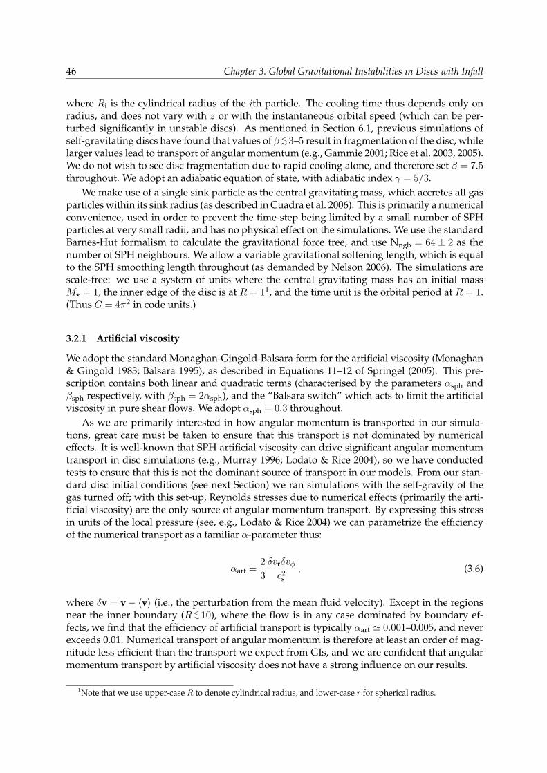
46 Chapter 3. Global Gravitational Instabilities in Discs with Infall
where Ri is the cylindrical radius of the ith particle. The cooling time thus depends only onradius, and does not vary with z or with the instantaneous orbital speed (which can be per-turbed significantly in unstable discs). As mentioned in Section 6.1, previous simulations ofself-gravitating discs have found that values of β <∼3–5 result in fragmentation of the disc, whilelarger values lead to transport of angular momentum (e.g., Gammie 2001; Rice et al. 2003, 2005).We do not wish to see disc fragmentation due to rapid cooling alone, and therefore set β = 7.5throughout. We adopt an adiabatic equation of state, with adiabatic index γ = 5/3.
We make use of a single sink particle as the central gravitating mass, which accretes all gasparticles within its sink radius (as described in Cuadra et al. 2006). This is primarily a numericalconvenience, used in order to prevent the time-step being limited by a small number of SPHparticles at very small radii, and has no physical effect on the simulations. We use the standardBarnes-Hut formalism to calculate the gravitational force tree, and use Nngb = 64 ± 2 as thenumber of SPH neighbours. We allow a variable gravitational softening length, which is equalto the SPH smoothing length throughout (as demanded by Nelson 2006). The simulations arescale-free: we use a system of units where the central gravitating mass has an initial massM? = 1, the inner edge of the disc is at R = 11, and the time unit is the orbital period at R = 1.(Thus G = 4π2 in code units.)
3.2.1 Artificial viscosity
We adopt the standard Monaghan-Gingold-Balsara form for the artificial viscosity (Monaghan& Gingold 1983; Balsara 1995), as described in Equations 11–12 of Springel (2005). This pre-scription contains both linear and quadratic terms (characterised by the parameters αsph andβsph respectively, with βsph = 2αsph), and the “Balsara switch” which acts to limit the artificialviscosity in pure shear flows. We adopt αsph = 0.3 throughout.
As we are primarily interested in how angular momentum is transported in our simula-tions, great care must be taken to ensure that this transport is not dominated by numericaleffects. It is well-known that SPH artificial viscosity can drive significant angular momentumtransport in disc simulations (e.g., Murray 1996; Lodato & Rice 2004), so we have conductedtests to ensure that this is not the dominant source of transport in our models. From our stan-dard disc initial conditions (see next Section) we ran simulations with the self-gravity of thegas turned off; with this set-up, Reynolds stresses due to numerical effects (primarily the arti-ficial viscosity) are the only source of angular momentum transport. By expressing this stressin units of the local pressure (see, e.g., Lodato & Rice 2004) we can parametrize the efficiencyof the numerical transport as a familiar α-parameter thus:
αart =2
3
δvrδvφc2
s, (3.6)
where δv = v− 〈v〉 (i.e., the perturbation from the mean fluid velocity). Except in the regionsnear the inner boundary (R<∼10), where the flow is in any case dominated by boundary ef-fects, we find that the efficiency of artificial transport is typically αart ' 0.001–0.005, and neverexceeds 0.01. Numerical transport of angular momentum is therefore at least an order of mag-nitude less efficient than the transport we expect from GIs, and we are confident that angularmomentum transport by artificial viscosity does not have a strong influence on our results.
1Note that we use upper-case R to denote cylindrical radius, and lower-case r for spherical radius.
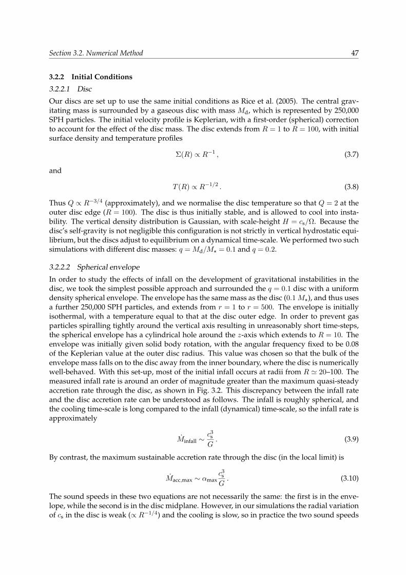
Section 3.2. Numerical Method 47
3.2.2 Initial Conditions
3.2.2.1 Disc
Our discs are set up to use the same initial conditions as Rice et al. (2005). The central grav-itating mass is surrounded by a gaseous disc with mass Md, which is represented by 250,000SPH particles. The initial velocity profile is Keplerian, with a first-order (spherical) correctionto account for the effect of the disc mass. The disc extends from R = 1 to R = 100, with initialsurface density and temperature profiles
Σ(R) ∝ R−1 , (3.7)
and
T (R) ∝ R−1/2 . (3.8)
Thus Q ∝ R−3/4 (approximately), and we normalise the disc temperature so that Q = 2 at theouter disc edge (R = 100). The disc is thus initially stable, and is allowed to cool into insta-bility. The vertical density distribution is Gaussian, with scale-height H = cs/Ω. Because thedisc’s self-gravity is not negligible this configuration is not strictly in vertical hydrostatic equi-librium, but the discs adjust to equilibrium on a dynamical time-scale. We performed two suchsimulations with different disc masses: q = Md/M? = 0.1 and q = 0.2.
3.2.2.2 Spherical envelope
In order to study the effects of infall on the development of gravitational instabilities in thedisc, we took the simplest possible approach and surrounded the q = 0.1 disc with a uniformdensity spherical envelope. The envelope has the same mass as the disc (0.1M?), and thus usesa further 250,000 SPH particles, and extends from r = 1 to r = 500. The envelope is initiallyisothermal, with a temperature equal to that at the disc outer edge. In order to prevent gasparticles spiralling tightly around the vertical axis resulting in unreasonably short time-steps,the spherical envelope has a cylindrical hole around the z-axis which extends to R = 10. Theenvelope was initially given solid body rotation, with the angular frequency fixed to be 0.08of the Keplerian value at the outer disc radius. This value was chosen so that the bulk of theenvelope mass falls on to the disc away from the inner boundary, where the disc is numericallywell-behaved. With this set-up, most of the initial infall occurs at radii from R ' 20–100. Themeasured infall rate is around an order of magnitude greater than the maximum quasi-steadyaccretion rate through the disc, as shown in Fig. 3.2. This discrepancy between the infall rateand the disc accretion rate can be understood as follows. The infall is roughly spherical, andthe cooling time-scale is long compared to the infall (dynamical) time-scale, so the infall rate isapproximately
Minfall ∼c3
sG. (3.9)
By contrast, the maximum sustainable accretion rate through the disc (in the local limit) is
Macc,max ∼ αmaxc3
sG. (3.10)
The sound speeds in these two equations are not necessarily the same: the first is in the enve-lope, while the second is in the disc midplane. However, in our simulations the radial variationof cs in the disc is weak (∝ R−1/4) and the cooling is slow, so in practice the two sound speeds
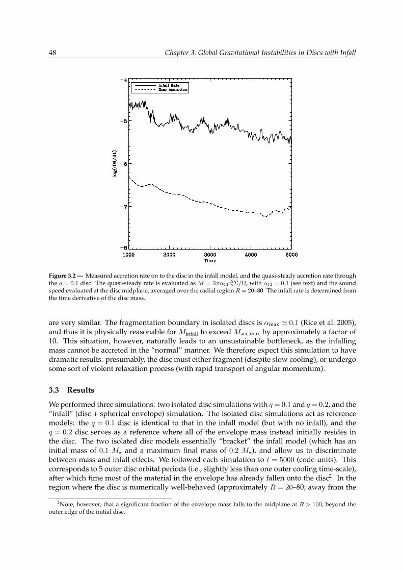
48 Chapter 3. Global Gravitational Instabilities in Discs with Infall
Figure 3.2 — Measured accretion rate on to the disc in the infall model, and the quasi-steady accretion rate throughthe q = 0.1 disc. The quasi-steady rate is evaluated as M = 3παGIc
2s Σ/Ω, with αGI = 0.1 (see text) and the sound
speed evaluated at the disc midplane, averaged over the radial regionR= 20–80. The infall rate is determined fromthe time derivative of the disc mass.
are very similar. The fragmentation boundary in isolated discs is αmax ' 0.1 (Rice et al. 2005),and thus it is physically reasonable for Minfall to exceed Macc,max by approximately a factor of10. This situation, however, naturally leads to an unsustainable bottleneck, as the infallingmass cannot be accreted in the “normal” manner. We therefore expect this simulation to havedramatic results: presumably, the disc must either fragment (despite slow cooling), or undergosome sort of violent relaxation process (with rapid transport of angular momentum).
3.3 Results
We performed three simulations: two isolated disc simulations with q = 0.1 and q = 0.2, and the“infall” (disc + spherical envelope) simulation. The isolated disc simulations act as referencemodels: the q = 0.1 disc is identical to that in the infall model (but with no infall), and theq = 0.2 disc serves as a reference where all of the envelope mass instead initially resides inthe disc. The two isolated disc models essentially “bracket” the infall model (which has aninitial mass of 0.1 M? and a maximum final mass of 0.2 M?), and allow us to discriminatebetween mass and infall effects. We followed each simulation to t = 5000 (code units). Thiscorresponds to 5 outer disc orbital periods (i.e., slightly less than one outer cooling time-scale),after which time most of the material in the envelope has already fallen onto the disc2. In theregion where the disc is numerically well-behaved (approximately R = 20–80; away from the
2Note, however, that a significant fraction of the envelope mass falls to the midplane at R > 100, beyond theouter edge of the initial disc.
Section 3.3. Results 49
disc boundaries) we are thus able to follow the dynamics for tens of dynamical time-scales,allowing the instabilities to develop in a physical manner.
3.3.1 Isolated Discs
Many previous studies have studied the transport properties of GI in low-mass (q<∼0.25) discs(e.g., Lodato & Rice 2004; Boley et al. 2006; Cossins et al. 2009). Our low-mass (q = 0.1) isolateddisc is essentially identical to that used in previous simulations (Rice et al. 2005; Cossins et al.2009), and its expected behaviour is well understood. The transport of angular momentumis dominated by high-order (m ∼ 10) spiral density waves, and the dynamics are consistentwith the local approximation. The characteristic length-scale of such spiral density waves is inthe order of disc scale height H . This simulation therefore serves two purposes here: it actsas a code test, as our calculation should reproduce previous results, and it also provides uswith a reference model with which to compare our “disc with infall” calculation3. Previousstudies have also shown that increasing the disc mass results in the GI generating more powerin the lower-m, global spiral modes (Lodato & Rice 2005). We therefore ran a second referencesimulation, with q = 0.2, so that we are able to distinguish the effects of infall from those thatare simply due to the increasing disc mass.
Our isolated disc simulations essentially repeat these previous studies, and we observe thesame general behaviour described in (for example) Lodato & Rice (2004) and Cossins et al.(2009). The time evolution of the simulations is shown in Fig. 3.3, which shows the midplanedensity evolution from t = 2000 to t = 4000. The isolated discs initially cool and become gravi-tationally unstable, and then develop long-lived spiral density waves which transport angularmomentum in a quasi-steady manner. Both discs quickly settle into a self-regulating state,with Q ' 1 at all radii (see Fig. 3.4). The maximum density contrast in the spiral arms reachesapproximately 1.5 orders of magnitude. The drop in surface density at small radii is due tothe artificial pressure gradient introduced by the inner boundary, and is not physical; for thisreason, we neglect the inner region of the discs (R ≤ 20) in our subsequent analysis. Someadditional power in low-order spiral modes is seen in the more massive (q = 0.2) disc, but forthe most part the transport is well-characterised by a local model, where energy released byaccretion is locally balanced by the imposed cooling.
The induced global spiral density waves can be examined by decomposing the disc’s struc-ture into Fourier modes. In order to compute the Fourier amplitudes, we divided the disc intoconcentric annuli and computed the amplitudes of the azimuthal modes for each annulus. Wethen integrated these amplitudes radially to give global Fourier amplitudesAm, wherem is theFourier mode:
Am =1
Ndisc
∣∣∣∣∣∣
80∑
R=20
Nann∑
j=1
exp−imφj
∣∣∣∣∣∣. (3.11)
Here Nann is the number of SPH particles in each annulus, and Ndisc is the total number ofparticles in all the annuli (i.e., the disc mass). m is the azimuthal mode number, and φj is
3For numerical reasons q = 0.1 is also approximately the lowest mass disc that can be well-resolved in thesesimulations. The resolution requirements in such simulations essentially amount to always ensuring that the discscale-height is resolved into several SPH smoothing lengths (Nelson 2006). In a self-gravitating disc the scale-heightis proportional to the disc mass, so for three-dimensional simulations a factor of two decrease in the disc masstypically costs more than an order of magnitude in computation time (an increase of ∼ 23 in particle number, plusa shortening of the time-step). Consequently, long-duration simulations of discs with q 0.1 remain prohibitivelyexpensive.
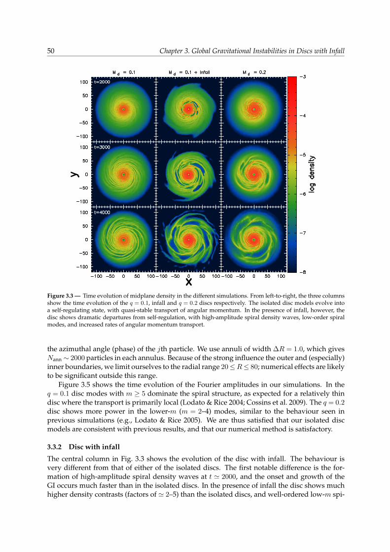
50 Chapter 3. Global Gravitational Instabilities in Discs with Infall
Figure 3.3 — Time evolution of midplane density in the different simulations. From left-to-right, the three columnsshow the time evolution of the q = 0.1, infall and q = 0.2 discs respectively. The isolated disc models evolve intoa self-regulating state, with quasi-stable transport of angular momentum. In the presence of infall, however, thedisc shows dramatic departures from self-regulation, with high-amplitude spiral density waves, low-order spiralmodes, and increased rates of angular momentum transport.
the azimuthal angle (phase) of the jth particle. We use annuli of width ∆R = 1.0, which givesNann ∼ 2000 particles in each annulus. Because of the strong influence the outer and (especially)inner boundaries, we limit ourselves to the radial range 20≤R≤ 80; numerical effects are likelyto be significant outside this range.
Figure 3.5 shows the time evolution of the Fourier amplitudes in our simulations. In theq = 0.1 disc modes with m ≥ 5 dominate the spiral structure, as expected for a relatively thindisc where the transport is primarily local (Lodato & Rice 2004; Cossins et al. 2009). The q = 0.2disc shows more power in the lower-m (m = 2–4) modes, similar to the behaviour seen inprevious simulations (e.g., Lodato & Rice 2005). We are thus satisfied that our isolated discmodels are consistent with previous results, and that our numerical method is satisfactory.
3.3.2 Disc with infall
The central column in Fig. 3.3 shows the evolution of the disc with infall. The behaviour isvery different from that of either of the isolated discs. The first notable difference is the for-mation of high-amplitude spiral density waves at t ' 2000, and the onset and growth of theGI occurs much faster than in the isolated discs. In the presence of infall the disc shows muchhigher density contrasts (factors of ' 2–5) than the isolated discs, and well-ordered low-m spi-

Section 3.3. Results 51
0
1
2
3
4
5
0 20 40 60 80 100
Q(R
)
R
q = 0.1q = 0.2
Disc + Infall
Figure 3.4 — Azimuthally-averaged Toome Q parameter for the three different simulations, plotted at t = 3500.Note the strong divergence from Q ' 1 in the infall simulation.
0.001
0.01
0.1
1
1000 1500 2000 2500 3000 3500 4000 4500 5000
Am
Time
q = 0.1, m = 1= 2= 3
q = 0.2Disc + Infall
0.001
0.01
0.1
1
1000 1500 2000 2500 3000 3500 4000 4500 5000
Am
Time
q = 0.1, m = 4= 5= 8
q = 0.2Disc + Infall
Figure 3.5 — Left: Time evolution of the lowest-order Fourier modes, Am, in the three simulations: q = 0.1 (dotted),q = 0.2 (dashed) and disc + infall (solid). Blue, red and black lines denotem= 1,2 & 3 respectively. The q = 0.1 discshows significantly less power in these low-order modes than the other models. Right: Time evolution of higher-order Fourier modes, Am, in the three simulations: q = 0.1 (dotted), q = 0.2 (dashed) and disc + infall (solid). Hereblue, red and black denote m = 4,5 & 8 respectively. For these higher-order modes, the differences between thedifferent models are much less pronounced than in figure on the left.
ral structures. It is also worth noting that the disc does not fragment, despite being subject tohigh rates of infall; instead it is able to transport angular momentum fast enough to preventany “pile-up” of the infalling material.
In order to make a detailed comparison between the infall model and the isolated discs,it is first necessary to define the disc in the infall model (excluding envelope gas). We definethe disc as all gas within 3 scale-heights of the midplane, with the scale-height computed as

52 Chapter 3. Global Gravitational Instabilities in Discs with Infall
10-7
10-6
10-5
10-4
20 30 40 50 60 70 80 90
Σ(R
)
R
q = 0.1
q = 0.2
Disc + Infall
10-2
10-1
100
20 30 40 50 60 70 80 90
c s(R
)
R
q = 0.1
q = 0.2
Disc + Infall
Figure 3.6 — Azimuthally-averaged radial profiles of surface density Σ (top) and sound speed cs (bottom), plottedfor all three simulations at t= 3500. In both cases the disc with infall lies between the q = 0.1 and q = 0.2 disc (exceptnear the outer disc edge at R = 100), suggesting that disc mass and temperature are not the primary differencesbetween these simulations.
8.8
8.9
9
9.1
9.2
9.3
9.4
0 500 1000 1500 2000 2500 3000 3500 4000
log(
<t c
ool/m
> )
time
q = 0.1
q = 0.2
Disc + Infall
Figure 3.7 — Time evolution of the mass-weighted cooling time for the three different models, averaged over theradial range R = 60–80, plotted in arbitrary units (on a logarithmic scale). The infall model shows no significantdifferences with respect to the q = 0.2 disc, and differs only by a factor of ' 2 from the q = 0.1 disc, allowing us torule out variations in the cooling time-scale as a factor in the enhanced GIs seen.
H = cs/Ω at the midplane. Again we restrict our analysis to the region 20 ≤ R ≤ 80, to preventboundary effects from becoming dominant. The total mass in the disc at R ≤ 100 at the endof the simulation is (t = 5000) is 0.14 M?, an increase of 0.04 M? from the initial disc mass.The disc is also more radially extended than the isolated discs, with significant mass at R >100 (and consequently higher temperatures at R>∼90). Fig.3.6 shows the azimuthally-averagedsurface density and temperature (sound speed) profiles for all three models. Within the region
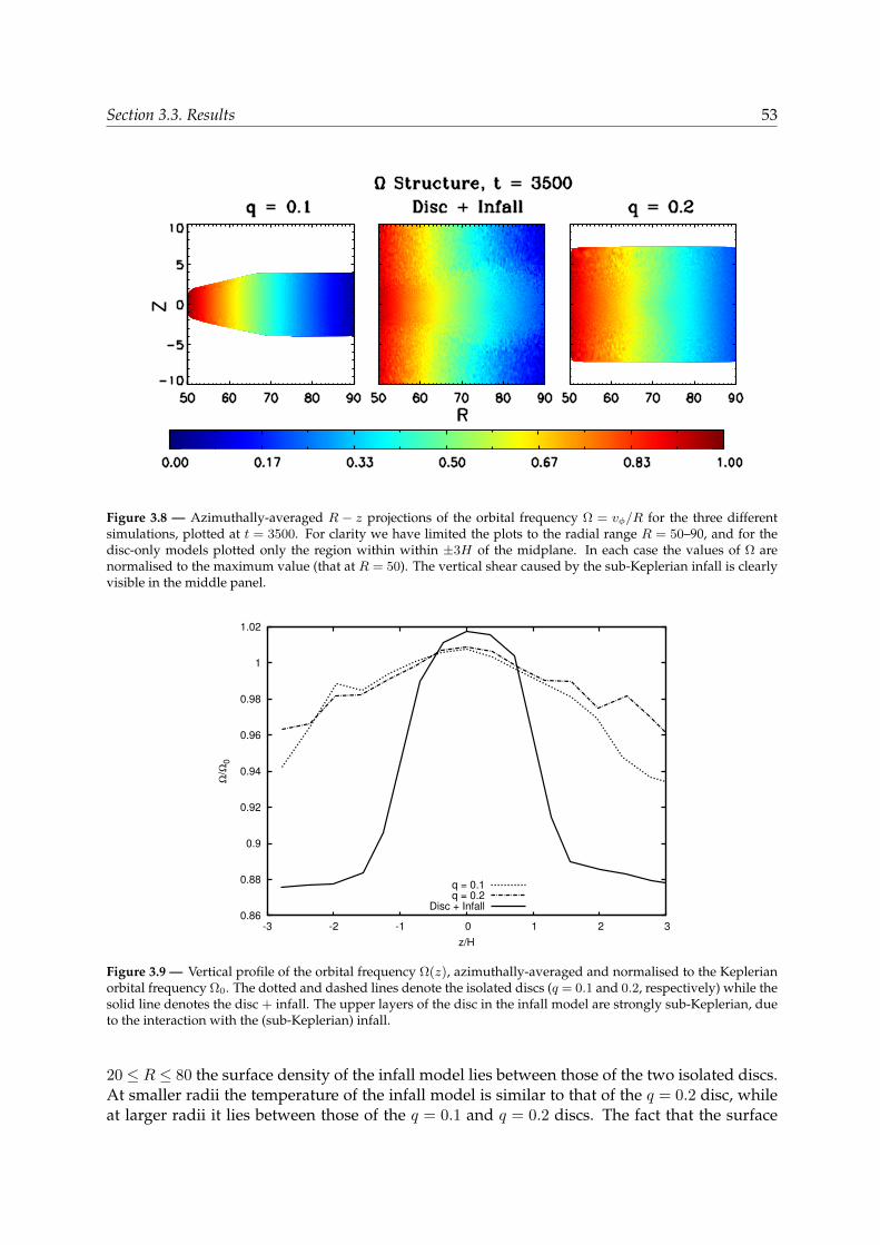
Section 3.3. Results 53
Figure 3.8 — Azimuthally-averaged R − z projections of the orbital frequency Ω = vφ/R for the three differentsimulations, plotted at t = 3500. For clarity we have limited the plots to the radial range R = 50–90, and for thedisc-only models plotted only the region within within ±3H of the midplane. In each case the values of Ω arenormalised to the maximum value (that at R = 50). The vertical shear caused by the sub-Keplerian infall is clearlyvisible in the middle panel.
0.86
0.88
0.9
0.92
0.94
0.96
0.98
1
1.02
-3 -2 -1 0 1 2 3
Ω/Ω
0
z/H
q = 0.1q = 0.2
Disc + Infall
Figure 3.9 — Vertical profile of the orbital frequency Ω(z), azimuthally-averaged and normalised to the Keplerianorbital frequency Ω0. The dotted and dashed lines denote the isolated discs (q = 0.1 and 0.2, respectively) while thesolid line denotes the disc + infall. The upper layers of the disc in the infall model are strongly sub-Keplerian, dueto the interaction with the (sub-Keplerian) infall.
20 ≤ R ≤ 80 the surface density of the infall model lies between those of the two isolated discs.At smaller radii the temperature of the infall model is similar to that of the q = 0.2 disc, whileat larger radii it lies between those of the q = 0.1 and q = 0.2 discs. The fact that the surface
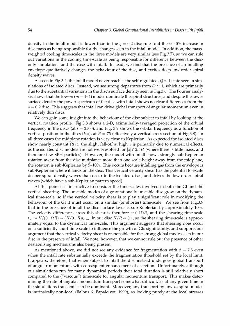
54 Chapter 3. Global Gravitational Instabilities in Discs with Infall
density in the infall model is lower than in the q = 0.2 disc rules out the ' 40% increase indisc mass as being responsible for the changes seen in the infall model. In addition, the mass-weighted cooling time-scales in the three models are very similar (see Fig.3.7), so we can ruleout variations in the cooling time-scale as being responsible for difference between the disc-only simulations and the case with infall. Instead, we find that the presence of an infallingenvelope qualitatively changes the behaviour of the disc, and excites deep low-order spiraldensity waves.
As seen in Fig.3.4, the infall model never reaches the self-regulated, Q' 1 state seen in sim-ulations of isolated discs. Instead, we see strong departures from Q ' 1, which are primarilydue to the substantial variations in the disc’s surface density seen in Fig.3.6. The Fourier analy-sis shows that the low-m (m= 1–4) modes dominate the spiral structures, and despite the lowersurface density the power spectrum of the disc with infall shows no clear differences from theq = 0.2 disc. This suggests that infall can drive global transport of angular momentum even inrelatively thin discs.
We can gain some insight into the behaviour of the disc subject to infall by looking at thevertical rotation profile. Fig.3.8 shows a 2-D, azimuthally-averaged projection of the orbitalfrequency in the discs (at t = 3500), and Fig. 3.9 shows the orbital frequency as a function ofvertical position in the discs Ω(z), at R = 75 (effectively a vertical cross section of Fig.3.8). Inall three cases the midplane rotation is very close to Keplerian. As expected the isolated discsshow nearly constant Ω(z); the slight fall-off at high z is primarily due to numerical effects,as the isolated disc models are not well-resolved for |z|>∼2.5H (where there is little mass, andtherefore few SPH particles). However, the model with infall shows strongly sub-Keplerianrotation away from the disc midplane: more than one scale-height away from the midplane,the rotation is sub-Keplerian by 5–10%. This occurs because infalling gas from the envelope issub-Keplerian where it lands on the disc. This vertical velocity shear has the potential to excitedeeper spiral density waves than occur in the isolated discs, and drives the low-order spiralwaves (which have a sub-Keplerian pattern speed).
At this point it is instructive to consider the time-scales involved in both the GI and thevertical shearing. The unstable modes of a gravitationally unstable disc grow on the dynam-ical time-scale, so if the vertical velocity shear is to play a significant role in modifying thebehaviour of the GI it must occur on a similar (or shorter) time-scale. We see from Fig.3.9that in the presence of infall the disc surface layer is sub-Keplerian by approximately 10%.The velocity difference across this shear is therefore ' 0.1ΩR, and the shearing time-scaletsh ∼ H/(0.1ΩR) ∼ (H/0.1R)tdyn. In our disc H/R ∼ 0.1, so the shearing time-scale is approx-imately equal to the dynamical time-scale. This argument suggests that shearing does occuron a sufficiently short time-scale to influence the growth of GIs significantly, and supports ourargument that the vertical velocity shear is responsible for the strong global modes seen in ourdisc in the presence of infall. We note, however, that we cannot rule out the presence of otherdestabilising mechanisms also being present.
As mentioned above, we did not see any evidence for fragmentation with β = 7.5 evenwhen the infall rate substantially exceeds the fragmentation threshold set by the local limit.It appears, therefore, that when subject to infall the disc instead undergoes global transportof angular momentum, with consequent enhancement of accretion. Unfortunately, althoughour simulations run for many dynamical periods their total duration is still relatively shortcompared to the (“viscous”) time-scale for angular momentum transport. This makes deter-mining the rate of angular momentum transport somewhat difficult, as at any given time inthe simulations transients can be dominant. Moreover, any transport by low-m spiral modesis intrinsically non-local (Balbus & Papaloizou 1999), so looking purely at the local stresses
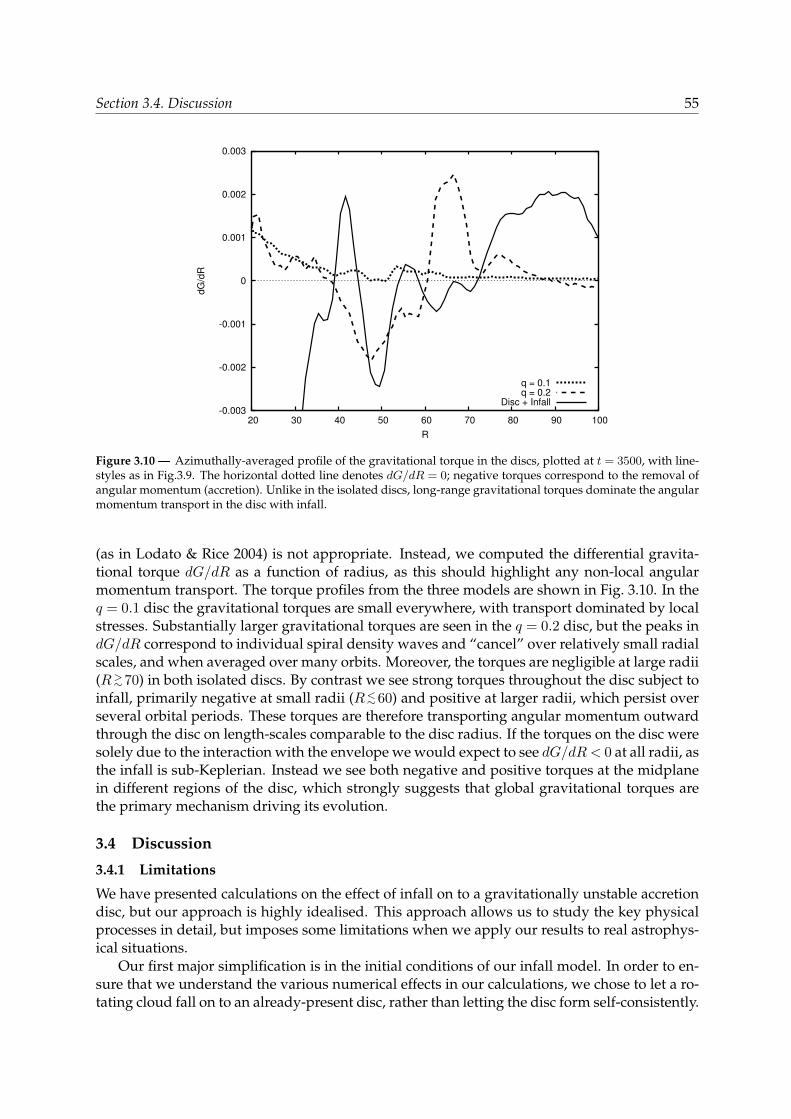
Section 3.4. Discussion 55
-0.003
-0.002
-0.001
0
0.001
0.002
0.003
20 30 40 50 60 70 80 90 100
dG/d
R
R
q = 0.1q = 0.2
Disc + Infall
Figure 3.10 — Azimuthally-averaged profile of the gravitational torque in the discs, plotted at t = 3500, with line-styles as in Fig.3.9. The horizontal dotted line denotes dG/dR = 0; negative torques correspond to the removal ofangular momentum (accretion). Unlike in the isolated discs, long-range gravitational torques dominate the angularmomentum transport in the disc with infall.
(as in Lodato & Rice 2004) is not appropriate. Instead, we computed the differential gravita-tional torque dG/dR as a function of radius, as this should highlight any non-local angularmomentum transport. The torque profiles from the three models are shown in Fig. 3.10. In theq = 0.1 disc the gravitational torques are small everywhere, with transport dominated by localstresses. Substantially larger gravitational torques are seen in the q = 0.2 disc, but the peaks indG/dR correspond to individual spiral density waves and “cancel” over relatively small radialscales, and when averaged over many orbits. Moreover, the torques are negligible at large radii(R>∼70) in both isolated discs. By contrast we see strong torques throughout the disc subject toinfall, primarily negative at small radii (R<∼60) and positive at larger radii, which persist overseveral orbital periods. These torques are therefore transporting angular momentum outwardthrough the disc on length-scales comparable to the disc radius. If the torques on the disc weresolely due to the interaction with the envelope we would expect to see dG/dR < 0 at all radii, asthe infall is sub-Keplerian. Instead we see both negative and positive torques at the midplanein different regions of the disc, which strongly suggests that global gravitational torques arethe primary mechanism driving its evolution.
3.4 Discussion
3.4.1 Limitations
We have presented calculations on the effect of infall on to a gravitationally unstable accretiondisc, but our approach is highly idealised. This approach allows us to study the key physicalprocesses in detail, but imposes some limitations when we apply our results to real astrophys-ical situations.
Our first major simplification is in the initial conditions of our infall model. In order to en-sure that we understand the various numerical effects in our calculations, we chose to let a ro-tating cloud fall on to an already-present disc, rather than letting the disc form self-consistently.

56 Chapter 3. Global Gravitational Instabilities in Discs with Infall
The advantages of our set-up are two-fold. First, we can control the accretion rate on to the disc,and ensure that the ratio between infall rate and theoretical accretion rate is approximatelyconstant over the duration of our simulation (as seen in Fig.3.2). Second, we can compare ourresults directly to our isolated disc models, where the physics is well-understood, and thusisolate the effects of infall from the myriad of other potential effects. However, the trade-off isthat the simulations are highly idealised, and not always realistic. In particular, we note thatquasi-spherical infall is only expected in the early stages of protostellar collapse, when the discand envelope masses are likely to be much larger than those considered here (e.g., Boley 2009;Vorobyov & Basu 2009). Our results have relevance to almost any case of infall on to a gravi-tationally unstable disc (as any infall is, by definition, sub-Keplerian), but we note that care betaken when applying our results to real systems.
Our second major simplification lies in our treatment of the disc thermodynamics. Ourscale-free cooling law has previously been studied in great detail (Gammie 2001; Rice et al. 2003;Lodato & Rice 2004; Cossins et al. 2009), but it is recognised to be a poor approximation to realsystems. The effect of our scale-free cooling law can be seen in Fig. 3.6: the disc temperatureincreases slightly with radius. Real discs almost invariably have cooling time-scales that areshorter (relative to the local dynamical time-scale) at large radii than at small radii, and arethus not scale-free (e.g., Rafikov 2007; Clarke 2009). A more realistic treatment would requirean opacity-based cooling prescription (e.g., Boley et al. 2006; Stamatellos et al. 2007), but thiswould introduce several new free parameters to the problem. Again, our simplifications arenot entirely physical in this regard, but do allow us to study the important processes in detail.Essentially we have chosen to perform a well-controlled numerical experiment instead of aphysically realistic simulation, and our results should be interpreted with this in mind.
3.4.2 Comparison to Previous Work
The majority of previous work in this area has studied the transport properties of isolated grav-itationally unstable discs (Laughlin & Bodenheimer 1994; Lodato & Rice 2004; Rice et al. 2005;Boley et al. 2006; Cossins et al. 2009). Our reference simulations exhibit the same behaviour asin these previous studies, as discussed in Section 3.3.1. However, the influence of infall on theevolution of GIs has not yet been explored in great detail. Krumholz et al. (2007) studied angu-lar momentum transport in a self-consistently-formed disc subject to a very high rate of infall.They found very high accretion rates, equivalent to ∼30% of the total disc mass per dynam-ical time-scale, with effective α-values that exceeded unity. Most of the power was found inthe m = 1 mode, and Krumholz et al. (2007) attributed this very rapid accretion to the SLINGinstability (Adams et al. 1989; Shu et al. 1990). We note, however, that the discs formed inthese simulations were much more massive than those considered here, with q ∼ 0.5–1. It haslong been known that low-order spiral modes can drive rapid accretion in massive discs (e.g.,Laughlin et al. 1998), and in this regards the results of Krumholz et al. (2007) are not directlycomparable to those of our simulations.
In addition, a number of recent studies have used one- and two-dimensional simulations tostudy the formation and evolution of protostellar discs (e.g., Hueso & Guillot 2005; Vorobyov& Basu 2007, 2009; Vorobyov 2009; Visser & Dullemond 2010; Zhu et al. 2009, 2010). Thesesimulations are less computationally intensive than 3-D simulations, and are therefore ableto follow the evolution of the system for much longer time-scales. They also make use ofmore physically realistic prescriptions for both infall and thermodynamics, forming discs self-consistently from collapsing clouds and incorporating realistic models for radiative heatingand cooling. These simulations generally predict that most of the GIs’ power is found in low-order spiral modes, due to both infall and the relatively high masses of the discs which form.
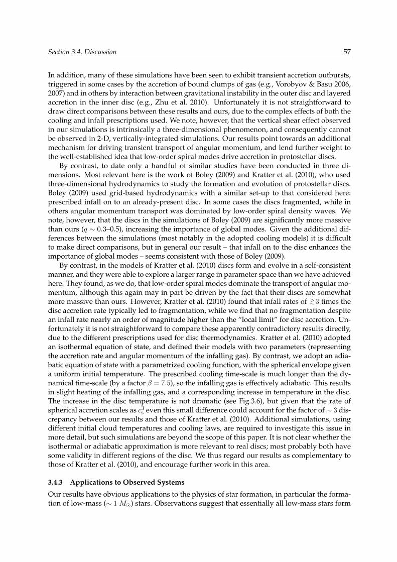
Section 3.4. Discussion 57
In addition, many of these simulations have been seen to exhibit transient accretion outbursts,triggered in some cases by the accretion of bound clumps of gas (e.g., Vorobyov & Basu 2006,2007) and in others by interaction between gravitational instability in the outer disc and layeredaccretion in the inner disc (e.g., Zhu et al. 2010). Unfortunately it is not straightforward todraw direct comparisons between these results and ours, due to the complex effects of both thecooling and infall prescriptions used. We note, however, that the vertical shear effect observedin our simulations is intrinsically a three-dimensional phenomenon, and consequently cannotbe observed in 2-D, vertically-integrated simulations. Our results point towards an additionalmechanism for driving transient transport of angular momentum, and lend further weight tothe well-established idea that low-order spiral modes drive accretion in protostellar discs.
By contrast, to date only a handful of similar studies have been conducted in three di-mensions. Most relevant here is the work of Boley (2009) and Kratter et al. (2010), who usedthree-dimensional hydrodynamics to study the formation and evolution of protostellar discs.Boley (2009) used grid-based hydrodynamics with a similar set-up to that considered here:prescribed infall on to an already-present disc. In some cases the discs fragmented, while inothers angular momentum transport was dominated by low-order spiral density waves. Wenote, however, that the discs in the simulations of Boley (2009) are significantly more massivethan ours (q ∼ 0.3–0.5), increasing the importance of global modes. Given the additional dif-ferences between the simulations (most notably in the adopted cooling models) it is difficultto make direct comparisons, but in general our result – that infall on to the disc enhances theimportance of global modes – seems consistent with those of Boley (2009).
By contrast, in the models of Kratter et al. (2010) discs form and evolve in a self-consistentmanner, and they were able to explore a larger range in parameter space than we have achievedhere. They found, as we do, that low-order spiral modes dominate the transport of angular mo-mentum, although this again may in part be driven by the fact that their discs are somewhatmore massive than ours. However, Kratter et al. (2010) found that infall rates of >∼3 times thedisc accretion rate typically led to fragmentation, while we find that no fragmentation despitean infall rate nearly an order of magnitude higher than the “local limit” for disc accretion. Un-fortunately it is not straightforward to compare these apparently contradictory results directly,due to the different prescriptions used for disc thermodynamics. Kratter et al. (2010) adoptedan isothermal equation of state, and defined their models with two parameters (representingthe accretion rate and angular momentum of the infalling gas). By contrast, we adopt an adia-batic equation of state with a parametrized cooling function, with the spherical envelope givena uniform initial temperature. The prescribed cooling time-scale is much longer than the dy-namical time-scale (by a factor β = 7.5), so the infalling gas is effectively adiabatic. This resultsin slight heating of the infalling gas, and a corresponding increase in temperature in the disc.The increase in the disc temperature is not dramatic (see Fig.3.6), but given that the rate ofspherical accretion scales as c3
s even this small difference could account for the factor of∼ 3 dis-crepancy between our results and those of Kratter et al. (2010). Additional simulations, usingdifferent initial cloud temperatures and cooling laws, are required to investigate this issue inmore detail, but such simulations are beyond the scope of this paper. It is not clear whether theisothermal or adiabatic approximation is more relevant to real discs; most probably both havesome validity in different regions of the disc. We thus regard our results as complementary tothose of Kratter et al. (2010), and encourage further work in this area.
3.4.3 Applications to Observed Systems
Our results have obvious applications to the physics of star formation, in particular the forma-tion of low-mass (∼ 1 M) stars. Observations suggest that essentially all low-mass stars form

58 Chapter 3. Global Gravitational Instabilities in Discs with Infall
with discs (e.g., Haisch et al. 2001), and disc accretion is thought to play a major role in thebuild-up of stellar mass. Moreover, in the earliest, embedded phases gravitational instability islikely to be the dominant mechanism for angular momentum transport: such discs are insuffi-ciently ionized to sustain transport via magnetohydrodyamic turbulence (Matsumoto & Tajima1995; Gammie 1996), but both observations and theory suggest that they are indeed massiveenough to be gravitationally unstable (e.g., Greaves et al. 2008; Andrews et al. 2009; Hueso &Guillot 2005; Vorobyov & Basu 2009). Our results argue that accretion in such discs is likelyto be highly transient, and in general terms are consistent with a picture where the bulk of thestellar mass is accreted during a small number of intense outbursts (e.g., Armitage et al. 2001;Lodato & Rice 2005; Vorobyov & Basu 2006, 2010; Zhu et al. 2010).
The consequences of our results for massive star formation are less clear. Although discsare expected to form around massive, forming stars, observational evidence of their existenceis somewhat thin (e.g., Cesaroni et al. 2006, 2007). It is clear, however, that if such discs doindeed exist they are likely to be gravitationally unstable, but in this scenario the maximumstable disc accretion rate (<∼10−5 M yr−1; Levin 2003; Cesaroni et al. 2006; Rafikov 2007) ismuch too low for these massive stars to accumulate their mass in a plausible time-scale. Ithas previously been suggested that the formation of massive stars is likely to be dominatedby transient episodes and highly variable accretion (Cesaroni et al. 2007). Our results suggestthat the global gravitational torques driven by infall on to the disc result in exactly this type ofbehaviour, and may be an important accretion mechanism in massive star formation.
In addition, we suggest that our results may have important consequences for the forma-tion of massive stars close to super-massive black holes. A large population of massive O-and Wolf-Rayet-type stars is now known to exist within ∼ 0.1 pc of the super-massive blackhole (SMBH) at the centre of the Galaxy (Genzel et al. 2003; Ghez et al. 2005), and a popularscenario for the formation of these stars is “in situ” formation via the fragmentation of an ac-cretion disc around the SMBH (Levin & Beloborodov 2003; Nayakshin 2006). This picture has anumber of attractive features, but an open question has always been how the stars attain theirfinal masses. Both analytic theory and numerical simulations suggest that the initial fragmentmasses are small, ∼ 1 M, and that the bulk of the stellar mass is subsequently accreted fromthe SMBH disc (e.g., Alexander et al. 2008; Bonnell & Rice 2008). However, the estimated infallrates through the Hill sphere on to these protostellar discs are extremely high, ∼ 10−4 Myr−1
(Milosavljevic & Loeb 2004), and in the local limit these discs are expected to fragment, prevent-ing rapid growth of the protostars and limiting the resulting stellar masses (see also Matzner& Levin 2005; Kratter & Matzner 2006). Our results suggest that discs subject to high infallrates may instead be able to transport angular momentum much more rapidly, through globalmodes of the GI, and this mechanism provides a potential solution to the “accretion problem”of massive star formation at the centre of the Galaxy.
3.5 Summary
We have presented numerical simulations of gravitationally unstable accretion discs subject toinfall from a surrounding envelope. Our numerical set-up is highly idealised, but this allowsus to study the angular momentum transport properties of the system in detail. Our disc hasa relatively slow cooling rate (tcoolΩ = 7.5), and we find that the disc does not fragment eventhough the infall rate on to the disc is an order of magnitude greater than the “quasi-steady”accretion rate in the self-regulating self-gravitating disc. Instead, despite relatively low discmasses (Md/M? ' 0.14), we see evidence that angular momentum is transported rapidly bytorques from low-order, global, spiral density waves, which are excited by the interaction be-

Section 3.5. Summary 59
tween the disc and the infalling envelope. This drives accretion at a rate significantly higherthan is possible in a local model, and we suggest that this mechanism may play an importantrole in a number of different astrophysical systems.
Acknowledgements
We are grateful for stimulating discussions with a number of colleagues, in particular GiuseppeLodato, Phil Armitage, Peter Cossins, Chris Matzner, Kaitlin Kratter & Steve Balbus. We alsothank the anonymous referee for several useful comments. DH is supported by an Oort Schol-arship from Leiden Observatory, and by a Huygens Scholarship from the Netherlands Organi-zation for International Co-operation in Higher Education (NUFFIC). RDA & YL acknowledgesupport from the from the Netherlands Organisation for Scientific Research (NWO) throughVIDI grant 639.042.607. RDA also acknowledges further support from the NWO throughVIDI grant 639.042.404, and from a Science & Technology Facilities Council (STFC) AdvancedFellowship (ST/G00711X/1). Visualizations of SPH simulations were created using SPLASH(Price 2007). The simulations presented in this paper were run on the Huygens supercomputer,supported by Netherlands National Computing Facility Project SH-080-08.


Chapter 4Evolution of CO lines in time-dependent
models of protostellar disk formation
Abstract. Context. Star and planet formation theories predict an evolution in the density, temperature,and velocity structure as the envelope collapses and forms an accretion disk. While continuum emissioncan trace the dust evolution, spectrally resolved molecular lines are needed to determine the physicalstructure and collapse dynamics.Aims. The aim of this work is to model the evolution of the molecular excitation, line profiles, and re-lated observables during low-mass star formation. Specifically, the signatures of disks during the deeplyembedded stage (Menv >M?) are investigated.Methods. The semi-analytic 2D axisymmetric model of Visser and collaborators has been used to de-scribe the evolution of the density, stellar mass, and luminosity from the pre-stellar to the T-Tauri phase.A full radiative transfer calculation is carried out to accurately determine the time-dependent dust tem-peratures. The time-dependent CO abundance is obtained from the adsorption and thermal desorptionchemistry. Non-LTE near-IR, FIR, and submm lines of CO have been simulated at a number of timesteps.Results. In single dish (10–20′′ beams), the dynamics during the collapse are best probed through highlyexcited 13CO and C18O lines, which are significantly broadened by the infall process. In contrast to thedust temperature, the CO excitation temperature derived from submm/FIR data does not vary duringthe protostellar evolution, consistent with C18O observations obtained with Herschel and from ground-based telescopes. The near-IR spectra provide complementary information to the submm lines by prob-ing not only the cold outer envelope but also the warm inner region. The near-IR high-J (≥ 8) absorptionlines are particularly sensitive to the physical structure of the inner few AU, which does show evolu-tion. The models indicate that observations of 13CO and C18O low-J submm lines within a ≤1 ′′ (at 140pc) beam are well suited to probe embedded disks in Stage I (Menv < M?) sources, consistent with re-cent interferometric observations. High signal-to-noise ratio subarcsec resolution data with ALMA areneeded to detect the presence of small rotationally supported disks during the Stage 0 phase and var-ious diagnostics are discussed. The combination of spatially and spectrally resolved lines with ALMAand at near-IR is a powerful method to probe the inner envelope and disk formation process during theembedded phase.
D. Harsono, R. Visser, S. Bruderer, E. F. van Dishoeck, L. E. KristensenA&A, 555, 45 (2013)
4.1 Introduction
THE semi-analytical model of the collapse of protostellar envelopes (Shu 1977; Cassen &Moosman 1981; Terebey et al. 1984) has been used extensively to study the evolution of
gas and dust from core to disk and star (Young & Evans 2005; Dunham et al. 2010; Visseret al. 2009). Others have explored the effects of envelope and disk parameters representativeof specific evolutionary stages on the spectral energy distribution (SED) and other diagnos-tics (Whitney et al. 2003a; Robitaille et al. 2006; Robitaille et al. 2007; Crapsi et al. 2008; Tobin
62 Chapter 4. CO lines evolution
et al. 2011). These studies have focused primarily on the dust emission and its relation to thephysical structure. On the other hand, spectroscopic observations toward young stellar objects(YSOs) performed by many ground-based (sub)millimeter and infrared telescopes also containinformation on the gas structure (Evans 1999). The molecular lines are important in revealingthe kinematical information of the collapsing envelope as well as the physical parameters ofthe gas based on the molecular excitation. The Herschel Space Observatory and the AtacamaLarge Millimeter/submillimeter Array (ALMA) provide new probes of the excitation and kine-matics of the gas on smaller scales and up to higher temperatures than previously possible. Itis therefore timely to simulate the predicted molecular excitation and line profiles within thestandard picture of a collapsing envelope. The aim is to identify diagnostic signatures of thedifferent physical components and stages and to provide a reference for studies of more com-plex collapse dynamics.
A problem that is very closely connected to the collapse of protostellar envelopes is theformation of accretion disks. The presence of embedded disks was inferred from the excessof continuum emission at the smallest spatial scales through interferometric observations (eg.Keene & Masson 1990; Brown et al. 2000; Jørgensen et al. 2005a, 2009). Their physical structurecan be determined by the combined modeling of the SED and the interferometric observations(Jørgensen et al. 2005a; Brinch et al. 2007b; Enoch et al. 2009). However, the excess continuumemission at small scales can also be due to other effects of a (magnetized) collapsing rotatingenvelope (pseudo-disk, Chiang et al. 2008). Therefore, resolved molecular line observationsfrom interferometers such as ALMA are needed to clearly detect the presence or absence of astable rotating embedded disk (Brinch et al. 2007b, 2008; Lommen et al. 2008; Jørgensen et al.2009; Tobin et al. 2012).
A number of previous studies have modeled the line profiles based on the spherically sym-metry inside-out collapse scenario described by Shu (1977) (eg., Zhou et al. 1993; Hogerheijde& Sandell 2000; Hogerheijde 2001; Lee et al. 2003, 2005; Evans et al. 2005). Also, numerical hy-drodynamical collapse models have been coupled with chemistry and line radiative transfer tostudy the molecular line evolution in 1D (Aikawa et al. 2008) and 2D (Brinch et al. 2007b; vanWeeren et al. 2009). Best-fit collapse parameters (e.g., sound speed and age) are obtained butdepend on the temperature structure and abundance profile of the model. Visser et al. (2009)and Visser & Dullemond (2010) developed 2D semi-analytical models that describe the densityand velocity structure as matter moves onto and through the forming disk. This model hasbeen coupled with chemistry (Visser et al. 2009, 2011), but no line profiles have yet been sim-ulated. The current paper presents the first study of the CO molecular line evolution within2D disk formation models. CO and its isotopologs are chosen because it is a chemically stablemolecule and readily observed.
Observationally, most early studies of low-mass embedded YSOs focused on the low−J(Ju ≤ 6) (sub-)millimeter CO lines in 20–30 ′′ beams, thus probing scales of a few thousandAU in the nearest star-forming regions (e.g., Belloche et al. 2002; Jørgensen et al. 2002; Leeet al. 2003; Young et al. 2004; Crapsi et al. 2005). More recently, ground-based high-frequencyobservations of large samples up to Ju=7 are becoming routinely available (Hogerheijde et al.1998; van Kempen et al. 2009b,a,d) and Herschel-HIFI (de Graauw et al. 2010) has opened upspectrally resolved observations of CO and its isotopologs up to Ju = 16 (Eu = 660 K) (Yıldızet al. 2010, 2012). In addition, the PACS (Poglitsch et al. 2010) and SPIRE (Griffin et al. 2010)instruments provide spectrally unresolved CO data from Ju = 4 to Ju = 50 (Eu = 55− 7300K), revealing multiple temperature components (e.g., van Kempen et al. 2010; Herczeg et al.2012; Goicoechea et al. 2012; Manoj et al. 2013). Although the interpretation of the higher Julines requires additional physical processes than those considered here (Visser et al. 2012), our
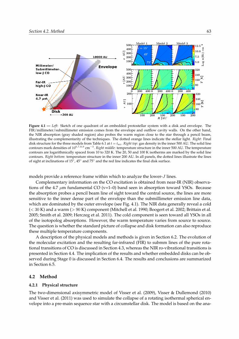
Section 4.2. Method 63
Disk200 AU
Near-IR
4.7 μm
Far-IR
high-J CO
Figure 4.1 — Left: Sketch of one quadrant of an embedded protostellar system with a disk and envelope. TheFIR/millimeter/submillimeter emission comes from the envelope and outflow cavity walls. On the other hand,the NIR absorption (gray shaded region) also probes the warm region close to the star through a pencil beam,illustrating the complementarity of the techniques. The dotted orange lines indicate the stellar light. Right: Finaldisk structure for the three models from Table 6.1 at t= tacc. Right top: gas density in the inner 500 AU. The solid linecontours mark densities of 106,7,8,9 cm−3. Right middle: temperature structure in the inner 500 AU. The temperaturecontours are logarithmically spaced from 10 to 320 K. The 20, 50 and 100 K isotherms are marked by the solid linecontours. Right bottom: temperature structure in the inner 200 AU. In all panels, the dotted lines illustrate the linesof sight at inclinations of 15, 45 and 75 and the red line indicates the final disk surface.
models provide a reference frame within which to analyze the lower-J lines.Complementary information on the CO excitation is obtained from near-IR (NIR) observa-
tions of the 4.7 µm fundamental CO (v=1–0) band seen in absorption toward YSOs. Becausethe absorption probes a pencil beam line of sight toward the central source, the lines are moresensitive to the inner dense part of the envelope than the submillimeter emission line data,which are dominated by the outer envelope (see Fig. 4.1). The NIR data generally reveal a cold(< 30 K) and a warm (> 90 K) component (Mitchell et al. 1990; Boogert et al. 2002; Brittain et al.2005; Smith et al. 2009; Herczeg et al. 2011). The cold component is seen toward all YSOs in allof the isotopolog absorptions. However, the warm temperature varies from source to source.The question is whether the standard picture of collapse and disk formation can also reproducethese multiple temperature components.
A description of the physical models and methods is given in Section 6.2. The evolution ofthe molecular excitation and the resulting far-infrared (FIR) to submm lines of the pure rota-tional transitions of CO is discussed in Section 4.3, whereas the NIR ro-vibrational transitions ispresented in Section 4.4. The implication of the results and whether embedded disks can be ob-served during Stage 0 is discussed in Section 6.4. The results and conclusions are summarizedin Section 6.5.
4.2 Method
4.2.1 Physical structure
The two-dimensional axisymmetric model of Visser et al. (2009), Visser & Dullemond (2010)and Visser et al. (2011) was used to simulate the collapse of a rotating isothermal spherical en-velope into a pre-main sequence star with a circumstellar disk. The model is based on the ana-
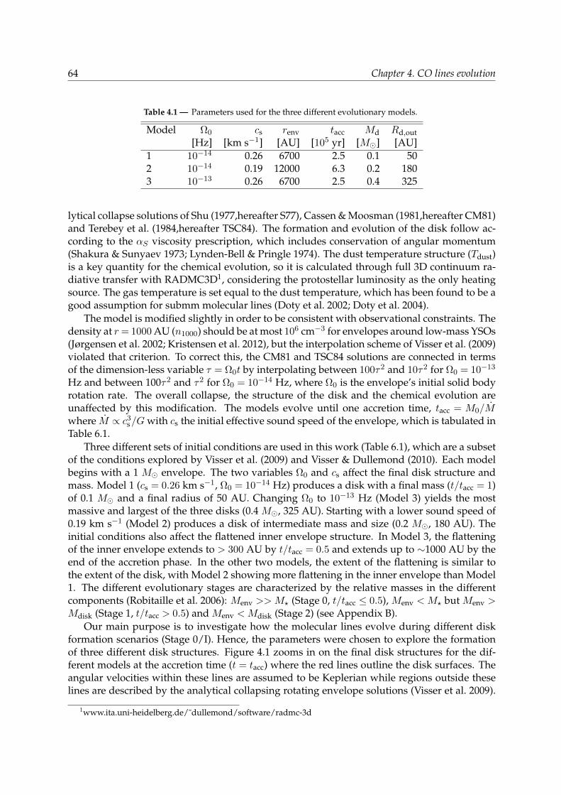
64 Chapter 4. CO lines evolution
Table 4.1 — Parameters used for the three different evolutionary models.
Model Ω0 cs renv tacc Md Rd,out[Hz] [km s−1] [AU] [105 yr] [M] [AU]
1 10−14 0.26 6700 2.5 0.1 502 10−14 0.19 12000 6.3 0.2 1803 10−13 0.26 6700 2.5 0.4 325
lytical collapse solutions of Shu (1977,hereafter S77), Cassen & Moosman (1981,hereafter CM81)and Terebey et al. (1984,hereafter TSC84). The formation and evolution of the disk follow ac-cording to the αS viscosity prescription, which includes conservation of angular momentum(Shakura & Sunyaev 1973; Lynden-Bell & Pringle 1974). The dust temperature structure (Tdust)is a key quantity for the chemical evolution, so it is calculated through full 3D continuum ra-diative transfer with RADMC3D1, considering the protostellar luminosity as the only heatingsource. The gas temperature is set equal to the dust temperature, which has been found to be agood assumption for submm molecular lines (Doty et al. 2002; Doty et al. 2004).
The model is modified slightly in order to be consistent with observational constraints. Thedensity at r= 1000 AU (n1000) should be at most 106 cm−3 for envelopes around low-mass YSOs(Jørgensen et al. 2002; Kristensen et al. 2012), but the interpolation scheme of Visser et al. (2009)violated that criterion. To correct this, the CM81 and TSC84 solutions are connected in termsof the dimension-less variable τ = Ω0t by interpolating between 100τ2 and 10τ2 for Ω0 = 10−13
Hz and between 100τ2 and τ2 for Ω0 = 10−14 Hz, where Ω0 is the envelope’s initial solid bodyrotation rate. The overall collapse, the structure of the disk and the chemical evolution areunaffected by this modification. The models evolve until one accretion time, tacc = M0/Mwhere M ∝ c3
s/G with cs the initial effective sound speed of the envelope, which is tabulated inTable 6.1.
Three different sets of initial conditions are used in this work (Table 6.1), which are a subsetof the conditions explored by Visser et al. (2009) and Visser & Dullemond (2010). Each modelbegins with a 1 M envelope. The two variables Ω0 and cs affect the final disk structure andmass. Model 1 (cs = 0.26 km s−1, Ω0 = 10−14 Hz) produces a disk with a final mass (t/tacc = 1)of 0.1 M and a final radius of 50 AU. Changing Ω0 to 10−13 Hz (Model 3) yields the mostmassive and largest of the three disks (0.4 M, 325 AU). Starting with a lower sound speed of0.19 km s−1 (Model 2) produces a disk of intermediate mass and size (0.2 M, 180 AU). Theinitial conditions also affect the flattened inner envelope structure. In Model 3, the flatteningof the inner envelope extends to > 300 AU by t/tacc = 0.5 and extends up to ∼1000 AU by theend of the accretion phase. In the other two models, the extent of the flattening is similar tothe extent of the disk, with Model 2 showing more flattening in the inner envelope than Model1. The different evolutionary stages are characterized by the relative masses in the differentcomponents (Robitaille et al. 2006): Menv >>M? (Stage 0, t/tacc ≤ 0.5), Menv <M? but Menv >Mdisk (Stage 1, t/tacc > 0.5) and Menv <Mdisk (Stage 2) (see Appendix B).
Our main purpose is to investigate how the molecular lines evolve during different diskformation scenarios (Stage 0/I). Hence, the parameters were chosen to explore the formationof three different disk structures. Figure 4.1 zooms in on the final disk structures for the dif-ferent models at the accretion time (t = tacc) where the red lines outline the disk surfaces. Theangular velocities within these lines are assumed to be Keplerian while regions outside theselines are described by the analytical collapsing rotating envelope solutions (Visser et al. 2009).
1www.ita.uni-heidelberg.de/˜dullemond/software/radmc-3d
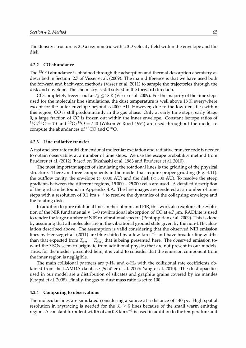
Section 4.2. Method 65
The density structure is 2D axisymmetric with a 3D velocity field within the envelope and thedisk.
4.2.2 CO abundance
The 12CO abundance is obtained through the adsorption and thermal desorption chemistry asdescribed in Section 2.7 of Visser et al. (2009). The main difference is that we have used boththe forward and backward methods (Visser et al. 2011) to sample the trajectories through thedisk and envelope. The chemistry is still solved in the forward direction.
CO completely freezes out at Td ≤ 18 K (Visser et al. 2009). For the majority of the time stepsused for the molecular line simulations, the dust temperature is well above 18 K everywhereexcept for the outer envelope beyond ∼4000 AU. However, due to the low densities withinthis region, CO is still predominantly in the gas phase. Only at early time steps, early Stage0, a large fraction of CO is frozen out within the inner envelope. Constant isotope ratios of12C/13C = 70 and 16O/18O = 540 (Wilson & Rood 1994) are used throughout the model tocompute the abundances of 13CO and C18O.
4.2.3 Line radiative transfer
A fast and accurate multi-dimensional molecular excitation and radiative transfer code is neededto obtain observables at a number of time steps. We use the escape probability method fromBruderer et al. (2012) (based on Takahashi et al. 1983 and Bruderer et al. 2010).
The most important aspect of simulating the rotational lines is the gridding of the physicalstructure. There are three components in the model that require proper gridding (Fig. 4.11):the outflow cavity, the envelope (> 6000 AU) and the disk (< 300 AU). To resolve the steepgradients between the different regions, 15 000 – 25 000 cells are used. A detailed descriptionof the grid can be found in Appendix 4.A. The line images are rendered at a number of timesteps with a resolution of 0.1 km s−1 to resolve the dynamics of the collapsing envelope andthe rotating disk.
In addition to pure rotational lines in the submm and FIR, this work also explores the evolu-tion of the NIR fundamental v=1–0 rovibrational absorption of CO at 4.7 µm. RADLite is usedto render the large number of NIR ro-vibrational spectra (Pontoppidan et al. 2009). This is doneby assuming that all molecules are in the vibrational ground state given by the non-LTE calcu-lation described above. The assumption is valid considering that the observed NIR emissionlines by Herczeg et al. (2011) are blue-shifted by a few km s−1 and have broader line widthsthan that expected from Tgas = Tdust that is being presented here. The observed emission to-ward the YSOs seem to originate from additional physics that are not present in our models.Thus, for the models presented here, it is valid to consider that the emission component fromthe inner region is negligible.
The main collisional partners are p-H2 and o-H2 with the collisional rate coefficients ob-tained from the LAMDA database (Schoier et al. 2005; Yang et al. 2010). The dust opacitiesused in our model are a distribution of silicates and graphite grains covered by ice mantles(Crapsi et al. 2008). Finally, the gas-to-dust mass ratio is set to 100.
4.2.4 Comparing to observations
The molecular lines are simulated considering a source at a distance of 140 pc. High spatialresolution in raytracing is needed for the Ju ≥ 5 lines because of the small warm emittingregion. A constant turbulent width of b = 0.8 km s−1 is used in addition to the temperature and

66 Chapter 4. CO lines evolution
infall broadening to be consistent with the observed C18O turbulent widths toward quiescentgas surrounding low-mass YSOs with beams > 9 ′′ (Jørgensen et al. 2002).
The simulated spectral cubes are convolved with Gaussian beams of 1 ′′, 9 ′′ and 20 ′′ withthe convol routine in the MIRIAD data reduction package (Sault et al. 1995). The telescopes thatobserve the low-J rotational lines (Ju ≤ 5) typically have≥ 15 ′′ beams, as does Herschel-HIFI forthe higher-J lines with Ju ≈ 10. A 9 ′′ beam is appropriate for observations of Ju > 5 performedwith, e.g., the ground-based APEX telescope at 650 GHz and with Herschel-PACS and HIFI forJu > 14. A 1 ′′ beam simulates interferometric observations to be performed with ALMA. Thesubmm lines are rendered nearly face-on (i∼ 5) since this is the simplest geometry to quantifythe disk contribution. For studies of the evolution of the velocity field, an inclination of 45 istaken. The NIR lines are analyzed for 45 and 75 inclination to study the different excitationconditions between lines of sight through the inner envelope and the disk (Fig. 4.1). A line ofsight of 45 probes the inner envelope and does not go through the disk while a line of sightof 75 grazes the top layers of the disk. Both a pencil beam approximation toward the centeris taken as well as the full RADLite simulation to study the radiative transfer effects on thoselines.
4.2.5 Caveats
The synthetic CO spectra were simulated without the presence of fore- and background mate-rial, such as the diffuse gas of the large-scale cloud where these YSOs are forming. The over-all emission of the large-scale cloud can affect the observed line profiles within a large beam(> 15 ′′), in particular the Ju ≤ 4 lines of 12CO and 13CO and the Ju ≤ 2 lines of C18O. Alsonot included in the simulations are energetic components such as jets, shocks, UV heating andwinds. These energetics strongly affect the 12CO lines, especially the intensity of the Ju ≥ 6rotational transitions (Spaans et al. 1995; van Kempen et al. 2009b; Visser et al. 2012). Lumi-nosity flares associated with episodic accretion events can affect the CO abundance structureas discussed in Visser & Bergin (2012). Their effect on the evolution of the CO line profile andexcitation is beyond the scope of this paper. In general, a higher CO flux is expected during anaccretion burst.
4.3 FIR and submm CO evolution
The FIR and submm CO lines up to the 10− 9 transition (Eu = 290–304 K) have been simulatedwith i=5. The geometrical effects on the line intensities (13CO and C18O) are less than 30%for different inclinations and the derived excitation temperatures differ by less than 5%, whichis smaller than the rms error on the derived temperatures. On the other hand, inclinationstrongly affects the derived moment maps and interpretation of the velocity field, therefore aninclination of 45 is used in Section 4.3.4.
4.3.1 Line profiles
The first time step used for the molecular line simulation is at t = 1000 years (t/tacc ∼ 10−3),where the central heating is not yet turned on. The evolution of the mass and the effectivetemperature is shown in the Appendix 4.B. The effective temperature during this time step is10 K and the models are still spherically symmetric. The TSC84 velocity profile for this timestep reaches a maximum radial component of 10 km s−1 at 0.1 AU. However, CO is frozen outin the inner envelope, so the FIR and submm lines (populated up to Ju ≤ 8) show neither wingemission nor blue asymmetry as typical signposts of an infalling envelope. Instead, the CO

Section 4.3. FIR and submm CO evolution 67
Figure 4.2 — Left: Normalized C18O line profiles as functions of evolution for Ju = 3, 6 and 9 at t/tacc = 0.13 (red),0.50 (green) and 0.96 (black) for i = 5 orientation for Model 1. The lines are convolved to beams of 20 ′′ (top), 9 ′′
(middle) and 1 ′′ (bottom). Right: ceo 3-2 (red), 6-5 (blue) and 9-8 (black) FWHM evolution within a 9 ′′ beam for the3 different models at i = 5 orientation.
lines probe the static outer envelope at this point, where the low density has prevented COfrom freezing out.
The line profiles change shape once the effective source temperature increases to above afew thousand K at t > 104 yr (see Fig. 4.2 and Appendix 4.B for the line profile evolution). Theline profiles become more asymmetric (Fig. 4.12) toward higher excitation and smaller beams,because in both cases a larger contribution from warm, infalling gas in the inner envelope andoptical depth affect the emission lines. The line widths are due to a combination of thermalbroadening, turbulent width and velocity structure, but examination of models without a sys-tematic velocity field confirm that the increase in broadening is mostly due to infall (see alsoLee et al. 2003). Models 2 and 3 show narrower lines during Stage I (t/tacc ≥ 0.5) since theyare relatively more rotationally dominated than in Model 1. As shown in Fig. 4.2, the higher-J(Ju ≥ 5) lines are broadened significantly during Stage 0.
Figure 4.3 — Left: Examples of single-temperature fits through the 12CO (squares) and C18O (triangles) lines ob-tained from Model 1 fluxes at t/tacc = 0.9 in a 9′′ beam. The red line shows the linear fit from Ju = 2 up to Ju = 10while the blue line is the fit up starting from Ju = 4 up to Ju = 10. The gray shaded regions indicate one stan-dard deviation from the best fit. Right: Evolution of the rotational temperature (Trot) from a single-temperature fitthrough Ju = 2− 10. The different colors are for different isotopologs: 12CO (black), 13CO (green) and C18O (blue).The typical errors are 15, 5 and 3 K for 12CO, 13CO and C18O, respectively. The different panels show the results fordifferent models as indicated.
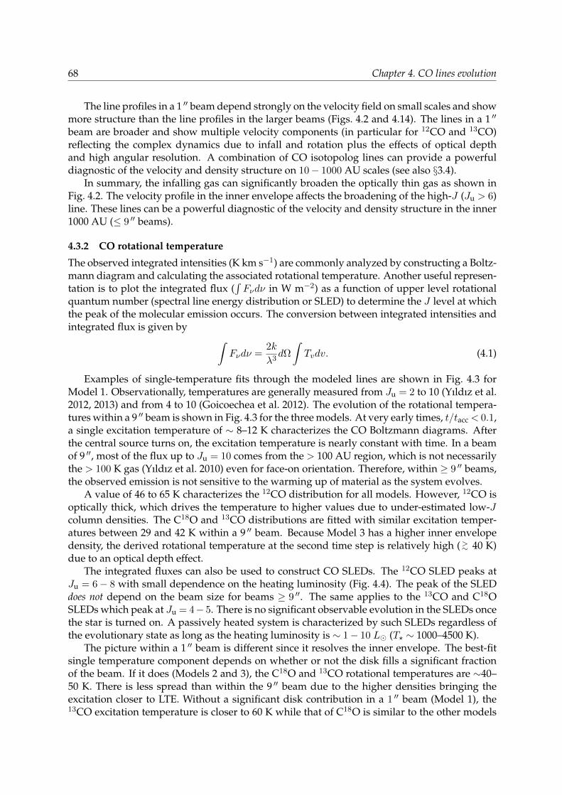
68 Chapter 4. CO lines evolution
The line profiles in a 1 ′′ beam depend strongly on the velocity field on small scales and showmore structure than the line profiles in the larger beams (Figs. 4.2 and 4.14). The lines in a 1 ′′
beam are broader and show multiple velocity components (in particular for 12CO and 13CO)reflecting the complex dynamics due to infall and rotation plus the effects of optical depthand high angular resolution. A combination of CO isotopolog lines can provide a powerfuldiagnostic of the velocity and density structure on 10− 1000 AU scales (see also §3.4).
In summary, the infalling gas can significantly broaden the optically thin gas as shown inFig. 4.2. The velocity profile in the inner envelope affects the broadening of the high-J (Ju > 6)line. These lines can be a powerful diagnostic of the velocity and density structure in the inner1000 AU (≤ 9 ′′ beams).
4.3.2 CO rotational temperature
The observed integrated intensities (K km s−1) are commonly analyzed by constructing a Boltz-mann diagram and calculating the associated rotational temperature. Another useful represen-tation is to plot the integrated flux (
∫Fνdν in W m−2) as a function of upper level rotational
quantum number (spectral line energy distribution or SLED) to determine the J level at whichthe peak of the molecular emission occurs. The conversion between integrated intensities andintegrated flux is given by
∫Fνdν =
2k
λ3dΩ
∫Tvdv. (4.1)
Examples of single-temperature fits through the modeled lines are shown in Fig. 4.3 forModel 1. Observationally, temperatures are generally measured from Ju = 2 to 10 (Yıldız et al.2012, 2013) and from 4 to 10 (Goicoechea et al. 2012). The evolution of the rotational tempera-tures within a 9 ′′ beam is shown in Fig. 4.3 for the three models. At very early times, t/tacc < 0.1,a single excitation temperature of ∼ 8–12 K characterizes the CO Boltzmann diagrams. Afterthe central source turns on, the excitation temperature is nearly constant with time. In a beamof 9 ′′, most of the flux up to Ju = 10 comes from the > 100 AU region, which is not necessarilythe > 100 K gas (Yıldız et al. 2010) even for face-on orientation. Therefore, within ≥ 9 ′′ beams,the observed emission is not sensitive to the warming up of material as the system evolves.
A value of 46 to 65 K characterizes the 12CO distribution for all models. However, 12CO isoptically thick, which drives the temperature to higher values due to under-estimated low-Jcolumn densities. The C18O and 13CO distributions are fitted with similar excitation temper-atures between 29 and 42 K within a 9 ′′ beam. Because Model 3 has a higher inner envelopedensity, the derived rotational temperature at the second time step is relatively high (>∼ 40 K)due to an optical depth effect.
The integrated fluxes can also be used to construct CO SLEDs. The 12CO SLED peaks atJu = 6− 8 with small dependence on the heating luminosity (Fig. 4.4). The peak of the SLEDdoes not depend on the beam size for beams ≥ 9 ′′. The same applies to the 13CO and C18OSLEDs which peak at Ju = 4− 5. There is no significant observable evolution in the SLEDs oncethe star is turned on. A passively heated system is characterized by such SLEDs regardless ofthe evolutionary state as long as the heating luminosity is ∼ 1− 10 L (T? ∼ 1000–4500 K).
The picture within a 1 ′′ beam is different since it resolves the inner envelope. The best-fitsingle temperature component depends on whether or not the disk fills a significant fractionof the beam. If it does (Models 2 and 3), the C18O and 13CO rotational temperatures are ∼40–50 K. There is less spread than within the 9 ′′ beam due to the higher densities bringing theexcitation closer to LTE. Without a significant disk contribution in a 1 ′′ beam (Model 1), the13CO excitation temperature is closer to 60 K while that of C18O is similar to the other models
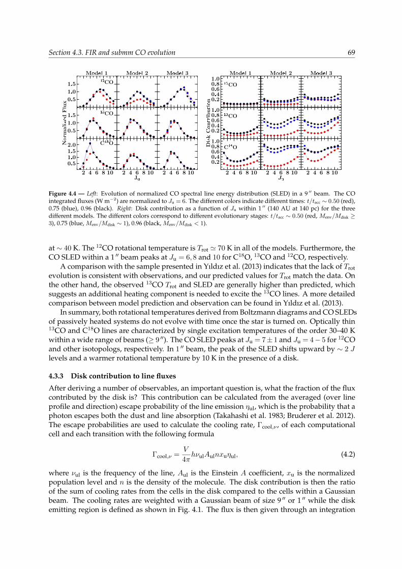
Section 4.3. FIR and submm CO evolution 69
Figure 4.4 — Left: Evolution of normalized CO spectral line energy distribution (SLED) in a 9 ′′ beam. The COintegrated fluxes (W m−2) are normalized to Ju = 6. The different colors indicate different times: t/tacc ∼ 0.50 (red),0.75 (blue), 0.96 (black). Right: Disk contribution as a function of Ju within 1 ′′ (140 AU at 140 pc) for the threedifferent models. The different colors correspond to different evolutionary stages: t/tacc ∼ 0.50 (red, Menv/Mdisk ≥3), 0.75 (blue, Menv/Mdisk ∼ 1), 0.96 (black, Menv/Mdisk < 1).
at ∼ 40 K. The 12CO rotational temperature is Trot ' 70 K in all of the models. Furthermore, theCO SLED within a 1 ′′ beam peaks at Ju = 6,8 and 10 for C18O, 13CO and 12CO, respectively.
A comparison with the sample presented in Yıldız et al. (2013) indicates that the lack of Trotevolution is consistent with observations, and our predicted values for Trot match the data. Onthe other hand, the observed 13CO Trot and SLED are generally higher than predicted, whichsuggests an additional heating component is needed to excite the 13CO lines. A more detailedcomparison between model prediction and observation can be found in Yıldız et al. (2013).
In summary, both rotational temperatures derived from Boltzmann diagrams and CO SLEDsof passively heated systems do not evolve with time once the star is turned on. Optically thin13CO and C18O lines are characterized by single excitation temperatures of the order 30–40 Kwithin a wide range of beams (≥ 9 ′′). The CO SLED peaks at Ju = 7± 1 and Ju = 4− 5 for 12COand other isotopologs, respectively. In 1 ′′ beam, the peak of the SLED shifts upward by ∼ 2 Jlevels and a warmer rotational temperature by 10 K in the presence of a disk.
4.3.3 Disk contribution to line fluxes
After deriving a number of observables, an important question is, what the fraction of the fluxcontributed by the disk is? This contribution can be calculated from the averaged (over lineprofile and direction) escape probability of the line emission ηul, which is the probability that aphoton escapes both the dust and line absorption (Takahashi et al. 1983; Bruderer et al. 2012).The escape probabilities are used to calculate the cooling rate, Γcool,ν , of each computationalcell and each transition with the following formula
Γcool,ν =V
4πhνulAulnxuηul, (4.2)
where νul is the frequency of the line, Aul is the Einstein A coefficient, xu is the normalizedpopulation level and n is the density of the molecule. The disk contribution is then the ratioof the sum of cooling rates from the cells in the disk compared to the cells within a Gaussianbeam. The cooling rates are weighted with a Gaussian beam of size 9 ′′ or 1 ′′ while the diskemitting region is defined as shown in Fig. 4.1. The flux is then given through an integration
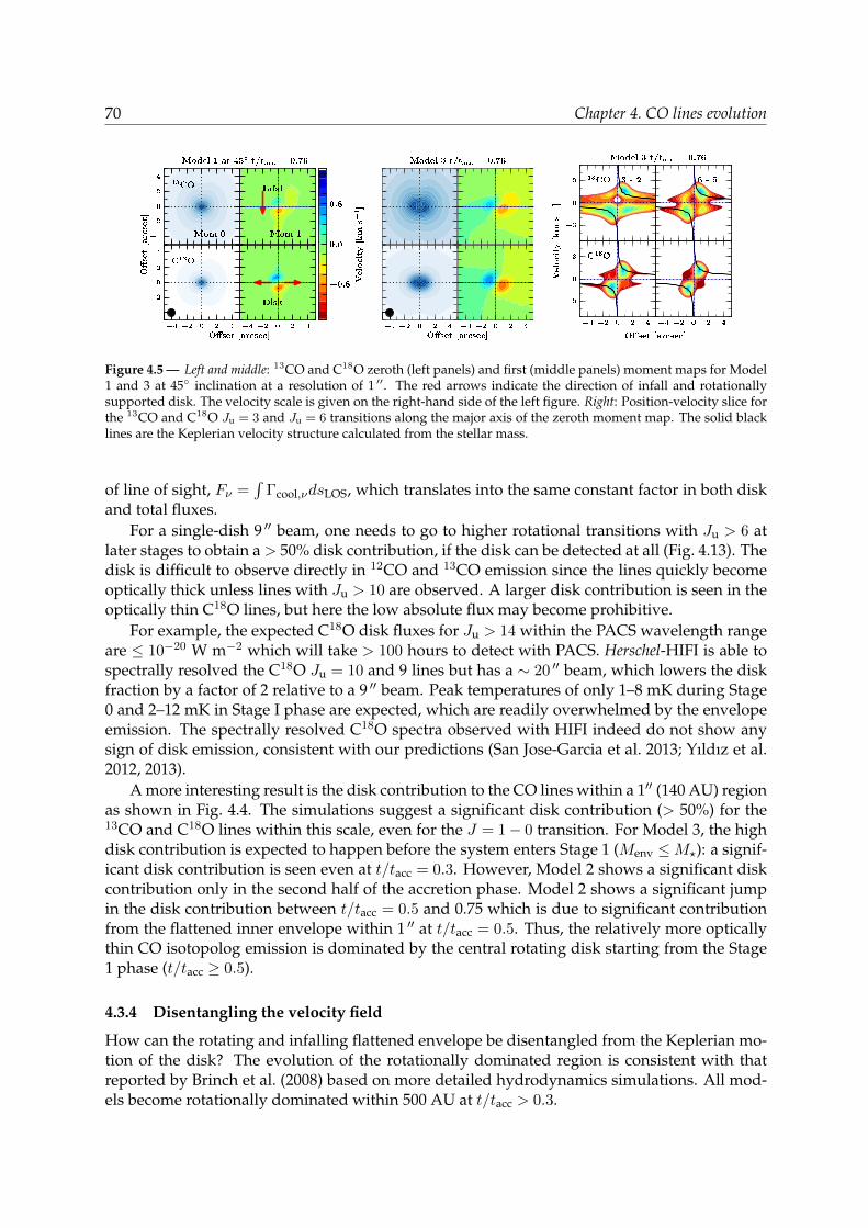
70 Chapter 4. CO lines evolution
Figure 4.5 — Left and middle: 13CO and C18O zeroth (left panels) and first (middle panels) moment maps for Model1 and 3 at 45 inclination at a resolution of 1 ′′. The red arrows indicate the direction of infall and rotationallysupported disk. The velocity scale is given on the right-hand side of the left figure. Right: Position-velocity slice forthe 13CO and C18O Ju = 3 and Ju = 6 transitions along the major axis of the zeroth moment map. The solid blacklines are the Keplerian velocity structure calculated from the stellar mass.
of line of sight, Fν =∫
Γcool,νdsLOS, which translates into the same constant factor in both diskand total fluxes.
For a single-dish 9 ′′ beam, one needs to go to higher rotational transitions with Ju > 6 atlater stages to obtain a > 50% disk contribution, if the disk can be detected at all (Fig. 4.13). Thedisk is difficult to observe directly in 12CO and 13CO emission since the lines quickly becomeoptically thick unless lines with Ju > 10 are observed. A larger disk contribution is seen in theoptically thin C18O lines, but here the low absolute flux may become prohibitive.
For example, the expected C18O disk fluxes for Ju > 14 within the PACS wavelength rangeare ≤ 10−20 W m−2 which will take > 100 hours to detect with PACS. Herschel-HIFI is able tospectrally resolved the C18O Ju = 10 and 9 lines but has a ∼ 20 ′′ beam, which lowers the diskfraction by a factor of 2 relative to a 9 ′′ beam. Peak temperatures of only 1–8 mK during Stage0 and 2–12 mK in Stage I phase are expected, which are readily overwhelmed by the envelopeemission. The spectrally resolved C18O spectra observed with HIFI indeed do not show anysign of disk emission, consistent with our predictions (San Jose-Garcia et al. 2013; Yıldız et al.2012, 2013).
A more interesting result is the disk contribution to the CO lines within a 1′′ (140 AU) regionas shown in Fig. 4.4. The simulations suggest a significant disk contribution (> 50%) for the13CO and C18O lines within this scale, even for the J = 1− 0 transition. For Model 3, the highdisk contribution is expected to happen before the system enters Stage 1 (Menv ≤M?): a signif-icant disk contribution is seen even at t/tacc = 0.3. However, Model 2 shows a significant diskcontribution only in the second half of the accretion phase. Model 2 shows a significant jumpin the disk contribution between t/tacc = 0.5 and 0.75 which is due to significant contributionfrom the flattened inner envelope within 1 ′′ at t/tacc = 0.5. Thus, the relatively more opticallythin CO isotopolog emission is dominated by the central rotating disk starting from the Stage1 phase (t/tacc ≥ 0.5).
4.3.4 Disentangling the velocity field
How can the rotating and infalling flattened envelope be disentangled from the Keplerian mo-tion of the disk? The evolution of the rotationally dominated region is consistent with thatreported by Brinch et al. (2008) based on more detailed hydrodynamics simulations. All mod-els become rotationally dominated within 500 AU at t/tacc > 0.3.

Section 4.3. FIR and submm CO evolution 71
Figure 4.6 — Velocity as function of distance of the peak intensity position from the protostar, as measured in eachchannel map and for the same transitions as in Fig. 4.5. The red and blue colors represent the red- and blue-shiftedcomponents. The solid black line indicates the expected Keplerian structure from the stellar mass in the model,where as the dashed lines indicate the v ∝ R−1 relation as a comparison.
The presence of an embedded disk can be inferred from the presence of elongated 13CO andC18O integrated intensity maps (moment 0 of Fig. 4.5) coupled with the moment 1 map. In thepresence of a stable disk, the zeroth moment map is elongated perpendicular to the outflowaxis with a double peaked structure. This feature is not seen in Model 1 (Fig. 4.5 left) sincethe disk is much smaller than the 1 ′′ beam. In the case of Model 3, the relatively massive diskexhibits a double peaked zeroth moment map which is perpendicular to the outflow direction.
A velocity gradient is seen in the moment 1 maps for both Models 1 and 3. With the highresolution of the modeled spectra, it is possible to differentiate between the disk and envelope(Hogerheijde 2001). The presence of a velocity gradient along the major axis of the elongation inthe moment 1 map is a clear sign of a stable embedded disk in the case of Model 3. In addition,from the analysis in Sect. 4.3.3, we can also attribute the bulk of optically thin emission inModel 3 to the disk. Meanwhile, the infalling rotating envelope contribution can be detectedthrough the fact that the moment 1 map is not perfectly aligned but skewed. On the otherhand, a velocity gradient without the presence of elongation in the zeroth moment map suchas in Model 1 (Fig. 4.5) indicates an infalling envelope.
Position-velocity (PV) diagrams provide another way to study the velocity structure. Fig-ure 4.5 shows PV slices following the direction of the major axis of the disk (PA = 90) in theintegrated intensity map in the 3–2 and 6–5 lines. A simple way to analyze PV diagrams isto separate the diagram into four quadrants and examine which quadrants have considerableemission. An infall dominated PV diagram without rotation is symmetric about the velocityaxis with all four quadrants filled (Ohashi et al. 1997b). The presence of rotation breaks thesymmetry in the PV diagram and causes the peak positions to be off-centered. As found previ-ously in hydrodynamical simulations by Brinch et al. (2008), infall dominates the PV diagramsat early times while rotation dominates the later times. These features have been observed to-ward low-mass YSOs which suggests that generally the infalling rotating envelope dominatesthe PV diagrams (eg. Sargent & Beckwith 1987; Hayashi et al. 1993; Saito et al. 1996; Ohashiet al. 1997b; Hogerheijde 2001).
Focusing on Model 3 at t/tacc = 0.76 (near the end of Stage I) as shown in Fig. 4.5, the C18OPV diagrams show a clearer pure rotation dominated structure than the 13CO lines. They canthus be used to constrain the stellar mass as long as the inclination is known. Also, the higher-J
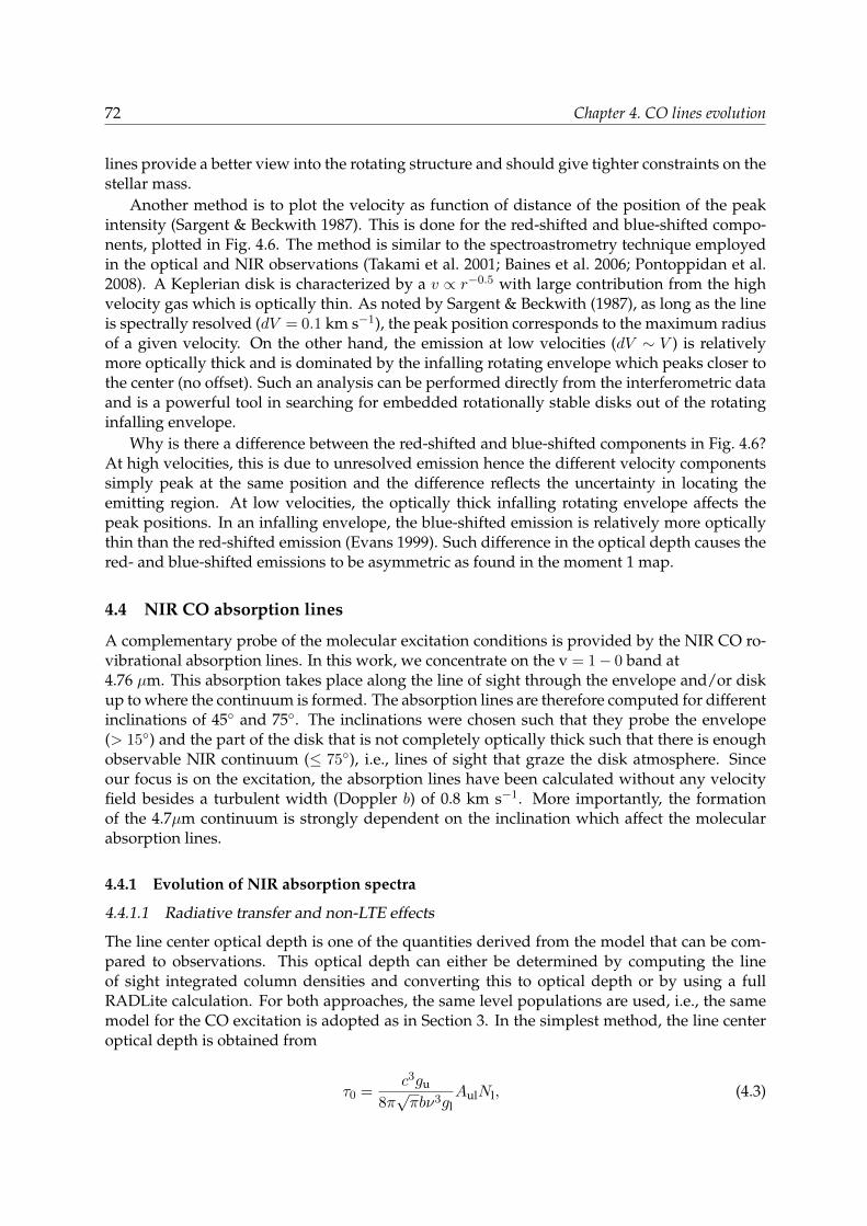
72 Chapter 4. CO lines evolution
lines provide a better view into the rotating structure and should give tighter constraints on thestellar mass.
Another method is to plot the velocity as function of distance of the position of the peakintensity (Sargent & Beckwith 1987). This is done for the red-shifted and blue-shifted compo-nents, plotted in Fig. 4.6. The method is similar to the spectroastrometry technique employedin the optical and NIR observations (Takami et al. 2001; Baines et al. 2006; Pontoppidan et al.2008). A Keplerian disk is characterized by a v ∝ r−0.5 with large contribution from the highvelocity gas which is optically thin. As noted by Sargent & Beckwith (1987), as long as the lineis spectrally resolved (dV = 0.1 km s−1), the peak position corresponds to the maximum radiusof a given velocity. On the other hand, the emission at low velocities (dV ∼ V ) is relativelymore optically thick and is dominated by the infalling rotating envelope which peaks closer tothe center (no offset). Such an analysis can be performed directly from the interferometric dataand is a powerful tool in searching for embedded rotationally stable disks out of the rotatinginfalling envelope.
Why is there a difference between the red-shifted and blue-shifted components in Fig. 4.6?At high velocities, this is due to unresolved emission hence the different velocity componentssimply peak at the same position and the difference reflects the uncertainty in locating theemitting region. At low velocities, the optically thick infalling rotating envelope affects thepeak positions. In an infalling envelope, the blue-shifted emission is relatively more opticallythin than the red-shifted emission (Evans 1999). Such difference in the optical depth causes thered- and blue-shifted emissions to be asymmetric as found in the moment 1 map.
4.4 NIR CO absorption lines
A complementary probe of the molecular excitation conditions is provided by the NIR CO ro-vibrational absorption lines. In this work, we concentrate on the v = 1− 0 band at4.76 µm. This absorption takes place along the line of sight through the envelope and/or diskup to where the continuum is formed. The absorption lines are therefore computed for differentinclinations of 45 and 75. The inclinations were chosen such that they probe the envelope(> 15) and the part of the disk that is not completely optically thick such that there is enoughobservable NIR continuum (≤ 75), i.e., lines of sight that graze the disk atmosphere. Sinceour focus is on the excitation, the absorption lines have been calculated without any velocityfield besides a turbulent width (Doppler b) of 0.8 km s−1. More importantly, the formationof the 4.7µm continuum is strongly dependent on the inclination which affect the molecularabsorption lines.
4.4.1 Evolution of NIR absorption spectra
4.4.1.1 Radiative transfer and non-LTE effects
The line center optical depth is one of the quantities derived from the model that can be com-pared to observations. This optical depth can either be determined by computing the lineof sight integrated column densities and converting this to optical depth or by using a fullRADLite calculation. For both approaches, the same level populations are used, i.e., the samemodel for the CO excitation is adopted as in Section 3. In the simplest method, the line centeroptical depth is obtained from
τ0 =c3gu
8π√πbν3gl
AulNl, (4.3)

Section 4.4. NIR CO absorption lines 73
Figure 4.7 — Evolution of the 12CO (red), 13CO (blue) and C18O (black) absorption lines for Model 1 at i= 45. Theevolution of the absorption lines for Model 2 is shown at the bottom panel. The lower rotational levels are indicatedon top of the first spectrum. All of the 13CO lines are multiplied by 5 and C18O lines by 25.
where ν is the line frequency and Nl is the lower level column density along the line of sight.The main difference between the methods is that RADLite solves the radiative transfer equa-tion along the line of sight and thus accounts for continuum and line optical depth effects andscattered continuum photons, while such effects are not considered in the column density ap-proach. In addition, RADLite accounts for the continuum formation, while a ray through thecenter does not. Thus, the two methods effectively compare the total mass present along a rayand the observed mass as probed by the line optical depth returned by RADLite. The opticaldepth is extracted from the RADLite spectra using the line-to-continuum ratio at the line center.
As discussed and illustrated extensively in Appendix 4.C.1, the two approaches can givevery different results, especially for the higher J lines for which the line optical depths candiffer by more than an order of magnitude. The main reason is illustrated in Fig. 4.16, whichshows the region where the NIR continuum arises. For small inclinations, the continuum isessentially point-like, but for higher inclinations larger radii contribute significantly and thecontinuum is no longer a point source. Thus, for high inclinations, the high-J lines start ab-sorbing off-center, away from warm gas in the inner few AU that are included in the columnmethod. The location of the continuum is typically at >10 AU at i = 75 which results in twoto three orders of magnitude difference in total column density. For the case of i ∼ 45, theresult depends on the physical structure in the inner few AU but the absorption can miss thewarm high density region close to the midplane of the disk where most of the J ≥ 10 is located(Fig. 4.15).
Figure 4.17 also compare LTE and non-LTE spectra. Consistent with Section 3, significantdifferences are found for the higher pure rotational levels which are subthermally excited.However, the radiative transfer effect is generally more important than the non-LTE effectsfor viewing angles through the disk/inner envelope surface.
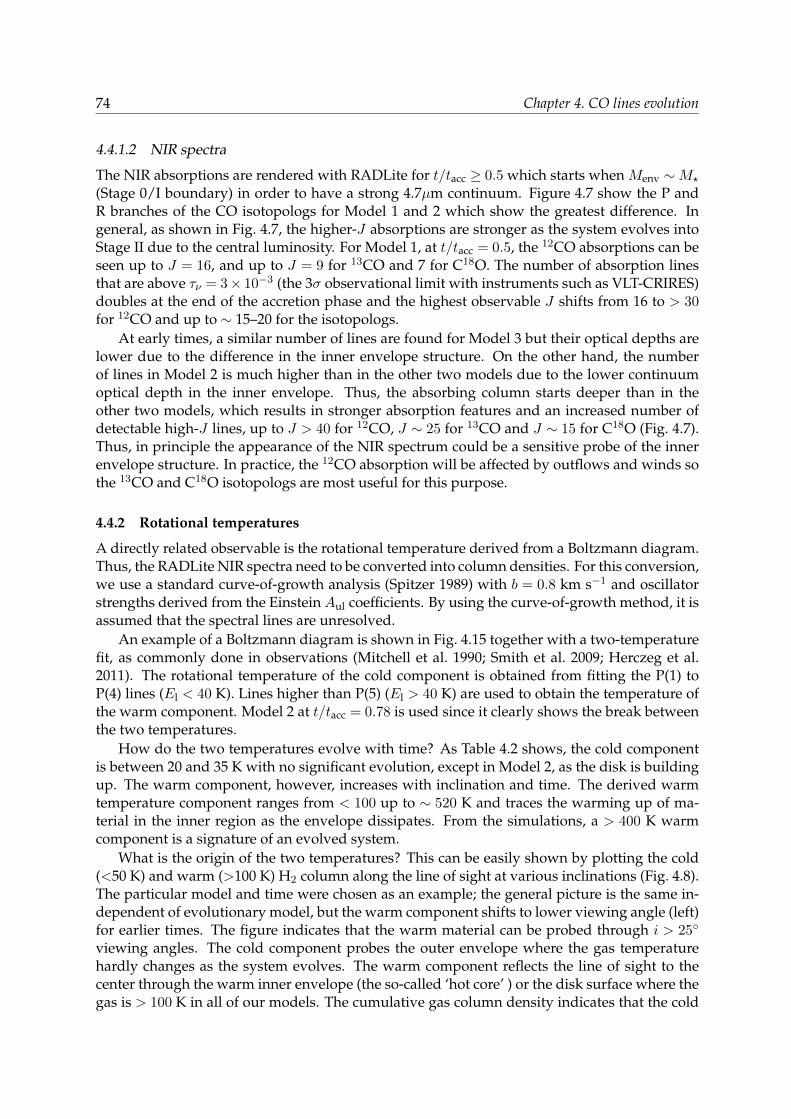
74 Chapter 4. CO lines evolution
4.4.1.2 NIR spectra
The NIR absorptions are rendered with RADLite for t/tacc ≥ 0.5 which starts when Menv ∼M?
(Stage 0/I boundary) in order to have a strong 4.7µm continuum. Figure 4.7 show the P andR branches of the CO isotopologs for Model 1 and 2 which show the greatest difference. Ingeneral, as shown in Fig. 4.7, the higher-J absorptions are stronger as the system evolves intoStage II due to the central luminosity. For Model 1, at t/tacc = 0.5, the 12CO absorptions can beseen up to J = 16, and up to J = 9 for 13CO and 7 for C18O. The number of absorption linesthat are above τν = 3× 10⁻³ (the 3σ observational limit with instruments such as VLT-CRIRES)doubles at the end of the accretion phase and the highest observable J shifts from 16 to > 30for 12CO and up to ∼ 15–20 for the isotopologs.
At early times, a similar number of lines are found for Model 3 but their optical depths arelower due to the difference in the inner envelope structure. On the other hand, the numberof lines in Model 2 is much higher than in the other two models due to the lower continuumoptical depth in the inner envelope. Thus, the absorbing column starts deeper than in theother two models, which results in stronger absorption features and an increased number ofdetectable high-J lines, up to J > 40 for 12CO, J ∼ 25 for 13CO and J ∼ 15 for C18O (Fig. 4.7).Thus, in principle the appearance of the NIR spectrum could be a sensitive probe of the innerenvelope structure. In practice, the 12CO absorption will be affected by outflows and winds sothe 13CO and C18O isotopologs are most useful for this purpose.
4.4.2 Rotational temperatures
A directly related observable is the rotational temperature derived from a Boltzmann diagram.Thus, the RADLite NIR spectra need to be converted into column densities. For this conversion,we use a standard curve-of-growth analysis (Spitzer 1989) with b = 0.8 km s−1 and oscillatorstrengths derived from the Einstein Aul coefficients. By using the curve-of-growth method, it isassumed that the spectral lines are unresolved.
An example of a Boltzmann diagram is shown in Fig. 4.15 together with a two-temperaturefit, as commonly done in observations (Mitchell et al. 1990; Smith et al. 2009; Herczeg et al.2011). The rotational temperature of the cold component is obtained from fitting the P(1) toP(4) lines (El < 40 K). Lines higher than P(5) (El > 40 K) are used to obtain the temperature ofthe warm component. Model 2 at t/tacc = 0.78 is used since it clearly shows the break betweenthe two temperatures.
How do the two temperatures evolve with time? As Table 4.2 shows, the cold componentis between 20 and 35 K with no significant evolution, except in Model 2, as the disk is buildingup. The warm component, however, increases with inclination and time. The derived warmtemperature component ranges from < 100 up to ∼ 520 K and traces the warming up of ma-terial in the inner region as the envelope dissipates. From the simulations, a > 400 K warmcomponent is a signature of an evolved system.
What is the origin of the two temperatures? This can be easily shown by plotting the cold(<50 K) and warm (>100 K) H2 column along the line of sight at various inclinations (Fig. 4.8).The particular model and time were chosen as an example; the general picture is the same in-dependent of evolutionary model, but the warm component shifts to lower viewing angle (left)for earlier times. The figure indicates that the warm material can be probed through i > 25
viewing angles. The cold component probes the outer envelope where the gas temperaturehardly changes as the system evolves. The warm component reflects the line of sight to thecenter through the warm inner envelope (the so-called ‘hot core’ ) or the disk surface where thegas is > 100 K in all of our models. The cumulative gas column density indicates that the cold

Section 4.5. Discussion 75
Table 4.2 — NIR rotational temperatures derived from τ0 > 10−3 lines for i = 45 and 75.
12CO 13CO C18Ot/tacc i Tcold Twarm Tcold Twarm Tcold Twarm
[] [K] [K] [K] [K] [K] [K]Model 1
0.50 45 21± 9 80± 9 18± 11 49± 18 19± 13 ...75 20± 9 66± 8 17± 10 44± 10 18± 10 ...
0.76 45 26± 10 142± 21 19± 11 72± 20 19± 14 ...75 25± 12 260± 67 25± 12 273± 69 19± 13 ...
0.96 45 28± 10 201± 36 28± 13 207± 46 21± 16 ...75 25± 10 271± 61 25± 13 301± 80 20± 13 ...
Model 20.50 45 34± 20 245± 61 34± 25 253± 61 29± 23 183± 51
75 31± 20 293± 85 31± 20 302± 86 27± 19 209± 670.78 45 31± 20 327± 100 31± 20 340± 110 28± 19 264± 89
75 20± 11 489± 210 19± 11 481± 192 18± 11 423± 2300.94 45 28± 18 402± 156 28± 18 410± 152 26± 17 333± 139
75 18± 11 544± 255 17± 10 527± 223 17± 10 495± 308
Model 30.50 45 21± 6 193± 37 16± 8 42± 21 19± 9 ...
75 16± 7 37± 7 16± 10 ... 16± 11 ...0.76 45 23± 9 287± 80 22± 9 304± 85 17± 11 ...
75 22± 8 289± 81 21± 8 302± 83 17± 10 ...0.96 45 22± 9 366± 128 21± 8 381± 129 17± 10 ...
75 18± 8 361± 121 18± 7 371± 119 16± 9 ...
material is mostly absorbed at R > 100 AU while the warmer gas component is probing theinner few AU (i > 60) up to ∼20 AU (i ∼ 45). The excitation temperature of the warm com-ponent reflects the density structure in the inner few AU. With the lower densities and warmertemperatures in Model 2, which decreases the effective continuum optical depth, higher warmtemperatures can be observed as the absorption probes deeper to smaller radii than the othertwo models.
4.5 Discussion
We have presented the evolution of CO molecular lines based on the standard picture of aprestellar core collapsing to form a star and 2D circumstellar disk. The main aim of this workis to study the evolution of observables that are derived from the spectra such as rotationaltemperatures, line profiles, and velocity fields. Specifically, signatures of disk formation duringthe embedded stage that can be obtained with the most commonly used molecule, CO, areinvestigated.
4.5.1 Detecting disk signatures in the embedded phase
How can one determine whether disks have formed in the earliest Stage 0? As discussed inSection 4.3.3, it is difficult to isolate an embedded disk component in single-dish observations.The disk contribution to the observed flux within > 9 ′′ beams is only significant (>60%) for

76 Chapter 4. CO lines evolution
Figure 4.8 — Integrated gas column density along the different viewing angles for Model 2. The red and blues linesindicate the warm (T > 100 K) and cold gas (T < 50 K), respectively. The approximate continuum optical depths,τc = 1 and 10, are also shown to indicate the amount material that is missed by properly solving the radiativetransfer equation.
the 13CO and C18O Ju > 9 lines at t/tacc > 0.75. However, the absolute fluxes are too low to bedetected. Thus, spatially resolved observations at sub-arcsec scale are needed.
What are the signatures of an embedded rotationally supported disk on subarcsecond scales?We have analyzed some of the simulated images during the Stage 0 phase at a resolution of 0.1 ′′
as can readily be observed with ALMA. Figure 4.9 shows the C18O 3–2 moment-one map dur-ing the Stage 0 phase of Model 1 with a disk extending up to 20 AU at a resolution of 1, 0.3and 0.1 ′′. Velocity gradients are present in all of the moment-one maps although it is weakerwithin a 1 ′′ beam. The right panel of the figure shows the spectroastrometry (Fig. 4.6) withinthe different resolutions. The velocity gradient within a 0.5–1 ′′ beam exhibits a v ∝ R−1 rela-tion since the inner envelope dominates the emission. Within the smaller beams, the velocitygradient is resolved into two components: v ∝ R−1 (blue dashed line) due to envelope andv ∝ R−0.5 (black dashed line) due to the stable disk. A v ∝ R−0.5 can be seen when the disk ismarginally resolved, however, the derived stellar mass is far below the real stellar mass. It isvery important that the disk is fully resolved in order to derive the stellar mass. With the C18Olines, a resolved embedded disk in Stage 0 would have the following features:
• Elongated moment-zero map.• A transition between an infalling envelope to a rotating disk: a skewed moment-one map.• The Keplerian structure exhibits a clear v ∝R−0.5 (Fig. 4.6 and bottom of Fig. 4.9 ) velocity
gradient perpendicular to the outflow.

Section 4.5. Discussion 77
Figure 4.9 — C18O 3–2 moment-one (left) and spectroastrometry (right) for Model 1 at the end of Stage 0 convolvedto a 1 ′′ (top), 0.3 ′′ (middle) and 0.1 ′′ (bottom) as shown by the solid circle. The Keplerian structure at this stageextends up to 20 AU (0.14 ′′ radius). The black dashed line in the right panel shows the v ∝ R−0.5 and the bluedashed line indicates the v ∝ R−1 relation.
It is possible to search for rotationally supported disks in Stage 0 sources with characteristicsof Model 1 with the full ALMA array in less than 30 minutes for the C18O 2–1 transition or upto 4 hours for the 6–5 transition. For Models 2 and 3, the disks have grown up to ∼ 50 AU nearthe end of Stage 0 and up to twice more massive, thus it will take less than 2 hours to observethem with ALMA in the 6–5 transition and less than 30 minutes in the 2–1 and 3–2 transitions.Therefore, ALMA will allow us, for the first time, to test whether rotationally supported diskshave grown beyond 10 AU by the end of the Stage 0 phase.
The question of when rotationally supported disks form is crucial to the physical and chem-ical evolution of accretion disks. In our evolutionary models, the disks have radii up to 50 AUat the end of Stage 0 phase and can be as small as 20 AU. Dapp & Basu (2010) and Dapp et al.(2012) numerically showed that disks do not grow beyond 10 AU during the Stage 0 phase inthe presence of magnetic fields due to the magnetic breaking problem (see also Li et al. 2011;Joos et al. 2012). This is consistent with the lack of observed rotationally supported disks to-ward Stage 0 objects so far (Brinch et al. 2009; Maury et al. 2010). On the other hand, there is agrowing body of observational evidence for rotating disks in Stage I YSOs (Brinch et al. 2007b;Lommen et al. 2008; Jørgensen et al. 2009; Takakuwa et al. 2012). The size of the rotationallysupported disk depends on the initial parameters of the collapsing envelope. In our models,the sizes of Models 2 and 3 are consistent with the observed Keplerian velocity structure inStage I sources (Jørgensen et al. 2009).
An additional caveat is that our models lead to a Keplerian disk with a flattened inner en-velope on similar scales as the stable disk. Hydrodynamical simulations, on the other hand,show a stable disk embedded in a much larger rotating flattened structure and with more tur-bulent structure (Brinch et al. 2008; Kratter et al. 2010). Furthermore, the 3D simulations byHarsono et al. (2011) suggest that 50% of the embedded disk is sub-Keplerian due to interac-tion with the envelope. The predicted moment 1 maps and spectroastrometry with the current
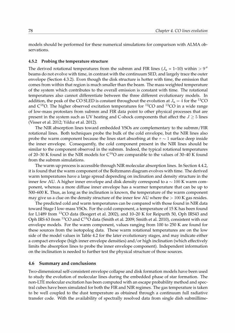
78 Chapter 4. CO lines evolution
models should be performed for these numerical simulations for comparison with ALMA ob-servations.
4.5.2 Probing the temperature structure
The derived rotational temperatures from the submm and FIR lines (Ju = 1–10) within > 9 ′′
beams do not evolve with time, in contrast with the continuum SED, and largely trace the outerenvelope (Section 4.3.2). Even though the disk structure is hotter with time, the emission thatcomes from within that region is much smaller than the beam. The mass weighted temperatureof the system which contributes to the overall emission is constant with time. The rotationaltemperatures also cannot differentiate between the three different evolutionary models. Inaddition, the peak of the CO SLED is constant throughout the evolution at Ju = 4 for the 13COand C18O. The higher observed excitation temperatures for 12CO and 13CO in a wide rangeof low-mass protostars from submm and FIR data point to other physical processes that arepresent in the system such as UV heating and C-shock components that affect the J ≥ 5 lines(Visser et al. 2012; Yıldız et al. 2012).
The NIR absorption lines toward embedded YSOs are complementary to the submm/FIRrotational lines. Both techniques probe the bulk of the cold envelope, but the NIR lines alsoprobe the warm component because the lines start absorbing at the τ ∼ 1 surface deep insidethe inner envelope. Consequently, the cold component present in the NIR lines should besimilar to the component observed in the submm. Indeed, the typical rotational temperaturesof 20–30 K found in the NIR models for C18O are comparable to the values of 30–40 K foundfrom the submm simulations.
The warm up process is accessible through NIR molecular absorption lines. In Section 4.4.2,it is found that the warm component of the Boltzmann diagram evolves with time. The derivedwarm temperatures have a large spread depending on inclination and density structure in theinner few AU. A higher inner envelope and disk density correspond to a ∼ 100 K warm com-ponent, whereas a more diffuse inner envelope has a warmer temperature that can be up to500–600 K. Thus, as long as the inclination is known, the temperature of the warm componentmay give us a clue on the density structure of the inner few AU where the > 100 K gas resides.
The predicted cold and warm temperatures can be compared with those found in NIR datatoward Stage I low-mass YSOs. For the cold component, a temperature of 15 K has been foundfor L1489 from 13CO data (Boogert et al. 2002), and 10–20 K for Reipurth 50, Oph IRS43 andOph IRS 63 from 13CO and C18O data (Smith et al. 2009; Smith et al. 2010), consistent with ourenvelope models. For the warm component, values ranging from 100 to 250 K are found forthese sources from the isotopolog data. These warm rotational temperatures are on the lowside of the model values in Table 4.2 for the later evolutionary stages, and may indicate eithera compact envelope (high inner envelope densities) and/or high inclination (which effectivelylimits the absorption lines to probe the inner envelope component). Independent informationon the inclination is needed to further test the physical structure of those sources.
4.6 Summary and conclusions
Two-dimensional self-consistent envelope collapse and disk formation models have been usedto study the evolution of molecular lines during the embedded phase of star formation. Thenon-LTE molecular excitation has been computed with an escape probability method and spec-tral cubes have been simulated for both the FIR and NIR regimes. The gas temperature is takento be well coupled to the dust temperature as obtained through a continuum full radiativetransfer code. With the availability of spectrally resolved data from single dish submillime-
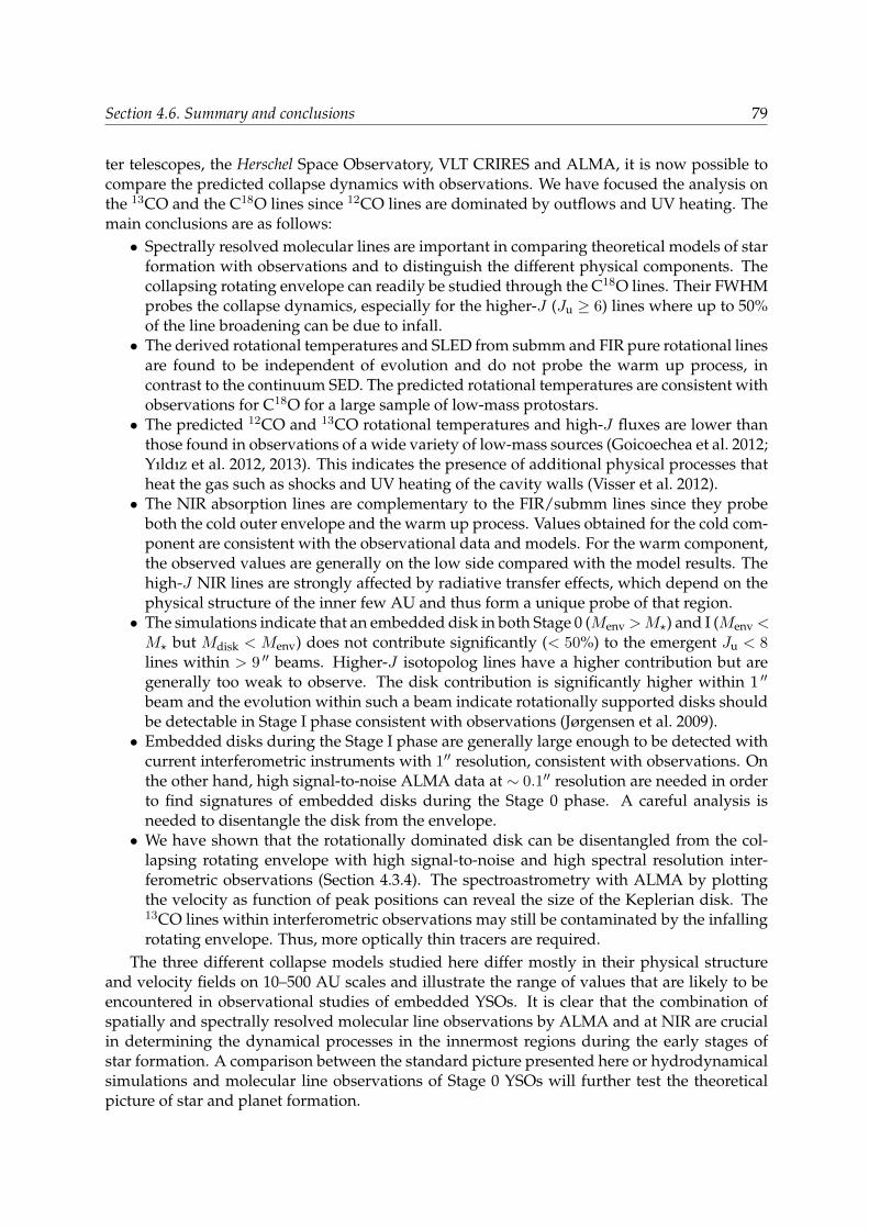
Section 4.6. Summary and conclusions 79
ter telescopes, the Herschel Space Observatory, VLT CRIRES and ALMA, it is now possible tocompare the predicted collapse dynamics with observations. We have focused the analysis onthe 13CO and the C18O lines since 12CO lines are dominated by outflows and UV heating. Themain conclusions are as follows:• Spectrally resolved molecular lines are important in comparing theoretical models of star
formation with observations and to distinguish the different physical components. Thecollapsing rotating envelope can readily be studied through the C18O lines. Their FWHMprobes the collapse dynamics, especially for the higher-J (Ju ≥ 6) lines where up to 50%of the line broadening can be due to infall.• The derived rotational temperatures and SLED from submm and FIR pure rotational lines
are found to be independent of evolution and do not probe the warm up process, incontrast to the continuum SED. The predicted rotational temperatures are consistent withobservations for C18O for a large sample of low-mass protostars.• The predicted 12CO and 13CO rotational temperatures and high-J fluxes are lower than
those found in observations of a wide variety of low-mass sources (Goicoechea et al. 2012;Yıldız et al. 2012, 2013). This indicates the presence of additional physical processes thatheat the gas such as shocks and UV heating of the cavity walls (Visser et al. 2012).• The NIR absorption lines are complementary to the FIR/submm lines since they probe
both the cold outer envelope and the warm up process. Values obtained for the cold com-ponent are consistent with the observational data and models. For the warm component,the observed values are generally on the low side compared with the model results. Thehigh-J NIR lines are strongly affected by radiative transfer effects, which depend on thephysical structure of the inner few AU and thus form a unique probe of that region.• The simulations indicate that an embedded disk in both Stage 0 (Menv >M?) and I (Menv <M? but Mdisk < Menv) does not contribute significantly (< 50%) to the emergent Ju < 8lines within > 9 ′′ beams. Higher-J isotopolog lines have a higher contribution but aregenerally too weak to observe. The disk contribution is significantly higher within 1 ′′
beam and the evolution within such a beam indicate rotationally supported disks shouldbe detectable in Stage I phase consistent with observations (Jørgensen et al. 2009).• Embedded disks during the Stage I phase are generally large enough to be detected with
current interferometric instruments with 1′′ resolution, consistent with observations. Onthe other hand, high signal-to-noise ALMA data at ∼ 0.1′′ resolution are needed in orderto find signatures of embedded disks during the Stage 0 phase. A careful analysis isneeded to disentangle the disk from the envelope.• We have shown that the rotationally dominated disk can be disentangled from the col-
lapsing rotating envelope with high signal-to-noise and high spectral resolution inter-ferometric observations (Section 4.3.4). The spectroastrometry with ALMA by plottingthe velocity as function of peak positions can reveal the size of the Keplerian disk. The13CO lines within interferometric observations may still be contaminated by the infallingrotating envelope. Thus, more optically thin tracers are required.
The three different collapse models studied here differ mostly in their physical structureand velocity fields on 10–500 AU scales and illustrate the range of values that are likely to beencountered in observational studies of embedded YSOs. It is clear that the combination ofspatially and spectrally resolved molecular line observations by ALMA and at NIR are crucialin determining the dynamical processes in the innermost regions during the early stages ofstar formation. A comparison between the standard picture presented here or hydrodynamicalsimulations and molecular line observations of Stage 0 YSOs will further test the theoreticalpicture of star and planet formation.

80 Chapter 4. CO lines evolution
1.0 km s−1
−1500 −500 0 500 1500R [AU]
−1000
−500
0
500
1000
1500
z[A
U]
t/tacc = 0.28
104
106
108
1010
n(H
2)[cm
−3]
Figure 4.10 — Gas density and velocity field for Model 3 at t/tacc = 0.13 and 0.28 within 1500 AU. The densitycontours start from log(n/cm−3) = 5.5 and increase by steps of 0.5 up to log(n/cm−3) = 9. There are vertical andradial motions in the disk, which are not captured in this figure.
Acknowledgements
We would like to thank Steve Doty for stimulating discussions on continuum and line radia-tive transfer and for allowing us to use his chemistry code. We are also grateful to Kees Dulle-mond for providing RADMC (and RADMC3D) and to Klaus Pontoppidan for RADLite. Wethank the anonymous referee for the constructive comments, which have improved this paper.This work is supported by the Netherlands Research School for Astronomy (NOVA) and bythe Space Research Organization Netherlands (SRON). Astrochemistry in Leiden is supportedby the Netherlands Research School for Astronomy (NOVA), by a Spinoza grant and grant614.001.008 from the Netherlands Organisation for Scientific Research (NWO), and by the Eu-ropean Community’s Seventh Framework Programme FP7/20072013 under grant agreement238258 (LASSIE).
4.A Two dimensional RT grid
The grid needs to resolve the steep density and velocity gradients at the boundaries betweenadjacent components as shown in Fig. 4.10. Improper gridding can lead to order-of-magnitudedifference in the high-J (J ≥ 6) line fluxes. The escape probability code begins with a set ofregularly spaced cells on a logarithmic grid to resolve both small and large scales. Any cellswhere the abundance or density at the corners differs by more than a factor of 5, or where thetemperature at the corners differs by more than a factor of 1.5, are split into smaller cells untilthe conditions across each cell are roughly constant. The full non-LTE excitation calculationtakes about five minutes for a typical number of cells of 15 000 (Stage I) – 25 000 (Stage 0).
Figure 4.11 presents an example of the gridding in our models. Such gridding is mostimportant for early time steps where the outflow cavity opening angle is small. The refiningensures that the non-LTE population calculation converges and high-J emission which comesfrom the inner region can escape.
4.B FIR and submm lines
Figure 4.12 shows the mass evolution of the evolutionary models which indicates the times atwhich the models enter various evolutionary stages. Figure 4.12 presents the C18O 9–8 linesfor the three different evolutionary models convolved to a 9 ′′ beam. Most of the line is emitted

Section 4.C. NIR molecular lines 81
from the inner envelope region. The line is generally broader in later stages due to a com-bination of thermal, turbulent width and velocity structure. However, the width of the linedepends on whether the emitting region is infall or rotation dominated. Figures 4.13 and 4.14shows the Ju =3, 6 and 9 line profiles for the different models and how they change withindifferent beams. The disk contribution to the observed lines within a 9 ′′ beam is presented inFig. 4.13 which is close to negligible for the low-J lines.
4.C NIR molecular lines
4.C.1 Inner disk
The formation of NIR continuum and the region where absorption happens depend on thephysical structure in the inner few AU as will discussed extensively in the next section. Fig-ure 4.15 shows the inner 5 AU structure of the three different models. In both Models 1 and3, the 104.5 cm−3 density contour extends up to the line of sight of 45 due to the presence ofcompact disk and massive disk, respectively. On the other hand, the density structure is flatterin Model 2. Thus, the NIR continuum emission is emitted through the high temperature region(mostly the red region in the temperature plot) and encounters more material along the line ofsight to an observer in Models 1 and 3. Consequently, the emission from the region close to themidplane of the disk will not contribute to the NIR continuum. Figure 4.8 presents an exampleof the radial contribution to the column density along a line of sight from the star. At viewingangles < 45, most of the warm material is located at 10–40 AU from the star along the lineof sight while most of the cold material is located > 50 AU. The inner disk and high densityregion (< 1 AU) is only accessible through i ≥ 75 in our models.
4.C.2 Radiative transfer effects
Section 4.4 discusses the RADLite results with respect to the predicted observables. In thissection, we present the comparison between RADLite and a simple calculation using the inte-grated column density (column method, equation 4.3) to examine the radiative transfer effectsin particular where the 4.7 µm continuum is formed and its affect on the simulated absorptionlines.
Figure 4.11 — Example of the gridding used in the Stage 0 phase to resolve the small extent of the outflow cavityand to resolve the density and velocity gradient from the disk midplane to the envelope. The color contours are thesame as in Fig. 4.10. The structure shown is for Model 1 at t/tacc = 0.13.
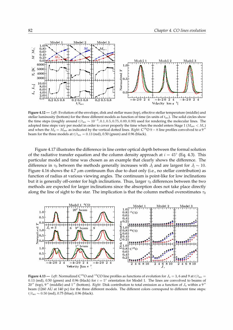
82 Chapter 4. CO lines evolution
Figure 4.12 — Left: Evolution of the envelope, disk and stellar mass (top), effective stellar temperature (middle) andstellar luminosity (bottom) for the three different models as function of time (in units of tacc). The solid circles showthe time steps (roughly around t/tacc ∼ 10−3,0.1,0.5,0.75,0.89,0.99) used for rendering the molecular lines. Theadopted time steps vary per model in order to cover properly the time when the model enters Stage 1 (Menv <M?)and when the Md = Menv as indicated by the vertical dotted lines. Right: C18O 9− 8 line profiles convolved to a 9 ′′
beam for the three models at t/tacc = 0.13 (red), 0.50 (green) and 0.96 (black).
Figure 4.17 illustrates the difference in line center optical depth between the formal solutionof the radiative transfer equation and the column density approach at i = 45 (Eq. 4.3). Thisparticular model and time was chosen as an example that clearly shows the difference. Thedifference in τ0 between the methods generally increases with Jl and are largest for Jl ∼ 10.Figure 4.16 shows the 4.7 µm continuum flux due to dust only (i.e., no stellar contribution) asfunction of radius at various viewing angles. The continuum is point-like for low inclinationsbut it is generally off-center for high inclinations. Thus, larger τ0 differences between the twomethods are expected for larger inclinations since the absorption does not take place directlyalong the line of sight to the star. The implication is that the column method overestimates τ0
Figure 4.13 — Left: Normalized C18O and 13CO line profiles as functions of evolution for Ju = 3, 6 and 9 at t/tacc =0.13 (red), 0.50 (green) and 0.96 (black) for i = 5 orientation for Model 1. The lines are convolved to beams of20 ′′ (top), 9 ′′ (middle) and 1 ′′ (bottom). Right: Disk contribution to total emission as a function of Ju within a 9 ′′
beam (1260 AU at 140 pc) for the three different models. The different colors correspond to different time steps:t/tacc ∼ 0.50 (red), 0.75 (blue), 0.96 (black).
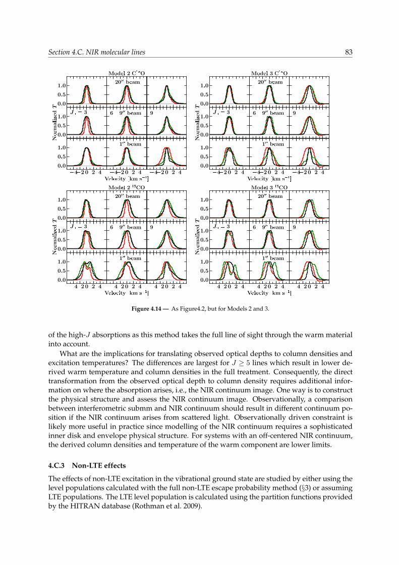
Section 4.C. NIR molecular lines 83
Figure 4.14 — As Figure4.2, but for Models 2 and 3.
of the high-J absorptions as this method takes the full line of sight through the warm materialinto account.
What are the implications for translating observed optical depths to column densities andexcitation temperatures? The differences are largest for J ≥ 5 lines which result in lower de-rived warm temperature and column densities in the full treatment. Consequently, the directtransformation from the observed optical depth to column density requires additional infor-mation on where the absorption arises, i.e., the NIR continuum image. One way is to constructthe physical structure and assess the NIR continuum image. Observationally, a comparisonbetween interferometric submm and NIR continuum should result in different continuum po-sition if the NIR continuum arises from scattered light. Observationally driven constraint islikely more useful in practice since modelling of the NIR continuum requires a sophisticatedinner disk and envelope physical structure. For systems with an off-centered NIR continuum,the derived column densities and temperature of the warm component are lower limits.
4.C.3 Non-LTE effects
The effects of non-LTE excitation in the vibrational ground state are studied by either using thelevel populations calculated with the full non-LTE escape probability method (§3) or assumingLTE populations. The LTE level population is calculated using the partition functions providedby the HITRAN database (Rothman et al. 2009).
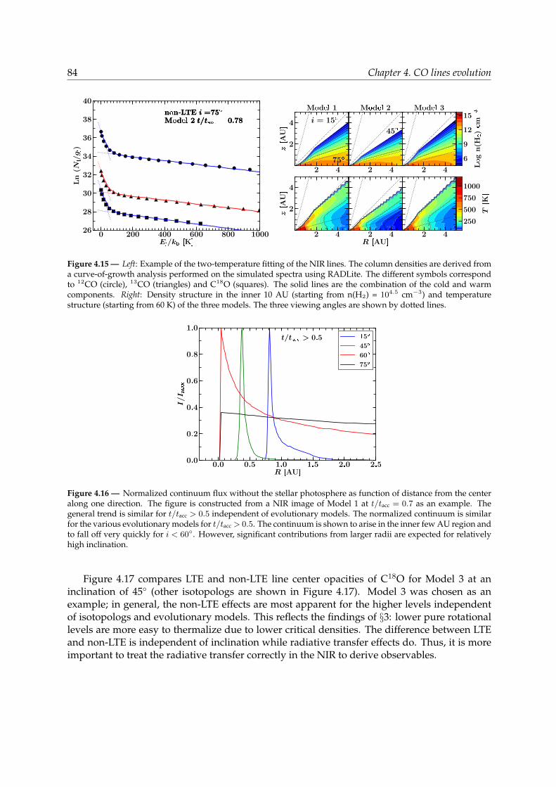
84 Chapter 4. CO lines evolution
Figure 4.15 — Left: Example of the two-temperature fitting of the NIR lines. The column densities are derived froma curve-of-growth analysis performed on the simulated spectra using RADLite. The different symbols correspondto 12CO (circle), 13CO (triangles) and C18O (squares). The solid lines are the combination of the cold and warmcomponents. Right: Density structure in the inner 10 AU (starting from n(H2) = 104.5 cm−3) and temperaturestructure (starting from 60 K) of the three models. The three viewing angles are shown by dotted lines.
Figure 4.16 — Normalized continuum flux without the stellar photosphere as function of distance from the centeralong one direction. The figure is constructed from a NIR image of Model 1 at t/tacc = 0.7 as an example. Thegeneral trend is similar for t/tacc > 0.5 independent of evolutionary models. The normalized continuum is similarfor the various evolutionary models for t/tacc > 0.5. The continuum is shown to arise in the inner few AU region andto fall off very quickly for i < 60. However, significant contributions from larger radii are expected for relativelyhigh inclination.
Figure 4.17 compares LTE and non-LTE line center opacities of C18O for Model 3 at aninclination of 45 (other isotopologs are shown in Figure 4.17). Model 3 was chosen as anexample; in general, the non-LTE effects are most apparent for the higher levels independentof isotopologs and evolutionary models. This reflects the findings of §3: lower pure rotationallevels are more easy to thermalize due to lower critical densities. The difference between LTEand non-LTE is independent of inclination while radiative transfer effects do. Thus, it is moreimportant to treat the radiative transfer correctly in the NIR to derive observables.
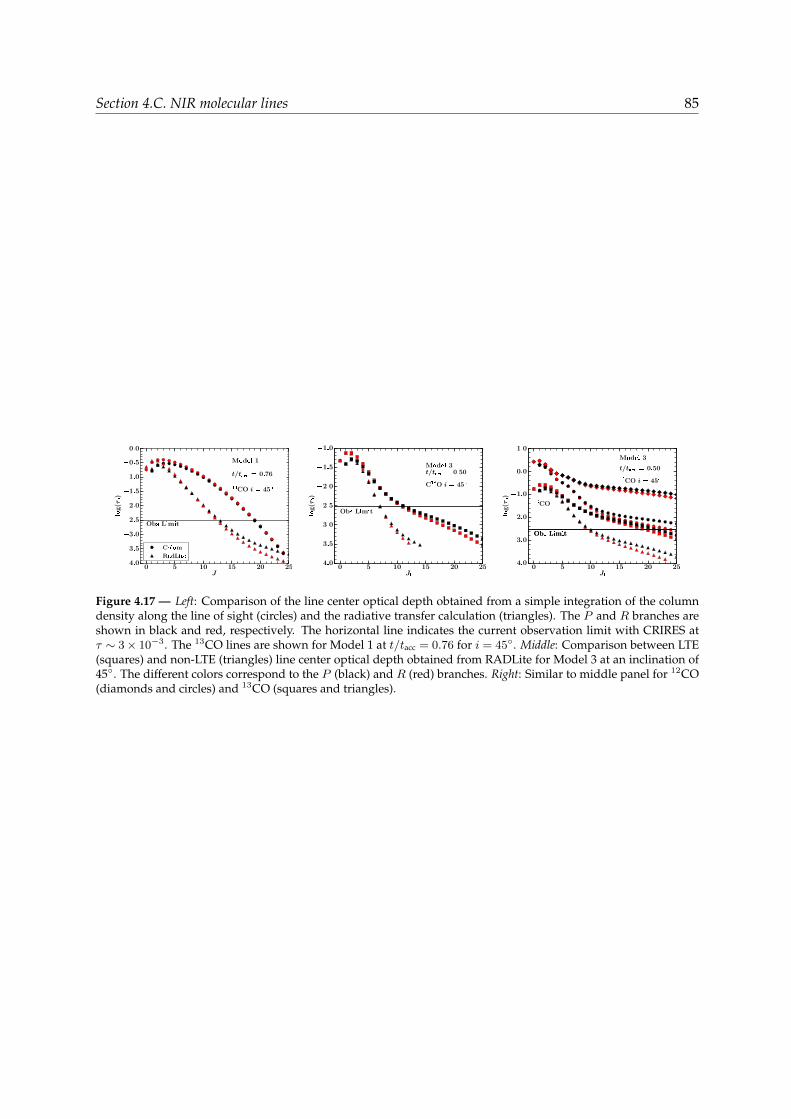
Section 4.C. NIR molecular lines 85
Figure 4.17 — Left: Comparison of the line center optical depth obtained from a simple integration of the columndensity along the line of sight (circles) and the radiative transfer calculation (triangles). The P and R branches areshown in black and red, respectively. The horizontal line indicates the current observation limit with CRIRES atτ ∼ 3× 10⁻³. The 13CO lines are shown for Model 1 at t/tacc = 0.76 for i = 45. Middle: Comparison between LTE(squares) and non-LTE (triangles) line center optical depth obtained from RADLite for Model 3 at an inclination of45. The different colors correspond to the P (black) and R (red) branches. Right: Similar to middle panel for 12CO(diamonds and circles) and 13CO (squares and triangles).


Chapter 5Rotationally-supported disks around
Class I sources in Taurus: diskformation constraints
Abstract. Context. Disks are observed around pre-main sequence stars, but how and when they formis still heavily debated. While disks around young stellar objects have been identified through thermaldust emission, spatially and spectrally resolved molecular line observations are needed to determinetheir nature. Only a handful of embedded rotationally supported disks have been identified to date.Aims. We identify and characterize rotationally supported disks near the end of the main accretion phaseof low-mass protostars by comparing their gas and dust structures.Methods. Subarcsecond observations of dust and gas toward four Class I low-mass young stellar objectsin Taurus are presented at significantly higher sensitivity than previous studies. The 13CO and C18O J =2–1 transitions at 220 GHz were observed with the Plateau de Bure Interferometer at a spatial resolutionof ≤0.8 ′′ (56 AU radius at 140 pc) and analyzed using uv-space position velocity diagrams to determinethe nature of their observed velocity gradient.Results. Rotationally supported disks (RSDs) are detected around 3 of the 4 Class I sources studied.The derived masses identify them as Stage I objects; i.e., their stellar mass is higher than their enve-lope and disk masses. The outer radii of the Keplerian disks toward our sample of Class I sources are≤ 100 AU. The lack of on-source C18O emission for TMR1 puts an upper limit of 50 AU on its size. Flat-tened structures at radii > 100 AU around these sources are dominated by infalling motion (υ ∝ r−1). Alarge-scale envelope model is required to estimate the basic parameters of the flattened structure fromspatially resolved continuum data. Similarities and differences between the gas and dust disk are dis-cussed. Combined with literature data, the sizes of the RSDs around Class I objects are best describedwith evolutionary models with an initial rotation of Ω = 10−14 Hz and slow sound speeds. Based on thecomparison of gas and dust disk masses, little CO is frozen out within 100 AU in these disks.Conclusions. Rotationally supported disks with radii up to 100 AU are present around Class I embeddedobjects. Larger surveys of both Class 0 and I objects are needed to determine whether most disks formlate or early in the embedded phase.
D. Harsono, J. K. Jørgensen, E. F. van Dishoeck, M. R. Hogerheijde, S. Bruderer, M. V. Persson,J. C. Mottram
A&A, 562 , A77 (2014)
5.1 Introduction
ROTATIONALLY supported accretion disks (RSDs) are thought to form very early during thestar formation process (see, e.g., Bodenheimer 1995). The RSD transports a significant frac-
tion of the mass from the envelope onto the young star and eventually evolves into a proto-planetary disk as the envelope dissipates. The presence of an RSD affects not only the physicalstructure of the system but also the chemical content and evolution as it promotes the pro-duction of more complex chemical species by providing a longer lifespan at mildly elevatedtemperature (Aikawa et al. 2008; Visser et al. 2011; Aikawa et al. 2011). Although the standard
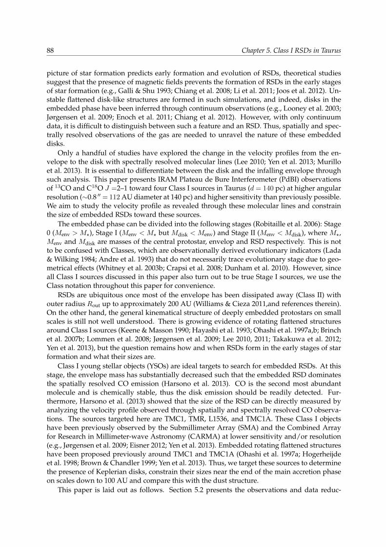
88 Chapter 5. Class I RSDs in Taurus
picture of star formation predicts early formation and evolution of RSDs, theoretical studiessuggest that the presence of magnetic fields prevents the formation of RSDs in the early stagesof star formation (e.g., Galli & Shu 1993; Chiang et al. 2008; Li et al. 2011; Joos et al. 2012). Un-stable flattened disk-like structures are formed in such simulations, and indeed, disks in theembedded phase have been inferred through continuum observations (e.g., Looney et al. 2003;Jørgensen et al. 2009; Enoch et al. 2011; Chiang et al. 2012). However, with only continuumdata, it is difficult to distinguish between such a feature and an RSD. Thus, spatially and spec-trally resolved observations of the gas are needed to unravel the nature of these embeddeddisks.
Only a handful of studies have explored the change in the velocity profiles from the en-velope to the disk with spectrally resolved molecular lines (Lee 2010; Yen et al. 2013; Murilloet al. 2013). It is essential to differentiate between the disk and the infalling envelope throughsuch analysis. This paper presents IRAM Plateau de Bure Interferometer (PdBI) observationsof 13CO and C18O J =2–1 toward four Class I sources in Taurus (d = 140 pc) at higher angularresolution (∼0.8 ′′ = 112 AU diameter at 140 pc) and higher sensitivity than previously possible.We aim to study the velocity profile as revealed through these molecular lines and constrainthe size of embedded RSDs toward these sources.
The embedded phase can be divided into the following stages (Robitaille et al. 2006): Stage0 (Menv > M?), Stage I (Menv < M? but Mdisk < Menv) and Stage II (Menv < Mdisk), where M?,Menv and Mdisk are masses of the central protostar, envelop and RSD respectively. This is notto be confused with Classes, which are observationally derived evolutionary indicators (Lada& Wilking 1984; Andre et al. 1993) that do not necessarily trace evolutionary stage due to geo-metrical effects (Whitney et al. 2003b; Crapsi et al. 2008; Dunham et al. 2010). However, sinceall Class I sources discussed in this paper also turn out to be true Stage I sources, we use theClass notation throughout this paper for convenience.
RSDs are ubiquitous once most of the envelope has been dissipated away (Class II) withouter radius Rout up to approximately 200 AU (Williams & Cieza 2011,and references therein).On the other hand, the general kinematical structure of deeply embedded protostars on smallscales is still not well understood. There is growing evidence of rotating flattened structuresaround Class I sources (Keene & Masson 1990; Hayashi et al. 1993; Ohashi et al. 1997a,b; Brinchet al. 2007b; Lommen et al. 2008; Jørgensen et al. 2009; Lee 2010, 2011; Takakuwa et al. 2012;Yen et al. 2013), but the question remains how and when RSDs form in the early stages of starformation and what their sizes are.
Class I young stellar objects (YSOs) are ideal targets to search for embedded RSDs. At thisstage, the envelope mass has substantially decreased such that the embedded RSD dominatesthe spatially resolved CO emission (Harsono et al. 2013). CO is the second most abundantmolecule and is chemically stable, thus the disk emission should be readily detected. Fur-thermore, Harsono et al. (2013) showed that the size of the RSD can be directly measured byanalyzing the velocity profile observed through spatially and spectrally resolved CO observa-tions. The sources targeted here are TMC1, TMR, L1536, and TMC1A. These Class I objectshave been previously observed by the Submillimeter Array (SMA) and the Combined Arrayfor Research in Millimeter-wave Astronomy (CARMA) at lower sensitivity and/or resolution(e.g., Jørgensen et al. 2009; Eisner 2012; Yen et al. 2013). Embedded rotating flattened structureshave been proposed previously around TMC1 and TMC1A (Ohashi et al. 1997a; Hogerheijdeet al. 1998; Brown & Chandler 1999; Yen et al. 2013). Thus, we target these sources to determinethe presence of Keplerian disks, constrain their sizes near the end of the main accretion phaseon scales down to 100 AU and compare this with the dust structure.
This paper is laid out as follows. Section 5.2 presents the observations and data reduc-
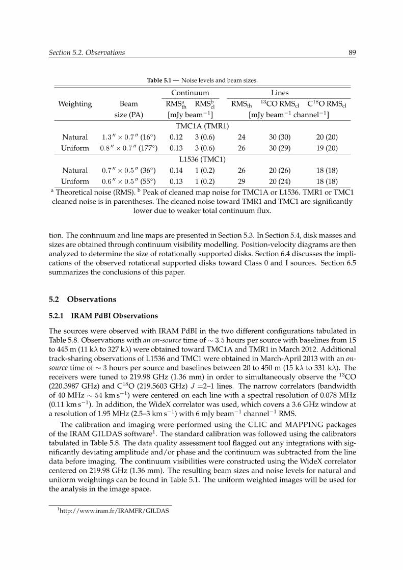
Section 5.2. Observations 89
Table 5.1 — Noise levels and beam sizes.
Continuum LinesWeighting Beam RMSa
th RMSbcl RMSth
13CO RMScl C18O RMScl
size (PA) [mJy beam−1] [mJy beam−1 channel−1]TMC1A (TMR1)
Natural 1.3 ′′ × 0.7 ′′ (16) 0.12 3 (0.6) 24 30 (30) 20 (20)Uniform 0.8 ′′ × 0.7 ′′ (177) 0.13 3 (0.6) 26 30 (29) 19 (20)
L1536 (TMC1)Natural 0.7 ′′ × 0.5 ′′ (36) 0.14 1 (0.2) 26 20 (26) 18 (18)Uniform 0.6 ′′ × 0.5 ′′ (55) 0.13 1 (0.2) 29 20 (24) 18 (18)
a Theoretical noise (RMS). b Peak of cleaned map noise for TMC1A or L1536. TMR1 or TMC1cleaned noise is in parentheses. The cleaned noise toward TMR1 and TMC1 are significantly
lower due to weaker total continuum flux.
tion. The continuum and line maps are presented in Section 5.3. In Section 5.4, disk masses andsizes are obtained through continuum visibility modelling. Position-velocity diagrams are thenanalyzed to determine the size of rotationally supported disks. Section 6.4 discusses the impli-cations of the observed rotational supported disks toward Class 0 and I sources. Section 6.5summarizes the conclusions of this paper.
5.2 Observations
5.2.1 IRAM PdBI Observations
The sources were observed with IRAM PdBI in the two different configurations tabulated inTable 5.8. Observations with an on-source time of ∼ 3.5 hours per source with baselines from 15to 445 m (11 kλ to 327 kλ) were obtained toward TMC1A and TMR1 in March 2012. Additionaltrack-sharing observations of L1536 and TMC1 were obtained in March-April 2013 with an on-source time of ∼ 3 hours per source and baselines between 20 to 450 m (15 kλ to 331 kλ). Thereceivers were tuned to 219.98 GHz (1.36 mm) in order to simultaneously observe the 13CO(220.3987 GHz) and C18O (219.5603 GHz) J =2–1 lines. The narrow correlators (bandwidthof 40 MHz ∼ 54 km s−1) were centered on each line with a spectral resolution of 0.078 MHz(0.11 km s−1). In addition, the WideX correlator was used, which covers a 3.6 GHz window ata resolution of 1.95 MHz (2.5–3 km s−1) with 6 mJy beam−1 channel−1 RMS.
The calibration and imaging were performed using the CLIC and MAPPING packagesof the IRAM GILDAS software1. The standard calibration was followed using the calibratorstabulated in Table 5.8. The data quality assessment tool flagged out any integrations with sig-nificantly deviating amplitude and/or phase and the continuum was subtracted from the linedata before imaging. The continuum visibilities were constructed using the WideX correlatorcentered on 219.98 GHz (1.36 mm). The resulting beam sizes and noise levels for natural anduniform weightings can be found in Table 5.1. The uniform weighted images will be used forthe analysis in the image space.
1http://www.iram.fr/IRAMFR/GILDAS
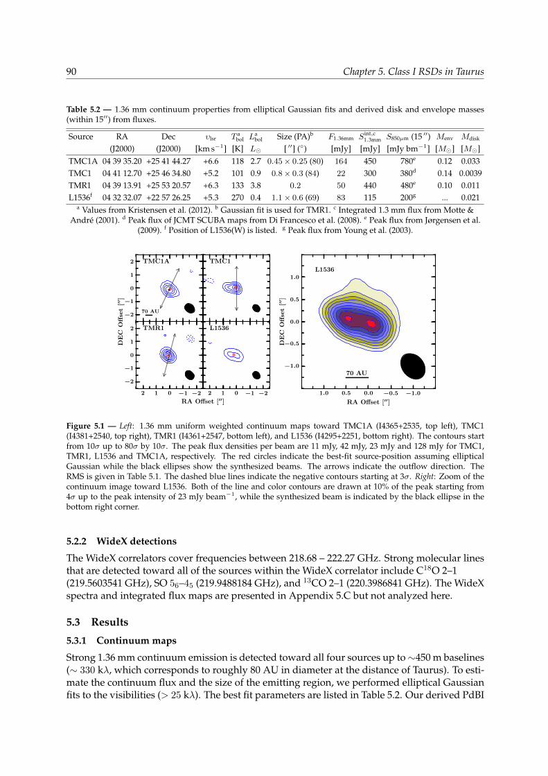
90 Chapter 5. Class I RSDs in Taurus
Table 5.2 — 1.36 mm continuum properties from elliptical Gaussian fits and derived disk and envelope masses(within 15′′) from fluxes.
Source RA Dec υlsr T abol L
abol Size (PA)b F1.36mm Sint,c
1.3mm S850µm (15 ′′) Menv Mdisk
(J2000) (J2000) [km s−1] [K] L [ ′′] () [mJy] [mJy] [mJy bm−1] [M] [M]TMC1A 04 39 35.20 +25 41 44.27 +6.6 118 2.7 0.45× 0.25 (80) 164 450 780e 0.12 0.033TMC1 04 41 12.70 +25 46 34.80 +5.2 101 0.9 0.8× 0.3 (84) 22 300 380d 0.14 0.0039TMR1 04 39 13.91 +25 53 20.57 +6.3 133 3.8 0.2 50 440 480e 0.10 0.011L1536f 04 32 32.07 +22 57 26.25 +5.3 270 0.4 1.1× 0.6 (69) 83 115 200g ... 0.021
a Values from Kristensen et al. (2012). b Gaussian fit is used for TMR1. c Integrated 1.3 mm flux from Motte &Andre (2001). d Peak flux of JCMT SCUBA maps from Di Francesco et al. (2008). e Peak flux from Jørgensen et al.
(2009). f Position of L1536(W) is listed. g Peak flux from Young et al. (2003).
−2
−1
0
1
2 TMC1A
70 AU
TMC1
−2−1012
RA Offset [′′]
−2
−1
0
1
2
DE
CO
ffse
t[′′ ]
TMR1
−2−1012
L1536
−1.0−0.50.00.51.0
RA Offset [′′]
−1.0
−0.5
0.0
0.5
1.0D
EC
Off
set
[′′ ]
70 AU
L1536
Figure 5.1 — Left: 1.36 mm uniform weighted continuum maps toward TMC1A (I4365+2535, top left), TMC1(I4381+2540, top right), TMR1 (I4361+2547, bottom left), and L1536 (I4295+2251, bottom right). The contours startfrom 10σ up to 80σ by 10σ. The peak flux densities per beam are 11 mJy, 42 mJy, 23 mJy and 128 mJy for TMC1,TMR1, L1536 and TMC1A, respectively. The red circles indicate the best-fit source-position assuming ellipticalGaussian while the black ellipses show the synthesized beams. The arrows indicate the outflow direction. TheRMS is given in Table 5.1. The dashed blue lines indicate the negative contours starting at 3σ. Right: Zoom of thecontinuum image toward L1536. Both of the line and color contours are drawn at 10% of the peak starting from4σ up to the peak intensity of 23 mJy beam−1, while the synthesized beam is indicated by the black ellipse in thebottom right corner.
5.2.2 WideX detections
The WideX correlators cover frequencies between 218.68 – 222.27 GHz. Strong molecular linesthat are detected toward all of the sources within the WideX correlator include C18O 2–1(219.5603541 GHz), SO 56–45 (219.9488184 GHz), and 13CO 2–1 (220.3986841 GHz). The WideXspectra and integrated flux maps are presented in Appendix 5.C but not analyzed here.
5.3 Results
5.3.1 Continuum maps
Strong 1.36 mm continuum emission is detected toward all four sources up to∼450 m baselines(∼ 330 kλ, which corresponds to roughly 80 AU in diameter at the distance of Taurus). To esti-mate the continuum flux and the size of the emitting region, we performed elliptical Gaussianfits to the visibilities (> 25 kλ). The best fit parameters are listed in Table 5.2. Our derived PdBI

Section 5.3. Results 91
Table 5.3 — 13CO and C18O 2–1 integrated flux densities [Jy km s−1] within a 5 ′′ box around continuum position.
Line SourcesTMC1A TMC1 TMR1 L1536
13CO 2–1a 12.2± 0.08 4.5± 0.07 10.5± 0.06 3.2± 0.08
C18O 2–1a 5.3± 0.08 2.2± 0.09 3.0± 0.06 1.2± 0.08a Integrated flux error is calculated through 1.2×σrms
√FWZI × δυ. FWZI is the full width
zero intensity as calculated from the number of channels > 5σ.
1.36 mm fluxes are < 30% lower than the single-dish fluxes tabulated in Motte & Andre (2001).The only exception is L1536 for which 72% of the singe-dish flux is recovered, which indicates alack of resolved out large-scale envelope around L1536. The deconvolved sizes indicate a largefraction of the emission is within < 100 AU diameter, consistent with compact flattened duststructures.
Figure 5.1 presents the uniform weighted continuum maps with red circles indicating thecontinuum positions (Table 5.2). The total flux of TMC1A is ∼ 30% lower than in Yen et al.(2013) within a 4.0 ′′ × 3.5 ′′ beam, which indicates that some extended structure is resolved-out in our PdBI observations. The peak fluxes of our cleaned maps agree to within 15% withthose reported by Eisner (2012) except toward L1536, which is a factor of two lower in ourmaps. However, our image toward L1536 (Fig. 5.1) shows that there are two peaks whose sumis within 15% of the peak flux reported in Eisner (2012). The position in Table 5.2 is centered onthe Western peak and the two peaks are separated by ∼ 70 AU. The analysis in the next section(Section 5.4) is with respect to the Western peak. The maps indicate the presence of elongatedflattened structure perpendicular to the outflow direction found in the literature (TMC1: 0;TMR1: 165; TMC1A: 155; L1536: None2, Ohashi et al. 1997a; Hogerheijde et al. 1998; Brown& Chandler 1999). Such elongated dust emission is indicative of flattened disk-like structures.
5.3.2 Molecular lines: maps and morphologies
The 13CO and C18O 2–1 lines are detected toward all sources. Figure 5.2 presents the spectraintegrated within a 1 ′′ box around the continuum position. The integrated line flux densitieswithin a 5 ′′ box are tabulated in Table 5.3. The molecular line emission is strongest towardTMC1A and weakest toward L1536, while most of the emission around the systemic velocity isresolved out. This can be seen in the 13CO channel map toward TMC1A (Figs. 5.2 and 5.3, seeAppendix 5.A for channel maps toward other sources) where most of the emission is absentnear υlsr = 6.6 km s−1. In contrast to 13CO, the C18O line is detected around the systemic veloc-ities (±2 km s−1) as shown in Fig. 5.2 except toward TMC1A, which shows emission within thevelocity range comparable to that of 13CO.
Single-dish observations of 13CO J =3–2 (except for L1536, which is the J =2–1 transition)and C18O J =2–1 are also shown in Fig. 5.2 (right). The comparison indicates that a large part ofthe emission at the systemic velocity originating from the large-scale envelope is filtered out inour PdBI observations. The PdBI spectra within a 1 ′′ box around each source are also broaderthan the single-dish spectra. Thus, our PdBI observations are probing the kinematics withinthe inner few hundreds of AU.
The zeroth moment (i.e., velocity-integrated flux density) maps, are shown in Fig. 5.4 to-
2Recent 12CO 3–2 observations with the JCMT do not show any indication of a bipolar outflow from this source,see Appendix 5.D.
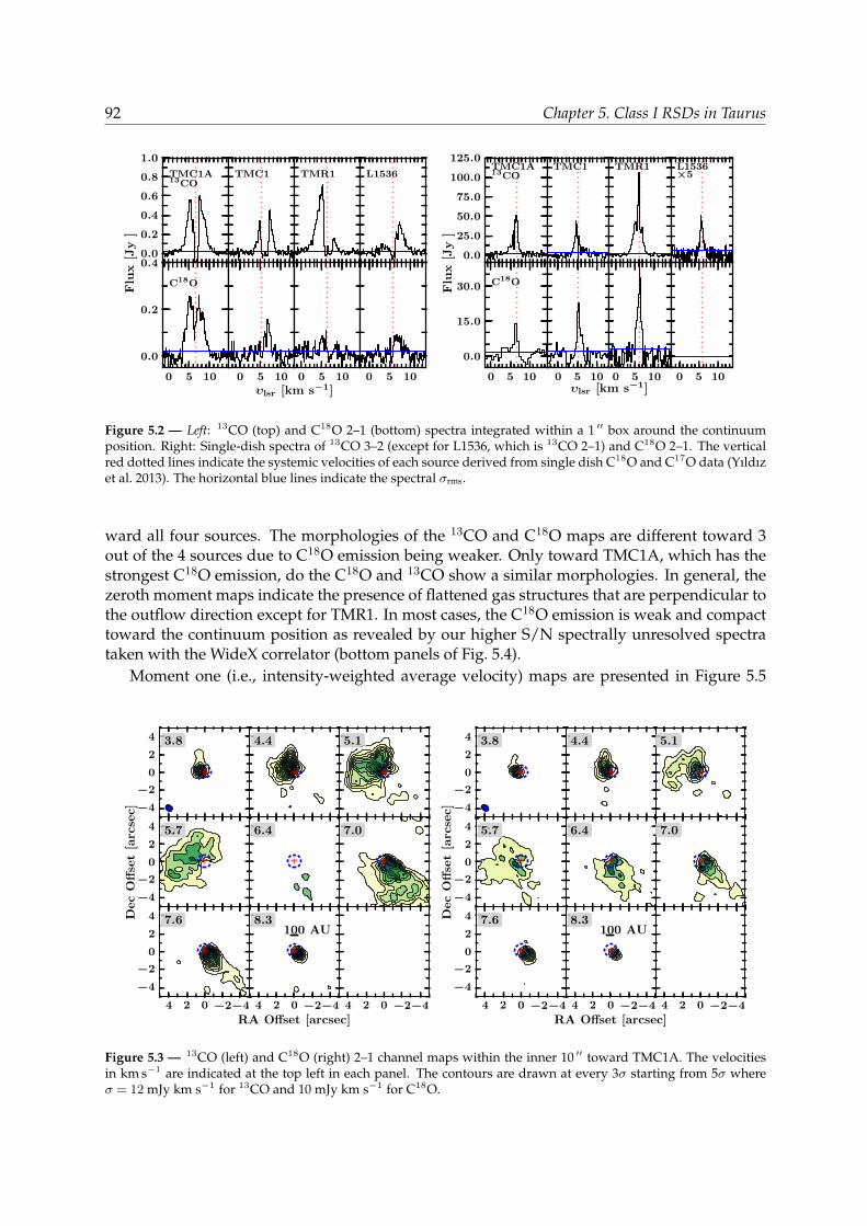
92 Chapter 5. Class I RSDs in Taurus
0.0
0.2
0.4
0.6
0.8
1.0
TMC1A13CO
0 5 10
0.0
0.2
0.4
Flu
x[J
y]
C18O
TMC1
0 5 10
υlsr [km s−1]
TMR1
0 5 10
L1536
0 5 10
0.0
25.0
50.0
75.0
100.0
125.0TMC1A13CO
0 5 10
0.0
15.0
30.0Flu
x[J
y]
C18O
TMC1
0 5 10υlsr [km s−1]
TMR1
0 5 10
L1536×5
0 5 10
Figure 5.2 — Left: 13CO (top) and C18O 2–1 (bottom) spectra integrated within a 1 ′′ box around the continuumposition. Right: Single-dish spectra of 13CO 3–2 (except for L1536, which is 13CO 2–1) and C18O 2–1. The verticalred dotted lines indicate the systemic velocities of each source derived from single dish C18O and C17O data (Yıldızet al. 2013). The horizontal blue lines indicate the spectral σrms.
ward all four sources. The morphologies of the 13CO and C18O maps are different toward 3out of the 4 sources due to C18O emission being weaker. Only toward TMC1A, which has thestrongest C18O emission, do the C18O and 13CO show a similar morphologies. In general, thezeroth moment maps indicate the presence of flattened gas structures that are perpendicular tothe outflow direction except for TMR1. In most cases, the C18O emission is weak and compacttoward the continuum position as revealed by our higher S/N spectrally unresolved spectrataken with the WideX correlator (bottom panels of Fig. 5.4).
Moment one (i.e., intensity-weighted average velocity) maps are presented in Figure 5.5
−4
−2
0
2
4 3.8 4.4 5.1
−4
−2
0
2
4 5.7 6.4 7.0
−4−2024
RA Offset [arcsec]
−4
−2
0
2
4Dec
Off
set
[arc
sec]
7.6
−4−2024
8.3100 AU
−4−2024
−4
−2
0
2
4 3.8 4.4 5.1
−4
−2
0
2
4 5.7 6.4 7.0
−4−2024
RA Offset [arcsec]
−4
−2
0
2
4Dec
Off
set
[arc
sec]
7.6
−4−2024
8.3100 AU
−4−2024
Figure 5.3 — 13CO (left) and C18O (right) 2–1 channel maps within the inner 10 ′′ toward TMC1A. The velocitiesin km s−1 are indicated at the top left in each panel. The contours are drawn at every 3σ starting from 5σ whereσ = 12 mJy km s−1 for 13CO and 10 mJy km s−1 for C18O.
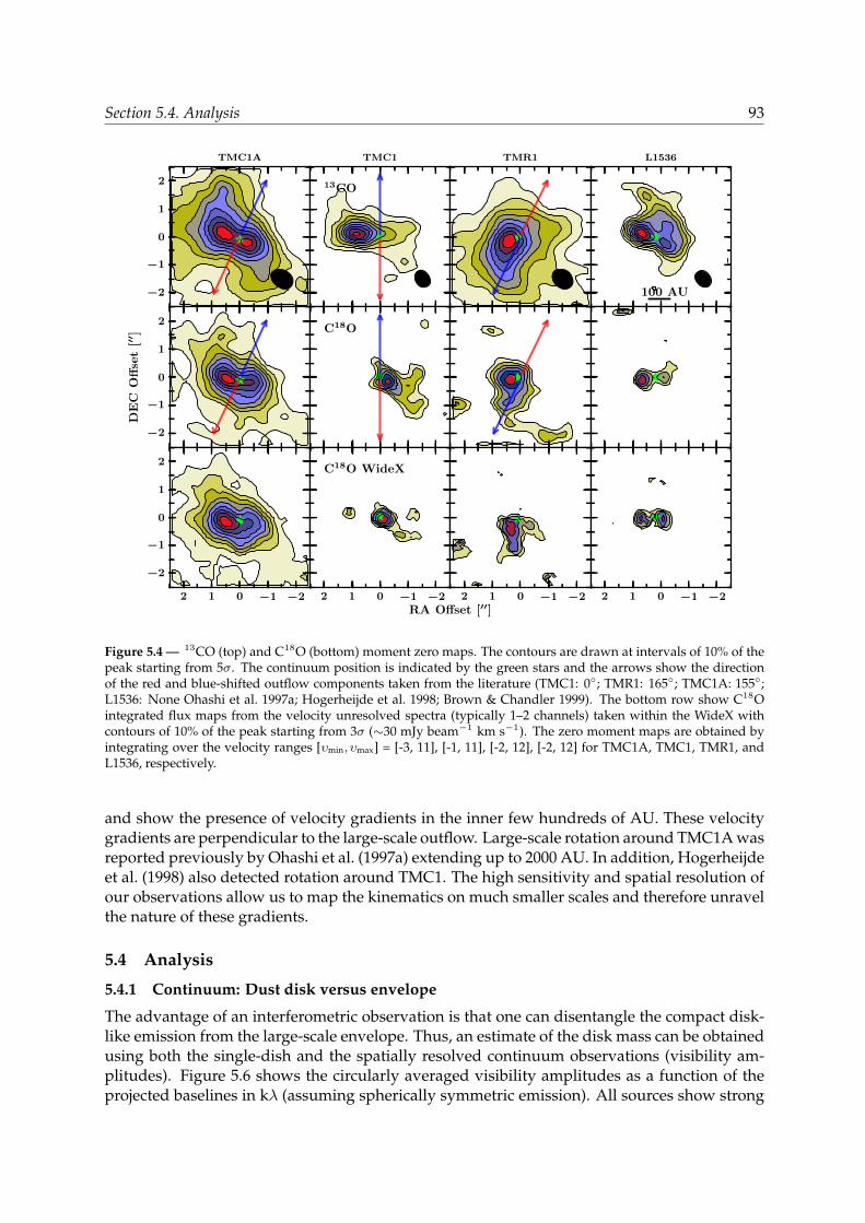
Section 5.4. Analysis 93
−2
−1
0
1
2
TMC1A
−2
−1
0
1
2
DE
CO
ffse
t[′′ ]
−2−1012
−2
−1
0
1
2
13CO
TMC1
C18O
−2−1012
C18O WideX
TMR1
−2−1012
RA Offset [′′]
100 AU
L1536
−2−1012
Figure 5.4 — 13CO (top) and C18O (bottom) moment zero maps. The contours are drawn at intervals of 10% of thepeak starting from 5σ. The continuum position is indicated by the green stars and the arrows show the directionof the red and blue-shifted outflow components taken from the literature (TMC1: 0; TMR1: 165; TMC1A: 155;L1536: None Ohashi et al. 1997a; Hogerheijde et al. 1998; Brown & Chandler 1999). The bottom row show C18Ointegrated flux maps from the velocity unresolved spectra (typically 1–2 channels) taken within the WideX withcontours of 10% of the peak starting from 3σ (∼30 mJy beam−1 km s−1). The zero moment maps are obtained byintegrating over the velocity ranges [υmin, υmax] = [-3, 11], [-1, 11], [-2, 12], [-2, 12] for TMC1A, TMC1, TMR1, andL1536, respectively.
and show the presence of velocity gradients in the inner few hundreds of AU. These velocitygradients are perpendicular to the large-scale outflow. Large-scale rotation around TMC1A wasreported previously by Ohashi et al. (1997a) extending up to 2000 AU. In addition, Hogerheijdeet al. (1998) also detected rotation around TMC1. The high sensitivity and spatial resolution ofour observations allow us to map the kinematics on much smaller scales and therefore unravelthe nature of these gradients.
5.4 Analysis
5.4.1 Continuum: Dust disk versus envelope
The advantage of an interferometric observation is that one can disentangle the compact disk-like emission from the large-scale envelope. Thus, an estimate of the disk mass can be obtainedusing both the single-dish and the spatially resolved continuum observations (visibility am-plitudes). Figure 5.6 shows the circularly averaged visibility amplitudes as a function of theprojected baselines in kλ (assuming spherically symmetric emission). All sources show strong
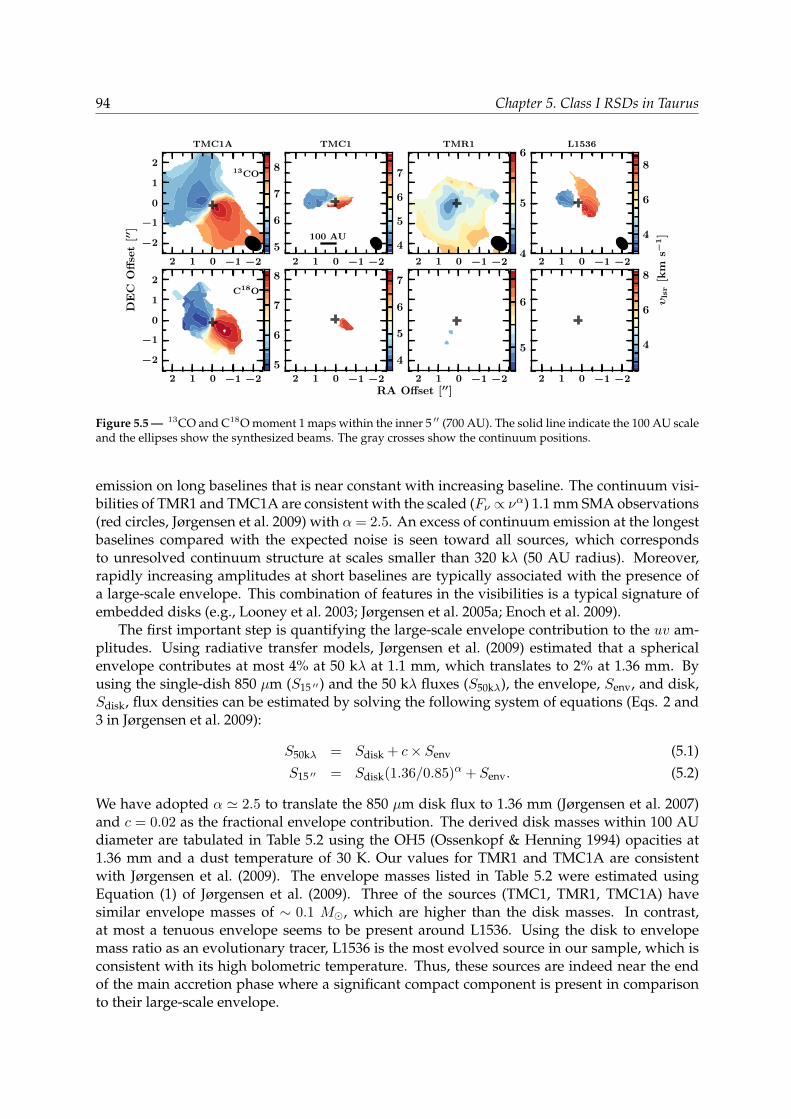
94 Chapter 5. Class I RSDs in Taurus
−2−1012
−2
−1
0
1
213CO
TMC1A
−2−1012RA Offset [′′]
−2
−1
0
1
2
DE
CO
ffse
t[′′ ]
C18O
−2−1012
100 AU
TMC1
−2−1012
−2−1012
TMR1
−2−1012
−2−1012
L1536
−2−1012
5
6
7
8
5
6
7
8
4
5
6
7
4
5
6
7
4
5
6
5
6
4
6
8
4
6
8
υls
r[k
ms−
1]
Figure 5.5 — 13CO and C18O moment 1 maps within the inner 5 ′′ (700 AU). The solid line indicate the 100 AU scaleand the ellipses show the synthesized beams. The gray crosses show the continuum positions.
emission on long baselines that is near constant with increasing baseline. The continuum visi-bilities of TMR1 and TMC1A are consistent with the scaled (Fν ∝ να) 1.1 mm SMA observations(red circles, Jørgensen et al. 2009) with α = 2.5. An excess of continuum emission at the longestbaselines compared with the expected noise is seen toward all sources, which correspondsto unresolved continuum structure at scales smaller than 320 kλ (50 AU radius). Moreover,rapidly increasing amplitudes at short baselines are typically associated with the presence ofa large-scale envelope. This combination of features in the visibilities is a typical signature ofembedded disks (e.g., Looney et al. 2003; Jørgensen et al. 2005a; Enoch et al. 2009).
The first important step is quantifying the large-scale envelope contribution to the uv am-plitudes. Using radiative transfer models, Jørgensen et al. (2009) estimated that a sphericalenvelope contributes at most 4% at 50 kλ at 1.1 mm, which translates to 2% at 1.36 mm. Byusing the single-dish 850 µm (S15 ′′) and the 50 kλ fluxes (S50kλ), the envelope, Senv, and disk,Sdisk, flux densities can be estimated by solving the following system of equations (Eqs. 2 and3 in Jørgensen et al. 2009):
S50kλ = Sdisk + c× Senv (5.1)S15 ′′ = Sdisk(1.36/0.85)α + Senv. (5.2)
We have adopted α ' 2.5 to translate the 850 µm disk flux to 1.36 mm (Jørgensen et al. 2007)and c = 0.02 as the fractional envelope contribution. The derived disk masses within 100 AUdiameter are tabulated in Table 5.2 using the OH5 (Ossenkopf & Henning 1994) opacities at1.36 mm and a dust temperature of 30 K. Our values for TMR1 and TMC1A are consistentwith Jørgensen et al. (2009). The envelope masses listed in Table 5.2 were estimated usingEquation (1) of Jørgensen et al. (2009). Three of the sources (TMC1, TMR1, TMC1A) havesimilar envelope masses of ∼ 0.1 M, which are higher than the disk masses. In contrast,at most a tenuous envelope seems to be present around L1536. Using the disk to envelopemass ratio as an evolutionary tracer, L1536 is the most evolved source in our sample, which isconsistent with its high bolometric temperature. Thus, these sources are indeed near the endof the main accretion phase where a significant compact component is present in comparisonto their large-scale envelope.
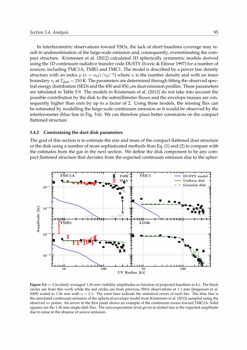
Section 5.4. Analysis 95
In interferometric observations toward YSOs, the lack of short baselines coverage may re-sult in underestimation of the large-scale emission and, consequently, overestimating the com-pact structure. Kristensen et al. (2012) calculated 1D spherically symmetric models derivedusing the 1D continuum radiative transfer code DUSTY (Ivezic & Elitzur 1997) for a number ofsources, including TMC1A, TMR1 and TMC1. The model is described by a power law densitystructure with an index p (n = n0(r/r0)−p) where n is the number density and with an innerboundary r0 at Tdust = 250 K. The parameters are determined through fitting the observed spec-tral energy distribution (SED) and the 450 and 850 µm dust emission profiles. These parametersare tabulated in Table 5.9. The models in Kristensen et al. (2012) do not take into account thepossible contribution by the disk to the submillimeter fluxes and the envelope masses are con-sequently higher than ours by up to a factor of 2. Using these models, the missing flux canbe estimated by modelling the large-scale continuum emission as it would be observed by theinterferometer (blue line in Fig. 5.6). We can therefore place better constraints on the compactflattened structure.
5.4.2 Constraining the dust disk parameters
The goal of this section is to estimate the size and mass of the compact flattened dust structureor the disk using a number of more sophisticated methods than Eq. (1) and (2) to compare withthe estimates from the gas in the next section. We define the disk component to be any com-pact flattened structure that deviates from the expected continuum emission due to the spher-
10−2
10−1
TMC1A PdBI
SMA
TMC1 DUSTY model
Uniform disk
Gaussian disk
10 100UV Radius [kλ]
10−2
10−1
Am
plitu
de
[Jy]
TMR1
10 100
L1536
Figure 5.6 — Circularly averaged 1.36 mm visibility amplitudes as function of projected baselines in kλ. The blackcircles are from this work while the red circles are from previous SMA observations at 1.1 mm (Jørgensen et al.2009) scaled to 1.36 mm with α = 2.5. The error bars indicate the statistical errors of each bin. The blue line isthe simulated continuum emission of the spherical envelope model from Kristensen et al. (2012) sampled using theobserved uv points. An arrow in the first panel shows an example of the continuum excess toward TMC1A. Solidsquares are the 1.36 mm single-dish flux. The zero-expectation level given in dotted line is the expected amplitudedue to noise in the absence of source emission.

96 Chapter 5. Class I RSDs in Taurus
Table 5.4 — Disk sizes and masses derived from continuum visibilities modelling using uniform, Gaussian andpower-law disk models.
Object ParametersRdisk Mdisk i PA[AU] [10−3 M] [] []
Uniform diskTMC1A 30 – 50 48±6 20–46 60–99TMC1 7 – 124 4.7+4
−2 30–70 65–105TMR1 7 – 40 15±2 5–30 -15–15L1536 100 – 171 22±5 30–73 60–100
Gaussian diskTMC1A 17–32 48±6 24–56 62–96TMC1 7–80 4.5+4
−2 30–70 65–105TMR1 7–20 15±2 5–30 -15–15L1536 53–112 24±4 33–75 60–100
Power-law diskTMC1A 80–220 41±8 24–76 60–99TMC1 41–300 5.4+20
−0 20–80 55–115TMR1 7–55 10+100
−9 2–45 -25–40L1536 135–300 19+18
−4 20–56 50–68
ical envelope model. In the following sections, the disk sizes will be estimated by fitting thecontinuum visibilities with the inclusion of emission from the large-scale structure describedabove. As the interferometric observation recovers a large fraction of the single-dish flux to-ward L1536, its large-scale envelope contribution is assumed to be insignificant, and thereforenot included. The best-fit parameters are found through χ2 minimization on the binned ampli-tudes. The range of values of Rdisk, Mdisk, i and PA shown in Table 5.4 correspond to modelswith χ2 between χ2
min and χ2min + 15.
5.4.2.1 Uniform disk
The first estimate on the disk size and mass is obtained by fitting a uniform disk model assum-ing optically thin dust emission (see Fig. 5.7, Eisner 2012). Uniform disks are described by a
constant intensity I within a diameter θud whose flux is given by F =∫I cosθ dΩ = Iπ
(θud2
)2.
The visibility amplitudes are given by:
V (u, v) = F × 2J1 (πθruv)
πθruv, (5.3)

Section 5.4. Analysis 97
0.0
0.2
0.4
0.6
0.8
1.0
0.5
0.8
1.0
Un
iform
70
140
210 AU
0.0
0.2
0.4
0.6
0.8
1.0
Norm
ali
zedI(r
)
0.5
0.8
1.0
Norm
ali
zed
Am
pli
tud
e
Gau
ssian41
110
221 AU
0.0 0.5 1.0 1.5 2.0
r [arcsec]
0.0
0.2
0.4
0.6
0.8
1.0
1 10 100
UV radius [kλ]
0.5
0.8
1.0 Pow
er
law
500
326
107
47 AU
Figure 5.7 — Left: Normalized intensity profiles for the three different continuum models: Uniform disk (top),Gaussian Disk (middle), and power-law disk (bottom). Right: Normalized visibilities as function of uv radius. Forcomparison, the L1536 binned data are shown in gray circles.
where J1 is the Bessel function of order 1 and ruv is the projected baseline in terms of λ. Depro-jection of the baselines follow the formula given in Berger & Segransan (2007):
uPA = u cosPA+ v sinPA, (5.4)vPA = −u sinPA+ v cosPA, (5.5)
ruv,i =√
(u2PA + v2
PA cos(i)2), (5.6)
where PA is the position angle (East of North) and i is the inclination.The best fit parameters are tabulated in Table 5.4 with disk masses estimated using a dust
temperature of 30 K and OH5 opacities (Table 5 of Ossenkopf & Henning 1994) within θud2 ra-
dius. The disk radii vary between 7 to 171 AU. The smallest disk size is found toward TMR1,which suggests that most of its continuum emission is due to the large-scale envelope. More-over, disk sizes around TMR1 and TMC1A are 65%–90% lower than those reported by Eisner(2012,Table 3) since we have included the spherical envelope contribution. This illustrates theimportance of including the large-scale contribution in analyzing the compact structure.
5.4.2.2 Gaussian disk
The next step is to use a Gaussian intensity distribution, which is a slightly more realistic inten-sity model that represents the mm emission due to an embedded disk. The visibility amplitudesare described by the following equation:
V (u, v) = F × exp
(−πθGruv
4 log 2
), (5.7)
where θG is the FWHM of the Gaussian distribution and F is the total flux.

98 Chapter 5. Class I RSDs in Taurus
The difference between the Gaussian fit presented in Table 5.2 and this section is the inclu-sion of the large-scale emission. In Table 5.2, the Gaussian fit gives an estimate of the size ofemission in the observed total image, while this section accounts for the simulated large-scaleenvelope emission in order to constrain the compact flattened structure. The free-parametersare similar to the uniform disk except that the size of the emitting region is defined by full-width half maximum (FWHM ). For a Gaussian distribution, most of the radiation (95%) isemitted from within 2σG ∼ 0.85×FWHM , thus we define the disk radius to be 0.42×FWHM .The best-fit parameters are tabulated in Table 5.4 and the corresponding emission is includedin Fig. 5.6. The resulting disk sizes are slightly lower than those derived using a uniform disk.
The visibility amplitudes in Fig. 5.6 show the presence of an unresolved point source com-ponent at long baselines indicated by the arrow in the first panel. Jørgensen et al. (2005a) notedthat a three components model (large-scale envelope + Gaussian disk + point-source) fits thecontinuum visibilities. By using such models, the disk sizes generally increase by 20–30 AUwith the addition of an unresolved point flux, which is comparable to the uniform disk mod-els. Such models were first introduced by Mundy et al. (1996) since the mm emission seems tobe more centrally peaked than a single Gaussian. The unresolved point flux is more likely dueto the unresolved disk structure since the free-free emission contribution is expected to be lowtoward Class I sources (Hogerheijde et al. 1998).
5.4.2.3 Power-law disk
The next step in sophistication is to fit the continuum visibilities with a power-law disk struc-ture. The difference is that the first two disk models are based on the expected intensity pro-file of the disk, while the power-law disk models use a more realistic disk structure. Simi-lar structures were previously used by Lay et al. (1997, see also Lay et al. 1994; Mundy et al.1996; Dutrey et al. 2007; Malbet et al. 2005). We adopt a disk density structure described byΣdisk = Σ50AU (R/50AU)−p where Σ50 AU is the surface density at 50 AU with a temperaturestructure given as Tdisk = 1500 (R/0.1AU)−q. The inner radius is fixed at 0.1 AU with a dustsublimation temperature of 1500 K, while the disk outer radius is defined at 15 K. The freeparameters are p, q, Σ50AU, i and PA where i is the inclination with respect of the plane of thesky in degrees (0 is face-on) and PA is the position angle (East of North). The visibilities areconstructed by considering the flux from a thin ring given by:
dS =2π cos i
d2Bν(T )
(1− exp−τ
)R dR, (5.8)
where d is the distance, i is the inclination (0 is face-on), τ = Σ(R)κcos i is the optical depth and
Bν(T ) is the Planck function. For the dust emissivity (κ), we adopt the OH5 values. Since themodel is axisymmetric, the visibilities are given by a one-dimensional Hankel transform whichis given by the analytical expression:
V (u, v) = dS × J0 (2πRruv) , (5.9)
where J0 is the Bessel function of order 0. The total amplitude at a given ruv is integrated overthe whole disk.
The first advantage of such modelling is the treatment of the optical depth which givesbetter mass approximations. Secondly, the unresolved point-flux is already included in themodel by simulating the emission from the unresolved disk component. Figure 5.7 shows thenormalized visibilities for a fixed p = 0.9 and a number of Rdisk. The best-fit parameters aretabulated in Table 5.4.
Section 5.4. Analysis 99
The derived disk masses obtained by integrating out to ∼ 50 AU radius are similar to thosefrom the 50 kλ point (Table 5.2). This is expected as the 1.3 mm continuum emission (κOH5 =0.83 cm2g−1) is on average nearly optically thin (Jørgensen et al. 2007). The optical depth canbe up to 0.4 at radii < 10 AU for the best-fit power-law disk models with i > 70. A widerange of ‘best-fit’ masses is found toward TMR1, which is mainly due to the uncertainties inthe inclination.
More recently, Eisner (2012) presented embedded disk models derived from continuumdata by fitting the I band image, SED and 1.3 mm visibilities. Our continuum disk radii towardTMC1A and TMR1 are consistent with their results. However, the high quality of our dataallow us to rule out disks withRout > 100 AU toward TMR1. On the other hand, our disk radiustoward L1536 is a factor of 3 higher than that reported in Eisner (2012) due to the difference inthe treatment of the large-scale envelope.
In summary, different methods have been used to constrain the disk parameters from ther-mal dust emission. The first two models, Gaussian and uniform disk models, are based on theintensity profile, while the power-law disk models use a simplified disk structure with givendensity and temperature profiles. The intensity based models find the smallest disk sizes, whilethe power-law disk models predict up to a factor of two larger disk sizes. On the other hand, thedisk masses from these fitting methods are similar. The advantage of the power-law disk mod-eling is the determination of the density and temperature structures including the unresolvedinner part of the disk. The continuum images provide no kinematic information, however, sothe important question is whether these flattened structures are rotationally supported disksand if so, whether the continuum sizes agree with those of RSDs.
5.4.3 Line analysis: Keplerian or not?
The nature of the velocity gradient can already be inferred from the moment maps. First, the13CO integrated flux maps shown in Fig. 5.4 indicate the presence of flattened gas structuresperpendicular to the outflow direction. Second, the velocity gradient is also oriented perpen-dicular to the outflow within hundreds of AU, which is a similar size scale to the compact duststructure measured in Section 5.4.2. On the other hand, the velocity gradient does not showa straight transition from the red to the blue shifted component as expected from a Kepleriandisk. Taking TMC1A as an example, the blue-shifted emission starts at the North side andskews inward toward the continuum position. Such a skewed moment 1 map is expected fora Keplerian disk embedded in a rotating infalling envelope (Sargent & Beckwith 1987; Brinchet al. 2008). Thus, the moment maps indicate the presence of a rotating infalling envelopeleading up to a rotationally dominated structure.
In image space, position velocity (PV) diagrams are generally used to determine the natureof the velocity gradient. Analysis of such diagrams starts by dividing it into four quadrantsaround the υlsr and source position. A rotating structure occupies two of the four quadrantsthat are symmetric around the center, while an infalling structure will show emission in allquadrants (e.g., Ohashi et al. 1997a; Brinch et al. 2007b). In addition, one can infer the presenceof outflow contamination by identifying a velocity gradient in PV space along the outflowdirection (e.g., Cabrit et al. 1996).
Figure 5.8 presents PV diagrams at a direction perpendicular to the outflow direction; forL1536, the direction of elongation of the continuum was taken. In general, the PV diagrams areconsistent with Keplerian profiles, except for TMR1. The PV diagram toward TMR1 seems toindicate that the 13CO line is either dominated by infalling material or the source is orientedtoward us, which is difficult to disentangle. However, recent 12CO 3–2 and 6–5 maps presentedin Yıldız et al. (in prep.) suggest that the disk is more likely oriented face-on (i < 15). Further-
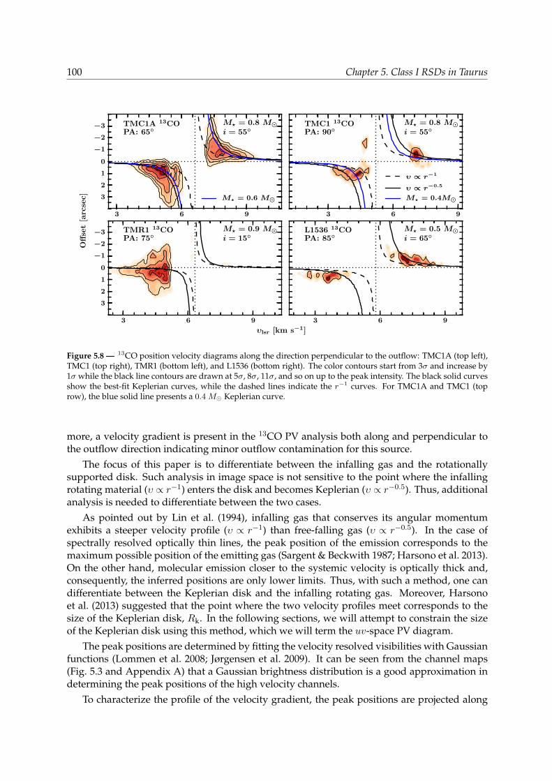
100 Chapter 5. Class I RSDs in Taurus
3 6 9
−3
−2
−1
0
1
2
3
TMC1A 13COPA: 65
M? = 0.8 Mi = 55
M? = 0.6 M
3 6 9
TMC1 13COPA: 90
M? = 0.8 Mi = 55
υ ∝ r−1
υ ∝ r−0.5
M? = 0.4M
3 6 9
υlsr [km s−1]
−3
−2
−1
0
1
2
3
Off
set
[arc
sec]
TMR1 13COPA: 75
M? = 0.9 Mi = 15
3 6 9
L1536 13COPA: 85
M? = 0.5 Mi = 65
Figure 5.8 — 13CO position velocity diagrams along the direction perpendicular to the outflow: TMC1A (top left),TMC1 (top right), TMR1 (bottom left), and L1536 (bottom right). The color contours start from 3σ and increase by1σ while the black line contours are drawn at 5σ, 8σ, 11σ, and so on up to the peak intensity. The black solid curvesshow the best-fit Keplerian curves, while the dashed lines indicate the r−1 curves. For TMC1A and TMC1 (toprow), the blue solid line presents a 0.4 M Keplerian curve.
more, a velocity gradient is present in the 13CO PV analysis both along and perpendicular tothe outflow direction indicating minor outflow contamination for this source.
The focus of this paper is to differentiate between the infalling gas and the rotationallysupported disk. Such analysis in image space is not sensitive to the point where the infallingrotating material (υ ∝ r−1) enters the disk and becomes Keplerian (υ ∝ r−0.5). Thus, additionalanalysis is needed to differentiate between the two cases.
As pointed out by Lin et al. (1994), infalling gas that conserves its angular momentumexhibits a steeper velocity profile (υ ∝ r−1) than free-falling gas (υ ∝ r−0.5). In the case ofspectrally resolved optically thin lines, the peak position of the emission corresponds to themaximum possible position of the emitting gas (Sargent & Beckwith 1987; Harsono et al. 2013).On the other hand, molecular emission closer to the systemic velocity is optically thick and,consequently, the inferred positions are only lower limits. Thus, with such a method, one candifferentiate between the Keplerian disk and the infalling rotating gas. Moreover, Harsonoet al. (2013) suggested that the point where the two velocity profiles meet corresponds to thesize of the Keplerian disk, Rk. In the following sections, we will attempt to constrain the sizeof the Keplerian disk using this method, which we will term the uv-space PV diagram.
The peak positions are determined by fitting the velocity resolved visibilities with Gaussianfunctions (Lommen et al. 2008; Jørgensen et al. 2009). It can be seen from the channel maps(Fig. 5.3 and Appendix A) that a Gaussian brightness distribution is a good approximation indetermining the peak positions of the high velocity channels.
To characterize the profile of the velocity gradient, the peak positions are projected along
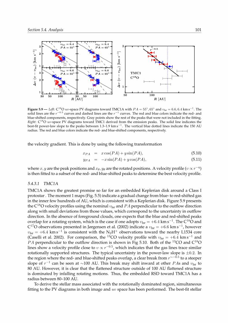
Section 5.4. Analysis 101
1
2
3υlsr = 6.4
PA = 55
30 50 100R [AU]
1
2
3
∆υ
(υ−υ
lsr)
[km
s−1]
υlsr = 6.6
PA = 55
υlsr = 6.4
PA = 65
30 50 100
υlsr = 6.6
PA = 65
50 100
R [AU]
1
2
∆υ
(υ−υ
lsr)
[km
s−1]
TMC1
C18O
r−0.5
Figure 5.9 — Left: C18O uv-space PV diagrams toward TMC1A with PA = 55,65 and υlsr = 6.6,6.4 km s−1. Thesolid lines are the r−0.5 curves and dashed lines are the r−1 curves. The red and blue colors indicate the red- andblue-shifted components, respectively. Gray points show the rest of the peaks that were not included in the fitting.Right: C18O uv-space PV diagrams toward TMC1 derived from the emission peaks. The solid line indicates thebest-fit power-law slope to the peaks between 1.3–1.9 km s−1. The vertical blue dotted lines indicate the 150 AUradius. The red and blue colors indicate the red- and blue-shifted components, respectively.
the velocity gradient. This is done by using the following transformation
xPA = x cos(PA) + y sin(PA), (5.10)yPA = −x sin(PA) + y cos(PA), (5.11)
where x, y are the peak positions and xθ, yθ are the rotated positions. A velocity profile (υ ∝ r−η)is then fitted to a subset of the red- and blue-shifted peaks to determine the best velocity profile.
5.4.3.1 TMC1A
TMC1A shows the greatest promise so far for an embedded Keplerian disk around a Class Iprotostar . The moment 1 maps (Fig. 5.5) indicate a gradual change from blue- to red-shifted gasin the inner few hundreds of AU, which is consistent with a Keplerian disk. Figure 5.9 presentsthe C18O velocity profiles using the nominal υlsr and PA perpendicular to the outflow directionalong with small deviations from those values, which correspond to the uncertainty in outflowdirection. In the absence of foreground clouds, one expects that the blue and red-shifted peaksoverlap for a rotating system, which is the case if one adopts υlsr = +6.4 km s−1. The C18O andC17O observations presented in Jørgensen et al. (2002) indicate a υlsr = +6.6 km s−1, howeverυlsr = +6.4 km s−1 is consistent with the N2H+ observations toward the nearby L1534 core(Caselli et al. 2002). For comparison, the 13CO velocity profile with υlsr = +6.4 km s−1 andPA perpendicular to the outflow direction is shown in Fig 5.10. Both of the 13CO and C18Olines show a velocity profile close to υ ∝ r−0.5, which indicates that the gas lines trace similarrotationally supported structures. The typical uncertainty in the power-law slope is ±0.2. Inthe region where the red- and blue-shifted peaks overlap, a clear break from r∼−0.5 to a steeperslope of r−1 can be seen at ∼100 AU. This break may shift inward at other PAs and υlsr to80 AU. However, it is clear that the flattened structure outside of 100 AU flattened structureis dominated by infalling rotating motions. Thus, the embedded RSD toward TMC1A has aradius between 80–100 AU.
To derive the stellar mass associated with the rotationally dominated region, simultaneousfitting to the PV diagrams in both image and uv space has been performed. The best-fit stellar
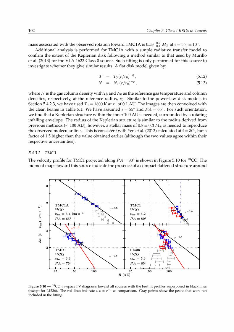
102 Chapter 5. Class I RSDs in Taurus
mass associated with the observed rotation toward TMC1A is 0.53+0.2−0.1 M at i = 55 ± 10.
Additional analysis is performed for TMC1A with a simple radiative transfer model toconfirm the extent of the Keplerian disk following a method similar to that used by Murilloet al. (2013) for the VLA 1623 Class 0 source. Such fitting is only performed for this source toinvestigate whether they give similar results. A flat disk model given by:
T = T0 (r/r0)−q , (5.12)N = N0 (r/r0)−p , (5.13)
whereN is the gas column density with T0 andN0 as the reference gas temperature and columndensities, respectively, at the reference radius, r0. Similar to the power-law disk models inSection 5.4.2.3, we have used T0 = 1500 K at r0 of 0.1 AU. The images are then convolved withthe clean beams in Table 5.1. We have assumed i = 55 and PA = 65. For such orientation,we find that a Keplerian structure within the inner 100 AU is needed, surrounded by a rotatinginfalling envelope. The radius of the Keplerian structure is similar to the radius derived fromprevious methods (∼ 100 AU), however, a stellar mass of 0.8± 0.3 M is needed to reproducethe observed molecular lines. This is consistent with Yen et al. (2013) calculated at i= 30, but afactor of 1.5 higher than the value obtained earlier (although the two values agree within theirrespective uncertainties).
5.4.3.2 TMC1
The velocity profile for TMC1 projected along PA = 90 is shown in Figure 5.10 for 13CO. Themoment maps toward this source indicate the presence of a compact flattened structure around
2
3
TMC1A13COυlsr = 6.4 km s−1
PA = 65
r−0.5TMC113COυlsr = 5.2
PA = 89
r−0.9
25 50 100R [AU]
2
3
∆υ
(υ−υ
lsr)
[km
s−1]
TMR113COυlsr = 6.3
PA = 75
r−0.5
r−1.0
25 50 100
L153613COυlsr = 5.3
PA = 85
r−0.5
Figure 5.10 — 13CO uv-space PV diagrams toward all sources with the best fit profiles superposed in black lines(except for L1536). The red lines indicate a υ ∝ r−1 as comparison. Gray points show the peaks that were notincluded in the fitting.
Section 5.4. Analysis 103
the continuum position. Similar to TMC1A, the PV diagram also indicates a rotationally dom-inated structure. However, in contrast to TMC1A, the 13CO line is best described by an r−1
profile indicating that it traces infalling rotating gas, while the C18O line is fitted well with ar−0.5 slope as shown in Fig. 5.9 indicative of an RSD. Such discrepancy can occur if the twolines are tracing different regions. The moment zero maps in Fig. 5.4 already gave some indi-cation that the 13CO and C18O emissions do not arise from similar structure. Furthermore, thedisk mass toward TMC1 as inferred through the continuum is the lowest in our sample, henceit is also possible that the embedded RSD is not massive enough to significantly contribute toboth the 13CO and C18O emission. The relatively more optically thick 13CO traces the innerenvelope and thus is dominated by its kinematics, while the rotationally supported structuresignificantly contributes to the C18O line. A smooth extrapolation of the envelope down to100–150 AU scales predicts C18O emission < 18% of the observe emission at > 1.5 km s−1, sug-gesting that the majority of the emission at these velocities originates in a disk (see also modelsby Harsono et al. 2013, figure 8). Hence, using the C18O line, the fit indicates the presence of anRSD extending between 100–150 AU in radius. The best-fit stellar mass is 0.54+0.2
−0.1 M at i= 55
with typical error of ±0.2 km s−1 on the determination of υlsr. The stellar mass is a factor of 1.5lower than that previously derived by Hogerheijde et al. (1998) as indicated by the black linesin Fig. 5.8. However, a stellar mass of 0.4 M also reasonably fits the 13CO PV diagram. Inaddition, the discrepancy between the 13CO and C18O velocity profiles may suggest that themost stable RSD is less than the C18O break point. Thus, we will use 100 AU as the size of theRSD toward TMC1.
5.4.3.3 TMR1
The determination of the velocity profile toward TMR1 is difficult. Adopting υlsr = +6.3 km s−1
(Kristensen et al. 2012; Yıldız et al. 2013), the red-shifted peaks do not coincide with the blue-shifted peaks as expected from a symmetric rotating infalling structure in the absence of fore-ground clouds. The 13CO velocity profile is uncertain with a slope between 0.5 to 1 (Fig. 5.10).However, a velocity gradient is present in the PV analysis along and perpendicular to the out-flow direction, which suggest outflow contamination toward TMR1. With the 5σ thresholdused for this analysis, only 3 peaks are available in the C18O line, which are located alongthe blue outflow lobe as inferred from the 12CO J =3–2 and J =6–5 maps in Yıldız et al, inprep. The on-source C18O line is detected within the WideX correlator, which is double peakedwithin 100 AU diameter (Fig. 5.4). Thus, the non-detection of the turn-over from r−1 to r−0.5
indicates that the disk is much smaller than the synthesized beam (< 0.7 ′′ = 98 AU diameter).Also, the RSD has to be less massive than TMC1 and TMC1A due to the lack of on-source C18Oemission and rotational motion. Thus, the compact flattened dust structure at > 50 kλ towardthis source cannot be fully associated with an RSD. The molecular emission from TMR1 mustbe mostly due to the infalling rotating envelope and the entrained outflow gas similar to theconclusion of Jørgensen et al. (2009).
5.4.3.4 L1536
Figure 5.10 shows the uv-space PV diagram with systemic velocity of υlsr = +5.3 km s−1. Thepeak positions were shifted to the center of the two peaks seen in the continuum (Fig. 5.1) andthe C18O integrated map (Fig. 5.4). The dominant motion at low velocity offsets (∆υ = ±2km s−1) is infall, while a flatter slope with a power-law close to r−0.5 best describes the highvelocity components. If the peak positions were not shifted, only the blue-shifted peaks followthe r−0.5 profile starting from 70–80 AU. The flat velocity profile is based on 4 points and it
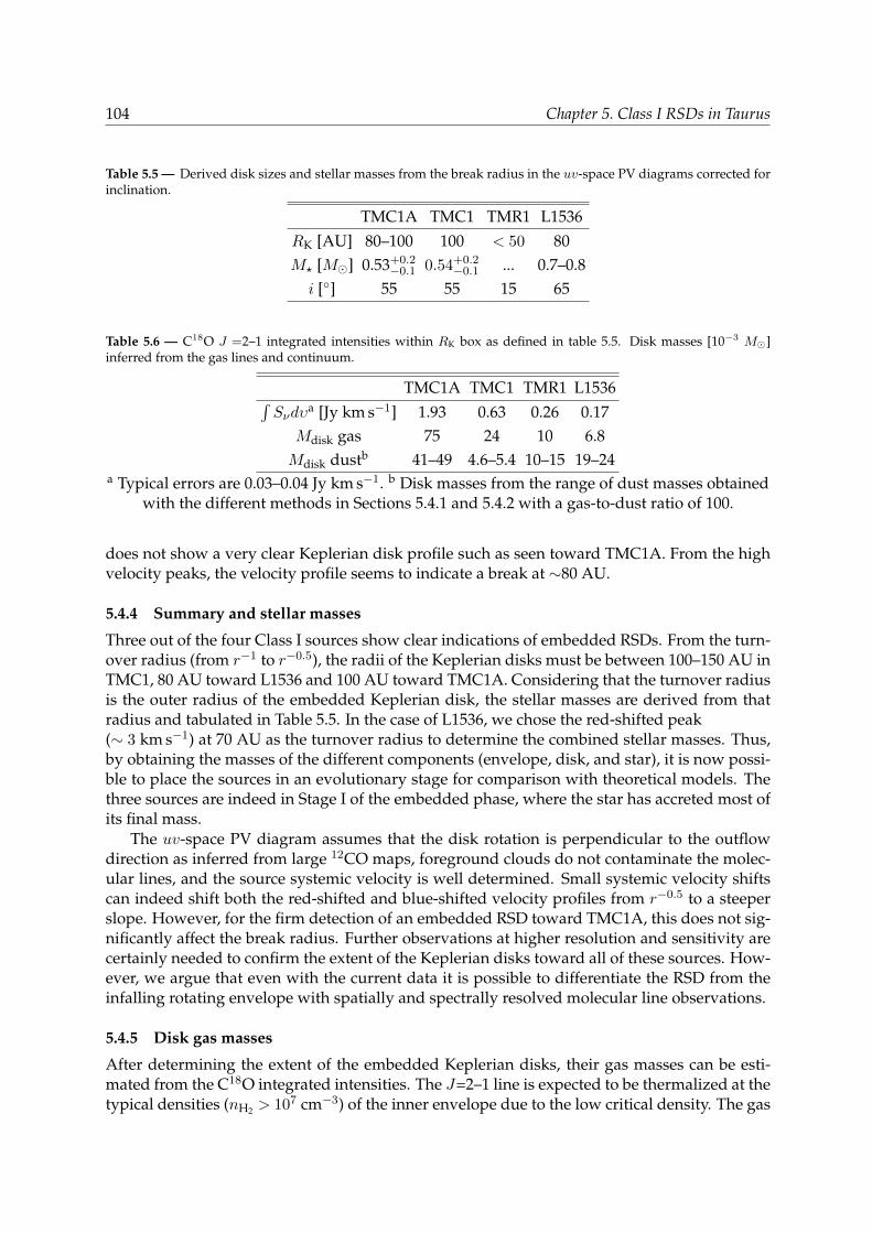
104 Chapter 5. Class I RSDs in Taurus
Table 5.5 — Derived disk sizes and stellar masses from the break radius in the uv-space PV diagrams corrected forinclination.
TMC1A TMC1 TMR1 L1536RK [AU] 80–100 100 < 50 80M? [M] 0.53+0.2
−0.1 0.54+0.2−0.1 ... 0.7–0.8
i [] 55 55 15 65
Table 5.6 — C18O J =2–1 integrated intensities within RK box as defined in table 5.5. Disk masses [10−3 M]inferred from the gas lines and continuum.
TMC1A TMC1 TMR1 L1536∫Sνdυ
a [Jy km s−1] 1.93 0.63 0.26 0.17Mdisk gas 75 24 10 6.8Mdisk dustb 41–49 4.6–5.4 10–15 19–24
a Typical errors are 0.03–0.04 Jy km s−1. b Disk masses from the range of dust masses obtainedwith the different methods in Sections 5.4.1 and 5.4.2 with a gas-to-dust ratio of 100.
does not show a very clear Keplerian disk profile such as seen toward TMC1A. From the highvelocity peaks, the velocity profile seems to indicate a break at ∼80 AU.
5.4.4 Summary and stellar masses
Three out of the four Class I sources show clear indications of embedded RSDs. From the turn-over radius (from r−1 to r−0.5), the radii of the Keplerian disks must be between 100–150 AU inTMC1, 80 AU toward L1536 and 100 AU toward TMC1A. Considering that the turnover radiusis the outer radius of the embedded Keplerian disk, the stellar masses are derived from thatradius and tabulated in Table 5.5. In the case of L1536, we chose the red-shifted peak(∼ 3 km s−1) at 70 AU as the turnover radius to determine the combined stellar masses. Thus,by obtaining the masses of the different components (envelope, disk, and star), it is now possi-ble to place the sources in an evolutionary stage for comparison with theoretical models. Thethree sources are indeed in Stage I of the embedded phase, where the star has accreted most ofits final mass.
The uv-space PV diagram assumes that the disk rotation is perpendicular to the outflowdirection as inferred from large 12CO maps, foreground clouds do not contaminate the molec-ular lines, and the source systemic velocity is well determined. Small systemic velocity shiftscan indeed shift both the red-shifted and blue-shifted velocity profiles from r−0.5 to a steeperslope. However, for the firm detection of an embedded RSD toward TMC1A, this does not sig-nificantly affect the break radius. Further observations at higher resolution and sensitivity arecertainly needed to confirm the extent of the Keplerian disks toward all of these sources. How-ever, we argue that even with the current data it is possible to differentiate the RSD from theinfalling rotating envelope with spatially and spectrally resolved molecular line observations.
5.4.5 Disk gas masses
After determining the extent of the embedded Keplerian disks, their gas masses can be esti-mated from the C18O integrated intensities. The J=2–1 line is expected to be thermalized at thetypical densities (nH2 > 107 cm−3) of the inner envelope due to the low critical density. The gas
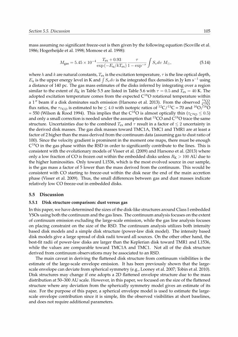
Section 5.5. Discussion 105
mass assuming no significant freeze-out is then given by the following equation (Scoville et al.1986; Hogerheijde et al. 1998; Momose et al. 1998):
Mgas = 5.45× 10⁻⁴ Tex + 0.93
exp (−Eu/kTex)
τ
1− exp−τ
∫Sυdυ M, (5.14)
where h and k are natural constants, Tex is the excitation temperature, τ is the line optical depth,Eu is the upper energy level in K and
∫Sνdυ is the integrated flux densities in Jy km s−1 using
a distance of 140 pc. The gas mass estimates of the disks inferred by integrating over a regionsimilar to the extent of RK in Table 5.5 are listed in Table 5.6 with τ = 0.5 and Tex = 40 K. Theadopted excitation temperature comes from the expected C18O rotational temperature withina 1 ′′ beam if a disk dominates such emission (Harsono et al. 2013). From the observed
13COC18O
flux ratios, the τ13CO is estimated to be ≤ 4.0 with isotopic ratios of 12C/13C = 70 and 16O/18O= 550 (Wilson & Rood 1994). This implies that the C18O is almost optically thin (τC18O ≤ 0.5)and only a small correction is needed under the assumption that 13CO and C18O trace the samestructure. Uncertainties due to the combined Tex and τ result in a factor of ≤ 2 uncertainty inthe derived disk masses. The gas disk masses toward TMC1A, TMC1 and TMR1 are at least afactor of 2 higher than the mass derived from the continuum data (assuming gas to dust ratio of100). Since the velocity gradient is prominent in the moment one maps, there must be enoughC18O in the gas phase within the RSD in order to significantly contribute to the lines. This isconsistent with the evolutionary models of Visser et al. (2009) and Harsono et al. (2013) whereonly a low fraction of CO is frozen out within the embedded disks unless RK > 100 AU due tothe higher luminosities. Only toward L1536, which is the most evolved source in our sample,is the gas mass a factor of 5 lower than the mass derived from the continuum. This would beconsistent with CO starting to freeze-out within the disk near the end of the main accretionphase (Visser et al. 2009). Thus, the small differences between gas and dust masses indicaterelatively low CO freeze-out in embedded disks.
5.5 Discussion
5.5.1 Disk structure comparison: dust versus gas
In this paper, we have determined the sizes of the disk-like structures around Class I embeddedYSOs using both the continuum and the gas lines. The continuum analysis focuses on the extentof continuum emission excluding the large-scale emission, while the gas line analysis focuseson placing constraint on the size of the RSD. The continuum analysis utilizes both intensitybased disk models and a simple disk structure (power-law disk model). The intensity baseddisk models give a large spread of disk radii toward all sources. On the other other hand, thebest-fit radii of power-law disks are larger than the Keplerian disk toward TMR1 and L1536,while the values are comparable toward TMC1A and TMC1. Not all of the disk structurederived from continuum observations may be associated to an RSD.
The main caveat in deriving the flattened disk structure from continuum visibilities is theestimate of the large-scale envelope emission. It has been previously shown that the large-scale envelope can deviate from spherical symmetry (e.g., Looney et al. 2007; Tobin et al. 2010).Disk structures may change if one adopts a 2D flattened envelope structure due to the massdistribution at 50–300 AU scale. However, in this paper, we focused on the size of the flattenedstructure where any deviation from the spherically symmetry model gives an estimate of itssize. For the purpose of this paper, a spherical envelope model is used to estimate the large-scale envelope contribution since it is simple, fits the observed visibilities at short baselines,and does not require additional parameters.

106 Chapter 5. Class I RSDs in Taurus
5.5.1.1 Comparison to disk sizes and masses from SED modelling
A number of 2D envelope and disk models have been published previously constrained solelyusing continuum data. More recently, Eisner (2012) used the combination of high resolu-tion near-IR images, the SED and millimeter continuum visibilities to constrain the structuresaround TMR1, TMC1A and L1536. The size of his disk is defined by the centrifugal radius,which is the radius at which the material distribution becomes more flattened (Ulrich 1976).His inferred sizes are consistent with the extent of RSDs in our sample (TMR1: 30–450 AU;L1536: 30–100 AU; TMC1A: 100 AU), but our higher resolution data narrow this range. For thecase of TMR1, we can definitely rule out any disk sizes > 100 AU.
Others have used a similar definition of the centrifugal radius using the envelope structuregiven by Ulrich (1976) with and without disk component (e.g., Eisner et al. 2005; Gramajo et al.2007; Furlan et al. 2008). Thus, the value of Rc gives an approximate outer radius of the RSD.These models are then fitted to the SED and high resolution near-IR images without interfero-metric data. In general, the values of Rc derived from such models are lower (at least by factorof 2) than the extent of the RSDs as indicated by our molecular line observations. By trying tofit the models to the near-IR images which are dominated by the hot dust within the disk, theyput more weight to the inner region. Thus, we argue that spatially resolved millimeter data arenecessary in order to place better constraints on the compact flattened structure.
The disk masses derived in our work from both 50 kλ flux and uv modelling are consistentwith each other. These values are typically higher by a factor of 2 and a factor of 8 for TMC1A3
than the disk masses reported by Eisner (2012) and Gramajo et al. (2010,only toward TMR1).The discrepancy may be due to the difference in the combination of the assumed inclination,the adopted envelope structure, and definition of the flattened structure.
5.5.2 Constraints on disk formation
A number of RSDs toward other embedded YSOs have been reported in the literature, whichare summarized in Table 5.7. The values are obtained from analysis that included interferomet-ric molecular line observations. Keplerian radii, RK, between 80 and 300 AU are found towardthese sources with disk masses in the range 0.004–0.055 M around 0.2–2.5 M stars. Mostof the observed RSDs are found toward Stage I sources (M? > Menv), while RSDs are claimedtoward three Stage 0/I sources. From the sample, large (≥ 100 AU) RSDs are generally foundtoward sources where M?/Mtot > 0.65 with Mtot = M? +Menv +Mdisk.
How do these disks compare to disk formation models? Semi-analytical disk formationmodels by Visser et al. (2009), which are based on Terebey et al. (1984) and Cassen & Moosman(1981), predict that > 100 AU RSDs are expected by the end of the accretion phase (Menv <Mdisk, see also Young & Evans 2005). The disk sizes depend on the initial envelope temperatureor sound speed and the rotation rate. The evolution of RK within these models is shown inFig. 5.11 for the same initial conditions as Harsono et al. (2013) with comparable initial rotationrates to those measured by Goodman et al. (1993). Remarkably, the observed RSDs in Stage Ifall within the expected sizes from these semi-analytical models. On the other hand, most ofthe Class 0 disks fall outside of these models. From this comparison, the observed RSDs inStage I can be well represented by models with Ω = 10−14 Hz and cs = 0.19–0.26 km s−1.
In semi-analytical models, the disk forms as a consequence of angular momentum conser-vation. However, recent numerical simulations of collapse and disk formation with the pres-ence of magnetic fields do not always form a large RSD (> 100 AU). Galli et al. (2006) showed
3We note that our observed visibilities (Fig. 5.6) are a factor of 3 higher than that reported by Eisner (2012) forTMC1A at 50 kλ.
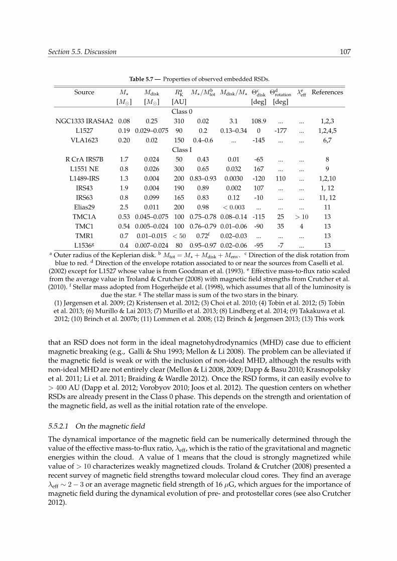
Section 5.5. Discussion 107
Table 5.7 — Properties of observed embedded RSDs.
Source M? Mdisk RaK M?/M
btot Mdisk/M? Θc
disk Θdrotation λe
eff References[M] [M] [AU] [deg] [deg]
Class 0NGC1333 IRAS4A2 0.08 0.25 310 0.02 3.1 108.9 ... ... 1,2,3
L1527 0.19 0.029–0.075 90 0.2 0.13–0.34 0 -177 ... 1,2,4,5VLA1623 0.20 0.02 150 0.4–0.6 ... -145 ... ... 6,7
Class IR CrA IRS7B 1.7 0.024 50 0.43 0.01 -65 ... ... 8
L1551 NE 0.8 0.026 300 0.65 0.032 167 ... ... 9L1489-IRS 1.3 0.004 200 0.83–0.93 0.0030 -120 110 ... 1,2,10
IRS43 1.9 0.004 190 0.89 0.002 107 ... ... 1, 12IRS63 0.8 0.099 165 0.83 0.12 -10 ... ... 11, 12
Elias29 2.5 0.011 200 0.98 < 0.003 ... ... ... 11TMC1A 0.53 0.045–0.075 100 0.75–0.78 0.08–0.14 -115 25 > 10 13TMC1 0.54 0.005–0.024 100 0.76–0.79 0.01–0.06 -90 35 4 13TMR1 0.7 0.01–0.015 < 50 0.72f 0.02–0.03 ... ... ... 13L1536g 0.4 0.007–0.024 80 0.95–0.97 0.02–0.06 -95 -7 ... 13
a Outer radius of the Keplerian disk. b Mtot = M? +Mdisk +Menv. c Direction of the disk rotation fromblue to red. d Direction of the envelope rotation associated to or near the sources from Caselli et al.
(2002) except for L1527 whose value is from Goodman et al. (1993). e Effective mass-to-flux ratio scaledfrom the average value in Troland & Crutcher (2008) with magnetic field strengths from Crutcher et al.(2010). f Stellar mass adopted from Hogerheijde et al. (1998), which assumes that all of the luminosity is
due the star. g The stellar mass is sum of the two stars in the binary.(1) Jørgensen et al. 2009; (2) Kristensen et al. 2012; (3) Choi et al. 2010; (4) Tobin et al. 2012; (5) Tobinet al. 2013; (6) Murillo & Lai 2013; (7) Murillo et al. 2013; (8) Lindberg et al. 2014; (9) Takakuwa et al.2012; (10) Brinch et al. 2007b; (11) Lommen et al. 2008; (12) Brinch & Jørgensen 2013; (13) This work
that an RSD does not form in the ideal magnetohydrodynamics (MHD) case due to efficientmagnetic breaking (e.g., Galli & Shu 1993; Mellon & Li 2008). The problem can be alleviated ifthe magnetic field is weak or with the inclusion of non-ideal MHD, although the results withnon-ideal MHD are not entirely clear (Mellon & Li 2008, 2009; Dapp & Basu 2010; Krasnopolskyet al. 2011; Li et al. 2011; Braiding & Wardle 2012). Once the RSD forms, it can easily evolve to> 400 AU (Dapp et al. 2012; Vorobyov 2010; Joos et al. 2012). The question centers on whetherRSDs are already present in the Class 0 phase. This depends on the strength and orientation ofthe magnetic field, as well as the initial rotation rate of the envelope.
5.5.2.1 On the magnetic field
The dynamical importance of the magnetic field can be numerically determined through thevalue of the effective mass-to-flux ratio, λeff, which is the ratio of the gravitational and magneticenergies within the cloud. A value of 1 means that the cloud is strongly magnetized whilevalue of > 10 characterizes weakly magnetized clouds. Troland & Crutcher (2008) presented arecent survey of magnetic field strengths toward molecular cloud cores. They find an averageλeff ∼ 2− 3 or an average magnetic field strength of 16 µG, which argues for the importance ofmagnetic field during the dynamical evolution of pre- and protostellar cores (see also Crutcher2012).
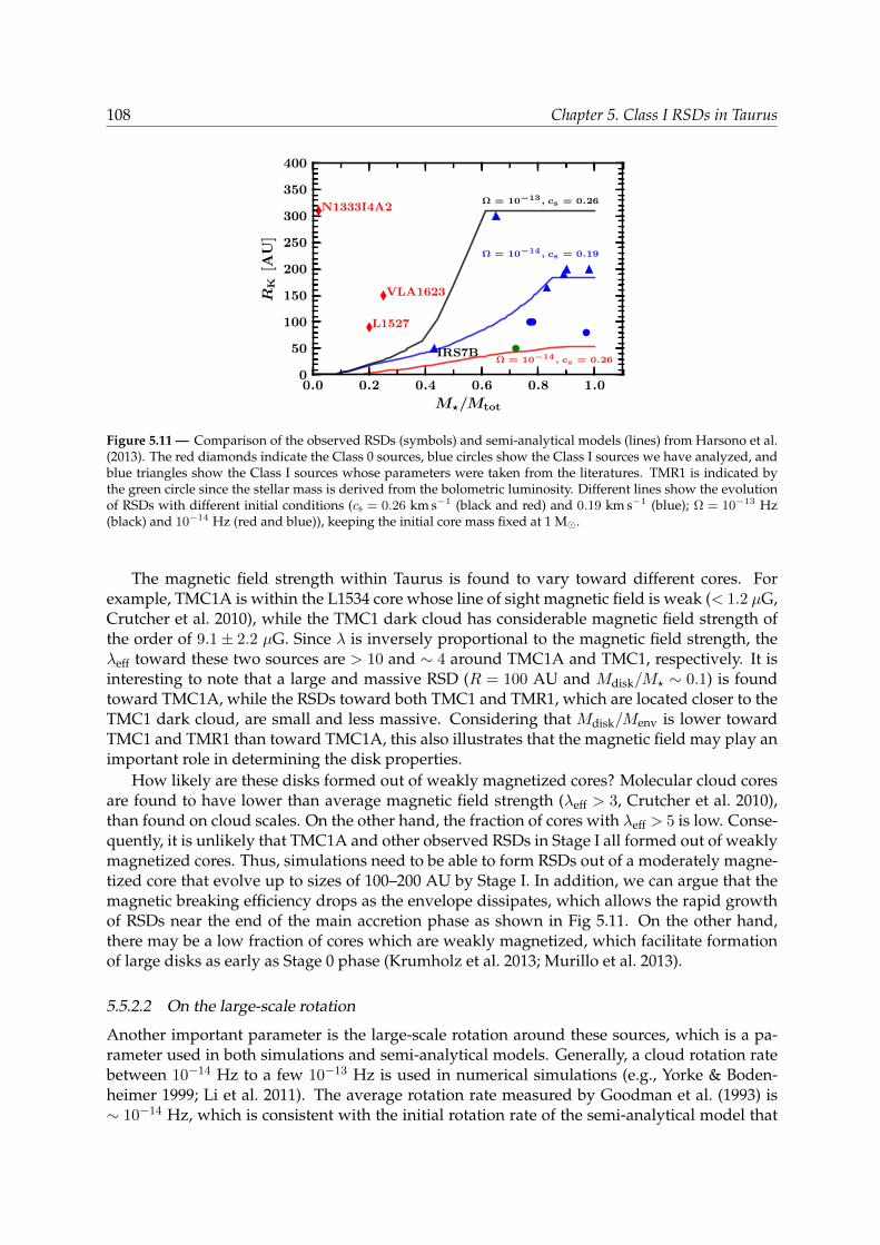
108 Chapter 5. Class I RSDs in Taurus
0.0 0.2 0.4 0.6 0.8 1.0
M?/Mtot
0
50
100
150
200
250
300
350
400
RK
[AU
]
Ω = 10−14, cs = 0.26
Ω = 10−14, cs = 0.19
Ω = 10−13, cs = 0.26N1333I4A2
L1527
VLA1623
IRS7B
Figure 5.11 — Comparison of the observed RSDs (symbols) and semi-analytical models (lines) from Harsono et al.(2013). The red diamonds indicate the Class 0 sources, blue circles show the Class I sources we have analyzed, andblue triangles show the Class I sources whose parameters were taken from the literatures. TMR1 is indicated bythe green circle since the stellar mass is derived from the bolometric luminosity. Different lines show the evolutionof RSDs with different initial conditions (cs = 0.26 km s−1 (black and red) and 0.19 km s−1 (blue); Ω = 10−13 Hz(black) and 10−14 Hz (red and blue)), keeping the initial core mass fixed at 1 M.
The magnetic field strength within Taurus is found to vary toward different cores. Forexample, TMC1A is within the L1534 core whose line of sight magnetic field is weak (< 1.2 µG,Crutcher et al. 2010), while the TMC1 dark cloud has considerable magnetic field strength ofthe order of 9.1± 2.2 µG. Since λ is inversely proportional to the magnetic field strength, theλeff toward these two sources are > 10 and ∼ 4 around TMC1A and TMC1, respectively. It isinteresting to note that a large and massive RSD (R = 100 AU and Mdisk/M? ∼ 0.1) is foundtoward TMC1A, while the RSDs toward both TMC1 and TMR1, which are located closer to theTMC1 dark cloud, are small and less massive. Considering that Mdisk/Menv is lower towardTMC1 and TMR1 than toward TMC1A, this also illustrates that the magnetic field may play animportant role in determining the disk properties.
How likely are these disks formed out of weakly magnetized cores? Molecular cloud coresare found to have lower than average magnetic field strength (λeff > 3, Crutcher et al. 2010),than found on cloud scales. On the other hand, the fraction of cores with λeff > 5 is low. Conse-quently, it is unlikely that TMC1A and other observed RSDs in Stage I all formed out of weaklymagnetized cores. Thus, simulations need to be able to form RSDs out of a moderately magne-tized core that evolve up to sizes of 100–200 AU by Stage I. In addition, we can argue that themagnetic breaking efficiency drops as the envelope dissipates, which allows the rapid growthof RSDs near the end of the main accretion phase as shown in Fig 5.11. On the other hand,there may be a low fraction of cores which are weakly magnetized, which facilitate formationof large disks as early as Stage 0 phase (Krumholz et al. 2013; Murillo et al. 2013).
5.5.2.2 On the large-scale rotation
Another important parameter is the large-scale rotation around these sources, which is a pa-rameter used in both simulations and semi-analytical models. Generally, a cloud rotation ratebetween 10−14 Hz to a few 10−13 Hz is used in numerical simulations (e.g., Yorke & Boden-heimer 1999; Li et al. 2011). The average rotation rate measured by Goodman et al. (1993) is∼ 10−14 Hz, which is consistent with the initial rotation rate of the semi-analytical model that
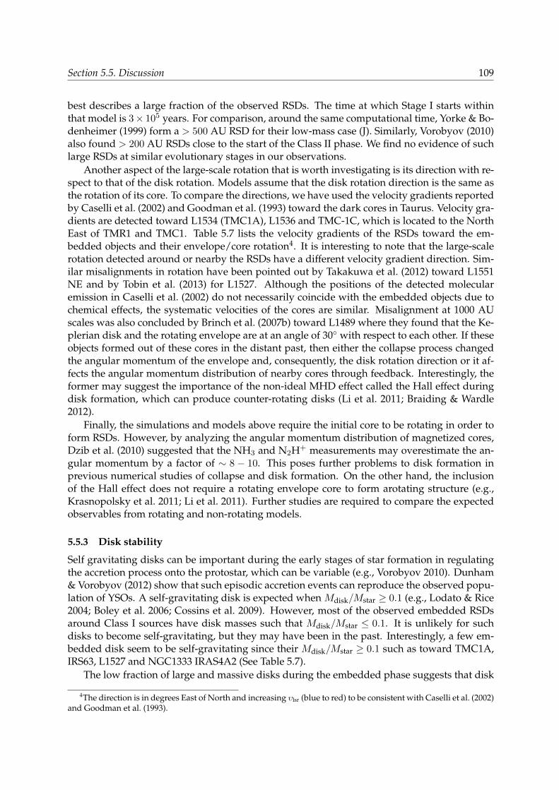
Section 5.5. Discussion 109
best describes a large fraction of the observed RSDs. The time at which Stage I starts withinthat model is 3× 10⁵ years. For comparison, around the same computational time, Yorke & Bo-denheimer (1999) form a > 500 AU RSD for their low-mass case (J). Similarly, Vorobyov (2010)also found > 200 AU RSDs close to the start of the Class II phase. We find no evidence of suchlarge RSDs at similar evolutionary stages in our observations.
Another aspect of the large-scale rotation that is worth investigating is its direction with re-spect to that of the disk rotation. Models assume that the disk rotation direction is the same asthe rotation of its core. To compare the directions, we have used the velocity gradients reportedby Caselli et al. (2002) and Goodman et al. (1993) toward the dark cores in Taurus. Velocity gra-dients are detected toward L1534 (TMC1A), L1536 and TMC-1C, which is located to the NorthEast of TMR1 and TMC1. Table 5.7 lists the velocity gradients of the RSDs toward the em-bedded objects and their envelope/core rotation4. It is interesting to note that the large-scalerotation detected around or nearby the RSDs have a different velocity gradient direction. Sim-ilar misalignments in rotation have been pointed out by Takakuwa et al. (2012) toward L1551NE and by Tobin et al. (2013) for L1527. Although the positions of the detected molecularemission in Caselli et al. (2002) do not necessarily coincide with the embedded objects due tochemical effects, the systematic velocities of the cores are similar. Misalignment at 1000 AUscales was also concluded by Brinch et al. (2007b) toward L1489 where they found that the Ke-plerian disk and the rotating envelope are at an angle of 30 with respect to each other. If theseobjects formed out of these cores in the distant past, then either the collapse process changedthe angular momentum of the envelope and, consequently, the disk rotation direction or it af-fects the angular momentum distribution of nearby cores through feedback. Interestingly, theformer may suggest the importance of the non-ideal MHD effect called the Hall effect duringdisk formation, which can produce counter-rotating disks (Li et al. 2011; Braiding & Wardle2012).
Finally, the simulations and models above require the initial core to be rotating in order toform RSDs. However, by analyzing the angular momentum distribution of magnetized cores,Dzib et al. (2010) suggested that the NH3 and N2H+ measurements may overestimate the an-gular momentum by a factor of ∼ 8 − 10. This poses further problems to disk formation inprevious numerical studies of collapse and disk formation. On the other hand, the inclusionof the Hall effect does not require a rotating envelope core to form arotating structure (e.g.,Krasnopolsky et al. 2011; Li et al. 2011). Further studies are required to compare the expectedobservables from rotating and non-rotating models.
5.5.3 Disk stability
Self gravitating disks can be important during the early stages of star formation in regulatingthe accretion process onto the protostar, which can be variable (e.g., Vorobyov 2010). Dunham& Vorobyov (2012) show that such episodic accretion events can reproduce the observed popu-lation of YSOs. A self-gravitating disk is expected when Mdisk/Mstar ≥ 0.1 (e.g., Lodato & Rice2004; Boley et al. 2006; Cossins et al. 2009). However, most of the observed embedded RSDsaround Class I sources have disk masses such that Mdisk/Mstar ≤ 0.1. It is unlikely for suchdisks to become self-gravitating, but they may have been in the past. Interestingly, a few em-bedded disk seem to be self-gravitating since their Mdisk/Mstar ≥ 0.1 such as toward TMC1A,IRS63, L1527 and NGC1333 IRAS4A2 (See Table 5.7).
The low fraction of large and massive disks during the embedded phase suggests that disk
4The direction is in degrees East of North and increasing υlsr (blue to red) to be consistent with Caselli et al. (2002)and Goodman et al. (1993).
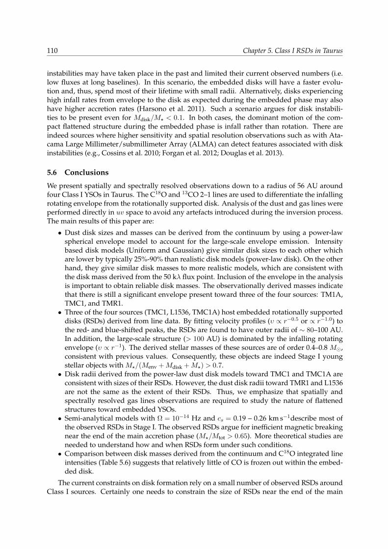
110 Chapter 5. Class I RSDs in Taurus
instabilities may have taken place in the past and limited their current observed numbers (i.e.low fluxes at long baselines). In this scenario, the embedded disks will have a faster evolu-tion and, thus, spend most of their lifetime with small radii. Alternatively, disks experiencinghigh infall rates from envelope to the disk as expected during the embedded phase may alsohave higher accretion rates (Harsono et al. 2011). Such a scenario argues for disk instabili-ties to be present even for Mdisk/M? < 0.1. In both cases, the dominant motion of the com-pact flattened structure during the embedded phase is infall rather than rotation. There areindeed sources where higher sensitivity and spatial resolution observations such as with Ata-cama Large Millimeter/submillimeter Array (ALMA) can detect features associated with diskinstabilities (e.g., Cossins et al. 2010; Forgan et al. 2012; Douglas et al. 2013).
5.6 Conclusions
We present spatially and spectrally resolved observations down to a radius of 56 AU aroundfour Class I YSOs in Taurus. The C18O and 13CO 2–1 lines are used to differentiate the infallingrotating envelope from the rotationally supported disk. Analysis of the dust and gas lines wereperformed directly in uv space to avoid any artefacts introduced during the inversion process.The main results of this paper are:
• Dust disk sizes and masses can be derived from the continuum by using a power-lawspherical envelope model to account for the large-scale envelope emission. Intensitybased disk models (Uniform and Gaussian) give similar disk sizes to each other whichare lower by typically 25%-90% than realistic disk models (power-law disk). On the otherhand, they give similar disk masses to more realistic models, which are consistent withthe disk mass derived from the 50 kλ flux point. Inclusion of the envelope in the analysisis important to obtain reliable disk masses. The observationally derived masses indicatethat there is still a significant envelope present toward three of the four sources: TM1A,TMC1, and TMR1.• Three of the four sources (TMC1, L1536, TMC1A) host embedded rotationally supported
disks (RSDs) derived from line data. By fitting velocity profiles (υ ∝ r−0.5 or ∝ r−1.0) tothe red- and blue-shifted peaks, the RSDs are found to have outer radii of ∼ 80–100 AU.In addition, the large-scale structure (> 100 AU) is dominated by the infalling rotatingenvelope (υ ∝ r−1). The derived stellar masses of these sources are of order 0.4–0.8 M,consistent with previous values. Consequently, these objects are indeed Stage I youngstellar objects with M?/(Menv +Mdisk +M?) > 0.7.• Disk radii derived from the power-law dust disk models toward TMC1 and TMC1A are
consistent with sizes of their RSDs. However, the dust disk radii toward TMR1 and L1536are not the same as the extent of their RSDs. Thus, we emphasize that spatially andspectrally resolved gas lines observations are required to study the nature of flattenedstructures toward embedded YSOs.• Semi-analytical models with Ω = 10−14 Hz and cs = 0.19 – 0.26 km s−1describe most of
the observed RSDs in Stage I. The observed RSDs argue for inefficient magnetic breakingnear the end of the main accretion phase (M?/Mtot > 0.65). More theoretical studies areneeded to understand how and when RSDs form under such conditions.• Comparison between disk masses derived from the continuum and C18O integrated line
intensities (Table 5.6) suggests that relatively little of CO is frozen out within the embed-ded disk.
The current constraints on disk formation rely on a small number of observed RSDs aroundClass I sources. Certainly one needs to constrain the size of RSDs near the end of the main
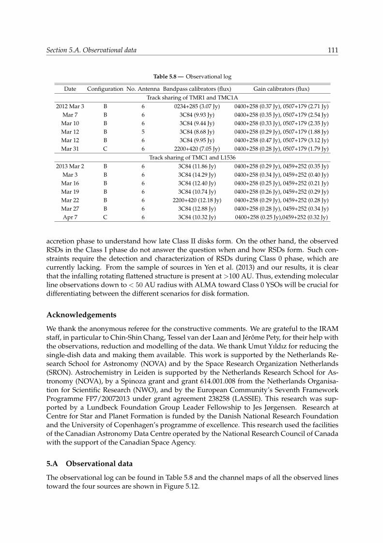
Section 5.A. Observational data 111
Table 5.8 — Observational log
Date Configuration No. Antenna Bandpass calibrators (flux) Gain calibrators (flux)Track sharing of TMR1 and TMC1A
2012 Mar 3 B 6 0234+285 (3.07 Jy) 0400+258 (0.37 Jy), 0507+179 (2.71 Jy)Mar 7 B 6 3C84 (9.93 Jy) 0400+258 (0.35 Jy), 0507+179 (2.54 Jy)Mar 10 B 6 3C84 (9.44 Jy) 0400+258 (0.33 Jy), 0507+179 (2.35 Jy)Mar 12 B 5 3C84 (8.68 Jy) 0400+258 (0.29 Jy), 0507+179 (1.88 Jy)Mar 12 B 6 3C84 (9.95 Jy) 0400+258 (0.47 Jy), 0507+179 (3.12 Jy)Mar 31 C 6 2200+420 (7.05 Jy) 0400+258 (0.28 Jy), 0507+179 (1.79 Jy)
Track sharing of TMC1 and L15362013 Mar 2 B 6 3C84 (11.86 Jy) 0400+258 (0.29 Jy), 0459+252 (0.35 Jy)
Mar 3 B 6 3C84 (14.29 Jy) 0400+258 (0.34 Jy), 0459+252 (0.40 Jy)Mar 16 B 6 3C84 (12.40 Jy) 0400+258 (0.25 Jy), 0459+252 (0.21 Jy)Mar 19 B 6 3C84 (10.74 Jy) 0400+258 (0.26 Jy), 0459+252 (0.29 Jy)Mar 22 B 6 2200+420 (12.18 Jy) 0400+258 (0.29 Jy), 0459+252 (0.28 Jy)Mar 27 B 6 3C84 (12.88 Jy) 0400+258 (0.28 Jy), 0459+252 (0.34 Jy)Apr 7 C 6 3C84 (10.32 Jy) 0400+258 (0.25 Jy),0459+252 (0.32 Jy)
accretion phase to understand how late Class II disks form. On the other hand, the observedRSDs in the Class I phase do not answer the question when and how RSDs form. Such con-straints require the detection and characterization of RSDs during Class 0 phase, which arecurrently lacking. From the sample of sources in Yen et al. (2013) and our results, it is clearthat the infalling rotating flattened structure is present at >100 AU. Thus, extending molecularline observations down to < 50 AU radius with ALMA toward Class 0 YSOs will be crucial fordifferentiating between the different scenarios for disk formation.
Acknowledgements
We thank the anonymous referee for the constructive comments. We are grateful to the IRAMstaff, in particular to Chin-Shin Chang, Tessel van der Laan and Jerome Pety, for their help withthe observations, reduction and modelling of the data. We thank Umut Yıldız for reducing thesingle-dish data and making them available. This work is supported by the Netherlands Re-search School for Astronomy (NOVA) and by the Space Research Organization Netherlands(SRON). Astrochemistry in Leiden is supported by the Netherlands Research School for As-tronomy (NOVA), by a Spinoza grant and grant 614.001.008 from the Netherlands Organisa-tion for Scientific Research (NWO), and by the European Community’s Seventh FrameworkProgramme FP7/20072013 under grant agreement 238258 (LASSIE). This research was sup-ported by a Lundbeck Foundation Group Leader Fellowship to Jes Jørgensen. Research atCentre for Star and Planet Formation is funded by the Danish National Research Foundationand the University of Copenhagen’s programme of excellence. This research used the facilitiesof the Canadian Astronomy Data Centre operated by the National Research Council of Canadawith the support of the Canadian Space Agency.
5.A Observational data
The observational log can be found in Table 5.8 and the channel maps of all the observed linestoward the four sources are shown in Figure 5.12.

112 Chapter 5. Class I RSDs in Taurus
−4
−2
0
2
4 3.6 4.1 4.6
−4
−2
0
2
4 5.2 5.7 6.2
−4−2024
RA Offset [arcsec]
−4
−2
0
2
4
Dec
Off
set
[arcse
c]
6.8
−4−2024
7.3100 AU
−4−2024
7.8
−4
−2
0
2
4 3.6 4.1 4.6
−4
−2
0
2
4 5.2 5.7 6.2
−4−2024
RA Offset [arcsec]
−4
−2
0
2
4
Dec
Off
set
[arcse
c]
6.8
−4−2024
7.3100 AU
−4−2024
7.8
−4
−2
0
2
4 2.8 3.4 4.0
−4
−2
0
2
4 4.7 5.3 5.9
−4−2024
RA Offset [arcsec]
−4
−2
0
2
4
Dec
Off
set
[arcse
c]
6.6
−4−2024
7.2100 AU
−4−2024
7.9
−4
−2
0
2
4 2.8 3.4 4.0
−4
−2
0
2
4 4.7 5.3 6.0
−4−2024
RA Offset [arcsec]
−4
−2
0
2
4
Dec
Off
set
[arcse
c]
6.6
−4−2024
7.2100 AU
−4−2024
7.9
−4
−2
0
2
4 2.3 3.1 4.0
−4
−2
0
2
4 4.8 5.7 6.5
−4−2024
RA Offset [arcsec]
−4
−2
0
2
4
Dec
Off
set
[arcse
c]
7.4
−4−2024
8.2100 AU
−4−2024
9.1
−4
−2
0
2
4 2.3 3.1 4.0
−4
−2
0
2
4 4.8 5.7 6.5
−4−2024
RA Offset [arcsec]
−4
−2
0
2
4
Dec
Off
set
[arcse
c]
7.4
−4−2024
8.2100 AU
−4−2024
9.1
Figure 5.12 — Top left: 13CO 2–1 channel maps similar to Fig. 5.3 toward TMC1. Top middle: C18O 2–1 channel mapstoward TMC1. Top right: 13CO 2–1 channel maps toward TMR1. Bottom left: C18O 2–1 channel maps toward TMR1.Bottom middle: 13CO 2–1 channel maps toward L1536. Bottom right: C18O 2–1 channel maps toward L1536.
Table 5.9 — 1D spherical envelope parameters as published by Kristensen et al. (2012).
Source p Y a rin nin n(1000AU)
[AU] [cm−3] [cm−3]TMC1 1.1 1800 3.7 8.5× 10⁷ 1.8× 10⁵
TMR1 1.6 900 8.8 4.1× 10⁸ 2.1× 10⁵
TMC1A 1.6 900 7.7 5.2× 10⁸ 2.2× 10⁵
a Y = rout/rin.
5.B Large-scale structure
The parameters of the large-scale envelope structure used to estimate the continuum emissionat short baselines are in Table 5.9.
5.C WideX data
Spectra toward all sources integrated within a 3 ′′ box around their continuum positions areshown in Fig. 5.13. The integrated flux density maps toward C18O, SO 56 − 45 and SO2 11111 −10010 (221.96521 GHz) are shown in Fig. 5.15. The SO emission toward all sources is much moreextended compared to the C18O emission, while the SO2 emission is compact.
5.D L1536
Figure 5.16 shows the 12CO J =3–2 spectral map obtained with JCMT, where there is no indi-cation of classical bipolar outflows are present.
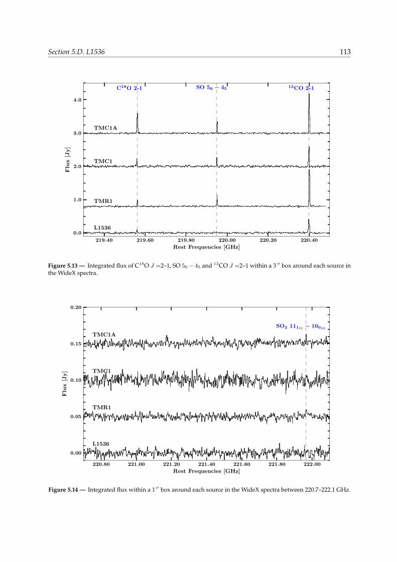
Section 5.D. L1536 113
219.40 219.60 219.80 220.00 220.20 220.40
Rest Frequencies [GHz]
0.0
1.0
2.0
3.0
4.0
Flu
x[J
y]
C18O 2-1 13CO 2-1SO 56 − 45
TMC1A
TMC1
TMR1
L1536
Figure 5.13 — Integrated flux of C18O J =2–1, SO 56 − 45 and 13CO J =2–1 within a 3 ′′ box around each source inthe WideX spectra.
220.80 221.00 221.20 221.40 221.60 221.80 222.00
Rest Frequencies [GHz]
0.00
0.05
0.10
0.15
0.20
Flu
x[J
y]
SO2 11111 − 10010
TMC1A
TMC1
TMR1
L1536
Figure 5.14 — Integrated flux within a 1 ′′ box around each source in the WideX spectra between 220.7–222.1 GHz.
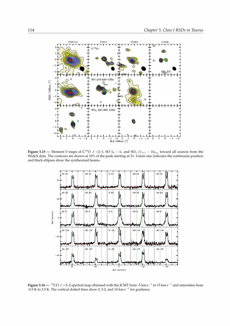
114 Chapter 5. Class I RSDs in Taurus
−2
−1
0
1
2
TMC1A
−2
−1
0
1
2
DE
CO
ffse
t[′′ ]
−2−1012
−2
−1
0
1
2
C18O
TMC1
SO 219.949 GHz
−2−1012
SO2 221.965 GHz
TMR1
−2−1012
RA Offset [′′]
100 AU
L1536
−2−1012
Figure 5.15 — Moment 0 maps of C18O J =2–1, SO 56 − 45 and SO2 11111 − 10010 toward all sources from theWideX data. The contours are drawn at 10% of the peak starting at 3σ. Green star indicates the continuum positionand black ellipses show the synthesized beams.
40 41
40 22
40 0
40 -18
40 -37
20 41
20 22
20 0
20 -18
20 -37
0 41
0 22
0 0
0 -18
0 -37
-20 41
-20 22
-20 0
-20 -18
-20 -37
-40 41
-40 22
-40 0
-40 -18
-40 -37
−40−2002040
∆α [arcsec]
−40
−20
0
20
40
∆δ
[arcse
c]
Figure 5.16 — 12CO J =3–2 spectral map obtained with the JCMT from -5 km s−1 to 15 km s−1 and intensities from-0.5 K to 3.5 K. The vertical dotted lines show 0, 5.2, and 10 km s−1 for guidance.
Chapter 6Volatile snowlines in embedded disks
around low-mass protostars
Abstract. Context. Models of the young solar nebula assume that the disk is hot initially such thatmost volatiles are in the gas phase. Water emission arising from within 50 AU radius has been detectedaround low-mass embedded young stellar objects. The question remains whether an actively accretingdisk can be warm enough to have gas-phase water up to 50 AU radius. No detailed studies have yetbeen performed on the extent of snowlines in an accreting disk embedded in a dense envelope (Stage 0).Aims. Quantify the location of gas-phase volatiles in the inner envelope and disk system for an activelyaccreting embedded disk.Methods. Two-dimensional physical and radiative transfer models have been used to calculate the tem-perature structure of embedded protostellar systems. The heating due to viscous accretion is addedthrough the diffusion approximation. Gas and ice abundances of H2O, CO2, and CO are calculated us-ing the density dependent thermal desorption formulation.Results. The midplane water snowline increases from 5 to ∼ 30 AU for accretion rates between 10−9–10−4 M yr−1. CO2 can remain in the solid phase within the disk for M ≤ 10−5 M yr−1 down to ∼ 40AU. CO is always in the gas phase for an actively accreting disk independent of disk properties and ac-cretion rate. The predicted optically thin water emission is consistent with the detected water emissiontoward the Stage 0 embedded young stellar objects. An accreting embedded disk can only account forwater emission arising from R < 50 AU, however, and drops rapidly for M ≤ 10−5 Myr−1. Thus, thisextent can be tested with future ALMA observations.Conclusion. Volatiles such as H2O, CH3OH, and CO2 sublimate out to 30 AU in the midplane in youngdisks and, thus, can reset the chemical content inherited from the envelope. A hot young solar nebulaout to 30 AU can only have occurred during the deeply embedded Stage 0, not during the T Tauri phaseof our early solar system.
D. Harsono, S. Bruderer, E. F. van Dishoeckin prep.
6.1 Introduction
The snowlines of various volatiles play a major role for planet formation. Beyond the snow-line, the high abundances of solids allow for efficient sticking to form larger bodies. Thus, theamount of larger bodies is increased by the presence of ices (e.g. Stevenson & Lunine 1988; Ros& Johansen 2013). Extensive studies have investigated the snowline in protoplanetary disksaround pre-main-sequence stars during which supposedly the solar system was formed (e.g.Lissauer 1987; Pollack et al. 1996). It is thought the early pre-solar nebula was (> 1500 K) suchthat both volatiles and refractories are in the gas phase (Cassen 2001; Scott 2007). This pushesthe water snowline up to beyond a few AU radius. The evidences of such a hot solar nebulacome from the history of the refractories, however the volatile content of comets seems to in-dicate that a part of the disk remains cold (see Pontoppidan et al. 2014). The evolution of the
116 Chapter 6. Volatile snowlines
snowline due to disk and star evolution and its accretion rate affect the chemical compositionin the region relevant to planet formation (e.g., Lodders 2004; Davis 2005; Oberg et al. 2011b).The most relevant volatiles are the known major ice species, H2O, CO2, and CO. Observationsand theoretical models of protoplanetary disks around pre-main sequence T-Tauri stars are notwarm enough to have gas-phase volatiles in the midplane beyond 30 AU and for the case ofH2O, only a few AU (e.g., D’Alessio et al. 1998; Dullemond et al. 2007). Such high temperatureat large radii could potentially only be achieved during the deeply embedded phase of starformation when the accretion rate is high. The question remains how hot can an embeddedaccreting disk become due to its high accretion rate (≥ 10−6 M yr−1, Dunham et al. 2014).
Spatially resolved warm water emission (Tex ∼ 120 K, Persson et al. 2014) has been recentlydetected from within the inner 50 AU radius of several deeply embedded (Class 0) low-massprotostars (e.g., Jørgensen & van Dishoeck 2010b; Persson et al. 2012). These are very youngobjects whose envelope mass is substantially larger than the mass at smaller scales (also de-noted as Stage 0, Robitaille et al. 2006). The emission is expected to arise from Tdust > 100 Kregions where the gas-phase water abundance is at its maximum (Fraser et al. 2001; Aikawaet al. 2008; Mottram et al. 2013). This inner region is, however, also where the disk forms (Lar-son 2003; Williams & Cieza 2011; Li et al. 2014a). Rotationally supported disks (RSDs) havebeen detected recently around low-mass protostars (e.g., Tobin et al. 2012; Murillo et al. 2013).This paper studies the volatiles content in such embedded disks to investigate the location oftheir snowlines when the accretional heating is included.
Direct observational evidence of snowlines of the major ice species toward protoplanetarydisks around pre-main sequence stars rely on the chemical changes that occur when a moleculeis absent from the gas phase. The commonly observed snowline is that of CO through thedetection of DCO+ and N2H+ lines, which are both destroyed in reactions with CO (e.g. vanDishoeck et al. 2003; Guilloteau et al. 2006; Qi et al. 2008; Mathews et al. 2013; Qi et al. 2013).The CO snowline location with respect to water and CO2 snowlines have direct impact on theamount of water present in giant planets atmospheres (Madhusudhan et al. 2011; Moses et al.2013). The water snowline has been inferred to be within a few AU from direct observation ofmid-infrared water lines (Pontoppidan et al. 2010; Zhang et al. 2013). Thus, significant progresshas been made in identifying snowlines in protoplanetary disks in the later stages and theirlocation with respect to gas giant formation (e.g., Kennedy & Kenyon 2008; Pontoppidan et al.2014). Yet, the accretion process through the disk begins in the early stages of star formation atthe time that the disk itself is forming. The amount of gaseous volatiles within embedded disksis, therefore, affected by their formation process which results in different chemical structuresof the emerging protoplanetary disks (Visser et al. 2011). A related question centers whetherthese volatiles are ‘inherited’ or ‘reset’ during the planet formation process (Pontoppidan et al.2014). The ‘reset’ scenario refers to the chemical processing of ices as the gas and dust areexposed to elevated temperatures (> 40 K) during their voyage from the envelope to the disk.
Water is the key volatile in star and planet formation; it is also the major constituent of iceson the grains that facilitate planet formation (Gibb et al. 2004; Oberg et al. 2011a) and a majorcoolant (Karska et al. 2013). Most of the water is formed during the pre-stellar stage, and thentransported through the envelope into the disk and planets. Tracing the water history fromearly stages of star formation to planet forming regions hints at the origin of water in planets(van Dishoeck et al. 2014). The crucial step that is yet relatively unexplored is the processing ofwater during the disk formation process.
The water vapor content around protostars is investigated by the ‘Water In Star-formingregions with Herschel’ key program (WISH, van Dishoeck et al. 2011). Due to the large beamof Herschel, a significant fraction of the detected water emission is from the large-scale envelope
Section 6.2. Physical and chemical structures 117
and the bipolar outflow (Kristensen et al. 2012; Herczeg et al. 2012; Mottram et al. 2014). Moreimportantly, most of the detected water emission comes from water in the outflow that willescape the system and will not be retained by the disk. In order to determine the amount ofwater vapor associated with the inner envelope or disk, an isotopolog of warm water (H18
2 O)was observed toward a few low-mass embedded protostars. Visser et al. (2013) reported adetection of the H18
2 O line (1096 GHz) with HIFI (de Graauw et al. 2010) toward the embeddedprotostar NGC 1333 IRAS2A. However, they found that the line is still optically thick with anemitting region of ∼ 100 AU. Thus, it remains difficult to constrain the amount of water vaporin embedded disks with single-dish observations.
Although H162 O line emission cannot be observed from the ground, except for masers, a
few of the rotational transitions of its isotopologs are observable such as H182 O and deuterated
water (HDO). Furthermore, interferometric facilities such as the Plateau de Bure Interferometry(PdBI) and the Submillimeter Array (SMA) can spatially and spectrally resolve these lines.With those facilities, Jørgensen & van Dishoeck (2010a,b) detected H18
2 O and HDO emissionoriginating from within the inner 25 AU radius of a Class 0 low-mass protostar. More recently,spatially and spectrally resolved warm water emission has been detected toward four low-massembedded protostars with the PdBI (Persson et al. 2012, 2013) and toward one high mass disk(van der Tak et al. 2006; Wang et al. 2012). From the kinematical information, both Jørgensen& van Dishoeck (2010b) and Persson et al. (2012) found that the water emission does not showKeplerian motion and concluded that it must be emitted from a flattened disk-like structurethat is still dominated by the radial infalling motions.
This paper investigates snowlines of volatiles within an accreting disk embedded in a mas-sive envelope. The spatial extent and the water vapor emission are compared with the ob-served values toward three deeply embedded protostars. The thermal structure of an activelyaccreting disk is computed including the additional heating due to the energy released fromthe viscous dissipation. Most previous studies of the thermal structure of an accreting diskfocused on the later evolutionary stage of disk evolution where the envelope has largely dissi-pated away. Furthermore, they focused on the midplane temperature structure (e.g., Sasselov& Lecar 2000; Lecar et al. 2006; Kennedy & Kenyon 2008). This additional heating shifts thesnowlines of volatiles outward to larger radii than in disks around pre-main sequence stars(Davis 2005; Garaud & Lin 2007; Min et al. 2011). The details of the physical and chemicalstructure of the embedded disk are presented in Section 6.2. Section 6.3 presents the snowlineslocation as function of disk and stellar properties. The results are compared with observationsand discussed in Section 6.4. Section 6.5 summarizes the main results and conclusions.
6.2 Physical and chemical structures
6.2.1 Physical structure
A simple parametrized embedded disk (disk + flattened envelope) model is used to constructthe density structure following Crapsi et al. (2008). The main parameters are disk mass (Mdisk)and disk radius (Rdisk). A number of parameters defining the envelope and the disk are fixedand summarized in Table 6.1. Through the combined continuum spectral energy distributionand submm continuum images modelling, the envelope masses toward the observed embed-ded sources (NGC1333 IRAS2A, IRAS4A, and IRAS4B) are found to be between 3 – 5M (Kris-tensen et al. 2012). For this purpose, the envelope mass is fixed at 1 M, which is appropriatefor the objects from which the water emission has been detected (Jørgensen et al. 2009; Kris-tensen et al. 2012).
For the large-scale envelope, a flattened envelope due to rotation as described by Ulrich
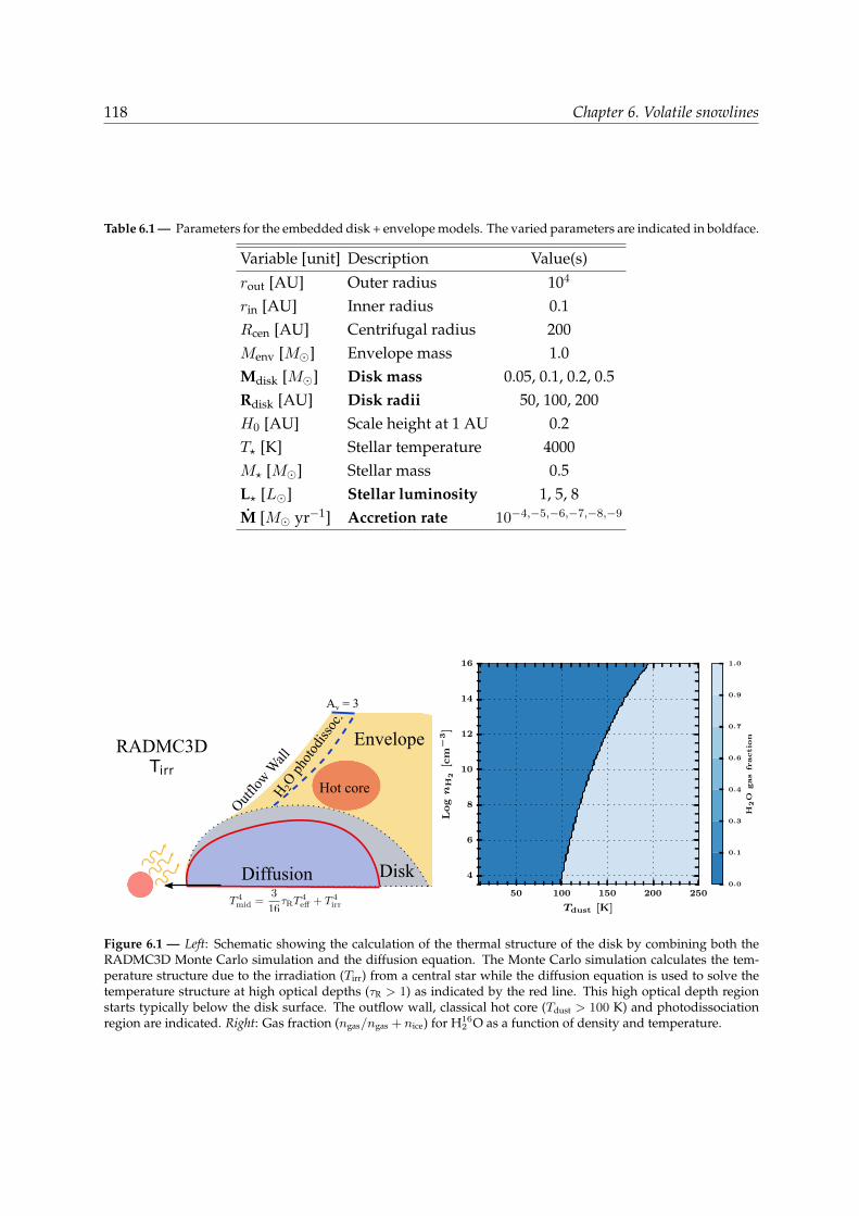
118 Chapter 6. Volatile snowlines
Table 6.1 — Parameters for the embedded disk + envelope models. The varied parameters are indicated in boldface.
Variable [unit] Description Value(s)rout [AU] Outer radius 104
rin [AU] Inner radius 0.1Rcen [AU] Centrifugal radius 200Menv [M] Envelope mass 1.0Mdisk [M] Disk mass 0.05, 0.1, 0.2, 0.5Rdisk [AU] Disk radii 50, 100, 200H0 [AU] Scale height at 1 AU 0.2T? [K] Stellar temperature 4000M? [M] Stellar mass 0.5L? [L] Stellar luminosity 1, 5, 8M [M yr−1] Accretion rate 10−4,−5,−6,−7,−8,−9
Diffusion
RADMC3D
Disk
Envelope
Tirr
Outflo
w Wall
H 2O
pho
todi
ssoc
.
Av = 3
Hot core
50 100 150 200 250
Tdust [K]
4
6
8
10
12
14
16
Logn
H2
[cm−
3]
0.0
0.1
0.3
0.4
0.6
0.7
0.9
1.0
H2O
gas
fractio
n
Figure 6.1 — Left: Schematic showing the calculation of the thermal structure of the disk by combining both theRADMC3D Monte Carlo simulation and the diffusion equation. The Monte Carlo simulation calculates the tem-perature structure due to the irradiation (Tirr) from a central star while the diffusion equation is used to solve thetemperature structure at high optical depths (τR > 1) as indicated by the red line. This high optical depth regionstarts typically below the disk surface. The outflow wall, classical hot core (Tdust > 100 K) and photodissociationregion are indicated. Right: Gas fraction (ngas/ngas + nice) for H16
2 O as a function of density and temperature.
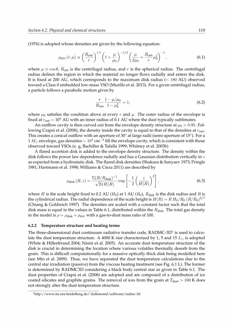
Section 6.2. Physical and chemical structures 119
(1976) is adopted whose densities are given by the following equation:
ρenv (r,µ) ∝(Rcen
r
)1.5(1 +
µ
µ0
)−1/2( µ
2µ0+Rcen
rµ2
0
)−1
, (6.1)
where µ ≡ cosθ, Rcen is the centrifugal radius, and r is the spherical radius. The centrifugalradius defines the region in which the material no longer flows radially and enters the disk.It is fixed at 200 AU, which corresponds to the maximum disk radius (∼ 180 AU) observedtoward a Class 0 embedded low-mass YSO (Murillo et al. 2013). For a given centrifugal radius,a particle follows a parabolic motion given by
r
Rcen
1− µ/µ0
1− µ20
= 1, (6.2)
where µ0 satisfies the condition above at every r and µ. The outer radius of the envelope isfixed at rout = 104 AU with an inner radius of 0.1 AU where the dust typically sublimates.
An outflow cavity is then carved out from the envelope density structure at µ0 > 0.95. Fol-lowing Crapsi et al. (2008), the density inside the cavity is equal to that of the densities at rout.This creates a conical outflow with an aperture of 30 at large radii (semi-aperture of 15). For a1M envelope, gas densities∼ 104 cm−3 fill the envelope cavity, which is consistent with thoseobserved toward YSOs (e. g, Bachiller & Tafalla 1999; Whitney et al. 2003b)
A flared accretion disk is added to the envelope density structure. The density within thedisk follows the power law dependence radially and has a Gaussian distribution vertically in zas expected from a hydrostatic disk. The flared disk densities (Shakura & Sunyaev 1973; Pringle1981; Hartmann et al. 1998; Williams & Cieza 2011) are described by
ρdisk (R,z) =Σ(R/Rdisk)−1
√2πH(R)
exp
[−1
2
(z
H(R)
)2], (6.3)
where H is the scale height fixed to 0.2 AU (H0) at 1 AU (R0), Rdisk is the disk radius and R isthe cylindrical radius. The radial dependence of the scale height is H(R) =RH0/R0 (R/R0)2/7
(Chiang & Goldreich 1997). The densities are scaled with a constant factor such that the totaldisk mass is equal to the values in Table 6.1, distributed within the Rdisk. The total gas densityin the model is ρ = ρdisk + ρenv with a gas-to-dust mass ratio of 100.
6.2.2 Temperature structure and heating terms
The three-dimensional dust continuum radiative transfer code, RADMC-3D1 is used to calcu-late the dust temperature structure. A 4000 K star characterized by 1, 5 and 15 L is adopted(White & Hillenbrand 2004; Nisini et al. 2005). An accurate dust temperature structure of thedisk is crucial in determining the location where various volatiles thermally desorb from thegrain. This is difficult computationally for a massive optically thick disk being modelled here(see Min et al. 2009). Thus, we have separated the dust temperature calculations due to thecentral star irradiation (passive) from the viscous heating treatment (see Fig. 6.1 L). The formeris determined by RADMC3D considering a black body central star as given in Table 6.1. Thedust properties of Crapsi et al. (2008) are adopted and are composed of a distribution of icecoated silicates and graphite grains. The removal of ices from the grain at Tdust > 100 K doesnot strongly alter the dust temperature structure.
1http://www.ita.uni-heidelberg.de/˜dullemond/software/radmc-3d

120 Chapter 6. Volatile snowlines
An actively accreting disk provides additional heating from the loss of mechanical en-ergy as the gas flows inward. The steady state accretion rate is typically between 10−5 −10−7 M yr−1 (Hueso & Guillot 2005). However, episodic accretion events such as those simu-lated by Vorobyov (2009) can have transient spikes with an accretion rate up to 10−4 M yr−1.Thus, disk accretion rates between 10−9–10−4 M yr−1 are adopted following the α disk for-malism (Shakura & Sunyaev 1973; Williams & Cieza 2011). The viscous heating rate per volumeis given by
Qvisc =9
4ρdiskvΩ2, (6.4)
where v = αcsH is the α dependent turbulent viscosity parameter, cs is the sound speed of thegas, and Ω is the Keplerian angular velocity. At steady state, the viscosity is related to the diskmass and the accretion rate through (Lodato 2008):
M = 3πvΣ. (6.5)
To explore the amount of heating, the viscosity term v is varied for the explored accretion ratesat a fixed disk mass. The effective temperature (Tvisc) associated with the total energy releasedat the inner radius assuming a hydrostatic disk is
σSBT4visc (R) =
∫Qvisc (R)dz =
3
8π
GM?
R3M
(1−
√R?R
). (6.6)
This is obtained by integrating over the viscous heating terms vertically for each radius. Fur-thermore, Tvisc is the effective temperature of the disk at the optically thin photosphere withoutthe addition of stellar irradiation. However, the real temperature at the midplane of an activedisk is proportional to the optical depth (Hubeny 1990): T 4
mid ∼ κRΣgasT4visc with κR the Rosse-
land mean opacity which results in higher midplane temperatures. Such a method is similarto that of Kennedy & Kenyon (2008) and Hueso & Guillot (2005) in the optically thick regime.Note that the heating from the accreting disk is caused by dissipation of energy of both gas anddust. To account for the irradiation from the accreting disk, Lvisc =
∫πσTvisc(R)4RdR is added
to the central luminosity L? by determining its blackbody spectrum at Tvisc at all radii.The following steps are taken to calculate the dust temperature of an accreting embedded
disk.• Monte Carlo dust continuum radiative transfer is used to simulate the photon propaga-
tion to determine the passively heated dust temperature structure (Tirr) due to the stellarluminosity (L? +Lvisc).• Viscous heating is added to the region of the disk where τR > 1. This is done by fixing the
midplane temperatures to Tmid =(
316κRΣgasT
4visc + T 4
irr)1/4. The vertical dust temperature
structure is calculated using the diffusion approximation∇D∇T 4 = 0 bounded by Tirr atthe surface and Tmid at the midplane where D = (3ρdustκR)−1. The diffusion is performedwithin the τR > 1 regions.
The addition of the viscous heating can increase the dust temperatures to > 2000 K. The typicaldust vaporization temperature is ∼ 1500 K, therefore, we have limited the dust temperatureto 1500 K. Gas opacities in the inner disk is not taken into account, which will affect the exacttemperature in that region. This does not change the location of the snowlines since they aredefined by dust temperatures Tdust ≤ 160 K.
The snowlines of protoplanetary disks without an envelope were obtained (see Fig. 6.8) andcompared with Min et al. (2011) to verify our approach. Using this formulation, the differencesin predicted water snowlines are typically within 2 AU at high accretion rates.

Section 6.3. Results 121
6.2.3 Molecular abundances
The aim of this paper is to calculate the 2D snowlines or snow ‘surfaces’ for CO, CO2, andH16
2 O in embedded disks. The region in which these volatiles freeze-out onto grains dependson the temperature and density structure. At steady state, the rate at which the molecule isadsorbed on the grain, Rads, is balanced by the thermal desorption rate, Rdes. The adsorptionrate is given by
Rads = nXndustπa2dust
√3kBTgas/mX, (6.7)
where mX is the molecular mass, nX is the number density of the molecule, Tgas is the gastemperature, ndust = 10−12 nH is the dust number density (Visser et al. 2009) with adust = 0.1 µmas the effective grain size, and kB is the Boltzmann constant. The thermal desorption rate is
Rthdes = 4πa2dustndustν1 exp(−Eb/kBTdust)ξ, (6.8)
where ν1 is the first-order pre-exponential factor as calculated from the binding energy, Eb(Hasegawa et al. 1992; Walsh et al. 2010)
ν1 =
√2NssEb
π2mXs−1 (6.9)
with the number of binding sites, Nss taken to be 8× 1014 cm−2 for a 0.1 µm grain followingVisser et al. (2011), and Tdust the dust temperature. A dimensionless factor ξ is used to switchbetween zeroth order to first order desorption when the ice thickness is less than a monolayer:
ξ =nice
max(nice,Nbndust)(6.10)
with Nb = 106 the number of binding sites per dust grain. The properties for each molecule aregiven in Table 6.2 along with the calculated pre-exponential factor ν1. These binding energiesassume pure ices. Figure 6.1 (R) shows an example of the gas fraction for water at differentdensities and temperatures. At steady state, the number density of solids of speciesX is simplygiven by
nice
ngas=ndustπa
2dust
(3kBTgas/mX
)1/2
ν1 exp (−Eb/Tdust) ξ. (6.11)
The typical timescales for adsorption are 4− 6× 10³ year at temperature of 50 K and numberdensities of 106 cm−3. This implies that the steady state assumption is not valid at lower densi-ties present in the large-scale envelope (r > 1000 AU) where the freeze-out timescales becomeslonger than the lifetime of the core (e.g., Jørgensen et al. 2005b). On the other hand, this paperfocuses on the gas phase abundances at small-scales r ≤ 100 AU where the number densitiesare nH > 106 cm−3. Photodesorption can be ignored at such high densities and within the disk,but it may be important at the disk’s surface and along the outflow cavity wall. Since the wa-ter vapor will also be rapidly photodissociated in those locations, these regions are not majorwater reservoirs (see Fig. 6.1 L). To approximate this region, water is assumed not to be presentwithin a region that is characterized by AV ≤ 3 or NH ≤ 6× 1021 cm−2. A more detailed gasphase abundance structure through a chemical network will be explored in the future.

122 Chapter 6. Volatile snowlines
Table 6.2 — Molecular parameters to calculateRdes.
Molecule νa1 Eb Refs.
[s−1] [K]CO 6.4× 10¹¹ 855 Bisschop et al. 2006CO2 8.2× 10¹¹ 2400 Burke & Brown 2010H16
2 O 2.1× 10¹² 5773 Fraser et al. 2001a First order desorption pre-exponential factor calculated from the binding energies.
0.0 0.1 0.2 0.3 0.4 0.5 0.6 0.7 0.8z/r
102
103
r = 1 AU
r = 5 AU
r = 25 AU
Mdisk = 0.1 MM = 10−5 M yr−1
1 10 100
R [AU]
101
102
103
Tdust
[K]
Tirr
Tvisc
Teff
0.0 0.1 0.2 0.3 0.4 0.5 0.6 0.7 0.8
z/r
102
103
Tdust
[K]
r = 1 AU
r = 5 AU
r = 25 AU
Mdisk = 0.1 M
M = 10−5 M yr−1
Disk
Embedded
Figure 6.2 — Left: Midplane radial (bottom) and vertical temperatures (top) at 1, 5, and 25 AU for a 0.1 M diskand an accretion rate of 10−5 M yr−1. The red dashed (bottom) and solid (top) lines indicate the thermal structureof a passively irradiated disk (Tirr) calculated by the Monte Carlo simulation. The blue solid lines indicate thetemperatures including the viscous heating (Teff =
(316κRΣgasT
4visc + T 4
irr)1/4). The viscous temperature as calculated
from Eq. 6.6 is indicated by the dotted blue lines. Right: Comparison of the vertical temperature structure at 1,5 and 25 AU between a protoplanetary disk (red) and an embedded disk (blue). The envelope mass is 1 M forthe embedded disk model. Right: Comparison of the vertical temperature structure at 1, 5 and 25 AU between aprotoplanetary disk (red) and an embedded disk (blue). The envelope mass is 1 M for the embedded disk model.
6.3 Results
6.3.1 Thermal structure of an actively accreting embedded disk
The locations at which various molecules can thermally desorb from the dust grain depend onthe temperature structure of the disk. Irradiated disks have a warm upper layer with a coolermidplane. Figure 6.2 (red dashed lines) shows the midplane (bottom) and vertical (top) temper-ature at a number of radii for an embedded disk passively irradiated by a 1 L central source.Here, we present the results for a 0.1 M disk embedded in a 1 M envelope (Fig. 6.2 left top).This result is also compared with a disk without any envelope in Fig. 6.2 (R). The differenceis small in the inner disk, and lies primarily at large radii where the midplane temperaturestructure (Tmid ∝ Σ) is weakly affected by the adopted envelope model. Even at r > 25 AU, thedifference is small since the centrifugal radius of the envelope is defined at 200 AU. This results

Section 6.3. Results 123
0 5 10 15 200
1
2
3
4
5
6
7
8
z[A
U]
M = 10−4 M yr−1
0 5 10 15 20
R [AU]
160 K
100 K
M = 10−5 M yr−1
0 5 10 15 20
M = 10−7 M yr−1
25
44
78
138
245
435
771
1366
Tdust
[K]
Figure 6.3 — Dust temperature structure in the inner 24 AU for three different accretion rates for a 0.1 M diskembedded in a 1 M envelope. A 1 L central heating source is adopted for these models. The two dashed linesindicate the 160 K and 100 K contours, which are important for the water snowlines.
in density pile-up, which is responsible for the increase of temperature, at 200 AU. A more flat-tened envelope model (Rc ∼ 50 AU) will result in a larger difference in the temperature. Theinner few AU are highly optically thick at the peak wavelength of the central source such thatfew photons reach these regions. This does not affect the exact location of the snowline sinceT >> Tdesorb as indicated in Fig. 6.1 (R) for water.
The temperatures of an actively accreting disk are indicated by the blue lines in Fig. 6.2.The dotted line shows the viscous temperature (Tvisc) as expected at the photosphere (opticallythin) while the solid blue lines show the effective dust temperature corrected for optical depthand passive irradiation. As previously found, the addition of viscous heating can raise thetemperatures in the inner few AU to > 1000 K (e.g., Calvet et al. 1991; D’Alessio et al. 1997;Davis 2005). The 2D dust temperature structure in the inner 20 AU is shown in Fig. 6.3 for threedifferent accretion rates. The disk temperature is above 100 K up to ≥ 10 AU for an accretionrate of 10−5 M yr−1. As noted in Eq. 6.6, the viscous temperature depends on stellar mass(0.5 M) and the accretion rate through the disk (see Kennedy & Kenyon 2008). In addition,the effective temperature within the disk depends on the disk mass through Σ and the centralluminosity (L?). Due to the R−3 dependence, the viscous heating is dominant in the inner fewAU as indicated in Fig. 6.2 (left bottom). Consequently, the passive irradiation due to the centralluminosity dominates the temperatures along the disk’s photosphere and the outflow cavitywall while the viscous dissipation dominates the heating deep within the disk.
6.3.2 Water snowline
Using the obtained dust temperatures, the gas and ice number densities are calculated at eachcell. To determine the snowline, the total available water mass is calculated adopting a waterabundance of 10−4 with respect to H2. The total available mass is then multiplied by the gasfraction to determine the total gas mass. The snowline is defined as the radius at which 50% ofthe total available water has frozen onto the grains (Mgas/Mice = 0.5) (e.g., Min et al. 2011). Thistypically occurs at ∼160 K at high density regions (nH ∼ 1014 cm−3, see dashed line in Fig. 6.3).
Figure 6.4 (L) presents the midplane snowline radius as a function of accretion rate. In theabsence of accretion heating, the water snowline is located at ∼ 5 AU. This does not strongly
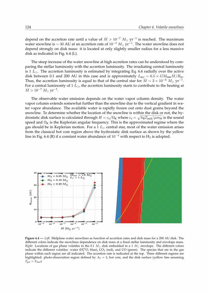
124 Chapter 6. Volatile snowlines
depend on the accretion rate until a value of M > 10−7 M yr−1 is reached. The maximumwater snowline is ∼ 30 AU at an accretion rate of 10−4 M yr−1. The water snowline does notdepend strongly on disk mass: it is located at only slightly smaller radius for a less massivedisk as indicated in Fig. 6.4 (L).
The steep increase of the water snowline at high accretion rates can be understood by com-paring the stellar luminosity with the accretion luminosity. The irradiating central luminosityis 1 L. The accretion luminosity is estimated by integrating Eq. 6.6 radially over the activedisk between 0.1 and 200 AU in this case and is approximately Lacc ∼ 0.5 × GMstarM/Rin.Thus, the accretion luminosity is equal to that of the central star for M ∼ 3× 10⁻⁶ M yr−1.For a central luminosity of 1 L, the accretion luminosity starts to contribute to the heating atM > 10−7 M yr−1.
The observable water emission depends on the water vapor column density. The watervapor column extends somewhat further than the snowline due to the vertical gradient in wa-ter vapor abundance. The available water is rapidly frozen out onto dust grains beyond thesnowline. To determine whether the location of the snowline is within the disk or not, the hy-drostatic disk surface is calculated through H = cs/ΩK where cs =
√kBTmid/µmH is the sound
speed and ΩK is the Keplerian angular frequency. This is the approximated regime where thegas should be in Keplerian motion. For a 1 L central star, most of the water emission arisesfrom the classical hot core region above the hydrostatic disk surface as shown by the yellowline in Fig. 6.4 (R) if a constant water abundance of 10−4 with respect to H2 is adopted.
10−9 10−8 10−7 10−6 10−5 10−4
M [M yr−1]
0
10
20
30
40
Rsnow
[AU
]
Menv = 1.0 ML? = 1 L
Md = 0.05 MMd = 0.10 MMd = 0.20 M
0 30 60 90
R [AU]
0
2
4
6
8
z[A
U]
H2OCO2
CO
CO2 + CO CO
Disk surface
Hot core
Photodissocated
M = 10−5 M yr−1
Figure 6.4 — Left: Midplane water snowlines as function of accretion rates and disk mass for a 200 AU disk. Thedifferent colors indicate the snowlines dependence on disk mass at a fixed stellar luminosity and envelope mass.Right: Locations of gas phase volatiles in the 0.1 M disk embedded in a 1 M envelope. The different colorsindicate the different volatiles: water (H16
2 O, blue), CO2 (red), and CO (green). The species that are in the gasphase within each region are all indicated. The accretion rate is indicated at the top. Three different regions arehighlighted: photo-dissociation region defined by AV = 3, hot core, and the disk surface (yellow line assumingTgas = Tdust).
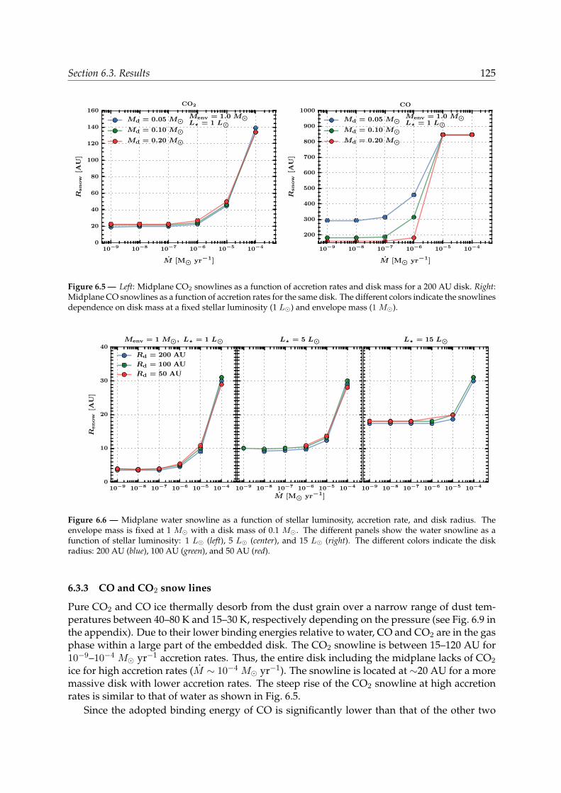
Section 6.3. Results 125
10−9 10−8 10−7 10−6 10−5 10−4
M [M yr−1]
0
20
40
60
80
100
120
140
160
Rsnow
[AU
]
Menv = 1.0 ML? = 1 L
CO2
Md = 0.05 MMd = 0.10 MMd = 0.20 M
10−9 10−8 10−7 10−6 10−5 10−4
M [M yr−1]
200
300
400
500
600
700
800
900
1000
Rsnow
[AU
]
Menv = 1.0 ML? = 1 L
CO
Md = 0.05 MMd = 0.10 MMd = 0.20 M
Figure 6.5 — Left: Midplane CO2 snowlines as a function of accretion rates and disk mass for a 200 AU disk. Right:Midplane CO snowlines as a function of accretion rates for the same disk. The different colors indicate the snowlinesdependence on disk mass at a fixed stellar luminosity (1 L) and envelope mass (1 M).
10−9 10−8 10−7 10−6 10−5 10−40
10
20
30
40
Rsnow
[AU
]
Menv = 1 M, L? = 1 L
Rd = 200 AU
Rd = 100 AU
Rd = 50 AU
10−9 10−8 10−7 10−6 10−5 10−4
M [M yr−1]
L? = 5 L
10−9 10−8 10−7 10−6 10−5 10−4
L? = 15 L
Figure 6.6 — Midplane water snowline as a function of stellar luminosity, accretion rate, and disk radius. Theenvelope mass is fixed at 1 M with a disk mass of 0.1 M. The different panels show the water snowline as afunction of stellar luminosity: 1 L (left), 5 L (center), and 15 L (right). The different colors indicate the diskradius: 200 AU (blue), 100 AU (green), and 50 AU (red).
6.3.3 CO and CO2 snow lines
Pure CO2 and CO ice thermally desorb from the dust grain over a narrow range of dust tem-peratures between 40–80 K and 15–30 K, respectively depending on the pressure (see Fig. 6.9 inthe appendix). Due to their lower binding energies relative to water, CO and CO2 are in the gasphase within a large part of the embedded disk. The CO2 snowline is between 15–120 AU for10−9–10−4 M yr−1 accretion rates. Thus, the entire disk including the midplane lacks of CO2
ice for high accretion rates (M ∼ 10−4 M yr−1). The snowline is located at ∼20 AU for a moremassive disk with lower accretion rates. The steep rise of the CO2 snowline at high accretionrates is similar to that of water as shown in Fig. 6.5.
Since the adopted binding energy of CO is significantly lower than that of the other two
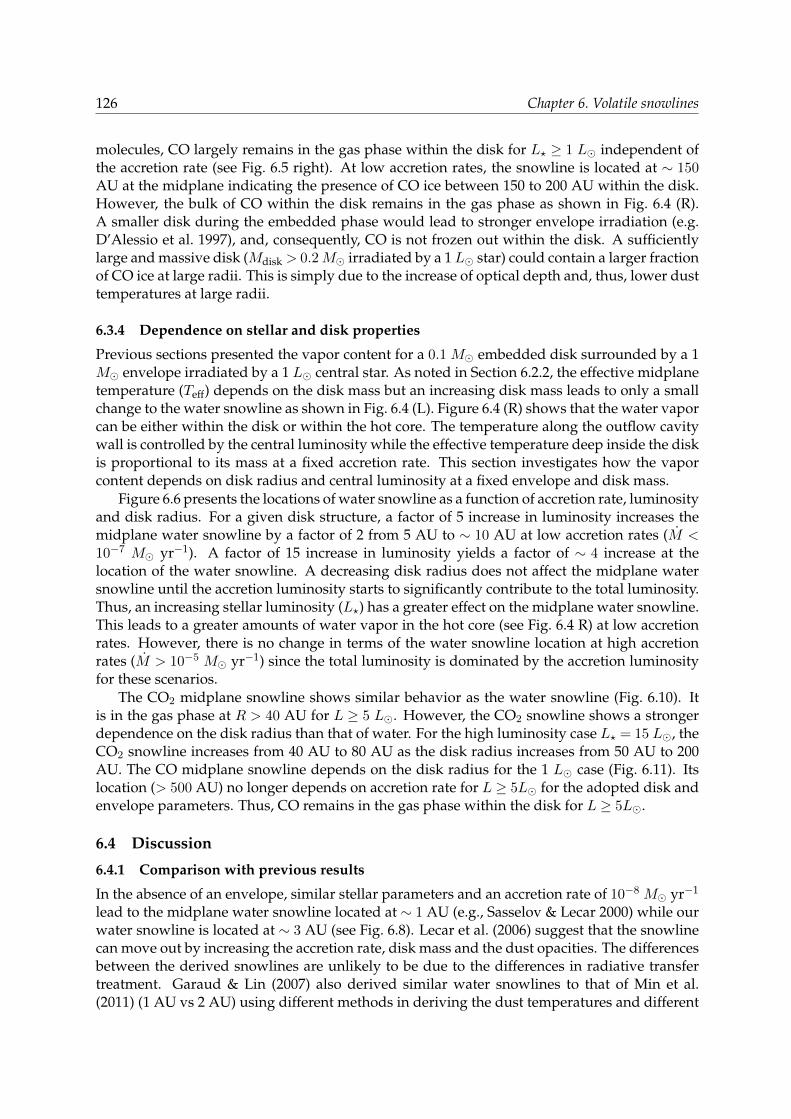
126 Chapter 6. Volatile snowlines
molecules, CO largely remains in the gas phase within the disk for L? ≥ 1 L independent ofthe accretion rate (see Fig. 6.5 right). At low accretion rates, the snowline is located at ∼ 150AU at the midplane indicating the presence of CO ice between 150 to 200 AU within the disk.However, the bulk of CO within the disk remains in the gas phase as shown in Fig. 6.4 (R).A smaller disk during the embedded phase would lead to stronger envelope irradiation (e.g.D’Alessio et al. 1997), and, consequently, CO is not frozen out within the disk. A sufficientlylarge and massive disk (Mdisk > 0.2M irradiated by a 1 L star) could contain a larger fractionof CO ice at large radii. This is simply due to the increase of optical depth and, thus, lower dusttemperatures at large radii.
6.3.4 Dependence on stellar and disk properties
Previous sections presented the vapor content for a 0.1 M embedded disk surrounded by a 1M envelope irradiated by a 1 L central star. As noted in Section 6.2.2, the effective midplanetemperature (Teff) depends on the disk mass but an increasing disk mass leads to only a smallchange to the water snowline as shown in Fig. 6.4 (L). Figure 6.4 (R) shows that the water vaporcan be either within the disk or within the hot core. The temperature along the outflow cavitywall is controlled by the central luminosity while the effective temperature deep inside the diskis proportional to its mass at a fixed accretion rate. This section investigates how the vaporcontent depends on disk radius and central luminosity at a fixed envelope and disk mass.
Figure 6.6 presents the locations of water snowline as a function of accretion rate, luminosityand disk radius. For a given disk structure, a factor of 5 increase in luminosity increases themidplane water snowline by a factor of 2 from 5 AU to ∼ 10 AU at low accretion rates (M <10−7 M yr−1). A factor of 15 increase in luminosity yields a factor of ∼ 4 increase at thelocation of the water snowline. A decreasing disk radius does not affect the midplane watersnowline until the accretion luminosity starts to significantly contribute to the total luminosity.Thus, an increasing stellar luminosity (L?) has a greater effect on the midplane water snowline.This leads to a greater amounts of water vapor in the hot core (see Fig. 6.4 R) at low accretionrates. However, there is no change in terms of the water snowline location at high accretionrates (M > 10−5 M yr−1) since the total luminosity is dominated by the accretion luminosityfor these scenarios.
The CO2 midplane snowline shows similar behavior as the water snowline (Fig. 6.10). Itis in the gas phase at R > 40 AU for L ≥ 5 L. However, the CO2 snowline shows a strongerdependence on the disk radius than that of water. For the high luminosity case L? = 15 L, theCO2 snowline increases from 40 AU to 80 AU as the disk radius increases from 50 AU to 200AU. The CO midplane snowline depends on the disk radius for the 1 L case (Fig. 6.11). Itslocation (> 500 AU) no longer depends on accretion rate for L ≥ 5L for the adopted disk andenvelope parameters. Thus, CO remains in the gas phase within the disk for L ≥ 5L.
6.4 Discussion
6.4.1 Comparison with previous results
In the absence of an envelope, similar stellar parameters and an accretion rate of 10−8 M yr−1
lead to the midplane water snowline located at ∼ 1 AU (e.g., Sasselov & Lecar 2000) while ourwater snowline is located at ∼ 3 AU (see Fig. 6.8). Lecar et al. (2006) suggest that the snowlinecan move out by increasing the accretion rate, disk mass and the dust opacities. The differencesbetween the derived snowlines are unlikely to be due to the differences in radiative transfertreatment. Garaud & Lin (2007) also derived similar water snowlines to that of Min et al.(2011) (1 AU vs 2 AU) using different methods in deriving the dust temperatures and different

Section 6.4. Discussion 127
opacities for similar accretion rates. The later takes into account the 2D vertical structure ofthe disk in detail. As Min et al. (2011) shows, most of the differences are due to the adopteddust opacities. Our value is 1 AU larger than the values tabulated in Min et al. (2011) adoptingdifferent dust opacity table. Furthermore, most of the previous studies adopt the minimummass solar nebula (MMSN) model where Σ ∝ R−1.5 instead of the R−1 2D parametric modelused in this paper (see e.g., Andrews et al. 2009). At the same accretion rate, the water snowlineis at ∼ 5 AU with the adopted disk embedded in a massive envelope models.
6.4.2 Caveats
The effect of convection in vertical direction is not included in this study. It is typically foundto be important in the case of high accretion rates (M > 10−6 M yr−1, D’Alessio et al. 1998,Min et al. 2011). Convection is found to cool the midplane temperatures at Tdust > 500 K. Thus,this should not affect the water (100–160 K), CO2 (∼ 50 K) and CO (∼ 20 K) snowlines.
Under the assumption of the steady state accretion disk model, the typical values of α > 1is obtained for the case of an accretion rate of M = 10−4 M yr−1. This is significantly higherthan that expected from magnetorotational instability (MRI) driven accretion in a MHD disk(α = 0.01, Balbus & Hawley 1998). King et al. (2007) indicated that α could be ∼ 0.4 for disksaround compact systems. Such a high value of α in our models are obtained since we have fixedthe density distribution for a high accretion rate. In reality, such a disk is unphysical. However,this is only encountered for the highest accretion rate of 10−4 M yr−1. Such a high accretionrate is expected to occur for a very short time. Furthermore, this paper explores the effect of theadopted accretion rates and disk masses for a given fixed parameters. Self-consistent modelsshould be explored in details in the future.
An additional heating term that is not included is the magnetospheric shock (Calvet &Gullbring 1998). For the case of high accretion rates, it is expected that the accretion proceedsstraight onto the star instead of stopping at Rin. The luminosity that it generates is given by
Lacc =GM?M
2R?. (6.12)
An accretion rate of 3× 10⁻⁷ M yr−1 will produce a shock luminosity equal to that of 1 L.Thus, the magnetospheric shock luminosity is expected to be one order of magnitude higherthan that of the accretion luminosity from the disk at a fixed accretion rate irradiated by a 1L central star. Currently, this is not included in the total luminosity as emitted by the centralstar. On the other hand, this is similar to the results with a higher central luminosity of 15 L.The qualitative effect on the water snowline with the inclusion of magnetospheric shock canbe explored by comparing the results at two different luminosities at a fixed accretion rate (seeSect 6.3.4).
6.4.3 Comparison with observations
The extent of the observed spatially resolved water emission toward low-mass embedded YSOsis between 25–90 AU (Jørgensen & van Dishoeck 2010b; Persson et al. 2012, 2014). The watersnowline is weakly affected by the envelope properties investigated here. The maximum mid-plane water snowline in our models is ∼ 30 AU with a disk mass of 0.1 M with Rdisk = 200AU and an accretion rate of 10−4 M yr−1. Thus, our results indicate that most of the wateremission at R < 50 AU would originate from the combine disk and hot core if accretion ratescan indeed be this high (see Fig. 6.4 R).
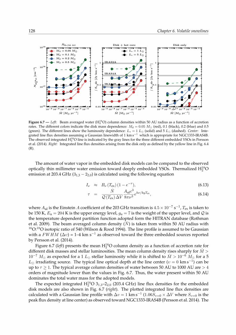
128 Chapter 6. Volatile snowlines
10−9 10−8 10−7 10−6 10−5 10−4
M [M yr−1]
1016
1017
1018
1019
NH
18
2O
[cm−
2]
NR<50 AU
Md = 0.05 MMd = 0.1 MMd = 0.2 MMd = 0.5 M
10−9 10−8 10−7 10−6 10−5 10−4
M [M yr−1]
0.01
0.1
1
∫Sνdν
[Jy
km
s−
1]
IRAS4B
IRAS4A
IRAS2A
Disk + hot core
L? = 1 LL? = 5 L
10−9 10−8 10−7 10−6 10−5 10−4
M [M yr−1]
0.01
0.1
1
∫Sνdν
[Jy
km
s−
1]
Disk only
Figure 6.7 — Left: Beam averaged water (H182 O) column densities within 50 AU radius as a function of accretion
rates. The different colors indicate the disk mass dependence: Md = 0.05 M (red), 0.1 (black), 0.2 (blue) and 0.5(green). The different lines show the luminosity dependence: L? = 1 L (solid) and 5 L (dashed). Center: Inte-grated line flux densities assuming a Gaussian linewidth of 1 km s−1 which is appropriate for NGC1333-IRAS4B.The observed integrated H18
2 O line is indicated by the gray lines for the three different embedded YSOs in Perssonet al. (2014). Right: Integrated line flux densities arising from the disk only as defined by the yellow line in Fig. 6.4(R).
The amount of water vapor in the embedded disk models can be compared to the observedoptically thin millimeter water emission toward deeply embedded YSOs. Thermalized H18
2 Oemission at 203.4 GHz (31,3 − 22,0) is calculated using the following equation
Iν ≈ Bν (Tex) (1− e−τ ), (6.13)
τ =N
Q (Tex) ∆V
Aulc3
8πν3ehν/kBTex , (6.14)
where Aul is the Einstein A coefficient of the 203 GHz transition is 4.5× 10⁻⁷ s−1, Tex is taken tobe 150 K, Eu = 204 K is the upper energy level, gu = 7 is the weight of the upper level, andQ isthe temperature dependent partition function adopted form the HITRAN database (Rothmanet al. 2009). The beam averaged column density (N ) is taken from within 50 AU radius with16O:18O isotopic ratio of 540 (Wilson & Rood 1994). The line profile is assumed to be Gaussianwith a FWHM (∆υ) = 1–4 km s−1 as observed toward the three embedded sources reportedby Persson et al. (2014).
Figure 6.7 (left) presents the mean H182 O column density as a function of accretion rate for
different disk masses and stellar luminosities. The mean column density rises sharply for M >10−7 M as expected for a 1 L stellar luminosity while it is shifted to M > 10−6 M for a 5L irradiating source. The typical line optical depth at the line center (υ = 0 km s−1) can beup to τ ≥ 1. The typical average column densities of water between 50 AU to 1000 AU are > 4orders of magnitude lower than the values in Fig. 6.7. Thus, the water present within 50 AUdominates the total water mass for the adopted models.
The expected integrated H182 O 31,3–22,0 (203.4 GHz) line flux densities for the embedded
disk models are also shown in Fig. 6.7 (right). The plotted integrated line flux densities arecalculated with a Gaussian line profile with ∆v = 1 km s−1 (1.06Sυ=0 ×∆V where Sυ=0 is thepeak flux density at line center) as observed toward NGC1333-IRAS4B (Persson et al. 2014). The
Section 6.4. Discussion 129
observed line widths toward IRAS2A and IRAS4A are 4 and 3 km s−1, respectively. Increasing∆υ slightly increases the model integrated line flux densities.
The predicted integrated line flux densities from actively accreting embedded disk mod-els are consistent with that observed toward NGC1333 IRAS4B if Md ≤ 0.2 M with M ∼3 × 10⁻⁷ M yr−1 for L = 1 L. Jørgensen et al. (2009) estimated from the continuum thatthe disk mass is ∼ 0.2 M, which is consistent with our results. Decreasing the disk mass im-plies a higher accretion rate is required to reproduce the observed water emission. A higheraccretion rate (∼ 5× 10⁻⁵ M yr−1) with lower disk mass is also consistent with the observedextent of water emission at ∼ 20 AU. A similar conclusion is reached for the case of IRAS4Awhose disk is estimated to be ∼ 0.5 M (Jørgensen et al. 2009). At these accretion rates, the ac-cretion luminosity is of the order of the adopted central luminosity (1 L). Since the bolometricluminosity toward NGC1333 IRAS4A and IRAS4B are a factor of 4–9 higher than the adoptedcentral luminosity, a model with a factor of 2 lower mass disk can also reproduce the observedflux density. With such a lower mass disk, the hot core is the dominant source of emissioninstead of the Keplerian disk.
IRAS2A shows stronger integrated line emission (∼ 1 Jy km s−1) relative to the other 2sources extending up to 90 AU radius. As pointed out above, a disk cannot be responsiblefor any warm water emission at R > 50 AU. Furthermore, Brinch et al. (2009) and Jørgensenet al. (2009) estimated that the disk is at most ∼ 0.05 M, which lowers the expected disk’scontribution to the observed water emission. There are two possible scenarios that can explainsuch a high water emission: a more luminous star (L? > 10 L) or an extremely high accretionrate (> 10−4 M yr−1). The former is consistent with the high bolometric luminosity of IRAS2A(Lbol = 35.7 L, Kristensen et al. 2012). In this case, most of the water emission arises from thehot core.
To quantify whether the water emission arises from the disk or the hot core, the integratedflux densities as expected to arise from the disk are shown in Fig. 6.7 (far right). For theadopted physical models, disks with masses Md ≥ 0.2 M with accretion rates of a few times10−5 M yr−1 can also reproduce the water emission without the hot core. However, as shownin Fig. 6.7, most of the emission arises from the hot core assuming a constant water abundanceof 10−4 with respect to H2.
The best cases for an actively accreting embedded disk scenario are IRAS4A and IRAS4B.More detailed modelling of their physical structure at < 100 AU radius is required to furtherconstrain the relation between disk accretion (envelope to disk) and stellar accretion rate (diskto star). Mottram et al. (2013) suggests that the infall rate from the large-scale envelope towardIRAS4A at 1000 AU to be ∼ 10−4 M yr−1. For the cases of disk masses between 0.2–0.5 M,the disk must also process the material at similar rate (within a factor of 10), which is consistentwith the models presented here.
6.4.4 Connecting to the young solar nebula
It is thought that the disk out of which the solar system formed (the solar nebula) was ini-tially hot enough to vaporize all material inherited from the collapsing cloud into atoms, theninto solids according to a condensation sequence as the nebula cools (Lewis 1974; Grossman& Larimer 1974). Evidence for energetic processing and subsequent condensation comes frommeteoritic data collected in the inner solar system (see Kerridge & Matthews 1988; Scott 2007;Apai & Lauretta 2010,for reviews). After the refractory phases have formed, more volatilespecies such as ices can also condense at larger distances from the young Sun, with the icecomposition depending on the temperature and pressure as well as the elemental abundanceratios (e.g., Lunine et al. 1991; Owen & Bar-Nun 1993; Mousis et al. 2009; Pontoppidan et al.
130 Chapter 6. Volatile snowlines
2014). Using cooling curves appropriate for the solar nebula, models show that various icesincluding H2O, CH3OH, NH3 and CO2 ice form by condensation out of warm gas out to atleast 20 AU (Mousis et al. 2012; Marboeuf et al. 2014). This condensation process is importantto explain the composition of volatiles in the atmospheres of solar-system giant planets andcomets.
Where and when does this heating and condensation in the disk actually occur? The aboveprocesses are usually discussed in the context of protoplanetary disks where the envelope hasdissipated and where the water snowline is eventually at a few AU once the disk has cooled.However, neither observations nor models of disks around solar-mass T-Tauri stars show anyevidence that disks are as warm as required above to have condensation happening out to 20AU (Beckwith et al. 1990; D’Alessio et al. 1998; Dullemond et al. 2007). The results from thispaper indicate that instead such a hot disk may be more common in the early stages of diskformation during the embedded phase. The disk is then expected to have the high accretionrates which provide the necessary additional heating. Furthermore, the high accretion ratesnecessary to push the midplane snowlines to 20 AU and beyond tend to occur for only a shorttime (e.g., Vorobyov 2009). Most volatiles including H2O, CH3OH, CO2 and CO presented herewill then be in the gas-phase within this 20–30 AU radius through sublimation of ices. Shortlyafter, the volatiles re-condense as the accretion rate decreases, with the process controlled bythe freeze-out timescale. The inclusion of the gas motions (radially and vertically) and kineticsdoes not allow for instantaneous re-condensation, thus some gas-phase volatiles should remainnear the snowline (Lewis & Prinn 1980; Ciesla & Cuzzi 2006).
A related question is whether the volatiles that are incorporated into planetesimals andeventually planets and icy bodies in the critical 5–30 AU zone are then inherited or reset duringthe disk formation process. Evolutionary models by Visser et al. (2009) and Visser et al. (2011)suggest that strongly bound ices such as H2O are largely pristine interstellar ices in the outerdisk, whereas more volatile species can have sublimated, recondensed and reprocessed sev-eral times on their way to the inner disk. However, these models have not included internalviscous dissipation as an additional heating source. A warmer early disk can facilitate ice evo-lution and formation of complex organic molecules in the temperature regime between 20–40K (Garrod et al. 2008; Nomura et al. 2009; Walsh et al. 2014; Drozdovskaya et al. 2014). Ourresults including the accretion heating indicate that significant ice re-processing may occur outto larger radii than thought before, well in the comet formation zone. Such a reset scenario issupported by the meteoritic data from the inner few AU, but the fraction of material that isreset at larger (e.g. Pontoppidan et al. 2014).
6.5 Summary and conclusions
Two-dimensional embedded disk models have been presented to investigate the location of thesnowlines of H2O, CO2 and CO. The dust temperature structure is calculated using the 3D dustradiative transfer code RADMC3D with a central heating source (L? + Lvisc). An additionalheating term from an actively accreting disk has been added through a diffusion approxima-tion. The main parameters that are explored in this paper are L?, envelope mass, disk radius,disk mass, and disk accretion rate. In addition, the extent of the snowline and optically thin wa-ter emission are compared with observations toward three deeply embedded low-mass YSOs.The following lists the main results of this paper.
• The midplane water snowline can extend up to ∼ 30 AU for a disk accreting at10−4 M yr−1. The CO2 snowline is located at 100 AU for the same accretion rate. BothH2O and CO2 can remain in the solid phase at large radii (R > 100 AU) in the midplane

Section 6.A. Snowline test 131
within the boundaries of an embedded hydrostatic disk.• CO is largely found to be in the gas phase within the embedded disk independent of
accretion rate and disk properties. Some CO could be frozen out at large radii in themidplane for a relatively massive disk (Md ≥ 0.1 M).• The predicted water snowlines in our actively accreting embedded disk models can ex-
plain the water emission within R < 50 AU emitted from the combined hot core and thedisk (see Fig. 6.4 R).• The predicted optically thin water emission is consistent with that observed toward
NGC1333 IRAS4A and IRAS4B for M > 10−6 M yr−1 for the adopted disk masses of 0.5M and 0.2 M, respectively. The observed size of water emission can also be explainedwith a slightly higher accretion rate model with a lower disk mass. The comparison withthe observed water emission toward IRAS2A suggests less disk’s contribution relativeto IRAS4A and IRAS4B. More detailed physical structure models of NGC1333 IRAS4Aand IRAS4B are needed to further quantify the disk’s contribution to the observed wateremission.• Significant chemical processing is expected to occur in the inner 100 AU region during the
disk formation process in Stage 0. Midplane temperatures between 20–40 K are expectedto be prevalent up to 100 AU radius, and 100 K out to 30 AU, for typical accretion ratesfound in the early phases of star formation. During these warm phases, the chemistryinherited from the collapsing cloud could be reset and more complex molecules couldform.
In connection to the solar system formation, the young disk is found to be warm enoughsuch that the water vapor can up to the 30 AU radius within the disk. It is important to realize,however, that a hot young solar nebula out to 30 AU can only occur during the deeply em-bedded phase, not the T Tauri phase of our solar system. Our models predict that most of theoptically thin water emission arises within the inner 50 AU radius. Future Atacama Large Mil-limeter Array (ALMA) observations spatially resolving the inner 50 AU will test the embeddedaccreting disk models coupled with better physical models for individual sources. This willlead to better understanding of the physical and chemical structure and evolution of disks inthe early stages of star formation.
Acknowledgements
We thank Atilla Juhasz for providing scripts for generating and analyzing RADMC3D inputand output files. We also thank Kees Dullemond for providing RADMC3D. We are grateful toCatherine Walsh for fruitful discussions. This work is supported by the Netherlands ResearchSchool for Astronomy (NOVA). Astrochemistry in Leiden is supported by the Netherlands Re-search School for Astronomy (NOVA), by a Royal Netherlands Academy of Arts and Sciences(KNAW) professor prize, and by the European Union A-ERC grant 291141 CHEMPLAN.
6.A Snowline test
Water snowlines were inferred and compared with results from Min et al. (2011) in Fig. 6.8using the minimum mass solar nebula (MMSN) model (Σ∝ r−1.5). The comparison shows thatour adopted method reproduces the water snowlines at high accretion rates. For low accretionrates M ≤ 10−9 M yr−1, our values are slightly smaller yet consistent with those reported inliterature.

132 Chapter 6. Volatile snowlines
−9 −7 −5
M [M yr−1]
1
10
100
logR
ice
[AU
]
Figure 6.8 — Snowlines for the MMSN disk without an envelope: black circles show the radii calculated with ourmethod and red squares are tabulated values from Min et al. (2011).
50 100 150 200 250
Tdust [K]
4
6
8
10
12
14
16
Logn
H2
[cm−
3]
0.0
0.1
0.3
0.4
0.6
0.7
0.9
1.0
CO
2gas
fractio
n
20 40 60 80
Tdust [K]
4
6
8
10
12
14
16
Logn
H2
[cm−
3]
0.0
0.1
0.3
0.4
0.6
0.7
0.9
1.0
CO
gas
fractio
n
Figure 6.9 — Gas fraction (ngas/ngas +nice) for CO2 (Top) and CO (Bottom) as a function of density and temperatures.
6.B CO2 and CO gas fraction
The CO2 and CO gas pressure dependent gas fraction abundance are shown in Fig. 6.9. Therange of density and temperature is the same as Fig. 6.1 (R) except for CO. Figures 6.10 and6.11 show the midplane CO2 and CO snowlines as a function of luminosity and Rd similar tothat of Fig. 6.6 for H2O.
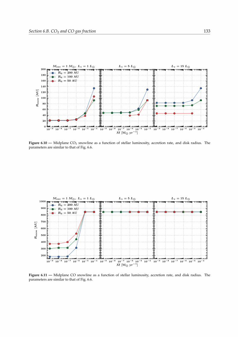
Section 6.B. CO2 and CO gas fraction 133
10−9 10−8 10−7 10−6 10−5 10−40
20
40
60
80
100
120
140
160
180
200
Rsnow
[AU
]
Menv = 1 M, L? = 1 L
Rd = 200 AU
Rd = 100 AU
Rd = 50 AU
10−9 10−8 10−7 10−6 10−5 10−4
M [M yr−1]
L? = 5 L
10−9 10−8 10−7 10−6 10−5 10−4
L? = 15 L
Figure 6.10 — Midplane CO2 snowline as a function of stellar luminosity, accretion rate, and disk radius. Theparameters are similar to that of Fig. 6.6.
10−9 10−8 10−7 10−6 10−5 10−4
200
300
400
500
600
700
800
900
1000
Rsnow
[AU
]
Menv = 1 M, L? = 1 L
Rd = 200 AU
Rd = 100 AU
Rd = 50 AU
10−9 10−8 10−7 10−6 10−5 10−4
M [M yr−1]
L? = 5 L
10−9 10−8 10−7 10−6 10−5 10−4
L? = 15 L
Figure 6.11 — Midplane CO snowline as a function of stellar luminosity, accretion rate, and disk radius. Theparameters are similar to that of Fig. 6.6.


Bibliography
Adams, F. C., Ruden, S. P., & Shu, F. H. 1989, ApJ, 347, 959Agertz, O., Moore, B., Stadel, J., et al. 2007, MNRAS, 380, 963Aikawa, Y., Furuya, K., Wakelam, V., et al. 2011, in The Molec-
ular Universe, IAU Symposium 280, ed. J. Cernicharo &R. Bachiller (Cambridge Univ. Press, Cambridge), 33–42
Aikawa, Y., Wakelam, V., Garrod, R. T., & Herbst, E. 2008, ApJ,674, 984
Alexander, R. D., Armitage, P. J., Cuadra, J., & Begelman,M. C. 2008, ApJ, 674, 927
Andre, P., Di Francesco, J., Ward-Thompson, D., et al. 2014, inProtostars and Planets VI, ed. H. Beuther, C. Dullemond,& T. Henning (Univ. of Arizona Press, Tucson), in press
Andre, P., Men’shchikov, A., Bontemps, S., et al. 2010, A&A,518, L102
Andre, P., Ward-Thompson, D., & Barsony, M. 1993, ApJ, 406,122
Andrews, S. M., Wilner, D. J., Hughes, A. M., Qi, C., & Dulle-mond, C. P. 2009, ApJ, 700, 1502
Apai, D. A. & Lauretta, D. S. 2010, Protoplanetary Dust: As-trophysical and Cosmochemical Perspectives (CambridgeUniv. Press, Cambridge)
Arce, H. G., Shepherd, D., Gueth, F., et al. 2007, in Protostarsand Planets V, ed. B. Reipurth, D. Jewitt, & K. Keil (Univ.of Arizona Press, Tucson), 245–260
Armitage, P. J., Livio, M., & Pringle, J. E. 2001, MNRAS, 324,705
Bachiller, R. & Tafalla, M. 1999, in NATO ASIC Proc. 540: TheOrigin of Stars and Planetary Systems, ed. C. J. Lada &N. D. Kylafis, 227
Baines, D., Oudmaijer, R. D., Porter, J. M., & Pozzo, M. 2006,MNRAS, 367, 737
Balbus, S. A. & Hawley, J. F. 1991, ApJ, 376, 214Balbus, S. A. & Hawley, J. F. 1998, Rev. Mod. Phys., 70, 1Balbus, S. A. & Papaloizou, J. C. B. 1999, ApJ, 521, 650Balsara, D. S. 1995, Journal of Computational Physics, 121, 357Batalha, N. M., Rowe, J. F., Bryson, S. T., et al. 2013, ApJ, 204,
24Beckwith, S., Skrutskie, M. F., Zuckerman, B., & Dyck, H. M.
1984, ApJ, 287, 793Beckwith, S. V. W., Sargent, A. I., Chini, R. S., & Guesten, R.
1990, AJ, 99, 924Bell, K. R., Cassen, P. M., Klahr, H. H., & Henning, T. 1997,
ApJ, 486, 372Bell, K. R. & Lin, D. N. C. 1994, ApJ, 427, 987Belloche, A. 2013, in EAS Publications Series 62, 25–66Belloche, A., Andre, P., Despois, D., & Blinder, S. 2002, A&A,
393, 927Berger, J. P. & Segransan, D. 2007, New Astron. Rev., 51, 576Bergin, E. A. & Tafalla, M. 2007, ARA&A, 45, 339Bisschop, S. E., Fraser, H. J., Oberg, K. I., van Dishoeck, E. F.,
& Schlemmer, S. 2006, A&A, 449, 1297Bjorkman, J. E. & Wood, K. 2001, ApJ, 554, 615Bodenheimer, P. 1995, ARA&A, 33, 199Boley, A. C. 2009, ApJ, 695, L53Boley, A. C., Mejıa, A. C., Durisen, R. H., et al. 2006, ApJ, 651,
517Bonnell, I. A. & Rice, W. K. M. 2008, Science, 321, 1060Boogert, A. C. A., Hogerheijde, M. R., & Blake, G. A. 2002,
ApJ, 568, 761Braiding, C. R. & Wardle, M. 2012, MNRAS, 422, 261Brinch, C., Crapsi, A., Hogerheijde, M. R., & Jørgensen, J. K.
2007a, A&A, 461, 1037Brinch, C., Crapsi, A., Jørgensen, J. K., Hogerheijde, M. R., &
Hill, T. 2007b, A&A, 475, 915Brinch, C. & Hogerheijde, M. R. 2010, A&A, 523, 25Brinch, C., Hogerheijde, M. R., & Richling, S. 2008, A&A, 489,
607Brinch, C. & Jørgensen, J. K. 2013, A&A, 559, A82Brinch, C., Jørgensen, J. K., & Hogerheijde, M. R. 2009, A&A,
502, 199Brittain, S. D., Rettig, T. W., Simon, T., & Kulesa, C. 2005, ApJ,
626, 283Brown, D. W. & Chandler, C. J. 1999, MNRAS, 303, 855Brown, D. W., Chandler, C. J., Carlstrom, J. E., et al. 2000, MN-
RAS, 319, 154Bruderer, S. 2010, PhD thesis, ETH ZurichBruderer, S., Benz, A. O., Stauber, P., & Doty, S. D. 2010, ApJ,
720, 1432Bruderer, S., van Dishoeck, E. F., Doty, S. D., & Herczeg, G. J.
2012, A&A, 541, A91Burke, D. J. & Brown, W. A. 2010, Phys. Chem. Chem. Phys.,
12, 5947Burkert, A. & Bodenheimer, P. 2000, ApJ, 543, 822Cabrit, S., Guilloteau, S., Andre, P., et al. 1996, A&A, 305, 527Calvet, N. & Gullbring, E. 1998, ApJ, 509, 802Calvet, N., Hartmann, L., & Strom, S. E. 2000, in Protostars
and Planets IV, ed. V. Mannings, A. P. Boss, & S. S. Russel(Univ. of Arizona Press, Tucson), 377
Calvet, N., Patino, A., Magris, G. C., & D’Alessio, P. 1991, ApJ,380, 617
Caselli, P., Benson, P. J., Myers, P. C., & Tafalla, M. 2002, ApJ,572, 238
Cassen, P. 2001, Meteoritics and Planetary Science, 36, 671Cassen, P. & Moosman, A. 1981, Icarus, 48, 353Cesaroni, R., Galli, D., Lodato, G., Walmsley, C. M., & Zhang,
Q. 2007, in Protostars and Planets V, ed. B. Reipurth, D. Je-witt, & K. Keil (Univ. of Arizona Press, Tucson), 197–212
Cesaroni, R., Galli, D., Lodato, G., Walmsley, M., & Zhang, Q.2006, Nature, 444, 703
Chandra, S. & Sharma, A. K. 2001, A&A, 376, 356Chiang, E. I. & Goldreich, P. 1997, ApJ, 490, 368Chiang, E. I., Joung, M. K., Creech-Eakman, M. J., et al. 2001,
ApJ, 547, 1077Chiang, H.-F., Looney, L. W., Tassis, K., Mundy, L. G., &
Mouschovias, T. C. 2008, ApJ, 680, 474Chiang, H.-F., Looney, L. W., & Tobin, J. J. 2012, ApJ, 756, 168Choi, M., Tatematsu, K., & Kang, M. 2010, ApJ, 723, L34Ciesla, F. J. & Cuzzi, J. N. 2006, Icarus, 181, 178Clarke, C. J. 2009, MNRAS, 396, 1066Commercon, B., Launhardt, R., Dullemond, C., & Henning, T.
2012a, A&A, 545, A98Commercon, B., Levrier, F., Maury, A. J., Henning, T., & Laun-
hardt, R. 2012b, A&A, 548, A39Cossins, P., Lodato, G., & Clarke, C. J. 2009, MNRAS, 393, 1157Cossins, P., Lodato, G., & Testi, L. 2010, MNRAS, 407, 181Crapsi, A., Devries, C. H., Huard, T. L., et al. 2005, A&A, 439,
135

136 Bibliography
1023Crapsi, A., van Dishoeck, E. F., Hogerheijde, M. R., Pontoppi-
dan, K. M., & Dullemond, C. P. 2008, A&A, 486, 245Crutcher, R. M. 2012, ARA&A, 50, 29Crutcher, R. M., Hakobian, N., & Troland, T. H. 2010, MNRAS,
402, L64Cuadra, J., Nayakshin, S., Springel, V., & Di Matteo, T. 2006,
MNRAS, 366, 358D’Alessio, P., Calvet, N., & Hartmann, L. 1997, ApJ, 474, 397D’Alessio, P., Canto, J., Calvet, N., & Lizano, S. 1998, ApJ, 500,
411Dapp, W. B. & Basu, S. 2010, A&A, 521, L56Dapp, W. B., Basu, S., & Kunz, M. W. 2012, A&A, 541, A35Davis, S. S. 2005, ApJ, 620, 994de Graauw, T., Helmich, F. P., Phillips, T. G., et al. 2010, A&A,
518, L6Di Francesco, J., Johnstone, D., Kirk, H., MacKenzie, T., & Led-
wosinska, E. 2008, ApJ, 175, 277Dib, S., Hennebelle, P., Pineda, J. E., et al. 2010, ApJ, 723, 425Doty, S. D., Schoier, F. L., & van Dishoeck, E. F. 2004, A&A,
418, 1021Doty, S. D., van Dishoeck, E. F., van der Tak, F. F. S., & Boon-
man, A. M. S. 2002, A&A, 389, 446Douglas, T. A., Caselli, P., Ilee, J. D., et al. 2013, MNRAS, 433,
2064Drozdovskaya, M. N., C., W., R., V., D., H., & van Dishoeck,
E. F. 2014, MNRAS, subm.Dullemond, C. P. & Dominik, C. 2004, A&A, 421, 1075Dullemond, C. P., Hollenbach, D., Kamp, I., & D’Alessio, P.
2007, in Protostars and Planets V, ed. B. Reipurth, D. Jewitt,& K. Keil (Univ. of Arizona Press, Tucson), 555–572
Dullemond, C. P. & Monnier, J. D. 2010, ARA&A, 48, 205Dunham, M. M., Evans, II, N. J., Terebey, S., Dullemond, C. P.,
& Young, C. H. 2010, ApJ, 710, 470Dunham, M. M., Stutz, A. M., Allen, L. E., et al. 2014, in Pro-
tostars and Planets VI, ed. H. Beuther, C. Dullemond, &T. Henning (Univ. of Arizona Press, Tucson), in press
Dunham, M. M. & Vorobyov, E. I. 2012, ApJ, 747, 52Durisen, R. H., Boss, A. P., Mayer, L., et al. 2007, in Protostars
and Planets V, ed. B. Reipurth, D. Jewitt, & K. Keil (Univ.of Arizona Press, Tucson), 607–622
Dutrey, A., Guilloteau, S., & Ho, P. 2007, in Protostars andPlanets V, ed. B. Reipurth, D. Jewitt, & K. Keil (Univ. ofArizona Press, Tucson), 495–506
Dzib, S., Loinard, L., Mioduszewski, A. J., et al. 2010, ApJ, 718,610
Eddington, A. S. 1937, The Observatory, 60, 99Eisner, J. A. 2012, ApJ, 755, 23Eisner, J. A., Hillenbrand, L. A., Carpenter, J. M., & Wolf, S.
2005, ApJ, 635, 396Enoch, M. L., Corder, S., Duchene, G., et al. 2011, ApJ, 195, 21Enoch, M. L., Corder, S., Dunham, M. M., & Duchene, G. 2009,
ApJ, 707, 103Evans, N., Calvet, N., Cieza, L., et al. 2009a, ArXiv e-printsEvans, II, N. J. 1999, ARA&A, 37, 311Evans, II, N. J., Dunham, M. M., Jørgensen, J. K., et al. 2009b,
ApJ, 181, 321Evans, II, N. J., Lee, J.-E., Rawlings, J. M. C., & Choi, M. 2005,
ApJ, 626, 919Fayolle, E. C., Bertin, M., Romanzin, C., et al. 2011, ApJ, 739,
L36Fedele, D., Bruderer, S., van Dishoeck, E. F., et al. 2013, ApJ,
776, L3Fleming, T. P., Stone, J. M., & Hawley, J. F. 2000, ApJ, 530, 464
Forgan, D., Armitage, P. J., & Simon, J. B. 2012, MNRAS, 426,2419
Fraser, H. J., Collings, M. P., McCoustra, M. R. S., & Williams,D. A. 2001, MNRAS, 327, 1165
Furlan, E., McClure, M., Calvet, N., et al. 2008, ApJ, 176, 184Galli, D., Lizano, S., Shu, F. H., & Allen, A. 2006, ApJ, 647, 374Galli, D. & Palla, F. 2013, ARA&A, 51, 163Galli, D. & Shu, F. H. 1993, ApJ, 417, 220Gammie, C. F. 1996, ApJ, 457, 355Gammie, C. F. 2001, ApJ, 553, 174Garaud, P. & Lin, D. N. C. 2007, ApJ, 654, 606Garrod, R. T., Weaver, S. L. W., & Herbst, E. 2008, ApJ, 682,
283Genzel, R., Schodel, R., Ott, T., et al. 2003, ApJ, 594, 812Ghez, A. M., Salim, S., Hornstein, S. D., et al. 2005, ApJ, 620,
744Gibb, E. L., Whittet, D. C. B., Boogert, A. C. A., & Tielens,
A. G. G. M. 2004, ApJ, 151, 35Gillett, F. C. & Forrest, W. J. 1973, ApJ, 179, 483Gingold, R. A. & Monaghan, J. J. 1977, MNRAS, 181, 375Goicoechea, J. R., Cernicharo, J., Karska, A., et al. 2012, A&A,
548, A77Goldflam, R., Kouri, D. J., & Green, S. 1977, J. Chem. Phys., 67,
4149Goodman, A. A., Benson, P. J., Fuller, G. A., & Myers, P. C.
1993, ApJ, 406, 528Gramajo, L. V., Whitney, B. A., Gomez, M., & Robitaille, T. P.
2010, AJ, 139, 2504Gramajo, L. V., Whitney, B. A., Kenyon, S. J., Gomez, M., &
Merrill, K. M. 2007, AJ, 133, 1911Greaves, J. S., Richards, A. M. S., Rice, W. K. M., & Muxlow,
T. W. B. 2008, MNRAS, 391, L74Griffin, M. J., Abergel, A., Abreu, A., et al. 2010, A&A, 518, L3Grossman, L. & Larimer, J. W. 1974, Reviews of Geophysics
and Space Physics, 12, 71Guilloteau, S., Pietu, V., Dutrey, A., & Guelin, M. 2006, A&A,
448, L5Haisch, Jr., K. E., Lada, E. A., & Lada, C. J. 2001, ApJ, 553, L153Harsono, D., Alexander, R. D., & Levin, Y. 2011, MNRAS, 413,
423Harsono, D., Jørgensen, J. K., van Dishoeck, E. F., et al. 2014,
A&A, 562, A77Harsono, D., Visser, R., Bruderer, S., van Dishoeck, E. F., &
Kristensen, L. E. 2013, A&A, 555, A45Hartmann, L., Calvet, N., Gullbring, E., & D’Alessio, P. 1998,
ApJ, 495, 385Hartmann, L. & Kenyon, S. J. 1985, ApJ, 299, 462Hartmann, L. & Kenyon, S. J. 1987, ApJ, 312, 243Hasegawa, T. I., Herbst, E., & Leung, C. M. 1992, ApJ, 82, 167Hayashi, C. 1981, in Fundamental Problems in the Theory of
Stellar Evolution, IAU Symposium 93, ed. D. Sugimoto,D. Q. Lamb, & D. N. Schramm (D. Reidel Publishing Co.,Dordrecht), 113–126
Hayashi, M., Ohashi, N., & Miyama, S. M. 1993, ApJ, 418, L71Hennebelle, P. & Ciardi, A. 2009, A&A, 506, L29Hennebelle, P. & Falgarone, E. 2012, A&A Rev., 20, 55Herczeg, G. J., Brown, J. M., van Dishoeck, E. F., & Pontoppi-
dan, K. M. 2011, A&A, 533, A112Herczeg, G. J., Karska, A., Bruderer, S., et al. 2012, A&A, 540,
A84Hogerheijde, M. R. 2001, ApJ, 553, 618Hogerheijde, M. R. & Sandell, G. 2000, ApJ, 534, 880Hogerheijde, M. R. & van der Tak, F. F. S. 2000, A&A, 362, 697Hogerheijde, M. R., van Dishoeck, E. F., Blake, G. A., & van
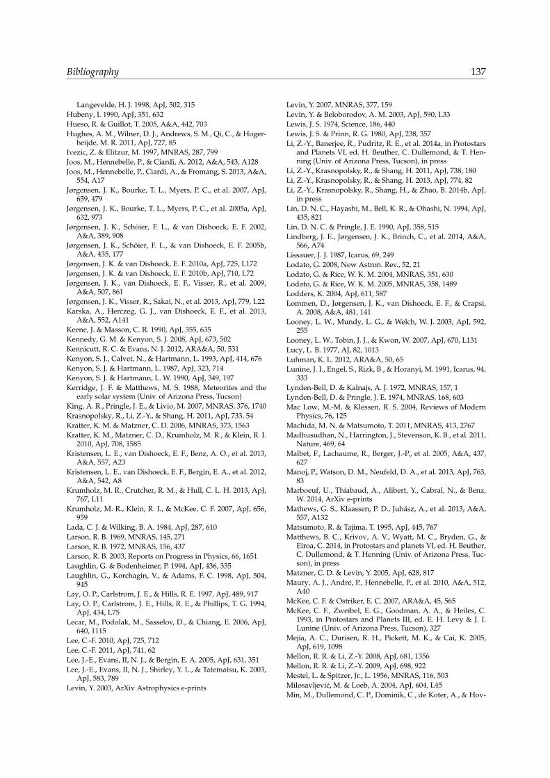
Bibliography 137
Langevelde, H. J. 1998, ApJ, 502, 315Hubeny, I. 1990, ApJ, 351, 632Hueso, R. & Guillot, T. 2005, A&A, 442, 703Hughes, A. M., Wilner, D. J., Andrews, S. M., Qi, C., & Hoger-
heijde, M. R. 2011, ApJ, 727, 85Ivezic, Z. & Elitzur, M. 1997, MNRAS, 287, 799Joos, M., Hennebelle, P., & Ciardi, A. 2012, A&A, 543, A128Joos, M., Hennebelle, P., Ciardi, A., & Fromang, S. 2013, A&A,
554, A17Jørgensen, J. K., Bourke, T. L., Myers, P. C., et al. 2007, ApJ,
659, 479Jørgensen, J. K., Bourke, T. L., Myers, P. C., et al. 2005a, ApJ,
632, 973Jørgensen, J. K., Schoier, F. L., & van Dishoeck, E. F. 2002,
A&A, 389, 908Jørgensen, J. K., Schoier, F. L., & van Dishoeck, E. F. 2005b,
A&A, 435, 177Jørgensen, J. K. & van Dishoeck, E. F. 2010a, ApJ, 725, L172Jørgensen, J. K. & van Dishoeck, E. F. 2010b, ApJ, 710, L72Jørgensen, J. K., van Dishoeck, E. F., Visser, R., et al. 2009,
A&A, 507, 861Jørgensen, J. K., Visser, R., Sakai, N., et al. 2013, ApJ, 779, L22Karska, A., Herczeg, G. J., van Dishoeck, E. F., et al. 2013,
A&A, 552, A141Keene, J. & Masson, C. R. 1990, ApJ, 355, 635Kennedy, G. M. & Kenyon, S. J. 2008, ApJ, 673, 502Kennicutt, R. C. & Evans, N. J. 2012, ARA&A, 50, 531Kenyon, S. J., Calvet, N., & Hartmann, L. 1993, ApJ, 414, 676Kenyon, S. J. & Hartmann, L. 1987, ApJ, 323, 714Kenyon, S. J. & Hartmann, L. W. 1990, ApJ, 349, 197Kerridge, J. F. & Matthews, M. S. 1988, Meteorites and the
early solar system (Univ. of Arizona Press, Tucson)King, A. R., Pringle, J. E., & Livio, M. 2007, MNRAS, 376, 1740Krasnopolsky, R., Li, Z.-Y., & Shang, H. 2011, ApJ, 733, 54Kratter, K. M. & Matzner, C. D. 2006, MNRAS, 373, 1563Kratter, K. M., Matzner, C. D., Krumholz, M. R., & Klein, R. I.
2010, ApJ, 708, 1585Kristensen, L. E., van Dishoeck, E. F., Benz, A. O., et al. 2013,
A&A, 557, A23Kristensen, L. E., van Dishoeck, E. F., Bergin, E. A., et al. 2012,
A&A, 542, A8Krumholz, M. R., Crutcher, R. M., & Hull, C. L. H. 2013, ApJ,
767, L11Krumholz, M. R., Klein, R. I., & McKee, C. F. 2007, ApJ, 656,
959Lada, C. J. & Wilking, B. A. 1984, ApJ, 287, 610Larson, R. B. 1969, MNRAS, 145, 271Larson, R. B. 1972, MNRAS, 156, 437Larson, R. B. 2003, Reports on Progress in Physics, 66, 1651Laughlin, G. & Bodenheimer, P. 1994, ApJ, 436, 335Laughlin, G., Korchagin, V., & Adams, F. C. 1998, ApJ, 504,
945Lay, O. P., Carlstrom, J. E., & Hills, R. E. 1997, ApJ, 489, 917Lay, O. P., Carlstrom, J. E., Hills, R. E., & Phillips, T. G. 1994,
ApJ, 434, L75Lecar, M., Podolak, M., Sasselov, D., & Chiang, E. 2006, ApJ,
640, 1115Lee, C.-F. 2010, ApJ, 725, 712Lee, C.-F. 2011, ApJ, 741, 62Lee, J.-E., Evans, II, N. J., & Bergin, E. A. 2005, ApJ, 631, 351Lee, J.-E., Evans, II, N. J., Shirley, Y. L., & Tatematsu, K. 2003,
ApJ, 583, 789Levin, Y. 2003, ArXiv Astrophysics e-prints
Levin, Y. 2007, MNRAS, 377, 159Levin, Y. & Beloborodov, A. M. 2003, ApJ, 590, L33Lewis, J. S. 1974, Science, 186, 440Lewis, J. S. & Prinn, R. G. 1980, ApJ, 238, 357Li, Z.-Y., Banerjee, R., Pudritz, R. E., et al. 2014a, in Protostars
and Planets VI, ed. H. Beuther, C. Dullemond, & T. Hen-ning (Univ. of Arizona Press, Tucson), in press
Li, Z.-Y., Krasnopolsky, R., & Shang, H. 2011, ApJ, 738, 180Li, Z.-Y., Krasnopolsky, R., & Shang, H. 2013, ApJ, 774, 82Li, Z.-Y., Krasnopolsky, R., Shang, H., & Zhao, B. 2014b, ApJ,
in pressLin, D. N. C., Hayashi, M., Bell, K. R., & Ohashi, N. 1994, ApJ,
435, 821Lin, D. N. C. & Pringle, J. E. 1990, ApJ, 358, 515Lindberg, J. E., Jørgensen, J. K., Brinch, C., et al. 2014, A&A,
566, A74Lissauer, J. J. 1987, Icarus, 69, 249Lodato, G. 2008, New Astron. Rev., 52, 21Lodato, G. & Rice, W. K. M. 2004, MNRAS, 351, 630Lodato, G. & Rice, W. K. M. 2005, MNRAS, 358, 1489Lodders, K. 2004, ApJ, 611, 587Lommen, D., Jørgensen, J. K., van Dishoeck, E. F., & Crapsi,
A. 2008, A&A, 481, 141Looney, L. W., Mundy, L. G., & Welch, W. J. 2003, ApJ, 592,
255Looney, L. W., Tobin, J. J., & Kwon, W. 2007, ApJ, 670, L131Lucy, L. B. 1977, AJ, 82, 1013Luhman, K. L. 2012, ARA&A, 50, 65Lunine, J. I., Engel, S., Rizk, B., & Horanyi, M. 1991, Icarus, 94,
333Lynden-Bell, D. & Kalnajs, A. J. 1972, MNRAS, 157, 1Lynden-Bell, D. & Pringle, J. E. 1974, MNRAS, 168, 603Mac Low, M.-M. & Klessen, R. S. 2004, Reviews of Modern
Physics, 76, 125Machida, M. N. & Matsumoto, T. 2011, MNRAS, 413, 2767Madhusudhan, N., Harrington, J., Stevenson, K. B., et al. 2011,
Nature, 469, 64Malbet, F., Lachaume, R., Berger, J.-P., et al. 2005, A&A, 437,
627Manoj, P., Watson, D. M., Neufeld, D. A., et al. 2013, ApJ, 763,
83Marboeuf, U., Thiabaud, A., Alibert, Y., Cabral, N., & Benz,
W. 2014, ArXiv e-printsMathews, G. S., Klaassen, P. D., Juhasz, A., et al. 2013, A&A,
557, A132Matsumoto, R. & Tajima, T. 1995, ApJ, 445, 767Matthews, B. C., Krivov, A. V., Wyatt, M. C., Bryden, G., &
Eiroa, C. 2014, in Protostars and planets VI, ed. H. Beuther,C. Dullemond, & T. Henning (Univ. of Arizona Press, Tuc-son), in press
Matzner, C. D. & Levin, Y. 2005, ApJ, 628, 817Maury, A. J., Andre, P., Hennebelle, P., et al. 2010, A&A, 512,
A40McKee, C. F. & Ostriker, E. C. 2007, ARA&A, 45, 565McKee, C. F., Zweibel, E. G., Goodman, A. A., & Heiles, C.
1993, in Protostars and Planets III, ed. E. H. Levy & J. I.Lunine (Univ. of Arizona Press, Tucson), 327
Mejıa, A. C., Durisen, R. H., Pickett, M. K., & Cai, K. 2005,ApJ, 619, 1098
Mellon, R. R. & Li, Z.-Y. 2008, ApJ, 681, 1356Mellon, R. R. & Li, Z.-Y. 2009, ApJ, 698, 922Mestel, L. & Spitzer, Jr., L. 1956, MNRAS, 116, 503Milosavljevic, M. & Loeb, A. 2004, ApJ, 604, L45Min, M., Dullemond, C. P., Dominik, C., de Koter, A., & Hov-
138 Bibliography
enier, J. W. 2009, A&A, 497, 155Min, M., Dullemond, C. P., Kama, M., & Dominik, C. 2011,
Icarus, 212, 416Mitchell, G. F., Maillard, J.-P., Allen, M., Beer, R., & Belcourt,
K. 1990, ApJ, 363, 554Momose, M., Ohashi, N., Kawabe, R., Nakano, T., & Hayashi,
M. 1998, ApJ, 504, 314Monaghan, J. & Gingold, R. 1983, Journal of Computational
Physics, 52, 374Monaghan, J. J. 1992, ARA&A, 30, 543Moses, J. I., Line, M. R., Visscher, C., et al. 2013, ApJ, 777, 34Motte, F. & Andre, P. 2001, A&A, 365, 440Mottram, J. C., Kristensen, L. E., van Dishoeck, E. F., et al.
2014, A&A, subm.Mottram, J. C., van Dishoeck, E. F., Schmalzl, M., et al. 2013,
A&A, 558, A126Mousis, O., Lunine, J. I., Madhusudhan, N., & Johnson, T. V.
2012, ApJ, 751, L7Mousis, O., Lunine, J. I., Thomas, C., et al. 2009, ApJ, 691, 1780Mundy, L. G., Looney, L. W., Erickson, W., et al. 1996, ApJ,
464, L169Murillo, N. M. & Lai, S.-P. 2013, ApJ, 764, L15Murillo, N. M., Lai, S.-P., Bruderer, S., Harsono, D., & van
Dishoeck, E. F. 2013, A&A, 560, A103Murray, J. R. 1996, MNRAS, 279, 402Myers, A. T., McKee, C. F., Cunningham, A. J., Klein, R. I., &
Krumholz, M. R. 2013, ApJ, 766, 97Nakano, T. & Nakamura, T. 1978, PASJ, 30, 671Nayakshin, S. 2006, MNRAS, 372, 143Nelson, A. F. 2006, MNRAS, 373, 1039Neufeld, D. A. 2012, ApJ, 749, 125Nisini, B., Antoniucci, S., Giannini, T., & Lorenzetti, D. 2005,
A&A, 429, 543Nomura, H., Aikawa, Y., Nakagawa, Y., & Millar, T. J. 2009,
A&A, 495, 183Oberg, K. I., Boogert, A. C. A., Pontoppidan, K. M., et al.
2011a, ApJ, 740, 109Oberg, K. I., Murray-Clay, R., & Bergin, E. A. 2011b, ApJ, 743,
L16Oberg, K. I., van Dishoeck, E. F., & Linnartz, H. 2009, A&A,
496, 281O’Dell, C. R. & Wen, Z. 1994, ApJ, 436, 194Ogino, S., Tomisaka, K., & Nakamura, F. 1999, PASJ, 51, 637Ohashi, N., Hayashi, M., Ho, P. T. P., & Momose, M. 1997a,
ApJ, 475, 211Ohashi, N., Hayashi, M., Ho, P. T. P., et al. 1997b, ApJ, 488, 317Oliveira, I., Olofsson, J., Pontoppidan, K. M., et al. 2011, ApJ,
734, 51Oliveira, I., Pontoppidan, K. M., Merın, B., et al. 2010, ApJ,
714, 778Ossenkopf, V. & Henning, T. 1994, A&A, 291, 943Owen, T. & Bar-Nun, A. 1993, Nature, 361, 693Persson, M. V., Jørgensen, J. K., & van Dishoeck, E. F. 2012,
A&A, 541, A39Persson, M. V., Jørgensen, J. K., & van Dishoeck, E. F. 2013,
A&A, 549, L3Persson, M. V., Jørgensen, J. K., van Dishoeck, E. F., & Har-
sono, D. 2014, A&A, 563, A74Pinto, R. F., Brun, A. S., Jouve, L., & Grappin, R. 2011, ApJ,
737, 72Poglitsch, A., Waelkens, C., Geis, N., et al. 2010, A&A, 518, L2Pollack, J. B., Hubickyj, O., Bodenheimer, P., et al. 1996, Icarus,
124, 62Pontoppidan, K. M., Blake, G. A., van Dishoeck, E. F., et al.
2008, ApJ, 684, 1323Pontoppidan, K. M., Meijerink, R., Dullemond, C. P., & Blake,
G. a. 2009, ApJ, 704, 1482Pontoppidan, K. M., Salyk, C., Bergin, E. A., et al. 2014, in
Protostars and Planets VI, ed. H. Beuther, C. Dullemond,& T. Henning (Univ. of Arizona Press, Tucson), in press
Pontoppidan, K. M., Salyk, C., Blake, G. A., & Kaufl, H. U.2010, ApJ, 722, L173
Price, D. J. 2007, PASA, 24, 159Pringle, J. E. 1981, ARA&A, 19, 137Qi, C., Oberg, K. I., Wilner, D. J., et al. 2013, Science, 341, 630Qi, C., Wilner, D. J., Aikawa, Y., Blake, G. A., & Hogerheijde,
M. R. 2008, ApJ, 681, 1396Rafikov, R. R. 2007, ApJ, 662, 642Rafikov, R. R. 2009, ApJ, 704, 281Rice, W. K. M., Armitage, P. J., Bate, M. R., & Bonnell, I. A.
2003, MNRAS, 339, 1025Rice, W. K. M., Lodato, G., & Armitage, P. J. 2005, MNRAS,
364, L56Robitaille, T. P. 2011, A&A, 536, A79Robitaille, T. P., Whitney, B. A., Indebetouw, R., & Wood, K.
2007, ApJ, 169, 328Robitaille, T. P., Whitney, B. A., Indebetouw, R., Wood, K., &
Denzmore, P. 2006, ApJ, 167, 256Ros, K. & Johansen, A. 2013, A&A, 552, A137Rothman, L., Gordon, I., Barbe, A., et al. 2009, Journal of
Quantitative Spectroscopy and Radiative Transfer, 110, 533Roueff, E. & Lique, F. 2013, Chemical Reviews, 113, 8906Safronov, V. S. 1969, Evoliutsiia doplanetnogo oblaka.Saito, M., Kawabe, R., Kitamura, Y., & Sunada, K. 1996, ApJ,
473, 464San Jose-Garcia, I., Mottram, J. C., Kristensen, L. E.and van
Dishoeck, E. F., et al. 2013, A&A, 553, A125Santos-Lima, R., de Gouveia Dal Pino, E. M., & Lazarian, A.
2012, ApJ, 747, 21Sargent, A. I. & Beckwith, S. 1987, ApJ, 323, 294Sasselov, D. D. & Lecar, M. 2000, ApJ, 528, 995Sault, R. J., Teuben, P. J., & Wright, M. C. 1995, Astronomical
Data Analysis Software and Systems IV, 77, 433Schneider, N., Csengeri, T., Hennemann, M., et al. 2012, A&A,
540, L11Schoier, F. L., van der Tak, F. F. S., van Dishoeck, E. F., & Black,
J. H. 2005, A&A, 432, 369Scott, E. R. D. 2007, Annual Review of Earth and Planetary
Sciences, 35, 577Scoville, N. Z., Sargent, A. I., Sanders, D. B., et al. 1986, ApJ,
303, 416Seifried, D., Banerjee, R., Pudritz, R. E., & Klessen, R. S. 2012,
MNRAS, 423, L40Shakura, N. I. & Sunyaev, R. A. 1973, A&A, 24, 337Shu, F. H. 1977, ApJ, 214, 488Shu, F. H., Tremaine, S., Adams, F. C., & Ruden, S. P. 1990,
ApJ, 358, 495Smith, R. J., Shetty, R., Stutz, A. M., & Klessen, R. S. 2012, ApJ,
750, 64Smith, R. L., Pontoppidan, K. M., Young, E. D., & Morris,
M. R. 2010, Meteoritics and Planetary Science Supplement,73, 5381
Smith, R. L., Pontoppidan, K. M., Young, E. D., Morris, M. R.,& van Dishoeck, E. F. 2009, ApJ, 701, 163
Spaans, M., Hogerheijde, M. R., Mundy, L. G., & vanDishoeck, E. F. 1995, ApJL, 455, 167
Spitzer, Jr., L. 1989, ARA&A, 27, 1Springel, V. 2005, MNRAS, 364, 1105

Nederlandse samenvatting 139
Springel, V. 2010, ARA&A, 48, 391Stamatellos, D., Whitworth, A. P., Bisbas, T., & Goodwin, S.
2007, A&A, 475, 37Steinacker, J., Baes, M., & Gordon, K. D. 2013, ARA&A, 51, 63Stevenson, D. J. & Lunine, J. I. 1988, Icarus, 75, 146Stone, J. M. & Norman, M. L. 1992, ApJ, 80, 753Strom, K. M., Strom, S. E., Edwards, S., Cabrit, S., & Skrutskie,
M. F. 1989, AJ, 97, 1451Takahashi, T., Silk, T., & Holenbach, D. J. 1983, ApJ, 275, 145Takakuwa, S., Saito, M., Lim, J., et al. 2012, ApJ, 754, 52Takami, M., Bailey, J., Gledhill, T. M., Chrysostomou, A., &
Hough, J. H. 2001, MNRAS, 323, 177Tasker, E. J., Brunino, R., Mitchell, N. L., et al. 2008, MNRAS,
390, 1267Terebey, S., Chandler, C. J., & Andre, P. 1993, ApJ, 414, 759Terebey, S., Shu, F. H., & Cassen, P. 1984, ApJ, 286, 529Tielens, A. G. G. M. 2005, The Physics and Chemistry of the
Interstellar Medium (Cambridge Univ. Press, Cambridge)Tielens, A. G. G. M. 2013, Reviews of Modern Physics, 85, 1021Tobin, J. J., Hartmann, L., Chiang, H.-F., et al. 2011, ApJ, 740,
45Tobin, J. J., Hartmann, L., Chiang, H.-F., et al. 2012, Nature,
492, 83Tobin, J. J., Hartmann, L., Chiang, H.-F., et al. 2013, ApJ, 771,
48Tobin, J. J., Hartmann, L., Looney, L. W., & Chiang, H.-F. 2010,
ApJ, 712, 1010Toomre, A. 1964, ApJ, 139, 1217Troland, T. H. & Crutcher, R. M. 2008, ApJ, 680, 457Ulrich, R. K. 1976, ApJ, 210, 377van der Tak, F. 2011, in IAU Symposium 280, ed. J. Cernicharo
& R. Bachiller (Cambridge Univ. Press, Cambridge), 449–460
van der Tak, F. F. S., Black, J. H., Schoier, F. L., Jansen, D. J., &van Dishoeck, E. F. 2007, A&A, 468, 627
van der Tak, F. F. S., Walmsley, C. M., Herpin, F., & Ceccarelli,C. 2006, A&A, 447, 1011
van Dishoeck, E. F., Bergin, E. A., Lis, D. C., & Lunine, J. I.2014, in Protostars and Planets VI, ed. H. Beuther, C. Dulle-mond, & T. Henning (Univ. of Arizona Press, Tucson), inpress
van Dishoeck, E. F., Jonkheid, B., & van Hemert, M. C. 2006,Faraday Discussions, 133, 231
van Dishoeck, E. F., Kristensen, L. E., Benz, A. O., et al. 2011,PASP, 123, 138
van Dishoeck, E. F., Thi, W.-F., & van Zadelhoff, G.-J. 2003,A&A, 400, L1
van Kempen, T. A., Green, J. D., Evans, N. J., et al. 2010, A&A,518, L128
van Kempen, T. A., van Dishoeck, E. F., Gusten, R., et al. 2009a,A&A, 507, 1425
van Kempen, T. A., van Dishoeck, E. F., Gusten, R., et al.2009b, A&A, 501, 633
van Kempen, T. A., van Dishoeck, E. F., Hogerheijde, M. R., &Gusten, R. 2009c, A&A, 508, 259
van Kempen, T. A., van Dishoeck, E. F., Salter, D. M., et al.2009d, A&A, 498, 167
van Leer, B. 1979, Journal of Computational Physics, 32, 101van Weeren, R. J., Brinch, C., & Hogerheijde, M. R. 2009, A&A,
497, 773
Visser, R. & Bergin, E. A. 2012, ApJ, 754, L18Visser, R., Doty, S. D., & van Dishoeck, E. F. 2011, A&A, 534,
A132Visser, R. & Dullemond, C. P. 2010, A&A, 519, A28Visser, R., Jørgensen, J. K., Kristensen, L. E., van Dishoeck,
E. F., & Bergin, E. A. 2013, ApJ, 769, 19Visser, R., Kristensen, L. E., Bruderer, S., et al. 2012, A&A, 537,
55Visser, R., van Dishoeck, E. F., Doty, S. D., & Dullemond, C. P.
2009, A&A, 495, 881Vorobyov, E. I. 2009, ApJ, 704, 715Vorobyov, E. I. 2010, ApJ, 723, 1294Vorobyov, E. I. & Basu, S. 2006, ApJ, 650, 956Vorobyov, E. I. & Basu, S. 2007, MNRAS, 381, 1009Vorobyov, E. I. & Basu, S. 2009, MNRAS, 393, 822Vorobyov, E. I. & Basu, S. 2010, ApJ, 719, 1896Vorobyov, E. I., Zakhozhay, O. V., & Dunham, M. M. 2013,
MNRAS, 433, 3256Walsh, C., Millar, T. J., & Nomura, H. 2010, ApJ, 722, 1607Walsh, C., Millar, T. J., Nomura, H., et al. 2014, A&A, 563, A33Wang, K.-S., van der Tak, F. F. S., & Hogerheijde, M. R. 2012,
A&A, 543, A22White, R. J. & Hillenbrand, L. A. 2004, ApJ, 616, 998Whitney, B. A. & Hartmann, L. 1993, ApJ, 402, 605Whitney, B. A., Wood, K., Bjorkman, J. E., & Cohen, M. 2003a,
ApJ, 598, 1079Whitney, B. A., Wood, K., Bjorkman, J. E., & Wolff, M. J. 2003b,
ApJ, 591, 1049Williams, J. P. & Cieza, L. A. 2011, ARA&A, 49, 67Wilson, T. L. & Rood, R. 1994, ARA&A, 32, 191Woodward, P. & Colella, P. 1984, Journal of Computational
Physics, 54, 115Woodward, P. R. 1978, ARA&A, 16, 555Wyatt, M. C. 2008, ARA&A, 46, 339Yang, B., Stancil, P. C., Balakrishnan, N., & Forrey, R. C. 2010,
ApJ, 718, 1062Yen, H.-W., Takakuwa, S., Ohashi, N., & Ho, P. T. P. 2013, ApJ,
772, 22Yıldız, U. A., Kristensen, L. E., van Dishoeck, E. F., et al. 2012,
A&A, 542, A86Yıldız, U. A., Kristensen, L. E., van Dishoeck, E. F., et al. 2013,
A&A, 556, A89Yıldız, U. A., van Dishoeck, E. F., Kristensen, L. E., et al. 2010,
A&A, 521, L40Yorke, H. W. & Bodenheimer, P. 1999, ApJ, 525, 330Young, C. H. & Evans, II, N. J. 2005, ApJ, 627, 293Young, C. H., Jørgensen, J. K., Shirley, Y. L., et al. 2004, ApJ,
154, 396Young, C. H., Shirley, Y. L., Evans, II, N. J., & Rawlings,
J. M. C. 2003, ApJ, 145, 111Zhang, K., Pontoppidan, K. M., Salyk, C., & Blake, G. A. 2013,
ApJ, 766, 82Zhou, S., Evans, N. J., Kompe, C., & Walmsley, C. M. 1993,
ApJ, 404, 232Zhu, Z., Hartmann, L., Gammie, C., & McKinney, J. C. 2009,
ApJ, 701, 620Zhu, Z., Hartmann, L., Gammie, C. F., et al. 2010, ApJ, 713,
1134Zweibel, E. G. 1988, ApJ, 329, 384

Nederlandse samenvatting
DETECTIES van exoplaneten tonen aan dat er ten minste een planeet om elke ster draait.Planeten worden gevormd in de accretieschijf die de nieuw gevormde ster voedt. Het on-
derwerp van dit proefschrift is het begrijpen van de processen die plaats vinden in de vroegstestadia van ster- en planeetvorming. De vorming en evolutie van deze schijven, die uiteindelijkde bouwstenen worden van planeten en leven, zijn nog niet goed begrepen.
Het overgrote deel van de chemische elementen die nodig zijn voor leven zoals wij hetkennen (SPONCH) worden geproduceerd in sterren. In de vroege stadia van het universumwerden alleen de chemische elementen tot lithium gevormd. Tijdens de levensloop van een sterworden in zijn kern via kernfusie elementen tot ijzer (Fe) aangemaakt dat later, bij het einde vande levensloop van de ster, in het universum terecht komen. Na verloop van tijd worden meervan deze zwaardere elementen geproduceerd en opgenomen in de volgende generatie(s) vansterren en planeten. De elementen worden op hun beurt opgenomen in simpele en complexemoleculen die ruimschoots aanwezig zijn in dichte wolken.
Ster en planeetvorming zijn nauw aan elkaar verbonden door de accretie schijf. Het conceptvan accretieschijven werd al voorgesteld door Kant en Laplace in de 18de eeuw. Het duurdeechter nog twee eeuwen voordat waarnemingen het direct bewijs leverden. De vorming enevolutie van accretieschijven hebben een fundamentele invloed op de hoeveelheid materiaaldat in de ster terecht komt en hoeveel er overblijft om planeten te vormen.
De vorming van sterren en planeten
Sterren worden gevormd door het langzaam ineenkrimpen van een koude, geconcentreerdekern (10 K = - 263deg C) bestaande uit gas en stof. Recente waarnemingen met de Herschelruimtetelescoop tonen aan dat deze kernen voorkomen in moleculaire wolken die bestaan uitdraadvormige structuren of filamenten (Fig. S.1). In deze structuren bestaat een verscheiden-heid aan grootte en massa van kernen. De kleinere kernen in het filament zullen later ster-ren van lage massa worden, zoals onze zon. Uit het materiaal van de kern wordt de ster enhet planeten stelsel gevormd. Recent is grote vooruitgang geboekt in het begrijpen van devorming van deze filamenten en de moleculaire wolken waarin ze zich bevinden. Superso-nische turbulentie in het interstellaire medium (ISM, de ruimte tussen de sterren) zorgt voorde samendrukking van gas in platte structuren en filamenten. Terwijl de kern materie vande moleculaire wolk opneemt, zal deze beginnen te krimpen onder zijn eigen zwaartekrachten uiteindelijk een protoster vormen. Dit proces wordt beheerst door een aantal bijkomendeprocessen zoals thermische druk, magnetische velden en turbulentie.
Een (proto)ster is een hete lichtgevende bol van gas die aangedreven wordt door de energiedie vrijkomt bij de nucleaire reacties in zijn kern. De verschillende stadia van de vorming vansterren met lage massa (M ≤ 2M, de massa van de zon is M) zijn redelijk goed begrepen invergelijking met sterren met een hogere massa, maar verschillende details blijven onduidelijk.Hoewel massievere sterren helderder en makkelijk waar te nemen zijn, zijn sterren met lageremassa talrijker. Het bestuderen van de fysische processen die plaatsvinden gedurende stervor-ming geeft inzicht in de vorming van ons eigen zonnestelsel en in het ontstaan van leven opaarde.
Bij de krimp als gevolg van behoud van energie en impuls wordt een accretieschijf ge-

142 Nederlandse samenvatting
Figuur S.1 — Samengestelde kleurenafbeelding van vijf verschillende golflengtes in het Zuiderkruis, genomen metde Photodetector Array Camera and Spectrometer (PACS) en de Spectral and Photometric Imaging Receiver (SPIRE)van de Herschel ruimtetelescoop. De meeste golflengtes vallen buiten het optisch bereik, maar zijn zichtbaar inhet infrarood door straling van het gas en stof dat zich rond de nieuwe ster bevindt. Deze materie is niet uniformverdeeld: de meest heldere straling komt uit de actieve stervormingsgebieden die verbonden zijn met de filamenten.Blauw geeft straling van het warme stof aan, en rood van koud stof. Credits: ESA en de SPIRE & PACS consortium.
vormd. De eerste theoretische studies van accretieschijven komen uit de jaren 70 door Shakuraen Sunyaev. Op dat moment was er reeds indirect bewijs voor het bestaan van accretieschij-ven rond jonge sterren, op basis van polarimetrische waarnemingen van atomaire optischelijnen. Het duurde tot 1989 voordat Strom en medewerkers de eerste statistische studies vanaccretieschijven uitvoerden, met behulp van de Infrared Astronomical Satellite (IRAS). Zij ver-richtten waarnemingen van accretieschijven door middel van de straling van het warme stof inde schijf. Hierna werd het belangrijkste bewijs voor het bestaan van schijven geleverd door dedirecte waarnemingen met Hubble in 1994 door ODell en medewerkers (Fig. S.2). Tegenwoor-dig weet men dat er zich rond elke jonge ster een accretischijf bevindt en dat deze een crucialerol speelt bij de planeet- en stervorming.
Op het moment van schrijven zijn er meer dan 1000 exoplaneten bekend en meer dan 3000kandidaten. Het meest aanvaarde scenario van planeetvorming is via het samenklonteren van
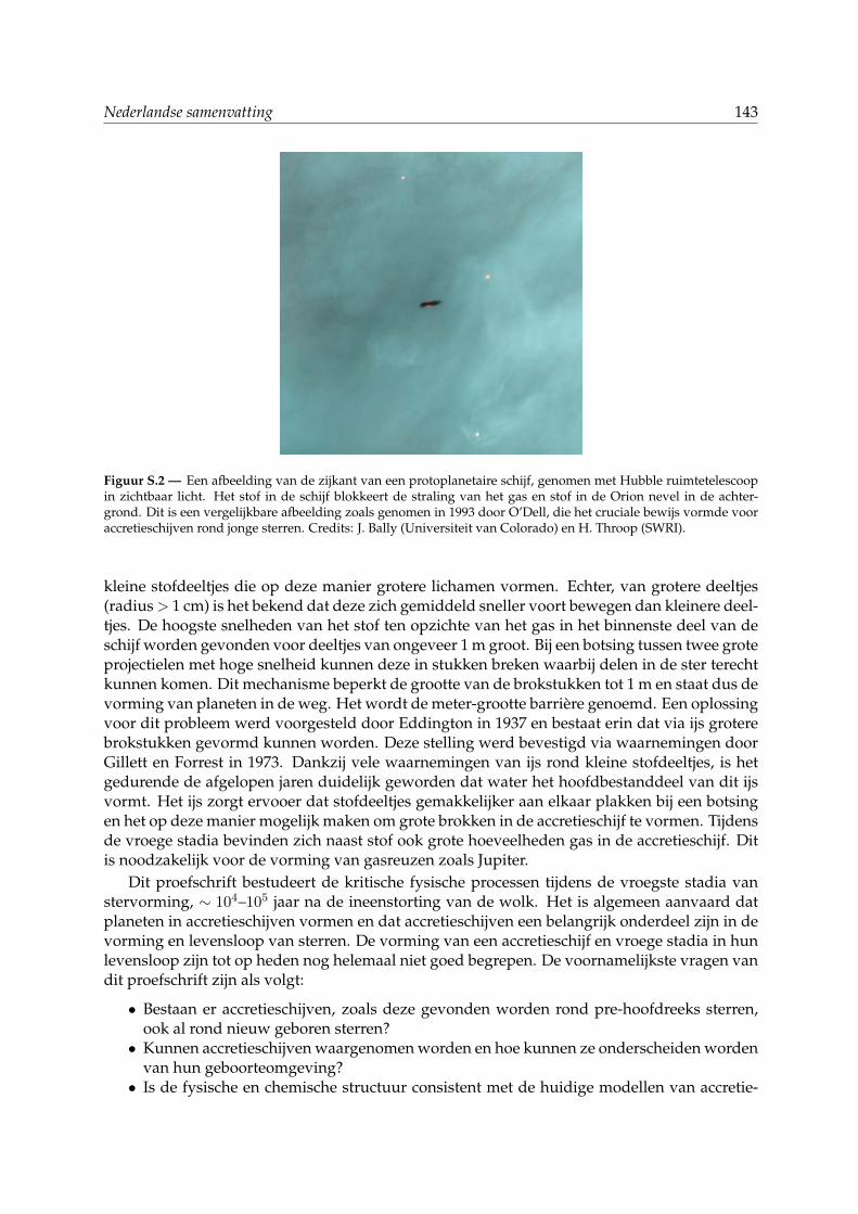
Nederlandse samenvatting 143
Figuur S.2 — Een afbeelding van de zijkant van een protoplanetaire schijf, genomen met Hubble ruimtetelescoopin zichtbaar licht. Het stof in de schijf blokkeert de straling van het gas en stof in de Orion nevel in de achter-grond. Dit is een vergelijkbare afbeelding zoals genomen in 1993 door O’Dell, die het cruciale bewijs vormde vooraccretieschijven rond jonge sterren. Credits: J. Bally (Universiteit van Colorado) en H. Throop (SWRI).
kleine stofdeeltjes die op deze manier grotere lichamen vormen. Echter, van grotere deeltjes(radius> 1 cm) is het bekend dat deze zich gemiddeld sneller voort bewegen dan kleinere deel-tjes. De hoogste snelheden van het stof ten opzichte van het gas in het binnenste deel van deschijf worden gevonden voor deeltjes van ongeveer 1 m groot. Bij een botsing tussen twee groteprojectielen met hoge snelheid kunnen deze in stukken breken waarbij delen in de ster terechtkunnen komen. Dit mechanisme beperkt de grootte van de brokstukken tot 1 m en staat dus devorming van planeten in de weg. Het wordt de meter-grootte barriere genoemd. Een oplossingvoor dit probleem werd voorgesteld door Eddington in 1937 en bestaat erin dat via ijs groterebrokstukken gevormd kunnen worden. Deze stelling werd bevestigd via waarnemingen doorGillett en Forrest in 1973. Dankzij vele waarnemingen van ijs rond kleine stofdeeltjes, is hetgedurende de afgelopen jaren duidelijk geworden dat water het hoofdbestanddeel van dit ijsvormt. Het ijs zorgt ervooer dat stofdeeltjes gemakkelijker aan elkaar plakken bij een botsingen het op deze manier mogelijk maken om grote brokken in de accretieschijf te vormen. Tijdensde vroege stadia bevinden zich naast stof ook grote hoeveelheden gas in de accretieschijf. Ditis noodzakelijk voor de vorming van gasreuzen zoals Jupiter.
Dit proefschrift bestudeert de kritische fysische processen tijdens de vroegste stadia vanstervorming, ∼ 104–105 jaar na de ineenstorting van de wolk. Het is algemeen aanvaard datplaneten in accretieschijven vormen en dat accretieschijven een belangrijk onderdeel zijn in devorming en levensloop van sterren. De vorming van een accretieschijf en vroege stadia in hunlevensloop zijn tot op heden nog helemaal niet goed begrepen. De voornamelijkste vragen vandit proefschrift zijn als volgt:
• Bestaan er accretieschijven, zoals deze gevonden worden rond pre-hoofdreeks sterren,ook al rond nieuw geboren sterren?• Kunnen accretieschijven waargenomen worden en hoe kunnen ze onderscheiden worden
van hun geboorteomgeving?• Is de fysische en chemische structuur consistent met de huidige modellen van accretie-
144 Nederlandse samenvatting
schijfvorming?• Hoe stabiel zijn accretieschijven in deze vroege fase, als materiaal uit het omhulsel nog
invalt op de schijf?• Hoeveel dragen accretieschijven bij aan de waagenomen moleculaire lijnen?
Stralingsprocessen: continuum en spectraallijnen
De eigenschappen van jonge sterren worden typisch afgeleid door middel van breedbandigeinfrarode straling van het stof. Door de UV straling van de jonge ster wordt het stof opge-warmd, vervolgens zal het stof deze warmte uitstralen bij langere golflengte in het (ver)infrarood.Het evenwicht tussen beiden bepaalt de temperatuur van het stof. Dus, hoe meer de (proto)sterstraalt, hoe warmer het stof. Tegelijkertijd neemt de (proto)ster nog materiaal op uit zijn omge-ving. In de vroege stadia van stervorming bevindt zich in de accretieschijf veel koud materiaalomdat alle UV straling snel door het stof is geabsorbeerd. Hierdoor is het moeijk om de groei-ende ster en accretieschijf te bestuderen. Theoretische modellen worden daarom gebruikt omde waargenomen straling te begrijpen.
Hoewel de warmtestraling van het stof de energie van het groeiende stelsel traceert, kun-nen alleen atomaire en moleculaire lijnen gebruikt worden om de structuur van de buiten-ste gaslagen van jonge schijven te bepalen. Een enorme rijkdom aan moleculen wordt in deverschillende fysische stadia gevonden. Door middel van waarnemingen van verschillendemoleculaire overgangen kunnen de verschillende fysische condities, zoals temperatuur, dicht-heid en snelheidsstructuren onderzocht worden. Belangrijk is dat deze overgangen zich opvaste frequenties bevinden. Koolstofmonoxide (CO) wordt hierin het meest gebruikt. Elke be-weging van het gas veroorzaakt een Doppler verschuiving van de waargenomen frequentie.Wanneer de lijnen spectraal opgelost kunnen worden kan op deze manier de beweging van hetgas bepaald worden.
Observationeel gereedschap
Om een jonge accretieschijf in zijn omhulsel te bestuderen zijn interferometrische waarnemin-gen op millimeter golflengte nodig. Op deze manier wordt warmtestraling van de accretie-schijf onderscheiden van de omgeving. Interferometrie is een techniek waarbij signalen vanmeerdere telescopen gecombineerd worden om op deze manier genoeg ruimtelijke resolutie teverkrijgen en zo de schijf op te kunnen lossen. Bijvoorbeeld, een 12 meter telescoop kan COstraling oplossen uit een gebied ter grote van 7000 AE (7000 astronomische eenheden, d.w.z.7000 keer de afstand van de aarde tot de zon). Twee van deze telescopen op een afstand van 1km van elkaar hebben een oplossend vermogen van 80 AE in hetzelfde gebied.
Interferometrische waarnemingen van stof en gas in het millimeter gebied zijn cruciaal ge-weest om de processen binnenin stervormingsgebieden aan te tonen. De afstand tussen deinterferometrische telescopen is variabel om zo, afhankelijk van de nood, verschillende reso-luties (0.5 ′′–20 ′′) te verkrijgen. Een paar telescopen op korte afstand wordt vooral gebruiktvoor het waarnemen van grootschalige structuren, zoals het omhulsel, terwijl een paar tele-scopen op grote afstand, en dus een hogere resolutie, gebruikt wordt om in te zoomen opde accretieschijf. Door meer dan twee telescopen met verschillende afstanden te combinerenin verschillende configuraties kunnen alle schalen tegelijkertijd waargenomen worden. Eenafbeelding wordt verkregen door de Fourier transformatie van een verzameling van deze ge-correleerde gegevens. Een stationaire groep telescopen maakt gebruik van de aardrotatie omgecorreleerde waarnemingen te verrichten. Vele gecorreleerde waarnemingen zijn nodig omeen volledige afbeelding te verkrijgen. Een typische waarneming in dit proefschrift heeft meer
Nederlandse samenvatting 145
dan 5.000 gecorreleerde waarnemingen. De nieuwste telescoop is de Atacama Large MillimeterArray (ALMA, 66 telescopen) in Chili. Met een dergelijke grote hoeveelheid telescopen zal hetmakkelijker zijn om de zwakke structuren in een stervormingsgebied waar te nemen.
Dit proefschrift
Dit proefschrift behandelt zowel de theoretische en obervationele aspecten van accretieschijf-vorming gedurende de vroege stadia van stervorming. Semi-analytische en numerieke hydro-dynamische modellen zijn samengevoegd met breedbandige stralingsoverdracht berekeningenvan het stof. De voorspelde moleculaire lijn emissies zijn vergeleken met de waarnemingen.Deze simulaties en voorspellingen worden gecombineerd met ruimtelijk en spectraal opgelostewaarnemingen van CO lijnen in iets verder gevolueerde schijven. De waarnemingen zijn uit-gevoerd met de Plateau de Bure Interferometer (PdBI) in Frankrijk. De volgende lijst geeft eenoverzicht van de resultaten van dit proefschrift.
• De breedbandige straling en de moleculaire lijnen worden gesimuleerd door drie dimen-sionale hydrodynamische simulaties inclusief magnetische velden in Hoofdstuk 2. Hetis een bekend probleem in de astrofysica dat de aanwezigheid van magnetische veldende vorming van accretieschijven kan belemmeren. Twee van deze simulaties worden ge-bruikt om de overeenkomsten en verschillen te onderzoeken tussen een simulatie waarinde schijf wel vormt, en een waarin dit niet gebeurt. De voorspellingen van 3D simula-ties worden vergeleken met 2D semi-analitische modellen van ster- en accretieschijfvor-ming. De vergelijking toont aan dat interferometrische waarnemingen, zoals geleverddoor ALMA, nodig zijn om de vormingsprocessen van accretieschijven te onderzoeken.Het zal daardoor mogelijk zijn om deze theoretische modellen in de nabije toekomst tetesten.• Tijdens de vroegste stadia van stervorming kan de accretieschijf koud en dik zijn. Dit lijdt
tot gravitationele samentrekking hierin, en zorgt op deze wijze voor instabiliteiten. Hier-bij komt dat deze instabiliteiten plaats vinden terwijl het omhullende materiaal verderop schijf valt. Dit soort instabiliteiten zijn voorgesteld als een mechanisme voor planeetvorming omdat ze een deel van de accretieschijf fragmenteren door de afkoeling. Hoofd-stuk 3 onderzoekt door middel van 3D simulaties of de schijf kan fragmenteren als er eengrote hoeveelheid materiaal ophoopt. Het resultaat suggereert dat de schijf niet breekt,maar gewelddadige verschuivingen ondergaat waardoor een grote hoeveelheid materiein n keer op in de ster terecht komt.• Hoofdstuk 4 presenteert de voorspelde evolutie van moleculaire lijnen en hun eigen-
schappen door middel van 2D modellen. De moleculaire emissielijnen van koolstofmo-noxide worden gesimuleerd en vergeleken met waarnemingen van de Herschel ruimtete-lescoop. De voorspellingen bij kortere golflengte worden vergeleken met die in het infra-rood. Veranderingen in de vibrationele en rotationele energie zorgt voor infrarode stra-ling, terwijl veranderingen in rotatie de oorzaak zijn van straling op langere golflengte.De verandering van energie is groter in het infrarode spectrum en is dus een betere maatvoor het warme gas.• Hoofdstukken 2 en 4 suggereren dat de jonge accretieschijf diep in het omhulsel alleen in
kaart kan worden gebracht door ruimtelijk en spectraal opgeloste waarnemingen van mo-leculaire lijnen. Deze emissie van de schijf is makkelijker te detecteren als een substantieelgedeelte van het omhulsel al is weggevallen, zoals verwacht voor verder geevolueerdesystemen. Hoofdstuk 5 presenteert interferometrische waarnemingen van 13CO en C18O21 lijnen voor vier jonge protosterren. Drie van deze vier objecten tonen de aanwezigheid

146 Nederlandse samenvatting
van roterende schijven aan. De grootte van de schijven is consistent met de 2D modellenvan schijfvorming.• Deze schijven kunnen niet alleen verwarmd worden door de jonge (proto)ster. Extra
warmte komt vrij als materie door de schijf naar binnen wordt getransporteerd richtingde ster, omdat het zijn impulsmoment en energie moet behouden. Dit energetische pro-ces verwarmt de schijf vanuit het centrum zodat ijs alleen ver weg van de centrale steraanwezig kan zijn. Hoofdstuk 6 presenteert een theoretische studie van de belangrijksteijs soorten (H2O, CO, CO2) van actieve schijven rond de jongste protosterren. Deze heteschijf wordt gedacht representatief te zijn voor de vroege stadia van de vorming van onszonnestelsel. Dit hoofdstuk presenteert het verband tussen de vroege stadia van stervor-ming tot de vorming van planeten. De voorspellingen worden vervolgens vergelekenmet de waargenomen emissie van water rond protosterren.
Toekomstperspectieven Huidige waarnemingen hebben de aanwezigheid van roterende schij-ven aangetoond in de binnenste paar 100 AU rond een aantal uiterst jonge protosterren. Ditproefschrift vergelijkt ook de omvang van het gebied waarover het gas volgens de wetten vanKepler beweegt met de schijfvormingsmodellen. Om de details van schijfvorming en evolutiein de vroege stadia van stervorming echter verder te kunnen bestuderen is de resolutie en ge-voeligheid die ALMA zal leveren nodig. Waarnemingen met hogere ruimtelijke en spectraleresolutie van moleculaire lijnen kunnen de Kepleriaanse schijf van het ineenstortende omhul-sel onderscheiden. De temperatuursverdeling over de schijf, die cruciaal is voor het onderzoeknaar het verwarmingsproces, vereist twee verschillende overgangen van een molecuul om hunexcitatie te kunnen onderzoeken en daaruit informatie over de temperatuur en dichtheid te ha-len. Verder is een hoog-gevoelige waarneming nodig om de snelheidsstructuren van de schijfte kunnen onderzoeken aangezien de moleculaire lijnen bij hoge snelheden veel zwakker zijnvergeleken met de centrale snelheid. Dit kan in de toekomst veel makkelijker worden gedaanom zo de kinematiek op de kleine schaal bloot te leggen. De chemische structuur van de jongeschijf is ook een essentieel onderdeel voor ons begrip van de vorming van planetaire stelsels.
Ringkasan
JUMLAH terbaru eksoplanet yang telah dideteksi menunjukkan bahwa paling tidak ada satuplanet mengorbit setiap bintang. Planet terbentuk di dalam cakram akresi yang menyedia-
kan bahan bagi bintang yang baru lahir. Tema disertasi ini adalah pemahaman proses-prosesfisis yang terjadi pada tahapan paling dini dari pembentukan bintang dan planet. Pembentu-kan dan evolusi dini cakram—yang akan menyediakan bangun dasar bagi planet-planet dankehidupan—tidaklah begitu dipahami dengan baik.
Sebagian besar unsur-unsur kimia yang penting bagi kehidupan (Belerang, Fosfor, Oksi-gen, Nitrogen, Karbon, dan Hidrogen, biasa disingkat SPONCH) sebagaimana kita ketahui,dibentuk di dalam bintang. Di alam semesta dini, hanya unsur-unsur ringan dari Hidrogenhingga Litium yang terbentuk. Siklus hidup bintang memperkaya medium antar bintang me-lalui reaksi nuklir pada inti bintang-bintang. Dalam reaksi ini terjadi fusi unsur-unsur ringanuntuk menghasilkan unsur-unsur yang lebih berat hingga terbentuknya besi (Fe). Dengon ber-jalannya waktu, semakin banyak unsur-unsur berat ini terbentuk dan kemudian menjadi ba-gian dari proses pembentukan bintang dan planet generasi-generasi selanjutnya. Unsur-unsurini akan membentuk molekul-molekul sepanjang proses pembentukan bintang dan planet.
Pembentukan bintang dan planet terkait sangat erat melalui cakram akresi. Teori cakramtelah diusulkan oleh Kant dan Laplace pada abad ke-18, namun dibutuhkan waktu 2 abaduntuk menemukan bukti pengamatan akan adanya cakram. Pembentukan dan evolusi cakrammenentukan jumlah material yang disalurkan kepada bintang dan yang tersisa untuk pem-bentukan planet-planet.
Pembentukan bintang dan planet
Bintang terbentuk dari kontraksi gumpalan gas dan debu yang dingin dan padat (10 K =−263 C. Pengamatan-pengamatan terbaru dengan menggunakan Teleskop Antariksa Her-schel menunjukkan bahwa gumpalan-gumpalan ini terletak di dalam suatu struktur berwujudfilamen (lihat Gambar S.1). Di dalam filamen-filamen ini terdapat gumpalan-gumpalan dangas molekul padat dengan berbagai ukuran dan massa. Sepanjang untaian filamen ini terda-pat inti-inti kecil yang akan membentuk bintang-bintang bermassa rendah seperti Mataharikita. Inti-inti padat ini menjadi tempat penyimpanan massa untuk pembentukan bintang dansistem tata surya. Baru-baru ini telah terjadi kemajuan penting dalam memahami pembentu-kan filamen-filamen ini dan awan-awan molekul di dalamnya. Pergolakan supersonik di da-lam materi antar bintang akan membuat gas termampatkan menjadi lembaran-lembaran danfilamen-filamen. Selagi inti menarik massa dari awan yang melingkupinya, ia mulai memam-pat akibat gaya gravitasinya sendiri. Rincian tepat bagaimana inti ini berkontraksi bergantungpada proses-proses fisis tambahan seperti tekanan termal, medan magnetik, dan pergolakangas.
Bayi bintang adalah sebuah bola gas panas yang bersinar karena ditenagai oleh energi yangdilepaskan dari akresi pada tahapan dini pembentukan bintang dan dari reaksi nuklir pada ta-hapan lanjut. Tahapan-tahapan pembentukan bintang bermassa rendah (M ≤ 2 M, massaMatahari adalah 1 M) relatif sudah dipahami dengan baik apabila dibandingkan denganpembentukan bintang bermassa tinggi, akan tetapi beberapa aspek masih belum jelas. Bintang-bintang masif (M ≥ 8 M) sangat terang dan lebih mudah untuk diamati, namun bintang-
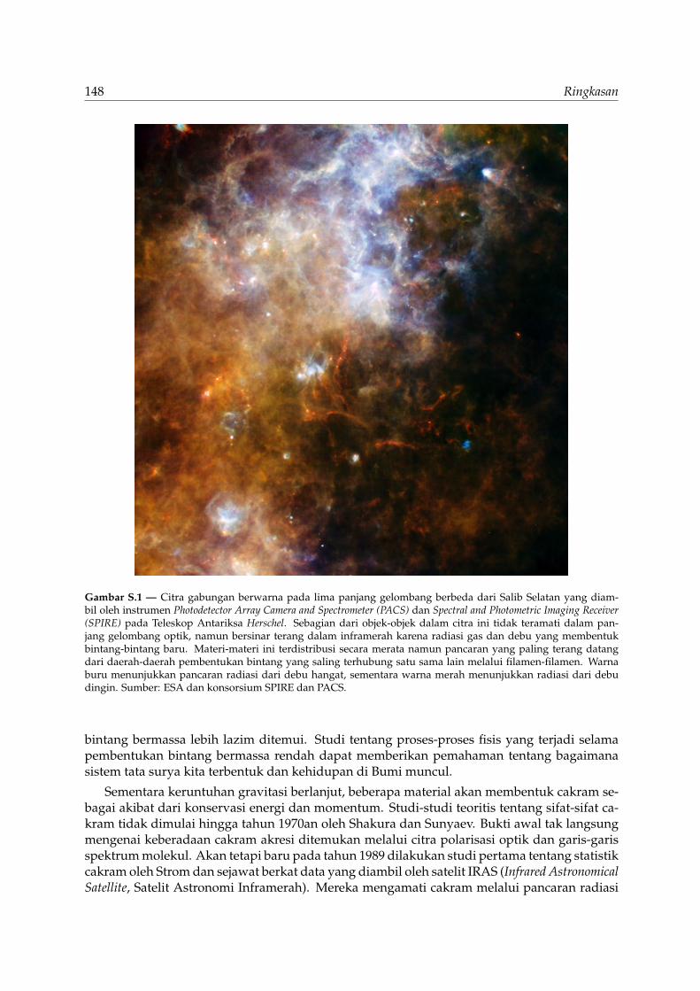
148 Ringkasan
Gambar S.1 — Citra gabungan berwarna pada lima panjang gelombang berbeda dari Salib Selatan yang diam-bil oleh instrumen Photodetector Array Camera and Spectrometer (PACS) dan Spectral and Photometric Imaging Receiver(SPIRE) pada Teleskop Antariksa Herschel. Sebagian dari objek-objek dalam citra ini tidak teramati dalam pan-jang gelombang optik, namun bersinar terang dalam inframerah karena radiasi gas dan debu yang membentukbintang-bintang baru. Materi-materi ini terdistribusi secara merata namun pancaran yang paling terang datangdari daerah-daerah pembentukan bintang yang saling terhubung satu sama lain melalui filamen-filamen. Warnaburu menunjukkan pancaran radiasi dari debu hangat, sementara warna merah menunjukkan radiasi dari debudingin. Sumber: ESA dan konsorsium SPIRE dan PACS.
bintang bermassa lebih lazim ditemui. Studi tentang proses-proses fisis yang terjadi selamapembentukan bintang bermassa rendah dapat memberikan pemahaman tentang bagaimanasistem tata surya kita terbentuk dan kehidupan di Bumi muncul.
Sementara keruntuhan gravitasi berlanjut, beberapa material akan membentuk cakram se-bagai akibat dari konservasi energi dan momentum. Studi-studi teoritis tentang sifat-sifat ca-kram tidak dimulai hingga tahun 1970an oleh Shakura dan Sunyaev. Bukti awal tak langsungmengenai keberadaan cakram akresi ditemukan melalui citra polarisasi optik dan garis-garisspektrum molekul. Akan tetapi baru pada tahun 1989 dilakukan studi pertama tentang statistikcakram oleh Strom dan sejawat berkat data yang diambil oleh satelit IRAS (Infrared AstronomicalSatellite, Satelit Astronomi Inframerah). Mereka mengamati cakram melalui pancaran radiasi
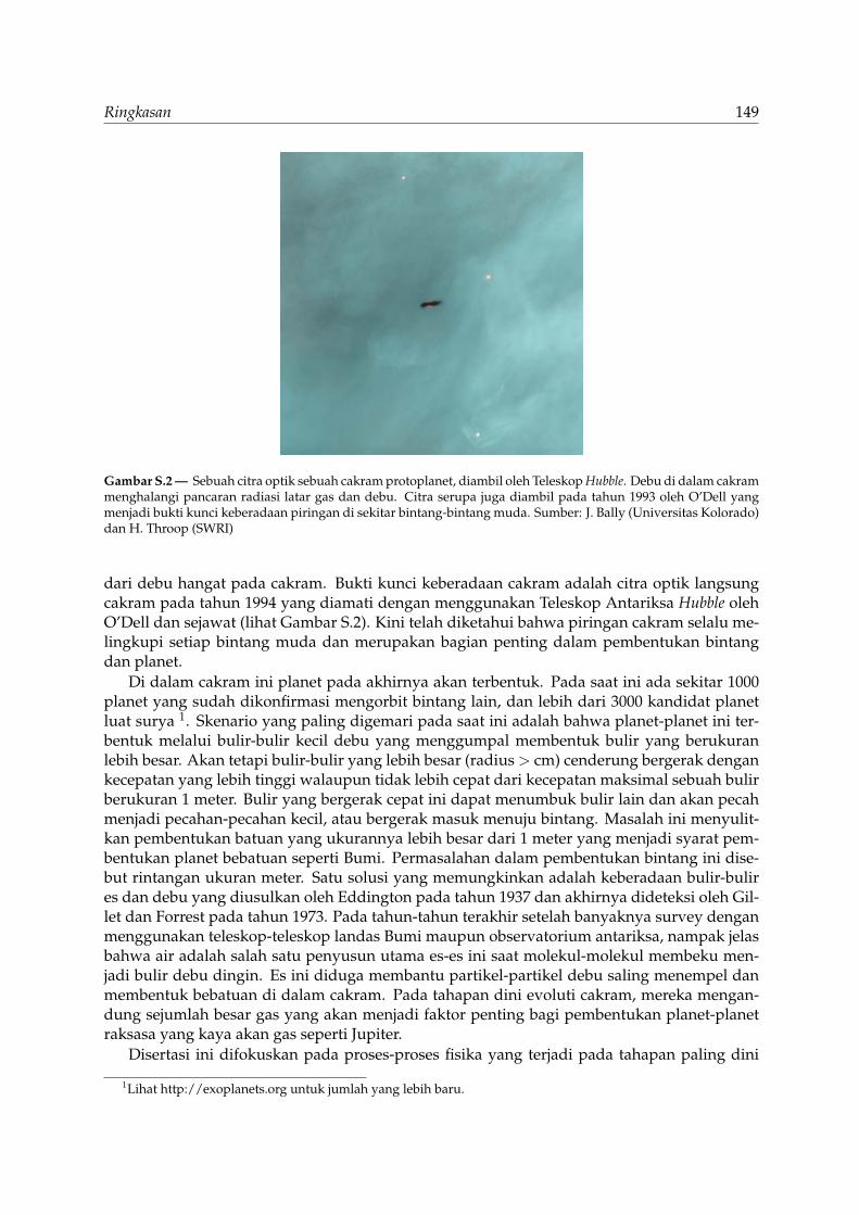
Ringkasan 149
Gambar S.2 — Sebuah citra optik sebuah cakram protoplanet, diambil oleh Teleskop Hubble. Debu di dalam cakrammenghalangi pancaran radiasi latar gas dan debu. Citra serupa juga diambil pada tahun 1993 oleh O’Dell yangmenjadi bukti kunci keberadaan piringan di sekitar bintang-bintang muda. Sumber: J. Bally (Universitas Kolorado)dan H. Throop (SWRI)
dari debu hangat pada cakram. Bukti kunci keberadaan cakram adalah citra optik langsungcakram pada tahun 1994 yang diamati dengan menggunakan Teleskop Antariksa Hubble olehO’Dell dan sejawat (lihat Gambar S.2). Kini telah diketahui bahwa piringan cakram selalu me-lingkupi setiap bintang muda dan merupakan bagian penting dalam pembentukan bintangdan planet.
Di dalam cakram ini planet pada akhirnya akan terbentuk. Pada saat ini ada sekitar 1000planet yang sudah dikonfirmasi mengorbit bintang lain, dan lebih dari 3000 kandidat planetluat surya 1. Skenario yang paling digemari pada saat ini adalah bahwa planet-planet ini ter-bentuk melalui bulir-bulir kecil debu yang menggumpal membentuk bulir yang berukuranlebih besar. Akan tetapi bulir-bulir yang lebih besar (radius > cm) cenderung bergerak dengankecepatan yang lebih tinggi walaupun tidak lebih cepat dari kecepatan maksimal sebuah bulirberukuran 1 meter. Bulir yang bergerak cepat ini dapat menumbuk bulir lain dan akan pecahmenjadi pecahan-pecahan kecil, atau bergerak masuk menuju bintang. Masalah ini menyulit-kan pembentukan batuan yang ukurannya lebih besar dari 1 meter yang menjadi syarat pem-bentukan planet bebatuan seperti Bumi. Permasalahan dalam pembentukan bintang ini dise-but rintangan ukuran meter. Satu solusi yang memungkinkan adalah keberadaan bulir-bulires dan debu yang diusulkan oleh Eddington pada tahun 1937 dan akhirnya dideteksi oleh Gil-let dan Forrest pada tahun 1973. Pada tahun-tahun terakhir setelah banyaknya survey denganmenggunakan teleskop-teleskop landas Bumi maupun observatorium antariksa, nampak jelasbahwa air adalah salah satu penyusun utama es-es ini saat molekul-molekul membeku men-jadi bulir debu dingin. Es ini diduga membantu partikel-partikel debu saling menempel danmembentuk bebatuan di dalam cakram. Pada tahapan dini evoluti cakram, mereka mengan-dung sejumlah besar gas yang akan menjadi faktor penting bagi pembentukan planet-planetraksasa yang kaya akan gas seperti Jupiter.
Disertasi ini difokuskan pada proses-proses fisika yang terjadi pada tahapan paling dini
1Lihat http://exoplanets.org untuk jumlah yang lebih baru.
150 Ringkasan
pembentukan bintang, ∼ 104−5 tahun setelah kontraksi gravitasi sebuah inti padat. Telah ba-nyak disepakati bahwa planet terbentuk di dalam cakram dan bahwa cakram memegang peranpenting dalam pembentukan dan evolusi bintang. Pembentukan dan evolusi dini bintang ti-dak sepenuhnya dipahami. Pertanyaan-pertanyaan utama disertasi ini adalah sebagai berikut:• Apakah cakram seperti yang mengitari bintang-bintang pra-deret utama sudah ada ke-
tika bintang baru saja lahir?• Apakah cakram tersebut dapat diamati dan bagaimana mereka dapat dibedakan dari
selubung yang menjadi tempat kelahiran bintang?• Apakah struktur fisis dan kimiawi cakram ini konsisten dengan model mutakhir pem-
bentukan cakram?• Sestabil apakah cakram yang terbenam di dalam selubung dan dapatkah mereka me-
nahan laju keruntuhan tinggi dari selubung?• Seberapa besar cakram yang terbenam berkontribusi pada garis-garis molekul yang dia-
mati?
Proses radiatif: Kontinum debu dan garis-garis molekul
Karakteristik bintang muda secara umum dipelajari dari radiasi kontinum yang dipancarkanoleh debu. Debu menghangat dengan cara memproses ulang pancaran radiasi bintang padaenergi tinggi (gelombang pendek) menjadi foton energi rendah (gelombang panjang). Strukturtemperatur debu ini dikendalikan oleh energi yang dipancarkan oleh bayi bintang seiring den-gan pengumpulan material-material dari ruang lingkupnya. Debu tersebut kemudian men-angkap cahaya dengan cara penyerapan atau hamburan. Debu hangat pada cakram meman-carkan cahaya inframerah. Akan tetapi, pada tahapan dini pembentukan bintang, selubungyang dingin dan masif akan menghalangi radiasi yang dipancarkan cakram. Dengan demi-kian, sulit untuk mempelajari secara langsung pertumbuhan bintang dan cakram yang barulahir tersebut. Model-model teoritis kemudian digunakan untuk memahami radiasi yang dia-mati.
Apabila emisi termal debu digunakan untuk mengamati jejak energi keseluruhan sistemyang sedang tumbuh, maka garis-garis emisi atom dan molekul digunakan untuk mengamatimassa dominan dari sekitar bintang-bintang muda. Alam semesta diisi oleh berbagai molekulyang berada pada berbagai kondisi fisis yang berbeda. Melalui pengamatan berbagai tran-sisi molekuler kita dapat menyelidiki berbagai kondisi fisis yang menghasilkan transisi mo-lekul tersebut, antara lain temperatur, kepadatan, dan struktur kecepatan. Yang paling pen-ting, transisi-transisi ini diskret sedemikian rupa sehingga mereka dipancarkan hanya padafrekuensi tertentu. Transisi molekuler yang paling lumrah ditemui adalah yang berasal darikarbon monoksida (CO). Jejak pergerakan gas dapat diamati dari pergeseran Doppler yangterjadi pada frekuensi yang diamati. Dengan demikian, dengan mengamati frekuensi darigaris-garis yang diamati, kita dapat mempelajari kinematika dari gas-gas ini.
Perkakas pengamatan
Untuk mempelajari cakram yang terbenam di dalam selubungnya dibutuhkan pengamatan in-terferometri pada panjang gelombang milimeter. Pengamatan inin dibutuhkan agar kita dapatmengamati emisi debu termal dari selubung bagian dalam dimana cakram tersebut berada.Interferometri adalah sebuah teknik yang menggabungkan dan mengkorelasikan sinyal dariberbagai teleskop, untuk dapat mencapai resolusi spasial yang tinggi, yang dibutuhkan untukmengamati cakram. Sebagai contoh, sebuah teleskop 12 m dapat mengamati radiasi CO darisuatu wilayah sebesar 7000 AU (7000 kali jarak Bumi ke Matahari). Dua buah teleskop seperti
Ringkasan 151
ini yang terpisahkan sejauh 1 km dapat mengamati radiasi yang sama dari wilayah sebesar 80AU. Pengamatan-pengamatan gas dan debu dengan menggunakan interferometri pada pan-jang gelombang milimeter dan submilimeter telah menjadi kunci dalam menyibakkan carakerja wilayah wilayah pembentukan bintang. Teleskop-teleskop ini terpisahkan sejauh jaraktertentu sehingga dapat mencakup berbagai resolusi sudut (0.5”–20”). Jarak antara kedua te-leskop ini disebut dengan garis dasar (baseline). Sepasang teleskop yang terpisahkan sejauhgaris dasar pendek akan mengamati radiasi yang dipancarkan selubung, sementara sepasangteleskop yang terpisahkan sejauh garis dasar sangat panjang akan dapat mengamati radiasidari cakram. Dengan menggabungkan berbagai konfigurasi kita dapat mengamati seluruhskala fisis secara serempak. Berbeda dengan pengamatan teleskop konvensional citra darisebuah pengamatan interferometri dibangun melalui transformasi Fourier dari koleksi fluksyang sudah dikorelasikan. Pasangan teleskop yang diam memanfaatkan rotasi Bumi untukmengamati dan memperoleh fluks yang terkorelasi. Kita membutuhkan banyak fluks yangterkorelasi untuk dapat membangun citra yang terpercaya. Pengamatan yang digunakan da-lam disertasi ini lazimnya memiliki lebih dari 5000 titik fluks yang terkorelasi. Fasilitas terbarudalam interferometri milimeter adalah Rangakaian Milimeter Besar Atacama (Atacama LargeMilimeter Array atau ALMA, terdiri atas 66 teleskop) di Cile. Dengan jumlah teleskop yang be-gitu besar akan lebih mudah mengamati struktur-struktur redup suatu pembentukan bintangyang sedang berjalan.
Disertasi ini dan pandangan ke depan
Disertasi ini menjelajahi baik aspek teoritis maupun observasional dari pembentukan cakrampada tahapan dini pembentukan bintang. Model semi analitis dan model hidrodinamika nu-merik telah digabungkan dengan berbagai perkakas hantaran radiasi kontinum debu. Garis-garis emisi molekuler yang diprediksikan kemudian dibandingkan dengan pengamatan. Si-mulasi dan prediksi ini juga didampingi dengan pengamatan spasial dan spektral resolusitinggi garis-garis emisi CO dengan ketebalan optik yang rendah dari objek-objek bintang mudayang tidak terlalu tertanam (i.e. lebih lanjut dalam tahapan evolusinya) dalam selubung.Pengamatan-pengamatan ini dilakukan dengan menggunakan Interferometer Plateau de Bure(PDBI) di Perancis. Berikut ini adalah garis-garis besar hasil disertasi ini:• Dalam Bab 2 garis-garis kontinum dan molekuler disimulasikan dengan menggunakan
simulasi hidrodinamika tiga dimensi yang mengikutkan medan magnetik. Keberadaanmedan magnetik dapat mencegah terbentuknya cakram. Ini merupakan sebuah perma-salahan yang sudah diketahui dalam astrofisika. Dua dari simulasi-simulasi ini digu-nakan untuk meneliti persamaan dan kesamaan antara simulasi yang membentuk ca-kram dan yang tidak. Prediksi-prediksi simulasi tiga dimensi kemudian dibandingkandengan model-model semi-analitis dua dimensi pembentukan bintang dan cakram. Per-bandingan antara keduanya menunjukkan bahwa dibutuhkan pengamatan-pengamataninterferometris seperti yang akan dihantarkan oleh ALMA untuk dapat mempelajari pro-ses pembentukan cakram. Dengan demikian di masa depan akan dimungkinkan untukmenguji model-model teoritis ini.• Pada tahapan terdini pembentukan bintang cakram dalam keadaan dingin dan masif. Ini
akan mengarah pada kontraksi gravitasi ke dalam dirinya sendiri dan dengan demikianmenciptakan ketidakstabilan. Sebagai tambahan, ketidakstabilan terjadi saat material-material di sekitar jatuh di atas cakram tersebut. Ketidakstabilan seperti ini telah diusul-kan sebagai mekanisme pembentukan planet dengan adanya pecahan-pecahan cakram.Bab 3 menyelidiki, dengan simulasi tiga dimensi, apakah cakram dapat pecah apabila
152 Ringkasan
sejumlah besar materi jatuh menumpuk di atasnya. Hasilnya menunjukkan bahwa ca-kram tidak terpecah tetapi mengalami penyaluran materi yang pesat menuju bintang.• Bab 4 menghadirkan prediksi evolusi karakteristik garis-garis molekuler dengan meng-
gunakan model dua dimensi. Emisi garis-garis molekuler karbon monoksida disimu-lasikan dengan mengikutkan garis-garis molekular yang dimati oleh Herschel baru-baruini. Prediksi-prediksi pada daerah gelombang panjang (milimeter) dibandingkan dengangaris-garis pada daerah inframerah. Dua himpunan garis-garis ini berasal dari daerahyang berbeda. Pancaran pada daerah inframerah disebabkan oleh energi yang dilepas-kan karena pergantian rotasi dan getaran molekul sementara pada gelombang panjangdisebabkan oleh pergantian rotasi. Terjadi pergantian energi yang lebih besar pada dae-rah inframerah sehingga dengan demikian kita dapat menyelidiki komponen gas yanglebih hangat.• Bab 2 dan 4 menunjukkan bahwa cakram yang terbenam dalam-dalam dapat dengan mu-
dah dikuak oleh pengamatan spasial dan spektral resolusi tinggi garis-garis molekuler.Pancaran ini seharusnya dipancarkan oleh cakram jika sejumlah besar selubung telahterlempar menjauh sebagaimana diharapkan dalam sistem-sistem yang telah berevolusilebih lanjut. Bab 5 menghadirkan pengamatan interferometris garis-garis 13CO dan C18Opada transisi rotasi J = 2− 1 dari empat protobintang yang telah dikenal dengan baik.Tiga dari empat benda ini mengisyaratkan keberadaan cakram yang berotasi. Ukurancakram-cakram ini selaras dengan model dua dimensi pembentukan cakram.• Keberadaan cakram-cakram ini dapat menjadi sumber pemanasan tambahan. Cakram
melepaskan energi saat ia menghantarkan material ke arah dalam menuju bintang, ka-rena cakram harus mempertahankan konservasi momentum sudut dan energi. Prosesenerjik ini memanaskan cakram sedemikian rupa sehingga es hanya dapat ditemukanjauh dari bintang pusat. Bab 6 menghadirkan studi teoritis spesies-spesies utama es(H2O, CO, CO2) pada sebuah cakram aktif di sekitar protobintang yang terbenam. Ca-kram panas ini diduga diperlukan untuk pembentukan Tata Surya kita. Dengan demi-kian bab ini menghadirkan hubungan antara tahapan-tahapan dini pembentukan bin-tang dan pembentukan sistem keplanetan. Prediksi-prediksi yang dibuat kemudian di-bandingkan dengan emisi air yang teramati di sekitar protobintang.
Pandangan ke masa depan. Pengamatan-pengamatan pada saat ini telah menguak kebera-daan cakram berotasi pada jarak beberapa ratus AU dari protobintang terselubung. Disertasiini juga membandingkan cakupan cakram terbenam yang disangga rotasi dengan model pem-bentukan cakram. Akan tetapi dibutuhkan resolusi spasial dan kpekaan yang akan dimilikiALMA untik lebih lanjut mempelajari detil-detil pembentukan cakram dan proses evolusi padatahapan-tahapan terdini pembentukan bintang. Pengamatan garis-garis molekul dengan reso-lusi spasial dan spektral yang lebih tinggi akan dapat membedakan antara cakram Kepleriandengan selubung yang runtuh. Untuk menyelidiki struktur temperatur suatu cakram (yangpenting untuk menyelidiki proses pemanasan) dibutuhkan pengamatan dua transisi berbedadari suatu molekul agar kondisi eksitasinya dapat diselidiki. Lebih lanjut suatu pengamatandengan kepekaan tinggi dibutuhkan untuk menyelidiki struktur kecepatan suatu cakram. Halini disebabkan karena emisi molekuler pada kecepatan tinggi lebih lemah dari pada pusat ga-ris. Akan lebih mudah pada masa depan untuk menguak kinematika pada skala kecil. Strukturkimiawi cakram-cakram muda juga akan menjadi penting dalam memahami pembentukan si-stem keplanetan.
Curriculum vitae
IWas born in Sumenep, Indonesia, which is located on the island of Madura. It is located about40 minutes from a few nice, serene white sand beaches. I attended a Catholic primary school
’Sang Timur’ built by the Dutch missionaries. After 11 years living in Indonesia, my brotherand I migrated to United States (apparently, I was persistent in wanting to leave). I finishedmy last year of primary school (6th year) in the greater Los Angeles area, a few minutes awayfrom the Santa Monica beach.
After finishing high school at Chaminade College Preparatory (West Hills, California) in2003, I started my B.Sc. in astrophysics at the University of California, Los Angeles with a minorin mathematics. During this time, I worked with Dr. Michael Muno on compiling X-ray fluxesfrom O and B stars in young stellar clusters using data taken by the Chandra X-ray Observatory.In the middle of my third year, I participated in the Research Experience for Undergraduate(REU) program in La Serena, Chile, which is located on ocean terraces. The program is hostedby Cerro-Tololo Inter-American Observatory (CTIO). I worked with Dr. Roberto de Propris onthe luminosity function of cluster galaxies using images taken by the Hubble Space Telescope.During my stay, I gained some experience in observation utilizing the 1 meter and the 4 meterVictor M. Blanco telescope.
I moved to Leiden, a few minutes from the beach, after obtaining my B.Sc. degree to con-tinue my studies in astronomy supported by Oort and Huygens scholarships. For my minorproject, I worked with Dr. Richard Alexander on characterizing the transport properties of self-gravitating disks. For my major project, continuing my trend in shifting to the lower energypart of the spectrum, I worked with Dr. Lars Kristensen and Dr. Ruud Visser on submillime-ter and near-IR molecular emission from young stellar objects in the Serpens molecular cloud.Thus, I have completely moved from looking for keV photons to meV radiation (6 orders ofmagnitude in energy) in roughly 4 years.
After my M.Sc., I started my Ph.D. in Leiden. I organized the astrochem seminars in my first2 years. I was also a teaching assistant for the ‘Star and Planet Formation’ course by Prof. Ewinevan Dishoeck, and the ‘Radiation Processes in Astrophysics’ course by Dr. Elena Rossi. Duringthe past 4 wonderful years, I have presented the results of my thesis in international confe-rences in Europe and in the USA. I also had the opportunity to visit the James Clerk MaxwellTelescope in Hawaii. After finishing, I will be a postdoctoral researcher at Institute for Theore-tical astrophysics (ITA) in Heidelberg, Germany. For the first time, I will be living inland awayfrom the beaches.
154 Curriculum vitae
Refereed publications
16. D. Harsono et al., Disciminating protostellar disk formation models with continuum and spectralline observations, 2014, A&A, subm.
15. M. N. Drozdovskaya et al., Methanol along the path from envelope to protoplanetary disk, 2014,MNRAS, subm.
14. C. Walsh et al., ALMA hints at the presence of two companions in the disk around HD100546,2014, ApJL, 791, L6
13. J. E. Lindberg et al., ALMA observations of the kinematics and chemistry of disc formation, 2014,A&A, 566, A74
12. M. V. Persson et al., The deuterium fractionation of water on solar-system scales in deeply-embedded low-mass protostars, 2014, A&A, 563, A74
11. D. Harsono et al., Rotationally-supported disks around Class I sources in Taurus: disk formationconstraints 2014, A&A, 562, A77
10. N. Murillo et al., A Keplerian disk around a Class 0 source: ALMA observations of VLA1623A,2013, A&A, 560, A103
9. J. K. Jørgensen et al., A recent accretion burst in the low-mass protostar IRAS 15398-3359:ALMA imaging of its related chemistry, 2013, ApJL, 779, 22
8. G. S. Mathews et al., ALMA imaging of the CO snowline of the HD 163296 disk with DCO+,2013, A&A, 557, 132
7. U. A. Yıldız et al., Water in low-mass star-forming regions with Herschel (WISH-LM) High-JCO survey observed with HIFI, 2013, A&A, 556, 89
6. D. Harsono et al., Evolution of CO lines in time-dependent models of protostellar disk formation,2013, A&A, 555, 45
5. L. E. Kristensen et al., Water in star-forming regions with Herschel (WISH): II. Evolution of557 GHz 110-101 emission in low-mass protostars, 2012, A&A, 542, 8
4. R. Visser et al., Modelling Herschel observations of hot molecular gas emission from embeddedlow-mass protostars, 2012, A&A, 537, 55
3. D. Harsono, R. D. Alexander and Y. Levin, Global gravitational instabilities in embeddeddiscs, 2011, MNRAS, 413, 423
2. D. Harsono, and R. De Propris. The luminosity function of galaxies to MBgV riz ∼ −14 in z∼ 0.3 clusters, 2009, Astronomical Journal, 137, 3091
1. D. Harsono , and R. De Propris. The cluster galaxy luminosity function at z = 0.3: a recentorigin for a faint-end upturn?, 2007, MNRAS, 380, 1036

Acknowledgements
THese past few years could not be ever more enjoyable and entertaining without certaingroups of people that accompanied me. I certainly cannot name them all. Also, my deepest
gratitudes go beyond these simple words below.Simon, without your patience and constant guidance through the details of radiative trans-
fer, a large part of this thesis would not be in the state that it is now. I enjoyed our skypeconversations during some un-Godly hours. Dear Lars, I have you to thank for introducing meto the world of astrochemistry and shocks. Without your guidance and advices, things wouldhad turned out differently or possibly more ‘confused’. Ruud, it was a pleasure having youas my office mate for a brief moment and introducing me to ‘simple’ chemical models. Greg,your straightforward comments on both scientific and non-scientific aspects gave me a refres-hing look in this whole craziness called ‘life’. Richard Alexander, I have enjoyed learning aboutdisks and simulations from you. Roberto de Propris, I have you to thank for my first scientificpublication. More importantly, you were the one that sent me the link to Leiden and told meto apply even though the deadline has passed. Things in Leiden would not have run smoothlywithout the excellent support from the computer group and the secretaries.
Linda and Carl, I truly appreciated the countless times the two of you dragged me out ofmy office to enjoy movies, drinks, and dinners. I finally got to ski because of the two of you.Fike and Cindy, I enjoyed so many conversations and complaints that we shared. Oxalis andMaarten, many thanks for bringing colors and arts into our lives. Finally, the past years wouldnot be the same without your company and occasional gossips at Annie’s in the late evenings.
To the board games/beach/park group: Giorgia, Bernadetta, Thibaut, Emilie, Stefania, Ras-mus, Daniel Risquez, Carmen Blasco, Steven Rieder, Jeroen Bedorf, Tri, Markus, Eva, Nikta,Yuri Cavechi, Atakan Gurkan, I have enjoyed all of our entertaining nights and days. It wasmy pleasure being the ‘Game Master’ for the Huygens-Oort Diplomacy game, and I hope itwill never happen again. To Giorgia, your tiramisu is truly the original one. To Michiko andBernadetta, those Japanese snacks, sushi dinners, and afternoon teas were greatly missed afteryou left. To Emilie, watching Thibaut dance was one of the highlights of my summer. Belgianbeers trip, swimming in the evenings, Essen trips, and centreparc trips were all legen-wait forit...dary. Let’s have our own Tuxedo night.
Dear Ted and Hailey, I have enjoyed your company every time I am in the Los Angelesarea. The hospitality and friendliness of your family members both in US and China are muchappreciated. To James Wigglesworth, Emin Menachekanian, and others, we need more KoreanBBQ times. Dearest Indara, it was wonderful meeting up in Munich after all these years andour skype chats are entertaining.
Irene, having you as my office mate made my working hours enjoyable. I have to appreciatethe fact that you did not use that ruler extensively. Dearest Edith, all of the conversations,laughs, margaritas, cakes, and the coffees during the past few months are much appreciated:they were ‘almost as good’ as legendary. To my Brazillian buddy Isa, my weekends in the officeand coffee breaks would not be the same without you. You made me laugh every weekend inthe office.
Adwin Boogert, our drinks and conversations in Pasadena certainly pushed me toward go-ing to Leiden. I enjoyed our random skype chats and sight-seeing in Utrecht during your shortvisit in the Netherlands. Dear Stella Kafka, your enthusiasm is truly inspirational and thanks
156 Acknowledgements
for the all of the advices, letters, and a short Washington D. C. tour to a Mexican restaurant. Ihope to see you soon in Athens.
Dear Joe and Kirsty, you taught me how to properly enjoy Eurovision (with British hu-mours). Pam, the coffee breaks and Friday borrels would not be the same without your pre-sence and keeping me confused at times. Geoff and Star, I miss our board game nights. Ca-therine, your Irish craziness certainly came in at the right moment. Magnus and Mihaela, yourhospitality in Malmo, Bucharest, and Leiden is never forgotten, so... where to next. Niels, justremember that I am always wrong and the cake is a lie. Thanks for making the 5th floor cor-ridor in Leiden as loud as possible: Jeanette, Kalle, Umut, Christian B., Kuo-Song, Silvia V.,Thanja, Xiaohu, Koju, Paola, Mihkel, Maria, Alan, Anton, Atilla, and Nienke. My experiencein Garching and biergartens would not be the same without: Davide, Stephanie R, Nadia, andAnna. Dear Agata, we actually managed to graduate on the same day!
My weekends and afternoons would not have been as fun without the various people I metthrough Leiden social football club, badminton (Nuriltje), basketball, rowing for ‘Asopos deVliet’ (Remco van der Burg and Willem de Pous, the coaches), and futsal.
To my family members: Ko Elyon, Ci Jeanne, Mommy Fei-Fei, Om Tony, Ko Erwin, andCi Fenny, thank you for all of the support both from US and Indonesia and for sending mepictures of food that I have never tasted for the past years, I have put them in good use. To myparents, my dad, grandparents, and Om Ritwan, your constant support and teachings over theyears have made me the person that I am today.