1Scientific RepoRts | (2019) 9:1157 | https://doi.org/10.1038/s41598-018-38136-8

www.nature.com/scientificreports

Unsupervised feature extraction of anterior chamber oCt images for ordering and classificationpablo Amil1, Laura González2, elena Arrondo2, Cecilia salinas2, J. L. Guell2, Cristina Masoller 1 & Ulrich parlitz3

We propose an image processing method for ordering anterior chamber optical coherence tomography (oCt) images in a fully unsupervised manner. the method consists of three steps: Firstly we preprocess the images (filtering the noise, aligning and normalizing the resolution); secondly, a distance measure between images is computed for every pair of images; thirdly we apply a machine learning algorithm that exploits the distance measure to order the images in a two-dimensional plane. the method is applied to a large (~1000) database of anterior chamber OCT images of healthy subjects and patients with angle-closure and the resulting unsupervised ordering and classification is validated by two ophthalmologists.

Machine learning methods are extremely useful in biomedicine1,2 and in particular for glaucoma detection3–6. The use of such methods can help to optimize the available human resources, to increase accuracy in diagnosis, and to make treatment decisions faster.

Glaucoma is the leading cause of global irreversible blindness7. Early diagnosis and treatment is a challenge given that glaucoma presents no symptoms in its early stages8. Diagnostic of angle-closure is based on the clinical observation of the angle at the slit- lamp requiring a goniolens that is placed on the patient’s cornea. Anterior Segment Optical Coherence Tomography (AS-OCT) is a fast, useful and contact-less tool that allows visualization and measurement of the anterior chamber angle9–11. Various techniques exist and are being developed to improve image quality12–15, and work is also focused on the development of advanced tools to analyze such images16–18. However the quality of the images is not always enough for an accurate diagnosis and for example19, two glau-coma experts working together were unable to locate the scleral spur (see Fig. 8) in 28% of the images. Such land-mark is of utmost importance to determine most of the relevant features that are used in angle-closure diagnosis.

Previous approaches for processing anterior chamber OCT images used segmentation algorithms and further analysis, while others used manual landmark determination. In works by Tian et al.16 and Wu et al.20 segmenta-tion algorithms for OCT anterior chamber images were proposed, both discuss the difficulties of such task due to the noise in the image and to other artifacts. In21 the authors analyzed data from manual landmark determination to classify images into five subcategories of angle-closure glaucoma. They used both supervised and unsupervised feature selection and AdaBoost classifiers (supervised learning) to achieve accuracies in the range of 84~87%. In22 a method was proposed to extract almost 3000 features from the raw images, then, the most relevant features for classification were supervisedly selected, and machine learning was applied to the selected features. However, the fact that only 74 images were analyzed while 15 features were used, compromised the statistical significance of the study. In23 Histogram of Oriented Gradients (HOG) features of anterior chamber OCT images and Support Vector Machine (SVM, supervised learning) were used to classify different glaucoma subtypes, achieving accu-racies in the order of 80%.

In this paper we propose an image processing method that unsupervisedly orders OCT anterior chamber images according to what we demonstrate to be relevant extracted features. The reliability of the algorithm is tested with a large number of images (~1000). Importantly, our method is fully autonomous and can be used to analyze images with a wide spectrum of quality, even those with high levels of noise and artifacts.

1Universitat Politècnica de Catalunya, Rambla Sant Nebridi 22, 08222, Terrassa, Spain. 2instituto de Microcirugía Ocular, Josep Mar´ıa Lladó 3, 08035, Barcelona, Spain. 3Max Planck Institute for Dynamics and Self-Organization, Am Faßberg 17, 37077, Göttingen, Germany. Correspondence and requests for materials should be addressed to c.M. (email: cristina.masoller@upc.edu)

Received: 4 April 2018

Accepted: 19 December 2018

Published: xx xx xxxx

opeN

www.nature.com/scientificreports/

2Scientific RepoRts | (2019) 9:1157 | https://doi.org/10.1038/s41598-018-38136-8

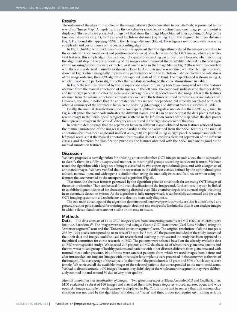
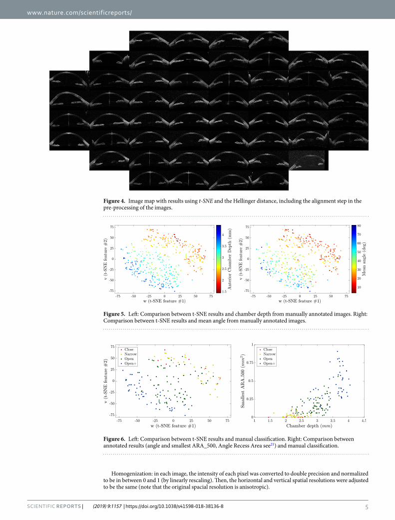
ResultsThe outcome of the algorithm applied to the image database (both described in Sec. Methods) is presented in the way of an “Image Map”. A regular grid in the coordinates space (w, v) is defined and one image per grid point is displayed. The results are presented in Figs 1–4 that show the Image Map obtained after applying IsoMap to the Euclidean distance (Fig. 1), to the aligned Euclidean distance (Eq. 4, Fig. 2), to the aligned Hellinger distance (Eq. 3, Fig. 3) and after applying t-SNE to the Hellinger distance (Fig. 4). These figures are ordered with increasing complexity and performance of the corresponding algorithm.

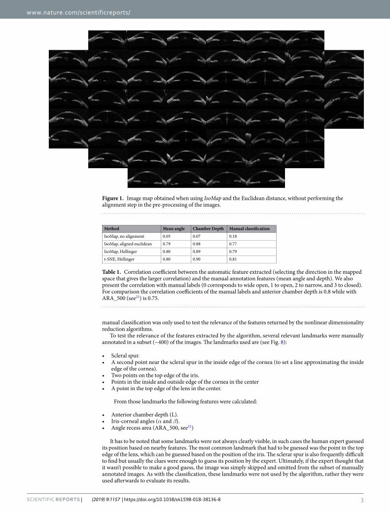
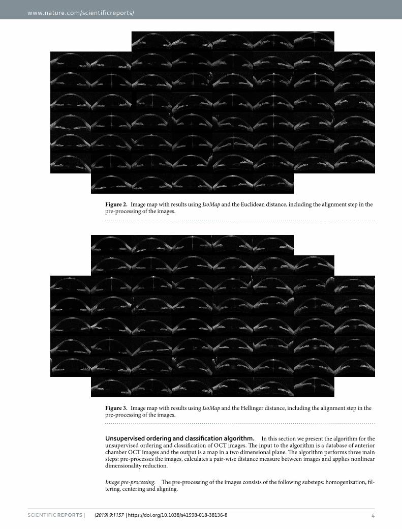
In Fig. 1 (IsoMap with Euclidean distance) it is apparent that the algorithm ordered the images according to the orientation (horizontal axis) and position (vertical axis) of each eye inside the OCT image, which are irrele-vant features, this simple algorithm is, then, not capable of extracting useful features. However, when including the alignment step in the pre-processing of the images which removed the variability detected by the first algo-rithm, meaningful features were extracted, as it can be seen in the Image Map in Fig. 2 (these features correlate with the features derived manually, as shown in Table 1). A similar map was obtained with the Hellinger distance, shown in Fig. 3 which marginally improves the performance with the Euclidean distance. To test the robustness of the image ordering, the t-SNE algorithm was applied (instead of IsoMap). The map obtained is shown in Fig. 4, which turned out to perform slightly better than IsoMap according to the correlations shown in Table 1.

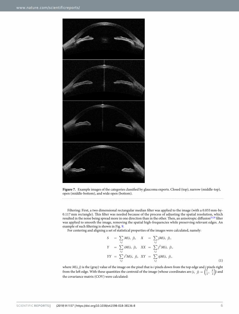
In Fig. 5 the features returned by the unsupervised algorithm, using t-SNE, are compared with the features obtained from the manual annotation of the images: in the left panel the color code indicates the chamber depth, and in the right panel, it indicates the mean angle (average of α and β) of each annotated image. Clearly, the features obtained from the manual annotation correlate very well with the features returned by the unsupervised algorithm. However, one should notice that the annotated features are not independent, but strongly correlated with each other. A summary of the correlation between the ordering (Mappings) and different features is shown in Table 1.

Finally, the manual classification done by two expert ophthalmologists is included in the t-SNE (w, v) map. In Fig. 6, left panel, the color code indicates the different classes, and it can be noticed that the data points that rep-resent images in the “wide-open” category are scattered in the left-down corner of the map, while the data points that represent images in the “closed” category are scattered in the right-top corner of the map.

In order to demonstrate that the separation between different classes obtained from features retrieved from the manual annotation of the images is comparable to the one obtained from the t-SNE features, the manual annotation features (mean angle and smallest ARA_500) are plotted in Fig. 6, right panel. A comparison with the left panel reveals that the manual annotation features also do not allow for a clear-cut separation of the different classes, and therefore, for classification purposes, the features obtained with the t-SNE map are as good as the manual annotation features.

DiscussionWe have proposed a new algorithm for ordering anterior chamber OCT images in such a way that it is possible to classify them, in a fully unsupervised manner, in meaningful groups according to relevant features. We have tested the algorithm with a large set of images classified by two expert ophthalmologists, and with a larger set of annotated images. We have verified that the separation in the different classes defined by the ophthalmologists (closed, narrow, open, and wide open) is similar when using the manually extracted features, or when using the features that are returned by the unsupervised algorithm (Fig. 6).

Therefore, the abstract features generated by the algorithm provide novel tools for assessing OCT images of the anterior chamber. They can be used for direct classification of the images and, furthermore, they can be linked to established quantities used for characterizing diseased eyes (like chamber depth, iris-corneal angle) resulting in an automatic detection system. As the algorithm is fully unsupervised, it can be easily automated and set up in OCT imaging systems to aid technicians and doctors in an early diagnosis.

The two main advantages of the algorithm demonstrated here over previous works are that it doesn’t need any ground truth or gold standard for training, and it does not rely on specific landmarks; thus, it can analyze images in which relevant landmarks are not visible or not easy to locate.

MethodsData. The data consists of 1213 OCT images taken from consenting patients at IMO (Ocular Microsurgery Institute, Barcelona)24. The images were acquired using a Visante OCT instrument (Carl Zeiss Meditec) using the “Anterior segment” scan and the “Enhanced anterior segment” scan. The original resolution of all the images is 256-by-1024 pixels corresponding to an area of 16 mm-by-8 mm. All the patients included in the study consented that their data and images could be used for research and teaching purposes and the study has been approved by the ethical committee for clinic research in IMO. The patients were selected based on the already available data at IMO (retrospective study). We selected 247 patients at IMO database, 81 of which were glaucoma patents and the rest was a mixed group of healthy patients and patients with other diseases different from glaucoma and with normal intraocular pressure, 104 of those were cataract patients, from which we used images from before and after intraocular lens implant (images with intraocular lens implants were processed in the same way as the rest of the images). The average age of the subjects (at the time of the procedure) is 42 years and 57% of such subjects are female. We retrieved all the available images of the selected patients that corresponded to the mentioned scans. We had to discard around 1400 images because they didn’t depict the whole anterior segment (they were deliber-ately zoomed in) and around 50 due to very poor quality.

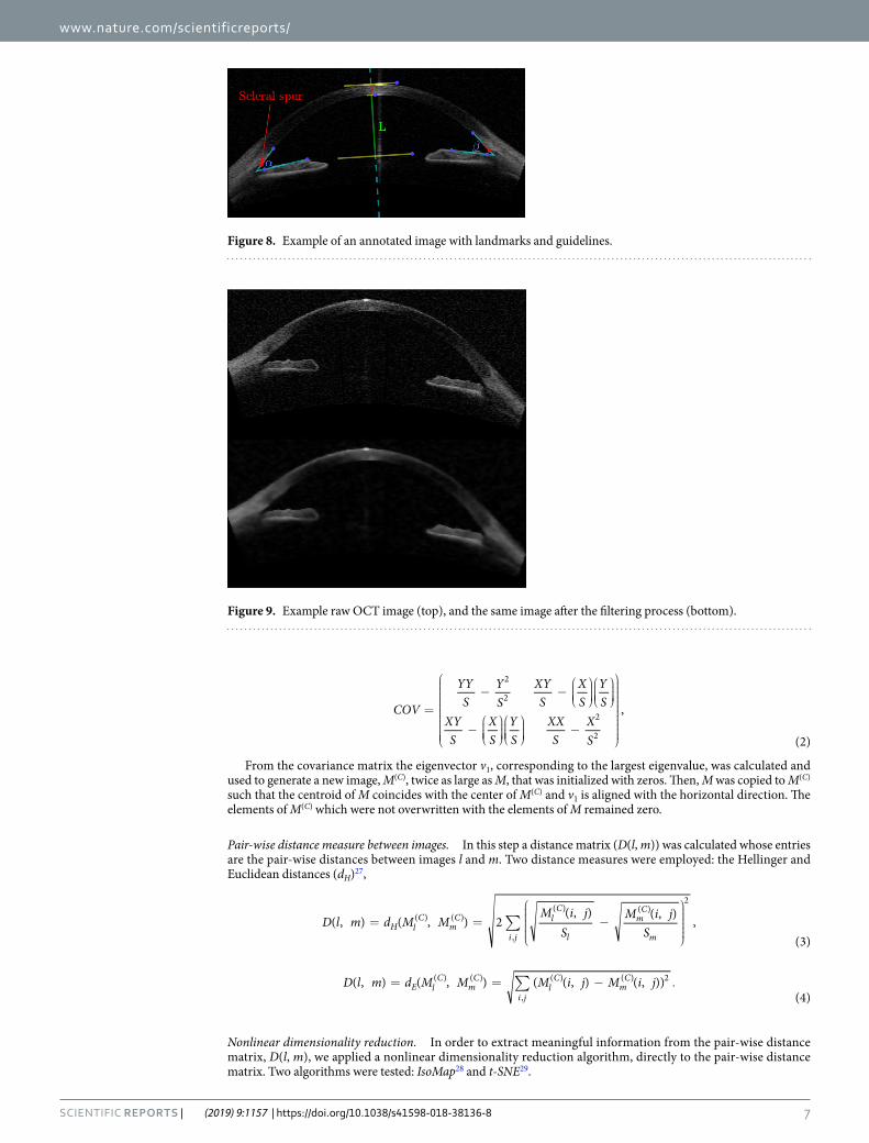
Manual annotation and classification of images. Two glaucoma experts (Elena Arrondo, MD and Cecilia Salinas, MD) evaluated a subset of 160 images and classified them into four categories: closed, narrow, open, and wide open. An image example in each category is displayed in Fig. 7. It is important to remark that this manual clas-sification was not used by the algorithm (as it does not “learn” and thus, it does not require any training set); the

www.nature.com/scientificreports/

3Scientific RepoRts | (2019) 9:1157 | https://doi.org/10.1038/s41598-018-38136-8

manual classification was only used to test the relevance of the features returned by the nonlinear dimensionality reduction algorithms.

To test the relevance of the features extracted by the algorithm, several relevant landmarks were manually annotated in a subset (~400) of the images. The landmarks used are (see Fig. 8):

• Scleral spur.• A second point near the scleral spur in the inside edge of the cornea (to set a line approximating the inside

edge of the cornea).• Two points on the top edge of the iris.• Points in the inside and outside edge of the cornea in the center• A point in the top edge of the lens in the center.

From those landmarks the following features were calculated:

• Anterior chamber depth (L).• Iris-corneal angles (α and β).• Angle recess area (ARA_500, see21)

It has to be noted that some landmarks were not always clearly visible, in such cases the human expert guessed its position based on nearby features. The most common landmark that had to be guessed was the point in the top edge of the lens, which can be guessed based on the position of the iris. The sclerar spur is also frequently difficult to find but usually the clues were enough to guess its position by the expert. Ultimately, if the expert thought that it wasn’t possible to make a good guess, the image was simply skipped and omitted from the subset of manually annotated images. As with the classification, these landmarks were not used by the algorithm, rather they were used afterwards to evaluate its results.

Figure 1. Image map obtained when using IsoMap and the Euclidean distance, without performing the alignment step in the pre-processing of the images.

Method Mean angle Chamber Depth Manual classification

IsoMap, no alignment 0.05 0.07 0.18

IsoMap, aligned euclidean 0.79 0.88 0.77

IsoMap, Hellinger 0.80 0.89 0.79

t-SNE, Hellinger 0.80 0.90 0.81

Table 1. Correlation coefficient between the automatic feature extracted (selecting the direction in the mapped space that gives the larger correlation) and the manual annotation features (mean angle and depth). We also present the correlation with manual labels (0 corresponds to wide open, 1 to open, 2 to narrow, and 3 to closed). For comparison the correlation coefficients of the manual labels and anterior chamber depth is 0.8 while with ARA_500 (see21) is 0.75.

www.nature.com/scientificreports/

4Scientific RepoRts | (2019) 9:1157 | https://doi.org/10.1038/s41598-018-38136-8

Unsupervised ordering and classification algorithm. In this section we present the algorithm for the unsupervised ordering and classification of OCT images. The input to the algorithm is a database of anterior chamber OCT images and the output is a map in a two dimensional plane. The algorithm performs three main steps: pre-processes the images, calculates a pair-wise distance measure between images and applies nonlinear dimensionality reduction.

Image pre-processing. The pre-processing of the images consists of the following substeps: homogenization, fil-tering, centering and aligning.

Figure 2. Image map with results using IsoMap and the Euclidean distance, including the alignment step in the pre-processing of the images.

Figure 3. Image map with results using IsoMap and the Hellinger distance, including the alignment step in the pre-processing of the images.

www.nature.com/scientificreports/

5Scientific RepoRts | (2019) 9:1157 | https://doi.org/10.1038/s41598-018-38136-8

Homogenization: in each image, the intensity of each pixel was converted to double precision and normalized to be in between 0 and 1 (by linearly rescaling). Then, the horizontal and vertical spatial resolutions were adjusted to be the same (note that the original spacial resolution is anisotropic).

Figure 5. Left: Comparison between t-SNE results and chamber depth from manually annotated images. Right: Comparison between t-SNE results and mean angle from manually annotated images.

Figure 6. Left: Comparison between t-SNE results and manual classification. Right: Comparison between annotated results (angle and smallest ARA_500, Angle Recess Area see21) and manual classification.

Figure 4. Image map with results using t-SNE and the Hellinger distance, including the alignment step in the pre-processing of the images.

www.nature.com/scientificreports/

6Scientific RepoRts | (2019) 9:1157 | https://doi.org/10.1038/s41598-018-38136-8

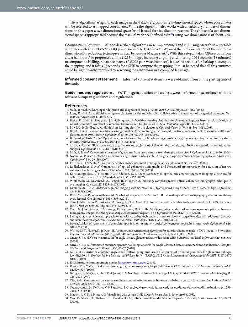
Filtering: First, a two dimensional rectangular median filter was applied to the image (with a 0.055 mm-by-0.117 mm rectangle). This filter was needed because of the process of adjusting the spatial resolution, which resulted in the noise being spread more in one direction than in the other. Then, an anisotropic diffusion25,26 filter was applied to smooth the image, removing the spatial high-frequencies while preserving relevant edges. An example of such filtering is shown in Fig. 9.

For centering and aligning a set of statistical properties of the images were calculated, namely:

∑ ∑

∑ ∑

∑ ∑

= =

= =

= =

S M i j X jM i j

Y iM i j XX j M i j

YY i M i j XY ijM i j

( , ), ( , ) ,

( , ), ( , ) ,

( , ), ( , ) ,(1)

i j i j

i j i j

i j i j

, ,

, ,

2

,

2

,

where M(i, j) is the (gray) value of the image on the pixel that is i pixels down from the top edge and j pixels right from the left edge. With these quantities the centroid of the image (whose coordinates are = ( )i j( , ) ,Y

SXS

) and the covariance matrix (COV) were calculated:

Figure 7. Example images of the categories classified by glaucoma experts. Closed (top), narrow (middle-top), open (middle-bottom), and wide open (bottom).

www.nature.com/scientificreports/

7Scientific RepoRts | (2019) 9:1157 | https://doi.org/10.1038/s41598-018-38136-8

=

− −

−

−

COV

YYS

YS

XYS

XS

YS

XYS

XS

YS

XXS

XS

,

(2)

2

2

2

2

From the covariance matrix the eigenvector v1, corresponding to the largest eigenvalue, was calculated and used to generate a new image, M(C), twice as large as M, that was initialized with zeros. Then, M was copied to M(C) such that the centroid of M coincides with the center of M(C) and v1 is aligned with the horizontal direction. The elements of M(C) which were not overwritten with the elements of M remained zero.

Pair-wise distance measure between images. In this step a distance matrix (D(l, m)) was calculated whose entries are the pair-wise distances between images l and m. Two distance measures were employed: the Hellinger and Euclidean distances (dH)27,

∑= =

−

D l m d M M

M i jS

M i jS

( , ) ( , ) 2( , ) ( , ) ,

(3)H l

Cm

C

i j

lC

l

mC

m

( ) ( )

,

( ) ( )2

∑= = − .D l m d M M M i j M i j( , ) ( , ) ( ( , ) ( , ))(4)

E lC

mC

i jl

Cm

C( ) ( )

,

( ) ( ) 2

Nonlinear dimensionality reduction. In order to extract meaningful information from the pair-wise distance matrix, D(l, m), we applied a nonlinear dimensionality reduction algorithm, directly to the pair-wise distance matrix. Two algorithms were tested: IsoMap28 and t-SNE29.

Figure 9. Example raw OCT image (top), and the same image after the filtering process (bottom).

Figure 8. Example of an annotated image with landmarks and guidelines.

www.nature.com/scientificreports/

8Scientific RepoRts | (2019) 9:1157 | https://doi.org/10.1038/s41598-018-38136-8

These algorithms assign, to each image in the database, a point in a n-dimensional space, whose coordinates will be referred to as mapped coordinates. While the algorithm also works with an arbitrary number of dimen-sions, in this paper a two dimensional space (w, v) is used for visualization reasons. The choice of a two dimen-sional space is appropriated because the residual variance (defined as in28) using two dimensions is of about 30%.

Computational runtime. All the described algorithms were implemented and run using MatLab in a portable computer with an Intel i7-7700HQ processor and 16 GB of RAM. We used the implementation of the nonlinear dimensionality reduction techniques written by van der Maaten et al.30. With this setup, it takes 5294 seconds (one and a half hours) to preprocess all the (1213) images including aligning and filtering, 1054 seconds (18 minutes) to compute the Hellinger distance matrix (735078 pair-wise distances), it takes 41 seconds for IsoMap to compute the mapping, and it takes 25 seconds for t-SNE to compute the mapping. It must be noted that all this runtimes could be significantly improved by rewriting the algorithms in a compiled language.

Informed consent statement. Informed consent statements were obtained from all the participants of the study.

Guidelines and regulations. OCT image acquisition and analysis were performed in accordance with the relevant European guidelines and regulations.

References 1. Sajda, P. Machine learning for detection and diagnosis of disease. Annu. Rev. Biomed. Eng. 8, 537–565 (2006). 2. Long, E. et al. An artificial intelligence platform for the multihospital collaborative management of congenital cataracts. Nat.

Biomed. Engineering 1, 0024 (2017). 3. Bizios, D., Heijl, A., Hougaard, J. L. & Bengtsson, B. Machine learning classifiers for glaucoma diagnosis based on classification of

retinal nerve fibre layer thickness parameters measured by Stratus OCT. Acta Ophthalmologica 88, 44–52 (2010). 4. Bowd, C. & Goldbaum, M. H. Machine learning classifiers in glaucoma. Opt. and Vision Science 85, 396–405 (2008). 5. Bowd, C. et al. Bayesian machine learning classifiers for combining structural and functional measurements to classify healthy and

glaucomatous eyes. Investig. Ophthalmol. & Vis. Sci. 49, 945–953 (2008). 6. Burgansky-Eliash, Z. et al. Optical coherence tomography machine learning classifiers for glaucoma detection: a preliminary study.

Investig. Ophthalmol. & Vis. Sci. 46, 4147–4152 (2005). 7. Tham, Y.-C. et al. Global prevalence of glaucoma and projections of glaucoma burden through 2040: a systematic review and meta-

analysis. Ophthalmol. 121, 2081–2090 (2014). 8. Mills, R. P. et al. Categorizing the stage of glaucoma from pre-diagnosis to end-stage disease. Am. J. Ophthalmol. 141, 24–30 (2006). 9. Nolan, W. P. et al. Detection of primary angle closure using anterior segment optical coherence tomography in Asian eyes.

Ophthalmol. 114, 33–39 (2007). 10. Friedman, D. S. & He, M. Anterior chamber angle assessment techniques. Surv. Ophthalmol. 53, 250–273 (2008). 11. Radhakrishnan, S. et al. Comparison of optical coherence tomography and ultrasound biomicroscopy for detection of narrow

anterior chamber angles. Arch. Ophthalmol. 123, 1053–1059 (2005). 12. Konstantopoulos, A., Hossain, P. & Anderson, D. F. Recent advances in ophthalmic anterior segment imaging: a new era for

ophthalmic diagnosis? Br. J. Ophthalmol. 91, 551–557 (2007). 13. Wojtkowski, M., Kowalczyk, A., Leitgeb, R. & Fercher, A. Full range complex spectral optical coherence tomography technique in

eye imaging. Opt. Lett. 27, 1415–1417 (2002). 14. Grulkowski, I. et al. Anterior segment imaging with Spectral OCT system using a high-speed CMOS camera. Opt. Express 17,

4842–4858 (2009). 15. Pérez-Merino, P., Velasco-Ocana, M., Martinez-Enriquez, E. & Marcos, S. OCT-based crystalline lens topography in accommodating

eyes. Biomed. Opt. Express 6, 5039–5054 (2015). 16. Tian, J., Marziliano, P., Baskaran, M., Wong, H.-T. & Aung, T. Automatic anterior chamber angle assessment for HD-OCT images.

IEEE Trans. on Biomed. Eng. 58, 3242–3249 (2011). 17. Console, J. W., Sakata, L. M., Aung, T., Friedman, D. S. & He, M. Quantitative analysis of anterior segment optical coherence

tomography images: the Zhongshan Angle Assessment Program. Br. J. Ophthalmol. 92, 1612–1616 (2008). 18. Leung, C. K.-s. et al. Novel approach for anterior chamber angle analysis: anterior chamber angle detection with edge measurement

and identification algorithm (ACADEMIA). Arch. Ophthalmol. 124, 1395–1401 (2006). 19. Sakata, L. M. et al. Assessment of the scleral spur in anterior segment optical coherence tomography images. Arch. Ophthalmol. 126,

181–185 (2008). 20. Wu, W., Li, Y., Huang, D. & Duan, H. A compound segmentation algorithm for anterior chamber angle in OCT image. In Biomedical

Engineering and Informatics (BMEI), 2011 4th International Conference on, vol. 1, 12–15 (IEEE, 2011). 21. Niwas, S. I. et al. Cross-examination for angle-closure glaucoma feature detection. IEEE J. Biomed. and Heal. Informatics 20, 343–354

(2016). 22. Niwas, S. I. et al. Automated anterior segment OCT image analysis for Angle Closure Glaucoma mechanisms classification. Comput.

Methods and Programs in Biomed. 130, 65–75 (2016). 23. Xu, Y. et al. Anterior chamber angle classification using multiscale histograms of oriented gradients for glaucoma subtype

identification. In Engineering in Medicine and Biology Society (EMBC), 2012 Annual International Conference of the IEEE, 3167–3170 (IEEE, 2012).

24. IMO. Instituto de microcirugía ocular, https://www.imo.es/en (2018). 25. Perona, P. & Malik, J. Scale-space and edge detection using anisotropic diffusion. IEEE Trans. on Pattern Anal. and Machine Intell.

12, 629–639 (1990). 26. Gerig, G., Kubler, O., Kikinis, R. & Jolesz, F. A. Nonlinear anisotropic filtering of MRI quitar data. IEEE Trans. on Med. Imaging 11,

221–232 (1992). 27. Cha, S.-H. Comprehensive survey on distance/similarity measures between probability density functions. Int. J. Math. Model.

Methods Appl. Sci. 1, 300–307 (2007). 28. Tenenbaum, J. B., De Silva, V. & Langford, J. C. A global geometric framework for nonlinear dimensionality reduction. Sci. 290,

2319–2323 (2000). 29. Maaten, L. V. D. & Hinton, G. Visualizing data using t-SNE. J. Mach. Learn. Res. 9, 2579–2605 (2008). 30. Van Der Maaten, L., Postma, E. & Van den Herik, J. Dimensionality reduction: a comparative review. J Mach Learn. Res 10, 66–71

(2009).

www.nature.com/scientificreports/

9Scientific RepoRts | (2019) 9:1157 | https://doi.org/10.1038/s41598-018-38136-8

AcknowledgementsThis work was supported by the BE-OPTICAL project (H2020-675512). C.M. also acknowledges partial support from Spanish MINECO/FEDER (FIS2015-66503-C3-2-P) and ICREA ACADEMIA.

Author ContributionsP.A. and U.P. designed the algorithm. P.A., C.S. and E.A. analysed the data. J.L.G., C.M. and U.P. conceived the study. P.A., C.M. and U.P. wrote the manuscript. All authors reviewed the manuscript.

Additional InformationCompeting Interests: The authors declare no competing interests.Publisher’s note: Springer Nature remains neutral with regard to jurisdictional claims in published maps and institutional affiliations.

Open Access This article is licensed under a Creative Commons Attribution 4.0 International License, which permits use, sharing, adaptation, distribution and reproduction in any medium or

format, as long as you give appropriate credit to the original author(s) and the source, provide a link to the Cre-ative Commons license, and indicate if changes were made. The images or other third party material in this article are included in the article’s Creative Commons license, unless indicated otherwise in a credit line to the material. If material is not included in the article’s Creative Commons license and your intended use is not per-mitted by statutory regulation or exceeds the permitted use, you will need to obtain permission directly from the copyright holder. To view a copy of this license, visit http://creativecommons.org/licenses/by/4.0/. © The Author(s) 2019