universitÉ du quÉbec en abitibi-tÉmiscamingue

UNIVERSITÉ DU QUÉBEC EN ABITIBI-TÉMISCAMINGUE

DYNAMIQUE DES COMMUNAUTÉS BRYOPHYTIQUES EN PESSIÈRE NOIRE À MOUSSES

DEL ' OUEST DU QUÉBEC : RÔLES DES ÎLOTS RÉSIDUELS POST-FEU

THÈSE

PRÉSENTÉE

COMME EXIGENCE PARTIELLE

DU DOCTORAT EN SCIENCES DE L'ENVIRONNEMENT

PAR

MARION BARBÉ

OCTOBRE 2016

« L'ART DE CHERCHER UNE AIGUILLE DANS UNE BOTTE DE FOIN ! »

Mise en garde

La bibliothèque du Cégep de l’Abitibi-Témiscamingue et de l’Université du Québec en Abitibi-Témiscamingue a obtenu l’autorisation de l’auteur de ce document afin de diffuser, dans un but non lucratif, une copie de son œuvre dans Depositum, site d’archives numériques, gratuit et accessible à tous.

L’auteur conserve néanmoins ses droits de propriété intellectuelle, dont son droit d’auteur, sur cette œuvre. Il est donc interdit de reproduire ou de publier en totalité ou en partie ce document sans l’autorisation de l’auteur.

Warning

The library of the Cégep de l’Abitibi-Témiscamingue and the Université du Québec en Abitibi-Témiscamingue obtained the permission of the author to use a copy of this document for non-profit purposes in order to put it in the open archives Depositum, which is free and accessible to all.

The author retains ownership of the copyright on this document. Neither the whole document, nor substantial extracts from it, may be printed or otherwise reproduced without the author's permission.

REMERCIEMENTS

Sans vouloir oublier personne ni trop en faire, en sachant pertinemment que l'on

faillira à ces deux points, les remerciements sont peut-être, après mûre réflexion, la

partie la plus délicate à rédiger d'une thèse. Peu à 1 'aise avec les épanchements

sentimentaux, je comparerais cet exercice à 1 'arrachage d 'un pansement : en un seul

coup, sans se poser trop de questions !

Sans plus attendre, je souhaite alors m'excuser auprès de ceux que je m'apprête à

oublier, qu'ils ne m'en tiennent pas rigueur et qu'ils reçoivent mes plus sincères

remerciements !

Que serait un doctorant sans directrice(eur) ni codirectrice(eur)? Une âme esseulée

dans les couloirs d'une quelconque université certainement. C'est pour cette raison,

que, le plus chaleureusement du monde, à la manière dont elle m'a accueillie à bras

ouverts sur le tarmac de l'aéroport de Rouyn-Noranda un soir de 23 janvier 2013

où les températures nocturnes ont chuté sous la barre des -45 °C, je remercie laDre

Nicole Fenton, ma directrice. Je souhaite à quiconque doit faire un doctorat d'avoir

la chance d'être dirigé par une directrice aussi disponible, attentive, réactive et

ouverte que Nicole. Présente du début à la fin, elle n'a jamais ménagé ses efforts

pour bonifier ce travail et était toujours partante pour explorer les questions les plus

rocambolesques, merci Nicole de ta patience et de ta passion ! De même, mes plus

sincères remerciements se dirigent vers le Dr Yves Bergeron, mon codirecteur, dont

l'expertise pointue et les commentaires pertinents ont contribué à améliorer

chacune des étapes de ce travail. Merci Nicole et merci Yves d'avoir misé sur moi,

puisse votre audace être récompensée par 1' aboutissement de ce travail.

Aussi, que serait une thèse sans d'éreintants étés de terrain ? Un vif merci à mes

assistants : Flora Joubier, Louis Dubois et Philippe Heine. Je vous ai usé jusqu'à la

corde et vous n'avez jamais bronché, vous êtes des machines humaines !

lV

Je me dirige maintenant d'un pas décidé à remercier celles qui sont partout et sans

qui rien ne serait possible, celles qui sont à la fois le sourire et le cœur de 1 'UQAT,

j'ai nommé Marie-Hélène Longpré et Danièle Laporte. Votre bonne humeur

contagieuse est la seule chose que j'envie aux étudiants dont les bureaux jouxtent

les vôtres. Merci à vous deux de votre sympathie, de votre gaieté et de votre

professionnalisme, vous avez éclairé chacune de mes journées au Québec !

Se lancer dans une thèse c'est comme se décider à partir en pleine mer. Dans le

même bateau que des dizaines d 'autres étudiants avec lesquels seront partagés

tempêtes déchaînées, liesses à la vue d'une terre, mutineries et pourquoi pas, le

scorbut dans le pire des cas. Autant donc s'entourer d'un équipage agréable puisque

le voyage sera long et semé d'embûches. J'ai eu cette chance et je remercie alors

chacun de mes compagnons de bordée et particulièrement : Dalenda Ben Amar,

Joëlle Castonguay, Noémie Graignic, Morgane Higelin, Aurore Lucas, Mélissande

Nagati, Marine Pacé, Raphaële Piché, Pauline Suffice, Sarah Verguez-Moniz, Arun

Bose, Benjamin Gadet. Un merci particulier à Louiza Moussaoui et Chafi Chaieb

avec lesquels je partage bon nombre des données utilisées dans cette thèse.

Merci aussi aux professeurs et professionnels de l'UQAT et de l'UQAM qui ont

chacun amené leurs grains de sel à ce travail : Danielle Charron, Annie Desrochers,

Mélanie Desrochers, Ann Gervais, Francine Tremblay, Pascal Drouin, Philippe

Duval, Raynald Julien, Ahmeed Koubaa, Frédéric Normand et Benoit Plante.

Un petit détour pour un grand merci à mes coauteurs Richard Caners, Pierre

Drapeau, Jean Faubert, Louis Imbeau, Martin Lavoie et Marc Mazerolle qui ont

bien voulu se joindre à cette aventure et m'éclairer de leurs expertises respectives.

Une mention spéciale est ici décernée à une collègue devenue une amie et avec qui

je partage le point commun d'aimer poursuivre des chimères. Un sincère merci à

Émilie Chavel, j'espère que nous aurons encore la chance de partager des idées

aussi extravagantes que transcendantes !

v

Et pour finir, et non des moindres, je remercie encore Louis Dubois, mon plus fidèle

assistant de terrain qui a poussé le masochisme à son apogée en récidivant trois

années de suite ! Merci à toi Louis, qui est devenu un peu plus qu'un assistant de

terrain et qui m ' a accompagné dans cette aventure de bout en bout ...

Je ne serai personne si j'omettais de remercier chacun des membres de ma famille

qui m ' ont offert le plus beau cadeau en acceptant de me laisser partir, au risque que

je m'attache au Québec et particulièrement à un Québécois ! Merci donc à mon

père, ma mère, ma grand-mère et ma sœur cadette qui ont été présents chaque

minute durant ces trois ans et demi. Je vous dédie cette thèse et vous remercie de

votre soutien depuis les tout premiers jours d'une scolarité qui s'est éternisée

jusqu'à aujourd 'hui ...

A V ANT-PROPOS

Cette thèse est présentée sous forme de quatre articles et deux articles annexes et

s'articule donc en quatre chapitres et deux chapitres annexes assortis d'une

introduction et d'une conclusion générales. Les articles, selon leurs avancements,

sont, pour certains déjà publiés et, pour d'autres, en préparation pour soumission

dans des revues scientifiques avec comité de lecture. Selon la revue visée, la forme

des articles varie sensiblement. Chacun des chapitres présentés dans ce document

résulte de relevés de terrain effectués sur un territoire d'étude commun ayant abouti

à l'obtention d'une base de données globale qui sera considérée en intégralité ou

partitionnée selon les objectifs dudit chapitre. Les répétitions, bien qu'elles rendent

la lecture redondante, sont alors inéluctables.

Les quatre chapitres présentés ici sont le fruit d'une étroite collaboration entre

chacun des coauteurs y ayant participé. Selon les traditions scientifiques et

académiques, ayant contribué à la collecte des données, à la réalisation des analyses

statistiques et à la rédaction, je me trouve première auteure de chacun d'eux. La

première coauteure est ma directrice la Dre Nicole 1. Fenton. L'ultime place de

coauteur revient à mon codirecteur le Dr Yves Bergeron. Tous deux ont pleinement

participé à chacune des étapes de cette thèse, de ses balbutiements jusqu'à son

aboutissement. Le cinquième chapitre compte parmi ses auteurs le Dr Richard

Caners qui a fourni de précieux conseils statistiques, bryologiques et rédactionnels.

Les lecteurs les plus opiniâtres trouveront, à la fin de cet ouvrage, deux chapitres

placés en annexe. La première annexe, conjointement réalisée avec une autre

étudiante au doctorat, Émilie Chavel, sera aussi intégrée dans la thèse de cette

dernière. En effet, ce travail est issu d'une collaboration entière entre Émilie et moi

même. Nous avons toutes deux participé à la récolte des données, à la réalisation

des analyses statistiques et à la rédaction de ce chapitre. La place de première

auteure fut difficile à départager et me fut cédée seulement au terme d'un combat

acharné de «pierre-feuille-ciseaux», lequel je remportais glorieusement ! Émilie

Chavel est donc la deuxième auteure de ce papier, les places de coauteurs reviennent

V111

à chacun de nos directeurs et codirecteurs respectifs : Dre Nicole J. Fenton, Dr

Louis Imbeau, Dr Marc J. Mazerolle, Dr Pierre Drapeau et Dr Yves Bergeron.

L'article rapporté dans la seconde annexe est, quant à lui, issu d'un travail

collaboratifavec un étudiant en géographie de l'Université Laval encadré par laDre

Nicole J. Fenton et moi-même durant son stage de fin d'études. Ayant réalisé

l'intégralité des cartes, la deuxième place de coauteur revient à cet étudiant, Louis

Dubois. Le spécialiste québécois de la bryologie, Jean Faubert, qui nous a fourni

les données de base pour la réalisation de ce travail, me fait 1 'honneur de son

expertise et occupe la troisième place de coauteur de cet article. Le cinquième

coauteur de ce travail est le Dr Martin Lavoie, superviseur de stage de fin d'études

de Louis Dubois à l'Université Laval. La Dre Nicole J. Fenton et le Dr Yves

Bergeron occupent respectivement les quatrième et dernière places de coauteurs.

Chapitre II. Barbé, M., Fenton, N.J. & Bergeron, Y. Are post-fire residual forest patches refugia for boreal bryophyte species? Implications for ecosystem based management and conservation. En revision dans Biodiversity and Conservation, Octobre 2016.

Chapitre III. Barbé, M. , Fenton, N.J. & Bergeron, Y. Boreal bryophyte response to natural fire edge creation. En revision dans Journal ofVegetation Science, Octobre 2016.

Chapitre IV. Barbé, M., Fenton, N.J. & Bergeron, Y. So close and yet so far away: long distance dispersal events govem bryophyte metacommunity re-assembly. Journal ofEcology, 104(6): 1707-1719.

Chapitre V. Barbé, M., Fenton, N.J., Caners, R. & Bergeron, Y. Time changes everything: inter-annual variation in bryophyte dispersal. En préparation pour Oecologia.

Annexe I. Barbé, M., Chavel, É.E., Fenton, N.J., Imbeau, L., Mazerolle, M.J., Drapeau, P. & Bergeron, Y. Dispersal ofbryophytes and ferus is facilitated by small mammals in the boreal forest. Ecoscience, DOl: 10.1080/11956860.2016.1235917.

Annexe II. Barbé, M., Dubois, L., Faubert, N.J., Lavoie, M., Bergeron, Y. & Fenton, N. Distribution range extension of 35 bryophyte species from sampling in the neglected south ofNorthem-Québec (Canada). En préparation pour Cana di an Field Naturalist.

TABLE DES MATIÈRES

AVANT-PROPOS ................... ... ..................... ... .................... ... ..................... .. .... vii LISTE DES FIGURES .......................................................................................... xv LISTE DES TABLEAUX ........ ... ..................... ... ..................... ... ........................ xxv RÉSUMÉ ......................................................................................................... XXlX

PROLOGUE ................................................................................................... XXXl

CHAPITRE I

INTRODUCTION GÉNÉRALE ..................... ... ..................... ... .................... ... ..... 1

1.1 Sujet d'étude .................................................................................................. 2 1.1.1 Terminologie et nomenclature ......................................................... 2 1.1.2 Dispersion ................................................................................ ... ..... 7 1.1.3 Une dépendance accrue aux microclimats et microhabitats

élevant les bryophytes au rang d'espèces bio-indicatrices ......... ... 10 1.1.4 Rôles des bryophytes au sein de 1 'écosystème .............................. 12

1.2 La forêt boréale comme terrain de jeu ......................................................... 13 1.2.1 Région d'étude .................................................. ... .................... ...... 14 1.2.2 Les feux de forêt et les îlots résiduels ........................................... 16 1.2.3 Rôles présumés des îlots résiduels ................................................ 18

1.3 Une aspiration: l'aménagement écosystémique ............. ... .................... .. .... 20 1.4 Objectifs ....................................................................................................... 21

CHAPITRE II

ARE POST -FIRE RESIDU AL FOREST PA TCHES REFUGIA FOR BOREAL BRYOPHYTE SPECIES? IMPLICATIONS FOR ECOSYSTEM BASED MANAGEMENT AND CONSERVATION ........................................................ 25

2.1 Abstract ........................... ... ..................... ... ..................... ... .................... .. .... 26 2.2 Résumé ........................................................................................................ 27 2.3 Introduction .................................................................................................. 28 2.4 Methods .......................... ... ..................... ... ..................... ... .................... .. .... 31

2. 4.1 Study are a ...................................................................................... 31 2.4.2 Bryophyte sampling .......................................... ... .................... ...... 33 2.4.3 Environmental variables sampling ................................................ 34 2.4.4 Data analyses ................................................................................. 36

2.4.4.1 Bryophyte richness and composition ...................... .. .... 37 2.4.4.2 Relationships between environmental variables,

habitat types, bryophyte richness and composition ...... 38

x

2.5 Results .......................................................................................................... 42 2.5.1 Bryophyte communities in the different habitat types ................... 42 2.5.2 Environmental characteristics of each habitat type ....................... 45 2.5.3 Relationships between bryophyte richness and composition,

and environmental variables .......................................................... 46

2.6 Discussion .................................................................................................... 53 2.6.1 Residual forest patches: hight quality habitats rather than

refugia ............................................................................................ 54 2.6.2 Spatial, temporal and structural attributes govem bryophyte

richness and composition ............................................................... 55 2.6.3 Forest interior species structural requirements .......... ... ................. 57 2.6.4 Implications for management and conservation ............................ 58

2. 7 Conclusions .................................................................................................. 59 2.8 Acknowledgements .................. ... ..................... ... .................... ... .................. 59 2.9 References .................................................................................................... 60

CHAPITRE III

BOREAL BRYOPHYTE RESPONSE TO NATURAL FIRE EDGE CREATION ........................................................................................................... 67

3.1 Abstract ........................................................................................................ 68 3.2 Résumé ......................................................................................................... 69 3.3 Introduction .................................................................................................. 70 3.4 Methods ........................................................................................................ 74

3.4.1 Study area ........................................... ... .................... ... .................. 74 3.4.2 Bryophyte sampling ....................................................................... 76 3.4.3 Explanatory forest type variables ....... ... ..................... .. .................. 77 3.4.4 Data analyses ................................................................................. 78 3.4.5 Models used ................................................................................... 81

3. 5 Results .......................................................................................................... 82 3.5.1 Bryophyte richness and composition ofthe different forest

types ............................................................................................... 82 3.5.2 Indicator species ofundisturbed cores and ofresidual edges ........ 86

3.5.2.1 Identification of the restricted and over represented species ........................................................................... 86

3.5.2.2 Life traits and habitat preferences ofrestricted and over represented species ................................................ 89

3.5.3 Bryophyte community similarity between forest types and distance of edge influence (DEI) ................................................... 89

3.6 Discussion .................................................................................................... 91 3.6.1 Bryophyte response to edge influence and the identification

of edge-sensitive and edge-preferring species ............................... 91

Xl

3.6.2 Bryophyte response to edge creation is mediated by residual patch stand structure ...................................................................... 93

3.6.3 Implications for conservation and management ............................ 95

3.7 Conclusions .................... ... ..................... ... .................... ... ..................... .. .... 96 3.8 Acknowledgements ...................................................................................... 97 3.9 References ....................... ... ..................... ... .................... ... ..................... ...... 97

CHAPITRE IV

SO CLOSE AND YE T SO FAR A W A Y: LONG DIS TANCE DISPERSAL EVENTS GO VERN BRYOPHYTE MET ACOMMUNITY RE-ASSEMBLY ..................................................................... ... ......................... 105

4.1 Abstract ...................................................................................................... 106 4.2 Résumé ...................................................................................................... 107 4.3 Introduction ..................... ... ..................... ... .................... ... ..................... .... 108 4.4 Materials and methods ............................................................................... 111

4.4.1 Study area .................................................................................... 111 4.4.2 Site selection and sampling ofbryophytes and environmental

variables ....................................................................................... 112 4.4.3 Data analyses .... ... ..................... ... ..................... ... .................... .... 117

4.5 Results ....................................................................................................... 122

4.5.1 Compositional similarity between the extant community and the propagule rain ................................................................. 122

4.5.2 Relationship between geographie distance and community similarity: relative importance of SDD vs LDD .......................... 126

4.5.3 Influence of geographie distance and residual patch characteristics on community similarity ...................................... 127

4. 5.4 The unimodal relationship between geographie distance and propagule rain community similarity .......................................... 130

4.6 Discussion .................................................................................................. 132

4. 6.1 Extant and propagule rain communities have distinct compositions ................................................................................ 132

4.6.2 Non-linear relationship between community similarity and geographie distance: LDD dominates SDD ................................ 133

4.6.3 Environmental characteristics ofthe landscape as main govemors of bryophyte metacommunity reassembly .................. 134

4.6.4 Bryophyte propagule rain over the landscape is homogenised by LDD events ............................................................................. 135

4.6.5 Limitations ofthe study ............................................................... 136 4.6.6 Implications, conservation and future research ........................... 137

4.7 Acknowledgements .................................................................................... 138 4.8 References .................................................................................................. 139

Xll

CHAPITRE V

TIME CHANGES EVERYTHING: INTER-ANNUAL VARIATION IN BRYOPHYTE DISPERSAL. .............................................................................. 145

5.1 Abstract ............. .. ..................... ... ..................... ... ..................... ... ............... 146 5.2. Résumé ....................................................................................................... 146 5.3. Introduction ................................................................................................ 147 5.4 Materials and Methods ............................................................................... 149

5.4.1 Study area ..................................................................................... 149 5.4.2 Interception of aerial propagule rains .......................................... 150 5.4.3 Weather variable choice ............................................................... 151 5.4.4 Relationship between weather and bryophyte phenology ........... 152 5.4.5 Data analyses ............................................................................... 155

5.4.5.1 Aerial propagule rain richness and composition among se as ons and between years .............................. 155

5.4.5.2 Relationships among weather variables and aerial propagule rain richness and composition .................... 156

5.4.5.3 Models used ................................................................. 157

5.5 Results .............................................................. ........................ ... ............... 158

5.5.1 Composition ofthe aerial propagule rain between years and among seasons ............................................................................. 158

5.5.2 Weather characteristics of each year and season ......................... 163 5.5.3 Relationships between aerial propagule rain community

composition and weather variables .............................................. 165

5.6 Discussion ............................... .... ............................................ .... ............... 169

5 .6.1 Seasonal aerial propagule rain composition is driven by winter conditions rather than differing species phenologies ........ 170

5.6.2 The unexpected inter-annual difference in aerial propagule rain composition ........................................................................... 171

5.6.2.1 The importance of summer conditions ........................ 172 5.6.2.2 The existence of a winter chilling process in

bryophytes? ................................................................. 173

5.6.3 Limitations ofthe study .................... .... .................... .... ............... 174 5.6.4 Conclusions .................................................................................. 174

5.7 Acknowledgements .................................................................................... 175 5.8 References ............................... .... .................... .... .................... .... ............... 175

X111

CHAPITRE VI

CONCLUSION GÉNÉRALE ............................................................................. 181

6.1 Limitations ................................................................................................. 184 6.2 Recommandations pour l'aménagement forestier écosystémique ............. 186 6.3 Perspectives en termes de conservation de la bryoflore ............................ 189

ANNEXE!

DISPERSAL OF BRYOPHYTES AND FERNS IS FACILITATED BY SMALL MAMMALS IN THE BOREAL FOREST ..................................... .. ... 191

A1.1 Abstract ...................................................................................................... 192 A1.2 Résumé ...................................................................................................... 192 A1.3 Introduction ..................... .... ....................... .................... .... ........................ 193 A1.4 Materials and methods ............................................................................... 195

Al.4.1 Study are a and sampling .............................................................. 195 A1.4.2 Statistical analyses ....................................................................... 198

A1.5 Results ....................................................................................................... 200 A1.6 Discussion .................................................................................................. 205 A1.7 Acknowldgements ..................................................................................... 208 A1.8 References .................................................................................................. 208

ANNEXE II

DISTRIBUTION RANGE EXTENSION OF 35 BRYOPHYTE SPECIES FROM SAMPLING IN THE NEGLECTED SOUTH OF NORTHERN-QUÉBEC (CANADA) ................................................................. 213

A2.1 Abstract .... .. ..................... ... ..................... ... ..................... ... ........................ 214 A2.2 Résumé ...................................................................................................... 214 A2.3 Introduction ..................... .... .................... .... ................... .... ........................ 215 A2.4 Methods ..................................................................................................... 216

A2.4.1 Study area .................................................................................... 216 A2.4.2 Bryophyte sampling ..................... ........................ ........................ 218 A2.4.3 Species cartography ..................................................................... 220 A2.4.4 Data analyses ............................................................................... 220

A2.5 Results ............................................................................ .... ....................... 221

A.2.5.1 Reworked status of occurrences and maps .................................. 221 A.2.5.2 Bryophyte preferences in terms ofmicrohabitats ........................ 232

A2.6 Discussion .................................................................................................. 235

A2.6.1 Distribution range extended at the whole boreal black spruce forest.. ............................................................................... 235

A2.6.2 Distribution range extended toward the north ............................. 236 A2.6.3 Implications for management and conservation .......................... 237

XlV

A2. 7 Acknowledgements .................. ... ..................... ... .................... ... ................ 238 A2. 8 References .................................................................................................. 238

APPENDIX A ..................................................................................................... 242 APPENDIX B ............. .. ..................... ... ..................... ... ..................... ... ............... 246 APPENDIX C ...................................................................................................... 252 APPENDIX D ..................................................................................................... 253 APPENDIX E ...................................................................................................... 254 APPENDIX F ...................................................................................................... 260 APPENDIX G ............ .. ..................... ... ..................... ... ..................... ... ............... 262 APPENDIX H ..................................................................................................... 268 APPENDIX I ....................................................................................................... 269 APPENDIX J ....................................................................................................... 273 APPENDIX K ..................................................................................................... 274 APPENDIX L. ............ ....................... ........................ ........................ .................. 275 APPENDIX M ..................................................................................................... 276 APPENDIX N ..................................................................................................... 277 APPENDIX 0 ..................................................................................................... 278 APPENDIX P ...................................................................................................... 280

BIBLIOGRAPHIE GÉNÉRALE ........................................................................ 281

LISTE DES FIGURES

Figure

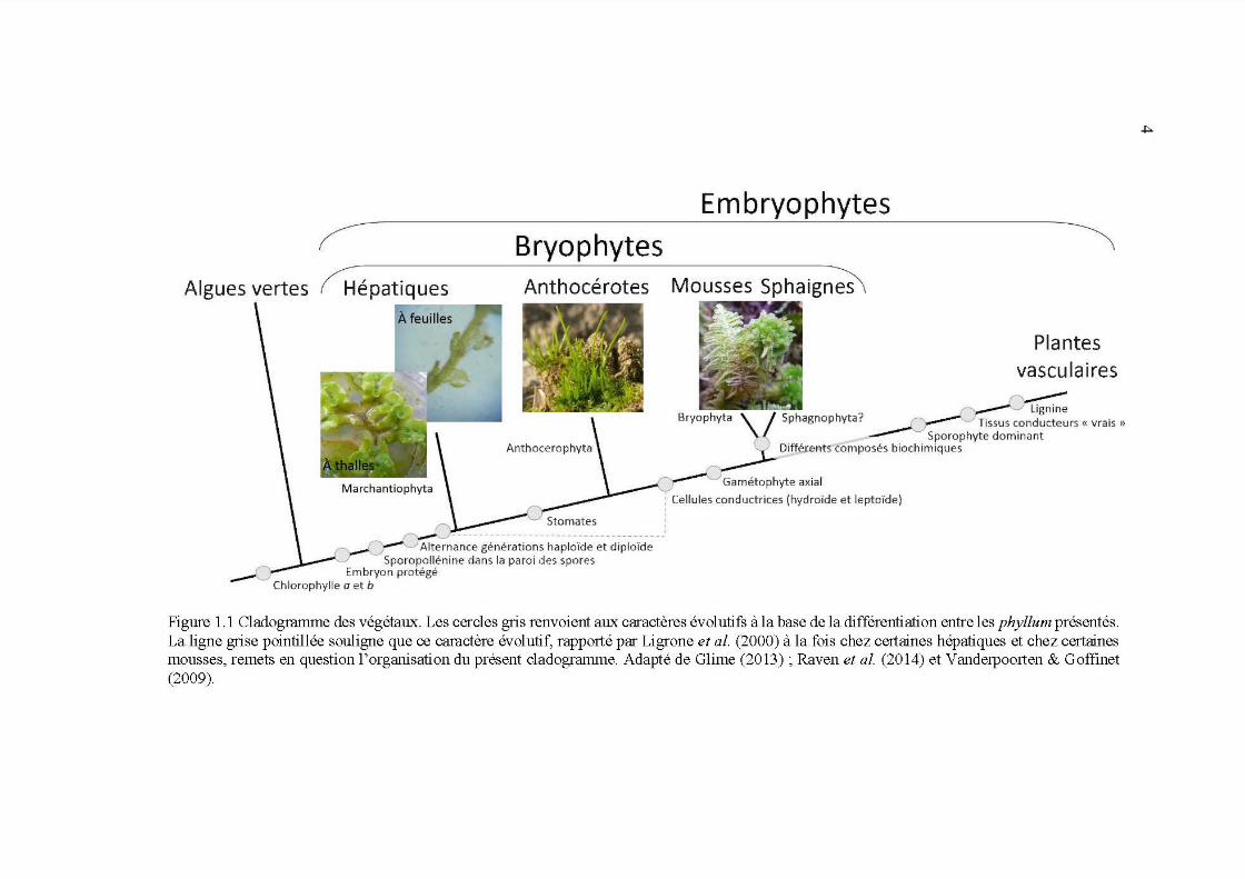
1.1 Cladogramme des végétaux. Les cercles gris renvoient aux caractères évolutifs à la base de la différentiation entre les phyllum présentés. La ligne grise pointillée souligne que ce caractère évolutif, rapporté par Ligrone et al. (2000) à la fois chez certaines hépatiques et chez certaines mousses, remets en question 1 'organisation du présent cladogramme. Adapté de Glime (2013); Raven et al. (2014) et Vanderpoorten &

Page

Goffinet (2009) ............................................................................................ 4

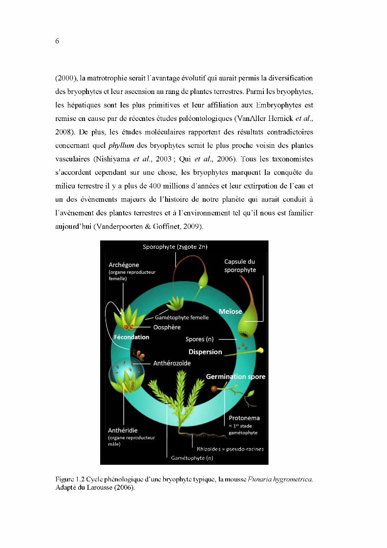
1.2 Cycle phénologique d'une bryophyte typique, la mousse Funaria hygrometrica. Adapté du Larousse (2006) .................................................. 6

1.3 Déposition moyenne des spores mesurée durant 30 jours en fonction de la distance au cœur d'une colonie d'Atrichum undulatum. La courbe présentée représente un patron de dispersion leptokurtique typique soit une «distribution exponentielle à queue épaisse» où la majorité des spores est déposée dans les premiers centimètres de la source et un nombre moindre à plus longue distance [adapté de V anderpoorten &

Goffinet (2009) issu de Miles & Longton (1992)]. ...................................... 8

1.4 Stratégies de dispersion de différentes espèces de bryophytes. (a) Thalle et (b) corbeilles à propagules de M archantia polymorpha ; ( c) sporophytes de Sphagnum angustifolium ; ( d) capsule de Sphagnum centrale après explosion, la traînée de spores orange est visible [issu de Sundberg (2010)]; (e) sporophyte déhiscent et (f) élatères présents dans le sporophyte de Ptilidium pulcherrimum ; (g) sporophytes déshydratés de Splachnum ampullaceum et (h) sporophytes transformés pour attirer les mouches de Tetraplodon angustatus ... ................................................... 9

1.5 Destruction d'un tapis d'Hylocomium splendens transplanté en pessière noire à mousses de l'été 2014 à l'été 2015. Le suspect, un micromammifère, a été identifié grâce aux défécations laissées sur place (cercle rouge). La zone définie par la ligne noire représente la partie broutée (pour consommation ou élaboration d'un nid), une section non endommagée du transplant est visible en bas à droite de l'image ............. 13

1.6 Région d'étude en pessière noire (zone gris clair), Québec, Canada. Les six sites de feux sont représentés en gris foncé, les peuplements de forêts continues non-brùlées sont indiqués par les étoiles (données issues de C. Chaieb ). Les lignes gris clair représentent les limites des régions administratives du Québec. Les routes principales sont indiquées par les lignes brunes .............................................................................................. 16

XVl

1. 7 Îlots résiduels de forêts ................ ... ..................... ... ..................... .. ................. 18

2.1 Location of the study are a in the province of Québec (a), of the six wildfires studied ( dark grey; b) and design used for bryophyte sampling in one residual forest patch ( c ). The main cities and ri vers are indicated as well as lakes (light grey). Circles, residual forest patches (5 per wildfire, sorne are superimposed because of the map scale ); triangles, undisturbed forests (39 sites). (c) Sampling design used in a residual forest patch (light grey) larger than 1 ha (in residual forest patches smaller than 1 ha, only one core plot was sampled) ...................................... 33

2.2 Mean species richness per 50m2 plots of (a) bryophytes per habitat type and life forms and of (b) "restricted" bryophytes per habitat type and life forms. Error bars refers to SD. Generalized linear mixed models were used to compare mean species richness datasets among habitat types except for the mean richness of total and sphagna species for which linear mixed model were used. Bars topped by different letters are significantly different as indicated by post-hoc tests equivalent of Tukey HSD ............... 43

2.3 Species and site plot of the Correspondence Analysis (CA) of the total matrix of 303 plots: black diamonds, undisturbed forest plots; grey squares, residual forest patch plots; light grey triangles, bumed matrix plots. Only the 45 most frequent species are indicated, positions of less frequent species are indicated by +. For complete names see Online Resource 2. The ellipses indicate habitat types centroids with a 95% confidence interval: dark grey, undisturbed forests; grey, residual forest patch es; light grey, bumed matrices ............................................................... 45

2.4 Relationships between environmental variables with a 95% confidence interval excluding 0 after model-averaging procedures and total, true mosses, liverworts and sphagna richnesses. In rows, species richness; in columns, environmental variables. Large crosses indicate no relation between the bryophyte taxonomie group and the environmental variable. On each panel: grey shade, 95% confidence interval of the relationship (indicated as a black solid line between dots that are raw data) between species richness and the environmental variable. For details on the signs ofthe relationships see Table 2.3 ................................................................... 50

2.5 Multivariate regression tree (MRT) of bryophyte community composition. The five-split, six-group model was the best model as selected by parsimony and cross validated error (CVRE). The amount of variation explained by the tree is the inverse of the error. This total is decomposed into the percentage explained by each split. The CV error indicated the potential for the unsuccessful classification of additional

samples and therefore illustrate the predictive power of the mo del (i.e. between 0 and 1, with 1 indicating poor predictive power). Each leaf is assigned the numberofplots within each group is indicated (n). For more details on terminal groups' compositions see Table 4. Abbreviations: CWD, coarse woody debris by decay class (1 to 5) from Thomas et al.

XVll

(1979); LS, low severity offire; HS, high severity offire ............................. 52

3.1 Location of the study area in the province of Québec (a), of the six wildfires studied ( dark grey; b) and of the design used for bryophyte sampling in one residual forest patch ( c ). The main cities and rivers are indicated as well as lakes (light grey). Circles, residual forest patches (5 per wildfire, sorne are superimposed because of the map scale ); triangles, undisturbed forests (39 sites). ( c) a residual forest patch (light grey) larger than 1 ha, the surrounding bumed matrix from the wildfire is indicated in darker grey. Squares represent the 50m2 plots in which bryophytes were sampled with the orientation of the edge plots. In residual forest patches smaller than 1 ha, only one core plot was sampled. The sampling design in undisturbed forest sites consists in only 3 plots of core distant at least 10 rn from each other. ....... ... .......................................................................... 75

3.2 Mean bryophyte species richness (a), and mean bryophyte richness of "restricted species" (b) per forest type and life form. Mean richness refers to the mean number of species recorded in the 50 m2 plots of each forest type. Residual edges are presented by orientation (N, north-facing; S, south-facing), the bold line indicates the mean richness of the ''total" edge without division into north and south. Error bars refer to SD. Generalized linear mixed models were used to compare mean species richness among forest types (upper case) and orientation of residual edges (lower case). Bars topped by different letters are significantly different as indicated by post-hoc tests equivalent of Tukey HSD; marginal significance of the tests is indicated by "*" (0.1 < a < 0.05). Bars topped by an upper case letter indicate that the forest types differed significantly, bars topped by a lower case letter indicate that the north-and south-facing edges were significantly different. ..................................... 83

3.3 Species and site plot of the Correspondence Analysis (CA) of the total matrix of 117 plots ofundisturbed cores, residual cores and edges. Only the 55 most frequent species are indicated, positions of less frequent species are indicated by +.For complete names and details on species life form see Appendix G. Symbols indicate plots and ellipses indicate type of forests: dark grey, undisturbed cores; grey, residual cores; light grey full line, residual north-facing edge; light grey hatched line, residual south-facing edge ........................................................................................... 85

XV111

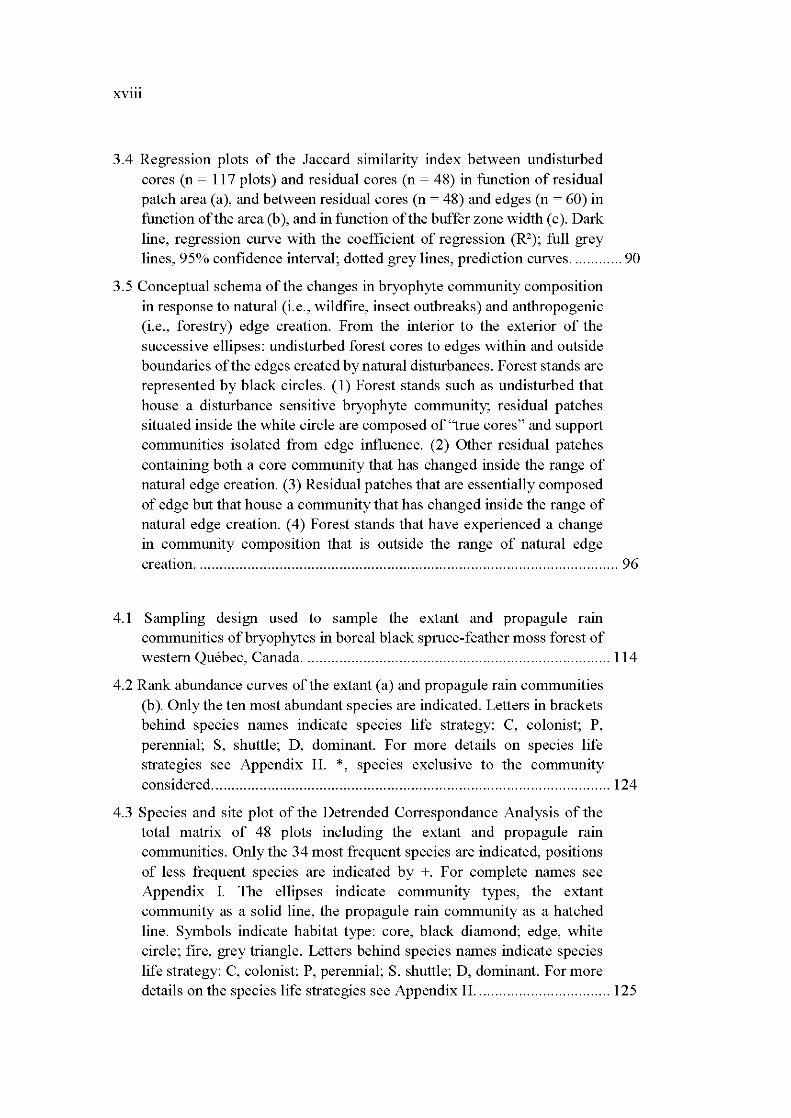
3.4 Regression plots of the Jaccard similarity index between undisturbed cores (n = 117 plots) and residual cores (n = 48) in function of residual patch area (a), and between residual cores (n = 48) and edges (n = 60) in function of the area (b ), and in function of the buffer zone width ( c ). Dark line, regression curve with the coefficient of regression (R2); full grey lines, 95% confidence interval; dotted grey lines, prediction curves ............. 90

3.5 Conceptual schema ofthe changes in bryophyte community composition in response to natural (i.e., wildfire, insect outbreaks) and anthropogenic (i.e., forestry) edge creation. From the interior to the exterior of the successive ellipses: undisturbed forest cores to edges within and outside boundaries of the edges created by natural disturbances. Forest stands are represented by black circles. (1) Forest stands such as undisturbed that house a disturbance sensitive bryophyte community; residual patches situated inside the white circle are composed of''true cores" and support communities isolated from edge influence. (2) Other residual patches containing both a core community that has changed inside the range of natural edge creation. (3) Residual patches that are essentially composed of edge but that ho use a community that has changed inside the range of natural edge creation. ( 4) Forest stands that have experienced a change in community composition that is outside the range of natural edge creation .......................................................................................................... 96

4.1 Sampling design used to sample the extant and propagule ram communities of bryophytes in boreal black spruce-feather moss forest of western Québec, Canada ............................................................................. 114

4.2 Rank abundance curves of the extant (a) and propagule rain communities (b). Only the ten most abundant species are indicated. Letters in brackets behind species names indicate species life strategy: C, colonist; P, perennial; S, shuttle; D, dominant. For more details on species life strategies see Appendix H. *, species exclusive to the community considered .................................................................................................... 124

4.3 Species and site plot of the Detrended Correspondance Analysis of the total matrix of 48 plots including the extant and propagule rain communities. Only the 34 most frequent species are indicated, positions of less frequent species are indicated by +. For complete names see Appendix 1. The ellipses indicate community types, the extant community as a solid line, the propagule rain community as a hatched line. Symbols indicate habitat type: core, black diamond; edge, white circle; fire, grey triangle. Letters behind species names indicate species life strategy: C, colonist; P, perennial; S, shuttle; D, dominant. For more details on the species life strategies see Appendix H .................................. 125

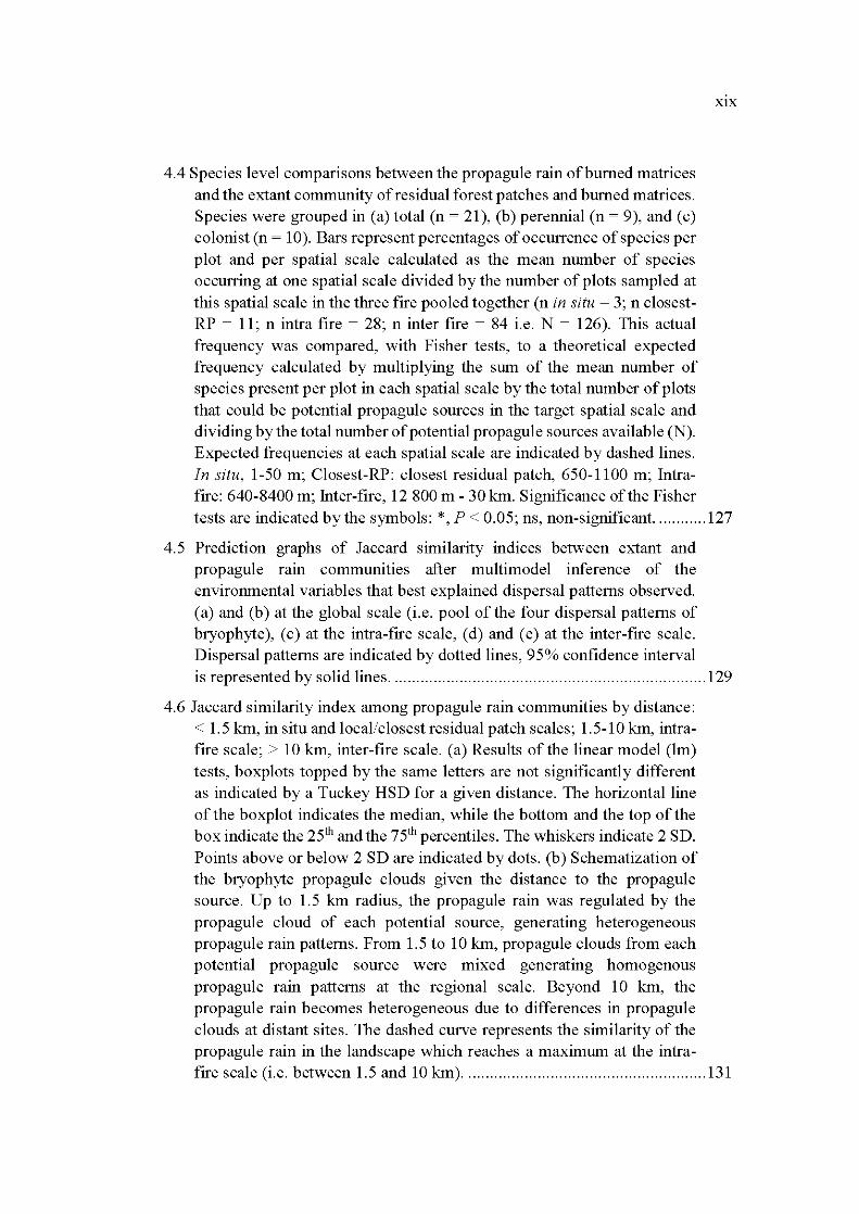
4.4 Species level comparisons between the propagule rain ofburned matrices and the extant community of residual forest patch es and burned matrices. Species were grouped in (a) total (n = 21), (b) perennial (n = 9), and (c) colonist (n = 1 0). Bars represent percentages of occurrence of species per plot and per spatial scale calculated as the mean number of species occurring at one spatial sc ale divided by the number of plots sampled at this spatial scale in the three fire poo led together (n in situ = 3; n closestRP = 11; n intra fire = 28; n inter fire = 84 i.e. N = 126). This actual frequency was compared, with Fisher tests, to a theoretical expected frequency calculated by multiplying the sum of the mean number of species present per plot in each spatial scale by the total number of plots that could be potential propagule sources in the target spatial scale and dividing by the total number of potential propagule sources available (N). Expected frequencies at each spatial scale are indicated by dashed lines. In situ, 1-50 rn; Closest-RP: closest residual patch, 650-1100 rn; Intrafire: 640-8400 rn; Inter-fire, 12 800 rn- 30 km. Significance of the Fisher

Xl X

tests are indicated by the symbols: *, P < 0.05; ns, non-significant. ........... 127

4.5 Prediction graphs of Jaccard similarity indices between extant and propagule rain communities after multimodel inference of the environmental variables that best explained dispersal patterns observed. (a) and (b) at the global scale (i.e. pool of the four dispersal patterns of bryophyte), (c) at the intra-fire scale, (d) and (e) at the inter-fire scale. Dispersal patterns are indicated by dotted lines, 95% confidence interval is represented by solid lines ......................................................................... 129

4.6 Jaccard similarity index among propagule rain communities by distance: < 1.5 km, in situ and local/closest residual patch scales; 1.5-10 km, intrafire scale; > 10 km, inter-fire scale. (a) Results of the linear model (lm) tests, boxplots topped by the same letters are not significantly different as indicated by a Tuckey HSD for a given distance. The horizontalline ofthe boxplot indicates the median, while the bottom and the top ofthe box indicate the 25th and the 75th percentiles. The whiskers indicate 2 SD. Points above or below 2 SD are indicated by dots. (b) Schematization of the bryophyte propagule clouds given the distance to the propagule source. Up to 1.5 km radius, the propagule rain was regulated by the propagule cloud of each potential source, generating heterogeneous propagule rain patterns. From 1.5 to 10 km, propagule clouds from each potential propagule source were mixed generating homogenous propagule rain patterns at the regional scale. Beyond 10 km, the propagule rain becomes heterogeneous due to differences in propagule clouds at distant sites. The dashed curve represents the similarity of the propagule rain in the landscape which reaches a maximum at the intra-fire scale (i.e. between 1.5 and 10 km) ........................................................ 131

xx

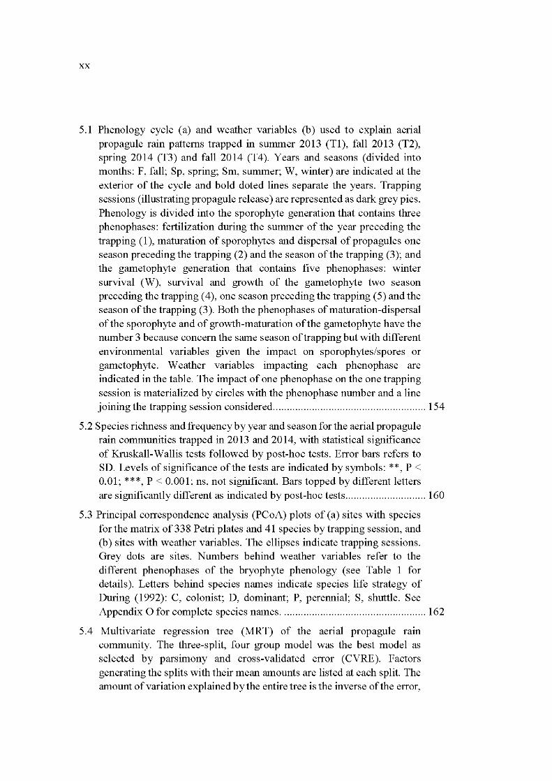
5.1 Phenology cycle (a) and weather variables (b) used to explain aerial propagule rain patterns trapped in summer 2013 (Tl), fall 2013 (T2), spring 2014 (T3) and faU 2014 (T4). Years and seasons (divided into months: F, faU; Sp, spring; Sm, summer; W, winter) are indicated at the exterior of the cycle and bold doted lin es separate the years. Trapping sessions (iUustrating propagule release) are represented as dark grey pies. Phenology is divided into the sporophyte generation that contains three phenophases: fertilization during the summer of the year preceding the trapping (1 ), maturation of sporophytes and dispersal of propagules one season preceding the trapping (2) and the season of the trapping (3); and the gametophyte generation that contains five phenophases: winter survival (W), survival and growth of the gametophyte two season preceding the trapping ( 4), one season preceding the trapping (5) and the season ofthe trapping (3). Both the phenophases of maturation-dispersal of the sporophyte and of growth-maturation of the gametophyte have the number 3 because concem the same season oftrapping but with different environmental variables given the impact on sporophytes/spores or gametophyte. Weather variables impacting each phenophase are indicated in the table. The impact of one phenophase on the one trapping session is materialized by circles with the phenophase number and aline joining the trapping session considered ....................................................... 154

5.2 Species richness and frequency by year and season for the aerial propagule rain communities trapped in 2013 and 2014, with statistical significance of KruskaU-WaUis tests followed by post-hoc tests. Error bars refers to SD. Levels of significance of the tests are indicated by symbols: ** , P < 0.01; ***, P < 0.001; ns, not significant. Bars topped by different letters are significantly different as indicated by post-hoc tests ............................. 160

5.3 Principal correspondence analysis (PCoA) plots of (a) sites with species for the matrix of 338 Petri plates and 41 species by trapping session, and (b) sites with weather variables. The ellipses indicate trapping sessions. Grey dots are sites. Numbers behind weather variables refer to the different phenophases of the bryophyte phenology (see Table 1 for details). Letters behind species names indicate species life strategy of During (1992): C, colonist; D, dominant; P, perennial; S, shuttle. See Appendix 0 for complete species names .................................................... 162

5.4 Multivariate regression tree (MRT) of the aerial propagule rain community. The three-split, four group model was the best model as selected by parsimony and cross-validated error (CVRE). Factors generating the splits with their mean amounts are listed at each split. The amount of variation explained bythe entire tree is the inverse of the error,

in this case 7.9%. This total is decomposed into percentage explained by each split. The CV error indicated the potential for the unsuccessful classification of additional samples (i.e. 5. 7% chance of successful classification). Each leaf is assigned a group number (indicated beneath the leaf on the graph) and the number of plots within each group or "leaf' is indicated. Numbers behind weather variables refer to phenophases of

X Xl

the phenological cycle, see Figure 5.1 for details ........................................ 166

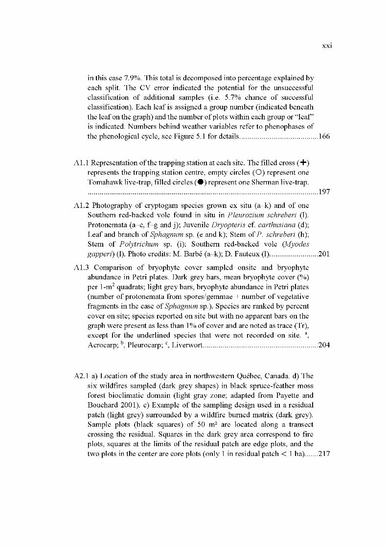
Al.l Representation ofthe trapping station at each site. The filled cross(+) represents the trapping station centre, empty circles (0) represent one Tomahawk live-trap, filled circles (e) represent one Sherman live-trap . ...................................................................................................................... 197

Al.2 Photography of cryptogam species grown ex situ (a-k) and of one Southem red-backed vole found in situ in P leurozium schreberi (1). Protonemata (a- c, f-g and j); Juvenile Dryopteris cf. carthusiana (d); Leaf and branch of Sphagnum sp. (e and k); Stem of P. schreberi (h); Stem of Polytrichum sp. (i); Southem red-backed vole (Myodes gapperi) (1). Photo credits: M. Barbé (a-k); D. Fauteux (1) ......................... 201

Al.3 Comparison of bryophyte cover sampled onsite and bryophyte abundance in Petri plates. Dark grey bars, mean bryophyte co ver (%) per 1-m2 quadrats; light grey bars, bryophyte abundance in Petri plates (number of protonemata from spores/gemmae + number of vegetative fragments in the case of Sphagnum sp. ). Species are ranked by percent cover on site; species reported on site but with no apparent bars on the graph were present as less than 1% of cover and are noted as trace (Tr), except for the underlined species that were not recorded on site. a,

Acrocarp; b, Pleurocarp; c, Liverwort ........................................................... 204

A2.1 a) Location of the study area in northwestem Québec, Canada. d) The six wildfires sampled (clark grey shapes) in black spruce-feather moss forest bioclimatic domain (light gray zone; adapted from Payette and Bouchard 2001 ). c) Example of the sampling design used in a residual patch (light grey) surrounded by a wildfire bumed matrix (clark grey). Sample plots (black squares) of 50 m2 are located along a transect crossing the residual. Squares in the clark grey area correspond to fire plots, squares at the limits of the residual patch are edge plots, and the two plots in the center are core plots ( only 1 in residual patch < 1 ha) ....... 217

XXll

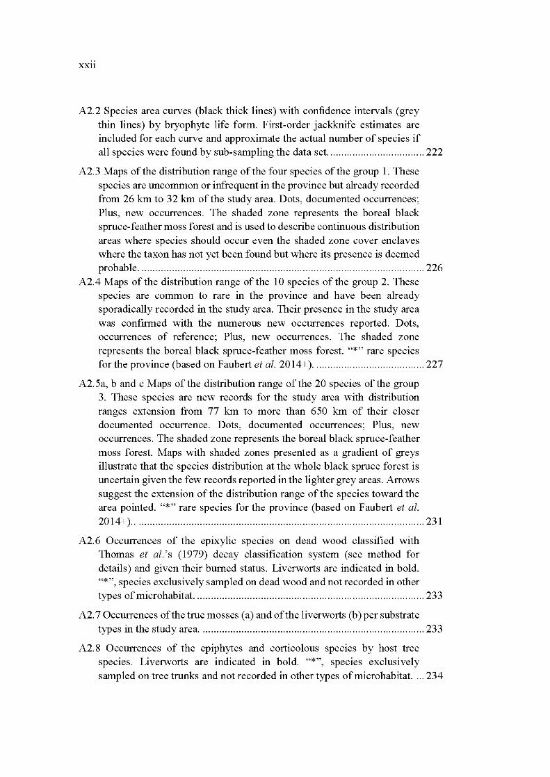
A2.2 Species area curves (black thick lines) with confidence intervals (grey thin lines) by bryophyte life form. First-order jackknife estimates are included for each curve and approximate the actual number of species if all species were found by sub-sampling the data set. .................................. 222

A2.3 Maps of the distribution range ofthe four species of the group 1. These species are uncommon or infrequent in the province but already recorded from 26 km to 32 km ofthe study area. Dots, documented occurrences; Plus, new occurrences. The shaded zone represents the boreal black spruce-feather moss forest and is used to de scribe continuous distribution areas where species should occur even the shaded zone cover enclaves where the taxon has not yet been found but where its presence is deemed probable ....................................................................................................... 226

A2.4 Maps of the distribution range of the 10 species of the group 2. These species are common to rare in the province and have been already sporadically recorded in the study area. Their presence in the study area was confirmed with the numerous new occurrences reported. Dots, occurrences of reference; Plus, new occurrences. The shaded zone represents the boreal black spruce-feather moss forest. "*" rare species for the province (based on Faubert et al. 20 14+ ) ........................................ 227

A2.5a, band c Maps of the distribution range ofthe 20 species of the group 3. These species are new records for the study area with distribution ranges extension from 77 km to more than 650 km of their closer documented occurrence. Dots, documented occurrences; Plus, new occurrences. The shaded zone represents the boreal black spruce-feather moss forest. Maps with shaded zones presented as a gradient of greys illustrate that the species distribution at the whole black spruce forest is uncertain given the few records reported in the lighter grey areas. Arrows suggest the extension of the distribution range of the species toward the area pointed. "*"rare species for the province (based on Faubert et al. 2014+) ......................................................................................................... 231

A2.6 Occurrences of the epixylic species on dead wood classified with Thomas et al. 's (1979) decay classification system (see method for details) and given their bumed status. Liverworts are indicated in bold. "*", species exclusively sampled on dead wood and not recorded in other types of microhabitat ................................................................................... 233

A2. 7 Occurrences of the true moss es (a) and of the liverworts (b) per substrate types in the study are a ................................................................................. 233

A2. 8 Occurrences of the epiphytes and corticolous species by host tree species. Liverworts are indicated in bold. "*", species exclusively sampled on tree trunks and not recorded in other types of micro habitat. ... 234

A2.9 Occurrences of the epixylic species on dead wood classified with Thomas et al. 's (1979) decay classification system (see method for details) and given their bumed status. Liverworts are indicated in bold. "*", species exclusively sampled on dead wood and not recorded in other

XX111

types of micro habitat. ................................................................................... 234

A2.1 0 Occurrences of the epixylic species on dead wood classified with Thomas et al. 's (1979) decay classification system (see method for details) and given their bumed status. Liverworts are indicated in bold. "*", species exclusively sampled on dead wood and not recorded in other types of micro habitat. ................................................................................... 234

LISTE DES TABLEAUX

Tableau

2.1 Mo dels tested and number of parameters estimated (K; includes random effects) for the model selection procedure performed with glmer (Kg!mer ), except for total and sphagna species richnesses that were tested with lme (K!me) (see Methods for details). The 12 parameters retained were grouped in four categories: temporal, severity, spatial and

Page

structural. ................................................................................................... 40

2.2 Model selection results for the different species richnesses (both global and restricted to undisturbed forest given species taxonomie groups). Model selection was performed on generalized linear mixed models (glmer) except for total and sphagna species richnesses that were tested with linear mixed models (lme ). Only models with L1AICc < 2 are presented, with number of parameters included (K), second-order Akaike information criterion (AICc), distance from the best model ( L1AICc), Akaike weight (wi), estimate of mo del adjustment by Spearman's Rho (p ), and value of the evidence-ratio between the best mo del and the second mo del. ..................................................................... 47

2.3 Model-averaged estimates of coefficients of parameters explaining species richness patterns. Unconditional standard error and lower and upper 95% confidence intervals are also shown. Significant parameters are indicated in bold with the sign of the relationship indicated between parentheses ........................ .. ...................... ... .............................................. 48

2.4 Composition and mean values of environmental variables of MRT terminal groups. Group composition is represented by the number of plots from each habitat type (ntotal = 303). Plots sampled in a single continuous forest stand or residual forest patch were never separated in MRT final groups. Three plots all from one residual forest patch were "remaining observations" and were not classified by the MRT. ............... 53

3.1 Life form, life strategy, substrate preference and humidity affinity of the 53 species identified as indicators of undisturbed cores and of residual edges. Affiliation to south (S) or north (N) edges are indicated as exponents ................................................................................................... 86

3.2 Comparison of the life traits and substrate preferences of the species identified as indicators (i.e. restricted and over represented species pooled together) of undisturbed cores and of residual edges following the three pairs of comparison. Values are number of species, frequencies are given in square brackets. N, number ofspecies involved

XXVl

in the comparison; n, number of species in each of the habitat type compared. Kruskal-Wallis tests were used for comparisons. Bold, significant test (a < 0. 0 5); "* ", marginally significant test (0 .1 < a < 0.05) ........................................................................................................... 88

4.1 Temporal, spatial and structural variables measured in each of the residual forest patch and bumed matrix area in the study. Isolation and canopy openness are means ± standard errors, all other variables are ab solute values ........................................................................................ 113

4.2 Ranking of the mo dels used to assess the role of spatial, temporal and structural variables on similarity between communities based on the L1AICci value. The response variable, Jaccard's similarity (SimJaccard), compared the propagule rain in each of the 50 m 2 plot of the bumed matrix (n = 3) to each of the 50m2 plot of the extant community (n = 21). In situ and local/closest residual patch scales were not analysed because of the small number of replicates. Only the models with a L1AICc < 2 and the first models with a L1AICc > 2 are indicated. Ki, number of parameters including the intercept; Wi, Akaike weight; p, model adjustment, are only indicated for the best model. See Appendix K for complete modellist. ....................................................................... 128

5.1 Mean and SD (±) ofthe 10 weathervariables by season in 2012 to 2014. Linear models were used to compare means among years except for underlined values for which generalized models were used because of their non-normality. Means followed by the same letter are not significantly different at P < 0.05 as indicated by post-hoc tests; letters indicate ranking (i.e: a < b < c) .... ........................................................... 164

5.2 Species composition of the groups determined by multivariate regression tree (MRT). Number are frequency of each species in all Petri plates per group. Bold, liverwort species; *, acrocarp species ........ 168

5.3 Weather variables of the groups determined by multivariate regression tree (MRT; Figure 5.4). Values are means of each variable classified by phenophase (see Figure 5.1 for details about numbering) per group ...... 169

Al.1 Number of Petri plates incubated with material brushed from five small mammal species trapped in the boreal forest. A separate Petri plate was used for each small mammal individual and represents the number of small mammals carrying viable diaspores ................................................. 200

A1.2 List of bryophyte and fern species brushed from five small mammal species trapped in boreal forests (n = 99 individuals trapped). Values refer to the number of bryophyte individuals grown in Petri plates

counted as number of protonemata germinated from spores/gemmae or as number of vegetative fragment. As one Petri plate may contain several protonema, the values in brackets represent the number of Petri plates in which the cryptogam species were found. In species richness of bryophytes and ferus protonemata of Sphagnum sp. and Sphagnum leaves were grouped together and unidentified protonemata and unidentified stems/leaves were omitted because we could not determine

XXVll

if they were new species or not. a, Acrocarp; b, Pleurocarp; c, Fern ............ 202

A2.1 Wildfire zones of bryophyte sampling spatial and physical characteristics [data from SOPFEU digital map of the fires in Québec (2011)] ............................................................................................ 219

A2.2 List of the 35 species with a distribution range extension for the south of the Northem-territories of Québec, Canada. Species are classified by life form. The number of documented and new occurrences, the status, the type of correction applied to their distribution, the distance to the closer documented occurrence, and details about microhabitat preferences of the species are indicated ....................................................... 224

RÉSUMÉ

La conscientisation aux problématiques environnementales survenue il y a une trentaine d'années a engagé une refonte de la foresterie. Il s 'agit alors de s'inspirer des patrons écologiques issus de la dynamique forestière naturelle. Sous l'égide de l'aménagement écosystémique, l'objectif principal de cette thèse est de rendre compte du rôle des îlots résiduels post-feu et des caractéristiques qui soutiennent ces rôles, dans la dynamique des communautés bryophytiques. Conjointement, nous ambitionnons d'améliorer les connaissances sur la dynamique des bryophytes en forêt boréale nord-américaine.

Les bryophytes furent échantillonnnées dans trois types de peuplement illustrant un gradient de sévérité de perturbation : forêts non perturbées témoins (données de C. Chaieb ), îlots résiduels post-feu et matrices brûlées. La variété des micro habitats en bordure des îlots résiduels expliquerait leurs richesses en bryophytes. En revanche, l'absence de plusieurs espèces forestières sensibles aux perturbations ne permet pas de définir les îlots résiduels comme des refuges i.e. , habitats aux caractéristiques environnementales et à la composition en espèces similaires à celle des forêts non perturbées. Cependant, les îlots résiduels de plus de 56 ans et 0.20 ha et de complexité structurelle modérée arboraient une communauté bryophytique plus similaire à celle des forêts non perturbées qu'à celles des matrices brûlées. La stratégie gagnante pour optimiser la richesse en bryophytes et maintenir les espèces sensibles consiste à imiter ces caractéristiques dans les îlots de rétention tout en conservant des peuplements forestiers non perturbés.

Dans les mêmes trois types de peuplements, en divisant les îlots résiduels en habitats de cœur (forêt à l'intérieur de l'îlot) et de bordure (zone de transition entre la matrice brûlée et le cœur de l ' îlot), nous avons mis en évidence la réponse des bryophytes à l'effet de bordure. L'hypothèse comme quoi les vieux et larges îlots résiduels abriteraient des communautés plus similaires à celles des forêts non perturbées en raison de la moindre pénétration de l'effet de bordure à l'intérieur du peuplement est rejetée. Les îlots résiduels, même de 3 à 11 ha, étaient dépourvus de cœur. Ce changement de communauté face à la création de bordures est naturel, ouvrant à la discussion quant à 1 'interprétation de la réponse des espèces à la création de bordures anthropiques.

En comparant la communauté bryophytique des îlots résiduels et des matrices brûlées aux espèces présentes dans la pluie de propagules aériennes interceptées dans les mêmes habitats, nous avons démontré leur non-concordance. La faible similarité entre ces communautés était expliquée par la prépondérance du transport à longue distance des propagules. Ce résultat suggère que les îlots résiduels, comme sources de propagules potentielles, ont une influence sur la recolonisation de la matrice brûlée à l'échelle locale, mais surtout régionale. Nous insistons donc sur la

xxx

nécessité de penser l'aménagement forestier à l'échelle régionale, et rapportons l'occurrence d'un processus controversé chez les bryophytes : la dispersion à longue distance.

La dépendance accrue des bryophytes aux conditions environnementales est un fait avéré. Pourrait-elle expliquer les patrons interannuel et intersaisonnier des pluies de propagules aériennes interceptées en pessière noire ? Oui, et la dispersion des propagules serait impactée par les conditions environnementales (principalement la température, l'humidité et la durée de l'hiver) concomitantes au relargage des propagules, mais aussi en amont de la libération des propagules (durant les phases de fertilisation et de croissance/maturation du gamétophyte). Cette étude préliminaire et ponctuelle recquiert d'être complémentée par des études à plus long terme. Cependant, elle représente une avancée considérable dans la compréhension des patrons de dispersion des espèces, sujet de première importance dans le contexte des changements globaux.

Pour poursuivre, nous avons étudié le recours, par les bryophytes, à des agents biotiques de dispersion. Le brossage de micromammifères capturés en pessière noire a permis de démontrer que 50% d'entre eux transportaient des propagules viables de bryophytes. La dynamique métapopulationnelle des bryophytes est assurée par cette interaction journalière avec les micromammifères, qm contribueraient à la dispersion d'une quantité substantielle de propagules.

Nous concluons en actualisant la Flore des bryophytes du Québec-Labrador et en redessinant l'aire de répartition de 35 bryophytes, dont 20 nouvelles pour notre région d'étude. L'extension de l'aire de répartition de ces espèces renvoie à la nécessité de poursuivre les campagnes d'échantillonnages bryologiques, d 'autant plus dans des endroits riches d'une bryoflore aussi remarquable que la pessière noire, où chercher une mousse revient un peu, avouons-le, à chercher une aiguille dans une botte de foin !

À l'issue de cette thèse, nous soulignons le bénéfice d'étudier les bryophytes afin de s'inspirer des patrons de perturbations naturelles et de mitiger les impacts délétères des coupes forestières sur l'écosystème. Un soin particulier quant à la conception des îlots résiduels à l'échelle locale, mais aussi quant à leur agencement à l 'échelle du paysage est requis pour conserver une bryo-diversité maximale. Ces conclusions soulèvent, de plus, l'impérieuse nécessité de préserver des peuplements forestiers âgés et continus pour conserver les espèces sensibles aux perturbations et à haut risque d'extirpation. Maintenir la bryoflore en forêt boréale exploitée est le prérequis indispensable à la régénération optimale des peuplements et à la résilience de cet écosystème, patrimoine naturel des plus remarquable de l'Amérique du Nord.

PROLOGUE

En toute innocence vous venez ici de franchir le seuil de tout un univers. Ouvrir ce

document c 'est comme s'autoriser à partir en voyage. Pourtant nous ne partons pas

si loin, non, contentons-nous de baisser les yeux et par la même occasion de baisser

notre garde ... Nous partons au cœur du sous-bois et nous allons, par curiosité

davantage que manque de pudeur, nous glisser sous les jupes des épinettes noires,

figures emblématiques des forêts boréales nord-américaines et plus précisément de

la pessière noire à mousses. Je vous emmène à la rencontre des plus minimes

occupantes du sous-bois, et non des moindres !

En effet, quels végétaux peuvent se targuer de marquer le passage entre la vie

terrestre et aquatique ? D'avoir conquis l'intégralité des continents ? Lesquels

peuvent encore, à l'instar du Phoenix qui renaît de ses cendres, s'enorgueillir de

posséder le don de reviviscence ? Si les arbres avaient autant de qualités, peut-être

auraient-ils mérité notre intérêt, mats, et au nsque de froisser les

« trachéophytologues », les voilà ici supplantés par celles mêmes qui leurs lèchent

les bottes, nous entendons bien parler des bryophytes ! Discrètes, mais non

désuètes, à qui sait se pencher et écouter, elles livreront leurs plus intimes secrets.

À l'Université du Québec en Abitibi-Témiscamingue, au cœur de la forêt boréale,

mieux vaut donc être atteint de surdité, puisqu'elles sont nombreuses, et elles en

ont des choses à dire ! Nous avons alors tendu 1 'oreille, et, au terme de ces trois

années et demie, nous venons vous présenter ce qu'elles ont bien voulu laisser

entendre.

Je vous abandonne alors à ces quelques menues pages et vous laisse entrer dans

l'univers des bryophytes qui incarne sobriété, naturel et quiétude, valeurs

fondamentales à l'opposé même de ma personnalité! Je vous offre cette ode aux

bryophytes et espère faire naître un nouvel attrait et, pourquoi pas même, une

nouvelle passion chez certains d'entre vous, car, comme l'écrit si justement

Véronique Brindeau: «pour qui s'éprend des mousses, le monde s'éclaire d'une

nouvelle et minuscule fenêtre » (Brindeau, 2012), une fenêtre qui plus jamais ne se

refermera.

CHAPITRE I

INTRODUCTION GÉNÉRALE

2

1.1 Sujet d'étude

De la lyrique « mousse plume » en passant par 1 'ostentatoire « hypne dorée » pour finir

par la survoltée « queue de chat électrique », les bryophytes ont de quoi attiser les

curiosités. Ainsi, et au risque de paraître sectaire, commençons pour une fois par le

commencement : les bryophytes !

1.1.1 Terminologie et nomenclature

L'origine grecque du mot bryophyte se rapporte à leur capacité à gonfler sous l'effet

de 1 'hydratation (V anderpoorten & Goffinet, 2009). Sous cette dénomination sont

regroupés les trois phyllum Bryophyta (mousses et sphaignes), Marchantiophyta

(hépatiques) et Anthocerophyta ( anthocérotes ; Figure 1.1 ; Glime, 2013 ). En réalité le

mot « bryophyte » est peu utilisé en français, excepté par les initiés, et on lui préfère

dans le langage courant, le mot« mousse ».

Seulement, vous 1' aurez compris, 1 'utilisation du mot « mousse » pose le problème de

ne plus pouvoir distinguer le règne du phyllum. Ce raccourci m'a d'ailleurs valu

plusieurs « discours de sourds » et les plus familiers avec 1 'excellent « Dîner de cons »

(Veber, 1998) comprendront le parallèle à l'échange entre Pierre Brochant et François

Pignon à propos d'un certain Juste Leblanc ! C'est pourquoi vous rencontrerez dans la

littérature la terminologie «mousses s.l. »soit« mousses sensu largo »qui renvoie aux

bryophytes et «mousses s.s. » soit « mousses sensu stricto » pour parler du phyllum

Bryophyta.

3

De plus, récemment, Crum (200 1) a introduit le phyllum Sphagnophyta pour distinguer

les sphaignes des mousses, originellement regroupées sous les Bryophyta. Par souci de

clarté, et bien que cette division ne fasse pas 1 'unanimité chez les taxonomistes, le terme

bryophyte sera utilisé dans la suite de ce document pour parler des mousses, sphaignes

et hépatiques divisées en trois phyllum distincts. Les anthocérotes ne seront pas

abordées étant donné qu'aucune n'a été relevée dans la région d'étude considérée.

Embryophytes Bryophytes ~

Algues vertes !'Hépatiques Anthocérotes Mousses Sphaign~

Alternance générations haploïde et diploïde Sporopollénine dans la paroi des spores

Embryon protégé Chlorophylle a et b

Plantes vasculaires

Lignine Tissus conducteurs « vrais >>

Sporophyte dominant composés biochimiques

Gamétophyte axial

Cellules conductrices (hydroïde et leptoïde)

Figure 1.1 Cladogramme des végétaux. Les cercles gris renvoient aux caractères évolutifs à la base de la différentiation entre les phyllum présentés. La ligne grise pointillée souligne que ce caractère évolutif, rapporté par Ligrone et al. (2000) à la fois chez certaines hépatiques et chez certaines mousses, remets en question l'organisation du présent cladogramme. Adapté de Glime (2013) ; Raven et al. (2014) et Vanderpoorten & Goffinet (2009).

5

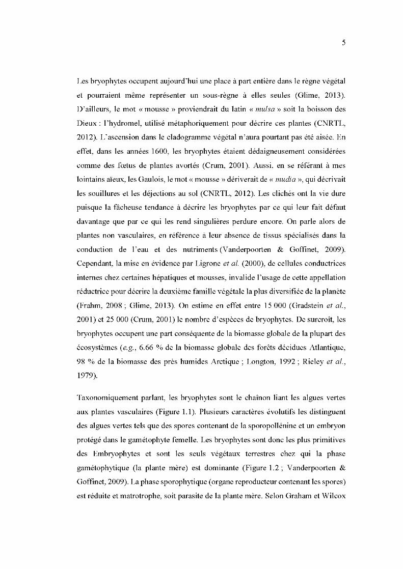
Les bryophytes occupent aujourd'hui une place à part entière dans le règne végétal

et pourraient même représenter un sous-règne à elles seules (Glime, 2013).

D'ailleurs, le mot «mousse » proviendrait du latin « mulsa » soit la boisson des

Dieux: l'hydromel, utilisé métaphoriquement pour décrire ces plantes (CNRTL,

2012). L'ascension dans le cladogramme végétal n'aura pourtant pas été aisée. En

effet, dans les années 1600, les bryophytes étaient dédaigneusement considérées

comme des fœtus de plantes avortés (Crum, 2001). Aussi, en se référant à mes

lointains aïeux, les Gaulois, le mot« mousse »dériverait de« mudia »,qui décrivait

les souillures et les déjections au sol (CNRTL, 2012). Les clichés ont la vie dure

puisque la fâcheuse tendance à décrire les bryophytes par ce qui leur fait défaut

davantage que par ce qui les rend singulières perdure encore. On parle alors de

plantes non vasculaires, en référence à leur absence de tissus spécialisés dans la

conduction de 1 'eau et des nutriments (V anderpoorten & Goffinet, 2009).

Cependant, la mise en évidence par Ligrone et al. (2000), de cellules conductrices

internes chez certaines hépatiques et mousses, invalide 1 'usage de cette appellation

réductrice pour décrire la deuxième famille végétale la plus diversifiée de la planète

(Frahm, 2008; Glime, 2013). On estime en effet entre 15 000 (Gradstein et al.,

2001) et 25 000 (Crum, 2001) le nombre d'espèces de bryophytes. De surcroît, les

bryophytes occupent une part conséquente de la biomasse globale de la plupart des

écosystèmes (e.g., 6.66 %de la biomasse globale des forêts décidues Atlantique,

98 % de la biomasse des près humides Arctique ; Longton, 1992; Rieley et al.,

1979).

Taxonomiquement parlant, les bryophytes sont le chaînon liant les algues vertes

aux plantes vasculaires (Figure 1.1). Plusieurs caractères évolutifs les distinguent

des algues vertes tels que des spores contenant de la sporopollénine et un embryon

protégé dans le gamétophyte femelle. Les bryophytes sont donc les plus primitives

des Embryophytes et sont les seuls végétaux terrestres chez qui la phase

gamétophytique (la plante mère) est dominante (Figure 1.2; Vanderpoorten &

Goffinet, 2009). La phase sporophytique (organe reproducteur contenant les spores)

est réduite et matrotrophe, soit parasite de la plante mère. Selon Graham et Wilcox

6

(2000), la matrotrophie serait l'avantage évolutif qui aurait permis la diversification

des bryophytes et leur ascension au rang de plantes terrestres. Parmi les bryophytes,

les hépatiques sont les plus primitives et leur affiliation aux Embryophytes est

remise en cause par de récentes études paléontologiques (VanAller Hernick et al.,

2008). De plus, les études moléculaires rapportent des résultats contradictoires

concernant quel phyllum des bryophytes serait le plus proche voisin des plantes

vasculaires (Nishiyama et al. , 2003 ; Qui et al., 2006). Tous les taxonomistes

s' accordent cependant sur une chose, les bryophytes marquent la conquête du

milieu terrestre il y a plus de 400 millions d'années et leur extirpation de l' eau et

un des évènements majeurs de l'histoire de notre planète qui aurait conduit à

l'avènement des plantes terrestres et à l'environnement tel qu ' il nous est familier

aujourd'hui (Vanderpoorten & Goffinet, 2009).

Figure 1.2 Cycle phénologique d'une bryophyte typique, lamousseFunaria hygrometrica. Adapté du Larousse (2006).

7

1.1.2 Dispersion

Les bryophytes sont retrouvées sur tous les continents et sous toutes les latitudes

excepté les eaux salines et les écosystèmes gelés en permanence (V anderpoorten &

Goffinet, 2009). De plus, contrairement aux végétaux vasculaires, les bryophytes

ne répondent pas au gradient latitudinal de diversité croissant des pôles vers

1' équateur ni ne possèdent des taux élevés d'endémisme (Frahm, 2008 ; Hodgetts,

1996 ; van Zanten & Pôcs, 1981). Certaines espèces ont une aire de répartition

continue sur plusieurs voire tous les continents ( e.g., Bryum argenteum, P leurozium

schreberi) et sont alors qualifiées de cosmopolites ou d'ubiquistes. D'autres taxons

possèdent des aires de distribution disjointes (e.g., Jsothecium holtii présente sur les

îles Britanniques, l'ouest de la France et de la Norvège ainsi qu'en Turquie sans

jonction entre ces localités ; Sabovljevié et al., 2005) expliquées par la dérive des

plaques continentales, des phénomènes d'extinctions locales et par leurs modes de

dispersion (Frahm, 2008).

Les bryophytes peuvent en effet se reproduire de façon sexuée et asexuée, chacune

dévolue à un type de dispersion donné. La reproduction asexuée est réalisée par le

biais de propagules produites à la base des feuilles (gemmae) ou de fragments

végétatifs (fragments de tiges ou feuilles qui se développeront pour donner un

nouvel individu; Benscoter, 2006; Miilson & Rydin, 2007; Rochefort et al., 2003).

Les propagules asexuées sont principalement utilisées pour la dispersion à courte

distance et pour l'expansion locale de la population étant donné leur taille et leur

fort potentiel germinatif, même en conditions suboptimales (Kimmerer, 1991 ;

Lôbel et al., 2006). A contrario, la reproduction sexuée est effectuée par

l'intermédiaire de propagules sexuées (spores) qui sont produites dans la capsule

du sporophyte (Figure 1.2). Ce mode de reproduction est dédié à la dispersion à

plus longue distance et expliquerait l'intercontinentalité des bryophytes (van Zanten

& Gradstein, 1988; van Zanten & Pôcs, 1981).

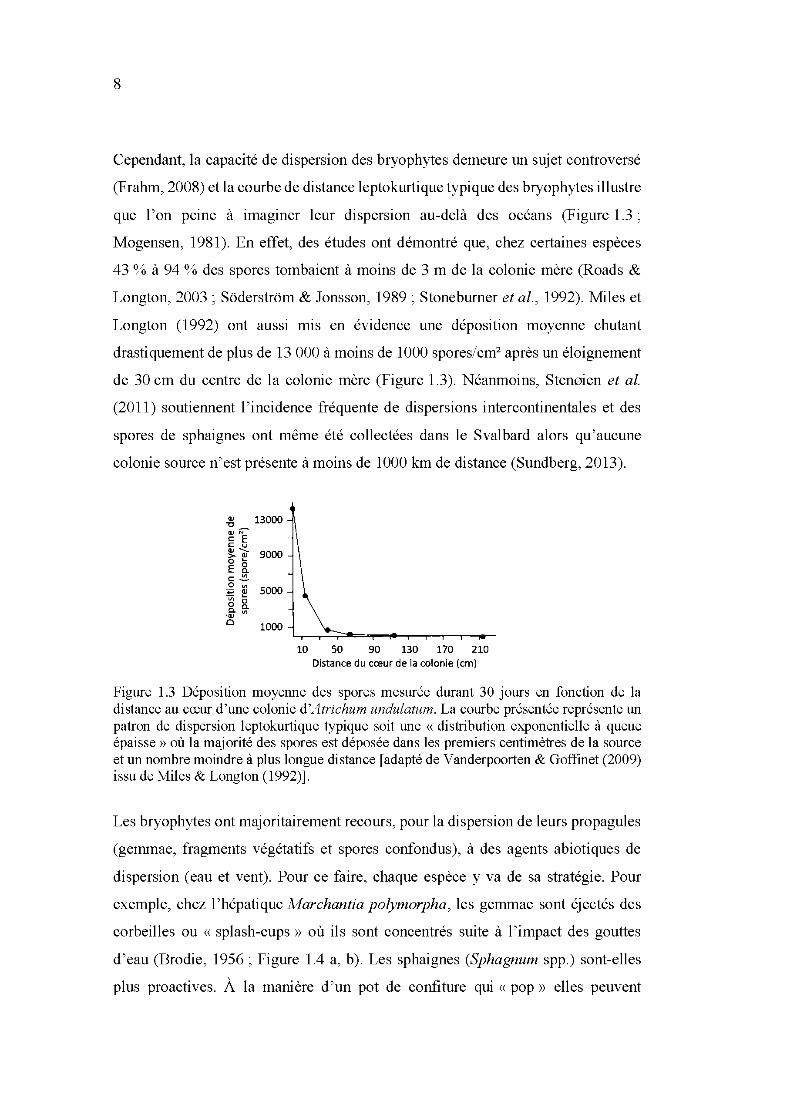
8

Cependant, la capacité de dispersion des bryophytes demeure un sujet controversé

(Frahm, 2008) et la courbe de distance leptokurtique typique des bryophytes illustre

que l'on peine à imaginer leur dispersion au-delà des océans (Figure 1.3;

Mogensen, 1981). En effet, des études ont démontré que, chez certaines espèces

43 % à 94 % des spores tombaient à moins de 3 rn de la colonie mère (Roads &

Langton, 2003 ; Soderstrom & Jonsson, 1989; Stoneburner et al., 1992). Miles et

Langton (1992) ont aussi mis en évidence une déposition moyenne chutant

drastiquement de plus de 13 000 à moins de 1000 spores/cm2 après un éloignement

de 30 cm du centre de la colonie mère (Figure 1.3). Néanmoins, Sten0ien et al.

(20 11) soutiennent l'incidence fréquente de dispersions intercontinentales et des

spores de sphaignes ont même été collectées dans le Svalbard alors qu'aucune

colonie source n'est présente à moins de 1000 km de distance (Sundberg, 2013).

QJ 13000 ""0 GJN c: E c: u QJ ..._

9000 >GJ 0 ~

E g_ c:~ 0 VI 5000 ~ QJ ·v; (; 0 a. '~ V't

0 1000

10 50 90 130 170 210 Distance du cœur de la colonie (cm)

Figure 1.3 Déposition moyenne des spores mesurée durant 30 jours en fonction de la distance au cœur d'une colonie d'Atrichum undulatum. La courbe présentée représente un patron de dispersion leptokurtique typique soit une « distribution exponentielle à queue épaisse » où la majorité des spores est déposée dans les premiers centimètres de la source et un nombre moindre à plus longue distance [adapté de Vanderpoorten & Goffinet (2009) issu de Miles & Langton (1992)].

Les bryophytes ont majoritairement recours, pour la dispersion de leurs propagules

(gemmae, fragments végétatifs et spores confondus), à des agents abiotiques de

dispersion (eau et vent). Pour ce faire, chaque espèce y va de sa stratégie. Pour

exemple, chez l' hépatique Marchantia polymorpha, les gemmae sont éjectés des

corbeilles ou « splash-cups » où ils sont concentrés suite à l'impact des gouttes

d'eau (Brodie, 1956 ; Figure 1.4 a, b). Les sphaignes (Sphagnum spp.) sont-elles

plus proactives. À la manière d 'un pot de confiture qui « pop » elles peuvent

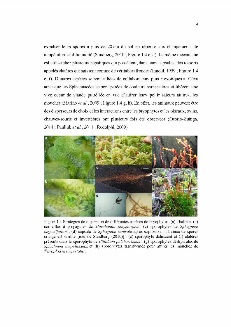
9

expulser leurs spores à plus de 20 cm du sol en réponse aux changements de

température et d'humidité (Sund berg, 2010 ; Figure 1.4 c, d). Le même mécanisme

est utilisé chez plusieurs hépatiques qui possèdent, dans leurs capsules, des ressorts

appelés élatères qui agissent comme de véritables frondes (lngold, 1959 ; Figure 1.4

e, f). D'autres espèces se sont alliées de collaborateurs plus «exotiques». C'est

ainsi que les Splachnacées se sont parées de couleurs carnassières et libèrent une

vive odeur de viande putréfiée en vue d 'attirer leurs pollinisateurs attitrés, les

mouches (Marino et al., 2009; Figure 1.4 g, h). En effet, les animaux peuvent être

des disperseurs de choix et les interactions entre les bryophytes et les oiseaux, ovins,

chauves-souris et invertébrés ont plusieurs fois été observées (Osorio-Zuîiiga,

2014 ; Pauli uk et al., 2011 ; Rudol phi, 2009).

Figure 1.4 Stratégies de dispersion de différentes espèces de bryophytes. (a) Thalle et (b) corbeilles à propagules de Marchantia polymorpha; (c) sporophytes de Sphagnum angustifolium ; ( d) capsule de Sphagnum centrale après explosion, la traînée de spores orange est visible [issu de Sundberg (2010)]; (e) sporophyte déhiscent et (f) élatères présents dans le sporophyte de Ptilidium pulcherrimum ; (g) sporophytes déshydratés de Splachnum ampullaceum et (h) sporophytes transformés pour attirer les mouches de Tetraplodon angustatus.

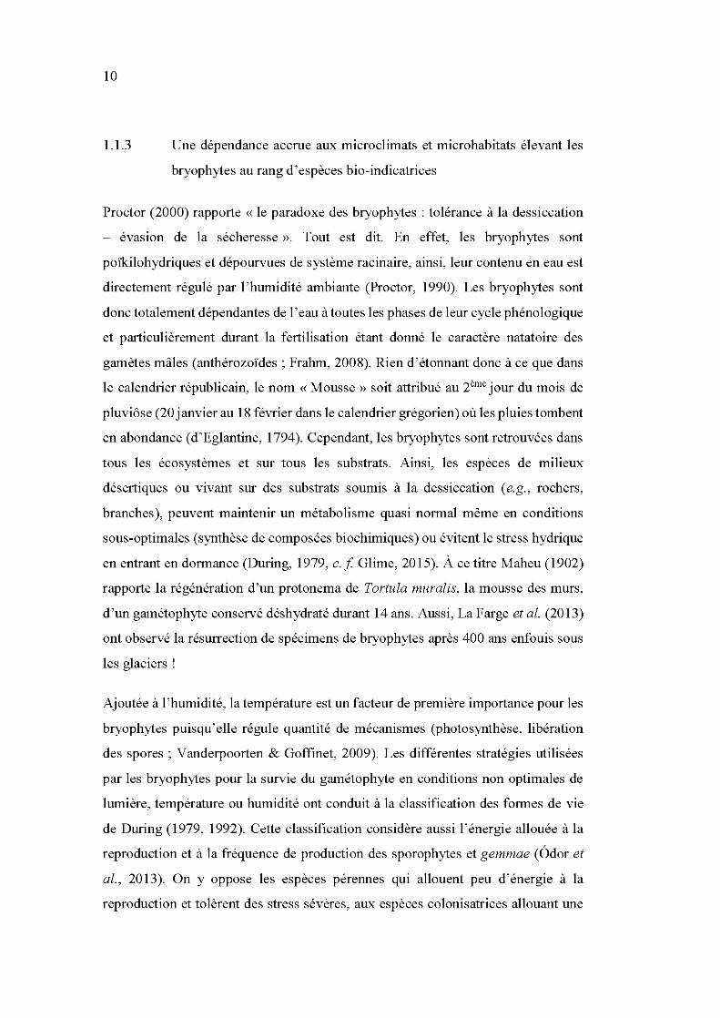
10

1.1.3 Une dépendance accrue aux microclimats et microhabitats élevant les

bryophytes au rang d'espèces bio-indicatrices

Proctor (2000) rapporte « le paradoxe des bryophytes : tolérance à la dessiccation

- évasion de la sécheresse ». Tout est dit. En effet, les bryophytes sont

poikilohydriques et dépourvues de système racinaire, ainsi, leur contenu en eau est

directement régulé par 1 'humidité ambiante (Proctor, 1990). Les bryophytes sont

donc totalement dépendantes de l'eau à toutes les phases de leur cycle phénologique

et particulièrement durant la fertilisation étant donné le caractère natatoire des

gamètes mâles (anthérozoïdes ; Frahm, 2008). Rien d 'étonnant donc à ce que dans

le calendrier républicain, le nom « Mousse » soit attribué au 2ème jour du mois de

pluviôse (20 janvier au 18 février dans le calendrier grégorien) où les pluies tombent

en abondance (d 'Eglantine, 1794). Cependant, les bryophytes sont retrouvées dans

tous les écosystèmes et sur tous les substrats. Ainsi, les espèces de milieux

désertiques ou vivant sur des substrats soumis à la dessiccation (e.g., rochers,

branches), peuvent maintenir un métabolisme quasi normal même en conditions

sous-optimales (synthèse de composées biochimiques) ou évitent le stress hydrique

en entrant en dormance (During, 1979, c. f Glime, 2015). À ce titre Maheu (1902)

rapporte la régénération d'un protonema de Tortula muralis, la mousse des murs,

d'un gamétophyte conservé déshydraté durant 14 ans. Aussi, La Farge et al. (2013)

ont observé la résurrection de spécimens de bryophytes après 400 ans enfouis sous

les glaciers !

Ajoutée à l'humidité, la température est un facteur de première importance pour les

bryophytes puisqu'elle régule quantité de mécanismes (photosynthèse, libération

des spores ; V anderpoorten & Goffinet, 2009). Les différentes stratégies utilisées

par les bryophytes pour la survie du gamétophyte en conditions non optimales de

lumière, température ou humidité ont conduit à la classification des formes de vie

de During (1979, 1992). Cette classification considère aussi l'énergie allouée à la

reproduction et à la fréquence de production des sporophytes et gemmae (Odor et

al., 2013). On y oppose les espèces pérennes qui allouent peu d'énergie à la

reproduction et tolèrent des stress sévères, aux espèces colonisatrices allouant une

11

grande part de leur énergie à la reproduction, particulièrement sexuée, et évitant les

stress sévères par entrée en dormance des propagules [Pohjamo (2008) adapté de

During (1979); Appendix H].

Les relations intimes entre les bryophytes et les conditions environnementales

expliquent leurs dépendances aux microclimats et microhabitats. Par microhabitat

nous entendons la plus petite unité de l'habitat (e.g., bois mort, rocher, trou) dont

l'ensemble forme l'habitat et évolue dans le temps et l'espace. Chaque microhabitat

sera donc optimal pour une espèce durant une période de temps limité. En

conséquence, 1' on s'attend à des changements de composition des communautés en

réponse aux changements de conditions microclimatiques et de microhabitats (Cole

et al., 2008 ; Mills & Macdonald, 2004, 2005). Ainsi, puisque les bryophytes

réagissent de façon prédictible et mesurable aux changements environnementaux,

elles sont de parfaites espèces bio-indicatrices de la qualité de l'habitat (Gignac,

2001, 2011). Les espèces supportant des variations microclimatiques plus

importantes et pouvant, de ce fait, occuper des microhabitats plus variés seront

qualifiées de « généralistes » (Frahm, 2008). Corollairement, ces espèces sont aussi

les moins sensibles aux perturbations, on y retrouve les espèces colonisatrices et

pionnières (e.g., Ceratodon purpureus, Pleurozium schreberii, Pohlia nutans;

Baldwin & Bradfield, 2010 ; Hylander & Johnson, 2010 ; Jonsson & Esseen, 1998).

D'autres espèces sont en revanche plus «délicates » et inféodées à un nombre

restreint de micro habitats, on parle d'espèces « spécialistes ». C'est le cas de

nombreuses hépatiques inféodées aux bois morts ( epixyliques ; e.g., Nowelia

curvifolia, Ptilidum pulcherimum) ou encore de certaines mousses liées aux rochers

(saxicoles e.g., Brachythecium erythrorizon, Racomitrium microcarpum). Ces

espèces sont plus sensibles aux modifications de 1 'habitat et plus généralement liées

à des conditions microenvironnementales plus stables telles que retrouvées dans les

forêts matures et non perturbées (Anderson & Hyttebom, 1991 ; Fenton & Frego,

200 5 ; Les ica et al., 1991 ).

12

1.1.4 Rôles des bryophytes au sein de 1' écosystème

Jadis, les bryophytes étaient utilisées pour divers usages domestiques. Par exemple,

en Suède et en Norvège, on calfeutrait les murs des chaumières avec des hypnes

(Hypnum spp.) ; les balais et les brosses étaient confectionnés avec le Polytric

commun (Polytrichum commune); les sphaignes (Sphagnum spp.), en mélange aux

poils de rennes, servaient à rembourrer les matelas ; l'hypne triquètre

(Rhytidiadelphus triquetrus) était utilisée pour emballer la porcelaine (d'Orbigny,

1846). Aujourd'hui, les sphaignes ont un intérêt économique et sont utilisées

comme isolant, comme substrat en horticulture pour la culture des champignons et

le rempotage des bulbes d'orchidées, mais aussi comme combustible. En Irlande,

les briques de tourbe représentaient 25 %de la consommation en combustible dans

les années 1980 (Glime, 2007). En Écosse, on utilise les sphaignes pour la

fabrication de certains whiskys (Golinski, 2016)!

Mais, davantage que ces usages anthropiques, c'est au sein de l'écosystème que les

rôles des bryophytes sont les plus marqués. Les bryophytes sont pleinement

impliquées dans le fonctionnement des écosystèmes et participent ardemment à la

production primaire nette (Turetsky, 2003, Turetsky et al., 2012). Les bryophytes,

et particulièrement les sphaignes, participent à la séquestration de 1 'azote suite à

l'association avec des cyanobactéries (Turestky, 2003) et contribueraient à la

fixation de plus de 50% de l'azote inorganique atmosphérique (3.4 kg Nha/an) en

forêts montagneuses Costa-ricaine (Clark et al., 2005). Les bryophytes participent

aussi au cycle du carbone (Vitt et Wieder, 2009) et les taux lents de décomposition

des sphaignes justifient l'appellation de «bombes à retardement» des tourbières.

Le tiers du carbone total mondial se serait accumulé dans ces écosystèmes durant

le dernier millénaire et leur décomposition pourrait augmenter le taux de C02 de

l'atmosphère de plus de 50% (O'Neill, 2000; Vanderpoorten & Goffinet, 2009).

De plus, les bryophytes participent au cycle des nutriments et les rendent

disponibles pour d'autres organismes (Brown & Bates, 1990; Coxson & Nadkarni,

1995) et à la dynamique hydrique des écosystèmes (Rixen & Mulder, 2005). Dans

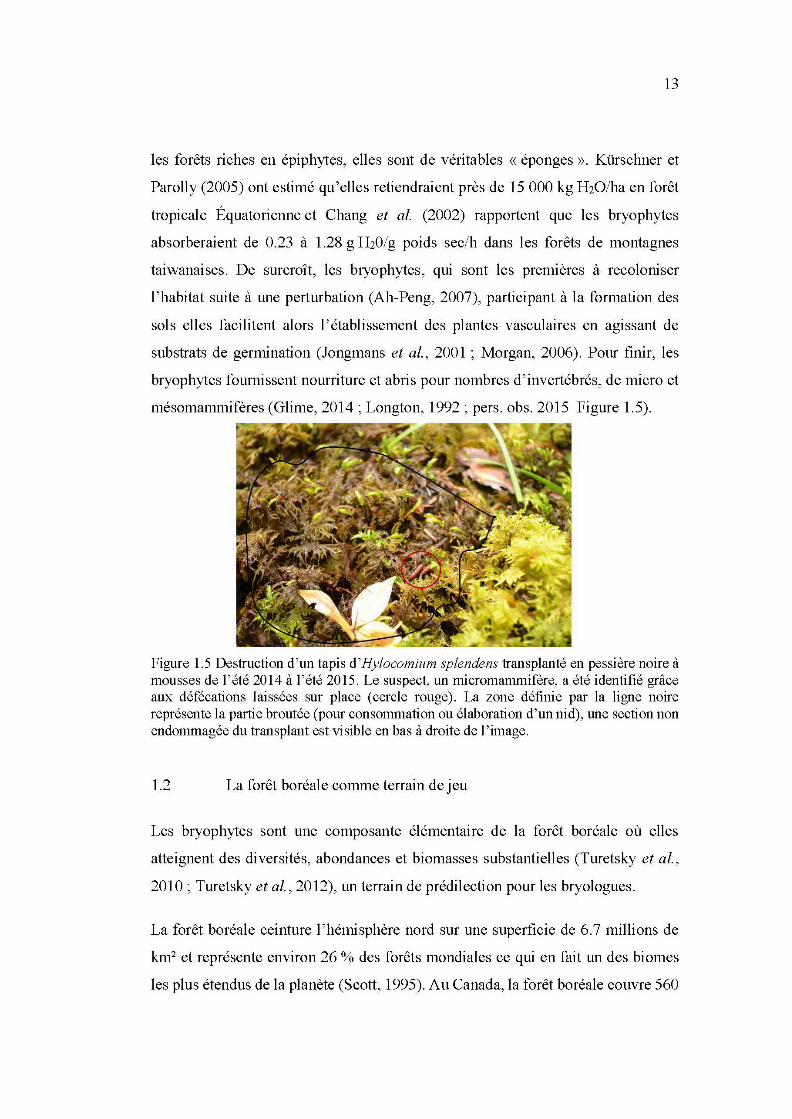
13

les forêts riches en épiphytes, elles sont de véritables « éponges». Kürschner et

Parolly (2005) ont estimé qu'elles retiendraient près de 15 000 kg H20/ha en forêt

tropicale Équatorienne et Chang et al. (2002) rapportent que les bryophytes

absorberaient de 0.23 à 1.28 g H20/g poids sec/h dans les forêts de montagnes

taïwanaises. De surcroît, les bryophytes, qui sont les premières à recoloniser

l'habitat suite à une perturbation (Ah-Peng, 2007), participant à la formation des

sols elles facilitent alors l' établissement des plantes vasculaires en agissant de

substrats de germination (Jongmans et al., 2001 ~ Morgan, 2006). Pour finir, les

bryophytes fournissent nourriture et abris pour nombres d'invertébrés, de micro et

mésomammifères (Glime, 2014 ~ Longton, 1992 ~ pers. obs. 2015 Figure 1.5).

Figure 1.5 Destruction d'un tapis d'Hylocomium splendens transplanté en pessière noire à mousses de l'été 2014 à l'été 2015. Le suspect, un micromammifère, a été identifié grâce aux défécations laissées sur place (cercle rouge). La zone définie par la ligne noire représente la partie broutée (pour consommation ou élaboration d'un nid), une section non endommagée du transplant est visible en bas à droite de l ' image.

1.2 La forêt boréale comme terrain de jeu

Les bryophytes sont une composante élémentaire de la forêt boréale où elles

atteignent des diversités, abondances et biomasses substantielles (Turetsky et al. ,

2010 ~ Turetsky et al., 20 12), un terrain de prédilection pour les bryologues.

La forêt boréale ceinture l' hémisphère nord sur une superficie de 6.7 millions de

km2 et représente environ 26% des forêts mondiales ce qui en fait un des biomes

les plus étendus de la planète (Scott, 1995). Au Canada, la forêt boréale couvre 560

14

000 km2. Plus localement, au Québec, elle est divisée en deux domaines

bioclimatiques : la sapinière à bouleau blanc et la pessière noire à mousses, elles

mêmes subdivisées, sur la base des précipitations et du relief, en sous-domaines de

l'est et de l'ouest (MRNQ, 1999; Saucier et al., 2009). En résultent alors des

différences fondamentales dans les régimes de perturbation, mais aussi dans la

proportion des essences végétales dominantes. Nous nous en tiendrons dans cette

étude à la pessière noire à mousses de 1' ouest du Québec.

1.2.1 Région d'étude

La pessière n01re à mousses ouest-québécoise s'étend sur 154 184 km2 et est

délimitée, à 1 'ouest par la frontière ontarienne et, à 1' est, par le bassin versant des

rivières Péribonka et Manouane. Au nord elle prend fin où commence la taïga et au

sud où commence la sapinière à bouleaux blancs de l'ouest (MRNQ, 1999). La

pessière noire à mousses occupe alors une bande continue de 300 km entre le 48°

38' et le 52° 00' de latitude nord.

Les peuplements de conifères dominent la région d'étude. L'essence principale est

représentée par l'épinette noire (Picea mariana (Mill.) Briton), en mélange au pin

gris (Pinus banksiana Lamb.), au peuplier faux-tremble (Populus tremuloides

Michx.), au sapin (Abies balsamea (L.) Mill.), au mélèze (Larix laricina (Du Roi)

K. Koch) et au bouleau à papier (Betula papyrifera Marshall). Les éricacées

dominent le sous-bois (e.g., Rhododendron groenlandicum (Oeder) Kron & Judd)

tandis que le sol est recouvert d'un tapis continu de mousses hypnacées (P leurozium

schreberi (Brid.) Mitt., Hylocomium splendens (Hedw.) Schimp. , Ptilium crista

castrensis) cédant la place aux sphaignes dans les sites mal drainés et plus acides

(Saucier et al., 2009).

L'intégralité de la région d'étude est située sur la Ceinture d'argile s'étendant du

nord-est de l'Ontario au nord-ouest du Québec (Allard, 1974). Les dépôts d'argile

laissés suite à la sédimentation du lac pro-glaciaire Barlow-Ojibway durant le

Wisconsinien atteignent par endroit 60 rn d'épaisseur (Vincent & Hardy, 1977). Le

15

relief est peu accidenté et 1 'altitude varie en moyenne entre 200 et 300 m. Le climat

est subpolaire continental avec une température moyenne annuelle de 1 oc et des

précipitations annuelles moyennes de 927.8 mm (relevés pour la période de 1981-

2010, station météorologique de Lebel-sur-Quévillon, Environnement Canada,

2015). La région est marquée par de longs hivers (précipitations neigeuses

annuelles moyennes de 312.9 cm) et par une saison de croissance courte ( 140 à 160

jours).

Notre région d 'étude couvre une superficie de 73 197 km2 (79° 69' 0, 50° 71' N -

74° 50' 0, 50° 71' N- 79° 69' 0, 48° 83' Net 74° 50' 0, 48° 83 N; Figure 1.6).

Ce territoire est intégralement localisé dans la région administrative du Nord-du

Québec, sur le territoire d'Eeyou Istchee Baie James. Nous y avons sélectionné six

zones de feu de taille, forme, âge et origine variés (Table A2.1) dans lesquels les

communautés bryophytiques ont été échantillonnées. En parallèle, des peuplements

de forêts continues non brûlées ont été sélectionnés sur le même territoire dans le

cadre d'un autre projet et seront utilisés à titre de témoins dans plusieurs des

chapitres de cette thèse (Chaieb et al., 2015).

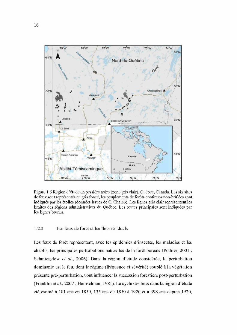
16

51 ' N

SO' N

48' N

1

~? .1

79' W 78' W

" A ~~ ~~

"'a 11:. .. \ \

* • * .. *

... La Sarre

Rouyn-Noranda

* *

' .. Matagami

À.

. Amos

lJ Val-d'Or

77' W 76' W

Nord-du-Québec

Abitibi-T émiscamingue

0 79'V\l

50 Km 178'W

1 77'W 1 76' W

~

75'W 74'W

,;

Chibougamau Â

51' N

/ SO' N (

49' N

48' N

Figure 1.6 Région d'étude en pessière noire (zone gris clair), Québec, Canada. Les six sites de feux sont représentés en gris foncé, les peuplements de forêts continues non-brûlées sont indiqués par les étoiles (données issues de C. Chaieb ). Les lignes gris clair représentent les limites des régions administratives du Québec. Les routes principales sont indiquées par les lignes brunes.

1.2.2 Les feux de forêt et les îlots résiduels

Les feux de forêt représentent, avec les épidémies d'insectes, les maladies et les

chablis, les principales perturbations naturelles de la forêt boréale (Pothier, 2001 ;

Schmiegelow et al., 2006). Dans la région d'étude considérée, la perturbation

dominante est le feu, dont le régime (fréquence et sévérité) couplé à la végétation

présente pré-perturbation, vont influencer la succession forestière post-perturbation

(Franklin et al., 2007; Heinselman, 1981). Le cycle des feux dans la région d'étude

été estimé à 101 ans en 1850, 135 ans de 1850 à 1920 et à 398 ans depuis 1920,

17

conduisant à un âge moyen des peuplements de 150 ans (Bergeron et al., 2004).

L'allongement des régimes de feu depuis les années 1850 est expliqué par la

modification des conditions climatiques et, plus récemment par l'addition des

actions anthropiques (i.e., suppression des feux, coupes) interférant avec les patrons

de perturbations naturelles (Bergeron et al., 2006).

La particularité première des perturbations naturelles résulte dans la création d'une

matrice forestière diversifiée. En effet, le feu a un impact hétérogène sur le paysage

conduisant à une mosaïque de peuplements d 'âges, de compositions et de structures

variables (Cyr et al., 2009) où les zones brûlées jouxtent des parcelles de forêts

rescapées des flammes (Bergeron et al., 2002 ; Mad oui et al., 201 0). Les conditions

météorologiques durant l'épisode de feu, la topographie du milieu (e.g., les

dépressions humides et les parois rocheuses peuvent agir comme des pare-feu

naturels) ainsi que la susceptibilité locale de la matrice à l'ignition expliquent cette

hétérogénéité (Ouarmim et al., 2015 ; Turner et al., 1994).

Les confettis de forêt rescapés du feu sont appelés « îlots résiduels » (Figure 1. 7).

La proportion des îlots résiduels dans la matrice brûlée est en moyenne de 10 % en

pessière noire à mousses québécoise (Madoui et al., 2011 ), mais cette proportion

varie en fonction de la taille et de la sévérité du feu (DeLong & Tanner, 1996). De

taille et forme variables, les îlots résiduels sont rarement distants de plus de 700 rn

de leur plus proche voisin (Perron et al., 2008). Certains îlots résiduels peuvent

avoir été épargnés « par chance » due à une modification soudaine des conditions

météorologiques (e.g. , changements de direction du vent, ondées) alors que d'autres

seraient épargnés du feu de façon récurrente. Ces derniers représentent des îlots

séculaires et pourraient avoir survécu au feu depuis plusieurs millénaires en raison

de conditions stationnelles les rendant peu susceptibles à l'ignition (Bergeron &

Harper, 2009; Ouarmim et al., 2015).

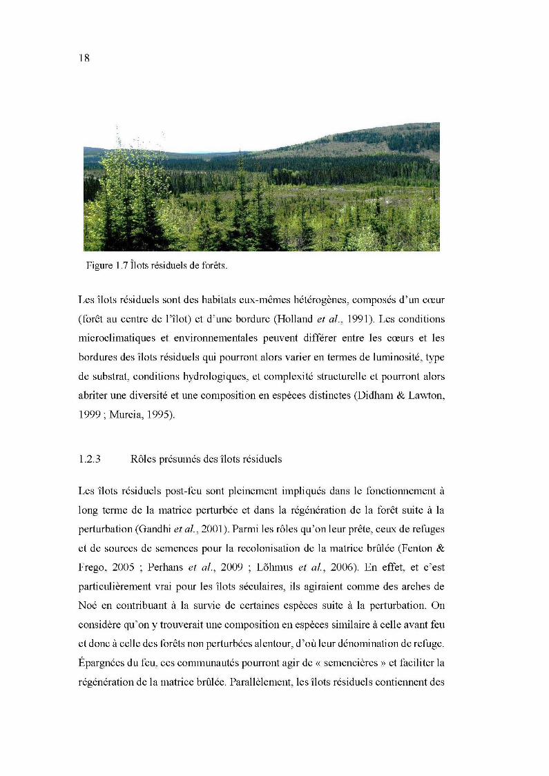
18

Figure 1.7 Îlots résiduels de forêts.

Les îlots résiduels sont des habitats eux-mêmes hétérogènes, composés d'un cœur

(forêt au centre de l'îlot) et d'une bordure (Rolland et al. , 1991). Les conditions

microclimatiques et environnementales peuvent différer entre les cœurs et les

bordures des îlots résiduels qui pourront alors varier en termes de luminosité, type

de substrat, conditions hydrologiques, et complexité structurelle et pourront alors

abriter une diversité et une composition en espèces distinctes (Didham & Lawton,

1999; Murcia, 1995).

1.2.3 Rôles présumés des îlots résiduels

Les îlots résiduels post-feu sont pleinement impliqués dans le fonctionnement à

long terme de la matrice perturbée et dans la régénération de la forêt suite à la

perturbation (Gandhi et al., 2001). Parmi les rôles qu'on leur prête, ceux de refuges

et de sources de semences pour la recolonisation de la matrice brûlée (Fenton &

Frego, 2005 ; Perhans et al., 2009 ; Lohmus et al. , 2006). En effet, et c'est

particulièrement vrai pour les îlots séculaires, ils agiraient comme des arches de

Noé en contribuant à la survie de certaines espèces suite à la perturbation. On

considère qu'on y trouverait une composition en espèces similaire à celle avant feu

et donc à celle des forêts non perturbées alentour, d'où leur dénomination de refuge.

Épargnées du feu, ces communautés pourront agir de« semencières » et faciliter la

régénération de la matrice brûlée. Parallèlement, les îlots résiduels contiennent des

19

legs biologiques (e.g., bois mort au sol ou sur pied, arbres rémanents) qm

représentent des microhabitats de qualité pour les espèces dépendantes de

conditions microenvironnementales stables et de microhabitats spécialisés

(Anderson & Hyttebom, 1991 ; Fenton & Frego, 2005; Lesica et al., 1991). Ces

legs biologiques sont des sources desquelles peut reprendre la colonisation de la

matrice et orientent la succession forestière post-perturbation (DeLong & Kessler,

2000 ; Lindenmayer et al. , 2006 ; Seidl et al., 2014). Les îlots résiduels seraient

donc des inocula et garantiraient le maintien d'espèces qui auraient sinon disparu à

long terme du paysage, étant donné leurs sensibilités aux perturbations et leurs

capacités de dispersion réduite.

Les îlots résiduels agiraient aussi comme des connecteurs pour les espèces mobiles

et participeraient à l ' enrichissement structurel de la matrice btûlée (Franklin et al.,

2007 ; Nappi et al., 2004; Neitlich & McCune, 1997). Les îlots résiduels réduisent

les distances à parcourir au sein de la matrice perturbée hostile et sont alors qualifiés

de «pas japonais » ou « stepping stones » (Chan-Mcleod & Moy, 2007; DeLong

& Kessler, 2000). Les organismes, selon leurs capacités de dispersion respectives,

requerront différents agencements spatiaux des îlots résiduels (dispersé, en

agrégat).

La résilience de l'écosystème, définie comme «le taux, la manière et le degré

auxquels les caractéristiques initiales d'une communauté sont restaurées suite à une

perturbation» (Halpern, 1988), est donc dépendante des îlots résiduels qui assurent

la survie de certaines espèces après la perturbation. La diversité des espèces

fonctionnellement équivalente («redondance fonctionnelle ») maintenue dans

l'écosystème après la perturbation en assure la résilience (Rosenfeld, 2002). Par

conséquent, la physionomie (aire et taille), l'âge, l'agencement spatial et la

complexité structurelle des îlots résiduels qui déterminent leurs qualités de refuges,

de sources de propagule et de pas japonais définissent le potentiel régénératif d 'un

écosystème (Drapeau et al., 2009; Honnay et al., 1999; Lee et al., 2015).

20

1.3 Une aspiration: l'aménagement écosystémique

Depuis les dernières décennies, en réponse à la demande croissante en produits

ligneux et dérivés, 1 'exploitation forestière s'est intensifiée modifiant

considérablement le paysage forestier nord-américain. La raréfaction des

peuplements anciens et surannés au profit d'un rajeunissement de la mosaïque

forestière (Cyr et al., 2009), en plus de la fragmentation du territoire engendrée par

les coupes forestières, ont conduit à la perte des écosystèmes naturels et à

l'isolement des populations. En Fennoscandinavie, où l'exploitation des ressources

forestières précède de près de 100 ans celle de l'Amérique du Nord (Mônkkônen &

Welsh, 1994), les études réalisées font office de pionnières et rapportent la

diminution de la biodiversité suite à l'exploitation (Imbeau et al., 2001 ; Siitonen,

2001 ). Cela laisse entrevoir des risques encourus en forêt boréale nord-américaine

où les espèces les plus sensibles aux perturbations et les moins mobiles, comme

c'est le cas des bryophytes, sont alors en sursis (Hazell & Gustafsson, 1999;

V anderpoorten & Goffinet, 2009). L'addition des coupes forestières aux épidémies

d'insectes et aux feux, perturbateurs naturels de la forêt boréale nord-américaine, a

accru la vulnérabilité des écosystèmes aux prises désormais à l'action simultanée

des perturbations anthropiques et naturelles (Gauthier et al., 2008). Ces constats,

abordés durant le Sommet de la Terre de Rio de Janeiro (1992) et lors du Processus

de Montréal (1994) ont conduit à l'élaboration de critères et d'indicateurs

d'aménagement forestier durable précipitant la refonte de la foresterie. Il s'agit

désormais de réduire les écarts entre les forêts aménagées et naturelles en

reproduisant les patrons spatiotemporels issus des perturbations naturelles afin de

poursuivre l'exploitation forestière en maintenant conjointement la biodiversité et

la fonctionnalité des écosystèmes (Gauthier et al., 2008 ; Perera et al., 2004).

En forêt boréale canadienne, la portraitisation des patrons spatiaux et temporels des

perturbations a débuté il y a 20 ans (Bergeron & Harvey, 1997 ; Cyr et al., 2009) et

a mené à l'émergence de plusieurs alternatives d'aménagement écosystémique.

Parmi celles-ci, on retient, dans le contexte de ce projet, les coupes à rétentions

21

variables(« green tree retention»; Franklin et Forman, 1987). Ces coupes visent à

maintenir la complexité spatiale et structurelle du paysage via le maintien de

bouquets d'arbres dans la matrice de coupe, comme ce serait le cas après un feu qui

épargne, çà et là, des îlots résiduels (Bergeron et al. 2002 ; Bergeron et al., 2006).

La taille, le nombre et l'agencement spatial (agrégé ou dispersé, bouquets ou îlots)

des parcelles de rétention, mais aussi le nombre et les essences d'arbres laissés sur

pied varient selon l'objectif d'aménagement encouru (Halpern et al., 2005). Dans

le meilleur des mondes on vise à imiter au mieux les desseins du feu en conservant

des parcelles de rétention qui auraient des rôles équivalant aux îlots résiduels post

feu. Seulement, pour ce faire, il apparaît nécessaire de préalablement posséder une

connaissance du rôle de ces îlots post-feu.

1.4 Objectifs

Cette thèse prend ici tout son sens et vise, dans une optique d'aménagement

écosystémique, à élucider le rôle des îlots résiduels post-feu dans la dynamique des

communautés bryophytiques en vue de s'en inspirer lors de la mise en place des

îlots de rétention dans les parterres de coupes. Bien que les rôles des îlots résiduels

aient été substantiellement étudiés suite aux perturbations anthropiques, les études

réalisées suite aux perturbations naturelles et notamment aux feux sont rares et

rapportent des résultats ambivalents (Hylander, 2009; Snall et al., 2005 ; Swanson

et Franklin, 1992). De plus, aucune étude n'a encore été entreprise en pessière noire

à mousses québécoise pourtant soumise à des régimes de feu singuliers. Formée

d'une mosaïque d'îlots résiduels, cet écosystème représente un système naturel

prédestiné pour les études portant sur la fragmentation, la biogéographie insulaire

(MacArthur et Wilson, 1967) et la dynamique des métapopulations (Hanski et

Simberloff, 1997).

L'intérêt d'utiliser les bryophytes pour répondre à cette question résulte de leur

ubiquité en pessière noire à mousses, mais aussi de leur capacité à répondre

finement aux modifications des conditions microenvironnementales (Pardow et

22

Lakatos 2013 ; Pharo et Zartman, 2007). De plus, les bryophytes sont parmi les

premières à recoloniser le territoire suite à une perturbation (Ah-Peng, 2007;

Jongmans et al., 2001). Initiatrices de la régénération forestière, elles constituent

alors un modèle biologique original et robuste pour étudier la résilience de

l'écosystème face aux perturbations.

Ce projet se divise en deux volets: (i) aménagement écosystémique, en vue de

bonifier les connaissances sur les patrons de perturbations naturelles à des fins de

gestion forestière ; (ii) bryologie, avec pour objectif d'améliorer les connaissances

fondamentales dans ce domaine.

Le volet « aménagement écosystémique » est scindé en trois sous-objectifs :

1.1. Documenter le rôle des îlots résiduels post-feu comme refuges pour les

communautés bryophytiques (Chapitre II). Par refuge, nous entendons un

habitat ou un microhabitat capable de supporter des conditions

environnementales et une communauté bryophytique similaire à celle

retrouvée dans une forêt non perturbée (basée sur Lancaster et Belyea, 1997

et Sedell et al., 1990). Dans un refuge les effets de la perturbation sont

atténués voire inexistants, nécessité fondamentale au maintien de nombreuses

espèces de bryophytes sensibles aux perturbations et à haut risque

d'extirpation (Fenton et Frego, 2005; Frisvoll et Prest0, 1997; Gustafsson et

Hallingback, 1988). Un refuge offrirait un « pied à terre » aux bryophytes afin

de leur faciliter la recolonisation de la matrice brûlée.

1.2. Estimer l'existence d'un effet de bordure dans les îlots résiduels post-feu et

la réponse des bryophytes à celui-ci (Chapitre III). L'effet de bordure a été

démontré comme délétère pour de nombreuses espèces dans des systèmes

anthropisés (Boudreault et al. , 2008 ; Hylander, 2005 ; Nelson et Halpern,

2005), qu'en est-il de bordures issues de perturbations naturelles ? Quelles

conclusions en tirer ?

1.3. Attester du rôle de sources de propagules des îlots résiduels post-feu pour les

communautés bryophytiques (Chapitre IV). Le rôle de refuge est intimement

23

lié à son corollaire de source de propagules puisque les colonies ayant survécu

à la perturbation dans les îlots résiduels seront des sources de propagules

potentielles. L'agencement spatial des îlots résiduels devrait influer sur les

patrons de dispersion des bryophytes (Baker et al., 2013 ; Chan-Mcleod et

Moy, 2007).

Le volet« bryologie » est, lui, divisé en quatre sous-objectifs :

2.1 Estimer les distances moyennes de dispersion des bryophytes en pessière

noire à mousses et valider ou réfuter le paradigme de la faible distance de

dispersion des bryophytes (Miles et Longton, 1992 ; Sundberg, 2013 ;

Chapitre IV).

2.2 Analyser la réponse des différentes phases du cycle phénologique des

bryophytes aux conditions climatiques en vue d'expliquer les patrons de

dispersion observés (Chapitre V)

2.3 Attester du recours à des agents biotiques de dispersion par les bryophytes

(Annexe 1).

2.4 Fournir un portrait bryologique préindustriel de la pessière noire à mousses

nord-américaine via l'actualisation de la Flore des bryophytes du Québec

Labrador (Faubert, 2012-2014; Annexe II).

CHAPITRE II

ARE POST-FIRE RESIDUAL FOREST PATCHES REFUGIA FOR BOREAL BRYOPHYTE SPECIES? IMPLICATIONS FOR ECOSYSTEM BASED

MANAGEMENT AND CONSERVATION

Marion Barbé, Nicole J. Fenton & Yves Bergeron

En révision dans Biodiversity and Conservation, Octobre 2016

26

2.1 ~bstract

Residual forest patches remaining after natural or anthropogenic disturbance may

facilitate regeneration of the fragmented forest. However, residual forest patch

function remains unclear, especially after natural wildfire. We investigate the role

of residual boreal forest patch es as refugia for bryophytes and ask the question, do

post-fire residual forest patches house bryophyte communities similar to those

encountered in undisturbed forests? Bryophytes were sampled in three habitat types

in black spruce boreal forests illustrating a gradient of disturbance severity:

undisturbed forests, residual patches and bumed matrices. Temporal, disturbance

severity, spatial and structural variables of habitats were also recorded. Bryophyte

community composition differed among habitat types with residual forest patches

characterized by loss of forest specialists and the addition of disturbance-prone

species. Consequently, residual patches were richer in species than undisturbed

forests. ~s residual patches did not conserve all species and especially forest

specialists, they were not refugia, but their high bryo-diversity suggests that they

represent habitats of high quality for post-disturbance community assembly.

Furthermore, we identify sorne temporal, spatial and structural characteristics of

residual patches that maintain bryophyte communities closest to that ofundisturbed

forests. The distinct bryoflora housed by residual forest patches and undisturbed

forests suggests that they represent complementary habitats. Consequently, both of

these habitats need to be conserved in order to not lose species and to maintain

landscape bryo-diversity.

Key-words: black spruce forest; community assembly; disturbance prone species;

forest remnant; forest interior species, forest remnant, liverworts.

27

2.2 Résumé

Les îlots résiduels issus de perturbations d'origines naturelles et anthropiques sont

supposés impliqués dans la régénération forestière. Cependant, les fonctions de ces

îlots résiduels, et particulièrement de ceux issus de feux de forêt naturels, demeurent

confuses. Nous avons étudié le rôle de refuge des îlots résiduels post-feu pour les

bryophytes. Ces îlots résiduels abritent-ils des communautés bryophytiques

similaires à celles retrouvées dans les forêts non perturbées ? Les bryophytes ont

été échantillonnées dans 39 forêts non perturbées et six feux naturels composés

d'îlots résiduels et de matrices brûlées de sorte à obtenir trois types d'habitats

illustrant un gradient d'intensité de perturbation. Des variables temporelles, de

sévérité de feu, spatiales et structurelles ont aussi été relevées dans les différents

types d'habitats. La composition des communautés diffèrait selon les types

d'habitats et les îlots résiduels étaient caractérisés par l'absence de certaines espèces

forestières et par la présence d'espèces favorisées par la perturbation. Les îlots

résiduels étaient plus riches en espèces que les forêts non perturbées. Bien que le

confinement de plusieurs espèces strictement forestières aux forêts non perturbées

ne permette pas de décrire nos îlots résiduels comme des refuges, nous soutenons

qu'ils sont des habitats de haute qualité participant au re-assemblage d'une

communauté bryophytique riche post-perturbation. Nous avons, en parallèle,

identifié des caractéristiques temporelles, spatiales et structurelles des îlots

résiduels leur permettant de supporter des communautés plus comparables à celles

des forêts non perturbées qu'à celles des matrices brûlées. Les bryoflores distinctes

des îlots résiduels et des forêts non perturbées suggèrent qu'ils représentent des

habitats complémentaires qui doivent être conservés de concert afin de ne pas

perdre d'espèces et de maintenir la bryo-diversité de l'écosystème.

Mots-clés : assemblage des communautés ; espèce favorisée par la perturbation ;

espèce forestière ; fragment forestier ; hépatiques ; pessière noire à mousses.

28

2.3 Introduction

Ecosystems are intrinsically subject to disturbances of various intensities and

frequencies (e.g. storms, wildfires, insect outbreaks), which temporarily modify

their functions. Following Halpem's (1988) definition, resilience is ''the rate,

manner, or degree to which initial community characteristics are restored" after a

disturbance. Resilience is believed to be enhanced by the diversity of functionally

equivalent species in an ecosystem (functional redundancy; Rosenfeld 2002).

However, functions provided by individual species could be lost after disturbance

ifspecies inter-relationships change or species are lost (Walker 1995; Creed 2000).

As anticipating the future roles of species after environmental changes is a

challenge, a precautionary approach is appropriate and all species, including the

infrequent or rare, should be conserved in order to ensure that ecosystem functions

persist. Our study was designed to identify habitats that fulfill a "life-boat" role for

species in a naturally disturbed landscape in order to ensure species conservation

and re-assembly of a functional post-disturbance community, and therefore

ecosystem resilience (Walker 1995).

V arious ecosystems are naturally disturbed by wildfire ( e.g. savannah, boreal forest;

Payette 1992; Higgins et al. 2000), which has heterogeneous impacts (Carlson et al.

2011). In many systems, patches of unbumt forest ("residual patches"; Andison

2014) that have partially or entirely escaped fire persist in the bumed matrix. The

characteristics of this mosaic of unbumed patches (i.e. spatial arrangement, size)

depend on fire frequency and severity as well as on the physical characteristics of

the landscape (i.e. topography, flammability) and the vegetation present at the time

of fire (Madoui et al. 201 0; Leonard et al. 20 14). The se residual forest patches are

believed to serve several functions such as refugia for species during the fire event,

and as propagule sources during landscape recolonization (Rosenvald and Lohmus

2006; Perhans et al. 2009; Robinson et al. 20 13). Residual patches also reduce the

travelling distance across the matrix for mobile species and promote structural

diversity in the regenerating landscape (Nappi et al. 2004). Consequently residual

29

patches will influence, together with the vegetation present before disturbance, the

composition, structure and successional trajectory of post-fire vegetation (Clarke

2002). However, the definition of refugia is not clear as they may be defined as

areas where the negative impacts of disturbance are diminished compared to the

surrounding area (based on Sedell et al. 1990 and Lancaster and Belyea 1997) but

at different scales, such as habitats (forest stands) or even microhabitats (i.e.

biological legacies such as dead wood). The working definition used here is that

refugia contribute to the recovery of biotic communities to a pre-disturbance state,

and therefore ensure the ecosystem functionality and resilience of the forest

landscape.

Over the last decade, the literature has focused on the importance of post-harvest

retention patches as refugia for species (Dynesius and Hylander 2007; Perhans et

al. 2009; Lee et al. 20 15) but there are few studies on post-fire residual forest

patches (Hylander and Johnson 2010; Robinson et al. 2013). Therefore, the natural

role that post-harvest retention patches are meant to emulate is yet undetermined.

Furthermore, no clear patterns in retention patch characteristics that influence

refugia capacity have emerged, as different studies around the globe highlight the

importance of spatial variables ( e.g. size affects invertebrates diversity; Lee et al.

2015), structural variables (e.g. deadwood affects bird and bryophyte communities;

; Rambo 2001; Drapeau et al. 2009), temporal variables (e.g. forest age affects plant

diversity; Honnay et al. 1999), and landscape variables (topography influences

refugia potential; Leonard et al. 2014; Chia et al. 2015; Robinson et al. 2016).

However, in North America, both the role of post-fire residual forest patches and

the characteristics that influence their value as refugia remain unclear

(Schmiegelow et al. 2006; Robinson et al. 2013). In this study we attempt to clarify

both of these elements by focusing on bryophyte assembly in a natural post-fire

patch system in the boreal forests of eastern North America.

30

Bryophytes dominate the boreal forest in terms of plant biomass and spec1es

richness (Turetsky et al. 2012). They occupy a variety of microhabitats, from the

forest floor for large feather mosses, to boulders, dead wood and tree bases for

specialist species (Dynesius and Hylander 2007). Forest bryophytes, and

particularly their early life stages (protonemata), are dependent on humid

microclimates (Lôbel and Rydin 20 10). Consequently, both natural and

anthropogenic disturbances that generate dry conditions may induce a local

reduction in bryophyte diversity (Ross-Davis and Frego 2002). This is particularly

true for drought-sensitive species that have a high local extirpation risk and require

specifie substrates, such as dead wood, to be maintained in the landscape (Rambo

2001; Pharo and Lindenmayer 2009). Residual forest patches from fire or harvest

may house such substrates and therefore may act as refugia to mitigate the species

extinction debt (sensu Tilman et al. 1994; Hylander and Johnsson 2010).

Specifically, through the comparison ofthree habitat types i.e. undisturbed forests

as control, residual forest patches and recently bumed matrices, this study examines

the role of post-fire residual patches as refugia for bryophytes by addressing two

questions: 1) do post-fire residual forest patches act as refugia for bryophyte

species? And, 2) what characteristics influence the ability ofpost-fire residual forest

patches to act as refugia? Following our working definition, a refugium refers to a

residual forest patch that contains a community of species (from common to

infrequent species) and environmental characteristics similar to th ose found in

undisturbed forests.

We hypothesise that residual patches share species with both recently bumed sites

and undisturbed forests and therefore contain a higher species richness than either

of these other habitat types (Hl), as implied by the intermediate disturbance

hypothesis (Connell 1979). We also expect that the presence of liverworts, given

their affinities with closed canopies and stable micro-climates and habitats (Lesica

et al. 1991; Fenton and Frego 2005), generates a shift in bryophyte community

composition from bumed matrix to undisturbed forests (H2). We also suppose that

31

stand age is the best predictor of bryophyte composition whereas stand structure is

the best predictor of bryophyte richness (Pi pp et al. 2001) (H3). In contrast to the

overall composition, the presence of liverwort species that are most sensitive to

forest harvest (Nelson and Halpern 2005), will be positively associated with stand

age and size [which is believed to enhance microhabitat quantity and quality (Pipp

et al. 2001 ; Fenton and Bergeron 2008)] and microhabitat diversity (Mills and

Macdonald 2004) (H4).

2.4 Methods

2.4.1 Study area

The study area covers a total of 73 197 km2 (79°69 W, 50°71 N- 74°50 W, 50°71

N - 79°69 W, 48°83 N - 74°50 W, 48°83 N) in the boreal black spruce (Picea

mariana Mill., Briton)-feather moss (Pleurozium schreberi (Brid.) Mitt.) forest of

western Québec, eastern Canada (Grondin 1996; Figure 2.1a). Stands are dominated

by P. mariana with Pinus banksiana Lamb., Populus tremuloides Michx, Abies

balsamea (L.) Mill. , and Betula papyrifera Marshall as secondary species. The

understory is dominated by ericaceous species [e.g. Rhododendron groenlandicum

(Oeder) Kron & Judd] and bryophyte species (feather mosses are replaced by

sphagna under more humid conditions). The region is relatively flat and the altitude

varies from 200 to 300 rn above sea level. The main surface deposits are clays left

by the withdrawal of the lake Barlow-Ojibway after the Wisconsonian glaciation

(Vincent and Hardy 1977). The climate is subpolar continental and average annual

temperature and precipitation are respectively 1 oc and 927.8 mm (1981 to 2010),

recorded at Lebel-sur-Quévillon, Québec, which is located at the center of the study

area (Environment Canada 2015).

The natural dynamics ofthe forests of the study area are primarily driven by stand

replacing wildfires. The fire cycle was estimated at 398 years since 1920 (Bergeron

et al. 2004), consequently, the average age ofthe forest is in excess of 150 years.

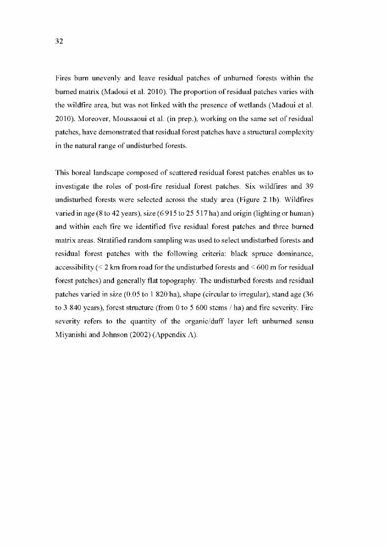
32

Pires hum unevenly and leave residual patches of unbumed forests within the

bumed matrix (Madoui et al. 2010). The proportion ofresidual patches varies with

the wildfire are a, but was not linked with the presence of wetlands (Madoui et al.

2010). Moreover, Moussaoui et al. (in prep.), working on the same set ofresidual

patches, have demonstrated that residual forest patches have a structural complexity

in the natural range of undisturbed forests.

This boreallandscape composed of scattered residual forest patches enables us to

investigate the roles of post-fire residual forest patches. Six wildfires and 39

undisturbed forests were selected across the study are a (Figure 2.1 b ). Wildfires

varied in age (8 to 42 years), size (6 915 to 25 517 ha) and origin (lighting or human)

and within each fire we identified five residual forest patches and three burned

matrix areas. Stratified random sampling was used to select undisturbed forests and

residual forest patches with the following criteria: black spruce dominance,

accessibility ( < 2 km from road for the undisturbed forests and < 600 rn for residual

forest patches) and generally flat topography. The undisturbed forests and residual

patches varied in size (0.05 to 1 820 ha), shape (circularto irregular), stand age (36

to 3 840 years), forest structure (from 0 to 5 600 stems 1 ha) and fire severity. Pire

severity refers to the quantity of the organic/duff layer left unbumed sensu

Miyanishi and Johnson (2002) (Appendix A).

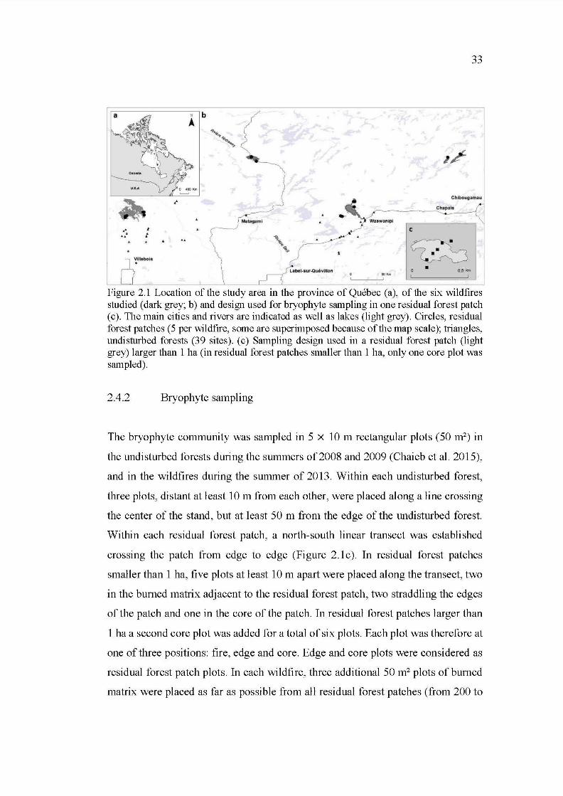
1 .

' b Â

. Lebel-sur .Quévillon

33

Chlbougamau

• ..... 0,5 Kr!~

Figure 2.1 Location ofthe study area in the province of Québec (a), of the six wildfires studied ( dark grey; b) and design used for bryophyte sampling in one residual forest patch (c). The main cities and rivers are indicated as well as lakes (light grey). Circles, residual forest patches (5 per wildfire, sorne are superimposed because ofthe map scale); triangles, undisturbed forests (39 sites). ( c) Sampling design used in a re si dual forest patch (light grey) larger than 1 ha (in residual forest patches smaller than 1 ha, only one core plot was sampled).

2.4.2 Bryophyte sampling

The bryophyte community was sampled in 5 x 10 rn rectangular plots (50m2) in

the undisturbed forests during the summers of 2008 and 2009 (Chaieb et al. 2015),

and in the wildfires during the summer of 2013. Within each undisturbed forest,

three plots, distant at least 10 rn from each other, were placed along aline crossing

the center of the stand, but at least 50 rn from the edge of the undisturbed forest.

Within each residual forest patch, a north-south linear transect was established

cros sing the patch from edge to ed ge (Figure 2.1 c). In re si dual forest patches

smaller than 1 ha, five plots at least 10 rn apart were placed along the transect, two

in the burned matrix adjacent to the residual forest patch, two straddling the edges

ofthe patch and one in the core of the patch. In residual forest patches larger than

1 ha a second core plot was added for a total of six plots. Each plot was therefore at

one ofthree positions: fire, edge and core. Edge and core plots were considered as

residual forest patch plots. In each wildfire, three additional 50 m2 plots of burned

matrix were placed as far as possible from all residual forest patches (from 200 to

34

8 500 rn) to ensure that as much of the bryophyte diversity of the bumed matrix was

sampled as possible. In total, the bryophyte community was sampled in 117 plots

in 39 undisturbed forests, 108 plots in 30 residual forest patch es, and 78 plots of

bumed matrix (2 plots surrounding the residual forest patches x 30 residual forest

patches plus 3 additional plots x 6 fires) for a total of 303 plots.

The bryophyte community was sampled with a modified form of ''floristic habitat

sampling" (Newmaster et al. 2005). In the original method, all habitats are searched

for species with no specifie reference to area. Here it was restricted to the 50 m 2

plots and all potential microhabitats (e.g. coarse woody debris, tree bases, peat

mounds and water holes) within the plots were searched and the bryophytes present

placed in individually marked paper bags. All microhabitats per plot were pooled

in order to obtain the species richness of the community per plot. Bryophyte

samples were dried until identification in the laboratory and vouchers are stored at

the Université du Québec in Abitibi-Témiscamingue, Canada. Nomenclature

follows Faubert (2012-2014) except for Sphagnum subtile (Russ.) Warnst., which

follows the nomenclature of the Flora of North America Editorial Committee

(2007).

2.4.3 Environmental variables sampling

The relative effect of four categories of environmental variables (i.e. temporal,

severity, spatial and structural; Appendix A) on bryophyte composition and

richness were studied. The temporal variable 'age of forest (years)' is defined as

the time sin ce the last fire. For est age was estimated by coring ten dominant trees

with an increment cor er in a circular plot 11.28 rn in radius ( 400 m2) placed at the

core of the undisturbed forest and residual forest patches (Chaieb et al. 2015,

Moussaoui et al. 2016). The age of the oldest tree was established as the minimum

age of the forest. In the forest stands were the ten dominant trees approached the

maximum life span of black spruce (i.e. > 180 years old), 14C dating of charcoal

35

particles from a soil pit was used (Simard et al. 2007). The age ofbumed matrices

was defined as the time since the last fire.

Fire severity was assessed using the thickness of the organic layer between the top

charcoallayer and the mineral soil of the soil pit (Miyanishi and Johnson 2002).

When the residual organic layer was > 4 cm, sites were categorized as originating

from a low-severity fire (Greene et al. 2007).

Spatial variables consisted of proxies of site area and shape and were calculated

using ArcGis 10.3.1 (ESRI 2015). Buffer zone width (rn) is defined as the average

offive distances from the core plot to five points placed along the edge of residual

forest patches and undisturbed forests. A low value corresponds to a reduced

distance from the core to the disturbed area (i.e. bumed matrix). Buffer zone width

was used instead of area as it better represents the isolation of the core bryophyte

community from the surrounding disturbed areas. Similarly, the residual forest

patch and undisturbed forest shape was estimated using the standard deviation (SD)

of the five distances used to determine buffer zone width. A low SD value

corresponds to low variability in the five distances and to a relatively rounder shape

(i.e. approaching a circle ), whereas a high SD value corresponds to a more

elongated or irregular shape. Buffer zone width and shape both equalled 0 in bumed

matrix sites.

Structural variables include tree and snag density (number of stems 1 ha), mean tree

height (rn), volume of coarse woody debris according of the decay class (m3 1 ha),

tree species richness (number of species), number of different microhabitats, and

the presence or absence ofwater holes. Tree and snag density, and volume of coarse

woody debris were calculated in the 400 m2 circular plots at the core of each

undisturbed forest and residual forest patch, while the line intersect method was

used at the edge and in the fire plots surrounding each residual patch. As these

values were not measured in the fire matrix plots, we calculate the mean value of

the two fire plots associated with all five residual forest patches in each fire and

used this value. All trees and snags with DBH > 9 cm and all coarse woody debris

36

> 5 cm in diameter were measured. Coarse woody debris were categorized using

Thomas et al. 's (1979) decay classification system for snags and dead woods:

classes 1 and 2 were grouped and correspond to "recently" fallen dead trees with

bark and branches intact; class 3 refers to dead woods without bark nor branches

and with softening wood; and classes 4 and 5 were grouped and refer to de ad woods

with a collapsed shape. Mean tree height of the ten dominant trees in the 400 m2

circular plots was estimated with a clinometer. Tree species richness was

determined for each plot as the number of species present both in the plot and at

less than 1 rn surrounding the plot (i.e. intersection with the plot edge or with

branches or canopy that can drop litter in the plot). The number of different

microhabitats and water hole presence 1 absence were recorded for each plot.

2.4.4 Data analyses

In order to overcome the different number of sites sampled per habitat type,

analyses were conducted at the plot level and we described the bryophyte

community of the three different habitat types along the disturbance severity

gradient: bumed matrix > residual forest patch > undisturbed forest.

R software 3.2.1 (R-Development-Core-Team 2015) was used for all statistical

analyses with a significance level of a = 0.05. As we used a nested design we tested

whether the spatial structure of the sampling influenced the models in the different

analyses with a LogLik ratio test (Pinheiro and Bates 1995). In all analyses, the

spatial structure had a significant effect, we therefore used mixed models. Random

effects corresponded to the forest stand and to the wildfire in which plots were

sampled. When normality and homoscedasticity assumptions were met, linear

mixed models (lme) were used with the package "nlme" 3.1-121 (Pinheiro and

Bates 2015). A square root transformation was applied as needed to fit a normal

distribution. If this was insufficient, no other transformations were investigated

because of their non-intuitive interpretation (Warton and Hui 2011), and

generalized linear mixed models (glmer) were applied with the package "lme4" 1.1-

8 (Bates et al. 20 15), with the appropriate link function. Models were followed by

37

post-hoc tests equivalent to Tukey HSD for mixed models with the package

"multcomp" 1.4-1 (Hothom et al. 20 15).

2.4.4.1 Bryophyte richness and composition

Bryophyte species were classified by their presence in a habitat type and by life

forms. We obtained four species richness datasets: total ( alllife forms ), true mosses,

liverworts and sphagna. The same life form divisions were applied to the species

only present in one of the three habitat types. We therefore obtained total, true

mosses, liverworts and sphagna richnesses for species only found in undisturbed

forests, residual forest patches or bumed matrices, defined as "restricted richnesses"

of each habitat type.

Bryophyte richness and composition were calculated at the plot level (n = 303) and

compared as total and means among the three habitat types. Individual fires and

forest stands were included as random variables to take into account the nested data

(see above ). In the analyses, no species richnesses were transformed except sphagna

richness, which was square root transformed. Total and sphagna species richness

were treated with linear mixed models (lme) due to their normal distributions

whereas generalized linear mixed mo dels (glmer) were used for the six other species

richnesses, with Poisson distributions.

In order to determine whether overall community composition differed among

habitat types, Correspondence Analysis (CA; Leps and Smilauer 2003) was

performed on presence-absence data of all species occurring more than five times

in the entire dataset (117 of 208 taxa; as required by the algorithm) using the

package "vegan" 2.3-0 (Oksanen et al. 2015). Specimens identified only to genus

for whom other species of the same genus were present were also removed from

the analysis, resulting in an ordination matrix of 110 species and 303 plots. The

significance of the differences in community composition among habitat types was

determined by Multi-Response Permutation Procedure (MRPP) with 2000

permutations.

38

2.4.4.2 Relationships between environmental variables, habitat types,

bryophyte richness and composition

Two analyses were undertaken to determine the relationship between bryophyte

richness and community composition and environmental variables. In order to only

examine non-correlated variables, relationships among numerical environmental

variables were tested through non-parametric Spearman rank correlations.

Variables with correlation coefficients < - 0.70 or > 0.70 and with P-values < 0.05

were removed from the analyses. Similarly, boxplots were used to examine

relationships between numerical and categorical variables. Retained environmental

variables were subsequently compared among undisturbed forests, residual forest

patches and bumed matrices via generalized linear mixed model (glmer), except for

"number of microhabitats" and "tree and snag density" that were tested via linear

mixed mo dels (lme) be cause they followed normal distributions.

First, the relative influences of the categories of environmental variables (temporal,

severity, spatial and structural) on bryophyte richness were assessed for total, true

mosses, liverworts and sphagna richness datasets. Of the "restricted" species

richness groups, we examined in detail species richness of the true mosses and

liverworts only found in undisturbed forests in order to understand what main

environmental characteristics of the stands justifytheir absence from residual forest

patches and bumed matrices. A model selection procedure using 32 candidate

mo dels generated from combinations of the environmental variables plus the null

mo del was performed for each richness variable (Table 2.1 ). As the two spatial

variables (are a and shape) were correlated, they were ne ver included together in

one model. We therefore have two global models, each including one ofthe spatial

variables. They are followed by 12 models testing each category of environmental

variables (with 2 models for the correlated spatial variables). The 18 other models

tested biologically relevant combinations of variables of different categories and

interaction terms (see Table 2.1 for details) with duplication ofthe models for each

of the spatial variables. The lack of convergence of certain models was corrected

39

by optimization of the model algorithm via the bobyqa function of the glmerControl

parameter (Powell 2009). The explanatory variable dataset ( environmental

variables) was standardised (on columns) to account for the different scales of

measurement. Candidate models were ranked based on the Akaike 's Information

Criterion corrected for small sample size (AICc) (Bumham and Anderson 2002)

using the package AICcmodavg 2.0-3 (Mazerolle 2015). Models with a delta AICc

(L1AICc) > 2.0 were considered to have substantially lower empirical support

(Bumham and Anderson 2002). The model with the lowest delta AICc was

considered the most parsimonious and indicated the environmental predictors that

best explained variations in species richness. In the case where several models had

a delta AICc < 2, evidence-ratio tests were performed to compare their respective

explanatory weight. Multimodel inference was used to illustrate the effect of each

explanatory variable of the most parsimonious model. When the value of the

evidence ratio between the two best models was weak, no one model was the

considered the best and multimodel inference was performed. We obtained 95%

confidence intervals and model predictions using the modavgpred function of the

AICcmodavg 2.0-3 package (Mazerolle 2015). Variables with 95% confidence

intervals excluding 0 have a significant effect on the explanatory variable (the

different species richnesses) and their predicted values were subsequent! y plotted

against values of the explanatory variable. No interaction terms excluded O. An

estimate ofmodel adjustment was indicated by Spearman's Rho.

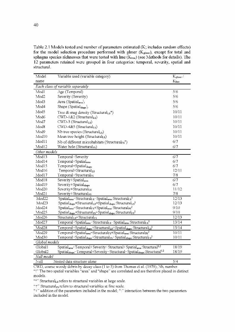
40

Table 2.1 Models tested and number of parameters estimated (K; includes random effects) for the model selection procedure performed with glmer (Kgtmer), except for total and sphagna species richnesses that were tested with lme (Kime) (see Methods for details). The 12 parameters retained were grouped in four categories: temporal, severity, spatial and structural.

Mo del name

Variable used (variable category)

Each class of variable separately

Mod1 Age (Temporal) Mod2 Severity (Severity) Mod3 Area (Spatialarca!) Mod4 Shape (Spatialshape!)

Mod5 Tree & snag density (StructuralLs*) Mod6 CWD-1&2 (StructuralLS) Mod7 CWD-3 (StructuralLs) Mod8 CWD-4&5 (StructuralLS) Mod9 Nb tree species (StructuralLS) Mod10 Mean tree height (StructuralLs)

Mod 11 Nb of different rn icrohabitats (StructuralFs t) Mod12 Water hole (StructuralFs) Other models Mod13 Mod14 Mod15 Mod16 Mod17 Modl8 Modl9 Mod20 Mod21 Mod22 Mod23 Mod24 Mod25 Mod26 Mod27

Temporal+Severity Temporal+Spatialarea Temporal+Spatialshape Temporal+StructuralLs

Temporal+StructuralFs Se verity+ Spatialarea Se verity+ Spatialshape Se verity+ StructuralLs Se verity+ StructuralFs Spatialarca +S tructuralLS+ Spatialarea: Structura1Ls1

Spatialshapc +StructuralLs+Spatial,hapc: Structura1Ls1

Spatialarea +S tructuralFs+ Spatialarea: Structura1Fs2

Spatialshape + S tructuralFs+ Spatialshape: Structura1Fs2

StructuralLs+StructuralFs Temporal+ S patialarea + StructuralLs+ Spatialarea: StructuralLS 1

Mod28 T emporal+Spatial,hapc +StructuralLS+Spatial,hapc: Structura1Ls1

Mod29 Temporal+ S patialarca + S tructuralFs+ Spatialarca: Structura1Fs2

Mod30 T emporal+Spatialshape +StructuralFs+ Spatialshape: Structura1Fs2

Global models Global! Spatialarea +Temporal+ Severi ty+ Structural+ Spatialarea: StructuraP ,2

Global2 Spatial,hape + T emporal+Severity+Structural+Spatial,hape: StructuraP.Z Null modeZ

Kg!mer /

K!me

5/6 5/6 5/6 5/6 10111

10111 10111 1011 1 10111 10111 617 6/7

617 617 617 1211 1 7/8 617 617 11112 7/8 12113 12113 9110 9110 12113 13114

13114 1011 1 1011 1

18119 18119

Null Nested data structure alone 5/4 CWD, coarse woody debris by decay class (1 to 5) from Thomas et al. (1979); Nb, number. ''!" The two spatial variables "area" and "shape" are correlated and are therefore placed in distinct models. "*" StructuralLs re fers to structural variables at large scale.

"t" StructuralFs re fers to structural variables at fine scale. "+" addition of the parameters included in the model; ":"interaction between the two parameters included in the model.

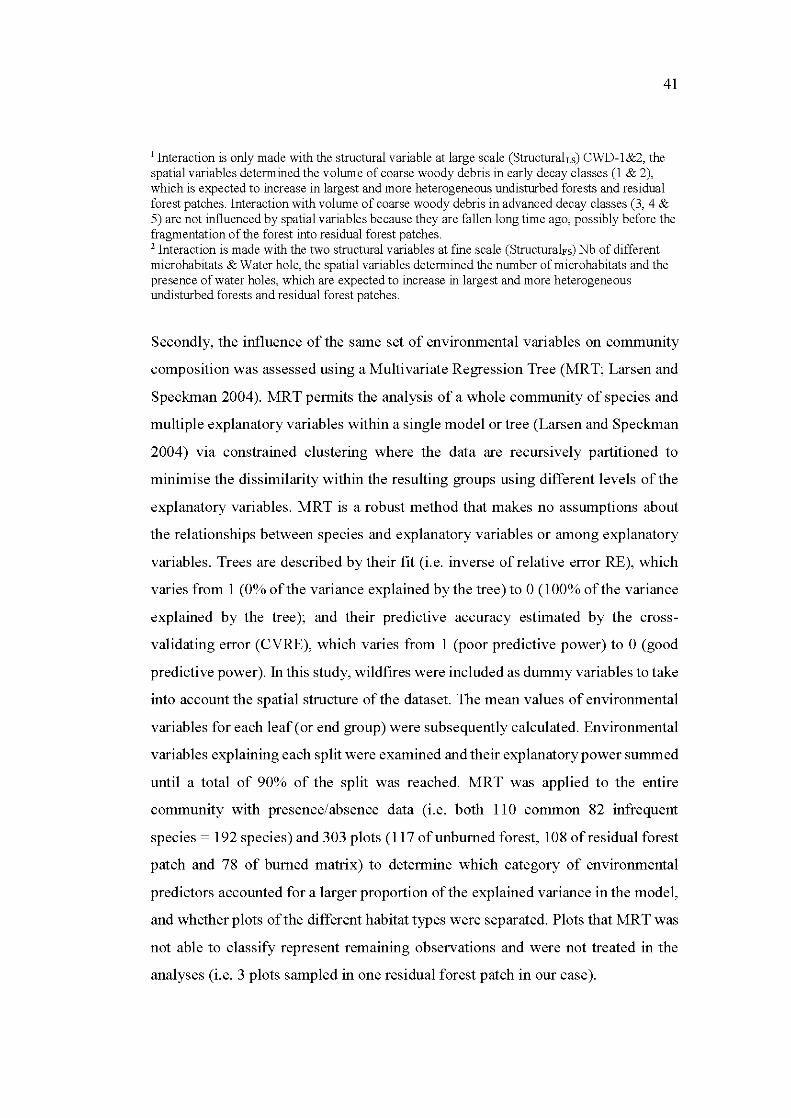
41

1 Interaction is only made with the structural variable at large scale (StructuralLs) CWD-1 &2, the spatial variables determined the volume of coarse woody debris in early decay classes (1 & 2), which is expected to increase in largest and more heterogeneous undisturbed forests and residual forest patches. Interaction with volume of coarse woody debris in advanced decay classes (3, 4 & 5) are not influenced by spatial variables because they are fallen long time ago, possibly before the fragmentation of the forest into re si dual forest patches. 2 Interaction is made with the two structural variables at fine scale (StructuralFs) Nb of different microhabitats & Water hole, the spatial variables determined the number of microhabitats and the presence ofwater holes, which are expected to increase in largest and more heterogeneous undisturbed forests and residual forest patches.

Secondly, the influence of the same set of environmental variables on community

composition was assessed using a Multivariate Regression Tree (MR T; Larsen and

Speckman 2004). MR T permits the analysis of a wh ole community of species and

multiple explanatory variables within a single model or tree (Larsen and Speckman

2004) via constrained clustering where the data are recursively partitioned to

minimise the dissimilarity within the resulting groups using different levels of the

explanatory variables. MRT is a robust method that makes no assumptions about

the relationships between species and explanatory variables or among explanatory

variables. Trees are described by the ir fit (i.e. inverse of relative error RE), which

varies from 1 (0% of the variance explained by the tree) to 0 (1 00% of the variance

explained by the tree ); and their predictive accuracy estimated by the cross

validating error (CVRE), which varies from 1 (poor predictive power) to 0 (good

predictive power). In this study, wildfires were included as dummy variables to take

into account the spatial structure of the dataset. The mean values of environmental

variables for each leaf (or end group) were subsequently calculated. Environmental

variables explaining each split were examined and their explanatory power summed

until a total of 90% of the split was reached. MRT was applied to the entire

community with presence/absence data (i.e. both 110 common 82 infrequent

species = 192 species) and 303 plots (117 ofunbumed forest, 108 ofresidual forest

patch and 78 of bumed matrix) to determine which category of environmental

predictors accounted for a larger proportion of the explained variance in the model,

and whether plots of the different habitat types were separated. Plots that MRT was

not able to classify represent remaining observations and were not treated in the

analyses (i.e. 3 plots sampled in one residual forest patch in our case).

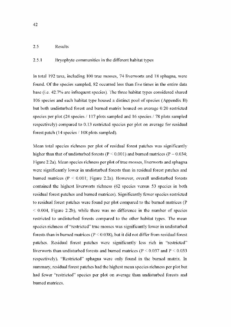
42

2.5 Results

2.5.1 Bryophyte communities in the different habitat types

In total 192 taxa, including 100 true mosses, 74 liverworts and 18 sphagna, were

found. Of the species sampled, 82 occurred less than five times in the entire data

base (i.e. 42.7% are infrequent species). The three habitat types considered shared

106 species and each habitat type housed a distinct pool of species (Appendix B)

but both undisturbed forest and bumed matrix housed on average 0.20 restricted

species per plot (24 species 1 117 plots sampled and 16 species 1 78 plots sampled

respectively) compared to 0.13 restricted species per plot on average for residual

forest patch ( 14 species 1 108 plots sampled).

Mean total species richness per plot of residual forest patches was significantly

higher than that ofundisturbed forests (P < 0.001) and bumed matrices (P = 0.034;

Figure 2.2a). Mean species richness per plot oftrue mosses, liverworts and sphagna

were significantly lower in undisturbed forests than in residual forest patches and

bumed matrices (P < 0.001; Figure 2.2a). However, overall undisturbed forests

contained the highest liverworts richness (62 species versus 53 species in both

residual forest patches and bumed matrices). Significantly fewer species restricted

to residual forest patches were found per plot compared to the bumed matrices (P

< 0.004, Figure 2.2b ), while there was no difference in the number of species

restricted to undisturbed forests compared to the other habitat types. The mean

species richness of "re stricte d" true mosses was significantly lower in undisturbed

forests than in bumed matrices (P < 0.038), but it did not differ from residual forest

patches. Residual forest patches were significantly less rich in "restricted"

liverworts than undisturbed forests and bumed matrices (P < 0.037 and P < 0.033

respectively). "Restricted" sphagna were only found in the bumed matrix. In

summary, residual forest patches had the highest mean species richness per plot but

had fewer "restricted" species per plot on average than undisturbed forests and

bumed matrices.

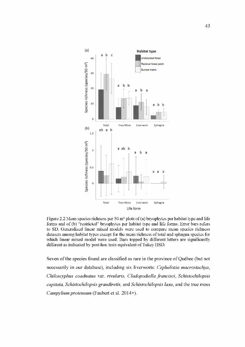
43

(a) Habitat type a b c

40 ~ ,.,,~,.., '"" N' Residus! forest patch E 0 Burned mstrix LI) ........ 30 "' cv "ü cv a. ~ a b b "' 20 "' cv c

..c; u

·;::

"' cv "ü

10

cv a. Vl

0

Total True Moss Liverwort Sphagna (b) ab a b

1.5

l 0 a ab b LI)

b ........ a a "' cv "ü cv a. ~

"' 0.5 "' cv a a a c

..c; u

---+ ·;::

"' cv 0 ïJ cv a. Vl

Total True Moss Liverwort Sphagna

Life form

Figure 2.2 Mean species richness per 50m2 plots of (a) bryophytes per habitat type and life forms and of (b) "restricted" bryophytes per habitat type and li fe forms. Error bars refers to SD. Generalized linear mixed models were used to compare mean species richness datasets among habitat types except for the mean richness of total and sphagna species for which linear mixed model were used. Bars topped by different letters are significantly different as indicated by post-hoc tests equivalent ofTukey HSD.

Seven of the species found are classified as rare in the province of Québec (but not

necessarily in our database), including six liverworts: Cephalozia macrostachya,

Chiloscyphus coadnatus var. rivularis, Cladopodiella francisci , Schistochilopsis

capitata, Schistochilopsis grandiretis, and Schistochilopsis faxa, and the true moss

Campylium protensum (Faubert et al. 2014+).

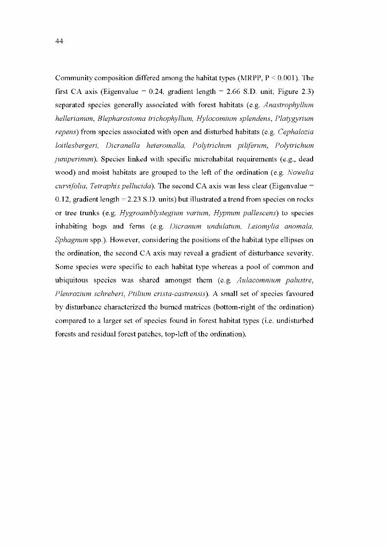
44

Community composition differed among the habitat types (MRPP, P < 0.001). The

first CA axis (Eigenvalue = 0.24, gradient length = 2.66 S.D. unit; Figure 2.3)

separated species generally associated with forest habitats ( e.g. Anastrophyllum

hellerianum, Blepharostoma trichophyllum, Hylocomium splendens, Platygyrium

repens) from species associated with open and disturbed habitats (e.g. Cephalozia

loitlesbergeri, Dicranella heteromalla, Polytrichum piliferum, Polytrichum

juniperinum). Species linked with specifie microhabitat requirements (e.g. , dead

wood) and moist habitats are grouped to the left of the ordination ( e.g. Nowelia

curvifolia, Tetraphis pellucida). The second CA axis was less clear (Eigenvalue =

0.12, gradient length = 2.23 S.D. units) but illustrated a trend from species on rocks

or tree trunks (e.g. Hygroamblystegium varium, Hypnum pallescens) to species

inhabiting bogs and ferus (e.g. Dicranum undulatum, Leiomylia anomala,

Sphagnum spp.). However, considering the positions of the habitat type ellipses on

the ordination, the second CA axis may reveal a gradient of disturbance severity.

Sorne species were specifie to each habitat type whereas a pool of common and

ubiquitous species was shared amongst them (e.g. Aulacomnium palustre,

Pleurozium schreberi, Ptilium crista-castrensis). A small set of species favoured

by disturbance characterized the bumed matrices (bottom-right of the ordination)

compared to a larger set of species found in forest habitat types (i.e. undisturbed

forests and residual forest patches, top-left of the ordination).

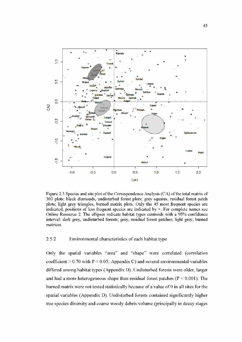
q

.... ci

q 0

0

~

'

•

•

•• •

Rh._ ..

• ..

TorŒlit ~ . :. •

• • •

•

. •

•

• Tomf21l

• •

•

* • Sphfal scà:rt + • • l e:no

.. •

•

• Ltopv~n ~ ;phmag Dic::tJnd • • • + + + Leprrp .~pkll1" : • Sphfus • • • • • ~i:l • - • ~ • ·~phcap. Cepeta ..

• • Tetpel Oie~ . ~ch Sphrub •

• •

•

45

... ' .. ------- - ----:~~~7~---~--i~~r:--AupL .. ~--.-~~p; :·--- --~~:---- -~---- - -~--- - ----------~- - --------~--- - ------- - ----

AtUJhel• .. ~~J : . Oicpo1 • OPolstr . . •..,...... • + Qncwoh Lopgut : • • •

+ Hertur t. ft • •

• • Bracur ~ • + • Ch~o ~ BraC8fl'l ·

Brare f •

-~ . .,. • lsomue -t Hyppal ~ • • Sphtenerum

• • • . . • •

•

-1.0

•

-0.5

• •1

Hygvar

0.0 0.5

CA1

• Poljln

• • lopbic

• • •

1.0 1.5 2.0

Figure 2.3 Species and site plot of the Correspondence Analysis (CA) of the total matrix of 303 plots: black diamonds, undisturbed forest plots; grey squares , residual forest patch plots; light grey triangles, burned matrix plots. Only the 45 most frequent species are indicated, positions of less frequent species are indicated by +. For complete names see Online Resource 2. The ellipses indicate habitat types centroids with a 95% confidence interval: clark grey, undisturbed forests; grey, residual forest patches; light grey, burned matrices

2.5.2 Environmental characteristics of each habitat type

Only the spatial variables "area" and "shape" were correlated (correlation

coefficient > O. 70 with P < 0.05; Appendix C) and several environmental variables

differed among habitat types (Appendix D). Undisturbed forests were older, larger

and had a more heterogeneous shape than residual forest patches (P < 0.001). The

burned matrix were not tested statistically be cause of a value of 0 in all sites for the

spatial variables (Appendix D). Undisturbed forests contained significantly higher

tree species diversity and coarse woody debris volume (principally in decay stages

46

4 and 5; P < 0.001) but had significantly fewer microhabitats (P < 0.001). Coarse

woody debris volume in decay stage 3 was significantly lower in residual forest

patches than in bumed matrices and undisturbed forests (P < 0.001). Not

surprisingly, residual forest patches and undisturbed forests differed from bumed

matrices by the presence of taller trees, but also by the presence of more water ho les

(P < 0.001 and P < 0.033 respectively). Furthermore, structural complexity [i.e.

coarse woody debris volume, canopy openness (Moussaoui et al. in prep.) as well

as humidity (calculated through the presence ofwater holes)] ofpost-fire residual

forest patches are situated in the natural range of variability found in undisturbed

forests.

2.5.3 Relationships between bryophyte richness and composition, and

environmental variables

The relationships between spectes richness and the 12 retained environmental

variables were examined through a model selection procedure. The strength of the

relationship between total, true mosses, liverworts and sphagna richness datasets

and the best models (i.e. with the lowest AICc) were strong (p > 0.68, Table 2.2),

and the weakest relationships were found for the richness of true mosses and

liverworts restricted to undisturbed forests (p = 0.34 and p = 0.42 respectively).

Global model 2 (with the spatial variable shape) was the best model for the total,

true mosses, liverworts and sphagna richnesses. For liverwort and sphagna

richnesses, Global model 1 (with the spatial variable area) was respectively only

2.48 and 1.12 times less parsimonious than Global model 2. For the richness of

species restricted to the undisturbed forests, the best models were not the global

models but those that included stand structural variables (Table 2.2).

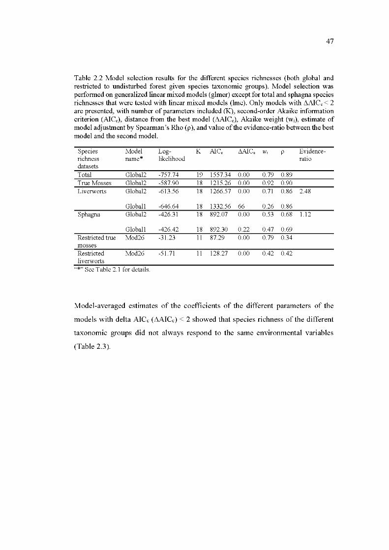
47

Table 2.2 Model selection results for the different species richnesses (both global and restricted to undisturbed forest given species taxonomie groups). Model selection was performed on generalized linear mixed models (glmer) except for total and sphagna species richnesses that were tested with linear mixed models (lme). Only models with L'lAI Cc < 2 are presented, with number of parameters included (K), second-order Akaike information criterion (AICc), distance from the best model (llAICc), Akaike weight (wi), estimate of model adjustment by Spearman's Rho (p ), and value of the evidence-ratio between the best model and the second model.

Species Mo del Log- K AI Cc L'AI Cc w, p Evidence-richness name* likelihood ratio datasets Total Global2 -757.74 19 1557.34 0.00 0.79 0.89 True Mosses Global2 -587.90 18 1215.26 0.00 0.92 0.90 Liverworts Global2 -613.56 18 1266.57 0.00 0.71 0.86 2.48

Globall -646.64 18 1332.56 66 0.26 0.86 Sphagna Global2 -426.31 18 892.07 0.00 0.53 0.68 1.12

Globall -426.42 18 892.30 0.22 0.47 0.69 Restricted true Mod26 -31.23 11 87.29 0.00 0.79 0.34 rn osses Restricted Mod26 -51.71 11 128.27 0.00 0.42 0.42 liverworts

"*" See Table 2.1 for details.

Model-averaged estimates of the coefficients of the different parameters of the

models with delta AICc (llAICc) < 2 showed that species richness ofthe different

taxonomie groups did not always respond to the same environmental variables

(Table 2.3).

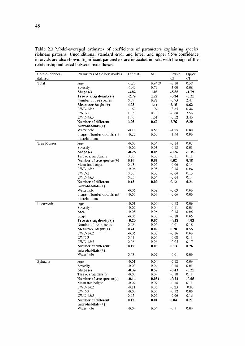
48

Table 2.3 Model-averaged estimates of coefficients of parameters explaining species richness patterns. Unconditional standard error and lower and upper 95% confidence intervals are also shown. Significant parameters are indicated in bold with the sign of the relationship indicated between parentheses.

Species riclmess Pararneters of the best mo dels Estima te SE Lower Upper datasets CI CI

Total Age -1.26 0.9409 -3.10 0.58 Severity -1.46 0.79 -3.00 0.08 Shape(-) -3.82 1.03 -5.85 -1.79 Tree & snag density (-) -2.72 1.28 -5.24 -0.21 Number oftree species 0.87 0.82 -0.73 2.47 Mean tree height (+) 4.38 1.14 2.15 6.62 CWD-1&2 -1.60 1.04 -3.65 0.44 CWD-3 1.03 0.78 -0.48 2.56 CWD-4&5 1.46 1.01 -0.52 3.45 Number of different 3.98 0.62 2.76 5.20 microhabitats (+) Water hole -0.18 0.54 -1.25 0.88 Shape : Number of different -0.27 0.60 -1.44 0.90 rnicrohabitats

True Mosses Age -0.06 0.04 -0.14 0.02 Severity -0.05 0.03 -0.12 0.01 Shape(-) -0.25 0.05 -0.36 -0.15 Tree & snag density 0.00 0.06 -0.11 0. 11 Number oftree species (+) 0.10 0.04 0.02 0.18 Mean tree height 0.03 0.05 -0.06 0.14 CWD-1&2 -0.06 0.05 -0.16 0.04 CWD-3 0.06 0.03 -0.00 0.13 CWD-4&5 0.05 0.04 -0.04 0.14 Number of different 0.18 0.02 0.12 0.24 microhabitats (+) Water hole -0.05 0.02 -0.09 0.00 Shape : Number of different -0.00 0.03 -0.06 0.06 rnicrohabitats

Liverworts Age -0.01 0.05 -0.12 0.09 Severity -0.02 0.04 -0.11 0.06 Are a -0.05 0.06 -0.16 0.06 Shape -0.06 0.06 -0.18 0.05 Tree & snag density (-) -0.23 0.07 -0.38 -0.08 Number oftree species 0.08 0.05 -0.01 0.18 Mean tree height (+) 0.41 0.07 0.28 0.55 CWD-1&2 -0.05 0.06 -0.16 0.06 CWD-3 0.01 0.05 -0.08 0.11 CWD-4&5 0.06 0.06 -0.05 0.1 7 Number of different 0.19 0.03 0.13 0.26 microhabitats (+) Water hole 0.03 0.02 -0.01 0.09

Sphagna Age -0.01 0.04 -0.12 0.09 Severity -0.07 0.04 -0.16 0.01 Shape(-) -0.32 0.57 -0.43 -0.21 Tree & snag density -0.03 0.07 -0.18 0.11 N umber oftree species (-) -0.14 0.054 -0.24 -0.05 Mean tree height -0.02 0.07 -0.16 0.11 CWD-1&2 -0.11 0.06 -0.23 0.00 CWD-3 -0.03 0.05 -0.12 0.06 CWD-4&5 0.05 0.06 -0.06 0.16 Number of different 0.12 0.04 0.04 0.21 microhabitats (+) Water hole -0.04 0.04 -0.11 0.03

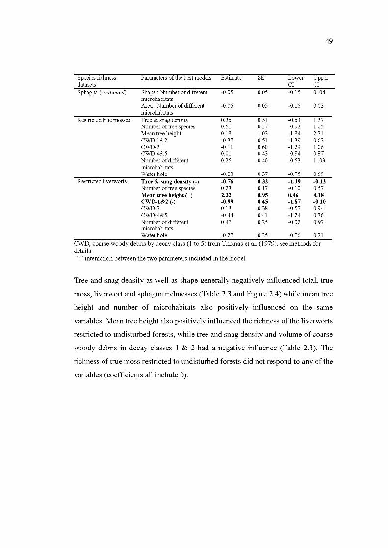
49

Species riclmess Pararneters of the best models Estima te SE Lower Upper datasets CI CI Sphagna (continued) Shape : Number of different -0.05 0.05 -0.15 0 .04

microhabitats Are a : Number of different -0.06 0.05 -0.16 0.03 microhabitats

Restricted true mosses Tree & snag density 0.36 0.51 -0.64 1.37 Number oftree species 0.51 0.27 -0.02 1.05 Mean tree height 0.18 1.03 -1.84 2.21 CWD-1&2 -0.37 0.51 -1.39 0.63 CWD-3 -0.11 0.60 -1.29 1.06 CWD-4&5 0.01 0.43 -0.84 0.87 Number of different 0.25 0.40 -0.53 1 .03 microhabitats Waterho1e -0.03 0.37 -0.75 0.69

Restricted liverworts Tree & snag density (-) -0.76 0.32 -1.39 -0.13 Number oftree species 0.23 0.17 -0.10 0.57 Mean tree height (+) 2.32 0.95 0.46 4.18 CWD-1&2 (-) -0.99 0.45 -1.87 -0.10 CWD-3 0.18 0.38 -0.57 0.94 CWD-4&5 -0.44 0.41 -1.24 0.36 Number of different 0.47 0.25 -0.02 0.97 microhabitats Water ho1e -0.27 0.25 -0.76 0.21

CWD, coarse woody debris by decay class (1 to 5) from Thomas et al. (1979), see methods for details. ":"interaction between the two parameters included in the model.

Tree and snag density as well as shape generally negatively influenced total, true

moss, liverwort and sphagna richnesses (Table 2.3 and Figure 2.4) while mean tree

height and number of microhabitats also positively influenced on the same

variables. Mean tree height also positively influenced the richness of the liverworts

restricted to undisturbed forests, while tree and snag density and volume of coarse

woody debris in decay classes 1 & 2 had a negative influence (Table 2.3). The

richness oftrue moss restricted to undisturbed forests did not respond to any ofthe

variables (coefficients all include 0).

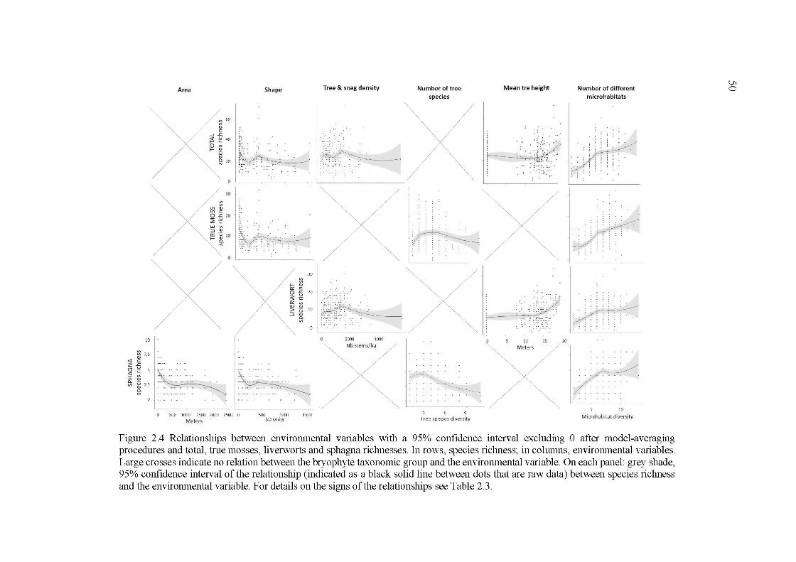
10

"' ~ 7.5 <( c z.c ~ -~ 5

:c ill c.. ·-Vl ~ 2.5

5}

/

A rea

~ 60 Q) c

~ ~ 40 f·.

0 "' r- Q) 'ü Q)

f} 20

"' "' Vl Q) Vl c

30

0 .c 20 2 g w "' ::> .~ ~~ 10

i.'·

Shape

: ..

. . . . . 5} ··-· .. - .. .. .

500 1000 1500 2000 2500 0

Meters

/ 30

"' "' r- Q) cr: c ~ ~ 20

cr: "' ~ -~ 10 ::; Q)

5}

500 1000 1500 SD units

Tree & snag density

. ,·· . ~ .

~i~

/

/

: ~~'~ . . . __..........--1 ~~-~~~-~ --:; : .. ~

/

. . .

2000 4000

Nb stems/ha

/ )<

Number of tree species

/

~ ... . . . . . . . . . . . .. . . . . . . . . . . . . . . . .

/

/ /""'-

3 6 9

Tree species diversity

Mean tre height

~-.:: - .. .

·.J .

/

/

Number of different microhabitats

' .. .. .

'

. . . . .

. . . . . . . .

: .. . ···: . . . : : .: . . :~· :· · ::· . . : :: ·

. :-~< _I_~~'>: ~ : . -:· . · . . ·: : ..... . .

10

Met ers

15 20

10

M icrohabitat diversity

Figure 2.4 Relationships between environmental variables with a 95% confidence interval excluding 0 after model-averaging procedures and total, true mosses, liverworts and sphagna richnesses. In rows, species richness; in columns, environmental variables Large crosses indicate no relation between the bryophyte taxonomie group and the environmental variable. On each panel: grey shade, 95% confidence interval of the relationship (indicated as a black solid line between dots that are raw data) between species richness and the environmental variable. For details on the signs of the relationships see Table 2.3.

Vl 0

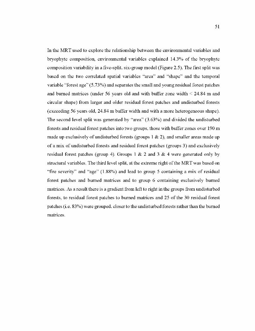
51

In the MR T used to explore the relationship between the environmental variables and

bryophyte composition, environmental variables explained 14.3% of the bryophyte

composition variability in a five-split, six-group model (Figure 2.5). The first split was

based on the two correlated spatial variables "area" and "shape" and the temporal

variable "forest age" (5.73%) and separates the small and young residual forest patches

and bumed matrices (under 56 years old and with buffer zone width < 24.84 rn and

circular shape) from larger and older residual forest patches and undisturbed forests

( exceeding 56 years old, 24.84 rn buffer width and with a more heterogeneous shape).

The second level split was generated by "area" (3.63%) and divided the undisturbed

forests and residual forest patches into two groups, those with buffer zones over 190 rn

made up exclusively ofundisturbed forests (groups 1 & 2), and smaller areas made up

of a mix of undisturbed forests and residual forest patches (groups 3) and exclusively

residual forest patches (group 4). Groups 1 & 2 and 3 & 4 were generated only by

structural variables. The third level split, at the extreme right of the MRT was based on

"fire severity" and "age" (1.88%) and lead to group 5 containing a mix of residual

forest patches and bumed matrices and to group 6 containing exclusively bumed

matrices. As a result there is a gradient from left to right in the groups from undisturbed

forests, to residual forest patches to bumed matrices and 25 of the 30 residual forest

patches (i.e. 83%) were grouped, closerto the undisturbed forests rather than the bumed

matrices.

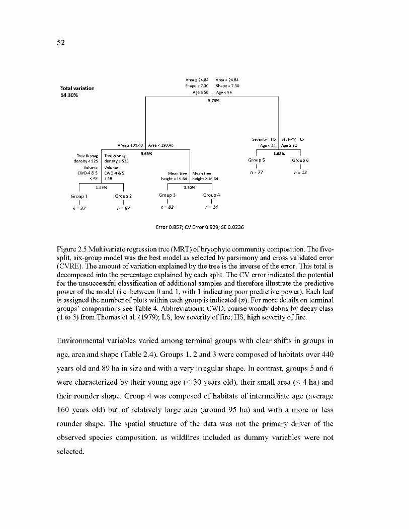
52

Total variation 14.30%

Area ~ 24.84 Area < 24.84

Shape~ 7.30 Shape < 7.30

Age ;, 56 Age < 56 1 5.73%

Area ~ 190.40 Area < 190.40

ree & snag T de nsity < 525

Volume

CWD-4&5 < 48

Tree &snag density ;, 525

Volume CW0-4&5 ;, 48

1 1.53%

1

Group 1 Group 2

1 1

n =27 n =87

3.63%

Mean tree Mean tree

height < 16.64 height ;, 16.64

1 1.50% 1

Group 3 Group 4

1 1 n =82 n = 14

Error 0.857; CV Error 0 .929; SE 0 .0236

Severity = HS Severity = LS

Age< 22 Age~ 22

1 1.88% 1

Group 5 Gro up 6

1 1 n = 77 n = 13

Figure 2.5 Multivariate regression tree (MRT) ofbryophyte community composition. The fivesplit, six-group model was the best model as selected by parsimony and cross validated error (CVRE). The amount of variation explained by the tree is the inverse ofthe error. This total is decomposed into the percentage explained by each split. The CV error indicated the potential for the unsuccessful classification of additional samples and therefore illustrate the predictive power of the model (i.e. between 0 and 1, with 1 indicating poor predictive power). Each leaf is assigned the number of plots within each group is indicated (n). For more details on terminal groups' compositions see Table 4. Abbreviations: CWD, coarse woody debris by decay class (1 to 5) from Thomas et al. (1979); LS, low severity offire; HS, high severity offire.

Environmental variables varied among terminal groups with clear shifts in groups in

age, area and shape (Table 2.4). Groups 1, 2 and 3 were composed of habitats over 440

years old and 89 ha in size and with a very irregular shape. In contrast, groups 5 and 6

were characterized by their young age(< 30 years old), their small area (< 4 ha) and

the ir rounder shape. Group 4 was composed of habitats of intermediate age (average

160 years old) but of relatively large area (around 95 ha) and with a more or less

rounder shape. The spatial structure of the data was not the primary driver of the

observed species composition, as wildfires included as dummy variables were not

selected.

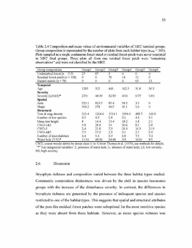
53

Table 2.4 Composition and mean values of environmental variables of MRT terminal groups. Group composition is represented by the number of plots from each habitat type (ntotat = 303). Plots sampled in a single continuo us forest stand or residual forest patch were never separated in MRT fmal groups. Three plots all from one residual forest patch were "remaining observations" and were not classified by the MRT.

Group composition Groupl Group2 Group3 Group4 Groul25 Group6 Undisturbed forest (n = 117) 27 87 3 0 0 0 Residual forest patch (n = 108) 0 0 79 14 12 0 Burned matrix (n = 78) 0 0 0 0 65 13

Temporal Age 1285 325 443 162.5 31.8 36.3 Se verity Severity (LS/HS)* 27/0 48/39 32/39 4110 0177 13/0 Spatial Are a 929.1 823.9 89.4 94.5 3.5 0 Shape 563.2 578 44.9 41.1 1.6 0 Structural Tree & snag density 219.4 1264.6 1514.1 1094.6 488.7 166.8 Number oftree species 4. 5 4. 9 2.8 3.1 3.4 3.1 Mean tree height 8 14.4 13.4 18.2 1.8 2.1 CWD-1 &2 5.8 28.8 13 30.6 8.1 2.8 CWD-3 2.4 21.8 7.3 29.3 16.3 21.9 CWD-4&5 7.5 17.3 2.3 3.1 2.1 3.3 Number of microhabitats 4.4 5.4 6.9 6.8 7. 5 7.4 Water ho le ~y 2:::2* 11116 48/36 34/48 5/9 16/61 8/5

CWD, coarse woody debris by decay class (1 to 5) from Thomas et al. (1979), see methods for details. "*"For categorical variables: Y, presence of water hale; N, absence of water hale; L S, law severity;

HS, high severity.

2.6 Discussion

Bryophyte richness and composition varied between the three habitat types studied.

Community composition distinctness was driven by the shift in species taxonomie

groups with the increase of the disturbance severity. In contrast, the differences in

bryophyte richness are generated by the presence of infrequent species and species

restricted to one of the habitat types. This suggests that spatial and structural attributes

of the post-fire residual forest patches were suboptimal for the most sensitive species

as they were absent from these habitats. However, as mean species richness was

54

particularly high in residual forest patches, we define these as high quality habitats

rather than refugia. The distinctness of the communities of the undisturbed forests and

of the residual forest patches suggests that each of these habitat types are

complementary and bring their own bryoflora to the landscape.

In light ofthese results, we make recommendations about management programs that

could maximize bryophyte diversity and therefore ecosystem resilience (Walker 199 5).

2.6.1 Residual forest patch es: hight quality habitats rather than refugia

Residual forest patches were on average more species rich than undisturbed forests and

bumed matrices ( 10 more species per plot in average), confirming our first hypothesis.

This may be in part explained by the intermediate disturbance hypothesis (Connell

1979), as newly arrived species cohabit with species that survived the disturbance and

the new conditions. While controversial (Fox 2013; Sheil and Burslem 2013), the meta

analysis of Kershaw and Mallik (20 13) confirmed the validity of this theory in tire

prone boreallandscapes, even though they have also pointed out the necessity of future

studies performed in landscapes with high cryptogam diversity. Furthermore, the

environmental selection of the species and the heterogeneity ofresidual forest patches

may also be used to explain their high species richness. Residual forest patches,

composed of both edge and core habitats that vary in light, substrate and moisture

conditions results in high microhabitat diversity (Araujo 2002), opening up the field of

possibilities for a large variety of species with specifie microhabitat requirements.

Residual forest patches therefore represent transient habitats where newly arrived

species co-habit with late serai species that have survived the disturbance.

Over half of the species were common to the three habitat types, including several

ubiquitous species (e.g. Dicranum polysetum, Pleurozium schreberi, Ptilium crista

castrensis) and habitat specialists inhabiting dead wood or rocks (e.g. Lophozia

ventricosa, Oncophorus whalenbergii, Plagiothecium cavifolium). In contrast, 42.7%

55

of the species occurred less than five times in the database, and both undisturbed forests

and bumed matrices were richer in restricted species than residual forest patches.

Furthermore, sphagna, true moss and liverwort taxonomie groups dominated the

bumed matrices, residual forest patches and continuous forests respectively. This shift

in species composition along the gradient of disturbance severity was also reported in

previous studies (Fenton and Frego 2005; Hylander and Johnson 2010). Our second

hypothesis was also supported as there was a shift from species typically found in open

stands and exposed substrates such as rocks or bumed soils to liverworts that are found

under closed canopy conditions, are drought-sensitive and are associated with mature

substrates such dead wood in advanced decay classes (Rambo 2001). The first group

of species is defined in the literature as disturbance-prone species and are expected to

be found directly after a disturbance event. In contrast, the second species group are

typical of forest interiors and are associated with undisturbed and continuous forest

habitats (Baldwin and Bradfield 20 10). Species that inhabit spatially and temporally

discrete pocket habitats such as specialized liverworts and certain true mosses are

repeatedly cited as driving the difference between undisturbed forests and other habitat

types (Dynesius and Hylander 2007; Fenton and Bergeron 2008). As these species were

lacking from our residual forest patches, these patches cannot be defined as refugia but

rather as high quality habitats after fire. However, 83% of the residual forest patches

studied (i.e. 25/30) have a bryophyte community composition more similar to the

undisturbed forests than to the burned matrices, which suggests that sorne

environmental attributes are lacking in the remaining 17% of residual forest patches.

2.6.2 Spatial, temporal and structural attributes govem bryophyte richness and

composition

Undisturbed forests and residual forest patches each harbour distinct bryophyte

communities. However, key environmental variables can increase the similarity of the

bryophyte community of residual forest patches to the bryophyte community of

56

undisturbed forests and therefore the potential of residual forest patches to be refugia.

As indicated in other studies, and predicted by our third hypothesis, stand age, are a and

shape were the best predictors of bryophyte composition whereas stand structure

mainly explained bryophyte diversity (Pipp et al. 2001; Fenton and Bergeron 2008).

Spatial characteristics of the site (area and shape) are negatively correlated with

bryophyte richness (see signs of the significant parameters of the selection model

procedure in Table 2.3), and also influenced on community composition (see MRT

results on Figure 2.5). These relationships may be explained by edge effects and the

fact that edges are particularly rich in microhabitats (Murcia 1995). Consequently, in

the smallest stands, where the edge: core ratio is enhanced, bryophyte richness is higher

than in the larger sites. On the other hand, the larger the site (or the wider the buffer

zone), the better protected are the species promoting forest interior species richness.

This leads to the distinctiveness ofbryophyte communities found in undisturbed forests

that are large in size and in residual forest patch es that are of mo derate size.

Furthermore, stand structural attributes such as mean tree height and density, tree

species diversity and dead wood volume influenced bryophyte richness, as has also

been found in other systems (Szôvényi et al. 2004; Arseneault et al. 20 12). Dead wood

volume (measured directly but also indirectly through mean tree height) is an important

predictor of bryophyte richness (Lesica et al. 1991; Rambo 2001) and is positively

linked to bryophyte richness, as well as stand height that influences on micro

environmental gradients (c.f. Barbier et al., 2008; c.f. Baker et al. 2014). The negative

correlation between bryophyte richness and stand density may be explained by

suppression ofthe understorey species and the lower dead wood availability in denser

stands (c.f. Barbier et al. 2008; Moussaoui et al. 2016). The negative influence oftree

species diversity on true moss es and sphagna richnesses may be explained by changes

in micro-environmental gradients (e.g. light, humidity, soil pH) generated by a high

diversity oftrees. Indeed, the addition ofbroadleave trees might be modified soillitter

and pH, which may be deleterious for sorne bryophyte species such as sphagnum linked

57

with acidic substrates (Gough et al. 2000). For instance, the addition of deciduous

species in coniferous stands changes leaf litter composition and diminishes soil acidity

and vice versa ( c.f. Barbier et al. 2008).

2.6.3 Forest interior species structural requirements

Our fourth hypothesis is only indirectly supported as the relationship between the

richness of species restricted to forest interiors and stand age is implied but not directly

demonstrated. Richness of liverwort species confined to undisturbed forests only

depends indirectly on forest age through its relationship with structural attributes

(Lesica et al. 1991). In this study, 24 species, of which 13 were liverworts, were

restricted to undisturbed forests (Appendix B). The richness ofliverworts restricted to

undisturbed forests was associated with moderate stand structural complexity: < 8 rn

tree height, density of 500 stems/ha and less than 10m3/ha of coarse woody debris in

earl y classes of decay. This relationship is logical as many liverworts are epixylics and

are closely linked with dead wood in advanced decay classes (Rambo 2001). Moreover,

mean tree height influences associations with corticolous bryophytes (Szôvényi et al.

2004) and in denser stands, dead wood volume is lower (Moussaoui et al., 2016). Forest

interior species as well as less frequent species deserve particular attention because

their dependence on discrete and pocket habitats enhances their vulnerability to

disturbance (0kland et al. 2003; Fenton and Bergeron 2008). However, the paucity of

records ofthese species (sorne occurred less than 5 times in the database ), weakens our

conclusions about their habitat preferences and the ir distribution patterns. Furthermore,

the large width of the confidence intervals presented here suggests that additional

mechanisms, not considered in this paper, governed bryophyte richness and

composition patterns. Neutral stochasticity and founder effects are mechanisms that

imply that community composition depends on the identity of species composing it

before disturbance (Vellend et al. 2014) and on the order of species arrivai (Herben

1995). They have been used to explain the limited prediction ability of environmental

58

variables on bryophyte diversity patterns (Fenton and Bergeron 2013). These concepts

are not investigated in this study, but may exp lain the limited power of our models, and

this is especially true for exclusive true moss richness, which was unrelated to the set

ofvariables used.

2.6.4 Implications for management and conservation

Threats to the environment generated by forest harvest intensification have led to the

development of ecosystem based management, which aims to reduce differences

between natural and managed forests. One proposed strategy within ecosystem based

management is the use of post-fire residual forest patches as templates for post-harvest

retention patches (Cyr et al. 2009). Bryophyte species ill-adapted to anthropogenic

disturbances are vulnerable to forest harvest and their loss can threaten ecosystem

resilience (Fenton and Frego 2005). We have shown that sorne characteristics of

residual forest patches (less than 56 years old, 0.20 ha in area i.e. 25 rn ofbuffer zone

width) may result in a bryophyte community similar to that found in the bumed matrix.

These patches, even though they contribute to landscape spatial complexity, mainly

house disturbance-prone species with high dispersal and establishment capacities

(sensu colonist species), which do not require dedicated efforts to be maintained in the

landscape. Residual forest patches over 56 years old and from 0.20 to 11 ha in area

(buffer zone from 25 to 190 rn width), and with a moderate tree height ( < 8 rn) can

support a bryophyte community more similar to that encountered in undisturbed

forests. These characteristics seem to enhance the "life-boat" potential ofthe residual

patches. However, the poor predictive power of our analyses suggests that additional

studies on the subject are needed before these features should be emulated in post

harvest retention patches. Despite this, these results highlight the importance of stand

size and shape on bryophyte richness and composition. W e suggest that retention

blocks left for moose (Alces alces) between 3 to 10 ha as proposed by Samson et al.

(2002), may be more suitable for conserving forest interior bryophytes than the

59

retention patches less than 0.20 ha used in eut blocks in the boreal forest of Québec

(Pouilot et al. 2010).

2.7 Conclusions

Despite not being refugia for bryophytes, residual forest patches house a highly

diversified bryophyte community. Residual forest patches house a wide variety of

bryophytes including four rare species for Québec. While residual forest patches have

been suggested as refugia for species sensitive to disturbance (Fenton and Frego 2005;

Nelson and Halpern 2005), they do not maintain forest interior species that remain

confined to undisturbed forest stands in black spruce boreal forests. Indeed,

characteristics found in undisturbed forests such as their advanced age, large size, and

abundance oftrees, snags and dead wood seem to be the key characteristics linked with

the presence of forest interior species. In the fire-prone boreal ecosystem studied,

residual forest patches are not refugia but complementary habitats to undisturbed

forests. Together, these habitats promote the landscape bryo-diversity. Consequently,

our results highlights the need for the preservation of undisturbed forest stands m

addition to use of forest retention in cutting stands.

2.8 Acknowledgements

This study was funded by the Université du Québec en Abitibi-Témiscamingue

(UQAT) and the National Science and Engineering Research Council (NSERC) in

partnership with Tembec, Eacom and Resolute Forest Products.

The authors especially thank Chafi Chaieb who has provided bryophyte samples from

the undisturbed forest sites and Julie Arseneault for their identification. Authors also

sincerely thank Emilie E. Chavel and Louiza Moussaoui who have provided sorne of

the environmental data used in this paper; Myriam Paquette, Flora Joubier, Louis

60

Dubois and Philippe Heine for the ir field assistance; Danielle Charron, Philippe Duval,

Raynald Julien, Danièle Laporte, Marie-Hélène Longpré, and Michel Poitras for their

technical support; Marc 1. Mazerolle for his relevant statistical advice; and Jean Faubert

for his precious help in the identification of the most difficult bryophyte sample.

2.9 References

Andison DW, McCleary K (2014) Detecting regional differences in within-wildfire hum patterns in western boreal Canada. Forest Chron 90:59-69

Araujo MB (2002) Biodiversity hotpots and zones of ecological transition. Conserv Biol16: 1662-1663

Arseneault J, Fenton NJ, Bergeron Y (2012) Effects of variable canopy retention harvest on epixylic bryophytes in boreal black spruce-feathermoss forests. Can J Forest Res 42:1467-1476.

Baker TP, Jordan GJ, Steel EA, Fountain-Jones NM, Wardlaw TJ, Baker SC (2014) Microclimate through space and time: microclimatic variation at the edge of regeneration forests over daily, yearly and decadal time scales. For Ecol Manag 334:174-184

Baldwin LK, Bradfield GE (2010) Resilience of bryophyte communities in regenerating matrix forests after logging in temperate rainforests of coastal British Columbia. Botany 88:297-314.

Barbier S, Gasselin F, Balandier P (2008) Influence of tree species on understory vegetation diversity and mechanisms involved- A critical review for temperate and boreal forests. Forest Ecol Manag 254:1-15

Bates D, Maechler M, Bolker B, Walker S (2015) R package "lme4 - Linear Mixed Effects Models using 'Eigen' and S4" version 1.1-8

Bergeron Y, GauthierS, Flannigan M, Kafka V (2004) Fire regimes at the transition between mixedwood and coniferous boreal forest in northwestem Que bec. Ecolo gy 85:1916-1932

Bumham KP, Anderson DR (2002) Model selection and multimodel inference: practical information-theorie approach, Second Edition. Springer, New York

61

Carlson DJ, Reich PB, Frelich LE (2011) Fine-scale heterogeneity in overstory composition contributes to heterogeneity of wildfire severity in southern boreal forest. J For Res-JPN 16:203-214

Chaieb C, Fenton NJ, Lafleur B, Bergeron Y (2015) Can we use forest inventory mapping as a coarse filter in ecosystem based management in the black spruce boreal forest? Forests 6:1195-1207

Chia EK, Bassett M, Nimmo DG, Leonard SWJ, Ritchie EG, Clarke MF, Bennett AF (2015) Pire severity and fire-induced landscape heterogeneity affect arboreal mammals in fire-prone forests. Ecosphere 6:1-14

Clarke PJ (2002) Habitat islands in fire-prone vegetation: do landscape features influence community composition? J Biogeogr 29:1-8

Connell JH (1979) Intermediate-disturbance hypothesis. Science 204:1345

Creed RP (2000) Is there a new keystone species in North American lakes and rivers? Oikos 91:405-408

Cyr D, GauthierS, Bergeron Y, Carcaillet C (2009) Forest management is driving the eastern North American boreal forest outside its natural range of variability. Front Ecol Environ 7:519-524

Drapeau P, Nappi A, Imbeau L, Saint-Germain M (2009) Standing deadwood for keystone bird species in the eastern boreal forest: managing for snag dynamics. Forest Chron 85:227-234

Dynesius M, Hylander K (2007) Resilience ofbryophyte communities to clear-cutting ofboreal stream-side forests. Biol Conserv 135:423-434

Environment Canada (2015) Canadian climate normals 1981-2010 Station data http: //climate. weather.gc.ca/climate normals/results 1981 2010 e.html ?stniD=60 51 &lang=e&StationN ame=Lebel+sur+Quevillon& Se arch Type=Contain s&stnNameSubmit=go&dCode=5&dispBack= l. Accessed 5 April2015

ESRI (2015) ArcGis Dekstop: Release 10.3.1. Environmental Systems Research Institute, Redlands, USA

Faubert J (2012-2014) Flore des bryophytes du Québec-Labrador (Vol. 1, 2 and 3). Société québécoise de bryologie, Saint-Valérien.

Faubert J, Leclerc S., Lavoie A., Lapointe M., Nadeau S. , Lamond M. & collaborateurs (2014+) Base de données des bryophytes du Québec-Labrador (BRYOQUEL) http://societequebecoisedebryologie.org. Accessed 4 June 2016

62

Fenton NJ, Bergeron Y (2008) Does time of habitat make old-growth forests species rich? Bryophyte richness in boreal Picea mariana forests. Biol Conserv 141:1389-1399

Fenton NJ, Bergeron Y (2013) Stochastic processes dominate during boreal bryophyte community assembly. Ecology 94:1993-2006

Fenton NJ, Frego KA (2005) Bryophyte (moss and liverwort) conservation under remnant canopy in managed forests. Biol Conserv 122:417-430

Flora of North America Editorial Committee (2007) Flora of North America, North of Mexico (Vol. 27), Bryophytes: Moss, Part 1. Oxford University Press, Oxford

Fox JW (2013) The intermediate disturbance hypothesis should be abandoned. Trends Ecol Evol 28:86-92

Gough L, Shaver GR, Carroll J, Royer DL, Laundre JA (2000) V ascular plant species richness in Alaskan arctic tundra: the importance of soil pH. J Ecol 88: 54-66

Greene DF, Macdonald SE, Haeussler S, Domenicano S, Noel J, Jayen K, Charron I, Gauthier S, Hunt S, Gielau ET, Bergeron Y, Swift L (2007) The reduction of organic-layer depth by wildfire in the North American boreal forest and its effect on tree recruitment by seed. Can J For Res 37:1012-1023

Grondin P (1996) Écologie forestière. In: Bérard JA, Côté M (eds) Manuel de foresterie. Presse de l'Université Laval, Québec, pp 133-279

Halpern CB (1988) Early successional pathways and the resistance and resilience of forest communities. Ecolo gy 69: 1703-1714

HerbenT (1995) Founder and dominance control: neglected concepts in the community dynamics of donal plants. Abstracta Botanica 19:3-10

Higgins SI, Bond W J, Troll ope WS (2000) Pire, resprouting and variability: a recipe for grass-tree coexistence in savanna. J Ecol 88:213-229

Honnay 0, Hermy M, Coppin P (1999) Effects of area, age and diversity of forest patches in Belgium on plant species richness, and implications for conservation and reforestation. Biol Conserv 87:73-84

Hothom T, Bretz F, Westfall P (2015) R package "multcomp- Simultaneous Inference in General Parametric Models" version 1.4-1

Hylander K, Johnson S (20 10) In situ survival of forest bryophytes in small-scale refugia after an intense forest fire. J V eg Sei 21: 1099-1109

63

Kershaw HM, Mallik AU (2013) Predicting plant diversity response to disturbance: applicability of the intermediate disturbance hypothesis and mass ratio hypothesis. Critical Review in Plant Sciences 32:383-395

Lancaster J, Belyea LR (1997) Nested hierarchies and scale-dependence of mechanisms offlow refugium use. J NAm Benthol Soc 16:221-238

Larsen DR, Speckman PL (2004) Multivariate regression trees for analysis of abundance data. Biometries 60:543-549

Lee S-II, Spense JR, Langor DW, Pinzon J (2015) Retention patch size and conservation of saproxylic beetles in boreal white spruce stands. For Ecol Manag 358:98-107

Leonard SWJ, Bennett AF, Clarke MF (2014) Determinants of the occurrence of unburnt forest patches: potential biotic refuges within a large, intense wildfire in south-eastern Australia. For Ecol Manag 314:85-93

Leps J, Smilauer P (2003) Multivariate analysis of ecological data using CANOCO. Cambridge University Press, Cambridge

LesicaP, McCune B, Cooper SV, Hong WS (1991) Differences in lichen and bryophyte communities between old-growth and managed second-growth forests in the Swan Valley, Montana. Can J Bot 69:1745-1755

Lôbel S, Rydin H (2010) Trade-offs and habitat constraints in the establishment of epiphytie bryophytes. Funct Ecol 24:887-897

Madoui A, Leduc A, Gauthier S, Bergeron Y (20 1 0) Spatial pattern analyses of postfire residual stands in the black spruce boreal forest of western Quebec. Int J Wildland Fire 19:1110-1126

Mazerolle MJ (2015) R package "AICcmodavg - Model Selection and Multimodel Inference Based on (Q)AIC(c)" version 2.0-3

Mills SE, Macdonald SE (2004) Predictors of moss and liverwort species diversity of microsites in conifer-dominated boreal forest. J Veg Sei 15:189-198

Miyanishi K, Johnson EA (2002) Process and patterns of duff consumption in the mixedwood boreal forest. Can J For Res 32:1285-1295

Moussaoui L, Fenton NJ, Leduc A, Bergeron Y (2016) Deadwood abundance in postharvest and post-fire residual patches: an evaluation of patch temporal dynamics in black spruce boreal forest. For Ecol Manag 368:17-27

Murcia C (1995) Edge effects in fragmented forests: implications for conservation. Trends Ecol Evol 10:58-62

64

Nappi A, Drapeau P, Savard J-PL (2004) Salvage logging after wildfire in the boreal forest: is it becoming a hot issue for wildlife? Forest Chron 80:67-74

Nelson CR, Halpern CB (2005) Short-term effects oftimber harvest and forest edges on ground-layer mosses and liverworts. Can J Bot 83:610-620

Newmaster SG, Belland RJ, Arsenault A, Vitt DH, Stephens TR (2005) The ones we left behind: comparing plot sampling and floristic habitat sampling for estimating bryophyte biodiversity. Divers Distrib 11:57-72

0kland RH, Rydgren K, 0kland T (2003) Plant species composition ofboreal spruce swamp forests: closed doors and windows of opportunity. Ecology 84:1909-1919

Oksanen J, Blanchet FG, Kindt R, Legendre P, Minchin PR, O'Hara RB, Simpson GL, Solymos P, Stevens MHH, Wagner H (2015) R package "vegan - Community Ecology package" version 2.3-0

Payette S (1992) Fire as a controlling process in the North American boreal forest. In: Shugart HH, Leemans R, Bonan G (eds) A systems analysis ofthe global boreal forest. Cambridge University Press, Cambridge, pp 144-169

Perhans K, Appelgren L, Jonsson F, Nordin U, Sôderstrôm B, Gustafsson L (2009) Retention patches as potential refugia for bryophytes and lichens in managed forest landscapes. Biol Conserv 142:1125-1133

Pharo EJ, Lindenmayer DB (2009) Biological legacies soften pine plantation effects for bryophytes. Biodivers Conserv 18:1751-1764

Pinheiro JC, Bates DM (1995) Approximations to the log-likelihood function in the nonlinear mixed-effects model. J Comput Graph Stat 4:12-35

Pinheiro JC, Bates DM (2015) R package "nlme- Linear and Nonlinear Mixed Effects Models" version 3.1-121

Pipp AK, Henderson C, Callaway RM (2001) Effects of forest age and forest structure on epiphytie lichen biomass and diversity in a Douglas-fir forest. Northwest Sei 75:12-24

Pouliot D, Paquet C, Déry S, Jetté J-P, Pouilot B, Pâquet J (2010) Guide pour la préparation et l'analyse des plans annuels d'interventions forestières de 2011-2012 et de 2012-2013 - Mesures associées aux dérogations à la coupe en mosaïque dans la pessière à mousses. Gouvernement du Québec, ministère des Ressources naturelles et de la Faune, Direction de 1' environnement et de la protection des forêts, Québec.

Powell MJD (2009) The BOBYQA algorithm for bound constrained optimization without derivatives, Report No. DAMTP 2009/NA06, Centre for Mathematical Sciences, University of Cambridge, Cambridge

65

R-Development-Core-Team (2015) R: A Language and Environment for Statistical Computing. R Foundation for Statistical Computing, Vienna

Rambo TR (200 1) Decaying logs and habitat heterogeneity: implications for bryophyte diversity in Western Oregon forest. Northwest Sei 75:270-277

Robinson NM, Leonard SWJ, Ritchie EG, Bassett M, Chia EK, Buckingham S, Gibb H, Bennett AF, Clarke MF (2013) Refuges for fauna in fire-prone landscapes: their ecological function and importance. J Appl Ecol 50:1321-1329

Robinson NM, Leonard SWJ, Bennett AF, Clarke MF (2016) Are forest gu1lies refuges for birds when burnt? The value oftopographical heterogeneity to avian diversity in a fire-prone landscape. Biol Conserv 200: 1-7

Rosenfeld JS (2002) Functional redundancy in ecology and conservation. Oikos 98:156-162

Rosenvald R, Lôhmus A (2008) For what, when, and where is green-tree retention better than clear-cutting? A review of the biodiversity aspects. For Ecol Manag 255:1-15

Ross-Davis AL, Fr ego KA (2002) Comparison of plantations and naturally regenerated clearcuts in the Acadian forest: forest floor bryophyte community and habitat features. Can J Bot 80:21-33

Samson C, Dussault C, Courtois R, Oue1let J-P (2002) Guide d'aménagement de l'habitat de l'orignal. Société de la faune et des parcs du Québec, Fondation de la faune du Québec et ministère des Ressources naturelles du Québec, Sainte-Foy

Sedell JR, Reeves GH, Hauer FR, Stanford JA, Hawkins CP ( 1990) Role of refugia in recovery from disturbances: modem fragmented and disconnected river systems. Environ Manage 14:711-724

Schmiegelow FK, Stepnisky DP, Stambaugh CA, Koivula M (2006) Reconciling salvage logging of boreal forests with a natural-disturbance management model. Conserv Biol20:971-983

Sheil D, Burslem DFRP (2013) Defining and defending Connell' s intermediate disturbance hypothesis: a response to Fox. Trends Ecol Evol 28:571-572

Simard M, Lecomte N, Bergeron Y, Bernier PY, Paré D (2007) Forest productivity decline caused by successional paludification of boreal soils. Ecol Appl 17:1619-1637

Szôvényi P, Hock ZS, T6th Z (2004) Phorophyte preferences of epiphytie bryophytes in a stream valley in the Carpathian Basin. J Bryol26:137-146

66

Thomas JW, Anderson RG, Maser C, Bull EL (1979) Wildlife habitats in managed forests ofthe Blue Mountains ofüregon and Washington. United States Department of Agriculture, Forest Service, Agricultural Handbook

Tilman D, May R, Lehman C, Nowak M (1994) Habitat destruction and the extinction debt. Nature 371:65-66

Turetsky MR, Bond-Lamberty B, Euskirchen E, Talbot J, Frolking S, McGuire AD, Tuittila E-S (2012) The resilience and functional role of moss in boreal and arctic ecosystems. New Phytol196:49-67

V ellend M, Srivastava DS, Anderson KM, Brown CD, Jankowski JE, Kleynhans EJ, Kraft NJB, Letaw AD, Macdonald AAM, Maclean JE, Myers-Smith IH, Norris AR, Xue X (2014) Assessing the relative importance of neutral stochasticity in ecological communities. Oikos 123:1420-1430

Vincent JS, Hardy L (1977) L' évolution et l' extinction des lacs glaciaires Barlow et Ojibway en territoire Québécois. Geogr Phys Quatem 31:357-372

Walker B (1995) Conserving biological diversity through ecosystem resilience. Conserv Biol 9:747-752

Warton DI, Hui FKC (2011) The arcsine is asinine: the analysis of proportions in ecology. Ecology 92:3-10

CHAPITRE III

BOREAL BRYOPHYTE RESPONSE TO NATURAL PIRE EDGE CREATION


En révision dans Journal of Vegetation Science, Octobre 2016

68

3.1 Abstract

Question: Changes in species richness and composition in plant communities as a

result of edge creation are well-documented in anthropogenically modified

landscapes, but what happens after natural disturbance? We investigate the

responses of boreal bryophytes to edge creation in a post-wildfire residual forest

patch system.

Location: Boreal black spruce-feather moss forest of western Québec, Canada.

Methods: Bryophyte community was sampled in 50 m2 plots: 117 plots in 39

undisturbed forest cores (control) and 108 plots in 30 residual forest patches from

wildfire divided, into 48 core plots, 30 north-facing edge plots and 30 south-facing

edge plots. Temporal, severity, spatial and structural characteristics of the stands

were also recorded to explain bryophyte communities composition.

Results: W e found that residual edges and cores were more species rich than

undisturbed cores, with the highest species richness found in the north-facing edges

of residual patches. Bryophyte community composition differed between

undisturbed cores and residual cores but did not differed between residual cores and

edges. Furthermore, species restricted (present in only one forest type) and over

represented (present more than 50% oftime in one forest type) in undisturbed cores

and residual edges were identified as indicators of each ofthese forest types-. Spatial

variables such as stand area and buffer zone width explained variations in

community composition after edge creation. Core and edge communities differed

more in patches over 3 ha than in smaller patches, but remained clearly different in

composition than undisturbed cores.

Conclusion: Change in community composition in response to edge creation is

observed in this naturally disturbed landscape. While edge influence is reduced in

large patches, the bryophyte community remains distinct from undisturbed cores,

which permit us to determine a 170 rn distance of edge influence (DEI) inside

69

residual patches. This natural response to edge creation forces us to no longer

consider anthropogenic edges as a control in the study of species response to

fragmentation, and reinforces the point that residual forests are not substitute of

continuous and undisturbed forests. The case of anthropogenic forest retention in

cuttings stands is therefore open to discussion.

Key-words: black spruce forest; edge influence; fragmentation; indicator species;

liverwort; moss; sphagna; wildfire.

3.2 Résumé

Question : Les modifications de la richesse spécifique et de la composition des

communautés végétales en réponse à la création de bordures sont principalement

documentées dans les paysages perturbés anthropiquement. Seulement, qu'advient

il suite à des perturbations naturelles ? Nous étudions la réponse de bryophytes

boréales à la création de bordures dans un système naturel composé d'îlots résiduels

post-feu.

Localisation : Pessière noire à mousses de 1' ouest du Québec, Canada.

Méthodes : La communauté bryophytique a été échantillonnée dans des placettes

de 50 m2 : 117 placettes dans 39 cœurs de forêts non perturbées (contrôle) et 108

placettes dans 30 îlots résiduels post-feu, divisés en 48 placettes de cœur, 30

placettes de bordure orientées au nord et 30 placettes de bordure orientées au sud.

Les caractéristiques temporelles, de sévérité de la perturbation, spatiales et

structurelles des peuplements ont aussi été relevées afin d'expliquer la composition

des communautés.

Résultats :Nous avons observé que les cœurs et les bordures d'îlots résiduels étaient

plus riches en espèces que les cœurs de forêts non perturbées, avec la plus grande

richesse spécifique trouvée dans les bordures orientées au nord par rapport à celles

orientées au sud. La composition de la communauté bryophytique diffèrait entre les

70

cœurs de forêts non perturbées et les cœurs d'îlots résiduels, mais ne diffèrait pas

entre les cœurs et les bordures d'îlots résiduels. De plus, les espèces exclusives

(présentes dans seulement un type d'habitat) et les espèces surreprésentées

(présentes à plus de 50% dans un seul type d'habitat) des cœurs de forêts non

perturbées et des bordures d'îlots résiduels ont été identifiées comme des

indicateurs de chacun de ces types d'habitats. Les variables spatiales telles que

l'aire du peuplement et la largeur de la zone tampon expliquaient les variations

observées dans la composition des communautés après la création des bordures. Les

communautés de cœur et de bordure diffèraient davantage dans les îlots résiduels

excédant 3 ha que dans les îlots résiduels de tailles inférieures, mais demeuraient

cependant clairement distinctes de celles des cœurs de forêts non perturbées.

Conclusions : Un changement de la composition des communautés en réponse à la

création de bordures est observé dans cet écosystème perturbé naturellement. Bien

que l'effet de bordure soit limité dans les îlots résiduels de plus grandes tailles, la

communauté bryophytique demeure distincte de celle trouvée dans les forêts non

perturbées. Cela nous permet d'identifier la distance d'influence de la bordure

jusqu'à 170 rn àl'intérieurdes îlots résiduels. Cette réponse des bryophytes à l'effet

de bordure est naturelle et nous contraint à ne plus utiliser les bordures créées

anthropiquement comme des contrôles lors de l'étude de la réponse des espèces à

la fragmentation. De plus, ces conclusions soulignent que les forêts résiduelles ne

sont pas des substituts des forêts continues et non perturbées. Le maintien d'îlots

de rétention dans les parterres de coupes est donc ouvert à réflexion.

Mots-clés : effet de bordure, espèces indicatrices, feu de forêt, fragmentation,

hépatique, mousse, pessière noire à mousses, sphaigne.

3.3 Introduction

The effects of habitat fragmentation on forest communities have and continue to

stimulate research in ecology as it is a major concem for biodiversity conservation.

Fragmentation, defined as the restriction of communities to forest habitat patches

71

of reduced size surrounded by an inhospitable matrix, is intimately associated with

edge effects (Fahrig 2003). Edges represent transient zones between disturbed areas

and forest interiors that do not experience the direct effects of disturbance (Holland

et al. 1991). Edge creation results in modified microclimatic conditions, such as

increased light transmittance, wind velocity, humidity and/or temperatures

(Saunders et al. 1991; Harper & Macdonald 2001; Harper et al. 2005). Communities

respond to these modified abiotic conditions with changes in species richness and

composition. Both habitat change and community response are not restricted to the

edge but can extend far inside the core of the forest (Murcia 1995; Harper &

Macdonald 2001) and therefore threaten forest interior species that require stable

micro-environmental conditions to survive (Rambo & Muir 1998; Newmaster et al.

2003).

The depth-of-edge influence (DEI; Harper & Macdonald 2001; Ries et al. 2004)

estimates how far the edge effect is felt inside the forest interior, in terms of changes

in environmental conditions but also in species richness and composition. DEI is

clearly ecosystem- and species-dependent and an alteration in microclimatic

conditions has been reported from studies on different forest ecosystems and varies

from 60 rn from the edge in mixed-wood boreal forests (Harper & Macdonald 2002)

to 40 rn in temperate rainforests (Davies-Colley et al. 2000). Community changes

in response to these modified microclimatic conditions have been documented 50

to 60 rn from the edge for bryophytes and lichens in temperate and boreal Canadian

forests and wetlands (Moen & Jonsson 2003; Rhéault 2003; Baldwin & Bradfield

2005; Boudreault et al. 2008) and 75 to 200 rn from the edge for epiphytie fems and

bryophytes in Ethiopian forests (Hylander et al. 2013).

The nature of the edge (generated by natural or anthropogenic disturbance ), time

since disturbance and patch shape influence the DEI. Indeed, edges are dynamic

and an edge effect is expected to decrease over time as the contrast between the two

sides ofthe edge are reduced (Harper & Macdonald 2002; Harper et al. 2014). Edge

effects are therefore expected to be less pronounced at regenerated edges (i.e., long

time sin ce the disturbance, old patch es) due smaller differences in temperature, or

72

solar energy on each side of the edge (Zheng & Chen 2000; Baker et al. 20 13).

Furthermore, residual patch characteristics such as small size and shape complexity

can increase edge effects (Ewers & Didham 2006, 2008; Laurance 2008). Similarly,

a reduction in distance to the nearest forest source can mitigate community response

to edge effects via an increased probability of recolonization at the edges, which is

particularly important for species with reduced dispersal capacities (Lohmus et al.

2006; Baker et al. 2013).

Predicting edge influence and estimating DEI is therefore crucial for biodiversity

conservation. This is especially true in ecosystems with increased anthropogenic

pressure, which leads to the proliferation of edges and to the substitution of core

habitats by edges (Harper et al. 2005). In boreal forests, wildfires generate many

edge habitats, particularly in fire skips or residual unbumed patches within fire

matrices (Harper et al. 2014), they are therefore ideally suited to perform studies on

edges. However, despite the rich body ofwork on edges, most studies have focused

on anthropogenic edges, including riparian edges, and on bryophytes, lichens and

invertebrate species (Hylander et al. 2005; Stewart & Mallik 2006; Boudreault et

al. 2008; Lee et al. 20 15). Edges from natural disturbances are substantially less

documented (Larrivée et al. 2008; Harper et al. 2014; Franklin et al. 2015).

Consequently, the use of continuous forests rather than natural edges as a control

in the study of species responses to anthropogenic edge effects might have led to

misinterpretati on.

Bryophytes dominate boreal forest vegetation both in terms of plant biomass and

species richness (Turetsky et al. 2012). They occupy a variety of microhabitats,

from the forest fioor for large feather mosses to boulders, dead wood and tree bases

for specialist mosses and liverworts (Dynesius & Hylander 2007). The

poikylohydric character of bryophytes (i.e. absence of specialized mechanisms for

regulating uptake and loss of water; Proctor 1990) generates their strong

dependence on moist microclimates (Proctor et al. 2007; Lôbel & Rydin 2010).

Edges created by both natural and anthropogenic disturbances are drier than forest

interiors due to the opening of the canopy and wind penetrance (Rolland 1991;

73

Baker et al. 2013), and the composition ofthe bryophyte community is expected to

change, specifically by the loss of the most drought-sensitive species (Ross-Davis

& Frego 2002; Fenton et al. 2003; Rosenvald & Lôhmus 2008). This effect may be

amplified at sun-exposed compared to shaded edges (Kivisto & Kuusinen 2000;

Hylander 2005).

W e therefore propose to reconsider the response of species to edges focusing on

bryophytes and using a system of residual patches from natural wildfires. The

general objective of this study is therefore to determine the response of bryophytes

to the creation of natural fire edges in boreal forests. This will generate a natural

control to better appreciate the response associated with anthropogenic edges. In a

related study (Barbé et al. in revision, refers to the Chapter II), we have

demonstrated that residual forest patches were richer in bryophyte species and

differed from undisturbed forests in terms of community composition. However,

we have not split residual forest patches into core and edge, we propose to bring

this level of comparison in this study comparing bryophyte richness and

composition among three forest types: undisturbed cores, residual cores and

residual edges. Three questions are successively investigated: (i) are bryophytes

sensitive to the creation of natural edges? (ii) is orientation of the edges a factor?

and (iii) are residual patches composed of ''true cores" i.e. do they house a

community similar to that found in undisturbed forests? Indicator species of

undisturbed forest cores and of edges will be identified and the depth-of-edge

influence for bryophytes will be determined.

The "mass effect" implies the coexistence of a myriad of species in transient zones

due to overlapping niches leading to the cohabitation among early-successional

( colonists ), mid-successional and late-seral species [perennial stayers, sensu During

(1992)] (Shmida & Wilson 1985; Auerbach & Shmida 1987). Given that together

with the results of Barbé et al. (in revision, refers to the Chapter II), we assume that

residual edges are more species rich than undisturbed and residual cores (Hl). We

also expect that community composition of undisturbed and residual cores are

distinct from communities found at residual edges given the association of

74

liverworts with closed canopies, humid and stable microhabitats (Lesica et al. 1991;

Fenton & Frego, 2005; H2). Subsequently, we assume to find more drought

sensitive species such as liverworts in more humid and less sun-exposed north

facing residual edges, while south-facing residual edges are expected to mainly

house stress-tolerant species (Kivistô & Kuusinen 2000; Hylander 2005). Finally,

we have demonstrated that patch are a and age influenced on bryophyte composition

(Barbé et al. in revision, refers to the Chapter II), we therefore aim to link these

findings with edge influence. We hypothesize that larger or older patches house a

community more similar to undisturbed cores given the enhanced isolation of core

communities and the prolonged time offered for microhabitat differentiation and

maturation in the core (Fenton & Bergeron 2008) (H3). In contrast, we hypothesize

that the compositional similarity between residual cores and residual edges will be

enhanced in small or young patches (H4).

3.4 Methods

3.4.1 Study area

The study area covers 73 197 km2 (79°69 W, 50°71 N- 74°50 W, 50°71 N- 79°69

W, 48°83 N - 74°50 W, 48°83 N) within the black spruce (Picea mariana Mill.,

Briton)-feather moss (P leurozium schreberi (Brid.) Mitt.) forest of western Québec,

eastern Canada (Saucier et al. 2009; Figure 3.1a). Stands are dominated by P.

mariana Mill., Briton with secondary species Pinus banksiana Lamb. , Populus

tremuloides Michx,Abies balsamea (L.) Mill., andBetula papyrifera Marshall. The

understory is dominated by ericaceous and bryophyte species (sphagna replace

feather mosses under more humid conditions). The topography of the region is flat

and the altitude varies from 200 to 300 m. The climate is subpolar continental with

average annual temperature and precipitation of 1 oc and 927.8 mm respectively

(1981 to 2010; Environment Canada 24th February 2015).

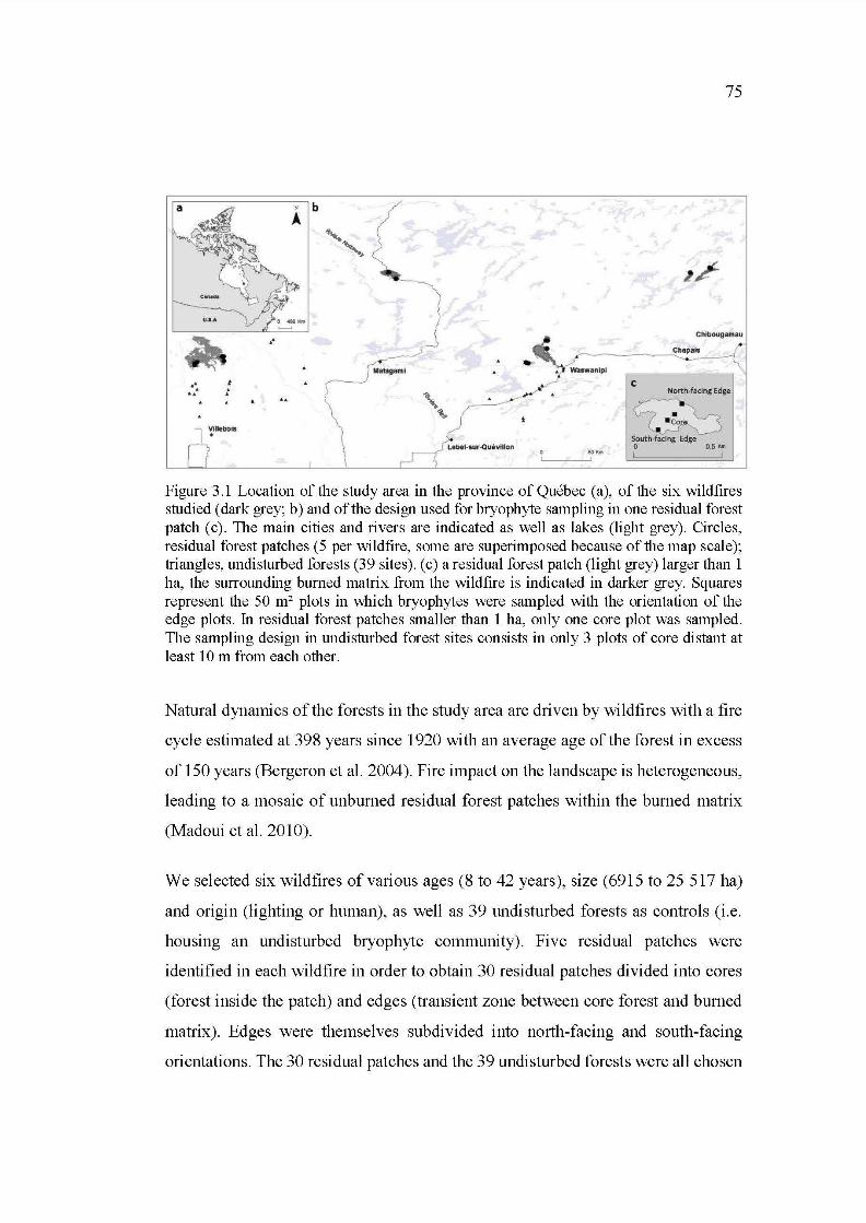
75

Chibougamau

Cha pals

Matagamf Wa.swanlpl

1 .

'"'"'

Figure 3.1 Location ofthe study area in the province of Québec (a), of the six wildfires studied ( dark grey; b) and of the design used for bryophyte sampling in one re si dual forest patch ( c). The main cities and ri vers are indicated as well as lakes (light grey). Circles, re si dual forest patch es (5 per wildfire, sorne are superimposed because of the map scale ); triangles, undisturbed forests (39 sites). ( c) a residual forest patch (light grey) larger than 1 ha, the sunounding burned matrix from the wildfire is indicated in darker grey. Squares represent the 50 m2 plots in which bryophytes were sampled with the orientation of the edge plots. In residual forest patches smaller than 1 ha, only one core plot was sampled. The sampling design in undisturbed forest sites consists in only 3 plots of core distant at least 10 rn from each other.

Natural dynarnics of the forests in the study area are driven by wildfires with a fire

cycle estirnated at 398 years since 1920 with an average age ofthe forest in excess

of 150 years (Bergeron et al. 2004). Fire impact on the landscape is heterogeneous,

leading to a rnosaic of unburned residual forest patches within the burned rnatrix

(Madoui et al. 2010).

We selected six wildfires ofvarious ages (8 to 42 years), size (6915 to 25 517 ha)

and origin (lighting or hurnan), as weil as 39 undisturbed forests as controls (i.e.

housing an undisturbed bryophyte cornrnunity). Five residual patches were

identified in each wildfire in arder to obtain 30 residual patches divided into cores

(forest inside the patch) and edges (transient zone between core forest and burned

rnatrix). Edges were thernselves subdivided into north-facing and south-facing

orientations. The 30 residual patches and the 39 undisturbed forests were ail chosen

76

based on the following criteria: black spruce dominance, accessibility ( < 600 rn

from path for residual patches and < 2 km from roads for undisturbed forests ), flat

topography with no obvious signs of seasonal flooding.

3.4.2 Bryophyte sampling

The bryophyte community was sampled following the method described in Chaieb

et al. (20 15) and Barbé et al. (in revision, re fers to the Chapter II). Three rectangular

plots of 50 m2 (5 x 10 rn) were placed along a line crossing the centre of the

undisturbed forest stands (undisturbed cores). Within each wildfire, five residual

forest patch es were selected and a north-south linear transe ct was designed to cross

each patch from edge to edge (Figure 3.1 b, c ). In re si dual patches smaller than 1 ha,

three plots at least 10 rn apart were used, two straddling the edges (one at the north

and one at the south) and one at the core of the patch. In residual patches larger than

1 ha in area a second core plot was added for a total of four plots. Each plot was

therefore at one of two positions in residual patches: edge or core. The north or

south orientation ofthe edge plots was also considered.

The bryophyte community sampling protocol was inspired by "floristic habitat

sampling" (Newmaster et al. 2005), and species were searched in all the

microhabitats available ( e.g. coarse woody debris , tree bases, waterholes) within

the 50 m2 plots. Bryophytes collected were placed in individually marked paper

bags. All microhabitats present in one plot were pooled in order to obtain the

bryophyte species richness at the plot level. Bryophyte samples were identified in

the laboratory and vouchers are stored at the Université du Québec in Abitibi

Témiscamingue, Canada. Nomenclature follows Faubert (2012-2014) except for

Sphagnum subtile (Russ.) Wamst., which follows the nomenclature of the Flora of

North America Editorial Committee (2007).

77

3.4.3 Explanatory forest type variables

Five categories of environmental variables (i.e. temporal, severity, spatial and

structural at coarse and fine scales) were recorded in each undisturbed forest and

residual patch to describe forest types (Appendix E). For further details about the

sampling of these variable see Barbé et al. (in revision, refers to the Chapter II).

Undisturbed forests were characterised by their greater age, their large area, their

high tree species diversity and coarse woody debris volume in advanced decay

classes (Appendix F). Residual patch cores were characterised by their richness in

trees and snags, their complex structure and the saturation of their microhabitat

[number of occupied microhabitat/number of microhabitat available (occupy +

empty)]. Residual patch edges contained a high volume of dead wood in decay class

three but there were not differences in terms of environmental variables between

north and south orientations.

Subsequently, age (yr), time since fire (yr), area (ha), shape (rn), buffer zone width

(rn) and isolation (rn) were used to explain the bryophyte community similarity

between undisturbed cores and residual cores and between residual cores and edges.

The age of the forest was estimated by coring ten dominant trees with an increment

cor er in a circular plot of 11.28 rn radius ( 400 m2) placed at the core of the

undisturbed forest and residual forest patch (Chaieb et al. 2015; Moussaoui et al.

2016). The age of the oldest tree was established as the minimum age of the forest.

In the sites were the ten dominant trees approached the maximum life span of black

spruce (i.e. > 180 years old), 14C dating of charcoal particles from a soil pit was

used (Simard et al. 2007). The time since the last fire was determined from the

SOPFEU digital map (20 11; 094-3003-regeco1.2 Geo83-P map, Society of forests

protection against fire, V al d'Or, Canada).

Area (ha), shape (rn), buffer zone width (rn) and isolation (rn) and were calculated

using Arc Gis (V ers ion 1 O. 3.1, Arc Gis Dekstop, ESRI, Redlands, US) after tracing

the shape ofthe residual patches with GPS in the field (GPSmap 62® Garmin Ltd.).

Buffer zone width is defined as the average of five distances from the core plot to

five points placed randomly at the edge of residual forest patches and undisturbed

78

forests. A low value corresponds to a reduced distance from the core to the burned

matrix. Buffer zone width was used in addition to area as it better represents the

isolation of core bryophyte communities from surrounding edges. Shape of the

residual forest patch and undisturbed forest was estimated using the standard

deviation of the same five distances used for the estimation of the buffer zone width.

A low value of SD corresponds to low variability in the five distances and to a

relatively homogeneous shape (i.e. close to circle ), whereas high SD value

corresponds to a more crooked shape. Isolation corresponds to the minimal distance

of a residual patch from the nearby undisturbed forest and refers to ' 'forest

influence" that affects the probability of re-establishment of the species and the

environmental conditions at residual patch edges (Baker et al. 2013). This measure

equals 0 for undisturbed forests.

3.4.4 Data analyses

The bryophyte community was sampled in 225 plots in 69 forest stands: 117 plots

in 39 undisturbed forests and 108 plots in 30 residual patches. In total, 165 plots

were core ( 48 core plots in 30 residual patch es + 3 core plots x 39 undisturbed

forests), the 60 plots remaining correspond to edge (2 edge plots x 30 residual

patches). Ofthe edge plots, halfare north-facingplots (n = 30) and halfsouth-facing

plots (n = 30). Each of the residual patches was affiliated with one wildfire zone

corresponding to the wildfire from which originated. Undisturbed forests were

assigned to the closest wildfire zone in order to take into account the spatial

structure ofthe data in analyses (distance ranged from 1.75 to 97 km).

In order to verify our first hypothesis we analysed both species richness and

composition among the three forest types (undisturbed cores, residual cores and

edges). ). A subsequent analysis considered the north-south orientation of the edges.

Species richness was studied dividing bryophytes by life forms (true moss,

liverwort, sphagna and total i.e. the three life forms grouped together). The same

life-form divisions were applied to the species only present in one of the three forest

79

types, defined as "restricted species". We therefore obtained total, true moss,

liverwort and sphagna richnesses for species only found in undisturbed forests and

residual forest patch cores and edges. All species richnesses followed Poisson

distributions and had homoscedastic variances and were therefore treated with

generalized linear mixed models with random effect (glmer; see models below).

Community composition was summarized using Correspondence Analysis (CA;

Leps and Smilauer, 2003) performed on presence-absence data of all species

occurring more than five times in the entire dataset (78 taxa) using the package

"vegan" (Version 2.3-0; statistical package R). Specimens identified only to genus

for whom other species of the same genus were present were removed from the

analysis (14 taxa), resulting in an ordination matrix of 100 species and 225 plots.

The significance of the resulting pattern was determined by Multi-Response

Permutation Procedure (MRPP) with 2000 permutations.

To verify our second hypothesis, we developed two types of indicator species:

species restricted to one of the forest type ( described above) and species over

represented in one forest type. Only species that were present at least ten times in

the entire data set were considered. Over represented species were determined by

calculating the proportion of occurrences within a given forest type when

considering all of the occurrences in a pair of forest types (undisturbed cores vs

residual cores; residual cores vs edges; north vs south edges). The difference in

number of plots per forest type was accounted for by weighting the number of

occurrences by the number of plots in each forest type. The observed frequency was

compared to a null hypothesis of no a priori association between species forest

types. The difference between observed and expected frequencies was tested for

significance with a Chi-square test (x2). A significant result indicated that the

species was over/under represented in the two habitat types compared. This method

of pairs of comparison was used instead of a comparison among the three forest

types together to avoid irrelevant combinations of forest types. Moreover this

method is more conservative given the expected frequency used in the Chi-square

80

tests was fixed at 50% whereas it would be reduced to 33% in comparison with

three habitat types. We therefore selected less indicator species.

In order to explain the differences in frequency of the restricted and over

represented species in the different pairs of forest types we compared their life

forms (acrocarp, pleurocarp, liverwort, sphagna), life strategy (colonist, perennial,

shuttle, dominant; adapted from During 1992), substrate preference (bog, obligate

or facultative epixylic, epiphytie, generalist, terricolous, rock, other; based on

Faubert 2012-2014), sexual mode (dioïque, autoïque, multiple, other; based on

Faubert 2012-2014), association or not with humid habitats (based on Faubert 2012-

2014 ), and whether they were earl y- or late-successional species (pioneer vs mature

species; based on Faubert 2012-2014) using Kruskal-Wallis tests (see models

below). In these analyses, restricted and over represented species of a forest type

were poo led together to represent patterns of indicator species as a wh ole for a forest

type.

Finally, m order to address third and fourth hypotheses, we compared the

compositional similarity between undisturbed coress and residual cores and then

between residual cores and edges. Jaccard's index of similarity was calculated

between the community ofundisturbed cores (n = 117 plots) and residual cores (n

= 48 plots). Jaccard's index was chosen because it compares the number of shared

species to the total number ofspecies in the combined assemblage while S0rensen 's

index compares the number of shared species to the mean number of species in a

single assemblage; Jost et al. 2011). The area, age, time since fire, shape, buffer

zone width and isolation of residual patches were used to explain the similarity

between the communities, using linear mixed models (lme; see models below).

The same procedure was repeated to explain the similarity between residual cores

(n = 48 plots) and edges (n = 60 plots) using the same set of environmental

variables. A high level of similarity between core and edge communities indicates

that the edge influence penetrates deep inside the core ofthe patch, which leads to

the homogenisation of the bryophyte community. While, not measured by the

81

traditional method of a linear transect of consecutive plots from the edge to the core

described in previous papers (Rhéault et al. 2003; Baldwin & Bradfield 2005;

Harper et al. 2014), we estimated the depth-of-edge influence (DEI) on bryophytes

via the size and the buffer zone width of residual patch es with the highest core-edge

similarity.

3.4.5 Models used

R software (Version 3.2.1, R Foundation for Statistical Computing, Vienna, AT)

was used for all statistical analyses with a significance level of a = 0.05. Results

with p-values between 0.1 and 0.05 are also discussed as "marginally significant"

because they suggest trends in the data, which are important to consider in order to

identify fine scale biological responses (Murtaugh 2014; de V alpine 2014). As we

used a nested design, we tested whether the spatial structure of the sampling

influenced the models in the different analyses with a LogLik ratio test (Pinheiro &

Bates 1995). In all analyses the spatial structure had a significant effect, we

therefore used mixed models with the random effects ''wildfire" and "forest stand".

When normality and homoscedasticity assumptions were met, linear mixed models

(lme) were used with the package "nlme" (V ers ion 3.1-121; statistical package R).

When the response variable was not normal or homoscedastic no transformations

were investigated be cause of the ir non-intuitive interpretation (Warton & Hui 2011)

and generalized linearmixed models with random effects (glmer) were applied with

the package "lme4" (V ers ion 1.1-8; statistical package R), with the appropriate link

function. Models were followed by post-hoc tests equivalent to Tukey HSD for

mixed mo dels performed with the package "multcomp" (Version 1.4-1; statistical

package R). When the assumption of homoscedasticity was violated, Kruskal

Wallis non-parametric tests equivalent to one-way ANOV A were used, followed

by post-hoc multiple comparison tests performed with the package "pgirmess"

1.6.2; statistical package R).

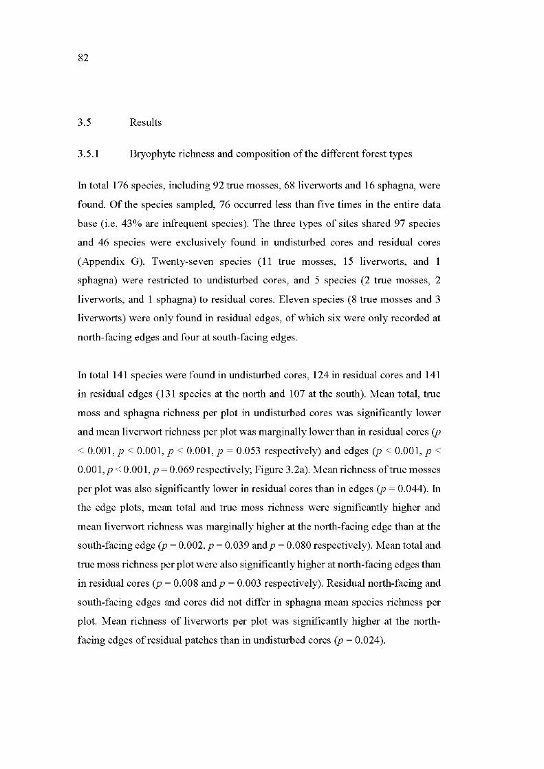
82

3.5 Results

3.5.1 Bryophyte richness and composition ofthe different forest types

In total176 species, including 92 true mosses, 68 liverworts and 16 sphagna, were

found. Of the species sampled, 76 occurred less than five times in the entire data

base (i.e. 43% are infrequent species). The three types of sites shared 97 species

and 46 species were exclusively found in undisturbed cores and residual cores

(Appendix G). Twenty-seven species (11 true mosses, 15 liverworts, and 1

sphagna) were restricted to undisturbed cores, and 5 species (2 true mosses, 2

liverworts, and 1 sphagna) to residual cores. Eleven species (8 true mosses and 3

liverworts) were only found in residual edges, of which six were only recorded at

north-facing edges and four at south-facing edges.

In total141 species were found in undisturbed cores, 124 in residual cores and 141

in residual edges ( 131 species at the north and 107 at the south). Mean total, true

moss and sphagna richness per plot in undisturbed cores was significantly lower

and mean liverwort richness per plot was marginally lower than in residual cores (p

< 0.001, p < 0.001, p < 0.001, p = 0.053 respectively) and edges (p < 0.001, p <

0.001,p < 0.001, p = 0.069 respectively; Figure 3.2a). Mean richness oftrue mosses

per plot was also significantly lower in residual cores than in edges (p = 0.044). In

the edge plots, mean total and true moss richness were significantly higher and

mean liverwort richness was marginally higher at the north-facing edge than at the

south-facing edge (p = 0.002, p = 0.039 and p = 0.080 respectively). Mean total and

true moss richness per plot were also significantly higher at north-facing edges than

in residual cores (p = 0.008 and p = 0.003 respectively). Residual north-facing and

south-facing edges and cores did not differ in sphagna mean species richness per

plot. Mean richness of liverworts per plot was significantly higher at the north

facing edges ofresidual patches than in undisturbed cores (p = 0.024).

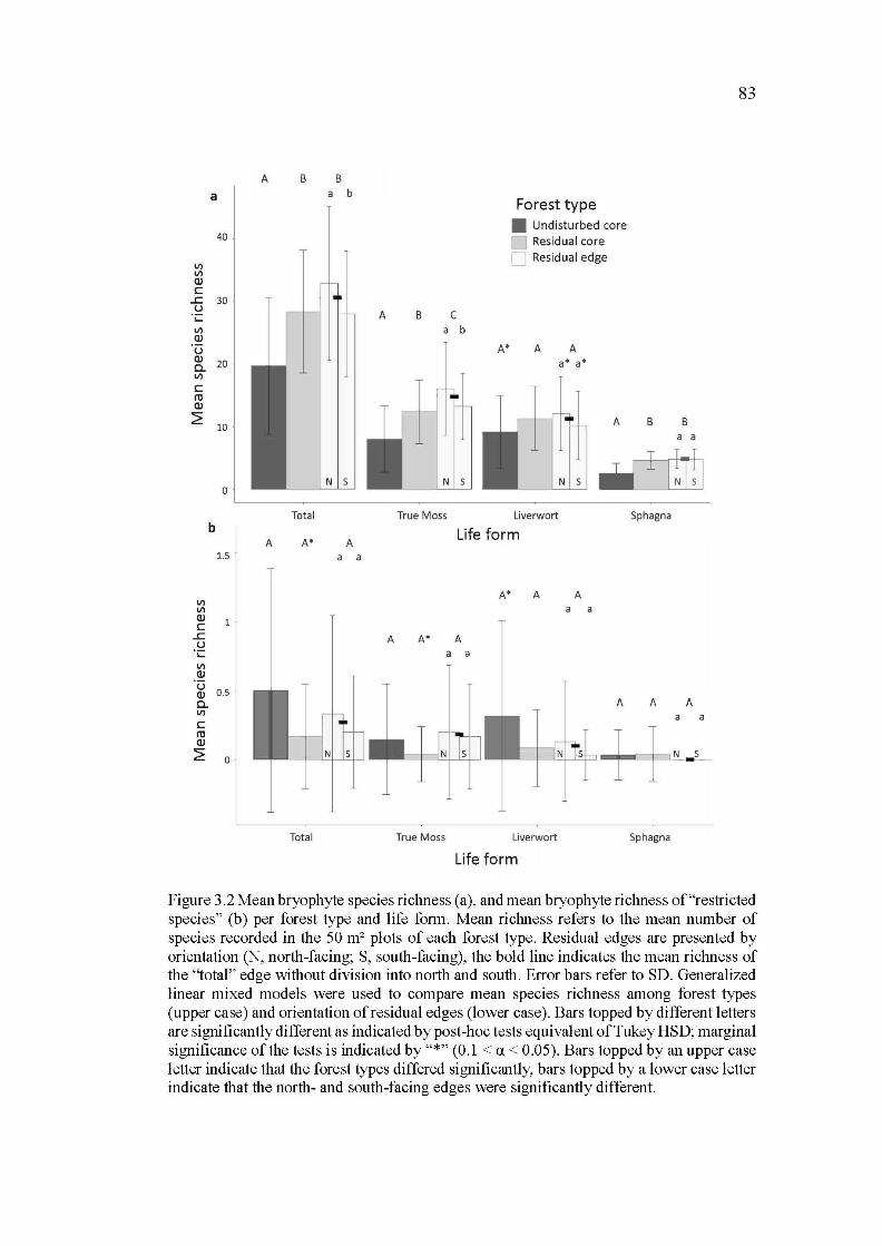
83

A B B

a a b Forest type

40 • Undisturbed core • Residual core

Vl D Residual edge

Vl aJ c

..c 30 u

·;:: Vl aJ .ü aJ 20 a. Vl

c ro aJ

~ 10

0

Total True Moss Liverwort Sphagna b Life form

A A* A 1.5 a a

A* A A Vl Vl a a aJ 1 c

..c A A* A u ·;:: a a Vl aJ u 0.5 aJ a. A A A Vl a a c ro aJ

~ 0 N s

Total True Moss Liverwort Sphagna

Life form

Figure 3.2 Mean bryophyte species richness (a), and mean bryophyte richness of"restricted species" (b) per forest type and life form. Mean richness refers to the mean number of species recorded in the 50 m2 plots of each forest type. Residual edges are presented by orientation (N, north-facing; S, south-facing), the bold line indicates the mean richness of the "total" edge without division into north and south. Error bars refer to SD. Generalized linear mixed models were used to compare mean species richness among forest types (upper case) and orientation of residual edges (lower case). Bars topped by different letters are significantly different as indicated by post-hoc tests equivalent ofTukey HSD; marginal significance of the tests is indicated by "*" (0.1 < a < 0.05). Bars topped by an upper case letter indicate that the forest types differed significantly, bars topped by a lower case letter indicate that the north- and south-facing edges were significantly different.

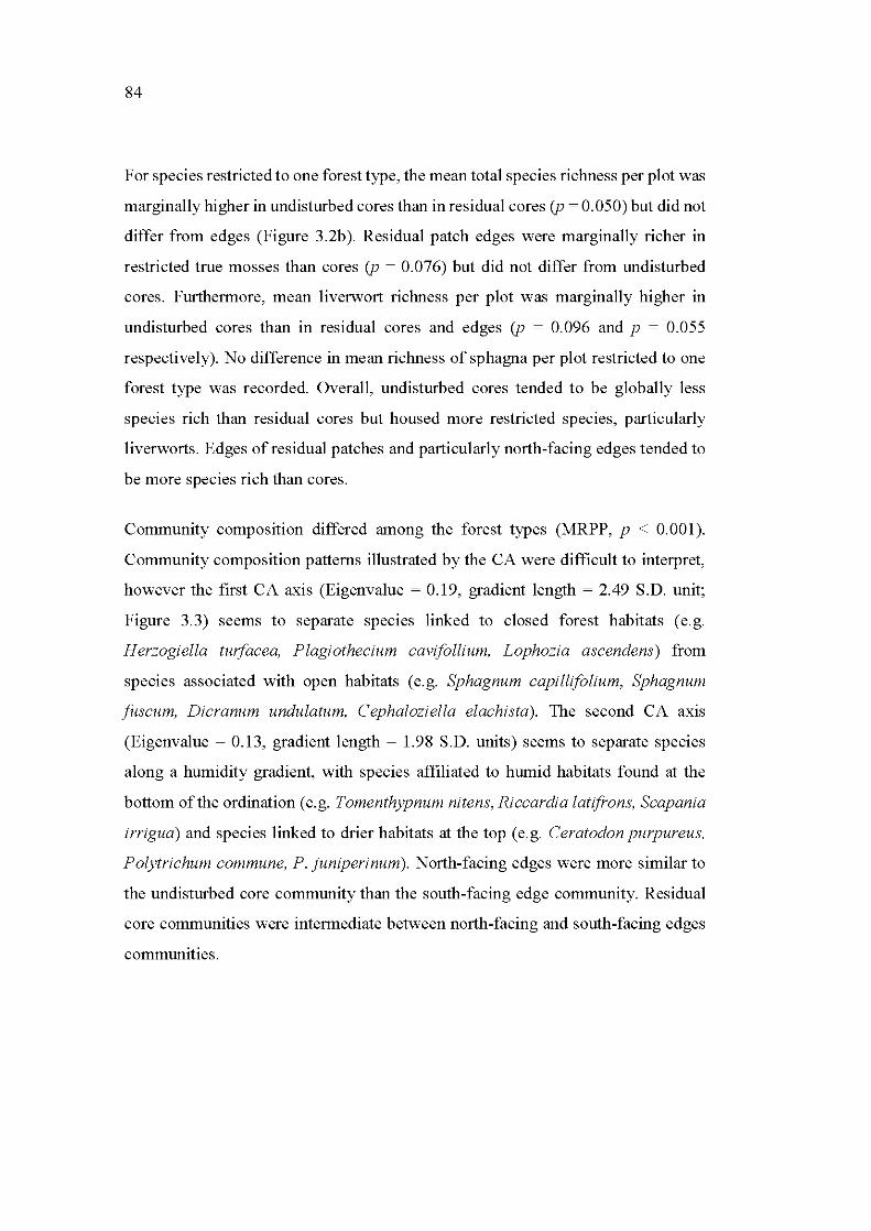
84

For species restricted to one forest type, the mean total species richness per plot was

marginally higher in undisturbed cores than in residual cores (p = 0.050) but did not

differ from edges (Figure 3.2b ). Residual patch edges were marginally richer in

restricted true mosses than cores (p = 0.076) but did not differ from undisturbed

cores. Furthermore, mean liverwort richness per plot was marginally higher in

undisturbed cores than in residual cores and edges (p = 0.096 and p = 0.055

respectively). No difference in mean richness of sphagna per plot restricted to one

forest type was recorded. Overall, undisturbed cores tended to be globally less

species rich than residual cores but housed more restricted species, particularly

liverworts. Edges of residual patches and particularly north-facing edges tended to

be more species rich than cores.

Community composition differed among the forest types (MRPP, p < 0.001).

Community composition patterns illustrated by the CA were difficult to interpret,

however the first CA axis (Eigenvalue = 0.19, gradient length = 2.49 S.D. unit;

Figure 3.3) seems to separate species linked to closed forest habitats ( e.g.

Herzogiella turfacea, Plagiothecium cavifollium, Lophozia ascendens) from

species associated with open habitats (e.g. Sphagnum capillifolium, Sphagnum

fuscum, Dicranum undulatum, Cephaloziella elachista). The second CA axis

(Eigenvalue = 0.13, gradient length = 1.98 S.D. units) seems to separate species

along a humidity gradient, with species affiliated to humid habitats found at the

bottom ofthe ordination (e.g. Tomenthypnum nitens, Riccardi a latifrons, Scapania

irrigua) and species linked to drier habitats at the top (e.g. Ceratodon purpureus,

Polytrichum commune, P. juniperinum). North-facing edges were more similar to

the undisturbed core community than the south-facing edge community. Residual

core communities were intermediate between north-facing and south-facing edges

communities.

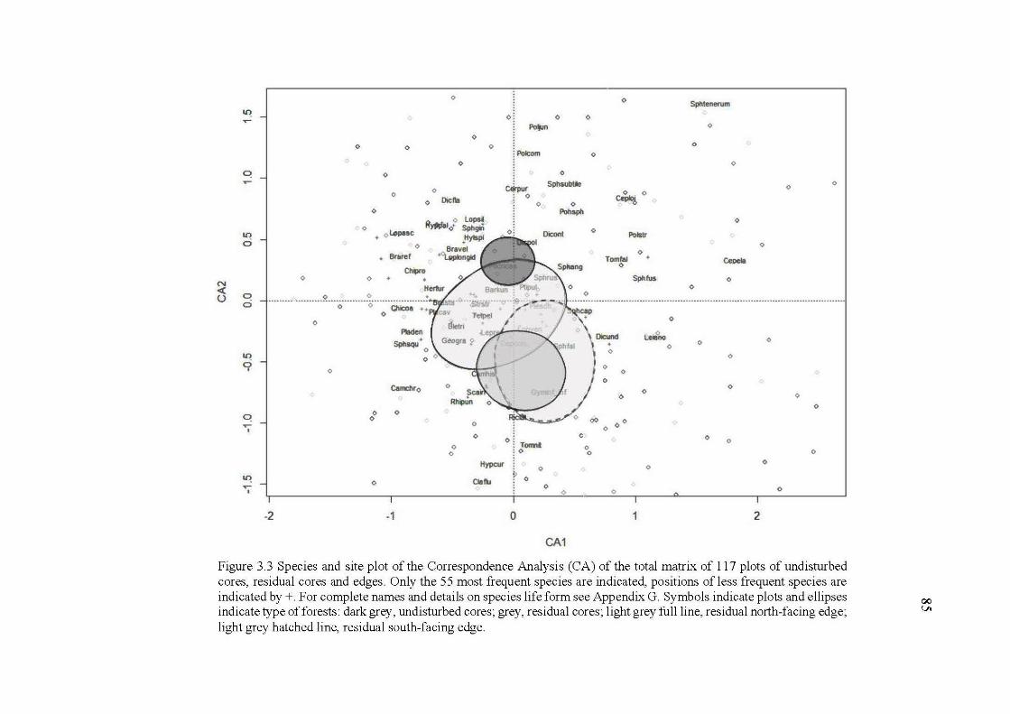
N ~ (.) 0

ci

~ .,.... 1

0

0 0

0

0

0 0

0 Oicfta 0

0 , 0 Lopasc

0

, Brlifef

Chlpro 0 0

0 0 • ......... ················o··········o······ëh~--~·:

0

-2

0

Cemchro

0 0 0

0

-1

0

0 0

0

0

0

0

ol 0

Polun

lPok»m 0

~ SphsubtJe

0 0 0

Pohsph

,..ol

ç

0

0

CA1

0

0

0

0

~ 0

0

Tomfal 0

Otcund

0 0

0

0

0

0

0

0

0 0

Polstr

0

Sphfus

0

Sphtenerum

0

0

0

0 0

0

0

Cepela

0 0

0 0

0

0 0

0

0 0

0

0

0

2

Figure 3.3 Species and site plot of the Correspondence Analysis (CA) of the total matrix of 117 plots of undisturbed cores, residual cores and edges. Only the 55 most frequent species are indicated, positions ofless frequent species are indicated by +. For complete names and details on species life form see Appendix G. Symbols indicate plots and ellipses indicate type of forests: dark grey, undisturbed cores; grey, residual cores; light grey full li ne, residual north-facing edge; light grey hatched line, residual south-facing edge.

00 VI

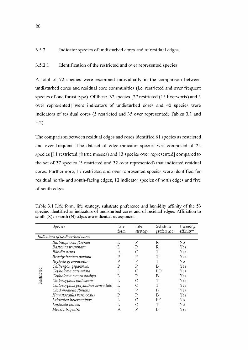
86

3.5.2 Indicator species ofundisturbed cores and ofresidual edges

3.5.2.1 Identification of the restricted and over represented species

A total of 72 spec1es were examined individually in the comparison between

undisturbed cores and residual core communities (i.e. restricted and over frequent

species of one forest type). Ofthese, 32 species [27restricted (151iverworts) and 5

over represented] were indicators of undisturbed cores and 40 species were

indicators of residual cores (5 restricted and 35 over represented; Tables 3.1 and

3.2).

The comparison between residual edges and cores identified 61 species as restricted

and over frequent. The dataset of edge-indicator species was composed of 24

species [11 restricted (8 true mosses) and 13 species over represented] compared to

the set of 37 species (5 restricted and 32 over represented) that indicated residual

cores. Furthermore, 17 restricted and over represented species were identified for

residual north- and south-facing edges, 12 indicator species of north edges and five

of south edges.

Table 3.1 Life form, life strategy, substrate preference and humidity affinity of the 53 species identified as indicators of undisturbed cores and of residual edges. Affiliation to south (S) or north (N) edges are indicated as exponents.

Species Li fe Li fe Substrate Humidity form strate~y preference affinity*

Indicators ofundisturbed cores

Ba rb ilophozi a jloe rkei L p R No Bazzania tricrenata L p R Y es Blindia acuta A c T Y es Brachythecium acutum p p T Y es Bryhnia gramnicolor p p T No

'"d Calliergon giganteum p p B Y es

~ Cephalozia catenulata L c EO Y es .:=: Cephalozia macrostachya L p B Y es .):j

"' Chiloscyphus palles cens L c T Y es <1.)

ç,::: Chiloscyphus polyanthos sensu lata L c T Y es Cladopodie lla flui tans L p B Y es Hamatocaulis vernicosus p p B Y es Leiocolea heterocolpos L c EF No Lophozia obtusa L c T No Meesia triquetra A p B Y es

87

Mylia taylori L p EF No Orthotrichum ohioense A p EP No Paludella squarrosa A p B Y es Platydictya subtilis p p EO No Pylaisia polyantha p p EP No Riccardia palmata L c EO Y es Scapania mucronata L c T No Schistochilopsis capitata L c T Y es Schistochilopsis grandiretis L p B No Sphagnum cuspidatum s D B Y es Tritomaria quinquedentata L p R No Ulota coarctata A p EP No

'"Cl Cepaloziella hampeana L c G No v

Hypnum imponens p p EF No ..... t: v v Rhizomnium pseudopunctatum A s T Y es > </).

0 v ..... Riccardia latifrons L c EF Y es 0.. v ..... Toment;lEnum nitens p p B Y es

Indicators of residual edges Barbilophozia hatcheri L c R No Cladopodiella francisciN L c T Y es Dicranum fulvums A p R No Dicranum spuriums A s R No

'"Cl Frullania eboracensisN L s EF No v ._. Orthotrichum speciosums A s EP No .s::

.t:J Plagiomnium mediumN A s T Y es til

~ Pohlia elongatas A c R No Polytrichum commune var. A p T No perigonialeN Polytrichum longisetumN A s B No SeJachnum ame,ullaceumN A c F No Brachythecium rejlexum p p EF No Brachythecium starkeiN p p G Y es Calypogeia muellerianaN L c G Y es Cephalozia connivensN L p B No

'"Cl Cephaloziella rubella L c G No v t: Ceratodon purpureus A c G No v Dicranum scoparium A p G No til v ..... Jamesoniella autumnali~ L c G No 0.. v

Plagiothecium cavifoliumN p p G No ..... ..... v Plagiothecium denticulatumN p p EF No > 0 P olytrichum juniperinum A p T Y es

Tomentypnum falcifolium p p B Y es Sphagnum wulfianums s D T Y es

*,bryophytes require water and moisture at different phases of their phenol ogy (Vanderpoorten & Goffinet 2009) but we distinguish here the species that are the most dependent on humid microhabitats for their survival (based on Faubert 2012-2014). Abbreviations for life forms: A, acrocarps; L, liverworts; P, pleurocarps; S, sphagna. Abbreviations for life strategies (based on During 1992): C, colonist; D, dominant; P, perennial; S, shuttle. Abbreviations for substrate preferences (based on Faubert 2012-2014): B, bog; EF, facultative epixylic; EO, obligate epixylic; EP, epiphyte; G, generalist; F, faeces; T, terricolous; R rock.

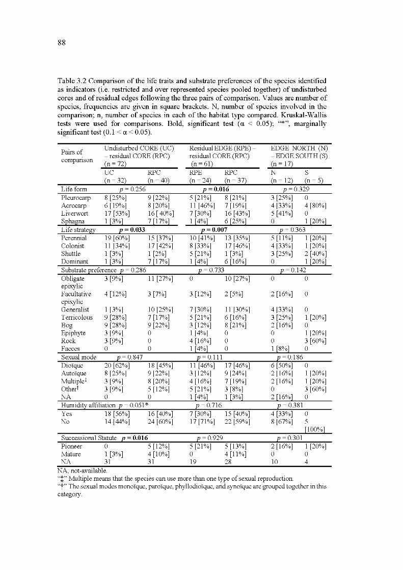
88

Table 3.2 Comparison of the life traits and substrate preferences of the species identified as indicators (i.e. restricted and over represented species poo led together) of undisturbed cores and of residual edges following the three pairs of comparison. Values are number of species, frequencies are given in square brackets. N, number of species involved in the comparison; n, number of species in each of the habitat type compared. Kruskal-Wallis tests were used for comparisons. Bold, significant test (a < 0.05); "*", marginally significant test (0.1 <a < 0.05).

Pairs of Undisturbed CORE (UC) Residual EDGE (RPE)- EDGE NORTH (N) - residual CORE (RPC) residual CORE (RPC) - EDGE SOUTH (S)

companson ~n = 722 ~n = 612 ~n = 172 uc RPC RPE RPC N s ~n = 322 ~n = 402 ~n = 242 ~n = 372 ~n = 122 ~n= 52

Life form p = 0.256 p = 0.016 p = 0.329 Pleurocarp 8 [25%) 9 [22%) 5 [21 %) 8 [21 %) 3 [25%) 0 Acrocarp 6 [19%) 8 [20%) 11 [46%) 7 [19%) 4 [33%) 4 [80%) Liverwort 17[53%) 16 [ 400/o) 7 [30%) 16 [43%) 5 [41 %) 0 S.Ehas;na 1 [3%] 7 [17%] 1 [4%] 6 [25%] 0 1 [20%] Life strategy l!. = 0.033 l!. = 0.007 P.= 0.363 Perennial 19 [60%) 15 [37%) 10[41%) 13 [35%) 5 [11 %) 1 [20%) Colonist 11 [34%) 17[42%) 8 [33%) 17 [46%) 4 [33%) 1 [20%) Shuttle 1 [3%) 1 [2%) 5 [21 %) 1 [3%) 3 [25%) 2 [ 400/o] Dominant 1 [3%) 7 [17%) 1 [4%) 6 [16%) 0 1 [20%) Substrate 12reference P. = 0.286 P.= 0.733 P.= 0.142 Obligate 3 [9%) 11 [27%) 0 10 [27%) 0 0 epixylic Facultative 4 [12%) 3 [7%) 3 [12%) 2 [5%) 2 [16%) 0 epixylic Generalist 1 [3%) 10 [25%) 7 [30%) 11 [30%) 4 [33%) 0 Terricolous 9 [28%) 7 [17%) 5 [21 %) 6 [16%) 3 [25%) 1 [20%) Bog 9 [28%) 9 [22%) 3 [12%) 8 [21 %) 2 [16%) 0 Epiphyte 3 [9%) 0 1 [4%) 0 0 1 [20%) Rock 3 [9%) 0 4 [16%) 0 0 3 [60%) Faeces 0 0 1 [4%) 0 1 [8%) 0 Sexual mode P.= 0.847 P.= 0.111 P. =0.186 Dioïque 20 [62%) 18 [45%) 11 [46%) 17 [46%) 6 [50%) 0 Autoïque 8 [25%) 9 [22%) 3 [12%) 9 [24%) 2 [16%) 1 [20%) Multiplet 3 [9%) 8 [20%) 4 [16%) 7 [19%) 2 [16%) 1 [20%) Othert 3 [9%) 5 [12%) 5 [21 %) 3 [8%) 0 3 [60%) NA 0 0 1 [4%] 1 [3%] 2 [16%] 0 Humidity affiliation p = 0. 051 * p = 0.716 p = 0.381 Y es 18 [56%) 16 [40%) 7 [30%) 15 [40%) 4 [33%) 0 No 14[44%) 24 [60%) 17[71%) 22 [59%) 8 [67%) 5

Successional Statute l!. = 0.016 P.= 0.929 P.= 0.301 Pioneer 0 5 [12%) 5 [21 %) 5 [13%) 2 [16%) 1 [20%) Mature 1 [3%) 4 [10%) 0 4 [11 %) 0 0 NA 31 31 19 28 10 4

NA, not-available. 'T'Multiple means that the species canuse more than one type of sexual reproduction. 'T' The sexual modes monoïque, paroïque, phyllodioïque, and synoïque are grouped together in this category.

3.5.2.2

89

Life traits and habitat preferences of restricted and over represented

spectes

Restricted and over represented species of undisturbed cores significantly differed

in life strategies and successional statute (p = 0.033 and p = 0.016 respectively;

Table 3.2) from species found in residual cores. Undisturbed cores were

significantly richer in perennial species and less rich in colonist and pioneer species

than residual cores. Species tended to be affiliated with more humid microhabitats

in undisturbed cores (p = 0.051, with 56% of the species linked to humidity in

undisturbed cores compared to 40% in residual cores; Table 3.2).

Residual cores and edges were also distinct in terms of the life form and strategy of

the restricted and over represented species (p = 0.016 and p = 0.007 respectively;

Table 3.2). Perennials and acrocarps were mainly found in the edges compared to

residual cores that were characterised by liverwort and colonist species. There were

no differences in life traits and substrate preference of the species found between

north- and south-facing edge orientations.

3.5.3 Bryophyte community similarity between forest types and distance of

edge influence (DEI)

In order to determine if post-fire residual patches have ''true cores" and to estimate

the DEI of bryophytes in boreal black spruce forests, Jaccard's index of similarity

was used. Similarity between undisturbed cores and residual cores and between

residual cores and edges varied from 2.05% to 49.80% and from 24.8% to 71%

respectively. Among the six environmental variables tested through the linear

mixed models, similarity between undisturbed forests and residual cores was

negatively correlated with residual patch area (p = 0.029, r = -0.56; Figure 3.4a)

and continuously diminishes with the increasing are a of the patch.

On the other hand, similarity between the core and the edge of one residual patch

was significantly negatively correlated toits area (p = 0.044, r = -0.67; Figure 3.4b)

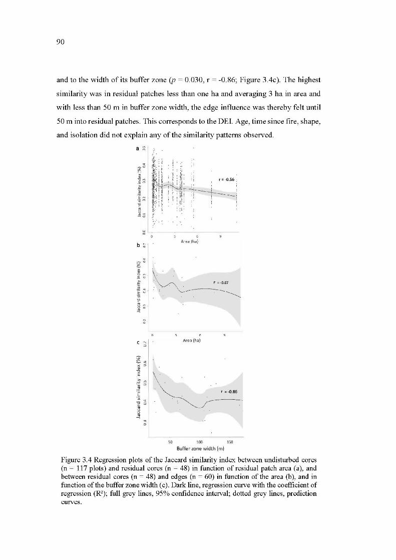
90

and to the width ofits buffer zone (p = 0.030, r = -0.86; Figure 3.4c). The highest

sirnilarity was in residual patches less than one ha and averaging 3 ha in area and

with less than 50 rn in buffer zone width, the edge influence was thereby felt until

50 rn into residual patches. This corresponds to the DEL Age, tirne since fire, shape,

and isolation did not explain any of the sirnilarity patterns observed.

0 0

b ;;

c ": 0

~ ~ x 0 Q)

"0 c::

~ 111 ·;::: 0

~

E

"' 0

6

Area !ha )

6

Area (ha)

r = -0.86

50 100 150

Buffer zone width (m)

Figure 3.4 Regression plots of the Jaccard similarity index between undisturbed cores (n = 117 plots) and residual cores (n = 48) in function ofresidual patch area (a), and between residual cores (n = 48) and edges (n = 60) in function of the are a (b ), and in function of the buffer zone width ( c ). Dark line, regression curve with the coefficient of regression (R2

); full grey lines, 95% confidence interval; dotted grey lines, prediction curves.

91

3.6 Discussion

Residual patches, and especially north-facing edges, represent sites of high

bryophyte richness. However, bryophytes were negatively affected by edges in a

species-dependant mann er, and indicator species of undisturbed cores and residual

edges were identified. Although the edge influence was mitigated in larger patches,

bryophyte communities in undisturbed cores and residual cores remained distinct,

as already found in Barbé et al. (in revision, refers to the Chapter II) for the residual

patch considered as a who le (i.e. including the edges ). The absence of "true cores"

in post-fire residual patches and the clear change in community composition

associated with these fragmented forest type represents the natural response of

bryophytes to edge creation. These conclusions offer new insights to bryophyte

response to edge creation that have up to now be en only examined on anthropogenic

edges.

3 .6.1 Bryophyte response to edge influence and the identification of edge

sensitive and edge-preferring species

Not surprisingly, species richness was higher in residual patches (cores and edges

confounded) than in undisturbed cores, with the most species richness found in

residual edges (Barbosa & Marquet 2002; Duelli et al. 2002; Baldwin & Bradfield

2005). Furthermore, as found in Swedish boreal forest and in Mediterranean

Quercus forests, edge orientation was influential (Hylander 2005; Belinchôn et al.

2007) with north-facing edges richer than south-facing edges. Our first hypothesis

is therefore confirmed. The high species richness of edges may be due to the fact

that they are at the interface between two distinct habitats (Holland et al. 1991;

Magura 2002), but also due to their structural complexity (i.e. reduced canopy,

greater dead wood volume and higher snag density; Chen et al. 1992; Oosterhoom

& Kappelle 2000). This results in high microhabitat diversity, opening a field of

possibilities for the coexistence of a myriad of species (Araûjo 2002), as suggested

by the "mass effect" (Shmida & Wilson 1985; Auerbach & Shmida 1987).

92

Furthermore, the lower level of microhabitat saturation may indicate that sorne

species cannot tolerate the environmental conditions of the edge, but the large

number of species suggests rather that these empty microhabitats represent

opportunities for colonization by new species.

We identified 69 species as indicators of undisturbed cores and residual edges.

Thirty-two of the species found were significantly more frequent or even restricted

to undisturbed cores. This included numerous pereruüal stayers associated with

bogs, and infrequent liverworts that are typically associated with closed-canopies,

high humidity and significant deadwood volume in advanced decay classes

(Baldwin & Bradfield 2005, 2007, 2010; Hylander et al. 2005; Hylander & Johnson

2010). Moreover, the abundance of sphagna-associated species (e.g., Calliergon

giganteum, Tomenthypnum nitens) was expected because ofthe paludified state of

sorne undisturbed old-growth stands in black spruce forests (Fenton et al. 2005).

This set of species that negatively responded to edge creation may be used as

indicators ofundisturbed forests, where structural attributes and microhabitats have

diversified over time resulting in increased species colonization and stable

microclimatic conditions (Fenton & Bergeron 2008; Pharo & Lindenmayer 2009).

The absence of these species from both residual cores and edges may also be

explained by the alteration of the regional dispersal processes as a result of

fragmentation of the forest landscape. Their metapopulation dynamics was

disrupted in response to the increased dispersal distance that change regional

distribution patterns but also local abundance of the species (Lôbel et al. 2006).

In contrast, sorne bryophyte spec1es [7 liverworts (71% colonists) and 16 true

mosses (68% acrocarps)] were positively affected by edge creation. These edge

preferring species have a high tolerance of disturbance but also have opportunistic

strategies such as high dispersal capacities and large niche breathe ( c.f. Baldwin &

Bradfield 2005; c.f. Ewers & Didham 2006). Therefore, not surprisingly, edges

house more acrocarps and shuttle species (sensu Paquette et al. 2016 adapted from

During 1992), which inhabit long-lived substrates such as granitic rocks and with

93

both high sexual and vegetative reproduction effort. Edge-indicator species are

linked to dry and exposed substrates, especially at the south-facing edges, which

are characterized by species inhabiting rocky substrates with marked humidity

variations (e.g. Dicranum fulvum, Dicranum spurium, Orthotrichum speciosum).

The more humid and colder conditions of north-facing edges (Hylander 2005;

Stewart & Mallik 2006) are more favourable for species vulnerable to dry

microclimates such as liverworts (Esseen & Renhom 1998; Moen & Jonsson 2003),

which explains the similarity in community composition between north-facing

edges and undisturbed cores (c .f. CA analysis). However, our north- and south

facing edges did not differ in terms of humidity (Appendix F), due to either the

short six month period used to measure microclimatic variables or to an inherent

property of edges in boreal black spruce forests prone wildfires. Indeed, in such

ecosystems, the rapid recovery of Sphagnum spp. in response to post-fire canopy

opening brings humidity and limits soil exposition to sunlight, reducing differences

on either side of the edge. The Alnus spp. belt surrounding sorne of our residual

patches can also have a similar effect.

Together, these results suggest that the bryophyte community of residual cores were

more similar to edges than to undisturbed cores communities, and therefore there is

little or no core. However, the inherent properties of boreal black spruce forest

described above, together with the richness of liverworts and overa11 community

composition of north edges indicated by the CA evoke the question: are these

residual patches essentia11y edges or are do the edges have core characteristics? We

cannot answer the question but as the cores do not meet our definition of a ''true

core", we reject our second hypothesis.

3.6.2 Bryophyte response to edge creation is mediated by residual patch stand

structure

Studies report that edge influence diminish over time and with increasing residual

patch area, shape homogeneity and proximity to forest sources (i.e. forest

94

influence), which result in dynamic boundaries (Ewers & Didham 2006; Laurance

2008; Baker et al. 2013; Harper et al. 2014). Consequently, we hypothesized that

old and large residual patches would house a core community more similar to

undisturbed cores than younger and smaller ones. Our results indicate the opposite,

as even in old (more than 3000 years old) or large (from 4 ha to more than 10 ha)

residual cores' bryophyte communities remain consistently distinct from

undisturbed core communities. Moreover, counterintuitively, similarity between

residual and undisturbed cores is negatively correlated with residual patch size and

the other spatial and temporal characteristics of patches were not influential on

community patterns. As stressed by Jokimaki et al. (1998) for invertebrates and Si

Laurent et al. (2007) for birds and small mammals in boreal forests , these results

suggest that bryophyte community composition is primarily driven by structural

attributes rather than by temporal or spatial characteristics of the stand.

In parallel, in spite of the dissimilarity between residual and undisturbed cores,

regardless of patch age, larger patches exhibited more distinct core and edge

communities. In boreal forest, both Jalonen & Vanha-Majamaa (2001) and Moen

& Jonsson (2003) have demonstrated that small residual patches (less than 1 ha) are

strongly influenced by edge creation leading to bryophyte richness decrease and a

decline in cover of liverworts. In this study the threshold value below which

similarity between cores and edges increased was 3 ha. For Baldwin & Bradfield

(2007) in temperate rain-forests, 3 ha also represents a threshold size that provides

a number of microhabitats capable of sustaining a diverse array of bryophyte

functional groups. Our fourth hypothesis is therefore only partially validated: even

if patches over 3 ha displayed contrasting bryophyte core and edge communities,

all of our residual patches did not contain ''true cores" and housed communities that

were more similar to residual edges than to undisturbed cores. Larger patches can

hold a broader set of microhabitats (Baldwin & Bradfield 2007) and larger trees for

microhabitat generation (e.g. dead wood; Moen & Jonsson 2003). Consequently,

the importance of the patch area is indirect and carried by stand structural attributes

that mediate bryophyte diversity after edge creation.

95

3.6.3 Implications for conservation and management

The apparent dissimilarity between undisturbed and residual cores in terms of

environmental conditions but also community composition leads us to contradict

sorne previous studies that have determined the DEI of bryophytes and lichens in

temperate and boreal Canadian forests at 50 to 60 rn from the edge (Rhéault 2003;

Baldwin & Bradfield 2005; Boudreault et al. 2008). The highest similarity between

residual cores and edges bryophyte communities was identified in patches with 50

rn buffer zone width, however we demonstrate that 11-ha residual patches (with 170

rn buffer zone width) house a bryophyte community distinct of undisturbed cores.

While both the initial community composition and environmental variables are

unknown, long-lived compositional and environmental dissimilarities between

residual patches and undisturbed forests remain visible up to 170 rn inside residual

patches, a possible indication of the DEI. Consequently, as also indicated by Barbé

et al. (in revision, refers to the Chapter II), the conservation of the most infrequent

and sensitive species requires the preservation of undisturbed forest stands. The

presence of significant edge influence in natural communities suggests that the real

challenge in planning retention in boreal forests is not to avoid edge influence but

to rather design retention patches in such a way as bryophyte compositional changes

in response to anthropogenic edges creation remain inside the range of

compositional changes generated by natural edges. As schematised in Figure 3. 5,

in the context of ecosystem based management we aim to create retention patches

inside the limits of natural edge creation as (2) or (3), although the habitat is

essentially composed of edge, and to avoid to create retention patches as ( 4).

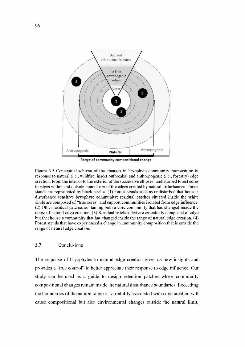
96

Out lim it ···· ..

/~ .... •••• •••••• anthropogenic edges ··· ... .. ·· .. ·. ·· ...

........... \

r .. . . . ............. .

·· .. ' ~ ··... . ... ············

J ............ : .· .·· . .. ··

···············j ......................... j······· Antropogenic · Natural Antropogenic

Range of community compositional change

Figure 3.5 Conceptual schema of the changes in bryophyte community composition in response to natural (i.e., wildfire, insect outbreaks) and anthropogenic (i.e., forestry) edge creation. From the interior to the exterior of the successive ellipses: undisturbed forest cores to edges within and outside boundaries of the edges created by natural disturbances. Forest stands are represented by black circles. (1) Forest stands such as undisturbed that house a disturbance sensitive bryophyte community; residual patches situated inside the white circle are composed of"true cores" and support communities isolated from edge influence. (2) Other residual patches containing both a core community that has changed inside the range of natural edge creation. (3) Residual patches that are essentially composed of edge but that house a community that has changed inside the range of natural edge creation. ( 4) Forest stands that have experienced a change in community composition that is outside the range of natural edge creation.

3.7 Conclusions

The response of bryophytes to natural edge creation gives us new insights and

provides a ''true control" to better appreciate their response to edge influence. Our

study can be used as a guide to design retention patches where community

compositional changes remain inside the natural disturbance boundaries. Exceeding

the boundaries ofthe natural range ofvariability associated with edge creation will

cause compositional but also environmental changes outside the natural limit,

97

which can threaten the resilience of the ecosystem. Species compositional change

in response to edge creation is not only a character of anthropogenic edges, but is a

natural component of the boreal forest dynamic. Finally, this study also re

emphasizes that sorne species can only be maintained by the conservation of old

growth stands, as they are not found in edges but neither in cores of residual forest

patches and therefore sustainable forest management needs to include both residual

forest stands and undisturbed old growth forests.


Funding for this project was provided by the Université du Québec en Abitibi

Témiscamingue (UQAT) and the National Science and Engineering Research

Council (NSERC) in partnership with Tembec, Eacom and Resolute Forest

Products.

The authors especially thank Chafi Chaieb who has provided bryophyte samples

from the undisturbed forest sites and Julie Arseneault for their identification.

Authors also sincerely thank Emilie E. Chavel and Louiza Moussaoui who have

provided sorne of the environmental data used in this paper; Myriam Paquette, Flora

Joubier, Louis Dubois and Philippe Heine for their field assistance; Danielle

Charron, Philippe Duval, Raynald Julien, Danièle Laporte, Marie-Hélène Longpré,

and Michel Poitras for their technical support; and Jean Faubert for his precious

help in the identification ofthe most difficult bryophyte sample.

3.9 References

Auerbach, M. & Shmida, A. 1987. Spatial scale and the determinants of plant species richness. Trends in Ecology and Evolution 2: 238-242.

Araûjo, M.B. 2002. Biodiversity hotpots and zones of ecological transition. Conservation Biology 16: 1662-1663.

Baker, S.C., Spies, T.A., Wardlaw, T.J., Balmer, J., Franklin, J.F. & Jordan, G.J. 2013. The harvested side of edges: Effect of retained forests on the re-

98

establishment of biodiversity in adjacent harvested areas. Forest Ecology and Management 302: 107-121.

Baldwin, L.K. & Bradfield, G.E. 2005. Bryophyte community differences between edge and interior environments in temperate rain-forest fragments of coastal British Columbia. Canadian Journal ofForest Research 35: 580-592.

Baldwin, L.K. & Bradfield, G.E. 2007. Bryophyte responses to fragmentation in temperate coastal rainforests: A functional group approach. Biological Conservation 136: 408-422.

Baldwin, L.K. & Bradfield, G.E. 2010. Resilience of bryophyte communities in regenerating matrix forests after logging in temperate rainforests of coastal British Columbia. Botany 88: 297-314.

Barbosa, O. & Marquet, P.A. 2002. Effects of forest fragmentation on the beetle assemblage at the relict forest of Fray Jorge, Chile. Oecologia 132: 296-306.

Belinch6n, R., Martînez, I., Escudero, A. , Aragon, G. & Valladares, F. 2007. Edge effects on epiphytie communities in a Mediterranean Quercus pyrenaica forest. Journal ofVegetation Science 18, 81-90.

Bergeron, Y., Gauthier, S., Flannigan, M. & Kafka, V. 2004. Fire regimes at the transition between mixedwood and coniferous boreal forest in northwestem Quebec. Ecology 85: 1916-1932.

Boudreault, C., Bergeron, Y., Drapeau, P. & L6pez, L.M. 2008. Edge effects on epiphytie lichens in remnant stands of managed landscapes in the eastern boreal forest of Canada. Forest Ecology and Management 255: 1461-1471.

Chaieb, C., Fenton, N.J., Lafleur, B. & Bergeron, Y. 2015. Can we use forest inventory mapping as a coarse filter in eco system based management in the black spruce boreal forest? Forests 6: 1195-1207.

Chen, J., Franklin, J.F. & Spies, T.A. 1992. Vegetation responses to edge environments in old-growth Douglas-tir forests. Ecological Application 2: 387-396.

Connell, J.H. 1979. Intermediate-disturbance hypothesis. Science 204: 1345.

Davies-Colley, R.J., Payne, G.W. & Van Elswijk, M. 2000. Microclimate gradients across a forest edge. New Zealand Journal ofEcology 24: 111-121.

de V alpine, P. 2014. The common sense of P values. Ecology 95: 617-621.

Duelli, P., Obrist, M.K. & Flückiger, P.F. 2002. Forest edges are biodiversity hotspots - also for neuroptera. Acta Zoologica Academiae Scientiarum Hungaricae 48: 75-87.

During, H.J. 1992. Ecological classification of bryophytes and lichens. In: Bates, J.W. & Farmer, A.M. (eds.) Bryophytes and Lichens in Changing Environment, pp. 1-31. Clarendon Press, Oxford, UK.

99

Dynesius, M. & Hylander, K. 2007. Resilience ofbryophyte communities to clearcutting ofboreal stream-side forests. Biological Conservation 135: 423-434.

Environment Canada. 2015. Canadian climate normals 1981-2010 Station data. Date of accession 24th February 2016. Available at: http: //climate.weather.gc.ca/climate normals/results 1981 2010 e.html?stniD =6051&lang=e&StationName=Lebel+sur+Quevillon&SearchType= Contains&stnN ameSubmit=go&dCode=5&dispBack= 1

Esseen, P.A. & Renhom, K.E. 1998. Edge effects on an epiphytie lichen in fragmented forests. Conservation Biology 12: 1307-1317.

Ewers, R.M. & Didham, R.K. 2006. Confounding factors in the detection of species responses to habitat fragmentation. Biological Reviews 81: 117-142.

Ewers, R.M. & Didham, R.K. 2008. Pervasive impact of large-scale edge effects on a beetle community. Proceedings oftheNationalAcademy ofSciences ofthe United States of America 105: 5426-5429.

Fahrig, L. 2003. Effects of habitat fragmentation on biodiversity. Annual Review of Ecology, Evolution and Systematics 34: 487-515.

Faubert, J. 2012-2014. Flore des bryophytes du Québec-Labrador (Vol. 1, 2 and 3). Société québécoise de bryologie, Saint-Valérien, Canada.

Fenton, N.J., Frego, K.A. & Sims, M.R. 2003. Changes in forest floor bryophyte (moss and liverwort) communities 4 years after forest harvest. CanadianJournal ofBotany 81: 714-731.

Fenton, N.J. & Frego, K.A. 2005. Bryophyte (moss and liverwort) conservation under remnant canopy in managed forests. Biological Conservation 122: 417-430.

Fenton, N., Lecomte, N. , Légaré, S. & Bergeron, Y. 2005. Paludification in black spruce (Picea mariana) forests of eastern Canada: Potential factors and management implications. Forest Ecology and Management 213: 151-159.

Fenton, N.J. & Bergeron, Y. 2008. Does time of habitat make old-growth forests species rich? Bryophyte richness in boreal Picea mariana forests. Biological Conservation 141: 1389-1399.

Flora ofNorth America Editorial Committee. 2007. Flora ofNorthAmerica, North ofMexico (Vol. 27), Bryophytes: Moss, Part 1. Oxford University Press, Oxford, UK.

Franklin, C.M.A., Harper, K.A. & Murphy, L.K. 2015. Structural dynamics at boreal forest edges created by a spruce budworm outbreak. Silva Fennica 49: 1-17.

Harper, K.A. & Macdonald, S.E. 2001. Structure and composition ofriparian boreal forest: new methods for analysing edge influence. Ecology 82: 649-659.

100

Harper, K. A. & Macdonald, S.E. 2002. Structure and composition of edges next to regenerating clear-cuts in mixed-wood boreal forest. Journal of Vegetation Science 13: 535-546.

Harper, KA., Macdonald, S.E, Burton, P.J., Chen, J., Brosofske, K.D., Saunders, S.C., Euskirchen, E.S., Roberts, D. , Jaiteh, M.S. & Esseen, P-A. 2005. Edge influence on forest structure and composition in fragmented landscapes. Conservation Biology 19: 768-782.

Harper, KA., Drapeau, P., Lesieur, D. & Bergeron, Y. 2014. Forest structure and composition at fire edges of different ages: Evidence of persistent structural features on the landscape. Forest Ecology and Management 314: 131-140.

Holland, M.M., Risser, P.G. & Naiman, R.J. 1991. Ecotones, the role of lands founder and dominance control: neglected concepts in the community dynamics of clonai plants capes boundaries in the management and restoration of changing environment. Springer Science & Business Media, USA.

Hylander, K. & Johnson, S. 2010. In situ survival of forest bryophytes in smallscale refugia after an intense forest fire. Journal of Vegetation Science 21: 1099-1109.

Hylander, K. 2005. Aspect modified the magnitude of edge effects on bryophyte growth in boreal forests. Journal of Applied Ecology 42, 518-525.

Hylander, K., Dynesius, M., Jonsson, B.G. & Nilsson, C. 2005. Substrate form determines the fate of bryophytes in riparian buffer strips. Ecological Applications 15: 674-688.

Hylander, K., Nemomissa, S. & Enkosa, W. 2013. Edge effects on understory epiphytie ferus and epiphyllous bryophytes in moist afromontane forests of Ethiopia. Polish Botanical Journal 58: 555-563.

Jalonen, J. & Vanha-Majamaa, I. 2001. Immediate effects of four different felling methods on mature boreal spruce forest understorey vegetation in southem Finland. Forest Ecology and Management 146: 25-34.

Jost, L., Chao, A. & Chazdon, R.L. 2011. Compositional similarity and ~ (beta) diversity. In: Magurran, A.E. & McGill, B.J. ( eds.) Biological diversity frontiers in measurement and assessment, pp. 66-84. Oxford University Press, NY, US.

Jokimaki, J. & Suhonen, J. 1998. Distribution and habitat selection of wintering birds in urban environments. Landscape and Urban Planning 39: 253-263.

Kivistô, L. & Kuusinen, M. 2000. Edge effects on the epiphytie lichen flora of Picea abies in middle boreal Finland. The Lichenologist 32, 387-398.

Larrivée, M., Drapeau, P. & Fahrig, L. 2008. Edge effects created by wildfire and clear-cutting on boreal forest ground-dwelling spiders. Forest Ecology and Management 255: 1434-1445.

101

Laurance, W.F. 2008. Theory meets reality: How habitat fragmentation research has transcended island biogeography theory. Biological Conservation 141: 1731-1744.

Lee, S-11., Spence, J.R., Langor, D.W. & Pinzon, J. 2015. Retention patch size and conservation ofsaproxylic beetles in boreal white spruce stands. Forest Ecology and Management 358: 98-107.

Leps, J. & Smilauer, P. 2003. Multivariate analysis of ecological data using CANOCO. Cambridge University Press, Cambridge, UK.

Lesica, P., McCune, B., Cooper, S.V. & Hong, W.S. 1991. Differences in lichen and bryophyte communities between old-growth and managed second-growth forests in the Swan Valley, Montana. Canadian Journal of Botany 69: 1745-1755.

Lôbel, S., Sniill, T. & Rydin, H. 2006. Metapopulation processes in epiphytes inferred from patterns of regional distribution and local abundance in fragmented forest landscapes. Journal ofEcology 94: 856-868.

Lôbel, S. & Rydin, H. 2010. Trade-offs and habitat constraints in the establishment of epiphytie bryophytes. Functional Ecology 24: 887-897.

Lohmus, P., Rosenvald, R. & Lohmus, A. 2006. Effectiveness of solitary retention trees for conserving epiphytes: differentiai short-term responses of bryophytes and lichens. Canadian Journal of Forest Research 36: 1319-1330.

Madoui, A., Leduc, A., Gauthier, S. & Bergeron, Y. 2010. Spatial pattern analyses of post-fire residual stands in the black spruce boreal forest of western Que bec. International Journal ofWildland Fire 19: 1110-1126.

Magura, T. 2002. Carabids and forest edge: spatial pattern and edge effect. Forest Ecology and management 157: 23-37.

Moen, J. & Jonsson, B.G. 2003. Edge effects on liverworts and lichens in forest patches in a mosaic of boreal forest and wetland. Conservation Biology 17: 380-388.

Moussaoui, L., Fenton, N.J. , Leduc, A. & Bergeron, Y. 2016. Deadwood abundance in post-harvest and post-fire residual patches: an evaluation of patch temporal dynamics in black spruce boreal forest. Forest Ecology and Management 368: 17-27.

Murcia, C. 1995. Edge effects in fragmented forests: implications for conservation. Trends in Ecology and Evolution 10: 58-62.

Murtaugh, P.A. 2014. In defense of P values. Ecology 95: 611-617.

Newmaster, S.G., Belland, R.J., Arsenault, A. & Vitt, D.H. 2003. Patterns of bryophyte diversity in humid coastal and inland ce dar hemlock forests of British Columbia. EnvironmentalReviews 11: S159-S185.

102

Newmaster, S.G., Belland, R.J., Arsenault, A. , Vitt, D.H. & Stephens, T.R. 2005. The ones we left behind: comparing plot sampling and floristic habitat sampling for estimating bryophyte biodiversity. Diversity and Dis tri butions 11: 57-72.

Oosterhoom, M. & Kappelle, M. 2000. Vegetation structure and composition along an interior-edge-exterior gradient in a Costa Rican montane cloud forest. Forest Ecology and Management 126: 291-307.

Paquette, M. , Boudreault, C., Fenton, N., Pothier, D. & Bergeron, Y. 2016. Bryophyte species assemblages in fire and clear-cut origin boreal forests. Forest Ecology and Management 359: 99-108.

Pharo, E.J. & Lindenmayer, D.B. 2009. Biologicallegacies soften pine plantation effects for bryophytes. Biodiversity and Conservation 18: 1751-1764.

Pinheiro, J.C. & Bates, D.M. 1995. Approximations to the log-likelihood function in the nonlinear mixed-effects model. Journal of computational and Graphical Statistics 4: 12-35.

Proctor, M.C.F. 1990. The physiological basis ofbryophyte production. Botanical Journal oftheLinnean Society 104,61-77.

Proctor, M.C.F., Oliver, M.J., Wood, A.J., Alpert, P., Stark, L.R., Cleavitt, N.L. & Mishler, B.D. 2007. Desiccation-tolerance in bryophytes: a review. The Bryologist 110: 595-621.

Rambo, T.R. & Muir, P.S. 1998. Bryophyte species associations with coarse woody debris and stand ages in Oregon. The Bryologist 101: 366-376.

Rhéault, H., Drapeau, P., Bergeron, Y. & Esseen, P-A. 2003. Edge effects on epiphytie lichens in managed black spruce forests of eastern North America. Canadian Journal of Forest Research 33: 23-32.

Ries, L. , Fletcher Jr, R.J. , Battin, J. & Sisk, T.D. 2004. Ecological responses to habitat edges: mechanisms, models, and variability explained. Annual Review of Ecology, Evolution, and Systematics, 35: 491-522.

Rosenvald, R. & Lohmus, A. 2008. For what, when, and where is green-tree retention better than clear-cutting? A review of the biodiversity aspects. Forest Ecology and Management 255: 1-15.

Ross-Davis, A.L. & Frego, K.A. 2002. Comparison of plantations and naturally regenerated clearcuts in the Acadian forest: forest floor bryophyte community and habitat features. Canadian Journal ofBotany 80: 21-33.

Saucier, J-P. , Grondin, P., Robitaille, A., Gosselin, J., Momeau, C., Richard, P., Brisson, J., Sirois, L., Leduc, A., Morin, H., Thiffault, E., Gauthier, S., Lavoie, C. & Payette, S. 2009. Écologie forestière. Éditions Multimondes, Québec, Canada.

Saunders, D.A., Hobbs, R.J. & Margules, C.R. 1991. Biological consequences of ecosystem fragmentation: A review. Conservation Biology 5: 18-32.

103

Shmida, A. & Wilson, M.V. 1985. Biological determinants ofspecies diversity. Journal ofBiogeography 12: 1-20.

Simard, M., Lecomte, N., Bergeron, Y., Bernier, P.Y. & Paré, D. 2007. Forest productivity decline caused by successional paludification of boreal soils. Ecological Applications 17: 1619-1637.

Stewart, K.J. & Mallik, A.U. 2006. Bryophyte responses to microclimatic edge effects across riparian buffers. EcologicalApplications 16: 1474-1486.

St-Laurent, M. H., Ferron, J., Hins, C. & Gagnon, R. 2007. Effects of stand structure and landscape characteristics on habitat use by birds and small mammals in managed boreal forest of eastern Canada. Canadian Journal of Forest Research 37: 1298-1309.

Turetsky, M.R., Bond-Lamberty, B., Euskirchen, E., Talbot, J., Frolking, S., McGuire, A.D. & Tuittila, E-S. 2012. The resilience and functional role of moss in boreal and arctic ecosystems. New Phytologist 196: 49-67.

Vanderpoorten, A. & Goffinet, B. 2009. Introduction to bryophytes. Cambridge University Press, Cambridge, UK.

Warton, D.I. & Hui, F.K.C. 2011. The arcsine is asinine: the analysis of proportions in ecology. Ecology 92: 3-10.

Zheng, D. & Chen, J. 2000. Edge effects in fragmented landscapes: a generic model for delineating are a of edge influences (D-AEI). Ecological M odelling 132: 175-190.

CHAPITRE IV

SO CLOSE AND YET SO FAR AWAY: LONG DISTANCE DISPERSAL EVENTS GO VERN BRYOPHYTE MET ACOMMUNITY RE-ASSEMBLY


Journal ofEcology 104(6): 1707-1719

106

4.1 ~bstract

1. Metapopulation dynamics have been used to explain bryophyte dispersal patterns

and they predict that population abundances vary with the spatial distribution of

habitat and with species traits. However, results from stand and landscape studies

are contradictory as both distance dependant and independent patterns have been

found. These studies have typically included only a few species, which limits inter

species comparison. It is the time to investigate bryophyte dispersal at the

metacommunity scale.

2. We studied bryophyte dispersal patterns in a system made up ofburned matrices

containing unburned residual forest patches. The importance of short versus long

distance dispersal was examined by comparing extant and propagule rain

communities in residual forest patches ofthree fire sites using both species and life

strategies.

3. Extant and propagule rain communities were distinct. Several propagule rain

species, of all life strategies, did not originate from the closest extant community,

suggesting that regional dispersal events are important, following the inverse

isolation hypothesis.

4. Temporal, spatial and structural characteristics of the environment had a greater

influence on dispersal than distance, which only influenced similarity patterns at

the regional scale, highlighting the importance of propagule source attributes for

the conservation ofbryophyte metacommunities.

5. Synthesis. Long distance dispersal may be the rule and not the exception in

bryophyte metacommunities. Therefore bryophyte metacommunity dynamics

depend on several dispersal scales, and residual forest patches can contribute both

to local and regional dias pore clouds. Species' environmental tolerance during

establishment and their ability to produce copious amounts of spores may be more

important filters in bryophyte metacommunity dynamics than dispersal distance.

107

Key-words: bryophyte, geographie distance, inverse isolation hypothesis, life

strategies, local dispersal, metapopulation theory, propagule cloud, regional

dispersal.

4.2 Résumé

1. La dynamique des métapopulations est souvent utilisée pour expliquer les patrons

de dispersion des bryophytes et prédit que 1' abondance des populations varie avec

la distribution spatiale de l'habitat et les traits des espèces. Cependant, des études

réalisées à l'échelle du peuplement et du paysage rapportent des résultats

ambivalents, démontrant tantôt la distance-dépendance et tantôt la distance

indépendance des patrons de dispersion des bryophytes. Ces études impliquent

généralement un nombre restreint d'espèces limitant les comparmsons

interspécifiques. L'heure est venue d'étudier la dispersion des bryophytes à

l'échelle de la métacommunauté entière.

2. Les patrons de dispersion des bryophytes ont été étudiés dans trois sites de feux

composés d'une mosaïque de parcelles brûlées et d'îlots résiduels non brûlés.

L'importance relative de la dispersion à courte et longue distances fut examinée en

comparant la communauté bryophytique présente «sur place » dans les îlots

résiduels à la composition de la pluie de propagules interceptée dans ces mêmes

îlots résiduels.

3. La communauté présente « sur place »et la pluie de propagules étaient distinctes.

Plusieurs espèces de la pluie de propagules n'étaient pas originaires de la

communauté «sur place » la plus proche, suggérant l'importance de la dispersion

régionale, en accord avec l'hypothèse d'isolement inverse.

4. Les patrons de dispersion des bryophytes sont davantage influencés par les

caractéristiques temporelles, spatiales et structurelles de 1' environnement que par

la distance géographique, qui influence seulement les patrons à l'échelle régionale.

Cela souligne l'importance des caractéristiques des îlots résiduels i.e. sources

108

potentielles de propagules pour la conservation des métacommunautés

bryophytiques.

5. Synthèse. La dispersion à longue distance pourrait être la règle et non l'exception

chez les bryophytes. Ainsi, la métacommunauté bryophytique dépend de plusieurs

échelles de dispersion et les îlots résiduels post-feu contribuent à la fois à la pluie

de propagules locale et régionale. La dynamique des métacommunautés de

bryophytes serait donc dépendante de la tolérance environnementale des espèces

lors de l'établissement et de leur capacité à produire de larges quantités de spores

davantage que de la distance géographique.

Mots-clés : bryophyte, dispersion locale, dispersion régionale, distance

géographique, hypothèse d'isolement inverse, nuage de propagules, stratégie de vie,

théorie des métapopulations.

4.3 Introduction

Dispersal is a key process in regulating population dynamics, along with

establishment and persistence (Clobert et al. 2012). This is particularly true for

species whose habitat is spatially discontinuous, either due to natural or

anthropogenic fragmentation (e.g. forest fire or forest harvest) or its inherently

patchy nature (e.g. deadwood) (Johst, Brandi & Eber 2002). Local populations of

these species are spatially segregated from others in an unhospitable matrix and

their persistence through time depends on a positive balance between population

colonization and extinction, i.e. the metapopulation concept (Hanski 1998;

Freckleton & Watkinson 2002). Populations are not isolated but exchange migrants

with neighbouring populations at a frequency that varies with matrix permeability

and mean dispersal distance (Snall, Ribeiro & Rydin 2003; Lôbel, Snall & Rydin

2006; Johst et al. 2011 ). This concept can be extended to the metacommunity when

multiple species are considered (Jacobson & Peres-Neto 2010).

109

It has long been thought that short distance dispersal (SDD) dominates most

metacommunities following the theory of island biogeography (MacArthur &

Wilson 1967), with long distance dispersal (LDD) occurring only sporadically.

However, it has also been recently suggested that the " inverse isolation hypothesis"

is more appropriate for species with fat dispersal tails and that LDD is therefore

more frequent than previously expected (Klein, Lavigne & Gouyon 2006;

Szôvényi, Sundberg & Shaw 2012; Sundberg 2013). This theory suggests that in

sites isolated from diaspore sources a higher proportion of diaspores originate from

a large set of distant sources rather than from the nearest source. This leads to high

genetic variation and species richness at these isolated sites (Sundberg 2005; Klein,

Lavigne & Gouyon 2006).

Bryophytes are an interesting group for studying dispersal as their habitats are

spatially and temporally patchy, they have large distribution ranges (Sôderstrôm

1998), their small and light spores (generally < 20 11m) are primarily dispersed by

the wind (During & van Tooren 1987), and they have rapid population

colonisation/extinction rates (Snall, Ehrlén & Rydin 2005). However, bryophyte

dispersal is not yet clearly understood. Two paradigms are suggested: ( 1) bryophyte

dispersal is spatially limited to the local scale (Miles & Longton 1992; Laaka

Lindberg, Korpelainen & Pohjamo 2006) and (2) as small bryophyte spores are

produced in great numbers, the few percent dispersed beyond the local scale

represent significant numbers (During & van Tooren 1987). In other studies,

distance independent dispersal has also been found (Sundberg 20 13; Lônnell,

Jonsson & Hylander 2014) with the suggestion that local habitat characteristics,

such as microsite limitation (i.e number of logs, quality of the substrate, Hylander

2009; Wiklund & Rydin 2004) and physical barriers limiting wind availability (i.e.

canopy or stand closure, Fenton & Bergeron 2006; Sundberg 2013), may influence

dispersal and colonisation. However studies dealing with LDD remain sparse and

typically use proxies, such as the genetic similarity of disjunct populations (Studlar,

Eddy & Spencer 2007; Lewis, Rozzi & Goffinet 20 14). To our knowledge this study

110

is the first to examine the relative importance of short and long distance dispersal

(i.e. SDD vs LDD) at the community level.

An interesting natural system for studying bryophyte metacommunity dynamics is

found in boreal forests. Forest fires are the dominant disturbance type in North

American boreal forests and they heterogeneously impact the landscape (Perera et

al. 2009; Carlson, Reich & Frelich 2011) leaving patches of unbumt forest

("residual patches") that have partially or entirely escaped fire (Burton et al. 2008;

Ouarmim et al. 2015). They may act as refuges for species during the fire

disturbance and as sources of propagules during recolonisation after the fire,

particularly for species with limited dispersal capacities extirpated from the

disturbed matrix. Consequently dispersal of species from these potential sources to

new suitable areas may govem the long-term survival of the metacommunity,

particularly in a dynamic landscape. In this study we examine three large fires each

with sever al residual forest patches nested within them across a 10 000 km2 region.

The general objective of this study was to determine the relative contribution of the

extant bryophyte community to the propagule rain at a given site. To achieve this,

three specifie objectives are addressed. First, the propagule rain community

composition is compared to the extant bryophyte community in both the bumed

matrix and the residual forest patches. Second, we aim to determine whether

geographie proximity results in greater compositional similarity between propagule

and extant communities. Our third objective is to investigate the relative roles of

geographie distance and environmental characteristics of the residual forest patches

in driving the dispersal patterns. Finally, in a fourth objective community

composition among propagule rains is compared. This comparison eliminates the

bias associated with the emergence method used to germinate propagules, which

only considers the species able to germinate on an artificial substrate.

W e hypothesise that the species found in the propagule rain community reflect the

extant community composition in terms of species richness and in proportion of

111

species life forms and life strategies (Hl). We expect that the similarity between

the propagule rain and the extant community will be negatively correlated with

geographie proximity and consequently that SDD occurs more than LDD (H2). We

also expect that the similarity between the propagule rain and extant communities

will be partially explained by spatial, temporal and structural attributes of the

residual forest patches in addition to geographie distance at local scales (H3).

Finally, we do not expect a relationship between the similarity of the propagule rain

community in two sites and their geographie proximity (H4). Indeed, SDD

dominance would produce as many propagule clouds as propagule sources in the

landscape and low similarity of propagule clouds regardless of the distance between

them.

4.4 Materials and methods

4.4.1 Study area

The study was conducted in the boreal forest in western Québec, Canada, within

the black spruce (Picea mariana Mill., Briton)-feather moss (Pleurozium schreberi

(Brid.) Mitt.) forest bioclimatic domain (Grondin 1996). Average annual

temperature and precipitation are respectively 1 °C and 927.8 mm (1981 to 2010),

recorded at the nearest weather station, Lebel-sur-Quévillon, Québec (55 to 140 km

from sites; Environment Canada 2015). Stands are dominated by P. mariana with

Pinus banksiana Lamb., Populus tremuloides Michx, Abies balsamea (L.) Mill. ,

and Betula papyrifera Marshall as secondary species. The understory is dominated

by ericaceous species [e.g. Rhododendron groenlandicum (Oeder) Kron & Judd]

and bryophyte species (primarily sphagna and fe ath er mosses ).

Natural fires dominate the disturbance regtme, and the average forest age is

approximately 140 years (Bergeron et al. 2002). Fires bum unevenly and leave

residual patches ofunbumed forests within the bumed matrix (Madoui et al. 2010).

The proportion of residual patches varies with the total area bumed, but does not

112

exceed 8% of the bumed area, with five one-ha or smaller residual patches per 100

ha (median), situated from 0 to 700 rn from each other (Perron, Bélanger &

V aillancourt 2008).

4.4.2 Site selection and sampling of bryophytes and environmental variables

Three fires in natural boreal black spruce forest were chosen in the North of Québec

(50° 56' N, 77° 53' W; 49° 75' N, 76° 29' W; 49° 91' N, 76° 13' W). Pires varied

in age from 18 to 29 years (i.e. two have occurred in 1997 and one in 1986) and in

size from 2 537 to 25 516 ha (SOPFEU 2011). Within each fire we identified three

residual forest patches, and three bumed matrix areas, for a total of nine residual

forest patches and nine areas of bumed matrix. Residual forest patches were all

dominated by black spruce but varied in size, age, isolation and forest structure

(Table 4.1 ).

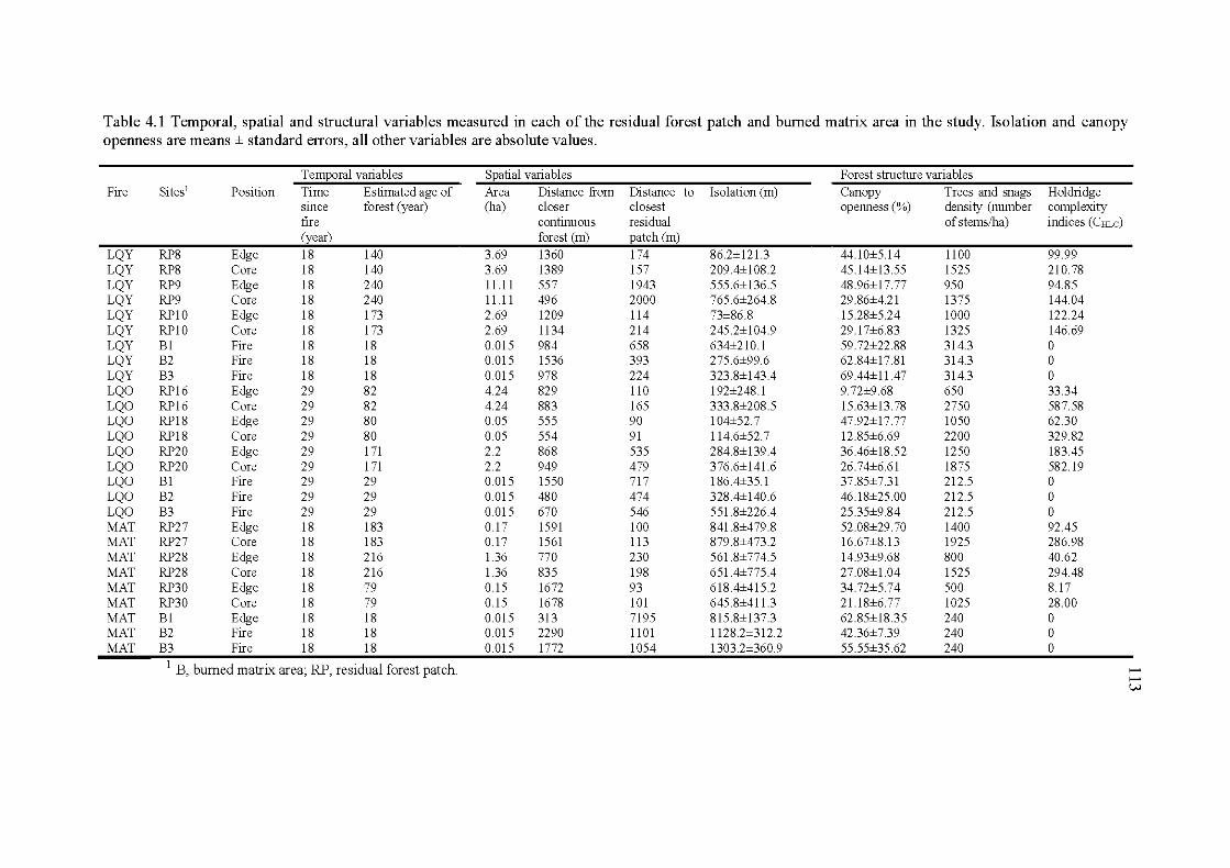
Table 4.1 Temporal, spatial and structural variables measured in each of the residual forest patch and burned matrix area in the study. Isolation and canopy openness are means ± standard errors, all other variables are absolute values.

Temporal variables Spatial variables Forest structure variables Fire Sites1 Position Ti me Estimated age of Are a Distance from Distance to Isolation (rn) Canopy Trees and snags Holdridge

sm ce forest (year) (ha) doser closest openness (%) density (number complexity fire continuous re si dual of stems/ha) indices (CHLC) (year) forest (rn) patch (rn)

LQY RP8 Edge 18 140 3.69 1360 174 86.2±121.3 44.10±5. 14 11 00 99 .99 LQY RP8 Core 18 140 3.69 1389 157 209.4±108.2 45 .14±1 3.55 1525 210.78 LQY RP9 Edge 18 240 11.11 557 1943 555.6±136.5 48 .96±17.77 950 94.85 LQY RP9 Core 18 240 11.11 496 2000 765.6±264.8 29 .86±4.21 1375 144.04 LQY RP10 Edge 18 173 2.69 1209 114 73±86.8 15.28±5.24 1000 122.24 LQY RP10 Core 18 173 2.69 1134 214 245.2±104.9 29.17±6.83 1325 146.69 LQY B1 Fire 18 18 0.015 984 658 634±210 .1 59. 72±22 .88 314.3 0 LQY B2 Fire 18 18 0.015 1536 393 275.6±99.6 62.84± 17.81 314.3 0 LQY B3 Fire 18 18 0.015 978 224 323.8±143.4 69 .44± 11.47 314.3 0 LQO RP16 Edge 29 82 4.24 829 110 192±248.1 9.72±9.68 650 33.34 LQO RP1 6 Core 29 82 4.24 883 165 333.8±208.5 15.63±13.78 2750 587.58 LQO RP18 Edge 29 80 0.05 555 90 104±52.7 47.92±17.77 1050 62 .30 LQO RP18 Core 29 80 0.05 554 91 114.6±52.7 12.85±6.69 2200 329.82 LQO RP20 Edge 29 171 2.2 868 535 284.8±139 .4 36.46±18.52 1250 183.45 LQO RP20 Core 29 171 2.2 949 479 376.6±141.6 26 .74±6.61 1875 582.1 9 LQO B1 Fire 29 29 0.015 1550 7 17 186.4±35.1 37.85±7.31 212.5 0 LQO B2 Fire 29 29 0.015 480 474 328.4±140.6 46 .18±25 .00 212.5 0 LQO B3 Fire 29 29 0.01 5 670 546 551.8±226.4 25.35±9.84 212.5 0 MAT RP27 Edge 18 183 0.17 1591 100 841.8±479.8 52 .08±29 .70 1400 92 .45 MAT RP27 Core 18 183 0.17 1561 113 879.8±473.2 16 .67±8.13 1925 286.98 MAT RP28 Edge 18 216 1.36 770 230 561.8±774.5 14.93±9.68 800 40.62 MAT RP28 Core 18 216 1.36 835 198 651.4±775.4 27.08± 1.04 1525 294.48 MAT RP30 Edge 18 79 0.15 1672 93 618.4±415.2 34.72±5.74 500 8.17 MAT RP30 Core 18 79 0.15 1678 101 645.8±411.3 21.18±6.77 1025 28 .00 MAT B1 Edge 18 18 0.01 5 313 7195 815.8±137.3 62 .85± 18.35 240 0 MAT B2 Fire 18 18 0.01 5 2290 1101 1128.2±312.2 42 .36±7.39 240 0 MAT B3 Fire 18 18 0.015 1772 1054 1303.2±360.9 55 .55±35 .62 240 0

1 B , bumed m atrix area; RP, residual forest patch. ....... ....... w

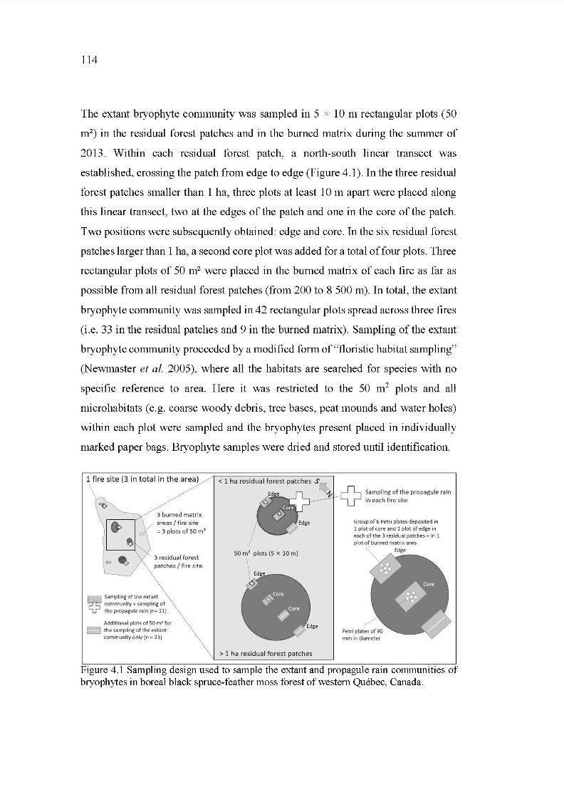
114

The extant bryophyte community was sampled in 5 x 10 rn rectangular plots (50

m2) in the residual forest patches and in the burned matrix during the summer of

2013. Within each residual forest patch, a north-south linear transect was

established, crossing the patch from edge to edge (Figure 4.1). In the three residual

forest patches smaller than 1 ha, three plots at least 10 rn apart were placed along

this linear transect, two at the edges of the patch and one in the core ofthe patch.

Iwo positions were subsequently obtained: edge and core. In the six residual forest

patches larger than 1 ha, a second core plot was added for a total of four plots. Three

rectangular plots of 50 m2 were placed in the burned matrix of each fire as far as

possible from all residual forest patches (from 200 to 8 500 rn). In total, the extant

bryophyte community was sampled in 42 rectangular plots spread across three fires

(i.e. 33 in the residual patches and 9 in the burned matrix). Sampling ofthe extant

bryophyte community proceeded by a modified form of"floristic habitat sampling"

(Newmaster et al. 2005), where all the habitats are searched for species with no

specifie reference to area. Here it was restricted to the 50 m2 plots and all

microhabitats (e.g. coarse woody debris, tree bases, peat mounds and water holes)

within each plot were sampled and the bryophytes present placed in individually

marked paper bags. Bryophyte samples were dried and stored until identification.

1 fire site (3 in total in the area

3 burned mat rix

a reas 1 f i re site = 3 plots of 50 m'

3 resid ual forest

patches 1 fi re site

~ Sampling of the extant community + sampling of the propagule rain (n= 21}

Addit ional plots of 50 m'for = the sampling of the extant community only (n = 21)

50 m' plots (5 x 10 m)

~Core

~Core

~ • :

> 1 ha residual fo rest patch es

Sampling of t he propagule ra in

in each f i re site

Group of 6 Petri plates deposited in 1 plot of core and 1 plot of edge in each of the 3 residual patch es+ in 1 plot of burned matrix a rea

Edge

mm in diameter

Figure 4.1 Sampling design used to sample the extant and propagule rain communities of bryophytes in boreal black spruce-feather moss forest of western Québec, Canada.

115

Propagule rain was sampled by the "emergence method" (Rudolph 1970; Ross

Davis & Frego 2004). Petri plate traps (90 mm in diameter) were filled with 78.5

cm2 ofnutrient agar made in sterile laboratory conditions [Parker Thompson's basal

nutrient medium of Klekowski (1969), described by C-Fern Project © (1995-

2014)]. All bryophyte propagule types were included (i.e. spores, gemmae and

possible vegetative fragments dispersed via the air; During & van Tooren 1987). In

each residual forest patch, a group of six Petri plates was placed in the centre of one

core and one edge 50 m2 extant community plot. In addition, a group of six Petri

plates was also placed in one of the three bumed matrix plots per fire. Propagule

rain was trapped during four sessions: the 11 th and 16th August (summer) and the

4th and 13th September (autumn) of2013 as well as the 9th and llth June (spring)

and the 14th and 19th September (autumn) of 2014. Two days are required in each

trapping session due to the distance among the fire sites (average of 128 km). The

total number of Petri plates exposed over the four sessions is 504 [ ( 6 x 2 x 9 + 3 x

6) x 4]. Petri plates were deposited in the forest for six hours from early moming

when capsules are moistened by dew to early aftemoon when capsules are dried

and temperatures are the warmest. During this period propagule release is triggered

by hydration-dehydration of the capsule and elators (V anderpoorten and Goffinet

2009). Petri plates were exposed on days that were both sunny and windy (wind

speeds between 3 and 10 km/h; i.e. optimal conditions for drying and explosion of

the capsule for propagule release; Glime 2013). After exposition, the Petri plates

were covered and placed in germination chambers for six months, under fluorescent

light tubes with continuous spectrum Verilux ® (48" and 32 Watt) with a 12 h/12

h light/dark regime. Germination chamber temperature was maintained at 22°C.

Petri plates were kept moist by misting with deionized water. When the nutrient

agar became too thin it was transferred onto a new Petri plate. Development of

bryophyte gametophytes was assessed twice a week to follow germination patterns

and to control potential bacterial or fungal contaminations. Minor contaminations

were manually removed from the nutrient agar with forceps. In the case of a major

contamination (i.e. all of the Petri plate was infected and survival of the

protonemata was compromised), protonemata were removed from the plate, bathed

116

in deionised water and transplanted onto a new Petri plate. Three control Petri plates

with virgin nutrient agar were placed in the germination chambers every three

months for the duration of the 6-month emergence period to identify potential

contaminants (air-borne bryophyte propagules). No bryophyte species developed

on any of the control plates, indicating that sample plates had not be en contaminated

during the laboratory growing period. Bryophyte culture with this method was

generally successful however, the principal bias is that only the species able to

germinate in the Petri plates were accounted for.

All bryophytes were identified in the laboratory following Faubert (2012, 2013,

2014) except for Sphagnum subtile (Russ.) Wamst., which follows the

nomenclature ofthe Flora of North America Editorial Committee (2007). Species

were classified by taxonomy and growth form (i.e. liverwort, acrocarp, pleurocarp,

and Sphagnum; Meusel 1935) and by life strategy following During (1992)

(Appendix H). Species' reproductive state in the field was also noted (i.e. sterile or

fertile with presence of sporophyte or gemmae, Appendix 1). Bryophyte species

richness and frequency were calculated per plot for the extant community and per

group of six Petri plates for the propagule rain (Appendices 1 and J). The frequency

of each species per plot and per group of six Petri plates was defined as the number

of microhabitats where a species was found per plot and as the number of Petri

plates of the group where a species was recorded. In the Petri plates, one individual

refers to a protonema in one Petri plate. While one protonema can generate several

stems making it difficult to distinguish individuals, we took monthly photographs

of the plates, and used these pictures to identify individuals. Due to the artificial

growing conditions in the Petri plates, bryophytes had unusual characteristics,

consequently certain specimens were only identified to genus, particularly sphagna

and members of the genera Ditrichum spp., Grimmia spp., Pohlia spp. , and

Polytrichum spp. Vouchers are conserved at the University of Québec in Abitibi

Témiscamingue, Qc, Canada.

117

The roles of temporal, spatial and forest structure variables in explaining patterns

of bryophyte dispersal were evaluated (Table 4.1 ). Temporal variables included

time since fire (years), determined from the SOPFEU digital map (2011) and the

age of the forest in the residual patch. The minimum stand age of the forest in the

residual patches (years) was estimated by coring ten dominant trees in the core of

the residual forest patches with an increment corer and counting the number of

rings. The age of the oldest tree was established as the minimum stand age. Spatial

variables were calculated using ArcGis 10.2 (ESRI 2013) and included residual

patch area (ha), distance to the closest residual patch (rn), shortest distance to

continuous forest (rn), and isolation (mean of five distances between the point of

interest and all forest sources, i.e. residual forest patch, continuous forest, residual

riparian forest; rn). Forest structure variables of the residual patches, i.e. canopy

openness (%), tree and snag density (number of stems 1 ha) and stand complexity,

were measured in the field during the summer of 2013. Canopy openness was

measured using a densiometer, a scored concave mirror, at the level of the

bryophyte layer (5 to 10 cm above the forest floor). The measure was taken in three

randomly chosen positions in each rectangular plot and averaged. Tree/snag density

was calculated in 11.28 rn radius (400m2) circular plots at the core of each residual

patch and with the line intersect method at the edge of each residual patch. All trees

and snags with DBH > 9 cm were included. Stand complexity was estimated using

the modified Holdridge index (CHcL) (Holdridge et al. 1971) computed only on

trees with DBH > 9 cm (Lugo et al. 1978).

4.4.3 Data analyses

Data analyses of species richness, assemblage and similarity were performed on the

extant and propagule rain communities found in the 21 plots where Petri plates had

been placed (i.e. core and edge plots in three residual forest patches per fire, and

one bumed matrix plot per fire) plus two additional bumed matrix plots per fire, for

118

a total of 27 plots. The additional bumed matrix plots were included for better

representation of the extant community in this environment.

R software 3.2.1 (R-Development-Core-Te am 20 15) was used for statistical

analyses with a significance level of a = 0.05. Results with p-values between 0.1

and 0.05 are also discussed as they suggest trends in the data, which are important

to consider in order to identify fine sc ale biological responses (Murtaugh 20 14; de

V alpine 2014 ).

As we used a nested design (plots of residual forests and bumed matrix in fires) we

tested whether the spatial structure of the sampling influenced the mo dels in the

different analyses with a LogLik test (Pinherio & Bates 1995). In cases where the

spatial structure did not influence the models, the simpler model without random

spatial effects (linear model, lm) was chosen in the spirit of parsimony. When the

spatial structure had a significant effect, we used linear mixed models (lme ), which

are equivalent to lm for a structured dataset.

Comparisons of the composition of extant and propagule ram communities

(objective 1) were made using rank abundance curves (Magurran 1988) performed

with the package "BiodiversityR" 2.5-3 (Kindt 2015). The overall composition of

the two communities was summarised in a detrended correspondence analysis

(DCA; Hill & Gauch 1980; Leps & Smilauer 2003) on presence-absence data of

species occurring more than five times in the entire data-set using the package

"vegan" 2.3-0 (Oksanen et al. 2015). Specimens identified only to genus and for

whom other species of the same genus were present were removed from the DCA

analysis as well as from the subsequent analyses of similarity, as the index was

calculated from DCA. The subsequent ordination matrix contained 65 species and

48 sites (27 plots of extant community and 21 plots of propagule rain). The

significance of the resultant pattern was determined by Multi-Response

Permutation Procedure (MRPP) on 2000 permutations.

119

In order to address the second objective, to determine the relationship between

geographie distance and compositional similarity of the propagule rain and extant

communities, Jaccard's index of similarity was used. Jaccard 's index was chosen

because it compares the number of shared species to the total number of species in

the combined assemblage while Smensen's index compares the number of shared

species to the mean number of species in a single assemblage; Jost, Chao &

Chazdon 2011). Jaccard's index of similarity was calculated between each

propagule rain groups (n = 21) and all the extant community plots where Petri plates

were placed (n = 21 ). Similarity between the propagule rain and the extant

community was then examined in function of the geographie distance between

them. Subsequently, in order to focus on the dispersal into the disturbed matrix, the

same analysis was completed considering only the propagule rain of the bumed

matrix (n = 3) but with all the extant community plots (n = 21 ). Geographie

distances were classified into spatial scales modified from Ross-Davis & Frego

(2004 ): 1. In situ, propagules of the extant community in a given sampling point

(50m2 plot of group of Petri plates); 2. Local, propagules from the closest potential

source, i.e. the closest residual patch (650-1100 rn); 3. Intra-fire, propagules from

all residual patches in a given fire (740-8400 rn); 4. Inter-fire, propagules from

communities in all residual patches from the otherfires (10-130 km). The intra- and

inter-fire scales together refer to the regional spatial scale. The spatial structure of

the sampling design influenced the results of this analysis, as indicated by the

LogLik test, and community similarity among spatial scales was therefore

compared using linear mixed models (lme) performed with the package "nlme" 3.1-

121 (Pinheiro 2015).

Patterns of individual species in the propagule rain of burned matrices were also

examined, to determine from which distance they could have been dispersed. For

this comparison, the origin of the species in the propagule rain of the bumed

matrices (n = 3) was determined in function of the extant community in all the plots,

i.e. 42 plots (21 plots where Petri plates were placed plus the 21 additional plots of

the linear transect and of the bumed matrix; see sampling design for details in

120

Figure 4.1 ). The additional plots increased the sampling of the extant community

to better represent potential propagule sources in the surrounding landscape. For

each record of each species found in the propagule rain of each fire we determined

in which extant community plots it was also found. The spatial scale (i.e. in situ,

local, regional) relative to the record in question was noted. If a species of the

propagule rain was encountered at two spatial scales in the extant community, each

distance was scored in the analysis. This analysis generated a matrix of species x

spatial scale, where the presence or absence of each species at each spatial scale is

indicated, which indicates the number of species that potentially dispersed from

each spatial scale in each fire, for ''total" (all species grouped together, n = 21),

"perennial" (n = 9) and "colonist" (n = 1 0) species groups. The three fires were then

averaged to have a mean number of species dispersed per spatial scale. In each

group (i.e. total, perennial or colonist) the mean number of species was then divided

by the number of plots sampled at each spatial scale in the three fires pooled

together (nin situ= 3; n closest-RP = 11; n intra fire = 28; n inter fire = 84 i.e. N =

126) in order to take into account the different number of potential propagule

sources analysed at each spatial scale. The value obtained was reported as a percent

of the total number of species present per plot in the four spatial scales. This actual

frequency was then compared to a theoretical expected frequency. Expected

frequency was calculated by multiplying the sum of the mean number of species

present per plot in each spatial sc ale by the number of plots that could be potential

propagule sources in the target spatial scale and dividing by the total number of

potential propagule sources available (N). We therefore obtained an expected

frequency specifie to each spatial scale weighted by the number of plots

participating in the propagule rain at this spatial scale. The difference between

actual and expected frequencies for total, perennial and colonist species was then

calculated and tested for significance with a Fisher test.

In the third objective we assessed the relative roles of geographie distance and nine

environmental variables ( divided into temporal, spatial and forest structure classes)

in influencing the similarity between extant community where Petri plates were

121

placed (n = 21) and propagule rain community ofbumed matrix (n = 3) at different

spatial scales. Again, Jaccard's index of similarity represented the similarity

between the extant and propagule rain communities. In this analysis, we only

considered the propagule rain of the bumed matrices in order to assess the relative

importance of geographie distance compared to environmental variables in

bryophyte dispersal after disturbance. We tested the pertinence of including a

quadratic relationship between similarity and distance but the inclusion of this term

did not result in a significant increase in explanatory power. In the spirit of

parsimony, we therefore retained a linear relationship with geographie distance in

our models. A model selection procedure using 18 candidate models plus the null

model was performed. The first model tested geographie distance (distance between

sites) and the nine following models tested each ofthe variables ofthe temporal (2

mo dels), the spatial ( 4 models) and the structure (3 mo dels) classes individually

(Appendix K). The eight other models tested biologically relevant combinations of

these variables and interaction terms among several variables in each class. The

global model combined together eight ofthe variables ofthe four different classes

plus an interaction term. Conflict between certain variables prevented the use of all

10 variables in the global mo del, even after algorithm optimization. Here we define

the global model as the most complex of the model set. The response variable

"similarity", expressed as a proportion follows a normal distribution and was used

without transformation in linear mixed models (lme) with random effects,

performed with the package "nlme" 3.1-121 (Pinheiro 2015). The explanatory

variable dataset was standardised (on columns) to account for the different scales

ofmeasurement. Candidate models were ranked based on the Akaike 's Information

Criterion corrected for small sample size (AICc) (Bumham & Anderson 2002)

using the package AICcmodavg 2.0-3 (Mazerolle 2015). Models with a delta AICc

(L1AICc) > 2.0 were considered to have substantially lower empirical support

(Bumham & Anderson 2002). The model with the lowest delta AICc was

considered as the most parsimonious and indicated the environmental variables that

best explained variations in community similarity. In order to illustrate the effect of

each explanatory variable of the most parsimonious model, multimodel inference

122

was used. We obtained 95% confidence intervals and model predictions using the

modavgpred function of the AICcmodavg 2.0-3 package (Mazerolle 2015).

Variables with 95% confidence intervals excluding 0 have a significant effect on

the explanatory variable ( community similarity) and the ir predicted values were

subsequently plotted against values of the explanatory variable. An estimate of

model adjustment was indicated by Spearman's Rho. These analyses were carried

out first on all dispersal scales combined to identify a general dispersal pattern and

secondly, intra- and inter-fire scales of dispersal were examined individually.

Finally, the influence of geographie distance on similarity was also examined in

only the propagule rain, to eliminate the bias associated with the emergence method

(objective 4). The 21 plots where Petri plates were placed were again used in the

analysis. We calculated Jaccard's similarity index to determine the relationship

between the similarity of the propagule rain in different plots and their geographie

distance, which was divided into three categories: < 1.5 km (i.e. propagules rain

communities at the in situ and local scales), between 1.5 and 10 km (i.e. propagule

rain communities at intra-fire scale) and > 10 km (i.e. propagule rain communities

at inter-fire scale). The spatial structure of the sampling did not influence this

analysis, therefore the relationship between geographie distance and community

similarity was tested by a linear model (lm), followed by Tukey HSD tests using

the package "ade4" 1.7-2 (Dray, Dufour & Thioulouse 2015).

4.5 Results

4.5.1 Compositional similarity between the extant community and the

propagule rain

Of the 123 taxa found, 23 were present in both the extant community and the

propagule rain. Nineteen species were exclusively found in the propagule rain, and

ofthese 32% were colonist, 37% were perennial and 26% were shuttle (Appendices

1 and J). In the extant community, 67% ofthe species sampled were seen fertile at

123

least once and 28% ofthese fertile species were encountered in the propagule rain

(Appendix I). In terms of species richness the extant community was dominated by

pleurocarps whereas acrocarps dominated the propagule rain (21 acrocarps: 25

pleurocarps and 20 acrocarps: 12 pleurocarps respectively). In contrast, extant and

propagule rain communities were equally divided between perennial and colonist

species ( 40 perennial: 45 colonist and 18 perennial: 18 colonist respectively,

Appendices I and J). Five shuttle species were present in each ofthe communities.

Rank abundance curves indicated that the ten most abundant species differed

between the extant community and the propagule rain (Figure 4.2a, b ). Half of the

species were pleurocarps and liverwort species in the extant community whereas in

the propagule rain most species were acrocarps. Of the ten most abundant species

in the extant community, half were perennials and one species was colonist, while

in the propagule rain community, half were colonists and four were perennials

(Figure 4.2a, b ).

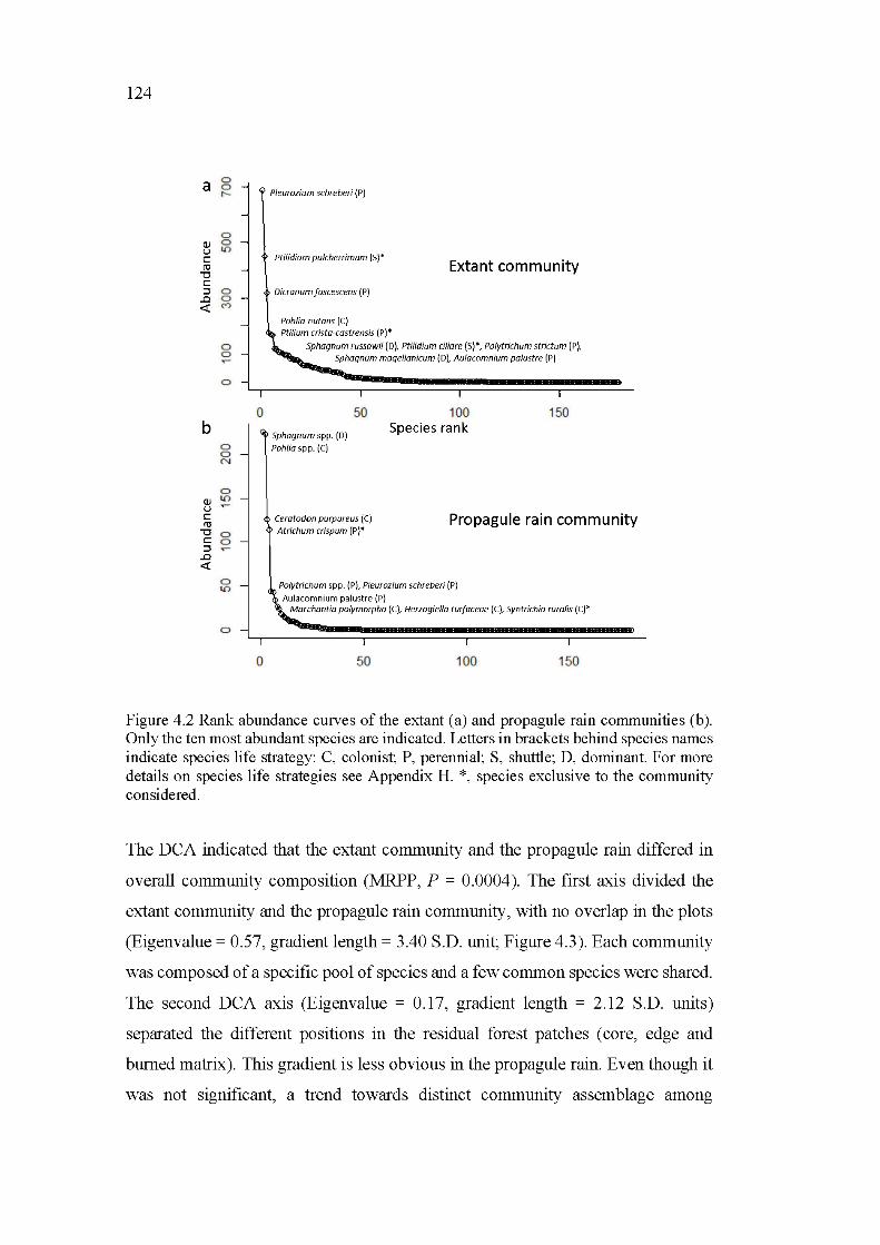
124

a 0 0 ,._

0 Q) 0 u 1.()

c rn

-a c :::J 0

.!:l 0 <l: <">

0 0

0

0 b

0 0 N

0 Q) 1.()

u c rn

-a 0 c 0 :::J

.!:l <l:

0 1.()

0

0

Pleurozium schreberi (P)

Ptilidium pulcherrimum (S)* Extant community

Dicranum fuscescens (P)

Pohlia nutans (C) Ptilium crista-castrensis (P)*

Sphagnum russowii (D), Ptilidium ciliare (5)*, Polytrichum strictum (P), Sphagnum magellanicum (D), Aulacomnium palustre (P)

50 100 150

Sphagnum spp. (D) Species rank

Poh/ia spp.(C)

Ceratodon purpureus (C) Propagule rain community Atrichum crispum (P)*

Polytrichum spp.(P), Pleurozium schreberi (P)

Aulacomnium palustre (P) Marchantia polymorpha (C), Herzogiel/a turfaceae (C), Syntrichia rurolis (C)*

50 100 150

Figure 4.2 Rank ab un dance curves of the extant (a) and propagule rain communities (b ). Only the ten most abundant species are indicated. Letters in brackets behind species names indicate species life strategy: C, colonist; P, perennial; S, shuttle; D, dominant. For more details on species life strategies see Appendix H. *, species exclusive to the community considered.

The DCA indicated that the extant conununity and the propagule rain differed in

overall conununity composition (MRPP, P = 0.0004). The first axis divided the

extant community and the propagule rain conununity, with no overlap in the plots

(Eigenvalue = 0.57, gradient length = 3.40 S.D. unit; Figure 4.3). Each community

was composed of a specifie pool of species and a few conunon species were shared.

The second DCA axis (Eigenvalue = 0.17, gradient length = 2.12 S.D. units)

separated the different positions in the residual forest patches (core, edge and

bumed matrix). This gradient is less obvious in the propagule rain. Even though it

was not significant, a trend towards distinct conununity assemblage among

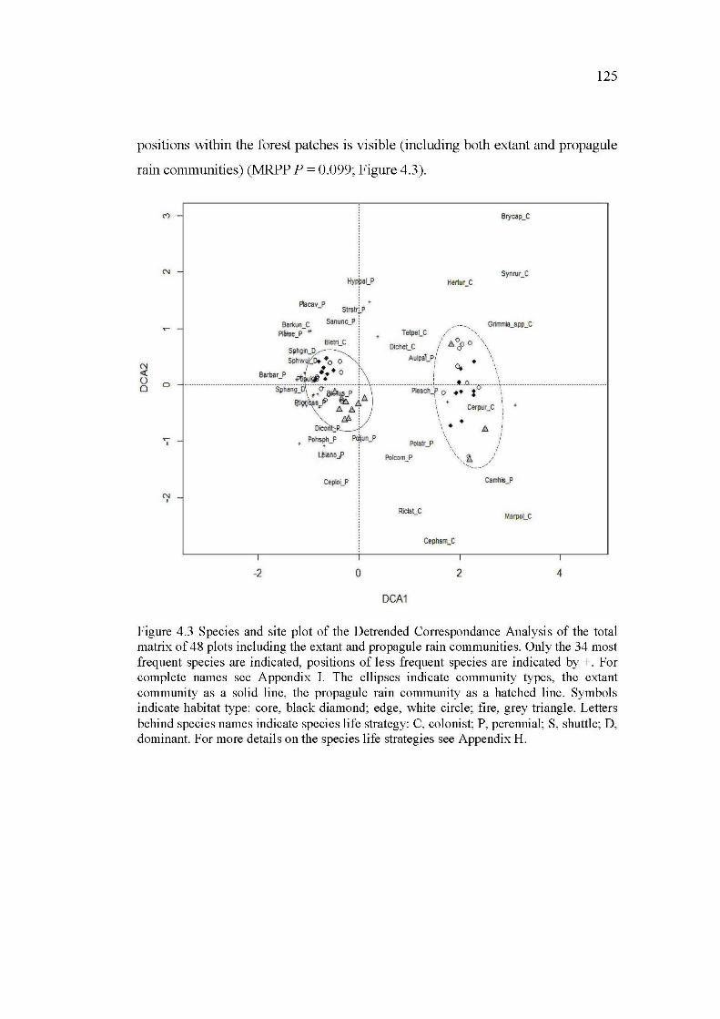
125

positions within the forest patches is visible (including both extant and propagule

rain communities) (MRPP P = 0.099; Figure 4.3).

N <( ü 0

-2

Hyllbai_P

~cav_P : + StrstrLP

Barkun C P~lae_P- "

Sanunc_P !

Bletri_C

Oicon

Pohsph_P +

Pciljun_P

~tano)'

Ceptoi_P

0

Brycap_C

Synrur_C Hertur_C

Grinmia_spp_C Tetpei_C

• Polstr_P

Polcom_P

Camhis_P

Rictat_C l.tarpoi_C

Cepham_C

2 4

DCA1

Figure 4.3 Species and site plot of the Detrended Correspondance Analysis of the total matrix of 48 plots including the extant and propagule rain communities. Only the 34 most frequent species are indicated, positions of less frequent species are indicated by +. For complete names see Appendix 1. The ellipses indicate community types, the extant community as a solid line, the propagule rain community as a hatched line. Symbols indicate habitat type: core, black diamond; edge, white circle; fire, grey triangle. Letters behind species names indicate species life strategy: C, colonist; P, perennial; S, shuttle; D, dominant. For more details on the species life strategies see Appendix H.

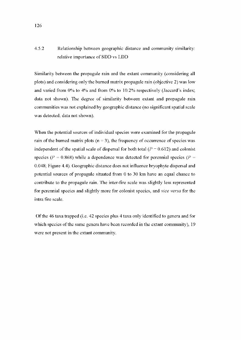
126

4.5.2 Relationship between geographie distance and community similarity:

relative importance of SDD vs LDD

Similarity between the propagule rain and the extant community ( considering all

plots) and considering only the bumed matrix propagule rain (objective 2) was low

and varied from 0% to 4% and from 0% to 10.2% respectively (Jaccard's index;

data not shown). The degree of similarity between extant and propagule rain

communities was not explained by geographie distance (no significant spatial scale

was detected; data not shown).

When the potential sources of individual species were examined for the propagule

rain of the bumed matrix plots (n = 3), the frequency of occurrence of species was

independent ofthe spatial scale of dispersal for both total (P = 0.612) and colonist

species (P = 0.868) while a dependence was detected for perennial species (P =

0.048; Figure 4.4). Geographie distance does not influence bryophyte dispersal and

potential sources of propagule situated from 0 to 30 km have an equal chance to

contribute to the propagule rain. The inter-fire scale was slightly less represented

for perennial species and slightly more for colonist species, and vice versa for the

intra fire scale.

Of the 46 taxa trapped (i.e. 42 species plus 4 taxa only identified to genera and for

which species of the same genera have been recorded in the extant community), 19

were not present in the extant community.

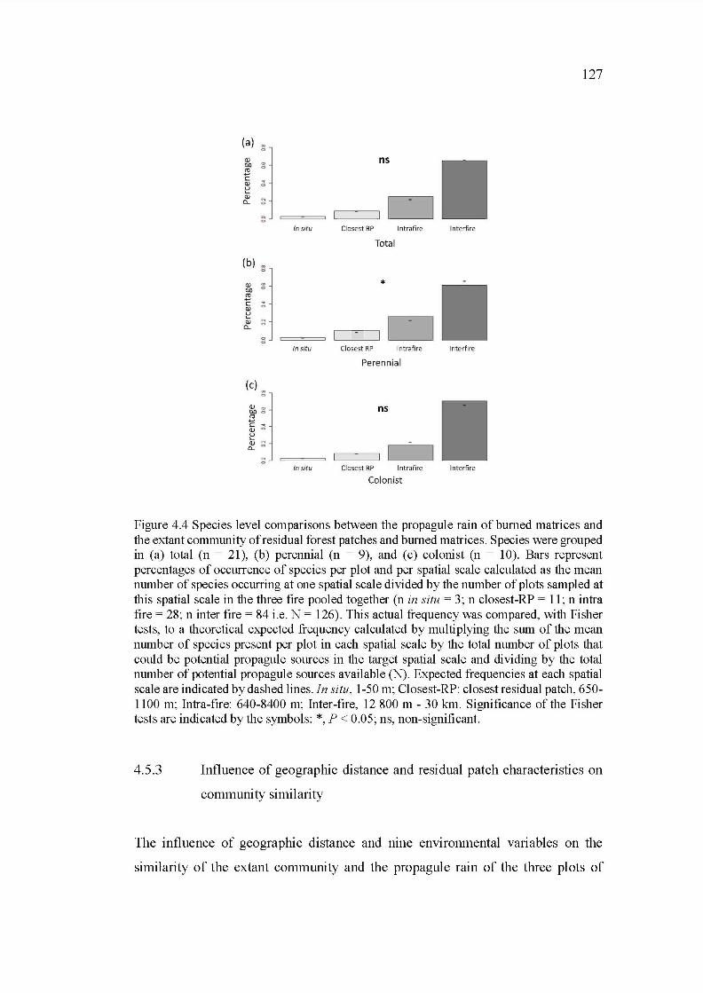
127

(a) :'l

Cl) ns 00 ~

"' ... c:

""' Cl) 0

~ Cl)

:l D a_

~ ln situ Closest RP lnt rafire lnterfire

Total

(b) ~

Cl) :':: * 00

"' ... c: ;; Cl) u ....

:l Cl) a_

~ ln situ Closest RP lntrafire lnterf ire

Perennial

(c) :'l

Cl) "' OO o ns "' ... c: d Cl)

~ Cl) :l 0..

~ ln situ Closest RP lnt rafire lnterfire

Colonist

Figure 4.4 Species level comparisons between the propagule rain of bumed matrices and the extant community ofresidual forest patches and bumed matrices. Species were grouped in (a) total (n = 21), (b) perennial (n = 9), and (c) colonist (n = 10). Bars represent percentages of occurrence of species per plot and per spatial scale calculated as the mean number of species occurring at one spatial scale divided by the number of plots sampled at this spatial scale in the three fire pooled together (nin situ = 3; n closest-RP = 11; n intra fire = 28; n inter fire = 84 i.e. N = 126). This actual frequency was compared, with Fisher tests, to a theoretical expected frequency calculated by multiplying the sum of the mean number of species present per plot in each spatial scale by the total number of plots that could be potential propagule sources in the target spatial scale and dividing by the total number of potential propagule sources available (N). Expected frequencies at each spatial scale are indicated by dashed lines.ln situ, 1-50 rn; Closest-RP: closest residual patch, 650-1100 rn; Intra-fire: 640-8400 rn; Inter-fire, 12 800 rn - 30 km. Significance of the Fisher tests are indicated by the symbols: *, P < 0.05; ns, non-significant.

4.5.3 Influence of geographie distance and residual patch characteristics on

community similarity

The influence of geographie distance and mne environmental variables on the

similarity of the extant community and the propagule rain of the three plots of

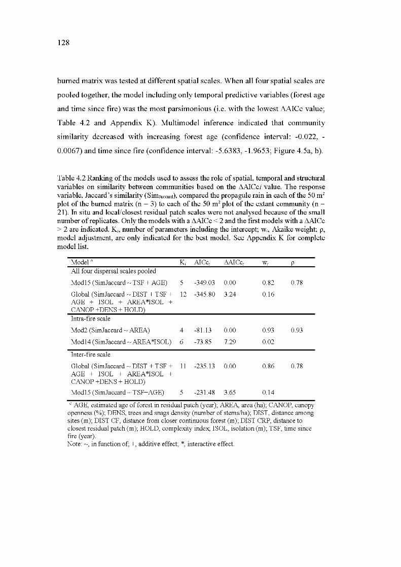
128

bumed matrix was tested at different spatial scales. When all four spatial scales are

pooled together, the model including only temporal predictive variables (forest age

and time since fire) was the most parsimonious (i.e. with the lowest L1AICc value;

Table 4.2 and Appendix K). Multimodel inference indicated that community

similarity decreased with increasing forest age (confidence interval: -0.022, -

0.0067) and time since fire (confidence interval: -5.6383, -1.9653; Figure 4.5a, b).

Table 4.2 Ranking of the models used to assess the role of spatial, temporal and structural variables on similarity between communities based on the L1AICci value. The response variable, Jaccard's similarity (SimJaccarct), compared the propagule rain in each of the 50 m1

plot of the bumed matrix (n = 3) to each of the 50 m1 plot ofthe extant community (n =

21). In situ and local/closest residual patch scales were not analysed because of the small number of replicates. Only the models with a L1AICc < 2 and the frrst models with a L1AICc > 2 are indicated. K,, number of parameters including the intercept; wi, Akaike weight; p, model adjustment, are only indicated for the best model. See Appendix K for complete modellist.

Madel o

All four dispersal scales poo led

Mod15 (SimJaccard ~TSF + AGE)

K AICc, L'AI Cc,

5 -349.03 0.00

w,

0.82

Global (SimJaccard ~ DIST +TSF+ 12 -345.80 3.24 0.16 AGE + ISOL + AREA *ISOL + CANOP +DENS + HOLD) Intra-fire scale

Mod2 (SimJ accard ~ AREA) 4 -81. 13

Mod14(SimJaccard~AREA*ISOL) 6 -73.85

Inter-fire scale

0.00

7.29

Global (SimJaccard ~ DIST +TSF+ 11 -235.13 0.00 AGE + ISOL + AREA *ISOL + CANOP +DENS + HOLD)

Mod15 (SimJaccard ~TSF+ AGE) 5 -231.48 3.65

0.93

0.02

0.86

0.14

p

0.78

0.93

0.78

o AGE, estimated age of forest in residual patch (year); AREA, are a (ha); CANOP, canopy openness (%); DENS, trees and snags density (num ber of stems/ha); DIST, distance among sites (rn); DIST CF, distance from closer continuous forest (rn); DIST CRP, distance to closest residual patch (rn); HOLD, complexity index; ISOL, isolation (rn); TSF, time since fire (year). Note: ~, in function of;+, additive effect; *, interactive effect.

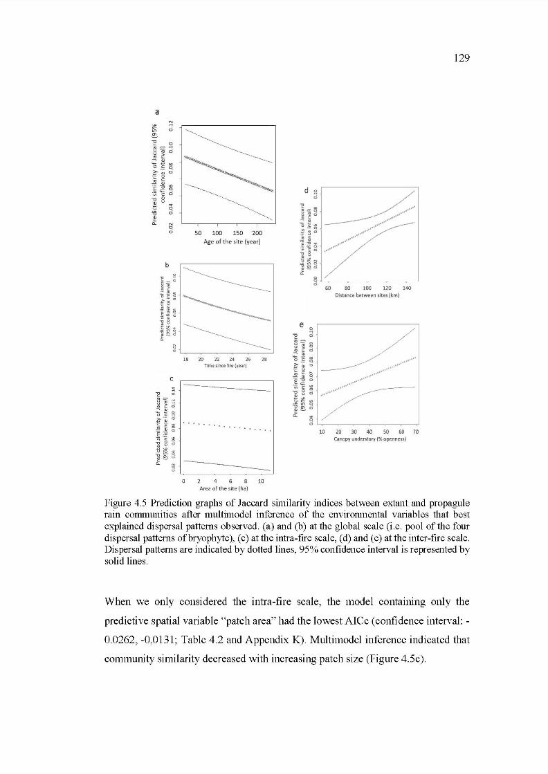
a

"E 0 ., _,... u ro o ~ r: ~ <li

0 ë ~ .~ ·~ 0

~ ~ .Ë ~ ~ ·v; c 0 ] 8 tl g :.a 0 <li

Ô: N 0

0 50 100 150 200 Age of the site (year)

18 20 22 24 26 28 Ti me si nee fi re (year)

c

0. 0 • • • 0 . 0

• • 0 • • . . . .

0 4 6 8 10 Area of the site (ha)

d ~~ 0

~ .. § ~ ~ j ······•··· ftl L. •••

15 -~ ~ ··········•· ·E ~ o ·········· ..!!! G.l ••••

! ~ g ~ ···•·••• ~ c 0 j •'

"" 0 ~ v ti~N

]~~ ;;:

e ~

~ o · 5:;ij'E ~ C! ci ~ <li

60 80 100 120 140 Distance between sites (km)

- ~ ~ .. ~ ·; ~ ~ ··········· ·c g ,... ····•······ .Jg QI q ~ ••••••••••

f~~ 1.~·······"····· (LI u 0 ••••• t)~ V\

:g ~ ~ ~

ô: ;g . 0 '--r---~~-~-~----.J

10 20 30 40 50 60 70 canopy understory (% openness)

129

Figure 4.5 Prediction graphs of Jaccard similarity indices between extant and propagule rain communities after multimodel inference of the environmental variables that best explained dispersal patterns observed. (a) and (b) atthe global scale (i.e. pool ofthe four dispersal patterns ofbryophyte ), ( c) at the intra-fire scale, ( d) and ( e) at the inter-fire sc ale. Dispersal patterns are indicated by dotted lines, 95% confidence interval is represented by solid lines.

When we only considered the intra-fire scale, the madel containing only the

predictive spatial variable " patch are a" had the lowest AI Cc (confidence interval: -

0.0262, -0,0131~ Table 4.2 and Appendix K). Multimodel inference indicated that

community similarity decreased with increasing patch size (Figure 4 .5c ).

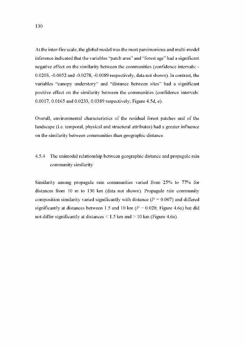
130

At the inter-fire scale, the global mo del was the most parsimonious and multi -model

inference indicated that the variables "patch area" and "forest age" had a significant

negative effect on the similarity between the communities (confidence intervals: -

0.0203, -0.0052 and -0.0278, -0.0089 respectively, data not shown). In contrast, the

variables "canopy understory" and "distance between sites" had a significant

positive effect on the similarity between the communities (confidence intervals:

0.0017, 0.0165 and 0.0233,0.0389 respectively; Figure 4.5d, e).

Overall, environmental characteristics of the residual forest patches and of the

landscape (i.e. temporal, physical and structural attributes) had a greater influence

on the similarity between communities than geographie distance.

4.5.4 The unimodal relationship between geographie distance and propagule rain

community similarity

Similarity among propagule ram communities varied from 25% to 77% for

distances from 10 rn to 130 km (data not shown). Propagule rain community

composition similarity varied significantly with distance (P = 0.007) and differed

significantly at distances between 1.5 and 10 km (P = 0.028; Figure 4.6a) but did

not differ significantly at distances < 1.5 km and > 10 km (Figure 4.6a).

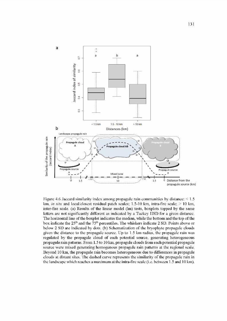
a

..... ci

> .... ·;:: ..!!! "' .Ë ci

Ill ..._. 0 x "' Q) ci

"0 c:

"E co u ">: u 0

~

M ci

b

0 1.5

0

a b a

EJ ~ ~ ~

~

< 1.5km 1.5-10km >10 km

Distances (km)

<10\ />10

'·······-·····-······-··-·---~~·-··---·-··-·----./ 1.5

131

o Distance from the propagule source (km)

Figure 4.6 Jaccard similarity index among propagule rain communities by distance: < 1.5 km, in situ and locallclosest residual patch scales; 1.5-10 km, intra-fire scale; > 10 km, inter-fire scale. (a) Results of the linear model (lm) tests, boxplots topped by the same letters are not significantly different as indicated by a Tuckey HSD for a given distance. The horizontalline of the boxplot indicates the median, while the bottom and the top of the box indicate the 25th and the 75th percentiles. The whiskers indicate 2 SD. Points above or below 2 SD are indicated by dots. (b) Schematization of the bryophyte propagule clouds given the distance to the propagule source. Up to 1.5 km radius, the propagule rain was regulated by the propagule cloud of each potential source, generating heterogeneous propagule rain patterns. From 1. 5 to 10 km, propagule clouds from each potential propagule source were mixed generating homogenous propagule rain patterns at the regional scale. Beyond 10 km, the propagule rain becomes heterogeneous due to differences in propagule clouds at distant sites. The dashed curve represents the similarity of the propagule rain in the landscape which reaches a maximum at the intra-fire scale (i.e. between 1.5 and 10 km).

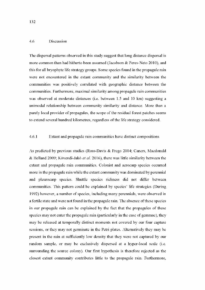
132

4.6 Discussion

The dispersal patterns observed in this study suggest that long distance dispersal is

more common than had hitherto been assumed (Jacobson & Peres-Neto 2010), and

this for all bryophyte life strate gy groups. Sorne species found in the propagule rain

were not encountered in the extant community and the similarity between the

communities was positively correlated with geographie distance between the

communities. Furthermore, maximal similarity among propagule rain communities

was observed at moderate distances (i.e. between 1.5 and 10 km) suggesting a

unimodal relationship between community similarity and distance. More than a

purely local provider of propagules, the scope of the residual forest patches seems

to extend several hundred kilometres, regardless ofthe life strategy considered.

4.6.1 Extant and propagule rain communities have distinct compositions

As predicted by previous studies (Ross-Davis & Frego 2004; Caners, Macdonald

& Belland 2009; Kôvendi-Jak6 et al. 2016), there was little similarity between the

extant and propagule rain communities. Colonist and acrocarp species occurred

more in the propagule rain while the extant community was dominated by perennial

and pleurocarp species. Shuttle species richness did not differ between

communities. This pattern could be explained by species' life strategies (During

1992) however, a number of species, including many perennials, were observed in

a fertile state and were not found in the propagule rain. The absence ofthese species

in our propagule rain can be explained by the fact that the propagules of these

species may not enter the propagule rain (particularly in the case of gemmae ), they

may be released at temporally distinct moments not covered by our four capture

sessions, or they may not germinate in the Petri plates. Alternatively they may be

present in the rain at sufficiently low density that they were not captured by our

random sample, or may be exclusively dispersed at a hyper-local scale (i.e.

surrounding the source colony). Our first hypothesis is therefore rejected as the

closest extant community contributes little to the propagule rain. Furthermore,

133

several perennial, colonist and shuttle species found in the propagule rain were not

present in the closest extant community or in any of the sampled communities. The

question ofthe origin ofthese propagules remains unanswered.

4.6.2 Non-linear relationship between community similarity and geographie

distance: LDD dominates SDD

The spatial limitation of bryophyte dispersal indicated by numerous studies (Miles

& Longton 1992; Laaka-Lindberg, Korpelainen & Pohjamo 2006) suggests that

community similarity should decrease with increasing distance. Our study indicates

that propagule rain composition is unrelated to distance from a putative propagule

source. When we compare the distances travelled by the propagules at the regional

scales (both intra- and inter-fire scales; average 21400 rn) with the distances

travelled at the in situ scale (average 25 rn), it becomes evident that regional

dispersal is common despite a significant handicap. This is true regardless of the

species life strategy, although slightly more for colonist than perennial species,

which may be justified by their life strategies. Indeed, colonist species are

characterized by a high reproductive effort and the production of numerous and

light spores (During, 1992). In contrast, perennial species have an overall low

sexual reproductive effort (Longton & Schuster 1983; During 1992), and while

many of them are commonly fertile there are few sporophytes per colony (Rydgren

& 0kland 2001; Cronberg 2002). Despite this, Longton & Schuster (1983) have

shown that Hylocomium splendens may produce large quantities of spores (around

100 000 per capsule) wh ose relatively small size ( 14-17 11m in diameter; Hill et al.

2007) favours wind dispersal. The tall sporophytes of these species enhance the

probability of spore uptake by the wind, and in this way one fertile colony with a

few capsules may release large numbers of spores to air layers several kilometers

high. Thus these spores can travel long distances due to stochastic wind events

(Lônnell, Jonsson & Hylander 2014). Coup led with the large colonies of perennial

134

and dominant species (i.e. sphagna), this may explain the high number of their

spores in the propagule rain.

Similarity between propagule rain and extant community was positively correlated

with increasing distance, leading to the rejection of our second hypothesis and

validating the occurrence of LDD in bryophyte metacommunities. The occurrence

of the LDD suggests that dispersal ability alone does not regulate bryophyte

colonisation of new areas. At least two non-mutually exclusive filters could also

apply to select species: sexual reproductive ability (i.e. quantity and viability of

spores), and environmental conditions at the establishment sites (Lônnell, Jonsson

& Hylander 2014; Mota de Oliveira & ter Steege 2015). Furthermore, the apparent

dominance of regional dispersal events suggests that dispersal mode is not affiliated

to the life strate gy group but rather depends on species traits. In the context of our

second objective, LDD did not appear to be the prerogative of colonist species. The

"inverse isolation hypothesis" already advanced by several authors (i.e. Szôvényi,

Sundberg & Shaw 2012; Sundberg 2013) seems to explain the patterns observed

here and bryophyte metacommunity dynamics depends on several dispersal scales,

and propagule sources therefore contribute both to local and regional diaspore

clouds (Sundberg 2005).

4.6.3 Environmental characteristics of the landscape as mam governors of

bryophyte metacommunity reassembly

As suggested in our third hypothesis, environmental characteristics of the local

habitat also explained the similarity patterns observed between extant and

propagule rain communities. Similarity increased with canopy openness, probably

due to increased wind speeds and therefore more efficient dispersal in more open

stands (Fenton & Bergeron 2006; Sundberg 2013). The pattern of decreasing

similarity with increasing time since fire, age and area of the residual forest patches

reflects that the oldest and largest patches may better m1m1c

135

"continuous/undisturbed" forests. They may shelter spec1es with specifie

microhabitat requirements (i.e. deadwood, canopy enclosure) typical of more

advanced stages of succession, increasing the dissimilarity with the propagule rain

assemblage composed of species of earliest successional stages. Cronberg (2002)

has also suggested that the maintenance of perennial species depends on the age of

the patch as sexual reproduction is less common in young patches compared to older

patches, which therefore contribute more to propagule clouds. Similarly, Lôbel,

Snall & Rydin (2006) demonstrated that many obligate epiphyte bryophytes are

affected by patch conditions that are linked to forest stand age. Maintaining old and

large sources is therefore critical for the persistence of late serai species that take

decades to reappear in a landscape without these refugia (Caners, Macdonald &

Belland 2009).

4.6.4 Bryophyte propagule ram over the landscape 1s homogenised by LDD

events

Our results suggest a nonlinear relationship between propagule rain community

similarity and distance. The propagule rain at the landscape scale was, as suggested

by the fourth hypothesis, composed of various propagule clouds and dispersal

within 1. 5 km of a focal point (SDD), resulted in little similarity between propagule

rain communities (Figure 4.6b ). Sundberg (2005) found similar results for sphagna.

However, beyond this distance up to 10 km from the focal point (> 1. 5 km and <

10 km), similarity among propagule rain communities was at its maximum as the

effects of SDD were diluted in a "regional cloud" of LDD contributing to the

homogenisation of the propagule rain across the landscape. As suggested by

Hylander (2009) and Sun db erg (20 13 ), the roles of micro site limitation and/or rapid

decline oflocal availability are masked by a higher regional propagule rain (LDD),

which corroborates our species level propagule results that indicated limited local

dispersal. Beyond 10 km, the similarity decreased due to the dominance of other

propagules clouds from more distant sources. Appropriate meteorological

136

conditions coupled with the absence of physical barriers to the wind in the

landscape matrix have been advanced to facilitate the LDD (Sundberg 2013).

Based on the spatial scales used in this study (both in the comparison between extant

and propagule rain communities and among propagule rain communities ), a

working definition of SDD and LDD can be formulated. We might conclude that

LDD refers to propagules dispersed from regional sources i.e. from 1.5 to overthan

100 km, whereas propagules dispersed from more local sources, under 1.5 km, are

included in SDD. However, definitions of LDD and SDD are system and taxon

dependent and this definition should only be applied to bryophytes of boreal black

spruce-feather moss forests of eastern Canada.

4.6.5 Limitations ofthe study

Results of this study should be interpreted with sorne degree of caution as

propagules traps cannot discriminate between the absence of a species and its non

detection due to unsuitability of ex situ growing conditions (Ross-Davis & Frego

2004). Also, the nutrient medium used to fill Petri plates does not seem suitable for

epixylic species such as various liverworts (Caners, Macdonald & Belland 2009).

Sterilised and moistened pieces of wood were tried to trap epixylic spec1es

(Kimmerer 1991) but they were rapidly contaminated by fungal hyphae.

One other limitation of the emergence method is linked to the timing of six hour

exposure ofthe Petri plates from the momingto early aftemoon. Indeed, propagules

are generally released in the moming (Johansson et al. 2015) and spores that are

released at distant sites may thus be primarily deposited later in the aftemoon and

the evening because of the extended transportation times. This timing could lead to

a bias with an excessive sampling of the propagules from local to very local scales

(SDD) compared to propagules from farther distances (LDD). This may have

affected our results, but would not lead to a different conclusion, given the evident

137

dominance of LDD. The exposure time may have affected the species trapped and

our study may even have minimized the proportion of propagules from distant

origins. Indeed, six hours of exposure may lead to less propagules from the regional

dispersal scale compared to an entire day of exposure (24 hours).

Finally, the propagule rain varies among seasons and years (Ross-Davis and Frego

2004). Similarly, sporophyte production and diaspore release varies among species

(Longton & Greene 1969; Damsholt 2002) and among years with climatic

conditions, such as precipitation and air humidity (Johansson et al. 2015; Rydgren,

Cronberg & 0kland 2006). This can affect the pool of propagules potentially

available to be trapped. However, our study is based on two trapping sessions in

two seasons of two years, capturing spring, summer and faU species. In addition,

the climatic conditions of the two years were substantially different (e.g. in

temperature, humidity, precipitation) and the compositions of the propagule

communities were significantly distinct in 2013 and 2014 (data not shown).

Consequently we suggest that a significant part of the natural variability in the

propagule rain that is due to seasonality and climate are included in this study.

Moreover, considering the extensive sampling design used (i.e. over 10 000 km2

region in the boreal forest) and the number of taxa recorded (i.e. 123), we estimate

that we present a realistic spatial pattern of the propagule rain and extant

community.

4.6.6 Implications, conservation and future research

The occurrence of LDD in bryophyte metacommunities explains the Holarctic

distribution of several bryophyte species (V anderpoorten & Goffinet 2009).

Furthermore, the preponderance of LDD in alllife strategies suggests that the traits

used to generate these groups, and especially the size of the spores, do not

adequately describe dispersal potential. Timing of propagule release, capsule

morphology and climatic events such as wind turbulence and air humidity seem

138

more limiting to bryophyte dispersal than spore stze (Johansson et al. 2014;

Johansson et al. 2015). Long distance dispersal capacities associated with species

life strategy is therefore put in doubt.

Results of this study corn pel us to no longer consider bryophyte dispersal patterns

as a purely local mechanism but rather as a regional one. More than the specifie

location of propagule sources, the distribution of sources across the landscape

determines bryophyte propagule dispersal and a fortiori bryophyte conservation.

Moreover, several filters ( e.g. sexual organ production, environmental

requirements, micro-habitat availability) may be more limiting than dispersal

capacity for bryophyte metacommunity assemblages. Future studies should be

performed to assess how germination requirements and habitat availability interact

with dispersal patterns. Finally, while our results are consistent with those for

sphagna, studies in other biomes could inform the generality ofthese findings.


Funding for this project was provided by the Université du Québec en Abitibi



Products.

The authors sincerely thank Emilie E. Chavel and Louiza Moussaoui who have

provided sorne of the environmental data used in this paper; Julie Arseneault, Louis

Dubois, Philippe Heine, Morgane Higelin, FloraJoubier, and Aurore Lucas fortheir

field and laboratory assistance; Danielle Charron, Pascal Drouin, Philippe Duval,

Noémie Graignic, Raynald Julien, Ahmed Koubaa, Danièle Laporte, Marie-Hélène

Longpré, Benoit Plante, Michel Poitras and Francine Tremblay for their technical

support; Marc J. Mazerolle and Jérémie Alluard fortheir relevant statistical advices;

and Jean Faubert for his precious help in the identification of the most difficult

bryophyte samples. The authors also acknowledge the associate editor Peter V esk

139

and the editor Mark Rees as well as the anonymous reviewers assigned to the

manuscript for their very helpful and constructive comments that have contributed

to the obvious improvement of the paper.

4. 8 References

Bergeron, Y., Leduc, A., Harvey, B.D. & Gauthier, S. (2002) Natural fire regime: a guide for sustainable management ofthe Canadian boreal forest. SilvaFennica, 36, 81-95.

Bumham, K.P. & Anderson, D.R. (2002) ModeZ selection and multimodel inference: practical information-theorie approach, Second Edition. Springer, New York.

Burton, P.J., Parisien, M.-A. , Hicke, J.A., Hall, R.J. & Freebum, J.T. (2008) Large fires as agents of ecological diversity in the North American boreal forest. International Journal ofWildland Fire, 17, 754-767.

C-Fern Project © (1995-2014). Nutrient Medium Preparation- Traditional Method. Available at: http://www.c-fem.org/index.php?option=com _ content&view=article&id=82&Itemi.

Caners, R.T., Macdonald, S.E. & Belland, R.J. (2009) Recolonisation potential of bryophyte dias pore banks in harvested boreal mixed-wood forest. Pla nt Ecology, 204, 55-68.

Carlson, D.J., Reich, P.B. & Frelich, L.E. (2011) Fine-scale heterogeneity in overstory composition contributes to heterogeneity of wildfire severity in southem boreal forest. Journal ofForest Research, 16, 203-214.

Clobert, J., Baguette, M., Benton, T.G., Bullock, J.M. & Ducatez, S. (2012) Dispersal ecology and evolution. Oxford University Press, Oxford.

Cronberg, N. (2002) Colonisation dynamics of the donal moss Hylocomium splendens on islands in a Baltic land uplift area: reproduction, genet distribution and genetic variation. Journal ofEcology, 90, 925-935.

Damsholt, K. (2002) Jllustrated flora of Nor die liverworts and hornworts. Lund: N ordic Bryological Society.

Dray, S., Dufour, A-B. & Thioulouse, J. (2015) R package "ade4 - Analysis of Ecological Data version 1.7-2: Exploratory and Euclidean Methods in Environmental Sciences" .

During, H.J. (1992) Ecological classifications of bryophytes and lichens. Bryophytes and lichens in a changing environment (eds J.W. Bates & A.M. Farmer), pp. 1-31. Clarendon Press, Oxford.

140

During, H.J. & van Tooren, B.F. (1987) Recent developments in bryophyte population ecology. Trends in Ecology and Evolution, 2, 89-93.

Environment Canada (20 15) Available at: http:/ /climate. weather.gc.ca/climate _ normals/results _1981_ 20 10 _ e.html ?stniD=60 51 &lang=e& StationN ame= Lebel+sur+Quevillon&SearchType=Contains&stnN ameSubmit=go& dCode=5&dispBack= 1

ESRI (2013) ArcGis Dekstop: Release 10.2. Environmental Systems Research Institute, Redlands, USA.

Faubert, 1. (2012-2014)Flore des bryophytes du Québec-Labrador (Vol. 1, 2 and 3). Société québécoise de bryologie, Saint-Valérien, Canada.

Fenton, N.J. & Bergeron, Y. (2006) Sphagnum spore avaibility in boreal forests. The Bryologist, 109, 173-181.

Flora of North America Editorial Committee (2007) Flora ofNorthAmerica, North ofMexico (Vol. 27), Bryophytes: Moss, Part 1. Oxford University Press, Oxford.

Freckleton, R.P. & Watkinson, A.R. (2002) Large-scale spatial dynamics of plants: metapopulations, regional ensembles and patchy populations. Journal of Ecology, 90, 419-434.

Glime, J.M. (2013) Introduction. Chapter 1. Bryophyte Ecology (Vol. 1). Physiological Ecology (ed J.M. Glime), Ebook sponsored by Michigan Technological University and the International Association of Bryologists. Last updated 15 August 2013. Available at http://www.bryoecol.mtu.edu/.

Grondin, P. (1996) Écologie forestière. Manuel deforesterie (eds J.A. Bérard & M. Côté), pp. 133-279. Presse de l'Université Laval, Québec.

Hanski, 1. (1998) Metapopulation dynamics. Nature, 396, 41-49. Hill, M.O. & Gauch, H.G.J. (1980) Detrended correspondence analysis: an

improved ordination technique. Vegetatio, 42, 47-58. Hill, M.O., Preston, C.D., Bosanquet, S.D.S. & Roy, D.B. (2007) BRYOATT

Attributes of British and Irish masses, liverworts and hornworts - With information on native status, size, life form, life history, geography and habitat. The Centre of Ecology and Hydrology (CEH), Monks Wood, Abbots Ripton, Huntingdon, Cambridgeshire, UK.

Holdridge, L.R., Grenke, W.C., Hatheway, W.H., Liang, T. & Tosi, J.A. (1971) Forest environments in tropical life zones; a pilot study. Pergamon Press, Oxford, New York.

Hylander, K. (2009) No increase in colonization rate of boreal bryophytes close to propagule sources. Ecology, 90, 160-169.

Jacobson, B. & Peres-Neto, P.R. (2010) Quantifying and disentangling dispersal in metacommunities: how close have we come? How far is there togo? Landscape Ecology, 35, 495-507.

141

Johansson, V., Lônnel, N., Sundberg, S. & Hylander, K. (2014) Release thresholds for moss spores: the importance of turbulence and sporophyte length. Journal of Ecology, 102,721-728.

Johansson, V., Lônnell, N., Rannik, Ü., Sundberg, S. & Hylander, K. (2015) Air humidity thresholds trigger active moss spore release to extend dispersal in space and time. Functional Ecology, DOl: 10.1111/1365-2435.12606.

Johst, K., Brandi, R. & Eber, S. (2002) Metapopulation persistence in dynamic landscapes: the role of dispersal distance. Oikos, 98, 263-270.

Johst, K., Drechsler, M. , van Teeffelen, A.J., Hartig, F., Vos, C.C., Wissel, S. & Opdam, P. (2011) Biodiversity conservation in dynamic landscapes: trade-offs between number, connectivity and turnover of habitat patches. Journal of Applied Ecology, 48, 1227-1235.

Jost, L., Chao, A. & Chazdon, R.L. (2011) Compositional similarity and ~ (beta) diversity. Biological diversity frontiers in measurement and assessment (eds A.E. Magurran & B.J. McGill), pp. 66-84. Oxford University Press, New York.

Kimmerer, R.W. (1991) Reproductive ecolo gy of Tetraphis pellucida. I. Population density and reproductive mode. The Bryologist, 94, 255-260.

Kindt, R. (2015) R package "BiodiversityR- Community Ecology and Suitability Analysis" version 2.5-3.

Klein, E.K., Lavigne, C. & Gouyon, P.-H. (2006) Mixing of propagules from dis crete sources at long distance: comparing a dispersal tail to an exponential. BMC Ecology, 6, DOl: 10.1186/1472-6785-6-3.

Klekowski, E.J. (1969). Reproductive biology ofthe Pteridophyta. III. A study of the Blechnaceae. Botanical Journal of the Linnean Society, 62, 361-377.

Kôvendi-Jakô, A., Mârialigeti, S., Bidlô, A. & Odor, P. (2016) Environmental drivers of the bryophyte propagule bank and its comparison with forest-floor assemblage in Central European temperate mixed forests. Journal of Bryology, DOl: 10.1080/03736687.2015.1115804.

Laaka-Lindberg, S., Korpelainen, H. & Pohjamo, M. (2006) Spatial distribution of epixylic hepatics in relation to substrate in a boreal old-growth forest. Journal of the Hattori Botanical Laboratory, 100, 311-323.

Leps, J. & Smilauer, P. (2003) Multivariate analysis of ecological data using CANOCO. Cambridge University Press, Cambridge, U.K.

Lewis, L.R., Rozzi, R. & Goffinet, B. (2014) Direct long-distance dispersal shapes as New World amphitropical disjunction in the dispersal limited dung moss Tetraplodon (Bryopsida: Splachnaceae). Journal of Biogeography, 41, 2385-2395.

142

Longton, R.E. & Schuster, R.M. (1983) Reproductive biology. New Manual of Bryology (ed R.M. Schuster), pp. 386-462. Hattori Botantical Laboratory, Nichinan.

Longton R.E. & Greene S. W. (1969) The growth and reproduction cycle of Pleurozium schreberi (Brid.) Mitt. Annals ofBotany, 33, 83-105.

Lôbel, S., Snall, T. & Rydin, H. (2006) Metapopulation processes in epiphytes inferred from patterns of regional distribution and local abundance in fragmented forest landscapes. Journal ofEcology, 94, 856-868.

Lônnell, N., Jonsson, B.G. & Hylander, K. (2014) Production of diaspores at the landscape level regulates local colonisation: an experiment with a sporedispersed moss. Ecography, 37, 591-598.

Lugo, A.E., Gonzalez-Liboy, J.A., Cintron, B. & Dugger, K. (1978) Structure, productivity, and transpiration of a subtropical dry forest in Puerto Rico. Biotropica, 10, 278-291.

MacArthur, R.H. & Wilson, E.O. (1967) The Theory of Island Biogeography. Princeton University Press, Princeton, New Jersey.

Madoui, A., Leduc, A., Gauthier, S. & Bergeron, Y. (2010) Spatial pattern analyses of post-fire residual stands in the black spruce boreal forest of western Que bec. International Journal ofWildland Fire, 19, 1110-1126.

Magurran, A.E. (1988) Ecological diversity and its measurement. Princeton University Press, Cambridge.

Mazerolle, M.J. (2015) R package "AICcmodavg - Model Selection and Multimodel Inference Based on (Q)AIC(c)" version 2.0-3.

Meusel, H. (1935) Wuchsformen und Wuchstypen der europaischen Laubmoosen. -NovaActaLeopoldinaN.F. , 3, 123-277.

Miles, C.J. & Longton, R.E. ( 1992) Deposition of moss spores in relation to distance from parent gametophytes. Journal ofBryology, 17, 355-368.

Mota de Oliveira, S. & ter Steege, H. (2015) Bryophyte communities in the Amazon forest are regulated by height on the host tree and site elevation. Journal of Ecology, 103, 441-450.

Murtaugh, P.A. (2014) In defense of P values. Ecology, 95, 611-617.

Newmaster, S.G., Belland, R.J., Arsenault, A., Vitt, D.H. & Stephens, T.R. (2005) The ones we left behind: comparing plot sampling and floristic habitat sampling for estimating bryophyte biodiversity. Diversity and Distributions, 11, 57-72.

Oksanen, 1., Blanchet, F.G., Kindt, R., Legendre, P., Minchin, P.R., O'Hara, R.B., Simpson, G.L., Solymos, P., Stevens, M.H.H. & Wagner, H. (2015) R package ''vegan- Community Ecology package" version 2.3-0.

Ouarmim, S., Ali, A.A., Asselin, H. , Hély, C. & Bergeron, Y. (2015) Evaluating the persistence of post-fire residual patches in the eastern Canadian boreal mixedwood forest. Boreas, 44, 230-239.

143

Perera, A.H., Dalziel, B.D., Buse, L.J. & Routledge, R.G. (2009) Spatial variability of stand-scale residuals in Ontario's boreal forest fire. Canadian Journal of Forest Research, 39, 945-961.

Perron, N., Bélanger, L. & Vaillancourt, M.-A. (2008) Organisation spatiale des peuplements et de la forêt résiduelle sous régimes de feu et de coupes. Aménagement écosystémique en forêt boréale, pp. 137-163. Presses de 1 'Université du Québec, Québec, Canada.

Pinheiro, 1. (2015) R package "nlme- Linear and Nonlinear Mixed Effects Models" version 3.1-121.

Pinheiro, J.C. & Bates, D.M. (1995) Approximations to the log-likelihood function in the nonlinear mixed-effects model. Journal of computational and Graphical Statistics, 4, 12-35.

R-Development-Core-Team. (2015) R: A Language and Environment for Statistical Computing. R Foundation for Statistical Computing, Vienna, Austria.

Ross-Davis, A.L. & Frego, K.A. (2004) Propagule sources of forest floor bryophytes: spatiotemporal compositional patterns. The Bryologist, 107, 88-97.

Rudolph, E.D. (1970) Local dissemination of plant propagules in Antarctica. Antarctic ecology (ed M.W. Holdgate), pp. 812-817. Academie Press, London.

Rydgren, K. & 0kland R.H. (2001) Sporophyte production in the donal moss Hylocomium splendens: the importance of shoot density. Journal of Bryology, 23, 91-96.

Rydgren, K., Cronberg, N. & 0kland, R.H. (2006) Factors influencing reproductive success in the donal moss, Hylocomium splendens. Oecologia, 147, 445-454.

Snall, T., Ribeiro, P.J. & Rydin, H. (2003) Spatial occurrence and colonisations in patch-tracking metapopulations: local conditions versus dispersal. Oikos, 103, 566-578.

Snall, T., Ehrlén, 1. & Rydin, H. (2005) Colonization-extinction dynamics of an epiphyte metapopulation in a dynamic landscape. Ecology, 86, 106-115.

SOPFEU (2011) Digital map ofthe fires in Québec from 1994to 2003; fl094-3003-regeco1.2 Geo83-P. Société de protection des forêts contre le feu, V al d'Or, Canada.

Sôderstrôm, L. (1998) Modelling the dynamics ofbryophyte populations. BryolORY for the Twenty-first Century (eds J.W. Bates, N.W. Ashton & J.G. Duckett), pp. 321-330. British Bryological Society, London.

Studlar, S.M., Eddy, C. & Spencer, 1. (2007) Survival of four mosses from west Virginia aftertwo hours in the stratosphere. Evansia, 24, 17-21.

Sundberg, S. (2005) Larger capsules enhance short-range spore dispersal in Sphagnum, but what happens further away? Oikos, 108, 115-124.

Sundberg, S. (2013) Spore rain in relation to regional sources and beyond. Ecography, 36, 364-373.

144

Szôvényi, P., Sundberg, S. & Shaw, J. (2012) Long-distance dispersal and genetic structure of natural populations: an assessment of the inverse isolation hypothesis in peat moss. Molecular Ecology, 21, 5461-5472.

de V alpine, P. (2014) The common sense of P values. Ecology, 95,617-621.

Vanderpoorten A. & Goffinet B. (eds) (2009) Introduction to bryophytes. Cambridge University Press, New York.

Wiklund, K. & Rydin, H. (2004) Ecophysiological contraints on spore establishment in bryophytes. FunctionalEcology, 18, 907-913.

CHAPITRE V

TIME CHANGES EVERYTHING: INTER-ANNUAL VARIATION IN BRYOPHYTE DISPERSAL

Marion Barbé, Nicole 1. Fenton, Richard Caners & Yves Bergeron

En préparation pour Oecologia

146

5.1 Abstract

In the current context of global changes that modify species distribution ranges, it

is urgent to identify climate variables that impact species dispersal patterns. We

investigate patterns of propagule release (sexual and asexual dispersal organels) of

boreal bryophyte communities in response to weather. We present the first

community level study that also examines the impact of weather on the different

phases of bryophyte phenology. Aerial bryophyte propagule rain was trapped

during summer and fall2013 and during spring and fall2014 and climatic variables

were collated for the years 2012, 2013 and 2014. The phases of the phenology and

the weather variables that influenced on propagule release one season to two years

before it were identified. Propagule release depends on weather conditions at the

time of dispersal (i.e. direct weather effects) but also on indirect weather effects

during the winter and summer one year preceding dispersal, that influence survival

and growth of the mother plant and of fertilization, respectively. We found that

propagule release depends on weather conditions occurring from one to several

seasons upstream, and especially on humidity, temperature and winter length. Using

an original method we provide concrete conclusions about bryophyte dispersal

dynamics in response to climate.

Key-words: boreal latitudes, weather conditions, propagule release, phenology,

phenophases.

5.2. Résumé

Dans le contexte actuel des changements globaux, responsables de la modification

des aires de distribution des espèces, il apparait opportun d'identifier les variables

climatiques jouant sur les patrons de dispersion des espèces. Nous étudions les

patrons de dispersion des propagules (organelles de dispersion sexuelle et

asexuelle) de communautés bryophytiques boréales en réponse au climat. Nous

présentons la première étude effectuée à 1' échelle de la communauté entière via la

147

division du cycle phénologique des bryophytes en différentes phases. La pluie de

propagules aérienne a été interceptée durant l'été et l'automne 2013 et durant le

printemps et l'automne 2014, en parallèle de compiler les variables climatiques de

la région pour la période 2012 à 2014. Les variables climatiques les plus influentes

sur chaque phase du cycle phénologique, une saison à deux ans avant la phase de

dispersion, ont été identifiée pour mettre en évidence laquelle de ces phases impacte

le plus le relargage des propagules. Le relargage des propagules dépendait de

variables climatiques contemporaines à la dispersion (i.e. conditions climatiques

directes) mais aussi de conditions climatiques indirectes durant l'hiver et l'été

précédent la dispersion, soit, respectivement, durant la survie et croissance de la

plante mère et durant la fertilisation. Ainsi, le relargage des propagules semble

gouverné par les conditions climatiques d'une à plusieurs saisons en amont et

particulièrement par 1 'humidité, la température et la longueur de 1 'hiver. À travers

cette méthode novatrice, nous fournissons des conclusions concrètes à propos de la

dynamique de dispersion des bryophytes en réponse au climat.

Mots-clés : écosystèmes boréaux, conditions climatiques, phénologie,

phénophases, relargage des propagules.

5.3. Introduction

How species diversity patterns are influenced by the impacts of environmental

factors on organisms' phenology and distribution has often been investigated

(Benson-Evans 1961; Dougherty et al. 1994; Xiao et al. 2013). Phenology is the

seasonality of events related to reproduction and growth (Stark 2002; c.f. Laaka

Lindberg 2005) and it includes the dispersal phase, which encompasses the

production, transport and establishment of propagules (seeds, spores or asexual

reproductive units; Bossuyt and Honnay 2006; Johst et al. 2011). Community

structure, dynamics and distribution depend on the phenology of species, which is

in turn modulated by climate and season (Glime 2013). Consequently, climate

changes are expected to influence species' phenology (Hughes 2000; Walther et al.

148

2002), particularly at northern latitudes where climate change impacts are predicted

to be more pronounced (Serreze et al. 2000; Wasley et al. 2006).

Northern ecosystems are dominated by bryophytes, which represent the principal

plant biomass, cover and diversity of the understory of boreal forests, bogs, and

fens, tundra, and alpine and subpolar feU-fields (Proctor 2011). Bryophytes are

poikylohydric and lack specialized mechanisms for regulating water uptake and

loss, which results in their strong dependency on moist microclimates (Lôbel and

Rydin 2010). This is also true of their phenology, which is composed of the

successive phases, [phenophases sensu Stark (2002)], vegetative growth,

gametangial initiation, fertilization, sporophyte development and propagule

dispersal. Sporophyte development and propagule dispersal depend on the prior

phenophases as sporophytes are matrotroph, and consequently represents a cost for

the gametophyte (Ehrlén et al. 2000; Bisang and Ehrlén 2002). The phenology of

only a few bryophyte species has been investigated (Stark 1997; Laaka-Lindberg

2005; Longton and Greene 1967, 1969). Recently bryophyte phenology has been

of interest as bryophytes are used as bio-indicators of climate changes (Gignac

2001; Slack 2011 ). Studies have shown that mean summer temperature, number of

days above 0°C, amount of winter or summer precipitation and humidity are

regulators of bryophyte phenology (Sundberg 2002; Johansson et al. 2015).

Furthermore, Pohjamo et al. (2006) pointed out the seemingly ambivalent influence

of rainy conditions on the liverwort Anastrophyllum hellerianum, which enhanced

the number of gemmae released but did not affect their dispersal distance patterns.

As these studies have all been based on individual bryophyte species, more general

patterns remain anecdotal.

We aim to fill this knowledge gap by investigating changes in bryophyte

community phenology in response to weather conditions. We trapped aerial

propagule rain during two seasons in two consecutive years in boreal black spruce

feather moss forests of eastern Canada, and describe seasonal and annual aerial

propagule rain patterns at the scale of the whole bryophyte metacommunity

149

(objective 1). We investigate the 'direct' influence of weather conditions on

propagule release, and the 'indirect' effects ofthe weather conditions on propagule

release through the ir actions on phenophases prior to propagule release (objective

2). To our knowledge, this study is the first performed at the metacommunity scale

linking weather variables to each bryophyte phenophase.

We expect that the composition of germinated bryophyte aerial propagule rain will

differ among se as ons as timing of propagule release varies among species (Hock et

al. 2004; Ross-Davis and Frego 2004; Hypothesis 1). In addition, slight variations

in abundance or presence of the less frequent species may be found among years,

but a same pool of basic species is expected given that the same species make up

the extant community (and therefore propagule releasers) among years (Hypothesis

2). Furthennore. we expect that each phenophase of bryophyte phenology will be

influenced by specifie weather variables (Hypothesis 3), such as water availability

during the fertilization phenophase or wind velocity during the dispersal

phenophase (Johansson et al. 2014). We therefore expect to highlight which

phenophases govem propagule release and identify the weather variables that have

the greatest influence on these phenophases.

5.4 Materials and Methods

5.4.1 Study area

The study was conducted within the black spruce (Picea mariana Mill., Briton)

feather moss (Pleurozium schreberi (Brid.) Mitt.) forest ofwestem Québec, eastern

Canada (Appendix L). Stands are dominated by P. mariana, but Pinus banksiana

Lamb., Populus tremuloides Michx, Abies balsamea (L.) Mill., and Betula

papyrifera Marshall are secondary species (Saucier et al. 2009). Ericaceous species

[e.g. Rhododendron groenlandicum (Oeder) Kron & Judd] and bryophyte species

dominate the forest understory. In the study area, the average forest age is

approximately 140 years (Bergeron et al. 2002).

150

The topography ofthe region is flat and altitude varies from 200 to 300 rn asl. The

climate is subpolar subhumid continental. Average annual temperature and total

annual precipitation are respectively 0.2 °C and 995.8 mm (1981 to 2010), recorded

at the Chapais 2 weather station, Chapais, Québec (100 to 240 km from our sites;

Environment Canada 2015a). The region is characterized by long winters with

312.9 cm of annual snowfall and by a short growing season of 140 to 160 days.

5.4.2 Interception of aerial propagule rains

The aerial propagule rain was sampled bythe "emergence method" (Rudolph 1970;

Ross-Davis and Frego 2004). In each trapping season 21 groups of six Petri plates

(90 mm in diameter) were placed in closed forests and recently bumed areas at

sampling points spread across the sampling are a ( 50° 56' N, 77° 53' W; 49° 75' N,

76° 29' W; 49° 91' N, 76° 13' W; see Barbé et al. 2016, and Appendix Land M for

more details on sites and sampling method). The aerial propagule rain was trapped

during four sessions: the 11-Aug and the 16-Aug (summer) and the 4-Sep and the

13-Sep ( autumn) of 2013 as well as the 9-Jun and the 11-Jun ( spring) and the 14-

Sep and 19-Sep (autumn) of 2014. Two days were required for each trapping

session due to the distance among the sampling points (average of 128 km). A total

of 504 Petri plates were exposed over the four sessions [(6 Petri plates x 21

sampling points) x 4 trapping sessions]. In 2013, all six Petri plate traps were filled

with 78. 5 cm2 of nutrient agar made in sterile laboratory conditions [Parker

Thompson's basal nutrient medium of Klekowski (1969), described by C-Fern

Project © (1995-2014)]. In 2014, only three of the Petri plates of the group were

filled with nutrient agar whereas the others three Petri plates were filled with pieces

of wood collected in the bumed matrix of each fire. Wood pieces were sterilized at

60°C for 24h to kill all organisms in the wood without destroying wood structure

(A. Koubaa pers. comm.). The sterilized wood was subsequently fragmented into

smaller pieces and placed into Petri plates; the wood placed in Petri plates

originated from the fire in which it was placed. During each day of aerial propagule

rain trapping, Petri plates were deposited in the forest for six hours and then covered

151

and randomly placed in germination chambers for six months, following the

protocol described in Barbé et al. (2016). Development ofbryophyte gametophytes

was assessed twice a week to follow germination patterns and to control potential

bacterial or fungal contamination. Three control Petri plates with virgin nutrient

agar were placed in the germination chambers every three months for the duration

ofthe 6-month emergence period to identify potential contaminants. No bryophyte

species developed on any of the control plates, indicating that sample plates had not

been contaminated during the laboratory growing period.

All bryophytes were identified following Faubert (2012-2014). Due to the artificial

growing conditions in the Petri plates, bryophytes had unusual characteristics,

consequently certain specimens were only identified to genus, particularly sphagna

and members of the genera Ditrichum spp., Grimmia spp., Pohlia spp., and

Polytrichum spp. Vouchers are conserved at the University of Québec in Abitibi

Témiscamingue, Qc, Canada. Species were classified by growth and life forms (i.e.

true mosses divided into acrocarps and pleurocarps, liverworts, sphagna) but also

by life strategy (i.e. colonist, perennial, shuttle, dominant; During 1992). The

dominant life strate gy group was composed of only sphagna species; therefore, the

taxonomie and life strategy groups are confounded. In the Petri plates, one

individual refers to a protonema. While one protonema can generate several stems

making it difficult to distinguish individuals, monthly photographs of the plates

were taken to follow individual germination events.

5.4.3 Weather variable choice

Weather data were collated from Environment Canada (20 15a, 20 15b) from the two

nearest weather stations Chapais (49° 46' N. 74° 32' 0) and Chapais 2 (49° 47' N.

74° 51' 0; Appendix L). Weathervariables were chosen that are known or supposed

to directly (e.g. precipitation, relative humidity, wind speed) or indirectly (e.g.

consecutive days without rain as proxy of drought period) influence bryophyte

phenological (Hedenas 2001; Sundberg 2002; Johansson et al. 2015). Ofthe initial

21 weather variables collated (Appendix N), the 10 uncorrelated variables

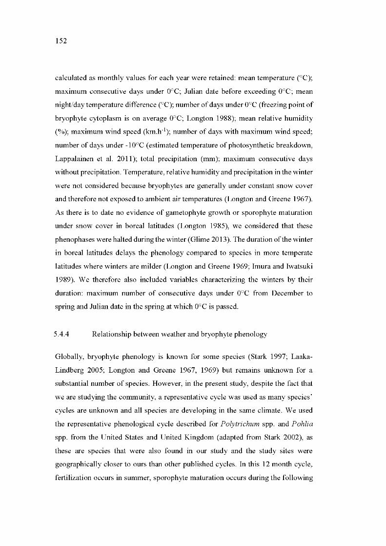
152

calculated as monthly values for each year were retained: mean temperature (°C);

maximum consecutive days under aoc; Julian date before exceeding a oc ; mean

night/day temperature difference (°C); number of da ys under a oC (freezing point of

bryophyte cytoplasm is on average aoc; Longton 1988); mean relative humidity

(%);maximum wind speed (km.h-1) ; number of days with maximum wind speed;

number of da ys un der -1 aoc ( estimated temperature of photosynthetic breakdown,

Lappalainen et al. 2a11); total precipitation (mm); maximum consecutive days

without precipitation. Temperature, relative humidity and precipitation in the winter

were not considered because bryophytes are generally under constant snow cover

and therefore not exposed to ambient air temperatures (Longton and Greene 1967).

As there is to date no evidence of gametophyte growth or sporophyte maturation

under snow cover in boreal latitudes (Longton 1985), we considered that these

phenophases were halted duringthe winter (Glime 2a13). The duration ofthe winter

in boreal latitudes delays the phenology compared to species in more temperate

latitudes where winters are milder (Longton and Greene 1969; Imura and Iwatsuki

1989). We therefore also included variables characterizing the winters by their

duration: maximum number of consecutive days under aoc from December to

spring and Julian date in the spring at which aoc is passed.

5.4.4 Relationship between weather and bryophyte phenology

Globally, bryophyte phenology is known for sorne species (Stark 1997; Laaka

Lindberg 2aa5; Longton and Greene 1967, 1969) but remains unknown for a

substantial number of species. However, in the present study, despite the fact that

we are studying the community, a representative cycle was used as many species '

cycles are unknown and all species are developing in the same climate. W e used

the representative phenological cycle described for Polytrichum spp. and Pohlia

spp. from the United States and United Kingdom (adapted from Stark 2aa2), as

these are species that were also found in our study and the study sites were

geographically closer to ours than other published cycles. In this 12 month cycle,

fertilization occurs in summer, sporophyte maturation occurs during the following

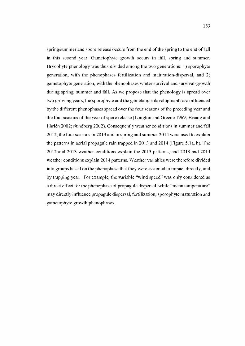
153

spring/summer and spore release occurs from the end ofthe springto the end offall

in this second year. Gametophyte growth occurs in fall, spring and summer.

Bryophyte phenology was thus divided among the two generations: 1) sporophyte

generation, with the phenophases fertilization and maturation-dispersal, and 2)

gametophyte generation, with the phenophases winter survival and survival-growth

during spring, summer and fall. As we propose that the phenology is spread over

two growing years, the sporophyte and the gametangia developments are influenced

bythe different phenophases spread overthe four seasons ofthe preceding year and

the four seasons ofthe year of spore release (Longton and Greene 1969; Bisang and

Ehrlén 2002; Sundberg 2002). Consequently weather conditions in summer and fall

2012, the four seasons in 2013 and in spring and summer 2014 were used to explain

the patterns in aerial propagule rain trapped in 2013 and 2014 (Figure 5.1a, b ). The

2012 and 2013 weather conditions explain the 2013 patterns, and 2013 and 2014

weather conditions exp lain 2014 patterns. Weather variables were therefore divided

into groups based on the phenophase that they were assumed to impact directly, and

by trapping year. For example, the variable ' 'wind speed" was only considered as

a direct effect for the phenophase of propagule dispersal, while "mean temperature"

may directly influence propagule dispersal, fertilization, sporophyte maturation and

gametophyte growth phenophases.

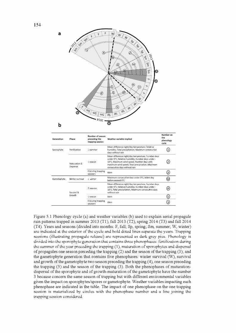
154

a

b

Number of season Numberon

Generation Phase precedine the Weather variable implied the phenolotv trapplnr session cycle

Mean difference night/day temperature; Relative (!) Sporophyte Fertilization 1 summer humidity; Total precipitation; Maximum consecutive

days without rain

Mean difference night/day terrperature; Number days

under O"'C; Relative humidity; Number days und er·

® 1 season 1o•c; Maximum wind speed; Number days with Maturation & maximum wind speed; Total precipitation; Maximum Dispersal consecutive days w ithout ra in

0 (du ring trapping idem ® session}

Gametophyte Winter survival 1 winter Maximum consecutive days unJer o•c; Julien day @ before exceed 0°(

Mean difference night/day temperature; Number days

2 seasons under O"'C; Relative humidity; Number days un der- ® lO"'C; Total precipitation; Maximum consecutive days

Survival & without rain Growth

1 season idem ® o (during trapping

idem ® session)

Figure 5.1 Phenology cycle (a) and weather variables (b) used to explain aerial propagule rain patterns trapped in summer 2013 (Tl), fall 2013 (T2), spring 2014 (T3) and fall 2014 (T4). Years and seasons (divided into months: F, fall; Sp, spring; Sm, summer; W, winter) are indicated at the exterior of the cycle and bold doted lin es separa te the years. Trapping sessions (illustrating propagule release) are represented as dark grey pies. Phenology is divided into the sporophyte generation that con tains three phenophases: fertilization during the summer of the year preceding the trapping ( 1 ), maturation of sporophytes and dispersal of propagules one season preceding the trapping (2) and the season of the trapping (3); and the gametophyte generation that contains five phenophases: winter survival (W), sutvival and growth of the gametophyte two season preceding the trapping ( 4 ), one season preceding the trapping (5) and the season of the trapping (3). Both the phenophases of maturationdispersal of the sporophyte and of growth-maturation of the gametophyte have the number 3 because concern the same season of trapping but with different environmental variables given the impact on sporophytes/spores or gametophyte. Weather variables impacting each phenophase are indicated in the table. The impact of one phenophase on the one trapping session is materialized by circles with the phenophase number and a line joining the trapping session considered.

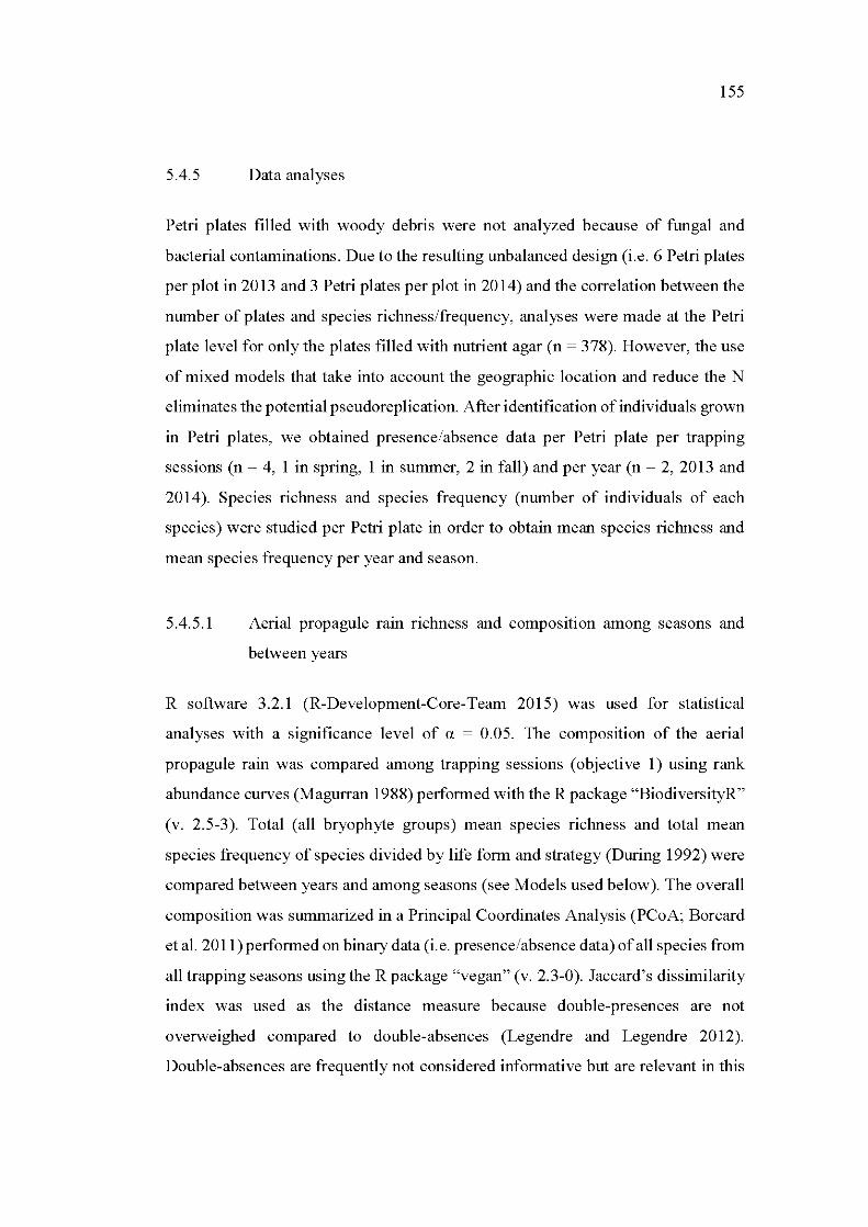
155

5.4.5 Data analyses

Petri plates filled with woody debris were not analyzed because of fungal and

bacterial contaminations. Due to the resulting unbalanced design (i.e. 6 Petri plates

per plot in 2013 and 3 Petri plates per plot in 2014) and the correlation between the

number of plates and species richness/frequency, analyses were made at the Petri

plate level for only the plates filled with nutrient agar (n = 378). However, the use

of mixed models that take into account the geographie location and reduce the N

eliminates the potential pseudoreplication. After identification of individuals grown

in Petri plates, we obtained presence/absence data per Petri plate per trapping

sessions (n = 4, 1 in spring, 1 in summer, 2 in faU) and per year (n = 2, 2013 and

2014). Species richness and species frequency (number of individuals of each

species) were studied per Petri plate in order to obtain mean species richness and

mean species frequency per year and season.

5.4.5.1 Aerial propagule rain richness and composition among seasons and

between years

R software 3.2.1 (R-Development-Core-Team 2015) was used for statistical

analyses with a significance level of a = 0.05. The composition of the aerial

propagule rain was compared among trapping sessions (objective 1) using rank

abundance curves (Magurran 1988) performed with the R package "BiodiversityR"

(v. 2.5-3). Total (aU bryophyte groups) mean species richness and total mean

species frequency of species divided by life form and strategy (During 1992) were

compared between years and among seasons (see Models used below). The overaU

composition was summarized in a Principal Coordinates Analysis (PCoA; Borcard

et al. 2011) performed on binary data (i.e. presence/absence data) of aU species from

aU trapping seasons using the R package "vegan" (v. 2.3-0). Jaccard's dissimilarity

index was used as the distance measure because double-presences are not

overweighed compared to double-absences (Legendre and Legendre 20 12).

Double-absences are frequently not considered informative but are relevant in this

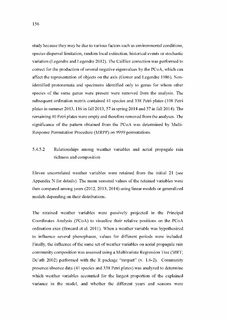
156

study be cause they may be due to various factors such as environmental conditions,

species dispersal limitation, random local extinction, historical events or stochastic

variation (Legendre and Legendre 20 12). The Cailliez correction was performed to

correct for the production of several negative eigenvalues by the PCoA, which can

affect the representation of objects on the axis (Gower and Legendre 1986). Non

identified protonemata and specimens identified only to genus for whom other

species of the same genus were present were removed from the analysis. The

subsequent ordination matrix contained 41 species and 338 Petri plates (108 Petri

plates in summer 2013, 116 in fall2013, 57 in spring 2014 and 57 in fall2014). The

remaining 40 Petri plates were empty and therefore removed from the analyses. The

significance of the pattern obtained from the PCoA was determined by Multi

Response Permutation Procedure (MRPP) on 9999 permutations.

5.4.5.2 Relationships among weather variables and aerial propagule ram

richness and composition

Eleven uncorrelated weather variables were retained from the initial 21 (see

Appendix N for details). The mean seasonal values ofthe retained variables were

then compared among years (2012, 2013, 2014) using linear models or generalized

models depending on their distributions.

The retained weather variables were passively projected in the Principal

Coordinates Analysis (PCoA) to visualize their relative positions on the PCoA

ordination axes (Borcard et al. 2011 ). Wh en a weather variable was hypothesized

to influence several phenophases, values for different periods were included.

Finally, the influence ofthe same set ofweather variables on aerial propagule rain

community composition was assessed using a Multivariate Regression Tree (MRT;

De'ath 2002) performed with the R package "mvpart" (v. 1.6-2). Community

presence/absence data ( 41 species and 338 Petri plates) was analyzed to determine

which weather variables accounted for the largest proportion of the explained

variance in the model, and whether the different years and seasons were

157

discriminated. Trees are described by their fit (i.e. inverse of relative error RE),

which varies from 1 (0% of the variance explained by the tree) to 0 (100% of the

variance explained by the tree ); and their predictive ac curac y estimated by the

cross-validating error (CVRE), which varies from 1 (poor predictive power) to 0

(good predictive power; De'ath 2002). Locations were included as dummy

variables to take into account the spatial structure of the dataset. Subsequently the

number ofbryophyte species and the weather variables for each leaf (i.e. end group)

were calculated. The amount of variation explained by the tree overall and by each

branch were also determined.

5.4.5.3 Models used

As our sampling design was spatially nested, we tested whether the spatial structure

ofthe sampling design influenced the models used to explain species richness and

frequency with LogLik tests (Pinheiro and Bates 1995). In cases where spatial

structure were not influential, the model without random spatial effects (lm, glm)

was chosen in the spirit of parsimony. When the spatial structure had a significant

effect, we used mixed models (lme, glmer). In cases where the assumptions of

normality were met, linear mo dels with or without random effects (lm, lme) were

performed with the R package "nlme" (v. 3.1-121). Where the assumption of

normality were not met generalized linear mixed models with or without random

effects (glm, glmer) were applied with the R package "lme4" (v. 1.1-8), with the

appropriate link function. Models were followed by Tukey HSD post-hoc tests

performed with the R package "multcomp" (v. 1.4-1). Overdispersion of the

generalized models was corrected as needed using Chi-square tests and the c-hat

values. The algorithm of non-converging models was optimized via bobyqa

function of the glmerControl parameter (Powell 2009). Finally when

homoscedasticity assumption was violated, Kruskal-Wallis non-parametric tests

equivalent to one-way ANOV A were used, followed by post-hoc multiple

comparison tests performed with the R package "pgirmess" (v. 1.6.2).

158

5.5 Results

5.5.1 Composition of the aerial propagule rain between years and among

seasons

In 2014 half the number of petri plates were used compared to 2013, however

species richness in 2014 was less than half ofthat in 2013. A total of 41 taxa were

identified during the four trapping sessions: 38 taxa in 2013 (31 in summer, 25 in

fall), and 16 in 2014 (14 in spring, 10 in fall; Appendix 0). Twelvetaxa were shared

between years while 25 taxa were found exclusively in 2013, and three exclusively

in 2014. One species was only found in the spring, nine species only in the summer

and nine only in the fall. The number of protonemata grown was 2740 in 2013 and

756 in 2014. Based on the rank abundance curves, the most abundant taxa were

recorded in the different years and seasons, although their order differed: Atrichum

crispum, Ceratodon purpureus, Pohlia spp., and Sphagnum spp (data not shown).

Three additional taxa Marchantia polymorpha, Plagiomnium

cuspidatumldrummondii and Polytrichum spp. were mainly found in 2013, while

Aulacomnium palustre, Herzogiella turfacea and Pleurozium schreberi were

mainly found in 2014.

Mean total species richness and frequency were both significantly higher in 2013

than in 2014 (bothP < 0.0001; Figure 5.2a, b). Onlythe mean species richness of

perennials differed between years and was significantly greater in 2013 than in 2014

(P = 0.003; Figure 5.2a) whereas the mean frequency of acrocarps, liverworts,

sphagna/dominants and colonists were significantly higher in 2013 than in 2014 (all

P < 0.001; Figure 5.2b). In contrast, pleurocarps and perennials were significantly

more frequent in 2014 than 2013 (both P < 0.001), boosted by the abundance of

P leurozium schreberi. In terms of seasons, mean total species richness and

frequency were both significantly higher in summer than in spring or faU (P < 0.001

and P = 0.003 respectively; Figure 5.2c, d). Propagule rain communities did not

differ among seasons in any mean species richnesses (Figure 5.2c). However,

159

acrocarps, liverworts, and colonists were significantly more frequent in summer

than in the other seasons (all P < 0.001; Figure 5.2d). Pleurocarps were also

significantly more frequent in the aerial propagule rain community in spring (P <

0.001) when sphagna were less frequent (P < 0.001).

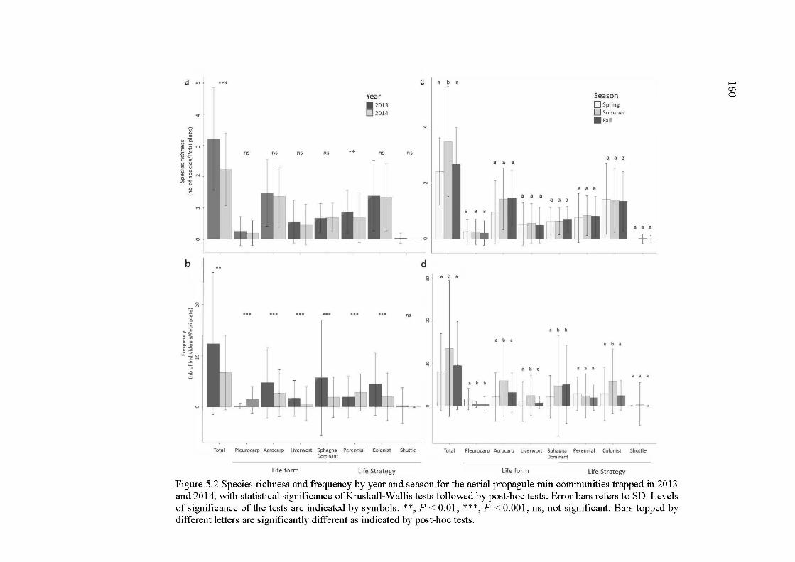
a "'

0

b

C a b a

ns ns ns ns

Year .2013 02014

ns ns

+- 0 d

Total Pleurocarp Acrocarp liverwort Sphaena Perennial Colonist Shuttle Dominant

Li fe form Life Strategy

a a a

a a a

• b •

• b •

• b •

a a a

• b b

Se a son Ospring Dsummer .Fall

a a a

a a a

• b •

Total Pleurocarp Acrocarp liverwort Sphagna Perennial Colonist Shuttle Dominant

Life form Life Strategy

Figure 5.2 Species richness and frequency by year and season for the aerial propagule rain communities trapped in 2013 and 2014, with statistical significance ofKruskall-Wallis tests followed by post-hoc tests. Error bars refers to SD. Levels ofsignificance of the tests are indicated by symbols: **, P < 0.01 ; ***, P < 0.001; ns, not significant. Bars topped by different letters are significantly different as indicated by post-hoc tests.

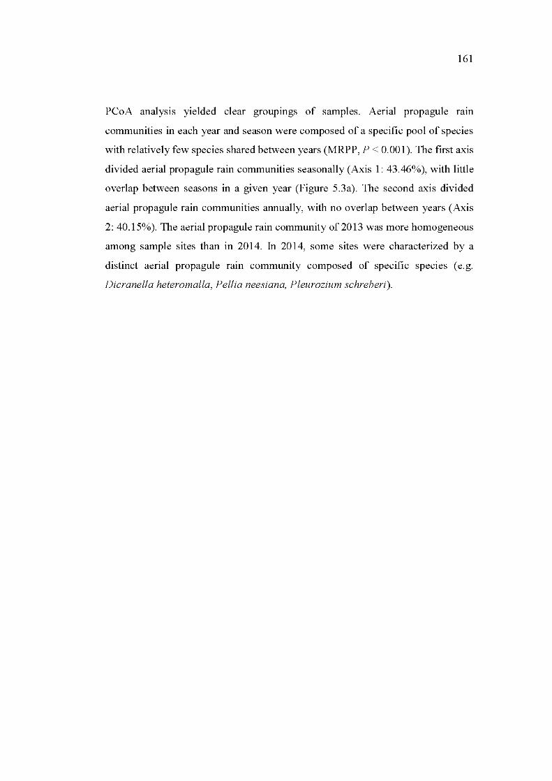
161

PCoA analysis yielded clear groupmgs of samples. Aerial propagule ram

communities in each year and season were composed of a specifie pool of species

with relatively few species shared between years (MRPP, P < 0.001). The first axis

divided aerial propagule rain communities seasonally (Axis 1: 43.46% ), with little

overlap between seasons in a given year (Figure 5.3a). The second axis divided

aerial propagule rain communities annually, with no overlap between years (Axis

2: 40.15%). The aerial propagule rain community of2013 was more homogeneous

among sample sites than in 2014. In 20 14, sorne sites were characterized by a

distinct aerial propagule rain community composed of specifie species ( e. g.

Dicranella heteromalla, Pellia neesiana, Pleurozium schreberi).

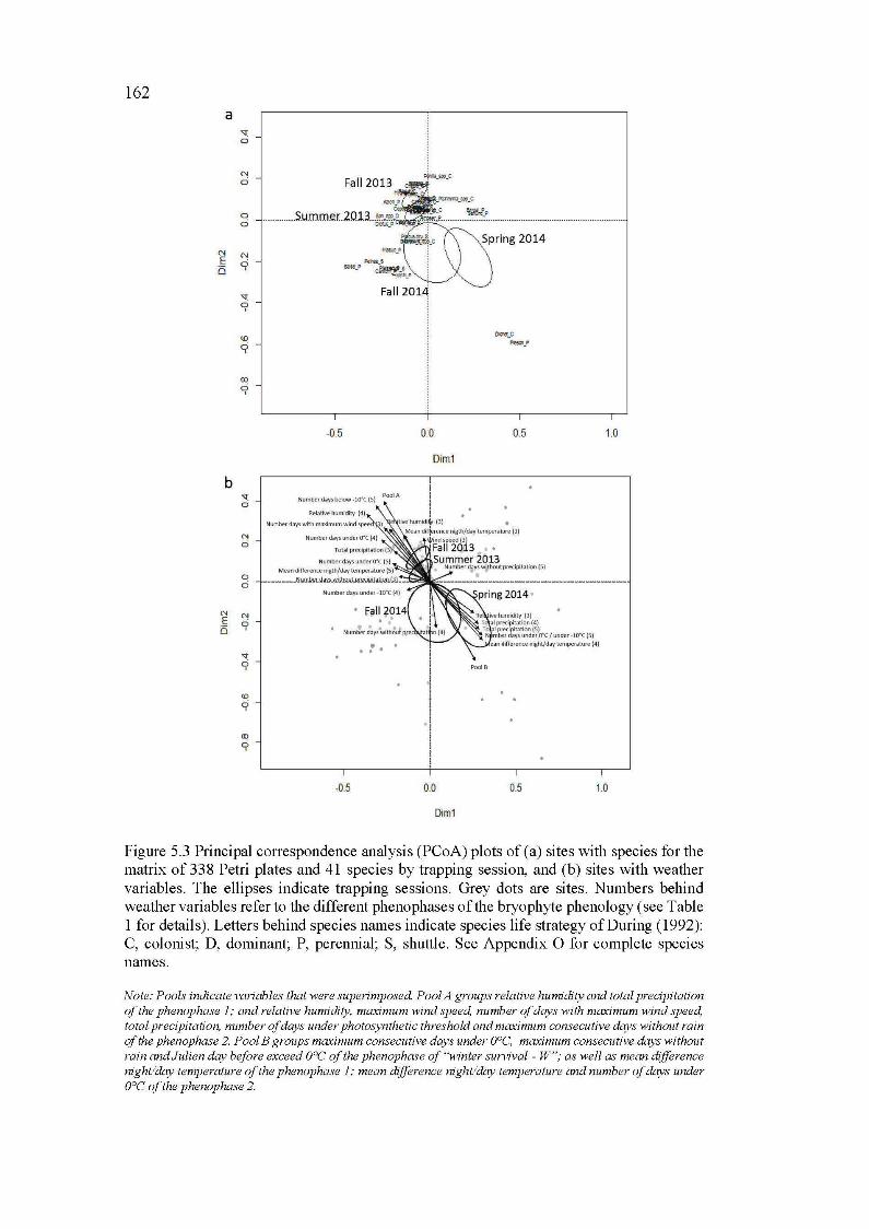
162 a

N E 0

b

N E 0

N ci Fall 2013

~-'19-C

6 ______________ s_ummer.2013. .. ~}"o ~ -

ro 9

N 0

0 ci

N

9

-0.5 00

Dim1

1 Number daysbelow-lo•c(S) PooiA 1

Relative humidity (4) 1

.,..,._c ..... _.

0.5

Nunber dd'f\ with m<~ximum wiod spee ) e live humidi~ {3) Me<1n difterence nigth/day temperature (3)

• ljl~irïd'h Summer 2013

Number d;ays withOut precipitation (S)

1.0

e.1n difference night/day temperature (4)

'<1: 9

1 i PooiB 1

1 <D

9

<D

9

1 1 1

·i ! 1 1 !

-0.5 0.0 0.5 1.0

Dim1

Figure 5.3 Principal correspondence analysis (PCoA) plots of (a) sites with species for the matrix of 338 Petri plates and 41 species by trapping session, and (b) sites with weather variables. The ellipses indicate trapping sessions. Grey dots are sites. Numbers behind weather variables re fer to the different phenophases of the bryophyte phenology ( see Table 1 for details). Letters behind species names indicate species !ife strategy ofDuring (1992): C, colonist; D, dominant; P, perennial; S, shuttle. See Appendix 0 for complete species nam es.

Note: Pools indicate variables that were superimposed PaolA groups relative humidity and total precipitation of the phenophase 1; and relative humidity, maximum wind speed, numher of days with maximum wind speed, total precipitation, number of days under photosynthetic threshold and maximum consecutive days without rain of the phenophase 2. Pool B groups maximum consecutive days und er 0°C, maximum consecutive days without rain and Julien day before exceed 0°C of the phenophase of "winter survival - W"; as well as mean difference nightlday temperature of the phenophase 1; mean difference nightlday temperature and number of days under 0°C of the phenophase 2.

163

S.S.2 Weather characteristics of each year and season

Globally, monthly mean temperature and precipitation from 2012 to 2014 coincided

with 30-year averages recorded for the study area (1981 to 2010; Appendix P)

although March 2012 and 2013 were S°C warmer and March 2014 was S°C colder

than the 30-year average s. Seasonal weather differed among the years (Table S.1 ).

Spring 2014 was significantly colder and dryer than springs 2012 and 2013, while

spring 2012 was significantly rainier than the springs of 2013 and 2014. Summer

2012 was significantly windier than summer 2014, while the falls 2012 and 2013

did not differ significantly.

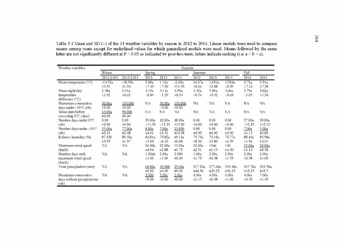
>-' 0\

Table 5.1 Mean and SD (±) of the 11 weather variables by season in 2012 to 2014. Linear models were used to compare ~

means among years except for underlined values for which generalized models were used. Means followed by the same letter are not significantly different at P < 0.05 as indicated by post-hoc tests; letters indicate rank:ing (i.e: a < b < c).

Weather variables Seasons

Win ter SEri~ Summer Fall 2012-2103 2013-2104 2012 2013 2014 2012 2013 2014 2012 2013

Mean temperature (0 C) -14.92a -18.59a 2.00a 1.1 2a -2.63a 16.07a 14.8 1a 15.84a 3.72a 3.31a ±3.31 ±1.34 ±7.43 ±7.50 ±11.93 ±0.66 ±2.08 ±0.39 ±7.16 ±7.58

Mean night/day 2.48a 2.91a 4.19a 4.14a 4.99a 4.42a 5.09a 4.66a 2.79a 3.02a temperature ±1. 92 ±0 .62 ±0 .89 ±1.29 ±0.94 ±0.76 ±0.92 ±0.63 ±1.05 ±1.30 difference (0 C) Maximum consecutive 50.00a 133.00b NA 50.00a 133.00b NA NA NA NA NA days under -10°C (nb) ±0.00 ±0 .00 ±0.00 ±0.00 Julian date before 63.00a 90.00b NA NA NA NA NA NA NA NA exceeding 0°C (date) ±0.00 ±0.00 Number days under 0°C 0.00 0.00 35.00a 42.00a 48.00a 0.00 0.00 0.00 27.00a 33.00a (nb) ±0.00 ±0.00 ±11.50 ±12.49 ±15.00 ±0.00 ±0.00 ±0.00 ±12.29 ±12.1 2 Number days under -1 0°C 55.00a 77.00a 8.00a 7.00a 23 .00b 0.00 0.00 0.00 7.00a 5.00a (nb) ±3. 21 ±2 .08 ±4.6 1 ±2.51 ±13.28 ±0.00 ±0.00 ±0.00 ±1.1 5 ±2.89 Relative humidity (%) 87.45b 80.50a 66.81a 73.82a 69 .1 4a 75.75a 75.18a 73.77a 88.49a 85.98a

±3.95 ±1.37 ±5.03 ±6.10 ±0.08 ±8.30 ±5.80 ±6.59 ±1.96 ±4.0 1 Maximum wind speed NA NA 26.00a 22 .00a 19.00a 22.00a 19ab 16b 19.00a 20.00a (kmlh) ±4.04 ±2.88 ±1.73 ±2.51 ± 1.15 ± 1.00 ±1.15 ±0.58 Number days with NA NA l. OOab 2.00a 2.00b l.OOa 2.00a 2.00a 3.00a 2.00a maximum wind speed ±1.00 ±1.00 ±0.00 ±1.73 ±0.58 ± 1.53 ±0.58 ±1.00 (kmlh) Total precipitation (mm) NA NA 60.80c 42 .00b 25 .60a 31 7.20a 277.60a 319.40a 347.70a 334.50a

±0 .00 ±0.00 ±0.00 ±46 .96 ±29.23 ±31 .25 ±13.25 ±19.5 Maximum consecutive NA NA 3.00b 5.00c 2.00a 4.00a 4.00a 6.00a 4.00a 7.00a days without precipitations ±0 .00 ±0.00 ±0.00 ±1. 15 ±0.58 ± 1.00 ±0.50 ±1.50 nb

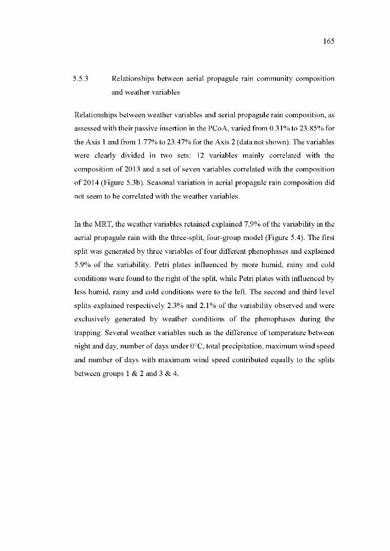
165

5.5.3 Relationships between aerial propagule rain community composition

and weather variables

Relationships between weather variables and aerial propagule rain composition, as

assessed with their passive insertion in the PCoA, varied from 0.31% to 23.85% for

the Axis 1 and from 1.77% to 23.47% for the Axis 2 (data not shown). The variables

were clearly divided in two sets: 12 variables mainly correlated with the

composition of 2013 and a set of seven variables correlated with the composition

of2014 (Figure 5.3b). Seasonal variation in aerial propagule rain composition did

not seem to be correlated with the weather variables.

In the MRT, the weather variables retained explained 7.9% of the variability in the

aerial propagule rain with the three-split, four-group model (Figure 5.4). The first

split was generated by three variables of four different phenophases and explained

5.9% of the variability. Petri plates influenced by more humid, rainy and cold

conditions were found to the right of the split, while Petri plates with influenced by

less humid, rainy and cold conditions were to the left. The second and third level

splits explained respectively 2. 3% and 2.1% of the variability observed and were

exclusively generated by weather conditions of the phenophases during the

trapping. Sever al weather variables such as the difference of temperature between

night and day, number of days under 0°C, total precipitation, maximum wind speed

and number of days with maximum wind speed contributed equally to the splits

between groups 1 & 2 and 3 & 4.

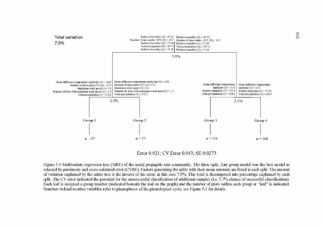
Total variation 7.9%

Relative humidity (4) < 87.23 Relat ive lnunidity (4) ~ 87.23 N tllilber of da ys tmder -1 ooc (5) < 32.5 Ntllilber of da ys tmder - 10°C (5) ~ 32.5

Relative humidity (1) < 75.46:1 Relative humidity ( 1) ~ 75.46 Total prec!p!ahon (1) < 297.4 Total preclp!at!On (1) ~ 297.4 Relative humidity (2) < 71.48 Relative lnunidity (2) ~ 71.48

5.9%

Mean difference temperature nigth/day (3) < 4.83 Mean difference temperatme nigth!day (3) ~ 4.83 Nmnber ofdays under ooc (3) < 17.5 Nmnber ofdays tmder ooc (3) ~ 17.5

Maximmn wind speed (3) < 24 Maxitnmn wind speed (3) ~ 24

Mean difference temperature Mean difference temperature nigth!day (3) < 5.55 nigth!day (3) ~ 5.55

Ntm1ber of days with maximum wind speed (3) ~ 1.5 Nmnber of days with maximum wind speed (3) < 1.5 Total precipitation (3) ~ 172.5 Total precipitation (3) < 172.5

2.3%

Group 1 Group 2

1 1

n= 57 n = 57

Relative htl1llidity (3) ~ 73.50 Relative lmmidity (3) < 73.50 Total precipitation (3) ~ 214.5 Total precipitation (3) < 2 14.5

2 .1%

Group 3 Group 4

1 1

n = 116 n = 108

Error 0.921 ; CV Error 0.943; SE 0.0273

Figure 5.4 Multivariate regression tree (l\IIRT) of the aerial propagule rain community. The three-split, four group model was the best model as selected by parsimony and cross-validated error (CVRE). Factors generating the splits with their mean amounts are listed at each split. The amount of variation explained by the entire tree is the inverse of the error, in this case 7.9%. This total is decomposed into percentage explained by each split. The CV error indicated the potential for the unsuccessful classification of additional samples (i.e. 5.7% chance of successful classification). Each leaf is assigned a group number (indicated beneath the leaf on the graph) and the number of plots within each group or "leaf' is indicated. Numbers behind weather variables refer to phenophases of the phenological cycle, see Figure 5.1 for details.

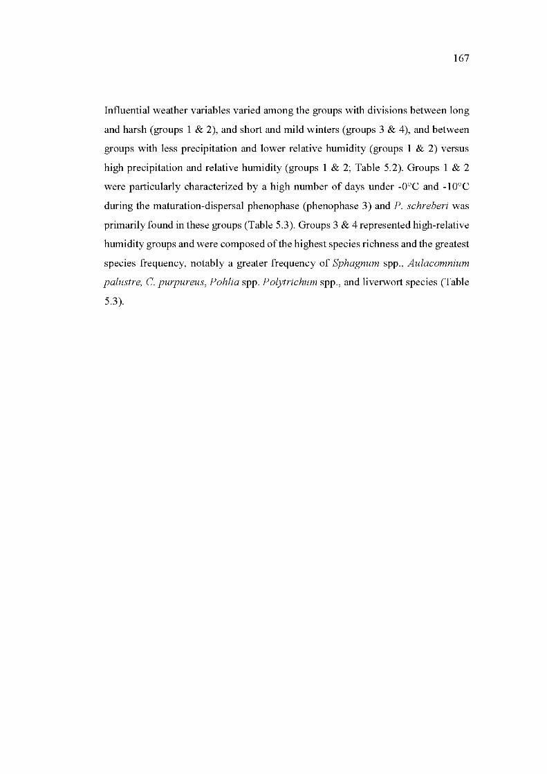
167

Influential weather variables varied arnong the groups with divisions between long

and harsh (groups 1 & 2), and short and mild winters (groups 3 & 4), and between

groups with less precipitation and lower relative humidity (groups 1 & 2) versus

high precipitation and relative humidity (groups 1 & 2; Table 5.2). Groups 1 & 2

were particularly characterized by a high number of days under -0°C and -1 Ü°C

during the maturation-dispersal phenophase (phenophase 3) and P. schreberi was

primarily found in these groups (Table 5.3). Groups 3 & 4 represented high-relative

humidity groups and were composed of the highest species richness and the greatest

species frequency, notably a greater frequency of Sphagnum spp., Aulacomnium

palustre, C. purpureus, Pohlia spp. Polytrichum spp., and liverwort species (Table

5.3).

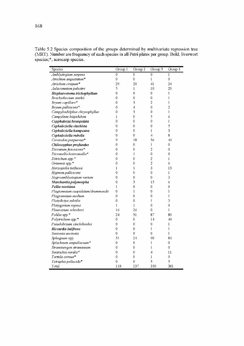
168

Table 5.2 Species composition of the groups determined by multivariate regression tree (MRT). Number are frequency of each species in all Petri plates per group. Bold, liverwort species;*, acrocarp species.

Species Group 1 Group 2 Group 3 Group 4

Amblystegium serpens 0 0 0 1 Atrichum angustatum * 0 0 1 0 Atrichum crispum* 29 20 41 24 Aulacomnium palustre 5 10 20

Blepharostoma trichophyllum 0 0 0 Brachythecium starkii 0 0 0 Bryum capillare* 0 3 2 Bryum pallescens* 0 4 0 2 Campyliadelphus chrysophyllus 0 3 0 1 Campylium hispidulum 1 0 5 6 Cepphalozia bicuspidata 0 0 0 Cephaloziella elachista 0 0 0 5 Cephaloziella hampeana 0 0 3

Cephaloziella rubella 0 0 4 8 Ceratodon purpureus* 9 18 56 44 Chiloscyphus profundus 0 0 1 0 D icranum foscescens * 0 0 2 0 Dicranella heteromalla* 0 0 0 Ditrichum spp. * 0 0 2 1 Grimmia spp. * 0 0 2 6 Herzogiella tuifacea 3 13 Hypnum pallescens 0 0 0 1 Hygroamblystegium varium 0 0 0 3 M archantia polymorpha 0 3 15 6 Pellia neesiana 0 0 0 Plagiomnium cuspidatuml drummondii 0 0 Plagiomnium medium 0 0 0 1 Platydictya subtilis 0 0 1 3 Platygyrium repens 0 0 Pleurozium schreberi 16 26 0 Pohlia spp. * 24 31 87 80 Polytrichum spp. * 0 0 14 44 Pseudobryum cinclidioides 0 0 0 Rie cardia latifrons 0 0 Sanionia uncinata 0 0 0 Sphagnum spp. 31 24 90 84 Splachnum ampullaceum* 0 0 1 0 Straminergon stramineum 0 0 0 Syntrichia ruralis* 0 0 4 11 Tor tula cernua * 0 0 1 0 Tetraphis pellucida* 0 0 5 5 Total 118 137 350 381

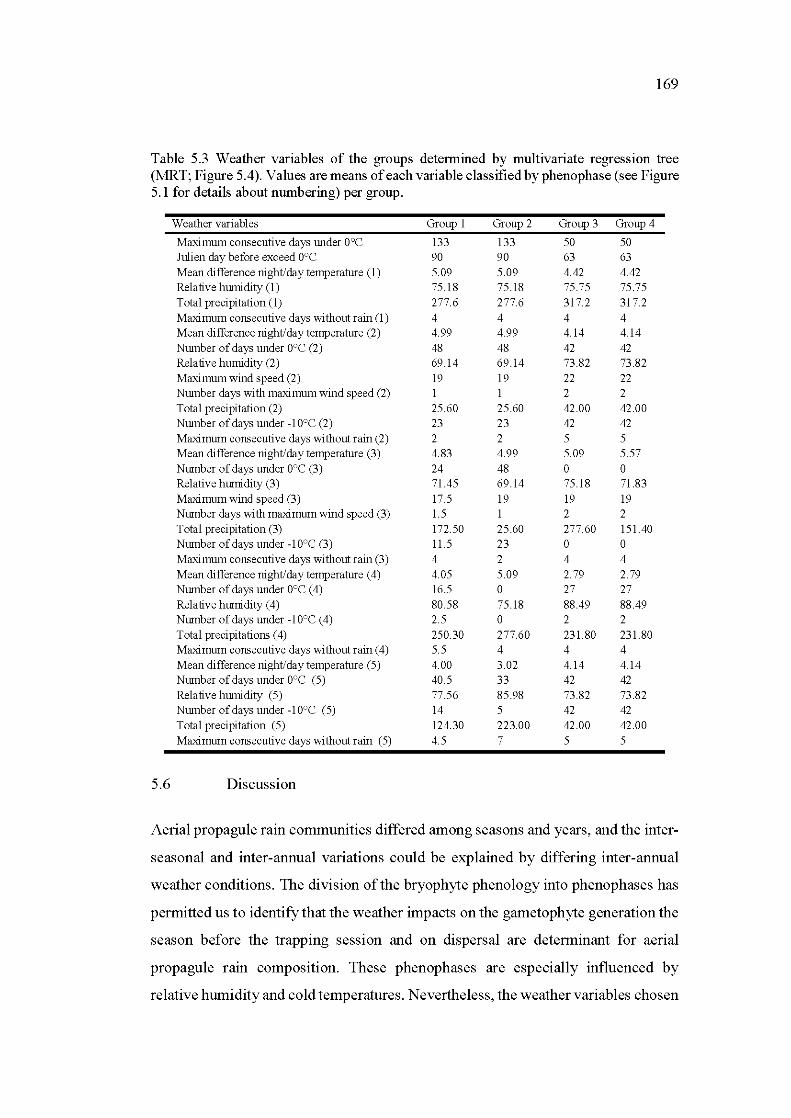
169

Table 5.3 Weather variables of the groups determined by multivariate regression tree (MRT; Figure 5.4). Values are means of each variable classified by phenophase (see Figure 5.1 for details about numbering) per group.

Weather variables Group 1 Group 2 Group 3 Group 4

Maximum consecutive days tmder 0°C 133 133 50 50 Julien day be fore exceed 0°C 90 90 63 63 Mean difference nightJday temperature (1) 5.09 5.09 4.42 4.42 Relative hurnidity (1) 75 .18 75.18 75 .75 75.75 Total precipitation (1) 277.6 277.6 317.2 31 7.2 Maximum consecutive days without rain (1) 4 4 4 4 Mean difference nightJday temperature (2) 4.99 4.99 4.14 4.14 Number of days under 0°C (2) 48 48 42 42 Relative hurnidity (2) 69.14 69.14 73.82 73.82 Maximum wind speed (2) 19 19 22 22 Number da ys with maximum wind speed (2) 2 2 Total precipitation (2) 25.60 25.60 42.00 42.00 Number of days under -1 0°C (2) 23 23 42 42 Maximum consecutive days without rain (2) 2 2 5 5 Mean difference nightJday temperature (3) 4.83 4.99 5.09 5.57 Number of days under 0°C (3) 24 48 0 0 Relative hurnidity (3) 71.45 69.14 75 .18 71.83 Maximum wind speed (3) 17.5 19 19 19 Nurnber da ys with maximum wind speed (3) 1.5 2 2 Total precipitation (3) 172.50 25.60 277.60 151.40 Nurnber of days under -1 0°C (3) 11.5 23 0 0 Maximum consecutive days without rain (3) 4 2 4 4 Mean difference nightlday temperature ( 4) 4.05 5.09 2.79 2.79 Nurnber of days under 0°C ( 4) 16.5 0 27 27 Relative hurnidity ( 4) 80.58 75.18 88.49 88.49 Nurnber of days under -1 0°C ( 4) 2.5 0 2 2 Total precipitations ( 4) 250.30 277.60 231.80 231.80 Maximum consecutive da ys wi tho ut rain ( 4) 5.5 4 4 4 Mean difference nightJday temperature (5) 4.00 3.02 4.14 4.14 Nurnber of days under 0°C (5) 40.5 33 42 42 Relative hurnidity (5) 77.56 85.98 73.82 73.82 Nurnber ofdays under -10°C (5) 14 5 42 42 Total precipitation (5) 124.30 223.00 42.00 42.00 Maximum consecutive days without rain (5) 4.5 7 5 5

5.6 Discussion

Aerial propagule rain communities differed among seasons and years, and the inter

seasonal and inter-annual variations could be explained by differing inter-annual

weather conditions. The division of the bryophyte phenology into phenophases has

permitted us to identify that the weather impacts on the gametophyte generation the

season before the trapping session and on dispersal are determinant for aerial

propagule rain composition. These phenophases are especially influenced by

relative humidity and cold temperatures. Nevertheless, the weathervariables chosen

170

only explain 7.9% of inter-annual variability in the aerial propagule ram

composition, reflecting the complex mechanisms linking bryophyte dispersal

patterns to regional weather.

5.6.1 Seasonal aerial propagule ram composition 1s driven by winter

conditions rather than differing species phenologies

Seasonal variations in the aerial propagule rain community have been reported in

the past (Hock et al. 2004; Ross-Davis and Frego 2004) and were explained by

differentiai timing in species phenology (Longton and Greene 1969; Longton

1985). In our study, we canuse species phenology to explain the greater number of

Sphagnum propagules trapped at the end of summer and fall. Indeed, certain

sphagna species are known as "late dispersers" and wait for the wettest conditions

of end of summer and fall for dispersal (Sundberg and Rydin 2002). Similarly, the

higher number of liverworts trapped in the hottest and wettest months of summer

may be due to their cold and drought sensitivity (Laaka-Lindberg 2005; Pohjamo

2008). However, seasonal aerial propagule rain patterns of the true mosses

(acrocarps and pleurocarps) seemed primarily explained by responses to weather

conditions, particularly winter length, rather than species phenology. Low acrocarp

richness and frequency in 20 14 compared to 20 13 may be explained by the fact that

numerous acrocarps are colonist or shuttle species that have stress tolerant

propagules or propagules that enter into dormancy [Pohjamo 2008 based on During

(1979)] that permit them to tolerate episodic stresses such as dry and cold

conditions. In contrast, pleurocarps, ofwhich many are perennial species (based on

During 1979, 1992), tolerate stress as gametophytes and continue to mature under

less suitable conditions [e.g. dry and cold periods; Pohjamo 2008 based on During

(1979)].

However, we demonstrate that specifie weather conditions also explain the

seasonality of the aerial propagule rain. Indeed, the lower species richness of spring

community compared to summer and fall communities may be linked with harsh

171

winter conditions that can delay sorne ofthe phenophases ofbryophyte phenology

(Longton and Greene 1969; Longton 1985). Gregory (1961) and Crum (2001)

report that northernmost latitudes are most "propagule rich" in summer and fall than

in mid-spring and early summer, which may be due to the fact that propagules

released in the summer and fall beneficiated from two or three maturation seasons

(previous faU and spring, and previous fall, spring and summer respectively)

whereas propagules released in spring have only beneficiated from the previous faU,

before halted sporophyte maturation during the winter (Glime 2013), and the early

spring when winter is not too long. This was especially true in 2014 where winter

prolonged until the end of April with several weeks under -10°C (compensation

point ofthe photosynthesis is reached, Lappalainen et al. 2011). These conditions

could lead to the inhibition of growth/maturation of gametophytes/sporophytes and

explained the poor pool of species trapped in 2014. However, keep in mind that our

conclusions about seasonality in the aerial propagule rain are biased by the trapping

design: spring trapping only occured in 2014 where the winter was harsher and

longer than in 2012-2013. Consequently, our first hypothesis cannot be validated

as both species phenology and weather conditions explained in part bryophyte

propagule rain patterns.

5.6.2 The unexpected inter-annual difference m aerial propagule ram

composition

Few species were shared between 2013 and 2014 aerial propagule rain communities

and in addition to finding a significant decrease in species richness and abundance

in 2014, we observed a marked change in community composition leading to the

rejection of our second hypothesis. The inter-annual difference was surprising as

most of the species trapped in 2013 were significantly less abundant or absent in

2014. This may in part be explained by the importance of maternai investment in

reproduction and the subsequent cost for the female gametophyte (Bisang and

Ehrlén 2002). Individuals that have invested in the formation and release of

propagules one year may have a reduced sporophyte development and propagule

172

release the next year, as they are energetically limited compared to other

individuals.

In this paper we have however focused on a second possibility, suggested by

Callaghan et al. ( 1997) and Slack (20 11), that bryophyte development may be

impacted by inter-annual climatic variations because of the exposure of the

gametophyte to environmental factors. As suggested in our third hypothesis, we

underline that specifie weather conditions influence directly and indirectly

propagule release acting on phenophases prior to and during dispersal. Critical

weather conditions influenced both growth and maturation of the gametophyte and

maturation and dispersal of the sporophytes that therefore impact on the

composition ofthe aerial propagule rain.

5.6.2.1 The importance of summer conditions

For bryophytes, gametangia development and antherozoid movements are entirely

dependent on water availability (Reynolds 1980). We found that precipitation and

humidity levels during the fertilization and growth-maturation of the gametophyte

dictate the pool oftrappable propagules one year later. In accordance with Sundberg

(2002) and Proctor (2011), we found that high summer humidity results in a richer

trappable species pool the next year. Consequently, propagule release in summer

and fall depend on moisture amounts in the previous summer and faU whereas

spring propagules depend in part on the conditions of the previous summer. The

suitable moisture conditions of 2012 can therefore exp lain the propagule richness

and abundance in 2013.

In addition, weather conditions during dispersal also influenced the trapped species

pool. The difference in temperature between night and day was positively

associated with species richness and composition, which may be explained by

associated changes in humidity that induce spore release (Johansson et al. 2015).

Dew formation is higher when there is a greater difference in night and day

173

temperatures and the evaporation of dew in the moming allows spore ejection via

drought-rehydratation of the capsule peristome and hygroscopie movements ofthe

elaters (Ingold 1959). Furthermore, heating of the air near the soil in the moming

after a cold night causes turbulence as the rises. This, along with strong gusts of

wind, could drive long distance dispersal of propagules after their ascension in the

air column.

5.6.2.2 The existence of a winter chilling process in bryophytes?

An interesting point raised by our study is the positive impact of low temperatures

on aerial propagule rain species richness and frequency. Indeed, one month of

cumulative days under -10°C the season before the propagule release resulted in

more species trapped. Bryophyte response to low temperatures depends on the

season (Rütten and Santarius 1992) and cold periods in the fall may act as signais

of winter's arrivai and invoke species to allocate energy to gametophyte survival

rather than to reproduction and dispersal.

Compared to fall, cold periods during the spring may act as signais of a delayed

summer time. In 2014, the long winter until April may have delayed photosynthesis

and invoked a "winter chilling process", already known for trees, which prevents

budburst at the "wrong period" after warming events in the middle of the winter

(Harrington et al. 20 10). Applied to bryophytes, we can imagine that the energy

allocated to sporophyte and spore production may have been more limited in 2014,

resulting in sporophyte abortion (Stark 2002) and may explain the poor diversity of

propagules trapped. The need of stimuli to initiate the development of sexual organs

has been reported by Glime (2013), who also underlines the poor knowledge about

initiation signais on bryophytes but deeper studies are required to confirm whether

the "winter chilling process" on bryophytes exists.

174

5.6.3 Limitations ofthe study

As stressed in Barbé et al. (2016), both the timing of Petri exposure (moming to

early aftemoon) and the emergence method used to germinate propagules bring

sorne biases. Indeed, we might have favoured the overrepresentation of local

propagules compared to more distant ones that are deposited later in the aftemoon

(Johansson et al. 2015), together with not differentiating between real absence and

a non-germination of one species ex situ (Ross-Davis and Frego 2004). We also

suspect to have favoured the trapping of sexual vs asexual propagules (heavier and

mainly used for local dispersal; Kimmerer 1991; Lôbel et al. 2006), which certainly

influenced on the patterns detected. Furthermore, the use of same representative

phenology for all bryophyte species as well as the non-consideration of the species

sexual investment are over-simplification of our system, however forced bythe lack

ofknowledge on the phenology of the majority of the species. Finally, keep in mind

that this study is a "snap shot" of propagule rain patterns and that we have used of

weather variables and trapping data oftwo years, while the chances of identifying

spurious patterns are higher than a long term study.

5.6.4 Conclusions

The understanding of bryophyte phenology in response to weather conditions is

crucial, especially in the contemporary context of climate changes and in the use of

bryophytes as bio-indicator species. This study is the first trying to disentangle the

influence of weather variables on the phenology of bryophyte metacommunities

dissected into phenophases. We report that propagule release depends on the

weather conditions during dispersal but also during survival and growth of the

mother gametophyte, particularly winter, and during the fertilization phenophase.

Consequently, propagule release seems govemed by indirect and direct effects of

humidity and temperature one to several preceding seasons. Further modelisation

studies, involving long term trapping and weather variables will offer clearer and

175

stronger answers about bryophyte dispersal patterns in response to regional climate,

but this work offers new avenues to address this complex subject.


Funding: This project was funded by the Université du Québec en Abitibi



Products.

The authors sincerely thank Julie Arseneault, Joëlle Castonguay, Louis Dubois,

Morgane Hi gelin, and Aurore Lucas for their field and laboratory assistance; Pascal

Drouin, Noémie Graignic, Ahmed Koubaa, Danièle Laporte, Marie-Hélène

Longpré, Benoit Plante and Francine Tremblay for their technical support, and Jean

Faubert for his precious help in the identification of the most difficult bryophyte

samples.

5.8 References

Barbé M, Fenton NJ, Bergeron Y (2016) So close and yet so far away: long-distance dispersal events govem bryophyte metacommunity reassembly. J Ecol DOl: 10.111 1/1365-2745.12637

Benson-Evans K (1961) Environmental factors and bryophytes. Nature 191:255-260.

Bergeron Y, Leduc A, Harvey BD, GauthierS (2002) Natural fire regime: a guide for sustainable management ofthe Canadian boreal forest. Silv Fenn 36:81-95.

Bisang 1, Ehrlén J (2002) Reproductive effort and cost of sexual reproduction in female Dicranum polysetum. Bryol 105:384-397.

Borcard D, Gillet F, Legendre P (2011) Numerical ecology with R. Springer, New York.

Bossuyt B, Honnay 0 (2006) Interactions between plant life span, seed dispersal capacity and fecundity determine metapopulation viability in a dynamic landscape. Landsc Ecol21:1195-1205.

176

C-Fern Project © (1995-2014) Nutrient Medium Preparation- Traditional Method. Available at: http ://www.c-fem.orglindex.php?option=com _ content&view=article&id=82&Itemi.

Callaghan TV, Carlsson BÂ, Sonesson M, Temesvary A (1997) Between-year variation in climate-related growth of circumarctic populations of the moss Hylocomium splendens. Funct Ecol 11:157-165.

Crum HA (200 1) The Structural Diversity of Bryophytes. University of Michigan Herbarium, Michigan.

De'ath G (2002) Multivariate regression trees: a new technique for modeling species-environment relationships. Ecolo gy 83:1105-1117.

Dougherty PM, Whitehead D, V ose, JM ( 1994) Environmental influences on the phenol ogy of pine. Ecol Bull 43:64-75.

During HJ (1979) Life strategies of bryophytes: a preliminary review. Lindbergia 5:2-18.

During HJ (1992) Ecological classification ofbryophytes and lichens. In: Bates JW, Farmer AM ( eds ). Bryophytes and lichens in a changing environment. Clarendon Press, Oxford, pp 1-31.

Environment Canada 2015a. Canadian Climate Normals 1981-201 Station Data. Available at: http :! /climate.weather.gc.ca/climate _ normalslindex _ e.html

Environment Canada 2015b. Climate. Monthly data report. Available at: http:/ /climate.weather.gc.ca/data _index_ e.html

Ehrlén J, Bisang I, Hedenas L (2000) Costs of sporophyte production in the moss, Dicranum polysetum. Plant Ecol149:207-217.

Faubert J (2012-2014) Flore des bryophytes du Québec-Labrador (Vol. 1, 2 and 3). Société québécoise de bryologie, Saint-Valérien.

Gignac LD (2001) Bryophyte as indicators of climate change. Bryol104:410-420.

Glime JM (2013) Introduction. Chapt. 1. In: Glime JM (ed) Bryophyte Ecology. Volume 1. Physiological Ecolo gy. Ebook sponsored by Michigan Technological University and the International Association of Bryologists. Last updated 15-Aug-2013 and available at: http://www.bryoecol.mtu.edu/.

Gower JC, Legendre P (1986) Metric and Euclidean properties of dissimilarity coefficients. J Classif 3:5-48.

Gregory PH (1961) The microbiology of the atmosphere. Leonard Hill Ltd, London.

Harrington CA, Gould PJ, St Clair JB (2010) Modeling the effects of winter environment on dormancy release of Douglas-tir. For Ecol Manag 259:798-808.

177

Hedenas L (200 1) Environmental factors potentially affecting char acter states in pleurocarpous mosses. Bryol104:72-91.

Hock Z, Szôvényi P, Tôth Z (2004) Seasonal variation in the bryophyte diaspore bank of open grasslands on dolomite rock. J Bryol 26:285-292.

Hughes L (2000) Biological consequences of global warming: is the signal already apparent? Trends Ecol Evol15:56-61.

lmura S, Iwatsuki Z (1989) Phenological study of Trachycystis microphylla (Dozy et Molk.) Lindb. (Mniaceae, Musci). Hikobia 10:303-308.

Ingold CT (1959) Peristome teeth and spore discharge in mosses. Trans Froc Bot Soc 38:76-88.

Johansson V, Lônnell N, Sundberg S, Hylander K (2014) Release thresholds for moss spores: the importance of turbulence and sporophyte length. J Ecol 102:721-729.

Johansson V, Lônnell N, Rannik Ü , Sundberg S, Hylander K (2015) Air humidity thresholds trigger active moss spore release to extend dispersal in space and time. Funct Ecol DOl: 10.1111/1365-2435.12606.

Johst K, Drechsler M, van Teeffelen AJ, Hartig F, Vos CC, Wissel S, Opdam P (2011) Biodiversity conservation in dynamic landscapes: trade-offs between number, connectivity and turnover of habitat patches. J Appl Ecol48: 1227-1235.

Klekowski EJ (1969) Reproductive biology ofthe Pteridophyta III. A study ofthe Blechnaceae. Bot J Linn Soc 62:361-377.

Laaka-Lindberg S (2005) Reproductive phenology in the leafy hepatic Lophozia silvicola Buch in southem Finland. J Bryol 27:253-259.

Lappalainen NM, Hyyryliiinen A, Huttunen S (2011) Seasonal and interannual variability of light and UV acclimation in mosses. In: Tuba Z, Slack NG, Stark LR ( eds) Bryophyte ecology and climate change. Cambridge University Press, New York, pp 71-90.

Legendre P, Legendre L (2012) Numerical Ecology, 3rd edn. Elsevier, Oxford.

Lôbel S, Rydin H (2010) Trade-offs and habitat constraint in the establishment of epiphytie bryophytes. Funct Ecol 24:887-897.

Longton RE (1985) Reproductive biology and susceptibility to air pollution in Pleurozium schreberi (Brid.) Mitt. (Musci) with particular reference to Manitoba, Canada. Monogr Systematic Bot Mo Bot Gard 11:51-69.

Longton RE ( 1988) Adaptations and strategies of polar bryophytes. Bot J Linn Soc 98:253-268.

178

Longton RE, Greene SW (1967) The growth and reproduction of Polytrichum alpestre Roppe on South Georgia. Philos Trans R Soc Lond Ser B, Biol Sei 252:295-322.

Longton RE, Greene SW (1969) The growth and reproduction cycle of Pleurozium schreberi (Brid.) Mitt. Ann Bot, New Ser 33:83-105.

Magurran AE ( 1988) Ecological diversity and its measurement. Princeton University Press, Cambridge.

Pinheiro JC, Bates DM (1995) Approximations to the log-likelihood function in the nonlinear mixed-effects model. 1 Comput Graph Stat 4:12-35.

Pohjamo M (2008) Should I stay or should I go? Reproductive and dispersal strategies of site-specifie liverwort species. Academie Dissertation, Department of Biological and Environmental Sciences & Department of Applied Biology, University of Helsinki, Helsinki, Finland.

Pohjamo M, Laaka-Lindberg S, Ovaskainen 0, Korpelainen H (2006) Dispersal potential of spores and asexual propagules in the epixylic hepatic Anastrophyllum hellerianum. Evolut Ecol20:415-430.

Powell MJD (2009) The BOBYQA algorithm for bound constrained optimization without derivatives. Report No. DAMTP 2009/NA06, Centre for Mathematical Sciences, University of Cambridge, Cambridge, UK.

Proctor MCF (2011) Climatic responses and limits ofbryophyte: comparisons and contrasts with vascular plants. In: Tuba Z, Slack NG, Stark LR (eds) Bryophyte ecology and climate change. Cambridge University Press, New York, pp 35-54.

R-Development-Core-Team (2015) R: A Language and Environmentfor Statistical Computing. R Foundation for Statistical Computing, Vienna, Austria.

Reynolds DN (1980) Gamete dispersal inMnium ciliare. Bryol 83:73-77.

Ross-Davis AL, Frego KA (2004) Propagule sources of forest floor bryophytes: spatiotemporal compositional patterns. Bryol 107:88-97.

Rudolph ED (1970) Local dissemination of plant propagules in Antarctica. In: Holdgate MW (ed) Antarctic ecology. Academie Press, London, pp 812-817.

Rütten D, Santarius KA (1992) Relationship between frost tolerance and sugar concentration of various bryophytes in summer and winter. Oecologia 91 :260-265.

Saucier JP, Grondin P, Robitaille A, Gasselin J, Momeau C, Richard PJH, Brisson 1, Sirois L, Leduc A, Morin H, Momeau C, Payette S, Gauthier S, Gasselin J, Lavoie C, Thiffaut E (2009) Écologie forestière. In: Ordre des ingénieurs forestiers du Québec ( ed) Manuel de foresterie. Éditions Multimondes, Québec, pp 165-315.

Serreze MC, Walsh JE, Chapin III FS, Osterkamp T, Dyurgerov M, Romanovsky V, Oechel WC, Morison J, Zhang T, Barry RG (2000) Observational evidence

179

of recent change in the northem high-latitude environment. Clim Chang 46:159-207.

Slack NG (20 11) The ecological value of bryophytes as indicators of climate change. In: Tuba Z, Slack NG, Stark LR (eds) Bryophyte ecology and climate change. Cambridge University Press, New York, pp 3-12.

Stark LR (1997) Phenology and reproductive biology of Syntrichia inermis (Bryopsida, Pottiaceae) in the Mojave Desert. Bryol 100:13-27.

Stark LR (2002) Phenology and its repercussions on the reproductive ecology of mosses. Bryol105:204-218.

Sundberg S (2002) Sporophyte production and spore dispersal phenology in Sphagnum: the importance of summer moisture and patch characteristics. Can J Bot 80:543-556.

Sundberg S, Rydin H (2002) Habitat requirements for establishment of Sphagnum from spores. J Ecol 90:268-278.

Walther G-R, PostE, Convey P, Menzel A, Parmesan C, Beebee TJC, Fromentin J-M, Hoegh-Guldberg 0, Bairlein F (2002) Ecological responses to recent climate change. Nature 416:389-395.

W asley J, Robinson SA, Lovelock CE, Popp L (2006) Climate change manipulations show Antartic flora is more strongly affected by elevated nutrients than water. Glob Chang Biol 12:1800-1812.

Xiao D, Tao F, Liu Y, Shi W, Wang M, Liu F, Zhang S, Zhu Z (2013) Observed changes in winter wheat phenology in the North China Plain for 1981~

2009. Intem J Biometeorol 57: 275-285

CHAPITRE VI

CONCLUSION GÉNÉRALE

182

Après avoir sillonné le sud d'Eeyou Istchee Baie James, sélectionné 30 îlots

résiduels dans six feux différents et récolté plus d'un million de spécimens de

bryophytes sur une surface équivalente à près de 48 terrains de tennis (9300 m2),

nos conclusions viennent ébranler plusieurs des stéréotypes à la fois sur les rôles

des îlots résiduels, mais aussi concernant la dynamique des populations

bryophytiques. À des fins d'aménagement écosystémique, cette thèse visait à

estimer les rôles de refuge et de source de propagules des îlots résiduels post-feu

tout en estimant les effets de bordure sur les communautés bryophytiques.

Conjointement, nous souhaitions éclaircir les patrons de dispersion, les réponses

aux conditions climatiques et la distribution des bryophytes en pessière noire à

mousses.

Pour commencer, nos travaux réfutent le rôle de refuge des îlots résiduels pour les

bryophytes étant donné 1 'absence de certaines caractéristiques environnementales,

mais aussi de plusieurs espèces, dont principalement des hépatiques forestières,

dans les îlots résiduels post-feu comparé aux forêts non perturbées. Cependant, la

richesse moyenne des bryophytes supérieure dans les îlots résiduels et la présence

de quatre espèces rares pour la province du Québec aboutit à les qualifier

d'« habitats de haute qualité » pour les bryophytes. De plus, certaines

caractéristiques spatiales et structurelles des îlots résiduels conduisent à une

composition des communautés de bryophytes plus similaire à celles retrouvées dans

les forêts non perturbées, fournissant des guides pour 1' aménagement des îlots de

rétention dans les parterres de coupes.

De sucroit, il apparaît que les îlots résiduels post-feu en forêt boréale soient

dépourvus d'habitat de cœur, où la composition de la communauté bryophytique

serait similaire à celle retrouvée dans les forêts non perturbées. Cette différence en

termes de composition en espèces est imputable à l'effet de bordure, ressenti même

dans les îlots résiduels les plus larges (de 3 à 11 ha) dans lesquels des espèces

inféodées aux vieilles forêts non perturbées sont absentes. Cette étude fournit alors

183

un contrôle de la réponse naturelle des bryophytes à l'effet de bordure, jusque là

falsifiée par des interprétations issues d'études réalisées dans des paysages

perturbés anthropiquement.

Conjointement à ces conclusions, nous corroborons le rôle de sources de propagules

des îlots résiduels post-feu qui participent à la recolonisation de la matrice brûlée,

non pas uniquement à 1 'échelle locale, mais aussi à 1' échelle régionale. Ces

conclusions renversent simultanément le paradigme d'une capacité de dispersion

limitée des bryophytes. En effet, nous rapportons 1 'occurrence de la dispersion à

longue distance (de 650 rn à 30 km ; échelle régionale) et ce, quelle que soit la

stratégie de vie des bryophytes. La topographie et les vents dominants de la région

pourraient expliquer les distances accrues parcourues par les propagules

bryophytiques en pessière noire.

À des fins purement bryologiques, nous rapportons l'existence d'une variabilité

interannuelle de la pluie de propagules aérienne des bryophytes en réponse aux

conditions climatiques. Après division du cycle phénologique des bryophytes en

différentes phases, nous démontrons que les conditions climatiques concomitantes,

mais aussi en amont de la dispersion des propagules gouvernent la composition de

la pluie de propagules. Ainsi, la fertilisation durant l'été, un an avant la dispersion

des propagules, mais aussi la croissance et la maturation du gamétophyte les saisons

précédant la libération des propagules, déterminent la pluie de propagules

disponible la saison voire l'année suivante. Le taux d'humidité, mais aussi la

température sont les conditions les plus influentes sur le cycle phénologique des

bryophytes. De plus, sous les latitudes nordiques, la longueur et la rudesse de la

saison hivernale sont de premières importances pour le déroulement du cycle

phénologique des bryophytes. Cependant, ce travail de type «capture d'écran»

necessite d'être complémenté par des études à plus long terme pour en asseoir les

conclusions.

184

La question du transport externe des bryophytes par des agents biotiques, les

micromammifères, est abordée dans l'annexe 1 ci-après. Spéculée par les

bryologues à maintes reprises (Carey, 2003 ; Kimmerer, 1994 ; Rydgren et al.,

2007), cette étude est la première à directement prouver cette interaction. À 1 'issue

d'un travail collaboratif entre mammalogistes et bryologues, ayant allié les

compétences respectives de chacun en trappe et brossage de mammifères et en

culture in vitro et identification de bryophytes, nous mettons en évidence le

transport de six taxa bryophytiques par cinq espèces de micromammifères en

pessière noire à mousses. Ce travail, bien qu'il puisse paraître anecdotique, rapporte

une interaction journalière entre deux groupes d'organismes cosmopolites de la

forêt boréale et qui pourraient avoir une portée plus conséquente qu'attendue sur la

dynamique des populations bryophytiques. Les micromammifères représentent

alors des « liens mobiles » (Couvreur et al., 2004) pleinement impliqués dans la

dynamique métapopulationnelle des bryophytes.

Finalement, cette thèse a permis le recensement de 168 espèces de bryophytes dans

la région d'étude. Le sud du Nord-du-Québec et l'Abitibi-Témiscamingue sont

qualifiés de« trous noirs» des connaissances en bryologie (comm. pers. J. Faubert,

2015). Au terme d'un an et demi d'identification, nous rapportons, en annexe 2,

l'extension d'aire de 35 espèces, dont 20 nouvelles pour la région d'étude et

étendons leurs aires de distribution vers le nord. Ce doctorat contribue alors à

l'actualisation du portrait bryologique préindustriel de la pessière noire à mousses

nord-américaine.

6.1 Limitations

Pour commencer, bien que chacune des identifications bryologiques fut vérifiée par

laDre Nicole Fenton et que les spécimens les plus récalcitrants furent envoyés pour

analyse au bryologue québécois, Mr Jean Faubert, l'étude des bryophytes force à

l'humilité et je tiens à souligner que les erreurs d'identification, particulièrement

concernant les spécimens germés en laboratoire, rn 'incombent intégralement.

185

Outre ce point fondamental, chacun des chapitres présentés ici jouit de ses limites

respectives, spécifiées durant ledit chapitre. C'est ainsi que les méthodes

d'interception, de collecte et de culture des propagules amènent chacune leurs lots

de biais.

D'aucuns noteront la variance limitée expliquée par les modèles présentés. Nous

souhaitons souligner qu'une telle variance reste néanmoins conséquente dans le

cadre de l'étude de processus biologiques à si fine échelle. C'est pourquoi, bien que

cela ne fasse pas 1 'unanimité dans la communauté scientifique, nous discutons des

résultats au-dessus du seuil de significativité arbitrairement fixé à 0.05 (i.e., 0.05 <

a < 0.1 ; Murtaugh, 20 14 ; de V alpine, 20 14 ). Les résultats de ce doctorat

concordent donc avec les conclusions de Fenton et Bergeron (2013) et Huntley et

al. (2010) rapportant l'invalidité d'utiliser une «photographie instantanée et

ponctuelle » des conditions de l'habitat pour modéliser les patrons de distribution

et dispersion des espèces, dans notre cas des bryophytes. La stochasticité neutre ou

encore les effets fondateurs impliquant que la composition d'une communauté

dépendent de l ' identité des espèces la composant avant la perturbation, mais aussi

de l'ordre d'arrivée des espèces (Herben, 1995; Vellend et al. , 2014) sont des

processus pouvant justifier la faible variance expliquée par nos modèles, et devront

être intégrés dans de futures études traitant de problématiques similaires.

Pour finir, bien que cette thèse traite de processus généraux (patrons de dispersion,

réponses aux effets de bordure et aux conditions climatiques), les résultats rapportés

ici demeurent effectifs pour les communautés bryophytiques en pessière noire à

mousses du Québec et c'est avec beaucoup de circonspection que nous proposerons

de les étendre à d'autres écosystèmes. Néanmoins, nous offrons des pistes de

réflexion solides et des méthodes reproductibles dans le cadre de futures études

dans d'autres écosystèmes et, pourquoi pas même, portant sur d'autres organismes.

186

6.2 Recommandations pour l'aménagement forestier écosystémique

L'aménagement forestier écosystémique ambitionne la poursuite de l'exploitation

forestière en parallèle du maintien de la biodiversité et de la fonctionnalité des

écosystèmes en s 'inspirant des patrons de perturbations naturelles (Bergeron et

Harvey, 1997). Ce projet s'inscrit pleinement dans ce contexte en rapportant le rôle

des îlots résiduels post-feu dans la dynamique de régénération forestière. En nous

penchant à une nouvelle échelle, celle des bryophytes, nous offrons un canevas à

très fines mailles pour 1' aménagement forestier. Les attributs des îlots résiduels mis

en exergue comme d'intérêt dans la dynamique des populations bryophytiques

devront être considérés lors de 1' élaboration des bouquets et îlots de rétention dans

les parterres de coupes. En effet, les caractéristiques des îlots résiduels post-feu,

qu'elles soient spatiales (e.g., aire et forme, isolement), temporelles (âge, temps

depuis la perturbation) ou structurelles (e.g., densité du peuplement, complexité)

font influencer à la fois la survie, la dispersion et la recolonisation des bryophytes,

elles-mêmes garantes de la résilience de 1 'écosystème suite à la perturbation.

Nous rapportons ainsi, à l'issue du chapitre II, l'importance des caractéristiques

temporelles, spatiales et structurelles des îlots résiduels pour la richesse spécifique

et la composition des communautés bryophytiques. Les îlots résiduels contenant un

peuplement forestier de plus de 56 ans pour une surface excédant 0.20 ha et une

structure horizontale et verticale modérée (i.e., < 8 rn de hauteur moyenne, 550

tiges/ha en moyenne et moins de 10 m3 /ha de bois mort au sol en début de

décomposition) contiennent une communauté bryophytique plus similaire à celle

des forêts non perturbées. De tels îlots résiduels participent au maintien des espèces

les plus sensibles à la perturbation telles que de nombreuses hépatiques forestières

non retrouvées dans la matrice perturbée. Bien que ces caractéristiques contribuent

à la persistance d'espèces sensibles, 1 'absence de plusieurs autres taxa dans les îlots

résiduels souligne la nécessité de 11 conserver des peuplements forestiers continus

et matures aux abords des zones de coupes, et de 2/ conserver des îlots de rétention

plus représentatifs de la compostion de la matrice pré-coupe. La conception d 'îlots

résiduels selon les critères cités ci-dessus, cumulée à la conservation de

187

peuplements non perturbés sont les clefs du maintien de la bryo-diversité dans les

paysages perturbés que cela soit naturellement ou de façon anthropique.

Ajoutés à ces caractéristiques, les résultats du chapitre III attestent de l'absence de

cœur même dans les îlots résiduels de plus de trois hectares. De plus, certaines

espèces retrouvées dans les forêts non perturbées demeurent absentes de l'intérieur

des îlots résiduels excédant 11 ha. Cela suggère que la fragmentation du paysage

suite à la perturbation engendre des conditions d'habitats distinctes entre les îlots

résiduels et les forêts non perturbées. Cet effet est cependant atténué dans les

bordures orientées au nord, qui contiennent davantage d'espèces inféodées aux

forêts non perturbées, comparées aux bordures orientées au sud. Cette conclusion

offre des perspectives intéressantes sur le plan de l'orientation des îlots de rétention.

De plus, ce travail souligne que les îlots de rétention ne pourront en aucun cas être

utilisés comme substituts des forêts non perturbées en vue de maintenir les espèces

sensibles à la création de bordures. Les conclusions des chapitres II et III renforcent

de surcroit l'inadéquation de maintenir des bouquets et des îlots forestiers de trop

petites superficies ( < 3 ha) dans les parterres de coupes.

Outre ces conclusions, le chapitre IV rapporte le rôle des îlots résiduels comme

sources de propagules à l'échelle locale, mais aussi, et principalement, à l'échelle

régionale. La dynamique des populations bryophytiques est donc influencée par des

sources de propagules i.e., des îlots résiduels, distants de plus de 30 km.

Ainsi, en se focalisant sur les bryophytes, cette étude suggère d'élargir notre angle

de vue pour concevoir un aménagement forestier à double échelle :

(i) lo

cale pour une conception individualisée des bouquets et îlots de rétention

ciblée sur l'âge, la taille et la structure des peuplements conservés dans les

parterres de coupes ;

188

(ii) du

paysage pour un agencement spatial optimal des bouquets et îlots de rétention

dans les unités d'aménagement et des unités d'aménagement elles-mêmes.

Les unités d'aménagement forestier sont divisées, par le Ministère des Forêts, de la

Faune, et des Parcs (MFFP) en compartiments d'organisation spatiale (COS) de 30

à 150 km2 (Nappi, 2013; MFPP, 2015). Dans les Plans d'Aménagement Forestier

Intégré (P AFI) de la pessière noire à mousses, un minimum de 30% de la superficie

productive des COS doit être maintenu en forêts résiduelles d'au moins 7 rn de

hauteur (Nappi, 2013 ; MFPP, 2015). Aussi, dans les territoires certifiés FSC

(Forest Stewardship Council) 10% de la superficie productive des COS devra être

conservés sous forme de forêts matures (> 90 ans; Dallaire & Légaré 2016). Bien

que les conclusions de cette thèse ne permettent pas de statuer sur la proportion de

forêts résiduelles à conserver au sein des COS, elles permettent d'étayer les

connaissances sur le design local (i.e., âge, superficie, structure) des îlots de

rétention à maintenir en vue d'optimiser la régénération forestière. Étant donné nos

résultats sur les distances potentiellement parcourues par les propagules

bryophytiques en forêt perturbée naturellement, la superficie minimale et

l'agencement des COS ainsi que l'agencement des forêts résiduelles à l'échelle du

paysage semblent des points fondamentaux. Aussi, une proportion donnée du

territoire devra être maintenue sous forme de forêts non perturbées. En effet, les

peuplements forestiers non perturbés considérés dans cette étude contribuent dans

leur ensemble au maintien d'espèces bryophytiques qui auraient sinon disparu du

territoire suite au feu. Ajoutée aux échelles spatiales locale et du paysage, 1 'échelle

temporelle devra donc être considérée. Il apparaît nécessaire de maintenir, au sein

de chaque COS, des vieux peuplements forestiers permanents non aménagés. Nous

entendons ici conserver des peuplements vieux au sens de l'âge de l'arbre vétéran

du peuplement, mais aussi de l'âge dont origine le peuplement lui-même. On parle

du temps depuis la dernière perturbation majeure encourue, qui peut

considérablement excéder celui de l'arbre le plus vieux (Arsenault, 2003 ;

Campbell & Fredeen, 2004). Dans cette étude certains peuplements originent de feu

de plus de 3000 ans, pour des arbres vétérans agés de 150 à 200 ans. De tels

189

peuplements sont indispensables pour les organismes sensibles aux perturbations et

requérant des conditions microclimatiques stables ainsi que des quantités et qualités

de legs biologiques données (e.g., bois mort en stade avancé de décomposition;

Siitonen, 2001), comme c 'est le cas des bryophytes (Humphrey et al., 2002; Lesica

et al., 1991 ; Rambo, 2001 ). Ces peuplements ne pourront en aucun cas être

substitués par les îlots de rétention dans les unités d'aménagements ; de leur

pérennité dépend celle des bryophytes les plus sensibles et, a fortiori, la résilience

de l'écosystème.

6.3 Perspectives en termes de conservation de la bryoflore

Dans ces travaux l'approche de« filtre brut» a été préférée à celle de« filtre fin»

en vue de focaliser sur la communauté bryophytique dans son ensemble et non sur

des espèces individuelles (Lindenmayer et al., 2000 ; Noss, 1987). Les bryophytes

sont utilisées comme espèces bio-indicatrices et sont traitées en termes de richesse

spécifique et de composition des communautés ce qui permet de tirer des

conclusions générales de leurs patrons de dispersion, colonisation et distribution.

Nous espérons que cette thèse contribuera à une gestion plus réfléchie des

écosystèmes forestiers en vue de maintenir leurs fonctionnalités et résiliences, mais

aussi, à la protection des bryophytes, patrimoine végétal remarquable et fragile des

forêts boréales canadiennes.

Au regard des conclusions du chapitre IV et de l'annexe I, nous rapportons

l'importance de l 'échelle régionale pour la dispersion et recolonisation du paysage

par les bryophytes. Cela suggérerait une moindre limitation des bryophytes par

leurs capacités de dispersion que par les conditions de l'environnement et la qualité

des microhabitats (Lônnell et al., 2014; Mota de Oliveira et ter Steege, 2015). De

plus, en parallèle de la conservation des bryophytes, il faudra veiller à préserver les

interactions entre d'autres organismes tels que les micromammifères, eux aussi

menacés par la fragmentation du territoire engendrée par l'exploitation forestière

(c.f Fisher et Wilkinson, 2005).

190

Les conclusions issues du chapitre V et de 1' annexe II démontrent de la pertinence

d'utiliser les bryophytes, à l'instar des lichens (Perhans et al. , 2009), des

micromammifères (Pearce & Venier, 2005) ou encore des coléoptères (Bouget et

al., 2014), comme sentinelles de l'environnement et indicatrices de l 'effet des

perturbations naturelles et anthropiques sur l'écosystème. Slack (2011) qualifie les

bryophytes de « Canaries dans une mine de charbon » étant donné leur sensibilité

aux changements des conditions environnementales. Cependant, leur utilisation

comme espèces bio-indicatrices requiert des connaissances fondamentales de leurs

aires de distributions, prérequis aussi indispensable à leur protection. À ce titre,

l'actualisation du portrait bryologique préindustriel de la pessière noire à mousses

du sud du Nord-du-Québec présenté en annexe II ci-après est une des fiertés de ce

doctorat. Les extensions d'aires et les occurrences de nouvelles espèces dans la

région soulignent qu'un travail conséquent demeure quant à la compréhension de

la dynamique des bryophytes, mais aussi, et en premier lieu, quant à leur

distribution.

Bien que cette thèse vtenne étayer les recommandations du MFFP en termes

d'aménagement forestier et les connaissances de la dynamique des bryophytes, il

soulève surtout un nombre conséquent de nouvelles questions : la croissance des

bryophytes diffère-t-elle dans les îlots résiduels et les forêts non perturbées ? Les

communautés bryophytiques sont-elles similaires entre les îlots résiduels post-feu

et les îlots de rétention post-coupe ? À quelle proportion de la dispersion participent

les agents biotiques ? Quelle part de la variabilité dans les patrons observés est

expliquée par la stochasticité et les effets fondateurs ? Quelle est l'aire de

distribution réelle des espèces de bryophytes en forêt boréale ?

L'étude des bryophytes permet d'affiner nos connatssances de la dynamique

forestière naturelle en vue de maintenir la capacité de l'écosystème à faire face aux

perturbations futures, qu 'il s'agisse de l'exploitation forestière comme des

changements climatiques. Ainsi, le vieil adage nippon disait vrai : «qui cherche la

source du fleuve, la trouvera en regardant les gouttes d'eau sur la mousse» ...

ANNEXE!

DISPERSAL OF BRYOPHYTES AND FERNS IS FACILITATED BY SMALL MAMMALS IN THE BOREAL FOREST

Marion Barbé, Émilie E. Chavel, Nicole J. Fenton, Louis Imbeau, Marc J.

Mazerolle, Pierre Drapeau & Yves Bergeron

Ecoscience, DOl: 10.1080/11956860.2016.1235917

192

A1.1 Abstract

Bryophytes and pteridophytes are important contributors to ecosystem services in

boreal regions. Abiotic agents are considered their main dispersers, but recent

studies suggest that biotic agents including invertebrates, birds, and large mammals

might also be efficient dispersal agents. Dispersal of cryptogams by ground

dwelling small mammals is often assumed to occur, but has yet to be demonstrated.

In this study, we present the first evidence of boreal cryptogam species being

dispersed by ground-dwelling small mammals. In 2013 and 2014, we recorded

bryophyte cover and fern presence in 35 sites in black spruce forest. We also

collected diaspores by brushing the fur of 99 ground-dwelling small mammals live

trapped in the same sites. Diaspores were then germinated on nutrient agar for six

months. Viable diaspores of five bryophyte species and one fern species were

successfully grown. No association was found between the cryptogam community

sampled on site and the diaspore community grown on artificial substrate. Unlike

abiotic agents that randomly disperse cryptogams, small mammals are more likely

to transport diaspores to suitable substrates where microhabitat requirements for

germination are met. Our results highlight the need to consider a broad spectrum of

dispersal agents when focusing on the community dynamics of cryptogams.

Key-words: boreal forest, cryptogams, microhabitat requirements, medium

range dispersal, rodents

A1.2 Résumé

Les cryptogames (bryophytes et pteridophytes) représentent une composante

fondamentale des régions boréales, et leur dispersion à moyenne et longue distance

dépend principalement d'agents abiotiques. Des études récentes suggèrent pourtant

l'importance d'agents biotiques tels que les invertébrés, les oiseaux et les grands

mammifères comme vecteur de dispersion. La dispersion des cryptogames par les

micromammifères est régulièrement admise mais n'a encore jamais été

193

formellement examinée. Dans cette étude, nous présentons la première preuve

tangible du transport des cryptogames boréaux par des micromammifères. Au cours

des étés 20 13 et 20 14, nous avons estimé le couvert des bryophytes et la présence

des fougères (communauté in situ) dans 35 sites en pessière noire à mousses.

Conjointement, nous avons brossé le pelage de 99 micromammifères de cinq

espèces différentes capturés vivants dans les mêmes sites. Le matériel végétal

collecté a été disposé durant six mois sur un gel nutritif d'agar afin d'étudier la

germination. Nous avons observé la germination de cinq espèces de bryophytes et

d'une espèce de fougère. Nous n 'avons trouvé aucune association entre la

communauté de cryptogames in situ présente dans les sites et la communauté

germée sur un substrat artificiel. Contrairement à la dispersion aléatoire par des

agents abiotiques, la dispersion par les micromammifères est plus susceptible de

transporter les diaspores vers des substrats propices à leur germination. Nos

résultats soulignent l'importance de considérer la dispersion par les

micromammifères dans 1' étude des dynamiques des communautés de cryptogames.

Mots-clef : cryptogames, dispersion à moyenne distance, extgences de

microhabitat, forêt boréale, rongeurs

A1.3 Introduction

Bryophytes [i.e., true mosses, liverworts and sphagna, following Crum (2001)] and

ferus play important roles in the functioning of the boreal forest. They provide many

organisms with shelter and food (Davidson et al. 1990; Haines & Renwick 2009),

and they contribute to numerous ecosystem services. For instance bryophytes and

ferus are implied in water filtration, nutrient retention, nitrogen fixation (through

the association of sorne bryophytes and aquatic ferus with cyanobacteria), and they

also provide germination substrates for tree seeds (Baker et al. 2003; Bay et al.

2013; Clark et al. 2005; DeLuca et al. 2007; George & Bazzaz 1999; Turetsky et al.

2012). The dispersal capacities of bryophytes and ferus remains a controversial

topic, as sorne studies have reported dispersal distances of only a few meters for

194

bryophytes and ferus (Sôderstrôm 1987; Tijek et al. 2011), whereas other studies

have demonstrated their ability to travel between 20 and 100 km and beyond (De

Groot et al. 2012; Hylander 2009; Sundberg 2013). Both bryophytes and ferus

reproduce sexually and asexually, although vegetative reproduction is less common

among ferus than bryophytes. Although still debated, it is assumed that the sexual

"dust-like spores" of bryophytes are effective dispersal agents contributing to long

distance dispersal. In contrast, vegetative propagation by asexual agents such as

gemmae and specialized brood-leaves or by vegetative fragments of leaves and

stems mainly supports short-distance dispersal and local population maintenance

(c.f. Boch et al. 2013; Eckert 2002; Lôbel & Rydin 2009; Muiioz et al. 2004;

Pohjamo et al. 2006). Fragments of mature individuals can also grow into new

individuals (Benscoter 2006; Miilson & Rydin 2007; Rochefort et al. 2003).

Bryophytes and ferus are believed to disperse mainly through abiotic agents, such

as water and wind (Johansson et al. 2014; Muiioz et al. 2004). Dispersal by biotic

agents also occurs, with evidence of transport by birds (Davison 1976; Lewis et al.

2014; Osorio-Zuiiiga 2014), large mammals and bats (Heinken et al. 2001; Parsons

et al. 2007, Pauliuk et al. 2011), as well as invertebrates (Kimmerer & Young 1995;

Marino et al. 2009; Rudolphi 2009). Such transport may be exozoochorous (i.e.,

extemal attachment on animal) or endozoochorous (i.e., internai, passing through

the digestive tracts), and consumption of both bryophytes and pteridophytes has

been shown (Arosa et al. 2010; Bochet al. 2013). Although one study has indirectly

linked bryophyte abundance to the dynamics of small mammal populations

(Rydgren et al. 2007), and sorne authors have speculated that small mammals

transport bryophytes (Carey 2003; Kimmerer 1994), to our knowledge, extemal

dispersal of bryophytes and ferus by ground-dwelling small mammals (a form of

mammiochory) has yet to be demonstrated. As boreal ground-dwelling small

mammals are in continuous contact with the cryptogam layer during their daily

activities, we hypothesize that dispersal of cryptogam species by small mammals is

likely to occur. We predict 1) that cryptogam diaspores are frequently dispersed by

all species of small mammals without any exclusive species-specific associations,

2) that the cryptogam species found on small mammal fur may reflect the extant

195

cryptogam community found on sites, and 3) that distinct life traits (e.g., formation

of large carpets, production of copious quantities of diaspores) may render sorne

cryptogam species more susceptible to be dispersed by small mammals than other

cryptogam species.

A1.4 Materials and methods

A1.4.1 Study area and sampling

The study area covers a total of8325 km2 (79°29'W, 49°00'N -75"39'W, 50°22'N)

in the western black spruce (Picea mariana)-feather moss (Pleurozium schreberi)

forest of Québec eastern Canada (Grondin 1996). This boreal region is

characterized by a subpolar continental climate. Average annual temperature and

precipitation are respectively 1 oc and 927.8 mm (1981 to 2010), recorded at the

nearest weather station, Lebel-sur-Quévillon, Québec (Environment Canada 20 15).

The main tree species are black spruce (P. mariana), jack pine (Pinus banksiana)

and balsam fir (A bi es balsamea), along with occasional broadleaf species such as

white birch (Betula papyrifera) and trembling aspen (Populus tremuloides). The

understory is primarily composed of ericaceous species (e.g., Rhododendron

groenlandicum). True mosses form a dense carpet and are slowly replaced by

Sphagnum species as drainage conditions deteriorate due to paludification with time

since fire (Fenton & Bergeron 2006). The region is also characterized by large,

recurrent and severe wildfires (8000 ha on average; Bergeron et al. 2004), although

fire is increasingly being replaced by forest management practices as the primary

agent of disturbance (hnbeau et al. 20 15).

We selected a total of 3 5 sites distributed among old undisturbed forest stands ( over

100 years old), post-fire remnant patches (3.9 ha [range: 0.4 - 11.1]) left after

wildfires that occurred over 20 years ago, green tree retention patches (0.7 ha

[range: 0.1 - 1.3]) left after recent clear-cutting (< 10 years), and linear cutblock

separators (60-100 rn large, connected to old-growth forests) that separate clearcut

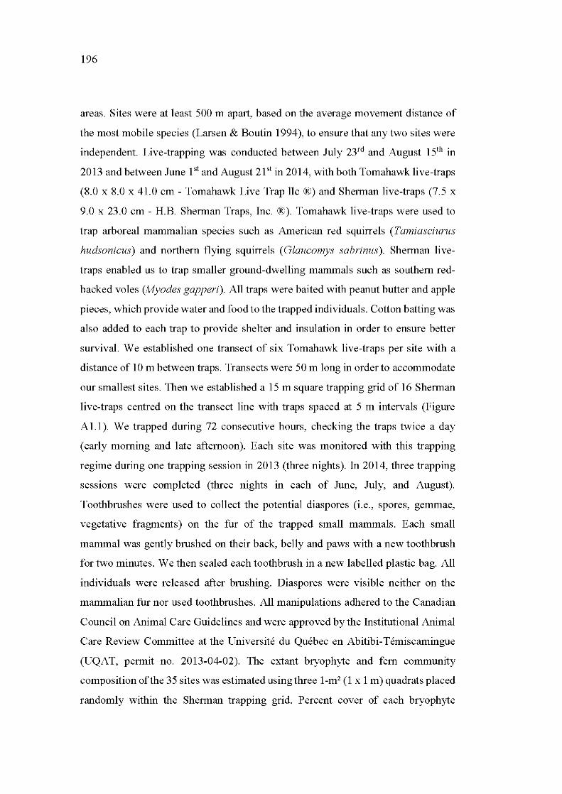
196

areas. Sites were at least 500 rn apart, based on the average movement distance of

the most mobile species (Larsen & Boutin 1994), to ensure that any two sites were

independent. Live-trapping was conducted between July 23rd and August 15th in

2013 and between June 1 stand August 21st in 2014, with both Tomahawk live-traps

(8.0 x 8.0 x 41.0 cm- Tomahawk Live Trap He®) and Sherman live-traps (7.5 x

9.0 x 23.0 cm- H.B. Sherman Traps, Inc. ®). Tomahawk live-traps were used to

trap arboreal mammalian species such as American red squirrels (Tamiasciurus

hudsonicus) and northern flying squirrels (Glaucomys sabrinus). Sherman live

traps enabled us to trap sma11er ground-dwelling mammals such as southern red

backed voles (Myodes gapperi). AU traps were baited with peanut butter and apple

pieces, which provide water and food to the trapped individuals. Cotton batting was

also added to each trap to provide shelter and insulation in order to ensure better

survival. We established one transect of six Tomahawk live-traps per site with a

distance of 10 rn between traps. Transects were 50 rn long in orderto accommodate

our sma11est sites. Then we established a 15 rn square trapping grid of 16 Sherman

live-traps centred on the transect line with traps spaced at 5 rn intervals (Figure

Al.l). We trapped during 72 consecutive hours, checking the traps twice a day

(earl y moming and late afternoon). Each site was monitored with this trapping

regime during one trapping session in 2013 (three nights). In 2014, three trapping

sessions were completed (three nights in each of June, July, and August).

Toothbrushes were used to co1lect the potential diaspores (i.e., spores, gemmae,

vegetative fragments) on the fur of the trapped sma11 mammals. Each sma11

mammal was gently brushed on their back, belly and paws with a new toothbrush

for two minutes. We then sealed each toothbrush in a new labe1led plastic bag. AU

individuals were released after brushing. Diaspores were visible neither on the

mammalian fur nor used toothbrushes. AU manipulations adhered to the Canadian

Council on Animal Care Guidelines and were approved by the Institutional Animal

Care Review Committee at the Université du Québec en Abitibi-Témiscamingue

(UQAT, permit no. 2013-04-02). The extant bryophyte and fern community

composition ofthe 35 sites was estimated usingthree 1-m2 (1 x 1 rn) quadrats placed

randomly within the Sherman trapping grid. Percent cover of each bryophyte

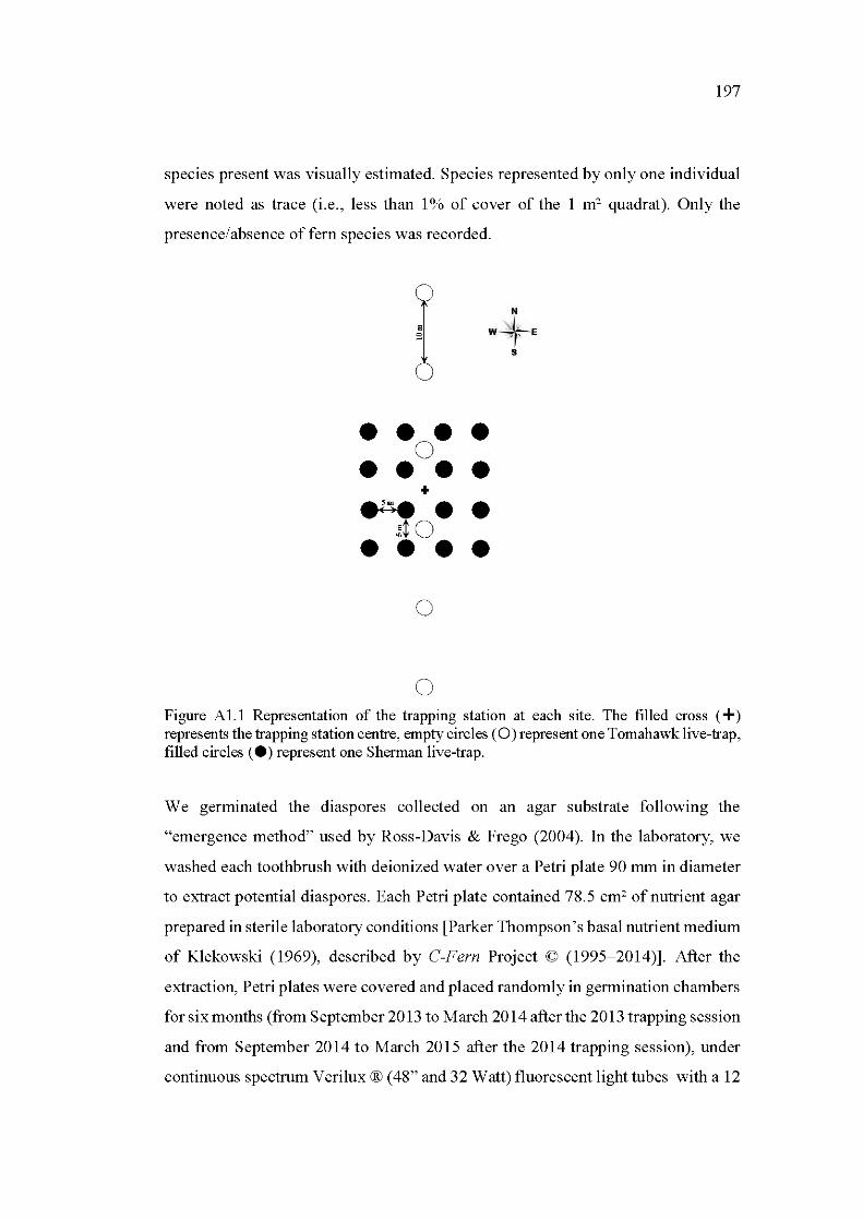
197

species present was visually estimated. Species represented by only one individual

were noted as trace (i.e., less than 1% of cover of the 1 m2 quadrat). Only the

presence/ absence of fern species was recorded .

• • • 0 • • • • • + -~"; . • • ~t o • • • •

0

0 Figure Al.l Representation of the trapping station at each site. The filled cross ( +) represents the trapping station centre, empty circles ( 0) represent one Tomahawk live-trap, filled circles (e ) represent one Sherman live-trap.

We germinated the diaspores collected on an agar substrate following the

"emergence method" used by Ross-Davis & Frego (2004). In the laboratory, we

washed each toothbrush with deionized water over a Petri plate 90 mm in diameter

to extract potential diaspores. Each Petri plate contained 78.5 cm2 of nutrient agar

prepared in sterile laboratory conditions [Parker Thompson's basal nutrient medium

of Klekowski (1969), described by C-Fern Project © (1995-2014)]. After the

extraction, Petri plates were covered and placed randomly in germination chambers

for six months (from September2013 to March 2014 afterthe 2013 trapping session

and from September 2014 to March 2015 after the 2014 trapping session), under

continuous spectrum Verilux ® (48" and 32 Watt) fluorescent light tubes with a 12

198

h/ 12 h light/dark regime. Petri plates were misted with deionized water as needed

to prevent them from drying out. Germination cham ber temperature was maintained

at 22 °C. When the nutrient agar became too thin, the entire content of the Petri

plate was transferred to a new Petri plate with fresh nutrient medium. When the

growing bryophytes and ferus were too tall for Petri plates to contain they were

placed in individual transparent plastic pots. Development of bryophyte

gametophytes was assessed twice a week following germination. Minor

contamination by fungus or algae was manually removed from the nutrient agar

with forceps. In the case of a major contamination, where the Petri plate was entirely

covered by fungus or algae and survival of the protonemata was compromised,

protonema were removed from the plate, bathed in deionized water and transplanted

in a new Petri plate. Three control Petri plates with virgin nutrient agar were placed

in the germination chambers every three months for the duration of the 6-month

emergence period to identify potential contaminants (air-borne diaspores). No

species developed on any ofthe control plates, indicatingthat sample plates had not

been contaminated during the laboratory growing period. Cryptogam culture with

this method was generally successful, even though it introduces a bias towards

cryptogam species able to germinate in artificial conditions.

All individuals were identified in the laboratory following Faubert (2013, 2014) for

bryophytes. Ferus were identified following Martineau (2014). Due to the artificial

growing conditions in Petri plates, bryophytes lacked sorne critical features for

species identification, which is why sorne specimens were only identified to genus,

in particular sphagna and members of the genera Pohlia sp. and Polytrichum sp.

A1.4.2 Statistical analyses

Data from 2013 and 2014 were pooled for analyses. Furthermore, we made no

distinction among the types of sites where small mammals were trapped due to the

low sample size in each site type ( old-growth forests, post-fire remnant patches,

green-tree retention patches and linear cut-block separators). We consequently

199

poo led data for all small mammals. We conducted analyses according to cryptogam

species taxonomie groups and life forms: liverworts, sphagna, and true mosses,

divided into acrocarpous and pleurocarpous groups. No distinction was made

between individuals germinated from spores or gemmae because we could not

distinguish among these two forms of diaspores on Petri plates. Vegetative

fragments (i.e., stem and leaf fragments) deposited on Petri plates were also

considered. To avoid overestimating the number of dispersed diaspores, cryptogam

individuals were counted using the number of individual proton erna and vegetative

fragments instead of the number of stems produced, given that a single proton erna

can generate several stems in one Petri plate. As it is difficult to distinguish

protonema once the plant is fully developed, monthly photographs of the plates

were used to identify individual protonema. We counted the number of protonema

germinated from spores/gemmae as well as the number of vegetative fragments in

each Petri plate. Species abundance was calculated as the number of individual of

each species per Petri plate. The extant community present on each site was

described using the mean percent co ver of each bryophyte species recorded in three

1-m2 quadrats. Ferus were considered present if observed in at least one of the three

1-m2 quadrats per site.

We compared the composition of the extant community and the diaspore

community grown in Petri plates using Kendall rank correlations (Legendre &

Legendre 2012). The individuals identified to genus in the Petri plates were

compared to the species from the same genus in the extant community (e.g.,

Polytrichum sp. from Petri plates were compared to Polytric hum commune sampled

on site). As there was no linear pattern between the two variables and because sorne

variables included outliers, the Kendall rank correlation was more appropriate than

the Pearson product-moment correlation to quantify the association between the

abundance of species grown in Petri plates and percent co ver of species in the extant

community. Similarly, to assess whether the abundance of species grown in Petri

plates was linked to their presence onsite, we used a second Kendall rank correlation

on the abundance of the cryptogam species grown in Petri plates and their cover in

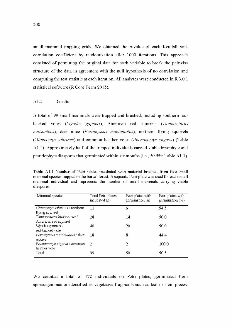
200

small mammal trapping grids. We obtained the p-value of each Kendall rank

correlation coefficient by randomization after 1000 iterations. This approach

consisted of permuting the original data for each variable to break the pairwise

structure of the data in agreement with the null hypothesis of no correlation and

computing the test statistic at each iteration. All analyses were conducted in R 3.0.1

statistical software (R Core Team 2015).

A1.5 Results

A total of 99 small mammals were trapped and brushed, including southem red

backed voles (Myodes gapperi), American red squirrels (Tamiasciurus

hudsonicus), deer mice (Peromyscus maniculatus), northem flying squirrels

(Glaucomys sabrinus) and common heather voles (Phenacomys ungava) (Table

A1.1 ). Approximately half of the trapped individuals carried viable bryophyte and

pteridophyte dias pores that germinated within six months (i.e., 50. 5%; Table A1.1 ).

Table A1.1 Number of Petri plates incubated with material brushed from five small mammal species trapped in the boreal forest. A separate Petri plate was used for each small mammal individual and represents the number of small mammals carrying viable dias pores.

Mammal species Total Petri plates Petri plates with Petri plates with incubated (n) germination (n) germination(%)

Glaucomys sabrinus 1 northem 11 6 54.5 flying squirrel Tamiasciurus hudsonicus 1 28 14 50.0 Am eric an red squirrel Myodes gapperi 1 40 20 50.0 red-backed vole Peromyscus maniculatus 1 deer 18 8 44.4 mouse Phenacomys ungava 1 common 2 2 100.0 heather vole Total 99 50 50.5

We counted a total of 172 individuals on Petri plates, germinated from

spores/gemmae or identified as vegetative fragments such as leaf or stem pieces.

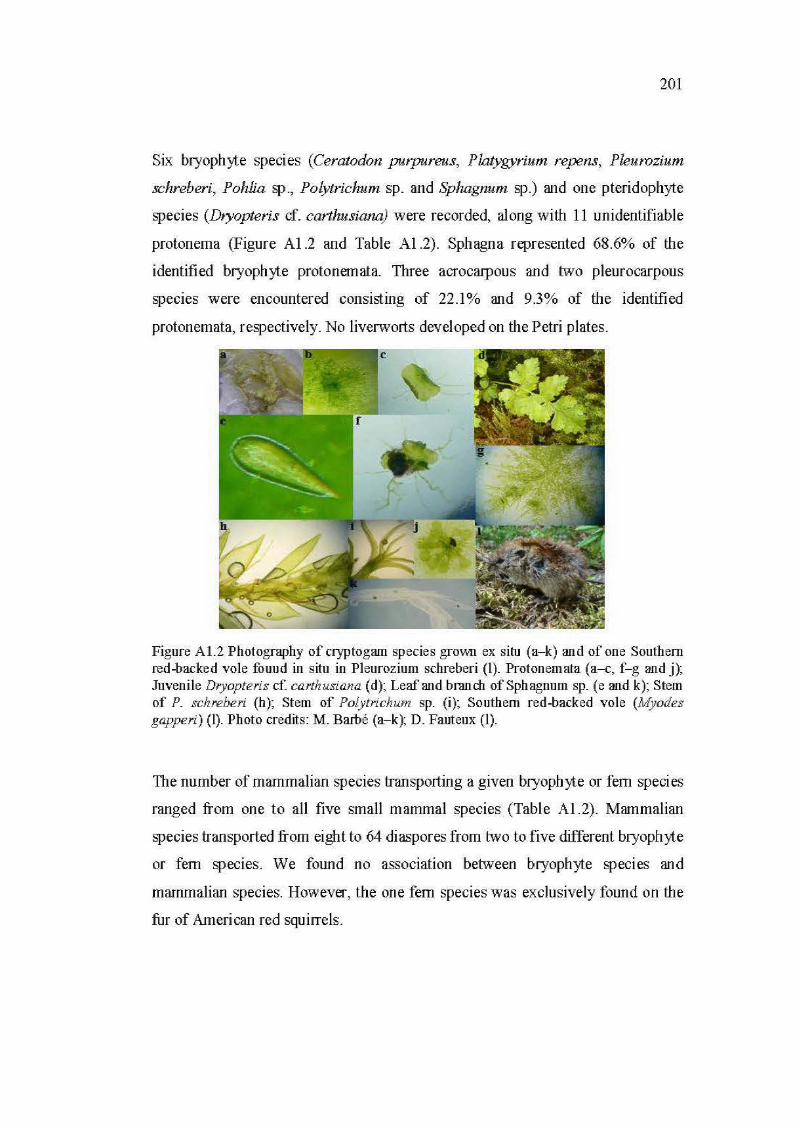
201

Six bryophyte species (Ceratodon purpureus, Platygyrium repens, Pleurozium

schreberi, Pohlia sp., Polytrichum sp. and Sphagnum sp.) and one pteridophyte

species (Dryopteris cf. carthusiana) were recorded, along with 11 unidentifiable

protonema (Figure A1.2 and Table A1.2). Sphagna represented 68.6% of the

identified bryophyte protonemata. Three acrocarpous and two pleurocarpous

species were encountered consisting of 22.1% and 9.3% of the identified

protonemata, respectively. No liverworts developed on the Petri plates.

Figure A l.2 Photography of cryptogarn species grovvn ex situ (a-k) and of one Southem red-backed vole found in situ in Pleurozium schreberi (l). Protonemata (a-c, f-g and j ); Juvenile Dryopteris cf carthusiana (d); Leafand branch ofSphagnum sp. (e and k); Stem of P. schreberi (h); Stem of Polytrichum sp. (i); Southem red-backed vole (Myodes gapperi ) (l). Photo credits: M. Barbé (a-k); D. Fauteux (l).

The number of mammalian species transporting a given bryophyte or fern species

ranged from one to ali five small mammal species (Table A1.2). Mammalian

species transported from eight to 64 diaspores from two to five different bryophyte

or fern species. We found no association between bryophyte species and

mammalian species. However, the one fern species was exclusively found on the

fur of American red squirrels.

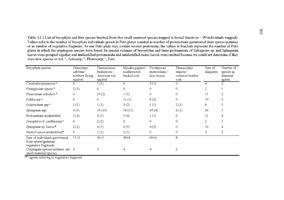
Table A1.2 List ofbryophyte and fern species brushed from five small mammal species trapped in boreal forests (n = 99 individuals trapped). Values refer to the number ofbryophyte individuals grown in Petri plates counted as number of protonemata germinated from spores/gemmae or as number ofvegetative fragment. As one Petri plate may contain several protonema, the values in brackets represent the number of Petri plates in which the cryptogam species were found. In species richness of bryophytes and ferns protonemata of Sphagnum sp. and Sphagnum leaves were grouped together and unidentified protonemata and unidentified stems/leaves were omitted because we could not determine if they were new species or not.", Acrocarp; b, Pleurocarp; c, Fern.

Bryophyte species Glaucomys Tamiasciurus Myodes gapperi 1 Peromyscus Phenacomys Sum of Number of sabrinus 1 hudsonicus 1 southern red- maniculatus 1 ungava 1 diaspores spec1es as northem flying Am eric an red backed vole deer mouse common heather dispersal sguirrel sguirrel vole agents

Ceratodon purpureus • 0 1 (1) 0 3 (1) 0 4 2

Platygyrium repens h 2 (1) 0 0 0 0 2

Pleurozium schreberi b 0 10 (2) 1 (1 ) 0 0 11 2

Pohlia spp" 0 0 11 (1) 8 (2) 0 19 2

Polytrichum spp" 1 (1) 1 (1) 3 (2) 1 (1) 2 (1) 8 5

Sphagnum spp. 6 (5) 19 (10) 18 (11) 47 (4) 6 (1) 96 5

Protonemata unidentified 2 (4) 3 (1) 5 (4) 1 (1) 0 11 4

Dryopteris cf. carthusiana c 0 2 (2) 0 0 0 2

Sphagnum sp. leaves* 2 (2) 4 (1) 6 (5) 4 (2) 0 16 4

Stems/Leaves unidentified * 0 1 (1) 2 (1 ) 0 0 3 2

Sum of individuals germinated 11+2 36+5 38+8 60+4 8 from spores/gemmae + vegetative fragments Cryptogam species richness per 3 5 4 4 2 small mammal species

"*"agents referrirlg to vegetative fragment.

N 0 N

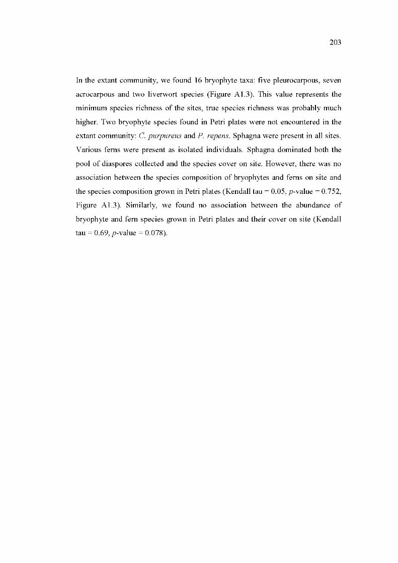
203

In the extant community, we found 16 bryophyte taxa: five pleurocarpous, seven

acrocarpous and two liverwort species (Figure A1.3). This value represents the

minimum species richness of the sites, true species richness was probably much

higher. Two bryophyte species found in Petri plates were not encountered in the

extant community: C. purpureus and P. repens. Sphagna were present in all sites.

Various ferus were present as isolated individuals. Sphagna dominated both the

pool of diaspores collected and the species cover on site. However, there was no

association between the species composition of bryophytes and ferus on site and

the species composition grown in Petri plates (Kendall tau = 0.05, p-value = 0.752,

Figure A1.3). Similarly, we found no association between the abundance of

bryophyte and fern species grown in Petri plates and their cover on site (Kendall

tau= 0.69, p-value = 0.078).

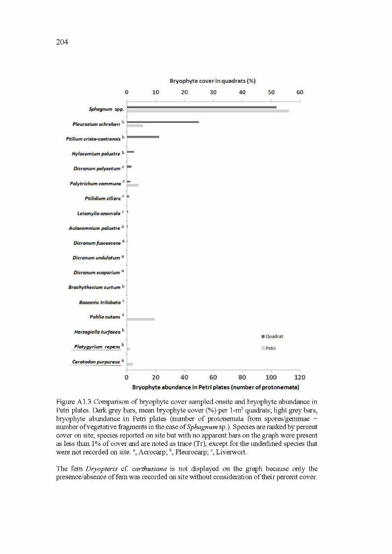
204

Bryophyte cover in quadrats (%)

0 10 20 30 40 50 60

Pleurozium schreberi b i='

Ptilium crista-costrensi~ b 1----•

Hylocomium palustre b ~

Dicranum polysetum a ~

Polytrichum comm,une a ~.

Ptilidium ci/fare c la

Leiomylia anom afa c

Aulacomnium palustre a

Dicranum fuscesce ns a

Dicranum undu/at,um a

Dicranum scoparium a

Brachythecium curtum b

Bazzania trilobata c

Pohlia nutans a !:--===

Herzogiella turfacea b 8Quadrat

Platygyrium repens b p Petri

Ceratodon purpureus a t-

0 20 40 60 80 100 120 Bryophyte abundance in Petri plates (number of protonemata)

Figure A 1.3 Comparison of bryophyte cover sampled onsite and bryophyte abundance in Petri plates. Dark grey bars, mean bryophyte cover (%) per 1-m2 quaclrats; light grey bars, bryophyte abundance in Petri plates (number of protonemata from spores/gemmae + number of vegetative fragments in the case of Sphagnum sp.). Species are ranked by percent cover on site; species reported on site but with no apparent bars on the graph were present as less than 1% of cover and are noted as trace (Tr), except for the underlined species that were not recorded on site. •, Acrocarp; b' Pleurocarp; ", Liverwort.

The fern Dryopteris cf. carthusiana is not displayed on the graph because on1y the presence/absence of fern was recorded on site without consideration oftheir percent co ver.

205

A1.6 Discussion

Southeru red-backed voles, American red squirrels, and deer mice were the most

abundant mammal species in our study sites. We found that these three species

along with northern flying squirrels and common heather voles were dispersal

agents for true moss es, sphagna and ferus. We also found that small mammals can

transport several species of bryophytes and in sorne cases, a copious amount of

viable diaspores of individual bryophyte species. Our results demonstrate that

ground-dwelling small mammals are not occasional dispersal agents but instead

represent important dispersers of bryophytes and ferus. Furthermore, ground

dwelling small mammals are in direct contact with the cryptogam layer and this

may enhance the dispersal of cryptogams that rarely produce spores or that are

poorly dispersed by the wind.

Mammalian species transported a fraction of species from the pool of bryophyte

genera available on sites. Keeping in mind that sorne of the taxa that germinated

were not identified to species due to germinating constraints, the pool of species

found in Petri plates only represented 20% of the species encountered on site. This

represents less than half ofwhat was found by Pauliuk et al. (2011) who collected

40% of the bryophytes species found in European dry grassland ecosystems on

large mammals. One factor explaining the low percent transported may be that none

ofthe species collected are known to have developed features on their diaspores to

actively rely on zoochory for dispersal ( e.g., spore ornamentation, colorful spores,

and sticky or odorous secretion to attract animal species; Demidova & Filin 1994;

Ignatov & Ignatova 2001; Rudolphi 2009). Alternatively, if the main agent

transported was spores, species phenology may have impacted our results, as not

all cryptogam species produced dispersal agents during our trapping sessions. For

instance, the over-abundance of sphagna diaspores may be explained by the

coincidence of diaspore release and our experiment (Sundberg & Rydin 2002).

In contrast, two species germinated in Petri plates that were not found in the extant

community, namely Ceratodon purpureus and Platygyrium repens. These species

206

may have bec orne attached to the fur of the small mammals wh en they dig in the

moss layer and mineral soil searching for food such as seeds and insects (Merritt

1981). This activity may result in sorne spores present in the soil propagule bank

becoming attached to their fur.

The only species of fern transported by a small mammal, D. cf carthusiana, is

common in the boreal forest and produces large amounts of spores easily dispersed

by wind (Rünk et al. 2012). However, ferus also reproduce by vegetative fragments

and alternative diaspores (c.f. Boch et al. 2013), which may be brushed off by

passing animais. In the present study, American red squirrels are the largest species

trapped on our study sites and the only one that carried fern spores. Despite this, we

found no apparent exclusive association between cryptogams and small mammals,

which can possibly be explained by the low number of individuals trapped for sorne

mammalian species.

Small mammal transport offers two main advantages over wind transport. First, as

small mammals and bryophytes share the same types of microhabitats (Fauteux et

al. 2012; Lohmus et al. 2007; Mills & Macdonald 2004) small mammals offer

oriented dispersal of the diaspores over the landscape. In contrast, during wind

dispersal all diaspores are randomly deposited in microhabitats up to several

kilometres away during wind dispersal (Lônnell 2011; van Zanten & Gradstein

1988). Secondly, ground-dwelling small mammals can transport species that are not

efficient at wind dispersal, due to either low sporophyte production or sporophyte

morphology. Ground-dwelling small mammals can transport cryptogam diaspores

within the ir home range (from several meters for de er mi ce, up to 3. 5 km for red

squirrels; Bowman et al. 2002; Larsen & Boutin 1994, 1995; Wells-Gosling &

Heaney 1984). Cryptogams could also be transported beyond small mammal home

ranges during mammalian species dispersal and establishment of new home ranges.

As a possible example, we brushed one individual that was carrying C. purpureus,

80 rn away from the closest C. purpureus colony found in a concurrent study

performed on the same study sites (Barbé et al. 20 16).

207

We showed that ground-dwelling small mammals disperse bryophytes and ferus.

However, additional species could be identified. Indeed, sorne species do not

germinate on the agar substrate and others may have germinated after 6 months.

However, as a concomitant study performed with the same protocol yielded the

germination of 46 bryophyte species (Barbé et al. 2016). We argue that the reduced

pool of species from this study is not due to the germination protocol. The

composition of the bryophyte aerial propagule rain will differ among seasons with

species phenology (Hock et al. 2004; Ross-Davis & Frego 2004; Stark 2002).

Moreover, weather conditions such as relative humidity, night temperatures and

rainfall might also have influenced cryptogam phenology via spore release (Glime

2014; Johansson et al. 2015), small mammal activity (Wr6bel & Bogdziewicz 2015)

and diaspore adherence to fur. In addition, other constraints associated with the

sampling methods could have affected the results such as the use of cotton balls for

the small mammal trapping in which diaspores might have been deposited during

the many hours spent by the animais in the traps. In the future, we recommend to

also collect the cotton balls provided in the traps. Finally, it may be important to

consider the effectiveness of toothbrushes at removing diaspores that are

electrostatically charged. Alternative collection methods on the fur might yield

different species, and this topic could be explored in future studies.

To our knowledge, we provide the first direct evidence of epizoochory involving

bryophytes and ferus and ground-dwelling small mammals in boreal forest

ecosystems. The daily interaction between small mammals and the cryptogam layer

could contribute to the directed transport of bryophyte and fern diaspores over

medium distances and towards suitable substrates. Persistence of bryophyte and

fern metapopulations depends on dispersal across the forest matrix and small

mammals are identified as "mobile link organisms" (sensu Couvreur et al. 2004)

that may parti ci pate in connecting fragmented bryophyte and fern populations. Our

results open the door for a timely revision of bryophyte and fern dispersal

mechanisms, extending the notion of epizoochory by ground-dwelling small

mammals to other cryptogams such as horsetail, lichen or liverwort species.

208

Al. 7 Acknowldgements

We thank Pierre Martineau for confirming fern identifications, and Dominique

Fauteux for lending photographs of small mammals. The authors thank all the field

and lab assistants who provided logistical support, and helped in collecting the

samples, growing the bryophytes and taking photos.

The work was supported by the Fonds de Recherche du Quebec-Nature et

Technologies (FRQNT) under the grant 2013-FM-170582; and the Natural

Sciences and Engineering Research Council of Canada (NSERC) under the grant

NSERC CRD 428686-11 Bergeron.

A1.8 References

Arosa ML, Ramos JA, Quintanilla D, Brown LG. 2010. First report offern (Culcita macrocarpa) spore consumption by a small mammal (Apodemus sylvaticus). Mamm Biol. 75:115-121.

Baker JA, Entsch B, McKay DB. 2003. The cyanobiont in anAzolla fern is neither Anabaena nor Nostoc. FEMS microbiology letters 229:43-47.

Barbé M, Fenton NJ, Bergeron Y. 2016. So close and yet so far away: long-distance dispersal events govern bryophyte metacommunity reassembly. J Ecol. DOl: 10.1111/1365-2745.12637

Bay G, Nahar N, Oubre M., Whitehouse MJ, Wardle DA, Zackrisson 0 , Nilsson M-C, Rasmussen U. 2013. Boreal feather mosses secrete chemical signais to gain nitrogen. New Phytol. 200:54-60.

Benscoter BW. 2006. Post-fire bryophyte establishment in a continental bog. J Veg Sei. 17:647--652.

Bergeron Y, GauthierS, Flannigan M, Kafka V. 2004. Pire regimes at the transition between mixedwood and coniferous boreal forest in N orthwestern Que bec. Ecology. 85:1916-1932.

Boch S, Berlinger M, Fisher M, Knop E, Nentwig W, Türke M, Prati D. 2013. Fern and bryophyte endozoochory by slugs. Oecologia. 172:817-822.

Bowman J, Jaeger JAG, Fahrig L. 2002. Dispersal distance of mammals is proportional to home range size. Ecology. 83:2049-2055.

C-Fern Project ©. 1995-2014. Nutrient Medium Preparation-Traditional Method. Available on: http://www.c-fern. org/index. php ?option=com _ content&view=article&id=82&Itemi.

209

Carey AB. 2003. Managing for wildlife: a key component for social acceptance of compatible forest management. Compatible Forest Management. Kluwer Academie Publishers.

Clark KL, Nadkarni NM, Gholz HL. 2005. Retention of inorganic nitrogen by epiphytie bryophytes in a tropical montane forest. Biotropica. 37:328-336.

Couvreur M, Christiaen B, V erheyen K, Herm y M. 2004. Large herbivores as mobile links between isolated nature reserves through adhesive seed dispersal. Appl Veg Sei. 7:229-236.

Crum HA. 2001. The Structural Diversity of Bryophytes. University of Michigan Herbarium, Michigan.

Davidson AJ, Harbome JB, Longton RE. 1990. The acceptability ofmosses as food for generalist herbivores, slugs in the Arionidae. Bot J Linn Soc. 104:99- 113.

Davison GWH. 1976. Role ofbirds in moss dispersal. Brit Birds. 69:65-66.

De Groot GA, During HJ, Ansell SW, Schneider S, Bremer P, Wubs REJ, Maas JW, Korpelainen H, Erkens RHJ. 2012. Diverse spore rains and limited local exchange shape fern genetic diversity in a recently created habitat colonized by long-distance dispersal. Ann Bot-London. 109:965-987.

DeLuca TH, Zackrisson 0, Gentili F, Sellstedt A, Nilsson MC. 2007. Ecosystem controls on nitrogen fixation m boreal feather moss communities. Oecologia. 152:121-130.

Demidova EE, Filin VR. 1994. False columella and spore release in Tetraplodon angustatus (Hedw.) Bruch et Schimp. in B.S.G. and T. mnioides (Hedw.) Bruch et Schimp. in B.S.G. (Musci: Splachnaceae). Arctoa. 3:1-6.

Eckert CG. 2002. The loss ofsex in clonai plants. Evol. Ecol. 15:501-520.

Environment Canada. 2015. Canadian climate normals 1981-2010 Station data. A vailable on: http: //climate.weather.gc.ca/climate _ normals/results _1981_ 2010 _ e.html?stniD =6051&lang=e&StationName=Lebel+sur+Quevillon&SearchType= Contains&stnN ameSubmit=go&dCode=5&dispBack= 1.

Faubert J. 2013. Flore des bryophytes du Québec-Labrador- Volume 2: Mousses, première partie. Société québécoise de bryologie, Saint-Valérien, Québec.

Faubert J. 2014. Flore des bryophytes du Québec-Labrador- Volume 3 :Mousses, seconde partie. Société québécoise de bryologie, Saint-Valérien, Québec.

Fauteux D, Imbeau L, Drapeau P, Mazerolle MJ. 2012. Small mammal responses to coarse woody debris distribution at different spatial scales in managed and unmanaged boreal forests. Forest Ecol Manag. 266: 194-205.

210

Fenton NJ, Bergeron Y. 2006. Facilitative succession in a boreal bryophyte community driven by changes in available moi sture and light. J V eg Sei. 17:65-76.

George LM, Bazzaz FA. 1999. The fern understory as an ecological filter: emergence and establishment of canopy tree-seedlings. Ecolo gy. 80:833-845.

Glime JM. 2014. Adaptive Strategies: Spore Dispersal Vectors. Chapt. 4-9. In: Glime JM, editor, Bryophyte Ecology. Volume 1. 4-9-1 Physiological Ecology. Ebook sponsored by Michigan Technological University and the International Association of Bryologists. Last updated 28 April 2014. Available on : www.bryoecol.mtu.edu.

Grondin P. 1996. Écologie forestière. In: Bérard LA, Côté M, editors, Manuel de foresterie. Presse de 1 'Université Laval, p. 133-279.

Haines WP, Renwick JAA. 2009. Bryophyte as food: comparative consumption and utilization of mosses by a generalist insect herbivore. Entomol Exp Appl. 133:296-306.

Heinken T, Lees R, Raudnitschka D, Runge S. 2001. Epizoochorous dispersal of bryophyte stem fragments by roe deer (Capreolus capreolus) and wild boar (Sus scrofa). J Bryol. 23:293-300.

Hock Z, Szôvényi P, T6th Z. 2004. Seasonal variation in the bryophyte diaspore bank of open grasslands on dolomite rock. J Bryol. 26:285-292.

Hylander K. 2009. No increase in colonization rate of boreal bryophytes close to propagule sources. Ecology. 90:160-169.

lgnatov MS, lgnatova EA. 2001. On the zoochory of Schistostega penna ta (Schistostegaceae, Mus ci). Arctoa. 10:83-96.

Imbeau L, St-LaurentMH, Marzell L, Brodeur V. 2015. Current capacityto conduct ecologically sustainable forest management in north eastern Canada reveals challenges for conservation ofbiodiversity. Can J For Res. 45:567-578.

Johansson V, Lônnell N, Sundberg S, Hylander K. 2014. Release thresholds for moss spores: the importance of turbulence and sporophyte length. J Ecol. 102:721-729.

Johansson V, Lônnell N, Rannik Ü, Sundberg S, Hylander K. 2015. Air humidity thresholds trigger active moss spore release to extend dispersal in space and time. Funct Ecol. DOl: 10.1111/1365-2435.12606

Kimmerer RW. 1994. Ecological consequences of sexual versus asexual reproduction inDicranumflagellare and Tetraphis pellucida. Bryologist. 97:20-25.

Kimmerer RW, Young CC. 1995. The role of slugs in dispersal of the asexual propagules of Dicranumjlagellare. Bryologist. 98:149-153.

211

Klekowski EJ. 1969. Reproductive biology of the Pteridophyta. III. A study of the Blechnaceae. Bot J Linn Soc. 62:361-377.

Larsen KL, Boutin S. 1994. Movements, survival, and settlement of red squirrel (Tamiasciurus hudsonicus) offspring. Ecology. 75:214-223.

Legendre P, Legendre L. 2012. Numerical Ecology, 3rd Edition. Elsevier.

Lewis LR, Behling E, Gousse H, Qian E, Elphick CS, Lamarre J-F, Bêty J, Liebezeit J, Rozzi R, Goffinet B. 2014. First evidence ofbryophyte diaspores in the plumage of trans equatorial migrant birds. PeerJ 2: e424. DOl: 10.7717/peerj.424

Lôbel S, Rydin G. 2009. Dispersal and life history strategies in epiphyte metacommumtles: alternative solutions to survival in patchy, dynamic landscapes. Oecologia. 161:569-579.

Lohmus A, Lohmus P, Vellak K. 2007. Substratum diversity explains landscapescale co-variation in the species-richness of bryophytes and lichens. Biol Conserv. 135:45-414.

Lônnell N. 2011. Wind dispersal of spores with focus on bryophytes. Plant Ecol 3:1- 37.

Miilson K, Rydin H. 2007. The regeneration capabilities of bryophytes for rich fen restoration. Biol Conserv. 135:43 5--442.

Marino P, Raguso R, Goffinet B. 2009. The ecology and evolution of fly dispersed dung mosses (Family Splachnaceae): Manipulating insect behavior through odour and visual eues. Symbiosis. 47:61-76.

Martineau P. 2014. Plantes de l'enclave argileuse Barlow-Ojibway - Québec. Éditions, P. Martineau, Rouyn-Noranda. ISBN : 978-2-9814410-0-3.

Merritt JF. 1981. Clethrionomys gapperi. Mammalian Species 146:1-9

Mills SE, Macdonald SE. 2004. Predictors of moss and liverwort species diversity ofmicrosites in conifer-dominated boreal forest. J Veg Sei. 15:189-198.

Mufioz J, Felicisimo ÂM, Cabezas F, Burgaz AR, Martinez 1. 2004. Wind as a longdistance dispersal vehicle in the Southern Hemisphere. Sciences. 304:1144-1147.

Osorio-Zufiiga F, Fonturbel FE, Rydin H. 2014. Evidence of mutualistic synzoochory between cryptogams and hummingbirds. Oikos. 123:553-558.

Parsons JG, Cairns A, Johnson CN, Robson SKA, Shilton LA, Westcott DA. 2007. Bryophyte dispersal by flying foxes: a novel discovery. Oecologia. 152:112-114.

Pauliuk F, Müller J, Heinken T. 2011. Bryophyte dispersal by sheep on dry grassland. Nova Hedwigia. 92:327-341.

212

Pohjamo M, Laaka-Lindberg S, Ovaskainen 0 , Korpelainen H. 2006. Dispersal potential of spores and asexual propagules in the epixylic hepatic Anastrophyllum hellerianum. Evol Ecol. 20:415--430.

R Core Te am. 2015. R: A language and environment for statistical computing. R Foundation for Statistical Computing, Vienna.

Rochefort L, Quinty F, Campeau S, Johnson K, Malterer T. 2003. North American approach to the restoration of Sphagnum dominated peatlands. Wetl Ecol Manag. 11:3-20.

Ross-Davis AL, Frego KA. 2004. Propagule sources of forest floor bryophytes: spatiotemporal compositional patterns. Bryologist. 107:88-97.

Rudolphi J. 2009. Ant-mediated dispersal of asexual moss propagules. Bryologist. 112:73-79.

Rünk K, Zobel M, Zobel K. 2012. Biological Flora ofthe British Isles: Dryopteris carthusiana, D. dilatata andD. expansa. 1 Ecol. 100:1039-1063.

Rydgren K, 0kland RH, Pico FX, Kroon HD. 2007. Moss species benefits from breakdown of cyclic rodent dynamics in boreal forests. Ecolo gy. 88:2320-2329.

Sôderstrôm L. 1987. Dispersal as a limiting factor for distribution among epixylic bryophytes. Symp Biol Hung. 35:475--483.

Stark LR. 2002. Phenology and its repercussions on the reproductive ecology of mosses. Bryol. 105:204-218.

Sundberg S, Rydin H. 2002. Habitat requirements for establishment of Sphagnum from spores. 1 Ecol. 90:268-278.

Sundberg S. 2013. Spore rain in relation to regional sources and beyond. Ecography. 36:364-373.

Tâj ek P, Bucharovâ A, Münzbergovâ Z. 2011. Limitation of distribution oftwo rare ferns in fragmented landscape. Acta Oecol. 37:495- 502.

Turetsky MR, Bond-Lamberty B, Euskirchen E, Talbot J, Frolking S, McGuire AD, Tuittila E-S. 2012. The resilience and functional role of moss in boreal and arctic ecosystems. New Phytol. 196:49-67.

van Zanten BO, Gradstein SR. 1988. Experimental dispersal geography of neotropicalliverworts. Beih Nova Hedwigia. 90:41-94.

Wells-Gosling N, Heaney LR. 1984. Glaucomys sabrinus. Mammalian species. 229:1-8.

Wr6bel A, Bogdziewicz M. 2015. It is raining mice and voles: which weather conditions influence the activity of Apodemus flavicollis and Myodes glareolus? Eur 1 Wildlife Res. 61:475-478

ANNEXE II

DISTRIBUTION RANGE EXTENSION OF 35 BRYOPHYTE SPECIES FROM SAMPLING IN THE NEGLECTED SOUTH OF NORTHERN-QUÉBEC

(CANADA)

Marion Barbé, Louis Dubois, Jean Faubert, Martin Lavoie, Yves Bergeron &

Nicole 1. Fenton

En préparation pour Canadian Field Naturalist

214

A2.1 Abstract

While the North American bryoflora is relatively well-known, sorne terri tories as

the south of the Northem-Québec administrative region (between 49 and 51 °N and

74 and 79°W) remain under sampled. We report the presence of 168 bryophyte taxa

for this region, of which 35 (14 true mosses, 20 liverworts, 1 sphagna) represent

noteworthy records. Occurrences of sorne taxa already known in the region but

previously under sampled were actualized, whereas 20 taxa are news for the region.

These inventories contribute both to actualize the status of occurrences and to

extend the distribution ranges ofthese taxa toward the north. Disjunct distribution

ranges of sorne taxa are linked together and their microhabitat preferences are

documented. This work is a substantial input to the Flora of the bryophytes of

Québec-Labrador and can be used to redefine protection priority ranks ofspecies in

North America.

Keywords: range extension; black spruce-feather moss forest; bryoflora; bryo

geography; boreal; liverwort; true moss; sphagna.

A2.2 Résumé

Malgré une globale bonne connaissance de la bryoflore nord-américaine, certaines

régions telles que le Nord-du-Québec, et particulièrement le sud entre le 49e et le

51 e parallèle nord, demeurent sous-échantillonnées. Nous rapportons ici la présence

de 168 taxons bryophytiques, dont 35 taxa (14 mousses, 20 hépatiques et 1

sphaigne) représentent des ajouts substantiels à la flore de la région. Certains de ces

taxons étaient déjà connus au Québec et 20 sont nouveaux pour le territoire

considéré. Ces récoltes permettent d'actualiser les statuts d'occurrences et

d'étendre l'aire de répartition de ces espèces vers le nord. Les aires de répartition

de plusieurs taxons considérées disjointes à ce jour sont ralliées et leurs préférences

en termes de microhabitats sont renseignées.

215

Ce travail représente un apport conséquent à aux connaissances de la flore des

bryophytes du Québec-Labrador et permettra de redéfinir les rangs de priorité de

conservation des espèces à l'échelle de l'Amérique du Nord.

Mots-clés : aire de répartition ; bryoflore ; forêt boréale ; hépatiques ; mousses ;

pessière noire ; Québec ; sphaignes.

A2.3 Introduction

Bryophytes (i.e. true mosses, liverworts and sphagna), jointly with lichens,

represent the most conspicuous components of the vegetation of the northem

latitudes (Turetsky et al. 20 12). They form a continuo us carpet of sever al

centimeters thick in coniferous boreal forests, represent a major element in net

primary productivity, understory biomass and in biodiversity (Bis bee et al. 2001;

Proctor 20 11). This is especially true in the bioclimatic su bd ornain of the boreal

black spruce feather-moss forest, which is characterized by shady, humid,

chemically poor and acidic conditions favouring a copious diversity of bryophyte

species, particularly Sphagnum spp. in poorly drained habitats (Fenton and

Bergeron 2006; Vile et al. 2011).

Bryophytes represent 25% ofthe plant diversity of Québec (Faubert et al. 2010). In

2016, the database of the bryophytes of Québec-Labrador listed 582 mosses, 231

liverworts and 62 sphagna species (Faubert et al. 2014+). However, the distribution

range of sorne species remains parti ally defined and even unknown in certain areas

(Faubert and Gagnon 20 13). This is the case in the administrative regions of Abitibi

Témiscamingue and the southem portion of the Northem-Québec, which are under

sampled compared to various other regions. However, knowledge of the real

distribution ranges of bryophytes is an elementary step in establishing conservation

plans and in orientating forest management practices in these regions where boreal

forests are disturbed both by natural wildfires and forest harvest. The addition of

cumulative disturbances to the landscape jeopardizes the resilience of the

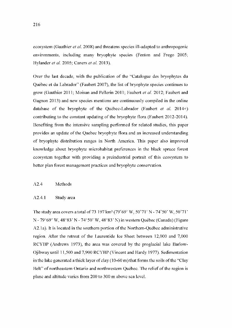
216

ecosystem (Gauthier et al. 2008) and threatens species ill-adapted to anthropogenic

environments, including many bryophyte species (Fenton and Frego 2005;

Hylander et al. 2005; Caners et al. 2013).

Over the last decade, with the publication of the "Catalogue des bryophytes du

Québec et du Labrador" (Faubert 2007), the list of bryophyte species continues to

grow (Gauthier 2011; Moisan and Pellerin 2011; Faubert et al. 2012; Faubert and

Gagnon 20 13) and new species mentions are continuously compiled in the online

database of the bryophyte of the Québec-Labrador (Faubert et al. 2014+)

contributing to the constant updating of the bryophyte flora (Faubert 2012-2014).

Benefiting from the intensive sampling performed for related studies, this paper

provides an update ofthe Quebec bryophyte flora and an increased understanding

of bryophyte distribution ranges in North America. This paper also improved

knowledge about bryophyte microhabitat preferences in the black spruce forest

ecosystem together with providing a preindustrial portrait of this ecosystem to

better plan forest management practices and bryophyte conservation.

A2.4 Methods

A2.4.1 Study area

The study area covers a total of73 197 km2 (79°69' W, 50°71' N- 74°50' W, 50°71'

N- 79°69' W, 48°83' N- 74°50' W, 48°83' N) in western Québec (Canada) (Figure

A2.1a). It is located in the southem portion of the Northem-Québec administrative

region. After the retreat of the Laurentide lee Sheet between 12,000 and 7,000

RCYBP (Andrews 1973), the area was covered by the proglacial lake Barlow

Ojibway until11,500 and 7,900 RCYBP (Vincent and Hardy 1977). Sedimentation

in the lake generated a thick layer of clay (10-60 rn) that forms the soils of the "Clay

Belt" of northeastem Ontario and northwestem Québec. The relief of the region is

plane and altitude varies from 200 to 300 rn above sea level.

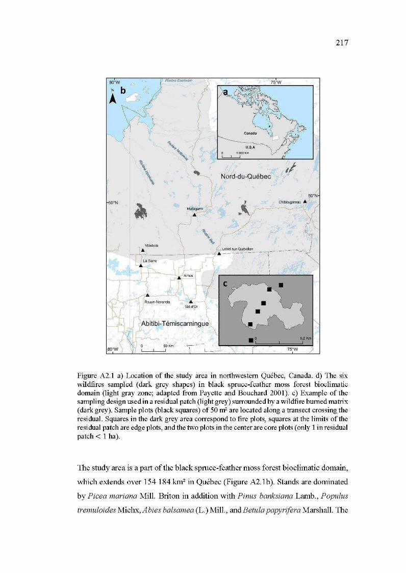
so·w N

Â

50"N

so·w

\! 1i.

"&· '$

"1-%. \

Villebois

Rivrere Eastmam

1'_,

"""-~< 01< .. ,. ~

' ._.

Matagami

•

75"W

U.S.A

o 1000Km L__L__J

Nord-du-Québec

Chibougamau Â

• Lebel-sur-Quévillon _ _ ---- --' -- - - - --ç·---------- \ \ :

1

Rouyn-Noranda :.t. Val-d'Or

Abitibi-T émiscamingue'

'.J 0 SOKm

217

Figure A2.1 a) Location of the study area in northwestem Québec, Canada. d) The six wildfires sampled (dark grey shapes) in black spruce-feather moss forest bioclimatic domain (light gray zone; adapted from Payette and Bouchard 2001). c) Example of the sampling design used in a residual patch (light grey) surrounded by a wildfire bumed matrix (dark grey). Sample plots (black squares) of 50m2 are located along a transect crossing the re si dual. Squares in the dark grey area correspond to fire plots, squares at the limits of the re si dual patch are edge plots, and the two plots in the center are core plots ( only 1 in residual patch < 1 ha).

The study area is a part of the black spruce-feather moss forest bioclimatic domain,

which extends over 154 184 km2 in Québec (Figure A2.1 b ). Stands are dominated

by Picea mariana Mill. Briton in addition with Pinus banksiana Lamb. , Populus

tremuloides Michx, A bi es balsamea (L.) MilL, and Betula papy rifera MarshalL The

218

understory 1s characterized by encaceous shrubs [ e.g. Rhododendron

groenlandicum (Oeder) Kron & Judd] on a ground cover of bryophytes (Saucier et

al. 2009). Average annual temperatures and precipitations are respectively 1 oc and

928 mm (1981 to 2010) (Lebel-sur-Quévillon weather station; Environment Canada

20 15). The region is characterized by long winters with 313 cm of annual snowfall

and by a short growing season (140 to 160 days). The natural dynamics of the

forests in the study area are primarily driven by stand replacing wildfires. The fire

cycle was estimated at 398 years since 1920 (Bergeron et al. 2004), consequently,

the average age ofthe forest is in excess of 150 years.

A2.4.2 Bryophyte sampling

Bryophytes were sampled according to a modified form of the "floristic habitat

sampling" of Newmaster et al. (2005). In the original method, all the habitats are

searched for species with no specifie reference to area. Here the sampling was

restricted to 50 m2 rectangular plots where bryophytes were recorded in all the

microhabitats present ( e.g. coarse woody debris, tree bases, peat mounds,

waterholes). We did not select habitats of interest for sampling certain taxa or the

maximum of species, but rather all species in all microhabitats within a specifie

are a.

Bryophytes were sampled in six wildfires varying in age, size and origin (Table

A2.1). Within each wildfire, we identified five residual patches and three bumed

matrix areas for a total of 30 residual patches from 36 to 3400 years (time since the

last wildfire) and 18 bumed matrices from 10 to 44 years (time sin ce the last

wildfire ). This sampling was designed in such a way be cause benefiting from

related studies (Barbé et al. 2016, refers to Chapter IV; Barbé et al. in revision,

refers to Chapter II) included in a thesis project focusing in the role of post-fire

residual patches in bryophyte community reassembly after disturbance. All the

residual patches were chosen based on the criteria of the dominance of black spruce,

accessibility ( < 600 rn from a road) and a flat topography. Patch es varied in size

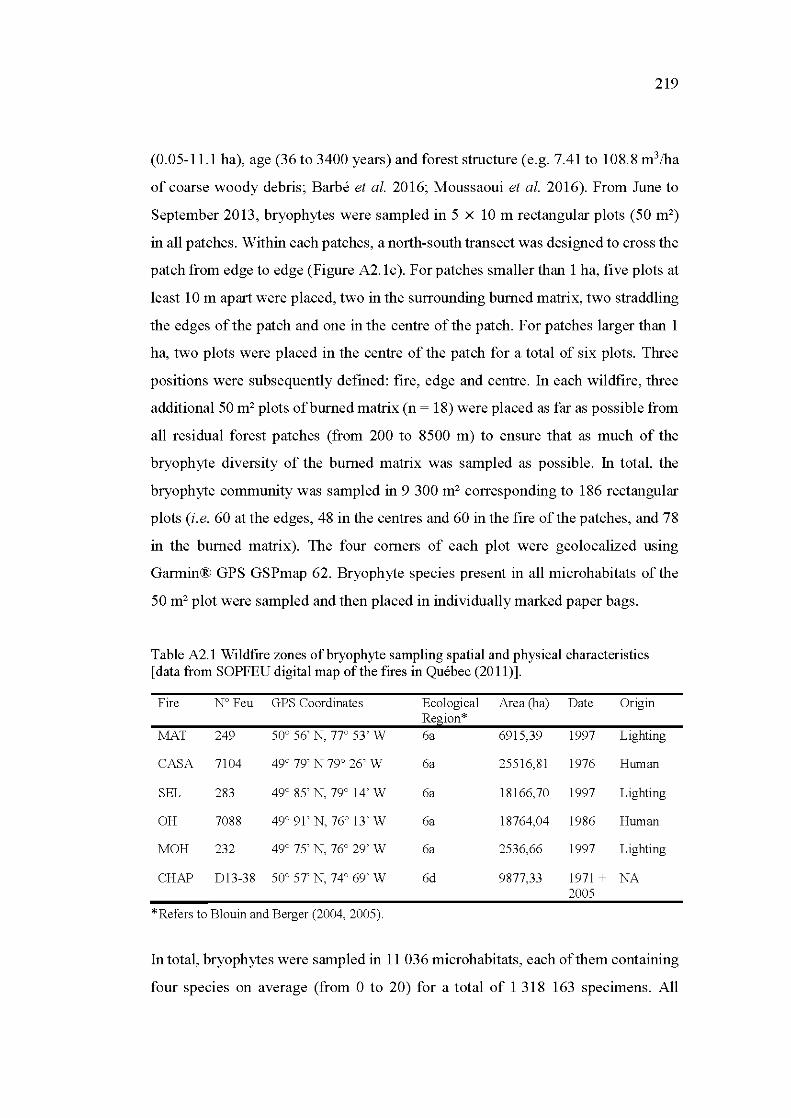
219

(0.05-11.1 ha), age (36 to 3400 years) and forest structure ( e.g. 7.41 to 108.8 m3 /ha

of coarse woody debris; Barbé et al. 2016; Moussaoui et al. 2016). From June to

September 2013, bryophytes were sampled in 5 x 10 rn rectangular plots (50m2)

in all patches. Within each patches, a north-south transect was designed to cross the

patch from edge to edge (Figure A2.1c ). For patch es smaller than 1 ha, five plots at

least 10 rn apart were placed, two in the surrounding bumed matrix, two straddling

the edges of the patch and one in the centre of the patch. For patches larger than 1

ha, two plots were placed in the centre of the patch for a total of six plots. Three

positions were subsequently defined: fire, edge and centre. In each wildfire, three

additional 50m2 plots ofbumed matrix (n = 18) were placed as far as possible from

all residual forest patches (from 200 to 8500 rn) to ensure that as much of the

bryophyte diversity of the bumed matrix was sampled as possible. In total, the

bryophyte community was sampled in 9 300m2 corresponding to 186 rectangular

plots (i.e. 60 at the edges, 48 in the centres and 60 in the fire of the patches, and 78

in the bumed matrix). The four corners of each plot were geolocalized using

Garmin® GPS GSPmap 62. Bryophyte species present in all microhabitats of the

50 m2 plot were sampled and then placed in individually marked paper bags.

Table A2.1 Wildfrre zones ofbryophyte sampling spatial and physical characteristics [data from SOPFEU digital map of the fires in Québec (2011)].

Fire N° Feu GPS Coordinates Ecological Area (ha) Date Origin Re ion*

MAT 249 50° 56' N, 77° 53' W 6a 6915,39 1997 Lighting

CASA 7104 49° 79' N 79° 26' W 6a 25516,81 1976 Hum an

SEL 283 49° 85' N, 79° 14' W 6a 18166,70 1997 Lighting

OH 7088 49° 91' N, 76° 13' W 6a 18764,04 1986 Hum an

MOH 232 49° 75' N, 76° 29' W 6a 2536,66 1997 Lighting

CHAP Dl3-38 50° 57' N, 74° 69' W 6d 9877,33 1971 + NA 2005

*Refers to Blouin and Berger (2004, 2005).

In total, bryophytes were sampled in 11 036 microhabitats, each of them containing

four species on average (from 0 to 20) for a total of 1 318 163 specimens. All

220

samples were dried and stored until identification to the species level in laboratory

using a stereomicroscope and a microscope. Damaged, senescent or too young

specimens were only identified to genus. Vouchers are store at the Université du

Québec en Abitibi-Témiscamingue (Québec, Canada). Nomenclature follows

Faubert (2012-2014) except for Sphagnum subtile (Russ.) Warnst., which follows

the nomenclature of the Flora of North America Editorial Committee (2007).

Microhabitats where species were recorded were qualitatively compared with data

from the Flora ofthe bryophyte ofthe Québec-Labrador (Faubert 2012-2014) in

order to underline potential specificities of the species to one micro habitat in the

study area.

A2.4.3 Species cartography

Distribution maps were produced only for species that present changes compared

to their original distributional range for the study area. New occurrences were

compared with those presented in the pub li shed Flora and online database of the

bryophytes of the Québec-Labrador (Faubert 2012-2014; Faubert et al. 2014+).

Documented occurrences of the species corresponds to GPS locations and were

used with the permission of the open access and participative online database of the

bryophytes ofthe Québec-Labrador currently updated with independent botanists'

records (Faubert et al. 2014+). Maps were generated using the geographie

information system ArcGis 10.3.1 (ESRI 2015). Original map layers come from the

Géolndex+ platform of the Geographie and Statistic Information Center (GéoStat

Center) of the Université Laval created with data from Statistics Canada,

geographie division, DMTI Spatial Inc., and ESRI. The projection used for all maps

was NAD83 CSRS MTM 10.

A2.4.4 Data analyses

Species were classified as rare ( < 5 occurrences; Faubert et al. 20 14+ ), infrequent

(5 to 10 occurrences), uncommon (10 to 30 occurrences), and common (> 30

221

occurrences). Rare, infrequent and uncommon spectes were mapped as dots,

whereas common species were mapped as shaded zones. Current status of

occurrence of certain species were re-estimated by comparison between

documented and new occurrences.

Microhabitats where species were found in the study area were compared with those

previously documented (Faubert 2012-2014 ). Microhabitats were classified as

humus (T - terricolous species living on soil and litter), bog (B - species living

among sphagna, in fens and bogs), dead wood (DW - facultative or obligate

epixylics), epiphyte (EP - strictly epiphyte or corticolous species living at the base

of trees) and rock (R - saxicolous species). Species inhabiting constantly humid

habitats (i.e. old dead wood totally collapsed, oozing rocks, water holes or edges of

creeks) were classified in the humus group but identified with a "W". At a fin er

scale, dead wood was categorized using Thomas et al. 's (1979) decay classification

system for snags and dead wood: classes 1 and 2 were grouped and correspond to

"recently" fallen dead trees with bark and branches intact; class 3 refers to dead

wood without bark or branches and with softening wood; and classes 4 and 5 were

grouped and refer to dead woods with a collapsed shape. Bumed wood was also

noted. Finally, the host tree species was recorded

A2.5 Results

A.2.5.1 Reworked status of occurrences and maps

The sampling effort was equivalent at each plot with an average of32 bags recorded

per plot regardless ofthe localization (edge, centre, fire, bumed matrice). The area

curves of the bryophyte species by life form generally plateaued, testifying to the

quality of the sampled design used (Figure A2.2). This is particularly true for

sphagna species for which the j ackknife estimate approximates the actual number

of species if all species were found by sub-sampling the data set (19 species

estimated: 18 species found). On the other hand, for true mosses and liverworts

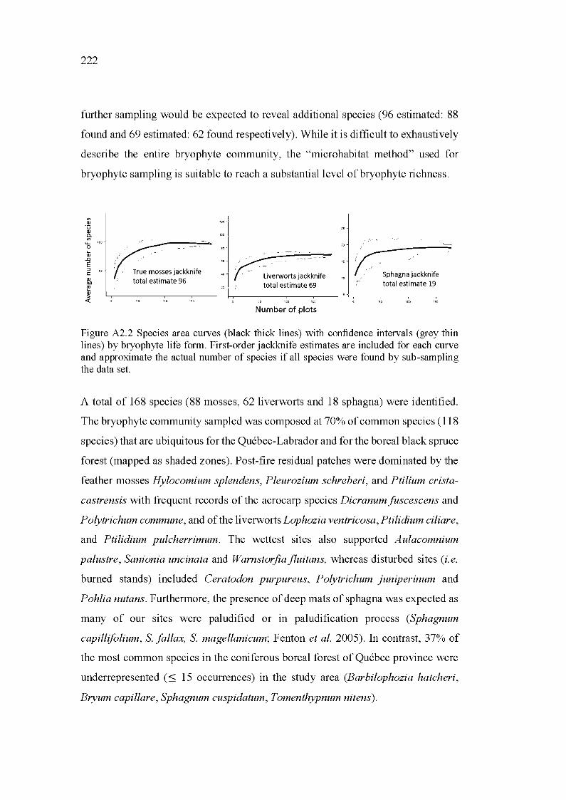
222

further sampling would be expected to reveal additional species (96 estimated: 88

found and 69 estimated: 62 found respectively). While it is difficult to exhaustively

describe the entire bryophyte community, the "microhabitat method" used for

bryophyte sampling is suitable to reach a substantiallevel ofbryophyte richness.

"' Q)

ÏJ Q) o. "' ..... 0

Q; .n E ::::1 c Q) nD

~ Q)

~

True masses jackknife total estimate 96

Liverworts jackknife total estimate 69

Number of plots

~ total es t i mate 19

Figure A2.2 Species area curves (black thick lines) with confidence intervals (grey thin lines) by bryophyte life form. First-order jackknife estimates are included for each curve and approximate the actual number of species if ali species were found by sub-sampling the data set.

A total of 168 species (88 mosses, 62 liverwmis and 18 sphagna) were identified.

The bryophyte community sampled was composed at 70% of common species ( 118

species) that are ubiquitous for the Québec-Labrador and for the boreal black spruce

forest (mapped as shaded zones). Post-fire residual patches were dominated by the

feather mosses Hylocomium splendens, Pleurozium schreberi, and Ptilium crista

castrensis with frequent records of the acrocarp species Dicranum fusees cens and

Polytrichum commune, and of the liverworts Lophozia ventricosa, Ptilidium ciliare,

and Ptilidium pulcherrimum. The wettest sites also supported Aulacomnium

palustre, Sanionia uncinata and Warnstorfiajluitans, whereas disturbed sites (i.e.

burned stands) included Ceratodon purpureus, Polytrichum juniperinum and

Pohlia nutans. Furthermore, the presence of deep mats of sphagna was expected as

many of our sites were paludified or in paludification process (Sphagnum

capillifolium, S. fallax, S. magellanicum; Fenton et al. 2005). In contrast, 37% of

the most common species in the coniferous boreal forest of Québec province were

underrepresented (s; 15 occurrences) in the study area (Barbilophozia hatcheri,

Bryum capillare, Sphagnum cuspidatum, Tomenthypnum nitens).

223

Thirty five other species (14 true mosses, 20 liverworts, and one sphagna) represent

noteworthyrecords (Table A2.2). Ofwhich, four species (group 1) were uncommon

or infrequent but were expected to be found because already recorded within 25 km

from the study area: Calypogeia sphagnicola, Fuscocephaloziopsis pleniceps,

Lophozia guttulata, and Sphenolobus hellerianus (Figure A2.3). Ten other species

(group 2), four true mosses: Brachythecium erythrorrhizon, Brachythecium starkii,

Isopterygiopsis muelleriana, and Polytrichum commune var. perigoniale and six

liverworts: Cephaloziella hampeana, Kurzia pauciflora, Lophozia ascendens,

Lophozia bicrenata, Odontoschisma francisci, and Schistochylopsis laxa were

common to rare for the province and already recorded near the study area but

sporadically (1 to 3 occurrences from 20 to 115 km; Figure A2.4).

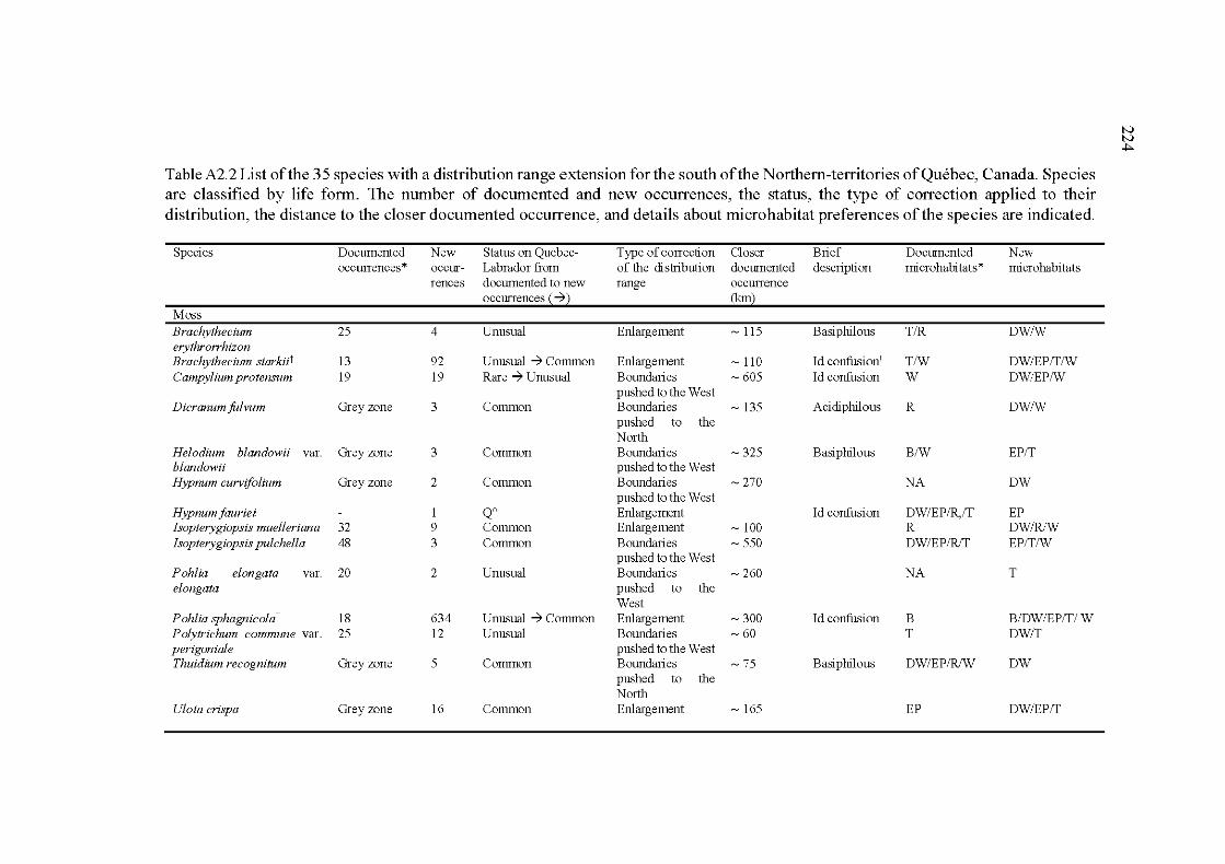
N N +:-.

Table A2.2 List of the 35 species with a distribution range extension for the south of the Northem-territories of Québec, Canada. Species are classified by life form. The number of documented and new occurrences, the status, the type of correction applied to their distribution, the distance to the closer documented occurrence, and details about microhabitat preferences of the species are indicated.

Species Docurnented New Status on Que bec- Type of correction Cl oser Brief Docurnented New occurrences* occur- Labrador from of the distribution docurnented description microhabitats* microhabitats

renees docurnented to new range occurrence occurrences -7

Moss Brachythecium 25 4 Unusual Enlargement - 115 Basiphilous TIR DWIW erythrorrhizon Brachythecium starkiit 13 92 Unusual -7 Common Enlargement - 110 Id confusion1 TIW DW/EP/TIW Campylium protensum 19 19 Rare -7 Unusual Boundaries -605 Id confusion w DW/EPIW

pushed tothe West Dicranumfolvum Grey zone 3 Common Boundaries - 135 Acidiphilous R DWIW

pushed to the North

Helodium blandowii var. Grey zone 3 Common Boundaries -325 Basiphilous BIW EP/T blandowii pushed tothe West Hypnum curvifolium Grey zone 2 Common Boundaries -270 NA DW

pushed tothe West Hypnum fauriei 1 Qo Enlargement Id confusion DW/EP/R,/T EP Isopterygiopsis muel! eriana 32 9 Common Enlargement -lOO R DW/RIW Isopterygiopsis pu/chelia 48 3 Common Boundaries -550 DW/EP/RIT EP/TIW

pushed tothe West Pohlia elongata var. 20 2 Unusual Boundaries -260 NA T elongata pushed to the

West Pohlia sphagnicolat 18 634 Unusual -7 Common Enlargement -300 Id confusion B B/DW/EP/T/W Polytrichum commune var. 25 12 Unusual Boundaries -60 T DW/T perigoniale pushed to the West Thuidium recognitum Grey zone 5 Common Boundaries -75 Basiphi1ous DW/EP/RIW DW

pushed to the North

Ulota crispa Grey zone 16 Common Enlargement - 165 EP DW/EP/T

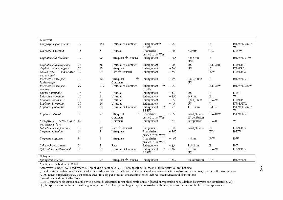
Liverwort Calypogeia sphagnicola t 12 151 Unusual ~ Corrunon Enlargement~ -25 B B/DW/EP/RIT/

BBSF? w Calypogeia suecica 15 6 Unusual Boundaries -300 < 2mm DW DW/W

pushed to the West Cephaloziella elachista 10 20 Infrequent ~ Unusual Enlargement -365 < 0,5 rrun B B/DW/EPfr/W

US§ Cephaloziella hamperma 16 56 Unusual ~ Corrunon Enlargement -20 us B/DW/R DW/EP!r Cephaloziella spinigera 10 10 Infrequent Enlargement -360 us B DW/EP!r Chiloscyphus coadunatus 17 29 Rare ~ Unusual Enlargement -550 R./W DW/EP/W var. rivularis Fuscocephaloziopsis 10 lOO Infrequent ~ Enlargement -490 0,6-0,8 mm B B/DW/EPfr loitlesbergerit Common us Fuscocephaloziopsis 29 219 Unusual ~ Corrunon Enlargement ~ -25 B/DW/W B/DW/EP/R./W plenicepst BBSF? Kurzia pauciflora 18 3 Unusual Enlargement -65 us B DW/T Leiocolea rutherma 15 Unusual Enlargement -450 3-5 rrun B w Lophozia ascendens 30 20 Unusual Enlargement -35 0,8-1,3 mm DW/W DW/EP Lophozia bicrenata 25 14 Unusual Enlargement - 45 us T DW/R.tr/W Lophozia guttulata t 21 82 Unusual ~ Corrunon Enlargement ~ -27 1-1 ,8 rrun B/DW B/DW/EP/R.tr/

BBSF? w Lophozia silvicola 3 77 Infrequent ~ Boundaries -350 Acidiphilous DW/R./W B/DW/EPfr

Common pushed to the West ID confusion Mesoptychia heterocolpos 67 2 Common Enlargement -670 Basiphilous DW/R. w var. heterocolpos Odontoschisma frrmcisci 18 19 Rare ~ Unusual Elargement -80 Acidiphilous w DW/EP/W Scaprmia apiculata 6 3 Infrequent Boundaries -360 DW BlOW

pushed tothe West Scaprmia uliginosa 9 Infrequent Boundaries -465 < 4mm R./W R./W

pushed to the West Schistochilopsis !axa 3 2 Rare Enlargement -35 1,5 -2 rrun B Btr Sphenolobus hellerianust 38 92 Unusual ~ Corrunon Enlargement ~ -26 < 1 mm DW/W DW/EP/W

BBSF? us S ha num Sphagnum tenerum 7 29 Infrequent ~ Unusual Enlargement -350 ID confusion NA B/DW/R.tr

*, refers to Faubert et al. 2014+ N

Acronyms: B, bog; DW, dead wood; EP, epiphytie or corticolous; NA, non-specified; R, rock; T, terricolous; W, wet habitats . N 1, identification confusion, species for which identification can be difficult due to a lack in diagnostic characters to discriminate among species of the same genera. V1

§,US, under sampled species, their minute size probably generates an underestimation oftheir real occurrences and distributions. t, significant addition to the Flora. BBSF?, questionable extension at the whole boreal black spruce forest bioclimatic domain [based on vegetation zones defined by Fayette and Bouchard (2001)]. Q0

, the species was confounded with Hypnum fertile . Therefore, presenting a map is impossible without a previous revision of the herbarium specimens.

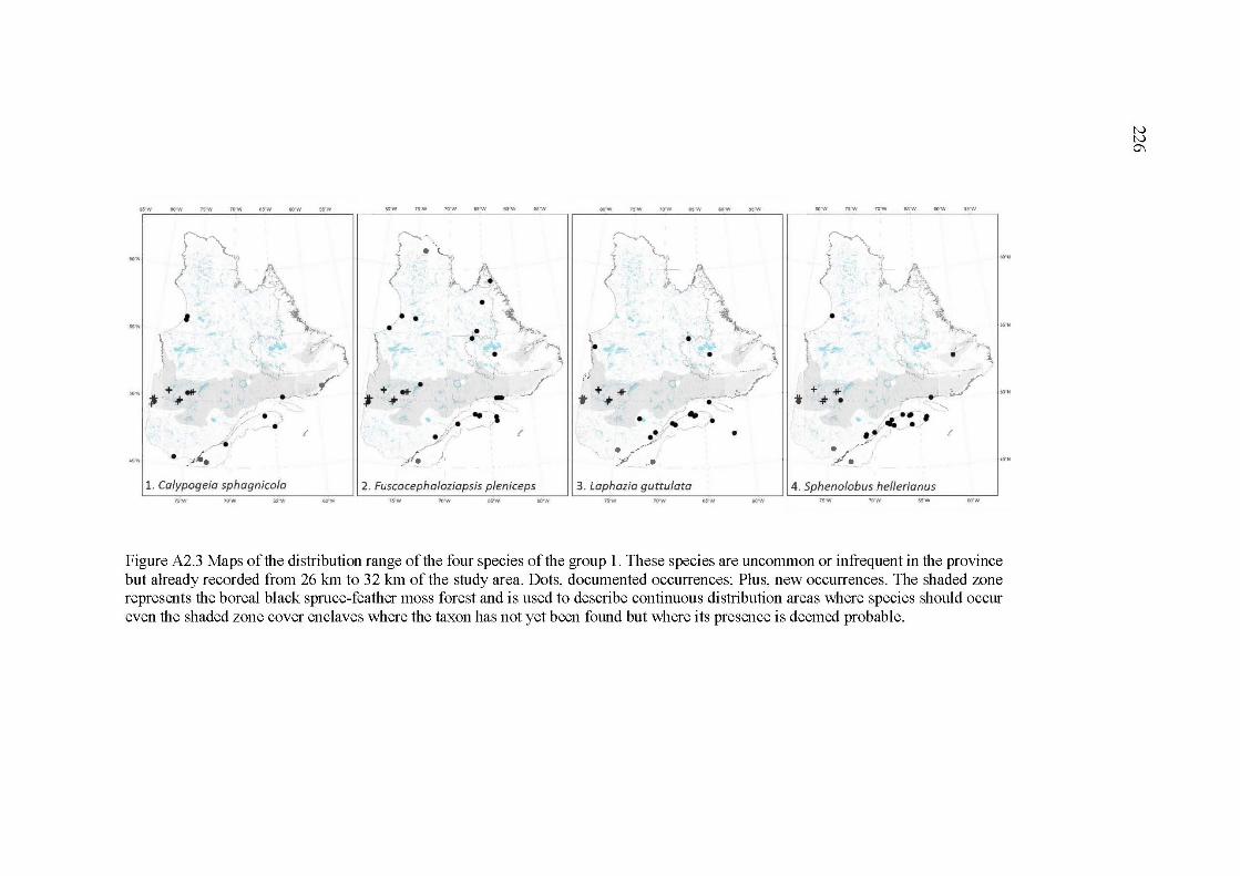
.. .,. .,.,. ,..., ..... .,.,. ..... 8ID"W 7~'W .,,. "'" ""

'"-, ? <-v ., ... J t /'~ (

Î'.y" .\

' .. ,. .... )

t.. ' ),. .. .• ( .r-~ 1

\

..

'; c-r > l !:\ ( 'il' 1 ~'. 'V""'-

'\ • -- ~

, ' ).""''•

' /''~? .. l l

• • "~" ~,..._..,. • '

~ ,-r~

+ .. ,r , .fi' • _.; + * -~/· -t .fi' •

+ • /""' .. ~../ t .fi' . ---.. / • . _, • (

• •

....

.. • .. ·' . ·'/ t' ,.. ,-/:-1. Calypogeia sphagnicola 2. Fuscocephaloziopsis pleniceps 3. Lophozia guttulata 4. Sphenolobus hellerianus

L-----------------------~

Figure A2.3 Maps of the distribution range of the four species of the group 1. These species are uncommon or infrequent in the province but already recorded from 26 km to 32 km of the study area. Dots, documented occurrences; Plus, new occurrences. The shaded zone represents the boreal black spruce-feather moss forest and is used to describe continuous distribution areas where species should occur even the shaded zone cover enclaves where the taxon has not yet been found but where its presence is deemed probable.

)

; • • •

+ • + +

• •• • •• (

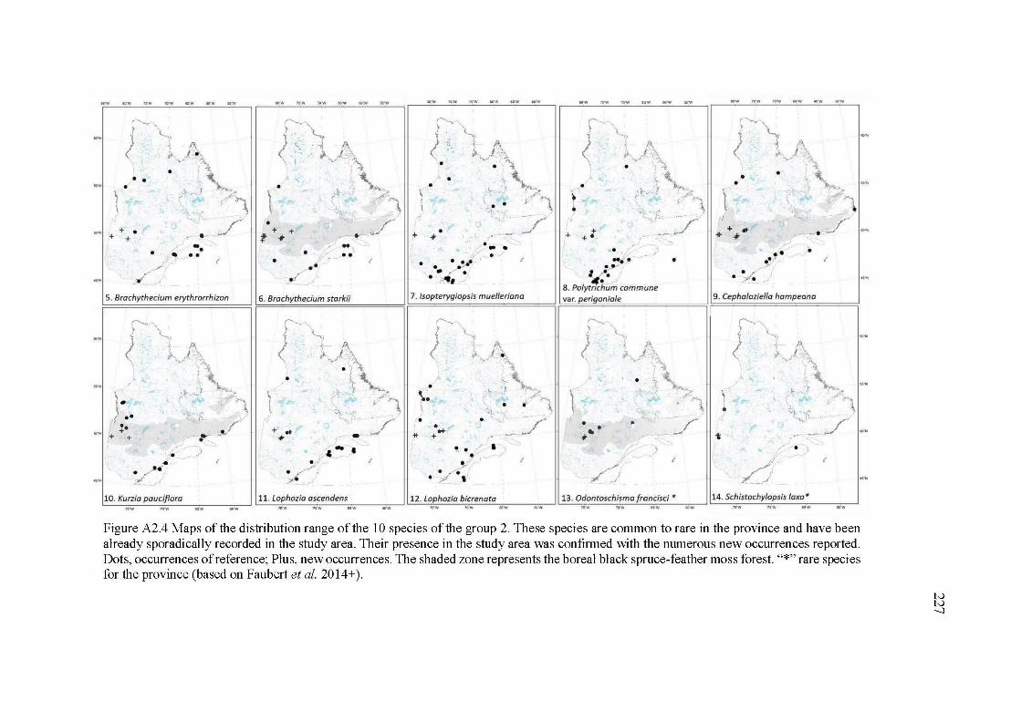
5. Brachythecium erythrorrhizon

; ~

~v'\ .~

~ ' t• :r... \ ••

!• _ . .-/ + + l'

• ~

.. •

\ •

+ + t .;- ·""

/ • + ..

• •• • (

•• .;

""" .... .... ('

; t..." J l A ~. "· ( 1 ~ \ ·•vl ..., • .1 . ~ A . ~

• ~ .. • ~~ • \,..,.,...

' ~ ~ ! !'1, \ 1 • .

.;-..J;''

+ + + •

/' ..J

• -. • • • • • .~·· t' • ::'· • . ._..., . '"-·;

~

; • •

) \

+ ... tir *

•

• • .. ' •

/ • ..J

1

8 . Polytrichum commune 6. Brochythecium storkii 7./sopterygiopsis muelleriona var. perigoniale 9. Cephaloziella hampeano F===============~~==============~:~~~~--------~·

1

( . "

+ ... .;-

• . ./""" ,..,

/ - _./

' ... '

! • r· • e+

* +

<-." l A "''t. ! • - "'\

• • • • •

#,.. lie,....

• r,'i.

..J /

(

· >~

! \.-,

J ) l /\ "· v~-~, < jvl ~, \ '\ '1'~, ~

) ) \,.., ..

~ '"1 ~ \ • \

• • /' / .... -"' 't _,

~

L1_0 _. K_u=rz::-ia--'p'--a_u-=c='=ifl_or_a_-::::::-__ =::--' ._1_1_. L--:o:':::p,-ho_z_ia_a-=s=ce_n_d_en_s=:------:=--' c:1:.=2.:.:. L:.:;oEp:-cho::z::ia:....:b=;,ic:::,r::.:en::a:.::ta=--:::::-----:=:--J <..::1.::..3 .'-'0:..,:d::,oc.:.n:..:to.::..sc:.:.h:;:;is='m:..:a...!.fi...:ro"cn=':et~·sc:.:.i_*----==-_J 14. Schistochylopsis /axa •

Figure A2.4 Maps of the distribution range of the 10 species of the group 2. These species are common to rare in the province and have been already sporadically recorded in the study area. Their presence in the study area was confirmed with the numerous new occurrences reported. Dots, occurrences of reference; Plus, new occurrences. The shaded zone represents the boreal black spruce-feather moss forest."*" rare species for the province (based on Faubert et al. 2014+).

228

Finally, 20 species (group 3) are new records for the study area with distribution

range extensions from 75 km to more than 670 km. Distribution ranges of the nine

true mosses: Campylium protensum, Dicranum fulvum, Hellodium blandowii var.

blandowii, Hypnum curvifolium, Jsopterygiopsis pulchella, Pohlia elongata var.

elongata, Pohlia sphagnicola, Thuidium recognitum, and Ulota crispa, ofthe 10

liverworts: Calypogeia suecica, Cephaloziella elachista, Cephaloziella spinigera,

Chiloscyphus coadnatus var. rivularis, Fuscocephaloziopsis loitlesbergeri,

Leiocolea rutheana, Lophozia silvicola, Mesoptychia heterocolpos var.

heterocolpos, Scapania apiculata, and Scapania uliginosa, and of the sphagna

Sphagnum tenerum were extended to include the study area (Figure A2.5a, b and

c).

Hypnum fauriei was sampled a single time in the study area. The spec1es 1s

presented for information purposes only given the uncertainties about its

distribution in Québec-Labrador (Faubert 2012-2014).

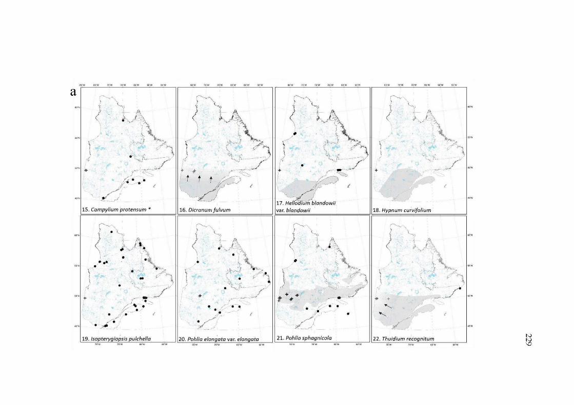
" 'W 75"W 70"W M'W &f/W

a

.... *

}'~

< l~\ __ /~ ' \ ]"i:o.

J . (~ 9 !t- ·----

- ~~~ ' ~~- <

17. ~ellirù~landowii

..

• • • • <

15. Campy/ium protensum * 16. Dicranum fulvum var. blandowii F===============~

\ 1

\

.... +

....

• •• •'

• ..

. ~/.

. ..

* • • • • ( • (

c.:1:.:9:..:· ..:.:/s:.,:o~p:.:t.:::er:..L.llgc.:io':f.p'=s"'is'-'p"-u.:::l:.:c:,:.h:;::el::.:la=----==----' 20. Poh/ia elon ata var. e/ongata ,..w

,.-.._

J (_'j'

If', ( # 4 1;,

l,j

)\ . ... l

,.. .... ~ ~ r.~"~ t + .. r

t .;- • ~

• r' • • . ' ..

21. Poh/ia sphagnico/a

+

} (

18. Hypnum curvifolium

; \....,~

\ .1\ 1 ~ ~ .1 ~

(

'"\ .. 1 \,..:;:

\ y "1 1

\ 'j

.r•

* _., /

' ' (

./

22. Thuidium recognitum

....

.....

....

N N 1.0

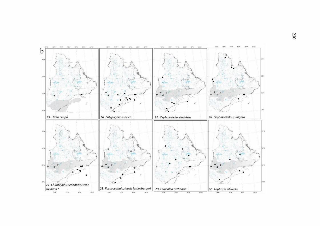
ww "w

b "--.,

2 \...1

1 A . 1 "' 11'-.._./'' \

' (~ .. \ ~ ~)_~ ' \

r ./

+ ·---~

t

,.J

23. U/ota crispa

,.., > (_t .1 .... J l. !\

( 1 ,. v~~ ., '\. .. ... "'?'"··-

~ "''"'1 \

+ ... /'" + + ~ --""

..

rivularis *

' \ ' \

+ #

..

• t .. . ·."' . r

.. ••

. / ~% -

" ' W

• (

+ * + +

"w

• -r

24. Calypageia suecica 25. Ce halaziella e/achista 26. Cephaloziel/a spinigera ~============~

" }

1 (

•

+ ... ... #

( -..(

11>.

..

• + ..

\ ! 1

.. •

28. Fuscocephaloziopsis loitlesbergeri 29. Leioco/ea rutheana

(

...-..__ ... ' ~~ ; 1 ~.

V\ :.:}

) ~"\. ... _

. '"1 \

• + *

/ * +

. ..-• •

(

30. Lophozia si/vico/a

""'

....

N w 0

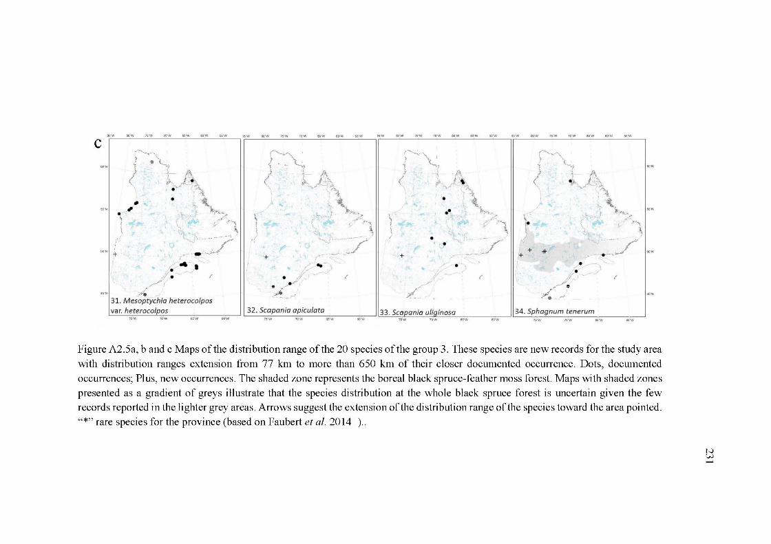
Figure A2 .5a, band c Maps of the distribution range of the 20 species of the group 3. These species are new records for the study area with distribution ranges extension from 77 km to more than 650 km of their closer documented occurrence. Dots, documented

occurrences; Plus, new occurrences. The shaded zone represents the boreal black spruce-feather moss forest. Maps with shaded zones presented as a gradient of greys illustrate that the species distribution at the whole black spruce forest is uncertain given the few records reported in the lighter grey areas. Arrows suggest the extension of the distribution range of the species toward the area pointed. "*" rare species for the province (based on Faubert et al. 2014+) ..

N w -

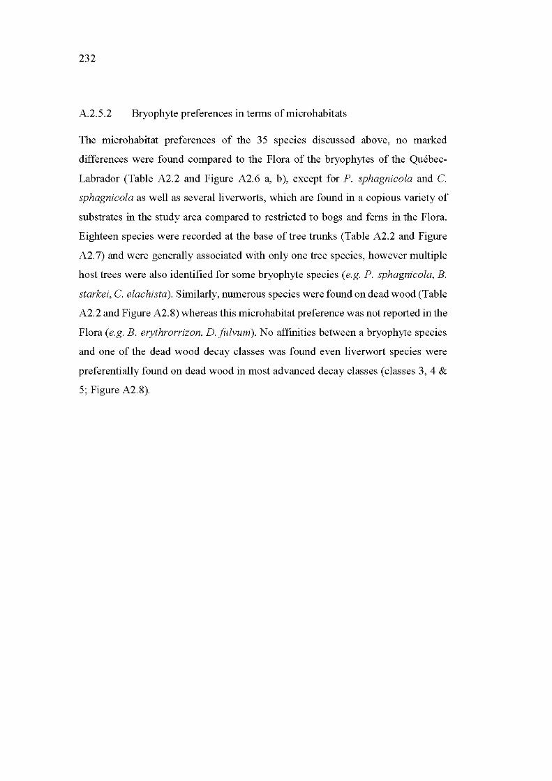
232

A.2.5.2 Bryophyte preferences in terms of micro habitats

The microhabitat preferences of the 35 species discussed above, no marked

differences were found compared to the Flora of the bryophytes of the Québec

Labrador (Table A2.2 and Figure A2.6 a, b ), except for P. sphagnicola and C.

sphagnicola as well as severalliverworts, which are found in a copious variety of

substrates in the study area compared to restricted to bogs and ferus in the Flora.

Eighteen species were recorded at the base of tree trunks (Table A2.2 and Figure

A2. 7) and were generally associated with only one tree species, however multiple

host trees were also identified for sorne bryophyte species ( e.g. P. sphagnicola, B.

starkei, C. elachista). Similarly, numerous species were found on dead wood (Table

A2.2 and Figure A2.8) whereas this microhabitat preference was not reported in the

Flora (e.g. B. erythrorrizon, D. fulvum). No affinities between a bryophyte species

and one of the dead wood decay classes was found even liverwort species were

preferentially found on dead wood in most advanced decay classes (classes 3, 4 &

5; Figure A2.8).

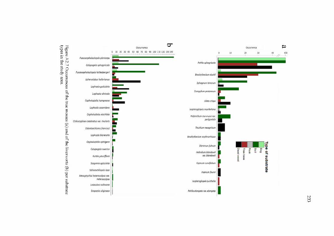
q ~. "dq; Dl >-! ....... (!)

~ ~ st~ (!) -1 Vl 0 s- (') ~(')

~ el (!) (!) ~ p (')

(!) Vl

0 >-+j

st. (!)

g s 0 Vl Vl

Dl ~

~ § p.. 0 >-+j

st (!)

....... ~ ·

~ a Vl

? '._!

"d (!) >-! Vl g. Vl g (!)

Occurrence cr-

0 10 20 30 40 50 60 70 80 90 100 110 120 130 140

Fuscocephalozlopsis pleniceps 1nc~· ;· ~~· ;:.~~~:;:;..;:::;::;:;:;:;

Ca/ypogeia sphagnico/a

Fuscocephaloziopsis loitlesbergeri

Sphenolobus hellerianus

Lophozia guttulata

Laphazia si/vico/a

Cephalozie/la hampeana

Lophozia ascendens

Cephalaziel/a e/achista

Chiloscyphus coadnatus var. rivularis

Odontoschisma !ranci sei

Lophozia bicrenata

Cephalozie/la spin/gera 1 r Ca/ypogeia suecica 11

Kurzla pauciflora 1 r

Scapania apiculata

Schistochilopsis /axa

Mesoptychio heteroco/pos var. heterocolpos

Leioco/ea rutheana

Scapania uliginosa

Poh/ia sphagnico/a

Brachythecium stark//

Sphagnum tenerum

Campylium protensum

U/ota crispa

lsopteryg/ops/s muel/er/ana

Po/ytrichum commune var. perigonia/e

Brachythecium erythrorrhizon

Oicranum fu/vum

Hellodium blandowii var. blandowii

Hypnum curvifo/ium

Hypnum faure/

lsopterygiopsis pu/chelia

r r r 1 1

Poh/ia elongata var. elongata Il

Occurrence

10 20 30

:? :;! ?1 w !i Œ 5I- - ·

l r

.:} "'0 ID 0 .... VI c: tr VI -.... Al -ID

~ 40 450

//-

N w w

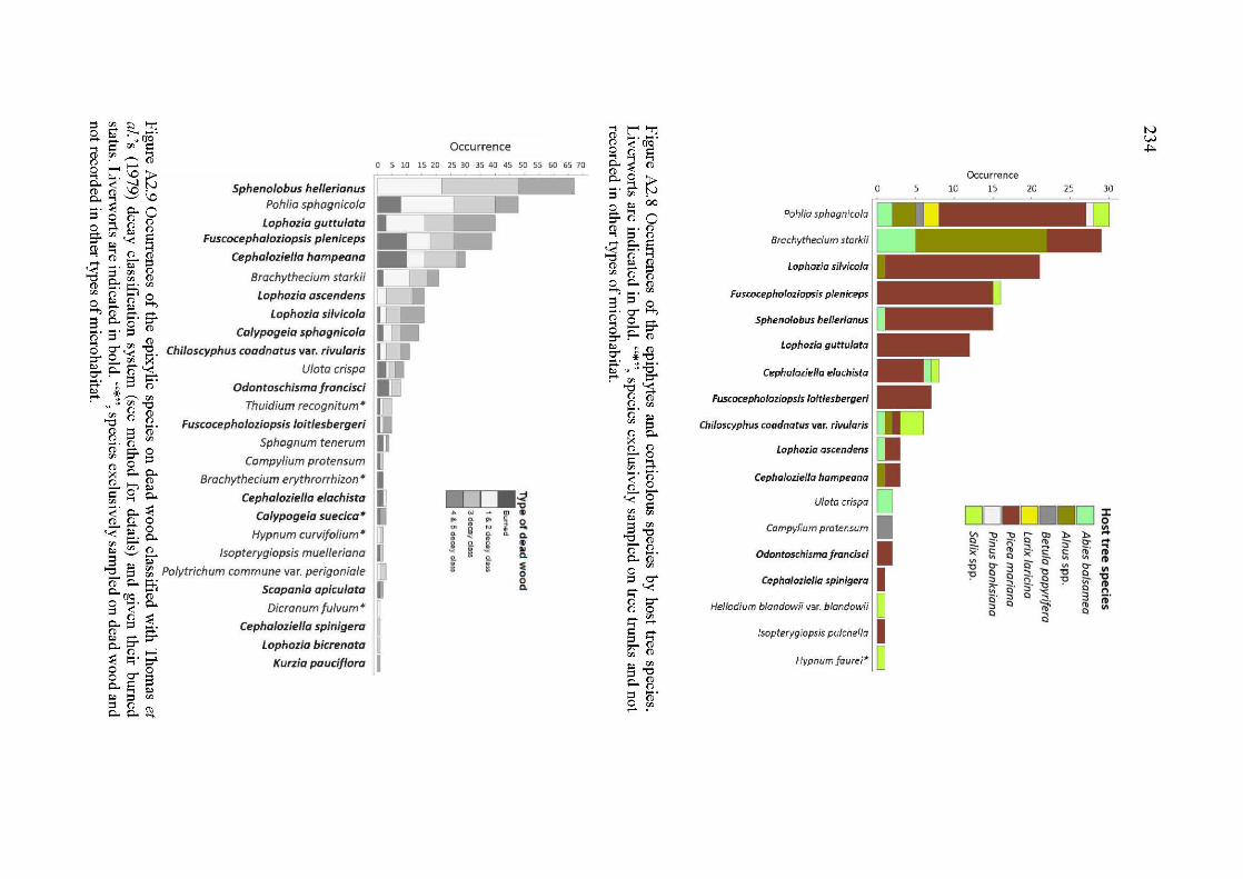
::SOO~'Tj

0 s- ~dei· ,..... cr oo~ ~ >-; ;:::; >-; (1) 00 ,-.._ (1) n . '""' OL'\0~ ...; '::l"-...JN o.. """ \0 . 8..Q--\Q ...... ~ o.. 0 ::s o (1) n o::+[;n Lt. 00 '-< ~ "';.. ::t l1l ...; n (1) .., (1) ....... ::s ,..... ...... ;.. n '-<::soo(l)

"'g ~ 8-; 00 oo n ..... o a;::._[;..,., ....,., (1) ::t. ;. s o.. 0 (1) ...... ËÏ ::s (1) n oo "ô a r::r <-< H. - 0 00 "" ..... ....... ...... '-< ~0...(1),_. ....... ~ s (=ï ...... ~

~ *--..oo ...... ~00>-o • ~ ~ (1) (1)

oo (1) n "ô ...... ~ s ~ ...... (1) 0 ~ ;. ::s

0 o.. 0...(1) ~

8" 00

~-

q b';.o >-; o.. o.. ~ ;:!.

~ 0 0 o..

Spheno/obus hel/erianus Pohlia sphagnico/a

Lophozia guttulata Fuscocephaloziopsis p/eniceps

Cephaloziella hampeana

Brachythecium stark ii

Lophozia ascendens

Lophozia si/vico/a

Calypogeia sphagnico/a

Chi/oscyphus coadnatus var. rivularis

U/ota crispa

Odantoschisma francisci

Thuidium recognitum*


Sphagnum tenerum

Campylium protensum

Brachythecium erythrorrhizon * Cephaloziel/a e/achista

Ca/ypogeia suecica *

Hypnum curvifolium* 00 ....... S ~ ~ /sopterygiopsis muelleriona

>-o êl g; Po/ytrichum commune var. perigoniale cr o... B-i o.. (Jq (ii 0 >-'·0,..

::s ~ ~ ~ ::s ;::+· ;.> ;. ::r 0...(1).__,

~=;·53 0 r::r 0 0 ~ s o.. >-; ;.> ;.> ::s 00 ::s (1) Cl) o... o.....,.

Scapania apiculata

Dicranum f ulvum * Cephaloziel/a spinigera

Lophozia bicrenata

Kurzia paucif/ora

Occurrence 0 5 10 15 20 25 30 35 40 45 50 55 60 65 70

"' ii" ~ Il. ;

.. "' ! Il. ;

a Q. Q) Ill Q.

:s; 0 0 Q.

(il''"Tl 8 ~-c@" >-; Q >-;

o..~ (1) (1) 0

~::+~ ::s 00 •

0 ;.> 00

;.(6o Q .... n ::s n

c':t O.. ~ ~ ~- ::t ~ ft 9 0 o.. g 1-+j 1--1-. 00.

s ::s 0 (=ï r::r ....,., a g.;. ::r p.. (1)

~ ~(1) 1-fo• *~ ~!"""'t'- v 1-fo• ;.> ~~"ô r+oo::r"' "ô~

(1) (1) n oo ...... ~ ;.>

(1) ::s ~ o.. n n ...-a 1;i ::+ ~- ('i" (1) 0 ~0

00 ~ ;.> 00

.§~ ,_.(!) (1) n o.. (ii" 0 00

::s r::r ~'-< (1) ::r (1) 0

a~ ::s r::i fr~ êl~ 0...(1) ::s 8. 0 (1) ...... ~

0

Poh/io sphognico/o

Brochythecium starkii

Lophozia si/vico /a

Fuscocephaloziopsis p/eniceps

Sphenolobus hellerianus

Lophozia guttulata

Cephaloziel/a e/achista


Chiloscyphus coadnatus var. rivularis

Lophozia ascendens .__ Cephaloziella hampeana Ill

Ulota crispa D Campylium protensum 1

Odontoschisma francisci 1 Cephaloziel/a spinigera 11

Hellodium blandowii var. blandowii 1 [

lsopterygiopsis pu/chelia 11 Hypnum faurei*

10 Occurrence

15 20 25 30

oo•o••o ~ "' "" "" r- IJJ ):,. ):,. .... 9.. 3' r;· Q ~ 5"" ~ :::: ;;:· c:: lb ;;:· c:: c:: tb" til "'~OQ Q~~ tl :gl:l3=:!"1::1"t1Cl 111 • :::. Cl ...,. Cl , "' "tl

~ ~- :;· ~ • Cl ~ ëï'5°S; ~ nï :::. lb Cl Ill Cl i3

N VJ ~

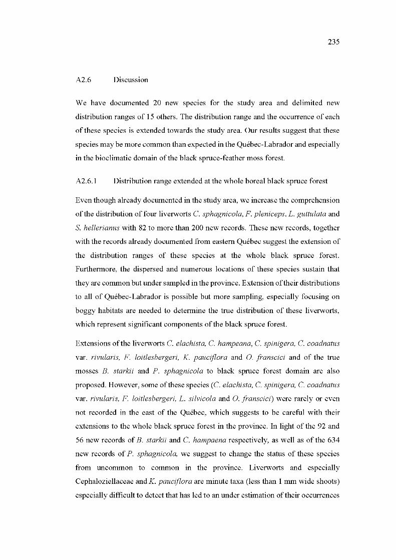
235

A2.6 Discussion

W e have documented 20 new spectes for the study are a and delimited new

distribution ranges of 15 others. The distribution range and the occurrence of each

ofthese species is extended towards the study area. Our results suggest that these

species may be more common than expected in the Québec-Labrador and especially

in the bioclimatic domain ofthe black spruce-feather moss forest.

A2.6.1 Distribution range extended at the who le boreal black spruce forest

Even though already documented in the study area, we increase the comprehension

ofthe distribution of four liverworts C. sphagnicola, F. pleniceps, L. guttulata and

S. hellerianus with 82 to more than 200 new records. These new records, together

with the records already documented from eastern Québec suggest the extension of

the distribution ranges of these species at the whole black spruce forest.

Furthermore, the dispersed and numerous locations of these species sustain that

they are common but under sampled in the province. Extension oftheir distributions

to all of Québec-Labrador is possible but more sampling, especially focusing on

boggy habitats are needed to determine the true distribution of these liverworts,

which represent significant components of the black spruce forest.

Extensions ofthe liverworts C. elachista, C. hampeana, C. spinigera, C. coadnatus

var. rivularis, F. loitlesbergeri, K. pauciflora and O. franscici and of the true

mosses B. starkii and P. sphagnicola to black spruce forest domain are also

proposed. However, sorne ofthese species (C. elachista, C. spinigera, C. coadnatus

var. rivularis, F. loitlesbergeri, L. silvicola and O. franscici) were rarely or even

not recorded in the east of the Québec, which suggests to be careful with their

extensions to the wh ole black spruce forest in the province. In light of the 92 and

56 new records of B. starkii and C. hampaena respectively, as well as of the 634

new records of P. sphagnicola, we suggest to change the status of these species

from uncommon to common in the province. Liverworts and especially

Cephaloziellaceae and K. pauciflora are minute taxa (less than 1 mm wide shoots)

especially difficult to detect that has led to an under estimation oftheir occurrences

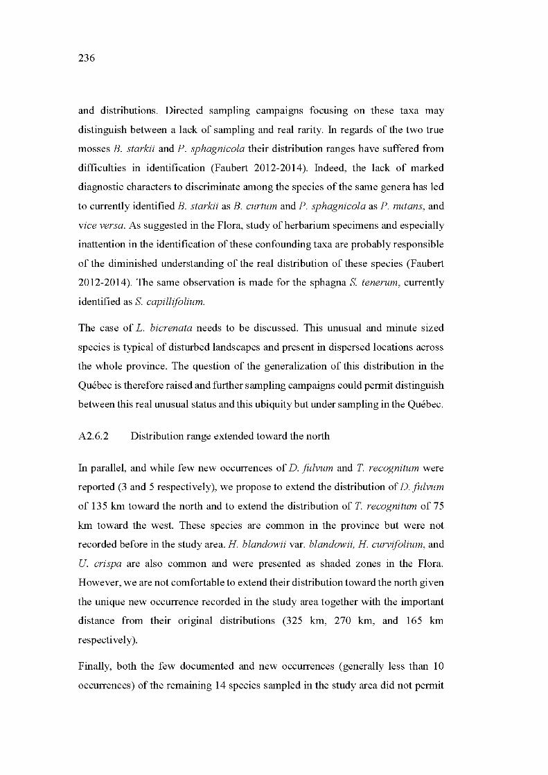
236

and distributions. Directed sampling campmgns focusing on these taxa may

distinguish between a lack of sampling and real rarity. In regards of the two true

mosses B. starkii and P. sphagnicola their distribution ranges have suffered from

difficulties in identification (Faubert 2012-2014). Indeed, the lack of marked

diagnostic characters to discriminate among the species of the same genera has led

to currently identified B. starkii as B. curtum and P. sphagnicola as P. nutans, and

vice versa. As suggested in the Flora, study of herbarium specimens and especially

inattention in the identification of the se confounding taxa are probably responsible

of the diminished understanding of the real distribution of these species (Faubert

2012-2014). The same observation is made for the sphagna S. tenerum, currently

identified as S. capillifolium.

The case of L. bicrenata needs to be discussed. This unusual and minute sized

species is typical of disturbed lands capes and present in dispersed locations across

the wh ole province. The question of the generalization of this distribution in the

Québec is therefore raised and further sampling campaigns could permit distinguish

between this real unusual status and this ubiquity but under sampling in the Québec.

A2.6.2 Distribution range extended toward the north

In parallel, and while few new occurrences of D. fulvum and T. recognitum were

reported (3 and 5 respectively), we propose to extend the distribution of D. fulvum

of 135 km toward the north and to extend the distribution of T. recognitum of 75

km toward the west. These species are common in the province but were not

recorded before in the study area. H. blandowii var. blandowii, H. curvifolium, and

U. cri spa are also common and were presented as shaded zones in the Flora.

However, we are not comfortable to extend their distribution toward the north given

the unique new occurrence recorded in the study area together with the important

distance from their original distributions (325 km, 270 km, and 165 km

respectively).

Finally, both the few documented and new occurrences (generally less than 10

occurrences) of the remaining 14 species sampled in the study area did not permit

237

to map their distribution as shaded zones. However, the new records of B.

erythrorrhizon, J. muelleriana, P. commune var. perigoniale, L. ascendens and L.

bicrenata enable us to link their disjunct distribution ranges between southem and

northem Québec. Furthermore, the records of C. protensum, J. pulchella, P.

elongata var. elongata, C. suecica, L. rutheana, M. heterocolpos var. heterocolpos,

S. apiculata, and S. uliginosa contribute to document their presence in the north of

the Québec, from 260 km to 670 km oftheir previously documented occurrences.

We conclude by highlighting the noteworthy records of the rare true mosses C.

protensum and H. fauriei and of the rare liverworts C. coadnatus var. rivularis, O.

franscisci, and S. laxa, which confirm the importance to improve bryophyte

sampling campaigns in the neglected regions ofthe Québec-Labrador.

A2.6.3 Implications for management and conservation

This study suggests that numero us bryophytes may be more common than expected

in Québec-Labrador. We present a substantially revised and updated list of the

bryoflora ofthe south ofthe Northem-Québec as well asto provide a bryological

preindustrial portrait of the boreal black spruce forest. Furthermore, these

actualizations ofbryophyte distributions can be used to redefine protection priority

ranks of the species but also to mo del their responses to forest harvest and global

changes. N aturally, keep in mind that this work not pro vide an exhaustive and static

portrait of the bryophyte flora in the study are a and that the maps presented will be

updated as result of new sampling campaigns. The records of uncommon,

infrequent, and rare species sustain that black spruce feather-moss forest is a bryo

diversity hotspot that require particular conservation attentions.

The south of the Northem-Québec is qualified of« black hole » ofthe knowledge

about bryoflora, which better suggests the paucity of the sampling campaigns in the

region rather than the species absence. Substantial works remain to be done to map

the real bryophyte distributions in the province, and especially in the boreal feather

moss forest where looking for a bryophyte is like looking for a needle in a haystack!

238

A2.7 Acknowledgements

Funding for this study was provided by fellowships from the Fonds de Recherche

du Quebec-Nature et Technologies (FRQNT), the Natural Sciences and

Engineering Research Council of Canada (NSERC) and the University of Quebec

in Abitibi-Témiscamingue (UQAT). The authors thank Louis Dubois, Philippe

Heine and Flora Joubier for their help in collecting bryophyte samples.

A2. 8 References

Allard, M. 1974. Géomorphologie des eskers abitibiens. Cahiers de géographie du Québec 18: 271-296.

Andison, D. W., and K. McCleary. 2014. Detecting regional differences in withinwildfire burn patterns in western boreal Canada. The Forestry Chronicle 90: 59-69.

Bergeron, J.-F. , P. Grondin, and J. Blouin. 1998. Rapport de classification écologique du sous-domaine bioclimatique de la pessière noire à mousses de l'ouest. Working paper RN98-3080. Ministère des Ressources naturelles du Québec, Direction des inventaires forestiers, Québec, Canada. 204 pages.

Bergeron, Y. , A. Leduc, B.D. Harvey, and S. Gauthier. 2002. Natural fire regime: a guide for sustainable management of the Canadian boreal forest. Silva Fennica 26: 81-95.

Bergeron, Y., S. Gauthier, M. Flannigan, and V. Kafka. 2004. Pire regimes at the transition between mixedwood and coniferous boreal forest in northwestern Quebec. Ecology 85: 1916-1932.

Bisbee, K. E., S. T. Gower, J. M. Norman, and E.V. Nordheim. 2001. Environmental controls on ground cover species composition and productivity in a boreal black spruce forest. Oecologia 129: 261-270.

Blouin, J., and J.-P. Berger. 2004. Guide de reconnaissance des types écologiques des régions écologiques 6c - Plaine du lac Opémisca, 6d - Coteaux du lac Assinica, 6e - Coteaux de la rivière Nestaocano, 6f - Coteaux du lac Mistassini et 6g - Coteaux du lac Manouane. Working paper 2004-3020. Ministère des Ressources naturelles, de la Faune et des Parcs, Forêt Québec. Direction des inventaires forestiers, Division de la classification écologique et productivité des stations, Québec, Canada, 210 pages.

Blouin, J., and J.-P. Berger. 2005. Guide de reconnaissance des types écologiques de la région écologique 6a- Plaine du lac Matagami et 6b -Plaine de la baie de Rupert. Working paper 2005-3037. Ministère des Ressources naturelles et

239

de la Faune. Direction des inventaires forestiers, Division de la classification écologique et productivité des stations, Québec, Canada, 188 pages.

Caners, R. T, S.E. Macdonald, and R. J. Belland. 2013. Linking the biological traits of boreal bryophytes to forest habitat change after partial harvesting. Forest Ecology and Management 303: 184-194

Environment Canada. 2015. Canadian climate normals 1981-2010 Station data. Accessed 1 February 2016. http://climate.weather.gc.ca/climate _ normals/results _1981_ 2010 _ e.html

ESRI. 2015. ArcGis Dekstop: Release 10.3.1. Environmental Systems Research Institute, Redlands, USA.

Faubert, J. 2007. Catalogue des bryophytes du Québec et du Labrador. Provancheria no 30. Mémoire de 1 'Herbier Louis-Marie, Université Laval, Québec, Canada. 140 pages.

Faubert, J. 2012-2014. Flora ofthe bryophytes ofthe Québec-Labrador (Vol. 1, 2 and 3 ). Société québécoise de bryologie, Saint-Valérien, Québec Canada.

Faubert, J., and J. Gagnon. 2013. Bryophytes nouvelles pour le Québec. Carnets de bryologie 3: 28-38.

Faubert, J., B. Tardif, and M. Lapointe. 2010. Les bryophytes rares du Québec. Espèces prioritaires pour la conservation. Working paper. Centre de données sur le patrimoine naturel du Québec (CDPNQ). Gouvernement du Québec, ministère du Développement durable, de l'Environnement et des Parcs, Direction du patrimoine écologique et des parcs, Québec, Canada. 147 pages.

Faubert, J., D. F. Bastien, M. Lapointe, and C. Roy. 2012. Cinq hépatiques nouvelles pour le Québec. Carnets de bryologie 2: 12-16.

Faubert, J., S. Leclerc, A. Lavoie, M. Lapointe, S. Nadeau, M. Lamond, and collaborateurs. 20 14+. Base de données des bryophytes du Québec-Labrador (BRYOQUEL). Accessed 2 March 2016. http :11 societequebecoisedebryol ogie. org.

Fenton, N. J., and K. A. Frego. 2005. Bryophyte (moss and liverwort) conservation under remnant canopy in managed forests. Biological Conservation 122: 417-430.

Fenton, N. J., and Y. Bergeron. 2006. Facilitative succession in a boreal bryophyte community driven by changes in available moisture and light. Journal of Vegetation Science 17: 65-76.

Fenton, N. J., N. Lecomte, S. Légaré, and Y. Bergeron. 2005. Paludification in black spruce (Picea mariana) forests of eastern Canada: Potential factors and management implications. Forest Ecology and Management 213: 151-159.

240

Flora of North America Editorial Committee. 2007. Flora of North America, North of Mexico (Vol. 27), Bryophytes: Moss, Part 1. Oxford University Press, Oxford, UK. 734 pages.

Gauthier, R. 2011. Le genre Tetrodontium (Tetraphidaceae, Mus ci) au Québec. Carnet de bryologie 1: 10-14.

Gauthier, S., M.-A. Vaillancourt, A. Leduc, L. De Grandpré, D. Kneeshaw, H. Morin, P. Drapeau, and Y. Bergeron. 2008. Aménagement écosystémique en forêt boréale. Presses de 1 'Université du Québec, Québec, Canada. 568 pages.

Hylander, K., M. Dynesius, B. G. Jonsson, and C. Nilsson. 2005. Substrate form determines the fate of bryophytes in riparian buffer strips. Ecological Applications 15: 674-688.

Madoui, A., A. Leduc, S. Gauthier, and Y. Bergeron. 2010. Spatial pattern analyses of post-fire residual stands in the black spruce boreal forest of western Quebec. International Journal ofWildland Pire 19: 1110-1126.

Mois an, C., and S. Pellerin. 2011. Présence de la céphalozie des marais (Cephalozia macrostachya Kaal. , Cephaloziaceae, Marchantiophyta) au Québec. Carnet de bryologie 1: 23-25.

Newmaster, S. G., R. J. Belland, A. Arsenault, D. H. Vitt, and T. R. Stephens. 2005. The ones we left behind: comparing plot sampling and floristic habitat sampling for estimating bryophyte biodiversity. Diversity and Distributions 11: 57-72.

Payette, S., and A. Bouchard. 2001. Le contexte physiographique et biogéographique. Pages 9-38 in Écologie des tourbières du Québec-Labrador. Edited by S. Payette and L. Rochefort. Les presses de l'Université Laval, Québec, Canada.

Proctor, M. C. F. 2011. Climatic responses and limits of bryophyte: comparisons and contrasts with vascular plants. Pages 35-54 in Bryophyte ecology and climate change. Edited by Z. Tuba, N. G. Slack and L. R. Stark. Cambridge University Press, New York, USA.

Saucier, J. P., P. Grondin, A. Robitaille, J. Gasselin, C. Morneau, P.J. H. Richard, J. Brisson, L. Sirois, A. Leduc, H. Morin, E. Thiffaut, S. Gauthier, C. Lavoie, and S. Payette. 2009. Écologie forestière. Pages 165-316 in Manuel de foresterie, 2nct Edition. Edited by Ordre des ingénieurs forestiers du Québec. Éditions Multimondes, Québec, Canada.

Thomas, J. W. , R. G. Anderson, C. Maser, andE. L. Bull. 1979. Wildlife habitats in managed forests of the Blue Mountains of Oregon and Washington. Agricultural Handbook No 553. United States Department of Agriculture, Forest Service, USA. 512 pages.

241

Turetsky, M. R., B. Bond-Lamberty, E. Euskirchen, J. Talbot, S. Frolking, A. D. McGuire, and E.-S. Tuittila. 2012. The resilience and functional role of moss in boreal and arctic ecosystems. New Phytologist 196: 49-67.

Vile, M. A., K. D. Scott, E. Brault, R. K. Wieder, and D. H. Vitt. 2011. Living on the edges: the effects of drought on Canada's western boreal peatlands. Pages 277-315 in Bryophyte ecology and climate change. Edited by Z. Tuba, N. G. Slack and L. R. Stark. Cambridge University Press, New York, USA.

Vincent, J. S., and L. Hardy. 1977. L'évolution et l'extinction des lacs glaciaires Barlow et Ojibway en territoire Québécois. Géographie Physique et Quaternaire 31: 357-372.

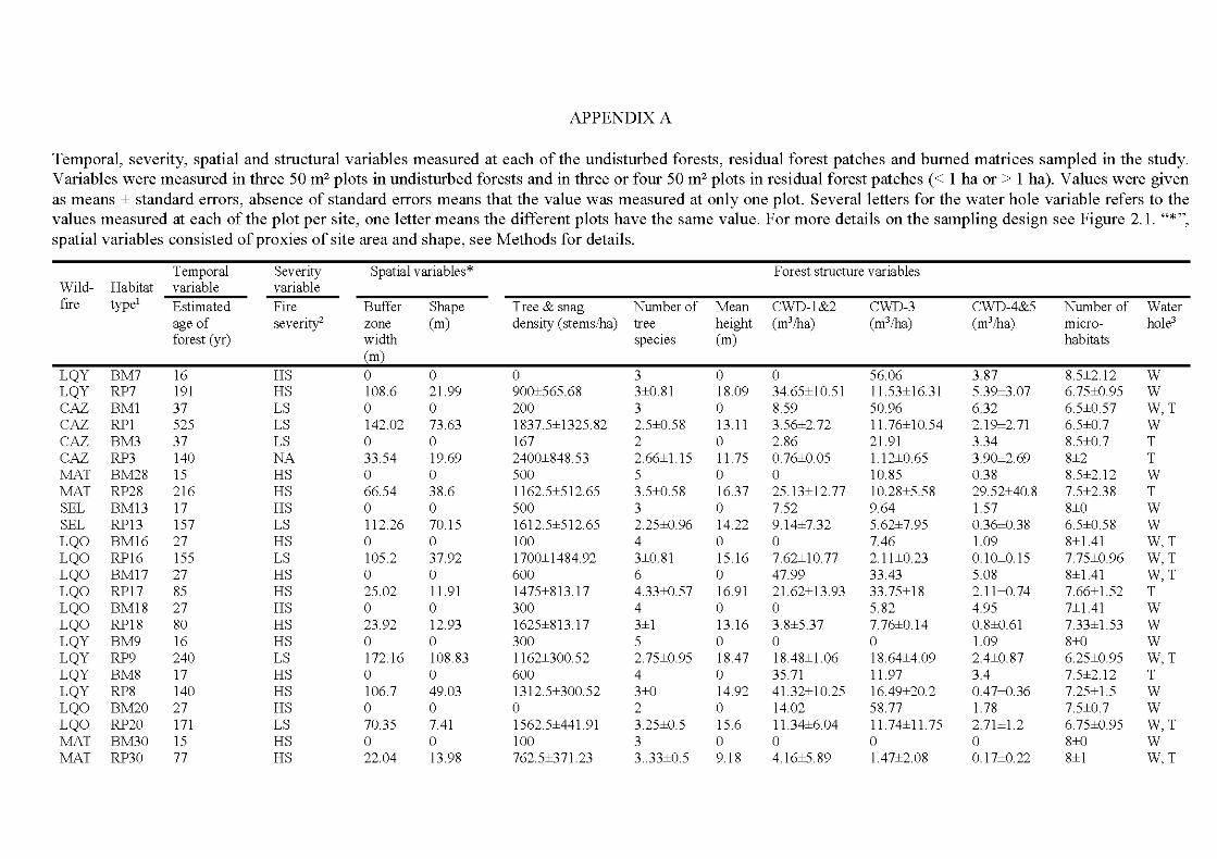
APPENDIXA

Temporal, severity, spatial and structural variables measured at each of the undisturbed forests, residual forest patches and bumed matrices sampled in the study. Variables were measured in three 50m2 plots in undisturbed forests and in three or four 50m2 plots in residual forest patches (< 1 ha or > 1 ha). Values were given as means ± standard errors, absence of standard errors means that the value was measured at only one plot. Severalletters for the water ho le variable refers to the values measured at each of the plot per site, one letter means the different plots have the same value. For more details on the sampling design see Figure 2.1. " *", spatial variables consisted of pro xi es of site are a and shape, see Methods for details.

Temporal Severity Spatial variables* Forest structure variables Wild- Habitat variable variable fire type1 Estimated Fire Buffer Shape Tree & snag Number of Mean CWD-1 &2 CWD-3 CWD-4&5 Number of Water

age of severity2 zone (rn) density (stems/ha) tree height (m3!ha) (mJ!ha) (m3!ha) illlCrO- hole3

forest (yr) width spec1es (rn) habitats (rn)

LQY BM7 16 HS 0 0 0 3 0 0 56.06 3.87 8.5±2. 12 w LQY RP7 191 HS 108.6 21.99 900±565.68 3±0.81 18.09 34.65±10.51 11.53±16.3 1 5.39±3.07 6.75±0.95 w CAZ BMl 37 LS 0 0 200 3 0 8.59 50.96 6.32 6.5±0.57 W, T CAZ RPl 525 LS 142.02 73.63 1837.5±1325.82 2.5±0.58 13.11 3.56±2.72 11.76±10.54 2.19±2.71 6.5±0.7 w CAZ BM3 37 LS 0 0 167 2 0 2.86 21.91 3.34 8.5±0.7 T CAZ RP3 140 NA 33.54 19.69 2400±848.53 2.66±1.15 11.75 0.76±0.05 1.12±0.65 3.90±2.69 8±2 T MAT BM28 15 HS 0 0 500 5 0 0 10.85 0.38 8.5±2.12 w MAT RP28 216 HS 66.54 38.6 1162.5±512.65 3.5±0.58 16.37 25.13±12.77 10.28±5.58 29.52±40.8 7.5±2.38 T SEL BM13 17 HS 0 0 500 3 0 7.52 9.64 1.57 8±0 w SEL RP13 157 LS 11 2.26 70.15 1612.5±512.65 2.25±0.96 14.22 9.14±7.32 5.62±7.95 0.36±0.38 6.5±0.58 w LQO BM1 6 27 HS 0 0 100 4 0 0 7.46 1.09 8±1.41 W, T LQO RP1 6 155 LS 105.2 37.92 1700±1484.92 3±0.81 15.16 7.62±10.77 2.11±0.23 0.10±0.15 7.75±0.96 W, T LQO BM1 7 27 HS 0 0 600 6 0 47.99 33.43 5.08 8±1.41 W, T LQO RP17 85 HS 25.02 11 .91 1475±813.17 4. 33±0.57 16.91 21.62±13.93 33.75±1 8 2.11±0.74 7.66±1.52 T LQO BM18 27 HS 0 0 300 4 0 0 5.82 4.95 7±1.41 w LQO RP18 80 HS 23.92 12.93 1625±813.17 3±1 13.16 3.8±5.37 7.76±0.14 0.8±0.61 7.33±1 .53 w LQY BM9 16 HS 0 0 300 5 0 0 0 1.09 8±0 w LQY RP9 240 LS 172.16 108.83 1162±300.52 2.75±0.95 18.47 18.48±1.06 18.64±4.09 2.4±0.87 6.25±0.95 W, T LQY BM8 17 HS 0 0 600 4 0 35.71 11 .97 3.4 7.5±2.12 T LQY RP8 140 HS 106.7 49.03 1312.5±300.52 3±0 14.92 41.32±10.25 16.49±20.2 0.47±0.36 7.25±1 .5 w LQO BM20 27 HS 0 0 0 2 0 14.02 58.77 1.78 7.5±0.7 w LQO RP20 171 LS 70.35 7.41 1562.5±441. 91 3.25±0.5 15.6 11.34±6.04 11.74±1 1.75 2.71±1.2 6.75±0.95 W, T MAT BM30 15 HS 0 0 100 3 0 0 0 0 8±0 w MAT RP30 77 HS 22.04 13.98 762.5±371.23 3 .. 33±0.5 9.18 4.16±5.89 1.47±2.08 0.17±0.22 8±1 W, T

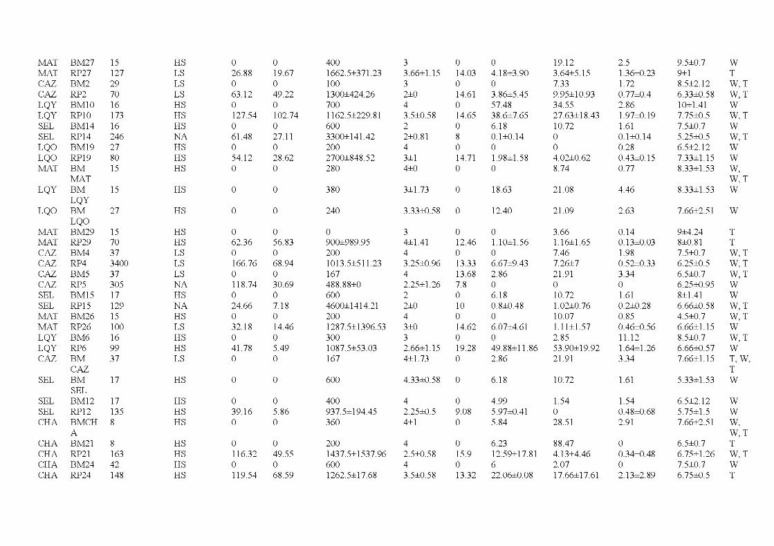
:MAT BM27 15 HS 0 0 400 3 0 0 19.1 2 2.5 9.5±0.7 w :MAT RP27 127 LS 26.88 19.67 1662.5±371 .23 3.66±1.15 14.03 4.18±3.90 3.64±5.1 5 1.36±0.23 9±1 T CAZ BM2 29 LS 0 0 100 3 0 0 7.33 1.72 8.5±2.12 W,T CAZ RP2 70 LS 63.12 49.22 1300±424.26 2±0 14.61 3.86±5.45 9.95±10.93 0.77±0.4 6.33±0.58 W,T LQY BM10 16 HS 0 0 700 4 0 57.48 34.55 2.86 10±1.41 w LQY RP10 173 HS 127.54 102.74 1162.5±229.81 3.5±0.58 14.65 38.6±7.65 27.63±18.43 1.97±0.19 7.75±0.5 W ,T SEL BM14 16 HS 0 0 600 2 0 6.18 10.72 1.61 7.5±0.7 w SEL RP14 246 NA 61.48 27.11 3300±141.42 2±0.81 8 0.1±0.14 0 0.1±0.14 5.25±0.5 W ,T LQO BM19 27 HS 0 0 200 4 0 0 0 0.28 6.5±2.12 w LQO RP1 9 80 HS 54.12 28 .62 2700±848.52 3±1 14.71 1.98±1.58 4.02±0.62 0.43±0.15 7.33±1. 15 w :MAT BM 15 HS 0 0 280 4±0 0 0 8.74 0.77 8.33±1.53 W ,

:MAT W ,T LQY BM 15 HS 0 0 380 3±1.73 0 18.63 21.08 4.46 8.33±1.53 w

LQY LQO BM 27 HS 0 0 240 3.33±0.58 0 12.40 21.09 2.63 7.66±2.51 w

LQO :MAT BM29 15 HS 0 0 0 3 0 0 3.66 0.14 9±4.24 T :MAT RP29 70 HS 62.36 56.83 900±989.95 4±1.41 12.46 1. 10±1.56 1.16±1.65 0.13±0.03 8±0.81 T CAZ BM4 37 LS 0 0 200 4 0 0 7.46 1.98 7.5±0.7 W , T CAZ RP4 3400 LS 166.76 68 .94 1013.5±511.23 3.25±0.96 13.33 6.67±9.43 7.26±7 0.52±0.33 6.25±0.5 W , T CAZ BM5 37 LS 0 0 167 4 13.68 2.86 21.91 3.34 6.5±0.7 W , T CAZ RP5 305 NA 118.74 30.69 488 .88±0 2.25±1.26 7.8 0 0 0 6.25±0.95 w SEL BM15 17 HS 0 0 600 2 0 6.18 10.72 1.61 8±1.41 w SEL RP15 129 NA 24.66 7.1 8 4600±1414.21 2±0 10 0.8±0.48 1.02±0.76 0.2±0.28 6.66±0.58 W , T :MAT BM26 15 HS 0 0 200 4 0 0 10.07 0.85 4.5±0.7 W , T :MAT RP26 100 LS 32.1 8 14.46 1287.5±1396.53 3±0 14.62 6.07±4.61 1.11±1.57 0.46±0.56 6.66±1.15 w LQY BM6 16 HS 0 0 300 3 0 0 2.85 11.12 8.5±0.7 W, T LQY RP6 99 HS 41.78 5.49 1087.5±53.03 2.66±1. 15 19.28 49.88±11. 86 53.90±19.92 1.64±1.26 6.66±0.57 w CAZ BM 37 LS 0 0 167 4±1.73 0 2.86 21.91 3.34 7.66±1.15 T,W,

CAZ T SEL BM 17 HS 0 0 600 4. 33±0.58 0 6.18 10.72 1.61 5.33±1.53 w

SEL SEL BM12 17 HS 0 0 400 4 0 4.99 1.54 1.54 6.5±2.12 w SEL RP12 135 HS 39.16 5.86 937.5±194.45 2.25±0.5 9.08 5.97±0.41 0 0.48±0.68 5.75±1.5 w CHA BMCH 8 HS 0 0 360 4±1 0 5.84 28 .51 2.91 7.66±2.51 W,

A W, T CHA BM21 8 HS 0 0 200 4 0 6.23 88.47 0 6.5±0.7 T CHA RP21 163 HS 116.32 49.55 1437.5±1537.96 2.5±0.58 15.9 12.59±17.81 4.13±4.46 0.34±0.48 6.75±1.26 W, T CHA BM24 42 HS 0 0 600 4 0 6 2.07 0 7.5±0.7 w CHA RP24 148 HS 119.54 68 .59 1262.5±17.68 3.5±0.58 13.32 22.06±0.08 17.66±17.61 2.13±2.89 6.75±0.5 T

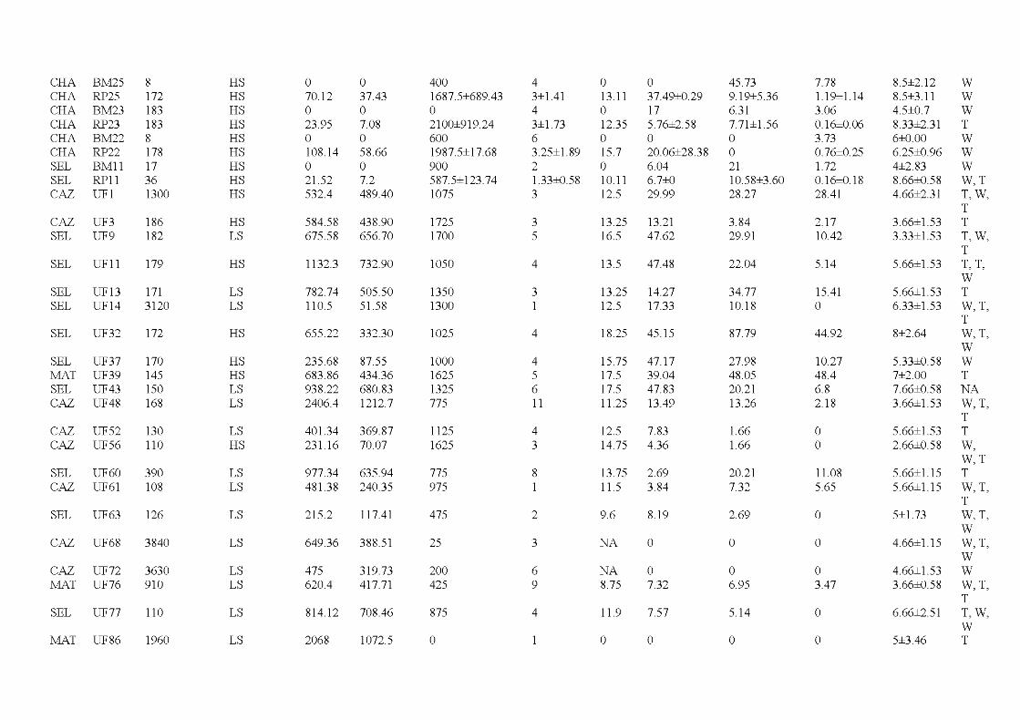
CHA BM25 8 HS 0 0 400 4 0 0 45.73 7.78 8.5±2.1 2 w CHA RP25 172 HS 70.12 37.43 1687.5±689.43 3±1.41 13.11 37.49±0.29 9.1 9±5.36 1. 19±1. 14 8.5±3.1 1 w CHA BM23 183 HS 0 0 0 4 0 17 6.31 3.06 4.5±0.7 w CHA RP23 183 HS 23.95 7.08 2100±919.24 3±1.73 12.35 5.76±2.58 7.71±1.56 0.16±0.06 8.33±2.31 T CHA BM22 8 HS 0 0 600 6 0 0 0 3.73 6±0.00 w CHA RP22 178 HS 108.14 58.66 1987.5±17.68 3.25±1.89 15.7 20.06±28.38 0 0.76±0.25 6.25±0.96 w SEL BM11 17 HS 0 0 900 2 0 6.04 21 1.72 4±2.83 w SEL RP11 36 HS 21.52 7.2 587.5±123.74 1.33±0.58 10.11 6.7±0 10.58±3.60 0.16±0.18 8.66±0.58 W,T CAZ UF1 1300 HS 532.4 489.40 1075 3 12.5 29.99 28 .27 28.41 4.66±2.31 T,W,

T CAZ UF3 186 HS 584.58 438.90 1725 3 13.25 13.21 3.84 2.17 3.66±1.53 T SEL UF9 182 LS 675.58 656.70 1700 5 16.5 47.62 29.91 10.42 3.33±1.53 T,W,

T SEL UF11 179 HS 1132.3 732.90 1050 4 13.5 47.48 22.04 5.14 5.66±1.53 T, T,

w SEL UF13 171 LS 782.74 505.50 1350 3 13.25 14.27 34.77 15.41 5.66±1.53 T SEL UF14 3120 LS 110.5 51.58 1300 1 12.5 17.33 10.1 8 0 6.33±1.53 W,T,

T SEL UF32 172 HS 655.22 332.30 1025 4 18.25 45.15 87.79 44.92 8±2.64 W,T,

w SEL UF37 170 HS 235.68 87.55 1000 4 15.75 47.17 27.98 10.27 5.33±0.58 w MAT UF39 145 HS 683.86 434.36 1625 5 17.5 39.04 48. 05 48.4 7±2.00 T SEL UF43 150 LS 938.22 680.83 1325 6 17.5 47.83 20.21 6.8 7.66±0.58 NA CAZ UF48 168 LS 2406.4 1212.7 775 11 11.25 13.49 13.26 2.18 3.66±1 .53 W,T,

T CAZ UF52 130 LS 401.34 369.87 1125 4 12.5 7.83 1.66 0 5.66±1 .53 T CAZ UF56 110 HS 231.16 70.07 1625 3 14.75 4.36 1.66 0 2.66±0.58 W,

W, T SEL UF60 390 LS 977.34 635 .94 775 8 13.75 2.69 20.21 11.08 5.66±1. 15 T CAZ UF61 108 LS 481.38 240.35 975 1 11.5 3.84 7.32 5.65 5.66±1. 15 W,T,

T SEL UF63 126 LS 215.2 117.41 475 2 9.6 8.19 2.69 0 5±1.73 W, T,

w CAZ UF68 3840 LS 649.36 388.51 25 3 NA 0 0 0 4.66±1.15 W, T,

w CAZ UF72 3630 LS 475 319.73 200 6 NA 0 0 0 4.66±1 .53 w MAT UF76 910 LS 620.4 41 7.71 425 9 8.75 7.32 6.95 3.47 3.66±0.58 W, T,

T SEL UF77 110 LS 814.12 708.46 875 4 11.9 7.57 5 .1 4 0 6.66±2.51 T,W,

w MAT UF86 1960 LS 2068 1072.5 0 0 0 0 0 5±3.46 T

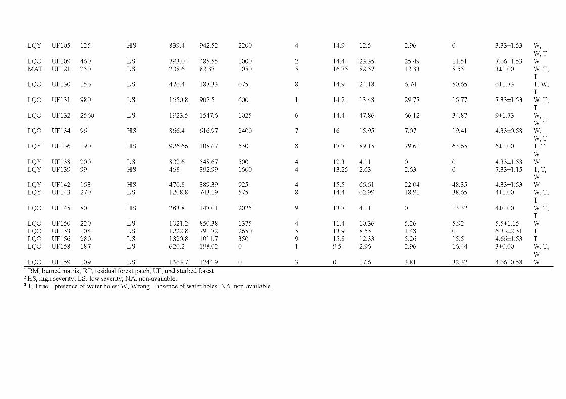
LQY UF105 125 HS 839.4 942.52 2200 4 14.9 12.5 2.96 0 3.33±1.53 W, W, T

LQO UF109 460 LS 793.04 485.55 1000 2 14.4 23.35 25.49 11.51 7.66±1.53 w :MAT UF1 21 250 LS 208.6 82. 37 1050 5 16.75 82.57 12.33 8.55 3±1.00 W, T,

T LQO UF130 156 LS 476.4 187.33 675 8 14.9 24.18 6.74 50.65 6±1.73 T,W,

T LQO UF131 980 LS 1650. 8 902.5 600 14.2 13.48 29.77 16.77 7.33±1.53 W,T,

T LQO UF132 2560 LS 1923.5 1547.6 1025 6 14.4 47.86 66.1 2 34.87 9±1.73 W,

W,T LQO UF134 96 HS 866.4 616.97 2400 7 16 15.95 7.07 19.41 4.33±0.58 W,

W,T LQY UF136 190 HS 926.66 1087.7 550 8 17.7 89.15 79.61 63.65 6±1.00 T, T,

w LQY UF138 200 LS 802.6 548.67 500 4 12.3 4.11 0 0 4.33±1.53 w LQY UF139 99 HS 468 392.99 1600 4 13.25 2.63 2.63 0 7.33±1. 15 T, T,

w LQY UF 142 163 HS 470.8 389.39 925 4 15.5 66.61 22.04 48.35 4.33±1 .53 w LQY UF 143 270 LS 1208.8 743.1 9 575 8 14.4 62.99 18.91 38.65 4±1.00 W,T,

T LQO UF 145 80 HS 283. 8 147.01 2025 9 13.7 4.11 0 13.32 4±0.00 W,T,

T LQO UF 150 220 LS 1021.2 850.38 1375 4 11 .4 10.36 5.26 5.92 5.5±1.15 w LQO UF 153 104 LS 1222.8 791.72 2650 5 13.9 8.55 1.48 0 6.33±2.51 T LQO UF 156 280 LS 1820. 8 1011.7 350 9 15.8 12.33 5.26 15.5 4.66±1 .53 T LQO UF 158 187 LS 620.2 198 .02 0 1 9.5 2.96 2.96 16.44 3±0.00 W,T,

w LQO UF159 109 LS 1663.7 1244.9 0 3 0 17.6 3.81 32.32 4.66±0.58 w

1 BM, bumed matrix; RP, residua1 forest patch; UF, undisturbed forest. 2 HS, high severity; LS, 1ow severity; NA, non-avai1ab1e. 3 T, True - presence of water ho1es; W, Wrong - absence of water ho1es, NA, non-avai1ab1e.

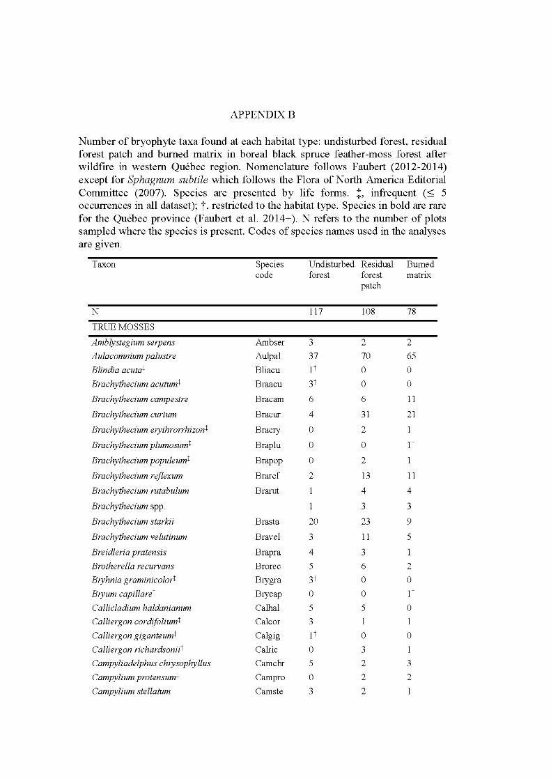
APPENDIXB

Number of bryophyte taxa found at each habitat type: undisturbed forest, residual forest patch and burned matrix in boreal black spruce feather-moss forest after wildfire in western Québec region. Nomenclature follows Faubert (2012-2014) except for Sphagnum subtile which follows the Flora of North America Editorial Committee (2007). Species are presented by life forms. t, infrequent ($ 5 occurrences in all datas et); t, restricted to the habitat type. Species in bold are rare for the Québec province (Faubert et al. 2014+). N refers to the number of plots sampled where the species is present. Codes of species names used in the analyses are gtven.

Taxon Species Undisturbed Residual Burned code forest forest matrix

patch

N 117 108 78

TRUE MOSSES

Amblystegium serpens Ambser 3 2 2

Aulacomnium palustre Aulpal 37 70 65

Blindia acutat Bliacu 1t 0 0

Brachythecium acutumt Braacu 3t 0 0

Brachythecium campestre Brac am 6 6 11

Brachythecium curtum Brac ur 4 31 21

Brachythecium erythrorrhizont Braery 0 2

Brachythecium plumosumt Braplu 0 0 1t

Brachythecium populeumt Brapop 0 2

Brachythecium reflexum Braref 2 13 11

Brachythecium rutabulum Brarut 1 4 4

Brachythecium spp. 3 3

Brachythecium starkii Bras ta 20 23 9

Brachythecium velutinum Bravel 3 11 5

Breidleria pratensis Brapra 4 3

Brotherella recurvans Brorec 5 6 2

Bryhnia graminicolort Bry gr a 3t 0 0

Bryum capillaret Brycap 0 0 1t

Callicladium haldanianum Calhal 5 5 0

Calliergon cordifoliumt Cale or 3 1

Calliergon giganteumt Calgig 1t 0 0

Calliergon richardsoniit Calric 0 3

Campyliadelphus chrysophyllus Camchr 5 2 3

Campylium protensumt Cam pro 0 2 2

Campylium stellatum Cam ste 3 2

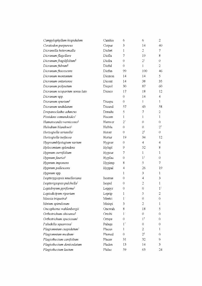
Campylophyllum hispidulum Cam his 6 6 2

Ceratodon purpureus Cerpur 3 14 40

Dicranella heteromalla Dichet 1 2 7

Dicranum fla ge !lare Dicfla 7 19 8

Dicranum fragilifoliumt Die fra 0 2t 0

Dicranum fulvumt Dicfu1 0 1 2

Dicranum fusees cens Die fus 99 100 46

Dicranum montanum Dicmon 14 14 5

Dicranum ontariense Dicont 14 38 35

Dicranum polysetum Dicpo1 30 87 60

Dicranum scoparium sensu lato Dicsco 17 18 12

Dicranum spp. 0 14 4

Dicranum spuriumt Dicspu 0 1 1

Dicranum undulatum Dicund 57 43 58

Drepanocladus aduncus Dreadu 5 7 2

Fissidens osmundoidest Fisosm 1 1

Hamatocaulis vemicosust Ham ver 2t 0 0

Helodium blandowiit He1b1a 0 0 2t

Herzogiella striatellat Herstr 0 2t 0

Herzogiella turfacea Hertur 19 34 12

Hygroamblystegium varium Hygvar 0 4 4

Hylocomium splendens Hy1sp1 9 52 8

Hypnum curvifolium Hypcur 7 1

Hypnum faurieit Hypfau 0 1t 0

Hypnum imponens Hypimp 8 5 7

Hypnum palles cens Hyppa1 4 26 19

Hypnum spp. 3

Isopterygiopsis muelleriana Isomue 0 4 3

I sopterigiopsis pulche llat Isopu1 0 2

Leptobryum pyriformet Leppyr 0 0 1t

Leptodictyum riparium Leprip 5 2

Meesia triquetrat Mee tri p 0 0

Mnium spinulosum Mnispi 3 2

Oncophorus wahlenbergii Oncwah 8 18 5

Orthotrichum ohioenset Orto hi 1t 0 0

Orthotrichum speciosumt Ortspe 0 1t 0

Paludella squarrosat Palsqu 1t 0 0

Plagiomnium cuspidatumt Pla eus 1 2

Plagiomnium medium! Plamed 0 2t 0

Plagiothecium cavifolium Placav 31 32 9

Plagiothecium denticulatum Pla den 13 14 3

Plagiothecium laetum Plalae 59 63 24

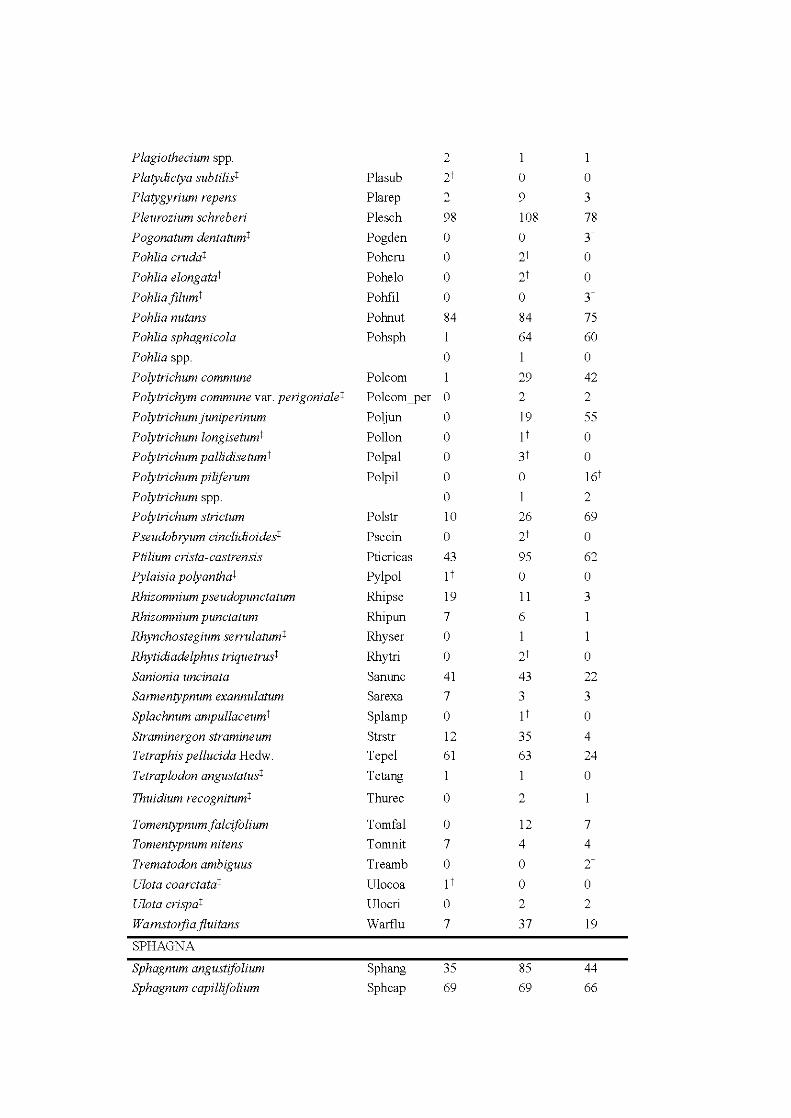
Plagiothecium spp. 2

Platydictya subtilist P1asub 2t 0 0

Platygyrium repens P1arep 2 9 3

Pleurozium schreberi P1esch 98 108 78

Pogonatum dentatumt Pogden 0 0 3t

Pohlia crudat Pohcru 0 2t 0

Pohlia elongatat Pohe1o 0 2t 0

Pohliafilumt Pohfi1 0 0 3t

Pohlia nutans Pohnut 84 84 75

Pohlia sphagnicola Pohsph 1 64 60

Pohlia spp. 0 0

Polytrichum commune Polcom 1 29 42

Polytrichym commune var. perigonialet Polcom_per 0 2 2

P olytrichum junipe rinum Po1jun 0 19 55

Polytrichum longisetumt Pollon 0 1t 0

Polytrichum pallidisetumt Po1pa1 0 3t 0

Polytrichum piliferum Po1pil 0 0 16t

Polytrichum spp. 0 1 2

Polytrichum strictum Po1str 10 26 69

Pseudobryum cinclidioidest Psecin 0 2t 0

Ptilium crista-castrensis Pticricas 43 95 62

Pylaisia polyanthat Py1po1 1t 0 0

Rhizomnium pseudopunctatum Rhipse 19 11 3

Rhizomnium punctatum Rhipun 7 6

Rhynchostegium serrulatumt Rhys er 0 1

Rhytidiadelphus trique trust Rhytri 0 2t 0

Sanionia uncinata San une 41 43 22

Sarmentypnum exannulatum Sarexa 7 3 3

Splachnum ampullaceumt Sp1amp 0 1t 0

Straminergon stramineum Strstr 12 35 4

Tetraphis pellucida Hedw. Tepe1 61 63 24

Tetraplodon angustatust Tetang 0

Thuidium recognitumt Th uree 0 2

Tomentypnum falcifolium Tomfa1 0 12 7

Tomentypnum nitens Tomnit 7 4 4

Trematodon ambiguus Treamb 0 0 2t

Ulota coarctatat Ulocoa 1t 0 0

Ulota crispat Ulocri 0 2 2

WamstOJfiafluitans Warflu 7 37 19

SPHAGNA

Sphagnum angustifolium Sphang 35 85 44

Sphagnum capillifolium Sphcap 69 69 66

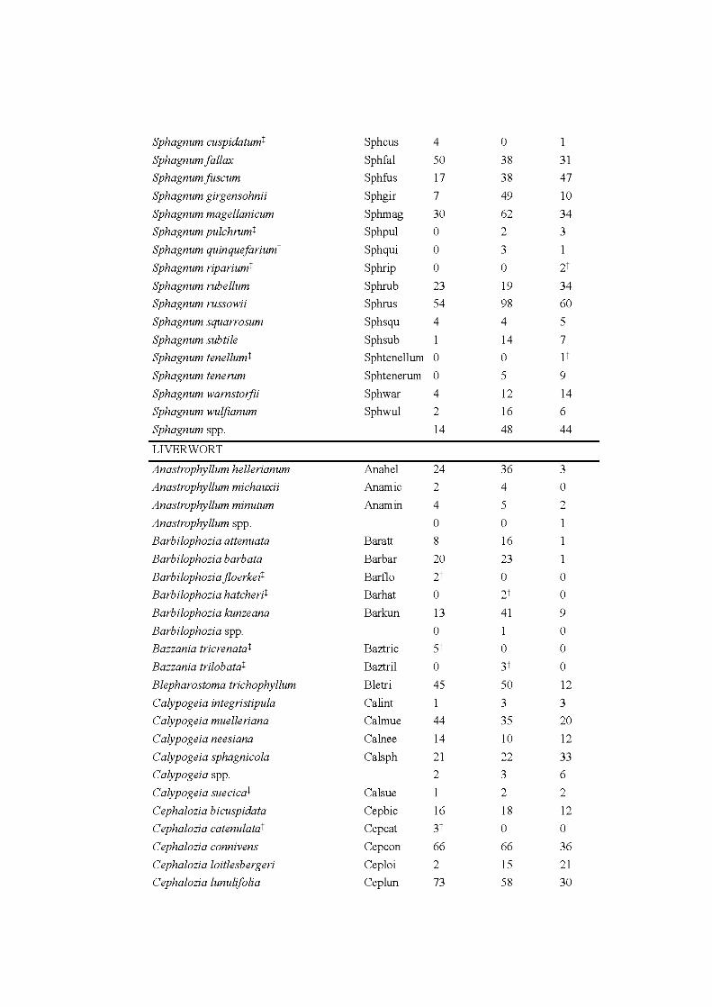
Sphagnum cuspidatumt Sphcus 4 0

Sphagnum fallax Sphfal 50 38 31 Sphagnum fuscum Sphfus 17 38 47

Sphagnum girgensohnii Sphgir 7 49 10

Sphagnum magellanicum Sphmag 30 62 34

Sphagnum pulchrumt Sphpul 0 2 3

Sphagnum quinquefariumt Sphqui 0 3

Sphagnum ripariumt Sphrip 0 0 2t

Sphagnum rubellum Sphrub 23 19 34 Sphagnum russowii Sphrus 54 98 60

Sphagnum squarrosum Sphsqu 4 4 5

Sphagnum subtile Sphsub 1 14 7

Sphagnum tenellumt Sphtenellum 0 0 p

Sphagnum te ne rum Sphtenerum 0 5 9

Sphagnum wamstorfii Sphwar 4 12 14 Sphagnum wulfianum Sphwul 2 16 6

Sphagnum spp. 14 48 44

LIVERWORT

Anastrophyllum hellerianum Anahel 24 36 3

Anastrophyllum michauxii Anamic 2 4 0

Anastrophyllum minutum Anamin 4 5 2

Anastrophyllum spp. 0 0 Barbilophozia attenuata Bara tt 8 16

Barbilophozia barbata Barbar 20 23 1

Barbilophozia floerkeit Barflo 2t 0 0

Barbilophozia hatcherit Bar hat 0 2t 0

Barbilophozia kunzeana Bar kun 13 41 9

Barbilophozia spp. 0 1 0 Bazzania tricrenatat Baztric 5t 0 0

Bazzania trilobatat Baztril 0 3t 0

Blepharostoma trichophyllum Ble tri 45 50 12

Calypogeia integristipula Ca lint 1 3 3

Calypogeia muelleriana Calmue 44 35 20

Calypogeia neesiana Calnee 14 10 12

Calypogeia sphagnicola Cals ph 21 22 33 Calypogeia spp. 2 3 6

Calypogeia suecicat Calsue 2 2

Cephalozia bicuspidata Cep bic 16 18 12

Cephalozia catenulatat Cepcat 3t 0 0

Cephalozia connivens Cepcon 66 66 36

Cephalozia loitlesbergeri Cep loi 2 15 21 Cephalozia lunulifolia Ceplun 73 58 30

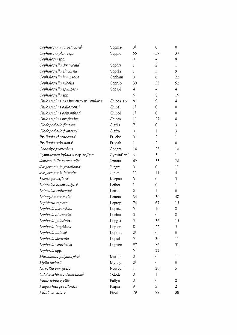
Cephalozia macrostachyat Cepmac 3t 0 0

Cephalozia pleniceps Cepple 55 59 37 Cephalozia spp. 0 4 8

Cephaloziella divaricatat Cep div 2 1

Cephaloziella elachista Ce pela 1 5 9

Cephaloziella hampeana Ce pham 9 6 22

Cephaloziella rubella Ceprub 39 33 52

Cephaloziella spinigera Cep spi 4 4 4

Cephaloziella spp. 6 8 16 Chiloscyphus coadunatus var. rivularis Chicoa riv 8 9 4

Chiloscyphus palles cens! Chi pal 1t 0 0

Chiloscyphus polyanthost Chi pol 1t 0 0

Chiloscyphus profundus Chi pro 11 27 8

Cladopodie Il a flui tans Claflu 7 0 3

Cladopodie lla franciscit Cl afra 0 3 Frullania eboracensist Fruebo 0 2 1

Frullania oakesianat Fruoak 2 0

Geocalyx graveolens Geogra 14 23 10

Gymnocolea injlata subsp. injlata Gyminf_inf 6 5

Jamesoniella autumnalis Jamaut 49 55 20

Jungermannia gracillimat Jungra 0 0 1t

Jungermannia leiantha Junlei 11 11 4

Kurzia pauciflorat Kurpau 0 0 3t

Leiocolea heterocolpost Leihet 1 0 1

Leiocolea rutheanat Leirut 2 0

Leiomylia anomala Leiano 34 30 48

Lepidozia reptans Leprep 74 67 15 Lophozia ascendens Lopasc 5 10 2

Lophozia bicrenata Loc bic 0 0 8t

Lophozia guttulata Lopgut 5 36 15

Lophozia longidens Loplon 8 22 5

Lophozia obtusat Lopobt 2t 0 0

Lophozia silvicola Lopsil 5 30 11

Lophozia ventricosa Lopven 97 86 31 Lophozia spp. 5 22 11

Marchantia polymorphat Marpol 0 0 1t

Mylia tayloriit Myltay 2t 0 0

Nowellia curvifolia Nowcur 11 20 5

Odotonschisma denudatumt Ododen 0

Pallavicinia lyeZliit Pallye 0 0 2t

Plagiochila porelloides Plapor 3 3 2

Ptilidium ciliare Pticil 79 99 38

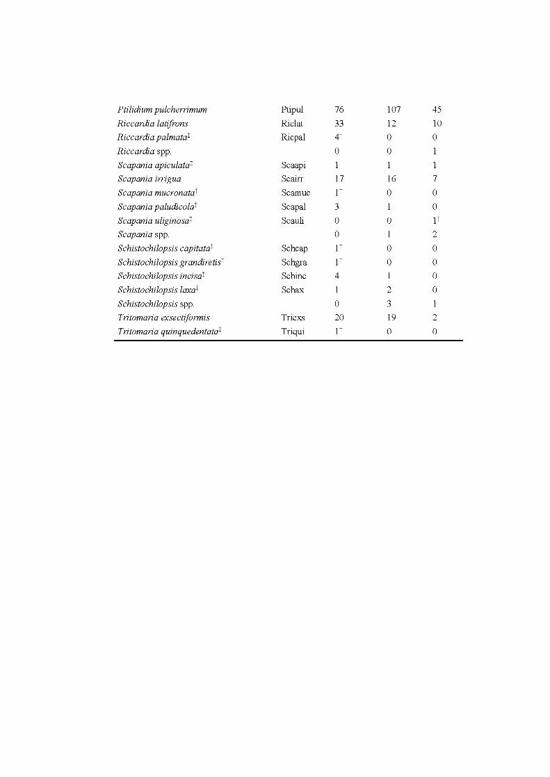
Ptilidium pulcherrimum Ptipul 76 107 45

Riccardia latifrons Ri clat 33 12 10

Riccardi a palmatat Ri cp al 4t 0 0

Riccardia spp. 0 0

Scapania apiculatat Scaapi 1 1 1

Scapania irrigua Scairr 17 16 7

Scapania mucronatat Scamuc 1t 0 0

Scapania paludicozat Scapa! 3 0

Scapania uliginosat Scauli 0 0 1t

Scapania spp. 0 1 2

Schistochilopsis capitatat Schcap 1t 0 0

Schistochilopsis grandiretist Schgra 1t 0 0

Schistochilopsis incisat Schinc 4 0

Schistochilopsis !axat Schax 2 0

Schistochilopsis spp. 0 3

Tritomaria exsectiformis Triexs 20 19 2

Tritomaria quinquedentatat Triqui 1t 0 0

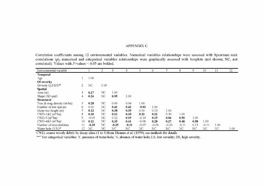
APPENDIXC

Correlation coefficients among 12 environmental variables. Numerical variables relationships were assessed with Spearman rank correlations (p ), numerical and categorical variables relationships were graphically assessed with boxplots (not shown; NC, not correlated). Values with P -values < 0.05 are bolded.

Environmental variable 2 3 4 5 6 7 8 9 10 11 12 Temporal Age 1.00 Ofseverity Severity (L S/HS)* 2 NC 1.00 Spatial Area (rn) 3 0.27 NC 1.00 Shape (SD unit) 4 0.26 NC 0.95 1.00 Structural Tree & snag density (nb/ha) 5 0.28 NC 0.00 0.04 1.00 Number oftree species 6 0.01 NC 0.42 0.42 -0.03 1.00 Mean tree height (rn) 7 0.12 NC 0.38 0.39 0.50 0.13 1.00 CWD-1 &2 (rn3/ha) 8 0.30 NC 0.23 0.30 0.32 0.22 0.30 1.00 CWD-3 (rn3/ha) 9 -0.05 NC 0.1 2 0.19 -0 .1 4 0.15 0.06 0.50 1.00 CWD-4&5 (rn3/ha) 10 0.12 NC 0.35 0.41 -0.08 0.28 0.27 0.48 0.58 1.00 Number of rnicrohabitats 11 -0.35 NC -0.35 -0.31 -0.07 -0.09 -0.20 -0.11 0 .1 3 -0.11 1.00 Water hole (YIN)* 12 NC NC NC NC NC NC NC NC NC NC NC 1.00

CWD, coarse woody debris by decay class (1 to 5) from Thomas et al. (1979), see methods for details. "*"For categorical variables : Y, presence of water hole; N, absence ofwater hole; L S, low severity; HS, high severity.

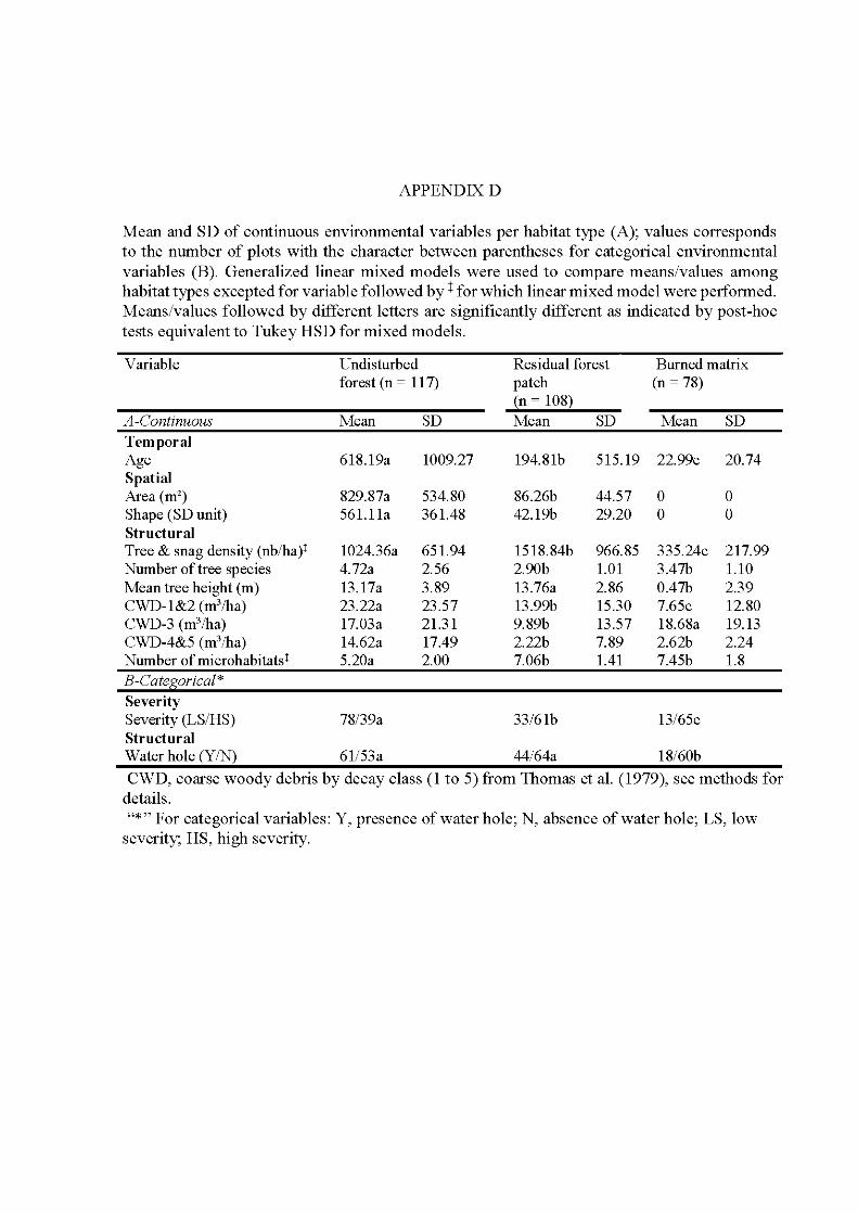
APPENDIX D

Mean and SD of continuous environmental variables per habitat type (A); values corresponds to the number of plots with the character between parentheses for categorical environmental variables (B). Generalized linear mixed models were used to compare means/values among habitat types excepted for variable followed by t for which linear mixed mo del were performed. Means/values followed by different letters are significantly different as indicated by post-hoc tests equivalent to Tukey HSD for mixed models.

Variable Undisturbed Residual forest Burned matrix forest (n = 117) patch (n = 78)

(n = 108) A -Continuow; Mean SD Mean SD Mean SD Temporal Age 618.19a 1009.27 194.81b 515.19 22.99c 20.74 Spatial Area (m2

) 829.87a 534.80 86.26b 44.57 0 0 Shape (SD unit) 561.11a 361.48 42.19b 29.20 0 0 Structural Tree & snag density (nb/ha)t 1024.36a 651.94 1518.84b 966.85 335.24c 217.99 Number of tree species 4.72a 2.56 2.90b 1.01 3.47b 1.10 Mean tree height (rn) 13.17a 3.89 13.76a 2.86 0.47b 2.39 CWD-1&2 (m3/ha) 23.22a 23.57 13.99b 15.30 7.65c 12.80 CWD-3 (m3/ha) 17.03a 21.31 9.89b 13.57 18.68a 19.13 CWD-4&5 (m3 /ha) 14.62a 17.49 2.22b 7.89 2.62b 2.24 Number of microhabitatst 5.20a 2.00 7.06b 1.41 7.45b 1.8 B-Cate orical*

Severity Severity (LS/HS) 78/39a 33/61b 13/65c Structural Water hole (YIN) 61/53a 44/64a 18/60b

CWD, coarse woody debris by decay class (1 to 5) from Thomas et al. (1979), see methods for details. "*"For categorical variables: Y, presence ofwater hole; N, absence ofwater hole; LS, low

severity; HS, high severity.

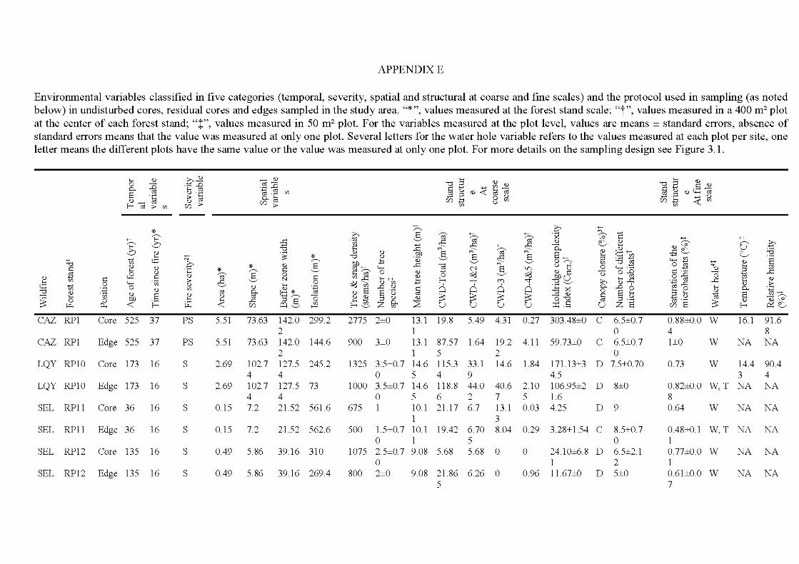
APPENDIXE

Environmental variables classified in five categories (temporal, severity, spatial and structural at coarse and fine scales) and the protocol used in sampling (as noted below) in undisturbed cores, residual cores and edges sampled in the study area. "*",values measured at the forest stand scale; "t", values measured in a 400m2 plot at the center of each forest stand; "t", values measured in 50 m2 plot. For the variables measured at the plot level, values are means ± standard errors, absence of standard errors means that the value was measured at only one plot. Severalletters for the water ho le variable refers to the values measured at each plot per site, one letter means the different plots have the same value or the value was measured at only one plot. For more details on the sampling design see Figure 3. 1.

.... <!) >,<!.l - <!) "OB ~~ "OB <!)

0 ~ .~:a œ- .s ~ ·- .D o. ,... ro

~ .$ tn g u <!)-<

,... ro g u a <!) ·- ro u <!.l '- ro •>:::: > .... O.t:a +-' ;::l +-' ;::l ..... u

<!)- ro <!.l ro lfltl 8 'fl lfltl <r: 'fl E--< ro > 'fl lfl > lfl > 'fl 'fl

+- _q +-

* ~ +- "" _g 5 ~ +- +- ~ 1:: +- '";:? ~ ~ K ~ +-+ ++ .s 'ffi <!) <!) ~ 0 '";:? à 'fl

~ ~ +- ~ P.. '--"' .... <!)~ u ~ à <!) ::2 <!) <!) 5 "' ~ "' a+-

<!) <1:: ++ .s~ 0 ~ .... +- fs: * "0 <!) 5 ~ 5 !3 ~.;3 '--"'

::0 til <.;:1 "' ~ tl <!) 0 ~ "OEJ <.--<.;3 +-+ <!) j 0 ?Jl+- ...r:: "' 'fl

0 El <!) * <!) 5 <=il u ~ 0

..,.

~ ~ .... <!) •>:::: * ~ '- 0l a <n <!) u '- ·- <!) u ~ ~~ 0 <!) +-'

~ ~ ü o.g ~ ·- 0 El t8 .5 <!) ~ 5 0 ~ 'fl~

<!) 0 '--"' ~a o.D <!) 'fl ~ > N 1-< +-+

tl E--< -.::!" ~-<,..r:: ·~ ~ ...r:: .... <!) .... '- 6 0 <!) 'fl ...... ("'") >, > .9 'fl <!) .... ~ 'fl 1 1 1 1 ·- '--"' <!) 1 <!)

<.;:1 til 0 'fl <!)

~* ·.p .D <!) g

~ ~ ~ ~ .-tJ K

o. .D 0 ro o .... o. •.;:J "0 <!) -~ <!) ro g. ro <!) a ~r~

0 s -~ s .... <!)

a ro++

~ .... 'fl <!) .§ <!) <!) 0 ~ {;l - <!) g .... ü C<î - ~ 0 0 1 .::::: .4: ...r:: ;::l~ :2 0"0 ro ·- ~

<!)

~e o::l5 'fl z g. :I1 .s u z a lfl a r.z.. p.. E--< r.z.. lfl >--< E--< '--"' E--<

CAZ RP1 Core 525 37 PS 5.51 73.63 142.0 299.2 2775 2±0 13.1 19.8 5.49 4.31 0.27 303.48±0 c 6.5±0.7 0.88±0.0 w 16.1 91.6 2 1 0 4 8

CAZ RP1 Edge 525 37 PS 5.51 73.63 142.0 144.6 900 3±0 13.1 87.57 1.64 19.2 4.11 59.73±0 c 6.5±0.7 1±0 w NA NA 2 1 5 2 0

LQY RP10 Core 173 16 s 2.69 102.7 127.5 245.2 1325 3.5±0.7 14.6 11 5.3 33 .1 14.6 1. 84 171. 13±3 D 7.5±0.70 0.73 w 14.4 90.4 4 4 0 5 4 9 4.5 3 4

LQY RP10 Edge 173 16 s 2.69 102.7 127.5 73 1000 3.5±0.7 14.6 11 8.8 44. 0 40.6 2.10 106.95±2 D 8±0 0.82±0.0 W, T NA NA 4 4 0 5 6 2 7 5 1.6 8

SEL RPll Core 36 16 s 0 .1 5 7.2 21.52 561.6 675 1 10.1 21.17 6 .7 13. 1 0.03 4.25 D 9 0.64 w NA NA 1 3

SEL RPll Edge 36 16 s 0 .1 5 7.2 21.52 562.6 500 1.5±0.7 10.1 19.42 6 .70 8.04 0.29 3.28±1.54 c 8.5±0.7 0.48±0.1 W, T NA NA 0 1 5 0 1

SEL RP12 Core 135 16 s 0.49 5 .86 39.1 6 310 1075 2.5±0.7 9.08 5.68 5 .68 0 0 24.10±6.8 D 6.5±2.1 0.77±0.0 w NA NA 0 1 2 1

SEL RP12 Edge 135 16 s 0.49 5 .86 39.1 6 269.4 800 2±0 9.08 21. 86 6 .26 0 0.96 11.67±0 D 5±0 0.61±0.0 w NA NA 5 7

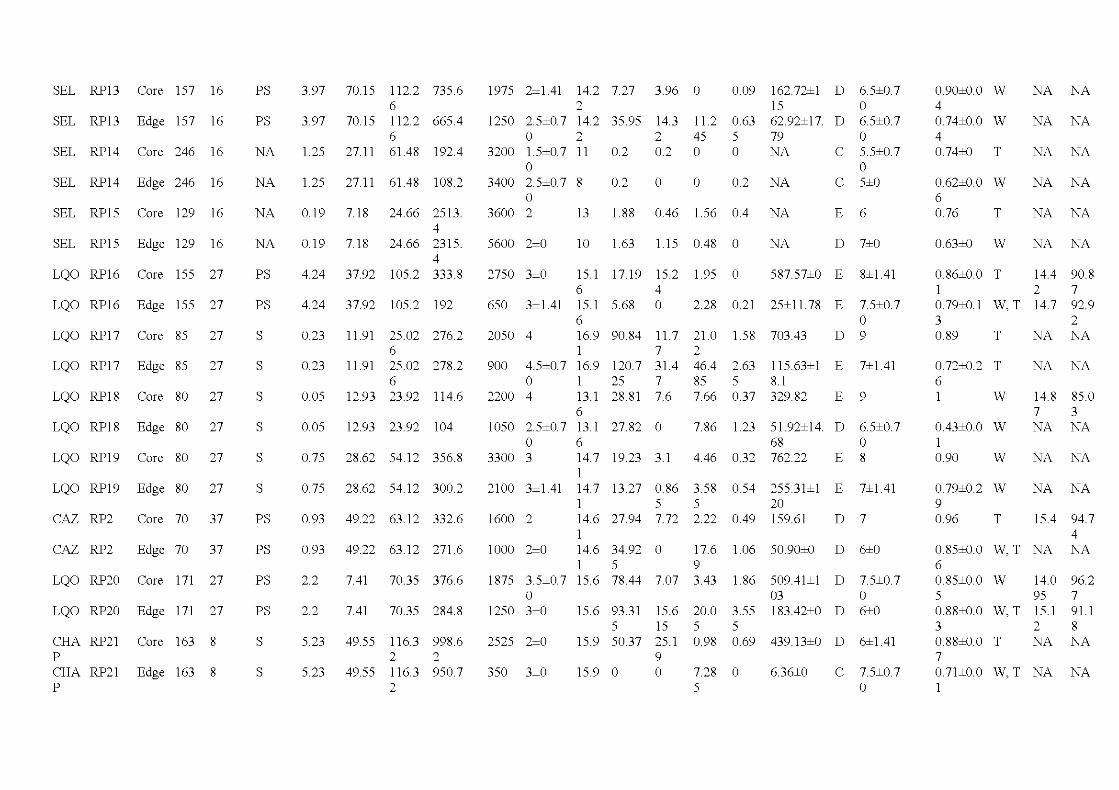
SEL RP13 Core 157 16 PS 3.97

SEL RP13 Edge 157 16 PS 3.97

SEL RP14 Core 246 16 NA 1.25

SEL RP14 Edge 246 16 NA 1.25

SEL RP15 Core 129 16 NA 0.1 9

SEL RP15 Edge 129 16 NA 0.1 9

LQO RP16 Core 155 27 PS 4. 24

LQO RP1 6 Edge 155 27 PS 4. 24

LQO RP17 Core 85 27 s 0.23

LQO RP17 Edge 85 27 s 0.23

LQO RP18 Core 80 27 s 0.05

LQO RP1 8 Edge 80 27 s 0.05

LQO RP19 Core 80 27 s 0.75

LQO RP19 Edge 80 27 s 0.75

CAZ RP2 Core 70 37 PS 0.93

CAZ RP2 Edge 70 37 PS 0.93

LQO RP20 Core 1 71 27 PS 2.2

LQO RP20 Edge 1 71 27 PS 2.2

CHA RP21 Core 163 8 s 5.23 p

CHA RP21 Edge 163 8 s 5.23 p

70.15

70.15

27.11

112.2 6 112.2 6 61.48

735.6

665.4

192.4

27.11 61.48 108 .2

7.18 24.66 2513. 4

7.18 24.66 2315. 4

37.92 105.2 333.8

37.92 105.2 192

11.91 25.02 276.2 6

11.91 25.02 278 .2 6

12.93 23.92 114.6

12.93 23.92 104

28 .62 54.12 356.8

28 .62 54.12 300.2

49.22 63.1 2 332.6

49.22 63.1 2 271.6

7.41 70.35 376.6

7.41 70.35 284.8

49.55

49.55

11 6.3 2 11 6.3 2

998 .6 2 950.7

1975 2±1.41 14.2 2

1250 2.5±0.7 14.2 0 2

3200 1.5±0.7 11 0

3400 2.5±0.7 8 0

3600 2 13

7.27 3.96 0 0.09

35.95 14.3 11.2 0.63 2 45 5

0.2 0.2 0 0

0.2 0 0 0.2

1. 88 0.46 1.56 0.4

162.72±1 D 6.5±0.7 15 0 62.92±17. D 6.5±0.7 79 0 NA C 5.5±0.7

0 NA c 5±0

NA E 6

5600 2±0 10 1.63 1.15 0.48 0 NA D 7±0

2750 3±0 15.1 6

650 3±1.41 15.1 6

2050 4 16.9 1

900 4.5±0.7 16.9 0 1

2200 4 13.1 6

1050 2.5±0.7 13.1 0 6

3300 3 14.7 1

2100 3±1.41 14.7 1

1600 2 14.6 1

1000 2±0 14.6 1

1875 3.5±0. 7 15.6 0

17.19 15.2 1.95 0 4

587.57±0 E 8±1.41

5.68 0

90.84 11.7 7

120.7 31.4 25 7 28.81 7.6

2.28 0.21 25±11.78 E 7.5±0.7 0

21.0 2 46.4 85 7.66

1.58 703.43 D 9

2.63 11 5.63±1 E 7±1.41 5 8.1 0.37 329.82 E 9

27.82 0 7.86 1.23 51.92±14. D 6.5±0.7 68 0

19.23 3.1 4.46 0.32 762.22 E 8

13.27 0.86 3.58 0.54 255.31±1 E 7±1.41 5 5 20

27.94 7.72 2.22 0.49 159.61 D 7

34.92 0 17.6 1.06 50.90±0 D 6±0 5 9 78.44 7.07 3.43 1. 86 509.41±1 D 7.5±0.7

03 0 1250 3±0 15.6 93.31 15.6 20.0 3.55 183.42±0 D 6±0

2525 2±0

350 3±0

5 15 15.9 50.37 25 .1

9 15.9 0 0

5 5 0.98 0.69 439.13±0 D 6±1.41

7.28 0 5

6.36±0 c 7.5±0.7 0

0.90±0.0 w 4 0.74±0.0 w 4 0.74±0 T

0.62±0.0 w 6 0.76 T

0.63±0 w

NA NA

NA NA

NA NA

NA NA

NA NA

NA NA

0.86±0.0 T 14.4 90.8 1 2 7 0.79±0.1 W, T 14.7 92.9 3 2 0.89 T NA NA

0.72±0.2 T 6 1 w

0.43±0.0 w 1 0.90 w

0.79±0.2 w 9

NA NA

14.8 85.0 7 3 NA NA

NA NA

NA NA

0.96

0.85±0.0 6

T 15.4 94.7 4

W,T NA NA

0.85±0.0 w 5 0.88±0.0 3

W, T

0.88±0.0 T 7

14.0 95 15.1 2 NA

0.71±0.0 1

W,T NA

96.2 7 91. 1 8 NA

NA

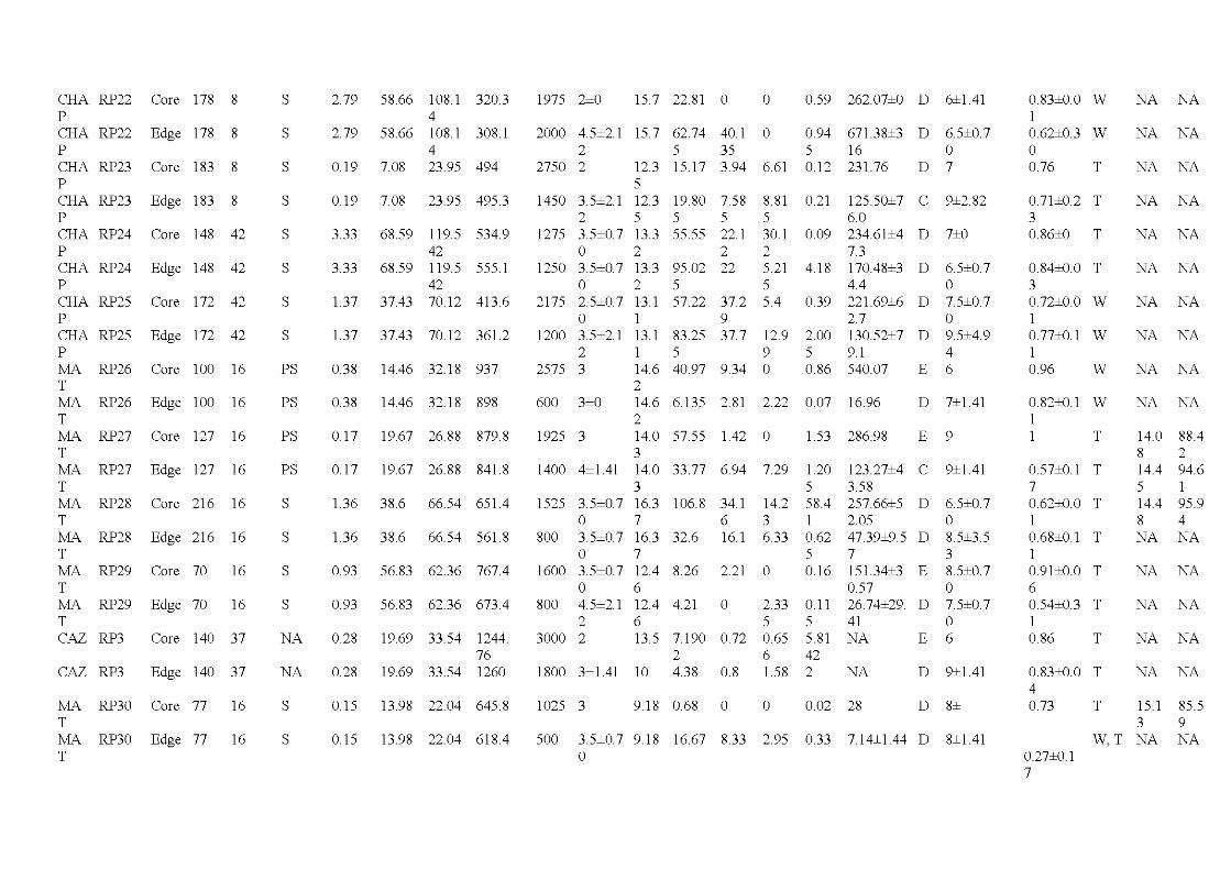
CHA RP22 Core 1 78 8 p

CHA RP22 Edge 1 78 8 p

CHA RP23 Core 183 8 p

CHA RP23 Edge 183 8 p





:tvfA RP26 Core 100 16 T :tvfA RP26 Edge 100 16 T :tvfA RP27 Core 127 16 T :tvfA RP27 Edge 127 16 T :tvfA RP28 Core 216 16 T :tvfA RP28 Edge 216 16 T :tvfA RP29 Core 70 16 T :tvfA RP29 Edge 70 16 T CAZ RP3 Core 140 37

CAZ RP3 Edge 140 37

:tvfA RP30 Core 77 16 T :tvfA RP30 Edge 77 16 T

s

s

s

s

s

s

s

s

PS

PS

PS

PS

s

s

s

s

NA

NA

s

s

2.79 58.66 108.1 320.3 4

2. 79 58.66 108.1 308.1 4

0.1 9 7.08 23.95 494

0 .1 9 7.08 23.95 495.3

3.33 68.59 11 9.5 534.9 42

3.33 68 .59 11 9.5 555.1 42

1.37 37.43 70.12 413.6

1.37 37.43 70.12 361.2

0 .38 14.46 32.18 937

0 .38 14.46 32.18 898

0 .17 19.67 26.88 879.8

0 .17 19.67 26.88 841.8

1.36 38.6 66.54 651.4

1.36 38.6 66.54 561.8

0 .93 56.83 62.36 767.4

0 .93 56.83 62.36 673.4

0 .28 19.69 33.54 1244. 76

0 .28 19.69 33.54 1260

0 .1 5 13.98 22.04 645 .8

0 .1 5 13.98 22.04 618.4

1975 2±0 15.7 22.81 0 0 0.59 262.07±0 D 6±1.41

2000 4. 5±2.1 15.7 62.74 40 .1 0 0.94 671.38±3 D 6.5±0. 7 2 5 35 5 16 0

2750 2 12.3 15.17 3 .94 6 .61 0.12 23 1.76 D 7 5

1450 3.5±2.1 12.3 19.80 7 .58 5 22.1 2

8.81 5 30.1 2 5 .21 5 5.4

0.21 2 5 5

1275 3.5±0.7 13.3 55.55 0.09 0 2

1250 3.5±0.7 13.3 0 2

2175 2.5±0.7 13.1 0 1

1200 3.5±2.1 2

2575 3

13.1 1 14.6 2

95.02 5

22

57.22 37.2 9

4. 18

0.39

83.25 37.7 12.9 2.00 5 9 5 40.97 9 .34 0 0.86

125.50±7 6.0 234.61±4 7.3 170.48±3 4.4 221.69±6 2.7 130.52±7 9.1 540.07

600 3±0 14.6 6.135 2.81 2.22 0.07 16.96 2

c 9±2.82

D 7±0

D 6.5±0.7 0

D 7.5±0.7 0

D 9.5±4.9 4

E 6

D 7±1.41

1925 3 14.0 57.55 1.42 0 3

1.53 286.98 E 9

1400 4±1.41 14.0 33.77 6 .94 7 .29 1.20 3 5

1525 3.5±0.7 16.3 106.8 34.1 14.2 58.4 0 7 6 3 1

800 3 .5±0.7 16.3 32.6 16.1 6 .33 0.62 0 7 5

1600 3 .5±0.7 12.4 8.26 2.21 0 0.16 0 6

800 4. 5±2.1 12.4 4.21 0 2

3000 2 6 13.5

1800 3±1.41 10

7.190 0 .72 2 4.38 0 .8

2.33 5 0 .65 6 1.58

0.11 5 5.81 42 2

123.27±4 3.58 257.66±5 2.05 47.39±9.5 7

c 9±1.41

D 6.5±0.7 0

D 8.5±3.5 3

151.34±3 E 0.57

8.5±0.7 0

26.74±29. D 7.5±0.7 41 0 NA E 6

NA D 9±1.41

1025 3 9.18 0.68 0 0 0.02 28 D 8±

500 3 .5±0. 7 9.18 16.67 8.33 2.95 0.33 7.14±1.44 D 8±1.41 0

0.83±0.0 w 1 0.62±0.3 w 0 0.76 T

0.71±0.2 T 3 0.86±0 T

0.84±0.0 T 3 0.72±0.0 w 1 0.77±0.1 w 1 0.96 w

0.82±0.1 w 1 1 T

0.57±0.1 T 7 0.62±0.0 T 1 0.68±0.1 T 1 0.91±0.0 T 6 0.54±0.3 T 1 0.86 T

0.83±0.0 T 4 0.73 T

NA NA

NA NA

NA NA

NA NA

NA NA

NA NA

NA NA

NA NA

NA NA

NA NA

14.0 88.4 8 2 14.4 94.6 5 1 14.4 95.9 8 4 NA NA

NA NA

NA NA

NA NA

NA NA

15.1 85.5 3 9

W,T NA NA 0.27±0.1 7

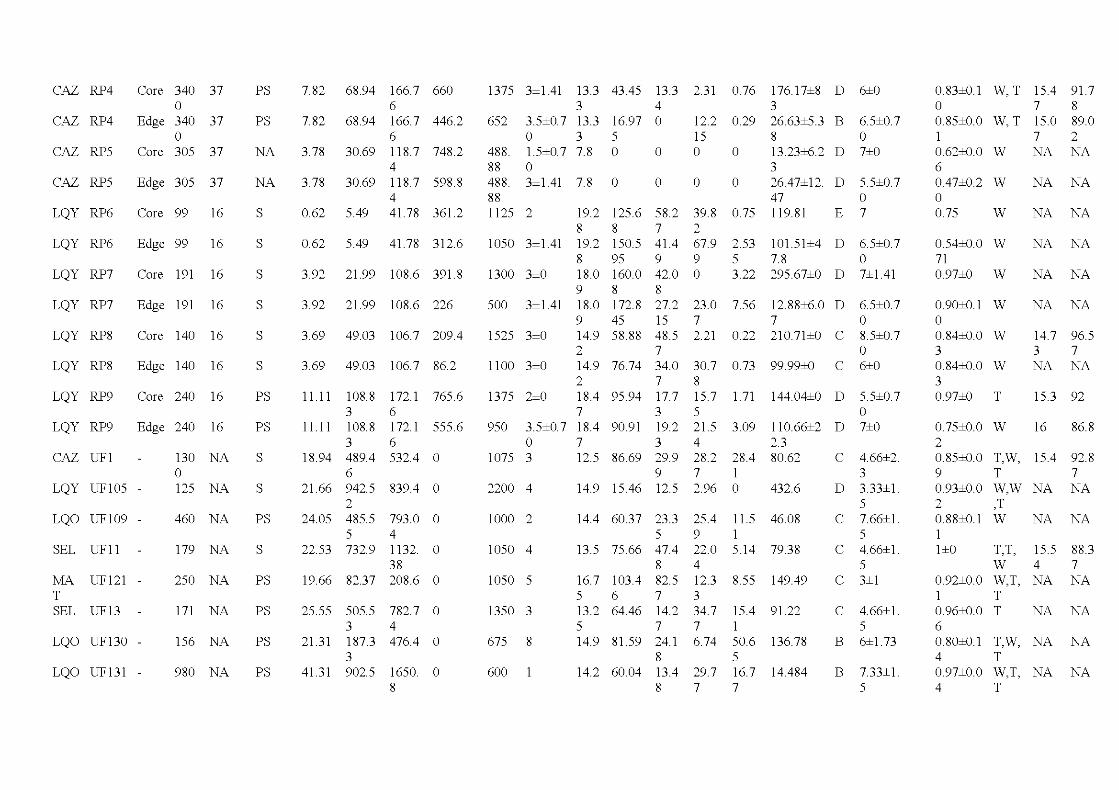
CAZ RP4 Core 340 37 0

CAZ RP4 Edge 340 37 0

CAZ RP5 Core 305 37

CAZ RP5 Edge 305 37

LQY RP6 Core 99 16

LQY RP6 Edge 99 16

LQY RP7 Core 191 16

LQY RP7 Edge 191 16

LQY RP8 Core 140 16

LQY RP8 Edge 140 16

LQY RP9 Core 240 16

LQY RP9 Edge 240 16

CAZ UF1

LQY UF105 -

LQO UF109 -

SEL UFll

MA UF121 -T SEL UF13

LQO UF130 -

LQO UF131 -

130 NA 0 125 NA

460 NA

179 NA

250 NA

171 NA

156 NA

980 NA

PS

PS

NA

NA

s

s

s

s

s

s

PS

PS

s

s

PS

s

PS

PS

PS

PS

7.82 68.94 166.7 660 6

7.82 68.94 166.7 446.2 6

3. 78 30.69 118.7 748.2 4

3.78 30.69 118.7 598.8 4

0.62 5.49 41.78 361.2

0 .62 5.49 41.78 312.6

3.92 21.99 108.6 391.8

3.92 21.99 108.6 226

3.69 49.03 106.7 209.4

3.69 49.03 106.7 86.2

11.11 108.8 172.1 765 .6 3 6

11.11 108.8 172.1 555 .6 3 6

18.94 489.4 532.4 0 6

21.66 942.5 2

24.05 485.5 5

22.53 732.9

19.66 82.37

25 .55

21.31

41. 31

505.5 3 187.3 3 902.5

839.4 0

793.0 0 4 1132. 0 38 208.6 0

782.7 0 4 476.4 0

1650. 0 8

1375 3±1.41

652 3.5±0.7 0 1.5±0.7 0

13.3 3 13.3 3 7.8

43.45 13.3 2.31 O. 76 4

16.97 0 5 0 0

12.2 0.29 15 0 0

D 6±0

B 6.5±0.7 0

D 7±0 488 . 88 488 . 88

3±1.41 7.8 0 0 0 0

176.1 7±8 3 26.63±5.3 8 13.23±6.2 3 26.47±12. 47

D 5.5±0.7

1125 2

1050 3±1.41

1300 3±0

500 3±1.41

1525 3±0

1100 3±0

1375 2±0

950 3.5±0.7 0

1075 3

2200 4

1000 2

1050 4

1050 5

1350 3

675 8

600

39.8 2 67.9 9 0

0 0.75 11 9.81 E 7

2.53 101.51±4 D 6.5±0.7 5 7.8 0 3.22 295.67±0 D 7±1.41

19.2 8 19.2 8 18.0 9 18.0 9 14.9 2 14.9 2 18.4 7 18.4 7 12.5

125.6 8 150.5 95 160.0 8 172.8 45 58.88

58 .2 7 41.4 9 42.0 8 27.2 15 48.5 7 34.0 7 17.7 3 19.2 3 29.9 9 12.5

23 .0 7.56 12.88±6.0 D 6.5±0.7 7 7 0 2.21 0.22 210.71±0 c 8.5±0.7

0 76.74

95.94

90.91

86.69

14.9 15.46

30.7 8 15.7 5 21.5 4 28 .2 7 2.96

14.4 60.37 23 .3 25.4 5 9

13.5 75.66 47.4 22.0 8 4

16.7 103.4 82.5 12.3 5 6 7 3 13.2 64.46 14. 2 34.7 5 7 7 14.9 81.59 24.1 6 .74

8 14.2 60.04 13.4 29.7

8 7

0.73 99.99±0 c 6±0

1.71 144.04±0 D 5.5±0.7 0

3.09 11 0.66±2 D 7±0 2.3

28.4 80.62 1 0 432.6

11.5 46.08 1 5.14 79.38

8.55 149.49

15.4 91.22 1 50.6 136.78 5 16.7 14.484 7

c 4.66±2. 3

D 3.33±1. 5

c 7.66±1. 5

c 4.66±1. 5

c 3±1

c 4.66±1. 5

B 6±1.73

B 7.33±1. 5

0.83±0.1 W , T 15.4 91.7 0 7 8 0.85±0.0 W , T 15.0 89.0 1 7 2 0.62±0.0 W NA NA 6 0.47±0.2 W NA NA 0 0.75 W NA NA

0.54±0.0 W NA NA 71 0.97±0 w

0.90±0.1 w 0 0.84±0.0 w 3 0.84±0.0 w 3 0.97±0 T

0.75±0.0 w 2

NA NA

NA NA

14.7 96.5 3 7 NA NA

15.3 92

16 86.8

0.85±0.0 T,W, 15.4 92.8 9 T 7 0.93±0.0 W,W NA NA 2 ,T 0.88±0.1 w 1 1±0 T,T,

w 0.92±0.0 W,T, 1 T 0.96±0.0 T 6 0.80±0.1 T,W, 4 T 0.97±0.0 W,T, 4 T

NA NA

15.5 88.3 4 7 NA NA

NA NA

NA NA

NA NA

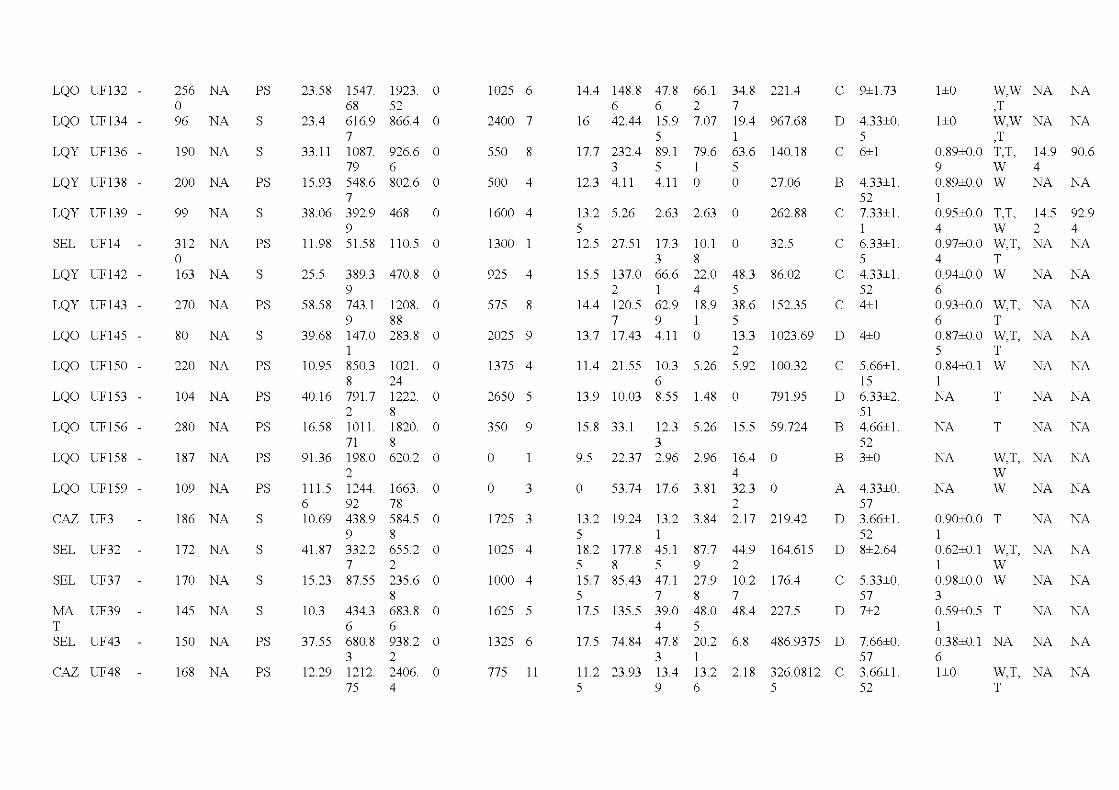
LQO UF132 -

LQO UF134 -

LQY UF136 -

LQY UF138 -

LQY UF139 -

SEL UF14

LQY UF142 -

LQY UF143 -

LQO UF145 -

LQO UF150 -

LQO UF153 -

LQO UF156 -

LQO UF158 -

LQO UF159 -

CAZ UF3

SEL UF32

SEL UF37

MA UF39 T SEL UF43

CAZ UF48

256 NA 0 96 NA

190 NA

200 NA

99 NA

312 NA 0 163 NA

270 NA

80 NA

220 NA

104 NA

280 NA

187 NA

109 NA

186 NA

172 NA

170 NA

145 NA

150 NA

168 NA

PS

s

s

PS

s

PS

s

PS

s

PS

PS

PS

PS

PS

s

s

s

s

PS

PS

23.58

23.4

33.11

15.93

38.06

11.98

25.5

58.58

39.68

10.95

40.16

16.58

91.36

111.5 6 10.69

41.87

15.23

10.3

37.55

12.29

1547. 68 616.9 7 1087. 79 548.6 7 392.9 9 51.58

389.3 9 743.1 9 147.0 1 850.3 8 791.7 2 1011. 71 198.0 2 1244. 92 438.9 9 332.2 7 87.55

434.3 6 680.8 3 1212. 75

1923. 0 52 866.4 0

926.6 0 6 802.6 0

468 0

110.5 0

470.8 0

1208. 0 88 283.8 0

1021. 0 24 1222. 0 8 1820. 0 8 620.2 0

1663. 0 78 584.5 0 8 655.2 0 2 235.6 0 8 683.8 0 6 938.2 0 2 2406. 0 4

1025 6

2400 7

550 8

500 4

1600 4

1300

925 4

575 8

2025 9

1375 4

2650 5

350 9

0

0 3

1725 3

1025 4

1000 4

1625 5

1325 6

775 11

14.4 148.8 47.8 66.1 34.8 221.4 6 6 2 7

16 42.44 15.9 7 .07 19.4 967.68 5 1

17.7 232.4 89.1 79.6 63.6 140.18 3 5 1 5

12.3 4.11 4.11 0 0 27.06

13.2 5.26 5 12.5 27.51

2.63 2.63 0

17.3 10.1 0 3 8

15.5 137.0 66. 6 22.0 48.3 2 1 4 5

14.4 120.5 62.9 18.9 38.6 7 9 1 5

13.7 17.43 4.11 0 13.3 2

11.4 21.55 10.3 5.26 5.92 6

13.9 10.03 8.55 1.48 0

262.88

32.5

86.02

152.35

1023.69

100.32

791.95

15.8 33.1 12.3 5.26 15.5 59.724 3

9.5 22.37 2.96 2.96 16.4 0 4

0 53.74 17.6 3.81 32.3 0 2

13.2 19.24 13.2 3 .84 2.17 219.42 5 1

c 9±1.73

D 4.33±0. 5

c 6±1

B 4.33±1. 52

c 7.33±1. 1

c 6.33±1. 5

c 4.33±1. 52

c 4±1

D 4±0

c 5.66±1. 15

D 6.33±2. 51

B 4.66±1. 52

B 3±0

A 4.33±0. 57

D 3.66±1.

18.2 177.8 45.1 87.7 44.9 164.615 D 52 8±2.64

5 8 5 9 2 15.7 85.43 47 .1 27.9 10.2 176.4 5 7 8 7 17.5 135.5 39.0 48.0 48.4 227.5

4 5

c 5.33±0. 57

D 7±2

17.5 74.84 47.8 20.2 6.8 486.9375 D 7.66±0. 57 3.66±1. 52

3 1 11.2 23.93 13.4 13.2 2.18 326.0812 c 5 9 6 5

1±0 W,W NA NA ,T

1±0 W,W NA NA ,T

0.89±0.0 T,T, 9 w 0.89±0.0 w 1 0.95±0.0 T,T, 4 w 0.97±0.0 W,T, 4 T 0.94±0.0 w 6 0.93±0.0 W,T, 6 T 0.87±0.0 W,T, 5 T 0.84±0.1 w 1 NA T

NA T

14.9 90.6 4 NA NA

14.5 92.9 2 4 NA NA

NA NA

NA NA

NA NA

NA NA

NA NA

NA NA

NA W,T, NA NA w

NA W NA NA

0.90±0.0 T NA NA 1 0.62±0.1 W,T, NA NA 1 w 0.98±0.0 W NA NA 3 0.59±0.5 T NA NA 1 0.38±0.1 NA NA NA 6 1±0 W,T, NA NA

T

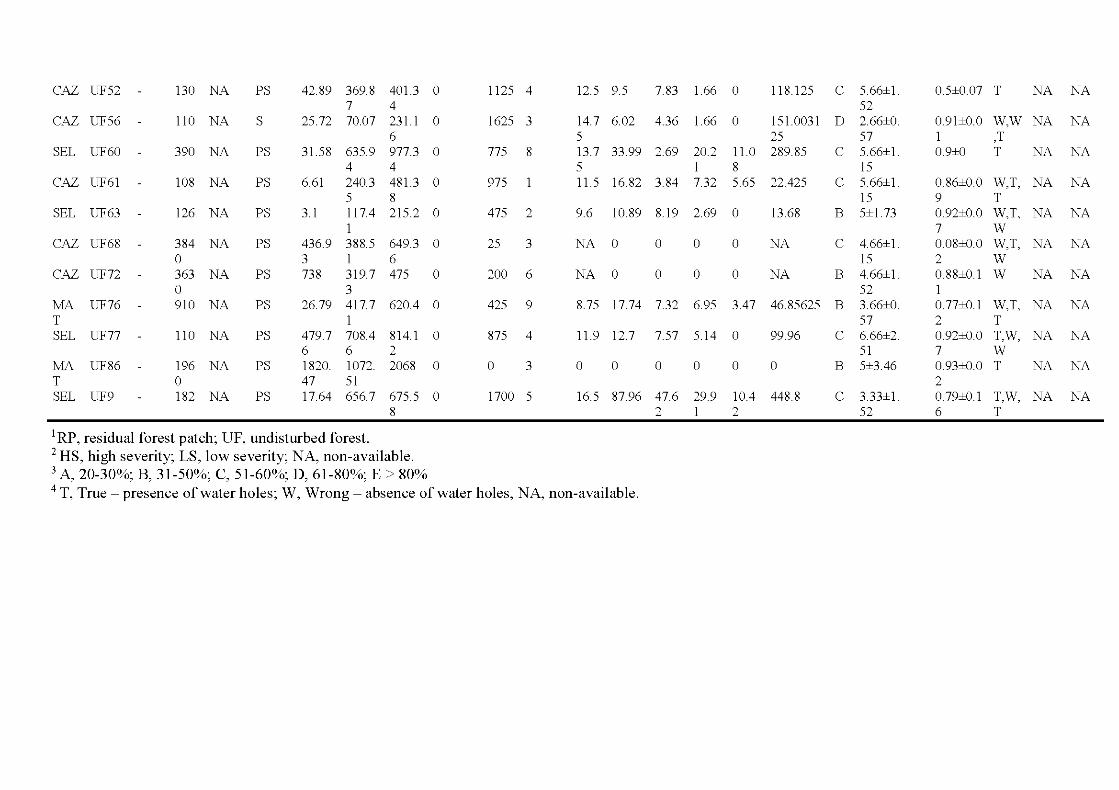
CAZ UF52 130 NA PS 42.89 369.8 401.3 0 1125 4 12.5 9.5 7.83 1.66 0 11 8.1 25 c 5.66±1. 0.5±0.07 T NA NA 7 4 52

CAZ UF56 110 NA s 25.72 70.07 231.1 0 1625 3 14.7 6.02 4.36 1.66 0 151.0031 D 2.66±0. 0.91±0.0 W,W NA NA 6 5 25 57 1 ,T

SEL UF60 390 NA PS 31.58 635.9 977.3 0 775 8 13.7 33.99 2.69 20.2 11.0 289.85 c 5.66±1. 0.9±0 T NA NA 4 4 5 1 8 15

CAZ UF61 108 NA PS 6.61 240.3 481.3 0 975 11.5 16.82 3.84 7.32 5.65 22.425 c 5.66±1. 0.86±0.0 W,T, NA NA 5 8 15 9 T

SEL UF63 126 NA PS 3.1 117.4 215.2 0 475 2 9.6 10.89 8. 19 2.69 0 13.68 B 5±1.73 0.92±0.0 W,T, NA NA 1 7 w

CAZ UF68 384 NA PS 436.9 388.5 649.3 0 25 3 NA 0 0 0 0 NA c 4.66±1. 0.08±0.0 W,T, NA NA 0 3 1 6 15 2 w

CAZ UF72 363 NA PS 738 319.7 475 0 200 6 NA 0 0 0 0 NA B 4.66±1. 0.88±0.1 w NA NA 0 3 52 1

:tvfA. UF76 910 NA PS 26.79 417.7 620.4 0 425 9 8.75 17.74 7.32 6.95 3.47 46.85625 B 3.66±0. 0.77±0.1 W,T, NA NA T 1 57 2 T SEL UF77 110 NA PS 479.7 708.4 814.1 0 875 4 11.9 12.7 7.57 5.1 4 0 99.96 c 6.66±2. 0.92±0.0 T,W, NA NA

6 6 2 51 7 w :tvfA. UF86 196 NA PS 1820. 1072. 2068 0 0 3 0 0 0 0 0 0 B 5±3.46 0.93±0.0 T NA NA T 0 47 51 2 SEL UF9 182 NA PS 17.64 656.7 675.5 0 1700 5 16.5 87.96 47.6 29.9 10.4 448.8 c 3.33±1. 0.79±0.1 T,W, NA NA

8 2 1 2 52 6 T

1 RP, residual forest patch; UF, undisturbed forest. 2 HS, high severity; LS, low severity; NA, non-available. 3 A, 20-30%; B, 31-50%; C, 51-60%; D, 61-80%; E > 80% 4 T, True - presence ofwater holes; W, Wrong - absence ofwater holes, NA, non-available.

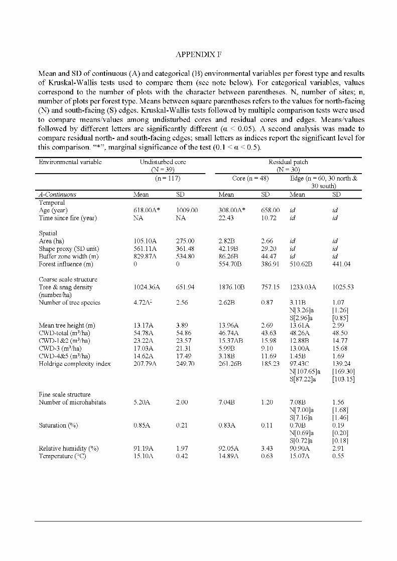
APPENDIXF

Mean and SD of continuous (A) and categorical (B) environmental variables per forest type and results of Kruskal-Wallis tests used to compare them (see note below). For categorical variables, values correspond to the number of plots with the character between parentheses. N, number of sites; n, number of plots per forest type. Me ans between square parentheses refers to the values for north-facing (N) and south-facing (S) edges. Kruskal-Wallis tests followed by multiple comparison tests were used to compare means/values among undisturbed cores and residual cores and edges. Means/values followed by different letters are significantly different (a < 0.05). A second analysis was made to compare residual north- and south-facing edges; smallletters as indices report the significant level for this comparison. "*",marginal significance ofthe test (0.1 < a < 0.5).

Environmental variable

Core (n = 48) Edge (n = 60, 30 north & 30 south

A-Continuous Mean SD Mean SD Mean SD Temporal Age (year) 618.00A* 1009.00 308.00A* 658.00 id id Time since fire (year) NA NA 22.43 10.72 id id

Spatial Area (ha) 105.10A 275.00 2.82B 2.66 id id Shape proxy (SD unit) 561.11A 361.48 42.19B 29.20 id id Buffer zone width (rn) 829.87A 534.80 86.26B 44.47 id id Forest influence (rn) 0 0 554.70B 386.91 510.62B 441.04

Coarse scale structure Tree & snag density 1024.36A 651.94 1876.10B 757.15 1233.03A 1025.53 (number!ha) Number oftree species 4.72At 2.56 2.62B 0.87 3.11B 1.07

N[3.26]a [1.26] S[2.96]a [0.85]

Mean tree height (rn) 13.17A 3.89 13.96A 2.69 13.61A 2.99 CWD-total (m3!ha) 54.78A 54.86 46.74A 43.63 48.26A 48.50 CWD-1&2 (m3!ha) 23.22A 23.57 15.37AB 15.98 12.88B 14.77 CWD-3 (m3/ha) 17.03A 21.31 5.99B 9.10 13.00A 15.68 CWD-4&5 (m3!ha) 14.62A 17.49 3.18B 11.69 1.45B 1.69 Holdrige complexity index 207.79A 249.70 261.26B 185.23 97.43C 139.24

N[107.65]a [169.30] S[87.22]a [103.15]

Fine scale structure Number of microhabitats 5.20A 2.00 7.04B 1.20 7.08B 1.56

N[7.00]a [1.68] S[7.16]a [1.46]

Saturation(%) 0.85A 0.21 0.83A 0.11 0.70B 0.19 N[0.69]a [0.20] S[0.72]a [0.18]

Relative humidity (%) 91.19A 1.97 92.05A 3.43 90.90A 2.91 Temperature (0 C) 15.10A 0.42 14.89A 0.63 15.07A 0.55

B-Cate orical Severity Severity (LS/HS)!

Structural at coarse scale Canopy closure (%) (A<B<C<D<E)!

Structural at fine scale Water hole (YIN)!

78/39A

3/27/60/27 /OA

61 /53A

15/27B 18/34B

l /0/3/30/14B 0/2/1 3/33/12C

22/26A 22/38A

id, variable was measured at the scale of the whole patch and is the same for cores and edges. !, LS, low severity; HS, high severity; A, 20-30% of closure; B, 30-50%, C, 50-60%; D, 60-80%; E, > 80%; Y, presence ofwater holes; N, absence ofwater holes.

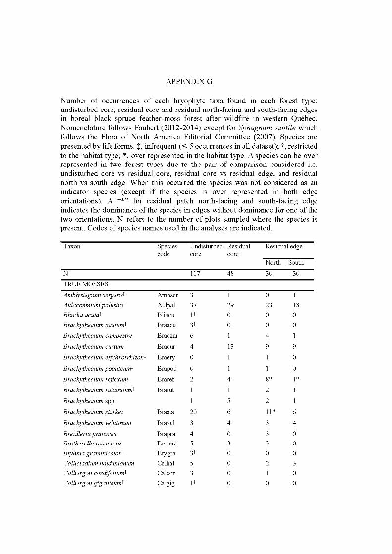
APPENDIX G

Number of occurrences of each bryophyte taxa found in each forest type: undisturbed core, residual core and residual north-facing and south-facing edges in boreal black spruce feather-moss forest after wildfire in western Québec. Nomenclature follows Faubert (2012-2014) except for Sphagnum subtile which follows the Flora of North America Editorial Committee (2007). Species are presented by life forms. t, infrequent (~ 5 occurrences in all datas et); t, restricted to the habitat type; *, over represented in the habitat type. A species can be over represented in two forest types due to the pair of comparison considered i.e. undisturbed core vs residual core, residual core vs residual edge, and residual north vs south edge. When this occurred the species was not considered as an indicator species ( except if the species 1s over represented in both edge orientations). A "*" for residual patch north-facing and south-facing edge indicates the dominance ofthe species in edges without dominance for one of the two orientations. N refers to the number of plots sampled where the species is present. Codes of species nam es used in the analyses are indicated.

Taxon

N

TRUEMOSSES

Amblystegium serpenst

Aulacomnium palustre

Blindia acutat

Brachythecium acutumt

Brachythecium campestre

Species code

Ambser

Aulpal

Bliacu

Braacu

Brac am

Brachythecium curtum Bracur

Brachythecium erythrorrhizont Braery

Brachythecium populeumt Brapop

Brachythecium rejlexum Braref

Brachythecium rutabulumt Brarut

Brachythecium spp.

Brachythecium starkei Brasta

Brachythecium velutinum Bravel

Breidleria pratensis Brapra

Brotherella recurvans Brorec

Bryhnia graminicolort Brygra

Callicladium haldanianum Calhal

Calliergon cordifoliumt Calcor

Calliergon giganteumt Calgig

Undisturbed Residual core core

117

3

37

p

3t

6

4

0

0

2

1

20

3

4

5

3t

5

3

1t

48

29

0

0

13

4

5

6

4

0

3

0

0

0

0

Residual edge

North South

30

0

23

0

0

4

9

8*

2

2

11 * 3

3

3

0

2

1

0

30

18

0

0

9

0

0

1*

6

4

0

0

0

3

0

0

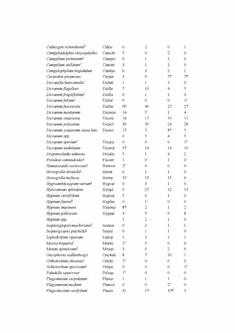
Calliergon richardsoniit Calric 0 2 0

Campyliadelphus chrysophyllus Camchr 5 0 2 0

Campylium protensumt Cam pro 0 0

Campylium stellatumt Cam ste 3 0

Campylophyllum hispidulum Cam his 6 3 2

Ceratodon purpureus Cerpur 3 0 7* 7*

Dicranella heteromazzat Dichet 0

Dicranum flagellare Dicfla 7 10 4 5

Dicranum fragilifoliumt Dicfra 0 1 1 0

Dicranum fulvumt Dicful 0 0 0 1t

Dicranum fusees cens Dicfus 99 46 27 27

Dicranum montanum Di cm on 14 9 1 4

Dicranum ontariense Dicont 14 17 10 11

Dicranum polysetum Dicpol 30 35 24 28

Dicranum scoparium sensu lato Dicsco 17 5 8* 5

Dicranum spp. 0 5 4 5

Dicranum spuriumt Dicspu 0 0 0 1t

Dicranum undulatum Die und 57 14 13 16

Drepanocladus aduncus Dreadu 5 1 4 2

Fissidens osmundoidest Fisosm 0 0

Hamatocaulis vemicosust Ham ver 2t 0 0 0

Herzogiella striatellat Herstr 0 0

Herzogiella tuifacea Hertur 19 13 15 6

Hygroamblystegium variumt Hygvar 0 3 1 0

Hylocomium splendens Hylspl 9 27 12 13

Hypnum curvifolium Hypcur 7 0 0

Hypnum faurieit Hypfau 0 1t 0 0

Hypnum imponens Hypimp 8* 2 2

Hypnum pallescens Hyppal 4 9 9 8

Hypnum spp. 1 2 0

Isopterygiopsis muellerianat Iso mue 0 2 1

Isopterigiopsis pulchellat Isopul 0 1 0

Leptodictyum riparium Leprip 3

Meesia triquetrat Mee tri 1t 0 0 0

Mnium spinulosumt Mnispi 3 0 2 0

Oncophorus wahlenbergii Oncwah 8 7 10 1

Orthotrichum ohioenset Orto hi 1t 0 0 0

Orthotrichum speciosumt Ortspe 0 0 0 1t

Paludella squarrosat Palsqu 1t 0 0 0

Plagiomnium cuspidatumt Placus 1 1 0

Plagiomnium mediumt Plamed 0 0 2t 0

Plagiothecium cavifolium Placav 31 17 10* 5

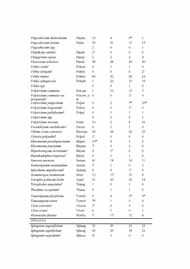
P lagiothecium denticulatum Pla den 13 4 9*

Plagiothecium laetum Plalae 59 31 15 17 Plagiothecium spp. 2 0 0 1

Platydictya subtilist Plasub 2t 0 0 0

Platygyrium repens Plarep 2 2 4 3

Pleurozium schreberi Plesch 98 48 30 30

Pohlia crudat Pohcru 0 0

Pohlia elongata! Pohelo 0 0 0 2t

Pohlia nutans Pohnut 84 32 28 24 Pohlia sphagnicola Pohsph 1 26 19 19

Pohlia spp. 0 0 0

Polytrichum commune Polcom 1 10 12 7

Polytrichym commune var. Polcom_p 0 0 2t 0 perigonialet er P olytrichum junipe rinum Poljun 0 2 7* 10*

Polytrichum longisetumt Pollon 0 0 1t 0

Polytrichum pallidisetum! Polpal 0 1 1 Polytrichum spp. 0 0 0

Polytrichum strictum Polstr 10 2 8 16

Pseudobryum cinclidioidest Psecin 0 1 1 0 Ptilium crista-castrensis Pticricas 43 44 26 25

Pylaisia polyanthat Pylpol 1t 0 0 0

Rhizomnium pseudopunctatum Rhipse 19* 4 5 2 Rhizomnium punctatum Rhipun 7 3 3 0

Rhynchostegium serrulatumt Rhys er 0 1t 0 0

Rhytidiadelphus trique trust Rhytri 0 1 1 0

Sanionia uncinata San une 41 18 14 11

Sarmentypnum exannulatum Sarexa 7 0 2

Splachnum ampullaceumt Splamp 0 0 1t 0 Straminergon stramineum Strstr 12 17 10 8

Tetraphis pellucida Hedw. Tepel 61 33 16 14 Tetraplodon angustatust Tetang 0 0

Thuidium recognitumt Thurec 0 0

Tomentypnum falcifolium Tomfal 0 4 5* 3*

Tomentypnum nitens Tomnit 7* 1 3 0 Ulota coarctatat Ulocoa p 0 0 0

Ulota crispat Ulocri 0 0

Wamstoifiafluitans Warflu 7 17 12 8

SPHAGNA

Sphagnum angustifolium Sphang 35 39 23 23

Sphagnum capillifolium Sphcap 69 29 18 22

Sphagnum cuspidatum! Sphcus 4t 0 0 0

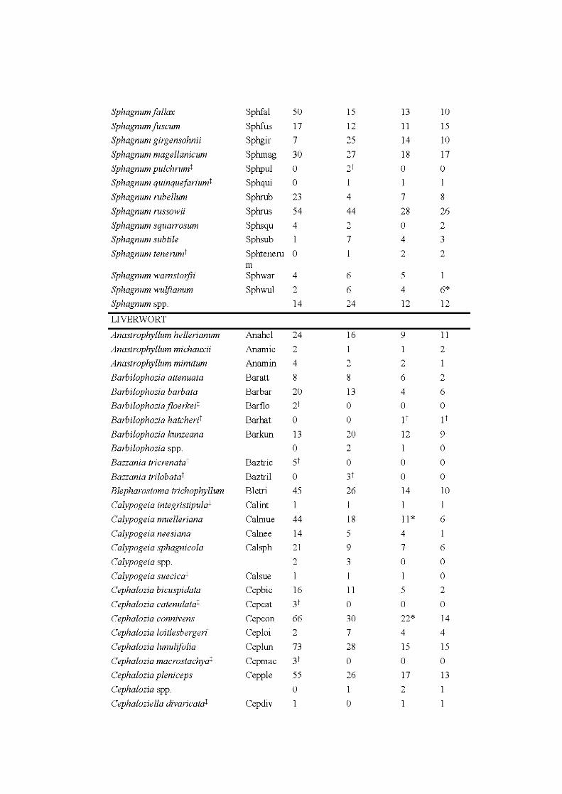
Sphagnum fallax Sphfal 50 15 13 10

Sphagnum fuscum Sphfus 17 12 11 15 Sphagnum girgensohnii Sphgir 7 25 14 10

Sphagnum magellanicum Sphmag 30 27 18 17

Sphagnum pulchrumt Sphpul 0 2t 0 0 Sphagnum quinquefariumt Sphqui 0 1

Sphagnum rubellum Sphrub 23 4 7 8

Sphagnum russowii Sphrus 54 44 28 26

Sphagnum squarrosum Sphsqu 4 2 0 2 Sphagnum subtile Sphsub 1 7 4 3 Sphagnum te ne rumt Sphteneru 0 2 2

rn Sphagnum wamstorfii Sphwar 4 6 5 Sphagnum wulfianum Sphwul 2 6 4 6*

Sphagnum spp. 14 24 12 12

LIVERWORT

Anastrophyllum he llerianum Anahel 24 16 9 11

Anastrophyllum michauxii Anamic 2 2 Anastrophyllum minutum Anamin 4 2 2

Barbilophozia attenuata Baratt 8 8 6 2

Barbilophozia barbata Bar bar 20 13 4 6 Barbilophozia floerkeit Barflo 2t 0 0 0 Barbilophozia hatcherit Bar hat 0 0 1t 1t

Barbilophozia kunzeana Bar kun 13 20 12 9

Barbilophozia spp. 0 2 1 0 Bazzania tricrenatat Baztric 5t 0 0 0 Bazzania trilobatat Baztril 0 3t 0 0 Blepharostoma trichophyllum Ble tri 45 26 14 10

Calypogeia integristipuZat Calint

Calypogeia muelleriana Calmue 44 18 11 * 6

Calypogeia neesiana Calnee 14 5 4 Calypogeia sphagnicola Calsph 21 9 7 6

Calypogeia spp. 2 3 0 0 Calypogeia suecicat Calsue 1 1 1 0 Cephalozia bicuspidata Cep bic 16 11 5 2 Cephalozia catenulatat Cepcat 3t 0 0 0

Cephalozia connivens Cep con 66 30 22* 14 Cephalozia loitlesbergeri Cep loi 2 7 4 4

Cephalozia lunulifolia Ceplun 73 28 15 15

Cephalozia macrostachyat Cepmac 3t 0 0 0 Cephalozia pleniceps Cepple 55 26 17 13

Cephalozia spp. 0 2 Cephaloziella divaricatat Cep div 0

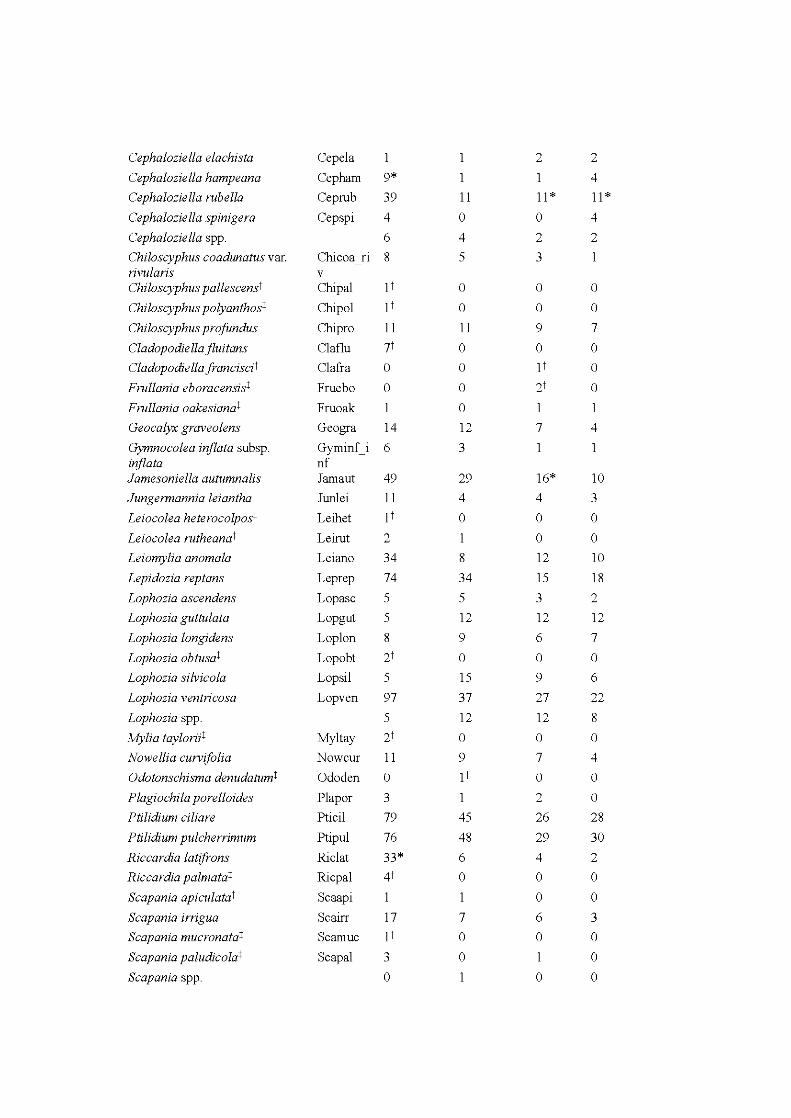
Cephaloziella elachista Cepela 2 2

Cephaloziella hampeana Ce pham 9* 4

Cephaloziella rubella Ceprub 39 11 11 * 11*

Cephaloziella spinigera Cep spi 4 0 0 4

Cephaloziella spp. 6 4 2 2

Chiloscyphus coadunatus var. Chicoa ri 8 5 3 1 rivularis v Chiloscyphus palles cens! Chipai p 0 0 0

Chiloscyphus polyanthost Chi pol 1t 0 0 0

Chiloscyphus profundus Chi pro 11 11 9 7

Cladopodie lia flui tans Claflu 7t 0 0 0

Cladopodie Il a francis ci! Clafra 0 0 1t 0

Frullania eboracensist Fruebo 0 0 2t 0

Frullania oakesianat Fruoak 1 0 1 1

Geocalyx graveolens Geogra 14 12 7 4

Gymnocolea injlata subsp. Gyminf_i 6 3 injlata nf Jamesoniella autumnalis Jamaut 49 29 16* 10

Jungermannia leiantha Junlei 11 4 4 3

Leiocolea heterocolpost Leihet 1t 0 0 0

Leiocolea rutheanat Leirut 2 1 0 0

Leiomylia anomala Leiano 34 8 12 10

Lepidozia reptans Leprep 74 34 15 18

Lophozia ascendens Lopasc 5 5 3 2

Lophozia guttulata Lopgut 5 12 12 12

Lophozia longidens Loplon 8 9 6 7

Lophozia obtusat Lopobt 2t 0 0 0

Lophozia silvicola Lopsil 5 15 9 6

Lophozia ventricosa Lopven 97 37 27 22

Lophozia spp. 5 12 12 8

Mylia tayloriit Myltay 2t 0 0 0

Nowellia curvifolia Nowcur 11 9 7 4

Odotonschisma denudatumt Ododen 0 1t 0 0

Plagiochila porelloides Plapor 3 1 2 0

Ptilidium ciliare Pticil 79 45 26 28

Ptilidium pulcherrimum Ptipul 76 48 29 30

Riccardia latifrons Ri clat 33* 6 4 2

Rie cardia palmatat Ri cp al 4t 0 0 0

Scapania apiculatat Scaapi 1 0 0

Scapania irrigua Scairr 17 7 6 3

Scapania mucronatat Scamuc p 0 0 0

Scapania paludicozat Scapa! 3 0 0

Scapania spp. 0 0 0

Schistochilopsis capitatat Schcap 1t 0 0 0

Schistochilopsis grandiretist Schgra 1t 0 0 0

Schistochilopsis incisat Schinc 4 1 0 0

Schistochilopsis laxat Schax 1 0 2 0

Schistochilopsis spp. 0 1 1 1

Tritomaria exsectiformis Triexs 20 9 5 5

Tritomaria quinquedentatat Triqui 1t 0 0 0

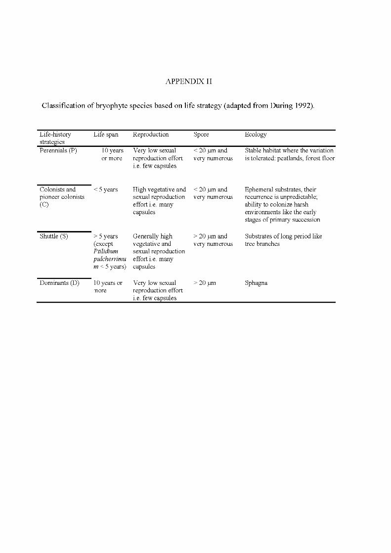
APPENDIX H

Classification ofbryophyte species based on life strategy (adapted from During 1992).

Life-history Life span Reproduction Spore Ecology strategies Perennials (P) 10 years Very low sexual < 20 f.!m and Stable habitat where the variation

or more reproduction effort very numerous is tolerated: peatlands, forest floor i.e. few capsules

Colonists and < 5 years High vegetative and < 20 f.!m and Ephemeral substrates, their pioneer colonists sexual reproduction very numerous recurrence is unpredictable; (C) effort i.e. many ability to colonize harsh

capsules environments like the early stages of primary succession

Shuttle (S) > 5 years Generally high > 20 f.!m and Substrates of long period like (except vegetative and very numerous tree branches Ptilidium sexual reproduction pulcherrimu effort i.e. many m < 5 years) capsules

Dominants (D) lü years or Very low sexual > 20 f.!m Sphagna nore reproduction effort

i.e. few capsules

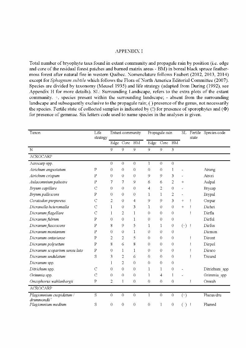
APPENDIX I

Total number of bryophyte taxa found in extant community and propagule rain by position (i.e. edge and core of the residual forest patches and bumed matrix areas - BM) in boreal black spruce feathermoss forest after natural fire in western Québec. Nomenclature follows Faubert (2012, 2013, 2014) except for Sphagnum subtile which follows the Flora of North America Editorial Committee (2007). Species are divided by taxonomy (Meusel 1935) and life strategy (adapted from During (1992), see Appendix H for more details). SL: Surrounding Landscape, refers to the extra plots of the extant community. +, species present within the surrounding landscape; - absent from the surrounding landscape and subsequently exclusive to the propagule rain; ()presence of the genus, not necessarily the species. Fertile state of collected samples is indicated by (!)for presence of sporophytes and (cD) for presence of gemmae. Six letters code used to name species in the analyses is given.

Taxon Life Extant community Propagule rain SL Fertile Species code strate gy state

Edge Core BM Edge Core BM

N 9 9 9 9 9 3

ACROCARP

Acrocarp spp. 0 0 0 1 0 0

Atrichum angustatum p 0 0 0 0 0 1 Atrang

Atrichum crispum p 0 0 0 9 9 3 Atrcri

Aulacomnium palustre p 7 7 9 6 6 2 + Aulpal

Bryum capillare c 0 0 0 4 2 0 Brycap

Bryum palle sc ens p 0 0 0 1 2 Brypal

Ceratodon purpureus c 2 0 4 9 9 3 + Cerpur

Dicranella heteromalla c 0 3 1 0 0 + Dichet

Dicranum jlagellare c 2 1 0 0 0 Die fla

Dicranum jùlvum p 0 0 0 0 0 Dicful

Dicranum jùscescens p 8 9 5 0 (+) ! Die fus

Dicranum montanum p 0 0 0 0 0 Dicmon

Dicranum ontariense p 2 2 5 0 0 0 Die ont

Dicranum polysetum p 8 6 8 0 0 0 Dicpol

Dicranum scoparium sensu lato p 0 1 1 0 0 0 Die seo

Dicranum undulatum s 3 2 6 0 0 0 Die und

Dicranum spp. 2 0 0 0 0

Ditrichum spp. c 0 0 0 0 Ditrichum _ spp

Grimmia spp. c 0 0 0 1 4 1 Grimm ia _ spp

Oncophorus wahlenbergii p 2 0 0 0 0 Onwah

ACROCARP

Plagiomnium cuspidatum 1 s 0 0 0 0 0 (+) Placus/dru drummondii t Plagiomnium medium s 0 0 0 0 0 (+) ! Plamed

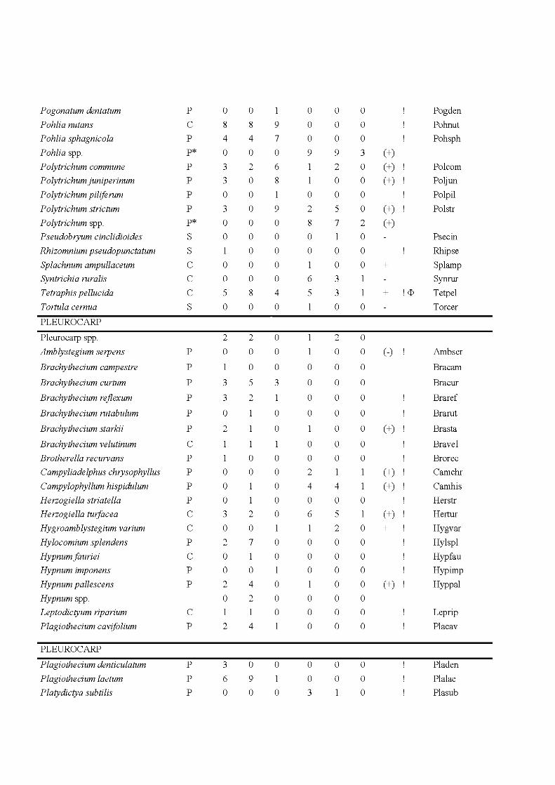
Pogonatum dentatum

Pohlia nutans

Pohlia sphagnicola

Pohlia spp.

Polytrichum commune

P olytrichum juniperinum

Polytrichum pilifernm

Polytrichum strictum

Polytrichum spp.

Pseudobryum cinclidioides

Rhizomnium pseudopunctatum

Splachnum ampullaceum

Syntrichia rnralis

Tetraphis pellucida

Tortula cernua

PLEUR OC ARP

Pleurocarp spp.

Amblystegium serpens

Brachythecium campestre

Brachythecium curtum

Brachythecium rejlexum

Brachythecium rntabulum

Brachythecium starkii

Brachythecium velutinum

Brotherella recurvans

C ampyliade lphus chrysophyllus

Campylophyllum hispidulum

Herzogiella striatella

Herzogiella turjacea

Hygroamblystegium varium

Hylocomium splendens

Hypnum fauriei

Hypnum imponens

Hypnum pallescens

Hypnum spp.

Leptodictyum riparium

Plagiothecium cavifolium

PLEUR OC ARP

P lagiothecium denticulatum

Plagiothecium laetum

Platydictya subtilis

p

c p

P*

p

p

p

p

P*

s s c c c s

p

p

p

p

p

p

c p

p

p

p

c c p

c p

p

c p

p

p

p

0

8

4

0

3

3

0

3

0

0

1

0

0

5

0

2

0

3

3

0

2

1

0

0

0

3

0

2

0

0

2

0

2

3

6

0

0

8

4

0

2

0

0

0

0

0

0

0

0

8

0

2

0

0

5

2

0

0

1

2

0

7

1

0

4

2

1

4

0

9

0

9

7

0

6

8

9

0

0

0

0

0

4

0

0

0

0

3

1

0

0

0

0

0

0

0

0

0

1

0

0

0

0

1

0

0

0

0

9

0

2

8

0

0

1

6

5

0

0

0

0

0

0

2

4

0

6

0

0

0

1

0

0

0

0

0

3

0

0

0

9

2

0

0

5

7

1

0

0

3

3

0

2

0

0

0

0

0

0

0

0

4

0

5

2

0

0

0

0

0

0

0

0

0

0

0

0

3

0

0

0

0

2

0

0

0

0

0

0

0

0

0

0

0

0

0

1

0

0

0

0

0

0

0

0

0

0

0

0

(+)

(+)

(+) !

(+)

(+)

+

+ ! <D

( -)

(+) !

(+)

(+)

(+) !

+

(+)

Pogden

Pohnut

Pohsph

Po1com

Po1jun

Po1pi1

Po1str

Psecin

Rhipse

Splamp

Synrur

Tetpel

Toreer

Ambser

Brac am

Brac ur

Braref

Brarut

Bras ta

Bravel

Brorec

Camchr

Cam his

Herstr

Hertur

Hygvar

Hylspl

Hypfau

Hypimp

Hyppal

Leprip

Placav

Pl aden

Plalae

Plasub

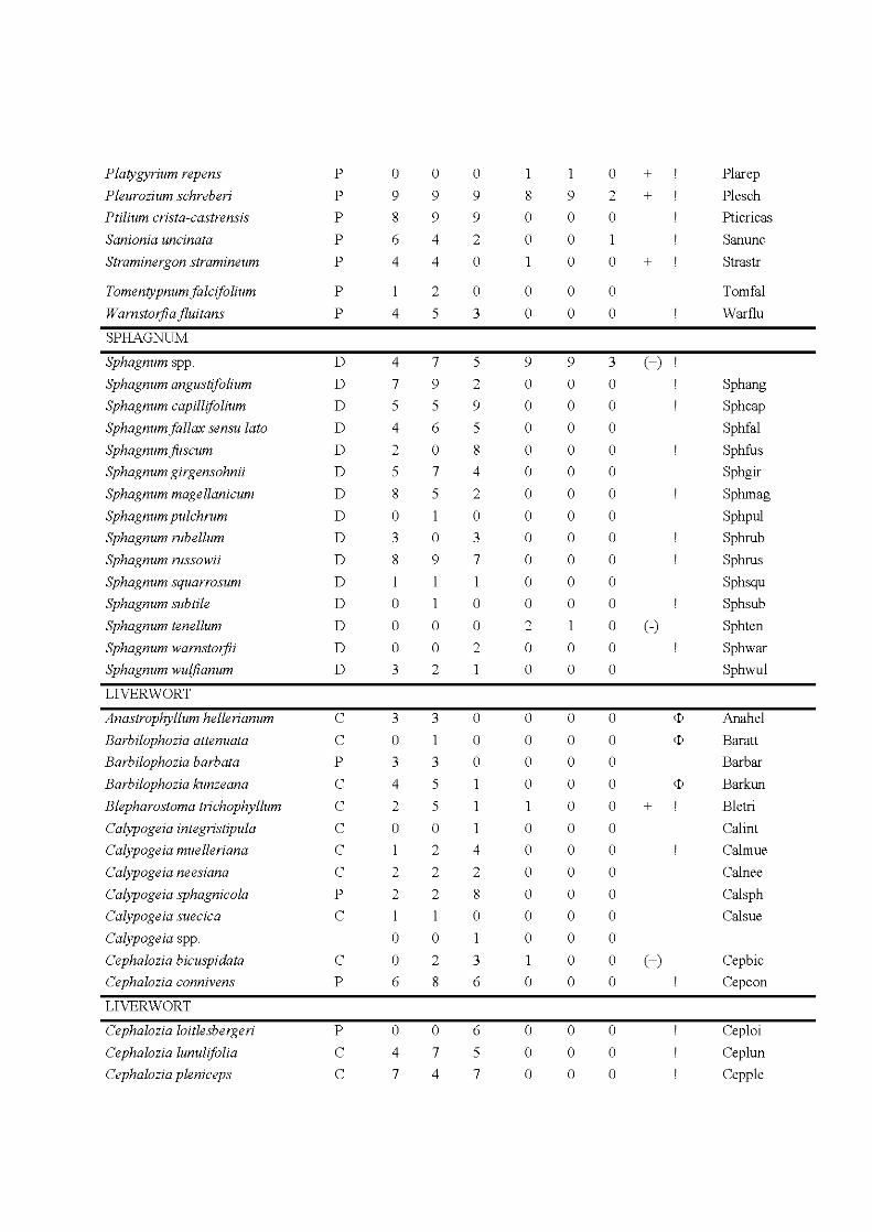
Platygyrium repens

Pleurozium schreberi

Ptilium crista-castrensis

Sanionia uncinata

Straminergon stramineum

Tomentypnum falcifolium

Warnstorfia fluitans

SPHAGNUM

Sphagnum spp.

Sphagnum angustifolium

Sphagnum capillifolium

Sphagnum fallax sensu lata

Sphagnum jùscum

Sphagnum girgensohnii

Sphagnum magellanicum

Sphagnum pulchrum

Sphagnum rubellum

Sphagnum russowii

Sphagnum squarrosum

Sphagnum subtile

Sphagnum tenellum

Sphagnum warnstorfii

Sphagnum wuljianum

LIVERWORT

Anastrophyllum hellerianum

Barbilophozia attenuata

Barbilophozia barbata

Barbilophozia kunzeana

Blepharostoma trichophyllum

Calypogeia integristipula

Calypogeia muelleriana

Calypogeia neesiana

Calypogeia sphagnicola

Calypogeia suecica

Calypogeia spp.

Cephalozia bicuspidata

Cephalozia connivens

LIVERWORT

Cephalozia loitlesbergeri

Cephalozia lunulifolia

Cephalozia pleniceps

p

p

p

p

p

p

p

D

D

D

D

D

D

D

D

D

D

D

D

D

D

D

c c p

c c c c c p

c

c p

p

c c

0

9

8

6

4

4

4

7

5

4

2

5

8

0

3

8

1

0

0

0

3

3

0

3

4

2

0

2

2

1

0

0

6

0

4

7

0

9

9

4

4

2

5

7

9

5

6

0

7

5

1

0

9

1

0

0

2

3

3

5

5

0

2

2

2

1

0

2

8

0

7

4

0

9

9

2

0

0

3

5

2

9

5

8

4

2

0

3

7

0

0

2

1

0

0

0

1

4

2

8

0

3

6

6

5

7

8

0

0

0

0

9

0

0

0

0

0

0

0

0

0

0

0

2

0

0

0

0

0

0

1

0

0

0

0

0

0

1

0

0

0

0

9

0

0

0

0

0

9

0

0

0

0

0

0

0

0

0

0

0

1

0

0

0

0

0

0

0

0

0

0

0

0

0

0

0

0

0

0

0

2

0

1

0

0

0

3

0

0

0

0

0

0

0

0

0

0

0

0

0

0

0

0

0

0

0

0

0

0

0

0

0

0

0

0

0

0

+ +

+

(+)

(-)

+

(+)

P1arep

P1esch

Pticricas

San une

Strastr

Tomfa1

Warflu

Sphang

Sphcap

Sphfa1

Sphfus

Sphgir

Sphmag

Sphpul

Sphrub

Sphrus

Sphsqu

Sphsub

Sphten

Sphwar

Sphwu1

Anahe1

Bara tt

Barbar

Bar kun

B1etri

Ca lint

Ca1mue

Ca1nee

Ca1sph

Ca1sue

Cep bic

Cep con

Cep1oi

Cep1un

Cepple

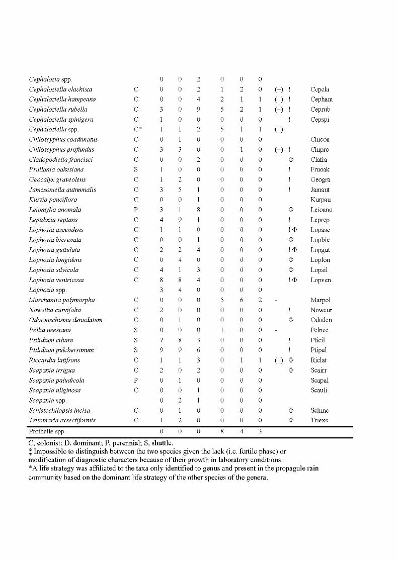
Cephalozia spp. 0 0 2 0 0 0

Cephaloziella elachista c 0 0 2 2 0 (+) ! Cepela

Cephaloziella hampeana c 0 0 4 2 (+) Cep ham

Cephaloziella rubella c 3 0 9 5 2 1 (+) Ceprub

Cephaloziella spinigera c 0 0 0 0 0 Ceps pi

Cephaloziella spp. C* 2 5 (+) Chiloscyphus coadunatus c 0 0 0 0 0 Chicoa

Chiloscyphus projùndus c 3 3 0 0 0 (+) Chi pro

Cladopodiella francis ci c 0 0 2 0 0 0 <D Cl afra

Frullania oakesiana s 0 0 0 0 0 Fruoak

Geocalyx graveolens c 2 0 0 0 0 Geogra

J amesonie Zia autumnalis c 3 5 0 0 0 Jamaut

Kurzia pauciflora c 0 0 0 0 0 Kurpau

Leiomylia anomala p 3 8 0 0 0 <D Leioano

Lepidozia reptans c 4 9 1 0 0 0 Leprep

Lophozia ascendens c 1 1 0 0 0 0 !<D Lopasc

Lophozia bicrenata c 0 0 0 0 0 <D Lopbic

Lophozia guttulata c 2 2 4 0 0 0 !<D Lopgut

Lophozia longidens c 0 4 0 0 0 0 <D Loplon

Lophozia silvicola c 4 3 0 0 0 <D Lopsil

Lophozia ventricosa c 8 8 4 0 0 0 !<D Lopven

Lophozia spp. 3 4 0 0 0 0

Marchantia polymorpha c 0 0 0 5 6 2 .tvrarpol

Nowellia curvifolia c 2 0 0 0 0 0 Nowcur

Odotonschisma denudatum c 0 0 0 0 0 <D Ododen

Pellia neesiana s 0 0 0 0 0 Pelnee

Ptilidium ciliare s 7 8 3 0 0 0 Pticil

Ptilidium pulcherrimum s 9 9 6 0 0 0 Ptipul

Riccardia latifrons c 1 3 0 1 1 (+) <D Ri clat

Scapania imgua c 2 0 2 0 0 0 <D Scairr

Scapania paludicola p 0 0 0 0 0 Scapal

Scapania uliginosa c 0 0 0 0 0 Scauli

Scapania spp. 0 2 0 0 0

Schistochilopsis incisa c 0 0 0 0 0 <D Schinc

Tritomaria exsectiformis c 2 0 0 0 0 <D Triexs

Prothalle spp. 0 0 0 8 4 3

C, colonist; D, dominant; P, perennial; S, shuttle. :j: Impossible to distinguish between the two species given the lack (i.e. fertile phase) or modification of diagnostic characters because oftheir growth in laboratory conditions. *A life strate gy was affiliated to the taxa only identified to genus and present in the propagule rain

community based on the dominant life strategy of the other species of the genera.

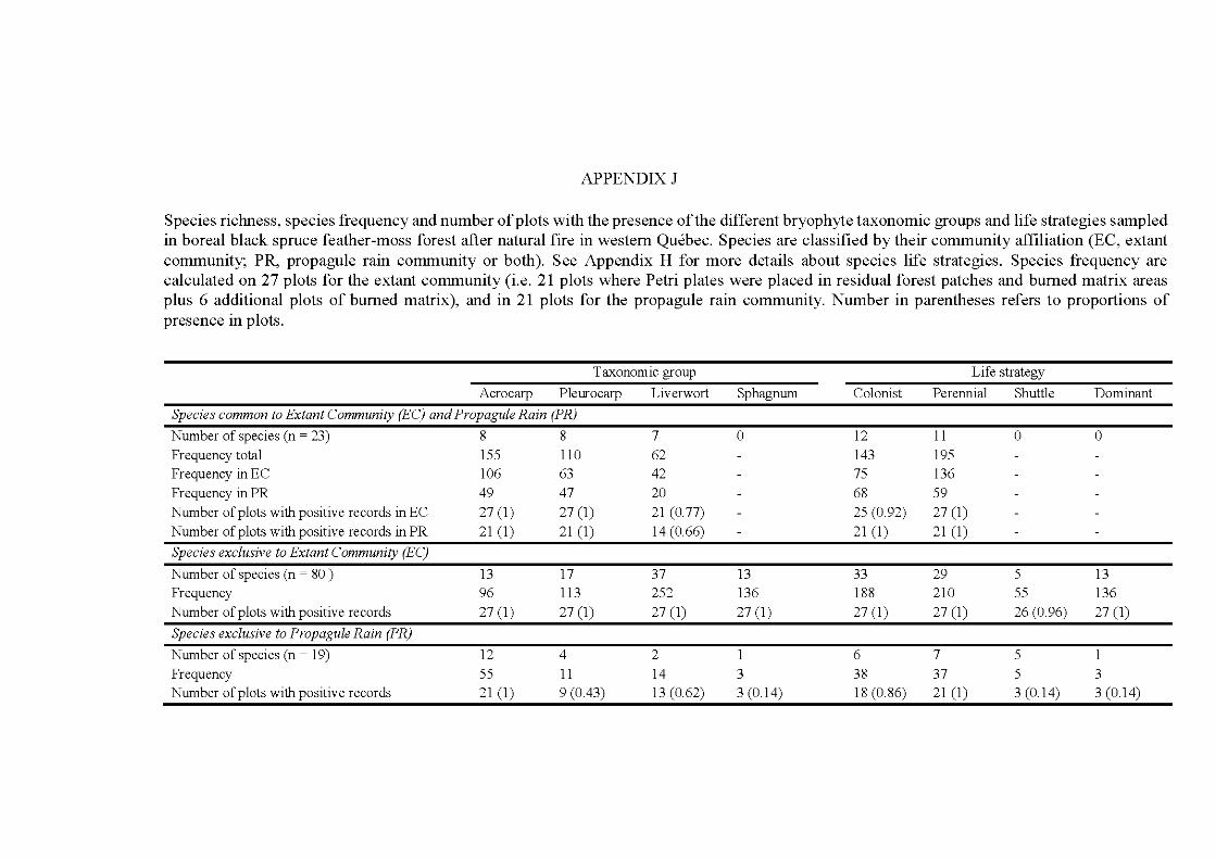
APPENDIXJ

Species riclmess, species frequency and number of plots with the presence of the different bryophyte taxonomie groups and life strategies sampled in boreal black spruce feather-moss forest after natural fire in western Québec. Species are classified by their community affiliation (EC, extant community; PR, propagule rain community or both). See Appendix H for more details about species life strategies. Species frequency are calculated on 27 plots for the extant community (i.e. 21 plots where Petri plates were placed in residual forest patches and bumed matrix areas plus 6 additional plots of bumed matrix), and in 21 plots for the propagule rain community. Number in parentheses refers to proportions of presence in plots.

Taxonomie group Life strategy

Acrocarp P leurocarp Liverwort Sphagnum Colonist Perennial Shuttle Dominant

Species common to Extant Community (EC) and Propagule Rain (PR)

Number of species (n = 23) 8 8 7 0 12 11 0 0

Frequency total 155 11 0 62 143 195 Frequency in EC 106 63 42 75 136 Frequency in PR 49 47 20 68 59

Number of plots with positive records in EC 27 (1) 27 (1) 21 (0.77) 25 (0.92) 27 (1) Number of plots with positive records in PR 21 (1) 21 (1) 14 (0.66) 21 (1 ) 21 (1)

Species exclusive to Extant Community (EC)

Number of species (n = 80) 13 17 37 13 33 29 5 13 Frequency 96 113 252 136 188 210 55 136

Number of plots with positive records 27 (1) 27 (1) 27 (1) 27 (1) 27 (1) 27 (1) 26 (0.96) 27 (1)

Species exclusive to Propagule Rain (PR)

Number of species (n = 19) 12 4 2 6 7 5 Frequency 55 11 14 3 38 37 5 3 Number of plots with positive records 21 (1) 9 (0.43) 13 (0.62) 3 (0.1 4) 18 (0.86) 21 (1) 3 (0.14) 3 (0.14)

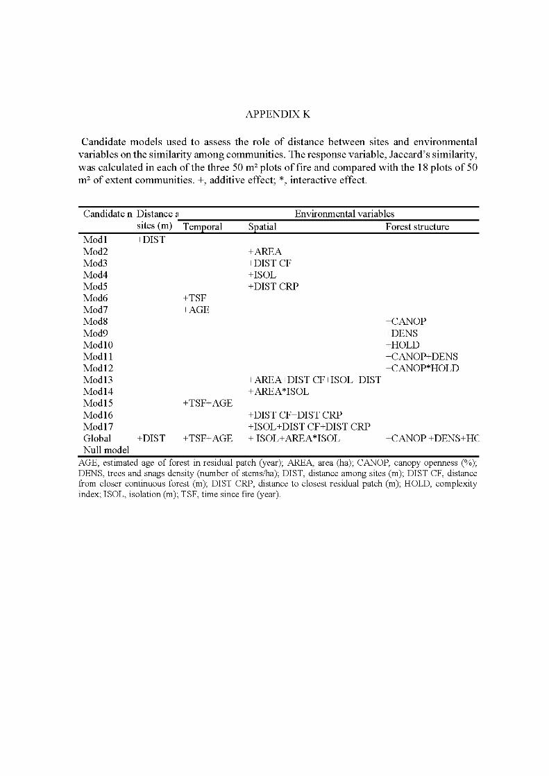
APPENDIXK

Candidate models used to assess the role of distance between sites and environmental variables on the similarity among communities. The response variable, Jaccard's similarity, was calculated in each of the three 50m2 plots offire and compared with the 18 plots of 50 m2 of extent communities. +, additive effect; *, interactive effect.

Candidate n Distance a Environmental variables ----------------------------------------------------sites (rn) Temporal Spatial Forest structure

Modl +DIST Mod2 Mod3 Mod4 Mod5 Mod6 Mod7 Mod8 Mod9 ModlO Modll Modl2 Modl3 Modl4 Modl5 Modl6 Modl7 Global +DIST Null model

+TSF +AGE

+TSF+ AGE

+AREA +DIST CF +ISOL +DIST CRP

+AREA+DIST CF+ISOL+DIST +AREA*ISOL

+DIST CF+DIST CRP +ISOL+DIST CF+DIST CRP

+CANOP +DENS +HOLD +CANOP+DENS +CANOP*HOLD

+TSF+ AGE + ISOL+AREA*ISOL +CANOP +DENS+HC

AGE, estimated age of forest in residual patch (year); AREA, area (ha); CANOP, canopy openness (%); DENS, trees and snags density (number of stems/ha); DIST, distance among sites (rn); DIST CF, distance from closer continuous forest (rn); DIST CRP, distance to closest residual patch (rn); HOLD, complexity index; ISOL, isolation (rn); TSF, time since fire (year).

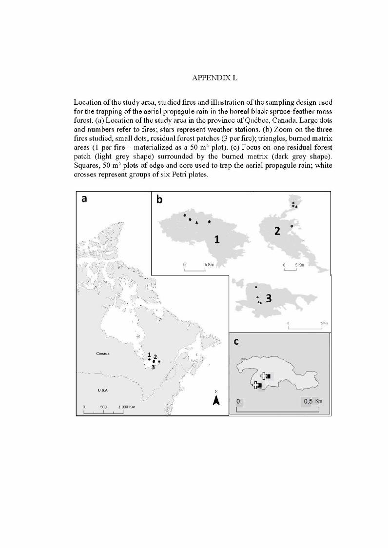
APPENDIXL

Location ofthe study area, studied fires and illustration of the sampling design used for the trapping of the aerial propagule rain in the boreal black spruce-feather moss forest. (a) Location ofthe study area in the province of Québec, Canada. Large dots and numbers refer to fires; stars represent weather stations. (b) Zoom on the three fires studied, small dots, residu al forest patch es (3 per fire ); triangles, burned matrix areas (1 per fire- materialized as a 50m2 plot). (c) Focus on one residual forest patch (light grey shape) surrounded by the burned matrix (clark grey shape). Squares, 50 m2 plots of edge and core used to trap the aerial propagule rain; white crosses represent groups of six Petri plates.

a

0

Canada

- - ·

b

. \ ·-, '*~ )

... ~.':-·· ... , ) ·( ·

'<~).1 •... ·2\ l • lt \ .... ··3 ····'

.......... ,. .... ____ .... ~ .........._

U.S.A

500 1000 Km

5Km 0 5 Km L______j

5 Km

c

0 0,5 Km

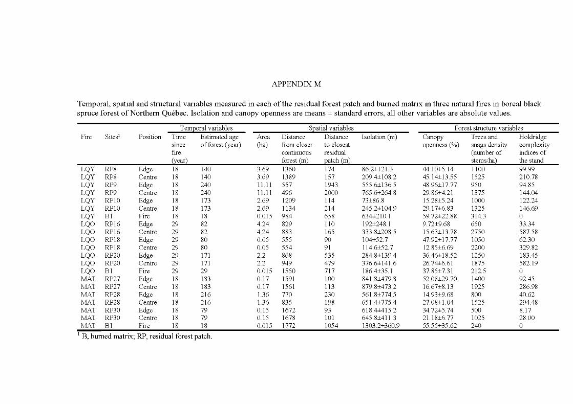
APPENDIX M

Temporal, spatial and structural variables measured in each of the residual forest patch and bumed matrix in three natural fires in boreal black spruce forest of Northem Québec. Isolation and canopy openness are means ± standard errors, all other variables are ab solute values.

T em12oral variables Sj2atial variables Forest structure variables Fire Sites1 Position Time Estimated age Are a Distance Distance Isolation (rn) Canopy Trees and Holdridge

sm ce of forest (year) (ha) from closer to closest openness (%) snags density complexity fire continuous re si dual (number of indices of (year) forest (rn) 12atch (rn) stems/ha) the stand

LQY RP8 Edge 18 140 3.69 1360 174 86.2±121.3 44. 10±5.14 1100 99.99 LQY RP8 Centre 18 140 3.69 1389 157 209.4±108 .2 45. 14±13.55 1525 21 0.78 LQY RP9 Edge 18 240 11 .11 557 1943 555 .6±136.5 48.96±17.77 950 94.85 LQY RP9 Centre 18 240 11 .11 496 2000 765.6±264.8 29.86±4.21 1375 144.04 LQY RP10 Edge 18 173 2.69 1209 11 4 73±86.8 15.28±5.24 1000 122.24 LQY RP10 Centre 18 173 2.69 1134 214 245.2±104.9 29.17±6.83 1325 146.69 LQY Bl Fire 18 18 0 .01 5 984 658 634±210.1 59.72±22.88 314.3 0 LQO RP1 6 Edge 29 82 4. 24 829 11 0 192±248. 1 9.72±9.68 650 33.34 LQO RP1 6 Centre 29 82 4. 24 883 165 333.8±208.5 15.63±13. 78 2750 587.58 LQO RP18 Edge 29 80 0 .05 555 90 104±52.7 47.92±17.77 1050 62.30 LQO RP18 Centre 29 80 0 .05 554 91 114.6±52.7 12.85±6.69 2200 329.82 LQO RP20 Edge 29 171 2.2 868 535 284.8±139.4 36.46±18.52 1250 183.45 LQO RP20 Centre 29 171 2.2 949 479 376.6±141.6 26.74±6.61 1875 582.19 LQO Bl Fire 29 29 0 .01 5 1550 717 186.4±35.1 37.85±7.31 212.5 0 MAT RP27 Edge 18 183 0 .1 7 1591 100 841.8±479.8 52.08±29.70 1400 92.45 MAT RP27 Centre 18 183 0 .1 7 1561 113 879.8±473.2 16.67±8.13 1925 286.98 MAT RP28 Edge 18 21 6 1.36 770 230 561.8±774.5 14.93±9.68 800 40.62 MAT RP28 Centre 18 21 6 1.36 835 198 651.4±775.4 27.08±1.04 1525 294.48 MAT RP30 Edge 18 79 0 .1 5 1672 93 618.4±415. 2 34.72±5.74 500 8.17 MAT RP30 Centre 18 79 0 .1 5 1678 101 645.8±41 1.3 21. 18±6.77 1025 28 .00 MAT B 1 Fire 18 18 0 .015 1772 1054 1303.2±360.9 55.55±35.62 240 0

1 B, bumed matrix; RP, res idual forest patch.

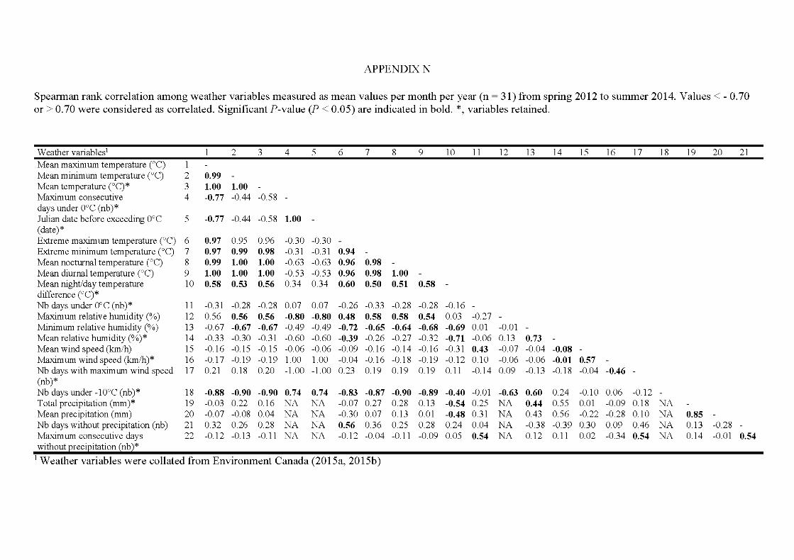
APPENDIXN

Spearman rank correlation among weather variables measured as mean values per month per year (n = 31) from spring 2012 to summer 2014. Values< - 0.70 or > 0.70 were considered as correlated. SignificantP-value (P < 0.05) are indicated in bold. *, variables retained.

Weather variables1 2 3 4 5 6 7 8 9 10 11 12 13 14 15 16 17 18 19 20 21 Mean maximum temperature (0 C) 1 Mean minimum temperature (0 C) 2 0.99 -

Mean temperature (0 C)* 3 1.00 1.00 -

Maximum consecutive 4 -0.77 -0.44 -0.58 -

days under ooc (nb)* Julian date before exceeding ooc 5 -0.77 -0.44 -0.58 1.00 -

(date)* Extreme maximum temperature (0 C) 6 0.97 0.95 0.96 -0.30 -0.30 -

Extreme minimum temperature (0 C) 7 0.97 0.99 0.98 -0.31 -0.31 0.94 -

Mean nocturnal temperature (0 C) 8 0.99 1.00 1.00 -0.63 -0.63 0.96 0.98 -

Mean diurnal temperature (0 C) 9 1.00 1.00 1.00 -0.53 -0.53 0.96 0.98 1.00 -

Mean night/day temperature 10 0.58 0.53 0.56 0.34 0.34 0.60 0.50 0.51 0.58 -

difference (°C)* Nb days under 0°C (nb)* 11 -0.31 -0.28 -0.28 0.07 0.07 -0.26 -0.33 -0.28 -0.28 -0.1 6 -

Maximum relative humidity (%) 12 0.56 0.56 0.56 -0.80 -0.80 0.48 0.58 0.58 0.54 0.03 -0.27 -

Minimum relative humidity (%) 13 -0.67 -0.67 -0.67 -0.49 -0.49 -0.72 -0.65 -0.64 -0.68 -0.69 0.01 -0.01 -

Mean relative humidity (%)* 14 -0.33 -0.30 -0.31 -0.60 -0.60 -0.39 -0.26 -0.27 -0.32 -0.71 -0.06 0.13 0.73 -

Mean wind speed (km/h) 15 -0.16 -0.15 -0.15 -0.06 -0.06 -0.09 -0.16 -0.14 -0.16 -0.31 0.43 -0.07 -0.04 -0.08 -

Maximum wind speed (km/h)* 16 -0.1 7 -0.19 -0.1 9 1.00 1.00 -0.04 -0.16 -0.1 8 -0.19 -0.1 2 0.10 -0.06 -0.06 -0.01 0.57 -

Nb days with maximum wind speed 17 0. 21 0.18 0.20 -1.00 -1.00 0.23 0.1 9 0.19 0.1 9 0.11 -0.1 4 0.09 -0.13 -0.1 8 -0.04 -0.46 -

(nb)* Nb days under -10°C (nb)* 18 -0.88 -0.90 -0.90 0.74 0.74 -0.83 -0.87 -0.90 -0.89 -0.40 -0.01 -0.63 0.60 0.24 -0.10 0.06 -0.12 -

Total precipitation (mm)* 19 -0.03 0.22 0.16 NA NA -0.07 0.27 0.28 0.13 -0.54 0.25 NA 0.44 0.55 0.01 -0.09 0.18 NA Mean precipitation (mm) 20 -0.07 -0. 08 0.04 NA NA -0.30 0.07 0.13 0.01 -0.48 0.31 NA 0.43 0.56 -0.22 -0.28 0.1 0 NA 0.85 -

Nb days without precipitation (nb) 21 0. 32 0.26 0.28 NA NA 0.56 0.36 0.25 0.28 0.24 0.04 NA -0.38 -0.39 0.30 0.09 0.46 NA 0.13 -0.28 -

Maximum consecutive days 22 -0.1 2 -0.13 -0.11 NA NA -0.1 2 -0.04 -0.11 -0.09 0.05 0.54 NA 0.12 0.11 0.02 -0.34 0.54 NA 0.1 4 -0.01 0.54 without reci itation nb *

1 Weather variables were collated from Environment Canada (2015a, 2015b)

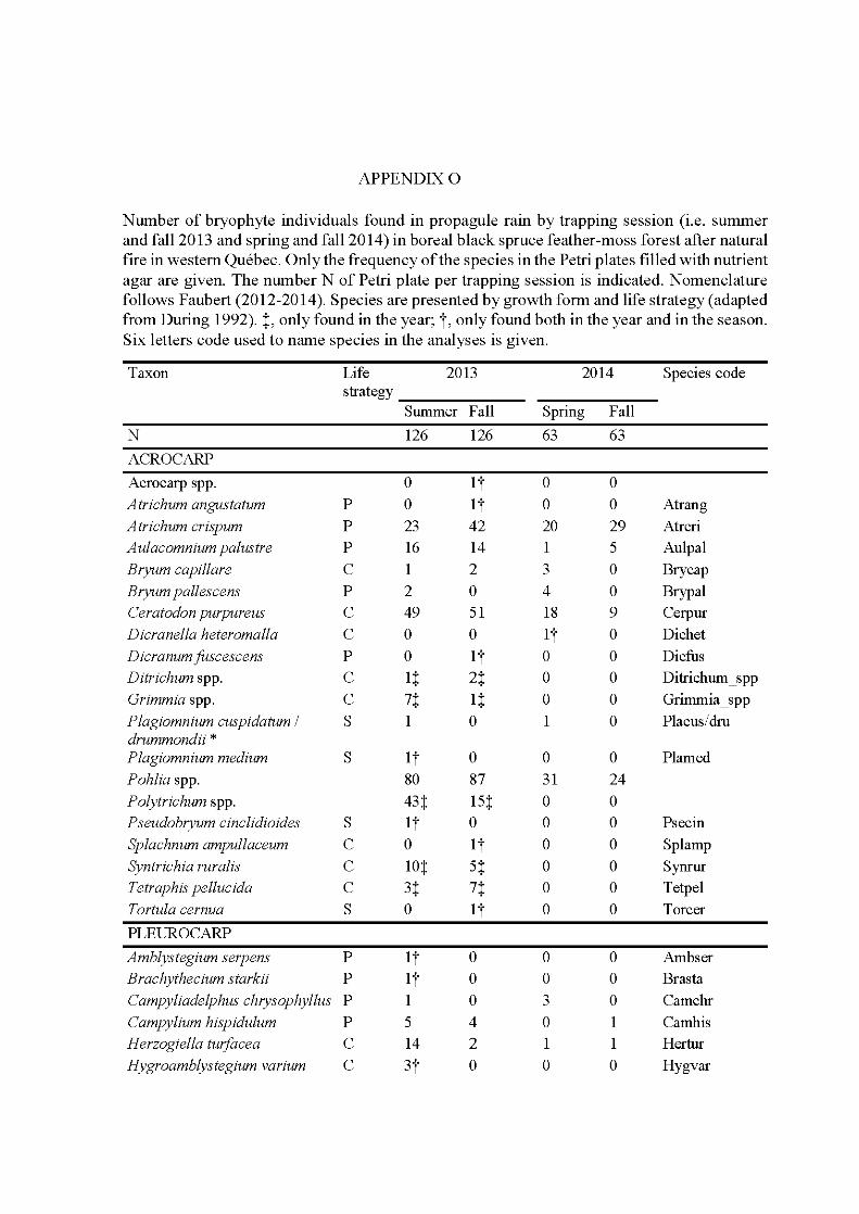
APPENDIXO

Number of bryophyte individuals found in propagule rain by trapping session (i.e. summer and fal12013 and spring and fal12014) in boreal black spruce feather-moss forest after natural fire in western Québec. Only the frequency of the species in the Petri plates filled with nutrient agar are given. The number N of Petri plate per trapping session is indicated. Nomenclature follows Faubert (2012-2014). Species are presented by growth form and life strategy (adapted from During 1992). t, only found in the year; t, only found both in the year and in the season. Six letters code used to name species in the analyses is given.

Taxon Life 2013 2014 Species code strategy

Summer Fall Spring Fall

N 126 126 63 63

ACROCARP

Acrocarp spp. 0 lt 0 0 Atrichum angustatum p 0 lt 0 0 Atrang Atrichum crispum p 23 42 20 29 Atrcri Aulacomnium palustre p 16 14 1 5 Aulpal Bryum capillare c 1 2 3 0 Brycap Bryum palles cens p 2 0 4 0 Brypal Ceratodon purpureus c 49 51 18 9 Cerpur Dicranella heteromalla c 0 0 lt 0 Dichet Dicranum fuscescens p 0 lt 0 0 Dicfus Ditrichum spp. c l:j: 2:j: 0 0 Ditrichum _spp Grimmia spp. c 7:j: 1:j: 0 0 Grimmia _spp Plagiomnium cuspidatum 1 s 1 0 1 0 Placus/dru drummondii * P lagiomnium medium s 1t 0 0 0 Plamed Pohlia spp. 80 87 31 24 Polytrichum spp. 43:j: 15:j: 0 0 Pseudobryum cinclidioides s lt 0 0 0 Psecin Splachnum ampullaceum c 0 lt 0 0 Splamp Syntrichia ruralis c lO:j: 5:j: 0 0 Synrur Tetraphis pellucida c 3:j: 7:j: 0 0 Tetpel T ortula cernua s 0 1t 0 0 Toreer

PLEUR OC ARP

Amblystegium serpens p 1t 0 0 0 Ambser Brachythecium starkii p lt 0 0 0 Bras ta

Campyliadelphus chrysophyllus p 1 0 3 0 Camchr Campylium hispidulum p 5 4 0 1 Camhis Herzogiella turfacea c 14 2 1 1 Hertur Hygroamblystegium varium c 3t 0 0 0 Hygvar

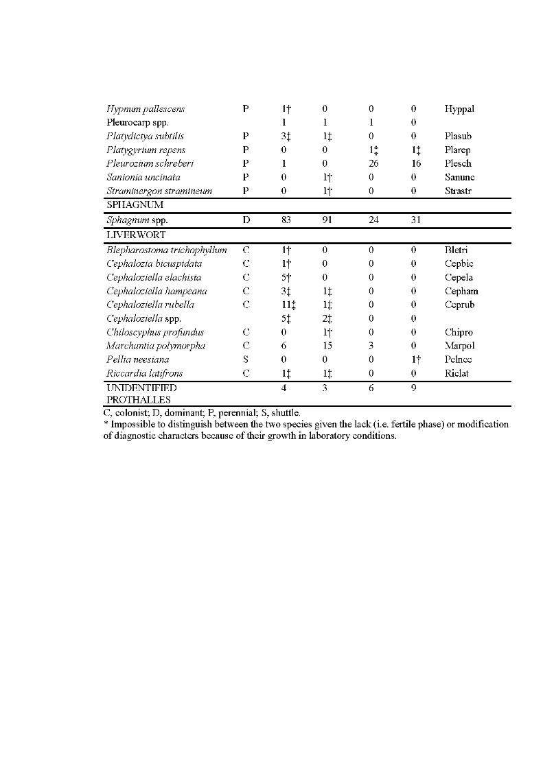
Hypnum palles cens p 1t 0 0 0 Hyppal

Pleurocarp spp. 1 1 1 0

P latydictya subtilis p 3t 1t 0 0 Plasub

P latygyrium repens p 0 0 1t 1t Plarep Pleurozium schreberi p 1 0 26 16 Plesch

Sanionia uncinata p 0 1t 0 0 Sanunc

Straminergon stramineum p 0 1t 0 0 Strastr

SPHAGNUM

Sphagnum spp. D 83 91 24 31 LIVERWORT

Blepharostoma trichophyllum c 1t 0 0 0 Bletri

Cephalozia bicuspidata c 1t 0 0 0 Cep bic

Cephaloziella elachista c St 0 0 0 Cepela

Cephaloziella hampeana c 3t 1t 0 0 Cep ham Cephaloziella rubella c llt 1t 0 0 Ceprub

Cephaloziella spp. St 2t 0 0

Chiloscyphus profundus c 0 1t 0 0 Chi pro

Marchantia polymorpha c 6 15 3 0 Marpol

Pellia neesiana s 0 0 0 1t Peinee

Riccardia latifrons c 1t 1t 0 0 Ri clat

UNIDENTIFIED 4 3 6 9 PROTHALLES

C, colonist; D, dominant; P, perennial; S, shuttle. *Impossible to distinguish between the two species given the lack (i.e. fertile phase) or modification of diagnostic characters because of their growth in laboratory conditions.

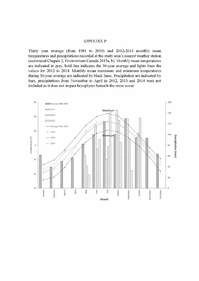
APPENDIX P

Thirty year average (from 1981 to 2010) and 2012-2014 monthly mean temperatures and precipitations recorded at the study area's nearest weather station (automated Chapais 2, EnvironmentCanada 2015a, b). Monthly mean temperatures are indicated in grey, bold line indicates the 30-year average and lights lines the values for 2012 to 2014. Monthly mean maximum and minimum temperatures during 30-year average are indicated by black lines. Precipitation are indicated by bars, precipitations from November to April in 2012, 2013 and 2014 were not included as it does not impact bryophytes beneath the snow cover.

30 = Average 1981-2010

c::z:::J2012 Maximum .-;,

20 =2013

=2014

~Average 1981·2010

10 ~2012

E ~2013

Q)

.3 - 2014 ~ ;; 0 x " "' x ~5 0; " i:i

c. E ~ Q) " >;: ..... "'

~ y

~ ~ ' -10 ~- %

~ Î' % y x

:/; y ·~ ~ .,,

; y ;;: x x "' )<. ~

y ~ ,

'} -20 " >< \ /; X. %

~ ~

" ~ r " %

-30 c:- > "ê .§. > "' >

~ (i; (i; (i; (i; :;; .. c: ~ "' ::! ~ co .0 .0 .0 .0

::> 2 ~ ..: E 0 E ~

::> 0 E .0 ..: ~ "' "' of '" > a: "' 0 0 Month "' z

160

140

120

100 "tl ... lt) n -a· ;::;:

80 Qj .... cr :::l

3 60 2.

40

20

0

BIBLIOGRAPHIE GÉNÉRALE

Ah-Peng, C. (2007). Diversité, distribution et biogéographie des bryophytes des coulées de laves du Piton de la Fournaise (La Réunion). Thèse de doctorat, Université de La Réunion., N° 00489749, version 1-7.

Allard, M. (1974). Géomorphologie des eskers abitibiens. Cahiers de géographie du Québec, 18(44), 271-296.

Andersson, L.I. & Hyttebom, H. (1991). Bryophytes and decaying wood- a comparison between managed and natural forest. Holarctic Ecology, 14, 121-130.

Arsenault, A. (2003). A note of the ecology and management of old-growth forests in the Montane Cordillera. The Forestry Chronicle, 79(3), 441-454.

Baker, S.C., Spies, T.A., Wardlaw, T.J., Balmer, J., Franklin, J.F. & Jordan, G.J. (2013). The harvested side of edges: Effect of retained forests on the reestablishment of biodiversity in adjacent harvested areas. Forest Ecology and Management, 302, 107-121.

Baldwin, L.K. & Bradfield, G.E. (2010). Resilience ofbryophyte communities in regenerating matrix forests after logging in temperate rainforests of coastal British Columbia. Botany, 88, 297-314.

Benscoter, B. W. 2006. Post-fire bryophyte establishment in a continental bog. Journal ofVegtation Science, 17(5), 647-652.

Bergeron, Y. & Harvey, B. (1997). Basing silviculture on natural ecosystem dynamics: An approach applied to the southem boreal mixedwood forest of Que bec. Forest Ecolo gy and Management, 92(1 ), 235-242.

Bergeron, Y. & Harper, K.A. (2009). Old growth forest in Canadian boreal: The exception rather than the rule? In: C. Wirth, G. Gleixner & M. Heimann (eds.), Old-growth forests: function, fa te and value. Springer-Verlag, Berlin.

Bergeron, Y., Leduc, A., Harvey, B.D. & Gauthier, S. (2002). Natural fire regime: a guide for sustainable management of the Canadian boreal forest. Silva fennica, 36(1), 81-95.

Bergeron, Y., Gauthier, S., Flannigan, M. & Kafka, V. (2004). Fire regimes at the transition between mixedwood and coniferous boreal forest in northwestem Quebec. Ecology, 85(7), 1916-1932.

Bergeron, Y., Cyr, D., Drever, C.R., Flannigan, M., Gauthier, S. , Kneeshaw, D., Lauzon, E., Leduc, A., Le Goff, H., Lesieur, D. & Logan, K. (2006). Past, current, and future fire frequencies in Que bec' s commercial forests: implications for the cumulative effects of harvesting and fire on age-class structure and natural disturbance-based management. Canadian Journal of Forest Research, 36, 2838-2744.

282

Boudreault, C. , Bergeron, Y. , Drapeau, P. & L6pez, L.M. (2007). Edge effects on epiphytie lichens in remnant stands of managed landscapes in the eastern boreal forest of Canada. Forest Ecology and Management, 255(5), 1461-1471.

Bouget, C., Larrieu, L. & Brin, A. (20 14 ). Key fe atur es for saproxylic beetle diversity derived from rapid habitat assessment in temperate forests. Ecological Jndicators, 36, 656-664.

Brindeau, V. (2012). Louange des mousses. Éditions Picquier, P., Arles, France.

Brodie, H.J. (1956). Raindrops as plant dispersal agents. Proceedings of the Indiana Academy of Science, 66, 65-73.

Brown, D.H. & Bates, J.W. (1990). Bryophyte and nutrient cycling. Botanical Journal of the Linnean Society, 104(1-3), 129-147.

Carey, A.B. (2003). Managing for wildlife: A key component for social acceptance of compatible forest management. In: R.A. Monserud, R. W. Haynes & A.C. Johnson (eds.), Compatible Forest Management (p. 401-425). Springer Netherlands.

Chaieb, C., Fenton, N.J., Lafleur, B. & Bergeron, Y. (2015). Can we use forest inventory mapping as a coarse filter in eco system based management in the black spruce boreal forest? Forests 6, 1195-1207.

Campbell, J. & Fredeen, A.L. (2004). Lobaria pulmonaria abundance as an indicator of macrolichen diversity in interior Cedar-Hemlock forests of eastcentral British Columbia. Canadian Journal ofBotany, 82, 970-982.

Chang, S.C., Lai, I.L. & Wu, J.T. (2002). Estimation offog deposition on epiphytie bryophytes in a subtropical montane forest ecosystem in northeastem Taiwan. Atmospheric Research, 64(1), 159-167.

Chan-Mcleod, A.C.A. & Moy, A. (2007). Evaluating residual tree patches as stepping stones and short-term refugia for red-legged frogs. The Journal of wildlife management, 71(6), 1836-1844.

Clark, K.L., Nadkami, N.M. & Gholz, H.L. (2005). Retention ofinorganic nitrogen by epiphytie bryophytes in a tropical montane forest. Biotropica, 37(3), 328-336.

CNRTL - Centre National de Ressources Textuelles et Lexicales. (2012). Disponible à 1 'adresse : http:/ /www.cnrtl.fr/definition/mousse

Cole, H.A., Newmaster, S.G., Bell, F.W., Pitt, D. & Stinson, A. (2008). Influence of microhabitat on bryophyte diversity in Ontario mixedwood boreal forest. Canadian Journal of Forest Research, 38(7), 1867-1876.

Couvreur, M., Bart, C., Kris, V. & Martin, H. (2004). Large herbivore as mobile links between isolated nature reserves through adhesive seed dispersal. Applied Vegetation Science, 7(2), 229-236.

283

Coxson, D.S. & Nadkarni, N.M. (1995). Ecological roles of epiphytes in nutrient cycles of forest ecosytems. In: M.D. Lowman & N.M. Nadkarni (eds.), Forest canopies (p. 495-543). Academie Press, San Diego.

Crum, H.A. (2001). StructuralDiversityofBryophytes. The UniversityofMichigan Herbarium, Ann Arbor, USA

Cyr, D. , Gauthier, S., Bergeron, Y. & Carcaillet, C. (2009). Forest management is drivingthe eastern part ofNorth-American boreal forest outside its natural range ofvariability. Frontiers in Ecology and the Environment, 7(10), 519-524.

d'Églantine, F. ( 1794). Calendrier de la république française, une et indivisible, au nom de la commission chargée de sa confection. Imprimerie de Vve Vitot et fils, Bruyère, France.

Dallaire, S. & Légaré S. (2016). Organisation spatiale et structure d 'âge des forêts - Instruction régionale pour la mise en œuvre de 1 'aménagement écosystémique. Rapport technique. Ministère des Forêts, de la Faune et des Parcs, Direction de la gestion des Forêts Nord-du-Québec, Québec, Canada.

D'Orbigny, C. (1846). Dictionnaire Universel d'Histoire Naturelle. Tome Huitième. M.M. Renard, Martinet et cie_ Paris.

de V alpine, P. (2014). The common sense of P values. Ecology, 95(3), 617-621.

DeLong, S.C. & Tanner, D. (1996). Managing the pattern of forest harvest: lessons from wildfire. Biodiversity and Conservation, 5, 1191-1205.

DeLong, S.C. & Kessler, W.B. (2000). Ecological characteristics of mature forest remnants le ft by wildfire. For est Ecology and Management, 131 (1 ), 93-106.

Didham, R.K. & Lawton, J.H. (1999). Edge structure determines the magnitude of changes in microclimate and vegetation structure in tropical forest fragments. Biotropica, 31(1), 17-30.

Drapeau, P., Nappi, A., Imbeau, L. & Saint-Germain, M. (2009). Standing deadwood for keystone bird species in the eastern boreal forest: managing for snag dynamics. The Forestry Chronicle, 85(2), 227-234.

During, H.J. (1979). Life strategies of bryophytes: a preliminary review. Lindbergia, 5(1 ), 2-17.

During, H.J. (1992). Ecological classification of bryophytes and lichens. In: J.W. Bates & A. M. Farmer (eds.), Bryophytes and Lichens in Changing Environment (p. 1-31 ). Oxford: Clarendon Press.

Environnement Canada. (2015). Données des stations pour le calcul des normales climatiques au Canada de 1981 à 2010. Disponible à: http: / /climat.meteo. gc.ca/ climate _ normals/results _1981 _ 20 10 _f.html ?stniD=6 051&StationName=Lebel+sur+Quevillon&SearchType=Contains&a mp;stnN ameSubmit=go&dCode=5&dispBack= 1

284

Faubert, 1. (2012-2014). Flore des bryophytes du Québec-Labrador (Vol. 1, 2 et 3). Société québécoise de bryologie, Saint-Valérien, Québec.

Fenton, N.J. & Frego, K.A. (2005). Bryophyte (moss and liverwort) conservation under remnant canopy in managed forests. Biological Conservation, 122, 417-430.

Fenton, N.J. & Bergeron, Y. (2013). Stochastic processes dominate during boreal bryophyte community assembly. Ecology, 94(9), 1993-2006.

Fisher, J.T. & Wilkinson, L. (2005). The response of mammals to forest fire and timber harvest in the North American boreal forest. Mammal Review, 35(1), 51-81.

Frahm, J-P. (2008). Diversity, dispersal and biogeography of bryophytes (mosses). Biodiversity and Conservation, 17(2), 277-284.

Franklin, J.F. & Forman, R.T.T. (1987). Creating landscape patterns by forest cutting: Ecological consequences and princip les. Landscape Ecology, 1( 1 ), 5-18.

Franklin, J.F., Mitchell, R.J. & Palik, B.J. (2007). Natural disturbance and stand development principles for ecological forestry. USDA - United States Department of Agriculture, Forest Service, Northern Research Station. Rapport Technique Général NRS-19.

Frisvoll, A. A & Prest0, T. (1997). Spruce forest bryophytes in central Norway and their relationship to environmental factors including modern forestry. Ecography, 20(1), 3-18.

Gandhi, K.J.K., Spence, J.R., Langor, D.W. & Morgantini, L.E. (2001). Pire residuals as habitat reserves for epigaeic beetles (Coleoptera: Carabidae and Staphylinidae). Biological Conservation, 102(2), 131-141.

Gauthier, S., Vaillancourt, M-A., Leduc, A., De Grandpré, L., Kneeshaw, D., Morin, H., Drapeau, P. & Bergeron, Y. (2008). Aménagement écosystémique en forêt boréale. Presses de l'Université du Québec, Québec.

Gignac, L.D. (2001). Bryophytes as indicators of climate change. The Bryologist, 1 04(3), 410-420.

Gignac, L.D. (2011). Bryophyte as predictors of climate change. In: Z. Tuba, N.G. Slack & L.R. Stark ( eds. ), Bryophyte Ecolo gy and Climate Change (p. 461-482). Cambridge: Cambridge University Press.

Glime, J.M. (2007). Economie and ethnie uses of bryophytes. In: Flora of North America Editorial Editorial Committee (ed.), Flora of North America North of Mexico, Vol. 27. Bryophyta, part 1. (p. 14-41). New York: Oxford University Press.

Glime, J.M. (2013). Meet the Bryophytes. Chapt. 2-1. In: J.M. Glime (ed.), Bryophyte Ecology. Volume 1. Physiological Ecology. Ebook 2-1-1 sponsored

285

by Michigan Technological University and the International Association of Bryologists. Disponible à l'adresse : www.bryoecol.mtu.edu

Glime, J.M. (2014). The Fauna: A Place to Call Home. Chapt. 1. In: J.M. Glime (ed.), Bryophyte Ecology. Volume 2. Bryological 1-1-1 Interaction. Ebook sponsored by Michigan Technological U niversity and the International Association ofBryologists. Disponible à l'adresse : www.bryoecol.mtu.edu

Glime, J.M. (2015). Water Relations: Physiological Adaptations. Chapt. 7-5. In: J.M. Glime (ed.), Bryophyte Ecology. Volume 1. 7-5-1 Physiological Ecology. Ebook sponsored by Michigan Technological University and the International Association ofBryologists. Disponible à l'adresse : www.bryoecol.mtu.edu

Golinski, G.K. (2016, 16 mai). The mystery ofthe history of Sphagnum subnitens Russow & Warnst. in western North America. Communication donnée à l'Université de Victoria (BC) dans le cadre de la 52ème réunion annuelle de l'Association Botanique du Canada (ABC)- Botanique de Pointe.

Gradstein, S.R., Churchill, S.P. & Salazar-Allen, N. (2001). Guide to the Bryophytes of Tropical America. Memoirs of the New York Botanical Garden, 86, 1-577.

Graham, L.E. & Wilcox, L. W. (2000). The origin of the alternation of generations in land plants: a focus on matrotrophy and hexose transport. Philosophical Transactions of the Royal Society ofLondon B, 355(1398), 757-767.

Gustafsson, L. & Hallingback, T. (1988). Bryophyte flora and vegetation of managed and virgin coniferous forests in south-west Sweden. Biological conservation, 44( 4), 283-300.

Halpern, C.B. (1988). Early successional pathways and the resistance and resilience of forest communities. Ecology, 69(6), 1703-1714.

Halpern, C.B. , McKenzie, D. , Evans, S.A. & Maguire, D.A. (2005). Initial responses of forest understories to varying levels and patterns of green-tree retention. EcologicalApplications, 15(1), 175-195.

Hanski, I. & Simberloff, D. (1997). The metapopulation approach, its history, conceptual domain and application to conservation. In: I. Hanski & M. Gilpin (eds.), Metapopulation biology: ecology, genetics, and evolution. Academie Press, San Diego.

Hazell, P. & Gustafsson, L. (1999). Retention oftrees at final harvest- evaluation of a conservation technique using epiphytie bryophyte and lichen transplants. Biological Conservation, 90(2), 133-142.

Heinselman, M.L. (1981). Fire and succession in the conifer forests of northern North America. In: D.C. West, H.H. Shugart & D.B. Botkin (eds.), Forest succession: concepts and applications. Springer-Verlag, New York.

286

Herben, T. (1995). Founder and dominance control: neglected concepts in the community dynamics of clonai plants. Abstracta Botanica, 19, 3-10.

Hodgetts, N.G. (1996). Threatened bryophytes in Europe. Anales del Instituto de Biologîa serie Botanica, 67(001), 183-200.

Holland, M.M., Risser, P.G. & Naiman, R.J. (1991). Ecotones, The role of landscapes boundaries in the management and restoration of changing environment. Springer US, US.

Honnay, 0., Henny, M. & Coppin, P. ( 1999). Effects of area, age and diversity of forest patches in Belgium on plant species richness, and implications for conservation and reforestation. Biological Conservation, 87(1), 73-84.

Humphrey, J.W., Davey, S., Peace, A.J., Ferris, R. & Harding, K. (2002). Lichens and bryophyte communities of planted and semi-natural forests in Britain: the influence of site type, stand structure and deadwood. Biological Conservation, 107, 165-180.

Huntley, B., Barnard, P., Altwegg, R., Chambers, L., Coetzee, B.W.T., Gibson, L., Hockey, P.A.R., Hole, D.G., Midgley, G.F., Underhill, L.G. & Willis, S.G. (2010). Beyond bioclimatic envelopes: dynamic species' range and abundance modelling in the context of climatic change. Ecography, 33(3), 621-626.

Hylander, K. (2005). Aspect modifies the magnitude of edge effects on bryophyte growth in boreal forests. Journal of Applied Ecology, 42(3), 518-525.

Hylander, K. (2009). No increase in colonization rate of boreal bryophytes close to propagule sources. Ecology, 90(1), 160-169.

Hylander, K. & Johnson, S. (2010). In situ survival of forest bryophytes in smallscale refugia after intense forest fire. Journal ofVegetation Science, 21, 1099-1109.

Imbeau, L., Mônkkônen, M. & Desrochers, A. (2001). Long-term effects offorestry on birds of the eastern Canadian boreal forests: a comparion with Fennoscandia. ConservationBiology, 15(4), 1151-1162.

Ingold, C.T. (1959). Peristome teeth and spore discharge in mosses. Transactions and proceedings of the Botanical Society, 38, 76-88.

Jongmans, A.G., van Breemen, N., Gradstein, S.R. & van Oort, F. (2001). How liverworts build hanging gardens from volcanic ash in Costa Rica. Catena, 44(1 ), 13-22.

Jonsson, B.G. & Esseen, P.A. (1998). Plant colonisation in small forest-floor patches: importance of plant group and disturbance traits. Ecography, 21(5), 518-526.

Kimmerer, R.W. (1991). Reproductive ecology of Tetraphis pellucida. II. Differentiai success of sexual and asexual propagules. The Bryologist, 94(3), 284-288.

287

Kimmerer, R.W. (1994). Ecological consequences of sexual versus asexual reproduction in Dicranum jlagellare and Tetraphis pellucida. The Bryologist, 97(1), 20-25.

Kürschner, H. & Parolly, G. (2005). Ecosociological studies in Ecuadorian bryophyte communities. III. Life form, life strategies, and ecomorphology of the submontane and montane epiphytie vegetation of S Ecuador. Nova Hedwigia, 80(1-2), 89-114.

La Farge, C., Williams, K.H. & England, J.H. (2013). Regeneration of Little lee Age bryophytes emerging from a polar glacier with implications of totipotency in extreme environments. Proceedings of the National Academy of Sciences, 11 0(24), 9839-9844.

Lancaster, J. & Belyea, L.R. (1997). Nested hierarchies and scale-dependence of mechanisms of flow refugium use. Journal of the NorthAmericanBenthological Society, 16(1), 221-238.

Larousse. (2006). Cycle des mousses. Dans le site des éditions Larousse. Disponible à 1 'adresse : http:! /www.larousse.fr/encyclopedie/animations/Cycle _des_ mousses/ 1100449

Lee, S-11, Spense, J.R., Langor, D.W. & Pinzon, J. (2015). Retention patch size and conservation of saproxylic beetles in boreal white spruce stands. For est Ecology andManagement, 358, 98-107.

Lesica, P., McCune, B., Cooper, S.V. & Hong, W.S. (1991). Differences in lichen and bryophyte communities between old-growth and managed second-growth forests in the Swan Valley, Montana. Canadian Journal ofBotany, 69, 1745-1755.

Ligrone, R., Duckett, J.G. & Renzaglia, K.S. (2000). Conducting tissues and phyletic relationships of bryophytes. Philosophical Transactions of the Royal Society, 355(1398), 795-813.

Lindenmayer, D.B., Margules, C.R. & Botkin, D.B. (2000). Indicators of biodiversity for ecologically sustainable forest management. Conservation Biology, 14(4), 941-950.

Lindenmayer, D.B., Franklin, J.F. & Fischer, J. (2006). General management princip les and a checklist of strategies to guide forest biodiversity conservation. Biological Conservation, 131(3), 433-445.

Lôbel, S., Snall, T. & Rydin, H. (2006). Metapopulation processes in epiphytes inferred from patterns of regional distribution and local abundance in fragmented forest landscapes. Journal ofEcology, 94, 856-868.

Lohmus, P., Rosenvald, R. & Lohmus, A. (2006). Effectiveness ofsolitaryretention trees for conserving epiphytes: differentiai short-term responses of bryophytes and lichens. Canadian Journal of Forest Research, 36(5), 1319-1330.

288

Longton, R.E. (1992). The role ofbryophytes and lichens in terrestrial ecosystems. In: J.W. Bates & A.M. Farmer (eds.), Bryophytes in a Changing Environment (p. 32-76). Oxford: Clarendon Press.

Lônnell, N., Jonsson, B.G. & Hylander, K. (2014). Production of diaspores at the landscape level regulates local colonization: an experiment with a sporedispersed moss. Ecography, 37(6), 591-598.

MacArthur, RH. & Wilson, E.O. (1967). The theory of island biogeography. Princeton University Press, Princeton.

Madoui, A., Leduc, A., Gauthier, S. & Bergeron, Y. (2010) Spatial pattern analyses of post-fire residual stands in the black spruce boreal forest of western Que bec. International Journal ofWildland Fire, 19, 1110-1126.

Madoui, A., Leduc, A., Gauthier, S. & Bergeron, Y. (2011). Spatial pattern analyses of post-fire residual stands in the black spruce boreal forest of western Que bec. International Journal ofWildland Fire, 19(8), 1110-1126.

Maheu, J. ( 1902). Régénération du Barbula muralis après 14 ans de sécheresse par protonemas foliaires primaires propagulifères et protonemas secondaires bulbigènes. Bulletin de la Société botanique de France, 69(3), 330-334.

Mals on, K. & Rydin, H. (2007). The regeneration capabilities of bryophytes for rich fen restoration. Biological Conservation, 135(3), 435-442.

Marino, P., Raguso, R. & Goffinet, B. (2009). The ecology and evolution of fly dispersed dung mosses (Family Splachnaceae ): Manipulating insect behavior through odour and visual eues. Symbiosis, 47, 61-76.

MFPP - Ministère des Forêts, de la Faune et des Parcs. (2015). Intégration des enjeux écologiques dans les plans d'aménagement forestier intégré de 2018-2023, Cahier 3.1.1 -Enjeux liés à la planification tactique de l'organisation spatiale des forêts dans la pessière à mousses. Rapport technique. Gouvernement du Québec, Direction de l'aménagement et de l'environnement forestiers, Québec, Canada.

Miles, C.J. & Longton, RE. (1992). Deposition of moss spores in relation to distance from parent gametophytes. Journal ofBryology, 17(2), 355-368.

Mills, S.E. & Macdonald, S.E. (2004). Predictors of moss and liverwort species diversity ofmicrosites in conifer-dominated boreal forest. Journal ofVegetation Science, 15(2), 189-198.

Mills, S.E. & Macdonald, S.E. (2005). Factors influencing bryophyte assemblage at different scales in the western Canadian boreal forest. The Bryologist, 108(1), 86-100.

Mogensen, G.S. (1981). The biological significance ofmorphological characters in bryophytes: The spore. The Bryologist, 84(2), 187-207.

289

Mônkkônen, M. & Welsh, D.A. (1994). A biogeographical hypothesis on the effects of human caused landscape changes in the forest bird communities of Europe and North America. Annales Zoologici Fennici, 31(1), 61-70.

Morgan, J.W. (2006). Bryophyte mats inhibit germination of non-native species in burnt temperate native grassland remnants. Biological Invasions, 8(2), 159-168.

Mota de Oliveira, S. & ter Steege, H. (2015). Bryophyte communities in the Amazon forest are regulated by height on the host tree and site elevation. Journal ofEcology, 103(2), 441-450.

MRNQ- Ministère des Ressources naturelles du Québec. (1999). Programme de connaissance des écosystèmes forestiers du Québec Méridional. Rapport de classification écologies de la pessière à mousses de l'ouest. ISBN : 2-551-19036-3. RN98-3080.

Murcia, C. (1995). Edge effects in fragmented forests: implications for conservation. Trends in Ecology and Evolution, 10(2), 58-62.

Murtaugh, P.A. (2014). In defense of P values. Ecology, 95(3), 611-617.

Nappi, A. (2013). Organisation spatiale en pessière. Fascicule 4.5. Dans : Bureau du forestier en chef, Manuel de détermination des possibilités forestières 2013-2018 (p. 149-155). Gouvernement du Québec, Roberval, Québec.

Nappi, A., Drapeau, P. & Savard, J-P.L. (2004). Salvage logging after wildfire in the boreal forest: Is it becoming a hot issue for wildlife? The For estry Chronicle, 80(1), 67-74.

Neitlich, P.N. & McCune, B. (1997). Hotspots of epiphytie lichen diversity in two young managed forests. Conservation Biology, 11(1), 172-182.

Nelson, C.R. & Halpern, C.B. (2005). Short-term effects of timber harvest and forest edges on ground-layer mosses and liverworts. Canadian Journal of Botany, 83(6), 610-620.

Nishiyama, T., Fujita, T., Shin-I, T., Seki, M., Nishide, H., Uchiyama, 1., Kamiya, A., Carninci, P., Hayashizaki, Y., Shinozaki, K., Kohara, Y. & Hasebe, M. (2003). Comparative genomics of Physcomitrella patens gametophytic transcriptome and Arabidopsis thaliana: implication for land plant evolution. Proceedings of the National Academy of Sciences of the USA, 100(13), 8007-8012.

Noss, R.F. (1987). From plant communities to landscapes in conservation inventories: a look at the Nature Conservancy (USA). Biological Conservation, 41(1), 11-37.

O'Neill, K.P. (2000). Role ofbryophyte-dominated ecosystems in the global carbon budget. In: E.J. Shaw & B. Goffinet (eds.), Bryophyte Biology, 1"'1 edition (p. 344-368). Cambridge: Cambridge University Press.

290

Odor, P. , Szurdoki, E., Botta-Dukit, Z. & Papp, B. (2013). Spatial pattern and temporal dynamics and bryophyte assemblages in saline grassland. Folia Geobotanica, 48(2), 189-207.

Osorio-Zufiiga, F., Fonturbel, F.E. & Rydin, H. (2014). Evidence of mutualistic synzoochory between cryptogams and hummingbirds. Oikos, 123, 553-558

Ouarmim, S., Ali, A.A., Asselin, H., Hély, C. & Bergeron, Y. (2015). Evaluating the persistence of post-fire residual patch es in the eastern Canadian boreal mixedwood forest. Boreas, 44, 230-239.

Pardow, A. & Lakatos, M. (2013). Dessication tolerance and global change: Implications for tropical bryophytes in lowland forests. Biotropica, 45(1), 27-36.

Pauliuk, F., Müller, 1. & Heinken, T. (2011). Bryophyte dispersal by sheep on dry grassland. Nova Hedwigia, 92(3-4), 327-341.

Pearce, 1. & Venier, L. (2005). Small mammals as bioindicators of sustainable boreal forest management. Forest Ecolo gy and Management, 208, 153-17 5.

Perera, A.H., Buse, L.J. & Weber, M.G. (eds.). (2004). Emulating Natural Forest Landscape Disturbances: Concepts and Applications. Columbia University Press, New York.

Perhans, K., Appelgren, L., Jonsson, F., Nordin, U., Sôderstrôm, B. & Gustafsson, L. (2009). Retention patches as potential refugia for bryophytes and lichens in managed forest landscapes. Biological Conservation, 142(5), 1125-1133.

Perron, N. , Bélanger, L. & Vaillancourt, M.-A. (2008). Organisation spatiale des peuplements et de la forêt résiduelle sous régimes de feu et de coupes. Dans : S. Gauthier, M-A. Vaillancourt, A. Leduc, L. De Grandpré, D. Kneeshaw, H. Morin, P. Drapeau & Y. Bergeron (eds), Aménagement écosystémique en forêt boréale (p. 137-163). Presses de l'Université du Québec, Québec.

Pharo, E.J. & Zartman, C.E. (2007). Bryophytes in a changing landscape: The hierarchical effects of habitat fragmentation on ecological and evolutionary processes. Biological Conservation, 135(3), 315-325.

Pohjamo, M. (2008). Should I stay or should I go? Reproductive and dispersal strategies of site-specifie liverwort species. Dissertation Académique, Université d'Helsinki, Publications en Botanique N° 38.

Pothier, D. (2001). Portrait de la forêt boréale québécoise. Le Naturalise Canadien, 125(3), 5-9.

Proctor, M.C.F. (1990). The physiological basis ofbryophyte production. Botanical Journal oftheLinnean Society, 104(1-3), 61-77.

Proctor, M.C.F. (2000). The bryophyte paradox: Tolerance of desiccation, evasion of drought. P lanf Ecology, 151 ( 1 ), 41-49.

291

Qiu, Y-L., Li, L., Wang, B. , Chen, Z. , Knoop, V., Groth-Malonek, M. , Dombrovska, 0., Lee, J., Kent, L., Rest, J., Estabrook, G.F., Hendry, T.A. , Taylor, D.W., Testa, C.M., Ambros, M., Crandall-Stotler, B., Duff, R.J., Stech, M., Frey, W., Quandt, D. & Davis, C.C. (2006). The deepest divergences in land plants inferred from phylogenomic evidence. Proceedings of the National Academy of Sciences of the USA , 103(42), 15511-15516.

Rambo, T.R. 2001. Decaying logs and habitat heterogeneity: implications for bryophyte diversity in Western Oregon forest. Northwest Science 75, 270-277.

Raven, P.H., Johnson, G.B., Mason, K.A., Losos, J.B. & Singer, S.R. (2014). Biologie, 3e édition. Édition De Boeck, Louvain-la-Neuve, Belgique.

Rieley, J.O., Richards, P.W. & Bebbington, A.D.L. (1979). The ecological role of bryophytes in a North Wales woodland. Journal ofEcology, 67(2), 497-527.

Rixen, C. & Mulder, C.P. (2005). hnproved water retention links high species richness with increased productivity in arctic tundra moss communities. Oecologia, 146(2), 287-299.

Roads, E. & Longton, R.E. (2003). Reproductive biology and population studies in two annual shuttle mosses. Journal of the Hattori Botanical Laboratory, 93, 305-318.

Rochefort, L. , Quinty, F., Campeau, S. , Johnson, K. & Malterer, T. (2003). North American approach to the restoration of Sphagnum dominated peatlands. Wetlands Ecology and Management, 11(1-2), 3-20.

Rosenfeld, J.S. (2002). Functional redundancy in ecology and conservation. Oikos, 98(1), 156-162.

Rudolphi, J. (2009). Ant-mediated dispersal of asexual moss propagules. The Bryologist, 112(1), 73-79.

Rydgren, K., 0kland, R.H., Pico, F.X. & De Kroon, H. (2007). Moss species benefits from breakdown of cyclic rodent dynamics in boreal forests. Ecology, 88(9), 2320-2329.

Sabovljevié, M., Frahm, J-P. & Herbiniaux, U. (2005). Taxonomie value, systematic position and the origin of German populations of Jsothecium holtii Kindb. based on molecular data. Lindbergia, 30, 107-112.

Saucier, J-P., Grondin, P., Robitaille, A., Gosselin, J., Momeau, C., Richard, P., Brisson, J. , Sirois, L., Leduc, A. , Morin, H. , Thiffault, E. , Gauthier, S., Lavoie, C. & Payette, S. (2009). Écologie forestière. Éditions Multimondes, Québec.

Schmiegelow, F.K., Stepnisky, D.P., Stambaugh, C.A. & Koivula, M. (2006). Reconciling Salvage Logging of Boreal Forests with a Natural-Disturbance Management Model. Conservation Biology, 20(4), 971-983.

Scott, G.A.J. (1995). Canada 's vegetation: A world perspective. McGill-Queen's University Press, Montréal, Canada.

292

Sedell, J.R., Reeves, G.H., Hauer, F.R., Stanford, J.A. & Hawkins, C.P. (1990). Role of refugia in recovery from disturbances: modem fragmented and disconnected river systems. EnvironmentalManagement, 14(5), 711-724.

Seidl, R., Rammer, W. & Spies, T.A. (2014). Disturbance legacies increase the resilience of forest ecosystem structure, composition, and functioning. Ecological Applications, 24(8), 2063-2077.

Siitonen, J. (2001). Forest management, coarse woody debris and saproxylic organisms: Fennoscandian boreal forests as exemple. Ecological Bulletins, 49, 11-41.

Slack, N.G. (2011). The ecological value of bryophytes as indicators of climate change. In: Z. Tuba, N.G. Slack & L.R. Stark (eds.), Bryophyte Ecology and Climate Change (p. 3-12). Cambridge: Cambridge University Press.

Snall, T., Ehrlén, J. & Rydin, H. (2005). Colonization-extinction dynamics of an epiphyte metapopulation in a dynamic lands cape. Ecology, 86( 1 ), 106-115.

Sôderstrôm, L. & Jonsson, B.G. (1989). Spatial pattern and dispersal in the leafy hepatic Ptilidium pulcherrimum. Journal ofBryology, 15(4), 793-802.

Sten0ien, H.K., Shaw, A.J., Shaw, B., Hassel, K. & Gunnarsson, U. (2011). North American origin and recent European establishments ofthe amphi-atlantic peat moss Sphagnum angermanicum. Evolution, 65(4), 1181-1194.

Stonebumer, A. , Lane, D.M. & Anderson, L.E. (1992). Spore dispersal distances in Atrichum angustatum (Polytrichaceae). Bryologist, 95(3), 324-328.

Sundberg, S. (2010). The Sphagnum air-gun mechanism resurrected. New Phytologist, 185(4), 886-889.

Sundberg, S. (2013). Spore rain m relation to regional sources and beyond. Ecography, 36,364-373.

Swanson, F.J. & Franklin, J.F. (1992). New forestry principles from ecosystem analysis of Pacifie Northwest forests. Ecological Applications, 2(3), 262-274.

Turetsky, M.R. (2003). The role of bryophytes in carbon and nitrogen cycling. The Bryologist, 106(3), 395-409.

Turetsky, M.R., Mack, M.C., Hollingsworth, T.N. & Harden, J.W. (2010). The role of mosses in ecosystem succession and function in Alaska's boreal forest. Canadian Journal of Forest Research, 40, 1237-1264.

Turetsky, M.R., Bond-Lamberty, B., Euskirchen, E., Talbot, 1., Folking, S., McGuire, A.D. & Tuittila, E-S. (20 12). The resilience and functional role of moss in boreal and arctic ecosystems. New Phytologist, 196, 49-67.

Turner, M.G., Hargrove, W.W., Gardner, R.H. & Romme, W.H. (1994). Effects of fire on lands cape heterogeneity in Yellowstone National Park, Wyoming. Journal ofVegetation Science, 5(5), 731-742.

293

van der Wal, R. & Brooker, R.W. (2004). Mosses mediate grazer impacts on grass abundance in arctic eco systems. Functional Eco/ogy, 18(1 ), 77-86.

van Zanten, B.O. & P6cs, T. (1981). Distribution and dispersal of bryophytes. In: W. SchultzeMotel (ed.),Advances inBryology 1 (p. 479-562). J. Cramer, Vaduz.

van Zanten, B.O. & Gradstein, S.R. (1988). Experimental dispersal geography of neotropicalliverworts. Beihefte zur NovaHedwigia, 90,41-94.

VanAller Hemick, L., Landing, E. & Bartowski, K.E. (2008). Earth's oldest liverworts: Metzgeriothallus sharonae sp. nov. from the Middle Devonian (Givetian) of eastern New York, USA Review ofPaleobotany andPalynology, 148(2), 154-162.

Vanderpoorten, A. & Goffinet, B. (2009). Introduction to bryophytes. Cambridge University Press, Cambridge, UK.

Veber, F. (1998). Le Dîner de cons. Gaumont Production, France.

Vellend, M., Srivastava, D.S., Anderson, K.M., Brown, C.D., Jankowski, J.E., Kleynhans, E.J., Kraft, N.J.B., Letaw, A.D., Macdonald, A.A.M., Maclean, J.E. , Myers-Smith, I.H., Norris, A.R. & Xue, X. (2014). Assessing the relative importance of neutral stochasticity in ecological communities. Oikos, 123(12), 1420-1430.

Vincent, J.S. & Hardy, L. (1977). L'évolution et l'extinction des lacs glaciaires Barlow et Ojibway en territoire Québécois. Géographie Physique et Quaternaire, 31(3-4), 357-372.

Vitt, D.H. & Wieder, R.K. (2009). The structure and function of bryophyte dominated peatlands. In: B. Goffinet & E.J. Shaw ( eds. ), B1yophyte Bio/ogy, 2m edition (p. 357-391). Cambridge: Cambridge University Press.

universitÉ du quÉbec en abitibi-tÉmiscamingue

Documents