universal potential estimates
TRANSCRIPT

Journal of Functional Analysis 262 (2012) 4205-4269
UNIVERSAL POTENTIAL ESTIMATES
TUOMO KUUSI AND GIUSEPPE MINGIONE
Abstract. We prove a class of endpoint pointwise estimates for solutions to
quasilinear, possibly degenerate elliptic equations in terms of linear and non-
linear potentials of Wolff type of the source term. Such estimates allow tobound size and oscillations of solutions and their gradients pointwise, and en-
tail in a unified approach virtually all kinds of regularity properties in terms ofthe given datum and regularity of coefficients. In particular, local estimates in
Holder, Lipschitz, Morrey and fractional spaces, as well as Calderon-Zygmund
estimates, follow as a corollary in a unified way. Moreover, estimates forfractional derivatives of solutions by mean of suitable linear and nonlinear po-
tentials are also implied. The classical Wolff potential estimate by Kilpelainen
& Maly and Trudinger & Wang as well as recent Wolff gradient bounds forsolutions to quasilinear equations embed in such a class as endpoint cases.
Contents
1. Introduction and main results 21.1. The case p ≥ 2, the role of coefficients and general strategy 31.2. The case p < 2 and linear potentials 71.3. Connections with the linear theory 81.4. Maximal estimates 91.5. Plan of the paper 102. Auxiliary results 112.1. General notation 112.2. On the notion of solution 122.3. Maximal operators 122.4. Regularity properties of a-harmonic functions 132.5. Comparison results 143. Maximal estimates and Theorems 1.8-1.9 183.1. The case 2− 1/n < p ≤ 2 and the proof of Theorem 1.9 193.2. The case p ≥ 2 and proof of Theorem 1.8 304. Endpoint estimates and Theorems 1.1, 1.4, 1.6 and 1.10 314.1. Proof of Theorems 1.4 and 1.6 314.2. Proof of Theorems 1.1 and 1.10 355. Further oscillation estimates and Theorems 1.2, 1.3 and 1.5 406. Cordes type theory via potentials and Theorem 1.7 417. A priori regularity estimates 438. Selected corollaries and refinements 458.1. Estimates in fractional spaces 458.2. Nonlinear Calderon-Zygmund and Schauder theories 468.3. A refinement 47References 48
1

2 T. KUUSI AND G. MINGIONE
1. Introduction and main results
The aim of this paper is to prove pointwise estimates for solutions to possiblydegenerate, quasilinear elliptic equations of the type
(1.1) −div a(x,Du) = µ ,
considered in a bounded domain Ω ⊂ Rn with n ≥ 2, where µ is a Borel measuredefined on Ω with finite total mass. The estimates presented here allow to givepointwise size and oscillation bounds for solutions and their derivatives in terms oflinear and nonlinear potentials of Wolff type of the datum µ. In turn they implya completely unified approach to regularity theory since they essentially capture allthe regularity properties of solutions with respect to the regularity properties ofthe given datum µ and of the coefficients x 7→ a(x, ·). Indeed, as a corollary wewill obtain nonlinear Calderon-Zygmund estimates in Sobolev spaces of integer andfractional order as well as (nonlinear) Schauder estimates. In turn, these reduce tothe known results when considering linear equations.
Our estimates also recover and extend both the classical pointwise nonlinear esti-mate obtained by Kilpelainen & Maly [16] and Trudinger & Wang [36, 37], and themore recent ones for the gradient obtained in [8, 30], and entail endpoint pointwisebounds for fractional derivatives of solutions. Moreover, new finer and optimal reg-ularity estimates in intermediate and non-interpolation spaces are demonstrated.Due to such a unifying character, we took the liberty to call the ones found hereuniversal estimates to emphasize their principal role.
In the rest of the paper, when considering a measure µ as in (1.1), up to lettingµbRn\Ω= 0, we shall assume that µ is defined on the whole Rn, having finite totalmass. The vector field a : Ω×Rn → Rn is assumed to be at least measurable in thecoefficients x, C1-regular in the gradient variable z ∈ Rn (far from the origin whenp < 2) and satisfying the following growth, ellipticity and continuity assumptions:
(1.2)
|a(x, z)|+ |∂a(x, z)|(|z|2 + s2)1/2 ≤ L(|z|2 + s2)(p−1)/2
ν(|z|2 + s2)(p−2)/2|λ|2 ≤ 〈∂a(x, z)λ, λ〉
whenever x ∈ Ω and z, λ ∈ Rn; the symbol ∂a in this paper will always denote thegradient of a(·) with respect to the gradient variable z. We shall moreover assumethat ∂a(·) is continuous with respect to the gradient variable z when p ≥ 2 andcontinuous outside the origin when p ≤ 2; finally, the partial map x 7→ ∂a(x, ·) isassumed to be measurable. Here and in the rest of the paper we are assuming thatν, L, s are fixed parameters such that 0 < ν ≤ L and s ≥ 0. The prototype of (1.1)is - choosing s = 0 - clearly given by the p-Laplacean equation with coefficients
(1.3) −div (γ(x)|Du|p−2Du) = µ , ν ≤ γ(x) ≤ L ,
while on the other hand the full significance of the results presented in this paperis in the nonlinear situation already when p = 2.
We recall that by a weak solution to the equation (1.1) we mean a function
u ∈W 1,ploc (Ω) such that the distributional relation∫
Ω
〈a(x,Du), Dϕ〉 dx =
∫Ω
ϕdµ
holds whenever ϕ ∈ C∞0 (Ω) has a compact support in Ω. In fact, our results con-tinue to hold for a class of a priori less regular solutions called very weak solutions,via approximation, see discussion in Section 2.2. For the same reason, without lossof generality, we shall assume that solutions will be of class C1 or C0, according tothe type of estimates treated. In other words, we shall confine ourselves to statethe results under the form of a priori estimates for more regular solutions.

UNIVERSAL POTENTIAL ESTIMATES 3
For the basic notation adopted in this paper we refer to Section 2.1 below; inparticular, by BR we shall indicate a general ball in Rn with the radius R > 0.
1.1. The case p ≥ 2, the role of coefficients and general strategy. Here wepresent the results for the case p ≥ 2. By now classical theorems from nonlinearpotential theory allow for pointwise estimates of solutions to (1.1) in terms of the(truncated) Wolff potential Wµ
β,p(x,R) defined by
(1.4) Wµβ,p(x,R) :=
∫ R
0
(|µ|(B(x, %))
%n−βp
)1/(p−1)d%
%, β > 0 .
These reduce to the standard (truncated) Riesz potentials when p = 2
(1.5) Wµβ/2,2(x,R) = Iµβ(x,R) =
∫ R
0
µ(B(x, %))
%n−βd%
%, β > 0 ,
with the first equality being true for non-negative measures.A fundamental fact due to Kilpelainen & Maly [16] - later deduced and extended
via different approaches by Trudinger & Wang in [36, 37] - is the estimate
(1.6) |u(x)| ≤ cWµ1,p(x,R) + c−
∫B(x,R)
(|u|+Rs) dξ ,
valid whenever B(x,R) ⊂ Ω, with x being a Lebesgue point of u. This result hasbeen upgraded to the gradient first in [30] for the case p = 2 and then in [8] for thecase p > 2, where the estimate
(1.7) |Du(x)| ≤ cWµ1/p,p(x,R) + c−
∫B(x,R)
(|Du|+ s) dξ
has been proved. See also [22] and Remark 1.2 below for another gradient estimateavoiding the use of nonlinear potentials.
Estimates (1.6) and (1.7) are the nonlinear counterparts of the well-known esti-mates valid for solutions to the Poisson equation
(1.8) −4u = µ
in Rn - here we take n ≥ 3, µ being a locally integrable function and u being theonly solutions to (1.8) decaying to zero at infinity. Such estimates, an immediateconsequence of the representation formula
(1.9) u(x) =1
n(n− 2)|B1|
∫Rn
dµ(ξ)
|x− ξ|n−2,
take on the whole space the form
(1.10) |u(x)| ≤ cI|µ|2 (x,∞) , and |Du(x)| ≤ cI|µ|1 (x,∞) .
It is important to note here that while (1.6) holds true when the dependenceon x 7→ a(x, ·) is just measurable, estimate (1.7) necessitates more regularity fromthe mapping x 7→ a(x, ·). Indeed, (1.7) implies the gradient boundedness for reg-ular enough measures, for which plain continuity of coefficients is known to beinsufficient, while for instance Dini continuity suffices. As we shall see in a fewmoments, intermediate - and essentially sharp - moduli of continuity of x 7→ a(x, ·)will appear in the next statements according to the estimates considered. Let usnotice that Wolff potential estimates are of basic importance to derive further exis-tence theorem for quasilinear equations, as shown for instance by Phuc & Verbitsky[33, 34].
The main aim of this paper is to show that the estimates (1.6) and (1.7) areparticular instances of more general endpoint estimates. While (1.6) and (1.7) aresize estimates, the new ones derived here will be oscillation estimates, allowing to

4 T. KUUSI AND G. MINGIONE
express properties like continuity and to get size bounds for fractional derivativesof solutions to (1.1), ultimately catching up regularity properties at every functionspace scale. There are actually several ways to express the concept of fractionaldifferentiability. It might appear at the beginning vague to extend pointwise esti-mates (1.6)-(1.7) to fractional derivatives, as these are obviously non-local objects.We shall here use a notion of fractional differentiability introduced by DeVore &Sharpley [5] that allows to describe fractional derivatives reducing the non-localityof the definition to a minimal status, i.e. using two points only.
Definition 1. Let α ∈ (0, 1], q ≥ 1, and let Ω ⊂ Rn be a bounded open subset.A measurable function v, finite a.e. in Ω, belongs to the Calderon space Cαq (Ω) ifand only if there exists a nonnegative function m ∈ Lq(Ω) such that
(1.11) |v(x)− v(y)| ≤ [m(x) +m(y)]|x− y|α
holds for almost every couple (x, y) ∈ Ω× Ω.
Such spaces are closely related to the usual fractional Sobolev spaces Wα,q (see[5]), and actually they coincide with Triebel-Lizorkin spaces for q > 1 in the sensethat Cαq ≡ Fαq,∞ when α ∈ (0, 1) and C1
q ≡ F 1q,2. Of course there could be more
than one function m(·) working in (1.11). For this reason in their original paperDeVore & Sharpley fix m(·) to be the sharp fractional maximal operator of orderα of v, i.e m = M#
α (v), see Definition 3 below. Indeed, notice that it follows fromthe definitions that the validity of (1.11) for some m ∈ Lq is equivalent to haveM#α (v) ∈ Lq whenever q > 1. Here we shall not be interested in the functional
theoretic properties of the spaces Cαq (Ω), for which we refer to [5], but only in thefact that (1.11) allows to identify m(·) as “a fractional derivative of order α” forv. For this reason, in the following by pointwise estimates on fractional derivativesof a function v(·) we shall mean estimates on a function as m(·) in (1.11). Withsuch a notation, and referring to the discussion at the beginning of Section 1.3below, we deduce that for the Poisson equation (1.8), and with abuse of notation,
it holds that “|∂αu(x)| ≤ I|µ|2−α(x,∞)” with α ∈ [0, 1]. In a few lines we shall see
that, notwithstanding the absence of representation formulae as (1.9), this kind ofrelation holds in the nonlinear case too, in a way that can be made perfectly precise.
The first result we present upgrades estimate (1.6) to low order fractional deriva-tives, and actually holds in the case p < 2 as well. In fact, our aim here is also todemonstrate a sharp connection between classical De Giorgi’s theory and nonlinearpotential estimates. Indeed, when considering solutions to homogeneous equationsas div a(x,Dw) = 0, with measurable dependence on x, De Giorgi’s theory providesthe existence of a universal Holder continuity exponent αm ∈ (0, 1), depending onlyon n, p, ν, L, such that
(1.12) w ∈ C0,αmloc (Ω) , |w(x)− w(y)| ≤ c−
∫BR
(|w|+Rs) dx ·(|x− y|R
)αm,
where the last inequality holds whenever x, y ∈ BR/2 and BR ⊂ Ω. The exponentαm can be thought as the maximal Holder regularity exponent associated to thevector field a(·), and is actually universal in that it is even independent of a(·) anddepends only on n, p, ν, L. It then holds
Theorem 1.1 (De Giorgi’s theory via potentials). Let u ∈ C0(Ω) ∩W 1,p(Ω) be aweak solution to the equation with measurable coefficients (1.1), and let (1.2) holdwith p > 2− 1/n. Let BR ⊂ Ω be such that x, y ∈ BR/8, then
|u(x)− u(y)| ≤ c[Wµ
1−α(p−1)/p,p(x,R) + Wµ1−α(p−1)/p,p(y,R)
]|x− y|α

UNIVERSAL POTENTIAL ESTIMATES 5
+c−∫BR
(|u|+Rs) dξ ·(|x− y|R
)α(1.13)
holds uniformly in α ∈ [0, α], for every α < αm, where the constant c depends onlyn, p, ν, L and α.
In general, counterexamples show that αm → 0 when L/ν → ∞, and this pre-vents estimate (1.13) to hold in general for the full range α ∈ [0, 1) when in presenceof measurable coefficients. Let us remark that the restriction to the case 2−1/n < pis motivated by the fact that this is the range in solutions to measure data problemsbelong to the Sobolev space W 1,1, and we can talk about the usual gradient. Inthis respect the lower bound p > 2 − 1/n is optimal as showed by the (so callednonlinear fundamental) solution
Gp(x) := c(n, p)
(|x|
p−np−1 − 1
)if 1 < p 6= n
log |x| if p = n
to the equation −4pu = δ, where δ is the Dirac measure charging the origin.To proceed with the results, in order to prove estimates for higher order fractional
derivatives we shall need more regularity on coefficients. Indeed, certain types ofpotential estimates will be allowed only in presence of suitably strong regularityof the partial map x 7→ a(x, ·), otherwise counterexamples would not allow for theclaimed statements. In this respect, we record in the last years a large interestin weaker forms of continuity of coefficients allowing for Calderon-Zygmund typeestimates and here we incorporate and extend also such kind of results. As alreadyin [3], we define the averaged operator
(1.14) (a)x,r(z) := −∫B(x,r)
a(ξ, z) dξ , for z ∈ Rn ,
whenever B(x, r) ⊆ Ω and then the averaged (and renormalized) modulus of con-tinuity of x 7→ a(x, ·) as follows:
(1.15) ω(r) :=
supz∈Rn,B(x,r)⊆Ω
−∫B(x,r)
(|a(ξ, z)− (a)x,r(z)|
(|z|+ s)p−1
)2
dξ
1/2
.
Accordingly, we shall consider various decay properties of ω(·); first, a definition.
Definition 2. A function h : [0,∞)→ [0,∞) will be called VMO-regular if
(1.16) limr→0
h(r) = 0 ,
while it will be called Dini-VMO regular if
(1.17)
∫ r
0
h(%)d%
%<∞ ∀ r > 0 .
Finally, h(·) will be called Dini-Holder regular of order α ∈ [0, 1] if
(1.18)
∫ r
0
h(%)
%αd%
%<∞ ∀ r > 0 .
The next result that again holds also when p < 2, is
Theorem 1.2 (Fractional nonlinear potential bound). Let u ∈ C1(Ω) be a weaksolution to (1.1), under the assumptions (1.2) with p > 2 − 1/n. For every α < 1there exists a positive number δ ≡ δ(n, p, ν, L, α) such that if
(1.19) limr→0
ω(r) ≤ δ,

6 T. KUUSI AND G. MINGIONE
then the pointwise estimate (1.13) holds uniformly in α ∈ [0, α], for a constantc ≡ c(n, p, ν, L, ω(·), α,diam (Ω)), as soon as x, y ∈ BR/8. In particular, if ω(·) isVMO in the sense of Definition 2, then (1.13) holds whenever α < 1.
Theorem 1.2 in particular covers the case coefficients x 7→ a(x, ·) are continuous,while in the model case (1.3) we are actually assuming that γ(·) is VMO regular- or with small BMO-norm when considering (1.19) - which is known to be anessentially optimal condition in order to get such type of results. Estimate (1.13)fails for the case α = 1, already when considering continuous coefficients. Instead,a form of Dini continuity must be assumed as follows:
Theorem 1.3 (Full interpolation estimate). Let u ∈ C1(Ω) be a weak solution to(1.1) under the assumptions (1.2) with p ≥ 2, and assume also that [ω(·)]2/p isDini-VMO regular, that is
(1.20)
∫ r
0
[ω(%)]2/pd%
%<∞ ∀ r <∞ .
Then (1.13) holds uniformly α ∈ [0, 1], whenever BR ⊂ Ω is a ball such thatx, y ∈ BR/8, where c ≡ c(n, p, ν, L, ω(·),diam(Ω)).
Theorem 1.3 also improves the classical results concerning Lipschitz continuity inthat it relaxes the standard Dini continuity, sufficient to prove pointwise gradientbounds already when µ = 0, to an integrated form of it. Let us remark thatassuming (1.20) still implies that x→ a(x, ·) is continuous, but not necessarily Dinicontinuous.
Remark 1.1 (Endpoint/Interpolation nature of the estimates). A main featureof this work is the endpoint nature of estimates as (1.13) - as well as of othersimilar estimates as (1.23), (1.26) and (1.28) below - in that they hold uniformlyup to including the borderline cases (1.6)-(1.7) (modulo constants) when this isallowed by the regularity of coefficients. It requires effort to make for instanceestimate (1.13) uniform in α ∈ [0, 1], that is to prove that it is a real interpolationendpoint estimate between (1.6) and (1.7). A primary goal of the paper is indeedin its unificatory role, also from the point of view of the proofs given.
Remark 1.2. When dealing with pointwise gradient estimates it has been shownin [21, 22] that the Wolff potential estimate (1.7) can be still improved. More pre-cisely Riesz potentials come back when dealing with gradient estimates. Since weare here interested in finding a universal estimate which covers both the case ofpointwise estimates for solutions and the one of gradient estimates, that is (1.13)with the range α ∈ [0, 1], we decide, when p > 2, to deal only with Wolff potentialsavoiding Riesz potentials in one end-point (C0,1-estimates). Anyway, Wolff poten-tials definitely disappear in the subquadratic case 1−2/n < p < 2 as we shall see inthe following; in fact, in a dual way, we shall there deal only with Riesz potentials,avoiding Wolff potentials in one end-point (L∞-estimates). More cases where Wolffpotentials are not necessary and weaker (maximal) operators can be considered,are the non-endpoint estimates proposed in Section 1.4 below.
Finally we move towards the maximal regularity of the operator in (1.1). Whenconsidering the homogeneous equation
div a(Dv) = 0
a version of De Giorgi’s theory is available - see [6, 26, 27] for a very neat presenta-tion - ultimately leading to the existence of a universal maximal regularity exponentαM ∈ (0, 1), depending only on n, p, ν and L such that whenever x, y ∈ BR/4,
(1.21) Dv ∈ C0,αMloc (Ω,Rn) , |Dv(x)−Dv(y)| ≤ c−
∫BR
(|Dv|+s) dξ ·(|x− y|R
)αM

UNIVERSAL POTENTIAL ESTIMATES 7
holds for any local solution v. Similarly to (1.12), αM can be defined as the largestexponent for which (2.5) below - a rigid, self-scaling version of (1.21) that in factimplies (1.21) - holds for every local solution v. We have now:
Theorem 1.4 (Gradient fractional bound). Let u ∈ C1(Ω) be a weak solution to(1.1), under the assumptions (1.2) with p ≥ 2, and assume that [ω(·)]2/p is Dini-Holder of order α < αM , i.e.
(1.22) S := supr
∫ r
0
[ω(%)]2/p
%αd%
%<∞ .
Then the pointwise estimate
|Du(x)−Du(y)|
≤ c[Wµ
1−(1+α)(p−1)/p,p(x,R) + Wµ1−(1+α)(p−1)/p,p(y,R)
]|x− y|α
+c−∫BR
(|Du|+ s) dξ ·(|x− y|R
)α(1.23)
holds uniformly in α ∈ [0, α], whenever x, y ∈ Ω and BR ⊂ Ω is a ball such thatx, y ∈ BR/4, for a constant c depending only on n, p, ν, L, ω(·), α, S and diam(Ω).
1.2. The case p < 2 and linear potentials. We shall here restrict to the case2 − 1/n < p ≤ 2 for the reasons already explained after Theorem 1.1. In [9] thefollowing estimate has been proved:
(1.24) |Du(x)| ≤ c[I|µ|1 (x,R)
]1/(p−1)
+ c−∫B(x,R)
(|Du|+ s) dξ ,
which is moreover conjectured to be sharp, and connects with the analogous one in[22] valid for the case p ≥ 2. Therefore, finding an estimate “interpolating” (1.6)and (1.24) appears to be problematic: while the first one features a nonlinearWolff potential, the second one includes linear potentials. We therefore opt for analternative: when looking for an estimate of the type (1.13) for α ≤ α < 1, i.e. weare not approaching a gradient estimate, we have that Theorems 1.1-1.2 still holdas seen in the previous section. Instead, when looking for an estimate that coversthe case (1.24) with a stable constant c remaining bounded as α → 1, we provean estimate which features only linear potentials. In this case we replace Wolff
potentials as Wµ1,p by slightly larger ones as [I
|µ|p ]1/(p−1). Nevertheless, the new
potentials share the scaling and homogeneity properties of Wolff potentials.
Theorem 1.5 (Linear potentials endpoint bound). Let u ∈ C1(Ω) be a weak so-lution to (1.1) under the assumptions (1.2) with 2− 1/n < p ≤ 2 and assume alsothat [ω(·)]σ is Dini-VMO-regular for some σ < 1, i.e.
(1.25)
∫ r
0
[ω(%)]σd%
%<∞ ∀ r <∞ .
Then there exists a constant c depending only on n, p, ν, L, ω(·), σ, diam(Ω), suchthat
|u(x)− u(y)| ≤ c[I|µ|p−α(p−1)(x,R) + I
|µ|p−α(p−1)(y,R)
]1/(p−1)
|x− y|α
+c−∫BR
(|u|+Rs) dξ ·(|x− y|R
)α(1.26)
holds uniformly in α ∈ [0, 1], whenever BR ⊂ Ω is a ball such that x, y ∈ BR/8.
Finally, when switching to the gradient estimates we come to a situation whichis completely similar to that of the Poisson equation −4u = µ, as equations as forinstance (1.3) are linear in the nonlinear field |Du|p−2Du.

8 T. KUUSI AND G. MINGIONE
Theorem 1.6 (Linear potentials gradient bound). Let u ∈ C1(Ω) be a weak solu-tion to (1.1) under the assumptions (1.2) with 2−1/n < p ≤ 2; assume that [ω(·)]σis Dini-Holder of order α for some σ < 1, i.e.
(1.27) S := supr
∫ r
0
[ω(%)]σ
%αd%
%<∞ , α ∈ (0, αM ) .
Then the pointwise estimate
|Du(x)−Du(y)| ≤ c[I|µ|1−α(x,R) + I
|µ|1−α(y,R)
]1/(p−1)
|x− y|α
+c−∫BR
(|Du|+ s) dξ ·(|x− y|R
)α(1.28)
holds uniformly in α ∈ [0, α], whenever BR ⊂ Ω is a ball such that x, y ∈ BR/4, fora constant c depending on n, p, ν, L, ω(·), α, σ, S, diam(Ω).
Situations in which the value σ = 1 is allowed in Theorems 1.5.-1.6 are presentedin Section 8 below. This happens for instance in (1.3) when γ(·) is Dini continuousin the classical sense.
1.3. Connections with the linear theory. For p = 2 estimate (1.13) is
(1.29) |u(x)− u(y)| ≤ c[I|µ|2−α(x,R) + I
|µ|2−α(y,R) +R−α −
∫BR
|u| dξ]|x− y|α ,
with actually c ≡ c(n, p, ν, L). Consider now the Poisson equation (1.8) here weagain take n ≥ 3 and u ∈ L1
loc(Rn) satisfying |u(x)| ≤ c|x|2−n asymptoticallyas |x| → ∞ (this for instance happens when µ is compactly supported). Therepresentation formula (1.9) gives
(1.30) |u(x)− u(y)| ≤ c [I2−α(|µ|)(x) + I2−α(|µ|)(y)] |x− y|α
whenever x, y ∈ Rn and α ∈ [0, 1]; here
Iβ(|µ|)(x) :=
∫Rn
d|µ|(ξ)|x− ξ|β−n
denotes the standard Riesz potential with β ∈ (0, n] (we omit the usual renormal-ization constant here). We have of course used the elementary inequality∣∣|x− ξ|2−n − |y − ξ|2−n∣∣ ≤ c(n)
∣∣|x− ξ|2−n−α + |y − ξ|2−n−α∣∣ |x− y|α .
Now, when Ω ≡ Rn, letting R → ∞ in (1.29) and using the decay of u, inequal-ity (1.30) follows from (1.29). A similar argument works for the gradient whenusing (1.23) in the case p = 2, i.e.
(1.31) |Du(x)−Du(y)| ≤ c[I|µ|1−α(x,R) + I
|µ|1−α(y,R) +R−α −
∫BR
|Du| dξ]|x− y|α
whenever x, y ∈ BR/8 and α < αM . Assuming again appropriate decay for |Du|and letting R→∞,
|Du(x)−Du(y)| ≤ c[I|µ|1−α(x) + I
|µ|1−α(y)
]|x− y|α .
follows for x, y ∈ Rn. In case of (1.8), the same is attainable via estimating thedifferentiated Riesz kernel as above. It is worth remarking here that, due to thenature of the proofs, in the basic linear case (1.8), we have that (1.31) holds forevery α < 1, with a constant c depending on α and being uniformly bounded as longas α is bounded away from 1. To see this we remark that for the Laplacean operatorin (1.21) we may take αM = 1. This is exactly the same estimate directly obtainableby the standard representation formula via fundamental solutions. Looking for amore general result in this direction we are led to a connection between our approach

UNIVERSAL POTENTIAL ESTIMATES 9
and the classical Cordes type perturbation theory, and we shall demonstrate anexample here. Let us consider equations as
(1.32) −div a(Du) = µ
and a “near-linearity” condition of the type
(1.33) supz∈Rn
|∂a(z)−A| ≤ δ ,
where A ∈ Rn×n is a fixed, elliptic matrix in the sense that
(1.34) ν|λ|2 ≤ 〈Aλ, λ〉 ≤ L|λ|2
holds whenever λ ∈ Rn. We then have
Theorem 1.7 (Cordes type theory via potentials). Let u ∈ C1(Ω) be a weaksolution to the equation (1.32) under the assumptions (1.2) with p = 2. For everyα < 1 there exists a number δ ≡ δ(n, p, ν, L, α) such that if (1.33) holds for a certainmatrix A ∈ Rn×n as in (1.34), then estimate (1.31) holds uniformly in α ∈ [0, α],with c ≡ c(n, ν, L, α).
It is at this point obvious to remark that in the case of Poisson equation (1.8)assumption (1.33) is satisfied with δ = 0 and A = I (the identity matrix).
1.4. Maximal estimates. Preliminary to the proof of the potential estimatesthere are additional results concerned with the pointwise estimate of certain max-imal operators of solutions. We here make a clear connection to classical resultsin Harmonic Analysis allowing for pointwise estimates of maximal operator of frac-tional and singular integrals. Further connections are given to the recent develop-ments in the nonlinear case [4, 3, 32] where Lq-estimates are obtained for maximaloperators: here we present L∞ estimates. See Section 2.3 below for the relevantdefinitions of maximal operators.
Theorem 1.8 (Superquadratic maximal estimates). Let u ∈ C1(Ω) be a weaksolution to (1.1) under the assumptions (1.2) with p ≥ 2; let BR ⊂ Ω be a ballcentered at x. Then
• For every α < 1 there exists a positive number δ ≡ δ(n, p, ν, L, α) such thatif (1.19) is satisfied, then the pointwise estimate
M#α,R(u)(x) +M1−α,R(Du)(x)
≤ c[Mp−α(p−1),R(µ)(x)
]1/(p−1)+ cR1−α −
∫BR
(|Du|+ s) dξ(1.35)
holds uniformly in α ∈ [0, α], for a constant c ≡ c(n, p, ν, L, ω(·), α,diam(Ω))• In addition, if (1.20) is in force, the estimate
M#α,R(u)(x) +M1−α,R(Du)(x)
≤ cWµ1−α(p−1)/p,p(x,R) + cR1−α −
∫BR
(|Du|+ s) dξ(1.36)
is satisfied uniformly in α ∈ [0, 1], with c ≡ c(n, p, ν, L, ω(·), σ,diam(Ω))• Finally, assume that (1.20) is in force together with
(1.37) supr
[ω(r)]2/p
rα≤ S
for some α ∈ [0, αM ). Then
M#α,R(Du)(x) ≤ c
[M1−α(p−1),R(µ)(x)
]1/(p−1)
+cWµ1/p,p(x,R) + cR−α −
∫BR
(|Du|+ s) dξ(1.38)

10 T. KUUSI AND G. MINGIONE
holds uniformly in α ∈ [0, α], for a constant c depending only on the pa-rameters n, p, ν, L, ω(·), α,diam(Ω), S
Notice that assumption (1.37) weakens (1.20) and refers to the standard Holdercontinuity.
Theorem 1.9 (Subquadratic maximal estimates). Let u ∈ C1(Ω) be a weak solu-tion to (1.1) under the assumptions (1.2) with 2 − 1/n < p ≤ 2; let BR ⊂ Ω be aball centered at x. Then
• For every α < 1 there exists a positive number δ ≡ δ(n, p, ν, L, α) such thatif (1.19) is satisfied, then estimate (1.35) holds uniformly in α ∈ [0, α], fora constant c ≡ c(n, p, ν, L, α,diam(Ω)).
• In addition, if (1.25) is in force, the estimate
M#α,R(u)(x) +M1−α,R(Du)(x)
≤ c[I|µ|p−α(p−1)(x,R)
]1/(p−1)
+ cR1−α −∫BR
(|Du|+ s) dξ(1.39)
holds uniformly in α ∈ [0, 1], with c ≡ c(n, p, ν, L, ω(·), σ, diam(Ω))• Finally, assume that (1.25) is in force together with
(1.40) supr
[ω(r)]σ
rα≤ S
for some σ < 1 and α ∈ [0, αM ). Then
M#α,R(Du)(x) ≤ c [M1−α,R(µ)(x)]
1/(p−1)
+c[I|µ|1 (x,R)
]1/(p−1)
+ cR−α −∫BR
(|Du|+ s) dξ(1.41)
holds uniformly in α ∈ [0, α], for a constant c depending only on the pa-rameters n, p, ν, L, ω(·), σ, α,diam(Ω), S.
Suitable versions of estimates (1.36) and (1.39) also follow in the case of measur-able coefficients; see Proposition 3.1 below. We also remark that Theorems 1.8-1.9imply slightly stronger - but not endpoint - versions of the results presented inSections 1.1-1.2. See Theorem 5.1 below.
Finally, we close the section by revisiting a well-known result of Kilpelainen andMaly [16]; here the classical pointwise estimate is upgraded to a pointwise estimatefor the (restricted) Hardy-Littlewood maximal operator. In case that both thesolution u and the measure µ are nonnegative, the result is a consequence of (1.6)and the weak Harnack inequality.
Theorem 1.10 (Kilpelainen & Maly ’94 revisited). Let u ∈ C0(Ω) ∩W 1,p(Ω) bea weak solution to (1.1), under the assumptions (1.2) with p > 2− 1/n. Then theinequality
MR(u)(x) ≤ cWµ1,p(x,R) + c−
∫BR
(|u|+Rs) dξ
holds for a constant c depending only n, p, ν, L, whenever BR ⊂ Ω.
1.5. Plan of the paper. Let us briefly outline the strategy by describing theorganization of the paper. In Section 2, after recalling a few preliminary definitionsand results, especially concerned with the regularity of homogeneous equations, wederive a few comparison lemmas allowing to treat with low regularity coefficients, asdescribed in Definition 2. Such lemmas require a rather delicate use of certain up-to-the-boundary Calderon-Zygmund type estimates for nonlinear equations recentlyderived in [18].

UNIVERSAL POTENTIAL ESTIMATES 11
In Section 3 we proceed with the proof of Theorems 1.8 and 1.9, the most delicateof which being the proof of the endpoint estimates (1.36) and (1.39). In orderto do this we shall use certain precise iteration methods and reference estimatesfrom standard De Giorgi’s theory for nonlinear equations. Let us observe thatthe approach given here gives a pointwise estimate on fractional operators, andtherefore allow to get L∞-bounds. This connects to classical, fundamental workof Tadeusz Iwaniec [14], who was the first to observe the main role of maximaloperators in nonlinear problems, and that has been a major source of inspirationfor several works in the field (see for instance [7, 17]).
Section 4 contains the main material of the paper, together with the proofs ofTheorems 1.1, 1.4, 1.6 and 1.10. Here we shall use pointwise iteration schemesin order to make fractional potentials appear. We shall finally come up with acertain hybrid estimate involving both the desired fractional potential term and anadditional error of excess type, i.e. the integral deviation of the solution (or of itsgradient) from its average; this last term will be then estimated by means of thesharp maximal function estimates of Section 1.4.
The remaining pointwise estimates, that are those appearing in Theorems 1.2, 1.3and 1.5, are derived in Section 5, essentially as a corollary of the results previouslyobtained; moreover a non-endpoint version of the pointwise estimates is presentedin Theorem 5.1. In Section 6 we give the proof of Theorem 1.7 using higher orderperturbations. In Section 7 we prove a Lipschitz regularity result already used inthe proof of the various pointwise estimates. This result might have its own interestin that it relaxes some well-known Dini continuity conditions usually assumed inseveral papers and holds in the full range p > 1 for W 1,p-solutions. Finally, inSection 8 we describe possible refinements and demonstrate applications by statinga few selected corollaries of our results.
Some of the results of this paper have been reported in the research announce-ment [20].
Acknowledgement. The authors are supported by the ERC grant 207573“Vectorial Problems” and by the Academy of Finland project “Potential estimatesand applications for nonlinear parabolic partial differential equations”. The authorsthank Paolo Baroni for a careful reading of a preliminary version of the paper.
2. Auxiliary results
2.1. General notation. In what follows we denote by c a general constant larger(or equal) than one, possibly varying from line to line; special occurrences will bedenoted by c1 etc; relevant dependencies on parameters will be emphasized usingparentheses. We also denote by B(x0, R) := x ∈ Rn : |x−x0| < R the open ballwith center x0 and radius R > 0; when not important, or clear from the context, weshall omit denoting the center as follows: BR ≡ B(x0, R). Unless otherwise stated,different balls in the same context will have the same center. We shall also denoteB ≡ B1 = B(0, 1). With A being a measurable subset with positive measure, andwith g : A→ Rk being a measurable map, we shall denote by
−∫A
g(x) dx :=1
|A|
∫A
g(x) dx
its integral average. When considering an L1-function µ we shall denote |µ|(A) :=‖µ‖L1(A), i.e. thinking of L1-functions as measures. Next we recall a few standardconsequences of the strict ellipticity of the vector field a(·) assumed in (1.2)2. Indeed- see also [28] - for c ≡ c(n, p, ν) > 0, and whenever z1, z2 ∈ Rn it holds that
(2.1) c−1(|z2|2 + |z1|2 + s2)(p−2)/2|z2 − z1|2 ≤ 〈a(x, z2)− a(x, z1), z2 − z1〉 .

12 T. KUUSI AND G. MINGIONE
Notice that when z1 = 0 = z2 we shall interpret the left hand side as zero. Obvi-ously, in the case p ≥ 2, the previous inequality implies
(2.2) c−1|z2 − z1|p ≤ 〈a(x, z2)− a(x, z1), z2 − z1〉 .
2.2. On the notion of solution. A function u ∈W 1,minp−1,1loc (Ω) is called a very
weak (distributional) solution to the equation (1.1) if it satisfies the distributionalrelation ∫
Ω
〈a(x,Du), Dϕ〉 dx =
∫Ω
ϕdµ
whenever ϕ ∈ C∞0 (Ω) has a compact support in Ω. Very weak solutions are usu-ally obtained by approximation via problems involving regular data µε ∈ C∞(Ω)converging weakly to µ, and regularized smooth operators aε converging to a in asuitably strong sense. Solutions obtained in this way are often called SOLA (So-lutions Obtained by Limiting Approximation). The relevant existence theory andcompactness properties are developed in the paper of Boccardo & Gallouet [2] towhich we refer, together with [8], for the approximation procedures. When µ isnonnegative, an alternative, essentially equivalent, existence theory for equations isdeveloped in [13, 16] based on the concept of p-superharmonic functions. Further-more, by standard regularity theory, when starting from a vector field satisfyingassumptions (1.2), approximating solutions belong to C1(Ω) and, in particular,they satisfy regularity assumptions of Theorems 1.1-1.10. By compactness results,statements of corresponding theorems continue to hold also for SOLA almost ev-erywhere. For such reasons, as already remarked in the Introduction, we confineourselves to state the results under additional regularity assumptions on the solu-tions and on the data, in the form of uniform a priori estimates.
2.3. Maximal operators. Here we recall the definitions of a few maximal opera-tors; a point we want to immediately emphasize here is that for our purposes it willbe necessary to consider only centered maximal operators as it will clear from thedefinitions given below. In the following, by f we shall always denote a possiblyvector valued map such that f ∈ L1(Ω;Rk) and Ω ⊂ Rn is a bounded subdomain.
Definition 3. Let β ∈ [0, n], x ∈ Ω and R < dist(x, ∂Ω), and let f be an L1(Ω)-function or a measure with finite mass; the function defined by
Mβ,R(f)(x) := sup0<r≤R
rβ|f |(B(x, r))
|B(x, r)|
is called the restricted (centered) fractional β maximal function of f .
Obviously, when β = 0 the one defined above is the classical (restricted) Hardy-Littlewood maximal operator, and we shall denote M0,R(f) ≡MR(f)
Definition 4. Let β ∈ [0, 1], x ∈ Ω and R < dist(x, ∂Ω), and let f ∈ L1(Ω); thefunction defined by
M#β,R(f)(x) := sup
0<r≤Rr−β −
∫B(x,r)
|f − (f)B(x,r)| dξ
is called the restricted (centered) sharp fractional maximal function of f .
Taking β = 0 in Definition 4 we find the usual Fefferman-Stein sharp maximaloperator. Let us observe that, by using the standard Poincare inequality, whenf ∈W 1,1(Ω,Rk) we obtain
(2.3) M#α,R(f)(x) ≤ cM1−α,R(Df)(x) ∀ α ∈ [0, 1] .

UNIVERSAL POTENTIAL ESTIMATES 13
2.4. Regularity properties of a-harmonic functions. Here we are concernedwith the regularity of a-harmonic functions, that is solutions v ∈ W 1,p
loc (Ω) to ho-mogeneous equations as
(2.4) div a(Dv) = 0
in a bounded domain Ω ⊂ Rn, with the vector field a : Rn → Rn satisfying (1.2).For such equations the maximal regularity is the one outlined in (1.21); for this werefer for instance to [6, 26, 27] and to the related bibliography. The next result thatin the present version can be retrieved from [8] - in turn building on [24] - encodesthe regularity properties of v in decay estimates for a suitable excess functionals ofthe gradient.
Theorem 2.1. Let v ∈W 1,ploc (Ω) be a weak solution to (2.4) under the assumptions
(1.2) with p > 1. Then there exist constants αM ∈ (0, 1] and c ≥ 1, both dependingonly on n, p, ν, L, but otherwise independent of the solution v and on the vector fielda(·), such that the estimate
(2.5) −∫B%
|Dv − (Dv)B% | dx ≤ c( %R
)αM−∫BR
|Dv − (Dv)BR | dx
holds whenever B% ⊆ BR ⊆ Ω are concentric balls. Moreover, it also holds that
(2.6) −∫B%
(|Dv|+ s) dx ≤ c−∫BR
(|Dv|+ s) dx,
again for a constant c depending only on n, p, ν, L.
We next turn our attention to the case of solutions to homogeneous equationswith measurable coefficients of the type
(2.7) div a(x,Dw) = 0 .
For such equations De Giorgi’s theory is available and provides the basic regularityresult in (1.12). This last result is encoded in the following Morrey type growthlemma, implying (1.12).
Theorem 2.2. Let w ∈ W 1,p(Ω) be a weak solution to equation (2.7) under theassumptions (1.2) with p > 1. Then there exist constants αm ∈ (0, 1] and c ≥ 1,both depending only on n, p, ν, L, such that the estimate
(2.8) −∫B%
(|Dw|+ s) dx ≤ c( %R
)−1+αm−∫BR
(|Dw|+ s) dx
holds whenever B% ⊆ BR ⊆ Ω are concentric balls.
The previous result is classical, and in this low integrability version has beenestablished in [28, Lemma 3.3] for the case p < n. The general case p > 1 can beobtained with a small variant as described in [29, Remark 11] (in this last referencethe case p = n is treated, but the one p > n follows exactly in the same fashion).
We finally state a result concerning boundary regularity and nonlinear Calderon-Zygmund theory (see for instance [31] for more on this subject).
Theorem 2.3. Let v ∈W 1,p(Ω) be a weak solution to the Dirichlet problem
(2.9)
div a(Dv) = 0 in BR
v = w on ∂BR ,
where the vector field a(·) satisfies (1.2), BR ⊂ Rn is a ball with radius R, andw ∈W 1,q(BR) is an assigned boundary datum with p ≤ q <∞. Then v ∈W 1,q(BR)and moreover the estimate
(2.10) ‖Dv‖Lq(BR) ≤ c(‖Dw‖Lq(BR) + s)
holds for a constant c depending only on n, p, ν, L and q.
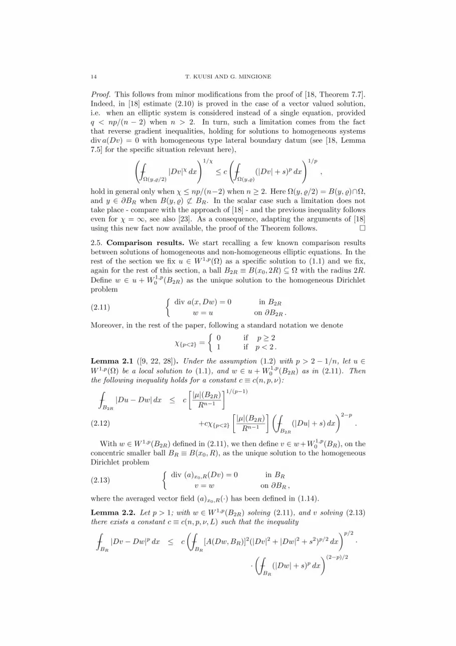
14 T. KUUSI AND G. MINGIONE
Proof. This follows from minor modifications from the proof of [18, Theorem 7.7].Indeed, in [18] estimate (2.10) is proved in the case of a vector valued solution,i.e. when an elliptic system is considered instead of a single equation, providedq < np/(n − 2) when n > 2. In turn, such a limitation comes from the factthat reverse gradient inequalities, holding for solutions to homogeneous systemsdiv a(Dv) = 0 with homogeneous type lateral boundary datum (see [18, Lemma7.5] for the specific situation relevant here),(
−∫
Ω(y,%/2)
|Dv|χ dx
)1/χ
≤ c
(−∫
Ω(y,%)
(|Dv|+ s)p dx
)1/p
,
hold in general only when χ ≤ np/(n−2) when n ≥ 2. Here Ω(y, %/2) = B(y, %)∩Ω,and y ∈ ∂BR when B(y, %) 6⊂ BR. In the scalar case such a limitation does nottake place - compare with the approach of [18] - and the previous inequality followseven for χ = ∞, see also [23]. As a consequence, adapting the arguments of [18]using this new fact now available, the proof of the Theorem follows.
2.5. Comparison results. We start recalling a few known comparison resultsbetween solutions of homogeneous and non-homogeneous elliptic equations. In therest of the section we fix u ∈ W 1,p(Ω) as a specific solution to (1.1) and we fix,again for the rest of this section, a ball B2R ≡ B(x0, 2R) ⊆ Ω with the radius 2R.
Define w ∈ u + W 1,p0 (B2R) as the unique solution to the homogeneous Dirichlet
problem
(2.11)
div a(x,Dw) = 0 in B2R
w = u on ∂B2R .
Moreover, in the rest of the paper, following a standard notation we denote
χp<2 =
0 if p ≥ 21 if p < 2 .
Lemma 2.1 ([9, 22, 28]). Under the assumption (1.2) with p > 2 − 1/n, let u ∈W 1,p(Ω) be a local solution to (1.1), and w ∈ u + W 1,p
0 (B2R) as in (2.11). Thenthe following inequality holds for a constant c ≡ c(n, p, ν):
−∫B2R
|Du−Dw| dx ≤ c
[|µ|(B2R)
Rn−1
]1/(p−1)
+cχp<2
[|µ|(B2R)
Rn−1
](−∫B2R
(|Du|+ s) dx
)2−p
.(2.12)
With w ∈W 1,p(B2R) defined in (2.11), we then define v ∈ w+W 1,p0 (BR), on the
concentric smaller ball BR ≡ B(x0, R), as the unique solution to the homogeneousDirichlet problem
(2.13)
div (a)x0,R(Dv) = 0 in BR
v = w on ∂BR ,
where the averaged vector field (a)x0,R(·) has been defined in (1.14).
Lemma 2.2. Let p > 1; with w ∈ W 1,p(B2R) solving (2.11), and v solving (2.13)there exists a constant c ≡ c(n, p, ν, L) such that the inequality
−∫BR
|Dv −Dw|p dx ≤ c
(−∫BR
[A(Dw,BR)]2(|Dv|2 + |Dw|2 + s2)p/2 dx
)p/2·
·(−∫BR
(|Dw|+ s)p dx
)(2−p)/2

UNIVERSAL POTENTIAL ESTIMATES 15
holds in the case 1 < p < 2, where
A(Dw,BR) ≡ A(Dw,BR)(x) :=|a(x,Dw(x))− (a)x0,R(Dw(x))|
(|Dw(x)|2 + s2)(p−1)/2
.
In the case p ≥ 2 it instead holds that
(2.14) −∫BR
|Dv −Dw|p dx ≤ c−∫BR
[A(Dw,BR)]2(|Dw|2 + s2)p/2 dx ,
with a similar dependence of the constant c.
Proof. By (1.2), using standard monotonicity argument (see (2.2)) or by using thefact that v is a quasi-minimizer of the functional
z 7→∫BR
|Du|p dx ,
see [12, Theorem 6.1] also for the definition, we have
(2.15)
∫BR
|Dv|p dx ≤ c(n, p, ν, L)
∫BR
(|Dw|2 + s2)p/2 dx .
Notice that by its very definition the averaged vector field (a)x0,R(·) still satis-fies (1.2). Therefore, using (2.1), the fact that both v and w are solutions, (1.2)1
and again Young’s inequality, we have∫BR
(|Dv|2 + |Dw|2 + s2)(p−2)/2|Dw −Dv|2 dx
≤ c∫BR
〈(a)x0,R(Dw)− (a)x0,R(Dv), Dw −Dv〉 dx
= c
∫BR
〈(a)x0,R(Dw)− a(x,Dw), Dw −Dv〉 dx
≤ c∫BR
A(Dw,BR)(|Dw|2 + s2)(p−1)/2|Dw −Dv| dx
≤ c∫BR
A(Dw,BR)(|Dw|2 + |Dv|2 + s2)(p−1)/2|Dw −Dv| dx
≤ 1
2
∫BR
(|Dv|2 + |Dw|2 + s2)(p−2)/2|Dw −Dv|2 dx
+ c
∫BR
[A(Dw,BR)]2(|Dv|2 + |Dw|2 + s2)p/2 dx .(2.16)
Ultimately, ∫BR
(|Dv|2 + |Dw|2 + s2)(p−2)/2|Dw −Dv|2 dx
≤ c∫BR
[A(Dw,BR)]2(|Dv|2 + |Dw|2 + s2)p/2 dx(2.17)
follows. We now start analyzing the case p < 2. Let us write
|Dv −Dw|p =[(|Du|2 + |Dw|2 + s2)(p−2)/2|Dv −Dw|2
]p/2·(|Dv|2 + |Dw|2 + s2)p(2−p)/4 ,
and therefore using the last estimate, together with (2.15) and Holder’s inequality,yields
−∫BR
|Dv −Dw|p dx

16 T. KUUSI AND G. MINGIONE
≤ c(−∫BR
(|Dv|2 + |Dw|2 + s2)(p−2)/2|Dv −Dw|2 dx dx)p/2
·(−∫BR
(|Dw|2 + s2)p/2 dx
)(2−p)/2
.
The statement for the case 1 < p < 2 now follows matching the last inequalitywith (2.17). In the case p ≥ 2 we go back to (2.16) and directly estimate
1
2
∫BR
|Dw −Dv|p dx+1
2
∫BR
(|Dw|2 + s2)(p−2)/2|Dw −Dv|2 dx
≤ c∫BR
(|Dv|2 + |Dw|2 + s2)(p−2)/2|Dw −Dv|2 dx
≤ c∫BR
A(Dw,BR)(|Dw|2 + s2)(p−1)/2|Dw −Dv| dx
≤ 1
4
∫BR
(|Dw|2 + s2)(p−2)/2|Dw −Dv|2 dx
+ c
∫BR
[A(Dw,BR)]2(|Dw|2 + s2)p/2 dx ,
implying the statement of the lemma for the case p ≥ 2.
The next Lemma is a corollary of the previous one used together with a suitableversion of Gehring’s lemma.
Lemma 2.3. Let p > 1; with w ∈ W 1,p(B2R) solving (2.11), and v solving (2.13)there exists a constant c ≡ c(n, p, ν, L) such that the inequality
(2.18) −∫BR
|Dv −Dw| dx ≤ c[ω(R)]σ −∫B2R
(|Dw|+ s) dx ,
holds, where ω(·) has been defined in (1.15) and σ is a positive (“small”) exponentdepending only on n, p, ν, L.
Proof. We start recalling a few basic results from elliptic regularity theory. The firstis a classical version of Gehring’s lemma, asserting that there exists an exponentq > p and a constant c, both depending only on n, p, ν, L, such that
(2.19)
(−∫BR
(|Dw|2 + s2)q/2 dx
)t/q≤ c−
∫B2R
(|Dw|2 + s2)t/2 dx
holds whenever t > 0 for a constant c depending on n, p, ν, L and also on t > 0.Actually Gehring’s lemma gives the previous inequality for t = p; the statement forthe general case t > 0 follows from a standard self-improving property of reverseHolder inequalities, as explained for instance in [28, Lemma 3.3]; moreover, weremark that although the statement is usually reported for the case p ≤ n, itcontinues to hold whenever p > 1; see also [12, Chapter 6] and [29, Remark 11].Combining (2.19) - for the choice t = 1 - with the up-to-the-boundary higherintegrability in (2.10) and using also (2.15) yields
(2.20)
(−∫BR
(|Dw|2 + |Dv|2 + s2)q/2 dx
)1/q
≤ c−∫B2R
(|Dw|+ s) dx
for a constant c depending only on n, p, ν, L. On the other hand, by Holder’sinequality we have∫
BR
[A(Dw,BR)]2(|Dv|2 + |Dw|2 + s2)p/2 dx

UNIVERSAL POTENTIAL ESTIMATES 17
≤(−∫BR
[A(Dw,BR)]2q/(q−p) dx
)(q−p)/q (−∫BR
(|Dv|2 + |Dw|2 + s2)q/2 dx
)p/q.
In turn we estimate, by means of (1.2)1 and (1.15), as follows:
−∫BR
[A(Dw,BR)]2q/(q−p) dx ≤ (2L)2p/(q−p) −∫BR
[A(Dw,BR)]2 dx ≤ c[ω(R)]2 .
Combining the last two estimates with (2.20) gives∫BR
[A(Dw,BR)]2(|Dv|2 + |Dw|2 + s2)p/2 dx
≤ c [ω(R)]2(q−p)/q
(−∫B2R
(|Dw|+ s) dx
)p.
Using the last estimate together with Lemma 2.2 and (2.19) leads to
(2.21)
(−∫BR
|Dv −Dw|p dx)1/p
≤ c[ω(R)]σ −∫B2R
(|Dw|+ s) dx
with σ defined by
(2.22) σ :=
2(q−p)pq if p ≥ 2
(q−p)q if 2− 1/n < p ≤ 2 .
Finally, (2.18) follows by using (2.21) together with Holder’s inequality.
In the rest of the paper we shall use the following quantity:
(2.23) σd :=
2/p if p ≥ 2
σ < 1 if 2− 1/n < p < 2 .
In other words, σd is a number that can be chosen arbitrarily close to 1 when p < 2.When additional Lipschitz regularity is available on w we can quantify the ex-
ponent σ in Lemma 2.3. This leads to the following improvement:
Lemma 2.4. Let p > 1; with w ∈W 1,p(B2R) solving (2.11), and v solving (2.13),assume also that w ∈W 1,∞(BR). Then the following inequality holds:
(2.24) −∫BR
|Dv −Dw| dx ≤ c[ω(R)]σd(‖Dw‖L∞(BR) + s) ,
where σd has been defined in (2.23). The constant c depends only on n, p, ν, L, qwhen p ≥ 2 and additionally on the number σ chosen in (2.23) when p ∈ (1, 2).
Proof. First the case 1 < p < 2; we go back to the proof of Lemma 2.3 and, thanksto (2.10), we may now estimate, for every q <∞
−∫BR
(|Dw|2 + |Dv|2 + s2)q/2 dx ≤ c−∫BR
(|Dw|2 + s2)q/2 dx
≤ c(‖Dw‖L∞(BR) + s)q
for a constant c ≡ c(n, p, ν, L, q). With this last estimate replacing (2.20) we canproceed as in the proof of Lemma 2.3, with the difference that we can now takeq to be any positive number; ultimately, this results in the fact that the numberσ in (2.22) can be taken arbitrarily close to 1. This ends the proof of the Lemmain the case p < 2 in view of the definition in (2.24). In the case p ≥ 2 the path

18 T. KUUSI AND G. MINGIONE
is straightforward: we take fully advantage of (2.14); recalling again the definitionin (1.15) we simply estimate(−∫BR
|Dv −Dw|p dx)1/p
≤ c
(−∫BR
[A(Dw,BR)]2(|Dw|2 + s2)p/2 dx
)1/p
≤ c(‖Dw‖L∞(BR) + s)
(−∫BR
[A(Dw,BR)]2 dx
)1/p
≤ c(‖Dw‖L∞(BR) + s)[ω(R)]2/p .
At this point (2.24) follows by using Holder’s inequality and again recalling thatσd = 2/p when p ≥ 2.
Finally, when Dini-VMO continuity of coefficients is available, the function w isindeed Lipschitz - a fact we will prove later, see Theorem 7.1 below. Therefore,combining (2.24) with (7.3) we obtain the following:
Lemma 2.5. Let p > 1; with w ∈W 1,p(B2R) solving (2.11), and v solving (2.13),let us assume that the function [ω(·)]σd is Dini-VMO, i.e. that the condition
(2.25)
∫ r
0
[ω(%)]σdd%
%<∞ ∀ r <∞ ,
is in force, where σd has been defined in (2.23). Then the following inequality holds:
(2.26) −∫BR
|Dv −Dw| dx ≤ c[ω(R)]σd −∫B2R
(|Dw|+ s) dx .
The constant c depends only on n, p, ν, L when p ≥ 2 and additionally on σ whenp ∈ (1, 2).
3. Maximal estimates and Theorems 1.8-1.9
In this section we give the proof of the maximal estimates presented in Sec-tion 1.4. After a preliminary list of lemmas, we shall present the results in thesubquadratic case 2− 1/n < p ≤ 2, and then we shall proceed with the case p ≥ 2.We recall that αM ∈ (0, 1] indicates the maximal Holder gradient regularity ex-ponent of solutions to homogeneous equations of the type (2.4), described in (2.5)and (1.21). Accordingly, by αm ∈ (0, 1] we denote the maximal Holder regularityexponent of solutions to homogeneous equations with measurable coefficients (2.7)as described in Theorem 2.2 and in (1.12).
Lemma 3.1. Let u be as in Theorem 1.1, then, with p > 2 − 1/n, there existconstants c1, c ≥ 1, depending only on n, p, ν, L, such that the following estimateholds whenever B% ⊆ BR ⊆ Ω are concentric balls:
−∫B%
(|Du|+ s) dξ ≤ c1
( %R
)−1+αm−∫BR
(|Du|+ s) dξ
+c
(R
%
)n [ |µ|(BR)
Rn−1
]1/(p−1)
+cχp<2
(R
%
)n [ |µ|(BR)
Rn−1
](−∫BR
(|Du|+ s) dξ
)2−p
.
Proof. It is based on a comparison argument using strict monotonicity; using The-orem 2.2 - we obviously define the function w in (2.11) as being the solution of thesame Dirichlet problem in the ball BR (instead of B2R) considered here - we have
−∫B%
(|Du|+ s) dξ ≤ −∫B%
(|Dw|+ s) dξ +
(R
%
)n−∫BR
|Du−Dw| dξ

UNIVERSAL POTENTIAL ESTIMATES 19
≤ c1( %R
)−1+αm−∫BR
(|Dw|+ s) dξ +
(R
%
)n−∫BR
|Du−Dw| dξ
≤ c1( %R
)−1+αm−∫BR
(|Du|+ s) dξ
+c
[(R
%
)1−αm+
(R
%
)n]−∫BR
|Du−Dw| dξ ,
and the statement follows using (2.12) in the previous inequality.
In a completely similar way goes the proof of the next lemma. We use (2.6)instead of (2.8) as “reference estimate”. Then we make a double comparison: firstwe use Lemma 2.3 (on BR) and then Lemma 2.1 (on B2R) twice, and therefore wefirst compare u with v and then w with v; we also use the fact ω(R) ≤ c(L).
Lemma 3.2. Let u ∈ W 1,p(Ω) be a weak solution to (1.1) under the assumptions(1.2) with p > 2− 1/n. Then there exist positive constants c, c1 > 1 and σ ∈ (0, 1),all depending only on n, p, ν, L such that the following estimate holds wheneverB% ⊆ BR ⊆ B2R ⊆ Ω are concentric balls:
−∫B%
(|Du|+ s) dξ ≤ c1 −∫B2R
(|Du|+ s) dξ + c
(R
%
)n [ |µ|(B2R)
Rn−1
]1/(p−1)
+c
(R
%
)n[ω(R)]
σ −∫B2R
(|Du|+ s) dξ
+cχp<2
(R
%
)n [ |µ|(B2R)
Rn−1
](−∫B2R
(|Du|+ s) dξ
)2−p
.(3.1)
Finally, using the same comparison scheme of the previous lemma, but takingthis time (2.5) as “reference estimate” and using Lemma 2.5, we have:
Lemma 3.3. Let u ∈ W 1,p(Ω) be a weak solution to (1.1) under the assumptions(1.2) with p > 2− 1/n, and assume that the function [ω(·)]σd is Dini-VMO regular,i.e. (2.25) holds with σd defined in (2.23). Then there exist constants c1, c ≥ 1depending only on n, p, ν, L, such that the following estimate holds whenever B% ⊆BR ⊆ B2R ⊆ Ω are concentric balls:
−∫B%
|Du− (Du)B% | dξ ≤ c1( %R
)αM−∫B2R
|Du− (Du)B2R| dξ
+c
(R
%
)n [ |µ|(B2R)
Rn−1
]1/(p−1)
+ c
(R
%
)n[ω(R)]σd −
∫B2R
(|Du|+ s) dξ
+cχp<2
(R
%
)n [ |µ|(B2R)
Rn−1
](−∫B2R
(|Du|+ s) dξ
)2−p
.(3.2)
In the case p < 2 the constant c depends also on the number σ < 1 chosen to defineσd in (2.23).
3.1. The case 2−1/n < p ≤ 2 and the proof of Theorem 1.9. Let us first give ageneral idea of the proof. In order to get the limiting potential estimates (1.6)-(1.7)the idea is to get a bound for the quantities of the type
−∫Bi
|u| dx and −∫Bi
|Du| dx ,
respectively, where Bi are balls geometrically shrinking at the point x. The moregeneral idea here is to get bounds for intermediate, “non-local” quantities as
|Bi|(1−α)/n −∫Bi
|Du| dx , 0 ≤ α ≤ 1 ,

20 T. KUUSI AND G. MINGIONE
and some higher-order analogs of them related to fractional maximal operators. Amain point of interest here, eventually helpful for the proof of the endpoint estimatesof the next section, is to show the proper uniform dependence of the estimates withrespect to α ∈ [0, 1]. The core of the ideas is therefore presented in the proof ofestimate (1.39).
Proof of Theorem 1.9. In the rest of the proof all the balls will be concentric andcentered at the point x ∈ Ω identified by the statement of the Theorem. Most of thetimes, the considered radii R will be such that R ≤ R, where the quantity R > 0will be in general chosen along the proof in dependence of the data n, p, ν, L, α, ω(·),essentially using conditions as (1.19). More precisely, we shall determine severalsmallness conditions of the type
(3.3) ω(R) ≤ δ ,
where δ will be a small quantity that will be reduced at several stages, as a de-creasing function of the quantities n, p, ν, L - and also α according to the statementwe will be proving; the quantity δ will be in other words implicitly determinedby several choices as (3.3). In this respect, we remark that satisfying an inequal-ity like (3.3) is always possible in the rest of the proof: when dealing with thecase α < α this is directly assumed in (1.19), while (3.3) is a consequence of anyof (1.20), (1.22) or (1.25) (recall that ω(·) is non-decreasing).
(**) Proof of (1.35). The proof is in two steps and works also in the case p ≥ 2.
Step 1: Validity of (1.35) for small radii R ≤ R. We shall confine ourselves toprove the estimate
(3.4) M1−α,R(Du)(x) ≤ c[Mp−α(p−1),R(µ)(x)
]1/(p−1)+ cR1−α −
∫BR
(|Du|+ s) dξ
while (1.35) follows from (3.4) by means of (2.3). We take concentric balls B% ⊂Br/2 ⊂ Br ⊂ BR with positive radii, and start observing the following identities,which will be actually used several times throughout the paper:
(3.5) r1−α[|µ|(Br)rn−1
]1/(p−1)
=
[|µ|(Br)
rn−p+α(p−1)
]1/(p−1)
and
r1−α[|µ|(Br)rn−1
](−∫Br
(|Du|+ s) dξ
)2−p
=|µ|(Br)
rn−p+α(p−1)
(r1−α −
∫Br
(|Du|+ s) dξ
)2−p
.(3.6)
We now use Lemma 3.2 (we take R ≡ r/2 there) and multiply both sides of (3.1)by %1−α; easy manipulations involving (3.5)-(3.6) give
%1−α −∫B%
(|Du|+ s) dξ ≤ c1(%r
)1−αr1−α −
∫Br
(|Du|+ s) dξ
+c
(r
%
)n−1+α [ |µ|(Br)rn−p+α(p−1)
]1/(p−1)
+cχp<2
(r
%
)n−1+α [ |µ|(Br)rn−p+α(p−1)
](r1−α −
∫Br
(|Du|+ s) dξ
)2−p
+c
(r
%
)n−1+α
[ω(R)]σr1−α −
∫Br
(|Du|+ s) dξ ,(3.7)

UNIVERSAL POTENTIAL ESTIMATES 21
which is valid whenever % ≤ r/2 ≤ R/2, for c, c1 ≡ c, c1(n, p, ν, L). We now choosea number H ≡ H(n, p, ν, L, α) > 2 large enough in order to have
(3.8) c1
(1
H
)1−α
≤ c1(
1
H
)1−α
=1
8
so that by taking % = r/H in (3.7) leads to( rH
)1−α−∫Br/H
(|Du|+ s) dx ≤ r1−α
8−∫Br
(|Du|+ s) dx
+ cHn
[|µ|(Br)
rn−p+α(p−1)
]1/(p−1)
+ cχp<2Hn
[|µ|(Br)
rn−p+α(p−1)
](r1−α −
∫Br
(|Du|+ s) dξ
)2−p
+ cHn [ω(R)]σr1−α −
∫Br
(|Du|+ s) dξ .
In turn we now choose R ≡ R(n, p, ν, L, α, ω(·)) in such a way that
(3.9) cHn [ω(R)]σ ≤ cHn
[ω(R)
]σ≤ 1/8
and this provides us( rH
)1−α−∫Br/H
(|Du|+ s) dξ ≤ r1−α
4−∫Br
(|Du|+ s) dξ
+ c
[|µ|(Br)
rn−p+α(p−1)
]1/(p−1)
+ cχp<2
[|µ|(Br)
rn−p+α(p−1)
](r1−α −
∫Br
(|Du|+ s) dξ
)2−p
,(3.10)
with c depending only on n, p, ν, L, α; observe that here we have used that Hdepends also on α via (3.8). Being r arbitrary and such that r ≤ R, in turn, (3.10)readily implies that
sup%≤R/H
%1−α −∫B%
(|Du|+ s) dξ ≤ (1/4)M1−α,R(|Du|+ s)
+c[Mp−α(p−1),R(µ)(x)
]1/(p−1)
+cχp<2[Mp−α(p−1),R(µ)(x)
][M1−α,R(|Du|+ s)]
2−p,
where c depends only on n, p, ν, L and α. On the other hand, we notice that
supR/H≤%≤R
%1−α −∫B%
(|Du|+ s) dξ ≤ HnR1−α −∫BR
(|Du|+ s) dξ
and therefore, recalling that H ≡ H(n, p, ν, L, α) as determined in (3.8), matchingthe last two estimates yields
M1−α,R(|Du|+ s)(x) ≤ (1/4)M1−α,R(|Du|+ s) + cR1−α −∫BR
(|Du|+ s) dξ
+c[Mp−α(p−1),R(µ)(x)
]1/(p−1)
+cχp<2[Mp−α(p−1),R(µ)(x)
][M1−α,R(|Du|+ s)(x)]
2−p.
In turn, when p < 2 we apply Young’s inequality, that is
(3.11) ab ≤ (p− 1)ε(p−2)/(p−1)a1/(p−1) + εb1/(2−p), a, b, ε > 0,

22 T. KUUSI AND G. MINGIONE
to get
cχp<2[Mp−α(p−1),R(µ)(x)
][M1−α,R(|Du|+ s)(x)]
2−p
≤ (1/4)M1−α,R(|Du|+ s)(x) + c[Mp−α(p−1),R(µ)(x)
]1/(p−1)(3.12)
so that combining inequalities above gives
M1−α,R(|Du|+ s)(x) ≤ (1/2)M1−α,R(|Du|+ s)(x) + cR1−α −∫BR
(|Du|+ s) dξ
+c[Mp−α(p−1),R(µ)(x)
]1/(p−1)
from which (3.4) finally follows provided we are assuming to deal with small radii
R ≤ R ≡ R(n, p, ν, L, α, ω(·)) determined in order to meet (3.9). We notice thatwhile the constant in (3.4) blows-up when p→ 2−1/n, it instead remains boundedwhen p → 2 as follows by looking at (3.11). The proof indeed applies to the casep = 2 when (3.11) is not needed.
Step 2: Removing the condition R ≤ R. We now, by means of standard ar-guments, show how to deduce the general form of (3.4), therefore avoiding to
consider the restriction R ≤ R. The main outcome is that the dependence onω(·) of R will be transferred to the constant c appearing in the final versionof (1.36) together with a dependence on diam (Ω). Assuming (3.4) to hold whenever
R ≤ R ≡ R(n, p, ν, L, α, ω(·)), we take R > R and observe that
M1−α,R(Du)(x) ≤M1−α,R(Du)(x) +
(R
R
)nR1−α −
∫BR
(|Du|+ s) dξ ,
and, trivially, Mp−α(p−1),R(µ)(x) ≤ Mp−α(p−1),R(µ)(x). In turn, by using esti-
mate (3.4) with R ≡ R to bound the second quantity appearing in the second-lastestimate, and properly enlarging the integrals, that is estimating
R1−α −∫BR
(|Du|+ s) dξ ≤(R
R
)nR1−α −
∫BR
(|Du|+ s) dξ ,
we have that (3.4) follows with a new constant c, which is obtained from the former
one by a magnification factor of [diam (Ω)/R]n. Recalling that R depends itself onn, p, ν, L, α and ω(·) the proof is complete.
(**) Proof of (1.39). In the following we shall write the proof in order to reportalso a few manipulations that will be used later and in particular when proving(1.41) and Theorem 1.6 below. We shall in this way emphasize how a certain setof estimates works in a dual way allowing to get estimates both below and beyondthe threshold given by Lipschitz continuity. Moreover, when we shall write that acertain constant c depends on σd, keeping the definition (2.22) in mind, we shallmean that it will actually depend on the number σ < 1 in (2.23), and this will onlyhappen in the case p < 2. We divide the proof in three steps.
Step 1: Dyadic sequence. We choose a geometric sequence Ri whose spread2H > 1 will be a certain function of the fixed quantities n, p, ν, L, and will be chosenin due course of the proof. More precisely we set
(3.13) Bi := B(x,R/(2H)i) := B(x,Ri) ,
for i = 0, 1, 2, . . ., and define
(3.14) Ai := −∫Bi
|Du− (Du)Bi | dξ , ki := |(Du)Bi −G| , G ∈ Rn .

UNIVERSAL POTENTIAL ESTIMATES 23
Here G is a fixed vector. We now select an integer H ≡ H(n, p, ν, L) ≥ 1 largeenough to have
(3.15) c1
(1
H
)αM≤ 1
16,
where αM is the maximal gradient regularity exponent defined via (2.5). Note thatthe stated dependence of H on n, p, ν, L also stems from a similar dependence ofαM . Applying (3.2) on arbitrary balls B% ≡ BR/(2H)i+1 ≡ Bi+1 ⊆ BRi/2 ⊂ BRiand using the fact that ω(·) is non-decreasing we gain
−∫Bi+1
|Du− (Du)Bi+1| dξ ≤ 1
16−∫Bi
|Du− (Du)Bi | dξ
+c(2H)n[|µ|(Bi)Rn−1i
]1/(p−1)
+ cχp<2(2H)n[|µ|(Bi)Rn−1i
](−∫Bi
(|Du|+ s) dξ
)2−p
+c(2H)n[ω(Ri)]σd −∫Bi
(|Du|+ s) dξ ,(3.16)
where c depends only on n, p, ν, L, σd. We reduce the value of R - in a way dependingonly on n, p, ν, L, σd and ω(·) - to get
(3.17) c(2H)n[ω(Ri)]σd ≤ 1/16⇐= 16c(2H)n[ω(R)]σd ≤ 1 ,
and using some further elementary estimates - in particular estimating
−∫Bi
|Du| dξ ≤ −∫Bi
|Du− (Du)Bi | dξ + ki + |G|
- and taking also (3.14) into account we obtain
Ai+1 ≤ (1/8)Ai + c[ω(Ri)]σd(ki + s+ |G|)
+c2
[|µ|(Bi)Rn−1i
]1/(p−1)
+ c2χp<2
[|µ|(Bi)Rn−1i
](−∫Bi
(|Du|+ s) dξ
)2−p
(3.18)
whenever i ≥ 0. Now, notice that
|ki+1 − ki| ≤ |(Du)Bi+1− (Du)Bi |
≤ −∫Bi+1
|Du− (Du)Bi | dξ
≤ (2H)n −∫Bi
|Du− (Du)Bi | dξ = (2H)nAi
holds whenever i ≥ 0 so that for m ∈ N we have
(3.19) km+1 =
m∑i=0
(ki+1 − ki) + k0 ≤ (2H)nm∑i=0
Ai + k0 .
To estimate the right hand side in (3.19) we observe that summing up (3.18) overi ∈ 0, . . . ,m− 1 yields
m∑i=1
Ai ≤1
2
m−1∑i=0
Ai + c2
m−1∑i=0
[|µ|(Bi)Rn−1i
]1/(p−1)
+c2χp<2
m−1∑i=0
[|µ|(Bi)Rn−1i
](−∫Bi
(|Du|+ s) dξ
)2−p
+c2
m−1∑i=0
[ω(Ri)]σd(ki + s+ |G|) ,

24 T. KUUSI AND G. MINGIONE
and therefore
m∑i=1
Ai ≤ A0 + 2c2
m−1∑i=0
[|µ|(Bi)Rn−1i
]1/(p−1)
+2c2χp<2
m−1∑i=0
[|µ|(Bi)Rn−1i
](−∫Bi
(|Du|+ s) dξ
)2−p
+2c2
m−1∑i=0
[ω(Ri)]σd(ki + s+ |G|)(3.20)
follows. For every integer m ≥ 1 (3.19) gives
km+1 ≤ cA0 + ck0 + c
m−1∑i=0
[|µ|(Bi)Rn−1i
]1/(p−1)
+cχp<2
m−1∑i=0
[|µ|(Bi)Rn−1i
](−∫Bi
(|Du|+ s) dξ
)2−p
+c3
m−1∑i=0
[ω(Ri)]σd(ki + s+ |G|) ,(3.21)
and the constants c, c3 depend only on n, p, ν, L, σd - recall the dependence of H.We also observe that trivially estimating
(3.22) k0 + k1 ≤ [1 + (2H)n]−∫BR
|Du−G| dξ
and keeping in mind the definition of A0 we end up with
km+1 ≤ c−∫BR
(|Du− (Du)BR |+ |Du−G|) dξ + c
m∑i=0
[|µ|(Bi)Rn−1i
]1/(p−1)
+cχp<2
m∑i=0
[|µ|(Bi)Rn−1i
](−∫Bi
(|Du|+ s) dξ
)2−p
+c3
m∑i=0
[ω(Ri)]σd(ki + s+ |G|) ,(3.23)
for every m ≥ 0. In the previous inequality we choose G = 0 and add s to bothsides, and finally multiply both sides by R1−α
m ; taking into account that Rm+1 ≤ Riwe get
R1−αm+1(km+1 + s) ≤ cR1−α −
∫BR
(|Du|+ s) dξ + c
m∑i=0
R1−αi
[|µ|(Bi)Rn−1i
]1/(p−1)
+cχp<2
m∑i=0
R1−αi
[|µ|(Bi)Rn−1i
](−∫Bi
(|Du|+ s) dξ
)2−p
+c3
m∑i=0
[ω(Ri)]σdR1−α
i (ki + s) .
In turn, using again identities (3.5)-(3.6) with R ≡ Ri and the very definition offractional maximal operator yields
R1−αm+1(km+1 + s) ≤ cR1−α −
∫BR
(|Du|+ s) dξ + c
m∑i=0
[|µ|(Bi)
Rn−p+α(p−1)i
]1/(p−1)

UNIVERSAL POTENTIAL ESTIMATES 25
+cχp<2 [M1−α,R(|Du|+ s)(x)]2−p
m∑i=0
|µ|(Bi)Rn−p+α(p−1)i
+c3
m∑i=0
[ω(Ri)]σdR1−α
i (ki + s) .(3.24)
Remark 3.1. Let us observe that if we restart from (3.16) and avoid to estimateas in (3.17) and the subsequent inequality, i.e. we avoid to introduce ki in (3.16)but we rather keep the integral averages, and eventually proceed as after (3.18), weobtain the following version of (3.23):
km+1 ≤ c−∫BR
(|Du− (Du)BR |+ |Du−G|) dξ + c
m∑i=0
[|µ|(Bi)Rn−1i
]1/(p−1)
+cχp<2
m∑i=0
[|µ|(Bi)Rn−1i
](−∫Bi
(|Du|+ s) dξ
)2−p
+c3
m∑i=0
[ω(Ri)]σd −∫Bi
(|Du|+ s) dξ .(3.25)
The main difference with (3.23) is that this last inequality does not need any small-
ness assumption on R as the one required to satisfy (3.17), but it rather works forany ball BR ⊆ Ω.
Step 2: A uniform upper bound. Here we really focalize on the case 2−1/n < p ≤2, therefore the exponent σd in (2.23) coincides with σ which is in turn a numberwe may choose to be strictly smaller than one; the associated constants will dependon the choice of σ and will blow-up as σ → 1. Starting from (3.24) we shall byinduction prove the following:
Lemma 3.4. There exists a constant c depending only on n, p, ν, L, σ, and a radiusR depending on n, p, ν, L, ω(·), σ, but both independent of α, such that
(3.26) R1−αm (km+1 + s) ≤ cM
holds for every integer m ≥ 0 and R ≤ R, where
M := R1−α −∫BR
(|Du|+ s) dξ
+ [M1−α,R(|Du|+ s)(x))]2−pI|µ|p−α(p−1)(x, 2R) +
[I|µ|p−α(p−1)(x, 2R)
]1/(p−1)
.(3.27)
Proof. The choice of the radius R is of course the one determined in Step 1. Notethat in the previous statement we are evaluating the Riesz potential on balls notnecessarily contained in Ω; this is not restrictive in that we are assuming withoutloss of generality that the measure µ is defined on the whole Rn. We start withsome preliminary estimates. Let us recall the elementary inequality
(3.28)
∞∑k=0
aqk ≤
( ∞∑k=0
ak
)q, q ≥ 1 ,
valid for any nonnegative sequence ak. We apply it with the choice q = 1/(p− 1)- obviously q ≥ 1 as p ≤ 2 - to get
(3.29)
m∑i=0
[|µ|(Bi)
Rn−p+α(p−1)i
]1/(p−1)
≤
[ ∞∑i=0
|µ|(Bi)Rn−p+α(p−1)i
]1/(p−1)
.
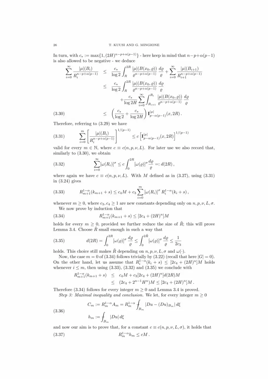
26 T. KUUSI AND G. MINGIONE
In turn, with c∗ := max1, (2H)n−p+α(p−1) - here keep in mind that n−p+α(p−1)is also allowed to be negative - we deduce
∞∑i=0
|µ|(Bi)Rn−p+α(p−1)i
≤ c∗log 2
∫ 2R
R
|µ|(B(x0, %))
%n−p+α(p−1)
d%
%+
∞∑i=0
|µ|(Bi+1)
Rn−p+α(p−1)i+1
≤ c∗log 2
∫ 2R
R
|µ|(B(x0, %))
%n−p+α(p−1)
d%
%
+c∗
log 2H
∞∑i=0
∫ Ri
Ri+1
|µ|(B(x0, %))
%n−p+α(p−1)
d%
%
≤(
c∗log 2
+c∗
log 2H
)I|µ|p−α(p−1)(x, 2R) .(3.30)
Therefore, referring to (3.29) we have
(3.31)
m∑i=0
[|µ|(Bi)
Rn−p+α(p−1)i
]1/(p−1)
≤ c[I|µ|p−α(p−1)(x, 2R)
]1/(p−1)
valid for every m ∈ N, where c ≡ c(n, p, ν, L). For later use we also record that,similarly to (3.30), we obtain
(3.32)
∞∑i=0
[ω(Ri)]σ ≤ c
∫ 2R
0
[ω(%)]σd%
%=: d(2R) ,
where again we have c ≡ c(n, p, ν, L). With M defined as in (3.27), using (3.31)in (3.24) gives
(3.33) R1−αm+1(km+1 + s) ≤ c4M + c3
m∑i=0
[ω(Ri)]σR1−αi (ki + s) ,
whenever m ≥ 0, where c3, c4 ≥ 1 are new constants depending only on n, p, ν, L, σ.We now prove by induction that
(3.34) R1−αm+1(km+1 + s) ≤ [2c4 + (2H)n]M
holds for every m ≥ 0, provided we further reduce the size of R; this will proveLemma 3.4. Choose R small enough in such a way that
(3.35) d(2R) =
∫ 2R
0
[ω(%)]σd%
%≤∫ 2R
0
[ω(%)]σd%
%≤ 1
2c3
holds. This choice still makes R depending on n, p, ν, L, σ and ω(·).Now, the case m = 0 of (3.34) follows trivially by (3.22) (recall that here |G| = 0).
On the other hand, let us assume that R1−αi (ki + s) ≤ [2c4 + (2H)n]M holds
whenever i ≤ m, then using (3.33), (3.32) and (3.35) we conclude with
R1−αm+1(km+1 + s) ≤ c4M + c3[2c4 + (2H)n]d(2R)M
≤ (2c4 + 2n−1Hn)M ≤ [2c4 + (2H)n]M .
Therefore (3.34) follows for every integer m ≥ 0 and Lemma 3.4 is proved.Step 3: Maximal inequality and conclusion. We let, for every integer m ≥ 0
Cm := R1−αm Am = R1−α
m −∫Bm
|Du− (Du)Bm | dξ
hm := −∫Bm
|Du| dξ(3.36)
and now our aim is to prove that, for a constant c ≡ c(n, p, ν, L, σ), it holds that
(3.37) R1−αm hm ≤ cM .

UNIVERSAL POTENTIAL ESTIMATES 27
Obviously, (3.26) implies
(3.38) R1−αm hm ≤ R1−α
m km + Cm ≤ cM + Cm ,
where M has been defined in (3.27), and therefore we look for a bound on Cm. Forthis we manipulate (3.18). Let us observe that, using (3.5) and (3.31) and keepingthe definition of M in (3.27) in mind, it follows that
(3.39)
[|µ|(Bi)Rn−1i
]1/(p−1)
≤ cRα−1i
[I|µ|p−α(p−1)(x, 2R)
]1/(p−1)
≤ cRα−1i M
for a constant c depending on n, p, ν, L. By (3.6) we similarly have[|µ|(Bi)Rn−1i
](−∫Bi
(|Du|+ s) dξ
)2−p
≤ cRα−1i [M1−α,R(|Du|+ s)(x)]
2−pI|µ|p−α(p−1)(x, 2R) ≤ cRα−1
i M .
Using the last two estimates in (3.18) yields
(3.40) Am+1 ≤ (1/8)Am + c(ki + s) + cRα−1m M .
In turn, using (3.26) to estimate
(3.41) km + s ≤ cRα−1m M ,
inequality (3.40) rewrites as
(3.42) Cm+1 ≤1
8
(Rm+1
Rm
)1−α
Cm + c5
(Rm+1
Rm
)1−α
M ≤ (1/8)Cm + c5M
with c5 ≥ 1 being a constant depending only on n, p, ν, L, σ. Now, by means of theprevious relation, we shall prove by induction that
(3.43) Cm ≤ 2c5M
holds whenever m ≥ 0. When m = 0 the previous inequality is a trivial consequenceof the definitions:
C0 ≤ R1−α −∫BR
|Du− (Du)BR | dξ ≤ 2M1−α,R(|Du|+ s)(x) ≤ 2M ≤ 2c5M .
On the other hand, assuming (3.43) and then using (3.42) gives
Cm+1 ≤ (c5/4)M + c5M ≤ 2c5M ,
and therefore (3.43) follows for every integer m ≥ 0. In turn, merging (3.43)with (3.38), we conclude with the proof of (3.37) for every integer m ≥ 0.
Now, let us now observe that, for a new constant c, still depending on n, p, ν, Land σ, it holds that
(3.44) M1−α,R(Du)(x) ≤ cM .
In fact, let us consider r ≤ R and determine the integer i ≥ 0 such that Ri+1 <r ≤ Ri; we then have
(3.45) r1−α −∫Br
|Du| dξ ≤(
RiRi+1
)nR1−αi −
∫Bi
|Du| dξ ≤ c(2H)nR1−αi hi ≤ cM ,
and (3.44) follows. Recalling the definition of M in (3.27) we in turn obtain
M1−α,R(|Du|+ s)(x) ≤ cR1−α −∫BR
(|Du|+ s) dξ + c[I|µ|p−α(p−1)(x, 2R)
]1/(p−1)
+c [M1−α,R(|Du|+ s)(x)]2−p
I|µ|p−α(p−1)(x, 2R) .(3.46)

28 T. KUUSI AND G. MINGIONE
When p < 2, by using Young’s inequality with conjugate exponents(1
2− p,
1
p− 1
)in (3.11), the last term in the previous inequality can be estimated by
(1/2)M1−α,R(|Du|+ s)(x) + c[I|µ|p−α(p−1)(x, 2R)
]1/(p−1)
,
and c depends only on n, p, ν, L and σ, remaining bounded as p approaches 2. Usingthe last inequality with (3.46), we finally conclude with a preliminary form of (1.39),that is
(3.47) M1−α,R(Du)(x) ≤ cR1−α −∫BR
(|Du|+ s) dξ + c[I|µ|p−α(p−1)(x, 2R)
]1/(p−1)
,
which is valid whenever R ≤ R and R ≡ R(n, p, ν, L, ω(·), σ) has been determinedaccording to the various restrictions imposed on the size of quantities like for in-stance c(n, p, ν, L, σ)[ω(R)]σ. Keep in mind that to estimate the first term appearingin (1.39) it is sufficient to use (2.3). The passage to the general case, i.e. when R
is not necessarily smaller than the determined R, follows now along the lines of theproof of (1.36), Step 2, modulo the obvious modifications. The final outcome is anestimate where the constant involved depends on n, p, ν, L, σ, ω(·) and diam (Ω).
Remark 3.2. No dependence on diam (Ω) appears in the constants of the proofs of(1.36) and (1.39) when the vector field is independent of x, i.e. a(x,Du) ≡ a(Du)as in this case we obviously do not need to operate restrictions on the size of radii.Indeed, we take R small enough to satisfy (3.17) and (3.32); when no dependenceon x is allowed these are automatically satisfied for every radius as ω(·) = 0.
(**) Proof of (1.41). We restart as in Step 2 of the proof of (1.39), by consideringthe sequence of shrinking balls in (3.13) with H ≥ 4 to be determined later, andthis time defining, in connection to (3.14),
(3.48) Ai := R−αi −∫Bi
|Du− (Du)Bi | dξ .
Next, we a priori restrict to the case R ≤ 1, so that Ri ≤ 1 for every i ≥ 0; usingthis fact, and since p ≤ 2 we may estimate
(3.49) R−αi
[|µ|(Bi)Rn−1i
]1/(p−1)
=
[|µ|(Bi)
Rn−1+α(p−1)i
]1/(p−1)
≤[|µ|(Bi)Rn−1+αi
]1/(p−1)
.
Moreover, from the case α = 1 of inequality (1.39) we have
−∫Bi
(|Du|+ s) dξ ≤ c[I|µ|1 (x,R)
]1/(p−1)
+ c−∫BR
(|Du|+ s) dξ
≤ c[I|µ|1 (x,R)
]1/(p−1)
+ cR−α −∫BR
(|Du|+ s) dξ =: K(3.50)
whenever i ≥ 0, and for a constant c ≡ c(n, p, ν, L, ω(·), σ,diam (Ω)). Consequently
R−αi
[|µ|(Bi)Rn−1i
](−∫Bi
(|Du|+ s) dξ
)2−p
≤[|µ|(Bi)Rn−1+αi
]K2−p
holds. Using Lemma 3.3 with % ≡ Ri+1 and 2R ≡ Ri, multiplying both sides of theresulting inequality (3.2) by R−αi+1, and finally using (3.49), (3.50) and the last twoinequalities, we have
Ai+1 ≤ c1
(Ri+1
Ri
)αM−αAi + c
(RiRi+1
)n+α [ |µ|(Bi)Rn−1+αi
]1/(p−1)

UNIVERSAL POTENTIAL ESTIMATES 29
+c
(RiRi+1
)n+α [ |µ|(Bi)Rn−1+αi
]K2−p + c
(RiRi+1
)n+α([ω(Ri)]
σ
Rαi
)K(3.51)
valid for every i ≥ 0, where c ≡ c(n, p, ν, L, ω(·), σ, diam (Ω)) and moreover c1 ≡c1(n, p, ν, L). Now we choose H ≡ H(n, p, ν, L, α) > 1 large enough in order toobtain
c1
(Ri+1
Ri
)αM−α= c1
(1
2H
)αM−α≤ c1
(1
2H
)αM−α≤ 1
4.
By using Young’s inequality (3.11) when p < 2 we estimate[|µ|(Bi)Rn−1+αi
]K2−p ≤
[|µ|(Bi)Rn−1+αi
]1/(p−1)
+ cK ≤ [M1−α,R(µ)(x)]1/(p−1)
(x) + cK
and using assumption (1.40)
[ω(Ri)]σ
Rαi≤ [ω(Ri)]
σ
Rαi≤ S .
The last three estimates used in (3.51) give
(3.52) Ai+1 ≤ (1/2)Ai + c6
[M1−α,R(µ)(x)]
1/(p−1)+K
for every i ≥ 0, where c6 ≡ c6(n, p, ν, L, ω(·), σ, diam (Ω), S). Iterating the previousrelation, it is easy to prove that
(3.53) Ai ≤ 2−iA0 + c6
i−1∑j=0
2−j
[M1−α,R(µ)(x)]1/(p−1)
+K
holds for every i ≥ 1. In turn, recalling (3.48), (3.50) and that R ≤ 1, we also have
supi≥0
Ai ≤ cR−α −∫BR
|Du| dx+ c6
[M1−α,R(µ)(x)]
1/(p−1)+K
≤ c
[M1−α,R(µ)(x)]
1/(p−1)+K
with a constant c depending only on n, p, ν, L, ω(·), α, S and diam (Ω). We nowobserve that, in view of the previous inequality and of the definition of K in (3.50),and recalling that H depends only on n, p, ν, L, α, in order to complete the prooffor the case R ≤ 1 it is sufficient to prove that
(3.54) M#α,R(Du)(x) ≤ c(n)Hn+α
[supi≥0
Ai
].
To this aim, with % ∈ (0, R], let i ∈ N be such that Ri+1 < % ≤ Ri; then it holds
%−α −∫B%
|Du− (Du)B% | dξ ≤ c%−α −∫B%
|Du− (Du)Bi | dξ
≤ c(2H)n+αR−αi −∫Bi
|Du− (Du)Bi | dξ
≤ c(n)Hn+α
[supi≥0
Ai
],
proving (3.54), and in turn (1.41) follows in the case R ≤ 1. We finally remove the
constraint R ≤ 1 as already done for estimate (1.35). The proof is complete.

30 T. KUUSI AND G. MINGIONE
3.2. The case p ≥ 2 and proof of Theorem 1.8. The proof follows the onegiven for Theorem 1.9, and we shall give the suitable modifications, keeping thenotation thereby introduced. The proof of (1.35) is exactly the same as for the casep ≤ 2, as already noticed above. As for the proof of (1.36) we start observing thatwe can restart from Step 2, as the content of Step 1 also works for the case p ≥ 2.Lemma 3.4 must be now replaced by the following:
Lemma 3.5. There exists a constant c, depending only on n, p, ν, L and a positiveradius R depending only on n, p, ν, L and ω(·), but both independent of α, such that
(3.55) R1−αm km+1 ≤ cR1−α −
∫BR
(|Du|+ s) dξ + cWµ1−α(p−1)/p,p(x, 2R) =: cM
holds for every integer m ≥ 0 and whenever R ≤ R.
The proof is essentially the same as for the case p < 2, but we replace (3.30) by
∞∑i=0
[|µ|(Bi)
Rn−p+α(p−1)i
]1/(p−1)
≤ c
∫ 2R
R
[|µ|(B(x0, %))
%n−p+α(p−1)
]1/(p−1)d%
%
+c
∞∑i=0
∫ Ri
Ri+1
[|µ|(B(x0, %))
%n−p+α(p−1)
]1/(p−1)d%
%
≤ cWµ1−α(p−1)/p,p(x, 2R) ,(3.56)
with c ≡ c(n, p, ν, L). We therefore arrive at (3.33) with the new definition of M
in (3.55). We also note that everywhere [ω(·)]σ is replaced by [ω(·)]2/p. From thispoint on the rest of the proof of the Lemma is as for the case p ≤ 2. We thenproceed with Step 3; we adopt the definitions in (3.36) and keeping (3.56) in mindwe replace (3.39) by the new estimate[
|µ|(Bi)Rn−1i
]1/(p−1)
≤ cRα−1i Wµ
1−α(p−1)/p,p(x, 2R) ≤ cRα−1i M
with M now being defined in (3.55). With this estimate and (3.18) we find onceagain the validity of (3.42) and from this point on the proof follows exactly the oneof Theorem 1.9.
Finally, we provide the modifications for the proof of (1.38). First, we noticethat (3.50) has to be replaced by
−∫Br
(|Du|+ s) dξ ≤ cWµ1/p,p(x,R) + c−
∫BR
(|Du|+ s) dξ
as we are now using estimate (1.36) with α = 1. Taking into account the firstequality in (3.49) and using Lemma 3.3 we arrive at the following analog of (3.51):
%−α −∫B%
|Du− (Du)B% | dx ≤ c1(%r
)αM−αr−α −
∫Br
|Du− (Du)Br | dx
+ c
(r
%
)n+α [ |µ|(Br)rn−1+α(p−1)
]1/(p−1)
+ c
(r
%
)n+α[ω(r)]
2/p
rα
Wµ
1/p,p(x,R) + c−∫BR
(|Du|+ s) dξ
,
which is valid for every % ≤ r/2 ≤ R/2. Here c ≡ c(n, p, ν, L, ω(·),diam (Ω)) andc1 ≡ c1(n, p, ν, L). Using this last inequality, taking % = Ri+1 and r = Ri, andproceeding as after (3.51) estimate (1.38) follows too and the proof of Theorem 1.8is complete.

UNIVERSAL POTENTIAL ESTIMATES 31
We finally proceed with further maximal estimates concerning the case when theequation has measurable coefficients, and therefore Holder continuity of solutionswith any exponent is not expected even in the case of zero right hand side.
Proposition 3.1. Let u ∈ W 1,p(Ω) be a weak solution to the equation with mea-surable coefficient (1.1), and let (1.2) hold with p > 2− 1/n. Then estimate (1.35)holds uniformly in α ∈ [0, α], whenever α < αm, for a constant c depending onlyn, p, ν, L and α.
Proof. The proof follows the lines of the proof of (1.35) of Theorem 1.8, at thebeginning of this section. The main difference is that we have to use Lemma 3.1instead of Lemma 3.2. Here we give the suitable modifications. Instead of (3.7) wehave that
%1−α −∫B%
(|Du|+ s) dx ≤ c1(%r
)αm−αr1−α −
∫Br
(|Du|+ s) dx
+c
(r
%
)n−1+α [ |µ|(Br)rn−p+α(p−1)
]1/(p−1)
+cχp<2
(r
%
)n−1+α [ |µ|(Br)rn−p+α(p−1)
](r1−α −
∫Br
(|Du|+ s) dx
)2−p
,(3.57)
holds whenever % ≤ r ≤ R. Next, we choose this time H ≡ H(n, p, ν, L, α) largeenough in order to have
c1
(1
H
)αm−α≤ c1
(1
H
)αm−α≤ 1
4.
Note that here we are using the fact that α < αm. By using this relation in (3.57)we arrive at (3.10) and the rest of the proof proceeds as for Theorem 1.8. Notethat here we do not need to choose small radii, therefore in the final estimate nodependence on diam (Ω) occurs.
4. Endpoint estimates and Theorems 1.1, 1.4, 1.6 and 1.10
In this section we give the proof of a certain number of theorems characterizedby the fact of featuring “endpoint estimates”. This means we shall prove estimateswith fractional potentials depending on α, and catching the borderline case α = 0,with all the constants involved in the estimates being stable, i.e. remaining boundedwhen α approaches zero. This time we start with the gradient estimates.
4.1. Proof of Theorems 1.4 and 1.6. Before the proof let us state a lemmawhose proof we include for the sake of completeness.
Lemma 4.1. Let µ be a Borel measure with finite total mass on Ω; let γ ∈ (0, 1),β ∈ [0, n], p > 1, and BR ⊂ Ω. Then
[Mβ,γR(µ)(x)]1/(p−1) ≤ maxγ(β−n)/(p−1), 1
(− log γ)|B1|1/(p−1)Wµ
β/p,p(x,R)
and
Mβ,γR(µ)(x) ≤ maxγβ−n, 1(− log γ)|B1|
I|µ|β (x,R)
hold.
Proof. For all ε > 0 there is 0 < r ≤ R such that
Mβ,γR(µ)(x) ≤ |B1|−1 |µ|(Bγr)(γr)n−β
+ ε.

32 T. KUUSI AND G. MINGIONE
We have
|µ|(Bγr)(γr)n−β
=
[(|µ|(Bγr)(γr)n−β
)1/(p−1)1
− log γ
∫ r
γr
d%
%
]p−1
≤ maxγβ−n, 1(− log γ)p−1
[∫ r
γr
(|µ|(B%)%n−β
)1/(p−1)d%
%
]p−1
≤ maxγβ−n, 1(− log γ)p−1
[Wµ
β/p,p(x,R)]p−1
and thus the first inequality stated in the lemma follows, while the second alsofollows via a completely similar argument.
Proof of Theorem 1.6. In the rest of the proof the points x, y and the radius R willbe those fixed in the statement of the theorem, therefore x, y ∈ BR/4. We go backto the proof of Theorem 1.9, proof of (1.39), Step 1, and we adopt the notationintroduced there. We restart from estimate (3.25) that we apply to a ball with ageneral radius r (i.e. we change notation and denote r instead of R in (3.25)) to bedetermined in a few lines; in particular ri := r/(2H)i and Bi = B(x, ri). Moreover,we shall use the restriction r ≤ R/2, where R is now the radius appearing in thestatement of the Theorem, so that in any case B(x, r) ⊂ BR. From the case α = 1of inequality (1.39) we have that
−∫Bi
(|Du|+ s) dξ ≤ c[I|µ|1 (x, r)
]1/(p−1)
+ c−∫B(x,r)
(|Du|+ s) dξ =: K(x, r)
holds whenever i ∈ N. By using the last inequality, easy manipulations to (3.25)then lead to
km+1 ≤ c−∫Br
|Du− (Du)B(x,r)|+ |Du−G|) dξ
+crαm∑i=0
[|µ|(Bi)
rn−1+α(p−1)i
]1/(p−1)
+ cχp<2rα
m∑i=0
[|µ|(Bi)rn−1+αi
][K(x, r)]2−p
+crαm∑i=0
[ω(ri)]σ
rαi[K(x, r) + s+ |G|] .(4.1)
Observe now that, as p ≤ 2 in the case under examination, estimating as in (3.31)we obtain
m∑i=0
[|µ|(Bi)
rn−1+α(p−1)i
]1/(p−1)
≤ rα(2−p)p−1
m∑i=0
[|µ|(Bi)rn−1+αi
]1/(p−1)
≤ c[I|µ|1−α(x, 2r)
]1/(p−1)
for a constant c depending only on n, p, ν, L, diam(Ω), σ,H and therefore, as in theproof of Theorem 1.9, ultimately depending only n, p, ν, L, diam(Ω). Similarly
m∑i=0
[ω(ri)]σ
rαi≤ c
∫ 2r
0
[ω(%)]σ
%αd%
%≤ cRα−α
∫ 2r
0
[ω(%)]σ
%αd%
%≤ cS
again holds for a constant depending only on n, p, ν, L, diam(Ω), σ. Merging thelast two inequalities with (4.1) we have
km+1 ≤ c−∫B(x,r)
(|Du− (Du)B(x,r)|+ |Du−G|) dξ + crα[I|µ|1−α(x,R)
]1/(p−1)
+crα[I|µ|1−α(x, 2r)
][K(x, r)]
2−p+ crα [K(x, r) + s+ |G|] ,

UNIVERSAL POTENTIAL ESTIMATES 33
where c ≡ c(n, p, ν, L, S,diam (Ω), σ). Letting m → ∞ in the previous estimate,and applying Young’s inequality with conjugate exponents(
1
2− p,
1
p− 1
)in (3.11) when p < 2, we deduce
|Du(x)−G| = limm→∞
km+1 ≤ c−∫B(x,r)
(|Du− (Du)B(x,r)|+ |Du−G|) dξ
+crα[I|µ|1−α(x,R)
]1/(p−1)
+ crα [K(x, r) + s+ |G|] .
Arguing in the same way for the point y we also obtain
|Du(y)−G| ≤ c−∫B(y,r)
(|Du− (Du)B(y,r)|+ |Du−G|) dξ
+crα[I|µ|1−α(y,R)
]1/(p−1)
+ crα [K(y, r) + s+ |G|] ,
and therefore, summing up the last two relations gives
|Du(x)−Du(y)| ≤ c−∫B(x,r)
(|Du− (Du)B(x,r)|+ |Du−G|) dξ
+c−∫B(y,r)
(|Du− (Du)B(y,r)|+ |Du−G|) dξ
+crα[I|µ|1−α(x,R) + I
|µ|1−α(y,R)
]1/(p−1)
+crα [K(x, r) +K(y, r) + s+ |G|] .(4.2)
We now fix G and r by taking
(4.3) G := (Du)B(x,3r) , r := |x− y|/2 ,
so that B(y, r) ⊂ B(x, 3r) and therefore
−∫B(x,r)
(|Du− (Du)B(x,r)|+ |Du−G|) dξ
+ c−∫B(y,r)
(|Du− (Du)B(y,r)|+ |Du−G|) dξ
≤ c(n)−∫B(x,3r)
|Du− (Du)B(x,3r)| dξ .(4.4)
Now, notice that as we are assuming that the initial ball BR is such that x, y ∈ BR/4,then we have necessarily |x − y| ≤ R/2 so that now r ≤ R/4 and B(x, 3r) ⊂B(x, 3R/4) ⊂ BR. Therefore we use (1.41) to estimate
−∫B(x,3r)
|Du− (Du)B(x,3r)| dξ ≤ crαM#α,3R/4(Du)(x)
≤ crα[M1−α,3R/4(µ)(x)
]1/(p−1)+ crα
[I|µ|1 (x, 3R/4)
]1/(p−1)
+c( rR
)α−∫B(x,3R/4)
(|Du|+ s) dξ
≤ crα[M1−α,3R/4(µ)(x)
]1/(p−1)+ cRα/(p−1)rα
[I|µ|1−α(x,R)
]1/(p−1)
+c( rR
)α−∫BR
(|Du|+ s) dξ .

34 T. KUUSI AND G. MINGIONE
We remark that the use of (1.41) is justified here as (1.40) is a consequence of (1.27)for a new constant depending on the number S used in (1.27), on ω(·) and ondiam (Ω), so that the final dependence on the constants remains unvaried; see Re-mark 4.1 below. The last two estimates and (4.2) give
|Du(x)−Du(y)| ≤ crα[M1−α,3R/4(µ)(x)
]1/(p−1)+ c
( rR
)α−∫BR
(|Du|+ s) dξ
+crα[I|µ|1−α(x,R) + I
|µ|1−α(y,R)
]1/(p−1)
+crα [K(x, r) +K(y, r) + s+ |G|](4.5)
for a constant c depending on n, p, ν, L, α, ω(·), S,diam (Ω) and σ; the dependenceon α ≥ α comes from the use of inequality (1.41). We devote ourselves to estimatethe various terms involved in the right hand side of (4.5). We again use inequal-ity (1.39) with α = 1 and recall that B(x, 3R/4) ⊂ BR to estimate as follows:
K(x, r) ≤ c[I|µ|1 (x, 3R/4)
]1/(p−1)
+ c−∫B(x,3R/4)
(|Du|+ s) dξ
≤ cRα/(p−1)[I|µ|1−α(x,R)
]1/(p−1)
+ cR−α −∫BR
(|Du|+ s) dξ
with a similar estimate being obviously true for K(y,R), i.e.
K(y, r) ≤ cRα/(p−1)[I|µ|1−α(y,R)
]1/(p−1)
+ cR−α −∫BR
(|Du|+ s) dξ .
Moreover, again by (1.39), we have
|G| ≤ c−∫B(x,3r)
|Du| dξ
≤ cRα/(p−1)[I|µ|1−α(x,R)
]1/(p−1)
+ cR−α −∫BR
(|Du|+ s) dξ .
Now, by Lemma 4.1 with the choice γ = 3/4, we obtain
M1−α,3R/4(µ)(x) ≤ c(n, α)I|µ|1−α(x,R)
Using the last four inequalities in (4.5) we conclude with
|Du(x)−Du(y)| ≤ crα[I|µ|1−α(x,R) + I
|µ|1−α(y,R)
]1/(p−1)
+ c( rR
)α−∫BR
(|Du|+ s) dξ
from which (1.28) follows taking into account (4.3).
Remark 4.1 (Trivial). Assumption (1.27) implies (1.40) for a new constant de-pending on S considered in (1.27), and diam (Ω). In fact, observe that if 0 < r ≤diam(Ω)/2 as ω(·) is nondecreasing then
[ω(r)]σ
rα≤ 2α
log 2
∫ 2r
r
[ω(%)]σ
%αd%
%≤ cS
and therefore
supr
[ω(r)]σ
rα≤ 2α[ω(diam(Ω))]σ
[diam(Ω)]α
+ cS .
Proof of Theorem 1.4. The proof follows the one for Theorem 1.6, and we reportthe necessary modifications. First, instead of estimate (1.39) we obviously have touse (1.36), with α = 1; consequently, the definition of K(·, r) changes in
K(x, r) := Wµ1/p,p(x, r) + c−
∫B(x,r)
(|Du|+ s) dξ ,

UNIVERSAL POTENTIAL ESTIMATES 35
while in (4.1), and everywhere later on, instead of [ω(·)]σ it appears [ω(·)]2/p. Yet,as already in (3.30) and (3.56), we estimate
m∑i=0
[|µ|(Bi)
rn−1+α(p−1)i
]1/(p−1)
≤ cWµ1−(1+α)(p−1)/p,p(x,R) ,
thereby obtaining
km+1 ≤ c−∫B(x,r)
(|Du− (Du)B(x,r)|+ |Du−G|) dξ
+crαWµ1−(1+α)(p−1)/p,p(x,R) + crα [K(x, r) + s+ |G|]
as a consequence of the previous estimates and (4.1). Writing the similar relationfor y and proceeding as in the proof of Theorem 1.6 we arrive eventually at
|Du(x)−Du(y)| ≤ c−∫B(x,r)
(|Du− (Du)B(x,r)|+ |Du−G|) dξ
+c−∫B(y,r)
(|Du− (Du)B(y,r)|+ |Du−G|) dξ
+crαWµ1−(1+α)(p−1)/p,p(x,R) + crαWµ
1−(1+α)(p−1)/p,p(y,R)
+crα [K(x, r) +K(y, r) + s+ |G|] .(4.6)
We make the same choice as in (4.3) and estimate as in (4.4); eventually, by thistime using (1.38) - with α = 1 - we have
−∫B(x,3r)
|Du− (Du)B(x,3r)| dξ ≤ crαM#α,3R/4(Du)(x)
≤ crα[M1−α(p−1),3R/4(µ)(x)
]1/(p−1)+ crαWµ
1/p,p(x, 3R/4)
+c( rR
)α−∫BR
(|Du|+ s) dξ
≤ crα[M1−α(p−1),3R/4(µ)(x)
]1/(p−1)+ cRαrαWµ
1−(1+α)(p−1)/p,p(x,R)
+c( rR
)α−∫BR
(|Du|+ s) dξ .
Finally, we estimate
K(x, r) + |G| ≤ cWµ1/p,p(x, 3R/4) + c−
∫B(x,3R/4)
(|Du|+ s) dξ
≤ cRαWµ1−(1+α)(p−1)/p,p(x,R) + cR−α −
∫BR
(|Du|+ s) dξ ,
while Lemma 4.1, with the choice γ = 3/4, implies[M1−α,3R/4(µ)(x)
]1/(p−1) ≤ c(n, p, α)Wµ1−(1+α)(p−1)/p,p(x,R) .
The last three inequalities - and the analog for K(y,R) - used in (4.2) give theassertion.
4.2. Proof of Theorems 1.1 and 1.10.
Proof of Theorem 1.1. Let r be such that r ≤ R/2; we take a geometric sequenceri of radii, whose spread 4H > 1 will be chosen later as a function of the pa-rameters n, p, ν, L. The points x, y ∈ Ω are those in the statement of the theorem.More precisely, with H ≥ 1, we set
(4.7) Bi := B(x, r/(4H)i) := B(x, ri) , Bi := B(x, ri/2) , i ≥ 0 ,

36 T. KUUSI AND G. MINGIONE
so that Bi+1 ⊂ Bi ⊂ Bi for every i ≥ 0, and moreover
Ai := −∫Bi
|u− (u)Bi | dξ , ki := |(u)Bi | .
Then we start observing that, by the Poincare inequality and Lemma 3.1 - appliedwith % ≡ ri+1 and R ≡ ri/2 - we have, after some easy manipulations
Ai+1 ≤ cri+1 −∫Bi+1
|Du| dξ
≤ c1c
(ri+1
ri
)αmri −∫Bi
(|Du|+ s) dξ + c
(riri+1
)n [ |µ|(Bi)rn−pi
]1/(p−1)
+cχp<2
(riri+1
)n [ |µ|(Bi)rn−pi
](ri −∫Bi
(|Du|+ s) dξ
)2−p
.
To estimate to the integrals appearing in the previous inequality we use Cacciop-poli’s inequality (4.13) below in the form
ri −∫Bi
(|Du|+ s) dξ ≤ c(Ai + ris) + c
[|µ|(Bi)rn−pi
]1/(p−1)
so that the last two inequalities together give
Ai+1 ≤ c2
(ri+1
ri
)αmAi + cHn
[|µ|(Bi)rn−pi
]1/(p−1)
+cχp<2Hn
[|µ|(Bi)rn−pi
](Ai + ris)
2−p+ cris .
Applying Young’s inequality (3.11) when p < 2 gives, for ε ∈ (0, 1)
Ai+1 ≤ c2[(
1
H
)αm+ ε
]Ai + c3
(Hn +Hn/(p−1)
)[ |µ|(Bi)rn−pi
]1/(p−1)
+ cris .
In the previous inequality constants c, c2 depend only on n, p, ν, L while c3 dependson such quantities and on ε, too. In view of this we choose H ≡ H(n, p, ν, L) largeenough and ε ≡ ε(n, p, ν, L) small enough in order to have(
1
H
)αm+ ε ≤ 1
2c2
and this in turn also determines the value of the constant c3; notice that here wehave used that αm depends only on n, p, ν, L. All in all we have proved
Ai+1 ≤ (1/2)Ai + c
[|µ|(Bi)rn−pi
]1/(p−1)
+ cris
for c ≡ c(n, p, ν, L) and for all integers i ≥ 0. We may now proceed exactly asafter (3.18), thereby getting relations analog to (3.20) and (3.21), that are
(4.8)
m∑i=1
Ai ≤ A0 + c
m−1∑i=0
[|µ|(Bi)rn−pi
]1/(p−1)
+ crs
and
(4.9) km+1 ≤ cA0 + ck0 + c
m−1∑i=0
[|µ|(Bi)rn−pi
]1/(p−1)
+ crs ,

UNIVERSAL POTENTIAL ESTIMATES 37
respectively; the previous two inequalities hold wheneverm ≥ 0. In turn, estimatingas in (3.56), the previous relation implies
km+1 ≤ cA0 + ck0 + crαm−1∑i=0
[|µ|(Bi)
rn−p+α(p−1)i
]1/(p−1)
+ crs
≤ c−∫B(x,r)
(|u|+ rs) dξ + crαWµ1−α(p−1)/p,p(x,R) .
Letting m→∞ now yields
|u(x)| = limm→∞
km ≤ c−∫B(x,r)
(|u|+ rs) dξ + crαWµ1−α(p−1)/p,p(x,R) .
We observe that if u solves (1.1) then u− g is still a solution to the same equationwhenever g ∈ R; therefore we gain
|u(x)− g| ≤ c−∫B(x,r)
(|u− g|+ rs) dξ + crαWµ1−α(p−1)/p,p(x,R) ,
for a constant c depending only on n, p, ν, L. Writing the previous relation for y i.e.
|u(y)− g| ≤ c−∫B(y,r)
(|u− g|+ rs) dξ + crαWµ1−α(p−1)/p,p(y,R) ,
and summing up the last two inequalities, yields
|u(x)− u(y)| ≤ c−∫B(x,r)
|u− g| dξ + c−∫B(y,r)
|u− g| dξ
+crα[Wµ
1−α(p−1)/p,p(x,R) + Wµ1−α(p−1)/p,p(y,R)
]+ crs .(4.10)
Then, similarly to the proof of Theorem 1.6, we take g = (u)B(x,3r) and r = |x−y|/2and therefore, as with such a choice it follows that B(y, r) ⊂ B(x, 3r), we canestimate
−∫B(x,r)
|u− g| dξ +−∫B(y,r)
|u− g| dξ ≤ 6n −∫B(x,3r)
|u− (u)B(x,3r)| dξ .
In turn, using estimate (1.35) - in the variant provided by Proposition 3.1 since weare now dealing with equations with measurable coefficients - we have
−∫B(x,3r)
|u− (u)B(x,3r)| dξ ≤ rαM#α,R/2(u)(x)
≤ crα[Mp−α(p−1),R/2(µ)(x)
]1/(p−1)+ c
( rR
)αR−∫B(x,R/2)
(|Du|+ s) dξ ,
for a new constant c depending on n, p, ν, L and now also on α < αm; notice thatwe have used that r ≤ R/8. To estimate the last integral we use Caccioppoli’sinequality (4.13) below (with a suitable choice of the radii) to have
R−∫B(x,R/2)
(|Du|+ s) dξ
≤ c−∫B(x,2R/3)
(|u|+Rs) dξ + cRα[|µ|(B(x, 2R/3))
Rn−p+α(p−1)
]1/(p−1)
≤ c−∫BR
(|u|+Rs) dξ + cRα[Mp−α(p−1),2R/3(µ)(x)
]1/(p−1).(4.11)

38 T. KUUSI AND G. MINGIONE
We have used the fact that since x ∈ BR/8 then B(x, 2R/3) ⊂ BR. Merging thelast three inequalities to (4.10), and noting that rs = (r/R)Rs ≤ (r/R)αRs, yields
|u(x)− u(y)| ≤ c( rR
)α−∫BR
(|u|+Rs) dξ
+crα[Mp−α(p−1),2R/3(µ)(x)
]1/(p−1)
+crα[Wµ
1−α(p−1)/p,p(x,R) + Wµ1−α(p−1)/p,p(y,R)
],
while in turn Lemma 4.1 gives
(4.12)[Mp−α(p−1),2R/3(µ)(x)
]1/(p−1) ≤ c(n, p, α)Wµ1−α(p−1)/p,p(x,R) .
The last two inequalities together give (1.13) and the proof is complete.
Proof of Theorem 1.10. Adapting the notation from the proof of Theorem 1.1, forevery 0 < % ≤ R/2 there is i ≥ 0 such that ri+1 < % ≤ ri and we have
−∫B(x,%)
|u| dξ ≤ (2H)n −∫Bi
|u| dξ.
Thus it is sufficient to prove that
−∫Bi
|u| dξ ≤ cWµ1,p(x,R) + c−
∫BR
(|u|+Rs) dξ
holds for every i ≥ 0. In turn, this is a consequence of estimates (4.8) and (4.9) inview of
−∫Bi
|u| dξ ≤ |(u)Bi |+−∫Bi
|u− (u)Bi | dξ = ki +Ai
and an estimate similar to (3.56).
We conclude with the Caccioppoli type estimate used in the proof of Theo-rem 1.1. Here we present a short proof, based on some self-improving properties ofreverse Holder inequalities and on the comparison estimate (2.12). Although theresult has a standard flavor we could not retrieve the next statement in the formneeded anywhere in the literature, while the proof presented here is particularlystraightforward.
Proposition 4.1. Let u ∈ W 1,p(Ω) be a weak solution to (1.1) with measurablecoefficients, and let (1.2) hold with p > 2 − 1/n. Then, for every γ ∈ (0, 1) thereexists a constant c ≡ c(n, p, ν, L, γ) such that
(4.13) −∫BγR
|Du| dξ ≤ c
R−∫BR
|u− (u)BR | dξ + c
[|µ|(BR)
Rn−1
]1/(p−1)
+ cs
holds whenever BγR ⊂ BR ⊂ Ω are concentric balls.
Proof. First, let us observe that a standard scaling argument allows to reduce tothe case R = 1; see [28, Lemma 4.1]. Then we may assume that (u)B1 = 0 as if u
solves (1.1) also u− (u)B1 does. Let γ < r ≤ 1 and wr ∈ u+W 1,p0 (Br) be defined
as the unique solution todiv a(x,Dwr) = 0 in Br
wr = u on ∂Br .
The standard energy estimate under assumptions (1.2) gives
(4.14) −∫Br
|D(wrφ)|p dξ ≤ c(−∫Br
|wr|p|Dφ|p dξ +−∫Br
sp|φ|p dξ)

UNIVERSAL POTENTIAL ESTIMATES 39
for all φ ∈ C∞0 (Br), where c ≡ c(n, p, ν, L) and thus Sobolev’s embedding yields(−∫Br
|wr|κ|φ|κ dξ)p/κ
≤ c(−∫Br
|wr|p|Dφ|p dξ +−∫Br
sp|φ|p dξ)
for some κ = κ(n, p) > p. Taking % such that γ ≤ % < r and a cut-off functionφ ∈ C∞0 (Br) such that 0 ≤ φ ≤ 1, φ = 1 in B%, and |Dφ| ≤ 4/(r − %), we arrive at(
−∫B%
|wr|κ dξ
)1/κ
≤ c
r − %
(−∫Br
|wr|p dξ)1/p
+ cs
with a constant c = c(n, p, ν, L). Reverse Holder inequalities have a self-improvingnature - see for example [13, Lemma 3.38] - therefore from the previous inequalitywe gain (
−∫B%
|wr|κ dξ
)1/κ
≤ c
(r − %)q−∫Br
|wr| dξ + cs,
where q = q(n, p) > 1 and c = c(n, p, ν, L). With the previous inequality in ourhands, going back to (4.14), choosing a suitable cut-off function φ, and applyingHolder’s inequality we obtain
(4.15) −∫B%
|Dwr| dξ ≤c
(r − %)1+q
(−∫Br
|wr| dξ + s
),
where γ ≤ % < r ≤ 1 and c ≡ c(n, p, ν, L). Applying the triangle inequalityrepeatedly gives
(4.16)
∫B%
(|Du|+ s) dξ ≤ c
(r − %)1+q
(∫Br
|u| dξ +−∫Br
|Du−Dwr| dξ + s
).
Notice that in the last estimate we have also used Poincare type inequality asu ≡ wr on ∂Br. To estimate the last integral in (4.16) we appeal to (2.12). Whenp < 2, Young’s inequality with conjugate exponents(
1
2− p,
1
p− 1
)in (3.11) implies
c[|µ|(B1)]
(r − %)1+q
(∫Br
(|Du|+ s) dξ
)2−p
≤ 1
2
∫Br
(|Du|+ s) dξ +c[|µ|(B1)]1/(p−1)
(r − %)(1+q)/(p−1)
and therefore, by (2.12)
c
(r − %)1+q
∫Br
|Du−Dwr| dξ ≤1
2
∫Br
(|Du|+ s) dξ +c[|µ|(B1)]1/(p−1)
(r − %)(1+q)/(p−1)
holds. Substituting this last estimate into (4.16) yields, whenever p > 2− 1/n∫B%
(|Du|+ s) dξ ≤ 1
2−∫Br
(|Du|+ s) dξ
+c
(r − %)(1+q)/(p−1)
(∫B1
|u| dξ + [|µ|(B1)]1/(p−1) + s
)for all γ ≤ % < r ≤ 1 and for a constant c depending only on n, p, ν, L. The result,that is (4.13) in the case R = 1, now follows applying the iteration Lemma 4.2below with the obvious choice ϕ(t) := ‖|Du|+ s‖L1(Bt) and R = 1.

40 T. KUUSI AND G. MINGIONE
Lemma 4.2. ([12, Chapter 6]) Let ϕ : [γR,R] → [0,∞), with γ ∈ (0, 1), be abounded function such that the inequality
ϕ(%) ≤ 1
2ϕ(r) +
A(r − %)κ
holds whenever γR < % < r < R, for fixed constants A, κ ≥ 0. Then we have
ϕ(γR) ≤ cA(1− γ)κRκ
for a constant c depending only on κ.
5. Further oscillation estimates and Theorems 1.2, 1.3 and 1.5
We shall need the following standard lemma (see for instance [5]).
Proposition 5.1. Let f ∈ L1(Ω); for every α ∈ (0, 1] the inequality
(5.1) |f(x)− f(y)| ≤ (c/α)[M#α,R(f)(x) +M#
α,R(f)(y)]|x− y|α
holds whenever x, y such that x, y ∈ BR/4, for a constant c depending only on n.
Proof of Theorem 1.2. With α < 1 being fixed in the statement, we have to proofthe uniform validity with respect to α ∈ [0, α] of inequality (1.13) as long as p >2 − 1/n and (1.19) holds for a suitable number δ. Without loss of generality wemay assume that α ≥ αm/2, where αm is the maximal Holder regularity exponentof the operator determined by the vector field a(·). In fact, when restricting tothe interval [0, αm/2] the result is a consequence of Theorem 1.1; we again recallthat αm > 0 depends on n, p, ν, L, and this serves to obtain the desired dependenceof the constants. Therefore it remains to prove that (1.13) holds uniformly inα ∈ [αm/2, α]. With x, y ∈ BR/8 this is in turn a consequence of estimate (1.35)that yields, after easy manipulations,
|u(x)− u(y)|
≤ (c/αm)[Mp−α(p−1),R/2(µ)(x) +Mp−α(p−1),R/2(µ)(y)
]1/(p−1) |x− y|α
+(c/αm)
[R−∫B(x,R/2)
(|Du|+ s) dξ +R−∫B(y,R/2)
(|Du|+ s) dξ
](|x− y|R
)α.
At this point (1.13) follows using Lemma 4.1 to estimate the terms involving themaximal operators as in (4.12), and Caccioppoli’s inequality (4.13) as after (4.11)to estimate the two integrals in the formula above.
Proof of Theorems 1.3 and 1.5. The proof goes exactly as the one for Theorem 1.2but estimates (1.36) and (1.39) must be used instead of (1.35) to cover the wholeinterval [αm/2, 1]. Notice that in the case 2−1/n < p ≤ 2, when using Theorem 1.1to cover the interval [0, αm/2], we also need the inequality
Wµ1−α(p−1)/p,p(·, R) ≤ c(n, p)
[I|µ|p−α(p−1)(·, R)
]1/(p−1)
which in fact holds when p ≤ 2. This is turn is based on (3.28) and the fact that1/(p− 1) ≥ 1 when p ≤ 2.
Proceeding exactly as in the proof of Theorem 1.2, but without introducingpotentials, and in particular without making use of Theorem 1.1, we have thefollowing maximal version of the results in the Introduction, which is of coursenon-endpoint, and therefore does not admit (1.6)-(1.7) as borderline cases.

UNIVERSAL POTENTIAL ESTIMATES 41
Theorem 5.1 (Non-endpoint estimates). Let u ∈ C1(Ω) be a weak solution to(1.1), under the assumptions (1.2) with p > 2 − 1/n. Let BR be a ball such thatx, y ∈ BR/4, then
• If ω(·) is VMO, then
|u(x)− u(y)| ≤ c[Mp−α(p−1),R(µ)(x) +Mp−α(p−1),R(µ)(y)
]1/(p−1) |x− y|α
+c−∫BR
(|u|+Rs) dξ ·(|x− y|R
)α(5.2)
holds for every α ∈ (0, 1), where c ≡ c(n, p, ν, L, ω(·),diam (Ω), α)• If p ≥ 2 and
supr
[ω(r)]2/p
rα≤ S 0 < α < αM
holds, then
|Du(x)−Du(y)| ≤ c[M1−α(p−1),R(µ)(x) +M1−α(p−1),R(µ)(y)
]1/(p−1) |x− y|α
+c−∫BR
(|Du|+ s) dξ ·(|x− y|R
)α(5.3)
holds for a constant c ≡ c(n, p, ν, L, ω(·),diam (Ω), α, S), where α ∈ (0, αM )• If p ≤ 2 and
supr
[ω(r)]σ
rα≤ S 0 < α < αM
is satisfied for some σ ∈ (0, 1), then (5.3) holds, provided the operatorM1−α(p−1),R(µ) is replaced by M1−α,R(µ)
6. Cordes type theory via potentials and Theorem 1.7
The proof of Theorem 1.7 is based on higher order perturbation of the referencesolution. Indeed, derivatives of solutions are themselves solutions to linear equationswith slowly oscillating coefficients and this allows for application of more efficientperturbation arguments.
Proof of Theorem 1.7. The proof is in two steps.Step 1: The first decay estimate. We start referring to the material presented in
Section 2.5, and we keep the notation used there; in particular, w is the functionintroduced in (2.11). In the following all the balls will be concentric and willbe centered at a fixed point x; we are assuming here that B2R ⊂ Ω. Let usimmediately notice that standard regularity theory implies that w ∈ W 2,2
loc (B2R)and that moreover w := Diw solves
(6.1) div (∂a(Dw)Dw) = 0
in B2R, which is a linear elliptic equation with measurable coefficients. As such,the following Caccioppoli type inequality holds for every λ ∈ Rn:
(6.2)
∫B5R/4
|D2w| dξ ≤ c
R
∫B2R
|Dw − λ| dξ
for a constant c depending on n, ν, L. We refer to [18], where this type of estimateis presented in L2; for the L1-version in (6.2) we refer to [28] and in particular to[30, Proposition 2.1]. Now, we define v ∈ W 1,2(BR) as the unique solution to theDirichlet problem
(6.3)
div ADv = 0 in BR
v = w on ∂BR

42 T. KUUSI AND G. MINGIONE
where the elliptic matrix A is the one from (1.33). We notice that the function vis smooth in the interior of BR, and in particular it satisfies the decay estimate
(6.4) −∫B%
|v − (v)B% | dξ ≤ c( %R
)−∫BR
|v − (v)BR | dξ ,
whenever B% ⊂ BR are concentric balls. We refer for instance to [12, Chapter 10],and again to [28] for the L1-version of the estimates used. On the other hand, bythe ellipticity of A and by equations of v and w we have
(6.5) −∫BR
|Dv −Dw|2 dξ ≤ c−∫BR
|∂a(Dw)−A|2|Dw|2 dx,
where c depends only on n, ν. Indeed, (1.34) and (6.1) yield∫BR
|Dv −Dw|2 dξ ≤ 1
ν
∫BR
〈A(Dv −Dw), Dv −Dw〉 dξ
=1
ν
∫BR
〈(∂a(Dw)−A)Dw,Dv −Dw〉 dξ
≤ 1
ν
∫BR
|∂a(Dw)−A||Dw||Dv −Dw| dξ(6.6)
and (6.5) follows via Young’s inequality. In turn, using (1.33) we have
−∫BR
|Dv −Dw|2 dξ ≤ cδ2 −∫BR
|Dw|2 dξ .
At this point, proceeding as for Lemma 2.3 we lower the previous estimates at theL1-level via reverse Holder inequalities (as w solves a linear elliptic equation), thatis we obtain the following analog of inequality (2.18):
−∫BR
|Dv −Dw| dξ ≤ cδ −∫B5R/4
|Dw| dξ .
Note that we are are using different enlarging of radii here, something that wasalready possible in Lemma 2.3. Use of the Poincare inequality (recalling that w =Diw) eventually yields
−∫BR
|v − w| dξ ≤ cR−∫BR
|Dv −Dw| dξ ≤ cδR−∫B5R/4
|D2w| dξ .
Finally, applying the previous estimate together with (6.2) we get the comparisonestimate we were looking for, i.e.
−∫BR
|v − w| dξ ≤ cδ −∫B2R
|Dw − λ| dξ .
This last estimate holds whenever λ ∈ Rn, and for every choice of i ∈ 1, . . . , n,where w = Diw. Arguing as in the proof of Lemmata 3.1-3.3, that is using (6.4)and comparing v and w via the last inequality, we have that
−∫B%
|Dw − (Dw)B% | dξ ≤[c1
( %R
)+ c
(R
%
)nδ
]−∫B2R
|Dw − λ| dξ
holds for every λ ∈ Rn. Eventually comparing u and w via Lemma 2.1, and choosingλ = (Du)B2R
in the previous inequality, yields
−∫B%
|Du− (Du)B% | dξ ≤[c1
( %R
)+ c
(R
%
)nδ
]−∫B2R
|Du− (Du)B2R| dξ
+
[c1
( %R
)+ c
(R
%
)n(1 + δ)
]|µ|(B2R)
Rn−1(6.7)

UNIVERSAL POTENTIAL ESTIMATES 43
whenever B% ⊂ BR ⊂ B2R ⊆ Ω are concentric balls, for new constants c, c1 stilldepending only on n, ν, L. The previous estimate will play in the following the samerole played by estimate (3.2) in the previous proofs.
Step 2: Maximal inequality and conclusion. We only have to prove the statementsfor “large” α, i.e. when α is far from 0, otherwise the assertion is already containedfor instance in Theorem 1.4, where the uniform validity of (1.31) is proved oncompact subsets of [0, αM ). In turn, recalling the proof of Theorem 1.4, we remarkthat it is sufficient to prove the uniform validity for α ∈ [αM/2, α] of the maximalinequality
(6.8) M#α,R(Du)(x) ≤ cM1−α,R(µ)(x) + cR−α −
∫BR
|Du| dξ
whenever αM/2 ≤ α < 1. This will in turn ensure the uniform validity of (1.31)on compact subsets of (0, 1) as observed on the proof of Theorem 1.2. We alsoobserve that (6.8) is actually a form of (1.41) adapted to the particular case underconsideration. In order to prove (6.8) we go back to Theorem 1.9, proof of (1.41).We perform the same choice as in (3.48) and we select the sequence of radii Ri =R/(2H)i with H > 1 to be selected as usual in a few lines. This time we relyon (6.7) that we multiply by R−αi+1, after taking % = Ri+1 and 2R = Ri. Propermanipulations then yield
Ai+1 ≤[c1H
α−1 + c2δHn+α
]Ai + c
[H−1+α + δHn+α
] [ |µ|(Bi)Rn−1+αi
],
where c, c1 and c2 depend on n, ν, L. By first choosing H ≡ H(n, ν, L, α) largeenough in order to have c1H
α−1 ≤ c1Hα−1 ≤ 1/4 and then determining δ ≡
δ(n, ν, L,H) ≡ δ(n, ν, L,H) small enough to get c2Hn+αδ ≤ c2H
n+αδ ≤ 1/4 weconclude with
Ai+1 ≤ (1/2)Ai + cM1−α,R(µ)(x) ,
where c depends now on n, ν, L, α. Notice that at this point we are determining thedependence of the constant δ appearing in (1.33) as a function of the parametersn, ν, L, α, as prescribed by the statement of Theorem 1.7. The last inequality istotally similar to (3.52), and from this point on we may proceed as in the proofof (1.41) to reach (6.8). The proof of Theorem 1.7 is therefore complete.
7. A priori regularity estimates
In this section we prove the local Lipschitz regularity results for solutions tohomogeneous equations that we used to prove the pointwise potential bounds. Wefound suitable to put this material at the end of the paper both because presentingthem earlier would have interrupted the proof of the main results and becauseTheorem 7.1, being actually a particular case of the general potential estimatesstated in the Introduction when p > 2− 1/n, admits a shorter proof in view of themethods previously presented elsewhere. Specifically, we consider homogeneousequations of type
(7.1) div a(x,Dw) = 0
with Dini-VMO coefficients and prove Theorems 7.1 below, which extends similarresults available in the literature where the usual Dini continuity is considered. Werecall that the number σd has been defined in (2.23).
Theorem 7.1. Let w ∈W 1,p(Ω) be a weak solution to (7.1) under the assumptions(1.2) with p > 1, and assume that the function [ω(·)]σd is Dini-VMO regular, i.e.
(7.2)
∫ r
0
[ω(%)]σdd%
%<∞ ∀ r <∞ .

44 T. KUUSI AND G. MINGIONE
Then Dw ∈ L∞loc(Ω) and moreover, for every BR ⊂ Ω it holds that
(7.3) ‖Dw‖L∞(BR/2) ≤ c−∫BR
(|Dw|+ s) dx
for a constant c depending only on n, p, ν, L, ω(·),diam (Ω) and the number σ < 1chosen to define σd in (2.23) in the case p < 2.
Proof. Step 1: Reduction to the case Dw ∈ C0(Ω). We briefly sketch how to reduceto the case that Dw is continuous, by means of a standard approximation argument.Observe that in the rest of the proof we can without loss of generality assume thatBR b Ω. Let us denote Ω′ b Ω a Lipschitz regular subdomain of Ω such thatBR ⊂ Ω′; we denote by wε = w ∗ φε a mollification of w via a standard smoothingmollifiers φεε (obtained by scaling from a single one φε(y) := ε−nφ(y/ε)) withε < dist(Ω′, ∂Ω). Here φ ∈ C∞(Rn) and it is such that suppφ = B1 and ‖φ‖L1 = 1.In the same way we define the smoothed vector fields by
aε(x, z) := (a ∗ φε)(x, z) =
∫Rna(x+ εy, z)φ(y) dy
whenever x ∈ Ω′ and z ∈ Rn. We then denote by wε ∈ wε + W 1,p0 (Ω′) the unique
solution to the following Dirichlet problem:div aε(x,Dwε) = 0 in Ω′
wε ≡ wε on ∂Ω′ .
By using standard monotonicity arguments we get wε → w strongly in W 1,p(Ω′).Moreover, standard regularity theory gives Dwε ∈ C0(Ω′). Assuming now thatestimate (7.3) works uniformly for Dwε - i.e. assuming that the theorem works fora priori locally Lipschitz solutions - we can easily infer the validity of (7.3) for wby using the strong convergence of the wεε.
Step 2: Pointwise estimate. We take BR ≡ B(x,R) ⊂ Ω and define v ∈W 1,p(BR) as the unique solution to the Dirichlet problem (2.13) (where w is nowthe solutions of (7.1) we are considering) and turn our attention to Lemma 2.4.This gives (2.24); in turn, combining this estimate with (2.5) - see for instance theproof of Lemma 3.1 - yields
−∫B%
|Dw − (Dw)B% | dy ≤ c( %R
)αM−∫BR
|Dw − (Dw)BR | dy
+c
(R
%
)n[ω(R)]σd(‖Dw‖L∞(BR) + s) ,
whenever 0 < % < R, with c ≡ c(n, p, ν, L, σd). We now want to proceed as in theproof of (1.39), Step 1. We choose a dyadic sequence of balls Bi := B(x,R/Hi) :=B(x,Ri) with H to be a (large) integer to be chosen a in a few lines, and we set
Ai := −∫Bi
|Dw − (Dw)Bi | dξ and ki := |(Du)Bi | .
Proceeding as in the proof of (1.39), Step 1, and therefore selecting H ≡ H(n, p,ν, L, σd) large enough in order to have cH−αM ≤ 1 we have
Ai+1 ≤ (1/2)Ai + c[ω(Ri)]σd(‖Dw‖L∞(BR) + s) ,
and therefore, summing up the previous relation and again proceeding as in theproof of (1.39), Step 1, we come to
km+1 ≤ ck0 + c(‖Dw‖L∞(BR) + s)
m∑i=0
[ω(Ri)]σd

UNIVERSAL POTENTIAL ESTIMATES 45
≤ ck0 + c(‖Dw‖L∞(BR) + s)
∫ 2R
0
[ω(%)]σdd%
%.
We then restrict to consider radii R ≤ R, with
c
∫ 2R
0
[ω(%)]σdd%
%≤ 1
2
so that, we ultimately get
(7.4) |Dw(x)| ≤ limm→∞
km+1 ≤ c−∫BR
(|Dw|+ s) dξ + (1/2)‖Dw‖L∞(BR) .
Step 3: Iteration and conclusion. We now take a ball BR ⊂ Ω as in the statement,and consider concentric balls BR/2 ⊂ B% ⊂ Br ⊂ BR. We apply estimate (7.4) onballs B(x, (r − %)) with x ∈ B%; this yields
(7.5) |Dw(x)| ≤ c−∫B(x,(r−%))
(|Dw|+ s) dξ + (1/2)‖Dw‖L∞(B(x,(r−%))) ,
for every x ∈ B%. Observing that B(x, (r − %)) ⊂ Br, and therefore triviallyestimating as
−∫B(x,(r−%))
(|Dw|+ s) dξ ≤ c
(r − %)n
∫BR
(|Dw|+ s) dξ
and ‖Dw‖L∞(B(x,(r−%))) ≤ ‖Dw‖L∞(Br), and finally taking the sup over B% in (7.5),leads to
‖Dw‖L∞(B%) ≤c
(r − %)n
∫BR
(|Dw|+ s) dξ + (1/2)‖Dw‖L∞(Br) .
In turn applying Lemma 4.2 with the choice ϕ(t) = ‖Dw‖L∞(Bt), we finally getthat estimate (7.3) holds for a constant c depending only on n, p, ν, L and provided
R ≤ R, where R depends only on n, p, ν, L and ω(·). The full statement now follows
arguing as in the proof (1.39), Step 2, to get rid of the constraint R ≤ R, so thatfinally a dependence on ω(·) and diam (Ω) of the constant c occurs in the final formof (7.3).
8. Selected corollaries and refinements
In this final section we want to point out a few possible additional results andcorollaries directly related to the theorems presented in the paper. In all the restof the section, as usual we deal with a priori estimates valid for a priori regularsolutions, while general statements can be as usual obtained by approximation [2, 8].One of the main aims here is to establish an intermediate Calderon-Zygmund typetheory, where fractional derivatives are bounded by the natural nonlinear fractionalpotentials.
8.1. Estimates in fractional spaces. Let us first outline how to get estimatesin Nikolskii and Holder spaces. The first application we present is about localregularity in fractional Sobolev spaces. We recall that a function v ∈ Lq(A) belongsto the Nikolskii space Nα,q(A) for α ∈ [0, 1] and q ≥ 1 iff
(8.1) [v]qα,q;A := sup|e|=1
sup|h|6=0
∫Ah
|v(x+ he)− v(x)|q
|h|αqdx <∞ ,
where A ⊂ Rn is an open subset and Ah ⊂ A denotes the subset of A consistingof all point having distance to the boundary larger than |h|. Such spaces are asubclass of a larger family of interpolation spaces called Besov spaces (see [1] andrelated references). We observe that Nα,∞ ≡ C0,α, so that estimates in this class ofspaces imply those in Holder spaces, and therefore nonlinear Schauder estimates.

46 T. KUUSI AND G. MINGIONE
By using for instance Theorem 1.3 we see that under the assumptions consideredthere we have, up to a standard covering argument, that the estimate
(8.2) [u]α,q;BR/2 ≤ c‖W1−α(p−1)/p,p(·, R)‖Lq(BR) +c
Rα
∫BR
(|u|+Rs) dx
holds with a constant c depending only on n, p, ν, L. The previous estimate tellsus that in order to look for fractional differentiability one can confine himself torequire the needed integrability properties of the potential. In turn, via (8.4) below,this immediately yields the necessary integrability assumptions on µ. Indeed, let usrecall that the Wolff potential is dominated by the so called Havin-Mazya potential,that is the composition of standard Riesz potentials appearing on the right handside of the next inequality
(8.3) Wβ,p(x,R) ≤ Iβ[Iβ(|µ|)1/(p−1)
](x) , βp < n , R > 0 .
In turn, the last inequality implies for instance bounds in Lebesgue spaces:
(8.4) ‖Wµβ,p‖
Lnγ(p−1)n−βγp (Ω)
≤ c‖µ‖Lγ(Ω) , βγp < n ,
in any open subset Ω ⊂ Rn; similar bounds are actually available in several otherrearrangement invariant functions spaces. We also observe that when instead ap-plying Theorem 1.2 we end up with an estimate similar to (8.2), but for the caseα = 1, the same cannot be covered when coefficients are simply VMO (an assump-tion that in this respect appears to be optimal to reach the regularity scale inquestion here).
We further remark that estimate (8.2) is an endpoint estimate in that, for thecases α = 0, 1, it gives back the basic estimates in Lebesgue spaces, and in particularthose for the gradient. Obviously, another similar, slightly sharper estimate can beobtained by using Theorem 5.1, and this involve maximal functions of the datum.Such estimates are anyway not of endpoint type.
Needless to say, the theorems stated in the Introduction provide regularity crite-ria in the Calderon spaces Cαq described in Definition 1. Such estimates appear tobe new even for linear equations. We remark that such spaces are relevant in sev-eral contexts, as for instance when considering the boundary regularity in ellipticvectorial problems [19].
8.2. Nonlinear Calderon-Zygmund and Schauder theories. Schauder esti-mates allow to get the Holder continuity of the gradient in a sharp way whencoefficients are Holder continuous; this is a classical topic (see for instance [11])and by the years several approaches to them have been developed. Let us firstshow how the approach found here allows to recover the well-known linear resultsfor equations of the type
div (B(x)Du) = f
where B(·) is an elliptic matrix with bounded and measurable entries. Indeed,
in this case, then it turns out that Du ∈ C0,αloc iff B ∈ C0,α
loc and f ∈ Ln/(1−α).This result immediately follows from Theorem 5.1, and in particular requires theweaker Lorentz type assumption f ∈ L(n/(1 − α),∞) ≡ Mn/(1−α). By usinginstead Theorem 1.4 we need slightly more stringent assumptions on coefficientsand a condition of the type f ∈ L(n/(1− α), 1), but we gain an endpoint estimatethat catches up the case α = 0 yielding gradient boundedness. Similar results cannow be obtained in the nonlinear case by imposing suitable conditions on nonlinearpotentials or on maximal operators via inequalities as for instance the ones in (5.3).

UNIVERSAL POTENTIAL ESTIMATES 47
When considering solutions to general equations as in (1.1) it is useful to considermeasures with a density property of Morrey type as for instance
(8.5) |µ|(B%) ≤ c%n−θ , θ ∈ [0, n]
which immediately implies the boundedness of restricted maximal operators
(8.6) Mθ,R(µ) ∈ L∞ .
Moreover, we recall that - see [29] for many references and notation about Morreyspaces - Iα(µ) ∈ Lθ/(θ−α),θ ⊂ Lθ/(θ−α) whenever α < θ; as a consequence, againvia (8.3) one derives and generalizes the classical one in Morrey spaces availablein the literature for linear problems. It is worth noticing here that such resultscannot be obtained via interpolation methods as Morrey spaces - i.e. conditionsas (8.5) - are not encodable via interpolation methods. Furthermore, when goingback to Holder estimates, Theorem 5.1 implies that under condition (8.5), 1 < θ <maxp, n, the solutions to equations with VMO coefficients are Holder continuouswith the exponent α = (p− θ)/(p− 1), giving, for instance, a quantitative versionof [16, Corollary 4.17]. Similarly, if 1−αM (p−1) < θ < 1 and coefficients are regularenough, say Lipschitz, then the gradient is Holder continuous with the exponentα = (1 − θ)/(p − 1) < αM . The results obtainable here under the condition (8.5)extend those previously obtained in [10, 25, 15, 35].
Finally, by using Theorems 1.8-1.9, Proposition 3.1 and Theorem 5.1, and yetrecalling (8.6), we immediately obtain the following corollary, which gives regularityproperties of u in terms of regularity of coefficients and familiar Marcinkiewicz(weak Lebesgue) spaces Mγ defined as
f ∈Mγ(A)⇐⇒ supλ≥0
λγ |x ∈ A : |f | > λ| <∞ .
where A ⊂ Rn is an open subset.
Corollary 8.1. Let u ∈W 1,p(Ω) be a weak solution to the equation with measurablecoefficients (1.1), and let (1.2) hold with p > 2− 1/n. Then
• u ∈ BMOloc when µ ∈ Mn/p(Ω) as long as p < n and u ∈ C0,αloc (Ω) if
µ ∈Mn/(p−α(p−1))loc as long as α < αm and p− α(p− 1) < n
• assume that the dependence x 7→ a(x, ·) is VMO in the sense of Theorem
1.2. Then u ∈ C0,αloc (Ω) if µ ∈ Mn/(p−α(p−1))
loc as long as α < 1 and p −α(p− 1) < n
• assume for simplicity that a(·) is independent i.e. a(x, z) ≡ a(z); then Du ∈C0,α
loc if µ ∈ Mn/(1−qα)loc as long as α < min1/q, αM with q := max1, p−
1.
Explicit local estimates in the various function spaces considered also follow fromthose in Theorems 1.8-1.9. Let us also remark that, since in the case considered inCorollary 8.1 the right hand side actually belongs to the dual ofW 1,p then a differentcomparison argument can eventually lead to omit the lower bound p > 2−1/n. Werefer to [21, 22] for further criteria for general gradient continuity.
8.3. A refinement. In (1.20) and (1.27) it is sometimes possible to take σ = 1when 2− 1/n < p ≤ 2. This happens for instance when the partial map
x→ a(x, z)
(|z|+ s)p−1
is truly Dini-continuous uniformly with respect to the gradient variable z in thesense that
(8.7) supz∈Rn
|a(x, z)− a(y, z)|(|z|+ s)p−1
≤ ω(|x− y|) and limr→0
ω(r) = 0 .

48 T. KUUSI AND G. MINGIONE
and
supr
∫ r
0
ω(%)d%
%<∞
hold. When considering the model case (1.3) this amounts to assume basically thatγ(·) is Dini-continuous in the usual sense. To check this we just observe that goingback to Section 2.5 and in particular to (2.14) and estimating
−∫BR
|Dv −Dw|p dx ≤ c‖A(Dw,BR)‖pL∞ −∫BR
(|Dv|2 + |Dw|2 + s2)p/2 dx
≤ c[ω(R)]p −∫BR
(|Dw|2 + s2)p/2 dx ,
we eventually obtain, via Holder’s inequality, that
−∫BR
|Dv −Dw| dx ≤ cω(R)‖|Dw|+ s‖L∞(BR) .
Using this last inequality (as an a priori estimate) in Theorem 7.1 we first obtainthat w ∈ W 1,∞(BR) and that estimate (7.3) actually holds (with the new andobvious choice of radii). This in turn allows to finally estimate
−∫BR
|Dv −Dw| dx ≤ cω(R)−∫B2R
(|Dw|+ s) dx .
This last estimate can be now used instead of (2.26) and the rest of the proof followsas for the case we where assuming the Dini type decay of the integral modulus ofcontinuity.
Another possible refinement follows by using additional assumptions on the op-erator a(·) considered in (1.1), as for instance done in [9]. In this case, combiningthe methods introduced in this paper with some of the estimates in [9], it is possibleto refine some the results presented in the Introduction - in particular those for thegradient - using slightly smaller potentials.
References
[1] Adams R. A. & Fournier J. J. F.: Sobolev Spaces. Second edition. Pure and Appl. Math. 140,
Elsevier/Academic Press, Amsterdam, 2003.[2] Boccardo L. & Gallouet T.: Nonlinear elliptic equations with right-hand side measures.
Comm. PDE 17 (1992), 641–655.
[3] Byun S.S. & Wang L.: Parabolic equations with BMO nonlinearity in Reifenberg domains.J. Reine Angew. Math. (Crelles J.) 615 (2008), 1–24.
[4] Caffarelli L. & Peral I.: On W 1,p estimates for elliptic equations in divergence form.
Comm. Pure Appl. Math. 51 (1998), 1–21.[5] DeVore R.A. & Sharpley R.C.: Maximal functions measuring smoothness. Mem. Amer. Math.
Soc. 47 (1984), no. 293.
[6] DiBenedetto E.: C1+α local regularity of weak solutions of degenerate elliptic equations.Nonlinear Anal. TMA 7 (1983), 827–850.
[7] DiBenedetto E. & Manfredi J.J.: On the higher integrability of the gradient of weak solutions
of certain degenerate elliptic systems. Amer. J. Math. 115 (1993), 1107–1134.[8] Duzaar F. & Mingione G.: Gradient estimates via nonlinear potentials. Amer. J. Math. 133
(2011), 1093–1149.[9] Duzaar F. & Mingione G.: Gradient estimates via linear and nonlinear potentials. J. Funct.
Anal. 259 (2010), 2961-2998.[10] Duzaar F. & Mingione G.: Gradient continuity estimates. Calc. Var. Partial Differential
Equations 39 (2010), 379–418.[11] Gilbarg D. & Trudinger N.S.: Elliptic partial differential equations of second order.
Grundlehren der Mathematischen Wissenschaften, Vol. 224. Springer-Verlag, Berlin-NewYork, 1977.
[12] Giusti E.: Direct methods in the calculus of variations. World Scientific Publishing Co., Inc.,
River Edge, NJ, 2003.

UNIVERSAL POTENTIAL ESTIMATES 49
[13] Heinonen J. & Kilpelainen T. & Martio O.: Nonlinear potential theory of degenerate elliptic
equations. Oxford Mathematical Monographs., New York, 1993.
[14] Iwaniec T.: Projections onto gradient fields and Lp-estimates for degenerated elliptic opera-tors. Studia Math. 75 (1983), 293–312.
[15] Kilpelainen T.: Holder continuity of solutions to quasilinear elliptic equations involving mea-sures. Potential Anal. 3 (1994), 265–272.
[16] Kilpelainen T. & Maly J.: The Wiener test and potential estimates for quasilinear elliptic
equations. Acta Math. 172 (1994), 137–161.[17] Kinnunen J. & Zhou S.: A local estimate for nonlinear equations with discontinuous coeffi-
cients. Comm. PDE 24 (1999), 2043–2068.
[18] Kristensen J. & Mingione G.: The singular set of minima of integral functionals. Arch. Ra-tion. Mech. Anal. 180 (2006), 331–398.
[19] Kristensen J. & Mingione G.: Boundary regularity in variational problems. Arch. Ra-
tion. Mech. Anal. 198 (2010), 369–455.[20] Kuusi T. & Mingione G.: Endpoint and intermediate potential estimates for nonlinear equa-
tions. Boll. Unione Mat. Ital. (9) 4 (2011), 149–157.
[21] Kuusi T. & Mingione G.: A surprising linear type estimate for nonlinear elliptic equations.C. R. Math. Acad. Sci. Paris 349 (2011), 889–892.
[22] Kuusi T. & Mingione G.: Linear potentials in nonlinear potential theory. Preprint 2011.
[23] Lieberman G. M.: Boundary regularity for solutions of degenerate elliptic equations. Nonlin-ear Anal. 12 (1988), 1203–1219.
[24] Lieberman G. M.: The natural generalization of the natural conditions of Ladyzhenskaya andUral’tseva for elliptic equations. Comm. PDE 16 (1991), 311–361.
[25] Lieberman G. M.: Sharp forms of estimates for subsolutions and supersolutions of quasilinear
elliptic equations involving measures. Comm. PDE 18 (1993), 1191–1212.[26] Lindqvist P.: Notes on the p-Laplace equation. Univ. Jyvaskyla, Report 102, (2006).
[27] Manfredi J.J.: Regularity of the gradient for a class of nonlinear possibly degenerate elliptic
equations. Ph.D. Thesis. University of Washington, St. Louis.[28] Mingione G.: The Calderon-Zygmund theory for elliptic problems with measure data.
Ann. Scu. Norm. Sup. Pisa Cl. Sci. (V) 6 (2007), 195–261.
[29] Mingione G.: Gradient estimates below the duality exponent. Math. Ann. 346 (2010), 571–627.
[30] Mingione G.: Gradient potential estimates. J. Europ. Math. Soc. 13 (2011), 459-486.
[31] Mingione G.: Nonlinear aspects of Calderon-Zygmund theory. Jahresbericht der DMV 112(2010), 159–191.
[32] Mingione G.: Nonlinear measure data problems. Milan J. Math. 79 (2011), 429–496.[33] Phuc N.C. & Verbitsky I. E.: Quasilinear and Hessian equations of Lane-Emden type. Ann. of
Math. (2) 168 (2008), 859-914.
[34] Phuc N.C. & Verbitsky I. E.: Singular quasilinear and Hessian equations and inequalities.J. Funct. Anal. 256 (2009), 1875-1906.
[35] Rakotoson J. M. & Ziemer W. P.: Local behavior of solutions of quasilinear elliptic equations
with general structure. Trans. Amer. Math. Soc. 319 (1990), 747–764.[36] Trudinger N.S. & Wang X.J.: On the weak continuity of elliptic operators and applications
to potential theory. Amer. J. Math. 124 (2002), 369–410.
[37] Trudinger N.S. & Wang X.J.: Quasilinear elliptic equations with signed measure data.Disc. Cont. Dyn. Systems 23 (2009), 477–494.
Tuomo Kuusi, Aalto University Institute of Mathematics, P.O. Box 11100 FI-00076Aalto, Finland
E-mail address: [email protected]
Dipartimento di Matematica, Universita di Parma, Parco Area delle Scienze 53/a,
Campus, 43124 Parma, ItalyE-mail address: [email protected].