understand magnetic maps
TRANSCRIPT

Page 1
Understand Magnetic Maps
1 May 2006
Magnetic maps contain valuable information that is unknown unless one has someunderstanding of the fundamental processes that create the patterns in those maps. Thisreport is intended to aid that understanding.
A casual and uninformed look at magnetic maps will indeed tell much about the shapeand location of buried features. However, an informed study of a map can provide additionaldetails about the depth, quantity, and identity of the magnetic materials that are underground. Basic knowledge of magnetic maps may also prevent foolish interpretations and wastefulexcavations.
The ideas in this report fall between those of a magnetic survey and its analysis; thesebordering topics receive some discussion here, but that part of the report is not verythorough. Some considerations for the processing and interpretation of magnetic data areincluded; also, some of the ideas here may help with decisions about field work. This reportis primarily for individuals who do magnetic surveys for archaeological applications; however,some of the topics may aid others who have different goals.
There are only a few illustrations of magnetic measurements in this report (mostillustrations have been calculated); this is because calculated maps isolate the importantfactors with greater clarity. An excellent compilation of magnetic maps of archaeologicalfeatures has recently been published by Tatyana Smekalova (Smekalova, Voss, andSmekalov 2005); that publication also includes an archaeological analysis of those magneticmaps, a topic that is lacking in my report. The best overall introduction to magnetic surveysand their understanding remains the publication by Sheldon Breiner (Breiner 1973); my reportis designed to supplement some parts of Breiner's publication.
The appearance of magnetic maps changes with location on the Earth; latitude has thegreatest effect. The maps that illustrate this report are typical of ones that can be measuredin most of the USA, northern Europe, Australia, and South Africa; for most of the calculatedmaps here, the angle of inclination of the magnetic field is assumed to be 70°. In other partsof the world, there can be significant differences in the appearance of magnetic maps. Thesedifferences are mentioned here, but Breiner (1973) has a more complete description of theselatitude effects. While this report mentions gradiometers, most of the illustrations anddiscussions are for total field magnetic surveys.
Topics generally get more detailed later in the report, and also later within eachsection. When one paragraph has more details than usual, the word "(technical)" is put at thestart of the paragraph.
The electronic version of this report has hyperlinks, primarily to figures; these areindicated with blue text. The captions for the figures are detailed, and the most importantinformation is with those figures (which are at the end of the report). If the report is read bylooking at the figures, the initial blue text (Figure ##) in a caption has a link back to theprimary discussion in the body of the report. Additional information about the figures isincluded in an appendix. Where a full page of figures has four panels, an individual panel

Preliminaries
Page 2
may be enlarged by clicking on it.The main sections of this report are as follows:
PreliminariesDifferent Styles of Magnetic MapsGeneral Effects in Magnetic MapsThe Magnetic LowsInduced and Remanent MagnetizationData ProcessingAnalysis of Magnetic MapsThe Components of the Magnetic FieldConclusion
PreliminariesA magnetic map illustrates changes in the magnetic field in an area. Objects that are
underground can warp the simple patterns of the Earth's magnetic field into complex shapes. A study of these shapes on a magnetic map can reveal much information about the featuresthat are underground. This information can include the location, size and shape, volume ormass, and depth of the features; in some cases, the age of a feature and its material (stone,soil, metal) may be estimated. Magnetic maps are created from numbers, often measured ata uniform interval in an area. Figure 1 shows a map that has a group of numbers in theircorrect spatial locations. Magnetic measurements are made with a magnetometer. Thereare many different types of magnetometers, and they are often given a prefix that describes afundamental physical aspect of their operation: Overhauser, cesium, fluxgate, proton. All ofthese types of magnetometers are excellent for archaeological surveys.
Each of these magnetometers measures the amplitude (also called the magnitude) ofthe Earth's magnetic field; this is complementary to a magnetic compass, which measuresdirection, but not amplitude. The technical name for this amplitude is flux density; in physicsand engineering books, this name is designated with the letter B. The typical unit for thisquantity is the nanotesla. The "nano" means billionth (US), while "tesla" honors an engineerwith that name; note that the letter T is not capitalized when the unit name is spelled.
A study of Figure 1 shows that there is a group of high numbers near the middle, andthat the numbers are negative toward the upper right; however, it is difficult to see the patternof the numbers. This pattern is clarified with the contour maps in Figure 2; each of thesemaps provides a different way of revealing the numbers in Figure 1.
In the upper left corner of Figure 2 (panel A), lines are drawn much like those on atypical topographic map. In panel B, high, average, and negative readings are plotted asshades of white, gray, and black. The wire frame map (panel D) is excellent for seeing thepeak in the numbers. The shaded relief map (panel C) is similar to this wire frame map if thisbump was viewed from overhead, and it was illuminated from the upper left (northwest) sideof the map.

Different styles of magnetic maps
Page 3
Different Styles of Magnetic MapsEach of the displays in Figure 2 has benefits and limitations. The line contour and
gray scale displays are most commonly applied to magnetic maps.Line contour maps have two major advantages. The first advantage is that they allow
a wide range of readings to be plotted. However, note that where the contour lines are veryclose together, they merge into a black area with little additional information, except that thereadings are extreme. The second advantage of these contour maps is that they readilyshow areas where the magnetic field changes rapidly with location. This information isvaluable for pairing magnetic highs with lows, and this is a fundamental part of understandingmagnetic maps. The area between a paired magnetic high and low has a high lateralgradient; this is revealed by the close spacing of the contour lines. A magnetic low willusually be associated with the high toward which it has the greatest lateral gradient.
If one has a printed copy of a line contour map, it may be possible to recreate thedigital values that compose the map; this is seldom possible with the other styles of magneticmaps in Figure 2. Therefore, a line contour map has a greater archival value. It is generallynot necessary to label contour lines with the values of the anomaly or field. This is becausethe actual values of the magnetic field are not too important; it is changes in the field that areimportant.
Line contour maps can also be saved as graphics files that have a high resolution;they can be vector files, rather than raster files. The line contour maps in this report are allvector files; this allows them to be enlarged on a computer's monitor without losing resolutionand the sharpness of the contour lines. If magnetic maps are not very complex, vector filescan be smaller than bitmap files; on complex maps however, bitmap files will be smaller.
The major disadvantage of a line contour map is the fact that it is difficult to comparereadings across a wide area on a map. That is, it may be difficult to see patterns that areformed by similar readings across the width of a map; this is particularly true for large orcomplex magnetic maps.
Gray scale maps eliminate this problem, and that is their greatest advantage. If onepart of a map has a particular gray tone, then another part of the map with that same gray iscaused by similar or identical magnetic readings. This continuity can be a great aid forclarifying the shapes of complex features that may be revealed in a magnetic map.
The big limitation of gray scale maps is the small range of readings that can bedisplayed. More correctly, small amplitude anomalies cannot be displayed in those parts ofthe map where the surrounding values are high and also where they are low. If color can beadded to a map, then a much wider range of magnetic values can be plotted faithfully.
A shaded relief map, like that in panel C of Figure 2, has the advantage of familiarity,at least for someone who has seen vertical aerial photographs. These maps are calledshaded, but they actually have no shadows; this is a benefit, for shadows could obscureimportant patterns in the maps. Dark tones in a shaded relief map mean that the surface inthat area is pointed away from the direction of illumination. Shaded relief maps canaccentuate linear features if the illumination is set to the correct angle; they can also

Different styles of magnetic maps
Page 4
attenuate these features if the illumination is in a perpendicular direction. Shaded relief mapshave the disadvantage that they can increase the complexity of the patterns. This is becausea single high (mound) is now shown as a combination of dark and light; with a gray scalemap, the high would have a single tone.
The one outstanding benefit of a wire frame map is the fact that the amplitudes ofreadings are apparent, even to an inexpert viewer. The major disadvantage of this type ofmap is that peaks in the map can hide smaller anomalies that are behind them; in panel D ofFigure 2, the low area behind the peak is invisible. These maps also do not locate theanomalies very clearly; peaks are shifted proportionally to their amplitudes. Wire frame mapsare also called mesh or fishnet maps.
Several of the different types of maps in Figure 2 may be combined to illustrateanomalies more completely or more clearly. It is even possible to combine or overlay amagnetic map with the map of another type of survey (such as a resistivity survey), byplotting them with two of the different styles in Figure 2.
There are several different ways of selecting the interval between the contours in a linecontour map; Figure 3 illustrates these. If a single interval is applied, it may not be possibleto show both high amplitude and low amplitude anomalies clearly. In panel A, the contours ata high value merge to form a solid black area. If these high values are not very important,one may simply omit the contour lines for the largest anomalies; Figure 14 illustrates this. Asa second possibility, the map may be drawn with two or more intervals between the contourlines, as in panel B. The abrupt change in the spacing between the contour lines locateswhere this switch has been made. A logarithmic interval between contour lines can alsoallow both high amplitude and low amplitude anomalies to be displayed; panel C shows anexample. The contour interval for this map is approximately logarithmic, with lines at anomalylevels of 1, 2, 5, 10, 20, 50 and so forth; there is also a line at the zero level, and the samesequence continues for negative anomalies. If fewer contour lines are wished, the levels canbe at 1, 3, 10, 30, 100, 300 and so on. In panels A - C of Figure 3, the contour line for 0 isdrawn thicker than normal; this distinction can aid the understanding of a magnetic map.
(technical) The zero level contour is the background field that has been determinedfor the area; this is the regional value of the Earth's magnetic field. Along this contour line,the magnetic field from the feature is perpendicular to the field from the Earth, at least if thefeature is not too magnetic.
Panel D of Figure 3 is an equal area contour map. One advantage of this type of mapis that a good representation can be made of any data with an automatic procedure that doesnot require that a person study the readings in order to select the levels. One simply decideshow many contour lines to draw in the map; for this example, contour lines are to be drawn atnine levels. Next, the gridded values of the map are sorted with a fast computer program. The first contour level is determined by simply counting 10 per cent of the way through thesorted list, and selecting the value at that point for a contour line. Then the count continuesto 20 per cent for the next level, and so on to 90 per cent for the final contour level. Whilethis procedure will guarantee a rather good map that reveals the data, it will be difficult to

General effects in magnetic maps
Page 5
estimate the amplitudes of the anomalies from the map.Color can aid the visibility of a wide range of anomalies in a magnetic map; if several
different colors are included, the amplitude range that can be revealed in the map isincreased. Four different ways of employing color are illustrated in Figure 4.
General Effects in Magnetic MapsThe magnetic maps in Figures 1 - 4 show the same pattern: At the center, high values
are found in a rather circular area, and there is an arc-shaped region of low values on oneside of those highs. This pattern is common in most magnetic maps; it is caused by an objectthat is rather small for its distance (depth underground). The object could be a brick, amagnetic stone, a refilled hole, or a metal can. The pattern is called an anomaly, which justmeans that it is different from the surrounding parts of the map. More specifically, this patterncan be called a dipolar anomaly (not a dipole anomaly); it is called dipolar because there aretwo small, adjacent areas, one with positive readings and the other with negative readings.
Deeper objects cause broader magnetic anomalies; this effect is illustrated in Figure 5. The heading above each panel lists the peak magnetic anomaly; note that these peak valuesdrop even faster than the anomalies broaden. While a magnetic survey can detect objects atany depth, they must be quite massive in order to be detected if they are deep underground. It is definitely true that all magnetic maps accentuate shallow features. It is also true thatalmost the entire reading of a magnetic survey is caused by an object that is thousands ofkilometers distant: The core of the Earth.
A later section of this report will discuss how depth may be estimated from a magneticmap. It is important to estimate depth, for older features may be deeper underground.
There are several different types of magnetometers, and these may be distinguishedin two different ways. One distinction is between instruments that measure the total magneticfield (examples: Overhauser and cesium) from those that measure the magnitude of the fieldin only one direction (example: fluxgate). The second distinction is whether the instrument isbeing operated as a gradiometer or as a simple magnetometer. With a gradiometer, thereare a pair of moving magnetic sensors; these are almost always placed on a vertical line, andusually spaced by 0.5 or 1.0 m.
The phrase “total field magnetometer” is sometimes applied specifically to aninstrument that is not a gradiometer. However, the word magnetometer by itself means anytype of instrument that measures magnetic quantities; a gradiometer is one type ofmagnetometer. Magnetic susceptibility meters are not usually called magnetometers,although the plotted measurements of these instruments may be called magnetic maps. These types of maps are not described here; a description of magnetic susceptibility and itsvalue for archaeology has been given by Dalan and Banerjee (1998) and by Evans and Heller(2003).
Figure 6 shows that the magnetic anomalies from three different types of magneticinstruments are similar, although not identical. If a magnetic map does not indicate whichtype of measurement was made, it will probably be difficult to determine this from the patterns

General effects in magnetic maps
Page 6
on the map itself.There are special considerations for understanding maps of magnetic gradient. It is
conventional for the gradient to be calculated from the difference of the reading at the lowersensor minus the reading at the upper sensor. This allows a gradient map to show the samepolarity for its anomalies as those in a map of the total field. Note that this convention is theopposite of other gradients in physics; it is otherwise customary to define gradients aspositive if the reading increases with height. A gradient should always use the units of nT/m,and never nT/ft, even if the spacing between the magnetic sensors was in feet. With someinstruments, only the difference in the field between the two sensors of a gradiometer will bemeasured and mapped; this difference will not be divided by the spacing between thesensors. Finally, none of these "gradiometer" measurements are true gradients; the sensorsare too far apart to measure the true gradient of the magnetic field.
What are the relative advantages of a survey that is done with or without agradiometer? A gradiometer allows greater spatial resolution of buried features and itaccentuates nearby or shallow features. If a single moving sensor is used rather than agradiometer, the instrument will be lighter in weight and it will be easier to operate in brushyareas; while this instrument will detect features that are deeper, the correction of temporalchanges in the magnetic field will be more difficult. A magnetometer with a single sensor canbe operated in brush by holding it on a horizontal staff that can be pushed into foliage; this isdifficult with any vertical gradiometer. While the measurement spacing with a gradiometermust be smaller than that with a magnetometer, that is not a fair comparison because of thegreater spatial resolution that is possible with a gradiometer.
Magnetometers can also be categorized by the physical principle of their operation(Dobrin and Savit 1988 p. 660 - 669; Robinson and Coruh 1988 p. 342 - 357). The mainoperational distinctions between these types may be summarized as follows: Protonmagnetometers can be simple to operate, but they are very slow in making measurements. Overhauser magnetometers are much faster, and they require less electrical power for theiroperation. Cesium magnetometers can make measurements where the gradient of themagnetic field is fairly high; however, they require more power than other instruments andthey are rather sensitive to the orientation of the sensors. Fluxgate magnetometers are evenmore sensitive to orientation; however, these instruments can make measurements even ifmagnetic gradients are extremely high. Fluxgate instruments can be noisier than othermagnetometers, but they can also measure the magnetic field in one direction. More detailedcomparisons between magnetometers have been given by Bartington and Chapman (2004)and by Hrvoic and others (2003).
For archaeological surveys at historical sites, it can be valuable to have an instrumentthat has a high tolerance for magnetic gradients. This is because artifacts of iron and steelcan be very magnetic, and anomalies may not be fully-mapped unless the instrument can stillmake good readings even with the high gradients that may be found near these metallicartifacts. When fluxgate sensors are operated as gradiometers, it is not practical to changethe spacing between sensors; however, the other instruments allow this change. While the

General effects in magnetic maps
Page 7
differences above can be very important for some specific applications, all of these differenttypes of magnetometers can be suitable for archaeological surveys.
The spatial resolution of a magnetic survey is reduced as features are deeperunderground. Figure 7 illustrates this with a feature that has the shape of an E. Notice howquickly the shape becomes rounded; these illustrations show the truth of the statement that amagnetic map is a blurred image of buried features. The amplitudes of the anomaliesdecreases so much with increasing height that it is necessary then to decrease the intervalbetween contour lines. Height or depth in this report means the distance between themagnetic sensor and the feature; this distance is the sum of two lengths: The height of thesensor above the ground, and the depth of the feature below the surface.
The calculated maps in Figure 7 are for a total field magnetometer; Figure 8 showshow the resolution of a survey can be increased with a gradiometer. With a total fieldmagnetometer, the amplitude of the anomaly from a small feature decreases with the cube ofthe distance to the feature. With a gradiometer, this decrease can approach the fourth powerof distance. While it can be valuable to minimize the effect of nearby buildings on a magneticsurvey (by using a gradiometer), it can also be valuable to detect deeper features (with amagnetometer, rather than a gradiometer). Figure 9 illustrates how a gradiometer attenuatesdeeper features.
(technical) As the sensor spacing of a gradiometer approaches zero, the amplitudesof the anomalies caused by small features drop with the fourth power of distance; as thespacing gets very large, the exponent approaches three.
Figure 10 shows some effects in magnetic maps that are important to remember. Inthe northern hemisphere, most magnetic anomalies will have a rather weak low to the northof a magnetic high; in the southern hemisphere, the pattern will be the same, but the low willbe to the south. This is the same pattern that will be mapped if a magnetic object is overheadin the northern hemisphere (see panel B). Overhead objects that may be detected by amagnetic survey include metal roofs, water tanks, and electrical power transformers on poles. The features that are detected by a magnetometer are usually more magnetic than thesurrounding soil; however, features that are less magnetic can also be detected, and thedifference of their maps is important. Panel D in Figure 10 shows that these features will bedetected primarily as magnetic lows. The detection of such a magnetic low requires that thesoil itself be rather magnetic; magnetic soil is particularly likely near slow rivers and in areaswith limestone bedrock. The limestone itself (along with sandstone) is essentiallynon-magnetic, and so buildings or rubble composed of sedimentary stone can be detected bytheir magnetic lows. Air cavities in magnetic soil and tunnels in magnetic rock, such as lava(Barba and others 1990), can also be detected as lows.
While Figure 10 shows the mirroring of anomalies between the northern and southernhemispheres, Figure 11 shows how the patterns change in either hemisphere. Magneticmaps are simplest at the far north, for small features there cause high anomalies that arecircular and centered on the buried features. At lower latitudes, the shapes of the anomaliesfrom even simple features are more complex; both a high and a low are caused by a single

General effects in magnetic maps
Page 8
object, and neither pattern may be centered over the feature. While this complicatesmagnetic maps, once the principle is understood, it causes no problems for understandingthe patterns.
(technical) At non-polar latitudes, it is possible to convert the measurements on a mapso that high values are centered above each feature; this process is called a reduction to thepole (Blakely 1995 p. 330); it is generally not worth the effort. Since there will often be manydifferent angles of magnetic remanence at archaeological sites, it is not practical to changeall magnetic anomalies to their shape at the north pole in a single map.
Two numbers are listed at the top of each panel in Figure 11. The Ie number showsthe inclination or dip angle of the Earth's magnetic field. This angle increases with increasinglatitude, although faster than the angle of latitude. The north magnetic pole is located wherethis angle is 90° at the Earth's surface; in the northern hemisphere, this point is currently westof Axel Heiberg Island in northern Canada. At an elevation of a few hundred kilometersabove the Earth's surface, the inclination angle is 90° in northwestern Greenland; this is thenorthern geomagnetic pole, and aurora are centered on this point; note that this is called thegeomagnetic pole, not the magnetic pole.
Near the equator, the Earth's field is almost horizontal, and magnetic objects arerevealed with magnetic lows. At non-equatorial locations, when magnetic surveys are doneon vertical surfaces, lows can also be centered at magnetic objects. The reason is the samein both cases, and this explanation will be given later in this report; however, the generalresult can be summarized this way: Magnetic readings are high along and near a line thatgoes through a magnetic object in the direction of the Earth's field; magnetic readings are lowin all other locations.
There are other important effects of latitude. Figure 12 shows how a buildingfoundation might be revealed by a magnetic survey in much of the world. As surveys aredone closer to the equator, the anomalies from north-south walls can decrease until theybecome invisible; see Figure 13 (Radhakrishna Murthy 1998 p. 235).
Elongated objects can cause unusual patterns in magnetic maps; Figure 14 showsexamples; since the magnitude of the anomalies is not important, their highs have not beenfully-contoured. The most common elongated feature that is found by magnetic surveys is apipe. It appears that pipes that have been formed from sheet steel that has been rolled into acylinder can cause the pattern shown in panel A; there may be little effect from remanentmagnetization and the pipe has a linear low on the north side of the linear high. Smallerpipes may have been created by extruding or casting molten metal; these pipes appear tohave a strong remanent magnetization along their length. As panel B illustrates, there can bea strong low at one end of the pipe and a high at the other end.
Magnetic features that are long and vertical may be grounding rods, wells, or perhapsprivies filled with metal. The lower two panels in Figure 14 reveal patterns from long, verticalobjects. These are similar to the anomalies caused by compact objects, with one majordifference: The lows that are associated with these elongated objects are much fainter thannormal. The relative amplitudes of the magnetic high and low of an anomaly can be

General effects in magnetic maps
Page 9
summarized by the ratio of the absolute values of these values. A compact magnetic object,such as the one in the calculated map of Figure 3, has a ratio of 10.5 (if the inclination of theEarth's field is 70°). The magnetic object that is 8 m long in panel C of Figure 14 has thisratio increased to 24. If the object has effectively an infinite length, it is equivalent to amagnetic monopole, which can be considered to be one end of a long bar magnet; the ratioof the amplitudes of the high to the low for a monopole is 157 (again assuming Ie = 70°). Theanomalies at the ends of the horizontal pipe in panel B of Figure 14 are both monopolar; theassociated highs and lows to the north of the main anomalies are too faint to appear in thecontours of that map (the high/low ratio is 143).
The large-area magnetic anomaly shown in Figure 15 has a ratio of its high to its lowof 92. These magnetic measurements can be approximated by the magnetic map of amonopole (Figure 16). This suggests that there is a well near the peak of the magneticanomaly. An excavation at this location was made by David Orr (National Park Service) andthe top of an iron-filled and brick-lined dug well was uncovered there. The calculated map ofFigure 16 clarifies other characteristics of a monopole and therefore a well: The low does notencircle the magnetic high; instead, the low readings are on one side of a straight line, andthe high values are on the other side. This straight line goes in a magnetic east-westdirection.
The amplitude of a magnetic anomaly changes not only with distance to an object(Figure 5), but also with the distribution of the magnetic material. If a given quantity ofmagnetic material is located in a compact volume, the anomaly will be higher than if thematerial is spread out. This effect is revealed in Figure 17; it means that the quantity ofmaterial that is underground cannot be estimated from the amplitude of the anomaly alone,even if the depth is known.
How closely spaced should magnetic readings be made? A survey is moreeconomical if readings can be widely spaced, and a waste of time if they are unnecessarilyclose together. The first factor to consider is the height that has been selected for themagnetic sensor; this height has probably been chosen on the basis of convenience, andperhaps by knowing what spatial resolution is needed. If shallow features must be detected,the measurement spacing can be as small as about half the sensor height without makingexcessive and unneeded readings.
The effects of changes in measurement spacing are revealed in Figures 18 - 20. Forthese surveys, the sensor height was about 0.8 m. The map made with a measurementspacing of 0.3 m (Figure 20) appears to define each anomaly very well. However, the mapwith a measurement spacing of 1.5 m (Figure 18) detects many important anomalies and alsodefines the brick wall quite well. The map in Figure 20 has 25 times the number ofmeasurements as the map in Figure 18, and it required about ten times longer to do thesurvey. However, the map in Figure 20 is not ten times better than the map in Figure 18. This shows that the choice of measurement spacing is not an easy or a theoretical decision. One procedure that may minimize wasted time is to start a survey with a coarse spacingbetween readings, and then resurvey small areas that have revealed important anomalies

General effects in magnetic maps
Page 10
with a finer spacing.If one was to look only at the magnetic map of Figure 18, made with a measurement
spacing of 1.5 m, and not know the additional details that could be detected in Figure 20 (witha spacing of 0.3 m), one may never realize what remains invisible in the lower resolution mapof Figure 18. That is, it may be difficult to tell by looking at a magnetic map that themeasurement spacing may have been too broad.
Fortunately or not, many other faults can be apparent in the measurements of a map,and Figure 21 shows some types of errors. A repetitive pattern, like that in panel A, must bedue to the operator of the survey, and not to a failing of the equipment. A magnetic object isalternately near and far from the magnetic sensor; perhaps this is metal in a shoe, or it couldbe iron in the display console. The pattern can be prevented by eliminating every bit of ironthat is possible, and staying as distant from the sensor as possible; these patterns aresufficiently irregular that it is very difficult to remove them once they have appeared in amagnetic map.
Moving cars, trucks, and trains are always a problem for magnetic surveys; they are somassive that they are detected at a large distance, even with a gradiometer. With a total fieldsensor, the noise caused by moving vehicles is almost always a magnetic low; the anomalywith a gradiometer may be different. Why a low? This will be explained in more detailshortly, but it is due to the fact that the Earth's field is concentrated in the very magneticvehicle, so the field must be reduced in areas more distant from the vehicle. Since the carmay be nearby for several measurements, its passage will be revealed by a linear low alonga line of traverse. A fairly good correction for the errors due to a passing vehicle is possible: Replace each bad reading with the average of the readings on adjacent and unaffectedcolumns.
Since lightning is a large electrical current, it creates a large magnetic field; thislightning noise is readily detected by magnetic surveys for a distance of 10 km or so. Eachlightning strike will probably affect only one magnetic measurement; the polarity of the noisemay be either positive or negative. These one-point errors, like those in panel C of Figure 21,can be removed from a magnetic map by replacing each faulty value with the average of thefour adjacent good measurements. Median filtering can automatically remove isolated errorslike these: Each measurement is replaced by the median of the values that are found in asmall rectangular window around each point. Note that this process will change values evenwhere that is not needed.
The irregularities shown in panel D of Figure 21 are seen in many maps, particularlywhere the amplitudes of the anomalies are small. The complexity of the contour lines iscaused by fundamental limitations and the noisiness of the electrical circuitry of themagnetometer; gradiometers, having two sensors, can increase this noise. This noisinessincreases with the speed at which the magnetic measurements are made. At some sites,iron debris in the soil, or pockets of soil with differing magnetic properties, can contribute to ageneral noisiness like that seen in panel D. If a survey is done in a city with severalelectrified busses or trains that are 1 km or so distant, the magnetic field from the changing

The magnetic lows
Page 11
electrical currents may also cause a random noise. While this type of noise can be maskedby applying a window averaging to the measurements, this smoothing should not be done ifthe data are to be analyzed. Only the unaltered readings should be analyzed.
The Magnetic LowsThe areas of low readings that are found in magnetic maps contain almost as much
information as the high readings. The mixture of highs and lows in a magnetic map hassome similarity to a weather map that shows contours of air pressure. Both types of mapshave about the same number of highs and lows; however, these highs and lows are pairedmore closely in a magnetic map than in a weather map.
The magnetic maps that have illustrated this report typically show low readings thatare immediately adjacent to highs. These may be called dipolar (or perhaps bipolar) pairs ofanomalies. The high readings and the associated and adjacent low readings are caused by asingle object in the soil, not by two objects. While it is reasonable that a single magneticobject should cause high readings, the origin of the auxiliary low is explained in Figure 22.
This figure shows how magnetic objects may shift and concentrate the naturalmagnetic flux from the Earth. In Figure 22, these flux lines are plotted as they dip down tothe right. If there was no magnetic object in the middle of the area, the number of flux lineswould remain the same, and all of the lines would be parallel. The magnetic object simplyattracts nearby lines of flux into the object itself. That is, the flux lines are not created ordestroyed by the magnetic object, they are just moved. Since the magnetic anomaly isproportional to the density of these flux lines, it can also be said that wherever there is amagnetic high, a low must be nearby.
(technical) It might seem reasonable that one could construct a magnetic feature thatcauses no magnetic low. Why not put a smaller amount of magnetic material where that lowwould be measured; could the magnetic high from that new material then cancel out the low? It does not; it just shifts the low to the side. Notice in Figure 17 that even the triangular objecthas a magnetic low at the tapered end of the feature. If the inclination of the field is 90°,there is still a low that surrounds the circular high (panel A of Figure 11).
Since the idea of the magnetic low is so important, it will be explained a second way. Rather than a big magnetic object, consider a small object, like that in the middle of the greencircle in Figure 23; this may be a grain of magnetite (lodestone), or it could be a cannonball. This object is called a magnetic dipole; for this name, the object must be either small or atleast compact (somewhat spherical, but even a cube is rather compact). The object does notactually have to be small, for the entire Earth is a good magnetic dipole.
The lines of magnetic flux around the object are drawn in Figure 23 as rather ovalshapes. These lines of flux are just the pattern that you will see if you set a permanentmagnet on a table and you sprinkle iron particles around it; the iron will form chains along thedirection of the flux lines. If this object is magnetized by the Earth's magnetic field, theprimary field within the object will be in the direction of that field. However, in large areasoutside the object, the direction of the field from the object will be opposite to the Earth's field.
The magnetic lows
Page 12
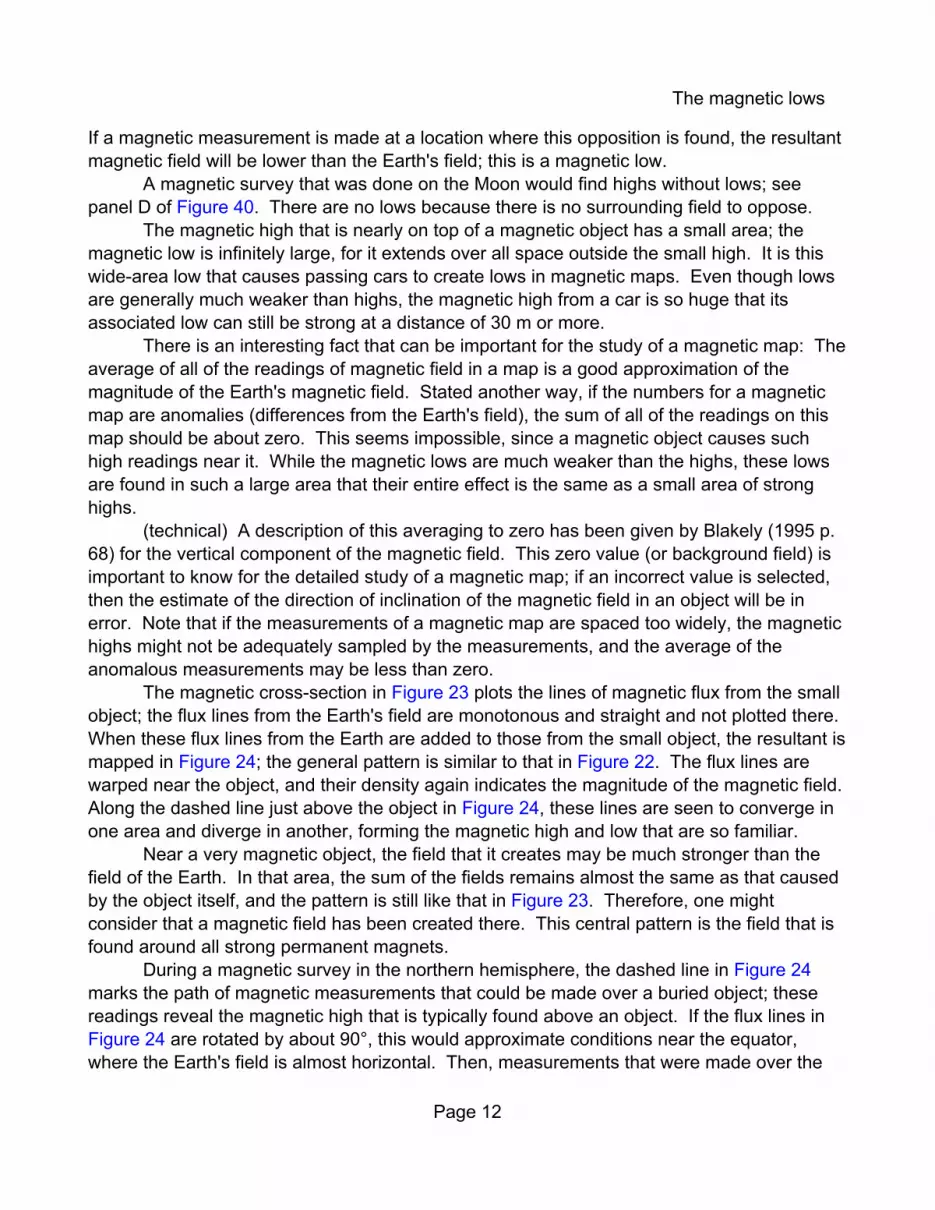
If a magnetic measurement is made at a location where this opposition is found, the resultantmagnetic field will be lower than the Earth's field; this is a magnetic low.
A magnetic survey that was done on the Moon would find highs without lows; seepanel D of Figure 40. There are no lows because there is no surrounding field to oppose.
The magnetic high that is nearly on top of a magnetic object has a small area; themagnetic low is infinitely large, for it extends over all space outside the small high. It is thiswide-area low that causes passing cars to create lows in magnetic maps. Even though lowsare generally much weaker than highs, the magnetic high from a car is so huge that itsassociated low can still be strong at a distance of 30 m or more.
There is an interesting fact that can be important for the study of a magnetic map: Theaverage of all of the readings of magnetic field in a map is a good approximation of themagnitude of the Earth's magnetic field. Stated another way, if the numbers for a magneticmap are anomalies (differences from the Earth's field), the sum of all of the readings on thismap should be about zero. This seems impossible, since a magnetic object causes suchhigh readings near it. While the magnetic lows are much weaker than the highs, these lowsare found in such a large area that their entire effect is the same as a small area of stronghighs.
(technical) A description of this averaging to zero has been given by Blakely (1995 p.68) for the vertical component of the magnetic field. This zero value (or background field) isimportant to know for the detailed study of a magnetic map; if an incorrect value is selected,then the estimate of the direction of inclination of the magnetic field in an object will be inerror. Note that if the measurements of a magnetic map are spaced too widely, the magnetichighs might not be adequately sampled by the measurements, and the average of theanomalous measurements may be less than zero.
The magnetic cross-section in Figure 23 plots the lines of magnetic flux from the smallobject; the flux lines from the Earth's field are monotonous and straight and not plotted there. When these flux lines from the Earth are added to those from the small object, the resultant ismapped in Figure 24; the general pattern is similar to that in Figure 22. The flux lines arewarped near the object, and their density again indicates the magnitude of the magnetic field. Along the dashed line just above the object in Figure 24, these lines are seen to converge inone area and diverge in another, forming the magnetic high and low that are so familiar.
Near a very magnetic object, the field that it creates may be much stronger than thefield of the Earth. In that area, the sum of the fields remains almost the same as that causedby the object itself, and the pattern is still like that in Figure 23. Therefore, one mightconsider that a magnetic field has been created there. This central pattern is the field that isfound around all strong permanent magnets.
During a magnetic survey in the northern hemisphere, the dashed line in Figure 24marks the path of magnetic measurements that could be made over a buried object; thesereadings reveal the magnetic high that is typically found above an object. If the flux lines inFigure 24 are rotated by about 90°, this would approximate conditions near the equator,where the Earth's field is almost horizontal. Then, measurements that were made over the

The magnetic lows
Page 13
top of the magnetic object would find low readings, just like the low values that are plotted inpanel D of Figure 11. In the northern hemisphere, if one makes magnetic measurements ona vertical surface, magnetic lows are also found next to magnetic objects. This condition canbe created in Figure 24 by rotating the dashed line by 90° about the middle of the square sothat the line is vertical.
Figure 23 and Figure 24 illustrate two different ways of thinking about magneticobjects; both ways give an equivalent result and both ways of reasoning are correct. InFigure 23, one thinks of the object as creating a magnetic field; in Figure 24, one thinks of theobject as warping the Earth's field. If an object is magnetized by the Earth (inducedmagnetization), then either approach works fine. However, if an object has remanentmagnetization, then it is better to consider it as creating a magnetic field, as in Figure 23. This is because the magnetic field from that permanent or remanent magnetization isprobably not in the direction of the Earth's field. Induced and remanent magnetization will bediscussed in the next section of this report.
Remanent magnetization can be revealed in a magnetic map and its direction can beestimated. This direction might indicate if an object has been burned or fired where it rests inthe soil, or if it was fired or formed somewhere else and later moved to the location where it isfound.
The direction of remanent magnetization is the same as the direction that isdetermined from an archaeomagnetic sample that has been taken from an excavation. Likethat archaeomagnetic sample, a magnetic map has the potential for revealing the age that afeature was created.
This direction of remanent magnetization is suggested by the direction from amagnetic high to a low, and also by the ratio of the amplitudes of the anomaly high to theassociated low. However, one must be careful, for this direction may be altered in amagnetic map. Figure 25 shows two sources of this change: The slope of the groundsurface, and the warping of an anomaly by other anomalies that are nearby.
It is not uncommon for a high in a magnetic map to have no low nearby that is clearlyassociated with the high. Figure 39 is a map where highs predominate. However, there isalways a low associated with every high; this low may simply be invisible in a map.
There are two general causes for the apparent lack of lows: A nearby high may haveobscured a low; variability and noisiness in the measurements may also distort a low andmake it unrecognizable. In Figure 39, the closely spaced objects cause highs that overlap(that is, objects are unresolved); many lows are squeezed out by these highs. Even wherethe north sides of objects are clear of other anomalies, these lows are indistinct. This iscaused by the noisiness of the measurements; the noise may be due to the magnetometer'selectronics, to the survey procedures, and to natural variability of the soil. In panel D ofFigure 21, the high is clear, while the low is so distorted that it is almost invisible. In rarecases, a low that is associated with a high may be distant, as in the pipe example in panel Bof Figure 14.
The low spatial resolution of the map in Figure 39 is caused by the large height of the

Induced and remanent magnetization
Page 14
magnetic sensor (0.95 m). When magnetic maps were measured with the magnetic sensoron the surface of the soil, the resolution was excellent. The amplitudes of the lows weremuch larger, and they were clarified into simple arc-shapes, such as that seen in Figure 3.
Induced and Remanent MagnetizationTwo types of magnetism create the anomalies in magnetic maps. Induced magnetism
might be called the effect of a good magnetic "conductor"; Figure 22 is a typical illustration ofthis effect. Remanent magnetism is the effect of a permanent magnet.
It is valuable to distinguish these two types of magnetism. It appears that steel usuallyhas a high remanent magnetization, while iron may have a high induced magnetization. Thisdifference may therefore allow the age of artifacts to be estimated.
Figure 26 illustrates one way of thinking about the difference between induced andremanent magnetization; in fact, this figure summarizes a simple procedure that allowsquantitative measurements of the two types of magnetization. When rotating the object, it isimportant that it be along a line that goes through the magnetic sensor and is in the directionof the Earth's field, in both its inclination and declination.
The magnetic maps in Figure 27 and Figure 28 show how the anomalies change whenan object with just induced or just remanent magnetization is rotated to different angles. Onecan see how these effects can create both the oscillating pattern (remanence) and the shift oroffset (due to induced magnetization) in Figure 26.
The amount of induced or remanent magnetization in an object is called its magneticmoment. This property can be quantified with the unit ampere-meter-squared, Am2. Forobjects that are weakly magnetic, a unit that is 1000 times smaller may be applied; this iscalled the milliampere-meter-squared, mAm2. These units quantify the total amount ofmagnetic material in an object. The same unit is applied to induced and remanentmagnetization; the sum of these two quantities is called total magnetization. A car may havea magnetic moment of 500 Am2, while the magnetic moment of a brick may be 10 mAm2.
In order to compare these quantities from one material to the next, one can divideeach magnetic moment by the mass or the volume of that object; these values might becalled relative magnetic moments. However, when the magnetic moment of an object isdivided by its volume, the result is called the intensity of magnetization of the object; this hasthe unit of Amperes per meter, A/m.
When the remanent magnetization of an object is divided by its induced magnetization,the result is called the Q ratio (sometimes referred to as the Koenigsberger ratio). In Figure29, an object is assumed to have induced magnetization (Mi) and / or remanentmagnetization (Mr). While the directions of these magnetizations remain the same for eachmap, the Q ratio changes. If the magnetization is only induced, the direction from themagnetic high toward the low is that of the Earth's magnetic field; if an object has beenrecently fired and magnetized in place, then its remanent magnetization would also pointtoward magnetic north.
For the illustrations in Figure 29, remanent and induced magnetization point in two

Data processing
Page 15
different directions; this figure shows how the angle from the magnetic high toward the lowrotates from magnetic north toward the direction of remanence as the Q ratio increases. Asmany as four arrows in each panel indicate important magnetic directions. Note that thedirection from the magnetic high to the low is never the direction of remanent magnetization,although it gets very close to that direction for a high Q ratio (Schnetzler and Taylor 1984). Also note that the direction of total magnetization and the direction of the high-low angle arenot the same, although they are close together.
The Q ratio affects the magnetic maps of clusters of objects. At archaeological sites,these clusters are found as lenses of discarded debris; brick walls are simply clusters ofbricks that have differing directions of magnetization. Figure 30 illustrates how magneticmaps change with the Q ratio of randomly magnetic objects. The calculations for the figurewere made over a layer of 121 dipoles, marked with X's in the figure. The random directionsof remanent magnetization can create very complex magnetic maps, without any trace of asimple low to the north of the cluster.
The individual anomalies that are apparent in the magnetic map of Figure 30 occurwhere the magnetizations of a group of nearby dipoles are accidentally oriented in about inthe same direction. There are only about a dozen highs and lows in panels C and D of Figure30; this is because of the low spatial resolution of the maps. Had the calculations been madecloser to the layer of dipoles, there would have been 121 highs and 121 lows in each map.
Brick walls are typically detected with maps that are similar to panel C in Figure 30;this is because the Q ratio for brick is often around 5 - 10. Walls constructed of magneticstone show the same pattern (Barba and others 1996). The brick wall in Figure 20 isrevealed with a simple and linear pattern; this is only because this wall was thoroughly heatedand remagnetized in a fire that destroyed the building. The heat was sufficient to realign theremanent magnetization of the brick.
The random directions of remanent magnetization of brick not only complicate amagnetic map, they also reduce the amplitude of the anomalies. A single brick may cause alarger anomaly than a small cluster of bricks; this is because the large remanentmagnetization of one brick may be partly canceled out by an opposite direction ofmagnetization of an adjacent brick. If there is a large and compact mass of fired objects,such as pot sherds, the remanent magnetization may have essentially disappeared, leavingonly induced magnetization.
Data ProcessingThis is the step that falls between making the magnetic measurements and plotting a
map of the findings. This step is discussed because it may affect the appearance of a mapand one's understanding of it.
Magnetic measurements are affected by temporal changes in the Earth's magneticfield. A gradiometer automatically provides a good correction. If a gradiometer is not used, asecond and stationary magnetometer (called a base station) may make readings insynchronization with those of the moving magnetometer; if so, the pairs of readings may

Data processing
Page 16
simply be subtracted. If the readings of this base station are not synchronized with those ofthe moving magnetometer, good corrections for temporal changes are still possible if thetimes of all the readings are recorded: One just estimates the base station reading at eachtime that a mapping measurement is made. That base station value is subtracted from themapping measurement; a linear interpolation can be made between the base stationreadings.
If a base station fails, and no temporal correction of the magnetic measurements ismade, magnetic maps may be affected as shown in the top panels of Figure 31; thesecalculated maps assume that traverses were along north-south lines. Weymouth andLessard (1986) give examples of maps with uncorrected temporal change.
Even without a base station, temporal effects in a magnetic map may be estimated byseeing how the readings change with time in areas of the map where magnetic anomalies areweak. The lower panels in Figure 31 illustrate that a moderately good correction may bepossible. A more detailed discussion of the correction of temporal change has been given byTabbagh (2003).
Modern magnetometers make their measurements very quickly, and this allows one toexplore large areas with a good spatial resolution. The close spacing of the measurementsaccentuates faults that were found with earlier and slower magnetometers, but which may nothave been visible in their lower resolution maps. These faults are shown in Figure 32; similarfaults are also apparent in parts of Figure 15.
The errors are apparent as undulations on the contour lines. While these faults maynot have a serious effect on the interpretation of a magnetic map, they definitely make themap look inferior. Figures 33 - 39 describe the correction of the faults in the original readingsof Figure 32.
The magnetic map of Figure 32 reveals about two dozen magnetic anomalies that arecaused by circular blocks of glassy slag, a remanent of the iron industry of Denmark in aboutthe year 1000 . The slag blocks were formed in pits below furnaces; the blocks contain someiron that is readily detected by a magnetic survey. The blocks are typically about 0.25 m thickand have a diameter of about 0.75 m; their upper surfaces may be about 0.3 m underground(Voss 1995).
The magnetic measurements that create Figure 32 were surveyed along lines thatwent alternately to the north and south; the lines were spaced by 0.25 m. The undulations onthe contour lines would be much less if the line spacing was 0.5 m, rather than 0.25 m; thesmall spacing between the lines of traverse accentuates changes in the direction of thecontour lines. If the line spacing had been 1 m, it is unlikely that any undulations would bevisible in the resulting map. It is the close spacing between the lines that accentuates thefaults, but this narrow spacing is needed in order to have a high spatial resolution.
It is easy to remove the undulations that are unwanted in Figure 32; see Figure 33. Since the data processing for this figure has altered the amplitudes and widths of theanomalies, an interpretation of this smoothed map would lead to errors in estimates of thedepth and quantity of magnetic materials that are underground. It may be important to try to

Data processing
Page 17
determine if the measurements of a published magnetic map have been smoothed; if thecontour lines are seen to be too smooth for the stated measurement interval, then it is likelythat the map has been altered for the worse, even though it may look prettier.
The faults that are in the magnetic map of Figure 32 would have been greatlydiminished or invisible if the survey was done with measurement traverses going in only onedirection; Figure 34 shows the great improvement that is possible. However, this is not anefficient use of field time, and faults remain invisible in the map.
The two faults that are discussed here are called heading error and locational error. Itis possible to separate these faults with a study of the contours on a magnetic map; seeFigure 35. However, it is easier to find these faults with a little arithmetic. First, check forheading error by calculating the averages of the readings along lines of traverse. Figure 36shows the result for this example, and Figure 37 shows the improvement that a correctionprovides.
The undulations that remain in Figure 37 are primarily caused by locational errors inthe readings. The vertical columns of numbers in the map are incorrectly located; they havea shift that alternates between the north and the south direction. This shift can be quantifiedas shown in Figure 38. This fault may then be undone by correcting the coordinates of thereadings, and the result in Figure 39 has a great improvement over the original map of Figure32. This shifting of the measurements along lines of traverse is easiest to do if the distanceis a multiple of the measurement or gridding interval; otherwise, interpolation between thereadings (gridding) is required to determine the new values.
The effects of bidirectional traverses may also be determined by measuring a singleline in both directions. If this test is done exactly the same as the survey of a large area, itcan furnish the information that is needed to correct both heading and locational error in thelarge-area survey.
While both heading and locational error will be found in almost all original magneticmeasurements, both effects may not be apparent or cause difficulty in specific maps andlocations. The effects of heading errors are most apparent where the lateral gradient of themeasurements is low. The effects of locational errors are most apparent wherealong-traverse gradients are high.
One step in data processing is a reformatting of the readings. The originalmeasurements will typically be stored in a computer file with a temporal or serial order; eachline of data from the magnetometer will have two numbers for the coordinate of the location ofthe reading; that same line will also include the magnetic reading, and perhaps the time ofmeasurement. These original measurements will then be converted into a matrix of numbers,without individual coordinates or times; this matrix will look much like the group of numbers inFigure 1. This conversion or reformatting is done with the process called gridding, and it is apart of most computerized mapping programs. The default settings of the program that doesthis gridding are almost never suitable for magnetic maps. This default setting will likelymake a magnetic map that looks good, but the readings will probably have been altered somuch that the magnetic anomalies have been modified and therefore it may not be possible

Data processing
Page 18
to interpret the map correctly.If magnetic measurements are made at uniform intervals along lines, the gridding
operation should exactly retain each original value; no values should be added or subtracted. Some magnetic surveys will have the readings at a slightly irregular spacing along lines oftraverse; this is done because it is easier than to make them at a fixed and constant spacing. In this case, the gridding will change essentially all of the original readings to new values. Itis important that the gridding be done so that each new value depends only on up to two orthree original readings that are nearest each grid point along a line of traverse; this new valueshould not be affected by any of the readings on adjacent lines of traverse. If this procedureis not followed, then the magnetic measurements have been smoothed, and again aninterpretation can give incorrect values for the depth and quantity of magnetic material.
It is always best that data processing be the minimal amount that allows an adequatemap. The failings of each possible process that might be applied to the data must beunderstood. Some of these failings are most apparent at locations on a magnetic map wherethere are abrupt or one-point changes in the magnetic field. The upper panels of Figure 40show how two common faults may be recognized in a magnetic map.
While magnetometers can make their measurements very quickly, the operators of theequipment cannot walk very fast. For this reason, the readings are often very closely-spacedalong lines whose spacing is much greater. It is better if the two spacings are the same;magnetic maps are clearer and more certain if the spacing between measurements alongtraverses is the same as the spacing between lines of traverse. This is often not practical,and panel C of Figure 40 shows the distorted patterns that may appear on a magnetic map. The visual appearance of these distortions may be reduced by interpolating additionalcolumns of values between the lines of measurement. These interpolated values are usuallyquite different from the measurements that would have been made at those missinglocations; this means that an interpretation of the resulting map will lead to errors.
A magnetic map, by itself, has little value; it is important that additional information beincluded with the text for each map. The most important item is what type of magneticmeasurements are in the map (total field, vertical component, gradiometer). The height ofthe magnetic sensor, and the spacing between the sensors of a gradiometer should also belisted. The contour interval should be stated; alternatively, a gray or color scale is needed, orthe amplitudes of some anomalies may be noted. The size of the area should be indicatedwith a scale on the map, and the direction of magnetic north should be marked. The intervalbetween measurements along lines can be noted; this may be both in time and distance. The spacing between lines should be listed, and the traversing directions also. Theinformation with a map can mention what material is at the surface and the topographic reliefin the area. The equipment manufacturer and the model of the instrument can be noted. Thedate of survey and also the time could be important for a check on noise interference andperhaps temporal changes. Any data processing that was applied should be stated anddescribed sufficiently so that an independent reader will know what has been done.

Analysis of magnetic maps
Page 19
Analysis of Magnetic MapsSeveral different types of analysis may be applied to magnetic maps. These types
might be called Anomaly description, Archaeological identification, and Analyticalinterpretation; any one of these analyses might be called a geophysical interpretation.
An anomaly description might result in something like "An L-shaped pattern is locatedat ..." or "Of 83 identified anomalies, 28 per cent had amplitudes greater than 5 nT". Thistype of analysis summarizes and counts anomalies, and possibly does some categorizationof them by their shape or amplitude. Perhaps a map is included that has a simplification ofthe anomalous patterns into straight or curved lines. No technical knowledge of geophysicsis required for this type of analysis.
An archaeological identification might result in a statement such as "This anomaly maybe caused by a Bronze-age burial tomb", or "These lines mark the walls of ancient gardenterraces". This type of analysis requires archaeological knowledge, and it can be the mostvaluable analysis of all. This analysis is based on knowledge of the archaeological featuresthat are expected at the site where the survey was done; the interpreter probably hasexperience with excavations that have been done after geophysical surveys at similar sites.
An analytical interpretation may also be called a technical, a quantitative, or aparametric analysis. This might result in statements such as "A mass of iron that could be aslarge as 4 kg could be as deep as 1.3 m at this point" or "A volume of soil with a susceptibilityof 0.02 has the cross-section shown in the figure". This type of analysis requires amoderately good knowledge of geophysics.
All of these types of analysis are valuable. They may also be combined. Anarchaeological identification along with an analytical interpretation can be particularly rich ininformation for the archaeologist.
Little assistance is needed for an analysis that is an anomaly description. I do notknow enough about archaeological identification to be of much help to you. However, anintroduction to some of the ideas of analytical interpretation is included here.
Figure 41 is a graph that shows a line of data that crosses over a compact magneticobject, marked with a green circle at the bottom. This graph illustrates an excellent way ofestimating the depth of an object: It is simply equal to the width of the anomaly at half of itspeak amplitude. This "depth" is the sum of the actual depth of the object underground plusthe height of the magnetic sensor above the surface. This approximation is accurate forcompact objects; if an object is spread out into a lens, this procedure would give an estimateof depth that is greater than the actual depth; it is not always possible to determine from amagnetic map if an object is spread out and not compact.
The width is best measured along a line that goes through the peak of the anomalyand has a direction toward the associated magnetic low; this may be along a magneticnorth-south line. However, the width of the anomaly caused by a compact feature is aboutthe same along an east-west line. If an anomaly high is not very circular, this may mean thatthe object is not compact; however, an average of the diameters of that anomaly can stillprovide a valuable estimate of maximum depth. This procedure is correct for a total field

Analysis of magnetic maps
Page 20
magnetometer; if a magnetic map from a gradiometer is being studied, the depths with thisprocedure will likely be a bit too shallow. The procedure can be applied to surveys that havebeen done at a wide range in the inclination of the Earth's magnetic field (RadhakrishnaMurthy 1998 p. 242). If the anomaly is predominantly a magnetic low, this procedure can beapplied to that low.
The half width rule can also help with the analysis of linear magnetic anomaliescaused by long features; this assumes that the features have a compact cross-section. InFigure 17, the calculated anomaly of the square prism has a half width of 1.5 m; this is alsothe distance between the calculation surface and the middle of the prism.
While features must be compact for this simple analysis, they do not have to be small. If a feature is compact or rather spherical, then the depth estimate is to its middle, no matterhow large it is. In fact, it is not possible to say much about the size of a feature from theshape of its magnetic anomaly; however, the peak amplitude of the anomaly might provideinformation about the volume or mass of the feature. The equation in the upper right cornerof Figure 41 shows the method. Since the analysis indicates that the magnetic moment ofthe object is about 1 Am2 (which was the assumption for the calculation), the anomaly couldbe caused by iron having a mass of 30 kg. While there are many possible errors in this typeof estimate, it is valuable to be able to distinguish the anomaly of a nail from a cannonball;without this analysis, that distinction could not be made just by looking at the magnetic map.
The green symbols on the calculated magnetic maps in this report locate the magneticsources; these are not at the peaks of the magnetic anomalies. These calculated maps allowone to estimate the offset between this peak anomaly and the center of the magnetic feature. This offset is typically a short distance from the magnetic high toward the magnetic low. Ifthis offset is not considered, a small test excavation that is placed at the peak of a magneticanomaly may fail to locate a small feature. If a feature is larger, such as one of the squaresin Figure 10, the anomaly may be significantly offset from the feature; an excavation on theedge of the anomaly may fail to detect the edge of the feature. By failing to detect that edge,the feature may not be identified as anything unusual.
Analytical interpretations often require elaborate mathematics or specialized computerprograms. These procedures are valuable, but they can hide fundamental and simple ideasabout magnetics. Fortunately, it is possible to approximate the anomaly of one type offeature using simple geometry; Figure 42 shows the method, which is described in detail byNettleton (1942). At a time when it was not practical to use computers for analysis, thisprocedure was applied by Elizabeth Ralph (University of Pennsylvania Museum) for theanalysis of a buried wall in southern Italy (Rainey and Lerici 1967 p. 60).
Some general principles of magnetics can aid the interpretation of magnetic maps. The anomalies of features remain the same if the distance to the features divided by the sizeof the features remains constant; this assumes that the magnetic moment of the featuresincreases with their size, or that their susceptibility remains constant. A spherical magneticshell causes the same anomaly as a solid sphere, except perhaps for amplitude. An infinitelybroad and flat magnetic stratum is completely invisible to a magnetic survey (Blakely 1995 p.

The components of the magnetic field
Page 21
285). This means that one may add or subtract any infinite strata without altering ananalysis. It is easiest to study a hole in a magnetic solid by assuming that the hole has anegative value for its magnetic moment, while the value for the surrounding is zero.
Many geophysical books give good introductions to the procedures for the technicalanalysis of magnetic maps. For a full understanding of quantitative interpretation, there is nopublication that is better than the book by Blakely (1995).
Some of the clearest descriptions of magnetic principles have been given by earlyauthors (Heiland 1940; Haanel 1904). Perhaps many of the writers of current books onceread those authors and found the topics so clear that they thought it was not necessary torepeat the discussions in their books. Since the units for magnetic quantities are different inthese early books, that can make them more difficult to read.
The Components of the Magnetic FieldThe magnetic field is a vectorial quantity; it has both a magnitude and a direction.
Three numbers describe the magnetic field at any point, but usually only one of thesenumbers is measured or mapped. The upper two panels in Figure 43 shows maps of thedifferent patterns that are measured with two types of magnetometers; fluxgatemagnetometers often measure just the vertical component of the magnetic field. Both mapsare similar, and both are valuable for magnetic exploration.
The total field map in panel A of Figure 43 can be calculated from the maps of threeperpendicular components of the magnetic field, shown in panels B - D. This must not be asimple addition of the readings from each map (that is called a scalar addition); instead, itmust be a vectorial addition, which is the square root of the sums of the squares of themagnetic fields in the three maps.
While the magnetic field can be described by three measurements that have beenmade in perpendicular directions, it can also be described by a magnitude (panel A of Figure43) along with two angles. These angles are the inclination (vertical angle) and declination(horizontal angle) of the magnetic field. Calculations of these directions are plotted at the topof Figure 44 for the same object that is mapped in Figure 43. Note that changes in the angleof the field are very small. The declination angle can be measured with a typical magneticcompass; indeed, a simple compass can be suitable for detecting very massive iron objects. The inclination angle can be measured with what is called a dip meter; this is just a magneticcompass whose needle swings in a vertical direction. A dip meter can be made moderatelysensitive to magnetic features by counterbalancing the tendency of the needle to point in thedirection of inclination of the Earth's field.
The gradient of the magnetic field that is measured most commonly is the verticalgradient (Figure 6). However, it can also be valuable to measure horizontal gradients; thelower two panels in Figure 43 show the maps of these gradients for a single dipolar object. Since these maps show three associated anomalies from a single object, these anomaliesare more complex than those from other magnetic measurements; this same complexity isapparent in the shaded relief map in Figure 2. In spite of their complexity, these horizontal

Conclusion
Page 22
gradients aid some types of magnetic surveys. A survey with sensors to the left and right ofthe line of traverse can double the rate at which an area is explored for rare features. Withairborne surveys, it is difficult to mount sensors along a vertical line, for this increases windresistance; horizontal sensors are easily positioned inside an aircraft, for example at the tipsof the wings.
If a magnetic map is measured with adequate resolution, then the different maps inFigures 43 and 44 may generally be converted from one to the other by applyingmathematical procedures. These ideas have been summarized by Gunn (1975). This leadsto the important result that a magnetic map that has been measured with one componentcannot be said to be superior to another map that has a different component.
ConclusionMagnetic maps contain much more information than just the shape and pattern of the
high readings. Why waste this information?
You are welcome to copy this report and give it to anyone else. Should you distribute anypart of the report widely, such as on the internet, please tell me.
Bruce W. BevanGeosight356 Waddy DriveWeems, Virginia 22576USA
Details About the FiguresFigure 1: The values of the anomaly have been calculated; they assume a magnetic
dipole at a depth of 1 m below the calculation surface; this dipole has a magnetic moment of1 Am2 and it is located at the middle of the plot. The Earth's field was assumed to have theparameters: Be = 57,000 nT; Ie = 70°; De = 30° (grid angle); the dipole is magnetized in thedirection of the Earth's field. The numbers are centered on the calculation points.
Figure 2: Each of these maps has the same data, and it is described in the note forFigure 1. For these maps, the calculations were made at intervals of 0.1 m; the range of theanomaly values is -17.3 nT to 181.2 nT.
Figure 3: Again, the data are the same as that in Figure 2. With the multiple intervalplot, contours are drawn with a spacing of 2 nT between -20 and +20 nT; this spacing is 20nT for contour lines having values greater than 20 nT. In the map with a logarithmic interval,contours are at levels of -10, -5, -2, -1, 0, 1, 2, 5, 10, 20, 50, and 100. In the equal area plot,the contours are at levels of -7.9, -4.9, -3.5, -2.6, -1.8, -1.0, 0.1, 1.7, and 13.6. It appears thatan equal area plot is used by the Geometrics program called MagMap2000.
Figure 4: The same data is plotted here as that in Figure 2.Figure 5: This is the same dipole that has been applied to prior examples. As before,

Details about the figures
Page 23
the direction of magnetization of the dipole continues to be that of the Earth's field.Figure 6: The dipole source for the calculations is the same as that in Figure 1; for the
gradient maps, the lower sensor was assumed to be 1 m above the dipole. The sensorseparation for the gradiometer measurements was assumed to be 1 m for the total field, and0.5 m or the vertical component. The contour interval is either 5 nT or 5 nT/m. Additionaltypes of total field magnetometers include potassium, rubidium, and helium instruments. Theanomaly range in the three panels is: A = -17.3 to 181.2 nT; B = -20.2 to 158.8 nT/m; C =-23.3 to 268.8 nT/m.
Figure 7: Pottery kilns may have this shape (Smekalova, Myts, and Melnikov 1995); inorder to have the highest spatial resolution of these kilns, the authors made theirmeasurements with the magnetic sensor directly on the surface of the soil. Each arm of theE-shaped feature has a square cross-section with sides that are 0.5 m wide. The height ofthe sensor is determined from the upper surface of this feature, which has a magneticsusceptibility of 0.01. The Earth's field has parameters: Be = 57,000 nT; Ie = 70°; De = 45°. The anomaly range in the four panels is: A = -21.4 to 85.2 nT; B = -9.1 to 41.7 nT; C = -4.9to 27.4 nT; D = -3.0 to 19.9 nT.
Figure 8: The magnetic model is identical to that in Figure 7. The calculations weremade of the total field, and the vertical spacing between the sensors was assumed to be 0.5m. The anomaly range in the four panels is: A = -58.9 to 113.0 nT/m; B = -14.8 to 44.6nT/m; C = -7.0 to 22.9 nT/m; D = -3.8 to 14.8 nT/m.
Figure 9: These calculations are for magnetic dipoles. The Earth's field was assumedto be: Be = 57,000 nT; Ie = 70°.
Figure 10: The square feature (green outline) has a thickness of 0.5 m, and thecalculations were made at a height of 1.5 m above the top of its surface. The magneticsusceptibility of the feature is +/-0.1, and the (total field) contour interval is 20 nT. TheEarth's field was assumed to have the parameters: Be = 57,000 nT, Ie = +/-70°, De = 0. Theanomaly range in the four panels is: A, B, and C = -42.5 to 263.4 nT; D = -263.4 to 42.6 nT.
Figure 11: The parameters of the square feature are the same as those in Figure 10,and the sensor height is also 1.5 m. For these total field maps, the contour interval is 10 nT. The anomaly range in the four panels is: A = -11.0 to 281.8 nT; B = -55.9 to 220.5 nT; C =-89.9 to 101.5 nT; D = -84.1 to 26.6 nT.
Figure 12: The cross-section of the modeled foundation is a square with sides that are0.5 m long. The total field calculations were made at a height of 0.5 m above the top of thisfeature, and the contour interval is 5 nT. The feature has a susceptibility of 0.01. Theparameters of the Earth's field were assumed to be: Be = 57,000 nT; Ie = 70°; De = 0.
Figure 13: The parameters are exactly the same as for Figure 12 with the exceptionthat Ie = 0. If the north-south walls are not perfectly regular, then segments of those walls willbe detected on a magnetic survey.
Figure 14: For each of these calculations, the Earth's field was assumed to have theparameters: Be = 57,000; Ie = 70°; De = 30°; the calculations were made at a height of 0.5 mabove the top of the features. In panels A - C, the magnetic moment of the 8-m long bar was

Details about the figures
Page 24
set at 10 Am2; in panel D, the strength of the monopole was -10 Am. The anomaly range andcontour interval in the four panels is: A = -246.2 to 790.5 nT, contours at 25 nT; B = -384.6 to379.3, contours at 25 nT; C = -17.0 to 406.7, contours at 1 nT; D = -24.2 to 3774.2, contoursat 2 nT interval.
Figure 15: This survey was done in June, 1992, with an Overhauser magnetometer(model GSM-19FG, manufactured by Gem Systems) at the US Civil War battlefield atPetersburg, Virginia. The height of the total field sensor was 0.8 m, and a base stationmagnetometer allowed the correction of temporal changes. Bidirectional traverses weremade in an east-west direction and the measurement spacing and line spacing were both 2.5ft. Magnetic north was about 7° west of grid north during this survey. This survey isdescribed in an earlier publication (Bevan 1996).
Figure 16: The magnetic parameters of the calculation were those from the site: Be =53,200 nT; Ie = 66°; De = -7°. The monopole was located at E526.1 S144.8 at a depthunderground of 6.2 ft (1.9 m); its strength was -193.4 Am.
Figure 17: The cross-sectional areas (A) of the square, rectangular, and triangularprisms are: 1 m2, 8 m2, and 4 m2. The magnetic susceptibilities are listed as k values in thefigure. The flux density of the Earth's magnetic field (Be) was assumed to be 57,000 nT. Themagnetic moment per unit of length for each prism is then A * k * Be / (400 * pi) = 0.91 Am. The calculations were made with aid of the algorithm of Won and Bevis (1987).
Figure 18: This cellar locates the Taylor House on the battlefield of the US Civil War atPetersburg, Virginia. The survey was done on 13 August 1991, and it is described in anearlier report (Bevan 1996). The instrument was a Gem Systems model GSM-19FGOverhauser magnetometer, which measures the total magnetic field of the Earth; temporalcorrections were made with a base station magnetometer. The sensor height was 0.85 mand unidirectional traverses were made going toward the east; the line and measurementspacings were both 5 ft. The change in the spacing of the contour lines shows where theinterval switches between 5 and 25 nT.
Figure 19: The same area was explored for this map as in Figure 18. This survey wasdone on 27 January 1992, and the sensor height was 0.8 m. For this map, lines ofmeasurement traverse went alternately to the east and west. Except for this, the equipmentand procedures were the same as those for Figure 18.
Figure 20: This survey was done during the period of 25 - 27 June 1992; theprocedures and sensor height were the same as those for the map of Figure 18, althoughtraverses were made to the west only. For these surveys, the magnetic sensor was carriedon the end of a horizontal bar. Figures 18 and 19 could have been derived from themeasurements of this survey (by simply decimating the data), but separate surveys weredone for each map; this resulted in an interesting finding about seasonal changes in themagnetic anomaly of the brick foundation.
Figure 21: The dipole source at the middle of each map is the one in Figure 1. Inpanel A, every other point is up to 5 nT too high then up to -5 nT too low. For panel B, fivereadings along north-south lines were altered at two locations into triangular lows that

Details about the figures
Page 25
extended to a depth of -5 nT. In panel C, the spikes had either polarity. Rather than amedian filter, it may be better to calculate the laplacian at each point (this is the differencebetween the value there and the average of the four adjacent values); if this laplacianexceeds a threshold, the original reading can be replaced by the average of the four adjacentreadings. A pseudorandom number generator furnished the continuous noise pattern inpanel D.
Figure 22: Each flux line was traced with short line segments. The direction of fluxlines distant from the magnetic feature was set at the value for the Earth's field (70°). Afterone short segment was drawn, the direction for the next segment was determined by the ratioof the calculated magnetic field in the horizontal and vertical directions. At the boundary ofthe magnetic feature, the direction changes abruptly: The ratio of the tangent of the angle ofthe flux to the magnetic permeability is the same on both sides of boundaries (Lorrain andCorson 1970 p. 402; Grant and West 1965 p. 317). As this figure shows, the angle of a fluxline is farthest from the normal to a magnetic boundary in the more magnetic material. Inorder to show the divergence and convergence of the flux lines, the magnetic susceptibility ofthe feature was assumed to have a very high value; however, no correction was made fordemagnetization.
Figure 23: These flux lines were plotted just as those in Figure 22, except that thereare no boundaries to cross for this example. This object has been assumed to be a magneticdipole. While the flux lines look rather oval, they are not actually elliptical and they delineatea more complex curve. Unlike Figures 22 and 24, the spatial density of flux lines in this figureis not proportional to the field.
Figure 24: The dense flux lines near the object have not been drawn.Figure 25: The central dipole in each map is the standard dipole of Figure 2. For
panel D, a second dipole with a moment of 20 Am2 has been added at a depth of 6 m belowthe sensor surface; the direction of magnetization of this dipole is the same as the Earth'sfield.
Figure 26: For an accurate test, The object should remain at a constant distance fromthe magnetic sensor as it is rotated.
Figure 27: The rectangular box has a thickness of 2 m and a magnetic moment of 1Am2; the calculations of the total field were made at a height of 1 m above the top of the box. The parameters of the Earth's field were assumed to be: Be = 57,000 nT; Ie = 70°; De = 0. The amplitude of the magnetic high changes only within the range of 8.0 to 8.2 nT for thesefour calculated maps; the anomaly is highest when the length of the box is orientednorth-south. These illustrations show why it is important to have a compact sample when itsmagnetic properties are measured with the procedure in Figure 26.
Figure 28: Except for the change from induced to remanent magnetization (in ahorizontal direction) the parameters of the calculations are the same as for Figure 27. Inpanel D, note in particular that the anomalies have been shifted to the south. As with theillustration in Figure 27, the amplitudes of the magnetic highs and lows change very little withrotation; the magnitude of these anomalies ranges between 4.2 and 4.4 nT.

Details about the figures
Page 26
Figure 29: The induced magnetization has a direction I = 70°, D = 30°; the remanentmagnetization has a direction I = 30°, D = -45°. The vectorial sum of the two magnetizationsremains 1 Am2 for the calculations of each panel. Only the horizontal angles of the directionsare plotted in the figure. The Earth's field has the assumed magnitude of 57,000 nT. In panelD, the angle from the magnetic high to the low is 1.9° east from the direction of remanentmagnetization.
Figure 30: The Earth's field was assumed to be: Be = 57,000 nT; Ie = 70°; De = 0. Atotal of 121 dipoles have been placed in a regular matrix on a single level, which is 0.5 mbelow the calculations; the algebraic sum of the magnetic moments for each dipole is 0.01Am2. The directions of remanence are randomly chosen over a sphere; these directionsremain the same in panels B - D. If n is the number of dipoles (each with the same magneticmoment, composed of both induced and a significantly larger remanent component), then theanomaly will be change as follows with n:
n * induced + (square root of n) * remanent.Therefore, if n is small, the anomaly may be mostly from remanence, and if n is large, it maybe mostly from induction. The anomaly range in the four panels is: A = -43.9 to 115.9 nT; B= -23.9 to 69.7 nT; C = -19.2 to 45.2 nT; D = -58.1 to 46.6 nT.
Figure 31: The basic magnetic map in Figure 2 has been altered by adding amagnetic field to the calculated values; this addition increases in a linear fashion from the leftto right throughout the grid to a maximum of 20 nT. The partial corrections were done bysubtracting the reading at the north end of each column from every reading on that column. As alternatives, one could also subtract the median or mode value of each column from thatcolumn, or similarly subtract the average reading of each column after the readings farthestfrom the average have been removed.
Figure 32: This survey was done on 6 September 1995 using an Overhausermagnetometer (a model GSM-19GW, manufactured by Gem Systems). It was operated in itsdifference mode, and was connected to a second stationary sensor for temporal correction. One operator carried the sensor, while a second operator (at a distance of about 2 m) carriedthe readout console. The measurement interval along lines was 0.5 s and about 0.1 m; theline spacing was 0.25 m and traverses went alternatively to the north and south. The 14,954measurements in this gridded map were made in a span of three hours. Each north-southcolumn of readings (with a slightly irregular measurement spacing) was converted to auniform interval of 0.25 m by a quadratic interpolation between the measurements. Note thatthe contour lines on the north sides of anomalies show lesser undulations than on the southside; this is because the two errors partially cancel each other on the north side, while theerrors are magnified on the south side. This project was described in a 192-page report thatwas prepared for Olfert Voss (this and the following seven figures were taken from thatreport). A summary of the report was published by Bevan and Smekalova (2001); however,the original report has many more details about this survey and its analysis. The striations onthe contour lines in Figure 15 have the same origin as those in this figure.
Figure 33: The smoothing was done with a weighted average. The weighting of the

Details about the figures
Page 27
three readings on the central north-south column was two, while the weighting of the sixreadings on the adjacent columns was one; the sum was divided by 12.
Figure 34: For this survey, the measurement spacing was closer than it needed to befor the sensor height that was chosen; this close spacing was selected for this test in order toensure the best possible data for this magnetic map, and to be certain that all of the featuresthat might possibly be detected at this sensor height would be revealed.
Figure 35: The simplified contour line at the top encloses higher readings within theoval. The polarity of the line shifts that are found on other contour maps may be the oppositeof what is shown here. The polarity of the heading error is dependent on the location and Qratio of the iron that causes the fault. The polarity of the locational error may change with theoperator, and how the sensor is carried. The amplitude of the locational error will probablyincrease with traverse speed.
Figure 36: For some data, it can be important to eliminate the readings that weremade near strong anomalies before calculating these line averages; that care was notneeded for this map. The heading error was found to be very consistent during this survey. This consistency is not always found, particularly when there is a change in equipmentoperators, or the survey takes more than a day.
Figure 37: The correction works best where there is a low lateral gradient in themagnetic map. The addition was made to only half of the data, rather than adding andsubtracting a smaller amount from all of the data; this is because the analysis of a magneticmap is essentially unchanged if any small constant is added to all values.
Figure 38: For the cross-correlation, one of each pair of lines being examined wasshifted in increments of 0.01 m while interpolating the values at the coordinates of theadjacent line; the distance for the greatest correlation is plotted in this figure.
Figure 39: It is likely that most of the faults that remain in this magnetic map are errorsin location. These faults appear to be primarily caused by an imperfect registration betweenthe fiducial markers that were put in the data when crossing 1-m intervals along traversesand the magnetic field readings; this is because the time delay between a fiducial marker andthe following reading had no effect on the coordinate given that following reading.
Figure 40: The basic magnetic source of Figure 2 is centered in each of these maps. In panel A, the averaging window was 3x3 measurements or 0.3 m square; this averaginghad little effect on the central anomaly. In panel B, the calculations were made at intervals of0.5 m, and then interpolated to a spacing of 0.1 m; that is, four columns and rows wereinserted for every original. In panel C, calculations were made at intervals of 0.1 m alongnorth-south lines that were spaced by 1 m; while all of the calculations are correct, theinterpolation of the contours distorts the anomaly. In panel D, the direction of the remanentmagnetization was its usual value (Ir = 70°; Dr = 30°); the background field was set to zero. The rather circular contour lines shift as the Ir-Dr angle changes. If Ir = 90°, then thecontours would be centered in the map.
Figure 41: The magnetic moments are reasonable values for the different materials,and are based on my measurements of many samples. The magnetic moment listed for a

References
Page 28
brick wall should also be suitable for a cluster of potsherds; this value is lower than that forfired earth because of the random directions of remanent magnetization in the brick wall. Thehalf width rule has been described by Breiner (1957 p. 31) and by Telford, Geldart, andSheriff (1990 p. 87). Other depth rules have been discussed by Mares (1984 p. 134),Radhakrishna Murthy (1998 p. 246), and Blakely (1995 p. 238).
Figure 42: The units of the vertical axis are in nT if the Earth's field is vertical with amagnitude of 57,000 nT and the susceptibility of the prism is 0.01. The basic idea of thisprocedure can be extended to the calculation of the magnetic anomalies of polyhedra with theaid of the solid angles of their facets (Singh and Guptasarma 2001; Furness 1994).
Figure 43: The standard dipole of Figure 2 is used here again. The Earth's field hasthe values: Be = 57,000; Ie = 70°; De = 30°. The dipole is located at the middle of each mapand at a depth of 1 m below the calculation surface; the magnetic moment is 1 Am2. Thecontour interval is 5 nT. The negative of the vertical component is displayed so that thepolarity will be the same as that in panel A. The anomaly range in the four panels is: A =-17.3 to 181.2 nT; B = -9.3 to 191.1 nT; C = -91.7 to 74.6 nT; D = -86.5 to 77.2 nT.
Figure 44: The standard dipole of Figure 2 and 43 is applied here. The anomalyrange in the four panels is: A = 69.58 to 70.13°; B = 29.76 to 30.24°; C = -229.4 to 194.5 nT;D = -248.1 to 186.7 nT.
ReferencesBarba, Luis, Karl Link, Agustin Ortiz, and Albert Hesse, 1996. Magnetic study of
archaeological stone foundations at Loma Alta, Michoacan, Mexico. Page 786 - 788 inExpanded Abstracts of the 66th SEG Annual Meeting, Society of ExplorationGeophysicists (Tulsa, Oklahoma).
Barba P., L. A., Linda Manzanilla, R Chavez, Luis Flores, and A. J. Arzate, 1990. Caves andtunnels at Teotihuacan, Mexico; a geological phenomenon of archaeological interest. Chapter 24 (p. 431 - 438) in: Archaeological Geology of North America, edited byNorman P. Lasca and Jack Donahue. Geological Society of America (Boulder,Colorado).
Bartington, G., and C. E. Chapman, 2004. A high-stability fluxgate magnetic gradiometer forshallow geophysical survey applications. Archaeological Prospection 11:19 - 34.
Bevan, B. W., and T. N. Smekalova, 2001. Magnetization directions of iron slag in Denmark. Page 7 - 25 in: Filtering, Optimisation and Modelling of Geophysical Data inArchaeological Prospecting, edited by Mauro Cucarzi and Paola Conti. Fondazioneing. Carlo Maurilio Lerici (Rome).
Bevan, Bruce W., 1996. Geophysical Exploration for Archaeology. Geosight TechnicalReport Number 4. Geosight (Weems, Virginia).
Blakely, Richard J., 1995. Potential Theory in Gravity and Magnetic Applications. CambridgeUniversity Press (Cambridge).
Breiner, S., 1973. Applications Manual for Portable Magnetometers. Geometrics (San Jose,California). Available in PDF form on the web at: www.geometrics.com

References
Page 29
Dalan, Rinita A., and Subir K. Banerjee, 1998. Solving archaeological problems usingtechniques of soil magnetism. Geoarchaeology 13(1):3 - 36.
Dobrin, Milton B., and Carl H. Savit, 1988. Introduction to Geophysical Prospecting, fourthedition. McGraw-Hill (New York).
Evans, Michael E., and Friedrich Heller, 2003. Environmental Magnetism. Academic Press(Amsterdam).
Furness, Peter, 1994. A physical approach to computing magnetic fields. GeophysicalProspecting 42(5):405 - 416.
Grant, F. S., and G. F. Grant, 1965. Interpretation Theory in Applied Geophysics. McGraw-Hill (New York).
Gunn, P. J., 1975. Linear transformations of gravity and magnetic fields. GeophysicalProspecting 23(2):300 - 312.
Haanel, Eugene, 1904. On the Location and Examination of Magnetic Ore Deposits byMagnetometric Measurements. Department of the Interior (Ottawa).
Heiland, C. A., 1940. Geophysical Exploration (1968 reprint). Hafner Publishing (New York).Hrvoic, Ivan, Greg M. Hollyer, Mike Wilson, and Anthony Szeto, 2003. Development of a
high sensitivity potassium magnetometer for near surface geophysical mapping. FirstBreak 21(May):81 - 87.
Lorrain, Paul, and Dale Corson, 1970. Electromagnetic Fields and Waves, second edition. W. H. Freeman (San Francisco).
Mares, Stanislav, 1984. Introduction to Applied Geophysics. D. Reidel (Dordrecht).Nettleton, L. L., 1942. Gravity and magnetic calculations. Geophysics 8:293 - 310.Radhakrishna Murthy, I. V., 1998. Gravity and Magnetic Interpretation in Exploration
Geophysics. Memoir 40 of the Geological Society of India (Bangalore).Rainey, Froelich G., and Carlo M. Lerici, 1967. The Search for Sybaris, 1960 - 1965. Lerici
Editori (Rome).Robinson, Edwin S., and Cahit Coruh, 1988. Basic Exploration Geophysics. John Wiley
(New York).Schnetzler, C. C., and P. T. Taylor, 1984. Evaluation of an observational method for
estimation of remanent magnetization. Geophysics 49(3):282 - 290.Singh, Bijendra, and D. Guptasarma, 2001. New method for fast computation of gravity and
magnetic anomalies from arbitrary polyhedra. Geophysics 66(2):521 - 526.Smekalova, Tatyana N., Olfert Voss, Sergey L. Smekalov, 2005. Magnetic Survey for
Archaeology. Publishing House of Polytechnic University (St. Petersburg).Smekalova, T. N., V. L. Myts, and A. V. Melnikov, 1995. Magnetometric investigation of
Medieval pottery centers in mountainous Crimea. Pages 441 - 448 in: Archaeometryin South-Eastern Europe (PACT 45), edited by I. Liritzis and G. Tsokas. PACTBelgium (Rixensart).
Tabbagh, Jeanne, 2003. Total field magnetic prospection: Are vertical gradiometermeasurements preferable to single sensor survey? Archaeological Prospection. 10:75 - 81.

References
Page 30
Telford, W. M., L. P. Geldart, and R. E. Sheriff, 1990. Applied Geophysics, second edition. Cambridge University Press (Cambridge).
Voss, O., 1995. "Snorup - an iron producing settlement in West Jutland, 1st - 7th centuryAD". Proceedings of the Conference: The Importance of Ironmaking. May 8 - 13,Stockholm University (Norberg, Sweden).
Weymouth, J. W., and Y. A. Lessard, 1986. Simulation studies of diurnal corrections formagnetic prospection. Prospezioni Archeologiche 10:37 - 47.
Won, I. J., and Michael Bevis, 1987. Computing the gravitational and magnetic anomaliesdue to a polygon: Algorithms and Fortran subroutines. Geophysics 52(2):232 - 238.
Publication history:22 May 2006, corrected typographical errors.1 May 2006, original report.

-3 -2 -1 0 1 2 3East coordinate, m
Numerical values
-3
-2
-1
0
1
2
3N
orth
coo
rdin
ate,
m
-0.2
-0.2
-0.2
-0.3
-0.5
-0.8
-1.2
-1.5
-1.7
-1.8
-1.6
-1.4
-1.1
-0.1
-0.0
0.1
0.1
0.0
-0.4
-1.2
-2.0
-2.5
-2.5
-2.2
-1.8
-1.5
0.0
0.2
0.6
1.2
1.7
1.4
-0.1
-2.2
-3.5
-3.6
-3.1
-2.4
-1.8
0.1
0.6
1.7
3.6
6.5
8.4
5.5
-0.9
-4.9
-5.4
-4.3
-3.2
-2.3
0.2
1.0
3.1
8.1
18.9
33.0
30.1
7.0
-6.5
-7.8
-5.9
-4.0
-2.7
0.2
1.2
4.1
13.0
39.4
95.5
109.0
29.4
-8.6
-10.9
-7.4
-4.7
-3.0
0.0
0.9
3.7
13.1
45.7
131.7
165.0
36.2
-13.4
-13.2
-8.3
-5.0
-3.2
-0.3
0.1
1.6
6.8
22.7
55.0
53.8
-0.1
-17.3
-13.1
-8.0
-4.8
-3.0
-0.7
-0.7
-0.5
0.4
2.6
3.6
-4.0
-14.4
-14.9
-10.6
-6.7
-4.2
-2.7
-0.9
-1.2
-1.7
-2.4
-3.7
-6.2
-9.7
-11.5
-10.2
-7.5
-5.1
-3.4
-2.3
-1.0
-1.4
-2.0
-2.8
-4.1
-5.7
-7.0
-7.4
-6.5
-5.1
-3.7
-2.6
-1.9
-1.0
-1.3
-1.8
-2.4
-3.2
-4.0
-4.6
-4.6
-4.1
-3.4
-2.6
-2.0
-1.5
-0.9
-1.1
-1.5
-1.9
-2.4
-2.8
-3.0
-3.0
-2.7
-2.3
-1.9
-1.5
-1.2
Figure 1: The numbers of a magnetic map. This matrix shows readings at intervals of 0.5 m,as they may be measured with a magnetic survey. The values are positive or negativedepending on if the reading was greater or less than the value of the Earth's field. TheEarth's magnetic field was assumed to be 57,000 nanotesla (abbreviated nT). Therefore, thenumber 165 means than the total field at that point was actually 57,165 nT. It is difficult tosee the pattern of these numbers, so this matrix is almost always converted into a contourmap, like those in the following figures.

-3 -2 -1 0 1 2 3East coordinate, m
Line contour
-3
-2
-1
0
1
2
3
Nor
th c
oord
inat
e, m
-3 -2 -1 0 1 2 3East coordinate, m
Gray scale
-3
-2
-1
0
1
2
3
Nor
th c
oord
inat
e, m
-3 -2 -1 0 1 2 3East coordinate, m
Shaded relief
-3
-2
-1
0
1
2
3
Nor
th c
oord
inat
e, m
Wire frame
A B
C D
Figure 2: Four different types of maps. Each has important advantages. A line contour mapis excellent for showing high lateral gradients in the measurements by the close spacing ofthe lines; tick marks along the contours of this map reveal magnetic lows. A gray scale mapindicates the pattern of readings that are similar, even if the areas are distant from each otheron a map. A shaded relief map has the familiar appearance of an aerial photograph. A wireframe map clarifies the amplitudes of the readings.

-3 -2 -1 0 1 2 3East coordinate, m
Constant interval
-3
-2
-1
0
1
2
3
Nor
th c
oord
inat
e, m
-3 -2 -1 0 1 2 3East coordinate, m
Mulltiple interval
-3
-2
-1
0
1
2
3
Nor
th c
oord
inat
e, m
-3 -2 -1 0 1 2 3East coordinate, m
Logarithmic interval
-3
-2
-1
0
1
2
3
Nor
th c
oord
inat
e, m
-3 -2 -1 0 1 2 3East coordinate, m
Equal area
-3
-2
-1
0
1
2
3
Nor
th c
oord
inat
e, m
A B
C D
Figure 3: Four different types of line contour maps. These differ in the spacing or intervalbetween contour lines. A constant interval map readily shows the amplitudes of anomalies. If multiple intervals are used, high and low amplitudes may be displayed more completely. With a logarithmic interval, extremely wide ranges of readings can be seen. An equal areamap leaves no large blank areas; for this type of map, the area enclosed between eachadjacent pair of contour levels is the same.

-3 -2 -1 0 1 2 3East coordinate, m
Colored line
-3
-2
-1
0
1
2
3
Nor
th c
oord
inat
e, m
-3 -2 -1 0 1 2 3East coordinate, m
Stepped spectrum
-3
-2
-1
0
1
2
3
Nor
th c
oord
inat
e, m
-3 -2 -1 0 1 2 3East coordinate, m
Continuous colors
-3
-2
-1
0
1
2
3
Nor
th c
oord
inat
e, m
-3 -2 -1 0 1 2 3East coordinate, m
Stepped colors
-3
-2
-1
0
1
2
3
Nor
th c
oord
inat
e, m
A B
C D
Figure 4: Four different applications of color. It is conventional that high values be plotted asred, orange, or yellow, while low values are plotted as green or blue. If the map has coloredlines, it is possible to make a good print of it with black ink. A stepped spectrum map allowsthe display of a wide range of readings. The map with continuous colors allows one to easilydistinguish areas with high and low readings. A compromise between these maps can bemade with the version showing stepped colors.

-3 -2 -1 0 1 2 3East coordinate, m
Depth 0.5 m, 25 nT contours, peak 1419 nT
-3
-2
-1
0
1
2
3
Nor
th c
oord
inat
e, m
-3 -2 -1 0 1 2 3East coordinate, m
Depth 1 m, 5 nT contours, peak 181 nT
-3
-2
-1
0
1
2
3
Nor
th c
oord
inat
e, m
-3 -2 -1 0 1 2 3East coordinate, m
Depth 2 m, 1 nT contours, peak 23 nT
-3
-2
-1
0
1
2
3
Nor
th c
oord
inat
e, m
-3 -2 -1 0 1 2 3East coordinate, m
Depth 4 m, 0.2 nT contours, peak 2.8 nT
-3
-2
-1
0
1
2
3
Nor
th c
oord
inat
e, m
A B
C D
Figure 5: The effect of depth. If an object is deeper underground, its anomaly is broader,and its amplitude is lower. The peak of the anomaly also moves away from the middle of theobject, marked with an X here. For small or compact objects, if distance is doubled, then thepeak amplitude of the anomaly drops by a factor of about eight. Compare the peaks at adepth of 0.5 m and 1 m; their ratio is 7.8, which is close to the value 8.

-3 -2 -1 0 1 2 3East coordinate, m
Total field
-3
-2
-1
0
1
2
3
Nor
th c
oord
inat
e, m
-3 -2 -1 0 1 2 3East coordinate, m
Vertical gradient of total field
-3
-2
-1
0
1
2
3
Nor
th c
oord
inat
e, m
-3 -2 -1 0 1 2 3East coordinate, m
Vertical gradient of vertical component
-3
-2
-1
0
1
2
3
Nor
th c
oord
inat
e, m
A B
C
Figure 6: The three most common types of magnetic measurements. Total field readings aremade with a single magnetic sensor; this will likely be part of a cesium, Overhauser, or aproton magnetometer. If two of these sensors are aligned one above the other, then themagnetic gradient is measured (panel B). A slightly different magnetic gradient is measuredwith a fluxgate magnetometer (panel C). For this instrument, only that part of the magneticfield in the vertical direction is measured. With a gradiometer, the difference in the readingsbetween sensors at two heights is determined; this difference is divided by the spacingbetween the sensors to give a magnetic value in nT/m.

-3 -2 -1 0 1 2 3East coordinate, m
Height: 0.3 m; contours: 10 nT
-3
-2
-1
0
1
2
3
Nor
th c
oord
inat
e, m
-3 -2 -1 0 1 2 3East coordinate, m
Height: 0.6 m; contours: 5 nT
-3
-2
-1
0
1
2
3
Nor
th c
oord
inat
e, m
-3 -2 -1 0 1 2 3East coordinate, m
Height: 0.9 m; contours: 3 nT
-3
-2
-1
0
1
2
3
Nor
th c
oord
inat
e, m
-3 -2 -1 0 1 2 3East coordinate, m
Height: 1.2 m; contours: 2 nT
-3
-2
-1
0
1
2
3
Nor
th c
oord
inat
e, m
A B
C D
Figure 7: The blurring of shapes with increasing height (or depth). The E-shape of thisfeature becomes more rounded at a greater distance. This is a failing that magnetic surveysshare with all other types of geophysical exploration. The resolution of buried features can beimproved by using a gradiometer (see Figure 8) or by reducing the height of the magneticsensor.

-3 -2 -1 0 1 2 3East coordinate, m
Height: 0.3 m; contours: 10 nT/m
-3
-2
-1
0
1
2
3
Nor
th c
oord
inat
e, m
-3 -2 -1 0 1 2 3East coordinate, m
Height: 0.6 m; contours: 5 nT/m
-3
-2
-1
0
1
2
3
Nor
th c
oord
inat
e, m
-3 -2 -1 0 1 2 3East coordinate, m
Height: 0.9 m; contours: 3 nT/m
-3
-2
-1
0
1
2
3
Nor
th c
oord
inat
e, m
-3 -2 -1 0 1 2 3East coordinate, m
Height: 1.2 m; contours: 2 nT/m
-3
-2
-1
0
1
2
3
Nor
th c
oord
inat
e, m
A B
C D
Figure 8: The increased resolution of a gradiometer. These maps can be compared toFigure 7. The gradiometer map at a height of 0.9 m (panel C) shows about the sameresolution as a total field map at a height of 0.6 m (panel B in Figure 7). The price for havinga greater resolution with a gradiometer must be paid by making measurements at a closerspacing.

-6 -4 -2 0 2 4 6North coordinate, m
-100
0
100
200
300
Mag
netic
ano
mal
y, n
T
-100
0
100
200
300
Mag
netic
gra
dien
t, nT
/m
M
agne
tic g
radi
ent,
nT/m
Compare total field and gradient
Total field magnetometerGradient, 0.5 m spacingGradient, 1.0 m spacing
M = 1 Am2
depth = 1 m M = 27 Am2
depth = 3 m
surface
Figure 9: The decreased sensitivity of a gradiometer for deep objects. Two objects (greencircles) are at different depths, and the deeper one is more magnetic. With theseparameters, the total field magnetometer detects both objects with about the same peakanomaly. With the gradiometer, the deeper object has a weaker anomaly. This attenuationof deeper objects increases as the spacing between the gradiometer's sensors is smaller.

-6 -3 0 3 6East coordinate, m
Southern hemisphere
-6
-3
0
3
6
Nor
th c
oord
inat
e, m
-6 -3 0 3 6East coordinate, m
Northern hemisphere
-6
-3
0
3
6
Nor
th c
oord
inat
e, m
-6 -3 0 3 6East coordinate, m
Overhead feature
-6
-3
0
3
6
Nor
th c
oord
inat
e, m
-6 -3 0 3 6East coordinate, m
Less magnetic feature
-6
-3
0
3
6
Nor
th c
oord
inat
e, m
A
B
C
D
A B
C D
Figure 10: Important effects in magnetic maps. Panel A shows the typical map of a buriedfeature; the magnetic low is toward the north. If this feature was overhead (panel B), or thesurvey was done in the southern hemisphere (panel C), the magnetic high would be towardthe north. If the feature was less magnetic than the surrounding soil, then the principalmagnetic anomaly would be a low (panel D).

-6 -3 0 3 6East coordinate, m
Ie = 90; Be = 57,000 nT
-6
-3
0
3
6
Nor
th c
oord
inat
e, m
-6 -3 0 3 6East coordinate, m
Ie = 60; Be = 52,000 nT
-6
-3
0
3
6
Nor
th c
oord
inat
e, m
-6 -3 0 3 6East coordinate, m
Ie = 30; Be = 41,000 nT
-6
-3
0
3
6
Nor
th c
oord
inat
e, m
-6 -3 0 3 6East coordinate, m
Ie = 0; Be = 34,000 nT
-6
-3
0
3
6
Nor
th c
oord
inat
e, m
A B
C D
Figure 11: The effect of latitude in magnetic maps. Near the north pole (panel A), themagnetic field is strong, and highs are centered on magnetic features. Near the equator(panel D), the Earth's field (Be) is weaker, and lows are centered on magnetic features. Magnetic anomalies are fainter and more complex at the equator than at the pole. Atintermediate latitudes, a magnetic low is found north of the magnetic high.

-6 -3 0 3 6East coordinate, m
Square feature
-6
-3
0
3
6
Nor
th c
oord
inat
e, m
-6 -3 0 3 6Line coordinate, m
-20
-10
0
10
20
30
40NS line
EW line
Figure 12: The magnetic anomaly of a square feature with a square hole. This maptherefore approximates the anomaly of the foundation of a square building. Magnetic lowsare found on the north sides of both east-west walls. Profiles along north-south andeast-west lines are plotted below. The amplitudes of the anomalies are slightly lower alongthe east-west profile. This effect increases at lower latitudes; see Figure 13.

-6 -3 0 3 6East coordinate, m
Square feature at equator
-6
-3
0
3
6
Nor
th c
oord
inat
e, m
-6 -3 0 3 6Line coordinate, m
-40
-30
-20
-10
0
10
20
NS line
EW line
Figure 13: Invisible walls at the equator. This feature is the same as that in Figure 12. When magnetic maps are measured near the equator, features that extend in a north-southdirection may not be detected. Magnetic anomalies are created where the Earth's fieldcrosses the boundary between materials that differ in their magnetism. Since the Earth's fieldis horizontal here, no magnetic boundaries are crossed along the north-south walls until theeast-west walls are encountered.

-6 -3 0 3 6East coordinate, m
Magnetized in Earth's direction
-6
-3
0
3
6
Nor
th c
oord
inat
e, m
-6 -3 0 3 6East coordinate, m
Magnetized along length
-6
-3
0
3
6
Nor
th c
oord
inat
e, m
-6 -3 0 3 6East coordinate, m
Vertical, magnetized in Earth's direction
-6
-3
0
3
6
Nor
th c
oord
inat
e, m
-6 -3 0 3 6East coordinate, m
Monopole
-6
-3
0
3
6
Nor
th c
oord
inat
e, m
A B
C D
Figure 14: Anomalies of long, thin objects. These objects are typically pipes or shafts; theymay be gun barrels or wells. A corrugated iron pipe may be detected as in panel A, althougha cast iron pipe may cause the very different anomaly in panel B. If this iron pipe is vertical inthe earth, then the anomaly can be like that in Panel C. Wells may be revealed on magneticmaps similar to the patterns shown in panels C or D; if the iron extends to a great depth, thenpanel D illustrates the anomaly.

450 500 550 600East coordinate, ft
Magnetic anomaly of a well near Fort Morton
-250
-200
-150
-100
-50N
orth
coo
rdin
ate,
ft
Figure 15: The magnetic map of a well. The anomaly extends over a wide area; thenorth-south span of the map is 200 ft (61 m). The map is drawn with three contour intervals;changes in line spacing reveal these breaks. The highest anomalies have a contour intervalof 100 nT; intermediate contours are at 20 nT intervals; the remaining weaker anomalies areplotted with a contour interval of 5 nT. The highest anomaly, at E527.5 S145, has anamplitude of 2763 nT; the anomaly low to the north has a value of -30 nT.

450 500 550 600East coordinate, ft
Calculated field of the monopole model of a well near Fort Morton
-250
-200
-150
-100
-50N
orth
coo
rdin
ate,
ft
Figure 16: An approximation of the magnetic map of the well. This calculation shows thesame general pattern as the measurements in Figure 15. The magnetic map of a well maybe very similar to the map of a magnetic monopole, which is a mathematical approximation ofthe end of a very long magnetic object. The green X in the figure locates this monopole,which is only 1.4 ft (0.4 m) distant from the magnetic high that it causes.

-6 -4 -2 0 2 4 6North coordinate, m
-40
-20
0
20
40
60
80M
agne
tic a
nom
aly,
nT
Calculated anomalies of 2-D prismsBe = 57,000 nT; Ie = 70o; De = 0Calculations 1 m above tops of prisms
Three prisms: Square, k = 0.02
Rectangular, k = 0.0025
Triangular, k = 0.005
Figure 17: The effect of the concentration or dispersal of magnetic materials. As materialsare spread out, their anomaly decreases. These calculations were made for three featuresthat extend for a long distance perpendicular to the page. The amount of magnetic materialper unit length is the same for each of the three features. The feature with a squarecross-section gives the strongest anomaly, while the feature with a rectangular cross-sectionhas the weakest anomaly.

-120 -100 -80 -60 -40 -20 0 20 40East coordinate, ft
Measurement spacing = 5 ft (1.5 m), contours at 5 and 25 nT interval
20
40
60
80
100
120N
orth
coo
rdin
ate,
ft
Figure 18: The magnetic map of the buried brick wall of a cellar. The green rectanglelocates this cellar. Only part of the wall was detected, for the brick had been removed fromthe northern wall. Although this survey was done with a large spacing between themeasurements (5 ft = 1.5 m), the part of the cellar wall that remains was delineated. The twofollowing maps show how resolution improved with a closer spacing between the readings.

-120 -100 -80 -60 -40 -20 0 20 40East coordinate, ft
Measurement spacing = 2.5 ft (0.8 m), contours at 5 and 25 nT interval
20
40
60
80
100
120N
orth
coo
rdin
ate,
ft
Figure 19: A higher resolution magnetic map of the area shown in Figure 18. For thissurvey, the spacing between the readings was 2.5 ft (0.8 m) in both the north-south andeast-west directions. More anomalies are now apparent in this map, and the areas of theanomalies are smaller. Four times as many measurements were made for this map as forthe map in Figure 18.

-120 -100 -80 -60 -40 -20 0 20 40East coordinate, ft
Measurement spacing = 1 ft (0.3 m), contours at 5 and 25 nT interval
20
40
60
80
100
120N
orth
coo
rdin
ate,
ft
Figure 20: A very high resolution magnetic map. The measurement spacing was only 1 ft(0.3 m) for this survey. It is likely that the resolution of a magnetic map of this area would notbe improved if the measurement spacing was reduced below 1 ft. The anomalies on thismap are small and detailed. However, the magnetic anomaly of the brick foundation is hardlymore distinct here than in was in the map with a measurement spacing of 5 ft (Figure 18).

-3 -2 -1 0 1 2 3East coordinate, m
Noise: Approximate a magnetic pace
-3
-2
-1
0
1
2
3
Nor
th c
oord
inat
e, m
-3 -2 -1 0 1 2 3East coordinate, m
Noise: Approximate 2 passing cars
-3
-2
-1
0
1
2
3
Nor
th c
oord
inat
e, m
-3 -2 -1 0 1 2 3East coordinate, m
Noise: +/-10 nT spikes for 2 percent of data
-3
-2
-1
0
1
2
3
Nor
th c
oord
inat
e, m
-3 -2 -1 0 1 2 3East coordinate, m
Noise: Uniform random for all data to +/-5 nT
-3
-2
-1
0
1
2
3
Nor
th c
oord
inat
e, m
A B
C D
Figure 21: Errors in magnetic maps. These faults may be found in both total field andgradient maps. Panel A shows the pattern that may be caused by a magnetic object that isrepeatedly close to the magnetic sensor; shoes can cause this pattern. Passing vehiclesusually cause the magnetic readings to drop; panel C shows a pair of linear lows (at W1 andE1), aligned with the north-south direction of traverse. Lightning can cause a few one-pointerrors, like those in panel C. The most common type of noise is that in panel D;imperfections in magnetometers are the typical cause of this type of error.

Figure 22: Warping of flux lines in a magnetic object. This shows the cross-section of a longobject. The paths of the lines of magnetic flux from the Earth are plotted. Since the featurewithin the green square is more magnetic than the surrounding, flux lines are concentrated inthat feature. The magnetic anomaly that is measured is proportional to the spatial density ofthese flux lines. Just above the feature, along the dashed line, these flux lines are closertogether, causing a magnetic high. To the north of the feature, the lines are spaced morewidely, yielding a magnetic low.

Figure 23: The magnetic field of a small object. This object is located at the green circle. Itis magnetized by the Earth's field, and the rather oval lines show the paths of magnetic fluxfrom the object; these lines are too dense to draw in small sectors above and below theobject. The flux lines are drawn as red where they will add to the Earth's magnetic field,causing high readings. The lines are blue where they will subtract from the Earth's field, andwhere a magnetic low will be found. Magnetic measurements along the dashed line will yieldthe typical dipolar magnetic anomaly that is plotted at the top.

Figure 24: A summation of the Earth's magnetic field with that from a small object. This issimply a redrawing of Figure 23, after the Earth's field has been added to the field from thesmall object. As with Figure 22, a magnetometer will read higher values where the lines ofmagnetic flux are closer together (directly over the object) and lower values where the linesare farther apart (on the north side of the object). The curve above is a plot of this changealong the dashed line that goes through the flux map.

-3 -2 -1 0 1 2 3East coordinate, m
Slope down to west
-3
-2
-1
0
1
2
3
Nor
th c
oord
inat
e, m
-3 -2 -1 0 1 2 3East coordinate, m
Flat surface
-3
-2
-1
0
1
2
3
Nor
th c
oord
inat
e, m
-3 -2 -1 0 1 2 3East coordinate, m
Slope down to south
-3
-2
-1
0
1
2
3
Nor
th c
oord
inat
e, m
-3 -2 -1 0 1 2 3East coordinate, m
Lateral interference
-3
-2
-1
0
1
2
3
Nor
th c
oord
inat
e, m
A B
C D
Figure 25: Magnetic lows that are rotated due to topography. If a magnetic map is measuredon a flat surface, the low readings can be toward magnetic north, as in panel B. If the groundsurface slopes down by 20° toward the west, this low is rotated to the west; see panel A. Asimilar slope to the south can also cause a rotation of the anomaly, and panel C shows alsothat the anomaly peak has moved to the south of the source (the green X). A magnetic lowcan be shifted by the anomaly of a nearby object; panel D illustrates this effect.

Figure 26: Distinguishing remanent from induced magnetization. Check the reading at amagnetometer when the test object is distant. Then, bring the object close to the magneticsensor and rotate it a few times. The readings will oscillate about an average value. Thedifference between that average and the field with no object nearby is proportional to theinduced magnetization. The amplitude of the oscillations is proportional to the remanentmagnetization of the object. This curve is a plot of how a sequence of readings can allowthese two magnetic sources or effects to be distinguished.

-6 -3 0 3 6East coordinate, m
Rotation = 0
-6
-3
0
3
6
Nor
th c
oord
inat
e, m
-6 -3 0 3 6East coordinate, m
Rotation = 30 degrees
-6
-3
0
3
6
Nor
th c
oord
inat
e, m
-6 -3 0 3 6East coordinate, m
Rotation = 60 degrees
-6
-3
0
3
6
Nor
th c
oord
inat
e, m
-6 -3 0 3 6East coordinate, m
Rotation = 90 degrees
-6
-3
0
3
6
Nor
th c
oord
inat
e, m
A B
C D
Figure 27: Changes in the magnetic map of a rotating object. This box-like object (greenrectangle) is magnetized by induction; that is, it has induced magnetization. As the object isrotated, the magnetic low remains on the north side of the object, although the shape of theanomaly otherwise changes.

-6 -3 0 3 6East coordinate, m
Rotation = 0
-6
-3
0
3
6
Nor
th c
oord
inat
e, m
-6 -3 0 3 6East coordinate, m
Rotation = 30 degrees
-6
-3
0
3
6
Nor
th c
oord
inat
e, m
-6 -3 0 3 6East coordinate, m
Rotation = 60 degrees
-6
-3
0
3
6
Nor
th c
oord
inat
e, m
-6 -3 0 3 6East coordinate, m
Rotation = 90 degrees
-6
-3
0
3
6
Nor
th c
oord
inat
e, m
A B
C D
Figure 28: Rotating an object that has remanent magnetization. In this case, the magneticlow rotates with the object. For these calculations, the remanent magnetization is directedalong the length of the box, which is otherwise the same as that in Figure 27. Note that thereare small changes in the anomalies with rotation. These differences are caused by the factthat the direction of the Earth's field remains the same, while the direction of the field from thebox changes; the summation of the two fields therefore changes as the box rotates.

-3 -2 -1 0 1 2 3East coordinate, m
Q = 0 (only Mi)
-3
-2
-1
0
1
2
3
Nor
th c
oord
inat
e, m
-3 -2 -1 0 1 2 3East coordinate, m
Q = 0.5 (Mr = 0.5 * Mi)
-3
-2
-1
0
1
2
3
Nor
th c
oord
inat
e, m
-3 -2 -1 0 1 2 3East coordinate, m
Q = 1 (Mr = Mi)
-3
-2
-1
0
1
2
3
Nor
th c
oord
inat
e, m
-3 -2 -1 0 1 2 3East coordinate, m
Q = infinity (only Mr)
-3
-2
-1
0
1
2
3
Nor
th c
oord
inat
e, m
R ELM
Earth'sfieldA B
C D
Figure 29: Rotation of a magnetic low due to the contribution of remanent magnetization. With induced magnetization alone (panel A), the low is toward magnetic north. Withremanent magnetization alone (panel D), the low is close to the direction of the remanence. Panels B and C show how the low rotates as the remanence increases, while inductiondecreases. Arrows in each panel indicate as many as four directions: green E = Earth'sfield; red R = remanent magnetization; black M = total magnetization; blue L = angle fromhigh to low. The direction from the high to the low is not the same as the direction of totalmagnetization.

-2 -1 0 1 2East coordinate, m
Remanent alone
-2
-1
0
1
2
Nor
th c
oord
inat
e, m
-2 -1 0 1 2East coordinate, m
Induced alone
-2
-1
0
1
2
Nor
th c
oord
inat
e, m
-2 -1 0 1 2East coordinate, m
Remanent = induced
-2
-1
0
1
2
Nor
th c
oord
inat
e, m
-2 -1 0 1 2East coordinate, m
Remanent = 3 * induced
-2
-1
0
1
2
Nor
th c
oord
inat
e, m
A B
C D
Figure 30: Magnetic maps of a cluster of objects. If each object is magnetized by induction,the magnetic pattern is the common and simple one shown in panel A. If each object hasonly remanent magnetization, and the direction is different for each object, then the map isquite complex, as seen in panel D. If there is a "mixture" of remanent and inducedmagnetization, then the magnetic map can be moderately complex but still show a magneticlow to the north.

-3 -2 -1 0 1 2 3East coordinate, m
Temporal change: Unidirectional traverse
-3
-2
-1
0
1
2
3
Nor
th c
oord
inat
e, m
-3 -2 -1 0 1 2 3East coordinate, m
Temporal change: Bi-directional traverse
-3
-2
-1
0
1
2
3
Nor
th c
oord
inat
e, m
-3 -2 -1 0 1 2 3East coordinate, m
Partial correction of above
-3
-2
-1
0
1
2
3
Nor
th c
oord
inat
e, m
-3 -2 -1 0 1 2 3East coordinate, m
Partial correction of above
-3
-2
-1
0
1
2
3
Nor
th c
oord
inat
e, m
A B
C D
Figure 31: The effect of uncorrected temporal change in the Earth's magnetic field. If amagnetic survey is done without a base station or gradiometer, magnetic anomalies can bedistorted. The maps in the upper two panels should look like the map in Figure 2. The twolower panels show how partial corrections may be made by estimating the temporal changeand subtracting it. In practice, the correction is more difficult than these illustrations suggest,for magnetic maps and temporal changes are generally more complex.

Figure 32: A striated magnetic map. Most magnetic maps will have the two faults that causethese striations (which are undulations or waves on the contours). The following figuresillustrate the correction of these faults. This magnetic map illustrates the detection of buriedblocks of iron-containing slag near the town of Snorup in Denmark. The survey was done forOlfert Voss (Nationalmuseet) by Tatyana Smekalova (St.-Petersburg State University) andmyself. The contour interval is 2 nT, and the sensor height was 95 cm.

Figure 33: A simple but unsuitable elimination of the striations. Each reading has beenreplaced by the average of that reading and the eight adjacent readings in a square windowthat is 0.5 m wide. While this window averaging creates very smooth contour lines, theamplitudes of the anomalies are reduced, and their widths are increased. This, plus thelower spatial resolution of this map, makes it unsuitable for a geophysical interpretation.

Figure 34: Another simple but unsuitable correction. The faults in the magnetic map ofFigure 32 are apparent only because of the bi-directional traverses that were made. Ifunidirectional traverses are used, the faults are still in the map, but they cannot be seen. Themeasurement traverses for Figure 32 alternated between north-going and south-going, andthese lines were spaced by 0.25 m. This figure shows only the readings from the north-goingtraverses, now with a line spacing of 0.5 m. The patterns in this map have an error oflocation that is about 0.1 m; also, since it is inefficient to make unidirectional traverses, or tothrow away measurements, this is not a good correction.
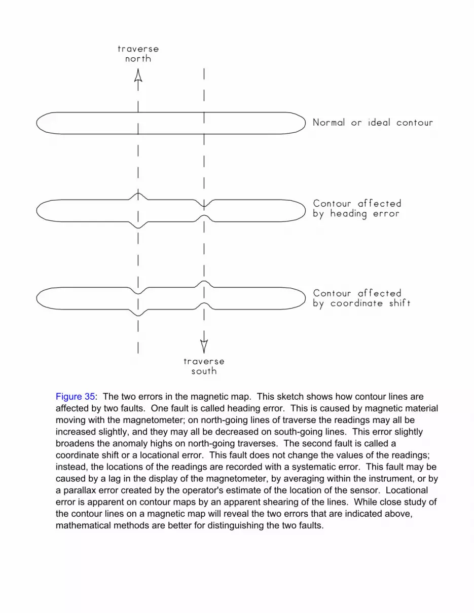
Figure 35: The two errors in the magnetic map. This sketch shows how contour lines areaffected by two faults. One fault is called heading error. This is caused by magnetic materialmoving with the magnetometer; on north-going lines of traverse the readings may all beincreased slightly, and they may all be decreased on south-going lines. This error slightlybroadens the anomaly highs on north-going traverses. The second fault is called acoordinate shift or a locational error. This fault does not change the values of the readings;instead, the locations of the readings are recorded with a systematic error. This fault may becaused by a lag in the display of the magnetometer, by averaging within the instrument, or bya parallax error created by the operator's estimate of the location of the sensor. Locationalerror is apparent on contour maps by an apparent shearing of the lines. While close study ofthe contour lines on a magnetic map will reveal the two errors that are indicated above,mathematical methods are better for distinguishing the two faults.

Figure 36: A verification of the heading error. On north-going traverses, the average readingalong each column was always higher than the average found on south-going traverses. While the difference is small, it was large enough to have a significant effect on the magneticmap. The moving iron that causes this heading error may have been in the clothing of eitheroperator of the equipment; iron within the circuitry of the display console, or on the sensorcables or connectors, could also contribute; finally, a small amount of magnetic dust on thesensor could cause some of this heading error.

Figure 37: After the correction for heading error. The striations in the magnetic map arereduced, although not eliminated. The improvement (compared to the original in Figure 32) ismost apparent in the areas with faint anomalies. This correction was done by adding about0.7 nT to all of the readings along south-going lines of traverse; this 0.7 nT is just thedifference between the two curves in Figure 36.

Figure 38: A verification of the locational error. These curves show that the northcoordinates of all of the readings were shifted by about 0.08 m forward along the direction oftraverse. This analysis was done with a cross-correlation between adjacent lines of traverse. While this allows for the best and most precise correction, one can also just estimate theaverage spatial amplitude of the undulations on the contour lines.

Figure 39: After the correction for locational error. The regular undulations in the contourlines of the original map (Figure 32) have now been eliminated, although random undulationsremain. This map has lost none of the information of the original readings, but is now mucheasier to view. The locational error was corrected by shifting the coordinates of the readings;the north-going traverses were shifted to the north by about 0.08 m, and the south-goingtraverses were shifted to the south, also by about 0.08 m.
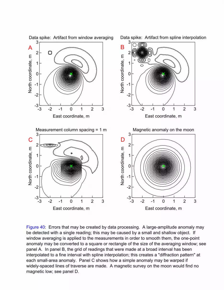
-3 -2 -1 0 1 2 3East coordinate, m
Data spike: Artifact from window averaging
-3
-2
-1
0
1
2
3
Nor
th c
oord
inat
e, m
-3 -2 -1 0 1 2 3East coordinate, m
Data spike: Artifact from spline interpolation
-3
-2
-1
0
1
2
3
Nor
th c
oord
inat
e, m
-3 -2 -1 0 1 2 3East coordinate, m
Measurement column spacing = 1 m
-3
-2
-1
0
1
2
3
Nor
th c
oord
inat
e, m
-3 -2 -1 0 1 2 3East coordinate, m
Magnetic anomaly on the moon
-3
-2
-1
0
1
2
3
Nor
th c
oord
inat
e, m
A
C
B
D
Figure 40: Errors that may be created by data processing. A large-amplitude anomaly maybe detected with a single reading; this may be caused by a small and shallow object. Ifwindow averaging is applied to the measurements in order to smooth them, the one-pointanomaly may be converted to a square or rectangle of the size of the averaging window; seepanel A. In panel B, the grid of readings that were made at a broad interval has beeninterpolated to a fine interval with spline interpolation; this creates a "diffraction pattern" ateach small-area anomaly. Panel C shows how a simple anomaly may be warped ifwidely-spaced lines of traverse are made. A magnetic survey on the moon would find nomagnetic low; see panel D.

-4 -2 0 2 4North coordinate, m
-40
0
40
80
120
160
200
Mag
netic
ano
mal
y, n
T
Anomaly peak = Ba(peak)
Half of peak
Dipole sourceDepth, d = 1 m
Zero level
Width, w = 1 m
Be = 57,000 nTIe = 70o
M = 1 Am2
Ba(peak) = 200 * M / d3
where M = magnetic moment, Am2
For an object with a mass of 1 kg:M (steel) = 0.3 Am2
M (iron) = 0.03 Am2
M (fired earth) = 0.003 Am2
M (brick wall) = 0.0003 Am2
Figure 41: The analysis of a magnetic anomaly. This analysis may be applied to manyanomalies, but particularly to those that are caused by objects whose diameter is less thantheir distance. The depth from the magnetic sensor to the middle of a compact feature isabout equal to the width of the anomaly that it causes at half its peak amplitude. This iscalled the "half width rule", which is an abbreviation for "full width half amplitude", and whichcan be further summarized as d = w. Once this depth has been approximated, the mass ofthe object can be estimated from the anomaly peak with the aid of the equation in the figure;for this estimate, it is necessary to assume what type of material is underground.

-5 -4 -3 -2 -1 0 1 2 3 4 5North coordinate, m
-60
-40
-20
0
20
40
60
80
100
Mag
netic
ano
mal
y, n
o un
its
Cross-section ofrectangular feature
Angular size oflower surface
Anomaly fromupper surface
Anomaly fromlower surface
Resultanttotal anomaly =upper - lower
line of measurement
A geometric calculation of the magnetic anomalyof a long feature with a rectangular cross-section
Figure 42: The geometric calculation of an anomaly. This simple approximation can aidone's thinking about the anomalies from elongated objects. The magnetic anomaly that iscaused by the upper surface of the rectangular prism is proportional to the angular size ofthat surface as it changes along the line of measurement; the same process applies to theanomaly from the lower surface. The difference of the two anomalies gives the resultantanomaly of the whole prism. If the magnetic field is vertical, there is no contribution to theanomaly from the sides of the prism.

-3 -2 -1 0 1 2 3East coordinate, m
Total field
-3
-2
-1
0
1
2
3
Nor
th c
oord
inat
e, m
-3 -2 -1 0 1 2 3East coordinate, m
- Vertical component
-3
-2
-1
0
1
2
3
Nor
th c
oord
inat
e, m
-3 -2 -1 0 1 2 3East coordinate, m
North component
-3
-2
-1
0
1
2
3
Nor
th c
oord
inat
e, m
-3 -2 -1 0 1 2 3East coordinate, m
East component
-3
-2
-1
0
1
2
3
Nor
th c
oord
inat
e, m
A B
C D
Figure 43: Three perpendicular components of a magnetic anomaly. Some magnetometers(such as cesium and proton) measure the total field of the Earth; these instruments findanomalies like that in panel A. Fluxgate magnetometers measure one component of the totalfield; three perpendicular components are plotted in panels B - D. The vectorial sum of thesethree components is the total field, in panel A.

-3 -2 -1 0 1 2 3East coordinate, m
Northerly gradient, 5 nT/m
-3
-2
-1
0
1
2
3
Nor
th c
oord
inat
e, m
-3 -2 -1 0 1 2 3East coordinate, m
Easterly gradient, 5 nT/m
-3
-2
-1
0
1
2
3
Nor
th c
oord
inat
e, m
-3 -2 -1 0 1 2 3East coordinate, m
Inclination angle, 0.01 degrees
-3
-2
-1
0
1
2
3
Nor
th c
oord
inat
e, m
-3 -2 -1 0 1 2 3East coordinate, m
declination angle, 0.02 degrees
-3
-2
-1
0
1
2
3
Nor
th c
oord
inat
e, m
A B
C D
Figure 44: Four more variations on a magnetic map. For the same dipolar anomaly that ismapped in Figure 43, different aspects of the magnetic field may be plotted. The direction ofthe magnetic field is mapped in the upper two panels; inclination angle is the dip angle belowhorizontal, and the declination angle is the angle east of grid north. While gradiometerstypically have their two sensors along a vertical line, these sensors may also be placed alonga horizontal line; the magnetic maps that could then be measured over compact objects areplotted in panels C and D.