uncertainty quantification in unfolding elementary particle
TRANSCRIPT

POUR L'OBTENTION DU GRADE DE DOCTEUR ÈS SCIENCES
acceptée sur proposition du jury:
Prof. F. Nobile, président du juryProf. V. Panaretos, directeur de thèse
Prof. Ph. Stark, rapporteurProf. S. Wood, rapporteur
Prof. A. Davison, rapporteur
Uncertainty quantification in unfolding elementary particle spectra at the Large Hadron Collider
THÈSE NO 7118 (2016)
ÉCOLE POLYTECHNIQUE FÉDÉRALE DE LAUSANNE
PRÉSENTÉE LE 22 JUILLET 2016
À LA FACULTÉ DES SCIENCES DE BASECHAIRE DE STATISTIQUE MATHÉMATIQUE
PROGRAMME DOCTORAL EN MATHÉMATIQUES
Suisse2016
PAR
Mikael Johan KUUSELA


“If everybody tells you it’s possible,
then you are not dreaming big enough.”
— Bertrand Piccard and André Borschberg,
while crossing the Pacific Ocean
on a solar-powered aircraft
To my parents


Acknowledgements
I would first and foremost like to sincerely thank my advisor Victor Panaretos for the opportu-
nity of carrying out this work as a member of the Chair of Mathematical Statistics at EPFL and
for his tireless support and advice during these past four years. The opportunity of doing a PhD
that combines statistical research with an intriguing applied problem from CERN was truly
a dream come true for me and these years have indeed been very exciting and intellectually
satisfying. I believe that during this work we have been able to make important contributions
to both statistical methodology and to data analysis at the LHC and all this would not have
been possible without Victor’s continuous support.
Throughout this work, I have served as a Statistics Consultant on unfolding issues for the
Statistics Committee of the CMS experiment at CERN. This interaction has significantly im-
proved my understanding of the statistical issues that are pertinent to LHC data analysis and
I hope that my contributions to the committee’s work have improved the way unfolding is
carried out at the LHC. I would like to thank the Statistics Committee members, and especially
Olaf Behnke, Bob Cousins, Tommaso Dorigo, Louis Lyons and Igor Volobouev, for stimulating
discussions, which have often provided me with new insights and research directions. I am
also grateful to Volker Blobel, Mikko Voutilainen and Günter Zech for very helpful discussions
about unfolding.
During autumn 2014, I was visiting Philip Stark at the Department of Statistics at the University
of California, Berkeley. I am extremely grateful to Philip for agreeing to host me and to Victor
for providing the opportunity for this visit. I would especially like to thank Philip for taking
the time to discuss strict bounds confidence intervals with me. It was these discussions and
the support of both Philip and Victor that eventually led to the work described in Chapter 7 of
this thesis.
During this work, I have had the great opportunity of discussing research questions with many
outstanding statisticians. Besides Victor and Philip, I would especially like to thank Anthony
Davison, Peter Green, George Michailidis and Simon Wood for discussions that were very
helpful for this work.
I would also like to thank Fabio Nobile, Victor Panaretos, Anthony Davison, Philip Stark and
Simon Wood for agreeing to evaluate this thesis as members of my thesis committee and
i

Acknowledgements
for providing insightful feedback on this work. I am also grateful to my colleagues Anirvan
Chakraborty, Pavol Gurican, Valentina Masarotto and Yoav Zemel for providing comments
on selected parts of this thesis and to Marie-Hélène Descary for helping with the French
translation of the abstract.
I would like to gratefully acknowledge the Swiss National Science Foundation for partially
funding this project. I am also grateful to EPFL for providing such a supportive, stimulating
and international working environment and to CUSO for the organizing the fantastic statistics
summer and winter schools up on the Swiss Alps.
I would also like to thank all my friends in Lausanne, in Helsinki and in the Bay Area for all the
memorable moments and fun experiences we have shared over the years. I am also grateful to
the current and former SMAT, STAT and STAP group members for this nice time that we have
spent together at EPFL. I would especially like to thank Yoav for being such a great officemate
during these past 4.5 years and for helping me out with many mathematical questions.
Finally, I would like to thank my parents for all their support during my studies which culmi-
nate in this thesis.
Lausanne, July 10, 2016 M. K.
ii

Abstract
This thesis studies statistical inference in the high energy physics unfolding problem, which is
an ill-posed inverse problem arising in data analysis at the Large Hadron Collider (LHC) at
CERN. Any measurement made at the LHC is smeared by the finite resolution of the particle
detectors and the goal in unfolding is to use these smeared measurements to make non-
parametric inferences about the underlying particle spectrum. Mathematically the problem
consists in inferring the intensity function of an indirectly observed Poisson point process.
Rigorous uncertainty quantification of the unfolded spectrum is of central importance to
particle physicists. The problem is typically solved by first forming a regularized point estima-
tor in the unfolded space and then using the variability of this estimator to form frequentist
confidence intervals. Such confidence intervals, however, underestimate the uncertainty,
since they neglect the bias that is used to regularize the problem. We demonstrate that, as a
result, conventional statistical techniques as well as the methods that are presently used at
the LHC yield confidence intervals which may suffer from severe undercoverage in realistic
unfolding scenarios.
We propose two complementary ways of addressing this issue. The first approach applies to
situations where the unfolded spectrum is expected to be a smooth function and consists
in using an iterative bias-correction technique for debiasing the unfolded point estimator
obtained using a roughness penalty. We demonstrate that basing the uncertainties on the
variability of the bias-corrected point estimator provides significantly improved coverage
with only a modest increase in the length of the confidence intervals, even when the amount
of bias-correction is chosen in a data-driven way. We compare the iterative bias-correction
to an alternative debiasing technique based on undersmoothing and find that, in several
situations, bias-correction provides shorter confidence intervals than undersmoothing. The
new methodology is applied to unfolding the Z boson invariant mass spectrum measured in
the CMS experiment at the LHC.
The second approach exploits the fact that a significant portion of LHC particle spectra are
known to have a steeply falling shape. A physically justified way of regularizing such spectra is
to impose shape constraints in the form of positivity, monotonicity and convexity. Moreover,
when the shape constraints are applied to an unfolded confidence set, one can regularize the
length of the confidence intervals without sacrificing coverage. More specifically, we form
iii

Abstract
shape-constrained confidence intervals by considering all those spectra that satisfy the shape
constraints and fit the smeared data within a given confidence level. This enables us to derive
regularized unfolded uncertainties which have by construction guaranteed simultaneous
finite-sample coverage, provided that the true spectrum satisfies the shape constraints. The
uncertainties are conservative, but still usefully tight. The method is demonstrated using
simulations designed to mimic unfolding the inclusive jet transverse momentum spectrum at
the LHC.
Keywords: bias-variance trade-off, deconvolution, empirical Bayes, finite-sample coverage,
high energy physics, iterative bias-correction, Poisson inverse problem, shape-constrained
inference, strict bounds confidence intervals, undersmoothing.
iv

Résumé
Cette thèse traite de l’inférence statistique dans le cas du problème d’unfolding en physique
des hautes énergies, qui est un problème inverse mal posé apparaissant lors de l’analyse des
données au Grand collisionneur de hadrons (Large Hadron Collider (LHC) en anglais) au
CERN. Toutes les mesures prises au LHC sont perturbées à cause de la résolution finie des
détecteurs de particules et l’objectif du unfolding est d’utiliser ces mesures corrompues afin
de faire de l’inférence non-paramétrique sur le spectre sous-jacent des particules. D’un point
de vue mathématique, le problème consiste à inférer la fonction d’intensité d’un processus de
Poisson ponctuel observé indirectement.
La quantification rigoureuse de l’incertitude du spectre unfoldé est d’une importance ma-
jeure pour les physiciens. Le problème est typiquement résolu en formant tout d’abord un
estimateur ponctuel régularisé dans l’espace unfoldé et en utilisant par la suite la variabilité
de cet estimateur afin de former des intervalles de confiance fréquentistes. Cependant, de tels
intervalles sous-estiment l’incertitude puisqu’il néglige le biais introduit lors de la régulari-
sation du problème. Nous démontrons qu’il en résulte que les techniques conventionnelles
en statistique ainsi que les méthodes qui sont présentement utilisées au LHC produisent des
intervalles de confiance qui peuvent présentés de sérieux problèmes de sous-couverture pour
des scénarios réalistes d’unfolding.
Nous proposons deux façons complémentaires afin d’aborder ce problème. La première
approche s’applique aux situations pour lesquelles on s’attend à ce que le spectre soit une
fonction lisse et elle utilise une technique itérative de correction du biais afin de réduire le
biais de l’estimateur ponctuel unfoldé obtenu en pénalisant la rugosité. Nous démontrons
qu’en basant les incertitudes sur la variabilité de l’estimateur ponctuel qui a été corrigé, la
couverture est significativement améliorée, et il en découle seulement une augmentation
modeste de la longueur des intervalles, et ce, même lorsque la quantité de correction du biais
est choisie en fonction des données. Nous comparons les intervalles de confiance obtenus
avec la méthode itérative de correction du biais à une autre méthode de réduction du biais
basée sur le sous-lissage, et nous trouvons que dans plusieurs situations, la correction du biais
produit des intervalles de confiance plus courts que ceux obtenus par l’autre méthode. La
nouvelle méthodologie est appliquée afin de faire l’unfolding du spectre de masse invariante
du boson Z mesuré à l’expérience CMS au LHC.
v

Résumé
La seconde approche exploite le fait qu’une portion significative des spectra de particules
du LHC sont connus pour décroître de façon très raide. Une manière de régulariser de tels
spectra, justifiée par la physique, est d’imposer des contraintes sur leur forme telles que la
positivité, la monotonocité et la convexité. De plus, lorsque les contraintes de forme sont
appliquées à un ensemble de confiance unfoldé, il est possible de régulariser la longueur
des intervalles de confiance sans pour autant sacrifier la probabilité de couverture. Plus
précisément, nous formons des intervalles de confiance en considérant tous les spectra qui
satisfont les contraintes de forme et qui ajustent les données pour un niveau de confiance
donné. Ceci nous permet d’obtenir des incertitudes régularisés qui ont par construction une
probabilité de couverture simultanée garantie pour des échantillons de taille finie, à condition
que le vrai spectre satisfasse les contraintes de forme. Les incertitudes sont conservatrices,
mais elles ont tout de même une longueur qui est utile en pratique. La méthode est démontrée
à l’aide de simulations qui ont été conçues afin d’imiter l’unfolding du spectre de quantité de
mouvement transversale des jets inclusifs au LHC.
Mots-clés : Bayes empirique, compromis biais-variance, correction itérative du biais, cou-
verture pour des échantillons de taille finie, déconvolution, inférence sous des contraintes
de forme, intervalles de confiance à bornes strictes, physique des hautes énergies, problème
inverse de Poisson, sous-lissage.
vi

ContentsAcknowledgements i
Abstract iii
Résumé v
Notation and abbreviations xi
1 Introduction 1
2 Unfolding at the Large Hadron Collider 7
2.1 Overview of LHC experiments . . . . . . . . . . . . . . . . . . . . . . . . . . . . . 7
2.2 Statistics at the LHC . . . . . . . . . . . . . . . . . . . . . . . . . . . . . . . . . . . 9
2.3 Unfolding in LHC data analysis . . . . . . . . . . . . . . . . . . . . . . . . . . . . . 11
3 Preliminaries 15
3.1 Forward model for unfolding . . . . . . . . . . . . . . . . . . . . . . . . . . . . . . 15
3.2 Discretization . . . . . . . . . . . . . . . . . . . . . . . . . . . . . . . . . . . . . . . 17
3.2.1 Semi-discrete formulation . . . . . . . . . . . . . . . . . . . . . . . . . . . 18
3.2.2 Spline discretization . . . . . . . . . . . . . . . . . . . . . . . . . . . . . . . 18
3.2.3 Histogram discretization . . . . . . . . . . . . . . . . . . . . . . . . . . . . 20
3.3 Uncertainty quantification using frequentist confidence intervals . . . . . . . . 22
3.3.1 Confidence intervals in unfolding . . . . . . . . . . . . . . . . . . . . . . . 22
3.3.2 Interpretation and use of frequentist confidence intervals . . . . . . . . . 24
3.4 Test scenarios . . . . . . . . . . . . . . . . . . . . . . . . . . . . . . . . . . . . . . . 26
3.4.1 Test setup 1: Two peaks on a uniform background . . . . . . . . . . . . . 26
3.4.2 Test setup 2: Inclusive jet transverse momentum spectrum . . . . . . . . 27
4 Current unfolding methods 31
4.1 Existing unfolding methodology . . . . . . . . . . . . . . . . . . . . . . . . . . . . 31
4.1.1 Overview . . . . . . . . . . . . . . . . . . . . . . . . . . . . . . . . . . . . . . 31
4.1.2 Tikhonov regularization . . . . . . . . . . . . . . . . . . . . . . . . . . . . . 33
4.1.3 D’Agostini iteration . . . . . . . . . . . . . . . . . . . . . . . . . . . . . . . . 35
4.1.4 Other methods . . . . . . . . . . . . . . . . . . . . . . . . . . . . . . . . . . 37
4.2 Undercoverage of the unfolded confidence intervals . . . . . . . . . . . . . . . . 37
vii

Contents
5 Point estimation of smooth spectra 41
5.1 Regularization using a smoothness prior . . . . . . . . . . . . . . . . . . . . . . . 41
5.1.1 Proper smoothness prior using boundary conditions . . . . . . . . . . . . 42
5.2 Regularized point estimators . . . . . . . . . . . . . . . . . . . . . . . . . . . . . . 44
5.2.1 Posterior mean estimation . . . . . . . . . . . . . . . . . . . . . . . . . . . 44
5.2.2 Maximum a posteriori and penalized maximum likelihood estimation . 45
5.2.3 Positivity-constrained Gaussian approximation . . . . . . . . . . . . . . . 46
5.2.4 Unconstrained Gaussian approximation . . . . . . . . . . . . . . . . . . . 47
5.3 Choice of the regularization strength . . . . . . . . . . . . . . . . . . . . . . . . . 48
5.3.1 Empirical Bayes . . . . . . . . . . . . . . . . . . . . . . . . . . . . . . . . . . 48
5.3.2 Hierarchical Bayes . . . . . . . . . . . . . . . . . . . . . . . . . . . . . . . . 51
5.3.3 Weighted cross-validation . . . . . . . . . . . . . . . . . . . . . . . . . . . . 52
5.3.4 Other methods . . . . . . . . . . . . . . . . . . . . . . . . . . . . . . . . . . 53
5.4 Simulation study . . . . . . . . . . . . . . . . . . . . . . . . . . . . . . . . . . . . . 54
5.4.1 Convergence studies for empirical Bayes . . . . . . . . . . . . . . . . . . . 54
5.4.2 Comparison of empirical Bayes and hierarchical Bayes . . . . . . . . . . . 57
5.4.3 Comparison of empirical Bayes and cross-validation . . . . . . . . . . . . 59
6 Uncertainty quantification for smooth spectra 63
6.1 Conventional interval estimates . . . . . . . . . . . . . . . . . . . . . . . . . . . . 64
6.1.1 Empirical Bayes credible intervals . . . . . . . . . . . . . . . . . . . . . . . 64
6.1.2 Hierarchical Bayes credible intervals . . . . . . . . . . . . . . . . . . . . . 65
6.1.3 Gaussian confidence intervals and bootstrap resampling . . . . . . . . . 65
6.1.4 Bootstrap percentile intervals . . . . . . . . . . . . . . . . . . . . . . . . . . 67
6.1.5 Basic bootstrap intervals . . . . . . . . . . . . . . . . . . . . . . . . . . . . . 68
6.1.6 Other bootstrap intervals . . . . . . . . . . . . . . . . . . . . . . . . . . . . 69
6.2 Iteratively bias-corrected percentile intervals . . . . . . . . . . . . . . . . . . . . 69
6.2.1 Iterative bootstrap bias-correction . . . . . . . . . . . . . . . . . . . . . . . 70
6.2.2 Percentile intervals from the bias-corrected point estimator . . . . . . . . 71
6.3 Comparison of iterative bias-correction with conventional interval estimates . 73
6.4 Iterative bias-correction for linear estimators and Gaussian data . . . . . . . . . 80
6.4.1 Iterative bias-correction for linear estimators . . . . . . . . . . . . . . . . 80
6.4.2 Coverage for Gaussian observations . . . . . . . . . . . . . . . . . . . . . . 84
6.4.3 Data-driven iteratively bias-corrected intervals . . . . . . . . . . . . . . . 86
6.4.4 Data-driven undersmoothed intervals . . . . . . . . . . . . . . . . . . . . 88
6.4.5 Simulation study . . . . . . . . . . . . . . . . . . . . . . . . . . . . . . . . . 90
6.5 Unfolding with data-driven bias-correction . . . . . . . . . . . . . . . . . . . . . 99
6.6 Real data demonstration: Z boson invariant mass spectrum . . . . . . . . . . . 104
6.6.1 Description of the data . . . . . . . . . . . . . . . . . . . . . . . . . . . . . . 104
6.6.2 Unfolding setup and results . . . . . . . . . . . . . . . . . . . . . . . . . . . 106
viii

Contents
7 Shape-constrained uncertainty quantification for steeply falling spectra 109
7.1 Regularization of steeply falling spectra using shape constraints . . . . . . . . . 110
7.2 Outline of the strict bounds construction . . . . . . . . . . . . . . . . . . . . . . . 111
7.3 Unfolding with shape-constrained strict bounds . . . . . . . . . . . . . . . . . . 114
7.3.1 Confidence set in the smeared space . . . . . . . . . . . . . . . . . . . . . 114
7.3.2 Strict bounds via duality . . . . . . . . . . . . . . . . . . . . . . . . . . . . . 115
7.3.3 Constraints of the dual program . . . . . . . . . . . . . . . . . . . . . . . . 118
7.3.4 Conservative discretization of the dual constraints . . . . . . . . . . . . . 121
7.3.5 Summary . . . . . . . . . . . . . . . . . . . . . . . . . . . . . . . . . . . . . . 128
7.4 Demonstration: Inclusive jet transverse momentum spectrum . . . . . . . . . . 128
8 Concluding remarks 133
8.1 Discussion and outlook . . . . . . . . . . . . . . . . . . . . . . . . . . . . . . . . . 133
8.2 Conclusions . . . . . . . . . . . . . . . . . . . . . . . . . . . . . . . . . . . . . . . . 136
Appendices 139
A Technical details 139
A.1 Single-component Metropolis-Hastings sampler for unfolding . . . . . . . . . . 139
A.2 Implementation details for shape-constrained strict bounds . . . . . . . . . . . 141
B Full simulation results 143
B.1 Full simulation results for Section 6.3 . . . . . . . . . . . . . . . . . . . . . . . . . 143
B.2 Full simulation results for Section 6.4.5 . . . . . . . . . . . . . . . . . . . . . . . . 153
B.3 Full simulation results for Section 6.5 . . . . . . . . . . . . . . . . . . . . . . . . . 166
Bibliography 177
Curriculum Vitae 187
ix


Notation and abbreviations
Notation
1A(·) indicator function of the set A
‖ ·‖wp weighted �p -norm, ‖x‖w
p = ‖diag(w )x‖p
bias(θ) bias of the estimator θ, bias(θ) = Eθ(θ)−θ
C k (E) the space of functions from E to R with k continuous derivatives
cov(X ) covariance matrix of the random vector X
δx (·) Dirac measure at x
diag(a) diagonal square matrix whose diagonal elements are given by the vector a
Eβ(X ) expectation of random vector X under parameter β
In×n identity matrix of size n ×n
K † Moore–Penrose pseudoinverse of the linear operator K
K −1(A) preimage of the set A under mapping K
Nd0 d-dimensional natural numbers including 0
N (μ,Σ) multivariate normal distribution with mean μ and covariance Σ
φ(·) standard normal probability density function
Φ(·) standard normal cumulative distribution function
Pβ(A) probability of event A under parameter β
Poisson(λ) d-variate probability distribution whose components are independent
and Poisson distributed with parameters λi , i = 1, . . . ,d
Rd+ positive d-dimensional real numbers, Rd+ = {x ∈Rd : xi ≥ 0, i = 1, . . . ,d}
RI Cartesian exponentiation of R with respect to index set I , RI =∏i∈I R
SE(θ) standard error of the estimator θ, SE(θ) = (var(θ))1/2
σmax(A) the largest singular value of the matrix A
V ∗ algebraic dual space of the vector space V
var(X ) variance of the random variable X
X ∼ PX the random variable X follows the distribution PX
Xna.s.−→ X the sequence of random variables Xn converges almost surely to X
X a∼ PX the random variable X follows approximately the distribution PX
X (1), . . . , X (n) i.i.d.∼ PX the random variables X (1), . . . , X (n) are independent and identically
distributed with distribution PX
zα α-quantile of the N (0,1) distribution
xi

Notation and abbreviations
Abbreviations
BC bias-correction
CMS Compact Muon Solenoid (experiment)
CV cross-validation
EB empirical Bayes
ECAL electromagnetic calorimeter
EM expectation-maximization (algorithm/iteration)
HB hierarchical Bayes
HCAL hadron calorimeter
HEP high energy physics
i.i.d. independent and identically distributed
ISE integrated squared error
LHC Large Hadron Collider
MAP maximum a posteriori (estimator)
MC Monte Carlo
MCEM Monte Carlo expectation-maximization (algorithm/iteration)
MCMC Markov chain Monte Carlo
MISE mean integrated squared error
MLE maximum likelihood estimator
MMLE marginal maximum likelihood estimator
PMLE penalized maximum likelihood estimator
SE standard error
SQP sequential quadratic programming
SVD singular value decomposition
UQ uncertainty quantification
US undersmoothing
xii

1 Introduction
The Large Hadron Collider (LHC) at CERN, the European Organization for Nuclear Research, is
the world’s largest and most powerful particle accelerator. Located near Geneva, Switzerland,
this machine was built to study some of the most profound questions about the physical
universe, such as the origin of mass, the nature of dark matter and the asymmetry between
ordinary matter and antimatter. This is done by colliding two beams of protons, traveling at
speeds very close to the speed of light, and then studying the particles that emerge from these
collisions. The collision events are recorded using massive underground particle detectors,
resulting in data streams of the order of 100 terabytes per second. These data are then analyzed
using a variety of statistical techniques with the aim of obtaining new insight into the physical
world. The LHC datasets are not only enormously large, but also have complex internal
structure. As a result, the statistical analysis of these data poses major, and sometimes unique,
computational and methodological challenges.
This thesis focuses on a particular data analysis task arising at the LHC called the unfolding
problem (Prosper and Lyons, 2011; Cowan, 1998; Blobel, 2013; Zech, 2016). Let X be some
physical quantity of interest studied at the LHC experiments. This could, for example, be
the momentum, invariant mass or production angle of particles. Whenever we make a mea-
surement of X , the limited resolution of the particle detectors causes us to observe a noisy
version Y of this quantity. The noisy value Y is called a smeared or folded version of X . The
smearing causes the observed, detector-level spectrum of Y to be a blurred version of the
true, particle-level spectrum of X . The unfolding problem is then to use observations from
the smeared spectrum to make inferences about the actual physical spectrum of X . This is
illustrated in Figure 1.1.
The main challenge in unfolding is that it is an ill-posed statistical inverse problem (Kaipio
and Somersalo, 2005; Engl et al., 2000). This means that even though the mapping K from
the true space into the smeared space is well-behaved, the inverse mapping K −1 (or more
generally the pseudoinverse K †) is unstable with respect to statistical fluctuations in the
smeared observations. In other words, within the statistical uncertainties, the smeared data
can be explained by the actual physical solution but also by a large family of wildly oscillating
1

Chapter 1. Introduction
Smeared spectrum
Folding←−−−Unfolding−−−−→
True spectrum
Figure 1.1: The finite resolution of particle detectors causes the observed particle spectra to besmeared versions of the true physical spectra. The unfolding problem is to use the smearedspectrum to make inferences about the true physical spectrum.
unphysical solutions, and the smeared observations alone cannot distinguish among these
alternatives.
Physical solutions can nevertheless be obtained by introducing additional a priori information
about physically plausible spectra. This is called regularization and statistically corresponds
to reducing the variance of the unfolded point estimator by introducing a small amount
of bias. Two complementary ways of regularizing the unfolding problem are studied in
this work. In the first one, we use the knowledge that most physical spectra are smooth
functions. We do this by employing a roughness penalty that discourages large oscillations
and encourages physically more plausible smooth solutions. In the second one, we rule
out unphysical solutions by imposing physically motived shape constraints in the form of
positivity, monotonicity and convexity. Such shape constraints are particularly well-suited to
unfolding so-called steeply falling spectra, which decay rapidly over many orders of magnitude
and which are commonplace in LHC data analysis.
Mathematically, both the true observations X and the smeared observations Y can be mod-
eled as realizations of two interrelated Poisson point processes. The particle spectra then
correspond to the intensity functions of these processes. Denoting the true intensity by f and
the smeared intensity by g , the two are related by g = K f , where the mapping K represents
the response of the particle detector. As such, unfolding is an example of a Poisson inverse
problem (Antoniadis and Bigot, 2006; Reiss, 1993) and closely related to deconvolution in
optics and image reconstruction in positron emission tomography.
A feature that however distinguishes unfolding from many other inverse problems is the need
for rigorous uncertainty quantification in the unfolded space. Indeed, a simple point estimate
of the unfolded spectrum is of little use to a particle physicist who wishes to use the spectrum
to, for example, test theory predictions, compare and combine different experiments and
extract further theoretical parameters. To properly carry out these tasks requires the ability
to quantify the uncertainty of the unfolded spectrum. Indeed, one could say that in most
physics analyses the main scientific output are the uncertainties and the point estimate is only
of secondary interest. In this work, we understand uncertainty quantification as the task of
2

constructing frequentist confidence intervals in the unfolded space and providing appropriate
statistical methodology for doing this is the main goal of this thesis. Such intervals can then be
used as the statistical starting point for the above mentioned more complex inferential tasks.
It turns out that uncertainty quantification in unfolding is a highly nontrivial problem that
touches upon several key research topics in contemporary statistics, including post-selection
inference (Berk et al., 2013), construction of adaptive nonparametric confidence intervals
(Low, 1997) and uncertainty quantification in penalized regression problems, such as lasso
regression (Javanmard and Montanari, 2014) and spline smoothing (Ruppert et al., 2003,
Chapter 6). The main issue is that most existing uncertainty quantification techniques build
the confidence intervals based on the variability of the regularized point estimator. This
underestimates the uncertainty and results in confidence intervals that may suffer from
serious undercoverage, since the bias that is used to regularize the problem is ignored. But
one cannot simply widen the confidence intervals by an amount corresponding to the bias
since this amount is unknown. Neither can one simply remove all the bias since this would
unregularize the problem and lead to unacceptably large uncertainties.
Given this background, the main contributions of this thesis can be stated as follows:
1. We demonstrate that both existing uncertainty quantification techniques used in LHC
data analysis as well as standard frequentist and Bayesian approaches can severely under-
estimate the uncertainty in the unfolded space, leading to major frequentist undercover-
age in realistic unfolding scenarios (Sections 4.2 and 6.3). This happens because existing
techniques fail to adequately account for the bias.
2. We propose using an iterative bias-correction technique (Kuk, 1995; Goldstein, 1996) for
reducing the bias of roughness-penalized point estimators in order to obtain improved
uncertainty quantification in the unfolded space (Section 6.2). We demonstrate that the
resulting confidence intervals can attain nearly nominal coverage with only a modest
increase in interval length (Sections 6.3, 6.4.5 and 6.5). The coverage is improved as the
bias is reduced, but the small amount of residual bias that remains is enough to regularize
the interval length.
3. We compare the iterative bias-correction to an alternative debiasing technique based on
undersmoothing and find that, in several realistic situations, the bias-corrected confi-
dence intervals are shorter than the undersmoothed intervals (Sections 6.4.5 and 6.5).
4. We propose a novel data-driven procedure for choosing the amount of debiasing in un-
certainty quantification (Section 6.4). The method is applicable to both bias-corrected
and undersmoothed confidence intervals. Even when the amount of debiasing is cho-
sen in a data-driven way, both methods attain nearly the desired target coverage, but
bias-correction produces shorter confidence intervals than undersmoothing. Both de-
biased intervals are orders of magnitude shorter than unregularized intervals and only
moderately longer than non-bias-corrected intervals, which tend to suffer from major
undercoverage (Sections 6.4.5 and 6.5).
3

Chapter 1. Introduction
5. We propose a novel way of regularizing the problem of unfolding steeply falling spectra
using shape constraints. Following the strict bounds methodology of Stark (1992), we apply
the shape constraints directly to an unregularized unfolded confidence set. This enables
us to derive regularized unfolded confidence intervals with guaranteed simultaneous
finite-sample frequentist coverage, provided that the true spectrum satisfies the shape
constraints (Chapter 7).
Secondary contributions of this work include formulation of the unfolding problem using Pois-
son point processes (Section 3.1), statistical description of the existing unfolding techniques
(Section 4.1), the proposal of using empirical Bayes estimation to choose the regularization
strength (Section 5.3.1), comparison of empirical Bayes and cross-validation for choosing the
regularization strength (Section 5.4.3), extension of the strict bounds methodology of Stark
(1992) to Poisson noise (Section 7.3), introduction of a new way of imposing and discretizing
monotonicity and convexity constraints in strict bounds (Section 7.3) and the proposal of
using the single-component Metropolis–Hastings algorithm of Saquib et al. (1998) to sample
unfolded posterior distributions (Section A.1).
The rest of this thesis is structured as follows. Chapter 2 provides background on the LHC
and the role that unfolding plays in the analysis of LHC data. Chapter 3 sets the stage for the
rest of the thesis: it provides the appropriate statistical model for unfolding using Poisson
point processes, explains how we discretize the problem, formalizes how the uncertainty is
quantified using frequentist confidence intervals and introduces the unfolding test scenarios
that are used in the simulation studies through this work. Chapter 4 provides an overview of
the statistical methodology that is currently used to solve the unfolding problem at the LHC
and demonstrates that the existing methods can suffer from severe undercoverage. Chap-
ters 5 and 6 investigate in detail uncertainty quantification when the true spectrum is expected
to be a smooth function. We follow the standard practice of first constructing roughness
penalized point estimates and then using these point estimates to construct confidence in-
tervals. Chapter 5 explains how these point estimates are formed and focuses in particular
on the choice of the regularization strength. Chapter 6 then explains how to use the point
estimates to construct confidence intervals. We review a number of standard frequentist and
Bayesian constructions and demonstrate that all these approaches can suffer from severe
undercoverage when applied to the unfolding problem. We then introduce the iteratively
bias-corrected confidence intervals and demonstrate that they yield significantly improved
coverage performance. This chapter also provides the comparison between bias-corrected
and undersmoothed intervals and applies the new methodology to unfolding the Z boson
invariant mass spectrum measured in the CMS experiment at the LHC. The shape-constrained
strict bounds confidence intervals are studied in Chapter 7, where we also apply the resulting
methodology to a simulated dataset designed to mimic unfolding the inclusive jet transverse
momentum spectrum in the CMS experiment. Chapter 8 closes the thesis with discussion and
conclusions. The appendices provide further technical details and simulation results.
Out of the main contributions of this work listed above, items 1, 2 and 5 appear in the journal
4

article Kuusela and Panaretos (2015) and in the preprint Kuusela and Stark (2016), and the
present text is partially based on those papers. In particular, Chapters 5 and 6 are an extended
version of Kuusela and Panaretos (2015) and Chapter 7 is based on Kuusela and Stark (2016).
Also Sections 2.1 and 3.1 in particular borrow heavily from Kuusela and Panaretos (2015), while
Chapter 4 extends the results of Kuusela and Stark (2016). Some of the secondary contributions
have also partially appeared in the author’s MSc thesis Kuusela (2012).
All the simulation studies presented in this thesis were implemented by the author in
MATLAB R2014a.
5


2 Unfolding at the Large Hadron Col-lider
This chapter puts this work into context by providing background on the LHC experiments
and on the role that unfolding plays in the statistical analysis of their data. We first describe in
Section 2.1 how LHC experiments detect particles and other physical phenomena. We then
provide in Section 2.2 an overview of the statistical methods that are used in LHC data analysis,
while the role of unfolding is described in Section 2.3.
2.1 Overview of LHC experiments
The Large Hadron Collider (LHC) is a circular proton-proton collider located in a 27 km long un-
derground tunnel at CERN near Geneva, Switzerland. With a center-of-mass energy of 13 TeV
(the electron volt, eV, is the customary unit of energy in particle physics, 1 eV ≈ 1.6 ·10−19 J),
the LHC is the world’s most powerful particle accelerator. The protons are accelerated in
bunches of billions of particles and bunches moving in opposite directions are made to collide
inside four large particle detectors called ALICE, ATLAS, CMS and LHCb. The bunches collide
every 25 ns, resulting in some 40 million collisions per second in each detector, out of which
the few hundred most interesting ones are stored for further analysis. This results in datasets
of the size of roughly 30 petabytes per year, which are stored and analyzed using a global
network of supercomputing centers.
Out of the four experiments, ATLAS and CMS are multipurpose detectors capable of per-
forming a large variety of physics analyses ranging from the discovery of the Higgs boson to
precision studies of quantum chromodynamics. The other two detectors, ALICE and LHCb,
specialize in studies of lead-ion collisions and b-hadrons, respectively. In this section, we
provide an overview of the CMS experiment, but similar principles also apply to ATLAS and, to
some extent, to other high energy physics experiments.
The CMS experiment (CMS Collaboration, 2008), an acronym for Compact Muon Solenoid, is
situated in an underground cavern along the LHC ring near the village of Cessy, France. The
detector, weighing a total of 12 500 tons, has a cylindrical shape with a diameter of 14.6 m
7

Chapter 2. Unfolding at the Large Hadron Collider
Figure 2.1: Illustration of the detection of particles at the CMS experiment (Barney, 2004).Each type of particle leaves its characteristic trace in the various subdetectors. This enablesthe identification of different particles and the measurement of their energies and trajectories.Copyright: CERN, for the benefit of the CMS Collaboration.
and a length of 21.6 m. The construction, operation and data analysis of the experiment is
conducted by an international collaboration of over 4000 scientists, engineers and technicians.
When two protons collide at the center of CMS, their energy is transformed into matter in
the form of new particles. A small fraction of these particles are exotic, short-lived particles,
such as the Higgs boson or the top quark. Such exotic particles are the focal point of the
scientific interest of the high energy physics community. They decay almost instantly into more
familiar, stable particles, such as electrons, muons or photons. Using various subdetectors,
the energies and trajectories of these particles can be recorded in order to study the properties
and interactions of the exotic particles created in the collisions.
The layout of the CMS detector is illustrated in Figure 2.1. The detector is immersed in a 3.8 T
magnetic field created using a superconducting solenoid magnet. This magnetic field bends
the trajectory of any charged particle traversing the detector. This enables the measurement of
the particle’s momentum: the larger the momentum, the less the particle’s trajectory is bent.
CMS consists of three layers of subdetectors: the tracker, the calorimeters and the muon
detectors. The innermost detector is the silicon tracker, which consists of an inner layer of
pixel detectors and an outer layer of microstrip detectors. When a charged particle passes
through these semiconducting detectors, it leaves behind electron-hole pairs and hence
creates an electric signal. These signals are combined into a particle track using a Kalman
filter in order to reconstruct the trajectory of the particle.
8

2.2. Statistics at the LHC
The next layer of detectors are the calorimeters, which are devices for measuring energies
of particles. The CMS calorimeter system is divided into an electromagnetic calorimeter
(ECAL) and a hadron calorimeter (HCAL). Both of these devices are based on the same general
principle: they are made of extremely dense materials with the aim of stopping the incoming
particles. In the process, a portion of the energy of these particles is converted into light in a
scintillating material and the amount of light, which depends on the energy of the particle, is
measured using photodetectors inside the calorimeters. The ECAL measures the energy of
particles that interact mostly via the electromagnetic interaction, in other words, electrons,
positrons and photons. The HCAL, on the other hand, measures the energies of hadrons, that
is, particles composed of quarks. These include, for example, protons, neutrons and pions.
The HCAL is also instrumental in measuring the energies of jets, which are collimated streams
of hadrons produced by quarks and gluons, and in detecting the so-called missing transverse
energy, an energy imbalance caused by non-interacting particles, such as neutrinos, escaping
the detector.
The outermost layer of CMS consists of muon detectors, whose task is to identify muons
and measure their momenta. Accurate detection of muons was of central importance in
the design of CMS since muons provide a clean signature for many exciting new physics
processes. This is because there is a very low probability for other particles, with the exception
of the non-interacting neutrinos, to pass through the CMS calorimeter system. For example,
the four-muon decay mode played an important role in the discovery of the Higgs boson
(CMS Collaboration, 2012b).
The information of all CMS subdetectors is combined (CMS Collaboration, 2009) to identify the
stable particles (muons, electrons, positrons, photons and various types of hadrons) produced
in each collision event; see Figure 2.1. For example, a muon will leave a track in both the
silicon tracker and the muon chamber, while a photon produces a signal in the ECAL without
an associated track in the tracker. The information about these individual particles is then
used to reconstruct higher-level physics objects, such as jets or missing transverse energy.
2.2 Statistics at the LHC
This section gives a brief overview of statistical techniques that are used in LHC data analysis.
Cowan (1998) and Cranmer (2015) provide accessible introductions to statistical data analysis
in high energy physics, while Behnke et al. (2013) provides a more in-depth treatment, includ-
ing various more technical aspects. Good sources of information are also the proceedings of
the PHYSTAT conference series Prosper et al. (2008) and Prosper and Lyons (2011). ATLAS and
CMS Collaborations (2011) is a key reference on the statistical methodology that was used in
the search for the Higgs boson at the LHC; see also van Dyk (2014).
Physics analyses at the LHC can be broadly speaking divided into two categories which we
shall call discovery analyses and measurement analyses. In the first case, one is performing
a search for some new particle or phenomenon and the aim is to use LHC data to establish
9

Chapter 2. Unfolding at the Large Hadron Collider
whether such new physics exists or not. Examples of such analyses include the discovery of
the Higgs boson (ATLAS Collaboration, 2012a; CMS Collaboration, 2012b) and searches for
dark matter and extra dimensions (CMS Collaboration, 2012a). In measurement analyses,
on the other hand, one is interested in studying in detail the properties of some physical
phenomenon whose existence has already been previously established. Examples include
studies of the properties of the W boson (ATLAS Collaboration, 2012b) and the top quark
(CMS Collaboration, 2012d), to name just a few. Somewhat different statistical methods
are used in discovery and measurement analyses, but, irrespective of the analysis type, the
statistical methods that are used at the LHC fall predominantly under the frequentist paradigm
of statistics (Lyons, 2013).
The main statistical tools for discovery analyses are hypothesis tests and one-sided confidence
intervals. To illustrate this, let us consider the following simplified model of a single-channel
discovery analysis:
y ∼ Poisson(b +μs), (2.1)
where y is the event count in the experiment, b ≥ 0 is the expected number of background
events from known physics processes, s > 0 is the expected number of signal events from
the new physics process and μ≥ 0 is a signal strength modifier. Hence, μ= 0 corresponds to
the absence of new physics and μ= 1 to the predicted strength of the new signal. Then the
search for the new phenomenon boils down to testing the null hypothesis H0 : μ= 0 against
the alternative H1 : μ= 1. The p-value of this test is typically converted to the scale of Gaussian
standard deviations (σ) and, by convention, one calls a p-value corresponding to 3σ evidence
for the new phenomenon, while 5σ constitutes a discovery of the new phenomenon. Most
discovery analyses also form a one-sided 95 % confidence interval [0,μ] for μ, where μ is called
an upper limit for μ. If the 95 % upper limit μ< 1, then one concludes that the phenomenon
can be excluded at 95 % confidence level.
In reality, the statistical models that are used in discovery analyses involve several search
channels. Moreover, both the background prediction b and the signal strength s depend on
some nuisance parameters ξ, b = b(ξ) and s = s(ξ), and the proper handling of these nuisance
parameters in the hypothesis test and in the upper limit is one of the key statistical challenges
in this type of analyses. Another challenge concerns multiple testing, or the look-elsewhere-
effect (Gross and Vitells, 2010). For example, in the search for the Higgs boson, the hypothesis
test was performed separately for each value mH of the Higgs mass and both non-multiplicity-
corrected local p-values and multiplicity-corrected global p-values were reported. In the case
of most LHC discovery analyses, the sensitivity of the search (i.e., the power of the hypothesis
test) is optimized by employing machine learning techniques (Bhat, 2011), typically in the
form of either neural networks or boosted decision trees.
In measurement analyses, the appropriate statistical tools are point estimators and confidence
intervals and sets. Most of these analyses are performed in a parametric mode, where some
10

2.3. Unfolding in LHC data analysis
theory-motivated parametric model is fitted to LHC data. The statistical model is typically of
the form
y ∼ Poisson(μ(θ)
), (2.2)
where y ∈ Nn0 are binned observations (see Section 3.2) and the Poisson mean μ ∈ Rn+ is
parameterized by some parameter θ ∈Rp , p n, which is of scientific interest. The Poisson
distribution follows from the fact that most LHC data can be modeled using Poisson point
processes (see Section 3.1). The task is then to both estimate θ and to quantify its uncertainty.
In most cases, θ can be estimated simply using the maximum likelihood estimator (MLE)
and confidence intervals and sets can be obtained from standard MLE asymptotics. A simple
extension of this procedure, where the maximum likelihood fit is performed using unbinned
data, is also commonly used at the LHC.
Measurement analyses are also where unfolding is employed. In essence, unfolding can be
seen as a generalization of problem (2.2) to a situation where the physical parameter-of-
interest is no longer finite-dimensional. In that case, the problem becomes ill-posed and
maximum likelihood fits and asymptotics are no longer viable. As we will see, the estima-
tion problem needs to be regularized and this makes uncertainty quantification extremely
challenging. We next proceed to explain why unfolding is needed in LHC measurement anal-
yses in the first place and the rest of this thesis is then devoted to providing methods for
solving the problem, with a particular emphasis on how to quantify the uncertainty of the
unfolded solution.
2.3 Unfolding in LHC data analysis
The need for unfolding stems from the fact that any quantity measured at the LHC detectors
is corrupted by stochastic noise. Let X be the true physical value of some quantity observed
in the detector. Then the actual recorded value of this quantity, say Y , is a slightly perturbed
version of X . That is, the conditional distribution of Y given X , p(Y |X ), is supported on a
continuum of values around X . For instance, let E be the true energy of an electron hitting
the CMS ECAL. Then the observed value of this energy follows to a good approximation the
Gaussian distribution N(E ,σ2(E )
), where the variance satisfies (CMS Collaboration, 2008)(
σ(E )
E
)2
=(
S�E
)2
+(
N
E
)2
+C 2, (2.3)
where S, N and C are fixed constants.
The effect of this smearing is that the observed spectrum of particles is “blurred” with respect
to the true physical spectrum. This becomes an issue for many measurement analyses, where
the scientific goal is to infer this true spectrum and, as a result, the analyses need to use
unfolding to “undo” the smearing. This would be a simple task if a physics-driven parametric
11

Chapter 2. Unfolding at the Large Hadron Collider
model were available for the true spectrum, but unfortunately in most measurement analyses
parametric assumptions are either considered too strong or no well-justified parametric model
exists and regularized nonparametric inferences are needed instead.
Unfolding is used annually by dozens of LHC measurement analyses. Examples include studies
of the characteristics of jets (CMS Collaboration, 2012c, 2013b) as well as the properties of
the W boson (ATLAS Collaboration, 2012b) and the top quark (CMS Collaboration, 2012d,
2013c), to name just a few. Unfolding has recently also been used to measure differential cross
sections associated with the Higgs boson (CMS Collaboration, 2016). In the early phases of
this work, we used the CERN Document Server (https://cds.cern.ch/) to survey all papers
published by the CMS Collaboration in year 2012 in order to understand how often unfolding
is used in LHC data analysis. That year, CMS published a total of 103 papers out of which
16 made direct use of unfolding. Many more also indirectly relied on unfolded results for
example through parton distribution functions (Forte and Watt, 2013), which are estimated
using simultaneous fits to several unfolded spectra (NNPDF Collaboration, 2015). We expect
similar statistics to also hold for the other three LHC experiment.
A pertinent question is whether unfolding, and the challenges related to it, could be avoided
altogether by simply performing the analysis in the smeared space (Lyons, 2011). The answer
to this question depends on what the ultimate goal of the analysis is and how the results are
expected to be used. Unfolding is needed at least when the purpose of the analysis is one of
the following:
• Comparison of experiments with different responses: The only direct way of compar-
ing the spectra measured in two or more experiments with different resolution functions
is to compare the unfolded spectra.
• Input to a subsequent analysis: Certain tasks, such as the estimation of parton distribu-
tions functions or the fine-tuning of Monte Carlo event generators, are typically easiest
to carry out using unfolded input spectra.
• Comparison with future theories: When the spectra are reported in the unfolded space,
a theorist can directly use them to compare with any new theoretical predictions which
might not have existed at the time of the original measurement. (This justification
is controversial since alternatively one could publish the detector response and the
theorist could use it to smear their new predictions. One counterargument is that it
is not straightforward to publish and communicate all the systematic uncertainties
affecting the detector response.)
• Exploratory data analysis: The unfolded spectrum could reveal features and structure
in the data which are not considered in any of the existing theoretical models.
These considerations ultimately boil down to the question of what is the best way of commu-
nicating the information contained in LHC data so that the format is most useful for further
scientific use. Arguably, the ideal solution would be to use the unfolded space, but existing
12

2.3. Unfolding in LHC data analysis
unfolding techniques (see Chapter 4) do not provide a reliable way of doing this. The aim of
this work is to contribute towards improving the situation by providing unfolding methodology
with better statistical performance and guarantees.
13


3 Preliminaries
This chapter lays the foundations for the rest of this work. We first introduce and justify in
Section 3.1 the appropriate forward model for unfolding based on indirectly observed Poisson
point processes. Section 3.2 then explains different ways of discretizing this model. Section 3.3
defines the various forms of frequentist confidence intervals that we aim to construct in this
work and explains why such intervals yield useful uncertainty quantification. We close the
chapter by introducing in Section 3.4 the unfolding scenarios that are used in the simulation
studies throughout this thesis.
3.1 Forward model for unfolding
Most data in experimental high energy physics can be modeled as a Poisson point process
(Cranmer, 2015). Let E ⊆ R be a compact interval and V a space of (sufficiently regular)
functions on E . Then the random measure M on state space E is a Poisson point process (Reiss,
1993) with a positive intensity function f ∈V if and only if:
(i) M(B) ∼ Poisson(λ(B)) with λ(B) =∫B f (s)ds for every Borel set B ⊆ E ;
(ii) M(B1), . . . , M(Bn) are independent for pairwise disjoint Borel sets Bi ⊆ E , i = 1, . . . ,n.
In other words, the number of points M(B) observed in the set B ⊆ E follows a Poisson
distribution with mean∫
B f (s)ds and point counts in disjoint sets are independent random
variables.
The appropriate statistical model for unfolding in an indirectly observed Poisson point process,
where the Poisson process M represents the true, particle-level spectrum of events. The
smeared, detector-level spectrum is represented by another Poisson process N with state
space F ⊆R. We assume that F is a compact interval and denote by W the space of (sufficiently
regular) functions on F . Let g ∈W be the intensity function of N . The intensities f and g are
related by a bounded linear operator K : V →W so that g = K f . In what follows, we assume K
15

Chapter 3. Preliminaries
to be a Fredholm integral operator, that is,
g (t ) = (K f )(t ) =∫
Ek(t , s) f (s)ds, (3.1)
with a sufficiently regular integration kernel k. Throughout this work, we assume that k is
known, although in practice there is usually some amount of uncertainty associated with it;
see the discussion in Chapter 8. The unfolding problem is then to make inferences about the
true intensity f given a single observation of the smeared Poisson process N .
This Poisson inverse problem (Antoniadis and Bigot, 2006; Reiss, 1993) is ill-posed in the sense
that, for most realistic forward operators K , it is possible for true intensities f which are very
far apart in V to map into smeared intensities g which are very close to each other in W . From
the perspective of point estimation, this means that the naïve approach of first estimating g
using, for example, a kernel density estimate g and then estimating f using f = K †g , where K †
is the pseudoinverse of K , is unstable with respect to the Poisson fluctuations of g . Indeed, in
most cases, the pseudoinverse K † is an unbounded, and hence discontinuous, linear operator
(Engl et al., 2000). From the perspective of uncertainty quantification, the ill-posedness means
that the set of those solutions f ∈V which are consistent with our smeared observations need
not be bounded, resulting in possibly arbitrarily large uncertainties.
To better understand the physical justification and meaning of this model, let us consider the
unfolding problem at the point level. Denoting by Xi the true, particle-level observations,
the Poisson point process M can be written as M =∑τi=1δXi (Reiss, 1993, Section 1.2), where
δXi is a Dirac measure at Xi ∈ E and τ, X1, X2, . . . are independent random variables such that
τ ∼ Poisson(λ(E)) and the Xi are identically distributed with probability density f (·)/λ(E),
whereλ(E ) =∫E f (s)ds. In the case of LHC data, the total number of points τ can be assumed to
be Poisson distributed by the law of rare events and the observations X1, X2, . . . are independent
since individual collision events are independent.
When the particle corresponding to Xi passes through the detector, the first thing that can
happen is that it might not be observed at all because of the limited efficiency and acceptance
of the device. Mathematically, this corresponds to thinning of the Poisson process (Reiss,
1993, Section 2.4). Let Zi ∈ {0,1} be a variable indicating whether the point Xi is observed
(Zi = 1) or not (Zi = 0). We assume that τ, (X1, Z1), (X2, Z2), . . . are independent and that the
pairs (Xi , Zi ) are identically distributed. Then the thinned true process is given by M∗ =∑τi=1 ZiδXi =
∑ξi=1δX ∗
i, where ξ = ∑τ
i=1 Zi and the X ∗i are the true points with Zi = 1. The
thinned process M∗ is a Poisson point process with intensity function f ∗(s) = ε(s) f (s), where
ε(s) = P (Zi = 1|Xi = s) is the efficiency of the detector for a true observation at s ∈ E .
For each observed point X ∗i ∈ E , the detector measures a noisy value Yi ∈ F . We assume
the noise to be such that the the smeared observations Yi are independent and identically
16

3.2. Discretization
distributed. The probability density of Yi is given by
p(Yi = t ) =∫
Ep(Yi = t , X ∗
i = s)ds =∫
Ep(Yi = t |X ∗
i = s)p(X ∗i = s)ds. (3.2)
It follows from this that the smeared observations Yi constitute a Poisson point process
N =∑ξi=1δYi , whose intensity function g is given by
g (t ) =∫
Ep(Yi = t |X ∗
i = s)ε(s) f (s)ds. (3.3)
We hence identify that the kernel k in Equation (3.1) is given by
k(t , s) = p(Yi = t |X ∗i = s)ε(s). (3.4)
By the definition of X ∗i and ε(s), this can also be written as
k(t , s) = p(Yi = t |Xi = s, Xi observed)P (Xi observed|Xi = s). (3.5)
Notice that if we are in the special case where k(t , s) = k(t − s), then unfolding corresponds to
a deconvolution problem (Meister, 2009) for Poisson point process observations.
3.2 Discretization
LHC data are typically analyzed in a binned form where the Poisson point processes are
discretized using a histogram. This is done both for convenience and for computational
reasons. Indeed, in many analyses, there may be billions of observations and treating them
individually would not be computationally feasible.
In the case of unfolding, it is natural to carry out the histogram discretization for the smeared
space F , and this is indeed done in most unfolding techniques, including the ones studied in
this work. Let {Fi }ni=1 be a partition of the smeared space F consisting of n histograms bins of
the form
Fi =⎧⎨⎩[Fi ,min,Fi ,max), i = 1, . . . ,n −1,
[Fi ,min,Fi ,max], i = n,(3.6)
where Fi ,max = Fi+1,min, i = 1, . . . ,n−1. Let us furthermore denote by yi the number of smeared
observations falling on interval Fi , that is, yi = N (Fi ), i = 1, . . . ,n. Since N is a Poisson point
process, it follows that the histogram of smeared observations y = [y1, . . . , yn
]T consists of
independent and Poisson distributed event counts. The expected value of these counts is
given by μ= [∫F1g (t )dt , . . . ,
∫Fn
g (t )dt]T. Using Equation (3.1), we find that the components
of the smeared mean μ are related to the true intensity f by
μi =∫
Fi
g (t )dt =∫
Fi
∫E
k(t , s) f (s)ds dt =∫
Eki (s) f (s)ds, i = 1, . . . ,n, (3.7)
17

Chapter 3. Preliminaries
where ki (s) = ∫Fik(t , s)dt . We assume here that k and f are sufficiently regular so that the
order of integration can be changed. Notice that at this stage we have incurred a loss of
information by replacing the individual observations by the bin counts yi , but we have not
made any implicit assumptions regarding the true intensity f .
The situation is less straightforward with regard to the discretization of the true space E . The
problem is that relating the smeared mean μ directly to a histogram discretization of the
true process M requires making assumptions about the shape of f inside the true bins. The
following sections describe some options that are available for treating the true space E .
3.2.1 Semi-discrete formulation
The most straightforward option is to simply not discretize the problem further. That is, we
consider a semi-discrete problem formulation where the smeared space is discretized using a
histogram, but the true intensity f is treated as an object of the infinite-dimensional function
space V . The semi-discrete forward mapping from f to μ is then given by
K : V →Rn , f →μ= [K1 f , . . . ,Kn f]T, (3.8)
where the functionals Ki are given by Equation (3.7),
Ki : V →R, f →μi =∫
Eki (s) f (s)ds. (3.9)
The corresponding statistical model is
y ∼ Poisson(μ), with μ=K f , (3.10)
and the notation is taken to imply that the components of y are independent. Our task is then
to make non-parametric inferences regarding f under this model. We use this semi-discrete
formulation in Chapter 7, when we construct shape-constrained confidence intervals for
functionals of f .
3.2.2 Spline discretization
A common approach in non-parametric regression problems is to effectively turn the infinite-
dimensional problem (3.10) into a finite-dimensional one by considering a basis expansion
of f in the form f (s) =∑pj=1β jφ j (s), where {φ j }p
j=1 is a finite dictionary of basis functions.
Since the true spectra f are typically expected to be smooth functions, a particularly attractive
representation for f is provided by using splines (de Boor, 2001; Schumaker, 2007; Wahba,
1990). Let Emin = s0 < s1 < s2 < ·· · < sL < sL+1 = Emax be a sequence of L +2 knots in the true
space E = [Emin,Emax]. Then an order-m spline with knots si , i = 0, . . . ,L +1, is a piecewise
polynomial, whose restriction to each interval [si , si+1), i = 0, . . . ,L, is an order-m polynomial
(that is, a polynomial of degree m −1) and which has m −2 continuous derivatives at each
18

3.2. Discretization
−1 −0.5 0 0.5 10
0.2
0.4
0.6
0.8
1
Figure 3.1: B-spline basis with L = 9 interior knots on the interval [−1,1].
interior knot si , i = 1, . . . ,L. An order-m spline with L interior knots can be written as a linear
combination of p = L+m basis functions. In this work, we employ the spline discretization
in Chapters 5 and 6, where we focus on order-4 cubic splines which consist of third degree
polynomials and are twice continuously differentiable.
Various basis systems {φ j }pj=1 can be used to express splines of arbitrary order. We focus on the
B-spline basis B j , j = 1, . . . , p, which consists of spline basis functions of minimal local support
(de Boor, 2001). This basis has good numerical properties and is also conceptually simple in
the sense that each basis coefficient β j controls the value of f only locally on the support of B j .
Figure 3.1 illustrates the B-spline basis. We use the MATLAB Curve Fitting Toolbox (Mathworks,
2014a) to construct, evaluate and perform basic operations on B-splines. These algorithms
are based on recursive use of lower-order B-spline basis functions; see de Boor (2001).
When we plug the B-spline basis expansion f (s) =∑pj=1β j B j (s) into Equation (3.7), we find
that the smeared means are given by
μi =p∑
j=1
(∫E
ki (s)B j (s)ds
)β j =
p∑j=1
Ki , jβ j , i = 1, . . . ,n, (3.11)
where we have denoted
Ki , j =∫
Eki (s)B j (s)ds, i = 1, . . . ,n, j = 1, . . . , p. (3.12)
Hence unfolding reduces to inferring the spline coefficients β in the Poisson regression
problem
y ∼ Poisson(μ), with μ= Kβ. (3.13)
This forward model is correct if the true intensity f is indeed a spline with the knot sequence
{si }L+1i=0 . For other smooth functions, the model is only approximately correct and the severity
of the approximation error depends on how well f can be represented using a spline. If f
19

Chapter 3. Preliminaries
is non-smooth, then other types of basis expansions may be more appropriate than splines.
For example, if f is known to contain sharp spikes, then a wavelet basis expansion could be
considered. However, such situations seem to be rare in HEP unfolding applications.
Since any Poisson intensity function is known to be positive, we would also like to constrain
the B-spline f (s) =∑pj=1β j B j (s) to be a positive function. This can be done by requiring that
β ∈Rp+ = {x ∈Rp : xi ≥ 0, i = 1, . . . , p
}. (3.14)
Since the B-spline basis functions B j are positive, this is a sufficient condition for the positivity
of f . However, this is not in general a necessary condition for the positivity of f (except for
order-1 and order-2 B-splines). Restricting ourselves to the family of B-splines induced by the
constraint β ∈ Rp+ hence entails a reduction in the family of spline functions available to us
in comparison to all positive splines (de Boor and Daniel, 1974), but, given the shape of the
B-spline basis functions (see Figure 3.1), this reduction is unlikely to be restrictive in practice.
Also other qualitative shape constraints can be easily imposed on the B-spline basis (Pya and
Wood, 2015). For example, a sufficient condition for f to be decreasing is
β j+1 −β j ≤ 0, j = 1, . . . , p −1. (3.15)
Similarly,
β j+2 −2β j+1 +β j ≥ 0, j = 1, . . . , p −2 (3.16)
is a sufficient condition for f to be convex, provided that the knots are uniformly spaced.
O’Sullivan (1986, 1988) was one of the first authors to employ regularized B-splines in statistical
applications. The approach was later popularized by Eilers and Marx (1996) in the form of
P-splines where a difference penalty is applied to the basis coefficients β j . The use of B-splines
in the HEP unfolding problem was pioneered by Blobel (1985). Also the recent contributions
by Dembinski and Roth (2013) and Milke et al. (2013) use splines to discretize the unfolding
problem. However, none of these techniques is presently widely used in LHC experiments.
3.2.3 Histogram discretization
The discretization that is used in most LHC unfolding analyses directly relates the smeared
mean histogram μ to a histogram discretization λ of the true Poisson point process M . Let
{E j }pj=1 be a partition of the true space E consisting of p histogram bins of the form
E j =⎧⎨⎩[E j ,min,E j ,max), j = 1, . . . , p −1,
[E j ,min,E j ,max], j = p,(3.17)
20

3.2. Discretization
with E j ,max = E j+1,min, k = 1, . . . , p−1. The histogram of expected number of true events within
each true bin E j is then given by
λ=[∫
E1
f (s)ds, . . . ,∫
Ep
f (s)ds
]T
. (3.18)
The elements of μ and λ are related by (Cowan, 1998, Chapter 11)
μi =∫
Eki (s) f (s)ds =
p∑j=1
∫E j
ki (s) f (s)ds =p∑
j=1
∫E j
ki (s) f (s)ds∫E j
f (s)dsλ j =
p∑j=1
Ki , jλ j , (3.19)
where the elements of the smearing or response matrix K are given by
Ki , j =∫
E jki (s) f (s)ds∫E j
f (s)ds, i = 1, . . . ,n, j = 1, . . . , p. (3.20)
Equivalently, the (i , j )th element of K is the probability that an event in the true bin E j
propagates to the smeared bin Fi (Kuusela, 2012, Proposition 2.11),
Ki , j = P (Y ∈ Fi |X ∈ E j ), (3.21)
where X is a true particle-level event and Y is the corresponding smeared detector-level event.
The corresponding statistical model then becomes
y ∼ Poisson(μ), with μ= Kλ, (3.22)
and the goal of unfolding is to make inferences about λ given a realization of y .
Notice that each element Ki , j depends on the shape of f within the true bin E j . Intuitively,
the distribution of true events within E j has an effect on the probability of finding these
events within the smeared bin Fi . The dependence on f will cancel out only if f is constant
within E j , in which case Ki , j = 1E j ,max−E j ,min
∫E j
ki (s)ds (notice that this corresponds to taking
f to be an order-1 spline with the knots placed at the boundaries between the true bins; see
Section 3.2.2). The more f deviates from a constant within E j , the larger its effect on Ki , j . This
dependence is particularly strong for steeply falling spectra, where f may change by several
orders of magnitude within E j .
In real LHC analyses, f is obviously unknown. Most analyses address this by replacing f in
Equation (3.20) by an ansatz f MC obtained using a Monte Carlo (MC) event generator, and
this is also the approach we follow in Chapter 4 when we study existing unfolding techniques.
In other words, unfolding is performed using using the response matrix K MC with elements
K MCi , j =
∫E j
ki (s) f MC(s)ds∫E j
f MC(s)ds, i = 1, . . . ,n, j = 1, . . . , p, (3.23)
21

Chapter 3. Preliminaries
instead of the actual response matrix K . The resulting statistical model y ∼ Poisson(K MCλ) is
correct only if f MC is proportional to f within each true bin E j . When this is not the case, the
model is only approximately correct, and the more the shape of f MC deviates from that of f
within the true bins E j , the larger the modeling error. The situation can be alleviated by using
smaller true bins E j , but the drawback is that this increases the dimension of λ and hence
increases the ill-posedness of the problem.
It is sometimes argued that the unfolding problem should be regularized by increasing the size
of the true bins E j (Zech, 2011). In the present formulation, this only superficially circumvents
the ill-posedness of the problem since with wide bins the Monte Carlo dependence of K MC
becomes increasingly acute. However, in the formulation that we develop in Chapter 7, the
true bins can be made arbitrarily large, while avoiding the Monte Carlo dependence altogether.
3.3 Uncertainty quantification using frequentist confidence inter-
vals
A central goal in this work is to quantify our uncertainty regarding the intensity function f
using frequentist confidence intervals. The aim of this section is to define what we mean by this
(Section 3.3.1) and to explain how to interpret and use the resulting intervals (Section 3.3.2).
3.3.1 Confidence intervals in unfolding
Let θ = H f be some real-valued feature of f that we are interested in, with the functional
H : V →R relating f to the quantity of interest θ. Unless explicitly stated, H need not be linear.
Let α= (0,1) and let y ∼ Poisson(K f ), where K is the semi-discrete forward mapping from
Section 3.2.1. Then a frequentist confidence interval for θ with confidence level (or coverage
probability) 1−α is a random interval[θ(y),θ(y)
]that satisfies
P f(θ ∈ [θ(y),θ(y)
])≥ 1−α, ∀ f ∈V. (3.24)
In other words, under repeated sampling of y , the random intervals[θ(y),θ(y)
]must cover
the true value of θ at least 100× (1−α) % of the time, and this must hold true for any true
intensity f . Constructing confidence intervals for a given fixed f is trivial—the challenging
part is to provide a construction where (3.24) is satisfied for any f in V , or at least in a large
subset of V . (Indeed, the author has on several occasions witnessed a situation where a Monte
Carlo ansatz f MC is used to construct confidence intervals and the coverage is then checked
for data y generated by this same spectrum f MC, when the check should be done for one or
more spectra that are different from f MC. Such error can be surprisingly difficult to spot in
complex data analysis situations.)
In practice, we are often interested in multiple features of f . Let {θi }i∈I be a collection of
quantities of interest, where θi = Hi f with Hi : V → R for each i ∈ I . Then the confidence
22

3.3. Uncertainty quantification using frequentist confidence intervals
statement can either be pointwise or simultaneous with respect to the index set I . More
specifically, we call a collection of random intervals[θi (y),θi (y)
], i ∈ I , pointwise confidence
intervals for {θi }i∈I with confidence level 1−α if
P f(θi ∈
[θi (y),θi (y)
])≥ 1−α, ∀i ∈ I , ∀ f ∈V. (3.25)
The intervals[θi (y),θi (y)
], i ∈ I , are called simultaneous confidence intervals for {θi }i∈I with
confidence level 1−α if
P f(θi ∈
[θi (y),θi (y)
],∀i ∈ I
)≥ 1−α, ∀ f ∈V. (3.26)
In the latter case, the 100× (1−α) % coverage probability concerns the whole collection of
intervals[θi (y),θi (y)
], i ∈ I , simultaneously, while in the former case the coverage statement
is made for each index i ∈ I separately.
It is sometimes more natural to view a collection of 1−α simultaneous confidence intervals
for {θi }i∈I as the Cartesian product∏
i∈I[θi (y),θi (y)
]in which case we call this subset of RI
a 1−α simultaneous confidence set or, when these is no risk of confusion, simply a 1−α
confidence set for {θi }i∈I ∈ RI . A confidence set may also be a more general subset of RI .
More specifically, a random set C (y) ⊆ RI is a 1−α confidence set for {θi }i∈I if it holds that
P f({θi }i∈I ∈C (y)
)≥ 1−α, ∀ f ∈V .
If the index set I is finite, then pointwise intervals can always be conservatively adjusted
to satisfy a simultaneous confidence statement. Namely, let[θi (y),θi (y)
], i = 1, . . . , p, be a
collection of 1−α′ pointwise confidence intervals for {θi }pi=1. Then
P f(θ1(y) ≤ θ1 ≤ θ1(y), . . . ,θp (y) ≤ θp ≤ θp (y)
)≥ 1−p∑
i=1
(1−P f
(θi (y) ≤ θi ≤ θi (y)
))(3.27)
≥ 1−p∑
i=1α′ = 1−pα′, (3.28)
where we have used the inequality P(⋂
i Ai) ≥ 1−∑i
(1−P(Ai )
). We hence see that if we
construct p pointwise confidence intervals at confidence level 1− αp , then their simultaneous
coverage probability is at least 1−α. This is called Bonferroni correction of the pointwise
confidence intervals.
The functionals that we specifically consider in this work are either point evaluators, Hs f =f (s), s ∈ E , or integrals over bins, Hi f = ∫Ei
f (s)ds, i = 1, . . . , p, where the bins Ei are of the
form (3.17). In the former case, we are interested in 1−α pointwise confidence bands for f ,
that is, collections of random intervals[f¯
(s; y), f (s; y)], s ∈ E , that satisfy
P f(
f¯
(s; y) ≤ f (s) ≤ f (s; y))≥ 1−α, ∀s ∈ E , ∀ f ∈V. (3.29)
23

Chapter 3. Preliminaries
This is the setup we study in Chapter 6. (In practice, the confidence bands are computed on a
grid of s values, but this grid can be made arbitrarily dense.) The latter case corresponds to
forming confidence intervals[λi (y),λi (y)
], i = 1, . . . , p, for the expected true histogram λ ∈Rp
defined in Equation (3.18), and this is the setup we study in Chapters 4 and 7. We consider
these intervals both in their pointwise (or rather, binwise) form,
P f(λi ∈
[λi (y),λi (y)
])≥ 1−α, ∀i ∈ 1, . . . , p, ∀ f ∈V , (3.30)
and in their simultaneous form,
P f(λ ∈ [λ1(y),λ1(y)
]×·· ·× [λp (y),λp (y)])≥ 1−α, ∀ f ∈V. (3.31)
In the rest of this work, we mostly write confidence intervals for θ in the form[θ,θ
]omitting
the y dependence. It is however important to keep in mind that, in the frequentist definition of
a confidence interval (3.24), it is the interval[θ,θ
]that is random and the quantity of interest
θ is fixed. This is in contrast with a Bayesian credible interval satisfying P(θ ∈ [θ,θ
]∣∣y)≥ 1−α,
where θ is random and the interval[θ,θ
]is fixed.
3.3.2 Interpretation and use of frequentist confidence intervals
We now discuss the interpretation of frequentist confidence intervals and explain why they are
useful in carrying out a number of statistical tasks. We treat this question generically without
particular reference to the unfolding problem. We focus on the case of univariate confidence
intervals, but the discussion can be easily generalized to confidence sets.
Let θi be some quantity of interest and let[θi ,θi
]be a 1−α confidence interval for θi . For
simplicity, we assume that the coverage probability of the interval is exactly 1−α, that is,
P(θi ∈
[θi ,θi
])= 1−α. Let us assume that we make n independent repetitions of the measure-
ment for θi and let us denote the confidence interval of the j th repetition by[θi , j ,θi , j
]. Then
the interpretation that is most often given to frequentist confidence intervals is that, when n is
large enough, 100× (1−α) % of the intervals[θi , j ,θi , j
], j = 1, . . . ,n, will cover the true value
of θi .
However, in practice, most scientific experiments are only done once. For example, if θi is the
mass of the Higgs boson, then for the foreseeable future, we only have one particle accelerator
where this value can be measured. For this reason, an interpretation that the author finds
more attractive is to consider the implications of frequentist coverage for multiple quantities
of interest. Let {θi }mi=1 be a collection of m quantities of scientific interest. In the case of
high energy physics, these could, for example, be the mass of the top quark, the branching
ratio of the Z → l+l− decay mode, the value of the strong coupling constant, the value of
the weak mixing angle and so forth. If the measurements of each θi are independent and
if m is large enough, then frequentist coverage implies that 100× (1−α) % of the intervals[θi ,1,θi ,1
], i = 1, . . . ,m, will cover their corresponding true values θi , i = 1, . . . ,m. In other
24

3.3. Uncertainty quantification using frequentist confidence intervals
words, if we make a large number of independent measurements of different quantities of
interest θi , then 100× (1−α) % of our inferences are correct in the sense that the resulting
confidence interval covers the corresponding true value of θi . For example, if all the intervals
published by LHC experiments were 95 % confidence intervals and if all the measurements
were in mutually exclusive channels, then, in the long run, 95 % of these results would be
correct in the sense that the published interval covers the actual physical value of the corre-
sponding quantity. (In practice the situation is more complicated as systematic uncertainties
introduce correlations between measurements.) This interpretation of frequentist confidence
intervals is advocated, for example, by Wasserman (2004, Section 6.3.2).
More rigorously, let Zi , j = 1{θi ∈
[θi , j ,θi , j
]}be the indicator variable showing whether the
interval[θi , j ,θi , j
]covers θi . Then, for every i , j , we have that Zi , j ∼ Bernoulli(1−α) and,
assuming that both the different measurements and the repetitions of the same measurement
are independent, the Zi , j are i.i.d. random variables with mean μ= E(Zi , j
)= 1−α. Then, by
the strong law of large numbers,
#{
Zi , j = 1}n
j=1
n= 1
n
n∑j=1
Zi , ja.s.−→μ= 1−α, when n →∞. (3.32)
That is, the fraction of intervals that cover θi when the i th measurement is repeated n times
converges almost surely to 1−α as n →∞. This corresponds to the conventional interpretation
of frequentist confidence intervals. But we also have that
#{
Zi ,1 = 1}m
i=1
m= 1
m
m∑i=1
Zi ,1a.s.−→μ= 1−α, when m →∞. (3.33)
That is, as the number of measurements m grows, the fraction of intervals[θi ,1,θi ,1
], i =
1, . . . ,m, that cover their corresponding quantity of interest θi , i = 1, . . . ,m, converges almost
surely to 1−α. This leads to the alternative interpretation of the intervals via coverage in
independent measurements of unrelated quantities of interest. This is illustrated in Figure 3.2.
A frequentist 1−α confidence interval for θi is useful for carrying out a number of statistical
tasks. By the duality between confidence intervals and hypothesis tests, a test that rejects
the null hypothesis H0 : θi = θi ,0 when θi ,0 ∉[θi ,θi
]has significance level α (e.g., Casella and
Berger, 2002, Theorem 9.2.2). In other words, we can perform a hypothesis test by simply
checking whether the null value θi ,0 is contained within the interval[θi ,θi
]. Two or more
independent confidence intervals for the same quantity of interest θi can also be combined
by making an appropriate multiplicity correction and then considering the intersection of the
multiplicity-corrected intervals. For example, a simple calculation shows that if[θi ,1,θi ,1
]and[
θi ,2,θi ,2]
are two independent confidence intervals for θi with confidence level�
1−α, then
their intersection is a 1−α confidence interval for θi . Furthermore, confidence intervals and
more generally confidence sets with appropriate multiplicity corrections can be propagated to
further analyses using a construction similar to the one outlined later in Section 7.2. To enable
25

Chapter 3. Preliminaries
Repetitions
Mea
suremen
ts
Figure 3.2: Frequentist confidence intervals imply coverage not only for independent rep-etitions of the same measurement, but also for independent measurements of unrelatedquantities of interest {θi }.
this kind of use, it can be helpful to publish confidence intervals at all possible confidence
levels in the form of a confidence distribution (Xie and Singh, 2013).
3.4 Test scenarios
We close this chapter by introducing the two unfolding scenarios that will be primarily used
in the simulation studies throughout this thesis. The first corresponds to a case where it
is reasonable to assume the spectrum to be a smooth function and is primarily used in
Chapters 5 and 6. The second corresponds to a situation where the spectrum is most naturally
regularized using shape constraints and is primarily studied in Chapter 7. Both cases are also
used in Chapter 4 to demonstrate the shortcomings of existing unfolding methods.
3.4.1 Test setup 1: Two peaks on a uniform background
The first test case we consider consists of two Gaussian peaks on top of a uniform background.
Such an intensity resembles situations where invariant mass peaks are observed on top of
some background events. More specifically, we let the intensity of the true process M be
f (s) =λtot
{π1N (s|−2,1)+π2N (s|2,1)+π3
1
|E |}
, s ∈ E . (3.34)
where λtot = E(τ) =∫E f (s)ds > 0 is the expected number of true observations and |E | denotes
the length of the interval E . The mixing proportions πi sum to one and are set to π1 = 0.2,
26

3.4. Test scenarios
π2 = 0.5 and π3 = 0.3. We consider the sample sizes λtot = 1 000, λtot = 10 000 and λtot = 50 000,
which we call the small, medium and large sample size cases, respectively. We take both the
true space E and the smeared space F to be the interval [−7,7]. We assume the smeared
intensity g to be given by the Gaussian convolution
g (t ) = (K f )(t ) =∫
EN (t − s|0,1) f (s)ds, t ∈ F. (3.35)
This corresponds to a situation where the true points Xi are smeared by additive standard
Gaussian noise, that is, Yi = Xi +εi , where Xi and εi are independent and εi ∼ N (0,1). Points
that are smeared beyond the boundaries of F are discarded from the analysis. The resulting
true intensity f and smeared intensity g in the case of the medium sample size are shown in
Figure 3.3(a). Notice that in classical deconvolution theory (Meister, 2009) this setup belongs to
the most difficult class of deconvolution problems since the Gaussian noise has a supersmooth
probability density function.
We discretize the smeared space F using a histogram of n = 40 equal-width bins. For the
experiments of Chapter 4, we discretize the true space E as described in Section 3.2.3 using a
histogram of p = 30 equal-width bins. In Chapters 5 and 6, we use the spline discretization
described in Section 3.2.2. More specifically, we discretize the true space E using cubic B-
splines with L = 26 uniformly placed interior knots corresponding to p = L + 4 = 30 basis
coefficients.
3.4.2 Test setup 2: Inclusive jet transverse momentum spectrum
We use the inclusive jet transverse momentum spectrum (CMS Collaboration, 2011, 2013b)
as an example of a steeply falling particle spectrum. A jet is a collimated stream of energetic
particles. Observing a jet in an LHC particle detector signifies that a quark or a gluon was
created in the proton-proton collision. By the theory of quantum chromodynamics, quarks
and gluons cannot exist as isolated objects. They will hence create other particles from the
vacuum around them in a process called hadronization, and the end result of this process is
a stream of particles in the form of a jet. The inclusive jet transverse momentum spectrum
is the average number of jets as a function of their transverse momentum pT, that is, their
momentum in the direction perpendicular to the proton beam. The transverse momentum
pT is measured in units of electron volts (eV). Measurement of this spectrum constitutes an
important test of the Standard Model of particle physics and provides constraints on the free
parameters of the theory.
Our aim is to provide a simulation setup that mimics unfolding the inclusive jet pT spectrum
in the CMS experiment (CMS Collaboration, 2008) at the LHC. We generate the data using the
particle-level intensity function
f (pT) = LN0
( pT
GeV
)−α (1− 2�
spT
)βe−γ/pT , 0 < pT ≤
�s
2, (3.36)
27

Chapter 3. Preliminaries
−5 0 50
500
1000
1500
2000
2500
Inte
nsity
(a) Two peaks on a uniform background
TrueSmeared
400 600 800 10000
5000
10000
15000
Transverse momentum pT
Inte
nsity
(b) Inclusive jet pT spectrum
TrueSmeared
Figure 3.3: Illustration of the unfolding scenarios that we consider in our simulation studies.Figure (a) shows the intensity functions for the two peaks on a uniform background test setupand Figure (b) for the inclusive jet transverse momentum spectrum. The first case servesas an example of a spectrum that is naturally regularized using a roughness penalty, whilethe second case is an example of a steeply falling spectrum, which can be regularized usingshape constraints.
where L > 0 is the integrated luminosity (a measure of the amount of collisions produced in the
accelerator, measured in units of inverse barns, b−1),�
s is the center-of-mass energy of the
proton-proton collisions and N0, α, β and γ are positive parameters. This parameterization
was used in early inclusive jet analyses at the LHC (CMS Collaboration, 2011) and is motivated
by physical considerations. For example, the(1− 2�
spT
)βterm corresponds to a kinematic
cut-off at pT =�
s2 .
Let p ′T denote the smeared transverse momentum. When the jets are reconstructed using
calorimeter information, the smearing can be modeled as additive Gaussian noise, p ′T = pT+ε,
where ε|pT ∼N(0,σ(pT)2
)with the variance σ(pT)2 satisfying (cf. Equation (2.3))(
σ(pT)
pT
)2
=(
N
pT
)2
+(
S�pT
)2
+C 2, (3.37)
where N , S, and C are fixed positive constants (CMS Collaboration, 2010). The smeared
intensity is then given by the convolution
g (p ′T) =
∫EN(p ′
T −pT∣∣0,σ(pT)2) f (pT)dpT, p ′
T ∈ F. (3.38)
Hence the forward kernel is given by k(p ′T, pT) = N
(p ′
T − pT∣∣0,σ(pT)2
)and the unfolding
problem becomes a heteroscedastic Gaussian deconvolution problem.
At the center-of-mass energy�
s = 7 TeV and in the central part of the CMS detector, realistic
values for the parameters of f (pT) are given by N0 = 1017 fb/GeV, α= 5, β= 10 and γ= 10 GeV
and for the parameters of σ(pT)2 by N = 1 GeV, S = 1 GeV1/2 and C = 0.05 (M. Voutilainen,
28

3.4. Test scenarios
personal communication, 2012). We furthermore set L = 5.1 fb−1, which corresponds to
the size of the CMS 7 TeV dataset collected in 2011. We let the true and smeared spaces be
E = F = [400 GeV,1000 GeV] and partition both spaces into n = p = 30 equal-width bins of the
form (3.6) and (3.17). The resulting intensity functions are illustrated in Figure 3.3(b).
29


4 Current unfolding methods
This chapter provides an overview of the statistical methods that are presently used at the
LHC for solving the unfolding problem. The focus is on the methods that are implemented
in the ROOUNFOLD software framework (Adye, 2011), which is the unfolding software that is
most commonly used by LHC analyses. We explain in Section 4.1 that the problem is currently
regularized by biasing the solution towards a Monte Carlo ansatz of the unknown intensity
function f . The uncertainty of the solution is then quantified by using the variance of the
regularized point estimator, ignoring the regularization bias. We demonstrate in Section 4.2
that this may lead to serious underestimation of the uncertainty, resulting in confidence
intervals whose coverage probability can be much smaller than expected.
An accessible introduction to the statistical methodology used in HEP unfolding is given in
Cowan (1998, Chapter 11). Blobel (2013) and Zech (2016) provide thorough reviews of current
unfolding methodology and literature. Many statistical issues pertinent to unfolding at the
LHC are also discussed in the proceedings of the unfolding workshop at the PHYSTAT 2011
conference (Prosper and Lyons, 2011).
4.1 Existing unfolding methodology
4.1.1 Overview
The unfolding methods that are presently used in LHC data analysis consist predominantly of
those methods that are provided in the ROOUNFOLD (Adye, 2011) software framework. These
methods are:
(i) Bin-by-bin correction factors;
(ii) Matrix inversion;
(iii) SVD variant of Tikhonov regularization (Höcker and Kartvelishvili, 1996);
(iv) TUNFOLD variant of Tikhonov regularization (Schmitt, 2012);
31

Chapter 4. Current unfolding methods
(v) D’Agostini iteration with early stopping (D’Agostini, 1995).
All these methods use the smeared histogram y ∼ Poisson(μ) to estimate λ, the histogram
version of the true spectum f , defined by Equation (3.18).
The bin-by-bin correction factor method (Cowan, 1998, Section 11.3) relates μ and λ, which
are assumed to share the same binning, by estimating the binwise ratios Ci =λi /μi using a
Monte Carlo event generator and a detector simulation software. Unfolding is then performed
with the help of these Monte Carlo correction factors C MCi =λMC
i /μMCi by estimating the true
histogram using λi = C MCi yi . This approach gives correct results only if the Monte Carlo
simulation is performed using the correct, but obviously unknown, true spectrum. As such,
the results have an extremely strong dependence on the MC ansatz, which makes it practically
impossible to rigorously quantify the uncertainty associated with an unfolded spectrum
obtained using bin-by-bin corrections. This is by now well-recognized by the LHC experiments
and the method has been largely phased out in LHC data analysis, at least within the CMS
collaboration. Historically the method has however been extensively used for example at the
HERA experiments at DESY, at the Tevatron experiments at Fermilab and also in early LHC
data analysis at CERN.
The other methods provided in ROOUNFOLD relate μ and λ using the full response matrix
K MC as described in Section 3.2.3. This yields the statistical model y ∼ Poisson(K MCλ
). Also
here the response matrix depends on the MC ansatz, but the dependence is not as strong as
in the bin-by-bin method, which effectively replaces the full response matrix by a diagonal
approximation. For brevity, we omit the superscript in K MC in the rest of this chapter, but it is
worth keeping in mind that when histogram discretization is used the forward model is only
approximate.
The matrix inversion method estimates λ using the relation μ = Kλ by simply plugging in
y for μ and then inverting the response matrix, that is, λ= K −1 y . This approach obviously
requires that K be an invertible square matrix. Furthermore, since there is no regularization,
the approach gives sensible results only if K is well-conditioned. This happens if the width of
the forward kernels ki (s) is small in comparison to the size of the true bins E j , in which case
the response matrix becomes almost diagonal. If this is the case for true bins that are small
enough so that the MC dependence of K can be safely neglected, then the unfolding problem
is trivially solved using the matrix inverse. However, in most cases, the response matrix K is
badly ill-conditioned, in which case the solution corresponding to the matrix inverse contains
large, unphysical oscillations and some form of regularization is needed.
Two types of regularized unfolding are implemented in ROOUNFOLD and widely used in LHC
data analysis. The first approach regularizes the problem with the help of a Tikhonov-type
penalty term which biases the unfolded solution λ towards λMC, a Monte Carlo prediction of
32
4.1. Existing unfolding methodology
the true histogram,
λMC =[∫
E1
f MC(s)ds, . . . ,∫
Ep
f MC(s)ds
]T
. (4.1)
The second approach uses an expectation-maximization iteration to find the maximum likeli-
hood estimator (MLE) of λ and regularizes the problem by stopping the iteration prematurely
before convergence to the MLE. The iteration is started from λMC and hence the early stop-
ping introduces a bias towards the MC prediction. The following sections describe these
approaches in greater detail.
4.1.2 Tikhonov regularization
The Tikhonov regularized techniques (Tikhonov, 1963; Phillips, 1962) estimate λ by solving
λ= argminλ∈Rp
((y −Kλ)TΣ−1(y −Kλ)+2δP (λ)
), (4.2)
where Σ= diag(y+), with y+,i = max(1, yi ), is an estimate of the covariance Σ of y , δ> 0 is a
regularization parameter and P (λ) is a penalty term that regularizes the otherwise ill-posed
problem by penalizing physically implausible solutions. Here the first term is a Gaussian
approximation to the Poisson likelihood under the model y ∼ Poisson(Kλ) and, as such,
Tikhonov regularization can be regarded as approximate penalized maximum likelihood
estimation; see Section 5.2. The regularization strength δ controls the relative importance
of the data-fit term (y −Kλ)TΣ−1(y −Kλ) and the penalty term P (λ). Various data-driven
procedures for selecting δ have been proposed; see Sections 4.2 and 5.3. We also note that
there does not appear to be a standard way of handling zero event counts in the estimation
of the covariance Σ. In this work, we simply replace the zero counts by ones, but this detail
has little to no impact on our results as we always consider situations where the probability of
obtaining a zero count is very small.
Two variants of Tikhonov regularization, which differ in their choice of P (λ), are commonly
used at the LHC. In the singular value decomposition (SVD) variant (Höcker and Kartvelishvili,
1996), the penalty term is given by
P (λ) =
∥∥∥∥∥∥∥∥∥∥L
⎡⎢⎢⎢⎢⎣λ1/λMC
1
λ2/λMC2
...
λp /λMCp
⎤⎥⎥⎥⎥⎦∥∥∥∥∥∥∥∥∥∥
2
2
, (4.3)
where λMC = (λMC
j
)pj=1 is the Monte Carlo prediction of λ given by Equation (4.1) and the
33

Chapter 4. Current unfolding methods
matrix L is given by
L =
⎡⎢⎢⎢⎢⎢⎢⎢⎢⎢⎣
−1 1
1 −2 1
1 −2 1. . .
. . .. . .
1 −2 1
1 −1
⎤⎥⎥⎥⎥⎥⎥⎥⎥⎥⎦. (4.4)
This corresponds to a discretized second derivative with reflexive boundary conditions (Hansen,
2010). In other words, the method favors solutions where the second derivative of the binwise
ratio of λ and λMC is small. The method is named after the singular value decomposition
following the numerical procedure used by Höcker and Kartvelishvili (1996), but the use of the
SVD is by no means essential in the method—once δ and the form of P (λ) are fixed, the same
unfolded solution can be obtained using various numerical procedures.
The other form of Tikhonov regularization available in ROOUNFOLD, and also as a standalone
software package, is the TUNFOLD variant (Schmitt, 2012). In this case, the penalty term is of
the form
P (λ) = ‖L(λ−λ0)‖22, (4.5)
where, by default, λ0 =λMC and various choices are available for L, including, but not limited
to, the identity matrix, the discretized first derivative and the discretized second derivative. In
other words, by default, both implementations of Tikhonov regularization introduce a bias
towards a Monte Carlo ansatz of λ and this bias can be sizable even in cases where the MC
dependence of the response matrix K is small.
With a calculation similar to Sections 5.2.3 and 5.2.4, one can easily show that, for the SVD
penalty (4.3), the solution of (4.2) is given by
λ= (K TΣ−1K +2δLTL)−1K TΣ−1 y , (4.6)
where L = L diag(λMC)−1. Similarly, for the TUNFOLD penalty (4.5), the estimator is given by
λ= (K TΣ−1K +2δLTL)−1(K TΣ−1 y +2δLTLλ0
). (4.7)
Notice that both estimators are available in closed form and, if we ignore the data-dependence
of Σ (and possibly also the data-dependence of an estimator of δ), the SVD solution is a linear
transformation of y and the TUNFOLD solution an affine transformation of y .
Both methods quantify the uncertainty of λ using 1−α Gaussian confidence intervals (see
34

4.1. Existing unfolding methodology
Section 6.1.3) given by[λ j − z1−α/2
√var
(λ j), λ j + z1−α/2
√var
(λ j)]
, j = 1, . . . , p, (4.8)
where z1−α/2 is the 1−α/2 standard normal quantile and var(λ j)
is the estimated variance
of λ j . The intervals are typically computed at 68.3 % confidence level, that is, with z1−α/2 = 1.
Using its linearity, the covariance of the SVD estimator can be estimated with
cov(λ)= (K TΣ−1K +2δLTL
)−1K TΣ−1K
(K TΣ−1K +2δLTL
)−1. (4.9)
Similarly, for TUNFOLD, we can estimate
cov(λ)= (K TΣ−1K +2δLTL
)−1K TΣ−1K
(K TΣ−1K +2δLTL
)−1. (4.10)
The variances in Equation (4.8) are then estimated using the diagonal elements of the co-
variance matrix, var(λ j)= cov
(λ)
j , j . Notice that in SVD the MC prediction λMC affects both
the length and the location of the confidence intervals, while in TUNFOLD it only affects the
location of the intervals.
4.1.3 D’Agostini iteration
The D’Agostini method (D’Agostini, 1995) solves the unfolding problem iteratively. Given a
starting point λ(0) > 0, the (t +1)th step of the iteration is
λ(t+1)j =
λ(t )j∑n
i=1 Ki , j
n∑i=1
Ki , j yi∑pk=1 Ki ,kλ
(t )k
. (4.11)
This method can be derived as an expectation-maximization (EM) iteration (Dempster et al.,
1977) for finding the MLE of λ in the Poisson regression problem y ∼ Poisson(Kλ), λ≥ 0. The
derivation is given, for example, in McLachlan and Krishnan (2008, Section 2.5) or Kuusela
(2012, Section 4.1.2); see also Section 5.3.1 for a brief description of the EM algorithm. The
standard EM convergence theorems of Wu (1983) are not directly applicable to the D’Agostini
iteration, but Vardi et al. (1985, Theorem A.1) show that the iteration (4.11) converges to an
MLE of λ, that is, λ(t ) t→∞−→ λMLE, where λMLE ∈ Rp+ is a global maximizer of the likelihood
function
L(λ; y) = p(y |λ) =n∏
i=1
(∑pj=1 Ki , jλ j
)yi
yi !e−
∑pj=1 Ki , jλ j , λ ∈R
p+. (4.12)
The convergence result holds even when the MLE is not unique (that is, when K does not have
full column rank).
Regularization is achieved by stopping the iteration (4.11) prematurely before convergence to
35

Chapter 4. Current unfolding methods
the MLE. Denoting the number of iterations by T , the regularized point estimator is λ=λ(T ).
The effect of this is to create a bias towards λ(0), the starting point of the iteration, and the
number of iterations T serves as a regularization strength controlling the bias-variance trade-
off of the solution. In the ROOUNFOLD implementation of the method, the starting point is
the MC prediction, λ(0) =λMC, where λMC is given by Equation (4.1).
ROOUNFOLD quantifies the uncertainty in the D’Agostini iteration using the Gaussian con-
fidence intervals (4.8) with z1−α/2 = 1 and with the variance var(λ j)
estimated using error
propagation. That is, by using a linearized approximation of the iteration (4.11), the covariance
of λ(t+1) can be estimated (Cowan, 1998, Section 1.6) using
cov(λ(t+1))= J (t+1) Σ (J (t+1))T, (4.13)
where J (t+1) is the Jacobian of λ(t+1) evaluated at y and Σ = diag(y+) is an estimate of the
covariance of y . Denote ε j =∑ni=1 Ki , j and M (t )
i , j =λ(t )
j
ε j
Ki , j∑pk=1 Ki ,kλ
(t )k
. Then the elements of the
Jacobian are given by (Adye, 2011)
J (t+1)j ,i =
∂λ(t+1)j
∂yi= M (t )
i , j +λ(t+1)
j
λ(t )j
J (t )j ,i −
p∑k=1
n∑l=1
ylεk
λ(t )k
M (t )l , j M (t )
l ,k J (t )k,i , (4.14)
where J (0)j ,i = 0 for all j , i . The variances are then estimated using the diagonal elements
of the covariance, var(λ j) = cov
(λ)
j , j = cov(λ(T )
)j , j . As usual, this estimate ignores the
data-dependence of T . It should also be mentioned that the error propagation procedure
in D’Agostini (1995, Section 4) omits the last two terms in Equation (4.14) and hence under-
estimates the variance of λ (Adye, 2011). This has been corrected in ROOUNFOLD, which
calculates the variance using the full Jacobian (4.14).
The iteration (4.11) has been discovered independently in various fields where the experi-
mental data consist of Poisson counts. The first authors to derive the method seem to have
been Richardson (1972) in optics and Lucy (1974) in astronomy. In these fields, the iteration is
typically called the Richardson–Lucy algorithm. Shepp and Vardi (1982), Lange and Carson
(1984) and Vardi et al. (1985) apply the method to image reconstruction in positron emission
tomography. In HEP, the method was popularized by the work of D’Agostini (1995), but it was
already studied earlier by Kondor (1983) and Mülthei and Schorr (1987a,b, 1989). See also the
recent review by Zech (2013). In the HEP community, the D’Agostini iteration is sometimes
called “Bayesian” unfolding since D’Agostini (1995) derives the iteration using a repeated
application of Bayes’ theorem. However, this does not correspond to the way statisticians
usually understand Bayesian inference. The author’s position is that the iteration is best
understood as a fully frequentist technique for finding the (regularized) MLE of λ and should
not be called “Bayesian”.
36

4.2. Undercoverage of the unfolded confidence intervals
4.1.4 Other methods
Several other methods, which we review here briefly, have also been proposed for solving the
HEP unfolding problem. RUN (Blobel, 1985, 1996) is a penalized maximum likelihood method
(see Section 5.2.2) with a roughness penalty and B-spline discretization of the unfolded space.
TRUEE (Milke et al., 2013) is a C++ implemenation of RUN. ARU (Dembinski and Roth,
2013) is similar to RUN, but uses an entropy penalty instead of a second derivative penalty.
Volobouev (2015) proposes an approach similar to Silverman et al. (1990) where the EM
iteration is smoothed on each step of the algorithm. Smoothing is also considered in the
original paper by D’Agostini (1995), but by default ROOUNFOLD does not smooth the EM
iteration (Adye, 2011). Choudalakis (2012) proposes to solve the problem using Bayesian
inference, but does not address the choice of the regularization strength.
4.2 Undercoverage of the unfolded confidence intervals
The two most common regularized unfolding methods in current use at the LHC are the
SVD variant of Tikhonov regularization (Höcker and Kartvelishvili, 1996) and the D’Agostini
iteration (D’Agostini, 1995) with early stopping. As explained in Section 4.1 both of these
methods are regularized by biasing the solution towards a Monte Carlo prediction λMC of
the true histogram λ. In this section, we demonstrate that if the uncertainty of the unfolded
solution is quantified using the Gaussian confidence intervals of Equation (4.8), which is
essentially what is implemented in current unfolding software (Adye, 2011; Schmitt, 2012),
then the resulting confidence intervals may suffer from serious undercoverage. This happens
because the confidence intervals ignore the bias from the regularization and discretization of
the problem. In our simulations, we use fairly small bins in the true space and hence the first
effect is the dominant one. With larger bins, the discretization bias would also contribute to
the undercoverage.
We study the coverage of the methods using 1 000 independent replications of the two un-
folding scenarios described in Section 3.4. In each case, we take the MC ansatz f MC, which
is used to compute the smearing matrix in Equation (3.23) and the MC prediction λMC in
Equation (4.1), to be a slightly perturbed version of the unknown true spectrum f . For the two
peaks on a uniform background test case (Section 3.4.1), we consider the medium sample size
λtot = 10 000 and use the MC ansatz
f MC(s) =λtot
{π1N
(s∣∣−2,1.12)+π2N
(s∣∣2,0.92)+π3
1
|E |}
, (4.15)
where λtot and πi , i = 1, . . . ,3, are set to their correct values. In other words, we assume that
the MC event generator predicts a spectrum where the left peak is slightly wider and the
right peak slightly narrower than in f . For the inclusive jet transverse momentum spectrum
(Section 3.4.2), we assume that the MC spectrum is given by Equation (3.36) with the parameter
values N0 = 5.5 ·1019 fb/GeV, α = 6 and β = 12, with the rest of the parameters set to their
37

Chapter 4. Current unfolding methods
correct values. In other words, we take the MC spectrum to fall off slightly faster than f in
both the power-law and the energy cut-off terms. The value of N0, which has little effect on
the results, is chosen so that the overall scale of f MC is similar to f .
The coverage probability of the unfolded confidence intervals depends strongly on the reg-
ularization strength, which in the SVD method is controlled by the parameter δ and in the
D’Agostini method by the number of iterations T . Figure 4.1 shows the empirical simultaneous
coverage of Bonferroni-corrected 95 % Gaussian confidence intervals as a function of the regu-
larization strength for the two methods and for the two peaks on a uniform background test
setup. (We plot the Bonferroni-corrected simultaneous coverage instead of the binwise cover-
age in order to be able visualize the effects on a single graph. If the binwise coverage is correct,
it implies that the Bonferroni-corrected simultaneous coverage is correct; see Section 3.3.1.)
With SVD unfolding, weak regularization yields nominal coverage, but, as the regularization
strength is increased, the coverage eventually drops to zero. With D’Agostini iteration, the
effect is qualitatively similar, with the difference that even with weak regularization (i.e., with
a large number of iterations) the empirical coverage appears to be slightly below the nominal
value of 95 %. The most likely explanation for this is that the linearization in Equation (4.13)
becomes inaccurate with a large number of iterations. Figure 4.2 shows the same experiments
for the inclusive jet transverse momentum spectrum. Also in this case the coverage varies
between zero and the nominal value depending on the choice of the regularization strength
(here also D’Agostini seems to eventually attain nominal coverage).
An obvious question to ask is where along the coverage curves of Figures 4.1 and 4.2 do typical
unfolding results lie? Unfortunately it is impossible to tell as the answer depends on the quality
of the MC predictions f MC and the way the regularization strength is chosen. There currently
exists no standard way of choosing the regularization strength in LHC data analysis and many
analyses make the choice using various non-standard heuristics. For example, ROOUNFOLD
documentation (Adye, 2011) recommends simply using four iterations for the D’Agostini
method, and many LHC analyses indeed seem to follow this convention. There is, however,
no principled reason for using four iterations which in our simulations would result in serious
undercoverage for the two peaks on a uniform background test setup and zero simultaneous
coverage for the inclusive jet transverse momentum spectrum; see Figures 4.1(b) and 4.2(b).
To obtain an idea of the coverage performance when the regularization strength is chosen
in a principled data-driven way, we study the empirical coverage of the methods with the
regularization strength chosen using weighted cross-validation as described in Section 5.3.3.
Figures 4.3 and 4.4 show the binwise coverage of the resulting 95 % Gaussian confidence
intervals (without multiplicity correction) and the simultaneous coverage of the corresponding
Bonferroni-corrected intervals. The former figure is for the two peaks on a uniform background
test setup and the latter for the inclusive jet transverse momentum spectrum (in both cases,
the D’Agostini runs where the cross-validation score was still decreasing after 20 000 iterations
were discarded from the analysis; there were 4 such runs in the first case and 3 in the second
case). We see that in both test cases and for both unfolding methods the confidence intervals
38

4.2. Undercoverage of the unfolded confidence intervals
10−1
100
101
102
103
104
105
0
0.2
0.4
0.6
0.8
1
(a) SVD variant of Tikhonov regularization
Regularization strength δ
Sim
ulta
neou
s co
vera
ge
0 10 20 30 40 50
0
0.2
0.4
0.6
0.8
1
(b) D’Agostini iteration
Number of iterations
Sim
ulta
neou
s co
vera
ge
Figure 4.1: Empirical simultaneous coverage of Bonferroni-corrected 95 % Gaussian confi-dence intervals as a function of the regularization strength for the two peaks on a uniformbackground test setup. Figure (a) shows the coverage for the SVD variant of Tikhonov regular-ization and Figure (b) for the D’Agostini iteration. The error bars are the 95 % Clopper–Pearsonintervals and the nominal confidence level is shown by the horizontal dotted line. With strongregularization, both methods undercover substantially.
10−1
100
101
102
103
104
105
0
0.2
0.4
0.6
0.8
1
(a) SVD variant of Tikhonov regularization
Regularization strength δ
Sim
ulta
neou
s co
vera
ge
0 10 20 30 40 50
0
0.2
0.4
0.6
0.8
1
(b) D’Agostini iteration
Number of iterations
Sim
ulta
neou
s co
vera
ge
Figure 4.2: Same as Figure 4.1, but for the inclusive jet transverse momentum spectrum.
suffer from substantial undercoverage. In the two-peak case, the undercoverage is the worst
around the larger peak on the right, while, in the case of the steeply falling jet transverse
momentum spectrum, the undercoverage occurs mostly in the tails of the spectrum. By
varying the Monte Carlo prediction f MC, one can easily obtain even further reductions in the
coverage.
Some caution should however be exercised in interpreting these findings in the context of
existing LHC unfolding results. Namely, the current LHC practice is to treat the Monte Carlo
model dependence as a systematic uncertainty of the unfolded result. A common way to take
this uncertainty into account is to compute the unfolded histograms using two or more Monte
Carlo event generators and to use the observed differences as an estimate of the systematic
39

Chapter 4. Current unfolding methods
−5 0 50
0.2
0.4
0.6
0.8
1(a) SVD, weighted CV
Bin
wis
e co
vera
ge
Simultaneous coverage:0.357 (0.327,0.388)
−5 0 50
0.2
0.4
0.6
0.8
1(b) D’Agostini iteration, weighted CV
Bin
wis
e co
vera
ge
Simultaneous coverage:0.279 (0.251,0.308)
Figure 4.3: Empirical binwise and simultaneous coverage of the 95 % Gaussian confidenceintervals for the two peaks on a uniform background test setup when the regularizationstrength is chosen using weighted cross-validation. Figure (a) shows the coverage for the SVDvariant of Tikhonov regularization and Figure (b) for the D’Agostini iteration. The simultaneouscoverage is given for Bonferroni-corrected intervals. The uncertainties are the 95 % Clopper–Pearson intervals and the nominal confidence level is shown by the horizontal dotted line.Both methods suffer from severe undercoverage.
400 600 800 1000
0.2
0.4
0.6
0.8
1(a) SVD, weighted CV
Bin
wis
e co
vera
ge
Transverse momentum pT (GeV)
Simultaneous coverage:0.541 (0.510,0.572)
400 600 800 1000
0.6
0.7
0.8
0.9
1(b) D’Agostini iteration, weighted CV
Bin
wis
e co
vera
ge
Transverse momentum pT (GeV)
Simultaneous coverage:0.817 (0.792,0.841)
Figure 4.4: Same as Figure 4.3, but for the inclusive jet transverse momentum spectrum.
uncertainty. The success of this approach obviously depends on how well the Monte Carlo
models represent the space of plausible truths and on whether the true f is in some sense
“bracketed” by these models.
We conclude that the coverage of the existing unfolding methods is a delicate function of
the Monte Carlo prediction f MC, the size of the true bins E j , the choice of the regularization
strength and the way these factors are taken into account as systematic uncertainties. With
some luck, the coverage may be close to the nominal value, but there is ample room for error.
In general, it seems very difficult, if not impossible, to provide rigorous statistical guarantees
for these methods, especially when the regularization relies so heavily on a specific ansatz of
the unknown intensity function f .
40

5 Point estimation of smooth spectra
The construction of confidence intervals for smooth spectra typically proceeds in two steps:
one first forms a regularized point estimate of the spectrum and then uses the variability of
this estimator to quantify the uncertainty of the solution. In order to do this, we need to make
the following choices:
(i) Which regularized point estimator f to use?
(ii) How to choose the regularization strength?
(iii) How to use the variability of f to form confidence intervals?
In this chapter, we focus on the first two questions. We first explain in Section 5.1 how a priori
information about smoothness can be introduced using a Bayesian smoothness prior. We
then present in Section 5.2 various Bayesian and frequentist unfolded point estimators and
draw connections between the two paradigms. In Section 5.3, we focus on the crucial question
concerning the choice of the regularization strength and present empirical Bayes, hierarchical
Bayes and cross-validation techniques for making this choice. We argue in favor of empirical
Bayes and support our argument with a simulation study presented in Section 5.4.
5.1 Regularization using a smoothness prior
Let us consider the spline discretization of the unfolding problem (see Section 3.2.2) leading
to the forward model
y ∼ Poisson(Kβ), (5.1)
where the spline coefficients β ∈ Rp+ in order to enforce the positivity constraint and the
elements of K are given by
Ki , j =∫
Fi
∫E
k(t , s)B j (s)ds dt , i = 1, . . . ,n, j = 1, . . . , p. (5.2)
41

Chapter 5. Point estimation of smooth spectra
In the Bayesian framework, inferences concerning β are based on the posterior distribution,
whose density is given by
p(β|y ,δ) = p(y |β)p(β|δ)
p(y |δ)= p(y |β)p(β|δ)∫
Rp+
p(y |β′)p(β′|δ)dβ′ , β ∈Rp+. (5.3)
Here p(y |β) is the Poisson likelihood function given by
p(y |β) =n∏
i=1
(∑pj=1 Ki , jβ j
)yi
yi !e−
∑pj=1 Ki , jβ j , β ∈R
p+, (5.4)
and p(β|δ) is the density of the prior distribution which is used to regularize the otherwise
ill-posed problem and which may depend on some hyperparameter δ. The denominator
p(y |δ) is the marginal density of the smeared observations y . Seen as a function of δ, it may
also be understood as the likelihood of the hyperparameter δ in which case it is called the
marginal likelihood function.
When we have a priori information that the true intensity f should be smooth, the prior p(β|δ)
should be chosen to reflect this. In this work, we consider the Gaussian smoothness prior
p(β|δ) ∝ exp(−δ‖ f ′′‖2
2
)= exp
(−δ∫
E
{f ′′(s)
}2 ds
)(5.5)
= exp
⎛⎝−δ∫E
{(p∑
j=1β j B j (s)
)′′}2
ds
⎞⎠ (5.6)
= exp(−δβTΩβ
), β ∈R
p+, δ> 0, (5.7)
where Ω is a p ×p matrix whose elements are given by Ωi , j =∫
E B ′′i (s)B ′′
j (s)ds. The probability
mass of this prior is concentrated on positive intensities whose curvature ‖ f ′′‖22 is small. In
other words, the prior favors smooth solutions.
The hyperparameter δ controls the concentration of the prior distribution and serves as a
regularization strength that controls the trade-off between smooth solutions and fidelity to the
data. For large values of δ, the prior is concentrated near the origin resulting in strong regular-
ization, while, for small values of δ, the prior becomes nearly flat on Rp+ which corresponds to
weak regularization. The choice of an appropriate value of δ is explored in Section 5.3.
5.1.1 Proper smoothness prior using boundary conditions
The prior defined in Equation (5.7) is improper. Indeed, the rank of the matrix Ω is p −2
corresponding to the two-dimensional null space of the second derivative operator. Take for
42

5.1. Regularization using a smoothness prior
example β= a1 with a > 0. Then
p(β|δ) ∝ exp
⎛⎝−δ∫E
{(a
p∑j=1
B j (s)
)′′}2
ds
⎞⎠= exp(0) = 1, ∀a > 0, (5.8)
where we have used the property that for B-splines∑p
j=1 B j (s) = 1, ∀s ∈ E . In other words, the
prior density is constant in the direction of the vector 1 and cannot be normalized in this
direction.
In principle, this is not an issue, since the posterior density p(β|y ,δ) would still be proper.
Indeed, Kuusela (2012, Proposition 5.3) showed the following result:
Proposition 5.1. Consider the likelihood p(y |β) given by (5.4) and assume that Ki , j > 0, ∀i , j .
Let q(β|δ) ≥ 0 be an unnormalized, possibly improper prior density for β depending on hyper-
parameter δ. Then the unnormalized posterior q(β|y ,δ) = p(y |β)q(β|δ) is normalizable, that
is,∫R
p+
q(β|y ,δ)dβ ∈ (0,∞), if the prior density function is bounded and its support is a subset of
Rp+ of strictly positive Lebesgue measure.
The problem, however, is that, for an improper prior, it becomes difficult to interpret p(y |δ) as
a marginal likelihood. Indeed, if p(β|δ) is improper, we have
∑y∈Nn
0
p(y |δ) = ∑y∈Nn
0
∫R
p+
p(y |β)p(β|δ)dβ (5.9)
=∫R
p+
∑y∈Nn
0
p(y |β)p(β|δ)dβ=∫R
p+
p(β|δ)dβ=∞ (5.10)
and p(y |δ) is not a proper probability density. The interchange of summation and integration
is allowed here by the monotone convergence theorem since the summands p(y |β)p(β|δ)
are positive for each y ∈Nn0 . As we are particularly interested in empirical Bayes procedures
that rely on the marginal likelihood p(y |δ), we prefer to use a smoothness prior that can be
properly normalized in order to avoid any undesired complications.
To obtain a normalizable smoothness prior, we replace the matrix Ω in Equation (5.7) by an
augmented version ΩA, whose elements are given by
ΩA,i , j =
⎧⎪⎪⎪⎨⎪⎪⎪⎩Ωi , j +γL, if i = j = 1,
Ωi , j +γR, if i = j = p,
Ωi , j , otherwise,
(5.11)
where γL,γR > 0 are fixed constants. In other words, we add the constant γL to the first element
on the diagonal and the constant γR to the last element on the diagonal. The augmented
matrix ΩA is positive definite and hence defines a proper prior density.
This change can be justified by imposing Aristotelian boundary conditions (Calvetti et al.,
43

Chapter 5. Point estimation of smooth spectra
2006) on f . The idea is to condition on the boundary values f (Emin) and f (Emax) and then
introduce additional hyperpriors for these values. Since f (Emin) =β1B1(Emin) and f (Emax) =βp Bp (Emax), we can equivalently condition on β1 and βp . Assuming that β1 and βp are
independent in the hyperprior, the smoothness prior becomes
p(β|δ) = p(β2, . . . ,βp−1|β1,βp ,δ)p(β1|δ)p(βp |δ), β ∈Rp+, (5.12)
with p(β2, . . . ,βp−1|β1,βp ,δ) ∝ exp(−δβTΩβ
). It is convenient to take the hyperpriors to be
the truncated Gaussians
p(β1|δ) ∝ exp(−δγLβ
21
), β1 ≥ 0, (5.13)
p(βp |δ) ∝ exp(−δγRβ
2p
), βp ≥ 0. (5.14)
The prior is then given by
p(β|δ) ∝ exp(−δβTΩAβ
), β ∈R
p+, (5.15)
where the elements of ΩA are given by Equation (5.11).
In addition to defining a proper smoothness prior, the Aristotelian boundary conditions
provide further regularization on the boundaries. Namely, Equations (5.13) and (5.14) can be
understood to penalize large values of f on the boundaries. As a result, the construction helps
to keep the variance of the unfolded intensity under control near the boundaries.
5.2 Regularized point estimators
In this section, we introduce various regularized point estimators motivated by the Bayesian
framework described in Section 5.1. We present the estimators in decreasing order of com-
putational complexity. The price to pay for this increasing computational tractability is a
decreasing fidelity to the original Bayesian formulation. In the author’s experience, one can
also expect the quality of the unfolded point estimates to roughly follow the order in which
the estimators are presented here, with the posterior mean typically giving the best point
estimation performance. However, for reasonable sample sizes and for a fixed regularization
strength δ, the differences between these estimators tend to be rather small in practice.
5.2.1 Posterior mean estimation
The most common Bayesian point estimate is the posterior mean
βPM = E(β|y ,δ
)=∫R
p+βp(β|y ,δ)dβ. (5.16)
44

5.2. Regularized point estimators
The use of the posterior mean can be justified using a decision-theoretic argument: namely,
the posterior mean minimizes the posterior expected loss under the �2 loss function L(β, β) =‖β− β‖2
2 (Bernardo and Smith, 2000, Proposition 5.2). Heuristically, it is a point estimate that
corresponds to the center of mass of the posterior distribution.
In practice, the posterior mean cannot be obtained in closed form for the unfolding problem.
The problem is that, for the Poisson likelihood function (5.4), the denominator of Bayes’ rule
in Equation (5.3) and the integral in Equation (5.16) are intractable high-dimensional integrals.
A numerical approximation can nevertheless be obtained using Markov chain Monte Carlo
(MCMC) sampling (Robert and Casella, 2004), where the main idea is to construct a Markov
chain on Rp+ whose equilibrium distribution is the posterior p(β|y ,δ). An approximation of
the posterior mean can then be obtained as the empirical mean of a realization of this Markov
chain. Under regularity conditions for the MCMC sampler, one can show that the empirical
mean converges almost surely to the true posterior mean as the length of the chain tends to
infinity (Tierney, 1994, Theorem 3).
It turns out that the basic MCMC samplers are not well-suited for the unfolding problem: the
Gibbs sampler is computationally inefficient since no fast algorithms exist for sampling from
the non-standard full posterior conditionals; and, for the multivariate Metropolis–Hastings
sampler, it is difficult to find good proposal distributions since the posterior tends to have very
different scales for different components of β. To overcome these difficulties, we adopt the
single-component Metropolis–Hastings (also known as the Metropolis-within-Gibbs) sampler
of Saquib et al. (1998, Section III.C). Denoting β−k = [β1, . . . ,βk−1,βk+1, . . . ,βp
]T, the sam-
pler replaces the full posterior conditional of the Gibbs sampler p(βk |β−k , y ,δ) with a more
tractable approximation (Gilks et al., 1996; Gilks, 1996). One then samples from this approxi-
mate full posterior conditional and corrects for the approximation error using a Metropolis–
Hastings acceptance step. In our case, we approximate the full posterior conditionals using
either truncated Gaussians or the exponential distribution. The details of the sampler are
given in Appendix A.1.
5.2.2 Maximum a posteriori and penalized maximum likelihood estimation
Another common Bayesian point estimator is the maximum a posteriori (MAP) estimator
βMAP = argmaxβ∈Rp
+
p(β|y ,δ) (5.17)
corresponding to the mode of the posterior density. The decision-theoretic justification for
the MAP estimator is that it arises as the limit of decisions minimizing the posterior expected
loss for the 0-1 loss function Lε(β, β) = 1{‖β− β‖2 > ε
}as ε→ 0 (Bernardo and Smith, 2000,
Proposition 5.2). Heuristically, the MAP estimator is sensitive to the height of the posterior
probability density and it can differ substantially from the center of posterior probability mass
given by the posterior mean βPM in cases where the posterior is multimodal or skewed.
45

Chapter 5. Point estimation of smooth spectra
Notice that
βMAP = argmaxβ∈Rp
+
log p(β|y ,δ) = argmaxβ∈Rp
+
(log p(y |β)+ log p(β|δ)
)(5.18)
= argmaxβ∈Rp
+
(l (β; y)−δβTΩAβ
)= βPMLE, (5.19)
where l (β; y) = log p(y |β) is the log-likelihood of β. This shows that the MAP estimator
βMAP with the Gaussian smoothness prior coincides with the penalized maximum likelihood
estimator (PMLE) βPMLE with the roughness penalty βTΩAβ. In other words, the Bayesian
and frequentist solutions of the problems are the same. This shows that in ill-posed inverse
problems the two paradigms are closely related and a Bayesian prior can be understood as a
frequentist penalty term, and vice versa.
The MAP/PMLE solution is easier to compute than the posterior mean since obtaining the
estimator involves solving a non-linear optimization problem instead of computing a high-
dimensional integral. The estimator can be computed using standard non-linear programming
techniques (see, e.g., Nocedal and Wright (2006) and Bazaraa et al. (2006)) or using the problem-
specific one-step-late expectation-maximization algorithm (Green, 1990a,b).
5.2.3 Positivity-constrained Gaussian approximation
A further computational simplification can be obtained by using a Gaussian approximation
to the Poisson likelihood in the MAP/PMLE solution. For large intensities, the smeared
histogram y is approximately Gaussian
y a∼ N (Kβ,Σ), (5.20)
where the covariance is given by Σ= diag(Kβ). In practice, we estimate the covariance using
Σ= diag(y+), where y+,i = max(1, yi ) in order to guarantee that Σ is positive definite.
The log-likelihood function can hence be approximated using
l (β; y) = log p(y |β) ≈−1
2(y −Kβ)TΣ−1(y −Kβ)+C , β ∈R
p+, (5.21)
where C is a constant that does not depend on β. Plugging this into Equation (5.19) yields the
Gaussian approximated point estimator
βG+ = argmaxβ∈Rp
+
(−1
2(y −Kβ)TΣ−1(y −Kβ)−δβTΩAβ
)(5.22)
= argminβ∈Rp
+
((y −Kβ)TΣ−1(y −Kβ)+2δβTΩAβ
). (5.23)
Let Σ−1 = M TM and ΩA = N TN be the Cholesky factorizations of Σ−1 and ΩA. The estimator
46

5.2. Regularized point estimators
can then be rewritten as
βG+ = argminβ∈Rp
+
(‖MKβ−M y‖2
2 +‖�
2δNβ‖22
)(5.24)
= argminβ∈Rp
+
∥∥∥∥∥[
MK�2δN
]β−
[M y
0
]∥∥∥∥∥2
2
. (5.25)
This is a positivity-constrained least-squares problem. The problem cannot be solved in
closed form, but there exist efficient algorithms for obtaining the solution iteratively in a finite
number of steps. In this work, we compute the estimator βG+ using the MATLAB function
lsqnonneg, which uses the NNLS algorithm described in Lawson and Hanson (1995, p. 161).
5.2.4 Unconstrained Gaussian approximation
A further simplification can be obtained by dropping the positivity constraint in Equation (5.23).
The resulting estimator is
βG = argminβ∈Rp
((y −Kβ)TΣ−1(y −Kβ)+2δβTΩAβ
). (5.26)
We recognize that this form corresponds to the well-known techniques of Tikhonov regular-
ization (Tikhonov, 1963; Phillips, 1962) and ridge regression (Hoerl and Kennard, 1970). The
optimization problem can again be rewritten as
βG = argminβ∈Rp
∥∥∥∥∥[
MK�2δN
]β−
[M y
0
]∥∥∥∥∥2
2
, (5.27)
which is a standard unconstrained least-squares problem. Since the matrix
[MK�2δN
]has full
column rank, the solution is given by
βG =([
MK�2δN
]T[MK�2δN
])−1[MK�2δN
]T[M y
0
](5.28)
= (K TM TMK +2δN TN)−1
K TM TM y (5.29)
= (K TΣ−1K +2δΩA)−1
K TΣ−1 y . (5.30)
The matrix operations needed to compute βG are many orders of magnitude faster than
running the MCMC to obtain βPM. If we ignore the data-dependence of Σ (and possibly also
the data-dependence of an estimator of δ), the estimator βG has the added benefit of being a
linear function of y , while the other estimators considered here are nonlinear in y .
47

Chapter 5. Point estimation of smooth spectra
5.3 Choice of the regularization strength
The regularization strength δ controls the bias-variance trade-off of the unfolded estimator
and has a major impact on the solution. The appropriate choice of this parameter is of central
importance in order to obtain reasonable solutions. In this section, we introduce various
data-driven ways of choosing δ motivated by both Bayesian and frequentist ideas. The focus
will be on choices that primarily aim to provide good point estimation performance.
5.3.1 Empirical Bayes
We first consider empirical Bayes (EB) estimation of the hyperparameter δ. Carlin and Louis
(2009, Chapter 5) provides an extensive introduction to empirical Bayes methods, while for
example Wood (2011) and Ruppert et al. (2003, Section 5.2) study empirical Bayes selection of
the regularization strength in semi- and non-parametric regression models. This approach
can be understood as a hybrid between the frequentist and Bayesian paradigms. The main
idea is to use the marginal likelihood L(δ; y) = p(y |δ) to perform maximum likelihood esti-
mation of δ. In other words, we seek to estimate δ using the marginal maximum likelihood
estimator (MMLE)
δMMLE = argmaxδ>0
L(δ; y) = argmaxδ>0
p(y |δ) = argmaxδ>0
∫R
p+
p(y |β)p(β|δ)dβ. (5.31)
The estimated regularization strength δMMLE is then plugged into any of the point estima-
tors described in Section 5.2 to obtain the unfolded solution. Notice that, by the bijective
equivariance property of maximum likelihood estimators (see, e.g., Panaretos (2016, Propo-
sition 3.17)), the empirical Bayes approach is invariant to bijective transformations of the
hyperparameter δ.
The main challenge in this construction is the computation of δMMLE. Since the marginal
likelihood is given by an intractable integral, one cannot directly evaluate, let alone maximize,
the objective function in Equation (5.31). One could consider Monte Carlo integration in the
form of
p(y |δ) ≈ 1
S
S∑s=1
p(y |β(s)), β(1), . . . ,β(S) i.i.d.∼ p(β|δ), (5.32)
but this does not work well in practice since most of the β(s)’s fall on regions of the parameter
space where the likelihood p(y |β(s)) is numerically zero.
These issues can be circumvented using the expectation-maximization (EM) algorithm (Demp-
ster et al., 1977; McLachlan and Krishnan, 2008) to find the MMLE. The EM algorithm is a
widely applicable technique for computing maximum likelihood estimates. Let L(θ; y) = p(y |θ)
be a likelihood function that we seek to maximize and assume that for algorithmic or nu-
merical reasons this is difficult to accomplish. Let z be some unobserved latent variables
48

5.3. Choice of the regularization strength
chosen in such a way that the likelihood function L(θ; y , z) = p(y , z |θ) can be easily maximized.
Using standard EM terminology, we call y the incomplete data and (y , z) the complete data.
The algorithm then alternates between the expectation step (E-step) and the maximization
step (M-step). In the E-step, one computes the conditional expectation of the complete-data
log-likelihood given the observations y and the current iterate θ(t ),
Q(θ;θ(t )) = E(l (θ; y , z)
∣∣y ,θ(t ))= E(log p(y , z |θ)
∣∣y ,θ(t )) , (5.33)
where l (θ; y , z) = logL(θ; y , z) = log p(y , z |θ). In the subsequent M-step, one then obtains the
next iterate by maximizing this conditional expectation with respect to the parameter θ,
θ(t+1) = argmaxθ
Q(θ;θ(t )). (5.34)
The resulting iteration is guaranteed to increase the incomplete-data likelihood, that is,
L(θ(t+1); y) ≥ L(θ(t ); y) for all t = 0,1,2, . . . (Dempster et al., 1977, Theorem 1). Under fur-
ther regularity conditions, it can be shown that the sequence of iterates θ(t ), t = 0,1,2, . . . ,
converges to a stationary point of the incomplete-data likelihood (Wu, 1983).
In our case, the incomplete-data likelihood is given by the marginal likelihood L(δ; y) = p(y |δ)
and we take (y ,β) to be the complete data. The complete-data log-likelihood is then given by
l (δ; y ,β) = log p(y ,β|δ) = log p(y |β)+ log p(β|δ). (5.35)
On the E-step, we need to evaluate the conditional expectation
Q(δ;δ(t )) = E(l (δ; y ,β)
∣∣y ,δ(t ))= E(
log p(y ,β|δ)∣∣y ,δ(t )) (5.36)
= E(
log p(β|δ)∣∣y ,δ(t ))+const, (5.37)
where the constant does not depend on δ. Notice that here the expectation is taken over the
posterior p(β|y ,δ(t )). On the M-step, we then maximize this expectation with respect to δ to
obtain the next iterate,
δ(t+1) = argmaxδ>0
Q(δ;δ(t )) = argmaxδ>0
E(
log p(β|δ)∣∣y ,δ(t )). (5.38)
Here the E-step still involves an intractable integral
E(
log p(β|δ)∣∣y ,δ(t ))=∫
Rp+
p(β|y ,δ(t )) log p(β|δ)dβ, (5.39)
which this time around can be computed using Monte Carlo integration. We simply need
to sample{β(s)
}Ss=1 from the posterior p(β|y ,δ(t )) using the single-component Metropolis–
Hastings algorithm described in Appendix A.1 and the value of the integral is then approxi-
49

Chapter 5. Point estimation of smooth spectra
mately given by the empirical mean
E(
log p(β|δ)∣∣y ,δ(t ))≈ 1
S
S∑s=1
log p(β(s)|δ), β(1), . . . ,β(S) ∼ p(β|y ,δ(t )). (5.40)
Monte Carlo integration is better behaved here than in Equation (5.32) since the sample is
from the posterior instead of the prior and hence most of the β(s)’s lie within the bulk of
prior density p(β|δ). The logarithm also helps to stabilize the computations. Since we have
replaced the E-step by a Monte Carlo approximation, the resulting iteration is typically called
a Monte Carlo expectation-maximization (MCEM) algorithm (Wei and Tanner, 1990; Casella,
2001). A similar algorithm has been used in tomographic image reconstruction by Geman and
McClure (1985, 1987) and Saquib et al. (1998).
To summarize, the MCEM iteration for finding the MMLE is given by:
E-step: Sample β(1), . . . ,β(S) from the posterior p(β|y ,δ(t )) and compute
Q(δ;δ(t )) = 1
S
S∑s=1
log p(β(s)|δ). (5.41)
M-step: Set δ(t+1) = argmax δ>0 Q(δ;δ(t )).
This algorithm admits a rather intuitive interpretation: In the E-step, the posterior sample{β(s)
}Ss=1 summarizes our current best understanding of β given the hyperparameter value δ(t ).
This sample is then plugged into the prior and in the M-step the hyperparameter is updated
so that the prior matches the posterior sample as well as possible.
For the Gaussian smoothness prior given by Equation (5.15), the M-step is available in closed
form. The prior density is given by
p(β|δ) =C (δ)exp(−δβTΩAβ), β ∈Rp+, (5.42)
where C (δ) = δp/2/∫
Rp+
exp(−βTΩAβ)dβ is a normalization constant. Hence the log-prior is
log p(β|δ) = p
2logδ−δβTΩAβ+const, (5.43)
where the constant does not depend on δ. Substituting this into Equation (5.41), we find that
the maximizer on the M-step is given by
δ(t+1) = 12
pS
∑Ss=1 (β(s))TΩAβ(s)
. (5.44)
Algorithm 1 summarizes the resulting MCEM iteration for finding the marginal maximum
likelihood estimator δMMLE. To facilitate the convergence of the MCMC sampler, we start the
Markov chain from the posterior mean of the previous iteration. Devising a good stopping
rule for the MCEM iteration is non-trivial because of the Monte Carlo error associated with
50

5.3. Choice of the regularization strength
Algorithm 1 MCEM algorithm for finding the MMLE
Input:y — Smeared dataδ(0) > 0 — Initial guessNEM — Number of MCEM iterationsS — Size of the MCMC sampleβinit — Starting point for the MCMC sampler
Output:δMMLE — MMLE of the hyperparameter δ
Set β=βinit;for t = 0 to NEM −1 do
Sample β(1), . . . ,β(S) ∼ p(β|y ,δ(t )) starting from β using the single-componentMetropolis–Hastings sampler described in Appendix A.1;
Set δ(t+1) = 1/(
2pS
∑Ss=1 (β(s))TΩAβ
(s));
Compute β= 1S
∑Ss=1β
(s);end forreturn δMMLE = δ(NEM);
the iterates δ(t ) (Booth and Hobert, 1999). Because of this, we run the algorithm for a fixed
number of iterations NEM and verify the convergence graphically.
5.3.2 Hierarchical Bayes
The fully Bayesian way of handling the unknown regularization strength δ is to use a Bayesian
hierarchical model. This hierarchical Bayes (HB) approach places a hyperprior p(δ) on the
hyperparameter δ and then performs Bayesian inference for both β and δ using the joint
posterior
p(β,δ|y) = p(y |β)p(β|δ)p(δ)
p(y). (5.45)
As such, this approach does not simply consider a single value of δ but instead a distribution
of probable values of δ. The marginal posterior of the spline coefficients β is obtained by
integrating out the hyperparameter
p(β|y) =∫R+
p(β,δ|y)dδ. (5.46)
We then use the mean of the marginal posterior E(β|y) as a point estimator of β. This is again
in practice computed as the empirical mean of an MCMC sample from the posterior.
Notice that the marginal posterior (5.46) corresponds to simply using p(β) =∫R+p(β|δ)p(δ)dδ
as the prior in the original Bayes’ rule (5.3). So hierarchical Bayes can be understood as
weighting the contributions of the smoothness priors p(β|δ) for different δ with the weights
51

Chapter 5. Point estimation of smooth spectra
given by the hyperprior p(δ). When seen from this perspective, the choice of δ is entirely driven
by the hyperprior p(δ) instead of the observations y . The main difficulty in hierarchical Bayes
indeed concerns the selection of the hyperprior and the approach is known to be sensitive
to this non-trivial choice (Gelman, 2006), an observation confirmed by our simulations in
Section 5.4.2.
In this work, we consider hyperpriors of the form
p(δ) ∝ 1[L,∞)(δ)δa−1e−bδ, (5.47)
where a, b and L are parameters chosen in such a way that the density can be normalized.
This includes as special cases the Pareto(−a,L) distribution (a < 0, b = 0 and L > 0) and the
Gamma(a,b) distribution (a > 0, b > 0 and L = 0). The hyperprior family (5.47) is conditionally
conjugate. Indeed, the full posterior conditional for δ is given by
p(δ|β, y) = p(δ|β) ∝ p(β|δ)p(δ) (5.48)
∝ 1[L,∞)(δ)δp/2+a−1 exp(−(βTΩAβ+b)δ
), (5.49)
which has the same form as Equation (5.47). When p/2+a > 0 and βTΩAβ+b > 0, p(δ|β, y)
is the Gamma(p/2+a,βTΩAβ+b) distribution truncated to the interval [L,∞). This makes
it straightforward to incorporate sampling from the joint posterior (5.45) into the single-
component Metropolis–Hastings sampler. We loop over all the unknowns and for each βk
use the sampler described in Appendix A.1 given the current value of δ, while for δ we simply
sample from the truncated Gamma distribution (5.49) given the current value of β.
5.3.3 Weighted cross-validation
The most common frequentist technique for choosing the regularization strength δ is to use
cross-validation (CV) (Stone, 1974). The approach is based on choosing δ to minimize the
prediction error
E((y∗ − μ)TΣ−1(y∗ − μ)
)= E
(p∑
i=1
(y∗i − μi )2
var(y∗i )
), (5.50)
where y∗ is a new smeared observation, μ= K β is an estimate of the smeared mean histogram
μ= Kβ and Σ= cov(y∗) = cov(y) is the diagonal covariance matrix of the smeared observa-
tions. Here β = β(δ) may be any of the unfolded point estimators discussed in Section 5.2.
The covariance is included in the prediction error to account for the heteroscedasticity of
the problem.
The prediction error (5.50) can be estimated using weighted leave-one-out cross-validation
52

5.3. Choice of the regularization strength
(Green and Silverman, 1994, Section 3.5.3)
CV(δ)= n∑
i=1
(yi − μ−i
i
)2
y+,i, (5.51)
where μ−ii is an estimate of the i th smeared bin obtained without using the smeared ob-
servation yi in that bin and the denominator y+,i = max(1, yi ) is an estimate of the variance.
More specifically, μ−ii = kT
i β−i , where kT
i is the i th row of K and β−i is the
unfolded solution obtained using K −i = [k1, . . . ,ki−1,ki+1, . . . ,kn]T as the smearing matrix,
y−i = [y1, . . . , yi−1, yi+1, . . . , yn]T as the smeared data and δ as the regularization strength. The
CV estimate of δ is then the minimizer of the CV criterion (5.51), δCV = argmin δ>0 CV(δ).
Notice that cross-validation chooses δ to optimize the prediction error in the smeared space
and not the estimation error in the unfolded space. As such, it will not necessarily guarantee
optimal unfolding performance. Wood (2011) suggests that (generalized) cross-validation
may be more variable and more susceptible to overfitting than empirical Bayes. This happens
because the optimum of the CV objective function tends to be less pronounced than that of
the EB objective. Reiss and Ogden (2009) provide a theoretical comparison of the two methods
and conclude that empirical Bayes tends to be more stable and less prone to issues with local
optima. Our simulation results in Section 5.4.3 support these findings.
Evaluation of the cross-validation criterion (5.51) requires computing n point estimates for
each value of δ. Hence, minimization of this function is in practice too slow for the posterior
mean βPM and the MAP/PMLE estimator βMAP/βPMLE. In our simulations in Section 5.4.3,
we use the positivity-constrained Gaussian approximation βG+ to compute the CV criterion.
An even faster solution would be provided by the unconstrained Gaussian approximation βG,
since, for estimators of the form (5.30), one can show (Green and Silverman, 1994, Section 3.5.3)
that the CV criterion is given by
CV(δ)= n∑
i=1
1
y+,i
(yi − μi
1−Hi ,i
)2
, (5.52)
where H = K(K TΣ−1K +2δΩA
)−1K TΣ−1. Notice that in this case only one point estimate
needs to be computed for each value of δ.
5.3.4 Other methods
In this work, we focus on empirical Bayes, hierarchical Bayes and cross-validation techniques
for choosing δ. Nevertheless, several other methods, some of which we mention here for
completeness, have also been proposed in the literature. The TUnfold software (Schmitt,
2012) implements the L-curve technique of Hansen (1992) as well as a heuristic that aims
to minimize the correlations in the unfolded space. Volobouev (2015) proposes to use the
Akaike information criterion (Akaike, 1973, 1974) with a correction for the finite sample size.
53

Chapter 5. Point estimation of smooth spectra
Other potential methods include the Morozov discrepancy principle (Morozov, 1966) and
goodness-of-fit testing in the smeared space (Veklerov and Llacer, 1987).
5.4 Simulation study
In this section, we perform simulation studies comparing empirical Bayes, hierarchical Bayes
and cross-validation in the two peaks on a uniform background test setup described in Sec-
tion 3.4.1.
5.4.1 Convergence studies for empirical Bayes
We first verify the convergence of the MCEM iteration. In all the experiments described in this
thesis, we start the MCEM iteration from δ(0) = 1 ·10−5 and run it for NEM = 30 iterations. We
use the single-component Metropolis–Hastings sampler to generate S = 1 000 post-burn-in
observations from the posterior. As the starting point of the sampler, we use the positivity-
constrained least-squares spline fit to the smeared data without unfolding. That is, βinit =minβ≥0 ‖Kβ− y‖2
2, where K is given by Equation (5.2) with k(t , s) = δ0(t − s) with δ0 denoting
the Dirac delta function. Unless otherwise indicated, the boundary hyperparameters are set
to γL = γR = 5.
Figure 5.1(a) illustrates the convergence of the MCEM iteration for the different sample sizes.
We find that in each case 30 iterations is sufficient for the convergence of the algorithm and
that the convergence appears to be the faster the larger the sample size. The Monte Carlo
variation of the estimates is also small. For the small, medium and large sample sizes, the
algorithm converged to the hyperparameter estimates δMMLE = 2.2 ·10−4, δMMLE = 1.2 ·10−6
and δMMLE = 4.1 ·10−8, respectively.
Figure 5.2 shows a realization of the unfolded intensities f when the spline coefficients
are estimated using the mean E(β|y , δMMLE) of the empirical Bayes posterior p(β|y , δMMLE),
obtained by plugging the estimated hyperparameter δMMLE into Equation (5.3). We find that
in each case the unfolded point estimator captures the two-peak shape of the true intensity.
Unsurprisingly, the quality of the point estimate improves with increasing sample size. We
also note that the estimates appear to be biased downwards near the larger peak. A central
theme in Chapter 6 will be the development of confidence bands around these solutions and
accommodating this bias will play a key role in our discussion.
To further study how empirical Bayes point estimation behaves as a function of the sample
size, we repeat the experiment on a logarithmic grid of sample sizes ranging from λtot = 5 000
up to λtot = 100 000. For each sample size, we unfold 200 independent realizations of the
smeared data y and estimate the mean integrated squared error (MISE) of f as the sample
54

5.4. Simulation study
0 10 20 3010
−8
10−7
10−6
10−5
10−4
10−3
Hyp
erpa
ram
eter
δ
Iteration
(a) Convergence of MCEM
λtot
= 1000
λtot
= 10000
λtot
= 50000
2.2 2.3 2.4
−8.5
−8
−7.5
−7
−6.5
log(
MIS
E /
λto
t2
)
log(log(λtot
))
(b) Convergence of MISE
Figure 5.1: Convergence studies for empirical Bayes unfolding in the two peaks on a uniformbackground test setup. Figure (a) illustrates the convergence of the Monte Carlo expectation-maximization (MCEM) iteration and shows that the algorithm converges faster for largersample sizes. Figure (b) shows the convergence of the mean integrated squared error (MISE)as the expected sample size λtot grows. The error bars are 95 % confidence intervals and thedotted straight line is a least-squares fit to the convergence curve.
mean of the integrated squared errors
ISE =∫
E
(f (s)− f (s)
)2 ds. (5.53)
As λtot →∞, one would expect the MISE to diverge, but MISE/λ2tot should converge to zero,
and this is indeed what we observe in Figure 5.1(b).
In the classical problem of deconvolving a density function smeared by Gaussian noise, the
optimal convergence rate of the MISE is of the order (logn)−k (Meister, 2009), where n is the
number of i.i.d. smeared observations and k > 0 depends on the smoothness of the true density.
Our setup differs slightly from the classical one in the sense that we observe a realization of a
smeared Poisson point process and try to estimate the intensity function of the correspond-
ing true process. We also perform the estimation on a compact interval, which introduces
boundary effects near the end points of the interval. Nevertheless, one could conjecture that
MISE/λ2tot converges at the rate (logλtot)−k , in which case the values in Figure 5.1(b) should
fall on a straight line with slope −k. This indeed appears to approximately be the case: the
MISE/λ2tot values seem to follow fairly well the line with slope −k =−5.67, which is also shown
in the figure. However, in a more careful inspection, it appears that the convergence curve
may have a slightly convex shape. There are two potential explanations for this: either the
beginning of the curve is not yet in the asymptotic regime or the convergence rate is slightly
slower than (logλtot)−k . If the rate is indeed slower than expected, this might be due to the
fact that we have kept the dimension of the spline basis fixed when increasing λtot. As a result,
the discretization error from the spline fit should eventually slow down the convergence rate.
55

Chapter 5. Point estimation of smooth spectra
−6 −4 −2 0 2 4 60
2000
4000
6000
8000
10000
12000
(a) EB posterior mean, λtot
= 50000In
tens
ity
Unfolded intensityTrue intensity
−6 −4 −2 0 2 4 60
500
1000
1500
2000
2500
(b) EB posterior mean, λtot
= 10000
Inte
nsity
Unfolded intensityTrue intensity
−6 −4 −2 0 2 4 60
50
100
150
200
250
(c) EB posterior mean, λtot
= 1000
Inte
nsity
Unfolded intensityTrue intensity
Figure 5.2: Unfolded intensities f in the two peaks on a uniform background test setup, whenthe regularization strength is estimated using the marginal maximum likelihood estimatorδMMLE and the spline coefficients are estimated using the mean of the resulting empiricalBayes posterior E(β|y , δMMLE).
56

5.4. Simulation study
5.4.2 Comparison of empirical Bayes and hierarchical Bayes
In this section, we compare the performance of empirical Bayes (EB) and hierarchical Bayes
(HB) in point estimation of f . For hierarchical Bayes, the point estimate is the mean E(β|y)
of the marginal posterior (5.46), and, for empirical Bayes, we use the mean of the empirical
Bayes posterior E(β|y , δMMLE). The performance of the point estimates is quantified using the
integrated squared error (ISE) defined by Equation (5.53).
We consider hierarchical Bayes with the following uninformative hyperpriors:
(a) Pareto(1,10−10);
(b) Pareto(1/2,10−10);
(c) Gamma(0.001,0.001);
(d) Gamma(1,0.001).
All of these are nearly flat for some transformation of δ. Indeed, hyperprior (a) is nearly
uniform for 1/δ, (b) for 1/�δ, (c) for log(δ) and (d) for δ. Hyperprior (c) is often used in the
literature; see, for example, Browne and Draper (2006), Ruppert et al. (2003, Section 16.3) and
Young and Smith (2005, Section 3.8). Gelman (2006) however argues that (b) should provide
better results. Hyperprior (a) is studied, for example, by Browne and Draper (2006). One
could also naïvely expect (d) to be a sensible choice, as it is nearly flat for the untransformed
hyperparameter δ itself. Notice that all of these hyperpriors are proper probability densities
guaranteeing that the joint posterior (5.45) is also proper.
We study the performance of the methods for 1 000 repeated observations of the two peaks
on a uniform background test setup (Section 3.4.1). The hierarchical Bayes MCMC sampler
was started from (βinit,δ(0)). The remaining parameters were set to the same values as in
Section 5.4.1.
Figure 5.3 shows boxplots of the pairwise relative ISE differences (ISEHB,i − ISEEB,i )/ISEEB,i
between the two methods for the different hyperpriors. Positive values in the figure indicate
that HB incurred a larger error than EB. When tested using the Wilcoxon signed-rank test, the
differences between the methods for sample sizes λtot = 1 000 and λtot = 10 000 are statistically
significant at any reasonable significance level, except for hyperprior (c) with λtot = 10 000,
which is only significant at the 2 % level (two-sided p-value 0.011). For sample sizeλtot = 50 000,
the differences are statistically significant at the 5 % level for hyperpriors (a)–(c), but not for
hyperprior (d), where the two-sided p-value is 0.50.
Figure 5.3 enables us to make a number of observations. Firstly, there are fairly large differ-
ences between the different hyperpriors, especially when there is only a limited amount of
data available. For λtot = 1 000, the median performance of HB ranges from 17 % better to 30 %
worse than EB, depending on the hyperprior used. The performance is generally better for
hyperpriors that favor small values of δ. In particular, hyperprior (d) tends to regularize too
57

Chapter 5. Point estimation of smooth spectra
−0.5
0
0.5
1
1.5
2
(a) −0.166 (b) −0.072 (c) 0.029 (d) 0.298
Rel
ativ
e IS
E d
iffer
ence
λtot
= 1000
−0.5
0
0.5
1
1.5
(a) −0.074 (b) −0.042 (c) −0.007 (d) 0.072
Rel
ativ
e IS
E d
iffer
ence
λtot
= 10000
−0.5
0
0.5
1
1.5
(a) 0.015 (b) 0.013 (c) 0.017 (d) 0.007
Rel
ativ
e IS
E d
iffer
ence
λtot
= 50000
Figure 5.3: Relative pairwise integrated squared error differences between empirical Bayesand hierarchical Bayes with the hyperpriors (a) Pareto(1,10−10), (b) Pareto(1/2,10−10),(c) Gamma(0.001,0.001) and (d) Gamma(1,0.001). The numbers below the boxplots showthe median relative differences. Positive values indicate that the error of hierarchical Bayeswas larger than that of empirical Bayes.
58

5.4. Simulation study
strongly. Secondly, as the sample size grows, the performance of the methods becomes in-
creasingly similar. For λtot = 50 000, there is little difference between the different hyperpriors
and between EB and HB. Thirdly, EB is in each case competitive with HB and the superiority of
the two methods depends on which HB hyperprior is used. The performance of EB is similar to
hyperprior (c) which seems to be the most common choice in HB literature (see the beginning
of this section). Most importantly, EB achieves this performance without making any extra
distributional assumptions about δ.
We conclude from this that, especially for small sample sizes, the performance of HB is indeed
sensitive to the choice of the hyperprior, while EB achieves comparable performance without
the need to make this choice. Furthermore, as discussed in Section 5.3.2, it is difficult to
interpret HB as making a data-driven choice of δ. Instead, the choice is fully driven by the
hyperprior p(δ) and some hyperpriors are better suited for each particular situation that
others. For example, there are no guarantees that hyperprior (a) would always lead to best
performance. On the other hand, the choice of δ in EB is fully data-driven. For these reasons,
we prefer to primarily focus on EB instead of HB techniques in the reminder of this work.
5.4.3 Comparison of empirical Bayes and cross-validation
In this section, we compare empirical Bayes and cross-validation by unfolding 1 000 repeated
observations of the two peaks on a uniform background test setup (Section 3.4.1). We esti-
mate the spline coefficients using the positivity-constrained Gaussian approximation βG+(Section 5.2.3) with the regularization strength δ chosen using either weighted cross-validation
(Section 5.3.3) or marginal maximum likelihood estimation (Section 5.3.1). The CV criterion
(5.51) is minimized by performing a grid search on logδ between [−35,0].
Figure 5.4 shows boxplots of the integrated squared error for the two methods and for the
different sample sizes. We observe that the median performance of CV is slightly better
for λtot = 1 000, but, for larger sample sizes, EB leads to better median performance. More
strikingly, we find that the variability of the CV estimates is much larger for each sample size
and that there is in particular a long tail of very poor CV estimates (notice that the plot is
on a log scale; on a linear scale, the tail is so long that the boxplots are barely visible). To
obtain further insight into this evident instability of the CV estimates, Figure 5.5 shows the
estimated hyperparameter values δ for the two methods. We see that the CV estimates are
much more variable than the EB estimates and that there is in particular a long tail of small
hyperparameter values leading to the large ISE values seen in Figure 5.4. In other words, CV
tends to overfit the data in a non-negligible number of cases. For each sample size, there is
also a cluster of estimates at log(δCV) =−35, which was the lower bound of the search grid. In
those cases, the minimum of the CV criterion is most likely situated at even smaller values
of δ. The EB estimates, on the other hand, appear to be well-clustered around a reasonable
value of δ without the heavy tail of the CV estimates.
These findings are fully consistent with those of Wood (2011, see in particular Figure 1), who
59

Chapter 5. Point estimation of smooth spectra
103
104
105
CV EB
ISE, λtot
= 1000
104
105
106
107
CV EB
ISE, λtot
= 10000
105
106
107
108
CV EB
ISE, λtot
= 50000
Figure 5.4: Integrated squared errors for weighted cross-validation and empirical Bayes in thetwo peaks on a uniform background test setup, with the spline coefficients estimated usingthe positivity-constrained Gaussian approximation βG+ .
compares the CV and EB objective functions and finds that EB tends to have a much more
pronounced optimum, leading to increased protection against overfitting and less variable
estimates. We are not able to directly compare the objective functions since the marginal
likelihood p(y |δ) cannot be evaluated for our model, but Figure 5.5 indicates that also in our
case the EB objective is better-behaved than the CV objective. Notice also that we are not
able to guarantee that the MCEM iteration converges to a global optimum of the marginal
likelihood, but, even if some of the estimates were local optima, the algorithm as a whole
appears to be much more stable than cross-validation. For these reasons, we use empirical
Bayes instead of cross-validation to choose δ in the remainder of this work.
60

5.4. Simulation study
−35 −30 −25 −20 −15 −10 −50
50
100
150
(a) CV, λtot
= 1000
log(δCV)
−35 −30 −25 −20 −15 −10 −50
100
200
300
400
(b) EB, λtot
= 1000
log(δMMLE)
−35 −30 −25 −20 −15 −10 −50
50
100
150
200
250
(c) CV, λtot
= 10000
log(δCV)
−35 −30 −25 −20 −15 −10 −50
200
400
600
800
(d) EB, λtot
= 10000
log(δMMLE)
−35 −30 −25 −20 −15 −10 −50
50
100
150
200
250
(e) CV, λtot
= 50000
log(δCV)
−35 −30 −25 −20 −15 −10 −50
200
400
600
800
(f) EB, λtot
= 50000
log(δMMLE)
Figure 5.5: Estimated regularization strengths δ for weighted cross-validation (CV) and empir-ical Bayes (EB) in the two peaks on a uniform background test setup.
61


6 Uncertainty quantification for smoothspectra
In this chapter, we study unfolded uncertainty quantification when then true spectrum f is
known to be a smooth function. In other words, we aim to construct confidence bands around
unfolded point estimates, such as the ones shown in Figure 5.2. When constructing interval
estimates, we use the regularized point estimation techniques developed in Chapter 5 as our
starting point.
Our focus in this chapter is on 1−α pointwise confidence bands. That is, we aim to form a
collection of random intervals[
f¯(s; y), f (s; y)
]which, for any s ∈ E , α ∈ (0,1) and intensity
function f ∈ V , satisfy P f(
f¯(s; y) ≤ f (s) ≤ f (s; y)
) ≥ 1−α. In practice, it is very difficult to
satisfy this inequality for all f and all s, unless we have strong a priori information about the
smoothness of f (Low, 1997; see also Section 7.2). So we can at best hope to form confidence
bands whose coverage probability does not fall much below 1−α.
We first describe in Section 6.1 a number of conventional interval estimates that are often
treated in the non-parametric regression literature. We then introduce in Section 6.2 an
iterative technique for constructing bias-corrected confidence intervals. We use a simulation
study in Section 6.3 to demonstrate that, due to the inherent bias of the regularized point
estimates, the conventional interval estimates can suffer from drastic undercoverage, while
the iteratively bias-corrected intervals yield close-to-nominal coverage with only a modest
increase in interval length. We then analyze in Section 6.4 a simplified version of the unfolding
problem, where the point estimates are linear functions of the smeared data and the noise
is Gaussian, and use this setup to develop a data-driven way of choosing the number of
bias-correction iterations. In that section, we also compare the iterative bias-correction to an
alternative debiasing method based on undersmoothing and find that, at least in the test cases
we have looked at, bias-correction yields shorter intervals than undersmoothing. Section 6.5
explains how the data-driven bias-correction can be applied to the full unfolding problem.
These techniques are then applied in Section 6.6 to unfolding the Z boson invariant mass
spectrum as measured in the CMS experiment at the Large Hadron Collider.
63

Chapter 6. Uncertainty quantification for smooth spectra
6.1 Conventional interval estimates
In this section, we introduce various standard interval estimates that are often treated in the
literature. We will later demonstrate in Section 6.3 that all these intervals tend to suffer from
major undercoverage in the unfolding problem. This happens because the intervals fail to
properly account for the bias that is introduced to regularize the ill-posed problem.
6.1.1 Empirical Bayes credible intervals
For each s ∈ E , the empirical Bayes posterior p(β|y , δMMLE) induces a posterior distribution
for f (s) through the transformation
f (s) =p∑
j=1β j B j (s). (6.1)
The 1−α empirical Bayes credible interval for f (s) is then simply the interval whose endpoints
are the α/2 and 1−α/2 quantiles of this posterior. The MCMC sample{β(s)
}Ss=1 can be trivially
transformed to a sample from the posterior of f (s) by applying the transformation (6.1) to
each posterior observation β(s). The credible interval is then computed using the empirical
quantiles of this posterior sample.
The empirical Bayes credible intervals are wider than purely frequentist constructions, such as
those presented in Sections 6.1.3–6.1.5, which are based on the variability of the point estima-
tor β. This is because the intervals include an extra component of uncertainty corresponding
to the prior p(β|δMMLE). One can argue that this extra width accounts for the bias of β. Indeed,
when there is no smearing, the noise is Gaussian and there are no constraints on β, one can
show (Ruppert et al., 2003, Section 6.4; Hastie and Tibshirani, 1990, Section 3.8.1) that the
empirical Bayes intervals replace the standard error of f (s) by√var
(f (s)
)+E(bias2
β
(f (s)
)∣∣δMMLE
), (6.2)
where the expectation is taken with respect to the prior p(β|δMMLE). Here the second term
quantifies the “average bias” of f (s). The end result is that, subject to conditions on the choice
of the regularization parameter, one expects the average coverage probability to be close to
the nominal value (Nychka, 1988; Wahba, 1983):
1
m +1
m+1∑i=1
P f(
f¯
(si ; y) ≤ f (si ) ≤ f (si ; y))≈ 1−α, (6.3)
where {si }m+1i=1 is a grid of values in the true space. For these reasons, the empirical Bayes
intervals are often studied in the non-parametric regression literature; see, for example,
Ruppert et al. (2003, Section 6.4), Wood (2006a) and Marra and Wood (2012).
64

6.1. Conventional interval estimates
This discussion highlights an obvious limitation of the empirical Bayes intervals. Namely,
average coverage of the type of Equation (6.3) does not give guarantees about pointwise
coverage. Indeed, in practice, the intervals tend to undercover in areas of non-negligible bias
and overcover for the rest of the function (Ruppert and Carroll, 2000), a finding supported by
our simulation studies in Section 6.3.
6.1.2 Hierarchical Bayes credible intervals
The fully Bayesian solution to uncertainty quantification in unfolding is to use hierarchical
Bayes credible intervals. These are defined the same way as the empirical Bayes credible
intervals of Section 6.1.1, except that now one considers the intervals induced by the marginal
posterior p(β|y) given in Equation (5.46).
The hierarchical Bayes intervals are often argued to improve upon the empirical Bayes intervals
by also taking into account the uncertainty concerning the choice of the hyperparameter δ
(Ruppert et al., 2003, Sections 6.4 and 16.3). However, in practice, the performance of the
intervals depends on the choice of the hyperprior p(δ) and, as we will see in Section 6.3, the
intervals suffer from the same issues concerning the bias as the empirical Bayes intervals.
Hierarchical Bayes intervals have been studied in the literature for several models that are
related to unfolding. Examples include Weir (1997) with applications in tomography and
Fahrmeir et al. (2004), who compare HB and EB intervals in generalized additive models and
find their coverage performance to be roughly the same.
6.1.3 Gaussian confidence intervals and bootstrap resampling
Let β be any of the point estimators discussed in Section 5.2. Most frequentist uncertainty
quantification techniques are based on using the variability of β as a measure of its uncer-
tainty. Assume that β is approximately unbiased and Gaussian, that is, β a∼N (β,V ), for some
covariance matrix V . Then f (s) = ∑pj=1 β j B j (s) = c Tβ, where c = [B1(s), . . . ,Bp (s)]T, is also
approximately unbiased and Gaussian, f (s) a∼N (c Tβ,c TV c), with f (s) = c Tβ. Hence we have
the approximate pivot
f (s)− f (s)�c TV c
a∼N (0,1). (6.4)
Inversion of this pivot leads to the confidence interval[f (s)− z1−α/2
√c TV c , f (s)+ z1−α/2
√c TV c
](6.5)
=[
f (s)− z1−α/2
√var
(f (s)
), f (s)+ z1−α/2
√var
(f (s)
)], (6.6)
65

Chapter 6. Uncertainty quantification for smooth spectra
with approximate coverage probability 1−α,
P f
(f (s)− z1−α/2
√var
(f (s)
)≤ f (s) ≤ f (s)+ z1−α/2
√var
(f (s)
))≈ 1−α. (6.7)
This shows that in some cases it can indeed be reasonable to base the uncertainties on the
variability of a point estimator.
There are however a number of reasons why this approach might fail for unfolding. Firstly,
even if β was approximately unbiased and Gaussian, the covariance V and hence the variance
var(
f (s))
is usually unknown. Secondly, due to the Poisson noise and the positivity constraint,
the distribution of β tends to be asymmetric, especially for components that correspond to ar-
eas where the true intensity f (s) is small. Thirdly, and most importantly, regularization makes
the estimator β biased and this bias is not taken into account by the Gaussian interval (6.6).
These issues can be addressed using bootstrap resampling (Efron and Tibshirani, 1993; Davi-
son and Hinkley, 1997). Let us first consider the unknown variance var(
f (s))
and postpone
the discussion of asymmetry and bias to the following sections. The basic idea is the fol-
lowing: Imagine we had a sample of point estimators f (s). Then we could easily estimate
the variance of f (s) using the sample variance and replace var(
f (s))
in (6.6) by this estimate.
Obviously such sample is not available to us, but, if we knew μ= Kβ, we could generate one
by resampling new observations y∗ from the y∗ ∼ Poisson(μ) distribution. The key idea in
(parametric) bootstrapping is to replace the unknown μ by an estimate μ and then carry out
the resampling from the y∗ ∼ Poisson(μ) distribution. In our case, a reasonable estimator of μ
is the MLE μ= y . High energy physicists typically call bootstrap resamples “toy experiments”
or “toy data”.
To be more specific, bootstrap estimation of the variance of f (s) proceeds as follows:
1. Resample y∗(1), . . . , y∗(RUQ) i.i.d.∼ Poisson(μ).
2. For each r = 1, . . . ,RUQ, compute the estimator f ∗(r )(s) corresponding to y∗(r ).
3. Estimate var(
f (s))
using the sample variance of{
f ∗(r )(s)}RUQ
r=1. Denote the resulting
estimate by var∗(
f (s)).
The bootstrap version of the Gaussian confidence interval (6.6) is then obtained by replacing
var(
f (s))
with the bootstrap variance estimate var∗(
f (s)). The resulting interval is[
f (s)− z1−α/2
√var∗
(f (s)
), f (s)+ z1−α/2
√var∗
(f (s)
)]. (6.8)
For computational reasons, we keep the regularization strength δ fixed to its original value
δ = δ(y) when computing the resampled estimator f ∗(r )(s). The effect of this is that the
bootstrap sample{
f ∗(r )(s)}RUQ
r=1 does not include the variability caused by the data-driven
choice of δ.
66

6.1. Conventional interval estimates
Notice that for the unconstrained Gaussian approximation βG of Section 5.2.4 we can obtain
an estimate of var(
f (s))
without using the bootstrap. Ignoring the data-dependence of Σ and δ,
the covariance of βG is given by
V = cov(βG)= (K TΣ−1K +2δΩA
)−1K TΣ−1 cov(y)Σ−1K
(K TΣ−1K +2δΩA
)−1. (6.9)
We can hence estimate this using
V = cov(βG)= (K TΣ−1K +2δΩA
)−1K TΣ−1K
(K TΣ−1K +2δΩA
)−1, (6.10)
which leads us to estimate the variance of f (s) in (6.6) using var(
f (s))= c TV c .
6.1.4 Bootstrap percentile intervals
Bootstrap percentile intervals provide a way of handling asymmetries in f (s) by considering ap-
proximate 1−α confidence intervals of the form[
f ∗α/2(s), f ∗
1−α/2(s)]. Here f ∗
α/2(s) and f ∗1−α/2(s)
are the empirical α/2 and 1−α/2 quantiles of the bootstrap sample{
f ∗(r )(s)}RUQ
r=1 obtained
using the procedure described in Section 6.1.3.
The method can be motivated (Davison and Hinkley, 1997, Section 5.3.1) as follows: Suppose
f (s) has an asymmetric sampling distribution around f (s) and assume that there exists
a transformation φ = m( f (s)), with m increasing, such that the sampling distribution of
φ = m( f (s)) is symmetric around φ. In other words, the distribution of φ−φ is symmetric
around zero. Denoting the α/2 and 1−α/2 quantiles of this distribution by qα/2 and q1−α/2,
we have
1−α= P f(qα/2 ≤ φ−φ≤ q1−α/2
)(6.11)
= P f(−q1−α/2 ≤φ− φ≤−qα/2
)(6.12)
= P f(qα/2 ≤φ− φ≤ q1−α/2
)(6.13)
= P f(φ+qα/2 ≤φ≤ φ+q1−α/2
), (6.14)
where the third equality follows from the symmetry of the distribution. We do not know the
quantiles qα/2 and q1−α/2, but we can estimate them using the quantiles of φ∗ − φ, where φ∗
is a bootstrap replication of φ. In other words, qα/2 ≈ φ∗α/2 − φ and q1−α/2 ≈ φ∗
1−α/2 − φ, where
φ∗α/2 and φ∗
1−α/2 are the empirical α/2 and 1−α/2 quantiles of the bootstrap sample{φ∗(r )
}RUQ
r=1 .
Substituting these into Equation (6.14), we find
1−α≈ P f(φ∗α/2 ≤φ≤ φ∗
1−α/2
)(6.15)
= P f(m−1(φ∗
α/2) ≤ m−1(φ) ≤ m−1(φ∗1−α/2)
)(6.16)
= P f(
f ∗α/2(s) ≤ f (s) ≤ f ∗
1−α/2(s))
. (6.17)
As a result,[
f ∗α/2(s), f ∗
1−α/2(s)]
provides an approximate 1−α confidence interval for f (s).
67

Chapter 6. Uncertainty quantification for smooth spectra
Notice that the final interval does not require us to know the transformation m.
The main problem with this approach is that the required transformation m may not exist. In
particular, this approach cannot be used to correct for the bias in f (s). To see why, assume
that the distribution of f (s) is centered around f (s)+b, where b is the bias. One could then try
to use the transformation φ= m( f (s)) = f (s)−b, but this would center φ around f (s) instead
of the required value φ.
6.1.5 Basic bootstrap intervals
Basic bootstrap intervals quantify the uncertainty of f (s) using approximate 1−α confidence
intervals of the form[2 f (s)− f ∗
1−α/2(s), 2 f (s)− f ∗α/2(s)
]. These intervals can be used to partially
account for the bias of f (s).
The basic interval is based on estimating the quantiles of f (s)− f (s) using the bootstrap
(Davison and Hinkley, 1997, Section 5.2). Let qα/2 and q1−α/2 be the α/2 and 1−α/2 quantiles
of f (s)− f (s). Then
1−α= P f(qα/2 ≤ f (s)− f (s) ≤ q1−α/2
)(6.18)
= P f(
f (s)−q1−α/2 ≤ f (s) ≤ f (s)−qα/2)
. (6.19)
The bootstrap estimates of the quantiles are given by qα/2 ≈ f ∗α/2(s) − f (s) and q1−α/2 ≈
f ∗1−α/2(s)− f (s). Substituting these into Equation (6.19), yields
P f(2 f (s)− f ∗
1−α/2(s) ≤ f (s) ≤ 2 f (s)− f ∗α/2(s)
)≈ 1−α. (6.20)
Hence[2 f (s)− f ∗
1−α/2(s), 2 f (s)− f ∗α/2(s)
]is an approximate 1−α confidence interval for f (s).
To enable this approach to probe the bias of f (s), we need to employ a bootstrap sampling
scheme which is different from the one introduced in Section 6.1.3. Since the smeared
data y can be parameterized using either the smeared mean μ or the spline coefficients β,
there are at least two reasonable ways of obtaining the bootstrap replicates y∗. In Sec-
tions 6.1.3 and 6.1.4, we used y∗ ∼ Poisson(μ) with μ = y , but an alternative procedure
would be to use y∗ ∼ Poisson(K β). It is easy to see that if the former procedure was used,
then the distribution of f ∗(s)− f (s) would not capture the bias of f (s), but, with the latter
procedure, the bias is partially included. In an attempt to account for the bias, we will hence
construct the basic intervals using the sampling scheme y∗ ∼ Poisson(K β), although we will
see in Section 6.3 that in practice the performance of the resulting intervals leaves much room
for improvement.
68

6.2. Iteratively bias-corrected percentile intervals
6.1.6 Other bootstrap intervals
Several methods have been proposed for improving the performance of bootstrap confidence
intervals. We mention in particular the BCa intervals of Efron (1987), with BCa standing for
bias-corrected and accelerated. The BCa intervals modify the quantiles used in percentile
intervals to account for the bias of f (s) and the dependence of var(
f (s))
on f (s). We consid-
ered using BCa intervals to improve upon the basic and percentile intervals, but in practice we
found that a better strategy is to directly correct the point estimator β for the bias instead of
correcting the bootstrap percentiles; see Section 6.2. The reason is that this allows us to form
confidence intervals that also account for the uncertainty of the bias-correction. Furthermore,
in the presence of a significant bias, the BCa intervals would be formed using quantiles that
are very far in the tails of the bootstrap distribution and hence difficult to estimate accurately
using simulations.
A rather different approach consists in changing the way the bootstrap resampling is per-
formed. Beran (1995), for example, studies the problem of constructing a confidence ball
for μ ∈ Rn in the model y ∼ N (μ, I ), with the ball centered at the James–Stein estimator
μJS = (1− (n −2)
/‖y‖22
)y and its radius calibrated using the bootstrap to yield the desired
coverage probability. He shows that the calibration should not be done using y∗ ∼N (μJS, I )
or y∗ ∼ N (y , I ). Instead, the resampling scheme should be y∗ ∼ N (μCL, I ), where μCL is a
modified James–Stein estimator, with the property that ‖μCL‖2 estimates ‖μ‖2 well. In our
case, this would correspond to centering the confidence intervals around f , but calibrating
their length based on some modification of β. However, it is not immediately clear how β
should be modified to obtain accurate bootstrap calibration and the location of the resulting
intervals would in any case be suboptimal because of the bias in f .
6.2 Iteratively bias-corrected percentile intervals
When the variability of a regularized point estimator β is used to construct confidence intervals,
the intervals either ignore or only partially account for the bias of the estimator. This is the
case for all the intervals discussed in Section 6.1 and we will see in Section 6.3 that this
translates into poor coverage performance. In this section, we propose solving this problem
by iteratively bias-correcting β and then basing the intervals on the variability of the bias-
corrected estimator βBC instead of the original estimator β. This approach has analogies with
the work of Javanmard and Montanari (2014), who use debiasing to quantify the uncertainty
in �1-regularized lasso regression.
At first it may seem counterintuitive that debiasing the point estimator β could yield improved
uncertainty quantification—the bias is after all needed to regularize the ill-posed problem
and reducing the bias should increase the variance of the estimator. However, as illustrated in
Figure 6.1, the optimal bias-variance trade-off is different for point estimation and uncertainty
quantification. Each iteration of the bias-correction procedure will shift the balance towards
69

Chapter 6. Uncertainty quantification for smooth spectra
(a) Unbiased (b) Optimal point estimation (c) Optimal UQ
Figure 6.1: Bias-variance trade-off for point estimation and uncertainty quantification. Theunbiased estimator in Figure (a) has a large variability illustrated by the shaded region andneeds to be regularized by introducing a bias. Optimal bias-variance trade-off for point esti-mation tends to look like Figure (b), where the variability is not a good measure of uncertainty.Figure (c) illustrates a better bias-variance trade-off for uncertainty quantification where thebalance is shifted towards the direction of less bias and more variance. Now the variabilityprovides a good measure of uncertainty with better coverage than in Figure (b) but smallersize than in Figure (a).
the direction of less bias and more variance and by doing so will improve the coverage of the
intervals at the expense of increased interval length. Indeed, for uncertainty quantification,
there is a trade-off between the coverage and the length of the confidence intervals. The results
of this chapter however indicate that, by stopping the bias-correction iteration early enough,
it is possible to balance the coverage-length trade-off in such a way that the intervals have
nearly nominal coverage with only a modest increase in interval length. In other words, the
iterative bias-correction is able to remove so much of the bias that the coverage is close to
the nominal value, but the small amount of residual bias that remains is enough to regularize
the interval length. A similar phenomenon has been observed by Javanmard and Montanari
(2014) in debiased lasso regression.
6.2.1 Iterative bootstrap bias-correction
Our debiasing procedure is based on a repeated application of the bootstrap bias-correction.
Kuk (1995) and Goldstein (1996) have used a similar iterative bias-correction technique in
generalized linear mixed models with an emphasis on point estimation, while Cornillon et al.
(2013, 2014) employ the approach to improve the predictive performance of linear nonpara-
metric smoothers. We are however not aware of previous applications of the procedure to
uncertainty quantification in ill-posed inverse problems.
Let β be any of the unfolded point estimators considered in Section 5.2. The bias of β is given
by bias(β) = Eβ(β)−β, where Eβ(·) denotes the expectation when the observations y follow
the Poisson(Kβ) distribution. The conventional bootstrap bias estimate (Davison and Hinkley,
70

6.2. Iteratively bias-corrected percentile intervals
1997) replaces the unknown parameter β by its estimate β. Denoting the observed value of β
by β(0), the bootstrap bias estimate is given by
bias(0)
(β) = Eβ(0) (β)− β(0), (6.21)
where in practice the expectation is estimated using simulations. The bias-corrected estimator
is then obtained by subtracting the estimated bias,
β(1) = β(0) − bias(0)
(β). (6.22)
This is not a perfectly unbiased estimator since in Equation (6.21) the unknown parameter β
was replaced by the estimate β(0). But since β(1) should be less biased than β(0), we could hope
to obtain a better estimate of the bias by replacing β(0) in Equation (6.21) by β(1). This leads to
a new bias estimate
bias(1)
(β) = Eβ(1) (β)− β(1), (6.23)
with the corresponding bias-corrected point estimate
β(2) = β(0) − bias(1)
(β). (6.24)
The same logic leads us then to replace β(1) in Equation (6.23) by β(2) and so on. The result is
the following iterative bootstrap bias-correction procedure:
1. Estimate the bias: bias(t )
(β) = Eβ(t ) (β)− β(t ).
2. Compute the bias-corrected estimate: β(t+1) = β(0) − bias(t )
(β).
For nonlinear estimators β, the expectation Eβ(t ) (β) will in practice have to be computed by
resampling RBC i.i.d. observations from the Poisson(K β(t )) distribution. For computational
reasons, we do not resample the regularization strength δ when computing the expectation
but instead keep it fixed to its original value δ. We also enforce the positivity constraint by
setting any negative entries to zero. The resulting bias-correction procedure is summarized in
Algorithm 2. Notice that the procedure is fully generic in the sense that it does not depend on
the specific forms of the point estimates β and δ. The choice of the number of bias-correction
iterations NBC is discussed in Sections 6.4.3 and 6.5.
6.2.2 Percentile intervals from the bias-corrected point estimator
Let βBC denote the bias-corrected estimate of the spline coefficientsβ obtained using NBC bias-
correction iterations and let fBC(s) =∑pj=1 βBC, j B j (s) be the corresponding intensity function
estimate. Since fBC should be less biased than f , we can use the techniques presented in
Sections 6.1.3–6.1.5 with fBC to obtain improved confidence intervals. Since in most cases fBC
is not be available in closed form, we need to resort to a double bootstrap: We first resample
71

Chapter 6. Uncertainty quantification for smooth spectra
Algorithm 2 Iterative bootstrap bias-correction
Input:β(0) — Observed value of the estimator βδ — Estimated value of the regularization strength δ
NBC — Number of bias-correction iterationsRBC — Size of the bootstrap sample
Output:βBC — Bias-corrected point estimate
for t = 0 to NBC −1 do
Sample y∗(1), y∗(2), . . . , y∗(RBC) i.i.d.∼ Poisson(K β(t ));For each r = 1, . . . ,RBC, compute the estimator β∗(r ) using y∗(r ) as the smeared data andδ as the regularization strength;
Compute bias∗(t )
(β) = 1RBC
∑RBCr=1 β
∗(r ) − β(t );
Set β′(t+1) = β(0) − bias
∗(t )(β);
Set β(t+1) = max(β
′(t+1),0), where the maximum is taken element-wise;
end forreturn βBC = β(NBC);
new i.i.d. observations y∗(r ),r = 1, . . . ,RUQ, and compute the corresponding regularized point
estimates β∗(r ). We then run the iterative bootstrap bias-correction (Algorithm 2) for each
of these to obtain a bootstrap sample of bias-corrected spline coefficients β∗(r )BC along with
the corresponding intensity function estimates f ∗(r )BC . We can then use one of the bootstrap
interval estimates discussed in Sections 6.1.3–6.1.5 to construct an approximate confidence
interval for f (s) based on{
f ∗(r )BC (s)
}RUQ
r=1 . We again keep δ fixed to its original estimated value δ
throughout this procedure.
The simplest approach would be to use the bootstrap version of the Gaussian confidence
interval given in Equation (6.8). However, preliminary simulations showed that the Gaussian
intervals suffer from slight undercoverage in areas where the true intensity f (s) is small. This is
due to the skewness of the sampling distribution of fBC(s) caused by the positivity constraint.
As explained in Section 6.1.4, this kind of asymmetries can be taken into account using the
1−α bootstrap percentile intervals[
f ∗BC,α/2(s), f ∗
BC,1−α/2(s)], where f ∗
BC,α/2(s) and f ∗BC,1−α/2(s)
denote the empirical α/2 and 1−α/2 quantiles of{
f ∗(r )BC (s)
}RUQ
r=1 . The percentile intervals were
indeed found to yield better coverage performance than the Gaussian intervals and, as a
result, we will primarily use them to quantify the uncertainty of f . The resulting uncertainty
quantification procedure is summarized in Algorithm 3.
72

6.3. Comparison of iterative bias-correction with conventional interval estimates
Algorithm 3 Iteratively bias-corrected percentile intervals
Input:y — Smeared dataδ — Estimated value of the regularization strength δ
NBC — Number of bias-correction iterationsRBC — Size of the bootstrap sample for bias-correctionRUQ — Size of the bootstrap sample for uncertainty quantification
Output:[f¯
(s), f (s)]
— Iteratively bias-corrected 1−α percentile interval for f (s)
Sample y∗(1), y∗(2), . . . , y∗(RUQ) i.i.d.∼ Poisson(μ) with μ= y ;for r = 1 to RUQ do
Compute the estimator β∗(r ) using y∗(r ) as the smeared data and δ as the regularizationstrength;Compute β∗(r )
BC using Algorithm 2 with NBC bias-correction iterations, RBC bootstrap
replicates and regularization strength δ;Compute f ∗(r )
BC (s) =∑pj=1 β
∗(r )BC, j B j (s);
end forreturn
[f¯
(s), f (s)]= [ f ∗
BC,α/2(s), f ∗BC,1−α/2(s)
];
6.3 Comparison of iterative bias-correction with conventional in-
terval estimates
In this section, we perform a simulation study comparing the following unfolded confidence
intervals:
(i) Iteratively bias-corrected percentile intervals (Section 6.2.2) induced by either the poste-
rior mean βPM (Section 5.2.1) or the positivity-constrained Gaussian approximation βG+(Section 5.2.3);
(ii) Bootstrap percentile intervals (Section 6.1.4) induced by βG+ ;
(iii) Basic bootstrap intervals (Section 6.1.5) induced by βG+ ;
(iv) Empirical Bayes credible intervals (Section 6.1.1);
(v) Hierarchical Bayes credible intervals (Secction 6.1.2) for the four hyperpriors studied in
Section 5.4.2.
We compare the methods using the two peaks on a uniform background test setup of Sec-
tion 3.4.1. For methods (i)–(iv), the regularization strength δ is chosen using the MMLE as
described in Section 5.3.1. The boundary hyperparameters as well as the parameters of the
MCMC sampler and the MCEM iteration are set as in Sections 5.4.1 and 5.4.2. The number
of bias-correction iterations is set to NBC = 15, NBC = 10 and NBC = 5 for the small, medium
and large sample size cases, respectively. In method (i), the bias estimates are obtained using
73

Chapter 6. Uncertainty quantification for smooth spectra
RBC = 10 bootstrap observations and the bootstrap confidence intervals in methods (i)–(iii)
are formed using a bootstrap sample of size RUQ = 200. All the intervals are formed at 95 %
pointwise confidence level and all coverage studies are performed using 1 000 independent
replications.
Figure 6.2 shows the iteratively bias-corrected percentile intervals induced by the posterior
mean βPM for the different sample sizes. We observe that the bias-corrected point estimator
fBC is able to capture the two peaks of the true intensity f better than the posterior mean. The
price to pay for this is an increased wiggliness of fBC, especially near the boundaries of the
true space E . The percentile intervals induced by fBC also capture the shape of f well and, for
these particular realizations, cover the true value of f throughout the spectrum.
Depending on the number of bias-correction iterations used, computing the intervals shown
in Figure 6.2 took 14–39 hours on a quad-core 2.7 GHz Intel Core i5 processor, with the outer
bootstrap loop parallelized to the four cores of the setup. This is too long to perform a meaning-
ful coverage study for these intervals. In order to get a handle on the coverage probability of the
iteratively bias-corrected intervals, we use a computational simplification, where we replace
the posterior mean βPM with the positivity-constrained Gaussian approximation βG+ , whose
computation is orders of magnitude faster than running the MCMC for the posterior mean.
The iteratively bias-corrected percentile intervals induced by βG+ are shown in Figure 6.3. By
comparing these intervals with those of Figure 6.2, we conclude that there is little difference
between using βPM and βG+ to form the intervals. The main difference is that the intervals
constructed using βG+ appear to be somewhat more wiggly near the tails of f , which is also
where the Gaussian approximation deviates most from the underlying Poisson distribution.
Given the overall similarity of the two intervals, we expect the coverage performance of the
intervals induced by βG+ to be similar to those induced by βPM.
Figure 6.4(a) compares the empirical coverage of the iteratively bias-corrected percentile
intervals based on βG+ to the alternative methods in the case of the medium sample size.
We find that the coverage of the bias-corrected intervals is close to the nominal value 95 %
throughout the spectrum. The alternative bootstrap methods, on the other hand, suffer from
severe undercoverage. The non-bias-corrected percentile intervals in particular fail to cover
the truth at the larger peak at s = 2, where their empirical coverage is 0.327 (0.298, 0.357)
(95 % Clopper–Pearson interval). The Bayesian constructions, on the other hand, overcover
for most of the spectrum, but, in the area around s = 2, where the bias is the largest, also these
intervals suffer from undercoverage. Interestingly, the coverage of the bias-corrected intervals
does not seems to suffer from the fact that the regularization strength δ was kept fixed to
δMMLE throughout the bootstrap computations.
To get further insight into the iterative bias-correction, we show in Figure 6.4(b) the empirical
coverage of the bias-corrected intervals induced by βG+ for various choices of the number of
bias-correction iterations NBC. Notice that for NBC = 0 these are simply the standard percentile
intervals. For one bias-correction iteration, we already observe a major improvement in the
74

6.3. Comparison of iterative bias-correction with conventional interval estimates
−6 −4 −2 0 2 4 60
2000
4000
6000
8000
10000
12000
(a) Bias−corrected percentile intervals, posterior mean, λtot
= 50000
Inte
nsity
Non−bias−correctedBias−correctedTrue intensity
−6 −4 −2 0 2 4 60
500
1000
1500
2000
2500
(b) Bias−corrected percentile intervals, posterior mean, λtot
= 10000
Inte
nsity
Non−bias−correctedBias−correctedTrue intensity
−6 −4 −2 0 2 4 60
50
100
150
200
250
(c) Bias−corrected percentile intervals, posterior mean, λtot
= 1000
Inte
nsity
Non−bias−correctedBias−correctedTrue intensity
Figure 6.2: Iteratively bias-corrected percentile intervals induced by the posterior mean βPM,and the corresponding point estimates, in the two peaks on a uniform background test setup.The regularization strength is chosen using the MMLE and the number of bias-correctioniterations is (a) 5, (b) 10 and (c) 15, depending on the sample size λtot. The intervals are formedfor 95 % nominal pointwise coverage.
75

Chapter 6. Uncertainty quantification for smooth spectra
−6 −4 −2 0 2 4 60
2000
4000
6000
8000
10000
12000
(a) Bias−corrected percentile intervals, Gaussian approx., λtot
= 50000In
tens
ity
Non−bias−correctedBias−correctedTrue intensity
−6 −4 −2 0 2 4 60
500
1000
1500
2000
2500
(b) Bias−corrected percentile intervals, Gaussian approx., λtot
= 10000
Inte
nsity
Non−bias−correctedBias−correctedTrue intensity
−6 −4 −2 0 2 4 60
50
100
150
200
250
(c) Bias−corrected percentile intervals, Gaussian approx., λtot
= 1000
Inte
nsity
Non−bias−correctedBias−correctedTrue intensity
Figure 6.3: Iteratively bias-corrected percentile intervals induced by the positivity-constrainedGaussian approximation βG+ , and the corresponding point estimates, in the two peaks on auniform background test setup. The regularization strength is chosen using the MMLE andthe number of bias-correction iterations is (a) 5, (b) 10 and (c) 15, depending on the samplesize λtot. The intervals are formed for 95 % nominal pointwise coverage.
76

6.3. Comparison of iterative bias-correction with conventional interval estimates
coverage, with more iterations further increasing the coverage. To obtain nearly nominal
coverage, NBC = 10 or more iterations is needed in this particular case. The price to pay
for this improved coverage is an increase in the length and wiggliness of the intervals. This
is illustrated in Figure 6.5, where a realization of the bias-corrected intervals is shown for
different amounts of bias-correction iterations. Crucially, we observe that, even with a fairly
large number of bias-correction iterations, the interval length is only modestly increased,
while, at the same time, there is a significant improvement in the coverage performance. For
example, at NBC = 10, where the coverage is close to the nominal value, the bias-corrected
intervals are only moderately longer than the standard percentile intervals, which suffer from
significant undercoverage.
These effects become much more pronounced when the sample size is reduced. Figure 6.6
shows the empirical coverage of the different methods for λtot = 1 000. We observe that in
this case both the Bayesian intervals and the standard bootstrap intervals suffer from drastic
undercoverage. All these methods fail in particular at the larger peak at s = 2, where the
empirical coverage of the conventional methods is less than 50 %, with non-bias-corrected
percentile intervals in particular having close to zero coverage. The bias-corrected percentile
intervals with NBC = 15 bias-correction iterations also have undercoverage at s = 2, but their
empirical coverage 0.863 (0.840, 0.884) is still significantly better than that of the alternative
methods. Moreover, with more bias-correction iterations, the coverage of the bias-corrected
intervals would be further improved. With NBC = 50 iterations, the coverage would be close to
the nominal value, but obviously the interval lengths will also be longer, although still fairly
reasonable for this particular realization (see Figures B.7(b) and B.9 in the appendix).
Figure 6.7, which shows a realization of the different intervals for λtot = 1 000, helps us better
understand the observed coverage performance of each interval type (the hierarchical Bayes
intervals for the Pareto(1/2,10−10) and Gamma(0.001,0.001) hyperpriors, which are not shown
in the figure, lie between the two hierarchical Bayes intervals that are shown). The percentile
intervals, which only quantify the variability of f , fail to cover since they completely ignore the
sizeable bias in f . The width of the basic intervals is similar to that of the percentile intervals,
but they are shifted to account for the bias. However, the effect is not large enough to yield
adequate coverage performance. The empirical Bayes credible intervals are wider than the
percentile intervals and, as explained in Section 6.1.1, this extra width can be understood to
partially accommodate the bias, but clearly even wider intervals would be needed to fully
account for the bias. For hierarchical Bayes, the location and width of the intervals depends
on the choice of the hyperprior. The weaker the regularization implied by the hyperprior,
the better the coverage and the longer the intervals. However, even for the Pareto(1,10−10)
hyperprior, the intervals are not wide enough to fully accommodate the bias. Finally, the
bias-corrected intervals account for the bias much better than the other methods, but are also
longer and more wiggly than the alternative constructions. Out of the intervals shown, the
bias-corrected intervals provide the most realistic measure of the unfolded uncertainty, while
the other methods underestimate the uncertainty.
77

Chapter 6. Uncertainty quantification for smooth spectra
−6 −4 −2 0 2 4 60
0.2
0.4
0.6
0.8
1
Em
piric
al c
over
age
(a) Comparison of coverage performance, λtot
= 10000
Bias−corrected, 10 iters.EB
HB, Pareto(1,10−10)
HB, Pareto(1/2,10−10)HB, Gamma(0.001,0.001)HB, Gamma(1,0.001)Bootstrap basicBootstrap percentile
−6 −4 −2 0 2 4 60
0.2
0.4
0.6
0.8
1
Em
piric
al c
over
age
(b) Effect of bias−correction on coverage performance, λtot
= 10000
0 1 2 3 4 510153050
Figure 6.4: Coverage studies in unfolding the two peaks on a uniform background test setupwith sample size λtot = 10 000. Figure (a) compares the empirical coverage of the iterativelybias-corrected percentile intervals induced by βG+ to the alternative empirical Bayes (EB),hierarchical Bayes (HB) and bootstrap intervals. The number of bias-correction iterationsis set to 10 and the regularization strength is chosen using the MMLE, expect for HB wherefour different uninformative hyperpriors are considered. Figure (b) shows the coverage of thebias-corrected intervals when the number of bias-correction iterations is varied between 0and 50. All the intervals are for 95 % nominal pointwise coverage shown by the horizontal line.
78

6.3. Comparison of iterative bias-correction with conventional interval estimates
−5 0 50
1000
2000
3000BC iterations: 0
−5 0 50
1000
2000
3000BC iterations: 1
−5 0 50
1000
2000
3000BC iterations: 2
−5 0 50
1000
2000
3000BC iterations: 3
−5 0 50
1000
2000
3000BC iterations: 4
−5 0 50
1000
2000
3000BC iterations: 5
−5 0 50
1000
2000
3000BC iterations: 10
−5 0 50
1000
2000
3000BC iterations: 15
−5 0 50
1000
2000
3000BC iterations: 30
−5 0 50
1000
2000
3000BC iterations: 50
Figure 6.5: Iteratively bias-corrected percentile intervals induced by βG+ in the two peaks on auniform background test setup with λtot = 10 000 as the number of bias-correction iterationsis varied. The true intensity is shown by the dashed line, the point estimate correspondingto βG+ by the solid line and the bias-corrected point estimate by the dotted line. The intervalshave 95 % nominal pointwise coverage.
79

Chapter 6. Uncertainty quantification for smooth spectra
−6 −4 −2 0 2 4 60
0.2
0.4
0.6
0.8
1E
mpi
rical
cov
erag
e
Bias−corrected, 15 iters.EB
HB, Pareto(1,10−10)
HB, Pareto(1/2,10−10)HB, Gamma(0.001,0.001)HB, Gamma(1,0.001)Bootstrap basicBootstrap percentile
Figure 6.6: Same as Figure 6.4(a), but for sample size λtot = 1 000 and NBC = 15 bias-correctioniterations.
The full results of the simulations carried out in this section are provided in Appendix B.1. In
particular, the appendix shows that, in the large sample size case with λtot = 50 000, the itera-
tively bias-corrected intervals again attain close-to-nominal coverage, while the conventional
bootstrap intervals still undercover. The Bayesian intervals also continue to overcover, but in
this case also their coverage at s = 2 is at or above the nominal value of 95 %.
6.4 Iterative bias-correction for linear estimators and Gaussian data
To gain further insight into iteratively bias-corrected uncertainty quantification, we study in
this section an analytically more tractable simplification of the problem where the data y
follow a Gaussian distribution and the estimator β is a linear function of y . In this case, we can
write down in closed form both the bias-corrected estimators β(t ) and the coverage probability
of the associated Gaussian confidence intervals. This leads us to propose a data-driven way of
choosing the number of bias-correction iterations NBC. We also consider undersmoothing
as an alternative to bias-correction and present some empirical evidence suggesting that
bias-correction tends to provide shorter confidence intervals than undersmoothing.
6.4.1 Iterative bias-correction for linear estimators
In this section, we investigate the iterative bias-correction procedure described in Section 6.2.1
in the case where the estimator β is a linear function of the data y , that is, β= Ay , for some
p ×n matrix A. We also assume that n ≥ p and that the expectation of y is a linear function
80

6.4. Iterative bias-correction for linear estimators and Gaussian data
−5 0 50
100
200
(a) Bias−corrected, 15 iters.
−5 0 50
100
200
(b) EB
−5 0 50
100
200
(c) HB, Pareto(1,10−10)
−5 0 50
100
200
(d) HB, Gamma(1,0.001)
−5 0 50
100
200
(e) Bootstrap, basic
−5 0 50
100
200
(f) Bootstrap, percentile
Figure 6.7: A single realization of (a) the iteratively bias-corrected percentile intervals with 15bias-correction iterations, (b) the empirical Bayes (EB) credible intervals, (c)–(d) the hierar-chical Bayes (HB) credible intervals for the two extremal hyperpriors, (e) the basic bootstrapintervals and (f) the standard bootstrap percentile intervals in unfolding the two peaks on auniform background test setup with sample size λtot = 1000. Intervals (a), (e) and (f) are basedon the positivity-constrained Gaussian approximation βG+ . Also shown are the correspondingpoint estimates f (solid lines) and the true intensity f (dashed lines). In Figure (a), also thebias-corrected point estimate fBC (dotted line) is shown. All the intervals are formed for 95 %nominal pointwise coverage.
81

Chapter 6. Uncertainty quantification for smooth spectra
of the unknown β, that is, Eβ(y) = Kβ, for some n ×p matrix K . This is the case for example
in the Poisson regression model (5.1) that pertains to unfolding. Besides the linearity of the
expectation, we do not make further distributional assumptions regarding y in the present
section.
The bias estimate on the t th step of the iteration is given by
bias(t )
(β) = Eβ(t ) (β)− β(t ). (6.25)
Under the stated assumptions, this becomes
bias(t )
(β) = A Eβ(t ) (y)− β(t ) = AK β(t ) − β(t ) = (AK − I )β(t ). (6.26)
Notice that the bias estimate is available in closed form without the need for bootstrap resam-
pling. It follows that the corresponding bias-corrected estimator is given by
β(t+1) = β(0) − bias(t )
(β) = β(0) − (AK − I )β(t ). (6.27)
Let J (t ), t = 0,1,2, . . . , be the sequence of p ×p matrices defined by
J (0) = I , (6.28)
J (t ) = I + (I − AK )J (t−1), t = 1,2, . . . (6.29)
We proceed to show that β(t ) = J (t )β(0) for every t = 0,1,2, . . . The claim obviously holds for β(0).
Now assume that β(t ) = J (t )β(0). Then
β(t+1) = β(0) − (AK − I )J (t )β(0) = (I + (I − AK )J (t ))β(0) = J (t+1)β(0), (6.30)
and the claim follows by induction. Dropping the superscript in β(0), we conclude that the
bias-correction iteration is given by
β(t ) = J (t )β, t = 0,1,2, . . . , with J (0) = I , J (t ) = I + (I − AK )J (t−1), (6.31)
where β is the original non-bias-corrected point estimate of β.
We have the following result:
Proposition 6.1. Assume that AK ∈Rp×p is invertible and consider the iteration J (t ) = T(
J (t−1)),
t = 1,2, . . . , defined by Equation (6.29). Then it holds that:
(a) J = (AK )−1 is the unique fixed point of the iteration;
(b) If ‖I −AK ‖ < 1, for some matrix norm ‖·‖ that satisfies ‖M N‖ ≤ ‖M‖‖N‖, then J (t ) t→∞−→ J
in the metric induced by ‖ ·‖.
82

6.4. Iterative bias-correction for linear estimators and Gaussian data
Proof.
(a) Any fixed point must satisfy J = T (J ) = I + (I − AK )J . That is, AK J = I , whose unique
solution is J = (AK )−1.
(b) For all p ×p matrices X and Y , we have
‖T (X )−T (Y )‖ = ‖I + (I − AK )X − I − (I − AK )Y ‖ (6.32)
= ‖(I − AK )(X −Y )‖ ≤ ‖I − AK ‖‖X −Y ‖. (6.33)
Hence, T is a contraction if ‖I − AK ‖ < 1. The result then follows from the Banach
fixed-point theorem (see, e.g., Theorem 5.1-2 and Corollary 5.1-3 in Kreyszig (1978)).
The bias-corrected point estimate βBC = J β = (AK )−1β = (AK )−1 Ay corresponding to the
fixed point J is indeed unbiased:
Eβ
(βBC
)= (AK )−1 A Eβ(y) = (AK )−1 AKβ=β. (6.34)
Hence, if ‖I − AK ‖ < 1, the bias-correction iteration for linear estimators converges to the
unbiased estimator βBC = (AK )−1 Ay . If A and K are both invertible square matrices, then
βBC = K −1 y .
The condition ‖I −AK ‖ < 1 can be interpreted as a requirement that A be sufficiently close to a
left inverse of K . The condition is satisfied for example for Tikhonov regularization (Tikhonov,
1963; Phillips, 1962) and ridge regression (Hoerl and Kennard, 1970), with
β= (K TK +2δI)−1K T y . (6.35)
To see this, let K = U SV T be the singular value decomposition of K with S =[
S
0
]∈ Rn×p ,
where S = diag(σ1, . . . ,σp ) ∈ Rp×p contains the singular values σ1 ≥ σ2 ≥ ·· · ≥ σp ≥ 0 of K .
Then
AK = (K TK +2δI)−1K TK (6.36)
= (V S2V T +2δI)−1V S2V T (6.37)
=V(S2 +2δI
)−1S2V T (6.38)
and hence
I − AK =V(
I − (S2 +2δI)−1S2)V T. (6.39)
As a result, the singular values of I − AK are given by 1− σ2i
σ2i +2δ
= 2δσ2
i +2δ, i = 1, . . . , p, and the
83

Chapter 6. Uncertainty quantification for smooth spectra
2-norm of I − AK is
‖I − AK ‖2 =σmax(I − AK ) = 2δ
σ2p +2δ
≤ 1, (6.40)
where the inequality is strict if σp > 0, that is, if K has full rank. Proposition 6.1 then shows
that the bias-correction iteration converges to the estimator
βBC = (AK )−1 Ay = (K TK)−1(K TK +2δI
)(K TK +2δI
)−1K T y = (K TK)−1K T y , (6.41)
provided that K has full rank. Notice that this is simply the least-squares estimator of β.
6.4.2 Coverage for Gaussian observations
When the observations y follow a Gaussian distribution and the estimator β is a linear function
of y , we can write down in closed form the coverage probability of the Gaussian confidence
intervals described in Section 6.1.3. This is given by the following result:
Proposition 6.2. Assume y ∼ N (Kβ,Σ), where Σ ∈ Rn×n is a known covariance matrix and
K ∈ Rn×p . Let β = Ay with A ∈ Rp×n be a linear estimator of β and let θ = c Tβ be the corre-
sponding estimator of the quantity of interest θ = c Tβ. Then the confidence interval
[θ, θ
]= [θ− z1−α/2
√var
(θ), θ+ z1−α/2
√var
(θ)]
(6.42)
=[θ− z1−α/2
√c T AΣATc , θ+ z1−α/2
√c T AΣATc
](6.43)
has coverage probability
Pβ
(θ ≤ θ ≤ θ
)=Φ
(bias
(θ)
SE(θ) + z1−α/2
)−Φ
(bias
(θ)
SE(θ) + zα/2
), (6.44)
where bias(θ)= Eβ
(θ)−θ = c T(AK − I )β is the bias of θ, SE
(θ)=√var
(θ)=�
c T AΣATc is the
standard error of θ and Φ is the standard normal cumulative distribution function.
Proof. The sampling distribution of the estimator θ = c Tβ= c T Ay = (ATc)T y is given by
θ ∼N((ATc)TKβ, (ATc)TΣ(ATc)
)=N(c T AKβ,c T AΣATc
). (6.45)
Hence the bias and the standard error of θ are given by
bias(θ)= c T AKβ−c Tβ= c T(AK − I )β, SE
(θ)=√c T AΣATc . (6.46)
The coverage probability is
Pβ
(θ ∈ [θ, θ
])= 1−Pβ
(θ ∉ [θ, θ
])= 1−Pβ
(θ ≤ θ
)−Pβ
(θ ≥ θ
). (6.47)
84

6.4. Iterative bias-correction for linear estimators and Gaussian data
Here the latter term is given by
Pβ
(θ ≥ θ
)= Pβ
(θ ≥ θ+ z1−α/2
√c T AΣATc
)(6.48)
= Pβ
(θ−c T AKβ�
c T AΣATc≤ θ−c T AKβ�
c T AΣATc− z1−α/2
)(6.49)
= Pβ
(θ−c T AKβ�
c T AΣATc≤−bias
(θ)
SE(θ) − z1−α/2
)(6.50)
=Φ
(−bias
(θ)
SE(θ) − z1−α/2
), (6.51)
where we have used the fact that θ−c T AKβ�c T AΣATc
∼N (0,1).
An analogous calculation shows that
Pβ
(θ ≤ θ
)= Pβ
(θ ≤ θ− z1−α/2
√c T AΣATc
)= 1−Φ
(−bias
(θ)
SE(θ) − zα/2
). (6.52)
Hence
Pβ
(θ ∈ [θ, θ
])=Φ
(−bias
(θ)
SE(θ) − zα/2
)−Φ
(−bias
(θ)
SE(θ) − z1−α/2
)(6.53)
=Φ
(bias
(θ)
SE(θ) + z1−α/2
)−Φ
(bias
(θ)
SE(θ) + zα/2
). (6.54)
Notice that this result holds for any linear point estimator β, including the iterative bias-
correction described in Section 6.4.1. In our case, the quantity of interest θ = c Tβ is the point
evaluator for a B-spline, θ = f (s) =∑pj=1β j B j (s) = c Tβ, with c = [B1(s), . . . ,Bp (s)
]T.
We see from Equation (6.44) that the coverage is a function of the ratio of the bias and the
standard error of θ. Denoting this ratio by γ= bias(θ)/SE
(θ), the coverage is given by
C (γ) =Φ(γ+ z1−α/2
)−Φ(γ+ zα/2
). (6.55)
For γ= 0, that is, for zero bias, we obviously obtain the nominal coverage,
C (0) =Φ (z1−α/2)−Φ (zα/2) = 1− α
2− α
2= 1−α. (6.56)
The coverage is symmetric around γ= 0,
C (−γ) =Φ(−γ+ z1−α/2
)−Φ(−γ+ zα/2
)(6.57)
=Φ(−γ− zα/2
)−Φ(−γ− z1−α/2
)(6.58)
=Φ(γ+ z1−α/2
)−Φ(γ+ zα/2
)=C (γ). (6.59)
85

Chapter 6. Uncertainty quantification for smooth spectra
This shows that there is no difference in the coverage performance between positive and
negative biases.
The derivative of C (γ) is given by
C ′(γ) =Φ′ (γ+ z1−α/2)−Φ′ (γ+ zα/2
)=φ(γ+ z1−α/2
)−φ(γ+ zα/2
), (6.60)
where φ is the standard normal probability density function. By the symmetry of φ, the sign of
C ′(γ) is given by
C ′(γ)
⎧⎪⎪⎪⎨⎪⎪⎪⎩> 0, if γ< 0,
= 0, if γ= 0,
< 0, if γ> 0.
(6.61)
Since C (γ) is continuous, this shows that the maximum coverage is attained for γ= 0 and that
the coverage reduces monotonically from the nominal value 1−α as |γ| grows. That is, for
any non-zero amount of bias, the coverage will be strictly less than 1−α. Our key empirical
observation is that in ill-posed inverse problems there are biased estimators β such that the
coverage of the interval (6.43) is only slightly below 1−α, but the interval length is still orders
of magnitude shorter than that of an unbiased estimator.
6.4.3 Data-driven iteratively bias-corrected intervals
We have seen in Section 6.4.1 that for linear estimators β= Ay the bias-correction iteration is
given by β(t ) = J (t )β= J (t ) Ay , with J (t ) given by Equation (6.31). Since β(t ) is linear in y , the
coverage of the Gaussian intervals (6.43) induced by β(t ) is given by Equation (6.44), provided
that y is Gaussian. We also know by Section 6.4.2 that in order to obtain nominal 1−α coverage
we would need to run the iteration until convergence to an unbiased estimator, which would
inflate the interval length. At the same time, we have seen in Section 6.3 that, as long as the
iteration is stopped sufficiently early, the iteratively bias-corrected intervals can yield coverage
which is close to the nominal value while maintaining reasonable interval length.
Putting these observations together, we propose the following strategy for choosing the num-
ber of bias-correction iterations NBC:
At each iteration t , use Equation (6.44) to estimate for all quantities of interest
θi = c Ti β the coverage C (t )
i of the Gaussian intervals (6.43) induced by β(t ) and stop
the iteration once the smallest estimated coverage C (t ) = mini
C (t )i is greater than
1−α−ε, for some positive tolerance ε.
In our case, the quantities of interest {θi } are the point evaluators θi = f (si ) =∑pj=1β j B j (si ) =
c Ti β, with ci =
[B1(si ), . . . ,Bp (si )
]T, on a fine grid of values {si }m+1i=1 in the true space.
86

6.4. Iterative bias-correction for linear estimators and Gaussian data
The proposed criterion means that we concede that we are not able to obtain exactly the
nominal coverage 1−α using the intervals (6.43), but we instead try to guarantee that, for all
practical purposes, the coverage is close enough to 1−α. For example, if 95 % intervals have in
reality 94 % coverage, this would be considered satisfactory in most situations.
Notice also that the criterion does not necessarily lead to undercoverage. For example, if the
aim is to obtain intervals with 95 % coverage, one could use 99 % intervals with ε = 0.04 to
obtain 95 % intervals, provided that one can reliably estimate the coverage probability.
One could also argue that the proposed criterion simply turns the problem of choosing
NBC into the problem of choosing ε. While this is certainly a valid argument, it should be
emphasized that ε gives a direct handle on the coverage probability of the intervals. After
fixing ε, one can expect to obtain confidence intervals with coverage close to 1−α−ε, while
fixing NBC does not have such a clear meaning.
The main challenge with the proposed approach concerns the fact that the coverage probabil-
ity (6.44) depends on
bias(θ(t )
i
)= c Ti (J (t ) AK − I )β, (6.62)
where θ(t )i = c T
i β(t ) is the estimator of θi = c T
i β induced by β(t ). This bias is obviously unknown
and needs to be estimated. A first idea would be to simply estimate the bias by plugging in
the non-bias-corrected estimate β(0). However, as we have seen, this tends to underestimate
the bias. As a result, the coverage is overestimated, the bias-correction iteration is stopped
too early and the actual coverage is less than 1−α−ε. A second idea would be to plug in the
current bias-corrected estimate β(t ) and to estimate the bias of θ(t )i using
bias(θ(t )
i
)= c Ti (J (t ) AK − I )β(t ). (6.63)
The problem with this approach is that, as the bias-correction iteration proceeds, the bias
estimates and hence the coverage estimates become increasingly noisy. The problem is
aggravated by the fact that we take a minimum of the estimated coverages over the grid {si }m+1i=1 .
Indeed, the estimated coverages based on (6.63) often increase for the first few bias-correction
iterations and then suddenly start to decrease, while the actual coverage continues to improve.
This leads us to propose the following procedure: We estimate the coverage based on (6.63)
and check if the estimated coverage increased in comparison to the previous iteration. If the
estimated coverage decreased, we conclude that the bias estimate has become too noisy to be
reliable and estimate the bias by plugging in the previous estimate of β instead. Denoting this
previous estimate by β(T ), we then estimate the bias from that point onwards using
bias(θ(t )
i
)= c Ti (J (t ) AK − I )β(T ), t > T, (6.64)
keeping the estimate of β fixed to β(T ).
87

Chapter 6. Uncertainty quantification for smooth spectra
The resulting procedure for choosing the number of bias-correction iterations NBC is summa-
rized in Algorithm 4. The data-driven bias-corrected intervals with target coverage 1−α−ε
are then those induced by βBC = β(NBC), where NBC is the estimated number of bias-correction
iterations. Section 6.4.5 demonstrates that this approach performs reasonably well in practice.
6.4.4 Data-driven undersmoothed intervals
An alternative approach for addressing the issue of bias in nonparametric confidence intervals
is to employ undersmoothing (Hall, 1992). Let βδ be a regularized point estimator of β
depending on regularization strength δ. Undersmoothing consists in debiasing the estimator
by choosing δ to be smaller than the value that leads to optimal point estimation performance.
As in the case of iterative bias-correction, the confidence intervals induced by the variability of
the undersmoothed point estimator βUS will have improved coverage at the cost of increased
interval length.
Although undersmoothing has been extensively studied from a theoretical perspective, there
exist few, if any, data-driven ways of choosing the amount of undersmoothing (Hall and
Horowitz, 2013). Notice, however, that the data-driven procedure we introduced in Sec-
tion 6.4.3 can also be adapted to undersmoothing. Namely, let βδ = Aδy be a linear estimator
of β, where the matrix Aδ depends on the regularization strength δ. Then Proposition 6.2
can be used to write down for each δ the coverage probability of the Gaussian confidence
intervals (6.43) induced by βδ. We can then estimate this coverage probability as explained
in Section 6.4.3 and choose the largest δ for which all estimated coverage probabilities are
greater than 1−α−ε for some tolerance ε > 0. Denote this value by δUS. The data-driven
undersmoothed confidence intervals are then those induced by βUS = βδUS.
We compare in Section 6.4.5 the performance of undersmoothing and iterative bias-correction
in a number of deconvolution scenarios. We find that, at least in the situations that we
have investigated, iterative bias-correction provides better performance in the sense that,
for a given coverage probability, the iteratively bias-corrected intervals are shorter than the
undersmoothed intervals. Interestingly, our conclusions are opposite to those of Hall (1992),
who recommends undersmoothing instead of bias-correction in the context of kernel density
estimation. Due to a number of differences between our setup and that of Hall (1992), it is
rather difficult to pinpoint the exact reason for our differing findings, but one likely explanation
is that the intervals used by Hall (1992) do not account for the variability of the bias estimate,
while our intervals take this effect into account.
88

6.4. Iterative bias-correction for linear estimators and Gaussian data
Algorithm 4 Data-driven choice of the number of bias-correction iterations
Input:y — Smeared data following the N (Kβ,Σ) distributionA — The mapping from the data y to the non-bias-corrected estimator β, i.e., β= Ay1−α ∈ (0,1) — Nominal coverageε> 0 — Tolerance
Output:NBC — Estimated number of bias-correction iterations for target coverage 1−α−ε
Set β(0) = Ay ;Estimate the minimum coverage
C (0) = mini
[Φ
(bias
(θ(0)
i
)SE(θ(0)
i
) + z1−α/2
)−Φ
(bias
(θ(0)
i
)SE(θ(0)
i
) + zα/2
)],
where SE(θ(0)
i
)=√c Ti AΣATci and bias
(θ(0)
i
)= c Ti (AK − I )β(0);
Set J (0) = I ;Set t = 0;Set FIXED = FALSE;while C (t ) < 1−α−ε do � Iterate until estimated coverage larger than 1−α−ε
Set t ← t +1;Set J (t ) = I + (I − AK )J (t−1);Set β(t ) = J (t ) Ay ;Estimate the minimum coverage
C (t ) = mini
[Φ
(bias
(θ(t )
i
)SE(θ(t )
i
) + z1−α/2
)−Φ
(bias
(θ(t )
i
)SE(θ(t )
i
) + zα/2
)],
where SE(θ(t )
i
)=√c Ti J (t ) AΣ
(J (t ) A
)Tci and
bias(θ(t )
i
)={c Ti (J (t ) AK − I )β(t ), if FIXED = FALSE,
c Ti (J (t ) AK − I )β(T ), if FIXED = TRUE;
if C (t ) < C (t−1) and FIXED = FALSE then � Estimated coverage decreasedSet FIXED = TRUE;Set β(T ) = β(t−1);Re-estimate the minimum coverage
C (t ) = mini
[Φ
(bias
(θ(t )
i
)SE(θ(t )
i
) + z1−α/2
)−Φ
(bias
(θ(t )
i
)SE(θ(t )
i
) + zα/2
)],
where SE(θ(t )
i
)=√c Ti J (t ) AΣ
(J (t ) A
)Tci and bias(θ(t )
i
)= c Ti (J (t ) AK − I )β(T );
end ifend whilereturn NBC = t ;
89

Chapter 6. Uncertainty quantification for smooth spectra
6.4.5 Simulation study
6.4.5.1 Experiment setup
We demonstrate the ideas presented in Sections 6.4.1–6.4.4 using a deconvolution setup, where
we have n independent observations from the model
yi = g (ti )+ei , ei ∼N (0,σ2), (6.65)
where
g (t ) =∫
Ek(t , s) f (s)ds, t ∈ F, (6.66)
with k(t , s) = k(t − s) =N (t − s|0,1). We set E = F = [−7,7] and let the observation points ti
consist of a uniform grid of n = 40 points. We also assume that f vanishes on the boundary
of E , that is, f (−7) = f (7) = 0, and that f can be can be represented using a basis of p = 30
cubic B-splines, f (s) =∑pj=1β j B j (s). A basis that imposes the boundary constraints can be
obtained by constructing the usual B-spline basis for L = 28 uniformly placed interior knots
and dropping the first and the last basis functions. We then have that
g (ti ) =∫
Ek(ti , s) f (s)ds =
p∑j=1
β j
∫E
k(ti , s)B j (s)ds =p∑
j=1Ki , jβ j , (6.67)
with Ki , j =∫
E k(ti , s)B j (s)ds. This leads to the model
y ∼N (Kβ,σ2I ), (6.68)
where the noise level σ> 0 is assumed to be known.
We consider the noise levels σ= 0.001, 0.005 and 0.025 and the following two true functions f :
f1(s) =N (s|0,1); (6.69)
f2(s) =π1N (s|−2,1)+π2N (s|2,1), (6.70)
with π1 = 0.3 and π2 = 0.7. The first consists of a single Gaussian peak and the second
is a Gaussian mixture model with two peaks. Notice that f2 is similar to the test setup of
Section 3.4.1, but without the uniform background component. These functions are not
strictly speaking zero at s =−7 and s = 7, but for all practical purposes we can assume this to
be the case and restrict our attention to estimators that satisfy these boundary constraints.
This setup simplifies the actual unfolding problem in the following ways:
1. The observations y follow a Gaussian distribution instead of a Poisson distribution,
which significantly simplifies the problem as most formulas that were not available for
Poisson noise can now be written down in closed form;
90

6.4. Iterative bias-correction for linear estimators and Gaussian data
2. The variance of y is assumed to be homoscedastic and known, which simplifies the
construction of both point and interval estimators;
3. There is no positivity constraint, which further simplifies the construction and compu-
tation of the estimators;
4. The value of f at the boundaries is assumed to be known, which leads to a trivial
boundary condition;
5. The forward mapping is not integrated over bins in the smeared space.
We later demonstrate in Section 6.5 that, despite these simplifications, the conclusions of the
present section carry over to the full unfolding problem.
6.4.5.2 Estimators
As in Section 5.1, we regularize the problem using the smoothness prior
p(β|δ) ∝ exp(−δβTΩβ
), β ∈Rp , δ> 0, (6.71)
where Ωi , j =∫
E B ′′i (s)B ′′
j (s)ds. When the boundary values are fixed, Ω has full rank p and there
is no need to use the augmented form (5.11). It is convenient to reparameterize the problem in
terms of γ= 2δσ2. The prior then becomes p(β|γ) ∼ N(0,( γ
σ2 Ω)−1
). When both the prior and
the likelihood are Gaussian and there is no positivity constraint, the posterior is also Gaussian
and is given by
p(β|y ,γ) ∼N((
K TK +γΩ)−1K T y ,σ2(K TK +γΩ
)−1)
. (6.72)
In this case, the posterior mean, the maximum a posteriori estimator and the penalized
maximum likelihood estimator all coincide and are given by
β= (K TK +γΩ)−1K T y . (6.73)
Notice that this is linear in y .
The marginal distribution of y is also Gaussian and is given by
p(y |γ) ∼N
(0,σ2
(I + 1
γKΩ−1K T
) ). (6.74)
As a result, the marginal log-likelihood of γ is available in closed form and is given by
l (γ; y) = log p(y |γ) =−1
2
[log det
(I + 1
γKΩ−1K T
)+ 1
σ2 y T(
I + 1
γKΩ−1K T
)−1
y]+const,
(6.75)
where the constant does not depend on γ. We again estimate the regularization parameter γ
91

Chapter 6. Uncertainty quantification for smooth spectra
using the marginal maximum likelihood estimator (see Section 5.3.1),
γMMLE = argmaxγ>0
l (γ; y) = argmaxγ>0
log p(y |γ). (6.76)
The maximizer cannot be solved in closed form, but can be easily found numerically by
performing a grid search in logγ.
6.4.5.3 Results
Let us first focus on the one-peak function f1 and the intermediate noise level σ = 0.005.
We start by computing the point estimator β = (K TK + γMMLEΩ
)−1K T y corresponding to
the MMLE. We then apply iterative bias-correction and undersmoothing to β, form the corre-
sponding 95 % Gaussian confidence intervals (6.43) for f (s) and compute their actual coverage
probability (ignoring the variability of γMMLE) using Equation (6.44). Figure 6.8 shows the
coverage probability as a function of the interval length at s = 0, that is, at the top of the peak,
where the coverage problems are the most severe. This figure enables us to make a number
of key observations. Firstly, the coverage-length curves for both debiasing methods have a
strongly concave shape. In other words, one can obtain significant improvements in coverage
with only a modest increase in interval length. For example, within the range shown in the
figure, the coverage improves from the MMLE value 0.42 to nearly the nominal value 0.95,
but the interval length increases only by a factor of three. To put this in perspective, the
unregularized intervals with γ= 0 have nominal coverage but length 19476, which is six orders
of magnitude larger than the length of the MMLE intervals 0.030. Secondly, bias-correction
appears to be more powerful than undersmoothing in the sense that, for a given coverage
probability, the bias-corrected intervals are shorter than the undersmoothed intervals. To the
author’s best knowledge, this phenomenon, which occurs in all of our test cases, has not been
observed before.
We next investigate the data-driven choice of the number of bias-correction iterations and
the amount of undersmoothing. We use the tolerance ε = 0.01. That is, we aim to use the
nominal 95 % intervals to obtain 94 % coverage. Figure 6.9 shows the minimum estimated bias-
corrected coverage over 500 grid points for the different methods discussed in Section 6.4.3.
The methods differ in the way they estimate the bias that is needed to estimate the cover-
age. The curve labeled “β(0)” estimates the bias by plugging in for β the non-bias-corrected
estimate; the curve labeled “β(t )” estimates the bias by always plugging in for β the current
bias-corrected estimate; and the curve labeled “β(T )” estimates the bias by plugging in for β
the current bias-corrected estimate until the estimated coverage starts to decrease at which
point the estimate of β is fixed to the previous value β(T ). The actual coverage is shown by
the curve labeled “β”. We then use each of these methods to estimate the number of bias-
correction iterations NBC needed to obtain the target coverage 1−α−ε= 0.94. As discussed
in Section 6.4.3, the first method overestimates the coverage and chooses NBC = 1 iteration,
when at least 7 iterations would be needed to obtain the target coverage. The second method
92

6.4. Iterative bias-correction for linear estimators and Gaussian data
0.03 0.04 0.05 0.06 0.07 0.08 0.090.4
0.5
0.6
0.7
0.8
0.9
Interval length at s = 0
Cov
erag
e at
s =
0
Bias−correctionUndersmoothing
Figure 6.8: Coverage-length trade-off for iterative bias-correction and undersmoothing forthe one-peak function f1 and noise level σ= 0.005. Both methods start from the non-bias-corrected point estimator where the regularization strength is chosen using the MMLE andthen debias this estimator to obtain improved coverage.
0 5 10 15
0.82
0.84
0.86
0.88
0.9
0.92
0.94
Number of iterations
Min
imum
est
imat
ed c
over
age
β(0)
β(t)
β(T )
β
Figure 6.9: Estimated coverage as a function of bias-correction iterations for the one-peakfunction f1 and noise level σ= 0.005. The nominal coverage is shown by the horizontal solidline and the target coverage by the horizontal dashed line. The number of iterations is chosenbased on the point where the estimated coverage exceeds the target coverage. See the text fora description of the different estimates. The actual coverage is shown by the blue curve.
93

Chapter 6. Uncertainty quantification for smooth spectra
fails to achieve the target coverage since after 3 iterations the bias estimate becomes too noisy
and the estimated coverage starts to decrease. The third method chooses NBC = 6 iterations,
which is one iteration short of the optimal value. (For this particular realization, the procedure
chose a slightly unconservative number of iterations. However, on average, the procedure
tends to be more on the conservative side for this noise level.) These results look qualitatively
similar for undersmoothing and the other test scenarios—although for a very large amount of
noise, the third method also underestimates the number of iterations needed to obtain the
target coverage. In the rest of our simulations, we use the third method to choose the amount
of debiasing.
Figure 6.10 shows a realization of the non-bias-corrected intervals, the iteratively bias-corrected
intervals and the undersmoothed intervals with a data-driven choice of the amount of bias-
correction and undersmoothing. The debiased intervals are wider than the non-bias-corrected
ones, but only with a modest amount. We also see that the undersmoothed intervals are slightly
wider and more wiggly than the iteratively bias-corrected intervals, which is consistent with
our observations in Figure 6.8.
The empirical coverage and mean length of the different intervals under repeated sampling of
1 000 independent observations is shown in Figure 6.11. The curves labeled “data” are fully
data-driven and the curves labeled “oracle” estimate γ with the MMLE, but use the true value
of β to estimate the required amount of bias-correction and undersmoothing. The figure also
shows the coverage and length of the non-bias-corrected intervals when γ is chosen using
the MMLE or by minimizing the mean integrated squared error, which again requires oracle
knowledge of β. The debiased oracle intervals obviously achieve the target coverage 94 %
and this is effectively also the case for the data-driven debiased intervals. The data-driven
intervals are slightly longer than the oracle intervals, which can be attributed to the fact that
the data-driven procedure occasionally selects a conservative amount of bias-correction and
undersmoothing. We also observe that the undersmoothed intervals are consistently longer
than the bias-corrected ones, even though both intervals have similar coverage performance.
This difference is present also in the oracle intervals and is hence not an artifact of the plug-in
estimate of the coverage. We also see that both non-bias-corrected intervals have shorter
length but suffer from severe undercoverage. Notice that the undercoverage of the intervals
induced by the MMLE is not due to a failure of β as a point estimator. Indeed, the MISE
optimal point estimator has even worse coverage performance than the one corresponding to
the MMLE. This shows in a striking way that optimality in point estimation is different from
optimality in interval estimation.
These results are summarized in Table 6.1, which shows that the mean length of the data-driven
iteratively bias-corrected intervals is approximately 13 % shorter than the mean length of the
undersmoothed intervals. The table also includes the results for the low noise level σ= 0.001
and the high noise level σ = 0.025 situations. With σ = 0.001, the data-driven debiased
intervals attain the 94 % target coverage and there is little difference between iterative bias-
correction and undersmoothing. With σ= 0.025, the data-driven debiased intervals fall slightly
94

6.4. Iterative bias-correction for linear estimators and Gaussian data
−6 −4 −2 0 2 4 6
−0.1
0
0.1
0.2
0.3
0.4
0.5
f(s)
(a) Non−bias−corrected intervals, σ = 0.005
Non−bias−correctedTrueSmeared
−6 −4 −2 0 2 4 6
−0.1
0
0.1
0.2
0.3
0.4
0.5
f(s)
(b) Iteratively bias−corrected intervals, σ = 0.005
Bias−correctedTrueSmeared
−6 −4 −2 0 2 4 6
−0.1
0
0.1
0.2
0.3
0.4
0.5
f(s)
(c) Undersmoothed intervals, σ = 0.005
UndersmoothedTrueSmeared
Figure 6.10: Data-driven confidence intervals for the one-peak function f1 and noise levelσ = 0.005. The regularization strength is chosen using the MMLE and the amount of bias-correction and undersmoothing using the procedure described in Sections 6.4.3 and 6.4.4.The intervals have 95 % nominal coverage and 94 % target coverage.
95

Chapter 6. Uncertainty quantification for smooth spectra
−6 −4 −2 0 2 4 60
0.1
0.2
0.3
0.4
0.5
0.6
0.7
0.8
0.9
1(a) Empirical coverage (one peak, σ = 0.005)
Em
piric
al c
over
age
BC (data)BC (oracle)US (data)US (oracle)MMLEMISE
−6 −4 −2 0 2 4 60
0.01
0.02
0.03
0.04
0.05
0.06
0.07
0.08
0.09
0.1
(b) Mean interval length (one peak, σ = 0.005)
Mea
n le
ngth
BC (data)
BC (oracle)
US (data)
US (oracle)
MMLE
MISE
Figure 6.11: Empirical coverage and mean length of the data-driven bias-corrected (BC),undersmoothed (US) and non-bias-corrected intervals for the one-peak function f1 and noiselevel σ= 0.005. The curves labeled “data” are fully data-driven and the curves labeled “oracle”use knowledge of f1 to choose the amount of debiasing. The non-bias-corrected results aregiven for both the MMLE choice of the regularization strength as well as for the choice thatminimizes the MISE. The intervals have 95 % nominal coverage and 94 % target coverage.
96

6.4. Iterative bias-correction for linear estimators and Gaussian data
Table 6.1: Empirical coverage at s = 0 (the location of the peak) and mean interval length(averaged over both s and the sampling variability) for the one-peak function f1. The results areshown for bias-corrected (BC), undersmoothed (US), non-bias-corrected (MMLE & MISE) andunregularized intervals with 95 % nominal coverage and 94 % target coverage. The debiasedintervals are either fully data-driven or use oracle knowledge of f1 to choose the amount ofdebiasing. The uncertainties given in the parentheses are 95 % confidence intervals.
Noise level Method Coverage at s = 0 Mean length
σ= 0.001 BC (data) 0.936 (0.919, 0.950) 0.047 (0.045, 0.049)BC (oracle) 0.939 (0.922, 0.953) 0.028 (0.028, 0.028)US (data) 0.947 (0.931, 0.960) 0.047 (0.044, 0.049)US (oracle) 0.942 (0.926, 0.956) 0.029 (0.029, 0.029)MMLE 0.817 (0.792, 0.841) 0.017 (0.017, 0.017)MISE 0.402 (0.371, 0.433) 0.011Unregularized 0.956 (0.941, 0.968) 8063
σ= 0.005 BC (data) 0.932 (0.915, 0.947) 0.079 (0.077, 0.081)BC (oracle) 0.937 (0.920, 0.951) 0.064 (0.064, 0.064)US (data) 0.933 (0.916, 0.948) 0.091 (0.087, 0.095)US (oracle) 0.949 (0.933, 0.962) 0.070 (0.070, 0.070)MMLE 0.478 (0.447, 0.509) 0.030 (0.030, 0.030)MISE 0.359 (0.329, 0.390) 0.028Unregularized 0.952 (0.937, 0.964) 40316
σ= 0.025 BC (data) 0.865 (0.842, 0.886) 0.132 (0.129, 0.134)BC (oracle) 0.939 (0.922, 0.953) 0.155 (0.155, 0.155)US (data) 0.881 (0.859, 0.900) 0.171 (0.165, 0.177)US (oracle) 0.945 (0.929, 0.958) 0.171 (0.171, 0.171)MMLE 0.193 (0.169, 0.219) 0.062 (0.062, 0.062)MISE 0.374 (0.344, 0.405) 0.072Unregularized 0.946 (0.930, 0.959) 201580
short of the target coverage, but perform still significantly better than the non-bias-corrected
intervals induced by the MMLE, which for this noise level fail catastrophically. In each case,
the regularized intervals are several orders of magnitude shorter than the unregularized ones.
Table 6.2 shows the same results for the two-peak function f2. The general conclusions from
these results are similar to those of the one-peak situation. We notice however that in this
case at noise level σ= 0.001 the bias-corrected intervals seem to be slightly longer than the
undersmoothed ones, while in all other test cases the undersmoothed intervals have been
longer. This perhaps suggests that in low-noise situations, where little debiasing is needed, the
full bias-correction iterations are too coarse and undersmoothing benefits from the possibility
of making finer adjustments. Nevertheless, on a coverage-length plot similar to Figure 6.8,
bias-correction still lies above undersmoothing.
97

Chapter 6. Uncertainty quantification for smooth spectra
Table 6.2: Empirical coverage at s = 2 (the location of the larger peak) and mean intervallength (averaged over both s and the sampling variability) for the two-peak function f2. Theresults are shown for bias-corrected (BC), undersmoothed (US), non-bias-corrected (MMLE& MISE) and unregularized intervals with 95 % nominal coverage and 94 % target coverage.The debiased intervals are either fully data-driven or use oracle knowledge of f2 to choose theamount of debiasing. The uncertainties given in the parentheses are 95 % confidence intervals.
Noise level Method Coverage at s = 2 Mean length
σ= 0.001 BC (data) 0.960 (0.946, 0.971) 0.040 (0.038, 0.041)BC (oracle) 0.951 (0.936, 0.964) 0.026 (0.026, 0.026)US (data) 0.958 (0.944, 0.970) 0.038 (0.036, 0.040)US (oracle) 0.947 (0.931, 0.960) 0.025 (0.025, 0.025)MMLE 0.845 (0.821, 0.867) 0.014 (0.014, 0.014)MISE 0.235 (0.209, 0.263) 0.009Unregularized 0.942 (0.926, 0.956) 8063
σ= 0.005 BC (data) 0.934 (0.917, 0.949) 0.065 (0.064, 0.067)BC (oracle) 0.931 (0.913, 0.946) 0.053 (0.053, 0.053)US (data) 0.923 (0.905, 0.939) 0.076 (0.073, 0.078)US (oracle) 0.933 (0.916, 0.948) 0.058 (0.057, 0.058)MMLE 0.612 (0.581, 0.642) 0.027 (0.027, 0.027)MISE 0.539 (0.508, 0.570) 0.025Unregularized 0.963 (0.949, 0.974) 40316
σ= 0.025 BC (data) 0.859 (0.836, 0.880) 0.112 (0.110, 0.114)BC (oracle) 0.941 (0.925, 0.955) 0.129 (0.129, 0.129)US (data) 0.852 (0.828, 0.873) 0.149 (0.144, 0.154)US (oracle) 0.943 (0.927, 0.957) 0.139 (0.139, 0.139)MMLE 0.132 (0.112, 0.155) 0.051 (0.051, 0.051)MISE 0.582 (0.551, 0.613) 0.070Unregularized 0.939 (0.922, 0.953) 201580
These same experiments were repeated with the smearing kernel in Equation (6.66) re-
placed by the Laplace distribution with zero mean and unit variance, k(t , s) = k(t − s) =Laplace(t −s|0,1/
�2). The conclusions from the Laplace experiments were analogous to those
of the Gaussian experiments. The main difference was that the Laplace smearing seems less
sensitive to noise than the Gaussian smearing. For example, at σ= 0.025, the empirical cover-
age was almost at the target value 94 % for both debiasing methods and both test scenarios.
This difference is hardly surprising since the Laplace distribution is an example of an ordinary
smooth density and as such should lead to more tractable deconvolution problems than the
supersmooth Gaussian distribution (Meister, 2009).
For the case of Gaussian smearing, the full simulation results for the different scenarios are
given in Appendix B.2.
98

6.5. Unfolding with data-driven bias-correction
6.5 Unfolding with data-driven bias-correction
In this section, we demonstrate how to apply the ideas presented in Section 6.4 to the full
unfolding problem. One could in principle use the bootstrap to calibrate the iteratively
bias-corrected percentile intervals based on either the posterior mean βPM or the positivity-
constrained Gaussian approximation βG+ to yield 1−α− ε coverage. This would be done
by resampling new observations y∗ and using these to check the coverage of the intervals
for different numbers of bias-correction iterations NBC. However, this would mean three
layers of bootstrap resampling: one for estimating the bias, one for constructing the intervals
and one for calibrating the coverage of these intervals. While this is in principle doable, the
procedure would in practice be computationally extremely demanding. For this reason, we
opt for a computationally more tractable approach based on the unconstrained Gaussian
approximation described in Section 5.2.4.
Throughout this section, we use the MMLE as described in Section 5.3.1 to estimate the regu-
larization strength δ. If we ignore the data-dependence of Σ and δMMLE, the unconstrained
Gaussian estimator is linear in y , βG = Ay , with A = (K TΣ−1K +2δMMLEΩA
)−1K TΣ−1. We
then know by Section 6.4.1, that the corresponding iteratively bias-corrected estimator is
given by β(t ) = J (t )βG = J (t ) Ay , where J (t ) = I +(I −AK )J (t−1) and J (0) = I . The 1−α iteratively
bias-corrected Gaussian confidence intervals for θi = f (si ) =∑pj=1β j B j (si ) = c T
i β induced by
this estimator are
[θi , θi
]= [θi − z1−α/2
√var
(θi), θi + z1−α/2
√var
(θi)]
(6.77)
=[θi − z1−α/2
√c T
i J (t ) AΣ(
J (t ) A)Tci , θi + z1−α/2
√c T
i J (t ) AΣ(
J (t ) A)Tci
], (6.78)
where θi = c Ti β
(t ). If we assume that the sample size is large enough that the distribution of
y is close enough to the Gaussian N (Kβ,Σ) and again ignore the data-dependence of Σ and
δMMLE, then Proposition 6.2 can be used to write down the coverage of the interval (6.78). We
can then use Algorithm 4 to estimate this coverage and choose the number of bias-correction
iterations NBC to yield the target coverage 1−α− ε. An analogous approach can also be
implemented for data-driven undersmoothed Gaussian intervals as described in Section 6.4.4.
We demonstrate the performance of these data-driven debiased intervals by unfolding the
two peaks on a uniform background test setup described in Section 3.4.1 and also studied
in Sections 5.4 and 6.4.1. The MMLE of the regularization strength was obtained as in Sec-
tion 5.4.1 and the boundary hyperparameters were also set to the same values as in that
section. The number of bias-correction iterations was chosen to give 94 % target coverage for
the nominal 95 % intervals. The estimated number of bias-correction iterations was NBC = 16,
NBC = 16 and NBC = 12 for the small, medium and large sample size cases, respectively (the
same number of iterations for the small and medium sample size is a coincidence; on av-
erage a larger number of iterations is taken for the small sample size than for the medium
sample size). For undersmoothing, the respective estimated regularization strengths were
99

Chapter 6. Uncertainty quantification for smooth spectra
Table 6.3: Empirical coverage at s = 2 (the location of the larger peak) and mean intervallength (averaged over both s and the sampling variability) in unfolding the two peaks on auniform background test setup using data-driven iteratively bias-corrected, undersmoothedand non-bias-corrected Gaussian confidence intervals induced by the unconstrained Gaussianestimator βG. The regularization strength was chosen using the MMLE and the intervalshave 94 % pointwise target coverage and 95 % nominal coverage. The uncertainties in theparentheses are 95 % confidence intervals.
Sample size Method Coverage at s = 2 Mean length
λtot = 50 000 Bias-corrected 0.937 (0.920, 0.951) 2111 (2041, 2181)Undersmoothed 0.924 (0.906, 0.940) 2291 (2189, 2393)Non-bias-corrected 0.557 (0.526, 0.588) 737 (736, 739)
λtot = 10 000 Bias-corrected 0.918 (0.899, 0.934) 500 (489, 510)Undersmoothed 0.919 (0.900, 0.935) 633 (605, 661)Non-bias-corrected 0.342 (0.313, 0.372) 198 (197, 198)
λtot = 1 000 Bias-corrected 0.805 (0.779, 0.829) 68.9 (67.6, 70.2)Undersmoothed 0.855 (0.832, 0.876) 99.5 (95.9, 103.1)Non-bias-corrected 0.047 (0.035, 0.062) 29.2 (29.0, 29.3)
δUS = 3.0·10−6, δUS = 3.4·10−8 and δUS = 2.1·10−9, which should be compared with the MMLE
values δMMLE = 2.2 ·10−4, δMMLE = 1.2 ·10−6 and δMMLE = 4.1 ·10−8.
The resulting data-driven iteratively bias-corrected Gaussian intervals are shown in Figure 6.12.
The undersmoothed intervals are given in Appendix B.3, which also provides the Gaussian
intervals induced by the non-bias-corrected estimator βG. We find that the data-driven
procedure has reduced the bias of the estimators enough to provide improved uncertainty
estimates especially at the larger peak, while still managing to maintain the length of the
intervals within reasonable limits. The confidence bands are perhaps slightly more wiggly
than desired near the tails of the intensity, which can be partially attributed to the lack of the
positivity constraint in βG as well as to the weak boundary constraint employed here.
Figure 6.13 shows the empirical coverage and mean length of these intervals for 1 000 repeated
observations and sample size λtot = 10 000. Analogous plots for the other sample sizes are
given in Appendix B.3 and a summary of these results is given in Table 6.3. The conclusions
that emerge from these results are similar to those of Section 6.4.5. The coverage of the data-
driven debiased intervals is close to the 94 % target coverage, except for the small sample
size, where the intervals have slight undercoverage. In all cases, the coverage of the debiased
intervals is significantly better than that of the non-bias-corrected intervals, which suffer
from drastic undercoverage. As in Section 6.4.5, the bias-corrected intervals are shorter than
the undersmoothed ones. For example, at the medium sample size, the mean length (aver-
aged over both s and the sampling variability) of the bias-corrected intervals is 21 % smaller
than that of the undersmoothed intervals. As a result, we conclude that the bias-corrected
100

6.5. Unfolding with data-driven bias-correction
−6 −4 −2 0 2 4 6
0
2000
4000
6000
8000
10000
12000
(a) Iteratively bias−corrected Gaussian intervals, λtot
= 50000
Inte
nsity
Non−bias−correctedBias−correctedTrue intensity
−6 −4 −2 0 2 4 6
0
500
1000
1500
2000
2500
(b) Iteratively bias−corrected Gaussian intervals, λtot
= 10000
Inte
nsity
Non−bias−correctedBias−correctedTrue intensity
−6 −4 −2 0 2 4 6
−50
0
50
100
150
200
250
(c) Iteratively bias−corrected Gaussian intervals, λtot
= 1000
Inte
nsity
Non−bias−correctedBias−correctedTrue intensity
Figure 6.12: Unfolding of the two peaks on a uniform background test setup using data-driven iteratively bias-corrected Gaussian confidence intervals induced by the unconstrainedGaussian estimator βG. The intervals have 94 % pointwise target coverage and 95 % nominalcoverage. The regularization strength was chosen using the MMLE.
101

Chapter 6. Uncertainty quantification for smooth spectra
−6 −4 −2 0 2 4 60
0.2
0.4
0.6
0.8
1
Em
piric
al c
over
age
(a) Empirical coverage, λtot
= 10000
Bias−correctedUndersmoothedNon−bias−corrected
−6 −4 −2 0 2 4 60
200
400
600
800
1000
1200
1400
Mea
n le
ngth
(b) Mean interval length, λtot
= 10000
Bias−correctedUndersmoothedNon−bias−corrected
Figure 6.13: Empirical coverage and mean interval length in unfolding the two peaks on auniform background test setup using data-driven iteratively bias-corrected, undersmoothedand non-bias-corrected Gaussian confidence intervals induced by the unconstrained Gaussianestimator βG. The sample size was λtot = 10 000 and the regularization strength chosen usingthe MMLE. The intervals have 94 % pointwise target coverage (dashed horizontal line) and95 % nominal coverage (solid horizontal line).
102

6.5. Unfolding with data-driven bias-correction
−5 0 5−1000
0
1000
2000
3000
(a) 10th percentileIn
tens
ity
−5 0 5−1000
0
1000
2000
3000
(b) 25th percentile
Inte
nsity
−5 0 5−1000
0
1000
2000
3000
(c) 75th percentile
Inte
nsity
−5 0 5−1000
0
1000
2000
3000
(d) 90th percentile
Inte
nsity
Figure 6.14: Illustration of the variability of the data-driven iteratively bias-corrected Gaussianconfidence intervals in unfolding the two peaks on a uniform background test setup withsample size λtot = 10 000. The panels show realizations of the intervals for given percentilesof the sampling distribution of interval lengths (averaged over s). The intervals have 94 %pointwise target coverage and 95 % nominal coverage. The figures also show the true intensity(dashed line), the non-bias-corrected point estimate (solid line) and the bias-corrected pointestimate (dotted line).
intervals should be preferred over the undersmoothed ones for sample sizes λtot = 10 000 and
λtot = 50 000. For the small sample size λtot = 1 000, the situation however is not as clear-cut.
Namely, the bias-corrected intervals are shorter but also seem to undercover more than the
undersmoothed intervals. This is most likely an anomaly caused by the data-based estimate
of the coverage—for an oracle coverage, we would expect by Section 6.4.5 that both methods
attain the 94 % target coverage, with the bias-corrected intervals still remaining shorter than
the undersmoothed ones. Another difference in comparison to Section 6.4.5 is that there
is a significant increase in the interval length near the boundaries of the true space E . This
happens because the boundary constraint here is weaker than that of Section 6.4.5 and could
be addressed by including stronger a prior information about the behavior of f near the
boundary, if such information is available.
It should be noted that there is some amount of variation in the length and wiggliness of
the debiased confidence intervals. The realizations shown in Figure 6.12 are such that the
interval length (averaged over s) is close to the mean interval length (averaged over both s
103

Chapter 6. Uncertainty quantification for smooth spectra
and the sampling variability). To get a better sense of the sampling variability of the intervals,
Figure 6.14 shows realizations of the data-driven bias-corrected intervals for given percentiles
of the sampling distribution of interval lengths (averaged over s) for sample size λtot = 10 000.
Analogous plots for the other sample sizes are given in Appendix B.3. We conclude that even
in the more severe cases the length and wiggliness of the intervals remains tolerable.
6.6 Real data demonstration: Z boson invariant mass spectrum
6.6.1 Description of the data
In this section, we demonstrate the uncertainty quantification methodology developed in the
present chapter by unfolding the Z boson invariant mass spectrum measured in the CMS
experiment at the LHC. The Z boson is the carrier of the weak interaction and is produced
in large quantities at the LHC. Once created, it decays almost instantaneously to other types
of particles. Here we consider in particular the decay mode to a positron and an electron,
Z → e+e−. We use the smeared invariant mass spectrum published in CMS Collaboration
(2013a). These data were originally collected to calibrate the CMS electromagnetic calorimeter,
but also constitute an excellent testbed for unfolding since the true intensity f underlying these
data is known with great accuracy from previous experiments and theoretical considerations.
The electron and the positron from the Z decay pass first through the CMS silicon tracker
after which their energies Ei , i = 1,2, are measured in the ECAL; see Section 2.1. Using the
information from these two detectors, one can compute the invariant mass W of the electron-
positron system,
W 2 = (E1 +E2)2 −‖p1 +p2‖22, (6.79)
where pi , i = 1,2, are the momenta of the two particles and the equation is written in natural
units where the speed of light c = 1. Since ‖pi‖22 = E 2
i −m2e , where me is the rest mass of the
electron, one can calculate the invariant mass W using only the energy deposits Ei and the
opening angle between the two tracks in the tracker.
The invariant mass W is conserved in particle decays. It is also Lorentz invariant, that is, it has
the same value in every frame of reference. This implies that the invariant mass of the Z boson,
which is simply its rest mass m, is equal to the invariant mass of the electron-positron system,
W = m. As a result, the invariant mass spectrum of the electron-positron pair is directly also
the mass spectrum of the Z boson that produced the pair.
As a result of the time-energy uncertainty principle, the Z boson does not have a unique rest
mass m. Instead, the mass is known to follow the Cauchy (or Breit–Wigner) distribution,
p(m) = 1
2π
Γ
(m −mZ )2 + Γ2
4
, (6.80)
104

6.6. Real data demonstration: Z boson invariant mass spectrum
where mZ = 91.1876 GeV is the mode of the distribution (sometimes simply called the mass
of the Z boson) and Γ = 2.4952 GeV is the full width of the distribution at half maximum
(Beringer et al., Particle Data Group, 2012). Since the contribution of background processes
to the electron-positron channel near the Z peak is negligible (CMS Collaboration, 2013a),
the true intensity f (m) is proportional to p(m) and we can validate the unfolded results by
comparing the shape of the unfolded spectrum to that of p(m).
The Z boson invariant mass m is smeared by the noise in the energy measurements Ei . To a
first approximation, the detector response can be modeled as a convolution with a fixed-width
Gaussian kernel. However, a more realistic response can be obtained by replacing the left tail
of the kernel by a more slowly decaying function in order to account for energy losses in the
ECAL. The resulting response function is the so-called Crystal Ball function (Oreglia, 1980;
CMS Collaboration, 2013a),
CB(m|Δm,σ2,α,γ) =⎧⎨⎩Ce−
(m−Δm)2
2σ2 , m−Δmσ >−α,
C( γα
)γe−
α2
2( γα −α− m−Δm
σ
)−γ, m−Δm
σ ≤−α,(6.81)
where σ,α> 0, γ> 1 and C is a normalization constant chosen so that the function is a proba-
bility density. The Crystal Ball function is a Gaussian density with mean Δm and variance σ2,
where the left tail is replaced by a power law. The parameter α controls the location of the
transition from exponential decay into power-law decay and γ gives the decay rate of the
power-law tail. The integration kernel in Equation (3.1) is then given by
k(t , s) = k(t − s) = CB(t − s|Δm,σ2,α,γ), (6.82)
corresponding to a convolution with the Crystal Ball function (6.81).
The specific dataset we use is a digitized version of the lower left hand plot of Figure 11 in
CMS Collaboration (2013a). These data have center-of-mass energy 7 TeV and correspond to
an integrated luminosity of 4.98 fb−1 collected by the CMS experiment in 2011. The dataset
consists of 67 778 electron-positron events in 100 equal-width bins with smeared invariant
masses between 65 GeV and 115 GeV. Details of the event selection are given in CMS Collabo-
ration (2013a) and the references therein.
We estimate the parameters of the Crystal Ball response by dividing the dataset into two
independent samples by drawing a binomial random variable independently for each bin
with the number of trials equal to the observed bin contents. The bins of the resulting two
smeared histograms are marginally independent and Poisson distributed. Each event had a
70 % probability of belonging to the histogram y used in the unfolding demonstration; the
rest of the smeared events were used to estimate the Crystal Ball parameters.
We estimated the Crystal Ball parameters (Δm,σ2,α,γ) using maximum likelihood on the
full invariant mass range 65–115 GeV. To do this, we assumed that the true intensity f (m) is
proportional to the Breit–Wigner distribution (6.80) and also estimated the unknown propor-
105

Chapter 6. Uncertainty quantification for smooth spectra
tionality constant as part of the maximum likelihood fit. The likelihood function was obtained
by substituting Equations (6.80) and (6.82) into Equation (3.7). The maximum likelihood
estimates of the Crystal Ball parameters were
(Δm, σ2, α, γ) = (0.56 GeV,(1.01 GeV)2,1.95,1.40). (6.83)
In other words, the smeared events are on average shifted to the right by 0.56 GeV and have
an experimental resolution of approximately 1 GeV. As a cross-check of the fit, the expected
smeared histogram corresponding to the estimated Crystal Ball response was compared to the
smeared observations and the two were found to be in good agreement.
The procedure described here for estimating the forward mapping is similar to what would
be used to estimate the detector response from test beam measurements, but is unrealistic
in the sense that it requires at least partial knowledge of the unknown intensity f . A more
realistic alternative approach would be to use Monte Carlo detector simulations. That is, one
would generate simulated Z → e+e− events and propagate the true invariant masses X MCi
through a computer model of the CMS detector to obtain the corresponding smeared invariant
masses Y MCi . One would then use the pairs (X MC
i ,Y MCi ) to obtain an estimate of the smearing
kernel k(t , s), which could also be nonparametric. However, due to the unavailability of the
required MC sample, we did not pursue such more complex estimates of the forward mapping
in the present work.
6.6.2 Unfolding setup and results
We unfold the Z boson invariant mass spectrum using the n = 30 bins on the interval
F = [82.5 GeV,97.5 GeV]. The resulting subsampled smeared histogram y had 42 475 electron-
positron events. We let the true space be E = [81.5 GeV,98.5 GeV], which extends F by approx-
imately 1σ in order to account for events that are smeared into the observed interval from
outside its boundaries. The true space E was discretized using cubic B-splines with L = 34
uniformly placed interior knots corresponding to p = 38 unknown spline coefficients. This
overparameterization with p > n was found to improve the mixing the MCMC sampler. The
condition number of the resulting design matrix K was cond(K ) ≈ 8.1 ·103, indicating that
the problem is severely ill-conditioned. We used the values γL = γR = 50 for the boundary
hyperparameters.
We first used the MCEM iteration described in Algorithm 1 to obtain the MMLE of the reg-
ularization strength δ. The parameters of the algorithm were set to the same values as
in Section 5.4.1. The algorithm converged in approximately 10 iterations to the estimate
δMMLE = 7.0 ·10−8 with little Monte Carlo variation. We then used Algorithm 4 to obtain an
estimate of the number of bias-correction iterations needed to obtain 94 % target coverage
using the nominal 95 % Gaussian intervals. The choice of the number of bias-correction itera-
tions was based on the unconstrained Gaussian approximation βG as described in Section 6.5.
The estimated number of bias-correction iterations was NBC = 14.
106

6.6. Real data demonstration: Z boson invariant mass spectrum
Figure 6.15(a) shows the nominal 95 % Gaussian intervals induced by the bias-corrected
estimator βBC = J (14)βG. By Sections 6.4 and 6.5, we expect these intervals to have close to
94 % pointwise coverage and we indeed observe that the intervals cover the true intensity
f across the whole spectrum. (The proportionality constant of f was obtained using the
maximum likelihood fit described in Section 6.6.1.) The length of the bias-corrected intervals
seems very reasonable given the ill-posedness of the problem, although the intervals are a
bit more wiggly than desired at the tails of the mass peak, but this is the price that one has
to pay in order to obtain good coverage performance at the peak itself. Notice also how the
bias-corrected point estimator fBC improves upon the non-bias-corrected estimator at the
peak, where the original estimator clearly underestimates the size of the peak.
We also used Algorithm 3 with NBC = 14 iterations to compute the 95 % iteratively bias-
corrected percentile intervals based on the posterior mean βPM (see Section 5.2.1). The
regularization strength was set to δMMLE and the same bootstrap sample sizes were used as
in Section 6.3. The resulting intervals, which are shown in Figure 6.15(b), are fairly similar
to the iteratively bias-corrected Gaussian intervals and also cover the true intensity f across
the whole spectrum. However, the percentile intervals are less wiggly at the tails of the Z
peak. This difference is presumably due to the fact that the posterior mean βPM imposes the
positivity constraint while the Gaussian approximation βG does not. At the same time the
intervals are more rugged than the Gaussian intervals which is due to the finite size of the
bootstrap and MCMC samples. Strictly speaking, we are not able to make claims about the
coverage of these intervals based on our previous experiments. However, given the similarity
of the percentile intervals and the Gaussian intervals especially at the top of the Z peak one
could conjecture that the coverage of these intervals is also close to the target coverage 94 %.
Notice that both of these intervals neglect the uncertainty concerning the data-based deter-
mination of the smearing kernel. While it might be possible to incorporate this uncertainty
into the bootstrap-based intervals, we consider detailed studies of this effect to be beyond the
scope of the present work. In the particular case of the Z boson mass spectrum, we expect
the size of this effect to be small in comparison to the overall uncertainty since a fairly large
amount of data was used to constraint only 5 free parameters (the 4 parameters of the Crystal
Ball kernel and the unknown proportionality constant).
107

Chapter 6. Uncertainty quantification for smooth spectra
82 84 86 88 90 92 94 96 98
0
2000
4000
6000
8000
10000
12000
14000
Invariant mass (GeV)
Inte
nsity
(a) Iteratively bias−corrected Gaussian intervals
Non−bias−correctedBias−correctedTrue intensitySmeared data
82 84 86 88 90 92 94 96 98
0
2000
4000
6000
8000
10000
12000
14000
Invariant mass (GeV)
Inte
nsity
(b) Iteratively bias−corrected percentile intervals
Non−bias−correctedBias−correctedTrue intensitySmeared data
Figure 6.15: Data-driven iteratively bias-corrected confidence intervals in unfolding the Zboson invariant mass spectrum measured in the CMS experiment at the LHC. Figure (a) showsthe Gaussian intervals based on the unconstrained Gaussian estimator βG and Figure (b)the percentile intervals based on the posterior mean βPM. The number of bias-correctioniterations was calibrated to yield 94 % pointwise target coverage for the Gaussian intervals.The nominal coverage was 95 % and the regularization strength chosen using the MMLE.
108

7 Shape-constrained uncertainty quan-tification for steeply falling spectra
In this chapter, we study unfolded uncertainty quantification in situations where the true spec-
trum f is known to satisfy qualitative shape constraints in the form of positivity, monotonicity
and convexity. In particular, we construct regularized confidence intervals by exploiting the
fact that a large fraction of LHC spectra are known to be steeply falling. Such spectra are
positive, decreasing and, in most cases, also convex.
Typical examples of steeply falling spectra are the energy and transverse momentum spectra
of particle interactions. Recent LHC analyses that involve unfolding such spectra include the
measurement of the differential cross section of jets (CMS Collaboration, 2013b), top quark
pairs (CMS Collaboration, 2013c), the W boson (ATLAS Collaboration, 2012b) and the Higgs
boson (CMS Collaboration, 2016). More precise measurement of these and other steeply
falling particle spectra is the subject of several ongoing physics analyses at the LHC.
We form shape-constrained confidence intervals using the strict bounds construction described
in Stark (1992). In other words, we form the confidence intervals by considering all those true
intensities f that satisfy the shape constraints and fit the smeared observations y within a
given confidence level. This enables us to form confidence intervals for functionals of f with
guaranteed simultaneous frequentist finite-sample coverage. To the best of our knowledge, this
construction is the first one to yield usefully tight unfolded confidence intervals with rigorous
coverage guarantees.
We first explain in Section 7.1 how shape constraints can be used to regularize the unfolding of
steeply falling spectra. We then give in Section 7.2 an outline of the strict bounds construction,
while Section 7.3 provides details of the construction for shape-constrained unfolding. We
demonstrate the resulting confidence intervals in Section 7.4 by unfolding the steeply falling
inclusive jet transverse momentum spectrum described in Section 3.4.2.
109

Chapter 7. Shape-constrained uncertainty quantification for steeply falling spectra
Transverse momentum pT (GeV)
Inte
nsity
(1/
GeV
)
400 500 600 700 800 900 1000
0
4000
8000
12000
16000 TrueUnregularizedPositive + decreasing + convex
Figure 7.1: Illustration of using shape constraints to unfold a steeply falling particle spectrum.The unregularized solution (here a maximum likelihood spline fit) exhibits unphysical oscilla-tions, but when the solution is constrained to be positive, decreasing and convex, it becomesalmost indistinguishable from the true solution.
7.1 Regularization of steeply falling spectra using shape constraints
A priori shape information provides strong, physically justified regularization for the otherwise
ill-posed unfolding problem. This is illustrated in Figure 7.1, which shows the inclusive
jet transverse momentum spectrum of Section 3.4.2 unfolded with and without positivity,
monotonicity and convexity constraints. The curves in the figure are maximum likelihood
estimates for the spline discretization with L = 16 uniformly placed interior knots and the
shape constraints were applied by imposing Equations (3.14)–(3.16) on the spline coefficients.
The unregularized solution exhibits large unphysical oscillations, while the shape-constrained
solution can be barely distinguished from the true spectrum f . For increasing dimension
of the spline basis, the oscillations in the unregularized solution become even larger, but
the shape-constrained solution remains well-behaved. The spline basis is used here only for
illustration purposes; the shape-constrained uncertainty quantification method developed in
this chapter does not require f to be a spline.
There is an extensive literature on using shape-constraints to regularize non-parametric point
estimates; see, e.g., Robertson et al. (1988) and Groeneboom and Jongbloed (2014). The
seminal work on this topic is by Grenander (1956), who derived the nonparametric maximum
likelihood estimator of a density subject to a monotonicity constraint. However, most of this
work has focused on point estimation of density or regression functions without measurement
110

7.2. Outline of the strict bounds construction
error and using shape constraints to regularize deconvolution-type problems has received
only limited attention, with contributions by Wahba (1982), Stark (1992), Carroll et al. (2011)
and Pflug and Wets (2013). Especially the case of constructing shape-constrained confidence
intervals for indirect observations, which is our main topic of interest in the present chapter,
has been rarely treated in the literature, with the exception of Stark (1992), who provides a
general prescription for constructing shape-constrained finite-sample confidence intervals.
A similar construction is also sketched by Rust and Burrus (1972).
To the author’s best knowledge, monotonicity and convexity constraints have not been previ-
ously used to regularize unfolding of steeply falling particle spectra in high energy physics.
There exists a related line of work in nuclear spectroscopy, where Burrus (1965), Burrus and
Verbinski (1969) and O’Leary and Rust (1986) use a construction similar to ours to construct
positivity-constrained unfolded confidence intervals. However, these authors consider sit-
uations where the true spectrum contains one or more peaks, and hence monotonicity or
convexity constraints would not be appropriate. This is in contrast with differential cross
section measurements at the LHC, where the spectra are typically known to be decreasing and
usually also convex.
7.2 Outline of the strict bounds construction
We form the shape-constrained confidence intervals using the strict bounds construction of
Stark (1992). This is a generic way of forming confidence intervals with guaranteed simultane-
ous coverage for a set of functionals of f given the a priori information that f ∈C , where C ⊆V .
The a priori information we have in mind is that C consists of those functions that satisfy the
desired shape constraints, but, for the present section, C may be any subset of V .
Recall from Section 3.2.1 the semi-discrete statistical model
y ∼ Poisson(μ), with μ=K f , (7.1)
where K : V →Rn , f → [K1 f , . . . ,Kn f
]T, with the forward functionals K j , j = 1, . . . ,n, given by
Equation (3.9). Given this model, our aim in this section is to form simultaneous confidence
intervals for the vector
λ= [H1 f , . . . , Hp f]T, (7.2)
where Hk : V → R, f → Hk f , k = 1, . . . , p, are functionals corresponding to features of f that
are of scientific interest. We are particularly interested in functionals Hk that correspond to
the binned means of the true Poisson point process M ,
Hk : V →R, f →∫
Ek
f (s)ds, (7.3)
where the true bins Ek are as in Equation (3.17). The construction of the present section,
111

Chapter 7. Shape-constrained uncertainty quantification for steeply falling spectra
Rn
Smeared space
V
True space
yΞ
D =K −1(Ξ)C
f
K
μ
Rλk λkλk
Figure 7.2: Illustration of the strict bounds construction (Stark, 1992). The set Ξ is a 1−α
simultaneous confidence set for μ based on the smeared data y . Its preimage D is a 1−α
confidence set for f . If f ∈ C , then C ∩D is a regularized 1−α confidence set for f . Theextremal values of the functionals of interest over C ∩D yield the strict bound confidenceintervals [λk ,λk ], k = 1, . . . , p, which have conservative 1−α simultaneous coverage for thequantities of interest λk , k = 1, . . . , p.
however, is valid for any functionals Hk , including, for example, point evaluators Hk f = f (sk ),
derivatives Hk f = f ′(sk ) or nonlinear functionals, such as the location of the mode of f .
The strict bounds construction of confidence intervals for λ is illustrated in Figure 7.2. The
construction proceeds as follows:
1. For α ∈ (0,1), we first form a 1−α simultaneous confidence set for the smeared mean μ
based on the smeared data y . Let us denote this set by Ξ.
2. We then look at K −1(Ξ), the preimage of Ξ under the forward mapping K . This is a
1−α confidence set for the true intensity f in the unfolded space. Let us denote this set
by D , that is, D =K −1(Ξ).
3. We then regularize the confidence set D by intersecting it with the a priori constraints
C ⊆V . Provided that the actual intensity function f satisfies these constraints, the set
C ∩D is a 1−α confidence set for f .
4. We then look at the extremal values of the functionals of interest Hk over C ∩D . That is,
for each k = 1, . . . , p, we compute
λk = inff ∈C∩D
Hk f and λk = supf ∈C∩D
Hk f . (7.4)
It follows that the set [λ1,λ1]×·· ·× [λp ,λp ] is a 1−α simultaneous confidence set for
λ= [H1 f , . . . , Hp f]T.
112

7.2. Outline of the strict bounds construction
More formally, we have the following result:
Theorem 7.1 (Stark (1992)). Let μ = K f for K : V → Rn and let Ξ ⊆ Rn be a random set
satisfying P f(μ ∈Ξ
)≥ 1−α, ∀ f ∈V . Denote D =K −1(Ξ) and let
λk = inff ∈C∩D
Hk f and λk = supf ∈C∩D
Hk f for k = 1, . . . , p, (7.5)
where Hk are functionals on V and C ⊆V is such that f ∈C . Then
P f(λ ∈ [λ1,λ1]×·· ·× [λp ,λp ]
)≥ 1−α, ∀ f ∈C , (7.6)
where λ= [H1 f , . . . , Hp f]T.
Proof. By definition, f ∈K −1(Ξ) ⇔K f ∈Ξ⇔μ ∈Ξ. Hence P f (μ ∈Ξ) = P f ( f ∈K −1(Ξ)) =P f ( f ∈ D). Since P f (μ ∈ Ξ) ≥ 1−α, ∀ f ∈ V , we also have that P f ( f ∈ D) ≥ 1−α, ∀ f ∈ V .
Since C ⊆V ,
P f ( f ∈ D) ≥ 1−α, ∀ f ∈V ⇒ P f ( f ∈ D) ≥ 1−α, ∀ f ∈C (7.7)
⇒ P f({ f ∈C }∩ { f ∈ D}
)≥ 1−α, ∀ f ∈C (7.8)
⇒ P f ( f ∈C ∩D) ≥ 1−α, ∀ f ∈C . (7.9)
We also have
f ∈C ∩D ⇒ inff ′∈C∩D
Hk f ′ ≤ Hk f ≤ supf ′∈C∩D
Hk f ′, ∀k (7.10)
⇒λk ≤λk ≤λk ,∀k ⇒λ ∈ [λ1,λ1]×·· ·× [λp ,λp ]. (7.11)
Hence
P f(λ ∈ [λ1,λ1]×·· ·× [λp ,λp ]
)≥ P f ( f ∈C ∩D) (7.12)
and by Equation (7.9) we have that P f(λ ∈ [λ1,λ1]×·· ·× [λp ,λp ]
)≥ 1−α, ∀ f ∈C .
Notice that as long as it is known by physical considerations that f ∈C , then [λ1,λ1]×·· ·×[λp ,λp ] is a regularized confidence set with guaranteed simultaneous finite-sample coverage.
However, the inequality in Equation (7.12) is generally strict and, as a result, the coverage
probability of [λ1,λ1]× ·· · × [λp ,λp ] is usually strictly greater than 1−α. In other words,
the construction is conservative in the sense that the resulting confidence set may have a
non-negligible amount of overcoverage, but it cannot undercover for any f ∈C .
Notice also that this construction is fully generic in the sense that it does not depend on the
specific form of the constraints C or the functionals Hk . In the rest of this chapter, we use the
construction to form shape-constrained confidence intervals, but in principle the approach
113

Chapter 7. Shape-constrained uncertainty quantification for steeply falling spectra
could also be applied with a smoothness constraint of the form C = {f ∈ V : ‖ f ′′‖2
2 ≤ τ}.
However, the coverage would only be guaranteed if the upper bound τ is known, which is
usually not the case.
With the strict bounds construction, the problem of forming confidence intervals for λ reduces
to solving the optimization problems inf f ∈C∩D Hk f and sup f ∈C∩D Hk f for k = 1, . . . , p. Since
supf ∈C∩D
Hk f =− inff ∈C∩D
−Hk f , (7.13)
we can without loss of generality focus on the minimization problem. Solving the minimization
problem inf f ∈C∩D Hk f is non-trivial since it involves an infinite-dimensional unknown subject
to an infinite set of constraints. We can nevertheless follow the approach of Stark (1992) to find
a conservative solution for this problem. Namely, we use Fenchel duality to turn the infinite-
dimensional minimization problem into a semi-infinite maximization problem with an n-
dimensional unknown and an infinite set of constraints. We then discretize the constraints in
such a way that any feasible point of the resulting finite-dimensional maximization problem
is guaranteed to yield a lower bound for inf f ∈C∩D Hk f . In other words, any such feasible point
provides a conservative confidence bound, with confidence level at least 1−α.
7.3 Unfolding with shape-constrained strict bounds
In this section, we explain in detail the construction of the shape-constrained strict bounds
for the unfolding problem. In doing so, we extend the existing methodology of Stark (1992) to
handle Poisson noise and present a novel way of imposing and discretizing the monotonicity
and convexity constraints. We first explain in Section 7.3.1 how to use Garwood intervals
to construct the smeared confidence set Ξ. In Section 7.3.2, we use Fenchel duality to turn
the infinite-dimensional primal program inf f ∈C∩D Hk f into a semi-infinite dual program.
Section 7.3.3 derives the explicit form of the dual constraints for different shape constraints
and Section 7.3.4 explains how these constraints can be discretized conservatively so that the
confidence level is maintained for the resulting finite-dimensional optimization problems.
The construction is summarized as a theorem in Section 7.3.5.
From this point onwards, we assume that the functionals Hk are linear and that the constraint
set C is convex. Further assumptions will be stated as we proceed.
7.3.1 Confidence set in the smeared space
The first step of the strict bounds construction is to form the confidence set Ξ for the smeared
mean μ under the model y ∼ Poisson(μ). This is straightforward since the components of y
are independent. For each j = 1, . . . ,n and for α′ ∈ (0,1), let[μ
j ,α′ ,μ j ,α′]
be a 1−α′ confidence
114

7.3. Unfolding with shape-constrained strict bounds
interval for μ j and assume that the interval depends on y j only. Then
P f(μ
1,α′ ≤μ1 ≤μ1,α′ , . . . ,μn,α′ ≤μn ≤μn,α′
)= n∏j=1
P f(μ
j ,α′ ≤μ j ≤μ j ,α′)≥ (1−α′)n . (7.14)
Hence, by settingα′ = 1−(1−α)1/n withα ∈ (0,1), we have thatΞ= [μ1,α′ ,μ1,α′
]×·· ·×[μn,α′ ,μn,α′
]is a 1−α simultaneous confidence set for μ, that is, P f
(μ ∈Ξ
)≥ 1−α.
We use the Garwood construction (Garwood, 1936) to form the binwise intervals[μ
j ,α′ ,μ j ,α′].
For each bin with a strictly positive event count, the 1−α′ Garwood intervals are
μj ,α′ =
1
2F−1χ2
(α′
2;2y j
)and μ j ,α′ = 1
2F−1χ2
(1− α′
2;2(y j +1)
), (7.15)
where F−1χ2 ( · ;k) is the quantile function (i.e., the inverse cumulative distribution function)
of the χ2 distribution with k degrees of freedom. If y j = 0, the upper bound is given by
Equation (7.15), but the lower bound is zero, μj ,α′ = 0. The Garwood intervals have guaranteed
1−α′ confidence level, but, due to the discreteness of the Poisson distribution, the actual
coverage probability is strictly greater than 1−α′ for any finite μ j (see Heinrich (2003, Section 6)
for a plot of the coverage probability of these intervals as a function of μ j ).
For the following sections, it will be convenient to write the hyperrectangle Ξ using its
center point y , that is, Ξ = {y + ξ ∈ Rn : ‖diag(l )−1ξ‖∞ ≤ 1
}, where, for each j = 1, . . . ,n,
y j =(μ
j ,α′ +μ j ,α′)/2 and l j =
(μ j ,α′ −μ
j ,α′)/2.
7.3.2 Strict bounds via duality
Our next task is to find a way to compute a conservative value for the lower bound inf f ∈C∩D Hk f .
We follow the approach of Stark (1992) and solve the problem using Fenchel duality (Luen-
berger, 1969, Section 7.12). For the primal problem
v(P ) = inff ∈C∩D
Hk f , (7.16)
the Fenchel dual is given by
v(D) = supf ∗∈C∗∩D∗
{inff ∈D
f ∗[ f ]+ inff ∈C
(Hk − f ∗)[ f ]
}, (7.17)
where C∗ = {f ∗ ∈ V ∗ : inf f ∈C (Hk − f ∗)[ f ] > −∞}
, D∗ = {f ∗ ∈ V ∗ : inf f ∈D f ∗[ f ] > −∞}
and
V ∗ is the algebraic dual space of V , that is, the set of all linear functionals on V . Here the
supremum over an empty set is defined to be −∞. Notice that the Fenchel dual divides the
dependence on C and D into two separate terms.
As shown for example in Stark (1992, Section 5), v(P ) and v(D) satisfy weak duality:
115

Chapter 7. Shape-constrained uncertainty quantification for steeply falling spectra
Theorem 7.2 (Weak Fenchel duality). Let the primal problem v(P ) and the dual problem v(D)
be as in Equations (7.16) and (7.17). Then v(P ) ≥ v(D).
Proof. For any f ∗ ∈V ∗,
inff ∈C∩D
Hk f = inff ∈C∩D
{f ∗[ f ]+ (Hk − f ∗)[ f ]
}(7.18)
≥ inff ∈C∩D
f ∗[ f ]+ inff ∈C∩D
(Hk − f ∗)[ f ] (7.19)
≥ inff ∈D
f ∗[ f ]+ inff ∈C
(Hk − f ∗)[ f ]. (7.20)
We have hence established the inequality
v(P ) = inff ∈C∩D
Hk f ≥ supf ∗∈V ∗
{inff ∈D
f ∗[ f ]+ inff ∈C
(Hk − f ∗)[ f ]
}(7.21)
= supf ∗∈C∗∩D∗
{inff ∈D
f ∗[ f ]+ inff ∈C
(Hk − f ∗)[ f ]
}= v(D). (7.22)
Weak duality suffices to guarantee that the solution of dual problem (7.17) provides a conser-
vative confidence bound. However, under further technical regularity conditions, detailed in
Luenberger (1969, Section 7.12) and Stark (1992, Section 10.1), one can also establish strong
duality v(P ) = v(D), in which case there is no slack from solving the dual problem instead of
the primal.
It turns out that the Fenchel dual (7.17) can be written using a finite-dimensional unknown.
Namely, by Stark (1992, Section 5) and Backus (1970), the set D∗ consists of those functionals
that are linear combinations of the forward functionals K j ,
D∗ = { f ∗ ∈V ∗ : f ∗ =ν ·K ,ν ∈Rn}, (7.23)
where ν ·K =∑nj=1ν j K j . The dual problem hence becomes
v(D) = supν∈Rn :ν·K ∈C∗
{inff ∈D
(ν ·K )[ f ]+ inff ∈C
(Hk −ν ·K )[ f ]
}. (7.24)
By a simple modification of the argument given in Stark (1992, Section 5), we find that the first
term in (7.24) can be expressed in closed form:
Lemma 7.3. Let D =K −1(Ξ), where Ξ= {y +ξ ∈Rn : ‖diag(l )−1ξ‖∞ ≤ 1}. Then
inff ∈D
(ν ·K )[ f ] ≥νT y −‖ν‖l1, (7.25)
where ‖ν‖l1 = ‖diag(l )ν‖1 is the weighted �1-norm. If the forward functionals {K j }n
j=1 are
linearly independent, then (7.25) holds with equality.
116

7.3. Unfolding with shape-constrained strict bounds
Proof. When f ∈ D ,
(ν ·K )[ f ] =νT(y +ξ) ≥νT y −|νTξ| =νT y −|(diag(l )ν)T(diag(l )−1ξ)| (7.26)
≥νT y −‖diag(l )ν‖1‖diag(l )−1ξ‖∞ ≥νT y −‖ν‖l1. (7.27)
Hence,
inff ∈D
(ν ·K )[ f ] ≥νT y −‖ν‖l1. (7.28)
To show that this lower bound is sharp, we employ the result of Stark (1992, Appendix A) which
shows that if {K j }nj=1 are linearly independent, then there exists functions
{fi}n
i=1 in V such
that K j [ fi ] = δi , j , where δi , j is the Kronecker delta, that is, δi , j = 1 if i = j and δi , j = 0 if i �= j .
We shall show that f =∑nj=1β j f j , where β j = y j − ν j
|ν j | l j , attains the lower bound in (7.28). We
have
K [ f ] =K[ n∑
j=1β j f j
]=
n∑j=1
β j K [ f j ] =n∑
j=1β j e j =
n∑j=1
(y j −
ν j
|ν j |l j
)e j = y +u, (7.29)
where u = −n∑
j=1
ν j
|ν j | l j e j and e j ∈ Rn has 1 in the j th position and 0 elsewhere. Since
‖diag(l )−1u‖∞ = 1, we have that K [ f ] = y +u ∈Ξ and hence f ∈ D . Moreover,
(ν ·K )[ f ] =νT(K [ f ]) =νT y +νTu =νT y −n∑
j=1
ν2j
|ν j |l j =νT y −
n∑j=1
|ν j |l j =νT y −‖ν‖l1,
(7.30)
and hence f attains the lower bound and the bound is sharp.
We have hence established the inequality
inff ∈C∩D
Hk f ≥ supν∈Rn :ν·K ∈C∗
{νT y −‖ν‖l
1 + inff ∈C
(Hk −ν ·K )[ f ]
}, (7.31)
which holds as an equality under regularity conditions. If the inequality is strict, the right-hand
side still yields a valid conservative bound.
We next characterize the set C∗ under the assumption that C is a convex cone, that is, C is
convex and satisfies that if f ∈C , then γ f ∈C for all γ≥ 0. This is satisfied for all the shape
constraints that we consider. We then have by Stark (1992, Section 6.2) the following result:
Lemma 7.4. Let C be a convex cone. Then the set C∗ = { f ∗ ∈V ∗ : inf f ∈C (Hk − f ∗)[ f ] >−∞}is
equivalently given by
C∗ = { f ∗ ∈V ∗ : inff ∈C
(Hk − f ∗)[ f ] = 0}= { f ∗ ∈V ∗ : (Hk − f ∗)[ f ] ≥ 0,∀ f ∈C
}. (7.32)
117

Chapter 7. Shape-constrained uncertainty quantification for steeply falling spectra
The second equality in Equation (7.32) is trivial and the first one follows by noting that if for
any f ∈C , (Hk − f ∗)[ f ] < 0, then (Hk − f ∗)[γ f ] = γ(Hk − f ∗)[ f ] can be made arbitrarily small
by taking γ→∞.
Hence, when C is a convex cone, the dual problem in Equation (7.31) simplifies further and is
given by
supν∈Rn
{νT y −‖ν‖l
1
}subject to (Hk −ν ·K )[ f ] ≥ 0, ∀ f ∈C . (7.33)
This is a semi-infinite program with an n-dimensional unknown and an infinite set of con-
straints.
7.3.3 Constraints of the dual program
In this section, we rewrite the dual constraint
(Hk −ν ·K )[ f ] ≥ 0, ∀ f ∈C , (7.34)
in an equivalent form that does not involve f . We do this for functionals Hk of the form (7.3)
and for the following shape constraints:
(P) f is positive, C = { f ∈V : f (s) ≥ 0,∀s ∈ E};
(D) f is positive and decreasing, C = { f ∈V : f (s) ≥ 0∧ f ′(s) ≤ 0,∀s ∈ E};
(C) f is positive, decreasing and convex, C = { f ∈V : f (s) ≥ 0∧ f ′(s) ≤ 0∧ f ′′(s) ≥ 0,∀s ∈ E}
.
The positivity constraint (P) holds for any Poisson intensity function f , while the monotonicity
constraint (D) and the convexity constraint (C) correspond to shapes that are typically expected
for steeply falling particle spectra.
Let the functional Hk be given by Equation (7.3). Then the left-hand side of the dual constraint
(7.34) can be rewritten as
(Hk −ν ·K )[ f ] = Hk f −n∑
j=1ν j K j f =
∫Ek
f (s)ds −n∑
j=1ν j
∫E
k j (s) f (s)ds (7.35)
=∫
E
(1Ek (s)−
n∑j=1
ν j k j (s)
)f (s)ds =
∫E
hk (s) f (s)ds, (7.36)
where 1Ek is the indicator function of Ek and we have denoted
hk (s) = 1Ek (s)−n∑
j=1ν j k j (s). (7.37)
The dual constraint hence becomes∫
E hk (s) f (s)ds ≥ 0, ∀ f ∈C .
118

7.3. Unfolding with shape-constrained strict bounds
We make the following assumptions concerning the function space V and the integration
kernels k j in Equation (3.9):
(A1) V consists of twice continuously differentiable functions on E , V =C 2(E);
(A2) The forward kernels k j are continuous on E , k j ∈C (E), j = 1, . . . ,n.
Notice that assumption (A2) implies that the functions hk are right-continuous on E . We also
mention that assumption (A1) can be relaxed, at least for the positivity constraint (P) and the
monotonicity constraint (D), but for simplicity we prefer to work with (A1). We then have the
following result:
Lemma 7.5. Assume (A1) and (A2). Then, for the shape constraints (P), (D) and (C), the dual
constraint∫
E hk (s) f (s)ds ≥ 0, ∀ f ∈C , can be equivalently written as
(P) hk (s) ≥ 0, ∀s ∈ E ; (7.38)
(D)∫s
Emin
hk (s′)ds′ ≥ 0, ∀s ∈ E ; (7.39)
(C)∫s
Emin
∫s′
Emin
hk (s′′)ds′′ ds′ ≥ 0, ∀s ∈ E ∧∫
Ehk (s)ds ≥ 0. (7.40)
Proof. The result for the positivity constraint (P) follows directly. For (D) and (C), the proof
employs integration by parts:
(D) We need to show∫E
hk (s) f (s)ds ≥ 0, ∀ f ∈C ⇔∫s
Emin
hk (s′)ds′ ≥ 0, ∀s ∈ E , (7.41)
where C corresponds to the monotonicity constraint (D). Integration by parts gives∫E
hk (s) f (s)ds =∫s
Emin
hk (s′)ds′ f (s)
∣∣∣∣Emax
Emin
−∫
E
∫s
Emin
hk (s′)ds′ f ′(s)ds (7.42)
=∫
Ehk (s)ds f (Emax)−
∫E
∫s
Emin
hk (s′)ds′ f ′(s)ds. (7.43)
It is clear from this form that the right-hand side of Equation (7.41) implies the left-hand
side. To show the converse, assume that∫s∗
Eminhk (s′)ds′ < 0 for some s∗ in the interior
of E . Then, by the continuity of the integral,∫s
Eminhk (s′)ds′ < 0 for all s ∈ (s∗ −δ, s∗ +δ)
for some δ> 0. Let us consider a function d ∈C which is a strictly positive constant on
the interval [Emin, s∗ −δ] and zero on [s∗ +δ,Emax]. Substituting d into Equation (7.43)
yields∫E
hk (s)d(s)ds =−∫s∗+δ
s∗−δ
∫s
Emin
hk (s′)ds′d ′(s)ds < 0, (7.44)
which is a contradiction. Hence∫s
Eminhk (s′)ds′ ≥ 0 for all s in the interior of E and, by the
continuity of the integral, for all s ∈ E .
119

Chapter 7. Shape-constrained uncertainty quantification for steeply falling spectra
(C) We need to show∫E
hk (s) f (s)ds ≥ 0, ∀ f ∈C (7.45)
⇔∫s
Emin
∫s′
Emin
hk (s′′)ds′′ ds′ ≥ 0, ∀s ∈ E ∧∫
Ehk (s)ds ≥ 0, (7.46)
where C corresponds to the convexity constraint (C). A second application of integration
by parts in Equation (7.43) gives∫E
hk (s) f (s)ds =∫
Ehk (s)ds f (Emax)−
∫s
Emin
∫s′
Emin
hk (s′′)ds′′ ds′ f ′(s)
∣∣∣∣Emax
Emin
(7.47)
+∫
E
∫s
Emin
∫s′
Emin
hk (s′′)ds′′ ds′ f ′′(s)ds (7.48)
=∫
Ehk (s)ds f (Emax)−
∫Emax
Emin
∫s
Emin
hk (s′)ds′ ds f ′(Emax) (7.49)
+∫
E
∫s
Emin
∫s′
Emin
hk (s′′)ds′′ ds′ f ′′(s)ds. (7.50)
We see from this expression that the right-hand side of Equation (7.45) implies the
left-hand side. To show the converse, take d ∈ C such that d(s) = a > 0 for all s ∈ E .
Substituting this into the left-hand side implies that we must have∫
E hk (s)ds ≥ 0. Let
us then assume that∫s∗
Emin
∫s′Emin
hk (s′′)ds′′ ds′ < 0 for some s∗ in the interior of E . By
the continuity of the integral, it follows that∫s
Emin
∫s′Emin
hk (s′′)ds′′ ds′ < 0 for all s ∈ (s∗ −δ, s∗ +δ) for some δ > 0. Let us consider a function d ∈ C which is linear and strictly
decreasing on the interval [Emin, s∗ −δ] and zero on [s∗ +δ,Emax]. Substituting d into
Equation (7.50) gives∫E
hk (s)d(s)ds =∫s∗+δ
s∗−δ
∫s
Emin
∫s′
Emin
hk (s′′)ds′′ ds′d ′′(s)ds < 0, (7.51)
which is a contradiction. Hence∫s
Emin
∫s′Emin
hk (s′′)ds′′ ds′ ≥ 0 for all s in the interior of E
and, by the continuity of the integral, for all s ∈ E .
By substituting hk from Equation (7.37) to the results of Lemma 7.5, we find that the constraints
on ν in the dual problem supν∈Rn
{νT y −‖ν‖l
1
}are given by
(P)n∑
j=1ν j k j (s) ≤ LP
k (s), ∀s ∈ E ; (7.52)
(D)n∑
j=1ν j k∗
j (s) ≤ LDk (s), ∀s ∈ E ; (7.53)
(C)n∑
j=1ν j k∗∗
j (s) ≤ LCk (s), ∀s ∈ E ∧
n∑j=1
ν j k∗j (Emax) ≤ Ek,max −Ek,min, (7.54)
120

7.3. Unfolding with shape-constrained strict bounds
where
k∗j (s) =
∫s
Emin
k j (s′)ds′, (7.55)
k∗∗j (s) =
∫s
Emin
∫s′
Emin
k j (s′′)ds′′ ds′, (7.56)
and the functions LPk , LD
k and LCk on the right-hand side are
LPk (s) = 1Ek (s), (7.57)
LDk (s) =
⎧⎪⎪⎪⎨⎪⎪⎪⎩0, s < Ek,min,
s −Ek,min, Ek,min ≤ s < Ek,max,
Ek,max −Ek,min, s ≥ Ek,max,
(7.58)
LCk (s) =
⎧⎪⎪⎪⎨⎪⎪⎪⎩0, s < Ek,min,12 (s −Ek,min)2, Ek,min ≤ s < Ek,max,12 (Ek,max −Ek,min)2 + (Ek,max −Ek,min)(s −Ek,max), s ≥ Ek,max.
(7.59)
Here LPk is piecewise constant, LD
k consists of two constant parts connected by a linear part
and LCk has a constant and a linear part connected by a quadratic part.
We have hence derived explicit expressions for the constraints of the semi-infinite dual
program corresponding to the lower bound λk = inf f ∈C∩D Hk f . We can follow similar rea-
soning to find the dual program corresponding to the upper bound λk = sup f ∈C∩D Hk f =− inf f ∈C∩D −Hk f . The end result is that λk is bounded from above by the solution (or any
feasible point) of infν∈Rn −{νT y −‖ν‖l1
}subject to the constraints
(P)n∑
j=1ν j k j (s) ≤−LP
k (s), ∀s ∈ E ; (7.60)
(D)n∑
j=1ν j k∗
j (s) ≤−LDk (s), ∀s ∈ E ; (7.61)
(C)n∑
j=1ν j k∗∗
j (s) ≤−LCk (s), ∀s ∈ E ∧
n∑j=1
ν j k∗j (Emax) ≤ Ek,min −Ek,max. (7.62)
Notice that the constraints (7.60)–(7.62) and (7.52)–(7.54) differ only in the sign of the right-
hand side.
7.3.4 Conservative discretization of the dual constraints
We now have explicit expressions for the semi-infinite dual programs corresponding to the
lower bound λk and the upper bound λk . However, these still cannot be easily solved on a
computer due to the infinite set of constraints. In this section, we discretize these constraints
in such a way that the confidence level is preserved. The resulting dual programs have a
121

Chapter 7. Shape-constrained uncertainty quantification for steeply falling spectra
finite-dimensional unknown and a finite number of constraints and can be hence solved using
standard numerical optimization tools.
In order to discretize the constraints, let s1 < s2 < ·· · < sm < sm+1 be a grid on E consisting of
m +1 grid points, with m � p. We assume that s1 = Emin, sm+1 = Emax and that there is a grid
point at each boundary between the true bins {Ek }pk=1. A first idea would be to simply impose
the constraints on the grid points {si }m+1i=1 . For example, for the positivity constraint (P), this
would correspond to requiring that
n∑j=1
ν j k j (si ) ≤±LPk (si ), i = 1, . . . ,m +1. (7.63)
However, this does not guarantee that the confidence level is preserved. Indeed, the discretized
feasible set would be larger than the original feasible set and the resulting confidence intervals
could be too short.
To guarantee the confidence level, we need to discretize the constraints in such a way that the
discretized feasible set is a subset of the original feasible set. This requires making sure that
the constraints are also satisfied between the grid points {si }m+1i=1 . We do this in the following
sections by finding on each interval [si , si+1) a convenient upper bound for the left-hand side
of the constraint relations (7.52)–(7.54) and (7.60)–(7.62) and then constraining this upper
bound to be below the right-hand size functions ±LPk , ±LD
k or ±LCk .
7.3.4.1 Positive intensities
Let us first consider the positivity constraint (P) and the lower bound λk , where the dual
constraint is given by Equation (7.52). For each j = 1, . . . ,n, let us write ν j = ν+j −ν−j with
ν+j ,ν−j ≥ 0. Then, for every s ∈ [si , si+1), we have the upper bound
n∑j=1
ν j k j (s) =n∑
j=1ν+j k j (s)−
n∑j=1
ν−j k j (s) (7.64)
≤n∑
j=1ν+j sup
ξ∈[si ,si+1)k j (ξ)−
n∑j=1
ν−j infξ∈[si ,si+1)
k j (ξ) (7.65)
=n∑
j=1ν+j ρi , j −
n∑j=1
ν−j ρi , j, (7.66)
where we have denoted ρi , j = supξ∈[si ,si+1) k j (ξ) and ρi , j = infξ∈[si ,si+1) k j (ξ). This bounds the
left-hand side of Equation (7.52) by a constant with respect to s on the interval [si , si+1). Since
the right-hand side LPk is also constant on [si , si+1), we simply need to enforce
∑nj=1ν
+j ρi , j −∑n
j=1ν−j ρi , j
≤ LPk (si ), for i = 1, . . . ,m, to obtain a conservative discretization of (7.52). This
construction is illustrated in Figure 7.3.
122

7.3. Unfolding with shape-constrained strict bounds
Figure 7.3: Illustration of the conservative discretization of the constraint∑n
j=1ν j k j (s) ≤ LPk (s),
for all s ∈ E , using a constant upper bound on each interval [si , si+1).
Let us arrange the scalars ρi , j and ρi , j
into the matrix
A =
⎡⎢⎢⎢⎣ρ1,1 · · · ρ1,n −ρ
1,1· · · −ρ
1,n...
. . ....
.... . .
...
ρm,1 · · · ρm,n −ρm,1
· · · −ρm,n
⎤⎥⎥⎥⎦ . (7.67)
Denote
ν=[ν+
ν−
]with ν+ =
⎡⎢⎢⎣ν+1
...
ν+n
⎤⎥⎥⎦ and ν− =
⎡⎢⎢⎣ν−1
...
ν−n
⎤⎥⎥⎦ , (7.68)
and let bPk ∈Rm be the vector with components bP
k,i = LPk (si ) = 1Ek (si ), i = 1, . . . ,m. Then the
discretized dual constraint can be simply written as Aν≤ bPk .
Since ν=ν+−ν− = Dν, where D = [In×n −In×n], and
‖ν‖l1 =
n∑j=1
l j |ν j | ≤n∑
j=1l j (ν+j +ν−j ) = l Tν with l =
[l
l
], (7.69)
we conclude that any feasible point of the linear program
supν∈R2n
(DT y − l )Tν
subject to Aν≤ bPk ,
ν≥ 0,
(7.70)
gives a conservative lower bound for λk subject to the positivity constraint (P). Similarly, any
feasible point of the linear program
infν∈R2n
−(DT y − l )Tν
subject to Aν≤−bPk ,
ν≥ 0,
(7.71)
123

Chapter 7. Shape-constrained uncertainty quantification for steeply falling spectra
yields a conservative upper bound. Notice that, in order to compute the positivity-constrained
confidence intervals, we simply need to solve for each bin two 2n-dimensional linear programs
subject to m +2n inequality constraints.
7.3.4.2 Decreasing intensities
The dual constraints (7.53) and (7.61) corresponding to the monotonicity constraint (D) can
be discretized using an approach similar to Section 7.3.4.1. However, since now the right-
hand side ±LDk can vary within the intervals [si , si+1), a constant upper bound similar to
Equation (7.66) would be too strong. The strategy we follow instead is to employ a first-order
Taylor expansion of k∗j in order to obtain a linear upper bound.
For any s ∈ [si , si+1), we have
k∗j (s) = k∗
j (si )+ (k∗j )′(ξ j )(s − si ) = k∗
j (si )+k j (ξ j )(s − si ), ξ j ∈ [si , s). (7.72)
This gives the bound
n∑j=1
ν j k∗j (s) =
n∑j=1
ν j k∗j (si )+
n∑j=1
ν+j k j (ξ j )(s − si )−n∑
j=1ν−j k j (ξ j )(s − si ) (7.73)
≤n∑
j=1ν j k∗
j (si )+n∑
j=1ν+j sup
ξ∈[si ,si+1)k j (ξ)(s − si )−
n∑j=1
ν−j infξ∈[si ,si+1)
k j (ξ)(s − si )
(7.74)
=n∑
j=1ν j k∗
j (si )+n∑
j=1ν+j ρi , j (s − si )−
n∑j=1
ν−j ρi , j(s − si ). (7.75)
In other words, we have established a linear upper bound for∑n
j=1ν j k∗j (s) on [si , si+1).
Since LDk is also linear on each interval [si , si+1), we can simply enforce the constraint at the
endpoints of the interval. By the continuity of LDk , we require, for each i = 1, . . . ,m, that⎧⎨⎩
∑nj=1ν j k∗
j (si ) ≤±LDk (si ),∑n
j=1ν j k∗j (si )+∑n
j=1ν+j ρi , jδi −∑n
j=1ν−j ρi , j
δi ≤±LDk (si+1),
(7.76)
where δi = si+1 − si . In fact, since∑n
j=1ν j k∗j (s) is continuous, the first inequality in Equa-
tion (7.76) is redundant and it suffices to simply enforce the second one.
Let Δ= diag({δi }m
i=1
), let K ∗ denote the m ×n matrix with elements K ∗
i , j = k∗j (si ), i = 1, . . . ,m,
j = 1, . . . ,n, and let bDk ∈ Rm be the vector with elements bD
k,i = LDk (si+1), i = 1, . . . ,m. Then
(K ∗D +ΔA)ν ≤ ±bDk gives a conservative discretization of the dual constraints (7.53) and
(7.61), where the matrices A and D are as in Section 7.3.4.1.
124

7.3. Unfolding with shape-constrained strict bounds
We hence conclude that any feasible point of the linear program
supν∈R2n
(DT y − l )Tν
subject to (K ∗D +ΔA)ν≤ bDk ,
ν≥ 0,
(7.77)
yields a conservative lower bound for λk subject to the monotonicity constraint (D). Similarly,
a conservative upper bound is given by any feasible point of
infν∈R2n
−(DT y − l )Tν
subject to (K ∗D +ΔA)ν≤−bDk ,
ν≥ 0.
(7.78)
Notice that computing the confidence interval again reduces to simply solving two linear
programs with 2n unknowns and m +2n inequality constraints.
7.3.4.3 Convex intensities
In the case of the convexity constraint (C), the right-hand side ±LCk of the dual constraints
(7.54) and (7.62) is a piecewise quadratic function. As such, the appropriate way of bounding
the left-hand side is to use a quadratic upper bound, which can be obtained by employing a
second-order Taylor expansion of k∗∗j .
For any s ∈ [si , si+1), we have
k∗∗j (s) = k∗∗
j (si )+ (k∗∗j )′(si )(s − si )+ 1
2(k∗∗
j )′′(ξ j )(s − si )2 (7.79)
= k∗∗j (si )+k∗
j (si )(s − si )+ 1
2k j (ξ j )(s − si )2, ξ j ∈ [si , s). (7.80)
This yields the bound
n∑j=1
ν j k∗∗j (s) =
n∑j=1
ν j k∗∗j (si )+
n∑j=1
ν j k∗j (si )(s − si )+ 1
2
n∑j=1
ν j k j (ξ j )(s − si )2 (7.81)
≤n∑
j=1ν j k∗∗
j (si )+n∑
j=1ν j k∗
j (si )(s − si )+ 1
2
n∑j=1
(ν+j ρi , j −ν−j ρi , j
)(s − si )2,
(7.82)
where the inequality is obtained as in Equation (7.75). We have hence established a quadratic
upper bound for∑n
j=1ν j k∗∗j (s) on [si , si+1) and we need to ensure that this parabola lies below
±LCk for every s ∈ [si , si+1). In other words, we need to require that
±LCk (s)−
n∑j=1
ν j k∗∗j (si )−
n∑j=1
ν j k∗j (si )(s − si )− 1
2
n∑j=1
(ν+j ρi , j −ν−j ρi , j
)(s − si )2 ≥ 0, (7.83)
125

Chapter 7. Shape-constrained uncertainty quantification for steeply falling spectra
for all s ∈ [si , si+1). Since LCk is quadratic on [si , si+1), the left-hand side in (7.83) is a parabola
and we need to make sure that this parabola is positive on the interval [si , si+1).
Let ai ,k s2 +bi ,k s + ci ,k be the parabola corresponding to the left-hand side of (7.83) and let
s∗i ,k =−bi ,k /(2ai ,k ) be the s-coordinate of its vertex. Then ai ,k s2+bi ,k s+ci ,k ≥ 0, ∀s ∈ [si , si+1),
is equivalent to requiring that⎧⎪⎪⎪⎨⎪⎪⎪⎩ai ,k s2
i +bi ,k si +ci ,k ≥ 0,
ai ,k s2i+1 +bi ,k si+1 +ci ,k ≥ 0,
1(si ,si+1)(s∗i ,k
)(ai ,k
(s∗i ,k
)2 +bi ,k s∗i ,k +ci ,k)≥ 0.
(7.84)
Here the first two conditions guarantee that the endpoints of the parabola lie above the s-axis,
while the last condition ensures that the vertex is above the s-axis when it is located on the
interval (si , si+1). As before, by the continuity of∑n
j=1ν j k∗∗j (s) and LC
k (s), the first condition is
redundant and can be dropped.
Since s∗i ,k depends nonlinearly on ν, the conservatively discretized dual program cannot be
expressed as a linear program. Nevertheless, any feasible point of the program
supν∈R2n
(DT y − l )Tν
subject to ai ,k s2i+1 +bi ,k si+1 +ci ,k ≥ 0, i = 1, . . . ,m,
1(si ,si+1)(s∗i ,k )(ai ,k (s∗i ,k )2 +bi ,k s∗i ,k +ci ,k ) ≥ 0, i = 1, . . . ,m,
−n∑
j=1(Dν)j k∗
j (Emax) ≥ Ek,min −Ek,max,
ν≥ 0,
(7.85)
yields a conservative lower bound for λk subject to the convexity constraint (C). Here D is as
in Section 7.3.4.1, s∗i ,k =− bi ,k
2ai ,kand the coefficients ai ,k , bi ,k and ci ,k , which depend on ν, are
given by
ai ,k =
⎧⎪⎪⎪⎨⎪⎪⎪⎩−Ai , si < Ek,min,
−Ai + 12 , Ek,min ≤ si < Ek,max,
−Ai , si ≥ Ek,max,
(7.86)
bi ,k =
⎧⎪⎪⎪⎨⎪⎪⎪⎩2Ai si −Bi , si < Ek,min,
2Ai si −Bi −Ek,min, Ek,min ≤ si < Ek,max,
2Ai si −Bi +Ek,max −Ek,min, si ≥ Ek,max,
(7.87)
ci ,k =
⎧⎪⎪⎪⎨⎪⎪⎪⎩−Ai s2
i +Bi si −Ci , si < Ek,min,
−Ai s2i +Bi si −Ci + 1
2 E 2k,min, Ek,min ≤ si < Ek,max,
−Ai s2i +Bi si −Ci − 1
2 E 2k,max + 1
2 E 2k,min, si ≥ Ek,max,
(7.88)
126

7.3. Unfolding with shape-constrained strict bounds
where
Ai = 1
2
n∑j=1
(ν+j ρi , j −ν−j ρi , j
), (7.89)
Bi =n∑
j=1(ν+j −ν−j )k∗
j (si ), (7.90)
Ci =n∑
j=1(ν+j −ν−j )k∗∗
j (si ). (7.91)
Similarly, a conservative upper bound is given by any feasible point of
infν∈R2n
−(DT y − l )Tν
subject to ai ,k s2i+1 +bi ,k si+1 +ci ,k ≥ 0, i = 1, . . . ,m,
1(si ,si+1)(s∗i ,k )(ai ,k (s∗i ,k )2 +bi ,k s∗i ,k +ci ,k ) ≥ 0, i = 1, . . . ,m,
−n∑
j=1(Dν)j k∗
j (Emax) ≥ Ek,max −Ek,min,
ν≥ 0,
(7.92)
where the coefficients are
ai ,k =
⎧⎪⎪⎪⎨⎪⎪⎪⎩−Ai , si < Ek,min,
−Ai − 12 , Ek,min ≤ si < Ek,max,
−Ai , si ≥ Ek,max,
(7.93)
bi ,k =
⎧⎪⎪⎪⎨⎪⎪⎪⎩2Ai si −Bi , si < Ek,min,
2Ai si −Bi +Ek,min, Ek,min ≤ si < Ek,max,
2Ai si −Bi −Ek,max +Ek,min, si ≥ Ek,max,
(7.94)
ci ,k =
⎧⎪⎪⎪⎨⎪⎪⎪⎩−Ai s2
i +Bi si −Ci , si < Ek,min,
−Ai s2i +Bi si −Ci − 1
2 E 2k,min, Ek,min ≤ si < Ek,max,
−Ai s2i +Bi si −Ci + 1
2 E 2k,max − 1
2 E 2k,min, si ≥ Ek,max,
(7.95)
and Ai , Bi and Ci are given by Equations (7.89)–(7.91).
These programs have a linear objective function, but the constraints are nonlinear. The
programs can nevertheless be solved using standard nonlinear programming methods, as long
as some care is taken when choosing the algorithm and its starting point; see Appendix A.2
for details. Notice also that, since any feasible point of these programs gives a conservative
bound, we do not necessarily need to find a global optimum. Instead, it suffices to find a good
enough feasible point.
127

Chapter 7. Shape-constrained uncertainty quantification for steeply falling spectra
7.3.5 Summary
Sections 7.3.1–7.3.4 along with Theorem 7.1 can be summarized as follows:
Theorem 7.6. Let y ∼ Poisson(K f ) with K : V →Rn , f → [K1 f , . . . ,Kn f
]T, where V =C 2(E)
with E ⊂R a compact interval. Let the forward functionals be given by
K j : V →R, f →∫
Ek j (s) f (s)ds, (7.96)
where k j ∈ C (E), and let the quantity of interest be λ =[∫
E1f (s)ds, . . . ,
∫Ep
f (s)ds]T
, where
{E j }pj=1 is a binning of E of the form (3.17). For α ∈ (0,1), set α′ = 1− (1−α)1/n and, for each
j = 1, . . . ,n, let
μj ,α′ =
1
2F−1χ2
(α′
2;2y j
)and μ j ,α′ = 1
2F−1χ2
(1− α′
2;2(y j +1)
). (7.97)
Let y and l be vectors in Rn with components y j =(μ
j ,α′ +μ j ,α′)/2 and l j =
(μ j ,α′ −μ
j ,α′)/2,
and denote D = [In×n −In×n
]and l = [
l T l T]T. Let λ(νk ) = (DT y − l )Tνk and λ(νk ) =
−(DT y − l )Tνk and, for each k = 1, . . . , p, let νlbk,P, νub
k,P, νlbk,D, νub
k,D, νlbk,C and νub
k,C be feasible
points of the programs (7.70), (7.71), (7.77), (7.78), (7.85) and (7.92), respectively. Then
(P) P f(λ ∈ [λ(νlb
1,P
),λ(νub
1,P
)]× ·· · × [λ(νlbp,P
),λ(νub
p,P
)]) ≥ 1−α, ∀ f ∈ C , where
C = { f ∈V : f (s) ≥ 0,∀s ∈ E};
(D) P f(λ ∈ [λ(νlb
1,D
),λ(νub
1,D
)]× ·· · × [λ(νlbp,D
),λ(νub
p,D
)]) ≥ 1−α, ∀ f ∈ C , where
C = { f ∈V : f (s) ≥ 0∧ f ′(s) ≤ 0,∀s ∈ E};
(C) P f(λ ∈ [λ(νlb
1,C
),λ(νub
1,C
)]× ·· · × [λ(νlbp,C
),λ(νub
p,C
)]) ≥ 1−α, ∀ f ∈ C , where
C = { f ∈V : f (s) ≥ 0∧ f ′(s) ≤ 0∧ f ′′(s) ≥ 0,∀s ∈ E}.
Notice that the theorem states that the resulting confidence intervals have guaranteed finite-
sample simultaneous coverage, provided that f satisfies the stated shape constraints. The
theorem is written for any feasible point of the conservatively discretized dual programs since,
especially for nonlinear programming, there is no guarantee that the output of a numerical
algorithm is a global optimum. But obviously in practice we wish to find as good a feasible
point as possible, leading to intervals with the least amount of slack. We next proceed to
demonstrate that, even though these intervals are conservative, they can still yield usefully
tight confidence bounds in a realistic unfolding scenario.
7.4 Demonstration: Inclusive jet transverse momentum spectrum
We demonstrate the shape-constrained strict bounds by unfolding the inclusive jet transverse
momentum spectrum described in Section 3.4.2 and also studied in Section 4.2. Here the
true intensity f obviously satisfies the positivity constraint (P) for all values of the transverse
128

7.4. Demonstration: Inclusive jet transverse momentum spectrum
momentum pT. It is also decreasing for pT � 2.0 and convex for pT � 2.8. In other words, the
monotonicity constraint (D) and the convexity constraint (C) are satisfied for intermediate and
large pT values, which are the main focus of inclusive jet analyses at the LHC (CMS Collabora-
tion, 2013b). Even without reference to a particular parameterization of the jet pT spectrum,
physical considerations lead us to expect that the spectrum is decreasing for intermediate and
large pT values and convex at least for intermediate pT values.
When computing the strict bounds, we discretize the dual constraints using m +1 = 10p +1
uniformly spaced grid points, which corresponds to subdividing each true bin Ek into 10
sub-bins. The intervals are computed at 95 % simultaneous confidence level. The remaining
parameters are as described in Section 3.4.2. All the experiments were implemented in
MATLAB R2014a; see Appendix A.2 for further details on the implementation.
Figure 7.4 shows the 95 % shape-constrained strict bounds for the inclusive jet pT spectrum.
The true value of λ is shown by the horizontal lines. To enable comparison with the true
intensity f , the binned quantities are converted to the intensity scale by dividing them by
the bin width. The results are shown both on the linear scale and the log scale. We see that
the confidence intervals cover λ in every bin. Notice in particular that the inferences are
well-calibrated also in the tail of the spectrum, even though the intensity varies over three
orders of magnitude. Furthermore, the shape constraints have a major impact on the length of
the intervals. With only the positivity constraint, the intervals are fairly wide (but presumably
still orders of magnitude shorter than unregularized intervals) and the lower bound is zero
at every bin. But, with the stronger monotonicity and convexity constraints, the intervals
become significantly tighter, leading to sharper inferences.
Figure 7.5 shows the dual constraints±LP10(s), ±LD
10(s) and±LC10(s) (see Equations (7.57)–(7.59))
and the corresponding optimal solutions∑n
j=1ν j k j (s),∑n
j=1ν j k∗j (s) and
∑nj=1ν j k∗∗
j (s) at the
10th true bin. We see that, despite the conservative discretization, the optimal solutions can be
very close to the constraints ±LP10(s), ±LD
10(s) and ±LC10(s). For the positivity-constrained lower
bound, the optimal solution is to have ν= 0, which is consistent with the lower bound λ10 = 0.
We also compared the conservatively discretized intervals with the potentially unconservative
intervals obtained using the naïve discretization where the dual constraint is only imposed
on the grid points {si }m+1i=1 as in Equation (7.63). We found that the conservatively discretized
intervals were not much wider then the unconservative ones. For the monotonicity and
convexity constraints, the length difference was less than 1 % in most bins. For the bin where
the difference was the largest, the conservatively discretized intervals were 13.2 %, 2.4 % and
2.0 % longer for the positivity, monotonicity and convexity constraints, respectively. We hence
conclude that the conservative discretization enables us to guarantee the confidence level
without excessively increasing the interval length.
By construction, the simultaneous coverage probability of the confidence intervals in Figure 7.4
is at least 95 %. To verify that this is indeed the case, we computed the intervals for 1 000
independent observations. We found that, for each replication, the intervals covered λ for all
129

Chapter 7. Shape-constrained uncertainty quantification for steeply falling spectra
(a) Inclusive jet pT spectrum, linear scale
Transverse momentum pT (GeV)
Inte
nsity
(1/
GeV
)
400 500 600 700 800 900 10000
2000
4000
6000
8000
10000
12000
14000
16000 TruePositivePositive + decreasingPositive + decreasing + convex
(b) Inclusive jet pT spectrum, log scale
Transverse momentum pT (GeV)
Inte
nsity
(1/
GeV
)
400 500 600 700 800 900 1000
101
102
103
104
TruePositivePositive + decreasingPositive + decreasing + convex
Figure 7.4: Shape-constrained uncertainty quantification in unfolding the inclusive jet trans-verse momentum spectrum. Figure (a) shows the 95 % shape-constrained strict boundson a linear scale and Figure (b) the same intervals on a log scale. These intervals have byconstruction guaranteed finite-sample simultaneous coverage.
130

7.4. Demonstration: Inclusive jet transverse momentum spectrum
400 600 800 1000
0
0.5
1
(a) Positive, lower bound
400 600 800 1000
−1
−0.5
0
(b) Positive, upper bound
400 600 800 1000
−5
0
5
10
15
20
25(c) Decreasing, lower bound
400 600 800 1000
−25
−20
−15
−10
−5
0
5(d) Decreasing, upper bound
400 600 800 1000
0
2000
4000
6000
8000
(e) Convex, lower bound
580 585 5900
2040
400 600 800 1000
−8000
−6000
−4000
−2000
0
(f) Convex, upper bound
540 590 640−800−400
0
Figure 7.5: The dual constraints ±LP10, ±LD
10 and ±LC10 (solid lines) and the corresponding
optimal solutions (dashed lines) for the 10th true bin and for the different shape constraints.The insets in Figures (e) and (f) show the quadratic part of the constraint in greater detail.
131

Chapter 7. Shape-constrained uncertainty quantification for steeply falling spectra
the shape constraints. In other words, the empirical coverage of the intervals is 100 % in this
particular example and the 95 % Clopper–Pearson interval for the actual coverage probability
is [0.996,1.000]. This confirms that the 95 % confidence level is indeed attained, but also
shows that the intervals are conservative in the sense that the actual coverage probability is
much greater than 95 %. This is in stark constrast with the methods that are presently used at
the LHC, which suffer from severe undercoverage in this problem; see Section 4.2.
132

8 Concluding remarks
We close with a discussion in Section 8.1, which is followed by a summary of our conclusions
in Section 8.2.
8.1 Discussion and outlook
In this section, we discuss various aspects of this work, with a particular emphasis on areas
where future work is needed and on directions to which the present work can be extended:
Estimation and uncertainty of the forward operator:
Throughout this work, we have assumed that the forward operator K is known, while
in reality it is usually estimated using either simulations or auxiliary measurements
and is hence uncertain. This raises two interesting methodological questions: Firstly,
how should one estimate and quantify the uncertainty of K ? And secondly, how should
one incorporate these estimates into the unfolding procedure? When a trustworthy
parametric model is available for K , which was the case when we considered unfolding
the inclusive jet pT spectrum (Section 3.4.2) or the Z boson invariant mass spectrum
(Section 6.6), then standard parametric techniques can be used to estimate and quantify
the uncertainty of K , and it should be feasible to incorporate the resulting uncertainties
into the bootstrap procedures of Chapter 6 and into the strict bounds construction
of Chapter 7. A significantly more challenging situation arises when nonparametric
estimates of K are needed. In this case, estimation of K essentially becomes a nonpara-
metric quantile regression problem and one is faced with the task of quantifying the
uncertainty of the quantiles and incorporating this uncertainty into either the bootstrap
or the strict bounds confidence intervals.
Further analysis of the iterative bias-correction and the coverage-length trade-off:
The empirical performance of the iteratively bias-corrected confidence intervals raises
several interesting theoretical and methodological questions. For example, in all but one
of our test cases (the minor exception being the two-peak function of Section 6.4.5 with
133

Chapter 8. Concluding remarks
noise level σ= 0.001), we have observed that the bias-corrected intervals are shorter
than the undersmoothed intervals, but it would be desirable to be able to establish
analytically what conditions need to be satisfied for this to happen and what factors
influence the size of the difference. This obviously also raises the question of whether
there are other generic methods that yield even shorter intervals for the same amount
coverage. In other words, is there a way to be above the bias-correction curve in a
coverage-length plot, such as the one in Figure 6.8, and would it be possible to derive a
theoretical upper bound for such a curve?
Iterative bias-correction in other applications:
The iteratively bias-corrected bootstrap confidence intervals introduced in Section 6.2
are fully generic in the sense that the basic construction is applicable to any point
estimator or noise model. The only requirement is the ability to sample from the
underlying statistical model. As such, it would be interesting to study how the approach
performs in other situations where uncertainty quantification is hampered by the bias.
In particular, it would be interesting to study whether the approach can be applied to
�1-regularized lasso regression and how it compares to existing debiasing techniques,
such as Javanmard and Montanari (2014), in that situation. Other potential applications
include, for example, scatterplot smoothing (Ruppert et al., 2003), generalized additive
models (Wood, 2006b) and Gaussian processes (Rasmussen and Williams, 2006). Notice
also that the iterative bias-correction is more widely applicable than undersmoothing,
since the latter requires a distinct regularization parameter that controls the size of the
bias, while the iterative bias-correction is also applicable to situations where no such
parameter can easily be identified.
Adaptive roughness penalties:
In some sense, the confidence intervals derived using a simple roughness penalty
fail to attain appropriate coverage because a penalty term of the form ‖ f ′′‖22 cannot
accommodate both large and small curvature at the same time. In this work, we solved
the problem by debiasing the point estimates, but a potentially viable alternative would
be to employ a spatially adaptive penalty term (e.g., Ruppert and Carroll, 2000; Pintore
et al., 2006). Such penalties would enable the amount of smoothing to adapt locally
to the shape of the intensity function. The drawback, however, is that typically the
adaptation is controlled by a high-dimensional regularization parameter whose data-
driven choice is even more challenging than the choice of the single regularization
parameter associated with the roughness penalty.
Overcoverage of the strict bounds intervals:
The shape-constrained strict bounds of Chapter 7 are conservative in the sense that their
coverage probability may be much larger than the nominal value. The main reason for
this is the way the infinite-dimensional confidence set C ∩D (see Section 7.2) is turned
into a finite number of confidence intervals. In essence, C ∩D is first mapped through
H : V → Rp , f → [H1 f , . . . , Hp f ]T and then the resulting set H (C ∩D) is bounded by
134

8.1. Discussion and outlook
the smallest possible �∞-ball. Here the main source of slack is presumably that the
geometry of �∞-balls might not be well-suited for bounding H (C ∩D). There are two
possibilities for reducing this slack. The first possibility (Stark, 1992, Section 10.2) is to
tune the geometry of Ξ so that the geometry of H (C ∩D) is better suited for bounding
with an �∞-ball. The second possibility, which to the author’s best knowledge has not
been proposed before, is to bound H (C ∩D) with some other set, instead of an �∞-ball,
that can be represented and communicated using a finite collection of numbers. For
example, if the geometry of H (C ∩D) resembles a hyperellipsoid, then an efficient way
of bounding it would be to use a weighted �2-ball. Such approach would resemble the
way uncertainties are quantified and communicated in classical well-posed Gaussian
regression problems.
Other types of shape constraints:
In Chapter 7, we considered shape constraints in the form of positivity, monotonicity
and convexity. While the positivity constraint is satisfied for any Poisson intensity
function, not all particle spectra satisfy the monotonicity and convexity constraints.
These would, for example, not be the appropriate shape constraints for the Z boson
invariant mass peak of Section 6.6 or for the intensity function of Section 3.4.1, which
consists of two peaks on a uniform background. A natural way of regularizing these
situations would be to use a unimodality constraint in the first case and a bimodality
constraint in the second case. More generally, it would be useful to generalize the
methodology of Chapter 7 to k-modal intensities (Hengartner and Stark, 1995). Another
useful generalization would be to consider intensities that have a concave part and a
convex part with an unknown changepoint between the two. Such shapes would be
able to handle, for example, the full inclusive jet pT spectrum of Equation (3.36) without
having to focus only on the steeply falling tail.
Regularization using wide bins:
As explained in Section 3.2.3, one cannot simply regularize the conventional unfolding
techniques by increasing the size of the true bins as this would increase the dependence
of the response matrix on the shape of the Monte Carlo prediction f MC inside the bins.
However, with the strict bounds intervals of Chapter 7, there is no such restriction. In
particular, one can use arbitrarily wide bins with the positivity constraint to obtain
regularized unfolded confidence intervals that have guaranteed coverage without mak-
ing any assumptions about f (except that it is regular enough so that all the integrals
are well-defined). This approach would be similar in spirit to that of Burrus (1965).
The drawback, of course, is that, by using wide bins, the resolution with which we probe
the function f decreases and we might end up missing important features of the true
solution.
Use of unfolded confidence intervals:
By the duality between hypothesis tests and confidence intervals, the uncertainties that
we have derived in Chapters 6 and 7 immediately yield a hypothesis test in the unfolded
135

Chapter 8. Concluding remarks
space. More specifically, the pointwise confidence bands of Chapter 6 can be used to
test a theory prediction at any single point s ∈ E and, with a multiple testing correction,
also at a finite number of points. The simultaneous confidence intervals of Chapter 7,
on the other hand, directly yield a test for the whole theory prediction without further
multiplicity corrections. For example, the 95 % strict bounds of Figure 7.4 can be used
to perform a test of a theory prediction at 5 % significance level by simply overlaying the
prediction on the confidence envelope and verifying whether it is inside the envelope at
each bin.
As noted in Section 3.3.2, unfolded confidence intervals can also serve as the basis for
more complex inferential tasks. For example, one could envisage using the strict bounds
construction of Section 7.2 with an identity smearing operator to combine two or more
multiplicity-corrected unfolded spectra. With an appropriate choice of the forward
operator, the construction can also be used to extract further physical parameters from
one or more unfolded measurements. A particularly pertinent topic for future research
would be to develop methodology for extracting rigorous parton distribution function
uncertainties (NNPDF Collaboration, 2015) from several unfolded spectra.
8.2 Conclusions
We have shown that unfolded confidence intervals can suffer from serious undercoverage in
realistic unfolding scenarios. This applies to both standard frequentist and Bayesian construc-
tions as well as to the methods that are currently used in LHC data analysis.
This does not happen due to some fault in the regularized point estimators. Instead, optimality
in uncertainty quantification is fundamentally different from optimality in point estimation
and methods that aim to achieve optimal point estimation do not necessarily yield good
uncertainty quantification performance.
There exist at least two ways of obtaining improved unfolded uncertainty quantification. The
first is to debias the regularized point estimators, which can be achieved by either using
iterative bias-correction or through undersmoothing. We have compared the two approaches
and found that, in several situations, bias-correction yields shorter confidence intervals than
undersmoothing. In both methods, the amount of debiasing can be chosen in a data-driven
way in order to approximately reach a given target coverage. For reasonable sample sizes and
noise levels, the debiased intervals can yield nearly nominal coverage with only a modest
increase in interval length.
The second possibility is to impose quantitative shape constraints. If such constraints are
applied directly to an unregularized unfolded confidence set, one can derive usefully tight
unfolded confidence intervals with rigorous finite-sample coverage guarantees. We have
provided a conservative way of doing this, but possibilities exist for reducing the slack of the
intervals.
136

8.2. Conclusions
We conclude that if physically justified shape information is available, then one should use the
shape-constrained intervals with their strong coverage guarantees. When no such information
is available, debiasing methods are still applicable and provide a way of obtaining much more
accurate uncertainty quantification than conventional techniques.
137


A Technical details
A.1 Single-component Metropolis-Hastings sampler for unfolding
In this section, we provide a description of the single-component Metropolis–Hastings sampler
that we use for sampling from the posterior p(β|y ,δ) in Chapters 5 and 6. This MCMC sampler
was originally proposed by Saquib et al. (1998, Section III.C) in the context of tomographic
image reconstruction.
For the posterior given by Equation (5.3), the logarithm of the kth full posterior conditional is
given by
log p(βk |β−k , y ,δ) =n∑
i=1yi log
( p∑j=1
Ki , jβ j
)−
n∑i=1
p∑j=1
Ki , jβ j (A.1)
−δp∑
i=1
p∑j=1
ΩA,i , jβiβ j +const := f (βk ,β−k ), (A.2)
where β−k =[β1, . . . ,βk−1,βk+1, . . . ,βp
]Tand the constant does not depend on βk . In the
standard Gibbs sampler, one would sample a new point β∗k from this full conditional given the
current position of the Markov chain β. Unfortunately, sampling from this univariate density
is difficult because of the log-term. We hence take a second-order Taylor expansion of the
log-term in (A.2) around βk , the current value of the kth component, to find
f (β∗k ,β−k ) ≈d1,k (β∗
k −βk )+ d2,k
2(β∗
k −βk )2 (A.3)
−δ
(ΩA,k,k (β∗
k )2 +2∑i �=k
ΩA,i ,kβiβ∗k
)+const := g (β∗
k ,β), (A.4)
where
d1,k =−n∑
i=1Ki ,k
(1− yi
μi
), d2,k =−
n∑i=1
yi
(Ki ,k
μi
)2
, (A.5)
139

Appendix A. Technical details
with μ = Kβ. The approximate full conditional corresponding to g (β∗k ,β) is a univariate
Gaussian N (mk ,σ2k ) with mean
mk = d1,k −d2,kβk −2δ∑
i �=k ΩA,i ,kβi
2δΩA,k,k −d2,k(A.6)
and variance
σ2k = 1
2δΩA,k,k −d2,k. (A.7)
If mk ≥ 0, we sample the new point β∗k from N (mk ,σ2
k ) truncated to the non-negative real
line. On the other hand, if mk < 0, we sample β∗k from an exponential distribution Exp(λk )
satisfying the condition
∂
∂β∗k
log p(β∗k |β)
∣∣∣β∗
k=0= ∂
∂β∗k
g (β∗k ,β)
∣∣∣β∗
k=0. (A.8)
This gives
λk =−d1,k +d2,kβk +2δ∑i �=k
ΩA,i ,kβi . (A.9)
We use the exponential distribution since rejection sampling from the positive Gaussian tail
with mk 0 would be computationally demanding. To summarize, the new point β∗k is
sampled from the approximate kth full posterior conditional given by
p(β∗k |β) =
⎧⎨⎩N+(mk ,σ2k ), if mk ≥ 0,
Exp(λk), if mk < 0,(A.10)
where β∗k ≥ 0 and N+(mk ,σ2
k ) denotes the truncation of N (mk ,σ2k ) to [0,∞).
To correct for the use of the approximate full conditional (A.10) instead of the actual full
conditional (A.2), we need to perform a Metropolis–Hastings acceptance step for the proposed
move to β∗k . Let us denote p(β∗
k |β) = q(β∗k ,βk ,β−k ) and p(β|y ,δ) = h(βk ,β−k ). Then the
probability of accepting β∗k is given by (Gilks et al., 1996)
a(β∗k ,β) = min
{1,
h(β∗k ,β−k )q(βk ,β∗
k ,β−k )
h(βk ,β−k )q(β∗k ,βk ,β−k )
}. (A.11)
If β∗k is rejected, the Markov chain remains at its current position β.
The resulting single-component Metropolis–Hastings sampler is summarized in Algorithm 5.
Note that the only free parameters in this MCMC sampler are the sample size S and the starting
point β(1). In particular, there is no tuning parameter to adjust the step size of the sampler.
Instead, the step sizes are automatically adapted to the scale of the full conditionals in the
same way as in the traditional Gibbs sampler.
140

A.2. Implementation details for shape-constrained strict bounds
Algorithm 5 Single-component Metropolis–Hastings sampler
Input:β(1) — Starting pointS — Size of the MCMC sample
Output:β(1),β(2), . . . ,β(S) — MCMC sample from p(β|y ,δ)
Set β=β(1);for s = 2 to S do
for k = 1 to p doSample β∗
k from p(β∗k |β) given by Equation (A.10);
Compute the acceptance probability a(β∗k ,β) given by Equation (A.11);
Sample U ∼ Unif(0,1);if U ≤ a(β∗
k ,β) thenSet βk =β∗
k ;end if
end forSet β(s) =β;
end forreturn β(1),β(2), . . . ,β(S);
A.2 Implementation details for shape-constrained strict bounds
The optimization problems yielding the shape-constrained strict bounds involve a relatively
high-dimensional solution space, numerical values at very different scales and fairly com-
plicated constraints. As a result, some care is needed in their numerical solution, including
verifying the validity of the optimization algorithms’ output.
For the positivity and monotonicity constraints, where the bounds can be found by linear
programming, we use the interior-point linear program solver as implemented in the linprog
function of the MATLAB Optimization Toolbox (Mathworks, 2014b). To find the convexity-
constrained bounds, we use the sequential quadratic programming (SQP) algorithm as imple-
mented in the fmincon function of the same toolbox.
The optimization problems described in Section 7.3.4 tend to suffer from numerical insta-
bilities when the solver explores large values of ν. We address this issue by introducing an
upper bound for ν. That is, for each j , we replace the constraint ν j ≥ 0 with the constraint
0 ≤ ν j ≤ M , where M is chosen to be large enough so that the upper bound is not active at the
optimal solution. (Notice that even if the upper bound was active, the solution of the modified
problem would still be a valid conservative confidence bound since the restricted feasible set
is a subset of the original feasible set.) We found that imposing the upper bound significantly
improves the stability of the numerical solvers. In the experiments of this thesis, M is set to
30 for the positivity constraint, 15 for the monotonicity constraint and 10 for the convexity
constraint.
141

Appendix A. Technical details
The solutions found by the optimization algorithms can violate the constraints within a
preset numerical tolerance. This could make the confidence bounds optimistic rather than
conservative. To ensure that this does not happen, we verify the feasibility of the solutions
returned by the optimization algorithms. In case a solution is infeasible, we iteratively scale
ν+ down and ν− up until it becomes feasible. Typically only a limited amount of fine-tuning
of this kind was required to obtain a feasible point.
The SQP algorithm needs to be initialized with a good feasible point. To find one, we first solve
the linear program corresponding to the unconservative discretization (see the beginning of
Section 7.3.4)
n∑j=1
ν j k∗∗j (si ) ≤±LC
k (si ), i = 1, . . . ,m +1. (A.12)
We then scale the solution as described above to make it feasible for the conservative dis-
cretization and the result is used as the starting point for SQP.
The implementation described here generally works robustly for unfolding the inclusive jet
spectrum of Section 3.4.2, but occasionally the algorithms return a suboptimal feasible point.
This maintains conservative coverage, but adjusting the tuning parameters of the algorithms
might help finding a better feasible point. For the lower bound, a feasible point can always
be found using ν= 0 (yielding the trivial bound of zero), while, for the upper bound, it may
happen that the algorithms do not find a feasible point, in which case the bound should be set
to +∞.
142

B Full simulation results
B.1 Full simulation results for Section 6.3
This section provides the full results of the simulation study of Section 6.3. More specifically,
the following pages include coverage studies (the analogue of Figure 6.4) and observed inter-
vals (the analogues of Figures 6.5 and 6.7) for each of the three sample sizes λtot = 1000, 10 000
and 50 000. The results are given in the order of decreasing sample size.
143

Appendix B. Full simulation results
−6 −4 −2 0 2 4 60
0.2
0.4
0.6
0.8
1
Em
piric
al c
over
age
(a) Comparison of coverage performance, λtot
= 50000
Bias−corrected, 5 iters.EB
HB, Pareto(1,10−10)
HB, Pareto(1/2,10−10)HB, Gamma(0.001,0.001)HB, Gamma(1,0.001)Bootstrap basicBootstrap percentile
−6 −4 −2 0 2 4 60
0.2
0.4
0.6
0.8
1
Em
piric
al c
over
age
(b) Effect of bias−correction on coverage performance, λtot
= 50000
0 1 2 3 4 510153050
Figure B.1: Coverage studies in unfolding the two peaks on a uniform background test setupwith sample size λtot = 50 000. Figure (a) compares the empirical coverage of the iterativelybias-corrected percentile intervals induced by βG+ to the alternative empirical Bayes (EB),hierarchical Bayes (HB) and bootstrap intervals. The number of bias-correction iterations wasset to 5 and the regularization strength chosen using the MMLE, expect for HB where fourdifferent uninformative hyperpriors were considered. Figure (b) shows the coverage of thebias-corrected intervals when the number of bias-correction iterations is varied between 0and 50. All the intervals are for 95 % nominal pointwise coverage shown by the horizontal line.
144

B.1. Full simulation results for Section 6.3
−5 0 50
5000
10000
(a) Bias−corrected, 5 iters.
−5 0 50
5000
10000
(b) EB
−5 0 50
5000
10000
(c) HB, Pareto(1,10−10)
−5 0 50
5000
10000
(d) HB, Gamma(1,0.001)
−5 0 50
5000
10000
(e) Bootstrap, basic
−5 0 50
5000
10000
(f) Bootstrap, percentile
Figure B.2: A single realization of (a) the iteratively bias-corrected percentile intervals with 5bias-correction iterations, (b) the empirical Bayes (EB) credible intervals, (c)–(d) the hierar-chical Bayes (HB) credible intervals for the two extremal hyperpriors, (e) the basic bootstrapintervals and (f) the standard bootstrap percentile intervals in unfolding the two peaks ona uniform background test setup with λtot = 50 000. Intervals (a), (e) and (f) are induced bythe positivity-constrained Gaussian approximation βG+ . Also shown are the correspondingpoint estimates f (solid lines) and the true intensity f (dashed lines). In Figure (a), also thebias-corrected point estimate fBC (dotted line) is given. All the intervals are formed for 95 %nominal pointwise coverage.
145

Appendix B. Full simulation results
−5 0 50
5000
10000
15000 BC iterations: 0
−5 0 50
5000
10000
15000 BC iterations: 1
−5 0 50
5000
10000
15000 BC iterations: 2
−5 0 50
5000
10000
15000 BC iterations: 3
−5 0 50
5000
10000
15000 BC iterations: 4
−5 0 50
5000
10000
15000 BC iterations: 5
−5 0 50
5000
10000
15000 BC iterations: 10
−5 0 50
5000
10000
15000 BC iterations: 15
−5 0 50
5000
10000
15000 BC iterations: 30
−5 0 50
5000
10000
15000 BC iterations: 50
Figure B.3: Iteratively bias-corrected percentile intervals induced by βG+ in the two peaks on auniform background test setup with λtot = 50 000 as the number of bias-correction iterationsis varied. The true intensity is shown by the dashed line, the point estimate corresponding toβG+ by the solid line and the bias-corrected point estimate by the dotted line. The intervalshave 95 % nominal pointwise coverage.
146

B.1. Full simulation results for Section 6.3
−6 −4 −2 0 2 4 60
0.2
0.4
0.6
0.8
1
Em
piric
al c
over
age
(a) Comparison of coverage performance, λtot
= 10000
Bias−corrected, 10 iters.EB
HB, Pareto(1,10−10)
HB, Pareto(1/2,10−10)HB, Gamma(0.001,0.001)HB, Gamma(1,0.001)Bootstrap basicBootstrap percentile
−6 −4 −2 0 2 4 60
0.2
0.4
0.6
0.8
1
Em
piric
al c
over
age
(b) Effect of bias−correction on coverage performance, λtot
= 10000
0 1 2 3 4 510153050
Figure B.4: Coverage studies in unfolding the two peaks on a uniform background test setupwith sample size λtot = 10 000. Figure (a) compares the empirical coverage of the iterativelybias-corrected percentile intervals induced by βG+ to the alternative empirical Bayes (EB),hierarchical Bayes (HB) and bootstrap intervals. The number of bias-correction iterations wasset to 10 and the regularization strength chosen using the MMLE, expect for HB where fourdifferent uninformative hyperpriors were considered. Figure (b) shows the coverage of thebias-corrected intervals when the number of bias-correction iterations is varied between 0and 50. All the intervals are for 95 % nominal pointwise coverage shown by the horizontal line.This figure is the same as Figure 6.4 in the main text.
147

Appendix B. Full simulation results
−5 0 50
1000
2000
(a) Bias−corrected, 10 iters.
−5 0 50
1000
2000
(b) EB
−5 0 50
1000
2000
(c) HB, Pareto(1,10−10)
−5 0 50
1000
2000
(d) HB, Gamma(1,0.001)
−5 0 50
1000
2000
(e) Bootstrap, basic
−5 0 50
1000
2000
(f) Bootstrap, percentile
Figure B.5: A single realization of (a) the iteratively bias-corrected percentile intervals with 10bias-correction iterations, (b) the empirical Bayes (EB) credible intervals, (c)–(d) the hierar-chical Bayes (HB) credible intervals for the two extremal hyperpriors, (e) the basic bootstrapintervals and (f) the standard bootstrap percentile intervals in unfolding the two peaks ona uniform background test setup with λtot = 10 000. Intervals (a), (e) and (f) are induced bythe positivity-constrained Gaussian approximation βG+ . Also shown are the correspondingpoint estimates f (solid lines) and the true intensity f (dashed lines). In Figure (a), also thebias-corrected point estimate fBC (dotted line) is given. All the intervals are formed for 95 %nominal pointwise coverage.
148

B.1. Full simulation results for Section 6.3
−5 0 50
1000
2000
3000BC iterations: 0
−5 0 50
1000
2000
3000BC iterations: 1
−5 0 50
1000
2000
3000BC iterations: 2
−5 0 50
1000
2000
3000BC iterations: 3
−5 0 50
1000
2000
3000BC iterations: 4
−5 0 50
1000
2000
3000BC iterations: 5
−5 0 50
1000
2000
3000BC iterations: 10
−5 0 50
1000
2000
3000BC iterations: 15
−5 0 50
1000
2000
3000BC iterations: 30
−5 0 50
1000
2000
3000BC iterations: 50
Figure B.6: Iteratively bias-corrected percentile intervals induced by βG+ in the two peaks on auniform background test setup with λtot = 10 000 as the number of bias-correction iterationsis varied. The true intensity is shown by the dashed line, the point estimate corresponding toβG+ by the solid line and the bias-corrected point estimate by the dotted line. The intervalshave 95 % nominal pointwise coverage. This figure is the same as Figure 6.5 in the main text.
149

Appendix B. Full simulation results
−6 −4 −2 0 2 4 60
0.2
0.4
0.6
0.8
1E
mpi
rical
cov
erag
e(a) Comparison of coverage performance, λ
tot = 1000
Bias−corrected, 15 iters.EB
HB, Pareto(1,10−10)
HB, Pareto(1/2,10−10)HB, Gamma(0.001,0.001)HB, Gamma(1,0.001)Bootstrap basicBootstrap percentile
−6 −4 −2 0 2 4 60
0.2
0.4
0.6
0.8
1
Em
piric
al c
over
age
(b) Effect of bias−correction on coverage performance, λtot
= 1000
0 1 2 3 4 510153050
Figure B.7: Coverage studies in unfolding the two peaks on a uniform background test setupwith sample size λtot = 1 000. Figure (a) compares the empirical coverage of the iterativelybias-corrected percentile intervals induced by βG+ to the alternative empirical Bayes (EB),hierarchical Bayes (HB) and bootstrap intervals. The number of bias-correction iterations wasset to 15 and the regularization strength chosen using the MMLE, expect for HB where fourdifferent uninformative hyperpriors were considered. Figure (b) shows the coverage of thebias-corrected intervals when the number of bias-correction iterations is varied between 0and 50. All the intervals are for 95 % nominal pointwise coverage shown by the horizontal line.Figure (a) is the same as Figure 6.6 in the main text.
150

B.1. Full simulation results for Section 6.3
−5 0 50
100
200
(a) Bias−corrected, 15 iters.
−5 0 50
100
200
(b) EB
−5 0 50
100
200
(c) HB, Pareto(1,10−10)
−5 0 50
100
200
(d) HB, Gamma(1,0.001)
−5 0 50
100
200
(e) Bootstrap, basic
−5 0 50
100
200
(f) Bootstrap, percentile
Figure B.8: A single realization of (a) the iteratively bias-corrected percentile intervals with 15bias-correction iterations, (b) the empirical Bayes (EB) credible intervals, (c)–(d) the hierar-chical Bayes (HB) credible intervals for the two extremal hyperpriors, (e) the basic bootstrapintervals and (f) the standard bootstrap percentile intervals in unfolding the two peaks ona uniform background test setup with λtot = 1 000. Intervals (a), (e) and (f) are induced bythe positivity-constrained Gaussian approximation βG+ . Also shown are the correspondingpoint estimates f (solid lines) and the true intensity f (dashed lines). In Figure (a), also thebias-corrected point estimate fBC (dotted line) is given. All the intervals are formed for 95 %nominal pointwise coverage. This figure is the same as Figure 6.7 in the main text.
151

Appendix B. Full simulation results
−5 0 50
100
200
300BC iterations: 0
−5 0 50
100
200
300BC iterations: 1
−5 0 50
100
200
300BC iterations: 2
−5 0 50
100
200
300BC iterations: 3
−5 0 50
100
200
300BC iterations: 4
−5 0 50
100
200
300BC iterations: 5
−5 0 50
100
200
300BC iterations: 10
−5 0 50
100
200
300BC iterations: 15
−5 0 50
100
200
300BC iterations: 30
−5 0 50
100
200
300BC iterations: 50
Figure B.9: Iteratively bias-corrected percentile intervals induced by βG+ in the two peaks on auniform background test setup with λtot = 1 000 as the number of bias-correction iterations isvaried. The true intensity is shown by the dashed line, the point estimate corresponding toβG+ by the solid line and the bias-corrected point estimate by the dotted line. The intervalshave 95 % nominal pointwise coverage.
152

B.2. Full simulation results for Section 6.4.5
B.2 Full simulation results for Section 6.4.5
This section gives the full results for the simulation study of Section 6.4.5. In particular, the
following pages include the equivalents of Figures 6.10 and 6.11 for the one-peak and two-peak
test cases and for the various sample sizes. The results are given first for the one-peak function
f1 of Equation (6.69) and then for the two-peak function f2 of Equation (6.70). For each test
case, the results are given in the order of increasing noise level.
153

Appendix B. Full simulation results
−6 −4 −2 0 2 4 6
−0.1
0
0.1
0.2
0.3
0.4
0.5
f(s)
(a) Non−bias−corrected intervals, σ = 0.001
Non−bias−correctedTrueSmeared
−6 −4 −2 0 2 4 6
−0.1
0
0.1
0.2
0.3
0.4
0.5
f(s)
(b) Iteratively bias−corrected intervals, σ = 0.001
Bias−correctedTrueSmeared
−6 −4 −2 0 2 4 6
−0.1
0
0.1
0.2
0.3
0.4
0.5
f(s)
(c) Undersmoothed intervals, σ = 0.001
UndersmoothedTrueSmeared
Figure B.10: Data-driven confidence intervals for the one-peak function f1 and noise levelσ = 0.001. The regularization strength is chosen using the MMLE and the amount of bias-correction and undersmoothing using the procedure described in Sections 6.4.3 and 6.4.4.The intervals have 95 % nominal coverage and 94 % target coverage.
154
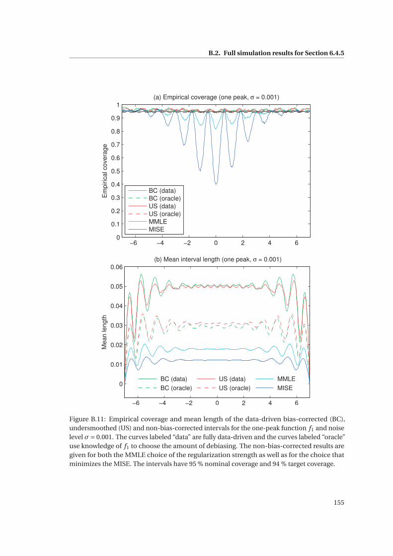
B.2. Full simulation results for Section 6.4.5
−6 −4 −2 0 2 4 60
0.1
0.2
0.3
0.4
0.5
0.6
0.7
0.8
0.9
1(a) Empirical coverage (one peak, σ = 0.001)
Em
piric
al c
over
age
BC (data)BC (oracle)US (data)US (oracle)MMLEMISE
−6 −4 −2 0 2 4 6
0
0.01
0.02
0.03
0.04
0.05
0.06(b) Mean interval length (one peak, σ = 0.001)
Mea
n le
ngth
BC (data)
BC (oracle)
US (data)
US (oracle)
MMLE
MISE
Figure B.11: Empirical coverage and mean length of the data-driven bias-corrected (BC),undersmoothed (US) and non-bias-corrected intervals for the one-peak function f1 and noiselevel σ= 0.001. The curves labeled “data” are fully data-driven and the curves labeled “oracle”use knowledge of f1 to choose the amount of debiasing. The non-bias-corrected results aregiven for both the MMLE choice of the regularization strength as well as for the choice thatminimizes the MISE. The intervals have 95 % nominal coverage and 94 % target coverage.
155

Appendix B. Full simulation results
−6 −4 −2 0 2 4 6
−0.1
0
0.1
0.2
0.3
0.4
0.5f(
s)(a) Non−bias−corrected intervals, σ = 0.005
Non−bias−correctedTrueSmeared
−6 −4 −2 0 2 4 6
−0.1
0
0.1
0.2
0.3
0.4
0.5
f(s)
(b) Iteratively bias−corrected intervals, σ = 0.005
Bias−correctedTrueSmeared
−6 −4 −2 0 2 4 6
−0.1
0
0.1
0.2
0.3
0.4
0.5
f(s)
(c) Undersmoothed intervals, σ = 0.005
UndersmoothedTrueSmeared
Figure B.12: Data-driven confidence intervals for the one-peak function f1 and noise levelσ = 0.005. The regularization strength is chosen using the MMLE and the amount of bias-correction and undersmoothing using the procedure described in Sections 6.4.3 and 6.4.4.The intervals have 95 % nominal coverage and 94 % target coverage. This figure is the same asFigure 6.10 in the main text.
156

B.2. Full simulation results for Section 6.4.5
−6 −4 −2 0 2 4 60
0.1
0.2
0.3
0.4
0.5
0.6
0.7
0.8
0.9
1(a) Empirical coverage (one peak, σ = 0.005)
Em
piric
al c
over
age
BC (data)BC (oracle)US (data)US (oracle)MMLEMISE
−6 −4 −2 0 2 4 60
0.01
0.02
0.03
0.04
0.05
0.06
0.07
0.08
0.09
0.1
(b) Mean interval length (one peak, σ = 0.005)
Mea
n le
ngth
BC (data)
BC (oracle)
US (data)
US (oracle)
MMLE
MISE
Figure B.13: Empirical coverage and mean length of the data-driven bias-corrected (BC),undersmoothed (US) and non-bias-corrected intervals for the one-peak function f1 and noiselevel σ= 0.005. The curves labeled “data” are fully data-driven and the curves labeled “oracle”use knowledge of f1 to choose the amount of debiasing. The non-bias-corrected results aregiven for both the MMLE choice of the regularization strength as well as for the choice thatminimizes the MISE. The intervals have 95 % nominal coverage and 94 % target coverage. Thisfigure is the same as Figure 6.11 in the main text.
157

Appendix B. Full simulation results
−6 −4 −2 0 2 4 6
−0.1
0
0.1
0.2
0.3
0.4
0.5
f(s)
(a) Non−bias−corrected intervals, σ = 0.025
Non−bias−correctedTrueSmeared
−6 −4 −2 0 2 4 6
−0.1
0
0.1
0.2
0.3
0.4
0.5
f(s)
(b) Iteratively bias−corrected intervals, σ = 0.025
Bias−correctedTrueSmeared
−6 −4 −2 0 2 4 6
−0.1
0
0.1
0.2
0.3
0.4
0.5
f(s)
(c) Undersmoothed intervals, σ = 0.025
UndersmoothedTrueSmeared
Figure B.14: Data-driven confidence intervals for the one-peak function f1 and noise levelσ = 0.025. The regularization strength is chosen using the MMLE and the amount of bias-correction and undersmoothing using the procedure described in Sections 6.4.3 and 6.4.4.The intervals have 95 % nominal coverage and 94 % target coverage.
158

B.2. Full simulation results for Section 6.4.5
−6 −4 −2 0 2 4 60
0.1
0.2
0.3
0.4
0.5
0.6
0.7
0.8
0.9
1(a) Empirical coverage (one peak, σ = 0.025)
Em
piric
al c
over
age
BC (data)BC (oracle)US (data)US (oracle)MMLEMISE
−6 −4 −2 0 2 4 60
0.02
0.04
0.06
0.08
0.1
0.12
0.14
0.16
0.18
0.2
(b) Mean interval length (one peak, σ = 0.025)
Mea
n le
ngth
BC (data)
BC (oracle)
US (data)
US (oracle)
MMLE
MISE
Figure B.15: Empirical coverage and mean length of the data-driven bias-corrected (BC),undersmoothed (US) and non-bias-corrected intervals for the one-peak function f1 and noiselevel σ= 0.025. The curves labeled “data” are fully data-driven and the curves labeled “oracle”use knowledge of f1 to choose the amount of debiasing. The non-bias-corrected results aregiven for both the MMLE choice of the regularization strength as well as for the choice thatminimizes the MISE. The intervals have 95 % nominal coverage and 94 % target coverage.
159

Appendix B. Full simulation results
−6 −4 −2 0 2 4 6
−0.1
0
0.1
0.2
0.3
0.4
f(s)
(a) Non−bias−corrected intervals, σ = 0.001
Non−bias−correctedTrueSmeared
−6 −4 −2 0 2 4 6
−0.1
0
0.1
0.2
0.3
0.4
f(s)
(b) Iteratively bias−corrected intervals, σ = 0.001
Bias−correctedTrueSmeared
−6 −4 −2 0 2 4 6
−0.1
0
0.1
0.2
0.3
0.4
f(s)
(c) Undersmoothed intervals, σ = 0.001
UndersmoothedTrueSmeared
Figure B.16: Data-driven confidence intervals for the two-peak function f2 and noise levelσ = 0.001. The regularization strength is chosen using the MMLE and the amount of bias-correction and undersmoothing using the procedure described in Sections 6.4.3 and 6.4.4.The intervals have 95 % nominal coverage and 94 % target coverage.
160

B.2. Full simulation results for Section 6.4.5
−6 −4 −2 0 2 4 60
0.1
0.2
0.3
0.4
0.5
0.6
0.7
0.8
0.9
1(a) Empirical coverage (two peaks, σ = 0.001)
Em
piric
al c
over
age
BC (data)BC (oracle)US (data)US (oracle)MMLEMISE
−6 −4 −2 0 2 4 6
0
0.005
0.01
0.015
0.02
0.025
0.03
0.035
0.04
0.045
0.05(b) Mean interval length (two peaks, σ = 0.001)
Mea
n le
ngth
BC (data)
BC (oracle)
US (data)
US (oracle)
MMLE
MISE
Figure B.17: Empirical coverage and mean length of the data-driven bias-corrected (BC),undersmoothed (US) and non-bias-corrected intervals for the two-peak function f2 and noiselevel σ= 0.001. The curves labeled “data” are fully data-driven and the curves labeled “oracle”use knowledge of f2 to choose the amount of debiasing. The non-bias-corrected results aregiven for both the MMLE choice of the regularization strength as well as for the choice thatminimizes the MISE. The intervals have 95 % nominal coverage and 94 % target coverage.
161

Appendix B. Full simulation results
−6 −4 −2 0 2 4 6
−0.1
0
0.1
0.2
0.3
0.4
f(s)
(a) Non−bias−corrected intervals, σ = 0.005
Non−bias−correctedTrueSmeared
−6 −4 −2 0 2 4 6
−0.1
0
0.1
0.2
0.3
0.4
f(s)
(b) Iteratively bias−corrected intervals, σ = 0.005
Bias−correctedTrueSmeared
−6 −4 −2 0 2 4 6
−0.1
0
0.1
0.2
0.3
0.4
f(s)
(c) Undersmoothed intervals, σ = 0.005
UndersmoothedTrueSmeared
Figure B.18: Data-driven confidence intervals for the two-peak function f2 and noise levelσ = 0.005. The regularization strength is chosen using the MMLE and the amount of bias-correction and undersmoothing using the procedure described in Sections 6.4.3 and 6.4.4.The intervals have 95 % nominal coverage and 94 % target coverage.
162

B.2. Full simulation results for Section 6.4.5
−6 −4 −2 0 2 4 60
0.1
0.2
0.3
0.4
0.5
0.6
0.7
0.8
0.9
1(a) Empirical coverage (two peaks, σ = 0.005)
Em
piric
al c
over
age
BC (data)BC (oracle)US (data)US (oracle)MMLEMISE
−6 −4 −2 0 2 4 60
0.01
0.02
0.03
0.04
0.05
0.06
0.07
0.08
0.09(b) Mean interval length (two peaks, σ = 0.005)
Mea
n le
ngth
BC (data)
BC (oracle)
US (data)
US (oracle)
MMLE
MISE
Figure B.19: Empirical coverage and mean length of the data-driven bias-corrected (BC),undersmoothed (US) and non-bias-corrected intervals for the two-peak function f2 and noiselevel σ= 0.005. The curves labeled “data” are fully data-driven and the curves labeled “oracle”use knowledge of f2 to choose the amount of debiasing. The non-bias-corrected results aregiven for both the MMLE choice of the regularization strength as well as for the choice thatminimizes the MISE. The intervals have 95 % nominal coverage and 94 % target coverage.
163

Appendix B. Full simulation results
−6 −4 −2 0 2 4 6
−0.1
0
0.1
0.2
0.3
0.4
f(s)
(a) Non−bias−corrected intervals, σ = 0.025
Non−bias−correctedTrueSmeared
−6 −4 −2 0 2 4 6
−0.1
0
0.1
0.2
0.3
0.4
f(s)
(b) Iteratively bias−corrected intervals, σ = 0.025
Bias−correctedTrueSmeared
−6 −4 −2 0 2 4 6
−0.1
0
0.1
0.2
0.3
0.4
f(s)
(c) Undersmoothed intervals, σ = 0.025
UndersmoothedTrueSmeared
Figure B.20: Data-driven confidence intervals for the two-peak function f2 and noise levelσ = 0.025. The regularization strength is chosen using the MMLE and the amount of bias-correction and undersmoothing using the procedure described in Sections 6.4.3 and 6.4.4.The intervals have 95 % nominal coverage and 94 % target coverage.
164

B.2. Full simulation results for Section 6.4.5
−6 −4 −2 0 2 4 60
0.1
0.2
0.3
0.4
0.5
0.6
0.7
0.8
0.9
1(a) Empirical coverage (two peaks, σ = 0.025)
Em
piric
al c
over
age
BC (data)BC (oracle)US (data)US (oracle)MMLEMISE
−6 −4 −2 0 2 4 60
0.02
0.04
0.06
0.08
0.1
0.12
0.14
0.16
0.18(b) Mean interval length (two peaks, σ = 0.025)
Mea
n le
ngth
BC (data)
BC (oracle)
US (data)
US (oracle)
MMLE
MISE
Figure B.21: Empirical coverage and mean length of the data-driven bias-corrected (BC),undersmoothed (US) and non-bias-corrected intervals for the two-peak function f2 and noiselevel σ= 0.025. The curves labeled “data” are fully data-driven and the curves labeled “oracle”use knowledge of f2 to choose the amount of debiasing. The non-bias-corrected results aregiven for both the MMLE choice of the regularization strength as well as for the choice thatminimizes the MISE. The intervals have 95 % nominal coverage and 94 % target coverage.
165

Appendix B. Full simulation results
B.3 Full simulation results for Section 6.5
This section gives the full results of the simulation study of Section 6.5. In particular, the
following pages include a realization of the different intervals as well as the equivalents of
Figures 6.13 and 6.14 for the three sample sizes λtot = 1 000, 10 000 and 50 000. The results are
given in the order of decreasing sample size.
166

B.3. Full simulation results for Section 6.5
−6 −4 −2 0 2 4 6
0
2000
4000
6000
8000
10000
12000
(a) Non−bias−corrected Gaussian intervals, λtot
= 50000
Inte
nsity
Non−bias−correctedTrue intensity
−6 −4 −2 0 2 4 6
0
2000
4000
6000
8000
10000
12000
(b) Iteratively bias−corrected Gaussian intervals, λtot
= 50000
Inte
nsity
Non−bias−correctedBias−correctedTrue intensity
−6 −4 −2 0 2 4 6
0
2000
4000
6000
8000
10000
12000
(c) Undersmoothed Gaussian intervals, λtot
= 50000
Inte
nsity
Non−bias−correctedUndersmoothedTrue intensity
Figure B.22: Unfolding of the two peaks on a uniform background test setup using Gaussianconfidence intervals induced by the unconstrained Gaussian estimator βG. The figure shows(a) the non-bias-corrected intervals, (b) the data-driven iteratively bias-corrected intervalsand (c) the data-driven undersmoothed intervals. The amount of bias-correction and under-smoothing is calibrated to give 94 % pointwise target coverage for intervals with 95 % nominalcoverage. The sample size was λtot = 50 000 and the regularization strength chosen usingthe MMLE.
167

Appendix B. Full simulation results
−6 −4 −2 0 2 4 60
0.2
0.4
0.6
0.8
1
Em
piric
al c
over
age
(a) Empirical coverage, λtot
= 50000
Bias−correctedUndersmoothedNon−bias−corrected
−6 −4 −2 0 2 4 60
1000
2000
3000
4000
5000
Mea
n le
ngth
(b) Mean interval length, λtot
= 50000
Bias−correctedUndersmoothedNon−bias−corrected
Figure B.23: Empirical coverage and mean interval length in unfolding the two peaks on auniform background test setup using data-driven iteratively bias-corrected, undersmoothedand non-bias-corrected Gaussian confidence intervals induced by the unconstrained Gaussianestimator βG. The sample size was λtot = 50 000 and the regularization strength chosen usingthe MMLE. The intervals have 94 % pointwise target coverage (dashed horizontal line) and95 % nominal coverage (solid horizontal line).
168

B.3. Full simulation results for Section 6.5
−5 0 5
0
5000
10000
15000
(a) 10th percentile
Inte
nsity
−5 0 5
0
5000
10000
15000
(b) 25th percentile
Inte
nsity
−5 0 5
0
5000
10000
15000
(c) 75th percentile
Inte
nsity
−5 0 5
0
5000
10000
15000
(d) 90th percentile
Inte
nsity
Figure B.24: Illustration of the variability of the data-driven iteratively bias-corrected Gaussianconfidence intervals in unfolding the two peaks on a uniform background test setup withsample size λtot = 50 000. The panels show realizations of the intervals for given percentilesof the sampling distribution of interval lengths (averaged over s). The intervals have 94 %pointwise target coverage and 95 % nominal coverage. The figures also show the true intensity(dashed line), the non-bias-corrected point estimate (solid line) and the bias-corrected pointestimate (dotted line).
169

Appendix B. Full simulation results
−6 −4 −2 0 2 4 6
−500
0
500
1000
1500
2000
2500
(a) Non−bias−corrected Gaussian intervals, λtot
= 10000In
tens
ity
Non−bias−correctedTrue intensity
−6 −4 −2 0 2 4 6
−500
0
500
1000
1500
2000
2500
(b) Iteratively bias−corrected Gaussian intervals, λtot
= 10000
Inte
nsity
Non−bias−correctedBias−correctedTrue intensity
−6 −4 −2 0 2 4 6
−500
0
500
1000
1500
2000
2500
(c) Undersmoothed Gaussian intervals, λtot
= 10000
Inte
nsity
Non−bias−correctedUndersmoothedTrue intensity
Figure B.25: Unfolding of the two peaks on a uniform background test setup using Gaussianconfidence intervals induced by the unconstrained Gaussian estimator βG. The figure shows(a) the non-bias-corrected intervals, (b) the data-driven iteratively bias-corrected intervalsand (c) the data-driven undersmoothed intervals. The amount of bias-correction and under-smoothing is calibrated to give 94 % pointwise target coverage for intervals with 95 % nominalcoverage. The sample size was λtot = 10 000 and the regularization strength chosen usingthe MMLE.
170

B.3. Full simulation results for Section 6.5
−6 −4 −2 0 2 4 60
0.2
0.4
0.6
0.8
1E
mpi
rical
cov
erag
e
(a) Empirical coverage, λtot
= 10000
Bias−correctedUndersmoothedNon−bias−corrected
−6 −4 −2 0 2 4 60
200
400
600
800
1000
1200
1400
Mea
n le
ngth
(b) Mean interval length, λtot
= 10000
Bias−correctedUndersmoothedNon−bias−corrected
Figure B.26: Empirical coverage and mean interval length in unfolding the two peaks on auniform background test setup using data-driven iteratively bias-corrected, undersmoothedand non-bias-corrected Gaussian confidence intervals induced by the unconstrained Gaussianestimator βG. The sample size was λtot = 10 000 and the regularization strength chosen usingthe MMLE. The intervals have 94 % pointwise target coverage (dashed horizontal line) and95 % nominal coverage (solid horizontal line). This figure is the same as Figure 6.13 in themain text.
171

Appendix B. Full simulation results
−5 0 5−1000
0
1000
2000
3000
(a) 10th percentile
Inte
nsity
−5 0 5−1000
0
1000
2000
3000
(b) 25th percentile
Inte
nsity
−5 0 5−1000
0
1000
2000
3000
(c) 75th percentile
Inte
nsity
−5 0 5−1000
0
1000
2000
3000
(d) 90th percentile
Inte
nsity
Figure B.27: Illustration of the variability of the data-driven iteratively bias-corrected Gaussianconfidence intervals in unfolding the two peaks on a uniform background test setup withsample size λtot = 10 000. The panels show realizations of the intervals for given percentilesof the sampling distribution of interval lengths (averaged over s). The intervals have 94 %pointwise target coverage and 95 % nominal coverage. The figures also show the true intensity(dashed line), the non-bias-corrected point estimate (solid line) and the bias-corrected pointestimate (dotted line). This figure is the same as Figure 6.14 in the main text.
172

B.3. Full simulation results for Section 6.5
−6 −4 −2 0 2 4 6
−100
−50
0
50
100
150
200
250
(a) Non−bias−corrected Gaussian intervals, λtot
= 1000
Inte
nsity
Non−bias−correctedTrue intensity
−6 −4 −2 0 2 4 6
−100
−50
0
50
100
150
200
250
(b) Iteratively bias−corrected Gaussian intervals, λtot
= 1000
Inte
nsity
Non−bias−correctedBias−correctedTrue intensity
−6 −4 −2 0 2 4 6
−100
−50
0
50
100
150
200
250
(c) Undersmoothed Gaussian intervals, λtot
= 1000
Inte
nsity
Non−bias−correctedUndersmoothedTrue intensity
Figure B.28: Unfolding of the two peaks on a uniform background test setup using Gaussianconfidence intervals induced by the unconstrained Gaussian estimator βG. The figure shows(a) the non-bias-corrected intervals, (b) the data-driven iteratively bias-corrected intervalsand (c) the data-driven undersmoothed intervals. The amount of bias-correction and un-dersmoothing is calibrated to give 94 % pointwise target coverage for intervals with 95 %nominal coverage. The sample size was λtot = 1 000 and the regularization strength chosenusing the MMLE.
173

Appendix B. Full simulation results
−6 −4 −2 0 2 4 60
0.2
0.4
0.6
0.8
1
Em
piric
al c
over
age
(a) Empirical coverage, λtot
= 1000
Bias−correctedUndersmoothedNon−bias−corrected
−6 −4 −2 0 2 4 60
20
40
60
80
100
120
140
160
180
Mea
n le
ngth
(b) Mean interval length, λtot
= 1000
Bias−correctedUndersmoothedNon−bias−corrected
Figure B.29: Empirical coverage and mean interval length in unfolding the two peaks on auniform background test setup using data-driven iteratively bias-corrected, undersmoothedand non-bias-corrected Gaussian confidence intervals induced by the unconstrained Gaussianestimator βG. The sample size was λtot = 1 000 and the regularization strength chosen usingthe MMLE. The intervals have 94 % pointwise target coverage (dashed horizontal line) and95 % nominal coverage (solid horizontal line).
174

B.3. Full simulation results for Section 6.5
−5 0 5
−100
0
100
200
300
(a) 10th percentile
Inte
nsity
−5 0 5
−100
0
100
200
300
(b) 25th percentile
Inte
nsity
−5 0 5
−100
0
100
200
300
(c) 75th percentile
Inte
nsity
−5 0 5
−100
0
100
200
300
(d) 90th percentile
Inte
nsity
Figure B.30: Illustration of the variability of the data-driven iteratively bias-corrected Gaussianconfidence intervals in unfolding the two peaks on a uniform background test setup withsample size λtot = 1 000. The panels show realizations of the intervals for given percentilesof the sampling distribution of interval lengths (averaged over s). The intervals have 94 %pointwise target coverage and 95 % nominal coverage. The figures also show the true intensity(dashed line), the non-bias-corrected point estimate (solid line) and the bias-corrected pointestimate (dotted line).
175


Bibliography
T. Adye. Unfolding algorithms and tests using RooUnfold. In H. B. Prosper and L. Lyons, editors,
Proceedings of the PHYSTAT 2011 Workshop on Statistical Issues Related to Discovery Claims
in Search Experiments and Unfolding, CERN-2011-006, pages 313–318, CERN, Geneva,
Switzerland, 17–20 January 2011.
H. Akaike. Information theory and an extension of the maximum likelihood principle. In B. N.
Petrov and F. Czáki, editors, Second International Symposium on Information Theory, pages
267–281, Akademiai Kiadó, Budapest, 1973.
H. Akaike. A new look at the statistical model identification. IEEE Transactions on Automatic
Control, 19(6):716–723, 1974.
A. Antoniadis and J. Bigot. Poisson inverse problems. The Annals of Statistics, 34(5):2132–2158,
2006.
ATLAS and CMS Collaborations. Procedure for the LHC Higgs boson search combination in
summer 2011. ATL-PHYS-PUB-2011-11, CMS NOTE-2011/005, 2011.
ATLAS Collaboration. Observation of a new particle in the search for the Standard Model
Higgs boson with the ATLAS detector at the LHC. Physics Letters B, 716(1):1–29, 2012a.
ATLAS Collaboration. Measurement of the transverse momentum distribution of W bosons in
pp collisions at�
s = 7 TeV with the ATLAS detector. Physical Review D, 85:012005, 2012b.
G. Backus. Inference from inadequate and inaccurate data, I. Proceedings of the National
Academy of Sciences, 65(1):1–7, 1970.
D. Barney. CMS-doc-4172. https://cms-docdb.cern.ch/cgi-bin/PublicDocDB/
ShowDocument?docid=4172, 2004. Retrieved 21.1.2014.
M. Bazaraa, H. Sherali, and C. Shetty. Nonlinear Programming: Theory and Algorithms. Wiley-
Interscience, 3rd edition, 2006.
O. Behnke, K. Kröninger, G. Schott, and T. Schörner-Sadenius, editors. Data Analysis in High
Energy Physics: A Practical Guide to Statistical Methods. Wiley, 2013.
R. Beran. Stein confidence sets and the bootstrap. Statistica Sinica, 5:109–127, 1995.
177

Bibliography
J. Beringer et al. Review of particle physics. Physical Review D, 86:010001, Particle Data Group,
2012.
R. Berk, L. Brown, A. Buja, K. Zhang, and L. Zhao. Valid post-selection inference. The Annals of
Statistics, 41(2):802–837, 2013.
J. M. Bernardo and A. F. M. Smith. Bayesian Theory. John Wiley & Sons, 2000.
P. C. Bhat. Multivariate analysis methods in particle physics. Annual Review of Nuclear and
Particle Science, 61:281–309, 2011.
V. Blobel. Unfolding methods in high-energy physics experiments. In CERN Yellow Report
85-09, pages 88–127, 1985.
V. Blobel. The RUN manual: Regularized unfolding for high-energy physics experiments. OPAL
Technical Note TN361, 1996.
V. Blobel. Unfolding. In O. Behnke, K. Kröninger, G. Schott, and T. Schörner-Sadenius, editors,
Data Analysis in High Energy Physics: A Practical Guide to Statistical Methods, pages 187–225.
Wiley, 2013.
J. G. Booth and J. P. Hobert. Maximizing generalized linear mixed model likelihoods with
an automated Monte Carlo EM algorithm. Journal of the Royal Statistical Society. Series B
(Statistical Methodology), 61(1):265–285, 1999.
W. J. Browne and D. Draper. A comparison of Bayesian and likelihood-based methods for
fitting multilevel models. Bayesian Analysis, 1(3):473–514, 2006.
W. R. Burrus. Utilization of a priori information by means of mathematical programming
in the statistical interpretation of measured distributions, June 1965. Oak Ridge National
Laboratory, ORNL-3743.
W. R. Burrus and V. V. Verbinski. Fast-neutron spectroscopy with thick organic scintillators.
Nuclear Instruments and Methods, 67(2):181–196, 1969.
D. Calvetti, J. P. Kaipio, and E. Someralo. Aristotelian prior boundary conditions. International
Journal of Mathematics and Computer Science, 1:63–81, 2006.
B. P. Carlin and T. A. Louis. Bayesian Methods for Data Analysis. Chapman & Hall/CRC, 3rd
edition, 2009.
R. J. Carroll, A. Delaigle, and P. Hall. Testing and estimating shape-constrained nonparametric
density and regression in the presence of measurement error. Journal of the American
Statistical Association, 106(493):191–202, 2011.
G. Casella. Empirical Bayes Gibbs sampling. Biostatistics, 2(4):485–500, 2001.
G. Casella and R. L. Berger. Statistical Inference. Duxbury, 2nd edition, 2002.
178

Bibliography
G. Choudalakis. Fully Bayesian unfolding. arXiv:1201.4612v4 [physics.data-an], 2012.
CMS Collaboration. The CMS experiment at the CERN LHC. Journal of Instrumentation, 3:
S08004, 2008.
CMS Collaboration. Particle-flow event reconstruction in CMS and performance for jets, taus,
and E missT . CMS Physics Analysis Summary CMS-PAS-PFT-09-001, 2009.
CMS Collaboration. Measurement of the inclusive jet cross section in pp collisions at 7 TeV,
2010. CMS-PAS-QCD-10-011, available at http://cds.cern.ch/record/1280682.
CMS Collaboration. Measurement of the inclusive jet cross section in pp collisions at�s = 7 TeV. Physical Review Letters, 107:132001, 2011.
CMS Collaboration. Search for dark matter and large extra dimensions in monojet events in
pp collisions at�
s = 7 TeV. Journal of High Energy Physics, 09:094, 2012a.
CMS Collaboration. Observation of a new boson at a mass of 125 GeV with the CMS experiment
at the LHC. Physics Letters B, 716(1):30–61, 2012b.
CMS Collaboration. Shape, transverse size, and charged-hadron multiplicity of jets in pp
collisions at�
s = 7 TeV. Journal of High Energy Physics, 06:160, 2012c.
CMS Collaboration. Measurement of the charge asymmetry in top-quark pair production in
proton-proton collisions at�
s = 7 TeV. Physics Letters B, 709(1–2):28–49, 2012d.
CMS Collaboration. Energy calibration and resolution of the CMS electromagnetic calorimeter
in pp collisions at�
s = 7 TeV. Journal of Instrumentation, 8(09):P09009, 2013a.
CMS Collaboration. Measurements of differential jet cross sections in proton-proton collisions
at�
s = 7 TeV with the CMS detector. Physical Review D, 87:112002, 2013b.
CMS Collaboration. Measurement of differential top-quark-pair production cross sections in
pp collisions at�
s = 7 TeV. The European Physical Journal C, 73:2339, 2013c.
CMS Collaboration. Measurement of differential cross sections for Higgs boson production in
the diphoton decay channel in pp collisions at�
s = 8 TeV. The European Physical Journal C,
76:13, 2016.
P.-A. Cornillon, N. Hengartner, N. Jegou, and E. Matzner-Løber. Iterative bias reduction:
a comparative study. Statistics and Computing, 23(6):777–791, 2013.
P.-A. Cornillon, N. W. Hengartner, and E. Matzner-Løber. Recursive bias estimation for multi-
variate regression smoothers. ESAIM: Probability and Statistics, 18:483–502, 2014.
G. Cowan. Statistical Data Analysis. Oxford University Press, 1998.
K. Cranmer. Practical statistics for the LHC. arXiv:1503.07622v1 [physics.data-an], earlier
versions published in CERN Yellow Reports CERN-2014-003 and CERN-2015-001, 2015.
179

Bibliography
G. D’Agostini. A multidimensional unfolding method based on Bayes’ theorem. Nuclear
Instruments and Methods A, 362:487–498, 1995.
A. C. Davison and D. V. Hinkley. Bootstrap Methods and Their Application. Cambridge Univer-
sity Press, 1997.
C. de Boor. A Practical Guide to Splines. Springer, revised edition, 2001.
C. de Boor and J. W. Daniel. Splines with nonnegative B-spline coefficients. Mathematics of
Computation, 28(126):565–568, 1974.
H. P. Dembinski and M. Roth. An algorithm for automatic unfolding of one-dimensional data
distributions. Nuclear Instruments and Methods in Physics Research A, 729:410–416, 2013.
A. P. Dempster, N. M. Laird, and D. B. Rubin. Maximum likelihood from incomplete data via
the EM algorithm. Journal of the Royal Statistical Society. Series B (Methodological), 39(1):
1–38, 1977.
B. Efron. Better bootstrap confidence intervals. Journal of the American Statistical Association,
82(397):171–185, 1987.
B. Efron and R. Tibshirani. An Introduction to the Bootstrap. Chapman & Hall, 1993.
P. H. C. Eilers and B. D. Marx. Flexible smoothing with B-splines and penalties. Statistical
Science, 11(2):89–102, 1996.
H. W. Engl, M. Hanke, and A. Neubauer. Regularization of Inverse Problems. Kluwer, 2000.
L. Fahrmeir, T. Kneib, and S. Lang. Penalized structured additive regression for space-time
data: A Bayesian perspective. Statistica Sinica, 14(3):731–761, 2004.
S. Forte and G. Watt. Progress in the determination of the partonic structure of the proton.
Annual Review of Nuclear and Particle Science, 63:291–328, 2013.
F. Garwood. Fiducial limits for the Poisson distribution. Biometrika, 28(3/4):437–442, 1936.
A. Gelman. Prior distributions for variance parameters in hierarchical models (comment on
article by Browne and Draper). Bayesian analysis, 1(3):515–534, 2006.
S. Geman and D. E. McClure. Bayesian image analysis: An application to single photon
emission tomography. In Proceedings of the American Statistical Association, Statistical
Computing Section, pages 12–18, 1985.
S. Geman and D. E. McClure. Statistical methods for tomographic image reconstruction.
Bulletin of the International Statistical Institute, LII(4):5–21, 1987.
W. R. Gilks. Full conditional distributions. In W. R. Gilks, S. Richardson, and D. J. Spiegelhalter,
editors, Markov Chain Monte Carlo in Practice, pages 75–88. Chapman & Hall, 1996.
180

Bibliography
W. R. Gilks, S. Richardson, and D. J. Spiegelhalter. Introducing Markov chain Monte Carlo. In
W. R. Gilks, S. Richardson, and D. J. Spiegelhalter, editors, Markov Chain Monte Carlo in
Practice, pages 1–19. Chapman & Hall, 1996.
H. Goldstein. Consistent estimators for multilevel generalized linear models using an iterated
bootstrap. Multilevel Modelling Newsletter, 8(1):3–6, 1996.
P. J. Green. Bayesian reconstructions from emission tomography data using a modified EM
algorithm. IEEE Transactions on Medical Imaging, 9(1):84–93, 1990a.
P. J. Green. On use of the EM for penalized likelihood estimation. Journal of the Royal Statistical
Society. Series B (Methodological), 52(3):443–452, 1990b.
P. J. Green and B. W. Silverman. Nonparametric Regression and Generalized Linear Models: A
Roughness Penalty Approach. Chapman & Hall, 1994.
U. Grenander. On the theory of mortality measurement: Part II. Scandinavian Actuarial
Journal, 1956(2):125–153, 1956.
P. Groeneboom and G. Jongbloed. Nonparametric Estimation Under Shape Constraints: Esti-
mators, Algorithms and Asymptotics. Cambridge University Press, 2014.
E. Gross and O. Vitells. Trial factors for the look elsewhere effect in high energy physics.
European Physical Journal C, 70(1–2):525–530, 2010.
P. Hall. Effect of bias estimation on coverage accuracy of bootstrap confidence intervals for a
probability density. The Annals of Statistics, 20(2):675–694, 1992.
P. Hall and J. Horowitz. A simple bootstrap method for constructing nonparametric confidence
bands for functions. The Annals of Statistics, 41(4):1892–1921, 2013.
P. C. Hansen. Analysis of discrete ill-posed problems by means of the L-curve. SIAM Review,
34(4):561–580, 1992.
P. C. Hansen. Discrete Inverse Problems: Insight and Algorithms. SIAM, 2010.
T. J. Hastie and R. J. Tibshirani. Generalized Additive Models. Chapman & Hall, 1990.
J. G. Heinrich. Coverage of error bars for Poisson data. CDF Public Note CDF/MEMO/STATIS-
TICS/PUBLIC/6438, 2003.
N. W. Hengartner and P. B. Stark. Finite-sample confidence envelopes for shape-restricted
densities. The Annals of Statistics, 23(2):525–550, 1995.
A. Höcker and V. Kartvelishvili. SVD approach to data unfolding. Nuclear Instruments and
Methods in Physics Research A, 372:469–481, 1996.
A. E. Hoerl and R. W. Kennard. Ridge regression: Biased estimation for nonorthogonal prob-
lems. Technometrics, 12(1):55–67, 1970.
181

Bibliography
A. Javanmard and A. Montanari. Confidence intervals and hypothesis testing for high-
dimensional regression. Journal of Machine Learning Research, 15(Oct):2869–2909, 2014.
J. Kaipio and E. Somersalo. Statistical and Computational Inverse Problems. Springer, 2005.
A. Kondor. Method of convergent weights – An iterative procedure for solving Fredholm’s
integral equations of the first kind. Nuclear Instruments and Methods, 216:177–181, 1983.
E. Kreyszig. Introductory Functional Analysis with Applications. John Wiley & Sons, 1978.
A. Y. C. Kuk. Asymptotically unbiased estimation in generalized linear models with random
effects. Journal of the Royal Statistical Society. Series B (Methodological), 57(2):395–407,
1995.
M. Kuusela. Statistical issues in unfolding methods for high energy physics. Master’s thesis,
Aalto University, 2012.
M. Kuusela and V. M. Panaretos. Statistical unfolding of elementary particle spectra: Empirical
Bayes estimation and bias-corrected uncertainty quantification. The Annals of Applied
Statistics, 9(3):1671–1705, 2015.
M. Kuusela and P. B. Stark. Shape-constrained uncertainty quantification in unfolding steeply
falling elementary particle spectra. arXiv:1512.00905v3 [stat.AP], submitted, 2016.
K. Lange and R. Carson. EM reconstruction algorithms for emission and transmission tomog-
raphy. Journal of Computer Assisted Tomography, 8(2):306–316, 1984.
C. L. Lawson and R. J. Hanson. Solving Least Squares Problems. SIAM, 1995.
M. G. Low. On nonparametric confidence intervals. The Annals of Statistics, 25(6):2547–2554,
1997.
L. B. Lucy. An iterative technique for the rectification of observed distributions. Astronomical
Journal, 79(6):745–754, 1974.
D. G. Luenberger. Optimization by Vector Space Methods. John Wiley & Sons, 1969.
L. Lyons. Unfolding: Introduction. In H. B. Prosper and L. Lyons, editors, Proceedings of
the PHYSTAT 2011 Workshop on Statistical Issues Related to Discovery Claims in Search
Experiments and Unfolding, CERN-2011-006, pages 225–228, CERN, Geneva, Switzerland,
17–20 January 2011.
L. Lyons. Bayes and frequentism: A particle physicist’s perspective. Contemporary Physics, 54
(1):1–16, 2013.
G. Marra and S. N. Wood. Coverage properties of confidence intervals for generalized additive
model components. Scandinavian Journal of Statistics, 39(1):53–74, 2012.
Mathworks. Curve Fitting Toolbox: User’s Guide, 2014a. Version 3.4.1.
182

Bibliography
Mathworks. Optimization Toolbox: User’s Guide, 2014b. Version 7.0.
G. J. McLachlan and T. Krishnan. The EM Algorithm and Extensions. Wiley-Interscience, 2nd
edition, 2008.
A. Meister. Deconvolution Problems in Nonparametric Statistics. Springer, 2009.
N. Milke, M. Doert, S. Klepser, D. Mazin, V. Blobel, and W. Rhode. Solving inverse problems
with the unfolding program TRUEE: Examples in astroparticle physics. Nuclear Instruments
and Methods in Physics Research A, 697:133–147, 2013.
V. A. Morozov. On the solution of functional equations by the method of regularization. Soviet
Mathematics Doklady, 7:414–417, 1966.
H. N. Mülthei and B. Schorr. On an iterative method for a class of integral equations of the
first kind. Mathematical Methods in the Applied Sciences, 9:137–168, 1987a.
H. N. Mülthei and B. Schorr. On an iterative method for the unfolding of spectra. Nuclear
Instruments and Methods in Physics Research A, 257:371–377, 1987b.
H. N. Mülthei and B. Schorr. On properties of the iterative maximum likelihood reconstruction
method. Mathematical Methods in the Applied Sciences, 11:331–342, 1989.
NNPDF Collaboration. Parton distributions for the LHC run II. Journal of High Energy Physics,
1504:040, 2015.
J. Nocedal and S. J. Wright. Numerical Optimization. Springer, 2nd edition, 2006.
D. Nychka. Confidence intervals for smoothing splines. Journal of the American Statistical
Association, 83(404):1134–1143, 1988.
D. P. O’Leary and B. W. Rust. Confidence intervals for inequality-constrained least squares
problems, with applications to ill-posed problems. SIAM Journal on Scientific and Statistical
Computing, 7(2):473–489, 1986.
M. J. Oreglia. A study of the reactions ψ′ → γγψ. PhD thesis, Stanford University, 1980.
F. O’Sullivan. A statistical perspective on ill-posed inverse problems. Statistical Science, 1(4):
505–527, 1986.
F. O’Sullivan. Fast computation of fully automated log-density and log-hazard estimators.
SIAM Journal on Scientific and Statistical Computing, 9(2):363–379, 1988.
V. M. Panaretos. Statistics for Mathematicians: A rigorous first course. Birkhäuser, 2016.
G. C. Pflug and R. J.-B. Wets. Shape-restricted nonparametric regression with overall noisy
measurements. Journal of Nonparametric Statistics, 25(2):323–338, 2013.
D. L. Phillips. A technique for the numerical solution of certain integral equations of the first
kind. Journal of the ACM, 9(1):84–97, 1962.
183

Bibliography
A. Pintore, P. Speckman, and C. C. Holmes. Spatially adaptive smoothing splines. Biometrika,
93(1):113–125, 2006.
H. B. Prosper and L. Lyons, editors. Proceedings of the PHYSTAT 2011 Workshop on Statistical
Issues Related to Discovery Claims in Search Experiments and Unfolding, CERN-2011-006,
CERN, Geneva, Switzerland, 2011.
H. B. Prosper, L. Lyons, and A. D. Roeck, editors. Proceedings of the PHYSTAT LHC Workshop
on Statistical Issues for LHC Physics, CERN–2008–001, CERN, Geneva, Switzerland, 2008.
N. Pya and S. N. Wood. Shape constrained additive models. Statistics and Computing, 25(3):
543–559, 2015.
C. E. Rasmussen and C. K. I. Williams. Gaussian Processes for Machine Learning. MIT Press,
2006.
P. T. Reiss and R. T. Ogden. Smoothing parameter selection for a class of semiparametric linear
models. Journal of the Royal Statistical Society. Series B (Statistical Methodology), 71(2):
505–523, 2009.
R.-D. Reiss. A Course on Point Processes. Springer-Verlag, 1993.
W. H. Richardson. Bayesian-based iterative method of image restoration. Journal of the Optical
Society of America, 62(1):55–59, 1972.
C. P. Robert and G. Casella. Monte Carlo Statistical Methods. Springer, 2nd edition, 2004.
T. Robertson, F. T. Wright, and R. L. Dykstra. Order Restricted Statistical Inference. John Wiley &
Sons, 1988.
D. Ruppert and R. J. Carroll. Spatially-adaptive penalties for spline fitting. Australian and New
Zealand Journal of Statistics, 42(2):205–223, 2000.
D. Ruppert, M. P. Wand, and R. J. Carroll. Semiparametric Regression. Cambridge University
Press, 2003.
B. W. Rust and W. R. Burrus. Mathematical Programming and the Numerical Solution of Linear
Equations. American Elsevier, 1972.
S. S. Saquib, C. A. Bouman, and K. Sauer. ML parameter estimation for Markov random fields
with applications to Bayesian tomography. IEEE Transactions on Image Processing, 7(7):
1029–1044, 1998.
S. Schmitt. TUnfold, an algorithm for correcting migration effects in high energy physics.
Journal of Instrumentation, 7:T10003, 2012.
L. L. Schumaker. Spline Function: Basic Theory. Cambridge University Press, 3rd edition, 2007.
184

Bibliography
L. A. Shepp and Y. Vardi. Maximum likelihood reconstruction for emission tomography. IEEE
Transactions on Medical Imaging, 1(2):113–122, 1982.
B. W. Silverman, M. C. Jones, J. D. Wilson, and D. W. Nychka. A smoothed EM approach to indi-
rect estimation problems, with particular reference to stereology and emission tomography.
Journal of the Royal Statistical Society. Series B (Methodological), 52(2):271–324, 1990.
P. B. Stark. Inference in infinite-dimensional inverse problems: Discretization and duality.
Journal of Geophysical Research, 97(B10):14055–14082, 1992.
M. Stone. Cross-validatory choice and assessment of statistical predictions. Journal of the
Royal Statistical Society. Series B (Methodological), 36:111–147, 1974.
L. Tierney. Markov chains for exploring posterior distributions. The Annals of Statistics, 22(4):
1701–1728, 1994.
A. N. Tikhonov. Solution of incorrectly formulated problems and the regularization method.
Soviet Mathematics: Doklady, 4:1035–1038, 1963.
D. A. van Dyk. The role of statistics in the discovery of a Higgs boson. Annual Review of
Statistics and Its Application, 1:41–59, 2014.
Y. Vardi, L. A. Shepp, and L. Kaufman. A statistical model for positron emission tomography.
Journal of the American Statistical Association, 80(389):8–20, 1985.
E. Veklerov and J. Llacer. Stopping rule for the MLE algorithm based on statistical hypothesis
testing. IEEE Transactions on Medical Imaging, 6(4):313–319, 1987.
I. Volobouev. On the expectation-maximization unfolding with smoothing. arXiv:1408.6500v2
[physics.data-an], 2015.
G. Wahba. Constrained regularization for ill posed linear operator equations, with applications
in meteorology and medicine. In S. S. Gupta and J. O. Berger, editors, Statistical Decision
Theory and Related Topics III, volume 2, pages 383–418. Academic Press, 1982.
G. Wahba. Bayesian “confidence intervals” for the cross-validated smoothing spline. Journal
of the Royal Statistical Society. Series B (Methodological), 45(1):133–150, 1983.
G. Wahba. Spline Models for Observational Data. SIAM, 1990.
L. Wasserman. All of Statistics: A Concise Course in Statistical Inference. Springer, 2004.
G. C. G. Wei and M. A. Tanner. A Monte Carlo implementation of the EM algorithm and the
poor man’s data augmentation algorithms. Journal of the American Statistical Association,
85(411):699–704, 1990.
I. S. Weir. Fully Bayesian reconstructions from single-photon emission computed tomography
data. Journal of the American Statistical Association, 92(437):49–60, 1997.
185

Bibliography
S. N. Wood. On confidence intervals for generalized additive models based on penalized
regression splines. Australian and New Zealand Journal of Statistics, 48(4):445–464, 2006a.
S. N. Wood. Generalized Additive Models: An Introduction with R. Chapman & Hall/CRC,
2006b.
S. N. Wood. Fast stable restricted maximum likelihood and marginal likelihood estimation of
semiparametric generalized linear models. Journal of the Royal Statistical Society. Series B
(Methodological), 73(1):3–36, 2011.
C. F. J. Wu. On the convergence properties of the EM algorithm. The Annals of Statistics, 11(1):
95–103, 1983.
M. Xie and K. Singh. Confidence distribution, the frequentist distribution estimator of a
parameter: A review (with discussion). International Statistical Review, 81(1):3–39, 2013.
G. A. Young and R. L. Smith. Essentials of Statistical Inference. Cambridge University Press,
2005.
G. Zech. Regularization and error assignment to unfolded distributions. In H. B. Prosper and
L. Lyons, editors, Proceedings of the PHYSTAT 2011 Workshop on Statistical Issues Related to
Discovery Claims in Search Experiments and Unfolding, CERN-2011-006, pages 252–259,
CERN, Geneva, Switzerland, 17–20 January 2011.
G. Zech. Iterative unfolding with the Richardson–Lucy algorithm. Nuclear Instruments and
Methods in Physics Research A, 716:1–9, 2013.
G. Zech. Analysis of distorted measurements: Parameter estimation and unfolding. Prelimi-
nary version of an upcoming report on unfolding techniques, 2016.
186


