r Human Brain Mapping 31:727–742 (2010) r

Unbiased Group-Level Statistical Assessment ofIndependent Component Maps by Means of

Automated Retrospective Matching

Dave R.M. Langers1,2*

1Department of Otorhinolaryngology/Head and Neck Surgery, University Medical Center Groningen,Groningen, The Netherlands

2Eaton-Peabody Laboratory, Massachusetts Eye and Ear Infirmary, Boston, Massachusetts

r r

Abstract: This report presents and validates a method for the group-level statistical assessment of inde-pendent component analysis (ICA) outcomes. The method is based on a matching of individual compo-nent maps to corresponding aggregate maps that are obtained from concatenated data. Group-levelstatistics are derived that include an explicit correction for selection bias. Outcomes were validated bymeans of calculations with artificial null data. Although statistical inferences were found to be incorrectif bias was neglected, the use of the proposed bias correction sufficed to obtain valid results. This wasfurther confirmed by extensive calculations with artificial data that contained known effects of interest.While uncorrected statistical assessments systematically violated the imposed confidence level thresholds,the corrected method was never observed to exceed the allowed false positive rate. Yet, bias correctionwas found to result in a reduced sensitivity and a moderate decrease in discriminatory power. Themethod was also applied to analyze actual fMRI data. Various effects of interest that were detectable inthe aggregate data were similarly revealed by the retrospective matching method. In particular, stimu-lus-related responses were extensive. Nevertheless, differences were observed regarding their spatial dis-tribution. The presented findings indicate that the proposed method is suitable for neuroimaginganalyses. Finally, a number of generalizations are discussed. It is concluded that the proposed methodprovides a framework that may supplement many of the currently available group ICA methods withvalidated unbiased group inferences. Hum Brain Mapp 31:727–742, 2010. VC 2009 Wiley-Liss, Inc.

Keywords: functional magnetic resonance imaging (fMRI); independent component analysis (ICA);group-level statistics; bias

r r

INTRODUCTION

In recent years, independent component analysis (ICA)has become increasingly popular as a blind source separa-tion tool to analyze multivariate data that are acquired infunctional magnetic resonance imaging (fMRI) experiments[Calhoun and Adali, 2006; Hyvarinen and Oja, 2000]. Likethe perhaps more familiar principal component analysis(PCA), ICA is a method that decomposes fMRI data setsinto components that are the (outer) product of a spatialmagnitude map and a corresponding time course. WhilePCA will result in components that are completely uncor-related, ICA employs higher-order statistical criteria to

Contract grant sponsor: Netherlands Organization for ScientificResearch (NWO) and Netherlands Organization for HealthResearch and Development (ZonMw); Contract grant number:016.096.011 (VENI grant).

*Correspondence to: Dave R.M. Langers, Department of Otorhino-laryngology/Head and Neck Surgery, University Medical CenterGroningen, Groningen, The Netherlands.E-mail: d.r.m.langers@med.umcg.nl

Received for publication 26 May 2008; Revised 29 July 2009;Accepted 3 August 2009

DOI: 10.1002/hbm.20901Published online 12 October 2009 in Wiley InterScience (www.interscience.wiley.com).

VC 2009 Wiley-Liss, Inc.

maximize independence, either in the time domainor—more often—in the spatial domain [Calhoun et al.,2001b; Correa et al., 2007]. Conceptually, the maximizationof spatial independence is closely related to the minimiza-tion of the overlap between the component maps [Langers,2009]. The application of ICA to fMRI data has been dem-onstrated to result in components that faithfully representvarious brain systems and that therefore are neurophysio-logically interpretable [McKeown et al., 1998].

ICA has a key advantage over ‘‘conventional’’ fMRI tech-niques based on mass-univariate multilinear regressionanalysis: it does not require any prior specification ofexpected hemodynamic response functions to model theneural activation related to the stimuli and/or tasks thatare employed in the experiment. This means that ICA isflexible enough to analyze experiments in which the charac-teristics of the responses are hard to predict, like forinstance experiments involving complex tasks with multi-modal stimuli from the natural environment [Bartels andZeki, 2005; Kohler et al., 2008; Malinen et al., 2007; van deVen et al., 2008], or resting state experiments in which noexplicit stimuli or tasks are employed at all [Esposito et al.,2008; Jafri et al., 2008; Ma et al., 2007; van de Ven et al.,2004]. Although this property makes ICA an excellent toolfor exploratory data analysis, it is much more difficult toemploy ICA in a confirmatory manner to test prior hypoth-eses. This is related to the lack of a natural meaning ororder of the various ICA components. These will typicallyinclude not only neural activation patterns, but for instancealso various artifacts that arise in relation to MR-imagingand physiology [McKeown et al., 2003]. Because neural acti-vation should in practice be largely independent from sour-ces of artifacts, these signal contributions will mostly beseparated into different components. Nevertheless, itrequires retrospective interpretation to assign meaning tothe results that are found. This is in contrast with conven-tional regression analyses where the interpretation is clearbecause regressors are designed a priori to reflect thehypothesis under investigation. While this problem canalready play a role at the level of individual subjects, itbecomes increasingly pressing when analyses at the popula-tion or group level are pursued. After all, it is uncertainwhether in different subjects or subgroups components canbe found with an identical or similar interpretation, and ifso, it remains unclear how to properly identify them andincorporate them into a group analysis.

Various procedures have been proposed to overcomethis difficulty [Calhoun et al., 2009]. Here, they will be pre-sented according to whether the data of multiple subjectsare combined before, during, or after the ICA step.

• AveragingData from multiple subjects can already be combinedbefore the ICA decomposition takes place. A straight-forward approach would be to employ direct averag-ing [Schmithorst and Holland, 2004]. This assumesthat effects of interest are fully repeatable across sub-

jects with regard to their magnitude, their spatial dis-tribution in the brain, as well as with regard to thecorresponding dynamics in time. The outcomes of theanalysis apply to the group as a whole; no informationis available about differences between individualsubjects.

• ConcatenationAll subjects can simultaneously be entered into a sin-gle ICA by combining the data of all subjects into anaggregate data set. Subject data can be concatenatedalong the temporal dimension by linking the timecourses [Calhoun et al., 2001c], along the spatialdimension by merging corresponding acquired maps[Svensen et al., 2002] or along a separate third dimen-sion by stacking individual data matrices into a datatensor [Beckmann and Smith, 2005; Lee et al., 2008].For all three classes of methods, subjects are allowedto differ in the overall magnitude of the components.However, they, respectively, constrain the effects of in-terest to be identical across subjects with regard totheir spatial distribution, their temporal dynamics, orboth.

• MatchingFinally, various group ICA methods combine theresults of subjects only after ICA is carried out on indi-vidual subjects. These methods impose no constraintson the independent components, which are allowed todiffer with respect to their magnitude, their spatialmaps, as well as their temporal dynamics. However,additional steps need to be undertaken to retrospec-tively match up the components across subjects. Com-ponents may be selected by subjective identification[Calhoun et al., 2001a; Malinen et al., 2007; McKeownet al., 1998] or by (semi)automatic classification [Cal-houn et al., 2004; De Martino et al., 2007; Esposito etal., 2005; Formisano et al., 2002; Moritz et al., 2003].Automated matching has also been employed to assessthe reproducibility of the outcomes of some nondeter-ministic ICA algorithms [Himberg et al., 2004; Yanget al., 2008].

Which of these methods is most suitable in a particularcontext will depend on the validity of the underlyingassumptions. For instance, identical spatial distributions canwell be assumed for homogeneous subject groups, but maybe unacceptable in studies that include patients with brainabnormalities. Temporal dynamics may be the same forstimulus- or task-evoked responses that are related to afixed paradigm, but these will vary for the spontaneousfluctuations that occur in resting state experiments. In someexperiments, responses may be assumed identical withinbut different across subgroups, and mixed methods may berequired [Guo and Pagnoni, 2008; Sui et al., in press].

The temporal concatenation method currently appearsto be the most widely applied method. It offers maximumflexibility with regard to response dynamics in time andexploits the more or less fixed modular organization of the

r Langers r

r 728 r

brain in space [Gazzaniga, 1989]. Conceptually, thismethod parallels the use of fixed effects (FFX) general lin-ear models in regression approaches. These types of meth-ods are suitable to assess the magnitude of effects ofinterest in the particular dataset under consideration.However, they are unable to generalize these statementsdirectly to the population or group level [Woods, 1996].Moreover, since identical spatial distributions are assumedin the analysis already, differences between such distribu-tions in subgroups cannot straightforwardly be statisticallytested or compared.

These limitations can be circumvented by additionalprocessing steps. Most notably, the extracted individualtime courses can be entered into a regression model that issubsequently evaluated on the basis of the full subjectdata [Calhoun et al., 2001c]. The outcomes of this back-projection step can then be submitted to a group analysis,like in conventional random effects (RFX) regression analy-ses [Friston et al., 1995]. However, because the regressorsare determined a posteriori, assessments are potentially bi-ased. In particular, the outcomes of the back-projection canbe predisposed to resemble the original aggregate inde-pendent components. This may decrease the observed var-iance across subjects and overestimate the significance ofstatistical outcomes. For group ICA methods that employaveraging, spatial concatenation, or tensor-ICA, back-pro-jection is also necessary if inferences at the voxel level arerequired. Similar problems may then arise during statisti-cal assessment.

Bias has recently received much attention in relation toneuroimaging analyses based on correlation, regression,and classification [Kriegeskorte et al., 2009; Vul et al.,2009]. So far, this discussion has not expanded into thefield of ICA. In fact, it appears that performance under thenull hypothesis has never been explicitly assessed for anygroup-level ICA method. This study aims to fill this gapby providing a validated framework for the purpose ofmaking group-level statistical inferences.

A retrospective matching method is proposed to bringthe extracted component maps of individual subjects intocorrespondence with aggregate component maps. Initially,no constraints are placed on the components at the sub-ject-level ICA stage. It is shown that the magnitude of theselection bias that is introduced at the group level as aresult of the retrospective matching can be predicted andcorrected for. Calculations are performed to test the statis-tical validity of the method under the null hypothesis, tocharacterize its discriminatory power in the presence ofeffects of interest, and to evaluate its practical performancein an actual fMRI experiment.

THEORY

Retrospective Matching

After preprocessing (involving, e.g., slice timing correc-tion, realignment, coregistration, spatial normalization,

smoothing, masking, and detrending), all fMRI data arecollected into a single L 3 V matrix Zk for each subjectk = 1,. . ., K. The matrix Zk contains the time courses ofV voxels in its columns and L flattened volume acquisi-tions in its rows. By means of PCA, these data may bereduced to a desired number of C components, resultingin a decomposition

Zk ffi FkYk: (1)

Fk is an L 3 C inflation matrix, and Yk is a C 3 V deflateddata matrix. The decomposition is inexact since not allprincipal components are typically retained, but optimal inthe sense that as much total signal power is preserved aspossible. By employing spatial ICA to extract maximallyindependent components, Yk may further be written as

Yk ¼ AkSk: (2)

Ak is an estimated C 3 C mixing matrix, and Sk is the cor-responding C 3 V source matrix with spatial maps.

The matrices Yk can be concatenated across subjects intoa single CK 3 V aggregate data matrix Y and reducedonce more using PCA.

Y �Y1

..

.

YK

264

375 ffi GX: (3)

G is a CK 3 C inflation matrix, and X is a C 3 V deflatedaggregate data matrix. Aggregate independent compo-nents can now be estimated by means of another ICAdecomposition.

X ¼ AS: (4)

At this point, a set of C aggregate independent componentmaps are available for the group in S, while at the sametime C individual independent component maps are avail-able for each subject in Sk. However, these components arenot yet known to correspond in any way.

The proposed method proceeds by determining sym-metric C 3 C product matrices Rk = SkS

T for all subjects.The entries of Rk contain the inner products between allpairs of aggregate and individual component maps. Theirabsolute values form a measure of the similarity betweenthe various maps. The goal is to determine a bijectivematching that maximizes the similarities between thepaired maps. This may be achieved by maximizing thesum of the absolute values of those entries in Rk that cor-respond with matched pairs. This is a classical combinato-rial optimization problem that is known as the ‘‘(linear)assignment problem.’’ It can in principle be solved by

r Unbiased Group ICA r

r 729 r

means of exhaustive search, but computationally more effi-cient methods are available. For instance, the Hungarianmethod, also known as the Kuhn–Munkres algorithm,finds a solution in polynomial time [Kuhn, 1955].

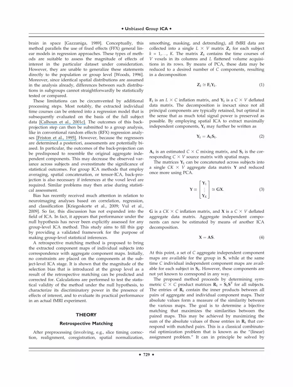
Finally, voxelwise statistics regarding the effects of inter-est can be derived by entering all individual maps thatwere retrospectively matched to the same aggregate com-ponent into a group level analysis. t-value statistical para-metric maps [SPM(t)] can be computed and thresholded todetect significant effects of interest. The entire retrospec-tive matching method is summarized in diagrammaticform in Figure 1.

Selection Bias

Because matching component maps are all selected toshow maximal resemblance with the same aggregate map,the expectation value of their mean across all subjects will

be nonzero. The magnitude of the resulting selection biaswill be assessed next. It will henceforth be assumed that,under the null hypothesis, the individual independentcomponent maps in all Sk constitute independent andidentically distributed (IID) samples from a single multi-variate normal distribution N(0,R). Also, the possiblerestriction that a single individual component cannot bematched to multiple aggregate components will beignored: it will be assumed that an aggregate componentis matched to the best matching individual component,independently of all other aggregate components.

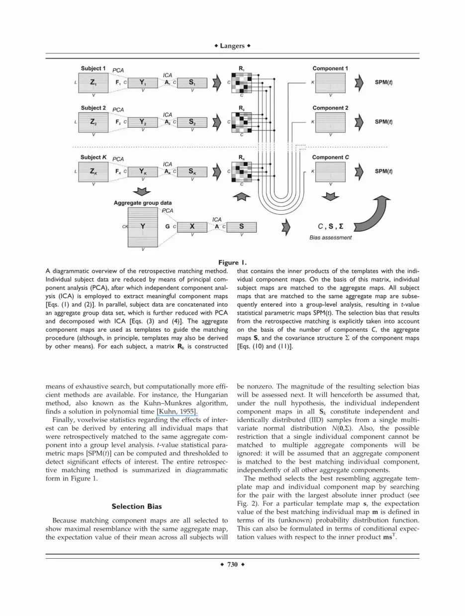
The method selects the best resembling aggregate tem-plate map and individual component map by searchingfor the pair with the largest absolute inner product (seeFig. 2). For a particular template map s, the expectationvalue of the best matching individual map m is defined interms of its (unknown) probability distribution function.This can also be formulated in terms of conditional expec-tation values with respect to the inner product msT.

Figure 1.

A diagrammatic overview of the retrospective matching method.

Individual subject data are reduced by means of principal com-

ponent analysis (PCA), after which independent component anal-

ysis (ICA) is employed to extract meaningful component maps

[Eqs. (1) and (2)]. In parallel, subject data are concatenated into

an aggregate group data set, which is further reduced with PCA

and decomposed with ICA [Eqs. (3) and (4)]. The aggregate

component maps are used as templates to guide the matching

procedure (although, in principle, templates may also be derived

by other means). For each subject, a matrix Rk is constructed

that contains the inner products of the templates with the indi-

vidual component maps. On the basis of this matrix, individual

subject maps are matched to the aggregate maps. All subject

maps that are matched to the same aggregate map are subse-

quently entered into a group-level analysis, resulting in t-value

statistical parametric maps SPM(t). The selection bias that results

from the retrospective matching is explicitly taken into account

on the basis of the number of components C, the aggregate

maps S, and the covariance structure R of the component maps

[Eqs. (10) and (11)].

r Langers r

r 730 r

EðmÞ ¼Zm

½m � PðmÞ�dm

¼Zm

½EðmjmsT ¼ mÞPðmsT ¼ mÞ�dm: (5)

(Note: P(m) refers to the distribution of the sample withthe maximum absolute inner product, not to the knownmultivariate normal distribution of all original samples!)

Because the maximum sample m is selected purely onthe basis of its inner product with s, its expectation valueunder a particular fixed conditional constraint msT ¼ m isprecisely equal to the expectation value of the originalmultivariate normal distribution under that constraint. Theconditional expectation value for a normally distributedvariable x satisfies

EðxjxsT ¼ xÞ ¼ xsRsRsT

(6)

[Johnson and Wichern, 2001]. This results in

EðmÞ ¼Zm

msRsRsT

PðmsT ¼ mÞ� �

dm ¼ sRsRsT

EðmsTÞ: (7)

The scalar quantity msT is the absolute maximum out of C

inner products. Since s is fixed and all individual maps

are assumed to be drawn from a multivariate normal dis-

tribution, the inner products themselves form samples

from a univariate normal distribution. This distribution’s

mean is zero and its variance r2 = sRsT.By partial integration, it can be shown that the maxi-

mum of the absolute values of C independent samplesfrom a univariate zero-mean unit-variance normal distri-bution has an expectation value MC equal to

Mc ¼Z1

0

1� erfczffiffiffi2

p� �� �

dz: (8)

Although the integral in Eq. (8) cannot be simplified fur-

ther, MC can easily be obtained to arbitrary accuracy by

means of numerical integration. It only weakly depends

on C; for example, M1 = H(2/p) = 0.80, M2 = 2/Hp = 1.13,

M10 = 1.88, M20 = 2.17, M100 = 2.75. In the context of fMRI,

MC should usually lie in a limited range near 2.0–2.5.It now follows that

EðmsTÞ ¼ Mc

ffiffiffiffiffiffiffiffiffiffisRsT

p: (9)

From Eq. (7), we arrive at the following expression, which

provides an exact prediction of the bias that occurs under

the null hypothesis when selecting the best matching com-

ponent map.

EðmÞ ¼ McsRffiffiffiffiffiffiffiffiffiffisRsT

p : (10)

Equation (10) relies on complete and exact knowledgeabout the covariance structure of the component maps.Typically, the number of subjects and extracted compo-nents is too small and the number of voxels too large toextract a sufficiently accurate estimate for the entire covari-ance matrix R. However, the noise can often be modeledby a D-dimensional Gaussian random field. Here, theobserved correlated noise will be assumed equivalent tothe convolution of an underlying uncorrelated noise signalwith some fixed Gaussian kernel, k, with known fullwidth at half maximum (FWHM). By explicitly writing outthe kernel, it can be shown that sR % R�s0R0 [see Eq. (A9)the Appendix]. The scalar R provides a measure for thenumber of voxels that are effectively correlated, analogousto the volume of a resel [Worsley et al., 1992]. If long-range correlations are present, R % (1.505�FWHM)D [seeEq. (A8) for the exact form]; if spatial correlations are

Figure 2.

A graphical illustration of the selection bias. Under the null-

hypothesis, the flattened component maps are assumed to com-

prise samples from a zero-mean multivariate normal distribution.

In this 2-D representation, the corresponding points form an

ellipsoidal data cloud. Those samples that have a negative inner

product with some provided template map s are flipped with

respect to their sign (*). The sample m with the largest inner

product (circled) will be selected as the best match to the tem-

plate. A closed form expression for the expectation value of m

can be derived in terms of the template s and the distribution’s

covariance structure R [see Eq. (10)]. Even though the original

multivariate normal distribution centers around zero, the bias of

the proposed retrospective matching method can thus be

estimated to be nonzero. Similar concerns may hold for other

statistical group ICA methods.

r Unbiased Group ICA r

r 731 r

completely absent, R = 1. The vector s0 contains a doublysmoothed template map; symbolically, s0 = k�k�s. Thematrix R0 is derived from R; it is strictly diagonal andobeys Rii

0 = Rii. In other words, it describes the variance inthe voxels, but disregards any covariance due to spatialcorrelations.

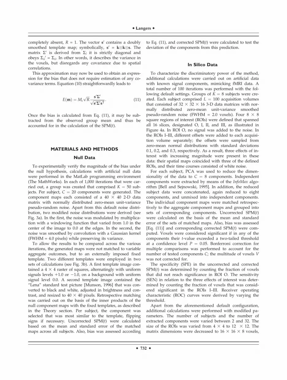
This approximation may now be used to obtain an expres-sion for the bias that does not require estimation of any co-variance terms. Equation (10) straightforwardly leads to

EðmÞ ¼ Mc

ffiffiffiffiR

p s0R0ffiffiffiffiffiffiffiffiffiffiffiffiffis0R0sT

p : (11)

Once the bias is calculated from Eq. (11), it may be sub-tracted from the observed group mean and thus beaccounted for in the calculation of the SPM(t).

MATERIALS AND METHODS

Null Data

To experimentally verify the magnitude of the bias underthe null hypothesis, calculations with artificial null datawere performed in the MatLab programming environment(The MathWorks). In each of 1,000 iterations that were car-ried out, a group was created that comprised K ¼ 50 sub-jects. Per subject, C ¼ 20 components were generated. Thecomponent maps each consisted of a 40 3 40 2-D datamatrix with normally distributed zero-mean unit-variancepseudo-random noise. Apart from this default noise distri-bution, two modified noise distributions were derived (seeFig. 3a). In the first, the noise was modulated by multiplica-tion with a windowing function that varied from 1.0 in thecenter of the image to 0.0 at the edges. In the second, thenoise was smoothed by convolution with a Gaussian kernel(FWHM = 4.0 pixels) while preserving its variance.

To allow the results to be compared across the variousiterations, the generated maps were not matched to variableaggregate outcomes, but to an externally imposed fixedtemplate. Two different templates were employed in twosets of calculations (see Fig. 3b). A first template image con-tained a 4 3 4 raster of squares, alternatingly with uniformsignals levels 11.0 or 21.0, on a background with uniformsignal level 0.0. A second template image contained the‘‘Lena’’ standard test picture [Munson, 1996] that was con-verted to black and white, adjusted in brightness and con-trast, and resized to 40 3 40 pixels. Retrospective matchingwas carried out on the basis of the inner products of thenull component maps with the fixed templates, as describedin the Theory section. Per subject, the component wasselected that was most similar to the template, flippingsigns if necessary. Uncorrected SPM(t) were calculatedbased on the mean and standard error of the matchedmaps across all subjects. Also, bias was assessed according

to Eq. (11), and corrected SPM(t) were calculated to test thedeviation of the components from this prediction.

In Silico Data

To characterize the discriminatory power of the method,additional calculations were carried out on artificial datawith known signal components, mimicking fMRI data. Atotal number of 100 iterations was performed with the fol-lowing default settings. Groups of K ¼ 8 subjects were cre-ated. Each subject comprised L ¼ 100 acquisition volumesthat consisted of 32 3 32 3 16 3-D data matrices with nor-mally distributed zero-mean unit-variance smoothedpseudo-random noise (FWHM = 2.0 voxels). Four 8 3 8square regions of interest (ROIs) were defined that spannedall 16 slices, designated O, I, II, and III, as illustrated inFigure 4a. In ROI O, no signal was added to the noise. Inthe ROIs I–III, different offsets were added to each acquisi-tion volume separately; the offsets were sampled fromzero-mean normal distributions with standard deviations0.1, 0.2, and 0.3, respectively. As a result, three effects of in-terest with increasing magnitude were present in thesedata: their spatial maps coincided with three of the definedROIs, and their time courses consisted of white noise.

For each subject, PCA was used to reduce the dimen-sionality of the data to C ¼ 8 components. Independentcomponents were extracted by means of the InfoMax algo-rithm [Bell and Sejnowski, 1995]. In addition, the reducedsubject data were concatenated, again reduced to eightcomponents, and unmixed into independent components.The individual component maps were matched retrospec-tively to the aggregate component maps and grouped intosets of corresponding components. Uncorrected SPM(t)were calculated on the basis of the mean and standarderror of the sets of matched maps. Also, bias was assessed[Eq. (11)] and corresponding corrected SPM(t) were com-puted. Voxels were considered significant if in any of thecomponents their t-value exceeded a two-tailed thresholdat a confidence level P ¼ 0.05. Bonferroni correction formultiple comparisons was performed to account for thenumber of tested components C; the multitude of voxels Vwas not corrected for.

The specificity (SPE) in the uncorrected and correctedSPM(t) was determined by counting the fraction of voxelsthat did not reach significance in ROI O. The sensitivity(SEN) in relation to the three effects of interest was deter-mined by counting the fraction of voxels that was consid-ered significant in the ROIs I–III. Receiver operatingcharacteristic (ROC) curves were derived by varying thethreshold.

Apart from the aforementioned default configuration,additional calculations were performed with modified pa-rameters. The number of subjects and the number ofextracted components were varied between 2 and 32. Thesize of the ROIs was varied from 4 3 4 to 12 3 12. Thematrix dimensions were decreased to 16 3 16 3 8 voxels,

r Langers r

r 732 r

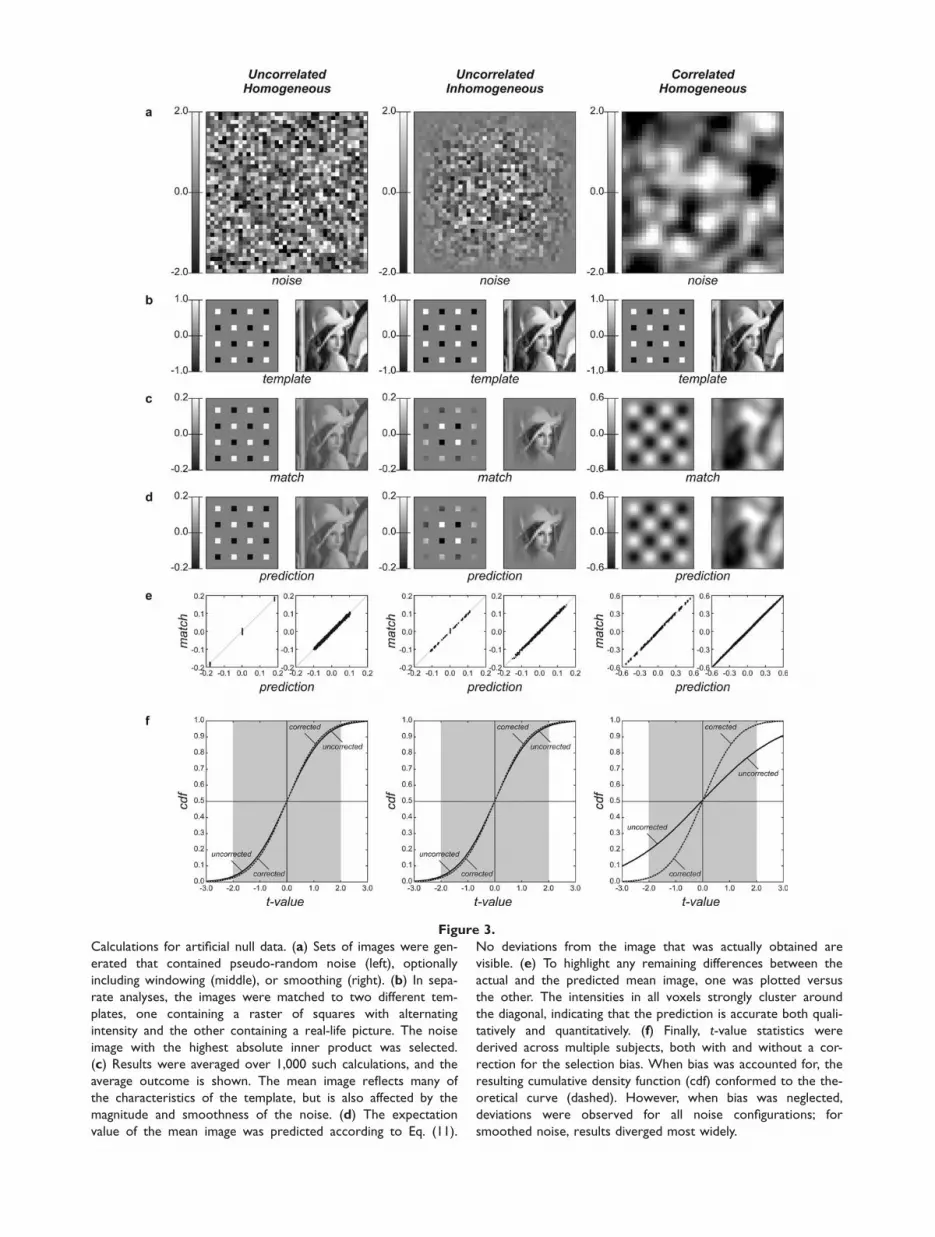
Figure 3.

Calculations for artificial null data. (a) Sets of images were gen-

erated that contained pseudo-random noise (left), optionally

including windowing (middle), or smoothing (right). (b) In sepa-

rate analyses, the images were matched to two different tem-

plates, one containing a raster of squares with alternating

intensity and the other containing a real-life picture. The noise

image with the highest absolute inner product was selected.

(c) Results were averaged over 1,000 such calculations, and the

average outcome is shown. The mean image reflects many of

the characteristics of the template, but is also affected by the

magnitude and smoothness of the noise. (d) The expectation

value of the mean image was predicted according to Eq. (11).

No deviations from the image that was actually obtained are

visible. (e) To highlight any remaining differences between the

actual and the predicted mean image, one was plotted versus

the other. The intensities in all voxels strongly cluster around

the diagonal, indicating that the prediction is accurate both quali-

tatively and quantitatively. (f) Finally, t-value statistics were

derived across multiple subjects, both with and without a cor-

rection for the selection bias. When bias was accounted for, the

resulting cumulative density function (cdf) conformed to the the-

oretical curve (dashed). However, when bias was neglected,

deviations were observed for all noise configurations; for

smoothed noise, results diverged most widely.

as well as increased to 64 3 64 3 32 voxels (scaling thesize of the ROIs accordingly). The number of acquisitionsper subject ranged from 25 to 400. The smoothness of thenoise varied from zero to FWHM = 4.0 voxels. Finally,results were determined for thresholds between P = 0.001and P = 0.1. For each setting, 100 simulations wereperformed.

In Vivo Data

To assess the performance of the method in a practicalsetting, the results from an fMRI study on 32 subjectswere analyzed. Written informed consent was obtained inapproved accordance with the requirements of the institu-tional committees on the use of human subjects at theMassachusetts Eye and Ear Infirmary, the MassachusettsGeneral Hospital, and the Massachusetts Institute ofTechnology.

Subjects were placed in supine position in the bore of a3.0-T MR system (Siemens Allegra), which was equippedwith a standard 12-channel transmit/receive head coil. Anoblique coronal functional imaging volume was positionedon the basis of high-resolution anatomical images. Thefunctional imaging runs consisted of a dynamic series ofT2*-sensitive echo planar imaging (EPI) sequences (TR � 8s; TE 30 ms; flip angle 90�; matrix 64 3 64 3 10; voxeldimensions 3.1 3 3.1 3 8.0 mm3, including a 2.0-mm slicegap). Each run comprised 36 EPI acquisitions, excludinginitial start-up scans that were discarded before the analy-sis. Per subject, between 5 and 11 runs were carried out. Asparse clustered volume scanning paradigm wasemployed to reduce the influence of acoustic scanner noise[Edmister et al., 1999; Hall et al., 1999; Langers et al.,2005]. The scanner coolant pump and fan were turned offduring functional imaging to reduce ambient noise levels.Cardiac triggering on the basis of a pulse-oximeter signalwas used to reduce the influence of cardiac motion [Gui-maraes et al., 1998]. In one subject, the cardiac signal wastoo weak to detect reliably, and a fixed TR of 7.5 s was set.

During the functional imaging sessions, a basic audiovi-sual task was performed by the subjects to control theirattention levels. Subjects viewed a projection screenthrough a mirror. On a uniform gray background, a blackcross was displayed that briefly turned red at pseudo-ran-dom intervals. Subjects were instructed to press a buttondevice each time they observed such a color change.Responses were monitored to ensure that subjects under-stood the task and stayed alert, and the achieved hit rateapproximately equaled 80–90%. Behavioral results were notanalyzed further for the purpose of this study. At the sametime, MR-compatible piezoelectric speakers that weremounted in insert ear plugs were used to deliver auditorystimuli. These stimuli consisted of four 32-s broadbandnoise bursts per run, separated by periods of silence. Thestimulus intensities of all bursts were equal within a run,

Figure 4.

Calculations for artificial data with true effects. (a) 3-D artificial

data were generated that contained pseudo-random smoothed

noise. Four rectangular regions were defined (O–III). Pseudo-

random offsets were added to model true effects of interest.

The root-mean-square power of these signals increased linearly

from region I to III (the magnitudes of these signals are exagger-

ated tenfold in this illustration); no signal was added to region

O. (b) The sensitivity (SEN) to the signals in regions I–III is plot-

ted as a function of the specificity (SPE) in region O, both for

corrected and uncorrected thresholding. The resulting receiver

operating characteristic (ROC) curves show that the discrimina-

tory power increased with increasing signal to noise level across

the regions I–III, but also reveal that bias correction leads to a

moderate decrease in discriminatory power.

r Langers r

r 734 r

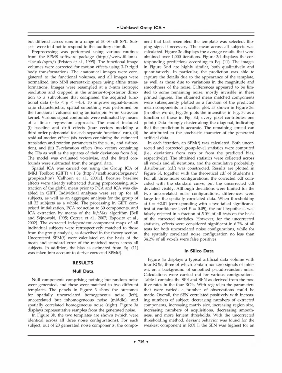
but differed across runs in a range of 50–80 dB SPL. Sub-jects were told not to respond to the auditory stimuli.

Preprocessing was performed using various routinesfrom the SPM8 software package (http://www.fil.ion.u-cl.ac.uk/spm/) [Friston et al., 1995]. The functional imagevolumes were corrected for motion effects using 3-D rigidbody transformations. The anatomical images were core-gistered to the functional volumes, and all images werenormalized into MNI stereotaxic space using affine trans-formations. Images were resampled at a 3-mm isotropicresolution and cropped in the anterior-to-posterior direc-tion to a subvolume that comprised the acquired func-tional data (�45 y þ45). To improve signal-to-noiseratio characteristics, spatial smoothing was performed onthe functional volumes using an isotropic 5-mm Gaussiankernel. Various signal confounds were estimated by meansof a linear regression approach. The model included(i) baseline and drift effects (four vectors modeling athird-order polynomial for each separate functional run), (ii)residual motion effects (six vectors containing the estimatedtranslation and rotation parameters in the x-, y-, and z-direc-tion), and (iii) T1-relaxation effects (two vectors containingthe TRs as well as the squares of their deviations from 8 s).The model was evaluated voxelwise, and the fitted con-founds were subtracted from the original data.

Spatial ICA was carried out using the Group ICA offMRI Toolbox (GIFT) v.1.3e (http://icatb.sourceforge.net/groupica.htm) [Calhoun et al., 2001c]. Because baselineeffects were already subtracted during preprocessing, sub-traction of the global mean prior to PCA and ICA was dis-abled in GIFT. Individual analyses were set up for allsubjects, as well as an aggregate analysis for the group ofall 32 subjects as a whole. The processing in GIFT com-prised initialization, PCA reduction to 30 components, andICA extraction by means of the InfoMax algorithm [Belland Sejnowski, 1995; Correa et al., 2007; Esposito et al.,2002]. The extracted independent component maps of allindividual subjects were retrospectively matched to thosefrom the group analysis, as described in the theory section.Uncorrected SPM(t) were calculated on the basis of themean and standard error of the matched maps across allsubjects. In addition, the bias as estimated from Eq. (11)was taken into account to derive corrected SPM(t).

RESULTS

Null Data

Null components comprising nothing but random noisewere generated, and these were matched to two differenttemplates. The panels in Figure 3 show the outcomesfor spatially uncorrelated homogeneous noise (left),uncorrelated but inhomogeneous noise (middle), andspatially correlated homogeneous noise (right). Figure 3adisplays representative samples from the generated noise.

In Figure 3b, the two templates are shown (which wereidentical across all three noise configurations). For eachsubject, out of 20 generated noise components, the compo-

nent that best resembled the template was selected, flip-ping signs if necessary. The mean across all subjects wascalculated. Figure 3c displays the average results that wereobtained over 1,000 iterations. Figure 3d displays the cor-responding predictions according to Eq. (11). The imagesin Figure 3c,d are highly similar, both qualitatively andquantitatively. In particular, the prediction was able tocapture the details due to the appearance of the template,as well as those due to variations in the magnitude andsmoothness of the noise. Differences appeared to be lim-ited to some remaining noise, mostly invisible in theseprinted figures. The obtained mean matched componentswere subsequently plotted as a function of the predictedmean components in a scatter plot, as shown in Figure 3e.(In other words, Fig. 3e plots the intensities in Fig. 3c as afunction of those in Fig. 3d; every pixel contributes onepoint.) Data strongly cluster along the diagonal, indicatingthat the prediction is accurate. The remaining spread canbe attributed to the stochastic character of the generatedartificial data.

In each iteration, an SPM(t) was calculated. Both uncor-rected and corrected group-level statistics were computed(i.e., deviations from zero or from the predicted bias,respectively). The obtained statistics were collected acrossall voxels and all iterations, and the cumulative probabilitydistribution (cdf) was constructed. Results are plotted inFigure 3f, together with the theoretical cdf of Student’s t.For all three noise configurations, the corrected cdf coin-cided with the standard curve, but the uncorrected cdfdeviated visibly. Although deviations were limited for thetwo uncorrelated noise configurations, differences werelarge for the spatially correlated data. When thresholdingat t ¼ 2.01 (corresponding with a two-tailed significancetest at confidence level P ¼ 0.05), the null hypothesis wasfalsely rejected in a fraction of 5.0% of all tests on the basisof the corrected statistics. However, for the uncorrectedstatistics, effects were considered significant in 6.7% of alltests for both uncorrelated noise configurations, while forthe spatially correlated noise configuration no less than34.2% of all voxels were false positives.

In Silico Data

Figure 4a displays a typical artificial data volume withfour ROIs, three of which contain nonzero signals of inter-est, on a background of smoothed pseudo-random noise.Calculations were carried out for various configurations.Table I contains the SPE and SEN as derived from the pos-itive rates in the four ROIs. With regard to the parametersthat were varied, a number of observations could bemade. Overall, the SEN correlated positively with increas-ing numbers of subject, decreasing numbers of extractedcomponents, increasing matrix size, increasing region size,increasing numbers of acquisitions, decreasing smooth-ness, and more lenient thresholds. With the uncorrectedthresholding method, deviant behavior was found for theweakest component in ROI I: the SEN was highest for an

r Unbiased Group ICA r

r 735 r

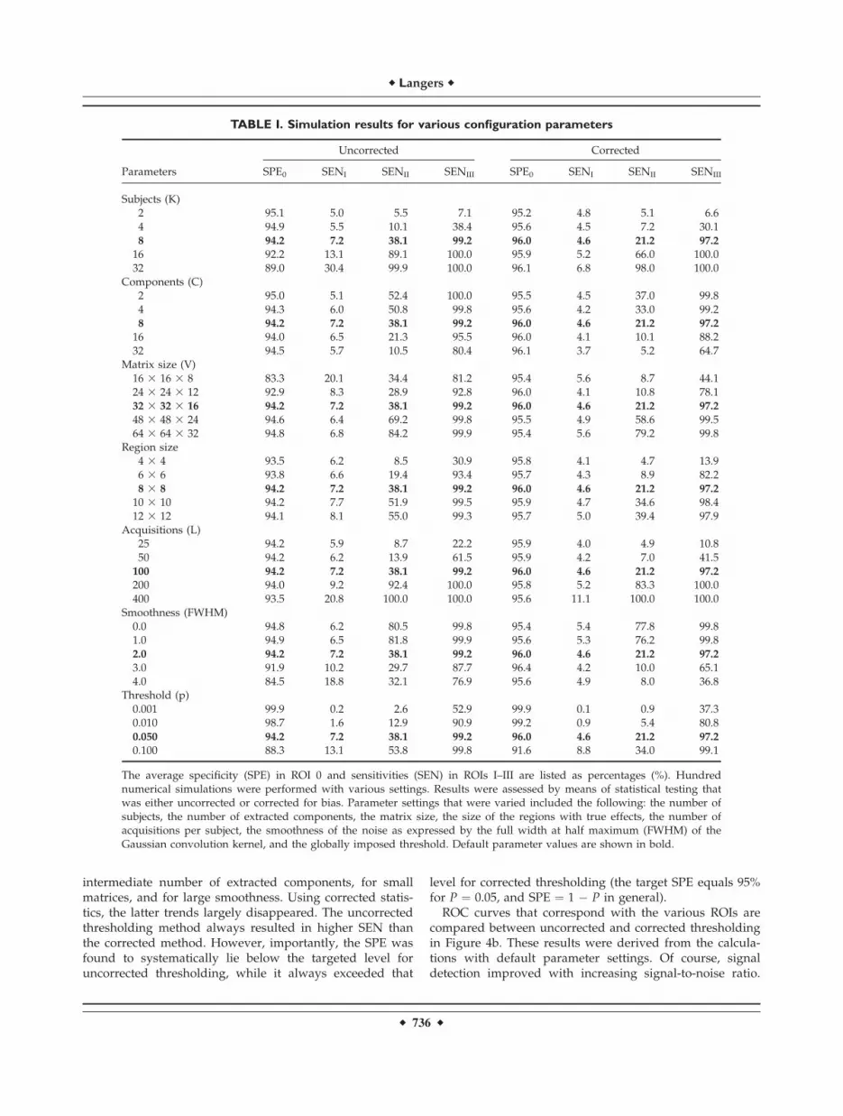
intermediate number of extracted components, for smallmatrices, and for large smoothness. Using corrected statis-tics, the latter trends largely disappeared. The uncorrectedthresholding method always resulted in higher SEN thanthe corrected method. However, importantly, the SPE wasfound to systematically lie below the targeted level foruncorrected thresholding, while it always exceeded that

level for corrected thresholding (the target SPE equals 95%for P ¼ 0.05, and SPE ¼ 1 � P in general).

ROC curves that correspond with the various ROIs arecompared between uncorrected and corrected thresholdingin Figure 4b. These results were derived from the calcula-tions with default parameter settings. Of course, signaldetection improved with increasing signal-to-noise ratio.

TABLE I. Simulation results for various configuration parameters

Parameters

Uncorrected Corrected

SPE0 SENI SENII SENIII SPE0 SENI SENII SENIII

Subjects (K)2 95.1 5.0 5.5 7.1 95.2 4.8 5.1 6.64 94.9 5.5 10.1 38.4 95.6 4.5 7.2 30.18 94.2 7.2 38.1 99.2 96.0 4.6 21.2 97.2

16 92.2 13.1 89.1 100.0 95.9 5.2 66.0 100.032 89.0 30.4 99.9 100.0 96.1 6.8 98.0 100.0

Components (C)2 95.0 5.1 52.4 100.0 95.5 4.5 37.0 99.84 94.3 6.0 50.8 99.8 95.6 4.2 33.0 99.28 94.2 7.2 38.1 99.2 96.0 4.6 21.2 97.2

16 94.0 6.5 21.3 95.5 96.0 4.1 10.1 88.232 94.5 5.7 10.5 80.4 96.1 3.7 5.2 64.7

Matrix size (V)16 3 16 3 8 83.3 20.1 34.4 81.2 95.4 5.6 8.7 44.124 3 24 3 12 92.9 8.3 28.9 92.8 96.0 4.1 10.8 78.132 3 32 3 16 94.2 7.2 38.1 99.2 96.0 4.6 21.2 97.2

48 3 48 3 24 94.6 6.4 69.2 99.8 95.5 4.9 58.6 99.564 3 64 3 32 94.8 6.8 84.2 99.9 95.4 5.6 79.2 99.8

Region size4 3 4 93.5 6.2 8.5 30.9 95.8 4.1 4.7 13.96 3 6 93.8 6.6 19.4 93.4 95.7 4.3 8.9 82.28 3 8 94.2 7.2 38.1 99.2 96.0 4.6 21.2 97.2

10 3 10 94.2 7.7 51.9 99.5 95.9 4.7 34.6 98.412 3 12 94.1 8.1 55.0 99.3 95.7 5.0 39.4 97.9

Acquisitions (L)25 94.2 5.9 8.7 22.2 95.9 4.0 4.9 10.850 94.2 6.2 13.9 61.5 95.9 4.2 7.0 41.5

100 94.2 7.2 38.1 99.2 96.0 4.6 21.2 97.2

200 94.0 9.2 92.4 100.0 95.8 5.2 83.3 100.0400 93.5 20.8 100.0 100.0 95.6 11.1 100.0 100.0

Smoothness (FWHM)0.0 94.8 6.2 80.5 99.8 95.4 5.4 77.8 99.81.0 94.9 6.5 81.8 99.9 95.6 5.3 76.2 99.82.0 94.2 7.2 38.1 99.2 96.0 4.6 21.2 97.2

3.0 91.9 10.2 29.7 87.7 96.4 4.2 10.0 65.14.0 84.5 18.8 32.1 76.9 95.6 4.9 8.0 36.8

Threshold (p)0.001 99.9 0.2 2.6 52.9 99.9 0.1 0.9 37.30.010 98.7 1.6 12.9 90.9 99.2 0.9 5.4 80.80.050 94.2 7.2 38.1 99.2 96.0 4.6 21.2 97.2

0.100 88.3 13.1 53.8 99.8 91.6 8.8 34.0 99.1

The average specificity (SPE) in ROI 0 and sensitivities (SEN) in ROIs I–III are listed as percentages (%). Hundrednumerical simulations were performed with various settings. Results were assessed by means of statistical testing thatwas either uncorrected or corrected for bias. Parameter settings that were varied included the following: the number ofsubjects, the number of extracted components, the matrix size, the size of the regions with true effects, the number ofacquisitions per subject, the smoothness of the noise as expressed by the full width at half maximum (FWHM) of theGaussian convolution kernel, and the globally imposed threshold. Default parameter values are shown in bold.

r Langers r

r 736 r

For the three signals of interest in the ROIs I, II, and III,the areas under the curves for the uncorrected methodequaled 0.5308, 0.8210, and 0.9953, respectively, while theywere 0.5148, 0.7561, and 0.9935 for the corrected method.This corresponds with binormal d-prime equal to 0.11,1.30, and 3.68 (uncorrected thresholding), and 0.05, 0.98,and 3.52 (corrected thresholding). These findings showthat correction for bias comes at the cost of a moderatereduction in discriminatory power.

In Vivo Data

The fMRI data were analyzed by means of ICA, bothwith individual and aggregate data. The individual maps

were retrospectively matched to the aggregate maps.Uncorrected and corrected SPM(t) were derived. Followingvisual inspection and interpretation of the componentmaps, 16 components were deemed to be of neural origin.The remaining 14 components were construed to arisefrom MRI-artifacts. Figure 5 illustrates the spatial mapsbelonging to a subset of ten components.

Figure 5a shows coronal slices from the aggregate groupmaps that were converted to SPM(z) by division by themap’s root-mean-square signal level. Results were thresh-olded at z ¼ 3.3, corresponding to a two-tailed confi-dence level P ¼ 0.001 (uncorrected for multiplecomparisons). Activation was well delineated and confinedto specific brain structures. Six neural components

Figure 5.

Results for data from an actual fMRI experiment with an audiovi-

sual stimulation paradigm. (a) Component maps from an

aggregate ICA with temporal concatenation were scaled to unit

root-mean-square signal power. Ten out of thirty components

are displayed as aggregate SPM(z) by means of a color code on

an anatomical background. Six of these components (1–6) were

interpreted to result from neural activation, while four other

components (7–10) were deemed MRI-artifacts. (b) Retrospec-

tive matching was carried out, and group statistics were deter-

mined that did not include any correction for bias. The

corresponding component maps are shown as uncorrected

SPM(t). Although some differences are obvious, the interpreta-

tion of the components relates well to those from the aggregate

analysis. (c) Similar statistics were derived that included an

explicit correction for the presence of bias, resulting in cor-

rected SPM(t). Activation was less significant than without bias

correction. Still, many of the components of interest could be

identified. In particular, auditory activation in response to the

employed sound stimuli was consistently found.

r Unbiased Group ICA r

r 737 r

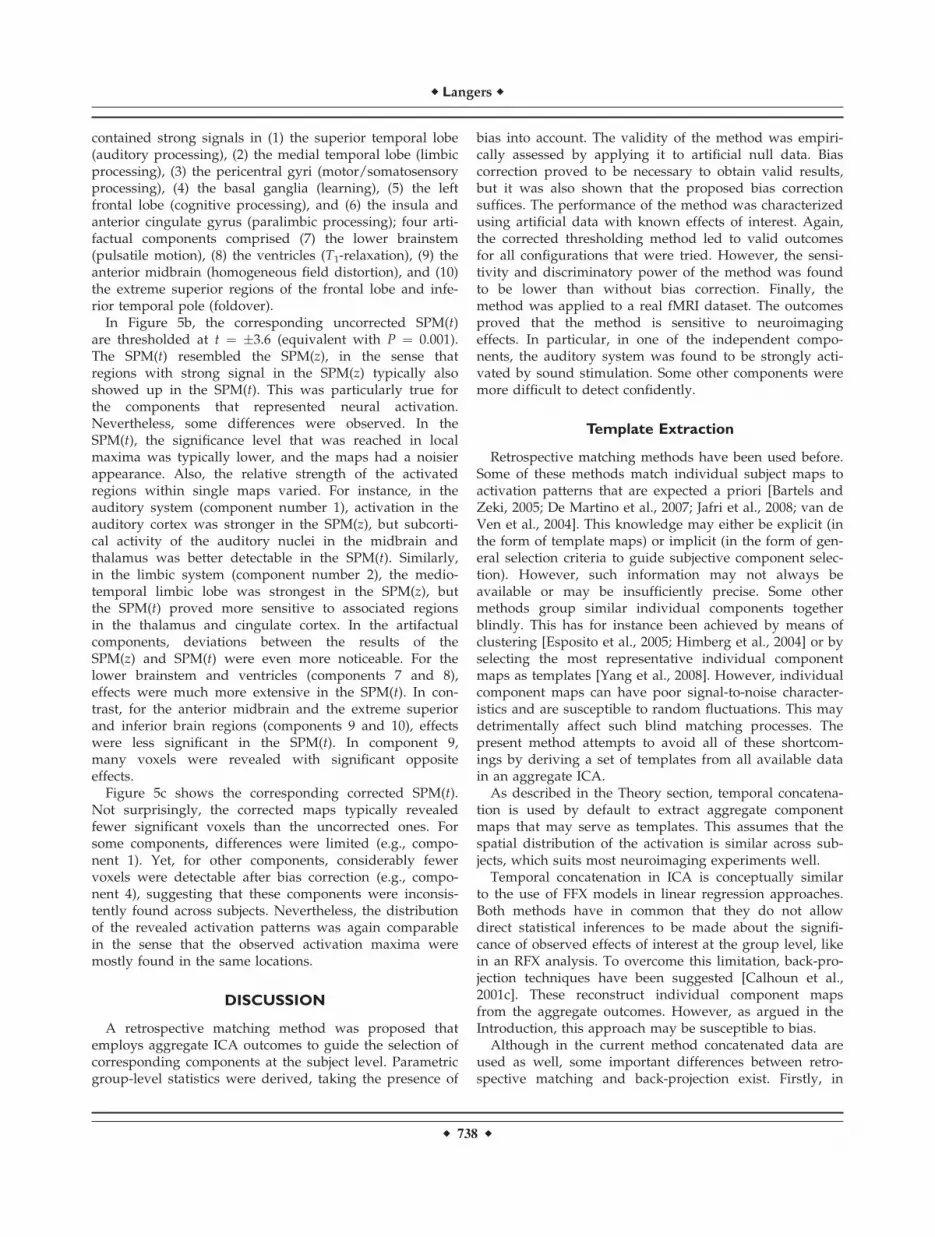
contained strong signals in (1) the superior temporal lobe(auditory processing), (2) the medial temporal lobe (limbicprocessing), (3) the pericentral gyri (motor/somatosensoryprocessing), (4) the basal ganglia (learning), (5) the leftfrontal lobe (cognitive processing), and (6) the insula andanterior cingulate gyrus (paralimbic processing); four arti-factual components comprised (7) the lower brainstem(pulsatile motion), (8) the ventricles (T1-relaxation), (9) theanterior midbrain (homogeneous field distortion), and (10)the extreme superior regions of the frontal lobe and infe-rior temporal pole (foldover).

In Figure 5b, the corresponding uncorrected SPM(t)are thresholded at t ¼ 3.6 (equivalent with P ¼ 0.001).The SPM(t) resembled the SPM(z), in the sense thatregions with strong signal in the SPM(z) typically alsoshowed up in the SPM(t). This was particularly true forthe components that represented neural activation.Nevertheless, some differences were observed. In theSPM(t), the significance level that was reached in localmaxima was typically lower, and the maps had a noisierappearance. Also, the relative strength of the activatedregions within single maps varied. For instance, in theauditory system (component number 1), activation in theauditory cortex was stronger in the SPM(z), but subcorti-cal activity of the auditory nuclei in the midbrain andthalamus was better detectable in the SPM(t). Similarly,in the limbic system (component number 2), the medio-temporal limbic lobe was strongest in the SPM(z), butthe SPM(t) proved more sensitive to associated regionsin the thalamus and cingulate cortex. In the artifactualcomponents, deviations between the results of theSPM(z) and SPM(t) were even more noticeable. For thelower brainstem and ventricles (components 7 and 8),effects were much more extensive in the SPM(t). In con-trast, for the anterior midbrain and the extreme superiorand inferior brain regions (components 9 and 10), effectswere less significant in the SPM(t). In component 9,many voxels were revealed with significant oppositeeffects.

Figure 5c shows the corresponding corrected SPM(t).Not surprisingly, the corrected maps typically revealedfewer significant voxels than the uncorrected ones. Forsome components, differences were limited (e.g., compo-nent 1). Yet, for other components, considerably fewervoxels were detectable after bias correction (e.g., compo-nent 4), suggesting that these components were inconsis-tently found across subjects. Nevertheless, the distributionof the revealed activation patterns was again comparablein the sense that the observed activation maxima weremostly found in the same locations.

DISCUSSION

A retrospective matching method was proposed thatemploys aggregate ICA outcomes to guide the selection ofcorresponding components at the subject level. Parametricgroup-level statistics were derived, taking the presence of

bias into account. The validity of the method was empiri-cally assessed by applying it to artificial null data. Biascorrection proved to be necessary to obtain valid results,but it was also shown that the proposed bias correctionsuffices. The performance of the method was characterizedusing artificial data with known effects of interest. Again,the corrected thresholding method led to valid outcomesfor all configurations that were tried. However, the sensi-tivity and discriminatory power of the method was foundto be lower than without bias correction. Finally, themethod was applied to a real fMRI dataset. The outcomesproved that the method is sensitive to neuroimagingeffects. In particular, in one of the independent compo-nents, the auditory system was found to be strongly acti-vated by sound stimulation. Some other components weremore difficult to detect confidently.

Template Extraction

Retrospective matching methods have been used before.Some of these methods match individual subject maps toactivation patterns that are expected a priori [Bartels andZeki, 2005; De Martino et al., 2007; Jafri et al., 2008; van deVen et al., 2004]. This knowledge may either be explicit (inthe form of template maps) or implicit (in the form of gen-eral selection criteria to guide subjective component selec-tion). However, such information may not always beavailable or may be insufficiently precise. Some othermethods group similar individual components togetherblindly. This has for instance been achieved by means ofclustering [Esposito et al., 2005; Himberg et al., 2004] or byselecting the most representative individual componentmaps as templates [Yang et al., 2008]. However, individualcomponent maps can have poor signal-to-noise character-istics and are susceptible to random fluctuations. This maydetrimentally affect such blind matching processes. Thepresent method attempts to avoid all of these shortcom-ings by deriving a set of templates from all available datain an aggregate ICA.

As described in the Theory section, temporal concatena-tion is used by default to extract aggregate componentmaps that may serve as templates. This assumes that thespatial distribution of the activation is similar across sub-jects, which suits most neuroimaging experiments well.

Temporal concatenation in ICA is conceptually similarto the use of FFX models in linear regression approaches.Both methods have in common that they do not allowdirect statistical inferences to be made about the signifi-cance of observed effects of interest at the group level, likein an RFX analysis. To overcome this limitation, back-pro-jection techniques have been suggested [Calhoun et al.,2001c]. These reconstruct individual component mapsfrom the aggregate outcomes. However, as argued in theIntroduction, this approach may be susceptible to bias.

Although in the current method concatenated data areused as well, some important differences between retro-spective matching and back-projection exist. Firstly, in

r Langers r

r 738 r

retrospective matching one and the same set of templatemaps is used in every subject. In contrast, in the temporalconcatenation method with back-projection, individualtime courses that are already tuned to correspond with theidentified aggregate components are fed back into theback-projection step. Secondly, the aggregate maps areonly used to select components in the proposed method,but they do not directly affect the calculation of the subjectcomponents themselves. Although this may still lead to aselection bias, this effect is predictable and can beaccounted for.

The potential presence of bias not only applies to tem-poral concatenation with back-projection, it also likelyplays an important role for many other group ICA meth-ods (the author is not aware of any studies that haveinvestigated this). Conveniently, the retrospective match-ing framework that is described in this article is not re-stricted to temporal concatenation per se. It can begeneralized to other ways of extracting templates. Forinstance, when using a fixed stimulus or task paradigm,the use of spatial concatenation, tensor ICA, or averagingto derive the template maps may be preferred. Becauseno assumptions were made about the templates, the retro-spective matching, bias correction, and statistical assess-ment can subsequently be carried out in identical fashion.Other group ICA methods that do not rely on aggregatedata may also be used to provide the necessary set oftemplates. For instance, prior knowledge can be incorpo-rated by using a fixed set of independently obtained tem-plate maps (e.g., from previous studies); the results ofclustering methods can be used by entering the clustercentroids into the analysis as templates; or, a set of mostrepresentative individual subject maps can be selected.This provides a lot of flexibility and makes the describedframework broadly applicable.

Bias assessment and Validity

The proposed matching procedure was carried out onthe basis of a matrix Rk that contained the inner productsbetween all pairs of individual and aggregate maps. Innerproducts are closely related to correlation coefficients,which have been applied in the context of independentcomponent matching before [Esposito et al., 2005; Yang etal., 2008]. ICA maps are often normalized to zero meanand unit variance, and this would actually render bothmeasures completely equivalent.

Inner products were employed because they are linearoperations. Under the null hypothesis, they give rise toparametric statistics. This simplified the description suffi-ciently such that the magnitude of the bias could be ana-lytically expressed in terms of the number of extractedcomponents, the composition of the template map, and the(co)variance structure of the component maps [Eq. (10)].

Some approximations were necessary to make it possibleto estimate these required quantities from the data, espe-cially in the presence of spatial correlations. Nevertheless,

the resulting expression [Eq. (11)] proved accurate. Thecalculations with artificial null data were set up to maxi-mize the effects of bias by including many subjects and byaveraging over many iterations. Even in these extremeconditions, the method was able to predict the resultingbias with high accuracy. While uncorrected statistics wereobviously invalid (especially for the configuration withsmoothed noise), the outcomes that were corrected for biasconformed to the expected t-statistics without any detecta-ble deviation.

Matching Algorithms

In the described method, subject components werematched to a fixed set of aggregate templates—and thus toeach other—by maximizing a joint measure of the similar-ity of all pairs of subject and group component mapssimultaneously. In this case, the sum of the absolute val-ues of the entries in Rk was maximized. One could con-sider maximizing the sum of some otherwise transformedsimilarity measure. For instance, the entries in Rk may betransformed according to a power law or logarithmic func-tion. Such transformations can be used to reduce the influ-ence of potential outliers. Alternatively, the actual innerproduct values may be replaced by their rank order toobtain a nonparametric measure. However, these alterna-tives were not pursued further in this initial study.

The described method employs the Hungarian methodto determine a global maximum for the similarity [Kuhn,1955]. Simpler matching algorithms can be considered. Forinstance, maps can be paired up one by one, by locatingthe single entry with the maximum absolute value in Rk.The matched components can subsequently be removedfrom further consideration by setting all their entries in Rk

equal to zero. By repeating this assignment procedureuntil all maps are matched up, a bijective matching can beobtained that cannot be improved upon without deterio-rating the match for at least some of the components. Thisalgorithm can be modified to match up only a designatedsubset of templates, as long as the number of aggregatetemplates does not exceed the number of subject compo-nents. (The same holds for the Hungarian method.)

If the matching is not required to be bijective, one couldsimply match up each group component with the subjectcomponent that shows the best resemblance. A subjectcomponent may then be matched to more than one groupcomponent, while other subject components may not bepaired to any group component at all. Still, for each groupcomponent, precisely one corresponding individual com-ponent would be selected in each subject. This approachcan match any number of group components to any num-ber of subject components (though all subjects still need tohave identical numbers of components C for the bias to becorrectly predicted).

Although results have not been reported for all of thesesuggested alternative methods, in some provisional analy-ses they performed satisfactorily as well.

r Unbiased Group ICA r

r 739 r

Performance and Power

In none of the calculations with artificial data any excessfalse positive rates were observed for the correctedmethod. The SPE was always equal to the required levelof 95%, or slightly more. In contrast, uncorrected statisticsreached this level for almost none of the calculations thatwere carried out. This proves that bias effects are generallysignificant, but can be avoided by the proper corrections.

In the Theory section, bias was predicted for the bestmatch out of C components. In other words, it wasassumed that the matching of a particular component isnot limited by the presence of other components. If thematching is required to be bijective, this assumption is vio-lated, because two group components are forbidden to bematched to the same subject component. This effectivelyrestricts the number of available components below C andmay lead to an overestimation of the bias in Eq. (11). Themagnitude of this effect is expected to be limited: thenumber of components only enters the predicted biasthrough MC, and MC was observed to depend only weaklyon C. Moreover, following ICA in the spatial domain, thevarious aggregate component maps are mutually mini-mally correlated. As a result, if a subject component wellresembles a particular group component, it seems lesslikely that it resembles another group component at thesame time. Finally, as far as this effect does play a role, itshould only increase type-II errors (false negatives). Theseare generally considered much less severe than type-Ierrors (false positives). Still, this can explain the margin-ally conservative behavior of the method that wasobserved in Table I (although this may also partly beattributed to the employed Bonferroni correction).

The SEN was always found to be lower for the correctedmethod as compared to the uncorrected method. To somedegree, this is attributable to the more stringent threshold-ing that is necessary to reach the required SPE. Yet, biascorrection was also found to lead to a moderate reductionin discriminatory power on the basis of the ROC curves.This is likely related to the fact that the bias is strongest inregions with strong effects. A correction for bias will there-fore affect the detected regions with strong activationmore heavily than the undetected regions with weak or noeffects. As a result, it seems inevitable that discriminatorypower will decrease when correcting for such bias.

The SEN was found to depend on a number of parame-ters. Obviously, effects became easier to detect with increas-ing amounts of evidence from available data (as determinedby the total numbers of subjects, the number of acquisitionsper subject, the regional volume per acquisition, the numberof voxels per region, and the number of voxels per resel).Furthermore, due to the correction for multiple compari-sons, signals were less detectable as the number of extractedcomponents increased beyond the true number of effects ofinterest. At the same time, reducing the number of extractedcomponents below the actual number of effects made theweakest component more difficult to detect.

When applied to real data, the retrospective matchingmethod was able to extract more or less the same compo-nents as the aggregate analysis. After correction for bias,various neural components of interest survived. Still, otherneural components were weak and resulted in few signifi-cant voxels. Similarly, some artifactual components wereconsistently observed in all subjects (e.g., components 7and 8), while other components revealed few significanteffects (e.g., components 9 and 10).

Such differences are to be expected, since the aggregateSPM(z) have a completely different interpretation than thegroup-level SPM(t). The SPM(z) represent a voxel statisticand identify effects that are strong in comparison withthose in the entire set of voxels. They do not allow anyconclusions to be drawn at the group level. The SPM(t),however, determine the significance of effects across allsubjects and do allow group-level assessments to be made.If certain effects are very strong in one subject, but absentin other subjects, they may affect the aggregate analysisand show up in the SPM(z), but they should normally notlead to significance at the group level in the SPM(t).Contrariwise, effects that are relatively weak but highlyconsistent across subjects may show up in the SPM(t) butnot in the SPM(z).

It seems likely that some components are difficult todetect at the group level, because they occur insufficientlyreliably across subjects. Other components should be easilydetectable if they show consistent activity. Indeed, exten-sive activation was detectable in the entire auditory sys-tem, which was of primary interest in relation to thestimulus paradigm.

In this study, statistical maps were determined thatreveal whether the null hypothesis can be rejected that noeffects of interest are present in a voxel. Another relevantquestion might be whether effects are different across mul-tiple subgroups, for instance in patients versus matchedcontrols. Although this has not been investigated in thisstudy, it is interesting to point out that such analyses areeasy to carry out by means of retrospectively matchedcomponent maps. If it can be assumed that the covariancestructure R of the component maps is identical for the twogroups, then the magnitude of the matching bias accord-ing to Eqs. (10) or (11) will also be identical in bothgroups. When testing whether the difference betweengroup means is significantly different from zero, the effectsof bias would exactly cancel. This makes any correctionsfor bias superfluous, simplifying the current methodtremendously.

ACKNOWLEDGMENTS

I would like to express my gratitude for the fruitfulcooperation with the Melcher Research Group at theEaton-Peabody Laboratory in Boston (USA) and particu-larly acknowledge the generous contributions of JenniferMelcher and Gianwen Gu who provided the fMRI data.

r Langers r

r 740 r

REFERENCES

Bartels A, Zeki S (2005): Brain dynamics during natural viewingconditions—A new guide for mapping connectivity in vivo.Neuroimage 24:339–349.

Beckmann C, Smith S (2005): Tensorial extensions of independentcomponent analysis for multisubject FMRI analysis. Neuro-Image 25:294–311.

Bell AJ, Sejnowski TJ (1995): An information-maximization approachto blind separation and blind deconvolution. Neural Comput7:1129–1159.

Calhoun VD, Adali T, McGinty VB, Pekar JJ, Watson TD, PearlsonGD (2001a): fMRI activation in a visual-perception task:Network of areas detected using the general linear modeland independent components analysis. Neuroimage 14:1080–1088.

Calhoun VD, Adali T, Pearlson GD, Pekar JJ (2001b): Spatial andtemporal independent component analysis of functional MRIdata containing a pair of task-related waveforms. Hum BrainMapp 13:43–53.

Calhoun VD, Adali T, Pearlson GD, Pekar JJ (2001c): A method formaking group inferences from functional MRI data usingindependent component analysis. Hum Brain Mapp 14:140–151.

Calhoun VD, Adali T, Pekar JJ (2004): A method for comparinggroup fMRI data using independent component analysis:Application to visual, motor and visuomotor tasks. MagnReson Imaging 22:1181–1191.

Calhoun VD, Adali T (2006): Unmixing fMRI with independentcomponent analysis. IEEE Eng Med Biol Mag 25:79–90.

Calhoun VD, Liu J, AdalI T (2009): A review of group ICA forfMRI data and ICA for joint inference of imaging, genetic, andERP data. Neuroimage 45:S163–S172.

Correa N, Adali T, Calhoun VD (2007): Performance of blindsource separation algorithms for fMRI analysis using a groupICA method. Magn Reson Imaging 25:684–694.

De Martino F, Gentile F, Esposito F, Balsi M, Di Salle F, Goebel R,Formisano E (2007): Classification of fMRI independent com-ponents using IC-fingerprints and support vector machineclassifiers. Neuroimage 34:177–194.

Edmister WB, Talavage TM, Ledden PJ, Weisskoff RM (1999):Improved auditory cortex imaging using clustered volumeacquisitions. Hum Brain Mapp 7:89–97.

Esposito F, Aragri A, Pesaresi I, Cirillo S, Tedeschi G, Marciano E,Goebel R, Di Salle F (2008): Independent component model ofthe default-mode brain function: Combining individual-leveland population-level analyses in resting-state fMRI. MagnReson Imaging 26:905–913.

Esposito F, Formisano E, Seifritz E, Goebel R, Morrone R, TedeschiG, Di Salle F (2002): Spatial independent component analysis offunctional MRI time-series: To what extent do results depend onthe algorithm used?Hum Brain Mapp 16:146–157.

Esposito F, Scarabino T, Hyvarinen A, Himberg J, Formisano E,Comani S, Tedeschi G, Goebel R, Seifritz E, Di Salle F (2005):Independent component analysis of fMRI group studies byself-organizing clustering. Neuroimage 25:193–205.

Formisano E, Esposito F, Kriegeskorte N, Tedeschi G, Di Salle F,Goebel R (2002): Spatial independent component analysisof functional magnetic resonance imaging time-series: Charac-terization of the cortical components. Neurocomputing 49:241–254.

Friston KJ, Holmes AP, Poline JB, Grasby PJ, Williams SC, Fracko-wiak RS, Turner R (1995): Analysis of fMRI time-series revis-ited. Neuroimage 2:45–53.

Gazzaniga MS (1989): Organization of the human brain. Science245:947–952.

Guimaraes AR, Melcher JR, Talavage TM, Baker JR, Ledden P,Rosen BR, Kiang NY, Fullerton BC, Weisskoff RM (1998):Imaging subcortical auditory activity in humans. Hum BrainMapp 6:33–41.

Guo Y, Pagnoni G (2008): A unified framework for groupindependent component analysis for multi-subject fMRI data.Neuroimage 42:1078–1093.

Hall DA, Haggard MP, Akeroyd MA, Palmer AR, Summerfield AQ,Elliott MR, Gurney EM, Bowtell RW (1999): ‘‘Sparse’’ temporalsampling in auditory fMRI. Hum Brain Mapp 7:213–223.

Himberg J, Hyvarinen A, Esposito F (2004): Validating theindependent components of neuroimaging time series via clus-tering and visualization. Neuroimage 22:1214–1222.

Hyvarinen A, Oja E (2000): Independent component analysis:Algorithms and applications. Neural Netw 13:411–430.

Jafri MJ, Pearlson GD, Stevens M, Calhoun VD (2008): A methodfor functional network connectivity among spatially independ-ent resting-state components in schizophrenia. Neuroimage39:1666–1681.

Johnson RA, Wichern DW (2001): Applied Multivariate StatisticalAnalysis, 5th ed. Englewood Cliffs, NJ: Prentice Hall.

Kohler C, Keck I, Gruber P, Lie CH, Specht K, Tome AM, LangEW (2008): Spatiotemporal group ICA applied to fMRI data-sets. Conf Proc IEEE Eng Med Biol Soc 2008:4652–4655.

Kriegeskorte N, Simmons WK, Bellgowan PSF, Baker CI (2009):Circular analysis in systems neuroscience: The dangers ofdouble dipping. Nat. Neurosci 12:535–540.

Kuhn HW (1955): The Hungarian method for the assignmentproblem. Naval Res Logistics Q 2:83–97.

Langers DRM (2009): Blind source separation of fMRI data bymeans of factor analytic transformations. Neuroimage 47:77–87.

Langers DRM, Van Dijk P, Backes WH (2005): Interactionsbetween hemodynamic responses to scanner acoustic noiseand auditory stimuli in functional magnetic resonance imag-ing. Magn Reson Med 53:49–60.

Lee J, Lee T, Jolesz FA, Yoo S (2008): Independent vector analysis(IVA): Multivariate approach for fMRI group study. Neuro-image 40:86–109.

Ma L, Wang B, Chen X, Xiong J (2007): Detecting functional con-nectivity in the resting brain: A comparison between ICA andCCA. Magn Reson Imaging 25:47–56.

Malinen S, Hlushchuk Y, Hari R (2007): Towards natural stimula-tion in fMRI—Issues of data analysis. Neuroimage 35:131–139.

McKeown MJ, Makeig S, Brown GG, Jung TP, Kindermann SS,Bell AJ, Sejnowski TJ (1998): Analysis of fMRI data by blindseparation into independent spatial components. Hum BrainMapp 6:160–188.

McKeown MJ, Hansen LK, Sejnowsk TJ (2003): Independent com-ponent analysis of functional MRI: What is signal and what isnoise?Curr Opin Neurobiol 13:620–629.

Moritz CH, Rogers BP, Meyerand ME (2003): Power spectrumranked independent component analysis of a periodic fMRIcomplex motor paradigm. Hum Brain Mapp 18:111–122.

Munson DC (1996): A note on Lena. IEEE Trans Image Process 5:3.Schmithorst VJ, Holland SK (2004): Comparison of three methods

for generating group statistical inferences from independent

r Unbiased Group ICA r

r 741 r

component analysis of functional magnetic resonance imagingdata. J Magn Reson Imaging 19:365–368.

Sui J, Adali T, Pearlson GD, Clark VP, Calhoun VD:A method foraccurate group difference detection by constraining the mixingcoefficients in an ICA framework. Hum Brain Mapp (in press).

Svensen M, Kruggel F, Benali H (2002): ICA of fMRI group studydata. Neuroimage 16:551–563.

van de Ven V, Bledowski C, Prvulovic D, Goebel R, Formi-sano E, Di Salle F, Linden DEJ, Esposito F (2008): Visualtarget modulation of functional connectivity networks re-vealed by self-organizing group ICA. Hum Brain Mapp 29:1450–1461.

van de Ven VG, Formisano E, Prvulovic D, Roeder CH, LindenDEJ (2004): Functional connectivity as revealed by spatial inde-pendent component analysis of fMRI measurements duringrest. Hum Brain Mapp 22:165–178.

Vul E, Harris C, Winkielman P, Pashler H (2009): Puzzlingly highcorrelations in fMRI studies of emotion, personality, and socialcognition. Perspect Psychol Sci 4:274–290.

Woods RP (1996): Modeling for intergroup comparisons of imag-ing data. Neuroimage 4:S84–S94.

Worsley KJ, Evans AC, Marrett S, Neelin P (1992): A three-dimen-sional statistical analysis for CBF activation studies in humanbrain. J Cereb Blood Flow Metab 12:900–918.

Yang Z, LaConte S, Weng X, Hu X (2008): Ranking and averagingindependent component analysis by reproducibility (RAICAR).Hum Brain Mapp 29:711–725.

APPENDIX

In this Appendix, an approximation will be derived forthe case when all covariance due to spatial correlations caneffectively be attributed to smoothing with a fixed kernel.

It will be assumed that the covariance structure R of thecomponent maps x, arranged as row vectors, equals thatwhich would be obtained if an underlying spatially uncor-related stochastic noise signal n were spatially convolvedwith some fixed kernel k according to x ¼ k�n. This isequivalent to

x~q ¼X~r

ðk~q�~rn~rÞ: (A1)

(The indices with vector arrows symbolically refer to allrelevant spatial coordinates simultaneously, and summa-tion is carried out over the entire voxel space.) Making useof the presumed absence of spatial correlations in theunderlying noise, it is found that

R~p~q ¼X~r

ðk~p�~rk~q�~rr2~r Þ; (A2)

where r describes the local root-mean-square power of theunderlying uncorrelated noise. It will be assumed that thisvaries only slowly as a function of location. More pre-

cisely, it will be assumed that it effectively does not varywithin the scope of the kernel. As a result, the above equa-tion may be simplified to

R~p~q ¼ r2~q

X~r

ðk~p�~rk~q�~rÞ: (A3)

Now, for a symmetrical convolution kernel, the prod-uct sR involving some arbitrary template map s willsatisfy

sRð Þ~q ¼X~p

�s~pR~p~q

�¼ r2

~q

X~p;~r

s~pk~p�~rk~q�~r� �

¼ r2~q

X~p;~r

k~q�~rk~r�~ps~p� � ¼ r2

~q k� k� sð Þ~q:(A4)

Although the unsmoothed r are unknown, the varianceof the smoothed signal is contained in the diagonal of R,and this can be determined from the data. Equation (A3)then allows r to be determined from

r2~q ¼

R~q~qP~r

k2~r: (A5)

For an isotropic Gaussian kernel with known full width athalf maximum (FWHM)

k~r / e�4lnð2Þj~rj2FWHM2 : (A6)

Without loss of generality, the convention will be followedthat the kernel is scaled such that it preserves low-fre-quency fluctuations and offsets.X

~r

k~r ¼ 1: (A7)

If the kernel is sufficiently smooth (i.e., if the FWHM issufficiently large), then the summations in the numeratorof Eq. (A5) as well as in Eq. (A7) can be replaced by inte-grals. In D dimensions, it is found that

R � 1P~r

k2~r¼ FWHM

ffiffiffiffiffiffiffiffiffiffiffip

lnð4Þr� �D

: (A8)

The interpretation of R is similar to the volume of a reso-lution element (resel) in Gaussian field theory.

Combining the previous equations, the followingapproximation is obtained:

sR ¼ Rðk� k� sÞR0: (A9)

Here, R0 is a diagonal matrix that is derived from R by set-ting all off-diagonal elements equal to zero.

r Langers r

r 742 r