type-ia supernova rates to redshift 2.4 from clash: the cluster lensing and supernova survey with...
TRANSCRIPT

DRAFT VERSION JANUARY 16, 2014Preprint typeset using LATEX style emulateapj v. 04/17/13
TYPE-IA SUPERNOVA RATES TO REDSHIFT 2.4 FROM CLASH: THE CLUSTER LENSING AND SUPERNOVASURVEY WITH HUBBLE
O. GRAUR1,2,3,4 , S. A. RODNEY1,20 , D. MAOZ2 , A. G. RIESS1,5 , S. W. JHA6 , M. POSTMAN5 , T. DAHLEN5 , T. W.-S. HOLOIEN6 ,C. MCCULLY6 , B. PATEL6 , L.-G. STROLGER5 , N. BENITEZ7 , D. COE5 , S. JOUVEL8 , E. MEDEZINSKI1 , A. MOLINO7 , M. NONINO9 ,L. BRADLEY5 , A. KOEKEMOER5 , I. BALESTRA9,10 , S. B. CENKO11,12 , K. I. CLUBB12 , M. E. DICKINSON13 , A. V. FILIPPENKO12 ,T. F. FREDERIKSEN14 , P. GARNAVICH15 , J. HJORTH14 , D. O. JONES1 , B. LEIBUNDGUT16,17 , T. MATHESON13 , B. MOBASHER18 ,
P. ROSATI16 , J. M. SILVERMAN19,21 , V. U18 , K. JEDRUSZCZUK3 , C. LI3 , K. LIN3 , M. MIRMELSTEIN2 , J. NEUSTADT3 , A. OVADIA3 ,AND E. H. ROGERS3
Draft version January 16, 2014
ABSTRACTWe present the supernova (SN) sample and Type-Ia SN (SN Ia) rates from the Cluster Lensing And Supernovasurvey with Hubble (CLASH). Using the Advanced Camera for Surveys and the Wide Field Camera 3 onthe Hubble Space Telescope (HST), we have imaged 25 galaxy-cluster fields and parallel fields of non-clustergalaxies. We report a sample of 27 SNe discovered in the parallel fields. Of these SNe, ∼ 13 are classifiedas SN Ia candidates, including four SN Ia candidates at redshifts z > 1.2. We measure volumetric SN Ia ratesto redshift 1.8 and add the first upper limit on the SN Ia rate in the range 1.8 < z < 2.4. The results areconsistent with the rates measured by the HST/GOODS and Subaru Deep Field SN surveys. We model theseresults together with previous measurements at z < 1 from the literature. The best-fitting SN Ia delay-timedistribution (DTD; the distribution of times that elapse between a short burst of star formation and subsequentSN Ia explosions) is a power law with an index of −1.00+0.06(0.09)
−0.06(0.10) (statistical) +0.12−0.08 (systematic), where the
statistical uncertainty is a result of the 68% and 95% (in parentheses) statistical uncertainties reported for thevarious SN Ia rates (from this work and from the literature), and the systematic uncertainty reflects the rangeof possible cosmic star-formation histories. We also test DTD models produced by an assortment of publishedbinary population synthesis (BPS) simulations. The shapes of all BPS double-degenerate DTDs are consistentwith the volumetric SN Ia measurements, when the DTD models are scaled up by factors of 3–9. In contrast,all BPS single-degenerate DTDs are ruled out by the measurements at > 99% significance level.Subject headings: supernovae: general – surveys – white dwarfs
Electronic address: [email protected] Department of Physics and Astronomy, The Johns Hopkins University,
Baltimore, MD 21218, USA2 School of Physics and Astronomy, Tel-Aviv University, Tel-Aviv 69978,
Israel3 Department of Astrophysics, American Museum of Natural History, New
York, NY 10024, USA4 CCPP, New York University, 4 Washington Place, New York, NY 10003,
USA5 Space Telescope Science Institute, Baltimore, MD 21218, USA6 Department of Physics and Astronomy, Rutgers, The State University of
New Jersey, Piscataway, NJ 08854, USA7 Instituto de Astrofısica de Andalucıa (CSIC), Granada, Spain8 Institut de Ciencies de l’Espai, (IEEC-CSIC), E-08193 Bellaterra
(Barcelona), Spain9 INAF - Osservatorio Astronomico di Trieste, Trieste, Italy10 INAF - Osservatorio Astronomico di Capodimonte, Via Moiariello 16,
I-80131 Napoli, Italy11 Astrophysics Science Division, NASA Goddard Space Flight Center,
Mail Code 661, Greenbelt, MD 20771, USA12 Department of Astronomy, University of California, Berkeley, CA
94720-3411, USA13 National Optical Astronomy Observatory, 950 North Cherry Avenue,
Tucson, AZ 85719, USA14 Dark Cosmology Centre, Niels Bohr Institute, University of Copen-
hagen, Juliane Maries Vej 30, DK-2100 Copenhagen, Denmark15 Physics Department, University of Notre Dame, Notre Dame, IN 46556,
USA16 European Southern Observatory, Garching bei Munchen, Germany17 Excellence Cluster Universe, Technische Universitaet Muenchen, 85748
Garching, Germany18 Department of Physics and Astronomy, University of California, River-
side, CA 92521, USA19 Department of Astronomy, University of Texas, Austin, TX 78712-
1. INTRODUCTIONAlthough Type-Ia supernovae (SNe Ia) have been used to
measure extragalactic distances and thus reveal the acceler-ating expansion of the universe (Riess et al. 1998; Schmidtet al. 1998; Perlmutter et al. 1999), the nature of the stellarsystem that leads to these explosions remains unclear (seereview by Howell 2011). The current consensus is that theprogenitor is a carbon-oxygen white dwarf (CO WD) that ac-cretes matter from a binary companion until the pressure ortemperature somewhere in the WD become high enough toignite the carbon and lead to a thermonuclear explosion ofthe WD (Leibundgut 2000). Different scenarios have beenproposed to explain the nature of the binary companion andthe process of mass accretion. The leading scenarios arethe single-degenerate scenario (SD; Whelan & Iben 1973), inwhich the binary companion is either a main-sequence star,a subgiant just leaving the main sequence, a red giant, or astripped “He star,” and the WD accretes mass from the sec-ondary through Roche-lobe overflow or a stellar wind. In thedouble-degenerate scenario (DD; Iben & Tutukov 1984; Web-bink 1984), the companion is a second CO WD and the twoWDs merge due to loss of energy and angular momentum togravitational waves.
Each of these scenarios predicts a different form of the dis-tribution of times that elapse between a short burst of star
0259, USA20 Hubble Fellow21 NSF Astronomy and Astrophysics Postdoctoral Fellow
arX
iv:1
310.
3495
v3 [
astr
o-ph
.CO
] 1
4 Ja
n 20
14
2 Graur et al.
formation and any subsequent SN Ia events, known as thedelay-time distribution (DTD; see Wang & Han 2012 andHillebrandt et al. 2013 for recent reviews). The DTD can bethought of as a transfer function connecting the star-formationhistory (SFH) of a specific stellar environment and that envi-ronment’s SN Ia rate. Thus, by measuring the SN Ia rate andcomparing it to the SFH, one might reconstruct the DTD. TheSN Ia DTD has been recovered using several techniques ap-plied to different SN samples collected from different types ofstellar environments (see review by Maoz & Mannucci 2012).The emerging picture is that of a power-law DTD with anindex of ∼ −1, a form that arises naturally from the DD sce-nario, although combinations of DTDs from a DD channeland a SD channel cannot be ruled out. One method to recoverthe DTD, Ψ(t), is to measure the SN Ia rate, RIa(t), as a func-tion of cosmic time t in field galaxies, and compare them tothe cosmic SFH, S(t):
RIa(t) =∫ t
0S(t− τ)Ψ(τ)dτ. (1)
Measurements of the volumetric SN Ia rates (i.e., the SN Iarates per unit volume) in field galaxies agree out to z ≈ 1.Graur et al. (2011, G11) provide a compilation of all SN Iarates measured up to 2011, and later measurements are pre-sented by Krughoff et al. (2011), Perrett et al. (2012), Bar-bary et al. (2012), Melinder et al. (2012), and Graur & Maoz(2013). Volumetric SN Ia rate measurements were first ex-tended to z > 1 by Dahlen et al. (2004), with additional dataanalyzed by Dahlen, Strolger, & Riess (2008, D08), using theHubble Space Telescope (HST) to survey the GOODS fields(Giavalisco et al. 2004; Riess et al. 2004). The HST/GOODSsurvey discovered 20 SNe Ia at 1 < z < 1.4 and 3 at 1.4 < z <1.8. G11 conducted a SN survey in the Subaru Deep Field(SDF) using the 8.2-m Subaru telescope and discovered 27SN Ia candidates at 1 < z < 1.5 and 10 at 1.5 < z < 2.
The SN Ia rate uncertainties at z > 1, and especially atz > 1.5, are dominated by small-number statistics. The threez> 1.4 HST/GOODS SNe Ia were discovered in host galaxieshaving a spectroscopic redshift (spec-z) and no active galac-tic nucleus (AGN) activity. On the other hand, the classifica-tion of the larger SDF SN sample from G11 relies on photo-metric redshift (photo-z) measurements that might be system-atically biased toward high redshifts (see their Section 4.2).While G11 also used several methods to weed out interlopingAGNs, there could still be some AGN contamination becauseeach SN in the SDF sample was only observed on one epoch.The HST/GOODS sample, while smaller than the SDF sam-ple, suffers from lower systematic uncertainties owing to thespectroscopic classification of the SN host galaxies and mea-surements of their redshifts, and a better sampling of the SNlight curves. Of the 10 z > 1.5 SN host galaxies in the SDFsample, only one galaxy has so far had its redshift and lack ofAGN activity confirmed spectroscopically (Frederiksen et al.2012).
Although the GOODS and SDF z > 1 SN Ia rates are con-sistent, their interpretation differs between the two groups.Based on the GOODS data, Dahlen et al. (2004, 2008) arguedthat the SN Ia rate declined at z > 0.8. Fitting this declin-ing SN Ia rate evolution, Strolger et al. (2004) and Strolger,Dahlen, & Riess (2010) surmised that the DTD is confined todelay times of 3–4 Gyr. In contrast, based on the SDF data,G11 found that the SN Ia rate evolution does not decline athigh redshifts, but rather levels off, as would be expected of a
power-law DTD.Two new SN surveys are attempting to resolve this conflict.
These surveys are components of two three-year HST Multi-Cycle Treasury programs that use the Advanced Camera forSurveys (ACS) and the new Wide Field Camera 3 (WFC3).Results from the Cosmic Assembly Near-infrared Deep Ex-tragalactic Legacy Survey (CANDELS; Grogin et al. 2011;Koekemoer et al. 2011) will be reported by Rodney et al.(in preparation). Here, we describe results from the ClusterLensing And Supernova survey with Hubble (CLASH; Post-man et al. 2012). CLASH imaged 25 galaxy clusters in 16broad-band filters from the near-ultraviolet (NUV) to the near-infrared (NIR) with the ACS and WFC3 cameras working inparallel mode. While one camera was pointed at the galaxycluster, the other one was used to observe a parallel field farenough from the galaxy cluster so as not to be significantlyaffected by strong lensing.
In this work, we report a sample of 27 SNe discovered inthe parallel fields of the 25 CLASH galaxy clusters. In Sec-tion 2, we describe the CLASH observations and our imagingand spectroscopic follow-up program. We report our SN sam-ple in Section 3, where we also conduct detection-efficiencysimulations and classify the SNe. Using our SN Ia sample,we measure SN Ia rates out to z ≈ 2.4 in Section 4 and usethem to test different forms of the DTD in Section 5. Finally,we summarize our results in Section 6. Throughout this work,we assume a Λ-cold-dark-matter cosmological model with pa-rameters ΩΛ = 0.7, Ωm = 0.3, and H0 = 70 km s−1 Mpc−1.Unless noted otherwise, all magnitudes are on the Vega sys-tem.
We designate our SN candidates according to the clusterand year in which they were discovered and the first three let-ters of the nickname given to them for internal tracking pur-poses. For example, CLI11Had is a CLASH (CL) SN thatwas discovered in one of the parallel fields around the ninth(or Ith) cluster, MACS0717.5+3745, in 2011, and was nick-named “Hadrian.” For the sake of brevity, we will henceforthrefer to our SN candidates simply as SNe.
2. OBSERVATIONS2.1. Imaging
The CLASH observation strategy is described in detail byPostman et al. (2012). During Cycles 18–20, CLASH ob-served 25 galaxy clusters in the redshift range 0.187–0.890.The central region of each galaxy cluster was imaged with16 broad-band filters from the NUV to the NIR using theACS and WFC3 cameras on HST. In ACS, we used the WideField Channel (WFC), with a field of view of 202′′ × 202′′and a pixel scale of 0.05′′ pixel−1. WFC3 includes twodetectors: an infrared channel (WFC3-IR) with a field ofview of 123′′ × 136′′ and a scale of 0.13′′ pixel−1; and anultraviolet–visible channel (WFC3-UVIS) with a field of viewof 162′′×162′′ and a scale of 0.04′′ pixel−1.
The orientation of HST and the cadence between succeed-ing visits to the galaxy cluster (“prime”) field were chosen sothat two ACS and two WFC3 parallel fields would each be ob-served on four separate occasions, with a median cadence of18 days. Each visit to a WFC3 parallel field consisted of oneorbit comprising two F160W filter exposures and one expo-sure in filters F125W and F350LP each (filter+system centralwavelengths λ0 ≈ 15,369, 12,486, and 5846 A, respectively).Visits to the ACS parallel fields consisted of one orbit whenthe prime field was imaged with either the ACS or WFC3-IR
CLASH SN Ia Rates to z = 2.4 3
cameras and two orbits when the prime field was imaged withthe WFC3-UVIS camera. During single-orbit visits, the par-allel ACS orbit comprised four F850LP filter exposures andone F775W filter exposure (filter+system central wavelengthsλ0 ≈ 9445 and 7764 A, respectively). When the ACS paral-lel fields were imaged over two orbits, they consisted of sixF850LP and two F775W exposures. These filters, the reddestin each camera, were chosen to detect high-redshift SNe. TheF350LP band was added to the WFC3 observations for addi-tional color information to aid in the classification of any SNediscovered in those fields. The HST angular resolution in oursearch bands is ∼ 0.10′′ and ∼ 0.17′′ in F850LP and F160W,respectively, slightly larger than the pixel scales of their re-spective cameras. Table 1 lists the typical exposure times and5σ limiting magnitudes reached in each of these filters.
The limiting magnitude in each filter was calculated usingthe method outlined in Kashikawa et al. (2004): we conductedaperture photometry on hundreds of blank regions in the im-age, fit a Gaussian to the negative side of the resultant his-togram (as the positive tail could be contaminated by lightfrom the sources in the image), and treated the standard devia-tion of the fit as an estimate of the average noise in the image.We used circular apertures with radii of 4, 3, and 5 pixels,which correspond to 0.20′′, 0.27′′, and 0.20′′ in the pixel scaleto which we drizzle the images taken with ACS, WFC3-IR,and WFC3-UVIS: 0.05, 0.09, and 0.04 arcsec pixel−1, respec-tively.
An additional 52 HST orbits were allocated for follow-up imaging or slitless spectroscopy of targets of opportunity,such as high-redshift SNe Ia. This cache of orbits was addedto the 150 similar HST orbits allocated to the CANDELS pro-gram, for a sum of 202 follow-up orbits for the combinedCLASH+CANDELS SN survey (PI: A. Riess).
Our HST reduction and image-subtraction pipeline is de-scribed in detail by Rodney et al. (in preparation). Briefly, theraw HST images were first calibrated using the STSDAS22 cal-ibration tools. The calibrations include bias correction, darksubtraction, and flat fielding. In the case of WFC3-IR im-ages, “up-the-ramp” fitting was used to remove cosmic ray(CR) events. Charge-transfer efficiency losses in the ACS im-ages were corrected using the algorithm of Anderson & Bedin(2010). Next, the subexposures in each filter were combinedusing MULTIDRIZZLE (Koekemoer et al. 2002). This stage alsoremoved the geometrical distortion of the HST focal plane.For each filter, we created “template” images comprised of allprevious observations in the same filter. This means that someSN light may be included in the template images, which wetake into account in Section 4. Finally, we subtracted the tem-plate images from the drizzled “target” images to produce thedifference images that were then searched for SNe. Owingto the stable point-spread-function (PSF) of HST, we did notneed to degrade the PSF of either the target or template im-ages to match the PSF of the images, as done in ground-basedSN surveys (e.g., G11).
Most of the CLASH galaxy clusters were observed in theB, V, Rc, Ic, and z′ bands with Suprime-Cam (Miyazaki et al.2002) at the prime focus of the 8.2-m Subaru telescope, for thepurpose of measuring the amount of shear induced on back-ground galaxies by weak lensing from the galaxy cluster, andfor deriving the photometric redshifts of the galaxies in theCLASH parallel fields. For an example of such observations
22 http://www.stsci.edu/institute/software hardware/pyraf/stsdas
TABLE 1TYPICAL EXPOSURE TIMES FOR CLASH PARALLEL FIELDS
Camera Filter Exposures Total Time 5σ Limiting Magnitude(s) (Vega mag)
ACS-WFC F850LP 4 1500 25.06 3600 25.4
ACS-WFC F775W 1 400 25.72 700 25.9
WFC3-IR F160W 2 1200 25.4WFC3-IR F125W 1 700 25.7WFC3-UVIS F350LP 1 650 27.5
of the CLASH galaxy cluster MACS1206, and a descriptionof their reduction, see Umetsu et al. (2012).
2.2. SpectroscopyThe host galaxies of all SN candidates, and in several cases
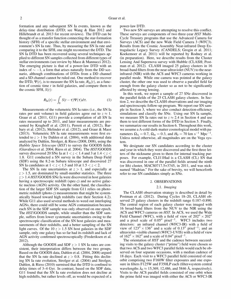
the SNe themselves, were followed up with spectroscopic ob-servations from several ground-based observatories, as de-tailed below, or with HST slitless spectroscopy, using theG800L ACS grism spectrograph. The ground-based observa-tories and instruments used for this work were the Low Reso-lution Imaging Spectrometer (LRIS; Oke et al. 1995) and theDEep Imaging Multi-Object Spectrograph (DEIMOS; Faberet al. 2003) on the Keck I and II 10-m telescopes, respectively;the Gemini Multi-Object Spectrograph (GMOS; Hook et al.2003) on the Gemini North and South telescopes (GeminiNand GeminiS, respectively); the Multi-Object Double Spec-trograph (MODS; Pogge et al. 2010) on the Large BinocularTelescope (LBT); and the FOcal Reducer and low dispersionSpectrograph (FORS; Appenzeller et al. 1998), the VIsibleMultiObject Spectrograph (VIMOS; Le Fevre et al. 2003),and the X-shooter spectrograph (Vernet et al. 2011) on theVery Large Telescope (VLT). Table 2 details which instru-ments were used to obtain spectra of each SN host galaxy.Several examples of SN host-galaxy spectra are shown in Fig-ure 1. The spectra of the SNe CLF11Ves, CLI11Had, andCLY13Pup are shown in Figure 2.
3. SUPERNOVA SAMPLEIn our survey, SNe can be discovered if they either brighten
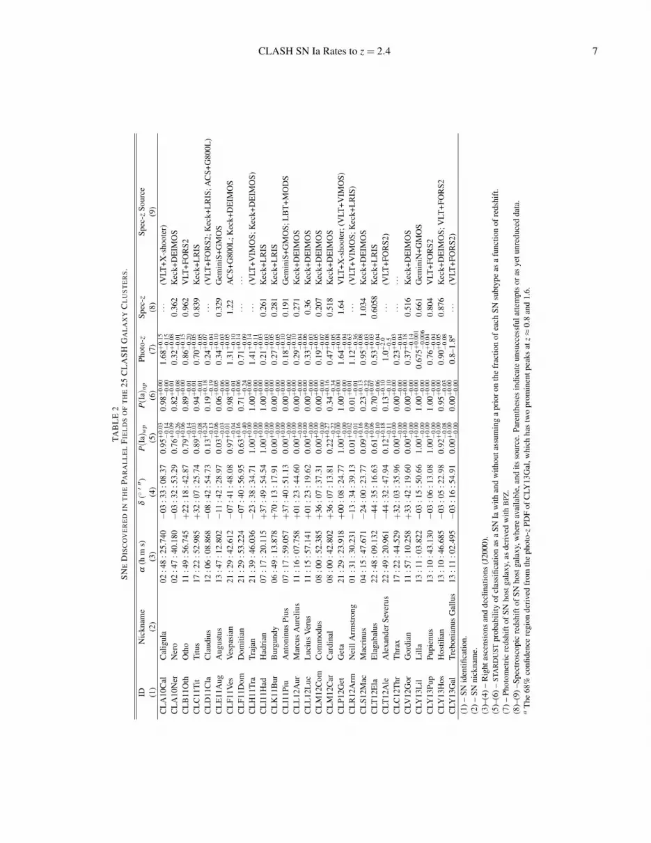
or decline between one search epoch and the next. By a“brightening” SN we do not mean that the SN is necessar-ily caught on the rising part of its light curve, but rather anycase in which the discovery flux is higher than the templateflux. As a result of the cadence of our survey, it is easier todiscover SNe either on the rise or near peak, as in these casesthe template image will contain no SN flux. In contrast, SNecaught while on the decline will invariably have some flux inall our images, thus reducing the flux in the difference imageand consequently their probability of detection. We have dis-covered a total of 20 brightening and 7 declining SNe in theparallel fields of the 25 CLASH clusters. Of these, 18 werediscovered in the ACS and 9 in the WFC3 fields. Nineteen (or70%) of the SN host galaxies have spectroscopic redshifts, asdetailed below in Section 3.3. We classify half of this sampleas SNe Ia, four of which are at z > 1.2. Our SN sample issummarized in Table 2 and displayed in Figure 3.
We have discovered 12 additional SN candidates in theprime fields. However, as the effects of gravitational lensingmust be taken into account to properly classify any SNe dis-covered behind the galaxy clusters, we leave their treatmentto a future paper. The complete photometry of all 39 SNe in
4 Graur et al.
1
2
3
4
Hα
[SII
]
Na
DCLI11Had, z = 0.261
0.5
1.5
2.5 Hα
Hβ
[OII
I]
[NII
]
[SII
]CLE11Aug, z = 0.329
0
2
4
6
[OII
]
[OII
I]
[Ne
V]CLC11Tit, z = 0.839
f λ[arbitrary
units]
0
3
6
9
12 [OII
]
CLS12Mac, z = 1.034
5000 6000 7000 8000 9000 100000
1
2
3
4
Ca
H&
KCLF11Ves, z = 1.22
Observed wavelength [A]
FIG. 1.— Examples of SN host-galaxy spectra. From top to bottom, wepresent spectra of the SN host galaxies CLI11Had, at z = 0.261, taken withKeck+LRIS; CLE11Aug, at z = 0.329, taken with GeminiS+GMOS (thegaps in this spectrum are the result of physical gaps between GMOS chips);CLC11Tit, at z= 0.839, obtained with Keck+LRIS; CLS12Mac, at z= 1.034,obtained with Keck+DEIMOS; and CLF11Ves, at z = 1.22, obtained withKeck+DEIMOS. All spectra have been binned into 10 A-wide bins. All fluxunits and have been arbitrarily scaled.
our sample will appear in a future paper by Graur et al. (inpreparation).
3.1. Candidate SelectionThe F850LP- and F160W-band subtraction images were si-
multaneously searched by eye and scanned with the source-identifying software SEXTRACTOR (Bertin & Arnouts 1996) toidentify variable objects. We set SEXTRACTOR to locate all ob-jects that had at least four connected pixels with flux 3σ abovethe local background level in both the regular subtraction im-age and in its negative, the latter in order to search for declin-ing SNe. To increase the detection efficiency in the F160Wband, the F160W- and F125W-band subtraction images weresearched by eye simultaneously (by toggling between them),as some SNe may appear brighter in the F125W band (see, forexample, the light-curve fit of CLI11Had in Figure 6). TheF850LP- and F775W-band subtraction images were not simi-larly toggled due to the high CR contamination in the F775W-band subtraction image.
To be regarded as SN candidates, the variable objects hadto pass the following criteria.
1. All objects with suspect residual shapes, such as thesubtraction residuals of bright galaxy cores or objectswith non-PSF shapes, were rejected.
2. The F850LP- and F160W-band images were comprised
0
2
4
6
8CLI11Had, z = 0.261
SN1992A, −1 day (SNID)
0
1
2
3 CLY13Pup, z = 0.804
SN2001ay, +3 days (SNID)
f λ[arbitrary
units]
3000 4000 5000 6000 7000 8000 9000 10000
0
1
2 CLF11Ves, z = 1.22
Hsiao et al. (2007), peak
Observed wavelength [A]
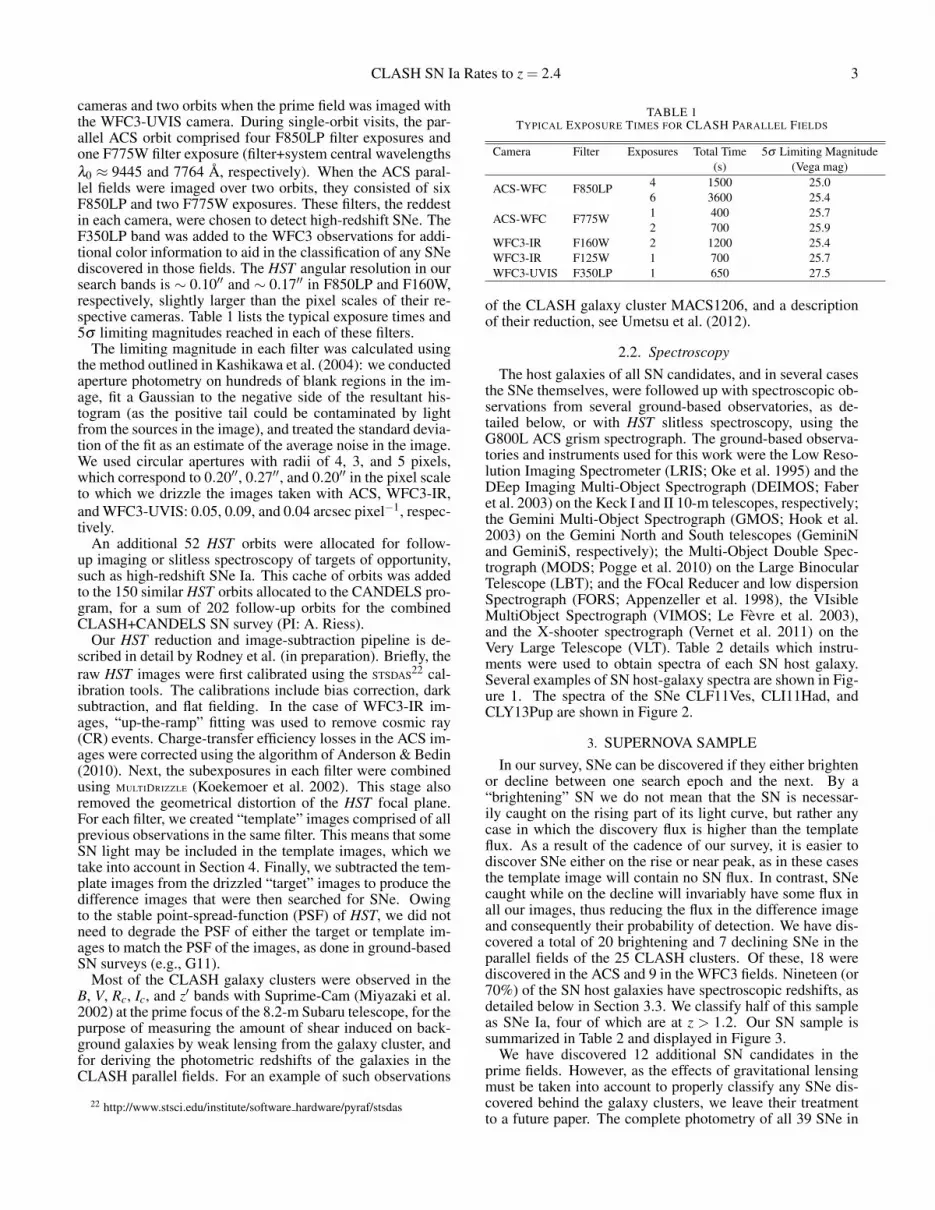
FIG. 2.— SN spectra. In black solid curves, we show the spectra of the SNeCLI11Had (top), at z = 0.261, taken with Keck+LRIS; CLY13Pup (center),at z = 0.804, taken with VLT+FORS2; and CLF11Ves (bottom), at z = 1.22,taken with the HST G800L ACS grism spectrograph. Overlaid on the spec-tra as red dashed curves are examples of SNe Ia from the literature shiftedto the same redshift and scaled so as to fit the data. The SN designation,along with that of the example SN Ia, are noted on the top left of each panel.The top and center spectra have been binned into 10 A-wide bins, while thebottom spectrum has been binned into 80 A-wide bins. All flux units arearbitrary. Beyond 5500 A, the spectrum of CLI11Had may be dominated byhost-galaxy light, as no correction for host-galaxy light was performed duringreductions.
of several subexposures (four or six in the F850LP bandand two in the F160W band). We used these subexpo-sures to create separate subtraction images, which werethen compared to the main subtraction image. The ob-ject had to appear in all of the subtraction images to beconsidered a likely candidate.
3. To be considered a declining SN, the object had to havea negative flux in the subtraction image and appear inboth the target and template images. Objects that onlyappeared in the template images were discarded as ei-ther CRs or noise spikes.
4. Objects with suspect residual shapes in the F775W- orF125W-band subtraction images were flagged for in-spection in the next search epoch. As a result of thecadence of the survey, any SNe detected in one of thefirst two search epochs would be visible in the othersearch epochs as well, so if the object under consider-ation did not reappear in a later epoch, it was rejected.No candidates were rejected if they did not appear inthe F775W- or F125W-band images.
3.2. Detection-efficiency SimulationsIn our survey, SNe can be missed because of many factors.
Generally, the fainter the SN, the less likely it is to be de-tected above the background. On average, F775W-band im-ages suffer from a background (composed of zodiacal light,earthshine, and airglow) level twice as high as F850LP-bandimages (Sokol, Anderson, & Smith 2012). The main sourcesof background for WFC3-IR observations are earthshine andzodiacal light, with the latter being the dominant source. Bothsources contribute less background at longer wavelengths (Gi-avalisco, Sahu, & Bohlin 2002), but as our F160W expo-sures are roughly twice as long as the F125W exposures, they

CLASH SN Ia Rates to z = 2.4 5
both display roughly the same number of background counts(Dressel 2012). There are other factors that affect the discov-ery probability of a SN, such as its proximity to the core ofits host galaxy (SNe that explode close to the cores of theirhost galaxies are harder to discover due to the noise fromthe higher background and the residuals from imperfect im-age subtractions).
To test the effect of these and other factors on our detec-tion efficiency, we planted ∼ 1000 fake point sources in theraw images at the start of our reduction pipeline. The fakeSNe were planted in random locations around galaxies chosenfrom SEXTRACTOR catalogs of the images following a Gaus-sian distribution centered on the center of the galaxy, as mea-sured by SEXTRACTOR, with a standard deviation of σ = 2R50,where R50 is the radius that contains 50% of the galaxy light.This distribution assured that the fake SNe approximately fol-lowed the light of the galaxy and that a large number wereplanted in galaxy cores (e.g., Forster & Schawinski 2008).Near the center of a bright galaxy, a SN could be obscureddue to the increased Poisson noise and residual subtractionartifacts from small inter-epoch registration errors. This isevaluated in Rodney et al. (in preparation), where we find thiseffect to be negligible, with less than 2% of galaxies abovez = 0.2 exhibiting core residuals that could obscure a SN. Themagnitudes of the fake SNe were drawn from flat distributionsin F850LP and F160W in the range 22–28 mag. To simulatethe appearance of real SNe Ia, the F775W and F125W magni-tudes, respectively, were randomly chosen from a SN Ia sim-ulation done with the SuperNova ANAlysis (SNANA23; Kessleret al. 2009b) software package, which was constructed to re-flect a realistic spread of SN Ia colors in the redshift rangez = 0–3, with host-galaxy extinction according to values cho-sen from an exponential of the form P(AV ) = e(−AV /τV ), withτV = 0.7, chosen to approximate the host-galaxy extinctionmodel of Riello & Patat (2005). This was done to ensure thatthe fake SNe resembled the colors of their real counterparts asclose as possible, and was of importance mainly in the WFC3fields, where the SN searchers toggled between the F160Wand F125W difference images. The PSF was simulated usingTINY TIM
24 (Krist, Hook, & Stoehr 2011).Figure 4 shows our detection efficiency, as a function of
the brightness of the fake SNe, in the F850LP and F160Wbands. The uncertainties of the measurements represent the68% binomial confidence intervals. We follow Sharon et al.(2010) and fit the efficiency measurements with the function
η(m;m1/2,s1,s2) =
(
1+ em−m1/2
s1
)−1
, m≤ m1/2(1+ e
m−m1/2s2
)−1
, m > m1/2,
(2)
where m is the magnitude in the F850LP band; m1/2 is themagnitude at which the efficiency drops to 50%; and s1 ands2 determine the range over which the efficiency drops from100% to 50%, and from 50% to 0, respectively. Our detectionefficiency drops to 50% at 25.2 and 25.0 mag in the F850LPand F160W bands, respectively.
3.3. Host-galaxy Redshifts
23 http://sdssdp62.fnal.gov/sdsssn/SNANA-PUBLIC/24 http://www.stsci.edu/hst/observatory/focus/TinyTim
Our classification method, as with most SN classificationtechniques, relies on a good knowledge of the redshift of ei-ther the SN or its host galaxy. As part of our survey strat-egy, we have endeavored to obtain spec-z measurements ofthe host galaxies of all the SNe in our sample, mostly withground-based observatories, as described above. Some of theSN host galaxies suspected of being at z > 1.2 (CLD11Claand CLF11Ves) were also followed up with HST slitless spec-troscopy using the ACS G800L grism. At this time, we haveacquired and reduced the spectra of 19 of the 27 SN hostgalaxies in our sample.
For the remaining eight SN host galaxies, we rely on photo-z measurements. A complete description of our photo-z tech-nique appears in Jouvel et al. (2013) and Molino et al. (inpreparation). Here, we give only a brief description of thistechnique. The spec-z and photo-z values of the SNe in oursample are listed in Table 2 and shown in Figure 5.
We estimated the redshift and spectral type of all SN hostgalaxies with photometry obtained from deep Subaru images(in the B, V , Rc, Ic, and z′ bands) and the Bayesian Photo-metric Redshift code (BPZ; Benıtez 2000). For the host galax-ies of SNe that were discovered in the WFC3 parallel fields,we also added galaxy photometry in the F125W and F160Wbands. Some host galaxies were previously imaged by theSloan Digital Sky Survey (SDSS; York et al. 2000), allowingus to include photometry in the u′, g′, r′, i′, and z′ bands aswell.
For each galaxy, BPZ calculates a likelihood, L(z,T ), asa function of redshift, z, and spectral type, T , comparingthe observed colors of the galaxies with the template li-brary, and then multiplies it by an empirical prior, p(z,T |m),which depends on the galaxy magnitude in some referenceband, m, yielding a full probability, p(z,T ), for each galaxy.The new version of BPZ (Benıtez, in preparation) includes anew template library comprising six spectral energy distri-bution templates originally from PEGASE (Fioc & Rocca-Volmerange 1997) and four early-type templates from Pol-letta et al. (2007). The PEGASE templates were recalibratedusing the Wuyts et al. (2008) FIREWORKS photometry andspectroscopic redshifts to optimize its performance togetherwith the new early-type galaxy templates. In total, we use fivetemplates for early-type galaxies, two for intermediate galax-ies, and four for starburst galaxies. The prior was calibratedusing the GOODS-MUSIC (Grazian et al. 2006), Hubble Ul-tra Deep Field (Coe et al. 2006), and COSMOS (Ilbert et al.2009) samples. Despite its compactness and simplicity, thislibrary produces results which are comparable or slightly bet-ter than the best available photo-z methods (see the methodcomparison in Hildebrandt et al. 2010), which often includetemplate libraries that are many times larger. As a result ofthe high-quality HST imaging used for its calibration and us-ing an approach similar to that developed by Coe et al. (2006),the representation of typical galaxy colors provided by this li-brary can be used to calibrate ground-based photometry to anaccuracy of ∼ 2% (Molino et al., in preparation).
3.4. Supernova ClassificationWe classify our SNe into SNe Ia, SNe Ib/c, or SNe II
by fitting light curves to their multi-band photometry usinga Bayesian approach first introduced by Jones et al. (2013),where it was used to classify the CANDELS SN UDS10Wil.The full description of this classification technique, namedthe Supernova Taxonomy And Redshift Determination UsingSNANA Templates (STARDUST), along with a detailed examina-
6 Graur et al.
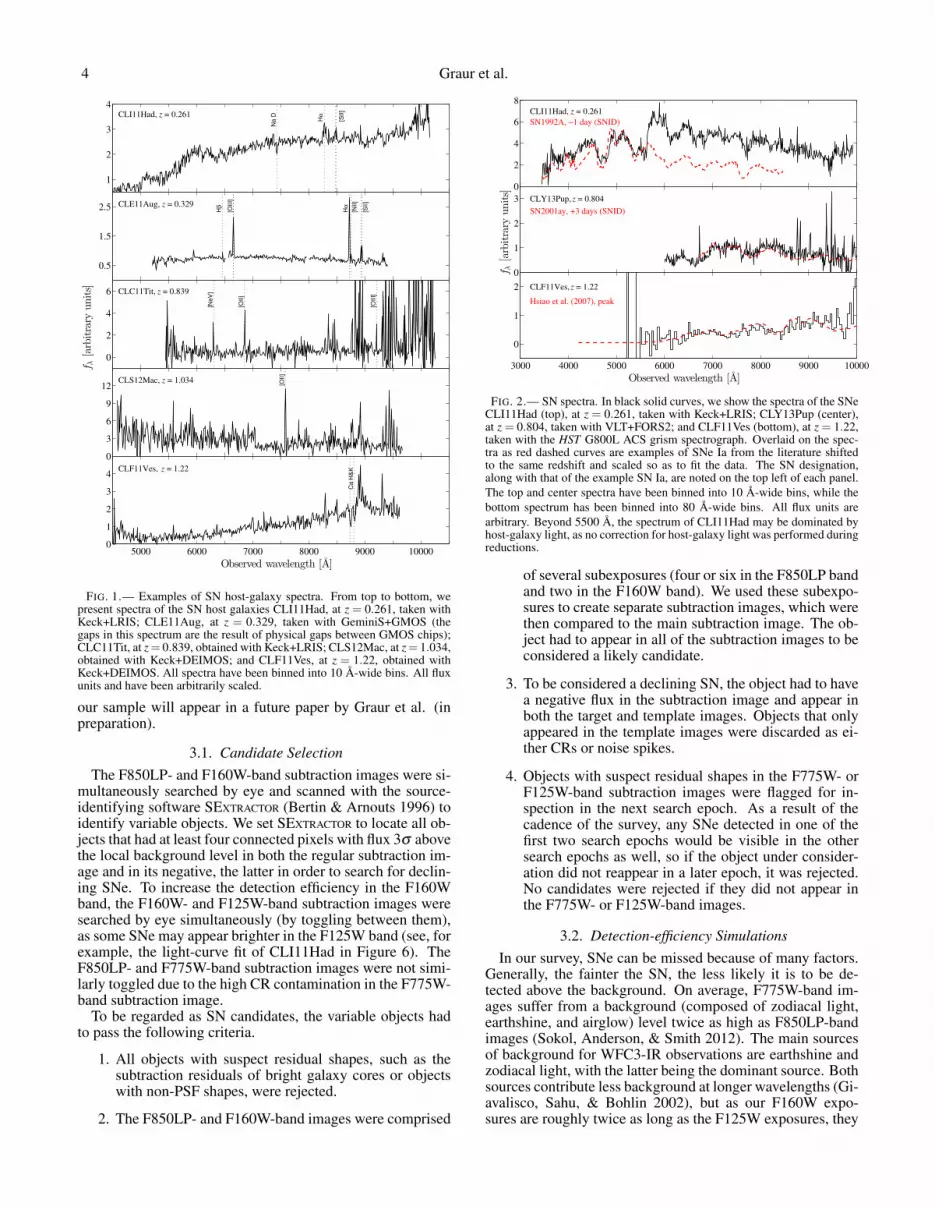
FIG. 3.— SNe discovered in the parallel fields of the CLASH clusters. North is up and east is left. In the triplet of tiles for each event, the left-hand tiles showthe SN host galaxies without any SN light, whereas the center tiles display the SN host galaxy as imaged when the SN was first discovered. For the decliningSNe CLK11Bur, CLL12Luc, CLA10Ner, CLV12Gor, CLF11Dom, CLT12Ela, and CLY13Gal, the left-hand and center tiles show the SN and host galaxy on thefirst and last visits to the field, respectively. The right-hand tiles show the subtraction in the F850LP or F160W bands for SNe discovered in the ACS or WFC3parallel fields, respectively. The stretch of the images and the location of the SN differ from panel to panel in order to highlight host-galaxy properties. Theheader of each panel gives the designation of the SN along with its redshift and camera. Spectroscopic redshifts (cases with no uncertainties in z noted) are givento three significant digits. Photometric redshifts are shown with their uncertainty; in cases where the photometric redshift is not well constrained, we note theapproximate peak of the probability density function.
CLASH SN Ia Rates to z = 2.4 7
TAB
LE
2S
NE
DIS
CO
VE
RE
DIN
TH
EPA
RA
LL
EL
FIE
LD
SO
FT
HE
25C
LA
SH
GA
LA
XY
CL
US
TE
RS.
IDN
ickn
ame
α(h
ms)
δ(′′′ )
P(I
a)w
pP(I
a)np
Phot
o-z
Spec
-zSp
ec-z
Sour
ce(1
)(2
)(3
)(4
)(5
)(6
)(7
)(8
)(9
)C
LA
10C
alC
alig
ula
02:4
8:2
5.74
0−
03:3
3:0
8.37
0.95
+0.
03−
0.14
0.98
+0.
00−
0.00
1.68
+0.
15−
0.15
···
(VLT
+X-s
hoot
er)
CL
A10
Ner
Ner
o02
:47
:40.
180−
03:3
2:5
3.29
0.76
+0.
09−
0.26
0.82
+0.
01−
0.08
0.32
+0.
08−
0.01
0.36
2K
eck+
DE
IMO
SC
LB
11O
thO
tho
11:4
9:5
6.74
5+
22:1
8:4
2.87
0.79
+0.
06−
0.14
0.89
+0.
00−
0.01
0.86
+0.
15−
0.20
0.96
2V
LT+F
OR
S2C
LC
11Ti
tTi
tus
17:2
2:5
2.98
5+
32:0
7:2
5.74
0.89
+0.
03−
0.08
0.94
+0.
01−
0.01
0.70
+0.
05−
0.05
0.83
9K
eck+
LR
ISC
LD
11C
laC
laud
ius
12:0
6:0
8.86
8−
08:4
2:5
4.73
0.13
+0.
24−
0.13
0.19
+0.
18−
0.19
0.24
+0.
07−
0.04
···
(VLT
+FO
RS2
;Kec
k+L
RIS
;AC
S+G
800L
)C
LE
11A
ugA
ugus
tus
13:4
7:1
2.80
2−
11:4
2:2
8.97
0.03
+0.
06−
0.03
0.06
+0.
05−
0.06
0.34
+0.
10−
0.03
0.32
9G
emin
iS+G
MO
SC
LF1
1Ves
Ves
pasi
an21
:29
:42.
612−
07:4
1:4
8.08
0.97
+0.
01−
0.04
0.98
+0.
00−
0.01
1.31
+0.
05−
0.10
1.22
AC
S+G
800L
;Kec
k+D
EIM
OS
CL
F11D
omD
omiti
an21
:29
:53.
224−
07:4
0:5
6.95
0.63
+0.
16−
0.40
0.71
+0.
06−
0.24
0.71
+0.
14−
0.09
···
···
CL
H11
Tra
Traj
an21
:39
:46.
036−
23:3
8:3
4.71
1.00
+0.
00−
0.00
1.00
+0.
00−
0.00
1.41
+0.
14−
0.11
···
(VLT
+VIM
OS;
Kec
k+D
EIM
OS)
CL
I11H
adH
adri
an07
:17
:20.
115
+37
:49
:54.
541.
00+
0.00
−0.
001.
00+
0.00
−0.
000.
21+
0.03
−0.
030.
261
Kec
k+L
RIS
CL
K11
Bur
Bur
gund
y06
:49
:13.
878
+70
:13
:17.
910.
00+
0.00
−0.
000.
00+
0.00
−0.
000.
27+
0.05
−0.
050.
281
Kec
k+L
RIS
CL
I11P
iuA
nton
inus
Pius
07:1
7:5
9.05
7+
37:4
0:5
1.13
0.00
+0.
00−
0.00
0.00
+0.
00−
0.00
0.18
+0.
10−
0.02
0.19
1G
emin
iS+G
MO
S;L
BT
+MO
DS
CL
L12
Aur
Mar
cus
Aur
eliu
s11
:16
:07.
758
+01
:23
:44.
600.
00+
0.00
−0.
000.
00+
0.00
−0.
000.
29+
0.10
−0.
040.
271
Kec
k+D
EIM
OS
CL
L12
Luc
Luc
ius
Ver
us11
:15
:57.
141
+01
:23
:19.
620.
00+
0.00
−0.
000.
00+
0.00
−0.
000.
33+
0.06
−0.
030.
36K
eck+
DE
IMO
SC
LM
12C
omC
omm
odus
08:0
0:5
2.38
5+
36:0
7:3
7.31
0.00
+0.
00−
0.00
0.00
+0.
00−
0.00
0.19
+0.
05−
0.07
0.20
7K
eck+
DE
IMO
SC
LM
12C
arC
ardi
nal
08:0
0:4
2.80
2+
36:0
7:1
3.81
0.22
+0.
27−
0.22
0.34
+0.
16−
0.34
0.47
+0.
08−
0.05
0.51
8K
eck+
DE
IMO
SC
LP1
2Get
Get
a21
:29
:23.
918
+00
:08
:24.
771.
00+
0.00
−0.
001.
00+
0.00
−0.
001.
64+
0.04
−0.
041.
64V
LT+X
-sho
oter
;(V
LT+V
IMO
S)C
LR
12A
rmN
eill
Arm
stro
ng01
:31
:30.
231−
13:3
4:3
9.13
0.01
+0.
02−
0.01
0.01
+0.
01−
0.01
1.12
+0.
63−
0.36
···
(VLT
+VIM
OS;
Kec
k+L
RIS
)C
LS1
2Mac
Mac
rinu
s04
:15
:47.
671−
24:0
0:2
3.77
0.09
+0.
16−
0.09
0.23
+0.
13−
0.22
0.95
+0.
08−
0.03
1.03
4K
eck+
DE
IMO
SC
LT12
Ela
Ela
gaba
lus
22:4
8:0
9.13
2−
44:3
5:1
6.63
0.61
+0.
06−
0.10
0.70
+0.
07−
0.06
0.53
+0.
03−
0.04
0.60
58K
eck+
LR
ISC
LT12
Ale
Ale
xand
erSe
veru
s22
:49
:20.
961−
44:3
2:4
7.94
0.12
+0.
18−
0.11
0.13
+0.
10−
0.10
1.0+
2.0
−0.
5···
(VLT
+FO
RS2
)C
LC
12T
hrT
hrax
17:2
2:4
4.52
9+
32:0
3:3
5.96
0.00
+0.
00−
0.00
0.00
+0.
00−
0.00
0.23
+0.
03−
0.04
···
···
CLV
12G
orG
ordi
an11
:57
:10.
258
+33
:42
:19.
600.
00+
0.00
−0.
000.
00+
0.00
−0.
000.
37+
0.18
−0.
140.
516
Kec
k+D
EIM
OS
CLY
13L
ilL
illa
13:1
1:0
3.82
2−
03:1
5:5
0.66
1.00
+0.
00−
0.00
1.00
+0.
00−
0.00
0.67
5+0.
001
−0.
006
0.66
1G
emin
iN+G
MO
SC
LY13
Pup
Pupi
enus
13:1
0:4
3.13
0−
03:0
6:1
3.08
1.00
+0.
00−
0.00
1.00
+0.
00−
0.00
0.76
+0.
04−
0.04
0.80
4V
LT+F
OR
S2C
LY13
Hos
Hos
tilia
n13
:10
:46.
685−
03:0
5:2
2.98
0.92
+0.
00−
0.08
0.95
+0.
00−
0.03
0.90
+0.
05−
0.08
0.87
6K
eck+
DE
IMO
S;V
LT+F
OR
S2C
LY13
Gal
Treb
onia
nus
Gal
lus
13:1
1:0
2.49
5−
03:1
6:5
4.91
0.00
+0.
00−
0.00
0.00
+0.
00−
0.00
0.8–
1.8a
···
(VLT
+FO
RS2
)(1
)–SN
iden
tifica
tion.
(2)–
SNni
ckna
me.
(3)–
(4)–
Rig
htas
cens
ions
and
decl
inat
ions
(J20
00).
(5)–
(6)–
STA
RD
UST
prob
abili
tyof
clas
sific
atio
nas
aSN
Iaw
ithan
dw
ithou
tass
umin
ga
prio
ron
the
frac
tion
ofea
chSN
subt
ype
asa
func
tion
ofre
dshi
ft.
(7)–
Phot
omet
ric
reds
hift
ofSN
host
gala
xy,a
sde
rived
with
BPZ
.(8
)–(9
)–Sp
ectr
osco
pic
reds
hift
ofSN
host
gala
xy,w
here
avai
labl
e,an
dits
sour
ce.P
aren
thes
esin
dica
teun
succ
essf
ulat
tem
pts
oras
yetu
nred
uced
data
.a
The
68%
confi
denc
ere
gion
deriv
edfr
omth
eph
oto-
zPD
Fof
CLY
13G
al,w
hich
has
two
prom
inen
tpea
ksat
z≈
0.8
and
1.6.

8 Graur et al.
22 23 24 25 26 270
0.2
0.4
0.6
0.8
1 F850LP
m1/2
= 25.2
s1 = 0.3
s2 = 0.2
Det
ecti
on e
ffic
iency
Apparent magnitude22 23 24 25 26 27
F160W
m1/2
= 25.0
s1 = 0.3
s2 = 0.2
Apparent magnitude
FIG. 4.— SN detection efficiency vs. magnitude in the F850LP (left) and F160W (right) bands. The uncertainties of the measurements are the 68% binomialconfidence intervals. The dotted lines mark where the best-fit efficiency curves drop to 50%, at 25.2 and 25.0 mag in the F850LP and F160W bands, respectively.
tion of any systematic biases it might introduce, will appearin a future paper by Rodney et al. (in preparation). Briefly, foreach SN we calculate the probability that it is a SN Ia, P(Ia),by comparing the observed fluxes (in all available bands andepochs) to light-curve models generated using the SNANA sim-ulation package. We classify a SN as a SN Ia if P(Ia) ≥ 0.5.However, as detailed below in Section 4, when deriving theSN Ia rates, we sum the P(Ia) values of all the SNe in oursample
The apparent magnitudes of each SN are measured withaperture photometry on the subtraction images of each epochusing the IRAF routine apphot and the same apertures describedin Section2.1. The zero-point magnitudes and aperture cor-rections for ACS filters are taken from Sirianni et al. (2005).For WFC3-IR and WFC3-UVIS, we use the zero-point mag-nitudes calculated for a 0.4′′ aperture, as of 2012 March 6,by the Space Telescope Science Institute.25 The aperture cor-rections for the WFC3 filters were calculated by measuringthe photometry of several bright stars using different aperturesand adopting the correction for a 0.4′′ aperture.
For the SN Ia simulations, we use the Guy et al. (2007)SALT226 model, with nuisance parameters for the redshift,stretch (x1), color (c), and time of peak brightness. The core-collapse (CC) SNe are generated from the SNANA library of 43CC SN templates, taken from the SN samples of the SDSS(Frieman et al. 2008; Sako et al. 2008; D’Andrea et al. 2010),Supernova Legacy Survey (SNLS; Astier et al. 2006), andCarnegie Supernova Project (Hamuy et al. 2006; Stritzingeret al. 2009; Morrell 2012). Each of these CC SN models alsohas parameters for redshift, host extinction (AV ), date of peakbrightness, and peak luminosity.
The remainder of our technique is fundamentally similarto other Bayesian light-curve classifiers (e.g., Kuznetsova &Connolly 2007; Poznanski, Maoz, & Gal-Yam 2007a; Rodney& Tonry 2009; Sako et al. 2011): we compute the likelihoodthat a given model matches the observable data, multiply itby priors for the model parameters, then marginalize over allmodels to derive the final posterior classification probability.
The simulated SNe are reddened and dimmed according
25 http://www.stsci.edu/hst/wfc3/phot zp lbn26 http://supernovae.in2p3.fr/∼guy/salt/
to the Cardelli, Clayton, & Mathis (1989) reddening lawand one of three host-galaxy dust extinction models: “low,”“medium,” and “high” dust models. For the simulated SNe Ia,the “low” dust model is the Barbary et al. (2012) skewedGaussian fit to the Astier et al. (2006) SNLS, while the “mid”and “high” dust models are taken from Kessler et al. (2009a)and Neill et al. (2006), respectively. For CC SNe, we usemodels composed of a half Gaussian centered at AV = 0 magand an exponential of the form e−(AV /τV ). These models havethree parameters: the standard distribution of the Gaussian,σAV ; the characteristic AV value, τV ; and the ratio between theGaussian and power-law components at AV = 0, A0. For the“low,” “mid,” and “high” dust models, the values of these pa-rameters are σAV = 0.15, 0.6, and 0.5 mag; τV = 0.5, 1.7, and2.8; and A0 = 1, 4, and 3 mag.
The peak magnitudes of each SN subtype are chosen ac-cording to their observed luminosity functions (LFs), whichare detailed in Table 3. The Li et al. (2011b) LFs, derivedfrom a local sample of SNe observed by the Lick Observa-tory Supernova Search (LOSS; Leaman et al. 2011; Li et al.2011a,b), were not originally corrected for host-galaxy ex-tinction. Here, we adopt “dust-free” LFs for SNe II-P andII-L such that when applying the “medium” dust model, theresultant simulated LFs approximate those published by Liet al. (2011b).
A further prior is placed on the fraction of each SN type asa function of redshift. The distribution of SN type fractionshas only been measured in the local universe (Li et al. 2011b),and it is expected to change with increasing redshift, once theSN Ia rate starts to deviate from the star-formation rate. How-ever, assuming a prior on the evolution of the SN type fractionrequires us to assume a prior on the CC SN and SN Ia ratesas a function of redshift. Such a prior might bias the SN Iarates measured in this work, and so we classify our SN sampletwice: once using this prior, and once assuming that the frac-tion of SN types remains constant with redshift. While the lat-ter assumption is probably not the case in reality, it expressesour lack of concrete knowledge on the subject. We reportthe classification probability, P(Ia), of each SN in our samplein Table 2 both with (P(Ia)wp) and without (P(Ia)np) the SNtype fraction prior. The uncertainty reported for each P(Ia)wpvalue takes into account uncertainties in both the extinction
CLASH SN Ia Rates to z = 2.4 9
TABLE 3SN LUMINOSITY FUNCTIONS USED FOR SN CLASSIFICATION
Type MR σ SourceIa −19.37 0.47 Wang et al. (2006)Ib −17.90 0.90 Drout et al. (2011)Ic −18.30 0.60 Drout et al. (2011)IcBL −19.00 1.10 Drout et al. (2011)II-P −16.56 0.80 Li et al. (2011b)II-L −17.66 0.42 Li et al. (2011b)IIn −18.25 1.00 Kiewe et al. (2012)Notes. The Li et al. (2011b) LFs have beencorrected for host-galaxy extinction, as det-ailed in the text.
and SN-fraction priors, while the uncertainty of P(Ia)np re-flects only the uncertainty in the extinction prior. For each ofthe SNe in our sample, the resultant P(Ia) values are consis-tent with each other, and while generally P(Ia)wp < P(Ia)np,the difference between the two values is small and has a negli-gible effect on the final SN Ia rates. The resultant light-curvefits, obtained without the SN-fraction prior, are presented inFigures 6–7.
SNe that were caught on the rise and were suspected of be-ing SNe Ia at z > 1 were followed up with further HST imag-ing in order to follow the evolution of their light curves. Inour sample, these include CLA10Cal, CLF11Ves, CLH11Tra,CLP12Get, CLR12Arm, and CLT12Ale. Three SNe werecaught sufficiently early, and were bright enough, to be fol-lowed up spectroscopically, either from the ground or withHST. These were CLI11Had, CLF11Ves, and CLY13Pup,whose spectra were obtained with Keck+LRIS, the ACSG800L grism, and VLT+FORS2, respectively. Using the Su-pernova Identification code (SNID27; Blondin & Tonry 2007),we classify CLI11Had and CLY13Pup as SNe Ia having thespec-z measured from each of their host galaxies. The best-fitting SNID templates are overlaid on the SN spectra in Fig-ure 2. Owing to its high redshift, the ACS G800L grismscaught CLF11Ves only in the rest-frame range ∼ 2500–4500 A, and SNID fails to classify the spectrum as belongingto any type of SN at z = 1.22. When allowed to fit for the SNredshift, SNID classifies CLF11Ves as either a SN Ia or SN Ibat z ≈ 0.95. Consequently, we do not claim to have spectro-scopic confirmation for CLF11Ves as a SN Ia, although in thebottom panel of Figure 2, we show that the spectrum could befit with the Hsiao et al. (2007) SN Ia template at peak and atz = 1.22.
Because declining SNe appear in all four epochs, their pho-tometry cannot be measured from the subtraction images.CLA10Ner, CLF11Dom, and CLL12Luc are well offset fromtheir respective host galaxies, so we measure their photome-try from the target images and assume any contamination bygalactic light is minimal. CLT12Ela is in a relatively faint(in the observed bands) area of its host galaxy. Here, too,we assume that any contamination by galactic light is mini-mal. As can be seen in Figure 3, CLK11Bur, CLV12Gor, andCLY13Gal exploded in relatively bright regions of their hostgalaxies, so contamination is a certainty. However, all threeof these SNe show signs of either a plateau or a slow declinein their light curves, and are classified as SNe II, as shown inFigures 6–7.
27 http://marwww.in2p3.fr/∼blondin/software/snid/index.html
CLA10Cal CLA10Ner
CLB11Oth CLC11Tit CLD11Cla CLE11Aug CLF11Ves
CLF11Dom CLH11Tra CLI11Had CLK11Bur CLI11Piu
Pro
bab
ilit
y P
(z)
CLL12Aur CLL12Luc CLM12Com CLM12Car CLP12Get
CLR12Arm CLS12Mac CLT12Ela CLT12Ale CLC12Thr
0 1 2 0
CLV12Gor
0 1 2 0
CLY13Lil
0 1 2 0
Redshift
CLY13Pup
0 1 2 0
CLY13Hos
0 1 2 3
CLY13Gal
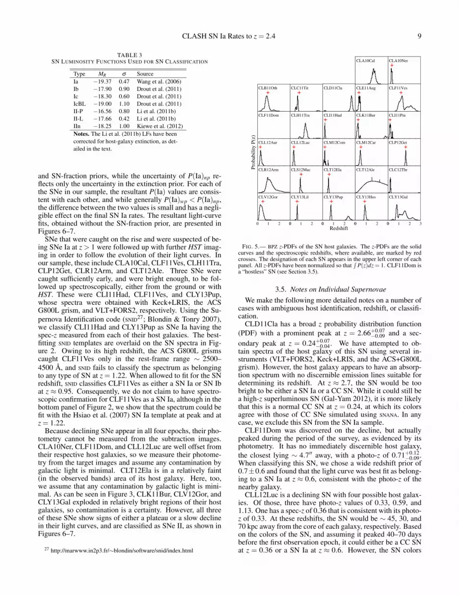
FIG. 5.— BPZ z-PDFs of the SN host galaxies. The z-PDFs are the solidcurves and the spectroscopic redshifts, where available, are marked by redcrosses. The designation of each SN appears in the upper left corner of eachpanel. All z-PDFs have been normalized so that
∫P(z)dz = 1. CLF11Dom is
a “hostless” SN (see Section 3.5).
3.5. Notes on Individual SupernovaeWe make the following more detailed notes on a number of
cases with ambiguous host identification, redshift, or classifi-cation.
CLD11Cla has a broad z probability distribution function(PDF) with a prominent peak at z = 2.66+0.07
−0.09 and a sec-ondary peak at z = 0.24+0.07
−0.04. We have attempted to ob-tain spectra of the host galaxy of this SN using several in-struments (VLT+FORS2, Keck+LRIS, and the ACS+G800Lgrism). However, the host galaxy appears to have an absorp-tion spectrum with no discernible emission lines suitable fordetermining its redshift. At z ≈ 2.7, the SN would be toobright to be either a SN Ia or a CC SN. While it could still bea high-z superluminous SN (Gal-Yam 2012), it is more likelythat this is a normal CC SN at z = 0.24, at which its colorsagree with those of CC SNe simulated using SNANA. In anycase, we exclude this SN from the SN Ia sample.
CLF11Dom was discovered on the decline, but actuallypeaked during the period of the survey, as evidenced by itsphotometry. It has no immediately discernible host galaxy,the closest lying ∼ 4.7′′ away, with a photo-z of 0.71+0.12
−0.09.When classifying this SN, we chose a wide redshift prior of0.7±0.6 and found that the light curve was best fit as belong-ing to a SN Ia at z ≈ 0.6, consistent with the photo-z of thenearby galaxy.
CLL12Luc is a declining SN with four possible host galax-ies. Of those, three have photo-z values of 0.33, 0.59, and1.13. One has a spec-z of 0.36 that is consistent with its photo-z of 0.33. At these redshifts, the SN would be ∼ 45, 30, and70 kpc away from the core of each galaxy, respectively. Basedon the colors of the SN, and assuming it peaked 40–70 daysbefore the first observation epoch, it could either be a CC SNat z = 0.36 or a SN Ia at z ≈ 0.6. However, the SN colors
10 Graur et al.
55860 55880 55900 55920 55940MJD [days]
23
24
25
26
27
Vega
mag
IIP(SDSS-015320)MJDpk=55887z=0.191AV=0.37RV=3.1∆m=0.6χ 2ν =0.4
CLI11Piu, z=0.191±0.001F850LP F775W
55980 56010 56040MJD [days]
24
25
26
Vega
mag
IIn(SDSS-012842)MJDpk=55994z=0.207AV=0.74RV=3.1∆m=2.7χ 2ν =3.1
CLM12Com, z=0.207±0.001F850LP F775W
55660 55680 55700 55720 55740MJD [days]
23
24
25
26
27
28
Vega
mag
IIP(SDSS-020038)MJDpk=55679z=0.222AV=0.00RV=3.1∆m=0.4χ 2ν =0.0
CLC12Thr, z=0.230±0.040F850LP F775W
55700 55725 55750 55775MJD [days]
22
23
24
25
26
27
Vega
mag
Ib(CSP-2007Y)MJDpk=55712z=0.273AV=0.37RV=3.1∆m=-0.1χ 2ν =0.5
CLD11Cla, z=0.240±0.070F850LP F775W
55840 55860 55880 55900 55920 55940MJD [days]
22
24
26
28Ve
ga m
ag
Ia(SALT2)MJDpk=55875z=0.261x1=0.16C=0.04β=4.1χ 2ν =0.6
CLI11Had, z=0.261±0.001F160W F125W F350LP
55920 55940 55960 55980 56000 56020MJD [days]
23
24
25
26
27
Vega
mag
IIP(SDSS-018834)MJDpk=55955z=0.271AV=0.37RV=3.1∆m=0.4χ 2ν =1.7
CLL12Aur, z=0.271±0.001F850LP F775W
55820 55840 55860 55880 55900MJD [days]
22
23
24
25
26
Vega
mag
IIP(SDSS-018700)MJDpk=55844z=0.281AV=0.74RV=3.1∆m=-1.9χ 2ν =0.6
CLK11Bur, z=0.281±0.001F850LP F775W
55680 55710 55740 55770 55800MJD [days]
23
24
25
26
27
Vega
mag
Ib(SDSS-019323)MJDpk=55734z=0.329AV=0.37RV=3.1∆m=0.4χ 2ν =0.7
CLE11Aug, z=0.329±0.001F850LP F775W
55880 55920 55960 56000MJD [days]
232425262728
Vega
mag
Ic(SDSS-015475)MJDpk=55913z=0.420AV=0.74RV=3.1∆m=-0.1χ 2ν =23.1
CLL12Luc, z=0.360±0.060F850LP F775W
55440 55480 55520 55560 55600MJD [days]
22
23
24
Vega
mag
Ia(SALT2)MJDpk=55499z=0.361x1=-1.11C=-0.03β=4.1χ 2ν =3.8
CLA10Ner, z=0.362±0.030F850LP F775W
56200 56240 56280 56320MJD [days]
21
22
23
24
25
Vega
mag
IIn(SDSS-012842)MJDpk=56219z=0.516AV=0.74RV=3.1∆m=-1.6χ 2ν =0.6
CLV12Gor, z=0.516±0.001F160W F125W F350LP
56040 56070 56100 56130MJD [days]
24
25
26
27
Vega
mag
Ic(SDSS-015475)MJDpk=56054z=0.518AV=0.37RV=3.1∆m=0.1χ 2ν =1.7
CLM12Car, z=0.518±0.001F850LP F775W
55680 55710 55740 55770 55800MJD [days]
23
24
25
26
27
Vega
mag
Ia(SALT2)MJDpk=55707z=0.600x1=-2.05C=0.19β=4.1χ 2ν =2.1
CLF11Dom, z=0.700±0.100F850LP F775W
56100 56130 56160 56190 56220MJD [days]
22
23
24
25
26
Vega
mag
Ia(SALT2)MJDpk=56139z=0.606x1=0.47C=-0.03β=4.1χ 2ν =0.9
CLT12Ela, z=0.606±0.001F850LP F775W
56400 56430 56460 56490 56520MJD [days]
24
26
28
30
Vega
mag
Ia(SALT2)MJDpk=56435z=0.661x1=-0.47C=0.34β=4.1χ 2ν =0.6
CLY13Lil, z=0.661±0.001F160W F125W F350LP
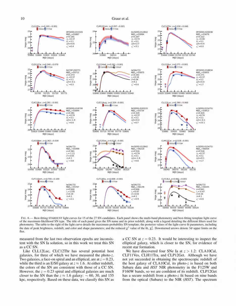
FIG. 6.— Best-fitting STARDUST light curves for 15 of the 27 SN candidates. Each panel shows the multi-band photometry and best-fitting template light curveof the maximum-likelihood SN type. The title of each panel gives the SN name and its prior redshift, along with a legend detailing the different filters used forphotometry. The table to the right of the light curve details the maximum-probability SN template; the posterior values of the light-curve fit parameters, includingthe date of peak brightness, redshift, and color and shape parameters; and the reduced χ2 value of the fit, χ2
ν . Downturned arrows denote 3σ upper limits on theflux.
measured from the last two observation epochs are inconsis-tent with the SN Ia solution, so in this work we treat this SNas a CC SN.
Like CLL12Luc, CLC12Thr has several potential hostgalaxies, for three of which we have measured the photo-z.Two galaxies, a face-on spiral and an elliptical, are at z= 0.23,while the third is an E/S0 galaxy at z≈ 1.6. At either redshift,the colors of the SN are consistent with those of a CC SN.However, the z = 0.23 spiral and elliptical galaxies are muchcloser to the SN than the z ≈ 1.6 galaxy: ∼ 60, 30, and 155kpc, respectively. Based on these data, we classify this SN as
a CC SN at z = 0.23. It would be interesting to inspect theelliptical galaxy, which is closer to the SN, for evidence ofrecent star formation.
We have discovered four SNe Ia at z > 1.2: CLA10Cal,CLF11Ves, CLH11Tra, and CLP12Get. Although we havenot yet succeeded in obtaining the spectroscopic redshift ofthe host galaxy of CLA10Cal, its photo-z is based on bothSubaru data and HST NIR photometry in the F125W andF160W bands, so we are confident of its redshift. CLP12Gethas a secure redshift from a photo-z fit based on nine bandsfrom the optical (Subaru) to the NIR (HST). The spectrum
CLASH SN Ia Rates to z = 2.4 11
56300 56350 56400 56450 56500 56550MJD [days]
22
23
24
25
Vega
mag
IIn(SDSS-013449)MJDpk=56389z=0.900AV=0.00RV=3.1∆m=-1.0χ 2ν =0.6
CLY13Gal, z=0.500±0.400F160W F125W F350LP
56400 56430 56460 56490 56520MJD [days]
23
24
25
26
Vega
mag
Ia(SALT2)MJDpk=56442z=0.804x1=-0.16C=-0.03β=4.1χ 2ν =0.7
CLY13Pup, z=0.804±0.001F850LP F775W
5568055710557405577055800MJD [days]
23
24
25
26
27
28
Vega
mag
Ia(SALT2)MJDpk=55717z=0.839x1=0.16C=0.04β=4.1χ 2ν =2.2
CLC11Tit, z=0.839±0.001F850LP F775W
5646056490565205655056580MJD [days]
23
24
25
26
27
Vega
mag
Ia(SALT2)MJDpk=56488z=0.876x1=0.47C=-0.03β=4.1χ 2ν =0.4
CLY13Hos, z=0.876±0.001F850LP F775W
555905562055650556805571055740MJD [days]
23242526272829
Vega
mag
Ia(SALT2)MJDpk=55633z=0.962x1=-0.16C=0.04β=4.1χ 2ν =0.5
CLB10Oth, z=0.962±0.001F850LP F775W
56150 56200 56250 56300 56350MJD [days]
24
25
26
27
28
29
Vega
mag
Ib(SDSS-014492)MJDpk=56224z=1.370AV=0.00RV=3.1∆m=-0.4χ 2ν =0.3
CLT12Ale, z=1.000±0.900F350LP F160W F125W
56120 56160 56200 56240MJD [days]
24
26
28
30
Vega
mag
Ic(SDSS-015475)MJDpk=56148z=1.103AV=0.37RV=3.1∆m=0.1χ 2ν =0.5
CLR12Arm, z=1.120±0.350F350LP F160W F125W
56160 56200 56240 56280MJD [days]
24
25
26
27
28
29
Vega
mag
Ic(SDSS-004012)MJDpk=56194z=1.034AV=0.00RV=3.1∆m=0.5χ 2ν =1.0
CLS12Mac, z=1.034±0.001F350LP F160W F125W
55680 55720 55760 55800 55840MJD [days]
24
25
26
27
28
Vega
mag
Ia(SALT2)MJDpk=55744z=1.220x1=-0.79C=-0.03β=4.1χ 2ν =0.9
CLF11Ves, z=1.220±0.010F850LP F775W
55830 55860 55890 55920MJD [days]
22232425262728
Vega
mag
Ia(SALT2)MJDpk=55868z=1.357x1=-0.16C=-0.11β=4.1χ 2ν =1.5
CLH11Tra, z=1.410±0.140F160WF140W
F850LPF775W
F350LP
56050 56100 56150 56200 56250 56300MJD [days]
24
26
28
30
Vega
mag
Ia(SALT2)MJDpk=56138z=1.644x1=0.47C=-0.11β=4.1χ 2ν =1.2
CLP12Get, z=1.640±0.040F160W F125W F350LP
55500 55550 55600 55650 55700 55750MJD [days]
24252627282930
Vega
mag
Ia(SALT2)MJDpk=55574z=1.830x1=0.79C=0.04β=4.1χ 2ν =3.0
CLA10Cal, z=1.680±0.150F814W F350LP F160W F125W
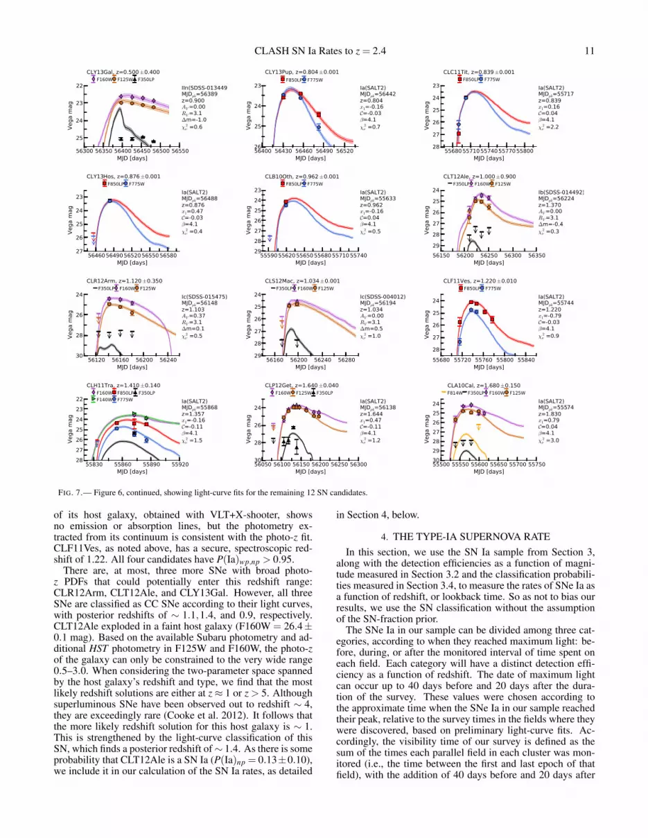
FIG. 7.— Figure 6, continued, showing light-curve fits for the remaining 12 SN candidates.
of its host galaxy, obtained with VLT+X-shooter, showsno emission or absorption lines, but the photometry ex-tracted from its continuum is consistent with the photo-z fit.CLF11Ves, as noted above, has a secure, spectroscopic red-shift of 1.22. All four candidates have P(Ia)wp,np > 0.95.
There are, at most, three more SNe with broad photo-z PDFs that could potentially enter this redshift range:CLR12Arm, CLT12Ale, and CLY13Gal. However, all threeSNe are classified as CC SNe according to their light curves,with posterior redshifts of ∼ 1.1,1.4, and 0.9, respectively.CLT12Ale exploded in a faint host galaxy (F160W = 26.4±0.1 mag). Based on the available Subaru photometry and ad-ditional HST photometry in F125W and F160W, the photo-zof the galaxy can only be constrained to the very wide range0.5–3.0. When considering the two-parameter space spannedby the host galaxy’s redshift and type, we find that the mostlikely redshift solutions are either at z≈ 1 or z > 5. Althoughsuperluminous SNe have been observed out to redshift ∼ 4,they are exceedingly rare (Cooke et al. 2012). It follows thatthe more likely redshift solution for this host galaxy is ∼ 1.This is strengthened by the light-curve classification of thisSN, which finds a posterior redshift of∼ 1.4. As there is someprobability that CLT12Ale is a SN Ia (P(Ia)np = 0.13±0.10),we include it in our calculation of the SN Ia rates, as detailed
in Section 4, below.
4. THE TYPE-IA SUPERNOVA RATEIn this section, we use the SN Ia sample from Section 3,
along with the detection efficiencies as a function of magni-tude measured in Section 3.2 and the classification probabili-ties measured in Section 3.4, to measure the rates of SNe Ia asa function of redshift, or lookback time. So as not to bias ourresults, we use the SN classification without the assumptionof the SN-fraction prior.
The SNe Ia in our sample can be divided among three cat-egories, according to when they reached maximum light: be-fore, during, or after the monitored interval of time spent oneach field. Each category will have a distinct detection effi-ciency as a function of redshift. The date of maximum lightcan occur up to 40 days before and 20 days after the dura-tion of the survey. These values were chosen according tothe approximate time when the SNe Ia in our sample reachedtheir peak, relative to the survey times in the fields where theywere discovered, based on preliminary light-curve fits. Ac-cordingly, the visibility time of our survey is defined as thesum of the times each parallel field in each cluster was mon-itored (i.e., the time between the first and last epoch of thatfield), with the addition of 40 days before and 20 days after
12 Graur et al.
TABLE 4SN IA NUMBERS AND RATES
Subsample 0.0 < z < 0.6 0.6 < z < 1.2 1.2 < z < 1.8 1.8 < z < 2.4Total 12 11 4 0SN host galaxies with spec-z 10 7 2 0Hostless SNe 0 1 0 0SNe Ia (raw) 2.4 6.4 4.1 0SNe Ia (efficiency-corrected) 2.4 7.0 8.0 0SN Ia rate without host-galaxy extinctiona 0.45+0.42,+0.10
−0.32,−0.13 0.42+0.21,+0.12−0.18,−0.05 0.27+0.21,+0.03
−0.13,−0.06 <0.6SN Ia rate [10−4 yr−1 Mpc−3] 0.46+0.42,+0.10
−0.32,−0.13 0.45+0.22,+0.13−0.19,−0.06 0.45+0.34,+0.05
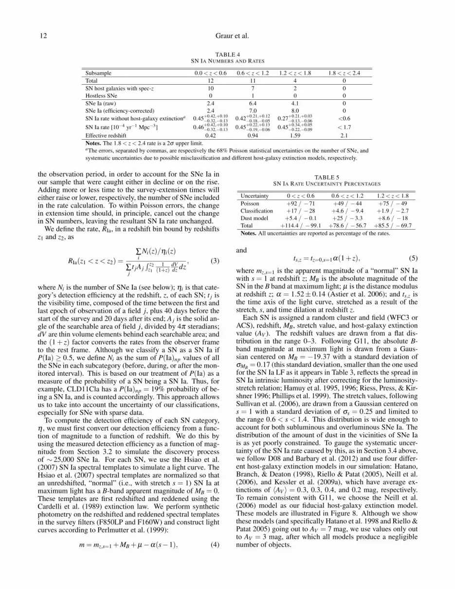
−0.22,−0.09 < 1.7Effective redshift 0.42 0.94 1.59 2.1Notes. The 1.8 < z < 2.4 rate is a 2σ upper limit.aThe errors, separated by commas, are respectively the 68% Poisson statistical uncertainties on the number of SNe, andsystematic uncertainties due to possible misclassification and different host-galaxy extinction models, respectively.
the observation period, in order to account for the SNe Ia inour sample that were caught either in decline or on the rise.Adding more or less time to the survey-extension times willeither raise or lower, respectively, the number of SNe includedin the rate calculation. To within Poisson errors, the changein extension time should, in principle, cancel out the changein SN numbers, leaving the resultant SN Ia rate unchanged.
We define the rate, RIa, in a redshift bin bound by redshiftsz1 and z2, as
RIa(z1 < z < z2) =∑i
Ni(z)/ηi(z)
∑jt jA j
∫ z2z1
1(1+z)
dVdz dz
, (3)
where Ni is the number of SNe Ia (see below); ηi is that cate-gory’s detection efficiency at the redshift, z, of each SN; t j isthe visibility time, composed of the time between the first andlast epoch of observation of a field j, plus 40 days before thestart of the survey and 20 days after its end; A j is the solid an-gle of the searchable area of field j, divided by 4π steradians;dV are thin volume elements behind each searchable area; andthe (1+ z) factor converts the rates from the observer frameto the rest frame. Although we classify a SN as a SN Ia ifP(Ia) ≥ 0.5, we define Ni as the sum of P(Ia)np values of allthe SNe in each subcategory (before, during, or after the mon-itored interval). This is based on our treatment of P(Ia) as ameasure of the probability of a SN being a SN Ia. Thus, forexample, CLD11Cla has a P(Ia)np = 19% probability of be-ing a SN Ia, and is counted accordingly. This approach allowsus to take into account the uncertainty of our classifications,especially for SNe with sparse data.
To compute the detection efficiency of each SN category,η , we must first convert our detection efficiency from a func-tion of magnitude to a function of redshift. We do this byusing the measured detection efficiency as a function of mag-nitude from Section 3.2 to simulate the discovery processof ∼ 25,000 SNe Ia. For each SN, we use the Hsiao et al.(2007) SN Ia spectral templates to simulate a light curve. TheHsiao et al. (2007) spectral templates are normalized so thatan unredshifted, “normal” (i.e., with stretch s = 1) SN Ia atmaximum light has a B-band apparent magnitude of MB = 0.These templates are first redshifted and reddened using theCardelli et al. (1989) extinction law. We perform syntheticphotometry on the redshifted and reddened spectral templatesin the survey filters (F850LP and F160W) and construct lightcurves according to Perlmutter et al. (1999):
m = mz,s=1 +MB +µ−α(s−1), (4)
TABLE 5SN IA RATE UNCERTAINTY PERCENTAGES
Uncertainty 0 < z < 0.6 0.6 < z < 1.2 1.2 < z < 1.8Poisson +92 / −71 +49 / −44 +75 / −49Classification +17 / −28 +4.6 / −9.4 +1.9 / −2.7Dust model +5.4 / −0.1 +25 / −3.3 +8.6 / −18Total +114.4 / −99.1 +78.6 / −56.7 +85.5 / −69.7Notes. All uncertainties are reported as percentage of the rates.
andts,z = tz=0,s=1α(1+ z), (5)
where mz,s=1 is the apparent magnitude of a “normal” SN Iawith s = 1 at redshift z; MB is the absolute magnitude of theSN in the B band at maximum light; µ is the distance modulusat redshift z; α = 1.52± 0.14 (Astier et al. 2006); and ts,z isthe time axis of the light curve, stretched as a result of thestretch, s, and time dilation at redshift z.
Each SN is assigned a random cluster and field (WFC3 orACS), redshift, MB, stretch value, and host-galaxy extinctionvalue (AV ). The redshift values are drawn from a flat dis-tribution in the range 0–3. Following G11, the absolute B-band magnitude at maximum light is drawn from a Gaus-sian centered on MB = −19.37 with a standard deviation ofσMB = 0.17 (this standard deviation, smaller than the one usedfor the SN Ia LF as it appears in Table 3, reflects the spread inSN Ia intrinsic luminosity after correcting for the luminosity-stretch relation; Hamuy et al. 1995, 1996; Riess, Press, & Kir-shner 1996; Phillips et al. 1999). The stretch values, followingSullivan et al. (2006), are drawn from a Gaussian centered ons = 1 with a standard deviation of σs = 0.25 and limited tothe range 0.6 < s < 1.4. This distribution is wide enough toaccount for both subluminous and overluminous SNe Ia. Thedistribution of the amount of dust in the vicinities of SNe Iais as yet poorly constrained. To gauge the systematic uncer-tainty of the SN Ia rate caused by this, as in Section 3.4 above,we follow D08 and Barbary et al. (2012) and use four differ-ent host-galaxy extinction models in our simulation: Hatano,Branch, & Deaton (1998), Riello & Patat (2005), Neill et al.(2006), and Kessler et al. (2009a), which have average ex-tinctions of 〈AV 〉 = 0.3, 0.3, 0.4, and 0.2 mag, respectively.To remain consistent with G11, we choose the Neill et al.(2006) model as our fiducial host-galaxy extinction model.These models are illustrated in Figure 8. Although we showthese models (and specifically Hatano et al. 1998 and Riello &Patat 2005) going out to AV = 7 mag, we use values only outto AV = 3 mag, after which all models produce a negligiblenumber of objects.

CLASH SN Ia Rates to z = 2.4 13
0 1 2 3 4 5 6 710
−4
10−3
10−2
10−1
100
101
<AV
>=0.4
0.3
0.3
0.2
AV
[mag]
dN
/dA
V
Neill et al. (2006)
Hatano et al. (1998)
Riello & Patat (2005)
Kessler et al. (2009)
FIG. 8.— SN Ia host-galaxy dust extinction models used in the derivationof the SN Ia rates. We use the Neill et al. (2006) model (solid black curve) asthe fiducial model. While the models shown here go out to AV = 7 mag, weuse values only to AV = 3 mag, as nearly all the objects produced by thesemodels fall in the range AV = 0–3 mag.
After choosing when the SN reached peak, the light curveis sampled according to the survey cadence in that particularcluster and field, and subtraction magnitudes are computed bysubtracting the flux in each search epoch from the flux of thereference image. Using the detection efficiency at the resul-tant magnitude in each search epoch, the SN is either discov-ered or missed. The resultant detection efficiency curves forSNe Ia that reached maximum light before, during, or afterthe monitored interval are shown in Figure 9.
We divide the SNe in our sample into three redshift bins:0 < z < 0.6, 0.6 < z < 1.2, and 1.2 < z < 1.8. In each redshiftbin, we compute the effective redshift, zeff, as
zeff(z1 < z < z2) =
∫ z2z1
z(1+z)η(z)dV∫ z2
z11
(1+z)η(z)dV. (6)
In each redshift bin, we take the minimal and maximal dif-ferences between the rate as computed with the fiducial dustmodel and with the models in Figure 8 as lower and uppersystematic uncertainties owing to dust extinction. Since weexpress the number of SNe Ia in our final sample as the sum ofall the SN P(Ia)np values, we also propagate the uncertaintiesin these values and add to the rates a systematic uncertaintydue to our classification technique. The systematic uncertain-ties from dust extinction and classification are then summed.G11 also considered the systematic uncertainty due to the ex-pected increase in extinction as a result of dust at high red-shifts (e.g., Mannucci, Della Valle, & Panagia 2007; Mattilaet al. 2012). However, G11 did not take into account the dif-ferent extinction models used here. Specifically, the Hatanoet al. (1998) extinction model adds a ∼ +9% systematic un-certainty to the SN Ia rate in the 1.2 < z < 1.8 bin, similar tothe ∼+10% systematic uncertainty G11 added to their SN Iarate at 1.5 < z < 2.0.
While we found no SNe at z > 1.8, Figure 9 shows thatWFC3 is still sensitive to SNe Ia out to z≈ 2.5. Consequently,we add a fourth redshift bin, 1.8 < z < 2.4, and compute a 2σ
upper limit to the SN Ia rate in that bin by taking the 95%Poisson uncertainty in the number of SNe found in the bin(zero), and considering the detection efficiency of the differ-
0.2
0.4
0.6
0.8
1
SNe peak after
monitored interval
0.2
0.4
0.6
0.8
1
Det
ecti
on
eff
icie
ncy
SNe peak during
monitored interval
0 0.5 1 1.5 2 2.5 30
0.2
0.4
0.6
0.8
1
Redshift
SNe peak before
monitored interval
F850LP
F160W
FIG. 9.— SN Ia detection efficiency as a function of redshift in the F850LP(solid black) and F160W (dashed red) bands for SNe Ia that reached maxi-mum light in the B band before (bottom), during (center), and after (top) themonitored interval.
ent SN categories in the center of the bin at z = 2.1.The resultant SN Ia rates, including both statistical and sys-
tematic uncertainties, are shown in Figure 11. Table 4 sum-marizes the SN Ia rates, with and without correction for host-galaxy dust extinction, and Table 5 shows the complete errorbudget of our SN Ia rates. Table 6 compares the rates fromthis work to previous rates from the literature. Where nec-essary, the measurements have been corrected to reflect thevalue of h = 0.7 used in this work. As Perrett et al. (2012) didnot take into account low-stretch, SN1991bg-like SNe Ia, wescale up their SN Ia rates by 15% (see their Section 6). As inG11, in instances where rates were originally reported in unitsof SNuB (SNe per century per 1010 L,B; Cappellaro et al.1999; Hardin et al. 2000; Pain et al. 2002; Madgwick et al.2003; Blanc et al. 2004), we have converted them to volumet-ric rates using the Botticella et al. (2008) redshift-dependentluminosity density function,
jB(z) = (1.03+1.76z)×108 L,B Mpc−3. (7)
5. THE TYPE-IA SUPERNOVA DELAY-TIMEDISTRIBUTION
In this section, we test different models of the DTD by con-volving them with various cosmic SFHs and fitting the re-sultant SN Ia rate histories to the SN Ia rate measurementsfrom the previous section, along with rates from the litera-ture. We include all the rate measurements from Table 6 ex-cept for Neill et al. (2006, 2007), which have been supersededby Perrett et al. (2012); Dahlen et al. (2004) and Kuznetsovaet al. (2008), which have been superseded by D08; Barris& Tonry (2006), which has been superseded by Rodney &

14 Graur et al.
TABLE 6SN IA RATE MEASUREMENTS
Redshift NIa Rate [10−4 yr−1 Mpc−3] Reference Redshift NIa Rate [10−4 yr−1 Mpc−3] Reference0.01 70 0.183±0.046 Cappellaro et al. (1999)a 0.55 72 0.55+0.07,+0.05
−0.07,−0.06 Perrett et al. (2012)e
< 0.019 274 0.265+0.034,+0.043−0.033,−0.043 Li et al. (2011a)b 0.552 41 0.63+0.10,+0.26
−0.10,−0.27 Neill et al. (2007)d
0.0375 516 0.278+0.112,+0.015−0.083,−0.000 Dilday et al. (2010)c 0.62 7 1.29+0.88,+0.27
−0.57,−0.28 Melinder et al. (2012)0.09 17 0.29+0.09
−0.07 Dilday et al. (2008) 0.65 23 1.49±0.31 Barris & Tonry (2006)d
0.098 19 0.24+0.12−0.12 Madgwick et al. (2003)a,d 0.65 10.09 0.49+0.17,+0.14
−0.17,−0.08 Rodney & Tonry (2010)0.1 516 0.259+0.052,+0.018
−0.044,−0.001 Dilday et al. (2010)c 0.65 91 0.55+0.06,+0.05−0.06,−0.07 Perrett et al. (2012)e
0.1 52 0.569+0.098,+0.058−0.085,−0.047 Krughoff et al. (2011)d 0.714 42 1.13+0.19,+0.54
−0.19,−0.70 Neill et al. (2007)d
0.11 90 0.247+0.029,+0.016−0.026,−0.031 Graur & Maoz (2013) 0.74 5.5 0.43+0.36
−0.32 Poznanski et al. (2007b)d
0.13 14 0.158+0.056,+0.035−0.043,−0.035 Blanc et al. (2004)a 0.74 20.3 0.79+0.33
−0.41 Graur et al. (2011)0.14 4 0.28+0.22,+0.07
−0.13,−0.04 Hardin et al. (2000)a 0.75 28 1.78±0.34 Barris & Tonry (2006)d
0.15 516 0.307+0.038,+0.035−0.034,−0.005 Dilday et al. (2010)c 0.75 14.29 0.68+0.21,+0.23
−0.21,−0.14 Rodney & Tonry (2010)0.15 1.95 0.32+0.23,+0.07
−0.23,−0.06 Rodney & Tonry (2010) 0.75 110 0.67+0.07,+0.06−0.07,−0.08 Perrett et al. (2012)e
0.16 4 0.16+0.10,+0.07−0.10,−0.14 Perrett et al. (2012)e 0.80 14 1.57+0.44,+0.75
−0.25,−0.53 Dahlen et al. (2004)d
0.2 17 0.189+0.042,+0.018−0.034,−0.015±0.42 Horesh et al. (2008) 0.80 18.33 0.93+0.25
−0.25 Kuznetsova et al. (2008)d
0.2 516 0.348+0.032,+0.082−0.030,−0.007 Dilday et al. (2010)c 0.807 5.25 1.18+0.60,+0.44
−0.45,−0.28 Barbary et al. (2012)0.25 1 0.17±0.17 Barris & Tonry (2006)d 0.83 25 1.30+0.33,+0.73
−0.27,−0.51 Dahlen et al. (2008)0.25 516 0.365+0.031,+0.182
−0.028,−0.012 Dilday et al. (2010)c 0.85 15.43 0.78+0.22,+0.31−0.22,−0.16 Rodney & Tonry (2010)
0.26 16 0.32+0.08,+0.07−0.08,−0.08 Perrett et al. (2012)e 0.85 128 0.66+0.06,+0.07
−0.06,−0.08 Perrett et al. (2012)e
0.3 31.05 0.34+0.16,+0.21−0.15,−0.22 Botticella et al. (2008) f 0.94 6.4 0.45+0.22,+0.13
−0.19,−0.06 CLASH (this work)0.3 516 0.434+0.037,+0.396
−0.034,−0.016 Dilday et al. (2010)c 0.95 13.21 0.76+0.25,+0.32−0.25,−0.26 Rodney & Tonry (2010)
0.35 5 0.530±0.024 Barris & Tonry (2006)d 0.95 141 0.89+0.09,+0.12−0.09,−0.14 Perrett et al. (2012)e
0.35 4.01 0.34+0.19,+0.07−0.19,−0.03 Rodney & Tonry (2010) 1.05 11.01 0.790.28,+0.36
−0.28,−0.41 Rodney & Tonry (2010)0.35 31 0.41+0.07,+0.06
−0.07,−0.07 Perrett et al. (2012)e 1.05 50 0.85+0.14,+0.12−0.14,−0.15 Perrett et al. (2012)e
0.368 17 0.31+0.05,+0.08−0.05,−0.03 Neill et al. (2007)d 1.187 5.63 1.33+0.65,+0.69
−0.49,−0.26 Barbary et al. (2012)0.40 3 0.69+0.34,+1.54
−0.27,−0.25 Dahlen et al. (2004)d 1.20 6 1.15+0.47,+0.32−0.26,−0.44 Dahlen et al. (2004)d
0.40 5.44 0.53+0.39−0.17 Kuznetsova et al. (2008)d 1.20 8.87 0.75+0.35
−0.30 Kuznetsova et al. (2008)d
0.42 2.4 0.46+0.42,+0.10−0.32,−0.13 CLASH (this work) 1.21 20 1.32+0.36,+0.38
−0.29,−0.32 Dahlen et al. (2008)0.442 0 0.00+0.50,+0.00
−0.00,−0.00 Barbary et al. (2012) 1.23 10.0 1.05+0.45−0.56 Poznanski et al. (2007b)d
0.45 9 0.73±0.24 Barris & Tonry (2006)d 1.23 27.0 0.84+0.25−0.28 Graur et al. (2011)
0.45 5.11 0.31+0.15,+0.12−0.15,−0.04 Rodney & Tonry (2010) 1.535 1.12 0.77+1.07,+0.44
−0.54,−0.77 Barbary et al. (2012)0.45 42 0.41+0.07,+0.05
−0.07,−0.06 Perrett et al. (2012)e 1.55 0.35 0.12+0.58−0.12 Kuznetsova et al. (2008)d
0.46 8 0.48±0.17 Tonry et al. (2003) 1.59 4.1 0.45+0.34,+0.05−0.22,−0.09 CLASH (this work)
0.467 73 0.42+0.06,+0.13−0.06,−0.09 Neill et al. (2006)d 1.60 2 0.44+0.32,+0.14
−0.25,−0.11 Dahlen et al. (2004)d
0.47 8 0.80+0.37,+1.66−0.27,−0.26 Dahlen et al. (2008) 1.61 3 0.42+0.39,+0.19
−0.23,−0.14 Dahlen et al. (2008)0.55 38 0.568+0.098,+0.098
−0.088,−0.088 Pain et al. (2002)a 1.67 3.0 0.81+0.79−0.60 Poznanski et al. (2007b)d
0.55 29 2.04±0.38 Barris & Tonry (2006)d 1.69 10.0 1.02+0.54−0.37 Graur et al. (2011)
0.55 6.49 0.32+0.14,+0.07−0.14,−0.07 Rodney & Tonry (2010) 2.1 0 < 1.7 CLASH (this work)g
Notes. Redshifts are means over the redshift intervals probed by each survey. NIa is the number of SNe Ia used to derive the rate. Where necessary, rateshave been converted to h = 0.7. Where reported, the statistical errors are followed by systematic errors, and separated by commas. Rates from this workare shown in bold.aRates have been converted to volumetric rates using Equation 7.bLi et al. (2011a) consider SNe Ia within 80 Mpc.cDilday et al. (2010) compute their rates using 516 SNe Ia at z < 0.5.dThese measurements have been superseded by more recent results, as detailed in Section 5.ePerrett et al. (2012) do not include SN1991bg-like SNe Ia in their rates. Here, their measurements are scaled up by 15% (see their Section 6).f Botticella et al. (2008) found a total of 86 SN candidates of all types. See their Section 5.2 for details on their various subsamples and classification techniques.g2σ upper limit on the SN Ia rate, as derived in Section 4.
Tonry (2010); Poznanski et al. (2007b), which has been su-perseded by G11; and Madgwick et al. (2003) and Krughoffet al. (2011), which have been superseded by Graur & Maoz(2013). We do not use the z > 2 upper limit from the previoussection as it is too high to affect the DTD fits. In total, we use50 SN Ia rate measurements, of which 41 are at z < 1 and 9are at z > 1.
Following G11, we test different SFHs, including the Cole
et al. (2001) parameterization fit to the data collected by Hop-kins & Beacom (2006, HB06); the SFH presented by Yukselet al. (2008, Y08) and upper (O08u) and lower (O08l) limitsfrom Oda et al. (2008, O08) which can be approximated asbroken power laws with a break at z = 1 and with varying in-dices before and after the break; and the recent Behroozi et al.(2013, B13) SFH. These SFHs, and the data they are basedon, are presented in Figure 10.

CLASH SN Ia Rates to z = 2.4 15
1 2 3 4 5 6 7 8 9−2.5
−2
−1.5
−1
−0.5
0
1+z
log(ρ
∗)[M
⊙yr
−1Mpc−3]
HB06
HB10
B13
HB06
Y08
O08l
O08u
B13
FIG. 10.— SFH measurements and parameterizations. SFH measurementcompilations up to 2006 from HB06 are shown in filled circles, and addi-tional measurements up to 2010 compiled by Horiuchi & Beacom (2010),here marked as HB10, are shown as filled squares. The most up-to-date com-pilation from B13 is shown as open triangles. The different parameterizationsare shown as curves and include the Cole et al. (2001) fit to the HB06 data(dashed); the Y08 (solid) and O08u/O08l (thin/thick dotted) power-law fits;and the B13 parameterization (dot-dashed). All data and parameterizationshave been rescaled to the Bell et al. (2003) “diet” Salpeter IMF.
When deriving SFH measurements, various authors use dif-ferent versions of the initial-mass function (IMF), leading todifferent scalings of the SFH. In order to maintain consistencyacross the different SFHs, we must choose one IMF and re-scale the SFHs accordingly. As in G11 and Graur & Maoz(2013), we assume a “diet” Salpeter IMF (Bell et al. 2003),which is similar to the Salpeter (1955) IMF with lower andupper mass limits of 0.1 and 125 M, respectively, but witha stellar mass-to-light (M/L) ratio that is scaled down by afactor of 0.7 in order to fit the M/L ratios measured in disks(Bell & de Jong 2001). The choice of this IMF requires us toscale down the SFHs of HB06, O08, and Y08, who assumed aSalpeter (1955) IMF, by a factor of 0.7. The B13 SFH, wherea Chabrier (2003) IMF was assumed, is scaled up by a fac-tor of 0.7. To allow comparisons with G11, we use the Y08SFH as the fiducial model in our DTD recoveries and the otherSFHs to estimate a systematic uncertainty in the values of theparameters of the DTD model tested below.
We test a power-law DTD of the form Ψ(t) =
Ψ1Gyr(t/1 Gyr)β , setting its index, β , and scaling, Ψ1Gyr,as free parameters, leaving 48 degrees of freedom for thefit. The DTD is set to zero before 40 Myr, to allow for8 M stars to evolve into CO WDs. The Y08 SFH yields abest-fit index value of β = −1.00+0.06(0.09)
−0.06(0.10) with a reduced
χ2 (χ2ν ) of 0.7, where the statistical uncertainties are the
68% and 95% (in parentheses) confidence regions, respec-tively. The other SFHs yield a systematic uncertainty of +0.12
−0.08,with χ2
ν values in the range 0.7–0.8, yielding a final valueof β =−1.00+0.06(0.09)
−0.06(0.10) (statistical) +0.12−0.08 (systematic). This
value is consistent with those obtained by G11 and Graur &Maoz (2013) and in a variety of different SN surveys andusing different DTD recovery techniques (see Maoz & Man-nucci 2012). Integrating the DTD over a Hubble time, we findthat the number of SNe Ia per formed mass, N/M∗, lies in therange (0.5–1.3) ×10−3 SNe M−1
, similar to the ranges found
0 0.5 1 1.5 2 2.5 30
0.2
0.4
0.6
0.8
1
1.2
1.4
1.6
1.8
2
SN
IaRate[10−
4Mpc−3yr
−1]
Y08
HB06
B13
O08l
O08u
Various
SDSS
SDSS DR7
SNLS
GOODS
SDF
CLASH
Redshift
0 1 2 3 4 5 6 7 8 9 10 11
Lookback Time [Gyr]
FIG. 11.— SN Ia rates from CLASH (filled, red squares) compared to ratesfrom the literature and best-fitting SN Ia rate evolutions derived by convolv-ing a power-law DTD with different SFHs. Circles denote data from surveyswith measurements out to z ≈ 1 from Cappellaro et al. (1999), Hardin et al.(2000), Pain et al. (2002), Tonry et al. (2003), Blanc et al. (2004), Botti-cella et al. (2008), Horesh et al. (2008), Rodney & Tonry (2010), Li et al.(2011a), Barbary et al. (2012), and Melinder et al. (2012). Filled circles de-note the most accurate and precise measurements at z < 1 and are from theSDSS Stripe 82 survey (Dilday et al. 2010, orange), SNLS (Perrett et al.2012, green), and SDSS DR7 (Graur & Maoz 2013, purple). The GOODSrates from Dahlen et al. (2008) are shown as triangles and the SDF rates fromGraur et al. (2011) are shown as diamonds. The z > 1.5 rates from thesetwo surveys are colored in black and blue, respectively. The thick curvesare convolutions of several SFHs (dashed, Hopkins & Beacom 2006; solid,Yuksel et al. 2008; thin/thick dotted, Oda et al. 2008; dot-dashed, Behrooziet al. 2013) with the best-fitting power-law DTDs. The shaded area is theconfidence region resulting from the combined 68% statistical uncertaintiesin the values of the power-law index fit with the above SFHs. The thin dashedlines indicate the 68% statistical uncertainty region obtained without the newCLASH measurements. All vertical error bars are sums of the statistical andsystematic uncertainties. The CLASH vertical error bars are composed of thesystematic uncertainty, shown as black thick lines, and the statistical uncer-tainty, shown as red thin lines. The horizontal error bars delineate the CLASHredshift bins. The Perrett et al. (2012) and z > 1.5 Dahlen et al. (2008) SN Iarates have been shifted by ∆z =+0.02 to disentangle them from other results.
by G11 and Graur & Maoz (2013). The best-fitting SN Ia ratehistories derived from each SFH, along with the 68% uncer-tainty region, are shown in Figure 11.
We investigate also the viability of a Gaussian DTD fit(Strolger et al. 2004, 2010) to the SN Ia rates. We start bytesting the Gaussian DTD proposed by D08, with a mean de-lay time of 3.4 Gyr and a standard deviation of 0.68 Gyr. Asin G11, we allow the scaling of this DTD to vary as a freeparameter. Coupled with the SN Ia rates, the only SFH thatdoes not disfavor this DTD is the HB06 SFH, with a reducedχ2 value of 1.1. All other SFHs result in SN Ia rate evolu-tions that are excluded at a > 95% significance level, with theO08 and B13 SFHs specifically excluded at a > 99% signifi-cance level. We next test a general Gaussian DTD, where weallow the mean delay time, standard deviation, and scaling tovary as free parameters, while requiring that 95% of the areaunder the DTD remain above a delay time of 40 Myr (thusensuring the resultant DTD retains a Gaussian shape). TheB13 and lower-limit O08 SFHs result in Gaussians that areexcluded at a > 95% significance level. The Y08, upper-limitO08, and HB06 SFHs, on the other hand, result in Gaussianswith means in the range µ = 2.7–3.3 Gyr with standard devi-ations of σ = 0.8–1.6 Gyr and reduced χ2 values of 0.9–1.3.These Gaussian DTDs are centered at slightly lower mean de-

16 Graur et al.
0 2 4 6 8 100
0.3
0.6
0.9
1.2
1.5 Gaussian
Y08: µ = 2.7, σ = 1.3
HB06: µ = 2.8, σ = 1.4
B13: µ = 2.8, σ = 1.4
O08l: µ = 1.6, σ = 0.8
O08u: µ = 3.3, σ = 1.6
SN
IaRate[10−
4Mpc−3yr
−1]
Lookback Time [Gyr]
0.0 0.5 1.0 1.5
Redshift
0 2 4 6 8 100
0.3
0.6
0.9
1.2
1.5 Broken power law
Y08: β = −1.46
HB06: β = −1.74
B13: β = −1.47
O08l: β = −1.94
O08u: β = −1.25
SN
IaRate[10−
4Mpc−3yr
−1]
Lookback Time [Gyr]
0.0 0.5 1.0 1.5
Redshift
FIG. 12.— Observed SN Ia rates compared to predicted SN Ia rate evolu-tion tracks from the convolution of different SFHs with a best-fitting (top)Gaussian DTD and (bottom) broken power-law DTD of the form Ψ(t) =Ψ(t/1 Gyr)−1/2 up to tc = 1.7 Gyr, and Ψ(t) ∝ tβ afterward. Symbols areas in Figure 11. The SFHs used for each fit are listed in the top panel alongwith best-fitting parameter values: the mean, µ , and standard deviation, σ , ofthe Gaussian DTD, in Gyr; and the slope of the second power law, β , of thebroken power-law DTD. The CLASH upper limit at z > 1.8, which was notused in the fits, has been removed.
lay times, but are wider, than the D08 Gaussian DTD. Theresultant fits to the SN Ia rate evolution are shown in Fig-ure 12. Although at first sight, it might appear that the z > 1.5SDF rate measurement is driving the exclusion of the Gaus-sian DTDs, most of the fitting power actually comes from theaccurate z < 1 SDSS and SNLS measurements.
As in G11, we test the further possibility that at earlytimes the DTD is dominated by the production efficiencyof double WD systems, which is described by a power lawof the form t−0.5 (Pritchet, Howell, & Sullivan 2008), untilsome cutoff time, tc, when a second physical process takesover, described as a power law having a different slope, tβ .Whereas in G11, we set the slope of the second power lawto β = −1 and fit for tc, here we set tc = 1.7 Gyr, the life-time of a 2 M star, the least massive star expected to producea ∼ 0.7 M CO WD (see Figure 4 of Girardi et al. 2000),and find that the best-fitting slope of the second power law
is β =−1.46+0.16(0.26)−0.13(0.22) (statistical) +0.48
−0.21 (systematic) with re-
duced χ2 values in the range 0.7–0.9.Finally, we test both DD and SD DTDs resulting from bi-
nary population synthesis (BPS) simulations. Here, we useupdated versions of the scaled models presented in Figures 2–3 of Nelemans, Toonen, & Bours (2013, for color versions ofthese DTD figures, see Wang & Han 2012; updated versionsof the models courtesy of G. Nelemans, private communica-tion). As in Nelemans et al. (2013), we designate the BPSDTD models by the groups that computed them: Yungelson(e.g., Yungelson 2010), the Yunnan group (Wang/Han et al.;e.g., Wang et al. 2010), the StarTrack code (Ruiter et al.; e.g.,Ruiter et al. 2009), the Brussels group (Mennekens et al.; e.g.,Mennekens et al. 2010), the Utrecht group (Claeys et al.; e.g.,Claeys et al. 2013), and the SeBa code (Bours/Toonen; e.g.,Toonen et al. 2012). We present the updated versions of thescaled BPS DTD models in Figure 13. As Nelemans et al.(2013) scaled the different DTDs to a Kroupa et al. (1993)IMF, we rescale them to the diet Salpeter IMF by multiplyingthem by a factor of 0.7. For comparison with the volumetricSN Ia rates, we convolve the different BPS DTDs with theB13 SFH, as parametrized by their Equation F1, which wereproduce here as
CSFR(z) =C
10A(z−z0)+10B(z−z0), (8)
where CSFR(z) is the cosmic SFH as a function of redshift,and the constants A, B, C, and z0 are given in Table 7 of B13as A =−0.997, B = 0.241, C = 0.180, and z0 = 1.243.
As has been commented elsewhere (e.g., Maoz & Mannucci2012; Nelemans et al. 2013), the BPS DTDs, both for DD andSD scenarios, fail to produce the number of observed SNe Ia.Here, we test the shape of the BPS DTDs by treating theirscaling as a free parameter. The resultant SN Ia rate evolu-tions are presented in Figure 14. The BPS DD models re-quire scalings by small factors of 3–9 and result in reducedχ2 values of χ2
ν<∼ 1, consistent with the SN Ia rates. The BPS
SD models, on the other hand, require large scaling factors of> 10 (except for the Wang/Han and Mennekens DTDs, whichrequire scaling factors of∼ 4) and result in reduced χ2 valuesof χ2
ν > 1.8, thus excluding all BPS SD models at a > 99%significance level.
The poor fits of the SD models are the result of their lowDTD amplitudes at long delay times. The accurate and precisez < 1 SN Ia rates, which are most sensitive to the long delay-time component of the DTD, have the most leverage on thescalings of the BPS SD DTDs. Because the SD models havelow amplitudes at long delay times, the z< 1 SN Ia rates forcescalings of large factors that then cause the resultant SN Ia rateevolutions to overshoot the z > 1 rates.
It is instructive to compare some of the SD DTD models,and their resultant SN Ia rate evolutions, in detail. The Claeysmodel has the lowest amplitude at long delay times, which iswhy its resultant SN Ia rate evolution overshoots all the othermodels in the bottom panel of Figure 14. On the other hand,although the Yungelson model only has an intermediate delay-time component, that component is at longer delay times thanthe Claeys model, so it results in a SN Ia rate evolution withless amplitude than the rate evolution produced by the Claeysmodel. Finally, the Ruiter model has the highest amplitude atlong delay times, after the Wang/Han model, which results ina low scaling. However, the Ruiter model has lower ampli-tude at short delay times, compared to all other DTD models
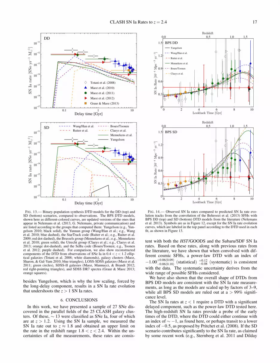
CLASH SN Ia Rates to z = 2.4 17
0.1 1 1010
−17
10−16
10−15
10−14
10−13
10−12
10−11
Delay time [Gyr]
SN
Iarate
[SNeyr−
1M
−1
⊙]
DD
Totani et al. (2008)
Maoz et al. (2010)
Maoz et al. (2011)
Maoz et al. (2012)
Graur & Maoz (2013)
0.1 1 1010
−17
10−16
10−15
10−14
10−13
10−12
10−11
Delay time [Gyr]
SN
Iarate
[SNeyr−
1M
−1
⊙]
Wang/Han et al.
Ruiter et al.
Bours/Toonen
Claeys et al.
Mennekens et al.
Yungelson
SD
FIG. 13.— Binary-population synthesis DTD models for the DD (top) andSD (bottom) scenarios, compared to observations. The BPS DTD models,shown here as different-colored curves, are updated versions of the ones thatappear in Nelemans et al. (2013, G. Nelemans, private communication) andare listed according to the groups that computed them: Yungelson (e.g., Yun-gelson 2010; black solid), the Yunnan group (Wang/Han et al.; e.g., Wanget al. 2010; blue dashed), the StarTrack code (Ruiter et al.; e.g., Ruiter et al.2009; red dot-dashed), the Brussels group (Mennekens et al.; e.g., Mennekenset al. 2010; green solid), the Utrecht group (Claeys et al.; e.g., Claeys et al.2013; orange dot-dashed), and the SeBa code (Bours/Toonen; e.g., Toonenet al. 2012; purple dashed). For comparison, we also show reconstructedcomponents of the DTD from observations of SNe Ia in 0.4 < z < 1.2 ellip-tical galaxies (Totani et al. 2008; white diamonds), galaxy clusters (Maoz,Sharon, & Gal-Yam 2010; blue triangles), LOSS-SDSS galaxies (Maoz et al.2011; green circles), SDSS-II galaxies (Maoz, Mannucci, & Brandt 2012;red right-pointing triangles), and SDSS DR7 spectra (Graur & Maoz 2013;orange squares).
besides Yungelson, which is why the low scaling, forced bythe long-delay component, results in a SN Ia rate evolutionthat undershoots the z > 1 SN Ia rates.
6. CONCLUSIONSIn this work, we have presented a sample of 27 SNe dis-
covered in the parallel fields of the 25 CLASH galaxy clus-ters. Of these, ∼ 13 were classified as SNe Ia, four of whichare at z > 1.2. Using the SN Ia sample, we measured theSN Ia rate out to z ≈ 1.8 and obtained an upper limit onthe rate in the redshift range 1.8 < z < 2.4. Within the un-certainties of all the measurements, these rates are consis-
0 2 4 6 8 100
0.3
0.6
0.9
1.2
1.5 BPS DD
Yungelson
Wang/Han et al.
Ruiter et al.
Mennekens et al.
Bours/Toonen
Claeys et al.
SN
IaRate[10−
4Mpc−3yr
−1]
Lookback Time [Gyr]
0.0 0.5 1.0 1.5Redshift
0 2 4 6 8 100
0.3
0.6
0.9
1.2
1.5 BPS SD
SN
IaRate[10−
4Mpc−3yr
−1]
Lookback Time [Gyr]
0.0 0.5 1.0 1.5
Redshift
FIG. 14.— Observed SN Ia rates compared to predicted SN Ia rate evo-lution tracks from the convolution of the Behroozi et al. (2013) SFHs withBPS DD (top) and SD (bottom) DTD models from the literature (Nelemanset al. 2013). Symbols are as in Figure 12, except for the SN Ia rate evolutioncurves, which are labeled in the top panel according to the DTD used in eachfit, as shown in Figure 13.
tent with both the HST/GOODS and the Subaru/SDF SN Iarates. Based on these rates, along with previous rates fromthe literature, we have shown that when convolved with dif-ferent cosmic SFHs, a power-law DTD with an index of−1.00+0.06(0.09)
−0.06(0.10) (statistical) +0.12−0.08 (systematic) is consistent
with the data. The systematic uncertainty derives from thewide range of possible SFHs considered.
We have also shown that the overall shape of DTDs fromBPS DD models are consistent with the SN Ia rate measure-ments, as long as the models are scaled up by factors of 3–9,while all BPS SD models are ruled out at a > 99% signifi-cance level.
The SN Ia rates at z < 1 require a DTD with a significantdelayed component, such as the power-law DTD tested here.The high-redshift SN Ia rates provide a probe of the earlytimes of the DTD, where the DTD could either continue withan index of ∼−1, as found here, or perhaps transit to a lowerindex of−0.5, as proposed by Pritchet et al. (2008). If the SDscenario contributes significantly to the SN Ia rate, as claimedby some recent work (e.g., Sternberg et al. 2011 and Dilday
18 Graur et al.
et al. 2012), its main effect would be on the high-redshiftrates. However, to have any real discriminatory power on thedifferent DTD models, the SN Ia rates at z > 1 must be moreaccurate and precise than they currently are. To make the mostefficient use of the CLASH SN sample, we will combine itwith the final CANDELS sample in a future paper. Together,the two samples will contain a similar number of SNe Iaas the Subaru/SDF sample from G11. However, their sys-tematic uncertainties will be lower, as they will make use oflight curves and spectroscopy, where available, as done in thiswork. Finally, the upcoming HST Frontier Fields program28
(PI: M. Mountain) will observe six pairs of galaxy clustersand blank fields containing field galaxies, using 140 orbits ofACS and WFC3 for each pair of galaxy cluster / blank fieldduring Cycles 21–23. Based on our work on CLASH andCANDELS, we expect that this survey, which will go deeperthan either of the previous surveys, will discover ∼ 20 SNe,including five z > 1.5 SNe Ia. Once this sample is added tothe combined CLASH+CANDELS SN sample, we may fi-nally have high-redshift SN Ia rates accurate enough to probethe early part of the DTD.
We thank Gijs Nelemans for sharing the BPS DTD mod-els with us, and Ori Fox, Patrick Kelly, Isaac Shivvers,Brad Tucker, and WeiKang Zheng for assistance with someof the Keck observations. Financial support for this workwas provided by NASA through grants HST-GO-12060 andHST-GO-12099 from the Space Telescope Science Institute(STScI), which is operated by Associated Universities forResearch in Astronomy, Inc., under NASA contract NAS 5-26555. O.G. and D.M. acknowledge support by the I-COREprogram of the PDC and the ISF, Grant 1829/12, and by agrant from the Israel Science Foundation. Support for S.R.was provided by NASA through Hubble Fellowship grant#HF-51312.01 awarded by STScI. This work was supportedby NASA Keck PI Data Awards (to Rutgers University, PI:S.W.J.), administered by the NASA Exoplanet Science Insti-tute. Supernova research at Rutgers University is additionallysupported by NSF CAREER award AST-0847157 to S.W.J.A.M. and N.B. acknowledge support from AYA2010-22111-C03-01 and PEX/10-CFQM-6444, and from the Spanish Min-isterio de Educacion y Ciencia through grant AYA2006-14056BES-2007-16280. M.N. is supported by PRIN INAF-2010.A.V.F. is also grateful for the support of NSF grant AST-1211916, the TABASGO Foundation, and the Christopher R.Redlich Fund. The Dark Cosmology Centre is funded by theDanish National Research Foundation. J.M.S. is supported by
an NSF Astronomy and Astrophysics Postdoctoral Fellowshipunder award AST-1302771. K.J., C.L., K.L., J.N., A.O., andH.E.R. were supported by the American Museum of NaturalHistory’s Science Research Mentoring Program under NASAgrant award NNX09AL36G.
This work is based, in part, on data collected at the SubaruTelescope, which is operated by the National AstronomicalObservatory of Japan. Additional data presented here wereobtained at the W. M. Keck Observatory, which is operatedas a scientific partnership among the California Institute ofTechnology, the University of California, and NASA; the Ob-servatory was made possible by the generous financial supportof the W. M. Keck Foundation. We wish to recognize and ac-knowledge the very significant cultural role and reverence thatthe summit of Mauna Kea has always had within the indige-nous Hawaiian community. We are most fortunate to have theopportunity to conduct observations from this mountain.
Part of the research presented here is based on observationsobtained at the Gemini Observatory, which is operated by theAssociation of Universities for Research in Astronomy, Inc.,under a cooperative agreement with the NSF on behalf of theGemini partnership: the NSF (United States), the NationalResearch Council (Canada), CONICYT (Chile), the Aus-tralian Research Council (Australia), Ministerio da Ciencia,Tecnologia e Inovacao (Brazil) and Ministerio de Ciencia,Tecnologıa e Innovacion Productiva (Argentina) [ProgramsGS-2011A-Q-16, GN-2011A-Q-14, and GN-2012A-Q-32].
This research is based in part on observations made withESO telescopes at the La Silla Paranal Observatory under pro-gram IDs 086.A-0660, 088.A-0708, and 089.A-0739; also, onobservations collected at the European Southern Observatory,Chile (ESO Programmes 086.A-0070, 087.A-0295, 089.A-0438 and 091.A-0067).
We used data obtained with the MODS spectrographs builtwith funding from NSF grant AST-9987045 and the NSFTelescope System Instrumentation Program (TSIP), with ad-ditional funds from the Ohio Board of Regents and the OhioState University Office of Research.
This research has made use of NASA’s Astrophysics DataSystem (ADS) Bibliographic Services and of the NASA/IPACExtragalactic Database (NED), which is operated by the JetPropulsion Laboratory, California Institute of Technology, un-der contract with NASA.
Facilities: Gemini:South (GMOS-S) Gemini:Gillett(GMOS-N) HST (ACS, WFC3) Keck:I (LRIS) Keck:II(DEIMOS) LBT (MODS) Subaru (Suprime-Cam) VLT:Antu(FORS2) VLT:Kueyen (X-shooter) VLT:Melipal (VIMOS)
28 http://www.stsci.edu/hst/campaigns/frontier-fields/
REFERENCES
Anderson, J., & Bedin, L. R. 2010, PASP, 122, 1035Appenzeller, I., et al. 1998, The Messenger, 94, 1Astier, P., et al. 2006, A&A, 447, 31Barbary, K., et al. 2012, ApJ, 745, 31Barris, B. J., & Tonry, J. L. 2006, ApJ, 637, 427Behroozi, P. S., Wechsler, R. H., & Conroy, C. 2013, ApJ, 770, 57 (B13)Bell, E. F., & de Jong, R. S. 2001, ApJ, 550, 212Bell, E. F., McIntosh, D. H., Katz, N., & Weinberg, M. D. 2003, ApJS, 149,
289Benıtez, N. 2000, ApJ, 536, 571Bertin, E., & Arnouts, S. 1996, A&AS, 117, 393Blanc, G., et al. 2004, A&A, 423, 881Blondin, S., & Tonry, J. L. 2007, ApJ, 666, 1024Botticella, M. T., et al. 2008, A&A, 479, 49Cappellaro, E., Evans, R., & Turatto, M. 1999, A&A, 351, 459Cardelli, J. A., Clayton, G. C., & Mathis, J. S. 1989, ApJ, 345, 245
Chabrier, G. 2003, PASP, 115, 763Claeys, J. S. W., Pols, O. R., & Izzard, R. G. 2013, in IAU Symposium, Vol.
281, IAU Symposium, ed. R. Di Stefano, M. Orio, & M. Moe, 236–239Coe, D., Benıtez, N., Sanchez, S. F., Jee, M., Bouwens, R., & Ford, H. 2006,
AJ, 132, 926Cole, S., et al. 2001, MNRAS, 326, 255Cooke, J., et al. 2012, Nature, 491, 228Dahlen, T., Strolger, L., & Riess, A. G. 2008, ApJ, 681, 462 (D08)Dahlen, T., et al. 2004, ApJ, 613, 189D’Andrea, C. B., et al. 2010, ApJ, 708, 661Dilday, B., et al. 2008, ApJ, 682, 262—. 2010, ApJ, 713, 1026—. 2012, Science, 337, 942Dressel, L. 2012, Wide Field Camera 3 Instrument Handbook for Cycle 21
v. 5.0Drout, M. R., et al. 2011, ApJ, 741, 97

CLASH SN Ia Rates to z = 2.4 19
Faber, S. M., et al. 2003, in Proceedings of the Society of Photo-OpticalInstrumentation Engineers (SPIE) Conference., ed. M. Iye & A. F. M.Moorwood, Vol. 4841, 1657
Fioc, M., & Rocca-Volmerange, B. 1997, A&A, 326, 950Forster, F., & Schawinski, K. 2008, MNRAS, 388, L74Frederiksen, T. F., Graur, O., Hjorth, J., Maoz, D., & Poznanski, D. 2012,
preprint (arXiv:1211.2208)Frieman, J. A., et al. 2008, AJ, 135, 338Gal-Yam, A. 2012, Science, 337, 927Giavalisco, M., Sahu, K., & Bohlin, R. C. 2002, New Estimates of the Sky
Background for the HST Exposure Time Calculator, Tech. rep.Giavalisco, M., et al. 2004, ApJ, 600, L103Girardi, L., Bressan, A., Bertelli, G., & Chiosi, C. 2000, A&AS, 141, 371Graur, O., & Maoz, D. 2013, MNRAS, 430, 1746Graur, O., et al. 2011, MNRAS, 417, 916 (G11)Grazian, A., et al. 2006, A&A, 449, 951Grogin, N. A., et al. 2011, ApJS, 197, 35Guy, J., et al. 2007, A&A, 466, 11Hamuy, M., Phillips, M. M., Maza, J., Suntzeff, N. B., Schommer, R. A., &
Aviles, R. 1995, AJ, 109, 1Hamuy, M., Phillips, M. M., Suntzeff, N. B., Schommer, R. A., Maza, J., &
Aviles, R. 1996, AJ, 112, 2398Hamuy, M., et al. 2006, PASP, 118, 2Hardin, D., et al. 2000, A&A, 362, 419Hatano, K., Branch, D., & Deaton, J. 1998, ApJ, 502, 177Hildebrandt, H., et al. 2010, A&A, 523, A31Hillebrandt, W., Kromer, M., Ropke, F. K., & Ruiter, A. J. 2013, Frontiers of
Physics, 8, 116Hook, I., et al. 2003, in Society of Photo-Optical Instrumentation Engineers
(SPIE) Conference Series, Vol. 4841, Society of Photo-OpticalInstrumentation Engineers (SPIE) Conference Series, ed. M. Iye &A. F. M. Moorwood, 1645–1656
Hopkins, A. M., & Beacom, J. F. 2006, ApJ, 651, 142 (HB06)Horesh, A., Poznanski, D., Ofek, E. O., & Maoz, D. 2008, MNRAS, 389,
1871Horiuchi, S., & Beacom, J. F. 2010, ApJ, 723, 329Howell, D. A. 2011, Nature Communications, 2, 350Hsiao, E. Y., Conley, A., Howell, D. A., Sullivan, M., Pritchet, C. J.,
Carlberg, R. G., Nugent, P. E., & Phillips, M. M. 2007, ApJ, 663, 1187Iben, Jr., I., & Tutukov, A. V. 1984, ApJS, 54, 335Ilbert, O., et al. 2009, ApJ, 690, 1236Jones, D. O., et al. 2013, ApJ, 768, 166Jouvel, S., et al. 2013, preprint (arXiv:1308.0063)Kashikawa, N., et al. 2004, PASJ, 56, 1011Kessler, R., et al. 2009a, ApJS, 185, 32—. 2009b, PASP, 121, 1028Kiewe, M., et al. 2012, ApJ, 744, 10Koekemoer, A. M., Fruchter, A. S., Hook, R. N., & Hack, W. 2002, in The
2002 HST Calibration Workshop : Hubble after the Installation of theACS and the NICMOS Cooling System, ed. S. Arribas, A. Koekemoer, &B. Whitmore, 337–+
Koekemoer, A. M., et al. 2011, ApJS, 197, 36Krist, J. E., Hook, R. N., & Stoehr, F. 2011, in Society of Photo-Optical
Instrumentation Engineers (SPIE) Conference Series, Vol. 8127, Societyof Photo-Optical Instrumentation Engineers (SPIE) Conference Series
Kroupa, P., Tout, C. A., & Gilmore, G. 1993, MNRAS, 262, 545Krughoff, K. S., Connolly, A. J., Frieman, J., SubbaRao, M., Kilper, G., &
Schneider, D. P. 2011, ApJ, 731, 42Kuznetsova, N., et al. 2008, ApJ, 673, 981Kuznetsova, N. V., & Connolly, B. M. 2007, ApJ, 659, 530Le Fevre, O., et al. 2003, in Society of Photo-Optical Instrumentation
Engineers (SPIE) Conference Series, Vol. 4841, Society of Photo-OpticalInstrumentation Engineers (SPIE) Conference Series, ed. M. Iye &A. F. M. Moorwood, 1670–1681
Leaman, J., Li, W., Chornock, R., & Filippenko, A. V. 2011, MNRAS, 412,1419
Leibundgut, B. 2000, A&A Rev., 10, 179Li, W., Chornock, R., Leaman, J., Filippenko, A. V., Poznanski, D., Wang,
X., Ganeshalingam, M., & Mannucci, F. 2011a, MNRAS, 412, 1473Li, W., et al. 2011b, MNRAS, 412, 1441Madgwick, D. S., Hewett, P. C., Mortlock, D. J., & Wang, L. 2003, ApJ,
599, L33Mannucci, F., Della Valle, M., & Panagia, N. 2007, MNRAS, 377, 1229Maoz, D., & Mannucci, F. 2012, PASA, 29, 447
Maoz, D., Mannucci, F., & Brandt, T. D. 2012, MNRAS, 426, 3282Maoz, D., Mannucci, F., Li, W., Filippenko, A. V., Valle, M. D., & Panagia,
N. 2011, MNRAS, 412, 1508Maoz, D., Sharon, K., & Gal-Yam, A. 2010, ApJ, 722, 1879Mattila, S., et al. 2012, ApJ, 756, 111Melinder, J., et al. 2012, A&A, 545, A96Mennekens, N., Vanbeveren, D., De Greve, J. P., & De Donder, E. 2010,
A&A, 515, A89+Miyazaki, S., et al. 2002, PASJ, 54, 833Morrell, N. I. 2012, in IAU Symposium, Vol. 279, Death of Massive Stars:
Supernovae and Gamma-Ray Bursts, 361–362Neill, J. D., et al. 2006, AJ, 132, 1126Neill, J. D., et al. 2007, in American Institute of Physics Conference Series,
Vol. 924, The Multicolored Landscape of Compact Objects and TheirExplosive Origins, ed. T. di Salvo, G. L. Israel, L. Piersant, L. Burderi,G. Matt, A. Tornambe, & M. T. Menna, 421–424
Nelemans, G., Toonen, S., & Bours, M. 2013, in IAU Symposium, Vol. 281,IAU Symposium, 225–231
Oda, T., Totani, T., Yasuda, N., Sumi, T., Morokuma, T., Doi, M., & Kosugi,G. 2008, PASJ, 60, 169 (O08)
Oke, J. B., Cohen, J. G., Carr, M., et al. 1995, PASP, 107, 375Pain, R., et al. 2002, ApJ, 577, 120Perlmutter, S., et al. 1999, ApJ, 517, 565Perrett, K., et al. 2012, AJ, 144, 59Phillips, M. M., Lira, P., Suntzeff, N. B., Schommer, R. A., Hamuy, M., &
Maza, J. 1999, AJ, 118, 1766Pogge, R. W., et al. 2010, in Society of Photo-Optical Instrumentation
Engineers (SPIE) Conference Series, Vol. 7735, Society of Photo-OpticalInstrumentation Engineers (SPIE) Conference Series
Polletta, M., et al. 2007, ApJ, 663, 81Postman, M., et al. 2012, ApJS, 199, 25Poznanski, D., Maoz, D., & Gal-Yam, A. 2007a, AJ, 134, 1285Poznanski, D., et al. 2007b, MNRAS, 382, 1169Pritchet, C. J., Howell, D. A., & Sullivan, M. 2008, ApJ, 683, L25Riello, M., & Patat, F. 2005, MNRAS, 362, 671Riess, A. G., Press, W. H., & Kirshner, R. P. 1996, ApJ, 473, 88Riess, A. G., et al. 1998, AJ, 116, 1009—. 2004, ApJ, 607, 665Rodney, S. A., & Tonry, J. L. 2009, ApJ, 707, 1064—. 2010, ApJ, 723, 47Ruiter, A. J., Belczynski, K., & Fryer, C. 2009, ApJ, 699, 2026Sako, M., et al. 2008, AJ, 135, 348—. 2011, ApJ, 738, 162Salpeter, E. E. 1955, ApJ, 121, 161Schmidt, B. P., et al. 1998, ApJ, 507, 46Sharon, K., et al. 2010, ApJ, 718, 876Sirianni, M., et al. 2005, PASP, 117, 1049Sokol, J., Anderson, J., & Smith, L. 2012, Assessing ACS/WFC Sky
Backgrounds, Tech. rep.Sternberg, A., et al. 2011, Science, 333, 856Stritzinger, M., et al. 2009, ApJ, 696, 713Strolger, L., Dahlen, T., & Riess, A. G. 2010, ApJ, 713, 32Strolger, L., et al. 2004, ApJ, 613, 200Sullivan, M., et al. 2006, AJ, 131, 960Tonry, J. L., et al. 2003, ApJ, 594, 1Toonen, S., Nelemans, G., & Portegies Zwart, S. 2012, A&A, 546, A70Totani, T., Morokuma, T., Oda, T., Doi, M., & Yasuda, N. 2008, PASJ, 60,
1327Umetsu, K., et al. 2012, ApJ, 755, 56Vernet, J., et al. 2011, A&A, 536, A105Wang, B., & Han, Z. 2012, NewAR, 56, 122Wang, B., Li, X.-D., & Han, Z.-W. 2010, MNRAS, 401, 2729Wang, L., Strovink, M., Conley, A., Goldhaber, G., Kowalski, M.,
Perlmutter, S., & Siegrist, J. 2006, ApJ, 641, 50Webbink, R. F. 1984, ApJ, 277, 355Whelan, J., & Iben, Jr., I. 1973, ApJ, 186, 1007Wuyts, S., Labbe, I., Schreiber, N. M. F., Franx, M., Rudnick, G., Brammer,
G. B., & van Dokkum, P. G. 2008, ApJ, 682, 985York, D. G., et al. 2000, AJ, 120, 1579Yuksel, H., Kistler, M. D., Beacom, J. F., & Hopkins, A. M. 2008, ApJ, 683,
L5 (Y08)Yungelson, L. R. 2010, Astronomy Letters, 36, 780