tree kernel engineering for proposition re-ranking
TRANSCRIPT

MLG 2006
Proceedings of theInternational Workshop onMining and Learning with Graphs
in conjunction with ECML/PKDD 2006
Thomas GartnerGemma C. GarrigaThorsten Meinl(Eds.)
Berlin, Germany, 18th September 2006

II

Preface
At a time where the amount of data collected day by day far exceeds the humancapabilities to extract the knowledge hidden in it, it becomes more and moreimportant to automate the process of learning. Typical data collections have twothings in common: They are huge and the information stored in them is highlystructured.
Graphs are one of the most popular data representations in mathematics,computer science, engineering disciplines, and other natural sciences. This work-shop on “Mining and Learning with Graphs” (MLG) thus concentrated on learn-ing from graphs and its subclasses such as — but not limited to — trees, se-quences (GTS). The primary goal of MLG was to bring together researchersworking on various aspects of mining and learning with graphs. It is hence inthe tradition of previous ECML/PKDD workshops on “Mining Graphs, Trees,and Sequences” (MGTS) but extends its scope to include other areas of machinelearning and data mining also concerned with graphs and their subclasses suchas:
• Algorithmic aspects of• Theoretical aspects of• Open problems in• Novel applications of• Evaluative studies of
the following — non-exclusive — list of topics
• Kernels and Distances for graphs.• GTS-structured output spaces.• Frequent GTS mining.• Learning with generative GTS models and compact (e.g., intensional) rep-
resentations like GTS transformations, grammars, or matchings.• Theoretical aspects of learning from GTS.• Probabilistic modelling of GTS.• GTS-based approaches to transductive and semi-supervised learning.
Compared to previous workshops on MGTS, MLG was able to attract arecord number of submissions (28 full and 6 short papers). For time and spacerestrictions, we could only accept 9 full papers and 15 short papers (most ofwhich were originally submitted as full papers).
For the first time, the workshop received the support of the PASCAL Networkof Excellence that sponsored the invited talk and the best paper award. Wemost sincerely thank the PASCAL network for this sponsoring; the programcommittee and additional reviewers for their reviews; as well as the authors fortheir high quality submissions.
Thomas Gartner, Gemma C. Garriga, Thorsten Meinl

IV
Workshop Co-Chairs
Thomas GartnerFraunhofer IAIS, Sankt Augustin, [email protected]
Gemma C. GarrigaUniveristat Politecnica de Catalunya, Barcelona, [email protected]
Thorsten MeinlUniversity of Konstanz, [email protected]
Program Commitee
Yasemin Altun, Toyota Technological Institute at Chicago, USA
Jose Balcazar, Universitat Politecnica de Catalunya, Spain
Hendrik Blockeel, Katholieke Universiteit Leuven, Belgium
Christian Borgelt, University of Magdeburg, Germany
Horst Bunke, University of Bern, Switzerland
Tiberio Caetano, National ICT, Australia
Ingrid Fischer, University of Konstanz, Germany
Peter Flach, University of Bristol, UK
Paolo Frasconi, Universita degli Studi di Firenze, Italy
Thore Graepel, Microsoft Research Cambridge, UK
Thomas Hofmann, TU Darmstadt, Germany
Thorsten Joachims, Cornell University, USA
Roni Khardon, Tufts University, USA
Kristian Kersting, University of Freiburg, Germany
Stefan Kramer, Technical University Munich, Germany
Jure Leskovec, Carnegie Mellon University, USA
Brian Milch, University of California in Berkeley, USA
Siegfried Nijssen, University of Freiburg, Germany
Alex J. Smola, National ICT, Australia
Gyorgy Turan, University of Illinois at Chicago, USA

V
Takeaki Uno, National Institute of Informatics, Japan
Jean-Philippe Vert, Ecole des Mines de Paris, France
Stefan Wrobel, Fraunhofer IAIS and University of Bonn, Germany
Xiaojin ”Jerry” Zhu, University of Wisconsin-Madison, USA
Additional Reviewers
Mario Boley
Bart Goethals
Tamas Horvath
Christine Korner
James Kwok
Quoc V. Le
Lukas Molzberger
Andrea Passerini
Simon Price
Jan Ramon
Antonio Robles-Kelly
Ajit Singh
Hendrik Stange
Marc Worlein

Table of Contents
Full Papers
Intersection Algorithms and a Closure Operator on Unordered Trees . . . . . 1Jose L. Balcazar, Albert Bifet, Antoni Lozano
Discriminative Identification of Duplicates . . . . . . . . . . . . . . . . . . . . . . . . . . . 13Peter Haider, Ulf Brefeld, and Tobias Scheffer
Frequent Hypergraph Mining . . . . . . . . . . . . . . . . . . . . . . . . . . . . . . . . . . . . . . . 25Tamas Horvath, Bjorn Bringmann, and Luc De Raedt
Frequent Subgraph Mining in Outerplanar Graphs . . . . . . . . . . . . . . . . . . . . 37Tamas Horvath, Jan Ramon, and Stefan Wrobel
Type Extension Trees: a Unified Framework for Relational FeatureConstruction . . . . . . . . . . . . . . . . . . . . . . . . . . . . . . . . . . . . . . . . . . . . . . . . . . . . . 49Manfred Jaeger
Flexible Tree Kernels based on Counting the Number of Tree Mappings . . 61Tetsuji Kuboyama, Kilho Shin, and Hisashi Kashima
Mining Interpretable Subgraphs . . . . . . . . . . . . . . . . . . . . . . . . . . . . . . . . . . . . . 73Siegfried Nijssen
A Linear Programming Approach for Molecular QSAR analysis . . . . . . . . . 85Hiroto Saigo, Tadashi Kadowaki, and Koji Tsuda
Matching Based Kernels for Labeled Graphs . . . . . . . . . . . . . . . . . . . . . . . . . . 97Adam Woznica, Alexandros Kalousis, Melanie Hilario
Short Papers
Combining Ring Extensions and Canonical Form Pruning . . . . . . . . . . . . . . 109Christian Borgelt
Structured Kernels for the Automatic Detection of Protein Active Sites . . 117Elisa Cilia, Alessandro Moschitti, Sergio Ammendola, and RobertoBasili
Learning Structured Outputs via Kernel Dependency Estimation andStochastic Grammars . . . . . . . . . . . . . . . . . . . . . . . . . . . . . . . . . . . . . . . . . . . . . . 125Fabrizio Costa, Andrea Passerini, and Paolo Frasconi

VII
Distance-Based Generalisation Operators for Graphs . . . . . . . . . . . . . . . . . . 133Vicent Estruch, Cesar Ferri, Jose Hernandez-Orallo, and Marıa JoseRamırez-Quintana
Conditional Random Fields for XML Trees . . . . . . . . . . . . . . . . . . . . . . . . . . . 141Florent Jousse, Remi Gilleron, Isabelle Tellier, and Marc Tommasi
Relational Sequences Alignment . . . . . . . . . . . . . . . . . . . . . . . . . . . . . . . . . . . . 149Andreas Karwath and Kristian Kersting
Unbiased Conjugate Direction Boosting for Conditional Random Fields . . 157Kristian Kersting and Bernd Gutmann
Tree Kernel Engineering for Proposition Reranking . . . . . . . . . . . . . . . . . . . . 165Alessandro Moschitti, Daniele Pighin, and Roberto Basili
Frequent Subgraph Miners: Runtimes Don’t Say Everything . . . . . . . . . . . . 173Siegfried Nijssen and Joost N. Kok
Graph Kernels versus Graph Representations: a Case Study in ParseRanking . . . . . . . . . . . . . . . . . . . . . . . . . . . . . . . . . . . . . . . . . . . . . . . . . . . . . . . . . 181Tapio Pahikkala, Evgeni Tsivtsivadze, Jorma Boberg, and TapioSlakoski
The Kingdom-Capacity of a Graph: On the Difficulty of Learning aGraph Labeling . . . . . . . . . . . . . . . . . . . . . . . . . . . . . . . . . . . . . . . . . . . . . . . . . . . 189Kristiaan Pelckmans, Johan A.K. Suykens, and Bart De Moor
Wrapper Induction: Learning (k,l)-Contextual Tree Languages Directlyas Unranked Tree Automata . . . . . . . . . . . . . . . . . . . . . . . . . . . . . . . . . . . . . . . . 197Stefan Raeymaekers and Maurice Bruynooghe
Mining Discriminative Patterns from Graph Structured Data withConstrained Search . . . . . . . . . . . . . . . . . . . . . . . . . . . . . . . . . . . . . . . . . . . . . . . . 205Kiyoto Takabayashi, Phu Chien Nguyen, Kouzou Ohara, HiroshiMotoda, and Takashi Washio
Two Connectionists models for graph processing: an experimentalcomparison on relational data . . . . . . . . . . . . . . . . . . . . . . . . . . . . . . . . . . . . . . 213Werner Uwents, Gabriele Monfardini, Hendrik Blockeel, FrancoScarselli, and Marco Gori
Edgar: the Embedding-baseD GrAph MineR . . . . . . . . . . . . . . . . . . . . . . . . . 221Marc Worlein, Alexander Dreweke, Thorsten Meinl, Ingrid Fischer,and Michael Philippsen
Author Index . . . . . . . . . . . . . . . . . . . . . . . . . . . . . . . . . . . . . . . . . . . . . . . . 229

VIII

Intersection Algorithms and a Closure Operatoron Unordered Trees
Jose L. Balcazar, Albert Bifet and Antoni Lozano
Universitat Politecnica de Catalunya,{balqui,abifet,antoni}@lsi.upc.edu
Abstract. Link-based data may be studied formally by means of un-ordered trees. On a dataset formed by such link-based data, a naturalnotion of support-based closure can be immediately defined. Abstract-ing information from subsets of such data requires, first, a formal notionof intersection; second, deeper understanding of the notion of closure;and, third, efficient algorithms for computing intersections on unorderedtrees. We provide answers to these three questions.
1 Introduction
Closure-based mining is well-established by now as one of the various approachesto summarize subsets of a large dataset. Sharing some of the attractive featuresof frequency-based summarization of subsets, it offers an alternative view withboth downsides and advantages; among the latter, there are the facts that, first,by imposing closure, the number of frequent sets is heavily reduced and, sec-ond, the possibility appears of developing a mathematical foundation that con-nects closure-based mining with lattice-theoretic approaches like Formal ConceptAnalysis.
Closure-based mining on itemsets is, by now, well understood, and thereare interesting algorithmic developments; thus, there have been subsequent ef-forts in moving towards closure-based mining on structured data, particularlysequences, trees and graphs; see the survey [4] and the references there. Oneof the differences with closed itemset mining stems from the fact that the settheoretic intersection no longer applies, and whereas the intersection of sets isa set, the intersection of two sequences or two trees is not one sequence or onetree. This makes it nontrivial to justify the word “closed” in terms of a standardclosure operator. Many papers resort to a support-based notion of closednessof a tree or sequence ([5], see below); others (like [1]) choose a variant of treeswhere a closure operator between trees can be actually defined (via least generalgeneralization). In some cases, the trees are labeled, and strong conditions areimposed on the label patterns (such as nonrepeated labels in tree siblings [10]or nonrepeated labels at all in sequences [8]).
Here we attempt at formalizing a closure operator for substantiating thework on closed trees, with no resort to the labelings: we focus on the case wherethe given dataset consists of unordered, unlabeled, rooted trees; thus, our only

2 Jose L. Balcazar, Albert Bifet and Antoni Lozano
relevant information is the root and the link structure (so that the appropri-ate notion of subtree, so-called top-down subtree, preserves root and links), andsolving the intersection problem along the same lines as in [3]. Thus, we onlyfocus on the basic operations needed to phrase closure-based mining on suchstructures, but with a mathematically very demanding approach. We first for-malize our structures and the notion of a tree being contained in another. Wealso evaluate the quantity of such combinatorial structures. We then move onto start our study of closure-based mining. Following the same path as in [7],we first need a notion of intersection: we will see that a natural notion of in-tersection of trees gives rise to intersection sets of trees, rather than individualtrees, as with the sequences in [7]. We study the cardinality of such intersectionsets, which we prove can be exponential in the worst case, although preliminaryexperiments suggest that intersection sets of cardinality beyond 1 hardly everarise unless looked for.
We then propose a notion of Galois connection with the associated closureoperator, in such a way that we can characterize support-based notions of clo-sure with a mathematical operator. We complete this paper with preliminaryalgorithmic studies. We propose a natural recursive algorithm to compute in-tersections, and a more sophisticated method following a dynamic programmingscheme; preliminary comparisons suggest that the dynamic programming algo-rithm is several orders of magnitude faster.
2 Preliminaries
2.1 Definitions
We will deal with rooted undirected trees with nodes of unbounded arity. Thiskind of trees will be referred throughout the paper simply as trees. The set ofall trees will be denoted with T . Additionally, we call binary tree a tree whosenodes have a maximum of two children. The letter D ⊂ T will represent a finitelist of data trees, sometimes treated as a set.
A tree t′ is a subtree of a tree t (written t′ � t) if t′ is a connected subgraphof t which contains the root of t (this is also known as top-down subtree). Wesay that t1, . . . , tk are the components of tree t if t is made of a node (the root)joined to the roots of all the ti’s. The components form a set, not a sequence;therefore, permuting them does not give a different tree. In our drawings, wefollow the convention that larger trees are drawn at the left of smaller trees. Inthe algorithms we will identify trees by strings in the following way, which willallow us to order trees lexicographically (the drawing convention corresponds tousing the lexicographically least identification).
Definition 1. We define the injective total function 〈·〉 : T → {0, 1}∗ recur-sively as follows. If t is a single node, then 〈t〉 = 01. Otherwise, suppose thatt1, . . . , tk are the components of t enumerated so that 〈t1〉 ≤ 〈t2〉 ≤ . . . ≤ 〈tk〉 (inlexicographical order). Then 〈t〉 = 0〈t1〉 . . . 〈tk〉1. We also define [·] : {0, 1}∗ → Tsuch that for any tree t, [〈t〉] = t, and is undefined for strings not in the imageof 〈·〉.

Intersection and Closure on Unordered Trees 3
The one-node tree [01] will be represented with the symbol , and the two-node tree [0011] by .
Definition 2. Given two trees, a common subtree is a tree that is subtree ofboth; it is a maximal common subtree if it is not a subtree of any other commonsubtree; it is a maximum common subtree if there is no common subtree of largersize.
Two trees have always some maximal common subtree but, as is shown inFigure 1, this common subtree does not need to be unique.
A: B: X: Y:X: Y:
Fig. 1. Trees X and Y are maximal common subtrees of A and B.
In fact, trees X and Y have the maximum number of nodes among thecommon subtrees of A and B. As is shown in Figure 2, just a slight modificationof A and B gives two maximal common subtrees of different sizes, showing thatthe concepts of maximal and maximum common subtree do not coincide ingeneral.
A’: B’: X’: Y:
Fig. 2. Both X ′ and Y are maximal common subtrees of A′ and B′, but only X ′ ismaximum.
2.2 Number of trees
The number of trees with n nodes is known to be Θ(ρnn−3/2), where ρ =0.3383218569 ([9]). We provide a more modest lower bound based on an easyway to count the number of binary trees; this will be enough to show in a fewlines an exponential lower bound on the number of trees with n nodes.
Define Bn as the number of binary trees with n nodes, and set B0 = 1 forconvenience. Clearly, a root without children is the only binary tree with one

4 Jose L. Balcazar, Albert Bifet and Antoni Lozano
node, so B1 = 1. Now, Bn is the sum of all products BiBj for every way toexpress n − 1 as i + j (meaning that the n − 1 nodes other than the root aredistributed into two subtrees having i and j nodes). So, we have
Bn =∑
i + j = n − 1i ≤ j
BiBj =bn−1
2 c∑i=0
BiBn−i−1.
The second summation can be rewritten as
Bn = B0Bn−1 +bn−1
2 c−1∑i=0
Bi+1Bn−i−2 = Bn−1 +bn−3
2 c∑i=0
Bi+1B(n−2)−(i+1)−1
which implies that Bn ≥ Bn−1 + Bn−2, thus showing that Bn is bigger than then-th Fibonacci number Fn (note that the initial values also satisfy the inequality,since F0 = 0 and F1 = F2 = 1). Since it is well-known that Fn+2 ≥ φn, whereφ > 1.618 is the golden number, we have the lower bound
φn−2 ≤ Fn ≤ Bn.
which is also a lower bound for the total number of trees with n nodes.
2.3 Number of subtrees
We can easily observe, using the trees A, B, X, and Y of Section 2.1, that twotrees can have an exponential number of maximal common subtrees.
Recall that the aforementioned trees have the property that X and Y aretwo maximal common subtrees of A and B. Now, consider the pair of treesconstructed in the following way using copies of A and B. First, take a path oflength n − 1 (thus having n nodes which include the root and the unique leaf)and “attach” to each node a whole copy of A. Call this tree TA. Then, do thesame with a fresh path of the same length, with copies of B hanging from theirnodes, and call this tree TB . Graphically:
A
n
A
A
A n
B
B
B
B
TA TB
All the trees constructed similarly with copies of X or Y attached to eachnode of the main path (instead of A or B) are maximal common subtrees of TA

Intersection and Closure on Unordered Trees 5
and TB . The fact that the copies are at different depths assures that all the 2n
possibilities correspond to different subtrees. Therefore, the number of differentmaximal common subtrees of TA and TB is at least 2n (which is exponential inthe input since the sum of the sizes of TA and TB is 15n). Any algorithm forcomputing maximal common subtrees has, therefore, a worst case exponentialcost due to the size of the output.
3 Closure operator and mining closed trees
Once a proper notion of intersection is available, we move on to build a notionof closed sets of trees, with a view towards a data mining framework operatingon tree-structured data.
For a notion of closed (sets of) trees to make sense, we expect to be givenas data a finite set (actually, a list) of transactions, each of which consisting ofits transaction identifier (tid) and an unordered tree. Transaction identifiers areassumed to run sequentially from 1 to N , the size of the dataset. We denoteD ⊂ T the dataset.
The support of a tree t in D is the number of transactions where t is a subtreeof the tree in the transaction. General usage would lead to the following notionof closed tree:
Definition 3. A tree t is closed for D if no tree t′ 6= t exists with the samesupport such that t � t′.
Note that t � t′ implies that t is a subtree of all the transactions where t′ isa subtree, so that the support of t is, at least, that of t′. Existence of a largert′ with the same support would mean that t does not gather all the possibleinformation about the transactions in which it appears, since t′ also appears inthe same transactions and gives more information (is more specific). A closedtree is maximally specific for the transactions in which it appears. However, notethat the example of the trees A and B given above provides two trees X and Ywith the same support, and yet mutually incomparable.
We aim at clarifying the properties of closed trees, providing a more detailedjustification of the term “closed” through a closure operator obtained from aGalois connection, along the lines of [6], [3], [7], or [2] for unstructured or oth-erwise structured datasets. However, given that the intersection of a set of treesis not a single tree but yet another set of trees, we will find that the notion of“closed” is to be applied to subsets of the transaction list, and that the notionof a “closed tree” t is not exactly coincident with the singleton {t} being closed.
3.1 Galois Connection
A Galois connection is provided by two functions, relating two lattices in a certainway. Here our lattices are plain power sets of the transactions, on the one hand,and of the corresponding subtrees, in the other. On the basis of the binaryrelation t � t′, the following definition and proposition are rather standard.

6 Jose L. Balcazar, Albert Bifet and Antoni Lozano
Definition 4. The Galois connection pair:
– For finite A ⊆ D, σ(A) = {t ∈ T∣∣ ∀ t′ ∈ A (t � t′)}
– For finite B ⊂ T , not necessarily in D, τD(B) = {t′ ∈ D∣∣ ∀ t ∈ B (t � t′)}
There are many ways to argue that such a pair is a Galois connection. Oneof the most useful ones is as follows.
Proposition 1. For all finite A ⊆ D and B ⊂ T , the following holds:
A ⊆ τD(B) ⇐⇒ B ⊆ σ(A)
Proof. By definition, each of the two sides is equivalent to
∀ t ∈ B ∀ t′ ∈ A (t � t′) 2
It is well-known that the compositions (in either order) of the two functionsthat define a Galois connection constitute a closure operator, that is, are mono-tonic, extensive, and idempotent (with respect, in our case, to set inclusion).
Corollary 1. ΓD = τD ◦ σ is a closure operator on the subsets of D.
Thus, we have now a concept of closed sets of trees; however, the notion ofclosure based on support as previously defined corresponds to single trees, andit is worth clarifying the connection between them, naturally considering theclosure of the singleton set containing a given tree, ΓD({t}). We point out thefollowing easy-to-check properties:
1. t ∈ ΓD({t})2. t′ ∈ ΓD({t}) if and only if ∀s ∈ D(t � s ⇒ t′ � s)3. t is maximal in ΓD({t}) (that is, ∀t′ ∈ ΓD({t})[t � t′ ⇒ t = t′]) if and only
if ∀t′(∀s ∈ D[t � s ⇒ t′ � s] ∧ t � t′ ⇒ t = t′)
The definition of closed tree can be phrased in a similar manner as follows:t is closed for D if and only if: ∀t′(t � t′ ∧ supp(t) = supp(t′) ⇒ t = t′).
Theorem 1. A tree t is closed for D if and only if it is maximal in ΓD({t}).
Proof. Suppose t is maximal in ΓD({t}), and let t � t′ with supp(t) = supp(t′).The data trees s that count for the support of t′ must count as well for thesupport of t, because t′ � s implies t � t′ � s. The equality of the supports thenimplies that they are the same set, that is, ∀s ∈ D(t � s ⇐⇒ t′ � s), and then,by the third property above, maximality implies t = t′. Thus t is closed.
Conversely, suppose t closed and let t′ ∈ ΓD({t}) with t � t′. Again, thensupp(t′) ≤ supp(t); but, from t′ ∈ ΓD({t}) we have, as in the second propertyabove, (t � s ⇒ t′ � s) for all s ∈ D, that is, supp(t) ≤ supp(t′). Hence, equalityholds, and from the fact that t is closed, with t � t′ and supp(t) = supp(t′), weinfer t = t′. Thus, t is maximal in ΓD({t}). 2

Intersection and Closure on Unordered Trees 7
Now we can continue the argument as follows. Suppose t is maximal in someclosed set of trees B. From t ∈ B, by monotonicity and idempotency, togetherwith aforementioned properties, we obtain t ∈ ΓD({t}) ⊆ ΓD(B) = B; beingmaximal in the larger set implies being maximal in the smaller one, so that tis maximal in ΓD({t}) as well. Hence, we have argued the following alternative,somewhat simpler, characterization:
Theorem 2. A tree is closed for D if and only if it is maximal in some closedset of ΓD.
Yet another simpler observation is that each closed set is uniquely definedthrough its maximal elements. In fact, our implementations chose to avoid du-plicate calculations and redundant information by just storing the maximal treesof each closed set. We could have defined the Galois connection so that it wouldprovide us “irredundant” sets of trees by keeping only maximal ones; the prop-erty of maximality would be then simplified into t ∈ ΓD({t}), which would notbe guaranteed anymore (cf. the notion of stable sequences in [3]). The formal de-tails of the validation of the Galois connection property would differ slightly (inparticular, the ordering would not be simply a mere subset relationship) but theessentials would be identical, so that we refrain from developing that approachhere; we would obtain a development somewhat closer to [3] than our currentdevelopment is. But there would be no indisputable advantages.
4 Intersection algorithms
Computing a potentially large intersection of a set of trees is not a trivial task,given that there is no ordering among the components: a maximal element ofthe intersection may arise through mapping smaller components of one of thetrees into larger ones of the other. Therefore, the degree of branching along theexploration is high.
4.1 Finding the intersection recursively
We start with a straightforward algorithm for finding all maximal common sub-trees of two trees in a recursive way. The basic idea is to exploit the recursivestructure of the problem by considering all the ways to match the components ofthe two input trees. Suppose we are given the trees t and r, whose components aret1, . . . , tk and r1, . . . , rn, respectively. If k ≤ n, then clearly (t1, r1), . . . , (tk, rk)is one of those matchings. Then, we recursively compute the maximal commonsubtrees of each pair (ti, ri) and “cross” them with the subtrees of the previouslycomputed pairs, thus giving a set of maximal common subtrees of t and r forthis particular identity matching. The algorithm explores all the (exponentiallymany) matchings and, finally, eliminates repetitions and trees which are notmaximal (by using recursion again).
We do not specify the data structure used to represent the trees. The onlycondition needed is that every component t′ of a tree t can be accessed with

8 Jose L. Balcazar, Albert Bifet and Antoni Lozano
Recursive Intersection(r, t)
1 if (r = ) or (t = )2 then S ← { }3 elseif (r = ) or (t = )4 then S ← { }5 else S ← {}6 nr ← #Components(r)7 nt ← #Components(t)8 for each m in Matchings(nr ,nt)9 do mTrees ← { }
10 for each (i, j) in m11 do cr ← Component(r, i)12 ct ← Component(t, j)13 cTrees ← Recursive Intersection(cr, ct)14 mTrees ← Cross(mTrees, cTrees)15 S ←Max Subtrees(S ,mTrees)16 return S
Fig. 3. Algorithm Recursive Intersection
an index which indicates the lexicographical position of its encoding 〈t′〉 withrespect to the encodings of the other components; this will be Component(t, i).The other procedures are as follows:
– #Components(t) computes the number of components of t, this is, thearity of the root of t.
– Matchings(n1, n2) computes the set of perfect matchings of the graphKn1,n2 , this is, of the complete bipartite graph with partition classes {1, . . . ,n1} and {1, . . . , n2} (each class represents the components of one of thetrees). For example,Matchings(2, 3) = {{(1, 1), (2, 2)}, {(1, 1), (2, 3)}, {(1, 2), (2, 1)}, {(1, 2),(2, 3)}, {(1, 3), (2, 1)}, {(1, 3), (2, 2)}.
– Cross(l1, l2) returns a list of trees constructed in the following way: for eachtree t1 in l1 and for each tree t2 in l2 make a copy of t1 and add t2 to it asa new component.
– Max Subtrees(S1, S2) returns the list of trees containing every tree in S1
and every tree in S2 that is not a subtree of another tree in S1, thus leavingonly the maximal subtrees. There is a further analysis of this procedure inthe next subsection.
The fact that, as has been shown, two trees may have an exponential numberof maximal common subtrees necessarily makes any algorithm for computing allmaximal subtrees inefficient. However, there is still space for some improvement.

Intersection and Closure on Unordered Trees 9
4.2 Finding the intersection by dynamic programming
In the above algorithm, recursion can be replaced by a table of precomputedanswers for the components of the input trees. This way we avoid repeatedrecursive calls for the same trees, and speed up the computation. Suppose weare given two trees r and t. In the first place, we compute all the trees that canappear in the recursive queries of Recursive Intersection(r, t). This is donein the following procedure:
– Subcomponents(t) returns a list containing t if t = ; otherwise, if t hasthe components t1, . . . , tk, then, it returns a list containing t and the trees inSubcomponents(ti) for every ti, ordered increasingly by number of nodes.
The new algorithm shown in Figure 4 constructs a dictionary D accessedby pairs of trees (t1, t2) (or, more precisely, by their codes (〈t1〉, 〈t2〉)), whenthe input trees are nontrival (different from and ). Inside the main loops,the trees which are used as keys for accessing the dictionary are taken from thelists Subcomponents(r) and Subcomponents(t), where r and t are the inputtrees.
Dynamic Programming Intersection(r, t)
1 for each sr in Subcomponents(r)2 do for each st in Subcomponents(t)3 do if (sr = ) or (st = )4 then D [sr , st ]← { }5 elseif (sr = ) or (st = )6 then D [sr , st ]← { }7 else D [sr , st ]← {}8 nsr ← #Components(sr)9 nst ← #Components(st)
10 for each m in Matchings(nsr ,nst)11 do mTrees ← { }12 for each (i, j) in m13 do csr ← Component(sr, i)14 cst ← Component(st, j)15 cTrees ← D [csr , cst ]16 mTrees ← Cross(mTrees, cTrees)17 D [sr , st ]←Max Subtrees(D [sr , st ],mTrees)18 return D [r , t ]
Fig. 4. Algorithm Dynamic Programming Intersection
Note that the fact that the number of trees in Subcomponents(t) is linearin the number of nodes of t assures a quadratic size for D. The entries of thedictionary are computed by increasing order of the number of nodes; this way, the

10 Jose L. Balcazar, Albert Bifet and Antoni Lozano
Max Subtrees(S1, S2)
1 for each r in S1
2 do for each t in S2
3 if r is a subtree of t4 then mark r5 elseif t is a subtree of r6 then mark t7 return sublist of nonmarked trees in S1 ∪ S2
Fig. 5. Algorithm Max Subtrees
information needed to compute an entry has already been computed in previoussteps.
The procedure Max Subtrees, which appears in the penultimate step of thetwo intersection algorithms presented, is shown in Figure 5. The key point in theprocedure Max Subtrees is the identification of subtrees made in steps 3 and5. By standard algorithms, it can be decided whether t1 � t2 in time O(n1n
1.52 )
([11]), where n1 and n2 are the number of nodes of t1 and t2, respectively.Finally, the table in Figure 6 shows an example of the intersections stored in
the dictionary by the algorithm Dynamic Programming Intersection withtrees A and B of Figure 1 as input.
Fig. 6. Table with all partial results computed
5 Conclusion
Closure-based structures have been proposed in several references in a contextof data mining. They may allow for summarizing the (huge) lattice of all the

Intersection and Closure on Unordered Trees 11
subsets of a dataset by reducing it to only closure sets: these may add up to amuch lesser quantity, and each closed subset of the dataset may offer some sortof actionable interpretation. We have studied such an approach to tree-like linkstructures.
Whereas we do not attempt at the design of specific algorithms here forcomputing closures yet, we have pointed out that the notion of closure given inthe previous section does provide the appropriate framework for a closure-baseddata mining task on tree-structured data. Moreover, the properties establishedhere suggest that it is possible to construct the lattice of closed sets of trees bymining first the closed trees and, then, organizing them into the desired lattice.
We describe a toy example of the closure lattice for a simple dataset con-sisting of six trees, thus providing additional hints on our notion of intersection;these were not made up for the example, but were instead obtained through sixdifferent (rather arbitrary) random seeds of the synthetic tree mining generatorof Zaki [12].
Fig. 7. Lattice of closed trees for the six input trees in the top row

12 Jose L. Balcazar, Albert Bifet and Antoni Lozano
The figure depicts the closed sets obtained. It is interesting to note that all theintersections came up to a single tree, a fact that suggests that the exponentialblow-up of the intersections sets, which is possible as explained in a previoussection, appears infrequently enough. Of course, the common intersection of thewhole dataset is (at least) a “pole” whose length is the minimal height of thedata trees.
The study of algorithmics for the construction of this lattice, or of a fragmentthereof (e.g. through frequency thresholds) since it will be usually quite large, willbe subject of further work, as well as the corresponding notions of implicationsor association rules for the framework of unordered trees.
References
1. Hiroki Arimura and Takeaki Uno. An output-polyunomial time algorithm formining frequent closed attribute trees. In ILP, pages 1–19, 2005.
2. Jaume Baixeries and Jose L. Balcazar. Discrete deterministic data mining asknowledge compilation. In Workshop on Discrete Math. and Data Mining at SIAMDM Conference, 2003.
3. Jose L. Balcazar and Gemma C. Garriga. On Horn axiomatizations for sequen-tial data. In ICDT, pages 215–229 (extended version to appear in TheoreticalComputer Science), 2005.
4. Yun Chi, Richard Muntz, Siegfried Nijssen, and Joost Kok. Frequent subtreemining – an overview. Fundamenta Informaticae, XXI:1001–1038, 2001.
5. Yun Chi, Yi Xia, Yirong Yang, and Richard Muntz. Mining closed and maximalfrequent subtrees from databases of labeled rooted trees. IEEE Trans. Knowl.Data Eng., 17(2):190–202, 2005.
6. B. Ganter and R. Wille. Formal Concept Analysis. Springer-Verlag, 1999.7. Gemma C. Garriga. Formal methods for mining structured objects. PhD Thesis,
2006.8. Gemma C. Garriga and Jose L. Balcazar. Coproduct transformations on lattices
of closed partial orders. In ICGT, pages 336–352, 2004.9. J. M. Plotkin and John W. Rosenthal. How to obtain an asymptotic expansion of a
sequence from an analytic identity satisfied by its generating function. J. Austral.Math. Soc. (Series A), 56:131–143, 1994.
10. Alexandre Termier, Marie-Christine Rousset, and Michele Sebag. DRYADE: a newapproach for discovering closed frequent trees in heterogeneous tree databases. InICDM, pages 543–546, 2004.
11. Gabriel Valiente. Algorithms on Trees and Graphs. Springer-Verlag, Berlin, 2002.12. Mohammed J. Zaki. Efficiently mining frequent trees in a forest. In 8th ACM
SIGKDD International Conference on Knowledge Discovery and Data Mining,2002.

Discriminative Identification of Duplicates
Peter Haider, Ulf Brefeld, and Tobias Scheffer
Humboldt Universitat zu BerlinUnter den Linden 6, 10099 Berlin, Germany
{haider,brefeld,scheffer}@informatik.hu-berlin.de
Abstract. The problem of finding duplicates in data is ubiquitous indata mining. We cast the problem of finding duplicates in sequential datainto a poly-cut problem on a fully connected graph. The edge weights canbe identified with parameterized pairwise similarities between objectsthat are optimized by structural support vector machines on labeledtraining sets. Our approach adapts the similarity measure to the data andis independent of the number of clusters. We present three large marginapproximations of learning the pairwise similarities: an integrated QP-formulation, a sequential multi-class approach and a pairwise classifier.We report on experimental results.
1 Introduction
The problem of identifying duplicates has applications ranging from recognizingobjects from different perspectives and angles to the identification of objectsthat are intentionally altered to obfuscate their true identity, origin, or purpose.This occurs, for instance, in the context of email spam and virus detection.
Spam and virus senders avoid mailing identical copies of their messages be-cause it would be an easy giveaway. Identifying a batch of messages would allowemail service providers to hold back the entire batch, and to identify hijackedservers that are being used to disseminate spam or viruses. Therefore, spamsenders generate messages according to templates. Table 1 shows an exampleof two spam messages that have been generated with a spamming tool. Slotsof a common template are filled according to a grammar; the tool also appliesobfuscation techniques such as random insertions of spaces.
In the database community, the “database deduping problem” is anotherpopular instance of the duplicate identification problem. Other occurrences ofthe problem include named entity resolution, and the grouping of images thatshow, for instance, the same person.
A natural approach to identifying duplicates is to group similar objects to-gether by a cluster algorithm. However, prominent algorithms like k-means orExpectation Maximization require the number of clusters beforehand. Moreover,given a problem at hand, it is often ambiguous to decide whether two objectsare similar or not.
Correlation clustering [3] meets our requirements by accounting for poten-tially infinitely many clusters. Its solution is equivalent to a maximum poly-cut

14 Peter Haider, Ulf Brefeld, and Tobias Scheffer
Hello,This is Terry Hagan.We are accepting your mo rtgage application.Our company confirms you are legible for a $250.000 loanfor a $380.00/month. Approval process will take 1 minute, so pleasefill out the form on our website:http://www.competentagent.com/application/Best Regards, Terry Hagan;Senior Account DirectorTrades/Fin ance Department North Office
Dear Mr/Mrs,This is Brenda Dunn.We are accepting your mortga ge application.Our office confirms you can get a $228.000 lo an for a $371.00per month payment. Follow the link to our website and submityour contact information. Easy as 1,2,3.http://www.competentagent.com/application/Best Regards, Brenda Dunn;Accounts ManagerTrades/Fin ance Department East Office
Table 1. Two spam mails from the same batch.
in a fully connected graph spanned by the objects and their pairwise similarities[11].
We address the problem of learning a duplicate detection hypothesis fromlabeled data. That is, we start from data in which all elements that are duplicatesof one another have been tagged as such. This allows us to learn the similarityfunction that parameterizes the clustering model such that it correctly groupsthe duplicates in the training data. The similarity measure can be learned bystructural SVMs in a discriminative way.
We firstly derive a loss augmented optimization problem that can be solveddirectly. Due to a cubic number of variables, solving this initial problem is hardlytractable for large data sets. Secondly, we present an approach that makes useof the sequential nature of the objects and thirdly, we approximate the optimalsolution by a pairwise classifier. Experiments detail characteristics of all threemethods.
The rest of our paper is structured as follows. We report on related work inSection 2 and introduce our problem setting together with the decoding strategyin Section 3. We present support vector algorithms for identifying duplicates inSection 4 and report on experimental results in Section 5. Section 6 concludes.
2 Related Work
The identification of duplicates has been studied with fixed similarity measures,such as the fraction of matching words [9, 8] and sentences [6]. Other applications

Discriminative Identification of Duplicates 15
include the identification of duplicates in data bases [5], and in centralized [14]and decentralized networks [23].
Correlation clustering on fully connected graphs is introduced in [2, 3]. A gen-eralization to arbitrary graphs is presented in [7] and [11] shows the equivalenceto a poly-cut problem. Approximation strategies to the NP-complete decodingare presented in [10, 17]. Finley and Joachims [13] investigated supervised clus-tering with structural support vector machines.
Prior information about the cluster structure of a data set allows for en-hancements to classical clustering algorithms such as k-means. E.g., Wagstaffet al. [21] incorporate the background knowledge as must-link and cannot-linkconstraints into the clustering process, while [4, 22] learn a metric over the dataspace that incorporates the prior knowledge.
Several discriminative algorithms have been studied that utilize joint spacesof input and output variables; these include max-margin Markov models [18],kernel conditional random fields [15], hidden Markov support vector machines[1], and support vector machines for structured output spaces [20]. These meth-ods utilize kernels to compute the inner product in input output space. Thisapproach allows to capture arbitrary dependencies between inputs and outputs.An application-specific learning method is constructed by defining appropri-ate features, and choosing a decoding procedure that efficiently calculates theargmax, exploiting the dependency structure of the features.
3 Preliminaries
The task is to find a model f such that given a set of instances x the truepartitioning y given as an adjacency matrix yields the highest score
y = argmaxy∈Y
f(x, y). (1)
We measure the quality of f by an appropriate, symmetric, nonnegative lossfunction ∆ : Y ×Y → R+
0 that details the distance between the true partition yand the prediction y = argmaxy f(x, y). A natural measure for two clusteringsis the Rand index [16]. The corresponding loss function ∆Rand is given by
∆Rand(y, y) = 1−QRand(y, y)
= 1−∑
j,k<j [[yjk = yjk]]|y|
=∑
j,k<j
[[yjk 6= yjk]]|y| ,
where [[σ]] is the indicator function which yields 1 if the proposition σ is trueand 0 otherwise. We can restate the optimization problem as finding a functionf that minimizes the expected risk
R(f) =∫
X×Y∆Rand(y, argmaxy f(x, y))dP (x,y) (2)

16 Peter Haider, Ulf Brefeld, and Tobias Scheffer
where P (x,y) is the (unknown) distribution of sets of objects and their cluster-ings. As in the classical setting we address this problem by searching a minimizerof the empirical risk given by
RS(f) =1n
n∑
i=1
∆Rand(y(i), argmaxy f(x, y)), (3)
regularized by ‖f‖2.Correlation clustering [3] maintains a symmetric similarity matrix whose el-
ements denote pairwise similarities between objects. This representation allowsto recast the problem as a poly-cut problem in a fully connected graph, whereobjects are identified with nodes and edges are weighted with the respective pair-wise similarities. The optimal partitioning can either be found by minimizingthe edge weights between clusters of objects or by maximizing the edge weightswithin clusters of objects. Following the latter leads to the integer optimizationproblem
y = argmaxy∈Y
f(x,y) = argmaxy∈Y
|x|∑
j=1
j−1∑
k=1
yjksim(xj , xk) (4)
where yjk indicates wether xj and xk belong to the same cluster. The set Ycontains all equivalence relations over x given as an adjacency matrix, that is,all y which satisfy the triangle inequality (1− yjk) + (1− ykl) ≥ (1− yjl) whereyjk ∈ {0, 1}. The maximum is attained by the partitioning y that maximizesthe within-cluster similarities. We follow [13] and use a parameterized similaritymeasure between two objects xj and xk given by
sim(xj , xk) =T∑
t=1
wtφt(xj , xk) = w>Φ(xj , xk), (5)
where Φ(xj , xk) = (..., φt(xj , xk), ...)> is the similarity vector of xj and xk; e.g.,in our running example φ234(xj , xk) might be an indicator function that equals1 if both mails are of the same mime-type. Substituting 5 into 4 shows that wecan rewrite f as a generalized linear model in joint input output space
f(x,y) =|x|∑
j=1
j−1∑
k=1
yjksim(xj , xk) (6)
=|x|∑
j=1
j−1∑
k=1
yjkw>Φ(xj , xk) (7)
= w>
|x|∑
j=1
j−1∑
k=1
yjkΦ(xj , xk)
︸ ︷︷ ︸=:Ψ(x,y)
(8)
= w>Ψ(x,y). (9)

Discriminative Identification of Duplicates 17
In the following we will refer to a sample S of n input output pairs(x(1),y(1)), . . . , (x(n),y(n)), drawn i.i.d. according to P (x,y). The i-th pair con-tains |x(i)| = mi instances x
(i)1 , . . . , x
(i)mi with adjacency matrix y(i) such that
y(i)jk = 1 if x
(i)j and x
(i)k are in the same partition. We denote the set of all
adjacency matrices of possible partitionings of the i-th set by Y(i).
4 Discriminative Identification of Duplicates
In this section we present three discriminative approaches to the identificationof duplicates: an integrated QP-formulation, a sequential multi-class approach,and a pairwise classifier.
4.1 Integrated Optimization Problem
Bansal et al. [3] show that exact inference is NP-complete. However, the optimalsolution can be approximated by substituting real valued edge weights zjk ∈[0, 1] for the integer valued edge weights yjk ∈ {0, 1}. The decoding problem inEquation 4 can be solved approximately by the following decoding strategy.
Decoding Strategy 1 Given m instances x1, . . . , xm ∈ X and a similar-ity measure simw : X × X → R. Over all values z ∈ Rm maximize∑m
j=1
∑j−1k=1 zjksim(xj , xk) subject to the constraints ∀j,k,l (1− zjk)+ (1− zkl) ≥
(1− zjl) and ∀j,k 0 ≤ zjk ≤ 1.
The substitution of the approximate labels, gives rise to the loss function∆Rand(y, z) =
∑j,k<j(|yjk − zjk|)/|y|. The optimization problem of the struc-
tural support vector machine in terms of approximate labels z can be stated asfollows.
Optimization Problem 1 Given n labeled clusterings, loss function ∆Rand,C > 0; over all w and ξi minimize ||w||2 + C
∑ni=1 ξi subject to the con-
straints ∀ni=1w
>Ψ(x(i),y(i)) + ξi ≥ maxz∈Z(i)
[w>Ψ(x(i), z) + ∆Rand(y(i), z)
]
and ∀ni=1ξi ≥ 0, where Z(i) consists of all possible approximate labelings of x(i)
which satisfy the triangle inequality.
Similar to [19] the loss can be integrated into the decoding of the top scoringclustering. This gives us
maxzi
d(i) +∑
j,k<j
zi,jk(w>Φ(x(i)j , x
(i)k )− e
(i)jk )
s.t. ∀j,k,l (1− zi,jk) + (1− zi,kl) ≥ (1− zi,jl),∀j, k 0 ≤ zi,jk ≤ 1,
where d(i) =P
j,k<j y(i)jk
|y(i)| and e(i)jk =
2y(i)jk−1
|y(i)| . Integrating the constraint into theobjective function leads to the corresponding Lagrangian
L(zi, λi, νi, κi) = d(i) + ν>i 1 + λ>i 1 +hw>Φ(x(i))− e(i) −A(i)λ>i − νi + κi
i>zi

18 Peter Haider, Ulf Brefeld, and Tobias Scheffer
where the coefficient matrix A(i) is defined as
A(i)jkl,j′k′ :=
+1 : if (j′ = j ∧ k′ = k) ∨ (j′ = k ∧ k′ = l)−1 : if j′ = j ∧ k′ = l
0 : otherwise
The substitution of the derivatives with respect to zi into the Lagrangian andelimination of κi removes its dependence on the primal variables and we resolvethe corresponding dual that is given by
minλi,νi
d(i) + ν>i 1 + λ>i 1
s.t. w>Φ(x(i))− e(i) −A(i)λi − νi ≤ 0
λi, νi ≥ 0.
Strong duality holds and the minimization over λ and ν can be combined withthe minimization over w. The reintegration into optimization problem 1 leadsto the integrated Optimization Problem 2 that can be solved directly.
Optimization Problem 2 Given n labeled clusterings, C > 0; over all w, ξi,λi, and νi, minimize ||w||2 + C
∑ni=1 ξi subject to the constraints 10-12.
∀ni=1 w>Ψ(x(i),y(i)) + ξi ≥ d(i) + ν>i 1 + λ>i 1, (10)∀n
i=1 w>Φ(x(i))− e(i) ≤ A(i)λi + νi, (11)∀n
i=1 λi, νi ≥ 0, (12)
The number of Lagrange multipliers λi in Optimization Problem 2 is cubic inthe number of instances mi; i.e., its solution becomes intractable for large datasets. In the following two sections we present two approaches that overcome thisdrawback.
4.2 Sequential Clustering
Our second approach accounts for the sequential nature of the data. In the server-sided batch detection scenario incoming mails have to be classified immediatelyupon arrival. In our running example each incoming email is either grouped toan existing batch or it becomes its own singelton batch.
Therefore, it suffices to maintain a window that contains the last m incomingmails. As soon as a new mail arrives it is substituted for the oldest mail in thewindow and a new clustering is computed. The latter step can be approximatedby finding a cluster or opening a new batch only for the latest mail, respectively.Algorithm 1 details this approach.
The adjacency matrix y can be obtained from the clustering C by yjk(C) =[[∃c ∈ C : xj ∈ c∧xk ∈ c]]. Given a fixed clustering of x1, . . . , xm−1, the decoding
Discriminative Identification of Duplicates 19
Algorithm 1 Sequential Clustering1 C ← {}2 for j = 1 . . . |x|3 cj = argmaxc∈C
Pxk∈c w>Φ(xk, xj)
4 ifP
xk∈cjw>Φ(xk, xj) < 0
5 C ← C ∪ {{xj}}6 else7 C ← C \ {cj} ∪ {cj ∪ {xj}}8 endif9 endfor10 return C
problem in 4 reduces to
maxy∈Y
m∑
j=1
j−1∑
k=1
yjksimw(xj , xk) = (13)
maxy∈Y
m−1∑
j=1
j−1∑
k=1
yjksimw(xj , xk) +m−1∑
k=1
ymksimw(xm, xk). (14)
The first summand of Equation 14 is constant; thus finding a cluster for xm
reduces to the Decoding Strategy 2, where the additional cluster c accounts forxm being dissimilar to its predecessors in the window.
Decoding Strategy 2 Given m instances x1, . . . , xm ∈ X , similarity measuresimw : X ×X → R, and a clustering C of instances x1, . . . , xm−1; over all valuesc ∈ {C⋃
c} maximize∑
xk∈c simw(xm, xk).
If we denote the set of all possible clusterings in which xj is reassigned to anycluster by Cj we derive the following minimization problem.
Optimization Problem 3 Given n labeled clusterings, C > 0; over all w andξij, minimize 1
2‖w‖2 + C∑
i,j ξij subject to the constraints ∀Ni=1, ∀mi
j=1, ∀C ∈C(i)
j w>Ψ(x(i),y(i)) + ξij ≥ [w>Ψ(x(i),y(C)) + ∆(y(i),y(C))]Since the number of clusters is upper bounded by the window size, |C| ≤ m,Optimization Problem 3 has at most n ·∑n
i=1 m2i constraints and can be solved
by standard techniques. This approach is equivalent to single-vector multi-classclassification [12]. Also note that the obtained solution for the weight vector wis independent of the used decoding strategy, and can thus be used with everyother approximation of correlation clustering as well.
4.3 Pairwise Classification
The multi-class approach can be further approximated by a binary classifier thatoutputs class +1 if two instances are similar and class −1 otherwise. Therefore,

20 Peter Haider, Ulf Brefeld, and Tobias Scheffer
we use all pairs of instances (x(i)j , x
(i)k ) within the training tuple (x(i),y(i)) as
inputs and define the labels υ(i)jk = +1 if y
(i)jk = 1, and υ
(i)jk = −1 if y
(i)jk = 0.
This leads us to the standard formulation of a binary support vector machine inOptimization Problem 4.
Optimization Problem 4 Given n labeled clusterings, C > 0; over allw and ξijk, minimize 1
2‖w‖2 + C∑
i,j,k ξijk subject to the constraints
∀Ni=1, ∀mi
j=1, ∀j−1k=1υ
(i)jk (w>Φ(x(i)
j , x(i)k ) + b) ≥ 1− ξijk.
The weight vector w can directly be used as parameter of the similarity mea-sure, i.e. the decision function of the binary classifier is equivalent to the pairwisesimilarity function. Analogously to the sequential clustering, the pairwise clas-sification allows the use of any decoding strategy.
However, this approach suffers several drawbacks compared to the two pre-viously devised solutions. Firstly, an application-specific loss function cannot beincorporated into the learning problem that implicitly minimizes the 0/1 error.Secondly, transitive dependencies within the training tuples are ignored, that isthe training instances are not i.i.d.
5 Empirical Evaluation
We investigate our approaches by applying them to an email batch identificationtask. We compare the presented training methods with the iterative learningprocedure for support vector machines with structured outputs by Finley andJoachims [13]. We explore the benefit of each approach and perform an erroranalysis.
In our experiments we use a slightly modified variant of the loss functionbased on the Rand index. Instead of normalizing over the number of all mails asin Equation 2 we use the number of emails in the current batch as normalization.That is, each wrong edge is weighted by the inverse size of its batch. The lossfunction 15 is linear in z and independent of the size of the batches, and thusbetter reflects the intuition about the quality of a batch detection method.
∆N (y∗,y, j) =∑
k 6=j
[[ [[y∗j = y∗k]] 6= [[yj = yk]] ]]∑k′ 6=j [[y
∗k′ = y∗k]]
. (15)
The feature functions are simple pairwise indicators or measures, such as equalityof sender or mimetype, difference of message length, edit-distance of the subjectlines, cosine distance of TFIDF-vectors, or differences in letter-bigram-counts.Each wrong edge gets weighted by the inverse of the number of members of itscorresponding batch, to even out the influences of large and small batches.
We evaluate our proposed methods on a set of 3000 emails, consisting of2000 spam mails collected by an email service provider, 1000 non-spam mailsfrom the public Enron corpus, and 500 newsletters. These mails were manually

Discriminative Identification of Duplicates 21
grouped into batches, resulting in 136 batches with at average 17.7 emails and598 remaining single mails. Our results are obtained through a cross validationprocedure, where each test set contains a non-singular batch and is filled up withrandomly drawn emails to a total size of 100 emails. The training data consistof nine sets of 100 emails each, sampled randomly from the remaining emails.
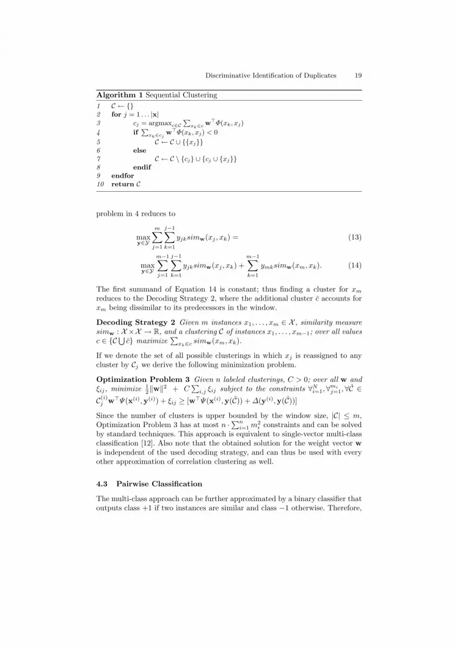
Each of the obtained models is applied to the test sets, using either the ap-proximative clustering based on the linear program, the sequential clusteringalgorithm, or the greedy clustering algorithm by [13]. Figure 1 shows the experi-mental results of three of the training methods. The integrated learning problemis not tractable for this amount of training data.
In a second experiment, we split each training and each test set in two halves,resulting in 18 sets of 50 emails each for training. That is, the total number oftraining emails remains the same but the integrated learning problem becomestractable. Figure 2 shows the results for this setting.
In both experiments, the LP-decoding strategy and the greedy clusteringalgorithm perform equally well. By contrast, the sequential clustering performssignificantly worse in most of the cases according to a paired t-Test on a 5%confidence level. However, this loss in performance comes with a gain in executiontime that is linear in the number of examples (see Table 2).
0
0.005
0.01
0.015
0.02
0.025
0.03
0.035
Nor
mal
ized
loss
per
mai
l
LP-ClusteringGreedy Clustering
Sequential Clustering
Iterative Multi-Class Pairwise
Fig. 1. Average loss and standard errors for m = 100.
Figure 3 details which fraction of the error is caused by the decoding andwhich by the learning algorithm. The dashed area indicates the error caused bythe training method. We quantify this error by counting the number of differentedges in the true and the predicted similarity matrix, respectively. The additionalerror of the subsequent decoding is indicated for all three decoding strategies.

22 Peter Haider, Ulf Brefeld, and Tobias Scheffer
0
0.005
0.01
0.015
0.02
0.025
0.03
0.035
Nor
mal
ized
loss
per
mai
l
LP-ClusteringGreedy Clustering
Sequential Clustering
Integrated Iterative Multi-Class Pairwise
Fig. 2. Average loss and standard errors for m = 50.
Except for the sequential decoding, the multi-class optimization leads to cor-rect clusterings that fulfill the transitivity constraints between triples of nodes.On the contrary, the solution of the pairwise optimization has the lowest errorbut fails to satisfy these transitivity constraints. Neither decoding strategy cancompensate the errors.
Table 2. Execution time of the decoding strategies in seconds.
Window size m 25 50 100 200
LP-Clustering 2.3 · 10−1 6.4 · 100 4.0 · 102
Greedy Clustering 6.4 · 10−4 2.5 · 10−3 9.9 · 10−3 4.0 · 10−2
Sequential Clustering 1.5 · 10−5 2.9 · 10−5 5.6 · 10−5 1.1 · 10−4
6 Conclusion
We devised three large margin approaches to supervised clustering of sequen-tial data. The integrated approach has at least cubic execution time and can besolved directly for small training sets. Treating the problem as multi-class clas-sification allowed us to use larger data sets. The pairwise classification approachis a rough but fast approximation of the original problem.
Experimental results were carried out on all combinations of learning algo-rithms and decoding strategies in our discourse area. The results showed thatthe LP-decoding performs equally well as the greedy algorithm presented in [13].
Discriminative Identification of Duplicates 23
0
1
2
3
4
5
6
7
8
Vio
late
d ed
ges
com
pare
d to
true
par
titio
n
LP−ClusteringGreedy Clustering
Sequential ClusteringSimilarity Matrix
Integrated Iterative Multi−Class Pairwise
Fig. 3. Fraction of the loss induced by the learning algorithm (similarity matrix) andthe decoding.
However, both methods are computationally expensive. The sequential decodingmakes use of the sequential nature of the data and leads to slightly increasedlosses.
References
1. Y. Altun, I. Tsochantaridis, and T. Hofmann. Hidden Markov support vectormachines. In Proceedings of the International Conference on Machine Learning,2003.
2. Nikhil Bansal, Avrim Blum, and Shuchi Chawla. Correlation clustering. In Pro-ceedings of the 43rd Symposium on Foundations of Computer Science, 2002.
3. Nikhil Bansal, Avrim Blum, and Shuchi Chawla. Correlation clustering. MachineLearning, 56(1-3):89–113, 2004.
4. Aharon Bar-Hillel, Tomer Hertz, Noam Shental, and Daphna Weinshall. Learningdistance functions using equivalence relations. In ICML ’03: Proceedings of theTwentieth International Conference on Machine Learning, 2003.
5. Mikhail Bilenko and Raymond J. Mooney. Adaptive duplicate detection usinglearnable string similarity measures. In Proceedings of the International Conferenceon Knowledge Discovery and Data Mining, 2003.
6. Sergey Brin, James Davis, and Hector Garcıa-Molina. Copy detection mechanismsfor digital documents. In Proceedings of the International Conference on Manage-ment of Data, 1995.

24 Peter Haider, Ulf Brefeld, and Tobias Scheffer
7. Moses Charikar, Venkatesan Guruswami, and Anthony Wirth. Clustering withqualitative information. In Proceedings of the 44th Annual IEEE Symposium onFoundations of Computer Science, 2003.
8. J. Cooper, A. Coden, and E. Brown. Detecting similar documents using salientterms. In Proceedings of the International Conference on Information and Knowl-edge Management, 2002.
9. J. Cooper, A. Coden, and E. Brown. A novel method for detecting similar doc-uments. In Proceedings of the 35th Annual Hawaii International Conference onSystem Sciences, 2002.
10. Erik D. Demaine and Nicole Immorlica. Correlation clustering with partial infor-mation. In Proceedings of the 6th International Workshop on Approximation Algo-rithms for Combinatorial Optimization Problems and 7th International Workshopon Randomization and Approximation Techniques in Computer Science, 2003.
11. Dotan Emanuel and Amos Fiat. Correlation clustering – minimizing disagreementson arbitrary weighted graphs. Lecture Notes in Computer Science, 2832:208–220,2003.
12. Michael Fink, Shai Shalev-Shwartz, Yoram Singer, and Shimon Ullman. Onlinemulticlass learning by interclass hypothesis sharing. In ICML ’06: Proceedings ofthe 23nd international conference on Machine learning, 2006.
13. Thomas Finley and Thorsten Joachims. Supervised clustering with support vectormachines. In Proceedings of the International Conference on Machine Learning,2005.
14. Aleksander Kolcz, Abdur Chowdhury, and Joshua Alspector. The impact of featureselection on signature-driven spam detection. In Proceedings of the First Confer-ence on Email and Anti-Spam, 2004.
15. J. Lafferty, X. Zhu, and Y. Liu. Kernel conditional random fields: representationand clique selection. In Proc. of the International Conference on Machine Learning,2004.
16. W. M. Rand. Objective criteria for the evaluation of clustering methods. Journalof the American Statistical Association, 66:622–626, 1971.
17. Chaitanya Swamy. Correlation clustering: maximizing agreements via semidefiniteprogramming. In Proceedings of the fifteenth annual ACM-SIAM symposium onDiscrete algorithms, 2004.
18. B. Taskar, C. Guestrin, and D. Koller. Max-margin Markov networks. In Advancesin Neural Information Processing Systems, 2004.
19. Ben Taskar, Vassil Chatalbashev, Daphne Koller, and Carlos Guestrin. Learn-ing structured prediction models: a large margin approach. In Proceedings of theInternational Conference on Machine Learning, 2005.
20. I. Tsochantaridis, T. Joachims, T. Hofmann, and Y. Altun. Large margin methodsfor structured and interdependent output variables. Journal of Machine LearningResearch, 6:1453–1484, 2005.
21. Kiri Wagstaff, Claire Cardie, Seth Rogers, and Stefan Schrödl. Constrainedk-means clustering with background knowledge. In ICML ’01: Proceedings of theEighteenth International Conference on Machine Learning, pages 577–584, SanFrancisco, CA, USA, 2001.
22. Eric P. Xing, Andrew Y. Ng, Michael I. Jordan, and Stuart Russell. Distancemetric learning, with application to clustering with side-information. In Advancesin Neural Information Processing Systems. The MIT Press, 2002.
23. Feng Zhou, Li Zhuang, Ben Y. Zhao, Ling Huang, Anthony D. Joseph, and JohnKubiatowicz. Approximate object location and spam filtering on peer-to-peer sys-tems. In Middleware, 2003.
Frequent Hypergraph Mining
Tamas Horvath1,2, Bjorn Bringmann3, and Luc De Raedt3
1 Department of Computer Science III, University of Bonn, Germany2 Fraunhofer IAIS, Sankt Augustin, Germany
3 Institute for Computer Science, Machine Learning Lab, University of Freiburg, Germany
Abstract. The class of frequent hypergraph mining problems is introduced whichincludes the frequent graph mining problem class and contains also the frequentitemset mining problem. We study the computational properties of different prob-lems belonging to this class. In particular, besides negative results, we presentpractically relevant problems that can be solved in incremental-polynomial time.Some of our practical algorithms are obtained by reductions to frequent graphmining and itemset mining problems. Our experimental results in the domain ofcitation analysis show the potential of the framework on problems that have nonatural representation as an ordinary graph.
1 Introduction
The field of data mining has studied increasingly expressive representations in the pastfew years. Whereas the original formulation of frequent pattern mining still employeditemsets [1], researchers have soon studied more expressive representations such assequences and episodes (e.g., [11]), trees (e.g., [4]), and more recently, graph mininghas become an important focus of research (e.g., [12, 13]). These developments havebeen motivated and accompanied by new and challenging application areas. Indeed,itemsets apply to basket-analysis, sequences and episodes to alarm monitoring, trees todocument mining, and graph mining to applications in computational chemistry.
In this paper, we introduce the next natural step in this evolution: the mining of la-beled hypergraphs. In a similar way that tree mining generalizes sequence mining, andgraph mining generalizes tree mining, hypergraph mining is a natural generalization ofgraph mining. The presented framework is especially applicable to problem domainswhich do not have a natural representation as ordinary graphs. One such applicationis used in the experimental section of this paper. It is concerned with citation analysis,more specifically, with analyzing bibliographies of a set of papers. The bibliography ofa paper can be viewed as a hypergraph, in which each author corresponds to a vertexand each paper to the hyperedge containing all authors of the paper. By mining for fre-quent subhypergraphs in the bibliographies of a set of papers (e.g. past KDD conferencepapers), one should be able to discover common citation patterns in a particular domain(such as SIGKDD). These patterns might then be employed in a recommender sys-tem that assists scientists while making bibliographies. A similar approach in a basket-analysis context allows one to represent the transactions over a specific period of timeof one family as a hypergraph, where the products correspond to the vertices and the

26 Tamas Horvath, Bjorn Bringmann, and Luc De Raedt
transactions to the hyperedges. Mining such data could provide insight into the overallpurchasing behavior of families.
The main contribution of this paper is the introduction of a general framework ofmining frequent hypergraphs. The framework can be specialized in a number of dif-ferent ways, according to the notion of the generalization relation employed as well asthe type of hypergraphs considered. We consider different problems where the gener-alization relation is defined by subhypergraph isomorphism, study their computationalproperties, and present positive and negative results. More specifically, we show thatthere is no output-polynomial time algorithm for the frequent hypergraph mining prob-lem even in the case of strong structural assumptions on the hyperedges. On the otherhand, by restricting the functions labeling the vertices, we get positive results. Someof the results are obtained by employing reductions from frequent hypergraph min-ing problems to ordinary graph mining and itemset mining problems. We present alsoexperiments in the above sketched citation analysis domain which indicate that thesereductions can effectively be applied in practice. Essentially, we gathered the bibliogra-phies of 5 SIGKDD, 30 SIGMOD, and 30 SIGGRAPH conferences and searched forfrequent hypergraphs in each conference.
The rest of the paper is organized as follows: in Section 2, we introduce the neces-sary notions concerning hypergraphs and in Section 3, we define the problem class offrequent hypergraph mining. In Section 4, we study the frequent subhypergraph miningproblem. In Section 5, we present some experiments using the citation analysis prob-lem, and finally, in Section 6, we conclude and list some problems for future work. Dueto space limitations, proofs are only sketched or even omitted in this short version.
2 Notions and Notations
We recall some basic notions and notations related to graphs and hypergraphs (see, e.g.,[2, 5] for detailed introductions into these fields). For a set S and non-negative integerk, [S]k denotes the family of k-subsets of S, i.e., [S]k = {S′ ⊆ S : |S′| = k}.Graphs and Hypergraphs An (undirected) graph G consists of a finite set V of ver-tices and a set E ⊆ [V ]2 of edges. G is bipartite if G has a vertex 2-coloring, i.e., ifV admits a partition into V1 and V2 such that E /∈ [V1]2 ∪ [V2]2 for every E ∈ E . Ahypergraph H is a pair (V, E), where V is a finite set and E is a family of nonemptysubsets of V such that
⋃E∈E E = V . The elements of V and E are called vertices and
edges (or hyperedges), respectively. H is r-uniform for some integer r > 0 if E ⊆ [V ]r.The rank of H , denoted r(H), is the cardinality of its largest hyperedge and the size ofH , denoted size(H), is the number of hyperedges of H .
Note that ordinary undirected graphs without isolated vertices form a special caseof hypergraphs, i.e., the class of 2-uniform hypergraphs. We note that every hypergraphH = (V, E) can be represented by a bipartite incidence graph B(H) = (V ∪ E , E ′),where E ′ = {{v, E} : v ∈ V,E ∈ E , and v ∈ E}.Labeled Hypergraphs A labeled hypergraph is a triple H = (V, E , λ), where (V, E)is a hypergraph, and λ, called labeling function, is a function mapping V to N.4 Unless
4 We will only consider labeling functions defined on the vertex set because any hypergraphH = (V, E , λ) with λ : V ∪ E → N satisfying λ(v) 6= λ(E) for every v ∈ V and E ∈ E

Frequent Hypergraph Mining 27
otherwise stated, by hypergraphs (resp. graphs) we always mean labeled hypergraphs(resp. labeled graphs), and denote the set of vertices, the set of edges, and the labelingfunction of a hypergraph (resp. graph) H by VH , EH , and λH , respectively. The set of allhypergraphs is denoted by H and Hr denotes the set of all r-uniform hypergraphs. Fora hypergraph H ∈ H and subset V ′ ⊆ VH , we denote the multiset5 {λH(v) : v ∈ V ′}by λH(V ′). A path connecting the vertices u, v ∈ VH is a sequence E1, . . . , Ek ofedges of H such that u ∈ E1, v ∈ Ek, and Ei ∩ Ei+1 6= ∅ for every i = 1, . . . , k − 1.A hypergraph is connected if there is a path between any pair of its vertices. The set ofconnected hypergraphs is denoted by Hc. Clearly, Hc ⊂ H.Injective Hypergraphs Depending on the labeling functions, in this paper we willconsider two special classes of hypergraphs. A hypergraph H ∈ H is node injectiveif λH is injective, and it is edge injective whenever λH(E) = λH(E′) if and only ifE = E′ for every E,E′ ∈ EH . The sets of node and edge injective hypergraphs will bedenoted by Hni and Hei, respectively. Clearly, Hni ⊆ Hei ⊆ H.Hypergraph Isomorphism Let H1,H2 ∈ H be hypergraphs. H1 and H2 are calledisomorphic, denoted by H1 ' H2, if there is a bijection ϕ : VH1 → VH2 such that ϕpreserves the labels, i.e., λH1(v) = λH2(ϕ(v)) for every v ∈ VH1 , and ϕ preserves thehyperedges in both directions, i.e., for every E ⊆ VH1 it holds that E ∈ EH1 if andonly if {ϕ(v) : v ∈ E} ∈ EH2 . Throughout this paper, two hypergraphs H1 and H2 areconsidered to be the same if H1 ' H2.Subhypergraphs A subhypergraph of a hypergraph H ∈ H is a hypergraph H ′ ∈ Hsatisfying VH′ ⊆ VH , EH′ ⊆ EH , and λH′(v) = λH(v) for every v ∈ VH′ .
3 Frequent Hypergraph Mining
Many problems in data mining can be viewed as a special case of the problem of enu-merating the elements of a quasiordered set6, which satisfy some monotone property(see, e.g., [3, 9]). In this section, we define a new class of subproblems of this enumera-tion problem, the class of frequent hypergraph mining problems. In the next section, wethen discuss the computational aspects of some problems belonging to this class. Westart with the definition of a more general problem class.
The Frequent Pattern Mining Problem Class (CFPM): Each problem belonging to thisclass is given by a fixed triple (LD,LP , 4), where LD is a transaction language,LP is a pattern language, and 4, called the generalization relation, is a quasi-orderon LD ∪ LP . For such a triple, the (LD,LP ,4)-FREQUENT-PATTERN-MININGproblem is defined as follows: Given a finite set D ⊆ LD of transactions and aninteger t > 0, called frequency threshold, compute the set F(LD,LP ,4)(D, t) offrequent patterns defined by
F(LD,LP ,4)(D, t) = {ϕ ∈ LP : |{τ ∈ D : ϕ 4 τ}| ≥ t} .
can be transformed into a hypergraph H ′ = (V ′, E ′, λ′) with V ′ = V ∪ {vE : E ∈ E},E ′ = {E ∪ {vE} : E ∈ E}, and with λ′ : V ′ → N mapping every new vertex vE ∈ V ′ \ Vto λ(E) and every v ∈ V to λ(v).
5 A multiset M is a pair (S, f), where S is a set and f defines the multiplicity of the elementsof S in M , i.e., f is a function mapping S to the cardinal numbers greater than 0.
6 A binary relation is a quasiorder (or preorder), if it is reflexive and transitive.

28 Tamas Horvath, Bjorn Bringmann, and Luc De Raedt
The transitivity of 4 implies that frequency is a monotone property, i.e., for every ϕ, θ ∈LP it holds that θ ∈ F(LD,LP ,4)(D, t) whenever ϕ ∈ F(LD,LP ,4)(D, t) and θ 4 ϕ.
We now define two subclasses of CFPM by restricting the transaction and patternlanguages to hypergraphs and graphs, respectively.
The Frequent Hypergraph Mining Problem Class (CFHM): It consists of the set of(LD,LP , 4)-FREQUENT-PATTERN-MINING problems satisfying LD,LP ⊆ H.
The Frequent Graph Mining Problem Class (CFGM): It is the set of (LD,LP , 4)-FREQUENT-PATTERN-MINING problems satisfying LD,LP ⊆ H2 (i.e., they aresets of labeled graphs).
Clearly, CFGM ( CFHM ( CFPM. Furthermore, the frequent itemset mining prob-lem [1] belongs to CFPM; for this problem we have LD = LP = {X ⊂ N : |X| < ∞}and 4 is the subset relation. In fact, the frequent itemset mining problem is containedby CFHM. Indeed, this problem can be considered as the (Hni
1 ,Hni1 , 4)-FREQUENT-
HYPERGRAPH-MINING problem, where 4 is the subhypergraph relation and the trans-action and pattern languages are the set of 1-uniform node injective hypergraphs.
To sketch the relation among frequent pattern mining problems, we need the no-tion of polynomial reduction. More precisely, let P1 = (LD,1,LP,1, 41) and P2 =(LD,2,LP,2, 42) be frequent pattern mining problems, and I1 = (D1, t1) and I2 =(D2, t2) be instances of P1 and P2, respectively. Then I1 is polynomially equivalent toI2 if there is a function f : LP,1 → LP,2 such that
(i) f is a bijection between F(LD,1,LP,1,41)(D1, t1) and F(LD,2,LP,2,42)(D2, t2) and(ii) the inverse of f on F(LD,2,LP,2,42)(D2, t2) can be computed in polynomial time.
The definition implies that ϕ ∈ LP,1 is frequent for I1 if and only if f(ϕ) ∈ LP,2 isfrequent for I2. Using the notion of polynomial equivalence, we say that P1 is polyno-mially reducible to P2 if there is a function g from the set of instances of P1 to the setof instances of P2 such that
(i) I is polynomially equivalent to g(I) for every I ∈ P1 and(ii) g can be computed in polynomial time.
Thus, if P1 is polynomial-time reducible to P2 then any enumeration algorithm solvingP2 can be used to solve P1.
The parameter of a (LD,LP , 4)-FREQUENT-HYPERGRAPH-MINING problem for-mulated above is the size of D defined by
size(D) = max
{ ∑
H∈Dsize(H), max
H∈Dr(H)
}.
Note that the size of the output, i.e. the set to be enumerated, can be exponential in thesize of the input. Because in such cases, it is impossible to compute them in time poly-nomial only in the size of the input, we investigate whether the enumeration problemscan be solved in incremental polynomial time or at least in output-polynomial time (orpolynomial total time) (see, e.g., [10]). In the first, more restrictive case, the algorithm

Frequent Hypergraph Mining 29
is required to list the first N elements of the output in time polynomial in the combinedsize of the input and the set of these N elements. In the second, more liberal case, thealgorithm has to solve the problem in time polynomial in the combined size of the in-put and the entire set to be enumerated. Note that the class of output-polynomial timealgorithms properly entails the class of incremental polynomial time algorithms.
To close this section, we note that several frequent hypergraph mining problems,even frequent graph mining problems, cannot be solved in output-polynomial time. InTheorem 1 below we present such a hard problem.
Theorem 1 Let LD ⊆ H2 and let LP ⊆ H2 be the set of complete graphs such thatevery vertex of every graph in LD ∪ LP is labeled by the same symbol, say 1, andlet 4 be the homomorphism 4h between labeled graphs7. Then, unless P = NP, the(LD,LP , 4h)-FREQUENT-GRAPH-MINING problem cannot be solved in output poly-nomial time.
Proof (sketch). Let G = (V, E) be an unlabeled graph and let G′ be the labeled graphobtained from G by assigning 1 to each vertex of G. Then, forD = {G′} and t = 1, wehave that G has a clique of size k if and only if there is a C ∈ F(LD,LP ,4h)(D, t) withk vertices. Since |F(LD,LP ,4h)(D, t)| ≤ |V |, the (LD,LP , 4h)-FREQUENT-GRAPH-MINING problem cannot be computed in output polynomial time (unless P = NP, ofcourse), as otherwise the NP-complete maximum clique problem [8] could be decidedin polynomial time by computing the largest pattern in |F(LD,LP ,4h)(D, t)|.
4 Frequent Subhypergraph Mining
By Theorem 1, the class CFGM, and thus the more general class CFHM as well, containsproblems that cannot be solved in output polynomial time (unless P = NP, of course).This negative result raises the challenge of identifying practically relevant and tractableproblems belonging to CFHM. In this section, we take a first step towards this directionby considering the problem of frequent hypergraph mining w.r.t. subhypergraph iso-morphism. This problem, called frequent subhypergraph mining, is a natural problemof the frequent hypergraph mining problem class CFHM and can be applied to manypractical problems. In Section 5, we will employ this setting to tackle the citation anal-ysis problem sketched in the introduction.
We start with the definition of the generalization relation used in this section. LetH1, H2 ∈ H. H1 can be embedded into H2 by subhypergraph isomorphism, denotedby H1 4i H2, if H2 has a subhypergraph isomorphic to H1. Note that 4i generalizesthe notion of subgraph isomorphism between ordinary labeled graphs to hypergraphs.Since 4i is a partial order on H, it is a generalization relation on every subset of H.Using 4i, we consider the following two problems of CFHM:
(i) The (H,H, 4i)-FREQUENT-HYPERGRAPH-MINING problem called the frequentsubhypergraph mining problem and
(ii) the (H,Hc, 4i)-FREQUENT-HYPERGRAPH-MINING problem called the frequentconnected subhypergraph mining problem.
7 A homomorphism from a hypergraph H1 ∈ H to a hypergraph H2 ∈ H, denoted H1 4h H2,is a function ϕ : VH1 → VH2 preserving the labels and edges.

30 Tamas Horvath, Bjorn Bringmann, and Luc De Raedt
Algorithm 1 FREQUENT SUBHYPERGRAPH MINING
Require: instance (D, t)Ensure: F(H,H,4i)(D, t)
1: F := ∅2: BD := {LB(H) : H ∈ D}3: Compute a next t-frequent bipartite subgraph B of the set BD if it exists;
otherwise return F4: if B corresponds to some hypergraph HB then
F := F ∪ {HB}5: goto 3
4.1 A Naıve Algorithm
Using the bipartite graph representation of hypergraphs, in this section we present anaıve algorithm solving the frequent subhypergraph mining problem. For an instance(D, t) of this problem, let n ∈ N be an upper bound on the labels occurring in thehypergraphs of D and let µ be an injection assigning an integer greater than n to everyfinite multiset of N.
For a hypergraph H ∈ H, let LB(H) ∈ H2 be the (labeled) bipartite graph suchthat
(i) (VLB(H), ELB(H)) is the unlabeled bipartite incidence graph of the unlabeled hy-pergraph (VH , EH), and
(ii) for every v ∈ VLB(H) = VH ∪ EH ,
λLB(H)(v) =
{λH(v) if v ∈ VH
µ(λH(v)) otherwise (i.e., v ∈ EH ) .
Clearly, a subgraph G of LB(H) represents a subhypergraph of H if and only if eachvertex of G corresponding to a hyperedge E ∈ EH is connected with exactly |E| ver-tices in G. Using the above transformation and considerations, the set F(H,H,4i)(D, t)of t-frequent subhypergraphs for the instance (D, t) can be computed by Algorithm 1.
Due to space limitations, we omit a detailed analysis of Algorithm 1 that does notwork in output polynomial time in the worst case. We note, however, that even this naıvealgorithm proved to be effective in time on the citation analysis domain (cf. Section 5).
4.2 Negative Results
In this section we investigate further problems obtained by structural restrictions hopingto identify tractable fragments of the frequent subhypergraph mining problem. Unfor-tunately, we have not been able to find any interesting positive result in this way. This isbecause, as indicate the negative results of this section, the problem remains hard evenfor very restricted hypergraph classes. Without proof, in Theorem 2 below we state thateven for 2-uniform hypergraphs (i.e., ordinary graphs), the frequent connected subhy-pergraph mining problem is intractable in output-polynomial time. Since this is one

Frequent Hypergraph Mining 31
of the most frequently considered frequent graph mining problems, the negative resultbelow may be of interest in itself.
Theorem 2 If P 6= NP, there is no output-polynomial time algorithm solving the fre-quent connected subhypergraph mining problem even in the case of 2-unary hyper-graphs (i.e., ordinary graphs).
As a further restriction, we consider the frequent subhypergraph mining problemrestricted to acyclic hypergraphs [7] because several NP-hard problems on hypergraphsbecome polynomial for acyclic hypergraphs. A hypergraph H ∈ H is α-acyclic ifone can remove all of its vertices and edges by deleting repeatedly either an edgethat is empty or is contained by another edge, or a vertex contained by at most oneedge [14]. Note that α-acyclicity is not a hereditary property, that is, α-acyclic hy-pergraphs may have subhypergraphs that are not α-acyclic. Consider for example thehypergraph H ∈ H such that EH = {{a, b}, {b, c}, {a, c}, {a, b, c}}. While H is α-acyclic, its subhypergraph obtained by removing the edge {a, b, c} is not α-acyclic. Toovercome this anomaly, the following proper subclass of α-acyclic hypergraphs is in-troduced in [7]: An α-acyclic hypergraph is β-acyclic, if each of its subhypergraphs isalso α-acyclic. Note that forests are 2-uniform β-acyclic hypergraphs.
Even for connected subhypergraphs of 3-uniform β-acyclic hypergraphs, we have anegative result. Let B3 denote the set of 3-uniform β-acyclic hypergraphs.
Proposition 3 Given a finite set D ⊆ B3 and integer t > 0, deciding whether H ∈F(B3,Hc,4i)(D, t) is NP-hard.
Proof (sketch). Using a polynomial reduction from the subforest isomorphism prob-lem8, one can show that deciding subhypergraph isomorphism between 3-uniform, con-nected, β-acyclic hypergraphs is NP-hard. This implies the statement.
Proposition 3 above indicates that for the frequent subhypergraph mining problem,the usual frequent pattern mining approaches (such as the level-wise one) will not workin incremental polynomial time (unless P = NP ) because they repeatedly test whethercandidate patterns satisfy the frequency threshold (see, e.g., [9]).
4.3 Tractable Cases
In contrast to the approach discussed in Section 4.2 above, in this section we considerfurther special cases of the frequent subhypergraph mining problem that are obtained bymaking assumptions on the labeling functions of the transaction hypergraphs. We firstconsider the problem for node injective hypergraphs, i.e., where the labeling functionsare injective. We show that for this case, the frequent subhypergraph mining problemis polynomially reducible to the frequent itemset mining problem and hence, it canbe solved in incremental-polynomial time [1]. We then generalize this positive result toedge injective hypergraphs, i.e., to hypergraphs not containing two different hyperedgesthat are mapped to the same multiset by the labeling function. Although node injective
8 Given a forest F and a tree T , decide whether T has a subgraph isomorphic to F . This problemis known to be NP-complete [8].

32 Tamas Horvath, Bjorn Bringmann, and Luc De Raedt
hypergraphs are a special case of edge injective hypergraphs, we discuss the two casesseparately because node injective hypergraphs can be used to model many practicalproblems and they permit a simplified algorithmic approach.
Node Injective Hypergraphs As mentioned above, many practical data mining prob-lems can be modeled by node injective hypergraphs, i.e., by hypergraphs fromHni. Suchapplications include problem domains consisting of a finite set of objects (vertices) witha unique identifier. For node injective hypergraphs, we consider the (Hni,Hni, 4i)-FREQUENT-HYPERGRAPH-MINING problem which is a special case of the frequentsubhypergraph mining problem.
As an example of a practical application of this problem, we consider the citationanalysis task mentioned in the introduction (cf. also Section 5): Given a setD of articlesand a frequency threshold t > 0, print each family F of groups of authors satisfying thefollowing property: there exists a subsetD′ ⊆ D of articles of cardinality at least t suchthat for every group F ∈ F of authors and for every article D ∈ D′ it holds that D citessome article written by (exactly) the authors belonging to F . In this enumeration prob-lem, we can assign a unique non-negative integer to each author, whose papers are citedby at least one article in D. We can use the node injective hypergraph representation ofa paper’s bibliography defined as follows. For each author cited in the bibliography, in-troduce a vertex and label it by the integer assigned to the author. Furthermore, for eachcited work add a hyperedge E to the set of hyperedges, where E consists of the verticesrepresenting the cited work’s authors. Clearly, the hypergraph obtained in this way isalways node injective. Our database D is a set of such node injective hypergraphs.
Theorem 4 below states that for node injective hypergraphs, the frequent subhyper-graph mining problem is polynomially reducible to the frequent itemset mining prob-lem. We recall that the frequent itemset mining problem can be considered as a problembelonging to the class CFHM (cf. Section 3). Notice that in the theorem below, subhy-pergraphs may be non-connected. The theorem is based on the fact that for every nodeinjective hypergraphs H1,H2 ∈ Hni, H1 4i H2 if and only if for every E1 ∈ EH1 ,there is a hyperedge E2 ∈ EH2 such that λH1(E1) = λH2(E2), i.e.,
H1 4i H2 ⇐⇒ {λH1(E) : E ∈ EH1} ⊆ {λH2(E) : E ∈ EH2} .
Note that the above equivalence implies that 4i can be decided efficiently for nodeinjective hypergraphs.
Theorem 4 The frequent subhypergraph mining problem for node injective hypergraphsis polynomially reducible to the frequent itemset mining problem.
Due to space limitation, we omit the proof of the theorem which is based on consideringthe set of vertex labels of a hyperedge as an item for every hyperedge occurring in thetransaction hypergraphs. Combining the above theorem with the results of [1], we havethe following result on listing frequent subhypergraphs for node injective hypergraphs.
Corollary 5 The frequent subhypergraph mining problem for node injective hyper-graphs can be solved in incremental polynomial time.

Frequent Hypergraph Mining 33
Algorithm 2 MINING EDGE INJECTIVE HYPERGRAPHS
Require: finite set D ⊆ Hei and integer t > 0Ensure: F(Hei,Hei,4i)
(D, t)
1: X :=S
H∈D{λH(E) : E ∈ EH}2: F := ∅3: k := 04: while k = 0 ∨ Lk 6= ∅ do5: k := k + 1
6: Ck :=
(X if k = 1
{Y1 ∪ Y2 ∈ [X]k : Y1, Y2 ∈ Lk−1} otherwise7: Lk := ∅8: forall X ′ ∈ Ck do9: Q := ∅
10: forall H ∈ D do11: if ∃H ′ ∈ H s.t. X ′ = {λH′(E) : E ∈ EH′} then12: if ∃(H ′′, f) ∈ Q s.t. H ′′ ' H ′ then13: change (H ′′, f) in Q to (H ′′, f + 1)14: else Q := Q ∪ {(H ′, 1)}15: endfor16: flag := TRUE17: forall (H, f) ∈ Q s.t. f ≥ t do18: F := F ∪ {H}19: if flag then20: Lk := Lk ∪ {X ′}21: flag := FALSE22: endif23: endfor24: endfor25: endwhile26: return F
Edge Injective Hypergraphs We now generalize the previous positive result to edgeinjective hypergraphs. Since a hypergraph now may contain two vertices with the samelabel, a family of multisets of labels doesn’t define a hypergraph uniquely. Hence, areduction to frequent itemset mining is not applicable to this case.
Theorem 6 The frequent subhypergraph mining problem for edge injective hypergraphscan be solved in incremental polynomial time.
Proof (sketch). Due to space limitations, we only sketch the proof. We first note thatsubhypergraph isomorphism between edge injective hypergraphs can be decided inpolynomial time. To compute the set of t-frequent hypergraphs, we use an Apriori-likealgorithm given in Algorithm 2.
In line 1 of the algorithm, X is initialized as the set of multisets corresponding to theedges in the transaction hypergraphs. In Ck (line 6), we compute a family of candidatesets of multisets. Each set in Ck consists of k multisets. For a set X’ in Ck (see the

34 Tamas Horvath, Bjorn Bringmann, and Luc De Raedt
Table 1. Datasets used. We list the total number of papers in the proceedings and the number ofauthors occurring in the reference lists of the corresponding papers.
dataset years papers authorsKDD 99-04 499 6966
SIGMOD 74-04 1404 11984SIGGRAPH 74-04 1519 13192
loop starting at line 8), we check for every H ∈ D whether H has a subhypergraphH ′ such that the set of multisets defined by the edges of H ′ is equal to X ′. Sinceedges are invectively labeled, H ′ must contain exactly k hyperedges. If H has such asubhypergraph H ′ then we check whether we have already found another hypergraphin the database which has a subhypergraph isomorphic to H ′. If yes, we increment thecounter of this subhypergraph (line 13); otherwise we add H ′ with frequency 1 to theset Q (line 14). In the loop (17–23) we update the set of frequent hypergraphs and Lk.One can show that this algorithm works in incremental polynomial time.
5 Experimental Evaluation
In this section, we evaluate our methods on the citation analysis problem discussed ear-lier. Three bibliographic datasets, the KDD, SIGMOD, and SIGGRAPH, were con-structed from the ACM Digital Library9. They correspond to the set of all reference listsof papers found in the proceedings of the respective conferences. The characteristics ofthe datasets are listed in Table 1.
Each paper was represented as a hypergraph, as described in Section 4.3. The result-ing hypergraphs are node injective, and in almost all cases, also disconnected. Becausemost existing graph miners only consider connected graphs, we added one special hy-peredge to each paper, which connects all authors cited in that paper.
We performed experiments with the naıve algorithm based on reduction to frequentbipartite graph mining (cf. Section 4.1), as well as with the reduction to frequent item-set mining (cf. Section 4.3). All experiments were run on a workstation, running SuseLinux 9.2, 3.2 GHz, 2GB of RAM. As graph miner, we employed Siegfried Nijssens’GASTON [12] and as itemset miner, Bart Goethals’ implementation10 of Apriori. Be-cause we did not employ a specialized hypergraph or graph miner, the data had to bepre- and post-processed. We used several perl-scripts to realize this. The pre- andpost-processing steps run in time linear in the number of hypergraphs.
5.1 Experimental Results
The number of frequent patterns for different frequency thresholds for the three datasetsis given in Figure 1. The runtime of the itemset miner was always below 0.1 seconds.Different from that, the naıve algorithm required much higher runtimes; 833.5, 16.8,
9 http://www.acm.org/10 http://www.cs.helsinki.fi/u/goethals/software/

Frequent Hypergraph Mining 35
Fig. 1. Number of frequent patterns for different frequency thresholds.
and 9.9 seconds for KDD, SIGGRAPH, and SIGMOD, respectively. These higherruntimes are essentially due to the problem that only a fraction of the frequent bipartitegraphs correspond in fact to subhypergraphs.
Despite the difference between the runtimes of the two approaches, our experimentsclearly indicate that both reductions can be quite effective in practice.
6 Conclusion and Further Research
The problem class CFHM of frequent hypergraph mining was introduced. It forms a nat-ural extension of traditional frequent itemset and graph mining. Several problems ofCFHM were studied and positive and negative complexity results were obtained. Cen-tral to our results is the use of reductions from hypergraph mining problems to itemsetand graph mining problems. These reductions are not only of theoretical interest, butallow us to set up a number of frequent hypergraph mining experiments even thoughwe have not implemented a frequent hypergraph mining system. To our knowledge, theuse of such reductions in data mining is new. Indeed, it is much more common in datamining to spend a lot of time and effort to develop new systems, even though they aresometimes only variants of existing ones. In our first step of studying some problemsof CFHM, we deliberately did not follow this common methodology, because there aremany problems of CFHM that are interesting (which implies the need for implementingmany variants and optimizations), and also, because we wanted to see how far the re-ductions would bring us. The experiments clearly indicate that - at least for the citationanalysis problems studied - reductions can be quite effective in practice. In addition,these experiments provide evidence that frequent hypergraph mining is indeed a usefulgeneralization of frequent itemset and graph mining and is likely to yield many inter-esting applications. Finally we list some open questions.
(i) One of the challenges is to identify further problems of CFHM that are enumerablein incremental or at least in output-polynomial time.
(ii) Besides subhypergraph isomorphism, it would be interesting to investigate frequenthypergraph mining problems, where the generalization relation is defined by (con-strained) homomorphisms.

36 Tamas Horvath, Bjorn Bringmann, and Luc De Raedt
(iii) Since many problems of CFHM can be reduced to frequent graph mining in bipartitegraphs, it would be interesting to develop frequent graph mining algorithms specificto bipartite graphs.
(iv) The work on frequent hypergraph mining can be related to multi-relational datamining [6], where each instance consists of multiple tuples over multiple tables ina relational database. Multi-relational data mining techniques have been applied tograph mining problems. Hence, the question arises if they are also applicable tohypergraph mining, and vice versa.
Acknowledgments
The authors thank Mario Boley and Stefan Wrobel for useful comments. Tamas Horvathwas partially supported by the DFG project (WR 40/2-2) Hybride Methoden und Sys-temarchitekturen fur heterogene Informationsraume.
References
1. R. Agrawal, H. Mannila, R. Srikant, H. Toivonen, and A. I. Verkamo. Fast Discovery ofAssociation Rules. In Advances in Knowledge Discovery and Data Mining, pages 307–328.AAAI/MIT Press, Cambridge, MA, 1996.
2. C. Berge. Hypergraphs. North Holland Mathematical Library, Vol. 445. Elsevier, Amster-dam, 1989.
3. E. Boros, K. Elbassioni, V. Gurvich, L. Khachiyan, and K. Makino. Dual Bounded Hy-pergraphs: A Survey. In Proc. of the 2nd SIAM Conference on Data Mining, pages 87–98,2002.
4. Y. Chi, R. R. Muntz, S. Nijssen, and J. N. Kok. Frequent Subtree Mining - An Overview.Fundamenta Informaticae, 66(1-2):161–198, 2005.
5. R. Diestel. Graph Theory. Springer, New York, 2nd edition, 2000.6. S. Dzeroski and N. Lavrac, editors. Relational Data Mining. Springer, New York, 2002.7. R. Fagin. Degrees of Acyclicity for Hypergraphs and Relational Database Schemes. Journal
of the ACM, 30(3):514–550, 1983.8. M. R. Garey and D. S. Johnson. Computers and Intractability: A Guide to NP-Completeness.
Freeman, San Francisco, CA, 1979.9. D. Gunopulos, R. Khardon, H. Mannila, S. Saluja, H. Toivonen, and R. S. Sharm. Discover-
ing All Most Specific Sentences. ACM Trans. on Database Systems, 28(2):140–174, 2003.10. D. S. Johnson, M. Yannakakis, and C. H. Papadimitriou. On Generating All Maximal Inde-
pendent Sets. Information Processing Letters, 27(3):119–123, 1988.11. H. Mannila, H. Toivonen, and A. I. Verkamo. Discovery of Frequent Episodes in Event
Sequences. Data Mining and Knowledge Discovery, 1(3):259–289, 1997.12. S. Nijssen and J. N. Kok. A Quickstart in Frequent Structure Mining Can Make a Difference.
In Proc. of the Tenth ACM SIGKDD International Conference on Knowledge Discovery andData Mining, pages 647–652. ACM Press, New York, NY, 2004.
13. X. Yan and J. Han. Gspan: Graph-based Substructure Pattern Mining. In Proc. of the 2002IEEE International Conference on Data Mining, pages 721–724. IEEE Computer Society,2002.
14. C. T. Yu and M. Z. Ozsoyoglu. An Algorithm for Tree-Query Membership of a DistributedQuery. In Proc. of Computer Software and Applications Conference, pages 306–312. IEEEComputer Society, 1979.

Frequent Subgraph Mining in Outerplanar Graphs?
Tamas Horvath1,2, Jan Ramon3, and Stefan Wrobel2,1
1 Dept. of Computer Science III, University of Bonn, Germany2 Fraunhofer IAIS, Sankt Augustin, Germany
3 Dept. of Computer Science, Katholieke Universiteit Leuven, Belgium
Abstract. In recent years there has been an increased interest in frequent patterndiscovery in large databases of graph structured objects. While the frequent con-nected subgraph mining problem for tree datasets can be solved in incrementalpolynomial time, it becomes intractable for arbitrary graph databases. Existingapproaches have therefore resorted to various heuristic strategies and restrictionsof the search space, but have not identified a practically relevant tractable graphclass beyond trees. In this paper, we define the class of so called tenuous outerpla-nar graphs, a strict generalization of trees, develop a frequent subgraph miningalgorithm for tenuous outerplanar graphs that works in incremental polynomialtime, and evaluate the algorithm empirically on the NCI molecular graph dataset.
1 Introduction
The discovery of frequent patterns in a database is one of the central tasks considered indata mining. In addition to be interesting in their own right, frequent patterns can alsobe used as features for predictive data mining tasks (see, e.g., [5]). For a long time, workon frequent pattern discovery has concentrated on relatively simple notions of patternsand elements in the database as they are typically used for the discovery of associationrules (simple sets of atomic items). In recent years, however, due to the significanceof application areas such as the analysis of chemical molecules or graph structures inthe WWW, there has been an increased interest in algorithms that can perform frequentpattern discovery in databases of structured objects such as trees or arbitrary graphs.
While the frequent pattern problem for trees can be solved in incremental poly-nomial time, i.e., in time polynomial in the combined size of the input and the set offrequent tree patterns so far computed, the frequent pattern problem for graph struc-tured databases in the general case cannot be solved in output polynomial time, i.e., intime polynomial in the combined size of the input and the set of all frequent patterns.Existing approaches to frequent pattern discovery for graphs have therefore resorted tovarious heuristic strategies and restrictions of the search space (see, e.g., [4, 5, 8, 17]),but have not identified a practically relevant tractable graph class beyond trees.
In this paper, we define the class of so called tenuous outerplanar graphs, which isthe class of planar graphs that can be embedded in the plane in such a way that all of itsvertices lie on the outer boundary, i.e. can be reached from the outside without crossingany edges, and which have a fixed limit on the number of inside diagonal edges. This
? A longer version of this paper has been accepted to ACM SIGKDD’06.

38 Tamas Horvath, Jan Ramon, and Stefan Wrobel
class of graphs is a strict generalization of trees, and is motivated by the kinds of graphsactually found in practical applications. In fact, in one of the popular graph miningdata sets, the NCI data set4, 94.3% of all elements are tenuous outerplanar graphs. Wedevelop an incremental polynomial time algorithm for enumerating frequent tenuousouterplanar graph patterns.
Our approach is based on a canonical string representation of outerplanar graphswhich may be of interest in itself, and further algorithmic components for mining fre-quent biconnected outerplanar graphs and candidate generation in an Apriori style al-gorithm. To map a pattern to graphs in the database, we define a special notion of blockand bridge preserving (BBP) subgraph isomorphism, which is motivated by applica-tion and complexity considerations, and show that it is decidable in polynomial timefor outerplanar graphs. We note that for trees, which form a special class of outerpla-nar graphs, BBP subgraph isomorphism is equivalent to subtree isomorphism. Thus,BBP subgraph isomorphism generalizes subtree isomorphism to graphs, but is at thesame time more specific than subgraph isomorphism. Since in many applications, sub-graph isomorphism is a non-adequate matching operator (e.g., when pattern matchingis required to preserve certain type of fragments in molecules), by considering BBPsubgraph isomorphism we take a first step towards studying the frequent graph miningproblem w.r.t. non-standard matching operators as well. Beside complexity results, wepresent also empirical results which show that the favorable theoretical properties of thealgorithm and pattern class also translate into efficient practical performance.
The paper is organized as follows. In Sections 2 and 3, we define the necessarynotions and the problem setting for this work, respectively. Section 4 describes our al-gorithm for mining frequent tenuous outerplanar graphs. Section 5 contains our experi-mental evaluation and finally, Section 6 concludes and discusses some open problems.Due to space limitations, proofs are omitted in this short version.
2 Preliminaries
We recall some notions related to graphs [7]. An undirected graph is a pair (V, E),where V 6= ∅ is a finite set of vertices and E ⊆ {e ⊆ V : |e| = 2} is a set of edges.A labeled undirected graph is a quadruple (V, E,Σ, λ), where (V, E) is an undirectedgraph, Σ 6= ∅ is a finite set of labels associated with some total order, and λ : V ∪E →Σ is a function assigning a label to each element of V ∪E. Unless otherwise stated, inthis paper by graphs we always mean labeled undirected graphs and denote the set ofvertices, the set of edges, and the labeling function of a graph G by V (G), E(G), andλG, respectively. Let G and G′ be graphs. G′ is a subgraph of G, if V (G′) ⊆ V (G),E(G′) ⊆ E(G), and λG′(x) = λG(x) for every x ∈ V (G′) ∪ E(G′). For a vertexv ∈ V (G), N(v) denotes the set of vertices of G connected by an edge with v.
A graph G is connected if there is a path between any pair of its vertices; it isbiconnected if for any two vertices u and v of G, there is a simple cycle containing uand v. A block (or biconnected component) of a graph is a maximal subgraph that isbiconnected. Edges not belonging to blocks are called bridges. The definitions imply
4 http://cactus.nci.nih.gov/

Frequent Subgraph Mining in Outerplanar Graphs 39
that the blocks of a graph are pairwise edge disjoint and that the set of bridges formsa forest. For the set of blocks and the forest formed by the bridges of a graph G itholds that their cardinalities are bounded by |V (G)| and they can be enumerated intime O (|V (G)|+ |E(G)|) [16].
Let G1 and G2 be graphs. G1 and G2 are isomorphic, denoted G1 ' G2, if thereis a bijection ϕ : V (G1) → V (G2) such that (i) {u, v} ∈ E(G1) iff {ϕ(u), ϕ(v)} ∈E(G2), (ii) λG1(u) = λG2(ϕ(u)), (iii) and if {u, v} ∈ E(G1) then λG1({u, v}) =λG2({ϕ(u), ϕ(v)}) hold for every u, v ∈ V (G1). In this paper, two graphs are consid-ered to be the same if they are isomorphic. G1 is subgraph isomorphic to G2 if G1 isisomorphic to a subgraph of G2. Deciding whether a graph is subgraph isomorphic toanother graph is NP-complete, as it generalizes e.g. the Hamiltonian path problem.
Outerplanar Graphs Informally, a graph is planar if it can be drawn in the plane in sucha way that no two edges intersect except at a vertex in common. An outerplanar graph isa planar graph which can be embedded in the plane in such a way that all of its verticeslie on the boundary of the outer face. Throughout this work we consider connectedouterplanar graphs and denote the set of connected outerplanar graphs over an alphabetΣ byOΣ . Clearly, trees are outerplanar graphs and hence, a graph is outerplanar iff eachof its blocks is outerplanar [7]. Furthermore, as the blocks of a graph can be computedin linear time [16] and outerplanarity of a block can be decided also in linear time [10,12], one can decide in linear time whether a graph is outerplanar.
A biconnected outerplanar graph G with n vertices contains at most 2n − 3 edgesand has a unique Hamiltonian cycle which bounds the outer face of a planar embeddingof G [7]. This unique Hamiltonian cycle can be computed efficiently [10]. Thus, G canbe considered as an n-polygon with at most n − 3 non-crossing diagonals. Below westate a bound for the number of cycles of G. Due to space limitation, we omit the proof.
Proposition 1 A biconnected outerplanar graph with d diagonals has at most 2d+1
cycles.
Given outerplanar graphs G and H , deciding whether H is subgraph isomorphicto G is an NP-complete problem. This follows from the fact that outerplanar graphsgeneralize forests and deciding whether a forest is subgraph isomorphic to a tree isNP-complete [6]. The following stronger negative result is shown in [15].
Theorem 2 Deciding whether a connected outerplanar graph H is subgraph isomor-phic to a biconnected outerplanar graph G is NP-complete.
If, however, H is also biconnected, the following positive result holds [10].
Theorem 3 Let G,H be biconnected outerplanar graphs. Then one can decide in timeO
(|V (H)| · |V (G)|2) whether H is subgraph isomorphic to G.
For the special case of trees, the following positive result holds [11].5
Theorem 4 The problem whether a tree H is subgraph isomorphic to a tree G can bedecided in time O
(|V (H)|1.5 · |V (G)|).
5 The bound in Theorem 4 is improved by a log factor in [14]. For the sake of simplicity, wegeneralize the algorithm in [11] to outerplanar graphs in the long version of this paper. Wenote that the complexity of our algorithm can also be improved using the idea of [14].

40 Tamas Horvath, Jan Ramon, and Stefan Wrobel
3 The Problem Setting
In this section we define the frequent subgraph mining problem for a practically relevantclass of outerplanar graphs with respect to a matching operator that preserves the patterngraph’s bridge and block structure. To define the mining problem, we need the notionsof tenuous outerplanar graphs and BBP subgraph isomorphism.
Tenuous Outerplanar Graphs Let d ≥ 0 be some integer. A d-tenuous outerplanargraph G is an outerplanar graph such that each block of G has at most d diagonals.For an alphabet Σ and integer d ≥ 0, Od
Σ denotes the set of connected d-tenuousouterplanar graphs labeled by the elements of Σ. The class of d-tenuous outerplanargraphs forms a practically relevant graph class e.g. in chemoinformatics. As an example,out of the 250251 pharmacological molecules in the NCI dataset, 236180 (i.e., 94.3%)compounds have an outerplanar molecular graph. Furthermore, among the outerplanarcompounds, there is no molecular graph having a block with more than 11 diagonals.In fact, there is only one compound containing a block with 11 diagonals; 236083 (i.e.,99.99%) compounds among the outerplanar graphs have at most 5 diagonals per block.
BBP Subgraph Isomorphism We continue our problem definition by introducing amatching operator between outerplanar graphs. Let G,H ∈ OΣ . A bridge and blockpreserving (BBP) subgraph isomorphism from H to G, denoted H 4BBP G, is a sub-graph isomorphism from H to G mapping (i) the set of bridges of H to the set of bridgesof G and (ii) different blocks of H to different blocks of G. Notice that for trees, whichare special outerplanar graphs (i.e., block-free), BBP subgraph isomorphism is equiv-alent to the ordinary subtree isomorphism. Thus, BBP subgraph isomorphism can beconsidered as a generalization of subtree isomorphism to outerplanar graphs which ismore specific than ordinary subgraph isomorphism.
Besides complexity reasons raised by Theorem 2, the use of BBP subgraph isomor-phism as matching operator is motivated by recent results in chemoinformatics whichindicate that more powerful predictors can be obtained by considering matching opera-tors that map certain fragments of the pattern molecule to certain fragments of the targetmolecule. One natural step towards this direction is to require that only ring structures(i.e., blocks) can be mapped to ring structures and that edge disjoint ring structures aremapped to edge disjoint ring structures.
The FTOSM Problem Using the above notions, we define the frequent d-tenuous out-erplanar subgraph mining problem (FTOSM) as follows: Given (i) an alphabet Σ, (ii)a finite set D ⊆ Od
Σ of transactions for some integer d ≥ 0, and (iii) an integer thresh-old t > 0, enumerate the set of all connected d-tenuous outerplanar graphs in Od
Σ thatmatch at least t graphs in D w.r.t. BBP subgraph isomorphism, i.e., enumerate the set
F tΣ,d(D) = {H ∈ Od
Σ : Πt(D,H)} , (1)
where Πt(D,H) is the frequency property defined by
Πt(D,H) = |{G ∈ D : H 4BBP G}| ≥ t . (2)
Frequent Subgraph Mining in Outerplanar Graphs 41
By definition, F tΣ,d(D) does not contain isomorphic graphs. Furthermore, it is closed
downwards w.r.t. BBP subgraph isomorphism, i.e., G1 ∈ F tΣ,d(D) whenever G2 ∈
F tΣ,d(D) and G1 4BBP G2. GivenD and t, we call a graph H satisfying (2) t-frequent.
The parameters of the FTOSM problem are the cardinality of the transaction dataset(i.e., |D|) and the size of the largest graph in D (i.e., max{|V (G)| : G ∈ D}). Sinced is usually small, it is assumed to be a constant. Note that the cardinality of F t
Σ,d(D)can be exponential in the above parameters of D. Clearly, in such cases it is impossibleto enumerate F t
Σ,d(D) in time polynomial in the parameters of D. We therefore askwhether the FTOSM problem can be solved in incremental polynomial time (see, e.g.,[9]), that is, whether there exists an enumeration algorithm listing the first k elements ofF t
Σ,d(D) in time polynomial in the combined size of D and the set of these k elementsfor every k = 1, . . . , |F t
Σ,d(D)|.We note that in the literature (see, e.g., [9]) one usually considers also the notion
of output polynomial time (or polynomial total time) complexity for enumeration algo-rithms. Algorithms in this more liberal class are required to enumerate a set S in thecombined size of the input and the entire set S. Thus, in contrast to incremental poly-nomial time, an output polynomial time algorithm may have in worst-case a delay timeexponential in the size of the input before printing the kth element for some k ≥ 1.
Although several algorithms mining frequent connected subgraphs from datasetsof arbitrary graphs w.r.t. subgraph isomorphism have demonstrated their performanceempirically, we note that this general problem cannot be solved in output polynomialtime, unless P = NP. On the other hand, the frequent graph mining problem is solvablein incremental polynomial time when the graphs in the dataset are restricted to forestsand the patterns to trees. This follows e.g. from the results in [3]. Since tenuous outer-planar graphs form a practically relevant graph class that naturally generalizes trees, byconsidering the FTOSM problem we take a step towards going beyond trees in frequentsubgraph mining.
4 The Mining Algorithm
In this section we present Algorithm 1, an Apriori-like [1] algorithm, that solvesthe FTOSM problem in incremental polynomial time. For a set D ⊆ Od
Σ and integert ≥ 0, the algorithm computes iteratively the set of t-frequent k-patterns from the setof t-frequent (k− 1)-patterns. A k-pattern is a graph G ∈ Od
Σ such that the sum of thenumber of blocks of G and the number of vertices of G not belonging to any block is k.
In step 1 of the algorithm, we first compute the set of t-frequent 1-patterns, thatis, the set of t-frequent graphs consisting of either a single vertex or a single block.The first set, denoted by Fv in step 1, can be computed in linear time. The second set,denoted Fb, can be computed in time polynomial in the parameters of D; an efficientApriori-based algorithm for this problem is presented in Section 4.2.
In step 2 of the algorithm, we then compute the set of t-frequent 2-patterns, i.e., theset of graphs in Od
Σ consisting of either (1) a single edge or (2) two blocks having acommon vertex or (3) a block and a bridge edge having a common vertex. We denote thecorresponding three sets in step 2 by Fe, Fbb, and Fbe, respectively. In the definitionsof Fbb and Fbe, G1 1 G2 denotes the set of graphs that can be obtained from the

42 Tamas Horvath, Jan Ramon, and Stefan Wrobel
Algorithm 1 FREQUENTOUTERPLANARGRAPHS
Require: D ⊆ OdΣ for some alphabet Σ and integer d ≥ 0, and integer t > 0
Ensure: F tΣ,d(D) defined in Eq. (1)
1: L1 = Fv ∪ Fb, where
Fv = {H ∈ OΣ : |V (H)| = 1 ∧Πt(D, H)}Fb = {H ∈ Od
Σ : H is biconnected ∧Πt(D, H)}
2: L2 = Fe ∪ Fbb ∪ Fbe, where
Fe = {H ∈ OΣ : |E(H)| = 1 ∧Πt(D, H)}Fbb = {H ∈ G1 1 G2 : G1, G2 ∈ Fb ∧Πt(D, H)}Fbe = {H ∈ G1 1 G2 : G1 ∈ Fb ∧G2 ∈ Fe ∧Πt(D, H)}
3: k = 24: while Lk 6= ∅ do5: k = k + 16: Ck = GENERATECANDIDATES(Lk−1)7: Lk = {H ∈ Ck : Πt(D, H)}8: endwhile9: return ∪k
i=1Li
union of G1 and G2 by contracting6 a vertex from G1 with a vertex from G2 that havethe same label. Clearly, G1 1 G2 ⊆ Od
Σ for every G1, G2 ∈ OdΣ . The set Fe of t-
frequent edges can be computed in linear time. Since the cardinalities of both Fbb andFbe are polynomial in the parameters of D, and BBP subgraph isomorphism betweenouterplanar graphs can be decided in polynomial time by the result of Section 4.4 below,it follows that both Fbb and Fbe and hence, the set L2 of t-frequent 2-patterns can becomputed in time polynomial in the parameters of D.
In the loop 4–8, we compute the set of t-frequent k-patterns for k ≥ 3 in a waysimilar to the Apriori algorithm [1]. The crucial steps of the loop are the generationof candidate k-patterns from the set of t-frequent (k − 1)-patterns (step 6) and thedecision of t-frequency of the candidate patterns (step 7). In Sections 4.3 and 4.4 belowwe describe these steps in detail.
Putting together the results given in Theorems 7 – 10 stated in Sections 4.1 – 4.4,respectively, we can formulate the main result of this paper:
Theorem 5 Algorithm 1 is correct and solves the FTOSM problem in incremental poly-nomial time.
Before going into the technical details in Sections 4.1 – 4.4, we first describe a trans-formation on outerplanar graphs by means of block contraction that is used in differentsteps of the mining algorithm. More precisely, for a graph G ∈ OΣ , let G denote the
6 The contraction of the vertices u and v of a graph G is the graph obtained from G by intro-ducing a new vertex w, connecting w with every vertex in N(u)∪N(v), and removing u andv, as well as the edges adjacent to them.

Frequent Subgraph Mining in Outerplanar Graphs 43
graph over the alphabet Σ ∪ {#} derived from G by the following transformation: Foreach block B in G, (i) introduce a new vertex vB and label it by #, (ii) remove eachedge belonging to B, and (iii) for every vertex v of B, connect v with vB by an edgelabeled by #, if v is adjacent to a bridge or to another block of G; otherwise remove v.In the following proposition we state some basic properties of G.
Proposition 6 Let G ∈ OΣ . Then
(i) |V (G)| = 1 iff |V (G)| = 1 or G is biconnected,(ii) for every e ∈ E(G), at most one vertex of e is labeled by #, and
(iii) G is a free tree.
Since G is a tree, we call it the block and bridge tree (BB-tree) of G.
4.1 Canonical String Representation
One time consuming step of mining frequent d-tenuous outerplanar graphs is to testwhether a particular graph H ∈ Od
Σ belongs to some subset S of OdΣ . To apply ad-
vanced data structures that allow fast search in large subsets of OdΣ , we need to define
a total order on OdΣ . Similarly to many other frequent graph mining algorithms, we
solve this problem by assigning a canonical string to each element of OΣ such that(i) two graphs have the same canonical string iff they are isomorphic and (ii) for everyG ∈ OΣ , the canonical string of G can be computed efficiently. Using some canoni-cal string representation satisfying the above properties, a total order on OΣ and thus,on Od
Σ as well, can be defined by some total order (e.g. lexicographic) on the set ofstrings assigned to the elements of OΣ . Furthermore, property (i) allows one to decideisomorphism between two outerplanar graphs by comparing their canonical strings.
Although the canonical string representation for outerplanar graphs may be of someinterest in itself, due to space limitations we omit its definition which is based on theBB-tree G of G. By (iii) of Proposition 6, G is a free tree. Utilizing this property, wecan generalize the depth-first canonical representation for free trees (see, e.g., [2]) toouterplanar graphs, and state the following result:
Theorem 7 A canonical string representation of a graph in OΣ with n vertices can becomputed in time O
(n2 log n
).
4.2 Mining Frequent Biconnected Graphs
In this section we present Algorithm 2, an Apriori-like algorithm, that computes theset Fb of t-frequent d-tenuous biconnected graphs used in step 1 of Algorithm 1. Sinced is constant, Algorithm 2 runs in time polynomial in the parameters of D.
In step 1 of Algorithm 2, we first compute the set L0 of t-frequent cycles as follows:We list the cycles of G for every G ∈ D and count their frequencies. Proposition 1in Section 2 implies that the number of cycles of a d-tenuous outerplanar graph G isbounded by O (|V (G)|) if d is assumed to be constant. Furthermore, from [13, 16] itfollows that the cycles of a graph can be listed with linear delay. Since isomorphism

44 Tamas Horvath, Jan Ramon, and Stefan Wrobel
Algorithm 2 FREQUENTBICONNECTEDGRAPHS
Require: D ⊆ OdΣ for some alphabet Σ and integer d ≥ 0, and integer t > 0
Ensure: Fb defined in step 1 of Algorithm 1
1: let L0 ⊆ O0Σ be the set of t-frequent cycles in D
2: for k = 1 to d do3: let Ck ⊆ Ok
Σ \ Ok−1Σ be the set of biconnected graphs H such that
H ª∆ ∈ Lk−1 for every diagonal ∆ of H4: Lk = {H ∈ Ck : Πt(D, H)}5: endfor6: return
Sdk=0 Lk
between cycles can be decided efficiently, these results together imply that L0 can becomputed in time polynomial in the parameters of D.
In loop 2–5 of Algorithm 2, we compute the sets of t-frequent biconnected graphscontaining k diagonals for every k = 1, . . . , d. In particular, in step 3 we compute theset Ck of candidate biconnected graphs H ∈ Ok
Σ satisfying the following conditions:H has exactly k diagonals and the removal of any diagonal from H , denoted by ª instep 3, results in a t-frequent biconnected graph. Putting the above results together, wecan state the following theorem. (We omit the proof in this short version.)
Theorem 8 Algorithm 2 is correct and computes the set of t-frequent d-tenuous bicon-nected outerplanar graphs in time polynomial in the parameters of D.
4.3 Candidate Generation
In step 6 of Algorithm 1, we generate the set of candidate k-patterns. In this sectionwe give Algorithm 3, a generalization of the candidate generation algorithm for freetrees described in [3], that computes the set of candidate k-patterns from the set offrequent (k − 1)-patterns. Applying the candidate generation principle of the Apriorialgorithm [1], each candidate is obtained by joining two frequent (k − 1)-patterns thathave an isomorphic (k − 2)-pattern core.
In the outer loop 2–12 of the algorithm, we consider each possible pair G1, G2 offrequent (k − 1)-patterns, and in loop 3–11, each pair g1 and g2 of leaf subgraphs ofG1 and G2, respectively. By a leaf subgraph of a k-pattern H for k ≥ 2 we mean thesubgraph of H represented by a leaf of the BB-tree H . If G1 and G2 are the same graphsthen, for completeness, we consider also the case when g1 and g2 are isomorphic leafsubgraphs. We remove g1 and g2 from G1 and G2, respectively, denoted by ª in thealgorithm, and check whether the obtained graphs G′1 and G′2 are isomorphic (step 4).The removal of a biconnected component means the deletion of each of its edges andvertices except the distinguished vertex which is adjacent to a bridge or to another block.
If G′1 and G′2 are isomorphic then we consider every leaf subgraph g′1 of G′1 (loop 5–10) and check whether g2 can be attached to g′1 in G1 consistently with G2 (step 6).More precisely, let g′2 be a block or a vertex not belonging to a block in G2 such that g2
is hanging from g′2, i.e., the only edge adjacent to g2 is adjacent also to g′2. We say thatg2 can be attached to g′1 in G1 consistently with G2 if g′1 is isomorphic to g′2. Thus, if

Frequent Subgraph Mining in Outerplanar Graphs 45
Algorithm 3 GENERATECANDIDATES
Require: set Lk−1 of frequent k − 1-patterns for some k > 2Ensure: set Ck of candidate k-patterns
1: Ck = ∅2: forall G1, G2 ∈ Lk−1 do3: forall g1 ∈ Leaf(G1) and g2 ∈ Leaf(G2) do4: if G1 ª g1 ' G2 ª g2 then5: forall g′1 ∈ Leaf(G1 ª g1) do6: if g2 is attachable to g′1 consistently with G2 then7: attach g2 in G1 to g′1 consistently with G2 and denote the obtained graph by C8: if g1, g2 have the top two string encodings in C, C 6∈ Ck, and
C ª g ∈ Lk−1 for every g ∈ Leaf(C)9: then add C to Ck
10: endfor11: endfor12: endfor13: return Ck
the condition in step 6 holds then we attach g2 to g′1 consistently with G2 and denotethe obtained graph by C (step 7).
Notice that C can be generated in many different ways, depending on the particularchoice of g1 and g2. To reduce the amount of unnecessary computation, we consideronly those pairs which are among the top leaf subgraphs of C, i.e., which have the toptwo string encodings w.r.t. a center of C. By definition, a vertex representing a leafsubgraph of C is always a leaf in C. If this condition holds then we add C to the set ofcandidates in step 9 if for every leaf subgraph g of C, the (k− 1)-pattern obtained fromC by removing g is frequent (see step 8). We omit the proof of the following theorem.
Theorem 9 Let Ck be the output of Algorithm 3 and Lk the set of frequent k-patternsfor any k > 2. Then Lk ⊆ Ck, the cardinality of Ck is polynomial in the cardinality ofLk−1, and Ck can be computed in time polynomial in the size of Lk−1.
4.4 BBP Subgraph Isomorphism
Algorithms 1 and 2 contain the steps of deciding whether a candidate pattern H ∈ OdΣ is
t-frequent, i.e., whether it is BBP subgraph isomorphic to at least t graphs in D. Whilesubgraph isomorphism between outerplanar graphs is NP-complete even for very re-stricted cases (see Theorem 2), Theorem 10, the main result of this section, states thatBBP subgraph isomorphism can be decided efficiently between outerplanar graphs ifthe pattern graph H is connected. The connectivity is necessary, as otherwise the prob-lem would generalize the NP-complete subforest isomorphism problem [6]. We notethat the result of Theorem 10 generalizes the positive result on subtree isomorphismgiven in Theorem 4 and may thus be of some interest in itself.
Theorem 10 Let G,H ∈ OΣ such that H is connected. Then H 4BBP G can bedecided in polynomial time.

46 Tamas Horvath, Jan Ramon, and Stefan Wrobel
Table 1. Number of patterns (#C), number of frequent patterns (#FP), and runtime in seconds forcandidate generation and evaluation (T) with frequency thresholds 10%, 5%, 2%, and 1%
size 10% 5% 2% 1%(k) #C #FP T #C #FP T #C #FP T #C #FP T
1 86 7 107 144 11 169 582 25 380 2196 55 8242 74 16 446 216 24 570 1332 61 1118 6208 174 25543 139 41 1133 234 74 1393 510 170 2123 1516 659 56534 133 77 1232 266 154 2038 642 356 4079 2554 1776 118995 139 91 1071 319 222 2268 909 644 5603 4550 3886 204116 107 72 754 332 252 1847 1212 918 6105 7314 6490 288117 61 41 472 295 195 1168 1266 990 4964 10165 9058 349678 37 25 354 182 137 741 1086 893 3384 11479 10396 363919 20 13 205 137 116 602 956 803 2282 11129 10194 31721
10 8 5 130 131 119 594 828 700 1635 9370 8623 2341211 0 0 0 131 117 565 697 604 1360 7276 6818 1553012 0 0 0 115 107 536 707 665 1483 5533 5184 934513 0 0 0 78 64 412 1027 1022 2017 4395 4145 525214 0 0 0 27 21 250 1702 1700 2858 4303 4194 370715 0 0 0 4 3 89 2725 2715 3957 5422 5376 4089
Due to space limitations, we omit the proof of the above theorem. We only notethat the algorithm first computes the BB-trees of the input graphs G and H , and thencombines the subgraph isomorphism algorithms between labeled trees (generalizationof [11]) and labeled biconnected outerplanar graphs (generalization of [10]).
5 Experimental Evaluation
In our experiments, we used the NCI dataset consisting of 250251 chemical compounds.For our work, it was important to recognize that 236180 (i.e., 94.3%) of these com-pounds have outerplanar molecular graph. Thus, outerplanar graphs form a practicallyrelevant class of graphs. Among the outerplanar molecular graphs, there are 21963trees (i.e., 8.8% of the outerplanar subset). In the experiments, we have removed thenon-outerplanar graphs from the dataset. Altogether, the outerplanar molecules contain423378 blocks, with up to 11 diagonals per block. However, 236083 (i.e., 99.99%) ofthe outerplanar molecular graphs have at most 5 diagonals per block. This empiricalobservation validates our approach to assume the number of diagonals to be constant.
The database contains a wide variety of structures, and a low relative frequencythreshold is needed to mine a significant number of patterns. E.g. though there are15426 pairwise non-isomorphic cycles in the database, only a few of them are reallyfrequent; the only one above 10% is the benzene ring with frequency 66%.
Our results are given in Table 1. It shows the number of candidate (#C) and frequent(#FP) k-patterns discovered for k = 1, . . . , 15, as well as the runtime (T) in secondsfor the computation and evaluation of the candidates using the frequency thresholds10%, 5%, 2% and 1%. As expected, the number and the size of the discovered patternsis much larger when the frequency threshold is lower. Even though the embeddings of

Frequent Subgraph Mining in Outerplanar Graphs 47
(k − 1) patterns are computed (again) in level k, the time needed to complete one leveldoes not necessarily increase with k. It is interesting to note that after the number of fre-quent k-patterns drops a bit when k gets larger then 8, this number again increases whenk exceeds 12, and the number of frequent patterns gets close to the number of candidatepatterns. This is because this particular dataset contains large subsets with moleculessharing large biconnected structures (such as the HIV active substance dataset). Thetime needed for candidate generation is always smaller than 1% of the total time. Thetime needed for coverage testing per pattern depends on how much structure these pat-terns share. If the number of patterns is large, the time needed per pattern is usuallylower.
One can make several conclusions. First, our algorithm can mine an expressive classof molecular patterns from a relatively large database. Although the presented experi-ments happened entirely in memory (taking about 600Mb), our approach does not de-pend on storing intermediate results in memory between the different passes over thedatabase. This means that we could also perform this algorithm with a database ondisk. In our application e.g., this would bring an overhead of about 15 seconds per passover the database. Second, we can conclude that the complexity of the coverage testingscales well as the pattern size grows, as predicted by theory. In this application, dueto the implementation exploiting shared structure among patterns, the time needed forevaluation per pattern does not even depend in a clear systematic way on the patternsize.
6 Conclusion and Open Problems
We have defined the FTOSM problem motivated by chemical datasets and presented anApriori-based algorithm solving this enumeration problem in incremental-polynomialtime. To the best of our knowledge, no fragment of the frequent subgraph mining prob-lem beyond trees has so far been identified, for which the problem can be solved inincremental polynomial time. Our algorithm is based on a canonical string represen-tation of outerplanar graphs and further algorithmic components for mining frequentbiconnected outerplanar graphs and candidate generation in an Apriori style algorithm.Motivated by application and complexity considerations, we introduced a special kindof subgraph isomorphism which generalizes subtree isomorphism but is at the sametime more specific than ordinary subgraph isomorphism, and which is decidable inpolynomial time for outerplanar graphs. We presented also empirical results with alarge dataset indicating the effective practical performance of our algorithm. We be-lieve that the identification of tractable practical fragments of the frequent subgraphmining problem is an important challenge for the data mining community.
Besides working on optimization of the algorithm, e.g., on improving the time com-plexity of the coverage testing, it is natural to ask whether the positive result of thispaper can be generalized to arbitrary outerplanar graphs. Notice that our algorithm ex-ploits the constant bound on the number of diagonals only in the computation of the setFb of frequent biconnected graphs in step 1 of Algorithm 1. Therefore, to generalize theresult of this paper to arbitrary outerplanar graphs, it is sufficient to consider the follow-ing special problem: Given a finite setD ⊆ OΣ of biconnected outerplanar graphs and a

48 Tamas Horvath, Jan Ramon, and Stefan Wrobel
non-negative integer t, compute the set of t-frequent patterns in D w.r.t. BBP subgraphisomorphism. Notice that this problem definition implicitly requires t-frequent patternsto be biconnected because by definition, there is no BBP subgraph isomorphism froma non-biconnected graph to a biconnected outerplanar graph. We do not know whetherthis special problem can be solved in incremental or at least in output polynomial time.
Acknowledgments
Tamas Horvath and Stefan Wrobel were partially supported by the DFG project (WR40/2-1) Hybride Methoden und Systemarchitekturen fur heterogene Informationsraume.Jan Ramon is a post-doctoral fellow of the Fund for Scientific Research (FWO) ofFlanders.
References1. R. Agrawal, H. Mannila, R. Srikant, H. Toivonen, and A. I. Verkamo. Fast discovery of
association rules. In Advances in Knowledge Discovery and Data Mining, pp. 307–328.AAAI/MIT Press, 1996.
2. Y. Chi, R. R. Muntz, S. Nijssen, and J. N. Kok. Frequent subtree mining - An overview.Fundamenta Informaticae, 66(1-2):161–198, 2005.
3. Y. Chi, Y. Yang, and R. R. Muntz. Canonical forms for labelled trees and their applicationsin frequent subtree mining. Knowledge and Information Systems, 8(2):203–234, 2005.
4. D. J. Cook and L. B. Holder. Substructure discovery using minimum description length andbackground knowledge. J. of Artificial Intelligence Research, 1:231–255, 1994.
5. M. Deshpande, M. Kuramochi, N. Wale, and G. Karypis. Frequent substructure-based ap-proaches for classifying chemical compounds. IEEE Transactions on Knowledge and DataEngineering, 17(8):1036–1050, 2005.
6. M. R. Garey and D. S. Johnson. Computers and Intractability: A Guide to NP-Completeness.Freeman, San Francisco, CA, 1979.
7. F. Harary. Graph Theory. Addison–Wesley, Reading, Massachusetts, 1971.8. A. Inokuchi, T. Washio, and H. Motoda. Complete mining of frequent patterns from graphs:
Mining graph data. Machine Learning, 50(3):321–354, 2003.9. D. S. Johnson, M. Yannakakis, and C. H. Papadimitriou. On generating all maximal inde-
pendent sets. Information Processing Letters, 27(3):119–123, 1988.10. A. Lingas. Subgraph isomorphism for biconnected outerplanar graphs in cubic time. Theo-
retical Computer Science, 63:295–302, 1989.11. D. W. Matula. Subtree isomorphism in O(n
52 ). Annals of Discrete Mathematics, 2:91–106,
1978.12. S. L. Mitchell. Linear algorithms to recognize outerplanar and maximal outerplanar graphs.
Information Processing Letters, 9(5):229–232, 1979.13. R. C. Read and R. E. Tarjan. Bounds on backtrack algorithms for listing cycles, paths, and
spanning trees. Networks, 5(3):237–252, 1975.14. R. Shamir and D. Tsur. Faster subtree isomorphism. J. of Algorithms, 33(2):267–280, 1999.15. M. M. Sysło. The subgraph isomorphism problem for outerplanar graphs. Theoretical Com-
puter Science, 17:91–97, 1982.16. R. E. Tarjan. Depth first search and linear graph algorithms. SIAM J. on Computing,
1(2):146–160, 1972.17. X. Yan and J. Han. gSpan: Graph-based substructure pattern mining. In Proc. of the 2002
IEEE Int. Conference on Data Mining (ICDM), pp. 721–724, IEEE Computer Society, 2002.

Type Extension Trees: a Unified Framework for
Relational Feature Construction
Manfred Jaeger
Institut for Datalogi, Aalborg Universitet, Fredrik Bajers Vej 7E, DK-9220 Aalborg Ø[email protected]
Abstract. We introduce type extension trees as a formal representationlanguage for complex combinatorial features of relational data. Basedon a very simple syntax this language provides a unified framework forexpressing features as diverse as embedded subgraphs on the one hand,and marginal counts of attribute values on the other. We show by variousexamples how many existing relational data mining techniques can beexpressed as the problem of constructing a type extension tree and adiscriminant function.
1 Introduction
A key component of relational data mining methods is the construction of rel-evant features. Whereas in conventional (“propositional”) learning settings theset of possible features is usually given by the available attributes, one has inrelational learning the ability to construct new features by considering the rela-tional neighborhood of an entity. Taking into consideration related entities andtheir attributes, one obtains a basically unlimited supply of potential features.The space of features actually explored by specific relational learning methodsis often not very clearly defined and more or less only implicit in the learningalgorithm and its candidate feature generation mechanisms.
In this paper we study relational features in their own right. We proposetype extension trees (TETs) as a very simple, yet general and powerful repre-sentation language for relational features. We will illustrate the expressivenessand flexibility of type extension trees by showing how they can represent a greatvariety of different types of features used by different kinds of methods in graphmining, relational learning, and standard propositional learning.
This paper is mostly conceptual. Though intended to be eventually used inan implemented learning system, we introduce type extension trees in this pa-per mostly as a basis for an integrated view of existing data mining modelsand techniques. TETs provide a unified view along several dimensions: they ac-commodate relational features as considered in a variety of different disciplines,ranging from graph mining to statistical relational learning and probabilistic in-ductive logic programming (ILP); they provide a unified view of features of singleentities, tuples of entities, or whole datasets; they support all levels of separationor integration of the feature construction and model induction components in arelational learning procedure.

50 Manfred Jaeger
Type extension trees, thus, provide a common ground from which fundamen-tal aspects of different data mining techniques can be more clearly elucidated. Aunifying conceptual framework is all but indispensable for a theoretical analysisof differences and similarities between different data mining techniques, and canhelp to translate results and techniques across different areas.
2 Type Extension Trees
In this section we introduce syntax and semantics of type extension trees. Ourdefinitions are partly motivated by type extension axioms, which play a pivotalrole in finite model theory [4]. Type extension axioms and various generalizationshave been used to characterize the combinatorial structure of large random struc-tures [5, 13, 8, 1]. In the finite model theory setting the generating distribution isgiven, and one is interested in the asymptotic properties of random structures.In relational learning the situation is reversed: one observes one randomly gen-erated structure (the data), and would like to infer a model for the generatingprocess. A language that has been found to express the characteristic featuresof data sampled from known distributions is also a good candidate for speci-fying those features of data that are important for reconstructing an unknowngenerating model.
We now turn to defining type extension trees, starting with definitions relat-ing to relational structures, which serve as a general, abstract model for struc-tured data.
R denotes a relational signature (or vocabulary), i.e. a set of relation symbols(of any arities). We typically use r, s, t, . . . to denote symbols from R, and |r | todenote the arity of r. Throughout, we denote with u, v, w logical variables, andwith a, b, c, . . . constants (representing specific entities in a domain). Tuples ofvariables and constants are denoted in bold font: v, a, etc. The length of a tuplev is denoted |v |. An expression of the form r(u, v), r(a, v), etc. is called an atom.If all arguments are constants, the atom is ground. A literal is an atom or anegated atom. A type is a conjunction of literals. Types are denoted τ, σ, . . .. Weuse T to denote an empty conjunction, which is to be interpreted as a tautology.
Definition 1. A relational R-structure M consists of a domain M and aninterpretation function IM that assigns truth values to ground R-atoms, i.e.IM(r(a)) ∈ {true, false} for all r ∈ R and a ∈ M |r|. The size of M is thecardinality of M (in this paper always assumed to be finite).
In logic programming terminology, an R-structure is just an interpretation.An R-structure with only unary and binary relations can be seen as a graphwith colored nodes and edges. From a database perspective, an R-structure isa relational database with only boolean attributes. Using a boolean encodingof categorical attributes, one can represent databases with only categorical at-tributes as relational structures in the sense of definition 1.

Type Extension Trees 51
Definition 2. A type extension tree (TET) over R is a tree whose nodes arelabeled with R-types, and whose edges are labeled with (possibly empty) sets ofvariables.
A type extension tree is syntactically closely related to predicate logic formu-las, with subtrees corresponding to sub-formulas, and edge labels correspondingto variables that are quantified over. In analogy to standard predicate logic defi-nitions one defines the free variables of a TET, and the substitution of constantsa for free variables v.
TETs can be represented graphically as in figure 4 or equation (1). We alsowrite [τ, [w1, T1], . . . , [wm, Tm]] for a TET whose root is labeled with τ , andwhich has m subtrees T1, . . . , Tm reached by edges with labels w1, . . . , wm. Wewrite T (v) for a TET containing free variables v, and T (a) for the result ofsubstituting a for v in T .
The semantics of TETs differs from semantics of most formal languages inthat interpretations of TETs do not just return a truth value, but a complexcombinatorial structure. To motivate the following definitions, consider the first-order sentence τ(a) → ∃wσ(a, w). Interpreted over a structure M with a ⊆ M
this sentence is either true or false. Furthermore, one can replace the existentialquantifier ∃ with a counting quantifier like ∃≥10 stipulating the existence of atleast ten w with σ(a, w). The interpretation of the new sentence would still beeither true or false. However, instead of specifying exact truth conditions for thequantifier in front of w, we can also define the interpretation of the formula asthe number of b ∈ M such that σ(a, b) is true. This is basically how we will
interpret the TET τ(a)w− σ(a, w). For more complex TETs the interpretations
are not simply numbers, but more complex combinatorial specifications, whichare introduced by the following two definitions.
Definition 3. For a finite set D and k ∈ N define the set of all k-multisets overD as
multisets(D, k) := {f : D → {0, . . . , k} |∑
d∈D
f(d) = k}
Concrete multisets are written in the notation [d1 7→ k1, . . . , dq 7→ kq] (onlylisting the di ∈ D with f(di) = ki > 0).
Definition 4. The value space Vn(T ) of a TET T for structures of size n isinductively defined as follows:
– If T consists of a single node, then Vn(T ) = {true, false}.– If T = [τ, [w1, T1], . . . , [wm, Tm]], then
Vn(T ) = {true, false} × ×mi=1multisets(Vn(Ti), n
|wi|)
Example 1. The value space of the TET T (v) = τ(v)w− σ(v, w) over a structure
M of size n is Vn(T (v)) = {true, false} × multisets({true, false}, n). A tuplea ∈ M|v| defines a value V (T (a)) = (I, f) ∈ Vn(T (v)), where I ∈ {true, false} isthe truth value of τ(a) in M, and f ∈ multisets({true, false}, n) gives the counts

52 Manfred Jaeger
a1 a2 a3
r
s
t
Fig. 1. Example 2
of elements b ∈ M for which σ(a, b) is true, respectively false. The generaldefinition of the value of a tuple a in a structure M is given in the followingdefinition.
Definition 5. Let T (v) be a TET, M an R-structure of size n, and a ∈ M |v|.The value of the ground TET T (a) is defined as follows:
– V ([τ(a)]) = IM(τ(a))
– V ([τ(a), [w1, T1(a, w1)], . . . , [wm, Tm(a, wm)]]) =(IM(τ(a)), f(a, w1, T1), . . . , f(a, wm, Tm)), where
f(a, wi, Ti) : γ 7→|{b ∈ M |wi| | V (Ti(a, b)) = γ}| (γ ∈ Vn(Ti))
Example 2. Figure 1 shows three different structures for a vocabulary containingtwo binary relations s, t, and one unary relation r. The relational neighborhoodsof the entities a1, a2, a3 in the three structures have somewhat similar, yet unique,properties. Consider the following three TETs:
T1(v) : ⊤(v)u,w
− s(v, u), t(u, w), r(w)
T2(v) : ⊤(v)u− s(v, u)
w− t(u, w), r(w)
T3(v) : ⊤(v)w− r(w)
u− s(v, u)t(u, w)
The value space V7(T1(v)) is {t, f}× multisets({t, f}, 72). If M is a domainof seven entities, and a ∈ M , then V (T1(a)) = (t, [t 7→ l, f 7→ 72 − l]), where l isthe number of distinct tuples (b, c) ∈ M2 for which s(a, b)∧ t(b, c)∧ r(c) is true.Thus, T1(a) just gives the counts of paths leading from a via one s() and onet() relation to an entity with attribute r(). This count is 3 for a1, a2, a3, so thatV (T1(a1)) = V (T1(a2)) = V (T1(a3)).
The value space Vn(T2) is more complex. Values here not only encode thenumber of s − t-paths to an entity with attribute r, but also differentiate withregard to the number of different intermediate nodes on these paths. The precisevalues are (for legibility, multisets here written as column vectors):

Type Extension Trees 53
V (T2(a1)) = V (T2(a2)) =
t,
(
t,
[
t 7→ 1f 7→ 6
])
7→ 3
(
f,[
f 7→ 7])
7→ 4
V (T2(a3)) =
t,
(
t,
[
t 7→ 3f 7→ 4
])
7→ 1
(
f,[
f 7→ 7])
7→ 6
Thus, T2 distinguishes a1 from a3, but not from a2. Another variation is providedby T3(v), which counts the number of distinct endpoints c (but not the numberof distinct mid-points b): V (T3(a1)) = V (T3(a3)) 6= V (T3(a2)).
In the preceding example we found that type extension trees T2, T3 providedsomewhat more information than T1. This is formally captured in the followingdefinition, which provides a refinement concept related to those used in ILP-based learning methods.
Definition 6. Let T (v), T ′(v) be type extension trees. T ′ is called a refinementof T if there exist functions
Γn : Vn(T ′) → Vn(T ) (n ∈ N),
such that for all structures M of size n, and all a ∈ M |v|:
V (T ′(a)) = γ → V (T (a)) = Γn(γ).
Here we have defined refinement on a semantic basis. One can easily defineseveral syntactic operations on TETs that produce refinements (e.g. adding anew subtree to an existing TET).
Values V (T (a)) provide a very detailed quantitative picture of the “relationalneighborhood” of tuple a in structure M. For all but the simplest TETs, the fullvalue will be too complex to handle by a model induction algorithm. The complexfeature value V (T (a)), therefore, may need to be reduced or summarized.
Definition 7. A discriminant function for a TET T is a function
d : ∪n≥1Vn(T ) → R.
Discriminant functions can be employed in different ways. For example, a0,1-valued discriminant function turns T into a boolean feature. A collection ofTETs, each equipped with a boolean discriminant function, then defines a setof boolean features that can be used by standard propositional model inductionalgorithms. However, discriminant functions can also represent the final modelitself. For example, a discriminant function on T (v) with values in {1, 2, 3} couldrepresent a predictive model for a three-state class variable c(v).
3 Examples
In this section we show how several quite distinct relational data mining taskscan be represented as the problem of finding a TET and a discriminant function.

54 Manfred Jaeger
3.1 Frequent subgraphs
A key task in graph-based data mining is finding frequent subgraphs (see e.g. [19]).Consider, for example, a relational alphabet R = {r(·), t(·, ·)}. Figure 2 shows atwo node graph G over this vocabulary.
vw t( , )
r()G
Fig. 2. A two node subgraph
Now consider the TET
TG(v, w) = r(v)∅− ¬r(w)
∅− ¬t(v, v)
∅− t(w, w)
∅− t(v, w)
∅− ¬t(w, v) (1)
The value space Vn(TG(v, w)) is equivalent to the 6-fold product of {true, false}(independent of n). For any two entities a, b, the value V (TG(a, b)) determinesthe truth value of all the ground atoms r(a), r(b), . . . , t(b, a), and thus representsthe subgraph induced by a, b.
Now let de be the discriminant function on V(TG) that counts the numberof false components in V (TG). For any a, b, then de(V (TG(a, b))) is the editdistance between the subgraph induced by a, b and G.
Suppose, now, we want to determine whether our data M contains at leastk occurrences of 2-node subgraphs whose edit distance to G is at most l. Thisbecomes an evaluation of a TET-discriminant function by defining on the TET
T ′G = ⊤
v,w
− TG(v, w) (2)
the discriminant function dk,l defined by
dk,l(V (⊤), f((v, w), TG(v, w)) =
1 if∑
γ∈V(TG(v,w)):de(γ)≤l
f((v, w), TG(v, w))(γ) > k
0 else
Finally, the problem of finding all subgraphs G′ that are “approximatelyfrequent” (in the sense that graphs with edit distance to G′ at most l occur atleast k times) now becomes the problem of finding all TETs TG′ of the structure
⊤v
− TG′(v) with dk,l(V (TG′)) = 1.
This example shows how TETs and discriminant functions capture operationsat all stages of feature construction and model induction: a TET of the form (1)together with the discriminant function de is just a boolean feature that couldbe used by any model induction algorithm. However, full model induction taskscan also be expressed as a search for TETs and discriminant functions.

Type Extension Trees 55
Student
success: y,n
intelligence: y,n
advisor:
Professor
fame: y,n
funding: y,n
editor:
Journal
impact: y,n
Fig. 3. A simple PRM
3.2 Probabilistic Relational Models
In this section we consider probabilistic relational models (PRMs) in the senseof [17, 6]. PRMs in their simplest form (there exist various extensions) are aprobabilistic model for attribute values in a relational database. Figure 3 illus-trates a simple example PRM based on [17]. It consists of a database schemaconsisting of three tables ’student’, ’professor’ and ’journal’. All tables have oneor two boolean attributes. The student table also has a reference attribute ad-visor, which points to entries in the professor table, and the professor table hasa reference attribute editor pointing to the journal table. The dashed arrows infigure 3 indicates that the PRM provides a probabilistic model for the successattribute in the student table, and that according to this model the probabilityfor student.success values depends on the values of the intelligence attribute forthe given student, and on the value of the fame attribute of the student’s advisor.The complete specification of the PRM furthermore will contain the quantita-tive specification of the conditional distribution for student.success, which is notshown here.
Generally, the probabilities for attributes can be defined conditional on at-tribute values at any other table entries that can be reached by following asequence of references. References can also be followed in inverse order: for ex-ample, by first following the advisor reference from a student entry s, one findsan entry p in the professor table; by then following the inverse of the advisorreference from p, one finds all entries in the student table that have the sameadvisor as s. Similarly, the student.success attribute could also be defined con-ditional on the impact of journals for which the student’s advisor is an editor.Friedman et al. [6] call any such sequence of references a slot chain.
Slot chains essentially define the features used in a probabilistic relationalmodel. When the slot chain also contains one-to-many relationships, then aggre-gation operators will also be needed to define a feature. Features definable byslot chains can be represented as linear TETs:
T1(v) : ⊤w− advisor(v, w)
∅− fame(w) (3)
T2(v) : ⊤w− advisor(v, w)
u− advisor(u, w), u 6= w
∅− success(u) (4)

56 Manfred Jaeger
T1(v) counts how many famous and how many non-famous advisors entity v
has. T2(v) counts how many successful and non-successful entities u exist thathave the same advisor as v.
3.3 Relational Bayesian Networks
Relational Bayesian networks (RBNs) [7, 9] are related both to PRMs and toprobabilistic modeling languages based on logic programming (e.g. [18, 11]).RBNs also specify probability distributions over probabilistic relations on a givendomain. The representation language is quite different, however: an RBN repre-sentation is given by the specification of one probability formula for each proba-bilistic relation. A simple RBN encoding for the domain described in the previoussection could be given by assigning to the probabilistic relation success(v) theprobability formula
F (v) = noisy-or{(fame(w) : 0.8, 0.5) | w : advisor(v, w)}.
This formula can be read as a procedural computation rule for computing theprobability of a ground atom success(a) as follows: determine all objects w forwhich advisor(a, w) is true (which may or may not be exactly one); each suchw contributes a value of 0.8 if fame(w) is true, and a value of 0.5 if fame(w) isfalse to a multiset of probabilities; finally, compute a single probability value bycombining all the probabilities in the multiset with a noisy-or.
The reader is referred to [7, 9] for details on syntax and semantics of prob-ability formulas. The preceding small example should be sufficient, however, toillustrate the connection between RBNs and TETs: for the evaluation of the givenprobability formula for success(a) it is sufficient to know the value of T1(a) withT1 as in (3). More refined probability formulas could be constructed that definethe probability of success(a) also dependent on the feature T2(a). Generally,one can show that for each probability formula F (v) one can (automatically)construct a TET T (v), such that the evaluation of the probability formula forsome objects a only depends on the value V (T (a)). On the other hand, theprobability formula computes a probability value for each possible value of theTET. Thus, a probability formula is both an (implicit) definition of a TET, anda specification of a discriminant function on that TET.
3.4 Relational Decision Trees
Several approaches exist for adapting decision trees to relational settings [2, 12,15]. Internal nodes in such a decision tree are labeled by relational features,which can be expressed e.g. in a logical [2, 15] or graphical [12] notation.
Figure 4 shows a relational decision tree described in [15]. This is a decisiontree for a domain of web-pages with attributes like isStudent,isFaculty,isCoursedescribing the nature of a web page (student, faculty, course homepage etc.).Another attribute, path, describes whether or not the URL of a page contains adirectory path (i.e. pages for which path=false are top-level pages in a domain).

Type Extension Trees 57
0.99
Y N
Y N
Y N
0.02
0.81 0.14
∃w(l(w, v) ∧ ∃≥111ul(w, u))
∃w(l(w, v) ∧ ¬path(w))
avg{|{u | l(w, u)}| w : l(w, v)} > 21
⊤(v)
l(w, v)
l(w, u)
l(w, v),¬path(w)
ww
u
Fig. 4. Relational Decision Tree and Feature TET
The decision tree of figure 4 estimates the probability that a web-page v belongsto the isStudent class. For this it tests (at most) three different relational fea-tures: at the root node it is tested whether the page v is linked from anotherpage w which has at least 111 outgoing links (indicating, perhaps, a studentdirectory). The second node tests the feature whether v is linked from a pagewithout a directory path in the URL. The third node tests whether the averagenumber of outgoing links from pages w that also contain a link to v is at least21.
The TET shown on the right of figure 4 represents the combinatorial prop-erties that determine the truth value of the three features tested in the decisiontree: for each web page v, the truth value of a feature is a function of V (T (v))(where, in fact, for the truth values of the first and third feature only the valueof the left branch is relevant, and for the truth value of the second feature onlythe right branch is relevant). Furthermore, the probability estimates computedby the decision tree can be defined by a discriminant function on T .
3.5 From Features to Statistics
In standard “propositional” learning settings there is a clear distinction betweena data item and a data set. The latter is a collection of the former, and, moreover,the data items are typically assumed to be independent samples from somecommon underlying distribution (iid). The distinction between data item anddata set gives rise to the distinction between a feature and a statistic: the formerdescribes a property of an individual data item, the latter a property of a dataset as a whole.
It is well-known that this “iid” model of data is often inappropriate in thecontext of relational data (see e.g. [10]). Specifically, one can not regard theentities in a relational structure as independent data items.

58 Manfred Jaeger
⊤
v vv
C(v) C(v) C(v)
A1(v) A2(v) A3(v)
∅∅∅
Tnb
Fig. 5. Naive Bayes Sufficient Statistics
Seeing that in relational data there is no clear dividing line between dataitems and data sets, there can also not be a clear distinction between a featureand a statistic. Type extension trees provide a clear perspective on both thecommon nature and the remaining distinction between feature and statistic: astatistic is basically a feature expressed by a TET without free variables. Sucha TET represents a global property of a relational structure, without referenceto any particular entities in the structure
The following example illustrates the use of TETs to represent global statis-tics, and how standard propositional data can be treated as a special case ofrelational structures.
Example 3. Assume a relational signature R containing four unary relation sym-bols C, A1, A2, A3. A relational structure for R just consists of a collection ofentities, and the relations can be read as attributes in the conventional way, i.e.an R-structure can also be seen as a standard propositional dataset.
Consider the TET Tnb of figure 5. This is a TET without free variables. Itsvalues represent the 2-way marginal counts of attribute pairs C, Ai (i = 1, 2, 3).Thus, the value of Tnb for a given R-structure is just the minimal sufficientstatistic for learning a naive Bayes classifier for C given the Ai. Compare this to
Tsat = ⊤v− C(v)
∅− A1(v)
∅− A2(v)
∅− A3(v)
Values of Tsat are the full joint counts of C, A1, . . . , A3, and, thus, are sufficient forlearning a saturated model, i.e. without any constraints on the joint distributionof the C, A1, . . . , A3.
4 Discussion and Related Work
In the previous sections we have introduced type extension trees as a language forspecifying relational features. We have seen that the language is very expressive,and can represent different types of features that have been used within a widespectrum of different relational learning tasks.
One should compare TETs to two different classes of alternatives. First, wemay consider logics, database query or programming languages, which are notspecifically designed to specify relational features, but can be employed for thatpurpose. The advantage of TETs over existing predicate logics is the former’s

Type Extension Trees 59
ability to represent quantitative, combinatorial properties, whereas the latteronly define Boolean features. Database query languages like SQL can also re-trieve quite complex combinatorial information about the relational neighbor-hood of an entity. There are several advantages of the TET language over SQL,however: most importantly, the syntax of SQL is much more complex than thesyntax of TETs, and does not possess a similarly clearly defined semantics. Forexample, it is not clear how to distinguish SQL queries that refer to propertiesof single entities, from queries that refer to entity pairs, entity triples, etc. InTETs this distinction is clearly made by the number of free variables.
Second, TETs need to be compared to specific feature specification languagesused in existing learning frameworks. Such specification languages have beendefined in terms of e.g. fragments of first-order logic [3], graph fragments [14],and aggregation operators [16]. Most similar in spirit to TETs are perhaps theselection graphs of [12]. However, the latter are much more limited in only beingable to express boolean features of single entities. A key advantage of TETs overselection graphs and many other feature languages is their clear parsimonioussyntax, coupled with a precise formal semantics.
Apart from being an alternative to existing feature languages, TETs alsoprovide a solid basis for theoretical analyses of their characteristic properties.For example, identifying different feature languages with specific sub-classes ofTETs provides a basis for analyzing more clearly what kind of information thedifferent languages are able to extract.
5 Conclusion
We have introduced TETs as an expressive and principled framework for de-scribing features in relational domains. TETs provide a uniform language forspecifying features of single entities, tuples of entities, or a relational datasetas a whole. By combining TETs with the notion of discriminant functions oneobtains a coherent, integrated view of feature construction and model inductionthat can capture diverse data mining tasks such as graph mining and statisticalrelational learning.
So far, we have introduced TETs mostly as a conceptual tool. One prereq-uisite for using TETs in practice is to complement the language of TETs witha formal language for defining discriminant functions. Based on the TET treestructure it is quite easy to inductively define such languages in a way that issimilarly parsimonious and semantically clear as the TET language itself. Oneexample of such a language already exists in the language of probability formulas(section 3.3).
Here we have introduced TETs only for boolean data. However, all our ba-sic definitions can be directly generalized to non-binary data by only relaxingthe definition of literals to also include equational literals r(v) = A (A a pos-sible value of categorical attribute r), or s(v) ≥ q (q ∈ R a threshold value fornumerical attribute s).

60 Manfred Jaeger
References
1. A. Blass and Y. Gurevich. Choiceless polynomial time computation and the zero-one law. In Proc. of CSL 2000, pages 18–40, 2000.
2. H. Blockeel and L. de Raedt. Top-down induction of first-order logical decisiontrees. Artificial Intelligence, (101):285–297, 1998.
3. C. Cumby and D. Roth. Feature extraction languages for propositionalized rela-tional learning. In Proc. of the IJCAI-2003 workshop on learning statistical modelsfrom relational data, 2003. http://kdl.cs.umass.edu/srl2003.
4. H.-D. Ebbinghaus and J. Flum. Finite Model Theory. Perspectives in MathematicalLogic. Springer Verlag, 1995.
5. Ronald Fagin. Probabilities on finite models. Journal of Symbolic Logic, 41(1):50–58, 1976.
6. N. Friedman, Lise Getoor, D. Koller, and A. Pfeffer. Learning probabilistic re-lational models. In Proceedings of the 16th International Joint Conference onArtificial Intelligence (IJCAI-99), 1999.
7. M. Jaeger. Relational bayesian networks. In Dan Geiger and Prakash PundalikShenoy, editors, Proceedings of the 13th Conference of Uncertainty in ArtificialIntelligence (UAI-13), pages 266–273, Providence, USA, 1997. Morgan Kaufmann.
8. M. Jaeger. Convergence results for relational Bayesian networks. In Proceedingsof the 13th Annual IEEE Symposium on Logic in Computer Science (LICS-98),pages 44–55, IEEE Computer Society Press.
9. M. Jaeger. Complex probabilistic modeling with recursive relational Bayesian net-works. Annals of Mathematics and Artificial Intelligence, 32:179–220, 2001.
10. D. Jensen and J. Neville. Linkage and autocorrelation cause feature selectionbias in relational learning. In Proceedings of the 19th International Conference onMachine Learning (ICML–2002), pages 259–266, 2002.
11. K. Kersting and L. De Raedt. Towards combining inductive logic programmingand bayesian networks. In Proceedings of the Eleventh International Conferenceon Inductive Logic Programming (ILP-2001), Springer Lecture Notes in AI 2157,2001.
12. A. J. Knobbe, A. Siebes, and D. van der Wallen. Multi-relational decision treeinduction. In Proceedings of PKDD-99, pages 378–383, 1999.
13. Ph. G. Kolaitis and M.Y.Vardi. 0-1 laws and decision problems for fragments ofsecond-order logic. Information and Computation, 87:302–338, 1990.
14. S. Kramer and L. de Raedt. Feature construction with version spaces for biochem-ical applications. In Proc. of ICML-01, 2001.
15. J. Neville, D. Jensen, L. Friedland, and M. Hay. Learning relational probabilitytrees. In Proceedings of SIGKDDD’03, 2003.
16. C. Perlich and F. Provost. Aggregation-based featrue invention and relationalconcept classes. In Proc. of SIGKDD’03, 2003.
17. A. Pfeffer. Probabilistic Reasoning for Complex Systems. PhD thesis, StanfordUniversity, 2000.
18. T. Sato. A statistical learning method for logic programs with distribution seman-tics. In Proceedings of the 12th International Conference on Logic Programming(ICLP’95), pages 715–729, 1995.
19. Takashi Washio and Hiroshi Motoda. State of the art of graph-based data mining.SIGKDD Explor. Newsl., 5(1):59–68, 2003.

Flexible Tree Kernels based onCounting the Number of Tree Mappings
Tetsuji Kuboyama1, Kilho Shin2, and Hisashi Kashima3
1 Center for Collaborative Research, University of Tokyo, Japan4-6-1 Komaba, Meguro, Tokyo, 153-8505, Japan
[email protected] Research Center for Advanced Science and Technology, University of Tokyo, Japan
4-6-1 Komaba, Meguro, Tokyo, 153-8904, [email protected]
3 Tokyo Research Laboratory, IBM Japan, Ltd., 1623–14 Shimotsuruma, Yamato-shi,Kanagawa, 242–8502,Japan
Abstract. Functions counting the number of common sub-patterns be-tween trees have been promising candidates for kernel functions for treesin learning systems. There are several viewpoints of how two patternsbetween two trees can be regarded as the same. In the tree edit dis-tance, these viewpoints have been well formalized as the class of treemappings, and several distance measures have been proposed accordingto the classes of tree mappings. In this paper, we address the designproblem of new flexible tree kernels corresponding to four representativeclasses of tree mappings. Therefore, first, we develop four counting func-tions for tree mappings according to the four classes. Secondly, we provethat three of the four counting functions are kernel functions, and theother is not.
1 Introduction
The kernel method, a method of machine learning, provides a generic frameworkto address a variety of applications, and is being extensively studied [1].
This paper focuses on kernel methods for trees. In prior work, Collins andDuffy [2] presented the parse tree kernel as a counting function of common (sub-tree) patterns between trees. Kashima and Koyanagi [3] extended the parse treekernel by allowing elastic structure matching for a more flexible interpretationof the common patterns, which is referred to as an elastic tree kernel. However,it has yet to be shown that the counting function really satisfies the requiredproperties of a kernel function, i.e. semi-positive definiteness.
For tree edit distance, the problem of what is the common pattern betweentrees has been thoroughly studied. First, Tai [4] showed that the computation ofthe tree edit distance can be defined as an optimization problem of a commonpattern representation, the tree mapping. The tree mapping given by Tai is a

62 Tetsuji Kuboyama, Kilho Shin, and Hisashi Kashima
partial node-to-node mapping between two trees that preserves the two funda-mental orders defined over the sets of the nodes in the trees (i.e. the ancestor-descendent and sibling orders). This tree mapping is referred to as a Tai mapping.Inspired by Tai’s result, several subclasses of the Tai mapping class have beenproposed [5–9], each of which determines a variant of the tree edit distance.Recently, Kuboyama and Shin [10, 11] showed that many of the interesting map-ping classes fall into four fundamental classes, which are called the accordant,semi-accordant, alignable, and Tai mappings. The following inclusive relationshipholds among these classes.
Accordant $ Semi-Accordant $ Alignable $ Tai
This class hierarchy represents the flexibility of the interpretation of the com-mon patterns between trees. Note that Tai mapping is the most flexible in thishierarchy.
It is presumable that four tree kernels can be proposed by giving countingfunctions for tree mappings for these four classes. In fact, the counting functionof the elastic tree kernel [3] turned out to be that of the accordant mappings.This fact indicates the possibility that three more flexible tree kernels can bedesigned, since the elastic tree kernel [3] corresponds to the most restrictiveone among the four classes, even though the tree kernel was designed with theintention of designing the most flexible tree kernel possible.
This paper presents new tree kernels more flexible than existing ones byconsidering the following characteristics.
1. The counting functions for all four of the mapping classes have recursiveexpressions, which enable efficient evaluation by dynamic programing.
2. The counting functions for the accordant, semi-accordant, and Tai map-pings are positive semi-definite. In contrast, for the alignable mapping, acounterexample to positive semi-definiteness exists.
3. Hence, the counting functions for the Tai, semi-accordant, and accordantmappings are kernel functions whereas that for the alignable mapping isnot. The accordant case proves that the elastic tree kernel [3] is a kernelfunction.
This paper is organized as follows. In Sect. 2, tree kernels proposed in priorwork and the notion of tree mapping are described. In Sect. 3, the recursive ex-pressions of the counting functions are presented for each class of tree mappings.In Sect. 4, it is shown that the counting functions for the Tai, semi-accordant, andaccordant mapping classes are positive semi-definite. For the alignable mapping,a counterexample to positive semi-definiteness is presented. Finally, this paperis concluded in Sect. 5. Most of proofs are omitted due to the space limitation.
2 Background
2.1 Preliminaries
The trees considered in this paper are labeled rooted ordered trees. A labeledtree is a tree in which each node is labeled from a finite alphabet Σ. Let l be a

Flexible Tree Kernels based on Counting the Number of Tree Mappings 63
labeling function which assigns a label from a set Σ = {a, b, c, . . .} to each node.An ordered tree is a tree in which the left-to-right order among siblings is given.Let V (Ti) denote the set of nodes of a tree Ti (i = 1, 2).
An ancestor of a node is recursively defined as follows: the ancestor of a nodeis either the node itself, or an ancestor of the parent of the node. The notationx ≤ y denotes a node y is an ancestor of a node x, and x` y denotes the least(or nearest) common ancestor of x and y. If x ≤ y and x 6= y, then y is a properancestor of x, and denoted by x < y. A node x is to the left of a node y if x`yis a proper ancestor of both x and y, and the child of x`y on the path to x isto the left of the child of x`y on the path to y, and denoted by x ≺ y. In thispaper, a ‘tree’ refers to a labeled rooted ordered tree.
2.2 Tree Kernels
Collins and Duffy [2] presented the parse tree kernel as a counting function ofcommon subtrees, which is in the class of convolution kernels [12].
Since a common subtree between T1 and T2 uniquely defines a partial map-ping between V (T1) and V (T2), the parse tree kernel is regarded as a countingfunction of partial node-to-node mappings between trees. Then the kernel func-tion is basically defined as follows. (Note that the definition is slightly modifiedfrom the original.)
K(T1, T2) =∑
v1∈V (T1)
∑v2∈V (T2)
KSC(v1, v2),
where KSC(v1, v2) is the counting function of the number of the partial mappingsf that satisfy the following conditions.
– f is a mapping from a domain D j V (T1) to V (T2) with f(v1) = v2.– Any v ∈ D \ {v1} and its parent w in T1 satisfy: (1) v is a descendent of v1;
(2) w ∈ D; (3) w and f(w) have the same number of children; and (4) If vis the i-th child of w, then f(v) is also the i-th child of f(w).
A partial mapping satisfying the above conditions is referred to as a subtree-congruent mapping. The value of KSC(v1, v2) can be calculated by the followingequality.
KSC(v1, v2) ={
δl(v1),l(v2) ·∏#ch(v1)
i=1 (1 + KSC(v1i, v2i)) if #ch(v1) = #ch(v2);0 otherwise
where by #ch(v), vij , and l(vi), we denote the number of the children of v, thej-th child of vi, and the label attached to vi respectively; and δij is Kronecker’sdelta, i.e. δij = 1 if i = j and 0 otherwise.
The value of the kernel K(T1, T2) can be calculated by dynamic programmingin O(|V (T1)|·|V (T2)|) time. Note that the subtree-congruent mapping is injectiveand preserves the ancestor-descendant and the sibling orders between two trees.
Kashima and Koyanagi [3] thought that the subtree-congruent mapping istoo restrictive for HTML parse trees, and proposed an extended tree kernel, theelastic tree kernel, based on a more flexible mapping. Unfortunately, their workis incomplete for two reasons.
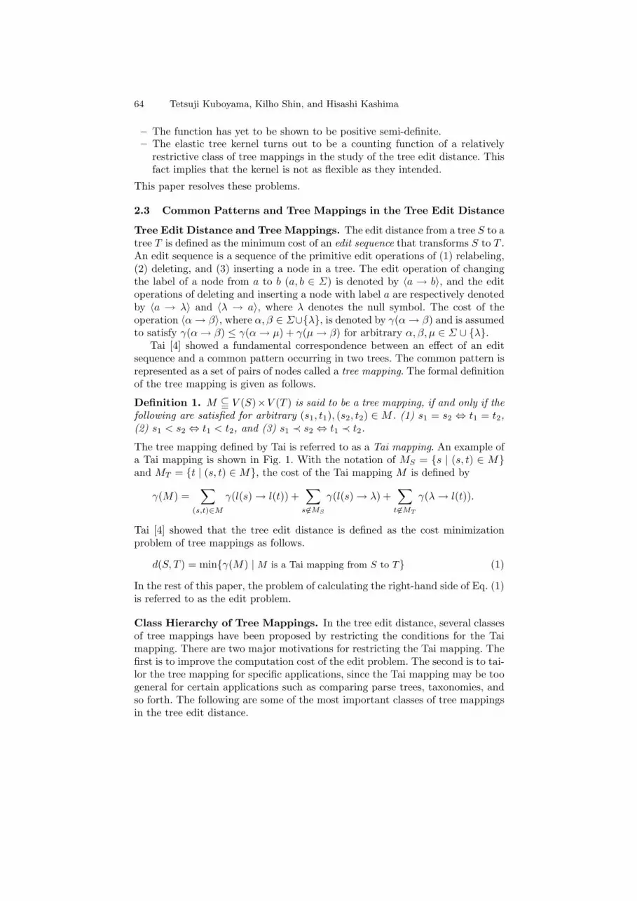
64 Tetsuji Kuboyama, Kilho Shin, and Hisashi Kashima
– The function has yet to be shown to be positive semi-definite.– The elastic tree kernel turns out to be a counting function of a relatively
restrictive class of tree mappings in the study of the tree edit distance. Thisfact implies that the kernel is not as flexible as they intended.
This paper resolves these problems.
2.3 Common Patterns and Tree Mappings in the Tree Edit Distance
Tree Edit Distance and Tree Mappings. The edit distance from a tree S to atree T is defined as the minimum cost of an edit sequence that transforms S to T .An edit sequence is a sequence of the primitive edit operations of (1) relabeling,(2) deleting, and (3) inserting a node in a tree. The edit operation of changingthe label of a node from a to b (a, b ∈ Σ) is denoted by 〈a → b〉, and the editoperations of deleting and inserting a node with label a are respectively denotedby 〈a → λ〉 and 〈λ → a〉, where λ denotes the null symbol. The cost of theoperation 〈α → β〉, where α, β ∈ Σ∪{λ}, is denoted by γ(α → β) and is assumedto satisfy γ(α → β) ≤ γ(α → µ) + γ(µ → β) for arbitrary α, β, µ ∈ Σ ∪ {λ}.
Tai [4] showed a fundamental correspondence between an effect of an editsequence and a common pattern occurring in two trees. The common pattern isrepresented as a set of pairs of nodes called a tree mapping. The formal definitionof the tree mapping is given as follows.
Definition 1. M j V (S)×V (T ) is said to be a tree mapping, if and only if thefollowing are satisfied for arbitrary (s1, t1), (s2, t2) ∈ M . (1) s1 = s2 ⇔ t1 = t2,(2) s1 < s2 ⇔ t1 < t2, and (3) s1 ≺ s2 ⇔ t1 ≺ t2.
The tree mapping defined by Tai is referred to as a Tai mapping. An example ofa Tai mapping is shown in Fig. 1. With the notation of MS = {s | (s, t) ∈ M}and MT = {t | (s, t) ∈ M}, the cost of the Tai mapping M is defined by
γ(M) =∑
(s,t)∈M
γ(l(s) → l(t)) +∑
s 6∈MS
γ(l(s) → λ) +∑
t6∈MT
γ(λ → l(t)).
Tai [4] showed that the tree edit distance is defined as the cost minimizationproblem of tree mappings as follows.
d(S, T ) = min{γ(M) | M is a Tai mapping from S to T} (1)
In the rest of this paper, the problem of calculating the right-hand side of Eq. (1)is referred to as the edit problem.
Class Hierarchy of Tree Mappings. In the tree edit distance, several classesof tree mappings have been proposed by restricting the conditions for the Taimapping. There are two major motivations for restricting the Tai mapping. Thefirst is to improve the computation cost of the edit problem. The second is to tai-lor the tree mapping for specific applications, since the Tai mapping may be toogeneral for certain applications such as comparing parse trees, taxonomies, andso forth. The following are some of the most important classes of tree mappingsin the tree edit distance.
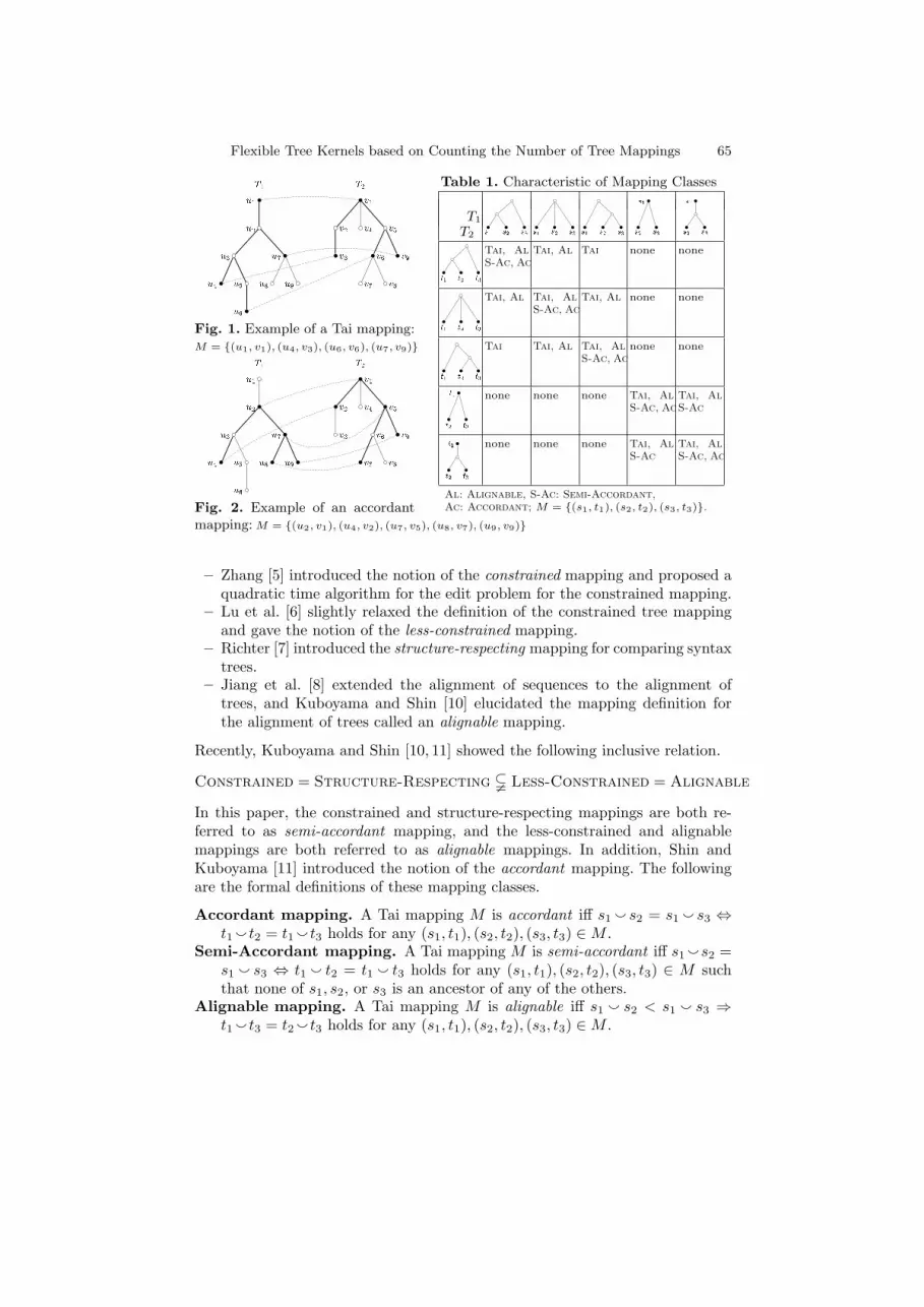
Flexible Tree Kernels based on Counting the Number of Tree Mappings 65T1u1u2u3u4 u5u6u7u8 u9
T2v1v2v3 v4 v5v6v7 v8 v9Fig. 1. Example of a Tai mapping:M = {(u1, v1), (u4, v3), (u6, v6), (u7, v9)}T1u1u2u3u4 u5u6
u7u8 u9T2v1v2v3 v4 v5v6v7 v8 v9
Fig. 2. Example of an accordantmapping: M = {(u2, v1), (u4, v2), (u7, v5), (u8, v7), (u9, v9)}
Table 1. Characteristic of Mapping Classes
T1
T2 s1 s2 s3 s1 s2 s3 s1 s2 s3 s1s2 s3 s1s2 s3t1 t2 t3 Tai, AlS-Ac, Ac
Tai, Al Tai none none
t1 t2 t3 Tai, Al Tai, AlS-Ac, Ac
Tai, Al none none
t1 t2 t3 Tai Tai, Al Tai, AlS-Ac, Ac
none nonet1t2 t3 none none none Tai, AlS-Ac, Ac
Tai, AlS-Act1t2 t3 none none none Tai, Al
S-AcTai, AlS-Ac, Ac
Al: Alignable, S-Ac: Semi-Accordant,Ac: Accordant; M = {(s1, t1), (s2, t2), (s3, t3)}.
– Zhang [5] introduced the notion of the constrained mapping and proposed aquadratic time algorithm for the edit problem for the constrained mapping.
– Lu et al. [6] slightly relaxed the definition of the constrained tree mappingand gave the notion of the less-constrained mapping.
– Richter [7] introduced the structure-respecting mapping for comparing syntaxtrees.
– Jiang et al. [8] extended the alignment of sequences to the alignment oftrees, and Kuboyama and Shin [10] elucidated the mapping definition forthe alignment of trees called an alignable mapping.
Recently, Kuboyama and Shin [10, 11] showed the following inclusive relation.
Constrained = Structure-Respecting $ Less-Constrained = Alignable
In this paper, the constrained and structure-respecting mappings are both re-ferred to as semi-accordant mapping, and the less-constrained and alignablemappings are both referred to as alignable mappings. In addition, Shin andKuboyama [11] introduced the notion of the accordant mapping. The followingare the formal definitions of these mapping classes.
Accordant mapping. A Tai mapping M is accordant iff s1 ` s2 = s1 ` s3 ⇔t1 ` t2 = t1 ` t3 holds for any (s1, t1), (s2, t2), (s3, t3) ∈ M .
Semi-Accordant mapping. A Tai mapping M is semi-accordant iff s1 `s2 =s1 ` s3 ⇔ t1 ` t2 = t1 ` t3 holds for any (s1, t1), (s2, t2), (s3, t3) ∈ M suchthat none of s1, s2, or s3 is an ancestor of any of the others.
Alignable mapping. A Tai mapping M is alignable iff s1 ` s2 < s1 ` s3 ⇒t1 ` t3 = t2 ` t3 holds for any (s1, t1), (s2, t2), (s3, t3) ∈ M .

66 Tetsuji Kuboyama, Kilho Shin, and Hisashi Kashima
T1 T2 � � � Ti| {z }F1 Ti+1 Ti+2 � � � Tn| {z }F2| {z }F1 � F2 = T1 � T2 � � � � � TnvT = v(F )
T1 T2 � � � Tn| {z }F = T1 � T2 � � � � � TnFig. 3. The composition of two forests F1 and F2, and a tree T = v(F ).
An example of an accordant mapping is shown in Fig. 2. Each class is charac-terized by the properties depicted in Tab. 1. It is easy to show that the elastictree kernel [3] turns out to be the counting function of the accordant mappingsbetween two trees.
3 Recursive Expressions of Counting Functions
In this section, first, we extend the notion of tree mappings to forests. Next, wegive the counting functions of the extended tree mappings between two forests.
3.1 Mapping Definition for Forests
A forest F is an ordered sequence of disjoint trees T1, . . . , Tn, denoted by T1 •· · · • Tn, or •n
i=1 Ti, and in particular denoted by ∅ if n = 0. The compositionof forests F1 and F2 in this order is denoted by F1 • F2 (See Fig. 3). The set ofnodes V (T1) ∪ · · · ∪ V (Tn) is denoted by V (F ).
Definition 2. Let F be a forest T1 • · · · • Tn and v be a node not included inV (F ). The tree v(F ) is defined as follows.
– V (v(F )) = (⋃n
i=1 V (Ti)) ∪ {v}.– x < y iff, for some i, either x, y ∈ V (Ti) and x < y in Ti, or y = v holds.– x ≺ y holds iff, for some i, either x, y ∈ V (Ti) and x ≺ y in Ti or x ∈ V (Ti),
y ∈ V (Tj) and i < j holds.
The notion of tree mappings is extended to forests as follows.
Definition 3. Let F1 and F2 be forests and C denote one of Accordant,Semi-Accordant, Alignable, or Tai. A non-empty mapping M ⊆ V (F1)×V (F2) is said to be a C-mapping if and only if M defines a C-mapping fromv1(F1) to v2(F2).
Let MC(F1, F2) denote the set of C-mappings between F1 and F2. The count-ing functions KC(F1, F2) are defined as follows, where the symmetric functionσ : Σ×Σ → R+
0 defines the similarity between labels of nodes, where R+0 denotes
the set of all non-negative real numbers.
KC(F1, F2) =∑
M∈MC(F1,F2)
σ(M); σ(M) =∏
(x1,x2)∈M
σ(l(x1), l(x2))
In the rest of this paper, a forest F ′ is called a subforest of a forest F if and onlyif V (F ′) is a subset of V (F ) and the ancestor-descendant and sibling orders ofF ′ are inherited from F .

Flexible Tree Kernels based on Counting the Number of Tree Mappings 67
3.2 Counting Function for Tai Mapping Class
KTai(F, ∅) = KTai(∅, F ) = 0KTai(v1(F ′
1) • F ′′1 , v2(F ′
2) • F ′′2 ) =
σ(l(v1), l(v2))(1 + KTai(F ′1, F
′2))(1 + KTai(F ′′
1 , F ′′2 ))
+KTai(v1(F ′1) • F ′′
1 , F ′2 • F ′′
2 ) + KTai(F ′1 • F ′′
1 , v2(F ′2) • F ′′
2 )−KTai(F ′
1 • F ′′1 , F ′
2 • F ′′2 ) (2)
The natural properties of the Tai mapping (Prop. 1 and Lem. 1) play a centralrole in proving the correctness of Eq. (2). Let M ′ = M ∩ (V (F ′
1) × V (F ′2)) and
M ′′ = M ∩ (V (F ′′1 )× V (F ′′
2 )) in the following proposition and lemma.
Proposition 1. Let F ′i be any subforest of Fi. Then the following hold.
1. If M is a Tai mapping from F1 to F2, then M ′ is also a Tai mapping fromF ′
1 to F ′2.
2. For non-empty M ⊆ V (F ′1)× V (F ′
2), the following two properties are equiv-alent.(a) M is a Tai mapping from F ′
1 to F ′2.
(b) M is a Tai mapping from F1 to F2.
Lemma 1. Let F ′i and F ′′
i be completely distinct. For non-empty M ⊆ (V (F ′1)∪
V (F ′′1 ))× (V (F ′
2) ∪ V (F ′′2 )), the following two conditions are equivalent.
1. M ∪ {(v1, v2)} is a Tai mapping from v1(F ′1) • F ′′
i to v2(F ′2) • F ′′
2 .2. M satisfies the following three conditions. (1) M = M ′ ∪ M ′′; (2) M ′ is a
Tai mapping from F ′1 to F ′
2; and (3) M ′′ is a Tai mapping from F ′′1 to F ′′
2 .The left-hand side of Eq.(2) is decomposed into the following two parts.
KTai(v1(F ′1) • F ′′
1 , v2(F ′2) • F ′′
2 ) =∑
(v1,v2)∈M σ(M) +∑
(v1,v2) 6∈M σ(M)
Assume (v1, v2) ∈ M . The mapping M \ {(v1, v2)} is identical to M ′ ∪M ′′ forsome Tai mappings M ′ from F ′
1 to F ′2 and M ′′ from F ′′
1 to F ′′2 by Lem. 1. To
the contrary, for arbitrary Tai mappings M ′ from F ′1 to F ′
2 and M ′′ from F ′′1 to
F ′′2 , M ′ ∪M ′′ ∪ {(v1, v2)} is also a Tai mapping from v1(F ′
1) •F ′′i to v2(F ′
2) •F ′′2
by Lem. 1.Therefore, since σ(M) = σ(l(v1), l(v2))σ(M ′)σ(M ′′), the following holds.∑
(v1,v2)∈M σ(M) = σ(l(v1), l(v2))(1 + KTai(F ′1, F
′2))(1 + KTai(F ′′
1 , F ′′2 ))
Let S1, S2, and S3 be as follows.S1 = {M ∈MTai(v1(F ′
1) • F ′′1 , v2(F ′
2) • F ′′2 ) | (v1, w) ∈ M ∧ w 6= v2},
S2 = {M ∈MTai(v1(F ′1) • F ′′
1 , v2(F ′2) • F ′′
2 ) | (w, v2) ∈ M ∧ w 6= v1}, and
S3 = {M ∈MTai(v1(F ′1) • F ′′
1 , v2(F ′2) • F ′′
2 ) | (v, w) ∈ M ⇒ v 6= v1 ∧ v 6= v2}.
By condition 2 of Prop. 1, the following holds.∑M∈S1
σ(M) = KTai(v1(F ′1) • F ′′
1 , F ′2 • F ′′
2 )−KTai(F ′1 • F ′′
1 , F ′2 • F ′′
2 ),∑M∈S2
σ(M) = KTai(F ′1 • F ′′
1 , v2(F ′2) • F ′′
2 )−KTai(F ′1 • F ′′
1 , F ′2 • F ′′
2 ), and∑M∈S3
σ(M) = KTai(F ′1 • F ′′
1 , F ′2 • F ′′
2 ).
The correctness of Eq. (2) is shown by adding together all of the above compo-nents.

68 Tetsuji Kuboyama, Kilho Shin, and Hisashi Kashima
3.3 Template of Counting Function for Subclasses of Tai Mappings
Since Prop. 1 and Lem. 1 do not hold for the subclasses of the Tai mapping, thenEq. (2) is not applicable. However, there exists a common template of countingfunctions applicable to all three of the subclasses.
C ∈ {Accordant, Semi-Accordant,Alignable}KC(∅, F ) = KC(F, ∅) = KC
f (T, ∅) = 0 (4)KC(T1 • F1, T2 • F2) = KC
1 (T1 • F1, T2 • F2) + KC(F1, F2) (5)KC
f (v(F1), T2 • F2) = KCt (v(F1), T2)−KC
f (T2, F1) + KCf (v(F1), F2)
−KC(F1, F2) + KC(F1, T2 • F2) (6)KC
t (v1(F1), v2(F2)) = σ(l(v1), l(v2)) · (1 + KC2 (F1, F2)) + KC
f (v1(F1), F2)+KC
f (v2(F2), F1)−KC(F1, F2) (7)
KC1 (F1, F2) and KC
2 (T1, T2) in the template are defined as follows.
KC1 (T1 • F1, T2 • F2) =
∑M∈S1
σ(M); KC2 (v1(F1), v2(F2)) =
∑M∈S2
σ(M),
where
S1 = {M ∈MC(T1 • F1, T2 • F2) |M ∩ (V (T1)× V (T2 • F2)) 6= ∅ ∨M ∩ (V (T1 • F1)× V (T2)) 6= ∅}, and
S2 = {M ∈MC(v1(F1), v2(F2)) | M ∪ {(v1, v2)} ∈ MC(v1(F1), v2(F2))}.
The recursive expressions for KC1 (F1, F2) and KC
2 (F1, F2) are given afterward.KC
t (T1, T2) takes two trees as the arguments, and KCf (T, F ) takes a tree and
a forest. Equations (5) to (7) are verified in a similar way to Eq. (2), and thefollowing Prop. 2 is used instead of Prop. 1 and Lem. 1.
Proposition 2. Let C be one of Accordant, Semi-Accordant, orAlignable. Further, let F ′
i be a subforest of Fi satisfying one of the follow-ing. (1) Fi = F ′
i ; (2) Fi = vi(F ′i ); or (3) Fi = Gi • F ′
i • Hi for some forestsGi,Hi. Then the following hold.1. For a C-mapping M from F1 to F2, M ′ = M ∩ (V (F ′
1) × V (F ′2)) is a C-
mapping from F ′1 to F ′
2.2. For arbitrary M ⊆ V (F ′
1) × V (F ′2), the following two properties are equiva-
lent. (1) M is a C-mapping from F ′1 to F ′
2; and (2)M is a C-mapping fromF1 to F2.
In the rest of this section, the following notations are used for Fi = •nij=1 T i
j (i =1, 2) and M ∈ MC(F1, F2): M1
j = M ∩ (V (T 1j ) × V (F2)), M2
j = M ∩ (V (F1) ×V (T 2
j )), and Mij = M1i ∩M2
j .The expressions of counting functions are stated without further proof of
their correctness due to the space limitation.

Flexible Tree Kernels based on Counting the Number of Tree Mappings 69
Expressions for KAcc1 and KSemi-Acc
1
C ∈ {Accordant, Semi-Accordant}KC
1 (T1 • F1, T2 • F2) = KCt (T1, T2)(KC
3 (F1, F2)− 1)+KC
f (T1, T2 • F2)−KCf (T1, F2) + KC
f (T2, T1 • F1)−KCf (T2, F1)
+KC(T1 • F1, F2) + KC(F1, T2 • F2)− 2KC(F1, F2) (8)
KC3 is defined as
KC3 (F1, F2) =
∑M∈S3
σ(M),
where
S3 = {M ∈MC(F1, F2) | Mij 6= ∅ ∧ Mkl 6= ∅ ⇒ (i, j) = (k, l)∨(i 6= j ∧ k 6= l)}.
C ∈ {Accordant, Semi-Accordant}KC
3 (F, ∅) = KC3 (∅, F ) = 0
KC3 (T1 • F1, T2 • F2) = KC
t (T1, T2)(1 + KC3 (F1, F2))
+ KC3 (F1, T2 • F2) + KC
3 (T1 • F1, F2)−KC3 (F1, F2) (9)
Expressions for KAlgn1 and KAcc
2
KAlgn1 (•m
i=1 T 1i ,•n
j=1 T 2j ) = κ1,1
1,1(1 + κ2,m2,n )
+∑n
j=2{(κ1,11,j − κ1,1
1,j−1)(1 + κ2,mj+1,n)
+∑m
i=2(κ1,ij,j − κ1,i−1
j,j − κ2,ij,j + κ2,i−1
j,j )(1 + κi+1,mj+1,n )}
+∑m
i=2{(κ1,i1,1 − κ1,i−1
1,1 (1 + κi+1,m2,n )
+∑n
j=2(κi,i1,j − κi,i
1,j−1 − κi,i2,j + κi,i
2,j−1)(1 + κi+1,mj+1,n )} (10)
Let a, b, c, and d satisfy 1 ≤ a ≤ b ≤ n1 and 1 ≤ c ≤ d ≤ n2.
κa,bc,d = KAlgn(•b
i=a T 1i ,•d
j=c T 2j ) (11)
KAcc2 (F1, F2) = KAcc
3 (F1, F2) (12)
Expressions for KSemi-Acc2 and KAlgn
2
C ∈ {Semi-Accordant,Alignable}KC
2 (F1, F2) = KC(F1, F2) (13)
The left-to-right recursive evaluation of Eq. (2) to Eq. (13) actually terminatedue to the base expression in Eq. (4). Each counting function can be evaluatedwith the time complexity O(n4) for the Tai, O(n2d2) for the alignable, O(n2) forthe semi-accordant, and O(n2) for the accordant mapping class, where n denotesthe size of trees, and d denotes the maximum degree by dynamic programing asin the case of the algorithms for the tree edit distance.

70 Tetsuji Kuboyama, Kilho Shin, and Hisashi Kashima
Remark. The counting functions in the parse tree kernel and the elastic treekernel both require a pair of nodes (sr, tr) in the mapping M such that sr ≥ sand tr ≥ t for any (s, t) ∈ M . It is easy to modify our counting functionsproposed in this paper to satisfy this restriction. Nevertheless, we believe ourcounting functions are more natural as the similarity measures between twotrees.
4 Positive Semi-Definiteness of Counting Functions
Assume that the label-similarity function σ is positive semi-definite. Then intu-ition may suggest that the positive semi-definiteness of KC can be inferred fromthe fact that KC(x, y) can be represented as a polynomial in σ(a, b).
However, this intuition is incorrect when C is Alignable. Consider thethree forests F1, F2, andF3 and the label-similarity function σ over Σ ={a, b, c, d, e, f, g, h} as shown in Fig. 4. The Gram matrix [KAlgn(Fi, Fj)] is givenby:
[KAlgn(Fi, Fj)] =
7 + 16ε + 8ε2 7 67 7 + 8ε 76 7 7 + 16ε + 8ε2
Since its determinant D coincides with −7 + ε · q(ε) for some quartic q(ε), D isnegative for a sufficiently small ε < 1 (ε > 0), and therefore, the matrix has atleast one negative eigenvalue. This fact means that KAlgn(x, y) is not a kernelfunction.
F1 F2 F3dea b fa b ga hb σ(x, y) =
8><>:1 if x = y ∈ {a, b, c}ε if x = y ∈ {d, e, f, g, h}0 if x 6= y
Fig. 4. A counterexample to positive semi-definiteness
In contrast, KC is positive semi-definite when C is one of Tai, Semi-Accordant, or Accordant (Cor. 1). Prop. 3 plays a key role to prove Cor. 1.
In Prop. 3, the following notations are used.
– When Aij are m-dimensional square matrices parameterized by (i, j) ={1, . . . , n}2, A denotes the derived mn-dimensional square matrix[Aij ]i,j=1,...,n; and the (mi + k, mj + l)-element of A is defined to be the(k, l)-element of Aij , and denoted by Aij
kl.– p is a homogeneous polynomial of degree d in the m2 variables
X11, X12, . . . , Xmm. Further, assume that p is given a representation of
p(X11, X12, . . . , Xmm) =∑
k∈{1,...,m}d
∑l∈{1,...,m}d
ck,lXk1l1 · · · · ·Xkdld ,
where k = (k1, . . . , kd) and l = (l1, . . . , ld). Note that such representation ofp is not unique.

Flexible Tree Kernels based on Counting the Number of Tree Mappings 71
Proposition 3. Let A be positive semi-definite. If there exists ck ∈ R for eachk ∈ {1, ..,m}d such that ck,l = ckcl, then the n-dimensional square matrix[p(Aij
11, . . . , Aijmm)]i,j=1,...,n is also positive semi-definite.
For a positive integer N , let FN denote the set of forests F such that |V (F )| ≤N . A universal tree TN is a tree with a finite set of nodes, into which each forestF ∈ FN is embedded preserving the ancestor-descendent and sibling orders.When a single order-preserving embedding eF : V (F ) → V (TN ) is assigned toeach F ∈ FN , a pair of TN and the set {eF | F ∈ FN} is used as a commonnumbering scheme of the nodes for any F ∈ FN .
Let C denote an arbitrary subclass of the Tai mapping, including, but notlimited to, Tai, Alignable, Semi-Accordant, and Accordant. The onlyrestriction imposed on C is to satisfy {(v1, v1), . . . , (vn, vn)} ∈ MC(F, F ) forarbitrary F , n and v1, . . . , vn ∈ V (F ), where MC(F1, F2) denotes the set ofC-mappings from F1 to F2.
The mapping class C is said to be absorbent if and only if, for an arbitrary N ,there exists a pair of a universal tree TN and a set of embedding {eF | F ∈ FN}such that: ∀(F1 ∈ FN )∀(F2 ∈ FN )∀(M ∈ V (F1) × V (F2))[M ∈ MC(F1, F2) ⇔(eF1 × eF2)(M) ∈ MC(TN , TN )]. In addition, C is said to be transitive if andonly if, for arbitrary M12 ∈ MC(F1, F2) and M23 ∈ MC(F2, F3), the mappingM13 = {(v1, v3) | ∃(v2)[(v1, v2) ∈ M12 ∧ (v2, v3) ∈ M23]} is also a C-mappingfrom F1 to F3.
If C is transitive, the inverse of a given C-mapping and the compositionof given C-mappings are all C-mappings. In particular, MC(F, F ) under mapcomposition forms a group.
Theorem 1. Let σ : Σ × Σ → R+0 be positive semi-definite. If C is absorbent
and transitive, the function KC |FN: FN × FN → R+
0 is positive semi-definitefor an arbitrary N .
It is easy to see that Accordant, Semi-Accordant, Alignable and Taiclasses are all absorbent. In contrast, the alignable mapping class is not transi-tive, while the others are. A counterexample to the transitivity of the alignablemapping is also given by Fig. 4: M12 = {(a, a), (b, b), (c, c)} ∈ MAlgn(F1, F2);M23 = {(a, a), (b, b), (c, c)} ∈ MAlgn(F2, F3); M13 = {(a, a), (b, b), (c, c)} 6∈MAlgn(F1, F3). Note that, for simplicity, in the mappings, labels are used toindicate the nodes. Corollary 1 gives the main assertion of this section.
Corollary 1. Let C be one of Tai, Semi-Accordant, or Accordant.KC |FN
: FN × FN → R+0 is positive semi-definite for an arbitrary N if and
only if σ : Σ ×Σ → R+0 is positive semi-definite.
Theorem 1 has a wide range of applications. For example, the subtree-congruent mapping class is absorbent and transitive. Moreover, let Leaf-Tai,Leaf-Semi-Accordant, and Leaf-Accordant respectively denote the sub-classes of Tai, Semi-Accordant and Accordant such that, for M belongingto the subclasses, x and y are both leaves if (x, y) ∈ M . They are also absorbentand transitive. Therefore, the counting functions for those mapping classes arepositive semi-definite.

72 Tetsuji Kuboyama, Kilho Shin, and Hisashi Kashima
5 Conclusion
A generalization of the tree kernels due to Collins and Duffy [2], and due toKashima and Koyanagi [3] is addressed in this paper. Based on the notion oftree mapping, which depicts a common sub-pattern between two trees, it isshown that these existing kernels are the counting functions of tree mappings.By focusing on four major classes of tree mappings proposed in the field ofthe tree edit distance, four counting functions of tree mappings are proposedaccording to the four classes. In addition, it is proved that three of the fourcounting functions are kernel functions, and the other is not by checking theirpositive semi-definiteness. One of the three tree kernels developed in this paperturns out to be the elastic tree kernel due to Kashima and Koyanagi. The othertwo tree kernels are more general than existing tree kernels in the interpretationof the common patterns occurring between two trees.
For future work, it is necessary to undertake an empirical analysis of theproposed tree kernels by applying them to real-world data in order to show theadequacy and effectiveness for specific applications.
Acknowledgments
We would like to thank the reviewers for their helpful comments. This work ispartly supported by Grant-in-Aid for Scientific Research No. 17700138 from theMinistry of Education, Culture, Sports, Science and Technology, Japan.
References1. Shawe-Taylor, J., Cristianini, N.: Kernel Methods for Pattern Analysis. Cambridge
University Press (2004)2. Collins, M., Duffy, N.: Convolution Kernels for Natural Language. Advances in
Neural Information Processing Systems 14, Vol.1 (NIPS). (2001) 625–6323. Kashima, H., Koyanagi, T.: Kernels for Semi-Structured Data. Proc. of the 9th
International Conference on Machine Learning (ICML). (2002) 291–2984. Tai, K.C.: The Tree-to-Tree Correction Problem. JACM 26 (1979) 422–4335. Zhang, K.: Algorithms for The Constrained Editing Distance between Ordered
Labeled Trees and Related Problems. Pattern Recognition 28 (1995) 463–4746. Lu, C.L., Su, Z.Y., Tang, G.Y.: A New Measure of Edit Distance between Labeled
Trees. LNCS 2108 (2001) 338–3487. Richter, T.: A New Measure of The Distance between Ordered Trees and its
Applications. Technical Report 85166-CS, Dept. of Computer Science, Univ. ofBonn (1997)
8. Jiang, T., Wang, L., Zhang, K.: Alignment of Trees — An Alternative to TreeEdit. Theoretical Computer Science 143 (1995) 137–148
9. Wang, J.L., Zhang, K.: Finding Similar Consensus between Trees: An Algorithmand A Distance Hierarchy. Pattern Recognition 34 (2001) 127–137
10. Kuboyama, T., Shin, K., Miyahara, T., Yasuda, H.: A Theoretical Analysis ofAlignment and Edit Problems for Trees. Theoretical Computer Science, The 9thItalian Conference. LNCS 3701 (2005) 323–337
11. Shin, K., Kuboyama, T.: An algebraic Foundation of The Tree Edit Distance.Technical report, Center for Collaborative Research, University of Tokyo (2005)
12. Haussler, D.: Convolution kernels on discrete structures. UCSC-CRL 99-10, Dept.of Computer Science, University of California at Santa Cruz (1999)

Mining Interpretable Subgraphs
Siegfried Nijssen
Institut fur Informatik, Albert-Ludwidgs-Universitat,Georges-Kohler-Allee, Gebaude 097, D-79110, Freiburg im Breisgau, Germany.
Abstract. We present a measure that estimates the interpretability ofa frequent subgraph. We show that a feature selection algorithm thatuses this measure creates a set of features that is smaller and equallypredictive as features obtained in earlier studies. A significant numberof the selected features turn out to be trees or cyclic graphs, leading usto the conclusion that such features are not as useless as suggested insome earlier studies. Finally, we show that a constraint on this measurecan be pushed in the mining process, thus leading to faster discovery ofinteresting subgraphs.
1 Introduction
One of the most important applications of graph mining is the analysis of molecu-lar datasets, where the aim is to predict accurately if an unseen molecule exhibitsa certain chemical activity or not. Traditional methodes proposed in the chemo-informatics community rely mostly on paths, but the data mining communityhas started the use of subgraphs in the hope of obtaining better classifiers, whereboth frequent pattern mining [10, 7] and kernel approaches [6, 9] have been in-vestigated.
In two recent papers, however, it was suggested that the additional complex-ity of taking into account subgraphs may not be justified [2, 9]. It was reportedthat for a large number of classifiers and a large number of datasets, featuresbased on paths yield more accurate classifiers.
In the local pattern mining approach, which is used for example in [2], classi-fication is typically approached as follows. First, given a dataset, a set of patterns(in this case, paths or subgraphs) is computed. During this search, a constraintis enforced such that only patterns are found that have sufficient correlation withthe activity of the molecules; for instance, the subgraph should occur more oftenin the active molecules than in the inactive ones.
Second, each pattern is used to create a new feature for the molecules: if amolecule contains a certain pattern, the feature correponding to the pattern getsvalue 1 (or true), otherwise the feature has value 0 (or false). On the resultingset of features, a classifier, such as a decision tree, is learned. This decision treeis finally used to predict the activity of new molecules.
It is indeed an interesting observation that a set of paths can contain thesame amount or even more information than a set of subgraphs. An equally

74 Siegfried Nijssen
interesting question is how these results can be explained. We believe that thereare several possible explanations:
– in [2] feature sets of equal size were determined for each type of pattern; ifone considers the contingency tables that achieve the best correlation values,there are usually significantly more subgraphs with exactly that table thanthere are subpaths, yielding features that are more correlated among eachother in case a fixed number of subgraphs are used;
– if subgraphs are considered, the amount of possible features is much larger;thus the risk of overfitting to the training data is also much larger.
In the study of [2] it was reported that by relaxing the correlation constraint,a more accurate classifier can be obtained. One could explain this by the argu-ment that the resulting additional features are in this case less correlated amongeachother.
In this paper, we investigate these observations further. Concretely, we pro-pose a measure to drastically cut down the number of frequent subgraphs thatare used as features, thus yielding classifiers that are more interpretable, and wepropose a feature selection method to avoid redundancy among the features. Weshow that the interpretability constraint can be pushed in the mining process,thus showing that there are efficient ways to search for patterns that are stillsimple, but also cyclic.
The paper is organized as follows. In section 2 we briefly reintroduce theformal concepts that are important in this paper. In section 3 we introduce ournotion of interpretable subgraphs. In section 4 we show how a constraint on in-terpretable subgraphs can be pushed in the mining process. Section 5 introducesour feature selection algorithm. Section 6 concludes.
2 Concepts
An essential task in the local pattern mining scenario is the computation of arelevant set of patterns. In the data mining community, these features are oftendetermined using a frequent subgraph mining algorithm. To formalize what afrequent subgraph is, we need the following definitions.
Definition 1 (Graphs). An undirected, labeled graph G(V, E, λ, Σ) consists ofa finite set V of vertices, a set E ⊆ {{u, v}|u, v ∈ V, u 6= v} of edges, an alphabetΣ and a labeling function λ : (V ∪ E) → Σ.
Definition 2 (Connected Graphs). A graph G(V,E, λ,Σ) is called connectediff for each pair of nodes u, v ∈ V there is a sequence of nodes v1, . . . , vn in Vwith v1 = u and vn = v and {vi, vi+1} ∈ E.
In this paper, we only consider connected graphs.
Definition 3 (Graph Isomorphism). Graphs G(V, E, λ, Σ) and G′(V ′, E′, λ′, Σ′)are called isomorphic if there exists a bijective function f : V → V ′ such that:∀v ∈ V : λ(v) = λ′(f(v)) ∧E = {{f(v1), f(v2)}|{v1, v2} ∈ E′} ∧ ∀e ∈ E : λ(e) =λ′(f(e)).

Mining Interpretable Subgraphs 75
Definition 4 (Subgraph). Given a graph G(V, E, λ, Σ), G′(V ′, E′, λ′, Σ′) iscalled a subgraph of G iff V ′ ⊆ V ∧ E′ ⊆ E ∧ ∀v ∈ V ′ : λ(v′) = λ(v) ∧ ∀e ∈ E′ :λ(e′) = λ(e).
If a graph H has a subgraph H ′ such that a graph G is isomorphic with H ′,then G is said to be subgraph isomorphic with H, denoted by H º G; fuction fdefines how subgraph G can be embedded in the larger graph H. The set of allembeddings of G in H is denoted by FHºG.
Definition 5 (Frequent Subgraph). Given a collection D of graphs and agraph G, the frequency of G, denoted by freq(G,D), is the cardinality of theset {G′ ∈ D|G′ º G}. A graph G is frequent if freq(G,D) ≥ minsup, for apredefined threshold minsup.
The problem that is solved by a frequent subgraph mining algorithm is to findall subgraphs that are frequent in a dataset. In the molecular setting the set offrequent subgraphs is usually computed on the active set of molecules, and theircorresponding frequencies on the inactive set of molecules are computed later.
Several algorithms have been proposed to solve the frequent subgraph min-ing problem, among which gSpan [10], Gaston [7] and MoFA [5, 8]. All thesealgorithms exploit the fact that the frequency constraint is anti-monotonic: ifG º H, then freq(G) ≤ freq(H). As a consequence of this property, algorithmsdo not need to consider all possible subgraphs of a database to find all frequentones: it is possible to search from small to large subgraphs, and stop searchingif a large graph is not frequent any more.
An important issue that subgraph miners have to address, is that there aremany ways to construct isomorphic subgraphs. For instance, a molecular frag-ment consisting of an oxygen (O) connected to a carbon (C), can be obtainedby connecting either a carbon to an oxygen, or by connecting an oxygen to acarbon. To avoid duplicates, only one of these two extensions should be allowed.Most subgraph miners solve this issue by using a canonical code that restricts inwhat ways a subgraph can be extended.
The degree of a node v, denoted by deg(v), is the number of nodes to whichthe node is directly connected by the edges in the graph. Several simple classesof subgraphs have been studied. A (free) tree is a connected graph in which|V | = |E|+ 1; a path is a tree in which no node has a degree higher than 2.
Assume that there are two graphs H and G, such that H º G, and freq(G) =freq(H), then for the purpose of classification graph H can be considered redun-dant: it covers exactly the same set of molecules as G, but is more specific, andtherefore more likely to overfit. Therefore, it is often useful to restrict the searchto subgraphs G for which there is no subgraph H for which freq(G) = freq(H).Such subgraphs are called free subgraphs. If there is no supergraph H for whichfreq(G) = freq(H), then subgraph G is called a closed subgraph.
Finally, if we know the frequency of a subgraph in both a set of active andinactive molecules, we can compute its correlation with that activity; this score—typically the result of a χ2 test— can be used to rank patterns. A top-kpattern miner finds all k subgraphs that obtain the highest positions in this

76 Siegfried Nijssen
ranking. The motivation is that only the highest scoring subgraphs are expectedto be important to classify molecules.
In [2], the classification of molecules was approached using a top-k free pat-tern mining algorithm. For several values of k the highest scoring patterns weredetermined; these patterns were used to build classifiers. Trees, graphs and pathswere considered as pattern domains. It was concluded in many cases that clas-sifiers based on paths achieved the highest predictive accuracy.
3 Interpretable subgraphs
A situation that occurs in many molecular data mining applications, is illus-trated by the following example. Assume that we have a (hypothetical) databasecontaining the following two highly active molecules:
Then we can derive the following substructure, which tries to encode a disjunc-tion of these two graphs, but which is chemically hard to interpret, as it containsonly part of an aromatic ring:
In this subgraph, some edges have been selectively included or excluded to obtainthe best fit to the data. This subgraph shows that there is sometimes a tensionbetween interpretability and predictive accuracy of subgraphs:
– if this subgraph obtains a superior accuracy score, one could believe that itis desirable that it is found;
– if this subgraph cannot be interpreted without looking through an enormousset of embeddings in the data, it may not be useful that it is found.
Thus, by interpretability we mean that less additional information has to beconsidered before the true value of the pattern can be determined by an expert.
A further problem is the size of the search space. If one allows individualremoval or inclusion of edges, the search space becomes larger. As a result of theadditional features, accuracy can increase, but on the other hand, if there areso many features to consider, it will be harder to interpret the features and todetermine which of the features are really of interest.
These issues also important when building accurate classifiers. On the onehand, tweaking of substructures can be desirable, as it could yield a better fitto the data; on the one hand, if too much tweaking is allowed, we might overfitto the data. It is a well-known problem to balance these issues.
Until now, two solutions are prevalent. In the approaches based on gSpanor Gaston [10, 7] the interpretability of subgraphs is neglected, thus allowing

Mining Interpretable Subgraphs 77
structural tweaking as in the example above. In MoFA [5, 8] the issue is addressedby hard-coding structural preference in the search: for example, rings of length5 or 6 are marked as special structural elements, and edges of such rings cannever be added individually, yielding more interpretable subgraphs and smallersearch spaces, but disallowing potentially interesting subgraphs such as in theexample above.
In this paper, we investigate an approach in which there is a parameter tobalance interpretability and structural freedom. We wish to allow structural free-dom, but want to implement a measure that allows us to express our preferencefor structures that are not too incomplete. There are many conceivable measures.Here, we take an approach that is based on considering how graphs match tothe data. What we can observe in general for the example fragment, is that it isincomplete: in every embedding of this subgraph, we can connect an additionaledge to the fragment. If we consider the original molecules as fragments, they aremore ‘complete’: there would usually be less possibilities to connect additionaledges to an embedding. Therefore, a reasonable measure seems to be based onthe number of edges that can be connected to an embedding of the subgraph.
Formally, we can compute this as follows:
missing(f) =∑
v∈VG
deg(f(v))− deg(v),
which is the number of edges that can be connected to the embedded subgraph.For a database D of graphs we can compute
missing(G) =
∑H∈D,G⊆H minf∈FHºG
missing(f)|{H ∈ D|H º G}| .
We believe that it is reasonable to consider only the best possible embedding(for example, an average over all embeddings would be skewed as the number ofembeddings can be exponential), therefore we choose to minimize the missingvalue. The measure clearly reflects the number of possibilities for extending thepattern in the minimal case.
The use of this measure can be two-fold. We can use it to express a preferencebetween structures that are more or less equivalent otherwise, thus in principlestill allowing unlimited structural freedom. Another possibility is to enforce aconstraint on this measure. In this case, we might not find some well-scoring sub-structures any more. On the other hand, structures satisfying such a constraintwould have the advantage that the resulting substructures are usually easier tointerpret, and the possibilities for overfitting are reduced.
It is important to observe that this constraint is neither monotonic noranti-monotonic. A given subgraph with a low missing value can obtain a highmissing value after extenion: assume that the newly added node is always con-nected to many other nodes in the data, then missing will go up. On the otherhand, the missing value can also go down. If we add an edge to the exam-ple fragment, we can obtain the second example molecule. This graph has lessmissing edges.
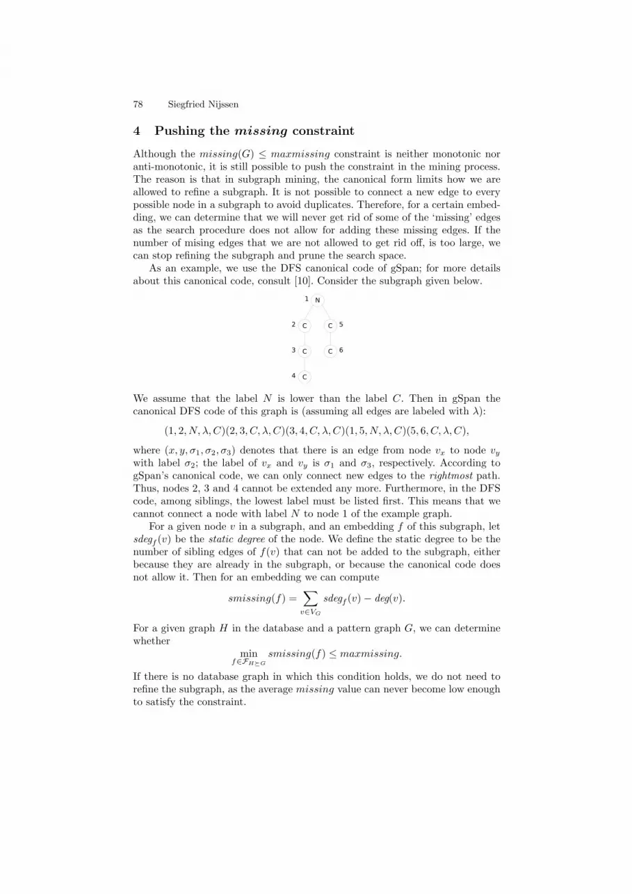
78 Siegfried Nijssen
4 Pushing the missing constraint
Although the missing(G) ≤ maxmissing constraint is neither monotonic noranti-monotonic, it is still possible to push the constraint in the mining process.The reason is that in subgraph mining, the canonical form limits how we areallowed to refine a subgraph. It is not possible to connect a new edge to everypossible node in a subgraph to avoid duplicates. Therefore, for a certain embed-ding, we can determine that we will never get rid of some of the ‘missing’ edgesas the search procedure does not allow for adding these missing edges. If thenumber of mising edges that we are not allowed to get rid off, is too large, wecan stop refining the subgraph and prune the search space.
As an example, we use the DFS canonical code of gSpan; for more detailsabout this canonical code, consult [10]. Consider the subgraph given below.
We assume that the label N is lower than the label C. Then in gSpan thecanonical DFS code of this graph is (assuming all edges are labeled with λ):
(1, 2, N, λ, C)(2, 3, C, λ, C)(3, 4, C, λ, C)(1, 5, N, λ, C)(5, 6, C, λ, C),
where (x, y, σ1, σ2, σ3) denotes that there is an edge from node vx to node vy
with label σ2; the label of vx and vy is σ1 and σ3, respectively. According togSpan’s canonical code, we can only connect new edges to the rightmost path.Thus, nodes 2, 3 and 4 cannot be extended any more. Furthermore, in the DFScode, among siblings, the lowest label must be listed first. This means that wecannot connect a node with label N to node 1 of the example graph.
For a given node v in a subgraph, and an embedding f of this subgraph, letsdegf (v) be the static degree of the node. We define the static degree to be thenumber of sibling edges of f(v) that can not be added to the subgraph, eitherbecause they are already in the subgraph, or because the canonical code doesnot allow it. Then for an embedding we can compute
smissing(f) =∑
v∈VG
sdegf (v)− deg(v).
For a given graph H in the database and a pattern graph G, we can determinewhether
minf∈FHºG
smissing(f) ≤ maxmissing.
If there is no database graph in which this condition holds, we do not need torefine the subgraph, as the average missing value can never become low enoughto satisfy the constraint.

Mining Interpretable Subgraphs 79
Name Size class 1 Size class 2
NCI HIV 417 1069Mutagenicity I [7] 2401 1936Mutagenicity II [4] 341 343Biodegradability [1] 143 185PTE [10] 340 —
Table 1. Properties of the datasets used in the experiments
In principle, to decide which edges can be connected to a subgraph accord-ing to the canonical form is computationally hard, as we need to solve graphisomorphism. However, the above given two rules can be used to approximatesdegf (v): nodes are static if either (1) they are a sibling of a node not on therightmost path or (2) they are a siblings of a node on the rightmost path, butthe label is too low. This approximation will not influence the correctness of thealgorithm, as it underestimates the number of missing edges.
Experimental Evaluation To test the influence of this pruning rule we have per-formed several experiments with an implementation of gSpan that includes thisconstraint. The properties of the datasets are listed in Figure 1.
We first performed experiments on the predictive toxicology dataset (PTE).Runtime experiments were performed on an Intel Pentium M processor runningat 1.1Ghz, and are listed in Table 2. In this table, the number of processedsubgraphs is the number of subgraphs that is enumerated by the graph miningalgorithm, including subgraphs for which missing is too high. We can observe
min- max- # processedsup missing runtime subgraphs
32 ∞ 5.9s 93032 2.0 3.7s 70616 ∞ 46.9s 440516 2.0 9.7s 219710 ∞ 261.8s 2275810 4.0 108.9s 1347210 3.0 57.0s 944910 2.0 19.9s 5344
Table 2. Experiments on the PTEdataset
min- max- # processedsup missing runtime subgraphs
200 ∞ 298.7s 2244200 3.0 298.9s 2231200 2.0 279.5s 2115150 ∞ 590.5s 6367150 2.0 533.9s 5790
Table 3. Experiments on the Muta-genesis I dataset
that the runtime improvement is much larger than the number of processedsubgraphs. The reason is that especially large subgraphs, for which computingsubgraph isomorphism is more expensive, are pruned.
Next, we performed a set of experiments on the Mutagenesis I dataset. Exper-iments were performed on an Intel Pentium IV running at 3.2Ghz. The minimumsupport threshold applies to the set of active molecules. We observe that on this

80 Siegfried Nijssen
dataset the influence of the constraint is almost negligible. A possible explanationis that in this dataset the molecules were encoded without hydrogens (contraryto the PTE dataset). Consequently, the branching factor of nodes in the data islower. A larger amount of the nodes therefore already have low missing value.The pruning opportunities are therefore reduced.
Finally, we performed an experiment in which the NCI HIV dataset was used;we determined the frequent patterns in the active molecules, and evaluated thepatterns also on the moderately active ones. The experiments were performedon an Intel Pentium IV 3.2Ghz again. For a minimum support of 6% we deter-mined that the runtime without constraint was 1500s, while it was only 691s ifa maxmissing constraint of 3.0 was applied. In this dataset the hydrogens werenot included in the encoding. Apperently, the amount of speed-up is not onlydependent on this encoding.
Dataset minsup Frequent Interpretable
Mutagenesis I 2.5% 48583 132Mutagenesis II 2.5% 7577 208Mutagenesis II 5.0% 1005 103HIV 6.0% 371374 350HIV 7.5% 58380 264Biodegradability 2.5% 168033 206Biodegradability 5.0% 34839 88
Table 4. Experiments showing the reduction in subgraphs by applying themaxmissing constraint
Finally, in Table 4 the results are reported of an experiment in which we com-pared the number of frequent subgraphs in the output of gSpan with and withouta maxmissing = 3.0 constraint. This shows that the maxmissing constraint isvery effective in reducing the number of subgraphs.
5 Ranking patterns
As discussed in the introduction, the simplest approach to rank subgraphs is toorder them according to the χ2 statistic of their correlation with the activityof molecules. However, such an absolute ordering may not always be justified.Assume that we have two subgraphs of which the TID lists (i.e., the lists ofgraphs in the database to which they map) are almost equal, then it might notbe justified to prefer the one pattern above the other pattern; the small differencemight just be noise in the data. For every pattern, we can therefore define a setof patterns that is close to it in terms of TID list, and for which we have noreason to prefer one pattern above the other.
One way then to cut the ties between patterns with almost equal TID lists,is to use the missing score. Thus, assuming that we have sorted all patterns onχ2, we can apply this procedure:

Mining Interpretable Subgraphs 81
1. Among the set of all patterns within a close distance from the topmostpattern, pick the pattern that scores best according to the missing score.Add this pattern to the result set.
2. Remove all patterns that are close to the chosen pattern (which includes thebest pattern), including the chosen pattern.
3. Go to step 1 for the remaining sorted list of patterns.
Observe that if two graphs have equal TID lists, and one is a subgraph of theother, the missing score can still cut ties. However, one cannot predict whetherthe subgraph or the supergraph will be preferred. Thus, we do not imply eitherclosed subgraph mining or free subgraph mining.
Parameters in this procedure are the distance measure and the thresholdon this measure. Currently, we have chosen symmetric difference as distancemeasure. As a rule of thumb, the threshold on the distance is lower than theminimum support threshold.
We first performed an experiment on the Mutagenesis I dataset. We useda minimum support of 150, a distance threshold of 30, and no interpretabilityconstraint. The total number of frequent patterns was 6367. If we apply theselection procedure given above, 297 fragments remain. The best 8 fragmentsare given below. For each fragment its χ2 value and its missing value are given.
C
C100
C
100
C
100
C
100
C
100
C100
C
100
C100
C
100
100
ON2
C
C100
C
100
C
100
C
100
C100
C
100
C100
C
100
100
C
C
100C100
C
100C
100
C
100
C100
100
(1) 401.0/4.3 (2) 384.8/1.8 (3) 364.9/4.0 (4) 352.8/3.1C
C100
C
100
C
100
C
100
C
100
C
100
C100
C
100
C100
C
100
100
N
C
1
C
100
O
N
1
C
1
C
100
C
C100
C100
C
100
C
100
C100
C
100
C
100100
(5) 348.5/4.6 (6) 337.4/3.2 (7) 334.4/3.5 (8) 327.5/5.3
We can observe that there is a large number of fragments involving aromaticbonds, which are labeled with ‘100’ in these figures. The first, third and fourthfragment still have significant differences in TID lists. Please note that the longchains in the patterns are not chains in the data. The method of [8] would notprune them. An example of a molecule that does not contain the first fragment,but does contain the third fragment, is given below:

82 Siegfried Nijssen
C
C100
C
100
C
100
C
100
C
100
N100
C
100
C
100
100
C
100
C
100
N
100
C
1
100
C
100
100
The problem is that the information of how this pattern matches (i.e., if thenon-branching chain in the pattern is also a non-branching chain in the data, asone could be tempted to think), is not readily available from the pattern and acloser inspectation of patterns and data is required; there might also be otherexplanations. It is not obvious for what reasons this particular fragment matchesas good as it does.
If however we apply a maximum value of 3.0 as constraint on the missingvalue, the number of frequent fragments that satisfies the constraint falls down to54. With the algorithm given above, using a threshold distance of 30, 44 becomeselected. The best 8 fragments are given below:
ON2
O
N
1
C
1
ON
2
O
1
C
1
ON1
(1) 384.8/1.8 (2) 322.8/2.9 (3) 303.2/2.0 (4) 312.1/1.9
O N2
O
1
C
1
C
100 C
C
100
C
100
C
100C
100
C
100
C 100 100
C
100
C100
C100
100
N
C
1C100
C
100C
100
C
100
C100
100
O
N1
C1
C
100
C
100
C100
C
100
C
100100
(5) 304.9/2.0 (6) 288.4/2.7 (7) 238.9/2.9 (8) 227.9/3.0
To a certain extent, we still have similar effects as in the previous experiment.The fifth fragment only contains one aromatic bond, because the given group canconnect to any aromatic ring, not only a six-ring, like in the seventh fragment.The effects are however much smaller.
Next, we performed several experiments on this dataset to compare the clas-sification accuracies of several classes of fragments. To make the results compa-rable to the results obtained in [2], we took the same settings as in that paper,except that we used our new algorithm to select the cyclic subgraphs that areused as features; so, the results are obtained after 10 fold crossvalidation, usingimplementations of Weka [3]. We restricted ourselves to the C4.5 decision tree

Mining Interpretable Subgraphs 83
Mutagenesis I Mutagenesis II BiodegradabilityAlgorithm Number of Accuracy Number of Accuracy Number of Accuracy
features features features
Paths 100 76.37 100 70.90 100 76.221000 79.73 1000 71.63 1000 74.10
Trees 100 70.94 100 70.39 100 71.961000 74.83 1000 71.55 1000 76.07
Graphs 100 70.79 100 70.53 100 71.821000 74.68 1000 72.06 1000 71.20
Selection 2.5% 82 79.94 93 76.02 83 72.56Selection 5.0% 48 78.35 58 70.91 54 72.87
Table 5. Accuracies on the Mutagenesis I, Mutagenesis II and Biodegradabilitydatasets; Selection x% denotes that a minimum support of x% was used
Algorithm Number of Accuracy Algorithm Number of Accuracyfeatures features
Paths 100 77.46 Selection 6.0% 4 107 82.771000 83.21 Selection 6.0% 8 93 82.30
Trees 100 77.06 Selection 7.5% 4 94 82.771000 75.95 Selection 7.5% 8 83 82.55
Graphs 100 77.061000 75.95
Table 6. Accuracies on the NCI HIV dataset; Selection x% y denotes that a minimumsupport of x% was used and a maximum distance of y
learner, as this algorithm achieved the best results in all experiments in [2]. Re-sults are listed in Table 5 and 6; results for Paths, Trees and Graphs are copiedfrom [2].
In all cases maxmissing was fixed to 3.0. The distance threshold was 60on Mutagenesis I, 2.5% on Mutagenesis II, and 2.5% on Biodegradability. In-terestingly, we achieve similar classification accuracies as for the paths in mostcases; only on the biodegradability dataset our results are disappointing. Theset of features that is passed to C4.5 is smaller in all cases. Also in terms of thesize of the decision tree, our classification method seems more interpretable; forexample, a decision tree learned on the entire Mutagenesis I dataset using 1000paths, contains 196 leaves, while the tree that is built on our features contains104 leaves.
Comparing these tables to table 4, the largest reduction in the number offeatures stems from the maxmising constraint.
In addition to the minimum support threshold, we also varied the distancethreshold on the NCI HIV dataset. Most results do not seem to be very sensi-tive to the choice of the parameters, with the exception perhaps of the minsupthreshold on the Mutagenesis II dataset.

84 Siegfried Nijssen
6 Conclusions
We argued that there is a general trade-off between pattern representations,mining efficiencies and classification accuracies. To illustrate this, we developeda measure to quantify the interpretability of a subgraph, and showed that thismeasure could be pushed in the mining process, with mixed success. We per-formed experiments with the features that were selected using a feature selectionmethod that takes this measure into account, and found that the classifiers wereaccurate in most cases, and possibly more interpretable.
There are many open issues in this approach. A broader study of inter-pretability measures might yield measures that approximate the average chemist’sidea of interpretability better. For instance, one could also base an interpretabil-ity measure on how well examples cluster on the frequent supergraphs of a sub-graph. We used an ad-hoc method to prefer structures that achieve a higherinterpretability score, but a more principled approach would be desirable. Fi-nally, in most experiments we applied feature selection only on pruned features.Our feature selection method did not work efficiently on large amounts of fea-tures. How to optimize this method is also an open question.
Acknowledgements This work was supported by the EU FET IST project IQ (“In-
ductive Querying”), contract number FP6-516169. We would like to thank Taneli
Mielikainen and Jeroen Kazius for discussions.
References
1. H. Blockeel, S. Dzeroski, B. Kompare, S. Kramer, B. Pfahringer, and W. Van Laer.Experiments in predicting biodegradability. In Appl. Art. Int. 18, pages 157–181,2004.
2. B. Bringmann, A. Zimmermann, L. De Raedt, and S. Nijssen. Don’t be afraid ofsimpler patterns. In PKDD, 2006.
3. E. Frank, M. Hall, L.E. Trigg, G. Holmes, and I.H. Witten. Data mining in bioin-formatics using weka. In Bioinformatics 20, pages 2479–2481, 2004.
4. C. Helma, T. Cramer, S. Kramer, and L. De Raedt. Data mining and machinelearning techniques for the identification of mutagenicity inducing substructuresand structure activity relationships of noncongeneric compounds. In Journal ofChemical Information and Computer Systems 44, pages 1402–1411, 2004.
5. H. Hofer, C. Borgelt, and M. Berthold. Large scale mining of molecular fragmentswith wildcards. In IDA, pages 380–389, 2003.
6. T. Horvath, T. Gartner, and S. Wrobel. Cyclic pattern kernels for predictive graphmining. In KDD, pages 158–167, 2004.
7. J. Kazius, S. Nijssen, J.N. Kok, T. Back, and A. IJzerman. Substructure miningusing elaborate chemical representation. In Journal of Chemical Information andModeling 46, 2006.
8. T. Meinl, C. Borgelt, and M. Berthold. Mining fragments with fuzzy chains inmolecular databases. In MGTS, pages 49–60, 2004.
9. N. Wale and G. Karypis. Acyclic subgraph-based descriptor spaces for chemicalcompound retrieval and classification. In Technical report, Univ. Minnesota, 2006.
10. X. Yan and J. Han. gSpan: Graph-based substructure pattern mining. In ICDM,pages 721–724, 2002.

A Linear Programming Approachfor Molecular QSAR analysis
Hiroto Saigo1, Tadashi Kadowaki2, and Koji Tsuda1
1 Max Planck Institute for Biological Cybernetics,Spemannstr. 38, 72076 Tubingen, Germany
{hiroto.saigo,koji.tsuda}@tuebingen.mpg.de,2 Bioinformatics Center, ICR, Kyoto University
Uji, Kyoto 611-0011, [email protected]
Abstract. Small molecules in chemistry can be represented as graphs.In a quantitative structure-activity relationship (QSAR) analysis, thecentral task is to find a regression function that predicts the activity ofthe molecule in high accuracy. Setting a QSAR as a primal target, wepropose a new linear programming approach to the graph-based regres-sion problem. Our method extends the graph classification algorithm byKudo et al. (NIPS 2004), which is a combination of boosting and graphmining. Instead of sequential multiplicative updates, we employ the lin-ear programming boosting (LP) for regression. The LP approach allowsto include inequality constraints for the parameter vector, which turnsout to be particularly useful in QSAR tasks where activity values aresometimes unavailable. Furthermore, the efficiency is improved signifi-cantly by employing multiple pricing.
1 Introduction
Nowadays we are facing a problem of screening a huge number of molecules in or-der to testify, e.g., if it is toxic to human or it has an effect on HIV virus, etc. Suchbioactivities or chemical reactivities are measured by laborious experiments, soselecting small number of good candidates for the later synthesis is important. Aquantitative structure-activity relationship (QSAR) analysis, a process to relatea series of molecular features with biological activities or chemical reactivities,is expected to decrease a number of expensive experiments. The conventionalQSAR analysis manipulates chemical data in a table in which molecules aredefined by individual rows and molecular properties (descriptors) in binary orreal values are defined by the associated columns. The prediction model is thenbuilt to be consistent to the structure-activity relationship. Our approach usesubgraphs as molecular properties instead of conventional descriptors. Since weknow that simple subgraphs are already included in conventional descriptors,and believe that enriching subgraph features would contribute to make a betterprediction model.

86 Saigo, Kadowaki, Tsuda
A graph is a powerful mathematical framework which can deal with manyreal-world objects. Several approaches based on kernel methods have been pro-posed [1–6], which all consider molecules as graphs and tried defining distancemeasures between molecules. However, these kernel methods lack interpretabil-ity, because the feature space is implicitly defined and it is difficult to figure outwhich features played an important role in prediction.
We take the boosting approach, which works in a feature space explicitlydefined by substructure indicators [7]. Therefore, it is rather easy to show thesubstructures contributed to activity predictions, which may lead to new findingsby chemists. Though the number of possible subgraphs in graph database areexponentially large, the recent advance of graph mining algorithms [8–12] sug-gests a way to handle them. The graph boosting method by Kudo et al. [7] hasto be modified in several ways for QSAR applications. First of all, the originalclassification algorithm should be modified to a regression algorithm, becausethe activity is real-valued. Very recently, Kadowaki et al.[13] used the graphboosting in a SAR task, where the problem is to predict a chemical compoundis active or not. However, the activity values are continuous and they are notobviously separated into active/non-active categories. Second, in publicly avail-able databases, the activity values are not always available, because, if somecompounds are obviously inactive, they do not bother to measure the activity.Therefore, for many compounds, one knows that their activities are low, but theactual values are not available. We need a mechanism to take those unusual datainto account. Finally, in AdaBoost, only one substructure is found by the searchof the whole pattern space. So, if one needs d substructures for good accuracy,the graph mining has to be done d times. For more efficiency, it is desirable thatmultiple substructures are derived by one mining call.
Among several boosting algorithms for regression [14], we found the linearprogramming (LP) boosting proposed by Demiriz et al. [15] is most appropriatefor our task. One reason is that the linear programming allows to include in-equality constraints which are useful for incorporating the compounds with lowactivities. Another reason is that it is possible to obtain multiple structures byone graph mining call, because the LP boost always updates all the parameterswhereas AdaBoost updates one parameter at a time. Finally, in the LP boost,the optimality of the solution can be evaluated by the duality gap, whereas, inAdaBoost, it is not obvious when to stop the iteration and it is hard to figureout the distance from the current solution to the optimal one.
In this paper, we will describe how the LP boost can be combined with thegraph mining algorithm to yield an efficient graph regression algorithm. In ex-periments using Endocrine Disruptors Knowledge Base (EDKB), our method isfavorably compared with the marginalized graph kernels [1] that are successfullyapplied to chemical data recently [5]. We also illustrate the speed up achievedby reducing the number of mining calls.

A Linear Programming Approach for Graph-based QSAR analysis 87
2 Graph Preliminaries
In this paper, we deal with undirected, labeled and connected graphs. To bemore precise, we define the graph and its subgraph as follows:
Definition 1 (Labeled Connected Graph). A labeled graph is representedin a 4-tuple G = (V,E,L, l), where V is a set of vertices, E ⊆ V × V is a setof edges, L ∈ R is a set of labels, and l : V ∪ E → L is a mapping that assignslabels to the vertices and edges. A labeled connected graph is a labeled graph suchthat there is a path between any pair of vertices.
Definition 2 (Subgraph). Let G′ = (V ′, E′,L′, l′) and G = (V,E,L, l) be la-beled connected graphs. G′ is a subgraph of G (G′ ⊆ G) if the following conditionsare satisfied: (1)V ′ ⊆ V , (2)E′ ⊆ E, (3)L′ ⊆ L, and (4)l′ ⊆ l. If G’ is a subgraphof G, then G is a supergraph of G’.
To apply a machine learning method to graphs, one has to represent a graph as afeature vector. One idea is to represent a graph of a set of paths as in marginalizedgraph kernels (MGK) [1]. MGK and similar methods are recently applied tothe classification of chemical compounds [4, 5]. Although the computation ofkernels (i.e., the dot product of feature vectors) can be done in polynomial timeusing the path representations, paths cannot represent structural features suchas loops and often end up with poor results (e.g., [16]). Therefore, we employthe substructure representation (Figure 1), where the feature vector consists ofbinary indicators of patterns (i.e., small graphs). Now our central issue is how toselect patterns informative for regression. We will adopt the boosting approachto solve the problem as described in the next section. In chemoinformatics, it iscommon that a set of small graphs (i.e., fingerprints) is determined a priori, andthe feature vector is constructed based on them [17]. However, we do not relyon ready-made fingerprints to search for unexplored features and to make ourmethod applicable to any graph regression problem in other areas of science.
(0,...,0,1,0,...,0,1,0,...)B
A
A
BA
AA
B
A
A
Fig. 1. Substructure representation of a graph. Each substructure is restored in thecorresponding position in a vector.

88 Saigo, Kadowaki, Tsuda
3 Graph Regression by Linear Programming
When a graph is represented as a vector of binary indicators of all possiblesubstructures, the dimensionality becomes too large for conventional regressionmethods such as ridge regression. In this work, we employ a regression methodbased on the LP (linear programming) boosting [15, 18], because it greedilyselects features in learning and can avoid computational problems in a systematicway. In feature selection, we need to search for the best feature in the wholepattern space. To perform the search efficiently, we adopted a data structurecalled DFS code tree [12] as will be described in the next section. A QSARproblem is basically considered as a graph regression problem, where graph-activity pairs are given as the training data, and the activities of test graphsare predicted by the learned regression function. However, one problem is thatthe activity is measured only for the chemicals that are suspected to be active.For apparently inactive chemicals, nobody bothers to measure their activities.Thus, in the database, we have a set of chemicals with real-valued activitiesand a set of chemicals known to be inactive but the actual activity values arenot available. The latter examples are called “clearly negative data”. In thefollowing formulation, those examples appear as inequality constraints of theweight vector.
Let x ∈ Rd be a feature vector. Given the training examples {xi, yi}mi=1
and clearly negative examples {xk}lk=1, our objective is to learn the regression
function
f(x) =d∑
j=1
αjxj .
where αj is a weight parameter. The objective function to minimize is as follows:
minα
m∑
i=1
|α>xi − yi|ε +l∑
k=1
|α>xk − z|+ +1C
n∑
j=1
|αj |
where z is a predetermined negative constant, C is the regularization parameterand | · |ε is the ε-insensitive loss [19], and | · · · |+ is the hinge loss, namely |t|+ =t (t ≥ 0), 0 (t < 0). We used the L1-regularizer to force most of the weights tobe exactly zero in solution. Even if the dimensionality is large, the number ofnon-zero weights is kept small by this regularizer. The solution is obtained bysolving the following linear programming.
minα,ξ
||α||1 + C
m∑
i=1
ξ+i + ξ−i + C
l∑
k=1
ξ′k (1)
s.t. α>xi − yi ≤ ε + ξ+i , ξ+
i ≥ 0, i = 1, . . . ,m (2)yi −α>xi ≤ ε + ξ−i , ξ−i ≥ 0, i = 1, . . . ,m (3)α>xk ≤ z + ξ′k, k = 1, . . . , l (4)

A Linear Programming Approach for Graph-based QSAR analysis 89
where ξ+i , ξ−i are slack variables for over-estimation and under-estimation, re-
spectively, and ξ′k is for clearly negative example. Let u+i , u−i , vk be the Lagrange
multipliers for the constraints (2), (3) and (4), respectively. Setting ui = u+i −u−i ,
the dual of the above problem is written as
minu,v
z
l∑
k=1
vk −m∑
i=1
yiui + ε
m∑
i=1
|ui| (5)
s.t. −1 ≤m∑
i=1
uixij −l∑
k=1
vkxkj ≤ 1, j = 1, · · · , d (6)
−C ≤ ui ≤ C, i = 1, . . . , m (7)0 ≤ vk ≤ C, k = 1, . . . , l (8)
Instead of the primal problem, we will solve the dual problem and recover thesolution for α from the Lagrange multipliers of the dual problem [15, 18].
When the number of features d is extremely large, it is computationallyprohibitive to solve the dual problem directly. Such a large scale problem istypically solved by the column generation (CG) algorithm [15, 18], where onestarts from a restricted problem with a small number of constraints and necessaryconstraints are added one by one. At each step, the restricted LP problem issolved, and the solution at step t is used to select the constraint added in stept+1. The procedure continues until the convergence, or we can trade the accuracywith the computational time by stopping it before convergence. In our case, theproblematic part is (6), so the column generation is performed with respect tothe constraints in (6).
The efficiency of the CG algorithm depends crucially on the pricing step,where the importance of each constraint is evaluated using an intermediate so-lution. Here we select the constraint which is violated the most.
j∗ = arg maxj
|m∑
i=1
uixij −l∑
k=1
vkxkj |. (9)
If the maximum value is below or equal to 1, the column generation is stopped.It is also possible to add multiple constraints at a time. For example, one cansort the constraints based on the score (9), and take the top t constraints. Thistechnique is called multiple pricing [20] and we will actually adopt it for reducingthe number of searches.
When the substructure representation of a graph is employed, the numberof all constraints is extremely large, thus we need a specialized machinery toobtain the maximally violated constraint. Since each constraint corresponds toa pattern, the search (9) is formulated as a graph mining problem as explainedbelow.

90 Saigo, Kadowaki, Tsuda
4 Weighted Substructure Mining
Graph mining algorithms such as gspan efficiently enumerate the set of patternsthat satisfy a predetermined condition [12]. Denote by G = {Gi}n
i=1 a graphdatabase including l clearly negative examples (n = m+ l), and let T = {Tj}d
j=1
be the set of all patterns, i.e., the set of all subgraphs included in at least onegraph in G. There are many variations of graph mining, but the most commonone is the frequent substructure mining, where the task is to enumerate allpatterns whose support is more than s,
Sfreq = {j |n∑
i=1
I(Tj ⊆ Gi) ≥ s}. (10)
On the other hand, what we need now is the weighted substructure mining tosearch for the best pattern in terms of the score
j∗ = arg maxj
∣∣∣∣∣n∑
i=1
wi(2xij − 1)
∣∣∣∣∣ , (11)
where xij is defined as xij := I(Tj ⊆ Gi), the weight for a training example iswi = ui − 1
m
∑mk=1 uk, and the weight for a clearly negative example is wi =
−vi + 1l
∑lk=1 vk.
The key idea of efficient graph mining is to exploit the anti-monotonicity,namely the frequency of a pattern is always smaller than or equal to that of itssubgraph. In frequent substructure mining (10), one constructs a tree-shapedsearch space (i.e., DFS code tree) where each node corresponds to a pattern(Figure 2). The tree is generated from the root with an empty graph, and thepattern of a child node is made by adding one edge. As the pattern gets larger,the frequency decreases monotonically. If the frequency of the generated patternTj is s, it is guaranteed that the frequency of any supergraph of Tj is less thans. Therefore, the exploration is stopped there (i.e., tree pruning). By repeatingnode generation until all possibilities are checked, all frequent subgraphs areenumerated.
In the tree expansion process, it often happens that the generated pattern isisomorphic to one of the patterns that have already been generated. It leads tosignificant loss of efficiency because the same pattern is checked multiple times.The gspan algorithm solves this problem by the minimum DFS code approach,and we also adopted it for pruning isomorphic patterns.
In weighted substructure mining (11), the search tree is pruned by a differentcondition. Let us rewrite the weight as wi = yidi where di = |wi| and yi =sign(wi). Then, the following bound is obtained: For any Tj ⊆ Tk,
∣∣∣∣∣n∑
i=1
wi(2xik − 1)
∣∣∣∣∣ ≤ γ,

A Linear Programming Approach for Graph-based QSAR analysis 91
A BA B
D
A B
E
A B C D A B
Tree of SubstructuresDatabase
C
A
B C
Fig. 2. Schematic figure of the tree-shaped search space of patterns (i.e., substructures)
where γ = max(γ+, γ−) and
γ+ = 2∑
{i|yi=+1,Tj⊆Gi}di −
n∑
i=1
diyi,
γ− = 2∑
{i|yi=−1,Tj⊆Gi}di +
n∑
i=1
diyi.
See [7] for the proof. When a pattern Tj is generated, the scores of its supergraphsTk are upperbounded as above. Thus, if the upperbound is less than the currentbest value, we can safely quit further exploration.
4.1 Use of multiple constraints
In practice we found that the computation time of our algorithm is dominatedby graph mining algorithm, so we propose to use multiple subgraphs for eachiteration (multiple pricing[20]) in order to decrease the number of graph mining.This can be performed by mining top k subgraphs at each graph mining. Inorder to implement this change, we use a band of τ to maintain top k subgraphswhich maximizes |∑m
i=1 uixij −∑l
k=1 vkxkj |. It should be noted that no matterhow many subgraphs we add for each iteration, the solution is kept optimal bysolving linear programming [18].
5 QSAR Experiments
We used Endocrine Disruptors Knowledge Base (EDKB) data provided by theNational Center for Toxicological Research3 for measuring performance of ouralgorithms. Endocrine disruption is caused by the interference of the endocrinesystem by environmental or exogenous chemicals. The E-SCREEN assay of theEDKB consists of 59 molecules with activities provided in real number (logRPP).
3 http://edkb.fda.gov/databasedoor.html

92 Saigo, Kadowaki, Tsuda
Table 1. 5-fold cross validation results on 59 molecules. For MGK, stopping probability0.5 is chosen from {0.1 . . . 0.9}. k = 3 is chosen for kNN, and a ridge 1e− 5 is used forridge regression. Proposed algorithm is stopped at 50 iteration.
Methods l1 error l2 error time[s] iterations subgraphs
MGK + kNN 0.338±0.0326 0.240±0.0485 10.1 - -MGK + ridge 0.343±0.0282 0.213±0.0470 10.3 - -
Proposed (ε = 0.01) 0.291±0.0185 0.157±0.00701 30.7 10.3 9.6Proposed (ε = 0.1) 0.239±0.0136 0.107±0.00481 46.4 15.2 14.2Proposed (ε = 0.2) 0.227±0.0124 0.101±0.00340 139 37.6 14.4Proposed (ε = 0.3) 0.237±0.0124 0.123±0.00424 200 50 6.2Proposed (ε = 0.5) 0.282±0.0200 0.170±0.00887 178 50 2
We also used 61 clearly negative data, and set z to the lowest active level in theactive data. The parameter C, which controls a generalization error, was set to0.2. The performance was measured by 5 fold cross validation on Linux withPentium4 2.4Ghz processor.
We compared our method with marginalized graph kernel (MGK) [1] in com-bination with ridge regression or kNN regression. MGK-based regression, how-ever, cannot correctly include the information of clearly negative data, thus wejust added them with labels as same value as the lowest active level in the ac-tive data. For comparison, we tried the same experimental setting on our graphregression algorithm, and denoted it as Proposed* in Table 2.
The results in the EDKB dataset are shown in Tables 1 and 2. For MGKwith kNN regression or ridge regression, we can observe that inclusion of negativedata degrades the performance. Performance of our our method was constantlybetter than MGK indifferent to regression algorithms suggests that our methodbetter extracted the structurally characteristic patterns. Also good performancesof “Proposed” over “Proposed*” in Table 2 validates our way of incorporatingclearly negative data.
All the extracted subgraphs from 120 molecules are illustrated in Figure 3.Subgraphs are ordered from the top left to the bottom right according to theirweights.
There are pros and cons both for classification and regression, i.e., classifica-tion involves a problem of discretization of activities while regression does not,but regression does not take into account clearly negative data. In this sense,our method is located between classification and regression.
While we built a regression model and found its component subgraphs, how-ever, those extracted subgraphs are sometimes not so easy to interpret. Forexample, if a simple carbohydrate chain with fixed length is extracted, there aremany ways of superimposing it on a molecule. Enriching atom and bond labelswould be a better way to overcome this difficulty, and we are investigating thisdirection.
We can see from Figure 4 that the decrease in the number of iterations untilconvergence is almost in proportion to k, and we can see a similar curve for

A Linear Programming Approach for Graph-based QSAR analysis 93
Table 2. 5-fold cross validation results on 120 molecules. For MGK, stopping prob-ability 0.5 is chosen from {0.1 . . . 0.9}. k = 3 is chosen for kNN, and a ridge 1e − 5is used for ridge regression. Proposed algorithm is stopped at 50 iteration. Proposed*method regards 61 negative data labeled as lowest active value in the active data.
Methods l1 error l2 error time[s] iterations subgraphs
MGK + kNN 0.474±0.0644 0.361±0.0469 29.0 - -MGK + ridge 0.454±0.0577 0.335±0.0431 29.1 - -
Proposed (ε = 0.01) 0.234±0.0114 0.100±0.00262 57.0 11.6 10.6Proposed (ε = 0.1) 0.232±0.0108 0.087±0.00207 112 21.6 20.6Proposed (ε = 0.2) 0.233±0.0132 0.101±0.00298 296 50 20.8Proposed (ε = 0.3) 0.249±0.0154 0.126±0.00420 289 50 15.6Proposed (ε = 0.5) 0.288±0.0201 0.163±0.00563 272 50 11.4
Proposed* (ε = 0.01) 0.277±0.0191 0.153±0.00997 51.2 10 9Proposed* (ε = 0.1) 0.267±0.0182 0.128±0.00731 88.8 16.6 17.6Proposed* (ε = 0.2) 0.250±0.0139 0.104±0.00430 173 29.8 25.6Proposed* (ε = 0.3) 0.238±0.0124 0.106±0.00299 322 50 22.2Proposed* (ε = 0.5) 0.278±0.0205 0.147±0.00691 329 50 11.8
the time until convergence. The l1 error and the number of subgraphs whichcontributed to the final ensemble almost did not change over different k, whichguarantees the appropriate termination of the algorithm. The optimal number ofk which let the learning algorithm converge the fastest depends on the data, butthe LP theory gives validity of the final ensemble independent of the selectionof k, and we observed no practical disadvantages just by setting k large.
6 Discussions
We have presented a graph regression algorithm using multiple subgraphs weightedby a linear programming. Experiments are carried out to show the usefulness ofthe algorithm in regression problems.
A method that first discovers all the subgraphs satisfying a certain condition,then classifies graphs by SVMs exists [21]. Our method, however, can discoversubgraphs and add them to an ensemble simultaneously, therefore can save thecost of discovering subgraphs which satisfies some condition but do not con-tribute to the final ensemble. Also, knowledge based SVMs [22, 23] can take intoaccount inequality constraints as well, but our algorithm is more efficient by thesame reason above.
The importance of aligning functional groups in QSAR/QSPR is discussedin [4] and [5]. Alignment of pharmacophore was used to be done manually, butour algorithm is alignment-free, and might be useful for this problem.
Our algorithm automatically selects sparse features due to sparse regularizer.This has an advantage in interpretability, and we are not required to define orpre-register key structures [24], or to find a pre-image [25]. However, combiningclassical features such as partial charges, logP etc. might be useful to build a

94 Saigo, Kadowaki, Tsuda
O O O
0.517 0.340 0.224 0.134 0.122 0.120
Cl O O
0.075 0.0704 0.0704 0.0491 0.0448 0.0395
O O
O
0.0356 0.0272 0.0260 0.0203 0.0114 -0.0764
Fig. 3. Extracted subgraphs from 120 molecules. Subgraphs are ordered from the topleft to the bottom right according to their weights. H atom is omitted, and C atom isrepresented as a dot for visual interpretability.
more precise model, and we are investigating this direction. Finally, we focusedon mentioning properties and applications of our method in chemistry, but theframework of graph classification and regression is general, and can be appliedto any data which consists of graphs.
Acknowledgments Computational resources were provided by the Bioinfor-matics Center, Institute for Chemical Research, Kyoto University, and the Su-percomputer Laboratory, Kyoto University.
References
1. H. Kashima, K. Tsuda, and A. Inokuchi. Marginalized kernels between labeledgraphs. In Proceedings of the twenty-first International Conference on MachineLearning, pages 321–328. AAAI Press, 2003.
2. T. Gartner, P. Flach, and S. Wrobel. On graph kernels: Hardness results andefficient alternatives. In Proceedings of the sixteenth Annual Conference on Com-putational Learning Theory and seventh Kernel Workshop, pages 129–143. SpringerVerlag, 2003.
3. L. Ralaivola, S.J. Swamidass, H. Saigo, and P. Baldi. Graph kernels for chemicalinformatics. Neural Netw., 18(8):1093–1110, 2005.
4. H. Frohrich, J. Wegner, F. Sieker, and Z. Zell. Kernel functions for attributedmolecular graphs - a new similarity based approach to adme prediction in classifi-cation and regression. QSAR & Combinatorial Science, 25(4):317–326, 2006.
5. P. Mahe, L. Ralaivola, V. Stoven, and J.P. Vert. The pharmacophore kernel forvirtual screening with support vector machines. Technical report, 2006. TechnicalReport HAL:ccsd-00020066.

A Linear Programming Approach for Graph-based QSAR analysis 95
0
5
10
15
20
25
10 20 30 40 50 0
20
40
60
80
100N
o. o
f ite
ratio
ns
Tim
e[s]
k
No. of iterationsTime[s]
0
10
20
30
40
50
10 20 30 40 50
0.16
0.18
0.2
0.22
0.24
No.
of s
ubgr
aphs
l1 e
rror
k
No. of subgraphsl1 error
Fig. 4. Speed up of the algorithm by multiple pricing. We can see the number ofboosting iterations and the time until convergence decreases in proportion to k (left),while keeping the number of subgraphs and l1 error almost constant (right).
6. T. Horvath, T. Gartner, and S. Wrobel. Cyclic pattern kernels for predictivegraph mining. In Proceedings of the tenth ACM SIGKDD international conferenceon Knowledge discovery and data minig, pages 158–167. ACM Press, 2004.
7. T. Kudo, E. Maeda, and Y. Matsumoto. An application of boosting to graphclassification. In Advances in Neural Information Processing Systems 17, pages729–736. MIT Press, 2005.
8. S. Kramer, L.D. Raedt, and C. Helma. Molecular feature mining in hiv data. InProceedings of the seventh ACM SIGKDD International Conference on KnowledgeDiscovery and Data Mining. ACM Press, 2001.
9. L.D. Raedt and S. Kramer. The level-wise version space algorithm and its applica-tion to molecular fragment finding. In Proceedings of the seventeenth InternationalJoint Conference on Artificial Intelligence. Morgan Kaufmann, 2001.
10. S. Kramer and L.D. Raedt. Feature construction with version spaces for biochem-ical applications. In Proceedings of the eighteenth International Conference onMachine Learning. AAAI Press, 2001.
11. A. Inokuchi. Mining generalized substructures from a set of labeled graphs. InProceedings of the fourth IEEE Internatinal Conference on Data Mining, pages415–418. IEEE Computer Society, 2005.
12. X. Yan and J. Han. gspan: Graph-based substructure pattern mining. In Proceed-ings of the 2002 IEEE International Conference on Data Mining, pages 721–724.IEEE Computer Society, 2002.
13. T. Kadowaki, T. Adachi, T. Kudo, S. Okamoto, N. Tanaka, C.E. Wheelock,K. Tonomura, K. Tsujimoto, H. Mamitsuka, S. Goto, and M. Kanehisa. Chemicalgenomic study in endocrine disruptors on metabolic pathways. submitted, 2006.
14. R. Meir and G. Ratsch. An introduction to boosting and leveraging. In LectureNotes in Computer Science: Advanced lectures on machine learning, pages 118–183,Heidelberg, 2003. Springer-Verlag.
15. A. Demiriz, K.P. Bennet, and J. Shawe-Taylor. Linear programming boosting viacolumn generation. Machine Learning, 46(1-3):225–254, 2002.
16. K. Tsuda and T. Kudo. Clustering graphs by weighted substructure mining. InProceedings of the twenty-third International Conference on Machine Learning,pages 953–960. ACM Press, 2006.

96 Saigo, Kadowaki, Tsuda
17. J. Gasteiger and T. Engel. Chemoinformatics: a textbook. Wiley-VCH, 2003.18. G. Ratsch, A. Demiriz, and K.P. Bennett. Sparse regression ensembles in infinite
and finite hypothesis spaces. Machine Learning, 48(1-3):189–218, 2002.19. B. Scholkopf and A. J. Smola. Learning with Kernels: Support Vector Machines,
Regularization, Optimization, and Beyond. MIT Press, 2002.20. D. G. Luenberger. Optimization by Vector Space Methods. Wiley, 1969.21. S. Kramer, E. Frank, and C. Helm. Fragment generation and support vector ma-
chines for including sars. SAR and QSAR in Environmental Research, 13(5):509–523, 2002.
22. O.L. Mangasarian and E.W. Wild. Knowledge-based kernel approximation. Jour-nal of Machine Learning Research, 5:1127–1141, 2004.
23. Q.V. Le, A.J. Smola, and T. Gartner. Simpler knowledge-based support vectormachines. In Proceedings of the twenty-third International Conference on MachineLearning. ACM Press, 2006.
24. C.A. James, D. Weininger, and J. Delany. Daylight theory manual, 2004.25. T. Akutsu and D. Fukagawa. Inferring a graph from path frequency. In Proceedings
of the sixteenth Annual Symposium on Combinatorial Pattern Matching, pages371–382. Springer, 2005.
Matching Based Kernels for Labeled Graphs
Adam Woznica and Alexandros Kalousis and Melanie Hilario
University of Geneva, Computer Science DepartmentRue General Dufour 24, 1211 Geneva 4, Switzerland
{woznica, kalousis, hilario}@cui.unige.ch
Abstract. For various classification problems it is most natural to represent train-ing examples as labeled graphs. As a result several kernel functions over thesecomplex structures have been proposed in the literature so far. Most of them ex-ploit the Cross Product Kernel between two sets resulting from the decomposi-tions of corresponding graphs into subgraphs of a specific type. The similaritiesbetween the substructures are often computed using the 0 − 1 Kronecker DeltaKernel. This approach has two main limitations: (i) in general most of the sub-graphs will be poorly correlated with the actual target variable, adversely affect-ing the generalization of a classifier and (ii) as no graded similarities on sub-parts are computed, the expressivity of the resulting kernels is reduced. To tacklethe above problems we propose here a class of graph kernels based on set dis-tance measures whose computation is based on specific pairs of points from thecorresponding graph decompositions. The actual matching of elements from thetwo sets depends on a graded similarity (standard Euclidean metric in our case)between the elements of the two sets. To make our similarity measure positivesemidefinite we exploit the notion of the proximity space induced by a given setdistance measure. To practically demonstrate the effectiveness of our approachwe report promising experimental results for the task of activity prediction ofdrug molecules.
1 Introduction
Support Vector Machines (SVMs), and Kernel Methods in general, are becoming in-creasingly popular for their performance [1]. As most of the real-world data can notbe easily represented in an attribute-value format many kernels for various kinds ofstructured data have been defined in the literature. In particular graphs are a widelyused tool for modeling structured data in the machine learning community and manykernels over these complex structures have been proposed so far. These kernels havebeen mainly applied for predicting the activity of chemical molecules represented byundirected labeled graphs where vertices are atoms and edges are covalent bonds.
However, due to the powerful expressiveness of graphs it has been proved that ker-nels over arbitrarily structured graphs, taking their full structure into account, can beneither computed [2] nor even approximated efficiently [3]. The most popular approachto tackle the above problem is based on a decomposition of graphs into particularsubparts which are compared via subkernels. The substructures considered are mainlywalks [2, 4–7], however, other researchers have experimented with shortest paths [8],

98 Adam Woznica and Alexandros Kalousis and Melanie Hilario
subtrees [3], cyclic and tree patterns [9] and limited-size general subgraphs centered ateach vertex [10].
The existing kernels based on decompositions have two main limitations. First, mostof them combine substructures using the Cross Product Kernel which takes all the pos-sible substructures of a given type into account. This might adversely affect the gener-alization of a classifier since most of the subgraphs, and hence attributes in the featurespace, will be poorly correlated with the actual class variable. Second, almost all theexisting graph kernels use the 1 − 0 matching kernel to compute similarities betweensubgraphs. This means that the expressivity of these kernels is reduced since they arenot able to find partial similarities.
To tackle the above problems we propose here a class of graph kernels that: (i) arebased on specific matchings of substructures (walks in our case) 1 from the correspond-ing decompositions of two graphs and (ii) compute graded similarities between thesesubparts. More precisely, we exploit kernels in the proximity space induced by set dis-tance measures where the mapping is defined by a given representation set [11]. Theset distance measures we experimented with focus only on specific pairs of points fromthe two sets of decompositions. The actual matching of the elements of the correspond-ing sets depends on the pairwise graded similarities with are computed by means ofthe standard Euclidean metric. Finally, all the considered distances are computable in apolynomial time which means that these kernels can be applied to large graph databases.To practically demonstrate the effectiveness of our approach we report experimental re-sults for the task of activity prediction of drug molecules for the Mutagenesis and theCarcinogenicity datasets.
2 Primer of graph theory
An undirected graph G = (V, E) is described by a finite set of vertices V = {v1, . . . , vn}and a finite set of edges E = {e1, . . . , em} such that E = {{vi, vj} : vi, vj ∈ V}.For labeled graphs there is additionally a set of labels L together with a functionlabel : V ∪ E → L that assigns a label to each vertex and edge. We denote a graphdatabase as G. The adjacency matrix A of G is defined as [A]ij = 1 ⇐⇒ {vi, vj} ∈ Eand [A]ij = 0 otherwise.
Some special graphs relevant to the existing graph kernels are walks, paths andtrees. A walk in a graph G is a sequence of vertices w = [v1, v2, . . . , vs+1] such thatvi ∈ V for 1 ≤ i ≤ s + 1 and {vi, vi+1} ∈ E for 1 ≤ i ≤ s. We define a length l(w) ofa walk as the number of vertices and edges in this sequence, i.e. in the above examplel(w) = 2s + 1. A path is a walk that never goes through the same edge twice. A tree isa connected, acyclic graph.
3 Motivation and Related work
As mentioned in Section 1 the idea of decomposition of graphs into subparts is reflectedin most kernels for these type of structures [2, 4, 5, 8–10, 3, 6]. This mechanism origi-
1 More precisely we focus here on walks without consecutive repetitions of the same cycles ofnodes. It should be stressed, however, that any type of subgraphs can be used.

Matching Based Kernels for Labeled Graphs 99
nates from kernels for general structured data where the computation of the similaritybetween two complex objects is based on the similarities of objects’ parts computed bymeans of subkernels [12, 13].
An integral part of the above kernels for graphs is the decomposition of these struc-tures into a multi-set of its parts (walks, paths, trees, cyclic pattern, etc.) and the finalkernel is defined as the Cross Product Kernel between the corresponding multi-sets ofdecompositions. For particular decompositions {g} = Gt and {g′} = G′t (t denotes thatthese subgraphs are of type t) of graphs G and G′, respectively, the above kernel can bewritten as:
K(G,G′) =∑
g∈Gt,g′∈G′tk(g, g′) (1)
where k is a kernel over specific types of graphs Gt and the summation over the elementsof the multisets takes into account their multiplicity.
From Equation 1 it is clear that all the possible subgraphs of a given type arematched by means of a subkernel. This might adversely affect the generalization ofa large margin classifier since due to the combinatorial growth of the number of distinctsubgraphs most of the features in the feature space will be poorly correlated with thetarget variable [14, 10]. Possible solutions to this problem include down-weighting ofthe contribution of larger subgraphs [15, 2], using prior knowledge to guide the selec-tion of relevant parts [16] or considering contextual information for limited-size sub-graphs [10]. The other solution would be to change the right side of Equation 1 suchthat the sum runs over specific elements of the corresponding sets excluding elementswhich are likely to be irrelevant for the given target variable. This kernel will be directlybased on specific pairs of elements from the two sets and can be written in a generalform as:
K : K(G, G′) = f({k(g, g′)|(g, g′) ∈ Gt × G′t}) (2)
i.e. it is some function of the set of pairwise elementary kernels, k(g, g′) where (g, g′) ∈Gt×G′t. The idea of using specific pairs of points in a set kernel is promising, however,it is easy to see that the kernel from Equation 2 is not positive semidefinite (PSD) ingeneral.
The other problem with general kernels based on decompositions is that most ofthem can only use the Kronecker Delta Kernel (i.e. kδ(x, y) = 1 ⇐⇒ x = y, kδ(x, y) =0 otherwise) on subgraphs. As a result the ability to find partial similarities is lost andthe expressivity of these kernels is reduced. A graded similarity on walks is consideredin the kernel from [6], however, it suffers from high computational complexity sinceit requires taking powers of the adjacency matrix of the direct product graph, leadingto huge runtime and memory requirements [8]. Finally, some of the kernels based onwalks suffer from the problem known as tottering, i.e. by iteratively visiting the samecycle of nodes, small identical substructures in input graphs can lead to high similarityscores. This problem was recognized in [5] where the authors proposed a modificationof the algorithm from [4] modifying the underlying random walk model, however, theiralgorithm did not lead to a significant improvement in performance.
To overcome the above problems we propose a class of set kernels that are basedon set distance measures. The final dissimilarity in the considered set distances is baseddirectly on specific pairs of points from two sets. Encouraged by the effectiveness of

100 Adam Woznica and Alexandros Kalousis and Melanie Hilario
walks in chemical domains we focus here on these type of structures (without repeti-tions of the same cycles of nodes) constructed from a depth first exploration emanatingfrom each node in a graph and yielding all the walks of length l [7]. All the consid-ered distances are computable in a polynomial time which means that our kernel canbe applied to large graph databases. The actual matching of the elements of the corre-sponding sets depends on the pairwise graded similarities which are computed by thestandard Euclidean metric. To make the final kernel PSD we define it in the proximityspace induced by set distance measures where the mapping is defined by a given repre-sentation set [11]. Mapping to a proximity spaceis a classical way to make a PSD kernelfrom measures of similarity or distances.
It should be noted that in parallel to kernels based comparison of particular sub-parts there exist other approaches for controlling computational complexity of graphkernels. One line of research focuses on special kinds of graphs such as strings, treesand nodes in graphs [17]. The resulting kernels are efficient, however, they loose mostof the modeling power of general graphs. An alternative direction explicitly controls thedimensionality of the feature space by generating sets of connected graphs that occurfrequently as subgraphs in the graph database and this frequency is beyond a user de-fined threshold [18, 19]. These kernels form an attractive alternative to kernels based ondecompositions since the corresponding feature space is constructed explicitly. On theother hand these methods bear difficulties since their efficiency is threshold-dependent.
4 Kernels on Graphs
In this section we define a class of kernels based on matchings for labeled graphs.The construction of these kernels is based on: (i) set distance measures which will bedescribed in Section 4.1 and (ii) kernels in proximity spaces induced by set distancemeasures (presented in Section 4.2).
4.1 Distances on Sets
A number of different measures have been proposed in the literature for defining dis-tances between sets of objects. We will briefly present some of them. Consider twosets A = {ai} ⊆ X and B = {bj} ⊆ X . Let d(., .) be a metric defined on X . Theset distance measure D defined on 2X as: D : D(A,B) = f({d(ai, bj)|(ai, bj) ∈A × B}), i.e. is some function of the pairwise distances, d(ai, bj), of the set of allpairs (ai, bj) ∈ A × B. A and B should be nonempty and finite sets. Within thisframework we can define the following set distance measures. The (Normalized) Av-erage Linkage,DAL, is defined as the (normalized) average of all pairwise distances,DAL(A,B) =
Pij d(ai,bj)
|A||B| . The Sum of Minimum Distances, DSMD, discussed in [20],is the sum of the minimum distances of the elements of the first set to the elementsof the second set and vice versa, normalized be the sum of cardinalities of the twosets, DSMD(A,B) = 1
|A|+|B| (∑
aiminbj{d(ai, bj)} +
∑bi
minaj{d(bi, aj)}). TheHausdorff distance measure, DH, discussed in [20], is one of the best known distancesmeasures between sets. By definition, two sets A and B are within the Hausdorff dis-tance D of each other iff every point of A is within distance D of at least one point

Matching Based Kernels for Labeled Graphs 101
of B and vice versa. The RIBL distance, DRIBL, is the sum of the minimum dis-tances of the elements of the smaller set to the elements of the larger, [21]. Formally if
|A| < |B| it is defined as DRIBL(A, B) =P
aiminbj
{d(ai,bj)}|B| and if |A| ≥ |B| then
DRIBL(A,B) =P
bjminai
{d(ai,bj)}|A| .
Another family of more elaborate distance measures is based on the definition ofa set of relations R = {Ri|Ri ⊆ A × B} between the two sets. The computationof the distance measure will be based on an Ri ∈ R that minimizes the sum of dis-tances computed on the elements that are part of the relation Ri. In the Surjections,DS, set distance measure the set of relations R consists of all the possible surjectionsof the larger to the smaller set [20]. In the Linkings, DL, distance measure the set ofrelations is the set of all possible linkings [20]. A linking is a mapping of one set tothe other where all elements of each set participate in at least one pair of the map-ping. For Fair Surjections, DFS, distance measure the set of relations is the set ofall fair surjections, [20]. A surjection is fair if it maps as evenly as possible the ele-ments of the larger set to the elements of the smaller set. For the above set distancemeasures the final distance of the two sets is defined as the minimum sum, over allRi, of the distances of the pairs of elements that participate in the surjection, link-
ings and fair surjections, respectively: DS∨L∨FS(A,B) =minRi∈R
P(ai,bj)∈Ri
d(ai,bj)
|Ri| .In the Matchings, DM, the set of all possible matchings is considered within whichthe minimum distance is computed [22]. In a matching each element of the two setsis associated with at most one element of the other set. This distance is given by:DM (A,B) = minRi∈R(
∑(ai,bj)∈Ri
d(ai, bj)+(|B−Ri(A)|+ |A−R−1i (B)|)× M
2 )where M is the maximum possible distance between two elements. DM is normalizedas DM (A,B) := 2DM (A,B)
DM (A,B)+(|A|+|B|)/2 .It should be noted that all of the set distance measures defined above take values
between 0 and 1. In the rest of the paper we will focus only on the DSMD, DH, DRIBL,DS, DL, DFS and DM set distance measures since these are the ones based only onspecific pairs of elements. The DAL will be examined only in comparative studies.
4.2 Set Kernels in the Proximity Space
To define a PSD kernel using the set distance measures from Section 4.1 we will usethe proximity space representation [11]. This space is defined by a given set distancemeasure and a representation set (set of prototypes) of learning instances. More pre-cisely, given a representation set S = {s1, . . . , sn} ⊆ 2X and a set distance measureD : 2X × 2X → R+
0 we define a mapping D(z, S) : 2X → Rn as D(z, S) =[D(z, s1), . . . , D(z, sn)]T where z ∈ 2X (here we assumed that our learning examplesare sets of objects). Since distance measures are nonnegative, all the data examples areprojected as points to a nonnegative orthotope of that vector space. The dimensionalityof this space is controlled by the size of the set S (usually the full training set).
The construction of the proximity space is justified by the fact that for an object si
belonging to the same class as z, D(z, si) should be small while for an object sj ofdifferent classes D(z, sj) should be large, resulting in a set of features with possiblyhigh discrimination power [11]. On the other hand if si is a characteristic object of a

102 Adam Woznica and Alexandros Kalousis and Melanie Hilario
particular class, then the feature D(z, si) has a large discrimination power while for sj
being an outlier D(z, sj) may discriminate poorly. The definition of a set kernel in theproximity space amounts to choosing a set distance measure, D, and a vectorial kernel,k, in the induced space. The resulting Gram matrix of the set kernel KP consists of theelements: (KPD
)ij = k(D(zi, S), D(zj , S)).
4.3 Matching Based Kernels
In this section we combine set distance measures and kernels defined in proximityspaces to define matching based kernels for graphs. To exploit set distance measureswe assign to each graph G the set of subgraphs obtained from a particular decompo-sition of G into subparts. In this work a graph will be decomposed into a set of walks(without repetitions of the same two-nodes-cycles) obtained from a depth first explo-ration emanating from each node in a graph and yielding all the walks of length l [7] 2.In particular for l = 1 a molecule is represented as a set of atoms; for l = 2 a com-pound is decomposed into a set of pairs with the first element being an atom and thesecond element being one of its adjacent bonds. It should be noted that for a moleculewith n atoms and m bonds, the complexity of extracting all the walks of length upto l is at most O(nαl) where α is the branching factor (slightly above two in organicchemistry) [7].
Given two decompositions into walks {g} = G and {g′} = G′ of graphs G and G′
the matching based kernel on graphs can be written as:
KPD (G,G′) = k(D(G, S), D(G′, S)) (3)
where D, k, S denote the set distance measure, the elementary kernel and the represen-tation set, respectively.
5 Experiments
We will experiment on two graph classification problems: Mutagenesis and Carcino-genicity. The Mutagenesis dataset was introduced in [23]. The application task is theprediction of mutagenicity of a set of 188 aromatic and heteroaromatic nitro-compoundswhich constitute the “regression friendly” version of this dataset. The other classifica-tion problem comes from the Predictive Toxicology Challenge and is defined over car-cinogenicity properties of chemical compounds [24]. This dataset lists the bioassays of417 chemical compounds for four type of rodents: male rats (MR), male mice (MR), fe-male rats (FR) and female mice (FM) which give rise to four independent classificationproblems. We transformed the original dataset (with eight classes) into a binary problemby ignoring EE (equivocal evidence), E (equivocal) and IS (inadequate study) classes,grouping SE (some evidence), CE (clear evidence) and P (positive) in the positive classand N (negative) and NE (no evidence) in the negative one.
2 As presented in Section 2 the length of a walk is defined as the number of its constituentvertices and edges.

Matching Based Kernels for Labeled Graphs 103
In the experiments we want to perform several comparisons of the SVM and kNNalgorithms with different distances over sets of subgraphs and using different decom-positions based on walks. First, for various set distance measures we want to explorethe performance of the linear kernel defined in the corresponding proximity spaces forvarious lengths of walks. This kernel will be used with the SVM method, resulting inthe SVMP algorithm. The goal of this experiment is to examine the influence of walklengths to the performance of the classifier. Second, we want to check how the perfor-mance of SVM with the above kernels compares with SVM with the following two setkernels taking all the elements of the two decompositions into account (i) the CrossProduct Kernel (CPK) with the linear kernel as an elementary kernel and (ii) the linearkernel in the proximity space induced by the DAL distance measure; kernels matchingall subgraphs are a standard way of tackling classification problems where instancesare represented as graphs. Third, we are going to examine how the SVMP algorithmcompares with the kNN algorithm where these distances are used directly. By doingthis we establish whether SVMP indeed provides an improvement over the simple kNNalgorithm. Finally, we would like to examine performance of the SVM algorithm wherea given molecule will be represented by a set of all walks of length smaller than (orequal to) a given value. The reason we use the linear kernel in the experimental setup isto make a fair comparison between the algorithms and to avoid the situation where animplicit mapping given by a nonlinear kernel will influence the results.
For SVMP and the SVM with the CPK the regularization parameter C was op-timized in an inner 10-fold cross validation loop over the set C = {0.1, 1, 10, 50}whereas for kNN algorithm the number of nearest neighbors was optimized over the set{1, 3, 9}. In all the experiments accuracy was estimated using stratified ten-fold cross-validation and controlled for the statistical significance of observed differences usingMcNemar’s test (sig. level=0.05).
6 Results
The first dimension of comparison is to examine the influence of lengths of walks tothe predictive performance of the SVM algorithm. The results for walks of length up toeleven are presented in Figure 1 3. From these results it is clear that the optimal lengthof walks depends on the actual application and the set distance measure. However, thefollowing findings can be observed. First, for all the datasets and for all the set distancemeasures (with the exception of FairSurjections and Hausdorff distance measures) thehighest predictive accuracy is obtained for walks of lengths between five and seven.Second, in Carcinogenicity for walks longer than seven a decay in performance is ob-served. Additionally, the poor performance of the FairSurjections can be noted whichmight be explained by the fact that FairSurjections distance measure maps as evenly aspossible the elements of the larger set to the elements of the smaller set which mightresult in a situation where irrelevant subgraphs from the two decompositions will bematched, affecting the performance of a classifier.
3 Due to the space limitation the results are only given for the Mutagenesis and the MR versionof the Carcinogenicity datasets. For other versions of the latter dataset similar trends hold.

104 Adam Woznica and Alexandros Kalousis and Melanie Hilario
1 2 3 4 5 6 7 8 9 10 1165
70
75
80
85
90
95
Walk length
Esi
mat
ed a
ccur
acy
(%)
Estimated accuracy vs. walk lengths, SVM, MUTAGENESIS
ALSMDHausdorffRIBLLinkingsSurjectionsFairSurjectionsMatchings
1 2 3 4 5 6 7 8 9 10 1152
54
56
58
60
62
64
66
68
70
Walk length
Esi
mat
ed a
ccur
acy
(%)
Estimated accuracy vs. walk lengths, SVM, MR
ALSMDHausdorffRIBLLinkingsSurjectionsFairSurjectionsMatchings
Fig. 1. Estimated accuracy vs. lengths of walks for different set distance measures in the Mutage-nesis and Carcinogenicity (MR) datasets.
1 2 3 4 5 6 7 8 9 10 110
2
4
6
8
10
12
14
Walk length
Per
cent
age
of e
mpt
y se
ts
Percentage of empty sets of walks vs walk lengths
MutagenesisFMFRMMMR
1 2 3 4 5 6 7 8 9 10 110
50
100
150
200
250
300
Walk length
Med
ian
card
inal
ity
Median of cardinalities of sets of walks vs walk lengths
MutagenesisFMFRMMMR
Fig. 2. Percentage of empty sets and medians of cardinalities vs. lengths of walks for the Muta-genesis and Carcinogenicity datasets.
One problem with the decomposition of molecules into set of walks where consec-utive repetitions of the same cycles of nodes are not allowed is that small molecules forhigh values of l will be associated with an empty set of walks. To get more insight intothis problem the first graph in Figure 2 presents the dependency between the lengthsof the considered walks and the percentage of molecules associated with empty sets.In particular in the Carcinogenicity datasets for walks of length equal to seven only sixmolecules are associated with empty sets. As a result one can expect that the perfor-mance of a classifier operating on such incomplete descriptors will be harmed. Indeed,a correlation between the percentage of empty set descriptors and the performance ofSVM for walks longer than seven can be observed. Based on the above discussion andon the results from Figure 1, we will focus in our consecutive experiments on walks oflength seven 4.
4 As mentioned the optimal walk length will probably depend on the actual application andideally should be learned as well. It means that the reported performance might be biasedcompared to the true generalization error, as we did not use training/validation partitions forthe walk length optimization.

Matching Based Kernels for Labeled Graphs 105
Table 1. Accuracy and significance test results of SVMP and kNN for the Mutagenesis and Car-cinogenicity datasets where walks of length seven are considered (+ stands for a significant win ofthe first algorithm in the pair, - for a significant loss and = for no significant difference). The firstsign in the parenthesis corresponds to the comparison of SVMP vs. kNN, the second to SVMP
vs. SVM with Cross Product Kernel and the last one to SVMP vs. SVMP with KPAL . Due tothe space limitation for the MM dataset only the results for SVMP are reported. Additionally thedefault accuracy (Def.) for each dataset is given.
Mutagenesis FR FM MR MMDist. SVMP KNN SVMP KNN SVMP KNN SVMP KNN SVMP
DSMD 86.7 (===) 81.4 64.7 (===) 64.1 62.7 (+==) 55.6 64.5 (==+) 59.6 67.0 (+==)DH 75.5 (=-=) 79.8 65.0 (=- -) 65.0 64.2 (===) 65.0 56.7 (===) 54.4 62.8 (===)DRIBL 85.1 (+==) 70.2 64.7 (=- -) 64.4 60.5 (+-=) 52.7 65.1 (+=+) 51.7 62.2 (===)DS 91.5 (+++) 83.0 63.5 (===) 64.1 61.0 (+==) 52.1 68.6 (+++) 54.1 63.4 (===)DL 88.3 (+=+) 82.4 65.5 (===) 64.1 59.3 (=-=) 54.4 66.3 (+++) 58.7 65.2 (+==)DFS 66.5 (=- -) 66.5 67.5 (===) 64.1 62.7 (===) 58.7 58.4 (===) 58.7 62.5 (===)DM 90.4 (+++) 72.9 67.2 (===) 64.4 61.0 (===) 56.4 66.9 (+++) 57.0 62.5 (+==)CPK 83.0 67.5 63.6 58.4 63.4KPAL 81.9 67.2 63.0 57.8 65.5Def. 66.5 65.5 59.0 55.8 61.6
The next dimension of comparison is the relative performance between SVMP andSVM with kernels based on all the elements of the two decompositions (the latter, asalready mentioned, is a standard approach to tackle graph problems). We experimentedwith the following kernels in this category: the Cross Product Kernel (CPK) and thelinear kernel in the proximity space induced by the DAL distance measure (KPAL). Themain point of this comparison is to examine whether there are cases in which differentways of matching the elements of two sets of subgraphs can be more beneficial thanthe standard averaging which matches everything with everything. The results (with thesignificance test results in parenthesis) are presented in Table 1. From the results it isclear that the relative performance of kernels based on specific pairs of elements andkernels based on averaging depends on the actual application. The strongest advantageof the former is in the Mutagenesis and the MR datasets whereas the opposite trendholds for the remaining datasets. Overall the choice of the appropriate way of matchingthe elements of two sets depends on the application and ideally should be guided bydomain knowledge, if such exists. Nevertheless, the relative performance of the differ-ent kernels provides valuable information about the type of problem we are facing. Forexample examining Mutagenesis and Carcinogenicity we see that although they cor-respond to the same type of classification problem, i.e. classification of graphs, in thelatter (except for the MR) averaging works better, hinting that the global structure ofthe molecules is important, whereas in the former averaging performs poorly, indicat-ing that matching specific components of the molecules is more informative. It shouldbe also noted that in all the datasets the differences between CPK and KPAL were notstatistically meaningful.
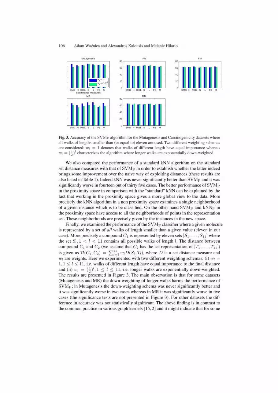
106 Adam Woznica and Alexandros Kalousis and Melanie Hilario
SMD H RIBL S L FS M0
20
40
60
80
100
Set distance measures
Mutagenesis
wl = 1
wl = (1/2)l
SMD H RIBL S L FS M0
20
40
60
80FR
SMD H RIBL S L FS M0
20
40
60
80FM
SMD H RIBL S L FS M0
20
40
60
80MR
SMD H RIBL S L FS M0
20
40
60
80MM
Fig. 3. Accuracy of the SVMP algorithm for the Mutagenesis and Carcinogenicity datasets whereall walks of lengths smaller than (or equal to) eleven are used. Two different weighting schemasare considered: wl = 1 denotes that walks of different length have equal importance whereaswl = ( 1
2)l characterizes the algorithm where longer walks are exponentially down-weighted.
We also compared the performance of a standard kNN algorithm on the standardset distance measures with that of SVMP in order to establish whether the latter indeedbrings some improvement over the naive way of exploiting distances (these results arealso listed in Table 1). Indeed kNN was never significantly better than SVMP and it wassignificantly worse in fourteen out of thirty five cases. The better performance of SVMP
in the proximity space in comparison with the “standard” kNN can be explained by thefact that working in the proximity space gives a more global view to the data. Moreprecisely the kNN algorithm in a non proximity space examines a single neighborhoodof a given instance which is to be classified. On the other hand SVMP and kNNP inthe proximity space have access to all the neighborhoods of points in the representationset. These neighborhoods are precisely given by the instances in the new space.
Finally, we examined the performance of the SVMP classifier where a given moleculeis represented by a set of all walks of length smaller than a given value (eleven in ourcase). More precisely a compound C1 is represented by eleven sets [S1, . . . , S11] wherethe set Sl, 1 < l < 11 contains all possible walks of length l. The distance betweencompound C1 and C2 (we assume that C2 has the set representation of [T1, . . . , T11])is given as D(C1, C2) =
∑11l=1 wlD(Sl, Tl), where D is a set distance measure and
wl are weights. Here we experimented with two different weighting schemas: (i) wl =1, 1 ≤ l ≤ 11, i.e. walks of different length have equal importance to the final distanceand (ii) wl = ( 1
2 )l, 1 ≤ l ≤ 11, i.e. longer walks are exponentially down-weighted.The results are presented in Figure 3. The main observation is that for some datasets(Mutagenesis and MR) the down-weighting of longer walks harms the performance ofSVMP; in Mutagenesis the down-weighting schema was never significantly better andit was significantly worse in two cases whereas in MR it was significantly worse in fivecases (the significance tests are not presented in Figure 3). For other datasets the dif-ference in accuracy was not statistically significant. The above finding is in contrast tothe common practice in various graph kernels [15, 2] and it might indicate that for some

Matching Based Kernels for Labeled Graphs 107
applications also larger subgraphs are correlated with the target variable. The other ob-servation is that, the performance of the representation based on all walks up to a givenlength is comparable to the one where the lengths were fixed to a specified value.
To situate the performance of our relational learner to other relational learning sys-tems we give the best results reported in the literature on the same benchmark datasets.For the Mutagenesis dataset we obtained 91.5 % accuracy (for the Surjections distance)while the best result from the literature (estimated with ten fold cross-validation) was90.4 % [5]. The results for the Carcinogenicity dataset are not directly comparable withother results from the literature since different evaluation metric was used (accuracyinstead area under ROC curve).
7 Conclusions and Future Work
It has been argued in [6] that a “good” kernel for graphs should fulfill at least the follow-ing requirements: (i) should be a good similarity measure for graphs, (ii) its computa-tional time should be possible in polynomial time, (iii) should be positive semidefiniteand (iv) should be applicable for various graphs. In this paper we propose a class ofkernels for graphs which are based on walks without repetitive occurrences of nodes,that are computable in polynomial time, that are positive semidefinite and are applica-ble to a wide range of graphs. Additionally the distinctive feature of our graph kernel isthat, instead of taking into account all the possible subgraphs of a given type, it matchesonly specific subparts. More precisely we proposed a class of kernels for graphs whichdirectly exploit the set distance measures. These kernels are defined in the proximityspace induced by set distance measures where the mapping is defined by a given rep-resentation set. To practically demonstrate the effectiveness of our approach we reportexperimental results for the task of activity prediction of drug molecules.
There are several possible directions for further work. First, we would like to ex-periment with non-PSD kernels such as the one from Equation 2. This is possible sincerecent experimental and theoretical results state that even a kernel which is non-PSDcan be plugged into the SVMs. Second, we will experiment with decompositions ofgraphs into substructures other than walks (e.g. the cyclic patterns from [9]). For suchsubgraphs the standard Euclidean metric can not be used directly and other, more gen-eral distances on graphs (e.g. the graph edit distance) need to be considered. Third, weare going to compare our methods with alternative ways of creating smoother featurespace as mentioned in Section 3. Finally we would like to avoid empty sets in the set ofsubgraphs representation of molecules as shown in Section 6. In particular we are go-ing to experiment with mining frequent (connected) subgraphs approach as presentedin [18, 19].
References
1. Shawe-Taylor, J., Cristianini, N.: Kernel Methods for Pattern Analysis. Cambridge Univer-sity Press (2004)
2. Gartner, T., Flach, P., Wrobel, S.: On graph kernels: Hardness results and efficient alterna-tives. In: Proceedings of the 16th Annual Conference on Computational Learning Theoryand the 7th Kernel Workshop. (2003)

108 Adam Woznica and Alexandros Kalousis and Melanie Hilario
3. Ramon, J., Gartner, T.: Expressivity versus efficiency of graph kernels. In: First InternationalWorkshop on Mining Graphs, Trees and Sequences (help with ECML/PKDD’03). (2003)
4. Kashima, H., Tsuda, K., Inokuchi, A.: Marginalized kernels between labeled graphs. In: Pro-ceedings of 20th International Conference on Machine Learning (ICML-2003), Washington,DC (2003)
5. Mahe, P., Ueda, N., Akutsu, T., Perret, J.L., Vert, J.P.: Extensions of marginalized graphkernels. In: ICML 2004. (2004)
6. Borgwardt, K.M., Ong, C.S., Schonauer, S., Vishwanathan, S., Smola, A.J., Kriegel, H.P.:Protein function prediction via graph kernels. Bioinformatics 21(1) (2005) i47–i56
7. Ralaivola, L., Swamidass, S.J., Saigo, H., Baldi, P.: Graph kernels for chemical informatics.Neural Networks (2005) 1093–1110
8. Borgwardt, K.M., Kriegel, H.P.: Shortest-path kernels on graphs. In: Proceedings of the 5thIEE Internatinal Conference on Data Mining. (2005)
9. Horvath, T., Gartner, T., Wrobel, S.: Cyclic pattern kernels for predictive graph mining. In:Proceedings of KDD’04. (2004)
10. Menchetti, S., Costa, F., Frasconi, P.: Weighted decomposition kernels. In: Proceedings of22nd International Conference on Machine Learning (ICML-2005). (2005)
11. Pekalska, E., Paclık, P., Duin, R.P.: A generalized kernel approach to dissimilarity-basedclassification. Journal of Machine Learning Research 2 (2001) 175–211
12. Haussler, D.: Convolution kernels on discrete structures. Technical report, UC Santa Cruz(1999)
13. Woznica, A., Kalousis, A., Hilario, M.: Kernels over relational algebra structures. In: TheNinth Pacific-Asia Conference on Knowledge Discovery and Data, Hanoi, Vietnam (2005)
14. Ben-David, S., Eiron, N., Simon, H.: Limitations of learning via embeddings in euclideanhalf spaces. Journal of Machine Learning Research 3 (2002) 441–461
15. Collins, M., Duffy, N.: Convolution kernels for natural language. In Dietterich, T.G., Becker,S., Ghahramani, Z., eds.: Advances in Neural Information Processing Systems 14, Cam-bridge, MA, MIT Press (2002)
16. Cumby, C., Roth, D.: On kernel methods for relational learning. In: Proceedings of 20thInternational Conference on Machine Learning (ICML-2003), Washington, DC (2003)
17. Gartner, T.: A survey of kernels for structured data. SIGKDD Explor. Newsl. 5(1) (2003)49–58
18. Deshpande, M., Kuramochi, M., Karypis, H.: Frequent sub-structure-based approaches forclassifying chemical compounds. In: Proceedings of ICDM’03. (2004)
19. Kramer, S., Readt, L., Helma, C.: Molecular feature mining in hiv data. In: Proceedings ofKDD’01. (2001)
20. Eiter, T., Mannila, H.: Distance measures for point sets and their computation. Acta Infor-matica 34(2) (1997) 109–133
21. Horvath, T., Wrobel, S., Bohnebeck, U.: Relational instance-based learning with lists andterms. Machine Learning 43(1/2) (2001) 53–80
22. Ramon, J., Bruynooghe, M.: A polynomial time computable metric between point sets. ActaInformatica 37(10) (2001) 765–780
23. Srinivasan, A., Muggleton, S., King, R., Sternberg, M.: Mutagenesis: ILP experiments in anon-determinate biological domain. In Wrobel, S., ed.: Proceedings of the 4th InternationalWorkshop on Inductive Logic Programming. Volume 237. (1994) 217–232
24. Helma, C., King, R.D., Kramer, S., Srinivasan, A.: The predictive toxicology challenge2000–2001. Bioinformatics 17 (2001) 107–108

Combining Ring Extensionsand Canonical Form Pruning
Christian Borgelt
European Center for Soft Computingc/ Gonzalo Gutierrez Quiros s/n, 33600 Mieres, Spain
Abstract. A common problem in frequent graph mining is the size ofthe output, which can easily exceed the size of the database to analyze.In the application area of molecular fragment mining a promising ap-proach to tackle this problem is to treat certain substructures as a unit.Among such structures, rings are most prominent, and by requiring thateither a ring is present as a whole in a fragment, or not at all, the sizeof the output can be reduced considerably. In this paper I present twoways to combine such ring mining with canonical form pruning.
1 Introduction
In recent years frequent graph mining has become an area of very active research.Given a database of (attributed) graphs, one tries to find all subgraphs that ap-pear with a user-specified minimum frequency. Some algorithms for this task relyon principles from inductive logic programming [5]. However, the vast majoritytransfers techniques from frequent item set mining. Examples are MolFea [9],FSG [10], MoSS/MoFa [1], gSpan [12], CloseGraph [13], FFSM [7], and Gaston[11]. A related, but slightly different approach is used in Subdue [4].
The basic idea is to grow subgraphs into the graphs of the database, addingan edge and maybe a node in each step, counting the number of graphs contain-ing each grown subgraph, and eliminating infrequent subgraphs. Unfortunately,with this method the same subgraph can be constructed in several ways, addingits nodes and edges in different orders. The predominant method to avoid theensuing redundant search is to define a canonical form of a graph that uniquelyidentifies it up to automorphisms: together with a specific way of growing thesubgraphs it enables us to determine whether a given subgraph can be prunedfrom the search tree (see, for example, [3] for a family of such canonical forms).
Another common problem in frequent graph mining is the size of the output,which can easily exceed the size of the database to analyze. To tackle this prob-lem, it can be useful to restrict the output to subgraphs with certain meaningfulproperties. In the application area of molecular fragment mining, for example,treating rings as units—that is, requiring that either a ring is present as a whole,or not at all—not only reduces the size of the output, but also improves its in-terpretability and speeds up the mining process considerably [6].
110 Christian Borgelt
However, [6] employed a repository of reported fragments in order to suppressduplicate fragments. The canonical form pruning approach is clearly preferable,in particular, because it makes the method substantially simpler to parallelize.In this paper I present two ways in which ring mining—that is, using extensionsby full rings instead of extensions by individual ring edges—can be combinedwith canonical form pruning: a filter approach and a reordering approach.
2 A Filter Approach to Ring Mining
Ring Preprocessing. Ring mining requires preprocessing the rings in thegraphs (here usually: molecules) to analyze: given a user-specified range of ringsizes, all rings within this size range are marked in the graphs [6]. Technically,there are two parts: a marker in the edge attribute, fundamentally distinguishingring edges from non-ring edges, and a set of flags identifying the different ringsan edge is contained in. (Note that an edge can be part of several rings.)
Filtering Open Rings. If we require the output to have only complete rings, wehave to identify and remove fragments with ring edges that do not belong to anycomplete ring. Since ring edges have been marked in the preprocessing, we knowwhich edges are ring edges. Using the same procedure as for the preprocessing,we mark rings in the fragment, but only set the ring flags, while the edge typemarker is kept. Afterwards we can find edges that belong to incomplete rings bysimply checking whether a ring edge (as identified by its type marker) did notreceive any ring flags. If there exists such an edge, the fragment is discarded.
Filtering Unclosable Rings. Canonical form pruning allows to restrict thepossible extensions of a fragment [3]. For the canonical forms of gSpan [12] andMoSS/MoFa [1] these are so-called rightmost extensions and maximum sourceextensions, respectively. Their effect is that due to previous extensions certainnodes in the graph become unextendable, that is, no new edge may be attachedto them. This can easily be exploited to prune the search. Obviously, a necessary(though not sufficient) condition for all rings being closed is that every node haseither zero or at least two incident ring edges. If there is a node with only oneincident ring edge, this edge must be part of an incomplete ring. Hence we canfilter fragments in the search by checking whether any non-extendable node hasonly one incident ring edge. If this is the case, the fragment can be discarded.
Merging Ring Extensions. The two filtering methods described above workon individual edges and hence they cannot always detect if an extension by a ringedge only leads to fragments with complete rings that are infrequent. Consider,for example, a database with two molecules: one is a ring with 5 carbon atoms,the other a ring with 6 carbon atoms (all bonds are single). If we want to findfragments that are part of both molecules, we need not consider any extension bya ring bond, since there is no common fragment with a complete ring. However,any single ring bond is contained in both fragments and thus it is, in itself, afrequent fragment. Therefore, by working on individual bonds, we only recognizeafter constructing the full 5-ring that there is no common fragment.

Combining Ring Extensions and Canonical Form Pruning 111
To avoid such redundant search, we add all edges of a ring that an extensionedge is contained in, thus distinguishing extensions that start with the samesingle edge, but lead into rings of different size or different composition. Then wedetermine the support and prune infrequent extensions, and finally we trim andmerge ring extensions that share the same initial edge. Note that the resultingsituation differs considerably from direct extensions by individual edges. In thefirst place, all extensions by ring edges, which are frequent as ring edges, butbecome infrequent when completed into rings (and thus cannot produce anyoutput), have been removed. In addition, for the remaining edges all embeddings(that is, occurrences of the fragment in the graph database), which lead toinfrequent fragments once rings are completed, have been eliminated.
3 A Reordering Approach to Ring Mining
Even with merging ring extensions the search is still based on an edge-by-edgescheme and thus fragments grow fairly slowly. It would be better if we could addcomplete rings in one step, thus adding several edges to the fragment. Unfortu-nately such an approach interferes with canonical form pruning, as is discussedbelow. However, the problems can be solved, although up to now I only achieveda solution for the breadth-first search canonical form of MoSS/MoFa [3].
Ring Preprocessing. Although for the filtering approach it is sufficient tomark rings in the user-specified size range, the reordering approach also needspseudo-rings, as I call them, to be marked. These are rings of smaller size thanthe user specified, which consist only of edges that are part of rings within theuser-specified size range. As an example consider the molecule shown on the leftof Figure 3: if only rings with 5 and 6 bonds are marked, this molecule containsa pseudo-ring of size 3 comprising the atoms labeled 1, 3, and 4.
Ring Extensions and Canonical Forms. If we add complete rings in one stepand want to use canonical form pruning, we have to order the new edges in sucha way that the result is (as far as possible) in canonical form. This can easily beachieved with a recursive procedure similar to the canonical form test. However,this can have the effect that—due to asymmetries in the ring—we commit toa numbering of the nodes that prevents us from finding certain fragments. Thereason is that in order to be in canonical form an (asymmetric) ring may need itsnodes to be numbered differently depending on whether it is considered purely(i.e. only ring edges are present) or whether it has branches attached to it.
As an example consider the molecules shown in Figure 1 and assume theorderings N ≺ O ≺ C and = ≺ -. The nodes of the pure ring can be numbered intwo ways in a breadth-first manner starting at the nitrogen atom (as shown inthe top part of Figure 1). Of course, they lead to different code words, which areshown in the middle. Since single bonds precede double bonds, the upper codeword is smaller and thus the left fragment is in canonical form. If, however, weconsider the ring with an oxygen atom attached (as shown in the lower part ofFigure 1), the alternative node numbering yields the canonical form. The reason

112 Christian Borgelt
NO O0 2
4
5
3
1
N 0-C1 0-C2 1-C3 2-C4 3-C5 4=C5
NO O0 1
3
5
4
2N 0-C1 0-C2 1-C3 2-C4 3=C5 4-C5
NO O0
2
4
6
3
1 5
N 0-C1 0-C2 1-C3 2-C4 2-O5 3=C6 5-C6
NO O0
1
3
6
5
2 4N 0-C1 0-C2 1-C3 1-O4 2-C5 3-C6 5=C6
Fig. 1. Attaching a branch to a ring can change the ordering for the canonical form.
is that the attached bond to the oxygen atom has to be inserted into rather thanappended to the code word. As a consequence we cannot simply commit to thenumbering of the nodes as it is prescribed by the canonical form of a ring, sincethis numbering may change when branches or other rings are added.
A second, even nastier problem is posed by connected or even nested rings:if two ring extensions follow each other, their edges may have to be “spliced” toconstruct a proper code word. In doing so, one has to take care that edges can bereordered in a sufficiently flexible way, so that no fragments get lost due to thecanonical form pruning. On the other hand, one also has to make sure that noduplicates result, which cannot be detected with a canonical form test. This isfairly difficult to achieve, in particular if the fragment contains branching pointsof equivalent ring edges, that is, ring edges that all start at the same node andhave the same edge attribute and the same destination node attribute.
Canonical Form Pruning for Ring Extensions. A strategy to overcome theabove problems consists in keeping (and thus also extending) fragments that arenot in canonical form, but that could become canonical once branches are added.Which non-canonical fragments to keep is determined as follows: adding all edgesof a ring can be seen as adding its initial edge as in an edge-by-edge procedure,and some additional edges, the positions of which are not yet fixed. Hence wesplit the code word into two parts: a fixed part, which would also be built byan edge-by-edge procedure, and a volatile part comprising the additional bonds.The fixed part is the prefix of the code word up to (and including) the last edgeadded in an edge-by-edge manner, and the volatile part is the suffix of the codeword after this edge. If the current code word deviates from the canonical codeword in the fixed part, the fragment is pruned, otherwise it is kept.
As an example consider the search tree shown in Figure 2. The search startsat the nitrogen atom and constructs the ring with both possible numberings ofthe nodes. The form in the left branch is canonic (indicated by a solid box), soit is kept. In the form in the right branch only the first ring bond (from thenitrogen atom to the right carbon atom) is fixed, every other bond is volatile.Since the code word for this fragment deviates from the canonical one only atthe 5th bond (see Figure 1), we may not discard it. However, we mark it asnon-canonical (indicated by a dashed box), so that it is not reported.
On the next level, adding the bond to the oxygen atom in the two possibleplaces yields, for each branch, one canonical (solid box) and one non-canonical

Combining Ring Extensions and Canonical Form Pruning 113
N
NO O0 2
4
5
3
1NO O0 1
3
5
4
2
NO O0 2
5
6
3
14
NO O0
2
4
6
3
1 5
NO O0 1
3
6
4
25
NO O0
1
3
6
5
2 4
NO O0
2
6
7
3
14 5
NO O0
123
45
6
7
Fig. 2. Search tree for an almost symmetric ring with two identical branches.
N0
1
586
24
3
79
586
24
7
N
N
N0 1
354
2N0
1
376
25
4
N0
1
576
24
3
N0
1
365
24
4
87
N0
1
365
24
8
97
Fig. 3. Splicing equivalent bonds of ring extensions to achieve canonical form.
fragment (no box). The non-canonical fragments both differ in the fixed part,which now consists of the first three bonds1, and hence they are both pruned.Extending the canonical fragments adds the other bond to an oxygen atom, thusmaking the fragment symmetric again (with the exception of the double bond).Hence the left fragment is in canonical form. The fragment in the right branch,however, is not canonical. Nevertheless it has to be kept: the first four bonds arefixed, but it deviates from the canonical code word only in the 7th bond.
In order to handle connected and nested rings, we have to consider how theedges of a ring extension may be “spliced” with edges already in the fragment.The problem here are branching points, where several equivalent edges start (i.e.edges with the same attribute and same attribute of the destination node). Asan example consider the molecule on the left of Figure 3, the relevant equivalentedges of which are highlighted. Part of an example search for this fragment(shown in the middle) starts from the nitrogen atom, adds a 6-bond ring andthen a 3-bond ring. If we only allowed, for example, shifts of new bonds to the leftup to equivalent bonds, we can only reach the upper form. However, the canonicalform is the lower one. On the other hand, we may not reorder equivalent edgesfreely, as this would interfere with keeping certain non-canonical fragments: thefragments in the first level of the search tree in Figure 2 differ only in the orderof the two equivalent bonds starting at the nitrogen atom. If adding another ringto this atom could change this order, duplicate fragments could result.
1 Note how adding the bond to the oxygen atom turned one of the volatile ring bondsinto a fixed one: everything preceding the bond characterizing an extension—whetherit is a single non-ring bond or the first bond of a ring extension—becomes fixed.

114 Christian Borgelt
N
N0 3
5
42
1
N0 2
4
31
2
N0 2
4
53
1
N0 3
5
41
2
N0 2
5
41
3
N0 3
5
41
2
N0 3
5
41
2
N0 2
4
53
1
N0 3
5
42
1
N0 3
5
41
2
N0 3
5
41
2
N0 2
5
41
3
N0 3
5
41
2
N0 1
4
53
2
N0 1
4
52
3
N0 3
5
41
2
N0 3
5
42
1
N0 2
4
53
1
N0 3
5
41
2
N0 1
4
53
2
N0 1
4
52
3
also incanonicalform
Fig. 4. Search tree for nested rings of different size (with ring order pruning).
As a consequence, the splicing rule for equivalent edges must be as follows: theorder of the equivalent edges already in the fragment must be maintained, andthe order of the equivalent new edges must be maintained (to avoid “flipping”rings). In addition, no new edge must be shifted into the fixed part. However,any sequence satisfying these conditions is acceptable and must be considered.In other words: the two sequences of equivalent edges—one from the existingfragment and one from the added ring—may be merged in a zipper-like manner,selecting the next edge from either list, but maintaining the order in each list.
This also explains why we need pseudo-rings: without them it would be im-possible in some cases to achieve canonical form. If, in the example, we couldonly add the 5-ring and the 6-ring, but not the 3-ring (see the right of Figure 3),the upward bond from the atom numbered 1 would always precede at least oneof the other two bonds that are equivalent to it. However, in the canonical form(shown at the top left of Figure 3) the upward bond succeeds both other bonds.
Unfortunately, the same fragment can now be reached in the same form indifferent ways. To see this, consider the search tree shown in Figure 4: the samefragment results in six different forms, each of which (including the canonicalform) occurs twice. Hence we need an additional test to augment canonical formpruning. The idea underlying this test is that the canonical form not only fixesan order of the bonds, but also an order of the rings: order the rings by the firstedge in the canonical form that is contained in them. Break ties by consideringthe second, third etc. edges in the canonical form the rings contain.
This ring order is exploited as follows: we mark all edges in the fixed part ofthe fragment as well as all new edges. Then we traverse the unmarked ring edges.For each of these edges we eliminate all rings it is contained in (by removing ringflags, which are set in the fragment in the same way as in the ring preprocessing).If by this procedure all ring flags of a marked edge (fixed edge or new edge) areremoved, this marked edge is part of a ring preceding the newly added one (w.r.t.the ring order defined above). Therefore it had to be added before the currentring. If, however, no marked edge loses all its ring flags, there exists a ring thatsucceeds the currently added one. This ring should rather be added later andthus the fragment is discarded, even if it is in canonical form.

Combining Ring Extensions and Canonical Form Pruning 115
2 2.5 3 3.5 4 4.5 5
0
5
10
15
20
25
time/secondsreordermerge ringsclose ringsrepository
2 2.5 3 3.5 4 4.5 5
0
2
4
6
8 fragments/104
reordermerge ringsclose ringsrepository
2 2.5 3 3.5 4 4.5 5
0
1
2
3
4
5 embeddings/106
reordermerge ringsclose ringsrepository
Fig. 5. Experimental results on theIC93 data. The horizontal axis showsthe minimal support in percent. Thecurves show the number of generatedfragments (top left), the number ofgenerated embeddings (top right), andthe execution time in seconds (bottomleft) for the four different strategies.Note that the dotted line (repository)is often covered by the solid line.
As an example consider again Figure 4. The canonical form (fragment atbottom left) shows that the 6-bond ring succeeds both the 3-bond ring and the5-bond ring, as it does not contain the first bond. The second bond shows thatthe 3-bond ring precedes the 5-bond ring. For the second fragment in canonicalform (see arrow) the test, as outlined above, fails, using any of the highlightededges. However, for the leftmost fragment in the bottom row the ring flag removalalways leaves a marked edge flagless and thus it is accepted.
4 Experiments
I incorporated the described methods into the MoSS program.2 As a test datasetI used the well-known subset of the Index Chemicus 1993 [8]. The results areshown in Figure 5: each curve corresponds to one of the approaches, which wereexecuted with (full) perfect extension pruning [2]. The black dotted line refers tothe repository-based approach, the solid black line to the reordering approach.The filter approach I used in two flavors: with ring extensions and consecu-tive merging (solid grey line) and using only open and unclosable ring filtering(dashed grey line). These results show that the somewhat complicated treatmentof ring extensions in order to combine them with canonical form pruning clearlypays off, as the reordering method hugely outperforms the filter approaches.2 MoSS is available for download under the Gnu Lesser (Library) Public License athttp://fuzzy.cs.uni-magdeburg.de/∼borgelt/moss.html.The test system was a Lenovo Thinkpad X60s (Intel Core [email protected], 1GB) withS.u.S.E. Linux 10.0, IBM’s Jikes compiler 1.22, and Sun’s Java 2 1.5.0 07.

116 Christian Borgelt
5 Conclusions
In this paper I developed two methods to combine canonical form pruning withring extensions, which are very useful for molecular fragment mining. The firstmethod is based on a filter approach, which exploits the requirement for closedrings to restrict the output and prune the search. This approach is simple andstraightforward, but not competitive in terms of running time or memory usageas the experiments show. Therefore it is indeed worthwhile to invest into the morecomplicated reordering method, which enables us to do full ring extensions, thusconsiderably reducing the height of the search tree and its number of nodes.
References
1. C. Borgelt and M.R. Berthold. Mining Molecular Fragments: Finding RelevantSubstructures of Molecules. Proc. IEEE Int. Conf. on Data Mining, 51–58. IEEEPress, Piscataway, NJ, USA 2002
2. C. Borgelt, T. Meinl, and M.R. Berthold. Advanced Pruning Strategies to SpeedUp Mining Closed Molecular Fragments. Proc. IEEE Conf. on Systems, Man andCybernetics, CD-ROM. IEEE Press, Piscataway, NJ, USA 2004
3. C. Borgelt. On Canonical Forms for Frequent Graph Mining. Proc. 3rd Int. Work-shop on Mining Graphs, Trees and Sequences, 1–12. ECML/PKDD 2005 Organi-zation Committee, Porto, Portugal 2005
4. D.J. Cook and L.B. Holder. Graph-Based Data Mining. IEEE Trans. on IntelligentSystems 15(2):32–41. IEEE Press, Piscataway, NJ, USA 2000
5. P.W. Finn, S. Muggleton, D. Page, and A. Srinivasan. Pharmacore DiscoveryUsing the Inductive Logic Programming System PROGOL. Machine Learning,30(2–3):241–270. Kluwer, Amsterdam, Netherlands 1998
6. H. Hofer, C. Borgelt, and M.R. Berthold. Large Scale Mining of Molecular Frag-ments with Wildcards. Intelligent Data Analysis 8:495–504. IOS Press, Amster-dam, Netherlands 2004
7. J. Huan, W. Wang, and J. Prins. Efficient Mining of Frequent Subgraphs in thePresence of Isomorphism. Proc. 3rd IEEE Int. Conf. on Data Mining, 549–552.IEEE Press, Piscataway, NJ, USA 2003
8. Index Chemicus — Subset from 1993. Institute of Scientific Information, Inc. (ISI).Thomson Scientific, Philadelphia, PA, USA 1993http://www.thomsonscientific.com/products/indexchemicus/
9. S. Kramer, L. de Raedt, and C. Helma. Molecular Feature Mining in HIV Data.Proc. 7th ACM SIGKDD Int. Conf. on Knowledge Discovery and Data Mining,136–143. ACM Press, New York, NY, USA 2001
10. M. Kuramochi and G. Karypis. Frequent Subgraph Discovery. Proc. 1st IEEE Int.Conf. on Data Mining, 313–320. IEEE Press, Piscataway, NJ, USA 2001
11. S. Nijssen and J.N. Kok. A Quickstart in Frequent Structure Mining Can Makea Difference. Proc. 10th ACM SIGKDD Int. Conf. on Knowledge Discovery andData Mining, 647–652. ACM Press, New York, NY, USA 2004
12. X. Yan and J. Han. gSpan: Graph-Based Substructure Pattern Mining. Proc. 2ndIEEE Int. Conf. on Data Mining, 721–724. IEEE Press, Piscataway, NJ, USA 2002
13. X. Yan and J. Han. Closegraph: Mining Closed Frequent Graph Patterns. Proc.9th ACM SIGKDD Int. Conf. on Knowledge Discovery and Data Mining, 286–295.ACM Press, New York, NY, USA 2003

Structured Kernels for Automatic Detection ofProtein Active Sites
Elisa Cilia1, Alessandro Moschitti1, Sergio Ammendola2, and Roberto Basili1
1 Department of Computer Science, System and ProductionUniversity of Rome, Tor Vergata,
Via Della Ricerca Scientifica s.n.c., 00133, Roma, [email protected]
{moschitti,basili}@info.uniroma2.it2 Ambiotec sas
SMEfield: biotechnology
Via F. Acqua Mariana 125, 00040, Roma, ITALYPI 07635910636
Abstract. In this paper, we design novel models based on Support Vec-tor Machines and Kernel Methods for the automatic protein active siteclassification. We devise innovative attribute-value and tree substruc-ture representations derived from biological and spatial information ofproteins. We experimented such models with the Protein Data Bank ad-equately pre-processed to make explicit the active site information. Ourresults show that structural kernels used in combination with polyno-mial kernels can be effectively applied to discriminate an active site fromother regions of a protein. Such finding is very important since it firstlyshows the successful identification of catalytic sites of a very large familyof catalytic proteins belonging to a broad classes of enzymes.
1 Introduction
Recent research in Bioinformatics has been devoted to the production and un-derstanding of genomic data. One important step in this direction is the studyof the relation between molecular structures and their functions, which in turndepends on the discovering of the protein active sites. As there is a large numberof synthesized proteins which have no associated function yet, i.e. whose functionremains unknown, automatic approaches for active site detection are critical.
Currently, the general strategy used to identify a protein active site involvesthe expertise of researchers and biologists accumulated in years of study onthe target protein as for example in [1]. This manual approach is conductedessentially using homology based strategies, i.e. inferring the function of a newprotein based on a close similarity to already annotated proteins. Sometimesproteins with the same overall tertiary structure can have different active sites,i.e. different functions and proteins with different overall tertiary structure can

118 Cilia et al.
show the same function and similar active sites. In these cases homology basedapproaches are inadequate. Moreover, there is no general automated approach toprotein active site detection, although it is evident its usefulness to restrict thenumber of candidate sites and also to automatically learn rules characterizingan active site [2].
In this paper we define the problem of determining protein active sites interms of a classification problem. We modeled protein active site based on bothattribute/value and structural representations. The former representation is a setof standard linear features whereas the latter is constituted by tree structuresextracted from graphs associated with proteins or their candidate sites. Thegraph nodes (or vertexes) represent amino acids (or better residues) and edgesrepresent distances in the three-dimensional space between these residues.
We applied these representations to SVMs using polynomial kernels, tree ker-nels and some combinations of them. To experimentally evaluate our approach,we created a data set, using the protein structures retrieved from the ProteinData Bank (PDB) [3] maintained by the Research Collaboratory for StructuralBioinformatics (RCBS) at http://www.rcbs.org. The combined kernels show thehighest F1 measure, i.e. 68%, in the detection of active sites. This is an importantand promising result considering that the baseline based on a random selectionof active sites has an upperbound of only 2%.
In the remainder of this article Section 2 describes the faced problem. Section3 describes the proposed linear and structural features. Section 4 describes theexperimental evaluation and reports the results of the classification experiments.Finally, in Section 5, we summarize the results of the previous sections andpropose other interesting future research lines.
2 Protein active site classification
An active site in a protein is a topological region which defines the protein func-tion, in other words it is a functional domain in the protein three-dimensionalstructure (see also [2]). In a cell there are many types of proteins which carry outdifferent functions. The enzymes are those proteins able to accelerate chemicalprocesses inside a cell. This type of proteins are distinguished from structuraland supplying proteins for their catalytical action on the large part of moleculesconstituting the living world. We limit our research to a particular class of en-zymes, the hydrolases.
Hydrolases are maybe the most studied and known type of enzymes. Theycatalyze hydrolysis reactions, generically consisting in the cleavage of a biochem-ical compound thanks to the addition of a water molecule (H2O). The character-istic of some hydrolases to catalyze reactions in the presence of a water moleculemotivates our model: as an hydrolase active site, we choose a sphere in a three-dimensional space centered in the coordinates of the oxygen atom of a watermolecule. This sphere includes a portion of the protein within its volume, thatis a number of amino acids which could reciprocally interact with other aminoacids in the surrounding space, or with water molecules. In this first analysis, we

Structured Kernels for Automatic Detection of Protein Active Sites 119
consider a sphere with a radius of 8 A, which is the maximum distance neededfor the water-residue interaction.
Figure 1(a), shows the active site of 1A2O protein structure and its repre-sentation according to our model. The protein residues are colored in light graywhereas the particular catalytic residues are in dark gray. The center of thesphere is the black colored oxygen atom of a water molecule.
(a) (b)
Fig. 1. (a) A sphere (positive example). (b) Distances.
2.1 The computational model
As stated in the previous section, we defined the functional site identification asa classification problem, where the objects we want to classify are protein activesites. We represent the portion of the protein contained in a spherical three-dim-ensional region with a completely connected graph. Each vertex of this graph isa residue and each edge represents the distance in the three-dimensional spacebetween a pair of vertexes.
Every amino acid is represented by two points in the three-dimensional space:one which represents an amino acid main-chain (the α-carbon atom of the aminoacid, Cα) and one which represents an amino acid side-chain (the centroid be-tween the coordinates of the atoms belonging to the amino acid side-chain, SC)(see Figure 1(b)). The same kind of approximation has been described in [4]because it seems to provide a good balance between fuzziness and specificity inthese kind of applications.
In Figure 1(b) the three-dimensional SC-SC distances and Cα-Cα distancesare indicated between the represented chain of three residues. An object (mod-eled by a graph centered on a water molecule) can be classified as being an activesite or not with a binary classifier. Thus, we consider as a positive example, agraph whose set of vertex includes all the catalytic amino acids and as a negativeexample a graph which contain no catalytic amino acid. Moreover, to reduce the

120 Cilia et al.
task complexity, we extract, from the initial completely connected graph, somespanning substructures which preserve the edges within the maximum interac-tion distance of 5 Abetween the side-chains of the residues.
The next section shows how the above representation model can be used alongwith Support Vector Machines to design an automatic active site classifier.
3 Automatic classification of active sites
Previous section has shown that the active site representation is based on graphs.To design the computational model of these latter, we have two possibilities: (1)we extract scalar features able to capture the most important properties of thegraph and (2) we can use graph based kernels [5] in kernel-based machines suchas Support Vector Machines [6]. Point (2) often leads to high computationalcomplexity. We approached such problem by extracting a tree forest from thetarget graph and applying efficient tree kernels [7].
3.1 Scalar features
Scalar features refer to typical chemical values of the molecules described in thetarget graph. We defined 5 different types of such features (see Table 1):
The first class of linear features (C1) encodes chemical and physical propertiesof the graph. This class represents properties such as hydrophobicity, polarity,polarizability and Van der Waals volume of the amino acids composing thesphere. The encoding is the same used in [8] where the features were used toclassify the function of proteins.
The second class of linear features (C2) encodes the amino acid compositionof a spherical region. There is a feature associated with every labeled vertex(amino acid) in the graph, weighted with the inverse of the distance from theoxygen atom of the water molecule which is the center of the sphere. This groupof features emphasizes the importance of the interaction distance of a residuewith respect to a water molecule.
The third class of features (C3) represents charge or neutrality of a sphericalregion. This is measured by counting the number of positively or negativelycharged amino acids.
Another group of linear features (C5) encodes the quantity of water in asphere. This is measured by counting the number of water molecules within thesphere radius. This group of features is motivated by the fact that biologistsobserved that an active site is usually located in a hydrophobic core of theprotein while on the surface the quantity of water is higher and the residuesexposed to the solvent are not hydrophobic.
Finally, the last class of linear features (C6) is the one which measures theatomic density of the sphere calculated as the total number of atoms in thesphere.
It should be noted that (a) the last two classes of linear features are madediscrete using a different number of value intervals. A feature is associated with

Structured Kernels for Automatic Detection of Protein Active Sites 121
Table 1. Representation: feature classes
Linear Features Description
1st Class Physical and chemical properties (amino acid attributes)2nd Class Amino acidic Composition3rd Class Charge/Neutrality5th Class Water molecule quantity6th Class Atomic density
Structural Features Description
4th Class Tree substructures from tertiary structure
an example if the measured value of a certain property falls in the correspon-dent range. (b) These features are often used to describe protein structures insimilar tasks of Bioinformatics [8] and to develop software for protein structureprediction like Modeler 7v7.
3.2 Structural features
We designed a class of structural features to encode the three-dimensional struc-ture (tertiary structure) or better, the spatial configuration characterizing aspherical region, i.e. the set of amino acids composing it with their 3D distances.As previously mentioned this representation results in a completely connectedgraph since every vertex is connected to any other vertex in the sphere graphthrough an edge labeled with the 3D distance of the pair.
Starting from this completely connected
Fig. 2. Graphical representationof a tree of a sphere
graph, we extract some tree substructuresusing heuristics: for example, the one whichpreserves the maximum interaction distancesto 5 Abetween the side-chains of the residuesand a minimum spanning tree algorithm. Suchheuristics is motivated by the observationthat to perform the catalytic function it isnecessary that the side-chains of the cat-alytic residues can interact with each otherand with the substrate. The maximum inter-action distance between atoms in differentresidue side-chains is usually of about 3-4A. We chose a cut-off distance of 5 Ato takeinto consideration our approximation in therepresentation of residues (Figure 1(b)).
The applied heuristics lead possibly to the separation in disconnected com-ponents of the initial graph. From each of these components, using the Primalgorithm [9], we extract the spanning tree which minimizes the cost functionc(T ), i.e. the interaction distances dxy between the side-chains of the residues xand y. Note that as some graphs contain more than one connected component,

122 Cilia et al.
the Prim algorithm is applied to each of them. This leads to the extraction of atree forest.
We add the water molecule (center of the sphere) as root node to the obtainedspanning tree. In Figure 2, we show a tree which can represent the sphericalregion in Figure 1(a). In bold light gray, we highlight the nodes which representcatalytic amino acids.
The tree substructures generated for each example constitute the featuresanalyzed by our tree kernel function. If two examples are described by two treeforests, we can use as a kernel function the summation of a tree kernels appliedto all possible pairs coming from such forests.
4 Experiments
In the subsequent subsections, we describe our classification experiments carriedout on the data set that we generated from the Protein Data Bank.
4.1 Experimental set-up
The evaluations were carried out using the SVM-light-TK software [10] (avail-able at http://ai-nlp.info.uniroma2.it/moschitti/) which encodes tree kernels inSVM-light [11]. We used the polynomial kernels for the linear features and treekernels for the structural feature processing. More precisely, we used the SSTand the PT kernels described in [7] on a simple tree, i.e. the main tertiary struc-ture3, or on a tree forest (see Section 3.2). The former kernels are indicated withSST T and PT T whereas the latter are called SST F and PT F. The kernel fortree forest is simply the summation of all possible pairs of trees contained in twoexamples.
We experimented our models with the protein structures downloaded fromthe Protein Data Bank (PDB). We adequately pre-processed PDB files to obtainall the information of interest for this task. In particular, we created a data setof 14,688 examples from 48 hydrolases from the PDB structures. The data set iscomposed of 171 positive examples and 14,571 negative examples, which meansa 1
125 ratio between positive and negative examples.The results were evaluated by applying a 5-fold cross validation4 on this data
set measuring the performance with the F1 measure 5.A noticeable attention was devoted to parameterization (cost factor, decay
factor, etc.)
3 The single tree structure is the most relevant one in the forest, that is, the tree whichcontains at least a catalytic amino acid and the two nearest residue side-chains ofthe sphere
4 We separated the data set into five parts, each one composed of examples belongingto a set of nine or ten protein structures randomly assigned to this set.
5 F1 assigns equal importance to Precision P and Recall R i.e. F1 = 2P ·RP+R

Structured Kernels for Automatic Detection of Protein Active Sites 123
Table 2. (a) Linear features performance. (b) Combined kernel performance.
(a)
Linear Precision Recall F1
C1 5.5% 66.7% 10.2%C2 55.9% 63.3% 59.4%C3 20% 3.3% 5.7%C5 2.2% 30% 4.1%C6 5.5% 13.3% 7.8%
(b)
Precision Recall F1 ±Std.Dev.
L 62.3% 55.4% 56.2% ±6.8
SST F 66.2% 31.8% 39.9% ±13.7
L+SST F 82.9% 58.6% 68.3% ±14.5
4.2 Experiment results
Table 2(a) reports the results on the 5 types of linear features using the poly-nomial kernel (degree 3). These results are only indicative as we did not run across validation procedure. We note that most linear features cannot discrimi-nate between active and non-active site. Only, the second class, which encodesthe structural information, shows a meaningful F1. The general low results oflinear features is caused by the remarkable complexity of the task as suggestedby the F1 upperbound of the random selection, i.e. ' 1.6%.
In order to boost the classification performance, we experimented with thestructural kernels. Table 2(b) summarizes the cross validation results: Row 2reports the results with polynomial kernels on all the linear features (L), Row3 shows the outcomes of the SST kernels on the tree forest (SST F) and Row 4illustrates the performance of the polynomial kernel summed to the SST kernelon the tree forest (L+SST F). The ± sign precedes the standard deviation eval-uated on the 5 folds. It is worth to note that the F1 obtained with the linearfeatures (56.24%) improves by 12 absolute points if we use the combined model(L+SST F), i.e. 68%.
We also experimented different variants of Tree Kernels, i.e. based on PTs.The results of the cross validation experiments are summarized in Table 3: Row 2reports the results with polynomial kernel plus SST F (applied to linear featuresand a forest structure), Row 3 reports the cross validation results of polynomialkernel plus SST T (applied to linear features and a tree structure) and finallyRow 4 illustrates the performance of the additive combination of polynomialwith the PT kernel (PT T) (on linear features and a tree structure).
The results show that the high- L+TK Precision Recall F1 ±Std.Dev.SST F 82.9% 58.6% 68.3% ±14.5SST T 79.7% 51.7% 62.3% ±10.4PT T 80.4% 41.2% 54.4% ±9.1
Table 3. Tree kernel impact
est F1 measure can be achieved withthe SST F but quite similar per-formance can be obtained repre-senting examples with only a treestructure in the forest, i.e. SST T.In contrast to our expectations thePT kernel, which may be considered the one most suitable for this task, showsthe lowest F1. The most plausible explanation is the highest complexity on de-riving its correct parameterization.

124 Cilia et al.
Overall, the very good F1 of our best model suggests that our classificationsystem can be a useful tool to help the biology researcher to study the proteinfunctions.
5 Conclusions
In this paper, we have studied the problem of the identification of protein func-tional sites. We have defined a novel computational representation based onbiological and spatial considerations and several classes of linear and structuralfeatures.
The experiments with SVMs using polynomial and tree kernels and theircombinations show that the highest F1, i.e. 68%, is achieved with the combinedmodel. Such finding is very important since it firstly shows the successful iden-tification of catalytic sites of a very large family of catalytic proteins belongingto a broad classes of enzymes. Moreover, our work highlights the importance ofstructural information in the detection of protein active sites. This result mo-tivates the need of structural representations which we efficiently modeled bymeans of tree kernels.
References
1. Cilia, E., Fabbri, A., Uriani, M., Scialdone, G.G., Ammendola, S.: The signa-ture amidase from sulfolobus solfataricus belongs to the cx3c subgroup of enzymescleaving both amides and nitriles: Ser195 and cys145 are predicted to be the activesites nucleophiles. The FEBS Journal 272 (2005) 4716–4724
2. Tramontano, A.: The ten most wanted solutions in Protein Bioinformatics. Chap-man & Hall/CRC Mathematical Biology and Medicine Series (2005)
3. Berman, H.M., Westbrook, J., Feng, Z., Gilliland, G., Bhat, T.N., Weissig, H.,Shindyalov, I.N., Bourne, P.E.: The protein data bank. Nucleic Acids Res 28(1)(2000) 235–242
4. Meng, E.C., Polacco, B.J., Babbitt, P.C.: Superfamily active site templates. PRO-TEINS: Structure, Function, and Bioinformatics 55 (2004) 962–976
5. Gartner, T.: A survey of kernels for structured data. Multi Relational Data Mining(MRDM) 5 (2003) 49–58
6. Vapnik, V.: The Nature of Statistical Learning Theory. Springer (1995)7. Moschitti, A.: Efficient convolution kernels for dependency and constituent syntac-
tic trees. In: Proceedings of The 17th European Conference on Machine Learning,Berlin, Germany, 2006, Berlin, Germany (2006)
8. Borgwardt, K.: Graph-based Functional Classification of Proteins using KernelMethods. Ludwig Maximilians University of Monaco (2004)
9. Prim, R.C.: Shortest connection networks and some generalizations. Bell Syst.Tech. Journal 36 (1957) 1389–1401
10. Moschitti, A.: A study on convolution kernel for shallow semantic parsing. In:Proceedings of the 42th Conference on Association for Computational Linguistic(ACL-2004), Barcelona, Spain (2004)
11. Joachims, T.: Making large-scale svm learning practical. In: Advances in KernelMethods - Support Vector Learning, B. Scholkopf, C. Burges and A. Smola editors(1999)

Learning Structured Outputs via Kernel
Dependency Estimation and Stochastic
Grammars
Fabrizio Costa1, Andrea Passerini1, and Paolo Frasconi1
Dipartimento di Sistemi e Informatica, Universita degli Studi di Firenze
Abstract. We focus on graph-valued outputs in supervised learningand propose a novel solution to the pre-image problem in the kerneldependency estimation framework. Output structures are generated bya stochastic grammar and the output feature space is directly associatedwith the set of productions for the grammar. The regression estimationstep learns to map input examples into a feature vector that counts thenumber of applications of each production rule. A max-propagation al-gorithm finally builds the predicted output according to the normalizedcounts. We test our method on a ambiguous context free grammar (CFG)parse tree reconstruction problem. We show on an artificial dataset thatmimics the prepositional attachment problem how learning the numberof applications of each production rule on a per example base allows CFGparser to better tackle ambiguity issues.
1 Introduction
A structured output prediction problem can be formulated as a supervised learn-ing problem in which the output or target space is not restricted in any wayand can be any set (e.g. a set of graphs or sequences). In this way, severalpredictions can be made collectively on the same input instance, still main-taining that instances are sampled independently. Formally, we denote by Xand Y the input and output spaces, respectively. Examples are in the formD = {(x1, y1), . . . , (xm, ym)} with xi ∈ X and yi ∈ Y and are sampled iden-tically and independently from a fixed and unknown distribution p. The costassociated with prediction errors is measured by a loss function V : Y ×Y 7→ IR.Learning consists of finding a function f : X 7→ Y in a given hypothesis spacesuch that the average loss V (y, f(x)) is minimized.
The above setting can be useful in many real world application domains.Structural bioinformatics offers interesting examples since there are several pre-diction tasks where the target is about a relation between two or more residuesin a protein chain. Problems of this kind include prediction of disulfide bridges,metal binding sites, beta sheet partners and contact maps. Correlation oftenplays a major role linking the prediction at different residues in the same chain.It is relatively safe, however, to assume that different protein chains are sam-pled independently. Thus, these structural bioinformatics problems fit the above

126 F. Costa et al.
framework choosing X to be a set of sequences and Y a set of graphs (whosevertices are the elements of the input sequence). Computational linguistics offersother interesting examples of sequential translation problems like POS-taggingand named entity recognition.
Typically, structured output prediction involves searching the output spaceY, where the search can be guided by a scoring function associated with theinput x and a candidate output y.
f(x) = argmaxy∈Y
S(x, y). (1)
Exhaustive search in spaces of graphs is generally intractable and heuristic meth-ods are necessary. Search in graph space can be implemented starting in someinitial state and iteratively moving in Y by applying some modification operatorto the current structure. In [2, 6], parse tree construction from input sequencesis formulated in the context of incremental dynamic grammars and recursiveneural networks were employed to learn the best operator to be applied at eachsearch step. In some special cases it is possible to define “unimodal” functionsS(x, y) for which hill climbing can be shown to be complete in solving Eq. 1.In [12], a unimodal function was proposed for scoring candidate protein contactmaps and a recursive neural network was trained in regression mode to predictthe value S(x, y) to be plugged in Eq. 1.
Weston et al. [13] and Tsochantaridis et al. [10] have proposed kernel-basedformulations of the problem in Eq. 1. Here we follow-up the kernel dependencyestimation (KDE) framework introduced in [13] and further specialized to thecase of sequential transductions in [1].
2 Kernel Dependency Estimation
In KDE [13, 1], both the input and the output portions of the data are mappedinto their feature spaces, denoted as FX and FY , respectively. As usual, thesemappings can be implicitly defined via two kernel functions:
κ(x, x′) = 〈φ(x), φ(x′)〉 (2)
λ(y, y′) = 〈ψ(y), ψ(y′)〉 (3)
where φ : X 7→ FX and ψ : Y 7→ FY are the input and the output featuremapping, respectively. Then every function f : X 7→ Y in the original domain,can be mapped to a corresponding function F : FX 7→ FY in the transformedspace defined as F (φ(x)) = ψ(f(x)). KDE consists of two separate steps: featureestimation and pre-image calculation, as detailed below.
Feature estimation problem. This step consists of predicting the image ofthe target ψ(y) given the input x. We need the assumption that FY hasfinite dimension no (or alternatively we could apply kernel PCA to reduceits dimensionality to a finite integer).

Learning Structured Outputs via KDE and SG 127
The feature estimation problem can be conveniently represented as a vector-output regression problem where one learns a function g : X 7→ FY fromexamples {(xi, ψ(yi))}. It can be shown that using kernel ridge regression,the no regression problems can be solved using a single matrix inversion,obtaining the general solution
g(x) =
m∑
i=1
ciκ(x, xi) (4)
being ci ∈ IRn0 the columns of the solution to the following linear problem:
C = Ψ(y)(K + γmIm)−1 (5)
being K the input kernel matrix and Ψ(y) the no ×m matrix with columnsψ(y). Efficient alternatives to the above approach consist of solving eachof the no regression problems by support vector regression [11] or usingmaximum margin regression [8, 7].
Pre-image calculation problem. Once the feature space representation ofthe target has been estimated as g(x), we are left with the problem of in-verting the output feature mapping ψ(y) in order to obtain a predictedf(x) ∈ Y. The approach suggested in [13, 1] consists of searching the spaceY for a structure whose image in FY is close to g(x):
f(x) = argminy∈Y
‖g(x) − ψ(y)‖2 (6)
When using kernel ridge regression, it can be shown that
‖g(x) − ψ(y)‖2 = λ(y, y) − 2
m∑
i,j=1
hijλ(yi, y)κ(xj , x) (7)
being H = {hij} = (K+µI)−1. In [1] the search problem of Eq.(6) is solvedby a graph theoretical algorithm in the case of output strings and k-gramoutput kernels.
3 Using stochastic grammars
We propose here an alternative KDE formulation where the pre-image prob-lem is solved via probabilistic inference in stochastic grammars. We focus onsupervised problems where input instances are arbitrary objects (e.g. strings)and the associated targets y are the result of a generative mechanism describedby a stochastic grammar which depends on the input instance. One example islanguage learning where x is a string in a finite alphabet T and y a parse treeof x (which is not necessarily unique if the grammar is ambiguous). Anotherexample is string transduction where x and y are strings in different alphabetsand y is generated by selecting suitable production rules on the basis of x. LetG(x) = {N,T,S, Π(x)} denote the stochastic grammar associated with x, where

128 F. Costa et al.
N is the set of nonterminal symbols, T the set of terminal symbols, S the set ofproduction rules and Π(x) the corresponding probabilities. In our notation wehave made explicit the assumption that the structure S of the grammar is fixedand given as background knowledge to the learner, while the parameters Π(x)depend on x and are unknown. Let L(x) be the language generated by G(x) andfor y ∈ L(x) let Pr(y|x) denote the probability that G(x) has generated y: inorder to solve the statistical learning problem outlined in the introduction, weneed that Pr(y|x) be a good model for p(y|x).
We link this generative process to KDE by choosing as features ψ(y) a realvector from which Π(x) can be conveniently obtained.
While in this phase there is in principle no constraint on the kind of stochasticgrammar to employ (context free, context sensitive, or even more expressive!),when we finally get down to the computation of the pre-image of ψ(y) we haveto opt for computationally tractable methods. To this end we choose a stochasticcontext free grammar to model the structured output information so to exploitefficient maximum-propagation algorithms (such as Viterbi [3]) which can, inpractice, run with complexity lower than O(|x|3). In this case ψ(y) is a vectorof frequency counts for the rules used in the parse tree y.
Formally, suppose G(x) is a stochastic context free grammar. Productionrules rkℓ have the form Ak 7→ αℓ with Ak ∈ N and αℓ ∈ (N ∪ T ∪ {ǫ})∗. Eachproduction rule rkℓ has an attached probability πk,ℓ with constraints
∑
ℓ πk,ℓ = 1for each k = 1 . . . , |N |. These probabilities are linked to the feature vector ψ(y)by the softmax function:
πk,ℓ =eψk,ℓ
∑
j=1 eψk,j
. (8)
In this way, the feature estimation step of KDE consists of solving the regressionproblem for a multinomial logit model, i.e. a generalized linear model [5]. Notehow the expressive power of the grammar describing the output structure isgreater than simple SCFG as the probabilities associated to each rule dependon the inputs x. Informally, first we learn ψ(y) i.e. the frequency counts of eachrule in G for the parse tree y then we give these estimates to a SCFG parserthat computes the pre-image of ψ(y) i.e. builds the actual parse tree. We callthe overall procedure KDE-SCFG.
For another approach to the task of learning the structured output of a SCFGparse tree in terms of its production rules see [9] where they learn a kernelmachine that discriminates among the entire space of parse trees factorized inan extended bottom-up tabular representation.
4 Experiments
4.1 The artificial task
We test the proposed method on an artificial dataset. We are interested in prob-lems where instances’ output structure cannot be well explained resorting only

Learning Structured Outputs via KDE and SG 129
to a SCFG (in this case we could use the standard parsing techniques). We sim-ulate a problem of interest in the NLP domain known as the PP-attachmentambiguity resolution problem which is known to be context-sensitive. The taskconsists in deciding which of two possible structural parse tree that involve apreposition is the correct one. To clarify the issue consider the following twosentences “eat a salad with a fork” and “eat a salad with tomatoes”: in the firstone the propositional phrase (PP) “with a fork” specifies a characteristic of theaction of eating, while in the second case it specifies a property of the salad; inthe first case we have a parse tree where the PP is attached to the verb ’eat’as in: (VP (V eat) (NP a salad) (PP with a fork)) while in the second case thePP is attached to the noun ’salad’ as in (VP (V eat) (NP a salad (PP withtomatoes))). A CFG that has access to the part of speech (POS) of the sentencewords only has no way to discriminate between the two alternatives which areboth syntactically correct: the disambiguation can happen only lexicalizing thegrammar i.e. making the rules dependent on the actual words, which is a wayto introduce a form of context-sensitiveness.
We simulate the PP-attachment problem using the following simple stochas-tic context free grammar G:
S → ScS|NV
V → wNP |vNP
N → n|ncV
NP → nP |ncV P
P → pn
w → 5
v → 4
n→ 2|3
p→ 1
c→ 0
whereN = {S, V,N,NP , P, c, n, p, v, w} and T = {0, 1, 2, 3, 4, 5} and {c, n, p, v, w}are the POS tags (pre-terminal). The probabilities are all uniform except for theS derivation for which we set a .2 probability of deriving ScS against a .8 prob-ability for NV .
To introduce the context-sensitiveness we collapse the POS tags ’v’ and ’w’ ina single tag ’x’: now, given the structure of G and a dataset wide global estimateof Π , the SCFG parser has no deterministic information as to which expansionrule to use for the verbal phrase: the resulting grammar is ambiguous. We wantto show that exploiting similarities between the inputs in sequential form wecan learn the probabilities associated to the different rules used to resolve theambiguity and inform the SCFG parser on a per example base on which rule toprefer hence obtaining a better parse tree.
4.2 Data preparation
We used Douglas Rohde’s Simple Language Generator (SLG) program1 to ran-domly produce sets of sentences according to G. We then post-processed the sets
1 http://tedlab.mit.edu/ dr/SLG/

130 F. Costa et al.
with two strategies: in the first one (Natural) we filtered out sentences with thesame sequence structure (and therefore with the same parse trees), while in thesecond set (Unique) we filtered out sentences with identical representation in theoutput feature space FY .
4.3 Results
We compared KDE-SCFG with a standard SCFG parser that makes use of prob-abilities globally estimated over the entire dataset. We employed a spectrum ker-nel [4] with k-mers of size 2 to 5 to compute κ. We use Collin’s evalb program2
to compute the bracketing F-measure and exact parse matching scores. We ran-domly split the dataset in two equally sized sets of 1,000 instances each, whichwere employed for model selection and final evaluation respectively, both per-formed by a 5-fold cross validation procedure. Table 1 reports micro-averagedresults of the 5-fold cross validation evaluation procedure, both for the entireevaluation set and focused on short sequences (< 35 terminals) only. The resultsindicate that the KDE-SCFG approach outperforms the SCFG parser signifi-cantly (p > .05 in all pairwise comparisons).
Table 1. Comparison between standard SCFG and KDE-SCFG
Filtering Natural Unique
Measure F-score Exact F-score Exact
SCFG<35 86.4 10.3 84.7 3.1
SCFG 85.8 8.1 84.4 0.5
KDE-SCFG<35 93.3 33.2 94.3 28.6
KDE-SCFG 91.5 26.1 89.6 4.8
5 Conclusions
We introduced a novel solution to the pre-image problem for kernel dependencyestimation using an output feature space associated to the frequency of contextfree grammar production rules. We showed that learning their frequency on aper instance base is an effective way to approximate a specific context sensitivegrammar on a simplified NLP problem significantly outperforming a standardstochastic context free parser. The key ideas introduced in this (preliminary)work can in principle be extended to more complex settings: as an exampleconsider associating the feature space with clauses in a probabilistic inductivelogic programming setting and running logical inference procedures to find anexplanation (proof) for the target concept.
2 http://nlp.cs.nyu.edu/evalb/
Learning Structured Outputs via KDE and SG 131
6 Acknowledgement
This work was in part supported by the APrIL Project under contract no. FP6-508861. The authors would like to thank Manfred Jaeger from Aalborg Universityfor useful comments and discussions.
References
1. C. Cortes, M. Mohri, and J. Weston. A General Regression Technique for Learn-ing Transductions. Proceedings of the 22nd international conference on Machinelearning, pages 153–160, 2005.
2. F. Costa, V. Lombardo, P. Frasconi, and G. Soda. Wide coverage incrementalparsing by learning attachment preferences. In F. Esposito, editor, AI*IA 2001:Advances in Artificial Intelligence, 7th Congress of the Italian Association for Ar-tificial Intelligence, volume 2175 of Lecture Notes in Computer Science, pages 297–307. Springer, 2001.
3. Karim Lari and Steve J. Young. The estimation of stochastic context-free gram-mars using the inside-outside algorithm. Computer Speech and Language, 4:35–56,1990.
4. C. Leslie, E. Eskin, and W.S. Noble. The spectrum kernel: a string kernel for svmprotein classification. In Proc. of the Pacific Symposium on Biocomputing, pages564–575, 2002.
5. P. McCullagh and J.A. Nelder. Generalized Linear Models. Chapman & Hall, 1983.6. P. Sturt, F. Costa, V. Lombardo, and P. Frasconi. Learning first-pass attachment
preferences with dynamic grammars and recursive neural networks. Cognition,88(2):133–169, 2003.
7. S. Szedmak and J. Shawe-Taylor. Multiclass and Multiview Learning at One-classComplexity. Technical report, ISIS Group Electronics and Computer Science, 2005.
8. S. Szedmak, J. Shawe-Taylor, and E. Parado-Hernandez. Learning via Linear Op-erators: Maximum Margin Regression. Technical report, Pascal Research Reports,2005.
9. Ben Taskar, Dan Klein, Mike Collins, Daphne Koller, and Christopher Manning.Max-margin parsing. In Dekang Lin and Dekai Wu, editors, Proceedings of EMNLP2004, pages 1–8, Barcelona, Spain, July 2004. Association for Computational Lin-guistics.
10. I. Tsochantaridis, T. Joachims, T. Hofmann, and Y. Altun. Large Margin Methodsfor Structured and Interdependent Output Variables. The Journal of MachineLearning Research, 6:1453–1484, 2005.
11. V.N. Vapnik. The Nature of Statistical Learning Theory. Springer, New York,1995.
12. A. Vullo and P. Frasconi. A bi-recursive neural network architecture for the predic-tion of protein coarse contact maps. In 1st IEEE Computer Society BioinformaticsConference (CSB’02), pages 187–196, Stanford, CA, 2002.
13. J. Weston, O. Chapelle, A. Elisseeff, B. Scholkopf, and V. Vapnik. Kernel depen-dency estimation. In NIPS, pages 873–880, 2002.

132 F. Costa et al.

Distance-Based Generalisation Operators forGraphs ?
Vicent Estruch, Cesar Ferri, Jose Hernandez-Orallo, and Marıa JoseRamırez-Quintana
DSIC, Univ. Politecnica de Valencia , Camı de Vera s/n, 46020 Valencia, Spain.{vestruch,cferri,jorallo,mramirez}@dsic.upv.es
Abstract. Distances and similarity functions between structured data-types, such as graphs, have been widely employed in machine learningsince they are able to identify similar cases or prototypes from whichdecisions can be made. In these distance-based methods the justificationof the labelling of a new case a is usually based on expressions such as“label(a)=label(b) because case a is similar to case b”. However, a moremeaningful pattern, such as “because case a and b have properties x andy” is usually more difficult to find since the connection of this patternwith the distance-based method might be inconsistent [4]. In this paperwe study possible consistent generalisation operators for the particularcase of graphs embedded in metric spaces.
1 Introduction
While in some learning problems the data can be described by a single-fixed rowof nomimal or numerical attributes, in most others, such as biomedicine or webmining, a structured representation language is needed.
In general, for structured-data domains (e.g. graph-based instances), thoseproperties inherent to the sort of data (e.g. common subgraphs, trees, cycles,etc.), might be important to achieve a competitive solution. This circumstancehas motivated that some learning techniques which directly deal with struc-tured data have been developed (multi-relational data mining [3]). Among them,distance-based methods are really popular for this purpose because several dis-tance functions can be found for different sorts of data. However, unlike the ILPapproaches, these methods do not give an explanation of their predictions. Itis due to the fact that matches between two objects (e.g. two molecules) areencoded by a number (their distance). Unfortunately, model comprehensibilitywould be useful in some contexts. Imagine, for instance, in molecule classifica-tion, how interesting it would be to describe a cluster of molecules by sayingwhat chemical structures these molecules have in common instead of saying that? This work has been partially supported by the EU (FEDER) and the Spanish MEC
under grant TIN 2004-7943-C04-02, ICT for EU-India Cross-Cultural DisseminationProject under grant ALA/95/23/2003/077-054, Generalitat Valenciana under grantGV06/301 and UPV under grant TAMAT.

134 Estruch et. al.
they are closed according to a certain distance measure used in the clusteringprocess.
Providing the possibility of this kind of descriptions for a distance-basedalgorithm would imply to incorporate a pattern language and generalisationoperators [7]. But in this case, the model (expressed in a hopeful comprehensiblepattern language) which generalises a set of elements could be inconsistent withthe distance employed. The idea was initially considered in [4] by introducing thenotion of distance-based binary generalisations. In [5], a more general frameworkin order to handle n-ary generalisation operators and to introduce the notion ofminimal distance-based generalisations is presented.
In this paper, we use some of the concepts introduced in [5], to study gen-eralisation operators and pattern languages for graph-based representations em-bedded in metric spaces. For this purpose, we consider two graph distance func-tions: the first one is described in [2, 8], and then we propose a second distancewhich is a bit more general. Next, a pattern language for graphs is introduced.This language is utilised to represent, in a comprehensible way, the generalisa-tion computed by the generalisation operator. Next, for each metric space, adistance-based generalisation operator is defined according to our framework.Studying these generalisation operators will let us know how difficult extractingconsistent patterns can be in each metric space.
2 Preliminaries
In this section we briefly review some basic concepts about graphs and graphdistances. For any concept not explicitly included we refer the reader to [2].
A graph is a 4-tuple G = (V,E, µ, ν) where V is a finite set of vertices, E isa set of edges (each one denoted as a pair of vertices belonging to V × V ), andµ and ν are functions which assign labels to vertices and edges respectively. Thenumber of nodes of a graph G = (V,E, µ, ν) is given by |V | and it is denoted as|VG|. The number of edges of a graph G is given by |E| and is denoted as |EG|.Given a graph G = (V,R, µ, ν), a subgraph of G is a graph S = (VS , ES , µS , νS)such that VS ⊆ V , ES ⊆ E ∩ (VS × VS), and µS and νS are the restrictions ofµ and ν to VS and ES respectively, that is µS(v) = µ(v) (res. νS(e) = ν(e)) ifv ∈ VS (res. e ∈ ES) and undefined in otherwise.
A graph G1 is isomorphic to a graph G2 if there is an edge (and label)preserving bijection between all vertices in G1 and G2. Let G, G1 and G2 begraphs. G is a common subgraph of G1 and G2 if it is a subgraph of G1 andG2. A common subgraph G of G1 and G2 is maximal, denoted as mcs(G1, G2),if there exists no other common subgraph G′ such that G is a subgraph of G′.A subgraph G1 of a graph G = (V,E, µ, ν) is said to be induced by a set ofvertices W ⊆ V if for any pair of vertices w1 and w2 of W , (w1, w2) is an edgeof G1 if and only if (w1, w2) ∈ E, that is, G1 is isomorphic to G. The conceptsof common subgraph and maximal common subgraph are trivially extended tosubgraphs induced by a set of vertices. We denote a maximal common subgraphof G1 and G2 induced by a set of vertices as vimcs(G1, G2). That is, vimcs looks

Distance-Based Generalisation Operators for Graphs 135
for a common set of vertices W in G1 and G2 such that W induces the maximalcommon subgraph and returns this common graph. Figure 1 illustrates with anexample the above concepts. Note that, in general, there can be more than onemaximal common subgraph induced by a set of vertices.
b
a
aa
a
aa
a
aa
G1
b
G2
aa
a a
aa
a
a a
a
Fig. 1. G1 is the maximal common subgraph of G1 and G2 whereas the subgraphsmarked with dashed points and lines are the two maximal common subgraphs of G1
and G2 induced by a set of vertices.
We denote as d1 and d2 the distances we are working with. The first one is definedin terms of the minimal cost mapping transforming one graph into other. It isshown that d1 can be expressed as d1(G1, G2) = |VG1 |+ |VG2 | − 2|Vvimcs(G1,G2)|(see [2]). By modifying the definition of cost mapping employed in [2] we havederived a more general distance d2 which can be calculated as d2(G1, G2) =|VG1 |+ |VG2 | − 2|Vmcs(G1,G2)|+ |EG1 |+ |EG2 | − 2|Emcs(G1,G2)|.
Regarding the graphs G1 and G2 in Figure 1, we have |VG1 | = |VG2 | = 5,|EG1 | = 5, |EG2 | = 6, Vmcs(G1,G2) = 5, Emcs(G1,G2) = 5 and Vvimcs(G1,G2) = 4.Hence, d1(G1, G2) = 2 and d2(G1, G2) = 1.
The computation of both distances in a feasible time might be a difficult taskbecause the computation of mcs is needed and it is NP -complete. However, weare not interested in its calculus but we will use them to illustrate that extractingmeaningful patterns in the metric space of graphs (G, d2) is easier than in (G, d1).The reason is that, as we will see, unlike mcs, the vicms of two graphs is notunique, and we would have to take all of them into account in order to define adistance-based generalisation operator in (G, d1).
3 Distance-based generalisation operators
In this section we present the main concepts related to our proposal of a gener-alisation framework based on distances. For more details see [5].
Our approach aims to define generalisation operators for data embedded in ametric space (X, d). These operators are denoted as ∆(E), where E is a finite setof elements (|E| > 2) of X to be generalised. In principle, a generalisation of Ewill be a particular set in 2X containing E. But, for the sake of comprehensibility,the generalisation computed by ∆(E) will be expressed by a pattern p belongingto a pattern language L. In fact, every pattern p represents a set of elements ofX and it is denoted by Set(p). In this way, we can say that an element x ∈ X iscovered by a pattern p, if x ∈ Set(p).

136 Estruch et. al.
Additionally, if for every E, ∆(E) computes a generalisation of E “explain-ing” the distances among the elements of E, we will say that ∆ is a distance-basedgeneralisation operator. Then, the objective will be to find possible distance-based generalisation operators for the metric space (X, d).
For this purpose, we will focus on a particular kind of metric spaces, the con-nected ones. Informally speaking, this property means that given two elementsin the metric space, we can always go from one to the other through elementsbelonging to the space such that these elements are at a minimal distance. Inorder to formally define what a connected space is, we need to introduce thenotion of δ-path and the length of a δ-path.
Given a metric space (X, d), I(X) = inf{d(x, y) : ∀x, y ∈ X, x 6= y} denotesthe infimum distance of X. Let δ be a real positive number such that δ = I(X).Then, if I(X) > 0, a δ − path is a sequence of elements P = {xi}n>0
i=0 ,∀xi ∈ X,if d(xi, xi+1) ≤ δ for all 0 ≤ i ≤ n− 1. Informally, if (I(X) = 0), a δ − path is acontinuous finite curve belonging to X. We also need the concept of the length ofa δ-path P which is denoted by L(P ). If P = {xi}n>0
i=0 , L(P ) =∑n−1
i=0 d(xi, xi+1).If P is a curve, L(P ) is just the length of the curve.
Let (X, d) be a metric space, two elements x, y ∈ X are connected by a δ-pathor equivalently, are δ-path connected, if there exists a δ-path P = {xi}n>0
i=0 suchthat x0 = x and xn = y. Next, we will say that X is a connected metric space,if for every pair of elements x and y belonging to X, they are δ-path connectedwith δ ≥ I(X). From this definition, we can say that a set S ⊆ X is connected,if for every pair of elements in S they are δ-path connected, being δ = I(X). Inwhat follows, we will use the term of x-connected space meaning that the metricspace is connected and its I(·) = x.
The notion of connected spaces and sets plays a key role in our approachsince much too specific generalisations can be rejected (see Example 1).
Example 1. Let us suppose we are clustering graphs with the distance d1 definedin Section 2. Imagine that each graph represents an organic compound and wewould be interested in extracting some patterns saying which kind of moleculescan be found in a cluster. One of the obtained clusters consists of two moleculesm1 and m2 which are depicted in Figure 2.
CH2CH2
CH2
X1
pattern p
CH2CH2
CH2
CH2CH2
CH2
Br
CH2
Cl
CH2
CH2
Bromine−cyclopropane CyclopropaneChlorine−cyclopropane
Fig. 2. The pattern p does not cover the cyclopropane molecule.
Let us obtain a pattern explaining the data distribution in this cluster. Forthis purpose, one could think of the pattern p (see Figure 2) saying “all themolecules with a cyclopropane structure and an extra atom”. But this patternmight be much too specific. Considering that the molecules are really graphs
Distance-Based Generalisation Operators for Graphs 137
in the space (G, d1), we could think that the pattern p overfits the data sincethe cyclopropane molecule, which would be placed “between” 1 m1 and m2,that is, d1(m1, cyclopropane) = d1(cyclopropane,m2) = 1, is not covered bythis pattern. Perhaps, a more natural pattern would be that one saying “all themolecules built from cyclopropane”.
The last reasoning can be modelled in terms of connections. We know that(G, d1) is a 1-connected space [6], and clearly, the set given by Set(p) is notconnected because the elements m1 and m2 are not connected by means of a1-path included in Set(p). That is, m1 and m2 are, at least, 2-path connectedsince d1(m1,m2) = 2. However, Set(“all the molecules builtfrom cyclopropane”) would be connected.
Finally, in order to define distance-based generalisation operators, the con-cept of “nerve” of a set of elements E is needed. A nerve of E, denoted by N(E),is simply a connected2 graph whose nodes are the elements belonging to E. Now,
Definition 1. (Distance-based generalisation operator) Let (X, d) be aconnected metric space and let L be a pattern language. Given a mapping ∆ :E → p ∈ L, we will say that ∆ is a (proper or hard) distance-based generalisationoperator if, for every E ⊆ X, E ⊂ Set(p), Set(p) is a connected set and thereexists a nerve N(E) such that,
– (proper) For every pair of elements x, y in E such that they are directlylinked in N(E), ∆(E) includes some I(X)-path P connecting x and y suchthat d(x, y) = L(P ).
– (hard) For every pair of elements x, y in E such that they are directlylinked in N(E), ∆(E) includes all I(X)-path P connecting x and y suchthat d(x, y) = L(P ).
Definition 1 can be difficult to understand. Let us see an example with abinary sets of elements E = {x, y}. In this case a proper distance-based operatorwill be that one computing a generalisation of E which includes some of the pathsbuilt from the elements placed “between” x and y. The generalisation is hard,if it includes all the paths built from the elements placed “between” of x and y.In what follows, we will refer to them as proper or hard operators. On the otherhand, independently to the operator, we can say that a pattern generalises Ein a proper or a hard way if Set(p) satisfies the conditions above (for furtherdetails see [5]).
The distinction between proper and hard is due to the fact that hard gener-alisations explains the distance among the elements better than the proper onesbecause it takes into account all the elements “between” two given elementsand not only some of them as proper generalisations do. In fact, in some cases,proper generalisations do not always have an intuitive interpretation in terms ofthe distance involved [5].1 Formally, given three elements x, y and z belonging to a metric space (X, d), we say
that z is in “between” of x and y if d(x, y) = d(x, z) + d(z, y).2 Here, the term connected refers to the well-known property for graphs.

138 Estruch et. al.
4 Generalising set of graphs
In this section, we study some distance-based generalisation operators for graphsembedded in the metric spaces (G, d1) and (G, d2). First, for each metric spaceand using the pattern language L that will be defined below, we try to charac-terise the hard operators. From these hard operators, we will see how complicatedthe metric space is in order to compute distance-based patterns.
The pattern language L we are working with is composed of two types ofpatterns: the first-kind (L1) and the second-kind (L2) patterns. The so-calledfirst-kind patterns will be a set of graphs built from an alphabet of labels contain-ing constant and variable symbols. Regarding the second-kind patterns, these areexpressed in terms of the first ones and they are specially introduced to improvethe expressiveness of (L1).
Definition 2. (First-kind patterns (L1)) Given G the set of all the graphsover an alphabet of constant symbols A. If X is a set of variable symbols suchthat for all Xi ∈ X, Xi represents any constant symbol in A, then the languageof first-kind patterns (L1) is defined as the set of all the graphs over the alphabetA ∪X.
Roughly speaking, the first-kind pattern is the intensional representation of aset of graphs sharing a particular topological structure, just as we show in thefollowing example.
Example 2. Given the first-kind pattern language (L1) defined from the set ofconstant symbols A = {a, b} and the set of variable symbols X = {X1, . . . , Xn, . . .},consider the patterns p1 in Figure 3.
P1 aX1
2X=
Fig. 3. An example of first-kind pattern.
This pattern represents only those graphs g in G made up of one edge andtwo vertices such that one of the vertices is labelled by the symbol a.
Although L1 permits quite interesting patterns, it still possesses some limita-tions. That is, imagine that we want to denote all the graphs in G having asubgraph in common. Despite the fact that this request seems usual, there is nopattern in L1 expressing it. For this reason, the class of the second-kind patternsis introduced.
Definition 3. (Second-kind patterns L2) Given the language of the the first-kind patterns L1, the language of the second-kind patterns L2 is defined as, L2 ={[p] : ∀p ∈ L1} ∪ {>}, where [p] denotes all the graphs g in G having a subgraphcovered by p and > denotes the whole space G.
Example 3. The second-kind pattern p depicted in Figure 4 represents the setof all the graphs in G containing the path3 a− a− b.
Next, let us define distance-based generalisation operators for (G, d1) and (G, d2).3 The concept of path referred here, is the well-known concept of path of a graph.

Distance-Based Generalisation Operators for Graphs 139
a a
b
a a
b
e1
a a
ba
e4a a
b
e2
a a
ba
e3
...=])[=Set(P
Fig. 4. An example of second-kind pattern using the notation [·].
4.1 Generalisation operators for (G, d1)
Before defining a generalisation operator, we have proved that the metric space(G, d1) is a 1-connected metric space [6]). Now, let us characterise hard gener-alisation operators in (G, d1) using L. Note that, for every finite set of graphs{gi}n>2
i=1 in G, an operator ∆({gi}n>2i=1 ) will return a pattern belonging either to
L1 or to L2. It can be shown that first-kind patterns do not represent connectedsets (see [6]) and therefore, according to Definition 1 they cannot represent aset computed by a generalisation operator. Then, the only possibility is that ∆computes a second-kind pattern. Thus, a hard operator is given by (see [6]):
∆({gi}n>2i=1 ) =
{[p] if conditions (1) and (2) hold> otherwise.
where conditions (1) and (2) are:(1) p is a subgraph of the mcs({ri}n
i=1), where mcs({ri}ni=1) 6= ∅ and each
ri denotes one of the possible vimcs({gi}ni=1).
(2) there exists a nerve N({gi}ni=1) such that for every pair of graphs, gi and
gj , directly linked in the nerve N , all the possible vimcs(gi, gj) are included in{ri}n
i=1.As we can appreciate, the above conditions are extremely restrictive. For
instance, regarding the two graphs depicted in the Figure 1, the pattern [a− b]generalises G1 and G2 since they have the edge a − b in common. However,this pattern is not hard because the common squared subgraph is an element“between” G1 and G2 but it is not covered by the pattern. In fact, p does notsatisfy condition (1) since [a−b] is not a common subgraph of the vicms(G1, G2).This fact gives us an idea about how difficult is computing hard operators inthis space. Imaging an algorithm implementing ∆, this would have to check ifa subgraph of a set of graphs G is in its turn a subgraph of the vicms(G).According to this observation, the algorithms in the literature approaching themaximum common subgraph among a set of graphs [1] cannot be used as animplementation of ∆ because it can not be ensured that the returned subgraphbelongs to the intersection of the vicms.
4.2 Generalisation operators for (G, d2)
The metric space (G, d2) is 1-connected as well [6]. One of the advantages ofworking with this metric space is that hard generalisation operators can becharacterised in a more natural way using L. Doing a similar analysis that inthe previous subsection, hard operators can be defined in (G, d2) as (see [6]):
∆({gi}n>2i=1 ) =
{[p] if p is a subgraph of the mcs({gi}n≥2
i=1 )> otherwise.

140 Estruch et. al.
Unlike the space (G, d1), the hard operators can be defined easier and imple-mented by using one of the several algorithms in the literature for searchingcommon subgraphs among a set of graphs since now ∆ directly uses the mcs ofthe set of graphs instead of the vicms of the set of graphs. Any subgraph returnedby these algorithms can be perfectly used to define a hard generalisation.
5 Conclusions
Graph based learning is a challenging field due to the growing interest shown byseveral disciplines in mining data represented by means of graphs. However, mostof the algorithms dealing with graphs, specially distance-based, do not return amodel using graph features (e.x. common paths, walks, etc.) explaining why asample has been labelled or grouped in one way. Although this kind of modelsis useful from a comprehensibility point of view, obtaining them could lead toinconsistency problems with the distance employed. In this work, we use someof the concepts of [5] to analyse which consistent models can be obtained whengraphs are embedded in metric spaces.
References
1. E. Bengoetxea. Inexact graph matching using estimation of distribution algorithms,PhD thesis, 2003.
2. H. Bunke. On a relation between graph edit distance and maximum common sub-graph. Pattern Recognition Letters, 18(8):689–694, 1997.
3. S. Dzeroski and N. Lavrac, editors. Relational Data Mining. 2001.4. V. Estruch, C. Ferri, J. Hernandez-Orallo, and M. J. Ramırez-Quintana. Distance
based generalisation. In Proc. of the ILP, pages 87–102, 2005.5. V. Estruch, C. Ferri, J. Hernandez-Orallo, and M. J. Ramırez-Quintana. On the
relationship between distance and generalisation. Technical report, DSIC,UPV,2006.
6. V. Estruch, C. Ferri, J. Hernandez-Orallo, and M. J. Ramırez-Quintana. Someresults about generalisations of graphs embedded in metric spaces. Technical report,DSIC,UPV, 2006.
7. A. Hotho and G. Stume. Conceptual clustering of text clusters. In Proc. of the WSon Frachgruppentreffen Maschinelles Lernen, FGML, pages 37–45, 2002.
8. A. Robles-Kelly and E.R. Hancock. Graph edit distance from spectral seriation.IEEE Trans. Pattern Anal. Mach. Intell., 27(3):365–378, 2005.

Conditional Random Fields for XML Trees
Florent Jousse1, Remi Gilleron2, Isabelle Tellier2, and Marc Tommasi2
INRIA Futurs and Lille University, LIFL, Mostrare Projecthttp://www.grappa.univ-lille3.fr/mostrare
[email protected], [email protected]
Abstract. We present xml Conditional Random Fields (xcrfs), a frame-work for building conditional models to label xml data. xcrfs are Con-ditional Random Fields over unranked trees (where every node has anunbounded number of children). The maximal cliques of the graph aretriangles consisting of a node and two adjacent children. We equip xcrfswith efficient dynamic programming algorithms for inference and param-eter estimation. We experiment xcrfs on tree labeling tasks for struc-tured information extraction and schema matching. Experimental resultsshow that labeling with xcrfs is suitable for these problems.
1 Introduction
We address the task of labeling xml documents with Conditional Random Fields(crfs). Many different problems in information science, such as informationextraction, data integration, data matching and schema matching, are performedon xml documents and can be dealt with using xml labeling.
Lafferty et al have introduced crfs in [4]. A crf represents a conditionaldistribution p(y|x) with an associated graphical structure. crfs have been suc-cessfully used in many sequence labeling tasks such as those arising in part-of-speech tagging [11], shallow parsing [10], named entity recognition [5] andinformation extraction [6, 8]; for an overview, see Sutton and McCallum’s sur-vey [9]. The idea of defining crfs for tree structured data has shown up onlyrecently. Basically, the propositions differ in the graphical structure associatedwith the crfs. In [7], the output variables are independent. Other approachessuch as [2, 12] define the graphical structure on rules of context-free or catego-rial grammars. Viola and Narasimhan in [14] consider discriminative context-freegrammars, trying to combine the advantages of nongenerative approaches (suchas crfs) and the readability of generative ones. All these approaches apply toranked rather than unranked trees. As far as we know, their graphical modelsare limited to edges.
We develop xcrfs, a new instance of crfs that properly accounts for theinherent tree structure of xml documents. In an xml document, every nodehas an unlimited number of ordered children, and a possibly unbounded numberof unordered attributes. The graphical structure for xcrfs is defined by: forordered (parts of the) trees, the maximal cliques of the graph are all triangles

142 Jousse et al
consisting of a node and two adjacent children; for unordered (parts of the) trees,the maximal cliques are edges consisting of a node and one child.
We define efficient dynamic programming algorithms for the inference prob-lem and the parameter estimation problem in xcrfs. Because of the unrankedproperty of xml trees, algorithms for xcrfs implement two recursions: an hor-izontal recursion following the child ordering and a vertical recursion followingthe sibling ordering.
We have implemented xcrfs in a system for labeling xml trees (treecrf.gforge.inria.fr). The system allows to label elements, attributes and textnodes of xml trees. In a first set of experiments, we show that attribute featuresand triangle features significantly improve the performance of xcrfs in xml treelabeling tasks. To the best of our knowledge, no alternative system for labelingtrees exists, because so far only ad hoc solutions have been used. Nevertheless,in a second set of experiments, we have applied xcrfs on xml tree labelingtasks for schema matching and structured information extraction. For instance,for schema matching on the real estate domain, we show that the xcrf systemperforms really well although it does not use domain constraints or integrityconstraints like the lsd system [3].
2 Conditional Random Fields
We refer to [9] for a complete introduction to crfs. A crf is a conditionaldistribution with an associated graphical structure. Let X and Y be two randomfields, let G be an undirected graph over Y . Let C be the set of all cliques of G.The conditional probability distribution is of the form:
p(y|x) =1
Z(x)
∏
c∈C
ψc(yc,x)
where ψc is the potential function of the clique c and Z(x) is a normalizationfactor. Each potential function has the form:
ψc(yc,x) = exp(
∑
k
λkfk(yc,x, c))
for some real-valued parameter vector Λ = {λk}, and for some set of real-valuedfeature functions {fk}. This form ensures that the family of distributions param-eterized by Λ is an exponential family. The feature function values only dependon yc, i.e. the assignments of the random variables in the clique c, and the wholeobservable x. The two main problems that arise for crfs are:
Inference: given an observable x, find the most likely labeling y for x, i.e.compute y = argmax
yp(y|x).
Training: given a sample set S of pairs {(x(i),y(i))}, learn the best real-valuedparameter vector Λ according to some criteria. In this paper, the criterionfor training is the maximum conditional penalized log-likelihood.

Conditional Random Fields for XML Trees 143
table
tr
td td
tr
td td td @class
account
client
name address
product
name price number id
Yǫ
Y1
Y1.1 Y1.2
Y2
Y2.1 Y2.2 Y2.3 Y2.4
Fig. 1. An ordered unranked tree, its labeling and its graph.
3 CRFs for XML Trees
xml documents are represented by their dom tree. We only consider elementnodes, attribute nodes and text nodes of the dom representation. Other typesof nodes1 are not concerned by labeling tasks. Attribute nodes are unordered,while element nodes and text nodes are ordered. We identify a node by a po-sition which is a sequence of integers n and we denote by xn the symbol inposition n in the tree x. The k ordered children of a node in position n are iden-tified by positions n.1 to n.k. The unordered children are identified by positionsn.(k + 1) and higher. As a running example, consider the two xml trees x (onthe left) and y (on the right) in Figure 1. The set of nodes for both trees is{ǫ, 1, 1.1, 1.2, 2, 2.1, 2.2, 2.3, 2.4}, ǫ being the root. The symbol in position 2.1 inx is td; in its labeling y, the label in position 2.1 is name. {2.1, 2.2, 2.3, 2.4} isthe set of children of 2, where 2.1, 2.2 and 2.3 are ordered children and 2.4 is anunordered child of 2.
With every set of nodes, we associate a random field X of observable variablesXn and a random field Y of output variables Yn where n is a position. Therealizations of Xn will be the symbols of the input trees, and the realizationsof Yn will be the labels of their labelings. In the following, we freely identifyrealizations of these random fields with ordered unranked trees.
For their ordered parts, the structure of xml trees is governed by the siblingand the child orderings. We translate this structural property into xcrfs, bydefining triangle feature functions that have the form:
fk
(
yn, yn.i, yn.(i+1),x, n.i)
. (3.1)
Their arguments are the labels assigned to the node n and to two consecutivechildren of it (n.i and n.(i+1)), the whole observable x, and the identifier of theclique in the tree n.i. For unordered parts of xml trees there is no next-siblingordering, feature functions are thus only defined over nodes (node features) andpairs of nodes (edge features).
In Figure 1 (bottom), we show the graph for our running example. We denoteby C the set of cliques in the dependency graph. We use fk to index every
1 comments, processing instructions...

144 Jousse et al
feature function. To shorten the presentation, node, edge and triangle featureare all written like in (3.1). Each fk is associated with a real-valued parameterλk, defining the vector Λ = {λk}. It is worth pointing out that the same set offeature functions with the same parameters is used for every clique in the graph.The conditional probability distribution for an xcrf can be written as:
p(y|x) =1
Z(x)
∏
n.i∈C
exp(
∑
k
λkfk(yn, yn.i, yn.(i+1),x, n.i))
where Z(x) =∑
y
(
∏
n.i∈C
exp(
∑
k
λkfk(yn, yn.i, yn.(i+1),x, n.i))
)
Inference xcrfs are a particular case of graphical models. The treewidth ofundirected graphs for xcrfs is 2. For every graph associated with an xcrf, ajunction tree can be computed in linear time. Then the belief propagation algo-rithm can be applied [13, 11]. However using the knowledge of the tree-shapedgraphical structures associated with xcrfs, we propose a dynamic program-ming algorithm for inference in xcrfs. The algorithm is based on the dynamicprogramming algorithm for probabilistic context-free grammars but introducesanother set of variables due to the possibily large number of children.
Training Training an xcrf means learning its parameter vector Λ. We aregiven iid training data S of pairs of the form (observable tree, labeled tree).Parameter estimation is performed by penalized maximum likelihood. The con-ditional log-likelihood, defined as LΛ =
∑
(x,y)∈S log p(y|x;Λ), is used. Thisfunction is concave and the global optimum is the vector of parameters withwhich the first derivative is null. However, finding analytically this derivativewith respect to all the model parameters is impossible. The L-BFGS gradientascent [1], which requires the computation of the partial derivatives of LΛ foreach parameter, is therefore used. To make these computations tractable, weintroduce a dynamic programming algorithm using both forward-backward vari-ables and inside-outside variables.
Z(x) can be computed in O(N ×M3) where N is the number of nodes ofx and M is the number of distinct labels in Y. This result can be extended tothe computation of the marginal probabilities in the gradient. This leads to anoverall complexity for training in O(N ×M3 ×G) where N is the total numberof nodes of the trees in the input sample S, M is the number of distinct labelsin Y, and G is the number of gradient steps. For linear chain crfs only a factorM2 occurs.

Conditional Random Fields for XML Trees 145
4 Experiments with the XCRF System
4.1 The XCRF System
The xcrf model is implemented by a freely available JAVA library2. For training,the parameters are estimated by maximizing the penalized log-likelihood. Thisimplementation is a stochastic system which allows to label element, attributeand text nodes of xml trees. It provides the ability to not label some nodesby assigning them a label which means “not labeled”. Labeling a medium-sized(about 1000 nodes) xml tree with an xcrf built on 100 features is almostimmediate. An xcrf is specified by an xml file. Feature functions are 0-1 valuedfunctions defined by xpath expressions. There are node features, edge features,attribute features (edge features for unordered children) and triangle features.
4.2 Feature Generation
Users can easily introduce domain knowledge via the definition of feature func-tions in xcrfs. But to be fair, in all our experiments, feature functions areautomatically generated from the training set, using a syntactic and domain-independent procedure. Structure features are node features, edge featuresand triangle features which are based on node symbols and labels. For instance,let 1p be 1 if and only if p is true. Consider a tree x = tr(td, td) and itslabeling y = 0(1, 2). The triangle feature f(yn, yn.i, yn.(i+1),x, n.i) = 1{yn=0}
1{yn.i=1} 1{yn.(i+1)=2} 1{xn=tr} 1{xn.i=td} 1{xn.(i+1)=td} is generated together withtwo edge features and three node features. Attribute features are based onattribute values. We also preprocess documents: additional information on thestructure (number of children, depth, etc.) or on the textual content of a leaf(ContainsComma, ContainsColon, IsANumber, etc) are encoded into attributes.Attribute features are therefore generated from both original and preprocessedattributes. Consider a node n of x which is labeled with 0 and has an at-tribute a at position i whose value is 2 labeled with 1. An attribute featuref(yn, yn.i,x, n.i) = 1{yn=0} 1{yn.i=1} 1{xn.i=2} is generated.
4.3 Interest of Triangle Features
We first want to experimentally evaluate the significance of the triangle features,and to show that learning is successful with small datasets.
To evaluate our system we provide recall, precision and F1-measure over thenumber of nodes. Precision and recall are the ratio of the number of correctlylabeled nodes to respectively the total number of labeled nodes and the totalnumber of nodes which had to be labeled. Using a simple accuracy measurewould take into account the nodes which are not labeled. The results wouldtherefore be biased.Triangle features. The “Courses” dataset4 collected by Doan consists of 960xml documents of about 20 nodes each, containing course information from five
2 http://treecrf.gforge.inria.fr/

146 Jousse et al
Features F1 %docs
Edge 52.19 0Edge & Attribute 84.91 26.51
Triangle 93.62 62.24Triangle & Attribute 99.84 98.93
Nb Docs F1 %docs
5 82.15 50.9710 91.34 69.1420 96.65 8250 98.77 93.82
Table 1. Left: Triangle features versus edge features. Right: Varying the size of thetraining set
universities. All xml tags are removed and replaced with a unique and thereforeuninformative one. The task consists in relabeling the xml documents with theoriginal 14 distinct tags. We train xcrfs with node and edge structure featuresthen with node, edge and triangle features. In both cases, we also train the xcrfswith or without attribute features. Results of Table 1 are means of 5 iterations inwhich xcrfs are trained on one fifth of the corpus and evaluated on the other 4fifths. They show the F1-measure on document nodes and the percentage of xml
documents that were completely correctly labeled. They confirm the relevanceof triangle features. Indeed, results are far better with triangle features thanwhen attribute features (containing also structural information) are added toedge features. Labeling is almost perfect with triangle and attribute features.Number of examples. We consider the same task using structure features andattribute features. This time, we want to evaluate the impact of the number ofexamples in the learning set. Experimental results in Table 1 show that withonly 20 documents for learning (192 in the previous experiment), the systemalready achieves more than 96% in F1-measure. When using more documents,the performances still rise, but very slowly. It is also interesting to note thatwhen the xcrf has about 300 feature functions, the labeling of these documentsis still immediate.
4.4 Experiments on Applicative Domains
Now, we apply our tree-labeling learning system to two applicative domains.The first one is structured information extraction, the second one is schemamatching, both considered as a labeling task.
film
title date directors
director director . . .
actors
actor actor . . .
Structured Information Ex-
traction. For this experiment,we take 558 xml documentsfrom the MovieDB corpus usedfor the xml Document Mining Challenge5. The average number of nodes in thesedocuments is 170. The task is to extract data according to the target dtd shownon the right. This purpose can be achieved by labeling the input xml documentsaccording to this dtd. Note that two nodes with the same input tag might belabeled with different output tags, depending on the context. For instance, thetag name can be labeled either by actor or by director. To evaluate the xcrf
4 http://anhai.cs.uiuc.edu/archive

Conditional Random Fields for XML Trees 147
Nb docs Recall Precision F1 % docs
5 100 97.91 98.94 71.3210 100 99.55 99.77 89.8420 100 99.99 99.99 99.63
Table 2. Results on MovieDB Structured IE.
system on this task, we run 10 experiments, each time randomly choosing 5, 10 or20 labeled documents on which an xcrf is trained and tested on the remainingdocuments. The results, very promising, are provided in Table 2.Schema Matching. For the problem of schema matching, we evaluate xcrfson the “Real Estate I” dataset4, collected by Doan. This corpus, built fromfive real estate websites, describes house listing information and contains about10000 documents of about 35 nodes each. Each of the five sources has its ownschema. A unique mediated schema with 16 tags is also known. The task thusconsists in labeling the nodes of the documents in their source schema with theircorresponding tag in the mediated schema. As in [3], for every experiment, it issupposed that mappings are known for three sources out of the five ones and thatdocuments labeled according to the mediated schema are the training set. We run20 experiments, each time choosing at random 3 sources with which an xcrf
with structure and attribute features is learnt. We took 5 labeled documentsfrom each source. All the documents from the remaining 2 sources are used toevaluate the xcrf. The system achieved an excellent recall of 99%, and 88%of F1-measure. Unfortunately, these results can not be compared to the onesachieved by the lsd system given in [3]. Indeed, [3] measure the ratio of correctmappings between a tag in the source schema and its corresponding tag in themediated schema. Since we are using a conditional model to label tree nodes, thesame tag in the source schema can be mapped to different tags in the mediatedschema depending on the context. Therefore, we can not provide this measure.However, it is still worth noting that we achieve very good results without usingthe domain knowledge, such as domain constraints or integrity constraints, thatwas used in the lsd system.
5 Conclusion
We have shown that xcrfs are a very relevant model for labeling xml trees.Experimental results show the significance of attribute and triangle features.Also, preliminary experimental results show that xcrfs perform very well ontasks such as structured information extraction or schema matching. Variousextensions are being considered.
First, when labeling an xml tree, one can be interested in labeling inside thetext nodes, i.e. assigning different labels to different parts of text. To do so, theuse of both the tree structure and the text sequence is needed. Thus, combining
5 http://xmlmining.lip6.fr/Corpus

148 Jousse et al
linear chain crfs and xcrfs could be a good way of taking advantage of boththe structured and the linear view of xml documents.
Second, in the xcrf system, parameter estimation is done by maximizingthe conditional probability p(y|x), meaning we try to maximize the number ofcompletely correctly labeled xml documents. Sometimes, for instance in schemamatching, one might instead prefer to maximize the number of correctly labelednodes. To do so, another criterion for learning could be the maximum pseudo-likelihood, which consists in maximizing the marginal probabilities p(yn|x).
References
1. Richard H. Byrd, Peihuang Lu, Jorge Nocedal, and Ciyou Zhu. A limited mem-ory algorithm for bound constrained optimization. SIAM Journal on Computing,16(5):1190–1208, 1995.
2. Stephen Clark and James R. Curran. Parsing the WSJ using CCG and log-linearmodels. In Proc. of ACL, pages 103–110, 2004.
3. AhHai Doan, Pedro Domingos, and Alon Halevy. Reconciling schemas of disparatedata sources: A machine-learning approach. In Proc. of the ACM SIGMOD Con-ference, pages 509–520, 2001.
4. John D. Lafferty, Andrew McCallum, and Fernando C. N. Pereira. Conditionalrandom fields: Probabilistic models for segmenting and labeling sequence data. InProc. of ICML, pages 282–289, 2001.
5. A. McCallum and W. Li. Early results for named entity recognition with condi-tional random fields. In Proc. of CoNLL’2003, 2003.
6. David Pinto, Andrew McCallum, Xing Wei, and W. Bruce Croft. Table extractionusing conditional random fields. In Proc. of the ACM SIGIR, pages 235–242, 2003.
7. S. Riezler, T. King, R. Kaplan, R. Crouch, J. Maxwell, and M. Johnson. Pars-ing the wall street journal using a lexical-functional grammar and discriminativeestimation techniques. In Proc. of ACL, pages 271–278, 2002.
8. Sunita Sarawagi and William W. Cohen. Semi-markov conditional random fieldsfor information extraction. In Proc. of NIPS, pages 1185–1192, 2004.
9. Charles Sutton and Andrew McCallum. Introduction to Statistical RelationalLearning, chapter An Introduction to Conditional Random Fields for RelationalLearning. MIT Press, lise getoor and ben taskar edition, 2006.
10. Fei Sha and Fernando Pereira. Shallow parsing with conditional random fields. InProc. of HLT-NAACL, pages 213–220, 2003.
11. Charles Sutton, Khashayar Rohanimanesh, and Andrew McCallum. Dynamic con-ditional random fields: Factorized probabilistic models for labeling and segmentingsequence data. In Proc. of ICML, pages 783–790, 2004.
12. Charles Sutton. Conditional probabilistic context-free grammars. Master’s thesis,University of Massachusetts, 2004.
13. Ben Taskar, Pieter Abbeel, and Daphne Koller. Discriminative probabilistic modelsfor relational data. In Proc. of UAI02, pages 485–492, 2002.
14. Paul Viola and Mukund Narasimhan. Learning to extract information fromsemistructured text using a discriminative context free grammar. In Proc. of theACM SIGIR, pages 330–337, 2005.
15. Hanna Wallach. Efficient training of conditional random fields. Master’s thesis,University of Edinburgh, 2002.

Relational Sequence Alignment
Andreas Karwath and Kristian Kersting
University of Freiburg, Institute for Computer Science, Machine Learning LabGeorges-Koehler-Allee, Building 079, 79110 Freiburg, Germany
{karwath,kersting}@informatik.uni-freiburg.de
Abstract. The need to measure sequence similarity arises in informa-tion extraction, music mining, biological sequence analysis, and otherdomains, and often coincides with sequence alignment: the more similartwo sequences are, the better they can be aligned. Aligning sequencesnot only shows how similar sequences are, it also shows where there aredifferences and correspondences between the sequences.Traditionally, the alignment has been considered for sequences of flatsymbols only. Many real world sequences such as protein secondary struc-tures, however, exhibit a rich internal structures. This is akin to theproblem of dealing with structured examples studied in the field of in-ductive logic programming (ILP). In this paper, we propose to use well-established ILP distance measures within alignment methods. Althoughstraight-forward, our initial experimental results show that this approachperforms well in practice and is worth to be explored.
1 Introduction
Sequential data are ubiquitous and are of interest to many communities. Suchdata can be found in virtually all application areas of machine learning includingcomputational biology, user modeling, speech recognition, empirical natural lan-guage processing, activity recognition, information extractions, etc. Therefore,it is not surprising that sequential data has been the subject of active researchfor decades. One of the many tasks investigated is that of sequence alignment.Informally speaking, a sequence alignment is a way of arranging sequences toemphasize their regions of similarity. Sequence alignments are employed in a va-riety of domains: in bioinformatics they are for instance used to identify similarDNA sequence, to produce phylogenetic trees, and to develop homology modelsof protein structures; in empirical language processing, they are for instance usedfor automatically summarizing, paraphrasing, and translating texts.
Most of the alignment approaches assume sequences of flat symbols. Manysequences occurring in real-world problems such as in computational biology,planning, and user modeling, however, exhibit internal structure. The elementsof such sequences can be seen as atoms in a relational logic. The application oftraditional alignment algorithms to such sequences requires one to either ignorethe structure of the atoms, which results in a loss of information, or to take allpossible combinations of arguments into account, which leads to a combinatorialexplosion in the number of parameters.

150 Andreas Karwath and Kristian Kersting
The main contribution of the present paper is a general approach to align re-lational sequences, i.e., sequences of ground atoms. In particular, we propose touse well-established ILP distance measures within traditional alignment meth-ods. Although straight-forward, our preliminary experimental results show thatthis approach performs well in practice and is worth to be explored.
We proceed as follows. After briefly reviewing alignment algorithms in Sec-tion 2, we discuss relational sequences and relational distance measures in Sec-tion 3. Before concluding, we present experimental results.
2 Sequence Alignment Algorithms
Alignment plays a major role in analyzing biological sequences. Consider e.g. theprotein fold recognition problem, which is concerned with how proteins fold innature, i.e., their three-dimensional structures. This is an important problem asthe biological functions of proteins depend on the way they fold. Given a sequenceof an unknown protein (query sequence) all approaches work in principle in asimilar fashion: they scan an existing database of amino acids sequences (frommore or less known proteins) and extract the most similar ones with regard tothe query sequence. The result is usually a list, ordered by some score, withthe best hits at the top of this list. The common approach for biologists, is toinvestigate these top scoring alignments or hits to conclude about the function,shape, or other features of query sequence.
One of the earliest alignment algorithm is that for global alignment byNeedleman and Wunsch in 1970 [15]. The algorithm is based on dynamic pro-gramming, and finds the alignment of two sequences with the maximal overallsimilarity w.r.t. a given pairwise similarity model. In the biological domain, thissimilarity model is typically represented by pair-wise similarity or dissimilarityscores of pairs of amino acids. These scores are commonly specified by using aso-called similarity matrix, like the PAM [3] or BLOSUM [6] families of sub-stitution matrices. The scores, or costs, associated with a match or mismatchbetween two amino acids, reflect to some extent the probability that this changein amino acids might have occurred over time of evolution.
More precisely, the Needleman-Wunsch algorithm proceeds as follows: ini-tially, for two sequences of length m and n, a matrix with m + 1 columns andn + 1 rows is created. The matrix then is filled with the maximum score asfollows:
Mi,j = max
Mi−1,j−1 + Si,j : a match or mismatchMi,j−1 + w : a gap in the first sequenceMi−1,j + w : gap in the second sequence
(1)
where Si,j is pairwise similarity of amino acids and w reflects a linear gap (insertstep) penalty. The overall score of the alignment can be found in cell Mm,n.
To calculate the best local alignment of two sequences, one often employsthe Smith-Waterman local alignment algorithm [19]. The main difference in this

Relational Sequence Alignment 151
algorithm when compared to the Needleman-Wunsch algorithm, is that all nega-tive scores are set to 0. When visualizing the resulting alignment matrix, strandsof non negative numbers correspond to a good local alignment. For both algo-rithms versions using affine gaps costs exist, i.e. one employs different kind ofgap costs for opening a gap or for extending one. To discourage the splitting ofconnected regions due the enforcement of a gap in the middle of the alignment,commonly extra gaps are allowed to be inserted at the end and at the beginningat either no additional costs or relatively low costs (padding costs).
In general, the alignments resulting from an global or local alignment, showthen the more conserved regions between two sequences. To enhance the de-tection of these conserved regions, commonly multiple sequence alignments areconstructed. Given a number of sequences belonging to the same class, i.e. inbiological terms believed to belong to the same family, fold, or are otherwisesomehow related, alignments are constructed aligning all sequences in one sin-gle alignment, a so-called profile. A common approach for the construction of amultiple alignment is a three step approach: First, all pairwise alignments areconstructed. Second, using this information as starting point a phylogenetic treeis created as guiding tree. Third, using this tree, sequences are joined consecu-tively into one single alignment according to their similarity. This approach isknown as the neighbour joining approach [18].
A good overview of alignment algorithms, including construction of multiplealignments and the generation of phylogenetic trees, can be found in Durbin etal. [4].
3 Alignment of Sequences of Relational Objects
The alignment algorithms discussed in the previous section assume a given sim-ilarity measure Si,j . Typically, this similarity measure is flat because the consid-ered sequences consist of flat symbols. Many sequences occurring in real-worldproblems such as in computational biology, planning, and user modeling, how-ever, exhibit internal structure. The elements of such sequences can elegantly berepresented as objects in a relational logic (see e.g. [13] for an introduction tologic). For example, the secondary structure of the Ribosomal protein L4 can berepresented as
st(null, short), he(h(right, alpha), long), st(plus, short), . . . ,
representing helices of a certain type and length, he(HelixType,Length), andstrands of a certain orientation and length, st(Orientation,Length). The sym-bols st, null, short, he, h, . . . have an associated arity, i.e., number of argu-ments such as st/2, he/2, and h/2 having arity 2, and plus/0, 1/0, . . . havingarity 0. A structured term is a placeholder or a symbol followed by its argu-ments in brackets such as h(right, X), medium, and he(h(right, X), medium). Aground term is one that does not contain any variables such as st(null, short),he(h(right, alpha), long), . . ..

152 Andreas Karwath and Kristian Kersting
Relational sequence alignment simply denotes the alignment of sequencesof such structured terms. More precisely, let x = x1, . . . , xn, n > 0, and y =y1, . . . , ym, m > 0, two sequences of logical objects and d(i, j) a similarity mea-sure indicating the score of aligning object xi with object yj . Then, the globalalignment problem seeks to find the match with highest score of both sequences intheir entirety. The local alignment problem seeks to find the subsequence matchwith highest score.
Indeed, the only required task needed is to define the similarity measure Si,j
in Equation (1). We propose to use one of the many distance measures developedwithin ILP [14]. As en example, consider one of the most basic measures proposedby Nienhuys-Cheng [16]. It treats ground structured terms as hierarchies, wherethe top structure is most important and the deeper, nested sub-structures are lessimportant. Let S denote the set of all symbols, then Nienhuys-Cheng distanced is inductively defined as follows:
∀c/0 ∈ S d(c, c) = 1∀p/n, q/m ∈ S : p/n 6= q/m d(p(t1, . . . , tn), q(s1, . . . , sm)) = 0∀p/n ∈ S d(p(t1, . . . , tn), p(s1, . . . , sn)) = 1
2n
∑ni=1 d(ti, si)
To solve the corresponding relational alignment problem, we simply set Si,j =1−d(xi, yi) in Equation (1). For sequences of more complex logical objects suchas interpretations and queries, a different, appropriate similarity function has tobe chosen. We refer to Jan Ramon’s PhD Thesis [17] for a nice review of them.
4 Preliminary Experiments
Our intention here is to investigate to which extent relational sequence alignmentis useful in real-world data sets. More precisely, we investigated the followingtwo questions: (Q1) Does the Nienhuys-Cheng measure provide better and moreinteresting alignments of sequences than a propositional one? (Q2) Is it possibleto use relational sequence alignment for prediction purposes? To this aim, weimplemented the alignment method and the Nienhuys-Cheng distance measure inPython. In the following, we will describe some preliminary experiments carriedout to investigate Q1 and Q2 and present their results.
4.1 Alignment of Protein Sequences
Here, we considered as real-world application the same data set as by Gutmannand Kersting [5], representing the five most populated folds in the SCOP classAlpha and beta proteins (a/b). The examples are sequences of secondary struc-ture elements of proteins which are similar in their three dimensional shape, butin general do not share a common ancestor (i.e. are not homologous). We haveperformed the experiments on the complete set of example proteins, as well ason a subset of proteins which do not share more than 40 per cent amino acid se-quence identity (cut 40). This subset was generated using the ASTRAL databasefor the SCOP version 1.63 1. Overall, there are 2082 example sequences.1 http://astral.berkeley.edu/scopseq-1.63.html

Relational Sequence Alignment 153
Seq4 - - he r a m st n m he r a m he r a m st p s he r a s he r a l st p lSeq3 he r a l he r 3 s he r a l st n s he r a s he r a m st p s he r a l st p s he r a sSeq2 he r 3 s st n s he r a m st n m - - - - - -Seq1 st n m st p m he r a l - st p m he r a m st p s he r a m st p s he r a s
(a) ∗ ∗ ∗ ∗ ∗ ∗ ∗ ∗ ∗ ∗(b) ∗ ∗ he(r,a,∗) ∗ ∗ ∗ ∗ ∗ ∗ ∗
Seq4 - - he(r,a,m) st(n,m) he(r,a,m) he(r,a,m) st(p,s) he(r,a,s) - -Seq3 he(r,a,l) he(r,3,s) he(r,a,l) st(n,s) he(r,a,s) he(r,a,m) st(p,s) he(r,a,l) st(p,s) he(r,a,s)Seq2 he(r,3,s) st(n,s) he(r,a,m) st(n,m) he(r,3,s) he(r,a,l) st(p,m) he(r,a,l) - -Seq1 st(n,m) st(p,m) he(r,a,l) st(p,m) - he(r,a,m) st(p,s) he(r,a,m) st(p,s) -
(c) ∗ ∗ he(r,a,∗) st(∗,∗) ∗ he(r,a,∗) st(p,∗) he(r,a,∗) ∗ ∗
Table 1. An alignment of four sequences using (a) the flat, (b) the back-translated flat, and (c) the relational approach. All symbols are abbreviatedand the original alignment is truncated. The relational approach captures theconserved region much better than the flat ones as shown by the lgg-consensussequences denoted in bold.
To answer question Q1 we aligned sequences from one fold into a multi-ple alignment. Here we used the global alignment algorithm Needleman-Wunschwith affine gap penalties and seek to find conserved regions, i.e. subsequencesin the multiple alignment, which express close similarity over all examples. Thequestion of finding the appropriate gap costs in computational Biology is com-monly answered by a trial and error approach. Here, we have solely concentratedon global alignments with affine gap costs using low padding costs. We have ar-bitrarily chosen the following gap costs: gap opening cost 1.5, gap extention cost0.5, and padding cost 0.25.
To visualize the conserved regions, we have extracted the consensus sequencein form of the lgg (least general generalization) of all atoms in each particularposition in the multiple alignment. An example of such a multiple alignment andthe consensus sequence can be found in Table 4.1 (c). Clearly, the consensussequence reflects a conserved region of the four sequences.
The complete alignment possessed two conserved regions with a numberof mismatches and gaps between. These conserved regions were not discov-ered when treating the sequence propositionally, i.e., each structured symbolst(null, short) is treated as a flat symbol st null short. In this case, usingthe Nienhuys-Cheng distance, only exact matches and pure mismatches are pos-sible. Because none of the aligned flat symbols matches exactly, the resultingconsensus sequence consist only of variables ∗, cf. Table 4.1 (a). Even, whentreating each of the aligned flat symbols as structured symbols again, the lggconsensus sequence does reveal much information, cf. Table 4.1 (b). This affir-matively answers Q1.
The more informative consensus sequences, however, come at an expense:even apparent unrelated sequences get higher similarity scores. For instance,in our data set, we found sequences from different folds, where the relationalalignment score is 4.75 times higher than the flat one. This could explain the

154 Andreas Karwath and Kristian Kersting
slightly lower predictive accuracy of the relational approach: a 10-fold cross-validated nearest neighbour classification (k=7) yielded 90.17% accuracy for therelational and 93.86% accuracy for the flat alignment approach for the completedataset.
In any case, the predictive performances themselves are interesting. They arecomparable to more sophisticated statistical relational learning results on similardata: LoHHMs 74.0% [8], Fisher kernels 84% [9], CRFs 92.96% [5]. This tendsto affirmatively answer Q2.
For the cut 40 subset, i.e. proteins in the five most populated classes notsharing more than 40 % amino acid sequence identity, the predictive performancedecreases substantially for both representations: for the flat representation to74.33 % and for the relational to 68.01 %. The reason for the decrease areobviously in the missing of close homologues in the cut 40 subset.
4.2 Alignment of Natural Language Sentences
Automatically paraphrasing sentences is of great practical importance for text-to-text NLP systems. Applications include text summarization and translation.For this task, Barzilay and Lee [1] proposed to use multiple (propositional)sequence alignment within clusters of similar sentences. Consider the followingfive sentences adapted from the example given by Barzilay and Lee:
1. A purple latex balloon blew himself up in a southern city Wednes-day, bursting two other balloons and deforming 27.
2. A latex balloon blew himself up in the area of Freiburg, on Sunday,bursting itself and disfiguring seven balloons.
3. A latex balloon blew himself up in the coastal resort of Cuxhaven,bursting three other balloons and deforming dozens more.
4. A purple latex balloon blew himself up in a garden cafe on Saturday,bursting 10 balloons and deforming 54.
5. A latex balloon blew himself up in the centre of Berlin on Sunday,bursting three balloons as well as itself and disfiguring 40.
The underlined sub-structures show the conserved regions computed by a propo-sitional sequence alignment using the same gap costs as in the protein exper-iment; the bold parts denote the conserved regions of the relational sequencealignment; and italic parts denote the use of lggs. The relational representationallows to encode additional information for each sentences. In particular, we usedBrill’s rule-based part of speech tagger, cf. [2], which is one of the most widelyused tools for assigning parts of speech to words, to annotate each word with itspart of speech tag. This yielded sequences such as
dt(a), jj(purple), nn(latex), nn(balloon), vbd(blew), prp(himself), in(up),in(in), dt(a), jj(southern), nn(city), nnp(wednesday), comma, vbg(bursting),
cd(two), jj(other), nns(balloons), cc(and), vbg(deforming), cd(27)

Relational Sequence Alignment 155
Decreasing the gap opening costs to 0.5 resulted in
1. A purple latex balloon blew himself up in a southern city Wednes-day , bursting two other balloons and deforming 27.
2. A latex balloon blew himself up in the area of Freiburg, on Sunday ,bursting itself and disfiguring seven balloons.
3. A latex balloon blew himself up in the coastal resort of Cuxhaven,bursting three other balloons and deforming dozens more.
4. A purple latex balloon blew himself up in a garden cafe on Saturday ,bursting 10 balloons and deforming 54.
5. A latex balloon blew himself up in the centre of Berlin on Sunday ,bursting three balloons as well as itself and disfiguring 40.
In both cases, the consensus regions of the propositional sequence alignmentsare proper sub-regions of the relational ones. This affirmatively answers Q1.
5 Related Work and Conclusions
Surprisingly few works investigated sequences of complex objects. Ketterlin [11]considered the clustering of sequences of complex objects but did not employlogical concepts. Likewise, Weskamp et al. [21] proposed an alignment algorithmfor graphs. Lee and De Raedt [12] and Jacobs [7] introduced ILP frameworks forreasoning and learning with relational sequences. Recently, Tobudic and Wid-mer [20] used relational instance-based learning for mining music data, wheresequential information is employed. To the best of our knowledge, however, thepresent paper proposes the first alignment approach for relational sequences,i.e., sequences of logical objects. The preliminary experimental results indicatethat the relational sequences alignment reveals useful information in practice fordifferent domains. That they are indeed more informative has been recently con-firmed by Kersting and Karwath [10] using an information-theoretic, empiricalargument on the protein data set.
The approach presented suggests a very interesting line of future research,namely to address the alignment of more complex logical objects such as interpre-tations, i.e., graphs. This has interesting applications e.g. in activity recognition,music mining, and plan recognition.
Acknowledgments: The authors thank Luc De Raedt for his support and RossKing for helpful discussions. The research was supported by the EU IST pro-gramme: FP6-508861, Application of Probabilistic ILP II ; FP6-516169, InductiveQueries for Mining Patterns and Models.
References
1. R. Barzilay and L. Lee. Learning to Paraphrase: An Unsupervised Approach UsingMultiple-Sequence Alignment. In Proc. of HLT-NAACL-03, pages 16–23, 2003.

156 Andreas Karwath and Kristian Kersting
2. E. Brill. Some advances in rule-based part of speech tagging. In Proceedings of theTwelfth National Conference on Artificial Intelligence (AAAI-94), 1994.
3. M. O. Dayhoff, R. M. Schwartz, and B. C. Orcutt. A model of evolutionary changein proteins. In M. O. Dayhoff, editor, Atlas of Protein Sequence and Structure,volume 5, chapter 22, pages 345–352. Nat. Biomedical Research Foundation, 1978.
4. R. Durbin, S. Eddy, A. Krogh, and G. Mitchinson. Biological Sequence Analysis.Cambridge University Press, 1998.
5. B. Gutmann and K. Kersting. TildeCRF: Conditional Random Fields for LogicalSequence. In Proceedings of the 15th European Conference on Machine Learning(ECML-06), 2006. (To appear).
6. S. Henikoff and J. G. Henikoff. Amino acid substitution matrices from proteinblocks. Proc. Natl Acad. Sci., 89:10915–10919, 1992.
7. N. Jacobs. Relational Sequence Learning and User Modelling. PhD thesis, Com-puter Science Department, Katholieke Universiteit Leuven, Belgium, 2004.
8. K. Kersting, L. De Raedt, and T. Raiko. Logial Hidden Markov Models. Journalof Artificial Intelligence Research (JAIR), 25:425–456, 2006.
9. K. Kersting and T. Gartner. Fisher Kernels for Logical Sequences. In Proc. of 15thEuropean Conference on Machine Learning (ECML-04), pages 205 – 216, 2004.
10. K. Kersting and A. Karwath. On Relational Sequence Alignments and Their Infor-mation Content. Short paper to be presented at the 16th International Conferenceon Inductive Logic Programming (ILP06), 2006.
11. A. Ketterlin. Clustering Sequences of Complex Objects. In Proc. of the 3rd Int.Conf. on Knowledge Discovery and Data Mining (KDD-97), pages 215–218, 1997.
12. S. D. Lee and L. De Raedt. Constraint Based Mining of First Order Sequences inSeqLog. In R. Meo, P. L. Lanzi, and M. Klemettine, editors, Database Support forData Mining Application, pages 155–176. Springer, July 2004.
13. J. W. Lloyd. Foundations of Logic Programming. Springer, Berlin, 2. edition, 1989.14. S. H Muggleton and L. De Raedt. Inductive Logic Programming: Theory and
Methods. Journal of Logic Programming, 19(20):629–679, 1994.15. S. Needleman and C. Wunsch. A general method applicable to the search for sim-
ilarities in the amino acid sequence of two proteins. J Mol Biol, 48(3):443–453,1970.
16. S.-H. Nienhuys-Cheng. Distance between Herbrand interpretations: A measure forapproximations to a target concept. In Proc. of the 8. International Conferenceon Inductive Logic Programming (ILP-97), pages 250–260, 1997.
17. J. Ramon. Clustering and instance based learning in first order logic. PhD thesis,Department of Computer Science, K.U. Leuven, Leuven, Belgium, October 2002.
18. N. Saitou and M. Nei. The neighbor-joining method: a new method for recon-structing phylogenetic trees. Mol. Evol. Biol, 4(4):406–425, 1987.
19. T. F. Smith and M. S. Waterman. Identification of common molecular subse-quences. Journal of Molecular Biology, 147:195–197, 1981.
20. A. Tobudic and G. Widmer. Relational IBL in Classical Music. Machine Learning,2006. (To be published).
21. N. Weskamp, E. Hllermeier, D. Kuhn, and G. Klebe. Graph Alignments: A NewConcept to Detect Conserved Regions in Protein Active Sites. In R. Giegerichand J. Stoye, editors, Proceedings German Conference on Bioinformatics, pages131–140, 2004.

Unbiased Conjugate Direction Boosting forConditional Random Fields
Kristian Kersting and Bernd Gutmann
University of Freiburg, Institute for Computer Science, Machine Learning Lab,Georges-Koehler-Allee, Building 079, 79110 Freiburg, Germany
{kersting,bgutmann}@informatik.uni-freiburg.de
Abstract. Conditional Random Fields (CRFs) currently receive a lotof attention for labeling sequences. To train CRFs, Dietterich et al. pro-posed a functional gradient optimization approach: the potential func-tions are represented as weighted sums of regression trees that are in-duced using Friedman’s gradient tree boosting method. In this paper,we improve upon this approach in two ways. First, we identify an expec-tation selection bias implicitly imposed and compensate for it. Second,we employ a more sophisticated boosting algorithm based on conjugategradients in function space. Initial experiments show performance gainsover the basic functional gradient approach.
1 Introduction
Sequential data are ubiquitous and are of interest to many communities. Suchdata can be found in virtually all application areas of machine learning includingcomputational biology, speech recognition, activity recognition, information ex-traction. Consider the protein secondary structure prediction problem [10], wherethe task is to assign a secondary structure class to each amino acid residue in theprotein sequence. This is an instance of the general sequence labeling problem:assign labels Y = 〈y1 . . . yn〉 to a sequence X = 〈x1 . . . xn〉 of objects.
One appealing approach to label sequences are Lafferty et al.’s conditionalrandom fields (CRFs) [6]. They are undirected models encoding the conditionaldependency P (Y |X) and have outperformed HMMs [11] on language processingtasks such as information extraction and shallow parsing. In contrast to genera-tively trained HMMs, the discriminatively trained CRFs are designed to handlenon-independent input features such as such as the molecular weight and theneighboring acids of an amino acid.
The great flexibility to include a wide array of features raises one importantquestions: where do the features and the parameters come from? In many practi-cal situations, even extremely simple undirected models such as the linear-chainCRFs considered in the present paper models can have severe training costs.Early approaches built large sets of feature conjunctions according to hand-built,general heuristics. This can result in extremely large feature sets, with millionsof parameters trained on hundreds of thousands of training examples; parameter

158 Kristian Kersting, Bernd Gutmann
estimation can literally take days [9]. Lafferty et al.’s [6] originally introduced it-erative scaling algorithm for parameter estimation of a given CRF was reportedto be exceedingly slow. Naive implementations of gradient ascent methods formaximizing the conditional likelihood P (Y |X) have been proposed but they aretypically quite slow too, because parameters highly interact. Therefore, it is notsurprising that fast and integrated feature induction and parameter estimationtechniques have been proposed.
McCallum’s Mallet system [9] employs the BFGS algorithm, which is asecond-order parameter optimization method that deals with parameter inter-actions, and induces features iteratively. Starting with a single feature, conjunc-tions of features are iteratively constructed that significantly increase conditionallog-likelihood if added to the current model. Mallet’s method is akin to theboosting idea [3] in that it creates new conjunctions (weak learners) based ona collection of misclassified instances, and assigns weights to the new conjunc-tions. Indeed, boosting has been applied to CRF-like models [1] and recentlyDietterich et al. [2] presented a boosting approach, which is competitive to Mal-let. It follows Friedman’s gradient tree boosting algorithm [4], i.e., the potentialfunctions are represented by sums of regression trees, which are grown stage-wisein the manner of Adaboost [3]. Each regression tree can be viewed as definingseveral new feature combinations, one corresponding to each path in the treefrom the root to a leaf. Thus, the features can be quite complex; even relationalconjunctions [5].
Despite elegancy, good performance, and flexibility, the gradient tree boostingapproach, however, has two drawbacks. First, it imposes an expectation selec-tion bias. In each boosting iteration, it generates functional gradient trainingexamples for all possible label-label pairs at a sequence position. Thus, there arepotentially quadratically many more expected than actually observed regressionexamples. We propose to quadratically raise the empirical frequency of observedlabel-label pairs. Second, only simple gradient ascent is employed so that maxi-mization in one direction could spoil past maximizations. We propose the use ofa more sophisticated boosting algorithm using conjugate directions. This way,we incorporate one of Mallet’s major advantages into the functional gradientboosting approach: second-order information is used to adjust search directionsso that previous maximizations are not spoiled. Experiments show for both mod-ifications performance gains over the basic functional gradient approach.
We proceed as follows. After briefly reviewing CRFs and Dietterich et al.’sgradient tree boosting for training them, we show how to account for its expec-tation selection bias in Section 3. In Section 4, we devise the conjugate gradientvariant. Before concluding, we experimentally evaluate our method in Section 5.
2 Linear-Chain CRFs
CRFs (see [6] for more details) are undirected graphical models that encodeconditional probability distributions using a given set of features. In the presentpaper, we will focus on linear-chain CRF models.

Unbiased Conjugate Direction Boosting for Conditional Random Fields 159
Representation: Let G be an undirected graphical model over sets of ran-dom variables X and Y . For linear-chain CRFs, X = 〈xi,j〉Ti
j=1 and Y = 〈Yi,j〉Tij=1
correspond to the input and output sequences such that Y is a labeling of anobserved sequence X. Now, they define the conditional probability of a state se-quence given the observed sequence as P (Y |X) = Z(X)−1 exp
∑Tt=1 Ψt(yt, X) +
Ψt−1,t(yt−1, yt, X), where Ψt(yt, X) and Ψt−1,t(yt−1, yt, X) are potential func-tions1 and Z(X) is a normalization factor over all state sequences X. Due tothe global normalization by Z(X), each potential has an influence on the overallprobability.
Training: To apply CRFs, one most choose the representation for the po-tentials Ψt(yt, X) and Ψt−1,t(yt−1, yt, X). Typically, it is assumed that the po-tentials factorize according to a set of features {fk}, which are given and fixed,so that Ψ(yt, X) =
∑αkgk(yt, X) and Ψ(yt−1, yt, X) =
∑βkfk(yt−1, yt, X) re-
spectively. The model parameters are now a set of real-valued weights αk, βk;one weight for each feature. Furthermore, one must estimate the weights αk, βk.To do so, a conditional maximum likelihood approach is typically followed. Thatis, the (conditional) likelihood of the training data given the current parameterΘm−1 is used to improve the parameters. Normally, one uses some sort of gra-dient search for doing this. The parameter in the next iteration are the currentplus the gradient of the conditional likelihood function: Θm = Θ0 + δ1 + . . .+ δm
where δm = ηm−M ·∂/∂Θm−1
∑i log P (yi|xi; Θm−1) is the gradient multiplied
by a constant ηm, which is obtained by doing a line search along the gradient.Training via Gradient Tree Boosting: Dietterich et al.’s non-parametric
approach interleaves both steps. More precisely, one starts with some initialpotential Ψ0, e.g. the zero function, and adds iteratively corrections Ψm = Ψ0 +∆1 + . . . + ∆m. In contrast to the standard gradient approach, ∆i denotes theso-called functional gradient, i.e.,
∆m = ηm · Ex,y [∂/∂Ψm−1 log P (y|x; Ψm−1)] .
Since the joint distribution P (x, y) is unknown, one cannot evaluate the expec-tation Ex,y. Dietterich et al. suggested to evaluate the gradient function at everyposition in every training example and fit a regression tree to these derived ex-amples. More precisely, setting F (yt−1, y,t,X) = Ψ(yt, X) + Ψ(yt−1, yt, X), thegradient becomes (see [2, 5] for more details),
∂ log P (Y |X)∂F (u, v, wd(X))
= I(yd−1 ⊆Θ u, yd ⊆Θ v)− P (yd−1 ⊆Θ u, yd ⊆Θ v|wd(X)),
where I is the indicator function, ⊆Θ denotes that u matches/subsumes y, andP (yd−1 ⊆Θ u, yd ⊆Θ v|wd(X)) is the probability that class labels u, v fit theclass labels at positions d, d − 1. By evaluating the gradient at every knownposition in the training data and fitting a regression model to these values, onegets an approximation of the expectation Ex,y [∂/∂Ψm−1] of the gradient. In
1 A potential function is a real-valued function that captures the degree to which theassignment yt to the output variable fits the transition from yt−1 and X.

160 Kristian Kersting, Bernd Gutmann
order to speed-up computations, not the complete input X is typically used butonly a window wd(X) = xd−s, . . . , xd, . . . , xd+s, where s is a fixed window size.
In the following, we will present two improvements of the boosting approach.
3 Expectation Selection Bias
Reconsider the functional gradient. The expectation basically consist of twoterms. The first term is the expected value of the potential function under theempirical distribution and the second term, which arises from the derivative ofthe normalization constant Z(X), is the expectation of the potential functionunder the current model distribution. Due to the second term, the set S ofgenerated examples the number K of given classes. For example, if we have 2classes and 100 training sequences of length 200, then the number of trainingexamples is 22×200 = 80, 000. For 4 classes, there are already 42×200 = 320, 000examples. Most of these examples are likely to have never been observed. In theworst case, for each observed yt−1, yt pair, we additionally generate K2 − 1expected examples. Thus, the regression tree learner is biased towards reducingthe variance of expected functional gradient training examples.
This suggests to quadratically raise the empirical frequency2 of observedexamples in S. To do so, we augment each functional gradient training example(((wt(Xi), k′,∆(k, k′, t)) with an additional frequency weight f . We set f toK2 − 1 if yt−1 = k′ and yt = k, and to 1.0 otherwise. Furthermore, as we getmore confident of the estimated model with increasing numbers of iterations t,we impose a decay of f using the inverted logistic function (K2−2) ·exp[−c ·(t−1)b] + 1, where c and b are constants; in our experiments C = 0.007 and b = 4.Within the regression tree learner, these weights are treated strictly as examplemultipliers. That is, the weighted variance is identical to the same analysis whenthe examples are replicated the specific number f of time.
4 Conjugate Direction Boosting
Reconsider the basic gradient-ascent optimization approach. One of the prob-lems with choosing the step size ηm doing a line search is that a maximizationin one direction could spoil past maximizations. This problem is solved by con-jugate gradient boosting methods [7, 8]. Conjugate gradient boosting methodscompute so-called conjugate directions d1, d2, . . . in the function space, whichare orthogonal and hence do not spoil previous maximizations. The step size isestimated along these directions doing line searches.
More precisely, following Li et al.’s notation [7], conjugate gradient boostingiteratively performs two steps starting with setting the first direction to ∆1:2 Weighting the empirical frequency has the appealing feature that it does not change
the functional gradient values ∆(k, k′, t). We only enforce a lower prediction varianceover ’observed’ training examples. This nicely fits our intuition that we are moreconfident in observed training examples in early iterations.

Unbiased Conjugate Direction Boosting for Conditional Random Fields 161
Algorithm 1 Conjugated Gradient Tree Boosting with line search.1: function CGTreeBoost(Data, L)2: for 1 ≤ m ≤ M do . Iterate Functional Gradient3: S := ∅4: for 1 ≤ k ≤ K do . Iterate through the class labels5: S := S∪GenWeightedExamples(k, Data, Fm−1, m) . Generate
examples6: ∆m :=FitRelRegressTree(S, L) . Functional gradient7: if m = 1 then8: d1 = ∆1 . Initial conjugate direction9: else
10: βm =〈∆m,∆m−∆m−1〉〈∆m−1,∆m−1〉 . Polak-Ribiere formula
11: dm = ∆m + βm · dm−1 . Next conjugate direction12: ηm :=LineSearch(Data, Fm−1, dm) . Line Search along dm
13: Fm := Fm−1 + ηm · dm . Model udpate14: return FM . Return Potential
1. (Conjugate directions) Given the current gradient ∆m, compute the em-pirical angle βm between ∆m and ∆m−1 on the training examples. Thecurrent gradient plus the old weighted gradient multiplied by the calculatedangle is added to the current model, dm = ∆m+βm ·dm−1. The angle βm canbe calculated by evaluating the Polak-Ribiere formula βm = 〈∆m,∆m−∆m−1〉
〈∆m−1,∆m−1〉for each example. Every weighted gradient dm is a linear combination ofthe gradients ∆1, . . . ,∆m. It can be shown that dt =
∑mi=1 βi,m ·∆i where
βm,m = 1 and βi,m =∏m
j=i+1 βj if i < m.2. (Line search) Compute the next model Fm by maximizing along the direc-
tion of dm, i.e.
Fm =∑m
k=1ηk · dk =
∑m
i=1
(∑m
j=1ηj · βi,j
)∆i .
Training CRFs using conjugate gradient boosting is realized in CGTreeBoostin Alg. 1. Note that it uses the example weighting scheme discussed in theprevious section. Furthermore, for the sake of simplicity and to stay close totraditional conjugate gradient for function optimization, we present the modelupdate step as simply adding a single function. In fact, dm is a linear combinationof all previously computed functional gradients and one needs to keep track ofthe βi,m. For a detailed discussion, we refer to [7, 8].
5 Preliminary Experiments
We implemented our approach in Yap 5.1.0 Prolog and investigate the followingtwo questions: Q1 Can unbiased boosting speed-up the training of CRFs, i.e.,faster improvements of the objective score, which is the conditional log-likelihood?Q2 Can conjugate gradient boosting improve the training of CRFs? To answerboth questions, we carried out experiments on two domains, traveling salesmanand protein secondary structure.
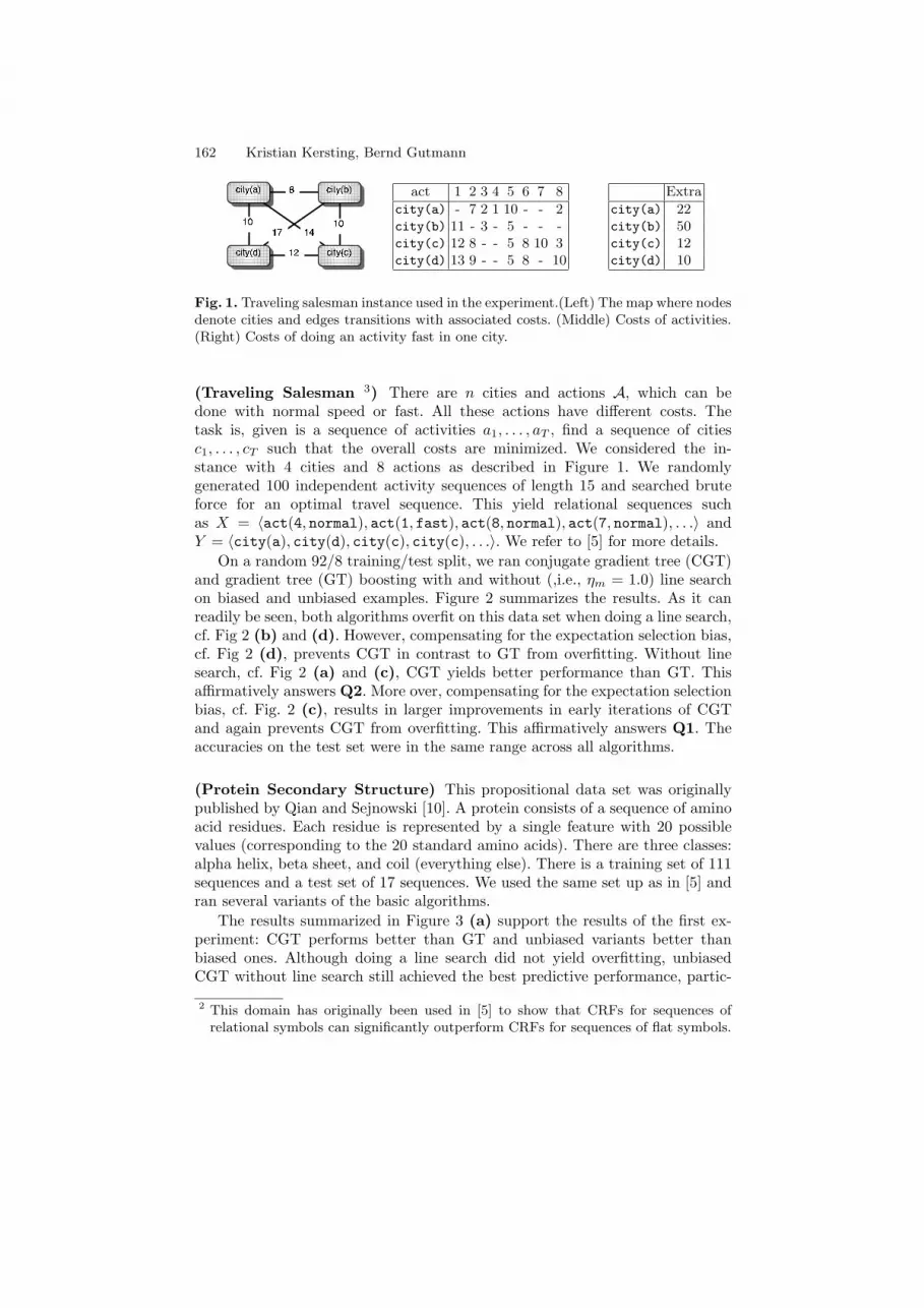
162 Kristian Kersting, Bernd Gutmann
act 1 2 3 4 5 6 7 8
city(a) - 7 2 1 10 - - 2city(b) 11 - 3 - 5 - - -city(c) 12 8 - - 5 8 10 3city(d) 13 9 - - 5 8 - 10
Extra
city(a) 22city(b) 50city(c) 12city(d) 10
Fig. 1. Traveling salesman instance used in the experiment.(Left) The map where nodesdenote cities and edges transitions with associated costs. (Middle) Costs of activities.(Right) Costs of doing an activity fast in one city.
(Traveling Salesman 3) There are n cities and actions A, which can bedone with normal speed or fast. All these actions have different costs. Thetask is, given is a sequence of activities a1, . . . , aT , find a sequence of citiesc1, . . . , cT such that the overall costs are minimized. We considered the in-stance with 4 cities and 8 actions as described in Figure 1. We randomlygenerated 100 independent activity sequences of length 15 and searched bruteforce for an optimal travel sequence. This yield relational sequences suchas X = 〈act(4, normal), act(1, fast), act(8, normal), act(7, normal), . . .〉 andY = 〈city(a), city(d), city(c), city(c), . . .〉. We refer to [5] for more details.
On a random 92/8 training/test split, we ran conjugate gradient tree (CGT)and gradient tree (GT) boosting with and without (,i.e., ηm = 1.0) line searchon biased and unbiased examples. Figure 2 summarizes the results. As it canreadily be seen, both algorithms overfit on this data set when doing a line search,cf. Fig 2 (b) and (d). However, compensating for the expectation selection bias,cf. Fig 2 (d), prevents CGT in contrast to GT from overfitting. Without linesearch, cf. Fig 2 (a) and (c), CGT yields better performance than GT. Thisaffirmatively answers Q2. More over, compensating for the expectation selectionbias, cf. Fig. 2 (c), results in larger improvements in early iterations of CGTand again prevents CGT from overfitting. This affirmatively answers Q1. Theaccuracies on the test set were in the same range across all algorithms.
(Protein Secondary Structure) This propositional data set was originallypublished by Qian and Sejnowski [10]. A protein consists of a sequence of aminoacid residues. Each residue is represented by a single feature with 20 possiblevalues (corresponding to the 20 standard amino acids). There are three classes:alpha helix, beta sheet, and coil (everything else). There is a training set of 111sequences and a test set of 17 sequences. We used the same set up as in [5] andran several variants of the basic algorithms.
The results summarized in Figure 3 (a) support the results of the first ex-periment: CGT performs better than GT and unbiased variants better thanbiased ones. Although doing a line search did not yield overfitting, unbiasedCGT without line search still achieved the best predictive performance, partic-
2 This domain has originally been used in [5] to show that CRFs for sequences ofrelational symbols can significantly outperform CRFs for sequences of flat symbols.

Unbiased Conjugate Direction Boosting for Conditional Random Fields 163
(a) Biased / No Line Search (b) Biased / Line Search
-150-120
-90-60-30
0 2 4 6 8 10 12 14 16 18 20
Tes
t Set
CLL
Iterations
0
-100
-200
-300
-400
-500
-600
-700
Tra
inin
g S
et C
LL
gradient tree boosting w/o line searchconjugate gradient tree boosting w/o line search
-150-120
-90-60-30
0 2 4 6 8 10 12 14 16 18 20
Tes
t Set
CLL
Iterations
0
-100
-200
-300
-400
-500
-600
-700
Tra
inin
g S
et C
LL
gradient tree boosting with line searchconjugate gradient tree boosting with line search
(c) Unbiased / No Line Search (d) Unbiased / Line Search
-150-120
-90-60-30
0 2 4 6 8 10 12 14 16 18 20
Tes
t Set
CLL
Iterations
0
-100
-200
-300
-400
-500
-600
-700
Tra
inin
g S
et C
LL
gradient tree boosting w/o line searchconjugate gradient tree boosting w/o line search
-150-120
-90-60-30
0 2 4 6 8 10 12 14 16 18 20
Tes
t Set
CLL
Iterations
0
-100
-200
-300
-400
-500
-600
-700
Tra
inin
g S
et C
LL
gradient tree boosting with line searchconjugate gradient tree bossting with line search
Fig. 2. Learning curves on the job scheduling domain. (c, d) compensated for theexpectation selection bias in contrast to (a, b). Cases (b, d) used a line search whereas(a,c) did not
ularly compared to the original GT, cf. Figure 3 (b). This affirmatively answersQ1 and Q2.
6 Conclusions
Training CRFs can be viewed as gradient ascent in function space. In this pa-per, we devised a novel algorithm for training CRFs, which employs conjugatedirections in function space. Furthermore, we identified an expectation selectionbias when training CRFs and presented an example weighting approach to com-pensate for it. Preliminary experiments are encouraging: the resulting approachcan indeed perform better than simple gradient tree boosting. To validate this,further experiments should be conducted.
Acknowledgments The authors thank Luc De Raedt for his support, AlanFern for interesting discussions, and Tom Dietterich for providing his version of
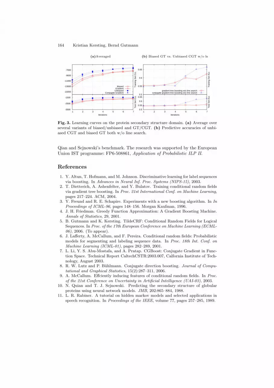
164 Kristian Kersting, Bernd Gutmann
(a)Averaged (b) Biased GT vs. Unbiased CGT w/o ls
-1500
-2500
-3500 1 2 3 4 5 6 7
Tes
t Set
CLL
Iterations
-7000
-9000
-11000
-13000
-15000
Tra
inin
g S
et C
LL
BiasedGradient
UnbiasedConjugate Gradient
0.65
0.6
0.55
0.5 1 2 3 4 5 6 7
Tes
t Set
Acc
Iterations
0.65
0.6
0.55
0.5
Tra
inin
g S
et A
cc
gradient tree boosting w/o line searchconjugate gradient tree boosting w/o line search
Fig. 3. Learning curves on the protein secondary structure domain. (a) Average overseveral variants of biased/unbiased and GT/CGT. (b) Predictive accuracies of unbi-ased CGT and biased GT both w/o line search.
Qian and Sejnowski’s benchmark. The research was supported by the EuropeanUnion IST programme: FP6-508861, Application of Probabilistic ILP II.
References
1. Y. Altun, T. Hofmann, and M. Johnson. Discriminative learning for label sequencesvia boosting. In Advances in Neural Inf. Proc. Systems (NIPS-15), 2003.
2. T. Dietterich, A. Ashenfelter, and Y. Bulatov. Training conditional random fieldsvia gradient tree boosting. In Proc. 21st International Conf. on Machine Learning,pages 217–224. ACM, 2004.
3. Y. Freund and R. E. Schapire. Experiments with a new boosting algorithm. In InProceedings of ICML-96, pages 148–156. Morgan Kaufman, 1996.
4. J. H. Friedman. Greedy Function Approximation: A Gradient Boosting Machine.Annals of Statistics, 29, 2001.
5. B. Gutmann and K. Kersting. TildeCRF: Conditional Random Fields for LogicalSequences. In Proc. of the 17th European Conference on Machine Learning (ECML-06), 2006. (To appear).
6. J. Lafferty, A. McCallum, and F. Pereira. Conditional random fields: Probabilisticmodels for segmenting and labeling sequence data. In Proc. 18th Int. Conf. onMachine Learning (ICML-01), pages 282–289, 2001.
7. L. Li, Y. S. Abu-Mostafa, and A. Pratap. CGBoost: Conjugate Gradient in Func-tion Space. Technical Report CaltechCSTR:2003.007, Calfornia Institute of Tech-nology, August 2003.
8. R. W. Lutz and P. Buhlmann. Conjugate direction boosting. Journal of Compu-tational and Graphical Statistics, 15(2):287–311, 2006.
9. A. McCallum. Effciently inducing features of conditional random fields. In Proc.of the 21st Conference on Uncertainty in Artificial Intelligence (UAI-03), 2003.
10. N. Quian and T. J. Sejnowski. Predicting the secondary structure of globularproteins using neural network models. JMB, 202:865–884, 1988.
11. L. R. Rabiner. A tutorial on hidden markov models and selected applications inspeech recognition. In Proceedings of the IEEE, volume 77, pages 257–285, 1989.

Tree Kernel Engineering for Proposition
Re-ranking
Alessandro Moschitti, Daniele Pighin, and Roberto Basili
Department of Computer ScienceUniversity of Rome ”Tor Vergata”, Italy{moschitti,basili}@info.uniroma2.it
Abstract. Recent work on the design of automatic systems for semanticrole labeling has shown that such task is complex from both modelingand implementation point of views. Tree kernels alleviate such complex-ity as kernel functions generate features automatically and require lesssoftware development for data pre-processing. In this paper, we studyseveral tree kernel approaches for boundary detection, argument classi-fication and, most notably, proposition re-ranking. The comparative ex-periments on Support Vector Machines with such kernels on the CoNLL2005 dataset show that very simple tree manipulations trigger automaticfeature engineering that highly improves accuracy and efficiency in everySRL phase.
1 Introduction
A lot of attention has been recently devoted to the design of systems for theautomatic labeling of semantic roles (SRL) as defined in two important projects:FrameNet [1], inspired by Frame Semantics, and PropBank [2] based on Levin’sverb classes. SRL is a complex task consisting in the recognition of predicateargument structures within natural language sentences.
Research on the design of automatic SRL systems has shown that (shallowor deep) syntactic information is necessary to achieve a good accuracy, e.g. [3,4].A careful analysis of literature features encoding such information reveals thatmost of them are fragments of syntactic trees of training sentences. Thus, anatural way to represent them is the adoption of tree kernels as described in[5]. Tree kernels show important advantages: first, we can implement them veryquickly as the feature extractor module only requires the writing of the procedurefor subtree extraction. In contrast, traditional SRL systems are based on theextraction of more than thirty features [6], which require the writing of at leastthirty different procedures. Second, combining tree kernels with a traditionalattribute-value SRL system allows us to obtain a more accurate system. Usuallythe combination of two traditional systems (based on the same machine learningmodel) does not result in an improvement as their features are more or lessequivalent as shown in [4]. Finally, the study of the effective structural features

166 Alessandro Moschitti, Daniele Pighin, and Roberto Basili
can inspire the design of novel linear features, which can be used with a moreefficient model (i. e. linear SVMs).
In this paper, we carry out tree kernel engineering [7,8] to increase the ac-curacy of the boundary detection, argument classification and proposition re-ranking steps. In the first two cases (Section 2.1), the engineering approachrelates to marking the nodes of the encoding subtrees to generate substructuresmore strictly correlated with a particular argument, boundary or predicate. Forthe latter case (Section 2.2), i. e. proposition re-ranking, we try both markinglarge parts of the tree that dominates the whole predicate argument structureand utterly reworking the syntactic structure. Our extensive experimentation ofthe proposed tree kernels with Support Vector Machines on the CoNLL 2005data set provides interesting insights on the design of performant SRL systems(Section 3).
2 A Model for Semantic Role Labeling
The SRL approach that we adopt is based on the deep syntactic parse [9] ofthe sentence that we intend to semantically annotate. The standard algorithmconcerns the classification of tree node pairs 〈p, a〉, where p is the node thatexactly dominates the target predicate and a is the node dominating a potentialargument. If 〈p, a〉 is selected as an argument, then the leaves of the tree rooted ina will be considered as the words constituting such argument. There are hundredsof pairs in a sentence, thus, if we use training corpora containing hundreds ofthousands of sentences, we have to deal with millions of instances.
To limit such complexity, we can divide the problem in two subtasks: (a)boundary detection, in which a single classifier is trained on many instances todetect if a node is an argument or not, i. e. if the sequence of words dominated bythe target node constitutes a correct boundary; and (b) argument classification,in which only the set of nodes corresponding to correct boundaries are consid-ered. These can be used to train a multiclassifier that, for such nodes, selectsthe most appropriate labeling. For example, n classifiers can be combined with aOne-vs-All approach, selecting for each argument node the role associated withthe maximum among the n scores provided by the individual role classifiers.
The main advantage of this approach is the use of just one computationallyexpensive classifier, i. e. the one for boundary detection. Regarding the featurerepresentation of 〈p, a〉, we can extract syntactic fragments from the sentence-parse tree proposed in [3], e.g. the Phrase Type or Predicate Word. An alternativeto the manual fragment extraction is the use of Tree Kernels as suggested in [5].Tree kernels are especially useful when the manual design of features is madecomplex by the use of a re-ranking module. This has been shown to be essentialto obtain state-of-the-art performance [10].
The next sections describe our tree kernel approaches for the classification ofboundaries and arguments and the re-ranking of complete predicative structures.

Tree Kernel Engineering 167
S
NP
NNP
Paul
VP
VBZ
delivers
NP
NP
DT
a
NN
talk
PP
IN
in
NP
JJ
formal
NN
style
(a) A parse tree
VP
VBZ
delivers
NP
NP
DT
a
NN
talk
(b) AST1
VP
VBZ
delivers
NP
NP-B
DT
a
NN
talk
(c) AST m
1
Fig. 1. Syntactic parse tree of the sentence John delivers a talk in formal style (a),AST1 (b) and AST m
1 (c) for the argument A1 a talk.
2.1 Kernels for Boundary Detection and Argument Classification
Once a basic kernel function is defined, we need to characterize the predicate-argument pair with a subtree. This allows the function to generate a large numberof syntactic features related to such pair. The approach proposed in [5] selectsthe minimal subtree that includes a predicate with one of its arguments. Forexample, Figure 1(a) shows the parse tree of the sentence Paul delivers a talk informal style whereas Frame (b) illustrates the AST1 subtree that characterizesthe predicate to deliver with its argument A1 a talk.
AST1s are very effective for argument classification but not for boundarydetection since two nodes that encode correct and incorrect boundaries maygenerate very similar AST1s [5]. To solve this problem, we simply mark theargument node with the label B, denoting the boundary property. This newsubtree is called a marked argument spanning tree (AST m
1 ) and it is shown inFigure 1(c). A positive example for the AST m
1 classifier is a subtree in which themarked node exactly covers the boundaries of an argument, whereas the markingof any other node within the same subtree results in a negative example.
2.2 Tree Kernels for the Proposition Re-ranking Task
Our re-ranking mechanism is similar to that described in [11], where a Viterbi al-gorithm is used to evaluate the most likely labeling schemes for a given predicateand a re-ranking mechanism selects the best annotation. The re-ranker is a bi-nary classifier trained with pairs 〈si, sj〉 where si and sj are taken from the set ofthe most m probable prepositions output by the Viterbi algorithm for the sametarget predicate. The classifier is meant to output a positive value if si is more

168 Alessandro Moschitti, Daniele Pighin, and Roberto Basili
S
NP-A0
NNP-A0
Paul
VP
VBZ
delivers
NP
NP-A1
DT-A1
a
NN-A1
talk
(a) AST cm
n
TREE
ARG0
A0
NNP
ARG1
rel
deliver
ARG2
A1
NP
ARG3
null
ARG4
null
ARG5
null
ARG6
null
(b) PAStl
Fig. 2. AST cm
n and PAStl representations of the example proposition.
accurate that sj and a negative value otherwise. Each candidate proposition si
can be described by a structural feature ti and by a vector of linear featuresvi representing information that cannot be captured by ti, e.g. the probabilityassociated with the annotation output by the Viterbi algorithm. As a whole,each classifier example ei is described by a tuple 〈t1i , t
2i , v
1i , v2
i 〉, where 〈t1i , v1i 〉
and 〈t2i , v2i 〉 describe the first and second candidate annotations, respectively.
Using the above tuple, we can define the following kernels:
Ktr(e1, e2) = Kt(t11, t
12) + Kt(t
21, t
22) − Kt(t
11, t
22) − Kt(t
21, t
12)
Kpr(e1, e2) = Kp(v11 , v1
2) + Kp(v21 , v2
2) − Kp(v11 , v
22) − Kp(v
21 , v1
2)
where Kt is a tree kernel function defined in [12] and Kp is a polynomial kernelapplied to the feature vectors. The final kernel that we use for re-ranking is thefollowing:
K(e1, e2) =Ktr(e1, e2)
|Ktr(e1, e2)|+
Kpr(e1, e2)
|Kpr(e1, e2)|.
Among the many different structural features that we tested with our re-ranker, the most effective are the completely marked argument structure span-ning tree (AST cm
n ) and the lemmatized type-only predicate argument structure(PASt).
An AST cmn (see Figure 2(a)) consists of the node spanning tree embracing
the whole argument structure: each argument node’s label is enriched with therole assigned to the node by the role multiclassifier, the labels of the descendantsof each argument node being accordingly modified down to pre-terminal nodes.Marking the nodes’ descendants is meant to force substructures to match onlyamong homogeneous argument types. This representation is meant to providerich syntactic and lexical information about the parse tree encoding the predicatestructure.

Tree Kernel Engineering 169
A PAStl (see Figure 2(b)) is a completely different structure that repre-sents the syntax of the predicate argument structure, i. e. the number, typeand position of each argument, minimizing the amount of lexical and syntacticinformation derived from the parse tree. The syntactic links between the argu-ment nodes are represented as a fake 1-level tree, which is shared by any PAStl
and therefore does not influence the evaluation of similarity between pairs ofstructures. Such structure accommodates sequentially all the arguments of anannotation, each slot being attached a pre-terminal node standing for the nodetype and a terminal symbolizing the syntactic type of the argument node. Ingeneral, a proposition consists of m arguments, with m < 7. In this case, all thenodes ARGi, i ≤ m ≤ 6 are attached a dummy descendant marked null. Thepredicate is represented by means of a pre-terminal node labeled rel to whichthe lemmatization of the predicate word is attached as a leaf node.
Table 1. Correct (+), incorrect (-) and overall (tot) number of potential argumentnodes from sections 2, 3 and 24 of the PropBank.
Section 2 Section 3 Section 24
+ - tot + - tot + - tot
12,741 185,178 197,919 7,023 139,823 146,846 8,234 130,489 138,723
Table 2. Performance improvement on the boundary detection and argument classifi-cation tasks using engineered tree kernels.
Boundary detection Argument classification
AST1 75.24 82.07AST m
1 75.06 77.17
3 Experiments
In these experiments we evaluate the impact of our proposed kernels on thedifferent phases of the SRL task. The resulting accuracy improvement confirmsthat the node marking approach enables the automatic engineering of effectiveSRL features.
The empirical evaluations were carried out within the setting of the CoNLL-2005 Shared Task [4] described in www.lsi.upc.edu/∼srlconll/ by means ofSVM-light-TK available at http://ai-nlp.info.uniroma2.it/moschitti/ whichencodes fast tree kernel evaluation [12] in SVM-light [13]. We used a regulariza-tion parameter (option -c) equal to 1 and λ = 0.4 (see [5]).
3.1 Boundary Detection and Argument Classification Results
For the boundary detection experiments we used Section 02 for training andSection 24 for testing, whereas for argument classification also Section 03 was

170 Alessandro Moschitti, Daniele Pighin, and Roberto Basili
used for training. Their characteristics in terms of potential argument nodes1
are shown in Table 1.
Table 3. Number of distinct annotations output by the Viterbi algorithm and of paircomparisons (i. e. re-ranker input examples) in the PropBank sections used for theexperiments.
Section 12 Section 23 Section 24
Annotations 24,494 26,325 16,240Comparisons 74,650 81,162 48,582
Table 4. Summary of the proposition re-ranking experiments with different trainingsets.
Training section AST cm
n PAStl PAStl + STD
12 - 78.27 77.6124 76.47 78.15 77.77
12+24 - 78.44 -
The results obtained using the AST1 and the AST m1 based kernels are re-
ported in Table 2 in rows 2 and 3, respectively. Columns 2 and 3 show theirrespective performance (in terms of F1 measure) on the boundary detection andargument classification phases. We note that: (1) on boundary detection, AST m
1 simprove the F1 over AST1 by about 7 points, i. e. 82.07 vs. 75.24. This suggeststhat marking the argument node simplifies the generalization process; (2) usingan engineered tree kernel also improves the argument classification task by about2 points, i. e. 77.17 vs. 75.06. This confirms the outcome on boundary detectionexperiments and the fact that we need to distinguish the target node from theothers.
3.2 Proposition Re-ranking Results
For our proposition re-ranking experiments, Section 23 was used for testing. Onsuch test set, considering the first 5 alternatives output by the Viterbi algorithm,our model has a lower bound of the F1 measure of 75.91 (corresponding tothe selection of the first alternative, i. e. the most likely with respect to theprobabilistic model) and an upper bound of 84.76 (corresponding to the informedselection of the best among the 5 alternatives, i. e. the theoretical output of aperfect re-ranker). The number of distinct annotations output by the Viterbi
1 As the automatic parse trees contain errors, some arguments cannot be associatedwith any covering node. This prevents us to extract a tree representation for them.Consequently, we do not consider them in our evaluation. In sections 2, 3 and 24there are 454, 347 and 731 such cases, respectively.

Tree Kernel Engineering 171
algorithm for each section that we used is shown in Table 3, Row 2. In Row 3,the number of pair comparisons, i. e. the number of training/test examples forthe classifier.
Table 4 summarizes the outcome of our experiments. First, we compared theaccuracy of the AST cm
n and PAStl classifiers trained on Section 24 (in Row 3,Columns 2 and 3) and discovered that the latter structure produces a notice-able F1 improvement, i. e. 78.15 vs. 76.47. Second, we added the local (to eachargument node) linear features commonly employed for the boundary detectionand argument classification tasks, as in [10] to the PAStl kernel (Column 4).The comparison with the simple PAStl on 2 different training sets (Rows 2and 3) shows that the introduction of the standard linear features produces aperformance decrease on both sections 12 and 24 . Finally, we trained our bestre-ranking kernel, i. e. the PAStl, with both sections 12 and 24 achieving an F1
measure of 78.44 (Row 4).These results suggest that: (1) the
F18081828384Thousandsoftrainingexamples20040060080010001200AST1msplitclassifierAST1splitclassifier
Fig. 3. Learning curve comparison forthe boundary detection phase betweenthe AST1 and AST m
1 F1 measures.
re-ranking task is very difficult froma ML point of view: in fact, addingor removing thousands of training ex-amples has only a small impact on theclassification accuracy; (2) the PAStl
kernel is much more effective than theAST cm
n one, which is always outper-formed. This may be due to the factthat two AST cm
n s always share a greatnumber of substructures, since mostalternative annotations tend to be veryalike and the small differences amongthem only affect a small part of theirenriched syntactic parse trees; (3) onthe other hand, the little amount oflocal parsing information encoded inthe PAStls allows for a good generalization process; (4) the introduction of thestandard, local linear features in our re-ranking model caused a performance lossof about 0.5 points on both Sections 12 and 24. This fact, which is in contrastwith what has been shown in [10], might be the consequence of the small trainingsets that we employed. In fact, local linear features tend to be very sparse andtheir effectiveness should be evaluated against a larger data set.
4 Conclusions
The design of automatic systems for the labeling of semantic roles requires thesolution of complex problems. Among others, feature engineering is made difficultby the structural nature of the data, i. e. features should represent informationcontained in automatic parse trees. A system based on tree kernels alleviate suchcomplexity as kernel functions can automatically generate effective features.
172 Alessandro Moschitti, Daniele Pighin, and Roberto Basili
In this paper, we have improved tree kernels by studying different strategies,e.g. AST m
1 s highly improve accuracy in both the boundary detection (about 7%)and argument classification subtasks (about 2%). We have also engineered dif-ferent structured features for the re-ranking module, which improves our systemof about 2.5 percent points. This is quite a good results as it approaches thestate-of-the-art using only a small fraction of all the available data. In the nearfuture, we would like to use more such data along with other kernels describedin [12].
Acknowledgments
This research is partially supported by the European project, PrestoSpace (FP6-IST-507336).
References
1. Johnson, C.R., Fillmore, C.J.: The framenet tagset for frame-semantic and syn-tactic coding of predicate-argument structure. In proceedings of NAACL 2000,Seattle WA. (2000)
2. Kingsbury, P., Palmer, M.: From Treebank to PropBank. In proceedings ofLREC’02, Las Palmas, Spain (2002)
3. Gildea, D., Jurasfky, D.: Automatic labeling of semantic roles. ComputationalLinguistic 28(3) (2002) 496–530
4. Carreras, X., Marquez, L.: Introduction to the CoNLL-2005 shared task: Semanticrole labeling. In proceedings of CoNLL-2005, Ann Arbor, Michigan, (2005)
5. Moschitti, A.: A study on convolution kernels for shallow semantic parsing. Inproceedings of ACL’04, Barcelona, Spain (2004)
6. Pradhan, S., Hacioglu, K., Krugler, V., Ward, W., Martin, J.H., Jurafsky, D.:Support vector learning for semantic argument classification. Machine LearningJournal (2005)
7. Moschitti, A., Coppola, B., Pighin, D., Basili, R.: Engineering of syntactic featuresfor shallow semantic parsing. In proceedings of the ACL Workshop on FeatureEngineering for Machine Learning in Natural Language Processing, Ann Arbor,Michigan, (2005)
8. Moschitti, A., Pighin, D., Basili, R.: Tree kernel engineering in semantic rolelabeling systems. In proceedings of the EACL Workshop on Learning StructuredInformation in Natural Language Applications, Trento, Italy, (2006)
9. Charniak, E.: A maximum-entropy-inspired parser. In: Proceedings of the 1stMeeting of NAACL. (2000)
10. Haghighi, A., Toutanova, K., Manning, C.: A joint model for semantic role labeling.In proceedings of CoNLL-2005, Ann Arbor, Michigan. (2005)
11. Moschitti, A., Pighin, D., Basili, R.: Semantic role labeling via tree kernel jointinference. In proceedings of CoNLL-X. (2006)
12. Moschitti, A.: Efficient convolution kernels for dependency and constituent syn-tactic trees. In proceedings of ECML 2006, Berlin, Germany. (2006)
13. Joachims, T.: Making large-scale SVM learning practical. In Scholkopf, B., Burges,C., Smola, A., eds.: Advances in Kernel Methods - Support Vector Learning. (1999)

Frequent Subgraph Miners:Runtimes Don’t Say Everything
Siegfried Nijssen1 and Joost N. Kok2
1 Albert-Ludwidgs-Universitat, Georges-Kohler-Allee, Gebaude 097, D-79110,Freiburg im Breisgau, Germany.
2 LIACS, Leiden University, Niels Bohrweg 1, 2333 CA, Leiden, The [email protected]
Abstract. In recent years several frequent subgraph miners were pro-posed. The authors of these new algorithms typically compared the run-times of their implementations with those of previous implementationsto confirm the efficiency of their methods. To get a better perspective onthe mutual benefits of the algorithms, Worlein et al. [9] performed an ex-perimental evaluation of re-implementations of several depth-first graphminers, where also some statistics beyond runtimes were compared. Inthis paper we present results of an additional experimental comparison ofseveral graph miners, which differs in the following aspects from this pre-vious study: (1) we compare original implementations; (2) we comparethese implementations on a larger set of measures than runtimes, thusproviding further insight in the benefits of the algorithms; (3) we includebreadth-first graph miners and free tree miners in the comparison.
1 Introduction
Given a database consisting of small graphs, for example, molecular graphs, theproblem of mining frequent subgraphs is to find all subgraphs that are subgraphisomorphic with a large number of example graphs in the database. Referencesto applications can be found in [2, 4, 8, 3]. The first frequent subgraph miner wasInokuchi et al.’s AGM algorithm (2000), for unconnected subgraphs. The algo-rithm was followed by the FSG algorithm of Kuramochi and Karypis [7] (2001),and an adaption of AGM, AcGM, for mining connected subgraphs [6] (2002).These initial algorithms performed the search breadth-first; the first depth-firstgraph miners were MoFA [2] and gSpan [10] (2002), followed by FFSM [5] (2003)and Gaston [8] (2004). In parallel, also free tree (cycleless graph) miners weredeveloped: both the breadth-first FreeTreeMiner (2003) and the depth-firstHybridTreeMiner (2004) by Chi et al. (see [3] for references). The develop-ment of new graph miners was motivated by the supposed inefficiency of earliergraph miners. In this paper, we perform a large set of experiments with the im-plementations of the graph and free tree miners that were used in most of theseoriginal publications.
We have several aims by doing these experiments. First, our study veri-fies earlier studies, both the studies of the original implementers, as the re-implementation study of [9]. This provides either additional evidence for the

174 Siegfried Nijssen and Joost N. Kok
results obtained in these studies, or will allow us to refute claims made in thesestudies, in both cases providing us additional insights in the effects of, for in-stance, implementation optimizations. Second, by computing additional mea-sures, we wish to obtain a deeper understanding in the true benefits of the graphmining algorithms. It can be observed that most graph mining algorithms canbe separated in separate components for ‘candidate generation’ and ‘candidateevaluation’. Until now, most algorithms provide a unique combination for each ofthese elements. By performing additional experiments, we can provide insight inthe question if it is useful to try out different combinations of these components.Thus, this study is complementary to the earlier graph mining study of [9], andour earlier study on the efficiency of frequent tree miners [3].
The paper is organized as follows. First, we shortly review the problem offrequent subgraph mining and the frequent subgraph miners. The main part ofthe paper consists of a large number of experiments. Finally, we conclude.
2 Concepts and Algorithms
In this section we briefly recall the most important concepts and algorithms.Concepts A labeled undirected graph is a quadruple (V,E, λ,Σ), where V is
a set of vertices, E ⊆ {e ⊆ V : |e| = 2} is a set of edges, and λ : V ∪ E → Σ isa function that assigns labels to the vertices and edges. In this paper, we onlyconsider connected graphs, in which there is a path between every pair of nodes.Graph G′ = (V ′, E′, λ′, Σ′) is a subgraph of graph G if V ′ ⊆ V , E′ ⊆ E, for allx ∈ V ′∪E′ : λ′(x) = λ(x) and Σ′ ⊆ Σ. Graph G and G′ are isomorphic iff thereis a bijective function φ : V → V ′ such that (1) ∀{v1, v2} ∈ E : {φ(v1), φ(v2)} ∈E′ and λ({v1, v2}) = λ′(φ({v1, v2})), (2) ∀v ∈ V : λ(v) = λ′(φ(v)). GraphG is subgraph isomorphic with G′, denoted by G′ º G, iff G is isomorphicwith a subgraph of G′. The corresponding function φ, which maps nodes fromthe subgraph to the supergraph, is called an embedding. Given a multiset ofgraphs D (also referred to as database graphs), the frequency (or support) ofa graph G, denoted by freq(G) is the cardinality of the set {G′ ∈ D|G′ º G}.Assuming that each database graph has an identifier, this set could alternativelyconsist of identifiers; we refer to this set as the transaction identifier (TID) listof the subgraph. Given a threshold minsup, a (pattern) graph G is frequentiff freq(G) ≥ minsup; frequent subgraph miners find all such subgraphs. Animportant property is the antimonotonicity property that states that if G ºG′, freq(G) ≤ freq(G′). If we start searching from the smallest subgraphs, aconsequence of this property is that we do not need to consider supergraphs ofinfrequent graphs; we can cut parts of the search space.
Two different subgraphs can be isomorphic with each other; let V = {v1, v2},E = {{v1, v2}} and Σ = {a, b}; then the graph G1 = (V, E, λ1, Σ) with λ1(v1) =a and λ1(v2) = b is isomorphic with the graph G2 = (V, E, λ2, Σ) havingλ2(v1) = b and λ2(v2) = a. Care has to be taken that frequent subgraph minersdo not find such isomorphic subgraphs multiple times. All algorithms addressthis issue by determining a canonical string for a graph. The idea is that every

Frequent Subgraph Miners: Runtimes Don’t Say Everything 175
graph has a corresponding string representation, for example, (v1, v2, a, b) for G1
and (v1, v2, b, a) for G2. By imposing a total order on the strings of isomorphicgraphs, for example, lexicographically, we can decide that one representationis the highest. This string is considered to be the canonical representation ofthe isomorphic graphs. As no polynomial algorithm is known to compute graphisomorphism or subgraph isomorphism, all graph mining algorithms use expo-nential search algorithms to find the canonical label or embeddings; free treemining algorithms, on the other hand, can exploit polynomial algorithms.
Breadth-First Algorithms The breadth-first algorithms have the samesetup as the original Apriori algorithm for mining frequent itemsets [1]. Theyiterate a process of generating candidate subgraphs and determining their sup-port in the database. Candidates are generated by joining two subgraphs thatwere previously found to be frequent. After the joined subgraph is obtained, it ischecked whether all its subgraphs are frequent; if not, the candidate is pruned.
To represent candidates, AcGM and FSG use a canonical string that is ob-tained from an adjacency matrix. FSG’s code allows for the quick computation ofthe canonical string for any given graph. AcGM’s representation is optimized tominimize the generation of non-canonical graphs. Chi et al.’s FreeTreeMineris similar to AcGM, but uses a polynomially computable canonical string.
The search for embeddings is improved by exploiting the observation thatan embedding for a supergraph is also an embedding for its subgraphs. In FSGand the FreeTreeMiner, a TID list is stored with every pattern graph. AcGMtakes the idea a step further by also storing one embedding for each databasegraph in the TID list, and using it as the start of the exponential search.
Depth-First Algorithms The depth-first algorithms do not subdivide thesearch into strict candidate generation and candidate evaluation phases. Es-sentially, each of these algorithms scans all embeddings of a subgraph in thedatabase, and collects from that scan the support of the refinements, i.e., theindividual edges and nodes that can be connected to the subgraph. The searchrecurses immediately on each of the frequent refinements.
To avoid duplicate subgraphs in the output, all depth-first graph miners usea special kind of canonical string, which has the property that every prefix ofthe string is also canonical. A refinement corresponds to extending a canonicalstring. For each extended string, it is checked whether it is canonical; any non-canonical string can be removed immediately. Although for every refined stringit has to be checked with an exponential algorithm if the resulting string is reallycanonical, an interesting property of most codes is that it often easy to decidethat a code is not canonical. As a small example, almost all codes sort siblingnodes in the order of their labels. This order limits which new siblings can beadded; we will call this the ‘label trick’. Such simple tricks limit which nodes inthe data have to be scanned for extensions. gSpan, FFSM and Gaston differin their canonical string, and consequently, also in the ‘easy’ rules that can beused to eliminate strings that are not canonical:

176 Siegfried Nijssen and Joost N. Kok
– gSpan uses a code that consists of a list of edges in the order of a depth-firsttraversal tree of the subgraph. Canonical refeinements can only connect toa node on the rightmost path of this tree. The ‘label trick’ applies to gSpan.
– FFSM uses a code that consists of a concatenation of columns of an adjacencymatrix. The last column of the adjacency matrix restricts to which nodesnew nodes can be connected; ‘label tricks’ can also be applied in FFSM.
– Gaston uses a code that consists of a concatenation of a code for paths,trees and cycles. The code allows to determine in O(1) time if a refinementleads to a non-canonical code for a tree. The ‘label trick’ can not be applied.
– The HybridTreeMiner uses another code to represent free trees. The codeis efficiently computable, and guarantees that trees or paths are never enu-merated more than twice.
To evaluate the frequency of subgraphs, several alternatives have been proposed.In gSpan and Gaston (RE variant) a TID list is maintained with every sub-graph. All embeddings are recomputed for graphs in the TID list. For eachembedding, refinements that are not pruneable by easy rules, are counted. Non-canonical refinements are pruned later.
An alternative is to not to recompute embeddings, but to store them, as onlyembeddings of subgraphs can lead to embeddings of supergraphs. Although thefrequency of refinements could be collected from the data, FFSM and Gaston(OS variant) use a more elaborate approach, in which the embeddings of somerefinements are obtained by joining the embeddings of other subgraphs. Themotivation is that this reduces the chances of building embedding lists for graphsthat are not frequent, as at least two subgraphs need to be frequent before anembedding list is constructed. However, to reduce the number of subgraphs forwhich the embedding list has to be stored at the same time, it is necessarythat joining is performed in a ‘local’ way in the search tree. To this purpose, allalgorithms require an additional set of embedding lists for graphs that are notcanonical.
3 Experiments
For our comparison, we obtained source code of the FreeTreeMiner, the Hy-bridTreeMiner and Gaston (RE, OS), and binaries of gSpan, FFSM, FSGand AcGM. The source code was compiled using the GNU C compiler and the O3compiler option. We used a range of 6 different datasets: (1) three tree datasets(A1, A3, A4) were generated using Zaki’s tree dataset generator [11]. A4 is equalto A1, except for the node labels. Most frequent trees in dataset A3 have diam-eter 2, and differ mainly in degree of the nodes; (2) two molecular datasets. ThePTE dataset was used in [10, 8], and includes hydrogens in the graph encoding;the Cancer datasets is a similar, although larger, dataset obtained from the Na-tional Cancer Institute, and does not include hydrogen in the encoding3; (3) aprotein secondary structure dataset of Huan et al. [4].3 We performed further experiments with molecular datasets and real-world tree
datasets. Results on these datasets are similar and omited due to space constraints.

Frequent Subgraph Miners: Runtimes Don’t Say Everything 177
A1
A3
A4
PTE
Can
cer
Pro
tein
Num
bero
fgra
phs
5000
1000
050
0034
032
557
40N
umbe
rofn
odes
6293
618
3743
6293
691
8985
7126
9502
Num
bero
fedg
es57
936
1737
4357
936
9317
9220
8122
016
Avg
max
num
ber
equa
llyla
bele
dno
des
2.7
3.9
12.6
11.9
19.2
25.6
Avg
num
bero
fnod
es12
.618
.412
.627
.026
.323
7.6
Avg
max
num
ber
equa
llyla
bele
dne
ighb
ors
1.7
3.2
5.2
2.6
2.7
1.1
Num
bero
fnod
ela
bels
1010
166
6720
Num
bero
fedg
ela
bels
11
14
31
Fig
.1.C
hara
cter
isti
csofth
edata
sets
.
PTE
Can
cer
Alg
orith
m2%
3%4%
5%4%
Gast
on
(OS
)9.
1MB
4.4M
B3.
4MB
3.0M
B43
0MB
Gast
on
(RE
)1.
5MB
1.3M
B1.
3MB
1.3M
B23
MB
FFS
M8.
2MB
4.1M
B3.
7MB
3.2M
B25
7MB
gSpa
n3.
8MB
2.8M
B2.
8MB
2.8M
B46
MB
AcG
M33
.9M
B5.
3MB
2.2M
B1.
6MB
434M
BFS
G12
3.5M
B25
.8M
B25
.8M
B25
.8M
B10
7MB
Fig
.2.M
emory
usa
ge
ofth
ealg
ori
thm
s.
1 10
100
100
0 0.6
0.8
11.
52
34
5
Run Time (Seconds)
Min
imum
Sup
port
(%
)
A1
Gas
ton
(RE
)G
asto
n (O
S)
gSpa
nF
FS
MH
ybrid
Tre
eMin
erF
reeT
reeM
iner
FS
GA
cGM
1 10
100
100
0
22.
53
45
7.5
1020
Run Time (Seconds)
Min
imum
Sup
port
(%
)
A3
Gas
ton
(RE
)G
asto
n (O
S)
gSpa
nF
FS
MH
ybrid
Tre
eMin
erF
reeT
reeM
iner
FS
G
10
100
100
0
2626
.527
27.5
2829
3031
Run Time (Seconds)
Min
imum
Sup
port
(%
)
A4
Gas
ton
(RE
)gS
pan
Fre
eTre
eMin
erF
SG
0.1 1 10
100
100
0
7 6
5 4
3 2
Run Time (Seconds)
Min
imum
Sup
port
(%
)
PT
E
Gas
ton
(RE
)G
asto
n (O
S)
gSpa
nF
FS
MF
SG
AcG
M
30
40
60
80
100
200
300
400
600
800
100
0
200
0
34
610
1520
Run Time (Seconds)
Min
imum
Sup
port
(%
)
Can
cer
Gas
ton
(RE
)G
asto
n (O
S)
gSpa
nF
FS
MF
SG
AcG
M
1 10
100
100
0 70
75
80
85
90
Run Time (Seconds)
Min
imum
Sup
port
(%
)
Pro
tein
Gas
ton
(RE
)G
asto
n (O
S)
FF
SM
FS
GA
cGM
Fig
.3.R
unti
me
exper
imen
tson
all
data
sets
.
A1
A3
Min
imum
supp
ort
30%
10%
8%6%
7.5%
4%3%
2.5%
Freq
uent
grap
hs83
818
552
3694
593
979
156
1826
5405
1045
1gS
pan
—S
ubop
timal
ity10
3%10
7%10
8%10
8%10
7%10
1%10
1%10
1%FF
SM
—S
ubop
timal
ity31
0%23
1%21
3%19
5%25
4%28
9%25
4%23
4%Jo
inef
ficie
ncy
99%
70%
62%
55%
100%
99%
91%
85%
Gast
on
—S
ubop
timal
ity20
7%13
6%12
5%11
5%21
2%21
4%16
1%13
6%Jo
inef
ficie
ncy
27%
41%
43%
47%
11%
29%
44%
52%
Join
nece
ssity
97%
95%
96%
97%
100%
98%
98%
99%
Hybrid
TreeM
iner
—S
ubop
timal
ity16
0%16
8%17
3%10
4%10
1%10
1%Jo
inef
ficie
ncy
21%
20%
21%
33%
39%
42%
Join
nece
ssity
96%
96%
94%
100%
100%
100%
PTE
Pro
tein
Can
cer
Min
imum
supp
ort
20%
6%3%
2%80
%75
%70
%9%
5%3%
Freq
uent
grap
hs19
023
2622
758
1369
4926
740
2762
9727
0933
118
1856
6315
566
gSpa
n—
Sub
optim
ality
139%
134%
137%
129%
--
-16
1%15
8%15
9%FF
SM
—S
ubop
timal
ity19
2%15
2%13
3%13
4%16
6%14
4%13
2%-
--
Join
effic
ienc
y61
%50
%45
%41
%38
%35
%35
%-
--
Gast
on
—O
vera
llsu
bopt
imal
ity17
6%14
9%15
1%16
5%18
0%21
9%24
1%17
0%15
7%14
7%Fr
eetre
esu
bopt
imal
ity16
0%12
5%10
9%10
3%12
9%11
1%10
4%15
6%13
9%12
6%C
yclic
join
effic
ienc
y10
0%10
0%94
%89
%70
%75
%80
%39
%29
%28
%C
yclic
join
nece
ssity
100%
100%
94%
90%
82%
68%
61%
94%
93%
93%
Free
tree
join
effic
ienc
y52
%37
%64
%75
%38
%49
%55
%27
%27
%27
%Fr
eetre
ejo
inne
cess
ity83
%73
%86
%90
%10
0%99
%99
%96
%95
%95
%
Fig
.4.C
hara
cter
isti
csofth
egSpan,FFSM
and
Gast
on
alg
ori
thm
son
the
A1,A
3,P
TE
,P
rote
inand
Cance
rdata
sets
.

178 Siegfried Nijssen and Joost N. Kok
Properties regarding the number of equally labeled nodes, edges and neigh-bors, are listed in Figure 1. These properties are important, as they yield ahigher branching factor in algorithms that perform an exponential search forembeddings. The datasets represent a broad range of such properties.
To perform our experiments we used two computers: all cyclic graph datasetswere mined on an AMD Athlon XP1600+ with 512MB main memory, runningMandrake Linux 10; all free tree datasets were mined on an Intel Pentium IV2.8Ghz with 512MB main memory, running Red Hat Linux 7.3.
The results of runtime experiments are given in Figure 3. The experimentsare measured using the Unix time command and are averaged over 3 runs.
The experiments show the importance of the branching factor of subgraphisomorphism algorithms. The depth first graph mining algorithms fail miserablyon the A4 dataset, which has a high branching factor (they run too long, orconsume too much memory); only the breadth-first FreeTreeMiner performswell. Otherwise, however, the FreeTreeMiner usually performs worse thanFSG. The A3 dataset shows the difference between breadth-first algorithms thathave to find one embedding per database graph (like FSG), and depth-firstalgorithms that have to find all embeddings. In some cases the breadth-firstgraph miners run out of memory, which is caused by extremely large sets ofcandidates.
The results on the cyclic datasets are similar to those on the tree datasets,and confirm the observations of previous publications.
The runtime experiments however do not show whether differences are due toa ‘better’ canonical form, as claimed by several authors, or due to more optimizedimplementations or memory-runtime trade-offs. Results of experiments to assessthe quality of the canonical form are listed in Figure 4. The following statisticsare listed in this table:
– frequent graphs: the number of frequent subgraphs resulting from the runsof all algorithms;
– suboptimality: the number of frequent subgraphs for which the canonicalstring test is computed, divided by the number of frequent subgraphs; thehigher this number is, the less well does the code prevent isomorphic graphsusing easy rules, and thus more redundant supports are computed;
– join efficiency: the number of joins that results in a frequent subgraph, di-vided by the total number of joins that is performed; the closer to 100% thisvalue is, the better does the algorithm succeed in only computing embeddinglists that are really frequent; in the case of Gaston, there is a distinctionbetween the joins between embedding lists of trees and of cyclic graphs;
– join necessity: the number of joins that results in a subgraph with supporthigher than zero, divided by the total number of joins that is performed; ifthis number would not be close to 100%, joining of embedding lists wouldnot make much sense, as we are performing many computations that analgorithm that collects extensions from data would not need to perform.
For Gaston and the HybridTreeMiner, we obtained these measures by chang-ing the source code. For gSpan and FFSM, we used the Valgrind tool available

Frequent Subgraph Miners: Runtimes Don’t Say Everything 179
A1 1% PTE 2% Protein 75%Algorithm 1× 3× 5× Regression 1× 2× 3× Regression 1× 2× 3×Gaston (OS) 4.6s 14.8s 26.1s 5.5x-1.4s 7.9s 15.2s 23.0s 7.5x+0.4s 60s 116s 183sGaston (RE) 8.7s 27.7s 48.0s 9.9x-1.8s 39.9s 76.3s 112.4s 36.2x3.7s 148s 398s 643s
(78s) (166s) (290s)FFSM 29.7s 55.7s 82.2s 26.3x+3.4s 177s 353s 554s
(148s) (398s) (643s)gSpan 15s 47s 81s 16.6x-2.2s 100s 186s 271s 85.4x+14.9sFSG 17s 35s 53s 9.1x+7.7s 316s 402s 489s 86.3x+229.8s 1253s 2264s 3275sAcGM 107s 170s 234s 63.5x+43.3sHybridTreeMiner 46s 146s 248s 48.9x-1.1sFreeTreeMiner 243s 715s 238.9x+1.5s
Fig. 5. Scale-up experiments on several datasets; experiments between brackets wereobtained on an Intel Pentium IV.
at www.valgrind.org. Valgrind makes it possible to count numbers of functioncalls, even with sufficient reliability for binaries that have been compiled withoutdebugging information. We counted the number of calls to the isCanonicalForm(FFSM) and isDuplicate (gSpan) functions, allowing us to determine the sub-optimality of the graph codes. The functionality of these functions was confirmedby the authors of the binaries.
The tables provide a large amount of information. Most interesting is thegood performance of gSpan’s code. In terms of optimality, this code performsbest in almost all cases. This result suggests that if we combine the code of gSpanwith the evaluation mechanisms of the other algorithms, we might achieve similarruntimes as for these other algorithms. Comparing Gaston to FFSM, Gastonis less optimal than FFSM on cyclic graphs, but joins more efficiently. Onlyconsidering trees in the molecular databases, Gaston’s code is more optimal.The good result of the HybridTreeMiner on the A3 dataset can be explainedby the fact that most frequent subtrees in this database turn out to be (single)centred; HybridTreeMiner’s tree code is optimized for such trees.
The most interesting observation is that there is no strong relation betweenthe runtime experiments and the efficiencies of the graph codes. Then what doesdetermine the efficiency of the graph miners?
More insights can be obtained from the experiments in Figure 5 and Fig-ure 2. In Figure 5, we repeat the same mining experiments for increasinglylarger datasets that are obtained by concatenating the same dataset multipletimes. In general, the algorithms scale linearly. The constant in the linear re-gression relates to the operations that are independent of the dataset size, suchas candidate generation. The time to count candidates is comparable in boththe breadth-first and depth-first graph miners that do not use embedding lists.The effort to find all embeddings is apparently negligibly higher than the effortto find only one. On the Protein dataset, however, the scale-up is not linear. Ifwe perform this experiment on two different computers, we can conclude thathe reason is the very small size of this dataset. Without using embedding lists,the data fit all within the cache of the CPU, and the computation is extremely

180 Siegfried Nijssen and Joost N. Kok
fast. On a computer with less cache (like the Athlon) the advantage of in-cachecomputations is lost more quickly as the dataset grows larger.
Finally, the memory usage experiments show that the runtime differencesbetween FFSM and gSpan are the result of a memory-CPU trade-off. Pleasenote that the differences in memory usage are strongly influenced by the choicesmade in the binaries for the amount of bits used to represent node labels, etc.,and are therefore only indicative.
4 Conclusions
In this study, we have confirmed that there is not a strong relation between thecanonical string that is used and the runtime behavior of the algorithms. Poly-nomially computable codes, such as used in frequent tree mining, are often lessefficient from a practical point of view. Of the many canonical codes that havebeen proposed, the DFS code that was introduced in gSpan perform consistentlymost well. Given its conceptual simplicity, this code should be preferred.
The differences between breadth-first and depth-first graph mining are sig-nificant. In most cases, the depth-first miners are faster and require less memory.
Many of the runtime differences between graph miners can be attributed totwo aspects. First, there are the typical high performance computing issues, suchas caching behavior; second, there is the memory usage-runtime trade-off.
References
1. R. Agrawal, H. Mannila, R. Srikant, H. Toivonen, and A. I. Verkamo. Fast discoveryof association rules. In Advances in Knowledge Discovery and Data Mining, pages307–328, 1996.
2. C. Borgelt and M. R. Berthold. Mining molecular fragments: Finding relevantsubstructures of molecules. In ICDM, pages 51–58, 2002.
3. Y. Chi, S. Nijssen, R. R. Muntz, and J. N. Kok. Frequent subtree mining—Anoverview. In Fundamenta Informaticae, volume 66, pages 161–198, 2005.
4. J. Huan, W. Wang, D. Bandyopadhyay, J. Snoeyink, J. Prins, and A. Tropsha.Mining family specific residue packing patterns from protein structure graphs. InRECOMB, pages 308–315, 2004.
5. J. Huan, W. Wang, and J. Prins. Efficient mining of frequent subgraphs in thepresence of isomorphism. In ICDM, pages 549–552, 2003.
6. A. Inokuchi, T. Washio, K. Nishimura, and H. Motoda. A fast algorithm for miningfrequent connected subgraphs. Technical Report RT0448, IBM Research, 2002.
7. M. Kuramochi and G. Karypis. Frequent subgraph discovery. In ICDM, pages313–320, 2001.
8. S. Nijssen and J. N. Kok. A quickstart in frequent structure mining can make adifference. In KDD, pages 647–652, 2004.
9. M. Worlein, T. Meinl, I. Fischer, and M. Philippsen. A quantitative comparisonof the subgraph miners MoFa, gSpan, FFSM, and Gaston. In PKDD, LNCS 3721,pages 392–403, 2005.
10. X. Yan and J. Han. gSpan: Graph-based substructure pattern mining. In ICDM,pages 721–724, 2002.
11. M. J. Zaki. Efficiently mining frequent trees in a forest. In KDD, pages 71–80,2002.

Graph Kernels versus Graph Representations: aCase Study in Parse Ranking
Tapio Pahikkala, Evgeni Tsivtsivadze, Jorma Boberg, and Tapio Salakoski
Turku Centre for Computer Science (TUCS)Department of Information Technology, University of Turku
Lemminkaisenkatu 14 A, FIN-20520 Turku, [email protected]
Abstract. Recently, several kernel functions designed for a data thatconsists of graphs have been presented. In this paper, we concentrateon designing graph representations and adapting the kernels for thesegraphs. In particular, we propose graph representations for dependencyparses and analyse the applicability of several variations of the graph ker-nels for the problem of parse ranking in the domain of biomedical texts.The parses used in the study are generated with the link grammar (LG)parser from annotated sentences of BioInfer corpus. The results indicatethat designing the graph representation is as important as designing thekernel function that is used as the similarity measure of the graphs.
1 Introduction
Structured data are a commonplace in areas such as natural language process-ing (NLP). One of the most frequently encountered data structures in NLPare graphs. Kernel methods (see e.g. [1, 2]) have been among the most success-ful and computationally effective learning algorithms that can take advantageof the structured representation of the data. Recently, kernel functions on in-stances that are represented by graphs were introduced by [3–7]. Inspired by thisresearch, we propose graph representations for dependency parses and analysethe applicability of the graph kernels for the problem of parse ranking in thedomain of biomedical texts.
The link grammar (LG) parser [8] used in our research is a full dependencyparser based on a broad-coverage hand-written grammar. The parses are gener-ated by the LG parser applied to BioInfer corpus [9] containing 1100 annotatedsentences. Due to the complexity of the biomedical text, the number of parsesgenerated per sentence is large. Recently, we introduced a method for depen-dency parse ranking [10] that uses regularized least-squares (RLS) algorithm [11]and grammatically motivated features. The method, called RLS ranker, workednotably better giving 0.42 correlation compared to 0.16 of the LG heuristicsmeasured with the Kendall’s τb correlation coefficient [12]. In [13], we furtherdeveloped the method by designing nonlinear kernel functions suitable for theproblem.

182 Tapio Pahikkala, Evgeni Tsivtsivadze, Jorma Boberg, and Tapio Salakoski
In this study, we concentrate on designing graph representations, which isoften overlooked. We demonstrate that designing an appropriate graph repre-sentation has a notable influence on the final results, comparable to the influ-ence of the kernel function. RLS using graph kernels is applied to the proposedgraph representations and the results indicate an improved correlation of 0.45.A detailed description of the data, RLS algorithm and the experimental setupused in this paper is given in [10]. We also show that the proposed approach canbe considered as a generalization over previously described method [10].
2 Graph Kernels
We now give a brief introduction to kernels considered in this study. Formally,let X denote the input space, which can be any set, and H denote the featurespace. For any mapping Φ : X → H, k(x, z) = 〈Φ(x), Φ(z)〉 is a kernel function.Following [3], we define a labeled graph representation of data points as follows.Below, Mi×j(R) denotes the set of real valued matrices of dimension i× j and[M ]i,j denotes the element of matrix M in the i-th row and j-th column. LetL = {l}r, r ∈ N+ be an enumeration of all possible labels. Let G = (V, E, h) bea graph that consists of the set of vertices V , the set of edges E ⊆ V × V , anda function h : V → L that assigns a label to each vertex of a graph. We assumethat the edge set of G is represented as an adjacency matrix A ∈ M|V |×|V |(R)whose rows and columns are indexed by the vertices V , and [A]i,j is one if thevertices vi ∈ V and vj ∈ V are connected with an edge, and zero otherwise.We also assume that the function h is represented as a label allocation matrixL ∈ M|L|×|V |(R) so that its element [L]i,j is one if vertex vj ∈ V has a labelli ∈ L and zero otherwise.
We also define the following relaxed version of the graph labeling. Let L bea vector space, for example, L = Rp. We can then define h : V → L to be afunction that assigns a label vector to each vertex of a graph. Its correspond-ing representation as a label allocation matrix is L ∈ M|L|×|V |(R) so that thecolumns of the matrix are the label vectors of the vertices.
Again, we follow [3], and define a class of kernel functions on labeled graphs.Let us consider the nth power An of the adjacency matrix of the graph G. Then,[An]i,j is the number of walks of length n from vertex vi to vertex vj . Whenwe take the labels of the vertices into account, we observe that [LAnLT]i,j isthe number of walks of length n between vertices labeled li and lj . Let G andG′ be labeled directed graphs and let 〈M, M ′〉F denote the Frobenius productof matrices M and M ′, that is, 〈M,M ′〉F =
∑i,j [M ]i,j [M ′]i,j . Let further γ ∈
Mn×n(R) be a positive semidefinite matrix whose eigen decomposition is UΛUT,where U is a matrix that contains the eigenvectors of γ and Λ is a diagonal matrixcontaining the eigenvalues of γ. We define the kernels kn between the graphs Gand G′ as follows
kn(G, G′) =∑n
i,j=0[γ]i,j〈LAiLT, L′A′jL′T〉F=
∑|L|k,l=1
∑ni,j=0[γ]i,j [LAiLT]k,l[L′A′
jL′T]k,l
=∑|L|
k,l=1
∑ni=0 φi,k,l(G)φi,k,l(G′)
(1)
Graph Kernels versus Graph Representations 183
where it is easy to see that, when γ is positive semidefinite, the features aredefined as φi,k,l(G) =
∑nj=0[
√ΛUT]i,j [LAjLT]k,l. By specializing [γ]i,j in (1),
we obtain several kernel functions with different interpretations. For example, ifwe set [γ]i,j = θiθj , where θ ∈ R+ is a parameter, we obtain the kernel
kn(G, G′) = 〈L(n∑
i=0
θiAi)LT, L′(n∑
i=0
θiA′i)L′T〉F . (2)
This kernel can be interpreted as an inner product in a feature space in whichthere is a feature φk,l per each label pair (k, l) so that its value φk,l(G) for agraph G is a weighted count of walks of length up to n from the vertices labeledl to the vertices labeled k. On the other hand, by setting [γ]i,j = θi when i = jand zero otherwise, we obtain the kernel
kn(G, G′) =n∑
i=0
θ2i〈LAiLT, L′A′iL′T〉F , (3)
which can be interpreted as an inner product in a feature space in which thereis a feature φi,k,l per each tuple (i, k, l), where l and k are labels and i is alength of a walk. Its value φi,k,l(G) for a graph G is θi times the count ofwalks of length i from the vertices labeled l to the vertices labeled k. Finally,with certain conditions on the coefficients [γ]i,j , we can also define k∞(G,G′) =limn→∞ kn(G,G′). One such kernel function is, for example, the exponentialgraph kernel kexp(G,G′) = 〈LeβALT, L′eβA′L′T〉F , where β is a parameter andeβA can be written as eβA = limn→∞
∑ni=0
βi
i! Ai. In this case, the coefficients
[γ]i,j are determined by the parameter β as follows: [γ]i,j = βi
i!βj
j! .
2.1 Graph Representations of the Parses
The output of the LG parser contains the following information for each inputsentence. The linkage consisting of pairwise dependencies between pairs of wordstermed links. An example of a parsed sentence is presented in Fig.1. In additionto the linkage structure, the parses contain information about the link types(the grammatical roles assigned to the links) used to connect word pairs. Thelink types present in Fig.1 are Mp, Js, Ss, etc. Further, the parse contains thepart-of-speech (PoS) tags of the words, such as verb (v), noun (n) and adjective(a) categories. In Fig.1, the assigned PoS tags, for example, to the words ab-sence, alpha-syntrophin, leads are n, n v, respectively. Different parses of a singlesentence have a different combination of these elements.
In our previous study [10], we proposed several grammatically motivatedfeatures that could be extracted from the above described dependency parses,namely the link type, link length, PoS, word & link type, word & PoS, link type &link length, grammatical bigram, and link bigram features that we will describebelow in more detail. In this paper, we are using graph kernels as similaritymeasures of the data points. Therefore, we now define a graph representation forthe parses. The representation is designed so that we are able to simulate thepreviously proposed (and some additional) features with the graph kernel.

184 Tapio Pahikkala, Evgeni Tsivtsivadze, Jorma Boberg, and Tapio Salakoski
Absence.n of alpha-syntrophin.n leads.v to structurally aberrant.a neuromuscular.a synapses.n deficient.a in utrophin.n .
AMVp A MVpMaJs
Jp
MpSs
JsE
n n
1
Mp
1
Js
1
MVp
Absence
Ss
3of alpha-syntrophin leads
v
to
Jp
4
n Mp Ssn
1 Absenceof 1
Js
alpha-syntrophin 1
MVp
to
3
Jp
3
3
leads3
2 2 3
v
2
4
3 3 2
Fig. 1. Example of parsed sentence (top). Graph representation of the beginning ofthe parse (middle). Walks of length 2 present in the parse (bottom). Note that some ofthe loops (the edges starting from and ending to the same node) have weights largerthan one, that is, there are several repetitions of the corresponding walks.
Graph representation. Let p be a parse generated from a sentence s and letG = (V,E, h) denote the graph representation of p. An example of the graphrepresentation is presented in Fig.1. Let us first define the vertices of p. For eachword in the sentence s, there is a corresponding vertex v ∈ V and the vertex islabeled with the word (the word vertices and their labels do not depend fromthe parse). Thus, if a word occurs several times in the sentence s, all of theoccurrences have their own vertices in the graph but the labels of the verticesare equal. For each link in the parse p, there is a corresponding vertex in V thatis labeled with its link type. Similarly to the word vertices, a parse may haveseveral occurrences of the same link type. In p, each word is assigned a PoS, forwhich there is a corresponding vertex in V labeled with the PoS. Further, eachlink in p has a length (the number of words that a link in the sentence spans)for which there is a corresponding vertex in V labeled with the length. In Fig.1,they are the vertices labeled with integers, for example, 1, 1, 3, etc.
The edges of G are defined as follows. A word vertex and its correspondingPoS vertex are connected with an edge. A link vertex and its correspondinglength vertex are connected with an edge. If two words are connected with alink in the parse p, the corresponding link vertex is connected with an edge toboth of the corresponding word vertices. The connection of a word vertex inthe graph with a link vertex (for example in Fig.1: absence—Mp, absence—Ss,of—Js, etc.) can be considered as the word & link type feature described in ourprevious study. Below, we show how these connections are used to create alsoword bigram and link bigram described previously [10].
Random walk features. Let G = (V,E, h) be a graph representation of aparse. Let us consider the second power of the adjacency matrix A of G, thatis, the walks of length 2 in the graph representation of the corresponding parse.

Graph Kernels versus Graph Representations 185
Those walks in the graph representation are illustrated in Fig.1. Note that in-tersection of the sets of the walks of length one and two is empty due to thebipartite property of the graph. Also because of this property, all of the walks oflength 2 have both the start and the end vertices in the same subset. Among thewalks of length two there is, for example, a walk between two word vertices iffthey are connected with a link in the parse, and between two link vertices iff thelinks are connected to the same word in the parse. Such connections were calledgrammatical bigrams and link bigrams in [10]. We also obtain walks between be-tween PoS vertices and link vertices, and between word vertices and link lengthvertices. Finally, a vertex has as many cycles as there are edges connected toit. If we consider the higher powers of the adjacency matrices, we obtain newfeatures, for example, link length pairs in the fourth power. In the higher pow-ers, we also obtain word and link bigrams, where the words and links are notconnected to each other in the parse.
Vector labeled graph representation. Using multiple labels for vertices offersa way to incorporate more information into the graph representation. This kindof representations have been considered by [6], for example. In addition to thegraph representation presented above, we define the following vector labeledrepresentation. Again, let p be a parse generated from a sentence s and letG = (V, E, h) denote the graph representation of p. For each word in the sentences, there is a corresponding vertex v ∈ V and the vertex is labeled with the wordand its PoS. In other words, all the elements of the label vector are zero exceptthe ones indexed by the word and its PoS. For each link in the parse p, thereis a corresponding vertex in V that is labeled with its link type and its length.Thus, instead of having the PoS and link length vertices as in the previous graphrepresentation of parses, they are used as vertex labels in this representation.We refine the representation further using the following five labels for the linklength instead of just one. Let l be the length of a link. Instead of using only l,we use l − 2, l − 1, l, l + 1, l + 2. Using this set of labels, we are able to matchsimilarities between links whose lengths are close to each other, while the singlelabel is useful only for exact matching of the link lengths. This representation hascertain connections that the previous one does not have, such as the connectionsbetween word and link length as well as between PoS and link type. On theother hand, it misses the connections between word and PoS as well as betweenlink type and link length that are in the previous representation.
When we consider the walks of length 2, that is, the label connections ob-tained using the second power of the adjacency matrix, we observe that themissing connections between word and PoS, for example, are among those walks.Note, however, that there are also connections between words and the PoS oftheir neighboring words, and there is no way to distinguish between these con-nections and the connections between words and their own PoS. The same prob-lem arises from the connections between link type and link length that are alsoamong the walks of length 2.

186 Tapio Pahikkala, Evgeni Tsivtsivadze, Jorma Boberg, and Tapio Salakoski
3 Experiments
We give a detailed description of the problem and the data in [10]. We evalu-ate the different variations of the graph kernel by performing a 10-fold cross-validation on the sentence level so that all the parses generated from a sentencewould always be in the same fold (see [14] for a fast n-fold cross-validation al-gorithm for RLS). The RLS algorithm has the regularization parameter λ thatcontrols the trade-off between the minimization of the training error and thecomplexity of the regression function. The appropriate values of this parameteris determined together with the kernel parameters by grid search with 10-foldcross-validation.
In our experiments, we evaluate the kernels kn and kn up to the third powerwith different parameters. In addition, we evaluate the following version of theexponential graph kernel kexp(G,G′) = 〈LAeβALT, L′A′eβA′L′T〉F . We multiplythe exponentiated adjacency matrix eβA by A, because then by setting β = 0,we obtain the original adjacency matrix A as a special case, and we can set thepreferred weight of the higher powers by a grid search on β.
We start by evaluating the graph kernel k0 with [γ]0,0 = 1, that is, thezeroth power of the adjacency matrix. The obtained performance of the RLSranker with k0 is 0.377. This corresponds to a kernel that counts the elementaryfeatures that are present in both parses, that is, the words, link types, PoS tags,and link lengths. Recall that the word vertices only depend on the sentence, andtherefore they are useless for the parse ranking. In our previous study [10], we alsofound out that the other elementary features are not as good as the combinationfeatures. We continue by evaluating k1 with [γ]i,j = 1 when i = j = 1 and zerootherwise. In other words, we use only the original adjacency matrices of thegraphs determined by the edges defined in Sect.2. The result of this experimentis 0.406 correlation points. The performance differences in these two experimentsare in correspondence to our previous study [10], in which we observed that theranking performances with the four elementary features were low compared totheir combinations that are present in the first power of the adjacency matrices.
The second powers of the adjacency matrices contain the elementary featurespresent in the zeroth power, the rest of the combination features proposed in theprevious study that are present in the first and the second powers, and also somenew combination features in the second power. To get a weighted combination ofthe first and the second power features, we evaluate the following kernel function
k(G,G′) = 〈L(A + θA2)LT, L′(A′ + θA′2)L′T〉F , (4)
where θ is a parameter for which we perform a grid search in range 2−5, 2−4, . . . , 25.The above kernel is equal to k2 in (2) except that we exclude the zeroth power.Note that due to the bipartite property, the kernel is also equal to k2 in (3) withthe zeroth power excluded. The performance with the best θ parameter is 0.429correlation points.

Graph Kernels versus Graph Representations 187
To analyse the usefulness of the walk features of length longer than 2, weevaluate the following two kernels
k(G,G′) = 〈L(A + θA2 + θ2A3)LT, L′(A′ + θA′2 + θ2A′3)L′T〉F , (5)
andk(G,G′) = 〈LALT, L′A′L′T〉F + θ〈LA2LT, L′A′2L′T〉F
+θ2〈LA3LT, L′A′3L′T〉F ,(6)
where the best θ parameters are found with a grid search. The first kernel issimilar to k3 in (2) with the zeroth power excluded, and the second kernel issimilar to k3 in (3) with the zeroth power excluded. The performance usingthe first and the second kernels with the best parameters are 0.422 and 0.429correlation points, respectively. We also performed some experiments with thefourth powers of the adjacency matrices but the results were worse than theabove two. The performance with the exponential graph kernel kexp(G,G′) is0.425 correlation points. According to the results, is seems that the walks oflength larger than 2 are not useful features when this kind of graph representationis used. In fact, they seem to be even harmful when they are mixed with thelower order features, for example, in the kernel (5).
We also evaluate the vector labeled graph representation presented in Sect.2.The results with the original adjacency matrix and with the kernel (4) are 0.364and 0.377, respectively. They are clearly worse than the ones with the singlelabeled graph representation and therefore we do not conduct more experimentswith the vector labeled representation. The low performance is probably due tothe noisy combination features that we discuss in Sect.2.1. The results indicatethat designing the graph representation is as important as designing the kernelfunction.
In order to validate the results with an unseen test set, we conduct a finalvalidation experiment on 600 sentences reserved for that purpose. We select thesingle labeled graph representation and the kernels (4) and (6) with the bestperforming parameter combinations, that is, the settings that give the highestranking performance in the parameter estimation experiments. The ranker istrained with the parameter estimation data and the results with the kernels (4)and (6) are 0.444 and 0.447 correlation points, respectively.
4 Conclusion
We propose graph representations for dependency parses and analyse the ap-plicability of several variations of the graph kernels for the problem of parseranking in the domain of biomedical texts. We use the graph kernels to generatefeatures that are based on the start and end labels of random walks betweenvertices in the graphs. The feature vector corresponding to a data point is de-termined by its graph representation and the kernel function. Both of them haveto be selected carefully in order to ensure a good performance of the machinelearning method. Several kernel functions have already been proposed for a data

188 Tapio Pahikkala, Evgeni Tsivtsivadze, Jorma Boberg, and Tapio Salakoski
that consists of graphs. In addition, our results underline the importance of thedesign of a good graph representation for the data points. The performanceachieved is promising when compared to our previous studies [10] and could beeven further improved by designing representations capturing additional priorknowledge about the problem to be solved.
Acknowledgments
This work has been supported by Tekes, the Finnish Funding Agency for Tech-nology and Innovation. We would like to thank CSC, the Finnish IT centerfor science, for providing us extensive computing resources and the anonymousreviewers for their insightful comments.
References
1. Scholkopf, B., Smola, A.J.: Learning with kernels. MIT Press (2002)2. Shawe-Taylor, J., Cristianini, N.: Kernel Methods for Pattern Analysis. Cambridge
University Press (2004)3. Gartner, T.: Exponential and geometric kernels for graphs. In: NIPS Workshop
on Unreal Data: Principles of Modeling Nonvectorial Data. (2002)4. Gartner, T., Flach, P.A., Wrobel, S.: On graph kernels: Hardness results and
efficient alternatives. In Scholkopf, B., Warmuth, M.K., eds.: COLT’03, Springer(2003) 129–143
5. Kashima, H., Inokuchi, A.: Kernels for graph classification. In: ICDM Workshopon Active Mining. (2002)
6. Suzuki, J., Sasaki, Y., Maeda, E.: Kernels for structured natural language data.In Thrun, S., Saul, L.K., Scholkopf, B., eds.: NIPS 16, MIT Press (2003)
7. Vishwanathan, S., Smola, A.J., Vidal, R.: Binet-cauchy kernels on dynamicalsystems and its application to the analysis of dynamic scenes. International Journalof Computer Vision (2006) To appear.
8. Sleator, D.D., Temperley, D.: Parsing english with a link grammar. TechnicalReport CMU-CS-91-196, Carnegie Mellon University, Pittsburgh, PA (1991)
9. Pyysalo, S., Ginter, F., Heimonen, J., Bjorne, J., Boberg, J., Jarvinen, J., Salakoski,T.: Bioinfer: A corpus for information extraction in the biomedical domain (2006)Submitted.
10. Tsivtsivadze, E., Pahikkala, T., Pyysalo, S., Boberg, J., Myllari, A., Salakoski, T.:Regularized least-squares for parse ranking. In Famili, A.F., Kok, J.N., Pena, J.M.,Siebes, A., Feelders, A.J., eds.: IDA’05, Springer (2005) 464–474
11. Poggio, T., Smale, S.: The mathematics of learning: Dealing with data. Notices ofthe American Mathematical Society (AMS) 50(5) (2003) 537–544
12. Kendall, M.G.: Rank Correlation Methods. 4. edn. Griffin (1970)13. Tsivtsivadze, E., Pahikkala, T., Boberg, J., Salakoski, T.: Locality-convolution
kernel and its application to dependency parse ranking. In Ali, M., Dapoigny, R.,eds.: IEA-AIE’06, Springer (2006) 610–618
14. Pahikkala, T., Boberg, J., Salakoski, T.: Fast n-fold cross-validation for regularizedleast-squares. In: Proceedings of the Ninth Scandinavian Conference on ArtificialIntelligence (SCAI 2006). (2006) To appear.

The Kingdom-Capacity of a Graph: On the Difficulty ofLearning a Graph Labeling
Kristiaan Pelckmans1, Johan A.K. Suykens1, and Bart De Moor1
K.U. Leuven, ESAT, SCD/SISTA, Kasteelpark Arenberg 10, Leuven, B-3001, Belgiume-mail:[email protected]
WWW home page:http://www.esat.kuleuven.ac.be/scd/
Abstract. This short paper1 establishes a measure of capacity of a fixed graphwhich can be used to characterize the complexity of learninglabels of a graph.2
We denote it as the Kingdom-capacity (K-capacity) of a graph. It is shown howthis notion is implied by the definition of an out-of-sample extension rule predict-ing the labels of unobserved nodes. An efficient way to compute the K-capacityof a given graph is derived, based on the analogy with a simplestrategy game. Itis shown how this measure of capacity can be used to constructa nontrivial gen-eralization bound for transductive inference of the labelsof the nodes of a givengraph.
The aim of learning over graphs received increasing attention in recent years, seee.g. [3]. Such tasks can often be abstracted in terms of associating a+1 or −1 label tothe respective nodes. Such problems can be related to the task of looking for a minimalcut and variations, see e.g. [11]. Capacity concepts are commonly used in graph theory,they mostly focus on issues of connectedness or are based on maximal matching or col-oring results. The Shannon capacity for example characterizes the maximal informationwhich can be transmitted through a network. An efficient SDP relaxation was devised,see e.g. [7]. This work aims at a similar result in the contextof learning over graphs.
Therefor, a capacity measure is defined and analyzed, characterizing the complexityof learning the labels of a fixed graph. This notion is analoguous to results of maximalmargin classifiers, and can directly be related to the VC dimension in learning theory[6, 12]. The naming convention is intentionally kept different to avoid confusion withtheVC-dimension of a graph which is defined differently, see e.g. [5].
The Kingdom-Capacity (K-capacity) expresses how many nodes can choose theirown label at will (’are king to a neighborhood’).Although this capacity is combinatorialin nature (and hence difficult to compute), it is indicated how a nontrivial upper- andlower-bound respectively can be computed efficiently. Morespecifically, linear pro-gramming problems are formulated yielding such a bound. Theformulation of thoseproblems is explained by analogy to a simple strategy game inwhich one determinesthe maximal number of king nodes who can all defend their territory (potentially) suc-cessfully. This notion can be directly related to capacity concepts of networks, see e.g.[1].
1 (KP): BOF PDM/05/161, FWO grant V4.090.05N; - (JS) is an associate professor and (BDM)is a full professor at K.U.Leuven Belgium, respectively. (SCD:) GOA AMBioRICS, CoEEF/05/006, (FWO): G.0407.02, G.0197.02, G.0141.03, G.0491.03, G.0120.03, G.0452.04,G.0499.04, G.0211.05, G.0226.06, G.0321.06, G.0553.06, (ICCoS, ANMMM, MLDM);(IWT): GBOU (McKnow), Eureka-Flite2 IUAP P5/22,PODO-II,FP5-Quprodis; ERNSI;
2 We like to thank professor J. Shawe-Taylor and the anonymousreviewers for constructiveremarks.

190 Pelckmans et al.
The following Section formulates this capacity, and motivates this capacity in learn-ing theory. Section 3 discusses a practical approach to efficiently assess this measure ofcomplexity. Section 4 discusses a numerical example, and reviews some further conse-quences of this line of thought.
1 GRAPH CUTS AND HYPOTHESIS SET
Let a graphG be defined as a set of nodesV = (v1, . . . , vn) and corresponding edges{wij ≥ 0 betweenvi andvj }
ni,j=1. Let the nodes have a corresponding label{qi ∈
{−1, 1}}ni=1. Let the vector of positive weightswi be defined as(wi1, . . . , win)T ∈
Rn+. Define the neighborhood functionf(v∗) of any nodev∗ as
f(v∗) =
n∑
j=1
w∗jqj = wT∗ q, (1)
whereq = (q1, . . . , qn)T ∈ {−1, 1}n. Then the neighborhood rule becomes ’sign(f(v∗))’as suggested e.g. in [3, 4]. Labelyi is defined to be consistent with its prediction rule if
qif(vi) = qi
n∑
j=1
wijqj = qi(wTi q) ≥ 0, (2)
and consistent with a marginρ > 0 if qi(wTi q) ≥ ρ. The set of different hypothical
labellingsq ∈ {−1, 1}n where each labeling is consistent with corresponding neigh-borhood rules with a certain marginρ > 0 is thus defined as
Hρ ={
q ∈ {−1, 1}n∣
∣
∣ qi(wTi q) ≥ ρ, ∀i = 1, . . . , n
}
. (3)
Let |Hρ| denote the cardinality of the setHρ. It is seen intuitively that this mechanismof self-consistency may be used to reduce the number of permitted labels:|Hρ| can beexpected to be smaller than2n. Before making this statement more precise, a motivationfor this restriction of the hypothesis set is given for the case of transductive learninggraph labels.
1.1 TRANSDUCTIVE INFERENCE ON GRAPHS
We show how the rate of learning of labels of the deterministic graphG can be ex-pressed in terms of (a bound on) the cardinality of this set. Therefor, the setting of trans-ductive learning is adopted: let a graphG = (W ,V) with n nodesV = {v1, . . . , vn}and connectionsW = {w1, . . . , wn} ⊂ R
n be fixed beforehand. Let to each nodea deterministic labelyi ∈ {−1, 1} be associated. The random mechanism becomesapparent through the choice of which nodes are seen during the training phase. Letthe random variableSi for an i = 1, . . . , n denote a randomly chosen node, gov-erned by a fixed but unknown distribution functionFS . Then we study sets of samplesS = {S1, . . . ,Sny
} which do not contain a node twice or more(sampled without re-placement). The algorithm observes the graphG and the labels of a subset of nodesyS
defined asYS = {ySj}
ny
j=1 whereSj ⊂ {1, . . . , n} andny < n. We observe a spe-cific setS0 ∈ S with corresponding sampleYSo = {ySo
1, . . . , ySo
ny}. Now, a crucial

Kingdom Capacity 191
assumption is that this sampleSo is taken i.i.d. from the nodes. Formally, let the actualclassification risk be defined as
R(FS ; q) =1
ny
∫
∑
i∈s
I(yiwTi q < 0) dFS(s), (4)
where the indicator functionI(z < 0) is defined as one ifz < 0 and zero otherwise.The empirical counterpart becomes
R(So; q) =1
ny
∑
i∈So
I(yiwTi q < 0). (5)
Application of Serfling’s tail inequality as in [9, 8] gives the following result.
Theorem 1 (Complexity of Learning) With probability0 < 1 − δ < 1, the followinginequality holds for all labelingsq ∈ Hρ:
R(FS ; q) ≤ R(So; q) +
√
(
n − ny + 1
n
)
ln |Hρ| − ln δ
2ny
. (6)
Proof: Since only a finite number of hypothesis can be chosen as stated previously,the bound follows directly from application of the Union bound on Serfling’s inequality,see e.g. [12], Ch. 4.It becomes apparent that a good upper-bound to|Hρ| is important for the usefulness ofthe bound. This theorem yields the formal motivation for thefollowing statementstheexpected loss of using the rule ’sign(wT q)’ on ny randomly sampled nodes would notbe too different from the loss observed. The learning problem computing a hypothesisq ∈ Hρ which corresponds maximally with theny provided labels becomes
minq∈{−1,1}n
∑
i∈So
I(yiqi < 0) s.t. q ∈ Hρ. (7)
Since the predictor rule ’sign(wT q)’ is to be constraint to be consistent on all nodeswith the labels (see definition ofHρ in (3)), this rule can be used to predict the labelof nodes which are not inSo. The study of an efficient algorithm to solve this learningproblem, and a formal relation to approaches based on a minimal cut is the topic of aforthcoming paper.
1.2 KINGDOM CAPACITY
We now advance to a more complex way to characterize the complexity of the classHρ. The Kingdom capacity (K-capacity) - denoted asϑ(ρ) - is defined as the maximalnumber of nodes which can chose their label at will (’king’) such that remaining nodes(’vassals’) can be labeled making the king nodes consistentwith theirselves. Letqs bedefined as the restriction of a vectorq ∈ {−1, 1}n to the set of indicess ⊂ {1, . . . , n}.Let q\s denote the set differenceq\qs (q\s is also denoted as the completion ofq).
Definition 1 (Kingdom Capacity) Given a fixed graphG = (V ,W), the K-capacityϑ(ρ) is defined as follows
ϑ(ρ) = maxs⊂{1,...,n}
|s| s.t. ∀qs ∈ {−1, 1}|s|, ∃q\s ∈ {−1, 1}n−|s|∣
∣
∣
qi(wTi q) ≥ ρ ∀i ∈ s. (8)

192 Pelckmans et al.
This definition is motivated by the following bound on the cardinality of the setHρ.
Theorem 2 (Bound to Cardinality) For any graphG with n nodes and a K-capacityof ϑ(ρ), the hypothesis classHρ contains at most a finite number of hypotheses. Thisnumber is bounded as follows The above reasoning yields
|Hρ| ≤
ϑ(ρ)∑
d=0
(
n
d
)
2d. (9)
Proof: At first, consider a fixed graphG with n nodes and corresponding con-nections{wij ≥ 0}i6=j. Let s be a subset of{1, . . . , n} of maximal cardinalitysuchthat for every assignment of+1 either−1 to the nodesqs, one can find a completionq\s ∈ {−1, 1}n−|s| such that for the nodes ins the ruleqi(w
Ti q) ≥ ρ holds. Formally
s ⊂ {1, . . . , n} : ∀qs ∈ {−1, 1}|s|, ∃q\s ∈ {−1, 1}n−|s| : qi(wiq) ≥ ρ, ∀i ∈ s.(10)
Remark that there may be more than one such setss ⊂ {1, . . . , n} of the same (max-imal) cardinality. More precisely, there may be maximally
(
n|s|
)
such a sets. This def-
inition implies that the graphG permits at most(
n|s|
)
2|s| different hypotheses. Indeed,
assume that|Hρ| >(
n|s|
)
2|s|. As q can only take two different values, there is at least
one subsets′ ⊂ {1, . . . , n} with higher cardinality (|s| < |s′|) such that all2|s′| possible
combinationsqs′ ∈ {−1, 1}|s′| satisfy the self-consistency, contradicting the assump-
tion of maximality.By definition, the K-capacity equals the cardinality of thismaximal sets, hence we
denote such a set assϑ(ρ). Since we do not restrict the maximal number of setssϑ(ρ),this bound holds for any given graph withn nodes and a K-capacity ofϑ(ρ), yielding(9).It is seen that this reasoning is similar in spirit to Sauer’slemma and extensions asdiscussed e.g. in [2].
2 ASSESSING THE K-CAPACITY
2.1 UPPER-BOUND TO THE K-CAPACITY: THRESHOLDING EDGES
A first method gives an intuitive bound on the K-capacity based on neglecting the non-important connections. More precisely, if a certain connection wij is larger than allother connections{wik}k 6=j , (i.e.wij ≥
∑
k 6=j wik − ρ) a cut of the former cannot becorrected by any combination of latter weights. Thus a necessary condition is that nocut may occur between nodevi and nodevj , hence reducing the maximal set of freenodes by a unit.
Proposition 1 (Bound by Thresholding Edges)Let ϑ(ρ) be defined as
ϑ(ρ) , maxs⊂{1,...,n}
|s| s.t. ∀i 6= j ∈ s : wij <∑
k 6=j
wik−ρ, AND wij <∑
k 6=i
wkj−ρ.
(11)Thenϑ(ρ) ≤ ϑ(ρ) ≤ n.

Kingdom Capacity 193
Proof: We show thatϑ(ρ) ≤ ϑ(ρ). Supposewij ≥∑
k 6=j wik − ρ andqiqj = −1(i.e. cut betweenvi andvj), then the following inequality holds
qi
wijqj +∑
k 6=j
wikqk
≤ −wij +∑
k 6=j
wik ≤ ρ, (12)
hence contradicting the condition of the K-capacity in (8).This implies that no cutcan be made between nodes with too strong a connection. Maximizing with this (only)necessary condition gives the upper-bound.To compute this quantity, construct a graphGρ with the samen nodesv as previously,and weightswρ such thatwij,ρ = wij if wij ≥
∑
k 6=j wik −ρ or wij ≥∑
k 6=i wkj −ρ,
for all i 6= j, or zero otherwise. Thenϑ(ρ) simply equals the number of disconnectedcomponents inGρ. Remark that this notion is related to the classical notion of capacityof a graph defined as follows (see e.g. [7])
cap(G) = maxs⊂{1,...,n}
|s| s.t. ∀i 6= j, wsi,sj= 0. (13)
This approach of thresholding often yields however overly pessimistic estimations (ϑ(ρ) ≈n) of the K-capacity, especially when all non-zero weights take values of similar mag-nitude.
2.2 UPPER-BOUND TO THE K-CAPACITY: LAZY KINGSA thighter upper-bound can be obtained from a convex optimization problem as fol-lows. To introduce the methodology, we encode the problem based on the analogy witha simple strategy game. Here, we set a node to aking if it can chose its own label freely.The remaining nodes are avassal, as they are to support their king’s will. This is en-coded as a binary variableξi for each nodevi: ξi = 1 means thatvi is a king,ξi = 0means thatvi is a vassal. Now it is clear that we look for the maximal numberof kingswhich can be supported by a given graph. The first formulationassumes the kings arelazy: they are happy as long as their are enough vassal neighbors which can be enslavedwhen needed. This means that they need not be suspicious and vassals are thus not gov-erned by a single king. This idea implements a necessary condition for the bound tohold, resulting in an upper-bound. Making this idea formal,we obtain that the numberof vassals (ξi = 0) multiplied by their connection weight should majorate theweightednumber of kings in a king’s vicinity, or for alli = 1, . . . , n:
vi king ⇒n
∑
j=1
wijξj ≤n
∑
j=1
wij(1 − ξi) − ρ. (14)
Reformulating the left hand side and forcing the constraintto be trivial whenξi = 0yields the expressions2
∑nj=1 wijξj ≤ (2 − ξi)
∑nj=1 wij − ρ for all i = 1, . . . , n.
Combining the above reasoning gives the integer programming problem
maxξi∈{0,1}
n∑
i=1
ξi s.t. 2n
∑
j=1
wijξj ≤ (2 − ξi)n
∑
j=1
wij − ξiρ, ∀i. (15)
Relaxing the integer constraints toξi ∈ [0, 1] for anyi = 1, . . . , n can only increase themaximum, motivating the upper-bound
θ(ρ) = maxξi
n∑
i=1
ξi s.t.
{
2∑n
j=1 wijξj ≤ (2 − ξi)∑n
j=1 wij − ξiρ
0 ≤ ξi ≤ 1∀i. (16)

194 Pelckmans et al.
Remark that since (15) may only take integer values, the integer part of this value maybe considered as the upper-bound without loss of generalitysuch that⌊θ(ρ)⌋ ≥ ϑ(ρ).The upper-bound is not tight as in typical situations (i.e. choice of label of the kingnode), a king may not win all its neighboring vassal nodes forits personal sake. Atthe time of labeling, competition of the vassal nodes will divide the vassal nodes overthe kings. The following section uses a fixed assignment of vassals to a unique king toobtain a lower-bound.
2.3 LOWER-BOUND TO THE K-CAPACITY: SUSPICIOUS KINGS
We show how one can compute efficiently a lower-bound to the K-capacity. what is thehighest number of suspicious kings who can govern their own disjoint subgraph simul-taneously and independently. To formalize this problem, let again the binary variableξi ∈ {0, 1} denote whether a nodevi is a vassal(ξi = 0), or aking (ξi = 1). Then,define for every nodevj a vector of binary variablesβj = (βj1, . . . , βjn)T ∈ {0, 1}n
encoding to which king node it will be dedicated: exactly oneelement ofβj is to beone, the others are zero. This property may be encoded as follows
∑
j 6=i
βij ≤ (1 − ξi), ∀i = 1, . . . , n. (17)
Furthermore, a node might be a king (ξi = 0), if it governs enough neighbors to possessa superiority over the remaining nodes when they would gather against the king (hencethe denominator ’suspicious’).
vi is a king⇒n
∑
j=1
wjiβji ≥
n∑
j=1
wji(1 − βji) + ρ. (18)
If not, it might thrown in its lot with a neighboring king (vassal), and the above con-straint becomes obsolete. This reasoning results in the following integer programmingproblem
θ(ρ) = max(
βij ∈ {0, 1}ξi ∈ {0, 1}
n∑
i=1
ξi s.t.
{∑
j 6=i βij ≤ (1 − ξi) ∀i
2∑n
j=1 wjiβji ≥ ξi
(
∑n
j=1 wji + ρ)
∀i,
(19)
where the binary variableξi determines whether the corresponding second constraint isrestrictive or trivially satisfied. A suboptimal solution to this problem is still a lower-bound. This motivates the following approximative methodology: In the first step, aconvex linear programming problem is solved:
(βij , ξi) = argmaxβij,ξi
n∑
i=1
ξi s.t.
∑
j 6=i βij ≤ (1 − ξi) ∀i
2∑n
j=1 wjiβji ≥ ξi
(
∑nj=1 wji + ρ
)
∀i
ξi ∈ [0, 1] ∀i
βij ∈ [0, 1] ∀i, j.
(20)

Kingdom Capacity 195
In the second stage, the estimatesβ andξ are rounded to the nearest integer solutionssatisfyingβij ∈ {0, 1} andξi ∈ {0, 1} gives a suboptimal solution. The cost resultingfrom this suboptimal procedure associates to the rounded arguments (sayθ(ρ)) is guar-anteed to be lower or equal toθ(ρ) by construction. This reasoning is summarized inthe following proposition:
Proposition 2 (Lower-bound to K-Capacity)
ϑ(ρ) ≥ θ(ρ) ≥ θ(ρ). (21)
3 ARTIFICIAL EXAMPLE
We discuss the merit of the K-capacity measure, based on a numerical case study. Con-sider a random graph consisting of 100 nodes, where the first fifty have a label+1 andthe last 50 label−1. The weights are generated by the following mechanism:
wij ∼
{
B(p) iff C(vi) = C(vj)B(1 − p) otherwise,
(22)
whereB(p) denotes a Bernoulli distribution with parameter0.5 < p < 1, andC(vi)denotes the class label of nodevi. This generating mechanism is motivated as follows:nodes from the same class are likely to be strongly connected(within), while connec-tions between the two classes are depreciated. Remark that this is another mechanismas the one discussed in the transductive setting in Subsection 2.1. The second exampleemploys the same mechanism, but generalizes to a range of different classes.
0 10 20 30 40 50 60 70 80 90 1000
10
20
30
40
50
60
70
80
90
100
ρ
K−
capa
city
lazy kingsK−capacitysuspicious kings
(a)0 5 10 15 20 25
0
10
20
30
40
50
60
70
80
90
100
Number of classes
K−
capa
city
lazy kingsK−capacitysuspicious kings
(b)
Fig. 1. Results of an artificial example.(a) Display of the K-dimension, the lower- and upper-bound in function of the marginρ for a random graph with 100 nodes.(b) Display of the K-dimension, the lower- and upper-bound in function of the number of different classes in thegenerating mechanism. It is seen that increasing both the margin ρ as well as the number ofunderlying different classes will make the lower- and upper-bound more tight.
Figure 1.a gives the result of a simulation study where one graph was generated asindicated, for various parametersρ ranging from0 to 50, and for100 nodes. Here weconsider the case of two different classes, a parameterp = 0.75. The figure displays

196 Pelckmans et al.
the K-capacity as a function of the parameterρ. The actual capacity was computed bynaive (and time-consuming) enumeration, while the upper- and lower-bound respec-tively follow from the linear programming formulation as discussed in the previoussection. Figure 1.b gives the result of a study of a set of random graph with 100 nodes,and a ranging number of classes ranging from 1 to 25. Again, both the actual K-capacityas the lower- and upper-bound discussed above are displayedas a function of the num-ber of underlying classes.
4 DISCUSSION
We discussed a measure of capacity of a graph which characterizes the range of label-ings which are self-consistent with a certain margin. Furthermore, this paper indicatedhow this capacity measure can be used to give probabilistic guarantees for learning ina transductive setting. In general, we described a relationship between a probabilisticapproach of learning on the one hand, and combinatorial tasks such as graph cut on theother. Specifically, we indicated how the crucial concept ofcapacity control and regu-larization in learning can be mapped to graph labeling and graph cuts by using a properextension operator. This paper is conceived as an exercise before approaching the morechallenging task of proving the learnability of a MINCUT-based algorithm of the labelsof anygraph with given size. This would require an integration of the above ideas withthe luckiness framework as described in [10].
References
1. Y.S. Abu-Mostafa and J.-M. St. Jacques. Information capacity of the Hopfield model.IEEEtrans. on Inf. Theory, 31:461–464, 1985.
2. M. Anthony and P.L. Bartlett.Neural Network Learning: Theoretical Foundations. Cam-bridge University Press, 1999.
3. A. Blum and S. Chawla. Learning from labeled and unlabeleddata using graph mincuts. InProceedings of the Eighteenth International Conference onMachine Learning, pages 19–26.Morgan Kaufmann Publishers, 2001.
4. A. Blum, J. Lafferty, M.R. Rwebangaria, and R. Reddy. Semi-supervised learning usingrandomized mincuts.24e International Conference on Machine Learning (ICML), 2004.
5. C. Cooper, M. Anthony, and G. Brightwell. The Vapnik-Chervonenkis dimension of a ran-dom graph.Discrete Mathematics, 138:43–56, 1995.
6. L. Devroye, L. Gyorfi, and G. Lugosi.A Probabilistic Theory of Pattern Recognition.Springer-Verlag, 1996.
7. L. Lovasz. On the Shannon capacity of a graph.IEEE Transactions on Information Theory,25:1–7, 1979.
8. R. El-Yaniv P. Derbeko and R. Meir. Explicit learning curves for transduction and applica-tion to clustering and compression algorithms.Journal of Artificial Intelligence Research,22:117–142, 2004.
9. R.J. Serfling. Approximation Theorems of Mathematical Statistics. John Wiley & Sons,1980.
10. J. Shawe-Taylor, P.L. Bartlett, R.C. Williamson, and M.Anthony. Structural risk min-imization over data-dependent hierarchies.IEEE Transactions on Information Theory,44(5):1926–1940., 1998.
11. J. Shi and J. Malik. Normalized cuts and image segmentation. IEEE transactions on PatternRecognition and Machine Intelligence, 22(8), aug. 2000.
12. V.N. Vapnik.Statistical Learning Theory. Wiley and Sons, 1998.

Wrapper Induction: Learning (k,l)-Contextual TreeLanguages Directly as Unranked Tree Automata
Stefan Raeymaekers and Maurice Bruynooghe
K.U.Leuven, Dept. of Computer Science, Celestijnenlaan 200A, 3001 Leuven, Belgium{stefanr,maurice}@cs.kuleuven.ac.be
Abstract. A (k, l)-contextual tree language can be learned from positive exam-ples only; such languages have been successfully used as wrappers for informa-tion extraction from web pages. This paper shows how to represent the wrapperas an unranked tree automaton and how to construct it directly from the exam-ples instead of using the(k, l)-forks of the examples. The former speeds up theextraction, the latter speeds up the learning.
1 Introduction
The class of(k, l)-contextual tree languages is a subclass of the class of regular un-ranked tree languages. Similar tok-contextual string languages, it can be learned frompositive examples only. It was introduced in [3] to represent wrappers that extract spe-cific information from structured documents such as web-pages.
Here, we use unranked tree automata to represent(k, l)-contextual tree languagesand describe how to learn such an automaton from the examplesinstead of using the(k, l)-forks of the examples. The former improves the efficiency ofthe extraction; thelatter improves the efficiency and reduces the memory needs of the learning phase.
After some preliminaries (Section 2),(k, l)-contextual tree languages are recalled inSection 3 and automata in Section 4. Section 5 describes the construction of an automa-ton that accepts a fork belonging to a given set and Section 6 that of an automaton thataccepts a tree belonging to a(k, l)-contextual tree language. We conclude in Section 7.
2 Preliminary Definitions
We define the alphabetΣ as a finite set of symbols. The setT (Σ) of all finite, unrankedtrees with nodes labelled by elements ofΣ can be recursively defined asT (Σ) ={f(w) | f ∈ Σ, w ∈ T (Σ)∗}. We usually denotef(ǫ), whereǫ is the empty se-quence, byf . The subtrees of a tree are inductively defined assub(f(t1, . . . , tn)) ={f(t1, . . . , tn)} ∪
⋃
i sub(ti). A tree languageis any subset ofT (Σ). The set of(k,l)-rootsof a treef(t1, . . . , tn) is the singleton{f} if l=1; otherwise, it is the set of treesobtained by extending the rootf with (k, l − 1)-roots ofk successive children oft (allchildren ifk > n). Formally:
R(k,l)(f(t1, . . . , tn)) =
if l=1 then{f}if l>1 andk>n thenf(R(k,l−1)(t1), . . . , R(k,l−1)(tn))
else⋃n−k+1
p=1 f(R(k,l−1)(tp), . . . , R(k,l−1)(tp+k−1)).

198 Stefan Raeymaekers and Maurice Bruynooghe
In this formula,f(S1, . . . , Sn), denotes the set{f(s1, . . . , sn) | si ∈ Si}. In a similarnotational extension,R(k,l)(T ) denotes
⋃
t∈T R(k,l)(t), the (k, l)-roots of a setT oftrees. Finally, a(k, l)-fork of a treet is a(k, l)-root of any subtree oft. Thus, the set of(k, l)-forks oft can be written asR(k,l)(sub(t)) and we denote it byF(k,l)(t). Then the(k, l)-forks of a set of treesT are defined asF(k,l)(T ) =
⋃
t∈T F(k,l)(t).
3 (k,l)-Contextual Tree Languages
3.1 Language and Learning
Definition 1. The (k,l)-contextual tree language based on the setG of trees is definedasL(k,l)(G) = {t ∈ T (Σ) | F(k,l)(t) ⊆ G}.
As shown in [3], the languageL(k,l)(F(k,l)(E)) is the most appropriate(k, l)-contextual tree language that can be learned from a set of positive examplesE as itis the most specific(k, l)-contextual language that accepts all the examples. General-ization is controlled by the choice of the parameters; they determine the minimal gran-ularity of the building blocks (the forks from the examples)that can be used in definingthe language. Negative examples can be used to adjust the parameter values [3].
Example 1.Below we show graphically the(3, 3)-forks of a treet. The first three ofthese forks are the(3, 3)-roots oft. Two trees from the languageL(k,l)(F(k,l)({t})) areshown on the right.
b c b c
a
b c b c b
at
a
b c b
a
a
c b c
a
a
b c b
a
b c b
a
b
c b c
a
b
b c b
a
c b c
a b c b c b c b c b c b
a
c b c
a
c b c
a
c b c
a
3.2 Wrapper Induction
To extract information from (semi)structured documents like HTML, we need to beable to select specific nodes (be it leaves or internal nodes)from a given tree. Thisselection is represented by marking the tree. A marked tree is an element ofT (ΣX)with Σ a given alphabet andX a marker. The marked alphabetΣX is defined asΣX =Σ ∪ {sX | s ∈ Σ}. Hence the nodes of a marked tree have either a marked or anunmarked label. Marking a nodes consists of replacing it by a marked equivalentsX .
A marking of a tree is correct (with regard to the extraction task) iff the nodes to beselected are the marked ones. A marking is partially correctif every node that is markedis a node to be selected. Given a tree and a tree language that accepts partially correctmarkings for a given task, we can retrieve all the target nodes in a way that is linearin the number of nodes as follows: In each run, a single node ofthe tree is marked;if this marked tree is accepted, the marked node is a target node. Using an automaton

Wrapper Induction: Learning (k,l)-Contextual Tree Languages 199
representation for the language, a more efficient method, that extracts all the nodes in asingle run, exists ([2]).
To learn a wrapper, we need to learn a language that accepts the partially correctmarked trees for the given task. The training examples consist of trees with a singlenode marked. Each marked node corresponds to an example of a target node of thetask. As there are an infinite number of possible text nodes, all text nodes in the treesthat are not recognized as a distinguishing context are generalized in a preprocessingstep by replacing them with a special symbol (@) (See [3] for more details). As arguedin [3], a further useful generalization is obtained by discarding all forks that do notcontain a marker. As a result, typical extraction tasks require less than 5 examples.
4 String and Tree Automata
4.1 Finite String Automata
Traditionally [1], a deterministic Finite String (or Sequence) Automaton (FSA) is atupleA = (Σi, Σo, QS , q0, δS , φS) whereΣi is a set of input symbols, called the inputalphabet,Σo is a set of output symbols, called the output alphabet,QS is a finite setof states,q0 ∈ QS is the initial state,δS : (QS × Σi) → QS is a transition functionfrom a pair consisting of a (current) state and an input symbol to a (next) state andφS is an output functionQS → Σo. We extend the transition function to a functionδS : (QS × Σ∗
i ) → QS, that is defined asδS(q, ǫ) = q, and∀w ∈ Σ∗i anda ∈ Σi,
δS(q, wa) = δS(δS(q, w), a). The result of applying an automaton on a given sequences of symbols from the alphabet is defined asφS(δS(q0, s)). Hence an FSA is a functionfrom sequences over an input alphabet to elements of an output alphabet. Automata thathave as output alphabetΣo = {accept, reject} are called acceptors. A state for whichevery prefix ending in that state and all strings starting with that prefix are rejected,is called a dead state. If a state does not contain a transition for an input symbol, atransition to an implicit dead state is assumed.
4.2 Bottom-up Finite Tree Automata.
A bottom-up tree automaton works similar to an FSA. The stateof a given tree is calcu-lated by calculating the state of its children, and then getting the state from the transitionfunction that is associated with the resulting sequence of states of the children, and thesymbol in the root of the tree. The evaluation recursively descends the tree to calculatefirst the states of the leafs and the lower trees, hence the name bottom-up. The automa-ton is deterministic when the evaluation of each tree leads to a unique state. Henceforthany tree automaton mentioned will be a deterministic bottom-up tree automaton.
Formally we define a deterministic bottom-up Finite Tree Automaton (FTA) as atuple T = (Σi, Σo, QT , δT , φT ) whereΣi is a set of input symbols,Σo is a set ofoutput symbols,QT is a set of tree states,φT is an output functionQT → Σo andδT : (Σi × Q∗
T ) → QT is a transition function from a pair consisting of an inputsymbol and a sequence of (child) states to a (next) state, such that for eacha ∈ Σ, theset{w ∈ Q∗
T | ((a, w) → q) ∈ δT } is a regular set of strings over the alphabetQT .

200 Stefan Raeymaekers and Maurice Bruynooghe
We extend the transition functionδT to a functionδT : (QT × T (Σi)) → QT . Givenaf(s) ∈ T (Σi), δT (f(s)) = δT (f, map(δT , s)). The functionmap(func, seq) returnsa sequence formed by the results of applying the functionfunc on each element of thesequenceseq. The result of applying a FTA on a given treet is defined asφT (δT (t)).
4.3 Representation of the Transition Function.
The transition function of a unranked tree automaton cannotbe defined by enumeration,as the number of different (a, w) pairs can be infinite. The set of state-strings leadingto a given state for a given input symbol can be represented asa string automaton. Wemerge all these automata into a single special FSAAT . Instead of one single initialstate, a functionα is used, that maps an input symbola of the tree automaton intoan initial stateα(a) of the FSA. The outputs for this FSA are tree states, such thatφS(δS(α(a), w) = δT (a, w). Note thatAT = (QT , QT , QS , α, δS , φS) (QT is as wellinput as output alphabet). WhenT is an acceptor, andφS has no value for a givenelement ofQS , it is assumed to return the dead tree state. A dead tree stateis a rejectingstate; for every input symbola, and every sequencew containing a dead state, it holdsthatδT (a, w) returns a dead state.
Example 2.Below is a tree automaton represented in the above formalism.
b c b
a
b
2 c b
a
b
2 3 b
a
b
2 3 2
a
b
a
b5
a) b)
The nodes in the graph represent string states (fromQS) of AT . The node alsoshows the value of the output function. If the node is a black dot, the output is a deadstate, otherwise, the number in the circle shows the tree state that is the output. A doublecircle indicates an accepting tree state. A transition is shown by an edge between twostring states. The label is the tree state (fromQT ) that triggers the transition. This treeacceptor accepts the set of forks from Example 1. The b-part illustrates the bottom-uprun of this automaton on a tree. The run ends in a state that outputs the accepting state5, hence the given tree is accepted.
5 Fork Set Acceptor
Here, we develop an acceptor for a set of forks. A first step introduces a constructingframework for tree automata. The initial automaton isT0 = (Σi, Σo, QT , δT , φT ), withΣi = ∅, Σo = {accept, reject}, QT = φT = ∅. AT = (QT , QT , QS , α, δS , φS)with QS = α = δS = φS = ∅ is an FSA used to representδT . We define alternative

Wrapper Induction: Learning (k,l)-Contextual Tree Languages 201
Algorithm 1 GetForksInput: A treet = f(w), the valuesk andl
Output: An arrayresult of l elements;result[i] (i < l) is the set of states from the(k, i)-roots of the input tree;result[l] the set of states from the(k, l)-forks (as a side effect theautomaton is updated).
1: defineRecFunc(x) asGetForks(x, k, l)2: childstates = map(RecFunc,w)3: result[l] = ∪c∈childstatesc[l] % the(k, l)-forks from the subtrees oft4: result[1] = {φ′
S(α′(f))} % the(k, 1)-root of t is the only(k, 1)-fork5: if w == ǫ then6: for i: 2 .. l do result[i] = {φ′
S(α′(f))} % the(k, 1)-root is the only(k, i)-root7: else8: for i: 2 .. l − 1 doresult[i] = ∅ % initialisation9: for i = l downto2 do
10: if length(childstates[i − 1]) < k then11: sequences = {childstates[i − 1]}12: else13: sequences = all sequences ofk consecutive sets inchildstates[i − 1]14: end if15: for all seq ∈ sequences do16: for every tupletup obtained by taking one element from each set ofseq do17: result[i] = result[i] ∪ {φ′
S(δ′S(α′(f), tup))}18: end for19: end for20: end for21: end if
functionsα′, δ′S , andφ′S for respectivelyα, δS , andφS . The functionα′ is defined such
thatα′(a) = α(a) for everya ∈ Σi. For everya /∈ Σi, the following side effects areperformed:a is added toΣi, a new states is added toQs, andα is extended withα(a) =s; finally the states is returned as function value. Similarly,δ′S(s, t) returnsδS(s, t),when the latter is defined. Otherwise a new stateq is added toQS , δS is extended withδS(s, t) = q, andq is returned as function value. Finally,φ′
S(s) = φS(s) when defined,otherwise a new tree statet is added toQT , φT is extended withφT (t) = reject, φS
is extended withφS(s) = t, andt is returned as function value. Below we assume thatthe functionδT is defined based on these alternative functions.
To construct a fork set acceptor, we create an initial automaton and, for every forkin the example trees of our language, we callδT and change the output of the final treestate fromreject to accept. To create an acceptor for the set of marked forks of a tree,we discard forks that are not marked. As forks from the same example tree have partsin common, some redundant work is done.
To avoid the redundancy, the algorithm GetForks below processes all forks froman example tree at once. Besides updating the automaton, it outputs an array ofl setsof output states. Fori < l, the ith element contains the states associated with all the(k, i)-roots of the input tree while thelth element contains the states associated with allthe(k, l)-forks of the input tree. Thanks to the recursive call, the states for the children

202 Stefan Raeymaekers and Maurice Bruynooghe
of a node are calculated only once and reused in the differentcombinations in whichthey form the(k, p)-roots of a node (for2 ≤ p ≤ l).
Note that the automaton of Example 2 is a (3,3)-fork set acceptors for the forks fromthe treet of Example 1. It is the minimization of the output from our algorithm.
Marked Fork Set AcceptorThe fork set acceptor can be further refined to disregardforks without a marked node. With only one node in the tree marked, only the rootsfrom the marked node itself, and the roots from itsl − 1 direct ancestors that containthe marker are to be processed. Hence from the children of every ancestor, only the k-1siblings before and after the child that is also an ancestor (or the marked node itself)need to be considered. Starting from the marked node, and using a data structure whereone has access to the parent, one can construct a variant of the algorithm that disregardsthe irrelevant parts of the input tree.
6 (k, l)-Contextual Tree Acceptor
To check whether a tree belongs to a(k, l)-contextual tree language defined by a setof forks, we need to run the associated fork set acceptor on each of the forks of thattree (and stop as soon as one is rejected). As different forksoverlap, such an acceptorwill perform a lot of redundant work. Instead, we use the forkset acceptor to constructa tree automaton that can process any tree bottom-up. To do so, we need to encode inthe automaton the transitions the fork set acceptor can do inall possible runs and toorganize it in such a way that it can simulate the fork acceptor runs for the forks in agiven tree. Note that the number of possible runs of a fork setacceptor is finite as theset of(k, l)-forks is finite. Below, we sketch the construction of such anautomaton.
Note that our(k, l)-contextual tree acceptor will associate an accepting state witheach node of an accepted tree. Indeed, if a tree is accepted, also its subtrees are acceptedas the forks of a subtree are a subset of the forks of the original tree. Hence, every treestate of the(k, l)-contextual tree acceptor will be either an accepting stateor the deadtree state.
6.1 Construction
The state associated with a tree node by the(k, l)-contextual tree acceptor correspondsto different states in different runs of the fork set acceptor because the node underconsideration belongs to different forks. Therefore, during construction, we have tomaintain “internal” information about the state of the forkset acceptor in each of thepossible runs. The internal representation of the string states (used to represent thetransition function of the automaton under construction) is a two dimensional array.Elements in columni contain states of nodes that are theith child of its parent in theruns of the fork set acceptor represented by the element, while elements in rowj containstates of nodes that arej levels deep in the runs of the fork set acceptor represented bythe element. In fact, one can do withk−1 rows (if extending the internal representationwith a control bit that indicates whether one has already hadk children in the sequence)and withl−1 columns, because the root need not be considered as a child. The internal

Wrapper Induction: Learning (k,l)-Contextual Tree Languages 203
representation of the tree states is a one dimensional array. The position correspondsto the level of the node in the represented runs of the fork setacceptor, i.e., similar tooutput of GetForks, the first element contains the states of the forks of which the nodeis root, while the other rows contain states of the node when it is a(k, p)-root (p < l);info to be used for computing the states of its parent node.
A high level description of the algorithm is shown in Algorithm 2. In what follows,we add a superscriptF when referring to functions of the fork set acceptor. The mainloop processes elements from an agenda. It contains string states for which the possibletransitions (represented by the fork set acceptor) have yetto be computed. This agendais initialised with a states for every symbolf in Σi. The internal representation of sucha states is the empty matrix (and a false control bit). The tree state that is the output ofs is a dead state when,φF
S (αF (f)) is a rejecting state. Otherwise,φS is extended withφS(s) = t with t a new tree state . Its internal representation is a one element arraycontaining the singletonφF
S (αF (f)) (it is not yet inserted inQT ).
Algorithm 2 Create(k, l)-contextual tree acceptorInput: A (k, l)-forks set acceptorTF and an empty(k, l)-contextual tree acceptorOutput: The(k, l)-contextual tree acceptorT = (Σi, Σo, QT ,AT , φT ).1: visited = ∅; initialize agenda
2: while agenda 6= ∅ do3: current = get and remove string state from agenda4: if φS(current) /∈ QT then5: addφS(current) to QT .6: for all s ∈ visited do7: q = result of transition froms, givenφS(current) (simulated byTF ).8: if q /∈ (agenda ∪ visited) then9: extendAT with δS(s, φS(current)) = q
10: addq to agenda
11: end if12: end for13: end if14: for all t ∈ QT do15: q = result of transition fromcurrent, givent (simulated byTF ).16: if q /∈ (agenda∪ visited) then17: extendAT with δS(current, t) = q
18: addq to agenda
19: end if20: end for21: addcurrent to visited
22: end while
In processing a string statecurrent from the agenda. It is first checked whethert, the tree state it outputs is already inQT . If not, it is added and, for each alreadyprocessed string states (in visited), the fork set acceptor is used to find (and eventually

204 Stefan Raeymaekers and Maurice Bruynooghe
create) the string stateq that is the result of the transition triggered byt (step 7)1. If q isnew, it is added to the agenda and the transition function is extended. Finally, for eachtree statet, the fork set acceptor is used to find the string stateq that is the result of thetransition fromcurrent that is triggered byt. Suchq are processed as above.
6.2 (k, l)-Contextual Marked Tree Acceptor
To obtain a marked tree set acceptor, we want to start from an acceptor that accepts aset of marked forks but also any unmarked fork. For the latter, more simple is to createan acceptor that accepts any unmarked tree. Then one can create an acceptor that is theunion of the latter with the marked fork acceptor. Given thisacceptor, one can proceedas above to obtain a marked tree acceptor. The latter acceptsall trees with a markednode, for which the set of marked forks is a subset of a given set of marked forks.
7 Conclusion
We proposed in this paper to represent(k, l)-contextual tree languages [3] by unrankedbottom-up tree automata. We introduced a method to learn the(k, l)-contextual treeacceptor directly from a given set of examples and discussedthe adaptation for use inthe wrapper induction task as it is defined in [3]. In a first step we defined an algorithmthat, given a set of example trees, constructs an acceptor for the (k, l)-forks of thesetrees. In a second step this fork set acceptor is used to generate the(k, l)-contextual treeacceptor for the same parametersk andl.
The direct construction from examples speeds up the learning phase while the use ofthe automata representation reduces the memory needs during learning and extraction.The new approach facilitates a more efficient extraction (see [2], showing speed-upfactors between 10 and 50) in the application of wrappers forinformation extractionfrom structured documents. Moreover, one can extract multiple fields within a singleautomaton, by combining their acceptors. The parametersk andl can be different foreach field. This results in further speed-ups.
References
1. E.F. Moore. Gedanken-experiments on sequential machines. In C.E. Shannon and J. Mc-Carthy, editors,Automata Studies, pages 129–153. Princeton University Press, Princeton, NJ,1956.
2. Stefan Raeymaekers and Maurice Bruynooghe. Extracting information from structured doc-uments with automata in a single run. InProc. 2nd Int. Workshop on Mining Graphs, Treesand Sequences (MGTS 2004, Pisa, Italy), pages 71–82, Pisa, Italy, 2004. University of Pisa.
3. Stefan Raeymaekers, Maurice Bruynooghe, and Jan Van den Bussche. Learning (k, l)-contextual tree languages for information extraction. InECML, pages 305–316, 2005.
1 The internal representations are used to identify the different transitions made by the fork setacceptor. We omit the details.

Mining Discriminative Patterns from GraphStructured Data with Constrained Search
Kiyoto Takabayashi1, Phu Chien Nguyen1, Kouzou Ohara1, Hiroshi Motoda2,and Takashi Washio1
1 I.S.I.R., Osaka University,8-1, Mihogaoka, Ibaraki, Osaka, 567-0047, Japan
{kiyoto ra,chien,ohara,washio}@ar.sanken.osaka-u.ac.jp2 AFOSR/AOARD
7-23-17, Roppongi, Minato-ku, Tokyo 106-0032, [email protected]
Abstract. A graph mining method, Chunkingless Graph-Based Induc-tion (Cl-GBI), finds typical patterns that appear in graph structureddata by the operation called chunkingless pairwise expansion which gen-erates pseudo-nodes from selected pairs of nodes in the data. Cl-GBIenables to extract overlapping subgraphs, while it requires more timeand space complexities. Thus, it happens that Cl-GBI cannot extractpatterns that need be large enough to describe characteristics of datawithin a limited time and a given computational resource. In such a case,extracted patterns may not be so much of interest for domain experts. Tomine more discriminative patterns which cannot be extracted by the cur-rent Cl-GBI, we introduce a search algorithm guided by domain knowl-edge or interests of domain experts. We further experimentally show thatthe proposed method can efficiently extract more discriminative patternsusing both synthetic and real world datasets.
1 Introduction
Over the last decade, there has been much research work on data mining whichintends to find useful and interesting knowledge from massive data. A numberof studies have been made in recent years especially on mining frequent pat-terns from graph structured data, or simply graph mining because of the highexpressive power of graph representation [1, 13, 6, 12, 4, 5].
Chunkingless Graph Based Induction (Cl-GBI) [8] is an extension of GraphBased Induction (GBI) [13] that can extract typical patterns from graph struc-tured data by stepwise pair expansion, i.e., by recursively chunking two adjoiningnodes. Similarly to GBI, Cl-GBI adopts the stepwise pair expansion principle,but never chunks adjoining nodes and contracts the graph. Instead, Cl-GBI re-gards a pair of nodes as a pseudo node and assigns a new label to it. Thisoperation can fully solve the reported problems caused by chunking, i.e., am-biguity in selecting nodes to chunk and incompleteness of the search. HoweverCl-GBI requires more time and space compelexities to gain the ability of extract-ing overlapping patterns. Thus, it happens that Cl-GBI cannot extract patterns

206 Kiyoto Takabayashi et al.
that need be large enough to describe characteristics of data within time andspace limitation. In such a case, extracted patterns may not be so much of in-terest for domain experts.
To improve the search efficiency, in this paper, we propose a method of guid-ing the search of Cl-GBI using domain knowledge or interests of domain experts.The basic idea is adopting patterns representing knowledge or interests of do-main experts as constraints on the search, in order to effectively restrict thesearch space and extract more discriminative or interesting patterns than thosewhich can be extracted by the current Cl-GBI. We also experimentally show theeffectiveness of the proposed search method by applying the constrained Cl-GBIto a synthetic dataset and the hepatitis dataset which is a real world dataset.
In this paper, we deal with only connected labeled graphs, and use informa-tion gain [10] as the discriminativity criterion. In what follows, “a pair” denotesa pair of adjoining nodes in a graph.
2 Constrained Search for Cl-GBI
2.1 Chunkingless Graph-Based Induction(Cl-GBI)
Stepwise pair expansion is an essential operation in GBI, which recursively gener-ates new nodes from pairs of two adjoining nodes selected according to a certaincriterion based on frequency, and replaces all of its occurrences in graphs with anode having a newly assigned label. Namely each graph is rewritten each timea pair is chunked, and never restored in any subsequent chunking 3. Althoughthanks to this chunking mechanism, GBI can efficiently extract patterns fromeither a huge single graph or a set of graphs, it involves ambiguity in selectingnodes to chunk, which causes a crucial problem, i.e., possibility of overlookingsome overlapping subgraphs due to inappropriate chunking order. Beam searchadopted by Beam-wise GBI(B-GBI) [6] can alleviate this problem by chunkingthe b (beam width) most frequent pairs and copying each graph into respectivestates, but not completely solve it because chunking process is still involved.
In contrast to GBI and B-GBI, Cl-GBI does not chunk a selected pair, butregards it as a pseudo node and assigns a new label to it. Thus, graphs are not“compressed” nor copied over the iterative pseudo-chunking process. We refer toeach iteration in Cl-GBI as “level”. The algorithm of Cl-GBI is shown in Fig. 1.The search of Cl-GBI is controlled by the following parameters: a beam width b,the maximal number of levels of pseudo-chunking N , and a frequency thresholdθ. In other words, at each level, the b most frequent pairs are selected from a setof pairs whose frequencies are not less than θ, and are pseudo-chunked.
2.2 Patterns Used as Constraints
The current Cl-GBI blindly extracts a huge number of frequent pairs withoutany clues other than frequency. However, if the goal is finding patterns which are3 This does not mean that the link information of the original graphs is lost. It is
always possible to restore how each node is connected in the extracted subgraphs.

Mining Discriminative Patterns with Constrained Search 207
Input. A graph database D, a beam width b, the maximal number of levels of pseudo-chunking N , a frequency threshold θ
Output. A set of typical patterns SStep 1. Extract all the pairs consisting of two connected nodes in the graphs, register
their positions using node id (identifier) sets. From the 2nd level on, extract all thepairs consisting of two connected nodes with at least one node being a new pseudo-node.
Step 2. Count frequencies of extracted pairs and eliminate pairs whose frequencies countbelow θ.
Step 3. Select the b most frequent pairs from among the remaining pairs at Step 2 (fromthe 2nd level on, from among the unselected pairs in the previous levels and the newlyextracted pairs). Each of the b selected pairs is registered as a new node. If either orboth nodes of the selected pair are not original but pseudo-nodes, they are restoredto the original patterns before registration.
Step 4. Assign a new label to each pair selected at Step 3 but do not rewrite the graphs.Go back to Step 1.
Fig. 1. Algorithm of Cl-GBI
INpatternD
DEE
af
b b
EXpatternA
CBB
df
g f
(a)
DDEE
af
b b
Ae C
Ae
D
Ac
extractdiscardextract
JBh
Cf
extract
ACB
Bdf
g f
Fe ediscard
( b )
Fig. 2. Examples of INpatterns and EXpatterns
either discriminative or of interest for domain experts, the current method is toonaive and inefficient in both time and space complexities. For example, when weanalyzed the hepatitis dataset [11] provided by Chiba University Hospital withCl-GBI, domain experts (medical doctors) expected that patterns interesting forthem were extracted, but in fact we could not find satisfactory ones.
Therefore, in this paper, we introduce domain knowledge or interests of do-main experts and impose them as constraints on patterns extracted in Cl-GBI.We represent such domain knowledge and interests as graphs and call them theconstraint patterns. Although various types of constraint patterns can be consid-ered, in this paper, we focus on the following two types of patterns: patterns to beincluded in extracted patterns and patterns not to be included in them. We referto them as INpatterns and EXpatterns, respectively, and define the following twotypes of constraints: “extracted patterns must include INpatterns” (Constraint1) and “extracted patterns must not include EXpatterns” (Constraint 2).
Figures 2 (a) and (b) show the examples of Constraints 1 and 2, respectively.Note that in case of Constraint 1, not only patterns including the given INpat-terns, but also patterns including at least one of their proper subgraphs shouldbe extracted in order not to prevent patterns satisfying the imposed constraintsfrom being generated in the succeeding steps based on the stepwise pair expan-sion principle. The case is illustrated at the far right in Fig. 2 (a). In addition, incase of Constraint 1, we can discard a pair if it does not include any node/link la-bels appearing in the given INpatterns as shown in Fig. 2 (a) because such a paircan never grow to a pattern that includes at least one of the given INpatterns.

208 Kiyoto Takabayashi et al.
2.3 Design of Constrained Search
To guide the search process of Cl-GBI using INpatterns/EXpatterns, we have tocheck if an enumerated pair includes them, which requires additional subgraphisomorphism checking known to be NP-complete [2]. Therefore, to reduce thecomputational cost, we should detect pairs that have no possibility of includ-ing constraint patterns before the checking. For that detection, we define twoconditions based on the number of node/link labels in a pattern.
First of all, for two arbitrary pairs, or patterns x and y, we define a quantityTnum as follows:
Tnum(x, y) =∑
Lk∈L(y)
f(x, Lk), (1)
where L(y) is a set of labels appearing in y, and f(x, Lk) is the number ofoccurrences of the label Lk ∈ L(y) in x. Note that if x is identical to y,Tnum(x, y) must be equal to Tnum(y, y). Similarly, Tnum(x, y) must be greaterthan Tnum(y, y) if y is a subgraph of x. Consequently, given a constraint patternTj , we can skip subgraph isomorphism checking for an enumerated pattern Pi ifTnum(Pi, Tj) < Tnum(Tj , Tj) because Pi never includes Tj .
Furthermore, it is noted that in order for Pi to include Tj , for every labelappearing in Tj , the number of its occurrences in Pi has to be greater than orequal to that in Tj . Namely, we can skip subgraph isomorphism checking forPi if Pi does not satisfy this condition. To check this condition, we define thefollowing boolean value Pinfo for two patterns x and y.
Pinfo(x, y) =∧
Lk∈L(y)
p(x, y, Lk), (2)
where
p(x, y, Lk) =
{true if f(x, Lk) ≥ f(y, Lk),false otherwise.
If Pinfo(Pi, Tj) is true, then subgraph isomorphism checking has to be done;otherwise it can be skipped.
These ideas are summarized in Fig. 3 as the algorithm, which is invokedin the algorithm shown in Fig. 1 and provides a set of candidate pairs to bepseudo-chunked at each level. PD(Pi, Tj) in Fig. 3 is the procedure for subgraphisomorphism checking, which returns true if Pi includes Tj ; otherwise false.
3 Experimental Evaluation
To evaluate the proposed method, we implemented Cl-GBI with the algorithmshown in Fig. 3 on PC (CPU: Pentium 4 3.2GHz, Memory: 4GB, OS: FedoraCore release 3) in C++, and applied this constrained Cl-GBI to both syntheticand real-world datasets consisting of directed graphs. The current system hasa limitation that either INpattern constraints or EXpattern constraints can be

Mining Discriminative Patterns with Constrained Search 209
ExtPair(D, T , L, Lv, M)
Input: a database D, a set of constraint patterns T , the current level Lv ,
a set of extracted pairs L (initially empty),
the constraint mode M (either “INpattern” or “EXpattern”);
Output: a set of extracted pairs L with newly extracted pairs;
begin
if Lv = 1 then
if M = “INpattern” then
Enumerate pairs in D, which consist of nodes or links
appearing in T , and store them in E;
else
Enumerate all the pairs in D and store them in E;
else
Enumerate pairs, which consist of one or both
pseudo nodes in L, and store them in E;
for each Pi ∈ E begin
if Pi is marked then L := L ∪ {Pi}; next;
else register := 1;
for each Tj ∈ T begin
if T num(Pi, Tj) ≥ T num(Tj , Tj) then
if Pinfo(Pi, Tj) = true then
if M = “INpattern” then
if PD(Pi, Tj) = true then mark Pi;
else
if PD(Pi, Tj) = true then
discard Pi; register := 0; break;
end
if register = 1 then L := L ∪ {Pi};end
return L;
end
Fig. 3. Algorithm of the constrained pattern extraction
imposed at a time. We verified the efficiency of the proposed method with thesynthetic dataset, and also confirmed that it could extract patterns which aremore discriminative than those by the current Cl-GBI with the real-world one.
3.1 Synthetic Dataset
Experimental Settings: The synthetic dataset was generated in a randommanner same as [9], and divided into two classes of equal size, “active” and“inactive”. Then, as discriminative patterns, we generated 4 kinds of subgraphs,or “basic patterns” shown in Fig. 4, and embedded them in transactions of theclass “active”. In Fig. 4, “f” and “IG” denote frequency and information gain,respectively. The statistics on the size of resulting graphs are shown in Table 1.
In this experiment, we used as INpatterns a subgraph of each basic patternshown in Fig. 4 separately to extract the corresponding basic pattern, and setthe parameters of Cl-GBI as follows: b = 5, 7, 10,N = 10, and θ = 0%.Experimental Results: We observed the computation time and the level atwhich the basic pattern was extracted by the constrained Cl-GBI in each case.The results are summarized in Table 2, in which t and level denote the observedcomputation time and level, respectively, and the values in the parentheses are

210 Kiyoto Takabayashi et al.
Table 1. Size of graphs of the synthetic dataset and the hepatitis dataset
Synthetic Hepatitisclassactive inactive R N
number of graphs 150 150 38 56average number of nodes in a graph 50 50 104 112
total number of nodes 7,524 7,502 3,944 6,296kinds of node labels 25 12
average number of links in a graph 498 495 108 117total number of links 74,631 74,198 4,090 6,577kinds of link labels 25 30
Table 2. Experimental results for the synthetic dataset
constraint b = 5 b = 7 b = 10pattern t[sec] level IG t[sec] level IG t[sec] level IG
a2 119(5976) 4(10) 0.0421 133(6537) 4(8) 0.0421 170(6810) 4(5) 0.0603b2 42(–) 4(–) 0.0421 32(–) 3(–) 0.0421 42(–) 3(–) 0.0603c2 168(–) 6(–) 0.0421 166(–) 5(–) 0.0421 150(–) 4(–) 0.0603d2 167(–) 6(–) 0.0421 92(–) 4(–) 0.0421 75(–) 3(–) 0.0603
(a1)
Fj
O
F
N
j
yz y
(b1)
Xq
Z
C
B
o
oe q
(c1) (d1) (a2)
E
A
cH
c F
jO
Fj
(b2)
X C
Bo
oe
q
(c2)
L S
Wh
h
w
w
(d2)
MA
f
c H
U
E
gf
nxc
V L
h
k
S
W
W
bw
h
vh
w w
bIG = 0.1238
f = 0.1133IG = 0.0850
f = 0.0800IG = 0.2042
f = 0.1767IG = 0.1441
f = 0.1300(a1)
Fj
O
F
N
j
yz y
(b1)
Xq
Z
C
B
o
oe q
(c1) (d1) (a2)
E
A
cH
c F
jO
Fj
(b2)
X C
Bo
oe
q
(c2)
L S
Wh
h
w
w
(d2)
MA
f
c H
U
E
gf
nxc
V L
h
k
S
W
W
bw
h
vh
w w
bIG = 0.1238
f = 0.1133IG = 0.0850
f = 0.0800IG = 0.2042
f = 0.1767IG = 0.1441
f = 0.1300
Basic patterns INpatterns
Fig. 4. Basic patterns and INpatterns used in the experiments for the synthetic dataset
corresponding results by the current Cl-GBI. “–” represents that the current Cl-GBI could not extract the basic pattern. The column “IG” in Table 2 denotesthe maximal information gain achieved by the current Cl-GBI at the same levelwith the same parameter settings.
From this table, we can see that the constrained Cl-GBI succeeded in extract-ing the basic pattern in all the cases at an early stage, while the current Cl-GBIextracted only patterns having considerably less information gain and could notextract some of basic patterns. From these results, it is said that the constrainedCl-GBI can extract patterns which are more discriminative than those by thecurrent Cl-GBI in a less computation time and smaller computational resources.
3.2 Real-world Dataset
Experimental Settings: As the real-world dataset, we used the two classes inthe hepatitis dataset, Response and Non-Response, denoted by R and N , respec-tively [3]. R consists of patients to whom the interferon therapy was effective,while N consists of those to whom it was not effective. We converted the recordsof each patient into a graph in the same way as [3]. The statistics on the size ofresulting graphs are shown in Table 1.
In this experiment, we used 4 sets of INpatterns shown in Fig. 5, in which(a) to (c) represent typical examination results for patients belonging to R [7],

Mining Discriminative Patterns with Constrained Search 211
Table 3. Experimental results for the hepatitis dataset
time[sec] max information gainoriginal 44,973 0.1139 (L:4, t:1292)No.1 9,355 0.1076 (L:3, t:18)No.2 6,893 0.1698 (L:5, t:376)No.3 20,495 0.1110 (L:3, t:55)No.4 4,970 0.1297 (L:4, t:39)
(d) No.4H N
5
dHGB
GPT_SD
CHE
(d) No.4H N
5
dHGB
GPT_SD
CHE
(c) No.3N
dGPT CHEH
N
dGPT
UH N
dGPT
VH
CHECHE
(c) No.3N
dGPT CHEH
N
dGPT
UH N
dGPT
VH
CHECHE
(b) No.2
N N
VH
dGPT
I-BIL ALB
N N
H
dGPT
I-BIL ALB
N N
UH
dGPT
I-BIL ALB
(b) No.2
N N
VH
dGPT
I-BIL ALB
N N
H
dGPT
I-BIL ALB
N N
UH
dGPT
I-BIL ALB
(a) No.1L
dGPT PLTH
L
dGPT
UH L
dGPT
VH
PLTPLT
(a) No.1L
dGPT PLTH
L
dGPT
UH L
dGPT
VH
PLTPLT
Fig. 5. INpatterns used in the experiments for the hepatitis dataset
while (d) is the most discriminative pattern extracted by the current Cl-GBI.We refer to the pattern which is the most discriminative one among extractedpatterns as the MDpattern. The node with the label “d” in Fig. 5 represents acertain point of time. For example, the leftmost pattern in Fig. 5 (a) means thatat a certain point of time, the value of GPT (glutamic-pyruvic transaminase) isHigh and the value of PLT (platelet) is Low. The parameters of Cl-GBI were setas follows: b = 10, N = 10, and θ = 0%.Experimental Results: We observed the computation time and informationgain of the MDpattern in each case. The results are shown in Table 3, in whichthe row “original” contains the results by the current Cl-GBI with the sameparameter settings. Namely, the MDpattern shown in Fig. 5 (d) is identical tothat in the case of “original”. “L” and “t” in parentheses denote the level andtime[sec] spent to extract the MDpattern, respectively.
From Table 3, it is found that the MDpatterns extracted by the constrainedCl-GBI are more discriminative than the MDpattern by the current Cl-GBI inthe cases of No.2 and No.4. In addition, the computation times in all the 4 casesusing INpatterns are much less than in the case of the current Cl-GBI. Fromthese results, we can say that given appropriate constraints, the constrained Cl-GBI could efficiently extract patterns which are more discriminative than thoseby the current Cl-GBI. In addition, note that the INpattern used in the case ofNo.4 which is the MDpattern obtained by the current Cl-GBI works as a goodconstraint. From this result, it is expected that running the constrained Cl-GBIrepeatedly with a small L using the MDpattern extracted by the previous runas the new INpattern might allow us to extract discriminative patterns in a lesscomputation time. Verifying this expectation is one of our future work.
4 Conclusion
In this paper, we proposed a constrained search method that effectively restrictsthe search space of Cl-GBI by imposing domain knowledge or interests of domainexperts as constraints on patterns to be searched, and embedded it in Cl-GBI,

212 Kiyoto Takabayashi et al.
resulting in the constrained Cl-GBI. Experimental results showed that given ap-propriate constraints, the constrained Cl-GBI can extract more discriminativepatterns in a less computation time than the current Cl-GBI. In addition, the re-sults also showed the possibility that discriminative patterns extracted in earliersteps in the search may work as good constraints in the constrained Cl-GBI.
As future work, we plan to further evaluate the constrained Cl-GBI by com-paring it with other graph mining methods including ones based on InductiveLogic Programming, and to verify the resulting patterns cooperating with do-main experts such as medical doctors.
References
1. Cook, D. J. and Holder, L. B.: Substructure Discovery Using Minimum DescriptionLength and Background Knowledge. Artificial Intelligence Research, Vol. 1, pp.231–255, (1994).
2. Fortin, S.: The Graph Isomorphism Problem. Technical Report TR96-20, Depart-ment of Computer Science, University of Alberta, (1996).
3. Geamsakul, W., Yoshida, T., Ohara, K., Motoda, H., Yokoi, H., and Takabayashi,K.: Constructing a Decision Tree for Graph-Structured Data and its Applications.Fundamenta Informaticae Vol. 66, No.1-2, pp. 131–160, (2005).
4. Inokuchi, A., Washio, T., and Motoda, H.: Complete Mining of Frequent Patternsfrom Graphs: Mining Graph Data. Machine Learning, Vol. 50, No. 3, pp. 321–354,(2003).
5. Kuramochi, M. and Karypis, G.: An Efficient Algorithm for Discovering FrequentSubgraphs. IEEE Trans. Knowledge and Data Engineering, Vol. 16, No. 9, pp.1038–1051, (2004).
6. Matsuda, T., Motoda, H., Yoshida, T., and Washio, T.: Mining Patterns fromStructured Data by Beam-wise Graph-Based Induction. Proc. of DS 2002, pp.422–429, (2002).
7. Motoyama, S., Ichise, R., and Numao, M.: Knowledge Discovery from InconstantTime Series Data. JSAI Technical Report, SIG-KBS-A405, pp. 27–32, in Japanese,(2005).
8. Nguyen, P. C., Ohara, K., Motoda, H., and Washio, T.: Cl-GBI: A Novel Approachfor Extracting Typical Patterns from Graph-Structured Data. Proc. of PAKDD2005, pp. 639–649, (2005).
9. Nguyen, P. C., Ohara, K., Mogi, A., Motoda, H., and Washio, T.: Constructing De-cision Trees for Graph-Structured Data by Chunkingless Graph-Based Induction.Proc. of PAKDD 2006, pp. 390–399, (2006).
10. Quinlan, J. R.: Induction of decision trees. Machine Learning, Vol. 1, pp. 81–106,(1986).
11. Sato, Y., Hatazawa, M., Ohsaki, M., Yokoi, H., and Yamaguchi, T.: A Rule Discov-ery Support System in Chronic Hepatitis Datasets. First International Conferenceon Global Research and Education (Inter Academia 2002), pp. 140–143, (2002).
12. Yan, X. and Han, J.: gSpan: Graph-Based Structure Pattern Mining. Proc. ofICDM 2002, pp. 721–724, (2002).
13. Yoshida, K. and Motoda, H.: CLIP: Concept Learning from Inference Patterns.Artificial Intelligence, Vol. 75, No. 1, pp. 63–92, (1995).
Two connectionist models for graph processing:an experimental comparison on relational data
Werner Uwents1, Gabriele Monfardini2
Hendrik Blockeel1, Franco Scarselli2, and Marco Gori2
1 Department of Computer Science, Katholieke Universiteit, Leuven, Belgium{hendrik,werner}@cs.kuleuven.be
2 Dipartimento di Ingegneria dell’informazioneUniversita di Siena, Siena, Italy
{marco,monfardini,franco}@dii.unisi.it
Abstract. In this paper, two recently developed connectionist models for lear-ning from relational or graph-structured data, i.e. Relational Neural Networks(RelNNs) and Graph Neural Networks (GNNs), are compared. We first introducea general paradigm for connectionist learning from graphs that covers both ap-proaches, and situate the approaches in this general paradigm. This gives a firstview on how they relate to each other. As RelNNs have been developed withlearning aggregate functions in mind, we compare them to GNNs for this spe-cific task. Next, we compare both with other relational learners on a number ofbenchmark problems (mutagenesis, biodegradability). The results are promisingand suggest that RelNNs and GNNs can be a viable approach for learning onrelational data. They also point out a number of differences in behavior betweenboth approaches that deserve further study.
1 Introduction
Object localization [1], image classification [2], natural language processing, bioinfor-matics, web page scoring, social networks analysis and relational learning are exam-ples of applications where the information of interest is encoded into the relationshipsbetween a set of basic entities. In those domains, data are suitably represented as se-quences, trees, and, more generally, directed or undirected graphs. In fact, nodes can benaturally used to denote concepts with edges specifying their relationships.
For example, relational databases contain information that is naturally representedby graphs: each tuple of a relation can be denoted by a node, while the relationshipsbetween different tuples are represented by edges. The nodes of the graph have labelsthat correspond to the attributes of the tuples, while some edge labels may define thedirection of the edge if the relationships between tuples are not symmetric. The appli-cation of machine learning techniques to relational databases is receiving an increasinginterest from researchers. A common application consists of predicting an attribute of arelation, i.e. learning from examples a function ϕ(G, n) that takes as input a databaseG and a tuple n and returns an attribute of n. When we consider the graphical repre-sentation, ϕ is a function on graphs, G is the graph representing the database and n is anode.

214 Uwents et. al.
Recently, new connectionist models were proposed, that are capable to elaborategraphs and trees directly, embedding the relationship between nodes into the proces-sing scheme. They extend support vector machines [3, 4], neural networks [5–7] andSOMs [8] to structured data. The main idea underlying these methods is to automa-tically obtain a flat internal representation of the information collected in the graphs.While in kernels for graphs the internal encoding is defined by the selected kernel, inneural network models it is automatically learned from examples. SOMs–SD are simi-lar, but implement an unsupervised learning framework, instead of a supervised one.
In this paper, we discuss and evaluate two connectionist models, i.e. Relational Neu-ral Networks (RelNNs) [9,10] and Graph Neural Networks (GNNs) [7], that have beenproposed recently. The models will be described in the next section, introducing a gen-eral paradigm that covers most of the existing neural network approaches to graph pro-cessing. Moreover, an experimental evaluation is carried out in section 4, to devise somedifferences between the two models and to assess their computational capabilities. Fi-nally, the conclusions are drawn in Section 5.
2 Terminology
In the following explanation, a graph G is a pair (N ,E), where N is a set of nodes(or vertices), and E is a set of edges (or arcs) between nodes: E ⊆ {(u, v)|u, v ∈ N}.We assume that edges are directed, i.e. each edge (u, v) is ordered and it has a headv and a tail u. The children ch[n] and the parents pa[n] of a node n are defined bych[n] = {u| (n, u) ∈ E} and pa[n] = {u| (u, n) ∈ E}. Nodes and edges can belabeled, and labels are represented by ln and l(u,v), respectively, while l defines all thelabels of the graph. Each node can also be labeled with a type kn. The type kn belongsto a finite set K and defines which object is represented by the node or, in other words,the table the tuple belongs to. The operator | · | denotes the cardinality or the absolutevalue of its argument, according to whether it is applied to a set or to a number. Thegoal is to approximate a target function τ(G, n) ∈ IRm that maps a graph G and oneof its nodes n into a vector of real numbers. There can be one target for a whole graph(graph classification), or a target for each node (node classification).
3 A general paradigm
Although there is a difference in motivation between graph and relational neural net-works [7,9], which is not discussed in this paper, they can be described using a commonprocessing paradigm. In this section, they will both be situated in this general frame-work. The main idea is to attach to each node n a vector of real numbers xn ∈ IRs
called state. The state contains a description of the concept represented by the noden and is evaluated locally at each node, i.e. the processing scheme is distributed. Thegoal here is to combine label information with subsymbolic contributions embedded ingraph topology. Such a task is accomplished computing xn as the output of a parametricfunction fkn
w , called state transition function, that combines the information attached tonode n and to its children ch[n]
xn = fknw (ln,xch[n], lch[n], l(n,ch[n])), n ∈ N , (1)

Two connectionist models for graph processing 215
where xch[n] and lch[n] are the states and the labels of the nodes in ch[n], respectively,and l(n,ch[n]) collects the labels of the edges connected to n. Different functions can beused for different node types kn. For each node n, an output vector on is also definedthat depends on the type kn, the state xn and the label ln of the node. The dependenceis described by a parametric output function gkn
w
on = gknw (xn, ln), n ∈ N . (2)
Thus, eqs. (1) and (2) define a method to compute an output on = ϕw(G, n) foreach node n of the graph G, taking into account the local descriptions and the relation-ships of all the nodes in G. Each input graph G is evaluated on an encoding network,which is obtained by substituting all of the nodes of G with “units” that compute thefunction fkn
w and are connected according to graph topology. Each “f -unit” is also con-nected to another unit that implements the output function gkn
w .In this framework, a learning set L consists of triples L = {(Gi, ni,j , tni,j )| 1 ≤
i ≤ p, 1 ≤ j ≤ qi}, where each triple (Gi, ni,j , tni,j ) denotes a graph Gi, one of itsnodes ni,j and the desired output tni,j . Moreover, p is the number of graphs in L andqi is the number of the supervised nodes in graph Gi, i.e. the nodes for which a desiredoutput is defined. The goal of the learning procedure is to adapt the parameters w sothat ϕw(G, ni,j) approximates the target tni,j
for the supervised nodes. In practice,learning is done by using gradient descent to minimize the quadratic error function
ew =p∑
i=1
qi∑j=1
(tni,j− ϕw(Gi, ni,j))2. (3)
RelNNs and GNNs have a different implementation of fknw and gkn
w and a differentcomputation of the states and the gradient. They also enforce additional constraints onthe input data.
3.1 Relational neural networks
Relational neural networks [9, 10] are a special case of the above described frameworkwith the following peculiarities:
1) The input graph G is acyclic and has a root node, from which there is a path to allother nodes. The root is the only supervised node of the graph.
2) The output function gknw is implemented by a layered feedforward neural network.
3) The transition function fknw , which does not use the labels ln and l(n,ch[n]), is
implemented by a recurrent neural network rknw that combines together the states
and the labels of the children of a node, storing the result into an internal statez(i) ∈ IRs.
Point (1) is a fundamental property of RelNNs. Since the graph is acyclic, the cor-responding encoding network is a large tree-like neural network whose components arethe neural network units implementing gkn
w and rknw . Thus, the states xn and the gradi-
ent ∂ew
∂w can be computed with a common backpropagation algorithm. More precisely,

216 Uwents et. al.
the states xn are evaluated by the networks rknw from bottom to top: first the states of the
nodes without children are calculated, then the states of their parents, and so on untilthe state of the root is obtained. Finally, the output is produced by gkn
w . On the otherhand, the gradient ∂ew
∂w is calculated by backpropagating the error from the root to theleaves (backpropagation through structure [5, 6]).
3.2 Graph neural networks
Graph neural networks have the following peculiarities:
1) Transition and output functions are the same for all nodes (fw = fknw and gw =
gknw ).
2) The transition function fw is implemented as a sum of contributions provided byall children. Each contribution is defined by the output of a feedforward neuralnetwork hw that takes as input the labels of the node n, of one of its child and ofthe edge that links the two nodes
fw(ln,xch[n], lch[n], l(n,ch[n])) =|ch[n]|∑
i=1
hw(ln,xchi[n], lchi[n], l(n,chi[n])). (4)
Unlike RelNNs, GNNs can process cyclic graphs. Thus, three issues have to beaddressed: (a) since the states xn are defined recursively, depending on each other, itmust be ensured that system (4) has a unique solution; (b) a method must be defined tocompute the states xn; (c) an algorithm is required to compute the gradient ∂ew
∂w .In fact, let F w and Gw be the vectorial functions obtained stacking all the instances
of fw and gw, respectively. Then eqs. (1) and (2) can be rewritten for GNN model as
x = F w(x, l) , o = Gw(x, l) , (5)
where l represents the vector containing all the labels and x collects all the states.Issue (a) can be solved by designing fw in such a way that the global function F w isa contraction mapping w.r.t. the state x (Banach fixed point theorem [11]). This goalcan be achieved by adding a penalty term to the error function [12]. Banach fixed pointtheorem also suggests a method to solve issue (b). In fact, the theorem states that if ρis a contraction mapping, then the dynamical system x(t + 1) = ρ(x(t)), where x(t)denotes the t-th iterate of x, converges exponentially fast to the solution of the equationx = ρ(x) for any initial state x(0). Eq. (5) can therefore be solved by iteration.
Finally, in order to design a learning algorithm, we can observe that the encodingnetwork represents a system having a settling behaviour. For this reason, the gradi-ent can be computed using Almeida–Pineda algorithm [13, 14], in combination with abackpropagation through structure algorithm.
4 Experimental results
In this section, GNNs and RelNNs are evaluated experimentally on some relationaldatasets. The considered problems include the modeling of queries produced by aggre-gate functions and two datasets dealing with QSAR problems that are often used tocompare machine learning techniques.

Two connectionist models for graph processing 217
Table 1. Accuracies on the aggregate function experiments. Results are averages over 3 runs.
Problem GNN RelNNcount 100 100sum 100 100max 62.8 45.9avg 92.4 99.7
median 79.0 85.5
Aggregate functions Modeling an aggregate function can be considered the minimalrequirement for a relational learner. An aggregate function is applied to a bag of tuplesand produces one tuple with one attribute that contains the result of the operation. Thus,for each function, data may be represented as a simple graph with one node (the resulttuple) that is connected to all the other nodes (the tuples of the bag). Our datasets con-tained 500 random bags: 300 in the training set, 100 in validation set and 100 in test set.Each bag included 5 to 10 tuples, while each tuple had 5 random real attributes in the in-terval [−0.8, 0.8]. The aggregate function to be learned considers only one attribute, theothers are noise. Table 1 shows the results obtained for the aggregate functions count,sum, maximum, average and median. Each bag is considered correctly predicted if theoutput of the network is within ±0.1 range of the target.
The results show that the performances achieved by the two connectionist modelsvary largely according to the considered aggregate function. This variance is partiallydue to the general difficulty of neural networks to approximate some kind of func-tions. Also, RelNNs combine the contributions of the children using a recurrent neuralnetwork that process a child at every time instance. If the input sequence is long, therecurrent neural network tends to forget the initial inputs. For this reason, the perfor-mance of RelNNs is worse on the maximum function, where the ability to remember avalue is more critical. This is only one tentative explanation, further work is needed tounderstand the different behavior of both approaches.
The mutagenesis dataset The mutagenesis dataset [17] is a small dataset, publiclyavailable and often used as a benchmark in ILP literature [15]. It contains the descrip-tions of 230 molecules and the goal is to predict which compounds are mutagenic.In [17] it is shown that 188 molecules out of 230 are learnable using linear regression.This subset was therefore called “regression–friendly”, while the remaining 42 com-pounds were termed “regression–unfriendly”. Many authors have reported their resultsonly on the “regression–friendly” part, often referred to as “the” mutagenesis dataset.
Each compound is provided with four global features (C+PS). Moreover, the atom-bond structure (AB) is also given which defines binary relationships between the atomsof each compound. Two graphical representations are possible:
1) Each compound is represented by a node labeled with the global features and con-nected to other nodes denoting the atoms that belong to the compound. Atom nodesare labeled with the type of the atom and are connected by edges to other nodes,according to the atom–bond structure.

218 Uwents et. al.
Table 2. A comparison of the performance of GNNs, RelNNs and other techniques (resultsfrom [15] and [16]) on the mutagenesis (regression-friendly, regression-unfriendly and wholedataset). FG denotes functional group features that have been be used as higher level features.
Method Knowledge Friendly Unfriendly WholeGNN AB+C+PS 94.3± 0.6 96.0± 1.4 90.5± 0.7
RelNN AB+C+PS 91.0± 1.8 86.8± 2.6 86.5± 2.1Neural Networks C+PS 89.0± 2.0
P-Progol AB+C 82.0± 3.0P-Progol AB+C+FG 88.0± 2.0MFLOG AB+C 95.7
FOIL AB 76boosted-FOIL not available 88.3
1nn(dm) AB 83± 2.0 72± 7.01nn(dm) AB+C 91± 2.0 72± 7.0
RDBC AB 84 79 83RDBC AB+C 83 79 82RSD AB+C+FG 92.6
SINUS AB+C+FG 84.5RELAGGS AB+C+FG 88.0
RS AB 88.9± 7.2RS AB+FG 89.9± 5.2RS AB+C+PS+FG 95.8± 3.3
TILDE AB 85 77TILDE AB+C 79 82
2) The compound is not represented. Nodes representing atoms are connected as in(1), while their labels are extended with the global features.
Our experimentation has been carried out using (1) for RelNNs and (2) for GNNs.To evaluate the results, we adopted a 10-fold cross-validation scheme and averaged theaccuracies over 5 runs. Results are shown in table 2.
GNNs clearly outperform other methods on the whole dataset and on the unfriendlypart. RelNNs produce a slightly lower result. It is also interesting to note that whereasmost of the approaches show a higher level of accuracy on the whole dataset than on theunfriendly part, the converse holds for our approaches. Such a behaviour may suggestthat the proposed connectionist models can capture particular features of the dataset,which cannot be captured by other methods and are distributed more homogeneouslyinside each single part (friendly and unfriendly) than between the parts.
The biodegradability dataset The biodegradability dataset, introduced by Dzeroski etal. [18], is very similar to the mutagenesis dataset. The aim is to classify 328 chemicalcompounds according to their degree of biodegradability: resistant, slow, moderate orfast. Five different representations can be used for learning. Three of them are global:P0, which includes molecular weight and logP, P1, which consists of counts of the dif-ferent types of functional groups in the molecule, and P2, which consists of countsof common substructures in the molecules. The other two regard the atoms: R0, con-taining atoms and bonds descriptions, and R1, including background predicates about

Two connectionist models for graph processing 219
Table 3. Results for biodegradability. First six rows are our results, the other results are reportedin [18]. The accuracy (+/-1) column gives the number of examples for which the classification ismaximum one class up or down from the true classification.
Method Knowledge Accuracy Accuracy (+/-1)GNN P0+P1+P2+R0 54.7 91.7GNN P0+P1+R0 53.5 89.9GNN P0+R0 50.6 91.0
RelNN P0+P1+P2+R0 57.6 92.1RelNN P0+R0 48.6 91.5
Feedforward NN P0 43.7 89.0C4.5 P0+P1 55.2 86.2C4.5 P0+P2 56.9 82.4
RIPPER P0+P1 52.6 89.8RIPPER P0+P2 57.6 93.9
M5’ P0+P1 53.8 94.5M5’ P0+P2 59.8 94.7
FFOIL P0+R0 53.0 88.7ICL P0+R1 55.7 92.6
SRT-C P0+P1 50.8 87.5SRT-C P0+P1+R1 55.0 90.0SRT-R P0+P1 49.5 91.9SRT-R P0+P1+R1 51.6 92.8
TILDE-C P0+R1 51.0 88.6TILDE-C P0+P1+R1 52.0 89.0TILDE-R P0+R1 52.6 94.0TILDE-R P0+P1+R1 52.4 93.9
functional groups and substructures. Representation and settings for our methods weresimilar to the mutagenesis experiment. Table 3 shows results for different methods.
The results for our models are comparable to the other results, but not better. Thismeans that counts of functional groups and substructures are probably good proposi-tionalizations of the relational data, as already suggested in [18]. When P1 and P2 areleft out, the performance of GNNs and RelNNs decreases. However, in this case theperformance is still better than when using the global properties P0 alone, so at leastpart of this information seems to be learned from the simple connectivity alone. One ofthe reasons why it is more difficult to learn the substructures from the simple atoms andbonds descriptions, could be that some of them are rather infrequent in the data.
5 Conclusions
In this paper, two recently connectionist models, i.e. Relational Neural Networks (RelNNs)and Graph Neural Networks (GNNs), were experimentally evaluated and compared.The results on the mutagenesis and the biodegradability datasets were promising andsuggested that RelNNs and GNNs can be viable approaches for learning on relationaldata. In particularly, GNNs achieved the current best result on mutagenesis. The exper-imentation of the models on other and more complex benchmarks and a comparativestudy of their theoretical properties is matter of future research.
220 Uwents et. al.
References
1. Bianchini, M., Maggini, M., Sarti, L., Scarselli, F.: Recursive neural networks for processinggraphs with labelled edges: Theory and applications. Neural Networks - Special Issue onNeural Networks and Kernel Methods for Structured Domains 18 (2005) 1040–1050
2. Francesconi, E., Frasconi, P., Gori, M., Marinai, S., Sheng, J., Soda, G., Sperduti, A.: Logorecognition by recursive neural networks. In Tombre, K., Chhabra, A.K., eds.: GREC ’97:Selected Papers from the Second International Workshop on Graphics Recognition, Algo-rithms and Systems. Springer-Verlag (1998) 104–117
3. Kondor, R., Lafferty, J.: Diffusion kernels on graphs and other discrete structures. In Sam-mut, C., Hoffmann, A.e., eds.: Proc. 19th International Conference on Machine Learning(ICML2002), Morgan Kaufmann Publishers Inc (2002) 315–322
4. Gartner, T.: Kernel-based learning in multi-relational data mining. ACM SIGKDD Explo-rations 5(1) (2003) 49–58
5. Sperduti, A., Starita, A.: Supervised neural networks for the classification of structures.IEEE Transactions on Neural Networks 8 (1997) 429–459
6. Frasconi, P., Gori, M., Sperduti, A.: A general framework for adaptive processing of datastructures. IEEE Transactions on Neural Networks 9(5) (1998) 768–786
7. Gori, M., Monfardini, G., Scarselli, F.: A new model for learning in graph domains. In: Proc.International Joint Conference on Neural Networks (IJCNN2005). (2005) 729–734
8. Hagenbuchner, M., Sperduti, A., Tsoi, A.C.: A self-organizing map for adaptive processingof structured data. IEEE Transactions on Neural Networks 14(3) (2003) 491–505
9. Blockeel, H., Bruynooghe, M.: Aggregation versus selection bias, and relational neural net-works. IJCAI-2003 Workshop on Learning Statistical Models from Relational Data, SRL-2003, Acapulco, Mexico, August 11 (2003)
10. Uwents, W., Blockeel, H.: Classifying relational data with neural networks. In: Proc. of the15th International Conference on Inductive Logic Programming, Bonn, Germany (2005)
11. Khamsi, M.A.: An Introduction to Metric Spaces and Fixed Point Theory. John Wiley &Sons Inc (2001)
12. Scarselli, F., Gori, M., Monfardini, G., Tsoi, A.C., Hagenbuchner, M.: A new neural net-work model for graph processing. Technical Report DII 01/05, Department of InformationEngineering, University of Siena (2005)
13. Almeida, L.: A learning rule for asynchronous perceptrons with feedback in a combinatorialenvironment. In Caudill, M., Butler, C., eds.: Proceedings of the IEEE International Confe-rence on Neural Networks. Volume 2., San Diego, 1987, IEEE, New York (1987) 609–618
14. Pineda, F.: Generalization of back–propagation to recurrent neural networks. Physical Re-view Letters 59 (1987) 2229–2232
15. Lodhi, H., Muggleton, S.H.: Is mutagenesis still challenging? In: Proceedings of the 15thInternational Conference on Inductive Logic Programming, ILP 2005, Late-Breaking Papers.(2005) 35–40
16. De Raedt, L., Blockeel, H.: Using logical decision trees for clustering. In: Proceedings ofthe 7th International Workshop on Inductive Logic Programming ILP 1997. Volume 1297 ofLecture Notes in Artificial Intelligence., Springer-Verlag (1997) 133–141
17. Debnath, A., Lopex de Compandre, R., Debnath, G., Schusterman, A., Hansch, C.: Structure-activity relationship of mutagenic aromatic and heteroaromatic nitro compounds. correlationwith molecular orbital energies and hydrophobicity. Journal of Medicinal Chemistry 34(2)(1991) 786–797
18. Dzeroski, S., Blockeel, H., Kompare, B., Kramer, S., Pfahringer, B., Van Laer, W.: Exper-iments in predicting biodegradability. Proceedings of the Ninth International Workshop onInductive Logic Programming 1634 (1999) 80–91

Edgar: the Embedding-baseD GrAph MineR
Marc Worlein,1 Alexander Dreweke,1 Thorsten Meinl,2 Ingrid Fischer2, andMichael Philippsen1
1 University of Erlangen-Nuremberg, Computer Science Department 2Martensstr. 3, 91058 Erlangen, Germany
{woerlein,dreweke,philippsen}@cs.fau.de2 ALTANA Chair for Bioinformatics and Information Mining
University of Konstanz, BOX M712, 78457 Konstanz, Germany{Thorsten.Meinl,Ingrid.Fischer}@inf.uni-konstanz.de
Abstract. In this paper we present the novel graph mining algorithmEdgar which is based on the well-known gSpan algorithm. The need foranother subgraph miner results from procedural abstraction (an impor-tant technique to reduce code size in embedded systems). Assembler codeis represented as a data flow graph and subgraph mining on this graphreturns frequent code fragments that can be extracted into procedures.When mining for procedural abstraction, it is not the number of dataflow graphs in which a fragment occurs that is important but the numberof all the non-overlapping occurrences in all graphs. Several changes inthe mining process have therefore become necessary. As traditional prun-ing strategies are inappropriate, Edgar uses a new embedding-based fre-quency; on average, saves 160% more instructions compared to classicalapproaches.
1 Introduction
Nowadays embedded systems are used in many fields such as automotive, cell-phones, and various consumer electronics. As consumers demand more and morefunctionality, the programs that run on these systems grow. To reduce the perpiece costs the manufacturers have to reduce the memory, space, and energy re-quirements. So they invest a great deal of effort in reducing the amount of code.Procedural abstraction (PA) is the most important technique to deal with coderepetitions: frequent code fragments are extracted and substituted with jumpsor procedure calls. Only one fragment remains in the resulting code.
This paper demonstrates that frequent graph mining can be applied success-fully to enhance procedural abstraction. This section briefly introduces proce-dural abstraction and frequent graph mining. Section 2 discusses related work.Section 3 describes our new subgraph miner satisfying all requirements for pro-cedural abstraction in detail. An evaluation is given in section 4.
1.1 Procedural Abstraction
Although there are compiler flags to avoid code bloat and smart linkers thatreduce code size, still many space-wasting code duplications remain in the com-

222 Worlein et al
(a) Suffix trie approach
(b) DFG approach
Fragment3
add r4, r2, #4 ldr r3, [r1]!
sub r2, r2, r3
mov pc, lr
add r4, r2, #4
ldr r3, [r1]!
sub r2, r2, r3
Fragment2
mov pc, lr
ldr r3, [r1]!
call Fragment3
call Fragment3
ldr r3, [r1]!
call Fragment2
call Fragment2
add r4, r2, #4 ldr r3, [r1]!
ldr r3, [r1]!
sub r2, r2, r3
add r4, r2, #4 ldr r3, [r1]!
sub r2, r2, r3
ldr r3, [r1]!
ldr r3, [r1]!
ldr r3, [r1]!
sub r2, r2, r3
sub r2, r2, r3
add r4, r2, #4
add r4, r2, #4
call Fragment1
call Fragment1
ldr r3, [r1]!
add r4, r2, #4
add r4, r2, #4
Fragment1
mov pc, lr
ldr r3, [r1]!
sub r2, r2, r3
Fig. 1: Running PA example: (a) sequencial PA on a basic block of ARM code and(b) the corresponding data flow graph extractions.
piled executables [4] (resulting from code templates, copy-and-paste program-ming, etc.). Code-size optimization is important for embedded systems [1] ascost and energy consumption depends on the size of the built-in memory andbecause more functionality fits into memory of a given size.
The main focus of code compaction based on PA is to detect repeated codefragments that can be extracted afterwards. Early compaction approaches con-sidered the whole code as a sequence of instructions and used suffix tries to detectcommon subsequences [7]. Therefore fast algorithms that keep the compile-timeshort are used. For embedded systems, a larger time budget is available sincethe cost per piece is more relevant than compile time.
Optimizing compiliers have passes that reorder the code sequence to e.g. keepthe instruction pipeline perfectly filled. Therfore the traditional linear suffix trieapproach cannot detect all semantically equivalent code, because the instruc-tion order may differs from occurrence to occurrence. Our new graph-based PAapproach transforms the instruction sequences of basic blocks3 into data flowgraphs (DFG) which are independent of the actual scheduling.
3 A basic block is a piece of code that ensures that if one instruction is executed allfollowing instructions will also be executed under all circumstances.

Edgar: the Embedding-baseD GrAph MineR 223
We explain the basic ideas of our approach to PA with the (synthetic) pieceof ARM code and its corresponding DFG shown on the left side of Fig. 1. Ourexample steps through the values of an array (register r1 points to the cur-rent element in the array) and performs some calculations. The upper part ofFig. 1 shows how the suffix trie based approaches detect the code fragmentldr r3,[r1]! → sub r2,r2,r3 twice. The lower part shows that graph-basedPA is more successful, even for this tiny example, because it finds two differentfragments of size three that both appear twice and that both result in a smallernumber of instructions. The varying order of instructions prevents suffix triesfrom detecting these fragments.
1.2 Frequent Subgraph Mining
add r4, r2, #4
add r4, r2, #4 ldr r3, [r1]!
ldr r3, [r1]!
sub r2, r2, r3
add r4, r2, #4ldr r3, [r1]!
sub r2, r2, r3
add r4, r2, #4 ldr r3, [r1]!
sub r2, r2, r3add r4, r2, #4 ldr r3, [r1]!
ldr r3, [r1]!
sub r2, r2, r3
ldr r3, [r1]!
sub r2, r2, r3
ldr r3, [r1]!
add r4, r2, #4 ldr r3, [r1]!
sub r2, r2, r3
sub r2, r2, r3
ldr r3, [r1]!
ldr r3, [r1]!
sub r2, r2, r3
sub r2, r2, r3
add r4, r2, #4 sub r2, r2, r3
. . . . . . . .
. . . . .
ldr r3, [r1]! sub r2, r2, r3 add r4, r2, #4
*
. . . . . . . .
Fig. 2: Parts of the search lattice for the example.
Several frequentsubgraph miningalgorithms havebeen publishedthat allow graphdatabases to besearched for fre-quent graph frag-ments by travers-ing the lattice ofsubgraphs [14].An example ofsuch a search lat-tice is given inFig. 2. The emptysubgraph (*) atthe top is followed by the subgraphs with just one node (i.e. 1 instruction).Each step downwards adds a new edge (and node, if necessary) to a subgraph.Real search lattices are much more complex than this example as the underlyingdatabases consist of many different and much bigger graphs.
add r4, r2, #4 ldr r3, [r1]!
ldr r3, [r1]!
sub r2, r2, r3
add r4, r2, #4 ldr r3, [r1]!
sub r2, r2, r3
Fragment
add r4, r2, #4 ldr r3, [r1]!
sub r2, r2, r3
Fig. 3: Two overlapping embeddings
A graph fragment is usu-ally considered frequent if itappears in a given numberof database graphs. Onlythe number of databasegraphs in which it occurs iscounted, no matter how of-ten a fragment is found in asingle database graph.
This counting scheme isinappropriate for PA where the total number of occurrences (called embeddings)of the graph fragment matters. In Fig. 1 the frequent fragment has a frequencyof 1 since it appears twice but only in one graph.
224 Worlein et al
However, not all embeddings are relevant for PA. If 2 embeddings overlap(as in Fig. 3) only the code for one of them can be extracted by PA. Whenone is extracted, the other embedding disappears. So only the number of non-overlapping embeddings matters.
2 Related Approaches
Within the graph mining community only a few algorithms have been publishedthat satisfy the requirements of PA. The well-known algorithms such as MoFa,gSpan, Gaston, or FFSM [15] use inappropriate graph-based frequency counting.Among the embedding-based algorithms, there are heuristic algorithms such asSubDue [3], GBI [12], or SEuS [8]. In contrast to Edgar, they only check heuristicsubsets of fragments, and do not find the optimal candidate in general. Thealgorithms of Vanetik [13] and Kuramochi [11] are similar to our approach as theycalculate the maximal independent set to determine edge-disjoint embeddings.But since two edge-disjoint embeddings can share a node (i.e. one instruction inour application) these algorithms are unsuitable for PA.
In the area of circuit synthesis on FPGAs (field-programmable gate arrays)similar problems arise [17]. High-level synthesis compilers produce recurring pat-terns that can be extracted to reduce the number of functional units. This socalled template generation is similar to frequent graph mining. But there seemsto be no attempt to do a complete detection as in our approach. Similar tous, [2,12,17] use a data flow graph-based approach to identify frequent patternsfor a hard-logic implementation on embedded systems. However, their heuristicsor restrictions to fragments with just one source node4 do not ensure that allrelevant patterns are detected.
3 Edgar (Embedding-baseD GrAph mineR)
For mining DFGs we have developed a new mining algorithm called Edgar thatis based on the well known gSpan algorithm [16]. We decided to start from gSpanbecause it is the best algorithm for mining with graph-based frequency [15].
3.1 gSpan
Fig. 2 shows parts of a search lattice. There are multiple paths to most subgraphs,which have to be filtered out to avoid duplicate detection of the correspondingfragments. Therefore gSpan builds a so-called dfs-code that represents the edgesin the order in which they are added to the fragment. As there are different pathsto each fragment, different codes exist. A global order on these codes allowsthe smallest one to be defined as canonical [16]. gSpan only extends fragmentswith canonical representation, because the non-canonical ones have already beencreated before.4 A source node has just outgoing and no incoming edges.

Edgar: the Embedding-baseD GrAph MineR 225
To detect non-canonical codes, a straightforward but expensive graph iso-morphism test can be used. To minimize these tests, gSpan groups all possibleextending edges into forward edges that insert a new node, and backward edgesthat just close cycles. Now, gSpan only extends fragments with forward edgesstarting at nodes on the right most path5 and backward edges starting at the lastadded node. This heuristic method eliminates many unnecessary paths. Canon-ical tests are only required for the paths that remain.
For each fragment gSpan only stores a list of database graphs in which thefragment appears (a so-called appearance list). Its size represents the frequencyof the fragment. To extend a fragment, only the graphs of that list have to bescanned (as opposed to the whole dataset).
3.2 Extending gSpan for PA
For Edgar, we have adopted the basic structures of the search lattice and gSpan’sbasic dfs-code including the right most extension rule. However, since the originalgSpan algorithm works on undirected graphs, we had to extend the dfs-code, theextension process, and the test for being canonical to work on directed graphsneeded for PA.
3 3
1
2
two embeddingsfor (1->2->3)
3 3
1
2
one embedding for (1->2)
Fig. 4: Embedding counts.
Edgar’s frequency-based prun-ing significantly differs from gSpan’s.For graph-based miners, the fre-quency of a fragment decreasesmonotonically with growing frag-ment size. Hence the search can bepruned as soon as an infrequentfragment is found. For embedding-based pruning all embeddings andnot only the supported graphs arerelevant. Therefore, first all embed-dings have to be stored (not justthe appearance lists). This leads tohigher memory requirements.6 Sec-ond, since there are cases in whichthe frequency increases with grow-ing fragment size (see Fig. 4) a corresponding frequency pruning is wrong.
Fortunately for PA it is not the set of all embeddings that matters, but thenon-overlapping subset (see section 1.2). The ones with maximal size (the max-imal number of embeddings) are the best, because extracting the embeddingsof such maximal non-overlapping sets results in best code compression. Addi-tionally, the maximal size decreases monotonically as the graph-based frequencydoes.
5 This is the path of forward edges, between the first and the last inserted node.6 It is better to keep embeddings rather than recomputing occurrences.

226 Worlein et al
This is obvious, because a non-overlapping subset for each fragment can begenerated by the embeddings of one of its successors. For each parent a non-over-lapping subset with the same size can be generated out of the maximal subset ofa child.7. This subset does not need to be a maximal subset, which therefore cancontain the same number or more embeddings. For each successor such a subsetcan be found, thus the maximal subset for each fragment is greater than orequal to the sets of its children, which allows pruning like the original frequency.
add r4, r2, #4 ldr r3, [r1]!
ldr r3, [r1]!
sub r2, r2, r3
add r4, r2, #4 ldr r3, [r1]!
sub r2, r2, r3
add r4, r2, #4 ldr r3, [r1]!
ldr r3, [r1]!
sub r2, r2, r3
add r4, r2, #4 ldr r3, [r1]!
sub r2, r2, r3
max. independent set for child (ldr->sub->add) independent subset for parent (ldr->sub)
Fig. 5: A parent’s subset induced by a child’s maximal one.
Edgar buildsa so-called colli-sion graph to de-termine the sizeof a maximal non-overlapping sub-set. In the col-lision graph theembeddings of afragment are rep-resented as nodeswhich are con-nected if the corresponding embeddings overlap. A maximum independent set inthe collision graph then represents a subset of maximal non-overlapping embed-dings on the graph database. Alternatively, a maximum clique in the invertedcollision graph8 also represents the desired subset. For computing the maximumindependent set/maximum clique – which is an NP-complete problem – standardalgorithms (like [6]) can be used. Edgar adapts the maximal clique algorithm ofKumlander [10] which at the moment is the fastest known algorithm.
4 Evaluation
Program # Inst.# of saved inst.
SFX DgSpan Edgar
bitcnts 3946 53 81 83crc 3584 46 68 119
dijkstra 4632 70 102 164patricia 5039 70 105 189qsort 4770 70 105 197
rijndael 7113 70 132 256search 3717 46 74 110sha 3897 55 82 120
total 36698 480 749 1238
Fig. 6: Saved instructions
We have evaluated our approach with asubset of the MiBench suite [9]. For em-bedded systems it is sufficient to staticallylink against the small dietlibc9 [5]. Addi-tionally all binaries were compiled with-Os to optimize for size. Table 6 com-pares the traditional suffix trie approach(SFX) with DgSpan, the directed graph-based gSpan algorithm, and with the em-bedding-based Edgar. Repeatedly for each
7 In the example in Fig. 5 only the unused add r4, r2, #4 has to be removed8 The inverted collision graph has an edge, if two nodes do not overlap9 Dietlibc is a cross platform C run-time library, supporting x86, ARM, Sparc, Alpha,
PPC, Mips, and s390 architectures, compatible with SUVv2 and POSIX.

Edgar: the Embedding-baseD GrAph MineR 227
approach, in each iteration the best fragment has been extracted until no furthershrinking was possible. The fragments are weighted by the number of instruc-tions they save. In total, Edgar saves 1238 as opposed to 480 instructions bySFX which is an improvement by a factor of 2.6. Edgar even saves more thanDgSpan, because DgSpan misses many fragments that appear several times inthe same basic block.
edges 200 300Connectivity 3 2Coverage 0.7 0.8Overlap 0.7 0.2Deviation 0.9 1.0SubVertexLabel 0.30 0.25SubEdgeLabel 0.20 0.25DelVertex 0.15 0.10DelEdge 0.35 0.40Substruct. nodes 3 6Substruct. edges 6 5 20
40
60
80
100
120
140
160
(gra
phS
ize-
1)*(
freq
uenc
y-1)
2x 5 random databases
average gSpanaverage Subdue
Fig. 7: SubDue vs. gSpan: best found fragments
From the relatedwork (section 2) onlySubDue is availablefor download. There-fore we have sim-ply compared Edgarand SubDue quanti-tatively. In both al-gorithms we used thesame weighting func-tion (graphSize −1) ∗ (frequency − 1) to estimate the instruction savings for a given fragment.For Edgar the support is set to two to find the overall best fragments. A realsubstitution of the found fragment is not trivial, so just the first run for bothalgorithms is taken for the results in Fig. 7. For the comparison ten differentrandom graphs with uniformly distributed node and edge labels10 - five with theparameters of the first column of the given table and the other half with thesecond values - are generated with the subgen tool of the SubDue-system. Fig. 7shows the average weight over the best three fragments (default configuration ofSubDue) for each algorithm. In most cases SubDue found the same fragmentsas Edgar but not the optimal number of independent embeddings, which lead tolesser ranking of those fragments.
5 Conclusion
Frequent graph mining renders PA more effective and helps to build cheaperand/or more powerful embedded systems. By using DFGs instead of code se-quences as a basis of frequent code detection more potential for outlining isfound. The better the candidates are with respect to size and frequency, thesmaller the resulting code. Compared to other sequential approaches our proto-type Edgar saves an average of 160 % more instructions.
In contrast to Edgar, common graph-based miners cannot be applied, sincethey do not work on directed graphs, they use heuristics that prune the searchspace prematurely, stumble over fragments that have nodes in common, or lackembedding-based frequency counting. The paper presented a new embedding-based frequency definition that is based on the maximal non-overlapping subsetof all embeddings and results in a valid pruning strategy.
10 25 node and 4 edge labels

228 Worlein et al
References
1. J. Bentley. Programming Pearls: Squeezing Space. Communications of the ACM,27(5):416–421, May 1984.
2. P. Brisk, A. Kaplan, R. Kastner, and M. Sarrafzadeh. Instruction generation andregularity extraction for reconfigurable processors. In Proc. of the Int’l Conf. onCompilers, Architecture, and Synthesis for Embedded Systems, pages 262–269, NewYork, 2002.
3. D. J. Cook and L. B. Holder. Substructure Discovery Using Minimum DescriptionLength and Background Knowledge. Artificial Intelligence Research, 1:231–255,1994.
4. S. K. Debray, W. Evans, R. Muth, and Bjorn de Sutter. Compiler Techniques forCode Compaction. ACM Trans. Progamming Languages and Systems, 22(2):378–415, 2000.
5. dietlibc - a libc optimized for small size. http://www.fefe.de/dietlibc/.6. F. V. Fomin, F. Grandoni, and D. Kratsch. Measure and Conquer: A Simple
o(n0.288n) Independent Set Algorithm. In Proc. of 17th ACM-SIAM Symp. onDiscrete Algorithms, pages 18–25, Miami, FL, January 2006.
7. C. W. Fraser, E. W. Myers, and A. L. Wendt. Analyzing and Compressing As-sembly Code. In Proc. ACM Symp. an Compiler Construction, pages 117–121,Montreal, C, 1984.
8. S. Ghazizadeh and S. S. Chawathe. SEuS: Structure extraction using summaries.In Discovery Science, volume 2534, pages 71–85. Springer, 2002.
9. M. Guthaus, J. Ringenberg, D. Ernst, T. Austin, T. Mudge, and R. Brown.MiBench: A free, commercially representative embedded benchmark suite. In Proc.4th IEEE Workshop on Workload Characterization, pages 3–14, Austin, TX, 2001.
10. D. Kumlander. A new exact Algorithm for the Maximum-Weight Clique Problembased on a Heuristic Vertex-Coloring and a Backtrack Search. In Proc. 5th Int’lConf. on Modelling, Computation and Optimization in Information Systems andManagement Sciences, pages 202–208, Metz, France, July 2004.
11. M. Kuramochi and G. Karypis. Finding frequent patterns in a large sparse graph.Data Min. Knowl. Discov., 11(3):243–271, November 2005.
12. P. C. Nguyen, K. Ohara, H. Motoda, and T. Washio. Cl-gbi: A novel approach forextracting typical patterns from graph-structured data. In Advances in KnowledgeDiscovery and Data Mining, 9th Pacific-Asia Conference Proc., volume 3518, pages639–649, Hanoi, Vietnam, May 2005. Springer.
13. N. Vanetik, E. Gudes, and S. E. Shimony. Computing frequent graph patternsfrom semistructured data. In Proc. IEEE Int’l Conf. on Data Mining ICDM, page458, Maebashi City, Japan, November 2002.
14. T. Washio and H. Motoda. State of the Art of Graph–based Data Mining. SIGKDDExplorations Newsletter, 5(1):59–68, July 2003.
15. M. Worlein, T. Meinl, I. Fischer, and M. Philippsen. A quantitative comparison ofthe subgraph miners MoFa, gSpan, FFSM, and Gaston. In Knowledge Discoveryin Database: PKDD 2005, volume 3721, pages 392–403, Berlin, 2005. Springer.
16. X. Yan and J. Han. gSpan: Graph–Based Substructure Pattern Mining. In Proc.IEEE Int’l Conf. on Data Mining ICDM, pages 721–723, Maebashi City, Japan,November 2002.
17. D. Zaretsky, G. Mittal, R. P. Dick, and P. Banerjee. Dynamic template generationfor resource sharing in control and data flow graphs. In 19th Int’ Conf. on VLSIDesign, pages 465–468, Hyderabad, India, January 2006.

Author Index
Ammendola, Sergio, 117
Balcazar, Jose L., 1Basili, Roberto, 117, 165Bifet, Albert, 1Blockeel, Hendrik, 213Boberg, Jorma, 181Borgelt, Christian, 109Brefeld, Ulf, 13Bringmann, Bjorn, 25Bruynooghe, Maurice, 197
Cilia, Elisa, 117Costa, Fabrizio, 129
De Moor, Bart, 189De Raedt, Luc, 25Dreweke, Alexander, 221
Estruch, Vicent, 133
Ferri, Cesar, 133Fischer, Ingrid, 221Frasconi, Paolo, 129
Gilleron, Remi, 141Gori, Marco, 213Gutmann, Bernd, 157
Haider, Peter, 13Hernandez-Orallo, Jose, 133Hilario, Melanie, 97Horvath, Tamas, 25, 37
Jaeger, Manfred, 49Jousse, Florent, 141
Kadowaki, Tadashi, 85Kalousis, Alexandros, 97Karwath, Andreas, 149Kashima, Hisashi, 61Kersting, Kristian, 149, 157Kok, Joost N., 173
Kuboyama, Tetsuji, 61
Lozano, Antoni, 1
Meinl, Thorsten, 221Monfardini, Gabriele, 213Moschitti, Alessandro, 117, 165Motoda, Hiroshi, 205
Nguyen, Phu Chien, 205Nijssen, Siegfried, 73, 173
Ohara, Kouzou, 205
Pahikkala, Tapio, 181Passerini, Andrea, 129Pelckmans, Kristiaan, 189Philippsen, Michael, 221Pighin, Daniele, 165
Raeymaekers, Stefan, 197Ramirez-Quintana, Marıa Jose, 133Ramon, Jan, 37
Saigo, Hiroto, 85Scarselli, Franco, 213Scheffer, Tobias, 13Shin, Kilho, 61Slakoski, Tapio, 181Suykens, Johan A.K., 189
Takabayashi, Kiyoto, 205Tellier, Isabelle, 141Tommasi, Marc, 141Tsivtsivadze, Evgeni, 181Tsuda, Koji, 85
Uwents, Werner, 213
Worlein, Marc, 221Washio, Takashi, 205Woznica, Adam, 97Wrobel, Stefan, 37