transient stability in power systems
TRANSCRIPT
UNESCO-EOLS
S
SAMPLE C
HAPTERS
POWER SYSTEM TRANSIENTS – Transient Stability in Power Systems - Udaya Annakkage, Ali Mehrizi-Sani
©Encyclopedia of Life Support Systems (EOLSS)
TRANSIENT STABILITY IN POWER SYSTEMS
Udaya Annakkage University of Manitoba, Winnipeg, Canada
Ali Mehrizi-Sani Washington State University, Pullman, USA
Keywords: Power system, wind energy system, synchronous generator, induction
generator, doubly-fed induction machine, excitation system, power system transients,
transient stability, modeling, simulation, initialization, swing equation, equal area
criterion, nodal equations, load modeling, numerical integration, multimachine system.
Contents
1. Introduction
1.1. Rotor angle stability
1.2. Voltage stability
1.3. Frequency stability
2. Models for Transient Rotor Angle Stability
3. The Swing Equation
4. Equal Area Criterion
5. Analysis of Multimachine Systems
6. Numerical Simulation
6.1. Overall algorithm
6.2. Component models
6.2.1. Synchronous generators
6.2.2. Excitation system
6.2.3. Load models
6.2.4. Numerical integration
6.2.5. Network interface
7. Transient Stability of Power Systems with Wind Energy Systems
7.1. Introduction
7.2. Model for transient stability studies
7.2.1. Doubly-fed induction machine model
7.2.2. Doubly-fed induction generator model for transient stability studies
7.2.3. DC-link voltage model
7.2.4. Mechanical model
7.2.5. Wind torque
7.3. Inclusion of a DFIG power system in transient stability simulation
7.4. Simplified model of an induction motor for transient stability studies
8. Conclusion
Glossary
Bibliography
Biographical Sketches
UNESCO-EOLS
S
SAMPLE C
HAPTERS
POWER SYSTEM TRANSIENTS – Transient Stability in Power Systems - Udaya Annakkage, Ali Mehrizi-Sani
©Encyclopedia of Life Support Systems (EOLSS)
Summary
Power systems are constantly subject to disturbances. Such disturbances cause the
power system to deviate from its steady state and experience transients. The ability of
the power system to recover from transients is the subject of transient stability analysis,
which is discussed in this chapter. Depending on the magnitude of the disturbance and
its main effect, different types of stability are defined: rotor angle stability, voltage
stability, and frequency stability, where the first two are further divided into small-
signal stability and large-signal stability. This chapter discusses the Equal Area
Criterion for assessing rotor stability for a single-machine connected to an infinite bus.
This is then extended to the case of multiple machines. Transient stability of power
systems with wind energy systems is also discussed in an in-depth example.
1. Introduction
Power systems never operate at steady state. The load on the system continuously
changes and the generators continuously respond to the load change to maintain the
system frequency within acceptable levels. The power system is also subject to
disturbances due to faults. Faults are detected by protection systems, and faulted
components are removed to prevent the disturbance from spreading into the rest of the
network. These disturbances result in a mismatch of power generation and consumption,
which in turn result in disturbing the system frequency, voltages, and the speed of
generators. A stable power system is capable of returning to a new steady state
operation with satisfactory voltage levels and system frequency. The stability of power
systems can be classified based on the following considerations (IEEE/CIGRE Joint
Task Force, 2004):
The physical nature of the resulting mode of instability as indicated by the main
variable in which instability can be observed.
The size of the disturbance, which influences the method of calculation and
prediction of stability.
The devices, processes, and the time span that must be taken into consideration in
order to assess stability.
This chapter is devoted to transient rotor angle stability. It is important to understand the
different forms of power system instability before going into the details of Transient
Rotor Angle Stability. A brief introduction to stability classification is given below. For
a more complete discussion, refer to the work by the IEEE/CIGRE Joint Task Force
(2004).
1.1. Rotor angle stability
In rotor angle instability, the instability is observed in the rotor angle of the machine,
either as monotonically increasing rotor angle that leads to loss of synchronism, or as
oscillatory swings of the rotor angle with increasing amplitude. This leads to the
following classification of rotor angle instability:
UNESCO-EOLS
S
SAMPLE C
HAPTERS
POWER SYSTEM TRANSIENTS – Transient Stability in Power Systems - Udaya Annakkage, Ali Mehrizi-Sani
©Encyclopedia of Life Support Systems (EOLSS)
Small-disturbance (small-signal) rotor angle stability is the ability of the power system
to maintain synchronism under small disturbances. If the changes in system variables
caused by the disturbance are sufficiently small that the behavior of the system can be
studied using linear approximations to the system equations, then the disturbance is
called a small disturbance. Instability occurs due to the insufficient damping torque.
Large-disturbance rotor angle stability (transient stability) is the ability of the power
system to maintain synchronism under large disturbances. If the changes in system
variables caused by the disturbance are large enough to make the linear approximation
to the system equations unacceptable, then the disturbance is called a large disturbance.
Instability occurs due to the insufficient synchronizing torque.
1.2. Voltage stability
Voltage stability is the ability of maintaining steady voltages at all busses after being
subjected to a disturbance from a given initial operating condition. This depends on the
ability to maintain/restore equilibrium between load demand and load supply from the
power system. Voltage Collapse refers to the process by which the sequence of events
accompanying voltage instability leads to a blackout or abnormally low voltages in a
significant part of the power system.
A voltage drop can also be resulted from rotor angle instability. When the rotor angle
separation between two groups of machines approaches 180º, the voltages at the
intermediate points (electric centre) drop to a low value. Voltage stability is divided into
two classes, large-disturbance and small-disturbance voltage stability.
Large-disturbance voltage stability refers to the systems ability to maintain steady
voltages following large disturbances such as system faults, loss of generation, or circuit
contingencies. Non-linear simulation is used to assess this.
Small-disturbance voltage stability refers to the systems ability to maintain steady
voltages following small disturbances such as incremental changes in system load. Both
linearized models and non-linear simulation are used to assess this.
The IEEE/CIGRE report clearly states that the distinction between rotor angle stability
and voltage stability is not made based on weak coupling between variations in active
power/angle and reactive power/voltage magnitudes. For highly stressed systems this
coupling is strong. The distinction is based on the opposing force that experiences the
sustained imbalance and the power system variable (rotor angle or voltage magnitude)
in which the consequent instability is apparent.
1.3. Frequency stability
Frequency Stability refers to the ability of a power system to maintain steady frequency
following a severe system upset resulting in a significant imbalance between generation
and load (Christie & Bose, 1996). A common situation is when a large disturbance leads
to a break up of the power system into smaller subsystems leaving each subsystem with
UNESCO-EOLS
S
SAMPLE C
HAPTERS
POWER SYSTEM TRANSIENTS – Transient Stability in Power Systems - Udaya Annakkage, Ali Mehrizi-Sani
©Encyclopedia of Life Support Systems (EOLSS)
a mismatch between the generation and load. In such situations the stability is
maintained either by load shedding or by generator tripping.
2. Models for Transient Rotor Angle Stability
During steady state operation the rotor of the machine rotates at the synchronous speed.
The balanced three phase currents in the stator winding produce a rotating magnetic
field in the air gap. This rotating magnetic field also rotates at the synchronous speed.
The flux linkages in the field winding (which is on the rotor) due to the rotating
magnetic field are constant during the steady state operation as both the rotor and the
rotating magnetic field rotate at the same speed.
During a disturbance, the rotor speed changes, and consequently, the field winding will
no longer see a constant flux linkage in it due to the rotating magnetic field. When the
disturbance occurs, the flux linkages in the field winding cannot change
instantaneously. There will be induced currents in the field winding and the damper
windings (including the rotor body) to counteract the change in flux. The currents
induced in the damper windings will decay quickly. The induced currents in the field
winding will take longer to decay. The initial period is known as the subtransient
period, whereas the subsequent period in which the induced currents in the damper
windings have decayed but the induced currents in the field winding are still present is
called the transient period.
If we are interested only in studying the behavior of the system during the first swing of
the rotor, the synchronous machine can be modeled as a constant internal voltage in
series with the transient reactance, representing constant flux linkage in the field
winding (Grainger & Stevenson, 1994). The phase angle of the constant internal voltage
represents the position of the rotor with respect to a reference axis rotating at the
synchronous speed.
For accurate studies, the transients in the damper windings and the field winding, as
well as the saliency of the machine, must be taken into account (the flux linkage and
hence the internal voltage are not constant) (IEEE Committee Report, 1981). In addition
to these, the presence of the excitation system controller will cause the field voltage to
change, and the presence of the speed governing system will cause the mechanical
torque (power) on the shaft to change. These effects must also be modeled for accurate
studies (IEEE Std 421.5, 1992).
The following example illustrates how to determine the variables of concern during
steady state operation, prior to the disturbance.
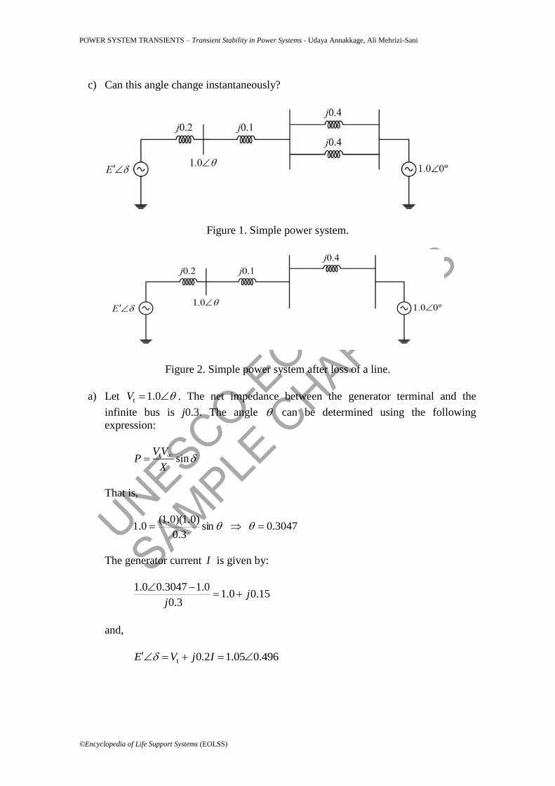
The synchronous machine shown in Figure 1 generates 1.0 pu output power. The
transient reactance dx of the generator is 0.2 pu as shown. The terminal voltage of the
generator ( tV ) and the infinite bus voltage ( V ) are both 1.0 pu.
a) Determine the magnitude ( E ) and phase angle ( ) of the internal voltage.
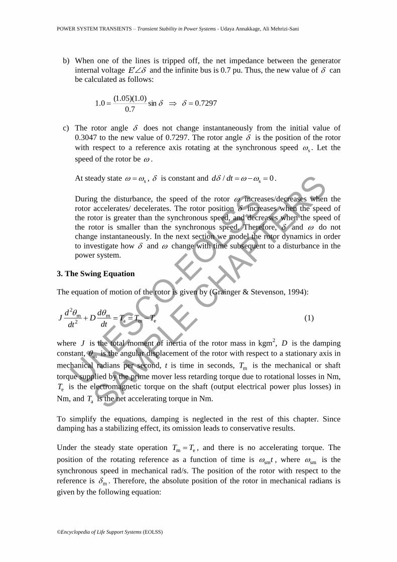
b) One of the transmission lines is suddenly tripped off (see Figure 2). Determine the
new phase angle of the internal voltage, assuming that E does not change.
UNESCO-EOLS
S
SAMPLE C
HAPTERS
POWER SYSTEM TRANSIENTS – Transient Stability in Power Systems - Udaya Annakkage, Ali Mehrizi-Sani
©Encyclopedia of Life Support Systems (EOLSS)
c) Can this angle change instantaneously?
Figure 1. Simple power system.
Figure 2. Simple power system after loss of a line.
a) Let t 1.0V . The net impedance between the generator terminal and the
infinite bus is j0.3. The angle can be determined using the following
expression:
t sinV V
PX
That is,
3047.0 sin3.0
)0.1)(0.1(0.1
The generator current I is given by:
15.00.13.0
0.13047.00.1j
j
and,
t 0.2 1.05 0.496E V j I
UNESCO-EOLS
S
SAMPLE C
HAPTERS
POWER SYSTEM TRANSIENTS – Transient Stability in Power Systems - Udaya Annakkage, Ali Mehrizi-Sani
©Encyclopedia of Life Support Systems (EOLSS)
b) When one of the lines is tripped off, the net impedance between the generator
internal voltage E and the infinite bus is 0.7 pu. Thus, the new value of can
be calculated as follows:
7297.0 sin7.0
)0.1)(05.1(0.1
c) The rotor angle does not change instantaneously from the initial value of
0.3047 to the new value of 0.7297. The rotor angle is the position of the rotor
with respect to a reference axis rotating at the synchronous speed s . Let the
speed of the rotor be .
At steady state s , is constant and s/ 0d dt .
During the disturbance, the speed of the rotor increases/decreases when the
rotor accelerates/ decelerates. The rotor position increases when the speed of
the rotor is greater than the synchronous speed, and decreases when the speed of
the rotor is smaller than the synchronous speed. Therefore, and do not
change instantaneously. In the next section we model the rotor dynamics in order
to investigate how and change with time subsequent to a disturbance in the
power system.
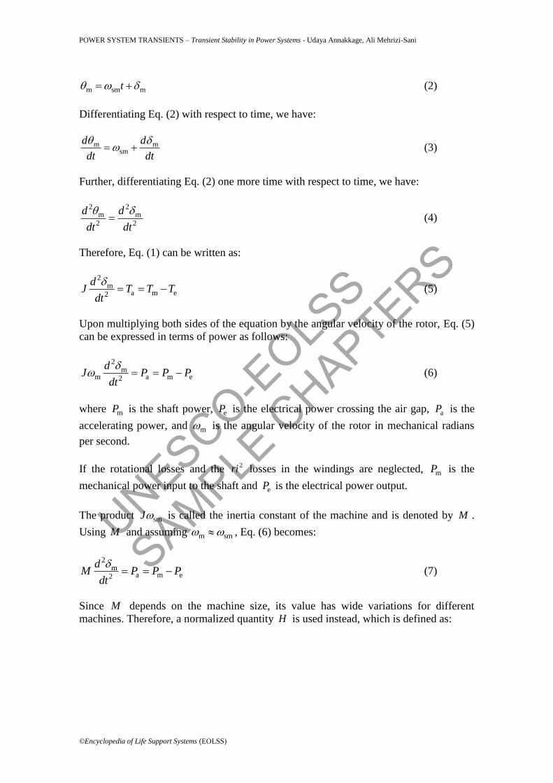
3. The Swing Equation
The equation of motion of the rotor is given by (Grainger & Stevenson, 1994):
2
m ma m e2
d dJ D T T T
dtdt
(1)
where J is the total moment of inertia of the rotor mass in kgm2, D is the damping
constant, m is the angular displacement of the rotor with respect to a stationary axis in
mechanical radians per second, t is time in seconds, mT is the mechanical or shaft
torque supplied by the prime mover less retarding torque due to rotational losses in Nm,
eT is the electromagnetic torque on the shaft (output electrical power plus losses) in
Nm, and aT is the net accelerating torque in Nm.
To simplify the equations, damping is neglected in the rest of this chapter. Since
damping has a stabilizing effect, its omission leads to conservative results.
Under the steady state operation m eT T , and there is no accelerating torque. The
position of the rotating reference as a function of time is smt , where sm is the
synchronous speed in mechanical rad/s. The position of the rotor with respect to the
reference is m . Therefore, the absolute position of the rotor in mechanical radians is
given by the following equation:
UNESCO-EOLS
S
SAMPLE C
HAPTERS
POWER SYSTEM TRANSIENTS – Transient Stability in Power Systems - Udaya Annakkage, Ali Mehrizi-Sani
©Encyclopedia of Life Support Systems (EOLSS)
m sm mt (2)
Differentiating Eq. (2) with respect to time, we have:
m msm
d d
dt dt
(3)
Further, differentiating Eq. (2) one more time with respect to time, we have:
2 2
m m
2 2
d d
dt dt
(4)
Therefore, Eq. (1) can be written as:
2
ma m e2
dJ T T T
dt
(5)
Upon multiplying both sides of the equation by the angular velocity of the rotor, Eq. (5)
can be expressed in terms of power as follows:
2
mm a m e2
dJ P P P
dt
(6)
where mP is the shaft power, eP is the electrical power crossing the air gap, aP is the
accelerating power, and m is the angular velocity of the rotor in mechanical radians
per second.
If the rotational losses and the 2ri losses in the windings are neglected, mP is the
mechanical power input to the shaft and eP is the electrical power output.
The product smJ is called the inertia constant of the machine and is denoted by M .
Using M and assuming m sm , Eq. (6) becomes:
2
ma m e2
dM P P P
dt
(7)
Since M depends on the machine size, its value has wide variations for different
machines. Therefore, a normalized quantity H is used instead, which is defined as:
UNESCO-EOLS
S
SAMPLE C
HAPTERS
POWER SYSTEM TRANSIENTS – Transient Stability in Power Systems - Udaya Annakkage, Ali Mehrizi-Sani
©Encyclopedia of Life Support Systems (EOLSS)
sm
2sm
rated
sm
rated
Kinetic energy of the rotor at synchronous speed in MJ
Machine rating in MVA
1
2
1
2 MJ/MVA
H
J
S
M
S
(8)
Therefore, M can be expressed in terms of H as:
rated
sm
2 MJ/mechanical radians
HM S
(9)
Substituting for M in Eq. (7) and dividing the resulting equation by ratedS gives:
2
a m em
2sm rated rated
2 P P Pd δH
ω S Sdt
(10)
Note that the right hand side of Eq. (10) is the per unit acceleration power.
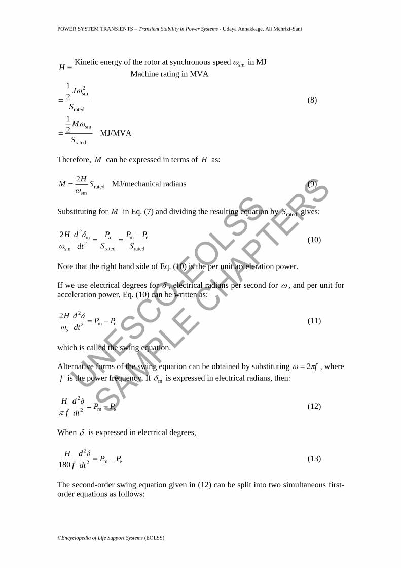
If we use electrical degrees for , electrical radians per second for , and per unit for
acceleration power, Eq. (10) can be written as:
2
m e2s
2H d δP P
ω dt (11)
which is called the swing equation.
Alternative forms of the swing equation can be obtained by substituting f 2 , where
f is the power frequency. If m is expressed in electrical radians, then:
2
m e2
H d δP P
f dt (12)
When is expressed in electrical degrees,
2
m e2180
H d δP P
f dt (13)
The second-order swing equation given in (12) can be split into two simultaneous first-
order equations as follows:
UNESCO-EOLS
S
SAMPLE C
HAPTERS
POWER SYSTEM TRANSIENTS – Transient Stability in Power Systems - Udaya Annakkage, Ali Mehrizi-Sani
©Encyclopedia of Life Support Systems (EOLSS)
2
m e2
H d δP P
f dt (14a)
s2
dδ
dt (14b)
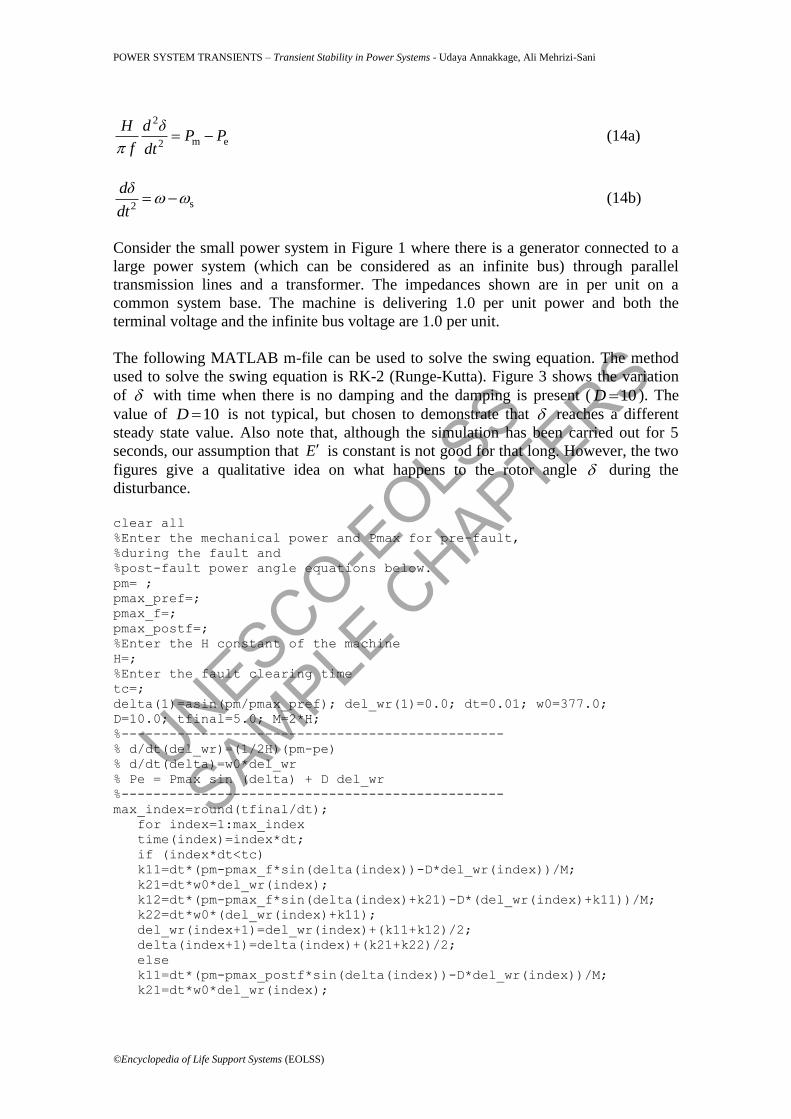
Consider the small power system in Figure 1 where there is a generator connected to a
large power system (which can be considered as an infinite bus) through parallel
transmission lines and a transformer. The impedances shown are in per unit on a
common system base. The machine is delivering 1.0 per unit power and both the
terminal voltage and the infinite bus voltage are 1.0 per unit.
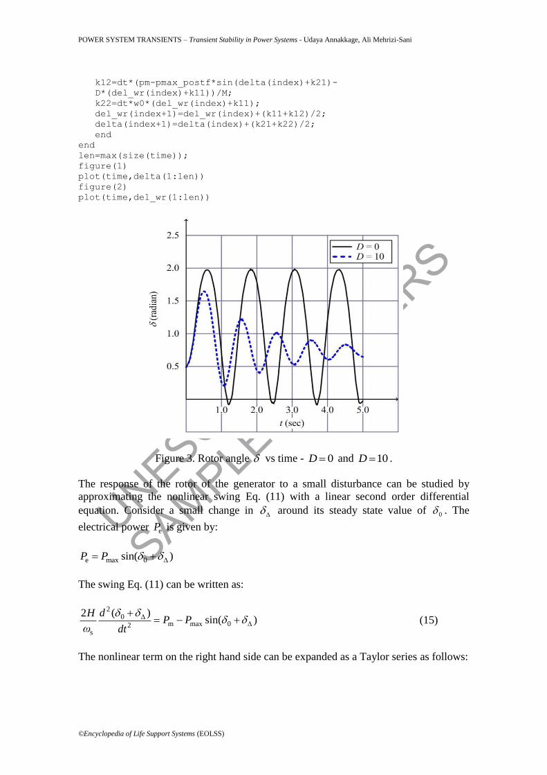
The following MATLAB m-file can be used to solve the swing equation. The method
used to solve the swing equation is RK-2 (Runge-Kutta). Figure 3 shows the variation
of with time when there is no damping and the damping is present ( 10D ). The
value of 10D is not typical, but chosen to demonstrate that reaches a different
steady state value. Also note that, although the simulation has been carried out for 5
seconds, our assumption that E is constant is not good for that long. However, the two
figures give a qualitative idea on what happens to the rotor angle during the
disturbance.
clear all
%Enter the mechanical power and Pmax for pre-fault,
%during the fault and
%post-fault power angle equations below.
pm= ;
pmax_pref=;
pmax_f=;
pmax_postf=;
%Enter the H constant of the machine
H=;
%Enter the fault clearing time
tc=;
delta(1)=asin(pm/pmax_pref); del_wr(1)=0.0; dt=0.01; w0=377.0;
D=10.0; tfinal=5.0; M=2*H;
%------------------------------------------------
% d/dt(del_wr)=(1/2H)(pm-pe)
% d/dt(delta)=w0*del_wr
% Pe = Pmax sin (delta) + D del_wr
%------------------------------------------------
max_index=round(tfinal/dt);
for index=1:max_index
time(index)=index*dt;
if (index*dt<tc)
k11=dt*(pm-pmax_f*sin(delta(index))-D*del_wr(index))/M;
k21=dt*w0*del_wr(index);
k12=dt*(pm-pmax_f*sin(delta(index)+k21)-D*(del_wr(index)+k11))/M;
k22=dt*w0*(del_wr(index)+k11);
del_wr(index+1)=del_wr(index)+(k11+k12)/2;
delta(index+1)=delta(index)+(k21+k22)/2;
else
k11=dt*(pm-pmax_postf*sin(delta(index))-D*del_wr(index))/M;
k21=dt*w0*del_wr(index);
UNESCO-EOLS
S
SAMPLE C
HAPTERS
POWER SYSTEM TRANSIENTS – Transient Stability in Power Systems - Udaya Annakkage, Ali Mehrizi-Sani
©Encyclopedia of Life Support Systems (EOLSS)
k12=dt*(pm-pmax_postf*sin(delta(index)+k21)-
D*(del_wr(index)+k11))/M;
k22=dt*w0*(del_wr(index)+k11);
del_wr(index+1)=del_wr(index)+(k11+k12)/2;
delta(index+1)=delta(index)+(k21+k22)/2;
end
end
len=max(size(time));
figure(1)
plot(time,delta(1:len))
figure(2)
plot(time,del_wr(1:len))
Figure 3. Rotor angle vs time - 0D and 10D .
The response of the rotor of the generator to a small disturbance can be studied by
approximating the nonlinear swing Eq. (11) with a linear second order differential
equation. Consider a small change in around its steady state value of 0 . The
electrical power eP is given by:
e max 0sin( )P P
The swing Eq. (11) can be written as:
2
0m max 02
s
( )2sin( )
dHP P
ω dt
(15)
The nonlinear term on the right hand side can be expanded as a Taylor series as follows:
UNESCO-EOLS
S
SAMPLE C
HAPTERS
POWER SYSTEM TRANSIENTS – Transient Stability in Power Systems - Udaya Annakkage, Ali Mehrizi-Sani
©Encyclopedia of Life Support Systems (EOLSS)
2
0max0max0max0max )sin(2
1)cos()sin()sin( PPPP
For small , the term 2
and higher order terms can be ignored. Then, Eq. (15) can be
written as:
2
m max 0 max 02s
( )2sin( ) cos( )
dHP P P
ω dt
(16)
But, m max 0sin( )P P . Therefore, Eq. (15) simplifies to:
2
max 02s
( )2cos( )
dHP
ω dt
(17)
Definition: The sensitivity of eP to at 0 is defined as the synchronizing power
coefficient pS . Note that p max 0cos( )S P . That is:
2
s p
2
( )
2
Sd
Hdt
(18)
Equation (18) describes a simple harmonic motion with the natural frequency of
oscillation nf given by:
s p
n2
S
H
4. Equal Area Criterion
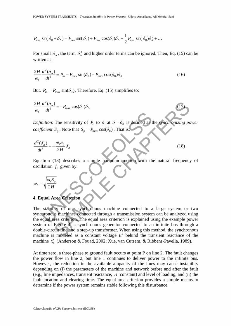
The stability of one synchronous machine connected to a large system or two
synchronous machines connected through a transmission system can be analyzed using
the equal area criterion. The equal area criterion is explained using the example power
system of Figure 4: a synchronous generator connected to an infinite bus through a
double-circuit line and a step-up transformer. When using this method, the synchronous
machine is modeled as a constant voltage E’ behind the transient reactance of the
machine dx (Anderson & Fouad, 2002; Xue, van Cutsem, & Ribbens-Pavella, 1989).
At time zero, a three-phase to ground fault occurs at point P on line 2. The fault changes
the power flow in line 2, but line 1 continues to deliver power to the infinite bus.
However, the reduction in the available ampacity of the lines may cause instability
depending on (i) the parameters of the machine and network before and after the fault
(e.g., line impedances, transient reactance, H constant) and level of loading, and (ii) the
fault location and clearing time. The equal area criterion provides a simple means to
determine if the power system remains stable following this disturbance.
UNESCO-EOLS
S
SAMPLE C
HAPTERS
POWER SYSTEM TRANSIENTS – Transient Stability in Power Systems - Udaya Annakkage, Ali Mehrizi-Sani
©Encyclopedia of Life Support Systems (EOLSS)
Figure 4. One-line diagram of a synchronous generator connected to an infinite bus.
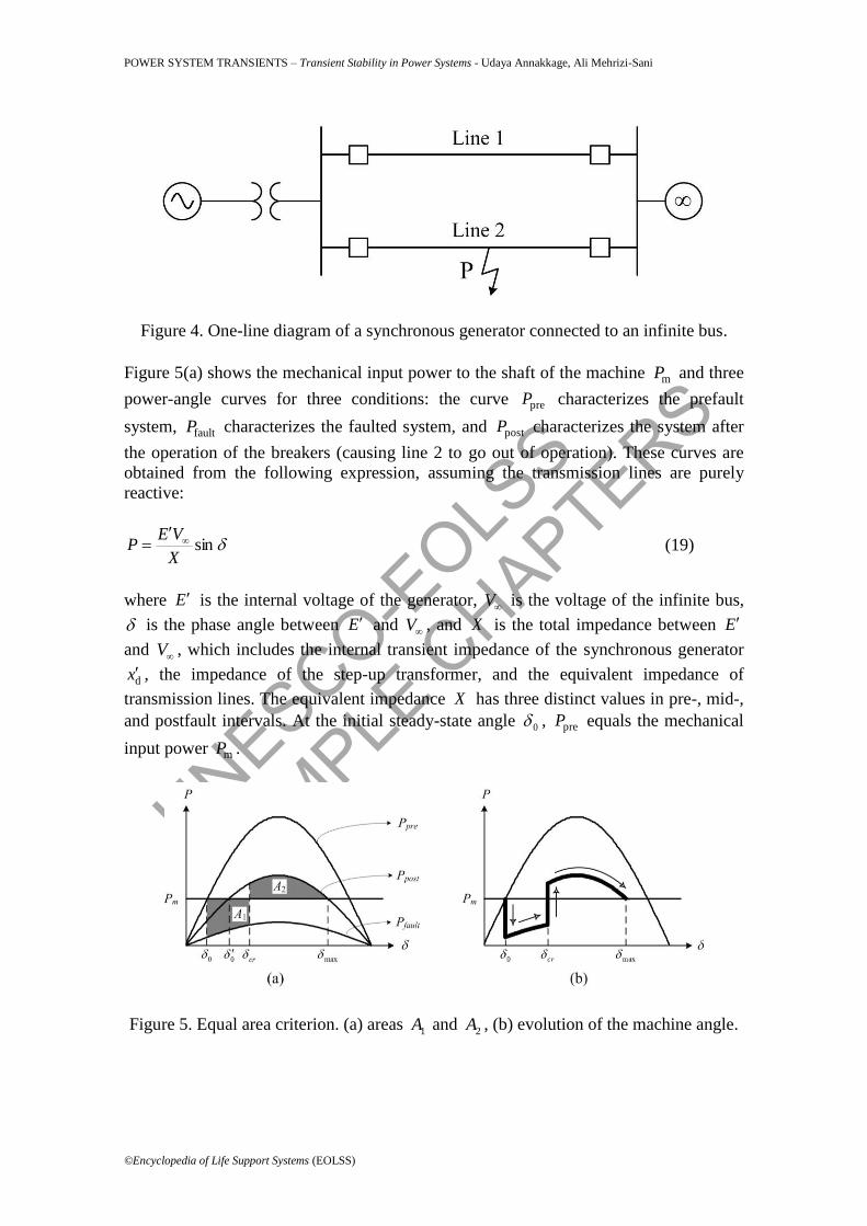
Figure 5(a) shows the mechanical input power to the shaft of the machine mP and three
power-angle curves for three conditions: the curve preP characterizes the prefault
system, faultP characterizes the faulted system, and postP characterizes the system after
the operation of the breakers (causing line 2 to go out of operation). These curves are
obtained from the following expression, assuming the transmission lines are purely
reactive:
sinX
VEP
(19)
where E is the internal voltage of the generator, V is the voltage of the infinite bus,
is the phase angle between E and V , and X is the total impedance between E
and V , which includes the internal transient impedance of the synchronous generator
dx , the impedance of the step-up transformer, and the equivalent impedance of
transmission lines. The equivalent impedance X has three distinct values in pre-, mid-,
and postfault intervals. At the initial steady-state angle 0 , preP equals the mechanical
input power mP .
Figure 5. Equal area criterion. (a) areas 1A and 2A , (b) evolution of the machine angle.
UNESCO-EOLS
S
SAMPLE C
HAPTERS
POWER SYSTEM TRANSIENTS – Transient Stability in Power Systems - Udaya Annakkage, Ali Mehrizi-Sani
©Encyclopedia of Life Support Systems (EOLSS)
Upon occurrence of the fault, cannot change instantaneously; however, the power-
angle characteristic of the system instantaneously shifts to the faultP curve, Figure 5(a),
causing the electric power eP delivered to the infinite bus to decrease. From the swing
equation, the mismatch between the mechanical input power and electrical output power
will cause the accelerating power to be positive. Therefore, the machine speed increases
beyond the synchronous speed, and as shown in Figure 5(b), increases. The increase
in the machine rotor speed (defined as r s ) increases the kinetic energy of the
machine. This energy is proportional to the area 1A , Figure 5(a), between mP and faultP
and between 0 and cr . At cr , the fault is cleared by tripping out line 2, and the
power-angle characteristic of the system suddenly shifts to the postP curve, Figure 5(b).
In this case, the new value of electrical output power eP is greater than the mechanical
input power mP . As a result, the machine decelerates and its kinetic energy decreases.
However, as long as the rotor speed is higher than the synchronous speed ( 0r ),
continues to increase. The maximum allowable increase of is max ; if increases
beyond max , the accelerating power m postP P becomes positive, causing the rotor to
accelerate and the angle to increase further. This eventually leads to too high a deviation
in the machine speed, and the machine will finally trip out.
The equal area criterion states that for the power system to remain stable, the area 1A
must be less than the area 2A (the area between mP and postP , and between cr and
max ). That is, the increase in the rotor energy before clearing the fault must be equal to
the decrease in the rotor energy after clearing the fault. In this case, the rotor swings
between max and 0 . Due to mechanical losses, the oscillations gradually damp until
the rotor angle settles to 0 , see Figure 5(a).
Consider the swing equation, reproduced below.
2
m e2s
2H dP P
ω dt
(20)
Since
r s
d
dt
(21)
we have
rm e
s
2 dHP P
ω dt
(22)
Multiplying both sides of Eq. (22) by r ,
UNESCO-EOLS
S
SAMPLE C
HAPTERS
POWER SYSTEM TRANSIENTS – Transient Stability in Power Systems - Udaya Annakkage, Ali Mehrizi-Sani
©Encyclopedia of Life Support Systems (EOLSS)
rr m e
s
2dH d
ω P Pω dt dt
(23)
and
2r
m e
s
dH dP P
ω dt dt
(24)
Integrating Eq. (24) with respect to time from ( r0 ; 0 ) to ( rx ; x ),
2 2r r0 m e
0s
2 x
x
HP P d
ω
(25)
But r0 0 and r 0x . Therefore,
m e0
0x
P P d
(26)
which can be expressed as:
m e e m0
c x
cP P d P P d
(27)
Note that the term
m e0
cP P d
is proportional to the kinetic energy absorbed by the rotating mass during the fault and
x
c
dPP me
is proportional to the kinetic energy released by the rotating mass after clearing the
fault. If the absorbed kinetic energy can be released to the network, then the machine is
stable.
The critical clearing time (angle) is the maximum time (angle) of clearing a fault upon
which the system can maintain its stability. This angle is found using the equal area
criterion 21 AA . The areas 1A and 2A in Figure 5(a) are obtained as follows:
cr
1 m fault m cr 0 fault cr 00
sin cos cosA P P d P P
(28a)
UNESCO-EOLS
S
SAMPLE C
HAPTERS
POWER SYSTEM TRANSIENTS – Transient Stability in Power Systems - Udaya Annakkage, Ali Mehrizi-Sani
©Encyclopedia of Life Support Systems (EOLSS)
max
2 post m post cr max m max crcr
sin cos cosA P P d P P
(28b)
Equate 1A and
2A to calculate the critical clearing angle as:
m max 0 fault 0 post max
cr
post fault
cos coscos
P P P
P P
(29)
-
-
-
TO ACCESS ALL THE 48 PAGES OF THIS CHAPTER,
Visit: http://www.eolss.net/Eolss-sampleAllChapter.aspx
Bibliography
Anderson P., Fouad A. (2002). Power System Control and Stability, 2nd Edition, New York, NY: John
Wiley-IEEE Press. [This is a classic textbook on power system dynamics, including synchronous
generators and their excitation systems, transmission systems, and loads].
Borghetti A., Caldon R., Mari A., Nucci C.A. (1997). On dynamic load models for voltage stability
studies, IEEE Trans. on Power Systems 12, 293-303. [This paper compares three different load models
under different simulation scenarios for voltage stability studies. It concludes that under some
perturbations, only higher order models are capable of correctly capturing the performance of the power
system].
Christie R.D., Bose A. (1996). Load frequency control issues in power system operations after
deregulation, IEEE Trans. on Power Systems 11, 1191-1200. [This paper discusses the challenges
introduced by deregulation. The paper identifies the likely deregulation scenarios, technical issues, and
technical solutions].
Fortescue C. (1918). Method of symmetrical coordinates applied to solution of polyphase networks,
Trans. of AIEE 37, 1027-1040. [This classic paper introduces the method of symmetrical components that
is used for the analysis of unbalanced three-phase power systems].
Grainger J.J., Stevenson W.D. (1994). Power System Analysis, New York, NY: McGraw-Hill. [This
textbook discusses operation of power system and includes topics such as transmission line models,
power flow analysis, fault analysis, rotor angle stability, and power system state estimation].
IEEE/CIGRE Joint Task Force on Stability Terms and Definitions (2004). Definitions and classification
of power system stability, IEEE Trans. on Power Systems 19, 1387-1401. [This paper provides a
definition of power system stability terms].
IEEE Committee Report (1981). Excitation systems models for power system stability studies, IEEE
Trans. on Power Apparatus and Systems 100, 494-509. [This report discusses models of synchronous
generator excitation systems for power system stability analysis].
UNESCO-EOLS
S
SAMPLE C
HAPTERS
POWER SYSTEM TRANSIENTS – Transient Stability in Power Systems - Udaya Annakkage, Ali Mehrizi-Sani
©Encyclopedia of Life Support Systems (EOLSS)
IEEE Std 421.5-1992 (1992). IEEE recommended practice for excitation system models for power system
stability studies. [This IEEE standard details the recommended practices for models for excitations
systems used for power system stability studies].
Jocic L.B., Ribbens-Pavella M., Siljak D.D. (1978). Multimachine power systems: Stability,
decomposition, and aggregation, IEEE Trans. on Automatic Control 23, 325-332. [This paper proposes an
approach for the study of transient stability of multimachine systems using vector Lyapunov functions].
Kayaikci M., Milanovic J.V. (2008). Assessing transient response of DFIG-based wind plants - The
influence of model simplifications and parameters, IEEE Trans. on Power Systems 23, 545-553. [This
paper discusses the performance of different models in predicting the transient response of DFIG
systems].
Krause P.C., Thomas C.H. (1965). Simulation of symmetrical induction machinery, IEEE Trans. on
Power Apparatus and Systems 84, 1038-1053. [This paper generalizing several commonly used reference
frames into a unified arbitrary reference frame theory that has been very actively used for the analysis of
electrical machinery, motor drives and controls. It is shown that any reference frame can be obtained by
assigning a particular speed to the arbitrary reference frame].
Kundur P. (1994). Power System Stability and Control, New York, NY: McGraw-Hill. [This textbook
provides a comprehensive view of power system stability issues].
Ledesma P., Usaola J. (2005). Doubly fed induction generator model for transient stability analysis, IEEE
Trans. on Energy Conversion 20, 388-397. [This paper presents a model of DFIG suitable for transient
stability analysis by assuming the current control loops are very fast and ignoring their effect on the
transient stability of the power system].
Luna A., de Araujo Lima F.K., Santos D., Rodríguez P., Watanabe E.H., Arnaltes S. (2011). Simplified
modeling of a DFIG for transient studies in wind power applications, IEEE Trans. on Industrial
Electronics 58, 9-20. [This paper provides a simplified model of DFIG for transient stability analysis
derived from the fifth-order model].
Muyeen S.M., Ali M.H., Takahashi R., Murata T., Tamura J., Tomaki Y., Sakahara A., Sasano E. (2007).
Comparative study on transient stability analysis of wind turbine generator system using different drive
train models, IET Renewable Power Generation 1, 131-141. [This paper provides a comparison of the
performance of six-, three-, and two-mass drive train models for wind turbine generator systems in
transient stability scenarios. The paper concludes that the two-mass model sufficiently represents a wind
turbine generator system for transient stability analysis purposes].
Pena R., Clare J.C., Asher G.M. (1996). Doubly fed induction generator using back-to-back PWM
converters and its application to variable-speed wind-energy generation, IEE Proc. Electric Power
Applications 143, 231-241. [This paper describes the design of a DFIG using back-to-back PWM voltage-
source converters in the rotor circuit. Independent control of active and reactive power drawn from the
supply using vector control is also studied].
PSS/E Version 33 (2011). Siemens PTI. [PSS/E is software used for study of transient stability of power
systems].
Rahimi M., Parniani M. (2010), Transient performance improvement of wind turbines with doubly fed
induction generators using nonlinear control strategy, IEEE Trans. on Energy Conversion 25, 514-525.
[This paper investigates the possibility of improvement of the transient performance of DFIG wind
turbines using a nonlinear control strategy].
Xue Y., van Cutsem T., Ribbens-Pavella M. (1989). Extended equal area criterion: Justifications,
generalizations, applications, IEEE Trans. on Power Systems 4, 44-52. [This paper revisits the extended
equal area criterion to study and remedy possible instability types that are likely to happen in real-world
scenarios by extending the method beyond the first swing stability].
UNESCO-EOLS
S
SAMPLE C
HAPTERS
POWER SYSTEM TRANSIENTS – Transient Stability in Power Systems - Udaya Annakkage, Ali Mehrizi-Sani
©Encyclopedia of Life Support Systems (EOLSS)
Biographical Sketches
Udaya D. Annakkage received the B.Sc. degree in electrical engineering from the University of
Moratuwa, Sri Lanka, in 1982, and M.Sc. and Ph.D. degrees from the University of Manchester, U.K., in
1984 and 1987 respectively. He is a Professor at the University of Manitoba, Winnipeg, Manitoba,
Canada. His research interests are power system stability and control, security assessment and control,
operation of restructured power systems, and power system simulation. He is a member of several
Working Groups and Task Forces of IEEE and CIGRE. He is an editor of IEEE Transactions on Power
Systems.
Ali Mehrizi-Sani received the B.Sc. degrees in electrical engineering and petroleum engineering from
Sharif University of Technology, Tehran, Iran, both in 2005, and the M.Sc. degree from the University of
Manitoba, Winnipeg, MB, Canada, and the Ph.D. degree from the University of Toronto, Toronto, ON,
Canada, both in electrical engineering, in 2007 and 2011, respectively. He is currently an Assistant
Professor at Washington State University, Pullman, WA, USA. His areas of interest include power
electronics and power system control and optimization. Dr. Mehrizi-Sani is a recipient of the NSERC
Postdoctoral Fellowship in 2011. He was a Connaught Scholar at the University of Toronto.