This content has been downloaded from IOPscience. Please scroll down to see the full text.

Download details:

IP Address: 130.63.180.147

This content was downloaded on 11/08/2014 at 08:07

Please note that terms and conditions apply.

Transformation of decelerating laser beams into accelerating ones

View the table of contents for this issue, or go to the journal homepage for more

2014 J. Opt. 16 085701

(http://iopscience.iop.org/2040-8986/16/8/085701)

Home Search Collections Journals About Contact us My IOPscience

Transformation of decelerating laser beamsinto accelerating ones

V V Kotlyar1,2, A A Kovalev1,2 and V A Soifer1,2

1 Laser Measurements Laboratory, Image Processing Systems Institute of the Russian Academy ofSciences, 151 Molodogvardejskaya street, Samara 443001, Russia2 Technical Cybernetics sub-department, S P Korolyov Samara State Aerospace University, 34Moskovskoye shosse, Samara 443086, Russia

E-mail: alexeysmr@mail.ru

Received 3 February 2014, revised 30 April 2014Accepted for publication 27 May 2014Published 25 July 2014

AbstractWe propose a method for obtaining paraxial accelerating two-dimensional laser beams on a finitesection of their path in which the complex amplitudes of familiar decelerating light beams arecomplex-conjugated and shifted along the optical axis. With this method, Fresnel and Laplacebeams accelerating along a square-root-parabola path and a paraxial ‘half-Bessel’ beam aregenerated. As distinct from the familiar diffraction-free accelerating Airy beams, the beamsunder analysis are found to be converging on the final section of the accelerating path.

Keywords: accelerating laser beam, decelerating laser beam, beam path, Fresnel beam,Laplace beamPACS numbers: 42.25.Bs, 42.25.Fx

(Some figures may appear in colour only in the online journal)

1. Introduction

Recently, non-paraxial accelerating Weber beams that retaintheir shape upon propagation on a parabolic path have beenconsidered [1]. Being similar to the ‘half-Bessel’ beams [2],the Weber beams can be described analytically, which isnot the case for the ‘half-Bessel’ beams. The Weber–Her-mite beams have also been known to present solutions ofthe paraxial equation of propagation [3]. A general theoryof 3D non-paraxial accelerating beams was developed in[4] on the basis of familiar solutions of Helmholtzequations in parabolic, oblate and flattened spheroid coor-dinates. These beams propagate on a circular arc. The Airybeams that propagate with a non-uniform acceleration on ahyperbolic trajectory were proposed in [5]. Although suchbeams are diverging upon propagation, thus not retainingtheir shape, the final section of their propagation path canbe more bent when compared with the conventional Airybeams [6].

In this work, we take a different approach to gen-erating the accelerating beams, which is as follows. There

are 2D paraxial light fields in which the complex amplitudefunction argument is related to variables as x2/z, where x isthe transverse coordinate and z is the longitudinal coordi-nate. An example is given by the light field generatedthrough diffracting a plane wave by a corner phase step [7]or a well-known solution of the problem of diffraction bythe edge of an opaque screen [8]. In this work, othersolutions of the paraxial equation of propagation are alsodiscussed. Light fields in which the complex amplitudefunction has the argument given by x2/z propagate on asquare-root parabola path, x = z1/2. Such beams are decel-erating because the acceleration, as the second derivative

along the trajectory, ″ = –x z3/2 has the opposite sign to thevelocity (the first derivative along the trajectory) x′= z–1/2.If, however, if the field amplitude at distance z0 is replacedby the complex-conjugated amplitude, and the axis origin issimultaneously shifted to point z0, the resulting light fieldwill propagate with acceleration along the path x= (z0− z)

1/2.In this work, we derive analytical relationships for thecomplex amplitudes of such accelerating beams. Thesebeams are not only accelerating, but also converging at a

Journal of Optics

J. Opt. 16 (2014) 085701 (8pp) doi:10.1088/2040-8978/16/8/085701

2040-8978/14/085701+08$33.00 © 2014 IOP Publishing Ltd Printed in the UK1

distance from the initial plane (z=0) to the focal plane(z= z0). Also we analyze paraxial ‘half-Bessel’ beams, whichare different from the non-paraxial ones [2].

2. Accelerating beams

Assume that at each particular distance z passed by a laserbeam the intensity maximum coordinate is given by xmax(z).For the beam to experience an acceleration at a certain pathsection, the first and second derivatives of the intensitymaximum coordinate xmax with respect to the passed distancez need to have the same sign [5]:

⎛⎝⎜

⎞⎠⎟

⎛⎝⎜

⎞⎠⎟ >

x

z

x

z

d

d

d

d0. (1)max

2max2

The most widely-known accelerating beams are Airybeams, with their complex amplitude given by [6]:

ξ ξ ξ= − −( ) ( )E x z i s is i( , ) A 4 exp 2 12 , (2)2 3

where (x, z) are the Cartesian coordinates, s= x/x0, ξ= z/(kx02),

k= 2π/λ is the wave number, λ is the wavelength, x0 is anarbitrary scaling factor, and Ai(x) is the Airy function (9,section 10.4). The beams’ intensity maximums have thecoordinates

= +x x yz

k x4, (3)

mmax 0

2

203

where ym is the coordinate of the mth zero of the function

Aiʼ(x). Then, = ( )x z z k xd /d / 2max2

03 and = ( )x z k xd /d 1/ 2 .2

max2 2

03

Thus, the condition in equation (1) is satisfied for any distancez> 0, with the acceleration x zd /d2

max2 having a constant value.

Below, we analyze laser beams characterized by a non-uni-form acceleration which is decreasing with the distancepropagated.

2.1. Airy beams with a hyperbolic path

The Airy beams with a hyperbolic path characterized at z= 0by the complex amplitude

⎡⎣ ⎤⎦α β= +E x i x x i x x( , 0) exp ( ) ( ) , (4)03

0

where x0 is a scaling factor and α, β aredimensionless parameters, were discussed in [5, 10, 11].The beam’s trajectory in the Fresnel diffraction regiontakes the form:

⎧

⎨⎪⎪

⎩⎪⎪

β αα

α

β αα

α=

− − >

+ + <

( )

( )x

z

kxy

kx

z

z

kxy

kx

z

312

, 0,

312

, 0.

(5)m

m

max0

03

0

03

3

3

Based on condition (1), the acceleration has been shown[5] to occur at the path section

⎧

⎨⎪⎪⎪

⎩⎪⎪⎪

α α βα

α α βα

> =−

>

+<

( )

( )

z z

kx

y

kx

y

2 3 3, 0,

2 3 3, 0,

(6)m

m

1

02

02

3

3

given that α β α< ysign ( ) (3 )m

1/3. For such a beam, the

acceleration decreases as z−3: α= − ( )x z kx zd /d / 62max

203 3 .

2.2. Hermite–GAUSS beams

It turns out that the well-known Hermite–Gauss beams [12]also possess an acceleration. Actually, let at z= 0, the lightfield be given by the complex amplitude:

⎜ ⎟⎛⎝⎜

⎞⎠⎟

⎛⎝

⎞⎠= = −E x z

x

wH

x

a( , 0) exp , (7)n

2

2

where (x, z) are the Cartesian coordinates, w is the Gaussianbeam waist radius, n and a are, respectively, the order andscale of the Hermite polynomial. Then, by taking the Fresneltransform we can show that at distance z from the initial planethere will be generated a field with the following complexamplitude distribution [13, 14]:

⎡⎣⎢

⎤⎦⎥

⎡⎣⎢⎢

⎤⎦⎥⎥

μ νμ

μ ν

= −

×

− +E x z z zx

w z

Hx

a z z

( , ) [ ( ) ] [ ( ) ] exp( )

( ) ( ), (8)

n n

n

( 1) 2 22

2

where zR= kw2/2, za= ka

2/2, μ(z) = 1 + iz/zR, ν(z) = 1 + iz(1/zR− 1/za).

For simplicity, let us analyze the case when n= 1. Then,the intensity of beam (8) in the plane found at distance z fromthe initial plane will be given by

⎡⎣⎢

⎤⎦⎥μ μ

= = −I x z E x zx

a z

x

w z( , ) ( , )

4

( )exp

2

( ). (9)2

2

2 3

2

2 2

Differentiating both parts of equation (9) with respect tox, we obtain the necessary condition for the intensityextremes:

μ=x

x

w z2

4

( ). (10)

3

2 2

when x= 0, there is a minimum (because the I(0, z) intensity iszero), whereas the maxima coordinates are given by

σ= ±x z2 ( ), (11)max 0

where ⎡⎣ ⎤⎦σ = + ( )z w z z( ) ( /2) 1 / R0

2 1/2

is the square root of the

intensity second-order moment for the fundamental mode(Gaussian beam).

2

J. Opt. 16 (2014) 085701 V V Kotlyar et al

It can be easily shown that the maximum intensity curveis defined by a hyperbola. The first- and second-order deri-vatives of xmax with respect to z are:

⎡⎣ ⎤⎦

= ±+

= ±+

( )

( )

x

z

w z

z z z

x

z

w

z z z

d

d 2 1,

d

d 2

1

1. (12)

R R

R R

max

2 2

2max2

2 2 3 2

From equation (12), the product ( )( )x z x zd /d d /dmax2

max2 is

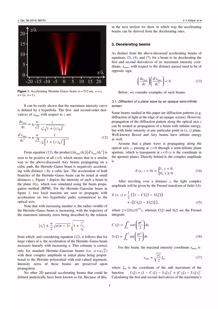
seen to be positive at all z> 0, which means that in a similarway to the above-discussed Airy beams propagating on acubic path, the Hermite–Gauss beam is negatively accelerat-ing with distance z by a cubic law. The acceleration of bothbranches of the Hermite–Gauss beam can be noted at smalldistances z. Figure 1 depicts the intensity of such a beam inthe plane Oxz, which was simulated using the beam propa-gation method (BPM). For the Hermite–Gaussian beam infigure 1, two local maxima are seen to propagate withacceleration on two hyperbolic paths symmetrical to theoptical axis.

Note that with increasing number n, the radius (width) ofthe Hermite–Gauss beam is increasing, with the trajectory ofthe outermost intensity zeros being described by the relation

⩽ − +xw

n nz

z2( 1) 1 ,n

R0

2

2

from which, and considering equation (12), it follows that forlarge values of n, the acceleration of the Hermite–Gauss beamincreases linearly with increasing n. This estimate is correct

only for standard Hermite–Gaussian beams (i.e. w = a 2 )with their complex amplitude in initial plane being propor-tional to the Hermite polynomial with real-valued argument.Intensity zeros of these beams are preserved uponpropagation.

No other 2D paraxial accelerating beams that could bedefined analytically have been known so far. Because of this,

in the next section we show in which way the acceleratingbeams can be derived from the decelerating ones.

3. Decelerating beams

As distinct from the above-discussed accelerating beams ofequations (2), (4), and (7), for a beam to be decelerating thefirst and second derivatives of its maximum intensity coor-dinate, xmax, with respect to the distance passed need to be ofopposite sign:

⎛⎝⎜

⎞⎠⎟

⎛⎝⎜

⎞⎠⎟ <

x

z

x

z

d

d

d

d0. (13)max

2max2

Below, we consider examples of such beams.

3.1. Diffraction of a plane wave by an opaque semi-infinitescreen

Some beams studied in this paper are diffraction patterns (e.g.diffraction of light at the edge of an opaque screen). However,propagation of the diffraction pattern along the optical axis zcan be treated as propagation of a beam with infinite energy,but with finite intensity at any particular point in (x, z) plane.Well-known Bessel and Airy beams have infinite energyas well.

Assume that a plane wave is propagating along theoptical axis z, passing at z= 0 through a semi-infinite planeaperture, which is transparent at x< 0 (x is the coordinate inthe aperture plane). Directly behind it, the complex amplitudeis

⎧⎨⎩= = <⩾E x z

xx

( , 0)1, 0,0, 0.

(14)

After traveling over a distance z, the light complexamplitude will be given by the Fresnel transform of field (14):

ξ ξ

ξ ξ

= − −

+ −

{[ ( ) ( )]

[ ( ) ( )]}

E x z C S

i C S

( , )1

21

, (15)

where ξ= [2/(λz)]1/2x, whereas C(ξ) and S(ξ) are the Fresnelintegrals:

⎛⎝⎜

⎞⎠⎟

⎛⎝⎜

⎞⎠⎟

∫

∫

ξ π

ξ π

=

=

ξ

ξ

Ct

t

St

t

( ) cos2

d ,

( ) sin2

d . (16)

0

2

0

2

For this beam, the maximal intensity coordinate xmax is

λ ξ=xz

2, (17)mmax

where ξm is the coordinate of the mth maximum of thefunction ξ ξ ξ ξ ξ= − − + −I C S C S( ) [1 ( ) ( ) ] [ ( ) ( ) ]2 2.Calculating the first and second derivatives of the maximum’s

Figure 1. Accelerating Hermite–Gauss beam (λ= 532 nm, w= λ,a= 2λ, n = 1).

3

J. Opt. 16 (2014) 085701 V V Kotlyar et al

coordinate xmax with respect to the passed distance z, we find:

λ ξ

λ ξ

=

= −

x

z z

x

z z z

d

d

1

2 2,

d

d

1

4 2. (18)

m

m

max

2max2

From equation (18), it is seen that condition (13) is validfor all z> 0. The deceleration of each maximum can be seen infigure 2, which shows the intensity of the beam ofequation (15).

Light field (14), (15) is a particular case of a more generalfield with its complex amplitude E+ν(x, z= 0) = {x

ν, x> 0; 0,x⩽ 0}. This field generates Weber–Hermite beams [3].Besides, the field (15) can be expressed via complementaryerror function (by A Torre):

⎛⎝⎜

⎞⎠⎟= −

E x zi k

zx( , )

1

2erfc

1

2. (19)

3.2. Two-dimensional hypergeometric beams and besselbeams

Just as it was done in [15], the solution to the paraxialequation of propagation

∂∂

+ ∂∂

=ikE

z

E

x2 0, (20)

2

2

will be sought for in the form E(x, z) = xpzqF(sxmzn), where F(x) is a function and s is a scaling factor. After reducing theresulting second-order differential equation to the Kummerequation, the relation for the complex amplitude of the 2Danalog of the 3D generalized Hypergeometric mode [16]takes the form:

⎛⎝⎜

⎞⎠⎟= −E x z z F a

ikx

z( , ) ,

1

2,

2, (21)a

11

2

where a is an arbitrary constant and 1F1(a,b,x) is the confluent

hypergeometric function (Kummer function) [9]. The deri-vative of any solution of equation (20), taken with respect toany Cartesian coordinate has also been known to be thesolution of equation (20). Therefore, it is possible to considera light beam with the amplitude

⎛⎝⎜

⎞⎠⎟= −E x z xz F a

ikx

z( , ) ,

3

2,

2. (22)a

11

2

In particular, putting a = 3/4, equation (22) gives thesolution of equation (20) in the form of a fractional-orderBessel beam:

⎡⎣⎢

⎤⎦⎥

⎡⎣⎢

⎤⎦⎥=

+ + +E x z

x

z zJ

kx

z z

ikx

z z( , )

4 ( )exp

4 ( ), (23)

0

2

0

2

0

14

where z0 is an arbitrary positive constant (intended to avoidsingularity in the plane z= 0). In order to derive equation (23),expression 13.6.1 from [9] has been used. For this beam, theintensity maximumʼs coordinates are

=+

xz z

ky

4 ( ), (24)

mmax0

where ym is the mth root of the equation′+ =[ ( ) ( ) ]J y J y J y y( ) 4 01/4 1/4 1/4 . Relationship (24) is similar

to (17), which implies that xmax is proportional to z1/2. Thus,we can infer that beam (23) is decelerating, as can be seenfrom figure 3, which depicts the intensity pattern simulated bythe BPM (λ= 532 nm, z0 = 20λ, simulation region: −20λ⩽x⩽ 20λ, 0⩽ z⩽ 80λ).

Note that field (22) at a= 1/2 is closely related with thefield (15). Using the relation between the Fresnel integrals andthe Kummer function [9, equation 7.3.25], it can be shownthat the field (15) is expressed via the field (22) as follows:

⎧⎨⎩⎛⎝⎜

⎞⎠⎟

⎫⎬⎭π= − − −

E x z ik

zx F

ikx

z( , )

1

21 (1 )

1

2,

3

2,

2.11

2

Figure 2. Diffraction of a plane wave by a semi-infinite aperture:intensity pattern in the Oxz-plane (λ = 532 nm, −5λ⩽ x⩽ 5λ,3λ⩽ z⩽ 8λ).

Figure 3. Intensity pattern in the Oxz-plane produced by the lightbeam of equation (23).

4

J. Opt. 16 (2014) 085701 V V Kotlyar et al

4. Transformation of decelerating beams intoaccelerating ones

From equations (1) and (13), a simple change of variablesz→ z0− z is seen to result in the acceleration turning intodeceleration, and vice versa. Actually, let us analyze a lightbeam with its complex amplitude derived from equation (15)by use of complex conjugation and substitution of ξ by

⎡⎣ ⎤⎦ξ λ= −z z x2/ ( )0 :

ξ ξ

ξ ξ

< = − −

− −

E x z z C S

i C S

( , )1

2{[1 ( ) ( ) ]

[ ( ) ( ) ] }. (25)

0

The light beam of equation (25) will be referred to asFresnel beam. Considering that

= =→∞ →∞

C x S xlim ( )1

2, lim ( )

1

2, (26)

x x

we find that in the vicinity of the focal plane z= z0, on theassumption that z< z0, the complex amplitude takes the form:

⎧⎨⎩→ − = ><( )E x z z

xx

, 00, 0,1, 0.

(27)0

The intensity pattern produced by beam (25) in the planeOxz is shown in figure 4.

The arguments ξ of Fresnel integrals (25) become ima-ginary immediately behind the plane z= z0, because 2/[λ(z0− z)] < 0. Note that since the imaginary part can be bothpositive and negative, there may be two solutions, with onlyone of them meeting the boundary condition

→ + = → −( ) ( )E x z z E x z z, 0 , 00 0 . Making us of the

identities for the Fresnel integrals of imaginary variables,=C iz iC z( ) ( ) and = −S iz iS z( ) ( ) [9, relations 7.3.18], the

complex amplitude behind the plane z= z0 can be shown to

take the form:

η η

η η

> = − −

+ −

E x z z C S

i C S

( , )1

2{[1 ( ) ( ) ]

[ ( ) ( ) ]}, (28)

0

where ⎡⎣ ⎤⎦η λ= −z z x2/ ( )0 . The second solution given by

η η

η η

> = + +

− −

E x z z C S

i C S

( , )1

2{[1 ( ) ( ) ]

[ ( ) ( ) ]}, (29)

0

does not satisfy the boundary condition.From comparison of (25) and (28), the light beam is seen

to accelerate at z< z0, forming a semi-infinite uniform focalspot at z= z0 and reversing to deceleration at z> z0, with theamplitude at z> z0 being a specular reflection of that at z< z0.In figure 5(a) is depicted the intensity pattern of light beam(25), (28) in the plane Oxz, whereas figure 5(b) shows theintensity profile in the plane z= z0. The results shown infigure 5 have been derived by FDTD-aided simulation forλ= 532 nm, z0 = 40λ, simulation domain −20λ⩽ x⩽ 20λ,0⩽ z⩽ 60λ. Intensity oscillations in the vicinity of point x= 0appear because the initial field is limited by the simulationdomain.

Similarly, substituting in (23) z+ z0 for z0− z andapplying complex conjugation, we obtain a light beamdescribed in the initial plane (z= 0) by the complex amplitude

⎛⎝⎜

⎞⎠⎟

⎛⎝⎜

⎞⎠⎟= = −E x z

x

zJ

kx

z

ikx

z( , 0)

4exp

4. (30)

0

2

0

2

0

14

With the initial field given by equation (30), the BPMtechnique was used to calculate the light beam intensity in theplane Oxz (at λ= 532 nm, z0 = 40λ), with figure 6(a) showingthat the focused beam is accelerating. Figure 6(b) showstransverse intensity distribution in the focal plane z0 = 40λ, thesize of the focal spot (full width at half-maximum) is 0,53 μm(i.e. 1λ). The asymmetry of the resulting focal spot is due to aπ/2-phase jump that field (30) undergoes at point x= 0. Thistype of focusing of the accelerating beam was earlier reportedin [17] for a radially symmetric Airy beam.

Assume that in the initial plane for x< 0, the amplitudeequals zero:

⎧⎨⎪

⎩⎪⎛⎝⎜

⎞⎠⎟

⎛⎝⎜

⎞⎠⎟= = − ⩾

<E x z

x

zJ

kx

z

ikx

zx

x

( , 0) 4exp

4, 0,

0, 0.

(31)0

2

0

2

0

14

Figure 7 shows the intensity pattern for beam (31), whichwas calculated using the BPM technique for the same para-meters as in figure 6.

Note that for other orders of Bessel function (31) asimilar intensity pattern is formed (figure 8).

From figure 8, the acceleration is seen to decrease withincreasing order of Bessel function. The accelerating paraxialbeams in equation (31) are similar to the non-paraxial ‘half-Bessel’ beams [2], prompting us to call them paraxial ‘half-Bessel’ beams.

Figure 4. Intensity pattern produced by light beam (25) in the planeOxz (wavelength λ= 532 nm, distance from z= 0 to the focal plane isz0 = 8λ. Simulation domain: −5λ⩽ x⩽ 5λ, 0⩽ z⩽ 5λ).

5

J. Opt. 16 (2014) 085701 V V Kotlyar et al

4.1. Diffraction of a Gaussian beam by a semi-infinite opaquescreen

Below, we analyze another example of a decelerating beamdescribed by an analytical function. Let a Gaussian beam ofwaist radius w pass through a semi-infinite planar aperture.The complex amplitude immediately behind the aperture is

⎧⎨⎪

⎩⎪⎛⎝⎜

⎞⎠⎟= = − <

⩾E x z

x

wx

x

( , 0)exp , 0,

0, 0.

(32)

2

2

Having traveled over distance z, the beamʼs complexamplitude will be defined by the Fresnel transform of field(32), taking the form [18]:

⎡⎣⎢⎢

⎤⎦⎥⎥

⎛⎝⎜

⎞⎠⎟= −

−−

( )E x z

ik

pz

ikx

z iz

ikx

p z( , )

8exp

2erfc

2, (33)

R

2

where = −p w ik z1/ /(2 )2 , zR= kw2/2 is the Rayleigh range,

Figure 5. Intensity profile of beam (25), (28), calculated by the FDTD-method: (a) intensity pattern in the plane Oxz and (b) intensity profilein the plane z= z0.

Figure 6. (a) Intensity pattern in the plane Oxz produced by the accelerating light beam with the intensity distribution in the initial plane givenby equation (30), (b) transverse intensity distribution in the focal plane z0 = 40λ.

Figure 7. Intensity pattern in the plane Oxz for an accelerating lightbeam with complex amplitude distribution in the initial plane givenby equation (31).

6

J. Opt. 16 (2014) 085701 V V Kotlyar et al

and erfc(x) is a complementary error function:

∫π= − = − −( )z z t terfc ( ) 1 erf ( ) 1

2exp d . (34)

z

0

2

Equation (33) can be reduced to the form:

⎛⎝⎜

⎞⎠⎟= − −( )E x z

ik

pz

ikx

zy iy( , )

8exp

2exp erfc ( ), (35)

22

where

⎜ ⎟

⎜ ⎟

⎜ ⎟⎛⎝

⎞⎠

⎛⎝

⎞⎠

⎡⎣⎢

⎛⎝

⎞⎠

⎤⎦⎥

= − = − +

×

−( )ykx

p z

x

w

z

z

iz

z

21

exp1

2arctg . (36)

R

R

1 4zR

z

2

2

When z→ 0, the argument of the y variable dependsalmost not at all on z: arg(y)≈ π/4. Because of this, the equationof the beam's path at small distances z takes the form:

η= −x wz

z

2, (37)

mR

max

where ηm is the mth maximum of the function |erfc[η(i – 1)]|2.Thus, we can infer that similarly to light beam (15), beam (35)is also decelerating.

By analogy with the generation of a uniform intensitydistribution on the semi-plane (using the beam of

equations (25), (28)), we shall form the distribution ofequation (32) in the plane z= z0 using an optical beam definedby the complex amplitude distribution:

⎡⎣⎢⎢

⎤⎦⎥⎥

⎡⎣⎢

⎤⎦⎥

=−

−− +

×−

( )E x z

ik

p z z

ikx

z z iz

ikx

p z z

( , )8 ( )

exp2

erfc2 ( )

, (38)

R0

2

0

0

where ⎡⎣ ⎤⎦= + −p w ik z z1/ / 2 ( )20 . Contained as a factor in

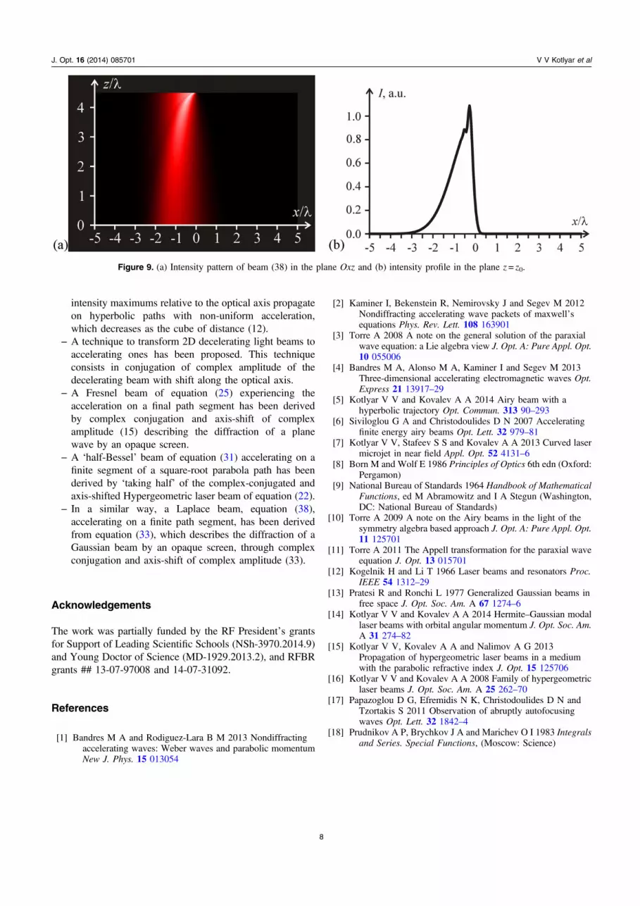
equation (38) is the probability, or Laplace, integral. Becauseof this, beams (38) will be referred to as Laplace beams. Fromthe path equation (37), beam (38) is also seen to be accel-erating near the plane z= z0. This can be noted fromfigure 9(a), which depicts the intensity pattern for beam (38)in the plane Oxz. Shown in figure 9(b) is the intensity profilein the plane z= z0.

5. Conclusions

Thus, we have obtained the following results.

− The well-known Hermite–Gauss modes and generalizedHermite–Gauss beams, equation (8), have been shown tobe accelerating, which implies that two outermost

Figure 8. Intensity pattern for beam (31) with different orders of Bessel function: 1(a), 3(b), and 5(c).

7

J. Opt. 16 (2014) 085701 V V Kotlyar et al

intensity maximums relative to the optical axis propagateon hyperbolic paths with non-uniform acceleration,which decreases as the cube of distance (12).

− A technique to transform 2D decelerating light beams toaccelerating ones has been proposed. This techniqueconsists in conjugation of complex amplitude of thedecelerating beam with shift along the optical axis.

− A Fresnel beam of equation (25) experiencing theacceleration on a final path segment has been derivedby complex conjugation and axis-shift of complexamplitude (15) describing the diffraction of a planewave by an opaque screen.

− A ‘half-Bessel’ beam of equation (31) accelerating on afinite segment of a square-root parabola path has beenderived by ‘taking half’ of the complex-conjugated andaxis-shifted Hypergeometric laser beam of equation (22).

− In a similar way, a Laplace beam, equation (38),accelerating on a finite path segment, has been derivedfrom equation (33), which describes the diffraction of aGaussian beam by an opaque screen, through complexconjugation and axis-shift of complex amplitude (33).

Acknowledgements

The work was partially funded by the RF President’s grantsfor Support of Leading Scientific Schools (NSh-3970.2014.9)and Young Doctor of Science (MD-1929.2013.2), and RFBRgrants ## 13-07-97008 and 14-07-31092.

References

[1] Bandres M A and Rodiguez-Lara B M 2013 Nondiffractingaccelerating waves: Weber waves and parabolic momentumNew J. Phys. 15 013054

[2] Kaminer I, Bekenstein R, Nemirovsky J and Segev M 2012Nondiffracting accelerating wave packets of maxwell’sequations Phys. Rev. Lett. 108 163901

[3] Torre A 2008 A note on the general solution of the paraxialwave equation: a Lie algebra view J. Opt. A: Pure Appl. Opt.10 055006

[4] Bandres M A, Alonso M A, Kaminer I and Segev M 2013Three-dimensional accelerating electromagnetic waves Opt.Express 21 13917–29

[5] Kotlyar V V and Kovalev A A 2014 Airy beam with ahyperbolic trajectory Opt. Commun. 313 90–293

[6] Siviloglou G A and Christodoulides D N 2007 Acceleratingfinite energy airy beams Opt. Lett. 32 979–81

[7] Kotlyar V V, Stafeev S S and Kovalev A A 2013 Curved lasermicrojet in near field Appl. Opt. 52 4131–6

[8] Born M and Wolf E 1986 Principles of Optics 6th edn (Oxford:Pergamon)

[9] National Bureau of Standards 1964 Handbook of MathematicalFunctions, ed M Abramowitz and I A Stegun (Washington,DC: National Bureau of Standards)

[10] Torre A 2009 A note on the Airy beams in the light of thesymmetry algebra based approach J. Opt. A: Pure Appl. Opt.11 125701

[11] Torre A 2011 The Appell transformation for the paraxial waveequation J. Opt. 13 015701

[12] Kogelnik H and Li T 1966 Laser beams and resonators Proc.IEEE 54 1312–29

[13] Pratesi R and Ronchi L 1977 Generalized Gaussian beams infree space J. Opt. Soc. Am. A 67 1274–6

[14] Kotlyar V V and Kovalev A A 2014 Hermite–Gaussian modallaser beams with orbital angular momentum J. Opt. Soc. Am.A 31 274–82

[15] Kotlyar V V, Kovalev A A and Nalimov A G 2013Propagation of hypergeometric laser beams in a mediumwith the parabolic refractive index J. Opt. 15 125706

[16] Kotlyar V V and Kovalev A A 2008 Family of hypergeometriclaser beams J. Opt. Soc. Am. A 25 262–70

[17] Papazoglou D G, Efremidis N K, Christodoulides D N andTzortakis S 2011 Observation of abruptly autofocusingwaves Opt. Lett. 32 1842–4

[18] Prudnikov A P, Brychkov J A and Marichev O I 1983 Integralsand Series. Special Functions, (Moscow: Science)

Figure 9. (a) Intensity pattern of beam (38) in the plane Oxz and (b) intensity profile in the plane z= z0.

8

J. Opt. 16 (2014) 085701 V V Kotlyar et al