TH

E

U N I V E RS

IT

Y

OF

ED I N B U

RG

H

School of Informatics, University of Edinburgh

Institute for Perception, Action and Behaviour

Transferring Impedance Control Strategies via ApprenticeshipLearning

by

Matthew Howard, Djordje Mitrovic and Sethu Vijayakumar

Informatics Research Report

School of Informatics January 2010http://www.informatics.ed.ac.uk/

Transferring Impedance Control Strategies viaApprenticeship Learning

Matthew Howard, Djordje Mitrovic and Sethu Vijayakumar

Informatics Research Report

SCHOOLof INFORMATICSInstitute for Perception, Action and Behaviour

January 2010

Under review for RSS 2010.

Abstract : We present a novel method for designing controllers for robots with variable impedance actuators. We takean imitation learning approach, whereby we learn impedance modulation strategies from observations of behaviour (forexample, that of humans) and transfer these to a robotic plant with very different actuators and dynamics. In contrastto previous approaches where impedance characteristics are directly imitated, our method uses task performance asthe metric of imitation, ensuring that the learnt controllers are directly optimised for the hardware of the imitator. Asa key ingredient, we use apprenticeship learning to model the optimisation criteria underlying observed behaviour, inorder to frame a correspondent optimal control problem for the imitator. We then apply local optimal feedback controltechniques to find an appropriate impedance modulation strategy under theimitator’s dynamics. We test our approachon systems of varying complexity, including a novel, antagonistic series elastic actuator and a biologically realistictwo-joint, six-muscle model of the human arm.

Keywords : Impedance control, apprenticeship learning, optimal control, variableimpedance actuators

Copyright c© 2010 University of Edinburgh. All rights reserved. Permission is hereby granted for this report to bereproduced for non-commercial purposes as long as this notice is reprinted in full in any reproduction. Applicationsto make other use of the material should be addressed to Copyright Permissions, School of Informatics, University ofEdinburgh, 2 Buccleuch Place, Edinburgh EH8 9LW, Scotland.

1 Introduction

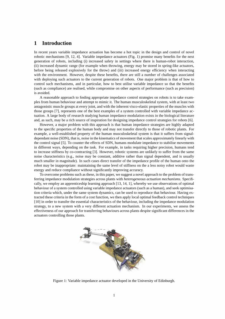
In recent years variable impedance actuation has become a hot topic in the design and control of novelrobotic mechanisms [9, 12, 4]. Variable impedance actuators (Fig. 1) promise many benefits for the nextgeneration of robots, including (i) increased safety in settings where there is human-robot interaction,(ii) increased dynamic range (for example when throwing, energy may be stored in spring-like actuators,before being released explosively for the throw) and (iii) increased energy efficiency when interactingwith the environment. However, despite these benefits, there are still a number of challenges associatedwith deploying such actuators to the current generation of robots. One major problem is that of how tocontrol such mechanisms, and in particular, how to best utilise variable impedance so that the benefits(such as compliance) are realised, while compromise on other aspects of performance (such as precision)is avoided.

A reasonable approach to finding appropriate impedance control strategies on robots is to take exam-ples from human behaviour and attempt to mimic it. The human musculoskeletal system, with at least twoantagonistic muscle groups at every joint, and with the inherent visco-elastic properties of the muscles withthose groups [7], represents one of the best examples of a system controlled with variable impedance ac-tuation. A large body of research studying human impedance modulation exists in the biological literatureand, as such, may be a rich source of inspiration for designing impedance control strategies for robots [6].

However, a major problem with this approach is that human impedance strategies are highly adaptedto the specific properties of the human body and may not transfer directly to those of robotic plants. Forexample, a well-established property of the human musculoskeletal system is that it suffers from signal-dependant noise (SDN), that is, noise in the kinematics of movement that scales approximately linearly withthe control signal [5]. To counter the effects of SDN, humansmodulate impedance to stabilise movementsin different ways, depending on the task. For example, in tasks requiring higher precision, humans tendto increase stiffness by co-contracting [3]. However, robotic systems are unlikely to suffer from the samenoise characteristics (e.g., noise may be constant, additive rather than signal dependent, and is usuallymuch smaller in magnitude). In such cases direct transfer ofthe impedance profile of the human onto therobot may be inappropriate: maintaining the same level of stiffness on the a less noisy robot would wasteenergy and reduce compliance without significantly improving accuracy.

To overcome problems such as these, in this paper, we suggesta novel approach to the problem of trans-ferring impedance modulation strategies across plants with heterogeneous actuation mechanisms. Specifi-cally, we employ an apprenticeship learning approach [13, 14, 1], whereby we use observations of optimalbehaviour of a system controlled using variable impedance actuators (such as a human), and seek optimisa-tion criteria which, under the same system dynamics, can be used to reproduce that behaviour. Having ex-tracted these criteria in the form of a cost function, we thenapply local optimal feedback control techniques[10] in order to transfer the essential characteristics of the behaviour, including the impedance modulationstrategy, to a new system with a very different actuation mechanism. In our experiments, we assess theeffectiveness of our approach for transferring behavioursacross plants despite significant differences in theactuators controlling those plants.

Figure 1: Variable impedance actuator developed in the University of Edinburgh.

1

Shoulder

Elbow

x

y

q1

q2

x

y

u triceps

u biceps

u motor 2

u motor 1

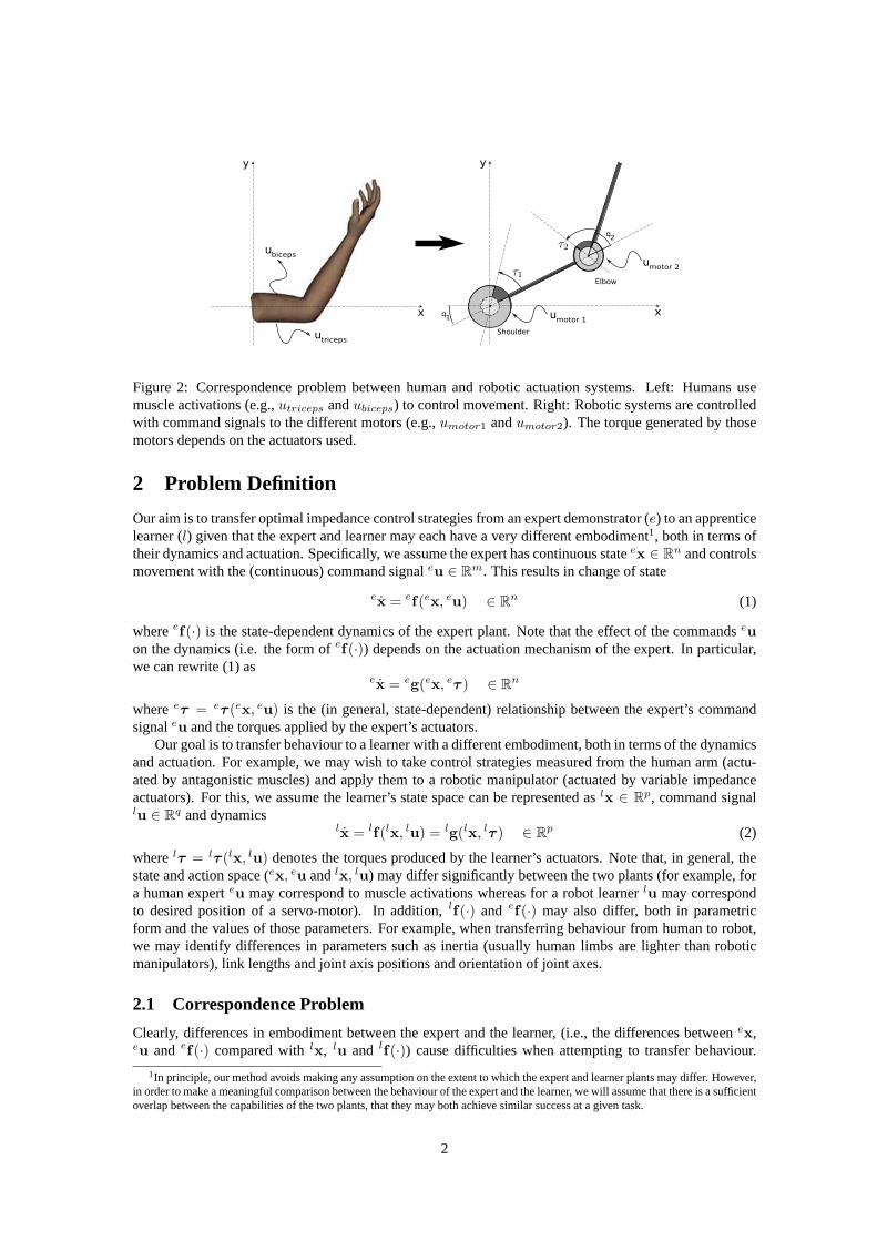
Figure 2: Correspondence problem between human and roboticactuation systems. Left: Humans usemuscle activations (e.g.,utriceps andubiceps) to control movement. Right: Robotic systems are controlledwith command signals to the different motors (e.g.,umotor1 andumotor2). The torque generated by thosemotors depends on the actuators used.

2 Problem Definition

Our aim is to transfer optimal impedance control strategiesfrom an expert demonstrator (e) to an apprenticelearner (l) given that the expert and learner may each have a very different embodiment1, both in terms oftheir dynamics and actuation. Specifically, we assume the expert has continuous stateex ∈ R

n and controlsmovement with the (continuous) command signaleu ∈ R

m. This results in change of state

ex = ef(ex, eu) ∈ Rn (1)

whereef(·) is the state-dependent dynamics of the expert plant. Note that the effect of the commandseu

on the dynamics (i.e. the form ofef(·)) depends on the actuation mechanism of the expert. In particular,we can rewrite (1) as

ex = eg(ex, eτ ) ∈ Rn

whereeτ = e

τ (ex, eu) is the (in general, state-dependent) relationship betweenthe expert’s commandsignaleu and the torques applied by the expert’s actuators.

Our goal is to transfer behaviour to a learner with a different embodiment, both in terms of the dynamicsand actuation. For example, we may wish to take control strategies measured from the human arm (actu-ated by antagonistic muscles) and apply them to a robotic manipulator (actuated by variable impedanceactuators). For this, we assume the learner’s state space can be represented aslx ∈ R

p, command signallu ∈ R

q and dynamicslx = lf(lx, lu) = lg(lx, lτ ) ∈ R

p (2)

wherelτ = l

τ (lx, lu) denotes the torques produced by the learner’s actuators. Note that, in general, thestate and action space (ex, eu andlx, lu) may differ significantly between the two plants (for example, fora human experteu may correspond to muscle activations whereas for a robot learner lu may correspondto desired position of a servo-motor). In addition,lf(·) and ef(·) may also differ, both in parametricform and the values of those parameters. For example, when transferring behaviour from human to robot,we may identify differences in parameters such as inertia (usually human limbs are lighter than roboticmanipulators), link lengths and joint axis positions and orientation of joint axes.

2.1 Correspondence Problem

Clearly, differences in embodiment between the expert and the learner, (i.e., the differences betweenex,eu and ef(·) compared withlx, lu and lf(·)) cause difficulties when attempting to transfer behaviour.

1In principle, our method avoids making any assumption on the extent to which the expert and learner plants may differ. However,in order to make a meaningful comparison between the behaviour of the expert and the learner, we will assume that there is a sufficientoverlap between the capabilities of the two plants, that they may both achieve similar success at a given task.

2

This correspondence problem is particularly severe in the dynamics domain, especially when there aredifferences in actuation.

As an example, consider the problem of transferring the control strategy used by a human to performsome task (e.g., punching a target) to a robotic imitator, asillustrated in Fig. 2. Imagine that we are givena set of recordings of the behaviour (e.g, in the form of muscle activation profiles measured with EMGsensors) and we wish to use this data to reproduce the movement on a robotic system. Depending on thehardware, there are a number of approaches we may take.

Firstly, if there is a close correspondence between the robot hardware and the human, a simple approachmight be to attempt todirectly transfer the behaviour, i.e., defineeu ≈ lu. This may be possible in specialcases where the hardware is explicitly designed to have similar actuation characteristics as the human. Forexample, if the robot is actuated with artificial muscles (e.g., McKibben muscles [8]), it may be possibleto directly feed the recorded muscle activations as a command signal to the robot actuators. However,while this approach has the benefit of simplicity, its applicability is clearly limited. In general such directcorrespondence between demonstrator and imitator is rarely available.

A second, and by far more common approach to imitation, is to do feature-based imitationof theobserved behaviour. The basis of this approach, is that salient featureseψ(ex(t), eu(t)) of the demonstratedbehaviour can be defined as equivalent to features of the behaviour of the robotic systemlψ(lx, lu) [2].For example, in the punching task (Fig. 2), these features might include the stiffness and damping profilesof the human arm that occur during movement. By drawing an equivalence between those profiles and theimpedance characteristics of the robotic arm, imitation can then be achieved by matching those featuresduring movement (e.g., using a variable impedance actuator).

The downside of this approach, however, is that it does not take into account the way in which thesefeatures affecttask performanceunder the dynamics of different plants. For example, in the punching task(Fig. 2), the impedance profile of the human may be relativelyhigh toward the end of the movement toensure that the target is hit accurately (e.g., to counter the effects of SDN). Naturally, this comes at the costof increased energy expenditure, since the human must co-contract to achieve this. However, for a (lessnoisy) robotic imitator, this may not be the optimal strategy. For example, the robot may be fairly accurate(compared to the human) even at relatively low impedance levels. As such, a better strategy for the robotmight be to keep the impedance levels at a steady, low level throughout the movement, thereby avoidingunnecessary energy consumption, but still achieving the task to the desired level of accuracy.

2.2 Apprenticeship Learning for Task-based Imitation

To avoid the problems associated with these standard approaches to imitation, in this paper we take adifferent approach in which the goal is to imitatethe objectives of the movement, rather than mimickingspecific features. Our approach is based on apprenticeship learning [13, 1], where the aim is to model thedemonstrated behaviour indirectly in the form of anobjective function, which, when optimised under thedemonstrator’s dynamics, reproduces that behaviour. Using this model, we can then find the equivalenttask goalsfor the imitator by defining correspondence at the level ofthe objective function that defines thetask. Furthermore, having learnt these task objectives, we can then optimise the imitated behaviour whilealso taking into account theimitator’s dynamics.

Specifically, we assume that we are given a set of demonstrationsD of some expert performing sometask, in the form of trajectories (in the state and action space of the demonstrator,ex, eu) of duration2

T . For example, these might consist of the joint positions, velocities (ex) and the muscle activations (eu)recorded from a human performing a punching task.

We assume that these trajectories can be described as optimal with respect to some (unknown) objectivefunction

eJ = eh(ex(T )) +

∫ T

0

el(ex, eu, t) dt (3)

whereeh(·), el(·) ∈ R are cost functions defined on the state and action space of thedemonstrator. Forexample,el(ex, eu, t) may describe the instantaneous work done by the demonstrator’s actuators (e.g., the

2For simplicity, through the paper we assume finite length trajectories of equal length. However, as discussed in [1], apprenticeshiplearning techniques are also readily extended to infinite horizon tasks.

3

Apprenticeship

Learning

Local Optimal

Feedback

Control

Learner

Behaviour

(robot)

Cost/Reward

Function

Planned Robot

Movements

Expert

Behaviour

(human)

Recorded

Movements

^

Figure 3: Schematic of our task-based imitation framework for behaviour transfer.

energy consumed by human muscles at a given activation and joint configuration). Note that here, sincethe optimality of the trajectoriesD depends on the dynamics of the demonstrator plantef(·), the recordedtrajectories will not, in general, be optimal under the dynamics of a different (learner) systemlf(·), i.e.,{ex, eu | ef(·)} 6= {lx, lu | lf(·)}. In other words, direct imitation of the demonstrator’s behaviour on theimitator plant is, in general,suboptimalwhen considering the dynamics of the imitator.

Instead, we propose to imitate behaviour based oncorrespondence in the objective functionsbetweenthe expert and learner. Specifically, the key to our approachis to define anequivalent objective function

lJ = lh(lx(T )) +

∫ T

0

ll(lx, lu, t) dt (4)

defined on the learner’s state and action space, where the terms lh(·), ll(·) ∈ R define cost terms with ameaningful correspondence to the cost termseh(·), el(·) of the expert. For example, if the termel(ex, eu, t)of a human demonstrator represents the energy consumption of the muscles, a meaningful analogue for arobotic manipulator would be to definell(lx, lu, t) as the power consumed by the motors. The goal ofimitation then, is to find the optimal behaviour for the learner {lx, lu} under the dynamicslf(·) withrespect to theequivalent objective function(4).

Note that, similar to feature-based approaches to imitation, in general the ease with which we can de-fine correspondence between cost functions for the two plants will depend on the specific dynamics andactuation of the demonstrator and imitator in question. Forexample, cost terms dependent on features suchas end-effector position may be defined as exactly correspondent, whereas terms dependent on propertiessuch as actuator commands will require definition of more complex terms, such as, the resultant torqueor impedance. However, a major benefit of our approach is thatin many cases it is much easier to definefeatures of correspondence at the level of the task, rather than at the detailed control level of the two plants.For instance, in the example of imitating human punching behaviour (Fig. 2), the selection of which dy-namics characteristics to match (e.g., impedance profiles,torque profiles etc.) in a feature-based imitationapproach will depend critically on the effect those have on the dynamics of the two plants. In contrast, withtask-based imitation, we only need to specify salient features (e.g., target accuracy, energy consumption)whereas the low-level details of the behaviour are handled by the control optimisation.

In the next section we turn to the implementation details of our approach for task-based imitation of be-haviour across systems with heterogeneous dynamics and actuation.

3 Method

A schematic overview of the proposed approach is illustrated in Fig. 3, where we show the different pro-cessing steps, and the inputs required at each stage. Reading from the top left, we first collect demonstra-tion data from an expert system (e.g., from a human) performing some task. This is fed into a module forapprenticeship learning along with information about the dynamics of the expert system. Based on thisinformation, a parametric model of the expert’s cost function is learnt with parametersw.

4

The output of this module is then fed to a second module for local optimal feedback control (OFC).The latter takes this parametric model along with information about the imitator (robot) plant dynamics andcorrespondence in terms of the cost functions. The OFC module finds the optimal control strategy for theimitator, with respect to the objectives defined by the learnt cost function. This is finally sent to the robotcontroller for realisation on the robotic hardware. In the following we briefly describe the implementationdetails of these two components.

3.1 Multiplicative Weights Apprenticeship Learning

For the apprenticeship learning component, we use a approach called Multiplicative Weights Apprentice-ship Learning (MWAL) recently proposed in [13]. The algorithm is based on principles of adversarial gametheory, and as such has been shown to be a robust method for apprenticeship learning [13]. Furthermore,due to its efficiency it well suited for learning in the robotics domain, where state and action spaces aretypically high-dimensional and continuous.

The method works on data that is given as trajectoriesD ={

(exk0 ,

euk0), · · · , (exk

T ,euk

T )}K

k=0of states

ex and actionseu recorded from the demonstrator under state dynamicsef(ex, eu). These are assumed tobe optimal with respect to an unknown cost function of the form

eJ =

nT∑

i=1

wiehi(

ex(T )) +

∫ T

0

N∑

i=nT

wieli(

ex, eu, t) dt. (5)

Here,wi are a set of weights (withwi > 0∀ i and∑

i wi = 1) andehi(·),eli(·) ∈ R are a set of (known)

basis functions. The latter may be made up of a set of bases fora generic function approximator (e.g.,Gaussian radial basis functions), or a set of salient features of the task (such as energy or accuracy costs).

The idea behind MWAL that the weightswi specifying the importance of the different components ofthe objective function (5) can be determined efficiently by considering the expected value of the observedbehaviourD with that of a second set of trajectoriestD that are optimised with respect to an estimate of theobjective function (5) with weightswi. Specifically, since the cost basesehi(·),

eli(·) are assumed known,for the two sets of trajectoriesD andtD, we can estimate their values under each of the bases separately.That is, for theith basis function

vi =1

K

K∑

k=0

∫ T

0

eli(exk(t), euk(t), t) dt (6)

if it is a running cost and

vi =1

K

K∑

k=0

ehi(exk(T ) (7)

if it is a terminal cost. We can then compare the difference inthese value estimates to adjust our estimatedweightswi, by scaling up those for which the value of the expert trajectories is lower (indicating a strongerpreference to minimise these components of the cost), and scaling down those for which the values arehigher (indicating the opposite). In successive iterations MWAL alternates between solving the forwardoptimal control problem to find trajectoriestD under the current estimate ofw, and then updating thatestimate based on the estimated valuesev = (v1, . . . , vN )D andtv = (v1, . . . , vN )tD. This proceeds untilconvergence on a set of weights that, when optimised, reproduces the demonstrated behaviourD.

MWAL is summarised in Algorithm 1 and full details of the approach can be found in [14]. Please notethat, for our implementation, we made two adjustments to thebasic approach. These were (i) introductionof a learning rate parameter,α to adjust the speed of learning, and (ii) normalisation of the vectorsev =ev/‖ev‖. andt

v = tv/‖tv‖. We found that the latter improved the robustness of learning especially forthe high-dimensional, continuous systems considered in our experiments. Furthermore, for the forwardoptimisation step (Step 6 of Algorithm 1) we use local a optimal feedback control technique, details ofwhich are described in the next section.

5

Algorithm 1 MWAL (modified from [13])1: Givenex, eu, ef , eli=1···N ,D2: Estimateev = (v1, . . . , vN ) from expert trajectoriesD for all i. Normalise:ev = ev/‖ev‖.

3: Let β =

(

1 +√

2 log k

T

)

−1

.

4: Initialise twi = 1k

for all i5: for t = 1, . . . , T do6: • Find trajectoriestD that optimiseJ =

∑N

i=1twi

eJi under dynamicsex = ef(ex, eu)7: • Estimatet

vi from trajectoriestD for all i8: • Let t+1wi = twiβ

−α(evi−tvi)

9: • Re-normalisew10: end for11: Return w

3.2 Task-based Behaviour Transfer

Having completed the apprenticeship learning stage, our next task is to find an appropriate behaviour forthe imitator based on our model of the demonstrator’s objectives. For this we use local optimal feedbackcontrol in order to optimise an equivalent cost function to that used by the demonstrator.

Specifically, we parametrise the cost function of the learner as a similar weighted combination of terms

lJ =

nT∑

i=1

willi(

lx(T )) +

∫ T

0

N∑

i=nT

willi(

lx, lu, t) dt. (8)

Here,lhi(·),lli(·) ∈ R are a set of basis functions that correspond to those of the expert (5), andwi are the

weights learn by MWAL in the previous step. At this point a design decision must be made as to whichcost baseslhi(·),

lli(·) can be defined for the learner with where appropriate correspondence to those of theexpertehi(·),

eli(·). In general, this will depend on the specific embodiments (dynamics and actuators) ofthe two plants. However, as noted in Sec. 2.2 in practical settings this is relatively easily resolved (and atworst, is no more difficult than specifying featureseψ(·), lψ(·) for standard feature-based imitation). Forexample, different terms might include energy terms for thetwo plants, or accuracy costs (as defined, forexample, in terms of the position of the end-effectors of thetwo plants). Further examples are given in theexperiments (Sec. 4).

Having defined correspondence in terms of these cost bases, and having learnt their relative importanceof in terms of the weightsw, all that remains is to find the optimal movement with respectto the objectivefunction (8) under the dynamics of the robot (2). Here, sincewe are interested in high-dimensional, con-tinuous robot control problems, our method of choice is to use local optimal feedback control. In the nextsection we briefly describe the details.

3.3 Local Optimal Feedback Control with ILQG

In our framework, solving the forward optimal control enters at two points. Firstly, in the apprenticeshiplearning stage, the optimal control problem must be solved is required at every iteration in order to findtrajectoriestD that are optimal with respect to the current estimate of the objective function (5). Secondly,as discussed in the preceding section optimisation is necessary in order to find the optimal movement forthe imitator with respect to the learnt cost function and thedynamics of the imitator plant. In both cases weneed a technique that (i) can cope with high-dimensional, non-linear systems and (ii) has high efficiency(since the commands must be optimised multiple times for multiple trajectories). For these reasons, in bothstages we use local OFC techniques.

Specifically, our algorithm of choice is the iterative localquadratic Gaussian (ILQG) algorithm [15, 10].The fundamental idea behind ILQG is that, when the dynamics process is non-linear and costs are non-quadratic, one can still apply the LQG solution approximately around a nominal trajectory and use localsolutions to iteratively improve the nominal solution.

6

Mot. 2 Mot. 1

x

yy

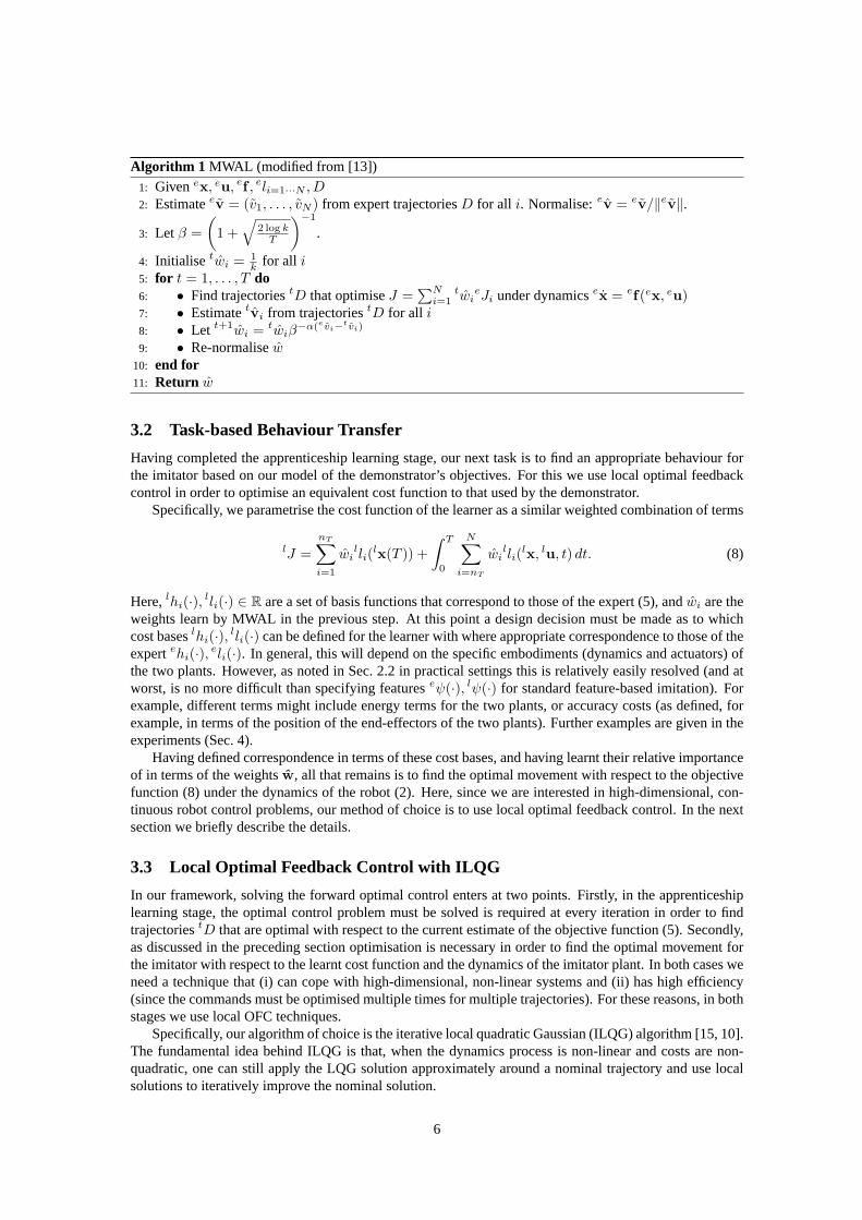
Figure 4: Dynamics model of the variable impedance actuator.

The ILQG algorithm starts with a time-discretised initial guess of a control sequence of lengthT .This is then iteratively improved it with respect to the given performance criteria. From the initial controlsequenceuj at thejth-iteration, the corresponding state sequencexj is retrieved using the deterministicforward dynamicsf with a standard Euler integrationxj(t + 1) = xj(t) + ∆t f(xj(t), uj(t)). Next, thedynamics are linearly approximated as with a Taylor expansion and similarly one can derive a quadraticapproximation of the cost function aroundxj(t) anduj(t) is made. Both approximations are formulatedas deviationsδxj(t) = xj(t) − xj(t) and δuj(t) = uj(t) − uj(t) of the current optimal trajectoryand therefore form a ‘local’ LQG problem. This linear quadratic problem can be solved efficiently via amodified Ricatti-like set of equations.

Having solved theses equations, a correction to the optimalcontrol signalδuj is obtained, with can thenbe used to improve the current optimal control sequence for the next iteration usinguj+1(t) = uj(t)+δuj .Finally, uj+1(t) is applied to the system dynamics and the new total cost alongthe along the trajectory iscomputed. The algorithm stops once the cost cannot be significantly decreased anymore. After conver-gence, ILQG returns an control sequenceu and a corresponding state sequencex which represents theoptimal trajectory. In our framework these trajectories are then either collected as sample data for Step 6of the MWAL algorithm, or used for optimal control of the imitator plant.

4 Experiments

In this section, we investigate the performance of our task-based imitation approach in two impedancecontrol scenarios. In the first, we look at problem involvingtransfer of behaviour from a complex, non-linear model of a antagonistic series elastic actuator (ref. Fig. 1), to that of a simpler system in which themodulation of impedance characteristics is decoupled in the control. In the second, we test the scalabilityto a more demanding problem in which we transfer behaviour from a biologically realistic two-joint, six-muscle model of the human arm to that of a simulated robotic imitator.

4.1 Impedance Modulation on a Single Joint

In our first experiment, we investigate how impedance modulation strategies may be extracted and trans-ferred from a complex, non-linear actuation mechanism to that of a simpler, idealised system. The purposeof this experiment is to assess the effectiveness of our approach on a simplified system and assess itsfeasibility, before scaling up to more complex, realistic problems.

The model of the antagonistic variable impedance actuator that we use is based on a system identifica-tion of the Edinburghseries elastic actuator. Inspired by human antagonistic muscles, this plant uses twomotors, connected to a pair of springs to adjust the equilibrium position, stiffness and torque around thejoint. The adjustments in stiffness are achieved by ‘co-contraction’, that is, simultaneous tensioning of thesprings (the full dynamics of the human-like antagonistic joint are described in detail in [11]. The layoutof the mechanical components (ref. 4) means that a rather complex relationship exists between the motor

7

commands and the resultant torques and impedance characteristics, making it difficult to find appropriatefeatures of the control for imitation. Here, we investigatetransfer of behaviour from this antagonistic plantto a similar joint with a very different actuation mechanism.

For simplicity, we model the controls of this joint as the vector eu ∈ R2 corresponding to the target

motor positions, and the state as the vectorex = (q, q) ∈ R2 corresponding to the instantaneous angle

and velocity of the joint. To generate examples of optimal behaviour for this plant, ILQG was used to plantrajectories for a ‘golf swing’ task. Specifically, as a ground truth, the demonstrator planned (using ILQG)trajectories that minimised the objective

eJ = w1(q(T ) − q∗)2 − w2q(T ) +

∫ T

0

w3τ2 dt (9)

whereq∗ = 30◦ is the target angle andτ is the torque applied around the axis of rotation of the joint. Theweighting of the three terms of (9) respectively correspondto (i) minimising the distance to the target (golfball) at the time of impactT , (ii) maximising the angular velocity of the arm atT , and (iii) minimisingenergy consumption during the movement. The trade-off between these objectives is determined by theweightswi.

For the learning,K = 30 trajectories from random start states were collected. Eachwas optimisedwith respect to the objective (9) under the dynamics of the antagonistic plant. These were then used astraining data for the MWAL component of our framework, in order to estimate the estimate the weightsw. To assess the performance of the MWAL component, we collected50 such data sets and measured theerror in estimated weights during learning. The latter was measured by the norm difference in the weightvectors for the true and estimated weights, i.e.

Ew[w, w] = ‖w − w‖. (10)

Fig. 5(a) shows the weight errorEw over 10 iterations of the MWAL algorithm with a relatively highlearning rate parameter (α = 50). As can be seen, a rapid convergence to a low error in weightsoccurred,with an final error of0.0941 ± 0.0247.

We then investigated the transfer of this behaviour to a second plant with similar characteristics, but adifferent actuation mechanism. For this, we selected an actuation scheme where the stiffness parameterscan be directly controlled. This is similar to robotic plants in which stiffness characteristics are activelycontrolled under feedback, or to plants where the stiffnesscan be mechanically adjusted, as in, for example,in the MACCEPA joint [4].

More specifically, the control vector for the second plant was modelled aslu = (q0, k)T ∈ R

2 whereq0 corresponds to the equilibrium position andk is the stiffness. These commands resulted in an appliedtorque

τ = −k(q0 − q) (11)

around the joint axis. For ease of comparison, all other dynamics parameters (e.g. link lengths, massesetc.) of the robot plant were fixed to the same values as those of the first plant (antagonistic joint). Notethat, for the two plants under consideration, correspondence in the first two terms of (9) is exact (sincethe dynamics of the two joints is identical). However, also note that there is a difference in the functionalform of the third term, arising from the differences in the relationship between the command signal and theresultant torquesτ .

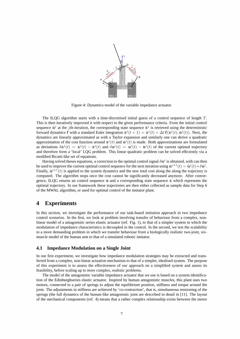
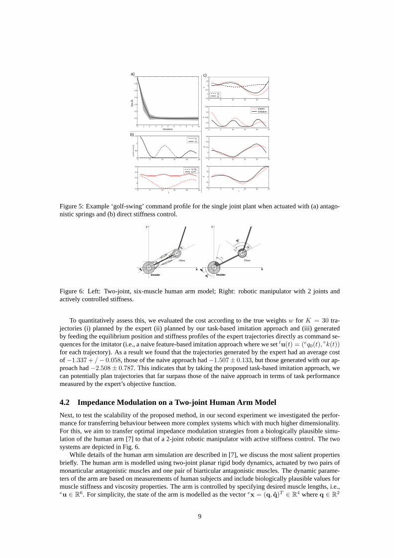
Using the weights learnt with MWAL, we then applied ILQG to plan optimal movements for the secondplant and compared the results. An example trajectory is shown in Fig. 5(a) & (b), where we show thecommand trajectory for the two plants (Fig. 5(a)) and the angular position, stiffness, resultant torques andangular velocity of the two plants, respectively, over the duration of the movement (Fig. 5(b)).

The first thing that we notice is that at the level of the planned commands (Fig. 5(a)), very differentstrategies appear to be optimal for the two plants. This reinforces the fact that, considering the differencesin actuation here,direct imitationis inappropriate. Second, Fig. 5(b) indicate that, while there is similarityin several features of the movement (e.g. the strategy of swinging the equilibrium position to away fromthe current actual position (Fig. 5(b), top) the correspondence is not exact since there are differences in theprofiles observed.

8

0 5 10 15 20 25-1.5

-1

-0.5

0

0.5

1

q

0 5 10 15 20 250.25

0.3

0.35

0.4

0.45

k

0 5 10 15 20 25 -0.2

0

0.2

0.4

0.6

0 5 10 15 20 25 -20

-10

0

10

20

q

t

0 5 10 15 20 250

0.5

1

1.5

muscle

comm

ands

0 5 10 15 20 25-0.2

0

0.2

0.4

0.6

motor commands

t

0 1 2 3 4 5 6 7 8 9 100

0.1

0.2

0.3

0.4

0.5

0.6

0.7

IterationsE

[w,w

]

a)

b)

c)

^

τ

.

uu

u =qu =k

0

1

2

qq

0

expertimitation

1

2

Figure 5: Example ‘golf-swing’ command profile for the single joint plant when actuated with (a) antago-nistic springs and (b) direct stiffness control.

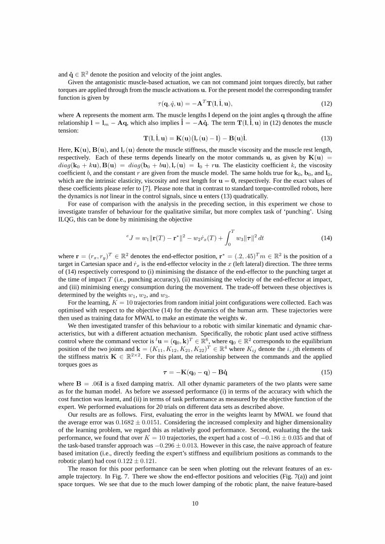
Figure 6: Left: Two-joint, six-muscle human arm model; Right: robotic manipulator with 2 joints andactively controlled stiffness.

To quantitatively assess this, we evaluated the cost according to the true weightsw for K = 30 tra-jectories (i) planned by the expert (ii) planned by our task-based imitation approach and (iii) generatedby feeding the equilibrium position and stiffness profiles of the expert trajectories directly as command se-quences for the imitator (i.e., a naive feature-based imitation approach where we setlu(t) = (eq0(t),

ek(t))for each trajectory). As a result we found that the trajectories generated by the expert had an average costof −1.337 + /− 0.058, those of the naive approach had−1.507± 0.133, but those generated with our ap-proach had−2.508 ± 0.787. This indicates that by taking the proposed task-based imitation approach, wecan potentially plan trajectories that far surpass those ofthe naive approach in terms of task performancemeasured by the expert’s objective function.

4.2 Impedance Modulation on a Two-joint Human Arm Model

Next, to test the scalability of the proposed method, in our second experiment we investigated the perfor-mance for transferring behaviour between more complex systems which with much higher dimensionality.For this, we aim to transfer optimal impedance modulation strategies from a biologically plausible simu-lation of the human arm [7] to that of a 2-joint robotic manipulator with active stiffness control. The twosystems are depicted in Fig. 6.

While details of the human arm simulation are described in [7], we discuss the most salient propertiesbriefly. The human arm is modelled using two-joint planar rigid body dynamics, actuated by two pairs ofmonarticular antagonistic muscles and one pair of biarticular antagonistic muscles. The dynamic parame-ters of the arm are based on measurements of human subjects and include biologically plausible values formuscle stiffness and viscosity properties. The arm is controlled by specifying desired muscle lengths, i.e.,eu ∈ R

6. For simplicity, the state of the arm is modelled as the vector ex = (q, q)T ∈ R4 whereq ∈ R

2

9

andq ∈ R2 denote the position and velocity of the joint angles.

Given the antagonistic muscle-based actuation, we can not command joint torques directly, but rathertorques are applied through from the muscle activationsu. For the present model the corresponding transferfunction is given by

τ(q, q,u) = −AT T(l, l,u), (12)

whereA represents the moment arm. The muscle lengthsl depend on the joint anglesq through the affinerelationshipl = lm − Aq, which also impliesl = −Aq. The termT(l, l,u) in (12) denotes the muscletension:

T(l, l,u) = K(u)(

lr(u) − l)

− B(u)l. (13)

Here,K(u), B(u), andlr(u) denote the muscle stiffness, the muscle viscosity and the muscle rest length,respectively. Each of these terms depends linearly on the motor commandsu, as given byK(u) =diag(k0 + ku),B(u) = diag(b0 + bu), lr(u) = l0 + ru. The elasticity coefficientk, the viscositycoefficientb, and the constantr are given from the muscle model. The same holds true fork0, b0, andl0,which are the intrinsic elasticity, viscosity and rest length for u = 0, respectively. For the exact values ofthese coefficients please refer to [7]. Please note that in contrast to standard torque-controlled robots, herethe dynamics isnot linear in the control signals, sinceu enters (13) quadratically.

For ease of comparison with the analysis in the preceding section, in this experiment we chose toinvestigate transfer of behaviour for the qualitative similar, but more complex task of ‘punching’. UsingILQG, this can be done by minimising the objective

eJ = w1‖r(T ) − r∗‖2 − w2rx(T ) +

∫ T

0

w3‖τ‖2 dt (14)

wherer = (rx, ry)T ∈ R2 denotes the end-effector position,r∗ = (.2, .45)Tm ∈ R

2 is the position of atarget in Cartesian space andrx is the end-effector velocity in thex (left lateral) direction. The three termsof (14) respectively correspond to (i) minimising the distance of the end-effector to the punching target atthe time of impactT (i.e., punching accuracy), (ii) maximising the velocity ofthe end-effector at impact,and (iii) minimising energy consumption during the movement. The trade-off between these objectives isdetermined by the weightsw1, w2, andw3.

For the learning,K = 10 trajectories from random initial joint configurations werecollected. Each wasoptimised with respect to the objective (14) for the dynamics of the human arm. These trajectories werethen used as training data for MWAL to make an estimate the weightsw.

We then investigated transfer of this behaviour to a roboticwith similar kinematic and dynamic char-acteristics, but with a different actuation mechanism. Specifically, the robotic plant used active stiffnesscontrol where the command vector islu = (q0,k)T ∈ R

6, whereq0 ∈ R2 corresponds to the equilibrium

position of the two joints andk = (K11,K12,K21,K22)T ∈ R

4 whereKij denote thei, jth elements ofthe stiffness matrixK ∈ R

2×2. For this plant, the relationship between the commands and the appliedtorques goes as

τ = −K(q0 − q) − Bq (15)

whereB = .06I is a fixed damping matrix. All other dynamic parameters of thetwo plants were sameas for the human model. As before we assessed performance (i)in terms of the accuracy with which thecost function was learnt, and (ii) in terms of task performance as measured by the objective function of theexpert. We performed evaluations for 20 trials on differentdata sets as described above.

Our results are as follows. First, evaluating the error in the weights learnt by MWAL we found thatthe average error was0.1682 ± 0.0151. Considering the increased complexity and higher dimensionalityof the learning problem, we regard this as relatively good performance. Second, evaluating the the taskperformance, we found that overK = 10 trajectories, the expert had a cost of−0.186 ± 0.035 and that ofthe task-based transfer approach was−0.296 ± 0.013. However in this case, the naive approach of featurebased imitation (i.e., directly feeding the expert’s stiffness and equilibrium positions as commands to therobotic plant) had cost0.122 ± 0.121.

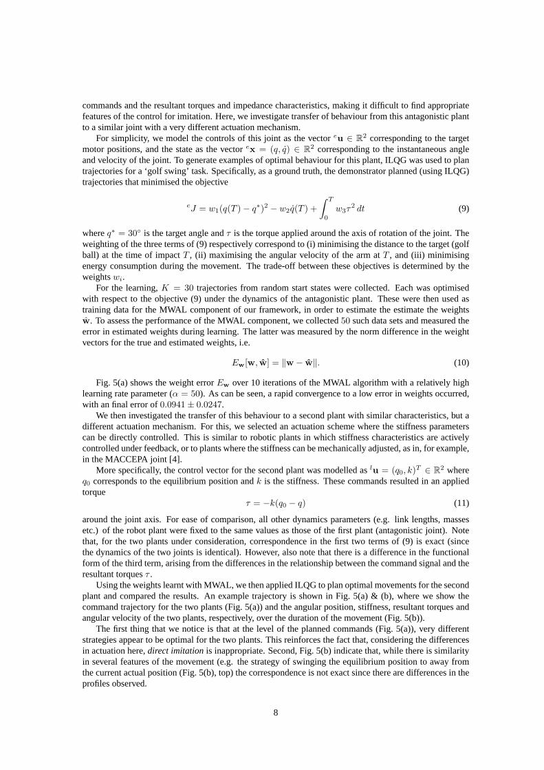
The reason for this poor performance can be seen when plotting out the relevant features of an ex-ample trajectory. In Fig. 7. There we show the end-effector positions and velocities (Fig. 7(a)) and jointspace torques. We see that due to the much lower damping of therobotic plant, the naive feature-based

10

0 10 20 30 40 50 60 70 80-0.1

0

0.1

0.2

0.3

0.4x

0 10 20 30 40 50 60 70 80

0.35

0.4

0.45

0.5

0.55

0.6

0.65

0.7y

0 10 20 30 40 50 60 70 80-1.5

-1

-0.5

0

0.5

1

1.5

0 10 20 30 40 50 60 70 80-1

-0.5

0

0.5

1

0 10 20 30 40 50 60 70 80-1.5

-1

-0.5

0

0.5

1

t0 10 20 30 40 50 60 70 80

-2

-1

0

1

2

3

t

Joint 1 Joint 2

τT

ask

spac

e ve

loci

tyT

ask

spac

e po

sitio

n

a)

b)

expertnaiveimitation

Figure 7: Example ‘punch’ stiffness profile for the two jointplant when actuated with (a) antagonisticmuscles (red) and (b) direct joint stiffness control (black).

imitation strategy produces highly unstable trajectories, increasing cost in terms of the integrated jointtorques (shaded area). On the other hand, by planning appropriate movements for the robotic plant usingthe task-based approach we get smooth trajectories that closely match those of the expert.

5 Conclusion

In conclusion, we have presented a task-based imitation learning approach for transfer of behaviour acrossplants with highly heterogeneous dynamics and actuation. Our framework is based on a two-step approachto learning, where in the first step, a parametric model of theobjective function underlying observed be-haviour is learnt using an apprenticeship learning approach. This enables us to find a task-based represen-tation of the data in terms of the objectives minimised. Using this model of the behaviour, and solvingthe correspondence problem in terms of the the components ofthe objective function, we then apply lo-cal optimal feedback control techniques to find a similarly optimal behaviour for the imitation, takinginto account the differences in actuation. Our experimentsshow the effectiveness of this approach, wherethe proposed approach actually exploits the dynamics characteristics of the imitator in order out-performstandard feature-based imitation approaches, and even surpass the task-performance of the expert.

In future work we intend to extend to build on the results by applying our approach to real recordingsof human muscle activations in a number of impedance controltasks, and achieve task-based imitation onour novel variable actuator designs.

References

[1] P. Abbeel and A. Y. Ng. Apprenticeship learning via inverse reinforcement learning. InInternationalConference on Machine Learning, 2004.

[2] A. Alissandrakis, C. L. Nehaniv, and K. Dautenhahn. Correspondence mapping induced state andaction metrics for robotic imitation.IEEE Transactions on Systems, Man and Cybernetics, 37(2):299–307, 2007.

11

[3] D. Franklin, G. Liaw, T. Milner, R. Osu, E. Burdet, and M. Kawato. Endpoint stiffness of the arm isdirectionally tuned to instability in the environment.Journal of Neuroscience, 27:7705–7716, 2007.

[4] R. Van Ham, B. Vanderborght, M. Van Damme, B. Verrelst, and D. Lefeber. Maccepa, the mechani-cally adjustable compliance and controllable equilibriumposition actuator: Design and implementa-tion in a biped robot.Robotics and Autonomous Systems, 55(10):761–768, 2007.

[5] C. M. Harris and D. M. Wolpert. Signal-dependent noise determines motor planning.Nature,394:780–784, 1998.

[6] N. Hogan. Impedance control - an approach to manipulation. part iii - applications.ASME, Transac-tions, Journal of Dynamic Systems, Measurement, and Control, 107:1–24, 1985.

[7] M. Katayama and M. Kawato. Virtual trajectory and stiffness ellipse during multijoint arm movementpredicted by neural inverse models.Biol. Cybern., 69:353–362, 1993.

[8] G. K. Klute, J. M. Czerniecki, and B. Hannaford. Mckibbenartificial muscles: Pneumatic actuatorswith biomechanical intelligence. InIEEE/ASME International Conference on Advanced IntelligentMechatronics, 1999.

[9] M. Lauria, M.-A. Legault, M.-A. Lavoie, and F. Michaud. Differential elastic actuator for roboticinteraction tasks. InICRA, 2008.

[10] W. Li and E. Todorov. Iterative linear-quadratic regulator design for nonlinear biological movementsystems. InInternational Conference on Informatics in Control, Automation and Robotics, volume 1,pages 222–229, 2004.

[11] D. Mitrovic, S. Klanke, and S. Vijayakumar. Exploitingsensorimotor stochasticityfor learning control of variable impedance actuators. Technical Report available at:www.ipab.informatics.ed.ac.uk/slmc/SLMCpeople/Mitrovic D.html, 2009.

[12] R. Schiavi, G. Grioli, S. Sen, and A. Bicchi. Vsa-ii: a novel prototype of variable stiffness actuatorfor safe and performing robots interacting with humans. InICRA, 2008.

[13] U. Syed, M. Bowling, and R. E. Schapire. Apprenticeshiplearning using linear programming. InInternational Conference on Machine Learning, 2008.

[14] U. Syed and R. E. Schapire. A game-theoretic approach toapprenticeship learning. InNIPS, 2008.

[15] E. Todorov and W. Li. A generalized iterative lqg methodfor locally-optimal feedback control ofconstrained nonlinear stochastic systems. InAmerican Control Conference, 2005.

12