towards simulation of elasto-plastic deformation: an investigation
TRANSCRIPT
Sadhana Vol. 27, Part 3, June 2002, pp. 251–294. © Printed in India
Towards simulation of elasto-plastic deformation: Aninvestigation
ARUN R RAO and U SHRINIVASA
Department of Mechanical Engineering, Indian Institute of Science,Bangalore 560 012, Indiae-mail: [email protected]
MS received 5 December 2001
Abstract. Can the deformation of a solid body during plastic flow be assumed tobe similar to that of fluids? Here we investigate the possibility of using a modifiedNavier–Stokes equation as the governing differential equation by including elasticresistance. We adopt the microscopic point of view to explain the material behaviourby laying special emphasis on strain localisation and tension instabilities. A springand damper model is constructed to obtain approximate simulation of the materialbehaviour. Based upon the understanding developed from simulating simple tests,we re-formulate the field equation using resistances to change in volume and shape.The new field equation reduces to the Navier–Stokes equation in the fluid limit andCauchy’s equation in the solid limit. The viscosity and second viscosity of fluidsare clearly defined. Bulk and shear modulii and solid damping determine the solidbehaviour. Pressure disappears from the field equation and so there is no need toinvoke the continuity equation. The four material parameters are determinable fromsimple measurments. This paper tries to capture the various steps of the investigationwhich lead to the final result.
Keywords. Elasto-plastic deformation; modified Navier–Stokes equation;strain localisation; tension instability; material behaviour; Cauchy’s equation.
1. Introduction
The mathematical theory of plasticity has been in use for many years but the formulation ofa field equation for simulation of elasto-plastic deformation is still a matter of discussion.Several engineering idealised theories are proposed but they fail to account for the variousphenomena observed. Due to the complicated nature of the plasticity problem, theory in earlierdays is chiefly confined to small deformation, viz. infinitesimal theory with some specialemphasis on hardening laws and, some special material responses (Hill 1950; Prager & Hodge1951; Prager 1955; Drucker 1960; Naghdi 1960). These theories are ‘rate-independent’ tocover some general class of materials with consideration of a few special properties such asmaterial anisotropy, creep and thermal effects.
A large amount of work is carried out by different schools of plasticity in the area of finitedeformation either in the Lagrangian or in the Eulerian coordinate systems using stress-based
251
252 Arun R Rao and U Shrinivasa
or strain-based approaches. The stress-based formulation (Green & Naghdi 1965, 1966) isin turn found inadequate (Naghdi & Trapping 1975) to explain some material properties andis non-trivial for implementing numerically. Later Naghdi and co-workers developed strain-based formulation (Naghdi & Trapp 1975; Casey & Naghdi 1981, 1983) to overcome thesedifficulties and made it suitable to solve numerically.
In the literature, we can often see the development of the constitutive equations for defor-mation theories on macroscopic scale (Barbeet al 2001). But the experimental observationsmade by Taylor & Elam (1923, 1925, 1926) reveals the importance of microscopic structureduring large deformation. These observations led further to development of various micro-scopic theories (Batdorf & Budiansky 1949; Koiter 1953; Kroner 1960; Budiansky & Wu1962; Hill 1965, 1966; Hutchinson 1970; Rice 1976; Bazant 1984) and more recently tothose of Qui & Weng (1992, 1995), Rubin (1996), Acharya & Beaudoin (2000), Bigonietal (2000), and Acharya (2001). All these workers tried to develop the theory by consideringvarious aspects of microstructure like single crystal or polycrystal deformation, strain local-isation, material anisotropy etc. Nowadays, these microstructure theories are covering moreand more ground as the physics of micro-mechanics is being deeply studied and understood(Bertram 1998) to provide answers to most of the questions.
With the development of theory, efforts are made to develop the plasticity theory in theEulerian coordinate system as it is found more suitable for large deformations. Kroner (1960)initiates work in Eulerian coordinate system and later it is carried out by the others (Backman1964; Lee & Liu 1967; Lee 1969; Dienes 1979, 1986; Leeet al 1983; Loret 1983; Nemat-Nasser 1983; Dafalias 1983, 1984; Atluri 1984; Agah-Tehraniet al 1987). In recent yearswe see some schools of plasticity use the ‘arbitrary Lagrangian-Eulerian’ description, whichcombines both Lagrangian and Eulerian descriptions to solve the problems (Haber 1984;Huetinket al1990; Ghosh & Suresh 1996; Braess & Wriggers, 2000).
Most of the existing plasticity theories depend heavily upon yield function to differentiatebetween elastic and plastic regions (Hill 1994). Yield function is dependent upon stress, plasticstrain and work hardening parameters and is usually determined by experiments. However,the existence of the yield surface or yield condition is questionable. Some investigators (Seth1963, 1964; Valanis 1971, 1975; Bodner & Partan 1975; Lee & Zaverl 1978, 1979; Stouffer& Bodner 1979) lay special emphasis on the possibility of developing the theory of plasticitywithout introducing a yield surface or yield condition.
A body is understood to deform simultaneously by elastic and plastic strains under theapplication of external load. In the classical theory of elasticity the linear trend of infinites-imal deformation is expressed by the generalised Hooke’s law. In actuality, the cyclic load-deformation or stress–strain curve is not a single-valued function but forms a hysteretic loop(Lazan 1968). Lazan (1968) also observed that all materials, composites and structural assem-blies do not behave in a perfectly elastic manner even at very low stresses. Inelasticity isalways present under all types of loading. Hence the constitutive equations for the elastic andthe plastic parts of the deformation cannot be treated independently. Elastic and plastic effectsshould dovetail into each other even when elastic behaviour is assumed to be unaffected bythe preceding plastic deformations. This supposition avoids any assumption of yield condi-tion or yield surface to determine any elastic–plastic boundary, which may or may not exist(Seth 1970) and is sometime also ambiguous in multi-axial cases (Chen & Lu 2000).
Existing plasticity theory is based on certain experimental observations on the macroscopicbehaviour of metals in the uniform state of combined stresses (Chakrabarty 1998). Theseobserved results are then idealised into a mathematical formulation to describe the behaviourof metals under complex stresses. However a lot of assumptions are involved to simplify the
Simulation of elasto-plastic deformation 253
complex phenomenon of plastic deformation. These assumptions make the theory incapableof explaining various material phenomenon such as the Bauschinger effect, anisotropy, timeand temperature effects, size effect, stress inhomogeneity, material damping etc.
Thus, existing models are able to explain some of the phenomenon observed, but leavebehind a lot of controversies. Each model is useful for a particular purpose with some well-defined boundary conditions. However, many phenomena occurring during plastic deforma-tion remain unexplained. Hence, there is an urgent need for a constitutive equation whichin general will correctly explain deformation behaviour and also the physics involved in thedeformation process. Therefore we try to develop a field equation from first principles (asagainst from experimental observations) which assumes a generalised relation between stress,strain and strain rate that could represent the material behaviour in the elastic range, transi-tion from the elastic to plastic state and in the plastic range, and later use the same to explainmost of the phenomena observed in practice.
2. Formulation
Zienkiewicz & Godbole (1975) pointed out that in metals, plasticity with large deformation,whose elastic strains are negligible, stands on the borderline of fluid and solid mechanics.Under equilibrium conditions both solid and fluid are identical provided dynamic forces areneglected. Thus one can conclude that the solution of a viscous flow problem is identicalto the solution of an equivalent incompressible elastic problem in which displacements areinterpreted as velocities and infinitesimal strain as strain rate (Zienkiewicz & Godbole 1974).Thus all the techniques available in the literature for the solution of one problem are applicableto the other. The analogy that in the plastic state metals behave like viscous fluids helps toexpress the formulation in the Eulerian coordinate system which seems more relevant in largeelastic–plastic deformation (Prager 1961). Further we see that in recent and current literature,most plasticity theories are inclined towards an Eulerian formulation in stress space setting.This is mainly because of its analogy with viscous fluid flow, the construction of the theoryin terms of Cauchy stresses and its rate being more fundamental. Cauchy’s stress tensorP isdefined in the current configuration as,
P = τij ei ⊗ ej
whereτij are the stress components andei andej are the unit co-ordinate vectors.
2.1 Contribution from the strain-rate tensor
Every material displays more or less viscous properties. For many important structural mate-rials, these properties appear to surface after the plastic state has been reached. It is normallybelieved that materials display viscous properties only in the plastic range. We however lookfor a universal model.
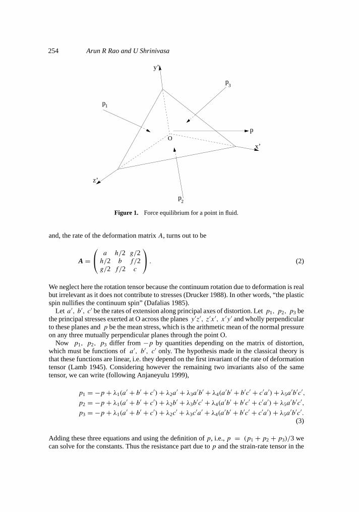
Consider the stress (following Lamb 1945) exerted across any small area situated at a pointO in the continuum (figure 1). The deviation of the state of stress denoted bypxx, pxy, . . .
from one of pressure uniform in all directions depends entirely on the motion of distortion(i.e. on instantaneous rate of deformation) in the neighbourhood of O, i.e. on 6 quantitiesa, b, c, f, g, h which are defined as,
a = ∂u/∂x, b =∂v/∂y, c =∂w/∂z,
f = ∂w
∂y+ ∂v
∂z, g =∂u
∂z+ ∂w
∂x, h =∂v
∂x+ ∂u
∂y, (1)
254 Arun R Rao and U Shrinivasa
O
z’
p1
y’
p3
p
x’
p2
Figure 1. Force equilibrium for a point in fluid.
and, the rate of the deformation matrixA, turns out to be
A = a h/2 g/2
h/2 b f/2g/2 f/2 c
. (2)
We neglect here the rotation tensor because the continuum rotation due to deformation is realbut irrelevant as it does not contribute to stresses (Drucker 1988). In other words, “the plasticspin nullifies the continuum spin” (Dafalias 1985).
Let a′, b′, c′ be the rates of extension along principal axes of distortion. Letp1, p2, p3 bethe principal stresses exerted at O across the planesy ′z′, z′x ′, x ′y ′ and wholly perpendicularto these planes andp be the mean stress, which is the arithmetic mean of the normal pressureon any three mutually perpendicular planes through the point O.
Now p1, p2, p3 differ from −p by quantities depending on the matrix of distortion,which must be functions ofa′, b′, c′ only. The hypothesis made in the classical theory isthat these functions are linear, i.e. they depend on the first invariant of the rate of deformationtensor (Lamb 1945). Considering however the remaining two invariants also of the sametensor, we can write (following Anjaneyulu 1999),
p1 = −p + λ1(a′ + b′ + c′) + λ2a
′ + λ3a′b′ + λ4(a
′b′ + b′c′ + c′a′) + λ5a′b′c′,
p2 = −p + λ1(a′ + b′ + c′) + λ2b
′ + λ3b′c′ + λ4(a
′b′ + b′c′ + c′a′) + λ5a′b′c′,
p3 = −p + λ1(a′ + b′ + c′) + λ2c
′ + λ3c′a′ + λ4(a
′b′ + b′c′ + c′a′) + λ5a′b′c′.
(3)
Adding these three equations and using the definition ofp, i.e.,p = (p1 + p2 + p3)/3 wecan solve for the constants. Thus the resistance part due top and the strain-rate tensor in the
Simulation of elasto-plastic deformation 255
principal coordinates become,
P′d = −pI + λ1J
′1I − 3λ1
a′ 0 0
0 b′ 00 0 c′
− 3λ4J
′3
a′ 0 0
0 b′ 00 0 c′
−1
+ λ4J′2I,
(4)
whereJ ′1, J ′
2 andJ ′3 are the first, second and third invariants of strain rate tensors in the
principal coordinates system. By transformingP′d in principal coordinates to the current
coordinates, we get,
Pd = LT P ′dL
= −pI + λ1(J1I − 3A) + λ4(J2I − 3Adj (A)). (5)
Hereλ1 andλ4 are the unknown material constants andJ1, J2 are the first two invariants ofthe strain rate tensor in the current coordinate system.
2.2 Contribution from the strain tensor
In classical elasticity theory, stresses are assumed to be linear functions of strains, and aregiven by the generalised Hooke’s law. Anjaneyulu (1999) considers all the three invariants ofthe strain tensor, to obtain a generalised relation as,
Pe = λI1I + 2µE + η1Adj (E) + η2I2I + η3I3I, (6)
whereE is the small strain tensor,
E = εxx εxy εxz
εyx εyy εyz
εzx εzy εzz
,
εxx = ∂u/∂x, εyy =∂v/∂y, εzz =∂w/∂z,
εxy = εyx = ∂u
∂y+ ∂v
∂x, εyz =εzy = ∂v
∂z+ ∂w
∂y, εzx =εxz = ∂w
∂x+ ∂u
∂z,
(7)
whereλ andµ are Lame’s constants,η1, η2, η3 are unknown material constants andI1, I2
andI3 are the first, second and third invariants of strain in the current coordinate system. Sinceplastic flow is usually associated with large deformation gradients, we consider it appropriateto use the Almansi strain tensor, which in spatial form is given by,
E∗ij = 1
2
[∂ui
∂xj
+ ∂uj
∂xi
− ∂uk
∂xi
∂uk
∂xj
]. (8)
The above strain tensorE∗ is an exact one in the Eulerian coordinate system and no approx-imations are involved (Fung 1965). While using the expression forPe there is no explicitreference to the original undeformed state. We need only the gradients ofPe to set up theequations of motions in the next section.
It is commonly accepted in practice that, during elasto-plastic flow, instantaneous unloadingis always linearly elastic to begin with. This is difficult ifη1, η2 andη3 have non-zero
256 Arun R Rao and U Shrinivasa
values. Therefore to be consistent with observations particularly on steels, we assume thatthe constantη1 = η2 = η3 = 0, which reduces the expression forPe to,
Pe = λK1I + 2µE∗, (9)
whereK1 = E∗kk.
2.3 Final form of the equations of motion
The final form of the equation of motion can be obtained by substituting the contributionsfrom strain and strain rate tensors in the equation for the law of balance of linear momentumin spatial (Eulerian) form (Malvern 1969),
ρDUDt
= ρB + (∇ · P T )T , (10)
where,B = [Bx By Bz
]Tis body force per unit mass alongx, y and z axes respectively,
ρ = ρ(x, t) is the mass density,U are velocities inx, y and z directions which providethe Eulerian form of reference andP the Cauchy stress tensor, which is defined in currentconfiguration. To obtain the complete expression for stress tensor, the two tensorsPd andPe
which correspond to the non-elastic and elastic parts respectively are added, i.e.P = Pd +Pe.Substituting the expressions obtained earlier, we get,
ρDUDt
= ρB + ∇T (−p + λK1 + λ1J1 + λ4J2) + [∇ · (2µE∗ − 3λ1A
− 3λ4Adj (A))]T . (11)
In the above equation of motion,λ1 is similar to the classical fluid viscosity andλ4 is anunknown nonlinear viscosity coefficient representing additional resistance to advection insolids. There is a new state variable called pressure,p, which is only a computationalintermediary and agrees with classical fluid pressure when elastic resistance is not there.This variable is equivalent to mean stress in solids (Zienkiewicz & Godbole, 1975). Thereare four dependent variables, the three components of the displacement vector, i.e.,u, v, w
and a pressure quantityp, all of which are functions of space variables and time. Thereforeto generate the additional equation required, the equation of motion has to be supplementedwith the continuity equation.
The law of conservation of mass i.e. continuity equation in spatial (Eulerian) form (Malvern1969) is given by,
Dρ/Dt + ρ(∇ · U) = 0 (12)
whereρ = ρ(x, t) is the mass density andU the velocities inx, y andz directions.For convenience in the later part of the paper we will express here the mass densityρ in
the form of volumetric strainυ as,
D
Dt
(1
υ
)+ 1
υ(∇ · U) = 0. (13)
The 1-D and 2-D forms of the new field equation in cartesian coordinates and in cylindricalcoordinate system reduces to the same form considering the strain in ther andz directions.But the second unknown material constantλ4 does not appear in this equation. Thus, eventhough it is believed that the 2-D cylindrical form in terms ofr andz is the reduced 3-Dcartesian coordinate form, it does not help us to obtain the importance of the second unknownmaterial constantλ4 which appears only in 3-D.
Simulation of elasto-plastic deformation 257
2.4 Dimensionless form of the equation of motion
So far the equations of motion developed are complex, difficult to interpret both geometricallyand physically, and to solve analytically if they are kept in the same form. These equationsshould be put into compact forms in order to compare their behaviour with experimentalobservations. Hence we carry out nondimensionalisation of the equations. This also helps(White 1994) to reduce the number and the complexity of the variables.
The dimensionless form of the 1-D equation of motion is obtained by nondimensionalisingthe terms as follows,
u = (u/u0) u0 = uu0 ⇒ du = u0du,
t = (t/t0) t0 = t t0 ⇒ dt = t0dt ,
x = (x/x0) x0 = xx0 ⇒ dx = x0dx,
p = (p/p0) p0 = pp0,
ρ = (ρ/ρ0) ρ0 = ρρ0,
Bx = (Bx/Bx0) Bx0 = BxBx0,
u = du
dt= u0du
t0dt= u0
t0˙u,
du
dx= u0du
x0dx,
du
dt= u0d ˙u
t0t0dt= u0d ˙u
t20dt
,
du
dx= u0d ˙u
t0x0dx,
where,u0, t0, x0 . . . etc. are the known scale factors andu, t , x . . . etc. are the correspondingnondimensionalised variables. Thus the 1-D form of the nondimensionalised field equationbecomes,
d ˙udt
+ ε0 ˙ud ˙udx
= ζ Bx + υd
dx
[−βp − 2γ
d ˙udx
+ 1
2χ
{2
du
dx− ε0
(du
dx
)2}]
,
(14)
where,
ε0 = u0/x0,
ζ = Bx0t20/u0,
υ = 1 + υ1 = 1 + (u0du/x0dx),
β = p0t20/(ρ0u0x0),
γ = λ1t0/(p0x20),
χ = (λ + 2µ)(t20/ρ0x
20),
are the dimensionless constants. We can writeβ as,
β = p0t20
ρ0u0x0= p0t
20
ρ0x20 (u0/x0)
.
258 Arun R Rao and U Shrinivasa
Let us define,
p0 = (u0/x0) (λ + 2µ). (15)
Then we get,
β = (u0/x0) (λ + 2µ)t20
ρ0x20 (u0/x0)
= (λ + 2µ)t20
ρ0x20
= χ.
Now we can writeχ as,
χ = (λ + 2µ)t20
ρ0 (u0/x0)2 u2
0
,
where (u0/x0)2 is the limiting strain during elasto-plastic loading say ‘ultimate strain’
whereas,u0/t0 = u0 is the rate of deformation, i.e. the velocity at which load is applied.Further we can see that,
(λ + 2µ)/ρ0 ∝ E/ρ = c2,
wherec is the 1-D wave velocity in the metal, i.e.
χ = β = %c2
u20
(u0
x0
)2
,
where% is a constant.From the dimensionless form we can see that 1/γ has a form similar to that of Reynolds
number Re in the case of fluids. Thereforeλ1 must be a material constant corresponding to thematerial viscosity term. Thus the 1-D equation of motion developed reduces to the simplifiedform
d ˙udt
+ ε0 ˙ud ˙udx
= ζ Bx + υd
dx
[β
(−p + du
dx− 1
2ε0
(du
dx
)2)
− 21
Re
d ˙udx
]. (16)
We can see that, during large deformation, the higher order terms of the equation play animportant role.
A similar procedure is carried out for 2-D and 3-D equations of motion to get the dimen-sionless forms. We consider some characteristic lengthl and a characteristic increment inlength1. The final form of the dimensionless 2-D equation of motion becomes,{
C1
C2
}= ζ
{Bx
By
}+ υ
{∂/∂x
∂/∂y
}(−βp + χ ′K1 + γ J1)
+ υ
[∂
∂x
∂
∂y
] [χ ′′[
Exx Exy
Eyx Eyy
]− 3γ
[a h/2
h/2 b
]],
Simulation of elasto-plastic deformation 259
where,
ζ = gt20/1, β = p0t
20/ρ0l1, γ = λ1t0/ρ0l
2,
χ ′ = λt20/ρ0l
2, χ ′′ = µt20/ρ0l
2,
υ = 1 + ε0
(∂u
∂x+ ∂v
∂y+ ε0
∂u
∂x
∂v
∂y
),
C1 = ∂ ˙u∂t
+ ε0
(˙u∂ ˙u∂x
+ ˙v ∂ ˙u∂y
),
C2 = ∂ ˙v∂t
+ ε0
(˙u∂ ˙v∂x
+ ˙v ∂ ˙v∂y
),
K1 = Kxx + Kyy,
Kxx = Exx = ∂u
∂x− ε0
2
((∂u
∂x
)2
+(
∂v
∂x
)2)
,
Kyy = Eyy = ∂v
∂y− ε0
2
((∂u
∂y
)2
+(
∂v
∂y
)2)
,
Exy = ∂u
∂y+ ∂v
∂x− ε0
(∂u
∂x
∂u
∂y+ ∂v
∂x
∂v
∂y
),
a = ∂ ˙u/∂x, b = ∂ ˙v/∂y, h = ∂ ˙v/∂x + ∂ ˙u/∂y.
The dimensionless form of the 3-D equation becomes,
∂ ˙U/∂t + ε0˙U · ∇ ˙U = ζ B + υ∇T (−βp + χ ′K1 + γ J1 + ηε0J2)
+ υ∇ · [χ ′′E − 3γA − 3ηε0Adj (A)], (17)
where,
K = Kxx + Kyy + Kzz,
Kxx = Exx = ∂u
∂x− ε0
2
((∂u
∂x
)2
+(
∂v
∂x
)2
+(
∂w
∂x
)2)
,
Kyy = Eyy = ∂v
∂y− ε0
2
((∂u
∂y
)2
+(
∂v
∂y
)2
+(
∂w
∂y
)2)
,
Kzz = Ezz = ∂w
∂z− ε0
2
((∂u
∂z
)2
+(
∂v
∂z
)2
+(
∂w
∂z
)2)
,
Exy = ∂u
∂y+ ∂v
∂x− ε0
(∂u
∂x
∂u
∂y+ ∂v
∂x
∂v
∂y+ ∂w
∂x
∂w
∂y
),
Eyz = ∂v
∂z+ ∂w
∂y− ε0
(∂u
∂y
∂u
∂z+ ∂v
∂y
∂v
∂z+ ∂w
∂y
∂w
∂z
),
Ezx = ∂w
∂x+ ∂u
∂z− ε0
(∂u
∂z
∂u
∂x+ ∂v
∂z
∂v
∂x+ ∂w
∂z
∂w
∂x
),
a = ∂ ˙u/∂x, b = ∂ ˙v/∂y, c = ∂ ˙w/∂z,
260 Arun R Rao and U Shrinivasa
f = ∂ ˙w∂y
+ ∂ ˙v∂z
, g = ∂ ˙u∂z
+ ∂ ˙w∂x
, h = ∂ ˙v∂x
+ ∂ ˙u∂y
,
J1 = a + b + c,
J2 = ab + bc + ca − 14(f 2 + g2 + h2),
η is the additional dimensional constant due to the unknown material constantλ4 whichappears only in 3-D,
η = λ4/ρ0l2.
Similarly, we can write the dimensionless form of the continuity equation as,
0 = ∂
∂t
(1
υ
)+ ε0
(˙u ∂
∂x
(1
υ
)+ ˙v ∂
∂y
(1
υ
)+ ˙w ∂
∂z
(1
υ
))
+ ε0
υ
(∂ ˙u∂x
+ ∂ ˙v∂y
+ ∂ ˙w∂z
). (18)
3. Model representation and solutions
The governing differential equations developed in the last section represent the elasto-plasticdeformation considering the effect of strain and strain rate. These equations consists of fourmaterial constants, viz.λ andµ which are Lame’s constants,λ1 which appears as a materialviscosity term, andλ4 which is an unknown material constant. The new material constantλ4 is associated with the second-order term in the governing differential equation and fromdimensionless analysis it shown that it has the dimension of kg/m with dimensionless constantη. In the literature there is no mention of such a constant and any corresponding data. In thissection we look into the various material phenomena which are observed during deformationof materials under loading. Since we do not have any data onη, we concentrate on theremaining resistance terms and investigate load deflection behaviour of simple models. Linearelastic resistance can be modelled with springs and nonlinear strain displacement behaviourcan also be modelled by considering nonlinear incremental analysis. Dampers do representviscous dissipation and therefore we begin by considering solids represented by grillages ofsprings and dampers and use of incremental loading. Our main focus is on mild steel of whichinclusions and other nonhomogeneities are an integral part.
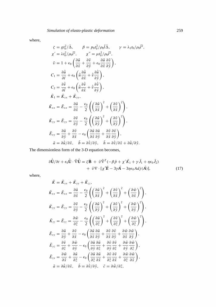
In the newly developed governing equations we see that for the usual tension test we canneglect acceleration terms and body force terms as they are very low while compared to theapplied load. Then the equation is governed by the gradients of strain and strain rate. Thestrain rate terms appear in the form of viscous resistance which is synonymous to materialdamping. To represent and to interpret the complex phenomenon occurring inside the material,we treat the material composed of a very large number of particles interconnected by springs(Timoshenko & Goodier 1970). We treat these hypothetical spring elements in parallel witha damper (figure 2) to represent the effect of momentum transfer between the particles.
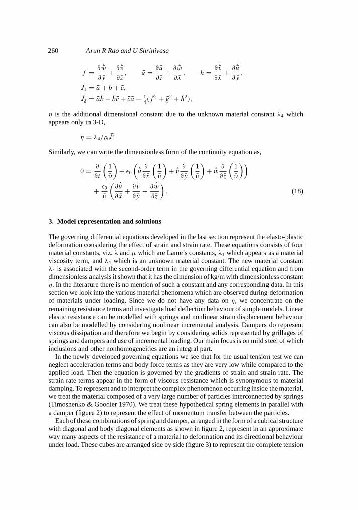
Each of these combinations of spring and damper, arranged in the form of a cubical structurewith diagonal and body diagonal elements as shown in figure 2, represent in an approximateway many aspects of the resistance of a material to deformation and its directional behaviourunder load. These cubes are arranged side by side (figure 3) to represent the complete tension
Simulation of elasto-plastic deformation 261
F
F
(a) (b)
Figure 2. Spring and damper model.(a)A complete cube with elements.(b) Eachelement in a cube.
test specimen in length, width and depth. This whole specimen can be treated as a homoge-neous material.
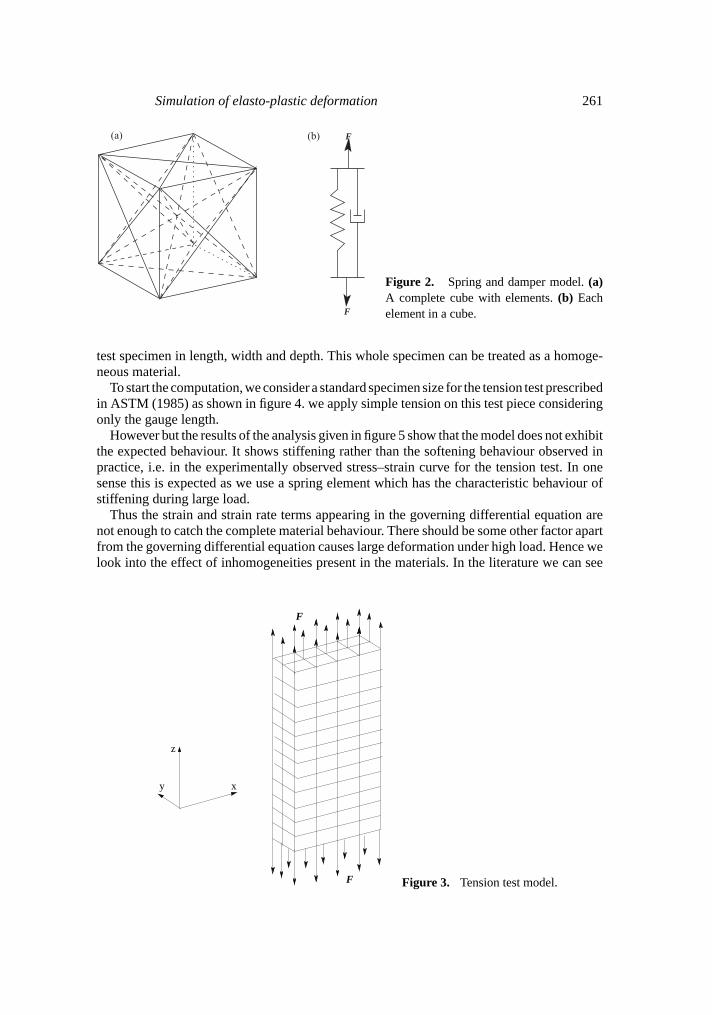
To start the computation, we consider a standard specimen size for the tension test prescribedin ASTM (1985) as shown in figure 4. we apply simple tension on this test piece consideringonly the gauge length.
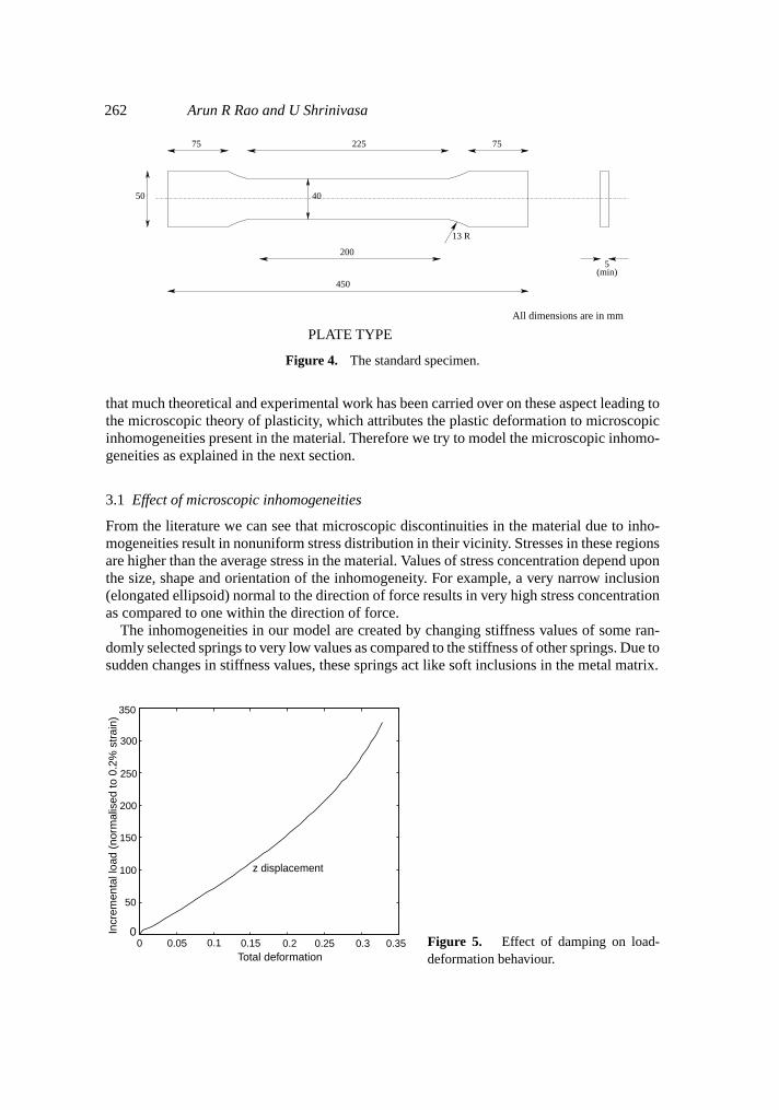
However but the results of the analysis given in figure 5 show that the model does not exhibitthe expected behaviour. It shows stiffening rather than the softening behaviour observed inpractice, i.e. in the experimentally observed stress–strain curve for the tension test. In onesense this is expected as we use a spring element which has the characteristic behaviour ofstiffening during large load.
Thus the strain and strain rate terms appearing in the governing differential equation arenot enough to catch the complete material behaviour. There should be some other factor apartfrom the governing differential equation causes large deformation under high load. Hence welook into the effect of inhomogeneities present in the materials. In the literature we can see
z
xy
F
F Figure 3. Tension test model.
262 Arun R Rao and U Shrinivasa
All dimensions are in mm
7522575
50 40
13 R
200
450
5(min)
PLATE TYPE
Figure 4. The standard specimen.
that much theoretical and experimental work has been carried over on these aspect leading tothe microscopic theory of plasticity, which attributes the plastic deformation to microscopicinhomogeneities present in the material. Therefore we try to model the microscopic inhomo-geneities as explained in the next section.
3.1 Effect of microscopic inhomogeneities
From the literature we can see that microscopic discontinuities in the material due to inho-mogeneities result in nonuniform stress distribution in their vicinity. Stresses in these regionsare higher than the average stress in the material. Values of stress concentration depend uponthe size, shape and orientation of the inhomogeneity. For example, a very narrow inclusion(elongated ellipsoid) normal to the direction of force results in very high stress concentrationas compared to one within the direction of force.
The inhomogeneities in our model are created by changing stiffness values of some ran-domly selected springs to very low values as compared to the stiffness of other springs. Due tosudden changes in stiffness values, these springs act like soft inclusions in the metal matrix.
0 0.05 0.1 0.15 0.2 0.25 0.3 0.350
50
100
150
200
250
300
350
z displacement
Incr
emen
tal l
oad
(nor
mal
ised
to 0
.2%
str
ain)
Total deformationFigure 5. Effect of damping on load-deformation behaviour.
Simulation of elasto-plastic deformation 263
0 10 20 30 40 50 60 70 80 90 100−100
−50
0
50
% number of elements
% c
hang
e in
forc
e du
e to
inho
mog
enei
ties
Compression range
Tension range
Material with 1% inhomogeneity
Material with 2% inhomogeneity
Material with 3% inhomogeneity
Material with 4% inhomogeneity
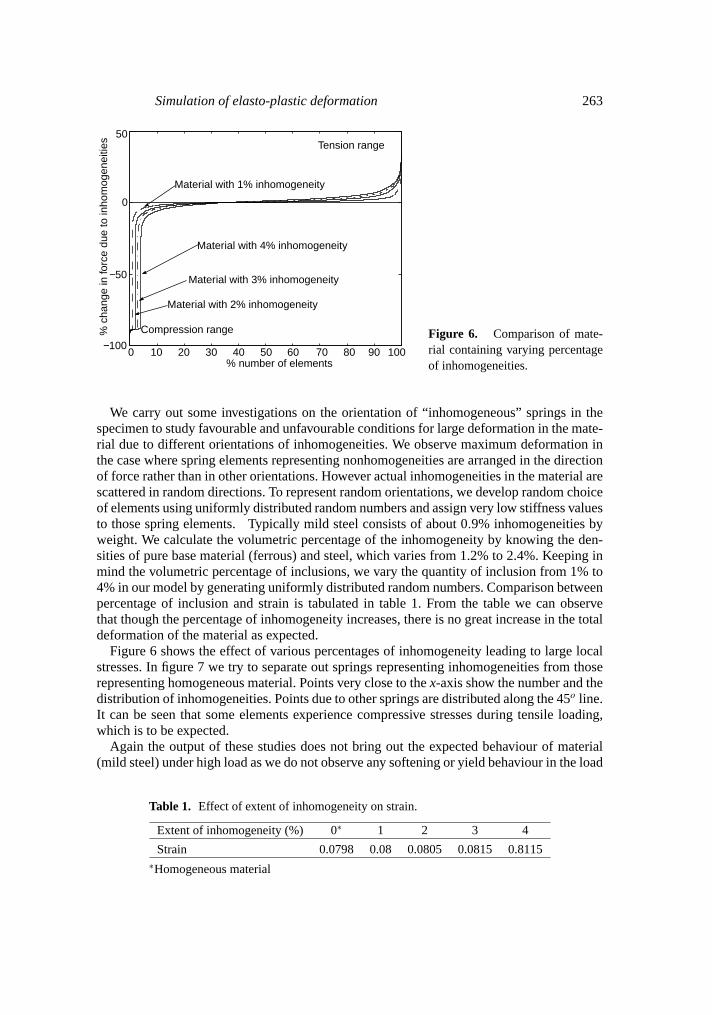
Figure 6. Comparison of mate-rial containing varying percentageof inhomogeneities.
We carry out some investigations on the orientation of “inhomogeneous” springs in thespecimen to study favourable and unfavourable conditions for large deformation in the mate-rial due to different orientations of inhomogeneities. We observe maximum deformation inthe case where spring elements representing nonhomogeneities are arranged in the directionof force rather than in other orientations. However actual inhomogeneities in the material arescattered in random directions. To represent random orientations, we develop random choiceof elements using uniformly distributed random numbers and assign very low stiffness valuesto those spring elements. Typically mild steel consists of about 0.9% inhomogeneities byweight. We calculate the volumetric percentage of the inhomogeneity by knowing the den-sities of pure base material (ferrous) and steel, which varies from 1.2% to 2.4%. Keeping inmind the volumetric percentage of inclusions, we vary the quantity of inclusion from 1% to4% in our model by generating uniformly distributed random numbers. Comparison betweenpercentage of inclusion and strain is tabulated in table 1. From the table we can observethat though the percentage of inhomogeneity increases, there is no great increase in the totaldeformation of the material as expected.
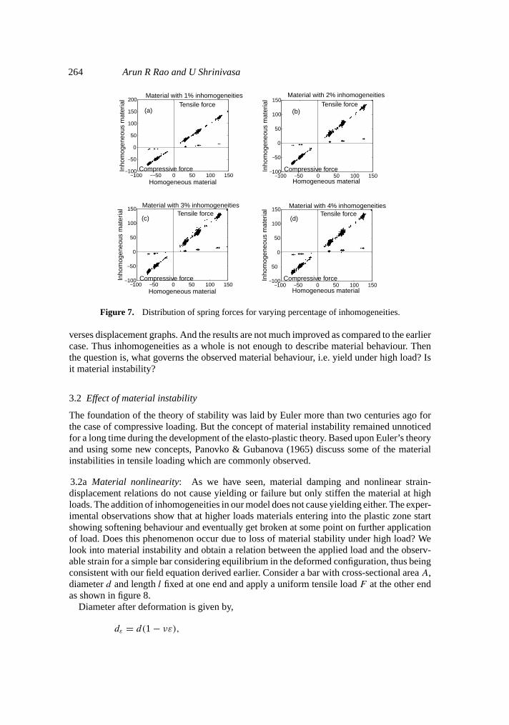
Figure 6 shows the effect of various percentages of inhomogeneity leading to large localstresses. In figure 7 we try to separate out springs representing inhomogeneities from thoserepresenting homogeneous material. Points very close to thex-axis show the number and thedistribution of inhomogeneities. Points due to other springs are distributed along the 45o line.It can be seen that some elements experience compressive stresses during tensile loading,which is to be expected.
Again the output of these studies does not bring out the expected behaviour of material(mild steel) under high load as we do not observe any softening or yield behaviour in the load
Table 1. Effect of extent of inhomogeneity on strain.
Extent of inhomogeneity (%) 0∗ 1 2 3 4
Strain 0.0798 0.08 0.0805 0.0815 0.8115∗Homogeneous material
264 Arun R Rao and U Shrinivasa
−100 −−50 0 50 100 150−100
−50
0
50
100
150
200
Homogeneous material
Inho
mog
eneo
us m
ater
ial Material with 1% inhomogeneities
−100 −50 0 50 100 150−100
−50
0
50
100
150
Homogeneous material
Inho
mog
eneo
us m
ater
ial
Material with 2% inhomogeneities
−100 −50 0 50 100 150−100
−50
0
50
100
150
Homogeneous material
Inho
mog
eneo
us m
ater
ial Material with 3% inhomogeneities
−100 −50 0 50 100 150−100
50
0
50
100
150
Homogeneous material
Inho
mog
eneo
us m
ater
ial Material with 4% inhomogeneities
Compressive force
Tensile force
Compressive force
Tensile force
Compressive force
Tensile force
Compressive force
Tensile force
(d)(c)
(a) (b)
Figure 7. Distribution of spring forces for varying percentage of inhomogeneities.
verses displacement graphs. And the results are not much improved as compared to the earliercase. Thus inhomogeneities as a whole is not enough to describe material behaviour. Thenthe question is, what governs the observed material behaviour, i.e. yield under high load? Isit material instability?
3.2 Effect of material instability
The foundation of the theory of stability was laid by Euler more than two centuries ago forthe case of compressive loading. But the concept of material instability remained unnoticedfor a long time during the development of the elasto-plastic theory. Based upon Euler’s theoryand using some new concepts, Panovko & Gubanova (1965) discuss some of the materialinstabilities in tensile loading which are commonly observed.
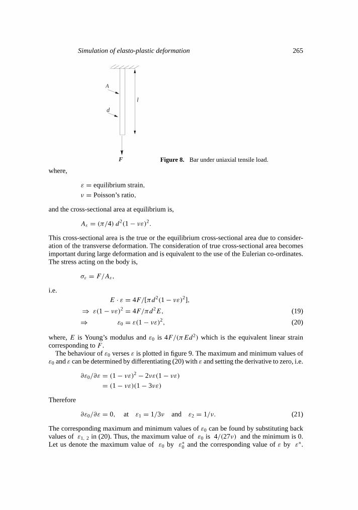
3.2a Material nonlinearity: As we have seen, material damping and nonlinear strain-displacement relations do not cause yielding or failure but only stiffen the material at highloads. The addition of inhomogeneities in our model does not cause yielding either. The exper-imental observations show that at higher loads materials entering into the plastic zone startshowing softening behaviour and eventually get broken at some point on further applicationof load. Does this phenomenon occur due to loss of material stability under high load? Welook into material instability and obtain a relation between the applied load and the observ-able strain for a simple bar considering equilibrium in the deformed configuration, thus beingconsistent with our field equation derived earlier. Consider a bar with cross-sectional areaA,diameterd and lengthl fixed at one end and apply a uniform tensile loadF at the other endas shown in figure 8.
Diameter after deformation is given by,
dε = d(1 − νε),
Simulation of elasto-plastic deformation 265
F
A
l
d
Figure 8. Bar under uniaxial tensile load.
where,
ε = equilibrium strain,
ν = Poisson’s ratio,
and the cross-sectional area at equilibrium is,
Aε = (π/4) d2(1 − νε)2.
This cross-sectional area is the true or the equilibrium cross-sectional area due to consider-ation of the transverse deformation. The consideration of true cross-sectional area becomesimportant during large deformation and is equivalent to the use of the Eulerian co-ordinates.The stress acting on the body is,
σε = F/Aε,
i.e.E · ε = 4F/[πd2(1 − νε)2],
⇒ ε(1 − νε)2 = 4F/πd2E, (19)
⇒ ε0 = ε(1 − νε)2, (20)
where,E is Young’s modulus andε0 is 4F/(πEd2) which is the equivalent linear straincorresponding toF .
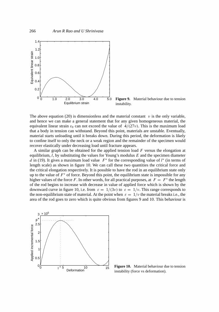
The behaviour ofε0 versesε is plotted in figure 9. The maximum and minimum values ofε0 andε can be determined by differentiating (20) withε and setting the derivative to zero, i.e.
∂ε0/∂ε = (1 − νε)2 − 2νε(1 − νε)
= (1 − νε)(1 − 3νε)
Therefore
∂ε0/∂ε = 0, at ε1 = 1/3ν and ε2 = 1/ν. (21)
The corresponding maximum and minimum values ofε0 can be found by substituting backvalues of ε1, 2 in (20). Thus, the maximum value ofε0 is 4/(27ν) and the minimum is 0.Let us denote the maximum value ofε0 by ε∗
0 and the corresponding value ofε by ε∗.
266 Arun R Rao and U Shrinivasa
0 1.0 2.0 3.0 4.0 5.00
0.2
0.4
0.6
0.8
1.0
1.2
1.4
Equilibrium strain
Equ
ival
ent l
inea
r st
rain
Figure 9. Material behaviour due to tensioninstability.
The above equation (20) is dimensionless and the material constantν is the only variable,and hence we can make a general statement that for any given homogeneous material, theequivalent linear strainε0 can not exceed the value of 4/(27ν). This is the maximum loadthat a body in tension can withstand. Beyond this point, materials are unstable. Eventually,material starts unloading until it breaks down. During this period, the deformation is likelyto confine itself to only the neck or a weak region and the remainder of the specimen wouldrecover elastically under decreasing load until fracture appears.
A similar graph can be obtained for the applied tension loadF versus the elongation atequilibrium,l, by substituting the values for Young’s modulusE and the specimen diameterd in (19). It gives a maximum load valueF ∗ for the corresponding value ofl∗ (in terms oflength scale) as shown in figure 10. We can call these two quantities the critical force andthe critical elongation respectively. It is possible to have the rod in an equilibrium state onlyup to the value ofF ∗ of force. Beyond this point, the equilibrium state is impossible for anyhigher values of the forceF . In other words, for all practical purposes, atF = F ∗ the lengthof the rod begins to increase with decrease in value of applied force which is shown by thedownward curve in figure 10, i.e. fromε = 1/(3ν) to ε = 1/ν. This range corresponds tothe non-equilibrium state of material. At the point whenε = 1/ν the material breaks i.e., thearea of the rod goes to zero which is quite obvious from figures 9 and 10. This behaviour is
0 5 10 150
0.5
1
1.5
2
2.5
3 × 10⁵
Deformation
App
lied
incr
emen
tal f
orce
F*
* l Figure 10. Material behaviour due to tensioninstability (force vs deformation).
Simulation of elasto-plastic deformation 267
similar to the observation made by Panovko & Gubanova (1965) in the case of loss of stabilityof a rod in tension. However any small irregularity in the diameter will make the rod breakcloser to 4/(27ν) and also at a lower value ofε0. For example, consider a uniform rod with aneck or a irregularity created in the bar artificially by removing some of the material at someposition. Initially, the load will be carried by the entire bar. But later as the load increases,the deformation confines to the neck or irregularity zone due to the high stress concentrationobserved in these areas. In this case, the material fails at a lower load than the maximumpossible.
Thus the material instability in tension has all the characteristics necessary to describenonlinear elastic and plastic deformation and also material breakage. However, the modelpredicts this behaviour at very high strains of about 1/ν (i.e. approximately 330% in the caseof steel withν = 0.3) and therefore is not adequate to explain yielding of a steel test specimenwhich occurs around a strain of 0.1%. So we take a re-look in the next section at the behaviourof materials with inhomogeneities in the light of the instabilities discussed in this section.
Before discussing the inhomogeneities, we first extend the instability criteria discussed for1-D to 3-D. On lines similar to 1-D, we also develop a relation between equilibrium stressesversus equilibrium strains in 3-D to investigate material instability. This relation is quiteuseful to discuss instability surfaces which are similar to the classical yield surfaces. The 3-Dversion is discussed in detail in appendix A.
From the discussion on the 1-D bar, we can see that the material enters the instability zoneonce it reaches the critical equilibrium strain. At this point, the curve changes its direction(slope becomes negative) and starts descending and reaches zero at some particular value ofequilibrium strain depending upon the value ofν i.e. at 1/(3ν). Hence we can define a newyield criterion or instability criterion as the point in the load-deformation curve, where theslope of the equivalent strain versus equilibrium strain curve becomes zero. To extend theabove to 3-D, we interpret the 1-D case as the one where dσ and dε are not correlated, i.e.different values of dε exist for the same value of dσ at this point. In 3-D we can write thisrelation as
dσ = Cdε, (22)
where dσ = (dσ1, dσ2, dσ3)T is a vector of incremental principal stresses anddε similarly
is the vector of incremental principal strains(dε1, dε2, dε3)T . HereC is a tensor which gives
one to one relation between incremental stresses and incremental strains in the equilibrium.The instability criterion now becomes Det[C] = 0, whereC is given by
[C] = ∂σx/∂εx ∂σx/∂εy ∂σx/∂εz
∂σy/∂εx ∂σy/∂εy ∂σy/∂εz
∂σz/∂εx ∂σz/∂εy ∂σz/∂εz
. (23)
There are no unique solutions for dε for a given dσ . The expression for each element in theabove matrixC is given in appendix A. Now we consider three different cases.
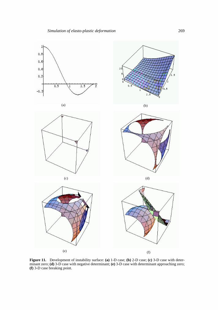
(a) εx = εx andεy = εz = −νεx : This gives the 1-D analysis discussed so far. From figure 11awe see that for zero values of strain, the determinant is one. This point corresponds to theorigin in figure 10. When the material reaches the instability point, the determinant goesto zero. Thus, this is the point where the material changes its behaviour. In the next range,we see that value of the determinant is negative till the material breaks.
268 Arun R Rao and U Shrinivasa
(b) εx = εx, εy = εy andεz = −ν(εx + εy): This is the 2-D case in principal strains. In thisthe determinant is a surface in equilibrium strainsεx andεy . The contour on theεx − εy
plane where the determinant is zero is the instability curve corresponding to the yieldcurve in 2-D and is shown in figure 11b.
(c) εx = εx, εy = εy, εz = εz: The instability surface obtained in 3-D case is explained stepby step in figures 11c to f. Here we observe that when the values of the strains are smallas compared to 1/(3ν), the instability surface (determinant = 0 surface) does not appear.As the strain values approach 1/(3ν) material is seen entering the instability zone and weobserve the development of the instability surface for which the determinant value is zero(figure 11c). Further figures show the development of the second surface as the value ofthe determinant goes to zero at the breakage point. The region outside of the instabilitysurface is the instability zone.
3.2b Behaviour of various terms near an inclusion:To continue our search for a suitablemodel, we now discuss the stress fields around inhomogeneities. To begin with we considerinclusion/inhomogeneities as spherical in 3-D, and around this region see how the variousterms appearing in the new field equation behave. With spherical voids, Qui & Weng (1992)observed excellent agreement with exact solution under hydrostatic loading and the finiteelement calculations are in accord with tensile behaviour of material.
In the case of 3-D, the complete stress at any point around spherical inclusion is obtainedas discussed by Timoshenko & Goodier (1970) in a polar coordinate system.
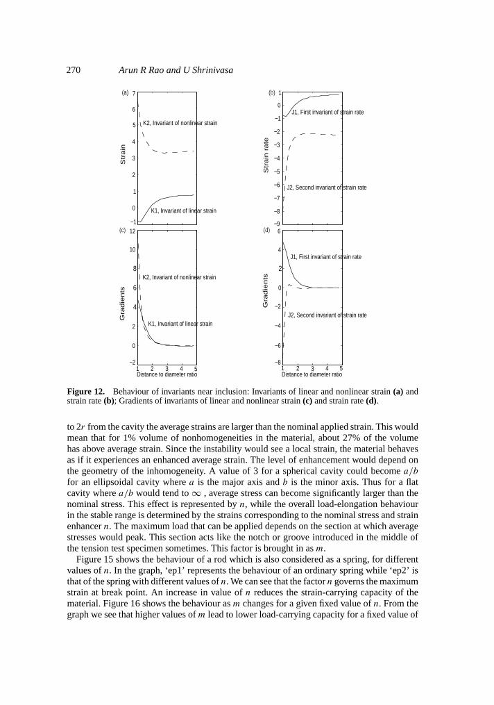
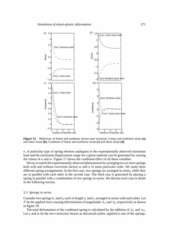
These equations are later transferred back to cartesian coordinates using the transformationmatrix and the graphs are plotted. Figures 12 to 14 show the behaviour of various terms nearan inclusion. It is interesting to note that there is a sharp variation within the length of tworadii of the inclusion.
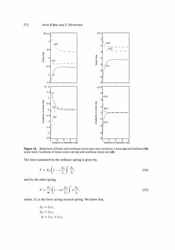
In figure 12 we see that the invariants of linear and nonlinear strains which appear in thenew field equations gradually change away from the cavity and later get stabilised at somefixed positive value. The same phenomenon can be observed with the first invariant of thestrain rate but the second invariant of the strain rate undergoes a sharp change before it isstabilised at some negative value. On the other hand, gradients of the invariants for strain andstrain rate change sharply before stabilising at zero.
Figure 13 shows a similar trend with the strains and their gradients. Figure 14 shows thebehaviour of strain rates and their gradients. Here also we see that axial and shear strain rateterms show sharp variations within a length of twice the radius before stabilising at someconstant values. As before, gradients of strain rate quantities show sharp variations beforegoing to zero.
In the case of the pressure termp we observe that the magnitude of pressure remainsconstant through the body, which means that the gradient of the pressure term is zero. A fewearlier authors have observed thatp does not contribute to plastic deformation.
We observe that nonlinear behaviour or region of instability of material occurs around thevalue of strain equal to 1/ν. But in practice, such a high value of strain is not observed duringtension testing. Typically, in the case of steel, yield behaviour occurs at around a strain of0.001 and the breaking phenomenon occurs at around 0.05 depending upon strain rate. Now,will we be able to derive this behaviour from what we learnt so far from our bar in tension?
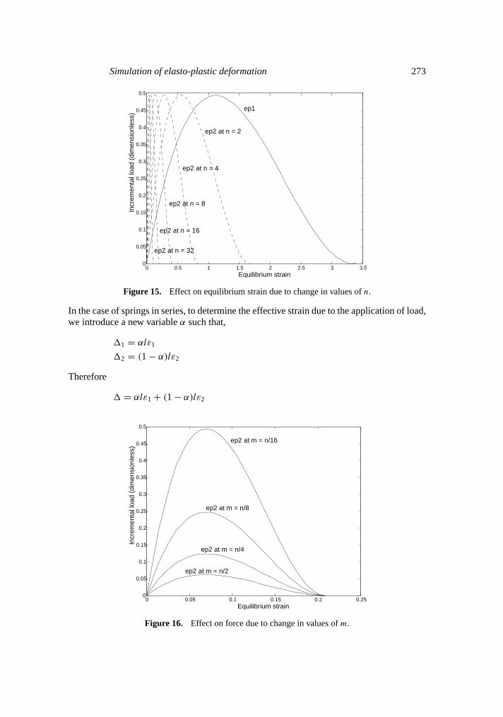
To bring down the value of the critical load,F ∗, and the corresponding critical strain duringmaterial instabilities to within the observed range, we introduce two new material variablesm andn, which correspond to force correction factor and strain correction factor respectively.Amongst the two, strain correction factor or actually strain enhancement factor is based onthe earlier discussion on computed strains around a spherical cavity. We find there that up
Simulation of elasto-plastic deformation 269
(e) (f)
(c) (d)
(a) (b)
Figure 11. Development of instability surface:(a) 1-D case;(b) 2-D case;(c) 3-D case with deter-minant zero;(d) 3-D case with negative determinant;(e)3-D case with determinant approaching zero;(f) 3-D case breaking point.
270 Arun R Rao and U Shrinivasa
1 2 3 4 5−2
0
2
4
6
8
10
12
K1, Invariant of linear strain
K2, Invariant of nonlinear strain
Distance to diameter ratio
Gra
die
nts
1 2 3 4 5−8
−6
−4
−2
0
2
4
6
J1, First invariant of strain rate
J2, Second invariant of strain rate
Distance to diameter ratio
Gra
die
nts
−1
0
1
2
3
4
5
6
7
K1, Invariant of linear strain
K2, Invariant of nonlinear strainS
tra
in
−9
−8
−7
−6
−5
−4
−3
−2
−1
0
1
J1, First invariant of strain rate
J2, Second invariant of strain rate
Str
ain
ra
te
(a) (b)
(c) (d)
Figure 12. Behaviour of invariants near inclusion: Invariants of linear and nonlinear strain(a) andstrain rate(b); Gradients of invariants of linear and nonlinear strain(c) and strain rate(d).
to 2r from the cavity the average strains are larger than the nominal applied strain. This wouldmean that for 1% volume of nonhomogeneities in the material, about 27% of the volumehas above average strain. Since the instability would see a local strain, the material behavesas if it experiences an enhanced average strain. The level of enhancement would depend onthe geometry of the inhomogeneity. A value of 3 for a spherical cavity could becomea/b
for an ellipsoidal cavity wherea is the major axis andb is the minor axis. Thus for a flatcavity wherea/b would tend to∞ , average stress can become significantly larger than thenominal stress. This effect is represented byn, while the overall load-elongation behaviourin the stable range is determined by the strains corresponding to the nominal stress and strainenhancern. The maximum load that can be applied depends on the section at which averagestresses would peak. This section acts like the notch or groove introduced in the middle ofthe tension test specimen sometimes. This factor is brought in asm.
Figure 15 shows the behaviour of a rod which is also considered as a spring, for differentvalues ofn. In the graph, ‘ep1’ represents the behaviour of an ordinary spring while ‘ep2’ isthat of the spring with different values ofn. We can see that the factorn governs the maximumstrain at break point. An increase in value ofn reduces the strain-carrying capacity of thematerial. Figure 16 shows the behaviour asm changes for a given fixed value ofn. From thegraph we see that higher values ofm lead to lower load-carrying capacity for a fixed value of
Simulation of elasto-plastic deformation 271
−1.5
−1
−0.5
0
0.5
1
1.5
2
2.5
Exx1, Linear strain
Exx2, Nonlinear strainS
tra
in
−2
−1.5
−1
−0.5
0
0.5
1
1.5Exz1, Linear shear strain
Exz2, Nonlinear shear strain
Str
ain
1 2 3 4 5−0.2
0
0.2
0.4
0.6
0.8
1
1.2
1.4
1.6
Exx1, Linear strain
Exx2, Nonlinear strain
Distance to diameter ratio
Gra
die
nts
1 2 3 4 5−3
−2
−1
0
1
2
3
4
Exz1, Linear shear strain
Exz2, Nonlinear shear
Distance to diameter ratio
Gra
die
nts
(a) (b)
(c) (d)
Figure 13. Behaviour of linear and nonlinear strains near inclusion: Linear and nonlinear strain(a)and shear strain(b); Gradients of linear and nonlinear strain(c) and shear strain(d).
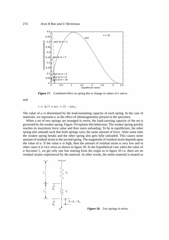
n. A particular type of spring element analogous to the experimentally observed maximumload and the maximum displacement range for a given material can be generated by varyingthe values ofn andm. Figure 17 shows the combined effect of all these variables.
We try to match the experimentally observed phenomenon by arranging two or more springsboth with and without correction factorsm andn in some particular order. We study threedifferent spring arrangements. In the first case, two springs are arranged in series, while theyare in parallel with each other in the second case. The third case is generated by placing aspring in parallel with a combination of two springs in series. We discuss each case in detailin the following section.
3.3 Springs in series
Consider two springsk1 andk2 each of lengthl1 andl2 arranged in series with each other. LetF be the applied force causing deformations of magnitudes11 and12 respectively as shownin figure 18.
The total deformation of the combined spring is calculated by the addition of11 and12.Let n andm be the two correction factors as discussed earlier, applied to one of the springs.
272 Arun R Rao and U Shrinivasa
−1.5
−1
−0.5
0
0.5
1
1.5
a
h/2
g/2S
trai
n ra
te
−5
−4
−3
−2
−1
0
1
2
3
A11
A12
A13
Str
ain
rate
1 2 3 4 5−2.5
−2
−1.5
−1
−0.5
0
0.5
1
1.5
2
a
h/2
g/2
Distance to diameter ratio
Gra
dien
ts o
f str
ain
rate
1 2 3 4 5−8
−6
−4
−2
0
2
4
6
8
A11
A12
A13
Distance to diameter ratio
Gra
dien
ts o
f str
ain
rate
(a) (b)
(c) (d)
Figure 14. Behaviour of linear and nonlinear strain rates near inclusion: Linear(a) and nonlinear(b)strain rates; Gradients of linear strain rate(c) and nonlinear strain rate(d).
The force sustained by the ordinary spring is given by,
F = F0
(1 − ν
11
l1
)211
l1, (24)
and for the other spring,
F = F0
m
(1 − nν
12
l2
)2
n12
l2, (25)
where,F0 is the force acting on each spring. We know that,
11 = l1ε1,
12 = l2ε2,
1 = l1ε1 + l2ε2.
Simulation of elasto-plastic deformation 273
0 0.5 1 1.5 2 2.5 3 3.50
0.05
0.1
0.15
0.2
0.25
0.3
0.35
0.4
0.45
0.5
ep1
Incr
emen
tal l
oad
(dim
ensi
onle
ss)
ep2 at n = 2
ep2 at n = 4
ep2 at n = 8
ep2 at n = 16
ep2 at n = 32
Equilibrium strain
Figure 15. Effect on equilibrium strain due to change in values ofn.
In the case of springs in series, to determine the effective strain due to the application of load,we introduce a new variableα such that,
11 = αlε1
12 = (1 − α)lε2
Therefore
1 = αlε1 + (1 − α)lε2
0 0.05 0.1 0.15 0.2 0.250
0.05
0.1
0.15
0.2
0.25
0.3
0.35
0.4
0.45
0.5
ep2 at m = n/16
Incr
emen
tal l
oad
(dim
ensi
onle
ss)
ep2 at m = n/8
ep2 at m = n/4
ep2 at m = n/2
Equilibrium strain
Figure 16. Effect on force due to change in values ofm.
274 Arun R Rao and U Shrinivasa
0 0.5 1 1.5 2 2.5 3 3.50
0.05
0.1
0.15
0.2
0.25
0.3
0.35
0.4
0.45
0.5
ep1
Equilibrium strain
Incr
emen
tal l
oad
(dim
ensi
onle
ss)
ep2 at m = 16ep2 at m = 8
ep2 at m = 4
ep2 at m = 2
ep2 at m = 1
n = 32
Figure 17. Combined effect on spring due to change in values ofn andm.
and
ε = 1/l = αε1 + (1 − α)ε2.
The value ofα is determined by the load-sustaining capacity of each spring. In the case ofmaterials, we representα as the effect of inhomogeneities present in the specimen.
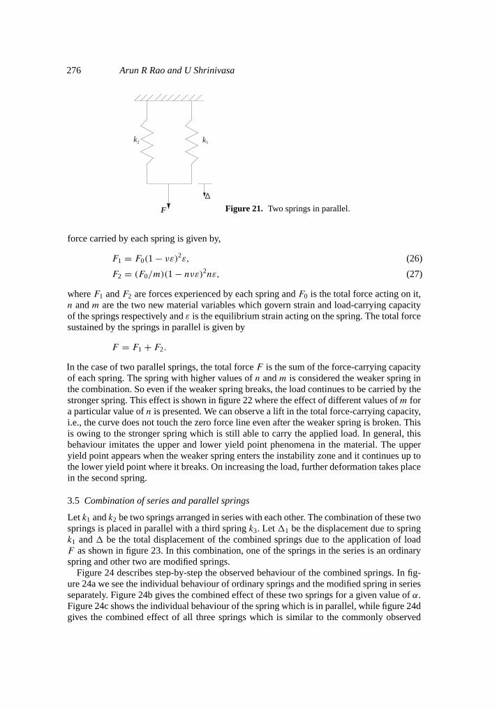
When a set of two springs are arranged in series, the load-carrying capacity of the set isgoverned by the weaker spring. Figure 19 explains this behaviour. The weaker spring quicklyreaches its maximum force value and then starts unloading. To be in equilibrium, the otherspring also unloads such that both springs carry the same amount of force. After some timethe weaker spring breaks and the other spring also gets fully unloaded. This causes someamount of residual strain in the second spring. The magnitude of residual strain depends uponthe value ofα. If the valueα is high, then the amount of residual strain is very low and inother cases it is vice versa as shown in figure 20. In the hypothetical case when the value ofα becomes 1, we get only one line starting from the origin as in figure 20 i.e. there are noresidual strains experienced by the material. In other words, the entire material is treated as
F
∆ = ∆1 + ∆2
l1
l2
k1
k2
∆2
∆1
Figure 18. Two springs in series.
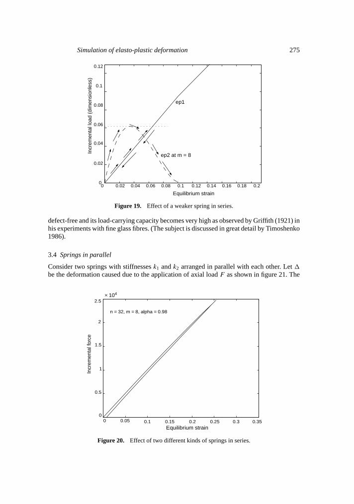
Simulation of elasto-plastic deformation 275
0 0.02 0.04 0.06 0.08 0.1 0.12 0.14 0.16 0.18 0.20
0.02
0.04
0.06
0.08
0.1
0.12
ep1
Equilibrium strain
Incr
emen
tal l
oad
(dim
ensi
onle
ss)
ep2 at m = 8
Figure 19. Effect of a weaker spring in series.
defect-free and its load-carrying capacity becomes very high as observed by Griffith (1921) inhis experiments with fine glass fibres. (The subject is discussed in great detail by Timoshenko1986).
3.4 Springs in parallel
Consider two springs with stiffnessesk1 andk2 arranged in parallel with each other. Let1
be the deformation caused due to the application of axial loadF as shown in figure 21. The
0 0.05 0.1 0.15 0.2 0.25 0.3 0.350
0.5
1
1.5
2
2.5
n = 32, m = 8, alpha = 0.98
Equilibrium strain
Incr
emen
tal f
orce
× 104
Figure 20. Effect of two different kinds of springs in series.
276 Arun R Rao and U Shrinivasa
F
k1k2
∆Figure 21. Two springs in parallel.
force carried by each spring is given by,
F1 = F0(1 − νε)2ε, (26)
F2 = (F0/m)(1 − nνε)2nε, (27)
whereF1 andF2 are forces experienced by each spring andF0 is the total force acting on it,n andm are the two new material variables which govern strain and load-carrying capacityof the springs respectively andε is the equilibrium strain acting on the spring. The total forcesustained by the springs in parallel is given by
F = F1 + F2.
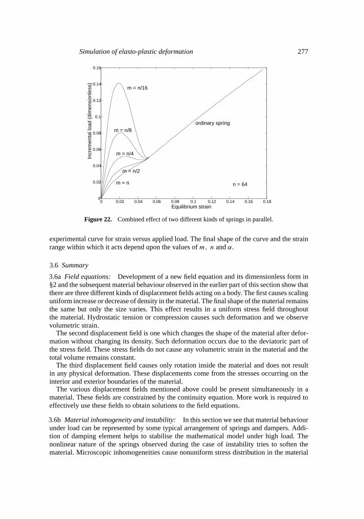
In the case of two parallel springs, the total forceF is the sum of the force-carrying capacityof each spring. The spring with higher values ofn andm is considered the weaker spring inthe combination. So even if the weaker spring breaks, the load continues to be carried by thestronger spring. This effect is shown in figure 22 where the effect of different values ofm fora particular value ofn is presented. We can observe a lift in the total force-carrying capacity,i.e., the curve does not touch the zero force line even after the weaker spring is broken. Thisis owing to the stronger spring which is still able to carry the applied load. In general, thisbehaviour imitates the upper and lower yield point phenomena in the material. The upperyield point appears when the weaker spring enters the instability zone and it continues up tothe lower yield point where it breaks. On increasing the load, further deformation takes placein the second spring.
3.5 Combination of series and parallel springs
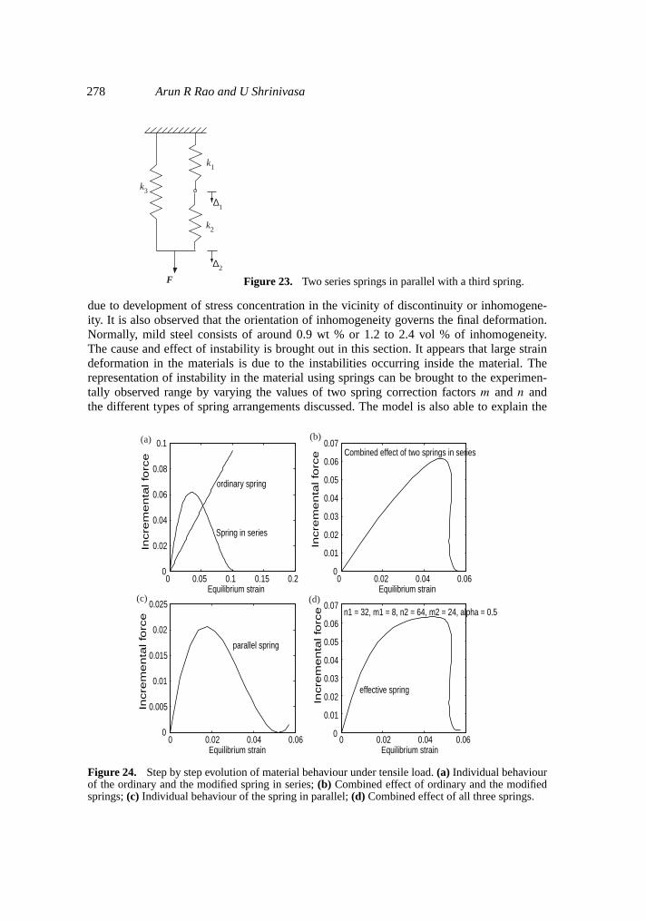
Let k1 andk2 be two springs arranged in series with each other. The combination of these twosprings is placed in parallel with a third springk3. Let 11 be the displacement due to springk1 and1 be the total displacement of the combined springs due to the application of loadF as shown in figure 23. In this combination, one of the springs in the series is an ordinaryspring and other two are modified springs.
Figure 24 describes step-by-step the observed behaviour of the combined springs. In fig-ure 24a we see the individual behaviour of ordinary springs and the modified spring in seriesseparately. Figure 24b gives the combined effect of these two springs for a given value ofα.Figure 24c shows the individual behaviour of the spring which is in parallel, while figure 24dgives the combined effect of all three springs which is similar to the commonly observed
Simulation of elasto-plastic deformation 277
0 0.02 0.04 0.06 0.08 0.1 0.12 0.14 0.16 0.180
0.02
0.04
0.06
0.08
0.1
0.12
0.14
0.16
m = n
Incr
emen
tal l
oad
(dim
ensi
onle
ss)
m = n/2
m = n/4
m = n/8
m = n/16
ordinary spring
n = 64
Equilibrium strain
Figure 22. Combined effect of two different kinds of springs in parallel.
experimental curve for strain versus applied load. The final shape of the curve and the strainrange within which it acts depend upon the values ofm, n andα.
3.6 Summary
3.6a Field equations: Development of a new field equation and its dimensionless form in§2 and the subsequent material behaviour observed in the earlier part of this section show thatthere are three different kinds of displacement fields acting on a body. The first causes scalinguniform increase or decrease of density in the material. The final shape of the material remainsthe same but only the size varies. This effect results in a uniform stress field throughoutthe material. Hydrostatic tension or compression causes such deformation and we observevolumetric strain.
The second displacement field is one which changes the shape of the material after defor-mation without changing its density. Such deformation occurs due to the deviatoric part ofthe stress field. These stress fields do not cause any volumetric strain in the material and thetotal volume remains constant.
The third displacement field causes only rotation inside the material and does not resultin any physical deformation. These displacements come from the stresses occurring on theinterior and exterior boundaries of the material.
The various displacement fields mentioned above could be present simultaneously in amaterial. These fields are constrained by the continuity equation. More work is required toeffectively use these fields to obtain solutions to the field equations.
3.6b Material inhomogeneity and instability: In this section we see that material behaviourunder load can be represented by some typical arrangement of springs and dampers. Addi-tion of damping element helps to stabilise the mathematical model under high load. Thenonlinear nature of the springs observed during the case of instability tries to soften thematerial. Microscopic inhomogeneities cause nonuniform stress distribution in the material
278 Arun R Rao and U Shrinivasa
F
k1
k2
∆2
∆1
k3
Figure 23. Two series springs in parallel with a third spring.
due to development of stress concentration in the vicinity of discontinuity or inhomogene-ity. It is also observed that the orientation of inhomogeneity governs the final deformation.Normally, mild steel consists of around 0.9 wt % or 1.2 to 2.4 vol % of inhomogeneity.The cause and effect of instability is brought out in this section. It appears that large straindeformation in the materials is due to the instabilities occurring inside the material. Therepresentation of instability in the material using springs can be brought to the experimen-tally observed range by varying the values of two spring correction factorsm andn andthe different types of spring arrangements discussed. The model is also able to explain the
0 0.05 0.1 0.15 0.20
0.02
0.04
0.06
0.08
0.1
Spring in series
ordinary spring
Equilibrium strain
Incre
me
nta
l fo
rce
0 0.02 0.04 0.060
0.01
0.02
0.03
0.04
0.05
0.06
0.07Combined effect of two springs in series
Equilibrium strain
Incre
me
nta
l fo
rce
0 0.02 0.04 0.060
0.005
0.01
0.015
0.02
0.025
parallel spring
Equilibrium strain
Incre
me
nta
l fo
rce
0 0.02 0.04 0.060
0.01
0.02
0.03
0.04
0.05
0.06
0.07
effective spring
n1 = 32, m1 = 8, n2 = 64, m2 = 24, alpha = 0.5
Equilibrium strain
Incre
me
nta
l fo
rce
(a) (b)
(c) (d)
Figure 24. Step by step evolution of material behaviour under tensile load.(a) Individual behaviourof the ordinary and the modified spring in series;(b) Combined effect of ordinary and the modifiedsprings;(c) Individual behaviour of the spring in parallel;(d) Combined effect of all three springs.
Simulation of elasto-plastic deformation 279
observations from Griffith’s experiments with thin wires. The practically observed materialphenomena which normally occur in sheet metal-forming processes like Bauschinger effect,material anisotropy, yield point phenomenon, stress inhomogeneity, solid solution strengthen-ing, strengthening from fine particles, fracture, residual stresses, etc. are explainable with thisnew model.
4. Reformulation
4.1 Field equation
The understanding of material behaviour in §3 shows that material deformation is only dueto changes in size and shape. These two factors are governed by strain and strain rate. Thefield equation developed in the earlier section consists of resistance due to three components:one is strain, the second is the dissipative part due to strain rate and the third is the pressureterm. In the case of solids the pressure term appears as a hydrostatic stress acting on thebody. From classical mechanics, it is known that deformation occurrs because of continuousaction of hydrostatic and deviatoric stresses. So going back to Lamb (1945) for the originalformulation and considering only small strain, we get
p′1 = −p + λ1(ε
′1 + ε′
2 + ε′3) + λ2ε
′1,
p′2 = −p + λ1(ε
′1 + ε′
2 + ε′3) + λ2ε
′2,
p′3 = −p + λ1(ε
′1 + ε′
2 + ε′3) + λ2ε
′3, (28)
whereε′1, ε′
2, ε′3 are the strains along each principal axes. Now, let us redefine the constant
λ2 as,
p′1 + p′
2 + p′3 = λ2(ε
′1 + ε′
2 + ε′3).
Therefore from the definition ofp we get,
p = (p′1 + p′
2 + p′3)/3 = λ2
(ε′
1 + ε′2 + ε′
3/3)
(29)
Substituting forp in (28) and rearranging the terms we get,
P′e = λ1(ε
′1 + ε′
2 + ε′3)I + λ2
ε′
1 0 00 ε′
2 00 0 ε′
3
− ε′
1 + ε′2 + ε′
3
3I
, (30)
which is in the form of total stress on the body expressed by the hydrostatic and deviatoricstresses. The values ofλ1 andλ2 can be calculated from uniaxial tension and torsional tests.From the torsional test we get,
p′1 = τ, p′
2 = −τ, p′3 = 0,
ε′1 = τ/2G, ε′
2 = −τ/2G, and ε′3 = 0,
whereτ is shear stress. Substituting in (30) and solving forλ1 andλ2 we get,
λ2 = 2G (31)
280 Arun R Rao and U Shrinivasa
whereG is modulus of rigidity. From the uniaxial tension test,
p′1 = σ, p′
2 = p′3 = 0,
ε′1 = σ/E, ε′
2 = ε′3 = −νσ/E.
Substituting in (30) and solving forλ1 we get,
λ1 = K, (32)
whereK is bulk modulus. Thus (30) becomes the resistance due to small strains as,
P′e = K(ε′
1 + ε′2 + ε′
3)I + 2G
ε′
1 0 00 ε′
2 00 0 ε′
3
− (ε′
1 + ε′2 + ε′
3)
3I
. (33)
Similarly, the resistance due to rate of deformation can be determined. Considerε′1, ε′
2, ε′3
as the rate of strain in each direction in the principal coordinate system. Now, we can rewrite(30) for strain rate terms by substituting the strain termsε′
1, ε′2, ε′
3 by ε′1, ε′
2, ε′3 with two
more new constantsλ3 andλ4. The value of new constantλ4 can be found using the torsiontest on a thin tube specimen.
pd1 = −τ, pd2 = τ, pd3 = 0,
ε′1 = −τ/2µ, ε′
2 = τ/2µ, ε′3 = 0,
⇒ λ4 = 2µ, (34)
whereµ is material viscosity term in the case of solids. The remaining unknown constantλ3
is considered to be one more viscosity term or secondary viscosity termµ′ (Lamb 1945) inthe case of solids. Thus the resistance due to strain rate is,
P′d = µ′ d
dt(ε′
1 + ε′2 + ε′
3)I + 2µd
dt
ε′
1 0 00 ε′
2 00 0 ε′
3
− (ε′
1 + ε′2 + ε′
3)
3I
.
(35)
To evaluate the constantsλ1, λ2, λ3, λ4, we consider only small strain conditions. At smallstrains the values of elastic constant are not affected by the material nonlinearity and instabilitywhich occur at higher loads. The values ofK andG can be obtained experimentally and arestandard for a given material. Similarly the value ofµ can be calculated from the torsionalvibration of a tube. The value ofµ′ can be calculated from the longitudinal vibration of a thinwire of the material.
Considering that deformation is continuous under the action of strain and strain rate, thetotal resistance for the deformation can be determined by adding the resistance from strainand strain rate terms. Thus adding (33) and (35) we get,
P′ = P′e + P′
d
=(
K + µ′ d
dt
)(ε′
1 + ε′2 + ε′
3)I
+ 2
(G + µ
d
dt
) ε′
1 0 00 ε′
2 00 0 ε′
3
− (ε′
1 + ε′2 + ε′
3)
3I
. (36)
Simulation of elasto-plastic deformation 281
This expression holds good for infinitesimal strain conditions where volume change is neg-ligible. But during large deformation, the volume does not remain constant (Bell 1990). Insuch cases the change in volume should be taken into consideration. Therefore the hydro-static pressure should be expressed in terms of volumetric strain or, in other words, in termsof strain invariants. Thus for large deformation, the above equation is modified as,
P′ =(
K + µ′ d
dt
)(S ′
1 + S ′2 + S ′
3)I
+ 2
(G + µ
d
dt
) e1 0 0
0 e2 00 0 e3
− S ′
1 + S ′2 + S ′
3
3I
, (37)
wheree1, e2, e3 are the principal stretches as defined by Fung (1965) andS ′1, S ′
2 and S ′3 are
the three invariants of the principal stretches,
S ′1 = e1 + e2 + e3,
S ′2 = e1e2 + e2e3 + e3e1,
S ′3 = e1e2e3.
To observe the material behaviour under external force, consider the elastic resistance part.The above equation reduces to,
P ′ = (3K − 2G)
(S ′
1 + S ′2 + S ′
3
3
)I + 2G
e1 0 0
0 e2 00 0 e3
. (38)
From the uniaxial tension test we get, σ 0 0
0 0 00 0 0
= (3K − 2G)
(S ′
1 + S ′2 + S ′
3
3
)I + 2G
e1 0 0
0 e2 00 0 e3
, (39)
whereσ is the principal stress. In the case of a bar which is symmetric along thez-axis,e2 = e3. Thus the change in volume is given by,
S ′1 + S ′
2 + S ′3 = e1 + 2e2 + e2(2e1 + e2) + e1e
22. (40)
By solving (39) we get,
σ = 2G(e1 − e2). (41)
In the case of material instability as explained by Panovko & Gubanova (1965), we get therelationship between the instability function(1 + e2)
2 andσ/G as,
p = A(1 + e2)2σ
= 2A(1 + e2)2G(e1 − e2),
⇒ p/2AG = (1 + e2)2(e1 − e2). (42)
Now, we can plote1 ande2 as a function ofσ/G. The value ofe1 can be calculated by assumingsome negative values fore2 and solving (41) using (40) forσ/G. These plots are as shown
282 Arun R Rao and U Shrinivasa
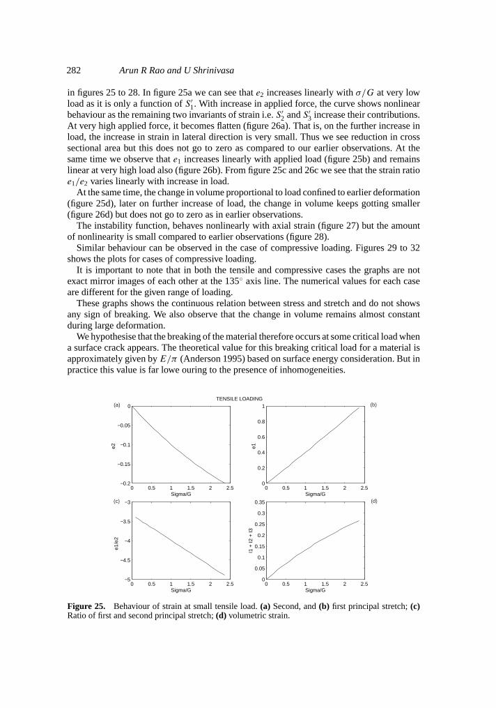
in figures 25 to 28. In figure 25a we can see thate2 increases linearly withσ/G at very lowload as it is only a function ofS ′
1. With increase in applied force, the curve shows nonlinearbehaviour as the remaining two invariants of strain i.e.S ′
2 andS ′3 increase their contributions.
At very high applied force, it becomes flatten (figure 26a). That is, on the further increase inload, the increase in strain in lateral direction is very small. Thus we see reduction in crosssectional area but this does not go to zero as compared to our earlier observations. At thesame time we observe thate1 increases linearly with applied load (figure 25b) and remainslinear at very high load also (figure 26b). From figure 25c and 26c we see that the strain ratioe1/e2 varies linearly with increase in load.
At the same time, the change in volume proportional to load confined to earlier deformation(figure 25d), later on further increase of load, the change in volume keeps gotting smaller(figure 26d) but does not go to zero as in earlier observations.
The instability function, behaves nonlinearly with axial strain (figure 27) but the amountof nonlinearity is small compared to earlier observations (figure 28).
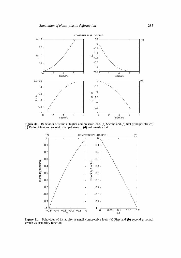
Similar behaviour can be observed in the case of compressive loading. Figures 29 to 32shows the plots for cases of compressive loading.
It is important to note that in both the tensile and compressive cases the graphs are notexact mirror images of each other at the 135◦ axis line. The numerical values for each caseare different for the given range of loading.
These graphs shows the continuous relation between stress and stretch and do not showsany sign of breaking. We also observe that the change in volume remains almost constantduring large deformation.
We hypothesise that the breaking of the material therefore occurs at some critical load whena surface crack appears. The theoretical value for this breaking critical load for a material isapproximately given byE/π (Anderson 1995) based on surface energy consideration. But inpractice this value is far lowe ouring to the presence of inhomogeneities.
0 0.5 1 1.5 2 2.5−0.2
−0.15
−0.1
−0.05
0
Sigma/G
e2
0 0.5 1 1.5 2 2.50
0.2
0.4
0.6
0.8
1
Sigma/G
e1
0 0.5 1 1.5 2 2.5−5
−4.5
−4
−3.5
−3
Sigma/G
e1/e
2
0 0.5 1 1.5 2 2.50
0.05
0.1
0.15
0.2
0.25
0.3
0.35
Sigma/G
I1 +
I2 +
I3
TENSILE LOADING (a) (b)
(c) (d)
Figure 25. Behaviour of strain at small tensile load.(a) Second, and(b) first principal stretch;(c)Ratio of first and second principal stretch;(d) volumetric strain.
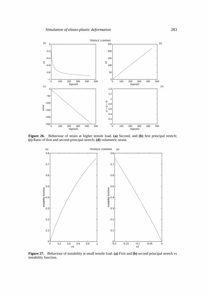
Simulation of elasto-plastic deformation 283
0 100 200 300 400 500−1
−0.8
−0.6
−0.4
−0.2
0
Sigma/G
e2
0 100 200 300 400 5000
50
100
150
200
250
Sigma/G
e1
0 100 200 300 400 500−250
−200
−150
−100
−50
0
Sigma/G
e1/e
2
0 100 200 300 400 5000
0.2
0.4
0.6
0.8
1
1.2
1.4
Sigma/G
I1 +
I2 +
I3
TENSILE LOADING (a) (b)
(c) (d)
Figure 26. Behaviour of strain at higher tensile load.(a) Second, and(b) first principal stretch;(c) Ratio of first and second principal stretch;(d) volumetric strain.
0 0.2 0.4 0.6 0.8 10
0.1
0.2
0.3
0.4
0.5
0.6
0.7
0.8
e1
Inst
abili
ty fu
nctio
n
−0.2 −0.15 −0.1 −0.05 00
0.1
0.2
0.3
0.4
0.5
0.6
0.7
0.8
e2
Inst
abili
ty fu
nctio
n
TENSILE LOADING (a) (b)
Figure 27. Behaviour of instability at small tensile load.(a) First and(b) second principal stretch vsinstability function.
284 Arun R Rao and U Shrinivasa
0 50 100 150 200 2500
0.5
1
1.5
2
2.5
e1
Inst
abili
ty fu
nctio
n
−1 −0.8 −0.6 −0.4 −0.2 00
0.5
1
1.5
2
2.5
e2
Inst
abili
ty fu
nctio
n
TENSILE LOADING (a) (b)
Figure 28. Behaviour of instability at higher tensile load.(a) First and(b) second principal stretchvs instability function.
0 0.5 1 1.50
0.05
0.1
0.15
0.2
Sigma/G
e2
0 0.5 1 1.5−0.5
−0.4
−0.3
−0.2
−0.1
0
Sigma/G
e1
0 0.5 1 1.5−3.4
−3.2
−3
−2.8
−2.6
−2.4
Sigma/G
e1/e
2
0 0.5 1 1.5−0.3
−0.25
−0.2
−0.15
−0.1
−0.05
0
0.05
Sigma/G
I1 +
I2 +
I3
COMPRESSIVE LOAD (a) (b)
(c) (d)
Figure 29. Behaviour of strain at small compressive load.(a) Second, and(b) first principal stretch;(c) Ratio of first and second principal stretch;(d) volumetric strain.
Simulation of elasto-plastic deformation 285
0 2 4 6 80
0.5
1
1.5
2
Sigma/G
e2
0 2 4 6 8−1.2
−1
−0.8
−0.6
−0.4
−0.2
0
0.2
Sigma/G
e1
0 2 4 6 8−3
−2.5
−2
−1.5
−1
−0.5
Sigma/G
e1/e
2
0 2 4 6 8−3
−2.5
−2
−1.5
−1
−0.5
0
Sigma/G
I1 +
I2 +
I3
COMPRESSIVE LOADING (a) (b)
(c) (d)
Figure 30. Behaviour of strain at higher compressive load.(a) Second and(b) first principal stretch;(c) Ratio of first and second principal stretch;(d) volumetric strain.
−0.5 −0.4 −0.3 −0.2 −0.1 0−1
−0.9
−0.8
−0.7
−0.6
−0.5
−0.4
−0.3
−0.2
−0.1
0
e1
Inst
abili
ty fu
nctio
n
0 0.05 0.1 0.15 0.21
−0.9
−0.8
−0.7
−0.6
−0.5
−0.4
−0.3
−0.2
−0.1
0
e2
Inst
abili
ty fu
nctio
n
COMPRESSIVE LOADING (a) (b)
Figure 31. Behaviour of instability at small compressive load.(a) First and(b) second principalstretch vs instability function.
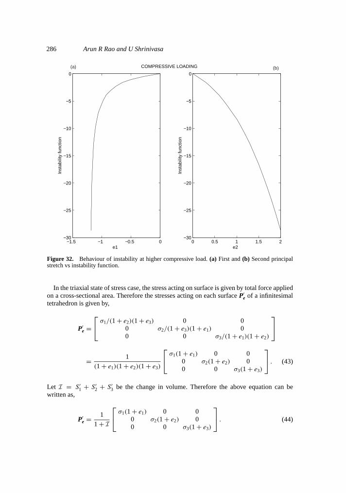
286 Arun R Rao and U Shrinivasa
−1.5 −1 −0.5 0−30
−25
−20
−15
−10
−5
0
e1
Inst
abili
ty fu
nctio
n
0 0.5 1 1.5 2−30
−25
−20
−15
−10
−5
0
e2
Inst
abili
ty fu
nctio
n
COMPRESSIVE LOADING (a) (b)
Figure 32. Behaviour of instability at higher compressive load.(a) First and(b) Second principalstretch vs instability function.
In the triaxial state of stress case, the stress acting on surface is given by total force appliedon a cross-sectional area. Therefore the stresses acting on each surfaceP′
e of a infinitesimaltetrahedron is given by,
P′e =
σ1/(1 + e2)(1 + e3) 0 0
0 σ2/(1 + e3)(1 + e1) 00 0 σ3/(1 + e1)(1 + e2)
= 1
(1 + e1)(1 + e2)(1 + e3)
σ1(1 + e1) 0 0
0 σ2(1 + e2) 00 0 σ3(1 + e3)
. (43)
Let I = S ′1 + S ′
2 + S ′3 be the change in volume. Therefore the above equation can be
written as,
P′e = 1
1 + I
σ1(1 + e1) 0 0
0 σ2(1 + e2) 00 0 σ3(1 + e3)
. (44)
Simulation of elasto-plastic deformation 287
Substituting (44) in (38) and writing each terms separately we get,
σ1 = (1 + e2)(1 + e3)
[(3K − 2G)
I3
+ 2Ge1
],
σ2 = (1 + e3)(1 + e1)
[(3K − 2G)
I3
+ 2Ge2
],
σ3 = (1 + e1)(1 + e2)
[(3K − 2G)
I3
+ 2Ge3
]. (45)
From the above equations we can write the first, second and third invariants of the stresstensor in terms of the strain tensor and the volumetric strain as,
21 = (3K − 2G)I + (2(3K − 2G)I/3 + 2G) S ′1
+ ((3K − 2G)I/3 + 2G) S ′2 + 6GS ′
3, (46)
22 = (1 + I)[3(2G − 3K)2 (I/3)2
+ (((2G − 3K)I/3 − 4G) (2G − 3K)I/3) S ′1
+ 4G (G − (2G − 3K)I/3) S ′2 + 12G2S ′
3
](47)
23 = (1 + I)2[(3K − 2G)3 (I/3)3 + 2G(3K − 2G)2 (I/3)2 S ′
1
+ 4G2(3K − 2G) (I/3) S ′2 + 8G3S ′
3
](48)
Thus by knowing strain and volumetric strain we can calculate the stress and stress invariants.Similarly we calculate strain and strain invariants by knowing stress and volumetric strainfrom (44) as,
a′ = (1 + I)(3K − 2G)I/3 − σ1
σ1 − 2G(1 + I),
b′ = (1 + I)(3K − 2G)I/3 − σ2
σ2 − 2G(1 + I),
c′ = (1 + I)(3K − 2G)I/3 − σ3
σ3 − 2G(1 + I)(49)
Now, we can write strain invariants in terms stress and volumetric strain as,
I ′1 = (1 + I)(3K − 2G)I/3 − σ1
σ1 − 2G(1 + I)+ (1 + I)(3K − 2G)I/3 − σ2
σ2 − 2G(1 + I)
+ (1 + I)(3K − 2G)I/3 − σ3
σ3 − 2G(1 + I), (50)

288 Arun R Rao and U Shrinivasa
I ′2 = (1 + I)(3K − 2G)I/3 − σ1
σ1 − 2G(1 + I)· (1 + I)(3K − 2G)I/3 − σ2
σ2 − 2G(1 + I)
+ (1 + I)(3K − 2G)I/3 − σ2
σ2 − 2G(1 + I)· (1 + I)(3K − 2G)I/3 − σ3
σ3 − 2G(1 + I)
+ (1 + I)(3K − 2G)I/3 − σ3
σ3 − 2G(1 + I)· (1 + I)(3K − 2G)I/3 − σ1
σ1 − 2G(1 + I), (51)
I ′3 = (1 + I)(3K − 2G)I/3 − σ1
σ1 − 2G(1 + I)· (1 + I)(3K − 2G)I/3 − σ2
σ2 − 2G(1 + I)·
(1 + I)(3K − 2G)I/3 − σ3
σ3 − 2G(1 + I). (52)
4.2 Final form of the equation
During large deformation, the small strain tensors are not able to provide the complete geo-metrical interpretation. Fung (1965) used the concept of stretch to interpret large deformationas,
e1 = 1 − (1 − 2ε1)1/2,
where he consideredε1 as a small strain component. However, here we treat it as a componentof the Almansi strain tensor. After some simplification we see that both stretch and strain areof the same order.
Equation (37) gives the final form of the resistance to deformation in the principal coordinatesystem. Using the transformation matrix, and going back to the spatial coordinate system,
P = LT P ′L
=(
K + µ′ d
dt
)(S1 + S2 + S3)I + 2
(G + µ
d
dt
)(E − S1 + S2 + S3
3I
),
(53)
whereE is the stretch tensor in the spatial coordinate system andS1, S2, S3 are the corre-sponding invariants.
E = I − (I − 2E∗)1/2,
S1 = Eii ,
S2 = − 12(EijEij − EiiEjj ),
S3 = det(E).
Now substitutingP in (10), the law of balance of linear momentum in Eulerian coordinateand simplifying, we get the final form of the equation of motion as,
ρDUDt
= ρB + ∇T
[(3K − 2G + (3µ′ − 2µ)
d
dt
)(S1 + S2 + S3
3
)]
+[∇ ·
(2
(G + µ
d
dt
)E)]T
. (54)
Simulation of elasto-plastic deformation 289
We observe that the above equation has only three variables, i.e. three displacements alongthree directions. The density term can be expressed in the form of volumetric strain aswe have seen during the earlier formulation. The pressure termp does not appear in thisformulation. Thus there is no one more equation, the continuity equation, as we did ear-lier. The change in material density during the deformation automatically takes care of themass conservation contrary to that assumed in the case of fluid. Fluid is expected to deformlarge by under shear load and therefore the effect of volume change is separately related tohydrostatic pressure during deformation. Thus an additional equation is required to take intoaccount the conservation of mass as a supplementary to the Navier–Stokes equation for flu-ids. This however is avoided in our final formulation above. As discussed earlier, the fourunknown material constantsK, G, µ′ andµ can be obtained from simple measurements.The equations are applicable from solids to fluids and therefore could form the basis for dis-cussing plasticity of solids by including their microscopic inhomogeneities as well as fordiscussing turbulence in fluids by including their microscopic structures as found in flowingfluids.
5. Conclusions
The finalised field equation is obtained in the Eulerian coordinate system using Almansistrain and Cauchy stress tensors without any major assumptions. The developed relationshows that deformation occurs due to continuous contribution from strain and strain rateterms. Under the action of load, material behaves like a compressible fluid and change involume occurs due to changes in strain invariants. The addition of the elastic effect in theformulation considers residual stresses and spring-back actions in the case of elasto-plasticdeformation. Elastic unloading naturally occurs in our formulation. Resistance to non-elasticdeformation comes from gradients of rate of deformation. The approach strengthens thetheory put forth by microscopic modelling of plastic deformation that local gradients causedby defects and microscopic inhomogeneities determine the plastic behaviour of materials.Instabilities during tension tests are brought out by the model. The role of inclusions andmicroscopic inhomogeneities in plastic flow can also be observed. The model explains theclassical understanding of the high strength of materials drawn into thin wires. Bauschingereffect, material anisotropy, yield point phenomenon, effect of stress inhomogeneities, andfracture are easily explained by the model. It also helps to understand material strengthening,ductility and failure phenomena.
Appendix A
Consider an equilibrium system with the forcesσx , σy andσz acting along thex, y andz direction respectively in the principal coordinate system. Letεx , εy and εz be the cor-responding strains as shown in figure A1. Now consider the situation where a bodyundergoes deformation in all three directions. We can write stresses acting at a point inequilibrium as,
σx = Eεx(1 + εy − ν(εx + εz))(1 + εz − ν(εx + εy)),
σy = Eεy(1 + εz − ν(εy + εx))(1 + εx − ν(εy + εz)),
σz = Eεz(1 + εx − ν(εz + εy))(1 + εy − ν(εz + εx)). (A1)
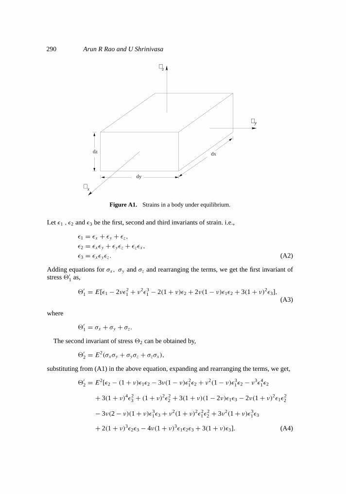
290 Arun R Rao and U Shrinivasa
dy
y
z
dz dx
x
∈
∈
∈
Figure A1. Strains in a body under equilibrium.
Let ε1 , ε2 andε3 be the first, second and third invariants of strain. i.e.,
ε1 = εx + εy + εz,
ε2 = εxεy + εyεz + εzεx,
ε3 = εxεyεz. (A2)
Adding equations forσx, σy andσz and rearranging the terms, we get the first invariant ofstress2′
1 as,
2′1 = E[ε1 − 2νε2
1 + ν2ε31 − 2(1 + ν)ε2 + 2ν(1 − ν)ε1ε2 + 3(1 + ν)2ε3],
(A3)
where
2′1 = σx + σy + σz.
The second invariant of stress22 can be obtained by,
2′2 = E2(σxσy + σyσz + σzσx),
substituting from (A1) in the above equation, expanding and rearranging the terms, we get,
2′2 = E2[ε2 − (1 + ν)ε1ε2 − 3ν(1 − ν)ε2
1ε2 + ν2(1 − ν)ε31ε2 − ν3ε4
1ε2
+ 3(1 + ν)4ε23 + (1 + ν)2ε2
2 + 3(1 + ν)(1 − 2ν)ε1ε3 − 2ν(1 + ν)2ε1ε22
− 3ν(2 − ν)(1 + ν)ε31ε3 + ν2(1 + ν)2ε2
1ε22 + 3ν2(1 + ν)ε3
1ε3
+ 2(1 + ν)3ε2ε3 − 4ν(1 + ν)3ε1ε2ε3 + 3(1 + ν)ε3]. (A4)
Simulation of elasto-plastic deformation 291
Similarly, the third invariant of stress2′3 can be determined,
2′3 = σxσyσz
= E3ε3[1 + (1 − 2ν)ε1 + ν(ν − 2)(ε21 − 2ε2) − ν(1 − ν + ν2)(ε1ε2 − 3ε3)
+ (1 − 2ν + 3ν2)ε3 + (1 + 3ν2 − 2ν3)ε2 + ν2(ε31 − 3ε1ε2 + 3ε3)]
2 (A5)
The elements of the matrixC which appear in (23) of §3 while developing the instabilitycriteria are given by,
σx/εx = −νεx(1 + εz − ν(εx + εy)) − νεx(1 + εy − ν(εx + εz))
+ (1 + εz − ν(εx + εy))(1 + εy − ν(εx + εz)),
σx/εy = εx(1 + εz − ν(εx + εy)) − νεx(1 + εy − ν(εx + εz)),
σx/εz = −νεx(1 + εz − ν(εx + εy)) + εx(1 + εy − ν(εx + εz)),
σy/εx = εy(1 + εz − ν(εx + εy)) − νεy(1 + εx − ν(εy + εy)),
σy/εy = −νεy(1 + εz − ν(εx + εy)) − νεy(1 + εx − ν(εy + εz)),
+ (1 + εz − ν(εx + εy))(1 + εy − ν(εx + εz)),
σy/εz = −νεy(1 + εz − ν(εx + εy)) + εy(1 + εx − ν(εy + εz)),
σz/εx = εz(1 + εy − ν(εx + εz)) − νεz(1 + εx − ν(εy + εz)),
σz/εy = −νεz(1 + εy − ν(εx + εz)) + εz(1 + εx − ν(εy + εz)),
σz/εz = −νεz(1 + εy − ν(εx + εz)) − νεz(1 + εx − ν(εy + εz))
+ (1 + εy − ν(εx + εz))(1 + εx − ν(εy + εz)).
References
Acharya A 2001 A model of crystal plasticity based on the theory of continuously distributed dislo-cations.J. Mech. Phys. Solids49: 761–784
Acharya A, Beaudoin A J 2000 Grain-size effect in viscoplastic polycrystals at moderate strains.J.Mech. Phys. Solids48: 2213–2230
Agah-Tehrani A, Lee E H, Mallet R L, Onat E T 1987 The theory of elasto-plastic deformation atfinite strain with induced anisotropy modeled as combined isotropic-kinematic hardening.J. Mech.Phys. Solids35: 519–539
Anderson T L 1995Fracture mechanics: Fundamental and applications(Boca Raton, FL: CRC Press)Anjaneyulu P 1999Towards elasto-plastic modelling, using modified Navier-Stokes equation. M E
thesis, Dept of Mechanical Engineering, Indian Institute of Science, BangaloreASTM 1985 Metals - Mechanical testing; elevated and low temperature tests, metallography. Annual
book of ASTM standards, (Philadelphia, PA:) Am. Soc. Testing Mater. 03.01, E-8Atluri S N 1984 On constitutive relations at finite strain; Hypo-elasticity and elasto-plasticity with
isotropic or kinematic hardening.Comput. Meth. Appl. Mech. Engng43: 137–171Backman M E 1964 From the relation between stress and finite elastic and plastic strains under
impulsive loading.J. Appl. Phys.35: 2524–2533
292 Arun R Rao and U Shrinivasa
Barbe F, Decker L, Jeulin D, Cailletaud G 2001 Intergranular and intragranular behaviour of poly-crystalline aggregates. Part 1: F.E. model.Int. J. Plasticity17: 513–536
Batdorf S B, Budiansky B 1949 A mathematical theory of slip based on the concept of slip.NACA TN 1871, April
Bazant Z P 1984 Microplane model for strain controlled inelastic behavior. InMechanics of engineer-ing materials(eds) C S Desai, R H Gallagher (London: John Wiley) pp 15–59
Bell J F 1990 Material objectivity in an experimentally based incremental theory of large finite plasticstrains.Int. J. Plasticity6: 293
Bertram A 1998 An alternative approach to finite plasticity based on material isomorphisms.Int. J.Plasticity52: 353–374
Bigoni D, Loret B, Radi E 2000 Localization of deformation in plane elastioplastic solids withanisotropic elasticity.J. Mech. Phys. Solids48: 1441–1466
Bodner S R, Parton Y 1975 Constitutive equations for elasto-viscoplastic strain hardening materials.J. Appl. Mech.42: 385–389
Braess H, Wriggers P 2000 Arbitrary Lagrangian Eulerian finite element analysis of free surface flow.Comput. Meth. Appl. Mech. Engng190: 95–109
Budiansky B, Wu T T 1962 Theoretical prediction of plastic strains in polycrystals.Proc. 4th US Natl.Congr. Appl. Mech.(New York: Am. Soc. Mech. Eng.) pp 1175–1185
Casey J, Naghdi P M 1981 On the characterization of strain-hardening in plasticity.J. Appl. Mech.48: 285–296
Casey J, Naghdi P M 1983 A remark on the defination of hardening, softening and perfectly plasticbehavior.Acta Mech.48: 91–94
Chakrabarty J 1998Theory of plasticity(Singapore:McGraw-Hill)Chen C, Lu T J 2000 A phenomenological framework of constitutive modelling for incompressible
and compressible elasto-plastic solids.Int. J. Solids Struct.37: 7769–7786Dafalias Y F 1983 Corotational rates for kinematic hardening at large plastic deformation.J. Appl.
Mech.50: 561–565Dafalias Y F 1984 The plastic spin concept and a simple illustration of its role in plastic transformations.
Mech. Mater.3: 223–233Dafalias Y F 1985 The plastic spin.J. Appl. Mech.52: 865–871Dienes J K 1979 On the analysis of rotation and stress rate in deformation bodies.Acta Mech.32:
217–232Dienes J K 1986 A discussion of material rotation and stress rate.Acta Mech.65: 1–11Drucker D C 1960 Plasticity.Proc. 1st Symp. Naval Structural Mechanics(Oxford: Pergamon) pp
407–455Drucker D C 1988 Conventional and unconventional plastic response and representation.Appl. Mech.
Rev.41: 151–168Fung Y C 1965Foundation of solid mechanics(Englewood Cliffs, NJ: Prentice Hall)Ghosh S, Suresh R 1996 R-s adapted arbitrary Lagrangian–Eulerian finite element method for metal
forming problems with strain localization.Int. J. Numer. Meth. Engng. 86: 3247–3272Green A E, Naghdi P M 1965 A general theory of an elastic-plastic continuum.Arch. Rational Mech.
Anal.18: 251–281Green A E, Naghdi P M 1966 A thermodynamic development of elasto-plastic continuum. In
Proc. IUTAM Symp. on Irreversible Aspects of Continuum Mechanics and Transfer of Physi-cal Characteristics in Moving Fluids(eds) H Parker, L I Sedov (New York: Springer-Verlag)pp 117–131
Griffith A A 1921 The phenomena of rapture of flow in solids.Philos. Trans. R. Soc. LondonA221:163–198
Haber R B 1984 A mixed Eulerian-Lagrangian displacement model for large deformation analysis insolid mechanics.Comput. Meth. Appl. Mech. Engng.43: 277–292
Hill R 1950The mathematical theory of plasticity(London: Oxford University Press)Hill R 1965 Continuum micromechanics of elastoplastic polycrystals.J. Mech. Phys. Solids13:
89–102
Simulation of elasto-plastic deformation 293
Hill R 1966 Generalized constitutive relations for incremental deformation of metal crystals by mul-tislip. J. Mech. Phys. Solids14: 95–102
Hill R 1994 Classical plasticity: a retrospective view and a new propasal.J. Mech. Phys. Solids42:1803–1826
Huetink J, Vreede P T, Van Der Lugt J 1990 Progress in mixed Eulerian–Lagrangian finite elementsimulation of forming processes.Int. J. Numer. Meth. Engng.30: 1441–1457
Hutchinson J W 1970 Elastic-plastic behaviour of polycrystalline metals and composites.Proc. R.Soc. LondonA319: 247–272
Koiter W T 1953 Stress-strain relations, uniqueness and variational theorms for elastic-plastic materialswith a singular yield surface.Q. Appl. Math.11: 350–354
Kroner E 1960 Allgemeine Kontinuumstheorie der Versetzungen und Eigenspannungen.Arch. Ratio-nal Mech. Anal.4: 273–334
Lamb R H 1945Hydrodynamics(New York: Dover)Lazan B J 1968Damping of materials and members in strutural mechanics(Oxford: Pergamon)Lee D, Zaverl F Jr 1978 A generalized strain rate dependent constitutive equation for anisotropic
materials.Acta Metall.26: 1771–1780Lee D, Zaverl F Jr 1979 A description of history dependent plastic flow behavior of anisotropic metals.
J. Engng. Mater. Technol. Trans. ASME101: 59–67Lee E H 1969 Elastic-plastic deformation at finite strains.J. Appl. Mech.36: 1–6Lee E H, Liu D T 1967 Finite strain elastic-plastic theory with application to plane-wave analysis.J.
Appl. Phys.38: 19–27Lee E H, Mallett R L, Wertheimer T B 1983 Stress analysis for anisotropic hardening in finite-
deformation plasticity.J. Appl. Mech.50: 554–560Loret B 1983 On the effects of plastic rotation in the finite deformation of anisotropic elastoplastic
materials.Mech. Mater.2: 287–304Malvern L E 1969Introduction to the mechanics of continuous medium(Englewood Cliffs, NJ:
Prentice Hall)Naghdi P M 1960 Stress-strain relations in plasticity and thermoplasticity.Proc. 2nd Symp. Naval
Structural Mechanics(Oxford: Pergamon) pp 121–167Naghdi P M, Trapp J A 1975a The significance of formulating plasticity theory with reference to
loading surfaces in strain space.Int. J. Engng. Sci.13: 785–797Naghdi P M, Trapp J A 1975b Restriction on constitutave equations of finitely deformed elastic-plastic
materials.Q. J. Mech. Appl. Math.28: 25–46Nemat-Nasser S 1983 On plastic flow of crystalline solids and geomaterials.J. Appl. Mech.50: 1114–
1126Panovko Y G, Gubanova I I 1965Stability and oscillations of elastic systems-paradoxes, fallacies,
and new concepts(New York: Consultants Bureau)Prager W 1955 The theory of plasticity: A survey of recent achivements (John Clyton Lecture).Proc.
Inst. Mech. Eng.169: 41–57Prager W 1961Introduction to mechanics of continua(Boston, MA: Ginn)Prager W, Hodge P G Jr1951Theory of perfectly plastic solids(New York: John Wiley)Qiu Y P, Weng G J 1992 A theory of plasticity for porous materials and particle-reinforced composites.
J. Appl. Mech. ASME59: 261–268Qiu Y P, Weng G J 1995 An energy approach to the plasticity of a two-phase composite containing
aligned inclusion.J. Appl. Mech. ASME62: 1039–1046Rice J R 1976 The localization of plastic deformation. InTheoretical and applied mechanics(ed.) W
T Koiter (Amsterdam: North Holland)Rubin M B 1996 On the treatment of elastic deformation in finite elastic-viscoplastic theory.Int. J.
Plasticity12: 951–965Seth B R 1963 Elastic-plastic transition in shells and tubes under pressure.Z. Angew. Math. Mech.
43: 345–351Seth B R 1964 Elastic-plastic transition in torsion.Z. Angew. Math. Mech.44: 229–233
294 Arun R Rao and U Shrinivasa
Seth B R 1970 Transition conditions: The yield condition.Int. J. Non-Linear Mech.5: 279–285Stouffer D C, Bodner S R 1979. A constitutive model for the deformation induced anisotropic plastic
flow of metals.Int. J. Engng. Sci.17: 757–764Taylor G I, Elam C F 1923 The distortion of an aluminium crystal during tensile test.Proc. R. Soc.
LondonA102: 643–667Taylor G I, Elam C F 1925 The plastic extension and fracture of aluminium crystals.Proc. R. Soc.
LondonA108: 28–51Taylor G I, Elam C F 1926 The distortion of iron crystals.Proc. R. Soc. LondonA112: 337–361.Timoshenko S P 1986Strength of materials, Part-2: Advanced theory and problems(Delhi: CBS)Timoshenko S P, Goodier J N 1970Theory of elasticityInt. edn (Singapore: McGraw-Hill)Valanis K C, 1971 A theory of viscoplasticity without a yield surface. Part I General theory.Arch.
Mech.23: 517–533Valanis K C 1975 On the foundation of the endochronic theory of viscoplasticity.Arch. Mech.27:
857–868White F M 1994Fluid mechanics(Singapore: McGraw Hill)Zienkiewicz O C, Godbole P N, 1974 Flow of plastic and visco-plastic solids with special referance
to extrusion and forming processes.Int. J. Numer. Meth. Engng.8: 3–16.Zienkiewicz O C, Godbole P N 1975 Viscous incompressible flow with special reference to non-
newtonian (plastic) fluids. InFinite elements in fluids(eds) Gallagheret al (Chichester: WileyInterscience) vol. 1, pp 25–55