Greedy Hash: Towards Fast Optimization forAccurate Hash Coding in CNN

Shupeng Su1 Chao Zhang1∗ Kai Han1,3 Yonghong Tian1,2

1Key Laboratory of Machine Perception (MOE), School of EECS, Peking University2National Engineering Laboratory for Video Technology, School of EECS, Peking University

3Huawei Noah’s Ark Lab{sushupeng, c.zhang, hankai, yhtian}@pku.edu.cn

Abstract

To convert the input into binary code, hashing algorithm has been widely used forapproximate nearest neighbor search on large-scale image sets due to its computa-tion and storage efficiency. Deep hashing further improves the retrieval quality bycombining the hash coding with deep neural network. However, a major difficultyin deep hashing lies in the discrete constraints imposed on the network output,which generally makes the optimization NP hard. In this work, we adopt the greedyprinciple to tackle this NP hard problem by iteratively updating the network towardthe probable optimal discrete solution in each iteration. A hash coding layer is de-signed to implement our approach which strictly uses the sign function in forwardpropagation to maintain the discrete constraints, while in back propagation thegradients are transmitted intactly to the front layer to avoid the vanishing gradients.In addition to the theoretical derivation, we provide a new perspective to visualizeand understand the effectiveness and efficiency of our algorithm. Experiments onbenchmark datasets show that our scheme outperforms state-of-the-art hashingmethods in both supervised and unsupervised tasks.

1 Introduction

In the era of big data, searching for the desired information has become an important topic in such avast ocean of data. Hashing for large-scale image set retrieval [7, 8, 21, 22] has attracted extensiveinterest in Approximate Nearest Neighbor (ANN) search due to its computation and storage efficiencywith the generated binary representation. Deep hashing further promotes the performance by learningthe image representation and hash coding in the same network simultaneously [30, 15, 18, 6]. Notonly the common pairwise label based methods [17, 30, 4], but also triplet [34, 35] and point-wise[19, 31] schemes have been exploited extensively.

Despite the considerable progress, it’s still a difficult task to realize the real end-to-end training ofdeep hashing owing to the vanishing gradient problem from sign function which is appended after theoutput of the network to achieve binary code. To be specific, the gradient of sign function is zerofor all nonzero input, and that is fatal to the neural network which uses gradient descent for training.Most of the previous works choose to first solve a relaxed problem discarding the discrete constraints(e.g., [34, 19, 31] replace sign function with tanh or sigmoid, [20, 36, 17] add a penalty term in lossfunction to generate feature as discrete as possible), and later in test phase apply sign function toobtain real binary code. Although capable of training the network, these relaxation schemes willintroduce quantization error which basically leads to suboptimal hash code. Later HashNet [4] andDeep Supervised Discrete Hashing (DSDH) [16] made a progress on this difficulty. HashNet starts

∗Corresponding author

32nd Conference on Neural Information Processing Systems (NeurIPS 2018), Montréal, Canada.

training with a smoothed activation function y = tanh(βx) and becomes more non-smooth byincreasing β until eventually almost behaves like the original sign function. DSDH solves the discretehashing optimization with the discrete cyclic coordinate descend (DCC) [26] algorithm, which cankeep the discrete constraint during the whole optimization process.

Although these two papers have achieved breakthroughs, there are still some problems worthy ofattention. On the one hand, they need to train a lot of iterations since DSDH updates the hashcode bit-by-bit, while HashNet requires to increase β iteratively. On the other hand, DCC whichis used to solve the discrete optimization by DSDH, can only be applied to the standard binaryquadratic program (BQP) problem with limited applications, while HashNet is still distracted byquantization error as β cannot increase infinitely. Therefore this paper proposes a faster and moreaccurate algorithm to integrate the hash coding with neural network.

Our main contributions are as follows. (1) We propose to adopt greedy algorithm for fast processing ofhashing discrete optimization, and a new coding layer is designed, in which the sign function is strictlyused in forward propagation against the quantization error, and later the gradients are transmittedintactly to the front layer which effectively prevents the vanishing gradients and updates all bitstogether. Benefitting from the high efficiency to integrate hashing with neural network, the proposedhash layer can be applied to various occasions that need binary coding. (2) We not only providetheoretical derivation, but also propose a visual perspective to understand the rationality and validityof our method based on the aggregation effect of sign function. (3) Extensive experiments show thatour scheme outperforms state-of-the-art hashing methods for image retrieval in both supervised andunsupervised tasks.

2 Greedy hash in CNN

In this section we will detailedly introduce our method and first of all we would like to indicatesome notations that would be used later. We denote the output of the last hidden layer in the originalneural network with H, which also serves as the input to our hash coding layer. B would be used torepresent the hash code, which is exactly the output of the hash layer. In addition, sgn() is the signfunction which outputs +1 for positive numbers and -1 otherwise.

2.1 Optimizing discrete hashing with greedy principle

Firstly we put the neural network aside and focus on approaching the discrete optimization problem,which is defined as follows:

minB

L(B),

s.t. B ∈ {−1, +1}N×K .(1)

N means there are N inputs, and K means using K bits to encode. Besides, L(B) can be any lossfunction you need to use, e.g., Mean Square Error loss, Cross Entropy loss and so on.

If we leave out the discrete constraint B ∈ {−1, +1}N×K , aiming to obtain the optimal continuousB, we can calculate the gradient and use gradient descent to iteratively update B as follows untilconvergence:

Bt+1 = Bt − lr ∗ ∂L

∂Bt, (2)

where t stands for the t-th iteration, and lr denotes the learning rate.

However, it is almost impossible for B calculated by Equation (2) to satisfy the requirement B ∈{−1, +1}N×K , and after considering the discrete constraint, the optimization (1) will become NPhard. One of the fast and effective methods to tackle NP hard problems is the greedy algorithm,which iteratively selects the best option in each iteration and ultimately reaches a nice point that issufficiently close to the global optimal solution. If Bt+1 calculated by Equation (2) is the optimalcontinuous solution without the discrete requirement, then applying the greedy principle, the closestdiscrete point to the continuous Bt+1, that is sgn(Bt+1), is probable to be the optimal discretesolution in each iteration thus we update B toward it greedily. Concretely we use the followingequation to solve the optimization (1) iteratively:

Bt+1 = sgn( Bt − lr ∗ ∂L

∂Bt). (3)

2

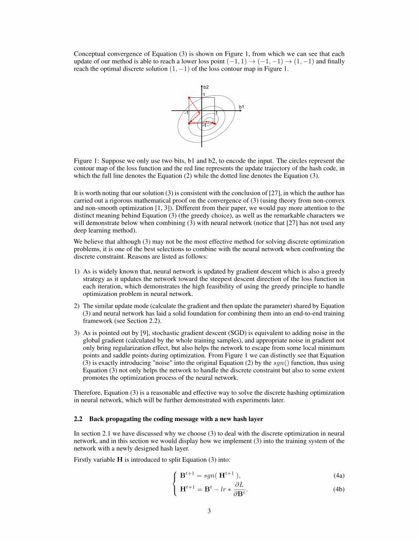
Conceptual convergence of Equation (3) is shown on Figure 1, from which we can see that eachupdate of our method is able to reach a lower loss point (−1, 1)→ (−1,−1)→ (1,−1) and finallyreach the optimal discrete solution (1,−1) of the loss contour map in Figure 1.

b2

b1

1

1-1

-1

Figure 1: Suppose we only use two bits, b1 and b2, to encode the input. The circles represent thecontour map of the loss function and the red line represents the update trajectory of the hash code, inwhich the full line denotes the Equation (2) while the dotted line denotes the Equation (3).

It is worth noting that our solution (3) is consistent with the conclusion of [27], in which the author hascarried out a rigorous mathematical proof on the convergence of (3) (using theory from non-convexand non-smooth optimization [1, 3]). Different from their paper, we would pay more attention to thedistinct meaning behind Equation (3) (the greedy choice), as well as the remarkable characters wewill demonstrate below when combining (3) with neural network (notice that [27] has not used anydeep learning method).

We believe that although (3) may not be the most effective method for solving discrete optimizationproblems, it is one of the best selections to combine with the neural network when confronting thediscrete constraint. Reasons are listed as follows:

1) As is widely known that, neural network is updated by gradient descent which is also a greedystrategy as it updates the network toward the steepest descent direction of the loss function ineach iteration, which demonstrates the high feasibility of using the greedy principle to handleoptimization problem in neural network.

2) The similar update mode (calculate the gradient and then update the parameter) shared by Equation(3) and neural network has laid a solid foundation for combining them into an end-to-end trainingframework (see Section 2.2).

3) As is pointed out by [9], stochastic gradient descent (SGD) is equivalent to adding noise in theglobal gradient (calculated by the whole training samples), and appropriate noise in gradient notonly bring regularization effect, but also helps the network to escape from some local minimumpoints and saddle points during optimization. From Figure 1 we can distinctly see that Equation(3) is exactly introducing "noise" into the original Equation (2) by the sgn() function, thus usingEquation (3) not only helps the network to handle the discrete constraint but also to some extentpromotes the optimization process of the neural network.

Therefore, Equation (3) is a reasonable and effective way to solve the discrete hashing optimizationin neural network, which will be further demonstrated with experiments later.

2.2 Back propagating the coding message with a new hash layer

In section 2.1 we have discussed why we choose (3) to deal with the discrete optimization in neuralnetwork, and in this section we would display how we implement (3) into the training system of thenetwork with a newly designed hash layer.

Firstly variable H is introduced to split Equation (3) into: Bt+1 = sgn( Ht+1 ), (4a)

Ht+1 = Bt − lr ∗ ∂L

∂Bt. (4b)

3

Just recall that H denotes the output of the neural network while B denotes the hash code, andwhat we’re going to do here is designing a new layer to connect H and B which should satisfy theEquations (4a) and (4b).

Knowing this, we could immediately find that what we need to do to implement Equation (4a)is simply using sign function in the forward propagation of the new hash layer, namely applyingB = sgn(H) forward.

As for the Equation (4b), if we add a penalty term ‖ H− sgn(H) ‖pp (entrywise matrix norm) in theobjective function to make it as close to zero as possible, then with Equation (4a) Bt = sgn(Ht), wehave:

Ht+1 = Ht − lr ∗ ∂L

∂Ht

= (Ht −Bt) + Bt − lr ∗ ∂L

∂Ht

= (Ht − sgn(Ht)) + Bt − lr ∗ ∂L

∂Ht

≈ Bt − lr ∗ ∂L

∂Ht.

(5)

Comparing (4b) with (5), we could finally implement Equation (4b) by setting:

∂L

∂Ht=

∂L

∂Bt(6)

in the backward propagation of our new hash layer, which means the gradient of B is back transmittedto H intactly. Our method has been summarized in Algorithm 1.

Algorithm 1 Greedy Hash

Prepare training set X and neural network FΘ, in which Θ denotes parameters of the network.repeat

- H = FΘ(X).- B = sgn(H) [forward propagation of our hash layer].- Calculate the loss function : Loss = L(B) + α ‖ H− sgn(H) ‖pp ,

where L can be any learning function such as the Cross Entropy Loss.- Calculate ∂Loss

∂B = ∂L∂B .

- Set ∂L∂H = ∂L

∂B [backward propagation of our hash layer].

- Calculate ∂Loss∂H = ∂L

∂H + α∂‖H−sgn(H)‖pp

∂H = ∂L∂B + α p ‖ H− sgn(H) ‖p−1

p−1.

- Calculate ∂Loss∂Θ = ∂Loss

∂H × ∂H∂Θ .

- Update the whole network’s parameters.until convergence.

2.3 Analyzing our algorithm’s validity from a visual perspective

In this section, we would provide a new perspective to visualize and understand the two most criticalparts in our algorithm:

Forward : B = sgn( H ), (7)

Backward :∂L

∂H=∂L

∂B. (8)

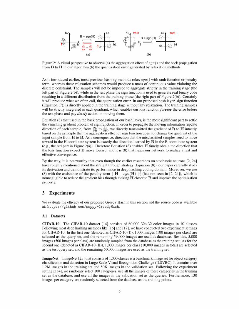
Firstly, suppose there are two categories of input images. We set H = (h1, h2) and B = (b1, b2)(namely we only use two bits to encode the input image). As is shown in the forward part of Figure2(a), sign function is trying to aggregate the data of each quadrant in H coordinate system into asingle point in B coordinate system, and obviously learning to move the misclassified samples to thecorrect quadrant in H coordinate system is our ultimate training goal.

4

B = sgn(H)h2

h1

b2

b1!"!#= !"

!%

(a)

B = sgn(H)h2

h1

b2

b1

train test

(b)

Figure 2: A visual perspective to observe (a) the aggregation effect of sgn() and the back propagationfrom B to H in our algorithm (b) the quantization error generated by relaxation methods.

As is introduced earlier, most previous hashing methods relax sgn() with tanh function or penaltyterm, whereas these relaxation schemes would produce a mass of continuous value violating thediscrete constraint. The samples will not be imposed to aggregate strictly in the training stage (theleft part of Figure 2(b)), while in the test phase the sign function is used to generate real binary coderesulting in a different distribution from the training phase (the right part of Figure 2(b)). Certainlyit will produce what we often call, the quantization error. In our proposed hash layer, sign function(Equation (7)) is directly applied in the training stage without any relaxation. The training sampleswill be strictly integrated in each quadrant, which enables our loss function foresee the error beforethe test phase and pay timely action on moving them.

Equation (8) that used in the back propagation of our hash layer, is the most significant part to settlethe vanishing gradient problem of sign function. In order to propagate the moving information (updatedirection of each sample) from ∂L

∂B to ∂L∂H , we directly transmitted the gradient of B to H intactly,

based on the principle that the aggregation effect of sign function does not change the quadrant of theinput sample from H to B. As a consequence, direction that the misclassified samples need to movetoward in the H coordinate system is exactly the direction learned by B in the B coordinate system(e.g., the red part in Figure 2(a)). Therefore Equation (8) enables H timely obtain the direction thatthe loss function expect B move toward, and it is (8) that helps our network to realize a fast andeffective convergence.

By the way, it is noteworthy that even though the earlier researches on stochastic neurons [2, 24]have roughly mentioned about the straight through strategy (Equation (8)), our paper carefully studyits derivation and demonstrate its performance in deep hashing coding domain. Moreover, we use(8) with the assistance of the penalty term ‖ H − sgn(H) ‖pp (has not seen in [2, 24]), which isnonnegligible to reduce the gradient bias through making H closer to B and improve the optimizationproperty.

3 Experiments

We evaluate the efficacy of our proposed Greedy Hash in this section and the source code is availableat: https://github.com/ssppp/GreedyHash.

3.1 Datasets

CIFAR-10 The CIFAR-10 dataset [14] consists of 60,000 32×32 color images in 10 classes.Following most deep hashing methods like [16] and [17], we have conducted two experiment settingsfor CIFAR-10. In the first one (denoted as CIFAR-10 (I)), 1000 images (100 images per class) areselected as the query set, and the remaining 59,000 images are used as database. Besides, 5,000images (500 images per class) are randomly sampled from the database as the training set. As for thesecond one (denoted as CIFAR-10 (II)), 1,000 images per class (10,000 images in total) are selectedas the test query set, and the remaining 50,000 images are used as the training set.

ImageNet ImageNet [25] that consists of 1,000 classes is a benchmark image set for object categoryclassification and detection in Large Scale Visual Recognition Challenge (ILSVRC). It contains over1.2M images in the training set and 50K images in the validation set. Following the experimentsetting in [4], we randomly select 100 categories, use all the images of these categories in the trainingset as the database, and use all the images in the validation set as the queries. Furthermore, 130images per category are randomly selected from the database as the training points.

5

3.2 Implementation details

Basic setting Our model is implemented with Pytorch [23] framework. We set the batch sizeas 32 and use SGD as the optimizer with a weight decay of 0.0005 and a momentum of 0.9. Forsupervised experiments we use 0.001 as the initial learning rate while for unsupervised experimentswe use 0.0001, and we divide both of them by 10 when the loss stop decreasing. In addition, wecross-validate the hyper-parameters α and p in the penalty term α ‖ H − sgn(H) ‖pp, which arefinally fixed with p = 3, α = 0.1 × 1

N ·K (using 1N ·K term to remove the impacts of the various

encoding length and input size) for CIFAR-10, while for ImageNet α = 1× 1N ·K .

Supervised setting We choose the Cross Entropy loss as our supervised loss function L, whichmeans we just apply softmax to classify the hash code B ∈ {−1, +1}N×K without adding anyretrieval loss (e.g., contrastive loss or triplet loss), and later we would display its outstanding retrievalperformance despite merely using single softmax. Moreover, for fair comparison with the previousworks, we use the pre-trained AlexNet [13] as our neural network, in which we append a new fclayer after fc7 to generate feature of desired length and then append our hash layer to produce binarycode. We have compared our method with DSDH [16], HashNet [4], DPSH [17], DTSH [29], DHN[36], NINH [15], CNNH [30], VDSH [33], DRSCH [32], DSCH [32], DSRH [34], DPLM [27],SDH [26], KSH [21] under this supervised setup. It is worth noting that some of aforementionedmethods such as DSDH have used the VGG-F [5] convolutional neural network, which composesof five convolutional layers and two fully connected layers the same as AlexNet (other methodsincluding ours have selected), thus we consider the comparison among them is fair even thoughVGG-F performs slightly better on the classification of the original 1,000 classes ImageNet.

Unsupervised setting Inspired by [12], we choose to minimize the difference on the cosine distancerelationships when the features are encoded from Euclidean space to Hamming space. Concretelywe use L =‖ cos(h1, h2)− cos(b1, b2) ‖22, in which cos means the cosine distance, and h means thefeature in Euclidean space while b means binary code in Hamming space. We use the pre-trainedVGG16 [28] network following the setting in [6, 18], and we append a new fc layer as well as ourhash layer to generate the binary code. We have compared with SAH [6], DeepBit [18], ITQ [8],KMH [10] and SPH [11] under this unsupervised setting.

3.3 Comparison on fast optimization

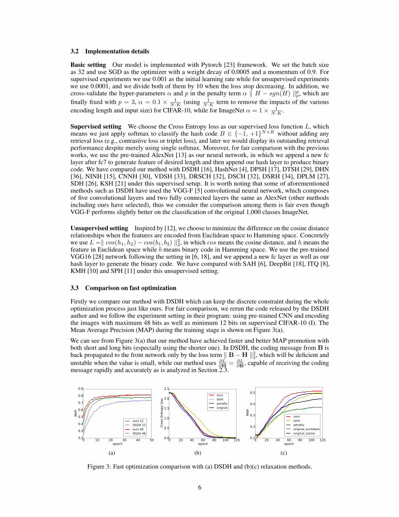
Firstly we compare our method with DSDH which can keep the discrete constraint during the wholeoptimization process just like ours. For fair comparison, we rerun the code released by the DSDHauthor and we follow the experiment setting in their program: using pre-trained CNN and encodingthe images with maximum 48 bits as well as minimum 12 bits on supervised CIFAR-10 (I). TheMean Average Precision (MAP) during the training stage is shown on Figure 3(a).

We can see from Figure 3(a) that our method have achieved faster and better MAP promotion withboth short and long bits (especially using the shorter one). In DSDH, the coding message from B isback propagated to the front network only by the loss term ‖ B−H ‖22, which will be deficient andunstable when the value is small, while our method uses ∂L

∂H = ∂L∂B , capable of receiving the coding

message rapidly and accurately as is analyzed in Section 2.3.

0 10 20 30 40 50epoch

0.2

0.3

0.4

0.5

0.6

0.7

0.8

0.9

MA

P

ours 12

DSDH 12

ours 48

DSDH 48

(a)

0 20 40 60 80 100 120epoch

0.0

0.5

1.0

1.5

2.0

2.5

Cro

ss E

ntr

opy loss

ours

tanh

penalty

original

(b)

0 20 40 60 80 100 120epoch

0.1

0.2

0.3

0.4

0.5

MA

P

ours

tanh

penalty

original_euclidean

original_cosine

(c)

Figure 3: Fast optimization comparison with (a) DSDH and (b)(c) relaxation methods.

6

Next we compare our algorithm with the relaxation methods. We use 16 bits to encode the imagesand we train the AlexNet from scratch here to further demonstrate the learning ability. The dynamicclassification loss and MAP are shown on Figure 3(b) and 3(c), in which label tanh means using tanhfunction as relaxation, penalty denotes method adding penalty term to generate features as discreteas possible, and original represents training without hash coding (the same length 16 but no longerlimited to binary). We use two schemes to retrieve these original features, the Euclidean distance andthe cosine distance.

As shown on Figure 3(b) and 3(c), our algorithm is one of the fastest methods to decrease theclassification loss and simultaneously is the fastest and greatest one to promote the MAP owing tothe better protection against quantization error. Among the results the tanh method is the slowestone probably due to the existence of saturation in tanh activation function. Moreover, it is interestingto discover that retrieval with hash binary code is better than the retrieval with original unrestrictedfeatures, probably because the softmax function generally needs adding retrieval loss to furtherconstrain the image feature (for smaller intra-class distance and larger inter-class distance), whichis exactly the merit of hashing that owns the nature of aggregating the inputs in each quadrant as isdemonstrated in Section 2.3.

Thus our Greedy Hash is able to realize faster and better optimization in hash coding with CNN, andsubsequently we will further demonstrate the accuracy of our generated hash code when comparedwith the state-of-the-art.

3.4 Comparison on accurate coding

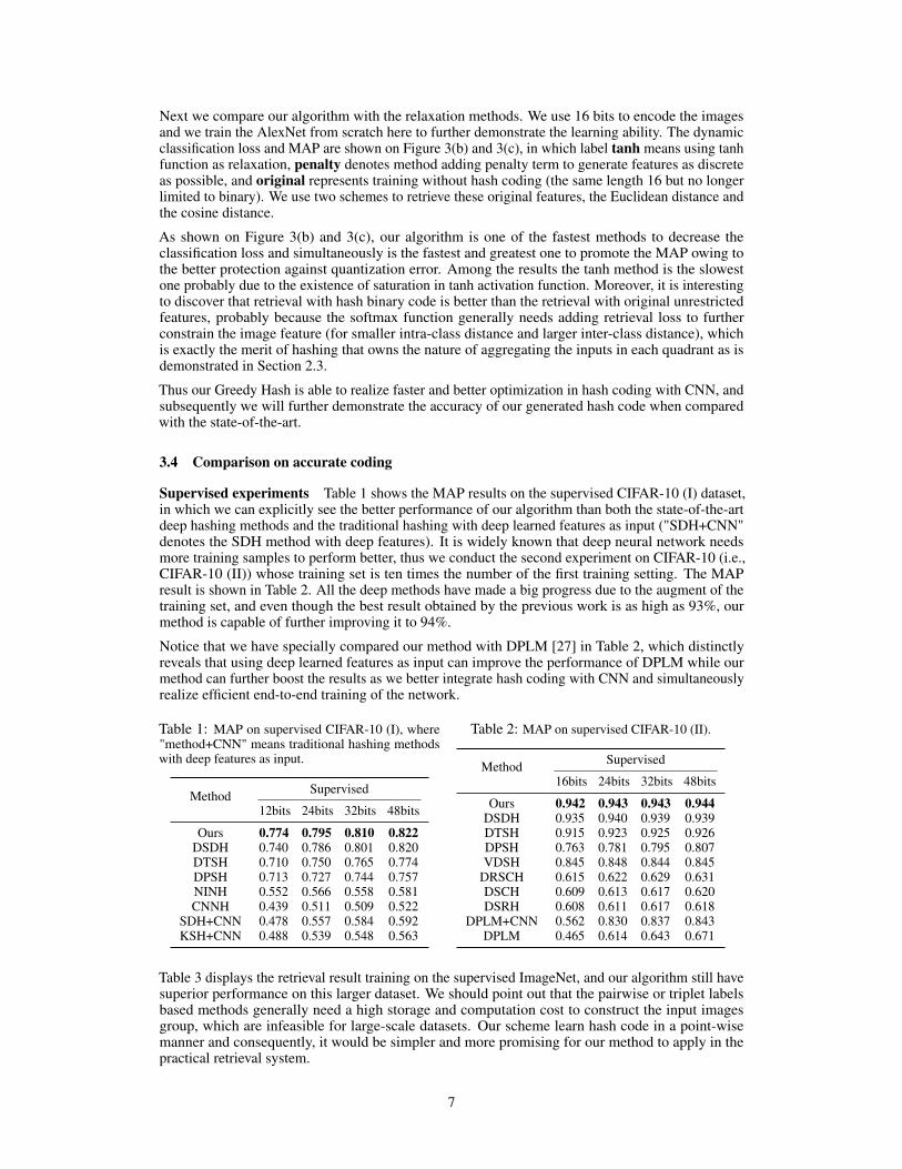
Supervised experiments Table 1 shows the MAP results on the supervised CIFAR-10 (I) dataset,in which we can explicitly see the better performance of our algorithm than both the state-of-the-artdeep hashing methods and the traditional hashing with deep learned features as input ("SDH+CNN"denotes the SDH method with deep features). It is widely known that deep neural network needsmore training samples to perform better, thus we conduct the second experiment on CIFAR-10 (i.e.,CIFAR-10 (II)) whose training set is ten times the number of the first training setting. The MAPresult is shown in Table 2. All the deep methods have made a big progress due to the augment of thetraining set, and even though the best result obtained by the previous work is as high as 93%, ourmethod is capable of further improving it to 94%.

Notice that we have specially compared our method with DPLM [27] in Table 2, which distinctlyreveals that using deep learned features as input can improve the performance of DPLM while ourmethod can further boost the results as we better integrate hash coding with CNN and simultaneouslyrealize efficient end-to-end training of the network.

Table 1: MAP on supervised CIFAR-10 (I), where"method+CNN" means traditional hashing methodswith deep features as input.

Method Supervised

12bits 24bits 32bits 48bits

Ours 0.774 0.795 0.810 0.822DSDH 0.740 0.786 0.801 0.820DTSH 0.710 0.750 0.765 0.774DPSH 0.713 0.727 0.744 0.757NINH 0.552 0.566 0.558 0.581CNNH 0.439 0.511 0.509 0.522

SDH+CNN 0.478 0.557 0.584 0.592KSH+CNN 0.488 0.539 0.548 0.563

Table 2: MAP on supervised CIFAR-10 (II).

Method Supervised

16bits 24bits 32bits 48bits

Ours 0.942 0.943 0.943 0.944DSDH 0.935 0.940 0.939 0.939DTSH 0.915 0.923 0.925 0.926DPSH 0.763 0.781 0.795 0.807VDSH 0.845 0.848 0.844 0.845

DRSCH 0.615 0.622 0.629 0.631DSCH 0.609 0.613 0.617 0.620DSRH 0.608 0.611 0.617 0.618

DPLM+CNN 0.562 0.830 0.837 0.843DPLM 0.465 0.614 0.643 0.671

Table 3 displays the retrieval result training on the supervised ImageNet, and our algorithm still havesuperior performance on this larger dataset. We should point out that the pairwise or triplet labelsbased methods generally need a high storage and computation cost to construct the input imagesgroup, which are infeasible for large-scale datasets. Our scheme learn hash code in a point-wisemanner and consequently, it would be simpler and more promising for our method to apply in thepractical retrieval system.

7

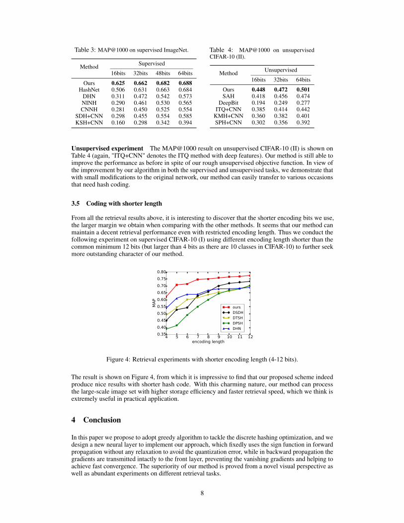
Table 3: MAP@1000 on supervised ImageNet.

Method Supervised

16bits 32bits 48bits 64bits

Ours 0.625 0.662 0.682 0.688HashNet 0.506 0.631 0.663 0.684

DHN 0.311 0.472 0.542 0.573NINH 0.290 0.461 0.530 0.565CNNH 0.281 0.450 0.525 0.554

SDH+CNN 0.298 0.455 0.554 0.585KSH+CNN 0.160 0.298 0.342 0.394

Table 4: MAP@1000 on unsupervisedCIFAR-10 (II).

Method Unsupervised

16bits 32bits 64bits

Ours 0.448 0.472 0.501SAH 0.418 0.456 0.474

DeepBit 0.194 0.249 0.277ITQ+CNN 0.385 0.414 0.442

KMH+CNN 0.360 0.382 0.401SPH+CNN 0.302 0.356 0.392

Unsupervised experiment The MAP@1000 result on unsupervised CIFAR-10 (II) is shown onTable 4 (again, "ITQ+CNN" denotes the ITQ method with deep features). Our method is still able toimprove the performance as before in spite of our rough unsupervised objective function. In view ofthe improvement by our algorithm in both the supervised and unsupervised tasks, we demonstrate thatwith small modifications to the original network, our method can easily transfer to various occasionsthat need hash coding.

3.5 Coding with shorter length

From all the retrieval results above, it is interesting to discover that the shorter encoding bits we use,the larger margin we obtain when comparing with the other methods. It seems that our method canmaintain a decent retrieval performance even with restricted encoding length. Thus we conduct thefollowing experiment on supervised CIFAR-10 (I) using different encoding length shorter than thecommon minimum 12 bits (but larger than 4 bits as there are 10 classes in CIFAR-10) to further seekmore outstanding character of our method.

4 5 6 7 8 9 10 11 12encoding length

0.35

0.40

0.45

0.50

0.55

0.60

0.65

0.70

0.75

0.80

MA

P

ours

DSDH

DTSH

DPSH

DHN

Figure 4: Retrieval experiments with shorter encoding length (4-12 bits).

The result is shown on Figure 4, from which it is impressive to find that our proposed scheme indeedproduce nice results with shorter hash code. With this charming nature, our method can processthe large-scale image set with higher storage efficiency and faster retrieval speed, which we think isextremely useful in practical application.

4 Conclusion

In this paper we propose to adopt greedy algorithm to tackle the discrete hashing optimization, and wedesign a new neural layer to implement our approach, which fixedly uses the sign function in forwardpropagation without any relaxation to avoid the quantization error, while in backward propagation thegradients are transmitted intactly to the front layer, preventing the vanishing gradients and helping toachieve fast convergence. The superiority of our method is proved from a novel visual perspective aswell as abundant experiments on different retrieval tasks.

8

Acknowledgments

This work was supported in part by the National Key R&D Program of China under Grant 2017YF-B1002400, the National Natural Science Foundation of China under Grant 61671027, U1611461 andthe National Key Basic Research Program of China under Grant 2015CB352303.

References[1] H. Attouch, J. Bolte, and B. F. Svaiter. Convergence of descent methods for semi-algebraic and tame

problems: proximal algorithms, forward–backward splitting, and regularized gauss–seidel methods. Math-ematical Programming, 137(1-2):91–129, 2013.

[2] Y. Bengio, N. Léonard, and A. Courville. Estimating or propagating gradients through stochastic neuronsfor conditional computation. arXiv preprint arXiv:1308.3432, 2013.

[3] J. Bolte, S. Sabach, and M. Teboulle. Proximal alternating linearized minimization or nonconvex andnonsmooth problems. Mathematical Programming, 146(1-2):459–494, 2014.

[4] Z. Cao, M. Long, J. Wang, and P. S. Yu. Hashnet: Deep learning to hash by continuation. In The IEEEInternational Conference on Computer Vision (ICCV), Oct 2017.

[5] K. Chatfield, K. Simonyan, A. Vedaldi, and A. Zisserman. Return of the devil in the details: Delving deepinto convolutional nets. arXiv preprint arXiv:1405.3531, 2014.

[6] T.-T. Do, D.-K. Le Tan, T. T. Pham, and N.-M. Cheung. Simultaneous feature aggregating and hashingfor large-scale image search. In Proceedings of the IEEE Conference on Computer Vision and PatternRecognition, pages 6618–6627, 2017.

[7] A. Gionis, P. Indyk, R. Motwani, et al. Similarity search in high dimensions via hashing. In Vldb,volume 99, pages 518–529, 1999.

[8] Y. Gong, S. Lazebnik, A. Gordo, and F. Perronnin. Iterative quantization: A procrustean approach tolearning binary codes for large-scale image retrieval. IEEE Transactions on Pattern Analysis and MachineIntelligence, 35(12):2916–2929, 2013.

[9] I. Goodfellow, Y. Bengio, A. Courville, and Y. Bengio. Deep learning, volume 1. MIT press Cambridge,2016.

[10] K. He, F. Wen, and J. Sun. K-means hashing: An affinity-preserving quantization method for learningbinary compact codes. In Computer Vision and Pattern Recognition (CVPR), 2013 IEEE Conference on,pages 2938–2945. IEEE, 2013.

[11] J.-P. Heo, Y. Lee, J. He, S.-F. Chang, and S.-E. Yoon. Spherical hashing. In Computer Vision and PatternRecognition (CVPR), 2012 IEEE Conference on, pages 2957–2964. IEEE, 2012.

[12] M. Hu, Y. Yang, F. Shen, N. Xie, and H. T. Shen. Hashing with angular reconstructive embeddings. IEEETransactions on Image Processing, 27(2):545–555, 2018.

[13] A. Krizhevsky. One weird trick for parallelizing convolutional neural networks. arXiv preprint arX-iv:1404.5997, 2014.

[14] A. Krizhevsky and G. Hinton. Learning multiple layers of features from tiny images. 2009.[15] H. Lai, Y. Pan, Y. Liu, and S. Yan. Simultaneous feature learning and hash coding with deep neural

networks. In 2015 IEEE Conference on Computer Vision and Pattern Recognition (CVPR).[16] Q. Li, Z. Sun, R. He, and T. Tan. Deep supervised discrete hashing. In Advances in Neural Information

Processing Systems, pages 2479–2488, 2017.[17] W.-J. Li, S. Wang, and W.-C. Kang. Feature learning based deep supervised hashing with pairwise labels. In

Proceedings of the Twenty-Fifth International Joint Conference on Artificial Intelligence, pages 1711–1717.AAAI Press, 2016.

[18] K. Lin, J. Lu, C.-S. Chen, and J. Zhou. Learning compact binary descriptors with unsupervised deep neuralnetworks. In Proceedings of the IEEE Conference on Computer Vision and Pattern Recognition, pages1183–1192, 2016.

[19] K. Lin, H.-F. Yang, J.-H. Hsiao, and C.-S. Chen. Deep learning of binary hash codes for fast image retrieval.In Computer Vision and Pattern Recognition Workshops (CVPRW), 2015 IEEE Conference on, pages27–35. IEEE, 2015.

[20] H. Liu, R. Wang, S. Shan, and X. Chen. Deep supervised hashing for fast image retrieval. In Proceedingsof the IEEE conference on computer vision and pattern recognition, pages 2064–2072, 2016.

[21] W. Liu, J. Wang, R. Ji, Y.-G. Jiang, and S.-F. Chang. Supervised hashing with kernels. In Computer Visionand Pattern Recognition (CVPR), 2012 IEEE Conference on, pages 2074–2081. IEEE, 2012.

[22] J. Masci, M. M. Bronstein, A. M. Bronstein, and J. Schmidhuber. Multimodal similarity-preservinghashing. IEEE transactions on pattern analysis and machine intelligence, 36(4):824–830, 2014.

[23] A. Paszke, S. Gross, S. Chintala, G. Chanan, E. Yang, Z. DeVito, Z. Lin, A. Desmaison, L. Antiga, andA. Lerer. Automatic differentiation in pytorch. 2017.

[24] T. Raiko, M. Berglund, G. Alain, and L. Dinh. Techniques for learning binary stochastic feedforwardneural networks. arXiv preprint arXiv:1406.2989, 2014.

9

[25] O. Russakovsky, J. Deng, H. Su, J. Krause, S. Satheesh, S. Ma, Z. Huang, A. Karpathy, A. Khosla,M. Bernstein, et al. Imagenet large scale visual recognition challenge. International Journal of ComputerVision, 115(3):211–252, 2015.

[26] F. Shen, C. Shen, W. Liu, and H. T. Shen. Supervised discrete hashing. In CVPR, volume 2, page 5, 2015.[27] F. Shen, X. Zhou, Y. Yang, J. Song, H. T. Shen, and D. Tao. A fast optimization method for general binary

code learning. IEEE Transactions on Image Processing, 25(12):5610–5621, 2016.[28] K. Simonyan and A. Zisserman. Very deep convolutional networks for large-scale image recognition.

arXiv preprint arXiv:1409.1556, 2014.[29] X. Wang, Y. Shi, and K. M. Kitani. Deep supervised hashing with triplet labels. In Asian Conference on

Computer Vision, pages 70–84. Springer, 2016.[30] R. Xia, Y. Pan, H. Lai, C. Liu, and S. Yan. Supervised hashing for image retrieval via image representation

learning. In AAAI, volume 1, page 2, 2014.[31] H.-F. Yang, K. Lin, and C.-S. Chen. Supervised learning of semantics-preserving hashing via deep neural

networks for large-scale image search. arXiv preprint arXiv:1507.00101, 2015.[32] R. Zhang, L. Lin, R. Zhang, W. Zuo, and L. Zhang. Bit-scalable deep hashing with regularized similar-

ity learning for image retrieval and person re-identification. IEEE Transactions on Image Processing,24(12):4766–4779, 2015.

[33] Z. Zhang, Y. Chen, and V. Saligrama. Efficient training of very deep neural networks for supervisedhashing. In Proceedings of the IEEE Conference on Computer Vision and Pattern Recognition, pages1487–1495, 2016.

[34] F. Zhao, Y. Huang, L. Wang, and T. Tan. Deep semantic ranking based hashing for multi-label imageretrieval. In Computer Vision and Pattern Recognition (CVPR), 2015 IEEE Conference on, pages 1556–1564. IEEE, 2015.

[35] Y. Zhou, S. Huang, Y. Zhang, and Y. Wang. Deep hashing with triplet quantization loss. arXiv preprintarXiv:1710.11445, 2017.

[36] H. Zhu, M. Long, J. Wang, and Y. Cao. Deep hashing network for efficient similarity retrieval. In AAAI,pages 2415–2421, 2016.

10